The Intermittent Travelling Salesman Problem

Tu-San Pham, Pieter Leyman and Patrick De Causmaecker

November 12, 2018

Abstract

In this paper, we introduce a new variant of the Travelling SalesmanProblem, namely the Intermittent Travelling Salesman Problem (ITSP),which is inspired by real world drilling/texturing applications. In thisproblem, each vertex can be visited more than once and there is a tem-perature constraint enforcing a time lapse between two consecutive visits.A branch-and-bound approach is proposed to solve small instances to op-timality. We furthermore develop four Variable Neighbourhood Searchmetaheuristics which produce high quality solutions for large instances.An instance library is built and made publicly available.

1 Introduction

In this paper, we study a new variant of the Travelling Salesman Problem (TSP).The problem is inspired by industrial drilling or texturing applications wherethe temperature of the workpiece is taken into account. The processing causesthe workpiece to locally heat up until it eventually melts the workpiece down.Therefore, the processing must be divided over time intervals, with time lapsesfor cooling down of the workpiece in between. This gives rise to an optimisationproblem of finding the best schedule to process the whole workpiece in theshortest time while respecting temperature constraints. In this paper, we studya simplified version of the problem where we assume linearity with identical andconstant cooling and heating speeds. We model the problem as a variant of theTravelling Salesman Problem in which some vertices are visited multiple timesand there is a time lapse between two consecutive visits of a vertex, which iscaused by the maximum temperature constraint, hence the name IntermittentTravelling Salesman Problem (ITSP).

The TSP is a well-studied problem in the field of combinatorial optimizationwith several variants. Extended reviews of the TSP can be found in e.g. Laporte(1992) and Johnson and McGeoch (1997). To the best of our knowledge, theITSP is the first variant with intermittent constraints. The ITSP bears simi-larities to the Vehicle Routing Problem (VRP) family. The following problemsshare similarities with the ITSP. We point out the important differences.

• The TSP with multiple visits (TSPM) (Gutin and Punnen, 2006): In theTSPM, a vertex must be visited a number of times. However, unlike theITSP, each visit is not associated with a processing time and there is notime constraint between visits.

1

• The TSP with Time Windows (TSPTW) (Dumas et al., 1995): TheTSPTW has time constraints associated with each vertex in the formof a time window. In contrast to the ITSP, the TSPTW does not considermultiple visits and the time constraints apply only for individual vertices.

• The Inventory Routing Problem (IRP) (Campbell et al., 1998): Each ver-tex (retailer) has a periodical (e.g. daily) requirement and an inventorycapacity that should not be exceeded. The problem consists of findingthe best shipping policy to deliver a product from a common supplierto several retailers, subject to the vehicle capacity constraints, productrequirements and inventory capacities of the retailers. The inventory con-straints are similar to the temperature constraints, be it that in the IRP,vehicle travelling routes are within one discrete period (e.g. a day). There-fore, route scheduling does not affect retailer inventory levels, in contrastwith the ITSP where travelling time directly affects vertex temperature.

In this paper, we provide a detailed description of the ITSP and analyseits properties. We study a decomposition model, a branch-and-bound approachand a metaheuristic. A decomposition model is proposed including a Mixed In-teger Programming (MIP) and a Linear Programming (LP) formulation for thesubproblems. These are integrated in a branch-and-bound approach shown tosolve small instances to optimality. We then develop a metaheuristic approachfor the larger instances. Two constructive heuristics are proposed. Those twoheuristics and two perturbation strategies are integrated in a Variable Neigh-borhood Search (VNS) framework resulting in four VNS metaheuristics. Weanalyse problem difficulty and create a problem library as a foundation for fur-ther research.

The structure of the paper is as follows: section 2 describes the ITSP in detailand analyses its difficulty. Section 3 introduces the building blocks of the branch-and-bound approach, namely a lemma, two subproblems and two correspondingmathematical models. Section 4 is devoted to the Variable Neighborhood Searchapproach. Experimental results are given in section 5 and finally a conclusionand future work follow in section 6.

2 Problem description

We consider the problem of visiting a number of vertices v ∈ V with a givendistance matrix cvu ≥ 0 defined for every pair of vertices (v, u) ∈ V × V withcvv = 0. We assume the triangle inequality holds. Each vertex v ∈ V needsto be processed for a certain time dv. Let t, ts and te be the current time,the beginning and the end of the current contiguous period of processing re-spectively. While being processed, the temperature of a vertex rises linearly,Tv(t) = Tv(ts) + (t− ts). While not being processed, the temperature cools lin-early, Tv(t) = max(Tv(te)− t, 0) with a minimum of 0, below which no coolingoccurs. The maximum temperature of a vertex is B, beyond which no processingis allowed. We assume that at the beginning of the processing, the temperatureof each vertex is 0. The ITSP asks for the processing schedule of shortest totalcompletion time.

We introduce some terminologies used throughout the paper:

2

• A processing-step is a processing interval without interruption at a vertex.

• A visit consists of one or more processing-steps at one vertex without anyvisits to other vertices in between.

The term ‘seconds’ is used to indicate time units. Due to the maximum temper-ature constraint, a processing-step can never exceed B seconds. For example, avertex v needs to be processed for 20 seconds while the maximum temperatureB allowed is 10 degrees. We let the increase in temperature during process-ing be one degree per second. Given this linear increase and decrease, v mustbe processed in at least two blocks of 10 seconds with a time lapse of at least10 seconds in between. Hence, we can say v is processed using at least twoprocessing-steps. If between those two processing-steps there is only waitingtime and no processing-steps at other vertices, we say node v is processed byone visit. Otherwise, we say v is processed by two visits.

For example, if the sequence of processing for an instance consisting of 2vertices is A−A−B with a waiting time between two processing intervals of A,we say A is processed in one visit and this visit includes two processing-steps.

We hereby discuss the number of processing-steps in optimal solutions. Theduration of a processing-step must be less than or equal to B time units whereB is the maximum temperature allowed. This results in the minimum numberof processing-steps required for a vertex v (denoted by φv), with processing timedv, given by:

φv = ddv/Be

In some instances where the maximum temperature is significantly smallerthan the average travelling time between vertices, we may have to divide theprocessing of v into more than φv processing-steps.

Such an example can be seen in figure 1. In this instance, vertex A has aprocessing time dA = 38 seconds while four other vertices all have a processingtime of 1 second. The maximum temperature B is 10 degrees. There are twosolutions considered: S1 where A is processed in 5 processing-steps (denotedby Ai, i = {1, .., 5}, with the corresponding processing times denoted by pAi);and S2 where A is processed in 4 processing-steps (Ai, i = {1, .., 4}), i.e. theminimum number of processing-steps required, with positive waiting times atthe third and the fourth processing-steps (wA3

, wA4> 0). In the figure, [v]

denotes the tour time to move from vertex A to vertex v, process v and thencome back to A. Despite the larger number of processing-steps, S1 has a betterobjective value (66) than S2 (69) due to no waiting time between processing-steps.

3 Branch-and-bound approach

3.1 Mathematical models and lemmas

In this section, the building blocks of the branch-and-bound approach, namelya lemma, two subproblems and two mathematical models to solve the subprob-lems, are introduced.

3

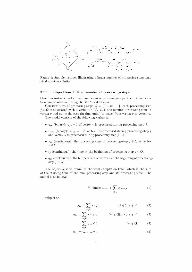
Figure 1: Sample instance illustrating a larger number of processing-steps mayyield a better solution.

3.1.1 Subproblem 1: fixed number of processing-steps

Given an instance and a fixed number m of processing-steps, the optimal solu-tion can be obtained using the MIP model below.

Consider a set of processing-steps Q = {0, ..,m − 1}, each processing-stepj ∈ Q is associated with a vertex v ∈ V . dv is the required processing time ofvertex v and cvu is the cost (in time units) to travel from vertex v to vertex u.

The model consists of the following variables:

• yjv (binary): yjv = 1 iff vertex v is processed during processing-step j.

• xjvu (binary): xjvu = 1 iff vertex v is processed during processing-step jand vertex u is processed during processing-step j + 1.

• sjv (continuous): the processing time of processing-step j ∈ Q at vertexv ∈ V .

• tj (continuous): the time at the beginning of processing-step j ∈ Q.

• qjv (continuous): the temperature of vertex v at the beginning of processing-step j ∈ Q.

The objective is to minimize the total completion time, which is the sumof the starting time of the final processing-step and its processing time. Themodel is as follows:

Minimize tm−1 +∑v∈V

sm−1,v (1)

subject to

yjv =∑u∈V

xjvu ∀j ∈ Q, v ∈ V (2)

yjv =∑u∈V

xj−1,uv ∀j ∈ Q|j > 0, v ∈ V (3)∑v∈V

yjv ≤ 1 ∀j ∈ Q (4)

y0,0 = ym−1,0 = 1 (5)

4

tj+1 ≥ tj +∑v∈V

sjv +∑v,u∈V

cvuxjvu ∀j ∈ Q|j 6= m− 1 (6)

∑j∈Q

sjv = dv ∀v ∈ V (7)

qj+1,v ≥ qjv + 2sjv − (tj+1 − tj) ∀j ∈ Q|j 6= m, ∀v ∈ V (8)

qjv + sjv ≤ B ∀j ∈ Q, v ∈ V (9)

sjv ≤ Byjv ∀j ∈ Q, v ∈ V (10)

xjvu ∈ {0, 1} ∀j ∈ Q, v, u ∈ S (11)

yjv ∈ {0, 1} ∀j ∈ Q, v ∈ V (12)

0 ≤ sjv ≤ B ∀j ∈ Q, v ∈ V (13)

0 ≤ tj ∀j ∈ Q (14)

0 ≤ qjv ≤ B ∀j ∈ Q, v ∈ V (15)

where (2) and (3) are linking constraints between x and y. (4) are flowconstraints while (5) imposes the starting and ending depot (vertex 0). Con-straints (6) define arrival times. Constraints (7) ensure total processing timesof vertices. Constraints (8) define arrival temperature of processing-steps. Thisequation comes from the linear increase and decrease of temperature, whichresults in the temperature at the beginning of the processing-step j + 1 beingdefined as qj+1,v = max(qjv + sjv − (tj+1 − (tj + sjv)), 0). (9) are temperatureconstraints and (10) are linking constraints between s and y. The rest are rangeconstraints.

3.1.2 Subproblem 2: fixed sequence of visits

Given a fixed sequence of visits, the optimal completion time can be obtained inpolynomial time using a Linear Programming (LP) model. Note that, unlike theMIP model in subproblem 1, this model only needs to consider visits eventuallyaggregating a number of processing-steps.

An example of a fixed sequence of visits can be found in figure 2. Thesequence has 4 visits, each of which is associated with a vertex, a processingtime and a waiting time. Visit 0, 1 and 3 include a single processing-step whoseprocessing time is smaller than or equal to the maximum temperature B (10time units) while visit 2 includes 2 processing-steps with total processing timep2 = 13 > B. Since its total processing time is larger than the maximumtemperature, a waiting time of w2 = B − p2 = 3 time units is required.

Figure 2: A fixed sequence of visits.

5

Given is a fixed sequence Σ of nΣ visits in which every vertex v ∈ V is visitedat least once. Let wi, pi and qi represent the waiting time, the total processingtime and the temperature at arrival of visit i (i ∈ {0, .., nΣ − 1}). Given a visiti associated with vertex v ∈ V , prei denotes the previous visit associated withthe same vertex (in the example in figure 2, pre2 = 0). Πv is the set of visitsassociated with vertex v ∈ V . An optimal visiting schedule of Σ, i.e. processingtimes and waiting times of its visits, can be calculated using the LP model asfollows.

Minimize

nΣ−1∑i=0

wi (16)

subject to

wi ≥ qi + pi −B i ∈ {0, ..., nΣ − 1}

(17)∑i∈Πv

pi = dv v ∈ V

(18)

qi ≥ qprei + (pprei − wprei)− cprei,prei+1 −i−1∑

k=prei+1

(cvkvk+1 + pk + wk) i ∈ {0, .., nΣ − 1}

(19)

wi, pi, qi ≥ 0 i ∈ {0, ..., nΣ − 1}(20)

The goal function (16) minimizes the total waiting time. Constraints (17)come from the statement of vertex temperature, namely that temperature uponarrival (qi) + processing time (pi) - waiting time (wi, corresponds with coolingdown of vertex) should never be larger than the maximum temperature (B).Constraints (18) make sure each vertex is processed exactly its required amountof time. Constraints (19) limit the temperature at the start of the ith visit frombelow by considering the arrival temperature (qprei), total processing time andwaiting time (pprei − wprei) of its previous visit and the tour time (travellingtimes plus processing times and waiting times) of all visits between prei and i(the remaining part of the equation). The program can be solved in polynomialtime in the number of variables which is proportional to nΣ.

6

Adding a visit to a sequence results in an increase in its total travellingtime. For any three vertices v, x, y ∈ V , let tvxy represent the travelling timeincreased when a visit of v is added between two consecutive visits of x and yin a sequence:

tvxy = cxv + cvy − cxy

We have the following:

Lemma 1. If, for a given sequence Σ, the optimal total waiting time WΣ =∑nΣ−1i=0 wi is less than or equal to minv,x,y∈V {tvxy}, no extension of Σ generated

by adding an extra visit can produce a shorter completion time.

Proof. Adding an extra visit increases the total travelling time by at leastminv,x,y∈V {tvxy} and reduces the waiting time by at most WΣ. Given thecondition WΣ ≤ minv,x,y∈V {tvxy}, the total processing time is increased.

3.2 Branch-and-bound approach

Based on the above subproblems and lemma, a branch-and-bound approach isproposed to solve the ITSP. We first present the data structure used in thealgorithm.

Each node of the search tree is a sequence of visits. Given a sequence, itsschedule, i.e. processing time and waiting time at each visit, is obtained usingthe LP model from subproblem 2. Since the total processing time is the samefor all nodes in the search tree, we omit it to simplify the model. A node ψin the search tree is a direct child of a node χ if ψ is created by inserting onemore visit into the sequence of χ. Since the triangle inequality holds, given anode χ with the total travelling time Tχ, the total travelling time of each of itsdescendants is larger than or equal to Tχ. Hence, we can say Tχ is a valid lowerbound for χ and all its descendants.

LBχ = Tχ

A node χ can be safely pruned when LBχ ≥ UB where UB is the globalupper bound of the search tree, i.e. Tχ∗ +Wχ∗ where χ∗ is the best solution sofar. A node is also pruned when the condition in lemma 1 is satisfied.

At the beginning of the search, the MIP model in subproblem 1 is solvedwith the minimum number of processing-steps Φ, which is calculated by addingup the minimum number of processing-steps of all vertices.

Φ =∑v∈V φv

The minimum number of processing-steps Φ ensures a feasible solution is alwaysfound. The solution given by subproblem 1 at this step provides an incumbentsolution, and hence the initial upper bound (UB) of the search tree.

The search is conducted in a best first search strategy using a priority queuewhose elements are always sorted ascendingly by the travelling times of theirsequences. The queue is initialized by all TSP sequences (i.e. all Hamiltoniantours of the input graph) whose travelling times are smaller than UB.

At each iteration, the sequence at the head of the queue is considered. If thepruning condition in lemma 1 is satisfied, the node is pruned. Otherwise, thebranching is conducted by generating and inserting all children of the sequence

7

considered into the priority queue so that the ascending order of travelling timesis still respected. In this manner, by the time the search terminates, the travel-ling time of the last sequence processed is the valid lower bound for the rest ofthe queue.

Everytime the number of processing-steps of the considered sequence is largerthan the processing-steps of the best solution, the MIP model in subproblem 1 issolved with the new number of processing-steps to obtain a new ITSP solution.If the new solution is better than the best solution, the best solution and UBare then updated accordingly. The search terminates when the gap between theUB and LB is closed or all nodes have been searched.

Since during the branching, different paths can lead to the same sequence,explored sequences are kept in a visited archive which is updated incrementallyduring the search. The algorithm is described in algorithm 1.

In line 1, the MIP model in subproblem 1 is solved with the minimum numberof processing-steps Φ. The resulting solution is the first incumbent solutionwhich provides the initial upper bound UB. In line 3, lower bound LB isobtained by solving the TSP on the original instance using Concorde (Applegateet al., 2006). If the gap is not closed after the initial phase, the priority queueQ is initialized with TSP sequences whose travelling times are smaller than UB(line 7). The visited archive is initialized in line 8 to keep track of the visitedsequences. The search is repeated until Q is emptied or the gap is closed. Ateach search step, the sequence at the head of the queue is selected and removedfrom the queue (line 10). LB is then updated accordingly (line 11 to 13). TheLP model in subproblem 2 is solved to obtain the corresponding ITSP solution(line 14). If the number of processing-steps of the obtained solution is largerthan the number of processing-steps of the best solution, the MIP model insubproblem 1 is solved with the new number of processing-steps (line 16). Thebest solution and UB are then updated accordingly (line 17-19). If lemma 1is not satisfied, the current sequence is branched, i.e. children sequences aregenerated and inserted into the queue (line 21 to 29). Otherwise, the branchingstops and the current sequence is pruned.

4 Variable Neighborhood Search

Variable Neighborhood Search (VNS) (Mladenovic and Hansen, 1997) is a meta-heuristic framework based on the systematic change of neighborhoods duringthe search in order to escape from the valleys containing local optima. The basicVNS uses a set of neighborhood structures denoted by Nk, k = {1, .., kmax}. Ateach iteration, a random solution from the kth neighborhood is generated. Alocal search procedure, which takes this random solution as the starting point,is then called to obtain a local optimum. The process repeats until some stop-ping criteria are met. The basic VNS framework is described in algorithm 2.A recent survey on the VNS can be found in (Hansen et al., 2010). The VNShas been successfully applied to many variants of the TSP (Sousa et al., 2015;Meng et al., 2018) and Vehicle Routing Problems (VRPs) (Wen et al., 2011;Pop et al., 2014).

In this paper, we use the general VNS (GVNS) (Hansen and Mladenovic,2002; Hansen et al., 2008), a variant of the VNS where the Variable Neighbor-hood Descent (VND) is used as the local search routine. The usual strategy

8

Algorithm 1: Branch-and-bound search

input : instance ins1 bestsol← solve subproblem 1 with the minimum number of

processing-steps Φ;2 UB ← objective value of bestsol;3 LB ← TSP travelling time given by Concorde;4 if LB = UB then5 optimal solution found, exit;6 end7 initialize queue Q with all TSP sequences whose travelling time < UB,

sorted in ascending order of travelling times;8 initialize visited archive ;9 repeat

10 current seq ← Q.dequeue() ;11 if travelling time of current seq > LB then12 LB ← travelling time of current seq ;13 end14 current sol← solve subproblem 2 to obtain the corresponding ITSP

solution of current seq ;15 if number of processing-steps of current sol > number of

processing-steps of bestsol then16 newsol← solve subproblem 1 with new number of

processing-steps ;17 if newsol is better than bestsol then18 update bestsol and UB ;19 end

20 end21 if stopping branching condition (according to lemma 1) is not satisfied

for current sol then22 list sequences← create list of all children sequences of

current seq;23 foreach seq in list sequences do24 if seq has not been visited then25 Q.enqueue(seq) ;26 update visited archive ;

27 end

28 end

29 end

30 until Q is emptied or gap closed ;

9

Algorithm 2: The VNS framework

input : A set of neighborhood structures Nk, k = 1, .., kmax1 x← construct the initial solution;2 repeat3 k ← 1;4 repeat5 Perturbation. Generate x′ randomly from Nk(x) ;6 Local search. x′′ ← apply some local search with x′ as the initial

solution;7 Neighborhood change. If x′′ is better than x, set x← x′′, (k ← 1)

and continue the search with N1; otherwise, set k ← k + 1;

8 until k = kmax;

9 until stopping condition is met ;

for exploration of several neighborhoods within deterministic local search is se-quential (Seq-VND) (Hansen et al., 2008), where a set of neighborhoods areused in the search. Local searches are performed in a pre-defined order of thisset. Everytime a better solution is found, the search returns to the first neigh-borhood in the list. The search stops when no improvement is found by anyneighbourhoods.

In the following sections, we define the necessary components to apply theGVNS for the ITSP: initial solution constructor, local search procedure andperturbation procedure.

4.1 Solution encoding

Before describing the VNS components, we hereby present the solution represen-tation. A solution is encoded as a list of processing-steps. Each processing-stepj consists of information of the corresponding vertex’s id (v), processing time(pj) and waiting time (wj) and the time that the processing actually starts (tj),i.e. the arrival time plus waiting time. To speed up the calculation, for eachvertex, a list of corresponding processing-steps is also recorded. The objectivevalue of a solution is the total processing time, i.e., the sum of the starting timeand the processing time of the last processing-step. An illustration of a solutionencoding can be found in figure 3.

4.2 Initial solution constructor

Two constructive heuristics are proposed, namely NearestVertex and LongestVer-tex.

NearestVertex This heuristic starts from a random vertex, progressively pro-cesses the current vertex maximally (e.g. until the maximum temperature isreached) and walks to a random vertex in a list of nearest vertices where pro-cessing can start before the cooling has stopped on the current one. If no suchvertex exists, the processing is continued at the same vertex after a properwaiting time. The algorithm is described in algorithm 3.

10

Figure 3: Solution encoding for an instance with 3 vertices. The solution in-cludes 5 processing-steps where vertex A is visited three times.

LongestVertex The heuristic picks a random vertex from the list of α verticeswith the longest remaining processing time. The processing of this vertex iscombined with the complete processing of other vertices, in order to facilitatethe cooldown of the current vertex, until it has been fully processed. Theheuristic is described in algorithm 4.

4.3 Local search

The local search procedure we choose is the Sequential VND (Hansen et al.,2008), where a set of neighborhoods is used. The Sequential VND iterativelyselects a move and calls the corresponding first improvement hill climbing localsearch to obtain a local optimum which is then used as the starting point forthe next iteration. The search terminates when no improvement is found byany neighborhood moves.

Thanks to the similarity in TSP and ITSP solution structures, neighborhoodclasses from the TSP are applicable for the ITSP. The following moves are usedin our algorithm: 2-opt (Croes, 1958), 3-opt (Bock, 1958) (Lin, 1965), or-optand remove-and-reinsert (Nilsson, 2003).

Due to the temperature constraints, evaluating the benefit of a move is costly.Therefore, we propose to estimate an ITSP move before actually proceedingwith the move. We illustrate this estimation using the 2-opt move as follows.Consider the TSP 2-opt move where edges (j, j + 1) and (k− 1, k) are replacedby (j, k−1) and (j+1, k) and the segment (j+1, k−1) is reversed (see figure 4),the move yields a benefit if cj,j+1 + ck−1,k − (cj,k−1 + cj+1,k) > 0 (in symmetricinstances). Therefore, checking if a move is beneficial in the TSP is O(1).

In the ITSP, due to the temperature constraints, arrival temperatures, start-ing times and waiting times of all processing-steps starting from k − 1 haveto be recalculated. The new objective value is estimated by only consideringprocessing-steps within an estimated radius r around j and k. The rational forthis estimation is that if there is a change in visiting times due to the temper-ature constraints, it is most likely caused by processing-steps in a small radiusaround the processing-steps involved in the move, since processing-steps of thesame vertices tend to be grouped together in a small segment. The estimationand the reasoning for it is illustrated in figure 4 where j = 3, k = 10 and themove reverses the segment from 4 to 9. In the new solution, time information

11

Algorithm 3: NearestVertex

input : Instance ins1 current← initialize solution with a random vertex ;2 repeat3 maximally process current;4 set nearby ← list of vertices where processing can start before the

cooling has stopped on current, ordered decreasingly by theirprocessing time left;

5 if set nearby is not empty then6 current← choose a vertex randomly from the α first vertices of

set nearby;

7 else8 ρ← processing time left on current;9 if ρ ≥ B then

10 wait at current for B time units;11 else12 wait at current for ρ time units;13 end

14 end

15 until there is no unprocessed vertex left ;

Algorithm 4: LongestVertex

input : Instance ins1 repeat2 list vertices← list of vertices ordered decreasingly by their

processing time left;3 current← choose a vertex randomly from α first vertices of

list vertices ;4 repeat5 maximally process current ;6 repeat7 next← find the nearest unprocessed vertex that can be

finished processing before current cools down completely ;8 maximally process next ;

9 until current is completely cooled down;

10 until current is completely processed ;

11 until there is no unprocessed vertex left ;

12

(starting time and waiting time) of processing-steps starting from 9 must berecalculated. To quickly estimate the move, only time information of the seg-ment (k − 1, k − r) (processing-steps 9 and 8 in the example) are recalculated.The time difference between the old solution and the new solution of k − r isforwarded to processing-step k (processing-step 10 in the example). Time in-formation of processing-steps in segment (k, k + r) (processing-steps 10, 11, 12)is then calculated, taking into account the forwarded time difference. The dif-ference between the starting time of processing-step k + r in the old solutionand k + r in the new solution (processing-step 12 in the example) will give anestimated delta objective to evaluate the move.

To calculate the new time information of processing-step 9 in the new se-quence, we need to look back to the processing-steps before it, i.e. processing-steps starting from 3 backwards to the beginning of the sequence, to check iftemperature constraints are violated. In the estimation, we look back only r = 2processing-steps before 3. As one can observe, the larger r is, the more precisethe estimation becomes.

If the estimated objective value is smaller than the original one, i.e. themove might be beneficial, we proceed with the move and recalculate the wholesolution to get the exact objective value. A similar scheme is applied for othermoves.

Figure 4: Move evaluation example.

For each neighborhood move, a first improvement hill climbing search isdeveloped. When a local optimum is reached, the processing time of eachprocessing-step is probably not optimal for the given sequence anymore. There-fore, a post processing is applied to adjust the processing time of each processing-step. This is done by solving the LP model in section 3.1 for the correspondingsequence.

4.4 Perturbation

Perturbation plays an important role in guiding the search to exploit new regionsof the search space. Starting at the local optimum given by the local searchprocedure, perturbation makes a large move to jump to a distant neighbor inorder to escape from the corresponding valley. We propose two perturbationmoves for the framework: ruin-and-recreate and modified hyperedges exchange.

13

Ruin-and-Recreate (RR) A RR move (Schrimpf et al., 2000) includes twophases: the ruin phase removes some vertices from the tour while the recreatingphase inserts those vertices into the tour. The RR for the ITSP is conducted asfollows: In the ruin phase, a seed vertex chosen randomly is removed from thesolution. Then a number of its closest vertices are also removed. Afterward,the recreate phase reinserts those vertices back into the tour using the bestinsertion strategy. The parameter of the RR move is the percentage of verticesbeing removed from the route.

Guided hyperedges exchange A hyperedge H = (a0, h) includes h consec-utive edges and starts from vertex a0. In hyperedges exchange, two hyperedgesH1 = (a0, h) and H2 = (b0, h) are removed from the tour leaving their ver-tices isolated. Those vertices are then reconnected to the tour randomly. Thehyperedges exchange move is illustrated in figure 5.

Figure 5: Hyperedges exchange.

In order to guide the algorithm to a promising region of the search space, weadopt the guided perturbation of (Burke et al., 2001) in the ITSP by utilizinginformation of the current tour. The quality of a hyperedge H = (a0, a1, .., ah−1)is evaluated by:∑

j∈H(cj,j+1 −minv∈V |v 6=vjcvj ,v) + µ∑j∈H wj

with wj the waiting time at processing-step j and µ the normalizing factor. Thefirst term of the formula measures the difference between the total distance fromeach visit to its successor in the hyperedge and to its closest neighbor. A largedifference indicates that there might be a chance to obtain a shorter path bydestroying and re-routing that path. The second aggregates the waiting timesalong the hyperedge. The reasoning behind this term is that if we have to waitfor a long time at a vertex, then it might be better to visit other vertices insteadof waiting there. The role of µ is to distribute the influence of the two termsequally. The value of µ is set as the ratio between the first term and the secondterm of the first hyperedge whose aggregate waiting time is positive (denotedby H∗).

µ =∑

j∈H∗ (cj,j+1−minv∈V |v 6=vjcvj,v)∑

j∈H∗ wj

In total, a high value of the function implies a poor quality hyperedge.In guided hyperedges exchange, hyperedges are sorted increasingly by their

quality values. At each perturbation step, a hyperedge is chosen randomly fromthe first θ percent of hyperedges in the list while the second hyperedge is chosencompletely randomly.

14

Algorithm 5: GVNS for the ITSP

1 x← construct the initial solution using LongestVertex or NearestVertex ;2 k ← Λmin;3 repeat4 Perturbation. x′ ← perturb x with strength k;5 Local search. x′′ ← apply VND with x′ as the starting point;6 Neighborhood change.7 if If x′′ is better than x then8 set x← x′′;9 continue the search with k ← Λmin;

10 else11 set k ← k + δΛ;12 end

13 until k ≤ Λmax or a timeout is reached ;

4.5 The GVNS for the ITSP

Given the components described earlier, the GVNS for the ITSP is conducted asfollows. The neighborhood change is given by different strength of perturbation.Perturbation strength k is initialized with its minimum value Λmin. At eachiteration, a random solution is generated by perturbing the current solutionwith strength k. This solution serves as the starting point for the Seq-VNDprocedure. If a better solution is found, the incumbent solution is updated andk is reset to Λmin. Otherwise, the solution is perturbed again with the samestrength. After n perturbations without improvement, where n is the number ofvertices of the instance, k is increased with a step of δΛ. The search terminateswhen k exceeds its maximum allowed value Λmax or a timeout is reached. OurGVNS algorithm for the ITSP is described in algorithm 5.

Given two construction heuristics and two perturbation types, four differentVNS metaheuristics are created. The two construction heuristics are namedNearest (NearestVertex) and Longest (LongestVertex) while the two perturba-tion types are named RR (Ruin-and-Recreate) and Exchange (guided hyper-edges exchange). Their combinations result in four different VNS metaheuris-tics: NearestRR, NearestExchange, LongestRR and LongestExchange respec-tively.

5 Experiment

5.1 Test instances

Since the problem is new in literature, we introduce a problem library consistingof two sets: set R includes instances generated randomly and set T includesinstances generated from instances of the TSPLIB (Reinelt, 1991). All instancesand best results are made publicly available at https://set.kuleuven.be/codes/itsp page.

There are two important features influencing the difficulty of an instance:(1) bound ratio which is the ratio between the maximum temperature (B) andthe average travelling time between vertices (C). (2) instance density which

15

Table 1: Density setting configuration

D0 D1 D2 D3 D4 D5 D6 D7 D8 D9 D10single-step (%) 100 90 80 70 60 50 40 30 20 10 102-steps (%) 0 10 20 30 40 40 50 60 70 70 703-steps (%) 0 0 0 0 0 10 10 10 10 20 104-steps (%) 0 0 0 0 0 0 0 0 0 0 10

determines the number of vertices of each type. In our test instances, there are 4types of vertices: 1, 2, 3 and 4-steps. A γ-step vertex needs at least γ processing-steps to finish, i.e. its processing time p lies in the range (γ − 1)B < p ≤ γB.The number of vertices of each type in an instance is determined by its densitysetting. There are in total 11 density settings from D0 to D10. Lower densitysetting results in sparser instance. The detailed percentages of each type ofvertex in each density setting are given in table 1.

In set R, vertex coordinates are generated randomly in a square box. Inset T, vertex coordinates are taken from the corresponding TSPLIB instance.Then, given a bound ratio and a density setting, processing times of vertices aregenerated accordingly. Instances are named after their size and settings. Forexample, an instance with size of 20 vertices, density setting D0 and bound ratio10 is named 20 D0 10. In case several instances have the same setting, an indexis appended at the end of their names, e.g. 20 D0 10 1 and 20 D0 10 2. Namesof instances in set T includes their original name. E.g. instance 77 D9 10 pr76is generated from instance pr76, consists of 77 vertices (including the depot),has density setting D9 and bound ratio 10. Similarly to set R, an index isused to distinguish instances generated from the same TSPLIB instance andsharing the same setting. Both set R and T include many subsets for differentexperiments which will be presented in more detail in the following sessions.

The experiment consists of two parts. In the first part, we evaluate theperformance of the branch-and-bound (BNB) approach and analyse problemdifficulty regarding their settings using small instances in set R. In the secondpart, the VNS approach is evaluated using instances from both sets R and T .All algorithms are implemented in Java. The MIP solver used is Gurobi 6.0.5(Gurobi Optimization, 2015). Tests for the BNB algorithm are carried out ona Core i7, 2.9 GHz Intel machine with 7.7 GB of RAM. Tests for the VNS arecarried out on a Linux-based PC cluster, with Intel Xeon E5-2680v3 2.5 GHzCPUs and a budget of 9GB of RAM for each core.

5.2 Evaluation of the branch-and-bound approach

Three different experiments are carried out for different purposes. Three subsetsof instances (R1, R2 and R3) with different sizes and settings are generatedconsequently.

In the first experiment on subset R1, the BNB performance with differentinstance sizes is evaluated. Instance size ranges from 6 to 12 vertices. For eachsize, 22 instances are generated corresponding to the combination of 11 densitysettings and 2 bound ratio settings (1 and 100).

In the second experiment on subset R2, we aim to analyse problem difficultyregarding bound ratio setting. Test instances have bound ratio ranging from 0.1

16

Table 2: Instance configuration of set R

Subset No. instances Instance size Bound ratio DensityR1 154 6,7,8,9,10,11,12 1,100 D0 to D10R2 200 10 0.1, 0.2, 0.4, ..., 51.2 (10 settings) D2R3 220 10 10 D0 to D10

to 51.2, the next ratio is double the current ratio ([0.1, 0.2, 0.4, ...25.6, 51.2]).Instance size and density setting are fixed as 10 vertices and D2 respectively forall instances. For each bound ratio, 20 instances are generated.

In the third experiment on subset R3, we analyse problem difficulty regardingdensity setting. There are 11 density settings as listed in table 1. Instance sizeis fixed as 10 vertices and bound ratio is 10 for all instances. For each densitysetting, 20 instances are generated. The summary of three subsets and theirconfigurations can be found in table 2.

A time limit of 1200 seconds is imposed on the MIP solver to solve subprob-lems and 3600 seconds on the BNB algorithm.

The results of this experiment are analysed in figure 6 and table 3. Figure 6shows the box plots of the running times of the algorithm on the three subsetswhile table 3 reports the average values of the running times, initializing timesand the size of the queue for each subset, categorized by the correspondingtargeted feature (instance size in R1, bound ratio in R2 and density setting inR3). In most of the test instances, optimal solutions are found, except somelarge instances in set R1. In the experiment, if the running time of an instanceexceeds the time limit (3600 seconds), its optimal solution is not found.

Figure 6a shows the results for experiment 1 on subset R1 of instances withdifferent sizes. We can see easily from the figure that problem difficulty dependshighly on instance size (which is predictable). The corresponding initializingtimes and queue sizes given in table 3 show that the larger an instance is, thelonger it takes to initialize the queue. This is caused by the exponential increasein the number of TSP sequences when the instance size increases. This suggeststhat the BNB approach is not scalable for big instances.

Figure 6b shows the results for experiment 2 on subset R2 including in-stances with the same size and density setting but different bound ratio. Asshown in the figure, problem difficulty increases when bound ratio increases.This can be explained as follows. A large bound ratio means a large differencebetween the maximum temperature B and the average travelling time C, whichleads to more waiting times in the solution. Since LB is the total travelling timeof the solution and UB is the sum of the total travelling time and the aggregatewaiting time, a large aggregate waiting time results in a large gap between LBand UB. A large gap makes an instance difficult for the BNB algorithm tosolve. This also results in a bad cut-off value for the initializing process, whichis reflected in the large initializing times and queue sizes in instances with largebound ratio in table 3. This explains why instances with high bound ratio set-tings tend to be more difficult. This also explains the small differences whenthe bound ratio exceeds 2. The larger the bound ratio is, the larger the aggre-gate waiting time in the solution is. However, when the bound ratio exceeds 2,the waiting times are mostly 0 and cannot go any lower. Therefore, given thesame instance size, instances with bound ratio exceeds 2 have similar level of

17

Table 3: Branch-and-bound results on the three subsets R1, R2 and R3 respec-tively

Running time Initializing time Queue sizeAvg (seconds) Std (%) Avg (seconds) Std (%) Avg (seconds) Std (%)

Instance size (R1)6 1.56 247.41 0.05 55.16 47.36 92.587 2.11 180.45 0.17 76.86 136.91 115.028 27.59 262.59 0.92 96.76 989.55 148.079 146.54 201.74 5.07 114.18 4763.86 170.4410 453.66 127.03 47.01 142.99 58412 176.0111 1366.57 111.49 1096.72 142.4 196706.68 162.2812 1982.27 79.28 1845.38 89.4 44230.86 194.8

Bound ratio (R2)0.1 1.39 43.54 0.5 86.92 9.3 83.920.2 2.38 68.44 0.99 106 41.95 94.210.4 4.22 110.14 1.54 95.92 159.8 159.980.8 3.66 93.09 1.11 86.14 125.5 181.241.6 9.14 108.87 3.65 131.55 849.6 141.383.2 17.97 64.99 7.33 102.9 1345.78 205.26.4 10.3 105.59 4.89 127.75 830.26 185.9312.8 12.54 97.3 5.93 137.03 1901.35 172.9625.6 16.34 92.38 6.02 112.16 1958.75 163.9551.2 16.02 91.12 7.82 129.12 1929.05 171.5Density setting (R3)D0 0.85 57.41 0 0 0 0D1 14.82 116.68 7.6 130.8 620.9 208.15D2 29.2 64.76 11.44 80.16 1002.95 134.64D3 81.44 98.12 42.63 146.54 10902.8 172.91D4 135.93 81.11 45.14 107.24 12652.8 167.87D5 778.6 58.78 133.93 70.58 57030.1 103.95D6 1003.41 43.59 120.4 79.78 89603.8 95.05D7 1142.34 32.23 96.66 62.74 128895.2 86.57D8 1212.93 14.93 78.84 67.38 94191.5 100.81D9 1350.65 3 152.95 22.23 232340.47 38.31D10 1615.17 9.93 414.89 38.63 275203.7 37.05

difficulty.Figure 6c shows the results for experiment 3 on subset R3 which aims to

compare the BNB performance on different density settings. Predictably, thedenser an instance is, the harder it is to solve. This can also be explained bythe large aggregate waiting time in dense instances.

To give some more insight into how the BNB works, we analyse the detailedresults of some selected instances from all 3 subsets in table 4. Informationreported includes: instance name, itsp size (e.g. minimum number of processing-steps), search status (FINISHED means optimum found, the queue is emptiedwithin the time limit or the gap is closed), running time, queue initializing time,size of the search queue, lower bound, upper bound and finally solution gap.What stands out in the table is that in D0 instances, the number of nodes inthe search tree is 0. This can be explained as follows. For D0 instances whereall vertices are 1-step vertices, a TSP solution makes a valid ITSP solution.Therefore, in those instances, the gaps are closed right at the initial phase whenthe lower bound and upper bound are obtained. That is why those instances areeasy to solve, resulting in small solving times of less than 2 seconds. In contrast,in big instances, the queue sizes are large and the time taken to initialize thequeue takes up all the time budget. This is the main reason why the BNB isnot scalable to big instances.

18

(a) Comparison on instancesize,subset R1.

(b) Comparison on boundratio,subset R2.

(c) Comparison on densitysetting,subset R3.

Figure 6: Branch-and-bound performance on different subsets.

Table 4: Detailed results on some selected instances in set R

Instance Itspsize Status Running timeQueue initializingtime

Queue size LB UB Gap

8 D9 100 16 FINISHED 466.67 2.56 4974 476 476 0.00%8 D9 1 16 FINISHED 156.72 2.36 3084 406 406 0.00%9 D0 100 10 FINISHED 0.15 0 0 334 334 0.00%9 D0 1 10 FINISHED 0.14 0 0 285 285 0.00%10 D1 1 12 FINISHED 2.95 1.36 128 412 412 0.00%10 D2 100 13 FINISHED 10.23 4.44 564 387 387 0.00%10 D2 51.2 10 13 FINISHED 39.2 18.7 5328 488 488 0.00%10 D2 51.2 11 13 FINISHED 5.72 1.94 318 361 361 0.00%10 D6 10 5 10 FINISHED 172.67 71.22 57194 502 502 0.00%10 D6 10 6 10 FINISHED 663.03 119.96 121862 498 498 0.00%11 D3 100 15 FINISHED 31.5 5.05 452 356 356 0.00%11 D3 1 15 FINISHED 4.17 0.99 191 315 315 0.00%12 D0 1 13 FINISHED 1.47 0 0 422 422 0.00%12 D4 100 17 FINISHED 2605.94 711.32 50962 486 486 0.00%12 D4 1 17 FINISHED 443.75 129.63 2128 384 384 0.00%12 D5 100 19 TIMEOUT 3600 3600 15611 348 598 41.81%12 D5 1 19 TIMEOUT 3600 1255.68 220195 298 416 28.37%12 D6 100 21 TIMEOUT 3600 3600 2734 395 633 37.60%12 D10 100 26 TIMEOUT 3600 3600 2475 376 845 55.50%

19

Table 5: Parameters tuning

Parameter Description Test values Best settingα Construction heuristics’ list length 10, 50 (%) 10r Estimated radius for local search 3, 10 (processing-steps) 3θ Hyperedges list size proportion 25, 75 (%) 75(Λmin,Λmax) Perturbation min strength and max strength (10, 60), (30, 90) (%) (30, 90)δΛ Perturbation strength step 5, 10 (%) 10

Table 6: The VNS performance on set R

NearestRR NearestExchange LongestRR LongestExchangeR1 0.00% 0.00% 0.08% 0.08%R2 0.00% 0.00% 0.16% 0.17%R3 0.00% 0.00% 0.01% 0.01%

5.3 Calibration of the metaheuristics

In order to tune the metaheuristic parameters, a tuning set is created by select-ing instances from all subsets of set R and T in such a way that instances ofall sizes and configurations are used. The size of the tuning set is 50 instances.For each parameter, 2 values are selected in a way that they cover most of itsvalue ranges. The combination of 5 sets of parameters, with 2 values for each,results in 32 experiments. Note that θ, the hyperedge list size proportion, isused in NearestExchange and LongestExchange only. For each instance, eachexperiment, the four metaheuristics (NearestRR, NearestExchange, LongestRRand LongestExchange) are applied for 10 runs with a time limit of 100 secondsfor each. The best setting is selected from the combination which gives thesmallest average deviation from best solutions. However, the one-way ANOVAtest performed on the results shows that there is no significant difference be-tween different parameter settings (F = 0.08, p = 0.99). The parameters, theirtested values and the best settings are listed in table 5.

5.4 Results and metaheuristics comparison

To evaluate and compare the four metaheuristics proposed in this paper, threeexperiments are conducted. The results of all experiments in this section arethe average of 5 runs.

In the first experiment, the four metaheuristics are tested on all three subsetsof set R which consists of small randomly generated instances. A time limit of5 seconds is imposed on all of them. Table 6 shows the average deviation fromthe optimal solution for each metaheuristic and instance set. It can be seenfrom the table that all metaheuristics perform very well on those instances,especially NearestRR and NearestExchange with the average deviation of 0%in all instance sets. LongestRR and LongestExchange show small deviationsespecially in set R2 but is still less than 0.2%.

For the second experiment, a set of special instances T1 are generated fromthe TSPLIB in a way that the optimal solutions are known. From a TSPLIBinstance, a special instance is generated by setting the maximum temperatureequal to 100, and the processing time of each vertex equal to 1. In such in-

20

stances, each vertex is visited exactly once. Therefore its optimal solution isthe optimal TSP solution (which is known) plus the number of vertices. T1includes 80 instances corresponding with 80 TSPLIB instances with the sizeranging from 14 to 3028 vertices. The time limit is set to 1800 seconds. Theresults for the second experiment are shown in figure 7. The first plot showsthe deviation of the metaheuristics’ results from the optimal solutions while therunning time is showed in the second plot. The results are good on NearestRRand NearestExchange with average optimality gaps of 4.09 and 4.21 respectivelywhile LongestRR and LongestExchange, with average gaps 13.39 and 14.14 re-spectively, reveal inefficiency in large instances.

NearestRR NearestExchange LongestRR LongestExchange

0

20

40

60

80

devia

tion f

rom

opti

mal (%

)

NearestRR NearestExchange LongestRR LongestExchange

0

250

500

750

1000

1250

1500

1750

runnin

g t

ime (

seconds)

Figure 7: Results on special instances of set T1.

In the third experiment, the four metaheuristics are tested on big instancesof set T2. 30 instances from the TSPLIB are randomly selected to generateinstances in this set. For each instance, we generate 10 instances correspondingto the combination of density settings D0, D2, D4, D7, D9 and bound ratio set-tings 0.1, 10. Therefore, set T2 consists of 300 instances. The sizes of instancesin set T2 vary from 49 to 5916 vertices and the number of minimum processing-steps (which is called the ITSP-size) ranges from 49 to 12422. Similarly to thesecond experiment, a time limit of 1800 seconds is imposed.

Since optimal solutions are unknown for those instances, we compare theresults with the best known solutions obtained so far for each instance. In table7, the results are reported by groups of instances. Reported information includesthe average deviation from the best know solutions and average running time.The first row of the table shows the results of each metaheuristic on the wholeset. The next four rows show the detailed performances of each metaheuristicon each subgroup of set T corresponding to 5 different density settings (D0 toD9). The last two lines show results on 2 subsets corresponding to 2 boundratio settings (0.1 and 10). The results diverge more on instances with a smallbound ratio.

A one-way ANOVA test on the results shows a statistically significant dif-ference between the four algorithms (F = 43.52, p < 0.001). It can be seen thatNearestRR performs the best among the four metaheuristics. Paired-samplest− tests between NearestRR and the other three metaheuristics all give p-valueless than 0.001.

The metaheuristics using NearestVertex outperform the ones using LongestVer-tex in general, especially in a small bound ratio setting (0.1). This can be ex-plained by the inclusion of the NearestVertex starting solution. This leads toa better performance, because it is more worthwhile to move to vertices that

21

Table 7: Metaheuristics performance on set T2

NearestRR NearestExchange LongestRR LongestExchange

Avg. dev (%)Avg. Time(seconds)

Avg. dev(%)

Avg. Time(seconds)

Avg. dev(%)

Avg. Time(seconds)

Avg. dev(%)

Avg. Time(seconds)

Overall 0.35 1187.52 0.76 1270.66 7.31 1266.16 7.95 1229.58Density

D0 0.48 949.49 1.24 1003.1 6.04 1040.01 7.01 985.58D2 0.44 1197.03 0.91 1284.02 7.83 1299.87 8.47 1187.41D4 0.28 1214.66 0.63 1288.11 6.96 1284.55 7.66 1269.08D7 0.28 1271.36 0.51 1381.5 7.37 1384.1 7.87 1358.81D9 0.24 1334.46 0.48 1429.08 8.55 1348.56 8.9 1373.51

Bound ratio0.1 0.68 1224.63 1.49 1249.34 14.51 1272.89 15.76 1245.0310 0.03 1151.44 0.06 1291.39 0.31 1259.62 0.35 1214.55

are close by, rather than to move to vertices which have the longest remainingprocessing time. This holds especially for higher density settings, since in thiscase more visits to each vertex are required, resulting in higher travelling timesfor LongestVertex. Furthermore, Ruin-and-Recreate outperforms HyperedgesExchange, because the former works with a closely connected subset of vertices,whereas the latter considers longer edges. Hence, it is shown that also for per-turbation it is better to change the solution by considering vertices closest tothose removed (ruin phase) rather than employing hyperedges. This results ina comparatively better performance of NearestRR and LongestRR versus Near-estExchange and LongestExchange respectively.

6 Conclusion and future work

In this paper we introduced a new variant of the TSP, namely the IntermittentTravelling Salesman Problem (ITSP), where a vertex may have to be visitedmore than once and there is a time lapse enforced between two consecutivevisits due to the temperature constraint. An exact branch-and-bound approachis proposed to solve small instances. Instance difficulty regarding its properties isanalysed based on the results from the exact approach. To tackle large instances,four VNS metaheuristics are built and compared with each other. An instancelibrary consisting of two sets is built and made publicly available. The first setR contains small, randomly generated instances while the second set T containslarge instances generated from instances of the TSPLIB. The results on smallinstances illustrate that all 4 metaheuristics result in very small deviation fromoptimal solutions, especially NearestRR and NearestExchange. On big instances,NearestRR performs the best on all instance sets while the performances of theother metaheuristics depend on instance properties.

The problem described in this paper is a simplification with respect to thereal world setting in that we approximated the cooling schemes by linear func-tions and supposed them to be uniform over the workpiece. In future work,quadratic or exponential cooling and heating functions will be studied, as well asthe influence of position dependent cooling and the interaction between nearbyvertices. The simplified problem in its own right, even though it is shown tobe accessible through usual combinatorial optimisation approaches, turns outto be particularly challenging. Interesting subjects to investigate in the futureare stronger exact approaches, e.g. based on decomposition, for - approximately- solving larger instances. Heuristic approaches relying on alternative problem

22

representations or approximate delta evaluation of the objective function alsodeserve further attention.

References

Applegate, D., Bixby, R., Chvatal, V., Cook, W., 2006. Concorde tsp solver.

Bock, F., 1958. An algorithm for solving “traveling salesman” and relatednetwork optimization problems, presented at the 14th national meeting ofthe operations research society of america, st. Louis, Missouri

Burke, E.K., Cowling, P.I., Keuthen, R., 2001. Effective local and guidedvariable neighbourhood search methods for the asymmetric travelling sales-man problem. In Workshops on Applications of Evolutionary Computation,Springer, pp. 203–212.

Campbell, A., Clarke, L., Kleywegt, A., Savelsbergh, M., 1998. The inventoryrouting problem. In Fleet management and logistics. Springer, pp. 95–113.

Croes, G.A., 1958. A method for solving traveling-salesman problems. Opera-tions research 6, 6, 791–812.

Dumas, Y., Desrosiers, J., Gelinas, E., Solomon, M.M., 1995. An optimal al-gorithm for the traveling salesman problem with time windows. Operationsresearch 43, 2, 367–371.

Gurobi Optimization, I., 2015. Gurobi optimizer reference manual; 2015. URLhttp://www. gurobi. com

Gutin, G., Punnen, A.P., 2006. The traveling salesman problem and its varia-tions, Vol. 12. Springer Science & Business Media.

Hansen, P., Mladenovic, N., 2002. Developments of variable neighborhoodsearch. In Essays and surveys in metaheuristics. Springer, pp. 415–439.

Hansen, P., Mladenovic, N., Perez, J.A.M., 2008. Variable neighbourhoodsearch: methods and applications. 4OR 6, 4, 319–360.

Hansen, P., Mladenovic, N., Perez, J.A.M., 2010. Variable neighbourhoodsearch: methods and applications. Annals of Operations Research 175, 1,367–407.

Johnson, D.S., McGeoch, L.A., 1997. The traveling salesman problem: A casestudy in local optimization. Local search in combinatorial optimization 1,215–310.

Laporte, G., 1992. The traveling salesman problem: An overview of exact andapproximate algorithms. European Journal of Operational Research 59, 2,231–247.

Lin, S., 1965. Computer solutions of the traveling salesman problem. The BellSystem Technical Journal 44, 10, 2245–2269.

23

Meng, X., Li, J., Dai, X., Dou, J., 2018. Variable neighborhood search for acolored traveling salesman problem. IEEE Transactions on Intelligent Trans-portation Systems 19, 4, 1018–1026.

Mladenovic, N., Hansen, P., 1997. Variable neighborhood search. Computers &operations research 24, 11, 1097–1100.

Nilsson, C., 2003. Heuristics for the traveling salesman problem. Technicalreport, Tech. Report, Linkoping University, Sweden.

Pop, P.C., Fuksz, L., Marc, A.H., 2014. A variable neighborhood search ap-proach for solving the generalized vehicle routing problem. In InternationalConference on Hybrid Artificial Intelligence Systems, Springer, pp. 13–24.

Reinelt, G., 1991. Tspliba traveling salesman problem library. ORSA journalon computing 3, 4, 376–384.

Schrimpf, G., Schneider, J., Stamm-Wilbrandt, H., Dueck, G., 2000. Recordbreaking optimization results using the ruin and recreate principle. Journalof Computational Physics 159, 2, 139–171.

Sousa, M.M., Ochi, L.S., Coelho, I.M., Goncalves, L.B., 2015. A variable neigh-borhood search heuristic for the traveling salesman problem with hotel se-lection. In Computing Conference (CLEI), 2015 Latin American, IEEE, pp.1–12.

Wen, M., Krapper, E., Larsen, J., Stidsen, T.K., 2011. A multilevel vari-able neighborhood search heuristic for a practical vehicle routing and driverscheduling problem. Networks 58, 4, 311–322.

24