STABILITY OF COMPRESSIVE ANDUNDERCOMPRESSIVE THIN FILM TRAVELLING WAVESAndrea Bertozzi1Center for Nonlinear and Complex Systemsand Departments of Mathematics and PhysicsDuke UniversityDurham, NC 27708-0320Andreas M�unchZentrum Mathematik (H4)Technische Universit�at M�unchenD-80290 M�unchenGermanyMichael Shearer2Center for Research in Scienti�c Computationand Department of MathematicsNorth Carolina State UniversityRaleigh, NC 27695{8205andKevin Zumbrun3Department of MathematicsIndiana UniversityBloomington, IN 47405-4301December 8, 19991Supported by a PECASE award from the O�ce of Naval Research, and a Sloan ResearchFellowship.2Adjunct Professor of Mathematics at Duke University. Research supported by NationalScience Foundation grant DMS 9504583 and by Army Research O�ce grant DAAG55-98-1-0128.3Research supported in part by the National Science Foundation under Grant No. DMS-9706842.

AbstractRecent studies of liquid �lms driven by competing forces due to surface ten-sion gradients and gravity reveal that undercompressive traveling waves play animportant role in the dynamics when the competing forces are comparable. In thispaper we provide a theoretical framework for assessing the spectral stability ofcompressive and undercompressive traveling waves in thin �lm models. Associatedwith the linear stability problem is an Evans function which vanishes precisely ateigenvalues of the linearized operator. The structure of an index related to theEvans function explains computational results for stability of compressive waves.A new formula for the index in the undercompressive case yields results consistentwith stability.In considering stability of undercompressive waves to transverse perturbations,there is an apparent inconsistency between long-wave asymptotics of the largesteigenvalue and its actual behavior. We show that this paradox is due to the unusualstructure of the eigenfunctions and we construct a revised long-wave asymptotics.We conclude with numerical computations of the largest eigenvalue, comparisonswith the asymptotic results, and several open problems associated with our �nd-ings.

2

1 IntroductionDriven �lms exhibit a variety of complicated dynamics ranging from rivulets and saw-tooth patterns in gravity driven ows [JdB92, SV85] to patterns in spin coating [FH94]and surfactant driven �lms [TWS89]. A theoretical framework for these problems isprovided by a lubrication approximation of the Navier-Stokes equations [MW99, Gre78].This yields a single partial di�erential equation for the �lm thickness as a function ofposition on the solid substrate and time.For directionally driven �lms, the driving force enters into the lubrication approxi-mation as the ux f in a scalar hyperbolic conservation law ut+(f(u))x = 0. Here u > 0is the �lm thickness and x is the direction of the driving force. For gravity driven ow onan incline, the tangential component of gravity yields a ux proportional to u3 [Hup82].For surface-tension gradient driven ows f is proportional to u2 [CHTC90]. In each ofthese cases, the ux is convex. Consequently, driven fronts in the �lm correspond tocompressive shock solutions, whose simplest form isu(x; t) = � u�; if x < st;u+; if x > st; (1.1)in which the shock speed s = (f(u�)� f(u+))=(u� � u+) satis�es the entropy conditionf 0(u+) < s < f 0(u�); (1.2)equivalently, characteristics enter the shock on each side. Small variations in height neara compressive shock are propagated towards the shock from both sides.In practice, the discontinuous fronts (1.1) are smoothed by di�usive e�ects, primarilythrough surface tension. In the lubrication approximation, surface tension appears as afourth order nonlinear regularization of the conservation law, but there is also secondorder nonlinear di�usion induced by the component of gravity normal to the incline,leading to the equationut + (f(u))x = � r � (u3r�u) + �r � (u3ru): (1.3)In this equation, > 0 and � � 0 are constants. The shock waves (1.1) correspond tosmooth traveling wave solutions of (1.3); for small � � 0; they typically have oscillatoryovershoots and undershoots on either side of the shock. Additionally, the nonlinearityin the fourth order di�usion causes a single very pronounced overshoot or `bump' on theleading edge of the shock (see Fig. 1a); this structure is often referred to as a capillaryridge in experiments. Capillary ridges produced by surface tension are well known tobe linearly unstable to long-wave perturbations in the transverse direction of the ow,producing the well-known �ngering instability [CC92, THSJ89, KT97, YC99]. The e�ectof larger � is to suppress the bump (see Fig. 1b). The disappearance of the bump (for �su�ciently large) is accompanied by a transverse stabilization of the wave [BB97].3

u+=0.1u+=0.01u+=0.001

u+=0.1u+=0.01u+=0.001

(a) (b)Figure 1: Compressive traveling waves for the ux f(u) = u3, connecting u� = 1 to u+;for three values of u+: (a): � = 0, = 1: All waves are linearly unstable to transverseperturbations. (b): � = 5, = 1. The waves with u+ = 0:1; 0:01 are linearly stable totransverse perturbations.Experiments with doubly driven �lm ow, in which gravitational and surface ten-sion gradient stresses are competing, have uncovered some new phenomena. While verythin �lms produce the characteristic capillary ridge followed by a �ngering instability[CHTC90], thicker �lms produce a wider capillary ridge that continues to broaden. Fur-thermore, the front, or leading edge of the �lm, remains planar; it does not experience�ngering [BMFC98, KT98].The lubrication approximation for this problem yields an equation of the form (1.3)with a non-convex ux f(u) = u2 � u3: (1.4)Numerical experiments [BMS99, MB99, M99] and analysis [BS99] with � small showthat the experimental observations can be explained by the presence of undercompres-sive shocks. In particular, while weak jump initial data give rise to compressive waves,moderately strong jumps can evolve into a double shock structure in which the lead-ing shock is undercompressive: the speed s of the shock violates the entropy condition(1.2). The trailing wave is compressive and travels at a slower speed. For stronger initialjumps, the solution evolves as a rarefaction wave connected to an undercompressive wave[MB99]; this structure explains discrepancies between earlier thin �lm experiments [LL]and analysis based on the classical theory of conservation laws, which considers onlycompressive waves. The presence of undercompressive shocks is due to the combinede�ects of the non-convex ux and the fourth order di�usion. Moreover, numerical com-putations [MB99] con�rm that the undercompressive leading wave is linearly stable totransverse perturbations, while the stability of the compressive shocks depends on theabsence of a capillary ridge. 4

The numerical simulations of [BMS99] also reveal a complicated relationship betweeninitial condition/far �eld boundary condition and asymptotic behavior of solutions. Morespeci�cally, for a range of far-�eld boundary conditions, the asymptotic solution couldeither be one of a number of compressive travelling waves (see e.g. Figure 2), or it couldapproach the two-wave structure described above, with an undercompressive leadingfront. The speci�c asymptotic solution that emerges in this case depends on the shapeof the initial data u(x; 0): For other far-�eld boundary conditions, only the two-wavestructure is realized asymptotically, irrespective of the shape of the initial data.In this paper we consider traveling wave solutions u(x; y; t) = u(x�st) of the generalequation ut + f(u)x = r � (b(u)ru) �r � (c(u)r�u) ; (1.5)in which we assume(H0) f; b; c 2 C2;(H1) c � � > 0; b � 0while keeping in mind the special case studied in [BMS99], corresponding to:f(u) = u2 � u3; b(u) = �u3; c(u) = u3; � � 0; > 0: (1.6)The existence of traveling waves is itself an interesting problem. For convex uxes,the existence of traveling waves can be proved by a shooting argument as in [KH75] orusing topological methods involving the Conley index as in [Ren96, BMS99]. The case ofa non-convex ux such as (1.4) is more complicated. In particular, the phase portrait forthe resulting traveling wave ODE can have more than two equilibria and the possibilityof multiple heteroclinic connections, including undercompressive ones. A recent proofof existence of undercompressive waves for the case (1.5, 1.6) with su�ciently smallD = � 1=3 � 0 was given in [BS99]. Moreover, non-existence of undercompressive wavesfor large D was also established. Numerical results exploring the e�ect of varying D overa large range are explored in [M99].In this paper, we focus on issues concerning the stability of travelling wave solutionsof (1.5). In Section 2, we consider stability to one-dimensional perturbations, and inSections 3 and 4 we consider multidimensional stability.A stability theory based on the Evans function [E, AGJ1, PW] has been developed fordynamical systems. These ideas led naturally to the study of one-dimensional stabilityof travelling waves, including systems of conservation laws with second order di�usion[GZ, ZH] and for scalar conservation laws with second order di�usion and third orderdispersion [D, HZ.2, Z.3]. Undercompressive waves arise in both cases. In this paper, weconstruct the Evans function for the scalar equation (1.5), in which undercompressivewaves are generated from the non-convex ux and fourth order di�usion.In Section 2, following the general approach of [GZ], we �nd a formula for an index� related to the Evans function. When � is negative, the travelling wave is unstable,since the presence of a positive growth rate is predicted. When positive, the index is5

10 30 50x

0

0.3

0.6

u

Uuc

1 2 3 4 5

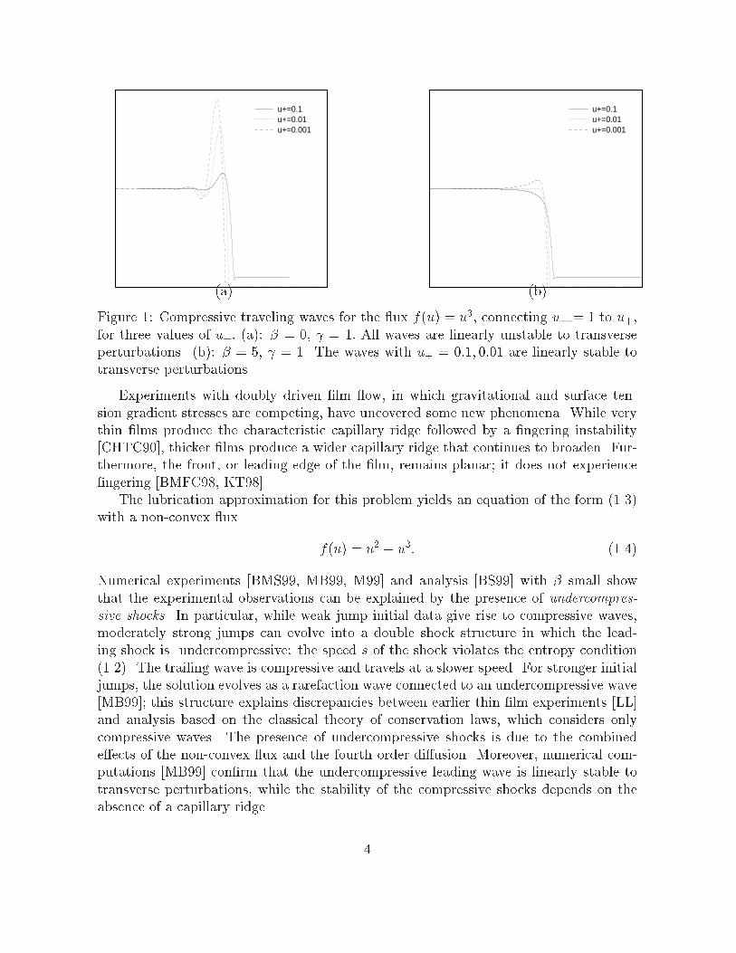
Figure 2: Compressive travelling waves for (1.6) with � = 0 and = 1, connectingu� � 0:332051 to u+ = 0:1. Waves numbered 1,3, and 5 are numerically stable inone space dimension, while waves 2 and 4 are unstable. All waves are unstable tomultidimensional perturbations. For this special value of u� there are an in�nite numberof compressive waves connecting to u+.6

an indicator of stability. (The index only predicts the parity of the number of unstableeigenvalues or positive growth rates; when the index is positive, we are assured onlythat there are an even number of unstable eigenvalues, not that there are none.) Thegeometry underlying this index is used in Section 2 to explain the following numericallyobserved feature: when there are multiple compressive waves for the same upstreamand downstream thicknesses, the waves come in pairs, one stable and one unstable toone-dimensional perturbations. An interesting open problem is to give a rigorous proofof stability. Such a proof would require further bounds on potential unstable eigenvalues(perhaps by a variant of Grillakis' method, as in [PW, AGJS, D, P]).For undercompressive waves, the index requires special treatment due to the behaviorof eigenfunctions associated with the linearization about the travelling wave. In this casewe derive a new simple expression for the index that we calculate easily from picturesof numerical results. This reduction turns out to be necessary for practical evaluationof the Evans function index in the case of traveling waves for higher order problems. Itis an improvement over the general theory developed in [D, GZ] and directly extends toarbitrary order systems.The di�erence between the compressive and undercompressive cases appears evenmore forcefully in the consideration of multidimensional stability. In Section 3, we outlinethe framework for a study of stability to two-dimensional perturbations. We focus onlong-wave perturbations, and show numerically in Section 4 that compressive wavesare unstable, in agreement with long-wave asymptotics developed in Section 3 (andalso in [BB97, KT98]). However, when considering undercompressive waves, there is amathematical puzzle we call the long-wave paradox: a formal calculation [KT98, BB97] ofthe low-frequency (long-wave) expansion of the growth rate of �ngering perturbations asa function of spatial frequency yields an explicit formula for the leading order asymptoticsof the growth rate of perturbations at long wave lengths. While this asymptotic formulaagrees well with computed eigenvalues in the case of compressive waves, it fails forundercompressive waves. In Section 3 we resolve the long-wave paradox by showinghow, for undercompressive waves, the formal calculation overlooks an interesting featureof the linearized problem. In Section 4, the resolution of the long-wave paradox is used tointerpret numerical calculations of growth rates, demonstrating that undercompressivewaves are stable to transverse perturbations.In Section 4, we also identify a curious feature of the growth rates. For parametervalues for which there is an undercompressive wave, there are also multiple travelingwaves, and moreover, the double shock structure collapses; the trailing compressive waveand the leading undercompressive wave have the same speed. The graphs of the growthrates (as a function of wave number) for the (unstable) compressive waves approach themaximum of the growth rates for the undercompressive wave and the compressive trailingwave. We interpret this observation in terms of the linearized equation, by observingthat the trajectories of the compressive traveling waves approach a combination of thetrajectories for the undercompressive wave and the trailing compressive wave.7

2 The One Dimensional CaseTo begin with, we consider solutions u = u(x; t) of equation (1.5) that are independentof y : ut + f(u)x = (b(u)ux)x � (c(u)uxxx)x: (2.1)Suppose there is a traveling wave solution, which (by adding a linear term to f , f(y) =~f(y) � sy,) we may take to be stationary:u(x; t) = u(x) (2.2)Then u = u(x) satis�es the traveling wave ODEc(u)u 000 = b(u)u 0 � (f(u)� f(u+)) (2.3)and boundary conditions limx!�1u(x) = u�: (2.4)In addition to the standing assumptions (H0), (H1), we assume standard nondegeneracyconditions from [ZH]4 :(H2) a� := f 0(u�) 6= 0:(H3) Solutions of (2.3) - (2.4) are (locally to u) unique up to translation.Remark (H2) holds if and only if (u�; 0; 0) are hyperbolic rest points of the �rst ordersystem (for u; u0; u00) associated with (2.3). Equivalently, it states that that the wavespeed is non-characteristic for the underlying conservation law ut + (f(u))x = 0.Linearizing (2.1) about u(�) givesvt = Lv := �(cvxxx)x + (bvx)x � (av)x;in which c = c(u(x)); b = b(u(x)); a = f 0(u(x))� b 0(u)ux + c 0(u)uxxx:Letting v(x; t) = e�tw(x); we obtain the eigenvalue problem Lw = �w :� (cw 000) 0 + (bw 0) 0 � (aw) 0 = �w: (2.5)Here, and below, 0 denotes di�erentiation with respect to x.To demonstrate linear stability of the travelling wave u, we want to show that ifRe� � 0; � 6= 0; then equation (2.5), with suitable boundary conditions at �1, has onlythe trivial solution w � 0: Our approach to this question is through the Evans functionD(�) (de�ned below) of [AGJS, GZ]. This is an analytic function whose zeroes in theright half plane (minus the exceptional point � = 0, which lies on the boundary of the4(H3) is the specialization to the scalar case of the more general (H3) in [ZH].8

essential spectrum) correspond precisely to eigenvalues of L . Moreover, as shown in[ZH, HZ.2], stability under quite general circumstances is equivalent to the condition:(D) D(�) has precisely one zero on fRe(�) � 0g, consisting of a simple root at � = 0.The Evans function itself is rather di�cult to evaluate; a more readily computablequantity is the stability index [J, PW, GZ, Z.2, Z.3]� := sgn D0(0) lim��!1 sgn D(�); (2.6)where the limit is along the real axis. This quantity, taking values � = �1, gives theparity of the number of zeroes of D(�) in the unstable half-plane Re� > 0: This followsfrom the observations that (i) � records the number of crossings ofD(�) through zero as �moves along the positive real axis, and (ii) non-real zeroes ofD appear in conjugate pairs,since L is real. In particular, � = �1 implies instability of the traveling wave, whereas� = 1 is consistent with stability. It is this computable index, and its interpretationin terms of the phase portrait of the traveling wave ODE, that provides much of thetheoretical explanation of the numerically observed stability phenomena.To construct the Evans function, we explore solutions of (2.5) as follows. Since theequation is fourth order, for each �, there will be a four dimensional set of solutions.For � 2 fRe(�) � 0g=f0g; we can choose a basis for the subspace S+ of solutions thatapproach zero as x �! 1 and a basis for the subspace U� of solutions that approachzero as x �! �1: Then � is an eigenvalue if S+ and U� have non-trivial intersection.That is, we need a condition for the intersection of two linear two-dimensional subspacesof functions. This condition is that the Evans functionD(�), de�ned to be the Wronskianof the two pairs of basis functions of S+ and U�, should vanish. In the present situation,the sign of the Wronskian is shown to be independent of x. The construction of theEvans function extends analytically to � = 0:In the construction ofD(�), we do not need to include information about whether theunderlying traveling wave is compressive or undercompressive. After the Evans functionis de�ned and related to stability of traveling waves, we then focus on the compressive andundercompressive cases in turn. In sections 2.5 and 2.6, we show that these cases di�ermost signi�cantly at � = 0, due to the fact that small disturbances propagate throughan undercompressive wave, rather than being absorbed, as they are for a compressivewave. This distinction reveals itself in the structure of the subspaces S+ and U�, but itcan already be seen in the behavior at x = �1; which we now discuss.2.1 Asymptotic eigenvalue equations.As x ! �1, behavior of (2.5) is governed by the asymptotic constant coe�cient equa-tions c�w 0000 = b�w 00 � a�w 0 � �w: (2.7)9

bb

bb

Im � Re �(a) �! +1

b

b

b

b

Im � Re �(b) � = 0, b� = 0, a� < 0Figure 3: Roots of equation (2.8)Here and below, we use subscripts � to indicate that quantities depending on u areevaluated at u = u(�1); respectively. E.g., c+ = c(u(1)): In particular, a� = f 0(u�);so that the sign of a� governs whether characteristics for the underlying conservationlaw point towards the stationary front, or away from the front. This distinction showsthe e�ect of the conservation law on the direction of propagation of small disturbances.The normal modes w := e��j x of (2.7) are determined by the characteristic equationc��4 � b��2 + a��+ � = 0: (2.8)First note that for � = 0; one of the roots is � = 0: This corresponds to the constantsolution of equation (2.7) when � = 0: For � 6= 0; we �nd that all solutions of (2.8) havenonzero real part.Recall that we need to distinguish solutions w(x) that decay at x = +1, for whichRe(�) < 0 (termed stable in Lemma 2.1 below) and solutions w(x) that decay at x = �1,for which Re(�) > 0 (termed unstable in Lemma 2.1).Lemma 2.1 For � 2 fRe(�) � 0g=f0g, (2.7) has two stable (i.e. negative real part)and two unstable roots, �1, �2 < 0 < �3, �4 (ordering by real parts). At � = 0, thereare two cases: (a� > 0) : �1 < �2 = 0 < �3; �4:(a� < 0) : �1; �2 < 0 = �3 < �4:Proof. (� 6= 0): First, observe that (2.8) has no imaginary roots � for � 2 fRe(�) �0g n f0g. For, setting � = ki in (2.8), we have the dispersion relation� = �a�ik � b�k2 � c�k4; (2.9)giving Re(�) < 0 unless k = 0. Thus, the number of stable/unstable roots is constant.Taking � ! +1, on the real axis, we have � � (��)1=4 = j�j1=4(�1)1=4, giving twostable and two unstable roots (Fig. 3(a)).(� = 0): At � = 0, we can factor (2.8) asc��3 � b��+ a� = 0; � = 0: (2.10)10

Clearly, the �rst equation has no imaginary roots for a� 6= 0, so, we can again countroots by homotopy, taking b� ! 0 to �nd � = ��a�c��1=3This gives two stable roots andone unstable root for a� < 0, together with � = 0; as claimed (Fig. 3(b)). The casea� > 0 is symmetric.Now write (2.7) as a �rst order systemW 0 = A �(�)W; A � := 0BB@ 0 1 0 00 0 1 00 0 0 1��=c �a=c b=c 0 1CCA� (2.11)in the phase variable W := (w;w 0; w 00; w 000)t. Throughout this paper we will identifysolutions of such fourth order scalar ODEs with solutions of their corresponding �rstorder system.For � 6= 0; each root �k is associated with an eigenfunction w(x) = e�kx; a solution of(2.7). Then W := (w;w 0; w 00; w 000)t is a solution of (2.11). Since the equation is linear,these exponential solutions can be combined linearly to form subspaces of solutions. Inkeeping with the strategy of distinguishing exponentially decaying from exponentiallygrowing solutions, we separate the corresponding subspaces of solutions S+;U�; whereS+ is the two-dimensional invariant subspace of solutions that decay as x �! 1; andU� is the two-dimensional invariant subspace of solutions that decay as x �! �1: Thecontent of the following Corollary is that not only are these subspaces two dimensionalfor � 6= 0; Re(�) � 0; but they also extend analytically to � = 0 as two dimensionalsubspaces, even though for � = 0 each subspace may have a non-decaying eigenfunction(depending on the sign of a�) as described in Lemma 2.1.In the case of a compressive wave, a� > 0 and a+ < 0. Thus for � = 0 both S+and U� are composed of decaying eigenfunctions at their respective in�nities in x. Onthe other hand, for an undercompressive wave, a� and a+ have the same sign. If theyare both negative then for � = 0, U� has one nondecaying eigenfunction at x ! �1while S+ has two decaying modes at 1. This behavior carries over to the non-constantcoe�cient case describing the full eigenvalue problem (2.5).Corollary 2.2 The stable/unstable subspaces S+=U� associated with A �(�) are eachtwo-dimensional on fRe(�) � 0g=f0g, and extend analytically in � to fRe� � 0g.More precisely, there exist bases fV +1 ; V +2 g; fV �3 ; V �4 g for the subspaces S+;U� :S+ = spanfV +1 ; V +2 g; (2.12)U� = spanfV �3 ; V �4 g: (2.13)The bases can be chosen to depend analytically on � and have the symmetry V �j (�) =V �j (�). 11

Proof. The dimension follows from Lemma 2.1. Likewise, since groups �1, �2 and �3,�4 remain spectrally separated on fRe� � 0g, the generalized eigenprojections ontotheir associated subspaces are each analytic, by standard matrix perturbation theory[K]. The eigenprojections are given by the resolvent formula P := R�(A � ��I)�1d�, � acontour enclosing ��1 , ��2 (resp. ��3 , ��4 ). If � is chosen to be symmetric with respect tocomplex conjugation, then P is as well, by the corresponding property of A � . Choosingan analytic basis of eigenvectors by the construction of [K, pp. 99{102], we retain theabove symmetry.2.2 Stable and unstable manifoldsIn the previous subsection, we froze the coe�cients in the ODE (2.5), by setting u = u+and u = u�: This allows us to capture the behavior of solutions of the nonconstantcoe�cient equation (2.5) as x �! �1:Given a solution �(x) of (2.5), we associate with it the vector of derivatives �(x) =(�(x); �0(x); �00(x); �000(x))t. Given such a vector �, the angle it makes with a subspaceT of the four dimensional phase space is the minimum of the angle between � and allvectors in T .On fRe� � 0g, de�ne S+ to be the subspace of solutions � of (2.5) whose corre-sponding vectors � approach, in angle, the subspace �S+ as x ! +1. Analogously,U� is de�ned to be the subspace of solutions � of (2.5) whose corresponding vectors �approach, in angle, the subspace �U� as x ! �1. The existence of these subspaces isestablished in [GZ] or [K.1, K.2, K.3].The existence of these subspaces, along with analytic dependence on �, follows by thegap lemma of [GZ,KS], or alternatively by earlier results of [J,K.1{3]; the full generality ofthe gap lemma is not needed here, since we have spectral separation of the subspaces S+,U� and the complementary A �-invariant subspaces, a helpful feature of the scalar case.The necessary hypotheses follow by analytic dependence of S+, U�, the aforementionedspectral gap, and exponential convergence of the coe�cients a, b, and c as x ! �1.Regarding the latter property, recall from Remark 1 that u� are hyperbolic rest pointsof (2.5) by virtue of (H2), hencej(d=dx)`(u� u�)j � Ce��jxj; x 7 0; ` = 0; 1; 2 (2.14)for some � > 0, and thusja� a�j; jb� b�j; jc � c�j � Ce��jxj; x 7 0: (2.15)Using a slight extension of these results (see [ZH] Lemma3.1, p. 779, or [GZ] Corollary2.4, p. 807), we can conclude in addition that there exist basis functions '�j (�; x) suchthat S+ = spanf'+1 ; '+2 g; (2.16)12

U� = spanf'�3 ; '�4 g; (2.17)which additionally have symmetry '�j (��) = '�j (�) so that '�j are real-valued for � real.This follows from the properties noted above, plus the existence of corresponding basisvectors V �j asserted in Corollary 2.2. Moreover, the basis functions '�j (�; x) are analyticin � at � = 0 and continuous elsewhere; the exterior products '+1 ^ '+2 and '�3 ^ '�4 areanalytic on all of fRe� � 0g; and '(��) = '(�) (see [GZ]).Because their associated eigenvalues may coalesce, �+1 , �+2 may not be individuallyanalytically continuable on fRe� � 0g; however, they are jointly continuable in the sensethat their span, or alternatively their exterior product, can be analytically de�ned.2.3 The Evans function.We now de�ne the Evans function, following [AGJS, GZ] as the Wronskian of the basisfunctions '+1 ; '+2 ; '�3 ; '�4 that characterize solutions decaying at +1; at �1; or both.D(�) := det0BBBBBBBBB@ '+1 '+2 '�3 '�4'+1 0 � � � ...'+1 00 ...'+1 000 � � � '�4 0001CCCCCCCCCA : (2.18)Properties:(P1) D(�) is analytic on fRe� � 0g.(P2) D(�) is real for real �.(P3) On fRe� � 0g=f0g, D(�) = 0 if and only if � is an eigenvalue of L.Only (P3) requires discussion. This follows from the characterization of eigenfunc-tions of L as nontrivial solutions of (L��)w = 0 lying in S+\U�, i.e. decaying at both�1. Evidently, vanishing of the Wronskian D(�) is equivalent to nontrivial intersectionof S+ and U�, by (2.16) - (2.17).The meaning of the Evans function at � = 0 is less immediate, but equally important.Note that � = 0 is an eigenvalue, with at least the eigenfunction ux; corresponding totranslations of u: Moreover, since ux decays at �1; it lies in both U� and S+; implyingD(0) = 0: Moreover, this zero of the Evans function does not interfere with either linearor nonlinear stability, as shown in [HZ.2, ZH], a result we alluded to earlier in formulatingcondition (D); and which we restate here for clarity.Proposition 2.3 Linearized stability of u(�) as a solution of (2.1) is equivalent to theEvans function condition (D). Moreover, linearized stability implies nonlinear stability.13

(Remark: [HZ.2] concerns also more general, dispersive{di�usive equations such asthe convex KdV-Burgers equation, or the nonconvex modi�ed KdV-Burgers equationstudied by [D, JMS, W].)Having de�ned the Evans function, we now begin to investigate whether or not it hasa positive zero. To this end, we use the stability index � (see (2.6)) which only requiresinformation about D(�) for su�ciently large � and the leading order behavior for real� near � = 0: The small � behavior depends crucially on whether the traveling wave iscompressive or undercompressive. The stability index will be shown to be a coordinate-independent orientation of the intersection of the stable/unstable manifolds of u+=u� in(2.3). The connection to stability is given throughProposition 2.4 The parity of the number of zeroes of D(�) in fRe(�) � 0g is odd(even) according to � > (<)0. In particular, � < 0 implies instability, whereas � > 0 isnecessary for stability.Proof. Using D(�) = D(�), we have that complex roots of D(�) appear in conjugatepairs. On the other hand, the number of real roots with � � 0 clearly has the parityclaimed. The connection to stability follows from Proposition 2.3.2.4 The Evans function as �!1.Following [GZ], we now evaluate the Evans function in the large j�j regime. Let � : C 4 !C 4 denote orthogonal projection onto the span of the �rst two standard basis elements,e1 = (1; 0; 0; 0)t and e2 = (0; 1; 0; 0)t. We have the following analog of Lemma 3.5 in[GZ]:Lemma 2.5 The projection � is full rank on the A �-invariant subspaces S+, U�. Equiv-alently, if V = (v1; v2; v3; v4)t and eV = (~v1; ~v2; ~v3; ~v4)t 2 S+ (resp. U�) are independent,then det� v1 ~v1v2 ~v2 � 6= 0.Proof. It is su�cient to treat the case that V , eV are eigenvectors of A � . If they areindependent genuine eigenvectors, then, by the companion matrix structure of (2.11), wehave V = (1; �; �2; �3), eV = (1; ~�; ~�2; ~�3), and det� v1 ~v1v2 ~v2 � = ~�� � 6= 0.The other possibility is that � = ~� and V = (1; �; �2; �3)t, ~V = (0; 1; 2�; 3�2)t forman eigenvector / generalized eigenvector pair. In this case, det� v1 ~v1v2 ~v2 � = 1 6= 0, also.This lemma allows us to express the sign ofD(�) for large � in terms of the projectionsof the basis vectors of S+, U� at � = 0. To this end, let the basis vectors V �j (j=1,...,4)have components V �jk (k=1,...,4). 14

Proposition 2.6 For � > 0 real, su�ciently large,sgn D(�) = sgn det� V +11 V +21V +12 V +22 � det� V �31 V �41V �32 V �42 � j�=0: (2.19)Proof. The proof follows arguments of Proposition 2.8 of [GZ], or the equivalent Propo-sition 7.3 of [ZH] for lower order systems of equations. The idea is to use an asymptoticargument for large � to show that the sign of the determinant in the Evans function canbe expressed in terms of the sign of the determinants in (2.19) provided � is su�cientlylarge. Then Lemma 2.5, which implies that the sign of the determinants in (2.19) areindependent of � (since they are continuous and can never vanish) gives the desiredresult.First we choose � su�ciently large so that the asymptotic arguments below are valid.We can rescale (2.5) by x = �1=4x, w(x) = w(x), a(x) = a(x), b(x) = b(x), c(x) = c(x),to obtain w0000 = �c�1w +O(j��1=4j(jwj + jw 0j+ jw 00j+ jw 000j)) (2.20)where jc 0j = O(��1=4). Applying Proposition 2.8 of [GZ], or the equivalent Proposition7.3 of [ZH], we �nd that in phase variables, the subspaces S+(x)=U�(x), de�ned by theevaluation of the stable/unstable subspace of (2.20) at an arbitrary x0, lies within angleO(��1=4) of the stable/unstable subspaces of the limiting equationsw0000 = �c�1w; (2.21)with coe�cient c held frozen at value c(x0). The subspaces of the limiting equationsare spanned by the stable/unstable normal modes of (2.21), readily calculated to be(1; �; �2; �3)t, where � = �j(x0) = (�c(x0)�1)1=4 (2.22)are fourth roots of (�c)�1.Converting back to the original scaling, the subspaces S+(x0)=U�(x0) de�ned by theevaluation of the stable/unstable subspace of (2.5) at x0, lie within angle O(��1=4) of thesubspaces spanned by f(1; �1; �21; �31)t; (1; �2; � � � ; �32)tg and f(1; �3; �23; �33); (1; �4; �24; �34)grespectively, where �j(x0) = (��=c(x0))1=4: (2.23)Recalling (see Section 2.2) that S+(x0)=U�(x0) are real-valued for � real, and thatfor large � �1, �2 and �3, �4 form complex conjugate pairs, we �nd therefore that15

0BB@ '+1 '+2 '�3 '�4'+1 0 '+2 0 '�3 0 '�4 0'+1 00 '+2 00 '�3 00 '�4 00'+1 000 '+2 000 '�3 000 '�4 0001CCA = (1 +O(j��1=4j)) �0BBB@ 1 1 1 1�1 �2 �3 �4�21 ...�31 � � � �341CCCA0BB@1=2 i=2 0 01=2 �i=2 0 00 0 1=2 i=20 0 1=2 �i=21CCA�M+ 00 M�� (x0) (2.24)where M�(x) are speci�c nonsingular real-valued coe�cient matrices. It follows, there-fore, thatD(�) = �(1 +O(j��1=4j)) det0BBB@ 1 1 1 1�1 �2 �3 �4�21 ...�31 � � � �34 1CCCAjx=x0 det� M+ 00 M� � :(2.25)Evaluating the Vandermonde determinant, and noting that all quantities involvedare real and nonvanishing, hence have sign independent of x0, we �nd thatsgn D(�) = sgn det i� 1 1�1 �2 � detM+jx=x0 det� 1 1�3 �4 � detM�jx=x0= sgn det i� 1 1�1 �2 � detM+jx=+1 det� 1 1�3 �4 �detM�jx=�1= sgn det� V +11 V +21V +12 V +22 � det� V �31 V �41V �31 V �42 � (�) (2.26)so long as � is real and su�ciently large.But, the right hand side of (2.26) is independent of � by Lemma 2.5.Remark: The matrices M� in the proof are used only as an intermediate book-keeping device, and play no role in the �nal computation.2.5 Evaluation at � = 0 in the Lax case.In this subsection, we restrict to the Lax case, for whicha� > 0 > a+: (2.27)Consulting Lemma 2.1 and Section 2.2, we �nd that S+(0), U�(0) consist of allsolutions of (2.5) that exponentially decay as x ! +1, �1 respectively. We cantherefore integrate (2.5) with � = 0 from either +1 or �1 to obtain16

c'000 = b'0 � a': (2.28)Note that (2.28) is exactly the variational equation for the traveling wave ODE (2.3).Indeed, one solution of (2.28) is ' = ux, corresponding to translation along the pro�le.By appropriate change of basis, we can arrange without loss of generality that'+1 (0; x) = '�4 (0; x) = u0(x): (2.29)We choose '+2 and '�3 to be any independent solutions of (2.28) decaying at �1.Note that the traveling wave ODE (2.3) can be written as a three dimensional au-tonomous system u0 = u1;u01 = u2; (2.30)u02 = b(u)c(u)u1 � f(u)� f(u�)c(u) ;which has equilibria at B = (u+; 0; 0) and M = (u�; 0; 0). A travelling wave solutionof (2.3) connecting u� to u+ corresponds to a heteroclinic orbit of (2.30) connectingM to B. For the Lax case, M has a two dimensional unstable manifold and B has atwo dimensional stable manifold. We now see that the subspace S+ (U�) at � = 0 iscomposed of functions ' with corresponding vectors (';'0; '00)t that span the tangentspace of W s(B) (W u(M)) along u(�). An illustration of this structure for the specialcase of (1.6) is presented at the end of this section.The next proposition, following the general approach introduced by Jones [J] relatesthe sign of D0(0) to the orientation with which these stable/unstable manifolds intersectin the phase space R3 of (2.3).Proposition 2.7 D(0) = 0, whilesgn D0(0) = sgn c(0)�1 det0@ ux '+2 '�3u0x '+02 '�03u00x '+002 '�003 1A (u+ � u�): (2.31)Proof. D(0) = det0B@ ux '+2 '�3 ux... ... ... ...u000x ('+2 )000 ('�3 )000 u000x 1CA = 0: (2.32)Similarly, a straightforward calculation (as in [GZ]) yieldsD0(0) = det0B@ ux '+2 '�3 ('�4� � '+1�)... ... ... ...u000x '+0002 '�0003 ('�4� � '+1�)000 1CA : (2.33)17

Di�erentiation of (2.5) with respect to � shows that the functions z = '+1�, '�4� satisfythe same variational equation(cz000)0 = (bz0)0 � (az)0 � ux; (2.34)decaying at +1, �1 respectively. Integrating from +1, �1 respectively, and sub-tracting, we �nd that ~z := '�4� � '+1� satis�esc~z000 = b~z0 � a~z + (u� � u+); (2.35)an inhomogeneous version of (2.28). Using (2.28), (2.35) to eliminate the fourth row in(2.33), we obtain D0(0) = c(0)�1 det0BB@ ux '+2 '�3 ~zu0x '+02 '�03 ~z0u00x '+002 '�003 ~z000 0 0 (u� � u+) 1CCA ; (2.36)giving the result.Remark: The right hand side of (2.36) is of form �, where the �rst factor, measures orientation of the intersection of the stable and unstable manifolds of theunderlying traveling wave ODE at u+, u� respectively, and the second factor, � = [u],is the Kreiss{Sakamoto{Lopatinski determinant arising in the study of inviscid stability.This is a special case of a very general relation pointed out in [ZS] between viscous andinviscid stability.Combining Proposition 2.6, Proposition 2.7, we haveCorollary 2.8 The stability index � := sgn D0(0)D(+1) satis�es� = sgn "0@ ux '+2 '�3u0x '+02 '�03u00x '+002 '�003 1A jx=0 �det� ux '+2u0x '+02 � jx=+1 det� '�3 ux'�03 u0x � jx=�1(u� � u+)#:We now present an example from [BMS99] and discuss how the machinery developedhere explains numerical observations of one dimensional stability of compressive waves.We consider (1.6) with � = 0 and = 1. For each u+ there is a range of u� for whichmultiple compressive traveling waves appear. For a special value of u� an in�nite numberof compressive waves occur. For the case u+ = 0:1, the special value is approximatelyu� = 0:332051. A detailed discussion of the phase portrait for this example is given in[BMS99]. Shown in Figure 4 is a Poincar�e section (at �xed u) from the phase portraitof (2.30). The stable manifold W s(B) is shown as a dashed line while the unstable18

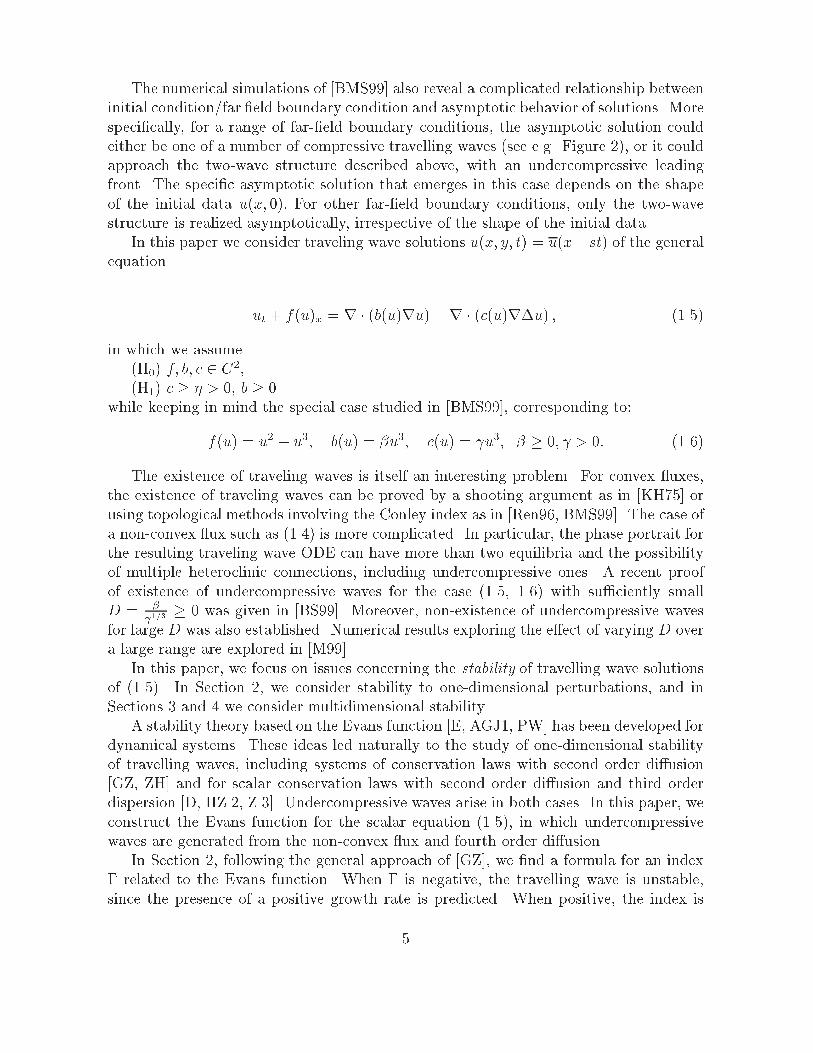
+� �W s(B)W u(M)u0

u00�0:18�0:28

�0:065�0:145Figure 4: Section of the invariant manifoldsW u(M) (solid line),W s(B) (dashed line) andW u(T ) (plus) with the Poincar�e plane P = f(u; u0; u00); u = (2u�+u+)=3g. Intersectionsof the solid and dashed lines mark points where trajectories connecting M to B hit P .The symbols around these intersections indicate whether the corresponding pro�le is astable (circles) or unstable (boxes) solution of the PDE, for the �rst two traveling waves�u. Arrows indicate the direction of (('+2 ); ('+2 )0) and (('�3 ); ('�3 )0) (the projection of thederivative vectors on the Poincar�e plane).manifold W u(M) is shown as a solid line. Note that this unstable manifold appears as aspiral whose center corresponds to the undercompressive connection. Each intersectionof these two curves denotes a point along a heteroclinic orbit of (2.30). The intersectiondenoted by a circle corresponds to a one-dimensionally stable compressive wave while thebox corresponds to a one dimensionally unstable compressive wave. The arrows on the�gure denote the orientation of a choice of basis vectors ('+2 ); ('+2 )0) and (('�3 ); ('�3 )0).Note that the orientation of these vectors switches at each successive crossing of thespiral. The vector (�ux; �u0x; �u00x) is into the Poincar�e plane. Following Corollary 2.8, thecorresponding stability indices �j alternate in sign. This is consistent with numericalobservations that the successive waves alternate stability. (Recall that u� are �xed. Theremaining terms det� ux '+2u0x '+02 � and det� '�3 ux'�03 u0x � �x a common orientation on thestable/unstable manifolds at u�/u+).Remark. As often happens, we obtain a rigorous instability result by this tech-nique, but it is only suggestive of stability. To obtain a complete stability result wouldrequire establishing nonexistence of pure imaginary eigenvalues (other than � = 0), aseparate (and quite interesting) unresolved issue.19

2.6 Evaluation at � = 0 in the undercompressive case.The undercompressive case, sgn a� = sgn a+; can be treated similarly. For example,Proposition 2.6 goes through unchanged. However, the behavior at � = 0 is signi�cantlydi�erent, as might be expected from the fact that long-wave behavior is dominated bythe convection rates a� in the far �eld. In the present, one-dimensional context, thisleads to a slightly modi�ed stability index. In the context of multi-dimensional stability,as we shall see later, the distinction is still more critical.Without loss of generality (and to be consistent with the thin �lm context [BMS99]),assume a� = f 0(u�); a+ = f 0(u+) < 0: (2.37)Note that this implies that there exists an intermediate equilibrium 5 um between u�and u+. The corresponding system of equations (2.30) describing the phase portraitfor the traveling wave has (at least) three equilibria B = (u+; 0; 0), M = (um; 0; 0),T = (u�; 0; 0). The undercompressive wave corresponds to a connection from T (whichhas a one dimensional unstable manifold) to B (with a two dimensional stable manifold).Appealing again to Section 2.2, we �nd that, as in the Lax case, S+ consists of allsolutions of (2.5) decaying exponentially at x = +1. However, recalling the discussionbefore Corollary 2.2, when � = 0; U� now consists of solutions that are only bounded asx! �1: Without loss of generality, when � = 0; choose again '+1 (x) = '�4 (x) = ux(x),and take '+2 , '�3 to be independent solutions of (2.5) in S+, U� respectively, where wecan choose the normalization '�3 (�1) = 1:Proposition 2.9 D(0) = 0, whilesgn D0(0) = � sgn (a�=c(0)) det0@ ux '+2 (z� � z+)u0x '+02 (z� � z+)0u00x '+002 (z� � z+)00 1A jx=0= sgn a� R1�1(1=c)(u� u�) det� ux '+2u0x '+02 �dx; (2.38)where z� satis�es the variational equationcz000 = bz0 � az � (u� u�); (2.39)with z+(+1) = 0; z�(�1) = (u+ � u�)=a�: (2.40)5Note that we are using slightly di�erent notation from [BMS99] in which u� and u+ always denotenearest equilibria. 20

Proof. As in the proof of Proposition 2.7,D(0) = det0B@ ux '+2 '�3 ux... ... ... ...u000x ('+2 )000 ('�3 )000 u000x 1CA = 0; (2.41)and D0(0) = det0B@ ux '+2 '�3 ('�4� � '+1�)... ... ... ...u000x '+0002 '�0003 ('�4� � '+1�)000 1CA : (2.42)Likewise, the decaying solutions ux and '+2 satisfy equation (2.28). However, '�3is asymptotically constant, '�3 (�1) = 1, hence satis�es the inhomogeneous equationc'000 = b'0 � a'+ a�: (2.43)Using the fact that ~z := '�4� � '+1� as before satis�es (2.35), we can use (2.28), (2.35),(2.43) to reduce the fourth row of (2.42), obtainingD0(0) = c�1 det0BB@ ux '+2 '�3 ~zu0x '+02 '�03 ~z0u00x '+002 '�003 ~z000 0 a� u� � u+ 1CCA : (2.44)Using the third column to eliminate (u+ � u�), we obtainD0(0) = c�1 det0BB@ ux '+2 '�3 z� � z+u0x '+02 '�03 (z� � z+)0u00x '+002 '�003 (z� � z+)000 0 a� 0 1CCA ; (2.45)where z� � z+ = ~z � �u��u+a� �'�3 are de�ned byz+ := '+1�; z� := '�4� ��u� � u+a� �'�3 : (2.46)Evaluation of (2.45) at x = 0 gives the �rst equality in (2.38). Integration of (2.34),together with (2.43), verify that z� both satisfy (2.39), with the claimed boundaryconditions at �1.Now de�ne � := det0@ ux '+2 z�u0x '+02 z�0u00x '+002 z�00 1A : (2.47)21

The reduction to a Melnikov integral in the second equality in (2.38) involves evalua-tion of � �+: Brie y, this follows (see, e.g., [GZ], proof of Lemma 3.4, or [GH, Sch])from the (inhomogeneous) Abel's formula, 0 = TrB + det0B@ ux '+2 0... ... 0u00x '+002 (u� u�) 1CA= det0B@ ux '+2 0... ... 0u00x '+002 (u� u�) 1CA ; (2.48)and Duhamel's principle/variation of constants, to evaluate � at x = 0. Here, B =B (�; x)0BB@ 0 1 00 0 1�a=c b=c 01CCA denotes the coe�cient matrix for (2.28) written as a �rst ordersystem.Combining Corollary 2.8 and Proposition 2.9, and recalling that, as x ! �1,(��3 ; ��3 0)! (1; 0) and sgn �uxx � sgn ��4 �ux = sgn �ux, we haveCorollary 2.10 The stability index � := sgn D0(0)D(+1) is given by� = sgn a� Z 1�1(1=c)(u� u�) det� ux '+2u0x '+02 � dx �ux(�1) det� ux '+2u0x '+02 � jx=+1(2.49)Note that the functions z� in (2.38) are uniquely speci�ed by (2.39){(2.40), modulospanf�ux; '+2 g. z� and z+ have an important interpretation as the variations, in thetraveling wave ODE,c(u)u000 = b(u)u0 � (f(u)� f(u�)� s(u� u�)); (2.50)of the unstable/stable manifolds of u+ and u�(s) as the shock speed s is varied. Likewise,1c(0) det0B@ ux '+2 (z� � z+)... ... ...u00x '+002 (z� � z+)00 1CA jx=0 = Z 1�1(1=c)(u� u�) det� ux '+2u0x '+02 �(2.51)can be recognized as @d@s js=0, where d(s) is theMelnikov separation function, measur-ing the distance (in 3-dimensional phase space) between the one dimensional unstablemanifold T and the two dimensional stable manifold of B along a �xed transverse sec-tion. Alternatively, it represents the orientation with which S+ and U� intersect in4-dimensional phase space of eqn. (2.50) augmented withs0 = 0: (2.52)22

The stability index � is a coordinate- and normalization-independent measure of theorientation.Calculation of �.We now turn to the calculation of the stability index for the undercompressive case,which hinges on the calculation of the sign of the Melnikov integral@d=@s = Z 1�1(1=c)(u� u�) det� ux '+2u0x '+02 � dx:This can be evaluated conveniently in terms of the left zero eigenfunction �0:We post-pone a discussion of the associated spectral theory to the next section. It transpires thatthe Melnikov integral arising in calculation of the stability index for undercompressiveshocks can be expressed alternatively ash�u� u�; k�0xi;= h�ux; k�0i = k; (2.53)where h�; �i denotes L2 inner product, u� is the state arising in the original formula (in thepresent setting, u� = u�; see [GZ] for more general situations), and k is an appropriatelychosen constant. The key simpli�cation of the Melnikov integral comes from the formulak�0x = (1=c) det� ux '+2u0x '+02 � ; (2.54)which we derive below. Comparing behaviors at +1, we �nd that the sign of theMelnikov integral is sgn (1=c) det��ux �+2�u0x �+2 0��0xjx=+1;and thus, referring back to (2.50), we obtain the simple expression:Proposition 2.11 For an undercompressive wave, the stability index � can be computedas � = sgn a��0x(+1)�ux(�1) (2.55)where �0 denotes the left zero eigenfunction.For the speci�c traveling wave computed numerically and shown in Figure 5 andfor the corresponding �0 shown in Figure 7, we observe that � = +1; consistent withstability of the undercompressive wave. To �nish the proof of Proposition 2.11 we showthe equality (2.54) then use integration by parts and the fact that �0(+1) = 0. Aswe discuss in more detail in the next section, �0 is uniquely speci�ed up to a constantfactor, is bounded, and satis�es the adjoint eigenvalue equation�(cz0)000 + (bz0)0 + az0 = 0:23

u+ = 0.1

Figure 5: The undercompressive wave corresponding to � = 0, = 1, and u+ = 0:1.It follows that the derivative �0x is uniquely speci�ed up to constant factor by the prop-erties that it decays at �1 and satis�es�cy000 + (by)0 + ay = 0; (2.56)obtained by setting y = z0.Now, observe that, by Abel's formula, the vector (e1; e2; e3) de�ned bye1 = det� u0x '+02u00x '+002 � ;e2 = � det� ux '+2u0x '+002 � ;and e3 = det� ux '+2u0x '+02 � ;must satisfy e1w+ e2w0 + e3w00 � constant for any solution w of the linearized travelingwave equation �cw000 + bw0 � aw = 0;of which both �ux and �+2 are solutions. 24

It follows that (e1; e2; e3) must satisfy the adjoint ODE to the linearized travelingwave equation written as �rst order system W 0 = BtW , where B is as in (2.6),Bt = 0@ 0 0 a=c�1 0 �b=c0 �1 0 1A ;from which we readily �nd that e3 satis�ese0003 � (be3=c)0 � (a=c)e3 = 0:Thus, (1=c) det� ux '+2u0x '+02 � = (1=c)e3satis�es (2.56) as claimed.Remarks.The formula (2.55) in Proposition 2.11 is new. The improved formula (2.56) inProposition 2.11 is not restricted to the special setting of thin �lm models. In fact, theideas used in its derivation, in particular (2.53) and (2.54), easily generalize to systemsof conservation laws of arbitrary order to yield an analogous result. These formulae arethe consequence of a general but somewhat nonstandard duality principle. 6This observation therefore represents a useful re�nement in the general theory. Forcomparison, the formula obtained in [GZ] for second order di�usive systems is analogous6In particular, note that the fact that e3=c satis�es the equation for z0 can be seen from the moregeneral relation (z0; z00; z000) ~S(w;w0; w00)t � constantfor solutions w of the linearized traveling wave ODE (in particular, decaying solutions of the adjointODE at � = 0) and solutions z of the adjoint eigenvalue ODE at � = 0, where~S := 0@�b+ c00 �c0 c2c0 �c 0c 0 01A : (2.57)For, by duality, this implies that (z0; z00; z000)S =: (e1; e2; e3), solves the adjoint of the traveling waveODE written as a �rst order system, and by inspection e3 = cz0.This relation, in turn, is a special case of(z; z0; z00; z000)S(w;w0; w00; w000)t � constantfor solutions w, z of the eigenvalue and (resp.) adjoint eigenvalue ODE at � = 0, whereS := 0@ a b+ c00 �c0 c�b� c00 2c0 c 0�c0 �c 0 01A ; (2.58)under assumption cw000 = bw0� aw. The duality relation (2.57) was pointed out in [LZ.2] in the second-order di�usive (system) case; the underlying relation (2.58) was pointed out in [ZH], Lemma 4.4, andthe extension to arbitrary higher order operators discussed in [ZH], proof of Theorem 6.3.25

to Corollary 2.10; in the third order scalar case treated in [D] the formula obtained areexplicitly evaluable, and the issue does not arise.As pointed out in [SSch] in the di�usive case, nonvanishing of the Melnikov integralis related to well-posedness of Riemann solutions near the undercompressive shock (u�,u+, s). There is, however, no analog of (2.31) in the di�usive case, for which scalar Laxshocks are always stable [S.1, H.1, H.2, H.3, JGK].In both Lax and undercompressive cases, the index � can be evaluated numerically.However, it does not give a conclusive result of stability, yielding only parity of thenumber of unstable eigenvalues of L.A complete numerical evaluation of stability can be performed e�ciently using analgorithm of Brin [Br], in which D(�) itself is evaluated numerically, and the windingnumber computed around fRe� � 0g. Moreover, the top eigenvalue can be computednumerically using the power method discussed in the following section. Furthermore, aswas done in [BMS99], nonlinear stability can be veri�ed numerically by perturbing thestationary wave and noting convergence or divergence of solutions of the PDE.3 Multi-dimensional stability and the long-waveparadox.This section addresses multi-dimensional stability and the long-wave paradox for stabil-ity of undercompressive shocks. Here we are concerned with how the spectrum of thelinearized operator depends on the transverse wave number. For this problem we presenttheoretical justi�cation for formal and numerical treatments of the spectral problem.A �rst order perturbation analysis of the spectrum can be readily carried out, both forsystems and for scalar equations, by Evans function calculations very similar to those ofthe previous section [ZS]. What we require here, however, is a second order expansion,or `di�usive correction' in the language of [ZS], since scalar shock fronts are alwaysneutrally stable to �rst order (see [ZS], or calculations just below). In the present, scalarsetting, this is much more convenient to carry out via standard, Fredholm solvabilitycalculations, justi�ed by passing to an appropriate weighted norm, than via the Evansfunction framework, and we shall therefore take this di�erent point of view in whatfollows.3.1 PreliminariesConsider now the multi-dimensional versionut + f(u)x = r � (b(u)ru) �r � (c(u)r�u) (3.1)of equation (2.1). Linearizing about u(�), and taking the Fourier transform in transversedirections, we obtainvt = Lkv := �(cvxxx)x + (bvx)x � (av)x � k2(bv � (cvx)x � cvxx)� k4cv (3.2)26

where c = c(u); b = b(u); a = f 0(u)� b0(u)ux + c0(u)uxxx; (3.3)and k is the wave number, v = v(x; k; t).Remark. Equation (3.2) is for two space dimensions as in the application to thin�lms. In the case of higher dimensions, rotational invariance yields the same transformedequation in which k becomes the modulus of the wavenumber.Associated with (3.2), we have the family(Lk � �I)w = 0 (3.4)of eigenvalue equations, where L0 is exactly the linearized operator about u(x) for theone-dimensional problem. In what follows, we will assume Lk is an analytic function ofk2; rather than just k, since in equation (3.2), Lk is a quadratic polynomial of k2:The question, assuming stability of the one-dimensional operator, is whether thespectrum of Lk remains stable as k is varied. Of particular interest (see e.g. [CE])is the variation for small k of the top eigenvalue �(k), where �(0) = 0 corresponds totranslation of the wave. For it is this mode, to leading order, that governs the propagationof disturbances along the front (see discussion [G, GM, HZ.2, K.1, K.2, K.3, KS, ZH, ZS]).Stability of �(k) for small k (i.e. Re� � 0) is called long-wave stability. This is theproblem of most interest since the fourth order di�usion necessarily causes the dominanteigenvalue to decay as �k4c for large values of jkj.3.2 Spectral Theory.A rigorous discussion of long-wave stability, in the context of conservation laws, requiresadditional spectral perturbation theory, beyond the usual Banach space theory of, e.g. [K,Y]. For, the eigenvalue �(0) = 0 of main interest is embedded in the essential spectrumof L0, [He, S.1, ZH] hence this standard theory does not apply. A priori there is noreason to expect an analytic development of �(k) at such a point; indeed, for systems ofconservation laws, it is a fundamental fact that �(�) is in general not analytic at k = 0.We refer the reader to [ZS] for further discussion of this general situation.However, in the present, scalar context, a much simpler treatment is possible by theweighted norm method of Sattinger [S.2]. Introducing the normkfk := kfkL2 ; (3.5)with (x) := e�� R x0 a(y)dy; 1 > � > 0; (3.6)has the e�ect of shifting the essential spectrum of L0 to the left, into the strictly stablecomplex half-plane, as is readily checked by the methods of [He, S.2] (see also [Z.2] for27

further details). Thus, in this norm, �(0) = 0 becomes an isolated eigenvalue, and wemay conclude from standard spectral theory the existence of analytical developments�(k) = �1k2 + � � � ; (3.7)and '(k) = '0 + '1k2 + � � � ; (3.8)of � and the associated right eigenfunction ' 2 L2.Likewise, there exists an analytic L2 left eigenfunction with respect to the L2 innerproduct, whence we can conclude existence of an analytic eigenfunction�(k) = �0 + �1k2 + � � � ; (3.9)with respect to the standard inner product, where �2� 2 L2, or equivalently� 2 L2�1 : (3.10)Moreover, �/' are the unique L2 eigenvalue/function pair for Lk in the vicinity of � = 0,and �/� the unique L2�1 pair.An interesting feature of these developments as compared to the usual (unweighted)type is that, depending on the signs of a�, '(k) or �(k) may be nondecaying, in factexponentially growing at �1. Nonetheless, as in the classical case, we have the followingresult, in which h�; �i denotes the standard L2(R) inner product:Proposition 3.1 Suppose that (consistent with one-dimensional stability) � = 0 is asimple eigenvalue of L0 (i.e., when k = 0), and that all other eigenvalues have negativereal part. Let �(k) as above denote the top eigenvalue of Lk. Then, for compactlysupported initial data v0, and x restricted to any bounded domain, the solution v(x; t) =eLktv0(x) of vt = Lkv satis�esv(x; t) = e�(k)tP(k)v0(1 +O(e��t)); � > 0; (3.11)where P(k) denotes the generalized spectral projection operatorP(k)g := '(k)h�(k); gi (3.12)associated with �(k).This can be seen from the corresponding classical result in L2, together with theobservation that is bounded above and below on compact domains. For a proof in thegeneral, systems setting, see [ZH], sections 5{6 and 8 (note: this result is independent ofthe regularity of �(�).)Proposition 3.1 states that the nonstandard eigenfunctions ', � still govern asymp-totic behavior on bounded domains, analogous to \resonant poles" in scattering theory28

[LP]. A useful corollary of this fact is that the power method can be used to �nd thetop eigenvalue/eigenfunction of Lk, by solving vt = Lkv starting with any compactly sup-ported initial data. This validates the numerical stability analysis of [BB97, BMFC98].Likewise, the classical formula�1 = h�0; L1'0i+ h�0; (L0 � �0)'1i = h�0; L1'0i (3.13)(Lk =: L0 + kL1 + � � � ) based on solvability conditions/ Fredholm alternative can beseen to apply, as a consequence of the equivalent formula in the norm. That all L2inner products are well-de�ned follows from consideration of the decay/growth of ', �as x ! �1, which reveals that they and their derivatives lie in L2, L2�1 , respectively.(By comparison, only a weak version of the Fredholm alternative survives for systems,see [ZH]).Remark. The introduction of the weighted norm k � k is equivalent to the change ofvariables z = w, from which observation we may deduce that (since such a changeof variables introduces only a nonzero constant multiplier) that zeroes of the Evansfunction correspond to eigenvalues with respect to norm. Moreover, this yields theuseful characterization of their generalized eigenfunctions as the intersection between thestable/unstable manifolds S+/U� de�ned as in Section 2.To investigate long-wave stability, we expand the operator Lk in powers of k2, Lk =L0 + k2L1 + k4L2, withL0 := L0; L1 = �b+ ddx �c ddx�+ c d2dx2 ; L2 = �c: (3.14)Using the fact that '0 = �ux, to �rst order we obtain�1ux = L1ux + L0�1:We multiply this equation with the left eigenfunction of L0, i. e., the solution ofL�0�0 = 0; (3.15)where L�0 = � d3dx3 �c ddx�+ ddx �b ddx�� a ddx (3.16)is the formal adjoint, and then integrate from �1 to +1, to get�1 Z 1�1 �0ux = Z 1�1 �0L1ux + Z 1�1 �0L0�1:Integration by parts of the last term yieldsZ 1�1 �0L0�1 = Z 1�1 �1L�0�0 = 0; (3.17)29

since the boundary terms vanish.Hence, �1 Z 1�1 �0ux = Z 1�1 �0L1ux;as in (3.13) if �0 is normalized by < �0; ux >= 1:Hence, using the explicit expression for L1 in (3.14), we obtain, after integration byparts �1 Z 1�1 �0�ux = �0c�uxx��1�1 � Z 1�1 �0(b�ux � c�uxxx)� Z 1�1 �0xc�uxx:Since the boundary terms vanish, the traveling wave ODE implies�1 Z 1�1 �0�ux = �Z 1�1 �0(f(�u)� f(u�)) � Z 1�1 �0xc�uxx: (3.18)To proceed further, we have to determine the left eigenfunction, by �nding a solutionof (3.15) with the appropriate behavior at �1.The discussion of the boundary conditions for �0 depends on the growth/decay rateof the traveling wave and the �rst order correction of the left eigenfunction, and leadsto di�erent results for the compressive and the undercompressive case.In the Lax or compressive case, (a� > 0 > a+), we have that the weight of(3.6) grows exponentially. Thus, functions in L2 decay exponentially at +1=�1, whilefunctions in L2�1 are allowed to it grow exponentially. Thus, the constant solution�0 � 1(u+�u�) of L�0w = �(cwx)xxx + (bwx)x + awx = 0 (3.19)is the unique L2�1 left eigenfunction, whereas �ux is the exponentially decaying righteigenfunction in L2. (Note: h�0; uxi = 1). This validates the formal calculation in[THSJ89, BB97] via (3.13), which in this case is equivalent to simple integration, yielding�1 = Z 1�1 f(u�)� f(�u)u+ � u� dx: (3.20)In the undercompressive case, (a�; a+ < 0), on the other hand, blows up asx ! +1 but decays as x ! �1. Thus, L2 functions may grow exponentially whileL2�1 functions must decay exponentially at �1. The latter fact implies that �0 in thiscase is not a constant function, hence the formal calculation of [THSJ89, BB97] no longercorresponds to (3.13).Moreover, numerical computations by the power method reveal that '1 indeed growsexponentially as x! �1. Thus, the calculation of the Lax case, by integration againsta constant is not valid to test stability in the undercompressive case, the resultingintegral being unbounded, hence the conclusion of instability by this test is false. (Of30

course, this fallacy would likewise be detected at the level of solving for '1.) This givesa simple explanation of the aforementioned long-wave paradox.We further examine the growth rate of '1 at �1 analytically: The slow growthrate ��(k; �) perturbing from the one-dimensional root ��(0; 0) = 0 of the characteristicequation for Lk� , �c��4 + b��2 � �a� � c�k4 � k2(b� � 2c��2) = � (3.21)(analogous to the one-dimensional version (2.7)), at k = 0; � = 0, gives��(k; �) = �(�+ b�k2 + c�k4)a� : (3.22)Now, let us consider the case b � 0 corresponding to the stability computations ofthe undercompressive wave in [BMFC98]. Here, �� = ��=a� +H:O:T:. Thus, in caseof stability, �1 < 0, we have��(k; �(k)) � ��(k; �1k2) � ��1k2a� < 0; (3.23)and so '(k) generically exhibits exponential growth as x! �1 for any small k > 0,the exception arising when S+ intersects U� precisely along the unique decaying solutioncorresponding to the remaining (positive) root. Indeed, '(k) (generically) decays at �1in case of instability!Remark. The growth of ' at �1 raises also an apparently subtle issue of competitionbetween exponential temporal decay eRe�(k)t and exponential spatial growth, and indeedthis issue is not resolved by considerations in the norm (where spatial growth is ignoredat�1). However, heuristically, note that at the order of �1, the dominant linear behaviorin the far �eld at �1 isek2�1te��1k2x=a� = exp(��1k2a� (x� a�t))which is precisely a translating wave with speed a� and shape corresponding to theeigenfunction in the far �eld. Thus the exponential growth of the eigenfunction andexponential decay of the eigenvalue combine to produce a translation in the far �eld.This is consistent with the fact that for the undercompressive wave, information passesthrough the waves and goes o� to �1 with speed a�. Preliminary numerical compu-tations [M99] verify that, in this regime, temporal decay indeed wins out over spatialgrowth.More detailed computations of [HoZ.3, Z.1], in the second order di�usive case carryover in straightforward fashion to the case of higher-order di�usion (see [HZ.2] for aone-dimensional version) to reveal that(Dk) Re�(k) � �k2; � < 0, for the top eigenvalue �(k) of Lk31

is a su�cient condition for linearized stability, independent of spatial growth of eigen-function ', or in our notation, �1 < 0: (3.24)3.3 Alternative solvability condition.As discussed above, in the undercompressive case, �0 � constant is no longer a lefteigenfunction for ux (as in the Lax case). Indeed, this is the key di�erence between Laxand undercompressive waves pointed out in [LZ.2]: the shock shift (represented at thelinearized level by the component of instantaneous translation ux) is not determined bymass, (i.e. projection h1; �i), but by a di�erent time-invariant of the solution h�0(�); �i,where �0 is an nonconstant bounded solution ofL��0 = 0; (3.25)with boundary conditions� �0(x)! 1 as x! +1�0(x)! 0 as x! �1: (3.26)The boundary conditions can be understood heuristically from the observation thatmass near +1 is swept inward by convection a+ < 0, to interact with the shock, whilemass near �1 is swept away by a� < 0, never a�ecting the shock (see [ZH], x10 for arigorous discussion). The condition at +1 may be deduced rigorously by considerationof growth/decay rates at +1 of solutions of the adjoint eigenvalue equation, whichreveals that solutions in L2�1 must in fact be bounded (note: growing solutions grow attoo great an exponential rate). The condition at +1 is clear, by exponential decay offunctions in L2�1 .3.4 Numerical ResultsIn this subsection, we describe numerical results for the thin �lm equationut + �u2 � u3�x = �r � �u3r�u� ; (3.27)which is equation (1.5) with b = 0; c = u3; f = u2 � u3: We focus exclusively onmultidimensional stability of one-dimensional traveling waves. A preliminary stabilityanalysis in [BMFC98] of compressive waves revealed that they were unstable against2-dimensional perturbations for a range of wavenumbers k > 0. On the other hand,the undercompressive wave was stable for all wavenumbers. These results agree withexperimental observations of the liquid front.In this paper, we calculate the critical growth rate �(k) for a variety of compres-sive and undercompressive traveling waves, and compare the results with the long-waveasymptotic result �(k) � �1k2 as k �! 0+; in which the coe�cient is calculated numer-ically from the formulae above. There are several interesting features of the behavior of�(k) for moderate k, linked to the presence of a countable family of compressive wavesfor the wave speed at which there is also an undercompressive wave.32

3.4.1 Computation of the largest eigenvalue using the power methodFor each of the traveling wave solutions, the values of the base pro�les �u on the �nitedi�erence grid are obtained by solving the traveling wave ODE, or by computing long-time solutions of the one-dimensional PDE. Then the dominant eigenvalue �(k) and thecorresponding eigenfunction are obtained for various wavenumbers k by solving (3.2)numerically. As in [BB97, BMFC98], we used a �nite di�erence scheme, with an implicitEuler time step to calculate v, then extracted the eigenvalue from the time evolutionof v after the exponential decay or growth rate in time had appeared. In addition,eigenvalues/functions were also con�rmed by inverse vector iteration, a particularly use-ful method for computing subdominant or pairs of complex conjugate eigenvalues as insection 3.4.3.We set parameters for the travelling waves by choosing u+ = 0:1, u� = 0:332051,and shift to a reference frame (by subtracting a linear term from the ux) so that thewave is stationary. For this choice of parameters, we �nd an in�nite number of travelingwave solutions, as observed in [BMS99], but, as discussed in Section 2.5, only everyother one is stable as a solution of the one-dimensional version of (3.27). For the sameparameters, there are two additional travelling waves: an undercompressive wave, fromuT � 1 � u� � u+ = 0:567949 to u+; and a trailing compressive wave from u� to uT :(The latter wave is termed trailing because it corresponds to compressive waves that trailthe undercompressive wave in numerical simulations [BMS99] of the partial di�erentialequation with a certain range of initial data, in the limit that the two wave speedscoincide.)Figure 6 shows stability curves (graphs of � = �(k)) for three of the compressivewaves from u� to u+ (the �rst three in the ordering of [BMS99] that are stable to one-dimensional perturbations), for the undercompressive wave and for the trailing wave.The results for the �rst and third traveling wave are shown by solid lines, with addi-tional symbols (bullets, pluses and diamonds) for the �rst, third, and �fth traveling wave.A dot-dash curve represents the eigenvalue for the undercompressive wave, and a dashedcurve for the trailing compressive wave. We do not use a solid line for the �fth compres-sive wave since it would coincide with the undercompressive and trailing compressivewave curves. From the �gure, we immediately observe that the compressive waves allhave a range of k > 0 for which they are unstable, whereas the undercompressive pro�leis linearly stable against transverse perturbations.Figure 6 also shows the following interesting phenomenon. Let �(k; i) denote thestability curve for the (2i�1)th traveling wave (recall that the even numbered waves areunstable to one dimensional perturbations), and let �uc(k) and �tr(k) denote the domi-nant eigenvalues for the undercompressive and trailing compressive waves, respectively.In Fig. 6, observe that the graphs of �(k; 3) and of maxf�uc(k); �tr(k)g are virtuallyindistinguishable. This observation suggests thatlimi!1�(k; i) = maxf�uc(k); �tr(k)g: (3.28)This unusual limiting behavior may be understood as follows: for large i; the (2i�1)th33

0 0.4 0.8k

−0.006

−0.004

−0.002

0

0.002

Reλ

Figure 6: The stability curves for general k. The results for the three simple compressivewaves are given by bullets, plus and diamonds. The curves for waves one and three are�lled in by solid lines. For the trailing compressive wave, the stability curve is given bya dashed line, and a dot-dashed line for the undercompressive base pro�le.traveling wave has a well-separated leading and trailing front which closely resembles adouble shock composed of a leading undercompressive shock, and a trailing compressiveshock having the same speed, each of which have traveling wave pro�les. Correspond-ingly, the compressive traveling wave trajectories in phase space (i.e., trajectories fromthe middle equilibrium M to the bottom equilibrium B) are approximated by the unionof a trajectory from M to T of the trailing compressive wave and the trajectory from Tto B of the undercompressive trajectories at these parameter values. Hence the eigen-values for these approximately composite waves are approximately given by the unionof the eigenvalues of the component undercompressive and trailing waves. These gen-eral principles are familiar from the study of multi-hump solitary wave solutions in thereaction{di�usion and nonlinear optics literature, [AJ1, AGJ1, L, S.1, S.2].Though the proofs (from the solitary wave theory) in general break down for systemsof conservation laws, due to the lack of a spectral gap at � = 0, in the present, scalarsetting they can be applied unchanged, after the usual weighting transformation to re-cover a spectral gap. (Alternatively, one could recall from Section 2.2 the fact that S+and U� remain spectrally separated at k = 0, � = 0, and carry out a direct proof usingEvans function methods. These issues are discussed in [Z.3]).Likewise, the eigenfunctions tend to be superpositions of the eigenfunctions (shiftedso they essentially do not overlap, in keeping with the trajectories themselves) of theundercompressive and trailing compressive waves. The growth rate of the compositionis then governed by the maximum of the growth rates of each part.This observation suggests the following property:34

At k = k1; where the two stability curves �uc(k), �tr(k) intersect, we might expecta loss of smoothness in �(k; i) for i ! 1; and possibly for large enough �nite i. Thebehavior near k = k1 is explored further in 3.4.3.3.4.2 Comparison with long-wave asymptoticsNext, we examine the range 0 < k < 0:1 in greater detail, and compare �(k) for eachcompressive wave with the asymptotic form �1k2; the coe�cients �1 being calculatedseparately for each wave from the formula (3.20). The results are shown in the log-logplot of Figure 7 (left). In this �gure, symbols correspond to computed values of �(k)with triangles for the trailing wave, and circles, pluses, and diamonds for waves one threeand �ve respectively. The times symbols on the right are for the undercompressive wave.The solid lines represent �1k2 for compressive waves one and three. The line for wave�ve is indistiguishable from that for wave three. The dashed line represents �1k2 for thetrailing wave and the dot-dashed line for the undercompressive wave.In Figure 7 (left), we note that the graphs of �(k; i); i = 1; 2 clearly approach theasymptotic curves as k ! 0; and stay reasonably close throughout the range 0 < k < 0:1:However, the graph of �(k; 3) switches over in this range of k from the asymptotic curveto the curve for the compressive trailing wave. We conclude the following property:Fig. 7 (left) suggests that the coe�cient �1i for the (2i � 1)th compressive travelingwave has a limit and that limi!1 �1i 6= �1tr:Moreover the numerics suggest that for larger i, the leading order long-wave asymptoticsagrees with the spectrum for a smaller range of k near zero. We conjecture that theanalytic expansion breaks down in the limit as k !1 where we are essentially linearizingabout a composite wave.For the undercompressive wave, the linear stability analysis for general k can bedone with the same numerical method as for the compressive case. To compute thecoe�cient of the long wave expansion �1, we have to start with (3.18), and use the non-constant eigenfunction �0 satisfying (3.15) with boundary conditions (3.26). Note thatthe argument presumes that �1 < 0, which can, in part, be justi�ed here by referring tothe numerical results for general k.The adjoint problem (3.15), (3.26) was solved by discretizing the equation with �nitedi�erences similar as for the general-k-problem, then solving for �0 iteratively in a processsimilar to the iterative vector-iteration process used to calculate eigenvectors for knowneigenvalues [Ke, PTVF]. Speci�cally, let p = (pi), i = 1 : : : N denote the vector ofgrid-values approximating �0, and Ldisc the discrete N �N -matrix representation of thecontinuous operator given by (3.15), and the discrete boundary conditionsp0 = p2 � 2p1 + p0 = 0; pn � pn�1 = pn � 2pn�1+ pn�2 = 0: (3.29)Then, successive approximations to �0 are obtained by solvingpnew := L�1discpoldjjL�1discpoldjj1 ;35

0.001 0.01 0.050.005k

5e−8

5e−7

5e−6

5e−5

Reλ

0.10.01k

−1e−6

−1e−5

−1e−4

Reλ

Figure 7: (left) Stability curves for the compressive pro�les for small k in a log-log plot.The symbols (circles, pluses, diamonds) represent the numerically calculated �(k) (forthe �rst, third and �fth wave, resp.). Solid lines show the �1k2 for waves one, three and�ve. The dashed line shows �1k2 for the trailing wave. (right) Stability curve for theundercompressive shock. Symbols denote the values computed for �(k) using the codefor general k, the dot-dashed line represents the long-wave approximation.where jj�jj1 denotes the discrete maximum norm. Note that, even though L�0 is singular,the spectrum of the discretized operator will typically not include the eigenvalue zero,i. e. this operator is invertible and the above step can be carried out. After very fewiterations, in fact we found in our numerical trials after the �rst iteration, the sequence ofdiscrete p becomes stationary. The vector thus obtained is eigenvector for the eigenvaluewith the smallest modulus, and hence a good approximation of �0. For the specialsituation of equation (3.27), the resulting �0(x) is shown in Figure 8. Also note thatthe normalization of p = 0 with respect to the maximum norm at each step prevents itfrom converging to the zero vector; on the other hand, the discrete boundary conditions(3.29) exclude convergence to a non-zero constant solution.This �0 is then used to evaluate (3.18). The resulting plot for �1k2 is shown inFigure 7 (right) as a dot-dashed line. The agreement with the numerical values �(k) isexcellent.3.4.3 The spectrum for higher order compressive wavesWe now present some more detailed computations showing the structure of the higherorder compressive waves. Using an iterative method similar to the one used to compute�0, we can compute the top two eigenvalues of the linearized operator corresponding totraveling waves three (i = 2) and �ve (i = 3).Figure 9 shows the top two eigenvalues and corresponding eigenfunctions for wavenumber three (i = 2). On the left, the solid line shows the top eigenvalue and thedotted line shows the bottom eigenvalue. The long-dashed line shows the dominant36

0 20 40x

0

0.5

1

π0

Figure 8: The non-constant left eigenfunction for the undercompressive pro�le.

0 0.05−4e−4

0

0 0.25 0.5k

−0.006

−0.003

0

0.001

Reλ

20 40 60x−st

−1

0

1

φ

Figure 9: (left) Spectrum of the �rst two eigenvalues (shown as solid and dotted lines)for the third compressive wave (i = 2). The dot-dashed line and long-dashed line showthe dominant eigenvalue for the undercompressive wave and trailing wave, respectively.The inset is an enlarged view of a region near k = 0, marked by a box with dotted linesin the outer graph. (right) The eigenfunctions for the �rst two eigenvalues of travelingwave three (i = 2) at k = 0. 37

0 0.05−6e−05

0

0 0.25 0.5k

−0.006

−0.003

0

0.001

Reλ

20 45 70x−st

−1

0

1

φ

Figure 10: (left) Spectrum of �rst two eigenvalues (shown as solid and dotted lines) forthe �fth (i = 3) compressive wave. The dot-dashed line and long-dashed line in theinset show the dominant eigenvalue for the undercompressive wave and trailing wave,respectively. (right) The eigenfunctions for the �rst two eigenvalues of traveling wave�ve (i = 3) at k = 0.eigenvalue for the trailing wave and the dot-dashed line the dominant eigenvalue for theundercompressive wave. It is clear for traveling wave three that the two eigenvalues arewell separated and that the second eigenvalue approaches a small but negative valueas k ! 0. On the right are the eigenfunctions for the top two modes at k = 0. Theeigenfunction with � = 0 is shown as the solid line; it agrees precisely with the translationmode ux shown via circles. The eigenfunction corresponding to the negative eigenvalueis shown via a dotted line; it corresponds to in�nitesimal but unequal shifts of theleading and the trailing edges of the wave, indicated by the observation that this waveis approximately cux for c > 1 near the trailing part of the wave and ux near the leadingpart of the wave. The small negative value of this eigenvalue at k = 0 re ects the factthat the wave is just stable against one-dimensional perturbations towards one of itsneighboring waves.Figure 10 shows the top two eigenvalues and corresponding eigenfunctions for wavenumber �ve (i = 3). On the left, the solid line shows the top eigenvalue and thedotted line shows the bottom eigenvalue. The long-dashed line showing the dominanteigenvalue for the trailing wave and the dot-dashed line the dominant eigenvalue forthe undercompressive wave are only shown in the inset as their agreement with the toptwo eigenvalues of wave number �ve is very good. Unlike traveling wave three, the twoeigenvalues are not well separated and appear to cross in the region marked with a boxand blown up in Figure 11. However, as for traveling wave three, the second eigenvalueapproaches a small but negative value as k ! 0. The inset shows an enlarged view of aregion near k = 0, delineated, in the outer graph, by a small box with dotted lines. For38

0.45 0.475k

−4.75e−3

−3.75e−3

Reλ

0.45 0.475k

−6e−5

0

6e−5

Imλ

Figure 11: (left) Enlarged view of the real part of the �rst two eigenvalues (show as solidand dotted lines) for the �fth compressive wave. The dot-dashed line and long-dashedline show the dominant eigenvalue for the undercompressive wave and trailing wave,respectively. (right) The imaginary part of the eigenvalues show on the left.a blow-up of the region near k = k1 marked by the larger box with solid lines, see �g. 11.On the right are the eigenfunctions for the top two modes at k = 0. The eigenfunctionwith � = 0 is shown as the solid line; again it agrees precisely with the translation modeux shown via circles. The eigenfunction corresponding to the negative eigenvalue isshown via a dotted line; it again corresponds to in�nitesimal but unequal shifts of theleading and the trailing edges of the wave.Figure 11 shows an enlarged view of Re �(k) and Im �(k) near the point where thetwo eigenvalues appear to cross in Figure 10. The line styles carry over from that �gure.As k approaches the intersection point, the top and second eigenvalues coalesce givingrise to a complex conjugate pair of eigenvalues, which reseparate into real eigenvaluesafter the intersection point. The imaginary part of the eigenvalues is shown to grow fromzero and then shrink back to zero during this transition (see right �gure). The verticaldotted lines on each graph have exactly the same k values and delineate the bifurcationpoints in k.AcknowledgementsWe thank Tom Witelski for helpful discussions on the use of vector iteration for com-puting discrete eigenvalues of di�erential operators.AM acknowledges support from ONR grant number N00014-96-1-0656 while at Dukeand the support of the Center for Mathematics at the Technical University of Munich.He thanks Prof. Ho�mann and Prof. Brokate for encouraging his visits to Duke and forproviding access to up-to-date work-stations for the numerical computations.39

References[AJ1] J.C. Alexander and C.K.R.T. Jones, Existence and stability of asymptoticallyoscillatory double pulses. J. Reine Angew. Math. 446 (1994), 49{79.[AGJ1] J.C. Alexander, R. Gardner and C.K.R.T. Jones, A topological invariant arisingin the stability analysis of travelling waves. J. Reine Angew. Math. 410 (1990),167{212.[AGJS] J.C. Alexander, M.N. Grillakis, C.K.R.T. Jones and B. Sandstede. Stability ofpulses on optical �bers with phase-sensitive ampli�ers. Z. Ang. Math. Phys. 48(1997), 175-192.[BB97] A. L. Bertozzi and M. P. Brenner. Linear stability and transient growth in drivencontact lines. Phys. Fluids, 9(3):530{539, March 1997.[BMFC98] A. L. Bertozzi, A. M�unch, X. Fanton, and A. M. Cazabat, Contact linestability and `undercompressive shocks' in driven thin �lm ow. Phys. Rev. Lett.,81(23):5169{5172, December 1998.[BMS99] A. L. Bertozzi, A. M�unch, and M. Shearer, Undercompressive shocks in thin�lm ow. Physica D., 134 (1999), 431{464.[BS99] A. L. Bertozzi and M. Shearer. Existence of undercompressive travelling wavesin thin �lm equations, 1999. SIAM J. Math. Anal., to appear.[Br] Leon Brin, Numerical Testing of Stability of viscous shock waves. Doctoral Thesis,1998[CC92] P. Carles and A. M. Cazabat. On the origin of the bump in the pro�le of surface{tension{gradient{driven spreading �lms. InMat. Res. Soc. Symp. Proc., volume 248,1992.[CHTC90] A. M. Cazabat, F. Heslot, S. M. Troian, and P. Carles. Finger instability ofthis spreading �lms driven by temperature gradients. Nature, 346(6287):824{826,August 1990.[CE] P. Collet and J.-P. Eckmann, instabilities and fronts in extended systems, PrincetonUniversity Press, Princeton, New Jersey, (1990).[D] Dodd, Stability of dispersive undercompressive shock waves, Ph.D. thesis, Univ.Maryland, 1995.[E] J.W. Evans, Nerve axon equations: I-IV, Ind. Univ. Math. J. 21 (1972) 877{885; 22(1972) 75{90; 22 (1972) 577{593; 24 (1975) 1169{1190.40

[FH94] Nathalie Fraysse and George M. Homsy. An experimental study of rivulet insta-bilities in centrifugal spin coating of viscous Newtonian and non-Newtonian uids.Phys. Fluids, 6(4):1491{1504, April 1994.[GJ.1] R. Gardner and C.K.R.T. Jones, A stability index for steady state solutions ofboundary value problems for parabolic systems, J. Di�. Eqs. 91 (1991), no. 2, 181{203.[GJ.2] R. Gardner and C.K.R.T. Jones, Traveling waves of a perturbed di�usion equationarising in a phase �eld model, Ind. Univ. Math. J. 38 (1989), no. 4, 1197{1222.[GZ] R. Gardner and K. Zumbrun, The gap lemma and geometric criteria for stabilityof viscous shock waves, Comm. Pure Appl. Math., 51 (1998), no. 7, 797{855.[G] J. Goodman, Stability of viscous scalar shock fronts in several dimensions. Trans.Amer. Math. Soc. 311 (1989), no. 2, 683{695.[GM] J. Goodman and J.R. Miller, Long-time behavior of scalar viscous shock fronts intwo dimensions. J. Dynam. Di�erential Equations 11 (1999), no. 2, 255{277.[Gre78] H. P. Greenspan. On the motion of a small viscous droplet that wets a surface.J. Fluid Mech., 84:125{143, 1978.[GH] J. Guckenheimer and P. Holmes,Nonlinear Oscillations, Dynamical Systems,and Bifurcations of Vector Fields. Applied Mathematical Sciences, 42. Springer-Verlag, New York-Berlin, 1983.[He] D. Henry, Geometric Theory of Semilinear Parabolic Equations. LectureNotes in Mathematics, 840. Springer-Verlag, Berlin-New York, 1981.[HoZ.3] D. Ho� and K. Zumbrun, Pointwise Green's function estimates for multi-dimensional scalar shock fronts. in preparation.[HoZ.4] D. Ho� and K. Zumbrun, Decay and asymptotic behavior of perturbed scalarshock fronts. Preprint.[H.1] P. Howard, Pointwise estimates for the stability of a scalar conservation law, Thesis,Indiana University (1998).[H.2] P. Howard, Pointwise estimates on the Green's function for a scalar linearconvection{di�usion equation J. Di�erential Equations 155(2) (1999), 327{367.[H.3] P. Howard, pointwise Green's function approach to stability for scalar conservationlaws. Comm. Pure Appl. Math. 52(10) (1999), 1295{1313.[HZ.2] P. Howard and K. Zumbrun, Pointwise estimates and stability for dispersive-di�usive shock waves, Preprint, 1999. 41

[Hup82] H. Huppert. Flow and instability of a viscous current down a slope. Nature,300:427{429, 1982.[IMP] E. Isaacson, D. Marchesin and B. Plohr, Transitional waves for conservation laws.SIAM J. Math. Anal. 21 (1990), 837{866.[JMS] D. Jacobs, W. McKinney and M. Shearer, Travelling wave solutions of the modi-�ed Korteweg-deVries-Burgers equation, J. Di�erential Equations 116 (1995), 448{467.[JdB92] J. M. Jerrett and J. R. de Bruyn. Finger instability of a gravitationally drivencontact line. Phys. Fluids A, 4(2):234{242, February 1992.[J] C. K. R. T. Jones, Some ideas in the proof that the FitzHugh-Nagumo pulse is stable.Nonlinear partial di�erential equations (Durham, N.H., 1982), 287{292, Contemp.Math., 17, Amer. Math. Soc., Providence, R.I., 1983.[J1] C.K.R.T. Jones, Stability of the travelling wave solution of the FitzHugh{Nagumosystem, Trans. Amer. Math. Soc. 286 (1984), no. 2, 431{469.[JGK] C. K. R. T. Jones, R. A. Gardner, and T. Kapitula, Stability of travelling wavesfor non-convex scalar viscous conservation laws, Commun. Pur. Appl. Math. 46(1993) 505{526.[K.1] T. Kapitula, Stability of weak shocks in �{! systems, Indiana Univ. Math. J. 40(1991), no. 4, 1193{12.[K.2] T. Kapitula, On the stability of travelling waves in weighted L1 spaces, J. Di�.Eqs. 112 (1994), no. 1, 179{215.[K.3] T. Kapitula, Multidimensional stability of planar travelling waves, Trans. Amer.Math. Soc. 349 (1997), no. 1, 257{269.[KS] T. Kapitula and B. Sandstede, Stability of bright solitary-wave solutions to per-turbed nonlinear Schrodinger equations, Phys. D 124 (1998), 58{103.[KT97] D. E. Kataoka and Sandra M. Troian. A theoretical study of instabilities at theadvancing front of thermally driven coating �lms. J. Coll. Int. Sci., 192:350{362,1997.[KT98] D. E. Kataoka and S. M. Troian. Stabilizing the advancing front of thermallydriven climbing �lms. J. Coll. Int. Sci., 203:335{344, 1998.[K] T. Kato, Perturbation theory for linear operators, Springer{Verlag, BerlinHeidelberg (1985).[Ke] C. T. Kelley. Iterative methods for linear and nonlinear equations. SIAM, Philadel-phia, 1995. 42

[KH75] N. Kopell and L. N. Howard. Bifurcations and trajectories joining critical points.Advances in mathematics, 18:306{358, 1975.[LP] P.D. Lax and R.S. Phillips, Scattering theory for domains with non-smooth bound-aries. Arch. Rational Mech. Anal. 68 (1978), 93{98.[L] X.-B. Lin, Asymptotic expansion for layer solutions of a singularly perturbedreaction-di�usion system. Trans. Amer. Math. Soc. 348 (1996), 713{753.[LZ.1] T.-P. Liu and K. Zumbrun, Nonlinear stability of an undercompressive shock forcomplex Burgers equation. Comm. Math. Phys. 168 (1995), 163{186.[LZ.2] T.-P. Liu and K. Zumbrun, On nonlinear stability of general undercompressiveviscous shock waves. Comm. Math. Phys. 174 (1995), 319{345.[LL] V. Ludviksson and E. N. Lightfoot. The dynamics of thin liquid �lms in the presenceof surface-tension gradients. Am. Inst. Chem. Engrs. J., 17(5):1166{1173, 1971.[M99] A. M�unch, Shock transitions in Marangoni-gravity driven thin �lm ow. Preprint,1999.[MB99] A. M�unch and A. L. Bertozzi. Rarefaction-undercompressive fronts in driven�lms. Physics of Fluids, 11(10), 1999.[MW99] A. M�unch and B. Wagner. Numerical and asymptotic results on the linearstability of a thin �lm spreading down a slope of small inclination. European Journalof Applied Mathematics, 10:297{318, 1999.[PW] R. L. Pego and M.I. Weinstein, Eigenvalues, and instabilities of solitary waves,Philos. Trans. Roy. Soc. London Ser. A 340 (1992), no. 1656, 47{94.[PTVF] William H. Press, Saul A. Teukolsky, William T. Vetterling, and Brian P. Flan-nery, Numerical Recipes in C: the Art of Scienti�c Computing, Cambridge Univ.Press, Second ed. 1992.[P] K. Promislow, preprint on stability of optical pulses.[Ren96] Michael Renardy. A singularly perturbed problem related to surfactant spread-ing on thin �lms. Nonlinear Analysis, Theory, Methods, Applications, 27(3):287{296,1996.[S.1] D. H. Sattinger, Weighted norms for the stability of traveling waves. J. Di�erentialEquations 25 (1977), 130{144.[S.2] D. H. Sattinger, On the stability of waves of nonlinear parabolic systems. Advancesin Math. 22 (1976), 312{355. 43

[Sch] S. Schecter, The saddle-node separatrix-loop bifurcation. SIAM J. Math. Anal. 18(1987), 1142{1156.[SSch] M. Shearer and S. Schecter, Transversality for undercompressive shocks in Rie-mann problems. Viscous Pro�les and Numerical Methods for Shock Waves (ed. M.Shearer). SIAM 1991, 209{236.[SV85] N. Silvi and E.B. Dussan V. On the rewetting of an inclined solid surface by aliquid. Physics of Fluids, 28:5{7, 1985.[Sl] M. Slemrod, Admissibility criteria for propagating phase boundaries in a van derWaals uid. Arch. Rat. Mech. Anal., 81 (1983), 301-315.[THSJ89] S. M. Troian, E. Herbolzheimer, S. A. Safran, and J. F. Joanny. Fingeringinstabilities of driven spreading �lms. Europhys. Lett., 10(1):25{30, September 1989.[TWS89] S. M. Troian, X. L. Wu, and S. A. Safran. Fingering instabilities in thin wetting�lms. Physical Review Letters, 62(13):1496{1499, March 1989.[W] C.C. Wu, New theory of MHD shock waves. Viscous Pro�les and Numerical Methodsfor Shock Waves (ed. M. Shearer). SIAM 1991, 209{236.[YC99] Yi Ye and Hsueh-Chia Chang. A spectral theory for �ngering on a prewettedplane. Physics of Fluids, 11(9):2494{2515, 1999.[Y] K. Yosida, Functional Analysis. Classics in Mathematics. Springer-Verlag, Berlin,1995.[Z.1] K. Zumbrun, Lp stability of multi-dimensional viscous shock fronts, in preparation.[Z.2] K. Zumbrun, Multi-dimensional stability of viscous shock waves, TMR summerschool notes, K�ochel am See meeting, May 1999, in preparation.[Z.3] K. Zumbrun, Stability of viscous shock waves, Indiana University lecture notes,Fall 1998.[ZH] K. Zumbrun and P. Howard, Pointwise semigroup methods and stability of viscousshock waves. Indiana Univ. Math. J. 47 (1998), no. 3, 741{871[ZS] K. Zumbrun and D. Serre, Viscous and inviscid stability of multi-dimensional planarshock fronts, Indiana Math. J. 48(3) (1999), pp. 937-992.[Z.note] K. Zumbrun, Calculation of scattering coe�cients for transitional shock waves,unpublished note, June (1998). 44