
Travelling waves and finite propagation in a reaction-diffusion equation
43
JOURNAL OF DIFFERENTIAL EQUATIONS 93, 19-61 (1991) Travelling Waves and Finite Propagation in a Reaction-Diffusion Equation ARTURO DE PABLO AND JUAN Lurs VAZQUEZ* Departanwrto de Matemdticas, Facultad de Ciewias, lfnioersidad Autdnoma de Madrid, 28049 Madrid, Spain Received April 18, 1989 We study the existence of travelling wave solutions and the property of finite propagation for the reaction-diffusion equation with m > 1, l>O. I~ER. and u=u(.Y, I) >O. We show that tralelling waves exist globally only if m + n = 2 and only for velocities Ic( > c* = 2 ,;%. In the study of propagation we must take into account that solutions of the Cauchy problem can be nonunique for n < 1. Finite propagation occurs for minimal solutions if and only if m + n > 2, and there exists a minimal velocity c* > 0 for m fn =2. Maximal solutions propagate instantly to the whole space if II < 1. ,c’ 1991 Academic Press. inc. 0. INTR~DuCTIOK In this paper we study the reaction-diffusion equation u, = (U’n).vs + h.i”, /z>o. (0.1) We consider nonnegative solutions u = u(x, t) defined in QT = R x (0, T), 0 < T < cc, with initial data u( x, 0) = u()( x) 3 0 for XER. (0.2) We are interested in the exponent range WI > I> II. The choice m > I implies a diffusion coefficient D(U) = mu”- ’ which vanishes for u = 0, while n < 1 means that the reaction coefficient R(u) = 1?zo1- ’ blows up as u -+ 0. Both terms have conflicting effects on the behaviour of the solutions to * Both authors supported by DGICYT, Project PB86-0112-C02. 19 OO22-0396/91 $3.00 Copyright 0 1991 by Academic Press, Inc. All rights of reproduction in any form reserved.
-
Upload
independent -
Category
Documents
-
view
0 -
download
0
Transcript of Travelling waves and finite propagation in a reaction-diffusion equation
JOURNAL OF DIFFERENTIAL EQUATIONS 93, 19-61 (1991)
Travelling Waves and Finite Propagation
in a Reaction-Diffusion Equation
ARTURO DE PABLO AND JUAN Lurs VAZQUEZ*
Departanwrto de Matemdticas, Facultad de Ciewias, lfnioersidad Autdnoma de Madrid, 28049 Madrid, Spain
Received April 18, 1989
We study the existence of travelling wave solutions and the property of finite propagation for the reaction-diffusion equation
with m > 1, l>O. I~ER. and u=u(.Y, I) >O. We show that tralelling waves exist globally only if m + n = 2 and only for velocities Ic( > c* = 2 ,;%.
In the study of propagation we must take into account that solutions of the Cauchy problem can be nonunique for n < 1. Finite propagation occurs for minimal solutions if and only if m + n > 2, and there exists a minimal velocity c* > 0 for m fn =2. Maximal solutions propagate instantly to the whole space if II < 1. ,c’ 1991 Academic Press. inc.
0. INTR~DuCTIOK
In this paper we study the reaction-diffusion equation
u, = (U’n).vs + h.i”, /z>o. (0.1)
We consider nonnegative solutions u = u(x, t) defined in QT = R x (0, T), 0 < T < cc, with initial data
u( x, 0) = u()( x) 3 0 for XER. (0.2)
We are interested in the exponent range WI > I> II. The choice m > I implies a diffusion coefficient D(U) = mu”- ’ which vanishes for u = 0, while
n < 1 means that the reaction coefficient R(u) = 1?zo1- ’ blows up as u -+ 0. Both terms have conflicting effects on the behaviour of the solutions to
* Both authors supported by DGICYT, Project PB86-0112-C02.
19 OO22-0396/91 $3.00 Copyright 0 1991 by Academic Press, Inc. All rights of reproduction in any form reserved.
20 DE PABLO AND VAZQUEZ
problem (O.l), (0.2). Thus, when 1=0, it is well known that the solutions u>O of the porous medium equation (PME)
u, = (urn)x.r, m> 1, (0.3)
exhibit finite propagation: if the support of u,, is bounded, so is the support of u(., t) for every t>O; see [OKC, Al, P]. We recall that such a phenomenon does not occur for (0.3) if m d 1, since the strong maximum principle holds in the sense that any nonnegative solution is actually strictly positive everywhere in its domain of definition CAB].
On the other hand, the singular reaction coefficient tends to make nonnegative solutions positive. Thus, in the pure reaction case
u, = h.P, n< I, (0.4)
even for u(0) = 0 there exists, besides the null solution U= 0, a positive solution
u(t) = eta (0.5)
with c( = l/( 1 -n), c = (L/a)a. Our main interest is to study the joint result of both conflicting effects.
We address the questions of existence of weak solutions, nonuniqueness, maximal and minimal solutions for the Cauchy problem (O.l), (0.2), existence of travelling wave solutions, finite propagation, and behaviour of the interfaces when they occur. We shall show that the outcome depends critically on whether p = nz + n - 2 is positive, zero, or negative.
Due to our interest in finite propagation and travelling waves we con- fine our discussion to one space dimension, x E R, though for convenience the existence theory is established for the N-dimensional analogue
u, = A (7.P) + AP. (0.6)
A detailed study of the problem in several space dimensions is performed in [dPV].
Equations like (0.1) occur for different values of the parameters in the reaction-diffusion literature, e.g., to describe thermal propagation with temperature-dependent thermal conductivity in reactive (2 > 0) or absorptive media (1~ 0) (cf. [KR, ZR, HV2] and its references).
Though we do not know of other contributions on Eq. (0.1) for our parameter range 1> 0, m > 1 > n, other ranges have been studied, some of them in great detail, like the purely diffusive cases 1= 0 mentioned above. Also the absorptive case ,I < 0 has been recently studied by a number of authors, (see, for example, [Ke, KP, BKP, KPV, HVl, HV2]). In this case finite propagation holds for m > 1 and for all 12, and solutions of the Cauchy problem are uniquely determined by the initial data.
TRAVELLING WAVESAND FINITE PROPAGATION 21
Another very active area is the study of (0.1 j with n > 1, for both /n= 1 and rn > 1. Here the main object of investigation is to determine the occurrence of blow up [Fu, W, EK, GKMS], quite unrelated to our results. There is existence and uniqueness of solutions of the Cauchy problem up to the blow-up time. The extension of our finite propagation results to this range is quite easy as we shall point out.
The case of linear diffusion m = 1 with 0 <n < 1 has been discussed (in several space dimensions) in [AE]; there is infinite propagation and no interfaces appear.
Finally, and perhaps more important in our context, is the extension of the results of this paper to the Fisher-type equations
u, = (z4”),y, + LzP( 1 - u) (0.7)
with 1, WI, II as above. The classical study [F, KPP] of existence and stability of travelling waves for the standard Fisher equation (m = II = 1 j has been extended to m > 1, n = 1 by [A2, AW]. We consider here the existence of travelling waves for all n E R, as well as the study of the solutions of the Cauchy problem and its propagation properties.
The authors thank Don Aronson and Paul Fife for their interest in this work.
1. OUTLINE OF RESULTS
1.1 The first results are concerned with the existence of solutions to the Cauchy problem
u,=d(u’“)+f(u), (x, t)~Q~=R~‘x(o, I’-) (1.1 J
ZI(X, 0) = q)(x), XER”
with N>, 1, O< T< co, and m> 1. To begin with, we consider a Lipschitz- continuous reaction function J the initial data u,EL~,,(R~), u,> 0, and satisfy a growth condition, roughly z+,(s)= O(/xl”/(“-‘I) as 1x1 -+ cx;. We then find that (1.1) admits a unique weak solution u 3 0 which is defined in a maximal cylinder Qr, T= T(u,); cf. Theorem 2.1. In particular, if z40(xj=o(Ix12/(m-1) ), then ZI is globally defined, T= a. Similar results are well known for f = 0; cf. [BCP].
We then proceed to construct solutions to problem (1.1) when ,f(zl) = tl” with n < 1. In this case f is not Lipschitz continuous at u = 0; it is not even continuous if n < 0, in which case we define f(0) = 0, f(u) = u‘* if u > 0. Convenient approximations from “above” and “below” allow us to obtain
22 DE PABLO AND VAZQUEZ
a maximal and a minimal solution to problem (l.l), i.e., weak solutions ii, t_l such that for any other solution u of the Cauchy problem,
Od_u<lL<U in QT; (1.2)
cf. Theorem 2.2. For initial data u,, z 0 we have _u E 0, while U(X, t) = eta as in (0.5), a case of nonuniqueness. More generally, the maximum principle holds in the class of maximal (resp., minimal) solutions. Therefore for any u0 2 0 we will have 6(x, t) 3 ct’ > 0; i.e., the maximal solution U(X, t) is strictly positve for every x E RN, t > 0. We show later on that whenever u,, has compact support so does _u( ., t) for every t > 0 if nz + IZ > 2 (finite propagation), thus ensuring that U and _u do not coincide in that case.
1.2. The rest of the paper considers one space dimension N= 1. Sections 3 and 4 are devoted to the study of solutions of (0.1) of the travelling wave (TW) form,
0, t) = (P(t), <=x-ctER, (1.3)
where CE R is the velocity of propagation of the wave. The profile q is a real nonnegative function. Two TWs differing from each other by a l-translation will be considered equal. If qp(< j = 0 for 5 > i;ya or E < to we call it a finite travelling wave. In that case we may always normalize to = 0. Using the symmetry x -+ --x under which the equation is invariant we may always assume that (p(t) = 0 for t 3 0. Finally we discard the trivial solution cp 3 0.
We find that global TWs (i.e., defined for all PER) exist only for m+n=2 and in this case only for velocities ICI > c* z 2 fi > 0; cf. Theorem 3.1. If we use for convenience the normalization 1= l/m, then the minimal velocity c* becomes 2. It also happens that all these TWs are finite.
Moreover, for c = c* there is only one TW while for c > c* there are infinitely many (essentially different) TWs. Nevertheless, only one of them belongs for each c to the class of minimal solutions (Theorem 4.1), while none is maximal (since maximal solutions are strictly positive).
1.3. We use the study of the TWs in Sections 5 and 6 to establish the property of finite propagation for minimal solutions of (O.l), (0.2) if m +na2 as follows: assume that u(x, 0) is a function with compact support, say u(x, 0) > 0 for a < x < b, u(x, 0) = 0 otherwise. Then the support of u( ., t) expands with time and two interfaces x = sr( t), x = s2( t) bound the positivity set of u respectively to the left and to the right in the (x, t)-plane. As in the porous medium case (see [Al, P]), it is easy to see that both sr( t) and sZ(t) are continuous nondecreasing functions.
If m + n= 2 we show that both interfaces propagate with velocity not less than c* and that the asymptotic velocity of Isi as t -+ cc is precisely c*;

TRAVELLING WAVES AND FINITE PROPAGATION 23
cf. Theorems 5.2, 5.5. Even more surprising, if U(X, 8) is flat enough the interfaces are precisely the straight lines
s,(t)=a-c*t, 32(t) = b + c*t; (1.4)
cf. Corollary 5.6. The propagation mechanism is explained by the equation of the interface,
a relation between the velocity of the interface and the shape of the solution near it. Let (x,, to) be a point on the interface x = s?(t), t > 0, of a minimal solution to (0.1 ), (0.2) with nz + n = 2, and assume that
Then there exists the forward time derivative D +sl(to) and
1 Am
db) + -qJ if -‘(to) 3 $G D+s*(tJ =
(1.5)
(1.6)
cf. Theorem 5.7. It is worth noting that the interface equation (1.6) contains a term reflecting the influence of the reaction Au”(n = 2 -m).
For nz + n > 2 the situation looks more like the /1= 0 case: the minimal velocity is 0 and the equation of the interface is just the usual (see [Al] ).
D+s(t(J=z(t,), (1.7)
with no contribution of the reaction term; cf. Theorem 6.1. On the contrary, when nz + n < 2 we have infinite speed of propagation
of all nonnegative solutions. In fact, any nontrivial solution 30 is strictly positive everywhere (.Theorem 6.2).
1.4. The existence of a minimal speed of propagation is a well-known phenomenon for the Fisher equation
UI=(z4m)~.Y+u(l-Lf); (1.8)
cf. [F, KPP]. In fact, travelling wave solutions of the form u(.x, t) = cp(x-et) with cp(--co)= 1, cp(co)=O, rp(t)>O for every PER exist for all speeds c 2 c * = 2, and there are no such travelling waves for 0 <ccc*. Observe that none of these waves is finite in our terminology; i.e., rp(c) is positive everywhere. The constant c* appears also as the asymptotic speed

24 DE PABLOANDVAZQUEZ
of_propagation for solutions whose initial data vanish for x 3 x0 E R, in the sense that
lim 24(x+ ct, t) = r-co I
0 if c>c* 1
if Odcdc*. (1.9)
These result hold for more general nonlinearities f of interest for biologi- cal applications as was shown in [AW].
The last section is devoted to extending the results about existence, comparison, and propagation properties in Sections 2, 5, and 6 to the generalized Fisher equation (0.7). In the case n = 1 (and m > 1). Aronson [A21 proves that there is a minimal speed of propagation c* =c*(m)>O in the sense of (1.9) and a bounded TW joining the levels 1 and 0 exists for every c $ c*. Since f(u) is Lipschitz continuous there is uniqueness of solution for the Cauchy problem in this situation.
We consider all possible values n E R. We find that there exists a unique TWjoining 1 to 0 for p=nz+n--230 and c>c*(p)>O; cf. Theorem7.1. This TW is finite if and only if II < 1 or c = c*, Curiously the solution with minimal speed is explicit if p = 1.
2. MAXIMAL AND MINIMAL SOLUTIONS
For the parameter range n < 1 the Cauchy problem (O.l), (0.2) does not admit in general a unique solution. We are thus led to choose particular solutions; and the most natural choices are the maximal and minimal solu- tions, whose existence we prove in this section. For this purpose we first approximate Eq. (0.1) by replacing the reaction term by a Lipschitz- continuous function J We are able to prove existence, uniqueness, and a comparison principle for the resulting problem. Then we study the limit of approximate solutions obtained by this method.
2.1. Consider, for N3 1, m > 1, the problem
u,=d(u”)+f(u) in Qr=R"x(O, T)
z&O)= u()(x) for xeRN, (2.1)
where f: [0, co) -P [0, co) is a Lipschitz-continuous function such that f(0) = 0.
If uo~L'(RN) nL"(RN) there exists a unique function UE C(QT)n Loo(QT) satisfying
TRAVELLING WAVES AND FINITE PROPAGATION 25
for each cp E C “(Qr) with compact support in x and for every 0 < t < T (cf. [BC, ACP, S]).
We say that u E C(QT) is a weak solution to problem (2.1) if u satisfies the identity (2.2). In the same way we consider a subsolution (resp., super- solution) to (2.1) if the equality in (2.2) is replaced by “<” (resp., “>“) for q 20.
If u0 is not bounded or not integrable we obtain a solution under certain growth restrictions on u0 similar to the ones used in [BCP] for 1= 0.
To this end we define the Banach space
Eo = {v E: J%,,(R”) : lIdI < ‘m 1,
where the norm lIr~l( ~ is defined for each r L 1 by
(2.3)
llqll,= sup R-‘N+2!+-1)) s IP( cl.u,
RPr BR
BR=(+xER~: lxl<R),and welet Ij’~Il*=lim,,, IIqII,. Wealsoconsider, for T> 0, the spaces
X,={~EL:,,(Q~):~(.,~)EE~VO<~<T)
YT= ke &(Qi-1 : gp E -WQ&, (2.4)
where p is the weight function p(x, t)=t’(l + Ix\~)-~:(~-‘;, y = (m - 1 + 2/N) -I. Finally we let
E,= X,n Y,. G.5)
Then we prove:
THEOREM 2.1. With the previous notation we have
(i) if u0 E E, there exists a unique u E E, continuous weak solution to (2.1) defined in a maximal time interval (0, T) where T= T( I(z+,I/ ,);
(ii) if u, v E E, are a subsolution and a supersolution, respectively, to problem (2.1), then
MO < uo in R”*ufv in Qr. (2351
The proof of this result is rather technical and we include it in a final Appendix. Even though it follows closely the proof given for the porous medium case in [BCP], our result contains a certain improvement of theirs even for f = 0. In fact they establish uniqueness of exact solutions of the Cauchy problem for u, = AZ/“, while we show comparison of sub- and supersolutions.

26 DE PABLO AND VAZQUEZ
Two further remarks are in order: firstly, the initial space E, is optimal, as was shown in [AC] for 2 =O. Note that a sufficient condition for a function q to belong to the space EO is
for 1x1 large, (2.7)
with CI < 2/(m - 1). Secondly, the maximal time T depends on the reaction term through the Lipschitz constant of J: If k is this Lipschitz constant, we get an expression for T:
1 T’k(m- 1)
log[ 1 + ck(m - 1) IIu,J ;-“I. (2.8)
Moreover, for the functions u0 verifying (2.7) for some CI < 2/(m - l), the solution u given by Theorem 2.1 is defined for all times, since (/ L~)I .+ = 0.
2.2. We now use the above result to study the problem
u, = A( urn) + h” in Qr=RNx (0, T)
u(x, 0) = UJX) for XER~, (2.9 j
for n < 1, nz> 1, 1>0, and N> 1. We obtain:
THEOREM 2.2. There exist two continuous weak solutions U, _u E E, to problem (2.9) defined in a time interval T= T(Ijq,JI*), such that any other solution 1.4 E E, satisfies
_u<udU in QT. (2.10)
DEFINITION 2.3. The functions U and _u in the previous theorem are called the maximal and the minimal solution, respectively.
Proof of Theorem 2.2. We first construct the maximal solution. For E > 0 let f, be the function
f = { ;lEn-ls if O<S<E E h” if s > E.
(2.11)
Note that f, is Lipschitz continuous with constant k, = &“-IA. Consider the problem
u, = 4u”) +f,(u) in QT u(x, 0) = u&) + & for XE RN.
(2.12)

TRAVELLING WAVES AND FINITE PROPAGATION 27
By Theorem 2.1 there exists a unique weak solution W&E E, with T, = T( (Iu,J/ *, k,). Since u = E is a subsolution to problem (2.12), by com- parison we have IV’ 3 E. Then if E r < e2 we have f,,( IP) = fE2(rP j and 1i+2 is a supersolution to problem (2.12) with E replaced by sr, which implies W&I < IP whenever they are defined. This bound implies that IV” is defined whenever P is. Now observe that
so that every W’ is defined in (0, T) and IV’ E ET. On the other hand, (u,~),> 0 is a nonincreasing and nonnegative sequence as E I 0. Thus we can define the limit
U = lim CI” 3 0. (2.13) E’O
Now let u E E, be any solution to problem (2.9) and consider the function
uE= max(u, Ej.
By Kato’s inequality [K], d[(u”)“] > sign+(tl- E) LI(u’“). Hence
(U”),=sign+(u-&)U,=sign+(u-E)d(u’”)+~sign+(u-&)~~
d d C(uE)“l +.L(u”)
in S’(Q,). Thus, since U&(X, 0) < uo(x) + E, 24’ is a subsolution to problem (2.9) and clearly U&E E,. By Theorem 2.1 we have ~8 < M+ so that u < M.&, and finally 14 6 Zr. Since ii is clearly a weak solution to (2.9), it is the maximal solution.
To construct the minimal solution we consider the problem
z4, = d(u’“) +f,(uj inQT U(X, 0) = uo(x j for xeRN,
(2.14j
where f, is as in (2.11). As above this problem has a unique weak solution W, E E, with T as above (note that W, < ii for any E > 0). Since J;(s) d ;isn, any solution UE E, to problem (2.9) is a supersolution to problem (2.14) and then W, < U. Moreover the family {w,},, o is nondecreasing as E L 0. Thus the minimal solution is defined by considering the limit
_u = lim MI, > 0. (2.15) Ed0
28 DEPABLOAND VAZQUEZ
It is easy to check that _u is in fact a solution to (2.9), and (2.10) holds. The continuity of U and _u follows from [dB, S]. 1
PROPOSITION 2.4. Let u& ui E E0 and let i?, U2, u’, _u2 E E, be the maxi- mal and minimal solutions to problem (2.9) corresponding to those initial values. Then
z&u; in RN*U1<i.i2 and g’d_u2 in QT. (2.16)
ProoJ The proof is immediate since comparison holds for the approximate functions 50~. E, &‘, EVE, and i~,2. 1
These concepts have an interest only if the maximal and the minimal solutions do not coincide; i.e., if uniqueness fails. For instance, if u0 = 0 we have the family of solutions
U,(x, t)= [A.(l-n)(t--)]~(‘-“), 730, (2.17)
branching away from the trivial solution u= 0. Note that for r < 0, U, is the unique solution to problem (2.12) with E= U,(x, 0)= [A(1 -n) (TI]~‘(~-~’ > 0; hence it is a supersolution to our problem. Letting z 7 0 we obtain that the maximal solution with ug E 0 is
U(x, t) = U,(x, t) = [a( 1 - n) t] 1:(’ -n’, (2.18)
while the minimal solution is, trivially, _u(?c, t) = 0. As a consequence we have:
COROLLARY 2.5. The maximal solutions to problem (2.9) are strictly positive for every x E RN, 0 < t -c T( /luOlj J.
2.3. When n > 1 the function f(tl) = Au” is Lipschitz continuous only on bounded u-intervals. Unless u is bounded, Theorem 2.1 cannot be applied. It is in fact well known that in general blow up occurs even for bounded initial data. The function
u(x, t) = [A(n - l)(T- t)]-l’(n-l) (2.19)
is a solution to (2.9) for 0 < t < T with positive and constant initial data, which blows up after a finite time T. Moreover, if 1 <n <m + 2/N there are no nontrivial positive solutions of (2.9) which exist for all times, while if n >m + 2/N there are choices of positive data for which the solution of (2.9) does exist for all times (cf. [GKMS]). We do not deal with the blow- up problem that falls far away from our present interest. We only point out that by using Theorem 2.1 and the above function (2.19) as a supersolu-

TRAVELLn\TGWAVESANDFINITEPROPAGATION 29
tion, we obtain for every u,, E L”(R”) a unique solution u E L”(Q.), where T is given by liuOll m = c, T-‘l(” ~ ‘I.
Finally the case n = 1 can be reduced to the porous medium equation by the resealing transformations given in formula (A.3); cf. [MP].
3. EXISTENCE OF TRAVELLING WAVES
In this section we look for travelling wave solutions of Eq. (O.l), i.e., solutions in the form U(X, t) = (p(5) with 5 = x - ct, c E R, and cp > 0.
The study of the TWs is easy in the porous medium case d = 0; cf. [Al]. For every c > 0 there is a finite TW with that speed that is best expressed in terms of the pressure variable
m v = - II m - 1
m-l . (3.11
This TW is the linear pressure front
u,(x, t)=c(ct-xx),, (3.2)
its twin TW moving to the left being v -c(~, t j = c(ct + X) + . Moreover, for every a > 0 there is a TW given by a positive profile cp = 40~. c such that ALEC”, p’(l)<O, cp(-ccj)=a;, cp(m)=a, and also a constant solu- tion cp - a. These latter solutions play no role in the study of finite propagation.
The absorptive case /2 < 0 in (0.1) has been recently studied by Herrero and Vazquez [HV2]. Finite TWs of three different types appear: heating waves, with expanding supports; cooling waves, with receding supports; and stationary TWs. The existence of TWs of the above types depends on nz and n, and in the corresponding domains exactly one solution exists for each speed.
The situation is very different in the reaction setting L > 0. To describe this case it is again convenient to use the pressure variable (3.1)~ In terms of v Eq. (0.1) becomes
0, = (m - 1) vv, + v; + pf, (3.3)
where fl= (m + n - 2)/(m - 1) and p = Am((m - l)/~r)~. We look again for linear waves of the form
v&c, t) = z(ct - x) + , z, CER,. (3.4)
30 DE PABLO AND VAZQUEZ
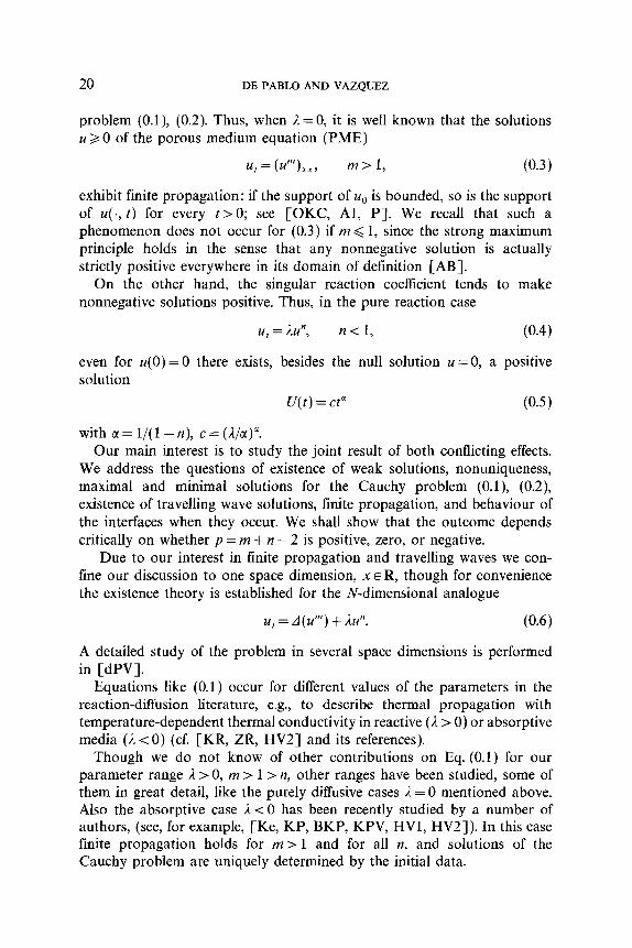
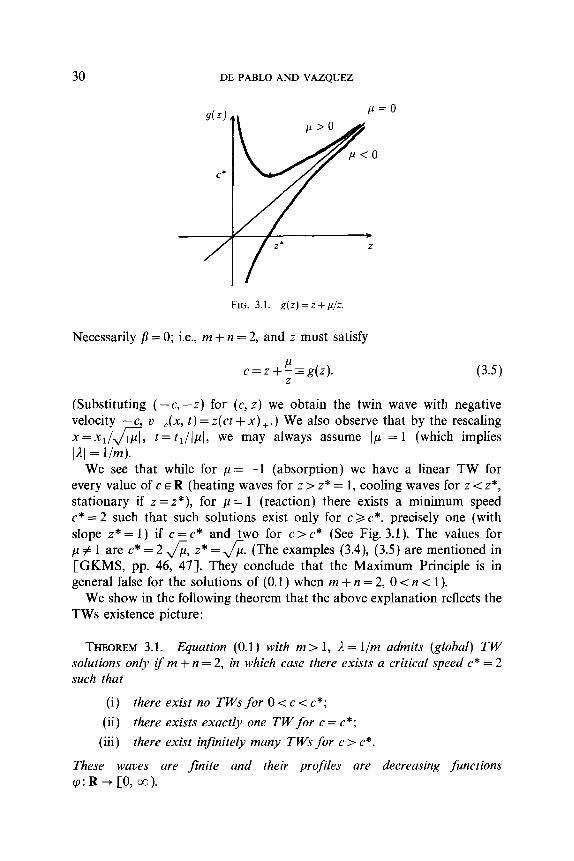
FIG. 3.1. g(z) = z + p/z
Necessarily /3 = 0; i.e., m + n = 2, and z must satisfy
c=z++g(z). (3.5)
(Substituting (-c, -z) for (c, z) we obtain the twin wave with negative velocity -c, U-,(X, t) = z(ct + x) +.) We also observe that by the resealing x = -dJGL t = tJlA, we may always assume (,u = 1 (which implies I;11 = l/m).
We see that while for p = -1 (absorption) we have a linear TW for every value of c E R (heating waves for z > z* = 1, cooling waves for z < z*, stationary if z=z* ), for p= 1 (reaction) there exists a minimum speed c* = 2 such that such solutions exist only for c 3 c*, precisely one (with slope z* = 1) if c= c* and two for c> c* (See Fig. 3.1). The values for p#l are c*=2&, z* = &. (The examples (3.4), (3.5) are mentioned in [GKMS, pp. 46, 471. They conclude that the Maximum Principle is in general false for the solutions of (0.1) when nz + n = 2, 0 -C N < 1).
We show in the following theorem that the above explanation reflects the TWs existence picture:
THEOREM 3.1. Equation (0.1) with m> 1, A= l/m admits (global) TW solutions only if m + n = 2, in which case there exists a critical speed c* = 2 such that
(i) there exist no TWs for 0 CC < c*;
(ii) there exists exactly one TW for c = c*;
(iii) there exist infinitely many TWs for c > c*.
These waves are finite and their profiles are decreasing functions cp:R-+[0,~1).

TRAVELLING WAVES AND FINITE PROPAGATION 3i
ProoJ Introducing U(X, t) = cp(t) into (O.l), this equation becomes
1 -ccp’=(cp’“)“+~ fp”, (3.6)
where ’ = d/d{. It is clear from standard results that any solution of (3.6) will be smooth in its positivity set. Moreover cp and (cp”‘)’ will be continuous in R so that (I$“)’ (to) = 0 at any point to where cp vanishes.
We now perform a phase-plane analysis. We consider the density and the flux variables, namely
and write (3.6) as
x=50, Y= -(q”)‘, (3.7)
-= 2 >yl-“y dX
dt m
dY -= 4
-2. p”‘y+l jy”. in i?7
The trajectories of this system are the solutions of
dY --=C-p+n--ly--E~(X, y). dX
(3.8)
We look for admissib/e trajectories, i.e., solutions of (3.9) for X> 0 such that the solution (X(c), Y(t)) of (3.8) is defined for every <ER and I; vanishes wherever X does. We remark that Eq. (3.6) is invariant under the
FIG. 3.2. II? + n = 2, c = 2.
5O3’93;1-3

32 DE PABLO AND VAZQUEZ
transformation 5 --t -<, c + -c, cp + cp. This reflects the fact that Eq. (0.1) is invariant under the symmetry x -+ -x, t -+ t. As we have already said we are reduced in this way to studying only positive velocities.
3.1. Case nz + y1= 2. In this case (3.8) becomes a linear system,
dX -= dt
-Y
dY -pi--CY
(3.10)
(dz = (l/nz) XiPrn dl), for which the origin is a focus if jc] CC* = 2 (a center if c=O) and a node if 14>2.
For 0 < JcI < 2 the solutions of (3.10) are (besides the trivial solution) spirals around the origin, moving counterclockwise with r, winding if c > 0, unwinding if c < 0. Any trajectory branch in the halfplane X2 0 connects two points in the Y-axis situated opposite with respect to the origin. This takes up a finite r-interval and also a finite t-interval. In fact any such branch has the form of a finite hump in (u, x)-representation, t fixed. For c = 0 the trajectories are circles but the same analysis applies.
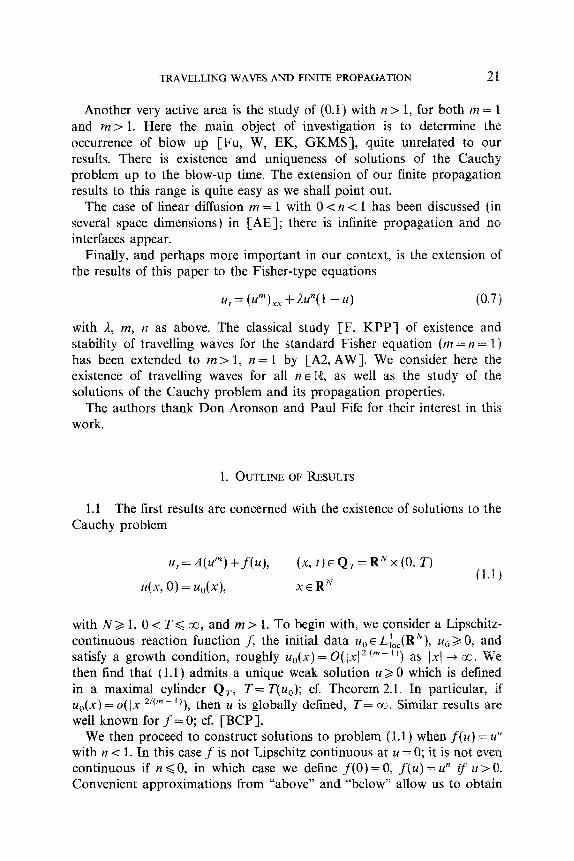
For c = 2 we get the stationary solution (0, 0) and the family of trajec- tories
kER. (3.11)
(See Fig. 3.2) For k = 0 this reduces to the straight line Y= X, which corresponds to
the linear wave vg = (2t - x), described in Section 1.2. For k < 0 we start, e.g., on the trajectory into the halfplane X20 and arrive at the X-axis in a finite l-interval, after which X becomes negative. The other branch, k > 0, goes into X-C 0 and crosses into X> 0 at a point (0, Y,) at which cp = 0 and (cp”)’ > 0. Summing up, we obtain no admissible trajectory branch if k # 0.
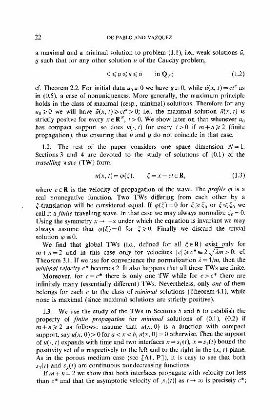
Finally for c > 2 the trajectories are given by
IY-z,Xl”=k IY-z2XJ2*,
for 0 6 k d co, and where z, < z2 are the solutions of z2 - cz + 1 = 0. For the same reasons as in the case c = 2, the only admissible trajectories are
(Y-z,X)“=k(zJ- YjiZ, (3.12)
for 0 <k< cc. The cases k =O, CC give two straight-line solutions corre- sponding to the two linear waves mentioned in Section 1.2 with slopes zi and z2 in (u, x)-plane. For each 0 <k < cc we obtain a solution that starts

TRAVELLING WAVES AND FINITE PROPAGATION 33
at (0,O) with slope zI, advances for X> 0 between Y = z I X and Y = z2 X, and behaves for large X like Y= ;,X. (See Fig. 3.3.)
Observe that since
Y(C) -= - (@‘Y(5)= _ as’) cp(sI) (
m sD,x-I ’ m-l >
(0 = -4’(r)
= -g (X-Cf), (3.13)
we may directly read in the above pictures the shape of the waves in the (v, x)-plane (t fixed). In particular, our admissible family of travelling waves satisfies 0 < zr < -all/aev d z2, which means that they are all finite with decreasing profiles.
3.2. Case m + IZ > 2. For c = 0 Eq. (3.9) can be integrated as
1 ; Y2+- x ‘n+“=a>O. (3.14)
m + il
As in the case m + n = 2, this is a closed curve whose branch in the region X20 is easily seen to be covered in a finite t-interval and has the form of a finite hump,
For c >O we observe that F(X, Y) = dY/dX vanishes in the half-plane X> 0 on the curve
Y=h(X)Ef p+n--l. (3.15)
FIG. 3.3. m + n = 2, c > 2

34 DE PABLO AND VAZQUEZ
Moreover, F= c for X= 0, while 0 < F-c c for Y > h(X); F> c for Y < 0 and F< 0 for 0 < Y < k(X). We see that the trajectories start either from points (0, YO), Y0 > 0, and are therefore not admissible, or from the origin. Even in the latter case the trajectory again cuts the Y-axis at a point (0, Y,), Y, < 0, after a linite l-interval; hence it is not admissible. In fact it provides a local TW defined in a finite c-interval.
3.3. Case m + n < 2. Again there exists no admissible solution of the system (3.8), because the trajectories approach the Y-axis away from the origin. This is seen for c = 0 through formula (3.14) (to be replaced by Y2 = a - 2 log (X) when m + n = 0). For c > 0 solutions tend as i increases to the Y-axisat apoint Y,<Oifm+n>Oor to -OX ifm+n<O. 1
4. THE BRANCH OF MINIMAL SOLUTIONS
In this section we study which travelling waves from those obtained in Section 3 are maximal or minimal according to Definition 2.3. We have already seen in Corollary 2.5 that the maximal solutions corresponding to nonnegative initial data are in fact strictly positive. Thus finite travelling waves, i.e., TWs vanishing for s - et b to, cannot be maximal solutions.
We list here, for the readers’ convenience, the TWs obtained in Theorem 3.1. For simplicity they are given in pressure variable and we put d = l/nz:
(i) if c = 2 there is only one TW,
v*(x, t)=(2t-x),, (4.1)
(ii) if c > 2 there are infinitely many TWs
gx, t) = 5 2-y’(X-CT), (4.2)
where X, is given by (3.12) for 0~ k< co. The limit cases are the linear TWs
v,,(x, t) = C,(X, tj = z,(c~ - x), , (4.3,)
v,2(x, t) = 6=(x, t) = z2(ct-x), , (4.3,)
0 <z, < 22 being the solutions of .? - cz + 1 = 0. The following ordering holds :
v,, < uk d u”k’ d v,, (4.4)

TRAVELLING WAVES AND FINITE PROPAGATION 35
for every 0 < k < k’ < cr,. We also have, for every 0 .< k < EC,
for s - ct = 0,
for x-ct L -tx. (4.5 J
THEOREM 4.1. The trace&g waves 11, if c = 2 and ~7,. if c > 2 are mini- mal solutions, All the other TUJs are neither maximal nor minimal solutions.
Observe that the set of minimal TW corresponds to the right-hand branch of the curve c = g(z), p > 0 in Fig. 3.1. It is also interesting to look at the limit c -+ DZ in both branches of the curve. On the right-hand branch we get z=zz(c)~ c for c large, so that
L~,.(x, t)zc(ct--.uj+, (4.6)
i.e., the porous medium linear wave. On the left-hand branch z = z,(c) ‘2 l/c and
L’,(X, t) = (zct - zx) * + t + 14.7)
which is the maximal solution with zero initial data. This allows us to consider the right-hand branch as the “good” branch.
4.1. We begin by proving the following:
LEMMA 4.2, For each c > 2 the travelling wave v=, is a minimal solution.
Proof. We will construct TW solutions to an approximate problem that are close to u=? = (((m - l)/nz) L~~~)‘~!~‘- I’m We follow the phase-plane arguments in Section 3. Consider the problem of finding TW solutions to the equation
with fE as in (2.11) (A = l/m), and with velocity 2 < c, 7 c. Putting 24(x, t) = cp,(-u - c, t) = (p&(5,) and using the density-flux variables
(3.7), the equation satisfied by the trajectories Y(X) analogous to (3.9) is now
dY z=c”-mX “‘-‘f,(x) Y-’
with the condition Y(0) = 0. It is clear that there exists a unique solution to (4.9) starting from each point (0, A) with A > 0 and with slope c, at that point. Consider the infimum of this nonintersecting family of solutions. It

36 DE PABLO AND VAZQUEZ
is easy to see that this infimum has slope c, at the origin. Let Y, be this trajectory. Let also 0 < zI, 2 < z2, E be the solutions of
z2-c,z+ 1 =o. (4.10)
In a first comparison with test functions of the form Y= MX we see that YE satisfies
Set h(X) = Y,(X) - z2, ,X Using (4.10), (4.11), and the fact that (l/n?) XZern for X3 E we have
h’(X)=c,-%-z~,~= z~.~: YE-X z1 ,/2(x) Z, E h(x) =L<_z-
E YE Y, Z& x
for X2 E. Integrating from E to X we have
h(X)</(&) ; ac, (7 where M, = zl, Jz2, E. Since II(E) G zl, Em we get, for x2 6,
(4.11)
f,(X) =
(4.12)
which together with (4.11) gives the convergence Y,(X) + Y(X) = z,X as E + 0 on compact sets of [O, co).
Next we obtain the convergence of the TW profiles. From the differential system satisfied by X and Y we have
x mP - ’ -t,(x) = c, y,(s) ds.
Using (4.11) and (4.12) we can estimate <,:
(4.13)
m em-l__im-1)/Z
Tzi z,,,[l fqPQ)J]
TRAVELLING WAVES AND FINITE PROPAGATION 31
for E < min{ X, X2}. This implies, for each solution 40, = X(?J,),
In - 1 d --2,E(1+~E)(-5E)++tE 7 in I
l,‘(m - 1 )
(4.14)
where 6, = ~,E(‘-‘~)‘~ , T = co” - ‘)j2. Thus (4.14) implies the convergence E
CPA-x - c, t) = %2c% I). (4.15)
On the other hand, if we choose c, in an appropriate way we can get (1 +6E)z2,r:<z2. In fact
Since for E > 0 small enough we have
l-c! E~~2.;~~l.~>p~il-~l, 2 2, c 42,
which only depends on c, we can choose c, = c/(1 + .$j. Now we define u,(x, t) = cp,(x + a, - c,t) with uE = (m/(m - l))( l/z2) t,.
Since qE z 0 on [0, co) the previous calculations imply that U, is a solution to (4.8) with u,(x, 0) <.L+,(x, 0) and U, + uz2 as E -+O. Therefore ur2 (which is the same, vz,) is a mmlmal solution. 1
4.2.
LEMMA 4.3. If c > 2 the travelling waves ij,, 0 < k < OCI, given in (4.2 )> (4.3,) are not minimal solutions.
ProoJ Consider first the TW with small slope uz, = Go and compare it with the TW v* in (4.1). We have v,, <v* at t = 0, but L’,, propagates with velocity bigger than v* does. Then u,, must forward v* and it is not a minimal solution.
We also use L’* to prove that neither Gk is a minimal solution for each 0 < k < 0~. Since ( -a/ax) Ek(O, 0) = z1 < 1, there exists a constant a > 0 small enough such that
5,(x, 0) d v*(x, 0) for --a <x. (4.16 j
38 DEPABLOAND VAZQUEZ
Also, if t, is small enough we have
~/J-u, t)<u*(-ua, t) for Odt<to. (4.17)
Now we compare in S = (--a, c;c, j x (0, to). If iYk were minimal, its approximating sequence from below o, as constructed in (2.15 j would satisfy v, < tl* in S, hence the limit 6, < u* in S, in contradiction with the interface movement. 1
Remark. The previous argument gives a local comparison principle for minimal solutions that is used later on.
To complete the proof of Theorem 4.1 we still must show that u* is also a minimal solution. This is done in the next section, as an easy application of Theorem 5.2.
5. FINITE PROPAGATION FOR MINIMAL SOLUTIONS IN THE CRITICAL CASE
We study in this section the propagation of solutions to problem (O.l), (0.2) and the existence of interfaces in the critical case m +n= 2. We establish the property of finite propagation with minimal speed, the asymptotic behaviour, and the equation satisfied by the interfaces.
For this purpose let us consider, for that Cauchy problem, the minimal solution u corresponding to an initial value u,, E E, (E, defied in (2.3)). Let P(t) be its positivity set at time t 2 0, P(t) = {x E R : u(x, t) > O}. We always assume, for simplicity, that u0 is continuous and that P(0) is bounded from the right. We study the right-hand interface
s(t) = sup P(t). (5.1)
There is no loss of generality in assuming that s(0) = 0 and II = l/m. A possible left-hand interface can be studied in the same way.
5.1. We first prove a finite propagation property.
THEOREM 5.1. If u is the minimal solution to problem (O.l), (0.2) there exists a continuous function d: [0, ‘;o) + [O, CYI) ulith d(0) = 0 such that for
every t, 2 t, 2 0,
0<s(t2)-s(t,)<d(t,-t,)<ccj.
In particular s( t ) is a continuous nondecreasing function.
(5.2)
TRAVELLING WAVES AND FINITE PROPAGATION 39
Proof. We use the pressure D = (nz/(m - 1)) IO+’ of our solution and we compare it with the TWs obtained before.
Let .~r =s(t,), 5: <x,, and set
M= max 0(x, tl), N= max ~(5, t), L = max(M, N). e .Y b \ r,<_r<q
Consider the linear TW
u- 6(X, t)=z[c(t-t,)-(S-x‘-f3)]+, -.
where 6 > 0, -7 = L/6, c = g(z) = z + l/z. We have
u;,(x, I,)>$ (6+x,-zc)2M>u(x, 11) for <dx<x,,
u... &(X, tl) >, 0 = D(X, t,) for x2x,,
Then, by the local comparison principle (see Remark to Lemma 4.3),
for every x25, t,<t<ttZ, which for the interfaces means
for every t < t < t 1, , 2; i.e., .s(t?)--.$tl)<g(L/6)(tz-tt,)+d. Now we choose 6 to minimize this quantity, thus getting
s(tZ)-.s(tl)<const.(t,-t,)“. (5.3)
The fact that s is nondecreasing follows from the same property for the porous medium equation (cf. [Al]), since solutions of our problem are supersolutions for the PME. 1
In fact in our case the support of the solutions not only expands but it does so with a speed not less than c* = 2 as we show next.
THEOREM 5.2. Let u be any solution to (0.1). Then for tz > tl b 0,
s(tJ - s(t,) > 3. tz-t, ‘- (5.4)
40 DE PABLO AND VAZQUEZ
ProoJ Step 1. We begin by constructing local TW solutions for the perturbed equation (4.8) with velocity 0 < c < 2, c Y 2. Let us consider the function
(5.5)
(5.6)
Put u(x, t) = ~(x - ct), 0 < c < 2. With X and Y as in (3.7) we look for trajectories of the equation
dY - = c - nLY’ - ‘.f(X) Y- l E F( x, Y) dX
(5.7)
for X> 0 and such that Y(0) =O. We know that there exists a unique trajectory Y = Y,(X) defined in [0, B) with B d +co and such that Y,(O) = 0, Y;(O) = c, and 0 < Y,(X) < cX; cf. Lemma 4.2. We now obtain a sharper estimate on Y, and B.
Consider, for some A& L > 0, c( > 1 to be determined later, the function
H(X) = MX- LX”.
Since for X > 1, F(X, Y) = c - X, Y, we have
H’ - F(‘Y, H)
= & [L2(gW- 1) - L(aM+M-c)X”-‘+M(M-c)+ l]
for 1 <Xc (M/L) ‘!(u-1’. We put M=c+6. Then, if l<cc<4/c* and 6 =6(a) is chosen small enough, we have H’-F(X, H) < 0 for 1 <X< (M/L)“‘*- I).
On the other hand, H(l)=c+S-L. With L=6 we get H(l)3 Y,(l). By standard comparison we obtain
Y,(X) < (c + 8)X- 6X”
for ldX<BdB,=((c+S)/6)‘:‘“-‘).

TRAVELLING WAVES AND FINITE PROPAGATION 41
In a similar fashion we can obtain the piece Y= Y,(X) of the trajectory in the quadrant X30, YGO, starting from the point (B, 0). An easy comparison gives
Y*(X)>(c+ 1)X-D,
for O<XdB, where D1=(c+2)B,. In particular, YJO)= -D> -I),: and Y;(O) = c.
Finally it is also easy to check, using the differential relationship between X, Y, and 5, that it takes the trajectory a finite t-interval to get from (0,O) to (B, 0) and (0, -D).
Once we have completed the trajectory for XB 0, we see the shape of the corresponding TW profile just by taking a look at the pressure front $= (wz/(fn- 1)) cp”-’ and (3.13). Clearly $ is a hump, and also cp. We have cp bounded by B,. By translation we may assume that ~(0) = 0.
Step 2. We now define the resealed humps. For any E > 0 the function
q?,(S) = &cp(&l-M*() (5.10)
satisfies the equation
(cpr)” + ccp: +.f&(cp,) = 0 for to<<dO,
(P,(5,) = cp,(O) = 0, (5.11)
where
L(S)=& * ‘yLfl(S/&) =
I
1 - cl-ms if Odsda
; (5.12) _ x2-ln if S>E. nz
Step 3. These functions qr. are used in comparison by putting them below our solution U. Let u0 be the initial value of u and suppose u,, is positive in some interval, say Us > 0 for all I’ <x < 0. Fix xi E (r, 0). It is clear, from the construction of (Pi and the continuity of ugl that there exist E>O and X~E (r, pi) such that
PAX - Xl I< %(-~) for x2<x<Xl,
q,(O) = (pJx* -x1) = 0. (5.13)
We prove the following comparison principle:
42 DE PABLO AND VAZQUEZ
LEMMA 5.3. Under the previous hypotheses,
45+ct, t)3(PE(5-X1j (5.15)
for every t > 0, xz < 5 <x1.
ProoJ: We first compare (Pi with I[*, where 1~~ is, for 6 > 0, the unique (smooth j solution to
w,), = (~~)x.y +fE(u6) in Q
u,(x, 0) = uo(x) + 6 for XER. (5.16J
The inequality (5.15) will be true for each 6 > 0 and then it will be true for the unique solution with 6 = 0. Finally, since our solution u is a super- solution to (5. 166 = 0 j, the result will follow. We then concentrate in proving (5.15) for ud.
Put ~‘(5, f)=uJ<+ct, t), cv,(<, t)=qC(c-~,). From (5.13) and (5.166), both functions solve the equation
2, = (z& + cz< + f,(z). (5.17)
Moreover
(5.18)
for every t > 0. Subtracting Eq. (5.17) applied first to IV and then to ulg, multiplying by p( wr - it’s’), where p is a smooth nonincreasing approxima- tion of the sign+ function, and integrating in (x,, x1) x (0, co)), we get in the usual way that
w,(5, tj ,< M’(5, t) for every xz<5:<x1. t>O.
Observe that p( IV: - wm) vanishes near the lateral boundaries. 1
Step 4. The complete proof of Theorem 5.2 now follows. By (5.15) and (5.13) we have for the interface s(t) of u
s(t)>ct-.Xx,,
c being any velocity less than 2 and x1 being as close to the origin as we like. By translation t --f t - t,, s -+ x - I, we get (5.4). 1
The construction of the local TWs used in the latter proof can also be used to end the proof of Theorem 4.1.
COROLLARY 5.4. The linear travelling wave v* in Theorem 4.1 is a mini- mal solution.

TRAVELLING WAVES AND FINITE PROPAGATION 43
Proof: Let _u be the minimal solution corresponding to the initial value n*(x, 0) = (-x), _ We only must prove that g > II* everywhere in Q. Let s0 < 0 be any given point. For c < 2, c z 2, let us consider the pressure front I+!I constructed in the previous theorem. Since -$‘(O) = c > 1 and li/ is bounded, there exist three points -x1 < .x2 < .x3 < 0 such that
&x)=t&-x3)~.x
for every .yl <.x<s,, and
$(s~1j=$(,x3j=o, ~(x2j= -X2.
Now we consider the resealed pressure corresponding to (5.10); i.e.:
Taking E = (x /Y )‘!(‘+‘) 0’2 we have
Then, as in Lemma 5.3 we have, for any t > 0,
t’(x, + ct, t) 2 ljit:(.vo) = -x0 = 21*(x0 + 24 I).
We conclude by letting c tend 2. 1
5.2.
We now obtain the asymptotic behaviour of the interface in terms of the shape of the initial value for large (xl.
THEOREM 5.5. Let o be the pressure of the minimal solution 11 to problem (O.l), (0.2). Assume that
lim 1(x, 0)
,x” -x Ix(=zix, (5.19)
Then the interface is asynptotically linear and s(tj/‘t -+ c as t -+ ~8, where
1 c = g(r) = z + - if r31,
z i.5.20 j
c=2 q- Obzdl.

44 DEPABLOANDVAZQUEZ
In particular, if v(x-, 0) has compact support, the asymptotic slopes of the right- and left-hand interfaces are +2.
Proo$ If z> 1, for any E >O there exist two constants a,, b, >O such that
for every x E R, where uz is the linear front vz(x, t) = z[g(z) t - X] + . If c is small enough? Z-E > 1 and aZeE is a minimal solution. Since a is also minimal, we have
in Q. As to the interfaces this means
g(z-&)t-aa,<s(t)<g(z+r:)t+b,
for t > 0, and thus
g(z-.sE)< lim SO<g(r+s). **cc t
Now let E + 0. For J = 1 we perform the same comparison from above and use
Theorem 5.2 from below to obtain lim, _ ~ s( t)/t = 2. Finally for z < 1 we use Theorem 5.2 and comparison from above with
V*(X - b, t), for some b > 0. In this case we get
2t < s(t) < b + 2t (5.21)
for every t > 0. 1
If the initial datum is flat enough, the same comparison method gives an exact description of the interface, which turns out to be a straight line.
COROLLARY 5.6. Let s(O) = 0 and suppose u,,(x) d 1x1 for x < 0. Then
s(t) = 2t (5.22)
for every t > 0.
Of course a similar estimate holds on the left if P(0) is bounded below by a ~0 and v0(3c) <x-a for x> a. In this way we obtain two straight lines as interfaces as announced in (1.4).
5.3. These comparison arguments can also be used to prove the equa- tion for the interface for minimal solutions to problem (0.1 j, (0.2).

TRAVELLINGWAVESANDFINITEPROPAGATION 45
THEOREM 5.7. Let u be a mininzal solzltion and let v be its pressure. Asszme for a point x0 = s(t,), t, > 0 on the interface it holds rhat
- lim p (x, to) = z(to) < cc. x/.q LX
(5.23 j
Then there exists the forward time derivative D’s at t = t, and
D+s(t,) = c(z(t,)), (5.24)
where
g(z)=;+; zy- Z>l 9 c(z) = (5.25)
2 if z< 1.
Proof. Let first z = z(t,) > 1. For any E > 0 there exists x, < +yO such that
v~+,(x-x~, O)<V(X, tO)<v,+,(x-xo, Oj
for x, d x. Moreover, there exists 6 > 0 such that
uzp,(O, t-tt,)<v(x,, t)<vzCF(O, t--t,)
for t, d t d t, + S. Then, by the local comparison principle,
v_,(.x-xxg, t-tt,)<v(x, t)<v,+,(x-X0, t-t())
for any x, d X, t, < t 6 t, + 6. This implies
g(z-&)b+S(tO)<S(tO+6)<g(?+&)6+S(tO).
Then
g(z - E) < D’-s( to) < g(z + E).
If z < 1 we conclude as in Theorem 5.5. 1
6. PROPOGATION FOR m+ n#2
Here we distinguish three cases, according to the relation between the exponents, namely n<2-m, 2-nz<n< 1, and n> 1.
If n = 1 we have already seen that Eq. (0.1) can be reduced to the porous medium equation by the transformation (A.3).
46 DEPABLOANDVAZQUEZ
If n > 1, every solution u is a local subsolution, in a neighbourhood of to 2 0, x0 = s(tO), where u is small, of the equation with n = 1. Thus the propogation properties are the same as in the PME.
If 2 -In <n < 1 we have that, when u is small, the minimal solution is a subsolution to the equation with critical exponent n = 2 - 111, and again we have, from Theorem 5.1, finite propagation. Moreover, we can show that this propagation is governed by the same equation for the interface as in the PME. Let u be a minimal solution to problem (O.l), (0.2), and let u be its pressure. Assume that P(0) = supp[v(-, 0)] is bounded from the right. Then a right-hand interface s = s(t) appears (it is continuous and nondecreasing, again by Theorem 5.1) and we have:
THEOREM 6.1. Urfder the previous notation, let (x,, to) be a point on the interface, and let n > 2 - m. Then
lchenever the limit exists.
ProoJ: We have seen in Section 3.2 that when m + IZ > 2 there exist local TW solutions 40, with velocity c > 0 and such that (- (m/(m - 1) 4~: ~ I)’ (0) = c. Then (6.1) follows in the same way as (5.23 j. i
When n < 2 -m we have a very different situation.
THEOREM 6.2. Any nomlegative solution to problem (0.1 ), (0.2) with n < 2 -m and u0 f 0 is strictly positive in R for any t > 0.
Proof: By the comparison theorem (Proposition 2.4), it is sufficient to prove the theorem for small data, for instance, for ~4~ such that 0 6 u0 6 6. Comparison with the explicit maximal solution (2.18) shows then that
0 d 24(x, t)< & (6.2)
for O< t < r and E= 0(6 + T’!(~--“)). Then, since n <2-m we have u’l< & m+‘Z-‘~2-‘r” for 0 < t < T, and u is a supersolution to the equation
uz= (Um)x,+pU2-” (6.3)
with p = &m+n-2. From Theorem 5.2 the minimal speed of propagation of 2.4 is c(E)>~&=O(E(~+“)~~-~ ). Letting E go to zero we obtain smaller solutions whose support propagates with minimals speeds C(E) + a. Since the family {P(t)) is expanding, we have P(t) E R for all t > 0. 1
TRAVELLING WAVES AND FINITE PROPAGATION 41
7. FISHER-TYPE EQUATIONS
7.1. We now apply the techniques used in studying Eq. (0.1 j to generalize the Fisher equation (1.9). We consider the equation
zl, = (Um).~x + wy 1 - u), (7.1)
where m > 1, A > 0 and IZ E R. We look for solutions to (7.1) in Q.=Rx(O,T)forsomeO<T<co,suchthatO<u(~,tjdlinQ..
For the existence of solutions and comparison principles we refer to Section 2. The results in that section are true for Eq. (7.1).
If n > 1, since the reaction term f(s) = A[s”( 1 -s)] + is a Lipschitz- continuous function, Theorem 2.1 holds true for Eq. (7.1). Then, for every measurable u0 such that 0 < u0 < 1, there exists a unique continuous weak solution II to (7.1 j, defined in Q = Q,, (recall (2.7), (2.8)) with u(., 0) = z+,. Moreover, since G = 1 and E_C =0 are particular solutions, we have, thanks to (2.6), 0 < u(x, t) < 1 in Q.
The situation for n < 1 is like in problem (2.9). The proof of Theorem 2.1 can be adapted with only slight modifications, thus obtaining, for each initial measurable data 0 < u0 < 1, a minimal and a maximal solution to (7.1). In fact these two solutions are different for some ranges of m and n. This follows by considering Eq. (7.1) with initial value u0 E 0. The minimal solution is trivially u = 0, while the maximal solution is the function U defined implicitly by
s
11(x. t) ds t, =
0 fw( 1 - s)’ t7.21
Observe that U(.X, t) > 0 for every x E R, t > 0, so that Corollary 2.5 is also valid in this situation.
7.2. To study the propagation properties of the minimal solutions to (7.1) we use the solutions to (0.1) and comparison arguments. We have two different situations corresponding to the different values of p = m + n - 2, i.e., corresponding to Section 5 for p = 0 and to Section 6 for p # 0. We always assume, as in the previous sections, A = l/m.
Case p=O. Since every solution to (7.1) is a subsolution to (0.1) with n = 2 -m, we have finite speed of propagation for minimal solutions to (7.1). To be precise let u be a minimal solution to (7.1), let s(t) be defined in (5.1), and assume s(O) < co. Then s(t) is a continuous nondecreasing function (cf. Theorem 5.1).
On the other hand, let (x,, to) be a point on the interface x = s(t). From the continuity of U, for every E > 0 there exist constants 6, T > 0 such that
505!93:i-4

48 DE PABLO AND VAZQUEZ
0 < u(x, t) <E in the neighbourhood S = (x0 - 6, x0 + 6) x (to, t, + r). Then u is a supersolution in S to the equation
24, = (z4’n).yx + r/u2 -‘?? (7.3)
with II= (1 - E)/PI. Theorem 5.2 then implies
s( t, + T) 3 s( to) + 2T JFE.
Letting E --f 0 we obtain a minimum speed of propagation c* 2 2. To get the equation for the interface (Theorem 5.7), assume again
0~ 21 <.s in a neighhborhood S of a point (x,, to) on the interface. Let u=(m/(m-l))u+’ be the pressure corresponding to our minimal solution u. Suppose that we have
-ho g (x, t,)=z> 1. (7.4)
We define, for each r > 1, p > 0, the function
6, ,k t) = rCsJr) -xl + , where
g,(r)=r+f.
Using Eq. (0.1) from above and (7.3) from below we get, for 6 >O small enough,
in S. Then
Now we let 6, E tend to 0 to obtain (5.24). These case z d 1 is similar. Finally we obtain, as an immediate corollary of Theorems 5.5 and 5.2,
the asymptotic behaviour of the interface of the minimal solution u:
(7.5)
Cnse p # 0. Here we can repeat the whole Section 6 using the results just obtained for p = 0. Thus we get the equation for the interface if p > 0 (Theorem 6.1) and infinite speed of propagation if p -C 0 (Theorem 6.2).
TRAVELLING WAVES AND FINITE PROPAGATION 49
7.3. We now concentrate on searching for travelling wave solutions to Eq. (7.1). Writting again u(x, t) = (p(t) with < = x - ct, c E R, we look for solutions of equation
-cql’=(q7-)~‘+~ (p”(l--qn)
suchthatO~cp~1~~(-~)=1,and~(+~)=O.Sincetheyjointhelevels 24 = 1 and u = 0, they are called change of phase type. They can be finite (i.e., (p(t) = 0 for t 2 co or cp(<) = 1 for < < tl), or positive (rp(<) > 0 for all r~R). 5
The case m = n = 1 has been introduced by Fisher [F] and also studied in the classical paper [KPP]. They have shown the existence of a unique TW solution for each speed c > c * =2 and nonexistence of TWs for 0 < c < c*. These waves are all positive.
The case HZ > 1, IZ = 1 has been studied in [A2, AWJ. In that case there also exists a minimum speed c * = c*(nz) > 0 such that for 0 < c < c* there are no TWs; for c = c* there exists a unique TW and it is finite, and for each c > c* there exists a unique TW which is positive. For example, when I~Z = 2 they find c*(2) = l/J2 by showing the explicit solution
(7.7)
(They use Eq. (7.1) with I-= 1 thus obtaining c*(2)= 1.) We study the existence of TWs in the whole range m > 1, n E R.
THEOREM 7.1. Equation (7.1) M+th m > 1, A= l/m admits TW solutions only if p=m+n-2 20. Moreover, for p>O there exists a critical speed c = c*(p) > 0 such that
(i) there exist no TWs for 0 < c < c*;
(ii) there exists a unique TWfor each c B c*.
The TW lliith c = c* is finite. The TW’s with c > c’ are finite if and only $ n < 1. Finally, c*(p) decreases as p increases. In particular c*(O)=2, c*( 1) = l/&, c*(p) + 0 as p + co.
Remark, For p = 1 and c = c* the TW profile is given by an explicit formula.
ProoJ:
Case p > 0. We perform as in Section 3 a phase-plane analysis, but here we introduce the variables
x=cp, y= -L @-I ( m-l >
) (7.8)
50 DE PABLO AND VAZQUEZ
corresponding to the density and the derivative of the pressure profile. With the new independent variable defined by dT = (l/m) X’ pm d<, Eq. (7.6) can be written as the nonsingular system
(7.9)
It has critical points at
(x, y) = (0, 01, (1, oj, (0, 4.
The phase-portraits are drawn in Fig. 7.1. We look for admissible trajectories for (7.9) (i.e., solutions to
(7.10)
dY c-Y XP-r(l-X) --- z- x Y
= H(X, Y, c) (7.11)
for 0 <X< 1) joining the points (1,0) and (0, Bj for some 0 <B < cm. The existence of a critical speed c*(p) can be obtained by comparison
with subsolutions for c small, with supersolutions for c large, and topologi- cal arguments, together with the monotonicity of H with respect to c and Y. As c increases, the trajectory approaching the saddle point (0, c) and the trajectory leaving (1,0) in Fig. 7.1.a move toward one another and at a critical value c* = c*(p) they coincide. This value is unique since dH/dC> 0. It also follows that c*(p) is decreasing as p increases. The resulting saddle-saddle connection corresponds to a finite TW. This follows by observing the behaviour of the trajectory near the critical points. We have
Y,*(O) = c*
Y,*(X) z M( 1 - X) as Xr 1. (7.12)
Thus, using the differential relation
dt=mXm-l&= -mX”‘-‘y--‘d~, (7.13)
we see that 5 tends to a finite <,, as X + 0 and that 0 < (p,*(t) < 1 for every t<hl, (Pc*(-~)=l, v,,*(t)=07 f or every 5 2 to. By translation we may assume 5” = 0. Moreover we have
( m ’ -- q?;- I
m-l > (0) = c*.
a
TRAVELLING WAVES AND FINITE PROPAGATION
b Y
51
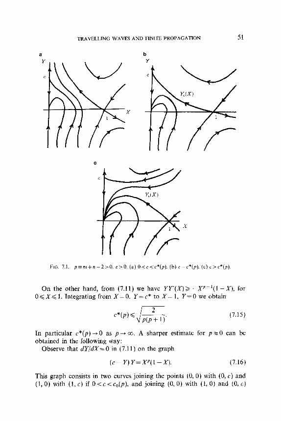
FIG. 7.1. p=m+n-2>0. c>O. (a) O<c<c*(p). (b) c=c*(p). (c) c>c*(p).
On the other hand, from (7.11) we have YY’(X)a -Xp-‘(1 -X), for O<X< 1. Integrating from X=0, Y=c* to X= 1, Y=O we obtain
’ 2 c*(p)< ~ J P(P+ 1)’
(7.15)
In particular c*(p) -+ 0 as p + cc. A sharper estimate for p % 0 can be obtained in the following way:
Observe that dY/dX= 0 in (7.11) on the graph
(c- Y)Y=XP(l-xx). (7.16)
This graph consists in two curves joining the points (0,O) with (0, c) and (1,O) with (1, c) if 0 <c < co(p), and joining (0,O) with (1,O) and (0, c)
52 DE PABLO AND VAZQUEZ
with (1, c) if c > c,(p). For c = co(p) = 2 Jm these two curves meet one another at a point (X, Y) = (p/(p + I), c/2). Looking at the sign of H in the different regions of [0, l] x [O, c] we see that a trajectory joining (0, c) with (1,O) cannot exist if cb c,(p). Then c*(p) <c,(p) for every p > 0 (note that c,(p) < 2).
For c > c* we have a saddle-node connection from (1,0) to (0,O). The trajectory Y,(X) must appraoch the origin above the branch of the curve (7.16) thru (0,O). Thus
Y,.(X) > 1 xp for XzO. (7.17) c
Using this estimate we see that the integral of (7.13) is finite for X%0 if n < 1, and the travelling wave cpC verities
( m m--l -- (P’, m-l >
’ (O)=O. (7.18)
In this case, n < 1, we see that rp, does not satisfy the equation for the inter- face (6.1) and it cannot be a minimal solution. On the contrary, when IZ 3 1 the unique solution must satisfy (6.1), and (7.18) cannot be true at any point co < co such that ~~(5~) = 0. We obtain in this way that the travelling wave pp, for c > c*(p) is finite if and only if n -C 1.
For p = 1 and c = l/fi, Eq. (7.11) admits the explicit solution Y(X) = c( 1 -A’), which after integration gives the finite TW defined by
-L& (-5)+ gc’ z & (7.19)
Thus c*(l) = l/&. When m = 2 and n = 1, (7.19) gives (7.7).
Case p = 0. We know from Section 7.2 that for m + n = 2 we only must consider velocities c > 2. On the other hand, the graph (7.16) becomes in this case a parabola
x= Y2-cY+l. (7.20)
This parabola joins (1,0) with (1, c), and intersects the Y-axis at two points (0, zi), 0 < z1 < z2 (zr = z2 = 1 if c= 2). It is easy to see that there exists a unique trajectory below this parabola, joining (LO) with (0, zl). This corresponds, for each c > 2, to a finite TW qC verifying
(
m m-1 -- v’, m-l >
’ (0) =zl. (7.21)
Of course if c > 2 the TW qpc does not satisfy the equation for the inter- face (5.24) and it is not a minimal solution to (7.1).
TRAVELLING WAVES AND FINITE PROPAGATION 53
Case p < 0. A local analysis around the origin of the (X, Y)-plane allows us to conclude in the same way as in Section 3.3 for Eq. (0.1) that a global nonnegative TW such that cp( - s) = 1, cp( + #UJ) =0 cannot exist. 1
Remark. It is not difficult to prove that the TWs depend continuously on 5, c, and p (cf. [HVZ] for 2 < 0). En particular, as p -+ 0 with c = c*(p) the TWs change the equation for the interface in passing to the limit. Thus for p > 0 the trajectory in Fig. 7.lb joins (LO) to (0, c), while for p = 0 the trajectory joins (LO) to (0, c/2).
APPENDIX
Proof of Theorem 2.1
hisfence. For u0 E E0 we define the truncatures z+,,[:
i
uob) if 1x1 < tz, uO(x) < IZ, u,,(x) = n if Ix/ d II, uO(x) > n,
0 if 1x1 > II.
Then z+,~ E L’(R”) n L”(RN). We have, for every r > 1,
(A.1)
uon 7 ~~09 IIUonllr /” ll~dlr if nr+csj. C-4.2)
For each n B 1 let U, be the unique solution to problem (2.1) with initial data zlon ; cf. [BC, Theorem 31. Observe that if k is the Lipschitz constant of f, then #!,, defined by
u,(x, f) = e%, ek(m-lh- 1
x, k(m - 1 j >
(A.3)
is a subsolution to the porous medium equation
w, = d(2.f”); (A.4)
cf [MP]. By Lemma 1.4 from [BCP], the solutions to (A.4) satisfy the estimate
where CL= (nz- 1+2/N))‘, and for (xl <R, 1 <r< R, 0~ t<c liw(., O)ll~-“‘, as well as
54 DE PABLO AND VAZQUEZ
for each r > 1, 0 < t 6 c I~Iv,(., 0)/l: -‘n. Since IV,, is a subsolution to (A.4) these estimates are also valid for K’,,. Now using (A.3) and noting that w,,(x, 0) = uOnr we have
for IxI< R, 1 d r < R, and 0 < t < T,(u,) = l/k(r?z - 1) log[l + c&m -- 1) lluOll f -“I, with the function
x(t) = ekr [ez;“,llPx9
(A.6)
and also
llU,(? t)ll,Gc(T) /I4l//r~ (A.7)
With this bound we can define the locally bounded limit II = lim,, _ x u,. It is a solution to (2.1) for
0 < t < T= lim T,ju,) r-cc
1 =k(m- 1)
log[l +ck(m- I) IIz4011;-m], (<4,8 1
and, in view of (A.6) and (A.7), UE E,. The continuity of u follows from Cd& Sl.
Comparison and Uniqueness. Let u, ~1 E E, be a subsolution and a supersolution, respectively, to (2.1) for some T> 0. Subtract the inequalities satisfied by u and v in (2.2) to get, for 0 < T < t < T,
JR,v (u-v)(t) v(t) G JR*, (14 - V)(T) v(r)
.f + J s L-(U-v)cp,+(urn - v’=) dq, + (f(u) -f(~))cpl(~~ 4 T Rh’
for every cp E C m(QT) with compact support in x. Set
urn - v” for 24 #v f(u) -f(u) for u#v u-v
b= U-V
a= tA.9) mu n,- 1 otherwise; k otherwise.
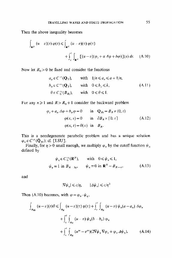
TRAVELLING WAVES AND FINITE PROPAGATION 55
Then the above inequality becomes
-I + J i [(u-u)(cp,+aA~+b~)](s)ds. (A.10)
T R”
Now let R, > 0 be fixed and consider the functions
a,, E C a(Qd, with l/r? d a, d a + l/n,
b,,E CYQr), with Odb,<k,
13 E C,“(B&), with 0 6 8 d 1.
(A.11)
For any n 2 1 and R > R, + 1 consider the backward problem
q,+a,&+b,cp=O in QRI = B, x (0, r)
cp(x, s) = 0 in s3B, x [0, t]
q$x, t)= 13(x) in B,.
(A.12)
This is a nondegenerate parabolic problem and has a unique solution pn E CX(&); cf. [LSU J.
Finally, for >j > 0 small enough, we multiply 40, by the cutoff function tj,, defined by
&E WR”), with 0 d $, G 1,
t+bq= 1 in BRpzq, $,,-0 in RN-B,-,, (A.13)
and
Then (A.lO) becomes, with w = cpII. $,,
56 DE PABLO AND VAZQUEZ
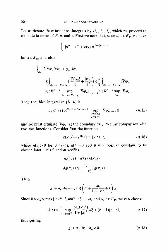
Let us denote these last three integrals by H,,, I,,, J,,, which we proceed to estimate in terms of R, n, and t. First we note that, since u, v E E,, we have
for XE B,, and also
<CR”-l sup lV%l r1-o - cRN- I sup IVq,,l. BR-~- &-I? ~BR
Then the third integral in (A.14) is
J, < C(T) R N-1+2dm-1) ,:;z, IVV,~(X, sjl (A.15) o<s<r
and we must estimate IVq,J at the boundary dB,. We use comparison with two test functions. Consider first the function
g(x, s) ==e’*(s’(l -I Jx12)-8, (A.16)
where h(s) > 0 for 0 <s < t, h(t) = 0 and /I is a positive constant to be chosen later. This function verifies
Then
g,+a, Ag+b,gd h’+
Since 0 da,, < max(mu”-I, mu”-‘} + l/n, and u, 11 E E,, we can choose
h(s)=J-r sup c;$$) &+(k+ l)(t-s), * xeRN
(A.17)
thus getting
gs+an Ag+b,cO. (A.18)
TRAVELLING WAVES AND FINITE PROPAGATION 57
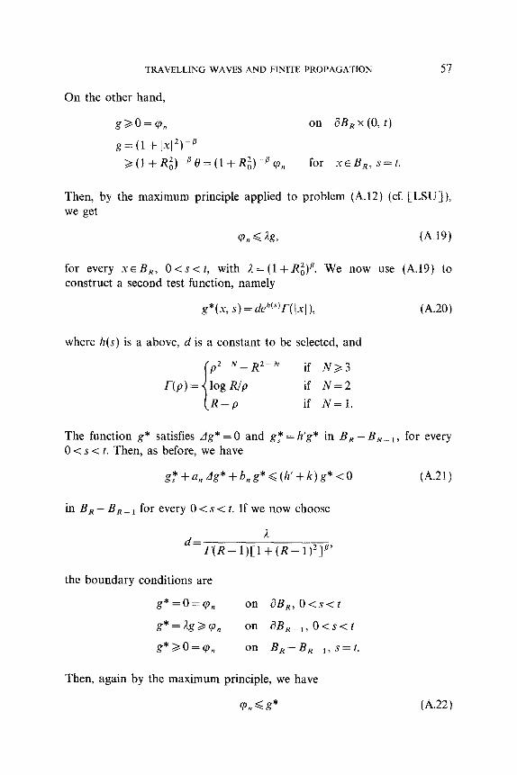
On the other hand,
g>o=cp, on dB, x (0, t)
g= (1 + I.x12)-”
>,(l+R~)~P~=(l+R~)-Pcp, for XEB,, s=t.
Then, by the maximum principle applied to problem (A.12) (cf. [LSU]), we get
cp,,~k3 (A.19)
for every s E B,, O<s<t, with il=(l+Ri)“. We now use (A.i9) to construct a second test function, namely
g*(.u, s) = df?‘“‘r( Ix/ ), (A.20)
where h(s) is a above, n is a constant to be selected, and
if N>3 if N=2 if N=l.
The function g* satisfies Ag* = 0 and g,* = kg* in B, - B,- ,, for every 0 <s < t. Then, as before, we have
g,*+a,Ag*+b,,g*d(k’+kjg*<O (A.21)
in B,-- B,-, for every 0 <s < t. If we now choose
A d=r(R-l)[l+(R-l)‘]B’
the boundary conditions are
g*=o=q, on dB,, 0cs-c t
g*=2g2qn on dB,-,, O<s<t
g*2o=p, on B,--B,-,, s=t.
Then, again by the maximum principle, we have
(A.22)

58 DE PABLO AND VAZQUEZ
in B,-B,-,, for every 0 < s < t. Since both cp,, and g* vanish on dB,, we must have
4y<arp,<o av ’ av ’ (A.23)
on dB, for every 0 < s < t, where a/& denotes the normal derivative. Thus, by the definition of d,
=c(T)A[l+(R-1)21-P &(“:‘)
<c(T, R,) RplP.
Going back to (A.15) we obtain
J,<c(r)R N-l+tm:(m-l)~2p , (A.24)
where c(r) depends also on N, tn, Ro, T, and the norms of u and z! in E, as used in the definition of h(s) but not on n or R. We take /?>m/(m-l)+(N-1)/2.
We now estimate H,,.
,< ~U--21~2 (A.25)
To estimate the latter factor multiply Eq. (A.12) by Av,~ and integrate to obtain
; j IVL,(~)12 + jr j a, 14P,12 BR T BR
w9+; j; jBR a,, IArp,12+; Jr’ Jb, F. n
Using this inequality together with (A.ll), (A.19), and (A.16) we get
I ff a, I&n12 < c(R)n. (A.26) * BR

TRAVELLING WAVES AND FINITE PROPAGATION 59
We now construct the approximation a,, to control the first integral in (A.25).
Let bEiE,O be a sequence of mollifiers in R”+ i, and let Lz: be the exten- sion by zero of a to RN+‘. Define
a, = a n, E = a * pB + l/I?, (A.27)
where a, is smooth and satisfies (A.ll). Since the estimates obtained do not depend on E > 0, they must still hold for
a, = lim a II, E = a + l/n. E--t0
We now divide the domain QRr into two regions, namely
QA= (ix,~)~Q~~:~ix, s)Q Ii&},
Qf=Q,,-Qf,.
If (x, s) E Qf, we have
(a,, - QJ2 < lin . 7
4,
while
If (x, s) E Qi we have
and, since 14, v E ET, we also have J: lu - vi2 < c(R: r). Using (A.26) together with these estimates we get
H, < c(R, z) c(n) with c(iz)g 0 (R, z fixed). (A.28)
We can also define the approximation b, to get in the same way
1, < c(R, 5) c(n) with c(n) n 0 (R, 5 fixed). (A.29)
Summing up, (A. 14) becomes (recalling (A. 19))
(A.30j
60 DE PABLO AND VAZQUEZ
for some S>O, R>R,+l, t>O, and every ~EC$(B~,) with 0<0<1. The fact that U, u E E, allows us to pass to the limit, R + co, z -+ 0, from where we obtain the comparison, and clearly also the uniqueness. 1
CAEI
CAlI
CA21
CAB1
[AC1
CAW
lAwI
CdBl
LB-1
CBCI
CEKI
CFI
CFul
REFERENCES
J. AGUIRRE AND M. ESCOBEDO, A Cauchy problem for u, - 4u = up with 0 <p < 1, Ann. Fat. Sri. Toulouse Math. 8, No. 2 [1986), 175-203. D. G. ARONSON, The porous medium equation, in “Some Problems in Nonlinear Diffusion” (A. Fasano and M. Primicerio, Eds.), Lecture Notes in Math., Springer- Verlag, New York/Berlin, 1986. D. G. ARONSON, Density-dependent interaction-diffusion systems. in “Proc. Adv. Seminar on Dynamics and Modelling of Reactive Systems,” Academic Press, New York, 1980. D. G. ARON~ON AND PEI. B~NILAN, Regularit des solutions de I’Cquation des milieux poreux dans R”, C. R. Acad. Sci. Paris 288 (1979), 103-105. D. G. ARONSON AND L. CAFFARELLI, The initial trace of a solution of the porous medium equation, Trans. Amer. Math. Sot. 280 (19831, 351-366. D. G. ARONSON, M. G. CRANDALL, AND L. A. PELETIER, Stabilization of solutions of a degenerate nonlinear diffusion problem, J. Nonlinear Anal. Theor]] diethods ilppl. 6 (1982), 1001-1022. D. G. ARONSON AND H. F. WEINBERGER, Nonlinear diffusion in population genetics, combustion and nerve propagation, in “Partial Differential Equations and Related Topics,” pp. 549, Lecture Notes in Mathematics, Pub., New York, 1975. E. DI BENEDETTO, Continuity of weak solutions to a general porous medium equation, Indiana Univ. hfath. .I 32, No. 1 (19831, 83-118. PH. B&LAN, M. G. CRANDALL, AND M. PIERRE, Solutions of the porous medium equation in R” under optimal conditions on initial values, Indiana Univ. Math. J. 33 (1984), 51-87. H. Btizrs AND M. G. CRANDALL, Uniqueness of solution of the initial value problem for u,-49(u) =0, J. Math. Pures Appi. 58 (1979), 153-163. M. ESCOBEDO AND 0. KAVIAN,. Variational problems related to self-similar solutions of the heat equation, J. Nonlinear Anal. Theory Methods Appl. (1987), 1103-l 133. R. A. FISCHER, The advance of advantageous genes, Ann. Eugenics 7 (1937), 355-369. H. FUJITA, On the blowing up of solutions of the Cauchy problem for u,=du+ u’+’ J Fat. Sci. Univ. Tokyo, Sect. I 13 (19661, 109.-124. >
[GKMS] V. A. GALAKTIONOV, S. P. KUKDWMOV, A. P. MIRHAILOV, A. A. SAMARSKII, “Blow-Up Solutions in Problems for Quasilinear Parabolic Equations,” Izd. Nauka, Moscow, 1987. [in Russian]
WV11 M. A. HERRERO AND J. L. VAZQUEZ, The one-dimensional nonlinear heat equation with absorption: Regularity of solutions and interfaces, SL4M J. Math. .4nal. 18, No. 1 (1987), 159-167.
CHv21 M. A. HERRERO AND J. L. VAZQUEZ, Thermal waves in absorbing media, J. Differential Equations 74, No. 2 (1988 j, 218-233.
WI T. KATO, Schriidinger operators with singular potential, Israel J. Math. 13 (1972), 133-148.

TRAVELLING WAVES AND FINITE PROPAGATION 01
W’l
[J-VI
WeI
W’pl
CL=Jl
loKc1
ldpV1
[PI
CRKI
IS1
WI
WI
S. KAMIN AND L. A. F%LETIER, Singular solutions of the heat equation with absorp- tion, Proc. Amer. Murh. Sot. 95, No. 2 (1985), 205-210. S. GAMIN, L. A. PELETIER, AND J. L. VAZQUEZ, Classification de solutions sing&&es g l’origin pour une tquation de la chaleur non lin&aire, C. R. Acad. Sci. Paris 305 (1987). 595-598. R. KERSNER, The behavior of temperature fronts in media with nonlinear thermal conductivity under absorption, Vestnik Moskoo. Unix. Ser. I Mat. Mekh. 33, No. 5 (1978), 4451. A. KOLMOGOROFF, I. PETRO~SKI’, AND N. PISCOUNOFF, l&de de l‘kquation de la
diffusion avec croissance de la quantite de mat&e et son application g un probltme biologique, Bull. Univ. Moskoc. Ser. Intentat., Sect. A 1 No. 6 (1937). l-25. 0. A. LADYZENSKAJA. V. A. SOLONNIKOV, AND N. N. URALCEVA. Linear and quasilinear equations of parabolic type, in “Translations of Math. Monographs,” Amer. Math. Sot., Providence, RI, Zh. Vyhisl. Mat. i Mur. Fiz. 12. No. 4 (1972 j, 1048-1053. 0. A. OLEINIK, A. S. KALASHNIKOV, Y. L. CZHOU, The Cauchy and boundary problems for equations of type of unsteady filtration, Ix. Akad. Nauk. SSSR Ser. iMat. 22 (1958), 687-704. [in Russian] A. DE PABLO AND J. L. VAZQ~Z, Balance between strong reaction and slow
diffusion, Comm. Partial Differential Equations 15 (1990), 159-183. L. A. PELETIER. The porous medium equation, in “Applications of Nonlinear Analysis in the Physical Sciences” (H. Amann et al., Eds.), pp. 229-241, Pitman, London, 1981. P. ROSENAU AND S. KAMIN, Thermal waves in an absorbing and convecting medium, Phgsica SD (1983), 273-283. P. E. SACKS, The initial and boundary problem for a class of degenerate parabolic equations, Comm. Partial Differential Equations 8 (1983), 693-733. F. B. WEISSLER, Existence and non-existence of global solutions for a semilinear heat equation, Israel J. Math. 38 (1981), 29-39. YA. B. ZELDOVICH AND Yu. P. RAIZER. “Physics of Shock Waves and High Temperature Hydrodynamic Phenomena,” Academic Press, New York. 1966.


![4.1.1] plane waves](https://static.fdokumen.com/doc/165x107/6322513728c445989105b845/411-plane-waves.jpg)