Travelling Salesman Problem (TSP) based

integration of Planning, Scheduling and

optimal Control for Continuous Processes

Vassilis M. Charitopoulos, Vivek Dua, Lazaros G. Papageorgiou*

Department of Chemical Engineering, Centre for Process Systems Engineering, University College

London, Torrington Place, London WC1E 7JE, United Kingdom

*Corresponding Author: l.papageorgiou@ucl.ac.uk

Advanced decision making in the process industries requires ecient use of information

available at dierent decision levels. Traditionally, planning, scheduling and optimal control

problems are solved in a decoupled way, neglecting their strong interdependence. Integrated

Planning, Scheduling and optimal Control (iPSC) aims to address this issue. Formulating

the iPSC, results in a large scale non-convex Mixed Integer Nonlinear Programming pro-

blem. In the present work, we propose a new approach for the iPSC of continuous processes

aiming to reduce model and computational complexity. For the planning and scheduling,

a Travelling Salesman Problem (TSP) based formulation is employed, where the planning

periods are modelled in discrete time while the scheduling within each week is in continuous

time. Another feature of the proposed iPSC framework is that backlog, idle production

time and multiple customers are introduced. The resulting problem is a Mixed Integer

Programming problem and dierent solution strategies are employed and analysed.

Keywords: process scheduling, planning, dynamic optimisation, enterprise wide optimisation, inte-

gration

1

1 Introduction

Decision making in the process industries is organised in a hierarchical manner and actions are taken

in a decentralised fashion with common objectives being the maximisation of protability, sustainabi-

lity and safety. Three of the most important functionalities in the chain of command of the industry,

involve medium-term planning, production scheduling and advanced process control. Process plan-

ning aims to organise the production and meet demands over long time horizons; a planning horizon

typically spans from weeks to months and key decisions include the determination of sales, backlog

and inventory levels. After the planning decisions have been made, a detailed schedule of production

is carried out for each planning week. Production scheduling deals with the optimal resource alloca-

tion of the manufacture in greater detail than planning; major decisions include, optimal production

and changeover times, sequencing of tasks and so forth. On a lower level in the decision pyramid,

advanced process control (APC) is located. APC, involves optimal and model based control strategies

that are responsible for the regulation of the process dynamics. For the case of continuous manufac-

turing systems, such as polymerisation processes, APC aims to secure the optimal operation between

transition of dierent production regimes as well as to maintain the desirable steady state operating

conditions. The ever increasing need to maintain protable and ecient operations in the industry

along with recent developments such as parallel computing and more ecient IT infrastructure indi-

cate the dawn of a new era in the way decision making is conducted. Concepts such as enterprise

wide optimisation (EWO), smart manufacturing1 and Industry 4.02 underline the need for ecient

use of information available among closely related functionalities of the supply chain like medium term

planning, production scheduling and optimal control.

1.1 Integration of process operations with control

In Figure 1, the automation pyramid based on the ISA 95 standards is envisaged.

2

Figure 1: ISA 95 automation pyramid

Based on the ISA 95 standards3 the levels of hierarchy that we focus on, within this article, are the

three top ones. As shown in Figure 1, the three problems involve dierent time scales and there is

information ow, from top to bottom and vice versa. Because of the interdependence existing among

these three problems, developing an integrated approach to model and solve the problem is likely to

yield better solutions and thus enhance process operations. Indeed, research work from the literature

indicate that integration of dierent decision layers of the automation pyramid can lead to more ecient

operations36.

Until recently, the integration was studied from two dierent perspectives: (i) integration of medium-

term planning and scheduling and (ii) integration of scheduling and control. For the problem of in-

tegration between planning and scheduling a number of modelling approaches have been proposed in

the literature with some researchers formulating the problem in a monolithic way while other rese-

archers employing aggregated modelling techniques or even the development of surrogate models for

the problem of scheduling7. Regardless of the modelling approach employed, due to the dierent time

scales the computational eort required for the solution of the problem grows rapidly with the length

of the planning horizon under consideration. To this eect, solution techniques such as Lagrangean

relaxation, rolling horizon and bi-level decomposition have been proposed, to name a few.

Integration of process scheduling and optimal control has been studied recently for both continuous

and batch processes8. The interactions between scheduling and control can dramatically aect the

economically optimal operation of the manufacture, since decisions such as production time, sequencing

of tasks and transition time are dependent on the dynamic status of the system. To be more specic,

3

the production rate for a continuous process can be seen as a function of the state variables of the

underlying control problem; the role of the controller is to keep the system around the desirable

steady state and reject disturbances that might occur because otherwise the production time would

be disrupted, jeopardizing the feasibility of the schedule under execution. The optimal sequencing of

tasks relies mostly on the transition times and so the control policy can have considerable impact on

the schedule as the transition time is practically the time that the controller needs to take the system

from one steady state to the next.

The simultaneous cyclic scheduling and dynamic optimisation of a single multi-product CSTR was

studied by Flores-Tlacuahuac et al.9. The authors proposed a time-slot based formulations for the

scheduling part of the problem, where equal number of slots and products were considered. Apart from

model based strategies, the use of parametrised PI controllers10 for the integration of cyclic scheduling

and control has been proposed. Zhuge and Ierapetritou11 proposed a framework for the closed loop

implementation of the integrated solution of scheduling and control (iSC) for continuous processes that

shared many similarities with model predictive control (MPC). The same authors, studied the iSC of

batch processes through multi-parametric programming; they designed the multi-parametric controller

oine and embedded the explicit solutions with additional constraints in the scheduling model12.

In general, the iSC is formulated as a mixed integer dynamic optimisation problem (MIDO) and

then following an numerical integration scheme is discretised into large scale mixed integer nonlinear

programming problem (MINLP) which can be computationally demanding. To ease the computational

burden for the case of iSC of a single multi-product CSTR the use of Benders decomposition has been

proposed as an alternative solution technique13. The use of fast MPC in the context of iSC has also

been reported, in which case linear piecewise ane approximations of the original nonlinear dynamics

were employed14. One of the main challenges in the iSC stems from the dierent time scales involved

in the two problems. Recently, time-scale bridging approaches have been proposed15;16 where the

main idea is to derive a low dimensional model for the dynamics of the system and thus create oine

a correlation between system outputs and set-points in order to speed up the required calculations.

More specically, in Baldea et al.17 a closed loop framework for the solution of the integrated cyclic

scheduling and control was presented. The authors derived the corresponding time scale bridging model

(SBM) and included it in the scheduling formulation as a set of soft constraints, while a scheduling-

oriented MPC was designed for the closed loop implementation of the integrated solution. For further

discussion the interested reader is referred to some recent reviews on the topic of iSC3;8;18.

4

Recently, the development of frameworks for integrated planning, scheduling and control (iPSC) has

started to receive attention. Prompted by the potential economic benets that the iSC has indicated,

the investigation of an even more integrated decision making framework that takes full advantage of all

the possible interactions involved in the three problems constitutes a promising direction. Within the

iPSC framework, the decisions involved in planning, scheduling and control are made simultaneously

with a common objective. It can be understood that iPSC poses many challenges despite the potential

benets; the time-scale problem is further exacerbated when planning decisions are considered, the way

that the three dierent problems are eectively linked constitutes another major factor that aects

model complexity. The iPSC of single unit continuous manufacturing processes, for short term planning

periods, was studied and formulated as an MINLP by Gutierrez-Limon et al.19. The authors employed

the scheduling and planning model of Dogan and Grossmann20 while for the control part of the iPSC

a nonlinear MPC (NMPC) scheme was used. Following this work, the transition times are xed oine

based on heuristics and thus are not considered as decision variables. Note that despite the use of

a NMPC scheme in the aforementioned work, disturbance rejection was not considered. The same

authors5 later on proposed a reactive heuristic strategy for the iPSC under the presence of unforeseen

events. Shi et al.21 considered the integration of planning, scheduling and dynamic optimisation of

continuous manufacturing processes. The authors, proposed a technique to create a exible-recipe

framework in which pairs of transition times and cost are determined oine. In order to alleviate

the computational complexity, they decomposed the problem, thus rendering it into a mixed integer

linear programming (MILP) problem, for which a bi-level decomposition solution procedure was also

proposed. Note that in their work, no disturbances are considered and the dynamic optimisation

provides only open-loop related information about the real dynamics of the process. Again the model

of Dogan and Grossmann20 was used as a basis for the integrated planning and scheduling and the

authors proposed an alternative way to calculate the inventory balance in every production period,

based on the trapezoid rule.

1.2 Motivation and problem statement

The objective of the present article is to provide a computationally ecient framework for the inte-

gration of planning, scheduling and optimal control for the deterministic case where no uncertainty is

considered at any of the levels of planning, scheduling and control. Motivated by the ever lasting need

for more ecient and reliable operations in the process industries we aim to explore the interdependence

5

of the decisions between the three dierent hierarchical levels which up until recently were considered

in a decoupled manner. In general, we consider single unit continuous manufacturing processes which

based on multiple steady states, that the underlying dynamic system exhibits, can produce a number

of dierent products.

Concisely, the iPSC problem can be stated as follows:

Given:

A single stage, multi-product continuous manufacturing process

Production planning horizon

Demands for each product at the end of each planning period

Process dynamics and steady state operating conditions of the process

Raw material, operating and inventory costs

Selling prices

Determine:

Dedicated production time and cost for each product in every planning period

Optimal production sequences

Optimal change-over times and cost

Inventory and backlog level for each product at the end of each period

Optimal dynamic trajectories of the process

Objective:

Maximise the production prot of the process; i.e. the revenue, minus inventory, backlog, operation,

production and transition costs under deterministic assumptions. Note, that since in the present work

no disturbances are considered at the level of dynamics, the optimal control part of the integrated

problem is concerned with open-loop policies and thus we restrict ourselves to open-loop stable systems

and the term optimal control is used in a dynamic optimisation sense.

Since the iPSC involves the optimal control of the process the problem is formulated as an MIDO

which is discretised into an MINLP. The degrees of freedom for the optimisation within the iPSC

6

involve among others: (i) production amounts within each planning period, (ii) assignment of products,

(iii) transition times for the changeovers between products, (iv) optimal dynamic trajectories and (v)

backlog of unmet demand. The remainder of the article is organised as follows: in section 2 the main

parts of the methodology developed for the integrated problem are described. Next, in section 3 the

proposed methodology is illustrated and compared through three dierent case studies with the time-

slot based formulation for the integrated problem highlighting the computational savings achieved.

Finally, in section 4 concluding remarks and future research directions are drawn.

2 Methodology

The majority of research work conducted for the integration of control with operations has focused on

time-slot based formulations. In the present work, we propose a Travelling Salesman Problem (TSP)

based framework for the integrated planning and scheduling problem that has two distinct features.

First, the time representation used herein is hybrid, i.e. the planning periods are modelled as discrete

time points while within each planning period a continuous time representation is followed. Secondly,

following the proposed TSP formulation the notion of time-slots is replaced by implicitly unique pairs

of products which can be produced in a sequential manner within each planning period.

2.1 Objective of the iPSC

As discussed in the previous section, the main reason that the iPSC is formulated in a simultaneous and

not sequential manner is to take advantage of the information available across the dierent decision

levels. Another reason and key objective of the present study is to provide a way of reecting the

process dynamics into process economics. The objective function of the integrated problem is the

maximisation of prot and is calculated as the revenue minus the costs associated with the inventory,

raw material consumption, backlogged demand and operation.

Eq.(1) represents the revenue (Φ1) of the production as the summation of the sales of every product

i, for every customer c, for every planning period (Scip) multiplied by its respective selling price (Pi).

Φ1 =∑

c

∑i

∑Pi

p

Scip (1)

7

Eq.(2) accounts for the total operational cost (Φ2) over the planning horizon which is calculated as

the product of the unitary operational cost (Coperi ) and the amount produced (Prip).

Φ2 =∑

i

∑p

Coperi Prip (2)

The total inventory cost is given by eq.(3) and is calculated as the product of the unitary inventory

cost (Cinvi ) and the inventory level (Vip) of product i at the end of every planning period p.

Φ3 =∑

i

∑p

Cinvi Vip (3)

When demand cannot be met, in the present work backlog is allowed under a penalty. The cost

associated with backlogged demand is calculated by eq.(4).

Φ4 =∑

c

∑i

∑p

CBicBcip (4)

where CBic stands for the unitary backlog cost and Bcip denotes the demand of customer c at the

end of planning period p for product i that is backlogged.

Another way planning, scheduling and optimal control interact is the calculation of the changeover

cost. In principle, the changeover cost is calculated as the product of a unitary changeover cost by the

binary variable that indicates the changeover occurrence. However, following the holistic approach that

the iPSC dictates, the changeover cost is practically the utilisation of resources for the achievement

of the next steady state, which from a control perspective is translated into the values of the control

input during the transition period. Apart from that, the changeover costs account for any o-spec

products that are manufactured during the transient period. In Figure 2, a conceptual graph for an

arbitrary schedule is given.

8

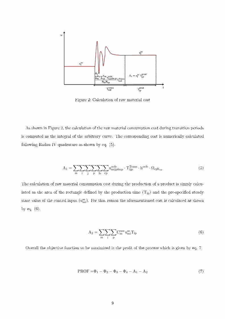
Figure 2: Calculation of raw material cost

As shown in Figure 2, the calculation of the raw material consumption cost during transition periods

is computed as the integral of the arbitrary curve. The corresponding cost is numerically calculated

following Radau IV quadrature as shown by eq. (5).

A1 =∑m

∑i

∑j

∑p

∑fe

∑cp

uocfemijpfecp · TTrans

ijp · hocfe · ΩcpNcp (5)

The calculation of raw material consumption cost during the production of a product is simply calcu-

lated as the area of the rectangle dened by the production time (Tip) and the pre-specied steady

state value of the control input (ussmi). For that reason the aforementioned cost is calculated as shown

by eq. (6).

A2 =∑m

∑i

∑p

Crawm uss

miTip (6)

Overall the objective function to be maximised is the prot of the process which is given by eq. 7.

PROF =Φ1 − Φ2 − Φ3 − Φ4 −A1 −A2 (7)

9

2.2 Modelling the planning and scheduling problem

For the integration of planning and scheduling in the present work a TSP model is employed. The model

was originally proposed by Liu et al.22 and proved to have computational benets in comparison with

the time-slot based formulation. Similar to the classic TSP problem where binary variables indicate

the path from one city to another, the changeovers between two dierent products are modelled in a

similar fashion. Following this model, the planning horizon is divided in typically equal-length planning

periods which are modelled as discrete time points and within each planning horizon continuous time

representation is employed for the detailed schedule. Next we present the equations that formulate the

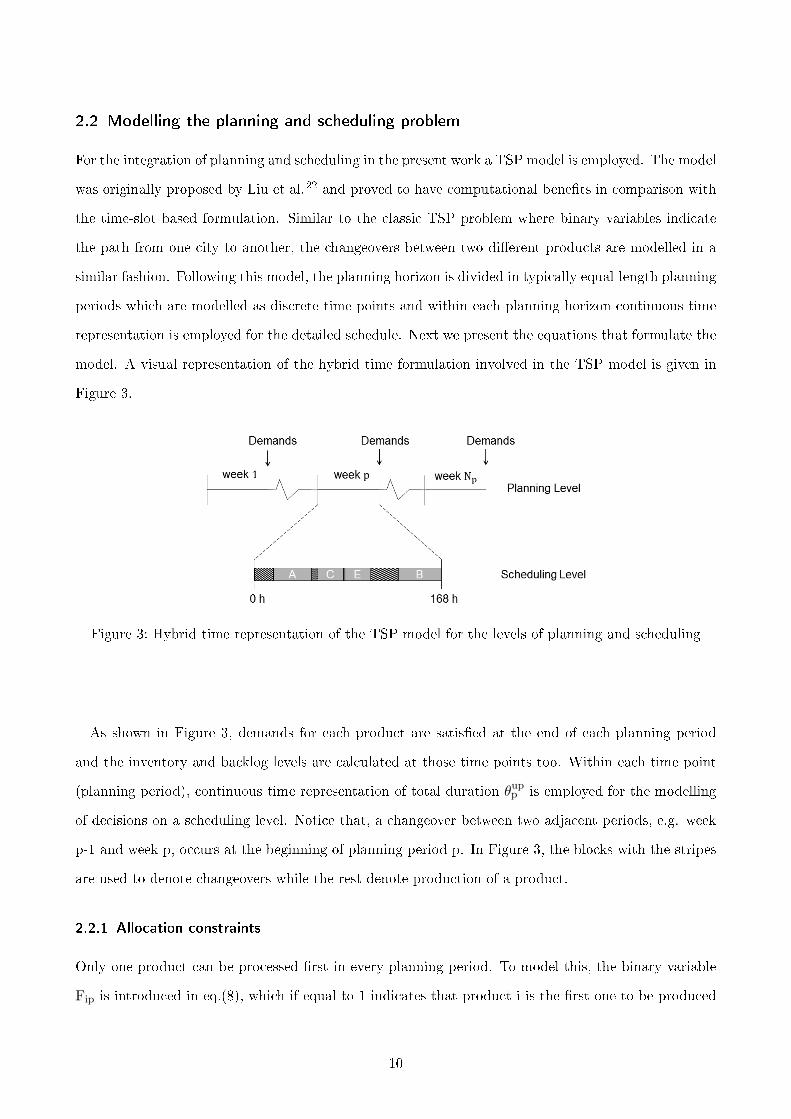
model. A visual representation of the hybrid time formulation involved in the TSP model is given in

Figure 3.

Figure 3: Hybrid time representation of the TSP model for the levels of planning and scheduling

As shown in Figure 3, demands for each product are satised at the end of each planning period

and the inventory and backlog levels are calculated at those time points too. Within each time point

(planning period), continuous time representation of total duration θupp is employed for the modelling

of decisions on a scheduling level. Notice that, a changeover between two adjacent periods, e.g. week

p-1 and week p, occurs at the beginning of planning period p. In Figure 3, the blocks with the stripes

are used to denote changeovers while the rest denote production of a product.

2.2.1 Allocation constraints

Only one product can be processed rst in every planning period. To model this, the binary variable

Fip is introduced in eq.(8), which if equal to 1 indicates that product i is the rst one to be produced

10

in planning period p and zero otherwise.

N∑i

Fip = 1 ∀p (8)

where i is the index of products, N is the total number of products and p is the planning period.

Eq.(9) ensures that only one product can be processed last in every planning period.

N∑i

Lip = 1 ∀p (9)

Similar to eq. (8) the binary variable Lip is used to indicate whether or not product i is the last one

to be processed in planning period p. Eq.(10) dictates that a product can be processed rst only if it

has been assigned to the planning period.

Fip ≤ Eip ∀i, p (10)

where Eip is a binary variable that indicates whether product i is assigned for production in planning

period p. To ensure that a product can be processed last, only if it has been assigned to the planning

period, eq.(11) is used.

Lip ≤ Eip ∀i, p (11)

Notice, that the binary variables Fip and Lip are indicative of the sequence of tasks performed within

each planning period as the order of the rest of tasks is computed implicitly by the changeovers.

2.2.2 Sequencing constraints

When moving from the production of a product i to another product j, a changeover occurs. To model

changeovers within the same planning period the binary variable Zijp is used if product i precedes

product j in planning period p.

11

N∑i 6=j

Zijp = Ejp − Fjp ∀j,p (12)

Eq. (12) denotes that a product if assigned to a planning period, unless the rst to be processed,

results in a changeover with another assigned product. Next through eq.(13) it is ensured that a

product unless the last to be processed, if assigned to the planning period, results in a changeover with

another assigned product.

N∑j6=i

Zijp = Eip − Lip ∀i, p (13)

Finally, to model changeovers across adjacent weeks eq.(14)-(15) are used.

N∑i

Zfijp = Fjp ∀j, p > 1 (14)

N∑j

Zfijp = Li,p−1 ∀i, p > 1 (15)

where the binary variable Zfijp is used to model changeovers between adjacent planning periods.

2.2.3 Symmetry breaking constraints

In order to avoid the enumeration of symmetric solutions and exclude infeasible production sub-cycles

the integer variable Oip (order index) is introduced and denotes the order at which the product i is

processed during planning period p. Eq. (16)-(18) ensure the exclusion of such subcycles.

Ojp − (Oip + 1) ≥ −M(1− Zijp) ∀i, j ∈ I, j 6= i, p (16)

Oip ≤ M · Eip ∀i,p (17)

12

Fip ≤ Oip ≤N∑i

Eip ∀i,p (18)

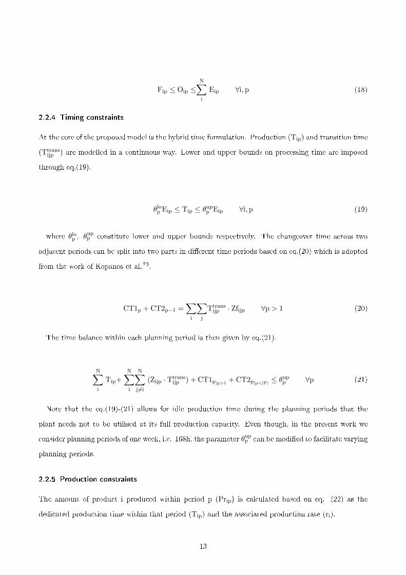
2.2.4 Timing constraints

At the core of the proposed model is the hybrid time formulation. Production (Tip) and transition time

(Ttransijp ) are modelled in a continuous way. Lower and upper bounds on processing time are imposed

through eq.(19).

θlop Eip ≤ Tip ≤ θup

p Eip ∀i,p (19)

where θlop , θ

upp constitute lower and upper bounds respectively. The changeover time across two

adjacent periods can be split into two parts in dierent time periods based on eq.(20) which is adopted

from the work of Kopanos et al.23.

CT1p + CT2p−1 =∑

i

∑j

Ttransijp · Zfijp ∀p > 1 (20)

The time balance within each planning period is then given by eq.(21).

N∑i

Tip+

N∑i

N∑j 6=i

(Zijp · Ttransijp ) + CT1p|p>1

+ CT2p|p<|P| ≤ θupp ∀p (21)

Note that the eq.(19)-(21) allows for idle production time during the planning periods that the

plant needs not to be utilised at its full production capacity. Even though, in the present work we

consider planning periods of one week, i.e. 168h, the parameter θupp can be modied to facilitate varying

planning periods.

2.2.5 Production constraints

The amount of product i produced within period p (Prip) is calculated based on eq. (22) as the

dedicated production time within that period (Tip) and the associated production rate (ri).

13

Prip = riTip ∀i, p (22)

Eq.(23) is used for the calculation of the backlog (Bcip) for the demand from customer c at the end

of the current planning period, as the amount of backlog at the previous planning period (Bci,p−1) plus

the demand (Dcip) of the current planning period minus the related sales (Scip).

Bcip = Bci,p−1 + Dcip − Scip ∀c, i,p (23)

The level of inventory (Vip) of product i at the end of planning period p, is related to the amount

produced and the sales for that product through eq. (24).

Vip = Vi,p−1 + Prip −∑

c

Scip ∀i,p (24)

In addition to eq. (24), eq. (25) may be included in the iPSC formulation so as to model capacity

considerations in terms of minimum (Vmini ) and maximum (Vmax

i ) allowable inventory levels.

Vmini ≤ Vip ≤ Vmax

i ∀i,p (25)

2.3 Dynamic optimisation (DO)

In this section, we present the mathematical formulation used for the dynamic optimisation/ optimal

control of the process. Consider the following generic continuous dynamic system which can be either

linear or nonlinear and is given by eq. (26)-(27).

dx

dt= f(x(t), u(t)) x0 = x(t|t=0) (26)

y(t) = h(x(t), u(t)) (27)

14

where x(t) ∈ X ⊆ Rnx , denotes the time-variant vector of state variables, u(t) ∈ U ⊆ Rnu , denotes

the time dependent control input vector and y(t) ∈ Y ⊆ Rny denotes the time dependent output vector.

Note that X, Y and Z correspond to their respective admissible set. f : Rnx+nu → Rn is a C2 vector

eld and h : Rnx+ny → Rny can be an either linear or nonlinear map. In order to transform the dynamic

system into an algebraic one, a discretisation scheme has to be employed. This can be done either

explicitly by integrating numerically eq. (26)-(27), considering them as boundary value problem (BVP)

through direct single or multiple shooting methods or implicitly following a simultaneous scheme. For

the case that constraints need to be considered the sequential methods are not appropriate as they

cannot facilitate such requirement easily24.

In the present work, orthogonal collocation on nite elements (OCFE) was chosen for the discreti-

sation of the dynamic problem because of its desirable properties in terms of numerical stability25;26.

OCFE belongs to the family of simultaneous approaches and is also known as direct transcription

method. Following OCFE, both the control and the state variables are discretised in time. The dom-

ain of time is discretised into a number of nite elements and within each nite element a number

of collocation points is considered. The DO problem is transformed into an nonlinear programming

(NLP) problem by approximating the control and state proles, across the nite elements, with a

family of orthogonal polynomials such as Lagrange or Legendre polynomials. A thorough discussion

on simultaneous solution strategies for dynamic optimisation is conducted in Biegler24.

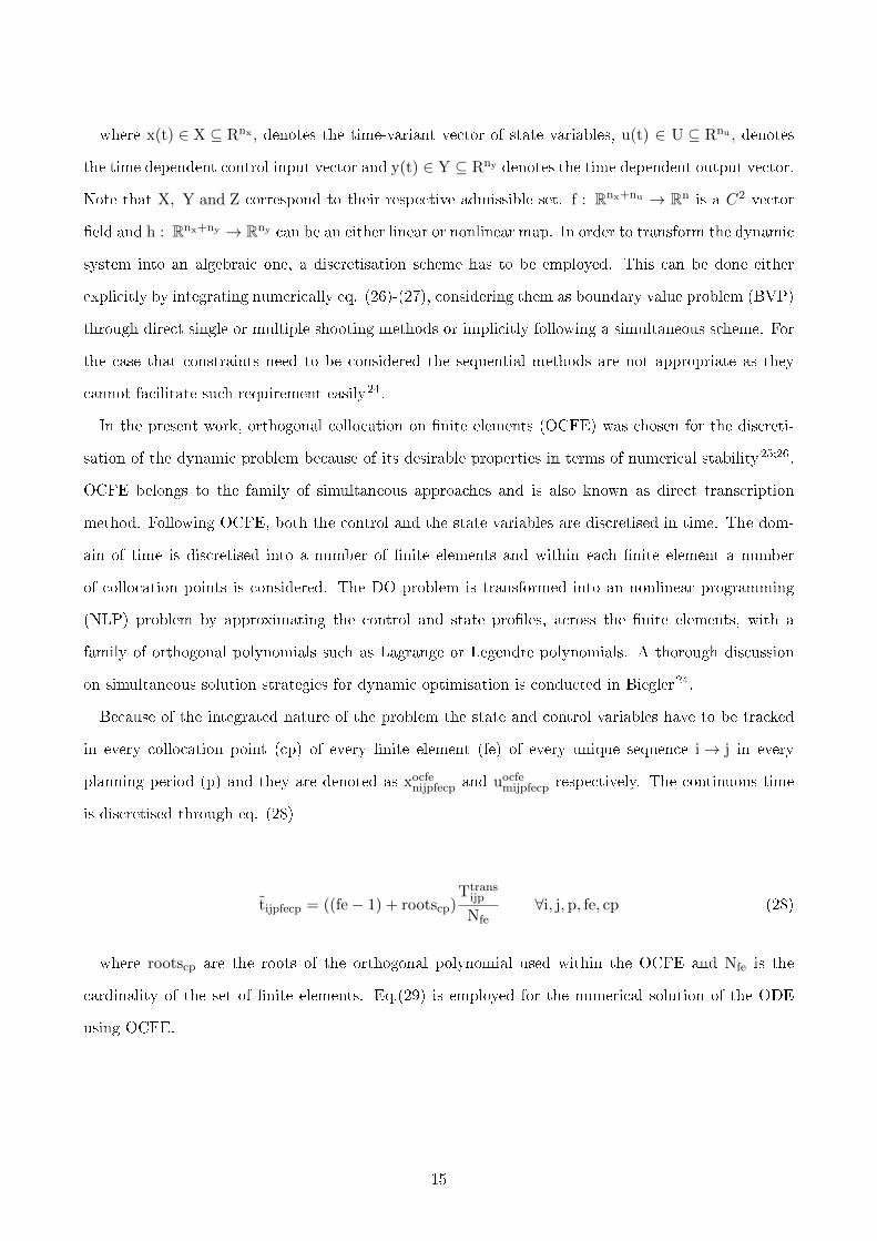
Because of the integrated nature of the problem the state and control variables have to be tracked

in every collocation point (cp) of every nite element (fe) of every unique sequence i→ j in every

planning period (p) and they are denoted as xocfenijpfecp and uocfe

mijpfecp respectively. The continuous time

is discretised through eq. (28)

tijpfecp = ((fe− 1) + rootscp)Ttrans

ijp

Nfe∀i, j, p, fe, cp (28)

where rootscp are the roots of the orthogonal polynomial used within the OCFE and Nfe is the

cardinality of the set of nite elements. Eq.(29) is employed for the numerical solution of the ODE

using OCFE.

15

xnijpfecp = fn(xocfenijpfecp, uocfe

mijpfecp, σ), ∀n,m, i, j,p, fe, cp (29)

Eq.(29) is used for the computation of the numerical value of the derivative of the nth state based

on the associated dierential equation that governs the related state. Note, that the right hand side of

eq.(29) denotes is the discretised equivalent from the ODE related to the nth state.Continuity of the

state variables across adjacent nite elements is imposed by eq.(30)

xocfeinit

nijpfe = xocfeinit

nijp,fe−1 + Ttransijp · hocfe

ncp∑cp=1

ΩcpNcpxnijp,fe−1,cp ∀n, i, j, fe > 1 (30)

The numerical solution of the state proles across the discretised domain is computed by eq.(31)

xocfenijpfecp = xocfeinit

nijpfe + Ttransijp · hocfe

ncp∑cpp=1

Ωcpp cpxnijpfecpp ∀n, i, j, fe, cp (31)

Note that in general, variable steps (hocfe) and continuity constraints on the proles of the control

variables may be employed, if required for the problem under study; however in the present work we

do not account for such cases.

2.4 Linking variables between DO, scheduling and planning model

Tracking the dynamic trajectory of the system can be translated into a regime of production. In the

context of iPSC, changeovers can be dened as the time needed by the system to move from one

steady state to the next one. Similarly, the production time can be dened as the time that the

system is stabilised around the desirable steady state in order to manufacture a certain amount of

products that would satisfy the demand. Ideally, one would have to perform a discretisation of the

dynamics across the entire dynamic trajectory but in the present work since no process disturbances are

considered we assume that once the steady state is achieved the system remains in steady state unless

a changeover occurs. Therefore, the discretisation of the dynamics is employed only for the transient

periods of changeovers. In general, the linking between the DO and the scheduling and planning model

is achieved with eq. (32)-(35).

16

xinnijp = xocfeinit

nijpfe ∀n, i, j, i 6= j, fe = 1 (32)

uinmijp = uocfe

mijpfecp ∀m, i, j, i 6= j, fe = 1, cp = 1 (33)

xfinnijp = xocfe

nijpNfeNcp∀n, i, j, i 6= j (34)

ufinmijp = uocfe

mijpNfeNcp∀m, i, j, i 6= j (35)

The new variables introduced here are xinnijp, uin

mijp, xfinnijp and ufin

mijp. The rst two variables dene

the value of the state and control inputs at the beginning of the transition and the last two are used

in a similar fashion for the end of the transition. Eq. (32) ensures that the value of the discretised

state variable (xocfeinitnijpfe ) at the beginning of the rst nite element is equal to the initial condition of

the system at the beginning of the transition, while eq. (33) is employed for the control input. At the

end of the transition the state of the system must have reached a certain value (xfinnijp) and eq. (34)

imposes that value of the discretised state variable at the last collocation point (Ncp) of the last nite

element (Nfe) is such that the transition terminates. Finally, eq. (35) has similar functionality with

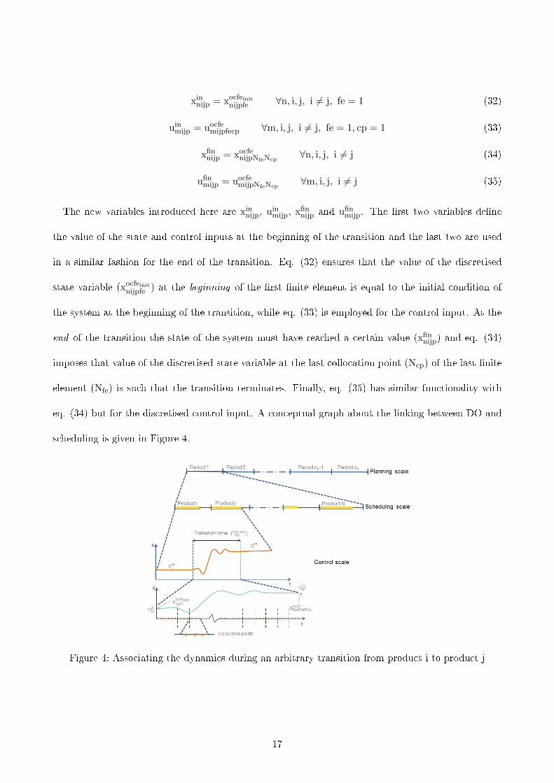
eq. (34) but for the discretised control input. A conceptual graph about the linking between DO and

scheduling is given in Figure 4.

Figure 4: Associating the dynamics during an arbitrary transition from product i to product j

17

In Figure 4, the multi-scale nature of the problem is illustrated. On the top graph, the planning scale

is modelled as discrete time points each of which is then expanded in a continuous time domain for the

scheduling scale. The scheduling scale is then further analysed into the control scale and it is shown

how the process moves from the production of product i to product j. At the beginning, the system

is regulated around the steady state of product i until a changeover occurs in which case a transition

from the steady state of product i (xssni) to the steady state of the next product, e.g. j, (x

ssnj) is initiated.

On the bottom graph, the dynamics of the system throughout this transition are envisaged. Note, that

the system at the beginning of the transition starts from (xssni) and thus the discretised state variable of

the rst nite element, i.e. xocfeinitnijpfe|fe=1

, must be equal to that value. During the dynamic optimisation,

the time is discretised in nite elements (intervals between consecutive blue dashed lines in Figure 4)

and within each nite element a certain number of collocation points are dened (orange dots).

2.5 Linking equations between DO and TSP planning and scheduling

Now that the linking variables between DO and scheduling have been established, it remains to provide

the physical meaning of these variables in terms of production scheduling. Since, xinnijp and xfin

nijp,

correspond to the initial and nal values of the transitions between dierent products it follows that

they are also associated with the steady state operation of the system when production takes place.

Indeed, the initial value of the state variables at the beginning of a transition should be equal to the

steady state of the product that was being processed before the changeover occurred. Similarly, since

the transition between two products is terminated once the system has reached the next steady state,

the nal value of the state variables at the end of the transition must be equal to the steady state of

the following product. The same holds for the control variables.

Since in the present work a TSP based planning and scheduling model is adapted, in contrast with

the time-slot based formulations, the binary variable that can be used to express mathematically the

aforementioned conditions is the Zijp for transitions that occur within the same planning period and

18

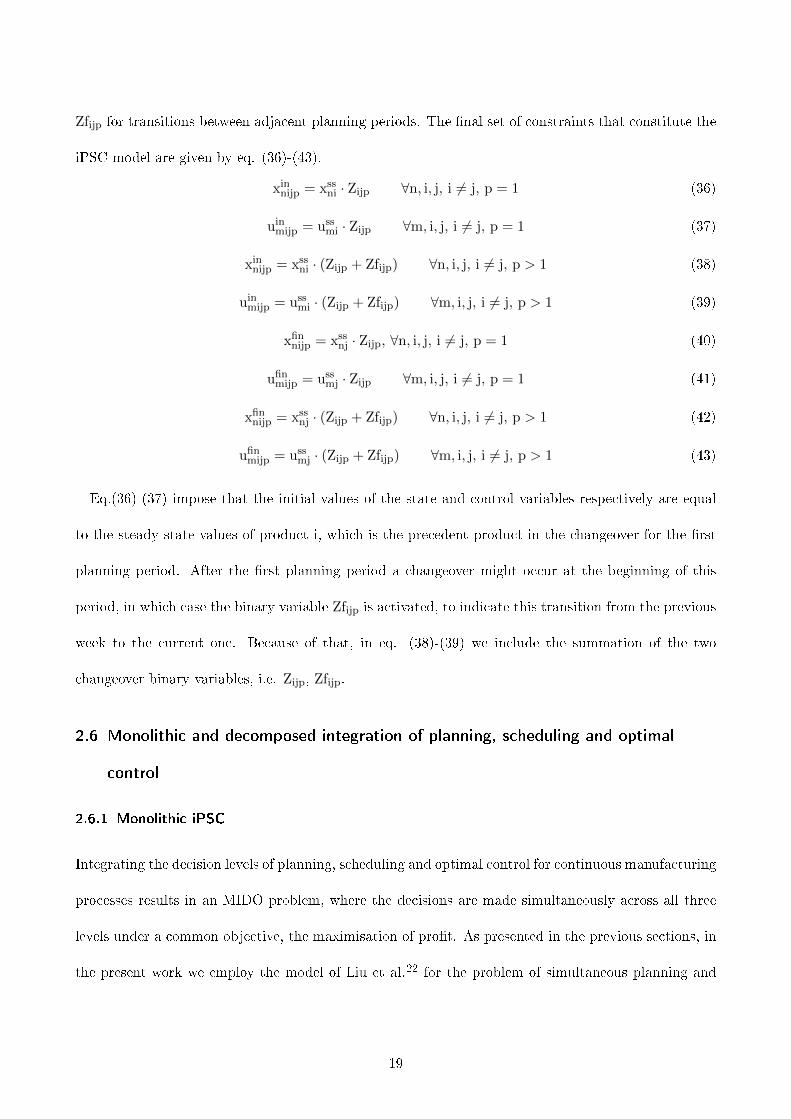
Zfijp for transitions between adjacent planning periods. The nal set of constraints that constitute the

iPSC model are given by eq. (36)-(43).

xinnijp = xss

ni · Zijp ∀n, i, j, i 6= j, p = 1 (36)

uinmijp = uss

mi · Zijp ∀m, i, j, i 6= j, p = 1 (37)

xinnijp = xss

ni · (Zijp + Zfijp) ∀n, i, j, i 6= j, p > 1 (38)

uinmijp = uss

mi · (Zijp + Zfijp) ∀m, i, j, i 6= j, p > 1 (39)

xfinnijp = xss

nj · Zijp, ∀n, i, j, i 6= j, p = 1 (40)

ufinmijp = uss

mj · Zijp ∀m, i, j, i 6= j, p = 1 (41)

xfinnijp = xss

nj · (Zijp + Zfijp) ∀n, i, j, i 6= j, p > 1 (42)

ufinmijp = uss

mj · (Zijp + Zfijp) ∀m, i, j, i 6= j, p > 1 (43)

Eq.(36)-(37) impose that the initial values of the state and control variables respectively are equal

to the steady state values of product i, which is the precedent product in the changeover for the rst

planning period. After the rst planning period a changeover might occur at the beginning of this

period, in which case the binary variable Zfijp is activated, to indicate this transition from the previous

week to the current one. Because of that, in eq. (38)-(39) we include the summation of the two

changeover binary variables, i.e. Zijp, Zfijp.

2.6 Monolithic and decomposed integration of planning, scheduling and optimal

control

2.6.1 Monolithic iPSC

Integrating the decision levels of planning, scheduling and optimal control for continuous manufacturing

processes results in an MIDO problem, where the decisions are made simultaneously across all three

levels under a common objective, the maximisation of prot. As presented in the previous sections, in

the present work we employ the model of Liu et al.22 for the problem of simultaneous planning and

19

scheduling and then OCFE is used for the discretisation of the dynamics of the system for the optimal

control. The optimal control is linked using the constraints and auxiliary variables presented in section

2.5. Overall, the monolithic model for the iPSC consists of the following:

Monolithic iPSC : max PROF = Φ1 − Φ2 − Φ3 − Φ4 −A1 −A2

Subject to : eq.(8)− (25) (TSP Planning − Scheduling)

eq.(28)− (31) (Dynamic Optimisation)

eq.(32)− (43) (Linking constraints)

2.6.2 Decomposed iPSC

To alleviate the computational burden associated with the monolithic formulation of the iPSC, in

the present work we propose a decomposition of the problem through the solution of oine DOs

and the development of linear metamodels to associate the transition time with transition cost. The

decomposition is based on the grounds of the following two observations:

1. Formulating and solving the monolithic iPSC results typically in large scale non-convex MINLPs

problems which are dicult to solve and the use of global optimisation solvers is rather dicult

due to the scale of the MINLPs21;27. Within the manufacture, being in a position to provide on

time good solutions is crucial and with the monolithic MINLPs such requirement may not be

always satised. Upon inspection, apart from the time-scale problem that is inherent to the iPSC,

the solution of the underlying dynamic optimisation problem constitutes the main bottleneck

because of the consideration of the transition times as decision variables. In the literature, ways

for dealing with this problem include, xing the transition time matrix in an oine step based on

heuristics19 or creating pre-computed recipes that include couples of transition time and cost21.

The disadvantage of following the aforementioned alternatives are for the rst one that it does

not reect a true integration among the levels of iPSC and the latter assumes that the decision

maker will always face one of the pre-specied realisations of transition time and cost.

20

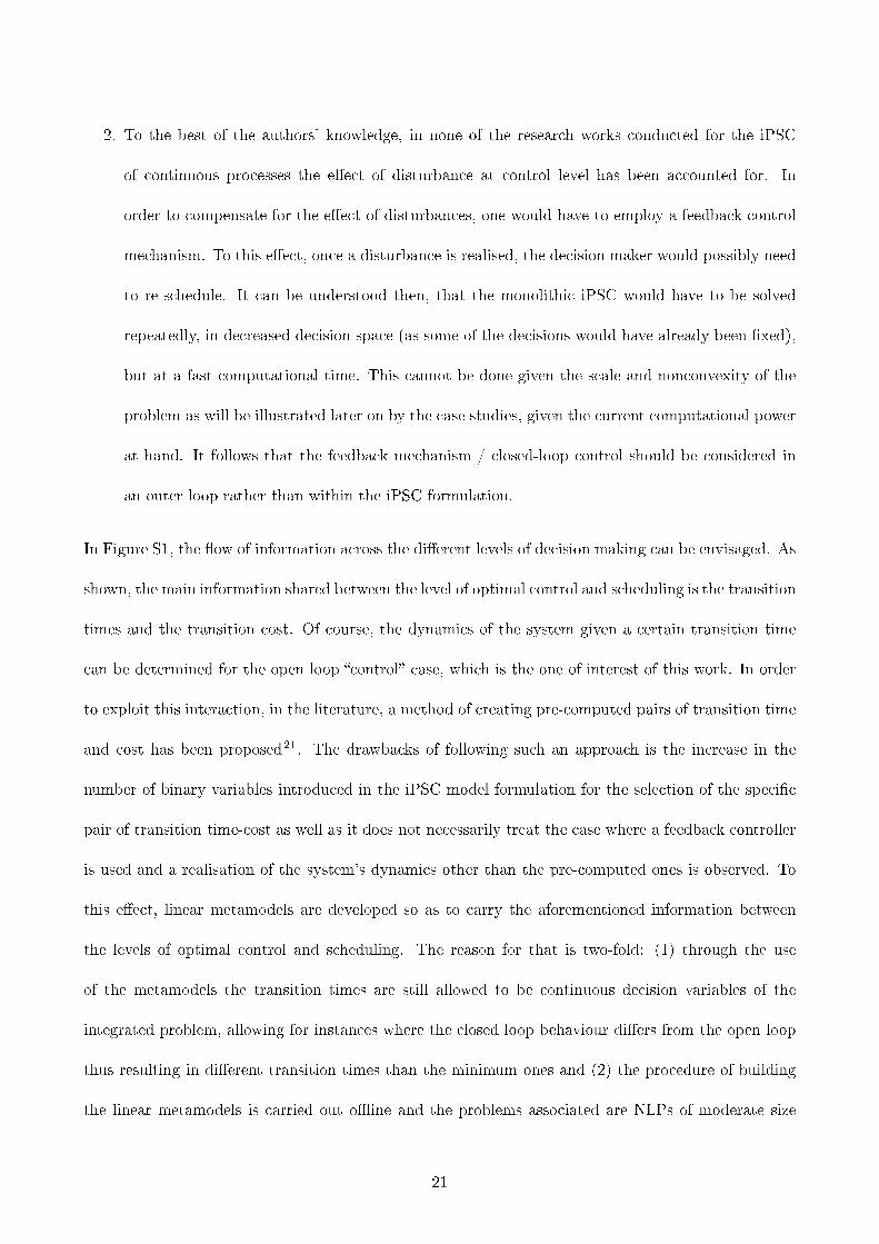
2. To the best of the authors' knowledge, in none of the research works conducted for the iPSC

of continuous processes the eect of disturbance at control level has been accounted for. In

order to compensate for the eect of disturbances, one would have to employ a feedback control

mechanism. To this eect, once a disturbance is realised, the decision maker would possibly need

to re-schedule. It can be understood then, that the monolithic iPSC would have to be solved

repeatedly, in decreased decision space (as some of the decisions would have already been xed),

but at a fast computational time. This cannot be done given the scale and nonconvexity of the

problem as will be illustrated later on by the case studies, given the current computational power

at hand. It follows that the feedback mechanism / closed-loop control should be considered in

an outer loop rather than within the iPSC formulation.

In Figure S1, the ow of information across the dierent levels of decision making can be envisaged. As

shown, the main information shared between the level of optimal control and scheduling is the transition

times and the transition cost. Of course, the dynamics of the system given a certain transition time

can be determined for the open loop control case, which is the one of interest of this work. In order

to exploit this interaction, in the literature, a method of creating pre-computed pairs of transition time

and cost has been proposed21. The drawbacks of following such an approach is the increase in the

number of binary variables introduced in the iPSC model formulation for the selection of the specic

pair of transition time-cost as well as it does not necessarily treat the case where a feedback controller

is used and a realisation of the system's dynamics other than the pre-computed ones is observed. To

this eect, linear metamodels are developed so as to carry the aforementioned information between

the levels of optimal control and scheduling. The reason for that is two-fold: (1) through the use

of the metamodels the transition times are still allowed to be continuous decision variables of the

integrated problem, allowing for instances where the closed loop behaviour diers from the open loop

thus resulting in dierent transition times than the minimum ones and (2) the procedure of building

the linear metamodels is carried out oine and the problems associated are NLPs of moderate size

21

for which global optimisation solvers can possibly be employed. As will be shown in the next section,

through the case studies examined, the law that correlates transition time and transition cost is of

logarithmic nature for large time scales but for shorter ones it can be approximated precisely by the

linear metamodels. As far as the dynamic open-loop trajectories are concerned, with the transition

time xed the control and state variables can be calculated through the solution of the related optimal

control problem in a subsequent step. However, for the deterministic case which is under study in the

present work the decomposed model will always choose the minimum transition times because it infers

minimum cost and so that particular dynamic trajectory is stored and employed.

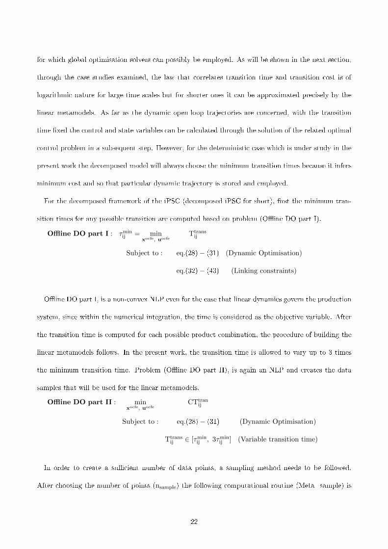
For the decomposed framework of the iPSC (decomposed iPSC for short), rst the minimum tran-

sition times for any possible transition are computed based on problem (Oine DO part I).

Offline DO part I : τminij = min

xocfe, uocfeTtrans

ij

Subject to : eq.(28)− (31) (Dynamic Optimisation)

eq.(32)− (43) (Linking constraints)

Oine DO part I, is a non-convex NLP even for the case that linear dynamics govern the production

system, since within the numerical integration, the time is considered as the objective variable. After

the transition time is computed for each possible product combination, the procedure of building the

linear metamodels follows. In the present work, the transition time is allowed to vary up to 3 times

the minimum transition time. Problem (Oine DO part II), is again an NLP and creates the data

samples that will be used for the linear metamodels.

Offline DO part II : minxocfe, uocfe

CTtranij

Subject to : eq.(28)− (31) (Dynamic Optimisation)

Ttransij ∈ [τmin

ij , 3τminij ] (Variable transition time)

In order to create a sucient number of data points, a sampling method needs to be followed.

After choosing the number of points (nsample) the following computational routine (Meta_sample) is

22

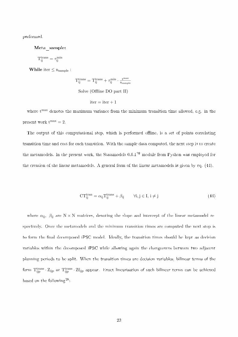
performed.

Meta_sample:

Ttransij = τmin

ij

While iter ≤ nsample :

Ttransij = Ttrans

ij + τminij · tmax

nsample

Solve (Offline DO part II)

iter = iter + 1

where tmax denotes the maximum variance from the minimum transition time allowed, e.g. in the

present work tmax = 2.

The output of this computational step, which is performed oine, is a set of points correlating

transition time and cost for each transition. With the sample data computed, the next step is to create

the metamodels. In the present work, the Statsmodels 0.6.128 module from Python was employed for

the creation of the linear metamodels. A general form of the linear metamodels is given by eq. (44).

CTtranij = αijT

transij + βij ∀i, j ∈ I, i 6= j (44)

where αij, βij are N×N matrices, denoting the slope and intercept of the linear metamodel re-

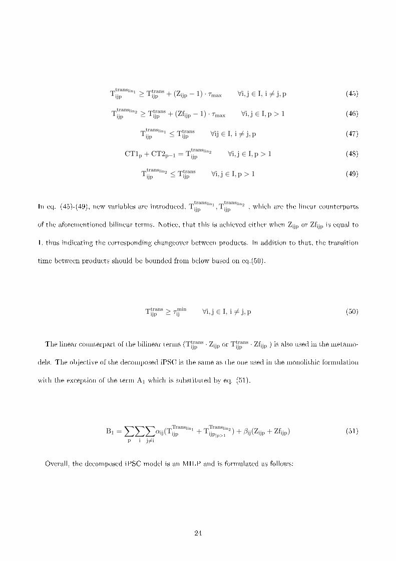
spectively. Once the metamodels and the minimum transition times are computed the next step is

to form the nal decomposed iPSC model. Ideally, the transition times should be kept as decision

variables within the decomposed iPSC while allowing again the changeovers between two adjacent

planning periods to be split. When the transition times are decision variables, bilinear terms of the

form Ttransijp · Zijp or Ttrans

ijp · Zfijp appear. Exact linearisation of such bilinear terms can be achieved

based on the following29:

23

Ttranslin1ijp ≥ Ttrans

ijp + (Zijp − 1) · τmax ∀i, j ∈ I, i 6= j,p (45)

Ttranslin2ijp ≥ Ttrans

ijp + (Zfijp − 1) · τmax ∀i, j ∈ I,p > 1 (46)

Ttranslin1ijp ≤ Ttrans

ijp ∀ij ∈ I, i 6= j,p (47)

CT1p + CT2p−1 = Ttranslin2ijp ∀i, j ∈ I, p > 1 (48)

Ttranslin2ijp ≤ Ttrans

ijp ∀i, j ∈ I, p > 1 (49)

In eq. (45)-(49), new variables are introduced, Ttranslin1ijp ,T

translin2ijp , which are the linear counterparts

of the aforementioned bilinear terms. Notice, that this is achieved either when Zijp or Zfijp is equal to

1, thus indicating the corresponding changeover between products. In addition to that, the transition

time between products should be bounded from below based on eq.(50).

Ttransijp ≥ τmin

ij ∀i, j ∈ I, i 6= j, p (50)

The linear counterpart of the bilinear terms (Ttransijp · Zijp or Ttrans

ijp · Zfijp ) is also used in the metamo-

dels. The objective of the decomposed iPSC is the same as the one used in the monolithic formulation

with the exception of the term A1 which is substituted by eq. (51).

B1 =∑

p

∑i

∑j6=i

αij(TTranslin1ijp + T

Translin2ijp|p>1

) + βij(Zijp + Zfijp) (51)

Overall, the decomposed iPSC model is an MILP and is formulated as follows:

24

Decomposed iPSC : max PROF = Φ1 − Φ2 − Φ3 − Φ4 − B1 −A2

Subject to : eq.(8)− (25) (TSP Planning − Scheduling)

eq.(45)− (50) (Time linearisation)

3 Case Studies

A number of case studies are presented in the next section to demonstrate the advantages of the propo-

sed modelling framework for the iPSC. The rst one examines the iPSC of a single-input single-output

(SISO) multi-product CSTR; the second one, a multiple-input multiple-output (MIMO) non-isothermal

multi-product CSTR while the third one studies methyl methacrylate (MMA) polymerisation process.

The pattern followed in this section is as follows: rst, a comparison between the monolithic and de-

composed iPSC models is given, for both the TSP and the time-slot based formulation, and then the

decomposed approach is tested under dierent planning horizons, namely 4, 6 and 12 weeks.

All the optimisation problems, for the monolithic approach, are formulated as MINLPs and solved

using GAMS 24.4.130 on a Dell workstation with 3.70 GHz processor, 16GB RAM and Windows 7 64-

bit operating system. Finally, the optimisation problems corresponding to the decomposed approach

are formulated as MILPs and modelled in GAMS 24.4.1 and solved using CPLEX 12.6.1.

Finally, for the comparison between the TSP and the time-slot based model for the iPSC some

modications need to be made with respect to the existence of idle time within the planning period,

backlog of unmet demand and inventory calculation. The time-slot based model was proposed by

Erdirik-Dogan and Grossmann20 (E-D &G) and the corresponding model is given in Appendix A.

As far as the inventory calculation is concerned the TSP model proposed by Liu et al.22, considers

inventory calculation on a weekly basis whereas E-D&G employ a linear overestimation of the inventory

curve; to this eect, eq.(A.14)-(A.17) are replaced by eq.(24). Next, in E-D&G, the demand serves as

lower bound to the level of sales at the end of each planning period and backlog is not considered; in

25

order to account for backlog, eq.(A.18) is replaced by eq.(23). Finally, idle time is allowed between

planning period by modifying eq.(A.11) as shown in eq.(52).

TeNsp +

∑i

∑j 6=i

τijZ′ijp ≤ Ts

1,p+1 ∀p = 1, . . . ,Np − 1 (52)

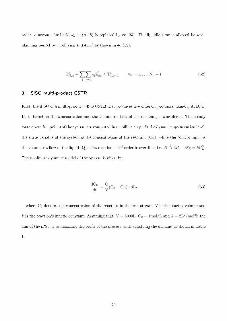
3.1 SISO multi-product CSTR

First, the iPSC of a multi-product SISO CSTR that produces ve dierent products, namely, A, B, C,

D, E, based on the concentration and the volumetric ow of the reactant, is considered. The steady

state operation points of the system are computed in an oine step. At the dynamic optimisation level,

the state variable of the system is the concentration of the reactant (CR), while the control input is

the volumetric ow of the liquid (Q). The reaction is 3rd order irreversible, i.e. Rk→ 3P, −RR = kC3

R.

The nonlinear dynamic model of the system is given by:

dCR

dt=

Q

V(C0 − CR)+RR (53)

where C0 denotes the concentration of the reactant in the feed stream, V is the reactor volume and

k is the reaction's kinetic constant. Assuming that, V = 5000L, C0 = 1mol/L and k = 2L2/mol2h the

aim of the iPSC is to maximise the prot of the process while satisfying the demand as shown in Table

1.

26

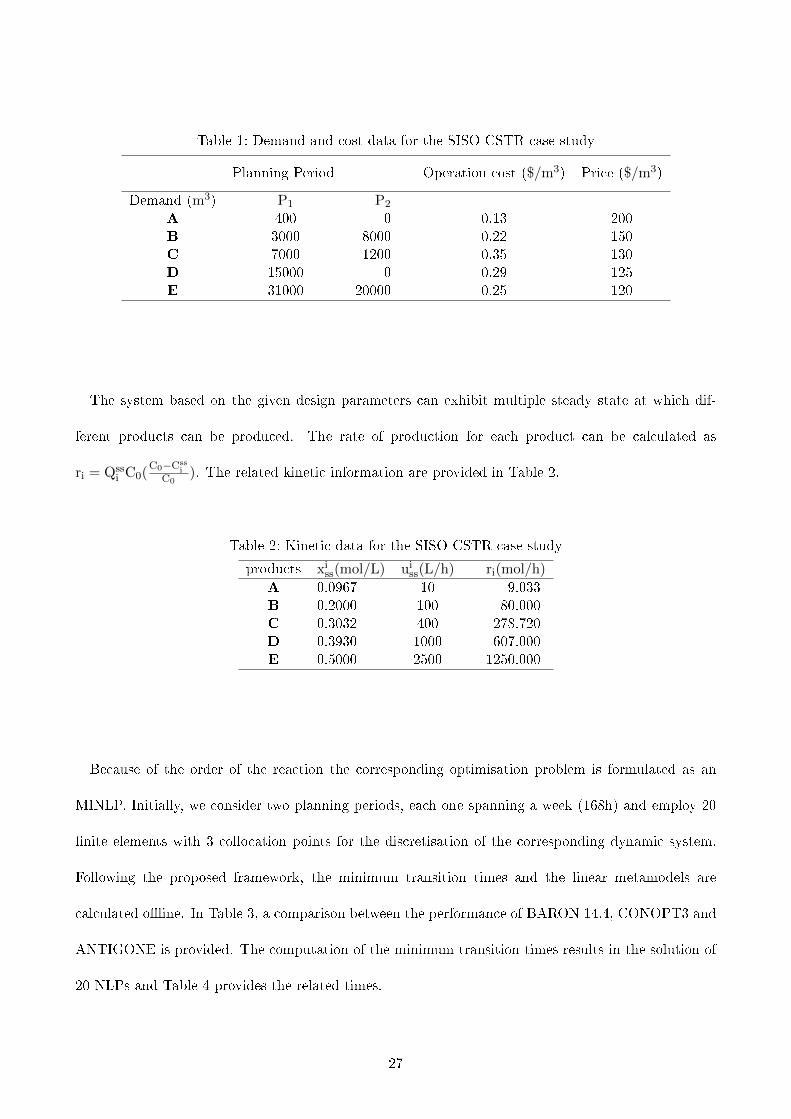
Table 1: Demand and cost data for the SISO CSTR case study

Planning Period Operation cost ($/m3) Price ($/m3)

Demand (m3) P1 P2

A 400 0 0.13 200B 3000 8000 0.22 150C 7000 1200 0.35 130D 15000 0 0.29 125E 31000 20000 0.25 120

The system based on the given design parameters can exhibit multiple steady state at which dif-

ferent products can be produced. The rate of production for each product can be calculated as

ri = Qssi C0(

C0−Cssi

C0). The related kinetic information are provided in Table 2.

Table 2: Kinetic data for the SISO CSTR case study

products xiss(mol/L) ui

ss(L/h) ri(mol/h)

A 0.0967 10 9.033B 0.2000 100 80.000C 0.3032 400 278.720D 0.3930 1000 607.000E 0.5000 2500 1250.000

Because of the order of the reaction the corresponding optimisation problem is formulated as an

MINLP. Initially, we consider two planning periods, each one spanning a week (168h) and employ 20

nite elements with 3 collocation points for the discretisation of the corresponding dynamic system.

Following the proposed framework, the minimum transition times and the linear metamodels are

calculated oine. In Table 3, a comparison between the performance of BARON 14.4, CONOPT3 and

ANTIGONE is provided. The computation of the minimum transition times results in the solution of

20 NLPs and Table 4 provides the related times.

27

Table 3: Problem statistics for the oine computation of the minimum transition time (τmini,j ) for the

SISO CSTR case study

Solver CONOPT3 BARON ANTIGONE

Type NLP NLP NLPSolution status Locally optimal Optimal OptimalConstraints 204 204 204Cont. Var. 266 266 266CPU (s)* 1.059 23,452 149.632

*Cumulative computational time for all the transitions

Table 4: Minimum transition times between products for the SISO CSTR case study

τmini,j (h) A B C D E

A - 0.21 0.47 0.85 1.64B 20.99 - 0.26 0.61 1.43C 24.6 3.62 - 0.31 1.21D 25.72 4.74 1.13 - 0.87E 26.34 5.38 1.76 0.64 -

The linear metamodels are built next following the sampling technique described in section 2.6.2.

While building the linear metamodels, the majority has a value of R2 ≥ 0.99 but some fail to reach this

desired threshold like the one shown in Figure 5 which corresponds to the transition from product C to

product A. The total number of metamodels that have R2 ≤ 0.99 are four out the twenty but for the

sake of computational complexity we allow this approximation as it still reects the impact that the

dynamics of the system have in the production scheduling. Note that piecewise linear approximation

could have been employed but that would lead in increase of the number of binary variables needed.

28

Figure 5: Graph of the linear metamodels built from sampling data for the transition from C to A

In general it was noticed based on the simulations that were conducted, that the law that governs

the relation between transition time and cost is of logarithmic nature for large time scales; however,

from a production scheduling perspective for the instance for the transition from C to A a delay of the

transition of the order of hours would probably result in rescheduling thus the eect of oset from the

metamodel can be circumvented. In any case, as mentioned in section 2.6.2, the aim of building the

corresponding metamodels is to provide a computationally favorable correlation between the process

dynamics and process economics within the context of iPSC. In Table S1, the corresponding coecients

of the slope and the intercept of the linear metamodels are given.

Once the metamodels are built, the monolithic and the decomposed integrated problems are formu-

lated and solved in GAMS. Results for the SISO CSTR case study for planning horizon of 2 weeks are

shown in Table 5.

29

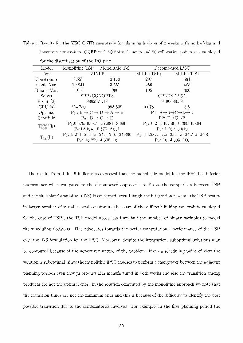
Table 5: Results for the SISO CSTR case study for planning horizon of 2 weeks with no backlog and

inventory constraints. OCFE with 20 nite elements and 20 collocation points was employed

for the discretisation of the DO part

Model Monolithic TSP Monolithic T-S Decomposed iPSC

Type MINLP MILP (TSP) MILP (T-S)Constraints 8,557 3,170 287 581Cont. Var. 10,841 3,551 256 488Binary Var. 105 300 105 300

Solver SBB/CONOPT3 CPLEX 12.6.1Prot ($) 8862971.18 9190688.58CPU (s) 274.780 995.539 0.078 3.5Optimal P1 : B→ C→ D→ A→ E P1: ABCDESchedule P2 : B→ C→ E P2: ECB

Ttransi,j,p (h)

P1:0.575, 0.687 , 57.881, 3.680 P1: 0.211, 0.256 , 0.305, 0.864P2:12.104 , 0.575, 2.631 P2: 1.762, 3.619

Ti,p(h)P1:19.271, 25.115, 24.712, 0, 24.800 P1: 44.282, 37.5, 25.115, 24.712, 24.8

P2:118.229, 4.305, 16 P2: 16, 4.305, 100

The results from Table 5 indicate as expected that the monolithic model for the iPSC has inferior

performance when compared to the decomposed approach. As far as the comparison between TSP

and the time slot formulation (T-S) is concerned, even though the integration through the TSP results

in larger number of variables and constraints (because of the dierent linking constraints employed

for the case of TSP), the TSP model needs less than half the number of binary variables to model

the scheduling decisions. This advocates towards the better computational performance of the TSP

over the T-S formulation for the iPSC. Moreover, despite the integration, suboptimal solutions may

be computed because of the nonconvex nature of the problem. From a scheduling point of view the

solution is suboptimal, since the monolithic iPSC chooses to perform a changeover between the adjacent

planning periods even though product E is manufactured in both weeks and also the transition among

products are not the optimal ones. In the solution computed by the monolithic approach we note that

the transition times are not the minimum ones and this is because of the diculty to identify the best

possible transition due to the combinatorics involved. For example, in the rst planning period the

30

transition from A to D instead of 25.72h which is minimum transition time is computed as 57.88h and

that results in not sucient production time for A and backlog of the related demand.

One could argue that the solution of the decomposed iPSC is aected by the approximation involved

in the metamodels. For that reason, the monolithic TSP model was solved again with all the binary

decision xed based on the solution of the decomposed iPSC and as expected the solutions computed

among the two are identical as shown in Table 6.

Table 6: Results of the SISO CSTR case study with xed sequencing decisions from the decomposed

iPSC

Model Monolithic TSP Decomposed iPSC

Type MINLP MILP (TSP)Constraints 8,557 277Cont. Var. 10,841 241Binary Var. 105 105

Solver SBB/CONOPT3 CPLEX 12.6.1Prot ($) 9161172.25 9190688.58CPU (s) 148.32 0.078Optimal P1: ABCDE P1: ABCDESchedule P2: ECB P2: ECB

Ttransi,j,p (h)

P1: 0.474, 0.575, 0.687, 1.944 P1: 0.211, 0.256 , 0.305, 0.864P2: 3.965, 8.142 P2: 1.762, 3.619

Ti,p(h)P1: 35.372, 37.5, 25.115,24.712, 24.8 P1: 44.282, 37.5, 25.115, 24.712, 24.8

P2: 16, 4.305, 100 P2: 16, 4.305, 100

Table 6 shows that indeed the solution computed by the decomposed iPSC is correct and feasible

for the original monolithic model. Notice, that even with all the binary variables xed, it takes

approximately 150s for SBB to compute the solution of the MINLP. It appears that the main bottleneck

in the monolithic iPSC is the nonconvex DO part where the transition times are treated as decision

variables. From a mathematical perspective this results in nonconvex bilinear terms which require

a global optimisation scheme, e.g. the use of a spatial branch and bound. The comparative prot

breakdown of the two solutions is given in Table 7.

31

Monolithic TSP Decomposed iPSC

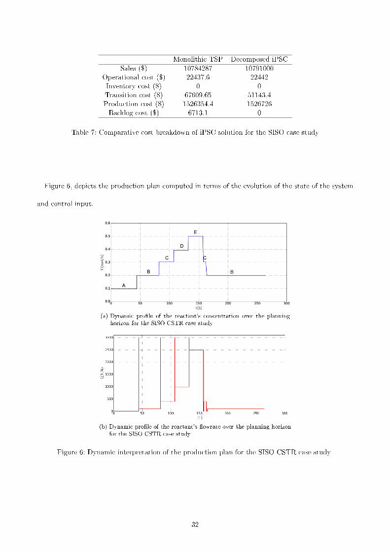
Sales ($) 10784287 10791000Operational cost ($) 22437.6 22442Inventory cost ($) 0 0Transition cost ($) 67609.65 51143.4Production cost ($) 1526354.4 1526726Backlog cost ($) 6713.1 0

Table 7: Comparative cost breakdown of iPSC solution for the SISO case study

Figure 6, depicts the production plan computed in terms of the evolution of the state of the system

and control input.

(a) Dynamic prole of the reactant's concentration over the planninghorizon for the SISO CSTR case study

(b) Dynamic prole of the reactant's owrate over the planning horizonfor the SISO CSTR case study

Figure 6: Dynamic interpretation of the production plan for the SISO CSTR case study

32

Next, the same example is examined but this time, the discretisation of the time DO part is performed

with 45 nite elements and 3 collocation point as design parameters for the OCFE. By doing so, the

trade-o between the degree of the discretisation scheme and the optimal solution is under investigation.

The minimum transition times and linear metamodels are computed again, using CONOPT3 and it

takes 10.65s to converge. Table 8, provides the minimum transition times and as can be noticed the

transition times are improved when compared to the ones computed with 20 nite elements.

Table 8: Minimum transition times for the SISO CSTR case study with OCFE of 45 nite elements

and 3 collocation points

τmini,j (h) A B C D E

A - 0.208 0.46 0.761 1.613B 20.709 - 0.252 0.552 1.414C 24.463 3.569 - 0.303 1.162D 25.388 4.682 1.212 - 0.852E 26.01 5.307 1.738 0.67 -

The monolithic and decomposed iPSC are solved again in GAMS and the results are provided in

Table S2. Increasing the number of nite elements employed for the discretisation of the continuous

dynamics on the one hand can potentially lead to more protable operation but it also exacerbates the

computational burden associated with the monolithic solution of the iPSC. Even in that case though,

as observed in Table S2 the solution of the monolithic formulation does not guarantee that the benets

of the integration can be exploited. Similar to the previous results, where the OCFE was employed with

20 nite elements, because of the nonconvexity that characterises the problem again longer transition

times and unnecessary changeovers between products occur that hindering the potential benets of

the integration. On the contrary, solving the corresponding DOs oine does not result to exhaustive

computational times and the decomposed iPSC framework does not get aected performance-wise.

Finally, we consider variable planning horizon and compare the performance between the TSP and

33

T-S formulation for the decomposed iPSC. As shown in Table S3, as the planning horizon increases

the TSP model for the decomposed iPSC outperforms the T-S model. For the case of planning horizon

of 12 weeks, for the same solution, TSP decomposed iPSC takes 4.4s while the T-S decomposed iPSC

needs 3440.21s.

3.2 MIMO multi-product CSTR

The next case study examines the iPSC of a non-isothermal MIMO CSTR where the decomposition

reaction of the form A→R takes place under the kinetic law: −Rb = krCb. The reaction is exothermic

and as such a cooling jacket is used; further details about the kinetics and design can be found in the

book of Camacho and Alba31. The system is controlled through the ow rate of the liquid (Fl) and

the coolant (Fc) while the corresponding states are the concentration of the decomposition product

(Cb) and the temperature of the liquid (Tl). The calculation of the steady state conditions is carried

out in an oine step and the related results are given in Table ??. The utility price for the coolant

Fc is $10/m3 while cost of product liquid Fl is $10/m3. The dynamic model of the system is derived

based on the mass and energy balances as shown in eq. (54)-(55), respectively where the concentration

of reactant A is assumed to be constant. Further details about the system can be found in the book

of Camacho and Alba31 and in Zhuge and Ierapetritou14. The rest of the data about the case study

are given in Tables S4-S5; the cost of backlog is calculated as half of the selling price of the related

product.

d(VlCb)

dt= Vlkr(Ca0 − Cb)− FlCb (54)

d(VlρlCplTl)

dt= FlρlCplTl0 − FlρlCplTl + FcρcCpc(Tc0 − Tc) + Vlkr(Ca0 − Cb)H (55)

34

Table 9: Design parameters of the MIMO multi-product CSTR case study

kr reaction constant 26 1h

Vl volume of the tank 24L3

ρl liquid density 800 kgm3

ρc coolant density 1000 kgm3

Cpl specic heat of liquid 3 kJkg·K

Cpc specic heat of coolant 4.19 kJkg·K

Tl0 entering liquid temperature 283KTc0 inlet coolant temperature 273KTc outlet coolant temperature 303K

Ca0 initial concentration of the reactant 4 molL

The minimum transition times as calculated by the oine DO, for discretisation with OCFE with

20 nite elements and 3 collocation points, are shown in Table 10. The coecients for the linear

metamodels that correlate transition time and cost are also given in Table S6. The transition times

computed indicate system's fast dynamics where rapid changeovers between manufacturing conditions

are achieved. This particular instance is very insightful as ideally, one would like to be in a position

to have the solution of the integrated problem at hand in times faster than the transition times. This

is because, assuming that the system is subject to disturbances at the level of process dynamics, then

deviation from the precomputed transition time/prole may lead to economic loss of the process. The

dynamic response of the system as shown in Figure 7, for the case of transition from product B to

product F, the fast transitions are achieved with rapid rate of change of the manipulated variables

while the proles of the state variables remain rather smooth.

35

Table 10: Minimum transition times between products for the MIMO case study

τmini,j (h) A B C D E F G H

A - 0.013278 0.028574 0.051289 0.044191 0.052304 0.036262 0.067748B 0.018478 - 0.01841 0.042275 0.033493 0.042478 0.032414 0.055689C 0.024308 0.005830 - 0.030435 0.018565 0.026075 0.027433 0.048667D 0.028820 0.010342 0.004997 - 0.011364 0.014089 0.025556 0.041064E 0.032483 0.014105 0.008174 0.032077 - 0.022706 0.024201 0.029812F 0.033071 0.014592 0.008761 0.023927 0.001137 - 0.025253 0.02738G 0.034146 0.021649 0.038830 0.062261 0.054110 0.062779 - 0.076709H 0.035896 0.017670 0.011920 0.037532 0.011257 0.030208 0.024550 -

(a) Dynamic prole of the concentration of the decompo-sition product

(b) Dynamic prole of the temperature of the liquid

(c) Dynamic prole of the ow rate of the coolant (d) Dynamic prole of the ow rate of the liquid

Figure 7: Dynamic response of the system for the transition from B to F

Formulating and solving the monolithic and decomposed iPSC the results shown in Table 11, are

36

computed.

Table 11: Results for the MIMO CSTR case study for planning horizon of 2 weeks. OCFE with 20

nite elements and 20 collocation points was employed for the discretisation of the DO part.

Model Monolithic TSP Monolithic T-S Decomposed iPSC

Type MINLP MILP (TSP) MILP (T-S)Constraints 45,703 8,965 647 4,157Cont. Var. 60,465 10,865 601 3,361Binary Var. 240 1,152 240 1,152

Solver SBB/CONOPT3 CPLEX 12.6.1Prot ($) 3075778.96 7710974.76CPU (s) 660.15 832.25 0.765 50.857Optimal P1 : B→ H→ A→ G P1: DFECBASchedule P2 : B→ C→ G→ A→ F P2: ABCDFEHG

Ttransi,j,p (h)

P1: 0.057, 0.212, 0.037 P1: 0.014, 0.001, 0.008, 0.018P2: 0.586, 0.019, 0.028, 0.796, 0.053 P2: 0.013, 0.018, 0.030, 0.014, 0.001, 0.030, 0.025

Ti,p(h)P1: 22.862, 6.476, 28.490, 57.648 P1: 24.038, 85.034, 4.856, 24.712, 2.671, 22.862, 28.490

P2: 1.429, 2.849, 12.464, 1.959, 95.663 P2: 1.959, 1.429, 0.178, 4.006, 10.629, 66.369, 6.476, 70.112

The multi-product MIMO CSTR case study, diers from the SISO CSTR case study that was

previously studied in the following two: (1) it has increased dimensionality in terms of control and

state variables and (2) the number of products is also increased from 5 to 8. The rst dierence,

aects mostly the DO part of the iPSC while the second aects the combinatorial nature on the level

of planning-scheduling of the iPSC. This eect, becomes apparent after the observation of the results

in Table 11. The solution computed through the monolithic approach, is clearly suboptimal because

not only the transition times computed are not the minimum possible ones but also because there is

a number of inconsistencies at a planning and scheduling level. More specically, again a changeover

occurs across the adjacent planning weeks which should not have occurred since product B is produced

in both weeks; next, the entire available time is not consumed especially in week 1 where a great

amount of demand, e.g. for product E, is backlogged despite the availability of processing time.

Because of the great dierence computed between the two solution approaches as shown in Table 11,

again the integer decisions as computed by the decomposed approach are xed in the monolithic model

37

and it is solved again in reduced space. Not surprisingly, with exception some of transition times

which were computed with larger values by the monolithic model, the solutions are identical in terms

of planning and scheduling decision while the dynamic proles are the same as well. In Figure 8, a

comparative graph with the owrate of the coolant as computed by the monolithic and the decomposed

model can be envisaged.

Figure 8: Comparative graph of the coolant owrate (Fc = f(t)) as computed by the decomposed and

the monolithic solution approach

Figure 8, shows that the monolithic approach computes a less optimal solution for the transition

from product H to product G as in the beginning the rst control move is 0 and then reaches the value

of 1000 m3/h.

Next, the computational performance of the T-S and TSP models for the decomposed iPSC is

compared based on three dierent planning periods, i.e. 4 weeks, 6 weeks and 12 weeks. The related

demand over the planning period for each product is given in Table S7.

As shown in Table S8, increasing the number of products has a signicant impact on the computa-

tional performance of both models since the number of binary variables is increased. However, even in

that case the computational performance of the TSP formulation is better than the one achieved by

the T-S formulation.

38

3.3 MMA polymerisation process

Next, the iPSC of the isothermal methyl-methacrylate polymerisation process32 is considered, where

dierent polymer grades are produced. The free radical polymerisation reaction takes place in a CSTR

isothermally, with azobisisobutyronitrile as initiator and toluene as the solvent. Graphically the system

under consideration is shown is Figure 9.

Figure 9: MMA polymerisation reactor

dCm

dt= −(kp + kfm)

√2f∗kl

kTd+ kTc

Cm

√Cl +

F(Cinm + Cm)

V(56)

dCl

dt= −klCl +

FlCinl − FCl

V(57)

dD0

dt= (0.5kTc + kTd

)2f∗kl

kTd+ kTc

Cl+kfm

√2f∗kl

kTd+ kTc

Cm

√Cl −

FD0

V(58)

dDl

dt= Mm(kp + kfm)

√2f∗kl

kTd+ kTc

Cm

√Cl −

FDl

Vkp (59)

y =Dl

D0(60)

u = Fl (61)

39

The dynamic model of the system is derived based on the following assumptions32: (i) constant

density and heat capacity of the reacting mixture and the coolant, (ii) insulated reactor and cooling

system, (iii) no polymer in the inlet streams, (iv) no gel eect caused by the low polymer conversion,

(v) constant reactor volume, (vi) negligible ow rate of the initiator solution compared to the ow

rate of the monomer stream, (vii) negligible inhibition and chain transfer to solvent reactions, (viii)

quasi-steady state and long chain hypothesis. Data about the kinetic and design information of the

MMA case study are given in Table 12. The system consists of four dierent states, namely: Cm is

the monomer concentration, Cl represents the concentration of the initiator, D0 denotes the molar

concentration of dead polymer chain while Dl the corresponding mass concentration.

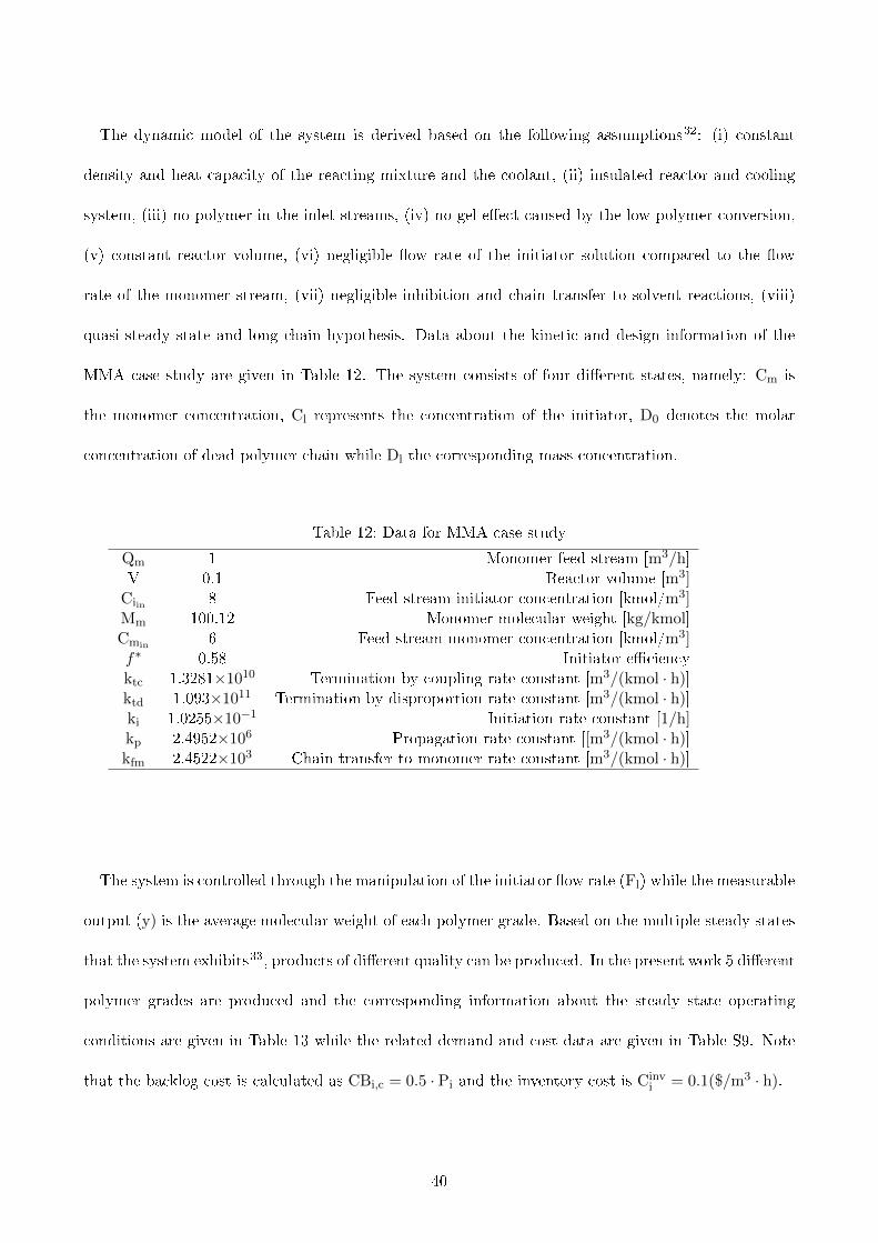
Table 12: Data for MMA case study

Qm 1 Monomer feed stream [m3/h]V 0.1 Reactor volume [m3]

Ciin 8 Feed stream initiator concentration [kmol/m3]Mm 100.12 Monomer molecular weight [kg/kmol]Cmin 6 Feed stream monomer concentration [kmol/m3]f∗ 0.58 Initiator eciencyktc 1.3281×1010 Termination by coupling rate constant [m3/(kmol · h)]ktd 1.093×1011 Termination by disproportion rate constant [m3/(kmol · h)]ki 1.0255×10−1 Initiation rate constant [1/h]kp 2.4952×106 Propagation rate constant [[m3/(kmol · h)]kfm 2.4522×103 Chain transfer to monomer rate constant [m3/(kmol · h)]

The system is controlled through the manipulation of the initiator ow rate (Fl) while the measurable

output (y) is the average molecular weight of each polymer grade. Based on the multiple steady states

that the system exhibits33, products of dierent quality can be produced. In the present work 5 dierent

polymer grades are produced and the corresponding information about the steady state operating

conditions are given in Table 13 while the related demand and cost data are given in Table S9. Note

that the backlog cost is calculated as CBi,c = 0.5 · Pi and the inventory cost is Cinvi = 0.1($/m3 · h).

40

Table 13: Steady state operating conditions for the MMA products

Products Cssm(kmol/m3) Css

l (kmol/m3) Dss0 (kmol/m3) Dss

l (kg/m3) y(kg/kmol) Fl(m3/h)

A 3.078 0.148 0.0195 292.546 15000 0.2048B 3.725 0.0615 0.0091 227.699 25000 0.0847C 3.978 0.0426 0.0067 202.380 30000 0.0586D 4.201 0.0302 0.0051 180.064 35000 0.0416E 4.583 0.0157 0.00315 141.866 45000 0.0217

The dynamic optimisation of the corresponding system is rather demanding as it results in numerical

issues, which stem from the dierent numerical scales associated with the state and control variables.

Following the proposed framework, rst the pairwise minimum transition times are computed oine

resulting in 20 DO problems. The DO problems are further discretised using OCFE with 3 collocation

points and 20 nite elements and the corresponding NLP problem are formulated and solved in GAMS

using BARON 14.4 and CONOPT3 as solvers. The results of the minimum transition times are given in

Table 14 while an example of the proles of the control input and system output during the transition

from product E to D is shown in Figure S2. The coecients for the linear metamodels for the MMA

case study can be found in Table S10.

Table 14: Minimum transition times for the MMA case study

τmini,j (h) A B C D E

A - 3.64 4.45 5.18 6.51B 2.65 - 2.61 3.58 5.13C 2.84 1.28 - 2.65 4.45D 2.93 1.48 1.17 - 3.72E 3.00 1.61 1.40 1.24 -

It is should be mentioned that both BARON and CONOPT3 converge to the same solution but

despite the fact that CONOPT3 is much faster it requires the provision of a good initialisation point

as noted while performing the numerical experiments. The computational statistics are given in Table

41

S11. The same problems were solved employing OCFE with 45 nite elements with slightly improved

results computed which for the sake of space are not reported herein.

After the minimum transition times have been computed, with transition time up to three times the

minimum one, i.e. Ttransi,p ∈ [τmin

i,j , 3τmini,j ] a series of optimisation problems are solved with the objective

to minimise the corresponding transition cost, i.e. the utilisation of control input. Once the linear

meta-models have been computed oine, both the monolithic and the decomposed one are formulated

and solved in GAMS and the corresponding statistics are given in Table 15.

Table 15: Results of the computational performance between the monolithic and the decomposed in-

tegrated model using the proposed TSP and the time-slot (T-S) based formulation for the

MMA case study

Model Monolithic TSP Monolithic T-S Decomposed TSP Decomposed T-SPlanning Horizon 2 weeks

Type MINLP MINLP MILP MILPConstraints 35,067 7,890 287 1,083Cont. Var. 37,767 10,811 236 951Binary Var. 105 300 105 300

Solver SBB/CONOPT3 CPLEX 12.6.1Prot ($) 11423.98 11423.98 15439.57 15439.57CPU (s) 8253.64 10,323.3 0.39 1.5Gap (%) 0.26295 0.26295 0 0

In Table S12, the decision made by the decomposed iPSC are shown while in Figure 10 the systems-

dynamic interpretation of the corresponding schedule for the rst planning period can be envisaged.

42

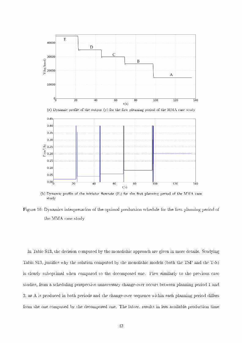
(a) Dynamic prole of the output (y) for the rst planning period of the MMA case study

(b) Dynamic prole of the initiator owrate (Fl) for the rst planning period of the MMA casestudy

Figure 10: Dynamics interpretation of the optimal production schedule for the rst planning period of

the MMA case study

In Table S13, the decision computed by the monolithic approach are given in more details. Studying

Table S13, justies why the solution computed by the monolithic models (both the TSP and the T-S)

is clearly suboptimal when compared to the decomposed one. First similarly to the previous case

studies, from a scheduling perspective unnecessary change-over occurs between planning period 1 and

2, as A is produced in both periods and the change-over sequence within each planning period diers

from the one computed by the decomposed one. The latter, results in less available production time

43

and an amount of demand to be backlogged, thus incurring additional costs.

Another interesting observation is the change-over performed at the second planning period from A

to E, from the decomposed iPSC. One by reading Table 14, would probably expect to have a changeover

between A and B as the transition time is less; however, the optimiser chooses the transition between

A and E and this is due to the less transition cost involved. This particular instance, stands for a very

clear example of where optimal control, planning and scheduling interconnect and how the proposed

decomposition captures these interdependences without strenuous computational times.

In order to demonstrate the computational potential of the proposed decomposition the same case

study was examined with planning horizons of 4, 6 and 12 weeks and a comparison between the TSP

and T-S formulation was conducted. As shown in Table 16, for short planning horizons the TSP and

T-S perform similarly but as larger planning horizons are considered the TSP outperforms the T-S

formulation. This can be justied by both the less number of equations and variables generated and

the symmetry breaking constraints used.

Table 16: Comparison between the decomposed TSP and T-S formulation for varying planning horizons

Planning horizon 4 weeks 6 weeks 12 weeks

Decomposed Model TSP T-S TSP T-S TSP T-S

Type MILP MILP MILP MILP MILP MILP

Constraints 583 2,185 879 3,287 1,767 6,593

Cont. Var. 516 1,901 776 2,851 1,556 5,701

Binary Var. 235 600 365 900 755 1,800

Solver CPLEX 12.6.1

Prot ($) 29563.4 29563.4 45831.07 45831.07 71570.46 71570.46

CPU (s) 0.328 235.031 1.654 1700 9.251 3600

Gap (%) 0 0 0 0 0 0.03

Finally, the case of multiple customers for planning horizon of 8 weeks is examined with a total of

10 customers. The related computational results are given in Table S14.

44

4 Concluding remarks

In the present work we dealt with the integrated Planning, Scheduling and optimal Control (iPSC)

of continuous manufacturing processes. A TSP based model is employed for the decision on the

levels of planning and scheduling and was compared to the time-slot based models adapted by the

majority of the research works for the integrated problem. As shown from the three dierent case

studies, the TSP and T-S based integration perform similarly for small planning horizons while for

larger planning horizons the TSP based model outperforms the T-S considerably. New features for

the integrated problem are studied such as multiple customers, inventory capacity as well as backlog

and idle production time within the planning period are allowed. Aiming to reduce the computational

complexity of the iPSC, a decomposition based on linear metamodels was proposed and tested under

the assumption that we account for the open loop performance of the underlying dynamic system.

The linear metamodels, associate the transition cost with the transition time between the dierent

products manufactured. Computational studies indicate that when disturbances are not considered at

the level of control then the solutions computed from the decomposed iPSC and the monolithic when

solved to global optimality are equivalent. Future work in our group is directed towards the extension

of the proposed framework for the closed loop implementation of the solution computed by the iPSC

so as to account for systematic disturbances.

Acknowledgments

The authors gratefully acknowledge nancial support from EPSRC grants EP/M027856/1 and EP/M028240/1.

Supporting Information

The Supporting Information is available free of charge via the Internet at http://pubs.acs.org/.

45

References

[1] Davis, J.; Edgar, T.; Porter, J.; Bernaden, J.; Sarli, M. Smart manufacturing, manufacturing

intelligence and demand-dynamic performance. Comput. Chem. Eng. 2012, 47, 145156.

[2] Lee, J.; Bagheri, B.; Kao, H.-A. A cyber-physical systems architecture for industry 4.0-based

manufacturing systems. Manuf. Lett. 2015, 3, 1823.

[3] Harjunkoski, I.; Nystrom, R.; Horch, A. Integration of scheduling and control-Theory or practice?

Comput. Chem. Eng. 2009, 33, 19091918.

[4] Grossmann, I. E. Enterprise-wide optimization: A new frontier in process systems engineering.

AIChE J. 2005, 51, 18461857.

[5] Gutiérrez-Limón, M. A.; Flores-Tlacuahuac, A.; Grossmann, I. E. A reactive optimization strategy

for the simultaneous planning, scheduling and control of short-period continuous reactors. Comput.

Chem. Eng. 2016, 84, 507515.

[6] Sarimveis, H.; Patrinos, P.; Tarantilis, C. D.; Kiranoudis, C. T. Dynamic modeling and control of

supply chain systems: A review. Comput. Oper. Res. 2008, 35, 3530 3561.

[7] Maravelias, C. T.; Sung, C. Integration of production planning and scheduling: Overview, chal-

lenges and opportunities. Comput. Chem. Eng. 2009, 33, 19191930.

[8] Baldea, M.; Harjunkoski, I. Integrated production scheduling and process control: A systematic

review. Comput. Chem. Eng. 2014, 71, 377390.

[9] Flores-Tlacuahuac, A.; Grossmann, I. E. Simultaneous cyclic scheduling and control of a multi-

product CSTR. Ind. Eng. Chem. Res. 2006, 45, 66986712.

[10] Chu, Y.; You, F. Integration of scheduling and control with online closed-loop implementation:

46

Fast computational strategy and large-scale global optimization algorithm. Comput. Chem. Eng.

2012, 47, 248268.

[11] Zhuge, J.; Ierapetritou, M. G. Integration of scheduling and control with closed loop implemen-

tation. Ind. Eng. Chem. Res. 2012, 51, 85508565.

[12] Zhuge, J.; Ierapetritou, M. G. Integration of scheduling and control for batch processes using

multi-parametric model predictive control. AIChE J. 2014, 60, 31693183.

[13] Chu, Y.; You, F. Integration of production scheduling and dynamic optimization for multi-product

CSTRs: Generalized Benders decomposition coupled with global mixed-integer fractional pro-

gramming. Comput. Chem. Eng. 2013, 58, 315333.

[14] Zhuge, J.; Ierapetritou, M. G. An integrated framework for scheduling and control using fast

model predictive control. AIChE J. 2015, 61, 33043319.

[15] Du, J.; Park, J.; Harjunkoski, I.; Baldea, M. A time scale-bridging approach for integrating

production scheduling and process control. Comput. Chem. Eng. 2015, 79, 5969.

[16] Baldea, M.; Daoutidis, P. Control of integrated process networks-A multi-time scale perspective.

Comput. Chem. Eng. 2007, 31, 426444.

[17] Baldea, M.; Du, J.; Park, J.; Harjunkoski, I. Integrated production scheduling and model predictive

control of continuous processes. AIChE J. 2015, 61, 41794190.

[18] Pistikopoulos, E. N.; Diangelakis, N. A. Towards the integration of process design, control and

scheduling: Are we getting closer? Comput. Chem. Eng. 2015,

[19] Gutierrez-Limon, M. A.; Flores-Tlacuahuac, A.; Grossmann, I. E. MINLP Formulation for Simul-

taneous Planning, Scheduling, and Control of Short-Period Single-Unit Processing Systems. Ind.

Eng. Chem. Res. 2014, 53, 1467914694.

47

[20] Dogan, M. E.; Grossmann, I. E. A decomposition method for the simultaneous planning and

scheduling of single-stage continuous multiproduct plants. Ind. Eng. Chem. Res. 2006, 45, 299

315.

[21] Shi, H.; Chu, Y.; You, F. Novel optimization model and ecient solution method for integrating

dynamic optimization with process operations of continuous manufacturing processes. Ind. Eng.

Chem. Res. 2015, 54, 21672187.

[22] Liu, S.; Pinto, J. M.; Papageorgiou, L. G. A TSP-based MILP model for medium-term planning

of single-stage continuous multiproduct plants. Ind. Eng. Chem. Res. 2008, 47, 77337743.

[23] Kopanos, G. M.; Puigjaner, L.; Maravelias, C. T. Production planning and scheduling of parallel

continuous processes with product families. Ind. Eng. Chem. Res. 2010, 50, 13691378.

[24] Biegler, L. T. An overview of simultaneous strategies for dynamic optimization. Chem. Eng.

Process 2007, 46, 10431053.

[25] Carey, G. F.; Finlayson, B. A. Orthogonal collocation on nite elements. Chem. Eng. Sci. 1975,

30, 587596.

[26] Hairer, E.; Wanner, G. Sti dierential equations solved by Radau methods. J. Comput. Appl.

Math. 1999, 111, 93111.

[27] Chu, Y.; You, F. Model-based integration of control and operations: Overview, challenges, advan-

ces, and opportunities. Comput. Chem. Eng. 2015, 83, 220.

[28] Seabold, J.; Perktold, J. Statsmodels: Econometric and Statistical Modeling with Python. 2010.

[29] Glover, F. Improved linear integer programming formulations of nonlinear integer problems. Ma-

nag. Sci. 1975, 22, 455460.

48

[30] Rosenthal, E. GAMS Development Corporation; GAMS Development Corporation: Washington,

DC, USA, 2008.

[31] Camacho, E. F.; Alba, C. B. Model Predictive Control ; Springer-Verlag: London, 2013.

[32] Daoutidis, P.; Soroush, M.; Kravaris, C. Feedforward/feedback control of multivariable nonlinear

processes. AIChE J. 1990, 36, 14711484.

[33] Verazaluce-Garcia, J. C.; Flores-Tlacuahuac, A.; Saldívar-Guerra, E. Steady-state nonlinear bi-

furcation analysis of a high-impact polystyrene continuous stirred tank reactor. Ind. Eng. Chem.

Res. 2000, 39, 19721979.

49

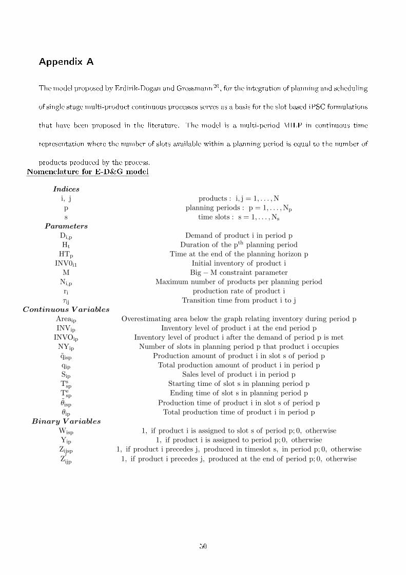
Appendix A

The model proposed by Erdirik-Dogan and Grossmann20, for the integration of planning and scheduling

of single stage multi-product continuous processes serves as a basis for the slot based iPSC formulations

that have been proposed in the literature. The model is a multi-period MILP in continuous time

representation where the number of slots available within a planning period is equal to the number of

products produced by the process.Nomenclature for E-D&G model

Indicesi, j products : i, j = 1, . . . ,Np planning periods : p = 1, . . . ,Np

s time slots : s = 1, . . . ,Ns

ParametersDi,p Demand of product i in period pHt Duration of the pth planning period

HTp Time at the end of the planning horizon pINV0i1 Initial inventory of product i

M Big −M constraint parameterNi,p Maximum number of products per planning periodri production rate of product iτij Transition time from product i to j

Continuous V ariablesAreaip Overestimating area below the graph relating inventory during period pINVip Inventory level of product i at the end period p

INVOip Inventory level of product i after the demand of period p is metNYip Number of slots in planning period p that product i occupiesqisp Production amount of product i in slot s of period pqip Total production amount of product i in period pSip Sales level of product i in period pTs

sp Starting time of slot s in planning period p

Tesp Ending time of slot s in planning period p

θisp Production time of product i in slot s of period pθip Total production time of product i in period p

Binary V ariablesWisp 1, if product i is assigned to slot s of period p; 0, otherwiseYip 1, if product i is assigned to period p; 0, otherwiseZijsp 1, if product i precedes j, produced in timeslot s, in period p; 0, otherwise

Z′ijp 1, if product i precedes j, produced at the end of period p; 0, otherwise

50

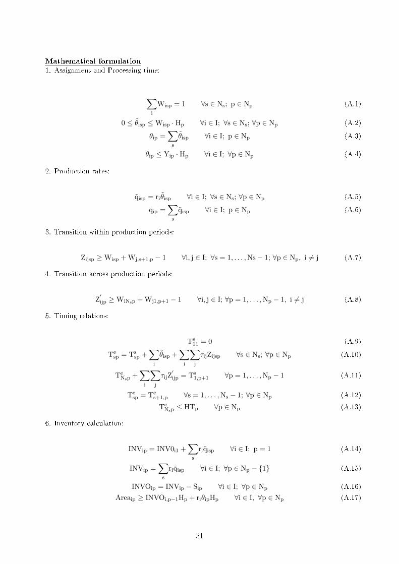
Mathematical formulation1. Assignment and Processing time:

∑i

Wisp = 1 ∀s ∈ Ns; p ∈ Np (A.1)

0 ≤ θisp ≤Wisp ·Hp ∀i ∈ I; ∀s ∈ Ns; ∀p ∈ Np (A.2)

θip =∑

s

θisp ∀i ∈ I; p ∈ Np (A.3)

θip ≤ Yip ·Hp ∀i ∈ I; ∀p ∈ Np (A.4)

2. Production rates:

qisp = riθisp ∀i ∈ I; ∀s ∈ Ns; ∀p ∈ Np (A.5)

qip =∑

s

qisp ∀i ∈ I; p ∈ Np (A.6)

3. Transition within production periods:

Zijsp ≥Wisp + Wj,s+1,p − 1 ∀i, j ∈ I; ∀s = 1, . . . ,Ns− 1; ∀p ∈ Np, i 6= j (A.7)

4. Transition across production periods:

Z′ijp ≥WiNsp + Wj1,p+1 − 1 ∀i, j ∈ I; ∀p = 1, . . . ,Np − 1, i 6= j (A.8)

5. Timing relations:

Ts11 = 0 (A.9)

Tesp = Ts

sp +∑

i

θisp +∑

i

∑j

τijZijsp ∀s ∈ Ns; ∀p ∈ Np (A.10)

TeNsp +

∑i

∑j

τijZ′ijp = Ts

1,p+1 ∀p = 1, . . . ,Np − 1 (A.11)

Tesp = Te

s+1,p ∀s = 1, . . . ,Ns − 1; ∀p ∈ Np (A.12)

TeNsp ≤ HTp ∀p ∈ Np (A.13)

6. Inventory calculation:

INVip = INV0i1 +∑

s

riqisp ∀i ∈ I; p = 1 (A.14)

INVip =∑

s

riqisp ∀i ∈ I; ∀p ∈ Np − 1 (A.15)

INVOip = INVip − Sip ∀i ∈ I; ∀p ∈ Np (A.16)

Areaip ≥ INVOi,p−1Hp + riθipHp ∀i ∈ I, ∀p ∈ Np (A.17)

51

7. Sales satisfaction:

Sip ≥ Dip ∀i ∈ I, ∀p ∈ Np (A.18)

8. Symmetry breaking constraints:

NYip =∑

s

Wisp ∀i ∈ I, ∀p ∈ Np (A.19)

Yip ≥Wisp ∀i ∈ I, ∀s ∈ Ns, ∀p ∈ Np (A.20)

Yip ≤ NYip ≤ NipYip ∀i ∈ I, ∀p ∈ Np (A.21)

NYip ≥ Nip − [(∑

i

Yip)− 1]−M(1−Wisp) ∀i ∈ I, ∀s ∈ Ns, ∀p ∈ Np (A.22)

NYip ≤ Nip − [(∑

i

Yip)− 1] + M(1−Wisp) ∀i ∈ I, ∀s ∈ Ns, ∀p ∈ Np (A.23)

Abbreviations MeaningAPC Advanced Process ControlBVP Boundary Value ProblemDO Dynamic OptimisationEWO Enterprise Wide OptimisationISA International Society of AutomationiPSC integrated Planning Scheduling and ControliSC integrated Scheduling and Control

MIDO Mixed Integer Dynamic OptimisationMILP Mixed Integer Linear ProgrammingMIMO Multiple Input Multiple OutputMINLP Mixed Integer Nonlinear ProgrammingMMA methyl-methacrylateMPC Model Predictive ControlNLP Nonlinear ProgrammingNMPC Nonlinear Model Predictive ControlOCFE Orthogonal Collocation on Finite ElementsRHS right-hand sideSBM time Scale Bridging ModelSISO Single Input Single OutputT-S Time-SlotTSP Travelling Salesman Problem

Table 17: Index of abbreviations

52

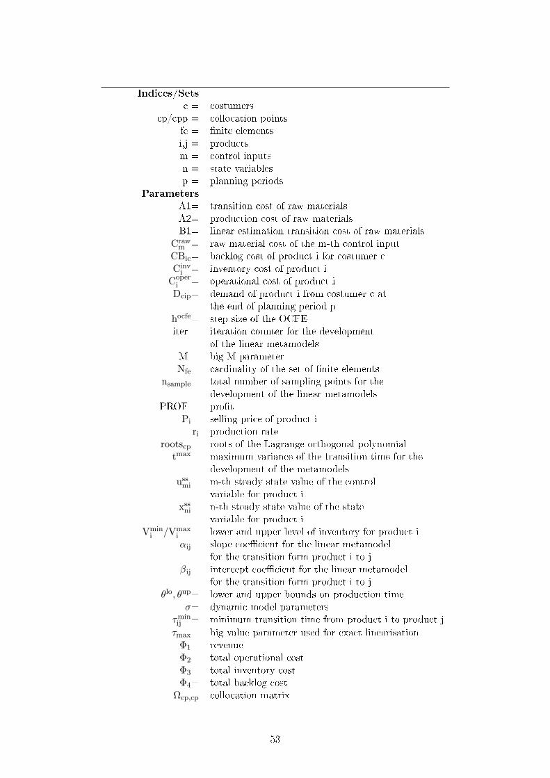
Indices/Setsc = costumers

cp/cpp = collocation pointsfe = nite elementsi,j = productsm = control inputsn = state variablesp = planning periods

ParametersA1= transition cost of raw materialsA2= production cost of raw materialsB1= linear estimation transition cost of raw materials

Crawm = raw material cost of the m-th control input

CBic= backlog cost of product i for costumer cCinv

i = inventory cost of product iCoper

i = operational cost of product iDcip= demand of product i from costumer c at

the end of planning period phocfe= step size of the OCFEiter = iteration counter for the development

of the linear metamodelsM = big-M parameterNfe= cardinality of the set of nite elements

nsample= total number of sampling points for thedevelopment of the linear metamodels

PROF = protPi= selling price of product i

ri production raterootscp= roots of the Lagrange orthogonal polynomial

tmax= maximum variance of the transition time for thedevelopment of the metamodels

ussmi= m-th steady state value of the control

variable for product ixss

ni= n-th steady state value of the statevariable for product i

Vmini /Vmax

i = lower and upper level of inventory for product iαij= slope coecient for the linear metamodel

for the transition form product i to jβij= intercept coecient for the linear metamodel

for the transition form product i to jθlo, θup= lower and upper bounds on production time

σ= dynamic model parametersτmin

ij = minimum transition time from product i to product j

τmax= big value parameter used for exact linearisationΦ1= revenueΦ2= total operational costΦ3= total inventory costΦ4= total backlog cost

Ωcp,cp collocation matrix

53

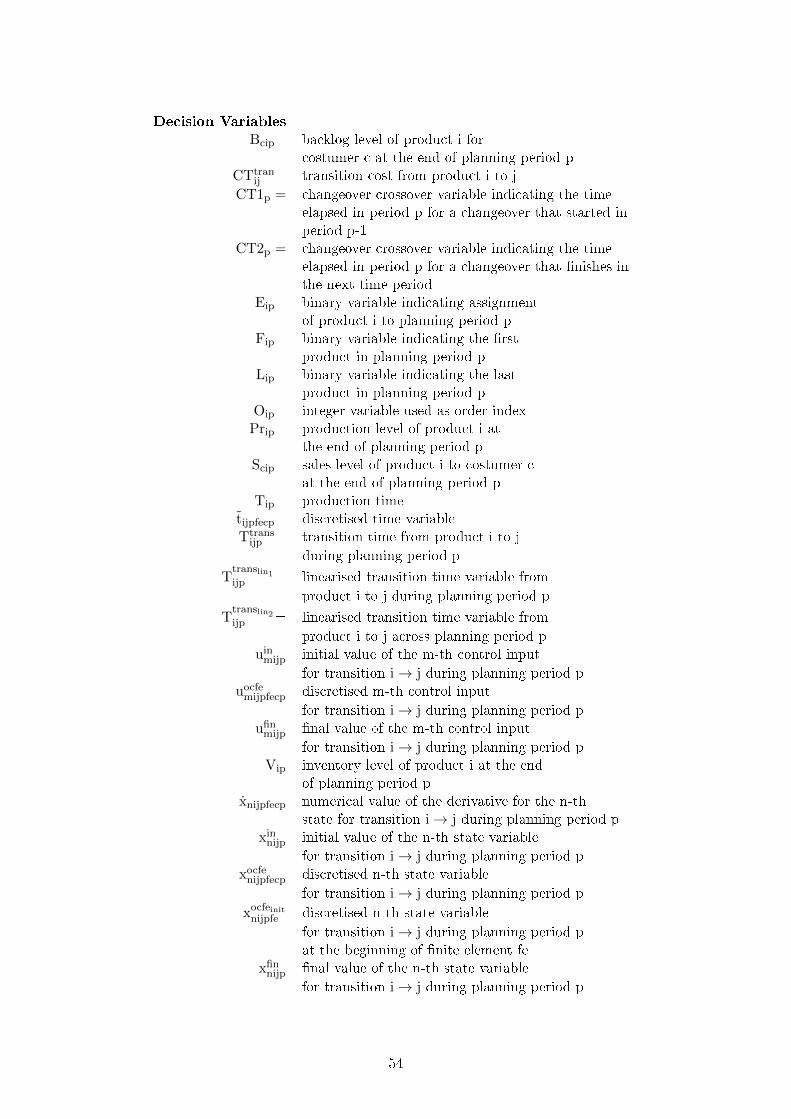
Decision VariablesBcip= backlog level of product i for

costumer c at the end of planning period pCTtran

ij = transition cost from product i to j

CT1p = changeover crossover variable indicating the timeelapsed in period p for a changeover that started inperiod p-1

CT2p = changeover crossover variable indicating the timeelapsed in period p for a changeover that nishes inthe next time period

Eip= binary variable indicating assignmentof product i to planning period p

Fip= binary variable indicating the rstproduct in planning period p

Lip= binary variable indicating the lastproduct in planning period p

Oip= integer variable used as order indexPrip= production level of product i at

the end of planning period pScip= sales level of product i to costumer c

at the end of planning period pTip= production time

tijpfecp= discretised time variableTtrans

ijp = transition time from product i to j

during planning period p

Ttranslin1ijp = linearised transition time variable from

product i to j during planning period p

Ttranslin2ijp = linearised transition time variable from

product i to j across planning period puin

mijp initial value of the m-th control input

for transition i→ j during planning period puocfe

mijpfecp discretised m-th control input

for transition i→ j during planning period pufin

mijp nal value of the m-th control input

for transition i→ j during planning period pVip inventory level of product i at the end

of planning period pxnijpfecp numerical value of the derivative for the n-th

state for transition i→ j during planning period pxin

nijp initial value of the n-th state variable

for transition i→ j during planning period pxocfe

nijpfecp discretised n-th state variable

for transition i→ j during planning period p

xocfeinitnijpfe discretised n-th state variable

for transition i→ j during planning period pat the beginning of nite element fe

xfinnijp nal value of the n-th state variable

for transition i→ j during planning period p

54

Zijp= binary variable indicating transitioni→ j during planning period p

Zfijp= binary variable indicating transitionbetween periods p - 1 and p from product i to j

Nomenclature

Contents

1 Introduction 2

1.1 Integration of process operations with control . . . . . . . . . . . . . . . . . . . . . . . 21.2 Motivation and problem statement . . . . . . . . . . . . . . . . . . . . . . . . . . . . . 5

2 Methodology 7

2.1 Objective of the iPSC . . . . . . . . . . . . . . . . . . . . . . . . . . . . . . . . . . . . 72.2 Modelling the planning and scheduling problem . . . . . . . . . . . . . . . . . . . . . . 10

2.2.1 Allocation constraints . . . . . . . . . . . . . . . . . . . . . . . . . . . . . . . . 102.2.2 Sequencing constraints . . . . . . . . . . . . . . . . . . . . . . . . . . . . . . . . 112.2.3 Symmetry breaking constraints . . . . . . . . . . . . . . . . . . . . . . . . . . . 122.2.4 Timing constraints . . . . . . . . . . . . . . . . . . . . . . . . . . . . . . . . . . 132.2.5 Production constraints . . . . . . . . . . . . . . . . . . . . . . . . . . . . . . . . 13

2.3 Dynamic optimisation (DO) . . . . . . . . . . . . . . . . . . . . . . . . . . . . . . . . . 142.4 Linking variables between DO, scheduling and planning model . . . . . . . . . . . . . . 162.5 Linking equations between DO and TSP planning and scheduling . . . . . . . . . . . . 182.6 Monolithic and decomposed integration of planning, scheduling and optimal control . . 19

2.6.1 Monolithic iPSC . . . . . . . . . . . . . . . . . . . . . . . . . . . . . . . . . . . 192.6.2 Decomposed iPSC . . . . . . . . . . . . . . . . . . . . . . . . . . . . . . . . . . 20

3 Case Studies 25

3.1 SISO multi-product CSTR . . . . . . . . . . . . . . . . . . . . . . . . . . . . . . . . . . 263.2 MIMO multi-product CSTR . . . . . . . . . . . . . . . . . . . . . . . . . . . . . . . . . 343.3 MMA polymerisation process . . . . . . . . . . . . . . . . . . . . . . . . . . . . . . . . 39

4 Concluding remarks 45

55