TRANSPORTATION SCIENCEVol. 38, No. 2, May 2004, pp. 245–255issn 0041-1655 �eissn 1526-5447 �04 �3802 �0245

informs ®

doi 10.1287/trsc.1030.0086©2004 INFORMS

Heuristics for the One-CommodityPickup-and-Delivery Traveling Salesman Problem

Hipólito Hernández-Pérez, Juan-José Salazar-GonzálezDEIOC, Facultad de Matemáticas, Universidad de La Laguna, 38271 La Laguna, Tenerife, Spain

{hhperez@ull.es, jjsalaza@ull.es}

This paper deals with a generalisation of the well-known traveling salesman problem (TSP) in which citiescorrespond to customers providing or requiring known amounts of a product, and the vehicle has a given

upper limit capacity. Each customer must be visited exactly once by the vehicle serving the demands whileminimising the total travel distance. It is assumed that any unit of product collected from a pickup customer canbe delivered to any delivery customer. This problem is called one-commodity pickup-and-delivery TSP (1-PDTSP).We propose two heuristic approaches for the problem: (1) is based on a greedy algorithm and improved witha k-optimality criterion and (2) is based on a branch-and-cut procedure for finding an optimal local solution.The proposal can easily be used to solve the classical “TSP with pickup-and-delivery,” a version studied inliterature and involving two commodities. The approaches have been applied to solve hard instances with upto 500 customers.

Key words : pickup and delivery; traveling salesman; heuristics; branch and cutHistory : Received: August 2002; revision received: March 2003; accepted: March 2003.

1. IntroductionThis paper presents two heuristic algorithms for the1-PDTSP. The problem is closely related to the well-known TSP, thus, a finite set of cities is given, and thetravel distance between each pair of cities is assumedto be known. In addition, one specific city is con-sidered to be a depot of a vehicle, while the othercities are identified as customers and are divided intotwo groups according to the type of service required(delivery or pickup). Each delivery customer requires agiven amount of the product and each pickup customerprovides a given amount of the product. Any amountof the product collected from a pickup customer canbe supplied to a delivery customer. It is assumed thatthe vehicle has a fixed upper limit capacity and muststart and end the route at the depot. The 1-PDTSPthen calls for a minimum distance route for the vehi-cle to satisfy the customer requirements without everexceeding the vehicle capacity. The route must be aHamiltonian tour through all the cities. As in mostof the papers on similar routing problems, we willassume that the travel distances are symmetric, evenif most of the ideas presented here could be extendedto also work on asymmetrical instances.We now introduce the notation useful in this paper.

The depot will be denoted by 1 and each customerby i �i = 2� � � � �n�. V = 1�2� � � � �n� is the vertex setand E is the edge set. For each pair of locations i� j�,the travel distance (or cost) cij of going between iand j is given. It is also given a nonzero demand

qi associated with each customer i, where qi < 0 ifi is a delivery customer and qi > 0 if i is a pickupcustomer. Let K =max

∑i∈V qi>0 qi�−

∑i∈V qi<0 qi�. The

capacity of the vehicle is represented by Q and isassumed to be a positive number. Note that typicallyQ ≤ K on a 1-PDTSP instance. Clearly, the depot canbe considered a customer by defining q1 =−∑n

i=2 qi,i.e., a customer absorbing or providing the remainingamount of product to ensure product conservation.Even more, in this basic version, we will assume thatthe depot can also provide the vehicle with the nec-essary load for guaranteeing the feasibility of someroutes that need a nonempty (or nonfull) load of thevehicle when coming out from the depot. Indeed,notice that a 1-PDTSP instance could admit a solu-tion for the vehicle even if there is no route withthe vehicle leaving the depot with an empty (or full)load. Still, it is possible to solve the 1-PDTSP withthis additional requirement by using an algorithm foranother basic 1-PDTSP with the depot replaced bytwo dummy customers. Another interesting observa-tion from the definition of the problem is that whenT ⊂ E is a set of edges that can be oriented defin-ing a feasible circuit

−→T for a 1-PDTSP instance, then

the circuit←−T obtained by orienting the edges in the

other sense is also a feasible route for the vehicle ofthe same instance (see Hernández-Pérez and Salazar-González 2004 for details).The 1-PDTSP was introduced in Hernández-Pérez

and Salazar-González (2004) together with an exact

245

Hernández-Pérez and Salazar-González: Heuristics for the Traveling Salesman Problem246 Transportation Science 38(2), pp. 245–255, © 2004 INFORMS

approach applied to solve instances with up to 40 cus-tomers, but there are in literature many other prob-lems closely related. We next point out some of them,starting with the problems involving one commodityand then the related problems involving several com-modities.Chalasani and Motwani (1999) study the special

case of the 1-PDTSP, where the delivery and pickupquantities are all equal to one unit. This problemis called Q-delivery TSP if Q is the capacity of thevehicle. Anily and Bramel (1999) consider the sameproblem with the name capacitated traveling salesmanproblem with pickups and deliveries (CTSPPD). They pro-pose heuristic algorithms, which could be appliedto a 1-PDTSP instance with general demands if theHamiltonian requirement on the route were relaxed,or directly to a 1-PDTSP instance if the demand val-ues are +1 or −1. In other words, as noticed in Anilyand Bramel (1999), CTSPPD can be considered the“splitting version” of the 1-PDTSP. Moreover, Anilyand Bramel (1999) give an important application ofthe CTSPPD in the context of inventory repositioning,and this application leads to the 1-PDTSP if the vehi-cle is required to visit each retailer exactly once, animportant constraint to guarantee a satisfactory ser-vice policy when the customer is external to the firm.Anily and Hassin (1992) introduce the swapping

problem, a more general problem, where several com-modities must be transported from many origins tomany destinations with a vehicle of limited capac-ity following a non-necessary Hamiltonian route, andwhere a commodity can be temporarily stored in anintermediate customer. This last feature is namedpreemption or drop in the process of transportation.The swapping problem on a line is analyzed inAnily et al. (1999). In the capacitated dial-a-ride prob-lem (CDARP) (also named single-vehicle many-to-manydial-a-ride problem), there is a one-to-one correspon-dence between pickup customers and delivery cus-tomers, and the vehicle should move one unit of acommodity (say, a person) from its origin to its des-tination with a limited capacity Q (see, e.g., Psaraftis1983, Guan 1998). When Q = 1, the nonpreemp-tive CDARP is known as the stacker crane problem(see, e.g., Frederickson et al. 1978). When there isno vehicle capacity, the nonpreemptive CDARP iscalled the pickup and delivery traveling salesman prob-lem (PDTSP) (see, e.g., Kalantari et al. 1985, Kuboand Kasugai 1990, Healy and Moll 1995, Renaudet al. 2000, Renaud et al. 2002). In Kalantari et al.(1985), the PDTSP is referred to as traveling sales-man problem with pickup and delivery (TSPPD) and inHealy and Moll (1995), the PDTSP is referred to asCDARP. The PDTSP is a particular case of the TSPwith precedence constraints (see, e.g., Bianco et al. 1994).Another related problem is the TSP with backhauls

(TSPB) (see, e.g., Gendreau et al. 1997), where anuncapacitated vehicle must visit all the delivery cus-tomers before visiting a pickup customer. See Savels-bergh and Sol (1995) for other references and variants(including time windows, and so on) of the so-calledgeneral pickup and delivery problem.Another known problem is the TSPPD, introduced

by Mosheiov (1994), and where the product collectedfrom pickup customers must be transported to thedepot and the product delivery to the demand cus-tomers should be transported from the depot, all doneusing a capacitated vehicle on a Hamiltonian route.Seen from this point of view, the TSPPD concernsa many-to-one commodity and another one-to-manydifferent commodity, and a classical application isthe collection of empty bottles from the customersbeing delivered to a warehouse and full bottles beingdelivered from the warehouse to the customers. Animportant difference when comparing TSPPD with1-PDTSP is that PDTSP is feasible if, and only if, thevehicle capacity is at least the maximum of the totalsum of the pickup demands and of the total sum ofthe delivery demands (i.e., K ≤ Q). This constraintis not required for the feasibility of the 1-PDTSP inwhich the vehicle capacity Q could even be equalto the biggest customer demand maxni=1 �qi�. As men-tioned by Mosheiov (1994), a TSPPD instance can beassumed to be in “standard form,” which means thatthe capacity of the vehicle coincides with the totalsum of products collected in the pickup customersand with the total sum of product delivered in thedelivery customers (i.e., K = Q). Hence, it is alwayspossible to assume that in a feasible TSPPD route,the vehicle starts at the depot fully loaded, it deliversand picks up amounts from the customers, and fin-ishes at the depot again fully loaded. This condition oftraversing the depot with a full (or empty) load is alsopresented in the other problems, like the CTSPPD,where the vehicle cannot go immediately from thedepot to a pickup customer, but it does not necessar-ily occur in general with the 1-PDTSP as observed.Anily and Mosheiov (1994) present approximation

algorithms for the TSPPD, here renamed TSP withdelivery and backhauls (TSPDB), and Gendreau et al.(1999) propose several heuristics tested on instanceswith up to 200 customers. Baldacci et al. (1999) dealwith the same problem, here named TSP with deliv-ery and collection (TSPDC) constraints, and present anexact algorithm based on a two-commodity networkflow formulation, which was able to prove optimal-ity of some TSPPD instances with 150 customers,even if it was not able to prove optimality of otherTSPPD instances with 25 customers. Hernández-Pérezand Salazar-González (2004) present a branch-and-cutalgorithm for the exact solution of TSPPD instances

Hernández-Pérez and Salazar-González: Heuristics for the Traveling Salesman ProblemTransportation Science 38(2), pp. 245–255, © 2004 INFORMS 247

Table 1 Characteristics of Closely Related Problems

Problem Name # Origins-Destinations Hamiltonian Pre-emption Q Load References

Swapping Problem m many to many no yes 1 yes Anily et al. (1999), Anily and Hassin (1992)Stacker Crane Problem m one to one no no 1 yes Frederickson et al. (1978)CDARP m one to one no no k yes Guan (1998), Psaraftis (1983), Savelsbergh and Sol (1995)PDTSP m one to one yes no yes Kalantari et al. (1985), Kubo and Kasugai (1990),

Renaud et al. (2002), Renaud et al. (2000)TSPPD, TSPDB, TSPDC 2 one to many yes no k yes Anily and Mosheiov (1994), Baldacci et al. (1999),

Gendreau et al. (1999), Mosheiov (1994)TSPB 2 one to many yes no yes Gendreau et al. (1997)CTSPPD, Q-delivery TSP 1 many to many no no k yes Anily and Bramel (1999), Chalasani and Motwani (1999)1-PDTSP 1 many to many yes no k no Hernández-Pérez and Salazar-González (2004)

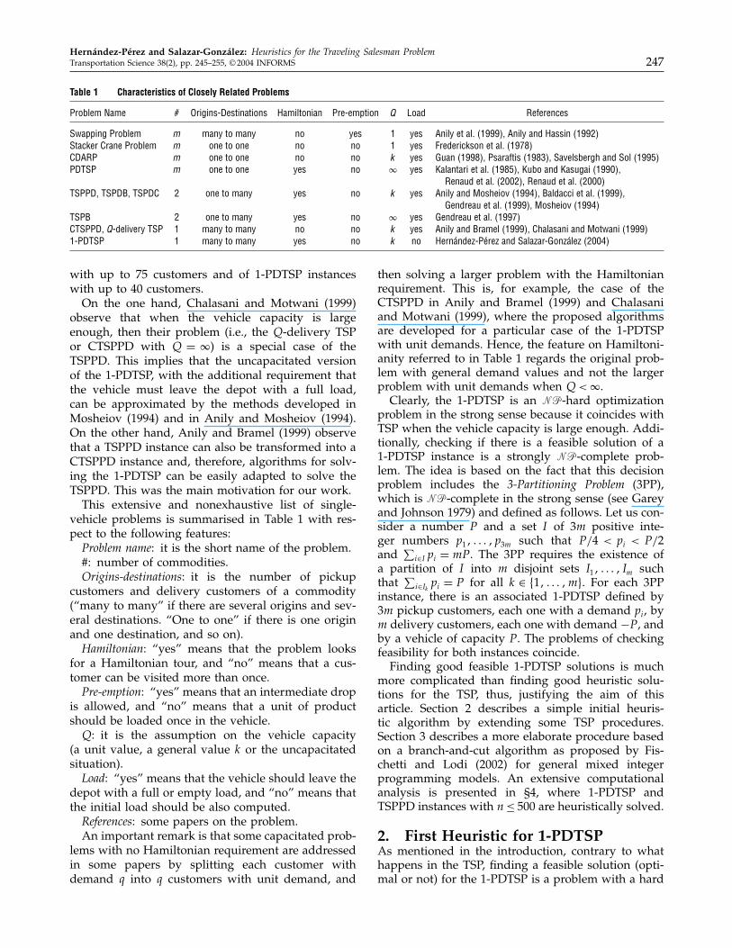
with up to 75 customers and of 1-PDTSP instanceswith up to 40 customers.On the one hand, Chalasani and Motwani (1999)

observe that when the vehicle capacity is largeenough, then their problem (i.e., the Q-delivery TSPor CTSPPD with Q = ) is a special case of theTSPPD. This implies that the uncapacitated versionof the 1-PDTSP, with the additional requirement thatthe vehicle must leave the depot with a full load,can be approximated by the methods developed inMosheiov (1994) and in Anily and Mosheiov (1994).On the other hand, Anily and Bramel (1999) observethat a TSPPD instance can also be transformed into aCTSPPD instance and, therefore, algorithms for solv-ing the 1-PDTSP can be easily adapted to solve theTSPPD. This was the main motivation for our work.This extensive and nonexhaustive list of single-

vehicle problems is summarised in Table 1 with res-pect to the following features:Problem name: it is the short name of the problem.#: number of commodities.Origins-destinations: it is the number of pickup

customers and delivery customers of a commodity(“many to many” if there are several origins and sev-eral destinations. “One to one” if there is one originand one destination, and so on).Hamiltonian: “yes” means that the problem looks

for a Hamiltonian tour, and “no” means that a cus-tomer can be visited more than once.Pre-emption: “yes” means that an intermediate drop

is allowed, and “no” means that a unit of productshould be loaded once in the vehicle.Q: it is the assumption on the vehicle capacity

(a unit value, a general value k or the uncapacitatedsituation).Load: “yes” means that the vehicle should leave the

depot with a full or empty load, and “no” means thatthe initial load should be also computed.References: some papers on the problem.An important remark is that some capacitated prob-

lems with no Hamiltonian requirement are addressedin some papers by splitting each customer withdemand q into q customers with unit demand, and

then solving a larger problem with the Hamiltonianrequirement. This is, for example, the case of theCTSPPD in Anily and Bramel (1999) and Chalasaniand Motwani (1999), where the proposed algorithmsare developed for a particular case of the 1-PDTSPwith unit demands. Hence, the feature on Hamiltoni-anity referred to in Table 1 regards the original prob-lem with general demand values and not the largerproblem with unit demands when Q<.Clearly, the 1-PDTSP is an ��-hard optimization

problem in the strong sense because it coincides withTSP when the vehicle capacity is large enough. Addi-tionally, checking if there is a feasible solution of a1-PDTSP instance is a strongly ��-complete prob-lem. The idea is based on the fact that this decisionproblem includes the 3-Partitioning Problem (3PP),which is ��-complete in the strong sense (see Gareyand Johnson 1979) and defined as follows. Let us con-sider a number P and a set I of 3m positive inte-ger numbers p1� � � � � p3m such that P/4 < pi < P/2and

∑i∈I pi = mP . The 3PP requires the existence of

a partition of I into m disjoint sets I1� � � � � Im suchthat

∑i∈Ik pi = P for all k ∈ 1� � � � �m�. For each 3PP

instance, there is an associated 1-PDTSP defined by3m pickup customers, each one with a demand pi, bym delivery customers, each one with demand −P , andby a vehicle of capacity P . The problems of checkingfeasibility for both instances coincide.Finding good feasible 1-PDTSP solutions is much

more complicated than finding good heuristic solu-tions for the TSP, thus, justifying the aim of thisarticle. Section 2 describes a simple initial heuris-tic algorithm by extending some TSP procedures.Section 3 describes a more elaborate procedure basedon a branch-and-cut algorithm as proposed by Fis-chetti and Lodi (2002) for general mixed integerprogramming models. An extensive computationalanalysis is presented in §4, where 1-PDTSP andTSPPD instances with n≤ 500 are heuristically solved.

2. First Heuristic for 1-PDTSPAs mentioned in the introduction, contrary to whathappens in the TSP, finding a feasible solution (opti-mal or not) for the 1-PDTSP is a problem with a hard

Hernández-Pérez and Salazar-González: Heuristics for the Traveling Salesman Problem248 Transportation Science 38(2), pp. 245–255, © 2004 INFORMS

computational complexity. Nevertheless, checking ifa given TSP solution is feasible for 1-PDTSP is atrivial task as it can be done in linear time on n.Indeed, let us consider a path

−→P defined by the vertex

sequence v1� � � � � vk for k ≤ n. Let l0�−→P � = 0 and

li�−→P � = li−1�

−→P �+qvi be the load of the vehicle coming

out from vi if it goes inside v1 with load l0�−→P �. Notice

that li�−→P � could be a negative. We denote

infeas�−→P � = k

maxi=0

{li�−→P �

}− k

mini=0

{li�−→P �

}−Q

the infeasibility of the path−→P . This value is independ-

ent of the orientation of the path (i.e., infeas�−→P � =

infeas�←−P �, where

←−P denotes the path

−→P in the oppo-

site direction), and a path−→P is said to be feasible if

infeas�−→P � ≤ 0. Then, the interval of potential loads of

the vehicle going out from vk is defined by the extremevalues

lk�−→P � = lk�

−→P �− k

mini=0

{li�−→P �

}lk�

−→P � = lk�

−→P �+Q− k

maxi=0

{li�−→P �

}�

Immediately, we also have the interval of potentialloads of the vehicle entering v1 to route

−→P

[lk�

−→P �− lk�

−→P �� lk�

−→P �− lk�

−→P �

]�

and of going out from v1 if the path is routed in thereverse order, defined by

l1�←−P � = Q− lk�

−→P �+ lk�

−→P �

l1�←−P � = Q− lk�

−→P �+ lk�

−→P ��

For example, if−→P is a path defined by customers

v1�v2�v3 with demands +2�−5�+1, respectively, andQ = 10, then the vehicle can enter and follow

−→P

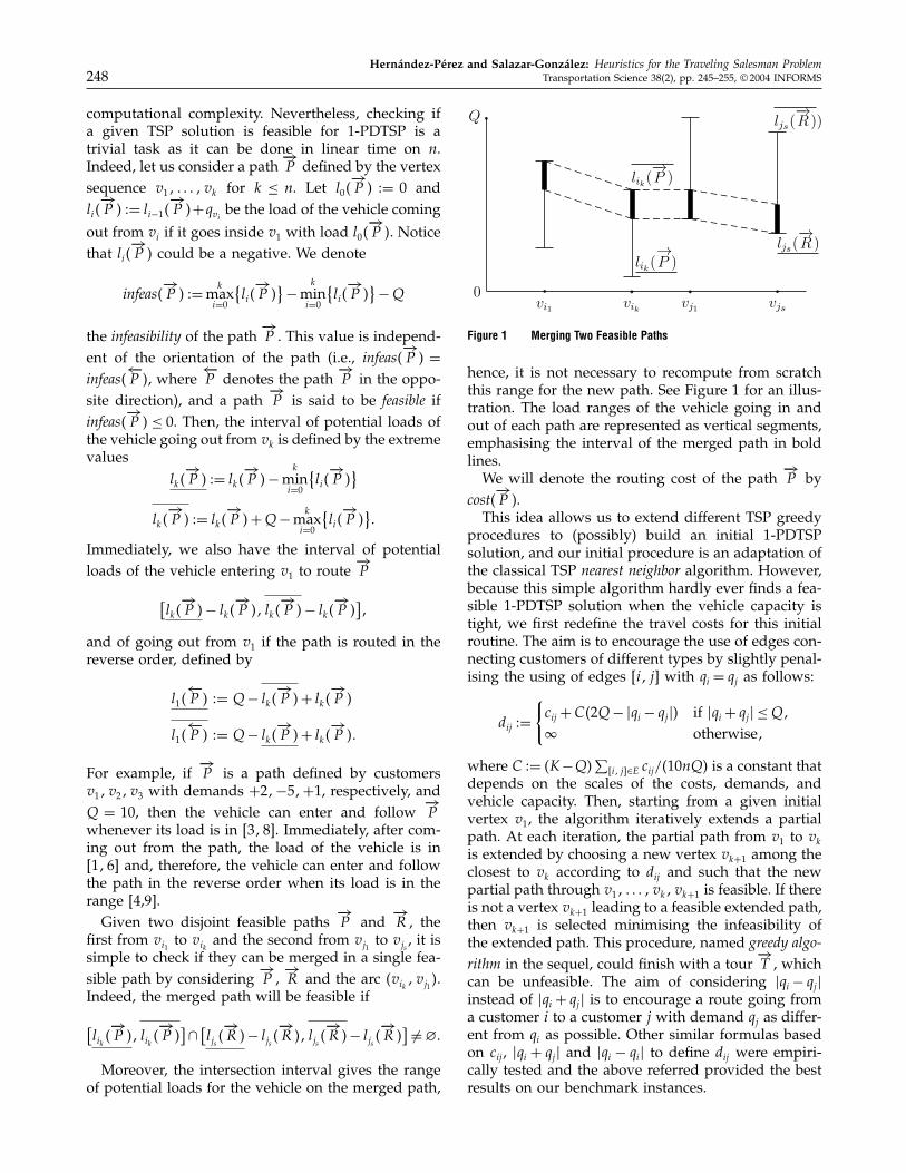
whenever its load is in �3�8�. Immediately, after com-ing out from the path, the load of the vehicle is in�1�6� and, therefore, the vehicle can enter and followthe path in the reverse order when its load is in therange [4,9].Given two disjoint feasible paths

−→P and

−→R , the

first from vi1 to vik and the second from vj1 to vjs , it issimple to check if they can be merged in a single fea-sible path by considering

−→P ,

−→R and the arc �vik � vj1�.

Indeed, the merged path will be feasible if

[lik �

−→P �� lik �

−→P �

]∩ [ljs �

−→R �− ljs �

−→R �� ljs �

−→R �− ljs �

−→R �

] �= �

Moreover, the intersection interval gives the rangeof potential loads for the vehicle on the merged path,

vi1 vik vj1 vjs

0

Q

lik(P )

lik(−→P )

ljs(−→R )

ljs(−→R ))

→

Figure 1 Merging Two Feasible Paths

hence, it is not necessary to recompute from scratchthis range for the new path. See Figure 1 for an illus-tration. The load ranges of the vehicle going in andout of each path are represented as vertical segments,emphasising the interval of the merged path in boldlines.We will denote the routing cost of the path

−→P by

cost(−→P ).

This idea allows us to extend different TSP greedyprocedures to (possibly) build an initial 1-PDTSPsolution, and our initial procedure is an adaptation ofthe classical TSP nearest neighbor algorithm. However,because this simple algorithm hardly ever finds a fea-sible 1-PDTSP solution when the vehicle capacity istight, we first redefine the travel costs for this initialroutine. The aim is to encourage the use of edges con-necting customers of different types by slightly penal-ising the using of edges �i� j� with qi = qj as follows:

dij ={cij +C�2Q− �qi − qj �� if �qi + qj � ≤Q�

otherwise�

where C = �K−Q�∑

�i� j�∈E cij/�10nQ� is a constant thatdepends on the scales of the costs, demands, andvehicle capacity. Then, starting from a given initialvertex v1, the algorithm iteratively extends a partialpath. At each iteration, the partial path from v1 to vkis extended by choosing a new vertex vk+1 among theclosest to vk according to dij and such that the newpartial path through v1� � � � � vk�vk+1 is feasible. If thereis not a vertex vk+1 leading to a feasible extended path,then vk+1 is selected minimising the infeasibility ofthe extended path. This procedure, named greedy algo-rithm in the sequel, could finish with a tour

−→T , which

can be unfeasible. The aim of considering �qi − qj �instead of �qi + qj � is to encourage a route going froma customer i to a customer j with demand qj as differ-ent from qi as possible. Other similar formulas basedon cij , �qi + qj � and �qi − qi� to define dij were empiri-cally tested and the above referred provided the bestresults on our benchmark instances.

Hernández-Pérez and Salazar-González: Heuristics for the Traveling Salesman ProblemTransportation Science 38(2), pp. 245–255, © 2004 INFORMS 249

Tour improvement procedures are adaptations ofthe 2-opt and 3-opt exchanges of edges described in Lin(1965) and Johnson and McGeoch (1997) for the TSP.These implementations avoid looking at all possibleexchanges for one that shortens the tour, in the spiritof work of Lin and Kernighan (1973), and are basedon a data structure that quickly identifies allowablecandidates for the exchanges (see also Helsgaun 2000)for a sophisticated variant. In our implementation, foreach vertex i, the data structure stores a list of 15remaining vertices j in order of increasing distance dij ,thus, defining allowable edges �i� j� to be inserted inexchanges.The execution of the proposed approach is repeated

for each initial vertex v1 when n < 100. For largerinstances, to keep the required computational effortsmall, only 100 vertices i with biggest �qi� are consid-ered as initial vertices v1. Therefore, this heuristic canbe seen as a multistart approach. In our experiments,we have observed that the loss of quality involvedin using truncated neighbor lists is not a major issuein practice, as also noticed in Johnson and McGeoch(1997). A pseudocode describing the overall proce-dure is next given.Step 1. Let N0 be the set of initial vertices in the

multistart procedure.Step 2. Select v1 ∈ N0, apply the greedy algorithm

starting from v1 and let−→T be the output.

Step 3. If−→T is feasible 1-PDTSP solution, set

−→T ∗ =−→

T and go to Step 4; otherwise, set−→T ′ = T and go to

Step 5.Step 4. Apply 2-opt procedure and 3-opt procedure to−→

T ∗, obtaining a new tour−→T minimising infeas�

−→T �,

subject to infeas�−→T � < 2K/n and cost�

−→T �≤ cost�

−→T ∗�. If

no−→T is found, go to Step 6; otherwise, go to Step 3.

Step 5. Apply 2-opt procedure and 3-opt procedure over−→T ′, obtaining a new tour

−→T minimising infeas�

−→T �, sub-

ject to infeas�−→T � < infeas�

−→T ′� and cost�

−→T �≤ cost�

−→T ∗�. If

no−→T is found, go to Step 6; otherwise, go to Step 3.

Step 6. If−→T ∗ improves the current best tour

−→T 1,

update−→T 1. Set N0 =N0\v1�. If N0 �= , go to Step 1;

otherwise, stop with the output−→T 1.

3. Incomplete Optimisation Algorithmfor 1-PDTSP

The branch-and-cut algorithm proposed inHernández-Pérez and Salazar-González (2004) wasable to solve to optimality instances with up to 40vertices. When trying to solve bigger instances, thesame approach is not expected to finish within areasonable computing time. Nevertheless, as pro-posed in Fischetti and Lodi (2002) for solving generalmixed integer linear programming (ILP) models, one

could use an available exact procedure to find thebest solution in a restricted feasible region within aniterative framework.Given two integer numbers h and k, let us assume

that a 1-PDTSP tour T h is known, and let �xhe e ∈ E� beits incident vector and Eh the edges in T h. We definek-neighborhood of T h the set � �T h� k� of all 1-PDTSPsolutions that differ from T h in no more than k edges.In other words, � �T h� k� is the set of the solutions ofthe ILP model plus the additional constraint∑

e∈Eh�1− xe�≤ k� (1)

Note that � �T h�0� = � �T h�1� = T h�, and � =� �T h�n� is the set of all feasible 1-PDTSP tours. One isthen interested in developing a procedure to find thebest solution in � �T h� k� for some k. The first heuristicdescribed in §2 contains an improvement procedurethat iteratively finds a good solution T h+1 exploring(partially) � �T h� k� for k = 3. The initial tour T 1 isprovided by the heuristic procedure described in §2.Clearly, the direct extension of this improvement pro-cedure to deal with some k > 3 could find better solu-tions, but it could require too much computationaleffort. Still, by modifying the branch-and-cut code inHernández-Pérez and Salazar-González (2004) to takeinto account constraint (1), one could expect to suc-ceed exploring � �T h� k� for some 3< k< n.Let us denote T h, the tour obtained with the h-th

call to the branch-and-cut algorithm. As noted byFischetti and Lodi (2002), the neighborhoods � �T h� k�for all T h are not necessarily disjoint subsets of �.Nevertheless, it is quite straightforward to also mod-ify the branch and cut to avoid searching in alreadyexplored regions. To this end, the branch-and-cutalgorithm at iteration h can be modified to take intoaccount the original ILP model, constraint (1), and theadditional inequalities∑

e∈El�1− xe�≥ k+ 1 (2)

for all l= 1� � � � � h− 1. Then, at iteration h, it exploresa totally different region, defined by � �T h� k�\⋃h−1

l=1� �T l� k�. The last iteration is the one where nonew solution was found.Fischetti and Lodi (2002) also noticed that by explo-

ring the remaining feasible 1-PDTSP region (i.e.,�\⋃h

l=1� �T l� k� if iteration h is the last iteration),the procedure would be an exact method. Becausethe remaining region tends to create a difficult prob-lem for a branch-and-cut algorithm on medium-largeinstances and because we are only interested in goodsolutions in short time, our approach does not executethis additional exploration.Solving each iteration could be, in some cases, a

difficult task in practice, hence, Fischetti and Lodi

Hernández-Pérez and Salazar-González: Heuristics for the Traveling Salesman Problem250 Transportation Science 38(2), pp. 245–255, © 2004 INFORMS

(2002) suggest the imposition of a time limit on eachbranch-and-cut execution and the modification of thevalue of k when it is achieved. In our implementa-tion, we found better results by reducing the numberof variables given to the branch-and-cut solver. Moreprecisely, instead of starting each branch-and-cut exe-cution with all possible variables, we only allow thefractional solutions to use variables associated withthe subset E ′ of promising edges. Subset E ′ is ini-tialised with the 10 shortest edges �i� j�, accordingto the distance dij described in §2, for each vertex i.In our experiments, we did not find advantages inenlarging E ′ even with the new edges in Eh of thecurrent solution. In this way, the branch-and-cut exe-cution of iteration h will not explore � �T h� k�.Also, to avoid heavy branch-and-cut executions, we

impose a limit of, at most, six node-deep levels whengoing down in the decision tree exploration. This ideauses the fact that the applied branch-and-cut algo-rithm, as mentioned in Hernández-Pérez and Salazar-González (2004), tends to explore a large number ofnodes, each one in a short time, hence, the idea triesto diversify the fractional solutions feeding the primalheuristic described in the next paragraph. Wheneverthe branch-and-cut execution at iteration h ends witha tour T h+1 better than T h, the next iteration is per-formed.An element of primary importance for this more

elaborated heuristic is the primal heuristic appliedinside the branch-and-cut algorithm. It is a proce-dure to find a feasible 1-PDTSP solution by usingthe information in the last fractional solution, and itis executed every six iterations of the cutting planeapproach and before every branching phase of thebranch-and-cut procedure. To implement it, we haveslightly modified the heuristic described in §2 to con-sider a given fractional solution �x∗

e e ∈ E ′�, whereE ′ is the set of edges with a variable in the model.More precisely, the new procedure to build an initial1-PDTSP solution chooses edges from E∗ = e ∈ E ′x∗e > 0� to be inserted in a partial tour T . The par-tial tour T is initialised with n degenerated pathsof G, each one Pi consisting in only one vertex vi.The edges are chosen from E∗ in decreasing orderof x∗

e whenever they merge two paths into a feasible1-PDTSP one. If E∗ is empty before T is a Hamil-tonian tour, then the initial greedy procedure of §2continues. The final tour is improved by running the2-opt and 3-opt procedures. Observe that the gener-ated solution could also contain edges from E\E ′, andeven so, it could not satisfy constraint (1). Therefore,the tour T h+1 obtained at iteration h (not the last) fromthe tour T h is not necessarily in � �T h� k�, and wehave even observed in our experiments that, in somecases, � �T h� k�∩� �T h+1� k�= . This last observation

suggests that considering constraint (2) in our branch-and-cut executions is not so relevant for our heuristicaims.To further speed the execution of the branch-and-

cut solver, one could replace (1) by 4 ≤∑e∈Eh�1− xe�

≤ k, since the primal heuristic procedure almost guar-antees that T h is the best tour in � �T h�3�. When kis a small number (as in our implementation, wherek= 5), we have also experimented with the replace-ment of each branch-and-cut execution with theprevious constraint by a sequence of branch-and-cutexecutions, each one with the equality

∑e∈Eh�1 − xe�

= l, for each l= 4�5� � � � � k, going to the next iterationas soon as a better tour T h+1 is found. We did notfind in our experiments any clear advantage in imple-menting these ideas, hence, each iteration consists ofone branch-and-cut execution solving ILP model withthe additional constraint (2).

4. Computational ResultsThe heuristic algorithms described in §§2 and 3 havebeen implemented in ANSI C, and ran on a personalcomputer AMD 1,333 MHz. under Windows 98. Thesoftware CPLEX 7.0 was the linear programming (LP)solver in our branch-and-cut algorithm.We tested the performance of the approaches both

on the 1-PDTSP and on the TSPPD using the randomgenerator proposed in Mosheiov (1994) as follows.We have generated n− 1 random pairs in the square�−500�500�× �−500�500�, each one corresponding tothe location of a customer and associated with a ran-dom demand in �−10�10�. The depot was located in(0,0) with demand q1 = −∑n

i=2 qi. The travel cost cijwas computed as the Euclidean distance between iand j . We generated 10 random instances for eachvalue of n in 20�30� � � � �60�100�200� � � � �500� and foreach different value of Q in 10�15� � � � �45�1�000�.The solution of the 1-PDTSP instances with Q= 1�000coincided with the optimal TSP tour in all the gen-erated instances. The case Q = 10 was the smallestcapacity because for each n, there is a customer in aninstance with demand ±10. Also, for each value ofn, 10 TSPPD instances were generated, each one withthe smallest possible capacity

Q=max{ ∑

qi>0 i∈V \1�qi� −

∑qi<0 i∈V \1�

qi

}�

Table 2 shows the results for the small instances(n≤ 60) and Table 3 shows the results of the medium-large instances (100 ≤ n ≤ 500). To evaluate the qual-ity of the generated feasible solutions, we have usedthe exact algorithm described in Hernández-Pérezand Salazar-González (2004) to compute the opti-mal value LB of the LP relaxation of the integerprogramming model for all instances, the optimal

Hernández-Pérez and Salazar-González: Heuristics for the Traveling Salesman ProblemTransportation Science 38(2), pp. 245–255, © 2004 INFORMS 251

Table 2 Statistics on Small Instances of the 1-PDTSP and TSPPD

n Q UB1/OPT UB1/LB UB1-t UB2/OPT UB2/LB UB2-t B&C

20 PDTSP 100.00 100.83 0.02 100.00 100.83 0.08 1.020 10 100.16 101.46 0.04 100.00 101.30 0.19 1.120 15 100.02 100.05 0.01 100.00 100.03 0.10 1.120 20 100.00 100.16 0.00 100.00 100.16 0.05 1.020 25 100.00 100.13 0.00 100.00 100.13 0.06 1.020 30 100.00 100.33 0.00 100.00 100.33 0.05 1.020 35 100.00 100.21 0.00 100.00 100.21 0.05 1.020 40 100.00 100.21 0.00 100.00 100.21 0.05 1.020 45 100.00 100.21 0.00 100.00 100.21 0.04 1.020 1 000 100.03 100.24 0.00 100.00 100.21 0.04 1.1

30 PDTSP 100.20 100.88 0.01 100.00 100.68 0.10 1.130 10 100.26 101.95 0.09 100.02 101.71 0.61 1.330 15 100.19 101.19 0.05 100.08 101.07 0.38 1.130 20 100.01 100.63 0.03 100.00 100.62 0.28 1.130 25 100.03 100.42 0.03 100.00 100.39 0.18 1.130 30 100.00 100.56 0.01 100.00 100.56 0.09 1.030 35 100.00 100.63 0.01 100.00 100.63 0.07 1.030 40 100.00 100.47 0.01 100.00 100.47 0.06 1.030 45 100.00 100.55 0.00 100.00 100.55 0.07 1.030 1 000 100.00 100.48 0.00 100.00 100.48 0.06 1.0

40 PDTSP 100.00 101.15 0.06 100.00 101.15 0.24 1.040 10 100.61 103.79 0.26 100.10 103.26 2.21 1.740 15 100.75 101.93 0.12 100.40 101.57 1.41 1.640 20 100.08 101.00 0.07 100.01 100.93 0.45 1.140 25 100.00 100.49 0.04 100.00 100.49 0.17 1.040 30 100.05 100.51 0.02 100.02 100.48 0.15 1.240 35 100.13 100.83 0.02 100.00 100.71 0.15 1.440 40 100.07 100.73 0.01 100.00 100.66 0.12 1.340 45 100.10 100.76 0.00 100.00 100.66 0.13 1.440 1 000 100.10 100.79 0.01 100.00 100.70 0.14 1.4

50 PDTSP 100.11 101.75 0.07 100.00 101.64 0.41 1.150 10 101.40 104.61 0.51 100.70 103.89 6.60 2.750 15 100.77 102.84 0.35 100.38 102.43 3.46 1.750 20 100.24 102.28 0.21 100.11 102.14 1.81 1.450 25 100.38 101.79 0.13 100.00 101.41 1.24 1.550 30 100.06 100.89 0.09 100.03 100.87 0.58 1.250 35 100.05 101.09 0.07 100.03 101.08 0.49 1.150 40 100.14 101.24 0.05 100.04 101.13 0.43 1.250 45 100.05 101.12 0.05 100.00 101.07 0.39 1.350 1 000 100.04 101.02 0.03 100.00 100.99 0.23 1.2

60 PDTSP 100.28 101.79 0.14 100.00 101.52 1.06 1.960 10 101.90 105.48 1.04 101.20 104.75 8.18 2.260 15 101.14 103.49 0.46 100.55 102.88 8.05 2.460 20 100.53 102.20 0.30 100.35 102.01 3.34 1.760 25 100.45 102.07 0.19 100.02 101.63 1.83 1.960 30 100.26 101.55 0.15 100.04 101.33 1.09 1.860 35 100.21 101.50 0.12 100.05 101.35 0.70 1.360 40 100.16 101.25 0.07 100.00 101.09 0.56 1.560 45 100.14 101.25 0.06 100.02 101.14 0.46 1.360 1 000 100.27 101.65 0.06 100.02 101.40 0.45 1.6

integer solution value OPT for the small instances,and the optimal value TSP of the TSP instance forthe medium-large instances. The reason for comput-ing the value TSP for large instances is to showhow it relates to LB on our benchmark instances.The use of value TSP as lower bound is done inGendreau et al. (1999) and, therefore, we also includeit in our tables to facilitate comparison. Moreover, the

relation between TSP and OPT also gives an idea ofthe added difficulty of solving a 1-PDTSP with respectto a TSP. The column headings have the followingmeanings:n: is the number of vertices;Q: is the capacity of the vehicle. Word “TSPPD”

means that it is a TSPPD instance with the tightestcapacity;

Hernández-Pérez and Salazar-González: Heuristics for the Traveling Salesman Problem252 Transportation Science 38(2), pp. 245–255, © 2004 INFORMS

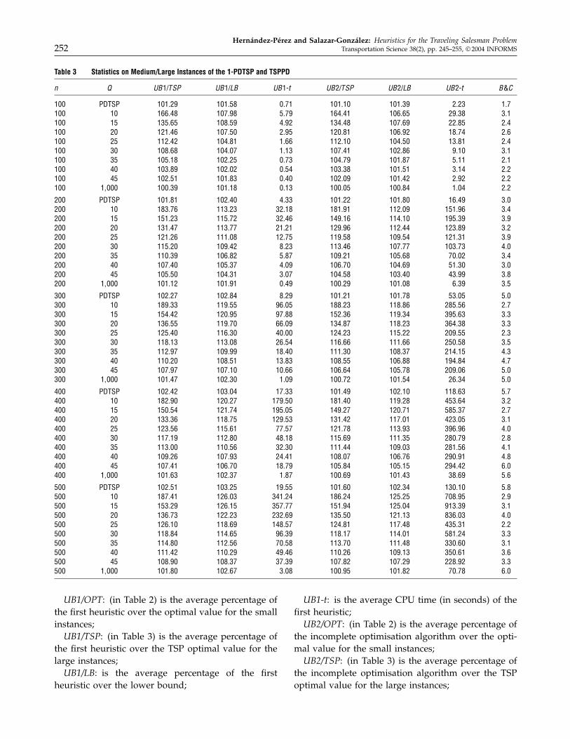
Table 3 Statistics on Medium/Large Instances of the 1-PDTSP and TSPPD

n Q UB1/TSP UB1/LB UB1-t UB2/TSP UB2/LB UB2-t B&C

100 PDTSP 101.29 101.58 0�71 101.10 101.39 2�23 1.7100 10 166.48 107.98 5�79 164.41 106.65 29�38 3.1100 15 135.65 108.59 4�92 134.48 107.69 22�85 2.4100 20 121.46 107.50 2�95 120.81 106.92 18�74 2.6100 25 112.42 104.81 1�66 112.10 104.50 13�81 2.4100 30 108.68 104.07 1�13 107.41 102.86 9�10 3.1100 35 105.18 102.25 0�73 104.79 101.87 5�11 2.1100 40 103.89 102.02 0�54 103.38 101.51 3�14 2.2100 45 102.51 101.83 0�40 102.09 101.42 2�92 2.2100 1 000 100.39 101.18 0�13 100.05 100.84 1�04 2.2

200 PDTSP 101.81 102.40 4�33 101.22 101.80 16�49 3.0200 10 183.76 113.23 32�18 181.91 112.09 151�96 3.4200 15 151.23 115.72 32�46 149.16 114.10 195�39 3.9200 20 131.47 113.77 21�21 129.96 112.44 123�89 3.2200 25 121.26 111.08 12�75 119.58 109.54 121�31 3.9200 30 115.20 109.42 8�23 113.46 107.77 103�73 4.0200 35 110.39 106.82 5�87 109.21 105.68 70�02 3.4200 40 107.40 105.37 4�09 106.70 104.69 51�30 3.0200 45 105.50 104.31 3�07 104.58 103.40 43�99 3.8200 1 000 101.12 101.91 0�49 100.29 101.08 6�39 3.5

300 PDTSP 102.27 102.84 8�29 101.21 101.78 53�05 5.0300 10 189.33 119.55 96�05 188.23 118.86 285�56 2.7300 15 154.42 120.95 97�88 152.36 119.34 395�63 3.3300 20 136.55 119.70 66�09 134.87 118.23 364�38 3.3300 25 125.40 116.30 40�00 124.23 115.22 209�55 2.3300 30 118.13 113.08 26�54 116.66 111.66 250�58 3.5300 35 112.97 109.99 18�40 111.30 108.37 214�15 4.3300 40 110.20 108.51 13�83 108.55 106.88 194�84 4.7300 45 107.97 107.10 10�66 106.64 105.78 209�06 5.0300 1 000 101.47 102.30 1�09 100.72 101.54 26�34 5.0

400 PDTSP 102.42 103.04 17�33 101.49 102.10 118�63 5.7400 10 182.90 120.27 179�50 181.40 119.28 453�64 3.2400 15 150.54 121.74 195�05 149.27 120.71 585�37 2.7400 20 133.36 118.75 129�53 131.42 117.01 423�05 3.1400 25 123.56 115.61 77�57 121.78 113.93 396�96 4.0400 30 117.19 112.80 48�18 115.69 111.35 280�79 2.8400 35 113.00 110.56 32�30 111.44 109.03 281�56 4.1400 40 109.26 107.93 24�41 108.07 106.76 290�91 4.8400 45 107.41 106.70 18�79 105.84 105.15 294�42 6.0400 1 000 101.63 102.37 1�87 100.69 101.43 38�69 5.6

500 PDTSP 102.51 103.25 19�55 101.60 102.34 130�10 5.8500 10 187.41 126.03 341�24 186.24 125.25 708�95 2.9500 15 153.29 126.15 357�77 151.94 125.04 913�39 3.1500 20 136.73 122.23 232�69 135.50 121.13 836�03 4.0500 25 126.10 118.69 148�57 124.81 117.48 435�31 2.2500 30 118.84 114.65 96�39 118.17 114.01 581�24 3.3500 35 114.80 112.56 70�58 113.70 111.48 330�60 3.1500 40 111.42 110.29 49�46 110.26 109.13 350�61 3.6500 45 108.90 108.37 37�39 107.82 107.29 228�92 3.3500 1 000 101.80 102.67 3�08 100.95 101.82 70�78 6.0

UB1/OPT: (in Table 2) is the average percentage ofthe first heuristic over the optimal value for the smallinstances;UB1/TSP: (in Table 3) is the average percentage of

the first heuristic over the TSP optimal value for thelarge instances;UB1/LB: is the average percentage of the first

heuristic over the lower bound;

UB1-t: is the average CPU time (in seconds) of thefirst heuristic;UB2/OPT: (in Table 2) is the average percentage of

the incomplete optimisation algorithm over the opti-mal value for the small instances;UB2/TSP: (in Table 3) is the average percentage of

the incomplete optimisation algorithm over the TSPoptimal value for the large instances;

Hernández-Pérez and Salazar-González: Heuristics for the Traveling Salesman ProblemTransportation Science 38(2), pp. 245–255, © 2004 INFORMS 253

UB2/LB: is the average percentage of the incom-plete optimisation algorithm over the lower bound;UB2-t: is the average CPU time (in seconds) of

the incomplete optimisation algorithm (including thetime of the first heuristic);B&C: is the average number of calls to the branch-

and-cut approach in the incomplete optimisationalgorithm.From Table 2, the basic heuristic described in §2

has a gap under 2% even on the hardest instances(i.e., Q = 10), and the computational effort was typi-cally smaller than 1 second. Moreover, the worst aver-age gap for the incomplete optimisation algorithm is1% over the optimum, and the average time is under1 minute. In general, the worst cases occur whenthe number of customers increase and the capacitydecreases. If the capacity is large enough (i.e., Q =1�000), the 1-PDTSP instances coincide with the TSPand the objective values computed by both heuris-tics are very close to the optimal TSP value. A similarbehavior is observed for the TSPPD instances wherethe worst gap is 0.28% for the first heuristic algorithm,while the incomplete optimisation algorithm alwaysfound an optimal TSPPD solution.When solving larger instances, it is not possible to

compute the exact gap between the heuristic and theoptimal value. From the instances where the optimumvalue has been calculated, one can conclude that UB2and UB1 are nearer the optimum value OPT thanthe LB. The improvement of the incomplete optimi-sation algorithm over the first heuristic is about 1%on these instances. Both approximation proceduresdo not exceed 25% of the LB. The average computa-tional time of the incomplete optimisation algorithmis close to 15 minutes for the hardest instances, whichis a reasonable time for this type of routing problem.Again, as in Table 2, the problem is more difficultwhen Q decrease and when n increase, as expected.In all cases, the TSPPD instances are more difficult forthe approaches than the TSP instances with the samevalue n, but they are much easier than the 1-PDTSPinstances.The quality of the first heuristic is worse when

the 2-opt and the 3-opt procedures are deactivated.Indeed, the heuristic costs in respect to LB arebetween 105% and 120% in the small instances andbetween 120% and 190% in the medium-large inst-ances, thus, proving that the first heuristic algorithmwithin only the multistart greedy scheme would guar-antee worse results. The greedy algorithm takes about1% of the total CPU time consumed by the firstheuristic approach, i.e., most of the effort is dedicatedto the 2-opt and 3-opt procedures.The number of calls to the branch-and-cut algo-

rithm in the incomplete optimisation algorithm wasvery small when n≤ 60, typically being 1 or 2. Hence,

0 60 120 180 240 300

Branch-and-Cut calls

13,700

13,800

13,900

14,000

14,100

0 1 2 3 4 5 6

Figure 2 Cost Value vs. Computational Time (Seconds) when Solvingan Instance

this means that the solution found by the initialheuristics tends to be also optimal of the definedneighborhood. Nevertheless, when 100≤ n≤ 500, thebranch-and-cut code runs about four times, thus,improving the original solution with some additionaleffort. We have run the code using constraints (1)–(2)with different values of k, and value 5 seemed to pro-vide the best compromise between solution qualityand computational effort on our benchmark instances.Also, the choice of fixing to zero some xe variables(i.e., the set definition of the set E ′ described in §3)produced the best results after experimenting withdifferent options.To illustrate the performance of the incomplete

optimisation algorithm, Figure 2 shows the cost of thegenerated feasible solutions when solving a 1-PDTSPinstance with n = 200 and Q = 15. Each black dotrepresents a solution improving a previous one. Thevertical axis represents the solution cost and the hor-izontal axis the time when the solution was found.Each vertical dashed line separates consecutive itera-tions. Iteration 0 is the initial heuristic, where incum-bent tour T ∗ was improved three times; only the besttour is plotted in the figure. The other iterations repre-sent branch-and-cut executions, and iteration 6 is thelast one where the last tour T 6 was not improved. Itis observed that the use of the branch-and-cut codeon the limited 1-PDTSP region defined by edges inE ′ and constraints (1)–(2) allows the incomplete opti-misation algorithm to escape from local optimumin an effective way, mainly in the initial iterations.Figure 3 shows a table with more details of the best

h 0 1 2 3 4 5

cost value 14�125 13�915 13�861 13�839 13�807 13�780time 3�5 30�4 67�2 93�3 123�9 151�4�Eh+1 \E ′ � 0 2 1 3 3 4�Eh+1 \Eh� — 19 13 6 12 5

Figure 3 Details of T h+1 Found at Iteration h when Solving an Instance

Hernández-Pérez and Salazar-González: Heuristics for the Traveling Salesman Problem254 Transportation Science 38(2), pp. 245–255, © 2004 INFORMS

tour found T h+1 at iteration h for each h= 0�1� � � � �5.In particular, it shows the cost value of T h+1, the timein seconds where it was found during iteration h, thenumber �Eh+1\E ′� of edges in T h+1 not in E ′ (the set ofedges associated with variables given to the branch-and-cut solver), and the number �Eh+1\Eh� of edges inT h+1 not in T h. From the table, one observes that theprimal heuristic can generate a new tour T h+1 usingedges even outside E ′.We have generated 1,000 instances, from which 100

are TSPPD instances and 100 are TSP instances. Notone of the remaining 800 1-PDTSP instances resultedin being infeasible, because both our heuristic algo-rithms found feasible solutions, even when Q = 10.Moreover, we also imposed a time limit of 1,800seconds to the overall execution of the incompleteoptimisation algorithm, but this limit was neverachieved, and no average time was bigger than 1,000seconds.Finally, to test the performance of our heuristic

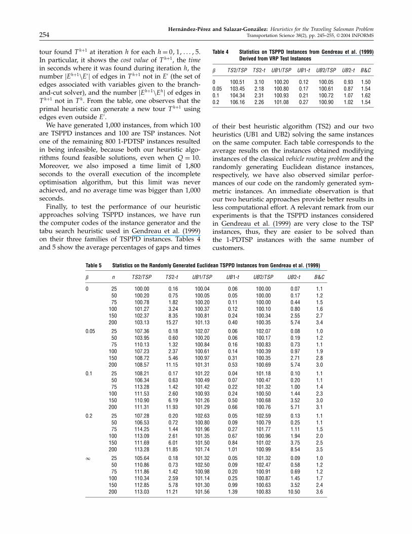
approaches solving TSPPD instances, we have runthe computer codes of the instance generator and thetabu search heuristic used in Gendreau et al. (1999)on their three families of TSPPD instances. Tables 4and 5 show the average percentages of gaps and times

Table 5 Statistics on the Randomly Generated Euclidean TSPPD Instances from Gendreau et al. (1999)

� n TS2/TSP TS2-t UB1/TSP UB1-t UB2/TSP UB2-t B&C

0 25 100.00 0�16 100.04 0.06 100.00 0�07 1.150 100.20 0�75 100.05 0.05 100.00 0�17 1.275 100.78 1�82 100.20 0.11 100.00 0�44 1.5

100 101.27 3�24 100.37 0.12 100.10 0�80 1.6150 102.37 8�35 100.81 0.24 100.34 2�55 2.7200 103.13 15�27 101.13 0.40 100.35 5�74 3.4

0.05 25 107.36 0�18 102.07 0.06 102.07 0�08 1.050 103.95 0�60 100.20 0.06 100.17 0�19 1.275 110.13 1�32 100.84 0.16 100.83 0�73 1.1

100 107.23 2�37 100.61 0.14 100.39 0�97 1.9150 108.72 5�46 100.97 0.31 100.35 2�71 2.8200 108.57 11�15 101.31 0.53 100.69 5�74 3.0

0.1 25 108.21 0�17 101.22 0.04 101.18 0�10 1.150 106.34 0�63 100.49 0.07 100.47 0�20 1.175 113.28 1�42 101.42 0.22 101.32 1�00 1.4

100 111.53 2�60 100.93 0.24 100.50 1�44 2.3150 110.90 6�19 101.26 0.50 100.68 3�52 3.0200 111.31 11�93 101.29 0.66 100.76 5�71 3.1

0.2 25 107.28 0�20 102.63 0.05 102.59 0�13 1.150 106.53 0�72 100.80 0.09 100.79 0�25 1.175 114.25 1�44 101.96 0.27 101.77 1�11 1.5

100 113.09 2�61 101.35 0.67 100.96 1�94 2.0150 111.69 6�01 101.50 0.84 101.02 3�75 2.5200 113.28 11�85 101.74 1.01 100.99 8�54 3.5

25 105.64 0�18 101.32 0.05 101.32 0�09 1.050 110.86 0�73 102.50 0.09 102.47 0�58 1.275 111.86 1�42 100.98 0.20 100.91 0�69 1.2

100 110.34 2�59 101.14 0.25 100.87 1�45 1.7150 112.85 5�78 101.30 0.99 100.63 3�52 2.4200 113.03 11�21 101.56 1.39 100.83 10�50 3.6

Table 4 Statistics on TSPPD Instances from Gendreau et al. (1999)Derived from VRP Test Instances

� TS2/TSP TS2-t UB1/TSP UB1-t UB2/TSP UB2-t B&C

0 100.51 3.10 100.20 0.12 100.05 0.93 1.500.05 103.45 2.18 100.80 0.17 100.61 0.87 1.540.1 104.34 2.31 100.93 0.21 100.72 1.07 1.620.2 106.16 2.26 101.08 0.27 100.90 1.02 1.54

of their best heuristic algorithm (TS2) and our twoheuristics (UB1 and UB2) solving the same instanceson the same computer. Each table corresponds to theaverage results on the instances obtained modifyinginstances of the classical vehicle routing problem and therandomly generating Euclidean distance instances,respectively, we have also observed similar perfor-mances of our code on the randomly generated sym-metric instances. An immediate observation is thatour two heuristic approaches provide better results inless computational effort. A relevant remark from ourexperiments is that the TSPPD instances consideredin Gendreau et al. (1999) are very close to the TSPinstances, thus, they are easier to be solved thanthe 1-PDTSP instances with the same number ofcustomers.

Hernández-Pérez and Salazar-González: Heuristics for the Traveling Salesman ProblemTransportation Science 38(2), pp. 245–255, © 2004 INFORMS 255

AcknowledgmentsThis work was partially done while the second author wasat the CRT, University of Montreal, by invitation of GilbertLaporte and supported by the Canada Research Chair inDistribution Management. The authors thank Daniele Vigofor providing them with the instances and the FORTRANcodes used in Gendreau et al. (1999), and they thank threeanonymous referees for their suggestions that improved anearly version of this paper. This work was partially fundedby Gobierno de Canarias (Research Project PI2000/116) andby Ministerio de Ciencia y Tecnología (Research ProjectTIC2000-1750-C06-02), Spain.

ReferencesAnily, S., J. Bramel. 1999. Approximation algorithms for the capaci-

tated traveling salesman problem with pickups and deliveries.Naval Res. Logist. 46 654–670.

Anily, S., R. Hassin. 1992. The swapping problem. Networks 22419–433.

Anily, S., G. Mosheiov. 1994. The traveling salesman problem withdelivery and backhauls. Oper. Res. Lett. 16 11–18.

Anily, S., M. Gendreau, G. Laporte. 1999. The swapping problemon a line. SIAM J. Comput. 29 327–335.

Baldacci, R., A. Mingozzi, E. Hadjiconstantinou. 2003. An exactalgorithm for the traveling salesman problem with mixeddelivery and collection constraints. Networks 42 26–41.

Bianco, L., A. Mingozzi, S. Riccardelli, M. Spadoni. 1994. Exactand heuristic procedures for the traveling salesman problemwith precedence constraints, based on dynamic programming.INFOR 32 19–32.

Chalasani, P., R. Motwani. 1999. Approximating capacitated routingand delivery problems. SIAM J. Comput. 28 2133–2149.

Fischetti, M., A. Lodi. 2003. Local branching. Math. Programming 9823–47.

Frederickson, G. N., M. S. Hecht, C. E. Kim. 1978. Approxima-tion algorithms for some routing problems. SIAM J. Comput. 7178–193.

Garey, M. R., D. S. Johnson. 1979. Computers and Intractability: AGuide to the Theory of ��-Completeness. W. H. Freeman andCompany, San Francisco, CA.

Gendreau, M., A. Hertz, G. Laporte. 1997. An approximation algo-rithm for the traveling salesman problem with backhauls. Oper.Res. 45 639–641.

Gendreau, M., G. Laporte, D. Vigo. 1999. Heuristics for the travelingsalesman problem with pickup and delivery. Comput. Oper. Res.26 699–714.

Guan, D. J. 1998. Routing a vehicle of capacity greater than one.Discrete Appl. Math. 81 41–57.

Healy, P., R. Moll. 1995. A new extension of local search applied tothe dial-a-ride problem. Eur. J. Oper. Res. 83 83–104.

Helsgaun, K. 2000. An effective implementation of the Lin-Kernighan traveling salesman heuristic. Eur. J. Oper. Res. 12106–130.

Hernández-Pérez, H., J. J. Salazar-González. 2004. A branch-and-cut algorithm for the traveling salesman problem with pickupand delivery. Discrete Appl. Math. 144.

Johnson, D. S., L. A. McGeoch. 1997. The traveling salesman prob-lem: A case study in local optimization. E. J. L. Aarts, J. K.Lenstra, eds. Local Search in Combinatorial Optimization. JohnWiley and Sons, Chichester, U.K.

Kalantari, B., A. V. Hill, S. R. Arora. 1985. An algorithm for the trav-eling salesman problem with pickup and delivery customers.Eur. J. Oper. Res. 22 377–386.

Kubo, M., H. Kasugai. 1990. Heuristic algorithms for the singlevehicle dial-a-ride problem. J. Oper. Res. Soc. Japan 33 354–364.

Lin, S. 1965. Computer solutions of the traveling salesman problem.Bell System Tech. J. 44 2245–2269.

Lin, S., B. W. Kernighan. 1973. An effective heuristic algorithm forthe traveling salesman problem. Oper. Res. 21 498–516.

Mosheiov, G. 1994. The travelling salesman problem with pick-upand delivery. Eur. J. Oper. Res. 79 299–310.

Psaraftis, H. 1983. Analysis of an O�n2� heuristic for the single vehi-cle many-to-many Euclidean dial-a-ride problem. Transporta-tion Res. 17 133–145.

Renaud, J., F. F. Boctor, G. Laporte. 2002. Perturbation heuristics forthe pickup and delivery traveling salesman problem. Comput.Oper. Res. 29 1129–1141.

Renaud, J., F. F. Boctor, I. Ouenniche. 2000. A heuristic for thepickup and delivery traveling salesman problem. Comput. Oper.Res. 27 905–916.

Savelsbergh, M. W. P., M. Sol. 1995. The general pickup and deliv-ery problem. Transportation Sci. 29 17–29.