CHAPTER 1

INTRODUCTION

1.1 Historical background

The health insurance is a social intervention that sought to

replace the “cash and carry system” of health care financing

and to increase access to basic quality health care through

the establishment of district-wide insurance schemes in Ghana

(International Labour Organization, 2005).

According to Act 650 (2003) of the national health insurance

law, the National Health Insurance Authority (NHIA) is

authorized to establish the following schemes: District Mutual

Health Insurance Scheme, Private Commercial Health Insurance

Schemes, and Private Mutual Health Insurance Scheme.

Currently, there are 145 district-wide health insurance

schemes operating in Ghana of which Brong Ahafo region has 19

administrative centres of NHIS.

According to Act 650 (2003), the role of the National Health

Insurance Authority (NHIA) is to register, license, and

regulate health insurance schemes and to accredit and monitor

health care providers operating under the schemes. It plays a

1

key role in guiding implementation efforts and management of

the national health insurance fund.

In order to mobilize funds to support implementation of the

district and municipal mutual health insurance schemes, the

government of Ghana instituted a health Levy of 2.5 percent on

specific goods and services made in or imported to Ghana. In

addition, 2.5 percent of the 17.5 percent social security

(known as SSNIT) contributions paid by formal sector employees

are automatically diverted to support the NHIS. Accordingly,

formal sector employees, their dependents, and SSNIT

pensioners are automatically enrolled in their district scheme

and are exempted from premiums. Additionally, grants and any

other voluntary contribution made to the Fund (Act 650, 2003).

1.2 Background of the study

The National Health Insurance Authority (NHIA) is located in

Accra. They have regional offices considered as an extension

of the operational division of NHIA and are to monitor and

evaluate the performance of the administrative centres of NHIS

in each region. Brong Ahafo region has nineteen (19)

administrative centres of NHIS to monitor and evaluate, and

2

report on performance of each scheme to the head office in

Accra.

Despite the fact that electronic means of communication exist

among schemes and the regional office in sunyani, an optimal

vehicular movement for inspection tour is a problem for the

regional authority.

1.3 Statement of the problem

The regional office of NHIA is faced with a problem of how to

carry out a physical inspection tour of district schemes known

as administrative centres of NHIS to obtain information about

their operational challenges particularly in the entry of

health claims unto the nationwide information and

communication technology platform of NHIA. Lack of inspection

and supervision at these administrative centres to ensure that

there was limited number of backlog of claims has necessitated

the regional authority to carry out this physical inspection

tour of district schemes.

The monitoring and evaluation officers were tasked to embark

upon an inspection tour of the administrative centres to check

on this operational difficulty and report to the regional

3

manager. They were required to maintain a desirable level of

movement so as to minimize vehicular fuel consumption.

In this research, we attempt to minimize the vehicular fuel

consumption which will reduce cost of travel by finding the

optimum distance. The preferred route is illustrated below:

Sunyani Municipal (Initial scheme) →Techiman Municipal →

Nkoranza District→ Atebubu→ Sene scheme→ Pru scheme→ Kintampo

North → Tano South → Wenchi District→ Jaman South→ Tain

District→ Jaman South→ Berekum Municipal → Dormaa District→

Asutifi district →Asunafo South →Asunafo North →Kintampo South

→Tano North → Sunyani Municipal.

This preferred route for the inspection tour is without any

mathematical model. The study aims at using a mathematical

model to determine whether the preferred route is optimum or

not.

1.4 Objective of the study

To model the tour of the Brong Ahafo NHIS administrative

centres as Traveling Salesman Problem,

To determine the optimal distance using the Omicron

Genetic Algorithm.

4

1.5 Significance of the study

The timely inspection tour to district schemes will address

concerns on backlog of claims and relatively increase the

number of claims entered unto the nationwide information and

communication technology platform of NHIA. When this is

achieved it becomes easy for the operations division of NHIA

to quickly know the amount to be paid to each health service

provider by the end of each month. This will ensure that NHIA

pay genuine health claims to health service providers and

reduce fraud in payment of claims. Economically, the nation

will save enough money to improve upon the quality of health

delivery in the country and minimize the rate of maternal and

child mortality in the country. It will serve as a point of

reference for health researchers about diseases that were

recorded and treated under the health insurance system in the

country.

This study will create the optimal inspection tour road map

for the regional authority and contribute to the reduction in

atmospheric pollution. This will reduce the rate at which

humans inhale toxic wastes from the vehicle and depletion of

the ozone layer.

5

1.6 Methodology and source of data

The inspection tour will be modeled as Traveling Salesman

Problem (TSP). Omicron Genetic Algorithm (OGA) will be applied

to solve the TSP model to achieve the objective of the

research.

The sunyani Roads and Highways Authority will be contacted for

the data on physical road networks linking the district where

scheme offices are located. Resources available on the

internet and the library will be used to obtain the needed

literature for this research.

After the relevant data on road distance is obtained, a

program code will be written in MATLAB to solve the propose

problem. The minimum system requirement for this program to

run is Microsoft window XP, with 1 GHz processing speed and

hard disk capacity of 20 gigabyte.

1.7 Organization of the study

The thesis is organized into five chapters.

Chapter 1 consists the historical background of the study, the

statement of the problem, the objective of the study,

6

significance of the study, methodology and source of data, and

organization of the study

Chapter 2 consists the literature review

Chapter 3 covers the methodology which consists of models and

methods of solution

Chapter 4 covers the collection of data, analysis and

discussion

Chapter 5 consists the conclusion and recommendation

7

CHAPTER 2

LITERATURE REVIEW

2.1 INTRODUCTION

This chapter presents a brief overview of publications and

related works on the application of Traveling Salesman Problem

(TSP) to problems facing industries. The traveling salesman

problem finds application in a variety of situations such as

location-routing problem, material flow system design, post-

box collection and vehicle routing.

The traveling salesman first gained fame in a book written by

German salesman Voigt in 1832 on how to be a successful

traveling salesman. He mentioned the TSP, although not by that

name, by suggesting that to cover as many locations as

possible without visiting any location twice is the most

important aspect of the scheduling of a tour.

According to Applegate et al. (2007), the origin of the name

“traveling salesman problem” is a bit of a mystery. This

suggests that there is no written documentation pointing to

the originator of the name “traveling salesman problem”.

8

Sur-Kolay et al. (2003) defined TSP as a permutation problem

with the objective of finding the shortest path (or the

minimum cost) on an undirected graph that represents cities to

be visited. The TSP starts at one city, visits all other

cities successively only once and finally returns to the

starting city. That is, given n cities and their permutations,

the objective is to choose pi such that the sum of all

Euclidean distances between each city and its successor is

minimized. This Euclidean distance between any two cities with

coordinate (x1, y1) and (x2, y2) is calculated by,

d=√ (|x1−x2|)2+(|y1−y2|)2

The TSP is a classic problem in optimization which has

attracted much attention of researchers and mathematicians for

several reasons. First, a large number of real-world problems

can be modeled through TSP. Secondly, it was proved to be NP-

Complete (non-deterministic polynomial-time) problem

(Papadimitriou et al., 1997). Thirdly, NP-Complete problems

are intractable in the sense that no one has found any really

efficient way of solving them for large problem size.

9

The TSP is known to be NP-hard (Garey and Johnson, 1979). That

is, when the problem size is large it takes exponential time

to compute and obtain an optimal solution. Over the past

decade, the largest TSP was solved involving 7,397 cities

(Applegate et al., 1994) and this took 3 to 4 years of

computational time. To address this, approximation algorithms

or heuristics and metaheuristics (Glover, 1986) have been

developed to reduce the computational time.

Karp and Held (1971) improved upon an initial 49 cities TSP

solved through the cutting-plane method by Dantzig et al.

(1954) and they set a vital precedence by not only solving two

larger TSP involving 57-city and 64-city instances but also

resolving the Dantzig et al. (1954) 49-city instances.

Crowder and Padberg (1980) presented a remarkable solution

that solved 318-city problems. The 318-city instance remained

as an impressive solution until further development in 1987

where Padberg and Rinaldi (1987) solved 532-city problems.

Grotschel and Holland (1991) extended Dantzig et al. (1954)

ideas which gave solutions to 666-city instances.

Applegate et al. (1990) developed computer program called

Concorde, written in C programming language, which has been 10

used to solve many instances of TSP. Gerhard Reinelt (1994)

published the Traveling Salesman Problem Library (TSPLIB), a

collection of benchmark instances of varying difficulty, which

had been used by many research groups for comparing results

from instances of TSP. Cook et al. (2005) computed an optimal

tour through a 33,810-city instance and 85,900-city instance

given by a microchip layout problem, currently the largest

solved TSPLIB instance. For many other instances with millions

of cities, solutions can be found that are guaranteed to be

within 1% of an optimal tour.

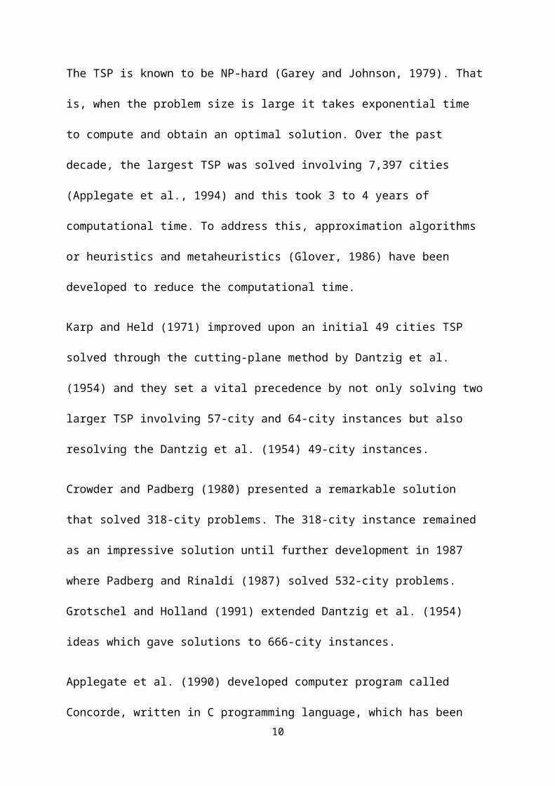
The Table 2.0 below indicates the year, the computer program

used to obtain solutions for TSP instances and the number of

cities that were solved with the Concorde computer program.

Table 2.0 TSP instances and number of cities

Year Computer program

Number of

cities

1992 Concorde 3038 cities

pcb303

8

1993 Concorde 4,461 cities

fnl446

1

1994 Concorde 7,397 cities pla739

11

7

1998 Concorde 13,509 cities

usa135

09

2001 Concorde 15,112 cities d15112

2004 Concorde 24,978 cities

sw2497

8

2004

Concorde with Domino-

Parity 33,810 cities

pla338

10

2006

Concorde with Domino-

Parity 85,900 cities

pla859

00

Since the original aim of TSP formulation is to find the

cheapest and shortest tour, it could be applied in

transportation processes, logistics, manufacturing,

telecommunication, genetics, and neuroscience. A classical TSP

application is automatic drilling of printed circuit boards

and threading of cells in a testable VLSI (Very Large Scale

Integration) circuit (Ravikumar, 1992), and x-ray

crystallography (Bland and Shallcross, 1989).

There are many different variations of the traveling salesman

problem. First we have the bottleneck traveling salesman

12

problem (Reinelt, 1994) is where we want to minimize the

largest edge cost in the tour instead of the total cost. That

is, we want to minimize the maximum distance the salesman

travels between any two adjacent cities.

The time dependent traveling salesman problem (Lawler et. al.,

1986) is the same as the standard traveling salesman problem

except we now have time periods. The cost cijt is the cost of

traveling from node i to node j in time period t.

13

CHAPTER 3

METHODOLOGY

3.1 INTRODUCTION

This chapter presents the models and methods of solution to

the Traveling Salesman Problem through Omicron Genetic

Algorithm (OGA). We will consider other methods such as tabu

search, simulated annealing, genetic algorithm and omicron

genetic algorithm that can be applied to solve TSPs. Some work

examples would be solved.

3.2 Formulation of the TSP model

The initial approach to solving a TSP is to formulate a

mathematical model of the problem. The nature of the

formulation looks at administrative centres of NHIS on a map

as nodes and draws a line to link each node. These lines are

the arc toured by the salesman. The length of a tour is

computed as the sum of lengths of the arcs.

The problem is defined as follows;

Let:

14

i. The total number of nodes on the map is represented as

n.

ii. The length between each node i and node j is represented

as d(i, j).

iii. For each link x(i, j) is 1, if link x(i, j) is part of the

tour else is 0.

iv. The edges v(i,j) = 0, indicates no distance between same

node.

v. The set of arcs of the graph is A.

Model for the problem P is:

P:ΜΙΝΙΜΙΖΕ =∑i,j

nd(i,j )x(i,j ) equation (1)

Subject to:

∑i=1

nx(i,j)=1 for all j=1,2,..,n equation (2)

∑i,j∈A

x(i,j)

≤(n−1) for all (i,j)∈A, equation (4)

x(i,j)∈{0,1} for all i,j=1,2,..,n equation (5)

15

∑j=1

nx(i,j)=1 for all i=1,2,..,n equation (3)

Equation (1) is the objective function which will minimize the

total length.

Equation (2) ensures that each node is visited from only one

other node.

Equation (3) ensures that each node departs to only one other

node.

Equation (4) ensures that each tour has not more that n-1 arcs

in the set of n.

Equation (5) is the integrality constraint which ensures that

the decision variable x is either 0 or 1.

In solving the TSP model, factors such as the condition of

some roads in the region will not be considered.

3.3 TABU SEARCH (TS)

The Tabu Search is a heuristic method proposed by Glover

(1986) to various combinatorial problems. It is one of the

best methods used at finding solutions close to optimality in

large combinatorial problems encountered in many practical

settings.

16

The principle of TS is to find Local Search whenever it

encounters a local optimum by allowing non-improving moves

such that cycling back to previously visited solutions is

prevented by the use of memories, called Tabu Lists also

referred as Tabu moves (Hillier and Lieberman, 2005), that

records the recent history of the search, and this is a key

idea that can be linked to Artificial Intelligence concepts.

Pham and Karaboga (2000) outlined three main approaches when

performing TS. These are as following: Forbidding approach

this strategy control what must be allowed to enter the Tabu

list, Freeing approach this strategy determines what exits in

the Tabu list and when it exists, and Short-term approach this

strategy manages the interplay between the forbidding strategy

and freeing strategy to select trial solutions that exist in

the tabu list.

Tabu (taboo) search has two basic elements that define its

search heuristics, that is, search space and its neighborhood

structure. The search space of a TS heuristic is simply the

space of all possible solutions that can be considered

(visited) during the search. A close link with the definition

of search space is the neighborhood structure. Each iteration

17

that is performed on the TSP, the local transformation that

can be applied to the current solution, defines a set of

neighboring solutions in the search spaces. This search space

can be defined as;

N(S) = {solutions obtained by applying a single local

transformation to S}

Where S denotes current solution and N(S) denotes the

neighborhood of S.

The tabu search algorithm can be summarized into the following

steps:

Step 1: Choose an initial solution, i in S. Set i* = i and k=0.

Step 2: Set k=k+1 and generate a subset G* of solution in N (i,

k) such that either one of the Tabu conditions is violated or

at least one of the aspiration conditions holds.

Step 3: Choose a best j in G* and set i=j.

Step 4: If f(i) < f(i*) then set i* = i.

Step 5: Update Tabu and aspiration conditions.

Step 6: If a stopping condition is met then stop. Else go to

Step 2.18

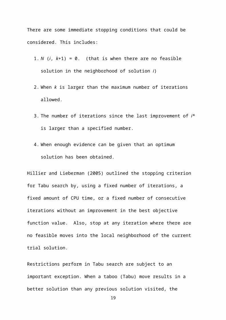
There are some immediate stopping conditions that could be

considered. This includes:

1. N (i, k+1) = 0. (that is when there are no feasible

solution in the neighborhood of solution i)

2. When k is larger than the maximum number of iterations

allowed.

3. The number of iterations since the last improvement of i*

is larger than a specified number.

4. When enough evidence can be given that an optimum

solution has been obtained.

Hillier and Lieberman (2005) outlined the stopping criterion

for Tabu search by, using a fixed number of iterations, a

fixed amount of CPU time, or a fixed number of consecutive

iterations without an improvement in the best objective

function value. Also, stop at any iteration where there are

no feasible moves into the local neighborhood of the current

trial solution.

Restrictions perform in Tabu search are subject to an

important exception. When a taboo (Tabu) move results in a

better solution than any previous solution visited, the 19

previous solution is discarded and its Tabu classification may

be overridden. A condition that allows such an override to

occur is called an aspiration criterion (Glover et al. 1995).

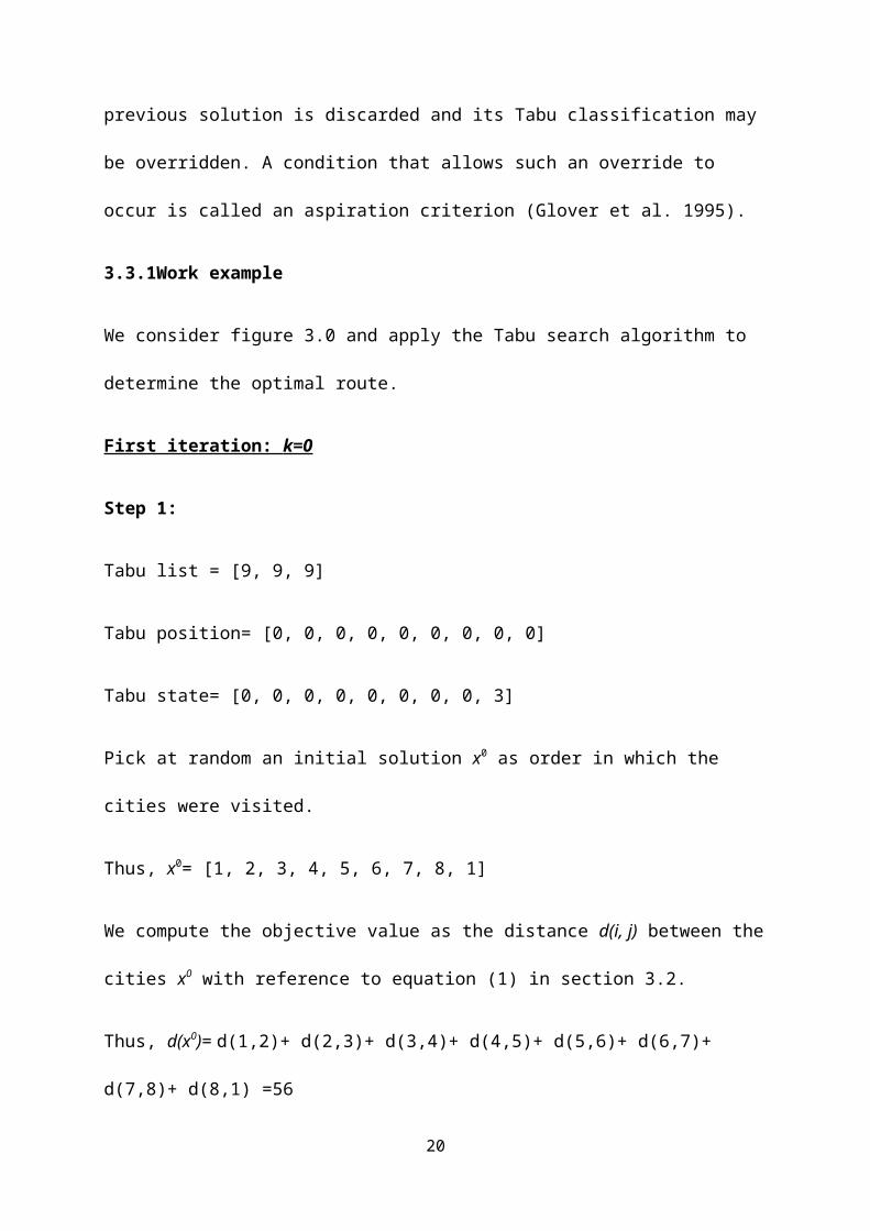
3.3.1Work example

We consider figure 3.0 and apply the Tabu search algorithm to

determine the optimal route.

First iteration: k=0

Step 1:

Tabu list = [9, 9, 9]

Tabu position= [0, 0, 0, 0, 0, 0, 0, 0, 0]

Tabu state= [0, 0, 0, 0, 0, 0, 0, 0, 3]

Pick at random an initial solution x0 as order in which the

cities were visited.

Thus, x0= [1, 2, 3, 4, 5, 6, 7, 8, 1]

We compute the objective value as the distance d(i, j) between the

cities x0 with reference to equation (1) in section 3.2.

Thus, d(x0)= d(1,2)+ d(2,3)+ d(3,4)+ d(4,5)+ d(5,6)+ d(6,7)+

d(7,8)+ d(8,1) =56

20

Save x0 as the best move so far.

Step 2:

The necessary move for x0 are;

move(2, 3)=[1,3,2,4,5,6,7,8,1]

move(3, 4)=[1,2,4,3,5,6,7,8,1]

move(4, 5)=[1,2,3,5,4,6,7,8,1]

move(5, 6)=[1,2,3,4,6,5,7,8,1]

move(6, 7)=[1,2,3,4,5,7,6,8,1]

move(7, 8)=[1,2,3,4,5,6,8,7,1]

We will apply formula (i) to calculate the move value for all the

moves move(i, j) and choose the best (one with minimum value).

Where i and j represents the move value.

Move(i, j)= [d(i-1, j)+d(j, i)+d(i, j+1)] - [d(i-1, i)+d(i, j)+d(j, j+1)]

equation (1)

Move(2, 3) i=2 , j= 3

=[d(2-1, 3)+d(3, 2)+d(2, 3+1)] –[d(2-1, 2)+d(2, 3)+d(3,

3+1)] = 8

Move(3, 4) i=3, j= 421

=[d(3-1,4)+d(4, 3)+d(3, 4+1)] –[d(3-1, 3)+d(3, 4)+d(4,

4+1)] = 1

Move(4, 5) i=4, j= 5

=[d(4-1,5)+d(5, 4)+d(4, 5+1)] –[d(4-1, 4)+d(4, 5)+d(5,

5+1)] = -7

Move(5, 6) i=5, j= 6

=[d(5-1,6)+d(6, 5)+d(5, 6+1)] –[d(5-1, 5)+d(5, 6)+d(6,

6+1)] = -4

Move(6, 7) i=6, j= 7

=[d(6-1,7)+d(7, 6)+d(6, 7+1)] –[d(6-1, 6)+d(6, 7)+d(7,

7+1)] = 11

Move(7, 8) i=7, j= 8

=[d(7-1,8)+d(8, 7)+d(7, 8+1)] –[d(7-1, 7)+d(7, 8)+d(8,

8+1)] = 7

since we are looking for minimum solution the best move value

is move(4,5)=-7

the new solution is obtained by swapping [4, 5]

Step 3:

22

The new solution is x1 = [1, 2, 3, 5, 4, 6, 7, 8, 1]

Objective value x1 =objective x0 +move value (4, 5)

= 56 -7

= 49

(i) We do tabu check on the solution x1 by representing the

solution by an attribute of the move operation [4, 5]

Since city 4 is not in the tabu list there is no restriction.

We update the Tabu list and its attribute.

Tabu list = [4, 9, 9]

Tabu position = [0, 0, 0, 1, 0, 0, 0, 0, 0]

Tabu state = [0, 0, 0, 1, 0, 0, 0, 0, 2]

(ii) Aspiration check is not necessary since the solution

was not Tabu listed

(iii) Check (i) and (ii) are successful hence we keep the new

solution

x1 = [1, 2 ,3 , 5, 4, 6, 7, 8, 1] = 49

Step 4

23

Since objective x1< objective x0, the best solution is 49 with

move (4, 5). Assign x0 x← 1.

x1 has the best current solution and has the best move value

that it is being Tabu listed.

Step 5

The loop condition is the stated number of iterations that do

not bring any improved solution. After such number of

iteration we go to step 6 to restart the Tabu search with a

new solution.

Step 6

This step may not be necessary since the improved solution has

been obtained.

Second iteration: k=1

Step 2:

The new solution x0 = [1, 2, 3, 5, 4, 6, 7, 8, 1]

The necessary move for x0 are;

move(2, 3)= [1, 3 ,2 , 4, 5, 6, 7, 8, 1]

move(3, 5)= [1, 2 ,5 , 3, 4, 6, 7, 8, 1]

24

move(5, 4)= [1, 2 ,3 , 4, 5, 6, 7, 8, 1]

move(4, 6)= [1, 2 ,3 , 5, 6, 4, 7, 8, 1]

move(6, 7)= [1, 2 ,3 , 5, 4, 7, 6, 8, 1]

move(7, 8)= [1, 2 ,3 , 5, 4, 6, 8, 7, 1]

we will calculate the move value and choose the best move

Move(2, 3) i=2 , j= 3

=[d(2-1, 3)+d(3, 2)+d(2, 3+1)] –[d(2-1, 2)+d(2, 3)+d(3,

3+1)] = 8

Move(3, 5) i=3, j= 5

=[d(3-1,5)+d(5, 3)+d(3, 5+1)] –[d(3-1, 3)+d(3, 5)+d(5,

4+1)] = 7

Move(5, 4) i=5, j= 4

=[d(5-1,4)+d(4, 5)+d(5, 4+1)] –[d(5-1, 5)+d(5, 4)+d(4,

4+1)] = -12

Move(4, 6) i=4, j= 6

=[d(4-1,6)+d(6, 4)+d(4, 6+1)] –[d(4-1, 4)+d(4, 6)+d(6,

6+1)] = -5

Move(6, 7) i=6, j= 725

=[d(6-1,7)+d(7, 6)+d(6, 7+1)] –[d(6-1, 6)+d(6, 7)+d(7,

7+1)] = 11

Move(7, 8) i=7, j= 8

=[d(7-1,8)+d(8, 7)+d(7, 8+1)] –[d(7-1, 7)+d(7, 8)+d(8,

8+1)] = 7

since we are looking for minimum solution the best move value

is move (5,4)=-12

the new solution is obtained by swapping [5, 4]

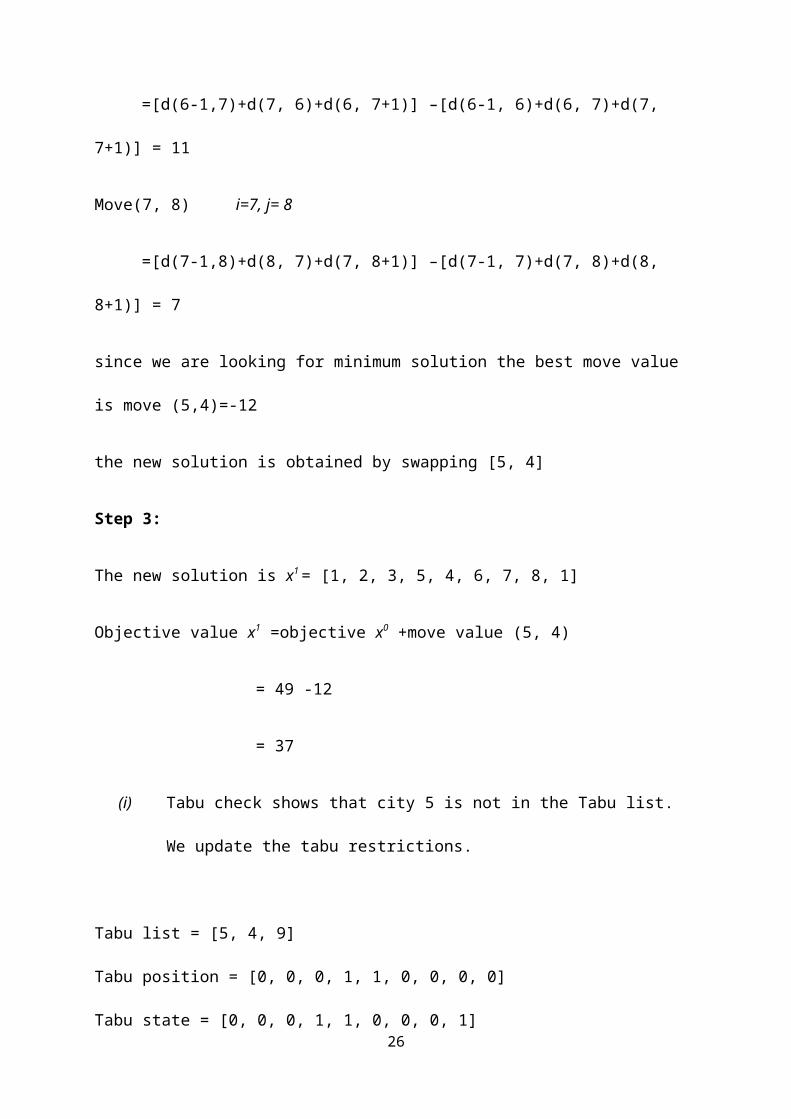
Step 3:

The new solution is x1 = [1, 2, 3, 5, 4, 6, 7, 8, 1]

Objective value x1 =objective x0 +move value (5, 4)

= 49 -12

= 37

(i) Tabu check shows that city 5 is not in the Tabu list.

We update the tabu restrictions.

Tabu list = [5, 4, 9]

Tabu position = [0, 0, 0, 1, 1, 0, 0, 0, 0]

Tabu state = [0, 0, 0, 1, 1, 0, 0, 0, 1]26

(ii) Aspiration check is not necessary

(iii) Check (i) and(ii) are successful hence we keep the new

solution

x1 = [1, 2, 3, 5, 4, 6, 7, 8, 1]

Step 4:

Since objective x1< objective x0, the best solution is 37 with

move (5, 4). Assign x0 x← 1.

x1 has the best current solution and has the best move value

that it is being Tabu listed.

Step 5

The loop condition is the stated number of iterations that do

not bring any improved solution. After such number of

iteration we go to step 6 to restart the Tabu search with a

new solution.

Step 6

This step may not be necessary since the improved solution has

been obtained.

The Tabu search continues until the optimal solution is

obtained.

27

3.4 SIMULATED ANNEALING (SA)

Simulated Annealing (SA) is a probabilistic metaheuristics

method proposed by Kirkpatrick, Gelett and Vecchi (1983) and

Cerny (1985) for locating a good approximation to a global

optimum of a given cost function in a discrete search space.

Simulated annealing algorithm according to Mahmoud (2007) is a

general purpose optimization technique. It has been derived

from the concept of metallurgy in which we have to crystallize

the liquid to required temperature. In this process the

liquids will be initially at high temperature and the

molecules are free to move. As the temperature goes down,

there shall be restriction in the movement of the molecules

and the liquid begins to solidify. If the liquid is cooled

slowly enough, then it forms a crystallize structure. This

structure will be in minimum energy state. If the liquid is

cooled down rapidly then it forms a solid which will not be in

minimum energy state. Thus the main idea in simulated

annealing is to cool the liquid in a control matter and then

to rearrange the molecules if the desired output is not

obtained. This rearrangement of molecules will take place

based on the objective function which evaluates the energy of 28

the molecules in the corresponding iterative algorithm. SA

aims to achieve global optimum by slowly converging to a final

solution, making downwards move hoping to reach global optimum

solution.

The application of simulated annealing to TSP usually starts

with a random generation and performs a series of moves to

change the generation gradually. Temperature is gradually

decreased from a high value to a value at which it is so small

that the system is frozen. For TSP, the energy decreases is

given by the difference between the lengths of the current

configuration and the new configuration.

The simulated annealing algorithm can be summarized into the

following steps:

Step 1: Generate a starting solution x and set the initial

solution as x(0) = x.

Step 2: set an initial counter as k=0, and determine an

appropriate starting temperature T.

Step 3: as long as the temperature is larger than some set

value, do the following

Step 4: choose a new solution x(1) in the neighborhood of x(0)

Step 5: compute δ = distance (x1) – distance (x0)

29

Step 6: if δ >0, accept the new solution x(1) and assign x(0) x← (1) and

keep x(0) as the new

solution

Step 7: else generate random number θ in (0, 1)

Step 8: if the random number θ ≤ e−( δT) , then set x(0) x← (1)

Step 9: until iteration counter equals the maximum iteration

number goto step 5

Step 9: stop when the temperature is lower or stopping

condition

Step 10: when a best solution x is not obtained continue to

step 1 and set k=k+1, else end.

3.4.1 Work example

A salesman chooses a route to visit each city exactly once

starting from city 1 and return to the same city. The number

on the edge linking to the next city is the distance between

each city. We consider that the reverse distance is the same

in each direction. The objective is to determine the route

that will minimize the total distance that the salesman should

travel.

30

4

4 15

56

3

11

10

7

5

111

2

7

5

68

313

8

5 2

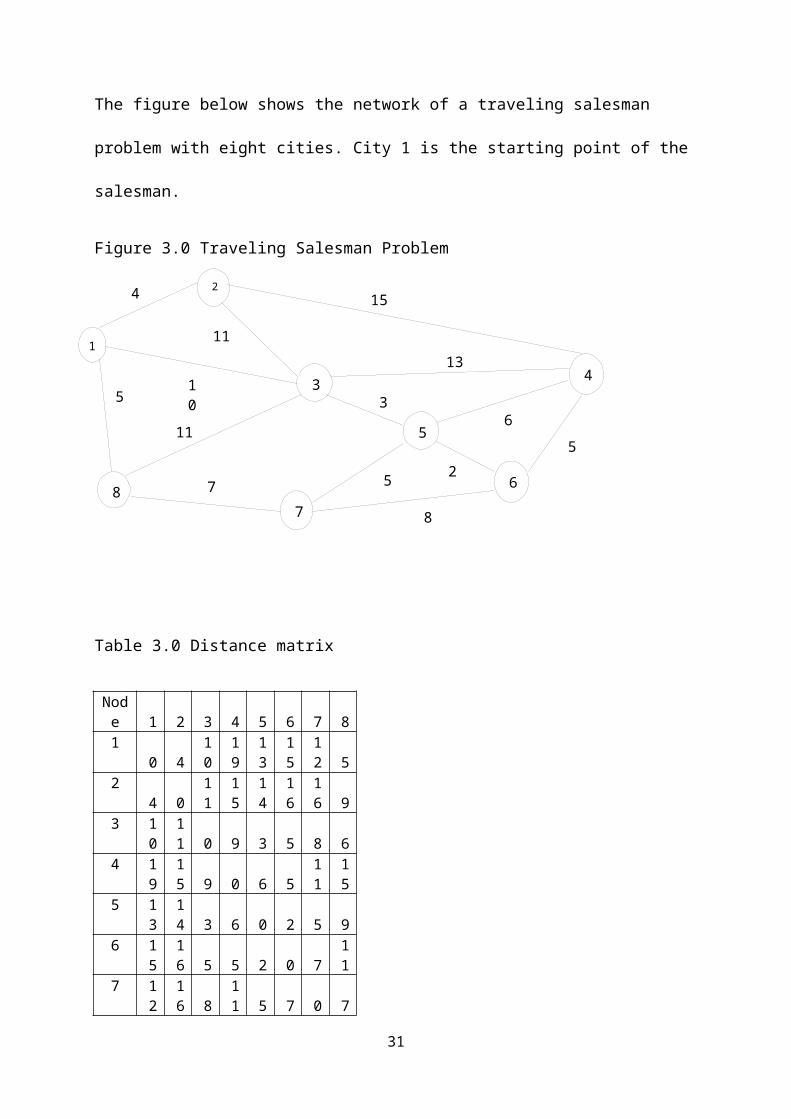
The figure below shows the network of a traveling salesman

problem with eight cities. City 1 is the starting point of the

salesman.

Figure 3.0 Traveling Salesman Problem

Table 3.0 Distance matrix

Node 1 2 3 4 5 6 7 81

0 410

19

13

15

12 5

24 0

11

15

14

16

16 9

3 10

11 0 9 3 5 8 6

4 19

15 9 0 6 5

11

15

5 13

14 3 6 0 2 5 9

6 15

16 5 5 2 0 7

11

7 12

16 8

11 5 7 0 7

31

85 9

15

18

12

14 7 0

Considering figure 3.0, we will take the initial solution for

the tour as;

x=1-2-3-4-5-6-7-8-1

We compute the objective value as the distance d(i, j) between the

cities x0 with reference to equation (1) in section 3.2.

The parameters to use are;

Initial temperature T0=20,

Updating of temperature (Tk) , Tk+1 = αTk and α=0.85

Stopping criteria T < 5 (final temperature)

Starting Iteration: k=0

x0=1-2-3-4-5-6-7-8-1

d (x0)=d(1,2)+ d(2,3)+ d(3,4)+ d(4,5)+ d(5,6)+ d(6,7)+ d(7,8)+

d(8,1)

d (x0)=56

Generate a new solution x1 in the neighborhood of x0 such as x1 =1-

3-2-4-5-6-7-8-1

32

d (x1)=d(1,3)+ d(3,2)+ d(2,4)+ d(4,5)+ d(5,6)+d(6,7)+ d(7,8)+

d(8,1)

d (x1)=64

δ=d(x1) - d(x0)

= 64 – 56 = 8

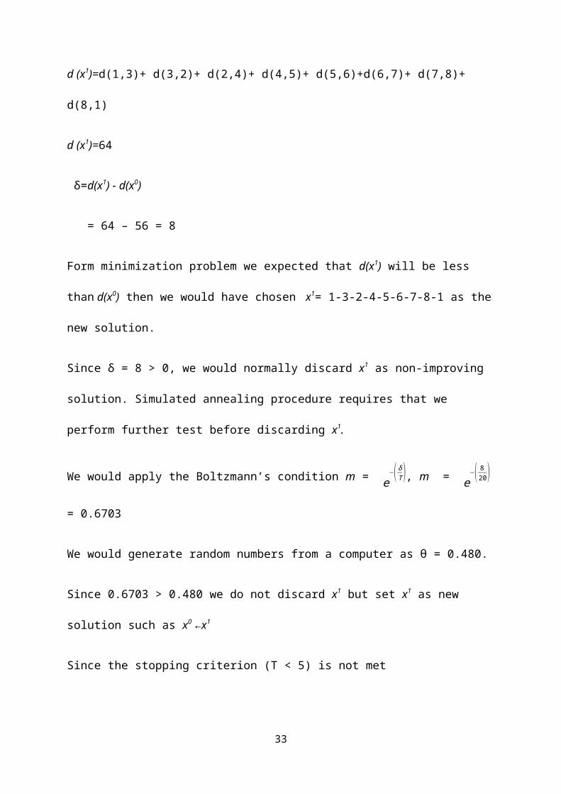
Form minimization problem we expected that d(x1) will be less

than d(x0) then we would have chosen x1= 1-3-2-4-5-6-7-8-1 as the

new solution.

Since δ = 8 > 0, we would normally discard x1 as non-improving

solution. Simulated annealing procedure requires that we

perform further test before discarding x1.

We would apply the Boltzmann’s condition m = e−( δT ), m = e

−( 820)

= 0.6703

We would generate random numbers from a computer as θ = 0.480.

Since 0.6703 > 0.480 we do not discard x1 but set x1 as new

solution such as x0 x← 1

Since the stopping criterion (T < 5) is not met

33

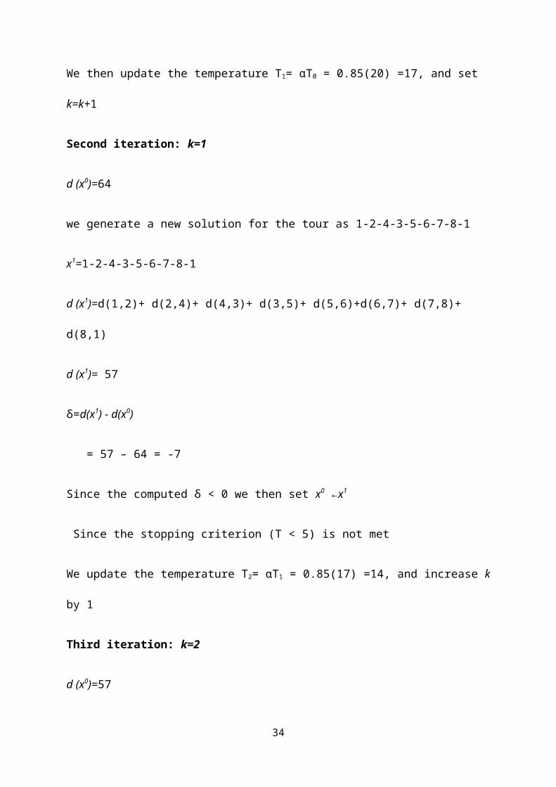
We then update the temperature T1= αT0 = 0.85(20) =17, and set

k=k+1

Second iteration: k=1

d (x0)=64

we generate a new solution for the tour as 1-2-4-3-5-6-7-8-1

x1=1-2-4-3-5-6-7-8-1

d (x1)=d(1,2)+ d(2,4)+ d(4,3)+ d(3,5)+ d(5,6)+d(6,7)+ d(7,8)+

d(8,1)

d (x1)= 57

δ=d(x1) - d(x0)

= 57 – 64 = -7

Since the computed δ < 0 we then set x0 ←x1

Since the stopping criterion (T < 5) is not met

We update the temperature T2= αT1 = 0.85(17) =14, and increase k

by 1

Third iteration: k=2

d (x0)=57

34

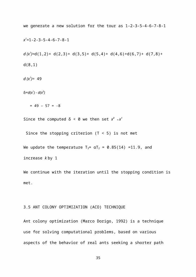
we generate a new solution for the tour as 1-2-3-5-4-6-7-8-1

x1=1-2-3-5-4-6-7-8-1

d (x1)=d(1,2)+ d(2,3)+ d(3,5)+ d(5,4)+ d(4,6)+d(6,7)+ d(7,8)+

d(8,1)

d (x1)= 49

δ=d(x1) - d(x0)

= 49 – 57 = -8

Since the computed δ < 0 we then set x0 ←x1

Since the stopping criterion (T < 5) is not met

We update the temperature T3= αT2 = 0.85(14) =11.9, and

increase k by 1

We continue with the iteration until the stopping condition is

met.

3.5 ANT COLONY OPTIMIZATION (ACO) TECHNIQUE

Ant colony optimization (Marco Dorigo, 1992) is a technique

use for solving computational problems, based on various

aspects of the behavior of real ants seeking a shorter path

35

between their colony and a source of food without using visual

cues (Hölldobler and Wilson, 1990). Real ants are capable of

adapting to changes in the environment, for example finding a

new shortest path once the old one is no longer feasible due

to a new obstacle (Beckers et al. 1992). Once the obstacle has

appeared those ants can find the shortest path that reconnects

a broken initial path. Ants which are just in front of the

obstacle cannot continue on the path and therefore they have

to choose between turning right or left. In this situation we

can expect half the ants to choose to turn right and the other

half to turn left.

The idea of this algorithm involves movement of ants in a

colony through different states of a problem influence by

trails and attractiveness. Each ant gradually constructs a

solution to a problem, evaluates the solution and modifies the

trail values on the components used in its solution. The

algorithm has a mechanism to reduce the possibility of getting

stuck in local optima (called trail evaporation) and biasing

the search process from a non-local perspective (called daemon

actions). Ants exchange information indirectly by depositing

pheromones detailing the status of their work which only ants 36

located where near can have a notion of them. The following

are some variations of the algorithm:

(i) Elitist ant system. The global best solution deposits

pheromone, detailing the status of their work, on every

iteration along with all the other ants.

(ii) Max-Min ant system (MMAS). Added Maximum and Minimum pheromone

amounts [τmax,τmin] Only global best or iteration best tour deposited

pheromone and all edges are initialized to τmax and reinitialized to

τmax when nearing stagnation (Hoos and Stützle, 1996).

(iii) Rank-based ant system (ASrank).This system ranks all solutions

according to their fitness. The amount of pheromone deposited is

then weighted for each solution, such that the solutions with better

fitness deposit more pheromone than the solutions with worse

fitness.

(iv) Continuous orthogonal ant colony (COAC). The pheromone deposit

mechanism is to enable ants to search for solutions collaboratively

and effectively by using an orthogonal design method, ants in the

feasible domain can explore their chosen regions rapidly and

efficiently, with enhanced global search capability and accuracy.

The orthogonal design method and the adaptive radius adjustment

method can also be extended to other optimization algorithms for

delivering wider advantages in solving practical problems.

37

Ant colony optimization algorithms have been applied to many

combinatorial optimization problems, ranging from assignment

problem to routing vehicles, network routing and urban

transportation systems, Scheduling problem, knapsack problem,

Connection-oriented network routing (Caro and Dorigo, 1998),

Connectionless network routing, Discounted cash flows in

project scheduling (Chen et al., 2010), and a lot of derived

methods have been adapted to dynamic problems in real

variables, stochastic problems, multi-targets and parallel

implementations. Ant colony optimization algorithms have been

used to produce near-optimal solutions to the travelling

salesman problem. Even though there exist several ACO

variants, the one that may be considered a standard approach

is presented next.

3.5.1 Standard Approach

ACO uses a pheromone matrix τ = {τij} for the construction of

potential good solutions. The initial values of τ are set τij = τinit

∀(i, j), where τinit > 0. It also takes advantage of heuristic

information using ηij = 1/d(i, j). Parameter α and β defines the

relative influence between the heuristic information and then

pheromone levels. While visiting city i, Ni represents the set 38

of cities not yet visited and the probability of choosing a

city j at city i is defined by equation (i);

Pi,j¿¿ (i)

At every generation of the algorithm, each of the m ants

constructs a complete tour using (1), starting at a randomly

chosen city. Pheromone evaporation is applied for all (i, j)

according to τij = (1 ρ− ) · τij, where parameter ρ ∈ (0, 1] determines

the evaporation rate. Considering an elitist strategy, the

best solution found so far rbest updates τ according to τij = τij + ∆τ,

where ∆τ = 1/l(rbest) if (i, j) ∈ rbest and ∆τ = 0 if (i, j) /∈ rbest. For one

of the best performing ACO algorithms, the MAX-MIN Ant System

(MMAS).

3.5.2 Population-based ACO

The Population-based ACOs (P-ACOs) were designed by Guntsch

and Middendorf (2006) for dynamic combinatorial optimization

problems. As the standard approach, the initial values of τ are

set τij = τinit ∀ (i, j), where τinit > 0. The P-ACO approach updates in a

different way the pheromone information than the standard

approach. P-ACO derives the pheromone matrix through a

population Q = {Qx} of q good solutions or individuals as

follows. First, at every iteration each of the m ants 39

constructs a solution using probabilities given in equation

(1), the best solution enters the population Q. Whenever a

solution Qin enters the population, then τij is updated according

to τij = τij + ∆τ, where ∆τ = ∆ if (i, j) ∈ Qin and ∆τ = 0 if (i, j) /∈ Qin.

After the first q solutions enter Q, i.e. the initialization of

the population is finished, one solution Qout must leave the

population at every iteration. The solution that must leave

the population is decided by an update strategy. Whenever a

solution Qout leaves the population, then

τij = τij − ∆τ, where ∆τ =∆ if (i, j) ∈ Qout and ∆τ =0 if (i, j) /∈ Qout. P-ACO

replaces the pheromone evaporation used by the standard

approach in this way. The value ∆ is a constant determined by

the following input parameters, size of the population q,

minimum or initial pheromone level τinit and maximum pheromone

level τmax. Thus, ∆=(τmax τ− init)/q (Guntsch and Middendorf, 2006).

3.5.2.1 FIFO-Queue Update Strategy

The FIFO-Queue update strategy was the first P-ACO strategy

designed by Guntsch and Middendorf (2006), trying to simulate

the behavior of the standard approach of ACO. In the FIFO-

Queue update strategy, Qout is the oldest individual of Q.

40

3.5.2.2 Quality Update Strategy

A variety of strategies were studied by Guntsch and Middendorf

(2002) and one of them is the Quality update strategy. The

worst solution (considering quality) of the set {Q, Qin} leaves

the population in this strategy. This ensures that the best

solutions found so far make up the population.

3.5.3 Omicron ACO

In the search for a new ACO analytical tool, Omicron ACO (OA)

was developed by Gómez and Barán (2004). OA was inspired by

MMAS, an elitist ACO currently considered among the best

performing algorithms for the TSP Stützle and Hoos (2000). It

is based on the hypothesis that it is convenient to search

nearby good solutions by Stützle and Hoos (2000).

The main difference between MMAS and OA is the way the

algorithms update the pheromone matrix. In OA, a constant

pheromone matrix τ0 with τ0 i, j = 1, ∀i, j is defined. OA maintains a

population Q = {Qx} of q individuals or solutions, the best

unique ones found so far. The best individual of Q at any

moment is called Q∗, while the worst individual Qworst.

41

In OA the first population is chosen using τ0. At every

iteration a new individual Qnew is generated, replacing Qworst ∈ Q,

if Qnew is better than Qworst and different from any other Qx ∈ Q.

After K iterations, τ is recalculated using the input parameter

Omicron (O). First, τ = τ0; then, O/q is added to each element τij

for each time an arc (i, j) appears in any of the q individuals

present in Q. The above process is repeated on every k

iteration until the end condition is reached. Note that 1 τ≤ ij ≤

(1 + O), where τij = 1 if arc (i, j) is not present in any Qx, while

τij = (1 + O) if arc (i, j) is in every Qx.

Even considering their different origins, OA results are

similar to the Population-based ACO algorithms described by

Guntsch and Martin Middendorf (2002). The main difference

between the OA and the Quality Strategy of P-ACO is that OA does

not allow identical individuals in its population. Also, OA

updates τ on every k iterations, while P-ACO updates τ every

iteration.

The ACO algorithm can be summarized into the following steps:

Step 1: Generate random individuals from initial population

derived from a pheromone matrix

Step 2: initialize an iteration counter k=0

Step 3: update the pheromone matrix42

Step 4: generate new individual using the updated pheromone

matrix

Step 5: the new individual replaces the worst individual

solution in the initial population.

Step 6: increment of the iteration counter k=k+1

Step 7: stop, if the termination condition is met.

3.6 GENETIC ALGORITHM (GA)

GA is a class of evolutionary algorithms inspired by Darwin

(1859) a theory of “survival of the fittest” (Herbert Spencer,

1864) and further discussed by Dawkins (1986). Genetic

algorithm has the biological principle that species live in a

competitive environment and their continuous survival depends

on the mechanics of “natural selection” (Darwin, 1868). This

algorithm uses a technique such as inheritance, mutation,

selection and crossover (also referred as recombination).

Holland (1975) invented genetic algorithm as an adaptive

search procedure.

GA is also an efficient search method that has been used for

path selection in networks. GA is a stochastic search

algorithm which is based on the principle of natural selection

43

and recombination. A GA is composed with a set of solutions,

which represents the chromosomes. This composed set is

referred to as population. Population consists of set of

chromosome which is assumed to give solutions. From this

population, we randomly choose the first generation from which

solutions are obtained. These solutions become a part of the

next generation. Within the population, the chromosomes are

tested to see whether they give a valid solution. This testing

operation is nothing but the fitness functions which are

applied on the chromosome. Operations like selection,

crossover and mutation are applied on the selected chromosome

to obtain the progeny. Again fitness function is applied to

these progeny to test for its fitness. Most fit progeny

chromosome will be the participants in the next generation.

The best sets of solution are obtained using heuristic search

techniques.

The performance of GA is based on efficient representation,

evaluation of fitness function and other parameters like size

of population, rate of crossover, mutation and the strength of

selection. Genetic algorithms are able to find out optimal or

44

near optimal solution depending on the selection function

Goldberg and Miller (1995); Ray et. al (2004).

According to Dr. Amponsah and Darkwah (2007), the genetic

algorithm introduced by Holland had the following similarity

of the evolutionary principles.

Table 3.1 below compares evolution to genetic algorithm.

Evolution Genetic Algorithm

An individual is a genotype of

the species

An individual is a solution of the

optimization problem

Chromosomes define the

structure of an individual

Chromosomes are used to represent the

data structure of the solution

Chromosomes consists of

sequence of cells called genes

which contain the structural

information

Chromosome consists of a sequence of

gene species which are placeholder

boxes containing string of data whose

unique combination give the solution

value

The genetic information or

trait in each gene is called an

allele

An allele is an element of the data

structure stored in a gene

placeholder

Fitness of an individual is an

interpretation of how the

Fitness of a solution consists in

evaluation of measures of the

45

chromosomes have adapted to the

competitive environment

objective function for the solution

and comparing it to the evaluations

for other solutions

A population is a collection of

the species found in a given

location

A population is a set of solutions

that form the domain search space.

A generation is a given number

of individuals of the

population indentified over a

period of time.

A generation is a set of solutions

taken from the population (domain)

and generated at an instant of time

or in an iteration

Selection is pairing of

individuals as parents for

reproduction

Selection is the operation of

selecting parents from the generation

to produce offspring.

Crossover is mating and

breeding of offspring by pairs

of parents whereby chromosomes

characteristics are exchanged

to form new individuals.

Crossover is the operation whereby

pairs of parents exchange

characteristics of their data

structure to produce two new

individuals as offspring.

Mutation is a random

chromosomal process of

modification whereby the

inherited genes of the

Mutation is random operation whereby

the allele of a gene in a chromosome

of the offspring is changed by a

46

offspring from their parents

are distorted. probability pm.

Recombination is a process of

nature's survival of the

fittest.

Recombination is the operation

whereby elements of the generation

and elements of the offspring form an

intermediate generation and less fit

chromosomes are taken from the

generation.

The two distinct elements in the GA are individuals and

populations. An individual is a single solution while the

population is the set of individuals currently involved in the

search process.

Given a population at time t, genetic operators are applied to

produce a new population at time t+1. A step- wise evolution of

the population from time t to t+1 is called a generation. The

Genetic Algorithm for a single generation is based on the

general GA framework of Selection, Crossover, Mutation and

Recombination.

3.6.1 Representation of individuals

47

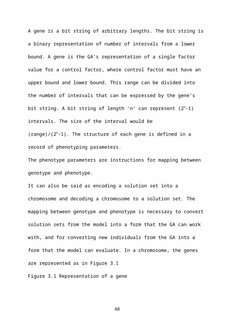
A gene is a bit string of arbitrary lengths. The bit string is

a binary representation of number of intervals from a lower

bound. A gene is the GA’s representation of a single factor

value for a control factor, where control factor must have an

upper bound and lower bound. This range can be divided into

the number of intervals that can be expressed by the gene’s

bit string. A bit string of length ‘n’ can represent (2n-1)

intervals. The size of the interval would be

(range)/(2n-1). The structure of each gene is defined in a

record of phenotyping parameters.

The phenotype parameters are instructions for mapping between

genotype and phenotype.

It can also be said as encoding a solution set into a

chromosome and decoding a chromosome to a solution set. The

mapping between genotype and phenotype is necessary to convert

solution sets from the model into a form that the GA can work

with, and for converting new individuals from the GA into a

form that the model can evaluate. In a chromosome, the genes

are represented as in Figure 3.1

Figure 3.1 Representation of a gene

48

10

10

11

10

11

11

01

01

gene 1 gene 2 gene 3 gene 4

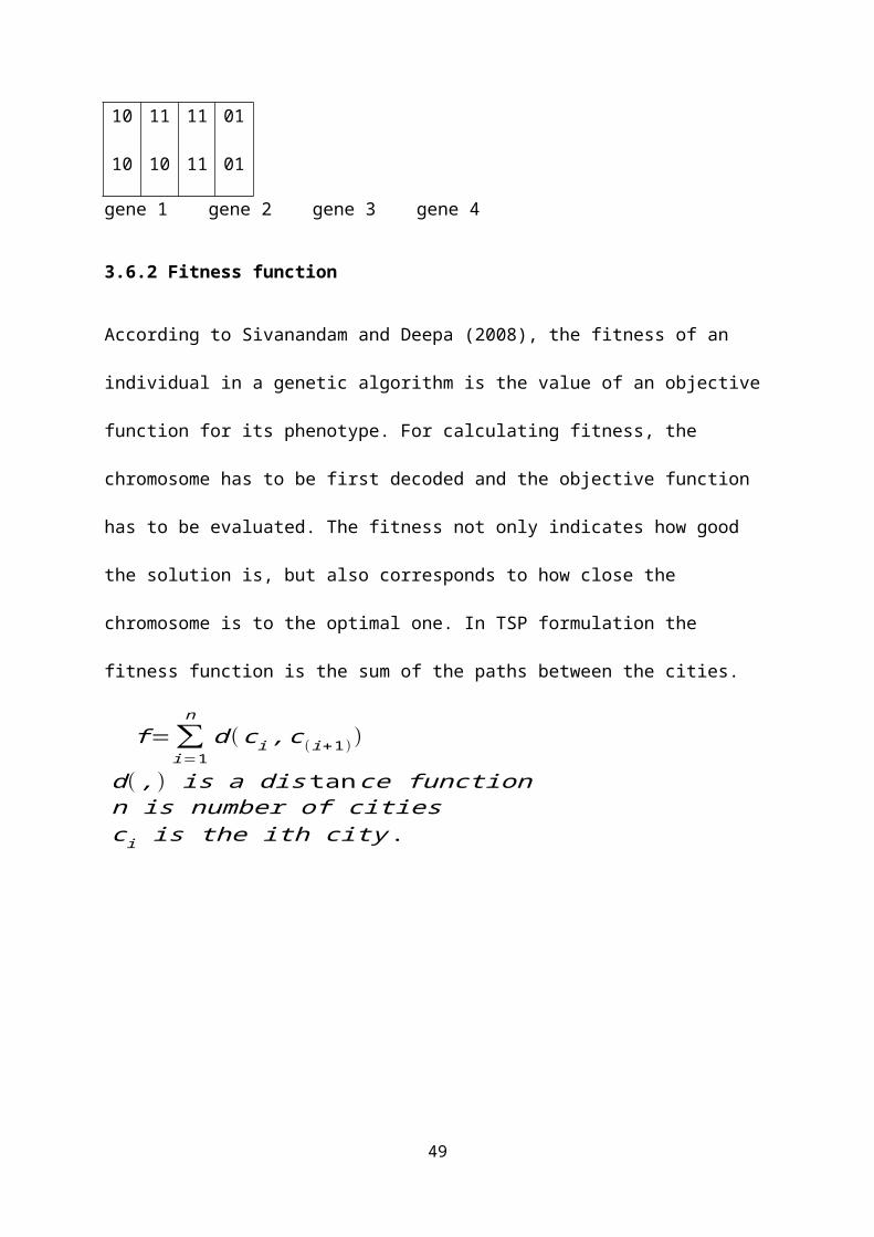
3.6.2 Fitness function

According to Sivanandam and Deepa (2008), the fitness of an

individual in a genetic algorithm is the value of an objective

function for its phenotype. For calculating fitness, the

chromosome has to be first decoded and the objective function

has to be evaluated. The fitness not only indicates how good

the solution is, but also corresponds to how close the

chromosome is to the optimal one. In TSP formulation the

fitness function is the sum of the paths between the cities.

f=∑i=1

nd(ci,c(i+1))

d(,) is a distance functionn is number of citiesci is the ith city.

49

3.6.3 Population

A population is a collection of individuals. A population

consists of a number of individuals

being tested, the phenotype parameters defining the

individuals and some information about search space. The two

important aspects of population used in Genetic Algorithms

are; the initial population generation and the population size

(Sivanandam and Deepa, 2008).

For each and every problem, the population size will depend on

the complexity of the problem. It is often a random

initialization of population is carried. In the case of a

binary coded chromosome this means, that each bit is

initialized to a random zero or one. But there may be

instances where the initialization of population is carried

out with some known good solutions.

Ideally, the first population should have a gene pool as large

as possible in order to be able to explore the whole search

space. All the different possible alleles of each should be

present in the population. To achieve this, the initial

population is, in most of the cases, chosen randomly.

50

Nevertheless, sometimes a kind of heuristic can be used to

seed the initial population. Thus, the mean fitness of the

population is already high and it may help the genetic

algorithm to find good solutions faster. But for doing this

one should be sure that the gene pool is still large enough.

Otherwise, if the population badly lacks diversity, the

algorithm will just explore a small part of the search space

and never find global optimal solutions.

The size of the population raises few problems too. The larger

the population

is, the easier it is to explore the search space. But it has

established that the time required by a GA to converge is O

(nlogn) function evaluations where n is the population size.

We say that the population has converged when all the

individuals are very much alike and further improvement may

only be possibly by mutation. Goldberg has also shown that GA

efficiency to reach global optimum instead of local ones is

largely determined by the size of the population. To sum up, a

large population is quite useful. But it requires much more

computational cost, memory and time. Practically, a population

size of around 100 individuals

51

is quite frequent, but anyway this size can be changed

according to the time and the memory disposed on the machine

compared to the quality of the result to be reached.

Population being combination of various chromosomes is

represented as in figure 3.2. This population consists of

four chromosomes.

Figure 3.2 Population of chromosomes

Population

Chromosome 11 1 1 0 0 0 1 0

Chromosome 20 1 1 1 1 0 1 1

Chromosome 31 0 1 0 1 0 1 0

Chromosome 41 1 0 0 1 1 0 0

3.6.4 Search strategies

The search process consists of initializing the population and

then breeding new individuals until the termination condition

is met. There can be several goals for the search process, one

of which is to find the global optima. This can never be

assured with the types of models that GAs work with. There is

always a possibility that the next iteration in the search 52

would produce a better solution. In some cases, the search

process could run for years and does not produce any better

solution than it did in the first little iteration.

Another goal is faster convergence. When the objective

function is expensive to run, faster convergence is desirable,

however, the chance of converging on local and possibly quite

substandard optima is increased.

Apart from these, yet another goal is to produce a range of

diverse, but still good solutions. When the solution space

contains several distinct optima, which are similar in

fitness, it is useful to be able to select between them, since

some combinations of factor values in the model may be more

feasible than others. Also, some solutions may be more robust

than others.

3.6.5 Encoding

Encoding is a process of representing individual genes. The

process can be performed using bits, numbers, trees, arrays,

lists or any other objects. The encoding depends mainly on

solving the problem. For example, one can encode directly real

or integer numbers.53

3.6.6 Breeding

The breeding process is the core of the genetic algorithm. It

is in this process, that the search process creates new and

hopefully fitter individuals. The breeding cycle consists of

three steps:

a. Selecting parents.

b. Crossing the parents to create new individuals (offspring

or children).

c. Replacing old individuals in the population with the new

ones.

3.6.6.1 Selection process

Selection is the process of choosing two parents from the

population for crossing. After deciding on an encoding, the

next step is to decide how to perform selection i.e., how to

choose individuals in the population that will create

offspring for the next generation and how many offspring each

will create. The purpose of selection is to emphasize fitter

individuals in the population in hopes that their offsprings

have higher fitness. Chromosomes are selected from the initial

54

population to be parents for reproduction. The problem is how

to select these chromosomes. According to Darwin’s theory of

evolution the best ones survive to create new offspring.

Selection is a method that randomly picks chromosomes out of

the population according to their evaluation function. The

higher the fitness function, the more chance an individual has

to be selected. The selection pressure is defined as the

degree to which the better individuals are favored. The higher

the selection pressured, the more the better individuals are

favored. This selection pressure drives the GA to improve the

population fitness over the successive generations.

Genetic Algorithms should be able to identify optimal or

nearly optimal solutions under a wise range of selection

scheme pressure. However, if the selection pressure is too

low, the convergence rate will be slow, and the GA will take

unnecessarily longer time to find the optimal solution. If the

selection pressure is too high, there is an increased change

of the GA prematurely converging to an incorrect (sub-optimal)

solution. In addition to providing selection pressure,

55

selection schemes should also preserve population diversity,

as this helps to avoid premature convergence.

Typically we can distinguish two types of selection scheme,

proportionate selection and ordinal-based selection.

Proportionate-based selection picks out individuals based upon

their fitness values relative to the fitness of the other

individuals in the population. Ordinal-based selection schemes

selects individuals not upon their raw fitness, but upon their

rank within the population. This requires that the selection

pressure is independent of the fitness distribution of the

population, and is solely based upon the relative ordering

(ranking) of the population.

Selection has to be balanced with variation form crossover and

mutation. Too strong selection means sub optimal highly fit

individuals will take over the population, reducing the

diversity needed for change and progress; too weak selection

will result in too slow evolution. The various selection

methods are discussed as follows:

3.6.6.1.1 Roulette selection

56

Roulette selection is one of the traditional GA selection

techniques. The commonly used reproduction operator is the

proportionate reproductive operator where a string is selected

from the mating pool with a probability proportional to the

fitness. The principle of roulette selection is a linear

search through a roulette wheel with the slots in the wheel

weighted in proportion to the individual’s fitness values. A

target value is set, which is a random proportion of the sum

of the fit nesses in the population. The population is stepped

through until the target value is reached. This is only a

moderately strong selection technique, since fit individuals

are not guaranteed to be selected for, but somewhat have a

greater chance. A fit individual will contribute more to the

target value, but if it does not exceed it, the next

chromosome in line has a chance, and it may be weak. It is

essential that the population not be sorted by fitness, since

this would dramatically bias the selection.

3.6.6.1.2 Random Selection

This technique randomly selects a parent from the population.

In terms of disruption of genetic codes, random selection is a

57

little more disruptive, on average, than roulette wheel

selection

3.6.6.1.3 Rank Selection

The Roulette wheel will have a problem when the fitness values

differ very much.

If the best chromosome fitness is 90%, its circumference

occupies 90% of Roulette wheel, and then other chromosomes

have too few chances to be selected. Rank Selection ranks the

population and every chromosome receives fitness from the

ranking. The worst has fitness 1 and the best has fitness N.

It results in slow convergence but prevents too quick

convergence. It also keeps up selection pressure when the

fitness variance is low. It preserves diversity and hence

leads to a successful search. In effect, potential parents are

selected and a tournament is held to decide which of the

individuals will be the parent. There are many ways this can

be achieved and two suggestions are,

1. Select a pair of individuals at random. Generate a random

number, R, between 0 and 1. If R < r use the first individual as

a parent. If the R>=r then use the second individual as the

parent. This is repeated to select the second parent. The

value of r is a parameter to this method.58

2. Select two individuals at random. The individual with the

highest evaluation becomes the parent. Repeat to find a second

parent.

3.6.6.1.4 Tournament Selection

Unlike, the Roulette wheel selection, the tournament selection

strategy provides selective

pressure by holding a tournament competition among Ni

individuals.

The best individual from the tournament is the one with the

highest fitness, which is the winner of Ni. Tournament

competitions and the winner are then inserted into the mating

pool. The tournament competition is repeated until the mating

pool for generating new offspring is filled. The mating pool

comprising of the tournament winner has higher average

population fitness. The fitness difference provides the

selection pressure, which drives GA to improve the fitness of

the succeeding genes. This method is more efficient and leads

to an optimal solution.

59

3.6.6.1.5 Boltzmann Selection

In Boltzmann selection a continuously varying temperature

controls the rate of selection according to a preset schedule.

The temperature starts out high, which means the selection

pressure is low. The temperature is gradually lowered, which

gradually increases the selection pressure, thereby allowing

the GA to narrow in more closely to the best part of the

search space while maintaining the appropriate degree of

diversity.

3.6.6.2 Crossover process

After the required selection process the crossover operation

is used to divide a pair of selected chromosomes into two or

more parts. Parts of one of the pair are joined to parts of

the other pair with the requirement that the length should be

preserved.

The point between two alleles of a chromosome where it is cut

is called crossover point. There can be more than one

crossover point in a chromosome. The crossover point i is the

space between the allele in the ith position and the one in (i +

1)th position. For two chromosomes the crossover points are the

60

same and the crossover operation is the swapping of similar

parts between the two chromosomes. The crossover operation may

produce new chromosomes which are less fit. In that sense the

crossover operation results in non-improving solution. The

following are crossover operations that can be applied on

chromosomes:

3.6.6.2.1 Single point crossover

The traditional genetic algorithm uses single point crossover,

where the two mating chromosomes are cut once at corresponding

points and the sections after the cuts exchanged. Here, a

cross-site or crossover point is selected randomly along the

length of the mated strings and bits next to the cross-sites

are exchanged. If appropriate site is chosen, better children

can be obtained by combining good parents else it hampers

string quality.

The figure 3.3 illustrates single point crossover and it can

be observed that the bits next to the crossover points are

exchanged to produce children. This crossover points can be

chosen randomly.

Figure 3.3 single point crossover

61

Parent 1 10110 |010Parent 2 10101|111

|

Child 1 10110|111Child 2 10101|010

To solve a traveling salesman problem, a simple crossover

reproduction scheme does not work as it makes the chromosomes

inconsistent. That is, some cities may be repeated while

others are missing out. This drawback of the simple crossover

mechanism is illustrated below;

Parent 1 1 2 3 4 | 5 6 7

Parent 2 3 7 6 1 | 5 2 4

Offspring 1 1 2 3 4 | 5 2 4

Offspring 2 3 7 6 1 | 5 6 7

From the illustration, cities 6 and 7 are missing in

offspring1 whiles cities 2 and 4 are visited more than once.

Offspring 2 too suffers from similar drawbacks. This drawback

is avoided in partially matched crossover mechanism which is

discussed in (iv).

3.6.6.2.2 Double point crossover

62

Apart from single point crossover, many different crossover

algorithms have been devised, often involving more than one

cut point. Adding more crossover points has the tendency to

reduce the performance of the genetic algorithm. The problem

with adding additional crossover points is that building

blocks are more likely to be disrupted. However, an advantage

of having more crossover points is that the problem space may

be searched more thoroughly.

In double point crossover, two crossover points are chosen and

the contents between these points are exchanged between two

mated parents.

In figure 3.4 the dotted lines indicate the crossover points.

Thus the contents between these points are exchanged between

the parents to produce new children for mating in the next

generation.

Figure 3.4 Double point crossover

Parent 1 11011010Parent 2 01101100

Child 1 11001110Child 2 01111000

63

Originally, genetic algorithms were using single point

crossover which cuts two chromosomes in one point and splices

the two halves to create new ones. But with this single point

crossover, the head and the tail of one chromosome cannot be

passes together to the offspring. If both the head and the

tail of a chromosome contain good genetic information, none of

the offspring obtained directly with single point crossover

will share the two good features. Using double point crossover

avoids this drawback and then, is largely considered better

than single point crossover. In genetic representation, genes

that are close on a chromosome have more chance to be passed

together to the offspring than those that are not. To avoid

all the problem of gene positioning, a good crossover

technique is to use a uniform crossover as recombination

operator.

3.6.6.2.3 Multi-point crossover (N-Point crossover)

There are two ways in this crossover. One is even number of

cross-sites and the other odd number of cross-sites. In the

case of even number of cross-sites, cross-sites are selected

randomly around a circle and information is exchanged. In the

64

case of odd number of cross-sites, a different cross-point is

always assumed at the string beginning.

3.6.6.2.4 Uniform crossover

In uniform crossover each gene in the offspring is created by

copying the corresponding gene from one or the other parent

chosen according to a random generated binary crossover mask

of the same length as the chromosomes. Where there is a 1 in

the crossover mask, the gene is copied from the first parent,

and where there is a 0 in the mask the gene is copied from the

second parent. A new crossover mask is randomly generated from

each pair parents. Offsprings, therefore contain a mixture of

genes from each parent. The number of effective crossing point

is not fixed, but will average L/2, where L is the chromosome

length.

In figure 3.5, new children are produced using uniform

crossover approach. It can be noticed, that while producing

child 1, when there is a 1 in the mask, the gene is copied

from the parent 1 else from the parent 2. On producing child

2, when there is a 1 in the mask, the gene is copied from

parent 2, when there is a 0 in the mask; the gene is copied

from the parent 1. 65

Figure 3.5 uniform crossover

Parent 1 1 0 1 1 0 0 1 1Parent 2 0 0 0 1 1 0 1 0Mask 1 1 0 1 0 1 1 0Child 1 1 0 0 1 1 0 1 0Child 2 0 0 1 1 0 0 1 1

66

3.6.6.2.5 Partially matched crossover (PMX)

This aligns two chromosomes or strings and two crossover

points are selected uniformly at random along the length of

the chromosomes. The two crossover points give a matching

selection, which is used to affect a cross through position-

by-position exchange operations.

Consider two strings:

Parent A 4 8 7 | 3 6 5 | 1 10 9 2

Parent B 3 1 4 | 2 7 9 | 10 8 6 5

Two crossover points were selected at random, and PMX proceeds

by position wise exchanges. In-between the crossover points

the genes get exchanged. That is, the 3 and the 2, the 6 and

the 7, the 5 and the 9 exchange places. This is by mapping

parent B to parent A. now mapping parent A to parent, the 7

and the 6, the 9 and the 5, the 2 and the 3 exchange places.

Thus after PMX, the offspring produces as follows:

Child A 4 8 6 | 2 7 9 | 1 10 5 3

Child B 2 1 4 | 3 6 5 | 10 8 7 9

Where each offspring contains ordering information which are

partially determined by each of its parents. 67

Sometimes it may be possible that by crossover operation, a

new population never gets generated. To overcome this

limitation, we do mutation operation. Here we use insertion

method, as a node along the optimal path may be eliminated

through crossover.

3.6.6.3 Mutation process

After crossover, the strings are subjected to mutation.

Mutation prevents the algorithm from been trapped in a local

minimum. Mutation plays the role of recovering the lost

genetic materials as well as for randomly disturbing genetic

information. If crossover is supposed to exploit the current

solution to find better ones, mutation is supposed to help for

the exploration of the whole search space. Mutation introduces

new genetic structures in the population by randomly modifying

some of its building blocks. The building block being highly

fit, low order, short defining length schemes, and encoding

schemes. Mutation helps escape from local minima’s trap and

maintains diversity in the population.

There are many different forms of mutation for different kinds

of representation. For binary representation, a simple

mutation can consist in inverting the value of each gene with 68

a small probability. The probability is usually taken about

1/L, where L is the length of the chromosome. Mutation of a

bit involves flipping a bit, changing 0 to 1 and vice-versa.

The following are some mutation carried on chromosomes:

i. Random swap mutation is when two loci (positions) are

chosen at random and their values swapped.

ii. Move-and –insert gene mutation is when a locus is

chosen at random and its value is inserted before or

after the value at another randomly chosen locus.

iii. Move-and –insert sequence mutation is very similar to

the gene move-and –insert but instead of a single locus a

sequence loci is moved and inserted before or after the

value at another randomly chosen locus.

iv. Uniform mutation probability sets a probability

parameter and for all the loci an allele with greater or

same probability as the parameter is mutated by reversing

its allele

For the TSP problem, mutation refers to a randomized exchange

of cities in the chromosomes. For instance, consider the

example shown in figure 3.6. Here cities 2 and 5 are

interchanged because of an inversion operation.

69

70

Figure 3.6 Mutation

4 2 6 1 5 3 7

4 5 6 1 2 3 7

3.6.6.4 Replacement

Replacement is the last stage of any breeding cycle. Two

parents are drawn from a fixed size population, they breed two

children, but not all four can return to the population, so

two must be replaced. That is, once offsprings are produced, a

method must determine which of the current members of the

population, if any, should be replaced by new solution. The

technique used to decide which individual stay in a population

and which are replaced in on a par with the selection in

influencing convergence. Basically, there are two kinds of

methods for maintaining the population; generational updates

and steady state updates.

In a steady state update, new individuals are inserted in the

population as soon as they are created, as opposed to the

generational update where an entire new generation is produced

71

at each time step. The insertion of a new individual usually

necessitates the replacement of another population member.

3.6.6.5 Search Termination (Convergence criteria)

The algorithm terminates when a conditions is satisfied. At

that point the solution with best fitness among the current

generation of the population is taken as the global solution

or the algorithm may terminate if one or more of the following

are satisfied:

i. a specified number of total iterations are completed;

ii. a specified number of iterations are completed

within which the solution of best fitness has not change;

iii. Specified number of iterations are completed in which

worst individual terminates the search when the least fit

individuals in the population have fitness less than the

convergence criteria. This guarantees the entire

population to be of minimum standard.

iv. When the sum of fitness in the entire population is

less than or equal to the convergence value in the

population recorded.

v. Using a median fitness criteria. Here at least half of

the individuals will be better than or equal to the

72

convergence value, which should have a good range of

solution to choose from.

3.7 Simple Genetic Algorithm (SGA)

An algorithm is a series of steps for solving a problem. A

genetic algorithm is a problem solving method that uses

genetics as its model of problem solving. It’s a search

technique to find approximate solutions to optimization and

search problems.

Simple Genetic Algorithm (SGA) presented by Goldberg (1989) is

an algorithm that captures most essential components of every

genetic algorithm. The structure of genetic algorithm usually

starts with guesses and attempts to improve the guesses by

evolution. A GA typically has the following aspects:

i) a representation of a guess called a chromosome can be a

binary sting or a more elaborate data structure,

ii) an initial pool of chromosomes can be randomly produced or

manually created,

iii) a fitness function measures the suitability of a

chromosome to meet a specified objective,

73

iv) a selection function decides which chromosomes will

participate in the evolution stage of the genetic algorithm

make up by the crossover and mutation operators, and

v) a crossover operator and a mutation operator. The crossover

operator exchange genes from two chromosomes and creates two

new chromosomes. The mutation operator changes a gene in a

chromosome and creates one new chromosome.

The simple Genetic Algorithm may be summarized into the

following steps:

Step 1: Code the individual of the search space

Step 2: Initialize the generation counter (g=1)

Step 3: Choose initial generation of population (solution)

Step 4: Evaluate the fitness of each individual in the

population

Step 5: Select individuals of best fitness ranking by fitness

proportionate probability

Step 6: Apply crossover operation on selected parents

Step 7: Apply mutation operation on offspring

74

Step 8: Evaluate fitness of offspring

Step 9: Obtain a new generation of population by combining

elements of the offspring and the old generation by keeping

the generation size unchanged

Step 10: Stop, if termination condition is satisfied

Step 11: Else g =g+1

The parameters that govern the GA search process are:

a. Population size: - It determines how many chromosomes and

thereafter, how much genetic material is available for

use during the search. If there is too little, the search

has no chance to adequately cover the space. If there is

too much, the GA wastes time evaluating chromosomes.

b. Crossover probability: - It specifies the probability of

crossover occurring between two chromosomes.

c. Mutation probability: - It specifies the probability of

doing bit-wise mutation.

d. Termination criteria: - It specifies when to terminate

the genetic search.

The SGAs are useful and efficient when the search space is

large, complex or poorly understood; when the domain knowledge

75

is scarce or expert knowledge is difficult to encode to narrow

the search space; when no mathematical analysis is available;

and when the traditional search methods fail.

3.7.1 Work example application of GA to TSP

We consider a TSP with eight cities in figure 3.0 and its

distance matrix in Table 3.0.

Initial population P= {Px}, where Px is an array index that

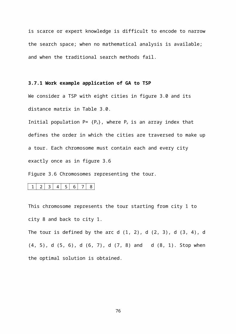
defines the order in which the cities are traversed to make up

a tour. Each chromosome must contain each and every city

exactly once as in figure 3.6

Figure 3.6 Chromosomes representing the tour.

1 2 3 4 5 6 7 8

This chromosome represents the tour starting from city 1 to

city 8 and back to city 1.

The tour is defined by the arc d (1, 2), d (2, 3), d (3, 4), d

(4, 5), d (5, 6), d (6, 7), d (7, 8) and d (8, 1). Stop when

the optimal solution is obtained.

76

Iteration 1: g=0

Step 1:

We generate some random individual solutions and pick two of

these solutions. We then evaluate their fitness. The shorter a

route the higher its fitness value. These random solutions

are;

P1= {1-3-8-7-6-5-4-2}, with f1=59

P2= {1-2-3-5-4-6-7-8}, with f2=43

Step 3:

This random individual solution represents the parents on

which we apply a partially matched crossover (PMX) operation.

P1= {1 3 8 7 6 5 4 2}

P2= {1 2 3 5 4 6 7 8}

Crossover is performed in the centre region to yield the

following offspring:

P1~ = 1 3 8 5 4 HH2

P2~ = 1 2 3 7 6 HH8

The 'H' positions are holes in the offspring left by the

deliberate removal of alleles which would otherwise be

replicated in the crossing region. These holes are filled by

77

cross-referencing with the parent of the alternate chromosome.

This can best be explained with this step:

1. Take the sixth hole in P1~ at index 6, the missing allele

value at this position in P1 is 5.

2. Search along P2 (the alternate parent of P1~) and match

the sixth allele encountered with a value of 5. This

occurs in P2 at index 4.

3. Fill H [6] in P1~ with the allele found at P1 [4], a value

of 7.

Applying this process to the remaining holes, we obtain the

following PMX offspring:

P1' = 13854762

P2' = 12376458

Step 4:

Apply mutation on the two offsprings. Allele index 3 is

selected for inversion. The value is simply exchanged with the

allele at an additional randomly selected index, let's say

index 6, as follows:

iP1' = 13754862

iP2' = 12476358

78

Hence, allele positions 3 and 6 have been exchanged.

Evaluate the objective function:

iP1' = (1-3-7-5-4-8-6-2), with f1= 74 km

iP2' = (1-2-4-7-6-3-5-8), with f2= 54 km

We choose offspring iP2' as new individual since it has a

shorter tour length.

Step 5:

The new individual replaces the old individual to obtain a new

population. Since the end condition is not met we continue the

next iteration and set the counter g=g+1

3.8 Omicron Genetic Algorithm (OGA)

Using SGA as a reference point, another version called Omicron

Genetic Algorithm (OGA) is a genetic algorithm designed

specifically for the TSP. The following are steps used in

OGA;

3.8.1 Codification

Every population of individual Px of P is a valid TSP tour and

is determined by the arcs (i, j) that compose the tour. The OGA

uses n-ary codification unlike binary codification used in SGA.

79

Considering a TSP with 6 cities c1,c2,c3,c4,c5 and c6, the tour

defined by the arcs (c1,c5), (c5,c3), (c3,c4), (c4,c2), (c2,c6) and (c6,c1) will

be codified with a string containing the visited cities in

order, that is {c1,c5,c3,c4,c2,c6}.

3.8.2 Reproduction

In the OGA, two parents (F1 and F2) are randomly selected from the

population P, as does an SGA reproduction. The selection of a

parent is done based on a probability proportional to the

fitness of each individual Px, fitness (Px) α 1/l (Px). In OGA

both parents randomly selected for reproduction generate only

one offspring unlike the SGA where two parents generate two

offspring. Once an offspring is generated in OGA, it replaces

the oldest element of P unlike in SGA p offspring are obtained

first to completely replace the old generation. In OGA

population exchange are made in a progressive way to obtain a

totally new generation.

3.8.3 Crossover and Mutation

To obtain an offspring who represents valid tour, the

crossover and mutation operators are done in a single

operation called Crossover-Mutation in OGA unlike the SGA 80

where crossover and mutation are done separately. To perform

the Crossover-Mutation, arcs of the problem are put in the

roulette, where every arc has a weight w or a probability to

be chosen. Crossover-Mutation gives a weight w of 1 to each

arc (i, j) belonging to set A, that is

w(i, j) =1 (∀ i, j) ∈ A, then a weight of O/2 is added to each arc(i,j) of

F1, that is

w(i,j)=w(i,j)+ O/2 ∀i, j F∈ 1, where Omicron (O) is an input parameter of

the OGA. Iteratively, arcs are randomly chosen using the

roulette in other to generate a new offspring.

To generate an offspring S1, an arc of a parent with a high

probability is selected and new information may be added to

allow for the creation of a valid tour to participate in the

roulette with probability greater than 0, which is similar to

mutation. The value O/2 is used because there are two parents

and then, wmax =O+1may be interpreted as the maximum weight an

arc can have in the roulette (when the arc belongs to both

parents). When the arc does not belong to any parent, it

obtains the minimum weight wmin in the roulette, that is wmin=1.

Then, O determines the relative weight between crossover and

mutation.

81

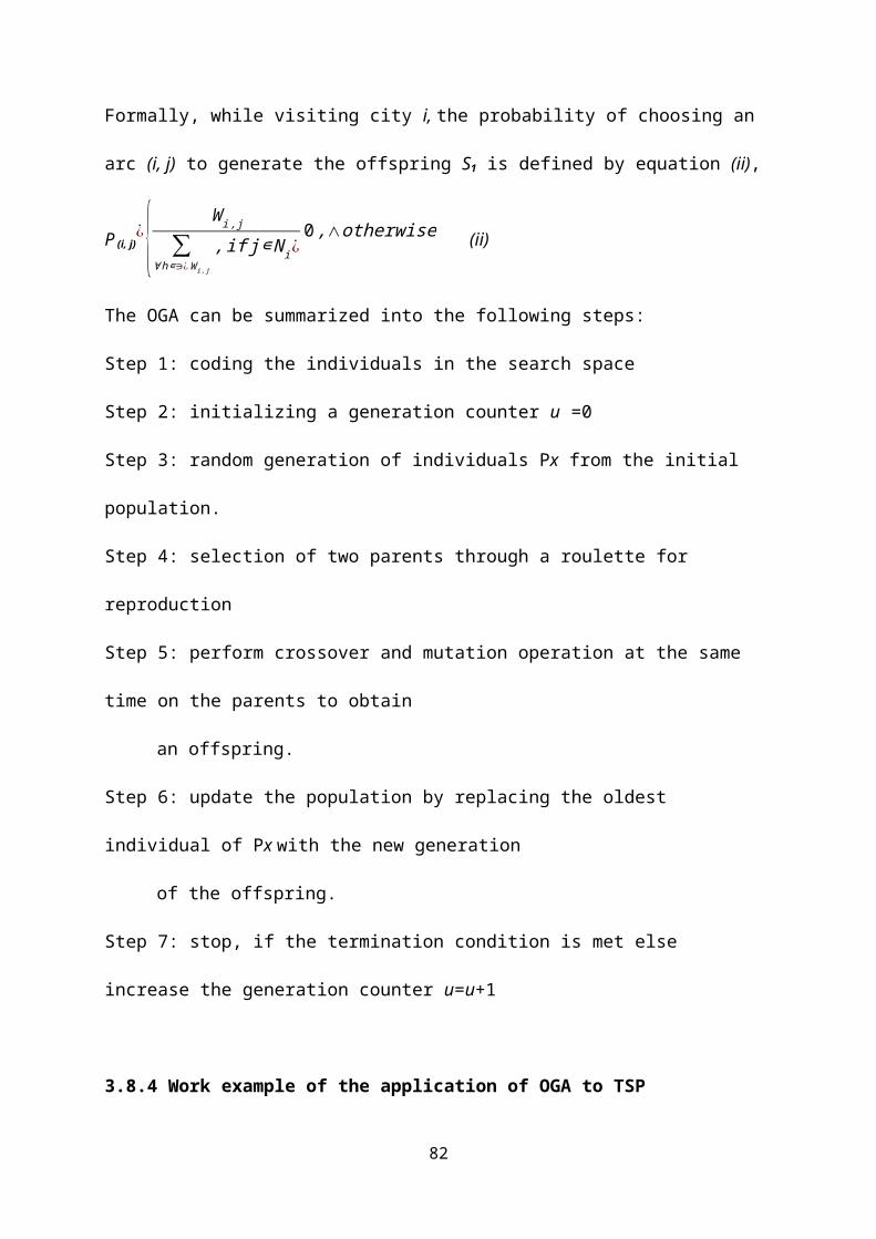
Formally, while visiting city i, the probability of choosing an

arc (i, j) to generate the offspring S1 is defined by equation (ii),

P (i, j)¿ { Wi,j

∑∀h∊∋¿Wi,j

,ifj∊Ni¿0,∧otherwise (ii)

The OGA can be summarized into the following steps:

Step 1: coding the individuals in the search space

Step 2: initializing a generation counter u =0

Step 3: random generation of individuals Px from the initial

population.

Step 4: selection of two parents through a roulette for

reproduction

Step 5: perform crossover and mutation operation at the same

time on the parents to obtain

an offspring.

Step 6: update the population by replacing the oldest

individual of Px with the new generation

of the offspring.

Step 7: stop, if the termination condition is met else

increase the generation counter u=u+1

3.8.4 Work example of the application of OGA to TSP

82

Step 1: Codification

We consider a TSP with eight cities c1, c2, c3, c4, c5, c6, c7

and c8 in figure 3.0

Initial population P= {Px}, where Px is an array index that

defines the order in which the cities are traversed to make up

a tour. The tour is defined by the arcs (c1, c2), (c2, c3),

(c3, c4), (c4,c5), (c5, c6), (c6, c7), (c7,c8), (c8,c1) . O =4

and p=5 are considered for this example.

83

Step 2: Reproduction

We assume an initial population is composed of 5 randomly

selected individual with their respective fitness fx. Nci is the

set of cities not yet visited. This initial population is

presented as;

First: P1 ={c1, c2, c3, c4, c5, c6, c7, c8}, with f1=46

Second: P2 = {c1, c3, c4, c6, c7, c8, c2, c5}, with f2=61

Third: P3 = {c3, c5, c1, c6, c2, c4, c8, c7}, with f3=84

Forth: P4 = {c2, c7, c8, c4, c3, c6, c1, c2}, with f4=74

Fifth: P5 = {c7, c3, c8, c4, c3, c2, c5, c1}, with f5=79

Two parents are randomly selected through the roulette where

the weights of solutions in the roulette are their fitness. We

assume the solutions P2 and P3 as the parents selected.

F1 = {c1, c3, c4, c6, c7, c8, c2, c5} = {(c1,c3),(c3,c4),

(c4,c6),(c6,c7),(c7,c8),(c8,c2),(c2,c5),(c5,c1)}

F2 = {c3, c5, c1, c6, c2, c4, c8, c7} ={(c3,c5),(c5,c1),

(c1,c6),(c6,c2),(c2,c4),(c4,c8),(c8,c7),(c7,c3)}

Step 3: Crossover and mutation

Iteration 1

We assume c7 as the random initial city.

Then, Nc7 is composed by {c1, c2, c3, c4, c5, c6, c8}

84

The arcs {(c7, c1), (c7, c2),(c7, c4),(c7,c5)} have weights of

1 in the roulette because they did not belong to any parent.

The arc (c7, c8) has weight of 1+ O = 5 in the roulette because

it belongs to both parents.

The arcs {(c7, c3), (c7, c6)} have weights of 1+ O/2 =3 in the

roulette because they belongs to one parents.

We assume arc (c7, c6) as randomly chosen through the

roulette.

85

Iteration 2

We pick c6 as the random initial city.

Then, Nc6 is composed by {c1, c2, c3, c4, c5, c8}

The arcs {(c6,c3), (c6,c5),(c6,c8)} have weights of 1 in the

roulette because they did not belong to any parent.

The arcs {(c6, c1), (c6,c2),(c6,c4)} have weights of 1+ O/2 = 3

in the roulette because it belongs to one parent.

We assume arc (c6, c3) as randomly chosen through the

roulette.

Iteration 3

We pick c3 as the random initial city.

Then, Nc3 is composed by {c1, c2, c4, c5, c8}

The arcs {(c3,c2), (c3,c8)} have weights of 1 in the roulette

because they does not belong to any parent.

The arcs {(c3, c1), (c3,c4),(c3,c5)} have weights of 1+ O/2 = 3

in the roulette because they belong to one parent.

We assume arc (c3, c4) as randomly chosen through the

roulette.

Iteration 4

We pick c4 as the random initial city.

Then, Nc4 is composed by {c1, c2, c5, c8}

86

The arc {(c4,c1),(c4,c5)} have minimum weight of 1 in the

roulette because it does not belong to any parent.

The arcs {(c4,c8),(c4, c2)} have weights of 1+ O/2 = 3 in the

roulette because it belongs to one parent.

We assume arc (c4, c1) as randomly chosen through the

roulette.

Iteration 5

We assume c1 as the random initial city.

Then, Nc5 is composed by {c2, c5, c8}

The arc {(c1,c2),(c1,c8)} have weights of 1 in the roulette

because it does not belong to any parent.

The arc (c1,c5) has weights of 1+ O = 5 in the roulette because

it belongs to both parent.

We pick arc (c1, c5) as randomly chosen through the roulette.

Iteration 6

We pick c5 as the random initial city.

Then, Nc5 is composed by {c2, c8}

The arc (c5, c8) has weight of 1 in the roulette because it

does not belong to any parent.

The arc (c5, c2) has weight of 1+ O/2 = 3 in the roulette

because it belongs to one parent.

87

We assume arc (c5, c2) as randomly chosen through the

roulette.

Iteration 7

We pick c2 as the random initial city.

Then, Nc2 is composed by {c8}

The arc (c2, c8) has weight of 1+O/2 in the roulette because

it belongs to one parent.

We assume (c2, c8) as the final arc.

The new offspring is S1 ={c7,c6,c3,c4,c1,c5,c2,c8}={(c7,c6),

(c6,c3),(c3,c4),(c4,c1),(c1,c5),(c5,c2),(c2,c8)}.

S1has 5 arcs in F1 {(c7,c6),(c3,c4),(c1,c5),(c5,c2),(c2,c8)} and

no arc in F2. Additionally, S1 has these arcs {(c6, c3), (c4,

c1)} which does not belong to any parent.

Step 4: Population update

The new offspring S1 replaces the oldest solution P3

P1 ={c1, c2, c3, c4, c5, c6, c7, c8}, with f1=56

P2 = {c1, c3, c4, c6, c7, c8, c2, c5}, with f2=61

P3 = {c7, c6, c5, c4, c3, c2, c1, c8}, with f3=61

P4 = {c2, c7, c8, c4, c3, c6, c1, c2}, with f4=74

P5 = {c7, c3, c8, c4, c3, c2, c5, c1}, with f5=79

88

We continue with the next iteration until the end condition is

satisfied.

3.9 New Strategies for OGA

New strategies referred to crossover, population update and

heuristic information are proposed for OGA. Considering that

the most relevant aspect mentioned in OGA is the crossover of

multiple parents, this new version is called Multi-Parent OGA

(MOGA).

3.9.1 Crossover

We consider the generation of offspring through the crossover

of multiple parents. This idea is not new and it was proposed

before Mühlenbein and Voigt (1995). More specifically, this

strategy proposes that the p individuals of P are parents

without any roulette intervention. Obviously, this crossover

of p parents eliminates competition among individuals during

reproduction. Nevertheless, the new population update strategy

proposed in the next section will solve this completion

problem. Considering that there are p parents instead of 2, a

weight of O/p is added to each arc (i, j) belonging to every Fx,

i.e. w(i, j) = w(i, j) + O/p ∀(i, j) ∈ Fx. This way, when an arc belongs to

89

the p parents, the weight of the arc will be wmax = O + 1. When

an arc does not belong to any parent, the weight of the arc

will be wmin = 1. This is done to maintain the weight limits

(wmax and wmin).

3.9.2 Population Update

To reduce the possibilities that a bad individual enters the

population, a competition strategy among offspring is

considered. This new strategy replaces the most traditional

parent competition strategy. This strategy consists on the

generation of t offspring {S1, ..., St} in one iteration. Only the

offspring with the best fitness (Sbest ∈ {S1... St}) is chosen to

enter P. As in the OGA population update strategy, Sbest replaces

the oldest individual of the population. Notice that the same

effect is obtained (competition among individuals) with a

different strategy.

3.9.3 Heuristic Information

Good TSP tours are composed with high probability by arcs with

short length. Thus, it seems a good idea to give them better

weights in the roulette. Then, considering the heuristic

90

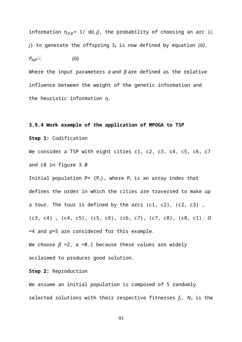
information η (i, j) = 1/ d(i, j), the probability of choosing an arc (i,

j) to generate the offspring S1 is now defined by equation (iii).

P(i,j)¿¿ (iii)

Where the input parameters α and β are defined as the relative

influence between the weight of the genetic information and

the heuristic information η.

3.9.4 Work example of the application of MPOGA to TSP

Step 1: Codification

We consider a TSP with eight cities c1, c2, c3, c4, c5, c6, c7

and c8 in figure 3.0

Initial population P= {Px}, where Px is an array index that

defines the order in which the cities are traversed to make up

a tour. The tour is defined by the arcs (c1, c2), (c2, c3) ,

(c3, c4) , (c4, c5), (c5, c6), (c6, c7), (c7, c8), (c8, c1). O

=4 and p=5 are considered for this example.

We choose β =2, α =0.1 because these values are widely

acclaimed to produces good solution.

Step 2: Reproduction

We assume an initial population is composed of 5 randomly

selected solutions with their respective fitnesses fx. Nci is the

91

set of cities not yet visited. This initial population is

presented as;

First: P1 = {c1, c2, c3, c4, c5, c6, c7, c8}, with f1=56

Second: P2 = {c1, c3, c4, c6, c7, c8, c2, c5}, with f2=61

Third: P3 = {c3, c5, c1, c6, c2, c4, c8, c7}, with f3=84

Forth: P4 = {c2, c7, c8, c4, c3, c6, c1, c2}, with f4=74

Fifth: P5 = {c7, c3, c8, c4, c3, c2, c5, c1}, with f5=79

Consider there are p parents randomly selected as P1, P2 and P3.

F1 = {c1, c2, c3, c4, c5, c6, c7, c8} =

{(c1,c2),(c2,c3),(c3,c4),(c4,c5),(c5,c6),(c6,c7),(c7,c8),

(c8,c1)}

F2 = {c1, c3, c4, c6, c7, c8, c2, c5} = {(c1,c3),(c3,c4),

(c4,c6),(c6,c7),(c7,c8),(c8,c2),(c2,c5),(c5,c1)}

F3 = {c3, c5, c1, c6, c2, c4, c8, c7} ={(c3,c5),(c5,c1),

(c1,c6),(c6,c2),(c2,c4),(c4,c8),(c8,c7),(c7,c3)}

Step 3: Crossover and mutation

Iteration 1

We assume c7 as the random initial city.

Then, Nc7 is composed by {c1, c2, c3, c4, c5, c6, c8}

The arcs {(c7, c3), (c7, c6), (c7, c8)} have weights wmax =

O+1=5 because they belong to p parents.

92

The arcs {(c7, c1), (c7, c2), (c7, c4), (c7, c5)} have weights

wmin =1 because it does not belongs to any p parents.

We assume arc (c7, c6) as randomly chosen through the

roulette.

Iteration 2

We assume c6 as the random initial city.

Then, Nc6 is composed by {c1, c2, c3, c4, c5, c8}

The arcs {(c6, c1), (c6, c2), (c6, c4), (c6,c5)}have weights

wmax = O+1=5 because they belong to p parents.

The arc {(c6, c3), (c6, c8)} have weights wmin =1 because it

does not belongs to any p parents.

We assume arc (c6, c2) as randomly chosen through the

roulette.

Iteration 3

We assume c5 as the random initial city.

Then, Nc5 is composed by {c1, c2, c3, c4, c8}

The arcs {(c2, c1), (c2, c3), (c2, c4), (c2, c5), (c2, c8)}

have weights wmax = O+1=5 because they belong to p parents.

No arc belongs to any p parents.

We assume arc (c2, c4) as randomly chosen through the

roulette.

Iteration 493

We assume c4 as the random initial city.

Then, Nc4 is composed by {c1, c3, c5, c8}

The arcs {(c4, c3), (c4, c5), (c4, c8)} have weights wmax =

O+1=5 because they belong to p parents.

The arc (c4, c1) has weight wmin =1 because it does not belongs

to any p parents.

We assume arc (c4, c3) as randomly chosen through the

roulette.

Iteration 5

We assume c3 as the random initial city.

Then, Nc3 is composed by {c1, c5, c8}

The arcs {(c3, c1), (c3, c5)} have weights wmax = O+1=5 because

they belong to p parents.

The arc (c3, c8) has weight wmin =1 because it does not belongs

to any p parents.

We assume arc (c3, c5) as randomly chosen through the

roulette.

Iteration 6

We assume c5 as the random initial city.

Then, Nc5 is composed by {c1, c8}

The arc {(c5, c1)} has weight wmax = O+1=5 because they belong

to p parents.94

The arc {(c5, c8)} has weight wmin =1 because it does not

belongs to any p parents.

We assume arc (c5, c1) as randomly chosen through the

roulette.

Iteration 7

We assume c1 as the random initial city.

Then, Nc1 is composed by {c8}

The arc {(c1, c8)} has weight wmax = O+1=5 because it belongs

to p parent.

The arc (c1, c8) is chosen because it is the unique

representation of the roulette.

The best offspring is S1 ={c7,c6,c2,c4,c3,c5,c1,c8}={(c7,c6),

(c6,c2),(c2,c4),(c4,c3),(c3,c5),(c5,c1),(c1,c8)}.

S1has 3 arcs in F1 {(c7,c6),(c4,c3),(c1,c8)}, 3 arcs in

F2{(c6,c7),(c4,c3),(c5,c1)} and 4 arcs in F3{(c6,c2),(c2,c4),

(c3,c5),(c5,c1)}.

The new best offspring Sbest ={c7,c6,c2,c4,c3,c5,c1,c8}={(c7,c6),

(c6,c2),(c2,c4),(c4,c3),(c3,c5),(c5,c1),(c1,c8)}.

Step 4: Population update

The best offspring Sbest is chosen to enter P

P1 = {c1, c2, c3, c4, c5, c6, c7, c8}, with f1=5695

P2 = {c1, c3, c4, c6, c7, c8, c2, c5}, with f2=61

P3 = {c3, c5, c1, c6, c2, c4, c8, c7}, with f3=84

P4 = {c2, c7, c8, c4, c3, c6, c1, c2}, with f4 =74

P5 = {c7, c3, c8, c4, c3, c2, c5, c1}, with f5=79

P6 = {c7, c6, c2, c4, c3, c5, c1, c8}, with f5= 68

We continue with the next iteration until the end condition is

satisfied.

96

CHAPTER 4

DATA COLLECTION, ANALYSIS AND RESULTS

The network for the traveling salesman consists of nineteen

(19) administrative centres of the National Health Insurance

Scheme (NHIS) among which the total distance is to be

minimized. These centres will be represented as nodes with

their respective names as shown in Table 4.0.

Table 4.0 Nodes and their respective administrative centres

Nodes Name of Centre

Nodes Name of Centre

1Sunyani Municipal 11 Tain District

2Berekum Municipal 12 Tano North

3 Dormaa District 13 Tano South

4 Jaman North 14Techiman Municipal

5 Jaman South 15 Atebubu6 Kintampo North 16 Asutifi District7 Kintampo South 17 Asunafo North

8Nkoranza District 18 Asunafo South

9 Pru 19 Wenchi District10 Sene

Figure 4.1 shown below is the geographical positioning of

administrative centres of NHIS in Ghana. The focus of our

study is Brong Ahafo region of Ghana.

97

Figure 4.1 Map of administrative centres of NHIS in Ghana.

The Table 4.1 below displays the matrix of edge distances (in

Km) of direct road link between the nineteen (19)

administrative centres of NHIS in the Brong Ahafo region with

sunyani as the starting node. The vertices v(i,i) = 0, indicates

98

distance between a node and itself. Where there is infinity

(inf) means no direct link between nodes. The matrix of edge

distances of road links between nodes is displayed in Table

4.1. They were obtained from the Ghana Highways Authority in

sunyani.

99

Table 4.1 Display of matrix of edge distances of road link between nodes.

Node 1 2 3 4 5 6 7 8 9

10 11

12

13

14 15

16

17

18

19

1 0 34

Inf

Inf

inf

Inf

Inf

Inf

Inf

Inf

Inf

41

54

66

Inf

70

Inf

inf

65

234 0

46

Inf

40

Inf

Inf

Inf

Inf

Inf

108

Inf

Inf

Inf

Inf

inf

Inf

Inf

Inf

3

inf 46 0

Inf

50

Inf

Inf

Inf

Inf

Inf

Inf

Inf

Inf

Inf

Inf

Inf

Inf

Inf

Inf

4

Inf

Inf

Inf 0

32

142

Inf

Inf

Inf

Inf 60

Inf

Inf

Inf

Inf

Inf

Inf

Inf

Inf

5

Inf 40

50 32 0

Inf

Inf

Inf

Inf

Inf

Inf

Inf

Inf

Inf

Inf

Inf

Inf

Inf

Inf

6

Inf

Inf

Inf

142

Inf 0

32

Inf

78

Inf 88

Inf

Inf

60

130

Inf

Inf

Inf

Inf

7

Inf

Inf

Inf

Inf

Inf 32 0

44

Inf

Inf

Inf

Inf

Inf

64

Inf

Inf

Inf

Inf

Inf

8

Inf

Inf

Inf

Inf

Inf

Inf

44 0

Inf

Inf

Inf

Inf

Inf

30 64

Inf

Inf

Inf

Inf

9

Inf

Inf

Inf

Inf

Inf 78

Inf

Inf 0

Inf

Inf

Inf

Inf

Inf 69

Inf

Inf

Inf

Inf

10

Inf

Inf

Inf

Inf

Inf

Inf

Inf

Inf

Inf 0

Inf

Inf

Inf

Inf 68

Inf

Inf

Inf

Inf

11

Inf

108

Inf 60

Inf 88

Inf

Inf

Inf

Inf 0

Inf

Inf

Inf

Inf

Inf

Inf

Inf

33

1241

Inf

Inf

Inf

Inf

Inf

Inf

Inf

Inf

Inf

Inf 0

36

Inf

Inf

Inf

Inf

Inf

Inf

1354

Inf

Inf

Inf

Inf

Inf

Inf

Inf

Inf

Inf

Inf

36 0

Inf

Inf

52

20

Inf

Inf

1466

Inf

Inf

Inf

Inf 60

64

30

Inf

Inf

Inf

Inf

Inf 0

Inf

Inf

Inf

Inf

30

15

Inf

Inf

Inf

Inf

Inf

130

Inf

64

69

68

Inf

Inf

Inf

Inf 0

Inf

inf

Inf

Inf

1670

Inf

Inf

Inf

Inf

Inf

Inf

Inf

Inf

Inf

Inf

Inf

52

Inf

inf 0

30

Inf

Inf

17

Inf

Inf

Inf

Inf

Inf

Inf

Inf

Inf

Inf

Inf

Inf

Inf

20

Inf

Inf

30 0

20

Inf

18

inf

Inf

Inf

Inf

Inf

Inf

Inf

Inf

Inf

Inf

Inf

Inf

Inf

Inf

Inf

Inf

20 0

inf

1965

inf

Inf

Inf

Inf

Inf

Inf

Inf

Inf

inf 33

Inf

Inf

30

Inf

inf

Inf

Inf 0

100

Program code based on the Floyd-Warshall algorithm is used to

compute all pair shortest possible path on the data in Table

4.1 to obtain a complete all pairs shortest path distance

matrix which will be used for our analysis. The shortest path

complete distance matrix is a complete undirected graph with

vertices v (i, j). The v (i, i) = v (j, j) = 0, indicates no distance

between same node. The all pairs shortest path distance matrix

is displayed in Table 4.2.

101

Table 4.2 Display of all pairs shortest path distance matrix

{di,j}

Nodes 1 2 3 4 5 6 7 8 9 10 11 12 13 14 15 16 17 18 19

1 0 34 80106 74

126

130 96

204

228 98 41 54 66

160 70 74 94 65

2 34 0 46 72 40160

164

130

238

262

108 75 88

100

194

104

108

128 99

3 80 46 0 82 50206

210

176

284

308

142

121

134

146

240

150

154

174

145

4106 72 82 0 32

142

174

153

220

285 60

147

160

123

217

176

180

200 93

5 74 40 50 32 0174

204

170

252

302 92

115

128

140

234

144

148

168

125

6126

160

206

142

174 0 32 76 78

198 88

167

180 60

130

196

200

220 90

7130

164

210

174

204 32 0 44

110

176

120

171

184 64

108

200

204

224 94

8 96130

176

153

170 76 44 0

133

132 93

137

150 30 64

166

170

190 60

9204

238

284

220

252 78

110

133 0

137

166

245

258

138 69

274

278

298

168

10228

262

308

285

302

198

176

132

137 0

225

269

282

162 68

298

302

322

192

11 98108

142 60 92 88

120 93

166

225 0

139

152 63

157

168

172

192 33

12 41 75121

147

115

167

171

137

245

269

139 0 36

107

201 86 56 76

106

13 54 88134

160

128

180

184

150

258

282

152 36 0

120

214 50 20 40

119

14 66100

146

123

140 60 64 30

138

162 63

107

120 0 94

136

140

160 30

15160

194

240

217

234

130

108 64 69 68

157

201

214 94 0

230

234

254

124

16 70104

150

176

144

196

200

166

274

298

168 86 50

136

230 0 30 50

135

17 74108

154

180

148

200

204

170

278

302

172 56 20

140

234 30 0 20

139

18 94128

174

200

168

220

224

190

298

322

192 76 40

160

254 50 20 0

159

19 65 99145 93

125 90 94 60

168

192 33

106

119 30

124

135

139

159 0

4.1 MODEL FORMULATION OF THE PROBLEM

102

The following assumptions and notations are used in developing

the model:

Let:

i. The total number of nodes is n

ii. d (i, j) the distance between node i (i=1,2,..,n) and node j(j=1,2,

…,n) is obtained from Table 4.2 and n =19.

iii. for each link (i, j), x(i, j)=1 if link (i, j) is part of the

tour else x(i, j) = 0

iv. The network is connected and therefore each city will

be visited.

v. A is the set of arcs of the network.

Referring to model formulation in chapter 3 section 3.2. The

tour length TL is defined as;

TL =∑i,j

nd(i,j)x(i,j)

103

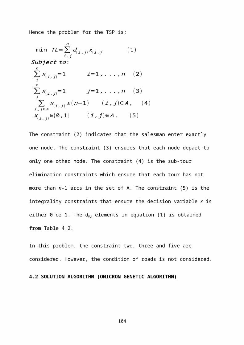
Hence the problem for the TSP is;

min TL=∑i,j

nd(i,j)x(i,j) (1)

Subject to:

∑i

nx

(i,j)=1 i=1,...,n (2)

∑j

nx(i,j)=1 j=1,...,n (3)

∑i,j∈A

x(i,j )

≤(n−1) (i,j)∈A, (4)

x(i,j)

∈{0,1} (i,j)∈A. (5)

The constraint (2) indicates that the salesman enter exactly

one node. The constraint (3) ensures that each node depart to

only one other node. The constraint (4) is the sub-tour

elimination constraints which ensure that each tour has not

more than n-1 arcs in the set of A. The constraint (5) is the

integrality constraints that ensure the decision variable x is

either 0 or 1. The d(i,j) elements in equation (1) is obtained

from Table 4.2.

In this problem, the constraint two, three and five are

considered. However, the condition of roads is not considered.

4.2 SOLUTION ALGORITHM (OMICRON GENETIC ALGORITHM)

104

Referring to steps in solving omicron genetic algorithm in

chapter 3 sections 3.8.3. The solution algorithm is summarized

into the following steps:

Step 1: coding the individuals in the search space

Step 2: initializing a generation counter u =0

Step 3: random generation of individuals Px from the initial

population.

Step 4: selection of multi parents through a roulette for

reproduction

Step 5: perform crossover and mutation operation at the same

time on the parents to obtain

an offspring.

Step 6: update the population by replacing the oldest

individual of Px with the new generation

of the offspring.

Step 7: stop, if the termination condition is met else

increase the generation counter u=u+1

4.3 COMPUTATION PROCEDURE AND RESULTS

105

Matlab program code (Appendix A) was written to determine the

optimal solution for the tour. This program was based on the

omicron genetic algorithm.

The program was run on Dell inspiron 6000 with a processor

speed of 2.0 GHz and 1.96 GB of RAM. Twenty one (21) number of

runs and 100 iterations in each run. The input data is taken

from Table 4.2.

4.3.1 THE COMPUTATIONAL PROCEDURES

Procedure 1: The centres were 19. A solution consists of

permutation of numbers

(n=1, 2, 3,…, 19). Nineteen (19) solutions formed

a population.

Procedure 2: 21 runs each of 100 iterations were performed.

Procedure 3: generate nineteen random individuals as

population.

Procedure 4: ten individuals are randomly selected from the

population as parents through a

roulette.

Procedure 5: perform crossover-mutation on two parents to

generate an offspring.

106

Procedure 6: out of the ten individual selected as parents

five offspring are generated from the

first iteration and only the offsprings with

better fitness are chosen to

replace the weaker parent.

Procedure 7: continue from procedure 4

107

4.3.2 THE RESULTS

The Table 4.3 show the solution and fitness value obtained for

each run.

Table 4.3 Display of solution and fitness value for each run.

No.: Solution

Fitness value

1 1 13 3 15 16 11 14 19 9 10 2 6 18 12 8 7 17 4 5 10822 1 7 3 12 14 10 11 18 9 4 13 17 5 16 2 19 6 15 8 12343 1 15 2 5 18 11 7 13 17 14 4 6 10 8 19 12 9 16 3 11054 1 13 12 18 17 16 7 6 11 14 19 8 15 10 9 4 5 3 2 11205 1 12 18 17 13 16 3 10 7 6 9 15 8 19 14 11 4 5 2 12276 1 3 8 10 9 15 7 19 4 18 16 5 6 13 12 17 2 11 14 11167 1 15 18 4 19 2 12 6 17 13 14 11 9 8 3 7 10 5 16 11748 1 13 17 16 18 6 9 15 10 3 2 5 4 11 19 8 7 14 12 13649 1 19 11 2 3 5 4 7 6 9 10 15 8 14 12 13 17 18 16 117010 1 14 6 7 8 19 2 3 12 13 17 18 16 15 10 9 11 4 5 119111 1 13 3 15 16 11 14 19 9 10 2 6 18 12 8 7 17 4 5 108212 1 16 18 3 5 4 11 17 13 12 8 15 10 9 7 6 14 19 2 126313 1 7 4 6 9 16 3 15 5 2 10 12 8 11 17 14 13 19 18 118214 1 13 3 15 16 11 14 19 9 10 2 6 18 12 8 7 17 4 5 108215 1 13 3 15 16 11 14 19 9 10 2 6 18 12 8 7 17 4 5 108216 1 16 18 3 5 4 11 17 13 12 8 15 10 9 7 6 14 19 2 126317 1 13 3 15 16 11 14 19 9 10 2 6 18 12 8 7 17 4 5 108218 1 16 18 3 5 4 11 17 13 12 8 15 10 9 7 6 14 19 2 126319 1 7 4 6 9 16 3 15 5 2 10 12 8 11 17 14 13 19 18 118220 1 17 3 5 7 13 15 10 18 6 2 12 8 4 9 14 11 16 19 104721 1 14 8 10 9 15 7 6 19 11 4 5 2 3 16 17 18 13 12 1042

The results from Table 4.3 show that the twenty-first run has

the minimum fitness value of 1042 km, which represents the

order in which the nodes will be visited. The tour is

represented as;

Sunyani Municipal (starting node) Techiman Municipal

Nkoranza District Sene Pru Atebubu

Kintampo South Kintampo North Wenchi District

108

Tain District Jaman North Jaman South

Berekum Municipal Dormaa District Asutifi District

Asunafo North Asunafo South Tano South

Tano North

Appendix B displays the steps and results in one iteration.

4.3.3 DISCUSSION

This work presented a study for finding optimal distance

selection technique using omicron genetic algorithm. The

results show a valid tour of optimal value 1042 km. Here the

best tour was obtained based on the minimum fitness value. The

order in which the nodes will be visited is;

1 - 14 - 8 - 10 - 9 - 15 - 7 - 6 - 19 - 11- 4 - 5 - 2 - 3 - 16 - 17 - 18 - 13 - 12

This represents the tour;

Sunyani Municipal (starting node) Techiman Municipal

Nkoranza District Sene Pru Atebubu

Kintampo South Kintampo North Wenchi District

Tain District Jaman North Jaman South

Berekum Municipal Dormaa District Asutifi District

Asunafo North Asunafo South Tano South

Tano North

109

110

CHAPTER 5

CONCLUSION AND RECOMMENDATION

5.1 CONCLUSION

This research work used the TSP model taking into account

physical road distances in order to determine the optimal

route for inspection tour of the administrative centres of

NHIS in the Brong Ahafo region. The study applied omicron

genetic algorithm for finding the optimum route. The results

show a valid tour of optimal value of 1042 km. Here the best

inspection tour was obtained based on the minimum fitness

value. The preferred route is;

Sunyani Municipal (starting node) Techiman Municipal

Nkoranza District Sene Pru Atebubu

Kintampo South Kintampo North Wenchi District

Tain District Jaman North Jaman South

Berekum Municipal Dormaa District Asutifi District

Asunafo North Asunafo South Tano South

Tano North

111

We conclude that the objective of the research was

successfully achieved through the application of Omicron

Genetic Algorithm.

5.2 RECOMMENDATION

Upon a study of application of Omicron Genetic Algorithm to

Traveling Salesman Problem for inspection tour of the National

Health Insurance Schemes, the following recommendation could

be considered:

1. The NHIA office in the Brong Ahafo region may use this

program code to optimize the inspection tour of the

administrative centres of the NHIS.

2. Students may use this work for further research on

omicron genetic algorithm.

112

REFERENCES

1. Ammar, E. E. and Youness, E. A. (2005). Study on multiobjective

transportation problem with fuzzy numbers. Applied Mathematics and

Computation. Vol. 166, pages 241-253.

2. Applegate, D., Bixby, R., Chvátal, V. and Cook, W. J.

(2007). The traveling salesman problem. Princeton University

Press: Princeton, NJ.

3. Beckers, R., Deneubourg, J. L. and Goss, S. (1992).

Trails and U-turns in the selection of the shortest path

by the ant Lasius niger. Journal of Theoretical Biology, Vol. 159,

pages 397–415.

4. Bland, R. G. and Shallcross, D. F. (1989). "Large Travelling

Salesman Problems arising from Experimentsin X-ray Crystallography: A

Preliminary Report on Computation". Operations Research Letters.

Vol 8, pages 125-128.

5. Miller, B. and Goldberg, D. E. (1995). “Genetic

algorithm, Tournamanet selection and effect of noise,

journal computer systems. Vol. 9, pages 193-212.

6. Caro, G. D. and Dorigo, M. (1998). “Extending AntNet for

best-effort quality-of-service routing,” Proceedings of

the First Internation Workshop on Ant Colony Optimization

113

(ANTS’98). Accessed at: (http://en.wikipedia.org/

Ant_colony_optimization.htm ). Accessed on 27/11/2010.

7. Chen, W. N., ZHANG, J. and Chung, H. (2010). “Optimizing

Discounted Cash Flows in Project Scheduling. An Ant Colony

Optimization Approach”, IEEE Transactions on Systems, Man,

and Cybernetics. Part C: Applications and Reviews. Vol.40

No.5, pages 64-77.

8. Crowder, H. and Padberg, M. W. (1980). “Solving Large-

Scale Symmetric Travelling Salesman Problems to

Optimality”. Management Science. Vol. 26, pages 495-509.

9. Dawkins, R. (1986). The Blind Watchmaker, Penguin,

London.

10. Dantzig, G. B., Fulkerson, D. R. and Johnson, S. M.

(1954). “Solution of a large-Scale Traveling-Salesman

Problem”. Operation Research. Vol. 2, pages 393-410.

11. Dorigo, M. (1992). Optimization, Learning and Natural

Algorithms, PhD thesis, Politecnico di Milano, Italy.

12. Garey, M. R. and Johnson D. S. (1979). Computers and

Intractability: A Guide to the Theory of NP-Completeness, W. H. Freeman,

San Francisco.

114

13. Gerard, Reinelt (1994). The Traveling Salesman:

Computational Solution for TSP Applications. Springer-

Verlag, Berlin.

14. Goldberg, D. E. (1989). "Genetic Algorithms in Search,

Optimization, and Machine Learning". Addison-Wesley, New York.

15. Glover, F. (1986). “Future Paths for Integer

Programming and Links to Artificial Intelligence”,

Computers and Operations Research. Vol 13, pages 533-549.

16. Glover, F., Kelly, J. P. and Laguna, M. (1995).

Genetic Algorithms and Tabu Search: Hybrids for

Optimization. Computers and Operations Research. Vol. 22, No.

1, pages 111 – 134.

17. Grotschel, M. and Holland, O. (1991). “Solution of

large-scale traveling salesman Problem”. Mathematical

Programming. Vol. 51(2), pages 141-202.

18. Gutin, G., Yeo, A. and Zverovich, A. (2002).

"Traveling salesman should not be greedy: domination

analysis of greedy-type heuristics for the TSP", Discrete

Applied Mathematics. Vol. 117 (1–3), pages 81–86.

19. Mühlenbein, H. and Voigt, H. (1995). Gene Pool

Recombination in Genetic Algorithms. In Osman, H. I. and

115

Kelly J. P., editors, Proceedings of the Meta-heuristics Conference,

pages 53–62, Norwell, USA. Kluwer Academic Publishers.

20. Held, M. and Karp, R. M. (1971). “The Traveling

Salesman Problem and Minimum Spanning Tress: Part II”.

Mathematical Programming. Vol 1, pages 6-25.

21. Holland, J. (1975). “Adaptation In Natural and

Artificial Systems,” University of Michigan Press, Ann

Arbor, MI.

22. Hölldobler, B. and Wilson, E. O. (1990). The ants

,Springer-Verlag, Berlin.

23. Hillier, F.S. and Lieberman, G. J. (2005).

Introduction to Operations Research. : McGraw-Hill. 8th

Ed. New York, NY

24. Hu, X., Zhang, J. and Li, Y. (2008). Orthogonal

methods based ant colony search for solving continuous

optimization problems. Journal of Computer Science and Technology.

Vol. 23(1), pages 2-18.

25. International Labour Organization (2005). Improving

social protection for the poor: Health insurance in

Ghana, The Ghana social trust pre-Piloted project final

report. ISBN 92-2-117144-2.

116

26. Kutschera, U. (2003). A Comparative Analysis of the Darwin-

Wallace Papers and the Development of the Concept of Natural Selection.

Institut für Biologie, Universität Kassel, Germany.

27. Kirkpatrick, S., Gelett, C. D. and Vecchi, M. P.

(1983). “Optimization by Simulated Annealing". Science New Series

Vol. 220, pages 671–680.

28. Lawler E. L., Lenstra J. K., Rinnooy Kan A. H. G. and

Shmoys, D. B. (1986). The Traveling Salesman. John Wiley and

sons. Chichester, UK,

29. Guntsch, M. and Middendorf, M. (2002). A Population

Based Approach for ACO. In S. Cagnoni, J. Gottlieb, E.

Hart, M. Middendorf, and G. Rinaldi, editors, Applications of

Evolutionary Computing, Proceedings of EvoWorkshops2002: EvoCOP,

EvoIASP, EvoSTim. Vol 2279, pages 71–80, Kinsale, Ireland, 3-

4. Springer-Verlag, Berlin.

30. Guntsch, M. and Middendorf, M. (2002). Applying

Population Based ACO to Dynamic Optimization Problems. In

Ant Algorithms, Proceedings of Third International Workshop ANTS 2002,

vol. 2463 of LNCS, pages 111–122.

31. Gómez, O. and Barán, B. (2004). Reasons of ACO’s

Success in TSP. In M. Dorigo, M. Birattari, C. Blum, L.

M. Gambardella, F. Mondada, and T. Stützle, editors, 117

Proceedings of ANTS 2004 – Fourth International Workshop on Ant Colony

Optimization and Swarm Intelligence, vol. 3172 of LNCS, Brussels,

Springer-Verlag, Berlin.

32. Gómez, O. and Barán, B. (2000). “Relationship between

Genetic Algorithms and Ant Colony Optimization

Algorithms”. Available at:

(http://www.cnc.una.py/invest/paper2/oga.pdf). Accessed

on 27/11/2010.

33. Padberg, M. W and Rinaldi, G. (1987). “Optimization

of a 532- city Symmetric Traveling Salesman Problem by

Branch and Cut”. Operations Research Letters. Vol. 6:17.

34. Papadimitriou, C. H. and Steglitz, K. (1997).

“Combinatorial Optimization: Algorithms and Complexity”. Prentice Hall

of India Private Limited, India.

35. Pham, D. T. and Karaboga, D. (2000). “Intelligent

Optimisation Techniques – Genetic Algorithms, Tabu

Search, Simulated Annealing and Neural Networks”.

London: Springer-Verlag, Berlin.

36. Ravikumar, C. P. (1992). "Solving Large-scale Travelling

Salesperson Problems on Parallel Machines”.Microprocessors and

Microsystems Vol. 16(3), pages 149-158.

118

37. Ray, S. S., Bandyopadhyay, S. and Pal, S. K. (2004).

“New Operators of Genetic Algorithms for Traveling

Salesman Problem”, ICPR 2004, pages 129-170.

38. Rosenkrantz, D. J., Stearns, R. E. and Lewis, P. M.

II (1977). "An Analysis of Several Heuristics for the

Traveling Salesman Problem". SIAM Journal on Computing Vol. 6

(5), pages 563–581.

39. Sivanandam, S. N. and Deepa, S. N. (2008).

“Introduction to Genetic Algorithms”, Springer-Verlag

Berlin Heidelberg.

40. Stützle, T. and Hoos, H. H. (2000). MAX MIN Ant System,

Future Generation Computer Systems. Vol 16, pages 889-914.

41. Mahmoud, T. M. (2007). “A genetic and simulated

annealing based algorithms for solving the flow

assignment problem in computer Networks”. World academy

of science, engineering and technology. Vol. 38, pages

360-366.

42. Thomas, S. and Holger, H. H. (2000). MAX-MIN Ant

System. Future Generation Computer Systems, Vol. 16(8), pages

889–914.

119

43. Zbigniew, M. (1994). Genetic Algorithms + Data

Structures = Evolution Programs. Springer-Verlag, Berlin.

2nd edition.

120

Appendix A

MatLab Programme

function OmicronGeneticAlgorithm()

clear all;

clc;

try

%*******Load distance matrix from Table 4.2*********

dmat = load('output.txt');

catch

disp(sprintf('Error loading distance matrix from source:'));

end

pop_size=size(dmat,1);

n = pop_size;

numofparent=10;

% Verify Inputs

[nr,nc] = size(dmat);

if n ~= nr || n ~= nc

error('Invalid XY or DMAT inputs!')

end

% Initialize the Population

pop = zeros(n,n);

for k = 1:pop_size

pop(k,:) = randperm(n);

end

%initialize the combine population

combinepop=pop;

121

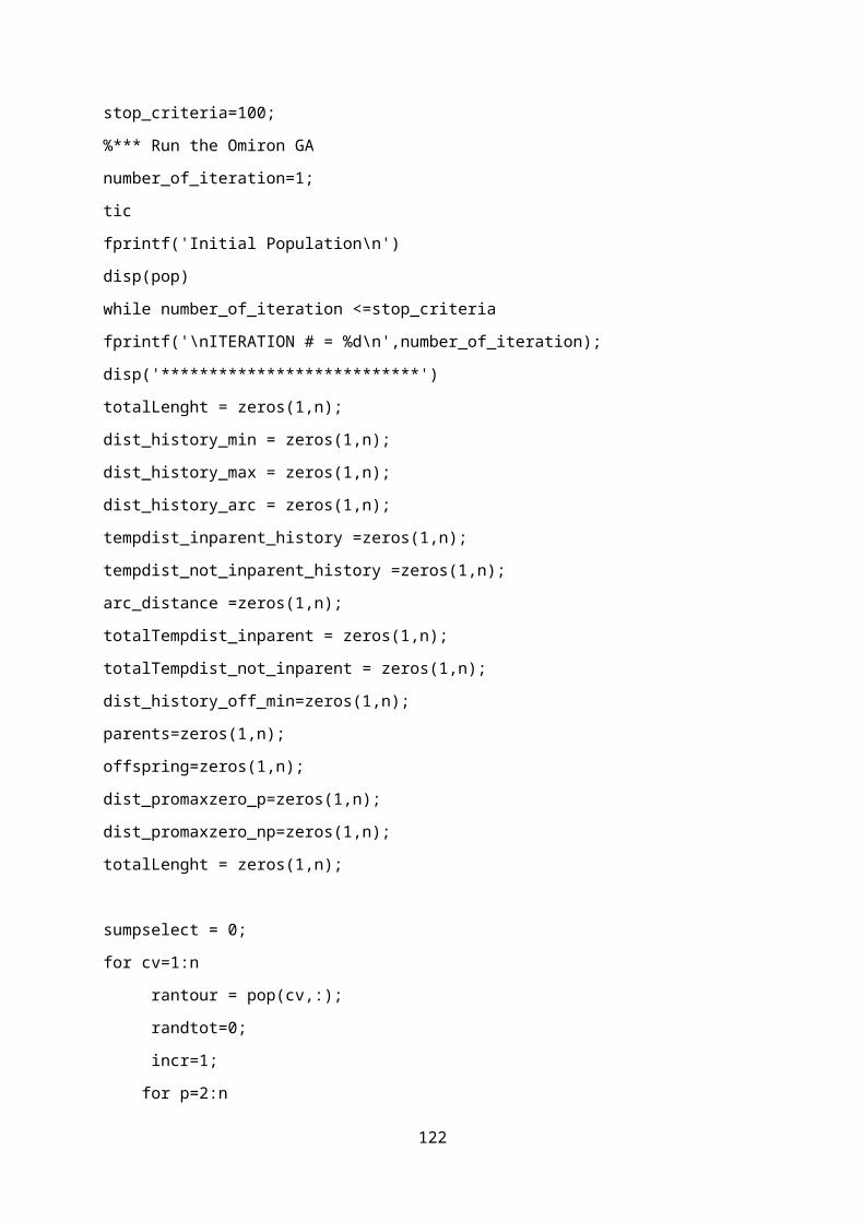
stop_criteria=100;

%*** Run the Omiron GA

number_of_iteration=1;

tic

fprintf('Initial Population\n')

disp(pop)

while number_of_iteration <=stop_criteria

fprintf('\nITERATION # = %d\n',number_of_iteration);

disp('***************************')

totalLenght = zeros(1,n);

dist_history_min = zeros(1,n);

dist_history_max = zeros(1,n);

dist_history_arc = zeros(1,n);

tempdist_inparent_history =zeros(1,n);

tempdist_not_inparent_history =zeros(1,n);

arc_distance =zeros(1,n);

totalTempdist_inparent = zeros(1,n);

totalTempdist_not_inparent = zeros(1,n);

dist_history_off_min=zeros(1,n);

parents=zeros(1,n);

offspring=zeros(1,n);

dist_promaxzero_p=zeros(1,n);

dist_promaxzero_np=zeros(1,n);

totalLenght = zeros(1,n);

sumpselect = 0;

for cv=1:n

rantour = pop(cv,:);

randtot=0;

incr=1;

for p=2:n

122

rcvalue = dmat(rantour(incr),rantour(p));

randtot = randtot + rcvalue;

incr=incr+1;

end

totalLenght(cv)=randtot;

%This calls a function to sum individual

sumpselect = fcn_sum_individual(sumpselect,randtot);

fprintf('\nPopulation #%d\t, Fitness value is =%d\n',cv,randtot)

end

spselect=0;

%Function for Roulette wheel selection, which returns results

[Excount,totalLenght,fitness]= fcn_RWS(sumpselect,n,totalLenght);

% Find the Min Route in the Population

[min_dist,index1] = min(totalLenght);

dist_history_min(cv) = min_dist;

% Find the Max Route in the Population

[max_dist,index2] = max(totalLenght);

dist_history_max(cv) = max_dist;

fprintf('\nMinimum Fitness value = %d\n',min_dist)

fprintf('\nMaximum Fitness value = %d\n',max_dist)

cpcounter=0;

zeroparent=zeros(1,n);

fprintf('\nParents selected are:\n')

disp('------------------------------------------------------')

for cparent=1:n

if Excount(cparent) >= 1.0

cpcounter=cpcounter+1;

zeroparent(cparent) =cparent;

123

if cpcounter==numofparent

break

end

end

end

%This is a function which returns parents selected

[parents]=fcn_selectparent(zeroparent,parents,pop,numofparent);

px=1;py=2; %for parent selection

for counter=1:numofparent,

route_track = zeros(1,n);

arc_in_parent=[];

arc_not_in_parent=[];

initNode = randperm(n);

route = initNode; %NODES

%begins. Generation of arcs

counterarc=2;store_arcs1=[]; store_arcs2=[];

if (py==numofparent) || (px<numofparent)

%This is a function which returns arc generated

[store_arcs1,store_arcs2]=

fcn_looparc(counterarc,store_arcs1,store_arcs2,n,parents,px,py);

for iter=1:n,

if iter == 1

Node = initNode(iter); %pick a NODE

route(iter) = [0];

else

ind=find(route==Node);

route(ind)=[0];

end

%fprintf('\nNUMBER %d RANDOM INITIAL NODE = %d',iter,Node);

124

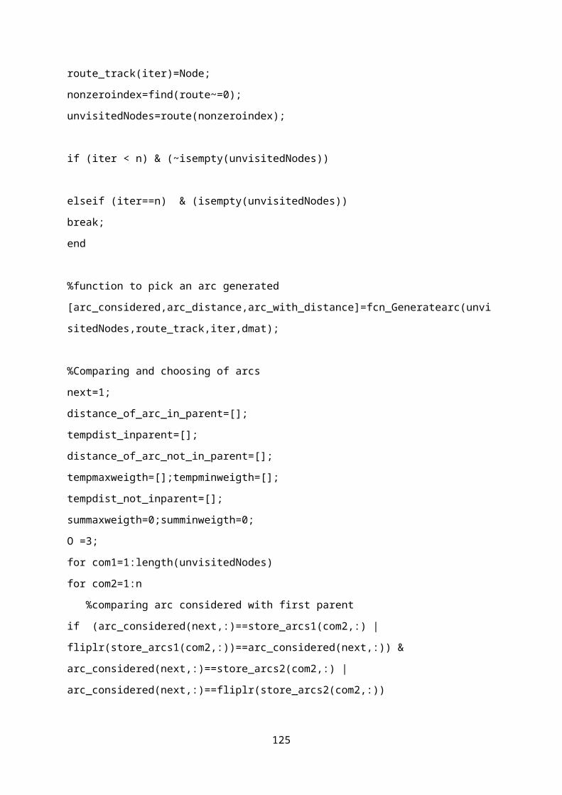
route_track(iter)=Node;

nonzeroindex=find(route~=0);

unvisitedNodes=route(nonzeroindex);

if (iter < n) & (~isempty(unvisitedNodes))

elseif (iter==n) & (isempty(unvisitedNodes))

break;

end

%function to pick an arc generated

[arc_considered,arc_distance,arc_with_distance]=fcn_Generatearc(unvi

sitedNodes,route_track,iter,dmat);

%Comparing and choosing of arcs

next=1;

distance_of_arc_in_parent=[];

tempdist_inparent=[];

distance_of_arc_not_in_parent=[];

tempmaxweigth=[];tempminweigth=[];

tempdist_not_inparent=[];

summaxweigth=0;summinweigth=0;

O =3;

for com1=1:length(unvisitedNodes)

for com2=1:n

%comparing arc considered with first parent

if (arc_considered(next,:)==store_arcs1(com2,:) |

fliplr(store_arcs1(com2,:))==arc_considered(next,:)) &

arc_considered(next,:)==store_arcs2(com2,:) |

arc_considered(next,:)==fliplr(store_arcs2(com2,:))

125

[weight]= fcn_CMArc_twoparent(O);

end

if arc_considered(next,:)==store_arcs1(com2,:) |

fliplr(store_arcs1(com2,:))==arc_considered(next,:)

%function to select arc in first parent

[heu_info,tempdist_inparent,distance_of_arc_in_parent,arc_in_parent]

=fcn_select_arcinfirstparent(next,arc_considered,arc_in_parent,arc_w

ith_distance,arc_distance,tempdist_inparent,distance_of_arc_in_paren

t);

[summaxweigth,maxweigth] =

fcn_assume_max_arc(heu_info,summaxweigth);

tempmaxweigth=[tempmaxweigth;maxweigth];

[weight]=fcn_CMArc_oneparent(O);

else

%function to select arc not found in first parent

[heu_info,tempdist_not_inparent,distance_of_arc_not_in_parent,arc_no

t_in_parent]=fcn_select_arcnotinfirstparent(next,arc_considered,arc_

not_in_parent,arc_with_distance,arc_distance,tempdist_not_inparent,d

istance_of_arc_not_in_parent);

%Function for arc with Min weigth

[summinweigth,minweigth] =

fcn_assume_min_arc(heu_info,summinweigth);

tempminweigth=[tempminweigth;minweigth];

weigth=1;

[weigth]=fcn_CMArc_noparent(weigth);

end

%comparing arc considered with next parent

if arc_considered(next,:)==store_arcs2(com2,:) |

arc_considered(next,:)==fliplr(store_arcs2(com2,:))

126

%Function to select arc in next parent

[heu_info,tempdist_inparent,distance_of_arc_in_parent,arc_in_parent]

=fcn_select_arcinfirstparent(next,arc_considered,arc_in_parent,arc_w

ith_distance,arc_distance,tempdist_inparent,distance_of_arc_in_paren

t);

%Function for arc with Max weigth

[summaxweigth,maxweigth] =

fcn_assume_max_arc(heu_info,summaxweigth);

tempmaxweigth=[tempmaxweigth;maxweigth];

[weight]=fcn_CMArc_oneparent(O);

else

%Function to select arc not found in next parent

[heu_info,tempdist_not_inparent,distance_of_arc_not_in_parent,arc_no

t_in_parent]=fcn_select_arcnotinfirstparent(next,arc_considered,arc_

not_in_parent,arc_with_distance,arc_distance,tempdist_not_inparent,d

istance_of_arc_not_in_parent);

%Function for arc with Min weigth

[summinweigth,minweigth] =

fcn_assume_min_arc(heu_info,summinweigth);

tempminweigth=[tempminweigth;minweigth];

weigth=1;

[weight]=fcn_CMArc_noparent(weigth);

end

totalTempdist_inparent = tempdist_inparent;

totalTempdist_not_inparent = tempdist_not_inparent;

end

next=next+1;

end

%prob_of_choosing_arc

127

prob_of_choosing_arc_p_parent = tempmaxweigth/summaxweigth;

prob_of_choosing_arc_n_parent = tempminweigth/summinweigth;

% Finds the Min distance of p parents

[tempdist_inparent_min_dist ,tempdist_inparent_index] =

min(totalTempdist_inparent);

tempdist_inparent_history = tempdist_inparent_min_dist;

% Find the Min distance of arc not in p parents

[tempdist_not_inparent_min_dist ,tempdist_not_inparent_index] =

min(totalTempdist_not_inparent);

tempdist_not_inparent_history = tempdist_inparent_min_dist;

% Find the arc with higher probability in p parent

[maxprob_inp,pidx] = max(prob_of_choosing_arc_p_parent);

dist_promaxzero_p = maxprob_inp;

% Find the arc with higher probability not in p parent

[maxprob_np,pnidx] = max(prob_of_choosing_arc_n_parent);

dist_promaxzero_np = maxprob_np;

% Display arcs

if ~isempty(tempdist_inparent)

%SET ZEROS IN THE NEXT NODE

next_Node=zeros(1);

%PICKS THE NEXT NODE

Node=fcn_selectnodeinparent(tempdist_inparent_index,arc_in_parent,pi

dx);

elseif ~isempty(tempdist_not_inparent) &

(isempty(tempdist_inparent))

%SET ZEROS IN THE NEXT NODE

128

next_Node=zeros(1);

%PICKS THE NEXT NODE

Node=fcn_selectnodenotinparent(tempdist_not_inparent_index,arc_not_i

n_parent,pnidx);

end

arc_in_parent=[]; %for arc picking

arc_not_in_parent=[];

end

%this keeps the offspring

offspring(counter,:)= route_track;

%Function to calculate distance for offspring

offspringtotalLenght=zeros(1,numofparent);

[offspringtotalLenght,tcv]=fcn_minDistforOffspring(offspringtotalLen

ght,n,dmat,offspring,counter);

%Finds index of offspring which are non zeros

offspringLenghtindex=find(offspringtotalLenght~=0);

offspringdistances = offspringtotalLenght(offspringLenghtindex);

[min_offspringdistances,offindx1] = min(offspringdistances);

dist_history_off_min(tcv) = min_offspringdistances;

%this append the offsprings to the initial population

tempcomindx=n+offspringLenghtindex;

combinepop(tempcomindx,:)=offspring(offspringLenghtindex,:);

%This appends the total length to the initial population

totalLenght(tempcomindx)=offspringdistances;

combinetotalLenght=totalLenght;

if py==numofparent

[comvalue,comindx]=sort(combinetotalLenght);

fprintf('\nBest solution in population are: \n')

129

disp(offspring);

fprintf('fitnesss value are: \n')

disp(offspringdistances)

disp('Combine population are:')

disp(combinepop(comindx,:));

disp('fitness value are:')

disp(comvalue')

pop=combinepop(comindx,:); %for the next initial population

end

%THIS PART GENERATES THE subsequent ARCS FOR THE PARENTS

px = px+2;

py = py+2;

end

end

number_of_iteration = number_of_iteration + 1;

t = toc;

end

disp(t)

end

function [weigth]=fcn_CMArc_noparent(weigth)

%Function for arc with max weight

weight=1;

end

function [weight]=fcn_CMArc_oneparent(O)

%Function for arc with max weight

weight=1 + O/2;

end

130

function [weight]=fcn_CMArc_twoparent(O)

%Function for arc with max weight

weight=1 + 2*(O/2);

end

function

[summaxweigth,weigth]=fcn_assume_max_arc(heu_info,summaxweigth)

beta=2.0; theta=0.3;

O=3; %Omicron(O) parameter

w_max= O +1;

weigth =(w_max^theta * heu_info^beta);

summaxweigth = summaxweigth + weigth;

end

function [summinweigth,minweigth] =

fcn_assume_min_arc(heu_info,summinweigth)

beta=2.0; theta=0.3;

w_min= 1;

summinweigth=0;

minweigth =(w_min^theta * heu_info^beta);

summinweigth= summinweigth + minweigth;

end

function [store_arcs1,store_arcs2]=

fcn_looparc(counterarc,store_arcs1,store_arcs2,n,parents,px,py)

%This is a function which returns arc generated

for looparc=1:n

if looparc~=n

genarc1(looparc,:)=parents(px,[looparc counterarc]);

genarc2(looparc,:)=parents(py,[looparc counterarc]);

else

131

genarc1(looparc,:)=parents(px,[n 1]);

genarc2(looparc,:)=parents(py,[n 1]);

end

counterarc = counterarc + 1;

store_arcs1 = [store_arcs1; genarc1(looparc,:)];

store_arcs2 = [store_arcs2; genarc2(looparc,:)];

end

end

function

[offspringtotalLenght,tcv]=fcn_minDistforOffspring(offspringtotalLen

ght,n,dmat,offspring,counter)

%Function to calculate distance for all offspring generated

for tcv=1:counter

temprantour = offspring(tcv,:);

temprandtot=0;

tincr=1;

for tp=2:n

temprcvalue = dmat(temprantour(tincr),temprantour(tp));

temprandtot = temprandtot + temprcvalue;

tincr=tincr+1;

end

offspringtotalLenght(tcv)=temprandtot;

end

end

function sumparent =fcn_sum_individual(sumparent,randtot)

%This sums the parent

sumparent = sumparent + randtot;

end

132

function [Excount,totalLenght,fitness]=

fcn_RWS(sumpselect,n,totalLenght)

%The roulette wheel selection function

spselect=0;

for sm=1:n

fitness(sm)=totalLenght(sm)/sumpselect;

%This calls a function sum individual

spselect = fcn_sum_individual(spselect,fitness(sm));

end

avgpselect=spselect/n;

for cavg=1:n

Excount(cavg)=fitness(cavg)/avgpselect;

end

end

function

[parents]=fcn_selectparent(zeroparent,parents,pop,numofparent)

%This is a function which returns parents selected

%Finds non zero index

nonzeroparentindex=find(zeroparent~=0);

lenparentindex=length(nonzeroparentindex);

%This selects the number of parents

for selectx=1:numofparent

parents(selectx,:)= pop(selectx,:);

end

for selecty=1:numofparent

fprintf('Parent %d:',selecty);

disp(parents(selecty,:))

end

end

133

function

[Node]=fcn_selectnodeinparent(tempdist_inparent_index,arc_in_parent,

pidx)

%function to select node in p parent

if ~isempty(tempdist_inparent_index)

next_Node =arc_in_parent(pidx,2);

else

next_Node =arc_in_parent(pidx);

end

Node= next_Node;

end

function

Node=fcn_selectnodenotinparent(tempdist_not_inparent_index,arc_not_i

n_parent,pnidx)

%function to select node not in p parent

if ~isempty(tempdist_not_inparent_index)

next_Node =arc_not_in_parent(pnidx,2);

else

next_Node =arc_not_in_parent(pnidx);

end

Node= next_Node;

end

function

[arc_considered,arc_distance,arc_with_distance]=fcn_Generatearc(unvi

sitedNodes,route_track,iter,dmat)

%function to pick arc generated

arc_considered=[];

dist_arc_considered=[];

for y=1:length(unvisitedNodes)

134

arc_considered =[arc_considered; route_track(iter)

unvisitedNodes(y)];

if arc_considered ~=arc_considered,

arc_considered=[arc_considered];

end

dist_arc_considered=[dist_arc_considered;dmat(route_track(iter),

unvisitedNodes(y))];

arc_distance = dist_arc_considered;

end

[arc_min_dist,arcdist_index] = min(arc_distance);

dist_history_arc(y) = arc_min_dist;

arc_with_distance=[arc_considered, arc_distance];

end

function

[heu_info,tempdist_inparent,distance_of_arc_in_parent,arc_in_parent]

=fcn_select_arcinfirstparent(next,arc_considered,arc_in_parent,arc_w

ith_distance,arc_distance,tempdist_inparent,distance_of_arc_in_paren

t)

%function to select arc in first parent

arc_in_parent =[arc_in_parent; arc_considered(next,:)];

distance_of_arc_in_parent=[distance_of_arc_in_parent;

arc_with_distance(next,:)];

tempdist_inparent = [tempdist_inparent; arc_distance(next,:)];

heu_info= (1 /arc_distance(next,:));

end

function

[heu_info,tempdist_not_inparent,distance_of_arc_not_in_parent,arc_no

t_in_parent]=fcn_select_arcnotinfirstparent(next,arc_considered,arc_

135

not_in_parent,arc_with_distance,arc_distance,tempdist_not_inparent,d

istance_of_arc_not_in_parent);

%function to select arc not in first parent

arc_not_in_parent =[arc_not_in_parent; arc_considered(next,:)];

distance_of_arc_not_in_parent=[distance_of_arc_not_in_parent;

arc_with_distance(next,:)];

tempdist_not_inparent = [tempdist_not_inparent;

arc_distance(next,:)];

heu_info= (1 /arc_distance(next,:));

end

136

Appendix B

Computational Results obtained from MatLab programITERATION # = 1

Initial Population------------------

Intpop1:[6 3 16 11 7 17 14 8 5 19 15 1 2 4 18 13 9 10 12],fitness=2607

Intpop2:[13 3 15 16 11 14 19 9 10 2 6 18 12 8 7 17 4 5 1],fitness=2559

Intpop3:[2 17 16 7 13 4 3 9 8 18 10 15 14 11 12 5 6 1 19],fitness=2537

Intpop4:[11 12 3 17 15 5 13 1 19 6 10 2 7 4 16 14 8 18 9],fitness=2847

Intpop5:[16 15 1 2 10 5 13 4 17 8 14 7 3 12 11 18 6 9 19],fitness=2848

Intpop6:[4 17 1 6 10 18 12 8 5 16 3 9 2 11 13 14 15 7 19],fitness=2775

Intpop7:[9 5 13 7 1 19 15 14 17 6 3 10 16 11 2 12 18 8 4],fitness=2899

Intpop8:[19 13 15 3 7 2 16 14 17 1 10 12 18 11 6 5 9 8 4],fitness=2966

Intpop9:[18 13 8 14 19 11 5 7 10 12 4 3 17 9 6 1 15 2 16],fitness=2347

Intpop10:[3 4 19 5 15 13 11 1 16 9 10 17 8 6 14 7 12 18 2],fitness=2526

Intpop11:[6 15 12 4 5 3 7 8 14 18 19 11 2 10 13 9 17 1 16],fitness=2528

Intpop12:[19 9 15 7 2 8 10 5 3 12 14 11 18 4 1 6 16 13 17],fitness=2304

Intpop13:[16 13 8 7 1 4 14 9 10 2 11 19 12 3 5 6 18 15 17],fitness=2440

Intpop14:[14 18 7 2 19 12 11 3 8 6 5 1 9 10 17 15 16 4 13],fitness=2977

Intpop15:[15 5 3 14 12 1 18 7 17 6 2 13 9 4 16 8 11 10 19],fitness=2878

Intpop16:[9 18 16 19 11 6 7 15 10 14 5 1 2 17 13 4 3 8 12],fitness=1905

Intpop17:[15 2 16 6 17 18 13 12 8 1 10 7 5 11 4 3 14 19 9],fitness=2209

Intpop18:[10 2 13 12 15 8 17 14 3 5 9 16 4 7 6 1 19 18 11],fitness=2607

Intpop19:[19 1 16 18 15 3 9 7 4 12 5 11 14 13 10 2 6 8 17],fitness=2734

Minimum Fitness value = 1905

Maximum Fitness value = 2977

Parents selected are:------------------------------------------------------Parent 1: [6 3 16 11 7 17 14 8 5 19 15 1 2 4 8 13 9 10 12]

Parent 2: [13 3 15 16 11 14 19 9 10 2 6 18 12 8 7 17 4 5 1]

Parent 3: [2 17 16 7 13 4 3 9 8 18 10 15 14 11 12 5 6 1 19]

Parent 4: [11 12 3 17 15 5 13 1 19 6 10 2 7 4 16 14 8 18 9]

Parent 5: [16 15 1 2 10 5 13 4 17 8 14 7 3 12 11 18 6 9 19]

Parent 6: [4 17 1 6 10 18 12 8 5 16 3 9 2 11 13 14 15 7 19]

Parent 7: [9 5 13 7 1 19 15 14 17 6 3 10 16 11 2 12 18 8 4]

Parent 8: [19 13 15 3 7 2 16 14 17 1 10 12 18 11 6 5 9 8 4]

137

Parent 9: [18 13 8 14 19 11 5 7 10 12 4 3 17 9 6 1 15 2 16]

Parent 10:[3 4 19 5 15 13 11 1 16 9 10 17 8 6 14 7 12 18 2]

Best solutions are: --------------------B1: [15 19 14 8 7 11 16 3 13 18 12 6 2 1 5 4 17 9 10],fitness=1978B2: [16 17 2 19 1 13 5 12 3 4 7 6 10 15 14 8 9 11 18],fitness=1889B3: [ 9 6 1 2 11 12 18 10 5 13 14 8 17 4 19 7 15 16 3],fitness=2488B4: [ 5 13 19 1 17 14 15 3 6 11 2 12 18 8 9 4 7 10 16],fitness=2604B5: [15 1 16 18 13 8 14 19 11 5 7 12 4 3 2 17 9 6 10],fitness=1967

Combine population is:

------------------------

Cpop1:[16 17 2 19 1 13 5 12 3 4 7 6 10 15 14 8 9 11 18],fitness=1889

Cpop2:[9 18 16 19 11 6 7 15 10 14 5 1 2 17 13 4 3 8 12],fitness=1905

Cpop3:[15 1 16 18 13 8 14 19 11 5 7 12 4 3 2 17 9 6 10],fitness=1967

Cpop4:[15 19 14 8 7 11 16 3 13 18 12 6 2 1 5 4 17 9 10],fitness=1978

Cpop5:[15 2 16 6 17 18 13 12 8 1 10 7 5 11 4 3 14 19 9],fitness=2209

Cpop6:[19 9 15 7 2 8 10 5 3 12 14 11 18 4 1 6 16 13 17],fitness=2304

Cpop7:[18 13 8 14 19 11 5 7 10 12 4 3 17 9 6 1 15 2 16],fitness=2347

Cpop8:[16 13 8 7 1 4 14 9 10 2 11 19 12 3 5 6 18 15 17],fitness=2440

Cpop9:[ 9 6 1 2 11 12 18 10 5 13 14 8 17 4 19 7 15 16 3],fitness=2488

Cpop10:[ 3 4 19 5 15 13 11 1 16 9 10 17 8 6 14 7 12 18 2],fitness=2526

Cpop11:[ 6 15 12 4 5 3 7 8 14 18 19 11 2 10 13 9 17 1 16],fitness=2528

Cpop12:[ 2 17 16 7 13 4 3 9 8 18 10 15 14 11 12 5 6 1 19],fitness=2537

Cpop13:[13 3 15 16 11 14 19 9 10 2 6 18 12 8 7 17 4 5 1],fitness=2559

Cpop14:[5 13 19 1 17 14 15 3 6 11 2 12 18 8 9 4 7 10 16],fitness=2604

Cpop15:[6 3 16 11 7 17 14 8 5 19 15 1 2 4 18 13 9 10 12],fitness=2607

Cpop16:[10 2 13 12 15 8 17 14 3 5 9 16 4 7 6 1 19 18 11],fitness=2607

Cpop17:[19 1 16 18 15 3 9 7 4 12 5 11 14 13 10 2 6 8 17],fitness=2734

Cpop18:[ 4 17 1 6 10 18 12 8 5 16 3 9 2 11 13 14 15 7 19],fitness=2775

Cpop19:[11 12 3 17 15 5 13 1 19 6 10 2 7 4 16 14 8 18 9],fitness=2847

Cpop20:[16 15 1 2 10 5 13 4 17 8 14 7 3 12 11 18 6 9 19],fitness=2848

Cpop21:[15 5 3 14 12 1 18 7 17 6 2 13 9 4 16 8 11 10 19],fitness=2878

Cpop22:[ 9 5 13 7 1 19 15 14 17 6 3 10 16 11 2 12 18 8 4],fitness=2899

Cpop23:[19 13 15 3 7 2 16 14 17 1 10 12 18 11 6 5 9 8 4],fitness=2966

Cpop24:[14 18 7 2 19 12 11 3 8 6 5 1 9 10 17 15 16 4 13],fitness=2977

ITERATION # = 2***************************

Population #1, Fitness value is =1889

Population #2, Fitness value is =1905

138

Population #3, Fitness value is =1967

Population #4, Fitness value is =1978

Population #5, Fitness value is =2209

Population #6, Fitness value is =2304

Population #7, Fitness value is =2347

Population #8, Fitness value is =2440

Population #9, Fitness value is =2488

Population #10 , Fitness value is =2526

Population #11 , Fitness value is =2528

Population #12 , Fitness value is =2537

Population #13 , Fitness value is =2559

Population #14 , Fitness value is =2604

Population #15 , Fitness value is =2607

Population #16 , Fitness value is =2607

Population #17 , Fitness value is =2734

Population #18 , Fitness value is =2775

Population #19 , Fitness value is =2847

Minimum Fitness value = 1889

Maximum Fitness value = 2847

139