Heuristics for the One-Commodity Pickup-and-Delivery Traveling Salesman Problem
Research ArticleSolving Dynamic Traveling Salesman Problem Using DynamicGaussian Process Regression
Stephen M Akandwanaho Aderemi O Adewumi and Ayodele A Adebiyi
School ofMathematics Statistics andComputer Science University of KwaZulu-Natal University RoadWestville Private Bag X 54001Durban 4000 South Africa
Correspondence should be addressed to Stephen M Akandwanaho stephenakandwanahogmailcom
Received 4 January 2014 Accepted 11 February 2014 Published 7 April 2014
Academic Editor M Montaz Ali
Copyright copy 2014 Stephen M Akandwanaho et al This is an open access article distributed under the Creative CommonsAttribution License which permits unrestricted use distribution and reproduction in any medium provided the original work isproperly cited
This paper solves the dynamic traveling salesman problem (DTSP) using dynamic Gaussian Process Regression (DGPR) methodThe problem of varying correlation tour is alleviated by the nonstationary covariance function interleaved with DGPR to generatea predictive distribution for DTSP tour This approach is conjoined with Nearest Neighbor (NN) method and the iterated localsearch to track dynamic optima Experimental results were obtained on DTSP instances The comparisons were performed withGenetic Algorithm and Simulated AnnealingThe proposed approach demonstrates superiority in finding good traveling salesmanproblem (TSP) tour and less computational time in nonstationary conditions
1 Introduction
A bulk of research in optimization has carved a niche insolving stationary optimization problems As a corollary aflagrant gap has hitherto been created in finding solutionsto problems whose landscape is dynamic to the core Inmany real-world optimization problems a wide range ofuncertainties have to be taken into account [1] These uncer-tainties have engendered a recent avalanche of research indynamic optimization Optimization in stochastic dynamicenvironments continues to crave for trailblazing solutionsto problems whose nature is intrinsically mutable Severalconcepts and techniques have been proposed for address-ing dynamic optimization problems in literature Brankeet al [2] delineate them through different stratificationsfor example those that ensure heterogeneity sustenance ofheterogeneity in the course of iterations techniques thatstore solutions for later retrieval and those that use differentmultiple populations The ramp up in significance of DTSPin stochastic dynamic landscapes has up to the hilt in thepast two decades attracted a raft of computational methodscongenial to address the floating optima (Figure 1) An in-depth exposition is available in [3 4] The traveling salesman
problem (TSP) [5] one of the most thoroughly studied NP-hard theory in combinatorial optimization arguably remainsa main research experiment that has hitherto been cast asan academic guinea pig most notably in computer scienceIt is also a research factotum that intersects with a wideexpanse of research areas for example it is widely studiedand applied by mathematicians and operation researchers ona grand scale TSPrsquos prominence ascribe to its flexibility andamenability to a copious range of problems Gaussian processregression is touted as a sterlingmodel on account of its stellarcapacity to interpolate the observations its probabilisticnature versatility practical and theoretical simplicity Thisresearch lays bare a dynamic Gaussian process regression(DGPR) with a nonstationary covariance function to giveforeknowledge of the best tour in a landscape that is subjectto change The research is in concert with the argumentationthat optima are innately fluid cognizant that size nature andposition are potentially volatile in the lifespan of the optimaThis skittish landscape most notably in optimization is a cuefor fine-grained research to track the moving and evolvingoptima and provide a framework for solving a cartload ofpent-up problems that are intrinsically dynamicWe colligateDGPRwith nearest neighbor (NN) algorithmand the iterated
Hindawi Publishing CorporationJournal of Applied MathematicsVolume 2014 Article ID 818529 10 pageshttpdxdoiorg1011552014818529
2 Journal of Applied Mathematics
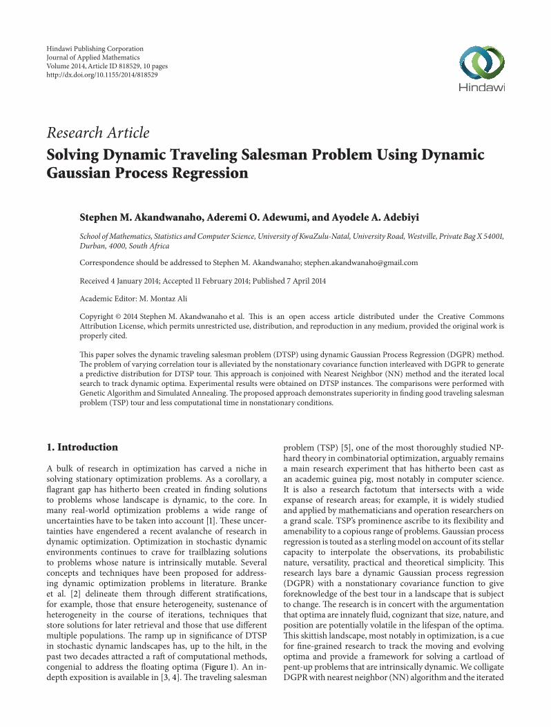
Figure 1 Nonstationary optima [6]
local search amedley whose purpose is to refine the solutionWe have arranged the paper in four sections Section 1 islimited to introduction Section 2rsquos ambit includes review ofall methods that form the mainspring of this work whichinclude Gaussian process TSP and DTSP We elucidateDGPR for solving the TSP in Section 3 Section 4 discussesresults obtained and draws conclusion
2 The Traveling Salesman Problem (TSP)
Thefirst researcher in 1932 considered the traveling salesmanproblem [7]Menger gives interestingways of solving TSPHelays bare the first approaches which were considered duringthe evolution of TSP solutions An exposition on TSP historyis available in [8ndash10]
Basic Definitions and Notations It is imperative to note thatin the gamut of TSP both symmetric and asymmetric aspectsare important threads in its fabric We factor them into thiswork through the following expressions
Basically a salesman traverses across an expanse of citiesculminating into a tourThe distance in terms of cost betweencities is computed by minimizing the path length
119891 (120587) =119899minus1
sum119894=1
119889120587(119894)120587(119894+1)
+ 119889120587(119899)120587(1)
(1)
Weprovide amomentary storage119863 for cost distanceThedis-tances between 119899 cities are stored in a distance matrix119863 Forbrevity the problem can also be situated as an optimizationproblem We minimize the tour length (Figure 5)
119899
sum119894=119899
119889119894120587(119894)
(2)
The distance matrix of TSP has got certain features whichcome in handy in defining a set of classes for TSP [11] If thecity point (119909
119894 119910119894) in a tour is accentuated then drawing from
Euclidean distance expression [11] we present the matrix 119862between separate distances as
119888119894119895= radic(119909
119894minus 119909119895)2
+ (119910119894minus 119910119895)2
(3)
Affixed to TSP are important aspects that we bring to the forein this paper We adumbrate a brief overview of symmetrictraveling salesman problem (STSP) and asymmetric travelingsalesman problem (ATSP) as follows
STSP akin to its name ensures symmetry in lengthThe distances between points are equal for all directionswhile ATSP typifies different distance sizes of points in bothdirections Dissecting ATSP gives us a handle to hash outsolutions
Let ATSP be expressed subject to the distance matrixIn combinatorial optimization an optimal value is soughtwhereby in this case we minimize using the followingexpression
119908120587(119899)120587(1)
+119899minus1
sum119894=1
119908120587(119894)120587(119894+1)
(4)
Reference [12] formulates ATSP in integer programming 1198992 minus119899 zero-one variables 119909
119894119895or else it is defined as
119910 =119899
sum119894=1
119899
sum119895=1
119908119894119895119909119894119895 (5)
such that119899
sum119894=1
119909119894119895= 1 119895 [119899]
119899
sum119895=1
119909119894119895= 1 119894 [119899]
sum119894isin119878
sum119895isin119878
119909119894119895le |119878| minus 1 forall |119878| lt 119899
119909119894119895= 0 or 1 119894 = 119895 isin [119899]
(6)
There are different rules affixed to ATSP inter alia to ensurea tour does not overstay its one-off visit to each vertex Therules also ensure that standards are defined for subtours
In the symmetry paradigm the problem is postulated Forbrevity we present subsequent work with tautness
119910 = sum1le119894le119895le119899
119908119894119895119909119894119895 (7)
such that119899
sum119894=1
119909119894119895= 2 119895 isin [119899]
sum119894isin119878
sum119895 = 119878
119909119894119895ge 2 forall3 le |119878| ge
119899
2
0 le 119909119894119895le 1 119894 = 119895 isin [119899]
119909119894119895forall119894 = 119895 isin [119899]
(8)
Journal of Applied Mathematics 3
TSP is equally amenable to the Hamiltonian cycle [11] and sowe use graphs to ram home a different solution approach tothe problemof traveling salesman In this approach we define119866 = (119881 119864) and (119890
119894isin 119864)119908
119894 This is indicative of the graph
theoryThe problem can be seen in the prism of a graph cyclechallenge Vertices and edges represent119881 and 119864 respectively
It is also plausible to optimize TSP by adopting both aninteger programming and linear programming approachespieced together in [13]
119899
sum119894=1
119899
sum119895=1
119889119894119895119909119894119895
119899
sum119894=1
119909119894119895= 1
119899
sum119895=1
119909119894119895= 1
(9)
We can also view it with linear programming for example
119898
sum119894=1
119908119894119909119894= 119908119879119909 (10)
Astounding ideas have sprouted providing profoundapproaches in solving TSP In this case few parallel edges areinterchanged We use the Hamilton graph cycle [11] equalitymatrix
forall119894 119895 119889119894119895= 1198891015840119894119895
sum119894119895isin119867
119889119894119895= 120572 sum119894119895isin119867
1198891015840119894119895+ 120573
(11)
subject to 120572 gt 0 120573 isin R The common denominator ofthese methods is to solve city instances in a shortest timepossible A slew of approaches have been cobbled togetherextensively in optimization and other areas of scientific studyThe last approach in this paper is to transpose asymmetricto symmetric The early work of [14] explicates the conceptThere is always a dummy city affixed to each city Thedistances are the same between dummies and bona fide citieswhich makes distances symmetrical The problem is thensolved symmetrically thereby assuaging the complexities ofNP-hard problems
[
[
0 1198891211988913
11988921
0 11988923
1198893111988932
0
]
]
larrrarr
[[[[[[[
[
0 infin infin minusinfin 11988921
11988931
infin 0 infin 11988912
minusinfin 11988931
infin infin 0 11988913
11988923
minusinfinminusinfin 119889
1211988913
0 infin infin11988921
minusinfin 11988923
infin 0 infin11988931
11988932
minusinfin infin infin 0
]]]]]]]
]
(12)
21 Dynamic TSP Different classifications of dynamic prob-lems have been conscientiously expatiated in [15] A widearray of dynamic stochastic optimization ontology rangesfrom a moving morphology to drifting landscapes Thedynamic optima exist owing to moving alleles in the natural
realm Nature remains the fount of artificial intelligenceOptimization mimics the whole enchilada including theintrinsic floating nature of alleles which provides fascinatinginsights into solving dynamic problems Dynamic encodingproblems were proposed by [16]
DTSP was initially introduced in 1988 by [17 18] Inthe DTSP a salesman starts his trip from a city and after acomplete trip he comes back to his own city again and passeseach city for once The salesman is behooved to reach everycity in the itinerary In DTSP cities can be deleted or added[19] on account of varied conditions The main purpose forthis trip is traveling the smallest distance Our goal is findingthe shortest route for the round trip problem
Consider a city population 119899 and 119890 as the problem athandwhere in this case we want to find the shortest path for 119899with a single visit on each The problem has been modeled ina raft of prisms A graph (119873 119864) with graph nodes and edgesdenoting routes between cities For purpose of elucidationthe Euclidean distance between cities is 119894 and 119895 is calculatedas follows [19]
119863119894119895= radic(119909
119894minus 119909119895)2
+ (119910119894minus 119910119895)2
(13)
211 Objective Function The predictive function for solvingthe dynamic TSP is defined as follows
Given a set of different costs (1198751 1198752 119875
119899(119905)) the dis-
tance matrix is contingent upon time Due to the changingroutes in the dynamic setting time is pivotal So it isexpressed as a function of distance cost The distance matrixhas also been lucidly defined in the antecedent sections Let ususe the supposition that 119863 = 119889
119894119895(119905) and 119894 119895 = 1 2 119899(119905)
Our interest is bounded on finding the least distance from119875119895and 119889
119894119895(119905) = 119889
119895119894(119905) In this example as aforementioned
time 119905 and of course cost 119889 play significant roles in thequality of the solution DTSP is therefore minimized usingthe following expression
119889 (119879 (119905)) =119899(119905)
sum119894=1
119889119879119894 119879119894+1
(119905) (14)
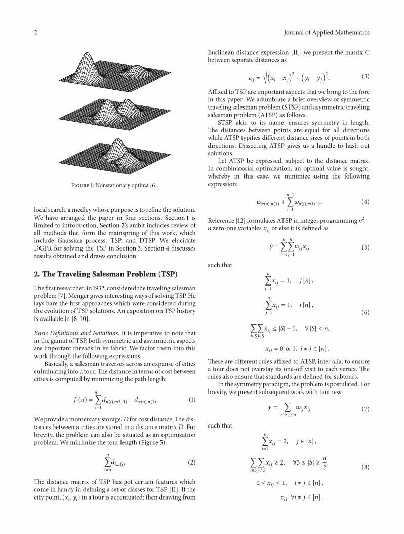
From Figures 2 3 and 4 DTSP initial route is con-structed upon visiting requests carried by the travelingsalesman AB 119862 119863 119864 [20] As the traveling salesman setsforth different requests (119883 119884) come aboutwhich compels thetraveling salesman to change the itinerary to factor in the newtrip layover demands 119860 119861 119862119863119883 119864 119884
22 Gaussian Process Regression In machine learning theprimacy of Gaussian process regression cannot be overstatedThe methods of linear and locally weighted regression havebeen outmoded by Gaussian process regression in solvingregression problems Gold mining was the major motivationfor this method where Krige whom Kriging is his brainchild[21] postulated that using posteriori the cooccurrence ofgold is encapsulated as a function of space With Krigersquosinterpolation mineral concentrations at different points canbe predicted
4 Journal of Applied Mathematics
A
B
C
D
E
Figure 2 Initial request A B C D E
A
B
C
D
E
X
Y
X
X
Figure 3 New requests for consideration
In Gaussian process we find a set of random variablesThe specifications include covariance function 119899(119909 1199091015840) andmean function 119901(119909) that parameterize the Gaussian processThe covariance function determines the similarity of differentvariables In this paper we expand the ambit of study tononstationary covariance
119901 (119891 (119909) sdot 119891 (1199091015840)) = 119873 (120583 Σ) (15)
In the equation 120583 = ( 120583(119909)120583(1199091015840)) and Σ = ( 119870(119909sdot119909) 119870(119909sdot119909
1015840)
119870(1199091015840sdot119909) 119870(119909
1015840sdot1199091015840)
) The matrices 119899 times 1 for 120583 and 119899 times 119899 for Σ are presented in
(15)GPR (Figure 6) has been extensively studied across the
expanse of predictionThis has resulted into different expres-sions to corroborate the method preference In this study wehave a constellation of training set P = (xi yi)mi=1 The GPRmodel [22] then becomes
yi = h (xi) + 120576i (16)
subject i = 1 to119898The probability density describes the likelihood for a
certain value to be assumed by a variable Given a set ofobservations bound by a number of parameters
119901 (119910 | 119883 119908) =119899
prod119894=1
119901 (119910119894| 119909119894 119908) sim 119873(119883119879119908 1205902
119899119868) (17)
In this case bias is denoted by 119908
A
B
C
D
E
X
Y
Figure 4 Previous route changed to meet new requests given to thetraveling salesman
0 5 10 15 20 250
20
40
60
80
100
120Optimal in non-stationary landscape
Cities
Dev
iatio
n
GPRDGPR
Figure 5 Minimum path generated by DGPR
Gaussian process is analogous to Bayesian with a frac-tional difference [23] In one of the computations by theBayesrsquo rule [23] is the Bayesian linear model parameterizedby covariance matrix and mean denoted by 119860minus1 and 119908respectively
119901 (119908 | 119883 119910) sim 119873(119908 = 120590minus2119899119860minus1119883119910119860minus1) (18)
where
119860 = 120590minus2119899119883119883119879 +
minus1
sum119901
(19)
Using posterior probability the Gaussian posterior is pre-sented as
119901 (119891119904| 119909119904 119883 119910) sim 119873(120590minus2
119898119909119879119904119860minus1119883119910 119909119879
119904119860minus1119909119904) (20)
Also the predictive distribution given the observed dataset
Journal of Applied Mathematics 5
0 5 10 15 20 250
10
20
30
40
50
60
70
80
90
100
Cities
Dev
iatio
n
GPRDGPR2-opt improvement
Figure 6 DGPR maintains superiority when juxtaposed with GPRand local search
helps to model a probability distribution of an interval notestimating just a point
119901 (119891119904| 119909119904 119883 119910) sim 119873(120590minus2
119898120601119879119904119860minus1Φ119910 120601119879
119904119860minus1120601119904) (21)
where by Φ = Φ(119883) 120601119904= 120601(119909
119904) and 119860 = 120590minus2
119899ΦΦ119879 + sum
minus1
119901 If
119860minus1 of size 119899 times 119899 is needed when 119899 is large We rewrite as
119873120601119879119904sum119875
Φ(119870 + 1205902119899119868)minus1
119910
120601119879119904sum119875
120601119904minus 120601119879119904sum119875
Φ(119870 + 1205902119899119868)minus1
Φ119879sum119875
120601119904
(22)
The covariance matrix119870 is Φ119879sum119901Φ
221 Covariance Function In simple terms the covariancedefines the correlation of function variables at a given time Ahost of covariance functions for GPR have been studied [24]In this example
119870(119909119894119909119895) = V0expminus(
119909119894minus 119909119895
119903)120590
+ V1+ V2120575119894119895 (23)
the parameters are V0(signal variance) V
1(variance of bias)
V2(noise variance) 119903 (length scale) and 120575 (roughness)
However in finding solutions to dynamic problems there is amounting need for nonstationary covariance functions Theproblem landscapes have increasingly become protean Thelodestar for this research is to use nonstationary covarianceto provide an approach to dynamic problems
A raft of functions have been studied A simple form isdescribed in [25]
119862N119878 (119909119894 119909119895) = 1205902
1003816100381610038161003816Σ11989410038161003816100381610038161410038161003816100381610038161003816Σ119895
1003816100381610038161003816100381614
100381610038161003816100381610038161003816100381610038161003816
Σ119894+ Σ119895
2
100381610038161003816100381610038161003816100381610038161003816
minus12
exp (minusQ119894119895)
(24)
With quadratic form
Q119894119895= (119909119894minus 119909119895)119879
(Σ119894+ Σ119895
2)
minus1
(119909119894minus 119909119895) (25)
Σ119894denotes the matrix of the covariance function
3 Materials and Methods
Gaussian process regression method was chosen in thiswork owing to its capacity to interpolate observations itsprobabilistic nature and versatility [26] Gaussian processregression has considerably been applied inmachine learningand other fields [27ndash29] It has pushed back the frontiers ofprediction and provided solutions to a mound of problemsfor instance making it possible to forecast in arbitrarypaths and providing astounding results in a wide range ofprediction problems GPR has also provided a foundation forstate of the art in advancing research inmultivariate Gaussiandistributions
A host of different notations for different concepts areused throughout this paper
(i) 119879 typically denotes the vector transpose(ii) 119910 denotes the estimation(iii) the roman letters typically denote what constitutes a
matrix
Our extrapolation is dependent on the training and testingdatasets from the TSPLIB [30] We adumbrate our approachas follows
(a) input distance matrix between cities(b) invoke Nearest Neighbor method for tour construc-
tion(c) tour encoding as binary for program interpretation(d) as a drifting landscape we set a threshold value 120579 isin T
where T is the tour and the error rate 120576 isin T for thepredicatability is
forall1le119895le119899
0 lt severity 119863119879(119865119894119895) le 120579
forall1le119895le119899
0 lt predict 119863119879120576(119865119894119895) le 120579
(26)
(e) get a cost sum(f) determine the cost minimum and change to binary
form(g) present calculated total cost(h) unitialize the hyperparameters (ℓ 1205902
119891 1205902119899)
(i) we use the nonstationary covariance function 119870(119883 minus1198831015840) = 1205902
119900+1199091199091015840 Constraints 119910
119894= 119891(119909
119894+ 120576119894) realized in
the TSP dataset 119863 = (119909119894 119910119894)119899119894=1
119910119894isin R distances for
different cities 119909119894isin R119889
(j) calculate integrated likelihood in a dynamic regres-sion
6 Journal of Applied Mathematics
100
110
120
130
140
150
160
170
180TSP tour
minus30 minus20 minus10 0 10 20 30 40 50 60 70
Figure 7 Generated tour in a drifting landscape for the best optimalroute
(k) output the predicted optimal path 119909lowast and its length119910lowast
(l) implement the local search method 119909lowast
(m) estimate optimal tour 119909lowast
(n) let the calculated route set the stage for iterations untilno further need for refinement
(o) let the optimal value be stored and define the start forsubsequent computations
(p) output optimal 119909 and cost (119910lowast)
31 DTSP as a Nonlinear Regression Problem DTSP is for-mulated as a nonlinear regression problem The nonlinearregression is part of the nonstationary covariance functionsfor floating landscapes [18]
119910119894= 119891 (119909
119894+ 120576119894) (27)
and119863 = (119909119894 119910119894)119899119894=1
where 119910119894isin R 119909
119894isin R119889 Our purpose is to
define 119901(119910lowast | 119909lowast 119863)
311 Gaussian Approximation The Gaussian approximationis premised on the kernel an important element of GPR
The supposition for this research is that once 119909 is known119910 can be determined By rule of thumb the aspects of a priori(when the truth is patent without need for ascertainment)and posteriori (when there is empirical justification forthe truth or the fact is buttressed by certain experiences)play a critical role in shaping an accurate estimation Thekernel determines the proximate between estimated andnonestimated
Nonstationarity on the other hand means that the meanvalue of a dataset is not necessarily constant andor thecovariance is anisotropicvaries with direction and spatiallyvariant as seen in [31] We have seen a host of nonstationary
kernels in literature as discussed in previous chapters forexample in [32]
119862NS (119909119894 119909119895) = int
R2119870119909119894(119906)119870119909119895(119906) 119889119906 (28)
For (119909119894 119909119895 119906) isinR2
119891 (119909) = intR2119870119909(119906) 120595 (119906) 119889119906 (29)
For R119901 119901 = 1 2 we ensure a positive definite functionbetween cities for dynamic landscapes
119899
sum119894=1
119899
sum119895=1
119886119894 119886119895119862NS (119909
119894 119909119895)
=119899
sum119894=1
119899
sum119895=1
119886119894 119886119895intR119901119870119909119894(119906)119870119909119895(119906) 119889119906
= intR119901
119899
sum119894=1
119886119894119870119909119894(119906)119899
sum119895=1
119886119895119870119909119895(119906) 119889119906
= intR119901(119899
sum119894=1
119886119894119870119909119894(119906))
2
119889119906 ge 0
(30)
In mathematics convolution knits two functions to formanother one This cross relation approach has been success-fully applied myriadly in probability differential equationsand statistics In floating landscapes we see convolution atplay which produces [31]
119862NS (119909119894 119909119895) = 12059021205902
1003816100381610038161003816Σ11989410038161003816100381610038161410038161003816100381610038161003816Σ119895
1003816100381610038161003816100381614
100381610038161003816100381610038161003816100381610038161003816
Σ119894+ Σ119895
2
100381610038161003816100381610038161003816100381610038161003816
minus12
exp (minusQ119894119895)
(31)
In mathematics a quadratic form reflects the homogeneouspolynomial expressed in
Q119894119895= (119909119894minus 119909119895)119879
(Σ119894+ Σ119895
2)
minus1
(119909119894minus 119909119895) (32)
A predictive distribution is then defined
119901 (119910lowast | 119883lowast 119863 120579) = intint119901 (119910lowast | 119883lowast 119863 exp (ℓlowast) exp (ℓ) 120579119910)
times 119901 (ℓlowast ℓ | 119883lowast 119883 ℓ 119883 120579ℓ) 119889ℓ 119889ℓlowast
(33)
From the dataset the most probable estimates are used withthe following equation
119901 (119910lowast | 119883lowast 119863 120579) asymp 119901 (119910lowast | 119883lowast exp (ℓlowast) exp (ℓ) 119863 120579119910)
(34)
Journal of Applied Mathematics 7
32 Hyperparameters in DGPR Hyperparameters define theparameters for the prior probability distribution [6] We use120579 to denote the hyperparameters From 119910 we get 120579 thatoptimizes the probability to the highest point
119901 (119910 | 119883 120579) = int119901 (119910 | 119883 ℓ 120579119910) sdot 119901 (ℓ | 119883 ℓ 119883 120579
ℓ) 119889ℓ
(35)
From the hyperparameters 119901(119910 | 119883 120579) we optimally definethe marginal likelihood and introduce an objective functionfor floating matrix
log119901 (119910 | 119883 exp (ℓ) 120579119910)
= minus1
2119910119879(119870119909119909+ 1205902119899119868)minus1
119910
minus1
2log 119870
119909119909+ 1205902119899119868 minus
119899
2log (2120587)
(36)
and |119872| is the factor of119872In this equation the objective function is expressed as
119871 (120579) = log119901 (ℓ | 119910119883 120579) = 1198881+ 1198882
sdot [119910119879119860minus1119910 + log |119860| + log |119861|](37)
and 119860 is119870119909119909+ 1205902119899119868 119861 is119870
119909119909+ 120590minus2119899119868
The nonstationary covariance119870119909119909
is defined as follows ℓrepresents the cost of119883 point
119870119909119909= 1205902119891sdot 11987514119903sdot 11987514119888sdot (1
2)minus12
119875minus12119904
sdot 119864 (38)
with
119875119903= 119901 sdot 1119879
119899
119875119888= 1119879119899sdot 119901119879
119875 = ℓ119879ℓ
119875119904= 119875119903+ 119875119888
119864 = exp [minus119904 (119883)]119875119904
ℓ = exp [119870119879119909119909[119870119909119909+ 120590minus2119899119868]minus1
ℓ]
(39)
After calculating the nonstationary covariance we thenmakepredictions [33]
119870119909119909= 1205901198912 sdot exp [minus1
2119904 (120590 ℓminus2119883 120590 ℓminus2119883)] (40)
4 Experimental Results
We use the Gaussian Processes for Machine Learning MatlabToolbox Its copious set of applicability dovetails with thepurpose for this experiment It was titivated to encompassall the functionalities associated with our study We used
0 5 10 15 20 250
20
40
60
80
100
120
Cities
Dev
iatio
n
GPRDGPR
SAGA
Figure 8 DGPR is juxtaposed with all other comparing methods inan instance of 22 cities for 200 iterations
Matlab due to its robust platform for scientific experimentsand sterling environment for prediction [26] 22-city datainstance were gleaned from the TSP library [34]
From the Dell computer we set initial parameters ℓ =2 1205902119891= 1 1205902
119899 The dynamic regression is lumped with the
local search method to banish the early global and localconvergence issues
For global method (GA) the following parameters aredefined Sample = 22 (119901
119888) = 1 (119901
119898) = 12 and 100 compu-
tations while SA parameters include 119879int = 100 119879end = 0025and 200 computations
The efficacy level is always observed by collating theestimated tour with the nonestimated [35ndash37]
deviation () =119910lowast minus 119910lowast
119910lowasttimes 100 (41)
The percentage of difference between estimated solutionand optimal solution = 1664 which is indicative of acomparable reduction with the existing methods (Table 1)The computational time by GPR is 46402 and distancesummation of 253000 The varied landscape dramaticallychanges the length of travel for the traveling salesman Thelength drops a notch suggestive of a better method and anopen sesame for the traveling salesman to perform his duties
The proposed DGPR (Figure 8) was fed with the sampleTSP tours The local search method constructs the initialroute and 2-opt method used for interchanging edges Thelocal method defines starting point and all ports of call topainstakingly ensure that the loop goes to every vertex onceand returns to the starting pointThe 2-opt vertex interchangecreates a new path through exchange of different vertices[38] Our study is corroborated by less computation timeand slumped distance when we subject TSP to predicting theoptimal pathTheGaussian process runs on the shifting sandsof landscape through dynamic instances The nonstationary
8 Journal of Applied Mathematics
0 2 4 6 8 100
2
4
6
8
10City locations
0 50 100 150 2000
20
40
60
80
Best solution
Iterations
Dev
iatio
n
Cities
Figure 9 An example of best solution in stationarity A sample of 22 cities generates a best route As seen in the figure there is a differencein optimality and time with nonstationarity
Table 1 The extracted data is collated to show forth variations indifferent methods
Method DTSP and DGPR collated dataNodes Optimal T D
GPR 22 25300 464 042DGPR 22 23100 382 024GA 22 288817 520 040SA 22 24400 550 2302-opt 22 24000 420 030
functions described before brings to bare the residual thesimilitude between actual and estimate In the computationspath is interpreted as [log
2119899] and an ultimate route as
119899[log2119899]
There are myriad methods over and above Simulated(Figure 10) Annealing and tabu search set forth by the fecun-dity of researchers in optimization The cost informationdetermines the replacement of path in a floating turf Thelowest cost finds primacy over the highest cost This processcontinues in pursuit of the best route (Figure 9) that reflectsthe lowest cost In the dynamic setting as the ports of callchange there is a new update on the cost of the pathThe costis always subject to changeThe traveling salesman is desirousto travel the shortest distance which is the crux of this study(Figure 11) In the weave of this work the dynamic facet ofregression remains at the heartbeat of our contribution Thelocal methods are meshed together to ensure quality of theoutcome As a corollary our study has been improved withthe integration of the Nearest Neighbor algorithm and theiterated 2-opt search method We use the same number ofcities each tour is improved by 2-opt heuristics and the bestresult is selected
In dynamic optimization a complete solution of theproblem at each time step is usually infeasible due to thefloating optima As a consequence the search for exact global
70
60
50
40
30
minus20 0 20 40 60
7
65 14
3 2
8910111213141516
1718
19
20
2122
Figure 10 Optimal path is generated for Simulated Annealing in 22cities
optima must be replaced again by the search for acceptableapproximations We generate a tour for the nonstationaryfitness landscape in Figure 7
5 Conclusion
In this study we use a nonstationary covariance functionin GPR for the dynamic traveling salesman problem Wepredict the optimal tour of 22 city dataset In the dynamictraveling salesman problem where the optima shift dueto environmental changes a dynamic approach is imple-mented to alleviate the intrinsic maladies of perturbationDynamic traveling salesman problem (DTSP) as a case ofdynamic combinatorial optimization problem extends theclassical traveling salesman problem and findsmany practicalimportance in real-world applications inter alia traffic jams
Journal of Applied Mathematics 9
0 1 2 3 4 5 6 7 8 9 100
1
2
3
4
5
6
7
8
9
10TSP tour generated in stationary algorithm
cn
t (s)
Figure 11 High amount of time and distance cost are needed tocomplete the tour vis-a-vis when prediction is factored
network load-balance routing transportation telecommu-nications and network designing Our study produces agood optimal solution with less computational time in adynamic environment A slump in distance corroborates theargumentation that prediction brings forth a leap in efficacyin terms of overhead reduction a robust solution born out ofcomparisons that strengthen the quality of the outcomeThisresearch foreshadows and gives interesting direction to solv-ing problems whose optima are mutable DTSP is calculatedby the dynamic Gaussian process regression cost predictedlocal methods invoked and comparisons made to refine andfossilize the optimal solution MATLAB was chosen as theplatform for the implementation because development isstraightforward with this language and MATLAB has manycomfortable tools for data analysis MATLAB also has anextensive cross-linking architecture and can interface directlywith Java classes The future of this research should bedirected to design new nonstationary covariance functions toincrease the ability to track dynamic optima Also changes insize and evolution of optima should be factored in over andabove changes in location
Conflict of Interests
The authors declare that there is no conflict of interestsregarding the publication of this paper
Acknowledgments
The authors would like to acknowledge W Kongkaew and JPichitlamken for making their code accessible which becamea springboard for this work Special thanks also go to theGovernment of Uganda for bankrolling this research throughthe PhD grant from Statehouse of the Republic of UgandaThe authors also express their appreciation to the incognitoreviewers whose efforts were telling in reinforcing the qualityof this work
References
[1] A Simoes and E Costa ldquoPrediction in evolutionary algorithmsfor dynamic environmentsrdquo Soft Computing pp 306ndash315 2013
[2] J Branke T Kaussler H Schmeck and C Smidt A Multi-Population Approach to Dynamic Optimization ProblemsDepartment of Computer Engineering Yeditepe UniversityIstanbul Turkey 2000
[3] K S Leung H D Jin and Z B Xu ldquoAn expanding self-organizing neural network for the traveling salesman problemrdquoNeurocomputing vol 62 no 1ndash4 pp 267ndash292 2004
[4] M Dorigo and L M Gambardella ldquoAnt colony system a coop-erative learning approach to the traveling salesman problemrdquoIEEETransactions on Evolutionary Computation vol 1 no 1 pp53ndash66 1997
[5] C Jarumas and J Pichitlamken ldquoSolving the traveling salesmanproblem with gaussian process regressionrdquo in Proceedings ofthe International Conference on Computing and InformationTechnology 2011
[6] KWeickerEvolutionaryAlgorithms andDynamicOptimizationProblems University of Stuttgart Stuttgart Germany 2003
[7] K Menger Das botenproblem Ergebnisse Eines Mathematis-chen Kolloquiums 1932
[8] G Gutin A Yeo and A Zverovich ldquoTraveling salesman shouldnot be greedy domination analysis of greedy-type heuristics forthe TSPrdquo Discrete Applied Mathematics vol 117 no 1ndash3 pp 81ndash86 2002
[9] A Hoffman and P Wolfe The Traveling Salesman Problem AGuided Tour of Combinatorial Optimization Wiley ChichesterUK 1985
[10] A Punnen ldquoThe traveling salesman problem aplications for-mulations and variationsrdquo in The Traveling Salesman Problemand Its Variations Combinatorial Optimization 2002
[11] E Ozcan and M Erenturk A Brief Review of Memetic Algo-rithms for Solving Euclidean 2d Traveling Salesrep ProblemDepartment of Computer Engineering Yeditepe UniversityIstanbul Turkey
[12] G Clarke and J Wright ldquoScheduling of vehicles from a centraldepot to a number of delivery pointsrdquoOperations Research vol12 no 4 pp 568ndash581 1964
[13] P Miliotis Integer Programming Approaches To the TravelingSalesman Problem University of London London UK 2012
[14] R Jonker and T Volgenant ldquoTransforming asymmetric intosymmetric traveling salesman problemsrdquo Operations ResearchLetters vol 2 no 4 pp 161ndash163 1983
[15] S Gharan and A Saberi The Asymmetric Traveling SalesmanProblem on Graphs with Bounded Genus Springer BerlinGermany 2012
[16] P Collard C Escazut and A Gaspar ldquoEvolutionary approachfor time dependent optimizationrdquo in Proceedings of the IEEE 8thInternational Conference on Tools with Artificial Intelligence pp2ndash9 November 1996
[17] H Psaraftis ldquoDynamic vehicle routing problemsrdquoVehicle Rout-ing Methods and Studies 1988
[18] M Yang C Li and L Kang ldquoA new approach to solvingdynamic traveling salesman problemsrdquo in Simulated Evolutionand Learning vol 4247 of Lecture Notes in Computer Sciencepp 236ndash243 Springer Berlin Germany 2006
[19] S S Ray S Bandyopadhyay and S K Pal ldquoGenetic operatorsfor combinatorial optimization in TSP and microarray geneorderingrdquo Applied Intelligence vol 26 no 3 pp 183ndash195 2007
10 Journal of Applied Mathematics
[20] E Osaba R Carballedo F Diaz and A Perallos ldquoSimulationtool based on a memetic algorithm to solve a real instanceof a dynamic tsprdquo in Proceedings of the IASTED InternationalConference Applied Simulation and Modelling 2012
[21] R Battiti and M Brunato The Lion Way Machine LearningPlus Intelligent Optimization Applied Simulation andModellingLionsolver 2013
[22] D Chuong Gaussian Processess Stanford University Palo AltoCalif USA 2007
[23] W Kongkaew and J Pichitlamken A Gaussian Process Regres-sion Model For the Traveling Salesman Problem Faculty ofEngineering Kasetsart University Bangkok Thailand 2012
[24] C Rasmussen and C Williams MIT Press Cambridge UK2006
[25] C J Paciorek and M J Schervish ldquoSpatial modelling usinga new class of nonstationary covariance functionsrdquo Environ-metrics vol 17 no 5 pp 483ndash506 2006
[26] C E Rasmussen and H Nickisch ldquoGaussian processes formachine learning (GPML) toolboxrdquo Journal of Machine Learn-ing Research vol 11 pp 3011ndash3015 2010
[27] F Sinz J Candela G Bakir C Rasmussen and K FranzldquoLearning depth from stereordquo in Pattern Recognition vol 3175of Lecture Notes in Computer Science pp 245ndash252 SpringerBerlin Germany 2004
[28] J Ko D J Klein D Fox and D Haehnel ldquoGaussian processesand reinforcement learning for identification and control of anautonomous blimprdquo in Proceedings of the IEEE InternationalConference on Robotics and Automation (ICRA rsquo07) pp 742ndash747 Roma Italy April 2007
[29] T Ide and S Kato ldquoTravel-time prediction using gaussianprocess regression a trajectory-based approachrdquo in Proceedingsof the 9th SIAM International Conference on Data Mining 2009(SDM rsquo09) pp 1177ndash1188 May 2009
[30] G Reinelt ldquoTsplib discrete and combinatorial optimiza-tionrdquo 1995 httpswwwiwruni-heidelbergdegroupscomoptsoftwareTSPLIB95
[31] C Paciorek Nonstationary gaussian processes for regression andspatial modelling [PhD thesis] Carnegie Mellon UniversityPittsburgh Pa USA 2003
[32] D Higdon J Swall and J Kern Non-Stationary Spatial Model-ing Oxford University Press New York NY USA 1999
[33] C Plagemann K Kersting and W Burgard ldquoNonstationaryGaussian process regression using point estimates of localsmoothnessrdquo inMachine Learning and Knowledge Discovery inDatabases vol 5212 of Lecture Notes in Computer Science no 2pp 204ndash219 Springer Berlin Germany 2008
[34] G Reinelt ldquoThe tsplib symmetric traveling salesman probleminstancesrdquo 1995
[35] J KirkMatlab Central[36] X Geng Z Chen W Yang D Shi and K Zhao ldquoSolving the
traveling salesman problem based on an adaptive simulatedannealing algorithm with greedy searchrdquo Applied Soft Comput-ing Journal vol 11 no 4 pp 3680ndash3689 2011
[37] A Seshadri Traveling Salesman Problem (Tsp) Using SimulatedAnnealing IEEE 2006
[38] M Nuhoglu Shortest path heuristics (nearest neighborhood2 opt farthest and arbitrary insertion) for travelling salesmanproblem 2007
Submit your manuscripts athttpwwwhindawicom
Hindawi Publishing Corporationhttpwwwhindawicom Volume 2014
MathematicsJournal of
Hindawi Publishing Corporationhttpwwwhindawicom Volume 2014
Mathematical Problems in Engineering
Hindawi Publishing Corporationhttpwwwhindawicom
Differential EquationsInternational Journal of
Volume 2014
Applied MathematicsJournal of
Hindawi Publishing Corporationhttpwwwhindawicom Volume 2014
Probability and StatisticsHindawi Publishing Corporationhttpwwwhindawicom Volume 2014
Journal of
Hindawi Publishing Corporationhttpwwwhindawicom Volume 2014
Mathematical PhysicsAdvances in
Complex AnalysisJournal of
Hindawi Publishing Corporationhttpwwwhindawicom Volume 2014
OptimizationJournal of
Hindawi Publishing Corporationhttpwwwhindawicom Volume 2014
CombinatoricsHindawi Publishing Corporationhttpwwwhindawicom Volume 2014
International Journal of
Hindawi Publishing Corporationhttpwwwhindawicom Volume 2014
Operations ResearchAdvances in
Journal of
Hindawi Publishing Corporationhttpwwwhindawicom Volume 2014
Function Spaces
Abstract and Applied AnalysisHindawi Publishing Corporationhttpwwwhindawicom Volume 2014
International Journal of Mathematics and Mathematical Sciences
Hindawi Publishing Corporationhttpwwwhindawicom Volume 2014
The Scientific World JournalHindawi Publishing Corporation httpwwwhindawicom Volume 2014
Hindawi Publishing Corporationhttpwwwhindawicom Volume 2014
Algebra
Discrete Dynamics in Nature and Society
Hindawi Publishing Corporationhttpwwwhindawicom Volume 2014
Hindawi Publishing Corporationhttpwwwhindawicom Volume 2014
Decision SciencesAdvances in
Discrete MathematicsJournal of
Hindawi Publishing Corporationhttpwwwhindawicom
Volume 2014
Hindawi Publishing Corporationhttpwwwhindawicom Volume 2014
Stochastic AnalysisInternational Journal of
2 Journal of Applied Mathematics
Figure 1 Nonstationary optima [6]
local search amedley whose purpose is to refine the solutionWe have arranged the paper in four sections Section 1 islimited to introduction Section 2rsquos ambit includes review ofall methods that form the mainspring of this work whichinclude Gaussian process TSP and DTSP We elucidateDGPR for solving the TSP in Section 3 Section 4 discussesresults obtained and draws conclusion
2 The Traveling Salesman Problem (TSP)
Thefirst researcher in 1932 considered the traveling salesmanproblem [7]Menger gives interestingways of solving TSPHelays bare the first approaches which were considered duringthe evolution of TSP solutions An exposition on TSP historyis available in [8ndash10]
Basic Definitions and Notations It is imperative to note thatin the gamut of TSP both symmetric and asymmetric aspectsare important threads in its fabric We factor them into thiswork through the following expressions
Basically a salesman traverses across an expanse of citiesculminating into a tourThe distance in terms of cost betweencities is computed by minimizing the path length
119891 (120587) =119899minus1
sum119894=1
119889120587(119894)120587(119894+1)
+ 119889120587(119899)120587(1)
(1)
Weprovide amomentary storage119863 for cost distanceThedis-tances between 119899 cities are stored in a distance matrix119863 Forbrevity the problem can also be situated as an optimizationproblem We minimize the tour length (Figure 5)
119899
sum119894=119899
119889119894120587(119894)
(2)
The distance matrix of TSP has got certain features whichcome in handy in defining a set of classes for TSP [11] If thecity point (119909
119894 119910119894) in a tour is accentuated then drawing from
Euclidean distance expression [11] we present the matrix 119862between separate distances as
119888119894119895= radic(119909
119894minus 119909119895)2
+ (119910119894minus 119910119895)2
(3)
Affixed to TSP are important aspects that we bring to the forein this paper We adumbrate a brief overview of symmetrictraveling salesman problem (STSP) and asymmetric travelingsalesman problem (ATSP) as follows
STSP akin to its name ensures symmetry in lengthThe distances between points are equal for all directionswhile ATSP typifies different distance sizes of points in bothdirections Dissecting ATSP gives us a handle to hash outsolutions
Let ATSP be expressed subject to the distance matrixIn combinatorial optimization an optimal value is soughtwhereby in this case we minimize using the followingexpression
119908120587(119899)120587(1)
+119899minus1
sum119894=1
119908120587(119894)120587(119894+1)
(4)
Reference [12] formulates ATSP in integer programming 1198992 minus119899 zero-one variables 119909
119894119895or else it is defined as
119910 =119899
sum119894=1
119899
sum119895=1
119908119894119895119909119894119895 (5)
such that119899
sum119894=1
119909119894119895= 1 119895 [119899]
119899
sum119895=1
119909119894119895= 1 119894 [119899]
sum119894isin119878
sum119895isin119878
119909119894119895le |119878| minus 1 forall |119878| lt 119899
119909119894119895= 0 or 1 119894 = 119895 isin [119899]
(6)
There are different rules affixed to ATSP inter alia to ensurea tour does not overstay its one-off visit to each vertex Therules also ensure that standards are defined for subtours
In the symmetry paradigm the problem is postulated Forbrevity we present subsequent work with tautness
119910 = sum1le119894le119895le119899
119908119894119895119909119894119895 (7)
such that119899
sum119894=1
119909119894119895= 2 119895 isin [119899]
sum119894isin119878
sum119895 = 119878
119909119894119895ge 2 forall3 le |119878| ge
119899
2
0 le 119909119894119895le 1 119894 = 119895 isin [119899]
119909119894119895forall119894 = 119895 isin [119899]
(8)
Journal of Applied Mathematics 3
TSP is equally amenable to the Hamiltonian cycle [11] and sowe use graphs to ram home a different solution approach tothe problemof traveling salesman In this approach we define119866 = (119881 119864) and (119890
119894isin 119864)119908
119894 This is indicative of the graph
theoryThe problem can be seen in the prism of a graph cyclechallenge Vertices and edges represent119881 and 119864 respectively
It is also plausible to optimize TSP by adopting both aninteger programming and linear programming approachespieced together in [13]
119899
sum119894=1
119899
sum119895=1
119889119894119895119909119894119895
119899
sum119894=1
119909119894119895= 1
119899
sum119895=1
119909119894119895= 1
(9)
We can also view it with linear programming for example
119898
sum119894=1
119908119894119909119894= 119908119879119909 (10)
Astounding ideas have sprouted providing profoundapproaches in solving TSP In this case few parallel edges areinterchanged We use the Hamilton graph cycle [11] equalitymatrix
forall119894 119895 119889119894119895= 1198891015840119894119895
sum119894119895isin119867
119889119894119895= 120572 sum119894119895isin119867
1198891015840119894119895+ 120573
(11)
subject to 120572 gt 0 120573 isin R The common denominator ofthese methods is to solve city instances in a shortest timepossible A slew of approaches have been cobbled togetherextensively in optimization and other areas of scientific studyThe last approach in this paper is to transpose asymmetricto symmetric The early work of [14] explicates the conceptThere is always a dummy city affixed to each city Thedistances are the same between dummies and bona fide citieswhich makes distances symmetrical The problem is thensolved symmetrically thereby assuaging the complexities ofNP-hard problems
[
[
0 1198891211988913
11988921
0 11988923
1198893111988932
0
]
]
larrrarr
[[[[[[[
[
0 infin infin minusinfin 11988921
11988931
infin 0 infin 11988912
minusinfin 11988931
infin infin 0 11988913
11988923
minusinfinminusinfin 119889
1211988913
0 infin infin11988921
minusinfin 11988923
infin 0 infin11988931
11988932
minusinfin infin infin 0
]]]]]]]
]
(12)
21 Dynamic TSP Different classifications of dynamic prob-lems have been conscientiously expatiated in [15] A widearray of dynamic stochastic optimization ontology rangesfrom a moving morphology to drifting landscapes Thedynamic optima exist owing to moving alleles in the natural
realm Nature remains the fount of artificial intelligenceOptimization mimics the whole enchilada including theintrinsic floating nature of alleles which provides fascinatinginsights into solving dynamic problems Dynamic encodingproblems were proposed by [16]
DTSP was initially introduced in 1988 by [17 18] Inthe DTSP a salesman starts his trip from a city and after acomplete trip he comes back to his own city again and passeseach city for once The salesman is behooved to reach everycity in the itinerary In DTSP cities can be deleted or added[19] on account of varied conditions The main purpose forthis trip is traveling the smallest distance Our goal is findingthe shortest route for the round trip problem
Consider a city population 119899 and 119890 as the problem athandwhere in this case we want to find the shortest path for 119899with a single visit on each The problem has been modeled ina raft of prisms A graph (119873 119864) with graph nodes and edgesdenoting routes between cities For purpose of elucidationthe Euclidean distance between cities is 119894 and 119895 is calculatedas follows [19]
119863119894119895= radic(119909
119894minus 119909119895)2
+ (119910119894minus 119910119895)2
(13)
211 Objective Function The predictive function for solvingthe dynamic TSP is defined as follows
Given a set of different costs (1198751 1198752 119875
119899(119905)) the dis-
tance matrix is contingent upon time Due to the changingroutes in the dynamic setting time is pivotal So it isexpressed as a function of distance cost The distance matrixhas also been lucidly defined in the antecedent sections Let ususe the supposition that 119863 = 119889
119894119895(119905) and 119894 119895 = 1 2 119899(119905)
Our interest is bounded on finding the least distance from119875119895and 119889
119894119895(119905) = 119889
119895119894(119905) In this example as aforementioned
time 119905 and of course cost 119889 play significant roles in thequality of the solution DTSP is therefore minimized usingthe following expression
119889 (119879 (119905)) =119899(119905)
sum119894=1
119889119879119894 119879119894+1
(119905) (14)
From Figures 2 3 and 4 DTSP initial route is con-structed upon visiting requests carried by the travelingsalesman AB 119862 119863 119864 [20] As the traveling salesman setsforth different requests (119883 119884) come aboutwhich compels thetraveling salesman to change the itinerary to factor in the newtrip layover demands 119860 119861 119862119863119883 119864 119884
22 Gaussian Process Regression In machine learning theprimacy of Gaussian process regression cannot be overstatedThe methods of linear and locally weighted regression havebeen outmoded by Gaussian process regression in solvingregression problems Gold mining was the major motivationfor this method where Krige whom Kriging is his brainchild[21] postulated that using posteriori the cooccurrence ofgold is encapsulated as a function of space With Krigersquosinterpolation mineral concentrations at different points canbe predicted
4 Journal of Applied Mathematics
A
B
C
D
E
Figure 2 Initial request A B C D E
A
B
C
D
E
X
Y
X
X
Figure 3 New requests for consideration
In Gaussian process we find a set of random variablesThe specifications include covariance function 119899(119909 1199091015840) andmean function 119901(119909) that parameterize the Gaussian processThe covariance function determines the similarity of differentvariables In this paper we expand the ambit of study tononstationary covariance
119901 (119891 (119909) sdot 119891 (1199091015840)) = 119873 (120583 Σ) (15)
In the equation 120583 = ( 120583(119909)120583(1199091015840)) and Σ = ( 119870(119909sdot119909) 119870(119909sdot119909
1015840)
119870(1199091015840sdot119909) 119870(119909
1015840sdot1199091015840)
) The matrices 119899 times 1 for 120583 and 119899 times 119899 for Σ are presented in
(15)GPR (Figure 6) has been extensively studied across the
expanse of predictionThis has resulted into different expres-sions to corroborate the method preference In this study wehave a constellation of training set P = (xi yi)mi=1 The GPRmodel [22] then becomes
yi = h (xi) + 120576i (16)
subject i = 1 to119898The probability density describes the likelihood for a
certain value to be assumed by a variable Given a set ofobservations bound by a number of parameters
119901 (119910 | 119883 119908) =119899
prod119894=1
119901 (119910119894| 119909119894 119908) sim 119873(119883119879119908 1205902
119899119868) (17)
In this case bias is denoted by 119908
A
B
C
D
E
X
Y
Figure 4 Previous route changed to meet new requests given to thetraveling salesman
0 5 10 15 20 250
20
40
60
80
100
120Optimal in non-stationary landscape
Cities
Dev
iatio
n
GPRDGPR
Figure 5 Minimum path generated by DGPR
Gaussian process is analogous to Bayesian with a frac-tional difference [23] In one of the computations by theBayesrsquo rule [23] is the Bayesian linear model parameterizedby covariance matrix and mean denoted by 119860minus1 and 119908respectively
119901 (119908 | 119883 119910) sim 119873(119908 = 120590minus2119899119860minus1119883119910119860minus1) (18)
where
119860 = 120590minus2119899119883119883119879 +
minus1
sum119901
(19)
Using posterior probability the Gaussian posterior is pre-sented as
119901 (119891119904| 119909119904 119883 119910) sim 119873(120590minus2
119898119909119879119904119860minus1119883119910 119909119879
119904119860minus1119909119904) (20)
Also the predictive distribution given the observed dataset
Journal of Applied Mathematics 5
0 5 10 15 20 250
10
20
30
40
50
60
70
80
90
100
Cities
Dev
iatio
n
GPRDGPR2-opt improvement
Figure 6 DGPR maintains superiority when juxtaposed with GPRand local search
helps to model a probability distribution of an interval notestimating just a point
119901 (119891119904| 119909119904 119883 119910) sim 119873(120590minus2
119898120601119879119904119860minus1Φ119910 120601119879
119904119860minus1120601119904) (21)
where by Φ = Φ(119883) 120601119904= 120601(119909
119904) and 119860 = 120590minus2
119899ΦΦ119879 + sum
minus1
119901 If
119860minus1 of size 119899 times 119899 is needed when 119899 is large We rewrite as
119873120601119879119904sum119875
Φ(119870 + 1205902119899119868)minus1
119910
120601119879119904sum119875
120601119904minus 120601119879119904sum119875
Φ(119870 + 1205902119899119868)minus1
Φ119879sum119875
120601119904
(22)
The covariance matrix119870 is Φ119879sum119901Φ
221 Covariance Function In simple terms the covariancedefines the correlation of function variables at a given time Ahost of covariance functions for GPR have been studied [24]In this example
119870(119909119894119909119895) = V0expminus(
119909119894minus 119909119895
119903)120590
+ V1+ V2120575119894119895 (23)
the parameters are V0(signal variance) V
1(variance of bias)
V2(noise variance) 119903 (length scale) and 120575 (roughness)
However in finding solutions to dynamic problems there is amounting need for nonstationary covariance functions Theproblem landscapes have increasingly become protean Thelodestar for this research is to use nonstationary covarianceto provide an approach to dynamic problems
A raft of functions have been studied A simple form isdescribed in [25]
119862N119878 (119909119894 119909119895) = 1205902
1003816100381610038161003816Σ11989410038161003816100381610038161410038161003816100381610038161003816Σ119895
1003816100381610038161003816100381614
100381610038161003816100381610038161003816100381610038161003816
Σ119894+ Σ119895
2
100381610038161003816100381610038161003816100381610038161003816
minus12
exp (minusQ119894119895)
(24)
With quadratic form
Q119894119895= (119909119894minus 119909119895)119879
(Σ119894+ Σ119895
2)
minus1
(119909119894minus 119909119895) (25)
Σ119894denotes the matrix of the covariance function
3 Materials and Methods
Gaussian process regression method was chosen in thiswork owing to its capacity to interpolate observations itsprobabilistic nature and versatility [26] Gaussian processregression has considerably been applied inmachine learningand other fields [27ndash29] It has pushed back the frontiers ofprediction and provided solutions to a mound of problemsfor instance making it possible to forecast in arbitrarypaths and providing astounding results in a wide range ofprediction problems GPR has also provided a foundation forstate of the art in advancing research inmultivariate Gaussiandistributions
A host of different notations for different concepts areused throughout this paper
(i) 119879 typically denotes the vector transpose(ii) 119910 denotes the estimation(iii) the roman letters typically denote what constitutes a
matrix
Our extrapolation is dependent on the training and testingdatasets from the TSPLIB [30] We adumbrate our approachas follows
(a) input distance matrix between cities(b) invoke Nearest Neighbor method for tour construc-
tion(c) tour encoding as binary for program interpretation(d) as a drifting landscape we set a threshold value 120579 isin T
where T is the tour and the error rate 120576 isin T for thepredicatability is
forall1le119895le119899
0 lt severity 119863119879(119865119894119895) le 120579
forall1le119895le119899
0 lt predict 119863119879120576(119865119894119895) le 120579
(26)
(e) get a cost sum(f) determine the cost minimum and change to binary
form(g) present calculated total cost(h) unitialize the hyperparameters (ℓ 1205902
119891 1205902119899)
(i) we use the nonstationary covariance function 119870(119883 minus1198831015840) = 1205902
119900+1199091199091015840 Constraints 119910
119894= 119891(119909
119894+ 120576119894) realized in
the TSP dataset 119863 = (119909119894 119910119894)119899119894=1
119910119894isin R distances for
different cities 119909119894isin R119889
(j) calculate integrated likelihood in a dynamic regres-sion
6 Journal of Applied Mathematics
100
110
120
130
140
150
160
170
180TSP tour
minus30 minus20 minus10 0 10 20 30 40 50 60 70
Figure 7 Generated tour in a drifting landscape for the best optimalroute
(k) output the predicted optimal path 119909lowast and its length119910lowast
(l) implement the local search method 119909lowast
(m) estimate optimal tour 119909lowast
(n) let the calculated route set the stage for iterations untilno further need for refinement
(o) let the optimal value be stored and define the start forsubsequent computations
(p) output optimal 119909 and cost (119910lowast)
31 DTSP as a Nonlinear Regression Problem DTSP is for-mulated as a nonlinear regression problem The nonlinearregression is part of the nonstationary covariance functionsfor floating landscapes [18]
119910119894= 119891 (119909
119894+ 120576119894) (27)
and119863 = (119909119894 119910119894)119899119894=1
where 119910119894isin R 119909
119894isin R119889 Our purpose is to
define 119901(119910lowast | 119909lowast 119863)
311 Gaussian Approximation The Gaussian approximationis premised on the kernel an important element of GPR
The supposition for this research is that once 119909 is known119910 can be determined By rule of thumb the aspects of a priori(when the truth is patent without need for ascertainment)and posteriori (when there is empirical justification forthe truth or the fact is buttressed by certain experiences)play a critical role in shaping an accurate estimation Thekernel determines the proximate between estimated andnonestimated
Nonstationarity on the other hand means that the meanvalue of a dataset is not necessarily constant andor thecovariance is anisotropicvaries with direction and spatiallyvariant as seen in [31] We have seen a host of nonstationary
kernels in literature as discussed in previous chapters forexample in [32]
119862NS (119909119894 119909119895) = int
R2119870119909119894(119906)119870119909119895(119906) 119889119906 (28)
For (119909119894 119909119895 119906) isinR2
119891 (119909) = intR2119870119909(119906) 120595 (119906) 119889119906 (29)
For R119901 119901 = 1 2 we ensure a positive definite functionbetween cities for dynamic landscapes
119899
sum119894=1
119899
sum119895=1
119886119894 119886119895119862NS (119909
119894 119909119895)
=119899
sum119894=1
119899
sum119895=1
119886119894 119886119895intR119901119870119909119894(119906)119870119909119895(119906) 119889119906
= intR119901
119899
sum119894=1
119886119894119870119909119894(119906)119899
sum119895=1
119886119895119870119909119895(119906) 119889119906
= intR119901(119899
sum119894=1
119886119894119870119909119894(119906))
2
119889119906 ge 0
(30)
In mathematics convolution knits two functions to formanother one This cross relation approach has been success-fully applied myriadly in probability differential equationsand statistics In floating landscapes we see convolution atplay which produces [31]
119862NS (119909119894 119909119895) = 12059021205902
1003816100381610038161003816Σ11989410038161003816100381610038161410038161003816100381610038161003816Σ119895
1003816100381610038161003816100381614
100381610038161003816100381610038161003816100381610038161003816
Σ119894+ Σ119895
2
100381610038161003816100381610038161003816100381610038161003816
minus12
exp (minusQ119894119895)
(31)
In mathematics a quadratic form reflects the homogeneouspolynomial expressed in
Q119894119895= (119909119894minus 119909119895)119879
(Σ119894+ Σ119895
2)
minus1
(119909119894minus 119909119895) (32)
A predictive distribution is then defined
119901 (119910lowast | 119883lowast 119863 120579) = intint119901 (119910lowast | 119883lowast 119863 exp (ℓlowast) exp (ℓ) 120579119910)
times 119901 (ℓlowast ℓ | 119883lowast 119883 ℓ 119883 120579ℓ) 119889ℓ 119889ℓlowast
(33)
From the dataset the most probable estimates are used withthe following equation
119901 (119910lowast | 119883lowast 119863 120579) asymp 119901 (119910lowast | 119883lowast exp (ℓlowast) exp (ℓ) 119863 120579119910)
(34)
Journal of Applied Mathematics 7
32 Hyperparameters in DGPR Hyperparameters define theparameters for the prior probability distribution [6] We use120579 to denote the hyperparameters From 119910 we get 120579 thatoptimizes the probability to the highest point
119901 (119910 | 119883 120579) = int119901 (119910 | 119883 ℓ 120579119910) sdot 119901 (ℓ | 119883 ℓ 119883 120579
ℓ) 119889ℓ
(35)
From the hyperparameters 119901(119910 | 119883 120579) we optimally definethe marginal likelihood and introduce an objective functionfor floating matrix
log119901 (119910 | 119883 exp (ℓ) 120579119910)
= minus1
2119910119879(119870119909119909+ 1205902119899119868)minus1
119910
minus1
2log 119870
119909119909+ 1205902119899119868 minus
119899
2log (2120587)
(36)
and |119872| is the factor of119872In this equation the objective function is expressed as
119871 (120579) = log119901 (ℓ | 119910119883 120579) = 1198881+ 1198882
sdot [119910119879119860minus1119910 + log |119860| + log |119861|](37)
and 119860 is119870119909119909+ 1205902119899119868 119861 is119870
119909119909+ 120590minus2119899119868
The nonstationary covariance119870119909119909
is defined as follows ℓrepresents the cost of119883 point
119870119909119909= 1205902119891sdot 11987514119903sdot 11987514119888sdot (1
2)minus12
119875minus12119904
sdot 119864 (38)
with
119875119903= 119901 sdot 1119879
119899
119875119888= 1119879119899sdot 119901119879
119875 = ℓ119879ℓ
119875119904= 119875119903+ 119875119888
119864 = exp [minus119904 (119883)]119875119904
ℓ = exp [119870119879119909119909[119870119909119909+ 120590minus2119899119868]minus1
ℓ]
(39)
After calculating the nonstationary covariance we thenmakepredictions [33]
119870119909119909= 1205901198912 sdot exp [minus1
2119904 (120590 ℓminus2119883 120590 ℓminus2119883)] (40)
4 Experimental Results
We use the Gaussian Processes for Machine Learning MatlabToolbox Its copious set of applicability dovetails with thepurpose for this experiment It was titivated to encompassall the functionalities associated with our study We used
0 5 10 15 20 250
20
40
60
80
100
120
Cities
Dev
iatio
n
GPRDGPR
SAGA
Figure 8 DGPR is juxtaposed with all other comparing methods inan instance of 22 cities for 200 iterations
Matlab due to its robust platform for scientific experimentsand sterling environment for prediction [26] 22-city datainstance were gleaned from the TSP library [34]
From the Dell computer we set initial parameters ℓ =2 1205902119891= 1 1205902
119899 The dynamic regression is lumped with the
local search method to banish the early global and localconvergence issues
For global method (GA) the following parameters aredefined Sample = 22 (119901
119888) = 1 (119901
119898) = 12 and 100 compu-
tations while SA parameters include 119879int = 100 119879end = 0025and 200 computations
The efficacy level is always observed by collating theestimated tour with the nonestimated [35ndash37]
deviation () =119910lowast minus 119910lowast
119910lowasttimes 100 (41)
The percentage of difference between estimated solutionand optimal solution = 1664 which is indicative of acomparable reduction with the existing methods (Table 1)The computational time by GPR is 46402 and distancesummation of 253000 The varied landscape dramaticallychanges the length of travel for the traveling salesman Thelength drops a notch suggestive of a better method and anopen sesame for the traveling salesman to perform his duties
The proposed DGPR (Figure 8) was fed with the sampleTSP tours The local search method constructs the initialroute and 2-opt method used for interchanging edges Thelocal method defines starting point and all ports of call topainstakingly ensure that the loop goes to every vertex onceand returns to the starting pointThe 2-opt vertex interchangecreates a new path through exchange of different vertices[38] Our study is corroborated by less computation timeand slumped distance when we subject TSP to predicting theoptimal pathTheGaussian process runs on the shifting sandsof landscape through dynamic instances The nonstationary
8 Journal of Applied Mathematics
0 2 4 6 8 100
2
4
6
8
10City locations
0 50 100 150 2000
20
40
60
80
Best solution
Iterations
Dev
iatio
n
Cities
Figure 9 An example of best solution in stationarity A sample of 22 cities generates a best route As seen in the figure there is a differencein optimality and time with nonstationarity
Table 1 The extracted data is collated to show forth variations indifferent methods
Method DTSP and DGPR collated dataNodes Optimal T D
GPR 22 25300 464 042DGPR 22 23100 382 024GA 22 288817 520 040SA 22 24400 550 2302-opt 22 24000 420 030
functions described before brings to bare the residual thesimilitude between actual and estimate In the computationspath is interpreted as [log
2119899] and an ultimate route as
119899[log2119899]
There are myriad methods over and above Simulated(Figure 10) Annealing and tabu search set forth by the fecun-dity of researchers in optimization The cost informationdetermines the replacement of path in a floating turf Thelowest cost finds primacy over the highest cost This processcontinues in pursuit of the best route (Figure 9) that reflectsthe lowest cost In the dynamic setting as the ports of callchange there is a new update on the cost of the pathThe costis always subject to changeThe traveling salesman is desirousto travel the shortest distance which is the crux of this study(Figure 11) In the weave of this work the dynamic facet ofregression remains at the heartbeat of our contribution Thelocal methods are meshed together to ensure quality of theoutcome As a corollary our study has been improved withthe integration of the Nearest Neighbor algorithm and theiterated 2-opt search method We use the same number ofcities each tour is improved by 2-opt heuristics and the bestresult is selected
In dynamic optimization a complete solution of theproblem at each time step is usually infeasible due to thefloating optima As a consequence the search for exact global
70
60
50
40
30
minus20 0 20 40 60
7
65 14
3 2
8910111213141516
1718
19
20
2122
Figure 10 Optimal path is generated for Simulated Annealing in 22cities
optima must be replaced again by the search for acceptableapproximations We generate a tour for the nonstationaryfitness landscape in Figure 7
5 Conclusion
In this study we use a nonstationary covariance functionin GPR for the dynamic traveling salesman problem Wepredict the optimal tour of 22 city dataset In the dynamictraveling salesman problem where the optima shift dueto environmental changes a dynamic approach is imple-mented to alleviate the intrinsic maladies of perturbationDynamic traveling salesman problem (DTSP) as a case ofdynamic combinatorial optimization problem extends theclassical traveling salesman problem and findsmany practicalimportance in real-world applications inter alia traffic jams
Journal of Applied Mathematics 9
0 1 2 3 4 5 6 7 8 9 100
1
2
3
4
5
6
7
8
9
10TSP tour generated in stationary algorithm
cn
t (s)
Figure 11 High amount of time and distance cost are needed tocomplete the tour vis-a-vis when prediction is factored
network load-balance routing transportation telecommu-nications and network designing Our study produces agood optimal solution with less computational time in adynamic environment A slump in distance corroborates theargumentation that prediction brings forth a leap in efficacyin terms of overhead reduction a robust solution born out ofcomparisons that strengthen the quality of the outcomeThisresearch foreshadows and gives interesting direction to solv-ing problems whose optima are mutable DTSP is calculatedby the dynamic Gaussian process regression cost predictedlocal methods invoked and comparisons made to refine andfossilize the optimal solution MATLAB was chosen as theplatform for the implementation because development isstraightforward with this language and MATLAB has manycomfortable tools for data analysis MATLAB also has anextensive cross-linking architecture and can interface directlywith Java classes The future of this research should bedirected to design new nonstationary covariance functions toincrease the ability to track dynamic optima Also changes insize and evolution of optima should be factored in over andabove changes in location
Conflict of Interests
The authors declare that there is no conflict of interestsregarding the publication of this paper
Acknowledgments
The authors would like to acknowledge W Kongkaew and JPichitlamken for making their code accessible which becamea springboard for this work Special thanks also go to theGovernment of Uganda for bankrolling this research throughthe PhD grant from Statehouse of the Republic of UgandaThe authors also express their appreciation to the incognitoreviewers whose efforts were telling in reinforcing the qualityof this work
References
[1] A Simoes and E Costa ldquoPrediction in evolutionary algorithmsfor dynamic environmentsrdquo Soft Computing pp 306ndash315 2013
[2] J Branke T Kaussler H Schmeck and C Smidt A Multi-Population Approach to Dynamic Optimization ProblemsDepartment of Computer Engineering Yeditepe UniversityIstanbul Turkey 2000
[3] K S Leung H D Jin and Z B Xu ldquoAn expanding self-organizing neural network for the traveling salesman problemrdquoNeurocomputing vol 62 no 1ndash4 pp 267ndash292 2004
[4] M Dorigo and L M Gambardella ldquoAnt colony system a coop-erative learning approach to the traveling salesman problemrdquoIEEETransactions on Evolutionary Computation vol 1 no 1 pp53ndash66 1997
[5] C Jarumas and J Pichitlamken ldquoSolving the traveling salesmanproblem with gaussian process regressionrdquo in Proceedings ofthe International Conference on Computing and InformationTechnology 2011
[6] KWeickerEvolutionaryAlgorithms andDynamicOptimizationProblems University of Stuttgart Stuttgart Germany 2003
[7] K Menger Das botenproblem Ergebnisse Eines Mathematis-chen Kolloquiums 1932
[8] G Gutin A Yeo and A Zverovich ldquoTraveling salesman shouldnot be greedy domination analysis of greedy-type heuristics forthe TSPrdquo Discrete Applied Mathematics vol 117 no 1ndash3 pp 81ndash86 2002
[9] A Hoffman and P Wolfe The Traveling Salesman Problem AGuided Tour of Combinatorial Optimization Wiley ChichesterUK 1985
[10] A Punnen ldquoThe traveling salesman problem aplications for-mulations and variationsrdquo in The Traveling Salesman Problemand Its Variations Combinatorial Optimization 2002
[11] E Ozcan and M Erenturk A Brief Review of Memetic Algo-rithms for Solving Euclidean 2d Traveling Salesrep ProblemDepartment of Computer Engineering Yeditepe UniversityIstanbul Turkey
[12] G Clarke and J Wright ldquoScheduling of vehicles from a centraldepot to a number of delivery pointsrdquoOperations Research vol12 no 4 pp 568ndash581 1964
[13] P Miliotis Integer Programming Approaches To the TravelingSalesman Problem University of London London UK 2012
[14] R Jonker and T Volgenant ldquoTransforming asymmetric intosymmetric traveling salesman problemsrdquo Operations ResearchLetters vol 2 no 4 pp 161ndash163 1983
[15] S Gharan and A Saberi The Asymmetric Traveling SalesmanProblem on Graphs with Bounded Genus Springer BerlinGermany 2012
[16] P Collard C Escazut and A Gaspar ldquoEvolutionary approachfor time dependent optimizationrdquo in Proceedings of the IEEE 8thInternational Conference on Tools with Artificial Intelligence pp2ndash9 November 1996
[17] H Psaraftis ldquoDynamic vehicle routing problemsrdquoVehicle Rout-ing Methods and Studies 1988
[18] M Yang C Li and L Kang ldquoA new approach to solvingdynamic traveling salesman problemsrdquo in Simulated Evolutionand Learning vol 4247 of Lecture Notes in Computer Sciencepp 236ndash243 Springer Berlin Germany 2006
[19] S S Ray S Bandyopadhyay and S K Pal ldquoGenetic operatorsfor combinatorial optimization in TSP and microarray geneorderingrdquo Applied Intelligence vol 26 no 3 pp 183ndash195 2007
10 Journal of Applied Mathematics
[20] E Osaba R Carballedo F Diaz and A Perallos ldquoSimulationtool based on a memetic algorithm to solve a real instanceof a dynamic tsprdquo in Proceedings of the IASTED InternationalConference Applied Simulation and Modelling 2012
[21] R Battiti and M Brunato The Lion Way Machine LearningPlus Intelligent Optimization Applied Simulation andModellingLionsolver 2013
[22] D Chuong Gaussian Processess Stanford University Palo AltoCalif USA 2007
[23] W Kongkaew and J Pichitlamken A Gaussian Process Regres-sion Model For the Traveling Salesman Problem Faculty ofEngineering Kasetsart University Bangkok Thailand 2012
[24] C Rasmussen and C Williams MIT Press Cambridge UK2006
[25] C J Paciorek and M J Schervish ldquoSpatial modelling usinga new class of nonstationary covariance functionsrdquo Environ-metrics vol 17 no 5 pp 483ndash506 2006
[26] C E Rasmussen and H Nickisch ldquoGaussian processes formachine learning (GPML) toolboxrdquo Journal of Machine Learn-ing Research vol 11 pp 3011ndash3015 2010
[27] F Sinz J Candela G Bakir C Rasmussen and K FranzldquoLearning depth from stereordquo in Pattern Recognition vol 3175of Lecture Notes in Computer Science pp 245ndash252 SpringerBerlin Germany 2004
[28] J Ko D J Klein D Fox and D Haehnel ldquoGaussian processesand reinforcement learning for identification and control of anautonomous blimprdquo in Proceedings of the IEEE InternationalConference on Robotics and Automation (ICRA rsquo07) pp 742ndash747 Roma Italy April 2007
[29] T Ide and S Kato ldquoTravel-time prediction using gaussianprocess regression a trajectory-based approachrdquo in Proceedingsof the 9th SIAM International Conference on Data Mining 2009(SDM rsquo09) pp 1177ndash1188 May 2009
[30] G Reinelt ldquoTsplib discrete and combinatorial optimiza-tionrdquo 1995 httpswwwiwruni-heidelbergdegroupscomoptsoftwareTSPLIB95
[31] C Paciorek Nonstationary gaussian processes for regression andspatial modelling [PhD thesis] Carnegie Mellon UniversityPittsburgh Pa USA 2003
[32] D Higdon J Swall and J Kern Non-Stationary Spatial Model-ing Oxford University Press New York NY USA 1999
[33] C Plagemann K Kersting and W Burgard ldquoNonstationaryGaussian process regression using point estimates of localsmoothnessrdquo inMachine Learning and Knowledge Discovery inDatabases vol 5212 of Lecture Notes in Computer Science no 2pp 204ndash219 Springer Berlin Germany 2008
[34] G Reinelt ldquoThe tsplib symmetric traveling salesman probleminstancesrdquo 1995
[35] J KirkMatlab Central[36] X Geng Z Chen W Yang D Shi and K Zhao ldquoSolving the
traveling salesman problem based on an adaptive simulatedannealing algorithm with greedy searchrdquo Applied Soft Comput-ing Journal vol 11 no 4 pp 3680ndash3689 2011
[37] A Seshadri Traveling Salesman Problem (Tsp) Using SimulatedAnnealing IEEE 2006
[38] M Nuhoglu Shortest path heuristics (nearest neighborhood2 opt farthest and arbitrary insertion) for travelling salesmanproblem 2007
Submit your manuscripts athttpwwwhindawicom
Hindawi Publishing Corporationhttpwwwhindawicom Volume 2014
MathematicsJournal of
Hindawi Publishing Corporationhttpwwwhindawicom Volume 2014
Mathematical Problems in Engineering
Hindawi Publishing Corporationhttpwwwhindawicom
Differential EquationsInternational Journal of
Volume 2014
Applied MathematicsJournal of
Hindawi Publishing Corporationhttpwwwhindawicom Volume 2014
Probability and StatisticsHindawi Publishing Corporationhttpwwwhindawicom Volume 2014
Journal of
Hindawi Publishing Corporationhttpwwwhindawicom Volume 2014
Mathematical PhysicsAdvances in
Complex AnalysisJournal of
Hindawi Publishing Corporationhttpwwwhindawicom Volume 2014
OptimizationJournal of
Hindawi Publishing Corporationhttpwwwhindawicom Volume 2014
CombinatoricsHindawi Publishing Corporationhttpwwwhindawicom Volume 2014
International Journal of
Hindawi Publishing Corporationhttpwwwhindawicom Volume 2014
Operations ResearchAdvances in
Journal of
Hindawi Publishing Corporationhttpwwwhindawicom Volume 2014
Function Spaces
Abstract and Applied AnalysisHindawi Publishing Corporationhttpwwwhindawicom Volume 2014
International Journal of Mathematics and Mathematical Sciences
Hindawi Publishing Corporationhttpwwwhindawicom Volume 2014
The Scientific World JournalHindawi Publishing Corporation httpwwwhindawicom Volume 2014
Hindawi Publishing Corporationhttpwwwhindawicom Volume 2014
Algebra
Discrete Dynamics in Nature and Society
Hindawi Publishing Corporationhttpwwwhindawicom Volume 2014
Hindawi Publishing Corporationhttpwwwhindawicom Volume 2014
Decision SciencesAdvances in
Discrete MathematicsJournal of
Hindawi Publishing Corporationhttpwwwhindawicom
Volume 2014
Hindawi Publishing Corporationhttpwwwhindawicom Volume 2014
Stochastic AnalysisInternational Journal of
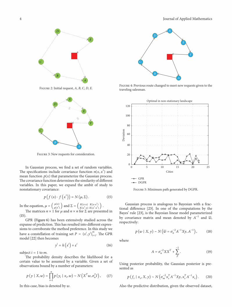
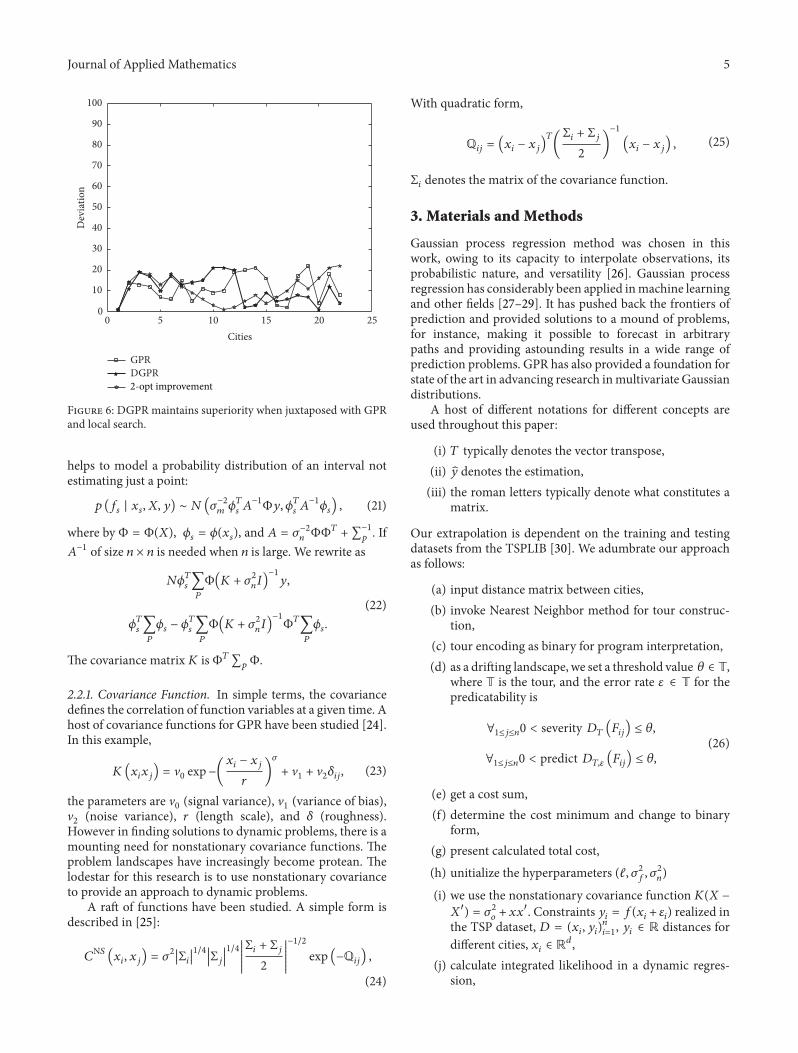
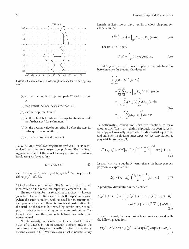
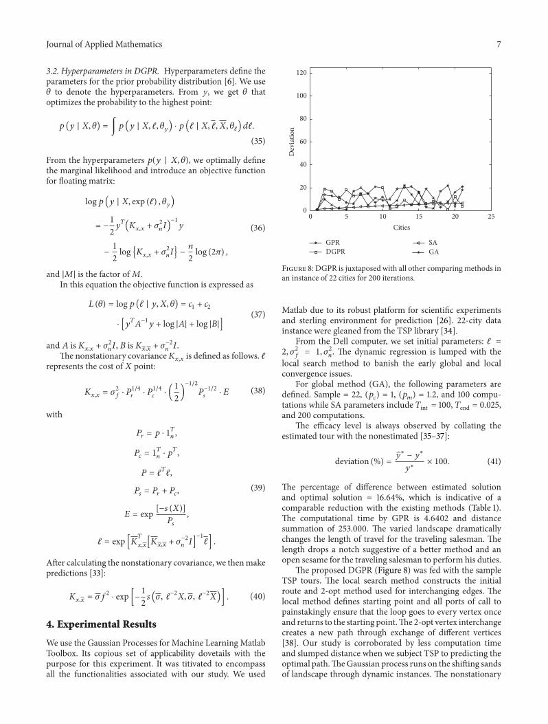
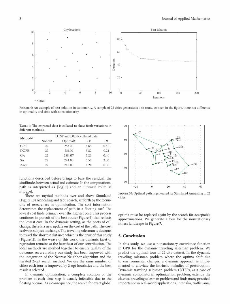
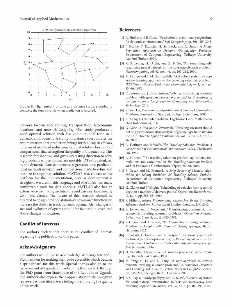
Copyright © 2022 FDOKUMEN