
Traveling ichabods - Washburn University Alumni Association ...
POLITECNICO DI MILANO
IMPERIAL COLLEGE LONDON
II Facolta di Ingegneria dei Sistemi – Milano Leonardo
Corso di Laurea Specialistica in Ingegneria Matematica
Numerical simulation of a train traveling in a
tunnel
Relatore: Prof. Luca Formaggia
Correlatore: Dr. Joaquim Peiro
Tesi di Laurea di:
Alessandro Proverbio
Matr. 708234
Anno Accademico 2008−2009

1
Nobody climbs mountains for scientific reasons. Science is used to raise money for the expeditions,but you really climb for the hell of it.
Sir Edmund Hillary, 1963.
Sommario
Negli ultimi 40 anni il trasporto ferroviario ha guadagnato progressivamente importanza. I trenihanno assunto un ruolo diverso passando da trasporto lento ad alternativa al trasporto aereo.Iltriplicarsi delle velocita ha quindi portato il conseguente sviluppo di problematiche aerodinamiche.Si e infatti reso necessario studiate sia forme sempre piu performanti sia considerare il comfortdei passeggeri.Questo lavoro si occupa di analizzare il problema aerodinamico di un treno che viaggia in untunnel. Tale situazione e di particolare interesse per via della criticita delle sollecitazioni a cui ilconvoglio ferroviario e sottoposto. Una buona conoscenza dei fenomeni aerodinamici caratteriz-zanti la situazione e in grado di permettere una migliore progettazione della struttura meccanicae di introdurre accorgimenti che aumentino il benessere dei viaggiatori.
Quando un treno entra in una galleria delle onde di pressione sono generate dal muso deltreno e si propagano lungo tutta la lunghezza della stessa venendo riflesse dal portale situato almargine opposto. Anche la coda del treno da origine ad onde che a loro volta vengono riflesse.Questi fenomeni fisici e la loro interazione diventa un problema molto complesso che richiede unatrattazione numerica. Il fenomeno in analisi risulta: tridimensionale, turbolento, non stazionarioe viscoso ma, grazie ad una notevole bibliografia, e stato possibile ridurre il modello ad un sistemadi equazioni monodimensionale, iperbolico non lineare scritto in forma conservativa.
Nel presente lavoro si e deciso di risolvere tale sistema con un metodo Galerkin discontinuospiegato nel capitolo 2. La sua peculiarita consiste nel non imporre la continuita tra la soluzionein un elemento della base ed i contigui. Esso ha la notevolissima proprieta di non introdurreviscosita numerica nella discretizzazione spaziale del problema, fatto importante per il problemadi propagazione di onde considerato. L’unica viscosita numerica presente e data dall’integrazionein tempo che nella formulazione originale viene affrontata con metodi Runge–Kutta o StrongStability Preserving Runge–Kutta.
La formulazione cosı scritta mostra pero delle oscillazioni non fisiche delle variabili nel tempoe lungo la galleria. Esse sono notevoli, tali da rendere necessarie mesh molto fitte o alti gradi dellabase polinomiale del metodo di Galerkin, con la conseguenza di appesantire notevolmente i tempidi calcolo.
Sono state ipotizzate due tipologie di errore che possono generare le oscillazioni. Ad ogniintervallo di tempo puo presentarsi un errore di integrazione numerica od un errore di proiezionedelle funzioni sulla base polinomiale. La variazione dell’entita di uno od entrambi questi errori adogni intervallo di tempo puo generare tali oscillazioni.
Nel capitolo 3 e stata condotta una profonda analisi della natura di tali oscillazioni che simostrano essere strettamente connesse al movimento del treno lungo gli elementi della mesh e chesi riducono e cambiano le proprie frequenze al variare del numero di punti di integrazione presenti.
Nel capitolo 4 si e descritto un metodo implicito implementato per la soluzione del nostroproblema. Esso offre la possibilita di inserire un passo temporale arbitrario senza dover rispettarevincoli di stabilita. Proprio per questa ragione si e optato per utilizzare un passo temporale chemuova il treno di un elemento per istante temporale. Cosı facendo si ha la possibilita di mantenerecostante l’errore di integrazione e proiezione. Nel capitolo 4 e stata inoltre condotta un’analisidell’accuratezza del metodo implicito.
A seguito dei risultati riportati nel capitolo 3, nel capitolo 5 si e presentata una nuova formu-lazione del problema che non assoggetti l’area ad errore di proiezione. Cio e stato possibile grazie
2

3
alla riscrittura delle incognite, ora private dell’area. Cosı facendo e stato possibile analizzare ilsolo errore di integrazione con i risultati presentati in sezione 5.1.2. Successivamente, in 5.2, estato eliminato l’errore di integrazione. Infine, in sezione 5.3, si e abbandonata la formulazioneintrodotta in questo capitolo per ritornare alla formulazione classica ma mantenendo la tecnica diintegrazione introdotta in 5.2. Questo ha permesso di evidenziare il solo errore di proiezione.
Il lavoro, di carattere prettamente numerico, risulta essere una analisi del metodo Galerkindiscontinuo applicato al problema di un treno viaggiante in una galleria.

Abstract
Over the past 40 years trains have gradually gained importance. Nowdays they play a differentrole than in the past because they have passed from being a slow transportation to represent analternative at the airplane. The fact that their speed has tripled introduces aerodynamic problemsand they require to study the shape both in order to have higher performances than to have morecomfortable trains.This work aims to analyze the problem of a train traveling in a tunnel. This is a very interestingscenary because of the critical stresses that structures have to deal. Understanding the aerody-namic phenomena allows to better design the structures and to increase passengers’ comfort.
When a train enters in a tunnel, pressure waves propagate form its nose all along the tunneland they are reflected by the exit portal. Also the tail generates waves that are reflected. Allthese phenomena and their interactions require to be studied with a numerical method. Thephysical phenomenon is 3D, turbulent, unsteady and viscous but it has been possible to reducethe model to a monodimensional hyperbolic system of non linear differential equations written ina conservative form.
In the present work we have used a discontinuous Galerkin (DG) approach, as explained inchapter 2. This method does not introduce numerical viscosity in the spatial discretization andthis is very useful property in a wave propagation problem. The only numerical viscosity is dueto the Runge–Kutta or Strong Stability Preserving Runge–Kutta methods adopted for the timestepping.
The method presents unexpected oscillations both in time than in space over the tunnel length.They are very strong and require high polynomial orders of the DG basis or large numbers of meshelements in order to be reduced. This necessity dramatically increases computational costs.
Two type of errors could generate the oscillations: a numerical quadrature error or an errordue to the projection of the functions on the polynomial basis.
In chapter 3 has been presented a deep analysis of the oscillations that appears to be connectedto the movement of the train along the mesh elements.
In chapter 4 we have described the implementation of an implicit method. It does not haveany stability constrain and gives us the possibility to fix an arbitrary timestep. This fact showsthat a timestep that moves the train of one element per time keeps the error constant.
Because of the results in chapter 3, in chapter 5 we have adopted a new formulation, able todo not project the area and its derivative on the polynomial basis and consequently avoiding theirprojection error. The function representing the area reproduces the effect of the train movementin our problem. This fact allows us to study the only integration error as done in section 5.1.2.Next, in section 5.2, we have erased the integration error. In the end, in section 5.2, we havegone back to the original formulation but have maintained the new integration formula in orderto analyze the only projection error.
4
Contents
1 Introduction 71.1 A brief history of transportation by train . . . . . . . . . . . . . . . . . . . . . . . 71.2 Analytical solution to the problem . . . . . . . . . . . . . . . . . . . . . . . . . . . 101.3 Derivation of the equations . . . . . . . . . . . . . . . . . . . . . . . . . . . . . . . 11
1.3.1 Governing equations . . . . . . . . . . . . . . . . . . . . . . . . . . . . . . . 121.3.2 Shape of the train . . . . . . . . . . . . . . . . . . . . . . . . . . . . . . . . 13
2 Numerical simulation by the explicit DG method 152.1 Discontinous Galerkin Method . . . . . . . . . . . . . . . . . . . . . . . . . . . . . 152.2 Discontinous Galerkin discretization . . . . . . . . . . . . . . . . . . . . . . . . . . 162.3 Stability of the explicit method . . . . . . . . . . . . . . . . . . . . . . . . . . . . . 182.4 Results in the explicit method . . . . . . . . . . . . . . . . . . . . . . . . . . . . . . 20
2.4.1 Numerical results . . . . . . . . . . . . . . . . . . . . . . . . . . . . . . . . . 212.4.2 Discussion on numerical results and their validation . . . . . . . . . . . . . 22
3 Investigation on the source of the oscillations 243.1 Numerical errors . . . . . . . . . . . . . . . . . . . . . . . . . . . . . . . . . . . . . 24
3.1.1 Integration error . . . . . . . . . . . . . . . . . . . . . . . . . . . . . . . . . 243.1.2 Projection error . . . . . . . . . . . . . . . . . . . . . . . . . . . . . . . . . . 25
3.2 Analysis of the solution obtained with the original formulation . . . . . . . . . . . 263.2.1 Number of elements . . . . . . . . . . . . . . . . . . . . . . . . . . . . . . . 263.2.2 Variation of th order of the polynomial basis . . . . . . . . . . . . . . . . . 273.2.3 Variation of the number of quadrature knots . . . . . . . . . . . . . . . . . 273.2.4 Effects of distributions of quadrature knots . . . . . . . . . . . . . . . . . . 293.2.5 Spectrum analysis . . . . . . . . . . . . . . . . . . . . . . . . . . . . . . . . 303.2.6 Accuracy of the method . . . . . . . . . . . . . . . . . . . . . . . . . . . . . 30
4 Implicit method 334.1 The DG approach using an implicit time stepping . . . . . . . . . . . . . . . . . . 33
4.1.1 Why an implicit method? . . . . . . . . . . . . . . . . . . . . . . . . . . . . 334.1.2 Backward Euler scheme properties . . . . . . . . . . . . . . . . . . . . . . . 344.1.3 Implicit solvers . . . . . . . . . . . . . . . . . . . . . . . . . . . . . . . . . . 38
4.2 Comparison between explicit and implicit . . . . . . . . . . . . . . . . . . . . . . . 414.2.1 Accuracy . . . . . . . . . . . . . . . . . . . . . . . . . . . . . . . . . . . . . 414.2.2 Computational costs . . . . . . . . . . . . . . . . . . . . . . . . . . . . . . . 43
5 An alternative treatment of the area in the DG formulation 475.1 New weak formulation without the area in the unknowns . . . . . . . . . . . . . . 47
5.1.1 Derivation of the new weak formulation . . . . . . . . . . . . . . . . . . . . 485.1.2 Oscillations in the solution with no area in the unknowns . . . . . . . . . . 50
5.2 Increasing of the integration accuracy . . . . . . . . . . . . . . . . . . . . . . . . . 525.3 Projection error . . . . . . . . . . . . . . . . . . . . . . . . . . . . . . . . . . . . . . 54
5.3.1 Error at different mesh sizes and polynomial orders . . . . . . . . . . . . . . 55
5

Contents 6
5.3.2 Comparison between the two formulations . . . . . . . . . . . . . . . . . . . 56
6 Conclusions and future work 586.1 Conclusions . . . . . . . . . . . . . . . . . . . . . . . . . . . . . . . . . . . . . . . . 586.2 Future work . . . . . . . . . . . . . . . . . . . . . . . . . . . . . . . . . . . . . . . . 59
Chapter 1
Introduction
In this work we deal the problem of a train travelling in a tunnel and the complexity of the sce-nary is represented by many aspects. In fact the modellation of the physical phenomenon and theapproximation used, that starts from Navier-Stokes equations and arrived to the governing equa-tions adopted, is a chain of assumptions that requires a deep explanation. Every approximationinfluences a term of the governing equations and we will describe them accurately.
In this chapter we will present an introduction to the reason of why the problem treated isimportant 1.1 and than we describe the physical model 1.3 and the governing equations 1.3.1.
1.1 A brief history of transportation by train
Over the last 60 years, a great deal of attention has been concentrated on the development ofairpalanes but studies on the trains have been taken aside because their low speeds and their fixedtracks carry to aerodynamic problems that could be not attractive from fluid dynamists. Nowthe train speed exceeds over 300 km/h and is nearly comparable with the past airplane velocities.Furthermore, the train system is playing much more roles in transport than the airplane so, sys-tematic work, is needed in the development of the train system [41].
Now, many countries are operating the high-speed railway trains, such as German Inter CityExpress (ICE), Japanese Shinkansen and French Train de Grande Vitesse (TGV); moreover, somecountries like South Korea and China are constructing high-speed train (HST) systems [51, 52].
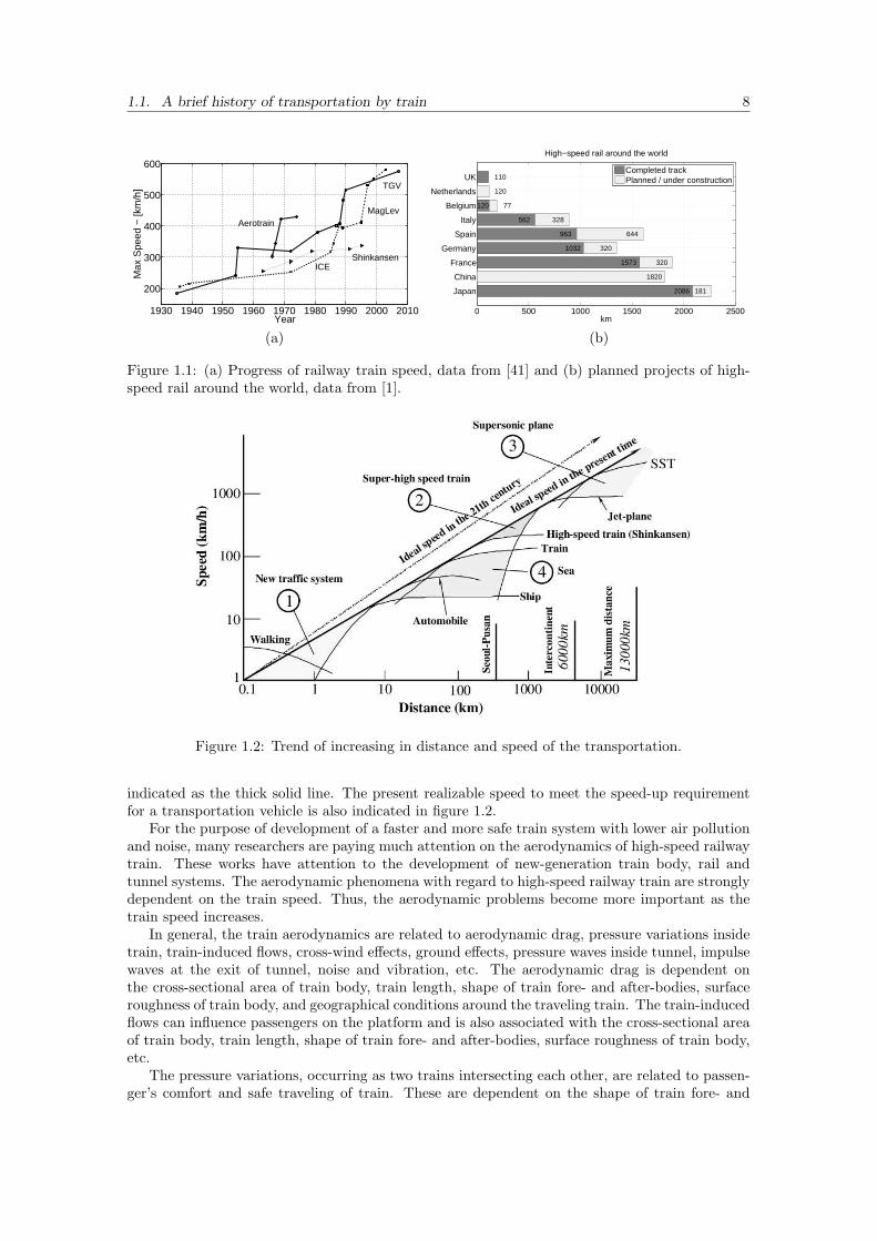
The maximum speed of trains has tripled by 1960s, as indicated by its evolution shown infigure 1.1(a), the demand for high-speed rail is steadily increasing in the world, see figure 1.1(b)and aerodynamic and aeroacoustic problems are now receiving a considerable attention as prac-tical engineering issues that should be urgently resolved. Many engineering problems which havebeen reasonably neglected at low speeds, are being raised with regard to aerodynamic noise andvibrations, impulse forces occurring as two trains intersect each other, impulse wave at the exitof tunnel or ear discomfort of passengers inside train, see for instance [41, 44, 48]. Basically theproblems are closely associated with the flows occurring around the train on the railway.
Moreover, much effort to speed up the train system has been paid on the improvement of electricmotor power rather than understanding the flow physics around the train and thereby finding aproper control method. This has led to larger energy losses and performance deterioration of thetrain, since the flows around train are more disturbed due to turbulence of the increased speed;consequently, the flow energies are being converted to aerodynamic drag, noise and vibrations.
Figure 1.2 shows Bouladon’s criterion for the speed of a transportation vehicle [8], in whichthe speed required for a transportation vehicle is given by a function of distance. The solid lineindicates the required speed according to the transportation distance, showing a general tendencythat the longer the transportation distance, the higher the speed required. This line also indicatesan increased gradient with time, thus leading to more increasing requirement for the speed-up of atransportation vehicle. An ideal speed required for transportation vehicle in the 21st century is also
7
1.1. A brief history of transportation by train 8
1930 1940 1950 1960 1970 1980 1990 2000 2010
200
300
400
500
600
TGV
ICEShinkansen
MagLevAerotrain
Year
Max
Spe
ed −
[km
/h]
0 500 1000 1500 2000 2500
Japan
China
France
Germany
Spain
Italy
Belgium
Netherlands
UK
km
High−speed rail around the world
2086 181
1820
1573 320
1032 320
963 644
562 328
120 77
120
110Completed trackPlanned / under construction
(a) (b)
Figure 1.1: (a) Progress of railway train speed, data from [41] and (b) planned projects of high-speed rail around the world, data from [1].
Figure 1.2: Trend of increasing in distance and speed of the transportation.
indicated as the thick solid line. The present realizable speed to meet the speed-up requirementfor a transportation vehicle is also indicated in figure 1.2.
For the purpose of development of a faster and more safe train system with lower air pollutionand noise, many researchers are paying much attention on the aerodynamics of high-speed railwaytrain. These works have attention to the development of new-generation train body, rail andtunnel systems. The aerodynamic phenomena with regard to high-speed railway train are stronglydependent on the train speed. Thus, the aerodynamic problems become more important as thetrain speed increases.
In general, the train aerodynamics are related to aerodynamic drag, pressure variations insidetrain, train-induced flows, cross-wind effects, ground effects, pressure waves inside tunnel, impulsewaves at the exit of tunnel, noise and vibration, etc. The aerodynamic drag is dependent onthe cross-sectional area of train body, train length, shape of train fore- and after-bodies, surfaceroughness of train body, and geographical conditions around the traveling train. The train-inducedflows can influence passengers on the platform and is also associated with the cross-sectional areaof train body, train length, shape of train fore- and after-bodies, surface roughness of train body,etc.
The pressure variations, occurring as two trains intersecting each other, are related to passen-ger’s comfort and safe traveling of train. These are dependent on the shape of train fore- and
1.1. A brief history of transportation by train 9
after-bodies, train width, and the distance between track lines. The cross-wind can also influencethe safe traveling of the train, relating to train height and perimeter, bridge system, etc.The impulse wave at the exit of tunnel influences the surrounding area around the train trackand is dependent on the cross-sectional area of train body, the cross-sectional area of tunnel, theshape of train fore- and after-bodies, the tunnel length, the kind of track, etc. The pressure vari-ations influence the structural strength of the train body, passenger’s comfort, and are associatedwith the cross-sectional area of the train body, cross-sectional area of tunnel, train length, tunnellength, etc.A train entering a tunnel generates a compression wave at the entry portal that moves at the speedof sound in front of the train. The friction of the displaced air with the tunnel wall produces apressure gradient and, as a consequence, a rise in pressure in front of the train. On reaching theexit portal of the tunnel, the compression wave is reflected back as an expansion wave but partof it exits the tunnel and radiates outside as a micro-pressure wave, see e.g. [53, 50, 19] andreferences therein. This wave could cause a sonic boom that may lead to structural vibration andnoise pollution in the surrounding environment. The entry of the tail of the train into the tunnelproduces an expansion wave that moves through the annulus between the train and the tunnel.When the expansion pressure wave reaches the entry portal, it is reflected towards the interior ofthe tunnel as a compression wave. These compression and expansion waves propagate backwardsand forwards along the tunnel and experience further reflections when meeting with the nose andtail of the train or reaching the entry and exit portals of the tunnel until they eventually dissipatecompletely [40].
The presence of this system of pressure waves in a tunnel affects the design and operation oftrains, and they are a source of energy losses, noise, vibrations and aural discomfort for passengers.These problems are even worse when two or more trains are in a tunnel at the same time. Auralcomfort is one of the major factors determining the area of new tunnels or the maximum train speedin existing ones. Current guidelines of the International Union of Railways (UIC) [1] recommenda maximum pressure increment below 4 kPa in any period of 4 s.
Numerical simulations of the three-dimensional (3D) flow generated by the train in the tunnelare currently possible but these flows are very difficult to model accurately due to the presenceof separation and turbulent transition. Some examples of such computations are given in thereferences [31, 13, 49, 21]. Even if a simpler inviscid model is used, these are computationallyexpensive simulations due to the need for the handling of bodies in relative motion through theuse of either sliding grids, overlapping grids or remeshing. The accurate modelling of the turbulentflows near the nose and train of the train is still an open problem [30].
Area-averaged one-dimensional (1D) simulations are the industry standard [1, 17] to produceguidelines for passenger aural comfort. They are computationally much cheaper: with simulationstaking a minutes rather than days, as in the 3D case. Also, there is ample experimental evidenceof the suitability of this approach for modelling pressure waves, e.g. [55], even in short tunnels[32].
For moderate values of the train speed and blockage ratio, i.e. the ratio between the areasof the train and the tunnel, it is acceptable to introduce simplifying assumptions that lead topractical and inexpensive techniques. For instance, one could assume that, for low train speeds,the flow is incompressible, as in the subway environment system [36], or, for moderate speeds,that the linear acoustic theory [23] is applicable, as in the wave-signature approach [33].
For higher speeds and blockage ratios, the industry standard method of solution is the methodof characteristics [15, 40, 54, 5, 1]. In this approach, the nose and tail of the train are treatedas area discontinuities where the flows across the discontinuity are linked by the equations of 1Dsteady flow with losses arising from 3D viscous flow effects modelled using pressure loss coefficients.For modern trains, with long noses and tails, their approximation as a discontinuity might not besuitable. This is often circumvented by approximating the nose and tail in a stepwise fashion. Analternative approach is to assimilate the motion of the train through the tunnel to a peristalticflow produced by a moving area and solve the associated system of governing equations usingfinite volume discretization techniques [42, 3, 2].
Our interest in modelling the pressure wave field generated by a train entering a tunnel by a
1.2. Analytical solution to the problem 10
discontinuous Galerkin (DG) discretization of the 1D area-averaged governing equations of variablearea flows arises from the ability of the DG method to propagate waves with minimum diffusionand dispersion numerical errors [46, 6].
1.2 Analytical solution to the problem
Solutions to the problem of a train passing in a tunnel can be found with classical gasdynamicstechniques and have been presented in [48]. We remark the ideas understanding two methods, thefirst based on standard gasdynamics equations and the second on total pressure losses.
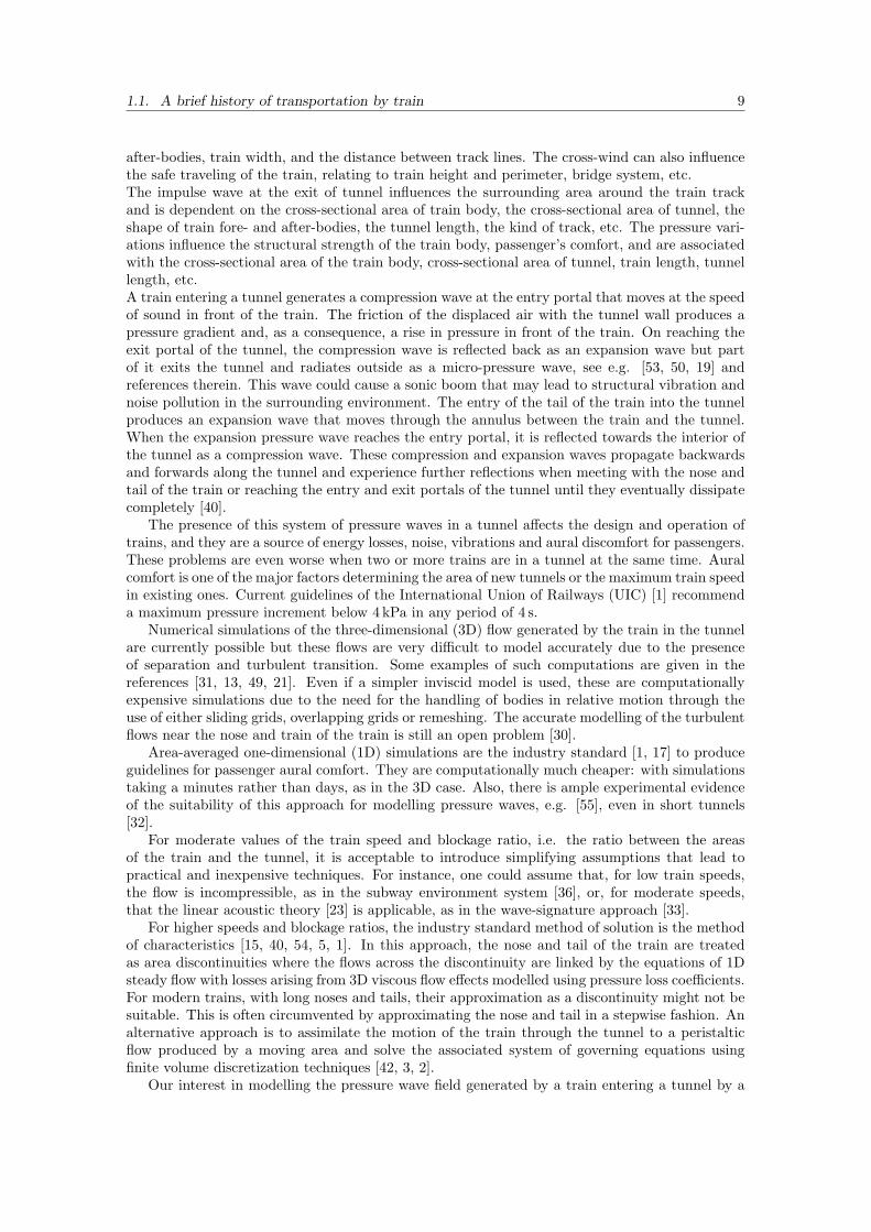
Unfortunately both the methods are not able to describe the entire solution but only the sevenpoints highlighted in figure 1.3.
Figure 1.3: Highlighted points on the domain.
In the first method, standard relations commonly used in gasdynamics are applied in order todescribe the phenomena going on in the tunnel. The losses are considered in momentum equationwith a distributed losses method. We distinguish the situation just after the entrance of thehead of train in the tunnel and just before the entrance of the tail. In the two situations theapproximations adopted change.
Tunnel domain is splitted in many regions and each one has different governing equation andapproximations. In the part where there is no train (0–1 and 4–5), viscosity effects are neglectedand the fluid is isoentropic and compressible fluid in order to consider the propagation of pressurewaves. In the nose and tail regions (1–2 and 3–4), losses are still missed and is considerd aquasisteady isoentropic flow but the relation is not exact despite the error is of a second orderimportance. The domain corresponding the body of the train (2–3) is an anular region wherelosses have to be considered because of the small area in the cross section but here we consider theeffect of losses on tail and nose introducing empirical drag coefficients. In the end, region (0–5),where there is the tunnel portal, the fluid is incompressible and the solution connect the internalsolution with the atmosferic steady condition.These approximations carry to a non linear system of 14 equtions but we can observe that thevariations of pressure, density and speed of the sound change reduced due to the problem analyzed.We can observe that the ratio beween omologues variables in two different points is close to 1 andwe can reduce to 8 the number of equations.Unfortunately in the first situation, the obtained system is the maximum degree of simplificationthis approch allows but, if we consider a scenary where the tail of the train has just entered in thetunnel we can set to zero the losses due to the tail and we can reduce at 5 the nuber of equations.
The second method is based on stagnation pressure loss.In the region of the portal in the tunnel (0–1) flow is unsteady but in all the other parts ofthe domain (1–5) we can consider a quasi steady flow and consider friction effects only wherethere is the train despite there in no compressibility in such region. The model described givesa 7 equations non-linear system but it is possible, with the same considerations of the previousmodel, to obtain 4 equations.

1.3. Derivation of the equations 11
Figure 1.4: Analytical solutions with the two methods presented in this paragraph compared witha numerical solution for a fixed point at Ma = 0.3 and β = 0.18 [48]. In full line the first methodand in broken line the second method.
Both the methods reported carry to not really accurated results. The strong dependence fromempirical coefficients, computed on all the domain, but that they have a local behaviour that coulddiffer from the average one, introduces errors. If we adopt a charateristics method for a numericalsolution, it differs less than 2% from the analytical methods, as shown in figure 1.4. Also the twomethods has a difference of less than 5%.The strong disadvantage of the method is that it is not able to analyze complicated situations i.e.tunnel network or presence of airshafts and that the solution is computed only for some pointsand not all over the domain.
This discussion, fully described in [48], shows how it is possible to compute a first raw result forthe problem analyzed by simply introducing strong approximation but the problem still remainsquite complicated despite the solution is not really accurated.
1.3 Derivation of the equations
The problem of a combines the effects of changes in the position of the train along the domainand the corresponding aerodynamic phenomena. The flow generated by a train traveling in atunnel is unsteady, compressible, three-dimensional and turbulent in nature therefor a correctdescription of the flow requires the solution of the three-dimensional unsteady equations of gasdynamics. However, experimental evidence ([3, 31]) shows that if the tunnel length is much largerthan its hydraulic diameter, the propagation of pressure disturbances takes place by means ofapproximately plane waves and the instantaneous distribution of the fluid dynamic variables isnearly uniform in each tunnel section, while intrinsically three-dimensional features are concen-trated only in the close vicinity of the train and tunnel ends and where the tunnel walls havea complex shape (abrupt changes of the cross-section area, mutual connections between tunnels,tunnel connections with the atmosphere).Despite 2D/3D flow models are more complete than one-dimensional generation/propagation mod-els, especially in the entry phase where 3D effects are important, they require a larger amountof computational resources that is not necessarily justified by the physics of the propagation ofcompression waves in a tunnel which is mainly a 1D phenomenon. In fact, the train–tunnel un-steady aerodynamics can be successfully described by a quasi-1D approximation of the physicalproblem, provided that local corrective models are adopted to better describe the regions where3D effects become important, such as train nose and tail, tunnel cross-section variations and con-nections between tunnels and ducts. The obvious advantage of a 1D approach resides in its lowcomputational cost, which allows to analyze complete, long tunnels or tunnel networks and to
1.3. Derivation of the equations 12
carry out parametric studies efficiently, while its drawback is that the reliability of its predictionspartly depends on the availability of experimental data [2].
The characteristic of the phenomenon lead us to use the one-dimensional equations for acompressible, unsteady flow [31, 24, 45]. The flow variables are considered to be uniform in eachcross section along the length of the tunnel.
1.3.1 Governing equations
In the present work we will deal with a hyperbolic system. The conservative form is written as
∂U∂t
+∂F(U)∂x
= S (1.1)
with appropriate initial and boundary conditions.In order to solve our problem we set the vector of conservative variables U and the flux vector
F as
U =
ρAρuAρEA
; F(U) =
ρuA(ρu2 + p)AρuHA
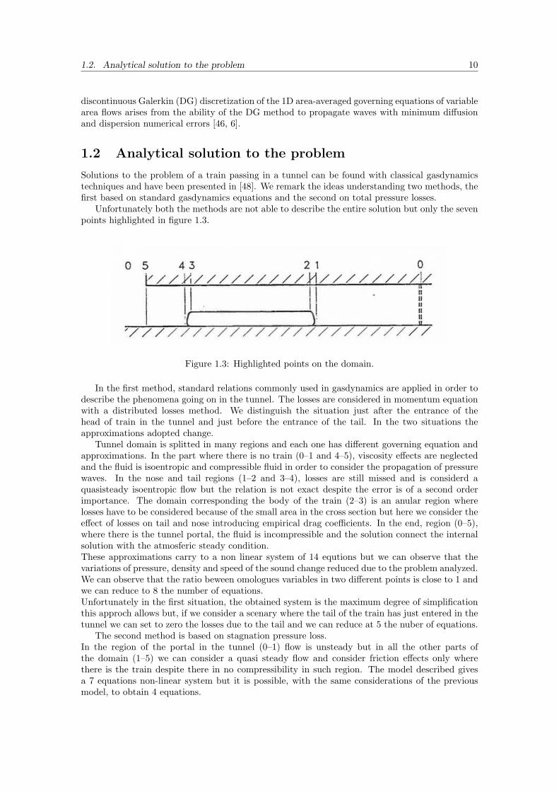
where ρ is the fluid density, p is the pressure, u is the velocity along the tunnel direction and Astands for the cross-sectional area. The air is modeled as ideal gas, therefore, the total energy Eand enthalpy H per unit mass are defined as E = e + 1
2u2 and H = E + p
ρ , respectively, wheree is the internal energy per unit mass. The pressure p is expressed, with the equation of state,as p = ρRT and the internal energy e is given by e = CvT . Here Cp and Cv denote the specificheat at constant pressure and volume, respectively, R = Cp − Cv, and T is the absolute statictemperature. The previous expressions can be combined to write the pressure as
p = (γ − 1)ρ(E − 12u2)
where γ = Cp/Cv is the ratio of specific heats of the fluid.The right-hand side of equation 1.1 represents the source term S that can be divided into three
terms as
S =
0p∂A∂x
0
+
0Dm
Dh
+
0QmQh
(1.2)
The first term derives from the 1D approximation of variable area. In a non-conservative formu-lation this term does not exist because it comes from the derivative changes.Friction and heat transfer effects are taken into account through the use of a “distributed loss”model [51, 52] in which Dm and Dh are the momentum and enthalpy dissipation associated withthe viscous and turbulent stresses on the solid walls and Qm and Qh are the momentum andenthalpy corrections for locally three dimensional flow regions.
Significant pressure waves are generated during train entry and train exit and the lateral extentof any region of separated flow just downstream of the nose is constrained by the tunnel wall, whichtherefore influences the contribution of the nose to pressure drag, causing additional aerodynamicdrag, which is typically much larger than drag due to local flow separations. . The wake regionbehind the tail may also change. The underlying phenomenon is inertial, not viscous; it wouldexist even in an ideal inviscid fluid. In a tunnel, therefore, pressure drag includes inertial dragas well as drag attributable to flow separations. Further pressure waves are generated when thenose leaves the tunnel, when the tail enters and leaves the tunnel, and when the nose and tail passalongside airshafts and cross-passages, etc. More gradual wavefronts are generated when tunnelshave larger cross sections.

1.3. Derivation of the equations 13
Following [37] the viscous and turbulent terms are modelled through the experimental frictioncoefficient of the train, Cft
, and of the tunnel, Cfg, as
Dm = −∮σ
12ρ(Cfg
u|u|+ Cft(u− V )|u− V |
)dσ ;
Dh = −∮σ
12ρCft
(u− V )|u− V | dσ(1.3)
where V is the train velocity and σ denotes the perimeter of the cross section. The correctionterms Qm and Qh account for pressure variations due to 3D effects and model the strength ofthe nose compression wave and of the tail expansion wave. According to references [3, 2], thesecorrections can be taken to be functions of the variation of the area due to the train nose and tailgiven by
Qm = Cd p∂A
∂x; Qh = −Cd V p
∂A
∂x(1.4)
where Cd is a coefficient that depends on the train velocity, the shape of the train nose and tailand the blockage ratio β, i.e. the ratio between the cross-sectional areas of the train and thetunnel.
In all the previews equations, inside the variables or the source term, a strong influence on thedynamics of the problem due to the area exists. Usually, the cross-sectional area of a tunnel canbe deduced with sufficient accuracy from geometrical considerations alone. It may be necessaryto make appropriate allowances for obstructions such as cables, signals and other equipment, butthe resulting uncertainties typically amount to only a small percentage of the final value [52].
−
t xn
Lt LnAT (1−β)
ATAT
xtxnA(x,t)
β
L =
xx
V
Figure 1.5: Notation used in the definition of the cross-sectional area A(x, t).
1.3.2 Shape of the train
The motion of the train within the tunnel is represented by the variation, in space and time, ofthe cross-sectional area. Here we approximate it as
A(x, t) =
AT x < xt,AT
2
(2− β + β cos(π(x−xt)
Lt))
x ∈ [xt, xt + Lt],AT (1− β) x ∈ [xt + Lt, xn − Ln],
AT
2
(2− β + β cos(π(x−xn)
Ln))
x ∈ [xn − Ln, xn],AT x > xn,
(1.5)
where AT is the tunnel area, L is the length of the train and V its speed, Ln and Lt are thelengths of the nose and of the tail of the train respectively, x is the coordinate along the tunnel,and xn and xt = xn − L are the positions of the nose and tail at a given time t. To illustrate thenotation, a sketch of the area variation, at a given time, is shown in Figure 1.5.
The initial conditions correspond to an empty tunnel with stationary air at atmospheric con-ditions. The boundary conditions at the entry and exit portal of the tunnel amount to prescribingatmospheric values of pressure and density.
1.3. Derivation of the equations 14
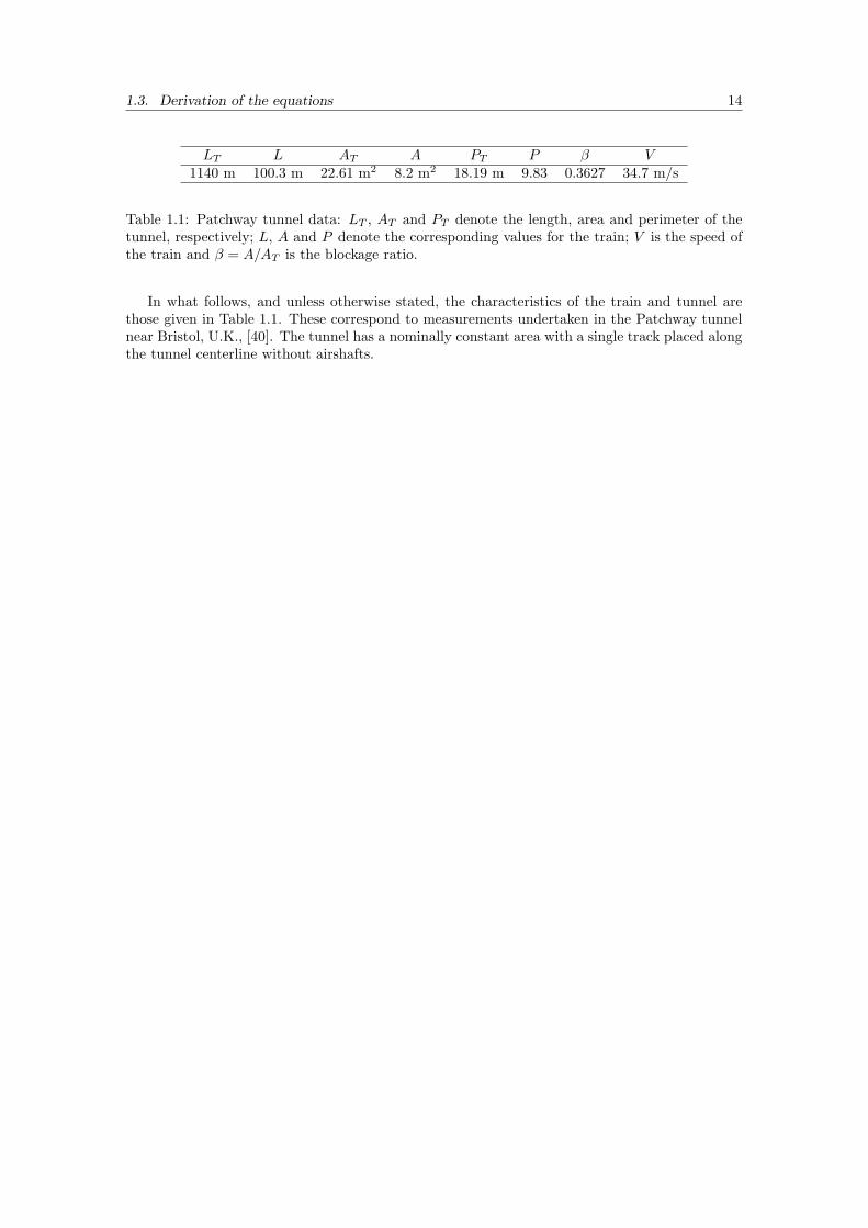
LT L AT A PT P β V1140 m 100.3 m 22.61 m2 8.2 m2 18.19 m 9.83 0.3627 34.7 m/s
Table 1.1: Patchway tunnel data: LT , AT and PT denote the length, area and perimeter of thetunnel, respectively; L, A and P denote the corresponding values for the train; V is the speed ofthe train and β = A/AT is the blockage ratio.
In what follows, and unless otherwise stated, the characteristics of the train and tunnel arethose given in Table 1.1. These correspond to measurements undertaken in the Patchway tunnelnear Bristol, U.K., [40]. The tunnel has a nominally constant area with a single track placed alongthe tunnel centerline without airshafts.

Chapter 2
Numerical simulation by theexplicit DG method
In this chapter we will describe the explicit method implemented for solving the fluid dynamicproblem of a train travelling in a tunnel.We will discuss the general Discontinous Galerkin approach properties then we will derive the DGequations, discute their validity and, in the last section, we will show some results obtained withthis formulation.
2.1 Discontinous Galerkin Method
The name of discontinuous Galerkin (DG) appears first in an article by Lesaint and Raviart in1974 but the method had suddenly be applied to hyperbolic and parabolic problems [10, 28]. Thefundamentals of DG method can be consulted in [35]. The idea underlaying the method is to splitthe domain in many subdomains, basically elements, and to solve in each of them a continuousGalerkin problem. The main problem to be solved are the internal boundary conditions necessaryto solve the problem on all the subdomains. We remark that the continuity is not ensured betweeneach element [39]. DG method has many characteristics we would like to remark:
• The solution inside the element is continous and described with a high order polynomial.If a discontinuity of the solution occours inside the element it can not be modeled properlybecause it will be represented with a polynomial. If discontinuoities are on the boundaryof an element, jumps are allowed by DG formulation and they are modeled properly. Anaccurate placement of the elements boundaries i necessary in order to have good not smoothsolutions;
• On a charateristics method boundary conditions must be imposed properly on every singlecharateristic line in hyperbolic problems. With a DG approach we impose boundary andinitial conditions on the borders like we do on ellitic problems because we are able to splitthe problem in space and in time and solve the evolutive problem as a system of ordinarydifferential equations relatively easily;
• DG are computationally more expensive than continuous Galerkin because they have to takein account the interface conditions but the higher degreeSolution of transient problems seemthey could advantageously solved with DG. This is due to the decupling in each element andto the block matrix that is able to be inverted easily of polynomial adopted in the basis andthe added number of freedom points produce a better solution and the exceeding in term ofcost could be reduced when we try to obtain highly accurate solutions;
• High order methods represents waves with accuracy since dispersion and diffusion errors arenullum as the order of the basis increase.
15

2.2. Discontinous Galerkin discretization 16
2.2 Discontinous Galerkin discretization
The discontinuous Galerkin method [35] is employed for the spatial discretization of equation (1.1)in a domain Ω = (a, b). The domain is discretized into Nel non-overlapping elements Ωe = (xle, x
re),
such that xre = xle+1 for e = 1, · · · , Nel, thus Ω =⋃Nel
e=1 Ωe. A weak formulation of (1.1) is writtenas ∫
Ω
w∂U∂t
dx+∫
Ω
w∂F(U)∂x
dx−∫
Ω
wS(U)dx = 0 (2.1)
where w is a test function. Carrying out the integral over the elemental regions Ωe we get
Nel∑e=1
[∫Ωe
w∂U∂t
dx+∫
Ωe
w∂F(U)∂x
dx−∫
Ωe
wS(U)dx]
= 0 (2.2)
and integrating the flux term by parts we obtain
Nel∑e=1
[∫Ωe
w∂U∂t
dx−∫
Ωe
dw
dxF(U)dx+ [wF(U) · n]x
re
xle−∫
Ωe
wS(U)dx]
= 0 (2.3)
The present DG formulation defines the solution U to be discontinuous across the interface, andthe introduction of an upwind numerical flux Fu permits information to be propagated betweenelements. The last equation becomes
Nel∑e=1
[∫Ωe
w∂U∂t
dx−∫
Ωe
dw
dxF(U)dx+ [wFu]x
re
xle−∫
Ωe
wS(U)dx]
= 0 (2.4)
The conservative variables, the flux and source terms are expanded in terms of a base ofLegendre polynomials Lp(ξ) defining a compact support within each element. The Legendrepolynomials of degree p = 0, · · · , P may be defined using Rodrigues’ formula as
Lp(ξ) =1
2pp!dp
dξp[(ξ2 − 1)p
](2.5)
where ξ is the space variable on the reference element Ωref = −1 ≤ ξ ≤ 1, with the elementalaffine mapping
xe(ξ) = xle1− ξ
2+ xre
1 + ξ
2, dx =
12
∆xedξ (2.6)
where ∆xe = xre − xle.The weak Galerkin formulation is obtained by introducing the Legendre polynomials as the
test functions, i.e.w |Ωe
(xe(ξ)) = Lp(ξ) (2.7)
and similarly
U |Ωe (xe(ξ), t) =P∑p=0
Lp(ξ)Up(t) (2.8)
F(U |Ωe(xe(ξ), t)) =
P∑p=0
Lp(ξ)Fp(t) (2.9)
S(U |Ωe(xe(ξ), t)) =
P∑p=0
Lp(ξ)Sp(t) (2.10)
The DG approach permits to decouple the problem into a discretized system of ordinary differentialequations on each element e where the only link between elements comes from the upwind fluxes.
2.2. Discontinous Galerkin discretization 17
Equation (2.4) can now be written as∫Ωe
Lq(ξ)P∑p=0
Lp(ξ)∂Up
∂tdx−
∫Ωe
dLq(ξ)dx
P∑p=0
Lp(ξ)Fpdx
+ [Lq(ξ)Fu]xr
xl −∫
Ωe
Lq(ξ)P∑p=0
Lp(ξ)Spdx = 0 q = 1, . . . , P
(2.11)
The orthogonal property of the Legendre polynomials permits the mass matrix elements to bewritten simply as
Mpq =∫ 1
−1
Lq(ξ)Lp(ξ)dξ =2
2p+ 1δpq, δpq =
1 p = q0 p 6= q
(2.12)
Using the formuladLp+1(ξ)
dξ=
m∑i=1
(2k + 1)Lk(ξ)− 2(m− p+ 1
2
)(2.13)
m =
p+ 1
2p = odd
p
2p = even
, k = p− (2i− 2) (2.14)
with p, q = 0, · · · , P , the elements of the stiffness matrix are given by
Dpq =∫ 1
−1
dLq(ξ)dξ
Lp(ξ)dξ = 2 δ∗pq,if p > q δ∗pq =
0 p+ q = even1 p+ q = odd
if p < q δ∗pq = 0(2.15)
The structural patterns of the mass and stiffness matrices, for any polynomial degree, are of theform
M =
• • • • • •
, D =
• • • • • • • • •
(2.16)
where the dots represent 3× 3 matrices and those coloured black are the non-zero entries. Multi-plying both sides of equation (2.11) by M−1 allows us to write it in matrix form as
d
dtUp =M−1
[DFp − Fulr
]+ Sp (2.17)
The numerical approximation of the non-linear terms F and S is performed as follows. Let X bea generic variable denoting either F or S. Integrating over the reference element and multiplyingby the Legendre polynomials expressions (2.9) and (2.10) can be written as∫ 1
−1
Lq(ξ)P∑p=0
Lp(ξ)Xp(t)dξ =∫ 1
−1
Lq(ξ)X(xe(ξ), t)dξ (2.18)
Multiplying both sides by the inverse mass matrix and evaluating the right-hand side through aquadrature rule with P + 1 points, permit us to write the components of the polynomial approxi-mation of X as
Xp(t) =2p+ 1
2
P+1∑i=1
wiLq(ξi)X(xe(ξi), t) (2.19)

2.3. Stability of the explicit method 18
where wi and ξi are the weights and zeros of the Gauss–Lobatto–Jacobi quadrature. These aregiven in [20] and are implemented in the open-source library polylib.c in Nektar++. The initialconditions are approximated in the same fashion by simply taking X = U(x, 0) in equation (2.19).
The upwind flux term is taken to be of the form
Fulr = Lp(1)F∗(Ure,U
le+1)− Lp(−1)F∗(Ur
e−1,Ule) (2.20)
with Lp(1) = 1 and Lp(−1) = (−1)p+1. Here F∗ is the numerical flux solution of the Riemannproblem that has to be solved at each elemental interface using the solution U on the two contigu-ous cells, with Ur
e = Ue(ξ = 1) and Ule = Ue(ξ = −1). Here we have calculated the numerical
flux at the interface through an exact Riemann solver [27].The time integration of the DG semi-discrete system (2.17), written as
dUdt
= R(U, t) (2.21)
is performed by an s-stage explicit Runge–Kutta (RK) method. Assuming that the solution attime t = tn, Un, is known, the solution at time tn+1 = tn + ∆t is calculated as
Un+1 = Un + ∆ts∑i=1
biRi (2.22)
where
Ri = R (Un + ∆Ui, tn + ci∆t) ; ∆Ui = ∆t
i−1∑j=1
aijRj (2.23)
and aij , bi and ci (i, j = 1, . . . , s) are constant coefficients often referred to as the components ofa Butcher array
c1 a11 · · · a1s
......
...cs as1 · · · ass
b1 · · · bs
(2.24)
The resulting timestepping scheme is explicit and thus subject to stability restrictions. These arediscussed and analyzed in the next section.
2.3 Stability of the explicit method
In this section we analyze the stability of the DG scheme in the linear case with a view to determinethe timestep restrictions of the explicit time integration (2.22). To this effect, we will consider theDG discretization of the linear advection equation
∂u
∂t+ a
∂u
∂x= 0 (2.25)
The DG semi-discrete system 2.17 applied to (2.25) is written as
M d
dtUe−DU
e+ FU
e+ GU
e−1= 0 (2.26)
with F = Lp(1)Lq(1) and G = −Lp(−1)Lq(1). These last two terms arise from an upwindapproximation of the interface flux term.
Our stability analysis essentially follows the methodology proposed in [46], but similar analyseshave been presented elsewhere [16, 18, 12, 29]. Here we assume a wave-like solution of the semi-discrete problem 2.26 given by an expansion of the form
Ue
= e−iωt[αe0iθ,αeiθ,αe2iθ, . . . ,αe(Nel−1)iθ]T (2.27)
2.3. Stability of the explicit method 19
−60 −40 −20 0 20−40
−30
−20
−10
0
10
20
30
40
Re(λ )
Im(λ
)
−6 −5 −4 −3 −2 −1 0 1
−3
−2
−1
0
1
2
3
Re(λ)
Im(λ
)
RK11
RK22
RK33
RK44
−6 −5 −4 −3 −2 −1 0 1
−3
−2
−1
0
1
2
3
Re(λ)
Im(λ
)
SSPRK12
SSPRK23
SSPRK34
SSPRK45
(a) (b) (c)
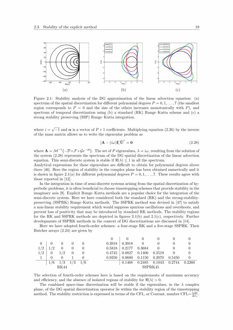
Figure 2.1: Stability analysis of the DG approximation of the linear advection equation: (a)spectrum of the spatial discretization for different polynomial degrees P = 0, 1, . . . , 7 (the smallestregion corresponds to P = 0 and the size of the others increases monotonically with P ), andspectrum of temporal discretization using (b) a standard (RK) Runge–Kutta scheme and (c) astrong stability preserving (SSP) Runge–Kutta integration.
where i =√−1 and α is a vector of P + 1 coefficients. Multiplying equation (2.26) by the inverse
of the mass matrix allows us to write the eigenvalue problem as
[A− (iω)I] Ue
= 0 (2.28)
where A =M−1−D+F+Ge−iθ. The set of P eigenvalues, λ = iω, resulting from the solution ofthe system (2.28) represents the spectrum of the DG spatial discretization of the linear advectionequation. This semi-discrete system is stable if <(λ) ≤ 1 in all the spectrum.Analytical expressions for these eigenvalues are difficult to obtain for polynomial degrees abovethree [46]. Here the region of stability in the complex plane has been obtained numerically and itis shown in figure 2.1(a) for different polynomial degrees P = 0, 1, . . . , 7. These results agree withthose reported in [12].
In the integration in time of semi-discrete systems arising from the spatial discretization of hy-perbolic problems, it is often beneficial to choose timestepping schemes that provide stability in theimaginary axis [9]. Explicit Runge–Kutta methods are a popular choice for the integration of thesemi-discrete system. Here we have considered both the standard (RK) and the strong-stability-preserving (SSPRK) Runge–Kutta methods. The SSPRK method was devised in [47] to satisfya non-linear stability requirement which would suppress spurious oscillations and overshoots, andprevent loss of positivity that may be introduced by standard RK methods. The stability regionsfor the RK and SSPRK methods are depicted in figures 2.1(b) and 2.1(c), respectively. Furtherdevelopments of SSPRK methods in the context of DG discretizations are discussed in [14].
Here we have adopted fourth-order schemes: a four-stage RK and a five-stage SSPRK. TheirButcher arrays (2.24) are given by
0 0 0 0 01/2 1/2 0 0 01/2 0 1/2 0 01 0 0 1 0
1/6 1/3 1/3 1/6
0 0 0 0 0 00.3918 0.3918 0 0 0 00.5818 0.2177 0.3684 0 0 00.4745 0.0827 0.1400 0.2519 0 00.9350 0.0680 0.1150 0.2070 0.5450 0
0.1468 0.2485 0.1043 0.2744 0.2260RK44 SSPRK45
The selection of fourth-order schemes here is based on the requirements of maximum accuracyand efficiency, and the absence of isolated regions of stability for <(λ) > 0.
The combined space-time discretization will be stable if the eigenvalues, in the λ complexplane, of the DG spatial discretization operator lie within the stability region of the timesteppingmethod. The stability restriction is expressed in terms of the CFL, or Courant, number CFL= a∆t
∆xe.
2.4. Results in the explicit method 20
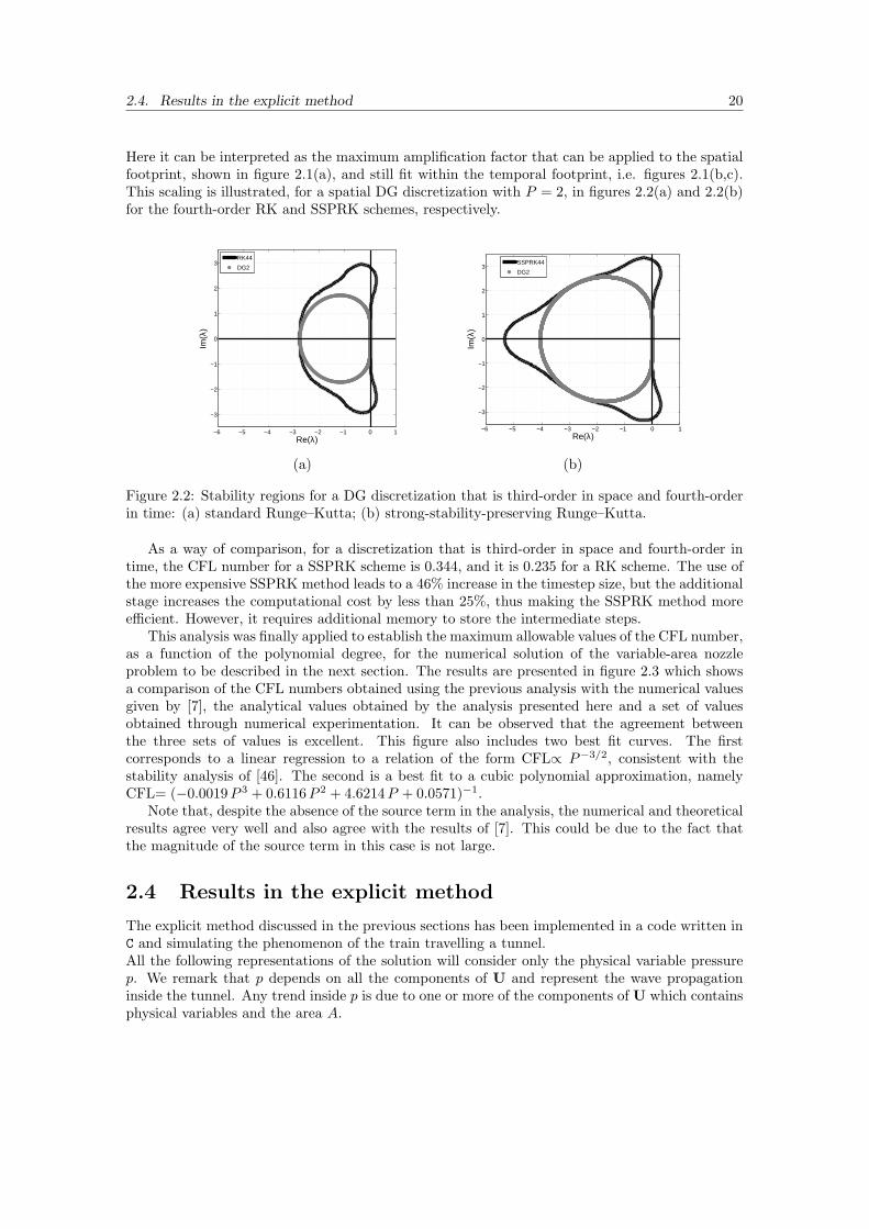
Here it can be interpreted as the maximum amplification factor that can be applied to the spatialfootprint, shown in figure 2.1(a), and still fit within the temporal footprint, i.e. figures 2.1(b,c).This scaling is illustrated, for a spatial DG discretization with P = 2, in figures 2.2(a) and 2.2(b)for the fourth-order RK and SSPRK schemes, respectively.
−6 −5 −4 −3 −2 −1 0 1
−3
−2
−1
0
1
2
3
Re(λ)
Im(λ
)
RK44
DG2
−6 −5 −4 −3 −2 −1 0 1
−3
−2
−1
0
1
2
3
Re(λ)
Im(λ
)
SSPRK44
DG2
(a) (b)
Figure 2.2: Stability regions for a DG discretization that is third-order in space and fourth-orderin time: (a) standard Runge–Kutta; (b) strong-stability-preserving Runge–Kutta.
As a way of comparison, for a discretization that is third-order in space and fourth-order intime, the CFL number for a SSPRK scheme is 0.344, and it is 0.235 for a RK scheme. The use ofthe more expensive SSPRK method leads to a 46% increase in the timestep size, but the additionalstage increases the computational cost by less than 25%, thus making the SSPRK method moreefficient. However, it requires additional memory to store the intermediate steps.
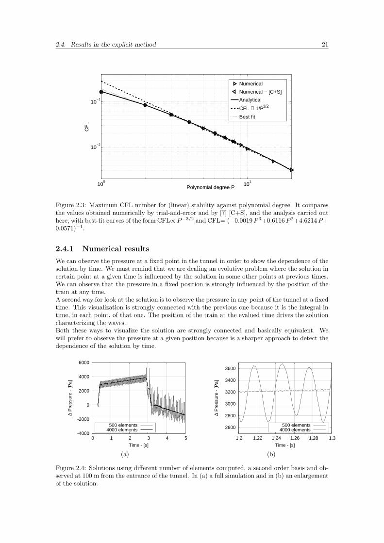
This analysis was finally applied to establish the maximum allowable values of the CFL number,as a function of the polynomial degree, for the numerical solution of the variable-area nozzleproblem to be described in the next section. The results are presented in figure 2.3 which showsa comparison of the CFL numbers obtained using the previous analysis with the numerical valuesgiven by [7], the analytical values obtained by the analysis presented here and a set of valuesobtained through numerical experimentation. It can be observed that the agreement betweenthe three sets of values is excellent. This figure also includes two best fit curves. The firstcorresponds to a linear regression to a relation of the form CFL∝ P−3/2, consistent with thestability analysis of [46]. The second is a best fit to a cubic polynomial approximation, namelyCFL= (−0.0019P 3 + 0.6116P 2 + 4.6214P + 0.0571)−1.
Note that, despite the absence of the source term in the analysis, the numerical and theoreticalresults agree very well and also agree with the results of [7]. This could be due to the fact thatthe magnitude of the source term in this case is not large.
2.4 Results in the explicit method
The explicit method discussed in the previous sections has been implemented in a code written inC and simulating the phenomenon of the train travelling a tunnel.All the following representations of the solution will consider only the physical variable pressurep. We remark that p depends on all the components of U and represent the wave propagationinside the tunnel. Any trend inside p is due to one or more of the components of U which containsphysical variables and the area A.
2.4. Results in the explicit method 21
100
101
10−2
10−1
Polynomial degree P
CF
L
Numerical
Numerical − [C+S]
Analytical
CFL ∝ 1/P3/2
Best fit
Figure 2.3: Maximum CFL number for (linear) stability against polynomial degree. It comparesthe values obtained numerically by trial-and-error and by [7] [C+S], and the analysis carried outhere, with best-fit curves of the form CFL∝ P−3/2 and CFL= (−0.0019P 3+0.6116P 2+4.6214P+0.0571)−1.
2.4.1 Numerical results
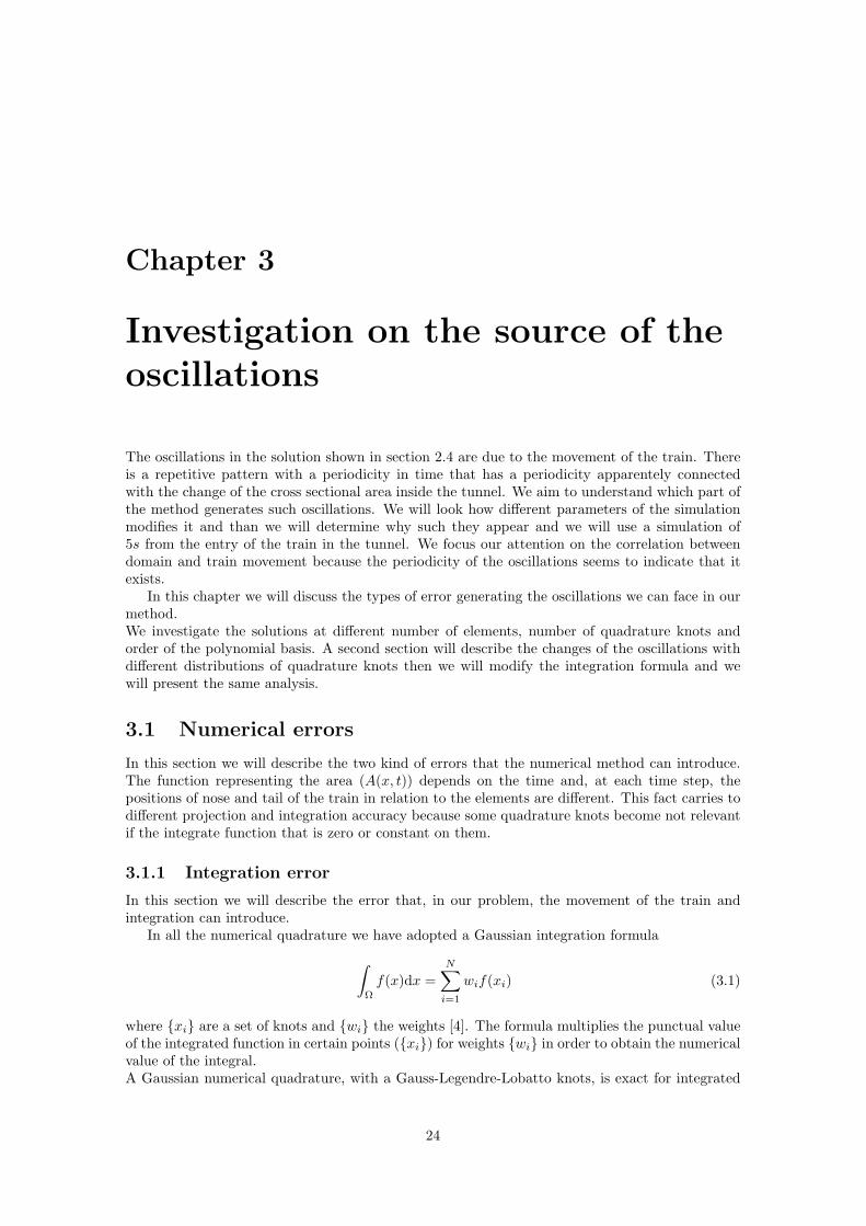
We can observe the pressure at a fixed point in the tunnel in order to show the dependence of thesolution by time. We must remind that we are dealing an evolutive problem where the solution incertain point at a given time is influenced by the solution in some other points at previous times.We can observe that the pressure in a fixed position is strongly influenced by the position of thetrain at any time.A second way for look at the solution is to observe the pressure in any point of the tunnel at a fixedtime. This visualization is strongly connected with the previous one because it is the integral intime, in each point, of that one. The position of the train at the evalued time drives the solutioncharacterizing the waves.Both these ways to visualize the solution are strongly connected and basically equivalent. Wewill prefer to observe the pressure at a given position because is a sharper approach to detect thedependence of the solution by time.
-4000
-2000
0
2000
4000
6000
0 1 2 3 4 5
∆ P
ress
ure
- [P
a]
Time - [s]
500 elements4000 elements 2600
2800
3000
3200
3400
3600
1.2 1.22 1.24 1.26 1.28 1.3
∆ P
ress
ure
- [P
a]
Time - [s]
500 elements4000 elements
(a) (b)
Figure 2.4: Solutions using different number of elements computed, a second order basis and ob-served at 100 m from the entrance of the tunnel. In (a) a full simulation and in (b) an enlargementof the solution.

2.4. Results in the explicit method 22
-4000
-3000
-2000
-1000
0
1000
2000
3000
4000
0 200 400 600 800 1000
∆ P
ress
ure
- [P
a]
Position - [m]
500 elements4000 elements
1400
1600
1800
2000
2200
2400
200 210 220 230 240 250
∆ P
ress
ure
- [P
a]
Position - [m]
500 elements4000 elements
(a) (b)
Figure 2.5: Solutions observed at 5s and computed using different numbers of elements and asecond order basis. In (a) a full simulation and in (b) an enlargement of the solution.
In figure 2.4 and 2.5 we observe the solution computed with our method. Strong oscillationsoccours. In figure 2.4 a periodicity of the oscillations is well clear in the zoomed part and weobserve a reduction of the period with the increased number of elements. This fact indicates anot physical nature of such oscillations because they depend on parameters of the simulation.In figure 2.5 oscillations still remains but sith a different pattern. We can see a first oscillatoryfrequency marking a strong trend with high amplitude and a second frequency with a doubleperiod. This fact suggest the overlapping of two numerical phenomena.
-2000
-1000
0
1000
2000
3000
4000
0 0.5 1 1.5 2 2.5 3 3.5 4 4.5 5 5.5
∆ P
ress
ure
- [P
a]
Time - [s]
Figure 2.6: Solution of the numerical simulation observed at 100m from the tunnel portal.
2.4.2 Discussion on numerical results and their validation
Good numerical solutions of the problem are presented in figure 2.6. In the solution observed ata fixed point we can see a clear effect of the train. The first steep increment of pressure at 0.3sin the entrance of the nose of the train and this stops when it has completely entered the tunnel.From 0.4s to 2.8s a smooth the pressure still increase in relation to the distribuited losses due to

2.4. Results in the explicit method 23
friction effects of the train on the tunnel walls. Than a strong decrement of the pressure occoursdue to the tail of the train that enters in the tunnel. After this moment all the trend is dominatedby viscsity effects. We highlight the small step from 3.2s to 3.6s that is the pressure incrementcorrelated with a pressure wave reflected by the tunnel exit portal.
-1
0
1
2
3
0 5 10 15 20 25 30 35 40
∆ P
ress
ure
- [k
Pa]
Time - [s]
x = 100m
-1.5
-1
-0.5
0
0.5
1
1.5
2
2.5
3
0 5 10 15 20 25 30 35 40
∆ P
ress
ure
- [k
Pa]
Time - [s]
x = 500m
(a) (b)
Figure 2.7: Solutions of the numerical simulation (solid line) compared with the experimental data(dashed line) . In (a) the solution observed at 100s from the tunnel portal and in (b) at 500m.
A good validation of the method is presented in figure 2.7 where we can observe a corre-spondence between the data recorded in an experimental situation and the one obtained with asimulation.That the correspondence is not as good as we can expect mainly when we observe thesimulation far from the tunnel portal. We do have to take in account that also experimental dataare affected by considerable errors due to the mesurements due to the fact the gauge is placed in asingle point in the section of the tunnel and the measures are unable to take in account the localaerodynamic effects that can occour.We remark that the error is only on the amplitude of the waves and never on the position ofthem. This also indicates that a reason of the not perfect agreement could be found in the notvery accurate friction coefficients.
Chapter 3
Investigation on the source of theoscillations
The oscillations in the solution shown in section 2.4 are due to the movement of the train. Thereis a repetitive pattern with a periodicity in time that has a periodicity apparentely connectedwith the change of the cross sectional area inside the tunnel. We aim to understand which part ofthe method generates such oscillations. We will look how different parameters of the simulationmodifies it and than we will determine why such they appear and we will use a simulation of5s from the entry of the train in the tunnel. We focus our attention on the correlation betweendomain and train movement because the periodicity of the oscillations seems to indicate that itexists.
In this chapter we will discuss the types of error generating the oscillations we can face in ourmethod.We investigate the solutions at different number of elements, number of quadrature knots andorder of the polynomial basis. A second section will describe the changes of the oscillations withdifferent distributions of quadrature knots then we will modify the integration formula and wewill present the same analysis.
3.1 Numerical errors
In this section we will describe the two kind of errors that the numerical method can introduce.The function representing the area (A(x, t)) depends on the time and, at each time step, thepositions of nose and tail of the train in relation to the elements are different. This fact carries todifferent projection and integration accuracy because some quadrature knots become not relevantif the integrate function that is zero or constant on them.
3.1.1 Integration error
In this section we will describe the error that, in our problem, the movement of the train andintegration can introduce.
In all the numerical quadrature we have adopted a Gaussian integration formula∫Ω
f(x)dx =N∑i=1
wif(xi) (3.1)
where xi are a set of knots and wi the weights [4]. The formula multiplies the punctual valueof the integrated function in certain points (xi) for weights wi in order to obtain the numericalvalue of the integral.A Gaussian numerical quadrature, with a Gauss-Legendre-Lobatto knots, is exact for integrated
24
3.1. Numerical errors 25
functions that are polynomials of, at maximum, 2N−1 order, where, N is the number of integrationpoints. The degree of precision changes in relation to the knots adopted [4].
-0.04
-0.02
0
0.02
0.04
0.06
0.08
0 0.1 0.2 0.3 0.4 0.5 0.6 0.7 0.8 0.9 1
Err
or L
2 [ ]
x/(Train length)
4 integration points6 integration points8 integration points
-0.2
-0.15
-0.1
-0.05
0
0.05
0.1
0.15
0.2
0.25
0 0.1 0.2 0.3 0.4 0.5 0.6 0.7 0.8 0.9 1
Err
or L
2 [ ]
x/(Element length)
4 integration points6 integration points8 integration points
(a) (b)
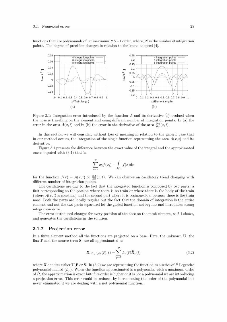
Figure 3.1: Integration error introduced by the function A and its derivative ∂A∂x evalued when
the nose is travelling on the element and using different number of integration points. In (a) theerror in the area A(x, t) and in (b) the error in the derivative of the area ∂A
∂x (x, t).
In this section we will consider, without loss of meaning in relation to the generic case thatin our method occurs, the integration of the single function representing the area A(x, t) and itsderivative.
Figure 3.1 presents the difference between the exact value of the integral and the approximatedone computed with (3.1) that is
N∑i=1
wif(xi)−∫
Ωi
f(x)dx
for the function f(x) = A(x, t) or ∂A∂x (x, t). We can observe an oscillatory trend changing with
different number of integration points.The oscillations are due to the fact that the integrated function is composed by two parts: a
first corresponding to the portion where there is no train or where there is the body of the train(where A(x, t) is constant) and the second part where it is cosinousoidal because there is the trainnose. Both the parts are locally regular but the fact that the domain of integration is the entireelement and not the two parts separated let the global function not regular and introduces strongintegration error.
The error introduced changes for every position of the nose on the mesh element, as 3.1 shows,and generates the oscillations in the solution.
3.1.2 Projection error
In a finite element method all the functions are projected on a base. Here, the unknown U, theflux F and the source term S, are all approximated as
X |Ωe(xe(ξ), t) =
P∑p=1
Lp(ξ)Xp(t) (3.2)
where X denotes either U,F or S. In (3.2) we are representing the function as a series of P Legendrepolynomial named (Lp). When the function approximated is a polynomial with a maximum orderof P , the approximation is exact but if its order is higher or it is not a polynomial we are introducinga projection error. This error could be reduced by incrementing the order of the polynomial butnever eliminated if we are dealing with a not polynomial function.
3.2. Analysis of the solution obtained with the original formulation 26
-0.08
-0.06
-0.04
-0.02
0
0.02
0.04
0.06
0.08
Aex
act -
Anu
m
x
time = 0.0
-0.08
-0.06
-0.04
-0.02
0
0.02
0.04
0.06
0.08
x
time = 0.4
-0.08
-0.06
-0.04
-0.02
0
0.02
0.04
0.06
0.08
x
time = 0.8
-0.3
-0.2
-0.1
0
0.1
0.2
0.3
dAex
act/d
x -
dAnu
m/d
x
x
time = 0.0
-0.3
-0.2
-0.1
0
0.1
0.2
0.3
x
time = 0.4
-0.3
-0.2
-0.1
0
0.1
0.2
0.3
x
time = 0.8
(a) (b)
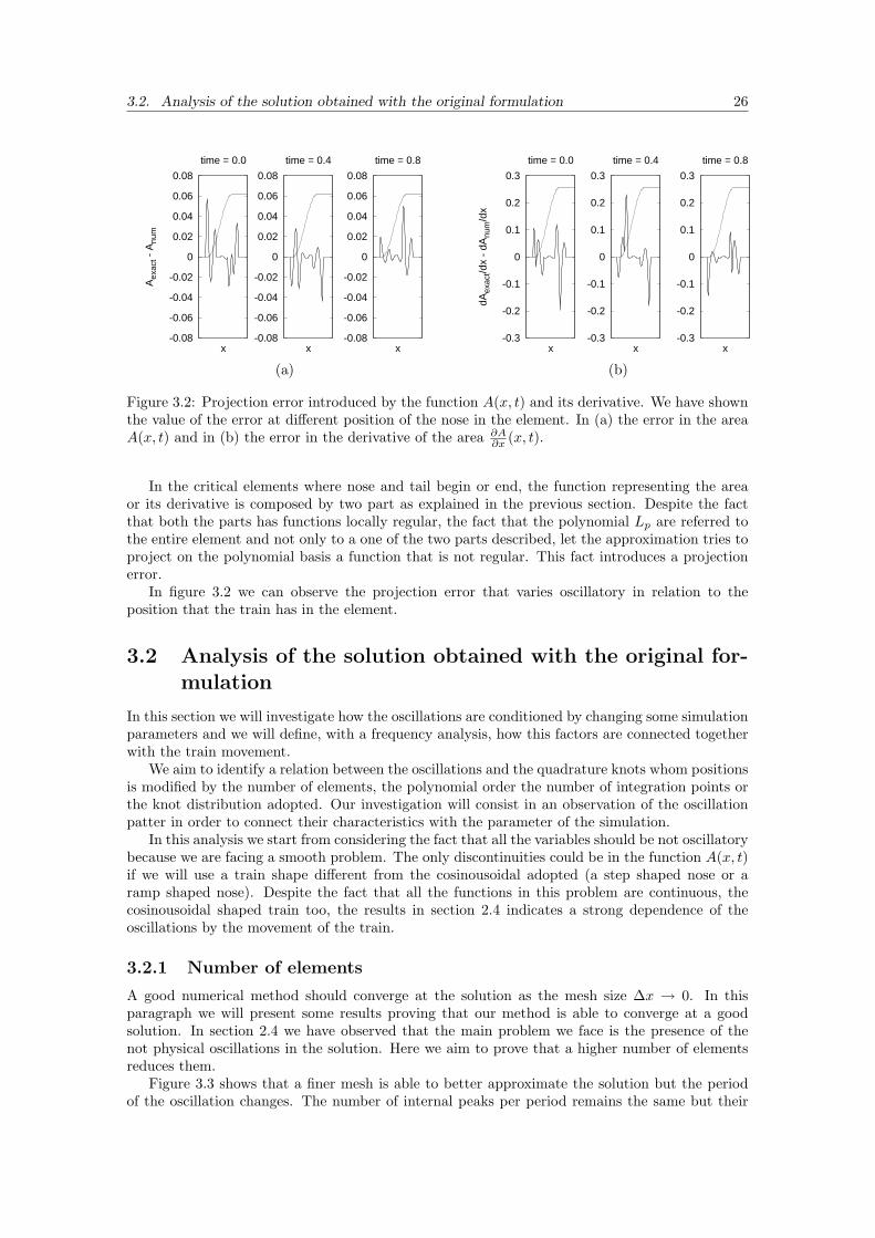
Figure 3.2: Projection error introduced by the function A(x, t) and its derivative. We have shownthe value of the error at different position of the nose in the element. In (a) the error in the areaA(x, t) and in (b) the error in the derivative of the area ∂A
∂x (x, t).
In the critical elements where nose and tail begin or end, the function representing the areaor its derivative is composed by two part as explained in the previous section. Despite the factthat both the parts has functions locally regular, the fact that the polynomial Lp are referred tothe entire element and not only to a one of the two parts described, let the approximation tries toproject on the polynomial basis a function that is not regular. This fact introduces a projectionerror.
In figure 3.2 we can observe the projection error that varies oscillatory in relation to theposition that the train has in the element.
3.2 Analysis of the solution obtained with the original for-mulation
In this section we will investigate how the oscillations are conditioned by changing some simulationparameters and we will define, with a frequency analysis, how this factors are connected togetherwith the train movement.
We aim to identify a relation between the oscillations and the quadrature knots whom positionsis modified by the number of elements, the polynomial order the number of integration points orthe knot distribution adopted. Our investigation will consist in an observation of the oscillationpatter in order to connect their characteristics with the parameter of the simulation.
In this analysis we start from considering the fact that all the variables should be not oscillatorybecause we are facing a smooth problem. The only discontinuities could be in the function A(x, t)if we will use a train shape different from the cosinousoidal adopted (a step shaped nose or aramp shaped nose). Despite the fact that all the functions in this problem are continuous, thecosinousoidal shaped train too, the results in section 2.4 indicates a strong dependence of theoscillations by the movement of the train.
3.2.1 Number of elements
A good numerical method should converge at the solution as the mesh size ∆x → 0. In thisparagraph we will present some results proving that our method is able to converge at a goodsolution. In section 2.4 we have observed that the main problem we face is the presence of thenot physical oscillations in the solution. Here we aim to prove that a higher number of elementsreduces them.
Figure 3.3 shows that a finer mesh is able to better approximate the solution but the periodof the oscillation changes. The number of internal peaks per period remains the same but their

3.2. Analysis of the solution obtained with the original formulation 27
positions are scaled in relation to the mesh size. Changing the mesh size means simply to reducethe physical space between two consecutive knots and consequently integrate the functions moreaccurately.This figure indicates that the lower oscillation frequency is dependent on the element size. Thisconfirms that the oscillations are due to the interaction between the movement of the train andthe mesh.
3160
3180
3200
3220
3240
3260
3280
1.2 1.22 1.24 1.26 1.28 1.3
∆ P
ress
ure
- [P
a]
Time - [s]
500 elements1000 elements4000 elements
Figure 3.3: The difference in the oscillations of the solution increasing the number of elementswith a 4th order base and 6 integration points.
3.2.2 Variation of th order of the polynomial basis
An analysis of the behaviour of the oscillations at different orders of the finite element basisand fixed number of integration points is shown in figure 3.4(a). The oscillations magnitude isincreased as the polynomial degree increases but the peaks maintain the same position and theperiod. This is due to the fact that the integrated function, containing a polynomial of the basis,has a higher order and consequently the numerical integration of the source term coefficients isless accurate.
Figure 3.4(b) plots simulations at different degrees but using a number of integration pointsadapted on the polynomial order. The oscillations are reduced as the degree and the order ofquadrature are increased because we have more points and the linear accuracy of the method letthe precision increase too.
3.2.3 Variation of the number of quadrature knots
In this analysis we simulate cases using different numbers of integration points but keeping constantthe order of the polynomial base. We aim to demonstrate that the oscillations are connected withthe position of the quadrature knots. Unfortunately the method used in this section is not able tomodify separately the number of quadrature knots in the computation of source term coefficientsand the order of the polynomial basis in the flux term. This is due to a program restriction.
Figure 3.5 shows strong oscillations in all the simulations. A closer look at the solution indicatesthat their amplitude is reduced by incrementing the number of quadrature points. This is expected

3.2. Analysis of the solution obtained with the original formulation 28
1270
1280
1290
1300
1310
1320
1330
1340
1.2 1.22 1.24 1.26 1.28 1.3
∆ P
ress
ure
- [P
a]
Time - [s]
1st order3rd order5th order7th order
1100
1200
1300
1400
1500
1600
1700
1800
1900
1.2 1.22 1.24 1.26 1.28 1.3
∆ P
ress
ure
- [P
a]
Time - [s]
1st order - 3 points3rd order - 5 points5th order - 7 points7th order - 9 points
(a) (b)
Figure 3.4: Solutions using different degrees of the polynomial basis. In (a) solutions with 9integration points and in (b) using a variable number of integration points.
(a) (b)
Figure 3.5: Effect of the variation of the number of integration points in the magnitude of theoscillations for a 3rd order basis. In (a) the solution with 4 integration points and in (b) anenlargement of the solutions with different number of quadrature knots within the box
3.2. Analysis of the solution obtained with the original formulation 29
because we are increasing the accuracy of the coefficients integration.Two periodic trends of the pressure can be observed. The first, with a lower frequency, dumpstheir amplitude. The second, let the pressure oscillate with a number of peaks equal to the numberof integration points adopted. The longest period of such oscillations seems to be related to themovement of the train. In fact, if we define the period as
T =∆xV
where ∆x is the mesh element size and V the speed of the train, we observe in figure 3.5 T = 0.065sis exactly the period of the lowest frequency pattern. This also suggests that the internal peaksoccur at the knots. We will advance in this investigation in sections 3.2.4 and 3.2.5.
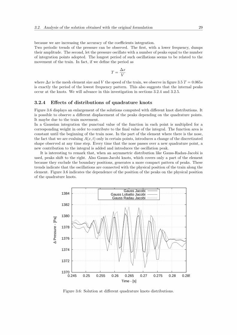
3.2.4 Effects of distributions of quadrature knots
Figure 3.6 displays an enlargement of the solutions computed with different knot distributions. Itis possible to observe a different displacement of the peaks depending on the quadrature points.It maybe due to the train movement.In a Gaussian integration the punctual value of the function in each point is multiplied for acorresponding weight in order to contribute to the final value of the integral. The function area isconstant until the beginning of the train nose. In the part of the element where there is the nose,the fact that we are evaluing A(x, t) only in certain points, introduces a change of the discretizatedshape observed at any time step. Every time that the nose passes over a new quadrature point, anew contribution to the integral is added and introduces the oscillation peak.
It is interesting to remark that, when an asymmetric distribution like Gauss-Radau-Jacobi isused, peaks shift to the right. Also Gauss-Jacobi knots, which covers only a part of the elementbecause they exclude the boundary positions, generates a more compact pattern of peaks. Thesetrends indicate that the oscillations are connected with the physical position of the train along theelement. Figure 3.6 indicates the dependence of the position of the peaks on the physical positionof the quadrature knots.
1370
1372
1374
1376
1378
1380
1382
1384
0.245 0.25 0.255 0.26 0.265 0.27 0.275 0.28 0.285
∆ P
ress
ure
- [P
a]
Time - [s]
Gauss JacobiGauss Lobatto JacobiGauss Radau Jacobi
Figure 3.6: Solution at different quadrature knots distributions.
3.2. Analysis of the solution obtained with the original formulation 30
3.2.5 Spectrum analysis
In this section we will observe the spectrum of the solution in order to have a confirmation ofthe connection between the frequencies observed in the previous plots in this section and theproperties of the solution spectrum. We expect to individuate a number of peaks equal to thenumber of integration points and a distance between them, in the space of the frequencies, relatedto the element size.
The numerical solution obtained is very complex and we have decided to enucleate a partof the solution where it is approximately linear (1s ≤ t ≤ 2.5s). Comparing the spectrum of alinear polynomial with the same properties of the solution in such part we will investigate thedifferences between the two spectra. All the following plots are referred to the difference betweenthe theoretical spectrum and the one of our solution.
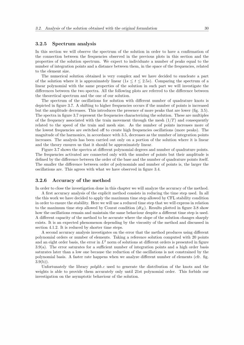
The spectrum of the oscillations for solution with different number of quadrature knots isdepicted in figure 3.7. A shifting to higher frequencies occurs if the number of points is increasedbut the amplitude decreases. This introduces the presence of more peaks that are lower (fig. 3.5).The spectra in figure 3.7 represent the frequencies characterizing the solution. These are multiplesof the frequency associated with the train movement through the mesh (1/T ) and consequentlyrelated to the speed of the train and mesh size. As the number of points increases more ofthe lowest frequencies are switched off to create high frequencies oscillations (more peaks). Themagnitude of the harmonics, in accordance with 3.5, decreases as the number of integration pointsincreases. The analysis has been carried out only on a portion of the solution where it is linearand the theory ensures us that it should be approximately linear.
Figure 3.7 shows the spectra at different polynomial degrees and number of quadrature points.The frequencies activated are connected only with the number of points but their amplitude isdefined by the difference between the order of the base and the number of quadrature points itself.The smaller the difference between order of polynomials and number of points is, the larger theoscillations are. This agrees with what we have observed in figure 3.4.
3.2.6 Accuracy of the method
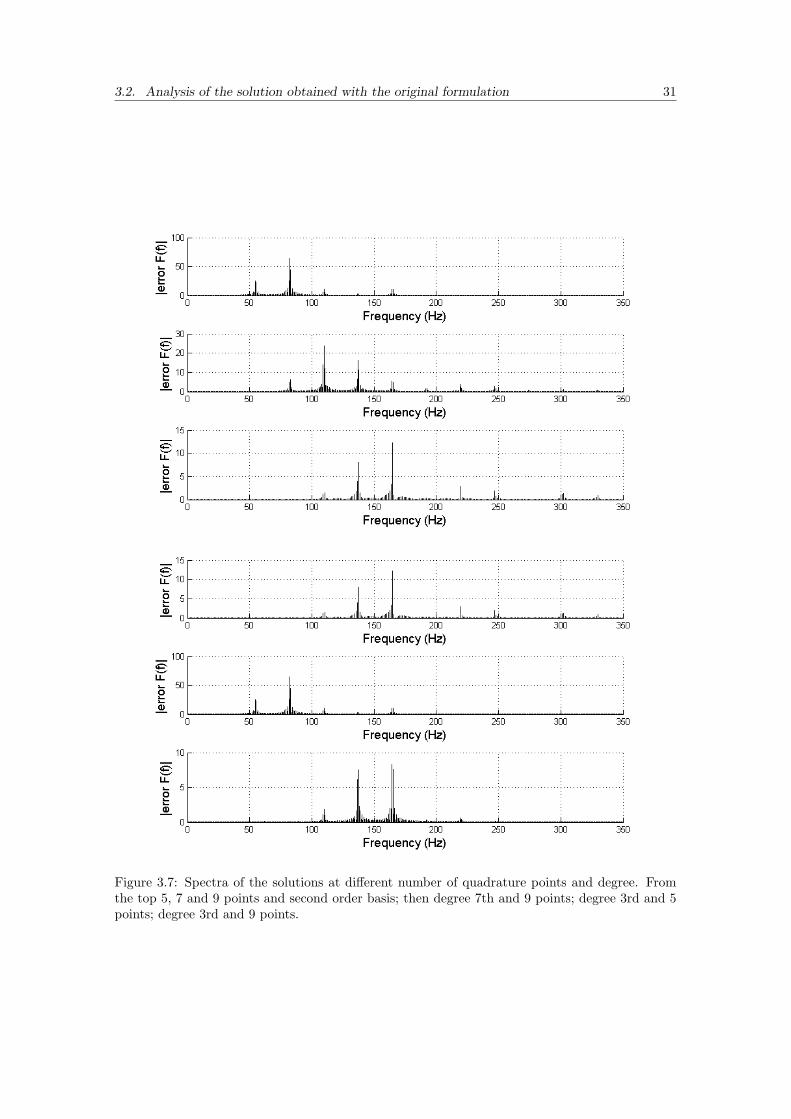
In order to close the investigation done in this chapter we will analyze the accuracy of the method.A first accuracy analysis of the explicit method consists in reducing the time step used. In all
the this work we have decided to apply the maximum time step allowed by CFL stability conditionin order to ensure the stability. Here we will use a reduced time step that we will express in relationto the maximum time step allowed by Courat condition (dtE). Results plotted in figure 3.8 showhow the oscillations remain and maintain the same behaviour despite a different time step is used.A different capacity of the method to be accurate where the slope of the solution changes sharplyexists. It is an expected phenomenon depending by the viscosity of the method and discussed insection 4.1.2. It is reduced by shorter time steps.
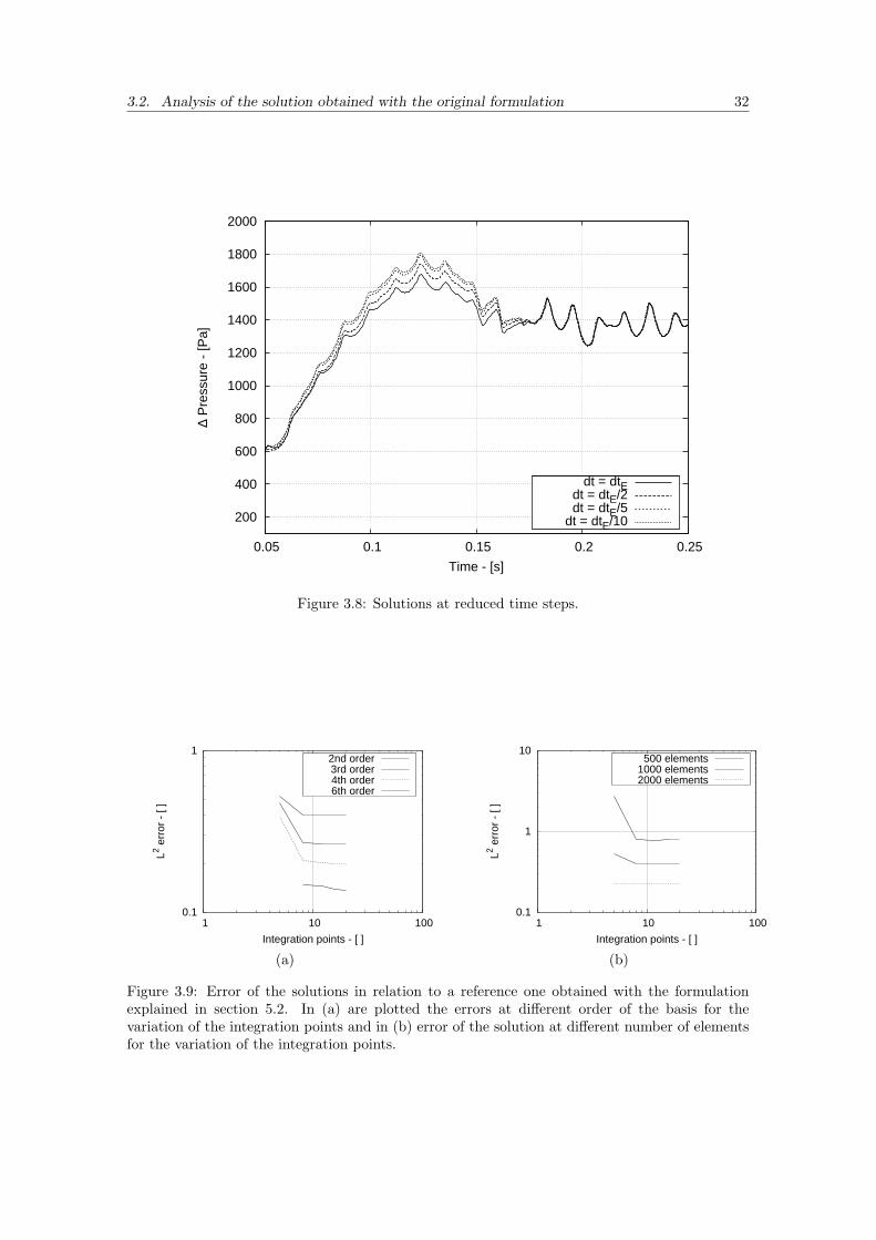
A second accuracy analysis investigates on the error that the method produces using differentpolynomial orders or number of elements. Taking a reference solution computed with 20 pointsand an eight order basis, the error in L2 norm of solutions at different orders is presented in figure3.9(a). The error saturates for a sufficient number of integration points and a high order basissaturates later than a low one because the reduction of the oscillations is not constrained by thepolynomial basis. A faster rate happens when we analyze different number of elements (cfr. fig.3.9(b)).
Unfortunately the library polylib.c used to generate the distribution of the knots and theweights is able to provide them accurately only until 21st polynomial order. This forbids ourinvestigation on the asymptotic behaviour of the solution.
3.2. Analysis of the solution obtained with the original formulation 31
Figure 3.7: Spectra of the solutions at different number of quadrature points and degree. Fromthe top 5, 7 and 9 points and second order basis; then degree 7th and 9 points; degree 3rd and 5points; degree 3rd and 9 points.
3.2. Analysis of the solution obtained with the original formulation 32
200
400
600
800
1000
1200
1400
1600
1800
2000
0.05 0.1 0.15 0.2 0.25
∆ P
ress
ure
- [P
a]
Time - [s]
dt = dtEdt = dtE/2dt = dtE/5
dt = dtE/10
Figure 3.8: Solutions at reduced time steps.
0.1
1
1 10 100
L2 err
or -
[ ]
Integration points - [ ]
2nd order3rd order4th order6th order
0.1
1
10
1 10 100
L2 err
or -
[ ]
Integration points - [ ]
500 elements1000 elements2000 elements
(a) (b)
Figure 3.9: Error of the solutions in relation to a reference one obtained with the formulationexplained in section 5.2. In (a) are plotted the errors at different order of the basis for thevariation of the integration points and in (b) error of the solution at different number of elementsfor the variation of the integration points.
Chapter 4
Implicit method
In this chapter we will present and investigate an implicit integration in time applied to theproblem analyzed. The idea is to solve the problem in space using the DG approach as describedin section 2.2 but to modify the time stepping scheme and use a backward Euler method insteadof a RK or a SSPRK scheme (as done in chapter 2) in order to erease the oscillations.
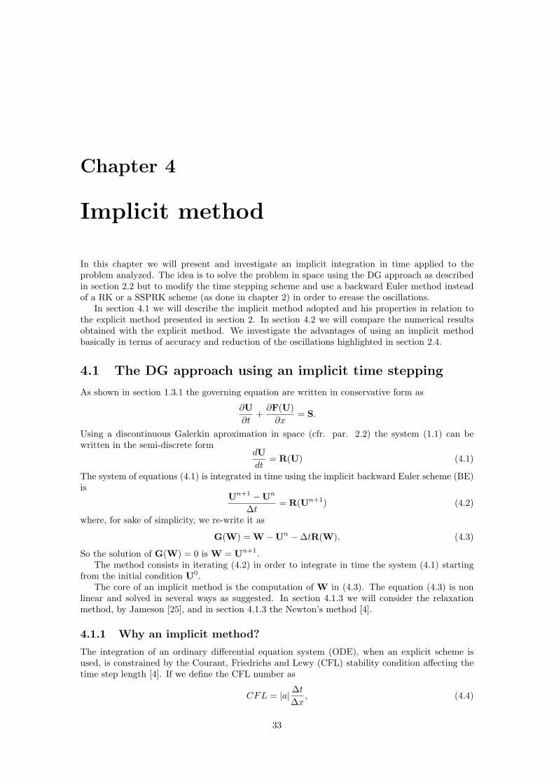
In section 4.1 we will describe the implicit method adopted and his properties in relation tothe explicit method presented in section 2. In section 4.2 we will compare the numerical resultsobtained with the explicit method. We investigate the advantages of using an implicit methodbasically in terms of accuracy and reduction of the oscillations highlighted in section 2.4.
4.1 The DG approach using an implicit time stepping
As shown in section 1.3.1 the governing equation are written in conservative form as
∂U∂t
+∂F(U)∂x
= S.
Using a discontinuous Galerkin aproximation in space (cfr. par. 2.2) the system (1.1) can bewritten in the semi-discrete form
dUdt
= R(U) (4.1)
The system of equations (4.1) is integrated in time using the implicit backward Euler scheme (BE)is
Un+1 −Un
∆t= R(Un+1) (4.2)
where, for sake of simplicity, we re-write it as
G(W) = W−Un −∆tR(W). (4.3)
So the solution of G(W) = 0 is W = Un+1.The method consists in iterating (4.2) in order to integrate in time the system (4.1) starting
from the initial condition U0.The core of an implicit method is the computation of W in (4.3). The equation (4.3) is non
linear and solved in several ways as suggested. In section 4.1.3 we will consider the relaxationmethod, by Jameson [25], and in section 4.1.3 the Newton’s method [4].
4.1.1 Why an implicit method?
The integration of an ordinary differential equation system (ODE), when an explicit scheme isused, is constrained by the Courant, Friedrichs and Lewy (CFL) stability condition affecting thetime step length [4]. If we define the CFL number as
CFL = |a|∆t∆x
, (4.4)
33
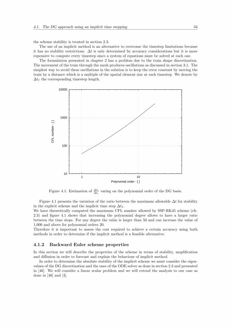
4.1. The DG approach using an implicit time stepping 34
the scheme stability is treated in section 2.3.The use of an implicit method is an alternative to overcome the timestep limitations because
it has no stability restrictions. ∆t is only determined by accuracy considerations but it is moreexpensive to compute every timestep since a system of equations must be solved at each one.
The formulation presented in chapter 2 has a problem due to the train shape discretization.The movement of the train through the mesh produces oscillations as discussed in section 3.1. Thesimplest way to avoid these oscillations in the solution is to keep the error constant by moving thetrain by a distance which is a multiple of the spatial element size at each timestep. We denote by∆tI the corresponding timestep length.
10
100
1000
10000
1 10
CF
L nu
mbe
r -
[ ]
Polynomial order - [ ]
Figure 4.1: Estimation of ∆ti∆te
varing on the polynomial order of the DG basis.
Figure 4.1 presents the variation of the ratio between the maximum allowable ∆t for stabilityin the explicit scheme and the implicit time step ∆tI .We have theoretically computed the maximum CFL number allowed by SSP-RK45 scheme (cfr.2.3) and figure 4.1 shows that increasing the polynomial degree allows to have a larger ratiobetween the time steps. For any degree the value is larger than 50 and can increase the value of1,000 and above for polynomial orders 20.Therefore it is important to assess the cost required to achieve a certain accuracy using bothmethods in order to determine if the implicit method is a feasible alternative.
4.1.2 Backward Euler scheme properties
In this section we will describe the properties of the scheme in terms of stability, amplificationand diffusion in order to forecast and explain the behaviour of implicit method.
In order to determine the absolute stability of the implicit scheme we must consider the eigen-values of the DG discretization and the ones of the ODE solver as done in section 2.3 and presentedin [46]. We will consider a linear scalar problem and we will extend the analysis to our case asdone in [46] and [4].

4.1. The DG approach using an implicit time stepping 35
Stability of the backward Euler method
Here we will consider the hyperbolic linear advection equation
∂u
∂t+ a
∂u
∂x= 0 (4.5)
with a > 0. Following the analysis in section 2.3 we have
M d
dtUe−DU
e+ FU
e+ GU
e−1= 0
and, by assuming a wave-like solution (2.27), we define the matrix A =M−1−D + F + Ge−iθin order to compute the spectrum of the DG spatial problem.
[A− (iω)I] Ue
= 0 (4.6)
The stability criteria <(λ) ≤ 1 ensures the stability of the spatial discretization.The second part of stability analysis in a hyperbolic equation is related to the time stepping.
In the explicit formulation, RK and SSP-RK methods were implemented but here we deal withan implicit backward Euler scheme.Due to the fact we are analyzing an implicit method, we expect that, according to the secondDahlquist barrier, first and second order Backward Differentiation Formula (BDF) are A-stablefor any degree of the DG polynomial [4].BE is the first order BDF method but it could also be read as an implicit RK scheme with thefollowing Butchers’ arrays
1 11
b Ac
0Backward Euler General R-K
.
The absolute stability region has been obtained from the spectrum of the operator representingthe scheme. Defining z = λ∆t is given by the eigenvalues and we can build the following stabilityfunction
S(z) = 1 + zbT (I− zA)−11 (4.7)
where 1 = (1, ..., 1)T . The stability region is the set of complex values z such that |S(z)| < 1. Forthe backward Euler the region of stability is represented in figure 4.2 and it is the complementaryof the circle enclosed in the right semiplane. The same figure shows the spectrum for a 4th orderpolynomial of DG. It is clear that BE is stable for any degree of DG polynomial order.
Amplification properties of the method
We have adopted a Von Neumann analysis to study the amplification error as explained in [4] and[46] based on the approximation of the solution with a Fourier series. If we consider the initialconditions
U0 =∞∑
k=−∞
αkeikx
where the vector αk representing the k − th the Fourier coefficent is
αk =1
2π
∫ 2π
0
U0(x)e−ikx.
If we define the size of the spatial element h = ∆x we have
U0e = U0(xe) =
∞∑k=−∞
αkeikehe = 0,±1,±2, ...
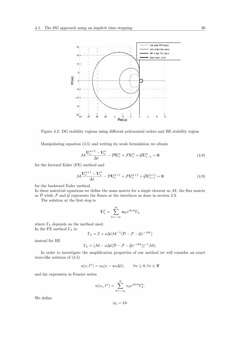
4.1. The DG approach using an implicit time stepping 36
Figure 4.2: DG stability regions using different polynomial orders and BE stability region
Manipulating equation (4.5) and writing its weak formulation we obtain
MUn+1e −Un
e
∆t−DUn
e + FUne + GUn
e−1 = 0 (4.8)
for the forward Euler (FE) method and
MUn+1e −Un
e
∆t−DUn+1
e + FUn+1e + GUn+1
e−1 = 0 (4.9)
for the backward Euler method.In these matricial equations we define the mass matrix for a single element asM, the flux matrixas D while F and G represents the fluxes at the interfaces as done in section 2.3.
The solution at the first step is
U1e =
∞∑k=−∞
αkeikehΓk
where Γk depends on the method used.In the FE method Γk is:
Γk = I + a∆tM−1(D −F − Ge−ihk)
instead for BEΓk = (M− a∆t(D −F − Ge−ihk))−1M).
In order to investigate the amplification properties of our method we will consider an exactwave-like solution of (4.5)
u(x, tn) = u0(x− an∆t), ∀n ≥ 0,∀x ∈ <
and his expression in Fourier series:
u(xe, tn) =∞∑
k=−∞
αkeikehΓnk .
We defineφk = kh
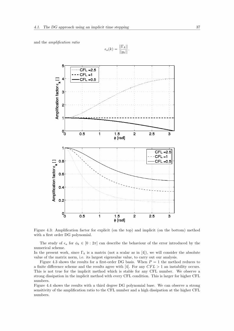
4.1. The DG approach using an implicit time stepping 37
and the amplification ratio
εa(k) =||Γk||||gk||
.
Figure 4.3: Amplification factor for explicit (on the top) and implicit (on the bottom) methodwith a first order DG polynomial.
The study of εa for φk ∈ [0 : 2π] can describe the behaviour of the error introduced by thenumerical scheme.In the present work, since Γk is a matrix (not a scalar as in [4]), we will consider the absolutevalue of the matrix norm, i.e. its largest eigenvalue value, to carry out our analysis.
Figure 4.3 shows the results for a first-order DG basis. When P = 1 the method reduces toa finite difference scheme and the results agree with [4]. For any CFL > 1 an instability occurs.This is not true for the implicit method which is stable for any CFL number. We observe astrong dissipation in the implicit method with every CFL condition. This is larger for higher CFLnumbers.Figure 4.4 shows the results with a third degree DG polynomial base. We can observe a strongsensitivity of the amplification ratio to the CFL number and a high dissipation at the higher CFLnumbers.

4.1. The DG approach using an implicit time stepping 38
Figure 4.4: Amplification factor for implicit method with third DG order basis
4.1.3 Implicit solvers
In this section we will describe the two approaches implemented in order to solve the implicitequation (4.3) at any iteration. Here we consider relaxation approach and Newton’s method.
Relaxation approach
This method has been proposed by Jameson [25, 26] and is based on the idea that the unknownW of the system of equations (4.3) could be considered as a steady state of an evolutive systemof differential equations.
For this propouse we define
f(W) = W−Un −∆tR(W) = 0 (4.10)
so that, the evolutive equation∂W∂τ
+ f(W) = 0 (4.11)
has a steady-state W that is the solution of (4.10) for τ →∞. We can apply an explicit methodto integrate the equation (4.11) in time as
Wk+1 −Wk
∆τ= f(Wk), (4.12)
or a RK scheme as done in the explicit method. This implies that a CFL condition must besatisfied.
The term f(W) in (4.10) can be substitued in (4.12) and an internal iteration becomes
Wk+1 = Wk −∆τ(Wk −Un −∆tR(Wk)). (4.13)
The method integrates in the non-physical time the equation (4.13) until τ is great enough to
consider W(k+1) a good approximation of Un+1. Here we consider∣∣∣∣∣∣Wk+1−Wk
∆t
∣∣∣∣∣∣L2
< tol asstopping criteria, where tol is a fixed value indicating the maximum difference allowed betweentwo iterations.
Figure 4.5 shows the trend of the error when we integrate equation (4.13). We expect thata relaxation scheme would be able to quickly reduce the error in the first iterations but that itwould be slower when we are close to the solution. Figure 4.5 instead indicates that the errortends to be reduced faster when we are close to the solution than when we are far from that.

4.1. The DG approach using an implicit time stepping 39
1e-05
0.0001
0.001
0.01
1 10 100 1000 10000 100000
Res
idua
l (W
k+1 -W
k )/ ∆
τ -
[ ]
iteration - [ ]
Figure 4.5: Error in the internal loop integrating the steady equation 4.13.
The choice of the initial guess To reduce the computational time in relaxation method and toensure the convergence of the Newton’s method the choice of the initial guess W0 is fundamental.We have evalued different methods for approximating the initial guess:
1. Extrapolation of an explicit Runge-Kutta step;
2. Previous implicit time step solution value;
3. Linear extrapolation on the two previous time iterations;
4. Quadratic extrapolation on the three previous time iterations.
The method based on RK extrapolation prediction fails due to the oscillation that could beobserved in the explicit method after few explicit timesteps.
Figure 4.6 shows the error recorded before the first internal iteration. Linear extrapolationis the best technique because it prevents errors due to sharp changes of slope in the solution. Aquadratic extrapolation does not, but it is able to introduce a prediction of the solution at thenext timestep that a constant extrapolation is not able to do.
The advantages of computing an accurate initial guess are small because, as we could observein figure 4.5, the first iterations of relaxation method are able to very quickly reduce the error.
Newton’s method
We will apply the Newton’s method it for computing the single implicit iteration of our implicitscheme. If we have:
T(x) = 0
the Jacobian matrix is defined as
(JT(x))ij(x) = (∂Ti∂xj
)(x).

4.1. The DG approach using an implicit time stepping 40
0
0.2
0.4
0.6
0.8
1
1.2
1 2 3 4 5 6 7
Res
idua
l (W
k+1 -W
k )/ ∆
τ -
[ ]
iteration - [ ]
Constant extrapolationLinear extrapolation
Quadratic extrapolation
Figure 4.6: Initial residual∣∣∣∣∣∣Wk+1−Wk
∆t
∣∣∣∣∣∣L2
at different timesteps using different extrapolationtechniques.
A step of the Newton’s method is given by [4]:
JT(x)(x(k))δx(k) = −T(x(k))x(k+1) = x(k) + δx(k) (4.14)
For the backward Euler method we have
U(n+1) −U(n)
∆t=M−1
[DF(n+1) − F(n+1)
]+ S(n+1)
therefore the function T becomes
T(U(n+1)) =U(n+1) −U(n)
∆t−M−1
[DF(n+1) − F(n+1)
]− S(n+1). (4.15)
The core of a Newton’s method is the computation of the Jacobian matrix that can be ana-lytically or numerically evalued. If we use an approximate one the method can loose some math-ematical properties in terms of velocity of convergence and it is named quasi-Newton method [4].An analytical differentiation of the function is very complicated in our problem hence we haveused the first order approximation
JT(x)ij =Ti(Wj + δW)− Ti(Wj)
δWj(4.16)
where the choice of δW is not critical and is setted a-priori.The size of the matrix is an important parameter defining the numerical problem because it
describes the computational costs. If we call Ne the number of elements in the mesh and Np thenumber quadrature knots in each element, JT(x) ∈ <N ×<N where N = 3NeNp. The building ofthe Jacobian matrix is very expensive and, in order to reduce the computational costs, we havefrozen it for a number of steps. This technique increases the computational efficiency because thecomputation of the matrix is not required every step but it reduces the speed of convergence of
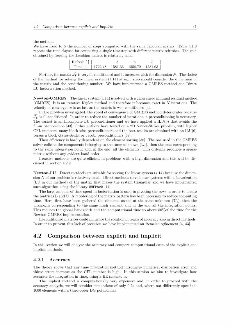
4.2. Comparison between explicit and implicit 41
the method.We have fixed to 5 the number of steps computed with the same Jacobian matrix. Table 4.1.3reports the time elapsed for computing a single timestep with different matrix refreshes. The gainobtained by freezing the Jacobian matrix is relatively small.
Refresh [ ] 1 3 5 7Time [s] 1722.48 1581.36 1558.72 1581.63
Further, the matrix JT is very ill-conditioned and it increases with the dimensionN . The choiceof the method for solving the linear system (4.14) at each step should consider the dimension ofthe matrix and the conditioning number. We have implemented a GMRES method and DirectLU factorization method.
Newton-GMRES The linear system (4.14) is solved with a generalized minimal residual method(GMRES). It is an iterative Krylov method and therefore it becomes exact in N iterations. Thevelocity of convergence is as fast as the matrix is well-conditioned [4].
In the problem investigated, the speed of convergence of GMRES method deteriorates becauseJT is ill-conditioned. In order to reduce the number of iterations, a preconditioning is necessary.The easiest is an Incomplete LU preconditioner and we have applied a ILU(0) that avoids thefill-in phenomenon [43]. Other authors have tested on a 2D Navier-Stokes problem, with higherCFL numbers, many block-wise preconditioners and the best results are obtained with an ILU(0)versus a block Gauss-Seidel or Jacobi preconditioners [38].
Their efficiency is hardly dependent on the element sorting [38]. The one used in the GMRESsolver collects the components belonging to the same unknown (Ui), then the ones correspondingto the same integration point and, in the end, all the elements. This ordering produces a sparsematrix without any evident band order.
Iterative methods are quite efficient in problems with a high dimension and this will be dis-cussed in section 4.2.2.
Newton-LU Direct methods are suitable for solving the linear system (4.14) because the dimen-sion N of our problem is relatively small. Direct methods solve linear systems with a factorization(LU in our method) of the matrix that makes the system triangular and we have implementedsuch algorithm using the library UMFPack [11].
The large amount of time spent in factorization is used in pivoting the rows in order to createthe matrices L and U. A reordering of the matrix pattern has been necessary to reduce computingtime. Here, first have been gathered the elements owned at the same unknown (Ui), then theunknowns corresponding to the same mesh element and in the end all the integration points.This reduces the global bandwidth and the computational time to about 50%of the time for theNewton-GMRES implementation.
Ill-conditioned matrices could influence the solution in terms of accuracy also in direct methods.In order to prevent this lack of precision we have implemented an iterative refinement [4, 43].
4.2 Comparison between explicit and implicit
In this section we will analyze the accuracy and compare computational costs of the explicit andimplicit methods.
4.2.1 Accuracy
The theory shows that any time integration method introduces numerical dissipation error andthiese errors increase as the CFL number is high. In this section we aim to investigate howaccurate the integration in time, using a BE scheme, is.
The implicit method is computationally very expensive and, in order to proceed with theaccuracy analysis, we will consider simulations of only 0.2s and, where not differently specified,1000 elements with a third-order DG polynomial.
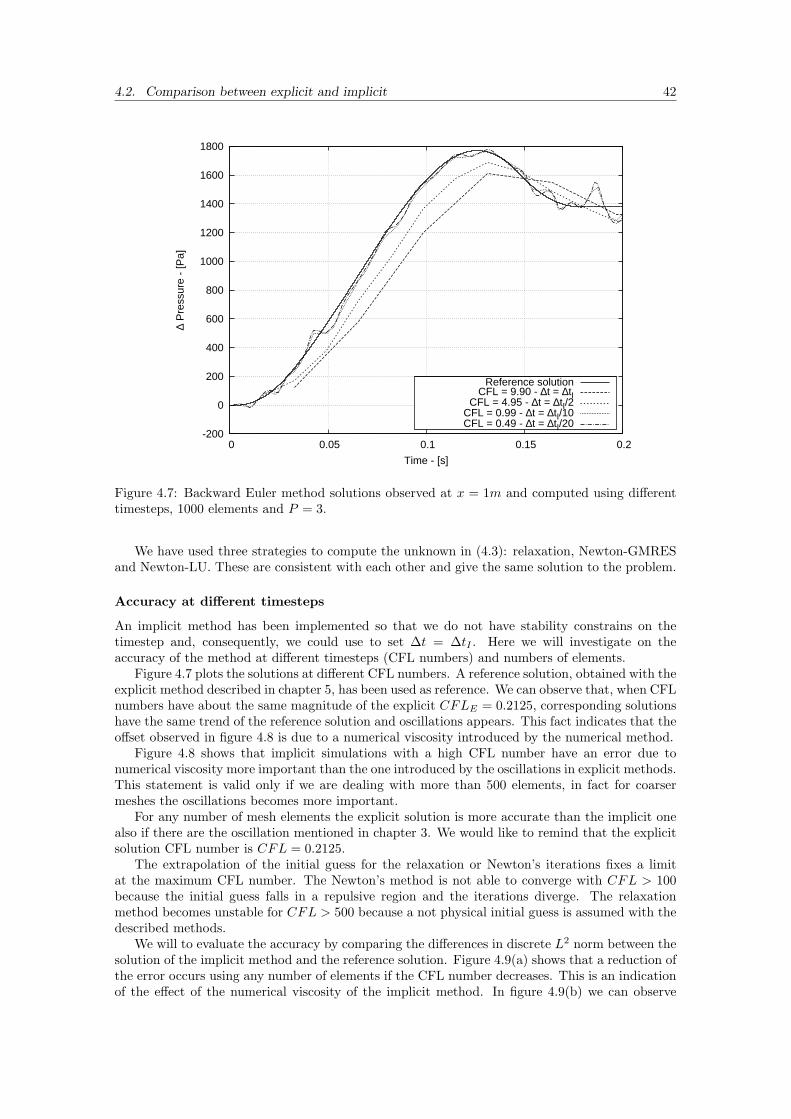
4.2. Comparison between explicit and implicit 42
-200
0
200
400
600
800
1000
1200
1400
1600
1800
0 0.05 0.1 0.15 0.2
∆ P
ress
ure
- [P
a]
Time - [s]
Reference solutionCFL = 9.90 - ∆t = ∆tI
CFL = 4.95 - ∆t = ∆tI/2CFL = 0.99 - ∆t = ∆tI/10CFL = 0.49 - ∆t = ∆tI/20
Figure 4.7: Backward Euler method solutions observed at x = 1m and computed using differenttimesteps, 1000 elements and P = 3.
We have used three strategies to compute the unknown in (4.3): relaxation, Newton-GMRESand Newton-LU. These are consistent with each other and give the same solution to the problem.
Accuracy at different timesteps
An implicit method has been implemented so that we do not have stability constrains on thetimestep and, consequently, we could use to set ∆t = ∆tI . Here we will investigate on theaccuracy of the method at different timesteps (CFL numbers) and numbers of elements.
Figure 4.7 plots the solutions at different CFL numbers. A reference solution, obtained with theexplicit method described in chapter 5, has been used as reference. We can observe that, when CFLnumbers have about the same magnitude of the explicit CFLE = 0.2125, corresponding solutionshave the same trend of the reference solution and oscillations appears. This fact indicates that theoffset observed in figure 4.8 is due to a numerical viscosity introduced by the numerical method.
Figure 4.8 shows that implicit simulations with a high CFL number have an error due tonumerical viscosity more important than the one introduced by the oscillations in explicit methods.This statement is valid only if we are dealing with more than 500 elements, in fact for coarsermeshes the oscillations becomes more important.
For any number of mesh elements the explicit solution is more accurate than the implicit onealso if there are the oscillation mentioned in chapter 3. We would like to remind that the explicitsolution CFL number is CFL = 0.2125.
The extrapolation of the initial guess for the relaxation or Newton’s iterations fixes a limitat the maximum CFL number. The Newton’s method is not able to converge with CFL > 100because the initial guess falls in a repulsive region and the iterations diverge. The relaxationmethod becomes unstable for CFL > 500 because a not physical initial guess is assumed with thedescribed methods.
We will to evaluate the accuracy by comparing the differences in discrete L2 norm between thesolution of the implicit method and the reference solution. Figure 4.9(a) shows that a reduction ofthe error occurs using any number of elements if the CFL number decreases. This is an indicationof the effect of the numerical viscosity of the implicit method. In figure 4.9(b) we can observe

4.2. Comparison between explicit and implicit 43
-200
0
200
400
600
800
1000
1200
1400
1600
1800
0 0.05 0.1 0.15 0.2
∆ P
ress
ure
- [P
a]
Time - [s]
Reference solutionExplicit solutionImplicit solution
Figure 4.8: Implicit and explicit solutions computed using 1000 elements, P = 3 and, for theimplicit timestep ∆t = ∆tI .
that a larger number of elements reduces the error. The CFL corresponding at the movement thetrain of one element per time is CFL = 9.9.
Long time simulations and oscillations in the method
The implicit method has been implemented to investigate if the oscillations will disappear usinga timestep that let the train advance one element per timestep.
Figure 4.10 shows implicit solutions on a long time interval and a timestep equal to ∆tI . Wecan notice that in the enlarged view 4.10(b) no oscillations appear. In fact the projection andintegration error does not disappear but it remains constant and it is able to produce an offsetbut not oscillations.
4.2.2 Computational costs
One of the initial aims of implicit methods was to reduce the computing time. Unfortunately itdoes not happen as explained in the following.
An accurate explicit simulation on all the tunnel length requires at least 2000 elements but thecomputational costs n the implicit scheme allow us to test te accuracy only on a smaller problemwhere the number of elements has been progressively increased from 50 to 400. Now we plotsimulation on the full tunnel length but for a short time of 0.1s. We are able to show in figure 4.11the computational cost of implicit: relaxation, Newton-GMRES and Newton-LU methods and ofthe explicit method.In this figure we see that relaxation method is the less expensive with all problem dimensionsn. Only for very small problems (n ≤ 100) the Newton method is competitive with Jameson’sapproach.Much less expensive than all the tested implicit methods is the explicit one that is two orders ofmagnitude faster.

4.2. Comparison between explicit and implicit 44
0.01
0.1
1
10
100
1000
0.1 1
Err
or L
2 - [
]
∆t/∆tI [ ]
500 elements750 elements
1000 elements2000 elements4000 elements 0.01
0.1
1
10
100
1000
100 1000 10000
Err
or L
2 - [
]
Number of elements - [ ]
CFL = 9.90 - ∆t = ∆tICFL = 4.65 - ∆t = ∆tI/2
CFL = 0.99 - ∆t = ∆tI/10CFL = 0.49 - ∆t = ∆tI/20
(a) (b)
Figure 4.9: Backward Euler method accuracy. In (a) errors using different number of element andin (b) using different timesteps ∆t.
-500
0
500
1000
1500
2000
2500
3000
3500
4000
0 0.5 1 1.5 2 2.5 3 3.5
∆ P
ress
ure
- [P
a]
Time - [s]
Reference Solution500 elements
1000 elements 3000
3100
3200
3300
3400
3500
3600
3700
3800
1 1.2 1.4 1.6 1.8 2 2.2 2.4
∆ P
ress
ure
- [P
a]
Time - [s]
500 elements1000 elements
(a) (b)
Figure 4.10: Backward Euler simulations on a long time interval (3.5s) and a timestep equal to∆t. In (a) the full simulation and in (b) an enlarged view of (a).
The main difference between a relaxation and a Newton’s method has been shown in figure4.12 and table 4.1. The first solves many times a cheap iteration, the second few times a reallyexpensive iteration.
Finally table 4.13 reports a profiling for the GMRES and the LU Newton’s solvers divided inthe two main tasks: computing the Jacobian matrix and solving the linear system.It is evident that, for the LU method, the largest amount of time has been spent in computingthe Jacobian matrix and its factorization, instead, in a GMRES method in the linear systemsolving. Due to this observation, we have changed the matrix pattern as described in 4.1.3 andperformances improve.
elements / iteration 1 2 3 4 5 6 7 8 9 10 11 12 131000 2 4 8 7 - - - - - - - - -2000 2 3 7 7 7 7 7 - - - - - -4000 2 2 7 7 7 7 7 7 7 7 7 7 7
Table 4.1: Number of iterations in the Newton’s method at each timestep.
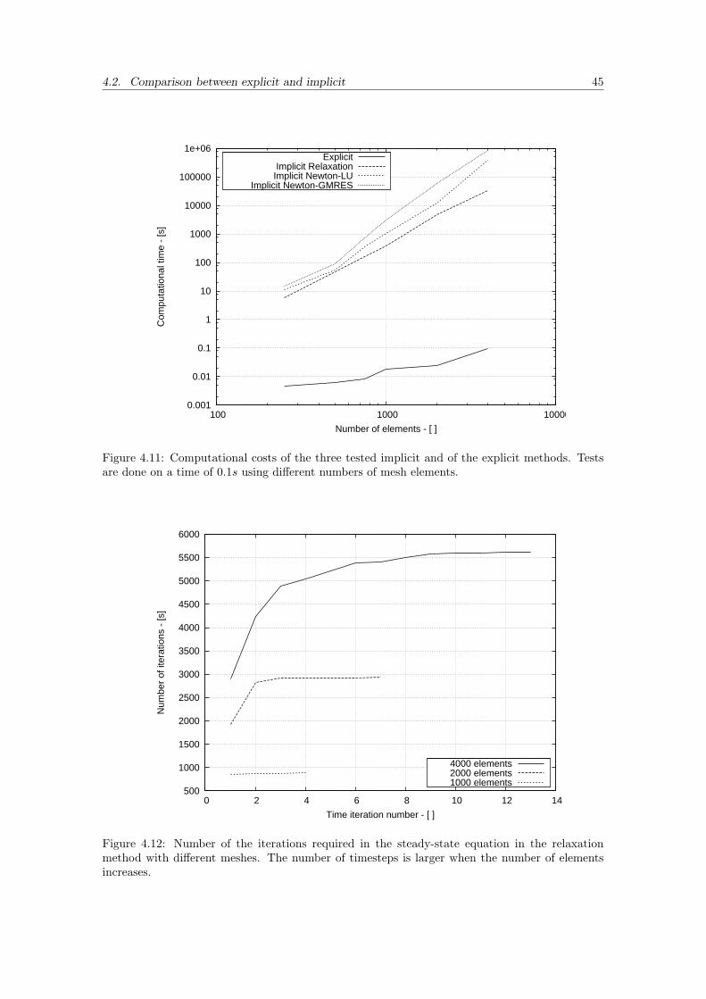
4.2. Comparison between explicit and implicit 45
0.001
0.01
0.1
1
10
100
1000
10000
100000
1e+06
100 1000 10000
Com
puta
tiona
l tim
e -
[s]
Number of elements - [ ]
ExplicitImplicit RelaxationImplicit Newton-LU
Implicit Newton-GMRES
Figure 4.11: Computational costs of the three tested implicit and of the explicit methods. Testsare done on a time of 0.1s using different numbers of mesh elements.
500
1000
1500
2000
2500
3000
3500
4000
4500
5000
5500
6000
0 2 4 6 8 10 12 14
Num
ber
of it
erat
ions
- [s
]
Time iteration number - [ ]
4000 elements2000 elements1000 elements
Figure 4.12: Number of the iterations required in the steady-state equation in the relaxationmethod with different meshes. The number of timesteps is larger when the number of elementsincreases.

4.2. Comparison between explicit and implicit 46
0.01
0.1
1
10
100
1000 10000
Com
puta
tiona
l tim
e -
[s]
Number of elements - [ ]
Newton-LU system solvingNewton-GMRES system solving
Newton-LU JacobianNewton-GMRES Jacobian
Figure 4.13: Costs of the different parts of the schemes (Jacobian matrix computation and solutionof the system) and comparison between Newton-GMRES and Newton-LU approaches.

Chapter 5
An alternative treatment of thearea in the DG formulation
In the analysis in section 3.2 we established that the oscillations are connected to the integrationof the source term and more precisely to the approximation of the area and its derivative.If the viscosity coefficients in the source term are set to zero (Euler equation) the oscillations stillappear and they are due to the pressure term of (1.2)
S =
0p∂A∂x
0
.If we consider that the source term is approximated as
S(U |Ωe (xe(ξ), t)) =P∑p=0
Lp(ξ)Sp(t). (5.1)
When we compute the Legendre coefficients (3.2) and reproject them on the physical space (5.1)two errors could occur. The first is due to the projection of the source term on the polynomialspace represented by (5.1) and the second one due to an inaccurate quadrature scheme (3.2).
In this chapter we will reformulate the weak problem by extracting the area from the unknownsand from the source term coefficients (section 5.1.1) in order to avoid the projection error. Wewill present the results obtained with this new formulation (section 5.1.2) and, in the last section5.3, we will isolate the projection error comparing the formulation used in chapter 3 with the newone.
5.1 New weak formulation without the area in the unknowns
Chapter 3 indicates that the oscillations are mainly due to an integration error but we can supposethat a part of their nature could be driven by a projection error. We can observe that thequadrature formula that computes only the pressure contribution in the source term can be writtenas
S1,p(t) =2p+ 1
2
N∑i=1
wiLq(ξi)p(xe(ξi), t)∂A
∂x(xe(ξi), t).
The idea followed in the next paragraphs is to rewrite the equations using a new set of variablefor eliminating the projection error. In fact this is a smooth problem and we expect that allthe variables are not oscillatory so, the only function with discontinuities, is the derivative of thearea. We aim to do not represent it by a projection on the Legendre base in order to avoid anyprojection error.
47

5.1. New weak formulation without the area in the unknowns 48
5.1.1 Derivation of the new weak formulation
The idea is to modify the weak formulation and the unknowns in order to take the area (andits derivative) out from the integral. This fact gives us the possibility to integrate the area asaccurately as we want and to dissociate the integrative error for the contribution of the area fromthe projection error of the source term.From the previous formulation where the unknowns are given by (1.2) now we will write U = UAand F = FA with
U =
ρρuρE
; F(U) =
ρu(ρu2 + p)ρuH
.We split the original source term in three parts
S1 =
0p∂A∂x
0
S2 =
0Dm
Dh
S3 =
0Cd p
∂A∂x
−Cd V p ∂A∂x
(5.2)
where Dm, Dh, Qm and Qh are equations (1.3) and (1.4).Here S1 and S3 depend on the area but S2 does not. So we write
S = S1∂A
∂xS2 = S1 S3 = S3
∂A
∂x(5.3)
so that
S1 =
0p0
S3 =
0Cd p−Cd V p
(5.4)
.For writing this new formulation we have to start from the weak form∫
Ω
w∂U∂t
dx+∫
Ω
w∂F(U)∂x
dx−∫
Ω
wS(U)dx = 0 (5.5)
where, substituting (5.4), we get:∫Ω
w∂U∂t
Adx+∫
Ω
w∂A
∂tUdx+
∫Ω
w∂F(U)A∂x
dx
−∫
Ω
w
[S2(U) +
(S1(U) + S3(U)
) ∂A∂x
]dx = 0
(5.6)
Integrating by parts and introducing the numerical fluxes Fu, we arrive to the equation:
Nel∑e=1
∫Ωe
w∂U∂t
Adx+∫
Ωe
w∂A
∂tUdx
−Nel∑e=1
∫Ωe
dw
dxF(U)Adx+
[wF
uA]xr
e
xle
−Nel∑e=1
∫Ωe
w
(S2(U) +
[S1(U) + S3(U)
) ∂A∂x
]dx = 0
(5.7)
In the Galerkin approach we chosen the weighting functions to be polynomials of Legendre basis
w |Ωe (xe(ξ)) = Lp(ξ) (5.8)

5.1. New weak formulation without the area in the unknowns 49
and if we will project all the function on such base we are able to evaluate the functions as:
U |Ωe (xe(ξ), t) =P∑p=0
Lp(ξ)Up(t) (5.9)
F(U |Ωe (xe(ξ), t)) =P∑p=0
Lp(ξ)Fp(t) (5.10)
Si(U |Ωe (xe(ξ), t)) =P∑p=0
Lp(ξ)Si,p(t) (5.11)
. The equation now becomes:∫Ωe
Lq(ξ)P∑p=0
Lp(ξ)∂Up
∂tA(ξ)dx+
∫Ωe
Lq(ξ)P∑p=0
Lp(ξ)∂A(ξ)∂t
Updx
−∫
Ωe
dLq(ξ)dx
P∑p=0
Lp(ξ)FpA(ξ)dx+[Lq(ξ)F
uA(ξ)
]xr
xl
−∫
Ωe
Lq(ξ)P∑p=0
Lp(ξ)(
S2,p +(S1,p + S3,p
) ∂A∂x
(ξ))
dx = 0
q = 1, . . . , P
(5.12)
In order to write the equation more compactly we define the matrices:
Mpq =∫
Ωi
Lp(ξ)Lq(ξ)A(ξ)dξ
MApq =∫
Ωi
Lp(ξ)Lq(ξ)∂A(ξ)∂t
dξ
MSpq =∫
Ωi
Lp(ξ)Lq(ξ)dξ
MSSpq =∫
Ωi
Lp(ξ)Lq(ξ)∂A(ξ)∂ξ
dξ
(5.13)
and the formulation becomes:
M∂Up
∂tA(ξ) +MAUp −DFpA(ξ) +
[Lq(ξ)F
uA(ξ)
]xr
xl
−MS S2,p −MSS(S1,p + S3,p
)= 0 q = 1, . . . , P
(5.14)
In the formulation obtained in this section we have extracted the area from the unknowns as(5.2) shows. This avoid us to project the function representing the area on the polynomial basisas happens with the other functions in (5.9), (5.10) and (5.11). This choice implies the generationof a new term in the weak formulation (5.14)
MAUp
where the motion of the train over the elements in contained. We remark that in (5.12) there is aderivative of the area in time due to the fact that A(x, t), in this new formulation, is not containedin the unknown. The term ∂A
∂t is equal to V ∂A∂x because the train has a rigid movement.
5.1. New weak formulation without the area in the unknowns 50
5.1.2 Oscillations in the solution with no area in the unknowns
In this section, the formulation cannot generate any projection error due to the area because thefunction A(x, t) and its derivatives are all contained in the in the component of the matrices (5.13)and, as shown in (5.12), the projection of functions on the Legendre basis occurs only for (5.9),(5.10) and (5.11) where there is no dependence by the area.The errors reported in this section are due only to a not accurate quadrature formula adopted forcomputing the matrices components (5.13).
In figure 5.1 we show solutions obtained with different numbers of quadrature points used forintegrating the matrices components where the order of the finite element basis and the numberof integration points of the source term are constant. When we increase the points the amplitudeof the oscillations are reduced but the number of peaks increases. This is the same phenomenonremarked in figure 3.5 and the reduction of the amplitude when more quadrature knots are usedsuggests that the error is due to an inappropriate numerical integration scheme or an insufficientnumber of points.
1260
1270
1280
1290
1300
1310
1320
1330
1.2 1.22 1.24 1.26 1.28 1.3
∆ P
ress
ure
- [P
a]
Time - [s]
8 integration points12 integration points16 integration points20 integration points
Figure 5.1: Solutions obtained using different number of integration points for the valuation ofthe matrices.
A second analysis keeps constant all the other parameters but the order of the polynomialbase. In figure 5.2(a) we observe that the number of peaks is the same for all the simulations butthe amplitude of the oscillations increases if the degree gets close to the number of quadraturepoints. This is due to the fact that the integrated function does not only depends on the area butalso on the Legendre base. If we increase its degree, the polynomial integrated has a higher orderand the quadrature becomes less accurate. What we expect now is that, if the degree is increasedaccording to the number of knots in figure 5.2(b) we observe that oscillations are reduced. Thisindicates the strong dependence of accuracy of the quadrature the solution on the quality of theintegration.
In figure 5.3 we have reported the trend of the error computed with different orders of polyno-mials when the integration points varies. We can observe a saturation of the error, delayed whenthe order is higher. Despite the number of points that we will use, we are not able to computethe integral correctly. In order to remove this constrain we need what will discuss in the nextparagraph.
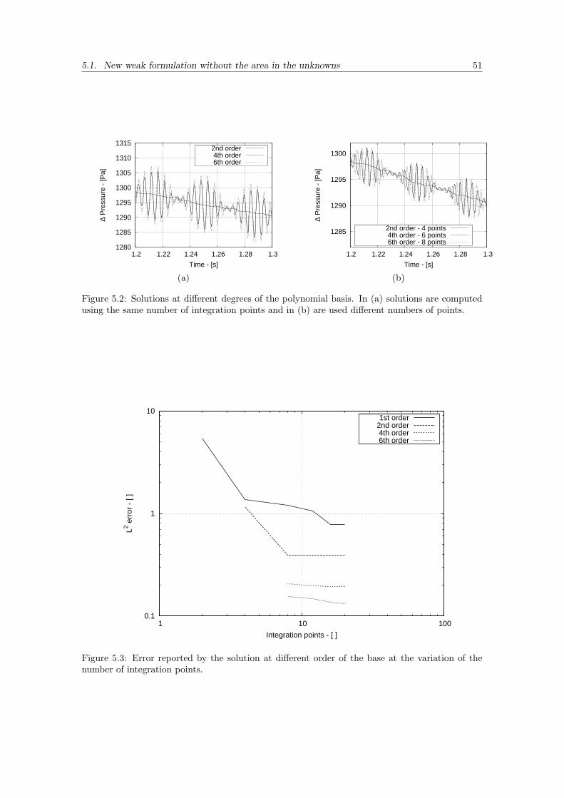
5.1. New weak formulation without the area in the unknowns 51
1280
1285
1290
1295
1300
1305
1310
1315
1.2 1.22 1.24 1.26 1.28 1.3
∆ P
ress
ure
- [P
a]
Time - [s]
2nd order4th order6th order
1285
1290
1295
1300
1.2 1.22 1.24 1.26 1.28 1.3
∆ P
ress
ure
- [P
a]
Time - [s]
2nd order - 4 points4th order - 6 points6th order - 8 points
(a) (b)
Figure 5.2: Solutions at different degrees of the polynomial basis. In (a) solutions are computedusing the same number of integration points and in (b) are used different numbers of points.
0.1
1
10
1 10 100
L2 err
or -
[ ]
Integration points - [ ]
1st order2nd order4th order6th order
Figure 5.3: Error reported by the solution at different order of the base at the variation of thenumber of integration points.
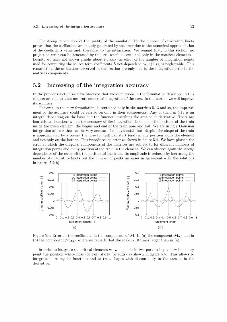
5.2. Increasing of the integration accuracy 52
The strong dependence of the quality of the simulation by the number of quadrature knotsproves that the oscillations are mainly generated by the error due to the numerical approximationof the coefficients value and, therefore, to the integration. We remind that, in this section, noprojection error can be generated by the area which is contained only in the matrices elements.Despite we have not shown graphs about it, also the effect of the number of integration pointsused for computing the source term coefficients S not dependent by A(x, t), is neglectable. Thisremark that the oscillations observed in this section are only due to the integration error in thematrices components.
5.2 Increasing of the integration accuracy
In the previous section we have observed that the oscillations in the formulation described in thischapter are due to a not accurate numerical integration of the area. In this section we will improveits accuracy.
The area, in this new formulation, is contained only in the matrices 5.13 and so, the improve-ment of the accuracy could be carried on only in their components. Any of them in 5.13 is anintegral depending on the basis and the function describing the area or its derivative. There arefour critical locations where the accuracy of the integration depends on the position of the traininside the mesh element: the begins and end of the train nose and tail. We are using a Gaussianintegration scheme that can be very accurate for polynomials but, despite the shape of the trainis approximated by a cosine, the nose (or tail) can start (end) in any position along the elementand not only on the border. This introduces an error as shown in figure 5.4. We have plotted theerror at which the diagonal components of the matrices are subject to for different numbers ofintegration points and many position of the train in the element. We can observe again the strongdependence of the error with the position of the train. Its amplitude is reduced by increasing thenumber of quadrature knots but the number of peaks increases in agreement with the solutionsin figures 5.2(b).
-0.01
-0.005
0
0.005
0.01
0.015
0.02
0 0.1 0.2 0.3 0.4 0.5 0.6 0.7 0.8 0.9 1
L2 nor
m c
oeffi
cien
t err
or -
[ ]
x/(element length) - [ ]
5 integration points10 integration points15 integration points
-0.1
-0.05
0
0.05
0.1
0.15
0.2
0 0.1 0.2 0.3 0.4 0.5 0.6 0.7 0.8 0.9 1
L2 nor
m c
oeffi
cien
t err
or -
[ ]
x/(element length) - [ ]
5 integration points10 integration points15 integration points
(a) (b)
Figure 5.4: Error on the coefficients in the components of M. In (a) the component M0,0 and in(b) the component MA0,0 where we remark that the scale is 10 times larger than in (a).
In order to integrate the critical elements we will split it in two parts using as new boundarypoint the position where nose (or tail) starts (or ends) as shown in figure 5.5. This allows tointegrate more regular functions and to treat shapes with discontinuity in the area or in thederivative.
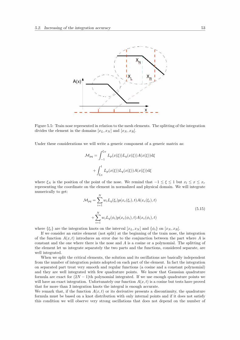
5.2. Increasing of the integration accuracy 53
Figure 5.5: Train nose represented in relation to the mesh elements. The splitting of the integrationdivides the element in the domains [xL, xN ] and [xN , xR].
Under these considerations we will write a generic component of a generic matrix as:
Mpq =∫ ξN
−1
Lp(x(ξ))Lq(x(ξ))A(x(ξ))dξ
+∫ 1
ξN
Lp(x(ξ))Lq(x(ξ))A(x(ξ))dξ
where ξN is the position of the point of the nose. We remind that −1 ≤ ξ ≤ 1 but xl ≤ x ≤ xrrepresenting the coordinate on the element in normalized and physical domain. We will integratenumerically to get:
Mpq =N∑i=1
wiLq(ξi)p(xe(ξi), t)A(xe(ξi), t)
+N∑i=1
wiLq(φi)p(xe(φi), t)A(xe(φi), t)
(5.15)
where ξi are the integration knots on the interval [xL, xN ] and φi on [xN , xR].If we consider an entire element (not split) at the beginning of the train nose, the integration
of the function A(x, t) introduces an error due to the conjunction between the part where A isconstant and the one where there is the nose and A is a cosine or a polynomial. The splitting ofthe element let us integrate separately the two parts and the functions, considered separate, arewell integrated.
When we split the critical elements, the solution and its oscillations are basically independentfrom the number of integration points adopted on each part of the element. In fact the integrationon separated part treat very smooth and regular functions (a cosine and a constant polynomial)and they are well integrated with few quadrature points. We know that Gaussian quadratureformula are exact for (2N − 1)th polynomial integrated. If we use enough quadrature points wewill have an exact integration. Unfortunately our function A(x, t) is a cosine but tests have provedthat for more than 3 integration knots the integral is enough accurate.We remark that, if the function A(x, t) or its derivative presents a discontinuity, the quadratureformula must be based on a knot distribution with only internal points and if it does not satisfythis condition we will observe very strong oscillations that does not depend on the number of
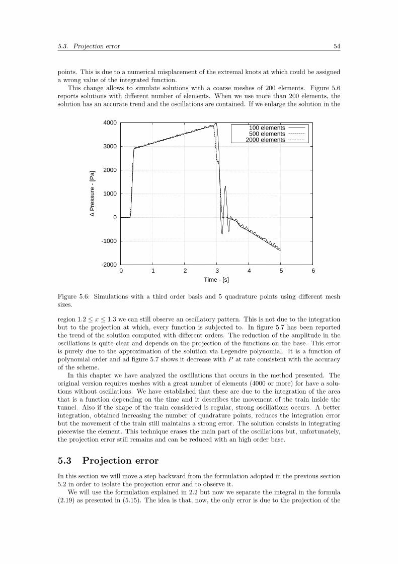
5.3. Projection error 54
points. This is due to a numerical misplacement of the extremal knots at which could be assigneda wrong value of the integrated function.
This change allows to simulate solutions with a coarse meshes of 200 elements. Figure 5.6reports solutions with different number of elements. When we use more than 200 elements, thesolution has an accurate trend and the oscillations are contained. If we enlarge the solution in the
-2000
-1000
0
1000
2000
3000
4000
0 1 2 3 4 5 6
∆ P
ress
ure
- [P
a]
Time - [s]
100 elements500 elements
2000 elements
Figure 5.6: Simulations with a third order basis and 5 quadrature points using different meshsizes.
region 1.2 ≤ x ≤ 1.3 we can still observe an oscillatory pattern. This is not due to the integrationbut to the projection at which, every function is subjected to. In figure 5.7 has been reportedthe trend of the solution computed with different orders. The reduction of the amplitude in theoscillations is quite clear and depends on the projection of the functions on the base. This erroris purely due to the approximation of the solution via Legendre polynomial. It is a function ofpolynomial order and ad figure 5.7 shows it decrease with P at rate consistent with the accuracyof the scheme.
In this chapter we have analyzed the oscillations that occurs in the method presented. Theoriginal version requires meshes with a great number of elements (4000 or more) for have a solu-tions without oscillations. We have established that these are due to the integration of the areathat is a function depending on the time and it describes the movement of the train inside thetunnel. Also if the shape of the train considered is regular, strong oscillations occurs. A betterintegration, obtained increasing the number of quadrature points, reduces the integration errorbut the movement of the train still maintains a strong error. The solution consists in integratingpiecewise the element. This technique erases the main part of the oscillations but, unfortunately,the projection error still remains and can be reduced with an high order base.
5.3 Projection error
In this section we will move a step backward from the formulation adopted in the previous section5.2 in order to isolate the projection error and to observe it.
We will use the formulation explained in 2.2 but now we separate the integral in the formula(2.19) as presented in (5.15). The idea is that, now, the only error is due to the projection of the

5.3. Projection error 55
3195
3200
3205
3210
3215
3220
3225
3230
3235
3240
3245
1.2 1.22 1.24 1.26 1.28 1.3
∆ P
ress
ure
- [P
a]
Time - [s]
2nd order4th order6th order
Figure 5.7: Simulation using different order of the polynomial base.
functions on the polynomial basis. In order to investigate it we will observe the solutions obtainedusing different number of elements and polynomial order then we will compare the formulationadopted in this section with the one described in section 5.1.1.
5.3.1 Error at different mesh sizes and polynomial orders
A first analysis is shown in figure 5.8 where solutions obtained using different number of elementsare plotted. We remark that the strongest oscillations are concentrated in a period of time whenthe beginning or end of the nose or tail is passing on the observed point. A larger number ofelements reduces the oscillations in terms of amplitude. That the oscillations are introduced bynose and tail of the train is evident by observing the solution at 5s in figure 5.10 where all thestrongest oscillations occurs when the tail passes the position of observation.
-2000
-1000
0
1000
2000
3000
4000
5000
0 1 2 3 4 5
∆ P
ress
ure
- [P
a]
Time - [s]
250 elements2000 elements 0
1000
2000
3000
4000
5000
2.8 3 3.2 3.4 3.6
∆ P
ress
ure
- [P
a]
Time - [s]
250 elements2000 elements
(a) (b)
Figure 5.8: Simulation using different number of elements with a third order polynomial basis. In(a) a long time simulation of 5s and in (b) an enlargement of the solution referred to the nose ofthe train.
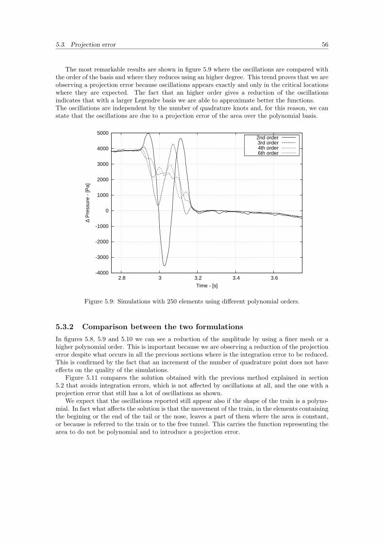
5.3. Projection error 56
The most remarkable results are shown in figure 5.9 where the oscillations are compared withthe order of the basis and where they reduces using an higher degree. This trend proves that we areobserving a projection error because oscillations appears exactly and only in the critical locationswhere they are expected. The fact that an higher order gives a reduction of the oscillationsindicates that with a larger Legendre basis we are able to approximate better the functions.The oscillations are independent by the number of quadrature knots and, for this reason, we canstate that the oscillations are due to a projection error of the area over the polynomial basis.
-4000
-3000
-2000
-1000
0
1000
2000
3000
4000
5000
2.8 3 3.2 3.4 3.6
∆ P
ress
ure
- [P
a]
Time - [s]
2nd order3rd order4th order6th order
Figure 5.9: Simulations with 250 elements using different polynomial orders.
5.3.2 Comparison between the two formulations
In figures 5.8, 5.9 and 5.10 we can see a reduction of the amplitude by using a finer mesh or ahigher polynomial order. This is important because we are observing a reduction of the projectionerror despite what occurs in all the previous sections where is the integration error to be reduced.This is confirmed by the fact that an increment of the number of quadrature point does not haveeffects on the quality of the simulations.
Figure 5.11 compares the solution obtained with the previous method explained in section5.2 that avoids integration errors, which is not affected by oscillations at all, and the one with aprojection error that still has a lot of oscillations as shown.
We expect that the oscillations reported still appear also if the shape of the train is a polyno-mial. In fact what affects the solution is that the movement of the train, in the elements containingthe begining or the end of the tail or the nose, leaves a part of them where the area is constant,or because is referred to the train or to the free tunnel. This carries the function representing thearea to do not be polynomial and to introduce a projection error.
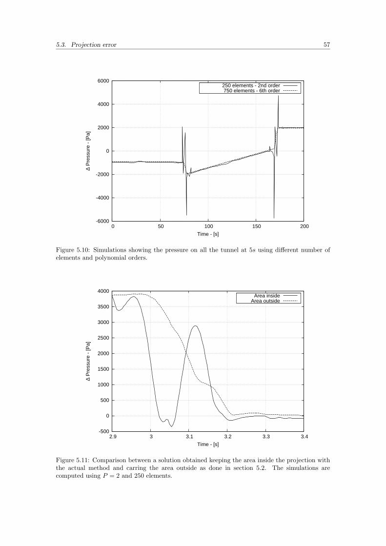
5.3. Projection error 57
-6000
-4000
-2000
0
2000
4000
6000
0 50 100 150 200
∆ P
ress
ure
- [P
a]
Time - [s]
250 elements - 2nd order750 elements - 6th order
Figure 5.10: Simulations showing the pressure on all the tunnel at 5s using different number ofelements and polynomial orders.
-500
0
500
1000
1500
2000
2500
3000
3500
4000
2.9 3 3.1 3.2 3.3 3.4
∆ P
ress
ure
- [P
a]
Time - [s]
Area insideArea outside
Figure 5.11: Comparison between a solution obtained keeping the area inside the projection withthe actual method and carring the area outside as done in section 5.2. The simulations arecomputed using P = 2 and 250 elements.
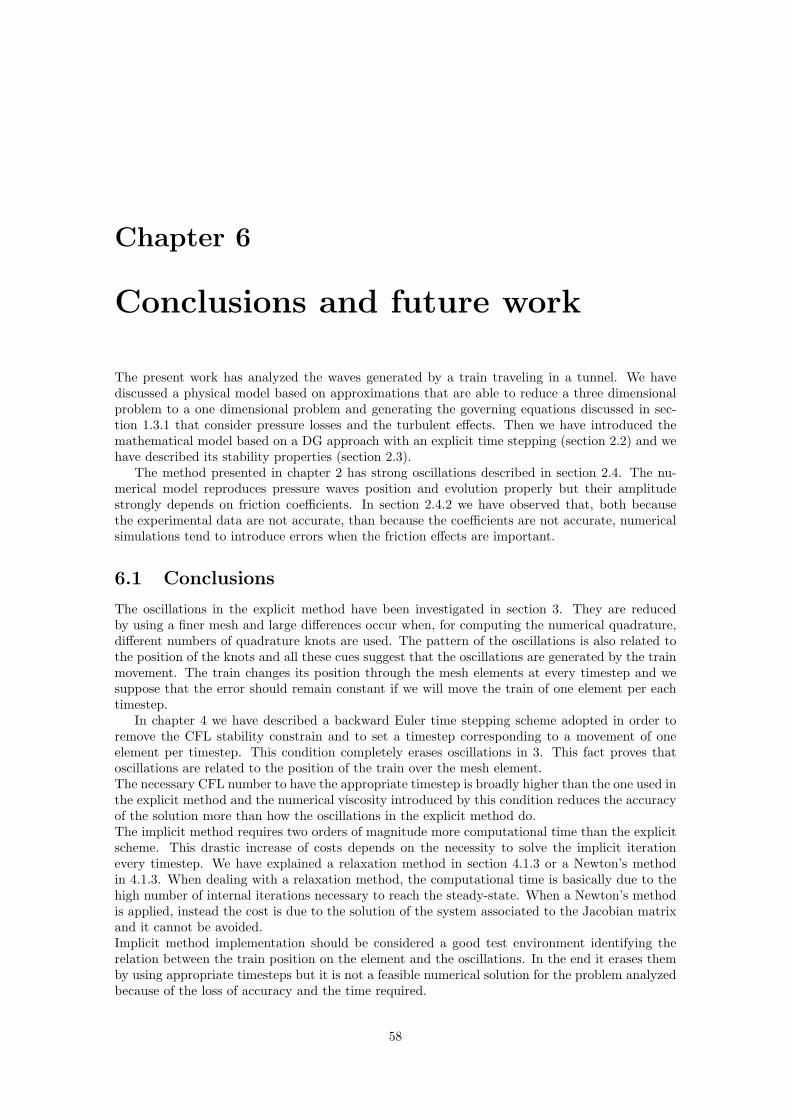
Chapter 6
Conclusions and future work
The present work has analyzed the waves generated by a train traveling in a tunnel. We havediscussed a physical model based on approximations that are able to reduce a three dimensionalproblem to a one dimensional problem and generating the governing equations discussed in sec-tion 1.3.1 that consider pressure losses and the turbulent effects. Then we have introduced themathematical model based on a DG approach with an explicit time stepping (section 2.2) and wehave described its stability properties (section 2.3).
The method presented in chapter 2 has strong oscillations described in section 2.4. The nu-merical model reproduces pressure waves position and evolution properly but their amplitudestrongly depends on friction coefficients. In section 2.4.2 we have observed that, both becausethe experimental data are not accurate, than because the coefficients are not accurate, numericalsimulations tend to introduce errors when the friction effects are important.
6.1 Conclusions
The oscillations in the explicit method have been investigated in section 3. They are reducedby using a finer mesh and large differences occur when, for computing the numerical quadrature,different numbers of quadrature knots are used. The pattern of the oscillations is also related tothe position of the knots and all these cues suggest that the oscillations are generated by the trainmovement. The train changes its position through the mesh elements at every timestep and wesuppose that the error should remain constant if we will move the train of one element per eachtimestep.
In chapter 4 we have described a backward Euler time stepping scheme adopted in order toremove the CFL stability constrain and to set a timestep corresponding to a movement of oneelement per timestep. This condition completely erases oscillations in 3. This fact proves thatoscillations are related to the position of the train over the mesh element.The necessary CFL number to have the appropriate timestep is broadly higher than the one used inthe explicit method and the numerical viscosity introduced by this condition reduces the accuracyof the solution more than how the oscillations in the explicit method do.The implicit method requires two orders of magnitude more computational time than the explicitscheme. This drastic increase of costs depends on the necessity to solve the implicit iterationevery timestep. We have explained a relaxation method in section 4.1.3 or a Newton’s methodin 4.1.3. When dealing with a relaxation method, the computational time is basically due to thehigh number of internal iterations necessary to reach the steady-state. When a Newton’s methodis applied, instead the cost is due to the solution of the system associated to the Jacobian matrixand it cannot be avoided.Implicit method implementation should be considered a good test environment identifying therelation between the train position on the element and the oscillations. In the end it erases themby using appropriate timesteps but it is not a feasible numerical solution for the problem analyzedbecause of the loss of accuracy and the time required.
58
6.2. Future work 59
In section 5 we have erased the oscillations in the explicit method. Oscillations can be due to thevariation of a projection error or to an integration one at each timestep, as explained in section 3.1.In section 5.1 we have introduced a new formulation in order to make the unknowns independentby the area. Unknowns do consequently not contain the error due to the projection of the areaon the polynomial basis because the area and its derivative are enclosed in the evaluation of thecomponents of the matrices. They are only subjected to the only integration error. Results shownin 5.1.2 report that oscillations are strongly reduced by the use of a larger number of quadraturepoints. This is very helpful in order to understand that the main part of the amplitude of themis due to a variable integration error.
Despite the regular shape of the train and the fact that we are using a Gaussian formula,integration error never disappears. In fact, when train is moving in the tunnel, the starting pointof its nose is not on the boundary point of the element but it is, in general, on an internal point.The area inside the first element containing the train nose is represented by a first part where itis constant and a second part where there is the nose and it has a sinusoidal or polynomial trend.The integration is based on the all element where the area is a piece-wise defined function. Thisfact introduces an integration error that cannot be erased by any number of integration points.In order to prevent this integration error, in section 5.2 we have split the quadrature on theelement in two parts. Now, with a sufficent number of integration points, the quadrature formulais exact and the oscillations that we could observe are very small and due to the projection of theunknowns on the Legendre basis.
In the last section we have analyzed how the projection error affects oscillations. In section5.3 we have used the original formulation and corrected the integration of the coefficients in thesource term in order to increase its accuracy. The projection error is a small amount of the totalone but it affects the part of the solution where nose and tail of the train are.
6.2 Future work
In the present work we have implemented a computationally very expensive implicit method ableto avoid the oscillations.The computational costs can be reduced in both the approaches adopted: relaxation and Newton’smethod.The relaxation approach presents a very slow convergence to the steady-state. It could be suitableto use a multigrid method [26] in order to reduce the number of elements or to use an adaptivemesh able to capture the important phenomena occuring only in certain domain regions.The Newton’s method find the reason of its slowness in the evaluation of the Jacobian matrix andthe solution of the linear system related. Could be interesting to test Incomplete LU factorizationpreconditioners with different fill-in parameters in the GMRES method, or the use of a block-wisepreconditioner [38]. Newton-LU method finds its only way to save time in a better reorderingof the matrix elements in order to reduce the band of the matrix ad to increase efficiency of thefactorization algorithm [4].Implicit method has an accuracy limited by the high CFL number introducing a strong numericalviscosity. High order methods are able to reduce such effect and to increment the accuracy but,in order to ensure the stability in our problem, we are able to use only a second order method.
The physical method presented can be extended to a network of tunnels in order to analyzemore complex situations. The generalization is straightforward but it could be complicated to setthe coupling conditions when the train is travelling the junction.
Bibliography
[1] Determination of railway tunnel cross-sectional areas on the basis of aerodynamic considera-tions. International Union of Railways (UIC), second edition, 2005.
[2] L. Vigevano A. Baron, P. Molteni. High-speed trains: Prediction of micro-pressure waveradiation from tunnel portals. Journal of Sound and Vibration, (296):59–72, 2006.
[3] S. Sibilla A. Baron, M. Mossi. The alleviation of the aerodynamic drag and wave effects ofhigh-speed trains in very long tunnels. Journal of Wind Engineering and Industrial Aerody-namics, (89):365–401, 2001.
[4] F. Sacco A. Quarteroni, F. Saleri. Numerical mathematics. Springer, 2003.
[5] J.A. Fox A.E. Vardy. Compressible and leaky trains in tunnels. Proc. Instn. Mech. Engrs.Part D, (201)(D3):209–215, 1987.
[6] M. Ainsworth. Dispersive and dissipative behaviour of high order discontinuous Galerkinfinite element methods. Journal of Computational Physics, (198):106–130.
[7] C-W. Shu B. Cockburn. Runge–kutta discontinuous galerkin methods for convection–dominated problems. Journal of Scientific Computing, (16) (3):173–261, 2001.
[8] G. Bouladon. Future, (3):15, 1970.
[9] Hirsch C. Numerical computation of internal and external flows. The fundamentals of com-putational fluid dynamics, volume 1. Butterworth-Heinemann, 2007.
[10] J. Pitkaaranta C. Johnson. An analysis of discontinous galerkin method for a scalar hyperbolicequation. Math. Comp., (46):1–26, 1986.
[11] T.A. Davis. UMFPACK Version 5.4.0 User Guide, May 2009. URL http://www.cise.ufl.edu/research/sparse/umfpack.
[12] J-F. Remacle E. Marchandise, N. Chevaugeon. Spatial and spectral superconvergence of dis-continuous Galerkin method for hyperbolic problems. Journal of Computational and AppliedMathematics, (215):484–494, 2008.
[13] R. Lohner E. Mestreau and S. Aita. Tgv tunnel entry simulations using a finite element codewith automatic remeshing. volume AIAA-93-0890, 1993.
[14] C. Dawson E.J. Kubatko, J.J. Westerink. Semi discrete discontinuous galerkin methods andstage-exceeding-order, strong-stability-preserving Runge–Kutta time discretizations. Journalof Computational Physics, (222):832–848, 2007.
[15] J.A. Fox and D.A. Henson. The prediction of the magnitude of pressure transients generatedby a train entering a single tunnel. Proceedings of the Institution of Civil Engineers, (49)(5):53–69, 1971.
60
Bibliography 61
[16] H.L. Atkins F.Q. Hu. Eigensolution analysis of the discontinuous Galerkin method withnonuniform grids. i. One space dimension. Journal of Computational Physics, (182):516–545,2002.
[17] A.E. Vardy G. Figura-Hardy, R.G. Gawthorpe. Guidance for aerodynamically sizing thecross-section of railway tunnels. volume BHR Group 1997, pages 319–329, 1997.
[18] S.P. Oliveira G. Seriani. Optimal blended spectral-element operators for acoustic wave mod-eling. Geophysics, (72)(5):95–106, 2007.
[19] R.G. Gawthorpe. Pressure effects in railway tunnels. Rail International, (April):371–414,2000.
[20] S.J. Sherwin G.E. Karniadakis. Spectral/hp element methods for computational fluid dynam-ics. Oxford University Press, second edition, 2005.
[21] D-H. Lee M-S. Kim H-B. Kwon, T-Y. Kim. Numerical simulation of unsteady compressibleflows induced by a high-speed train passing through a tunnel. volume (217), pages 111–124,2003.
[22] C. Hirsch. Numerical computation of internal and external flows. The fundamentals of com-putational fluid dynamics, volume Second. Butterworth-Heinemann, 2005.
[23] M.S. Howe. The compression wave generated by a high-speed train. Journal of AcousticalSociety of America, (104)(3):1158–1164, 1998.
[24] A. Roshko H.W. Liepmann. Elements of gas dynamics. John Wiley & Sons, 1976.
[25] A. Jameson. Steady State Solution of the Euler Equations for Transonic Flow. R. E Meyer,Academic Press, 1982.
[26] A. Jameson. Time dependent calculation using multigrid, with application to unsteady flowpast airfoils and wings. In 10th Computational Fluid Dynamics Conference. AIAA, 1991.
[27] C.P.T. Groth J.J. Gottlieb. Assessment of riemann solvers for unsteady one-dimensionalinviscid flows for perfect gases. Journal of Computational Physics, (278):437–458, 1988.
[28] C. Johnson. Numerical solution of partial differential equations by the finite element method.Cambridge University Press, 1987.
[29] T. Warburton J.S. Hesthaven. Nodal discontinuous Galerkin methods. Algorithms, analysis,and applications. Springer, 2008.
[30] M.A. Leschziner. Modelling turbulent separated flows in the context of aerodynamic appli-cations. Fluid Dynamics Research, (38):174–210, 2006.
[31] A.Tabbal L.T. Kisielewicz. Validated computational aerodynamics for trains. Journal ofWind Engineering and Industrial Aerodynamics, (49):449–458, 1993.
[32] H. Sockel M. Schultz. Pressure transients in short tunnels. Aerodynamics and Ventilation ofVehicle Tunnels, (38):221–237, 1991.
[33] C. Tournier M. William-Louis. A wave signature based method for the prediction of pressuretransients in railway tunnels. Journal of Wind Engineering and Industrial Aerodynamics,(93):521–531, 2005.
[34] R.L. Taylor O.C. Zienkiewicz. The finite element methods, The basis, volume 1. Butterworth-Heinemann, Oxford, 2000.
[35] S.J. Sherwin J. Peiro O.C. Zienkiewicz, R.L. Taylor. On discontinuous galerkin methods.International Journal of Numerical method in Engineering, (2):1119–1148, 2003.
Bibliography 62
[36] Administration Office of Research and Development. Subway environmental design handbook,volume I1, chapter Principles and applications. 1976.
[37] P. Reinke P.E. Vardy. Estimation of train resistance coefficients in tunnels from measurementsduring routine operation. volume (213), pages 71–87, 1999.
[38] J. Peraire P.O. Persson. Newton-gmres prconditioning for discontinuous galerkin of the navier-stokes equations. SIAM Journal on Scientific Computing, 2008.
[39] A. Quarteroni. Modellistica Numerica per Problemi Differenziali. Springer, third edition,2006.
[40] C.W. Pope R.G. Gawthorpe. Aerodynamics and ventilation of vehicle tunnels. the measure-ment and interpretation of transient pressures generated by trains in tunnels. pages 35–54,1976.
[41] T. Setoguchi R.S. Raghunathan, H-D Kim. Aerodynamics of high-speed railway trains.Progress in Aerospace Sciences, (38):469–514, 2002.
[42] A. Rudolf. Simulation of compressible flow in tunnel systems induced by trains travelling athigh speed. Thesis No 1806, 1998.
[43] Y. Saad. Iterative Methods for Sparse Linear Systems. SIAM, first edition, 2000. URLhttp://www-users.cs.umn.edu/$\sim$saad/books.html.
[44] J.A. Schetz. Aerodynamics of high-speed trains. Annual Review Fluid Mechanics, (33):371–414, 2001.
[45] A.H. Shapiro. The dynamics and thermodynamics of compressible flow, vol. 2. Ronald Press,1954.
[46] S.J. Sherwin. Dispersion analysis of the continuous and discontinuous galerkin formulations.Lecture Notes in Computer Science and Engineering, (11):425–431, 2000.
[47] C-W. Shu. Total-variation-diminishing time discretizations. SIAM Journal on Scientific andStatistical Computing, (9):1073–1084, 1988.
[48] H. Sockel. Handbook of fluid dynamics and fluid machinery. Schetz JA and Fuhs AE editors,1996.
[49] K. Fujii T. Ogawa. Numerical investigation of three-dimensional compressible flows inducedby a train moving into a tunnel. Computers & Fluids, (26)(6):565–585, 1997.
[50] R. Gregorie J-M. Rety V. Bourquin, M. Mossi. The importance of aerodynamics on thedesign of high-speed transportation systems in tunnels: an illustration with the tgv and theswissmetro. volume (213), pages 507–513, 1997.
[51] A. E. Vardy. Aerodynamic drag on trains in tunnels part 1: synthesis and definitions. Journalof Rail and Rapid Transit, (210):29–38, 1996.
[52] A. E. Vardy. Aerodynamic drag on trains in tunnels part 2: prediction and validation. Journalof Rail and Rapid Transit, (210):39–49.
[53] A.E. Vardy. Generation and alleviation of sonic booms from rail tunnels. volume (161)(EM3),pages 107–119, 2008.
[54] C.W. Pope W.A. Woods. A generalized flow prediction method for the unsteady flow gen-erated by a train in a single track tunnel. Journal of Wind Engineering and IndustrialAerodynamics, (7):331–360, 1981.
[55] W.A. Woods and C.W. Pope. On the range of validity of simplified one-dimensional theoriesfor calculating unsteady flows in railway tunnels. pages 115–150, 1979.
Copyright © 2022 FDOKUMEN