Traveling ichabods - Washburn University Alumni Association ...
Upload
independentCategory
view
2download
0
15
Traveling Salesman Problem
Author: Arthur M. Hobbs, Department of Mathematics, Texas A&M Uni-versity.
Prerequisites: The prerequisites for this chapter are graphs and trees. SeeSections 2.2, 9.1, 9.2, and 9.5, and Chapter 10 of Discrete Mathematics and ItsApplications.
IntroductionIn the traveling salesman problem, we are given a list of cities including our own,and we are asked to find a route using existing roads that visits each city exactlyonce, returns to our home city, and is as short as possible. However, it is usefulto formalize the problem, thus allowing other problems to be interpreted interms of the traveling salesman problem. Thus we have the following definition.
Definition 1 Given a graph G in which the edges may be directed, undi-rected, or some of each, and in which a weight is assigned to each edge, thetraveling salesman problem, denoted TSP, is the problem of finding a Hamiltoncircuit in G with minimum total weight, where the weight of a circuit is thesum of the weights of the edges in the circuit. Depending on the application,the weights on the edges will be called lengths or costs.
263
264 Applications of Discrete Mathematics
Notice that the Hamilton circuit problem, to determine whether or not agiven graph has a Hamilton circuit and to find one if it exists, is the special caseof the TSP in which each of the edge weights is 1. Also, the feature that mostdistinguishes the TSP from the shortest path problem solved in Section 9.6 ofDiscrete Mathematics and Its Applications is the requirement in the TSP thatevery vertex of the graph must be included in the solution to the TSP.
We want to emphasize that the TSP calls for a Hamilton circuit, not aHamilton path. Some applications would be more naturally stated in terms ofHamilton paths, but they can be translated into circuit problems (and this isdone in the examples). For theoretical purposes, it is much better to have thesymmetry that a Hamilton circuit allows, rather than having a pair of specialvertices serving as the ends of a Hamilton path. Also, there is a forward-lookingreason for favoring Hamilton circuits. The TSP is not solved, and any futurecomplete or partial solutions of the TSP will be stated in terms of Hamiltoncircuits, rather than Hamilton paths. Thus it is better that our work nowshould be stated in terms of Hamilton circuits, so that future solutions can beimmediately applied to it.
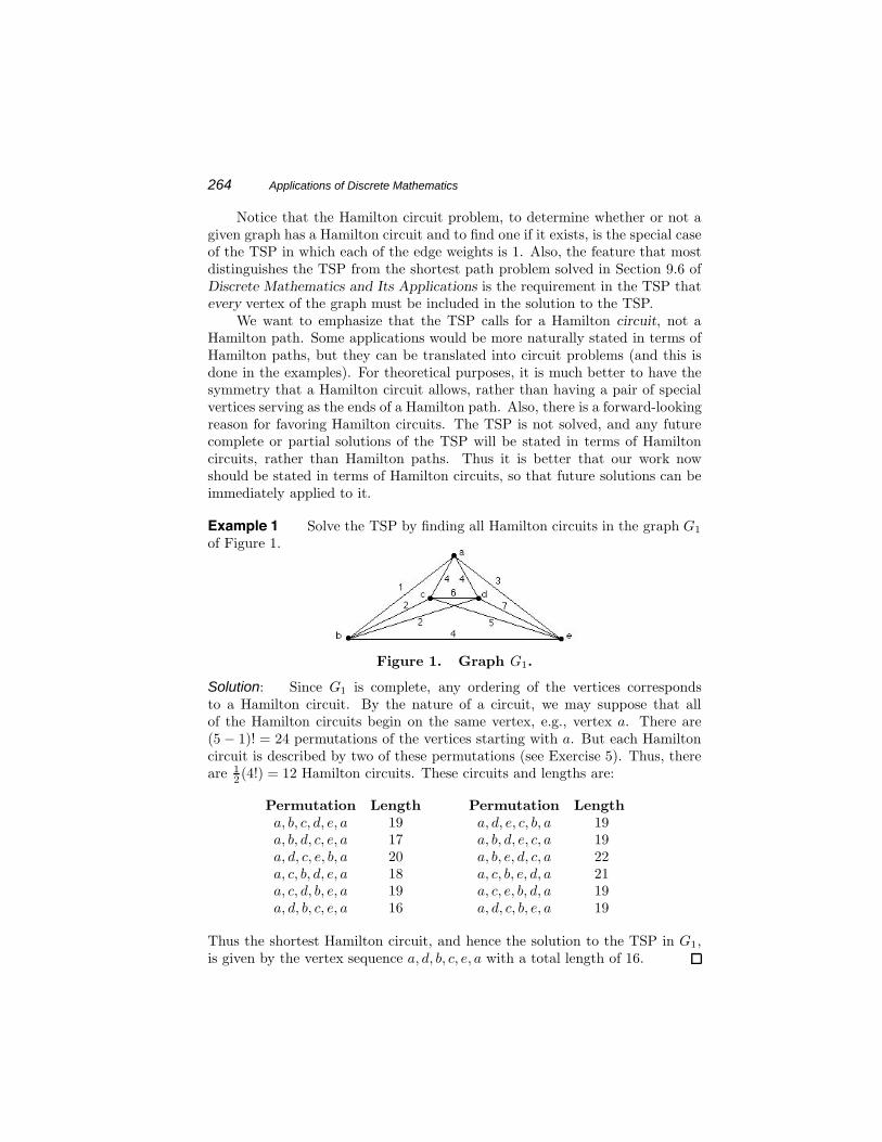
Example 1 Solve the TSP by finding all Hamilton circuits in the graph G1
of Figure 1.
Figure 1. Graph G1.
Solution: Since G1 is complete, any ordering of the vertices correspondsto a Hamilton circuit. By the nature of a circuit, we may suppose that allof the Hamilton circuits begin on the same vertex, e.g., vertex a. There are(5 − 1)! = 24 permutations of the vertices starting with a. But each Hamiltoncircuit is described by two of these permutations (see Exercise 5). Thus, thereare 1
2 (4!) = 12 Hamilton circuits. These circuits and lengths are:
Permutation Length Permutation Lengtha, b, c, d, e, a 19 a, d, e, c, b, a 19a, b, d, c, e, a 17 a, b, d, e, c, a 19a, d, c, e, b, a 20 a, b, e, d, c, a 22a, c, b, d, e, a 18 a, c, b, e, d, a 21a, c, d, b, e, a 19 a, c, e, b, d, a 19a, d, b, c, e, a 16 a, d, c, b, e, a 19
Thus the shortest Hamilton circuit, and hence the solution to the TSP in G1,is given by the vertex sequence a, d, b, c, e, a with a total length of 16.

Chapter 15 Traveling Salesman Problem 265
A variant of this procedure can be used when not all of the possible edgesare present or when some edges are directed and circuits are constrained to passthrough them in only the given direction. We may examine all the permutations,casting out those which do not correspond to Hamilton circuits. This is usefulif the graph is nearly complete. If many edges are not present, however, we maydo a depth-first search on paths starting at a, looking for those that extend toHamilton circuits. The following example illustrates the first possibility.
Example 2 Solve the TSP for the graph of Figure 2.
Figure 2. Graph G2.Solution: This graph has five vertices, but one edge of the complete graph isomitted. We again list all of the permutations of the vertices starting with a,but for some of the permutations, we note that the corresponding circuit doesnot exist in the graph:
Permutation Length Permutation Lengtha, b, c, d, e, a 14 a, d, e, c, b, a 11a, b, d, c, e, a 12 a, b, d, e, c, a 11a, d, c, e, b, a does not exist a, b, e, d, c, a does not exista, c, b, d, e, a 9 a, c, b, e, d, a does not exista, c, d, b, e, a does not exist a, c, e, b, d, a does not exista, d, b, c, e, a 7 a, d, c, b, e, a does not exist
Examining the six cases of sequences which do correspond to Hamilton circuitsin G, we find the shortest is a, d, b, c, e, a with total length 7.
These examples illustrate the most simple-minded algorithm for solvingthe traveling salesman problem: Just list all possible orderings of the verticeswith one fixed beginning vertex, cast out orderings that fail to correspond toHamilton circuits, and find the lengths of the rest, choosing the shortest. Ifthere are n vertices, then there are 1
2 (n − 1)! orderings to examine. If noHamilton circuit exists, the algorithm terminates, and the TSP has no solutionin the graph. Otherwise, a shortest circuit is found, and its length is known.Because we must examine 1
2 (n−1)! orderings of the vertices, this algorithm hascomplexity at least O((n−1)!); such complexity is much worse than exponentialcomplexity.
266 Applications of Discrete Mathematics
History
The roots of the traveling salesman problem problem are in the studies ofknight’s tours in chess and of Hamilton circuits. A knight’s tour is a sequenceof moves taken by a knight on a chessboard, that begins and ends on a fixedsquare a and visits all other squares, each exactly once. This can be seen as aHamilton circuit in a graph in which each square of the board is a vertex andtwo vertices are joined by an edge if and only if a knight’s move connects thecorresponding squares. A solution of the knight’s tour problem was given byLeonhard Euler [2].
The more general problem of Hamilton circuits apparently was first studiedin 1856 by T. P. Kirkman; he was particularly interested in Hamilton circuitson the edges and vertices of certain kinds of geometric solids [5].
However, it was William Rowan Hamilton who exhibited “The IcosianGame” in 1857 (the game was marketed in 1859) and thus gained so muchpublicity for the problem that the problem was named for him. “The IcosianGame” provided a 20-vertex graph drawn on a board and 20 numbered pegs toplace at the vertices; the object was to place the pegs in the order of a Hamiltoncircuit through the vertices of the graph. As a game “The Icosian Game” failed,but as publicity for a mathematical problem, however unintentionally, it wasvery effective. (One of the sources of mathematical interest in this game wasthat it serves as a model of a non-commutative algebra (“the Icosian calculus”)and thus can be viewed as part of “the origin of group theory” [1], an importantpart of modern mathematics.)
The traveling salesman problem appears to have been first described some-time in the 1930s.* The problem became important during the late 1930s, justas the modern explosive growth of interest in combinatorics began. It waspopularized by Merrill Flood of the RAND Corporation during the next twodecades. The first important paper on the subject appeared in 1954 [1]; in itthe authors George Dantzig, Ray Fulkerson, and Selmer Johnson of the RANDCorp. showed “that a certain tour of 49 cities, one in each of the [contiguous] 48states and Washington, D. C., has the shortest road distance” [1]. The workwas carried out using an ingenious combination of linear programming, graphtheory, and map readings.
The study of the TSP has grown enormously since then; a monographpublished in 1985 summarized the subject in 465 pages [6]. The literature onthe problem is still growing rapidly.
* This was perhaps done in a seminar conducted by Hassler Whitney in 1934 [1,3],
although he did not remember the event [1].

Chapter 15 Traveling Salesman Problem 267
ApplicationsEven if there were no applications for a solution to the TSP, this problem wouldbe important. It is an archetypical combinatorial problem: Other difficultcombinatorial problems, such as the problem of finding the size of a smallestset S of vertices in a graph G such that every vertex in G is adjacent to a vertexin S, would be already solved if we could find a solution to the TSP [7]. Thereare literally hundreds of such problems [4], and their study has become a hugemathematical industry.
But there are important applications. We present three of them here.Others appear in Exercises 10–13, and still more appear in [6, Chapter 2].
Example 3 Schoolbus Routing One of the earliest applications of theTSP was to the routing of school busses. In 1937, Merrill Flood studied thisproblem [1]: Suppose we have decided that a given school bus will pick up thechildren in a certain part of the city. What route will allow the bus to visiteach child’s home just once each morning and do so as cheaply as possible?This is just a restatement of the TSP in terms of a school bus, with children’shomes for vertices and roads for edges. Its solution may save a school districtthousands of dollars per year.
Example 4 Electronics In electrical circuit design, it is common for sev-eral components to be connected electrically to the same terminal (for example,to the ground terminal). Further, it is common for the components (memorychips, cpu’s, sockets, etc.) to be placed before the wiring diagram is completed.For example, memory chips on a computer’s motherboard are generally neatlyaligned in rows and columns on a certain area of the board. Once such compo-nents are placed on the board, we have a subset of the pins of these componentsthat must be electrically connected. Now, electricity flows easily in both direc-tions through a wire, so a tree of wires will serve for the connections, the pinsacting as vertices and the wires as edges. Because the pins on the componentsare small and because of the limited space available for printed wires, at mosttwo printed wires can be connected to each pin. But then the degree of eachvertex is at most two; thus the tree will be a path. Circuit boards are crowdedwith wires, so minimizing the total length of wire is necessary both to allow allof the wires to fit and to keep down the signal transfer time. Thus, in the com-plete graph on the pins to be connected together, we wish to find a Hamiltonpath of shortest length.
This problem can easily be converted into the form of a TSP. Add one newvertex to the graph, and join it to every other vertex by an edge of length 0.Then the Hamilton circuits in this augmented graph correspond one-to-one withHamilton paths in the complete graph, and a Hamilton circuit in the augmentedgraph is shortest if and only if the corresponding Hamilton path in the completegraph is shortest. (For further information, see Section 2.2 of [6].)
268 Applications of Discrete Mathematics
Array ClusteringOur third example involves a much more subtle use of the traveling salesmanproblem. But we must develop the problem quite far before we can get to theTSP. (See Section 2.5 of [6] for a more detailed treatment.)
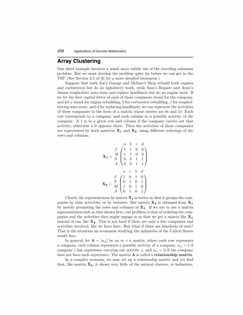
Suppose that both Joe’s Garage and Melissa’s Shop rebuild both enginesand carburetors but do no upholstery work, while Sam’s Repairs and Anne’sAnnex reupholster auto seats and replace headliners but do no engine work. Ifwe let the first capital letter of each of these companies stand for the company,and let a stand for engine rebuilding, b for carburetor rebuilding, c for reuphol-stering auto seats, and d for replacing headliners, we can represent the activitiesof these companies in the form of a matrix whose entries are 0s and 1s: Eachrow corresponds to a company, and each column to a possible activity of thecompany. A 1 is in a given row and column if the company carries out thatactivity; otherwise a 0 appears there. Then the activities of these companiesare represented by both matrices X1 and X2, using different orderings of therows and columns.
X1 =
⎛⎜⎜⎝a b c d
J 1 1 0 0M 1 1 0 0S 0 0 1 1A 0 0 1 1
⎞⎟⎟⎠
X2 =
⎛⎜⎜⎝a c b d
J 1 0 1 0S 0 1 0 1M 1 0 1 0A 0 1 0 1
⎞⎟⎟⎠.
Clearly the representation by matrix X1 is better in that it groups the com-panies by their activities, or by industry. But matrix X2 is obtained from X1
by merely permuting the rows and columns of X1. If we are to use a matrixrepresentation such as that shown here, our problem is that of ordering the com-panies and the activities they might engage in so that we get a matrix like X1
instead of one like X2. This is not hard if there are only a few companies andactivities involved, like we have here. But what if there are hundreds of each?That is the situation an economist studying the industries of the United Stateswould face.
In general, let A = [aij ] be an m × n matrix, where each row representsa company, each column represents a possible activity of a company, aij = 1 ifcompany i has experience carrying out activity j, and aij = 0 if the companydoes not have such experience. The matrix A is called a relationship matrix.
In a complex economy, we may set up a relationship matrix and yet findthat, like matrix X2, it shows very little of the natural clusters, or industries,
Chapter 15 Traveling Salesman Problem 269
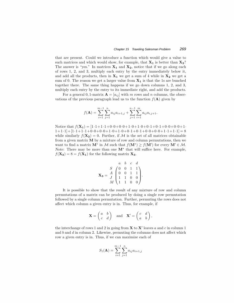
that are present. Could we introduce a function which would give a value tosuch matrices and which would show, for example, that X1 is better than X2?The answer is “yes.” In matrices X1 and X2, notice that if we go along eachof rows 1, 2, and 3, multiply each entry by the entry immediately below it,and add all the products, then in X1 we get a sum of 4 while in X2 we get asum of 0. The reason we get a larger value from X1 is that the 1s are bunchedtogether there. The same thing happens if we go down columns 1, 2, and 3,multiply each entry by the entry to its immediate right, and add the products.
For a general 0, 1-matrix A = [aij ] with m rows and n columns, the obser-vations of the previous paragraph lead us to the function f(A) given by
f(A) =m−1∑i=1
n∑j=1
aijai+1,j +n−1∑j=1
m∑i=1
aijai,j+1.
Notice that f(X1) = [1 ·1+1 ·1+0 ·0+0 ·0+1 ·0+1·0+0 ·1+0 ·1+0·0+0·0+1 ·1+1 ·1]+[1 ·1+1 ·1+0 ·0+0 ·0+1 ·0+1 ·0+0 ·1+0 ·1+0 ·0+0 ·0+1 ·1+1 ·1] = 8while similarly f(X2) = 0. Further, if M is the set of all matrices obtainablefrom a given matrix M by a mixture of row and column permutations, then wewant to find a matrix M∗ in M such that f(M∗) ≥ f(M′) for every M′ ∈ M.Note: There may be more than one M∗ that will suffice here. For example,f(X3) = 8 = f(X1) for the following matrix X3.
X3 =
⎛⎜⎜⎝a b c d
S 0 0 1 1A 0 0 1 1J 1 1 0 0M 1 1 0 0
⎞⎟⎟⎠.
It is possible to show that the result of any mixture of row and columnpermutations of a matrix can be produced by doing a single row permutationfollowed by a single column permutation. Further, permuting the rows does notaffect which column a given entry is in. Thus, for example, if
X =(
a bc d
)and X′ =
(c da b
),
the interchange of rows 1 and 2 in going from X to X′ leaves a and c in column 1and b and d in column 2. Likewise, permuting the columns does not affect whichrow a given entry is in. Thus, if we can maximize each of
S1(A) =m−1∑i=1
n∑j=1
aijai+1,j
270 Applications of Discrete Mathematics
and
S2(A) =n−1∑j=1
m∑i=1
aijai,j+1,
separately, we will maximize f(A).Now we come to the traveling salesman problem; we will use it as a tool,
and we will use it twice. First, to maximize S1, it suffices to minimize
−S1 =m−1∑i=1
n∑j=1
−aijai+1,j .
(This is needed because the TSP asks for a minimum.) Now, given matrix A,for each row i we introduce a vertex i. For any two rows k and l, we join themby an undirected edge with weight
ckl =n∑
j=1
−akjal,j .
In the resulting undirected graph G′3, each Hamilton path h describes a per-
mutation of the rows of A. Further, if A′ = [a′ij ] is formed from A by carrying
out this permutation of the rows for a minimum weight Hamilton path, then
m−1∑i=1
n∑j=1
−a′ija
′i+1,j
is precisely the sum of the weights along h. Since h is a minimum weightHamilton path in G′
3, this means that
m−1∑i=1
n∑j=1
a′ija
′i+1,j
is largest among all possible orderings of the rows of A.Thus the maximum value of this half of f(A) is found by finding a minimum
weight Hamilton path in G′3. To convert this method to the TSP (for possible
future solutions of the TSP as discussed before), add one more vertex 0 to G′3
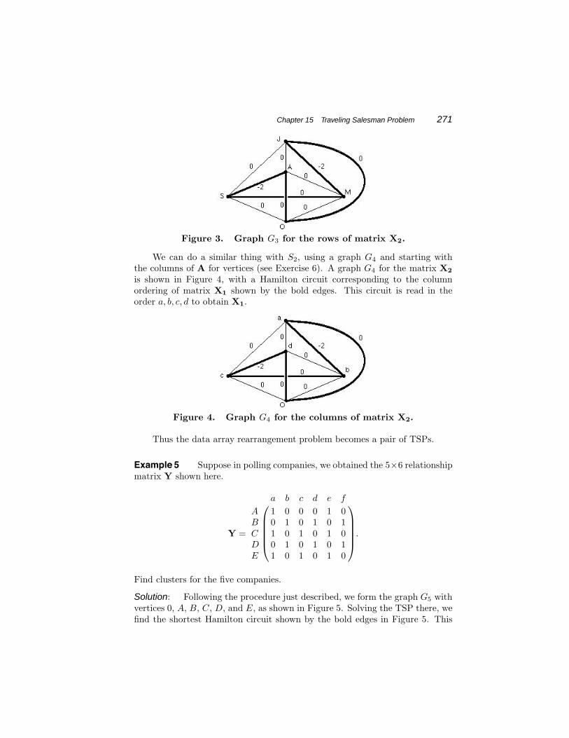
and join 0 to each other vertex by an edge of weight 0, thus forming graph G3.A solution of the TSP in G3 corresponds to a permutation of the rows of Athat maximizes S1. A graph G3 for the matrix X2 is shown in Figure 3, witha Hamilton circuit corresponding to the row ordering of matrix X1 shown bythe bold edges. This circuit is read in the order J, M, S, A.
Chapter 15 Traveling Salesman Problem 271
Figure 3. Graph G3 for the rows of matrix X2.
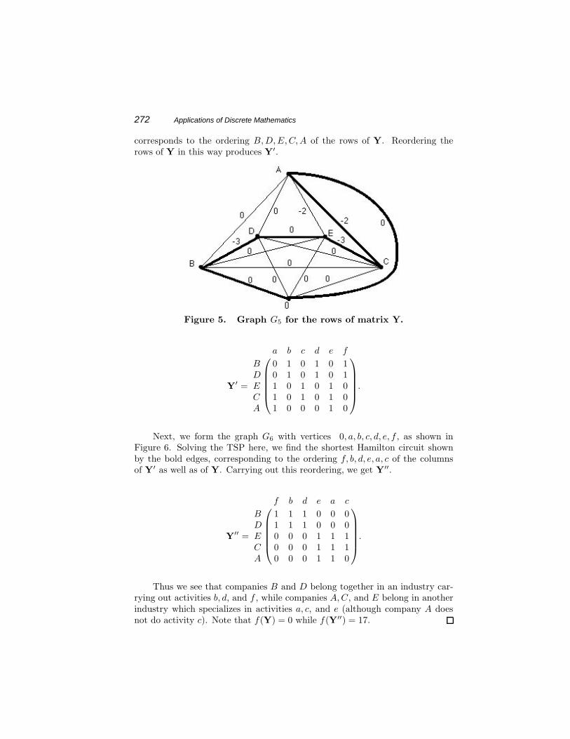
We can do a similar thing with S2, using a graph G4 and starting withthe columns of A for vertices (see Exercise 6). A graph G4 for the matrix X2
is shown in Figure 4, with a Hamilton circuit corresponding to the columnordering of matrix X1 shown by the bold edges. This circuit is read in theorder a, b, c, d to obtain X1.
Figure 4. Graph G4 for the columns of matrix X2.
Thus the data array rearrangement problem becomes a pair of TSPs.
Example 5 Suppose in polling companies, we obtained the 5×6 relationshipmatrix Y shown here.
Y =
⎛⎜⎜⎜⎜⎝
a b c d e f
A 1 0 0 0 1 0B 0 1 0 1 0 1C 1 0 1 0 1 0D 0 1 0 1 0 1E 1 0 1 0 1 0
⎞⎟⎟⎟⎟⎠.
Find clusters for the five companies.
Solution: Following the procedure just described, we form the graph G5 withvertices 0, A, B, C, D, and E, as shown in Figure 5. Solving the TSP there, wefind the shortest Hamilton circuit shown by the bold edges in Figure 5. This
272 Applications of Discrete Mathematics
corresponds to the ordering B, D, E, C, A of the rows of Y. Reordering therows of Y in this way produces Y′.
Figure 5. Graph G5 for the rows of matrix Y.
Y′ =
⎛⎜⎜⎜⎜⎝
a b c d e f
B 0 1 0 1 0 1D 0 1 0 1 0 1E 1 0 1 0 1 0C 1 0 1 0 1 0A 1 0 0 0 1 0
⎞⎟⎟⎟⎟⎠.
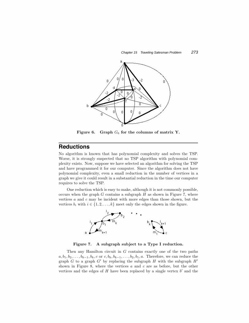
Next, we form the graph G6 with vertices 0, a, b, c, d, e, f , as shown inFigure 6. Solving the TSP here, we find the shortest Hamilton circuit shownby the bold edges, corresponding to the ordering f, b, d, e, a, c of the columnsof Y′ as well as of Y. Carrying out this reordering, we get Y′′.
Y′′ =
⎛⎜⎜⎜⎜⎝
f b d e a c
B 1 1 1 0 0 0D 1 1 1 0 0 0E 0 0 0 1 1 1C 0 0 0 1 1 1A 0 0 0 1 1 0
⎞⎟⎟⎟⎟⎠.
Thus we see that companies B and D belong together in an industry car-rying out activities b, d, and f , while companies A, C, and E belong in anotherindustry which specializes in activities a, c, and e (although company A doesnot do activity c). Note that f(Y) = 0 while f(Y′′) = 17.
Chapter 15 Traveling Salesman Problem 273
Figure 6. Graph G6 for the columns of matrix Y.
ReductionsNo algorithm is known that has polynomial complexity and solves the TSP.Worse, it is strongly suspected that no TSP algorithm with polynomial com-plexity exists. Now, suppose we have selected an algorithm for solving the TSPand have programmed it for our computer. Since the algorithm does not havepolynomial complexity, even a small reduction in the number of vertices in agraph we give it could result in a substantial reduction in the time our computerrequires to solve the TSP.
One reduction which is easy to make, although it is not commonly possible,occurs when the graph G contains a subgraph H as shown in Figure 7, wherevertices a and c may be incident with more edges than those shown, but thevertices bi with i ∈ {1, 2, . . . , k} meet only the edges shown in the figure.
Figure 7. A subgraph subject to a Type I reduction.
Then any Hamilton circuit in G contains exactly one of the two pathsa, b1, b2, . . . , bk−1, bk, c or c, bk, bk−1, . . . , b2, b1, a. Therefore, we can reduce thegraph G to a graph G′ by replacing the subgraph H with the subgraph H ′
shown in Figure 8, where the vertices a and c are as before, but the othervertices and the edges of H have been replaced by a single vertex b′ and the
274 Applications of Discrete Mathematics
four edges shown.
Figure 8. Replacement subgraph produced by the Type Ireduction from Figure 7.
The edge lengths in H ′ are as follows: edge (a, b′) has length l1 + l2 + . . . + lk,edge (b′, c) has length lk+1, edge (c, b′) has length m1, and edge (b′, a) has lengthm2 +m3 + . . .+mk+1. When a shortest Hamilton circuit has been found in G′,exactly one of the two paths a, b′, c or c, b′, a must be in it, and we can replacethat path by a, b1, b2, . . . , bk−1, bk, c or c, bk, bk−1, . . . , b2, b1, a, respectively, toobtain a shortest Hamilton circuit in G. Hereafter we will call the reduction ofreplacing H with H ′ a Type I reduction.
Type I reductions are also available in the undirected case, as illustratedin the following example.
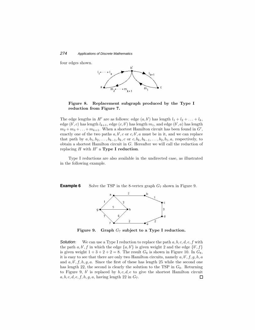
Example 6 Solve the TSP in the 8-vertex graph G7 shown in Figure 9.
Figure 9. Graph G7 subject to a Type I reduction.
Solution: We can use a Type I reduction to replace the path a, b, c, d, e, f withthe path a, b′, f in which the edge {a, b′} is given weight 2 and the edge {b′, f}is given weight 1 + 3 + 2 + 2 = 8. The result G8 is shown in Figure 10. In G8,it is easy to see that there are only two Hamilton circuits, namely a, b′, f, g, h, aand a, b′, f, h, g, a. Since the first of these has length 25 while the second onehas length 22, the second is clearly the solution to the TSP in G8. Returningto Figure 9, b′ is replaced by b, c, d, e to give the shortest Hamilton circuita, b, c, d, e, f, h, g, a, having length 22 in G7.
Chapter 15 Traveling Salesman Problem 275
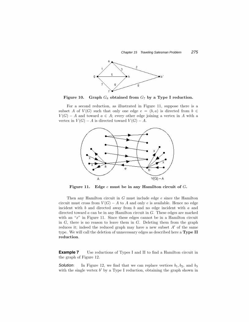
Figure 10. Graph G8 obtained from G7 by a Type I reduction.
For a second reduction, as illustrated in Figure 11, suppose there is asubset A of V (G) such that only one edge e = (b, a) is directed from b ∈V (G) − A and toward a ∈ A; every other edge joining a vertex in A with avertex in V (G) − A is directed toward V (G) − A.
Figure 11. Edge e must be in any Hamilton circuit of G.
Then any Hamilton circuit in G must include edge e since the Hamiltoncircuit must cross from V (G) − A to A and only e is available. Hence no edgeincident with b and directed away from b and no edge incident with a anddirected toward a can be in any Hamilton circuit in G. These edges are markedwith an “x” in Figure 11. Since these edges cannot be in a Hamilton circuitin G, there is no reason to leave them in G. Deleting them from the graphreduces it; indeed the reduced graph may have a new subset A′ of the sametype. We will call the deletion of unnecessary edges as described here a Type IIreduction.
Example 7 Use reductions of Types I and II to find a Hamilton circuit inthe graph of Figure 12.
Solution: In Figure 12, we find that we can replace vertices b1, b2, and b3
with the single vertex b′ by a Type I reduction, obtaining the graph shown in
276 Applications of Discrete Mathematics
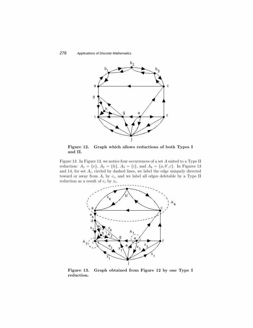
Figure 12. Graph which allows reductions of both Types Iand II.
Figure 13. In Figure 13, we notice four occurrences of a set A suited to a Type IIreduction: A1 = {e}, A2 = {h}, A3 = {i}, and A4 = {a, b′, c}. In Figures 13and 14, for set Ai, circled by dashed lines, we label the edge uniquely directedtoward or away from Ai by ei, and we label all edges deletable by a Type IIreduction as a result of ei by xi.
Figure 13. Graph obtained from Figure 12 by one Type Ireduction.
Chapter 15 Traveling Salesman Problem 277
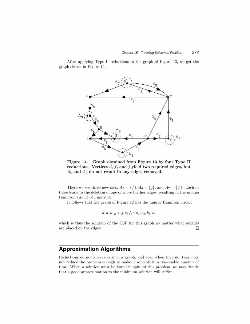
After applying Type II reductions to the graph of Figure 13, we get thegraph shown in Figure 14.
Figure 14. Graph obtained from Figure 13 by four Type IIreductions. Vertices d, f , and j yield two required edges, butA8 and A9 do not result in any edges removed.
There we see three new sets, A5 = {f}, A6 = {g}, and A7 = {b′}. Each ofthese leads to the deletion of one or more further edges, resulting in the uniqueHamilton circuit of Figure 15.
It follows that the graph of Figure 12 has the unique Hamilton circuit
a, d, h, g, i, j, e, f, c, b3, b2, b1, a,
which is thus the solution of the TSP for this graph no matter what weightsare placed on the edges.
Approximation AlgorithmsReductions do not always exist in a graph, and even when they do, they maynot reduce the problem enough to make it solvable in a reasonable amount oftime. When a solution must be found in spite of this problem, we may decidethat a good approximation to the minimum solution will suffice.
278 Applications of Discrete Mathematics
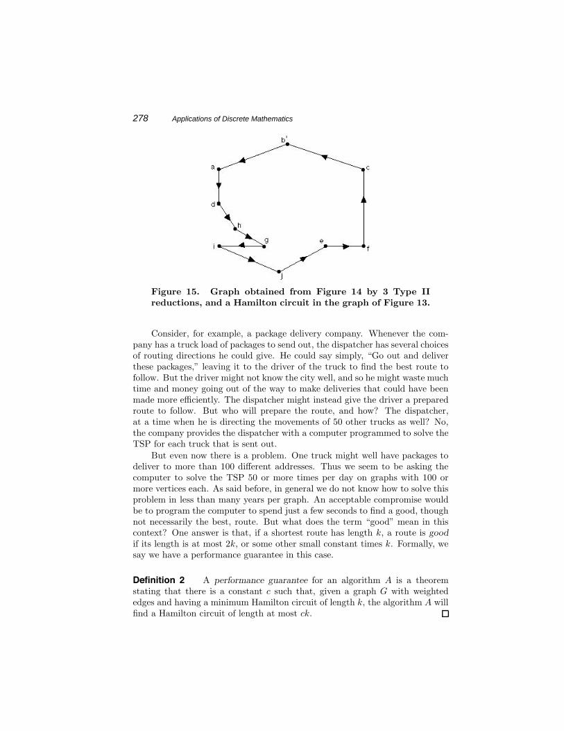
Figure 15. Graph obtained from Figure 14 by 3 Type IIreductions, and a Hamilton circuit in the graph of Figure 13.
Consider, for example, a package delivery company. Whenever the com-pany has a truck load of packages to send out, the dispatcher has several choicesof routing directions he could give. He could say simply, “Go out and deliverthese packages,” leaving it to the driver of the truck to find the best route tofollow. But the driver might not know the city well, and so he might waste muchtime and money going out of the way to make deliveries that could have beenmade more efficiently. The dispatcher might instead give the driver a preparedroute to follow. But who will prepare the route, and how? The dispatcher,at a time when he is directing the movements of 50 other trucks as well? No,the company provides the dispatcher with a computer programmed to solve theTSP for each truck that is sent out.
But even now there is a problem. One truck might well have packages todeliver to more than 100 different addresses. Thus we seem to be asking thecomputer to solve the TSP 50 or more times per day on graphs with 100 ormore vertices each. As said before, in general we do not know how to solve thisproblem in less than many years per graph. An acceptable compromise wouldbe to program the computer to spend just a few seconds to find a good, thoughnot necessarily the best, route. But what does the term “good” mean in thiscontext? One answer is that, if a shortest route has length k, a route is goodif its length is at most 2k, or some other small constant times k. Formally, wesay we have a performance guarantee in this case.
Definition 2 A performance guarantee for an algorithm A is a theoremstating that there is a constant c such that, given a graph G with weightededges and having a minimum Hamilton circuit of length k, the algorithm A willfind a Hamilton circuit of length at most ck.
Chapter 15 Traveling Salesman Problem 279
We have such an approximation algorithm in the case of graphs that satisfythe triangle inequality.
Definition 3 Let undirected graph G with vertices labeled 1, 2, . . . , n haveweight cij on edge {i, j} for all adjacent i and j. We say that G satisfies thetriangle inequality if cij ≤ cik + ckj for every choice of i, j, and k.
We call this the “triangle inequality” because it is the inequality satisfiedby the lengths of the three edges of a triangle in geometry. Its usefulness comesfrom the fact that, if we have a path a, b, c in a complete graph and if the vertex bis not needed in that path, there is a path of no greater length consisting of theedge {a, c}
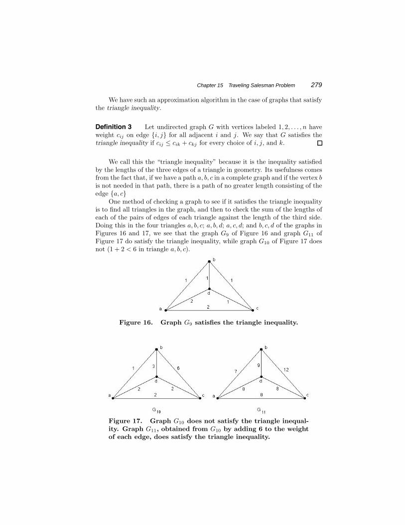
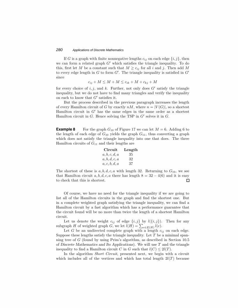
One method of checking a graph to see if it satisfies the triangle inequalityis to find all triangles in the graph, and then to check the sum of the lengths ofeach of the pairs of edges of each triangle against the length of the third side.Doing this in the four triangles a, b, c; a, b, d; a, c, d; and b, c, d of the graphs inFigures 16 and 17, we see that the graph G9 of Figure 16 and graph G11 ofFigure 17 do satisfy the triangle inequality, while graph G10 of Figure 17 doesnot (1 + 2 < 6 in triangle a, b, c).
Figure 16. Graph G9 satisfies the triangle inequality.
Figure 17. Graph G10 does not satisfy the triangle inequal-ity. Graph G11, obtained from G10 by adding 6 to the weightof each edge, does satisfy the triangle inequality.
280 Applications of Discrete Mathematics
If G is a graph with finite nonnegative lengths cij on each edge {i, j}, thenwe can form a related graph G′ which satisfies the triangle inequality. To dothis, first let M be a constant such that M ≥ cij for all i and j. Then add Mto every edge length in G to form G′. The triangle inequality is satisfied in G′
sincecij + M ≤ M + M ≤ cik + M + ckj + M
for every choice of i, j, and k. Further, not only does G′ satisfy the triangleinequality, but we do not have to find many triangles and verify the inequalityon each to know that G′ satisfies it.
But the process described in the previous paragraph increases the lengthof every Hamilton circuit of G by exactly nM , where n = |V (G)|, so a shortestHamilton circuit in G′ has the same edges in the same order as a shortestHamilton circuit in G. Hence solving the TSP in G′ solves it in G.
Example 8 For the graph G10 of Figure 17 we can let M = 6. Adding 6 tothe length of each edge of G10 yields the graph G11, thus converting a graphwhich does not satisfy the triangle inequality into one that does. The threeHamilton circuits of G11 and their lengths are
Circuit Lengtha, b, c, d, a 35a, b, d, c, a 32a, c, b, d, a 37
The shortest of these is a, b, d, c, a with length 32. Returning to G10, we seethat Hamilton circuit a, b, d, c, a there has length 8 = 32 − 4(6) and it is easyto check that this is shortest.
Of course, we have no need for the triangle inequality if we are going tolist all of the Hamilton circuits in the graph and find the shortest one. Butin a complete weighted graph satisfying the triangle inequality, we can find aHamilton circuit by a fast algorithm which has a performance guarantee thatthe circuit found will be no more than twice the length of a shortest Hamiltoncircuit.
Let us denote the weight cij of edge {i, j} by l({i, j}). Then for anysubgraph H of weighted graph G, we let l(H) =
∑e∈E(H) l(e).
Let G be an undirected complete graph with a length cij on each edge.Suppose these lengths satisfy the triangle inequality. Let T be a minimal span-ning tree of G (found by using Prim’s algorithm, as described in Section 10.5of Discrete Mathematics and Its Applications). We will use T and the triangleinequality to find a Hamilton circuit C in G such that l(C) ≤ 2l(T ).
In the algorithm Short Circuit, presented next, we begin with a circuitwhich includes all of the vertices and which has total length 2l(T ) because

Chapter 15 Traveling Salesman Problem 281
it includes each edge of T exactly twice. Listing this circuit as a sequence ofvertices, one at a time we delete second occurrences v of vertices, replacing eachwith the edge from the vertex immediately before v to the vertex immediatelyafter v in the sequence. Each time, the circuit length stays the same or isreduced because the graph satisfies the triangle inequality. For example, for thegraph G12 of Figure 18, we start with the vertex sequence a, b, c, b, a. Notingthe presence of a second occurrence of b, we replace it with the edge {c, a}, thusobtaining the vertex sequence a, b, c, a which describes a Hamilton circuit.
Figure 18. Graph G12. T is indicated by bold edges.
ALGORITHM 1 Short Circuit.
procedure Short Circuit(G: weighted complete undirectedgraph with n ≥ 3 vertices; T : minimal spanning tree in G)
T ′ := graph formed from T by replacing each edge of T withtwo parallel edges
v1 := vertex of degree 2 in T ′
C := the vertex sequence of an Euler circuit in T ′ beginningat v1
while a vertex other than v1 is repeated in Cbegin
v := the second occurrence of a vertex other that v1 in CC := C with v omitted
endend {C is a Hamilton circuit in G and l(C) ≤ 2l(T )}
Example 9 Use the Short Circuit algorithm to find a Hamilton circuit inthe graph G13 of Figure 19.
Solution: Note that G13 satisfies the triangle inequality. The edges of aminimal spanning tree are drawn bold in Figure 19. The circuit C describedin the algorithm is a, b, c, d, c, b, a, and l(C) = 2 + 3 + 3 + 3 + 3 + 2 = 16.
282 Applications of Discrete Mathematics
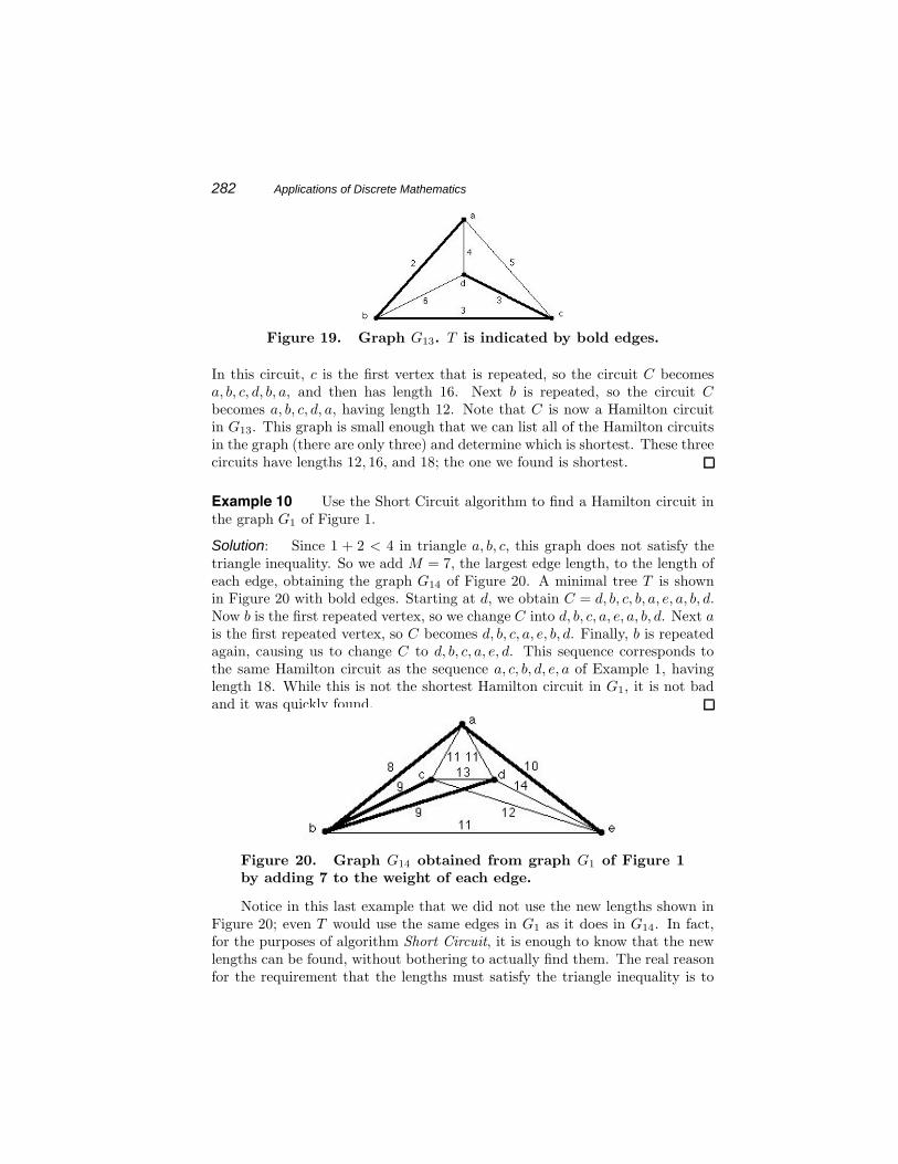
Figure 19. Graph G13. T is indicated by bold edges.
In this circuit, c is the first vertex that is repeated, so the circuit C becomesa, b, c, d, b, a, and then has length 16. Next b is repeated, so the circuit Cbecomes a, b, c, d, a, having length 12. Note that C is now a Hamilton circuitin G13. This graph is small enough that we can list all of the Hamilton circuitsin the graph (there are only three) and determine which is shortest. These threecircuits have lengths 12, 16, and 18; the one we found is shortest.
Example 10 Use the Short Circuit algorithm to find a Hamilton circuit inthe graph G1 of Figure 1.
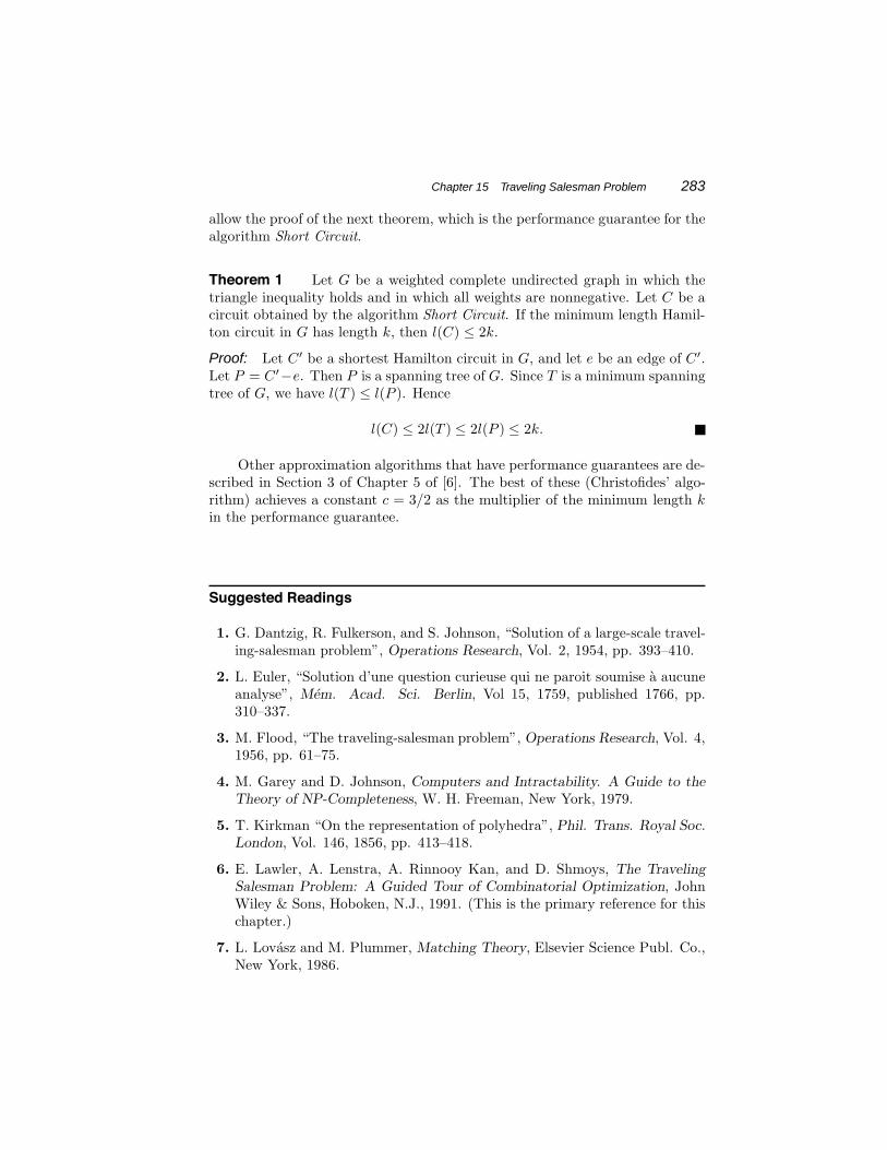
Solution: Since 1 + 2 < 4 in triangle a, b, c, this graph does not satisfy thetriangle inequality. So we add M = 7, the largest edge length, to the length ofeach edge, obtaining the graph G14 of Figure 20. A minimal tree T is shownin Figure 20 with bold edges. Starting at d, we obtain C = d, b, c, b, a, e, a, b, d.Now b is the first repeated vertex, so we change C into d, b, c, a, e, a, b, d. Next ais the first repeated vertex, so C becomes d, b, c, a, e, b, d. Finally, b is repeatedagain, causing us to change C to d, b, c, a, e, d. This sequence corresponds tothe same Hamilton circuit as the sequence a, c, b, d, e, a of Example 1, havinglength 18. While this is not the shortest Hamilton circuit in G1, it is not badand it was quickly found.
Figure 20. Graph G14 obtained from graph G1 of Figure 1by adding 7 to the weight of each edge.
Notice in this last example that we did not use the new lengths shown inFigure 20; even T would use the same edges in G1 as it does in G14. In fact,for the purposes of algorithm Short Circuit, it is enough to know that the newlengths can be found, without bothering to actually find them. The real reasonfor the requirement that the lengths must satisfy the triangle inequality is to
Chapter 15 Traveling Salesman Problem 283
allow the proof of the next theorem, which is the performance guarantee for thealgorithm Short Circuit.
Theorem 1 Let G be a weighted complete undirected graph in which thetriangle inequality holds and in which all weights are nonnegative. Let C be acircuit obtained by the algorithm Short Circuit. If the minimum length Hamil-ton circuit in G has length k, then l(C) ≤ 2k.
Proof: Let C′ be a shortest Hamilton circuit in G, and let e be an edge of C′.Let P = C′−e. Then P is a spanning tree of G. Since T is a minimum spanningtree of G, we have l(T ) ≤ l(P ). Hence
l(C) ≤ 2l(T ) ≤ 2l(P ) ≤ 2k.
Other approximation algorithms that have performance guarantees are de-scribed in Section 3 of Chapter 5 of [6]. The best of these (Christofides’ algo-rithm) achieves a constant c = 3/2 as the multiplier of the minimum length kin the performance guarantee.
Suggested Readings
1. G. Dantzig, R. Fulkerson, and S. Johnson, “Solution of a large-scale travel-ing-salesman problem”, Operations Research, Vol. 2, 1954, pp. 393–410.
2. L. Euler, “Solution d’une question curieuse qui ne paroit soumise a aucuneanalyse”, Mem. Acad. Sci. Berlin, Vol 15, 1759, published 1766, pp.310–337.
3. M. Flood, “The traveling-salesman problem”, Operations Research, Vol. 4,1956, pp. 61–75.
4. M. Garey and D. Johnson, Computers and Intractability. A Guide to theTheory of NP-Completeness, W. H. Freeman, New York, 1979.
5. T. Kirkman “On the representation of polyhedra”, Phil. Trans. Royal Soc.London, Vol. 146, 1856, pp. 413–418.
6. E. Lawler, A. Lenstra, A. Rinnooy Kan, and D. Shmoys, The TravelingSalesman Problem: A Guided Tour of Combinatorial Optimization, JohnWiley & Sons, Hoboken, N.J., 1991. (This is the primary reference for thischapter.)
7. L. Lovasz and M. Plummer, Matching Theory, Elsevier Science Publ. Co.,New York, 1986.
284 Applications of Discrete Mathematics
Exercises
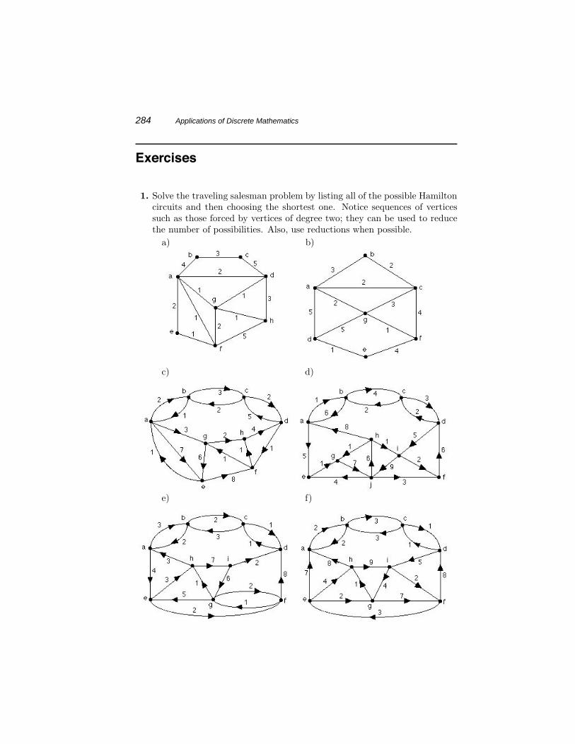
1. Solve the traveling salesman problem by listing all of the possible Hamiltoncircuits and then choosing the shortest one. Notice sequences of verticessuch as those forced by vertices of degree two; they can be used to reducethe number of possibilities. Also, use reductions when possible.
a) b)
c) d)
e) f)
Chapter 15 Traveling Salesman Problem 285
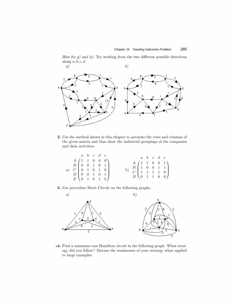
Hint for g) and h): Try working from the two different possible directionsalong a, b, c, d.
g) h)
2. Use the method shown in this chapter to permute the rows and columns ofthe given matrix and thus show the industrial groupings of the companiesand their activities.
a)
⎛⎜⎜⎜⎜⎝
a b c d e
A 1 1 0 0 0B 0 0 1 0 1C 0 1 0 1 0D 0 0 1 0 1E 0 1 0 1 0
⎞⎟⎟⎟⎟⎠ b)
⎛⎜⎜⎝a b c d e
A 1 1 0 0 1B 1 0 0 1 1C 1 1 1 1 0D 0 1 1 0 0
⎞⎟⎟⎠3. Use procedure Short Circuit on the following graphs.
a) b)
�4. Find a minimum cost Hamilton circuit in the following graph. What strat-egy did you follow? Discuss the weaknesses of your strategy when appliedto large examples.
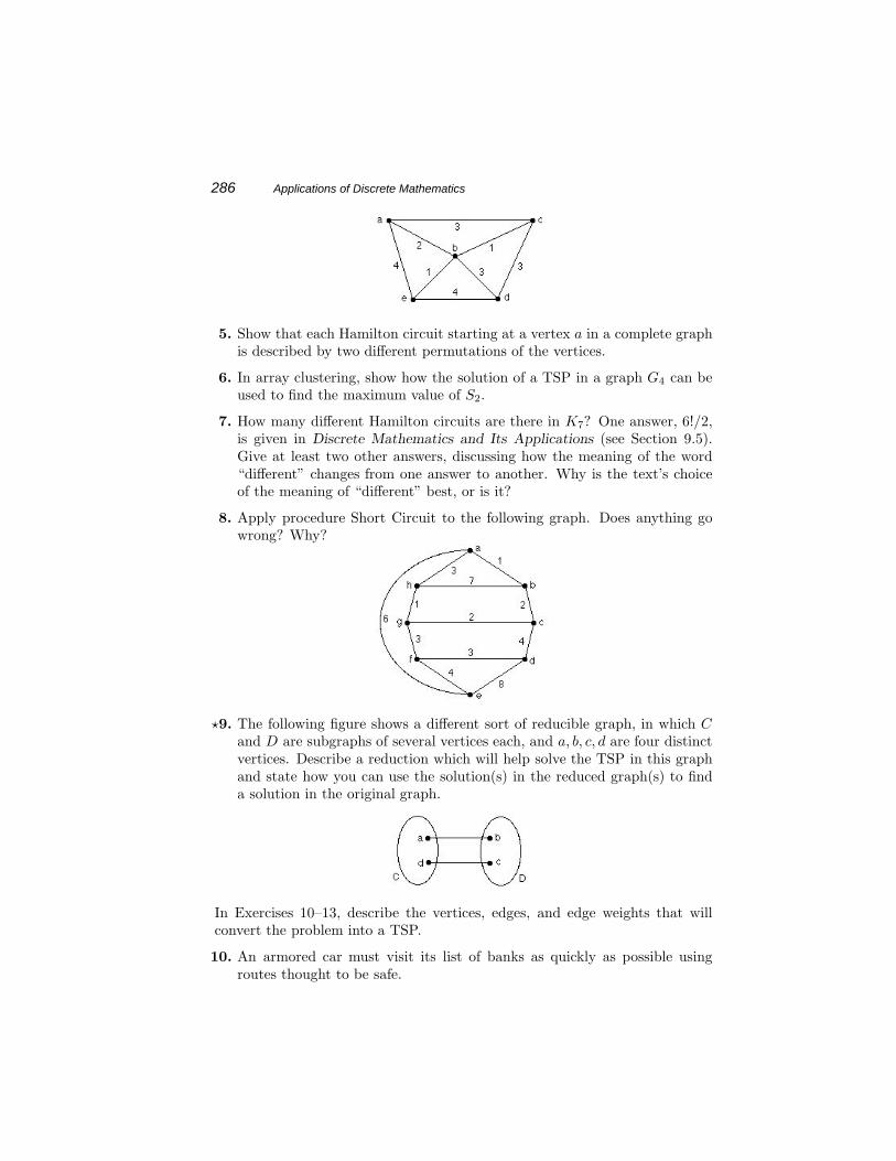
286 Applications of Discrete Mathematics
5. Show that each Hamilton circuit starting at a vertex a in a complete graphis described by two different permutations of the vertices.
6. In array clustering, show how the solution of a TSP in a graph G4 can beused to find the maximum value of S2.
7. How many different Hamilton circuits are there in K7? One answer, 6!/2,is given in Discrete Mathematics and Its Applications (see Section 9.5).Give at least two other answers, discussing how the meaning of the word“different” changes from one answer to another. Why is the text’s choiceof the meaning of “different” best, or is it?
8. Apply procedure Short Circuit to the following graph. Does anything gowrong? Why?
�9. The following figure shows a different sort of reducible graph, in which Cand D are subgraphs of several vertices each, and a, b, c, d are four distinctvertices. Describe a reduction which will help solve the TSP in this graphand state how you can use the solution(s) in the reduced graph(s) to finda solution in the original graph.
In Exercises 10–13, describe the vertices, edges, and edge weights that willconvert the problem into a TSP.
10. An armored car must visit its list of banks as quickly as possible usingroutes thought to be safe.
Chapter 15 Traveling Salesman Problem 287
11. A rail line from New York to San Francisco must pass through many spec-ified cities at a minimum cost.
12. A package delivery company with many trucks clusters the deliveries andassigns a truck to each cluster. Each truck should make its deliveries inminimum time. Note: In this exercise, we see the TSP as a subproblem ofa larger, even more difficult problem.
13. A commander needs to visit his front line units by the safest possible routes.Hint: Assign the degree of safety of a route a numerical value.
Computer Projects
1. Write a computer program to find all Type I reductions in a directed graph.
2. Write a computer program to find all Type II reductions in a directed graph.
3. Write a computer program calling on the procedures of Computer Projects1 and 2 to exactly solve the TSP in a directed graph of at most 50 vertices.
Copyright © 2022 FDOKUMEN