Carnegie Mellon UniversityResearch Showcase @ CMU

Department of Philosophy Dietrich College of Humanities and Social Sciences

1996

Using d-separation to calculate zero partialcorrelations in linear models with correlated errorsPeter SpirtesCarnegie Mellon University

Follow this and additional works at: http://repository.cmu.edu/philosophy

This Technical Report is brought to you for free and open access by the Dietrich College of Humanities and Social Sciences at Research Showcase @CMU. It has been accepted for inclusion in Department of Philosophy by an authorized administrator of Research Showcase @ CMU. For moreinformation, please contact research-showcase@andrew.cmu.edu.

NOTICE WARNING CONCERNING COPYRIGHT RESTRICTIONS:The copyright law of the United States (title 17, U.S. Code) governs the makingof photocopies or other reproductions of copyrighted material. Any copying of thisdocument without permission of its author may be prohibited by law.

Using D-separation to CalculateZero Partial Correlations

in Linear Modelswith Correlated Errors

Peter Spirtes

May 1996

Report CMU-PHIL-72

PhilosophyMethodologyLogic

Pittsburgh, Pennsylvania 15213-3890

Technical Report CMU-Phil-72

Using D-separation to Calculate Zero Partial Correlations inLinear Models with Correlated Errors

Peter Spirtes

Thomas Richardson

Christopher Meek

Richard Scheines

Clark Glymour

Abstract

It has been shown in Spirtes(1995) that X and Y are d-separated given Z in a directedgraph associated with a recursive or non-recursive linear model without correlated errors ifand only if the model entails that p^ z = 0. This result cannot be directly applied to a linearmodel with correlated errors, however, because the standard graphical representation of alinear model with correlated errors is not a directed graph. The main result of this paper isto show how to associate a directed graph with a linear model L with correlated errors, andthen use d-separation in the associated directed graph to determine whether L entails that aparticular partial correlation is zero.

In a linear structural equation model (SEM) some partial correlations may be equal to zero

for all values of the model's free parameters (for which the partial correlation is defined).

(When we refer to "all values" of the free parameters, we assume that there are no

constraints upon the models parameters except for the coefficients and the correlations

among the error variables that are fixed at zero.) In this case we will say that the SEM

linearly entails that the partial correlation is zero. It has been shown in Spirtes(1995) that

X and Y are d-separated given Z in a directed graph associated with a recursive or non-

recursive linear model with uncorrelated errors if and only if the model linearly entails that

PXY.Z = 0. This result cannot be directly applied to a linear model with correlated errors,

however, because the standard graphical representation of a linear model with correlated

errors is not a directed graph. The main result of this paper is to show how to associate a

directed graph with a linear model L with correlated errors, and then use d-separation in the

associated directed graph to determine whether L linearly entails that a particular partial

correlation is zero. The standard graph terminology in this paper, the standard terminology

for linear structural equation models, and the relationship between the two terminologies

are described in the Appendix.

If G is the graph of SEM L with correlated errors, let Transform(G) be the graph

resulting from replacing a double headed arrow between correlated errors E{ and £j with a

new latent variable T^ (i < j) and edges from TV to X{ and Xj, and then removing the error

terms from the graph. See Figure 1. A trek between X{ and Xj is an undirected path

between X{ and Xj that contains no colliders. If there is a trek Xi <— TV —> Xj in

Transform(G), we will say that Xi and Xj are d-adjacent in Transform(G). A trek Xj <—

TV —> X. is called a correlated error trek in Transform(G). In Transform(G), a

correlated error trek sequence is a sequence of vertices <Xi,.., Xk> such that no pair

of vertices adjacent in the sequence are identical, and for each pair of vertices Xr and Xs

adjacent in the sequence, there is a correlated error trek between X, and Xs. For example in

Figure 1, the sequence of vertices <X,A,B,C,D,Y> is a correlated error trek sequence

between X and Y.

*hi<4—•^ •6D

ID

.By

IY

Transform(G)

Figure 1

It might at first glance appear that for every parameterization of G, there is a

parameterization of Transform(G) with the same covariance matrix. The following theorem

shows that this is not the case.

Theorem 1: There exists a SEM L with measured variables X, correlated errors, graph

G, and correlation matrix Z(X) such that no linear parameterization of Transform(G) has

marginal correlation matrix

Proof. Assume that L has no structural equations, but every pair of errors is correlated in

L. G and Transform(G) are shown in Figure 2.

Transform(G)

Figure 2 ;'

Suppose that the marginal correlation matrix E(X) is the following:

fl.O 0.99 0.99"\

0.99 1.0 0.99

0.99 0.99 1.0^

Every parameterization of Transform(G) is of the following form:

(1)

Suppose first that the variance of each of the variables is equal to 1. It follows then that

(2)

corr(X,,X2) = 0.99 =

corr(X2,X3) = 0.99 = a^a^ (3)

corr(Xl,X3) = 0.99 =

From (1), the absolute values of each of the coefficients is less than one. From (2), it

follows that an, a2l, a22, a32, a13, and a33 all have absolute values greater than 0.99. Hence

varCT,) is greater than 1, which is a contradiction. It follows that there are no solutions to

(2) and (3).

Suppose now that we do not fix the variances of the exogenous variables at one. We will

show that if the corresponding set of equations has a solution, then so do (2) and (3),

which is a contradiction.

var(X, ) = l = o'112 var(7;) + d 13

2 var(r3) + b', ,2 var(£",)

var(X2) = 1 = a'212 varCr^ + o 1 ^ var(r2) + ^2 2

2 var^1 , ) (2')

var(X3) = 1 = a' 322 var(72) + a' 33

2 var(T3) + b' 332 var(£' 3)

caa(XltX2) = 0.99 = dn a'21 varCJ,)

X3) = 0.99 = o'22aI32var(r2) , (3')

X3) = 0.99 = a'13 a'33 var(r3)

Suppose now that 2' and 3' have a solution. Then set

a13=a'13Jvar(r3) a33=

These now form a solution to (2) and (3), which is a contradiction. .\

Lemma 1: If E is a positive definite matrix, then there exists a positive definite matrix E'

= E - 81, where 8 is a real positive number.

Proof. Suppose that E is a positive definite matrix. It follows then that for all solutions of

det(E - XL) = 0, A, is positive. Let the smallest solution of det(E - XL) = 0 be A,,. Let 8 be

less than \ and greater than 0. Let Z' = Z - 51. We will now show that all of the solutions

of det(Z' - VI) = 0 are positive. Z' - VI = Z- 81- VI = Z - (V + 5)1. If we set V = X -

5, then for each solution of det(Z - XI) = 0, there is a solution of det(Z - (V + 8)1) = 0.

Since V = X - 8, and 8 is less than X{y the smallest solution of det(Z' - VI) = 0 is greater

than 0. /.

A linear transformation of a set of random variables is lower triangular if and only if

there is an ordering of the variables such that the matrix representing the transformation is

zero for all entries a , when j > i.

Lemma 2: If Xp ..., Xn have a joint normal distribution N(0,Z), where Z is positive

definite, then there is a set of n mututally independent standard normal variables Tp ..., Tn,

such that Xp ..., Xn are a lower triangular linear transformation of Tp ..., Tn and for each

i, the coefficient of T{ in the equation for Xi is not equal to zero.

Proof. For every positive definite correlation matrix Z, a complete directed graph can be

given a linear parameterization that represents Z (Spirtes et al. 1993). The reduced form of

a complete directed graph is a lower triangular transformation of independent error

variables that is non-zero on the diagonal, because Z is positive definite. .\

Theorem 2: If G is the graph of SEM L with measured variables X, normally distributed

correlated errors, and marginal correlation matrix Z(X), {X, Y} u Z c X, and X is d-

separated from Y given Z in Transform(G), then p^ z = 0 in Z(i) .

Proof. First we will construct a latent variable model of ei,...,en. Then we will use this

model to form the latent variable model L' with graph G' that has marginal correlation

matrix Z(X) but no correlated errors, and in which X is d-separated from Y given Z in G\

It follows that PXYZ = 0 in Z(X).

Order the variables so that X is first, Y is second, followed by each variable with a

descendant in Z, followed by any remaining variables that have X or Y as descendants,

followed by the rest of the variables. Given this ordering, we will now refer to the

variables as X p . . . ^ , where for all i, X^ is the i* variable in the ordering. Suppose for the

graph in Figure 1 we are interested in whether p^ = 0 (i.e. Z = 0 ) . One renaming of the

variables for the graph in Figure 1 that is compatible with the ordering rules given above is

shown in Figure 3.

Transform(G)

Figure 3

Suppose that the correlation matrix among the error terms of L is E. We will show that

there is a latent variable model of Z of the form

where each of the T{ and E"{ are uncorrelated.

By hypothesis, £ is a positive definite matrix. By Lemma 1, there is a set of variables

e'p...,£'n with positive definite matrix £' = E - 81. As a first step to constructing a latent

variable model of e, we will construct a latent variable model of e\ represented by a

directed graph H. Note that H does not contain any of the X variables or e variables.

By Lemma 2, there is a set of variables Tp ..., Tn such that e ' p ..., e'n with correlation

matrix E'(s') are a lower triangular linear transformation of Tp . . . , Tn and for each i, the

coefficient of T{ in the equation for e^ is not equal to zero. That is

where a^ ^ 0. The transformation can be represented by a directed graph H in which for

each i, there are edges from T{ to e'j, j > i.

From the construction of//, there are no edges from Tj to e\ unless j = 1. Hence, for every

j * 1, in H every every trek between e\ and e'j contains Tv It follows that there is at most

one trek between e\ and eV. The edge from Tx to e\ is not zero. Hence if e{ and e- are not

correlated in L (i.e. X{ and Xj are not d-adjacent in Transform(G)) then the edge from T{ to

£j is zero. In the example from Figure 3, an = ai4 = ai5 = a{6 = 0.

Applying this strategy to each of the T{ variables in turn, we can now show that for each i

and r > i, if there is no trek between e'r and e^ containing a variable Tj5 where j < i, and Xr

is not d-adjacent to X{ in Transform(G) (i.e. E{ and £j are uncorrelated in L), then the T{ -»

e'r edge can be removed from the graph (i.e. air can be set to zero.) Suppose on the contrary

that there is no trek between e'r and e\ containing a variable Tj9 where j < i, and Xr is not d-

adjacent to X{ in Transform(G) (i.e. ei and E- are uncorrelated in L), but the T{ —» e'r edge is

not removed from the graph by this procedure (i.e. a^ is not set to zero.) By the

construction of//, if k > i, then there is no edge from Tk to e1^ It follows that if in H there

is no trek between e'r and e' containing a variable Tj? where j < i, then every trek between

E\ and any other variable contains the edge from T{ to e\9 which is not equal to zero.The T

—> e'r edge exists by hypothesis, so there is exactly one trek between E\ and E\ in / / .

Hence E\ and £'r are correlated in every parameterization of / / . (Note that this could not be

claimed if there were more than one trek between E\ and E\ since in that case the treks

might cancel each other.) Since the covariances between distinct £' variables are equal to the

correlations between the corresponding £ variables, it follows that E{ and £r are correlated in

L', and hence d-adjacent in Transform(G). This is a contradiction. The end result of this

process of edge removal for the graph in Figure 3 is shown in Figure 4.

£' XI X5 £' X4 £' X6 X2

Figure 4: H after extra edges are removed

From the latent variable model without correlated errors of the £! variables, we can now

form a latent variable model without correlated errors of the £ variables. For each i, let £' \

be a normally distributed variable with variance 8 that is independent of all of the T{, and all

of the other £'' variables. It follows then that

because the addition of the e'\ term does not change any of the correlations, and adds 8 to

the variance of eV

From the latent variable model without correlated errors of the e variables, we can now

form a latent variable model without correlated errors of Z(X). If we use the above

equation to replace each e{ in the SEM L, we form a SEM L' which has no correlated

errors, but has the same marginal covariance matrix as L. If the equations in L are:

then the equations in L' are:

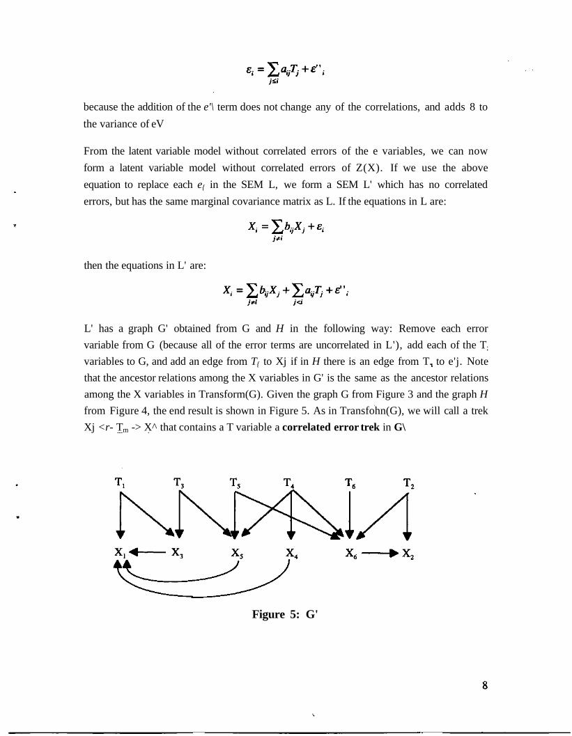
L' has a graph G' obtained from G and H in the following way: Remove each error

variable from G (because all of the error terms are uncorrelated in L'), add each of the T;

variables to G, and add an edge from T{ to Xj if in H there is an edge from T. to e'j. Note

that the ancestor relations among the X variables in G' is the same as the ancestor relations

among the X variables in Transform(G). Given the graph G from Figure 3 and the graph H

from Figure 4, the end result is shown in Figure 5. As in Transfohn(G), we will call a trek

Xj <r- Tm -> X^ that contains a T variable a correlated error trek in G\

Figure 5: G'

We will now show that if there is a correlated error trek between Xj and Xj in G' that

contains a variable Tr, then in Transform(G) there is a correlated error trek sequence

between X; and Xj, such that every variable in the correlated error trek sequence, with the

possible exception of the endpoints, has index (i.e. subscript) less than or equal to r

(henceforth referred to as the correlated error trek sequence in Transform(G) corresponding

to the correlated error trek between X^ and Xj in G\) The proof is by induction on r.

Suppose first that r = 1. If there is a correlated error trek between X{ and Xj in G' that

contains T{ then there are correlated error treks between X{ and X} in Transform(G), and

between Xj and X{. The concatenation of these two correlated error treks forms a correlated

error trek sequence in which (trivially) every variable in the sequence except for the

endpoints has an index less than or equal to 1. The induction hypothesis is that for all r < n,

if there is a correlated error trek between X{ and Xj in G' that contains Tr, then in

Transform(G) there is a correlated error trek sequence between X{ and Xj, such that every

variable in the sequence, with the possible exception of the endpoints has an index less than

r. Suppose now that in G1 there is a correlated error trek between X- and Xj such that the

trek contains Tn+1, where i, j > n+1. Since the edge between Tn+1 and X exists in G \ it

follows from the method of construction of G' that either there is a correlated error trek

between X{ and Xn+1 in G1 that contains some Tr, r < n+1, or Xn+1 and Xi are d-adjacent in

Transform(G). In the former case, by the induction hypothesis there is a correlated error

trek sequence between X{ and Xn+1 that, except for the endpoints, contains only vertices

whose indices are less than or equal to n+1. In the latter case, <Xi,Xn+1> is a correlated

error trek sequence between X and Xn+1. Similarly, there is a correlated error trek sequence

between Xn+1 and Xj that, except for the endpoints, contains only vertices whose indices

are less than or equal to n+1. These two correlated error trek sequences can be concatenated

to form a correlated error trek sequence between X- and Xj that, except for the endpoints,

contains only vertices whose indices are less than or equal to n+1. For the G1 shown in

Figure 5, there is a correlated error trek between X5 and Xg, and a corresponding correlated

error trek sequence <X5,X4,X6> in the graph Transform(G) in Figure 3.

We will now show that if Xx and X2 are d-connected given Z in G \ then X2 and X2 are d-

connected given Z in Transform(G) using Lemma 3.3.1+ (Richardson 1994, which is an

extension to the cyclic case of Lernma 3.3.1 in Spirtes et al. 1993). Lemma 3.3.1+ states

that there is a path in a directed graph G that d-connects X and Y given Z if and only if

there is a sequence of vertices Q and a set P of paths in G between pairs of adjacent

vertices in Q that have the following properties: (i) For each occurrence of a pair of adjacent

variables X{ and Xj in Q, i * j , and there is a unique path in P that d-connects Xi and X

given ZVfX^Xj}; (ii) if <Xi Cj Ck> is a subsequence of Q, the corresponding path between

Xj and Xj in P is into X-y and the corresponding path between Xj and X,, in P is into Xj (in

which case we say that the occurrence of Xj is a collider in Q) then Xj has a descendant in

Z; and (iii) if there is an occurrence of Xj that is a non-collider in Q, then Xj is not in Z.

Note that we do not require that a vertex occur only once in Q. Hence one occurrence of a

vertex in Q may be a collider, and another occurrence of the same vertex in Q may be a

non-collider.

Suppose now that there is an undirected path U that d-connects Xx and X2 given Z in G\

Intuitively, in G' we would like to form Q and P by breaking U into pieces, such that each

correlated error trek occurs as a separate piece. More formally, form a sequence Q of

vertices and an associated sequence P of paths in G' with the following properties: (i)

every vertex in Q is in X and occurs on U; (ii) no vertex occurs in Q more than once; (iii) if

A occurs before B in Q, then A occurs before B on U; (iv) if the subpath of U between A

and B is a correlated error trek, then A and B both occur in that order in Q. The path in P

associated with a pair A and B of adjacent vertices in Q is the subpath of U between A and

B. In the example in Figure 5, in G1 the d-connecting path between X{ and X2 given Z = 0

is Xj <r- X5 <- T4 -> X6 -> X2, Q = <XPX5,X6,X2>, and P = <X{ <- X5, X5 <- T4 ->

X6, X6 —> X2>. In this example, there are no colliders in Q.

Because U is a path that d-connects X{ and X2 given Z in G', it is easy to see that the paths

in P have the following properties in G': (i) Each path in Q d-coiyiects its endpoints Xi and

Xj given Z V X ^ } ; (ii) if there is an occurrence of Xi in Q that is a collider then Xi has a

descendant in Z; and (iii) if there is an occurrence of Xi in Q that is a non-collider, then X{

is not in Z.

We will now show how to construct a sequence of vertices Q' and a set P' of paths in

Transform(G) between pairs of adjacent vertices in Q' that have the following properties:

(i) For each occurrence of a pair of adjacent variables X^ and Xj in Q' there is a unique path

in P' that d-connects X^ and Xj given ZXfX^Xj}; (ii) if there is an occurrence of Xj in Q'

that is a collider, then X^ has a descendant in Z; and (iii) if there is an occurrence of X{ in

Q' that is a non-collider, then X^ is not in Z. It will follow from Lemma 3.3.1+ that X and

Y are d-connected given Z in Transform(G).

We will create Q' by several modifications of Q. Step (1) in creating Q' is to replace each

subsequence KX^JC^ of Q such that Xr and Xs are on a correlated error trek in Q, with the

corresponding correlated error trek sequence <Xr,..., Xs> in Transform(G). Note that each

10

occurrence of Xk between <Xr, ...,XS> is a collider in Q\ In the example, after the first

step Q' = <X1,X5,X4,X6,X2> and Pf = <X, <- X^ X5 <- T45 -> X4> X4 <- T^ -> X6, X6

—> X2>, i.e. we replaced the subsequence <X4,X6> in Q by <X5,X4,X6>.

Recall that the ancestor relations among the X variables (which includes the variables in Z)

in G' is the same as the ancestor relations among the X variables in Transform(G). After

stage (1) in creating Q', if Xk is not an ancestor of Z in Transform(G) (or in G'), but has

an occurrence in Q' that is a collider, it follows that Xk was added to Q' by replacing a

subsequence <XrJKs> of Q by a corresponding correlated error trek sequence <Xr, ... ,Xs>

in Transform(G). Hence any such Xk lies between some pair of vertices Xr and Xs that are

adjacent in Q. Because every vertex in <Xr, ..., Xs> in Q' (except for Xr and Xs) has an

index less than r and s, and Xk is not an ancestor of Z in G\ it follows from the ordering

of the variables that we chose, that Xr and Xs are not ancestors of Z in G\ Because Xr and

Xs are on U but not ancestors of Z in G', there is a subpath of U that is a directed path

from Xr to X{ and a subpath of U that is a directed path Xs to X2, or vice versa. In either

case, in G', Xr is an ancestor of X{ and Xs is an ancestor of X2, or Xr is an ancestor of X2

and Xs is an ancestor of XP Because in G\ Xr is an ancestor of Xx and Xs an ancestor of

X2 or vice-versa, and k < r and s, it follows from the ordering of the variables that Xk is

also an ancestor of X{ or X2 in G\ Hence Xk is an ancestor of X{ or X2 in Transform(G).

In the example, in Transform(G) X4 is not an ancestor of the empty set but is an ancestor of

Xp and it is between two vertices X5 and X6 which also are not ancestors of the empty set

but are ancestors of Xj or X2. '

If there is some vertex X, in Q' that is not an ancestor of Z, but occurs in Q' as a collider,

suppose without loss of generality that there is a vertex that is an ancestor of X{ but not of

Z, that occurs as a collider in Q\ Let Xa be the last occurrence of a collider in Q' that is an

ancestor of X{ but not of Z, if there is one, otherwise let Xa = X{. Step (2) in forming *Q'

and P' is to replace the subsequence <Xp...,Xa> by <XpXa> if Xa * Xp and replacing

the corresponding paths in P' by a directed path from Xa to X{ if Xa * Xx. (Such a

directed path exists if Xa * Xx because Xa is an ancestor of XP) This removes all

occurences of vertices between X{ and Xa that are not ancestors of Z, but are colliders in

Q\ In the example, Xa = X4, and after step 2, Q' = <XPX4,X6,X2> and P' = <X{ <- X4,

By definition, every vertex that occurs as a collider between Xa and X2 in Q' is an ancestor

of Z or of X2. Let Xb be the first vertex after Xa in Q' that is an ancestor of X2 but not of

Z, if there is one, otherwise let Xb = X2. Step (3) in forming Q' and P' is to replace the

11

subsequence <Xb, ...,X2> by <Xt,,X2> if Xb * X2, and replacing the corresponding paths

in P' by a directed path from Xb to X2 if Xb * X2. This removes all occurrences of

colliders between Xb and X2 that are not ancestors of Z. Note that all occurrences of

colliders that are left are between Xa and X,,, and every occurrence of a collider between Xa

and Xb is an ancestor of Z by construction. In the example, Xb = X2, and after step (3), Q'

and P' are unchanged.

We will now show that every path between a pair of variables Xu and Xv in P' d-connects

Xu and X,, given Z\{XU,XV}. If the path between X,, and Xv is also in P, then it d-connects

Xu and Xv given ZVjX^XJ because every path in P has this property. If the path between

Xu and Xv is not in P, but was added in step (1) of the formation of P\ then the path

between Xu and Xv is a correlated error trek, which d-connects Xu and Xv given

ZMX^XJ because no T variable is in Z. If the path between Xu and Xv is not in P, but

was added in step (2) of the formation of P\ then Xu = Xp Xv = Xa, and the path between

Xu and Xv is a directed path from Xa to Xx that does not contain any member of Z. Hence

the path d-connects Xu and X^ given Z. Similarly, if the path between path between Xu and

Xv is not in P, but was added in step (3) of the formation of P5 , then Xu = Xb, Xv = X2,

and the path between Xu and X^ is a directed path from Xb to X2 that does not contain any

member of Z. Hence the path d-connects X^ and Xv given Z.

We will now show that every vertex that occurs as a collider in Q' has a descendant in Z,

and every vertex that occurs as a non-collider in Q' is not in Z. Eyery vertex that occurs as

a collider in Q' is an ancestor of Z, because steps (2) and (3) in the formation of Q'

removed all occurrences of colliders that were not ancestors of Z. Every vertex that occurs

as a non-collider in Q and as a non-collider in Q' is not in Z, because every vertex that

occurs as a non-collider in Q is not in Z. The only vertices that may occur as non-colliders

in Q' but not in Q are Xa and Xb. Xa is not in Z, because either it is equal to X! or X2,

neither of which is in Z, or it is not an ancestor of Z by construction. Similarly, Xb is not

in Z.

Hence Q' is a sequence of paths that satisfy properties (i), (ii), and (iii). It follows from

Lemma 3.3.1+ that X{ and X2 are d-connected given Z in Transform(G).

By contraposition, since XY and X2 are d-separated in Transform(G), they are d-separated

given Z in G\ Because G' is the directed graph of a latent variable model L' with

correlation matrix that has marginal £(X), no correlated errors, and Xx and X2 are

12

d-separated given Z in G', it follows from Theorem 3 (Spirtes 1995) that p ^ ^ = 0 in

Theorem 3 : If G is the graph of SEM L with normally distributed correlated errors and

marginal correlation matrix X(X), and X is d-connected to Y given Z in Transform(G) then

L does not linearly entail that p ^ z = 0.

Proof. If X is not d-separated from Y given Z in Transform(G), then by Theorem 3

(Spirtes 1995) there is a parameterization of Transform(G) with correlation matrix E(X)

such that p ^ z * 0. By the convention adopted for new latent variables names in

Transform(G), no new latent variable was called T^ where j >i. For the sake of notational

convenience, we will also use the name T^ to refer to Tir In that parameterization,

Now define

It follows then that

which is a parameterization of L in which p ^ z * 0

Because the covariance matrix of the non-error variables in a linear SEM does not depend

upon whether the error terms are normally distributed, but depends only upon the linear

coefficients and the covariance matrix among the errors, Theorem 2 and Theorem 3 can

obviously be extended to the case where the error terms are not normally distributed.

13

Appendix

Sets of variables and defined terms are in boldface. A directed graph is an ordered pair

of a finite set of vertices V, and a set of directed edges E. A directed edge from A to B is

an ordered pair of distinct vertices <A,B> in V in which A is the tail of the edge and B is

the head; the edge is out of A and into B, and A is parent of B and B is a child of A. A

sequence of edges <E!,...,En> in G is an undirected path if and only if there exists a

sequence of vertices <Vi,...,Vn+1> such that for 1 < i < n either <Vi,Vi+i> = E* or

<Vi+i,Vj> = Ej. A path U is acyclic if no vertex occurring on an edge in the path occurs

more than once. A sequence of edges <Ei,...,En> in G is a directed path if and only if

there exists a sequence of vertices <Vi,...,Vn+i> such that for 1 < i < n <Vi,Vi+i> = Ei.

If there is an acyclic directed path from A to B or B = A then A is an ancestor of B, and B

is a descendant of A. A directed graph is acyclic if and only if it contains no directed

cyclic paths.1

Vertex X is a collider on an acyclic undirected path U in directed graph G if and only if

there are two edges on U that are directed into X. Three disjoint sets X, Y, and Z, X and

Y are d-separated given Z in G if and only if there is no acyclic undirected path U from a

member of X to a member of Y such that every non-collider on U is not in Z, and every

collider on U has a descendant in Z. For three disjoint sets X, Y, and Z, X and Y are d-

connected given Z in G if and only if X and Y are not d-separated given Z.

The variables in a linear structural equation model (SEM) can be divided into two sets, the

"error variables" or "error terms," and the substantive variables. Corresponding to each

substantive variable X< is a linear equation with Xj on the left hand side of the equation, and

the direct causes of plus the error term Et on the right hand side of the equation. Since we

have no interest in first moments, without loss of generality each variable can be expressed

as a deviation from its mean.

1An undirected path is often defined as a sequence of vertices rather than a sequence of edges. The twodefinitions are essentially equivalent for acyclic directed graphs, because a pair of vertices can be identifiedwith a unique edge in the graph. However, a cyclic graph may contain more than one edge between a pair ofvertices. In that case it is no longer possible to identify a pair of vertices with a unique edge.

14

Consider, for example, two SEMs Sx and S2 over X = {Xp X2, X3}, where in both SEMs

Xj is a direct cause of X2 and X2 is a direct cause of X3. The structural equations2 in Figure

6 are common to both S{ and S2.

X 2 = Pi X 1 + £2

X3 = P 2X 2 + e3

Figure 6: Structural Equations for SEMs Sj and S2

where ${ and p2 are free parameters ranging over real values, and ep e2 and e3 are error

terms. In addition suppose that e^ and e3 are distributed as multivariate normal. In Sx we

will assume that the correlation between each pair of distinct error terms is fixed at zero.

The free parameters of S{ are 0 = <p, P>, where p is the set of linear coefficients {p p P2}

and P is the set of variances of the error terms. We will use I^C©!) to denote the

covariance matrix parameterized by the vector Qx for model Sp and occasionally leave out

the model subscript if the context makes it clear which model is being referred to. If all the

pairs of error terms in a SEM S are uncorrelated, we say S is a SEM with uncorrelated

errors.

S2 contains the same structural equations as Sj, but in S2 we will allow the errors between

X2 and X3 to be correlated, i.e., we make the correlation between the errors of X2 and X3 a

free parameter, instead of fixing it at zero, as in S x. In S2 the fr^e parameters are 9 = <p,

P'>, where p is the set of linear coefficients {p!,p2} and P' is the set of variances of the

error terms and the correlation between e2 and e3. If the correlations between any of the

error terms in a SEM are not fixed at zero, we will call it a SEM with correlated errors.3

It is possible to associate with each SEM with uncorrelated errors a directed graph that

represents the causal structure of the model and the form of the linear equations. For

example, the directed graph associated with the substantive variables in Sx is Xx—» X2 —>

X3, because X{ is the only substantive variable that occurs on the right hand side of the

equation for X2, and X2 is the only substantive variable that appears on the right hand side

of the equation for X3. We generally do not include error terms in the directed graph

2 We realize that it is slightly unconventional to write the trivial equation for the exogenous variableXi in terms of its error, but this saves to give the error terms a unified and special status as providing allthe external sources of variation for the system

3We do not consider SEMs with other sorts of constraints on the parameters, e.g., equality constraints.

15

associated with a SEM unless the errors are correlated. We enclose measured variables in

boxes, latent variables in circles, and leave error variables unenclosed.

x

t^2

Figure 7. SEM S2 with correlated errors

The typical path diagram that would be given for S2 is shown in Figure 7. This is not

strictly a directed graph because of the double-headed arrow between error terms £2 and £3,

which indicates that £2and £3 are correlated. It is generally accepted that correlation is to be

explained by some form of causal connection. Accordingly if £2 and £3 are correlated we

will assume that either £2causes £3, ^causes £2, some latent variable causes both £2 and £3,

or some combination of these. In other words, double-headed arrows are an ambiguous

representation of a causal connection.

16

Bibliography

(T. Richardson) Properties of Cyclic Graphical Models, Master's Thesis, Carnegie MellonUniversity, 1994.

(P. Spirtes, C. Glymour and R. Scheines) Causation, Prediction, and Search, Springer-Verlag Lecture Notes in Statistics 81, N.Y., 1993.

(P. Spirtes) "Directed Cyclic Graphical Representation of Feedback Models", inProceedings of the Eleventh Conference on Uncertainty in Artificial Intelligence, ed. byPhilippe Besnard and Steve Hanks, Morgan Kaufmann Publishers, Inc., San Mateo, 1995.

17