Dynamics of Prediction Errors under the Combined Effect of Initial Condition and Model Errors

Dynamics of Prediction Errors under the Combined Effect of InitialCondition and Model Errors

C. NICOLIS, RUI A. P. PERDIGAO,* AND S. VANNITSEM

Institut Royal Meteorologique de Belgique, Brussels, Belgium

(Manuscript received 5 March 2008, in final form 16 September 2008)

ABSTRACT

The transient evolution of prediction errors in the short to intermediate time regime is considered under

the combined effect of initial condition and model errors. Some generic features are brought out and con-

nected with intrinsic properties. Under the assumption of small uncorrelated initial errors and of small

parameter errors, the conditions of existence of a time at which the mean quadratic error reaches a minimum

and of a crossover time at which the contribution of initial condition errors matches that of model errors are

determined. The results are illustrated and tested on representative low-order models of atmospheric dy-

namics exhibiting bistability, saddle-point behavior, and chaotic behavior.

1. Introduction

It is widely admitted that there are two main reasons

why predictions in meteorology are limited in time: (i)

the amplification in the course of the evolution of small

uncertainties in the initial conditions used in a predic-

tion scheme, usually referred to as initial errors, and (ii)

the presence of model errors, reflecting the fact that a

model is only an approximate representation of nature.

While the first kind of error is indicative of the property

of sensitivity to the initial conditions, suggesting that

atmospheric dynamics shares in this respect some key

properties of deterministic chaos, the second one is an

indicator of the property of sensitivity to the parameters

and more generally of the structural stability of the set

of evolution laws governing the system at hand.

There exists an extensive literature on both initial and

model errors, much of it devoted to numerical experiments

on large-scale numerical forecasting models (Dalcher

and Kalnay 1987; Tribbia and Baumhefner 1988, 2004;

Reynolds et al. 1994; Schubert and Schang 1996;

Krishnamurti et al. 2004; Ivanov and Chu 2007). Al-

though in practice the two sources of errors coexist and

their respective effects on the results cannot be clearly

identified, in most of the qualitative analyses reported

they are treated separately (Lorenz 1996; Nicolis 1992,

2003, 2004). The objective of the present work is to

address some generic features of the dynamics of pre-

diction errors under the combined effect of initial and

model errors and its connections with intrinsic proper-

ties. Furthermore, the crossovers between the two kinds

of errors and between the initial and intermediate time

regimes are considered.

Let x 5 ðx1, � � � , xnÞ be the variables participating in

the dynamics as captured by a certain model, and let m

be the parameter (or a combination of parameters) of

interest. The evolution laws have the general form

dx

dt5 f x, mð Þ, (1)

where f 5 ( f 1, � � � , f n) are typically nonlinear functions

of x and depend also on m. We suppose that the phe-

nomenon of interest as it occurs in nature is described

by an amended form of Eq. (1), where m takes a certain

(generally unknown) value mN and/or some extra terms

associated with physical processes not properly ac-

counted for by the model are incorporated, limiting

ourselves for the sake of the present study to the case

that the model (x) and ‘‘nature’’ (xN) variables span the

same phase space. The case in which the model varia-

bles span a subspace of the full phase space and only

* Current affiliation: Instituto Dom Luiz, University of Lisbon,

Lisbon, Portugal.

Corresponding author address: Catherine Nicolis, Institut Royal

Meteorologique de Belgique, Avenue Circulaire 3, B-1180 Brussels,

Belgium.

E-mail: [email protected]

766 J O U R N A L O F T H E A T M O S P H E R I C S C I E N C E S VOLUME 66

DOI: 10.1175/2008JAS2781.1

� 2009 American Meteorological Society

model errors are considered has recently been analyzed

by one of the present authors (Nicolis 2004).

We want to estimate the error between the solutions

of Eq. (1) and the ‘‘correct’’ evolution laws:

dxN

dt5 fNðxN , mNÞ

5 fðxN , mNÞ1 hgðxN , mNÞ.(2)

Let us set m 5 mN 1 dm. We assume that h is of the same

order of magnitude as dm, a fact that we express by h 5

gdm, where g is a factor of the order of 1, and introduce

the error u:

u 5 x� xN . (3)

We place ourselves under the conditions of a nearly

perfect model or perhaps, more appropriately, of a

weakly imperfect model (|dm/mN|� 1) and small initial

errors. We also assume structural stability of the un-

derlying evolution laws. This entails, in particular, that

the system is not crossing criticalities of any sort in the

range of variations of the parameters caused by the

error dm. As a corollary, the attractors of the model and

reference system are close in phase space. As it will turn

out, adopting this setting will allow us to conduct a

systematic study and identify some features of error

dynamics independent of the particular model consid-

ered, which could thus be qualified in this sense as

‘‘generic.’’ In many operationally oriented numerical

experiments on present-day realistic weather prediction

models, these conditions (as well as some other more

technically oriented ones enunciated in the sequel) may

not be satisfied. Even so, having an idealized limiting

case like the one considered here as a reference is helpful

in the sense that possible deviations from the generic

behaviors predicted by our analysis can be placed in the

proper perspective and attributed to such factors as large

initial errors or inadequacies in the parameterizations of

some of the physical processes present.

By expanding Eq. (1) in u and dm, subtracting (2)

from the result, and keeping the first nontrivial terms,

one obtains an equation of evolution for the error:

du

dt5 J � u 1 fdm, where (4a)

J 5›f

›x

� �N

and f 5›f

›m

� �N

�ggN (4b)

are the Jacobian matrix of f and the model error source

term, respectively, and the subscript N implies evalua-

tion of the corresponding quantities at x 5 xN, m 5 mN.

In most situations of interest xN is expected to have a

quite intricate, chaotic-like evolution in time. Equation

(4a) generalizes the parameterization proposed by

Dalcher and Kalnay (1987) when both initial and model

errors are present by establishing the link with the un-

derlying evolution laws.

In section 2, a systematic expansion of the solutions of

Eq. (4a) in the short to intermediate time regime is

carried out. Some general, model-independent features

are brought out, such as the role of the mechanisms of

error transfer between a particular initial direction to

components along other directions, the existence of an

extremum in the error evolution, and the relative im-

portance of the two sources of error in the global evo-

lution. In sections 3 and 4 the results are applied to bi-

stable systems and systems evolving around the saddle

point and compared to the exact expressions available

for such systems. The case of chaotic dynamics is con-

sidered in section 5 using Lorenz’s thermal convection

model as an example (Lorenz 1963). The main conclu-

sions are summarized in section 6.

2. Short to intermediate time expansion

The formal solution of the inhomogeneous Eq. (4a) is

given by

u tð Þ5 M t, 0ð Þ � u 0ð Þ1

ðt

0

dt9M t, t9ð Þ �f t9ð Þ, (5a)

where the fundamental (resolvent) matrix M(t, t0) as-

sociated with the Jacobian J satisfies the relation

dM t, t0ð Þ

dt5 J �M t, t0ð Þ. (5b)

In what follows we shall extract the behavior of the

error vector u and its norm N(u) in the regime of short

to intermediate times. We start by expanding u around

t 5 0, keeping terms up to O(t3):

u tð Þ5 u 0ð Þ1du

dt

� �0

t 11

2

d 2u

dt2

� �0

t2 11

6

d3u

dt3

!0

t3 1 � � � .

(6)

Utilizing Eq. (4a), we straightforwardly obtain (see

appendix A for details)

ui tð Þ5 ui 1 Ait 11

2Bit

2 11

6Cit

3 1 � � � , (7)

where the coefficients Ai, Bi, and Ci are given by (with

the understanding that all quantities involved are to be

evaluated at t 5 0 on the reference attractor)

MARCH 2009 N I C O L I S E T A L . 767

Ai 5 �j

Jijuj 1 fidm, (8a)

Bi 5 �jk

Jij Jjkuk 1�i

dJij

dtuj 1�

jJijfjdm 1

dfi

dtdm, and

(8b)

Ci 5�jk‘

Jij JjkJklu‘ 1 2�jk

dJij

dtJjkuk 1�

jkJij

dJjk

dtuk

1 �j

d2Jij

dt2uj 1�

jkJijJjkfkdm

1 �j

2dJij

dtfj 1 Jij

dfj

dt

� �1

d2fi

dt2

" #dm. (8c)

We next turn to the computation of the norm N(u), to

the same order. Choosing the Euclidean norm, we write

the quadratic error N(u) 5 |u2(t)| as

u2 tð Þ�� 5 �

iu2

i tð Þ

5 �i

ui 1 Ait 11

2Bit

2 11

6Cit

3 1 � � �

� �2

and keep all terms up to t3. This yields

u2ðtÞ�� 5�

iu2

i 1 2�i

Aiuit 1�iðA2

i 1 BiuiÞt2

1�i

AiBi 11

3Ciui

� �t3. (9)

The following comments are warranted, on inspecting

Eqs. (7)–(9).

1) At the level of ui(t), in addition to contributions due

to the evolution of the initial error uj by the Jacobian

matrix J and to the model error per se there are also

terms arising from their combined effect. These

terms show up as products of elements of the Jaco-

bian matrix or derivatives thereof and of compo-

nents of the model error source term f and its de-

rivatives (all derivatives being evaluated at t 5 0 on

the reference attractor).

2) At the level of |u2(t)|, in addition to the aforemen-

tioned contributions there are ‘‘direct’’ coupling

terms as well, in which the initial error components

ui themselves multiply contributions containing the

model error source term f.

3) According to Eqs. (7) and (8) there is a cascade

mechanism by which an initial error acting solely

along a particular component is transferred in the

course of time in phase space to eventually affect

components along other (initially error-free) direc-

tions as well.

Because local quantities are subjected to large fluc-

tuations, to proceed further we place ourselves in the

perspective of a statistical ensemble of forecasts and

perform an average of the square error (9) to get in-

formation independent of the initial condition chosen.

This averaging involves two kinds of processes: a first,

over the reference (‘‘nature’s’’) attractor, whose struc-

ture enters in Eqs. (5) through the state dependence of J

and f; and a second one, over the possible orientations

and magnitudes of the initial error vector u(0) per se. In

doing this we assume initially unbiased and uncorre-

lated errors ð�ui

�5 0,

�uiuj

�5�u2

i

�dkr

ij

�, keeping other-

wise the full form of the associated probability distribution

general. The usefulness of this latter type of averaging is

to provide hints on the overall predictive skill of a fore-

casting model. A nice illustration is provided by Lorenz’s

pioneering study (Lorenz 1982; see also Simmons and

Hollingsworth 2002) that led to the estimate of the

;2-day predictability horizon of the weather forecasts

from the European Centre for Medium-Range Weather

Forecasts (ECMWF) in the early 1980s.

Taking into account that in an ergodic system the

average of the time derivative of a bounded function is

zero, we obtain after a straightforward calculation (see

appendix B for details)

��u2�t��5�

i

�u2

i

�1 2�

i

�Jii

��u2

i

�t

1

�

ij

DJ2

ij

EDu2

j

E1�

ij

�JijJji

��u2

i

�

1�i

�f2

i

�dm2

!t2 1

"�ijk

�Jik JijJjk

��u2

k

�

11

3

�ijk

�JijJjkJki

�1�

ij

*d Jij

dtJji

+!�u2

i

�

1

*�

ifi �

jJijfj

+dm2

#t3 � � � .

(10)

The case of biased initial errors is briefly considered in

the end of section 5. We recognize (last term of the t2

part) the short time behavior of model error found in

previous work (Nicolis 2003, 2004). We also see that in

the process of averaging all direct coupling terms be-

tween initial and model errors have cancelled. There

subsists, however, a single contribution (last term in the

t3 part) where the error source term is evolved by the

Jacobian matrix. Notice that the Jacobian matrix enters

in Eq. (10) both through its diagonal elements and its

nondiagonal ones. As a rule these elements are not


related to each other because the matrix does not need

to be symmetric.

So far our formulation accounts for an arbitrary dis-

tribution of the magnitudes of the individual initial error

components. It is now instructive to consider the limit

where these errors are distributed isotropically in phase

space, a property translated by u2i

� �5 e2 independently

of i. In this limit, the only surviving term in Eq. (10) still

involving the time derivative of a phase space function

will vanish. Furthermore, the coefficient of the t part—

which constitutes the dominant contribution for short

times—displays the average of the sum of the diagonal

elements of J, which is known to be equal to the rate of

change of phase space volumes as the dynamics is pro-

ceeding. In dissipative systems—a class which encom-

passes most of the systems encountered in meteorology-

related problems—phase space volumes contract on

average, entailing that the sum in question is negative.

This leads us to the very general conclusion that the

mean quadratic error is bound to decrease for short

times. The magnitude of Si Jii will determine the extent

of this decreasing stage and, at the same time, the range

of validity of the t expansion. In particular, in near-

conservative systems where the sum is close to zero the

expansion is expected to provide an adequate descrip-

tion for an appreciable period of time.

If the system’s dynamics is unstable, the above-

mentioned decreasing trend will eventually be reversed

because the unstable modes will gradually take over,

even in the absence of model error. There is thus bound

to be, in such systems, a minimum of the mean square

error as a function of time attained at some value t* for

which the time derivative of the right-hand side of Eq.

(10) vanishes. As seen in sections 3–5, the t expansion of

Eq. (10) provides in many cases reasonable estimates of

this time, which can be further improved by alternative

(more global) approximation schemes like the Pade

approximants, as discussed further below.

Another interesting type of estimate afforded by our

formulation is that of the relative importance of the

contributions of initial (f-independent parts) and model

(f-dependent parts) errors. Clearly, because the con-

tributions of model errors start as terms of O(t2) there is

bound to be a time interval (which in certain cases may

be quite short; see examples in the following sections)

during which initial errors dominate model ones. As the

latter are gradually building up, the question arises as to

(i) their effect on the minimum attained at t* and (ii) the

existence of a crossover time �t for which the magnitudes

of the contributions of initial and model errors match

each other. Equation (10) allows one to check these

points and, in particular, to evaluate �t and compare it to

the value of the time t* when the mean square error

attains a minimum. Beyond this time �t, then, error dy-

namics will be dominated by model errors. Notice that a

crossover, if any, does not imply that the mean quadratic

error vanishes: its two constituent parts (initial and

model errors) reach equal magnitudes but do not cancel

each other (they would need for this to be of opposite

signs). Strict cancellation, if any, can only occur at the

level of Eq. (7) for the error itself prior to averaging, for

certain particular initial conditions. We stress again that

all estimates above can be carried out systematically

and in a quantitative manner in the limit where both

initial and parameter errors are small. Beyond this limit

they become system dependent and need to be consid-

ered on a case-by-case basis.

The general formulation and in particular the t ex-

pansion outlined above carry through in essentially the

same form for the class of norms generalizing the

Euclidean one by the presence of a ‘‘metric’’ gij,

N uð Þ 5 �ijgijuiuj. The question of occurrence of mini-

mum and crossover times is subtler because the Jaco-

bian matrix elements Jij are now weighted by the gij

terms. As an example, the t term in Eq. (10) is replaced

by �i Jij

� �gii u2

i

� �t or, in the limit where initial errors are

isotropically distributed, by e2SihJiiigiit. In a sense, be-

cause of the subsistence of the weighting factors gii

multiplying hJiii, the error dynamics in the isotropic case

under such a norm is mapped into the error dynamics in

the anisotropic case under a Euclidean norm. Although

no general statement can be made, one might expect (cf.

also the comment in the last paragraph of section 4

below) that some of the results of minimum and cross-

over times will subsist as long as the gii along the stable

directions retain a sufficiently significant value. Finally,

when norms that are not quadratic in u are adopted

(e.g., the magnitude |u| of the error vector) the terms

linear in u do not cancel in Eq. (10) and the model error

grows in a subquadratic fashion. Extracting generic

features then becomes more laborious, owing to the

nonanalytic dependencies introduced by the absolute

value function.

We stress that the assumptions of unbiased and un-

correlated errors used to derive Eq. (10), as well as the

one on isotropically distributed errors used in much of

the discussion following this equation, apply only for the

initial errors. As the system evolves, errors will not only

grow but will become, as a rule, strongly correlated by

the dynamics. They will also develop in an anisotropic

way and, for sufficiently long times, they will tend to be

oriented along the leading Lyapunov vectors. In nu-

merical weather prediction models used for operational

purposes, correlated and anisotropic ‘‘initial’’ errors

show up through the use of short forecasts in the process

of data assimilation. As long as these errors remain


small, they can be accounted for by the averaged ver-

sions of Eqs. (B1), (B3), and (B4), where no assump-

tions of randomness and isotropy such as were used in

deriving Eq. (10) are made. As a counterpart, no con-

clusions of a generality comparable to that of our earlier

ones can now be drawn because one needs to specify the

kinds of correlations and anisotropies that may be pres-

ent. This can only be done on a case-by-case basis.

Finally, by using the procedure leading to Eq. (10)

one may also compute the error along one particular

phase space direction a (a 5 1, . . . , n):

u2a tð Þ

� �5 u2

a

� �1 2 Jaah i u2

a

� �t

1 �j

�J2

aj

��u2

j

�1�Jaj Jja

��u2

a

�1 f2

a

� �dm2

" #t2

1 �jk

�JakJajJjk

��u2

k

�1

1

3

�jk

�Jaj JjkJka

�"

1 �j

�dJaj

dtJja

�!�u2

a

�1

�fa �

jJajfj

�dm2

#t3

1 � � � .

ð11Þ

This relation can be applied to evaluate the effect on a

particular component a of initial errors acting selec-

tively along a particular phase space direction b or a

combination of such directions. If the latter happens to

be associated with a positive Lyapunov exponent, the

growth of error will occur from the very start of the

evolution.

3. Bistable systems

Switching between simultaneously stable steady

states is a common phenomenon in meteorology in

connection, for instance, with the transitions between

different regimes of atmospheric circulation patterns

(Charney and DeVore 1979). The canonical form of

evolution equation for a bistable system is (Nicolis

1995)

dx

dt5 mx� x3. (12)

It admits the trivial steady state solution x0 5 0, which is

stable if m , 0; and if m . 0, two additional ones given

by x6 5 6m1/2, which are stable in this range of m values,

bifurcating from x0 5 0 when m crosses the value m 5 0.

Setting x 5 xN 1 u and m 5 mN 1 dm, the linearized

error Eq. (4a) becomes

duðtÞ

dt5 ðmN � 3x2

NÞuðtÞ1 dmxN . (13)

The solution of this equation subject to an initial error

u(0) 5 u is (we choose mN . 0, xN 5 m1/2N Þ

u tð Þ5dm

2m1/2N

1 expð�2mNtÞ u�dm

2m1/2N

� �. (14)

Notice that in the absence of model error the initial

error decreases here monotonously with time, owing to

the choice of one of the stable fixed points as a refer-

ence attractor. Squaring this expression and averaging

over all values of u sampled from a uniform distribu-

tion with hui 5 0, hu2i 5 e2, one obtains the mean

quadratic error

u2� �

5 expð�4mNtÞ e2 1dm2

4mN

� �

�dm2

2mN

expð�2mNtÞ1dm2

4mN

. (15)

By equating to zero the time derivative of this ex-

pression, one obtains the time t* at which a minimum is

attained:

t* 51

2mN

ln 1 1 4mN

e2

dm2

� �. (16)

We notice that t* is advanced as the model error source

term increases and postponed as the initial error source

term increases. In fact, the existence of a minimum at a

finite time t 5 t* is here due entirely to the presence of

model error because t*! ‘ as dm! 0 for e fixed. This

is a peculiarity of the class of models described by (12)

and (13), where there is no coexistence of stable and

unstable motions.

We come next to the t expansion. Setting J 5 22mN

and f 5 m1/2N in Eq. (10), one gets

u2 tð Þ� �

5 e2 1� 4mNt 1 8m2Nt2 �

32

3m3

Nt3

� �

1 dm2ðmNt2 � 2m2Nt3Þ1 � � � . (17)

This is just the expansion of Eq. (15) to the order t3,

thereby illustrating the consistency of the general for-

mulation of section 2. The time t* to attain the minimum

now satisfies a quadratic equation in t whose (unique)

positive solution reduces to (16) in the limit mN ! 0

(i.e., close to the bifurcation point). This provides an

illustration of the discussion following Eq. (10) because

in this limit the Jacobian tends to zero and the system

becomes weakly dissipative.

Equation (12) can also be solved exactly in the fully

nonlinear regime. For m . 0 this solution reads


x tð Þ5x 0ð Þm1/2ffiffiffiffiffiffiffiffiffiffiffiffiffiffiffiffiffiffiffiffiffiffiffiffiffiffiffiffiffiffiffiffiffiffiffiffiffiffiffiffiffiffiffiffiffiffiffi

x2 0ð Þ1 e�2mt½m� x2 0ð Þ�p . (18)

Evaluating this solution for a reference system xN where

m 5 mN, x(0) 5 xN(0), and a model system x where m 5

mN 1 dm, x(0) 5 xN(0) 1 u, one has then access to the

full nonlinear evolution of the instantaneous quadratic

error u2(t). Figure 1 depicts the time evolution of this

quantity as computed from the exact expression with

xN 0ð Þ 5 m1/2N (full line), the solution of the linearized

equation for the error [Eq. (15); dashed line] and the t

expansion [Eq. (17), dotted line] for a small value of mN.

As can be seen the agreement is quite satisfactory, as

expected from the comments made in connection with

Eq. (10) and Eqs. (16) and (17). The situation is quite

different for mN values far away from the bifurcation

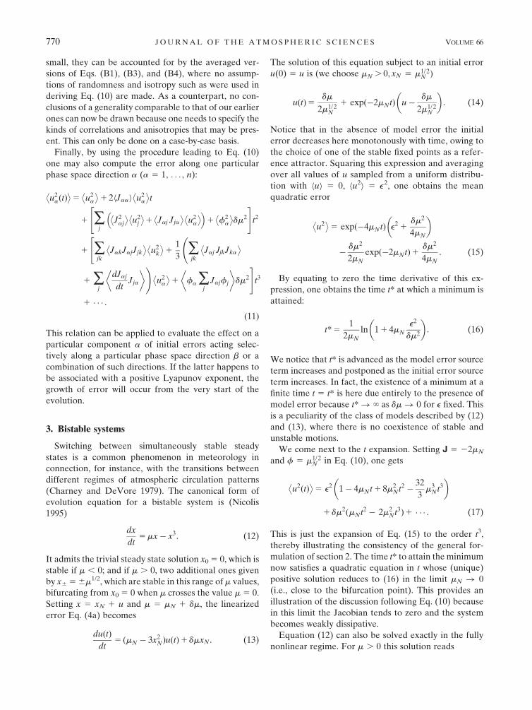
point (Fig. 2). The t expansion (dotted line) remains

here close to the exact solution (full line) for a short

period of time but subsequently exhibits a qualitatively

different behavior, missing the minimum versus time

altogether. The expansion can be improved significantly

(Fig. 2, dashed–dotted line) by performing a partial

resummation using a Pade approximant (Baker and

Graves-Morris 1996) of the form

u2� �

’e2 1 p1t 1 p2t2

1 1 q1t, (19)

in which the three coefficients p1, p2, and q1 are deter-

mined by requiring that its t expansion coincides with

Eq. (17) to the order t3. This approximation improves

the t3 expansion and prolongs its range of validity while

ensuring at the same time its positivity.

We turn now to the computation of the crossover time�t introduced in the end of section 2. By requiring that

the contributions in e2 and dm2 in Eq. (15) reach the

same value at t 5 �t, one obtains a quadratic equation for

exp �2mN�t

� �whose solution yields

�t 51

2mN

ln

dm2

2mN� 2e2

dm2

2mN� 2e

0BB@

1CCA. (20)

In Fig. 3 the time dependencies of the e2 and dm2 parts of

Eq. (15) and of its t expansion [Eq. (17)] are plotted

against time (full and dashed lines, respectively). In

both cases a crossover is found at a �t value quite close to

the estimate of Eq. (20), which turns out to be signifi-

cantly longer than the time t* for the total mean error

hu2(t)i to attain the minimum as computed for the same

parameter values (cf. Fig. 1). Notice that �t exists only as

long as the model error, as measured by dm2/(2mN), is

sufficiently large compared to initial error.

The simplicity of the model studied in this section

allows one to identify further the nature of the balance

realized at the crossover time �t. Clearly at t 5 �t the

mean quadratic error does not vanish, in agreement

with the general comment made at the end of section 2,

because the right-hand side of Eq. (15) does not admit a

real-valued root: the two parts of the mean quadratic

error do not cancel each other but rather attain equal

magnitudes. It is only at the level of Eq. (14) for the

(nonaveraged) error itself that a cancellation is possible,

provided that parameter dm and initial errors u have

opposite signs. As a by-product, for such realizations the

quadratic error |u(t)|2 would possess a minimum at u 5

0. In other words, the minimum of total error and match-

ing of its two components are linked for this class of re-

alizations. This is not so any longer for realizations in

which dm and u have the same sign and, as a corollary, for

the mean quadratic error itself.

4. Error dynamics around a saddle point

In the system considered in the preceding section, the

error evolution was taking place around a single, stable,

steady state solution of the reference system. Now, one

of the signatures of the complexity of atmospheric dy-

namics is the coexistence of stable motions reflecting

the presence of underlying regularities and unstable

motions interrupting these regularities in a seemingly

FIG. 1. Time evolution of the mean quadratic error in the

presence of both initial condition and model errors in the case of a

bistable system Eq. (12) with m 5 0.1. Initial condition errors are

randomly sampled from a uniform distribution around the steady

state solution of the exact system with e2 5 0.33 1026 and dm 5

1023. The full line depicts the exact solution, the dashed line the

linearized solution, and dotted line the result of the t expansion.

The number of realizations considered is 2 3 104.


erratic way (Nicolis and Nicolis 1995). To capture some

of the aspects of this property, we project Eq. (4a) along

the stable and unstable directions of a fixed point of a

saddle type, mimicking in this way, locally, what is ex-

pected to be happening globally in a strongly unstable,

hyperbolic dynamical system. In the minimal case of a

two-dimensional dynamics, Eq. (4a) then becomes

du1

dt5 mNu1 1 dmxN and

du2

dt5 �lNu2.

(21)

Here, xN is the coordinate of the saddle point along the

x axis, mN (mN . 0) plays the role of both the control

parameter subjected to uncertainty and of the positive

Lyapunov exponent, and 2lN (lN . 0) is the negative

Lyapunov exponent, supposed not to be subjected to

uncertainty. To satisfy the dissipativity condition, we

require lN . mN.

The solution of Eqs. (21) reads

u1 tð Þ5 u1emN t 1xN

mN

ðemN t � 1Þdm and

u2 tð Þ5 u2e�lN t,

(22)

from which the quadratic error can be deduced:

u2 tð Þ5 u21e2mN t 1 u2

2e�2lN t 1x2

N

m2N

ðemN t � 1Þ2dm2

1 2u1xN

mN

emN tðemN t � 1Þdm. (23)

Averaging over random initial errors u1h i 5 u2h i 5 0,ð

u21

� �5 u2

2

� �5 e2Þ, one obtains

u2� �

5 e2ðe2mN t 1 e�2lN tÞ1x2

N

m2N

ðemN t � 1Þ2dm2 (24a)

and the corresponding t expansion up to O(t3), the ana-

log of Eq. (10) with J11 5 mN, J22 5 2lN, J12 5 J21 5 0

and f1 5 xN, f2 5 0:

u2 tð Þ� �

5 2e2 1 2 mN � lN

� �e2t

1 ½2ðm2N 1 l2

NÞe2 1 x2

Ndm2�t2

14

3ðm3

N � l3NÞe

2 1x2NmNdm2

� �t3 1 � � � . (24b)

By setting the time derivative of hu2(t)i to zero one can

evaluate from Eqs. (24) the time t* for a minimum to

occur. Owing to the presence of the contributions due to

2lN, a minimum is bound to exist even in the absence of

model error. As pointed out earlier, this is a general

feature of systems in which stable and unstable motions

coexist (in this respect, the example of section 3 is an

exception). But because model error gives a positive

contribution to the time derivative it tends to advance

the value of t* in such a way that the contribution

containing exp(22lNt*) can still cancel those contain-

ing the positive exponentials. This confirms further the

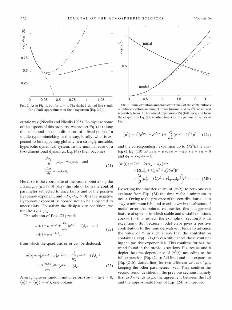
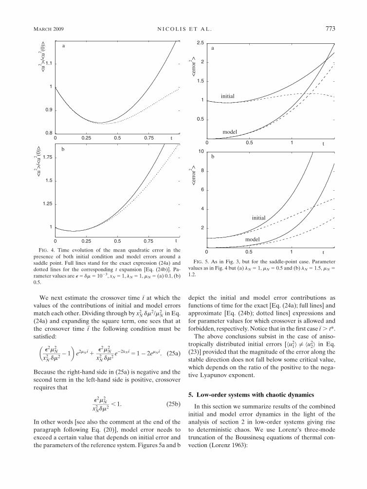
trend found in the previous sections. Figures 4a and b

depict the time dependence of hu2(t)i according to the

full expression [Eq. (24a); full line] and its t expansion

[Eq. (24b); dotted line] for two different values of mN,

keeping the other parameters fixed. They confirm the

second trend identified in the previous sections, namely

that as lN tends to mN the agreement between the full

and the approximate form of Eqs. (24) is improved.

FIG. 3. Time evolution and cross over time �t of the contributions

of initial condition and model errors (normalized by e2) considered

separately from the linearized expression (15) (full lines) and from

the t expansion Eq. (17) (dashed lines) for the parameter values of

Fig. 1.

FIG. 2. As in Fig. 1, but for m 5 1. The dashed–dotted line stands

for a Pade approximant of the t expansion [Eq. (19)].


We next estimate the crossover time �t at which the

values of the contributions of initial and model errors

match each other. Dividing through by x2N dm2/m2

N in Eq.

(24a) and expanding the square term, one sees that at

the crossover time �t the following condition must be

satisfied:

e2m2N

x2N dm2

� 1

� �e2mN

�t 1e2m2

N

x2N dm2

e�2lN�t 5 1� 2emN�t. (25a)

Because the right-hand side in (25a) is negative and the

second term in the left-hand side is positive, crossover

requires that

e2m2N

x2Ndm2

, 1. (25b)

In other words [see also the comment at the end of the

paragraph following Eq. (20)], model error needs to

exceed a certain value that depends on initial error and

the parameters of the reference system. Figures 5a and b

depict the initial and model error contributions as

functions of time for the exact [Eq. (24a); full lines] and

approximate [Eq. (24b); dotted lines] expressions and

for parameter values for which crossover is allowed and

forbidden, respectively. Notice that in the first case �t . t*.

The above conclusions subsist in the case of aniso-

tropically distributed initial errors [hu21i 6¼ hu

22i in Eq.

(23)] provided that the magnitude of the error along the

stable direction does not fall below some critical value,

which depends on the ratio of the positive to the nega-

tive Lyapunov exponent.

5. Low-order systems with chaotic dynamics

In this section we summarize results of the combined

initial and model error dynamics in the light of the

analysis of section 2 in low-order systems giving rise

to deterministic chaos. We use Lorenz’s three-mode

truncation of the Boussinesq equations of thermal con-

vection (Lorenz 1963):

FIG. 4. Time evolution of the mean quadratic error in the

presence of both initial condition and model errors around a

saddle point. Full lines stand for the exact expression (24a) and

dotted lines for the corresponding t expansion [Eq. (24b)]. Pa-

rameter values are e 5 dm 5 1023, xN 5 1, lN 5 1, mN 5 (a) 0.1, (b)

0.5.

FIG. 5. As in Fig. 3, but for the saddle-point case. Parameter

values as in Fig. 4 but (a) lN 5 1, mN 5 0.5 and (b) lN 5 1.5, mN 5

1.2.


dx

dt5 sð�x 1 yÞ,

dy

dt5 rx� y� xz, and

dz

dt5 xy� bz,

(26)

where x measures the rate of convective (vertical)

turnover, y the horizontal temperature variation, and z

the vertical temperature variation. Parameters s and b

account, respectively, for the intrinsic properties of the

material and for the geometry of the convective pattern.

In what follows we focus on the role of parameter r, the

(reduced) Rayleigh number, which provides a measure

of the strength of the thermal constraint to which the

system is subjected and is the main component respon-

sible for the thermal convection instability occurring in

the system. Model error and Jacobian matrix—the vector

fdm and the matrix J in Eqs. (10) and (11)—reduce

then to

fdm 5 ð0, �xdr, 0Þ and (27)

J 5

�s

r� �zðtÞ

�yðtÞ

s

�1

�xðtÞ

0

��xðtÞ

�b

264

375, (28)

where the bars indicate evaluation on the reference

attractor. The latter is chosen to correspond to the

typical values r 5 28, s 5 10, and b 5 8/3. Notice that

Si Jiih i 5 �ðs 1 b 1 1Þ takes here a constant (state-

independent) strongly negative value, reflecting the highly

dissipative character of the ongoing dynamics.

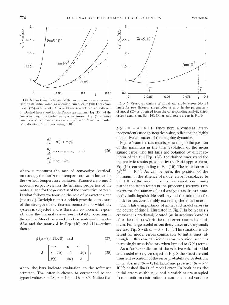
Figure 6 summarizes results pertaining to the position

of the minimum in the time evolution of the mean

square error. The full lines are obtained by direct so-

lution of the full Eqs. (26); the dashed ones stand for

the analytic results provided by the Pade approximant,

Eq. (19), corresponding to Eq. (10). The initial error is

hu2i1/2 5 1023. As can be seen, the position of the

minimum in the absence of model error is displaced to

the left as the model error is increased, confirming

further the trend found in the preceding sections. Fur-

thermore, the numerical and analytic results are prac-

tically indistinguishable well beyond the minimum for

model errors considerably exceeding the initial ones.

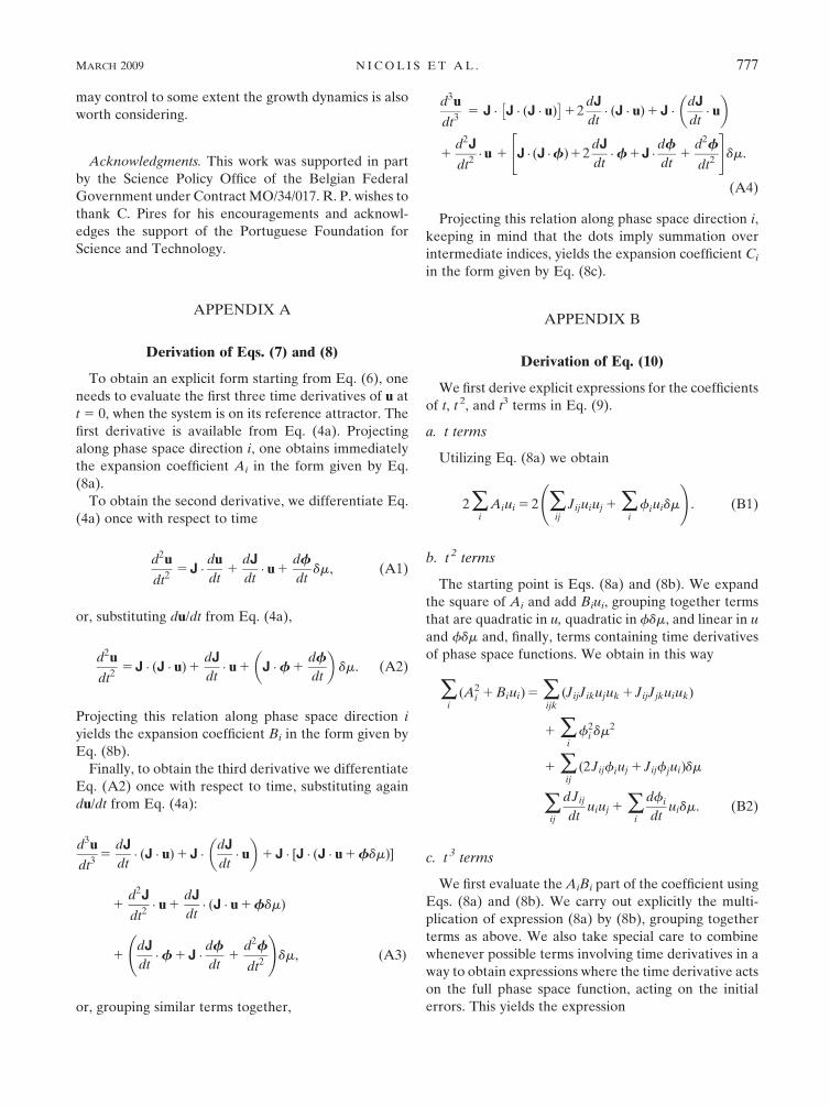
The relative importance of initial and model errors in

the course of time is illustrated in Fig. 7. In both cases a

crossover is predicted, located (as in sections 3 and 4)

after the time at which the total error attains its mini-

mum. For large model errors these times are very small;

see also Fig. 6 with dr 5 5 3 1023. The situation is dif-

ferent for model errors comparable to initial ones, al-

though in this case the initial error evolution becomes

increasingly unsatisfactory when limited to O(t3) terms.

As a further indicator of the relative roles of initial

and model errors, we depict in Fig. 8 the structure and

transient evolution of the error probability distributions

in the absence (dr 5 0; full lines) and presence (dr 5 5 3

1023; dashed lines) of model error. In both cases the

initial errors of the x, y, and z variables are sampled

from a uniform distribution of zero mean and variance

FIG. 6. Short time behavior of the mean square error, normal-

ized by its initial value, as obtained numerically (full lines) from

model (26) with r 5 28 1 dr, s 5 10, and b 5 8/3 for three different

dr. Dashed lines stand for the Pade approximant [Eq. (19)] of the

corresponding third-order analytic expansion, Eq. (10). Initial

condition of the mean square error is hu2i 5 1026 and the number

of realizations for the averaging is 105.

FIG. 7. Crossover times �t of initial and model errors (dotted

lines) for two different magnitudes of error in the parameter r

of model (26) as obtained from the corresponding analytic third-

order t expansion, Eq. (10). Other parameters are as in Fig. 6.


equal to 3.3 3 1024. For dr 5 0 the bulk of probability

density remains confined in a fairly narrow interval of

values. At the same time, a certain asymmetry is man-

ifested, reflected by the tendency to develop a (rather

modest) tail in the direction of large error values. The

situation changes considerably under the combined ac-

tion of initial and model errors: the distribution is now

much broader and displays, transiently, a bimodal struc-

ture at times that is considerable longer than the min-

imum or the crossover times (Figs. 6 and 7). We are

probably dealing here with an intermediate to long time

type of effect, reflecting the increasing delocalization of

the system in phase space induced by the presence of

model error.

Up to now, random (unbiased) initial condition errors

were used in the numerical experiments. However, there

is evidence that systematic initial condition errors are

present in the analyses used for operational forecasts.

These systematic errors can arise either from observa-

tional biases coming, for instance, from a progressive

degradation of the quality of a measurement device (see

e.g., Kalnay 2003) or from the data assimilation proce-

dure, which uses an imperfect model displaying some

systematic drifts. The presence of such biases has been

amply demonstrated during the reanalysis experiments

performed at the National Centers for Environmental

Prediction (NCEP; Kistler et al. 2001) or at ECMWF

(Simmons et al. 2004), through a detailed comparison

with observed data.

A natural question to be raised concerns the impact of

these systematic errors in operational forecasting on the

predictability of the system at hand under the simulta-

neous presence of model errors. This point is briefly

addressed here by introducing a systematic initial error

for one of the variables of the Lorenz model, namely the

variable z. The amplitude of this systematic error has

been taken equal to the standard deviation of the ran-

dom part of error added to each model variable at the

initial time.

Figure 9a depicts the time of the minimum for the

experiments, with and without systematic errors, as a

function of the amplitude of the model error perturba-

tion dr. An interesting feature is that the time of the

minimum for positive values of dr is now shifted toward

larger values. In addition, the minimum (normalized by

the initial value of the error) is deepening as compared

with the case in which systematic errors are absent (Fig.

9b). Notice that when the amplitude of the systematic

error is increased further, the deepening of the mini-

mum and its shift are also increased.

In the notation of section 2 and appendix B, the nu-

merical experiments summarized above correspond to

hui5 (0, 0, s) (s . 0), with f as in Eq. (27). Under these

conditions the initial model error coupling is absent at

the level of the first-order term of the short time ex-

pansion [Eq. (B1)] but gives a contribution at the level

of the second-order term [third to last term in Eq. (B2)].

Using the explicit form of the Jacobian, one sees that this

term yields a negative contribution under the conditions

of Fig. 9a, equal to ð2Jyz 1 JzyÞfyuzdr 5 ��x2sdr. Dis-

carding at this stage the O(t3) term, this will thus tend to

FIG. 8. Short to intermediate time probability density of hu2i1/2 in

the absence (full lines) and in the presence of model error, r 5 28

1 dr with dr 5 5 3 1023 (dashed lines). Other parameters are as in

Fig. 6; the number of realizations is 106.


increase the value of the time of minimum, which will be

given by

t* ’�ðcoefficient of t� termÞ

2ðcoefficient of t2 � termÞ, (29)

in agreement with Fig. 9a. Substituting into the ex-

pression of the error, one sees likewise that the value of

the error at its minimum tends to decrease, in agree-

ment with Fig. 9b.

In summary, a rich variety of behaviors can be found

in the dynamics of the error in the Lorenz system for

biased initial errors. In particular, a deepening of the

error minimum and a shift of this minimum toward large

times is obtained for some specific model and systematic

errors. These features could have considerable opera-

tional implications because a model subjected to certain

types of model errors could display different predict-

ability properties depending on the presence, or not, of

systematic errors in the initial conditions.

6. Conclusions

In this work some generic properties of the transient

evolution of prediction errors under the combined ef-

fect of initial condition and of model errors have been

derived, in the limit of small initial and parameter er-

rors. The regime considered was in the short to inter-

mediate time frame, as reflected by carrying out a power

series expansion of the error [Eq. (7)] and its norm [Eq.

(9)] limited to the O(t3) terms. In its most general form,

this expansion accounts for arbitrary types of initial and

model errors beyond the usually considered case of

unbiased (random) uncorrelated ones and brings out

clearly the mechanisms by which an initial error acting

along a particular phase space direction ends up con-

taminating, in the course of time, phase space directions

that were initially error free. Under the additional as-

sumption of uncorrelated and unbiased initial errors, a

simplified expression was derived [Eq. (10)], which al-

lowed us to identify conditions for the existence of a

time at which mean quadratic errors attain a minimum,

a crossover time at which the effects of initial conditions

and of model errors match each other, or, possibly, the

occurrence of inflexion points. In each case, the role of

the intrinsic dynamics and in particular its dissipative

character and the interplay between stability and in-

stability has been brought out.

These general properties have been tested and illus-

trated on a number of generic low-order models of

atmospheric dynamics. In all cases considered the cross-

over time was shown to exceed the time of the minimum.

Some quantitative relations were obtained showing how

the time of minimum is shifted as the magnitude of the

model error is increased. The case of biased (system-

atic) initial errors was also considered in a model giving

rise to deterministic chaos and was shown to be re-

sponsible for some qualitatively new properties. This

case, as well as the case of correlated and anisotropic

initial errors, definitely deserves a more comprehensive

study in the future. In this respect, an interesting

problem is to evaluate the impact on the crossover time

of error sources of the data assimilation process, known

to introduce preferential directions to the initial errors

in phase space.

Finally, it would be interesting to extend the work

reported here to account for multivariate systems (and

in particular for spatially extended ones), as well as for

cases in which the model and the reference variables do

not span the same phase space. The role of stochastic

perturbations and, in particular, the possibility that they

FIG. 9. (a) Time t* when mean errors attain their minimum value

and (b) relative size of the minimum against the magnitude of the

model error perturbation dr. Full lines stand for the case of unbi-

ased initial condition errors and dashed lines for the case of biased

ones. The amplitude of the bias is equal to the standard deviation

of the random part of the initial error of the variables of model

(26). Parameters are as in Fig. 6; the number of realizations is 105.


may control to some extent the growth dynamics is also

worth considering.

Acknowledgments. This work was supported in part

by the Science Policy Office of the Belgian Federal

Government under Contract MO/34/017. R. P. wishes to

thank C. Pires for his encouragements and acknowl-

edges the support of the Portuguese Foundation for

Science and Technology.

APPENDIX A

Derivation of Eqs. (7) and (8)

To obtain an explicit form starting from Eq. (6), one

needs to evaluate the first three time derivatives of u at

t 5 0, when the system is on its reference attractor. The

first derivative is available from Eq. (4a). Projecting

along phase space direction i, one obtains immediately

the expansion coefficient Ai in the form given by Eq.

(8a).

To obtain the second derivative, we differentiate Eq.

(4a) once with respect to time

d2u

dt25 J �

du

dt1

dJ

dt� u 1

df

dtdm, (A1)

or, substituting du/dt from Eq. (4a),

d2u

dt25 J � ðJ � uÞ1

dJ

dt� u 1 J �f 1

df

dt

� �dm. (A2)

Projecting this relation along phase space direction i

yields the expansion coefficient Bi in the form given by

Eq. (8b).

Finally, to obtain the third derivative we differentiate

Eq. (A2) once with respect to time, substituting again

du/dt from Eq. (4a):

d3u

dt35

dJ

dt� ðJ � uÞ1 J �

dJ

dt� u

� �1 J � ½J � ðJ � u 1 fdmÞ�

1d2J

dt2� u 1

dJ

dt� ðJ � u 1 fdmÞ

1dJ

dt�f 1 J �

df

dt1

d2f

dt2

!dm, ðA3Þ

or, grouping similar terms together,

d3u

dt35 J �

�J � ðJ � uÞ

�12

dJ

dt� ðJ � uÞ1 J �

dJ

dt� u

� �

1d2J

dt2�u 1 J � ðJ �fÞ12

dJ

dt�f1J �

df

dt1

d2f

dt2

" #dm.

(A4)

Projecting this relation along phase space direction i,

keeping in mind that the dots imply summation over

intermediate indices, yields the expansion coefficient Ci

in the form given by Eq. (8c).

APPENDIX B

Derivation of Eq. (10)

We first derive explicit expressions for the coefficients

of t, t 2, and t3 terms in Eq. (9).

a. t terms

Utilizing Eq. (8a) we obtain

2�i

Aiui 5 2 �ij

Jijuiuj 1 �i

fiuidm

!. (B1)

b. t 2 terms

The starting point is Eqs. (8a) and (8b). We expand

the square of Ai and add Biui, grouping together terms

that are quadratic in u, quadratic in fdm, and linear in u

and fdm and, finally, terms containing time derivatives

of phase space functions. We obtain in this way

�iðA2

i 1 BiuiÞ5 �ijkðJijJikujuk 1 JijJjkuiukÞ

1 �i

f2i dm2

1 �ijð2Jijfiuj 1 JijfjuiÞdm

�ij

dJij

dtuiuj 1 �

i

dfi

dtuidm. (B2)

c. t 3 terms

We first evaluate the AiBi part of the coefficient using

Eqs. (8a) and (8b). We carry out explicitly the multi-

plication of expression (8a) by (8b), grouping together

terms as above. We also take special care to combine

whenever possible terms involving time derivatives in a

way to obtain expressions where the time derivative acts

on the full phase space function, acting on the initial

errors. This yields the expression


�i

AiBi 5 �ijk‘

JijJjkJi‘uku‘ 1 �ij

Jijfifjdm2

1 �ij‘ðJijJi‘fju‘ 1 JijJj‘fiu‘Þdm

1 �ij‘

Ji‘dJij

dtuju‘

11

2�

i

df2i

dtdm2 1 �

ij

d

dtðJijfiÞujdm. (B3)

Turning next to the Ciui part of the coefficient of t3 term

in Eq. (9), we obtain, by utilizing Eq. (8c) and grouping

terms in the same way as above,

�i

Ciui 5 �ijk‘

JijJjkJk‘uiu‘

1 �ijk

JijJjkuifkdm

1 �ij

dJij

dtuifidm 1 �

ijk

dJij

dtJjkuiuk

1 �ijk

d

dtðJijJjkÞuiuk

1 �ij

d2Jij

dt2uiuj

1 �i

d2fi

dt21 �

ij

d

dtðJijfjÞui

" #dm. (B4)

Summing (B3) and (B4) divided by 3 yields the explicit

expression of the coefficient of the t3 term in Eq. (9).

The next step is to average expressions (B1)–(B4)

over the invariant density of the reference attractor and

the distribution of initial errors. The first operation

alone will eliminate a number of terms, expressed en-

tirely in terms of time derivatives of phase space func-

tions. The terms concerned by this elimination are the

last two terms in (B2), the last two terms in (B3), and the

last three terms in (B4). The reason is that in an ergodic

system phase space averages and long time averages

along a typical trajectory are equal:

dg

dt

� �5 lim

T!‘

1

T

ðT

0

dtdgðtÞ

dt5 lim

T!‘

1

TgðTÞ � gð0Þ½ �, (B5)

where the bracket stands for the phase space average.

Now for any bounded function g (the kind of function

one deals with in physical systems), g(T ) 2 g(0) is finite

and hence the term in the right-hand side of the last

equality of Eq. (B5) tends to zero in the long time limit.

Consider next the average of the remaining terms over

the distribution of initial errors. A further drastic simpli-

fication will occur in the case of unbiased errors, huji 5 0,

because all terms in dm surviving the first averaging will

give a vanishing contribution in (B1)–(B4). These are

the last term in (B1), the third term in (B2), the third

term in (B3), and the second and third terms in (B4).

Assuming further that initial errors are uncorrelated,

uiuj

� �5 u2

i

� �dkr

ij , will transform the fourth term in (B3)

into the total derivative of J2i‘, which will give a vanishing

contribution through the phase space averaging. Keeping

track of all these steps, one arrives finally at Eq. (10).

REFERENCES

Baker, G. A., Jr., and P. Graves-Morris, 1996: Pade Approximants.

Cambridge University Press, 746 pp.

Charney, J. G., and J. G. DeVore, 1979: Multiple flow equilibria in

the atmosphere and blocking. J. Atmos. Sci., 36, 1205–1216.

Dalcher, A., and E. Kalnay, 1987: Error growth and predictability

in operational ECMWF forecasts. Tellus, 39A, 474–491.

Ivanov, L. M., and P. C. Chu, 2007: On stochastic stability of re-

gional ocean models in wind forcing. Nonlinear Processes

Geophys., 14, 655–670.

Kalnay, E., 2003: Atmospheric Modeling, Data Assimilation, and

Predictability. Cambridge University Press, 364 pp.

Kistler, R., and Coauthors, 2001: The NCEP–NCAR 50-Year

Reanalysis: Monthly means CD-ROM and documentation.

Bull. Amer. Meteor. Soc., 82, 247–267.

Krishnamurti, T., J. Sanjay, A. Mitra, and T. Vijaya Kumar, 2004:

Determination of forecast errors arising from different com-

ponents of model physics and dynamics. Mon. Wea. Rev., 132,2570–2594.

Lorenz, E. N., 1963: Deterministic nonperiodic flow. J. Atmos. Sci.,

20, 130–141.

——, 1982: Atmospheric predictability experiments with a large

numerical model. Tellus, 34, 505–513.

——, 1996: Predictability: A problem partly solved. Proc. Seminar

on Predictability, Reading, Berkshire, United Kingdom, ECMWF,

1–18.

Nicolis, C., 1992: Probabilistic aspects of error growth in atmo-

spheric dynamics. Quart. J. Roy. Meteor. Soc., 118, 553–568.

——, 2003: Dynamics of model error: Some generic features. J.

Atmos. Sci., 60, 2208–2218.

——, 2004: Dynamics of model error: The role of unresolved scales

revisited. J. Atmos. Sci., 61, 1740–1753.

——, and G. Nicolis, 1995: Chaos in dissipative systems: Under-

standing atmospheric physics. Adv. Chem. Phys., 91, 511–570.

Nicolis, G., 1995: Introduction to Nonlinear Science. Cambridge

University Press, 254 pp.

Reynolds, C. A., P. J. Webster, and E. Kalnay, 1994: Random error

growth in NMC’s global forecasts. Mon. Wea. Rev., 122, 1281–

1305.

Schubert, S., and Y. Schang, 1996: An objective method for in-

ferring sources of model error. Mon. Wea. Rev., 124, 325–340.

Simmons, A. J., and A. Hollingsworth, 2002: Some aspects of the

improvement in skill of numerical weather prediction. Quart.

J. Roy. Meteor. Soc., 128, 647–677.

——, and Coauthors, 2004: Comparison of trends and variability in

CRU, ERA-40, and NCEP/NCAR analyses of monthly-mean

surface air temperature. ERA-40 Project Report Series 18, 38 pp.

Tribbia, J. J., and D. P. Baumhefner, 1988: The reliability of im-

provements in deterministic short-range forecasts in the

presence of initial state and modeling deficiencies. Mon. Wea.

Rev., 116, 2276–2288.

——, and ——, 2004: Scale interactions and atmospheric pre-

dictability: An updated perspective. Mon. Wea. Rev., 63,

703–713.


Dynamics of Prediction Errors under the Combined Effect of Initial Condition and Model Errors

Documents

Transcript of Dynamics of Prediction Errors under the Combined Effect of Initial Condition and Model Errors