Use of Dynamic Cone Penetration and Clegg Hammer Tests for Quality Control of Roadway Compaction and...

JOINT TRANSPORTATION RESEARCH PROGRAM

FHWA/IN/JTRP-2010/27

Final Report

USE OF DYNAMIC CONE PENETRATION AND CLEGG

HAMMER TESTS FOR QUALITY CONTROL OF

ROADWAY COMPACTIOIN AND CONSTRUCTION

Hobi Kim

Monica Prezzi

Rodrigo Salgado

April 2010

4/10 JTRP-2010/27 INDOT Office of Research and Development West Lafayette, IN 47906

INDOT Research

TECHNICAL Summary Technology Transfer and Project Implementation Information

TRB Subject Code: April 2010

Publication No. FHWA/IN/JTRP-2010/27, SPR-3009 Final Report

Use of Dynamic Cone Penetration and Clegg Hammer Tests for Quality Control of Roadway

Compaction and Construction

Introduction

Soil compaction quality control is currently

accomplished by determining the in-place

compacted dry unit weight and comparing it with

the maximum dry unit weight (γdmax) obtained

from a standard laboratory compaction test. INDOT

requires that the inplace dry unit weight for

compacted soil be over 95% of the laboratory

maximum dry unit weight. In order to determine the

inplace dry unit weight, INDOT engineers

generally use the nuclear gauge, which is hazardous

and also cumbersome due to strict safety

requirements. Thus, several tests, such as the

Dynamic Cone Penetration Test (DCPT) and the

Clegg Hammer Test (CHT), have been considered

as alternatives. In spite of significant research

performed to interpret the results of the DCPT and

CHT, no reliable correlations are available in the

literature to employ these tests for soil compaction

quality control. Therefore, the main goal of the

present study is to evaluate the use of the DCPT

and the CHT for compaction quality control and to

develop interpretation methods for the DCPT and

CHT.

In this research, a number of DCPTs and CHTs

was performed on road sites in Indiana, in a test

pit, and in a special test chamber at Purdue

University. A statistical approach was applied to

account for in situ compaction variability to

develop compaction quality criteria using the test

results.

Findings

Based on the test results provided by INDOT, we

developed correlations between maximum dry unit

weight (γdmax), optimum moisture content (OMC,

wcopt), plastic limit (PL), and liquid limit (LL) for

Indiana soils. The specification of many agencies

in the U.S. for density control (e.g., 95% relative

compaction) has been in effect for more than 30

years. The data available in the literature indicates

that the actual mean values of relative compaction

achieved on the sites were roughly two to three

percent greater than the specification

requirements, but about 20% of the test results did

not meet the specification requirements. Several

studies indicate that relative compaction on site is

normally distributed. Specifications accounting for

the variability would be desirable.

Based on the experimental program undertaken to

assess the Dynamic Cone penetration Test (DCPT)

and the Clegg Hammer Test (CHT), DCP criteria

for compaction quality control were suggested by

dividing the soils considered into three groups

based on the AASHTO soil classification. In

addition, the statistical variability of the test results

was considered in the development of the DCP

criteria for compaction quality control. Based on

the analysis of the data collected, the following

equations are proposed in this report.

(a) A-3 soils:

The minimum required blow count

(NDCP)req|0~12” for 0-12” penetration varies

from 7 to 10; it is a function of the coefficient of

4/10 JTRP-2010/27 INDOT Division of Research West Lafayette, IN 47906

uniformity Cu. The following equation was

proposed for A-3 soils:

(NDCP)req|0~12” = 4.0ln(Cu) + 2.6

The (NDCP)req|0~12” is the minimum required

blow count for 0-to-12 inch penetration that

implies an RC of 95% with high probability.

(b) “Granular” soil (A-1 and A-2 soils, except soils

containing gravel):

The minimum required blow count

(NDCP)req|0~12” for this type of soil is

influenced by the fine particles that are present in

the soil. Since the plasticity index and the amount

of fine particles contained in the “granular” soil

correlate with the OMC, the minimum required

blow count for “granular” soils is suggested as a

function of the OMC as follows:

(NDCP)req|0~12” = 59exp(-0.12wcopt)

where wcopt = optimum moisture content. The

(NDCP)req|0~12” is the minimum required blow

count for 0-to-12 inch penetration that implies an

RC of 95% with high probability.

(c) Silty, clayey soils:

The minimum required blow count correlates with

the plasticity index and the percentage of soil by

weight passing the #40 sieve. Thus, we propose

the minimum required blow count (NDCP)req for

silty clay soils as a function of the plasticity index

and the percentage of soil by weight passing the

#40 sieve (F40) according to:

(NDCP)req|0~6” = 17exp[-0.07PI(F40/100)]

where (NDCP)req|0~6” = minimum required blow

count for 0-to-6 inch penetration that implies an

RC of 95% with high probability, PI = plasticity

index, and F40 = % passing the # 40 sieve; and

(NDCP)req|6~12” =27exp[-0.08PI(F40/100)]

where (NDCP)req|6~12” = minimum required

blow count for 6-to-12 inch penetration that

implies an RC of 95% with high probability.

The relationship of Clegg Impact Value

(CIV) with relative compaction exhibited

considerable variability.

Implementation

The DCP criteria proposed in this study can be

tentatively used in soil compaction quality

control for soils like those studied in this

research. Based on the test results, we suggest

the use of DCPT as a tool for soil compaction

quality control. This research found that the

DCPT was effective in ensuring the required

relative compaction for soil compacted at the

specified water content.

Implementation projects can help refine the

findings of this research and facilitate the use of

the DCPT in routine projects by INDOT engineers. In

the long run, the DCPT can progressively replace the

nuclear density gauges, which are hazardous and also

cumbersome to use.

Since DCPT compaction control criteria are still in

the development stages, it is

recommended that further research be performed to

investigate the short and longterm feasibility of using

DCPT as a quality control tool in the context of field

implementation projects.

Contacts

For more information:

Prof. Monica Prezzi

Principal Investigator

School of Civil Engineering

Purdue University

West Lafayette IN 47907

E-mail: [email protected]

Indiana Department of Transportation

Office of Research and Development

1205 Montgomery Street

P.O. Box 2279

West Lafayette, IN 47906

Phone: (765) 463-1521

Fax: (765) 497-1665

mailto:[email protected]

4/10 JTRP-2010/27 INDOT Office of Research and Development West Lafayette, IN 47906

Purdue University

Joint Transportation Research Program


West Lafayette, IN 47907-1284

Phone: (765) 494-9310

Fax: (765) 496-7996

E-mail: [email protected]

http://www.purdue.edu/jtrp

mailto:[email protected]

http://www.purdue.edu/jtrp

Final Report


USE OF DYNAMIC CONE PENETRATION AND CLEGG HAMMER TESTS FOR

QUALITY CONTROL OF ROADWAY COMPACTION AND CONSTRUCTION

by

Hobi Kim

Monica Prezzi

Rodrigo Salgado

Geotechnical Engineering



Project No. C-36-36-VV

File No. 06-14-47

SPR-3009

Prepared in Cooperation with the


and the U.S. Department of Transportation

Federal Highway Administration

The contents of this report reflect the views of the authors, who are responsible for the facts and

the accuracy of the data presented herein. The contents do not necessarily reflect the official

views or policies of the Indiana Department of Transportation or the Federal Highway

Administration at the time of publication. The report does not constitute a standard, specification,

or regulation.

Purdue University

West Lafayette, IN 47907

April 2010

TECHNICAL REPORT STANDARD TITLE PAGE 1. Report No.

2. Government Accession No.

3. Recipient's Catalog No.


4. Title and Subtitle Use of Dynamic Cone Penetration and Clegg Hammer Tests for Quality

Control of Roadway Compaction and Construction

5. Report Date

April 2010

6. Performing Organization Code

7. Author(s)

Hobi Kim, Monica Prezzi, and Rodrigo Salgado

8. Performing Organization Report No.


9. Performing Organization Name and Address


Purdue University

550 Stadium Mall Drive

West Lafayette, IN 47907-2051

10. Work Unit No.

11. Contract or Grant No.

SPR-3009 12. Sponsoring Agency Name and Address


State Office Building

100 North Senate Avenue

Indianapolis, IN 46204

13. Type of Report and Period Covered

Final Report

14. Sponsoring Agency Code

15. Supplementary Notes

Prepared in cooperation with the Indiana Department of Transportation and Federal Highway Administration. 16. Abstract

Soil compaction quality control presently relies on the determination of the in-place compacted dry unit weight, which is then

compared with the maximum dry unit weight obtained from a laboratory compaction test. INDOT requires that the in-place dry unit

weight for compacted soil be over 95% of the laboratory maximum dry unit weight. In order to determine the in-place dry unit weight,

INDOT engineers generally use nuclear gauges, which are hazardous and also costly because of the required safety precautions. Thus,

several alternative tests such as the Dynamic Cone Penetration Test (DCPT) and the Clegg Hammer Test (CHT) were introduced as testing

tools for soil compaction quality control. However, no reliable correlations are available in the literature to employ these tests for soil

compaction quality control. The main objectives of this research were to evaluate the use of the DCPT and the CHT results to develop

criteria for soil compaction quality control. A number of DCPTs and CHTs was performed on Indiana road sites, in a test pit, and in the

soil test chamber at Purdue University. Since soil compaction varies from place to place, a statistical approach was applied to account for

the compaction variability in the development of the criteria for soil compaction quality control.

Based on the DCP tests performed on several INDOT road sites, as well as in the test pit at Purdue University, and the

requirement that the in-place dry unit weight of the fill material be over 95% of the laboratory maximum dry unit weight, minimum

required DCP blow counts (NDCP)req were proposed for soils belonging to three groups of the AASHTO (American Association of State

Highway and Transportation Officials) soil classification system.

For the DCPT, the minimum required blow count for 0-to-12 inch penetration, (NDCP)|0~12” associated with an RC of 95% for A-3

soil varied from 7 to 10; it is a function of the coefficient of uniformity. For A-1 soil and A-2 soils except those containing gravel, the

(NDCP)|0~12” was a function of the optimum moisture content. For silty clays, the minimum required blow counts, (NDCP)|0~6” and

(NDCP)|6~12” were a function of the plasticity index and the soil percentage passing the #40 sieve. Since the relationship of Clegg

Impact Value (CIV) with relative compaction exhibited considerable variability, no criterion for CHT was proposed.

Dynamic analyses hold promise in forming the basis for interpretation of the DCPT and CHT results since predictions of the

penetration process (DCPT) and accelerations (CHT) for sand under controlled conditions were very reasonable.

17. Key Words

Dynamic Cone Penetration Test (DCPT); Clegg Hammer

Test (CHT); Quality Control (QC); soil compaction;

dynamic analysis

18. Distribution Statement

No restrictions. This document is available to the public through the

National Technical Information Service, Springfield, VA 22161

19. Security Classif. (of this report)

Unclassified

20. Security Classif. (of this page)

Unclassified

21. No. of Pages

249

22. Price

Form DOT F 1700.7 (8-69)

TABLE OF CONTENTS

Page LIST OF TABLES ............................................................................................................. xi LIST OF FIGURES ......................................................................................................... xiii

CHAPTER 1. INTRODUCTION .................................................................................... 1

1.1. Background ............................................................................................................... 1

1.2. Research Objectives ................................................................................................. 3

1.3. Scope and Organization ............................................................................................ 4

CHAPTER 2. OVERVIEW ON SUBGRADE DESIGN AND CONSTRUCTION ... 7

2.1. Introduction .............................................................................................................. 7

2.2. Structural Response of Subgrade .............................................................................. 8

2.3. Geotechnical Design of Subgrade .......................................................................... 11

2.4. Fundamentals of Soil Compaction ......................................................................... 16

2.4.1. Background ...................................................................................................... 16

2.4.2. Structures and Engineering Properties of Compacted Soils ............................ 17

2.4.3. Compaction Characteristics of Soils ................................................................ 20

2.4.4. Variables Affecting Soil Compaction .............................................................. 24

2.5. Field Compaction of Subgrade ............................................................................... 28

2.6. Summary ................................................................................................................. 34

CHAPTER 3. QUALITY CONTROL OF SUBGRADE COMPACTION ............... 36

3.1. Introduction ............................................................................................................ 36

3.2. Density-Based Compaction Control Tests ............................................................. 39

3.2.1. Sand-Cone Test ................................................................................................ 39

3.2.2. Nuclear Gauge Test .......................................................................................... 40

3.3. Performance-Based Compaction Control Tests ..................................................... 44

3.3.1. California Bearing Ratio (CBR) Test ............................................................... 44

3.3.2. Resilient Modulus Test .................................................................................... 46

3.3.3. Plate Load Test ................................................................................................. 47

3.3.4. Light Falling-Weight Deflectomter Test .......................................................... 49

3.3.5. Soil Stiffness Gauge (SSG, Geogauge) Test .................................................... 52

3.3.6. Dynamic Cone Penetration Test ....................................................................... 54

3.3.7. Clegg Hammer Test ......................................................................................... 56

3.3.8. Continuous Compaction Control Test .............................................................. 60

3.4. Specifications for Quality Control of Subgrade Compaction ................................. 63

3.5. Summary ................................................................................................................. 68

CHAPTER 4. COMPACTION VARIABILITY OF SOIL......................................... 70

4.1. Introduction ............................................................................................................ 70

4.2. Basic Statistical Concepts ....................................................................................... 72

4.3. Sources of Compaction Variability ........................................................................ 74

4.4. Accounting for Compaction Variability in Determining the Specification Limits 81

4.5. Summary ................................................................................................................. 83

CHAPTER 5. ASSESSMENT OF DYNAMIC ANALYSIS ....................................... 86

5.1. Introduction ............................................................................................................ 86

5.2. Soil Response under Static Loading ....................................................................... 87

5.2.1. Background ...................................................................................................... 87

5.2.2. Shear Strength of Sands ................................................................................... 88

5.2.3. Shear Strength of Clays .................................................................................... 89

5.2.4. Limit Bearing Capacity of Shallow Footings ................................................... 90

5.2.5. Limit Base Capacity of Deep Footings ............................................................ 93

5.3. Soil Response under Dynamic Loading ................................................................. 97

5.3.1. Background ...................................................................................................... 97

5.3.2. Vertical Oscillation of Footings ....................................................................... 99

5.4. Suggested Model for the Interpretation of in situ Tests ....................................... 106

5.4.1. Selection of the Dynamic Model for the Clegg Hammer Test ....................... 106

5.4.2. Selection of the Dynamic Model for the Dynamic Cone Penetration Test .... 112

5.5. Summary ............................................................................................................... 117

CHAPTER 6. FIELD TESTS ON INDIANA SOILS ................................................ 121

6.1. Introduction .......................................................................................................... 121

6.2. Tests Performed in the Test Pit............................................................................. 122

6.2.1. Testing Method .............................................................................................. 122

6.2.2. Soil Properties ................................................................................................ 126

6.2.3. Test Results .................................................................................................... 129

6.3. Field Tests on A-3 Soils ....................................................................................... 136

6.3.1. Field Tests on SR25 ....................................................................................... 139

6.3.2. Field Tests on SR31 ....................................................................................... 142

6.3.3. Field Tests on I-70 ......................................................................................... 144

6.3.4. Summary of Test Results on A-3 Soils .......................................................... 148

6.4. Field Tests on A-1 and A-2 Soils ......................................................................... 151

6.4.1. Field Tests on SR31 (I) .................................................................................. 155

6.4.2. Field Tests on SR31 (II) ................................................................................. 158

6.4.3. Field Tests on SR31 (III) ................................................................................ 160

6.4.4. Field Tests on SR31 (Plymouth) .................................................................... 163

6.4.5. Field Tests on Access Road to Honda Plant .................................................. 166

6.4.6. Summary of Test Results on A-1 and A-2 Soils ............................................ 170

6.5. Field Tests on Silty Clay (A-4 to A-7 soil) .......................................................... 172

6.5.1. Field Tests on SR64 ....................................................................................... 174

6.5.2. Field Tests on SR66 ....................................................................................... 179

6.5.3. Field Tests on SR24 ....................................................................................... 184

6.5.4. Summary of Test Results on Silty Clay ......................................................... 189

6.6. Summary ............................................................................................................... 191

CHAPTER 7. DYNAMIC CONE PENETRATION TESTS AND CLEGG HAMMER TESTS PERFORMED IN A TEST CHAMBER ................................... 195

7.1. Introduction .......................................................................................................... 195

7.2. Test Equipment ..................................................................................................... 196

7.2.1. Test Chamber and Pluviation Procedure ........................................................ 196

7.2.2. Engineering Properties of Test Sand .............................................................. 199

7.2.3. Details of Instrumentation .............................................................................. 204

7.2.4. Test Procedure ................................................................................................ 210

7.3. Chamber Test Results ........................................................................................... 213

7.3.1. Static Test Results .......................................................................................... 213

7.3.2. Dynamic Test Results .................................................................................... 217

7.4. Summary ............................................................................................................... 222

CHAPTER 8. INTERPRETATION OF THE RESULTS USING DYNAMIC ANALYSIS .................................................................................................................... 223

8.1. Introduction .......................................................................................................... 223

8.2. Input Parameters for the Dynamic Analyses ........................................................ 224

8.3. Validation of the Results of the Tests Performed in the Purdue Test Chamber ... 229

8.3.1. Prediction of Static Test Results in Sand ....................................................... 229

8.3.2. Prediction of Dynamic Test Results in Sand .................................................. 231

8.4. Validation of the Preliminary Test Results in Clay .............................................. 234

8.5. Summary ............................................................................................................... 237

CHAPTER 9. SUMMARY AND CONCLUSIONS ................................................... 238

9.1. Summary ............................................................................................................... 238

9.2. Conclusions .......................................................................................................... 239

9.3. Suggestions for Future Research .......................................................................... 244

LIST OF REFERENCES ................................................................................................ 246

xi

LIST OF TABLES

Table Page Table 2.1 AASHTO soil classification (after ASTM D3282-93) ..................................... 12 Table 2.2 Minimum laboratory testing requirements for pavement designs (after ARA

2004) .......................................................................................................................... 14 Table 2.3 Geotechnical input parameters required for pavement design (after ARA 2004).

.................................................................................................................................... 15 Table 2.4 Typical ranges of maximum dry unit weights and optimum moisture contents

(modified after Gregg 1960) ...................................................................................... 23 Table 2.5 The relationship between γdmax, wcopt, plastic limit and liquid limit ................. 25 Table 3.1 Typical CBR ranges (Lavin 2003) .................................................................... 45 Table 3.2 Modulus of subgrade reaction of sands (MN/m2/m) ........................................ 48 Table 3.3 Modulus of subgrade reaction for clays* (MN/m2/m) ...................................... 48 Table 3.4 ISSMGE criteria for compaction QC based on the Zorn-LWD modulus ........ 51 Table 3.5 DCP criteria (NDCP) for a penetration of 0 to 150 mm (0 to 6 inch) ................. 56 Table 3.6 Various Clegg Hammer Test product configurations (Lafayette Instrument Co.,

2009) .......................................................................................................................... 58 Table 3.7 Summary of the correlations between CBR and CIV* ..................................... 59 Table 3.8 CIVs corresponding to 90% RC at optimum moisture content (modified after

GTI 2005) ................................................................................................................... 60 Table 3.9 Summary of compaction control specifications adopted by various

transportation agencies ............................................................................................... 66 Table 4.1 Variability of laboratory test (data from Liu and Thompson 1966) ................ 78 Table 4.2 Variability of relative compaction data from the literature .............................. 80 Table 6.1 Different compaction targets .......................................................................... 124 Table 6.2 The particle-size distribution analysis and classification of the soil sample .. 127 Table 6.3 Summary of compaction test and Atterberg limit tests ................................... 128 Table 6.4 Summary of the sand cone, DCPT, and CHT results ..................................... 130 Table 6.5 Summary of grain-size distribution analyses and compaction tests ............... 139 Table 6.6 Summary of the DCP results with the coefficient of uniformity (Cu) and

compaction properties on A-3 soil ........................................................................... 148 Table 6.7 Summary of grain-size distribution analyses and compaction tests ............... 155 Table 6.8 Summary of the DCP results together with compaction properties of “granular”

soils .......................................................................................................................... 170 Table 6.9 Summary of the plasticity and compaction properties of the soil samples ..... 173 Table 6.10 Summary of the DCP results with the plasticity and percent passing the #200

sieve on silty clay soils ............................................................................................. 189 Table 6.11 Relationship between NDCP, Cu, wcopt, PI, and percent the #40 passing sieve

.................................................................................................................................. 191

xii

Table 6.12 Relationship between (NDCP)req│0~12” and coefficient of uniformity (Cu) ..... 192 Table 6.13 Relationship between (NDCP)req│0~12” and optimum moisture content (wcopt) 192 Table 6.14 Relationship between NDCP, Cu, wcopt, PI, and percent the #40 passing sieve

.................................................................................................................................. 193 Table 7.1 Engineering properties of F-55 sand (data from Lee 2008) ............................ 200 Table 8.1 Input parameters for the dynamic analyses ..................................................... 224 Table 8.2 Maximum dry unit weight and specific gravity used for the dynamic analysis

.................................................................................................................................. 225 Table 8.3 Summary of measured and predicted static penetration resistance of the DCP

.................................................................................................................................. 231 Table 8.4 Summary of measured and predicted NDCP of clay in the test pit ................... 236 Table 9.1 Relationship between (NDCP)req│0~12” and coefficient of uniformity (Cu) ....... 240 Table 9.2 Relationship between (NDCP)req│0~12” and optimum moisture content (wcopt) . 241 Table 9.3 Relationship between NDCP, Cu, wcopt, PI, and percent the #40 passing sieve 243

xiii

LIST OF FIGURES

Figure Page Figure 2.1 Schematic of vertical stress distribution due to wheel load acting on pavements.

...................................................................................................................................... 7

Figure 2.2 Pavement behavior under moving wheel load (a) stresses acting on element along with the transient stress distribution, and (b) strain distribution with depth within the pavement layers and the subgrade (modified after Brown 1996). .............. 9

Figure 2.3 Strains developed in the subgrade versus time under repeated loads (modified after Huang 2004). ..................................................................................................... 11

Figure 2.4 Examples of compaction curves (modified after Lambe 1962). ..................... 17

Figure 2.5 Typical compaction curve for cohesionless sands and sandy gravels (modified after Foster 1962). ...................................................................................................... 19

Figure 2.6 INDOT family of curves (modified after INDOT Manual 2007). .................. 21

Figure 2.7 Relationships between maximum dry density, optimum moisture content, and Atterberg limits (data from Woods 1940 and INDOT Manual 2007)........................ 24

Figure 2.8 Relationship between maximum dry density and Atterberg limits: (a) maximum dry density vs. plastic limit, and (b) maximum dry density vs. liquid limit. .................................................................................................................................... 26

Figure 2.9 Effect of plasticity on compacted density for various compaction energies (Rollings and Rollings 1996). .................................................................................... 27

Figure 2.10 Stress distributions within soil under compactors (modified after Rollings and Rollings 1996). ........................................................................................................... 29

Figure 2.11 Typical growth curves: (a) A-1-b soil (well-graded sand), and (b) A-7-6 soil (heavy clay) (data from Lewis 1959). ........................................................................ 30

Figure 2.12 The effect of travel speed of the compactor in: (a) Well-graded sand; (b) Heavy clay (data from Selig and Yoo 1977). ............................................................. 32

Figure 3.1 Nuclear gauge measurements: (a) backscatter mode for density measurement, (b) direct transmission mode for density measurement, and (c) moisture detection (Troxler 2006). ........................................................................................................... 42

Figure 3.2 Schematic of LWD showing various component of the equipment (modified after Siddiki et al. 2008) ............................................................................................. 50

Figure 3.3 Schematic of the Geogauge (modified after Alshibli et al 2005). ................... 53

Figure 3.4 Schematic of the Dynamic Cone Penetrometer (modified after ASTM D 6951-03). ............................................................................................................................. 54

Figure 3.5 Photograph of Clegg Hammer Test (hammer weight, 10kg). ......................... 58

Figure 3.6 Geodynamik compactor equipped with monitoring system components (modified after Sandström and Pettersson 2004). ...................................................... 61

Figure 3.7 Smooth drum compaction monitoring systems for soil (White 2008). .......... 62

Figure 4.1 Variability in the compaction level achieved along an embankment. ............ 71

xiv

Figure 4.2 A normally distributed frequency curve. ......................................................... 73

Figure 4.3 Conceptual frequency diagram of in situ test results. .................................... 82

Figure 5.1 Expansion of a cavity from zero initial radius (modified after Salgado and Prezzi 2007). .............................................................................................................. 95

Figure 5.2 Sources of damping on soil. ........................................................................... 98

Figure 5.3 Mechanism of soil reaction mobilization: (a) vertical oscillation of a rigid shallow footing on soil and (b) the vertical oscillation of the soil due to a dropping object. ....................................................................................................................... 100

Figure 5.4 Lysmer’s reaction model: (a) schematic of the model; and (b) spring and dashpot and plots of Rs (t)-w and Rd (t) - w relationship. ........................................ 103

Figure 5.5 Pile-hammer-soil system of Smith model (modified after Smith 1960). ..... 105

Figure 5.6 Selected base reaction model (modified after Loukidis et al. 2008). ............ 108

Figure 5.7 DCPT (a) DCP test sequence; (b) discretization of DCP into lumped masses with soil reaction at the base. ................................................................................... 113

Figure 6.1 The photograph of the test pit ........................................................................ 123

Figure 6.2 Test pit: (a) Cross-sectional view of DCPT and CHT test locations, and (b) schematic view of the test pit with the test locations ............................................... 125

Figure 6.3 Particle-size distributions of the soil tested. .................................................. 126

Figure 6.4 Compaction curve for the soil ....................................................................... 127

Figure 6.5 Unconfined compression test results on the soil for different relative compaction ............................................................................................................... 129

Figure 6.6 Histograms of DCPT pit results: (a) 0-to-6 inch penetration and (b) 6-to-12 inch penetration. ....................................................................................................... 131

Figure 6.7 Histograms of DCPT pit results at 95% RC plotted together with the minimum required blow count: (a) 0-to-6 inch penetration and (b) 6-to-12 inch penetration. 133

Figure 6.8 Histograms of DCPT pit results plotted together with the minimum required blow count: (a) 0-to-6 inch penetration and (b) 6-to-12 inch penetration. ............... 134

Figure 6.9 The Clegg Hammer Test results in the test pit at five different relative compactions .............................................................................................................. 135

Figure 6.10 Particle-size distributions of A-3 soils. ....................................................... 137

Figure 6.11 Compaction curves of the soil samples from: (a) SR25 site, (b) SR31 site, and (c) I-70 site (Continued). .......................................................................................... 138

Figure 6.12 Histogram of DCPT results (SR25): 0-to-12 inch penetration. ................... 140

Figure 6.13 Histogram of DCPT results at 95.6% RC plotted together with the minimum required blow count (SR25): 0-to-12 inch penetration. ........................................... 141

Figure 6.14 Histogram of DCPT results plotted together with the minimum required blow count (SR25): 0-to-12 inch penetration. ................................................................... 141

Figure 6.15 Histogram of DCPT results (SR31): 0-to-12 inch penetration. ................... 143

Figure 6.16 Histogram of DCPT results at 96.7% RC plotted together with the minimum required blow count (SR31): 0-to-12 inch penetration. ........................................... 143

Figure 6.17 Histogram of DCPT results plotted together with the minimum required blow count (SR31): 0-to-12 inch penetration. ................................................................... 144

Figure 6.18 Histogram of DCPT results (I-70): 0-to-12 inch penetration. ..................... 145

Figure 6.19 Histogram of DCPT results at 95.0% RC plotted together with the minimum required blow count (I-70): 0-to-12 inch penetration. ............................................. 146

xv

Figure 6.20 Histogram of DCPT results plotted together with the minimum required blow count (I-70): 0-to-12 inch penetration. ..................................................................... 146

Figure 6.21 CIV versus relative compaction (I-70). ....................................................... 147

Figure 6.22 The coefficient of uniformity versus the (NDCP)req|0~12” for A-3 soils. ........ 150

Figure 6.23 Particle-size distributions of “granular” soils. ............................................. 151

Figure 6.24 Compaction curves for the soil samples from: (a) SR31 (I) and (b) SR31 (II) (c) SR31 (III) and (d) SR31 (Plymouth) (e) Honda access road site (Continued). .. 154

Figure 6.25 Histogram of DCPT results [SR31 (I)]: 0-to-12 inch penetration. .............. 156

Figure 6.26 Histogram of DCPT results at 95.1% RC plotted together with the minimum required blow count [SR31 (I)]: 0-to-12 inch penetration. ...................................... 157

Figure 6.27 Histogram of DCPT results plotted together with the minimum required blow count [SR31 (I)]: 0-to-12 inch penetration. .............................................................. 157

Figure 6.28 Histogram of DCPT results [SR31 (II)]: 0-to-12 inch penetration. ............. 159

Figure 6.29 Histogram of DCPT results at 94.7% RC plotted together with the minimum required blow count [SR31 (II)]: 0-to-12 inch penetration. ..................................... 159

Figure 6.30 Histogram of DCPT results plotted together with the minimum required blow count [SR31 (II)]: 0-to-12 inch penetration. ............................................................ 160

Figure 6.31 Histogram of DCPT results [SR 31 (III)]: 0-to-12 inch penetration. .......... 162

Figure 6.32 Histogram of DCPT results at 94.8% RC plotted together with the minimum required blow count [SR31 (III)]: 0-to-12 inch penetration. .................................... 162

Figure 6.33 Histogram of DCPT results plotted together with the minimum required blow count [SR31 (III)]: 0-to-12 inch penetration ............................................................ 163

Figure 6.34 Histogram of DCPT results [SR 31 (Plymouth)]: 0-to-12 inch penetration.164

Figure 6.35 Histogram of DCPT results at 95.0% RC plotted together with the minimum required blow count [SR 31 (Plymouth)]: 0-to-12 inch penetration. ....................... 165

Figure 6.36 Histogram of DCPT results plotted together with the minimum required blow count [SR 31 (Plymouth)]: 0-to-12 inch penetration. .............................................. 165

Figure 6.37 Histogram of DCPT results (access road to Honda plant): 0-to-12 inch penetration. ............................................................................................................... 166

Figure 6.38 Histogram of DCPT results at 95.3% RC plotted together with the minimum required blow count (access road to Honda plant): 0-to-12 inch penetration .......... 167

Figure 6.39 Histogram of DCPT results plotted together with the minimum required blow count (access road to Honda plant): 0-to-12 inch penetration. ................................ 167

Figure 6.40 CIV versus relative compaction (access road to Honda plant). ................... 168

Figure 6.41 The CHT results vs. water contents (access road to Honda plant). ............. 169

Figure 6.42 The optimum moisture content vs. the (NDCP)req│0~12” for “granular” soils. .................................................................................................................................. 171

Figure 6.43 Particle-size distributions of silty clay soils. ............................................... 172

Figure 6.44 Compaction curves of the soil samples from the SR66, SR64, and SR24 sites. .................................................................................................................................. 173

Figure 6.45 Histograms of DCPT results (SR64): (a) 0-to-6 inch penetration and (b) 6-to-12 inch penetration. .................................................................................................. 175

Figure 6.46 Histograms of DCPT results at 96.0% RC plotted together with the minimum required blow count (SR64): (a) 0-to-6 inch penetration and (b) 6-to-12 inch penetration. ............................................................................................................... 177

xvi

Figure 6.47 Histograms of the DCPT results plotted together with the minimum required blow count (SR64): (a) 0-to-6 inch penetration and (b) 6-to-12 inch penetration. .. 178


Figure 6.49 Histograms of DCPT results at 95.6% RC plotted together with the minimum required blow count (SR66): (a) 0-to-6 inch penetration, and (b) 6-to-12 inch penetration. ............................................................................................................... 182

Figure 6.50 Histograms of DCPT results plotted together with the minimum required blow count (SR66): (a) 0-to-6 inch penetration and (b) 6-to-12 inch penetration. .. 183


Figure 6.52 Histograms of DCPT results at 95.6% RC plotted together with the minimum required blow count (SR24): (a) 0-to-6 inch penetration, and (b) 6-to-12 inch penetration. ............................................................................................................... 187

Figure 6.53 Histograms of DCPT results plotted together with the minimum required blow count (SR24): (a) 0-to-6 inch penetration and (b) 6-to-12 inch penetration. .. 188

Figure 6.54 The (PI)(% passing the #40 sieve) versus the (NDCP)req│0~6” and (NDCP)req│6~12” for silty clayey soil. .................................................................................................. 190

Figure 7.1 Photograph of the soil chamber (modified after Lee 2008). ......................... 197

Figure 7.2 Schematic view of the sand pluviator (modified after Lee 2008). ................ 199

Figure 7.3 Grain size distribution of F-55 sand and Ottawa sand (modified after Lee 2008). ....................................................................................................................... 201

Figure 7.4 A SEM micrograph of F-55 sand grains. ...................................................... 202

Figure 7.5 Photographs of (a) DCP bar, and (b) set of plates used in the tests. ............. 205

Figure 7.6 Photographs of (a) the Pile Driving Analyzer, and (b) the accelerometers attached on the DCP bar. .......................................................................................... 207

Figure 7.7 Photographs of (a) the oscilloscope and (b) the CHT. .................................. 209

Figure 7.8 Static load test set-up for (a) the DCP tests, and (b) the plate load tests. ...... 212

Figure 7.9 Static load-settlement curves obtained for dense and medium dense sand using dynamic cone penetrometer. .................................................................................... 214

Figure 7.10 Load-settlement curves for the plates bearing on sand. .............................. 215

Figure 7.11 Photographs of the surface of the samples after testing on (a) dense sand and (b) medium dense sand. ............................................................................................ 216

Figure 7.12 Time history curves at several depths of (a) penetration, and (b) velocity. 218

Figure 7.13 Measured vs. calculated penetration per blow (mm/blow) at the DCP head. .................................................................................................................................. 219

Figure 7.14 Acceleration versus time history for Clegg Hammer Tests on dense sand. 220

Figure 7.15 CIV versus relative compaction for the sand sample. ................................. 221

Figure 8.1 G0 values for the test sand ............................................................................. 226

Figure 8.2 Comparison of predicted and measured capacities for plate load tests performed on dense and medium dense sand samples. ............................................ 230

Figure 8.3 Comparison of predicted and measured acceleration in the chamber. .......... 232

Figure 8.4 Predicted and measured CIV versus relative compaction. ............................ 233

Figure 8.5 Comparison of predicted and measured penetration per blow (mm/blow) at different depths in the test chamber. ........................................................................ 234

xvii

Figure 8.6 Predicted and measured CIV versus relative compaction for the pit tests. ... 235

1

CHAPTER 1. INTRODUCTION

1.1. Background

A pavement structure is mainly composed of the surface course, the base course, and the

subbase layers on a prepared subgrade. Subgrade, as the foundation of the pavement

structure, may often govern the pavement performance and, hence, the overall stability of

the pavement. Any pavement structure, either concrete or asphalt, is prone to excessive

stresses when constructed on a poor subgrade. Therefore, a quality subgrade enhances

pavement performance by supporting the traffic loads without undue deflection and

without creating stresses that damage a pavement structure.

In situ or nearby soil is typically used in the construction of a subgrade. This soil

is compacted at a water content near its optimum moisture content (OMC). Effective

assessment of subgrade compaction is essential to ensuring the stability of the subgrade

against traffic loads.

Subgrade compaction quality control is typically done by determining the in-place

compacted dry unit weight and water content of the subgrade and comparing the obtained

values with laboratory compaction test results. Typically, regardless of soil type, the

required dry unit weight for compacted soil should be over 95% of the laboratory

maximum dry unit weight determined by the standard Proctor test (Hilf 1991).

2

In order to determine the in-place dry unit weight and the water content of

compacted subgrade soils, field project engineers generally use nuclear moisture-density

gauges and sometimes sand cone tests. Many agencies specify these practices for quality

control. However, use of either the nuclear gauge or the sand-cone test is hazardous,

slow, labor-intensive, or, in certain cases, not practical at sites where there is a large

variability in fill materials along any tested section (Fiedler et al. 1998, Livneh and

Goldberg 2001, Nazzal 2003). Also, even though the dry unit weight and the water

content of subgrade soils are indicators of the compaction quality of the subgrade, these

measurements do not always reflect all of the geotechnical properties that govern the

subgrade behavior under traffic loads.

In response to this need for safe, simple, and quick but effective methods to assess

the quality of subgrade compaction on site, the Dynamic Cone Penetration Test (DCPT)

and the Clegg Hammer Test (CHT) were introduced.

The Dynamic Cone Penetrometer (DCP) is a dynamic in situ penetration test. The

DCP is composed of an upper shaft that is rigidly connected to an 8kg (17.6-lb) drop

hammer, a lower shaft that contains an anvil, at the top and a cone at the bottom, and the

cone, which has an apex angle of 60 degrees and is replaceable. In order to perform the

test, the hammer is dropped on the anvil and the cone rapidly penetrates the underlying

layers. The DCP measures the dynamic penetration resistance of soil in situ. The DCP is

portable and relatively inexpensive.

The Clegg Hammer Test (CHT) was developed by Dr. Baden Clegg in the 1970s

for compaction quality control of roadways and embankments (Clegg 1976, Garrick and

Scholer 1985). It consists of three components: (1) a flat-ended cylindrical hammer, (2) a

3

piezoelectric accelerometer attached on the top of the hammer, and (3) a guide tube. The

CHT measures the deceleration of the falling hammer when the hammer strikes the soil

surface. The accelerometer mounted on the hammer records the deceleration which is

expressed in terms of the Clegg Impact Value (CIV), defined as the ratio of the

deceleration to the tenth of gravitational acceleration (98m/s2).

In spite of significant research performed to interpret the test results of the DCPT

and the CHT, no reliable correlations are available in the literature between the results of

these tests and the compaction properties of the subgrade, mainly because most of the

studies have attempted to develop only empirical correlations of limited applicability.

Since the DCPT is a dynamic test, the results of the test reflect, to some extent,

the "dynamic" properties of the soil. In order to develop reliable correlations, the

underlying physics of this test needs to be considered. The DCPT can be modeled in a

way similar to how pile driving is simulated and the CHT in a way similar to how a

footing under impact loading is simulated.

1.2. Research Objectives

The main objective of this research was to develop methods to interpret the results of the

DCPT and the CHT. In order to achieve this goal, a series of DCPTs and CHTs was

performed on Indiana road sites, in a test pit, and in a test chamber at Purdue University,

West Lafayette, Indiana. Also, analytical and numerical solutions capable of simulating

the DCPT and the CHT processes were explored in this study. The main goals of this

research are as follows:

4

1. Assessment of results of DCPT and CHT performed on several road sites in the

state of Indiana;

2. Assessment of results of DCPT and CHT performed in sand samples prepared in a

test chamber and in clayey soil samples prepared in a test pit;

3. Selection of analytical models that simulate the DCPT and CHT;

4. Verification of the prediction capability of the analytical models using the test

results for both the DCPT and the CHT;

5. Development of correlations between the DCPT and the CHT results and soil

compaction properties.

1.3. Scope and Organization

This report presents background information on soil compaction and field compaction

quality control methods. It also includes the analytical models used to simulate the DCPT

and the CHT and the details of the experimental program. The results of the tests

performed on Indiana soils as well as those of tests performed on a soil pit and in a test

chamber are also discussed. Correlations between the DCPT and the CHT results and soil

compaction properties are proposed. The report is organized into nine chapters, which are

outlined below:

CHAPTER 1 provides an introduction.

5

CHAPTER 2 introduces background information on subgrade design and

construction.

CHAPTER 3 reviews field compaction tests for quality control of subgrade

compaction and also provides information on specifications used by transportation

agencies for soil compaction quality control.

CHAPTER 4 explains the sources of compaction variability and proposes a

procedure for the development of quality control criteria of soil compaction using in situ

test results.

CHAPTER 5 includes a literature review of dynamic analysis and the selection of

models for interpreting DCPT and CHT results.

CHAPTER 6 presents preliminary test results performed on a soil pit as well as

field test results of the DCPT and the CHT performed on several types of soils at Indiana

road sites. The test results also include the compaction properties of the soils tested.

CHAPTER 7 describes the DCPT and CHT performed on the chamber and the

details of the chamber test setup. The results of these tests performed under controlled

conditions were used to validate the analytical results.

6

CHAPTER 8 compares the predictions from the dynamic analysis with the DCPT

and the CHT results obtained in a test pit and in a special test chamber at Purdue

University.

CHAPTER 9 summarizes the findings of this research and provides

recommendations for future research.

7

CHAPTER 2. OVERVIEW ON SUBGRADE DESIGN AND CONSTRUCTION

2.1. Introduction

Based on their mechanical behavior, road pavements are categorized into three major

groups: flexible, rigid, and composite. Although these pavement types transfer the traffic

loads to its subgrade through different mechanisms (see Figure 2.1), the subgrade, which

is the pavement foundation, should support these loads without undergoing excessive

deformation. Moving traffic wheel loads are typically dynamic and repeated in nature

causing elastic and plastic deformations in the pavement. Generally, the failure of

pavement structures is largely because of plastic deformations.

Subgrade

Subgrade

(a) Flexible pavement (b) Rigid pavement

Figure 2.1 Schematic of vertical stress distribution due to wheel load acting on pavements.

8

Several factors affect the subgrade soil behavior [i.e., soil characteristics, method

of compaction, degree of saturation (water content), dry unit weight of subgrade, and

stress level and history]. In this chapter, we briefly discuss the subgrade response to

traffic loading as well as its design. Lastly, the soil compaction theory used in the

determination of the quality of pavement subgrade is discussed.

2.2. Structural Response of Subgrade

When a single moving wheel load acts on a pavement, the load creates a transient stress

pulse [see Figure 2.2 (a)]. Due to these imposed stresses, the pavement layers, including

the subgrade, deform. The deformation of each pavement layer and the subgrade can be

obtained by integrating a strain diagram as the one shown in Figure 2.2 (b). A significant

amount of the surface deflection takes place due to the deformation of the subgrade [refer

to Figure 2.2 (b)].

Huang (2004) indicated that the deformation of a properly compacted subgrade is

almost recoverable under small traffic loads. Since the plastic deformation of the

subgrade decreases with increasing number of load cycles, the deformation developed in

the subgrade becomes essentially recoverable after a large number of repeated load cycles

are applied to the pavement.

9

Subgrade

σz

σx

τxz

τzx

Time

σ (stress)

Vertical stressHorizontal stress

Shear stress

Granular layerAsphalt layer

z (depth )

εz (strain)

0

=∫ zz

dz wε

Subgrade

σz

σx

τxz

τzx

Time

σ (stress)

Vertical stressHorizontal stress

Shear stress

Granular layerAsphalt layer

z (depth )

εz (strain)

0

=∫ zz

dz wε

(a) (b)

Figure 2.2 Pavement behavior under moving wheel load (a) stresses acting on element along with the transient stress distribution, and (b) strain distribution with depth within the pavement layers and the subgrade (modified after Brown 1996).

10

In order to carry out a mechanistic pavement analysis and design, it is vital to

work with subgrade properties that reflect its dynamics. In this regard, the parameter

“resilient modulus” was introduced in California during the 1950s (Brown 1996). The

resilient modulus (MR), defined as the elastic modulus based on the recoverable strain

under repeated loading, is given by:

dR

rM σ

=ε

Eq. 2.1

where σd is the deviator stress, and εr is the recoverable (elastic) strain under repeated

loading.

Resilient modulus is one of the dynamic subgrade properties that can be used for

mechanical analysis of multilayered pavement structures. However, as shown in Figure

2.3, the subgrade behavior in the inelastic range also influences the subgrade behavior. In

order to understand the structural response of the subgrade, we should account for the

inelastic behavior as well as the elastic behavior of the subgrade since elastic soil

response takes place only at very small deformation levels (Salgado 2008).

11

Strain

Time

Elastic strain

Initial inelastic strain

Accumulated inelastic strain

Elastic strain

Figure 2.3 Strains developed in the subgrade versus time under repeated loads (modified after Huang 2004).

2.3. Geotechnical Design of Subgrade

Subgrade design has grown in importance over time. By the early 1920s, engineers relied

on the experience gained from the successes and failures of the pavements designed up to

that time (Schwartz and Carvalho 2007). As experience-based pavement design evolved,

there was a need to categorize the subgrade soil types by their quality as a pavement

material. Hogentogler and Terzaghi (1929) in U.S. Bureau of Public Roads (PR), later

became the Federal Highway Administration, suggested a soil classification system that

could be used in an empirical method of subgrade design without mechanical testing of

subgrade soils. According to this classification system, uniform subgrades were

designated from A-1 to A-8, while nonuniform subgrades, from B-1 to B-3. The Public

12

Roads Classification System was later modified into the American Association of State

Highway and Transportation Officials (AASHTO) soil classification system (ASTM

D3282) that is commonly used for subgrade design and construction (see Table 2.1).

Subgrade soils are currently classified per the AASHTO soil classification system.

Table 2.1 AASHTO soil classification (after ASTM D3282-93) General

Description Granular materials Silt-Clay materials

Group Classification

A-1 A-3 A-2 A-4 A-5 A-6 A-7

A-1-a A-1-b A-2-4 A-2-5 A-2-6 A-2-7

% passing

No. 10 50 max

No. 40 30 max

50 max

51 min

No. 200 15 max

25 max

10 max

35 max

35 max

35 max

35 max

36 min

36 min

36 min

36 min

Liquid limit 40 max

41 min

40 max

41 min

40 max

41 min

40 max

41 min

Plasticity Index

6 max N.P. 10

max 10

max 11

min 11

min 10

max 10

max 11

min 11

min Usual types of

significant constituent materials

Stone Fragments, Gravel and

Sand

Fine Sand

Silty or Clayey Gravel and Sand

Silty Soils

Clayey Soils

General rating as subgrade Excellent to Good Fair to Poor

Plasticity index of A-7-5 subgroup is equal to or less than LL minus 30. Plasticity index of A-7-6 subgroup is greater than LL minus 30.

At the end of the 1950s, the American Association of State Highway Officials

(AASHO) Road Test was conducted to study the performance of pavement structures

under actual traffic loading conditions (Croney 1977). The results obtained from the

ASSHO Road Test were used to establish a pavement design guide that primarily relies

13

on the index properties of the subgrade (i.e., California Bearing Ratio, CBR). This design

guide is popular among most of the transportation agencies in the U.S. However, some

state agencies have devised their own index tests that have been used in the design of

pavements. For example, Illinois uses the Illinois Bearing Ratio (IBR); Florida, the

Florida Limerock Bearing Ratio (LBR); Washington, California, and Minnesota use the

Resistance Value (R-value); and Texas uses the Texas triaxial classification value

(Christopher et al. 2006). Different state agencies take different approaches as well to

subgrade design with different field construction and monitoring [quality control (QC)

and quality assurance (QA)] methods and specifications for subgrade compaction.

The pavement design guide was developed on an empirical basis so it cannot

account for various design conditions, such as the dynamic nature of traffic loading,

climate conditions, and diverse material properties. Thus, FHWA introduced the

Mechanistic-Empirical (M-E) Pavement Design Guide (ARA 2004), which incorporated

the theories of mechanics into the design of pavements, to better predict the pavement

response for given loading conditions. At present, there are several design methods

available to consider the mechanical stability of pavements.

Several mechanical input parameters are required for the method in the M-E

Design Guide. Also, several laboratory and field tests are recommended to characterize

the subgrade soil. Table 2.2 shows the minimum laboratory testing requirements. After

performing the laboratory tests, the geotechnical input parameters for the methods in the

M-E Design Guide are obtained. Depending on the hierarchical level, different properties

may be required. Table 2.3 shows the geotechnical input parameters required for

pavement design.

14

Table 2.2 Minimum laboratory testing requirements for pavement designs (after ARA 2004)

Type of laboratory test Deep Cuts High Embankments At-Grade

Proctor test (compaction) ∨ ∨

Atterberg limits ∨ ∨ ∨

Gradation ∨ ∨

Shrink-Swell tests ∨ ∨

Permeability tests ∨

Consolidation tests ∨

Shearing and bearing strength ∨ ∨ ∨

Resilient modulus ∨ ∨ ∨

15

Table 2.3 Geotechnical input parameters required for pavement design (after ARA 2004).

Property Description

General

γτ In situ total unit weight

K0 Coefficient of lateral earth pressure

Stiffness/Strength of subgrade and Unbound Layers

kdynamic Backcalculated modulus of subgrade reaction

k1, k2, k3 Nonlinear resilient modulus parameters

MR Resilient modulus

CBR California Bearing Ratio

R R-value

ai Layer coefficient

DCPI Dynamic Cone Penetration Index

PI Plasticity Index

P200 Percent passing No. 200 sieve

AASHTO soil class and USCS soil classification

υ Poisson’s ratio

φ Interface friction angle

As mentioned in Table 2.3, the stiffness and strength properties of the subgrade

soil are required inputs in pavement design following the M-E Design Guide as many of

the geotechnical properties influence pavement performance.

16

2.4. Fundamentals of Soil Compaction

2.4.1. Background

Following the design process, the subgrade is built on site. At the time of construction,

field construction personnel ensure that the subgrade is constructed as designed. Proper

compaction of the subgrade determines its quality.

Compaction is the process by which the soil particles are artificially rearranged

and packed together into a denser state through the application of mechanical energy.

Compaction increases the concentration of soil solids, and therefore decreases its void

ratio. Since soil compaction forces the soil into a denser state, it is capable of resisting

more stresses with less deformation. Another benefit of soil compaction is that it

decreases the sensitivity of the soil to environmental changes, such as those caused (1) by

variability in water content and (2) freezing and thawing. As a result, soil compaction

also increases the uniformity of the subgrade.

Prior to the advent of compaction, earth fills were allowed to settle over a period

of a few years under their own self-weight before placement of the pavement on the fill.

Until the late 1920s, soil compaction was performed largely on a trial-and-error basis.

After Stanton (1928) first used soil compaction tests to determine the optimum moisture

content and maximum dry density, Proctor (1933) extended his study and presented the

effect of soil compaction on shear strength and permeability. He also contributed to

establishing the standard laboratory compaction test, popularly known as “Proctor test.”

17

2.4.2. Structures and Engineering Properties of Compacted Soils

After Proctor’s study, several significant research studies were done to explain the

compaction characteristics of soils (Lambe 1958a; Lambe 1958b; Seed and Chan 1959;

Lambe 1962; and Foster 1962). Figure 2.4 illustrates the compaction characteristics of

soil.

Line of optimums

S=100%

(Zero Air Void Curve, ZAVC)

wc (%)

High compactive effort

Low compactive effort

Optimum Moisture Contents (OMC)

γ d

Dry side Wet side

Figure 2.4 Examples of compaction curves (modified after Lambe 1962).

As can be seen in Figure 2.4, soils in a dried state cannot be compacted well.

Adding water helps the soil particles to slide against each other, thereby enabling dense

packing of particles within a given volume. This phenomenon occurs until the molding

18

water content reaches the optimum moisture content (OMC). However, if more water is

added to the soil mass after the OMC is reached, the water starts occupying space that

would otherwise have been occupied by soil solids and the compacted dry unit weight of

the soil therefore decreases. The compaction curve, which quantifies the relationship

between the dry unit weights and the molding water contents, depends on (1) the soil

type, (2) the amount of compaction effort, and (3) the compaction equipment type.

Knowledge of the change of soil fabric with water content is helpful in

understanding the compaction characteristics of soil (see Figure 2.4). At a given

compaction effort, by increasing the molding water content, the soil fabric becomes more

oriented and the pore-water tension between adjacent soil particles decreases. Soil

compacted on the dry side of optimum has a flocculated fabric; soil compacted on the wet

side of optimum has dispersed fabric. When the compaction effort increases, the soil

particles tend to have a relatively more parallel arrangement. Soils containing fine

particles with more elongated or platy shapes typically display this behavior. Silty-clay

materials (A-4, A-5, A-6, and A-7 soils), including some “granular” materials (some A-2

soils) fall in this category. Soils compacted on the dry side of optimum (flocculated) have

higher stiffness than soils compacted on the wet side of optimum (dispersed). In addition

to soil fabric and structure, suction can also have an impact on the stiffness of the

compacted soil, making the soil stronger, particularly for soils compacted at water

contents on the dry side of optimum.

However, for sandy soils, classified as A-3 soils, including some A-1 and A-2

soils, the soil fabric is completely different. These types of soils allow very fast drainage.

During compaction of these soils, there is little change of particle arrangement. Rather, if

19

water is added to the soil from a completely dry state, water films start to form around the

soil particles, resulting in an apparent cohesion in the soil. Therefore, these soils form a

loose honeycomb structure within a certain range of water contents. This effect is called

“bulking.” (refer to Figure 2.5).

wc (%)

γ d

Air dry

Complete Saturation

Moisture content at which maximum apparent cohesion exists

γ dmin

Figure 2.5 Typical compaction curve for cohesionless sands and sandy gravels (modified after Foster 1962).

When the apparent cohesion reaches its maximum value, the void spaces in the

soil are also at their maximum. Bulking disappears when the soil becomes completely

saturated because of no apparent cohesion.

20

2.4.3. Compaction Characteristics of Soils

Some researchers attempted to obtain general compaction curves and to establish

correlations between index properties and compaction parameters (γdmax and wcopt).

Woods and Litehiser (1938) performed an extensive laboratory testing program and

performed 1,383 Proctor tests on soils excavated in the state of Ohio. They observed that

numerous compaction test results for various soil types yielded a set of compaction

curves with similar shape and geometry. These compaction curves, plotted in one graph,

are called a “family of curves”. Similarly, the Indiana Department of Transportation

(INDOT) developed a family of curves based on numerous standard Proctor tests

performed on Indiana soils (INDOT Manual 2007, Figure 2.6). As shown in Figure 2.6,

most soils with the same maximum dry density have identical curves. In addition, the

compaction curves that have higher maximum dry unit weights have steeper slopes with

lower optimum moisture contents.

Once the family of curves is established, with just one point of the curve, the

maximum dry density and the optimum moisture content of the soil to be compacted in

situ can be estimated (AASHTO T272-04). This procedure, known as the one-point

Proctor test, has been used by several states agencies, including INDOT (INDOT Manual

2007).

21

105

110

115

120

125

130

135

140

145

150

0 4 8 12 16 20 24 28 32

Water content (%)

Wet

den

sity

(pcf

)

`

12

34

567

89

1011

12

13

14

15

1617

18

THESE CURVES SHO ULD NO T BE USED WITH GRANULAR MATERIALS

23.5

22.5

21.5

20.5

19.5

18.5

17.5

16.5

Wet

uni

t wei

ght (

kN/m

3 )

1 15.4 21.3

2 15.8 20.4

3 16.1 19.6

4 16.4 18.55 16.7 17.8

6 17.0 16.8

7 17.3 16.08 17.6 14.8

9 18.0 14.0

10 18.3 13.311 18.3 12.6

12 18.9 11.7

13 19.3 11.4

14 19.6 10.715 19.9 10.1

16 20.2 9.4

17 20.5 9.018 20.8 8.3

Max. Dry D it(kN/m3) (pcf)

98.2

100.4

102.2

104.1106.3

108.3

110.3112.3

114.3

116.5116.6

120.5

122.5

124.4126.6

128.8

130.4132.6

Curve No.

OMC (%)

Figure 2.6 INDOT family of curves (modified after INDOT Manual 2007).

22

With regard to the one-point Proctor test, Wermers (1963) showed the

effectiveness of the procedure based on 861 compaction tests. Wermers (1963) compared

results from the one-point Proctor test and the standard laboratory Proctor test and

concluded that the difference in the arithmetic mean between the results of the two test

methods was only -0.19 percent, indicating that the OMC obtained from Figure 2.6 was

0.19% higher on average than that obtained by the standard Proctor test. Wermers (1963)

also showed that the 92 percent of the γdmax values obtained from the one-point Proctor

tests was within 4.0 pcf (0.63 kN/m3) of the γdmax values obtained from the laboratory

Proctor tests.

Similarly, Gregg (1960) provided typical ranges of maximum dry densities and

optimum moisture contents of soils utilizing the AASHTO classification (see Table 2.4).

According to Gregg (1960), soils with higher maximum dry densities have a higher

content of well-graded sandy soils, while soils with lower maximum dry densities have a

higher content of silty-clayey soils.

23

Table 2.4 Typical ranges of maximum dry unit weights and optimum moisture contents (modified after Gregg 1960)

AASHTO Classification

Soil Description

Anticipated performance of compacted soil

Typical ranges of γdmax OMC

(%) pcf kN/m3

A-1-a A-1-b

Well-graded gravel/sand

mixtures

Good to excellent 115-142 18.1-22.3 7-15

A-2-4 A-2-5 A-2-6 A-2-7

Silty or clayey gravel

and sand

Fair to excellent 110-135 17.3-21.2 9-18

A-3 Fine sand Fair to good 100-115 15.7-18.1 9-15

A-4 Sandy silts and silts Poor to good 95-130 14.9-20.4 10-20

A-5 Elastic silts and clays Unsatisfactory 85-100 13.3-15.7 20-35

A-6 Silt-clay Poor to good 95-120 14.9-18.8 10-30

A-7-5 Elastic silty clay Unsatisfactory 85-100 13.3-15.7 20-35

A-7-6 Clay Poor to fair 90-115 14.1-18.1 15-30

24

2.4.4. Variables Affecting Soil Compaction

Woods (1938, 1940) carried out an extensive study to investigate the correlations

between the characteristics of soil and compaction parameters. Based on 1,318 test

results, Woods (1940) proposed a relationship between maximum dry density, optimum

moisture content, and Atterberg limits (see Figure 2.7). Woods (1940) also observed that

a unique relationship exists between the maximum dry density and the optimum moisture

content of a soil.

5

15

25

35

45

55

65

90 95 100 105 110 115 120 125 130 135

Max. dry density (pcf)

PL, L

L, w

c opt

(%)

Point of optimum (Woods 1940)Liquid limit (Woods 1940)Plastic limit (Woods 1940)Point of optimum (INDOT Manual 2007)

Figure 2.7 Relationships between maximum dry density, optimum moisture content, and Atterberg limits (data from Woods 1940 and INDOT Manual 2007).

Figure 2.7 also shows that, for a given compaction effort, the optimum moisture

content is generally only a few percentage points less than the plastic limit. Note that the

25

values presented by Woods (1940) are the arithmetic mean values of test results.

However, several researchers independently have found that a relationship exists between

dry unit weight, optimum moisture content, and the plasticity index (Basheer 2001;

Gurtug and Sridrahan 2003; Omar et. al. 2003; Sridharan and Nagaraj 2004; Sivrikaya

2007; Sivrikaya et al. 2008), and this relationship is well captured by the work of Woods

(1940).

Based on 102 test results obtained from Indiana soil samples, we also found that

γdmax and the OMC correlate well with the liquid limit, and especially, with the plastic

limit. see Figure 2.8). Using test results obtained in Indiana soil samples, we propose the

equations to compute the compaction properties using the plasticity index (see Table 2.5).

Since three equations with four parameters are presented in Table 2.5, one of the

parameters are provided, the other parameters can be obtained using the equations shown

in Table 2.5.

Table 2.5 The relationship between γdmax, wcopt, plastic limit and liquid limit

Parameters considered in developing the relationship Relationship R2

wcopt (%), γdmax (pcf) wcopt = 327.42exp(-0.0276γdmax) *

PL (%), γdmax (pcf) PL=-48.024ln(γdmax)+245.82 0.66

LL (%), γdmax (pcf) LL=-85.018ln(γdmax)+434.75 0.54

* The equation is the locus of the points of optimum in Figure 2.7.

26

5

10

15

20

25

30

35

40

90 95 100 105 110 115 120 125 130 135


PL, w

c opt

(%)

Plastic limit (data from INDOT)Point of optimum (INDOT manual 2007)Log. (Plastic limit (data from INDOT))Regression line (data from INDOT)

(a)

5

15

25

35

45

55

65

75

90 95 100 105 110 115 120 125 130 135


LL, w

c opt

(%)

Liquid limit (data from INDOT)Point of optimum (INDOT manual 2007)Log. (Liquid limit (data from INDOT))Regression line (data from INDOT)

(b)

Figure 2.8 Relationship between maximum dry density and Atterberg limits: (a) maximum dry density vs. plastic limit, and (b) maximum dry density vs. liquid limit.

27

With respect to the effect of plasticity on the soil compaction achievement,

Rollings and Rollings (1996) investigated the effect of plasticity on the unit weight of

soil. After normalizing 20 case studies with respect to the compaction energy, they found

that the more plastic soils had a larger difference between their standard compaction

effort and the modified compaction effort (see Figure 2.9). This research showed that for

a given compaction effort soils that exhibited lower plasticity could more easily achieve

the desired density.

Figure 2.9 Effect of plasticity on compacted density for various compaction energies (Rollings and Rollings 1996).

28

2.5. Field Compaction of Subgrade

On a construction site, there are many variables that control the quality of soil

compaction. Among these variables, as discussed in the previous section, the molding

water content of soils influences greatly the dry density of the subgrade. As a result, the

molding water content also influences the strength of the subgrade (Price 1978). In

addition, the molding water content strongly affects the ultimate moisture condition that

will exist in the subgrade. If the molding water content is close to optimum, then changes

in water content and volume of the compacted soil are minimized. A relatively constant

moisture condition helps reduce the degradation of stiffness and strength of the subgrade,

resulting in better uniformity of the subgrade.

In addition to the molding water content, the lift thickness and the condition of the

soil affect field compaction. The lift thickness controls the quality of soil compaction

because it affects the compaction energy experienced by soil located at the bottom of the

lift for a given compaction equipment. Typical lift thicknesses of soil in a loose state

range from eight to 18 inches, depending on the soil type and type of compactor used.

The foundation under the fill soil is also very critical. If the fill soil is not on firm

ground, some portion of the compaction effort might be dissipated during compaction of

the fill. Rollings and Rollings (1996) showed one example to explain the effect of

underlying soil stiffness by conducting a layered elastic analysis using the computer

program BISAR which is widely used for pavement analysis. In the example, the

modulus of elasticity of a firm foundation is assumed to be equal to 25,000 psi (172.4

MN/m2), corresponding to sandy soil, and the modulus of elasticity of a soft foundation is

29

assumed to be 5,000 psi (34.5 MN/m2), corresponding to soft clay. Based on the analysis,

the stress distributions under two different rollers for two different foundations were

obtained as shown in Figure 2.10 (Rollings and Rollings 1996). From the figure, the

stresses available for compacting a six-inch-thick lift of surface material are significantly

reduced for the soft clay foundation due to the dissipation of energy in deforming the soft

soil mass. Therefore, compaction of fills is a lot less effective over a weak foundation.

46,900lb Roller 7 tires, 120 psi

60 Ton Proof Roller 4 tires, 150 psi

Surface E=25,000psiE of underlying layer = 25,000 psi


46,900lb Roller 7 tires, 120 psi

60 Ton Proof Roller 4 tires, 150 psi



Figure 2.10 Stress distributions within soil under compactors (modified after Rollings and Rollings 1996).

30

Field compaction variables are also related to the characteristics of the

compactors: (1) mass, (2) travel speed, (3) number of passes, and (4) operating

frequency. These compactor characteristics influence the compaction energy, the stress

level, and the depth of influence.

Figure 2.11 shows typical relationships between the number of compactor passes

and the dry unit weight (these are called “typical growth curves”) that reflect the effect of

the mass of the compactors as well as the soil type.

14

15

16

17

18

19

20

21

0 5 10 15 20 25 30 35

Number of passes

Dry

uni

t wei

ght (

kN/m

3 ) Heavy roller (A-1-b)Light roller (A-1-b)Heavy roller (A-7-6)Light roller (A-7-6)

Figure 2.11 Typical growth curves: (a) A-1-b soil (well-graded sand), and (b) A-7-6 soil (heavy clay) (data from Lewis 1959).

31

The typical growth curves in Figure 2.11 were obtained for two types of soils

[well-graded sand (A-1-b) and heavy clay (A-7-6)] compacted with a heavy roller with a

wheel load of 22,400 lb (10.2 ton) and tire pressure of 140 psi (965 kPa) and a light roller

with a wheel load of 2,985lb (1.4 ton) and tire pressure of 36 psi (248 kPa). The heavy

roller compacted a 12-inch loose lift, while the light roller compacted a nine-inch loose

lift. The soils in all cases were compacted at moisture contents close to the optimum.

As shown in Figure 2.11, the larger the mass of the compactor and the number of

passes of the compactor, the greater its effectiveness. Also, the rate of increase of the dry

unit weight is higher initially and becomes negligible as the number of compactor passes

increases. Asymptotic curves were observed regardless of the soil type and the energy of

the compactor, although the soils compacted with heavier equipment reached an

asymptote at a lower number of passes than the lighter equipment.

Figure 2.12 exhibits the effect of travel speed of the compactor with a wheel load

of 17,000lb. It is interesting to note that the unit weight of soil increases for a given

number of passes of the compactor when the compaction equipment travels more slowly.

32

16

17

18

19

20

21

22

0 3 6 9 12 15 18

Number of passes

Dry

uni

t wei

ght (

kN/m

3 )

2.75 mph (Well graded sand)1.50 mph (Well graded sand)0.75 mph (Well graded sand)

(a)

12

13

14

15

16

17

18

0 3 6 9 12 15 18

Number of passes

Dry

uni

t wei

ght (

kN/m

3 )

2.75 mph (Heavy clay)1.50 mph (Heavy clay)0.75 mph (Heavy clay)

(b)

Figure 2.12 The effect of travel speed of the compactor in: (a) Well-graded sand; (b) Heavy clay (data from Selig and Yoo 1977).

33

Vibration increases the effectiveness of the compactor drastically in the case of

sandy soils, but less or minimally in the case of silty-clayey materials. The dynamic force

of the compactor helps the soil particles to rearrange and pack tighter into a given space.

Selig and Yoo (1977) concluded that, for several soil types, a peak develops in the

density vs. frequency curve for frequencies between 20Hz and 55Hz (generally, at about

40Hz). This “optimum” frequency depends on the compactor-soil system and therefore,

changes with the compacted state of the soil during compaction.

34

2.6. Summary

Moving traffic wheel loads are dynamic and repetitive in nature, causing elastic and

plastic deformations in the pavement. Generally, the failure of the pavement structure is

largely because of plastic deformations. Several factors affect subgrade soil behavior [i.e.,

the soil intrinsic variables, method of compaction, degree of saturation (water content),

the dry unit weight of subgrade, and the stress level and history].

FHWA developed the Mechanistic-Empirical (M-E) Pavement Design Guide

(ARA 2004), which incorporated the theories of mechanics into the design of pavements

to better predict the pavement response for given loading conditions. At present, there are

several design methods available to consider the mechanical stability of pavements.

Compaction leads to a drop in void ratio. The compaction curve quantifies this

phenomenon, which is a function of (1) soil type, (2) amount of the compaction effort,

and (3) the types of compaction equipment. Soil compacted on the dry side of optimum

has a flocculated fabric; soil compacted on the wet side of optimum has dispersed fabric.

If the compaction effort increases, the soil particles tend to develop a relatively more

parallel arrangement. This particle arrangement explains why soils compacted on the dry

side of optimum show higher stiffness than those soils compacted on the wet side of

optimum. Sandy soils, there is little change of particle arrangement during the

compaction process. Rather, “bulking” occurs between the air-dried and completely

saturated states.

35

Woods and Litehiser (1938) observed that numerous compaction test results for

various soil types yielded a set of compaction curves with a similar shape and geometry,

called the “the family of curves.” In the family of curves, soils that have higher maximum

dry densities have a higher content of well-graded “granular” soils, while soils that have

lower maximum dry densities have a higher content of silty-clayey soils. Also, it was

found that γdmax and the OMC correlate well with the liquid limit, and even better with the

plastic limit.

On a construction site, there are many variables that control the quality of soil

compaction. In addition to the characteristics of soils, the soil compaction variables are

generally related to characteristics of the compactor: (1) mass, (2) travel speed, (3)

number of passes and (4) operating frequency. Vibration of the compactor increases the

effectiveness of the compactor drastically in the case of sandy or gravelly soils but not

significantly in the case of silty-clayey materials.

36

CHAPTER 3. QUALITY CONTROL OF SUBGRADE COMPACTION

3.1. Introduction

Quality control (QC) of subgrade compaction is carried out in the following sequence.

First, project engineers determine the compaction quality control criterion in terms of the

in situ compacted unit weight and water content based on laboratory compaction tests

performed on subgrade samples. Second, a test pad is constructed in situ and a few

representative test spots are randomly selected and tested in order to establish the lift

thickness and the number of passes of the compactor required to meet the compaction QC

criterion proposed in the first step. The earthwork construction then proceeds, and field

inspectors perform compaction QC tests during the course of the construction to ensure

that the desired criterion is met.

QC of soil compaction in situ typically involves determining the in situ

compacted dry unit weight (γdfield) and the water content (wc) of a compacted lift of the

fill material and comparing the measured γdfield and wc with the laboratory compaction

test results. In other words, the compacted subgrade is assessed in terms of its dry unit

weight, expressed as a percentage of the laboratory maximum dry unit weight achieved in

the compaction test, and water content. For instance, the Indiana Department of

Transportation (INDOT) requires that the in situ dry unit weight of the fill material be

over 95% of the laboratory maximum dry unit weight (γdmax) and that the in situ water

37

content be within -2% and +1% of the laboratory optimum moisture content (OMC) for

all soil types (INDOT 2006). The in situ dry unit weight and the in situ water content are

typically measured in the field using: (1) a sand-cone apparatus together with drying of

soil in a stove or microwave oven, or (2) a nuclear gauge. At present, most agencies

employ nuclear gauges for field compaction QC because sand-cone tests are cumbersome

and time consuming to perform.

Although in-place dry unit weight has been the focus of QC, the strength and the

stiffness of the subgrade determine its performance in service. Measurement of

compacted dry unit weight is an indirect means to assess the mechanical response of

subgrade. Researchers have attempted to devise tests to assess the mechanical properties

of the compacted subgrade related to its in situ strength or stiffness. The California

Bearing Ratio (CBR) test and the Plate Load Test (PLT) were used in the past for this

purpose. The drawbacks of these tests are detailed in later sections.

Recently, some agencies have adopted relatively new dynamic in situ tests that

can be used to assess the strength or the stiffness of compacted subgrade subjected to

dynamic loading. Among the widely accepted are: 1) the Clegg Hammer Test (CHT),

which consists of rapid undamped impact elements, 2) the Soil Stiffness Gauge (SSG),

which is composed of small devices that measure the dynamic response of compacted

soil to low energy impulses applied over a range of frequencies, 3) the Light Falling-

Weight Deflectometer (LFWD) [such as the German Dynamic Plate (GDP), the Prima

100 LFWD, and the Transport Research Laboratory Foundation Tester (TFT)], which

consists of a mass falling on a bearing plate (Fleming et al. 2007). These tests typically

require a data acquisition system to capture the dynamic response of compacted soil.

38

The Dynamic Cone Penetration Test (DCPT) is used to measure dynamic in situ

penetration resistance of compacted soil as a function of depth. The test results are

expressed in terms of dynamic blow counts or in terms of depth of penetration per blow;

these can be correlated with both the stiffness and strength parameters of the subgrade.

All of these tests, however, have the shortcoming of providing an assessment of

the mechanical response of a very small portion of the fill volume around the testing

location. In order to overcome this limitation, research has been conducted to evaluate the

quality of compaction along the entire volume of the compacted soil using compaction

rollers using a Continuous Compaction Control (CCC) technique. Although the CCC

holds a lot of potential, there are issues that should be addressed before it is widely used

in practice. In this chapter, we review commonly used density-based compaction control

tests, along with existing in situ tests to evaluate the stiffness or strength of compacted

subgrade. The procedures, advantages and disadvantages of each test are also discussed.

Finally, the chapter summarizes the in situ compaction quality control specifications

adopted by various state agencies.

39

3.2. Density-Based Compaction Control Tests

3.2.1. Sand-Cone Test

The sand cone test was one of the most widely used tests performed on site to determine

the in situ unit weight of compacted soil until the nuclear gauge test gained popularity.

The test procedure involves the following steps: (1) dig a hole, (2) determine the weight

and water content of the soil removed from the hole, and (3) estimate the volume of the

excavated hole (ASTM D1556). The sand cone test typically uses Standard Ottawa Sand

(ASTM C778) to determine the volume of the hole created. Prior to determining the unit

weight of soil in-place, the unit weight of the Ottawa sand placed within a hole should be

calibrated.

There are several drawbacks associated with the use of the sand cone test in

measuring unit weight of compacted soil. It is a time-consuming because even skilled

technicians need more than 30 minutes on site to perform a single test (Krebs and Walker

1971), time during which all construction activity nearby the test spot stops. When the

soil excavated from the hole contains oversized particles such as gravels and cobbles, the

measurements are likely to be erroneous. In addition, the excavated hole must

independently hold its shape during testing, which is a difficult proposition especially for

A-1 and A-3 type soils. When vibration sources, such as construction traffic, are present

near the test location, they might densify the Standard Ottawa sand within the test hole

and, as a result, the unit weight of the compacted soil may be underestimated. Due to

these shortcomings, the sand cone test is now rarely used as a QC test.

40

3.2.2. Nuclear Gauge Test

As the highway construction industry searched for methods to build foundations quickly,

engineers explored faster QC tests to evaluate the quality of subgrade compaction. The

nuclear gauge came about in the early 1970s and gained in popularity when an industry-

wide calibration standard for this test was developed (Troxler 2000). The greatest

advantage of the nuclear gauge test over conventional destructive tests is that it is faster

to perform. The dry unit weight and the water content of soil can be obtained quickly

once the specific gravity of the in situ soil is known.

The nuclear gauge works on the principle of emitting gamma radiation and

detecting the reflected rays in order to determine the wet unit weight of the soil. Higher

density soils contain a greater number of electrons with which the photons of the gamma

radiation interact. Thus, the higher the wet unit weight of soil, the lower the number of

photons are returned to the receiver. Therefore, there is an inverse relationship between

the density of the soil and the returned photon count rate (Mooney et al. 2008). The dry

unit weight of compacted soil (defined as the mass of soil per unit volume) is then

calculated using the detected rate of gamma radiation with the previously established

calibration data considering the radioactive decay and the chemical composition of

measured materials (ASTM D 6938).

In addition to density measurement, the nuclear gauge is equipped to measure the

water content of soil. When the nuclear gauge source emits high-speed neutrons into the

soil, hydrogen atoms present in a soil-water medium retard these high-speed neutrons.

The number of slow-speed neutrons detected by the gauge indicates the amount of

hydrogen atoms present in the medium and, thus, its water content.

41

Nuclear gauges are typically operated in two modes to measure the unit weight of

the soil (see Figure 3.1). With respect to the accuracy of the test results, Winter and

Clarke (2002) concluded that the direct transmission mode yields a more accurate density

profile than the backscatter mode. The INDOT Manual (2007) also recommends the use

of the direct transmission mode for quality control of soil compaction on-site. For water

content measurement, the neutron source and detector are located near the bottom of the

gauge [refer to Figure 3.1 (c)].

(a)

Figure 3.1 Nuclear gauge measurements: (a) backscatter mode for density measurement (Cont’d).

42

(b)

(c)

Figure 3.1 Nuclear gauge measurements: (a) backscatter mode for density measurement, (b) direct transmission mode for density measurement, and (c) moisture detection

(Troxler 2006).

With respect to the accuracy of the test, the errors associated with calibration are

less in the case of the nuclear gauge test than for the sand cone test. In addition, when

heterogeneous soil conditions exist, nuclear gauge testing is likely to provide more

43

accurate measurements. This difference in accuracy is due to the larger representative

size of the volume covered by the source of the nuclear gauge, compared to the volume

of the excavated hole for the sand cone test.

However, in order to evaluate the accuracy of both tests, Noorany et al. (2000)

conducted laboratory tests using a large-size soil compaction apparatus (a tank 117cm

diameter and 122cm deep). The tank was filled with compacted clayey sand (SC) of

known weight and water content. Several nuclear gauge and sand cone tests were

performed side-by-side on the soil. They observed that the sand cone test results were

closer to the actual values than the nuclear gauge test results. A significant source of error

was due to the lower accuracy of the water content readings using the nuclear device.

Currently, although the nuclear gauge device is widely used for QC of subgrade

compaction, it possesses the following serious drawbacks that sometimes prevent its use.

The foremost drawback is that the nuclear gauge uses a radioactive material that can be

potentially dangerous to the health of the field personnel. Thus, the gauge operators must

be specially trained and be familiar with the applicable safety procedures and government

regulations. In addition, measurements may be affected by the chemical composition of

the soil tested (ASTM D 6938). For example, as the nuclear gauge indirectly measures

the water content by measuring the hydrogen present in the material, the measurement is

bound to involve more errors in the case of materials that already contain hydrogen atoms

in their chemical composition. Calibration of the nuclear gauge is essential for accurate

measurement of in situ compacted density. Consequently, several agencies in the U.S.

have begun abandoning the use of nuclear gauges for QC testing.

44

3.3. Performance-Based Compaction Control Tests

3.3.1. California Bearing Ratio (CBR) Test

The California Bearing Ratio (CBR) test is a static penetration test used to assess the

strength of pavement materials used for subgrade, subbase, or base course applications.

In order to evaluate the strength of the material, a piston bar of cross-sectional area equal

to three square inches (19.35 cm2) is plunged into the soil at a rate of 0.05 inch/minute

(1.27 mm/minute). The unit loads required for up to 12.7mm of penetration are recorded.

The ratio of the recorded unit load for a given penetration to that of a standard value for

the same penetration is taken as the CBR value. The standard values correspond to the

unit loads for well-graded crushed stone (AASHTO T193-99; ASTM D 1883-07; ASTM

D 4429-04). The CBR values for soil are typically reported at 2.54mm (0.1in.) of

penetration, and the reference stress corresponds to 6.9 MPa (1,000 psi) for this

penetration value. If penetration resistance is at its peak value during the test, the pressure

determined at 5.08mm (0.2in.) of penetration, which has a reference stress of 1,500 psi

(10.3 MPa), is taken as the CBR. Table 3.1 shows the typical ranges of CBR values for

various soil types.

The CBR was primarily proposed to evaluate the strength of cohesive materials

having maximum particle sizes of less than 19mm (0.75in.) (AASHTO T193-99; ASTM

D 1883-07; ASTM D 4429-04). Pavement design based on CBR values has been very

popular among various federal agencies.

45

Table 3.1 Typical CBR ranges (Lavin 2003)

Soil description AASHTO classification CBR values

High percentage of granular material A-1; A-2;some A-3 >15

Some granular material mixed with some silt and/or clay

A-2; A-3; some A-4; A-6; A-7 10~14

Sandy clays, sandy silts, light silt-clays,

some plasticity A-4 to A-7, low group indices 6~9

Plastic clays, fine silts, very silt-clays, clay

with mica A-4 to A-7, high group indices <6

The most important concern with respect to using CBR values in pavement design

is that the CBR test does not simulate the shear stresses that are generated due to repeated

traffic loading. In addition, it is possible to obtain the same CBR values for two

specimens that have very different stress-strain behavior (Turnbull 1950; Brown 1996).

Nevertheless, several transportation agencies in the U.S. still use the CBR test, even

though it has been abandoned by the California Department of Transportation (Caltrans),

the originator of the CBR. Due to the drawbacks associated with using the CBR test

results for pavement design, other tests, such as the Dynamic Cone Penetrometer (DCP),

the Lightweight Falling Weight Deflectometer (FWD), and the Clegg Hammer Test

(CHT), are being increasingly used in practice; these are described later in this section.

46

3.3.2. Resilient Modulus Test

The resilient modulus (MR) is defined as:

dR

rM σ

=ε

Eq. 3.1

where σd is the deviator stress and εr is the recoverable (elastic) strain under repeated

loading. In order to obtain the resilient modulus, a resilient modulus test should be

performed using either an unconfined compression or triaxial testing equipment to obtain

the soil stress-strain relationship under repeated loading conditions. After preparing the

sample for MR testing, the actuator mounted on the apparatus applies small repeated

loads. There are five stages of repeated axial cyclic stresses (13.8kPa, 27.6kPa, 41.4kPa,

55.2kPa, and 68.9kPa) for three levels of confining stresses (13.8kPa, 27.6kPa, and

41.4kPa), as per the AASHTO T 307 specification. Load and deformation sensors

continuously record the values during testing, and the stress-strain relationship of the

sample is established.

Although the resilient modulus testing simulates the response of the subgrade soil

to traffic loading conditions, it is impractical to use the MR test as a quality control

method because of the complex and time-consuming efforts involved in sample

preparation and performance of the test. Also, a sample prepared in a laboratory may not

simulate precisely the subgrade state and under which condition it exists at a construction

site.

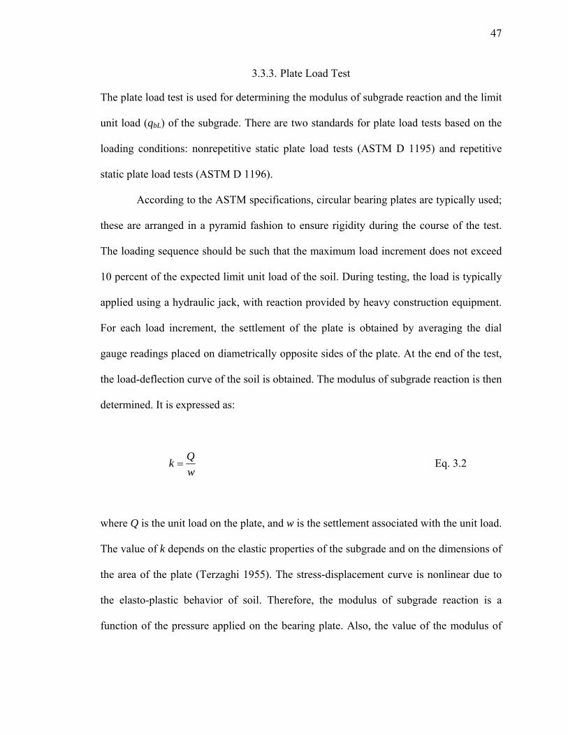
47

3.3.3. Plate Load Test

The plate load test is used for determining the modulus of subgrade reaction and the limit

unit load (qbL) of the subgrade. There are two standards for plate load tests based on the

loading conditions: nonrepetitive static plate load tests (ASTM D 1195) and repetitive

static plate load tests (ASTM D 1196).

According to the ASTM specifications, circular bearing plates are typically used;

these are arranged in a pyramid fashion to ensure rigidity during the course of the test.

The loading sequence should be such that the maximum load increment does not exceed

10 percent of the expected limit unit load of the soil. During testing, the load is typically

applied using a hydraulic jack, with reaction provided by heavy construction equipment.

For each load increment, the settlement of the plate is obtained by averaging the dial

gauge readings placed on diametrically opposite sides of the plate. At the end of the test,

the load-deflection curve of the soil is obtained. The modulus of subgrade reaction is then

determined. It is expressed as:

Qkw

= Eq. 3.2

where Q is the unit load on the plate, and w is the settlement associated with the unit load.

The value of k depends on the elastic properties of the subgrade and on the dimensions of

the area of the plate (Terzaghi 1955). The stress-displacement curve is nonlinear due to

the elasto-plastic behavior of soil. Therefore, the modulus of subgrade reaction is a

function of the pressure applied on the bearing plate. Also, the value of the modulus of

48

subgrade reaction depends on the size of the plate used for the test because the size

determines the mobilized mean confining stress that the soil below the plate experiences.

The larger the diameter of the plate, the greater is the depth to which the soil is stressed.

Terzaghi (1955) suggested typical values of the modulus of subgrade reaction for both

sands and clays determined using 30.4 cm by 30.4 cm square plates (refer to Tables 2.1

and 2.2). In sands, the modulus of subgrade reaction increases with depth.

Table 3.2 Modulus of subgrade reaction of sands (MN/m2/m)

Soil Characteristics Loose Medium Dense

Dry or Moist Sand 6-18 18-90 90-300

Submerged Sand 7.5 24 90

* These values are based on tests performed on 30.4cm×30.4cm square plates or beams 30.4cm wide. Values have been modified from Terzaghi (1955).

Table 3.3 Modulus of subgrade reaction for clays* (MN/m2/m)

Consistency of clay Stiff Very stiff Hard

Values of qu† (kPa) 96-192 192-383 > 383

Ranges for k 15-30 30-60 > 60

* These values are based on tests performed on 30.4cm×30.4cm square plates or beams 30.4cm wide. Values have been modified from Terzaghi (1955). † qu: unconfined compressive strength

A plate load test requires a reaction (e.g., a heavy truck) system to provide

reaction to the load increments applied on the plate. In addition, the test procedure is very

cumbersome and time consuming, requiring skilled personnel to conduct the test. Hence,

the plate load test is seldom used as a compaction quality control test.

49

3.3.4. Light Falling-Weight Deflectomter Test

The Light Weight Deflector (LWD) is a portable falling-weight deflectometer used to

measure the in situ elastic modulus (ELWD) of the compacted material. LWD is also

known as the Lightweight Falling Weight Deflector (LFWD) or as Portable-Falling-

Weight Deflectometer (PFWD).

The LWD is basically composed of a falling mass and a displacement-measuring

sensor attached at the center of a bearing plate (see Figure 3.2). The test is performed by

releasing the falling weight from a standard height onto the bearing plate using the top fix

and release mechanism. An impulse load is imparted on the compacted soil through the

plate. The resulting central deflection of the bearing plate is obtained either by

integrating the velocity measurements taken from a velocity transducer or by double

integrating the acceleration data taken from an accelerometer. A display shows the

central deflection and the ELWD, which is obtained from the elastic solution (Livneh and

Goldberg 2001; Alshibli et al. 2005; Lin et al 2006; Fleming et al 2007):

( )21− υ

=LWD Rqr

E fw

Eq. 3.3

where ELWD is the Young’s modulus of the subgrade (MPa); fR is the plate rigidity factor

(π/2 for a rigid plate), q is the maximum contact pressure (kPa), r is the radius of the

bearing plate (m), υ is the Poisson’s ratio of the soil, w is the peak deflection (mm),

which is obtained either by using a velocity sensor or an accelerometer.

50

In spite of the uncertainties associated with its application, some transportation

agencies have attempted to use the LWD as a compaction quality control method, mainly

due to its simplicity in operation (Lin et al. 2006; Nazzal et al. 2007).

(1)

(2)

(3)

(4)(5)

(6)

(7)(8)

(9) (9)

(1)

(2)

(3)

(4)(5)

(6)

(7)(8)

(9) (9)

(1) Grip(2) Top fix and release mechanism(3) Guide rod(4) Round grip(5) Falling weight (10kg)(6) Set of steel springs (buffer)(7) Measuring element that contains the sensor(8) Loading plate (diameter=30cm)(9) Carry grip

Figure 3.2 Schematic of LWD showing various component of the equipment (modified after Siddiki et al. 2008)

There are several different LWD models, depending on the manufacturer of the

device. The models differ in terms of the drop hammer weight, the height of fall, the size

of the bearing plate, the number of buffers available to dampen the impulse, the rate of

loading, the measuring sensor and the data acquisition. Regardless of the LWD model

used and the possible deformations in the measurements between the different models,

the data is used to estimate the elastic modulus of the soil.

51

Many studies in the literature have attempted to relate the elastic modulus ELWD to

the results of various other commonly used tests, such as the CBR test, the PLT, the

Geogauge, and the DCPT (Livneh and Goldberg 2001; Alshibli et al. 2005; Lin et al.

2006; Nazzal et al. 2007; Fleming et al. 2007; Kim et al. 2007).

Recently, the International Society for Soil Mechanics and Geotechnical

Engineering (ISSMGE 2005) established a specification for earthwork compaction QC

using LWD testing. In addition, the Minnesota Department of Transportation (MnDOT)

developed a pilot specification for the LWD. Table 3.4 shows the ISSMGE criteria for

compaction QC based on the Zorn-LWD modulus. The ELWD values correspond to the in

situ compacted dry unit weight values equal to or greater than 95% of the maximum dry

unit weight obtained with the Standard Proctor in the laboratory. A similar criterion was

also developed by the MnDOT Pilot Specification (Mooney et al. 2008).

Table 3.4 ISSMGE criteria for compaction QC based on the Zorn-LWD modulus

Level ELWD from Zorn LWD (MPa)

1m below subgrade 18 (cohesive) to 24 (cohesionless)

Top of subgrade 30 (cohesive) to 38 (cohesionless) Top of subbase layer 58 (rounded) to 68 (angular)

Top of base layer 70 (rounded) to 82 (angular)

Since the falling mass of the LWD induces both nonlinear elastic and plastic

deformation to the subgrade, the elastic modulus calculated with Eq. 3.3 may be in error.

To account for this shortcoming in LWD testing, some researchers have modeled the

subgrade soil as a combination of a linear spring and a damping material (Loizos et al.

52

2003). Due to the drawbacks discussed here, LWD testing has not yet gained popularity

among U.S. federal agencies as a compaction quality control method.

3.3.5. Soil Stiffness Gauge (SSG, Geogauge) Test

The soil stiffness gauge (SSG), also called the Geogauge, is a modified device that was

initially developed to locate buried land mines. With the consent of the U.S. Department

of Defense, the Federal Highway Administration (FHWA) in collaboration with

Humboldt Manufacturing Co., Bolt, Beranek & Newman (BBN), and CNA Consulting

Engineers, developed the Geogauge (Fiedler et al. 1998, see Figure 3.3).

The Geogauge measures the mechanical impedance of soil at the surface and

captures the force imparted to the soil along with the resulting surface deflection. The

Geogauge vibrates 25 times and induces displacements smaller than 1.27 × 10-6 m to the

ground at frequencies between 100 and 196 Hz (Geogauge manual 2007). In order to

analyze the test results, the developers of the Geogauge test employed the static elastic

solution that Poulos and Davis (1974) presented for computing the stiffness (k) of a

circular ring on a semi-infinite mass (Fiedler et al. 1998).

( )21 i

o

r Ekrr

=⎛ ⎞

− υ ω⎜ ⎟⎝ ⎠

Eq. 3.4

53

where E is the modulus of subgrade (MPa); ri/ro is the ratio of the radii of the Geogauge

ring (44.5mm / 57.15mm = 0.78); υ is the Poisson’s ratio.

Rubber

Electro-mechanicalshaker

Velocity Sensors

Process Control I/OTest Signal

Sensor signal processing

Foot

Rubber

Electro-mechanicalshaker

Velocity Sensors

Process Control I/OTest Signal

Sensor signal processing

Foot

Figure 3.3 Schematic of the Geogauge (modified after Alshibli et al 2005).

Since the static elastic solution, which is used for the interpretation of the test

results, does not account for the dynamic sequence of the test, the modulus computed

with Eq. 3.4 is not able to capture the dynamic sequence of the test. For example, the

Geogauge has several rubber isolators, which functions as a single degree of freedom

having specific spring and damping constants. Also, as shown in Figure 3.3, the foot

bears directly on the soil and supports the weight of the Geogauge dynamically against

the mechanical impedance of soil. Thus, in order to evaluate the soil compaction using

the test, it is necessary to account for the dynamic sequence of the test into the analysis.

54

3.3.6. Dynamic Cone Penetration Test

The Dynamic Cone Penetrometer (DCP) is a portable device that was first introduced by

Scala (1956) to assess the strength of subgrade. The DCP is a simple and easy-to-use

device that is widely used to measure the penetration resistance of in situ materials at

shallow depths.

0.3cm

57.5cm

Hammer 8kg (17.6lb)

100cm (Variable)

1.6cm

2.0cm

60°

Figure 3.4 Schematic of the Dynamic Cone Penetrometer (modified after ASTM D 6951-03).

The DCP consists of (1) an upper shaft that is rigidly connected to an 8kg (17.6lb)

drop hammer, (2) a lower shaft with an anvil at the top and a cone at the bottom, and (3) a

replaceable cone tip with an apex angle of 60 degrees and a diameter of 20mm (see

Figure 3.4). In order to perform a DCP test, the hammer is dropped from a standard fall

55

height. The energy transferred to the cone by the impact of the hammer on top of the

anvil enables penetration of the cone into the ground. A Dynamic Cone Penetration Index

(DCPI), expressed as the penetration per blow (mm/blow), is recorded as a function of

depth. Since the DCPI value corresponds to the penetration of the cone for only a very

small depth increment, little success has been achieved in correlating the DCPI with other

material properties (Salgado and Yoon 2003). Thus, the DCP blow count (NDCP), defined

as the number of blows required for a specified cone penetration [e.g., 0 to 150 mm (0 to

6 inch) or 0 to 300 mm (0 to 12 inch)] is often used instead.

In the last decade, several agencies, such as state DOTs and the U.S. Army Corp

of Engineers, have expressed interest in using the DCP for compaction QC (Amini 2003).

Table 3.5 shows the NDCP criteria corresponding to a depth of penetration equal to 0 to

150 mm (0 to 6 inch) according to several DOT agencies (note that the NDCP values

shown in the table were converted from DCPI values). The criteria proposed by the

Illinois and North Carolina DOTs are independent of the type of material, whereas the

Iowa and Minnesota DOTs proposed values for “frictional” and “cohesive” materials.

The values suggested by the Illinois and North Carolina DOTs correspond to a CBR =

8.0, which indicates a stable subgrade. The Iowa DOT DCP criteria are based on the

requirement that the compacted dry unit weight in situ should exceed 95% of the

laboratory compaction maximum dry unit weight.

56

Table 3.5 DCP criteria (NDCP) for a penetration of 0 to 150 mm (0 to 6 inch)

Agency

Materials

Illinois DOT (ILDOT) Iowa DOT

Minnesota DOT

(MnDOT)

North Carolina

DOT

“Frictional” soil

6.1a

3.4~4.4b 12.5c

4.0d “Cohesive” soil

Silt 3.8~4.4b 6.0c

Clay a DCP blow counts associated with a CBR of 8 (ILDOT 2005) b Iowa DOT classified the soil either “suitable soil” or “unsuitable soil” in each group of soil. The values show the ranges of it (Larsen et al. 2007) c The criteria of frictional soil apply for “granular” base layer; MnDOT recorded NDCP values only for blow counts that are higher than two (Burnham 1997) d DCP blow counts associated with a CBR of 8 (Gabr et al. 2000)

Most researchers have suggested criteria for the DCPT based only on the recorded

DCPI, without considering the impact of the increase in confining stresses with depth.

However, according to Jayawickrama et al. (2000), DCP blow counts at greater depths

are higher than those at shallow depths due to greater confinement. Also, other factors,

such as gradation and particle angularity, are typically not taken into account. Compared

to the other available compaction QC methods, This device has the potential of becoming

a useful testing method as an in situ compaction QC test method due to its simplicity and

quickness of operation.

3.3.7. Clegg Hammer Test

The Clegg Hammer Test (CHT) is an impact test device that was developed by Clegg

(1976) to evaluate the mechanical properties of compacted soil. Originally, Asai (1960)

developed an apparatus that had a dropping weight. The acceleration of the falling weight

was measured and correlated with the modulus of subgrade k determined by static plate

57

load tests. More sophisticated equipment, which were capable of measuring the

acceleration of the falling weight using two geophones, were also developed (Szendrei

and Freeme 1970).

Clegg (1976) realized that there was the need to develop simpler equipment for

compaction QC in situ. Clegg (1976) developed, in Australia, a test device for QC that

originally made use of a modified Proctor compaction hammer (hammer weight: 4.5kg

weight, and drop height: 0.45m) with an accelerometer attached at the top and encased in

a guide tube. Clegg (1976) also simplified the dynamic measuring technique by capturing

only the peak deceleration of the falling hammer, which was correlated to the stiffness or

the shear strength of the material at the location where the hammer was dropped. The

output of the CHT is displayed in terms of the Clegg Impact Value (CIV). One unit of

CIV is equal to 98.1m/s2, ten times the acceleration due to gravity. It is typically

determined after four hammer drops at a given test location.

Currently, five different CHT models are available on the market; the original

model developed by Clegg (1976) uses a modified compaction hammer. These models

have varying hammer weights and drop heights. The lighter ones are typically used for

evaluating relatively soft materials such as recreational turf and the playing ground for

baseball, while the heavier models are used for evaluating stiff materials, such as

compacted soil and base course material (Clegg 1983; Canaway et al. 1990; Rogers and

Waddington 1990; Erchul 1999). Figure 3.5 shows the 10kg CHT that was used in this

research.

58

Table 3.6 Various Clegg Hammer Test product configurations (Lafayette Instrument Co., 2009)

Product Model No. Drop weight (kg)

Drop height (m)

Diameter of the hammer

(m)

20kg CHT 95056A 20 0.30 0.13

10kg CHT 95055A 10 0.30 0.13

4.5kg CHT 95050A 4.5 0.45 0.05

2.25kg CHT 95049A 2.25 0.45 0.05

0.5kg CHT 95048A 0.5 0.45 0.05

Figure 3.5 Photograph of Clegg Hammer Test (hammer weight, 10kg).

Several research studies were carried out to correlate the CIV and the mechanical

properties of pavement materials. Since Clegg (1978, 1980) proposed that the CHT can

59

be used as an alternative to the CBR, several research studies have proposed relationships

between the CIV and the CBR (Yoder et al. 1982; Garrick and Scholer 1985; Mathur and

Coghlans 1987; Al-Amoudi et al. 2002). Table 3.7 is a summary of the correlations

developed between the CBR and the CIV. Janoo et al. (1999) investigated the use of the

CHT for evaluating the compressive strength of treated subgrade. Similarly, Guthrie and

Reese (2008) utilized the CHT for specifying a setting time for cement-treated base

material.

Table 3.7 Summary of the correlations between CBR and CIV*

Research Test condition /Material tested Correlation equation

Clegg (1980, 1983) In situ /Base course ( )20.072=CBR CIV

Mathur and Coghlans (1987) ( )1.8630.1085=CBR CIV

Al-Amoudi et al. (2002) Lab & In situ ( )1.6950.1691=CBR CIV

* These correlations were developed using 4.5kg CHT

Recently, the Gas Technology Institute (GTI 2005 and 2006) investigated the use

of the CHT as a quality control test to determine soil compaction parameters such as

compacted dry unit weight and moisture content. Table 3.8 shows the range of the CIV

for various soil types.

60

Table 3.8 CIVs corresponding to 90% RC at optimum moisture content (modified after GTI 2005)

CIV Sand (A-2*) Silty-clay (A-6*) Stone-base (A-1*)

10kg CHT 6-8 8-12 12-14

However, all the correlations proposed in the literature are empirical in nature.

These relationships should be used with caution as the CIV has been correlated with

properties that reflect the static response of the material, such as the CBR. As the CHT is

dynamic in nature, research needs to be done in order to relate the CIV with mechanical

properties that reflect the dynamic response of the material.

3.3.8. Continuous Compaction Control Test

The existing compaction quality control tests are completed by checking the compacted

in situ dry unit weight (γdfield) for a specified lift thickness, number of compactor passes,

and range of moisture content (wc). However, all the methods discussed in the previous

two sections of this chapter are performed at specific test locations at the construction site

and, hence, are based on spot checking.

In order to overcome the limitation of spot-checking tests, continuous compaction

control (CCC) was developed almost 30 years ago in Europe (Forssblad 1980; Thurner

and Sandström 1980). The basic principle of CCC is to make use of compaction rollers

that have a machine-integrated accelerometer that is used to record compaction roller-

ground interaction against the compaction energy. Using global positioning system (GPS)

along with the geographic information system (GIS), compaction roller-based

61

measurement of the soil response provides real-time data over the entire compacted area

(Rinehart and Mooney 2009). The recorded data reflect the dynamic ground stiffness or

strength, which indicates the compaction level achieved in the field.

In the last two decades, several manufacturers have developed compaction rollers

that can be used for CCC. Most of the companies install accelerometers in the drum of

the roller and use machine energy to compute the mechanical properties of the compacted

material (Camargo et al. 2007). Figure 3.6 shows one example of the compacter

manufactured by Geodynamik Co. The compactor in the figure is equipped with

compaction monitoring system components.

Figure 3.6 Geodynamik compactor equipped with monitoring system components (modified after Sandström and Pettersson 2004).

62

The main advantage of CCC is that the instrumented compactor enables field

personnel to perform real-time compaction QC. The QC checks are displayed on a

computer screen in the cab of the compactor (see Figure 3.7). With recent advances in

Global Positioning System (GPS) and Geographic Information System (GIS), many

researchers have been actively involved in developing CCC (White et al. 2004; Rahman

et al. 2008; White and Thompson 2008; Rinehart and Mooney 2009).

Figure 3.7 Smooth drum compaction monitoring systems for soil (White 2008).

However, in practice, there are currently several problems that need to be

addressed before CCC can be adopted as a quality control technique. First, there are no

standard parameters for CCC. Instead, there are more than six different CCC parameters

depending on the equipment manufacturer, as each has individually developed CCC to fit

their own model of the compactor (see Figure 3.7). Second, even though U.S.

transportation agencies are beginning to investigate the applications for CCC in

conjunction with field demonstration projects, only a few projects have been completed

63

and no widely accepted specifications are available in the U.S. (White et al., 2007).

Third, since CCC generates data for quality control of compaction over the entire project

area at every stage of the compaction process, the data files are too large to be easily

managed with state-of-the-art electronic technology. Thus, the development of related

technology is necessary for adopting CCC in practice. Finally, most practitioners are still

unfamiliar with CCC technology.

3.4. Specifications for Quality Control of Subgrade Compaction

A specification is defined as an explicit set of detailed statements prescribing materials,

dimensions, and quality of work for something to be built, installed, or manufactured

(American Heritage Dictionary 2001). Therefore, specifications for subgrade compaction

should detail all necessary requirements. In addition, specifications should be both

practical and reasonable so that construction is as economical as possible (both in terms

of cost and time). For example, if unrealistic levels of compaction are required,

contractors might not be able to satisfy such a specification requirement.

In the specification for compaction of soils in the field, there are typically three

items involved: (1) method specification; (2) end-product specification; and (3)

performance specification (TRB 2009)

In a method specification, the work procedure is detailed. It includes the

compactor type, mass, and travel speed, as well as the number of compactor passes. In

addition, the type of soil, molding water content, and lift thickness is described. In this

type of specification, the work procedure must be inspected to guarantee the quality of

64

compaction. Experience has shown, however, that this specification tends to obligate the

agency to accept the completed work regardless of quality (TRB 2009).

With an end-product specification, agencies specify the required values for the

dry unit weight and water content of the compacted soil. Agencies typically specify the

required relative compaction to be achieved in situ. In this specification, density-based

compaction control tests should be performed to ensure the quality of compaction. End-

product specifications allow contractors to choose techniques and work procedures to

improve the quality or economy, or both, of the compacted soil (TRB 2009).

A performance specification defines the performance characteristics of the final

product and links them to construction, materials, and other items under contractor

control (FHWA 2009). The performance of the compacted soil can be checked by in situ

tests. Performance is described in this specification by means of changes in physical

condition of compacted subgrade and its response to the load (TRB 2009). Since our final

goal is to have compacted soil that meets the performance requirements, this specification

is most appropriate to evaluate performance of the end product over time.

From these three categories of specifications for earthwork, which one is widely

adopted by agencies and how does it work? Wahls (1967) reviewed highway

specifications and showed that most U.S. DOT agencies relied on the end-product type of

specification, with density requirement checks. However, the specifications of several

states also included method requirements, such as the maximum lift thickness. Almost

half of the states employed 95% relative compaction (RC) as a requirement, while some

states specified either 100% or 90%. Wahls (1967) indicated that these variations in

65

density requirements resulted from engineering judgment and experience with local

construction practices rather than from theoretical considerations.

At present, most agencies adopt end-product specifications along with method

specifications, as shown in Table 3.9. The specifications of various agencies in the U.S.

indicate that most states follow the 95% RC specification for density requirement. Also,

water content is specified at about -2 to +2% of the optimum moisture content on average

before compaction. Some agencies have a slightly higher or lower RC requirement. In

general, 95% RC with an acceptable range for the soil moisture content (about -2 to +2%

of the optimum moisture content) is widely accepted as a criterion for soil compaction.

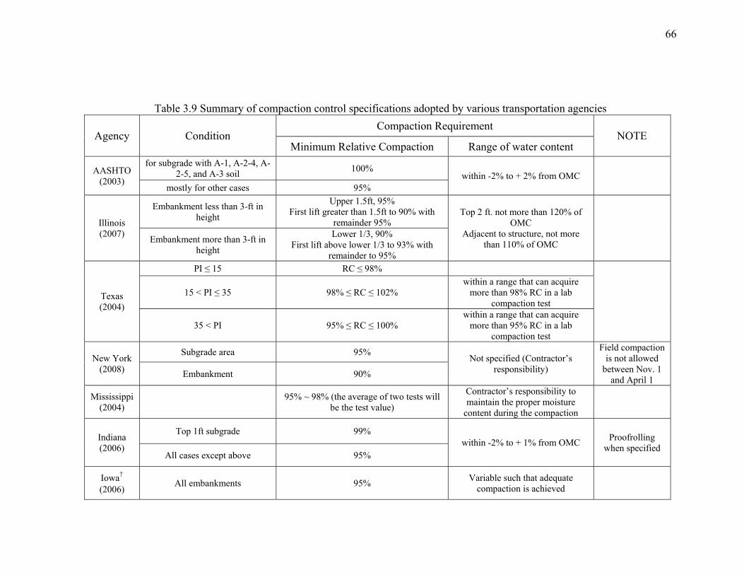
66

Table 3.9 Summary of compaction control specifications adopted by various transportation agencies

Agency Condition Compaction Requirement

NOTE Minimum Relative Compaction Range of water content

AASHTO (2003)

for subgrade with A-1, A-2-4, A-2-5, and A-3 soil 100%

within -2% to + 2% from OMC mostly for other cases 95%

Illinois (2007)

Embankment less than 3-ft in height

Upper 1.5ft, 95% First lift greater than 1.5ft to 90% with

remainder 95% Top 2 ft. not more than 120% of

OMC Adjacent to structure, not more

than 110% of OMC

Embankment more than 3-ft in

height

Lower 1/3, 90% First lift above lower 1/3 to 93% with

remainder to 95%

Texas (2004)

PI ≤ 15 RC ≤ 98%

15 < PI ≤ 35 98% ≤ RC ≤ 102%

within a range that can acquire more than 98% RC in a lab

compaction test

35 < PI 95% ≤ RC ≤ 100% within a range that can acquire

more than 95% RC in a lab compaction test

New York (2008)

Subgrade area 95% Not specified (Contractor’s

responsibility)

Field compaction is not allowed

between Nov. 1 and April 1 Embankment 90%

Mississippi (2004) 95% ~ 98% (the average of two tests will

be the test value)

Contractor’s responsibility to maintain the proper moisture

content during the compaction

Indiana (2006)

Top 1ft subgrade 99% within -2% to + 1% from OMC Proofrolling

when specified All cases except above 95%

Iowa† (2006) All embankments 95% Variable such that adequate

compaction is achieved

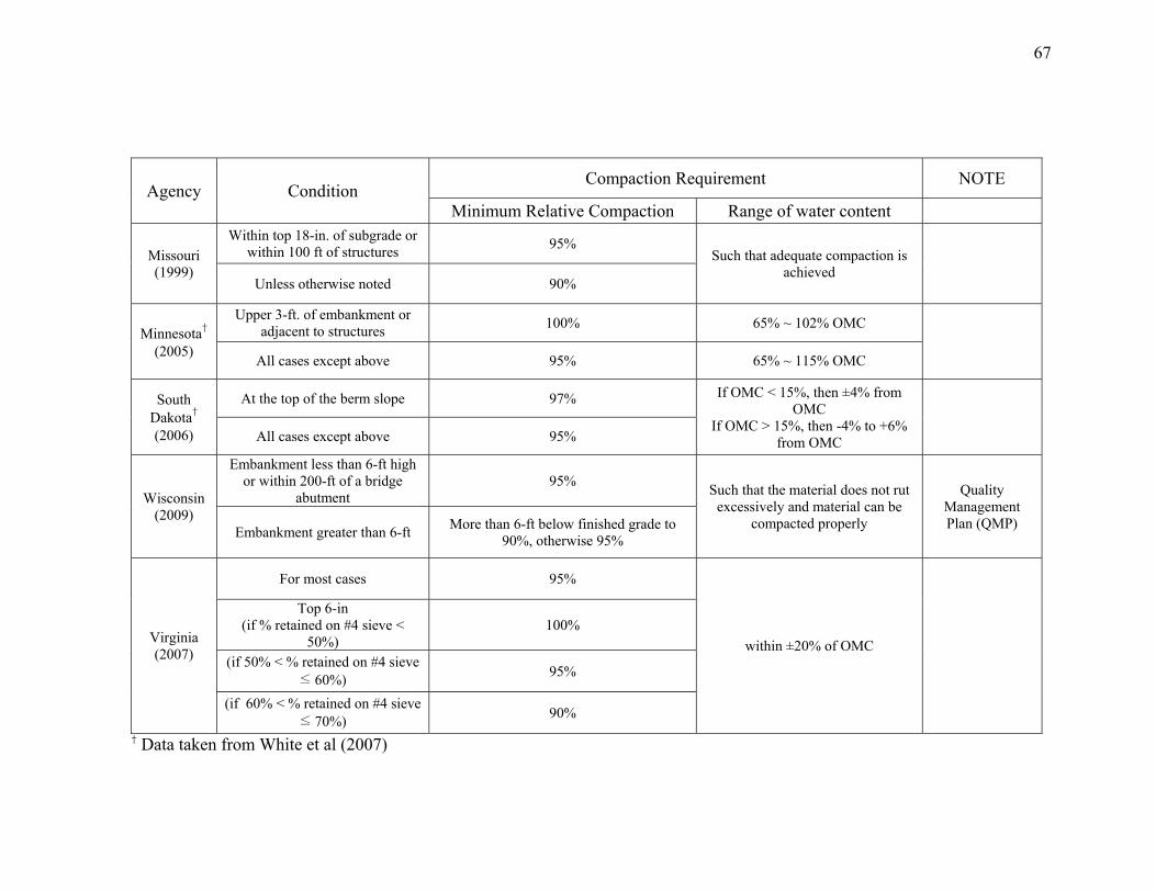
67

Agency Condition Compaction Requirement NOTE

Minimum Relative Compaction Range of water content

Missouri (1999)

Within top 18-in. of subgrade or within 100 ft of structures 95%

Such that adequate compaction is achieved

Unless otherwise noted 90%

Minnesota† (2005)

Upper 3-ft. of embankment or adjacent to structures 100% 65% ~ 102% OMC

All cases except above 95% 65% ~ 115% OMC

South Dakota† (2006)

At the top of the berm slope 97% If OMC < 15%, then ±4% from OMC

If OMC > 15%, then -4% to +6% from OMC

All cases except above 95%

Wisconsin (2009)

Embankment less than 6-ft high or within 200-ft of a bridge

abutment 95% Such that the material does not rut

excessively and material can be compacted properly

Quality Management Plan (QMP) Embankment greater than 6-ft More than 6-ft below finished grade to

90%, otherwise 95%

Virginia (2007)

For most cases 95%

within ±20% of OMC

Top 6-in (if % retained on #4 sieve <

50%) 100%

(if 50% < % retained on #4 sieve ≤ 60%) 95%

(if 60% < % retained on #4 sieve ≤ 70%) 90%

† Data taken from White et al (2007)

68

3.5. Summary

Quality Control (QC) of soil compaction typically involves determining the in-place

compacted dry unit weight (γdfield) and the water content (wc) of a compacted lift of fill

material and comparing the measured γdfield and wc with the laboratory compaction test

results. In order to measure the in situ dry unit weight and water content, most agencies

employ the nuclear gauge for field compaction QC because sand cone tests are

cumbersome and time consuming to perform. However, since the measurement of the

compacted dry unit weight of soil is an indirect means to assess the mechanical response

of subgrade, road engineers have attempted to devise testers that be used to assess the

mechanical properties of the compacted subgrade related to its in situ strength or

stiffness. The California Bearing Ratio test and the Plate bearing test were used for this

purpose, but these tests have been abandoned for QC testing due to their shortcomings.

Currently, there are some testers that have been developed for measuring the stiffness or

strength of subgrade: (1) the Clegg Hammer Test (CHT), (2) the Soil Stiffness Gauge

(SSG) test, and (3) the Light Falling-Weight Deflectometer (LFWD) test. These testers

have the potential to capture the dynamic response of compacted soil, although the

present analytical solutions for the tests do not account for the dynamic loading. For

greater depth, the Dynamic Cone Penetration test is used to measure the dynamic in situ

penetration resistance as a function of depth. The test result is in the form of dynamic

blow counts or penetration rates that are correlated with both the stiffness and the

strength parameters of subgrade. However, most researchers have suggested the criteria

69

for the DCPT using the DCPI alone without considering the confining effect. Also, the

other factors such as gradation and particle angularity exist that have not been accounted

for. As a result, the device will be a useful and versatile field quality control device once

a reasonable criterion is established.

All of the above, however, are spot tests and can only cover a very small portion

of the fill volume. The Continuous Compaction Control (CCC) technique is under

development to evaluate the quality of the compaction over the entire volume of

compacted soil, but it needs to be improved for practical use.

Typical specifications for field compaction indicate the type of laboratory

compaction tests to be used as a reference and specify the percentage of the reference

laboratory compaction test results that will be required in the field. Specifications for the

molding water content should also fall within a certain range of the OMC. In general, the

specification for density control (i.e. 95% relative compaction) has effectively functioned

for more than 30 years and therefore should ensure the performance of compacted soil.

70

CHAPTER 4. COMPACTION VARIABILITY OF SOIL

4.1. Introduction

Every construction material has variations in its composition and properties.

Geomaterials are more variable than other man-made materials that are used in the

construction industry, such as concrete and steel. When soils are compacted in-place, the

variability associated with compaction can be quite significant, even with

“homogeneous” soils (Yoder and Witczak 1975). Then, what is the source of this

variability in soil compaction? And why is compaction variability of soil important?

In the case of soil compaction, variability can be mainly classified as (1) spatial

variability, and (2) variability associated with the technique of measurement. First, even

areas compacted at few meters apart may exhibit variability. Second, every measurement

is bound to have some level of randomness. This randomness is caused by the testing

method itself and/or the person performing the test. Figure 4.1 illustrates how relative

compaction varies in space.

71

Relative Compaction (%)

Distance

DistanceRelative Compaction (%)

Distance

Distance

Figure 4.1 Variability in the compaction level achieved along an embankment.

Why is compaction variability important? For proper performance of a pavement

structure constructed over the subgrade, uniform compaction of the subgrade soil should

be achieved in the field (refer to CHAPTER 2). Nonuniformities of the subgrades may

induce local and permanent deformations, such as bumps, corrugations, and depressions

on the pavement surface. In addition, since compaction quality control test results are

subject to variance due to compaction variability, specification limits used for

compaction quality control are appropriate when they relate to a measure of the

variability in compacted soil (Hughes 1996), though the specifications of many

transportation agencies indicate a specific value for the quality control of soil compaction.

In this chapter, we will discuss the sources of soil variability, focusing on

compaction variability, and will review the literature pertinent to the typical variability

associated with compacted soil. The chapter then will present how to account for

compaction variability in determining the specification limits for soil compaction.

72

4.2. Basic Statistical Concepts

In order to quantify variability in soil, some basic statistical concepts need to be

understood. Figure 4.2 shows a normally distributed frequency curve that is obtained by

plotting the frequency histogram of n sampling units from a sample in the conceptual

population. The conceptual population is a complete set of all the values that is

impossible to measure (Devore 2004). A sample is a set of values that is a subset (a

portion) of the population. Sampling units are the values in a sample determined by

collecting information from a sample. A statistical distribution can be described in terms

of mean and variance, standard deviation, or coefficient of variation.

In the statistical distribution shown in Figure 4.2, the mean identifies the weighted

average of the values in the sampling units. The mean can be expressed as:

ni

i 1x

n=∑

μ = Eq. 4.1

where μ is the mean of the sampling units, n is the number of sampling units, and xi is the

value of the sample at i.

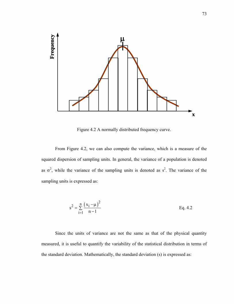
73

μ

Freq

uenc

y

x

μ

Freq

uenc

y

x

Figure 4.2 A normally distributed frequency curve.

From Figure 4.2, we can also compute the variance, which is a measure of the

squared dispersion of sampling units. In general, the variance of a population is denoted

as σ2, while the variance of the sampling units is denoted as s2. The variance of the

sampling units is expressed as:

( )2n i2

i 1

xs

n 1=

− μ= ∑

− Eq. 4.2

Since the units of variance are not the same as that of the physical quantity

measured, it is useful to quantify the variability of the statistical distribution in terms of

the standard deviation. Mathematically, the standard deviation (s) is expressed as:

74

( )2n i

i 1

xs

n 1=

− μ= ∑

− Eq. 4.3

A parameter used as a relative measure of variability is the coefficient of variation

(COV). The COV is expressed as:

( ) sCOV % 100⎛ ⎞= ×⎜ ⎟μ⎝ ⎠

Eq. 4.4

Since COV is dimensionless, it is useful for comparing the variability among

different measurements.

4.3. Sources of Compaction Variability

In order to quantify the variation of in-place soil compaction, it is necessary to identify

the sources of variability that are observed in compacted soil. There are three principal

sources contributing to variability in soil compaction:

(1) Spatial Variability of Compacted Soil

Natural soil may vary to some extent with space. In a natural soil deposit, spatial

variability results primarily from the natural geologic processes that lead to soil formation

and that continually modify the in situ soil characteristics (Phoon and Kulhawy 1996).

Although the variability of compacted soil is typically less than the variability of nature,

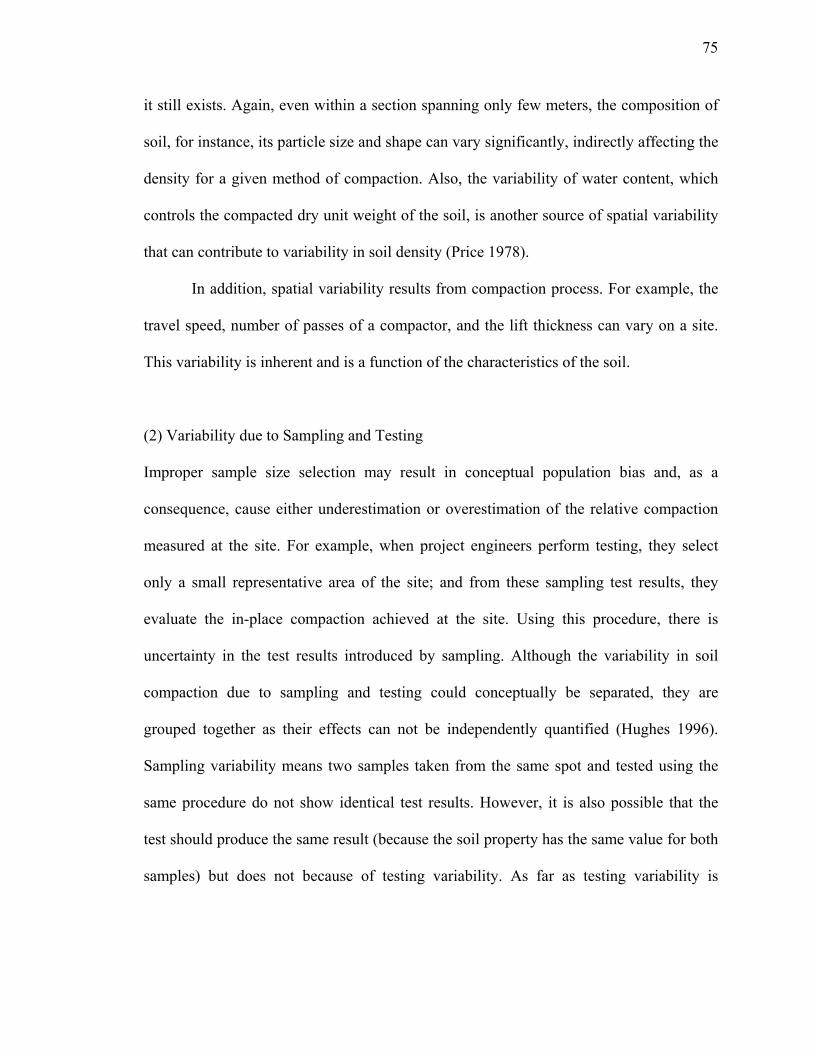
75

it still exists. Again, even within a section spanning only few meters, the composition of

soil, for instance, its particle size and shape can vary significantly, indirectly affecting the

density for a given method of compaction. Also, the variability of water content, which

controls the compacted dry unit weight of the soil, is another source of spatial variability

that can contribute to variability in soil density (Price 1978).

In addition, spatial variability results from compaction process. For example, the

travel speed, number of passes of a compactor, and the lift thickness can vary on a site.

This variability is inherent and is a function of the characteristics of the soil.

(2) Variability due to Sampling and Testing

Improper sample size selection may result in conceptual population bias and, as a

consequence, cause either underestimation or overestimation of the relative compaction

measured at the site. For example, when project engineers perform testing, they select

only a small representative area of the site; and from these sampling test results, they

evaluate the in-place compaction achieved at the site. Using this procedure, there is

uncertainty in the test results introduced by sampling. Although the variability in soil

compaction due to sampling and testing could conceptually be separated, they are

grouped together as their effects can not be independently quantified (Hughes 1996).

Sampling variability means two samples taken from the same spot and tested using the

same procedure do not show identical test results. However, it is also possible that the

test should produce the same result (because the soil property has the same value for both

samples) but does not because of testing variability. As far as testing variability is

76

concerned, the proficiency of the test operators, the test apparatus, and the test procedures

influence the variability to a great extent.

(3) Variability in the Results of Laboratory and Field Compaction Tests

This source of variability is unique to soil compaction. As presented in the previous

chapter, we know that relative compaction is defined as the ratio of the in-place dry unit

weight of soil to the maximum dry unit weight of soil obtained from the laboratory

compaction test. However, the question arises as to how closely laboratory compaction

tests can simulate actual field compaction. In the laboratory, the size of the standard mold

is only 4.5 in. (11.43 cm) in diameter and 4.6 in. (11.68 cm) in height (ASTM D 698).

Also, the energy imparted by the compaction hammer in the laboratory is different from

the energy that is produced by the field compaction equipment. Moreover, at a given site,

the number of laboratory compaction tests performed is limited. This means that when

calculating relative compaction values, we use a maximum dry unit weight value

obtained from a limited number of maximum dry unit weights taken from a small number

of laboratory compaction tests. For example, slightly different soils are grouped together

and regarded as the same soil when computing the relative compaction values.

To summarize, compaction variability results from the different soil composition

and variability in the compaction process. When attempting to estimate this variability

using tests, the estimates get distorted and magnified by variability due to sampling and

testing.

77

Liu and Thompson (1966) studied the variability in laboratory soil tests using

their laboratory test results along with the data available in Shook and Fang (1961),

Ballard and Weeks (1963), and Liu and Thornburn (1964). The laboratory soil tests

considered by Liu and Thompson (1966) included Atterberg limit tests (liquid limit and

plastic limit), laboratory compaction tests, and specific gravity tests. Table 4.1 is a

summary of the laboratory tests performed. The table shows the variation observed in the

test results based on three studies (Case A, Case B, and Case C). In order to investigate

the effect of sources of variability to the test results, the laboratory tests were performed

with the following three conditions:

1) Two technicians performed ten tests per person on three different types of soils

[A-6 (8), A-6 (9), and A-7-6 (15)] in a single laboratory using the same apparatus (Case

A, refer to Table 4.1)

2) Five technicians performed a single test per person on nine different types of

soils within a single laboratory using the same apparatus (Case B, refer to Table 4.1)

3) 99 laboratories performed a single set of tests per laboratory on three different

type of soils (Case C, refer to Table 4.1).

. Table 4.1 illustrates that the standard deviation of Case C is significantly larger

than the others. Also, the variability of the plasticity index between testers performing

tests in a given laboratory did not exceed a standard deviation of 2.54 (see Case B in

Table 4.1). Table 4.1 indicates that the standard deviation associated with the maximum

dry density was less than three pcf (0.47 kN/m3). The optimum moisture content showed

variation similar to those of the Atterberg limits. The variability in the specific gravity

test results appeared to be less.

78

Table 4.1 Variability of laboratory test (data from Liu and Thompson 1966)

Test property

No. of

soils

No. of operators per Lab

No. of Tests per operators

No. of

labs

s COV (%)

Average Range Average Range

Case A

LL (%) 3 2 10 1 0.70 0.56-0.85 2.0 1.5-2.5

PL (%) 3 2 10 1 0.72 0.64-0.88 3.6 3.0-4.0

PI (%) 3 2 10 1 0.84 0.64-0.99 6.0 3.7-8.7

Case B

LL (%) 9 5 1 1 1.10 0.44-2.14 4.0 1.7-7.7

PL (%) 9 5 1 1 1.03 0.37-2.20 6.5 2.3-13.2

PI (%) 9 5 1 1 1.53 0.94-2.54 14.6 6.7-33.8

Case C

LL (%) 3 1 1 99 3.20 1.7-5.4 7.8 6.2-9.9

PL (%) 3 1 1 99 2.80 2.1-3.5 12.3 9.1-15.5

PI (%) 3 1 1 99 3.90 2.4-5.7 43.5 17.8-78.0

γdmax (pcf)* 3 1 1 99 2.31 1.93-2.54 2.2 1.8-2.5

** 3 1 1 99 2.62 2.10-2.90 2.3 1.9-2.5

wcopt (%)* 3 1 1 99 1.70 1.10-2.67 9.3 7.0-12.9

** 3 1 1 99 1.24 0.83-1.96 8.6 6.3-12.9

Gs 3 1 1 65 0.07 0.06-0.12 2.9 2.0-4.4

Note: *standard Proctor test **modified Proctor test

79

With respect to the variability in relative compaction, Table 4.2 summarizes the

data compiled from the literature on the variability in the level of compaction of various

soil types tested. The variability in the statistical distribution of relative compaction

values depends on the moisture control, the uniformity in the compaction effort, the

variation observed in a given soil type, and the capacity of soil to be affected by the

compaction effort (Sherman et al. 1967). It is interesting to note that the mean values of

relative compaction (RC) presented in Table 4.2 were on average two to three percent

greater than the required relative compaction. Also, even with two to three percent higher

mean values than the required RC, about 10% up to 38% of the sample units did not

achieve the required RC as shown in Table 4.2.

The relative compaction data available in the literature is normally distributed.

Note that considerable scatter of RC values can exist, particularly in sandy soils (the data

for sandy soils are more scattered than those of silty-clay soils). The COVs of RC values

depends primarily on the type of soil. However, no strong correlation between the COVs

and the required RC was observed in Table 4.2. For example, COV ranged between 0.034

and 0.059 in case of 95% RC requirement and between 0.026 and 0.059 in case of 90%

RC requirement, except one case with 0.073.

Since considerable scatter of relative compaction values exists in subgrade

compaction, there is the need of performing field tests frequently to assess the quality of

subgrade compaction. This is another reason why quality control tests should be quick

and easy to perform.

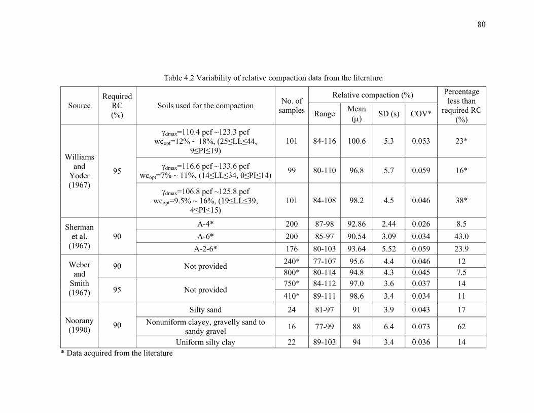
80

Table 4.2 Variability of relative compaction data from the literature

Source Required

RC (%)

Soils used for the compaction No. of samples

Relative compaction (%) Percentage less than

required RC (%)

Range Mean (μ) SD (s) COV*

Williams and

Yoder (1967)

95

γdmax=110.4 pcf ~123.3 pcf wcopt=12% ~ 18%, (25≤LL≤44,

9≤PI≤19) 101 84-116 100.6 5.3 0.053 23*

γdmax=116.6 pcf ~133.6 pcf wcopt=7% ~ 11%, (14≤LL≤34, 0≤PI≤14) 99 80-110 96.8 5.7 0.059 16*

γdmax=106.8 pcf ~125.8 pcf wcopt=9.5% ~ 16%, (19≤LL≤39,

4≤PI≤15) 101 84-108 98.2 4.5 0.046 38*

Sherman et al.

(1967) 90

A-4* 200 87-98 92.86 2.44 0.026 8.5 A-6* 200 85-97 90.54 3.09 0.034 43.0

A-2-6* 176 80-103 93.64 5.52 0.059 23.9

Weber and

Smith (1967)

90 Not provided 240* 77-107 95.6 4.4 0.046 12 800* 80-114 94.8 4.3 0.045 7.5

95 Not provided 750* 84-112 97.0 3.6 0.037 14 410* 89-111 98.6 3.4 0.034 11

Noorany (1990) 90

Silty sand 24 81-97 91 3.9 0.043 17 Nonuniform clayey, gravelly sand to

sandy gravel 16 77-99 88 6.4 0.073 62

Uniform silty clay 22 89-103 94 3.4 0.036 14 * Data acquired from the literature

81

4.4. Accounting for Compaction Variability in Determining the Specification Limits

In the previous section, we saw that several factors can lead to variability in soil

compaction. This variability should be accounted for while establishing the specification

criterion for soil compaction. For example, if the specification requirement is to obtain an

in-place compacted dry unit weight corresponding to 95% RC, this value should have

high probability of occurrence. Table 4.2 suggests that a mean RC value of roughly three

percent higher than the required RC needs to be achieved in order to obtain the required

RC in most of the compacted area.

In order to utilize in situ tests for a compaction QC, the criteria using the tests

need to account for compaction variability. In this regard, the following statistical

approach can be adopted. First, a minimum value of the test measurement that

encompasses at least a certain percentage (e.g., 80%) of occurrences in the frequency

diagrams of test results associated with the required RC is first selected (see Figure 4.3).

In the second step, the minimum value of the test measurement is tested for test results

less than the minimum required value. The test here is that the most of test measurements,

e.g.,90% of test measurements, corresponding to less than the required RC must be less

than the selected minimum value.

In the case of the DCPT, the blow count satisfying both requirements will be

referred to as the minimum required blow count. It provides reasonable assurance that, if

the measured blow count matches or exceeds it, the desired relative compaction will have

been achieved.

82

μR N

Freq

uenc

y of

test

res

ults

Test results

μR-i : Mean value of test results corresponding to less than the required RCμR : Mean value of test results at the required RCN : Minimum required value encompassing the majority of the test results

obtained at the required RC

μR-i

Frequency diagram of test results corresponding to the required RC

Frequency diagram of test results corresponding to less than required RC

μR N

Freq

uenc

y of

test

res

ults

Test results

μR-i : Mean value of test results corresponding to less than the required RCμR : Mean value of test results at the required RCN : Minimum required value encompassing the majority of the test results

obtained at the required RC

μR-i

Frequency diagram of test results corresponding to the required RC

Frequency diagram of test results corresponding to less than required RC

Figure 4.3 Conceptual frequency diagram of in situ test results.

83

4.5. Summary

When soils are compacted in-place, the variability associated with compaction can be

quite significant (Yoder and Witczak 1975). For proper performance of a pavement

structure constructed over a subgrade, uniform compaction of the subgrade soil should be

targeted in the field

In order to quantify variability in soil, some basic statistical concepts need to be

understood, such as mean, variance, standard deviation, and covariance (COV). Mean

identifies the weighted average of the values in the sampling units and can be expressed

as:

ni

i 1x

n=∑

μ = Eq. 4.1

where μ is the mean of the sampling units, n is the number of sampling units, and xi is the

value of the sample at i. Variance (s2) is a measure of the squared dispersion of sampling

units and is expressed as:

( )2n i2

i 1

xs

n 1=

− μ= ∑

− Eq. 4.2

The standard deviation is (s) is the square root of the variance.

84

A parameter used as a relative measure of variability is the coefficient of variation

(COV). Since COV is dimensionless, it is useful for comparing the variability among

different measurements. The COV is expressed as:

( ) sCOV % 100⎛ ⎞= ×⎜ ⎟μ⎝ ⎠

Eq. 4.4

Compaction variability results from the different soil composition and variability

in the compaction process. When attempting to estimate this variability using tests, the

estimates get distorted and magnified by variability due to sampling and testing.

Liu and Thompson (1966) showed that the variability of laboratory test results in

different laboratories was significantly larger than the variability for a single tester and

for two testers in a single laboratory. They also indicated that a careful tester was able to

reproduce the Atterberg limits according to the standard procedure with a standard

deviation of less than 1.0 and a coefficient of variation (COV) of less than 10 percent.

With respect to the variability of relative compaction on site, the mean values of

RC presented in several references were roughly two to three percent greater than the

specification requirements. Also, even the cases with two to three percent higher mean

values than the required RC, about 10% up to 38% of the sample units did not achieve the

required RC.

The relative compaction data available in the literature is normally distributed.

Note that considerable scatter of RC values can exist, particularly in sandy soils (the data

for sandy soils are more scattered than those of silty-clay soils). Thus, the COVs of the

85

RC values primarily depend on the type of soil. However, no strong correlation between

the COVs and the required RC was observed in the literature available.

When utilizing in situ tests for a compaction QC, the criteria using the tests need

to account for compaction variability. In this regard, a statistical approach can be adopted.

First, a minimum value of the test measurement that encompasses at least a certain

percentage of occurrences in the frequency diagrams of test results associated with the

required RC is first selected. In the second step, the minimum required value of the test

measurement is tested for test results less than the minimum required value. The test here

is that the most of test measurements corresponding to less than the required RC must be

less than the selected value. In the case of the DCPT, the blow count satisfying both

requirements will be referred to as the minimum required blow count. It provides

reasonable assurance that, if the measured blow count matches or exceeds it, the desired

relative compaction will have been achieved.

86

CHAPTER 5. ASSESSMENT OF DYNAMIC ANALYSIS

5.1. Introduction

When a dynamic in situ test such as dynamic cone penetrometer and Clegg Hammer are

performed on a site, the measurements made during the test reflect dynamic interaction of

the apparatus with the soil. If a load is applied very slowly on soil through in situ device,

no rate effects occur and the total resistance is equal to the static resistance. Rate effects

appear when the load is quickly applied to the soil. Dynamic resistance then mobilizes.

Thus, the total resistance R mobilized at the interface of the device with the soil consists

of a static component Rs and a dynamic component Rd (Salgado 2008):

s dR R R= + Eq. 5.1

The chapter starts by examining the static resistance. It then discusses dynamic

resistance. Methods for interpreting the results of two in situ dynamic tests, the Dynamic

Cone Penetration Test (DCPT) and the Clegg Hammer Test (CHT), are then presented,

including the dynamic models selected to analyze.

87

5.2. Soil Response under Static Loading

5.2.1. Background

The static soil response of in situ tests is represented by its bearing capacity. When we

determine the bearing capacity for the footing design, e.g., piling engineering, the most

widely used criterion is the ultimate bearing capacity at which the footing settlement is

about 10% of the pile diameter, denoted as qb,10% (Salgado 2008). However, the bearing

capacity considered here, for the dynamic analysis, is the limit-state bearing capacity,

denoted as qbL. The limit-state bearing capacity is the bearing capacity that is fully

mobilized resistance of the soil against the external forces when the soil below and

nearby the footing experiences overall failure. Since its limit bearing capacity is strongly

correlated with the shear strength of the soil, it is important to obtain the accurate shear

strength of the soil to precisely estimate the limit bearing capacity. With respect to the

shear strength of soil, the shear strength of sands is different from that of clays due to the

differences in their nature.

In addition, depending on the type of in situ tests, the bearing capacity is

differently addressed. In case of the Clegg Hammer test, since the load is transferred to

the soil surface, the bearing capacity of the Clegg Hammer is estimated using the bearing

capacity equations for shallow foundations. In case of the dynamic cone penetrometer,

the bearing capacity equations for deep foundations can be used for estimating the

bearing capacity of the dynamic cone penetrometer.

88

5.2.2. Shear Strength of Sands

Several factors determine the shear strength of sands: soil state variables (relative density

and confinement) the nature and characteristics of the soil particles, and environmental

factors (Salgado 2008). Once the intrinsic soil variables are determined according to the

nature of the sand, the shear strength of sands is the function of soil state variables. In

order to account for the soil state variables, Bolton (1986) proposed an empirical equation

that can account for the dilatancy of sands:

p c RA Iψφ = φ + Eq. 5.2

where φp = peak friction angle, φc = critical-state friction angle, Aψ = 3 for triaxial

conditions and to 5 for plane-strain conditions, and IR is the relative dilatancy index. IR is

defined in terms of the relative density and the mean effective stress level and is

expressed as:

'mp

R D QA

100I I Q ln R

p

⎡ ⎤⎛ ⎞σ⎢ ⎥⎜ ⎟= − −⎢ ⎥⎜ ⎟

⎝ ⎠⎣ ⎦ Eq. 5.3

where ID = DR / 100 (DR = relative density, %), Q and RQ = fitting parameters that depend

on the intrinsic characteristics of the sand, pA = reference stress ( = 100kPa = 0.1MPa ≈

1tsf ≈ 2000psf), and σ’mp = mean effective stress at peak shear strength.

89

Bolton (1986) found Q = 10 and RQ = 1 to correlate reasonably well with the

results of a large number of laboratory tests performed on many different clean silica

sands. Bolton’s empirical correlation adequately represents the shear strength of sands

accounting for dilatancy, which depends on the sand relative density and confinement.

Chakraborty and Salgado (2008) correlated the critical state φ, the peak friction

angle, relative density, and confining stress for stresses ranging from very low (single-

digit) values to 197kPa. They found that Q varies from 6.9 to 9.6 and RQ varies from 0.03

to 0.73 depending on the confinement level.

5.2.3. Shear Strength of Clays

In clays, the rate of loading is typically much faster than the rate of dissipation of pore

water pressure induced by loading, especially compared with sands. Randolph and

Murphy (1985) proposed a correlation between the ratio of the undrained shear strength

(su) to the effective stress (σ'v) and the critical-state friction angle φc of the clay based on

the research by Wroth (1984):

u c

v

s' 100

φ=

σ Eq. 5.4

where su = undrained shear strength of the clay and φc = critical-state friction angle.

Alternatively, the undrained shear strength of clay can be estimated from the cone

resistance qc (Salgado 2008):

90

c vu

k

qsN− σ

= Eq. 5.5

where qc = cone resistance, σv = total vertical stress, and Nk = the cone factor. Eq 5.5 is

essentially the bearing capacity equation with the surcharge, q0, equal to the total stress at

a desired depth. Salgado (2008) suggested that Nk should be of the order of ten based on

the Nk values reported in the literature.

5.2.4. Limit Bearing Capacity of Shallow Footings

In order to estimate the bearing capacity of shallow foundations, we commonly use the

bearing capacity equation, which independently accounts for the effect of soil cohesion,

surcharge, and soil unit weight (Loukidis and Salgado 2009). In sands, for a shallow

foundation embedded in a sand deposit acted upon by a vertical load, the bearing capacity

equation can be expressed in terms of the surcharge and the unit weight of soil (Lyamin

et al. 2007). In case of shallow foundations on the surface of sands, no surcharge exist

and hence, the bearing capacity equation can be reduced to

( )bLbL

footing

Qq = 0.5 s BNA γ γ= γ Eq. 5.6

where qbL = limit bearing capacity, QbL = limit load, Afooting = area of the footing, sγ =

shape factor, Nγ = bearing capacity factor accounting for the contribution of the self-

91

weight of soil on the footing bearing capacity, γ = unit weight representative of the soil

below the base of the footing, B = footing width.

In order to find qbL of a footing, we need to find the bearing capacity factor, Nγ

and the shape factor, sγ . Since these factors are functions of the mobilized friction angle

under the footing, we first must know the confinement below the footing, which controls

the mobilized friction angle. Below the footing, there is an infinite number of possible

slip planes located at different depths. Each of these planes is subjected to a different

confinement level and, hence, different friction angles could be calculated for each of

them. The mobilized friction angle is lower near the footing, where the mean effective

stress is larger, and higher, at a point away from the footing, where the mean effective

stress is smaller. Also, as the applied load on the footing increases, the mobilized friction

angles are developed due to the increase in confinement below the footing until the

footing reaches a limit state.

Based on numerical analysis, Loukidis and Salgado (2006) proposed an equation

to calculate a “representative” mean effective stress along the slip surface under circular

footings for estimating the mobilized friction angle in bearing capacity calculations as

follows:

0.7

mp AA

B' 13.6pp

⎛ ⎞γσ = ⎜ ⎟

⎝ ⎠ Eq. 5.7

92

where σ’mp = mean effective stress at peak shear strength and pA = reference stress ( =

100kPa = 0.1MPa ≈ 1tsf ≈ 2000psf).

Once we compute the representative mean effective stress mobilized below the

footing on the verge of bearing capacity failure, Eq. 5.2 and Eq. 5.3, suggested by Bolton

(1986), can be used to calculate the mobilized friction angle below the footing.

We can then compute the bearing capacity factor Nγ. Recently, Martin (2005)

arrived at exact solutions for φ up to 60°. The following equation fits very closely the Nγ

values suggested by Martin (Salgado 2008):

( ) ( )qN N 1 tan 1.32γ = − φ Eq. 5.8

where tanq

1 sinN e1 sin

π φ+ φ=

− φ, and φ = mobilized friction angle. With respect to the shape

factor for Nγ, Lyamin et al. (2007) proposed the following equation for a square footing: .

1 0.0336γ = + φs Eq. 5.9

Lyamin et al. (2007) suggested that, in the case of circular footings, the shape

factor of Eq. 5.9 should be multiplied by 1+0.002φ.

To summarize, we can compute the bearing capacity of shallow footings as

follows:

93

1. Compute σ’mp using Eq. 5.7

2. Compute the mobilized friction angle φ below the footing using Eq. 5.2 and Eq.

5.3.

3. Compute Nγ and sγ using Eq. 5.8 and Eq. 5.9, respectively.

4. Compute the limit bearing capacity (qbL) using Eq. 5.6.

The limit bearing capacity of shallow foundations on the surface of clays can be

calculated as follows:

bL c uq N s= Eq. 5.10

where qbL = limit bearing capacity, Nc = bearing capacity factor accounting for the

cohesion intercept. Salgado (2008) indicated that Nc is approximately equal to 5.14 based

on the slipline method.

5.2.5. Limit Base Capacity of Deep Footings

When a penetrating object is introduced vertically into the ground, it creates and

expands a cylindrical cavity into the soil (see Figure 5.1). Thus, a relationship exists

between the soil penetration resistance and the pressure required to expand a cylindrical

cavity in the soil from zero initial radius.

94

In sands, Salgado and Prezzi (2007) found that the base resistance increases

nonlinearly, at decreasing rates, with increasing vertical effective stress. This is

quantified by the following equation (Salgado and Prezzi 2007):

( )R0.841 0.0047D

bL hc c R

A A

q '1.64exp 0.1041 0.0264 0.0002 Dp p

−⎛ ⎞σ

⎡ ⎤= φ + − φ ⎜ ⎟⎣ ⎦⎝ ⎠

Eq. 5.11

where qbL = limit base resistance, φc is the critical-state friction angle, DR = relative

density (%), pA = reference stress ( = 100kPa = 0.1MPa ≈ 1tsf ≈ 2000psf), and σ’h is the

horizontal effective stress at the desired depth before penetration.

95

Plastic zone

0G

CL

CavityNonlinear elastic zone

AR

θσRσ

ARRadius

acφ

pφFriction angle

Radial stress

Rσ

Lp

Shear modulus0G : Max. shear modulus

pφ : Peak friction angle

Lp : Limit pressureRσ : Radial stressθσ : Effective hoop stress

Plastic zone

0G

CLCL

CavityNonlinear elastic zone

AR

θσRσ

ARRadius

acφ

pφFriction angle

Radial stress

Rσ

Lp

Shear modulus0G : Max. shear modulus



0G : Max. shear modulus



Figure 5.1 Expansion of a cavity from zero initial radius (modified after Salgado and Prezzi 2007).

96

Salgado (2008) also indicated that the analysis and experimental data show that

the limit base resistance qbL of a driven pile is approximately equal to the cone

penetration resistance qc in sands.

With respect to deep foundations in clays, the limit base resistance is controlled

by the undrained shear strength, which is similar to the limit base resistance of shallow

foundations in clays. Thus, the bearing capacity equation can be expressed as (Salgado

2008):

( )bL su su u 0q 5.14 s d s q= + Eq. 5.12

where ssu = shape factor, dsu = depth factor, and q0 = a surcharge. If the maximum values

of traditional shape and depth factors ssu=1.2 and dsu=1.5, proposed by Meyerhof (1951),

are used in Eq. 5.12, we get:

bL uq 9.25s= Eq. 5.13

It is common practice in piling engineering to round down 9.25 in Eq. 5.13 down

9.0 (Salgado 2008). Salgado et al. (2004) showed that qbL/su ranges from 11.0 (lower

bound) to 14.0. Salgado (2008) indicated that based on research to date, the range of

qbL/su lies approximately between 9 and 14.

97

5.3. Soil Response under Dynamic Loading

5.3.1. Background

Since dynamic pile driving began drawing the attention of engineers, several classical

formulae based on energy concepts have interested engineers. One example is the Dutch

formula that is expressed as (Sanglerat 1972):

( )( )

2h

uh p

M HR

PR A M M=

⎡ ⎤+⎣ ⎦

Eq. 5.14

where Ru = pile unit resistance in decanewton per cm2 (daN/cm2) or bar, PR = penetration

per blow in cm, Mh = mass of the hammer in kg, H = height of fall of the hammer in cm,

MP = mass of the pile in kg, and A = cross-sectional area of the pile in cm2.

Since this energy concept assumes that the driving energy is completely absorbed

by the pile, it does not account for the dynamic response of soil, and therefore, the

concept cannot capture the dynamic response of soil.

Certainly, a better approach is to model the soil by a set of springs and dashpots.

A spring constant may be used to represent static resistance, while the effects of loading

rate on resistance are modeled through a damping constant. In this framework, damping

reflects a gradual decrease of vibration with time.

For the most part, in soil dynamics, damping is classified into two types: radiation

and material damping (see Figure 5.2). Radiation damping is associated with the

98

attenuation of the waves due to the propagation of vibration over a larger space from a

small spot. Hence, sometimes it is also called “geometrical damping.” Material damping

refers to the absorption of energy due to hysteretic behavior of material during

oscillation. For example, viscous damping is one of the material damping that involves a

decrease in the amplitude of the wave because of viscosity. Another example is the

conversion of the energy of a traveling wave into heat (Kramer 1996). The damping

described here results in the loss of the energy during wave propagation.

Radiation damping

w

bRMaterial damping

Viscous damping

airwater

bRw

: Soil reaction

: Soil displacement Radiation damping

w

bRMaterial damping

Viscous damping

airwater

bRw

: Soil reaction

: Soil displacementbR

w: Soil reaction

: Soil displacement

Figure 5.2 Sources of damping on soil.

If the strains are large, material damping can be substantial and, if they are small,

it may be negligible. Radiation damping represents a purely geometric effect, which

99

exists at small and large strain amplitudes. For typical footings, radiation damping is

often larger than material damping (Trifunac et al. 2001).

5.3.2. Vertical Oscillation of Footings

We saw in the previous section that the total resistance acting at the soil surface due to

the dynamic load is composed of a static component and a dynamic component. Thus, the

dynamic in situ test results from dynamic cone penetration test or Clegg Hammer Test

reflect the dynamic response of soil. From the viewpoint of soil, the mechanism of soil

reaction mobilization caused by the vertical oscillation of a rigid footing on soil and the

vertical oscillation of the soil due to dropping objects is fundamentally identical (see

Figure 5.3). Accordingly, the development of the solution for the dynamic behavior of

foundations on soil therefore can be adopted in interpreting the results of dynamic in situ

tests.

100

Soil

k c

Soil

k c

(a)

Soil

ck

Soil

ck

(b)

Figure 5.3 Mechanism of soil reaction mobilization: (a) vertical oscillation of a rigid shallow footing on soil and (b) the vertical oscillation of the soil due to a dropping object.

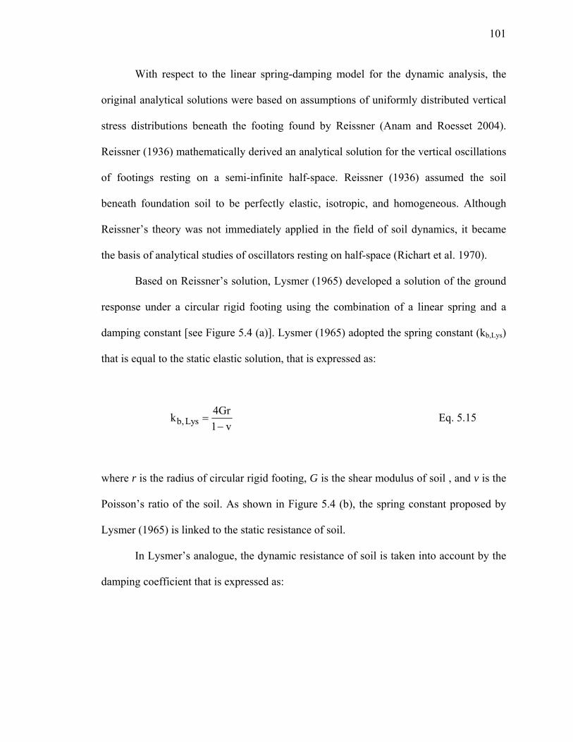
101

With respect to the linear spring-damping model for the dynamic analysis, the

original analytical solutions were based on assumptions of uniformly distributed vertical

stress distributions beneath the footing found by Reissner (Anam and Roesset 2004).

Reissner (1936) mathematically derived an analytical solution for the vertical oscillations

of footings resting on a semi-infinite half-space. Reissner (1936) assumed the soil

beneath foundation soil to be perfectly elastic, isotropic, and homogeneous. Although

Reissner’s theory was not immediately applied in the field of soil dynamics, it became

the basis of analytical studies of oscillators resting on half-space (Richart et al. 1970).

Based on Reissner’s solution, Lysmer (1965) developed a solution of the ground

response under a circular rigid footing using the combination of a linear spring and a

damping constant [see Figure 5.4 (a)]. Lysmer (1965) adopted the spring constant (kb,Lys)

that is equal to the static elastic solution, that is expressed as:

b, Lys4Grk1 v

=−

Eq. 5.15

where r is the radius of circular rigid footing, G is the shear modulus of soil , and v is the

Poisson’s ratio of the soil. As shown in Figure 5.4 (b), the spring constant proposed by

Lysmer (1965) is linked to the static resistance of soil.

In Lysmer’s analogue, the dynamic resistance of soil is taken into account by the

damping coefficient that is expressed as:

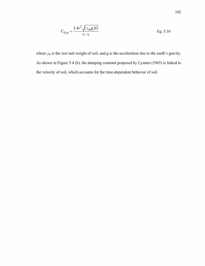
102

( )2

mLys

3.4r g GC

1γ

=− ν

Eq. 5.16

where γm is the wet unit weight of soil, and g is the acceleration due to the earth’s gravity.

As shown in Figure 5.4 (b), the damping constant proposed by Lysmer (1965) is linked to

the velocity of soil, which accounts for the time-dependent behavior of soil.

103

kb,Lys cLys

r

r : Radius of the footing

kb,Lys cLys

r

r : Radius of the footing

(a)

w

sR

,b Lysk

: Soil displacementw

w

sR

,b Lysk

: Soil displacementw

&w

dR

Lysc

&w : Soil velocity

&w

dR

Lysc

&w : Soil velocity&w : Soil velocity

(b)

Figure 5.4 Lysmer’s reaction model: (a) schematic of the model; and (b) spring and dashpot and plots of Rs (t)-w and Rd (t) - w relationship.

104

The main contribution of Lysmer’s study was that he established a bridge between

the elastic half-space theory and the mass-spring-dashpot system and provided values for

the spring and damping constants (Richart et al. 1970). According to the extensive review

of dynamic soil-structure interaction by Kausel (2010), a lot of researches have been

performed based on Lysmer’s analogue in the context of footing vibrations.

Davies and Karim (1995) performed dynamic analysis based on Lysmer’s

analogue to interpret the results of Clegg hammer test. Davies and Karim (1995)

conducted the analysis using an elastodynamic solution. From the analysis, they were

able to obtain the ground response to impact by a mass using the free-vibration condition

described by the equation of motion. Since the analytical results demonstrated very high

impact stresses, Davies and Karim (1995) concluded that the analysis was not directly

applicable to the interpretation of the CHT. However, this lack of compatibility of the

analysis with the CHT is also due to the fact that the analysis did not account for soil

nonlinearity.

Again, the linear-elastic spring constant illustrated in Figure 5.4 (a) is not able to

accurately simulate response of a footing on soil, as the static component should be

bounded by a limit bearing capacity, as discussed in previous sections.

Smith (1960) introduced a dynamic model to perform pile driving analysis. Smith

(1960) employed the linear-elastic, perfectly-plastic soil model to analyze the dynamic

response of soil. In the Smith (1960) model, the soil reaction is described through a

linear-elastic perfectly-plastic spring constant with the dashpot coefficient. Also, the pile

is divided into finite elements connected to springs (see Figure 5.5).

105

Ram M1

M4

Mn-1

Mn

CapblockPile Cap M2

K1

M1: Mass of the ram

Mi: Mass of the discretized pile elementStroke

M3

K2

K3

Kn-2

Kn-1

ks3 cs3

ks4 cs4

ks(n-1) cs(n-1)

ksn csnkb cb

Ki: Spring constant of the pileK1: Spring constant of the capblock

kb: Spring constant of the soil at baseksi: Spring constant of the soil at shaft csi: dashpot constant of soil at shaft

csi: dashpot constant of soil at base

Ram M1

M4

Mn-1

Mn

CapblockPile Cap M2

K1

M1: Mass of the ram


M3

K2

K3

Kn-2

Kn-1

ks3 cs3

ks4 cs4

ks(n-1) cs(n-1)

ksn csnkb cb

Ram M1

M4

Mn-1

Mn

CapblockPile Cap M2

K1

M1: Mass of the ram


M3

K2

K3

Kn-2

Kn-1

ks3 cs3

ks4 cs4

ks(n-1) cs(n-1)

ksn csnkb cb







Figure 5.5 Pile-hammer-soil system of Smith model (modified after Smith 1960).

With regard to the vertical oscillation of footings in deep soil (such as a pile base),

the dynamic response during pile driving events is often approached through the model

used for the oscillation of shallow footings on a semi-infinite half-space.

106

After the Smith (1960) model, some advanced models for pile driving analysis

also employed Lysmer’s framework to interpret the dynamic response of the pile base.

For example, in order to account for the elasto-plastic state of soil, Deeks and Randolph

(1995) incorporated a plastic slider along with sets of rheological model configurations

based on finite element results. However, Deeks and Randolph (1995) reported that the

results of analyses using Lysmer’s analogue were in good agreement with the dynamic

model presented by Deeks and Randolph (1995) when the Poisson’s ratio was less than

1/3.

5.4. Suggested Model for the Interpretation of in situ Tests

5.4.1. Selection of the Dynamic Model for the Clegg Hammer Test

Dynamic loading leads to nonlinear hysteretic response of the soil that reflects modulus

degradation and gradual increase of energy loss (Vucetic and Dobry 1991, Loizos and

Boukovalas 2005). Physically, when the impact mass is dropped onto the ground surface,

the impacted portion of soil first stores the energy with elastic deformation and then

absorbs the energy through hysteretic dissipation. When the soil resistance is mobilized

due to the impact, soil resistance cannot increase infinitely with an increase in

displacement. Rather, the resistance should be bound to a limit bearing capacity. Yet in

Lysmer’s analogue, the soil resistance against dynamic loading continuously increases as

the loading increases, regardless of the limit state.

107

During the Clegg Hammer Test, the data logger in the CHT captures the

maximum deceleration in terms of the Clegg Impact Value CIV (=98m/s2). In order to

correlate the CIV with soil properties, it is necessary to obtain the magnitude and

characteristics of the dynamic loads involved in the CHT. Also, the nonlinear response of

the soil under the Clegg hammer at the moment of impact needs to be modeled properly.

In addition, damping must be accurately represented.

Recently, Loukidis et al. (2008) proposed a base reaction model for interpreting

the dynamic response of soil. The proposed model accounts for soil nonlinearity and

hysteresis, viscous damping, and radiation damping. The proposed model consists of a

nonlinear spring connected in parallel to a radiation dashpot (see Figure 5.6).

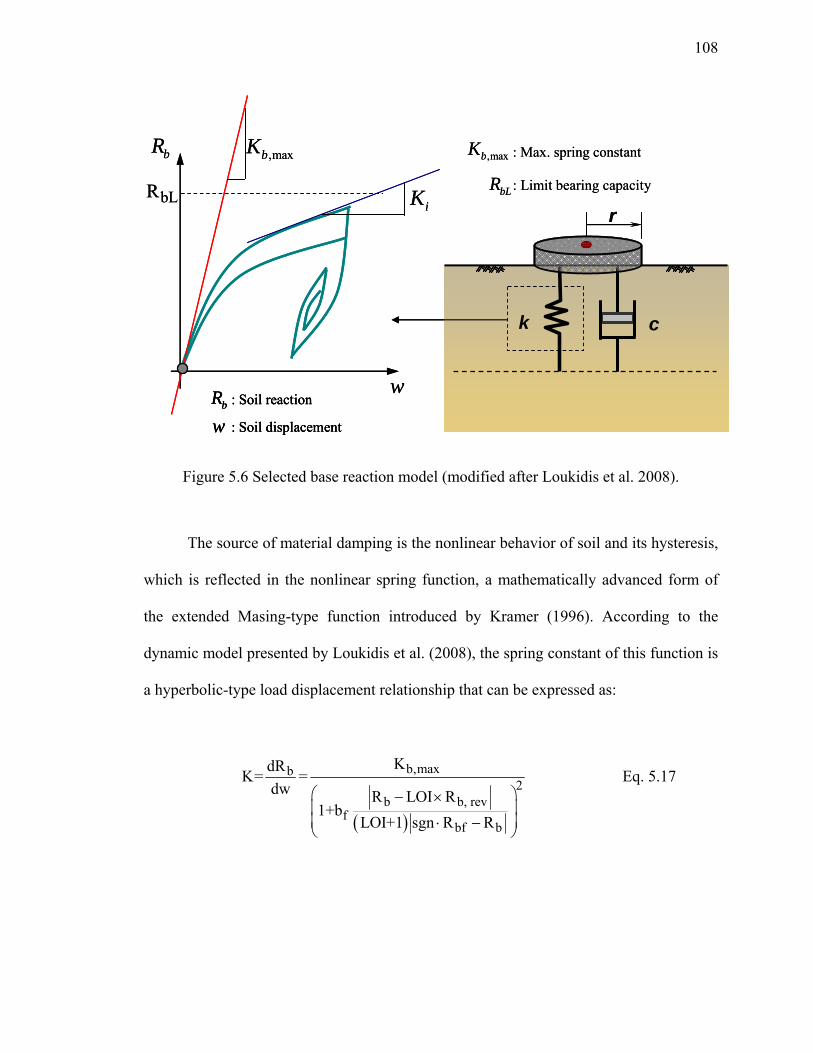
108

k c

r

w

bR

bLR

,maxbK

iK

bR : Soil reaction

w : Soil displacement

bLR : Limit bearing capacity

,maxbK : Max. spring constant

k c

r

w

bR

bLR

,maxbK

iK

bR : Soil reactionbR : Soil reaction

w : Soil displacementw : Soil displacement

bLR : Limit bearing capacity

,maxbK : Max. spring constant

Figure 5.6 Selected base reaction model (modified after Loukidis et al. 2008).

The source of material damping is the nonlinear behavior of soil and its hysteresis,

which is reflected in the nonlinear spring function, a mathematically advanced form of

the extended Masing-type function introduced by Kramer (1996). According to the

dynamic model presented by Loukidis et al. (2008), the spring constant of this function is

a hyperbolic-type load displacement relationship that can be expressed as:

( )

b,maxb2

b b, revf

bf b

KdRK= =dw R LOI R

1+bLOI+1 sgn R R

⎛ ⎞− ×⎜ ⎟⎜ ⎟⋅ −⎝ ⎠

Eq. 5.17

109

where Kb,max is the maximum elastic spring constant, Rb is the limit base capacity, Rb,rev is

the spring reaction at the last displacement reversal, and LOI is the loading index

parameter (LOI=0 for a virgin loading, 1 for other cases). The signum function is denoted

by sgn, which extracts the sign of a real number. bf is a model parameter that controls the

rate of degradation of the base spring constants. For modeling the radiation dashpot, the

Lysmer’s dashpot is adopted.

The dynamic model selected, originally presented by Loukidis et al. (2008),

accounts for the unloading-reloading response of soil due to dynamic loads. As shown in

Figure 5.6, the base reaction due to dynamic loading reaches Rbf asymptotically, with an

increase in the dynamic displacement. Also, if a setback takes place during the analysis,

Rb,rev is loaded at the point where the setback occurs. The path of the unloading-reloading

curves takes the same shape as that of the backbone curve. The selected model captures

hysteretic damping by using variables such as LOI, Rb,rev and the signum function

(Loukidis et al. 2008).

The selected model also accounts for viscous damping. According to Loukidis et

al. (2008), the dynamic limit bearing capacity Rbf is set as a function of the base velocity

and is expressed as:

( )nbf bL bR Q 1 m w⎡ ⎤= +⎢ ⎥⎣ ⎦

& Eq. 5.18

110

where QbL is the static limit load, and m and n are parameters controlling rate effects on

soil strength. Eq. 5.18 implies that the limit bearing capacity during dynamic behavior is

equal to the static limit load when the velocity of the footing is zero.

Using the rheological model combined the spring constant suggested by Loukidis

et al. (2008) and the dashpot constant suggested by Lysmer (1965), the equation of

motion can be applied to obtain the dynamic response of the Clegg hammer test.

The ground response to the impact of a mass M can be obtained using the solution

of the free-vibration problem:

Mw Cw Kw 0+ + =&& & Eq. 5.19

where K is the spring constant in Eq. 5.17, C is the damping constant in Eq. 5.16, and &&w ,

&w , and w are acceleration, velocity, and displacement, respectively. This is the classic

one-degree-of-freedom system governed by a linear differential equation.

The single degree of freedom (SDOF) transient response is fundamental to most

types of vibratory behavior. Even within SDOF with free vibration condition, however,

the solution of the equation of motion varies depending on how the spring constant and

damping characteristics are predetermined. In the analysis, soil nonlinearity and

hysteresis, radiation damping, and viscous damping are accounted for using Eq 5.16 to

5.18.

The equation of motion, even for a single-degree-of-freedom system, cannot be

solved explicitly if the ground acceleration varies with time or if the system involves

111

nonlinear behavior (Chopra 2007). Thus, in order to solve the problem, a numerical time-

stepping method, namely, the finite difference method is adopted in the analysis.

First, the time step (∆t) should be determined. Then, the equation of motion can

be rewritten as:

i i i iMw Cw K w 0+ + =&& & Eq. 5.20

Also, the spring constant can also be rewritten as:

( )( ) ( )( ) ( )

( )b,maxb ii 2

b b, revi 1 i 1f

bf b i 1

KdR dw

R LOI R1+b

LOI+1 sgn R R− −

−

=⎛ ⎞− ×⎜ ⎟⎜ ⎟⋅ −⎜ ⎟⎝ ⎠

Eq. 5.21

The equation of motion in eq. 5.20 is subjected to the boundary conditions

=&w initial impact velocity and w = 0 when the time is equal to zero. Using the boundary

condition, the equation of motion can be solved step-by-step using the following

procedure:

1. Compute (dRb)i using equation 5.20

2. Compute (Rb)i = (Rb)i-1 + (dRb)i

3. Compute the acceleration ( )i b i

iCw R

wM

⎡ ⎤+⎣ ⎦= −&

&&

112

4. Compute the velocity and displacement using the following equations:

i 1 i i

i 1 i i

w w w tw w w t

+

+

= + Δ= + Δ

& & &&

&

In the analysis, the numerical procedure may become unstable if we input very

small or large time increments.

5.4.2. Selection of the Dynamic Model for the Dynamic Cone Penetration Test

In the DCPT, the tester records the blow counts required for penetrating a certain depth

(e.g., 0-to-6 inches or 0-to-12 inches). For proper dynamic analysis of the DCPT, it is

essential to understand the sequence of the test. As shown in Figure 5.7 (a), when the

hammer drops and hits the anvil, the cone tip of the DCP penetrates the soil. Since the

diameter of the cone tip (2.0cm) is larger than that of the DCP bar (1.7cm), the side

resistance of soil can be neglected. Even in sandy soils, it was observed that the hole

made by the DCPT sustained itself in the field because of apparent cohesion.

In summary, we can model the DCPT with a series of steel elements along with

soil reaction at the base only (see Figure 5.7). For the base model, the same framework

used for the CHT was adopted.

113

Hammer (Weight)

Anvil

M1

M2

Mn-1

Mn

Rb

Hammer (Weight)

Anvil

M1

M2

Mn-1

Mn

Rb

(a) (b)

Figure 5.7 DCPT (a) DCP test sequence; (b) discretization of DCP into lumped masses with soil reaction at the base.

However, differences exist between the CHT and the DCPT. First, the CHT does

not have the overburden pressure that the DCPT has. At shallow depths, a significant

114

portion of the damping of soil takes place due to Rayleigh waves that the DCPT does not

have as it penetrates deeper. In order to account for the depth effect on pile base during

dynamic motion, Loukidis et al. (2008) proposed the equation based on the finite

difference analysis using FLAC. Based on the FLAC simulations, Loukidis et al. (2008)

suggested the static stiffness depth factor Df can be expressed as:

( ) ( )0.826

fDD 1.27 0.12ln 0.27 0.12ln exp 0.83B

⎡ ⎤⎛ ⎞⎢ ⎥= − ν − − ν − ⎜ ⎟⎝ ⎠⎢ ⎥⎣ ⎦

Eq. 5.22

where v is the Poisson’s ratio, B is the diameter of the DCPT, and D is the depth where

the tip is located. In case of dynamic depth factor, Loukidis et al. (2008) also found the

following correlation:

( )1.7f ,dyn fD D= Eq. 5.23

where Df,dyn is the dynamic depth factor. Then, the initial spring constant can be modified

as:

( )1.7b,max f LysK D K= Eq. 5.24

With respect to the dashpot constant, the embedment factor is equal to 1.3 when

D/B is large. Physically, this means that the vertical source of vibration creates the

115

oscillation of the soil not only downward, but also upward and laterally (Balthaus and

Kielbassa 1986). Considering this effect, Loukidis et al. (2008) conducted the FLAC

analysis and modified the damping constant that can be expressed as:

b emb Lys LysC C C 1.3C= = Eq. 5.25

As part of interpreting the dynamic response of the DCPT for soils, the ground

response to the impact of a mass M can be obtained using the following equation of

motion:

[ ]{ } [ ]{ } [ ]{ }i b i iM w C w K w R 0+ + + =&& & Eq. 5.26

where [K] is the matrix of the spring constant, [Cb] is the matrix of the damping constant,

and { &&w }, { &w }, and {w} are the matrixes of acceleration, velocity, and displacement,

respectively. This system of equations of motion can be solved numerically using the

finite difference technique. Using the time-stepping methods developed by Newmark

(1959), the displacement, velocity, and acceleration of each segment of DCP at time t+∆t

can be computed using the following equations:

{ }( ) [ ]

[ ] { }( ) { }( ) { }( )

[ ] { }( ) { }( ) { }( )

t t t t2

t+ teff

t t t

1 1 1R + M w + w + -1 wβΔt 2ββΔt1w

K+ C w + -1 w +Δt -1 w

βΔt β 2β

Δ

⎛ ⎞⎧ ⎫⎛ ⎞⎪ ⎪⎜ ⎟− ⎨ ⎬⎜ ⎟⎜ ⎟⎝ ⎠⎪ ⎪⎩ ⎭= ⎜ ⎟

⎧ ⎫⎛ ⎞ ⎛ ⎞γ γ γ⎜ ⎟⎨ ⎬⎜ ⎟ ⎜ ⎟⎜ ⎟⎝ ⎠ ⎝ ⎠⎩ ⎭⎝ ⎠

& &&

& &&

Eq. 5.27

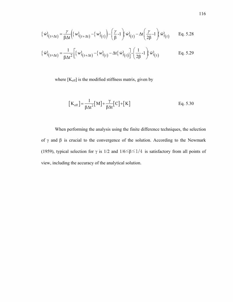
116

{ }( ) { }( ) { }( )( ) { }( ) { }( )t+ t t -1 Δt -1βΔt β 2βΔ +Δ

⎛ ⎞ ⎛ ⎞= − − −⎜ ⎟ ⎜ ⎟

⎝ ⎠ ⎝ ⎠& & &&t t t tw w w w wγ γ γ Eq. 5.28

{ }( ) { }( ) { }( ) { }( ) { }( )t+ t t t21 1Δt - -1

2ββΔtΔ +Δ⎛ ⎞⎡ ⎤= − − ⎜ ⎟⎢ ⎥⎣ ⎦ ⎝ ⎠

&& & &&t t tw w w w w Eq. 5.29

where [Keff] is the modified stiffness matrix, given by

[ ] [ ] [ ] [ ]eff 21 γK M C K

βΔtβΔt= + + Eq. 5.30

When performing the analysis using the finite difference techniques, the selection

of γ and β is crucial to the convergence of the solution. According to the Newmark

(1959), typical selection for γ is 1/2 and 1/6≤β≤1/4 is satisfactory from all points of

view, including the accuracy of the analytical solution.

117

5.5. Summary

An accurate method that evaluates the dynamic behavior of soil under dynamic loads is to

model the soil by using a set of springs and dashpots. A spring constant is associated with

the static resistance of soil and the damping of soil corresponds to the rate effect of soil

against dynamic loads. In this framework, the damping reflects a gradual decrease of

vibration with time.

When a load is applied gradually, as occurs in typical construction sequences, rate

effects gradually increase as the time to apply the load decreases. Thus, the total

resistance R (t) acting at the surface of the soil consists of the static component Rs (t) and

the dynamic component Rd (t) (Salgado 2008):

( ) ( ) ( )s dR t R t R t= + Eq. 5.2

With regard to the vertical oscillations of footings resting on soil, Lysmer (1965)

postulated the ground with the combination of a spring and a damping constant. Lysmer’s

analogue represents the spring constant that is expressed as:

b, Lys4Grk1 v

=−

Eq. 5.3

118

where r is the radius of the circular rigid footing, G is the shear modulus of the

soil, and v is the Poisson’s ratio of the soil (see Figure 5.3). Also, the damping coefficient

is given as:

( )2

mLys

3.4r g GC

1γ

=− ν

Eq. 5.4

where γm is the wet unit weight of the soil and g is the acceleration due to the

earth’s gravity.

The nonlinear stress-strain behavior of soils makes the analysis complex. The

impacted portion of the soil first stores the energy with elastic deformation and then

absorbs the energy due to hysteretic dissipation. Even though the analysis can be

improved by introducing soil nonlinearity, only a few attempts have been made (Abou-

Jaoude 2006).

In order to correlate the CIV with the ground conditions, it is necessary to obtain

the magnitude and characteristics of the dynamic loads involved in the CHT. Recently,

Loukidis et al. (2008) proposed a base reaction model accounting for soil nonlinearity

and hysteresis, viscous damping, and radiation damping. The proposed model consists of

a nonlinear spring connected in parallel to a radiation dashpot (see Figure 5.7). Radiation

dashpot is identical to Lysmer’s dashpot and is given by:

( )2

m maxLys

3.4r g GC

1γ

=− ν

Eq. 5.16

119

The source of material damping is the nonlinear behavior of soil and its hysteresis,

which is reflected in the nonlinear spring function, a mathematically advanced form of

the extended Masing type function introduced by Kremer (1996). The spring constant of

this function illustrates a hyperbolic-type load displacement relationship and can be

expressed as:

( )

b,maxb2

b b, revf

bf b

KdRK= =dw R LOI R

1+bLOI+1 sgn R R

⎛ ⎞− ×⎜ ⎟⎜ ⎟⋅ −⎝ ⎠

Eq. 5.17

where Kb,max is the maximum elastic spring constant, Rb is the limit base capacity,

Rb,rev is the spring reaction at the last displacement reversal, and LOI is the loading index

parameter (LOI=0 for a virgin loading, 1 for other cases). The signum function is denoted

by sgn, which extracts the sign of a real number. bf is a model parameter that controls the

rate of degradation of the base spring constants.

In order to interpret the dynamic response of the CHT for soils, the ground

response to impact by mass M can be obtained using the solution of the free-vibration

problem:

Mw Cw Kw 0+ + =&& & Eq. 5.19

120

where K is the spring constant in eq. 5.18, C is the damping constant in eq. 5.17;

and &&w , &w , and w are acceleration, velocity, and displacement respectively. This is a

classic one-degree-of-freedom system governed by a linear differential equation.

For the dynamic analysis of the DCPT, it is essential to understand the sequence

of the test. Differences exist between the CHT and the DCPT. First, the CHT does not

have the overburden pressure that the DCPT has. At shallow depths, a significant portion

of the damping of soil takes place due to Rayleigh waves that the DCPT does not have as

it penetrates deeper. Loukidis et al. (2008) proposed the equation that accounts for the

effect of embedment using the finite difference code FLAC.

As part of interpreting the dynamic response of the DCPT for soils, the ground

response to impact by mass M can be obtained using the equation of motion.

121

CHAPTER 6. FIELD TESTS ON INDIANA SOILS

6.1. Introduction

Since the Dynamic Cone Penetration Test (DCPT) and the Clegg Hammer Test (CHT)

were introduced, several researchers have attempted to use these tests for soil compaction

quality control (Burnham 1997, White et al 1999, Gabr et al. 2000, Jayawickrama et al.

2000, Salgado and Yoon 2003, Abu-Farsakh et al. 2005, GTI 2005, Ampadu and Arthur

2006). However, these studies did not develop specific correlations for the various types

of soil.

A comprehensive experimental program was undertaken to assess the use of the

DCPT and the CHT for compaction control. The experimental program consisted of tests

performed in a pit and in the field. The DCPTs and CHTs were performed on-site at

several INDOT highway construction projects in Indiana. In order to establish the soil

compaction quality control criteria using the DCPT and CHT, a number of tests were

performed along with other density-based tests such as the nuclear gauge and sand cone

tests. By doing so, the DCPT and CHT could be correlated with the dry unit weight

associated with the INDOT specification limit, which is RC ≥ 95%.

Since the dynamic behavior of both the DCPT and CHT are somewhat different,

depending on the soil type, the test results were summarized according to the type of soil,

categorized by the AASHTO classification. During testing, the soils containing a

122

significant amount of gravel-sized particles were excluded because the particle size

effects increase significantly considering the dimensions of both the DCPT and CHT.

This chapter presents the results of the tests performed in the test pit located on

the southern side of the Bowen Laboratory for Large-Scale Civil Engineering Research at

Purdue University in West Lafayette, Indiana, as well as the tests performed at several

INDOT construction sites.

A major thrust of this chapter is providing values of the minimum required blow

count for various soil types and 95% relative compaction. As defined in section 4.4, the

blow count satisfying both requirements will be referred to as the minimum required

blow count. It provides reasonable assurance that, if the measured blow count matches or

exceeds it, the desired relative compaction will have been achieved.

6.2. Tests Performed in the Test Pit

6.2.1. Testing Method

The purpose of the tests performed on the southern side of the Bowen Laboratory was to

investigate the DCPT and CHT results in well controlled conditions because on-site

construction conditions, water content in particular, fluctuate considerably due to weather.

The test pit, shown in Figure 6.1, has an internal diameter of 130cm and a height of

130cm.

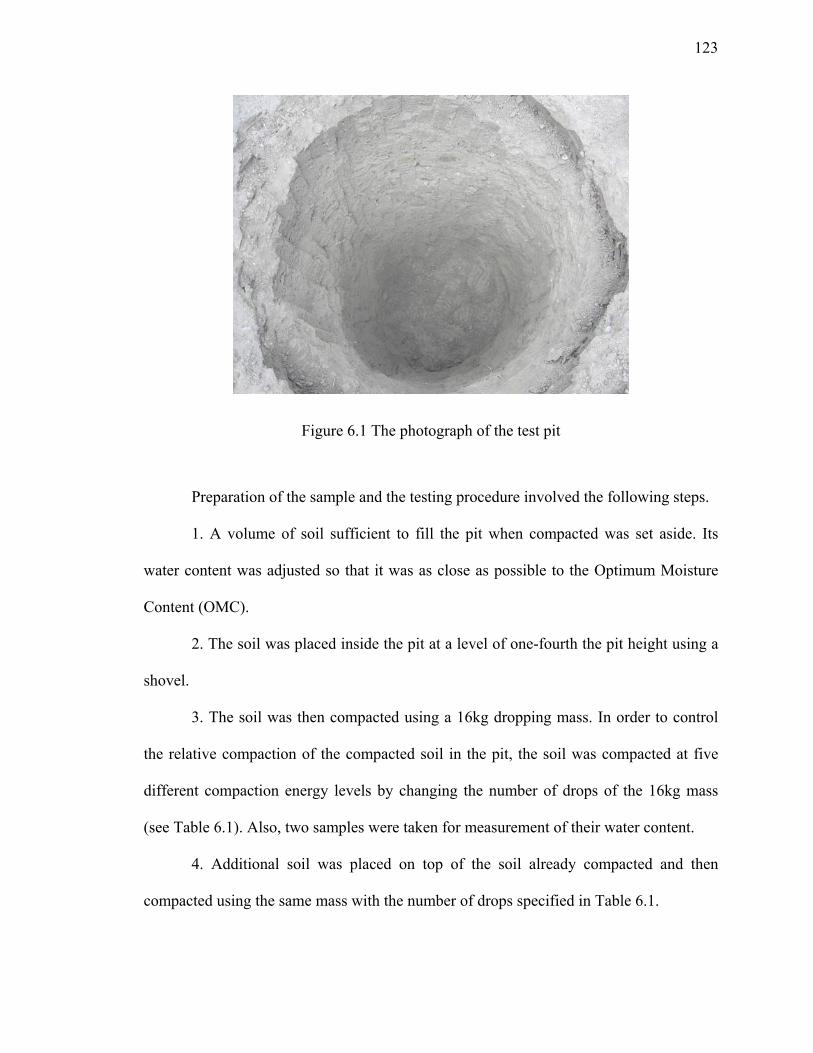
123

Figure 6.1 The photograph of the test pit

Preparation of the sample and the testing procedure involved the following steps.

1. A volume of soil sufficient to fill the pit when compacted was set aside. Its

water content was adjusted so that it was as close as possible to the Optimum Moisture

Content (OMC).

2. The soil was placed inside the pit at a level of one-fourth the pit height using a

shovel.

3. The soil was then compacted using a 16kg dropping mass. In order to control

the relative compaction of the compacted soil in the pit, the soil was compacted at five

different compaction energy levels by changing the number of drops of the 16kg mass

(see Table 6.1). Also, two samples were taken for measurement of their water content.

4. Additional soil was placed on top of the soil already compacted and then

compacted using the same mass with the number of drops specified in Table 6.1.

124

Table 6.1 Different compaction targets

Type Relative Compaction (RC)

Method of Compaction Test Performed

Case 1 81.6% 1 drop / layer DCPT - Five locations at

two depths

CHT - Five locations at

two depths

Case 2 86.5% 3 drops / layer




5. The first set of tests was carried out at the locations shown in Figure 6.2 (a) and

(b).

6. The procedure described for steps 2 to 4 was repeated as two more layers were

placed and compacted on top of the surface where the first set of tests was performed. A

second set of tests was then conducted as shown in Figure 6.2. A sand cone test was

conducted at the center of the sample to investigate the dry unit weight of the compacted

soil. Also, two samples were taken for water content measurements.

The CHT apparatus used for this research was a 10kg hammer type, Model

95005A, produced by a Lafayette company. The DCP apparatus used in the testing was

manufactured in accordance with ASTM D6951-03.

125

1

4

2

35 11

22

3344

55

CHT locationsCHT locations

DCPT locations

Sand Cone test

1

4

2

35 11

22

3344

55

CHT locationsCHT locations

DCPT locations

Sand Cone test

(a)

1.3m

1.3m

1144

2211

334455

5533

22

1144

2211

334455

5533

22

Second set of tests

First set of tests

1.3m

1.3m

1144

2211

334455

5533

221144

2211

334455

5533

22

1144

2211

334455

5533

221144

2211

334455

5533

22

Second set of tests

First set of tests

(b)

Figure 6.2 Test pit: (a) Cross-sectional view of DCPT and CHT test locations, and (b) schematic view of the test pit with the test locations

126

6.2.2. Soil Properties

The soil used for the tests was from a West Lafayette, Indiana location. The gradation of

the soil was determined by sieve and hydrometer analysis in accordance with ASTM

D422-63. Figure 6.3 shows the particle-size distribution of the soil.

The soil consisted mainly of silt-clay particles with a small percentage of sand.

The soil was classified as A-4 soil according to the American Association of State

Highway and Transportation Officials (AASHTO) classification system and CL (Sandy

lean clay) according to Unified Soil Classification System (USCS) following AASHTO

M145-91 and ASTM D2487-06, respectively. Table 6.2 summarizes the grain-size

distribution and classification of the soil used in the tests.

0

20

40

60

80

100

0.00010.0010.010.1110100

Grain size (mm)

Per

cent

fine

r by

wei

ght (

%)

SAND SILT CLAYGRAVEL

Figure 6.3 Particle-size distributions of the soil tested.

127

Table 6.2 The particle-size distribution analysis and classification of the soil sample

Soil %

passing No. 10

% passing No. 40

% passing No.200

Cu Cc Classification system

AASHTO USCS

Purdue Clay 0 72.3 52.1 54 0.86 A-4 CL

The compaction test was performed in accordance with ASTM D698-00,

Standard Test Methods for Laboratory Compaction Characteristics of Soils Using

Standard Effort. Figure 6.4 shows the moisture-density relationship of the Purdue soil

sample. The Zero-Air-Void Curve (ZAVC) that indicates the maximum possible dry unit

weight is also shown in Figure 6.4.

16

18

20

22

5 10 15 20

Water content (%)

Dry

unit

wei

ght (

kN/m

3)

ZAVC

Figure 6.4 Compaction curve for the soil

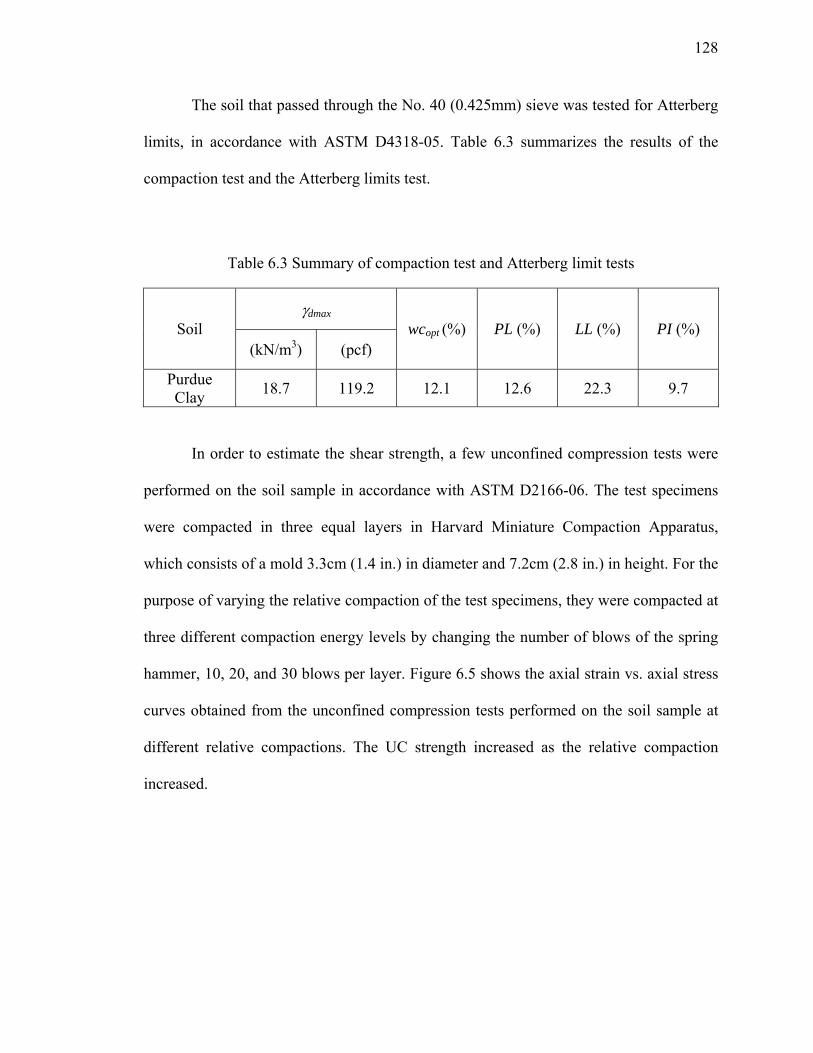
128

The soil that passed through the No. 40 (0.425mm) sieve was tested for Atterberg

limits, in accordance with ASTM D4318-05. Table 6.3 summarizes the results of the

compaction test and the Atterberg limits test.

Table 6.3 Summary of compaction test and Atterberg limit tests

Soil γdmax

wcopt (%) PL (%) LL (%) PI (%) (kN/m3) (pcf)

Purdue Clay 18.7 119.2 12.1 12.6 22.3 9.7

In order to estimate the shear strength, a few unconfined compression tests were

performed on the soil sample in accordance with ASTM D2166-06. The test specimens

were compacted in three equal layers in Harvard Miniature Compaction Apparatus,

which consists of a mold 3.3cm (1.4 in.) in diameter and 7.2cm (2.8 in.) in height. For the

purpose of varying the relative compaction of the test specimens, they were compacted at

three different compaction energy levels by changing the number of blows of the spring

hammer, 10, 20, and 30 blows per layer. Figure 6.5 shows the axial strain vs. axial stress

curves obtained from the unconfined compression tests performed on the soil sample at

different relative compactions. The UC strength increased as the relative compaction

increased.

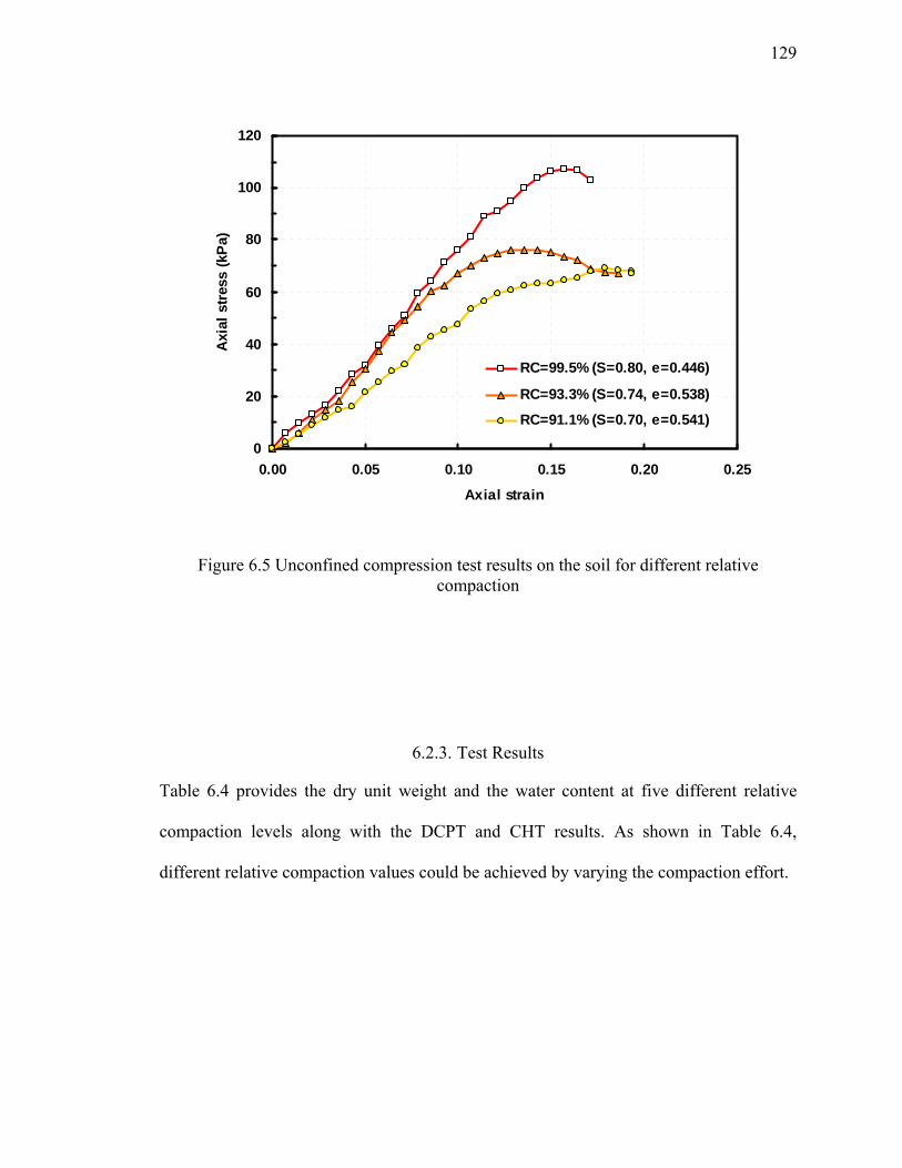
129

0

20

40

60

80

100

120

0.00 0.05 0.10 0.15 0.20 0.25

Axial strain

Axi

al s

tres

s (k

Pa)

RC=99.5% (S=0.80, e=0.446)

RC=93.3% (S=0.74, e=0.538)

RC=91.1% (S=0.70, e=0.541)

Figure 6.5 Unconfined compression test results on the soil for different relative compaction

6.2.3. Test Results

Table 6.4 provides the dry unit weight and the water content at five different relative

compaction levels along with the DCPT and CHT results. As shown in Table 6.4,

different relative compaction values could be achieved by varying the compaction effort.

130

Table 6.4 Summary of the sand cone, DCPT, and CHT results

Test Case 1 Case 2 Case 3 Case 4 Case 5

Relative Compaction (RC) 81.6% 86.5% 89.6% 91.3% 95.0%

γd (kN/m3) 15.3 16.2 16.8 17.1 17.8

(pcf) 97.4 103.1 106.9 108.8 113.2

wc (%) 13.3 13.7 12.4 13.8 11.5

CIV (Avg., 98m/s2) 4.6 7.8 9.5 9.8 10.6

NDCP (Avg.)

Penetrating 0-to-6 inches 1.3 3.0 6.4 6.9 7.7

Penetrating 6-to-12 inches 1.7 3.7 6.8 9.6 9.1

Table 6.4 also summarizes the DCPT and CHT results for the tests performed in a

pit. Both the DCPT and the CHT results, on average, indicate trends of increasing NDCP

and CIV with increasing relative compaction.

Figure 6.6 provides the distributions of all DCPT results conducted in the test pit

for 0-to-6 inch (NDCP│0~6”) and 6-to-12 inch (NDCP│6~12”) penetration. The test results

show that NDCP│0~6” varied between 1 and 10 and that NDCP│6~12” varied between 1 and 14

depending on the relative compaction. A significant increase in NDCP occurs RC > 90%,

which implies that the soil strength and bearing capacity drastically improve a RC

increases beyond 90%. Greater variability was observed for NDCP│6~12”.

131

0

2

4

6

8

10

12

14

1 2 3 4 5 6 7 8 9 10 11 12 13 14 15

DCP blow count for 0-to-6 inch penetration

Freq

uenc

y

RC=95.0% (wc=11.5%)RC=91.3% (wc=13.8%)RC=89.6% (wc=12.4%)RC=86.5% (wc=13.7%)RC=81.6% (wc=13.3%)

(a)

0

2

4

6

8

10

12

14

1 2 3 4 5 6 7 8 9 10 11 12 13 14 15


Freq

uenc

y


(b)

Figure 6.6 Histograms of DCPT pit results: (a) 0-to-6 inch penetration and (b) 6-to-12 inch penetration.

132

The approach presented in section 4.4 for development of compaction quality

control criteria is used here in connection with the pit test results. The minimum required

blow count is associated with 80% exceedance for the data shown in Figure 6.7. In other

words, the approach assures that the minimum required blow count includes at least 80%

of the occurrences in the histogram of the test results associated with 95% RC.

As shown in Figure 6.7(a), at a RC of 95%, an NDCP│0~6” equal to 8 is greater or

equal to 80% of the test results. Similarly, the minimum required blow count that is

greater or equal to 80% of the test results for a RC 95% is 12 [see Figure 6.7(b)].

The proposed minimum required blow count is then checked for the data

corresponding to all values of RC, as shown in Figure 6.8. Figure 6.8(a) shows that all

other test results are less than the selected value for 0-to-6 inch penetration. Figure 6.8(b)

shows that all the test results except one are below the selected value for 6-to-12 inch

penetration.

133

0

1

2

3

4

5

6

1 2 3 4 5 6 7 8 9 10 11 12 13 14 15

DCP blow counts for 0-to-6 inch penetration

Freq

uenc

y

RC=95.0% (wc=11.5%) NDCP = 8

(a)

0

1

2

3

4

5

6

1 2 3 4 5 6 7 8 9 10 11 12 13 14 15

DCP blow counts for 6-to-12 inch penetration

Freq

uenc

y

RC=95.0% (wc=11.5%)NDCP = 12

(b)

Figure 6.7 Histograms of DCPT pit results at 95% RC plotted together with the minimum required blow count: (a) 0-to-6 inch penetration and (b) 6-to-12 inch penetration.

134

0

2

4

6

8

10

12

14

1 2 3 4 5 6 7 8 9 10 11 12 13 14 15


Freq

uenc

y


NDCP = 8

(a)

0

2

4

6

8

10

12

14

1 2 3 4 5 6 7 8 9 10 11 12 13 14 15


Freq

uenc

y


NDCP = 12

(b)

Figure 6.8 Histograms of DCPT pit results plotted together with the minimum required blow count: (a) 0-to-6 inch penetration and (b) 6-to-12 inch penetration.

135

Figure 6.9 shows a plot of relative compaction versus the Clegg Impact Value

(CIV). Even though the test results, on average, indicate that the CIV increases with

increasing relative compaction, the CIV exhibits high variability at each relative

compaction value. The CHT results show that the CIV is, on average, 10.6 for an average

RC of 95%, but the range (9.0~13.3) was wide.

2

4

6

8

10

12

14

80 85 90 95 100


CIV

(Cle

gg Im

pact

Val

ue: 9

8m/s

2 )

Preliminary test results

Average of the test results

Figure 6.9 The Clegg Hammer Test results in the test pit at five different relative compactions

136

6.3. Field Tests on A-3 Soils

Three sites were selected for performing the tests on A-3 soil. All of the soils at the sites

were cohesionless and contained less than 10 percent passing the #200 sieve. A-3 soils

consist of clean, poorly graded sand. In addition to the density and confinement, the

engineering behavior of A-3 soil is mainly influenced by the relative proportions of the

different particle sizes present and the shapes of the soil particles.

Figure 6.10 shows the particle-size distribution of the soils tested. The soils

mainly consisted of sand particles with minimal percentages of fines and gravels. Those

soils are all non-plastic and classified as A-3 soils per the AASHTO classification system

and SP (Poorly graded sand) per USCS following AASHTO M145-91 and ASTM

D2487-06, respectively. The compaction tests were performed in accordance with ASTM

D698-00, Standard Test Methods for Laboratory Compaction Characteristics of Soils

Using Standard Effort. Figure 6.11 shows the compaction curves of the soils.

137

0

20

40

60

80

100

0.010.1110

Grain size (mm)

Per

cent

fine

r by

wei

ght (

%) I-70 (A-3)

SR31 (A-3)SR25 (A-3)

SAND SILTGRAVEL

Figure 6.10 Particle-size distributions of A-3 soils.

17

18

19

20

21

0 4 8 12 16 20

Water content (%)

Dry

uni

t wei

ght (

kN/m

3)

SR25ZAVCFitting curve

(a)

Figure 6.11 Compaction curves of the soil taken from (a) SR25 site.

138

15

16

17

18

19

20

0 4 8 12 16 20

Water content (%)

Dry

unit

wei

ght (

kN/m

3)

SR31ZAVCFitting curve

(b)

17

18

19

20

21

2 6 10 14 18

Water content (%)

Dry

uni

t wei

ght (

kN/m

3)

I-70ZAVCFitting curve

(c)

Figure 6.11 Compaction curves of the soil samples from: (a) SR25 site, (b) SR31 site, and (c) I-70 site (Continued).

139

Table 6.5 summarizes the grain-size distributions and classifications of the soil

taken from three sites. Each is discussed in detail next.

Table 6.5 Summary of grain-size distribution analyses and compaction tests

Site %

passing No. 10

% passing No. 40

% passing No.200

Cu Cc γdmax wcopt

(%) (kN/m3) (pcf)

SR 25 at Carroll Co. 75.4 23.1 1.2 5.06 1.02 18.5 117.9 12.1

SR 31 at Marshall Co. 84.2 61.6 0.8 2.92 0.84 17.1 108.5 12.8

I-70 at Indianapolis 74.3 27.7 1.0 6.01 0.86 18.4 117.1 12.1

6.3.1. Field Tests on SR25

An embankment was constructed using A-3 soil as fill material. Field DCP Tests were

performed on the embankment at the State Road 25 highway construction site located in

Carroll County, Indiana. Figure 6.12 shows the histogram of the DCPT results. The

relative compactions in Figure 6.12 were computed using a γdmax of 18.5 kN/m3 (117.9

pcf) taken from the laboratory Standard compaction test. The dry unit weight and the

water content were measured using the nuclear gauge tests. In each case, three nuclear

gauge tests were performed along with five DCP tests. The relative compaction and the

water content results in Figure 6.12 through Figure 6.14 are the average values from three

nuclear gauge tests.

140

Based on the test results shown in Figures 6.12, the minimum required blow count,

(NDCP)req│0~12”, that was associated with 80% exceedance for the test results in the

histogram of the test results corresponding to 95.6% RC was 8. However, (NDCP)req│0~12”

was increased by 9 in order to have two test results associated with less than 95% RC

equal to the minimum required blow count, as shown in Figure 6.13.

Figure 6.14 shows that the NDCP│0~12” of 9 works well when considered in the

context of all results. The blow counts for RC of less than 95% are less than the minimum

required blow count except for a case with 93.3%, where an unusually low water content

led to an abnormally high blow count. The test results corresponding to RC more than

95% supported this explanation because several DCP test results associated with RC

more than 95% are below the (NDCP)req│0~12” of 9, as shown in Figure 6.14.

0

2

4

6

8

10

12

14

4 5 6 7 8 9 10 11 12 13 14 15 16 17 18


Freq

uenc

y

RC=103.9% (wc=8.4%)RC=100.3% (wc=11.1%)RC=99.5% (wc=10.6%)RC=98.8% (wc=9.0%)RC=97.2% (wc=11.5%)RC=95.7% (wc=6.0%)RC=95.6% (wc=7.4%)RC=93.3% (wc=6.6%)RC=92.5% (wc=7.8%)

Figure 6.12 Histogram of DCPT results (SR25): 0-to-12 inch penetration.

141

0

1

2

3

4

5

6

4 5 6 7 8 9 10 11 12 13 14 15 16 17 18


Freq

uenc

y

RC=95.6% (wc=7.4%)NDCP = 9

Figure 6.13 Histogram of DCPT results at 95.6% RC plotted together with the minimum required blow count (SR25): 0-to-12 inch penetration.

0

2

4

6

8

10

12

14

4 5 6 7 8 9 10 11 12 13 14 15 16 17 18


Freq

uenc

y

RC=103.9% (wc=8.4%)RC=100.3% (wc=11.1%)RC=99.5% (wc=10.6%)RC=98.8% (wc=9.0%)RC=97.2% (wc=11.5%)RC=95.7% (wc=6.0%)RC=95.6% (wc=7.4%)RC=93.3% (wc=6.6%)RC=92.5% (wc=7.8%)

NDCP = 9

Figure 6.14 Histogram of DCPT results plotted together with the minimum required blow count (SR25): 0-to-12 inch penetration.

142


An embankment approaching a bridge was constructed using A-3 soil as a fill material at

a highway construction site on State Road 31 in Marshall County, Indiana.

Figure 6.15 shows the histogram of the DCPT blow counts for the site. In the

figure, relative compactions were computed using a γdmax of 17.1 kN/m3 (108.5pcf)

obtained from the laboratory Standard compaction test (see Table 6.5). Also, the dry unit

weight and the water content were measured using the nuclear gauge test. In each case,

three nuclear gauge tests were performed along with five DCP tests. The RC and the

water content results in Figures 6.15 through 6.17 represent the arithmetic mean values

from three nuclear gauge tests.

Based on the test results shown in Figure 6.16, the minimum required blow count

(NDCP)req│0~12” was determined. At the site, since DCP test results associated with 95%

RC were not acquired, the DCP test results corresponding to 96.7% were used to

determine the minimum required blow count. Based on the test results shown in Figure

6.16, the (NDCP)req│0~12” that is greater or equal to 80% of the blow counts associated with

96.7% RC was 7. In Figure 6.17, a NDCP│0~12” of 7 was assessed based on the RC values

associated with test results exceeding the selected value.

143

0

2

4

6

8

10

12

14

16

3 4 5 6 7 8 9 10 11 12 13 14


Freq

uenc

y

RC=101.4% (wc=8.3%)RC=100.6% (wc=8.6%)RC=100.0% (wc=11.4%)RC=99.0% (wc=9.1%)RC=97.8% (wc=9.4%)RC=96.7% (wc=9.4%)

Figure 6.15 Histogram of DCPT results (SR31): 0-to-12 inch penetration.

0

1

2

3

4

5

6

3 4 5 6 7 8 9 10 11 12 13 14


Freq

uenc

y

RC=96.7% (wc=9.4%)NDCP = 7

Figure 6.16 Histogram of DCPT results at 96.7% RC plotted together with the minimum required blow count (SR31): 0-to-12 inch penetration.

144

0

2

4

6

8

10

12

14

16

3 4 5 6 7 8 9 10 11 12 13 14


Freq

uenc

y


NDCP = 7

Figure 6.17 Histogram of DCPT results plotted together with the minimum required blow count (SR31): 0-to-12 inch penetration.

6.3.3. Field Tests on I-70

An embankment was constructed using A-3 soil as fill material as part of an I-70

extension project in Indianapolis, Indiana, and the DCPTs and CHTs were performed

during the construction. For each case of relative compaction, four DCPs and CHTs were

conducted along with three nuclear gauge tests.

Figure 6.18 shows the histogram of the DCPT results taken for site. Again, the

RC values were computed using a γdmax of 18.6 kN/m3 (117.1 pcf) obtained from the

laboratory Standard compaction test (see Table 6.5). Also, the RC and the water content

145

values in Figures 6.18 through 6.20 represent the arithmetic mean values from three


Based on the same approach that we employed for the previous sites, the

minimum required blow count that was associated with 80% exceedance for the test

results in the histogram of the test results corresponding to 95.0% RC was 8. However,

(NDCP)req│0~12” was increased by 10 in order to have the test results associated with 93.2%

RC be less or equal to the minimum required blow count, as shown in Figure 6.20. In

Figure 6.20, a NDCP│0~12” of 10 is shown to work well for cases with RC < 95% had lower

blow counts and cases with RC > 95% had higher blow counts.

0

1

2

3

4

5

6

3 4 5 6 7 8 9 10 11 12 13 14


Freq

uenc

y

RC=95.6% (wc=4.5%)RC=95.0% (wc=4.2%)RC=93.2% (wc=4.1%)

Figure 6.18 Histogram of DCPT results (I-70): 0-to-12 inch penetration.

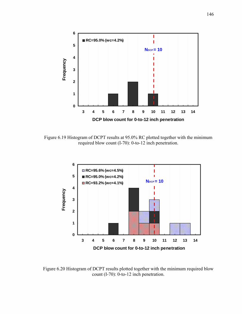
146

0

1

2

3

4

5

6

3 4 5 6 7 8 9 10 11 12 13 14


Freq

uenc

y

RC=95.0% (wc=4.2%)

NDCP = 10

Figure 6.19 Histogram of DCPT results at 95.0% RC plotted together with the minimum required blow count (I-70): 0-to-12 inch penetration.

0

1

2

3

4

5

6

3 4 5 6 7 8 9 10 11 12 13 14


Freq

uenc

y

RC=95.6% (wc=4.5%)RC=95.0% (wc=4.2%)RC=93.2% (wc=4.1%) NDCP = 10

Figure 6.20 Histogram of DCPT results plotted together with the minimum required blow count (I-70): 0-to-12 inch penetration.

147

Figure 6.21 shows RC versus CIV for the I-70 site. The CIV vs. RC relationship

is highly variable. The CHT results showed that the CIV associated with a RC of 95%

was on an average 5.6, with a 4.8~6.6 range.

4

5

6

7

8

9

10

92 93 94 95 96


CIV

(Cle

gg Im

pact

Val

ue: 9

8m/s

2 )

CHT result (I-70 site)


`

Figure 6.21 CIV versus relative compaction (I-70).

148

6.3.4. Summary of Test Results on A-3 Soils

Table 6.6 summarizes the DCP test results with the coefficient of uniformity (Cu) and the

compaction properties. Table 6.6 also contains the DCP test results performed in the

chamber at Purdue University. In the case of A-3 soils, the minimum required blow count,

(NDCP)req│0~12”, corresponding to a RC of 95% varies from 7 to 10.

Table 6.6 Summary of the DCP results with the coefficient of uniformity (Cu) and compaction properties on A-3 soil

Test site SR25 SR31 I-70 DCPT in the Chamber

AASHTO classification A-3 A-3 A-3 A-3

Coefficient of uniformity (Cu)

5.06 2.92 6.01 1.67

γdmax (kN/m3) 18.5 17.1 18.4 17.7†

(pcf) 117.9 108.5 117.1 112.3†

wcopt (%) 12.1 12.8 12.1 -

(NDCP)req│0~12” 9 7 10 4*

† Maximum dry unit weight were obtained using a vibratory table (ASTM D4253-00) * The minimum required blow counts are taken from the test results associated with a RC of 98.1%

The (NDCP)req│0~12” is higher for the SR25 and I-70 sites than for the SR31 site.

Two factors can explain this outcome. First, the Coefficient of uniformities (Cu) of the

soils at the SR25 and I-70 sites were both higher than that of the soil at the SR31 site (see

Table 6.6). So a higher Cu results in a higher minimum required blow count within a

small range. Second, the soils at the SR25 and I-70 sites involved higher percentages

149

retained on the #10 sieve (2 mm) than the SR31 site. This higher percentage of large size

particles may increase or sometimes distort the DCP test results. Note that, if the soil

contains a significant amount of gravel-size particles (more than 2mm in equivalent grain

size per the AASHTO classification), the DCPT should be avoided as a tool for soil

compaction quality control.

In summary, we propose the (NDCP)req│0~12” for A-3 soils that is a function of the

coefficient of uniformity as shown in Figure 6.22. The same figure shows the values

proposed by White et al. (1999). Based on numerous DCP tests on A-3 soil, White et al.

(1999) proposed that the DCP index would have to be less than or equal to 35mm/blow,

which is equivalent to NDCP│0~12” ≥ 8.7. This blow count was deemed required to achieve

DR ≥ 80% in 90% of the tests (Larsen et al. 2007). According to Lee and Singh (1971), a

DR of 80% is associated with a RC of 96%, while a RC of 95% corresponds to a DR of

75%. However, White et al. (1999) did not account for the difference in DCP test results

based on changes in the coefficient of uniformity.

150

NDCP = 4.0 Ln(Cu) + 2.6R2 = 0.99

0

4

8

12

16

1 4 7 10

Coefficient of uniformity (Cu)

ND

CP

the nominal DCP blow counts

Ayers et al. (1989)Test in the chamber(corresponding to RC=98.1%)

White et al. (1999)

Figure 6.22 The coefficient of uniformity versus the (NDCP)req|0~12” for A-3 soils.

With respect to the CHT results, the CIV versus RC relationship was found to be

highly variable. The CHT results showed that the CIV associated with a RC of 95% was,

on average, 5.6 with a 4.8~6.6 range at the I-70 site.

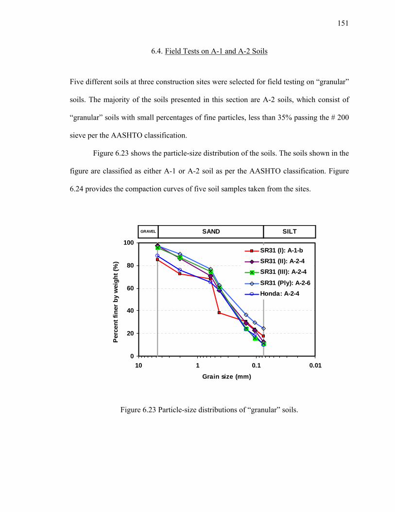
151

6.4. Field Tests on A-1 and A-2 Soils

Five different soils at three construction sites were selected for field testing on “granular”

soils. The majority of the soils presented in this section are A-2 soils, which consist of

“granular” soils with small percentages of fine particles, less than 35% passing the # 200

sieve per the AASHTO classification.

Figure 6.23 shows the particle-size distribution of the soils. The soils shown in the

figure are classified as either A-1 or A-2 soil as per the AASHTO classification. Figure

6.24 provides the compaction curves of five soil samples taken from the sites.

0

20

40

60

80

100

0.010.1110

Grain size (mm)

Perc

ent f

iner

by

wei

ght (

%)

SR31 (I): A-1-bSR31 (II): A-2-4SR31 (III): A-2-4

SR31 (Ply): A-2-6Honda: A-2-4

SAND SILTGRAVEL

Figure 6.23 Particle-size distributions of “granular” soils.

152

16

17

18

19

20

21

22

3 8 13 18

Water content (%)

Dry

unit

wei

ght (

kN/m

3)

ZAVCSR31 (I)SR31 (I) fitting curve

(a)

16

17

18

19

20

21

22

3 8 13 18

Water content (%)

Dry

unit

wei

ght (

kN/m

3 )

ZAVCSR31 (II)SR31 (II) fitting curve

(b)

Figure 6.24 Compaction curves for the soil samples from: (a) SR31 (I) and (b) SR31 (II).

153

16

17

18

19

20

21

22

3 8 13 18

Water content (%)

Dry

uni

t wei

ght (

kN/m

3 )

ZAVCSR31 (III)SR31 (III) fitting curve

(c)

16

17

18

19

20

21

22

4 8 12 16

Water content (%)

Dry

unit

wei

ght (

kN/m

3 )

ZAVCSR31 (Plymouth)SR31 (Plymouth) fitting curve

(d)

Figure 6.24 Compaction curves for the soil samples from: (c) SR31 (III) and (d) SR31 (Plymouth) (Continued).

154

16

17

18

19

20

21

22

3 8 13 18

Water content (%)

Dry

uni

t wei

ght (

kN/m

3 )

ZAVCHonda access roadHonda fitting curve

(e)

Figure 6.24 Compaction curves for the soil samples from: (a) SR31 (I) and (b) SR31 (II) (c) SR31 (III) and (d) SR31 (Plymouth) (e) Honda access road site (Continued).

155

Table 6.7 summarizes the compaction and the Atterberg limit test results with

AASHTO classification of the soils tested in this section.

Table 6.7 Summary of grain-size distribution analyses and compaction tests

Site Plasticity γdmax wcopt

(%) AASHTO

classification PL LL PI (kN/m3) (pcf)

SR31 (I) at Marshall Co. 15.0 17.1 2.1 19.1 121.3 10.2 A-1-b

SR31 (II) at Marshall Co. 13.4 21.7 8.3 19.2 122.4 10.5 A-2-4

SR31 (III) at Marshall Co. 15.5 17.1 1.6 19.0 120.6 12.0 A-2-4

SR31 at Plymouth 18.3 29.1 10.8 19.1 121.3 11.9 A-2-6

Access road to Honda plant 16.4 21.2 4.8 18.9 120.2 10.7 A-2-4

6.4.1. Field Tests on SR31 (I)

An embankment was constructed using A-1-b soil as fill material. The site is a part of the

extension project of State Road 31 in Marshall County, Indiana.


figure, the RC was computed using a γdmax of 19.1 kN/m3 (121.3 pcf) obtained from the

laboratory Standard compaction test (see Table 6.7). Also, the dry unit weight and the

water content were measured using the nuclear gauge test. In each case, three nuclear

gauge tests were performed along with five DCP tests. The RC and the water content

156



The same approach that we employed earlier was adopted in order to develop the

criteria for compaction quality control for the soil. Based on the test results shown in

Figure 6.26, the minimum required blow count that was associated with 80% exceedance

for the test results in the histogram of the test results corresponding to 95.1% RC was 18.

In Figure 6.27, a NDCP│0~12” of 18 is greater than all the DCP test results associated with a

RC of less than 95% and even some test results corresponding to a RC of more than 95%.

0

2

4

6

8

10

12

12 13 14 15 16 17 18 19 20 21 22 23 24 25 26 27 28 29 30


Freq

uenc

y

RC=102.0% (wc=10.7%)RC=98.2% (wc=12.0%)RC=98.3% (wc=9.9%)RC=98.9% (wc=11.5%)RC=99.6% (wc=9.2%)RC=96.1% (wc=11.0%)RC=95.1% (wc=10.8%)RC=92.4% (wc=9.3%)

Figure 6.25 Histogram of DCPT results [SR31 (I)]: 0-to-12 inch penetration.

157

0

1

2

3

4

5

6

12 13 14 15 16 17 18 19 20 21 22 23 24 25 26 27 28 29 30


Freq

uenc

y

RC=95.1% (wc=10.8%)NDCP = 18

Figure 6.26 Histogram of DCPT results at 95.1% RC plotted together with the minimum required blow count [SR31 (I)]: 0-to-12 inch penetration.

0

2

4

6

8

10

12

12 13 14 15 16 17 18 19 20 21 22 23 24 25 26 27 28 29 30


Freq

uenc

y


NDCP = 18

Figure 6.27 Histogram of DCPT results plotted together with the minimum required blow count [SR31 (I)]: 0-to-12 inch penetration.

158

6.4.2. Field Tests on SR31 (II)

This site is at the same location described in the previous section. However, the soil on

which the tests were performed was slightly different from those we collected from SR31

(I). This section summarizes the test results for this soil, which is an A-2-4 soil as per the

AASHTO classification.



laboratory Standard compaction test (see Table 6.7). The dry unit weight and the water

content were measured using the nuclear gauge test. In each case, three nuclear gauge

tests were performed in combination with five DCP tests. The RC and the water content




that was associated with 80% exceedance for the test results in the histogram of the test

results corresponding to 94.7% RC was 15 (see Figure 6.29).

Figure 6.29 shows that the (NDCP)req│0~12” of 15 is greater or equal to 80% of the

test results associated with a 94.7% RC. The (NDCP)req│0~12” of 15 is also greater or equal

to 80% of test results associated with a 96.3% RC, as shown in Figure 6.30. We also

observe that the minimum required blow count exceeds a majority of the DCP test results

regardless of the RC. This may be due to the fact that the soil associated with 94.7% and

96.3% RC values was compacted more to the dry of the optimum moisture content than

the test results corresponding to the other RC values.

159

0

2

4

6

8

10

9 10 11 12 13 14 15 16 17 18 19 20


Freq

uenc

y


Figure 6.28 Histogram of DCPT results [SR31 (II)]: 0-to-12 inch penetration.

0

1

2

3

4

5

6

9 10 11 12 13 14 15 16 17 18 19 20


Freq

uenc

y

RC=94.7% (wc=8.6%)

NDCP = 15

Figure 6.29 Histogram of DCPT results at 94.7% RC plotted together with the minimum required blow count [SR31 (II)]: 0-to-12 inch penetration.

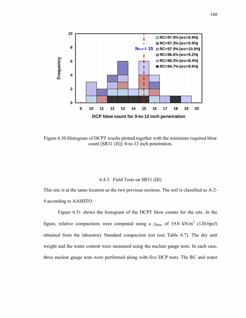
160

0

2

4

6

8

10

9 10 11 12 13 14 15 16 17 18 19 20


Freq

uenc

y


NDCP = 15

Figure 6.30 Histogram of DCPT results plotted together with the minimum required blow count [SR31 (II)]: 0-to-12 inch penetration.

6.4.3. Field Tests on SR31 (III)

This site is at the same location as the two previous sections. The soil is classified as A-2-

4 according to AASHTO.


figure, relative compactions were computed using a γdmax of 19.0 kN/m3 (120.6pcf)

obtained from the laboratory Standard compaction test (see Table 6.7). The dry unit

weight and the water content were measured using the nuclear gauge tests. In each case,

three nuclear gauge tests were performed along with five DCP tests. The RC and water

161

content values in Figures 6.31 through 6.33 represent the arithmetic mean values from

three nuclear gauge tests.


that was associated with at least 80% exceedance for the test results in the histogram of

the test results corresponding to 94.8% RC was 14. Note that in order to determine the

minimum required blow count for this site, test results corresponding to 94.8% RC tested

at wc=8.2% were used because other test results associated with 94.8% RC tested at

wc=6.6% were too dry considering the optimum moisture content of this soil, 12.0%. The

DCP blow count increases as the water content decreases due to the effect of a decreasing

degree of saturation and increased suction. The DCP blow counts tested at 97.5% RC

showed the effect of water content because the test results corresponding to 97.5% RC

are lower than all test results corresponding to 94.8% RC tested at wc=6.6% and some

test results corresponding to 94.0% RC tested at wc=6.3%.

162

0

2

4

6

8

6 7 8 9 10 11 12 13 14 15 16 17 18 19 20 21 22


Freq

uenc

y

RC=97.5% (wc=8.5%)RC=94.8% (wc=6.6%)RC=94.8% (wc=8.2%)RC=94.0% (wc=6.3%)

Figure 6.31 Histogram of DCPT results [SR 31 (III)]: 0-to-12 inch penetration.

0

1

2

3

4

5

6

6 7 8 9 10 11 12 13 14 15 16 17 18 19 20 21 22


Freq

uenc

y

RC=94.8% (wc=8.2%)

NDCP = 14

Figure 6.32 Histogram of DCPT results at 94.8% RC plotted together with the minimum required blow count [SR31 (III)]: 0-to-12 inch penetration.

163

0

2

4

6

8

6 7 8 9 10 11 12 13 14 15 16 17 18 19 20 21 22


Freq

uenc

y

RC=97.5% (wc=8.5%)RC=94.8% (wc=6.6%)RC=94.8% (wc=8.2%)RC=94.0% (wc=6.3%)

NDCP = 14

Figure 6.33 Histogram of DCPT results plotted together with the minimum required blow count [SR31 (III)]: 0-to-12 inch penetration

6.4.4. Field Tests on SR31 (Plymouth)

A subgrade embankment was constructed using A-2-6 soil as fill material as part of the

extension project of State Road 31 in Plymouth, Indiana.


figure, RC was computed using a γdmax of 19.1 kN/m3 (121.3 pcf) obtained from the

laboratory Standard compaction test (see Table 6.7). Also, the dry unit weight and the

water content were measured using nuclear gauge tests. In each case, three nuclear gauge

tests were performed along with ten DCP tests. The RC and the water content in Figures

6.34 through 6.36 represent the arithmetic mean values from three nuclear gauge tests.

164

Based on the test results, the minimum required blow count that was associated

with 80% exceedance for the test results in the histogram of the test results corresponding

to 95.0% RC was 13 (see Figure 6.35). In Figure 6.36, a minimum required blow count of

13 exceeds the blow counts of all DCP tests associated with RC less than 95%, except

one case, and even some test results corresponding to RC greater than 95%.

0

2

4

6

8

10

12

7 8 9 10 11 12 13 14 15 16 17 18 19 20 21 22 23 24 25


Freq

uenc

y


Figure 6.34 Histogram of DCPT results [SR 31 (Plymouth)]: 0-to-12 inch penetration.

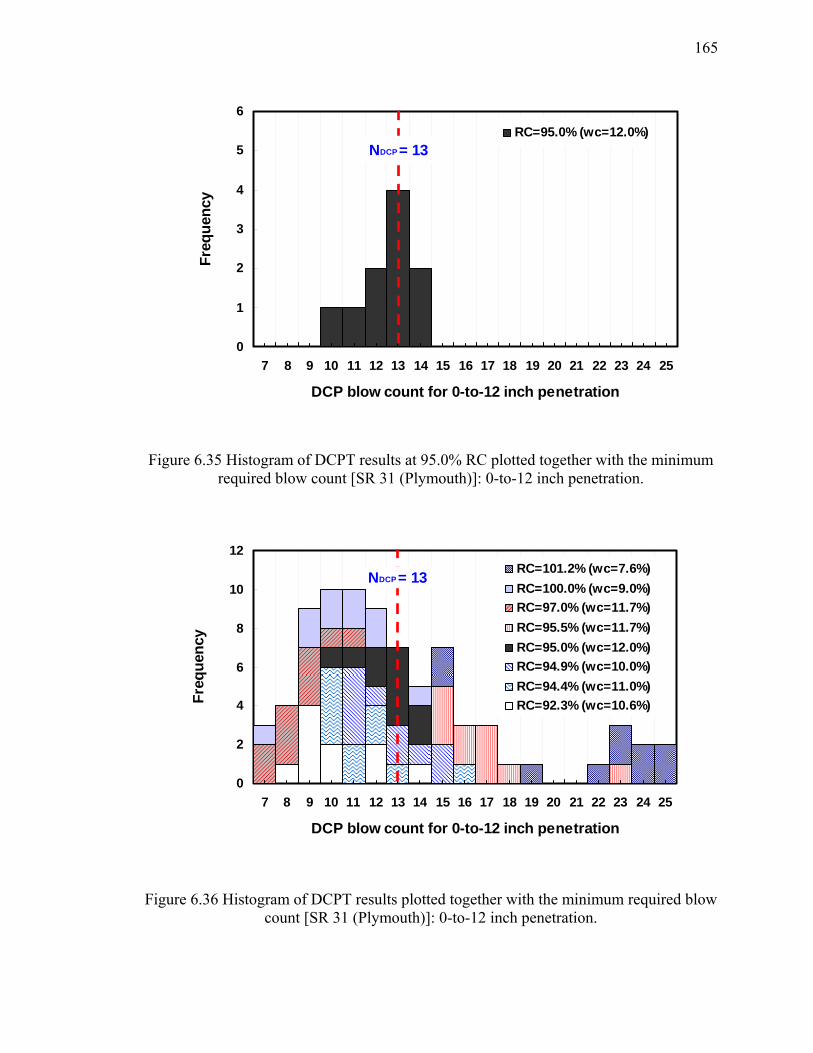
165

0

1

2

3

4

5

6

7 8 9 10 11 12 13 14 15 16 17 18 19 20 21 22 23 24 25


Freq

uenc

y

RC=95.0% (wc=12.0%)NDCP = 13

Figure 6.35 Histogram of DCPT results at 95.0% RC plotted together with the minimum required blow count [SR 31 (Plymouth)]: 0-to-12 inch penetration.

0

2

4

6

8

10

12

7 8 9 10 11 12 13 14 15 16 17 18 19 20 21 22 23 24 25


Freq

uenc

y


NDCP = 13

Figure 6.36 Histogram of DCPT results plotted together with the minimum required blow count [SR 31 (Plymouth)]: 0-to-12 inch penetration.

166

6.4.5. Field Tests on Access Road to Honda Plant

A subgrade embankment was constructed using A-2-6 soil as fill material. The site was a

road extension project for access to the Honda Plant located in Greensburg, Indiana.

DCPT, CHT, and nuclear gauge tests were conducted after every two roller pass

at this site. Thus, several different RC values, from a very low RC up to more than 100%

RC, were attained throughout the testing on the site. Figure 6.37 shows histogram of

DCPT results taken from the site. The (NDCP)req│0~12” that was associated with at least

80% exceedance for the test results in the histogram of the test results corresponding to

95.6% RC was 15 (see Figure 6.38). In the same way, a (NDCP)req│0~12” of 15 was assessed

with the entire test results (see Figure 6.39).

0

1

2

3

4

5

9 10 11 12 13 14 15 16 17 18 19 20 21 22


Freq

uenc

y

RC=101.8% (wc=12.8%) RC=101.7% (wc=11.6%)RC=97.0% (wc=10.3%) RC=96.2% (wc=11.5%)RC=95.3% (wc=10.6%) RC=91.5% (wc=9.9%)RC=89.0% (wc=12.2%)

Figure 6.37 Histogram of DCPT results (access road to Honda plant): 0-to-12 inch penetration.

167

0

1

2

3

4

5

9 10 11 12 13 14 15 16 17 18 19 20 21 22


Freq

uenc

y

RC=95.3% (wc=10.6%)

NDCP = 15

Figure 6.38 Histogram of DCPT results at 95.3% RC plotted together with the minimum required blow count (access road to Honda plant): 0-to-12 inch penetration

0

1

2

3

4

5

9 10 11 12 13 14 15 16 17 18 19 20 21 22


Freq

uenc

y

RC=101.8% (wc=12.8%) RC=101.7% (wc=11.6%)RC=97.0% (wc=10.3%) RC=96.2% (wc=11.5%)RC=95.3% (wc=10.6%) RC=91.5% (wc=9.9%)RC=89.0% (wc=12.2%)

NDCP = 15

Figure 6.39 Histogram of DCPT results plotted together with the minimum required blow count (access road to Honda plant): 0-to-12 inch penetration.

168

Figure 6.40 shows the CIV versus RC for the access road to Honda site. The trend

observed for the CHT results in the test pit (i.e., the higher the RC, the greater the CIV)

was not observed. The average of the test results also decreased as the RC increased. The

test results shown in Figure 6.40 can be explained by the water content of the soil tested

at each relative compaction. Figure 6.41 illustrates the water content versus the CHT test

results.

2

4

6

8

10

12

85 90 95 100 105


CIV

(Cle

gg Im

pact

Val

ue: 9

8m/s

2 )

Honda access road (CIV)Average of the test resultsExpon. (Average of the test results)Trend line

Figure 6.40 CIV versus relative compaction (access road to Honda plant).

169

2

4

6

8

10

12

8 9 10 11 12 13 14

Water content (%)

CIV

(Cle

gg Im

pact

Val

ue: 9

8m/s

2 )

Honda access road (CIV)Average of the test resultsPower (Average of the test results)Trend line

Wet side of OMC

Figure 6.41 The CHT results vs. water contents (access road to Honda plant).

The dynamic resistance of soil increases as the water content decreases due to the

effect of a decreasing degree of saturation and increased suction. Regardless of the effect

of water content on, more precisely, degree of saturation, the CIV versus relative

compaction was again highly variable.

170

6.4.6. Summary of Test Results on A-1 and A-2 Soils

In the case of “granular” soils (A-1 and A-2 soils except containing the gravels), the

minimum required blow count for 0-to-12 inch penetration, (NDCP)req│0~12”, is summarized

in Table 6.8 together with the compaction properties.

Table 6.8 Summary of the DCP results together with compaction properties of “granular” soils

Test site SR31 (I) SR31 (II) SR31 (III) SR31 (Plymouth) Honda

AASHTO classification A-1-b A-2-4 A-2-4 A-2-6 A-2-4

γdmax

(kN/m3) 19.1 19.2 19.0 19.1 18.9

(pcf) 121.3 122.4 120.6 121.3 120.2

wcopt (%) 10.2 10.5 12.0 11.9 10.7

(NDCP)req│0~12” 18 15 14 13 15

The composition of the “granular” soils in Table 6.8 consists of an A-3 soil with a

small percentage of fine particles (10 to 35 percent passing the #200 sieve). The

(NDCP)req│0~12” for this type of soil is influenced by the amount of fine particles that are

present in the soil. Also, the plasticity index of fine particles contained in the soil is also

one of the factors to control DCP blow counts. It is interesting to note that, as indicated in

171

Section 2.4.4, the optimum moisture content correlates both with the amount of fine

particles and with the plasticity index of soil. Based on this concept, we propose the

NDCP│0~12” as a function of the optimum moisture contents shown in Figure 6.42.

NDCP = 59 e-0.12wc opt

R2 = 0.73

8

12

16

20

24

10 11 12 13

Optimum Moisture Content (%)

ND

CP

Figure 6.42 The optimum moisture content vs. the (NDCP)req│0~12” for “granular” soils.

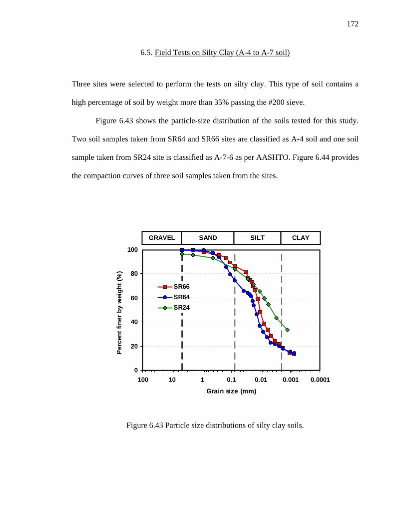
172

6.5. Field Tests on Silty Clay (A-4 to A-7 soil)

Three sites were selected to perform the tests on silty clay. This type of soil contains a

high percentage of soil by weight more than 35% passing the #200 sieve.

Figure 6.43 shows the particle-size distribution of the soils tested for this study.

Two soil samples taken from SR64 and SR66 sites are classified as A-4 soil and one soil

sample taken from SR24 site is classified as A-7-6 as per AASHTO. Figure 6.44 provides

the compaction curves of three soil samples taken from the sites.

0

20

40

60

80

100

0.00010.0010.010.1110100

Grain size (mm)

Per

cent

fine

r by

wei

ght (

%)

SR66SR64SR24

SAND SILT CLAYGRAVEL

Figure 6.43 Particle size distributions of silty clay soils.

173

14

16

18

20

22

4 8 12 16 20 24

Water content (%)

Dry

uni

t wei

ght (

kN/m

3)

ZAVC SR64SR66 SR24

Figure 6.44 Compaction curves of the soil samples from SR66, SR64, and SR24 sites.

Table 6.9 summarizes the grain-size distributions and classifications of the soil

taken from these sites.

Table 6.9 Summary of the plasticity and compaction properties of the soil samples

Site

% passing No.200 sieve

Plasticity γdmax wcopt (%)

AASHTO classification

PL LL PI (kN/m3) (pcf)

SR64 72.0 18.1 20.4 2.3 19.0 120.9 11.7 A-4

SR66 86.2 22.6 26.1 3.5 17.3 110.1 17.7 A-4

SR24 83.8 21.2 43.5 22.3 16.6 105.3 18.4 A-7-6

174


A subgrade embankment was constructed using A-4 soil as fill material. The site is

located at a construction site on State Road 64 in Gibson County, Indiana.

Figure 6.45 shows the histogram of DCPT blow counts for the site. The RC was

computed using a γdmax of 19.0 kN/m3 (120.9 pcf) obtained from the laboratory Standard

compaction test (see Table 6.9). Also, the dry unit weight and the water content were

measured using the sand cone tests. In each case, one sand cone test was performed along

with four DCP tests. In addition, the test results obtained from a test pad built by INDOT

(RC=92.2%) are also plotted in the figure.

175

0

2

4

6

8

10

5 6 7 8 9 10 11 12 13 14 15 16 17 18 19 20 21


Freq

uenc

y

RC=97.0% (wc=12.3%) RC=96.0% (wc=11.0%)RC=92.2% (wc=14.0%) RC=91.9% (wc=11.6%)RC=90.6% (wc=11.4%)

(a)

0

2

4

6

8

10

7 8 9 10 11 12 13 14 15 16 17 18 19 20 21 22 23 24 25 26


Freq

uenc

y


(b)

Figure 6.45 Histograms of DCPT results (SR64): (a) 0-to-6 inch penetration and (b) 6-to-12 inch penetration.

176

Based on the same approach we adopted for other types of soil, we take the

minimum required blow count, (NDCP)req│0~6” being greater than at least 80% of the

occurrences in the histograms of blow counts associated with 96.0% RC was 16 [see

Figure 6.46 (a)]. Similarly, the minimum required blow count, (NDCP)req│6~12” is equal to

26 [see Figure 6.46 (b)]. Comparison of the (NDCP)req│0~6” and (NDCP)req│6~12”” with all test

results is as shown in Figure 6.47. On this site, one out of 20 DCP test results associated

with 92.2% RC exceeded the (NDCP)req│0~6”. For 6-to-12 inch penetration, all DCP test

results associated with less than 95% RC were included by .(NDCP)req│6~12”.

177

0

1

2

3

4

5

6

5 6 7 8 9 10 11 12 13 14 15 16 17 18 19 20 21


Freq

uenc

y

RC=96.0% (wc=11.0%)

NDCP = 16

(a)

0

1

2

3

4

5

6

7 8 9 10 11 12 13 14 15 16 17 18 19 20 21 22 23 24 25 26


Freq

uenc

y

RC=96.0% (wc=11.0%)

NDCP = 26

(b)

Figure 6.46 Histograms of DCPT results at 96.0% RC plotted together with the minimum required blow count (SR64): (a) 0-to-6 inch penetration and (b) 6-to-12 inch penetration.

178

0

2

4

6

8

10

5 6 7 8 9 10 11 12 13 14 15 16 17 18 19 20 21


Freq

uenc

y


NDCP = 16

(a)

0

2

4

6

8

10

7 8 9 10 11 12 13 14 15 16 17 18 19 20 21 22 23 24 25 26


Freq

uenc

y


NDCP = 26

(b)

Figure 6.47 Histograms of the DCPT results plotted together with the minimum required blow count (SR64): (a) 0-to-6 inch penetration and (b) 6-to-12 inch penetration.

179


A subgrade embankment was constructed using A-4 soil as fill material. The site is at the

construction of State Road 66 located in Warrick County, Indiana.



laboratory Standard compaction test (see Table 6.9). The dry unit weight and the water

content were measured using the sand cone tests. In each case, one sand cone test was

performed along with four DCP tests. In addition, the test results obtained from the test

pad by INDOT (RC=92.0%) are also plotted in the figure.

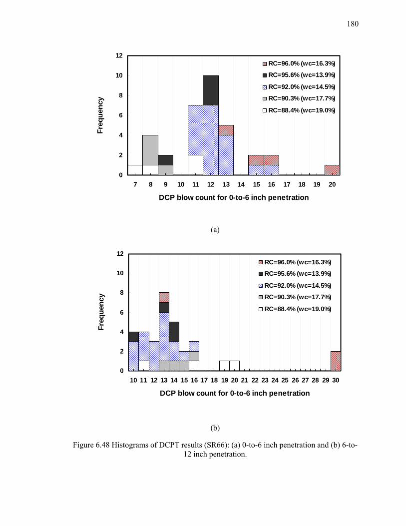
180

0

2

4

6

8

10

12

7 8 9 10 11 12 13 14 15 16 17 18 19 20


Freq

uenc

y

RC=96.0% (wc=16.3%)

RC=95.6% (wc=13.9%)

RC=92.0% (wc=14.5%)

RC=90.3% (wc=17.7%)

RC=88.4% (wc=19.0%)

(a)

0

2

4

6

8

10

12

10 11 12 13 14 15 16 17 18 19 20 21 22 23 24 25 26 27 28 29 30


Freq

uenc

y

RC=96.0% (wc=16.3%)

RC=95.6% (wc=13.9%)

RC=92.0% (wc=14.5%)

RC=90.3% (wc=17.7%)

RC=88.4% (wc=19.0%)

(b)


181

Based on the same approach we adopted to develop the DCP subgrade assessment

criteria for other types of soil, the minimum required NDCP│0~6” that is greater or equal to

at least 80% of occurrences in the histogram of test results associated with a 95.6% RC

was 12. Similarly, the minimum required NDCP│6~12” was equal to 14. However, those

blow counts do not exceed 90% of test measurements corresponding to less than the

required RC. Thus, the minimum required NDCP│0~6” of 15 and NDCP│6~12” of 20 were

reselected to satisfy the requirement (see Figure 6.49). Figure 6.50 shows the minimum

required blow counts for 0-to-6 inch penetration, (NDCP)req│0~6”, and for 6-to-12 inch

penetration, (NDCP)req│6~12”, plotted with all the test results. As shown in the Figure

6.50(a), one out of 20 DCP test results associated with 92.0% RC exceeded the

(NDCP)req│0~6”. In the case of the (NDCP)req│6~12”, no DCP test results associated with less

than required RC exceeded the minimum required blow count.

182

0

2

4

6

8

10

12

7 8 9 10 11 12 13 14 15 16 17 18 19 20


Freq

uenc

y

RC=95.6% (wc=13.9%)

NDCP = 15

(a)

0

1

2

3

4

5

6

10 11 12 13 14 15 16 17 18 19 20 21 22 23 24 25 26 27 28 29 30


Freq

uenc

y

RC=95.6% (wc=13.9%)

NDCP = 20

(b)

Figure 6.49 Histograms of DCPT results at 95.6% RC plotted together with the minimum required blow count (SR66): (a) 0-to-6 inch penetration, and (b) 6-to-12 inch penetration.

183

0

2

4

6

8

10

12

7 8 9 10 11 12 13 14 15 16 17 18 19 20


Freq

uenc

y

RC=96.0% (wc=16.3%)

RC=95.6% (wc=13.9%)

RC=92.0% (wc=14.5%)

RC=90.3% (wc=17.7%)

RC=88.4% (wc=19.0%)

NDCP = 15

(a)

0

2

4

6

8

10

12

10 11 12 13 14 15 16 17 18 19 20 21 22 23 24 25 26 27 28 29 30


Freq

uenc

y

RC=96.0% (wc=16.3%)

RC=95.6% (wc=13.9%)

RC=92.0% (wc=14.5%)

RC=90.3% (wc=17.7%)

RC=88.4% (wc=19.0%)

NDCP = 20

(b)

Figure 6.50 Histograms of DCPT results plotted together with the minimum required blow count (SR66): (a) 0-to-6 inch penetration and (b) 6-to-12 inch penetration.

184


A subgrade embankment was constructed using A-7-6 soil as fill material. The site is at

the construction of State Road 24 located in Fort Wayne, Indiana.



laboratory Standard compaction test (see Table 6.9). The laboratory Standard compaction

test and the sieve analysis results were provided by INDOT. The dry unit weight and the

water content were measured using a nuclear gauge test. In each case, one nuclear gauge

test was performed along with seven DCP tests.

185

0

2

4

6

8

10

12

14

1 2 3 4 5 6 7 8 9 10 11


Freq

uenc

y

RC=105.6% (wc=14.9%)

RC=102.1% (wc=15.8%)

RC=99.2% (wc=16.8%)

RC=98.4% (wc=18.7%)

RC=95.7% (wc=19.5%)

(a)

0

2

4

6

8

10

12

14

1 2 3 4 5 6 7 8 9 10 11


Freq

uenc

y

RC=105.6% (wc=14.9%)

RC=102.1% (wc=15.8%)

RC=99.2% (wc=16.8%)

RC=98.4% (wc=18.7%)

RC=95.7% (wc=19.5%)

(b)


186

Based on the same approach we adopted to develop the DCP subgrade assessment

criteria for other types of soil, the minimum required NDCP│0~6” that is greater or equal to

at least 80% of occurrences in the histogram of test results associated with a 95.7% RC

was 4 [see Figure 6.52 (a)]. Similarly, the minimum required NDCP│6~12” was equal to 5

[see Figure 6.52 (b)]. Figure 6.53 shows the minimum required blow counts for 0-to-6

inch penetration, (NDCP)req│0~6”, and for 6-to-12 inch penetration, (NDCP)req│6~12”, plotted

with all the test results.

187

0

2

4

6

8

10

12

14

1 2 3 4 5 6 7 8 9 10 11


Freq

uenc

y

RC=95.7% (wc=19.5%)

ND C P = 4

(a)

0

2

4

6

8

10

12

14

1 2 3 4 5 6 7 8 9 10 11


Freq

uenc

y

RC=95.7% (wc=19.5%)

ND C P = 5

(b)

Figure 6.52 Histograms of DCPT results at 95.6% RC plotted together with the minimum required blow count (SR24): (a) 0-to-6 inch penetration, and (b) 6-to-12 inch penetration.

188

0

2

4

6

8

10

12

14

1 2 3 4 5 6 7 8 9 10 11


Freq

uenc

y

RC=105.6% (wc=14.9%)

RC=102.1% (wc=15.8%)

RC=99.2% (wc=16.8%)

RC=98.4% (wc=18.7%)

RC=95.7% (wc=19.5%)

ND C P = 4

(a)

0

2

4

6

8

10

12

14

1 2 3 4 5 6 7 8 9 10 11


Freq

uenc

y

RC=105.6% (wc=14.9%)

RC=102.1% (wc=15.8%)

RC=99.2% (wc=16.8%)

RC=98.4% (wc=18.7%)

RC=95.7% (wc=19.5%)

ND C P = 5

(b)

Figure 6.53 Histograms of DCPT results plotted together with the minimum required blow count (SR24): (a) 0-to-6 inch penetration and (b) 6-to-12 inch penetration.

189

6.5.4. Summary of Test Results on Silty Clay

In order to develop for compaction quality control criteria DCPT-based for silty clayey

soil, the test results in the test pit are combined with the test results for the SR64, SR66

and SR24 sites. In the case of silty clayey soils, the minimum required blow counts for 0-

to-6 inch penetration, (NDCP)req│0~6”, and for 6-to-12 inch penetration, (NDCP)req│6~12”, are

given in Table 6.10 along with the Atterberg limits and percent passing the #40 and the

#200 sieve.

Table 6.10 Summary of the DCP results with the plasticity and percent passing the #200 sieve on silty clay soils

Test site SR64 SR66 SR24 Purdue test pit

AASHTO classification A-4 A-4 A-7-6 A-4

Percent passing the #40 sieve 97.4 96.8 93.4 72.3

Percent passing the #200 sieve 72.0 86.2 83.8 52.1

PL (%) 18.1 22.6 21.2 12.6

LL (%) 20.4 26.1 43.5 22.3

PI (%) 2.3 3.5 22.3 9.7

(NDCP)req|0~6” 16 15 4 8

(NDCP)req|6~12” 26 20 5 12

According to the AASHTO classification, a silty clayey soil contains a significant

amount of fine particles (from 35% to 100%). The dynamic resistance is influenced by

190

the amount of fine particles in addition to the plasticity index which is an indicator of the

characteristics of the fine particles. Thus, the minimum required blow count correlates

with the plasticity index and the amount of fine particles. Since the Atterberg limit tests

are performed using the soil passing the #40 sieve, according to ASTM D4318-05, we

propose the minimum required blow count for silty clayey soils as a function of the

plastic index (PI) and percent passing the #40 sieve. The relationship appears in Figure

6.51.

NDCP = 27e-0.08(PI)(%passing #40)/100

R2 = 0.95

NDCP= 17e-0.07(PI)(%passing #40)/100

R2 = 0.93

0

5

10

15

20

25

30

0 5 10 15 20 25

(PI× F40)/100

ND

CP

For 0-6 inches penetration

For 6-12 inches penetration

Figure 6.54 The (PI)(%passing the #40 sieve) versus the (NDCP)req│0~6” and (NDCP)req│6~12” for silty clayey soil.

191

6.6. Summary

A comprehensive experimental program was undertaken to assess the DCPT and the

CHT as tools for soil compaction quality control. The main objective of the experimental

program was to investigate the DCPT and CHT test results for various soil types on road

sites and also in a test pit at Purdue University. The DCP test results are summarized in

Table 6.11. Note that the minimum required blow counts should be rounded up to the

nearest integer.

Table 6.11 Relationship between NDCP, Cu, wcopt, PI, and percent the #40 passing sieve

Type of soil Parameters

in correlation

Relationship

A-3 soils NDCP│0~12” Cu NDCP│0~12” = 4.0 ln(Cu) +2.6 (see Figure 6.22, R2=0.99)

“Granular” soils NDCP│0~12” wcopt

NDCP│0~12” = 59exp(-0.12wcopt) (see Figure 6.42, R2=0.73)

Silty, clayey soils

NDCP│0~6” PI, %

passing the #40 sieve

NDCP│0~6” = 17exp[-0.07(PI)(%passing #40)/100]

(see Figure 6.51, R2=0.93)

NDCP│6~12” PI, %

passing the #40 sieve

NDCP│6~12” = 27exp[-0.08(PI)(%passing #40)/100]

(see Figure 6.51, R2=0.95)

In order to facilitate the use of DCP criteria as a quality tool in INDOT sites, we

also introduce the tables based on the relationships that were presented in Table 6.11.

First, for A-3 soils, we propose the (NDCP)req│0~12” for A-3 soils that is a function of the

192

coefficient of uniformity. Table 6.12 presents (NDCP)req│0~12” for typical coefficient of

uniformity values.

Table 6.12 Relationship between (NDCP)req│0~12” and coefficient of uniformity (Cu)

Coefficient of uniformity (Cu) NDCP│0~12” 2 6 3 7 4 9 5 10 6 10 7 11 8 11

Second, we propose the NDCP│0~12” as a function of the optimum moisture

contents. Table 6.13 presents (NDCP)req│0~12” for typical optimum moisture content values.

Table 6.13 Relationship between (NDCP)req│0~12” and optimum moisture content (wcopt)

optimum moisture content (wcopt) NDCP│0~12” 10 18 11 16 12 14 13 13 14 11

Lastly, we propose the minimum required blow count for silty clayey soils as a

function of the plastic index (PI) and percent passing the #40 sieve. Table 6.14 presents

(NDCP)req│0~12” for typical PI and percent passing the #40 sieve values.

193


PI (%) #40 passing sieve (%) NDCP│0~6” NDCP│6~12”

3

70 15 23 80 15 23 90 15 22 100 14 22

6

70 13 20 80 13 19 90 12 18 100 12 17

9

70 11 17 80 11 16 90 10 15 100 10 14

12

70 10 14 80 9 13 90 8 12 100 8 11

15

70 9 12 80 8 11 90 7 10 100 6 9

18

70 8 10 80 7 9 90 6 8 100 5 7

21

70 7 9 80 6 8 90 5 6 100 4 6

24

70 6 8 80 5 6 90 4 5 100 4 4

194

The DCPT appears to hold some promise as an economical tool for soil

compaction quality control. Minimum required blow counts for RC ≥ 95% with high

probability were determined, but these results are preliminary and further research is

advised. With respect to the CHT, considerable variability was observed. The research

team and the study advisory committee decided to not explore the CHT further at this

time.

195

CHAPTER 7. DYNAMIC CONE PENETRATION TESTS AND CLEGG HAMMER TESTS PERFORMED IN A TEST CHAMBER

7.1. Introduction

This chapter describes dynamic cone penetration tests, Clegg hammer tests, and static

load tests performed in a large-scale chamber. The chamber is located in the Bowen

Laboratory for Large-Scale Civil Engineering Research at Purdue University. The details

of the test chamber and pluviation procedure were presented by Lee (2008). The purpose

of the tests was to obtain dynamic test results as well as static test results under fully

controlled conditions in a large-scale test chamber, in order to avoid the uncertainties that

are inevitable in the field.

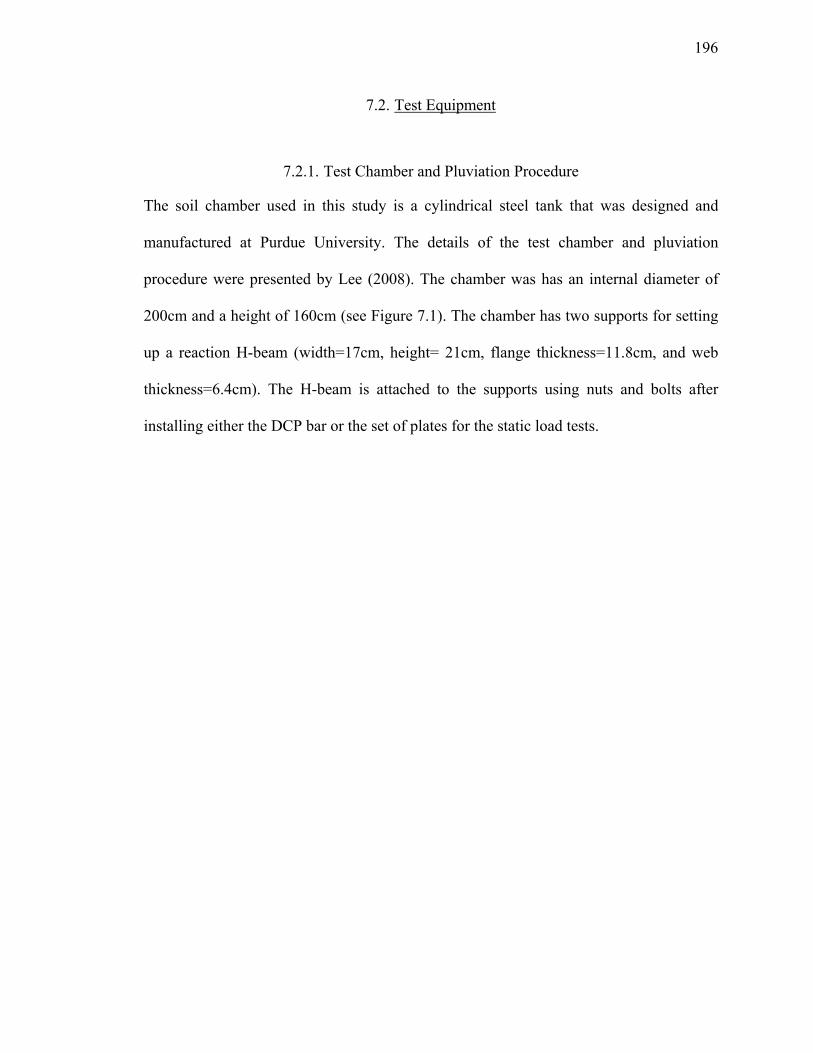
196

7.2. Test Equipment

7.2.1. Test Chamber and Pluviation Procedure

The soil chamber used in this study is a cylindrical steel tank that was designed and

manufactured at Purdue University. The details of the test chamber and pluviation

procedure were presented by Lee (2008). The chamber was has an internal diameter of

200cm and a height of 160cm (see Figure 7.1). The chamber has two supports for setting

up a reaction H-beam (width=17cm, height= 21cm, flange thickness=11.8cm, and web

thickness=6.4cm). The H-beam is attached to the supports using nuts and bolts after

installing either the DCP bar or the set of plates for the static load tests.

197

1.6 m

Reaction beam

Holes for draining

sand

1.6 m

Reaction beam

Holes for draining

sand

Figure 7.1 Photograph of the soil chamber (modified after Lee 2008).

A sand pluviator was used to prepare sand samples in the chamber with the

desired density. The sand pluviator enabled control of the relative density of the sand

deposited in the chamber. The pluviator also facilitated the pouring of sand into the

chamber. In order to facilitate the removal of the sand pluviated in the chamber after the

tests, the chamber contains two drain holes on the side (see Figure 7.1).

Figure 7.2 shows a schematic view of the sand pluviator used in this research. The

diameter of the sand pluviator is 190.5 cm. The pluviator consists of a shallow steel

cylinder of height 15.2 cm. The bottom of the cylinder has two layers: one layer is a

perforated circular steel plate and the other layer is a perforated acrylic plate of the same

198

size as the steel plate. When the holes of the plates are not aligned, then they work as a

shutter plate. These plates are positioned to produce an identical hole pattern for

pluviation to begin.

The relative density of the sand deposited in the chamber using the sand pluviator

is controlled by the dropping velocity of the sand particles. The relative density of the

sand deposited in the chamber is controlled by two factors: (1) the opening size of the

sieves at the bottom of the pluviator (see Figure 7.2), and (2) the sand drop height. The

two sieves located below the shutter plate have different opening sizes [No. 6 (3.35 mm)

and No. 16 (1.18 mm)].

199

Depositedsand

Rainingsand

Falling sand jets

Sandsupply

Chains

Diffusersieves

Shutter plate

Hoist

Depositedsand

Rainingsand

Falling sand jets

Sandsupply

Chains

Diffusersieves

Shutter plate

Hoist

Figure 7.2 Schematic view of the sand pluviator (modified after Lee 2008).

The pluviator falling height was controlled by a gantry crane of a 1,000 kg

capacity. The gantry crane moved the pluviator freely so that it could be located above

the chamber during sand deposition and away from it during testing.

7.2.2. Engineering Properties of Test Sand

According to the Unified Soil Classification System (USCS), the test sand was classified

as poorly graded sand. The test sand, referred to as F-55 sand, was obtained from the U.S.

Silica company in large quantities with consistent properties. It has engineering

200

properties similar to those of ASTM standard Ottawa sand (designated as ASTM C778-

06). Table 7.1 summarizes the engineering properties of F-55 sand.

Table 7.1 Engineering properties of F-55 sand (data from Lee 2008)

Engineering property Value

Specific Gravity (Gs) 2.65

Effective particle size (D10) 0.15mm

Mean particle size (D50) 0.23mm

Coefficient of Uniformity (Cu) 1.67

Coefficient of Curvature (Cc) 1.07

Percentage passing No.200 sieve (%) 0

Max. dry unit weight (γdmax) 17.66 kN/m3

Min. dry unit weight (γdmin) 14.62 kN/m3

Min. void ratio (emin) 0.78

Max. void ratio (emax) 0.47

Critical-state friction angle (φc) 32.8°

Grain shape description Rounded to subrounded

201

0

20

40

60

80

100

0.010.1110

Grain size (mm)

Per

cent

fine

r by

wei

ght (

%)

Ottawa sandF-55 sand

SAND SILTGRAVEL

Figure 7.3 Grain size distribution of F-55 sand and Ottawa sand (modified after Lee 2008).

Figure 7.4 shows a micrograph of the F-55 sand grains obtained using the

Scanning Electron Microscope (SEM). The micrograph shows that the shape of the sand

particles are rounded to subrounded. The dominant mineral of the sand is silica (SiO2),

which is the main mineral of quartz.

According to Lee (2008), the critical-state friction angle of F-55 sand was

obtained from the results of triaxial tests performed under confining pressures ranging

from 50 kPa to 200 kPa. Since axial strains greater than 26% were not reached in these

tests due to the limitations of the test apparatus, the extrapolation technique suggested by

Murthy et al. (2007) was used for determining the critical-state friction angle. The

critical-state friction angle was determined to be 32.8°.

202

Figure 7.4 A SEM micrograph of F-55 sand grains.

With respect to the scale effects in the chamber, two factors were considered.

First, the ratio of the diameter of the DCP to that of the sand particles sizes. If the size of

the soil particles becomes too large compared with the DCP diameter, the particulate

nature of soil (i.e., the geometry of the particles and their arrangement) will have too

great an influence on the test results. Related to this factor, Ovesen (1975) demonstrated

that, in centrifuge testing, the particle size effects become significant for pile

circumference to mean particle size (D50) ratios less than 40 for foundations on quartz

sand. Bolton et al. (1999) indicated that the soil particle size does affect cone

penetrometer measurements for the ratios of the width (B) of the cone to D50 below about

20. In this research, B/D50 was approximately 87 (tip) and 70 (bar), which were greater

than the suggested values in the literature. Certainly, the CHT satisfies this requirement

because the diameter of the Clegg Hammer is larger than that of the DCP.

203

Second, the ratio DL of chamber diameter to the diameter of the Clegg Hammer

and the DCP is another important factor. The tests on soil chambers cannot perfectly

simulate full-scale field tests due to the boundary effects of the chamber. Salgado et al.

(1998) indicated that initial values of relative density and stress state mainly control the

ratio DL at which the size effect is no longer important. In the case of cone, as in the case

of the DCP, Parkin et al. (1980) suggested that a chamber-to-penetrometer diameter ratio

of at least 50 is desirable for dense sand and 20 for loose sand. Been et al. (1986)

proposed that the ratio must be greater than 50 for dense sand to minimize the effect of

the chamber size on the test results. Similarly, Schnaid and Houlsby (1991) suggested,

based on numerical and experimental studies, that the chamber-to-probe diameter ratio

should be at least 50 in dense sand to eliminate chamber size effects. However, based on

the penetration-resistance analysis, Salgado et al. (1998) showed that, in order to

minimize chamber size effects on cone resistance, the ratio DL should be larger than 150.

In this study, the chamber-to-DCP diameter ratio was about 50.

For the plate load test, the chamber-to-plate diameter ratio is another factor that

needs to be addressed. According to Salgado and Lee (1999), the size effects in

calibration chambers are more pronounced in dense sands than in loose sands. Recently,

based on finite element analysis, Loukidis and Salgado (2009) showed that the slip

surfaces below a circular footing extended up to about eight times the circular footing

diameter to the sides in the dense sand with φ = 40°. In this study, the ratio of the

diameter of the chamber to the diameter of the CHT was 14.5 with φc = 32.8°.

204

7.2.3. Details of Instrumentation

(1) Static load tests

The DCP used for the static load tests is identical to the one described in section

3.3.6 and ASTM D6951-03. The plate load tests were performed with a steel plate

13.75cm in diameter, which is very close to the diameter of the Clegg Hammer (13.0 cm

in diameter). A set of circular steel bearing plates were arranged in pyramidal fashion to

ensure rigidity, as per ASTM D 1196-03. Figure 7.5 shows (a) the DCP bar and (b) the

set of plates installed for the static load test.

205

(a)

(b)

Figure 7.5 Photographs of (a) DCP bar, and (b) set of plates used in the tests.

206

The instrumentation used for both static loads tests (with the DCP or the plates)

was identical. In order to apply the load on the DCP or the plates, a hydraulic jacking

pump was used. The reaction to the applied load was provided by the H-beam connected

to the soil chamber. A load cell installed on the hydraulic jack was used for measuring

the load applied on the DCP or the plates. The maximum capacity of the load cell is 20

kN, with a resolution of 0.01N. Also, the maximum displacement of the Linearly

Variable Differential Transducers (LVDT) is 50mm, with a resolution of 0.0001mm. In

order to record the load cell and the LVDT data, a data acquisition system, the CR5000

manufactured by Campbell Scientific, was used.

(2) Dynamic Cone Penetrometer Tests

A Pile Driving Analyzer (PDA) was used to record the values the DCP

penetration data. The dynamic measurements were taken with two piezoelectric

accelerometers attached in pairs on both sides of the DCP head (see Figure 7.6). Figure

7.6 shows the equipment used in the dynamic load tests.

207

PDA

DCP hammer

Accelerometers

DCP bar

PDA

DCP hammer

Accelerometers

DCP bar

(a)

DCP bar

Accelerometers

DCP bar

Accelerometers

(b)

Figure 7.6 Photographs of (a) the Pile Driving Analyzer, and (b) the accelerometers attached on the DCP bar.

208

(3) Clegg Hammer Tests

The CHT apparatus (Model 95055A) used for the tests was manufactured by the

Lafayette Instrument Co., Lafayette, IN. As indicated in CHAPTER 3, this model

includes the hammer, which is 10kg weight, 0.3m diameter, and 0.13m drop height. An

accelerometer was attached on the hammer by the manufacturer. Tektronix Model No.

TDS 3014B Oscilloscope by Tektronix Co. was used to record the acceleration of the

hammer. Figure 7.7 shows the equipment used in the dynamic load tests.

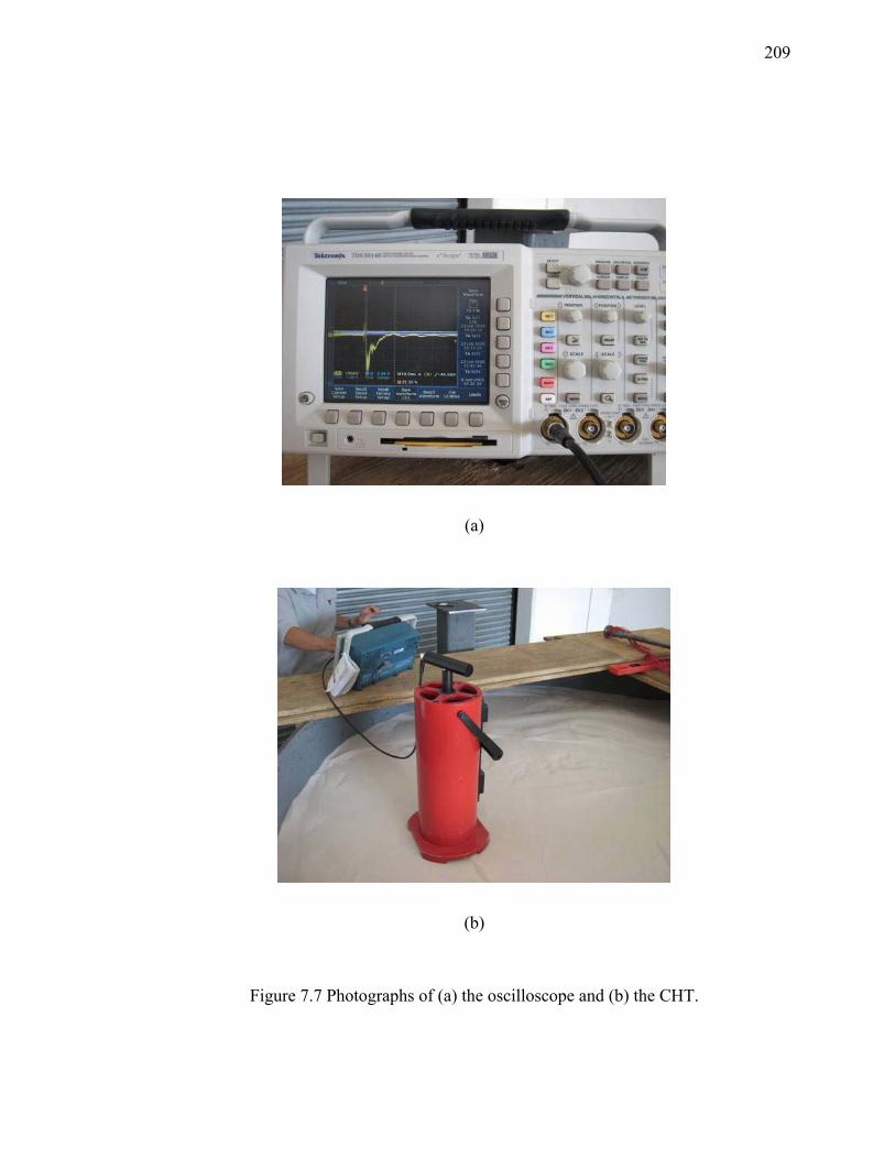
209

(a)

(b)

Figure 7.7 Photographs of (a) the oscilloscope and (b) the CHT.

210

7.2.4. Test Procedure

(1) Preparation of the sand samples in the chamber

Prior to performing the DCPT or CHT, the test sand was pluviated into the soil

chamber. The final height of the sand samples prepared in the chamber was about 140cm.

The target relative density values for dense and medium dense sand samples were about

91% and 58%, respectively, which correspond to relative compaction values of 98.1%

and 91.8%. Based on the preliminary tests, dense sand samples were prepared with a drop

height of 60cm using both sieves No. 6 and No.16, while medium dense sand samples

were prepared with a drop height of 40 cm using only sieve No.6. The variability in the

relative density values was about ±2.1% for dense sand samples and ±2.3% for medium

dense sand samples (Lee 2008).

(2) Test procedure for the static load tests

The DCP load tests were performed in accordance with ASTM D 1143. After

depositing the sand in the chamber, the DCP was inserted up to about 90cmin the sand

sample. The H-beam was then positioned and attached to the two supports on both sides

of the soil chamber. Four sets of nuts and bolts were used to firmly attach the H-beam to

each of the supports. The hydraulic jacking pump, the calibrated load cell, and the

LVDTs were placed in between the head of the DCP bar and the H-beam [see Figure 7.8

(a)]. The LVDTs were installed at equal distances from the center of the DCP. Magnetic

holders were used to attach the LVDTs to the reference beam. During the static load tests,

the load applied to the head of the DCP was measured by the load cell, while the

displacement of the DCP bar was measured by the two LVDTs. The load was applied in

211

increments of 0.1 kN. At each step, the load was maintained until the displacement

measurement was stabilized.

The plate load tests were performed in accordance with ASTM D 1196-93. After

placing the set of plates on the surface of the sand sample, the load cell and the LVDTs

were positioned in the same manner as in the DCP tests [see Figure 7.8 (b)].

212

(a)

(b)

Figure 7.8 Static load test set-up for (a) the DCP tests, and (b) the plate load tests.

LVDT

Reaction beam

plate

Hydraulic jack

Load cell

LVDT

Reaction beam

DCP

Hydraulic jack

Load cell

213

(3) Test procedure for the dynamic tests

The DCP used for this research has the same geometry presented in Section 3.3.6,

also specified in ASTM D6951-03. The DCP has an 8kg drop hammer, and the drop

height is 57.5cm. The DCP penetration per hammer blow was recorded during the test.

The CHT used for the research is Model No. 95055A manufactured by Lafayette

Co. The CHT has 10kg drop hammer, and the drop height is 30.0cm. When a CHT was

performed, the Clegg hammer was lifted and dropped from a fixed height that was

determined by the size of the cylinder surrounding the Clegg Hammer. For each hammer

blow, the acceleration was recorded using the oscilloscope.

7.3. Chamber Test Results

7.3.1. Static Test Results

(1) DCP load test results

Figure 7.9 presents the limit load versus settlement curves for the DCP load tests

performed in dense and medium dense sand samples. The ultimate load Qb,10% associated

with the load based on a settlement equal to 10% of the DCP diameter for dense sand was

2.7 times larger than that of medium dense sand.

214

0

2

4

6

8

10

12

14

16

0 500 1000 1500 2000 2500

Qb (N)

DCP

hea

d se

ttlem

ent (

mm

)

Dense sand (RC=98%)Medium dense sand (RC=92%)

Qb,10%

Figure 7.9 Static load-settlement curves obtained for dense and medium dense sand using dynamic cone penetrometer.

215

(2) Plate load test results

Figure 7.10 shows the load versus settlement curves obtained for the set of plates

tested on dense and medium dense sand samples. The limit load (QbL) for dense sand was

2.6 times larger than that of medium dense sand. Also, the load-settlement curve for

dense sand showed a peak value, while the curve for medium dense sand did not show

any peak. Different bearing capacity failure modes were observed on the sand surface for

these tests. In the case of the dense sand sample, the slip surfaces extended all the way to

the soil surface [see Figure 7.11 (a)], whereas no slip surfaces were observed on the

surface of the medium dense sand sample [Figure 7.11 (b)].

0

1000

2000

3000

4000

0 5 10 15 20 25

Settlement of the plate (mm)

Qb

(N)

Dense sand (RC=98%)

Medium dense sand (RC=92%)

Figure 7.10 Load-settlement curves for the plates bearing on sand.

216

(a)

(b)

Figure 7.11 Photographs of the surface of the samples after testing on (a) dense sand and (b) medium dense sand.

217

7.3.2. Dynamic Test Results

(1) DCP test results

Dynamic tests were performed for dense (RC=98.1%) sand samples only. Figures

7.12(a) and (b) show the penetration and velocity time history curves at the head of the

DCP for several depths. The figure shows that the penetration values decreased as the

depth of penetration increased.

218

0

10

20

30

40

50

0 0.01 0.02 0.03 0.04 0.05

Time (sec)

Pene

trat

ion

per b

low

(mm

)

Depth: 31cmDepth: 39cmDepth: 53cmDepth: 61cmDepth: 69cm

(a)

-1

0

1

2

3

4

5

0 0.01 0.02 0.03 0.04 0.05

Time (sec)

Vel

ocity

(m/s

)

Depth: 31cmDepth: 39cmDepth: 53cmDepth: 61cmDepth: 69cm

(b)

Figure 7.12 Time history curves at several depths of (a) penetration, and (b) velocity.

219

Figure 7.13 compares the measured displacement at the DCP head vs. the

calculated displacement from the PDA. The displacements at the DCP head were directly

measured using a ruler after each blow, while the calculated displacements were found

using the acceleration rates recorded by the PDA. The figure shows that the measured

and computed penetration values are in reasonable agreement.

0

10

20

30

40

50

60

0 10 20 30 40 50 60

Measured penetration per blow (mm/blow)

Calc

ulat

ed p

enet

ratio

n pe

r bl

ow (m

m/b

low

)

Figure 7.13 Measured vs. calculated penetration per blow (mm/blow) at the DCP head.

220

(2) CH test results

Figure 7.14 shows the acceleration vs. time curves for each blow. As the

measured acceleration with time history shows, initially acceleration values peaked

quickly and then decreased to almost zero within five milliseconds. The curves also show

that this trend was very similar regardless of the number of blows, but the maximum

acceleration decreased as the number of blows increased.

-2.0

0.0

2.0

4.0

6.0

8.0

0 5 10 15 20 25 30

Time (ms)

Cleg

g Im

pact

Val

ue (9

8m/s

2 )

4th blow2nd blow1st blow

Figure 7.14 Acceleration versus time history for Clegg Hammer Tests on dense sand.

Figure 7.15 shows the CIV (Clegg Impact Value) vs. the relative compaction of

the sand samples tested. In the case of a RC of 98.1%, CIV varied mostly between 5.0

and 9.2, but was mostly below 7.7. In the case of a RC of 91.8%, the CIV was not

recorded with many cases because of the lower limit of the data acquisition. However,

221

some CIV values were recorded and varied between 5.0 and 6.8. According to Lafayette

Co., the CIV can be recorded if the value exceeds 3.0 (Lafayette Co. 2008, personal

communication). To summarize, the CIV varied significantly even for the same relative

compaction.

2

4

6

8

10

88 91 94 97 100


CIV

(Cle

gg Im

pact

Val

ue: 9

8m/s

2 )

CHT results in the Chamber


Figure 7.15 CIV versus relative compaction for the sand sample.

222

7.4. Summary

The chapter discussed presented the Dynamic Cone Penetration Test (DCPT) and the

Clegg Hammer Test (CHT) performed in a test chamber. The test conditions and the test

program were explained. The test procedure for both the static tests and the dynamic tests

were discussed in detail. The dimensions of the test chamber were large enough and of

the silica sand particles small enough to minimize scale effects.

Static load tests were performed on the DCP rod and cone and on a plate with the

same size as the Clegg Hammer. In the case of the DCP, the ultimate load Qb,10%

associated with a settlement equal to 10% of the DCP diameter for dense sand was 2.7

times larger than that of medium dense sand. In the case of the plate with the same size as

the Clegg hammer, the limit load for dense sand was 2.6 times larger than that for

medium dense sand.

It was shown that integration of measured accelerations leads to reasonable

estimates of the penetration of the DCP into the soil. For CHT, the acceleration of the

Clegg hammer was recorded on the soil in a test chamber. The acceleration values peaked

quickly and then decreased to almost zero within five milliseconds. In the case of 98.1%

RC, the CIV varied between 5.0 and 9.2, but was mostly below 7.7. .

223

CHAPTER 8. INTERPRETATION OF THE RESULTS USING DYNAMIC ANALYSIS

8.1. Introduction

This chapter discusses the DCPT and CHT results by comparing them with the

predictions done using the analyses using the selected models presented in CHAPTER 5

and proposes a framework for the interpretation of the results of these tests for soils. The

predicted test results were compared with the results of preliminary tests performed in a

test pit outside the Bowen laboratory, presented in section 6.2, and with results of tests

performed in the soil chamber, presented in section 7.3. The measured DCP blow counts

(NDCP) were compared with the predicted values. The measured Clegg Impact Values

(CIV), which are the peak decelerations of the hammer upon impact with the soil, were

compared with the predicted maximum deceleration values.

224

8.2. Input Parameters for the Dynamic Analyses

The input parameters for the dynamic analyses are summarized in Table 8.1. Each is

discussed in detail next.

Table 8.1 Input parameters for the dynamic analyses

Input parameters Clegg Hammer Test (CHT)

Dynamic Cone Penetration Test

(DCPT)

In-place dry unit weight (γd) ∨ ∨

Specific gravity (Gs) ∨ ∨

Max. shear modulus (Gmax) ∨ ∨

Poisson’s ratio of the soil (v) ∨ ∨

Critical-state friction angle of the soil (φc) for sand ∨ ∨

Undrained shear strength (su) of clay ∨ ∨

Constants for viscous damping (m and n) ∨ ∨

Geometry of DCP bar and the tip (diameter of bar and tip and length) ∨

Geometry of Clegg Hammer (Radius, weight, and drop height) ∨

Impact velocity ∨

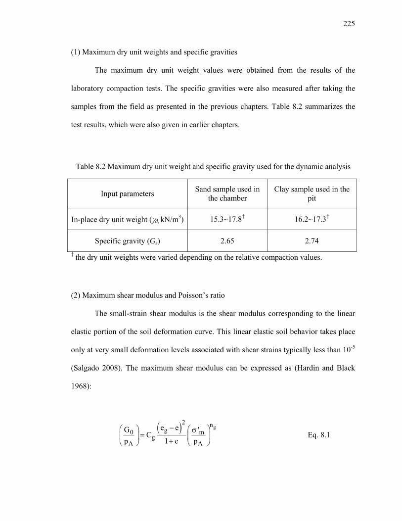
225

(1) Maximum dry unit weights and specific gravities

The maximum dry unit weight values were obtained from the results of the

laboratory compaction tests. The specific gravities were also measured after taking the

samples from the field as presented in the previous chapters. Table 8.2 summarizes the

test results, which were also given in earlier chapters.

Table 8.2 Maximum dry unit weight and specific gravity used for the dynamic analysis

Input parameters Sand sample used in the chamber

Clay sample used in the pit

In-place dry unit weight (γd, kN/m3) 15.3~17.8† 16.2~17.3†

Specific gravity (Gs) 2.65 2.74 † the dry unit weights were varied depending on the relative compaction values.

(2) Maximum shear modulus and Poisson’s ratio

The small-strain shear modulus is the shear modulus corresponding to the linear

elastic portion of the soil deformation curve. This linear elastic soil behavior takes place

only at very small deformation levels associated with shear strains typically less than 10-5

(Salgado 2008). The maximum shear modulus can be expressed as (Hardin and Black

1968):

( ) g

2 ng0 m

gA A

e eG 'Cp 1 e p

−⎛ ⎞ ⎛ ⎞σ=⎜ ⎟ ⎜ ⎟+⎝ ⎠ ⎝ ⎠

Eq. 8.1

226

where pA is a reference stress (= 100kPa = 0.1MPa ≈ 1tsf), σ'm = (σ'v + 2σ'h)/3 is the mean

effective stress after consolidation but before any shearing has taken place; Cg, eg, ng are

constants for a given soil. Thus, G0 varies depending on the in-place unit weight and

depth of soil. Figure 8.1 shows the distribution of computed G0 in a chamber.

0

0.1

0.2

0.3

0.4

0.5

0.6

0.7

0 10,000 20,000 30,000 40,000

Gmax (kPa)

Dep

th (m

)

RC=98%RC=96%RC=94%RC=92%RC=90%

Figure 8.1 G0 values for the test sand

The Poisson’s ratio of soil at very low strain ranges between 0.1 and 0.2 for sand

and is a little higher for clay. The value of Poisson’s ratio of saturated clay reaches 0.5

227

under undrained conditions. For the dynamic analysis, the Poisson’s ratio of 0.15 was

used for the sand, 0.3 for the clay.

(3) Shear strength of soil

The shear strength of sand is determined by the mobilized friction angle. The

critical-state friction angle values range from 28o to 36° for most clean silica sands

(Salgado 2008). In the dynamic analysis, the critical-state friction angle of 32.8o was used,

which was obtained from the triaxial compression tests, presented in CHAPTER 7.

The undrained shear strength of clay can be measured by performing Cone

Penetration Tests (CPT) in the field or by performing unconfined compression tests in the

laboratory. In the dynamic analysis, we used the undrained shear strength obtained from

the unconfined compression tests presented in CHAPTER 6.

(4) The geometry of in situ dynamic tests

The geometry of the DCP is specified in ASTM D 6951-03, which is used for the

dynamic analysis. The geometry of the CHT depends on the apparatus used. Since we

used Model 95055A in testing, the weight of the Clegg hammer of the model is 10kg

with a drop height of 0.3m.

(5) Impact velocity of Clegg hammer

With respect to the impact velocity of the Clegg hammer, the coefficient of

restitution is assumed to be 0 (perfectly plastic impact). The ratio of the rebound velocity

and the impact velocity is normally referred to as the coefficient of restitution. According

228

to Roesset et al. (1994), this coefficient is not very sensitive to the impact velocity. If the

principle of conservation of energy is applied, the following equations can be set:

( )212 c cT m u= Eq. 8.2

where T is energy at the time of impact (=29.42J from the geometry of Clegg hammer),

mc is the mass of Clegg hammer, and uc is the approach velocity of Clegg hammer right

before the impact. Hence, the Clegg hammer and underlying soil move together right

after the impact. Since this mass of the soil is very small, it is negligible. As a result,

based on Eq. 8.2., the impact velocity of the Clegg hammer is 2.40 m/s.

229

8.3. Validation of the Results of the Tests Performed in the Purdue Test Chamber

8.3.1. Prediction of Static Test Results in Sand

There are numerous methods available for estimating the static bearing capacity of a

circular footing (or of a circular plate, as is the case here for the Clegg Hammer Test). In

this research, as discussed in CHAPTER 5, the representative mean effective stress

suggested by Loukidis and Salgado (2006) was employed for the analysis.

Figure 8.2 compares computed bearing capacities with capacities obtained from

plate load tests performed on the sand in the chamber. For the comparison, the computed

bearing capacities using the representative mean effective stress suggested by Perkins and

Madson (2000) were also plotted on Figure 8.2. At two different relative compaction

values, the plate load test results validated the effectiveness of the representative mean

effective stress suggested by Loukidis and Salgado (2006).

230

500

1500

2500

3500

4500

5500

88 90 92 94 96 98 100


QbL

(N)

Plate load test resultsPerkins (2000)Loukidis and Salgado (2006)

Figure 8.2 Comparison of predicted and measured capacities for plate load tests performed on dense and medium dense sand samples.

With respect to the static bearing capacity of the DCP, the equation by Salgado

and Prezzi (2007) was adopted for the analysis. Again, the static load tests were

performed as discussed in section 7.3.1 and test results were compared with the solutions

based on the equation by Salgado and Prezzi (2007). Table 8.3 summarizes the measured

and predicted limit capacities.

231

Table 8.3 Summary of measured and predicted static penetration resistance of the DCP

Unit weight of sand

(KN/m3) DR G0 (MPa)

QbL (N)

Predicted Measured

16.25 58 34.8 1104 667

17.37 91 41.7 3098 1893

Based on the comparison, the equation overestimates the limit bearing capacity.

This is because the static load tests were conducted under low confining pressure

condition, hence Q=10 and R=1 cannot be adopted, which were used for the development

of the equation by Salgado and Prezzi (2007). Based on the comparison between test

results and the solution of the equation, static resistances by Salgado and Prezzi (2007)

were about 1.6 times larger than the measured static resistance as shown in Table 8.3.

Thus, the equation by Salgado and Prezzi (2007) could be rewritten as:

( )R0.841 0.0047D

bL hc c R

A A

q 'exp 0.1041 0.0264 0.0002 Dp p

−⎛ ⎞σ

⎡ ⎤= φ + − φ ⎜ ⎟⎣ ⎦⎝ ⎠

Eq. 8.3

8.3.2. Prediction of Dynamic Test Results in Sand

The equation of motion presented in section 5.4.1 was used for the dynamic analysis.

Based on the equation along with numerical scheme, the acceleration can be obtained.

Since the CHT is a Single Degree Of Freedom (SDOF) problem, spreadsheet can be used

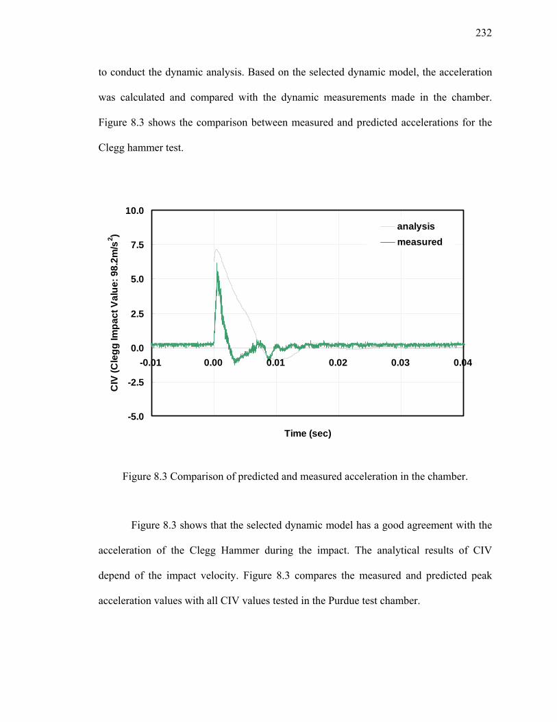
232

to conduct the dynamic analysis. Based on the selected dynamic model, the acceleration

was calculated and compared with the dynamic measurements made in the chamber.

Figure 8.3 shows the comparison between measured and predicted accelerations for the

Clegg hammer test.

-5.0

-2.5

0.0

2.5

5.0

7.5

10.0

-0.01 0.00 0.01 0.02 0.03 0.04

Time (sec)

CIV

(Cle

gg Im

pact

Val

ue: 9

8.2m

/s2 )

analysismeasured

Figure 8.3 Comparison of predicted and measured acceleration in the chamber.

Figure 8.3 shows that the selected dynamic model has a good agreement with the

acceleration of the Clegg Hammer during the impact. The analytical results of CIV

depend of the impact velocity. Figure 8.3 compares the measured and predicted peak

acceleration values with all CIV values tested in the Purdue test chamber.

233

2

4

6

8

10

88 91 94 97 100


CIV

(Cle

gg Im

pact

Val

ue: 9

8m/s

2 )

CHT results in a test ChamberAverage of the test resultsAnalytical results

Figure 8.4 Predicted and measured CIV versus relative compaction.

Figure 8.4 compares the predicted and measured penetration values for the

dynamic cone penetrometer at different depths. As shown in the figure, the dynamic

analysis shows good agreement with the penetration per blow gotten from the integration

of the acceleration values recorded in the test chamber. Figure 8.4 shows that the

dynamic model overestimates the penetration values by seven millimeters.

234

0

20

40

60

80

100

0.00 0.01 0.02 0.03 0.04 0.05

Time (sec)

Pen

etra

tion

per b

low

(mm

/blo

w)

Dynamic measurements at a depth of 29.3cmDynamic measurements at a depth of 44.8cmAnalysis at a depth of 30.0cmAnalysis at a depth of 45.0cm

Figure 8.5 Comparison of predicted and measured penetration per blow (mm/blow) at different depths in the test chamber.

8.4. Validation of the Preliminary Test Results in Clay

The dynamic models presented in CHAPTER 5 were also used to predict the penetration

of the DCP and the Clegg Impact Value (CIV). Unconfined compression tests were

performed on clay samples extracted from the test pit to obtain its undrained shear

strength, as discussed in section 6.2.

235

Figure 8.5 compares predicted and measured CIV for different relative

compaction values. The dynamic model shows good agreement with the average values

of the tests results performed in the test pit.

2

4

6

8

10

12

14

80 85 90 95 100


CIV

(Cle

gg Im

pact

Val

ue: 9

8m/s

2 )

Test resultsAverage of the test resultsAnalytical solution

Figure 8.6 Predicted and measured CIV versus relative compaction for the pit tests.

Dynamic analysis of dynamic penetration was conducted using the input

parameters that were given in section 8.2. Table 8.3 shows the summary of measured and

predicted NDCP of clay in the test pit.

236

Table 8.4 Summary of measured and predicted NDCP of clay in the test pit

RC of the clay NDCP

86.4% 89.6% 91.3% 95.0%

Test results

0-to-6 inch penetration 3.0 6.4 6.9 7.7


Analytical results



237

8.5. Summary

In this chapter, the dynamic response of the DCPT and CHT were predicted using the

dynamic model presented in CHAPTER 5. The test results were then compared with the

analytical results both in case of sand and clay. In order to predict the dynamic response

of the DCPT and CHT, the static bearing capacity should be accurately calculated.

For the CHT, the peak acceleration values were captured in the analysis and

showed good agreement with test results, though the test results were highly variable.

DCPT the penetration per blow was also predicted well by the selected dynamic model.

238

CHAPTER 9. SUMMARY AND CONCLUSIONS

9.1. Summary

The most common soil compaction quality control method involves the use of the nuclear

gauge to determine the in-place dry unit weight. However, the nuclear gauge is inherently

hazardous and costly because of strict safety-related requirements. Thus, several

alternative tests, such as the Dynamic Cone Penetration Test (DCPT) and the Clegg

Hammer Test (CHT), have been developed as alternatives. In spite of significant research

performed to interpret the results of DCPTs and CHTs, no reliable correlation is available

in the literature to employ these tests for soil compaction quality control.

The main goal of this study was to propose and evaluate possible interpretation

methods for the DCPT and the CHT. A number of DCPTs and CHTs were performed on

road sites in Indiana, in a test pit, and in a test chamber at Purdue University. The soils

tested were characterized through a series of laboratory tests (grain-size analysis, the

laboratory compaction test, and the Atterberg limits tests). Results were targeted

statistically to consider compaction variability to develop compaction criteria based on

the DCPT. Analytical solutions of the DCPT and the CHT were also explored in this

study for creating a basis to interpret test results.

239

9.2. Conclusions

Based on the findings of the present study, the following conclusions are drawn:

1. Correlations exist between compaction properties (γdmax and wcopt) and the plasticity

index (Basheer 2001; Gurtug and Sridrahan 2003; Omar et. al. 2003; Sridharan and

Nagaraj 2004; Sivrikaya 2007; Sivrikaya et al. 2008). Based on the test results provided

by INDOT, we also found a correlation between γdmax, Optimum Moisture Content

(OMC, wcopt), plastic limit (PL), and liquid limit (LL) for Indiana soils.

2. The specification of many agencies in the U.S. for density control (e.g., 95% relative

compaction) has effectively worked for more than 30 years and therefore can be used as a

basis for control of compaction.

3. The data available in the literature indicated that the actual mean value of relative

compaction achieved on the sites were roughly two to three percent greater than the

specification requirements and that about 20% of the test results did not meet the

specification requirement (90% or 95% relative compaction).

4. Based on the experimental program undertaken to assess the Dynamic Cone

penetration Test (DCPT) and the Clegg Hammer Test (CHT), DCP minimum required

blow count criteria were suggested by grouping the soil into three categories related to

240

AASHTO soil classification. In addition, statistical variability of the test results was

considered. As a result, the equations discussed next are proposed in this report.

(a) A-3 soil: the minimum required blow count (NDCP)req|0~12” for 0-12”

penetration corresponding to an RC of 95% varies from 7 to 10; it is a function of

coefficient of uniformity. The following equation was proposed for A-3 soils:

(NDCP)req|0~12” = 4.0 ln(Cu) +2.6

where Cu = the coefficient of uniformity. The (NDCP)req|0~12” is the minimum required

blow count for 0-to-12 inch penetration that implies an RC of 95% with high probability.

The minimum required blow count should be rounded up to the nearest integer. Table 9.1

presents (NDCP)req│0~12” for typical coefficient of uniformity values.

Table 9.1 Relationship between (NDCP)req│0~12” and coefficient of uniformity (Cu)

Coefficient of uniformity (Cu) NDCP│0~12” 2 6 3 7 4 9 5 10 6 10 7 11 8 11

241

(b) “Granular” soil (A-1 and A-2 soils except soils containing gravel): the

minimum required blow count (NDCP)req|0~12” for this type of soil is influenced by the fine

particles that are present in the soil. Since the plasticity index and the amount of fine

particles contained in the “granular” soil correlate with the OMC, the minimum required

blow count for “granular” soils was proposed as a function of the OMC as follows:

(NDCP)req|0~12”= 59exp(-0.12wcopt)

where wcopt = the optimum moisture content. The (NDCP)req|0~12” is the minimum required

blow count for 0-to-12 inch penetration that implies an RC of 95% with high probability.

The minimum required blow count should be rounded up to the nearest integer. Table 9.2

presents (NDCP)req│0~12” for typical optimum moisture content values.

Table 9.2 Relationship between (NDCP)req│0~12” and optimum moisture content (wcopt)

optimum moisture content (wcopt) NDCP│0~12” 10 18 11 16 12 14 13 13 14 11

242

(c) Silty, clayey soil: test results showed that the minimum required NDCP for this

soil correlates with the plasticity index and the percentage of soil by weight passing the

#40 sieve. Thus, we propose that the minimum required NDCP for silty clayey soils be

estimated as a function of the plasticity index and the percentage of soil by weight

passing the #40 sieve according to:

(NDCP)req|0~6” = 17exp[-0.07(PI)(%passing #40)/100]

where (NDCP)req|0~6” = minimum required blow count for 0-to-6 inch penetration that

implies an RC of 95% with high probability, PI = plasticity index; and

NDCP|6~12” = 27exp[-0.08(PI)(%passing #40)/100]

where (NDCP)req|6~12” = minimum required blow count for 6-to-12 inch penetration that

implies an RC of 95% with high probability. The minimum required blow counts should

be rounded up to the nearest integer. Table 9.3 presents (NDCP)req│0~12” for typical PI and

percent passing the #40 sieve values.

243


PI (%) #40 passing sieve (%) NDCP│0~6” NDCP│6~12”

3

70 15 23 80 15 23 90 15 22 100 14 22

6

70 13 20 80 13 19 90 12 18 100 12 17

9

70 11 17 80 11 16 90 10 15 100 10 14

12

70 10 14 80 9 13 90 8 12 100 8 11

15

70 9 12 80 8 11 90 7 10 100 6 9

18

70 8 10 80 7 9 90 6 8 100 5 7

21

70 7 9 80 6 8 90 5 6 100 4 6

24

70 6 8 80 5 6 90 4 5 100 4 4

244

5. The Clegg Impact Value (CIV) versus relative compaction exhibited considerable

variability.

6. Dynamic analyses hold promise in forming the basis for interpretation of the DCPT

and CHT, as prediction of the penetration process (DCPT) and accelerations (CHT) for

sand under controlled conditions were very reasonable.

9.3. Suggestions for Future Research

Based on the work performed in this study, the following is recommended for future

research.

1. Extensive testing could be performed on various types of soil in conjunction with

conventional density-control tests such as nuclear gauge tests. This would allow

refinement of the relationship between the minimum required DCP blow count (NDCP)req

and other geotechnical properties suggested in this research.

2. Theories should be explored further to develop more rigorous methods of

interpretation.

245

3. In order to employ the Clegg hammer test as a tool for compaction quality control,

refinement of the data acquisition system and change of geometry, weight and size of the

Clegg hammer should be considered.

246

LIST OF REFERENCES

American Association of State Highway and Transportation Officials, AASHTO (2003), “Standard Specifications for Transportation Materials and Methods of Sampling and Testing (23rd ed.).” Washington, D.C.

Abou-Jaoude, G. (2006). “Assessment of Static Pile Design Methods and Non-linear Analysis of Pile Driving.” Ph.D. dissertation, Dept. of Civil Eng., Purdue Univ., West Lafayette, IN.

Abu-Farsakh, M.Y., Nazzal, M.D., Alshibli, K., and Seyman, E. (2005). “Apploication of Dynamic Cone Penetrometer in Pavement Construction Control.” In Transportation Research Record: Journal of the Transportation Research Board, No. 1913, Transportation Research Board of the National Academies, Washington, D.C., pp. 53-61.

Adam, D. (2007). “Roller integrated continuous compaction control (CCC) technical contractual provisions and recommendations. Design and construction of pavements and rail tracks: geotechnical aspects and processed materials (eds A. G. Correia, Y. Momoya and F. Tatsuoka).” pp. 111–138. London: CRC Press.

Alshibli, K, Abu-Farsakh, M, and Seyman, E. (2005). “Laboratory Evaluation of the Geogauge and Light Falling Weight Defletometer as Construction Control Tools.” Journal of Materials in Civil Engineering, ASCE, Vol. 17, No. 5, pp. 560-569.

American Association of State Highway and Transportation Officials, AASHTO M145-91, “Standard specification for classification of soils and soil-aggregate mixtures for highway construction purposes.” Philadelphia, PA.

Ampadu, S.K. and Arthur, T.D. (2006). “The Dynamic Cone Penetrometer in Compaction Verification on a Model Road Pavement”, Geotechnical Testing Journal, Vol.29, No.1, pp.1-10.

Anam, I., and Roesset, J.M. (2004). “Dynamic Stiffness of Surface Foundations: An Explicit Solution.” International Journal of Geomechanics, ASCE, Vol. 4 No. 3, pp. 216-223.

Asai, S. (1960). “Measurement of bearing capacity of subgrade by drop impact method.” Soils and Foundations, Vol. 1, No. 1, pp. 42-52.

American Society for Testing and Materials, ASTM C778-06, “Standard Specification for Standard Sand.” Philadelphia, PA.

247

American Society for Testing and Materials, ASTM C127-07, “Standard Test Method for Density, Relative density (Specific gravity), and Absorption of Coarse Aggregate.” Philadelphia, PA.

American Society for Testing and Materials, ASTM D422-63, “Standard Test Method for Particle-Size Analysis of Soils.” Philadelphia, PA.

American Society for Testing and Materials, ASTM D698-00, “Standard Test Methods for Laboratory Compaction Characteristics of Soils using Standard Effort (12,400ft-lb/ft3 (600kN-m/m3)).” Philadelphia, PA.

American Society for Testing and Materials, ASTM D1196-93, “Standard Test Methods for Nonrepetitive Static Plate Load Tests of Soils and Flexible Pavement Components, for Use in Evaluation and Design of Airport and Highway Pavements” Philadelphia, PA.

American Society for Testing and Materials, ASTM D1556-07, “Standard Test Method for Density and Unit Weight of Soil in place by Sand-Cone Method.” Philadelphia, PA.

American Society for Testing and Materials, ASTM D1557-09, “Standard Test Methods for Laboratory Compaction Characteristics of Soils using Modified Effort (56,000ft-lb/ft3 (2,700kN-m/m3)).” Philadelphia, PA.

American Society for Testing and Materials, ASTM D2166-06, “Standard Test Methods for Unconfined Compressive Strength of Cohesive Soil.” Philadelphia, PA.

American Society for Testing and Materials, ASTM D2487-06, “Standard practice for classification of soils for engineering purposes (Unified Soil Classification System).” Philadelphia, PA.

American Society for Testing and Materials, ASTM D3282-93, “Standard Practice for Classification of Soils and Soil-Aggregate Mixtures for Highway Construction Purposes.” Philadelphia, PA.

American Society for Testing and Materials, ASTM D4253-00, “Standard Test Methods for Maximum Index Density and Unit Weight of Soils Using a Vibratory Table.” Philadelphia, PA.

American Society for Testing and Materials, ASTM D4318-05, “Standard Test Method for Liquid Limit, Plastic Limit, and Plasticity Index of Soils.” Philadelphia, PA.

American Society for Testing and Materials, ASTM D5874-02, “Standard Test Method for Determination of the Impact Value (IV) of a Soil.” Philadelphia, PA.

American Society for Testing and Materials, ASTM D6951-03, “Standard Test Method for Use of the Dynamic Cone Penetrometer in Shallow Pavement Applications.” Philadelphia, PA.

Amini, F. (2003). “Potential Applications of the Static and Dynamic Cone Penetrometers in MDOT Pavement Design and Construction.” FHWA/MS-DOT-RD-03-162, Jackson State University, Jackson, MS.

248

American Research Associate, Inc., ARA (2004). “Guide for Mechanistic-Empirical Design of New and Rehabilitated Pavement Structures.” Part 2. Design Input, NCHRP, TRB, National Research Council.

Ayers, M. E., Thompson, M. R., Uzarski, D. R. (1989). “Rapid Shear Strength Evaluation of In Situ Granular Materials.” In Transportation Research Record: Journal of the Transportation Research Board, No. 1227, Transportation Research Board of the National Academies, Washington, D.C., pp. 134-146.

Balthaus, H.G. and kielbasa, S. (1986). “Numerical Modeling of Pile Driving”, Proceedings, Second International Symposium on Numerical Models in Geomechanics, Ghent.

Been, K., Crooks, J.H.A., Becker, D.E., and Jefferies, M.G. (1986). “The Cone Penetration Test in Sands: Part I, State Parameter Interpretation.” Géotechnique, Vol. 36, No.2, pp.239-249.

Beyer, M., and Roesler, J. (2009), “Mechanistic-Empirical Design Concepts for Continuously Reinforced Concrete Pavements in Illinois.” ICT-09-040, UILU-ENG-2009-2011, Illinois Department of Transportation, Springfield, IL.

Bolton, M.D. (1986). “The strength and Dilatancy of Sands.”, Géotechnique, Vol. 36, No.1, pp. 65-78.

Bolton, M.D., Gui, M.W., Garnier, J., Corte, J.F., Bagge, G., Laue, J., and Renzi, R. (1999). “Centrifuge Cone Penetration Tests in Sand.” Géotechnique, Vol. 49, No.4, pp. 543-552.

Brown, S. F. (1996). “Soil Mechanics in Pavement Engineering.” Géotechnique, Vol. 46, No. 3, 1996, pp. 383-426

Bureau of Materials and Physical Research. (2005). Pavement Technology Advisory-Dynamic Cone Penetrometer. Testing and Data Collection, PTA-T4, Illinois Department of Transportation.

Burnham, T. R. (1997). “Application of the Dynamic Cone Penetrometer to Minnesota Department of Transportation Pavement Assessment Procedures.” Report No. MN/RC 97-19, Minnesota Department of Transportation.

Camargo, F., Larsen, B., Chadbourn, B., Roberson, R., and Siekmeier, J. (2006). “Intelligent compaction: a Minnesota case history.” Proc., 54th Annual University of Minnesota Geotech.Conf., Minneapolis, CD-ROM.

Canaway, P.M., Bell, M.J., Holmes, G., and Baker, S.W. (1990), “Standards for the Playing Quality of Natural Turf for Association Football.” ASTM STP1073, American Society of Testing Materials, pp 29-47.

Chakraborty, T. & Salgado, R. (2008). “Dilatancy of Sand at Very Low Confining Stresses.” Journal of Geotechnical and Geoenvironmental Engineering, accepted for publication.

249

Christian, J.T., Ladd, C.C., and Baecher, G.B. (1994). “Reliability applied to slope stability analysis.” Journal of the Geotechnical Engineering Division, ASCE, Vol. 120 No. 12, pp. 2180-2207.

Chopra, A.K., (2007). “Dynamics of Structures-theory and applications to earthquake engineering, 3rd ed.” Prentice Hall, New Jersey.

Christopher, B. R., Schwartz, C., and Boudreau, R., (2006). “Geotechnical aspects of pavements.” FHWA, Publication No. FHWA NHI-05-037.

Clegg, B. (1976). “An impact testing device for in situ base course evaluation.” Australian Road Res. Bur. Proc. Vol. 8, pp. 1-6.

Clegg, B. (1980). “An Impact Soil Test as Alternative to California Bearing Ratio.” In Proceedings of the 3rd ANZ Geomechanics Conference, Vol. 1, Wellington, New Zealand, pp. 225–230.

Clegg, B. (1983). “Design Compatible Control of Base Course Construction.” Australian. Road Research, Vol. 13, pp. 112-122.

Clegg Hammer Modulus (CHM). Clegg Impact Soil Tester Newsletter 14. Dr. Baden Clegg Pty Ltd., Jolimont, Western Australia, August 1999. www.clegg.com.au/information_list3.asp. Accessed October 20, 2009.

Croney, D. (1977). “The design and performance of road pavements.” Her Majesty’s Stationery Office, London, 673p.

Davies, T.G., and Karim, U.F. (1995). “An elastodynamic interpretation of impact test apparatus for soils”, Géotechnique, Vol. 45, No. 4, pp. 691-700.

Deeks, A.J. and Randolph, M.F. (1995). “A Simple Model for Inelastic Footing Response to Transient Loading.” International Journal for Numerical and Analytical Methods in Geomechanics, Vol. 19, No. 5, pp. 307-329.

Devore, J.L. (2004). Probability and Statistics for Engineering and the Science sixth edition, Brooks/Cole−Thomson Learning.

El-Naggar, M. and Novak, M. (1994). “Non-Linear Model for Dynamic Axial Pile Response.” Journal of Geotech. Eng. Div., ASCE, Vol. 120, No. 2, pp. 308-329.

Erchul, R. A. (1999). “Compaction Comparison Testing Using a Modified Impact Soil Tester and Nuclear Density Gauge,” STP 1358, Field Instrumentation for Soil and Rock, American Society for Testing and Materials, West Conshohocken, PA.

Essigman, M., Jr. (1976). “An Examination of the Variability Resulting from Soil Compaction”, Report, Joint Highway Research Project, Report No. JHRP-76-28, in cooperation with FHWA from the study, “Improving Embankment Design and Performance”, West Lafayette, IN.

Federal Highway Administration. (2004). “Performance specifications−Strategic roadmap.” Rep. Prepared for Federal Highway Administration, Report No. FHWA-IF-04-023, Washington D.C.

250

Fiedler, S., Nelson, C., Berkman, E. F., and DiMillio, A. (1998). “Soil Stiffness Gauge for Soil Compaction Control,” Public Road, FHWA, Vol. 61, No. 5. pp. 5-10.

Fleming, P, Frost, M, and Lambert, J. (2007). “Review of Lightweight Deflectometer for Routine In Situ Assessment of Pavement Material Stiffness,” In Transportation Research Record: Journal of the Transportation Research Board, No. 2004, Transportation Research Board of the National Academies, Washington, D.C., pp. 80-87.

Forssblad, L. (1980). “Compaction meter on vibrating rollers for improved compaction control,” Proc., Intl. Conf. on Compaction, Vol. II, Paris, pp. 541-546.

Foster, C.R. (1962). “Field Problems: Compaction,” Foundation Engineering, G.A.Leonards (ed.), McGraw-Hill, New York, pp. 1000-1024.

Gabr, M. A., K. Hopkins, J. Coonse, and T. Hearne. (2000). “DCP Criteria for Performance Evaluation of Pavement Layers,” Journal of Performance of Constructed Facilities, ASCE, Vol. 14, No. 4, pp. 141-148.

Garrick, N. W., Scholer, C. F. (1985). “Rapid Determination of Base Course Strength Using the Clegg Impact Tester.” In Transportation Research Record: Journal of the Transportation Research Board, No. 1022, Transportation Research Board of the National Academies, Washington, D.C., pp. 115-119.

Gas Technology Institute (GTI). (2005). “Evaluation of Soil Compaction Measuring Devices,” GRI-04/0067, Gas Technology Institute, Des Plaines, IL.

Gas Technology Institute. (2006). “Modification of Clegg Hammer as an Alternative to Nuclear Density Gauge to Determine Soil Compaction,” 4W-1850-NANZ, Gas Technology Institute, Des Plaines, IL.

Gregg, L. E.: Earthwork, in K. B. Woods (eds.). (1960). “Highway Engineering Handbook,” sec. 14, McGraw-Hill Book Co., New York.

Guthrie, W. S., and G. B. Reese. (2008). “Assessing Rutting Susceptibility of Cement-Treated Base Material Under Early Trafficking with Heavy Clegg Impact Soil Tester.” In Transportation Research Record: Journal of the Transportation Research Board, No. 2059, Transportation Research Board of the National Academies, Washington, D.C., pp. 72–79.

Hardin, B.O. and Black, W.L. (1968). “Vibration Modulus of Normally Consolidated Clay.” Journal of the Soil Mechanics and Foundations Division, ASCE, Vol. 94 No. 2, pp. 353-369.

Hilf, J.W. (1991). “Compacted Fill” In H.-Y. Fang (Ed.), Foundation Engineering Handbook, 2nd Edition, New York: Van Nostrand Reinhold, pp. 249-316.

Hogentogler, C.A., and Terzaghi, C. (1929). “Interrelationship of Load, Road, and Subgrade.” Public Roads, Vol. 10, No. 3., pp. 37-64.

Holtz, R.D., and Kovacs, W.D. (1981). An Introduction to Geotechnical Engineering, Prentice-Hall, Englewood Cliffs, New Jersey.

251

Holtz et al. (1990), “Guide to earthwork construction, State of the Art Report 8,” Transportation Research Board, National Research Council, Washington D.C., 107 p.

Houghton Miffin Company (2001). “American Heritage Dictionary.” Houghton Miffin Company.

Hughes, C. (1996). “Variability in Highway Pavement Construction,” Synthesis of Highway Practice 232, Transportation Research Board, National Research Council, Washington D.C., 38 p.

Huang, Y.H. (2004). Pavement Analysis and Design, 2nd edition, Pearson Prentice Hall, New Jersey, 775 p.

Illinois Department of Transportation. (2007). Standard Specifications for Road and Bridge Construction, Illinois Department of Transportation.

Indiana Department of Transportation. (2006). Indiana Department of Transportation Standard Specifications, Indiana Department of Transportation.

Indiana Department of Transportation. (2007). Certified Technician Program Training Manual for Construction Earthworks, Indiana Department of Transportation.

International Society for Soil Mechanics and Geotechnical Engineering (ISSMGE). (2005). “Roller-Integrated continuous compaction control (CCC): Technical Contractual Provisions, Recommendations,” TC3: Geotechnics for Pavements in Transportation Infrastructure, ISSMGE.

Janoo, V. C., Fricano, A. J., Barna, L. A., and Orchino, S. A. (1999). “Field testing of stabilized soils,” Journal of Cold Regions Engineering, ASCE, Vol. 31, No. 1, pp. 37-53.

Jayawickrama, P., Amarasiri, A.L., and P.E. Regino. (2000). “Use of Dynamic Cone Penetrometer to Control Compaction of Granular Fill,” In Transportation Research Record: Journal of the Transportation Research Board, No. 1736, Transportation Research Board of the National Academies, Washington, D.C., pp. 71-80.

Jumikis., A. R. (1962), Soil Mechanics, D. Van Nostrand Co., Princeton, New Jersey.

Kausel, E. (1974). “Forced Vibration of Circular Foundations on Layered Media,” PhD thesis, Massachusetts Institute of Technology.

Kausel, E. (2010). “Early history of soil-structure interaction.” Soil Dynamics and Earthquake Engineering, doi:10.1016/j.soildyn.2009.11.001.

Kim, J., Kang, H., Kim, D., Park, D., and Kim, W. (2007). “Evaluation of In Situ Modulus of Compacted Subgrades Using Portable Falling Weight Defletometer and Plate-Bearing Load Test,” Journal of Materials in Civil Engineering, ASCE, Vol. 19, No. 6, pp. 492-499.

Kramer, S.L. (1996). Geotechnical Earthquake Engineering, Prentice Hall, New Jersey, 653 p.

Krebs, R. D. and Walker, E. D. (1971), Highway Materials, Mc-Graw-Hill Companies, Inc., New York, 428 p.

252

Mathur, T. S., and Coghlans, G. T. (1987). “The use of the Clegg impact tester in managing and designing aggregate-surfaced roads,” Transportation Research Board, 4th Int. Conf. on Low-Volume Roads, Washington, D.C., pp. 232–236.

Meyerhof G.G. (1951). “The Ultimate Bearing Capacity of Foundations.” Géotechnique, Vol. 2, No.4, pp.301-332.

McConnell, K. G. (1995). Vibration testing, theory and practice, John Wiley & Sons, Inc, New York, 606 p.

Missouri Highways and Transportation Commission. (1999). Missouri Standard Specification for Highway Construction, Jefferson City, Missouri.

Mississippi Department of Transportation. (2004). Mississippi Standard Specification for Road and Bridge Consturction, Jackson, Mississippi.

Mooney, M. A., Nocks, C. S., Seldon, K. L., Bee, G. T., Senseney. C. T. (2008). “Improving Quality Assurance of MSE wall and Bridge approach Earthwork Compaction,” Report, Colorado Dept. of Transportation, Report No. CDOT 2008-11.

Nazzal, M. (2003). Field Evaluation of In-Situ Test Technology for QC/QA during Construction of Pavement Layers and Embankments, MS thesis, Louisiana State University, Louisiana.

Nazzal, M, Abu-Farsakh, M, Alshibli, K and L. Mohammad. (2007). “Deflectometer Device for In Situ Measurement of Elastic Modulus of Pavement Layers” In Transportation Research Record: Journal of the Transportation Research Board, No. 2016, Transportation Research Board of the National Academies, Washington, D.C., pp. 13-22.

Lambe, T.W. (1958a). “The structure of compacted clay,” Journal of the Soil Mechanics and Foundations Division, ASCE, Paper 1654, Vol. 84, No. SM 2, pp. 1-34.

Lambe, T.W. (1958b). “The engineering behavior of compacted clay,” Journal of the Soil Mechanics and Foundations Division, ASCE, Paper 1655, Vol. 84, No. SM 2, pp. 1-35

Lambe, T.W. (1962). “Soil Stabilization”, Foundation Engineering, G.A.Leonards (ed.), McGraw-Hill, New York, pp. 351-437.

Lambe, T.W., and Whitman, R.V. (1969). Soil Mechanics, John Wiley & Sons, Inc., New York, 553 p.

Larsen, B.W., White, D.J., and Jahren, C.T. (2007). “Embankment Construction QC/QA using DCP and Moisture Control: Iowa Case History for Unsuitable Soils.” Proceedings of the 2007 Mid-Continent Transportation Research Symposium, Ames, Iowa.

Lavin, P. (2003). Asphalt Pavements: a practical guide to design, production and maintenance for engineers and architects, Taylor & Francis Group, London.

253

Lee, J. (2008). Experimental Investigation of the Load Response of Model Piles in Sand, Ph.D. Dissertation, Dept. of Civil Eng., Purdue Univ., West Lafayette, IN.

Lee, K.L. and Singh, A. (1971). “Relative Density and Relative Compaction,” Journal of the Soil Mechanics and Foundations Division, ASCE, Vol. 97, No. 7, pp. 1049-1052.

Lee, W., Bohra, N., Altschaeffl, A., and White, T. (1993). “Subgrade Resilient Modulus for Pavement Design and Evaluation,” Report, Joint Highway Research Project, Report No. FHWA/INDOT/JHRP-92/23.

Lin, D, Liau, C, and J. Lin. (2006). “Factors Affecting Portable Falling Weight Deflectometer Measurements,” Journal of Geotechnical Geoenvironmental Engineering, ASCE, Vol. 132, No. 6, pp. 804-808.

Livneh, M., and Goldberg, Y. (2001). “Use of falling-weight deflectometer and light drop-weight for quality assessment during road formation and foundation construction.” Transportation Research Board, 80th Annual Meeting, Washington, D.C., Paper No. 01–0106.

Liu, T.K., and Thompson, M.R. (1966). “Variability of Some Selected Laboratory Soil Tests.” Proceedings, National Conference on Statistical Quality Control Methodology in Highway and Airfield Construction, pp. 375-395, University of Virginia.

Liu, T.K., and Thornburn, T.H. (1964). “Study of the Reproducibility of Atterberg Limits” Highway Research Record, No. 63, pp.23-40.

Loizos, A, Boukovalas, G and A. Karlaftis. (2003). “Dynamic Stiffness Modulus for Pavement Subgrade Evaluation,” Journal of Transportation Engineering, ASCE, Vol. 129, No. 4, pp. 434-443.

Loizos, A., and Boukovalas, G. (2005). “Pavement soil characterization using a dynamic stiffness model.” International Journal of Pavement Engineering, Vol. 6 No. 1, pp. 5–15.

Loukidis, D., Salgado, R., and Abou-Jaoude, G., (2008). Assessment of Axially-Loaded Pile Dynamic Design Methods and Review of INDOT Axially-Loaded Pile Design Procedure. FHWA/IN/JTRP-2008/6, Purdue University, West Lafayette, IN.

Loukidis, D., Salgado, R. (2009). “Bearing capacity of strip and circular footings in sand using finite elements.” Computers and Geotechnics, Vol. 36, No. 5, pp. 871-879.

Lumb, P. (1974). Application of statistics in soil mechanics, Soil mechanics-New horizons, Butterworth, London.

Lyamin, A., Salgado, R., Sloan, S.W., and Prezzi, M. (2007). “Two-and Three Dimensional Bearing Capacity of Footings in Sand.” Géotechnique, Vol.57, No.8, pp. 647-662.

Lysmer, J. (1965). Vertical Motion of Rigid Footings, Ph.D. Dissertation, Dept. of Civil Eng., Univ. of Michigan, Ann Arbor, Mich., 130 p.

254

Murthy, T.G., Loukidis, D., Carraro, J., Prezzi, M., and Salgado, R. (2007). “Undrained Monotonic Response of Clean and Silty Sands.” Géotechnique, Vol.57, No.3, pp. 273-288.

Noorany, I (1990). “Variability in Compaction Control.” Journal of Geotechnical Engineering, ASCE, Vol. 116, No. 7, pp. 1132-1136.

Ogden, B.D. (2007). “Railroad-Highway Grade Crossing Handbook - Revised Second Edition 2007,” FHWA-SA-07-010, Washington DC.

Oglesby, C.H. (1975). Highway Engineering Third Edition, John Wiley and Sons, Inc.

Ovesen, N. K. (1975). “Centrigugal testing applied to bearing capacity problems of footings on sand.” Géotechnique, Vol. 25, No.2, pp. 394-401.

Parkin, A.K., Holden, J., Aamot, K., Last, N., and Lunne, T. (1980). “Laboratory Investigations of CPT’s in Sand.” Report 52108-9, Norweigian Geotehncal Institute (NGI), Oslo.

Phoon, K.K. and Kulhawy, F.H. (1996). “On quantifying inherent soil variability” Uncertainty in the geologic environment; from theory to practice; Proceeding of Uncertainty ’96, Madison, Wisconsin.

Phoon, K.K. and Kulhawy, F.H. (1999). “Characterization of geotechnical variability,” Canadian Geotechnical Journal, Vol. 36, No. 4, pp. 612-624.

Poulos, H., and Davis, E.H. (1974). Elastic solutions for Soil and Rock Mechanics, John Wiley and Sons, Inc.

Price J.T. (1978). “Soil Compaction Specification Procedure for Desired Field Strength Response.” Report, Joint Highway Research Project, Report No. JHRP-78-7, in cooperation with FHWA from the study, “Improving Embankment Design and Performance”, West Lafayette, IN.

Proctor, R.R. (1933). Fundamental Principles of Soil Compaction, Engineering News-Record, Vol. 111, Nos. 9, 10, 12, and 13.

Rad, N.S. and Tumay, M.T. (1987). “Factors Affecting Sand Specimen Preparation by Raining”, Geotechnical Testing Journal, Vol.10, No.1, pp.31-37.

Rahman, F., Hossain, M., Hunt, M. M.., and Romanosch, S.A. (2008). “Soil Stiffness Evaluation for Compaction Control of Cohesionless Embankments.” Geotechnical Testing Journal, ASTM, Vol. 31, No.5, pp. 1-10.

Rethati, L., (1988), Probabilistic solutions in geotechnics, Elsevier, Amsterdam, The Netherlands, 451p.

Richart, F. E., Hall, J. R., and R. D. Woods, (1970), Vibrations of soils and foundations, Prentice-Hall, Inc, Englewood Cliffs, New Jersey, 414 p.

Rinehart, R.V. and Mooney, M.A. (2009). “Measurement Depth of Vibratory Roller-Measured Soil Stiffness.” Géotechnique, [doi: 10.1680/geot.8.101]

255

Rogers, J. N. III and Waddington, D. V. (1990). “Portable Apparatus for Assessing Impact Characteristics of Athletic Field Surfaces.” Natural and Artificial Playing Fields: Characteristics and Safety Features, ASTM STP 1073, American Society for Testing and Materials, Philadelphia, pp. 96-110.

Rollings, M.P., and Rollings, R.S. (1996). Geotechnical Materials in Construction, McGraw-Hill, New York, 525 p.

Roesset, J. M., Kausel, E., Cuellar, V., Monte, J. L., and Valerio, J. (1994). “Impact of Weight Falling onto the Ground.” Journal of Geotechnical Engineering, ASCE, Vol. 120 No. 8, pp.1394-1412.

Salgado, R. (2008). The Engineering of Foundations, McGraw-Hill, New York, 882 pp.

Salgado, R., Mitchell, J.K., and Jamiolkowski, M. (1998). “Calibration Chamber Size Effects on Penetration Resistance in Sand”, Journal of Geotechnical and Geoenvironmental Engineering, ASCE, Vol.124, No.9, pp.878-888.

Salgado, R., and Lee, J. (1999). Pile Design Based on Cone Penetration Test Results. FHWA/IN/JTRP-99/8, Purdue University, West Lafayette, IN.

Salgado, R., and S. Yoon. (2003). Dynamic Cone Penetration Test (DCPT) for Subgrade Assessment. FHWA/IN/JTRP-2002/30, Purdue University, West Lafayette, IN.

Salgado, R., Lyamin, A., Sloan, S. and Yu, H.S. (2004). “Two- and Three-dimensional Bearing Capacity of Footings in Clay.” Géotechnique, Vol. 54, No. 5, pp. 297-306.

Salgado, R. and Prezzi, M. (2007). “Computation of cavity expansion pressure and cone resistance in sand.” International Journal of Geomechanics, ASCE, Vol. 7 No. 4, pp. 251-265.

Sandström A.J., and Pettersson, C.B. (2004). "Intelligent systems for QA/QC in soil compaction", Proc., 83rd Annual Transportation Research Board Meeting, Washington, D.C.

Sanglerat, G., (1972), The penetrometer and soil exploration. Interpretation of penetration diagrams-theory and practice, Elsevier Publishing Co., Amsterdam, 464 p.

Scala, A. J. (1956). Simple Methods of Flexible Pavement Design Using Cone Penetrometers. New Zealand Engineering, Vol. 11, No. 2, pp. 34-44.

Schnaid, F. and Houlsby, G.T. (1991). “An Assessment of Chamber Size Effects in the Calibration of in Situ Tests in Sand”, Géotechnique, Vol. 41, No.3, pp.437-445.

Schwartz and Carvalho, (2007), Implementation of the NCHRP 1-37A Design Guide, Volume 2: Evaluation of Mechanistic-Empirical Design Procedure, MDSHA Project No. SP0077B41, The University of Maryland, College Park, Maryland.

Seed, H.B. and Chan, C.K., (1959), Structure and strength characteristics of compacted clays. Journal of the Soil Mechanics and Foundations Division, ASCE, Vol. 85, No. SM 5, pp. 87–128.

256

Selig, E. T. (1982). “Compaction Procedures, Specifications, and Control Considerations.” Transportation Research Record No. 897, pp. 1-8.

Sherman, G. B., Watkins, R. O., and Prysock, R. H. (1967). A Statistical Analysis of Embankment Compaction. Transportation Research Record No. 177, Washington, D.C., pp. 157-185.

Shook, J.F., and Fang, H. Y. (1961). “A Study of Operator Variability in the Determination of Liquid and Plastic Limits of Soils” Highway Research Record, No. 31, No. 9, pp.26-28.

Siddiki, N. Z., A. Khan, D. Kim, and T. Cole. (2008). “Use of In Situ Tests in Compaction Control of a Bottom Ash Embankment.” In Transportation Research Record: Journal of the Transportation Research Board, No. 2045, Transportation Research Board of the National Academies, Washington, D.C., 2008, pp. 10-18.

Smith, E.A.L. (1960). “Pile-Driving Analysis by the Wave Equation.” Journal, Soil Mechanics and Foundations Division, ASCE, Vol.86, EM 4, pp. 35-61.

Szendrei, M. E., and C. R. Freeme (1970), Road Responses to Vibration Tests, Journal of the Soil mechanics and foundations division, ASCE, Vol. 96, No. 6, pp. 2099-2124.

Stanton, T. E., (1928). Highway Fill Studies and Soil Stabilization, California Highways and Public Works, Vol. 16.

Terzaghi. K., (1955), “Evaluation of coefficients of subgrade reaction”, Géotechnique, Vol. 5, No. 4, pp. 297-326.

Terzaghi, K., Peck, R., and Mesri, G., (1996), Soil Mechanics in Engineering Practice, 3rd ed., John Wiley & Sons, Inc., New York, 549 p.

Texas Department of Transportation, 2004, Standard Specifications for Construction and Maintenance of Highways, Streets, and Bridges, Texas Department of Transportation

Thilakasiri, H. S, Gunaratne, M, Mullins, G, Stinnette, P., and Jory B. (1996), “Investigation of Impact Stresses Induced in Laboratory Dynamic Compaction of Soft Soils,” International Journal of Numerical and Analytical Methods in Geomechanics, Vol. 20, No. 1, pp. 753-767.

Thurner, H. and Sandström, Å. (1980). "A new device for instant compaction control." Proc., Intl. Conf. on Compaction, Vol. II, 611-614, Paris.

Transportation Research Board (2009), Glossary of Highway Quality Assurance Terms fourth update, Transportation Research Board of the National Academics, Number E-C137, Washington D.C., 36 p.

Trifunac, M. D., Hao, T. Y., and M. I. Todorovska, (2001), On Energy Flow in Earthquake Response, Report CE 01-03, Dept. of Civil Engineering, University of Southern California, Los Angeles, California.

257

Troxler, W.F., (2000), “Development and Industry Acceptance of Nuclear Gauges”, Constructing and Controlling Compaction of Earth Fills, ASTM STP 1384, D.W. Shanklin, K.R. Rademacher, and J.R. Talbot, Eds, American Society for Testing and Materials, West Conshohocken, PA.

Vesic, A. S., (1963), Bearing Capacity of Deep foundations in Sand, National Academy of Sciences, National Research Council, Highway Research Record, Vol. 39, pp. 112-153.

Vesic, A. S., (1973), Analysis of Ultimate Loads of Shallow Foundations, Journal of Soil Mechanics and Foundations Division, Vol. 99, No. SM1, pp. 45-73.

Virginia Department of Transportation, (2007), Road and Bridge Specifications, Virginia Department of Transportation.

Vucetic, M., and Dobry, R. (1991). “Effect of soil plasticity on cyclic response.” Journal of Geotech. Eng. Div., ASCE, Vol. 117, No. 1, pp. 89-107.

Wahls, H. E., (1967), Current Specifications, Field Practices and Problems in Compaction for Highway Purposes, Proc., 46rd Annual Transportation Research Board Meeting, Washington, D.C., pp. 98-111.

Wermers, L. G., (1963), Evaluation of Abbreviated Methods for Routine Soil Testing, Joint Highway Research Project Report No. 17, Purdue University, West Lafayette, IN.

White, D., K. Bergeson and M. Wermager. (1999), Embankment Quality: Phase II, Department of Civil and Construction Engineering. Iowa DOT Project TR-401, CTRE Project 97-08, Iowa State University, Ames, Iowa.

White, D., K. Bergeson and C. Jahren. (2002). “Embankment Quality: Phase III.” Department of Civil and Construction Engineering. Iowa DOT Project TR-401, CTRE Project 97-08, Iowa State University, Ames, Iowa.

White, D.J, Jaselskis, E.J., Schaefer, V.R., Cackler, E.T., Drew, I., and Li, L. (2004). “Field Evaluation of Compaction Monitoring Technology: Phase I.” Center for Transportation Research and Education, CTRE project 03-141, Iowa State University, Ames, IA.

White, D.J, Larson, B. W., Jahren, C., and J. Malama (2007). “Embankment Quality Phase IV: Application to Unsuitable Soils” IHRB Report No. TR-492, Center for Transportation Research and Education, CTRE project 03-136, Iowa State University, Ames, IA.

White, D., (2008), Report of the Workshop on Intelligent Compaction for Soils and HMA, the Earthworks Engineering Research Center, ER 08-01, Iowa State University, Ames, Iowa.

White, D., and M. J. Thompson (2008). Relationships between In Situ and Roller-Intergrated Compaction Measurements for Granular Soils. Journal of Geotechnical Geoenvironmental Engineering, ASCE, Vol. 134, No. 12, pp. 1763-1770.

258

Winter, M. G., and A. R. Selby, (1991), Clegg meter performance assessment with reference to the reinstatement environment, Institution of Highways and Transportation, Vol. 38, No. 6, pp. 17-24.

Winter M.G., and Clarke, B.G., (2002), “Methods for determining representative density-depth profiles using nuclear density gauges”, Géotechnique, Vol. 52, No. 7, pp. 519-525.

Wisconsin Department of Transportation. (2009). Standard Specifications for Highway and Structure Constructure, State of Wisconsin.

Woods, K. B., and R. R. Litehiser (1938), Soil Mechanics Applied to Highway Engineering in Ohio, Bulletin 99, Ohio University Experiment Station.

Yoder, E. J., and Witczak, M. W., (1975) Principles of Pavement Design, 2nd ed., John Wiley & Sons, New York.

Yoder, E. J., Shurig, D. G., and Colucci-Rios, B. (1982). Evaluation of Existing Aggregate Roads to Determine Suitability for Resurfacing, In Transportation Research Record: Journal of the Transportation Research Board, No. 875, Transportation Research Board of the National Academies, Washington, D.C., pp. 1-7.

Zorn Stendal. (2005). “Light Drop Weight Tester ZFG 2000 Operating manual.” Stendal, Germany.

Use of Dynamic Cone Penetration and Clegg Hammer Tests for Quality Control of Roadway Compaction and...

Documents

Transcript of Use of Dynamic Cone Penetration and Clegg Hammer Tests for Quality Control of Roadway Compaction and...