UNITED STATES COAST GUMR - DTIC

TakLEVELI•i=. ..-- .... Report USCG;A -,,, !"• ..

o. 00) Task No. 4714..22.1 C

Ott• A JTUDY TO LONDUCTEXPERIMENTS (,ONCERNING- TURBULENT DISPERSION OFfIL jLICKS,

ci??' Jung-Tai) LinS• Mohamed 'Gad-el- lak

S Heien-Ta/ Liu ..

.--- ;- U, S, DI• ------------- IO

0MT'

Doc nt i Ilable tthe U. S. public through theNational Technical Information Service,

Springfield, Virginia 22161

Prepared for

U. S. DEPARTMEWf OF TIWIFVTATIONUNITED STATES COAST GUMR

Office of Research and DevelopmentWashington, D.C. 20590

78 09 34.

NOTICE •

-This document is disseminated under the sponsorship of the Department of .Transportation in the interest of information exchange. The United States JGovernment assumes no liability for its contents or use thereof.

. ... rThe United States Government does not endorse products or manufacturers. ,"-Trade or manufacturers' names appear heri soeybeas te re -

considered essential to the object of this report.

The contents of this report do not necessarily reflect the official viewor policy of the U. S. Coast Guard and do not constitute a standard,specification, or regulation.

-- i

z I

-) I

t- I

" I.4

_"-i •'

- - ~ I,*gLY~ ~ ~ 2 ~,

Tecbnicel Report Documentarles Pel*No .. AMc ,o,2n No. 3. Rocip-ent's CO096.9 Ne.

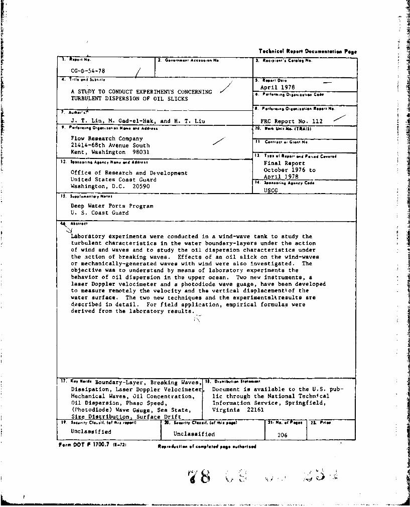
CG-D-54-78"?.fl I,~ "kf•,,,e 5. Iteoe, cove

• April 1978A STUDY TO CONDUCT EXPERIMENTS CONCERNING Ap e"•ri'e r ,0i.lohn C197

TURBULENT DISPERSION OF OIL SLICKS

.J. T. Lin, M. Gad-el-Hak, and H. T. Liu FRC Report No. 112

.low Research Companyn,.g ,,,oco, ..... ;o21414-68th Avenue South

Kent, Washington 98031 13 r..f A.p.,,.• Poe. C.e.,.d

)2. b rn, Ag..,c Me.m and Add,.0, Final Report fOffice of Research and Development October 1976 to

Offie o Resarc an DevlopentApril ].978United States Coast Guard Id , A0..,• C.doWashington, D.C. 20590

Deep Water Ports ProgramU. S. Coast Guard

4.4, Abotusct

Laboratory experiments were conducted in a wind-wave tank to study theturbulent characteristics in the water boundary-layers under the actionof wind and waves and to study the oil dispersion characteristics underthe action of breaking waves. Effects of an oil slick on the wind-wavesor mechanically-generated waves with wind were also investigated. Theobjective was to understand by means of laboratory experiments thebehavior of oil dispersion in the upper ocean. Two new instruments, alaser Doppler velocimeter and a photodiode wave guage, have been developedto measure remotely the velocity and the vertical displacementlof thewater surface. The two new techniques and the experimentalkresults aredescribed in detail. For field application, empirical formulas werederived from the labcratory results.

It. Ke" We'd$ Boundary-Layer, Breaking Waves, IO. 0obe, .-,-Dissipation, Laser Doppler Velocimeter, Document is available to the U.S. pub-Mechanical Waves, Oil Concentration, lic through the National Techn4 calOil Dispersian, Phase Speed, Information Service, Springfield,(Photodiode) Wave Gauge, Sea State, Virginia 22161Size Distribution Surface Drift

Unclassified Unclassified 206

Form DOT F 1700.7 (s-72) Re.d.,vcton. of c.,.ploed p.e. .. o'her.so4

I~

PREFACE

This report is submitted to the U.S. Coast Guard, Department of

Transportation, by Flow Research Company (FRC) in completion of the

research work on "A Study to Conduct Experiments Concerning Turbulent

Dispersion of Oil Slicks," under Contract No. DOT-CG-61688-A. The

objective of the research study was to characterize (qualitatively and

quantitatively) and to identify the mecnanisms behind turbulence due to

wind, waves and currents operating independently and coupled, with and

without an oil slick present.

This research study is a part of the integrated research program

sponsored by the Deepwater Ports program and the U.S. Coast Guard to

identify the sea-state threshold beyond which containment and recovery

of oil are impractical because of the natural dispersion of oil slicks.

Other parts of the research program include (i) a preliminary theoretical

study by Arthur D. Little Jnc. under Contract No. DOT-CG-61-505A (Raj,

1977), (if) a laboratory study by Massachusetts Institute of Technology

(MIT) under Contract No. DOT-CG-61-802A to investigate the effects of

oil properties on oil dispersion, and (iii) a field study by the Naval

Underwater Systems Center to conduct observations of surface layer

turbulence associated with wind stress and breaking waves.

The research team at FRC was headed by Dr. J. T. Lin and assisted

by Drs. M. Gad-el-Hak and H. T. Liu. Mr. R. Srnsky's assistance in

conducting experiments is gratefully acknowledged. Technical Services,

provided by M. Wallace, D. Turner, I. Smith, M. A. Kerstein and M.

McKenna in drafting, typing and editing is recognized gratefully. We

also acknowledge Drs. S. Veenhuizen and M. Rizk for their valuable

comments on the write-up of this report. The research study was moni-

tored by Mr. R. A. Griffiths of the Coast Guard. We gratefully acknowledge

his support and cooperation throughout the course of the research study.

.. ..

- .ii

- a

2' 5 'I a

I I - i =

* - I CI S ++ +""- a { 3 -- .--- m-T-,,, .--.-. s-I#3•'"- * Ii ... - .* -, - "

* -. + +. -_• U + c '- °• + " l + "-C * -, C C,}"=- -+ '• • :

*, +++• % -,+ . a .. -

*, ,. .,3.

,g . ,.

E 1 [ "1 . c 4 - *- I-n+J~

- - I'-I . . I -

o '* I * * I' 'I -Ii i* l i

"-o III II I+

Li I +

I I.

m | i, , , , _. S• ' ' , , , , i , liii i+ I i

TABLE OF CONTENTS

TECHNICAL REPORT DOCUMENTATION PAGE 1

PREFACE

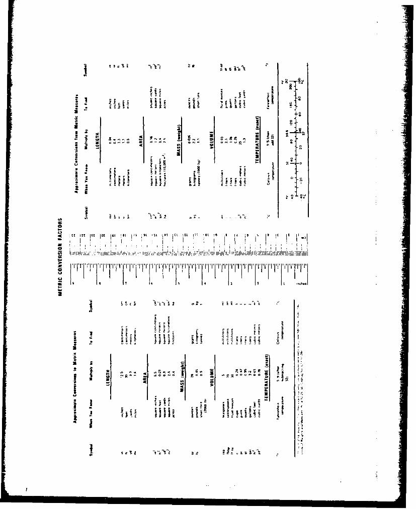
METRIC CONVERSION FACTORS iii

TABLE OF CONTENTS iv

LIST OF TABLES vi

LIST OF FIGURES vii

LIST OF SYMBOLS xi

1. INTRODUCTION I

2. EXPERIMENTAL SETUP 5

2.1 Wind-Wave Tank 5

2.2 Reverse Flow Control 6

2.3 Oil Feeding System 7

2.4 Selection of Oil 8

3. EXPERIMENTAL INSTRUMENTS AND TECHNIQUES 10

3.1 Hot-Wire and Hot-Film Probes 10

3.2 Laser Doppler Velocimeter 10

3.3 Capacitance Probes 12

3.4 Photodiode Wave Gauge 13

3.5 Data Acquisition and Processing 15

4. EFFECT OF WIND ON WATER MOTION 16

4.1 Air Boundary-Layer 17

4.2 Wave Characteristics 18

4.3 Surface Drift Velocity 19

4.4 Water Boundary-Layer 20

4.5 Mean Velocity 21

4.6 RMS Velocity Fluctuations 22

4.7 Velocity Spectra 25

5. EFFECTS OF WAVES ON WATER MOTION 28

5.1 Wave Characteristics 28


5.3 Water Boundary-Layer 34

5.4 Mean Velocity 35

5.5 RMS Velocity Fluctuations 36

5.6 Mean Square Velocity Time Derivatives 38

iv

5.7 Velocity Spectra 38

6. OIL DISPERSION 41

6.1 Flow Visualization 41 i.

6.2 Oil Concentration 42

7. CONCLUSIONS 45

7.1 Turbulence and Wave-Induced Motion 4_

7.2 Wave Growth Characteristics 46


7.4 Oil Dispersion 47

8. RECOMMENDATIONS FOR FUTURE RESEARCH .8


8.2 Turbulent Motion Versus Wave-Induced Motion 48

8.3 Taylor's Frozen Turbulence Hypothesis 49

8.4 Oil Concentration Flux 49

REFERENCES 50

Appendix A: Chronological Annotations 62

Appendix B: Comparison of Velocity Measurements by LDV and Hot-Film iProbes 71

Appendix C: Effects of Oil Slick on Wind-Waves 72

Appendix D: Effect of Oil Slick on Mechanically-Generated WavesWith Wind 77

TABLES 81

FIGURES 99

I

V

LIST OF TABLES

TABLE 1. -SUMMARY OF OIL PROPERTIES, ARCO DIESEL 82

TABLE 2. -WATER SURFACE DRIFT VELOCITY FOR WIND-WAVES 83

TABLE 3. -WATER BOUNDARY-LAYER THICKNESS FOR WIND-WAVES 84

TABLE 4. -AIR AND WATER SHEAR STRESSES 85

TABLE 5, -MEASUREMENTS OF VELOCITY IN WATER BOUNDARY-LAYER 86

TABLE 6. -MEASUREMENTS OF VELOCITY IN WATER BOUNDARY-LAYER 87




TABLE 10. -MEASURL-ZENTS OF VELOCITY IN WATER BOUNDARY-LAYER 91





TABLE 1 5. -MEASUREMENTS OF VELOCITY IN WATER BOUNDARY-LAYER 96



vi

LIST OF FIGURES

FIGURE 1. WIND-WAVE TANK. 100

FIGURE 2. OIL FEEDING SYSTEM SCHEMATIC. 101

FIGURE 3. LiOT-WIRE PROBE CALIBRATION. 102

FIGURE 4. HOT-FILM PROBE CALIBRATION. 103

FIGURE 5. LASER DOPPLER VELOCIMETER, 104

FIGURE 6. PLIOLITE PARTICLES PHOTOGRAPHIED WITH ELECTRONIC MICROSCOPE. 105

FIGURE 7. BLOCK DIAGRAM FOR PROCESSING OF LDV SIGNALS. 106

FIGURE 8. COMPARISON OF LDV OUTPUT WITH PITOT TUBE OUTPUT. 107

FIGURE 9. CALIBRATION OF CAPACITANCE PROBE. 108

FIGURE 10. SCHEMATIC OF PHOTODIODE WAVE GAUGE FOR WATER-WAVEMEASUREMENTS. 109

FIGURE 11. PHOTODIODE WAVE GAUGE SETUP. 110

FIGURE 12. OPERATIONAL PRINCIPLE OF WAVE GAUGE. ill

FIGURE 13. PHOTODIODE WAVE GAUGE CALIBRATION. 112

FIGURE 14. WAVE PROFILE MEASURED WITH PHOTODIODE WAVE GAUGE. 113

FIGURE 15. WAVE PROFILE MEASURED WITH CAPACITANCE PROBE. 114

FIGI",'E 16. DFrINITTON SKETCH FOR nIT. DISPERSION IN WIND-WAVES. 115

FIGURE, 17. PROFILES OF MEAN VELOCITY AND TURBULENCE INTENSITY IN AIRBOUNDARY-LAYER. 116

FIGURE 18. MEAN VELOCITY PROFILE IN AIR BOUNDARY-LAYER. 117

FIGURE 19. INSTANTANEOUS WATER SURFACE DISPLACEMENT OF WIND--WAVES. 118

FIGURE 2.0. WAVE ENERGY SPECTRUM. 1'.9

FIGURE 21. VARIATION OF RMS WAVE HEIGHT WITH WIND SPEED. 120

FIGURE 22. VARIATION OF DOMINANT WAVE FREQUENCY WITH WIND SPEED. 121

FIGURE 23. FETCH EFFECTS ON DOMINANT WAVE FREQUENCY. 122

FIGURE 24. VARIATION OF WAVF PHASE VELOCITY WITH WIND SPEED. 123

FIGURE 25. FETCH EFFECTS ON WAVE PHASE VELOCITY. 124

FIGURE 26. VARIATION OF DOMINANT WAVE LENGTH WITH WIND SPEED. 125

FIGURE 27. VARIATION OF DOMINANT WAVE SLOPE WITH WIND SPEED. 126

FIGURE 28. FETCH EFFECTS ON DOMINANT WAVE LENGTH. 127

FIGURE 29. VARIATION OF SURFACE DRIFT VELOCITY WITH FETCH. 128

FIGURE 30. DYED WATER BCUNDARY-LAYER. 129

FIGURE 31. WATER BOUNDARY-LAYER THICKNESS. 132

FIGURE 32. MEAN VELOCITY PROFILE IN WATER BOUNDARY-LAYER. 133

vii

FIGURE 33. MEAN VELOCITY DEFECT PROFILE IN WATER BOUNDARY-LAYER. 134

FIGURE 34. MEAN VELOCITY PROFILES IN WATER BOUNDARY-LAYER: EFFECTSOF WIND SPEED. 135

FIGURE 35. RMS OF LONGITUDINAL VELOCITY FLUCTUATIONS IN WATERBOUNDARY-LAYER. 136

FIGURE 36. RMS OF LONGITUDINAL VELOCITY FLUCTUATIONS IN WATERBOUNDARY-LAYER. 137

FIGURE 37. RMS OF VERTICAL VELOCITY FLUCTUATIONS IN WATER BOUNDARY-LAYER. 138

FIGURE 38. RMS OF VERTICAL VELOCITY FLUCTUATIONS IN WATER BOUNDARY-LAYER. 139

FIGURE 39. REYNOLDS STRESS PROFILES IN WATER BOUNDARY-LAYER. 140

FIGURE 40. DISSIPATION RATE IN WATER BOUNDARY-LAYER. 141

FIGURE 41. LOPIGITUDINAL VELOCITY SPECTRUM IN WATER BOUNDARY-LAYER. 142

FIGURE 42. LONGITUDINAL VELOCITY SPECTRA IN WATER BOUNDARY-LAYER. 143

FIGURE 43. VERTICAL VELOCITY SPECTRA IN WATER BOUNDARY-LAYER. 144

FIGURE 44. CO- AND QUAD-SPECTRUM OF LONGITUDINAL AND VERTICAL VELOCITIESIN WATER BOUNDARY-LAYER. 145

FIGURE 45. MAGNITUDE AND PHASE OF CROSS-SPECTRUM OF LONGITUDINAL ANDVERTICAL VELOCITIES IN WATER. 146

FIGURE 46. WATER SURFACE PHOTOGRAPH. 147

FIGURE 47. AIR BUBBLES ENTRAINED INTO WATER UNDER WAVE CREST. 149

FIGURE 48. WAVE ENERGY SPECTRA (CAPACITANCE PROBE). 150

FIGURE 49. DOMINANT PHASE SPEED, Cp VERSUS WAVE STEEPNESS. H/A 151PI

FIGURE 50. VARIATION OF WAVE HEIGHT WITH FETCH, 152

FIGURE 51. WAVE ENERGY SPECTA AT TWO FETCHES. 153

FIGURE 52. WAVE ENERGY SPECTRA WITH MECHANICALLY GENERATED WAVE. 154

FIGURE 53. VARIATION OF WAVE ENERGY SPECTRUM WITH WIND SPEED. 155

FIGURE 54. SURFACE DRIFT VELOCITY U VERSUS FETCH x. 156

FIGURE 55. SURFACE DRIFT CURRENT V VERSUS WAVE STEEPNESS H/X. 157

FIGURE 56. DYED WATER BOUNDARY, H - 7.62 cm, U. - 10 u/sec, x - 4 m. 158

FIGURE 57. THICKNESS OF WATER BOUNDARY-LAYER 6 VERSUS FETCH x. 159w

FIGURE 58. VERTICAL PROFILES OF LONGITUDINAL MEAN VELOCITY IN BREAKINGAND NON-EREAKING WAVES. 160

FIGURE 59. VERTICAL PROFILES OF VERTICAL MEAN VELOCITY IN BREAKING ANDNON-BREAKING WAVES. 161

FIGURE 60. VERTICAL PROFILES OF RMS LONGITUDINAL VELOCITY IN BREAKINGAND NON-BREAKING WAVES. 162

viii

i °

FIGURE 61. VERTICAL PROFILES OF RMS VERTICAL VELOCITY IN BREAKING ANDNON-BREAKING WAVES. 163

FIGURE 62. VERTICAL PROFILES OF RMS VELOCITY FLUCTUATIONS IN BREAKINGAND NON-BREAKING WAVES. 164

FIGURE 63. VERTICAL PROFILES OF MEAN SQUARE VELOCITY TIME DERIVATIVES INBREAKING AND NON-BREAKING WAVES. 165

FIGURE 64. SPECTRUM OF LONGITUDINAL VELOCITY FLUCTUATIONS IN BREAKINGWAVES. 166

FIGURE 65. SPECTRUM OF VERTICAL VELOCITY FLUCTUATIONS IN BREAKING WAVES. 167

FIGURE 6(l. SPECTRUM OF LONGITUDINAL VELOCITY FLUCTUATIONS IN BREAKINGWAVES. 168

FIGURE 67. SPECTRUM OF VERTICAL VELOCITY FLUCTUATIONS IN BREAKING WAVES. 169FIGURE 68. VERTICAL PROFILE OF INSTANTANEOUS OIL VOLUME CONCENTRATION. 170

FIGURE 69. VERTICAL PROFILES OF MEAN AND RMS OIL VOLUME CONCENTRATION. 171

FIGURE 70. VERTICAL PROFILE OF MEAN OIL VOLUME CONCENTRATION. 172

FIGURE 71. SIZE DISTRIBUTION OF OIL DROPLETS. 173

FIGURE 72. COMPARISON OF LONGITUDINAL MEAN VELOCITY PROFILE MEASURED INWIND-WAVES BY LDV AND HOT-FILM PROBES. 174

FIGURE 73. COMPARISON OF RMS LONGITUDINAL VELOCITY PROFILE MEASURED INWIND-WAVES. 175

FIGURE 74. TRANSIENT PROFILES OF WIND WAVES IN RESPONSE TO OILSLICK. 176

FIGURE 75. WIND-WAVE PROFILES WITHOUT OIL SLICK. 177

FIGURE 76. WIND-WAVE PROFILES WITH OIL SLICK.X - 4 m. VERTICAL SCALE 0.2 cm/div. HORIZONTAL SCALE0.5 sec/div. 178

FIGURE 77. VARIATION OF RMS WAVE HEJGHT WITH WIND SPEED. 179

FIGURE 78. VARIATION OF RMS WAVE HEIGHT WITH FETCH. 181

FIGURE 79. WAVE ENERGY SPECTRUM. 181

FIGURE 80. WAVE ENERGY SPECTRUM VARIATION WITH WIND SPEED. 182FIGURE 81. WAVE ENERGY SPECTRA MEASURED WITH AND WITHOUT OIL. 183

FIGURE 82. WAVE ENERGY SPECTRA MEASURED WITH AND WITHOUT OIL. 184

FIGURE 83. WAVE ENERGY SPECTRA MEASURED WITH AND WITHOUT OIL. 185

FIGURE 84. PROFILES OF MECHANICALLY GENERATED WAVES WITH WIND, VERTICALSCALE - 2 cm/DI"., HORIZONTAL SCALE - 0.5 sec/DIV. 186

FIGURE 85. A TYPICAL PROFILE OF NONBREAKING WAVES WITHOUT OIL. 187

FIGURE 86. TYPICAL PROFILE OF BREAKING WAVES WITHOUT OIL. 188

FIGURE 87. PROFILE OF MECHANICAL GENERATED WAVES WITH WIND AND OILSLICK.VERTICAL SCALE - 2 cm/div., HORIZONTAL SCALE , 0.5 sec/div. 189

FIGURE 88. VARIATION OF WAVE HEIGHTS WITH FETCH. 190

ix

JI

FIGURE 89. VARIATION OF RMS WAVE HEIGHTS WITH WIND SPEED. 191

FIGURE 90. COMPARISON OF WAVE ENERGY SPECTRA, H - 2.54 cm. 192O

FIGURE 91. COMPARISON OF WAVE ENERGY SPECTRA, H " 5.08 cm. 193A

FIGURE 92. COMPARISON OF WAVE ENERGY SPECTRA WITH AND WITHOUT OIL SLICK. 194

x4

I

SYMBOLS

Symbol Description Dimensions*

C instantaneous oil volume concentration

C, c mean and fluctuating oil volume con-centration

cd windstress coefficient

C wave phase speed LT_Cp

C wavedrag coefficient

d spacing of the LDV fringes L

E11 (k1 ) one dimensional wave number spectrum L3 T 211of turbulence

wave frequency (Hz) T-1

fd Doppler frequency T

f dominant wave frequency To -1 •

Af frequency shift by a Bragg cell T

g gravitational acceleration LT- 2

H dominant wave height L

H stroke of wave-maker Lwave number Lturbulence Reynolds number, - -2 /V

S(f) wave energy spectrum L T

Su(f), Sw(f) spectral density of longitudinal, L2T- 1

vertical velocity fluctuations

t time T

'9 toean longitudinal velocity LT-

Ud Stokes' surface drift velocity LT 1

U particle velocity LT-

U surface drift velocity LT 1

U wind speed in the free-stream LT_

u,v,w Cartesian velocity fluctuating components LT-

u, water friction velocity LT'

U*a air friction velocity LT- 1

L - length, T - time, M = mass

xi

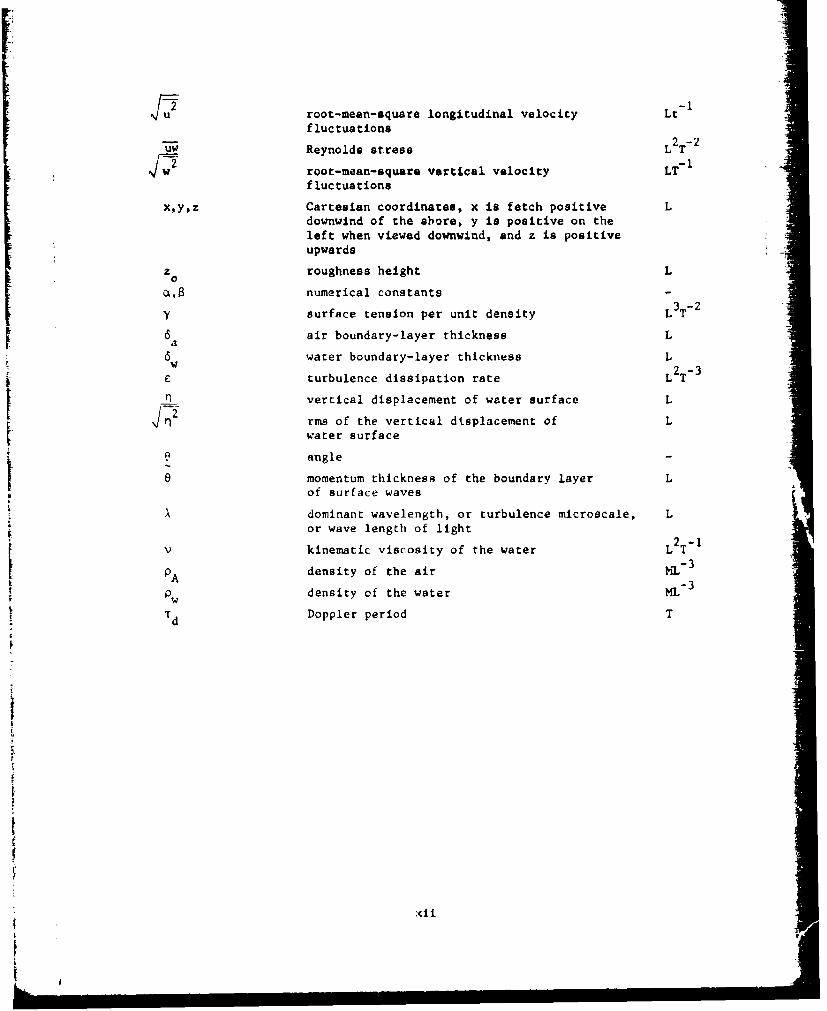
u root-mean-square longitudinal velocity Ltfluctuations

V" Reynolds stress L2T-

Sroot-mean-square vertical velocity LT_fluctuations

xyz Cartesian coordinates, x is fetch positive Ldownwind of the ebore, y is positive on theleft when viewed downwind, and z is positiveupwards

z roughness height L

(XB numerical constants

y surface tension per unit density L3 T-2

6 air boundary-layer thickness L

6aw water boundary-layer thickness L

turbulence dissipation rate L2 T-3

n vertical displacement of water surface L

rms of the vertical displacement of L

water surface

A angle

x emomentum thickness of the boundary layer L

dominant wavelength, or turbulence microscale, Lor wave length of light

v kinematic viscosity of the water L2 TI

PA density of the air

Pw density of the water ML

Td Doppler period T

xi i

i.

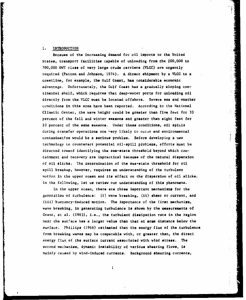
1. INTRODUCTION

Because of the increasing demand for oil imports to the United

States, transport facilities capable of unloading from the 200,000 to

700,000 DWT class of very large crude carriers (VLCC) are urgently

required (Patton and Johnson, 1974). A direct shipment by a VLCC to a

coastline, for example, the Gulf Coast, has considerable economic

advantage. Unfortunately, the Gulf Coast has a gradually sloping con-

tinental shelf, which requires that deep-water ports for unloading oil

directly from the VLCC must be located offshore. Severe sea and weather

conditions in this area have been reported. According to the National

Climatic Center, the wave height could be greater than five feet for 33

percent of the fall and winter seasons and greater than eight feet for

10 percent of the same seasons. Under these conditions, oil spiils

during transfer operations are vary likely to occur and environmental

contaminatlon would be a serious problem. Before developing a new

technology to counteract potential oil-spill problems, efforts must be

directed toward identifying the sea-state threshold beyond which con-

tainment and recovery are impractical because of the natural dispersion

of oil slicks. The determination of the sea-state threshold for oil

spill breakup, however, requires an understanding of the turbulent

motion in the upper ocean and its effect on the dispersion of oil slicks.

In the following, let us review our understanding of this phenomena.

In the upper ocean, there are three important mechanisms for the

generation of turbulence: (1) wave breaking, (ii) shear or current, and

(iii) buoyancy-induced motion. The importance of the first mechanism,

wave breaking, in generating turbulence is shown by the measurements of

Grant, et al. (1963), i.e., the turbulent dissipation rate in the region

near the surface has a larger value than that at some distance below the

surface. Phillips (1966) estimated that the energy flux of the turbulence

from breaking waves may be comparable with, or greater than, the direct

energy flux of the surface current associated with wind stress. The

second mechanism, dynamic instability of various shearing flows, is

mainly caused by wind-induced currents. Background shearing currents,

I

I

I

U

for example, caused by the confluence of different water masses are

often sources of appreciable turbulence in surface waters. The thirdAJ

mechanism, buoyant or convective instability, is important in regions

where substantial cooling or surface evaporation appears 8nd the surface

layer tends to be statically unstable. This mechanism results in free

convection characterized by an irregular cellular motion.

In addition to the three mechanisms of turbulence generation

previously described, stratification in the surface water requires some

consideration. In a stably stratified fluid, stratification can inhibit

the development of turbulence and the downward diffusion of turbulent Ienergy. Another aspect of the stratification effect stems from the

deepening of the mixed surface layer, and thux, the thermocline below

the mixed surface layer. A portion of the energy flux from the surface

is used to deepen the thermocline. Hence, the dynamics of the turbulencein surface waters cannot be separated from those of the mixed layer. IFor the present study, a sea in a strongly excited state is of concern

and thus, the stratification in surface waters, the deepening of the

mixed layer, and the bouyancy-induced instabilities, are expected not to

be important in the generation of turbulence. Hence, in the following

paragraph we briefly review the previous works concerning breaking wavesand wind-induced currents.

Breaking waves have not been investigated carefully until recently. • ILonguet-Higgins (1969a, 1969b, 1973, 1974) conducted theoretical studies

on the mechanisms of wave breaking. Banner and Phillips (1974) investi-

gated the incipient breaking of small-scale waves. Van Dorn and Pazan j(1975) measured the velocity in breaking waves in a wave channel. The

wind-induced drift currents have been investigated by many researchers.

Keulegan (1951) and Plate (1970) measured the surface current in wind-

wave tanks. Baines and Knapp (1965) measured the drift profiles in a

shallow channel. Bye (1965), Shemdin (1973) and Wu (1975) measured the

profiles of the wind-induced drift current in wind-wave tanks. Turbulence

measurements in the water near the ccean surface were conducted by

Shonting (1968), by Thorton, et al. (1977) and by Donelan (1977).

2

k • m i

Al

In order to understand the behavior of oil dispersion in the upper

ocean, it is necessary to know the turbulence characteristics (for

example, vertical profiles of mean velocity and turbv'lence inteneity).

These characteristics are not yet available from existing literatures.

Therefore, the first objective for the present research study is to

conduct laboratory measurements of the water velocity under the action

of wind and waves. From these measurements, one could obtain an empirical

formula so as to apply the laboratory results to the field situation.

As far as oil dispersion studies are concerned, we have found no

systematic work on oil slick breakup, however, some works on oil slick

drift are available and they are summarized briefly as follows.

Schwartzberg (1971) conducted laboratory experiments to study oil spills

under the action of wind. He measured the surface drift current with an

oil spill present. Pottinger and Reisbig (1973) conducted laboratory

measurements of the drift velocity of an oil lens. Reisbig et al.

(1973) investigated the coupled parallel effects of wind and waves on

oil spill drift. In the field, Murray (1975) observed the effect of

wind and current on the drift of large-scale oil slicks. The secondobjective of the present study is to investigate the oil dispersion. We

will determine the vertical penetration and the size distribution of the

oil droplets when the oil slick is broken.

Our approach is to conduct laboratory experiments in a wind tank.

FIrst, we investigate the water turbulence under the influence of wind.

Second, we add mechancially-generated waves in the tank to study the

effect of waves on the water turbulence. And, third, we select experi-

mental conditions for oil dispersion experiments.

We describe the experimental setup in Section 2 and the experimental

instruments and techniques in Section 3. New instruments, such as the

laser Doppler velocimeter and the photodiode wave gauge have been developed

to sense remotely the velocity and the vertical displacement of the water

surface. In Section 4, we present the measurements of water turbulence

under the predominant influence of wind. In Section 5, the effects of

waves on the water motion are presented. Vertical profiles of the mean

3

11

velocity, rms velocity fluctuations and other statistical quantities are

presented. In Section 6, we present the oil concentration measurements,

including the oil concentration profile and droplet size distribution.

Conclusions based on our present study are given in Section 7. Experi-

mental results are presented in tabular and/or figure form. Finally,

recomendations for future research is presented in Section 8.

4-

I2

Ii

1 47

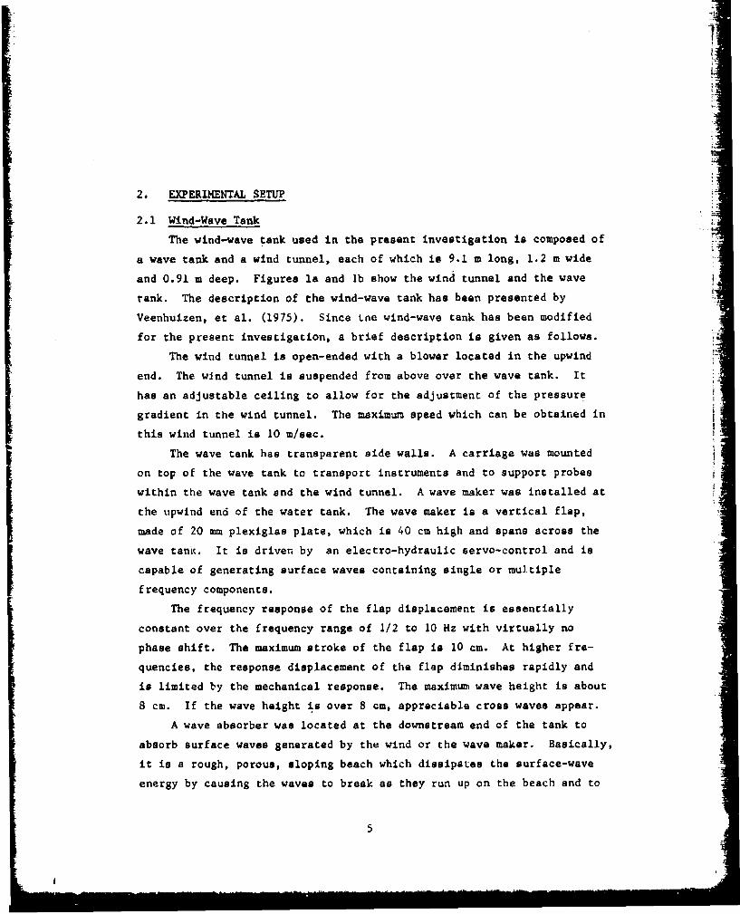
2. EXPERIMENTAL SETUP

2.1 Wind-Wave Tank

The wind-wave tank used in the present investigation is composed of

a wave tank and a wind tunnel, each of which is 9.1 m long, 1.2 m wide

and 0.91 m deep. Figures la and lb show the wind tunnel and the wave

tank. The description of the wind-wave tank has been presented by

Veenhuizen, et al. (1975). Since Lae wind-wave tank has been modified

for the present investigation, a brief description is given as follows.

The wind tunqel is open-ended with a blower located in the upwind

end. The wind tunnel is suspended from above over the wave tank. It

has an adjustable ceiling to allow for the adjustment of the pressure

gradient in the wind tunnel. The maximum speed which can be obtained in

this wind tunnel is 10 m/sec.

The wave tank has transparent side walls. A carriage was mounted

on top of the wave tank to transport instruments and to support probes

within the wave tank and the wind tunnel. A wave maker was installed at

the upwind end of the water tank. The wave maker is a vertical flap,

made of 20 mm plexiglas plate, which is 40 cm high and spans across the

wave tank. It is driven by an electro-hydraulic servo-control and is

capable of generating surface waves containing single or multiple

frequency components.

The frequency response of the flap displacement is essentially

constant over the frequency range of 1/2 to 10 Hz with virtually no

phase shift. The maximum stroke of the flap is 10 cm. At higher fre-

quencies, the response displacement of the flap diminishes rapidly and

is limited by the mechanical response. The maximum wave height is about

8 cm. If the wave height is over 8 cm, appreciable cross waves appear.

A wave absorber was located at the downstream end of the tank to

absorb surface waves generated by the wind or the wave maker. Basically,

it is a rough, porous, sloping beach which dissipates the surface-wave

energy by causing the waves to break as they run up on the beach and to

5

be drained of energy further as the fluid runs back down the beach

through many small openings on the beach surface. The wave absorber

(Figure 1) is constructed of a plastic grid, topped with 5 cm layers of

horse hair, and covered with a layer of herring fish netting. The wave

absorber extends across the width of the tank and is 1.5 m long. When

the absorber is at about a 10-degree angle to the water surface in the

tank, the reflection coefficient, defined as amplitude reflected/amplitude

incident, is measured to be less than 5 percent. Thus, the wave absorber

works effectively in damping out the upcoming waves.

2.2 Reverse Flow Control

When wind blows over the water surface, a drift layer in the surface

water sets up due to the shear stress exerted on the vater by the wind.

Through the action of viscosity, a water boundary-layer develops which

can become turbulent when the Reynolds number is sufficiently large.

The boundary-layer flow entrains the fluid from below, and its thickness

grows with fetch. To satisfy the continuity of the fluid and because of

the finite length of the wave tank, a reverse flow results in the lower

part of the tank. The drift layer and the reverse flow, together, form

a very complicated flow field. On the other hand, in the ocean except

the near shore region, such a reverse flow is negligible due to the

large scale of the flow field. Hence, it io desirable to minimize thereverse flow effects in the laboratory experiment.

A false bottom 15 cm above the tank floor was installed and a tran-

sition plate guided the reverse flow close to the wave absorber to flow

under the false bottom. In the upwind end of the false bottom, there

was a spacing of about I m between the end wall and the and of the false

bottom. The shape and dimensions of this transition plate were determined

by trial and error to maximize the flow under the false bottom and

minimize the reverse flow, i+ any, above it. For the case when wind

blows over the surface, the false bottom worked quite well and the reverse

flow was practically nealigible above the false bottom. When mechanically-

generated waves were added, the false bottom did not seem to control the

reverse flow well, so it was removed. The measurement here, however,

6'

iJ

6 2

showed that the drift layer, for the case of mechanically-generated

waves with wind, is not as deep as for the case when wind blows over the

surface, and thus, the reverse flow control may not be critical.

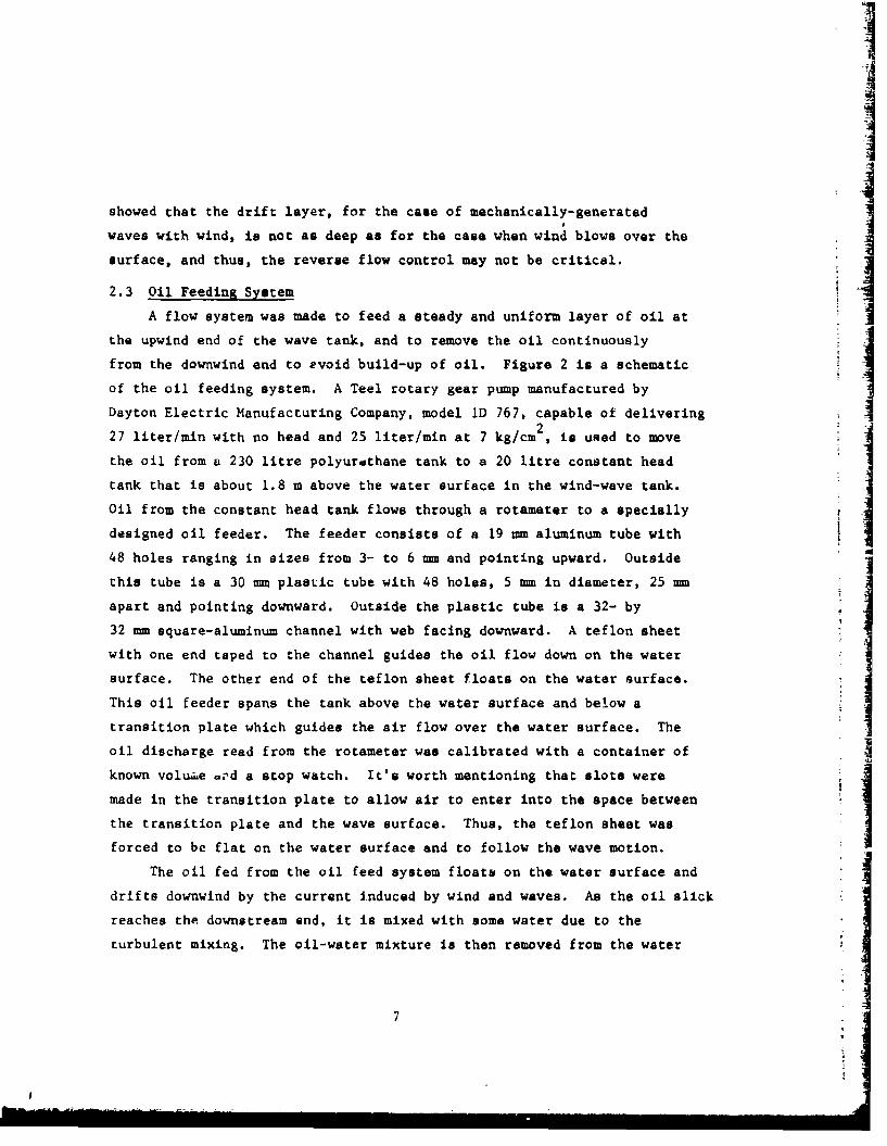
2.3 Oil Feeding System

A flow system was made to feed a steady and uniform layer of oil at

the upwind end of the wave tank, and to remove the oil continuously

from the downwind and to evoid build-up of oil. Figure 2 is a schematic

of the oil feeding system. A Teel rotary gear pump manufactured by

Dayton Electric Manufacturing Company, model ID 767, capable of delivering227 liter/min with no head and 25 liter/min at 7 kg/cm , is used to move

the oil from a 230 litre polyurathane tank to a 20 litre constant head

tank that is about 1.8 m above the water surface in the wind-wave tank.

Oil from the constant head tank flows through a rotameter to a specially

designed oil feeder. The feeder consists of a 19 mm aluminum tube with

48 holes ranging in sizes from 3- to 6 mm and pointing upward. Outside

this tube is a 30 mm plastic tube with 48 holes, 5 mm in diameter, 25 mm iapart and pointing downward. Outside the plastic tube is a 32- by

32 mm square-aluminum channel with web facing downward. A teflon sheetwith one end taped to the channel guides the oil flow down on the water

surface. The other end of the teflon sheet floats on the water surface.

This oil feeder spans the tank above the water surface and below a

transition plate which guides the air flow over the water surface. The

oil discharge read from the rotameter was calibrated with a container of

known voluie 0 Pd a stop watch. It's worth mentioning that slots were

made in the transition plate to allow air to enter into the space betweenthe transition plate and the wave surface. Thus, the teflon sheet was

forced to be flat on the water surface and to follow the wave motion.

The oil fed from the oil feed system floats on the water surface and

drifts downwind by the current induced by wind and waves. As the oil slick

reaches the downstream end, it is mixed with some water due to the

turbulent mixing. The oil-water mixture is then removed from the water

7

surface using a two-dimensional overflow drain that connects to a second

230 liter polyurethane tank which serves as a settling tank to allow the

oil to separate from the water. The recovered oil can be recycled for

the next experiment, and the water is discarded. This semi-closed system

permits a continuous operation for about 15 minutes, which is enough

time for completion of an experimental run of oil dispersion.

2.4 Selection of Oil

For the oil dispersion equipment, it is usually best to use crude

oils, e.g., Kuwait or Libyan crude. We did not use crude oils, however, A

because it is difficult to control their properties, since they can

vary from barrel to barrel. Moreover, the purpose of the present study

was to characterize and identify dispersion mechanisms acting on an oil

slick of any kind. An oil was selected based on the following criteria.The density and viscosity of the oil must be close to those of the crude

oils mentioned. The oil must not mix easily with the watec otherwise,

the oil properties could change significantly as the dispersed oildrifts along the wind-wave ýank. In othar words, we are not interested

in the emulsification process occurring in the present experiments. Theoil must separate easily from water when the mixture of oil and water

returns to the oil settling tank from the overflow drain located in thedownwind side of the wave absorber, thus, the oil can be recovered for

re-use. The oil must be able to form a thin sheet like the oil slick in

the ocean.To examine the rate of recovery and separation from water after

mixing, four kinds of oils, namely, vegetable oil, Texaco Almag oil,

Diesel oil No. 2 and mineral oil were tested for selecting the oil to be

used for the oil dispersion experiment. The oil sample was put in abottle with an equal amount of water and shaken for several seconds. A

general observation as to the rate of recovery into two separate fluids

was made and is described as follows. For vegetable oil, the rate of

recovery is slow. Foam appears on the boundary between fluids, and

water droplets are formed and are suspended in the oil. For Texaco

Almag oil the rate of recovery is also slow, and water droplets sus-

pended in oil are observed. Diesel oil No. 2 has fast recovery and

8

clean Eeparation. Mineral oil has slow recovery; droplets form and

suspend in both fluids, and the oil clings to the bottle.

Spreading on a water surface also was tested with the above and

additional oils in selecting the best-suited oil for the oil dispersion

experiment. A small quantity of the oil sample was poured on a water

surface. The resulting oil behavior was observed and is described as

follows. Diesel Oil No. 2 forms a film over the entire surface. Diesel

Oil No. 1 forms a film, but not as readily as the Diesel Oil No. 2.

Mineral Oil forms lenses, and a thick film adheres to the glass. Vege-

table Oil, Texaco Almag Oil and hydraulic oil No. 215 all form lenses.

Based on the tests described above, we selected Diesel oil No.

2 because it absorbs water least, separates from water quickly and can

form a thin oil film over the water surface. Prior to each experiment,

the physical properties of the oil, such as specific gravity and viscosity,

are measured. Table ] is the summary of the ci] properties. The

physical properties did not vary noticeably during the period of experi-ments. For example, on December 14, 1977, we measured the oil properties

I

before use, i.e., viscosity - 18.9 cm2/sec and specific gravity = 0.84.

After use during the same day, water had mixed with oil, and both viscosity

and specific gravity increased accordingly. New oil of about a quarter

volume of the used oil was then added to the used oil to ensure that the

oil properties remained practically unchanged. For example, between

Decembez 14, 1977 when new oil was first used and January 18, 1978,

viscosity and specific gravity increased by about 7- and 10 percent

respectively. Whenever we found that the specific gravity and viscosity

changed significantly, the recycled oil was drained and replaced by

fresh oil. As noted in Table 1, new oil was supplied for future experi-

ments on January 19. 1978. The interfacial tension at 20 C between

air and water and between air and oil are about 70- and 30 dyne/cm,

respectively.

9

L

3. EXPERIMENTAL INSTRUMENTS AND TECHNIQUES

3.1 Hot-Wire and Hot-Film Probes

For velocity measurements in the air, we used two hot-wire probes

manufactured by Thermo Systems Inc. (TSI 1210-TI.5) operated with two

constant-temperature hot-wire anemometers (TSI Model 1054B). A typical

calibration curve of the hot-wire probe is plotted in Figure 3. A

Pitot-static tube with a Gilmont micromanometer was used for calibration.

Twenty channels of hot-film anemometer (TS1 Models 1051-10 and

1053B) were used with ten cross-film probes (TSl Model 1284) to make

simultaneous measurements of the instantaneous longitudinal and vertical

velocity components in the water. The hot-film prcbes were mounted on a

probe strut which in turn was clamped on the instrument carriage. The

calibration was made by towing the hot-film probes along the wave tank.

The towing speed was registered with the rotational speed 3f the motor

which drove the towing system. A slot wheel with a light-emitting-diode

and a photocell was mounted on the motor shaft. As the motor turns, the

photocell registers a signal which corresponds to the speed at which the

slot wheel and the motor rotate. Figurer 4(a) and (b) show two cali-

brations of a hot-film probe for high and low speed ranges.

3.2 Laser Doppler Velocimeter

The hot-film probe is an accurate and sensitive instrument for

measuring velocity; however, if there exiists a reverse flow, the hot-

film Frobe is not useful iecause it senses speed but not the flow

direction. Hence, we cannot use the oet-film probe to measure velocity

in large amplitude waves, .!here large reverse flow results from the

oribital motion of the waves. To overcome this difficulty, we use a

laser Doppler velocimeter (LDV) developed at the Flow Research Company.

The LDV was designed to operate in the dual-beam backacatter mode, and

it has the frequency shift capability to measure velocity even when the

reverse flow is preset. Sums specifics which are relevant to the

present experiments are described briefly as follows. Detailed descrip-

tions of the design are given by Bachalo and Lin (1977).

10A

The LDV consists of a 4-watt Argon-ion laser (Spectra Physics Model I164-05), a set of transmitting and receiving optics, two acousto-optic !

modulators or Bragg cells (Isomet Corporation), a photomultiplier (RCA zi

7767/1C with Sll response), an ampl!'ier (Advantek SD7-0614B), a counter- !

type signal processor (Macrodyne Model 2096) and a bandpass filter

(Krohn-Hite Model 3103). The laser, the optics and the photomultiplier

were all mounted on a 1.2- by 0.91 m optical table which was made of

0.64 cm aluminum plates sandwiched w'ith honeycomb. The top surface of

the optical table was drilled with 0.64 cm threaded holes into which

optic stands can be mounted. The optical table was mounted on a steel

base, which was equipped with an oil Jack for adjustment of vertical I

displacement up to 48 cm. The surface also could be tilted in one

direction about + 30 deg. from its leveled position. I

Figures 5 (a) and (b) are a photograph and a schematic of the LDV. The

laser bean, projected from the laser housing is reflected twice by two

45 deg. mirrors, and then split into two beams with a splitter cube.

Both beams were frequency shifted with two Bragg cells and were then

focused with an achromatic lens at the measuring point. Due to the I• -i

interference of the two split light beams, a fringe pattern forms at the

focal point, and the fringe pattern moves at a speed corresponding to jthe frequency shifted by the Bragg cells. The speed at which the fringe

frame moves is calculated by df x 6f , where df is the fringe Ispacing and Af is net frequency shift. The fringe spacing df can be

fdcalculated by

dAf (3-1)

2 sin ( 0)

where X is the wavelength of the laser and 6 is the beam crossing

angle at the focal point.

The water was seeded with Pliolite plastic particles for scattering

purposes. The particles, manufactured by Goodyear Rubber Company, were

ground, sieved and filtered to remove large ones. Figure 6 shows a photo-graph of the particles viewed with an electronic microscope. The average

III

I1

particle size is less than 40 p. The particles had a specific Fravity

of about 1.03. Because of their small size, the particles can follow

the flow motion very well.

A receiving lens (0.5 m focal length) imaged the focal point onto a

pnotomultiplier through a pinhole 0.05 cm in diameter. The scattering

light from a seeded particle at the focal point was therefore collected

onto the photomultiplier. The photomultiplier output, which was propor-

tional to the scattered light intensity, was amplified, band-pass

filtered and fed into the Macrodyne signal processor.

The Macrodyne processor can process and validate the frequency

information in the signals, and, then, provide voltage output in both

analog and digital forms proportional to the Doppler shift period TdFigure 7 is a block diagram showing the various stages of data recording

and processing of the LDV. The particle vel-ci.ty Up can thus be

calculated from the difference between the Doppler shift frequency and

the frequency shift intruduced by the Brags cells,

up a df(fd - Af) (3-2)

where fd - l/Td is the Doppler shift frequency. The maximu, negative

velocity that can be resolved by the LDV is therefore U - -df Af .

The setup can be slightly modified for measurements of the instantaneous

vertical velocity by rotating the beam splitter cube and the two Bragg

cells 90 deg. Figure 8 shows a calibration curve of the LDV system

measured in an air jet. For the measurements in the air, we used water

droplets as seeding particles. The LDV measurement is i, good agreement

with the Pitot tube result. The calibration of the LDV in water is

described in Appendix B.

3.3 Capacitance Probe

For wave-height measurment, we used a capacitance gauge manufactured

by Flow Research Company (Model 1204). The capacitance gauge had a bare

stainless steel tube (1.6 mm o.d.) or a teflon coated wire as the sensor.

12

Calibration was made, before or after each run, by displacing the probe

at several predetermined vertical increments. Figure 9 is a typical

calibration curve of the capacitance probe. The calibration points were

fitted with a second degree polynomial.

3.4 Photodiode Wave Gauge

In case an oil slick is present, the capacitance probe fails to

measure surface wave height because of oil contamination. To avoid

contamination, we developed a photodiode wave gauge - a remote sensor

for measuring surface wave height. The photodiode wave gauge includes a

Reticon camera and a controller manufactured by Reticon Corp. (Model LC

OO V and RS 605) and a 4-watt-Argon-ion laser (Spectra Physics, Model

164-05). Figure 10 shows.a schamatic of the photodiode wave gauge,

and Figure 11 is a photograph of the experimental setup for remotely

sensing surface waves. The laser beam serves as a light source to

illuminate the interface between the air and the water or between che

air and the oil. Fluorescent dye (Fluorescein disodium salt) was pre-

mixed uniformly in the water. The concentration was about I ppm. By

vertically projecting the laser beam from the air to the water or to the

oil slick, a bright fluorescent beam is produced in the water and a

sharp dark-to-bright interface appeared on the water surface or the

surface of the oil slick. This dark-to-hright interface can be detected

by a vertical linear array of photodiodes mounted inside the Reticon

camera.

The photodiode array has 256 elements spaced 25.4 im center to

center. The air-water interface marked with the fluorescent dye was

focused on the photodlode array by optics including lenses and extension

tubes. The field-of-view can vary from a fraction of a centimeter to a

few meters. The spatial resolution in measuring the vertical displacement

of the air-water interface can be adjusted by varying the size of the

field-of-view. For example, the spatial resolution is 0.04 cm when the

field-of-view is 10 cm.

The position of the image of the air-water interface cr air-oil

interface was determined electronically by a scanning control. The

13

I7

scanning rate ranges from 0.4- to 40 ps, and thus, it ensures the fast

response of the photodiode wave gauge. Figure 12a shows a schematic of

the laser beam and the corresponding light intensity profile along thebeam in the vicinity of the air-woter interface. Figure 12b shows a -

complete scan of the VIDEO output of photodiodes. The scan started from

the first diode which was focused on the laser beam above the air-water

interface and ended at the last diode which was focused on the laser

beam below the interface. The vertical lines in Figure 12b represent

the analog pulses of the individual diodes, and, at the interface there

is a large jump in voltage output. When surface waves are present, the

air-water interface oscillated vertically and the pattern of the analog

pulses shown in Figure 12b moves accordingly. By detecting the posiLtion

of the sharp slope of the analog pulse one could therefore register the

vertical displacement of the water or oil surface. The registration was

done by comparing a THRESHOLD output with the VIDEO output. 'hen the

voltage outputL of an analog pulse is less than the threshold level, the

processor registers a logical "zero". When the voltage output exceeded

the threshold level within one ecan, the processor will register logical"ones" for the rest of the scan (Figure 12c). The registered logical

signal was then electronically counted to determine the position of the"nth" diode where the "zero"-to-"one" occurred and where the air-water

interface is imaged.

Calibration of the photodiode gauge was made by displacing it at

several vertical positions ;,ith predetermined increments. The diode

numbers are plotted versus the vertical displacement in Figure 13. The

calibration points are fitted with a straight line.

The performance cf the photodiode wave gauge was dynamically cali-

brated with a capacitance probe positioned side by side in close proximity

in a mechanically-generated wave. The wave frequency was seleczed to be

1.6 Hz for which the meniscus effects cn the performance of the capaci-

tance probe are not important. In Figures 14 and 15, we present the

wave profiles of mechanically-generated waves measured with the photodiode

14

wave gauge and the capacitance probe. The two wave profiles agree quite

well except in the regions near wave crests and troughs. Apparently,

near wave crests and troughs, the surface tension effect causes the

deviation between the wave profiles measured with the capacitance probe

and the photodiode wave gauge. Note that Sturm and Sorrell (1973)

conducted an experiment to determine the spatial and frequency response

of a capacitance gauge to surface waves. Because of meniscus eftects

due to surface tension, the capacitance probe has a spatial resolution

of about 6 nnm and a frequency response of 8 Hz.

3.5 Data Acquisition and Process

The signals measured with instruments described in previous sections

are transmitted to a minicomputer system which stores and processes

the data. The system consists of a Nova-800 minicomputer with a 32-K

core, suported by peripheral equipment. This peripheral equipment

includes: (I) two magnetic disk drives, an lomec and a Diablo, each

having a 2.5 M words capacity, (2) a Wang 9-track 800-BPI, magnetic-

tape drive, (3) a Houston Instruments DPI incremental plotter, and (4) a

Versatec model 1I00A electrostatic printer-plotter. In addition, the

computer is equipped with floating-point, integer-multiply-divide,

digital-I/0, and digital-analog-conversion hardware.

Analog data from the wind-wave tank is sent through signal condi-

tioners which adjust the voltage ranges by subtracting a d.c. level,

applying an amplification factor, and then low-pass filtering the signals

before analog-to-digital conversion (A/D) for the computer. Signal

conditioning is provided for 48 channelq of analog data. The A/D

converter, Analogic Corporation Series AN5800, has a capacity of 48 data

channels at 13-bit resolution, and an overall. sampling rate of 44,000

samples/sec. The data are multiplexed and sent to the computer interface

by the A/D converter. The computer records the digital data on a magnetic

disk on-line during the progress of the experiments for playing back

and processing at a later time. Data stored on the disk may be transferred

to magnetic tape for long-term storage, or it may be called into the com-

puter core for processing.

15

4. EFFECT OF WIND ON WATER MOTION

Measurements of velocity in the water were conducted for the case

when the wind dominated the motion. As waves were generated by wind,

the wave effect on the water motion was also investigated. We first imeasured the mean velocity and the rms longitudinal velocity in the air

boundary-layer over the water surface. Based on these measurements, we

could establish the wind conditions required for the present investi-

gation. The water surface displacement was measured to obtain the wave

characteristics for the experimental conditions which were of interest

here. The drift velocity on the water surface was measured to determine

the effect of wind speed on the surface drift velocity. The motion in

the water boundary-layer was visualized with dye, and the boundary-layer

thickness was determined from the visualization results. The effect of

wind speed and fetch on the evolution of the boundary-layer thickness

was established from the visualization results. A vertical array of

hot-film probes was positioned along the centerline of the wind-wavetank at several fetches to measure the velocity field in the water

boundary-layer. Vertical profiles of the mean velocity, the rims longi-3

tudinal and vertical velocity fluctuations, the Reynolds stress and

the turbulence dissipation rates were obtained. Velocity spectra were

calculated from the data of velocity fluctuations to estimate the Icontribution of the wave motion on the velocity field. From the measure- Iments to be described in the following, we could then determine the

effect of wind on the motion in the water boundary-layer under a mobile

water surface. IA definition sketch for the air and water boundary-layers to be

investigated here is drawn in Figure 16. The air boundary-layer is

characterized by a thickness 6 , and the water boundary-layer by a -'a

thickness 6 . The fetch, x , is measured from the downstream end ofw

the transition plate which guides the air flow over the water surface,

and z is positive upwards measuring from the undisturbed water surface.

16

!I

The dominant wavelength and height are denoted by X and H . The

freestream velocity is denoted by U,

4.1 Air Boundary-Layer

Figure 17 shows the mean velocity and turbulence intensity profiles

measured in the air boundary-layer at x a 5 m and'U•, 0 m/sec. The

profiles are similar to the ones measured by others in wind-wave tanks.

The rms of longitudinal velocity fluctuations has a maximum of about

12 percent of the freeatream wind speed. The boundary-layer thickness

is about 18 cm. A logarithmic profile is observed when plotting the

mean velocity profile on a semi-log plot, and a solid line, representing

lu/a- 5.75 log zlz,

is drawn on Figure 18 to approximate the logarithmic profile. The

friction velocity estimated from best fit is u~a 58 cm/sec and the

aerodynamic roughness is z a 0.04 cm. The maximum rms of longitudinal ¶

velocity fluctuation is about twice that of the air friction velocity.

These results show that the air turbulent boundary-layer over wind-waves j

is very similar to the turbulent boundary-layer over a rough flat plate,

and they are consistent with previous measurements by many investigators.

For a turbulent aic boundary-layer over wind-waves, Lin and

Veenhuizen (1975) collected experimental results of many invertigators.

They correlated the growth of the air boundary-lcyer thickness 6 with

the freestream velocity U. and the fetch by the expression

a ~ 4/5- (0.025+0.003) (-x) , for 0.2 < IL < 17 (4-1)U U2

where g is the gravitational acceleration. They also found that

the air friction velocity u*, can be expressed in the following form

4

17

U-C - -- U-2

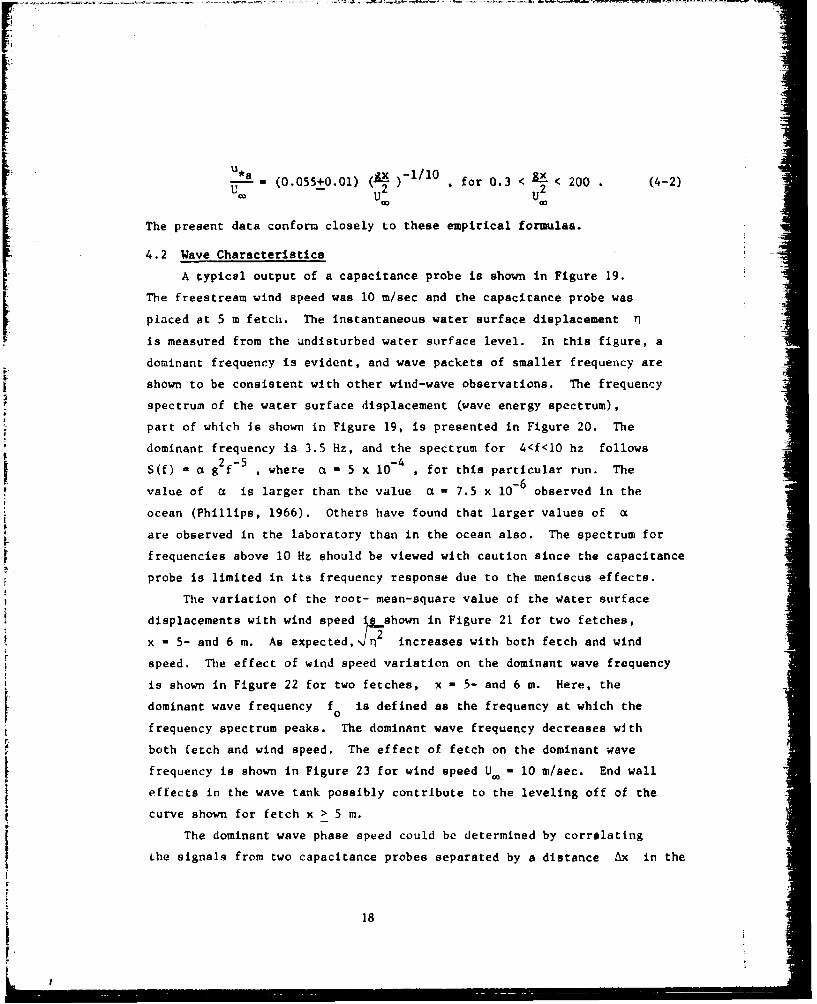
The present data conform closely to these empirical formulas.

4.2 Wave Characteristics

A typical output of a capacitance probe is shown in Figure 19.

The freestream wind speed was 10 m/sec and the capacitance probe wasplaced at 5 m fetch. The instantaneous water surface displacement q

is measured from the undisturbed water surface level. In this figure, aat

dominant frequency is evident, and wave packets of smaller frequency are

shown to be consistent with other wind-wave observations. The frequency

spectrum of the water surface displacement (wave energy spectrum),

part of which is shown in Figure 19, is presented in Figure 20. The

dominant frequency is 3.5 Hz, and the spectrum for 4<f<10 hz follows2f-5 -4

S(f) - a g f where a - 5 x 10 , for this particular run. TheI-6 -value of a is larger than the value a - 7.5 x observed in the

ocean (Phillips, 1966). Others have found that larger values of a

are observed in the laboratory than in the ocean also. The spectrum for

frequencies above 10 Hz should be viewed with caution since the capacitance

probe is limited in its frequency response due to the meniscus effects.

The variation of the root- mean-square value of the Water surface

displacements with wind speed ishown in Figure 21 for two fetches,

x -5- and 6 m. As expected,- -p12 increases with both fetch and wind

speed. The effect of wind speed variation on the dominant wave frequency

is shown in Figure 22 for two fetches, x - 5- and 6 m. Here, the

dominant wave frequency f is defined as the frequency at which thefrequency spectrum peaks. The dominant wave frequency decreases with

both fetch and wind speed. The effect of fetch on the dominant wave

frequency is shown in Figure 23 for wind speed U. - 10 m/sec. End wall

effects in the wave tank possibly contribute to the leveling off of the

curve shown for fetch x > 5 m.

The dominant wave phase speed could be determined by correlating

Lhe signals from two capacitance probes separated by a distance Ax in the

18

wind direction. For a simple train of waves, the phase speed can beAxmeasured as C- , where AT is the time lag at which the cross-

correlation has its first maximum. For a random train of waves, as is

the case with wind-waves, a more accurate determination of AT for eachwave component requires computing the Fourier transform of the cross-

correlation. The complex Fourier transform consists of a real part (co-

spectrum) and an imaginary part (quad-spectrum). At the dominant frequency,

-1 co-spectrumAT is related to the phase angle (- tan qud-Pectrum- by

AT Phase angleAT 360 x f Figure 24 shows the effect of wind speed variation on

0the wave phase speed C p for two fetches, x - 5 and 6 m. The phase

speed increases with increasing wind speed. Figure 25 shows fetch

effects on the wave phase speed Cp . The end wall effects possibly

contribute to the leveling off of the curve.

From the doffinant wave frequency f and the dominant wave phaseo

speed C. , one can easily compute the dominant wavelength

o - . Figure 26 shows the effect of wind speed variation on X forfo

two fetches, x - 5 and 6 m; X increases with both fetch and wind

speed. The dominant wave slope ,In-/X is shown in Figure 27 and it

increases with fetch and wind speed. Figure 28 shows the effects of

fetch on the dominant wavelength for wind speed U = 10 m/sec.

4.3 Surface Drift Velocity

The drift velocity on the water surface was measured using paper

disks which had been coated lightly with wax so Lhey would float. The

diameter of the disk was about 7 mm, and the trajectory of the disc

floating on the water surface was recorded with a 16-ums movie camera.

The time required to travel a known distance was registered with a

digital clock with 0.1 second resolution. For each run, the measurementsI

were repeated several times, and the mean and the standard deviation of

the measurements were determined. Table 2 lists the measured surfacedrift velocity in a tabulated form. Also shown are the number of floats

observed for each run as well as the standard deviation. Figure 29

19

• U

shows the variation of surface drift velocity Ua with fetch for wind

speeds U. - 4, 7 and 10 m/sec. The surface drift velocity U has

an average value of about 3.2 percent of the wind speed.

4.4 Water Boundary-Layer

The water boundary-layer that develops under the action of wind was

visualized with the dye technique. A flourescent dye was injected at the

beginning of the test section using an L-shape tube 2 mm in diameter.

A sheet of laser light was used to illuminate the fluorescent dye in a

vertical plane parallel to the wind direction, and a movie film recorded

the motion in the boundary layer. Figures 30 (a) through (f) show the

photographs of the dyed boundary layer for three wind speeds U. - 4-,7- and 10 m/lset and two fetches, x - 1.7- and 3.2 Tn. In the photographs,a bright horizontal line appears which represents the water surface.

The bright line is produced when the sheet of laser light intersects the

water surface. For U - 4 m/sec, the boundary layer appears to be

laminar at x - 1.7 m, and it becomes turbulent at x - 3 m as indicated

by the substantial increase in thickness. For U - 7- and 10 m/sec,

the flow is turbulent at both fetches as indicated by irregularity of

the dye boundary and by the eddy structure in the boundary layer. From

the dye visualization results, we determined the mean thickness and its

standard deviation of the water boundary-layer. Table 3 contains the

results, and Figure 31 shows the dependence of the water boundary-layer

thickness on fetch and wind speed. The boundary-layer thickness 6 iswnon-dimensionalized using the wind speed U. and the acceleration of.

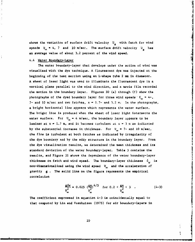
gravity g . The solid line on the figure represents the empirical

correlation

g6w 0.025 (gx)4/5 for 0.2 < gx < 3 (4-3)

UU2 U2 U2

The coefficient expressed in equation 4-3 is coincidentally equal to

that computed by Lin and Veenhuizen (1975) for air boundary-layers in

20

*1!

wind-wave tank experiments. The present data at small fetches for wind

speed U, a 4 m/sec deviate considerably from this formula. We observed

visually that at these fetches the water boundary-layer at wind speed

UC - 4 m/sec did not resemble the fully-developed turbulent boundary-

layers that were observed at the same fetches for higher wind speeds.

4.5 Mean Velocity

Mean velocity profiles in the water boundary-layer wire obtained by Iaveraging the signals from individual cross-element hot-film probes over

a period of 40 seconds. A typical mean velocity profile is shown in

Figure 32 for wind speed U. - 10 m/sec and fetch, x - 5 m. The

figure shows three different runs to check repeatability. At the watersurface, the mean drift velocity determined from the floating disk

measurement is plotted, and it is denoted by a cross symbol. Near the

water surface, the data show a sharp velocity gradient. The driftlayer determined from the mean velocity profile I-as a thickness of about

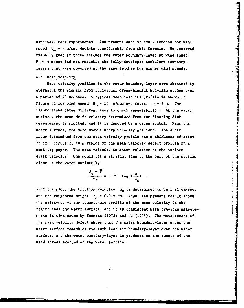
25 cm. Figure 33 is a replot of the mean velocity defect profile on asemi-log paper. The mean velocity is shown relative to the surface

drift velocity. One could fit a straight line to the part of the profile

close to the water surface by

-- 5.75 log (- )

From the Flot, the friction velvcity u, is determined to be 1.81 cm/sec,

and the roughness height z0 a 0.029 cm. Thus, the present result shows

the existence of the logarithmic profile of the mean velocity in the ,

region near the water surface, and it is consistent with previous measure-tprts in wind waves by Shemdin (1973) and Wu (1975). The measurement ofIthe mean velocity defect shows that the water boundary-layer under the

water surface resembles the turbulent air boundary-layer over tha water

surface, and the water boundary-layer is produced as the result of the

wind stress exerted on the water surface.

21

Table 4 shows the friction velocity as determined from similar Iprofiles for different wind speeds and fetches. Also shown is the

corresponding friction velocity for the air boundary-layer as computed

from the empirical formula expressed in Equation (4-2). The ratio of2 2 ,

the water shear stress (pu,) to the air shear stress (pup) at thew a=

air-water interface indicates the percentage of momentum that is extracted

from the air boundary-layer by the water boundary-layer. This ratio

increases as the fetch and the wind speed increases. At U - 10 m/sec,

and x - 6 m , the ratio has a value of 0.9, or equivalently, the ratio Iof the wave drag coefficient to the total wind drag coefficient is 0.1.

Based on the saturated wave energy spectrum, Phillips (1966) estimated

the ratio of the wave drag coefficient to the total wind drag coefficient

cw/Cd to be about 0.1; also Lin and Veenhuizen (1975) obtained the 4rztio c /c for wind waves by correlating many experimental data

w dobtained in wind-wave tanks, i.e.,

c 2cw a 3 P.W 9 T1 (4-4)

d a U 8

where p and pa are water density and air density and 0 is the

momentum thickness of the air boundary-layer. Their computed ratio

was cw/cd - 0.1 + 0.03, for 0.3 < 2x_< 17U4

Figure 34 shows mean velocity profiles in the water boundary-layer

at fetch x - 5 m, for three different wind speeds, U.. - 4-, 7- and

10 m/sec. The average velocity gradient and the thickness of the

boundary-layer both increase with wind speed.

4.6 RMS Velocity Fluctuations I

Figure 35 shows the vertical profiles of the rms value of longi-

tudinal velocity fluctuations in the water boundary-layer for fetch

x - 5 m and wind speed U - 10 m/sec for three repeated runs. Therms values monotonically decrease wiLh depth below the water surface.Its maximum value occurs close to the water surface and is about 20 percent

of the mean surface drift velocity and about 3.5 times the frictional

22

I

A

velocity u, intwater. In the turbulent air boundary-layer over the

water surface, previously-measured by Young et al. (1973) end Yu and Lin

(1975), the maximum rma longitudinal velocity fluctuations is about 15

percent of the air freestream velocity and is about three times the air

friction velocity. Hence, we have more evidence supporting that the

water boundary-layer under the water surface resembles the air

boundary-layer over the water surface. It should be noted, however, that

contains in part the contribution from the orbital motion of the

waves. It will be shown in Section 6.7 that this contribution is by no

means negligible.

Figure 36 shows the vertical profiles of the longitudinal velocity

fluctuations measured at fetch x a 5 m and for three different wind

speeds U. - 4-, 7- and 10 m/sec. The maximum rms value is about 20 percent

of the mean surface drift velocity for wind speeds 7- and 10 m/sec, and

10 percent for wind speed 4 m/sec. These results show that the waterboundary-layer for U,, W 4 m/sec has not been fully developed when

comparing with those for U - 7- and 10 m/sec.

The vertical profiles of the rms vertical velocity fluctuations in

the water boundary-layer Iwz at fetch x - 5 m and for wind speed

U. 10 m/sec.are shown in Figure 37. Data obtained in three repeated

runs are included and, the repeatability is fairly good. By comparison

between Figures 35 and 37, we obtain that the ratio of •w2 to

ranges between 0.70 near the water surface and 0.50 at larger depths.

The vertical velocity fluctuations again contain in part the contribution

from the orbital motion of the waves. Figure 38 shows the vertical

profiles of rms and .he vertical velocity fluctuations .f2 measured at

fetch x - 5 m for three different wind speeds, U. - 4-, 7- and 10 m/sec.

Except for the reduced magnitude, the behavior of Vwt is similar to

that of .

The Reynolds shear stress or the correlation between the longitudinal

and vertical velocity 2omponents uw is a very important quantity that

determines the vertical transfer of momentum in the water boundary-layer.

23

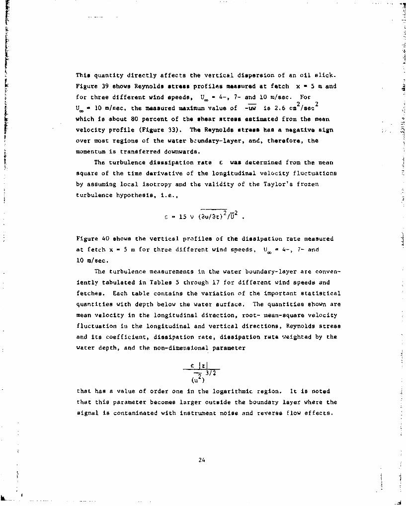
This quantity directly affects the vertical dispersion of an oil slick.

Figure 39 shows Reynolds stress profiles measured at fetch x - 5 m and

for three different wind speeds, U. - 4-, 7- and 10 m/sec. For

1- 0 m/sec. the measured maximum value of -uw is 2.6 cm 2

which is about 80 percent of the shear stress estimated from the mean

velocity profile (Figure 33). The Reynolds stress has a negative sign

over most regions of the water bzundary-layer, and, therefore, the

momentum is transferred downwards.

The turbulence disssipation rate C was determined from the mean

square of the time derivative of the longitudinal velocity fluctuations

by assuming local isotropy and the validity of the Taylor's frozen

turbulence hypothesis, i.e.,

2 -2C 15 V (au/at) 2U2

Figure 40 shows the vertical profiles of the dissipation rate measured

at fetch x - 5 m for three different wind speeds, U, = 4-, 7- and

10 m/sec.

The turbulence measurements in the water boundary-layer are conven-

iently tabulated in Tables 5 through 17 for different wind speeds and

fetches. Each table contains the variation of the important statistical

quantities with depth below the water surface. The quantities shown are

mean velocity in the longitudinal direction, root- mean-square velocity

fluctuation in the longitudinal and vertical directions, Reynolds stress

and its coefficient, dissipation rate, dissipation rate weighted by the

water depth, and the non-dimensional parameter

-) 3/2(u 2

that has a value of order one in the logarithmic region. It is noted

that this parameter becomes larger outside the boundary layer where the

signal is contaminated with instrument noise and reverse flow effects.

24

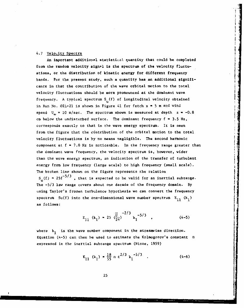
4.7 Velocity Spectra

An important additional statistical quantity that could be completed

from the random velocity signpl is the spectrum of the velocity fluctu-

ations, or the distribution of kinetic energy for different frequency

bands. For the present study, such a quantity has an additional signifi-

cance in that the contribution of the wave orbital motion to the total

velocity fluctuations should be more pronounced at the dominant wave

frequency. A typical spectrum S (f) of longitudinal velocity obtainedu

in Run No. OIL-21 is shown in Figure 41 for fetch x - 5 m and wind

speed U,. 10 m/sec. The spectrum shown is measured at depth z -0.8

cm below the undisturbed surface. The dominant frequency f - 3.5 Hz,

corresponds exactly to that in the wave energy spectrum. It is seen

from the figure that the contribution of the orbital motion to the total

velocity fluctuations is by no means negligible. The second harmonic

component at f - 7.0 Hz is noticeable. In the frequency range greater than

the dominant wave frequency, the velocity spectrum is, however, wider

than the wave energy spectrum, an indication of the transfer of turbulent

energy from low frequency (large scale) to high frequency (amall scale).

The broken line shown on the figure represents the relation

S (f) a 25f-5 3, that is expected to be valid for an inertial subrange.

The -5/3 law range covers about one decade of the frequency domain. By

using Taylor's frozen turbulence hypothesis we can convert the frequency

spectrum Su(f) into the one-dimensional wave number spectrum E11 (k 1 )

as follows:

-2/3 5/3El (k) 25 (U) kI (4-5)

where k is the wave number component in the streamnise direction.

Equation (4-5) can then be used to estimate the Kolmogorov's constant a

expressed in the inertial subrange spectrum (Hinze, 1959)

E 1 (k1 18 a2/3 -5/3

25l l k . (4-6)

25

MA

The value of a is calculated to be 1.79 by inserting U - 16.16 cm/secand E - 109 cm2 /sec. This value is reasonably close to the universal 1constant a Z 1.44 determined from many other turbulence measurements

(Phillips 1966). Lin (1974) observed the universal constant to be

ot a 1.66 by fitting experimental data to his semi-analytical spectrum

in the inertial and dissipation ranges. The Kolmogorov wave number,

SCE/V3) 1 / 4 ,i calculated to be 100 cm and the corresponding

Kolmogorov leng:h scale is 0.63 m. The turbulence microscale defined

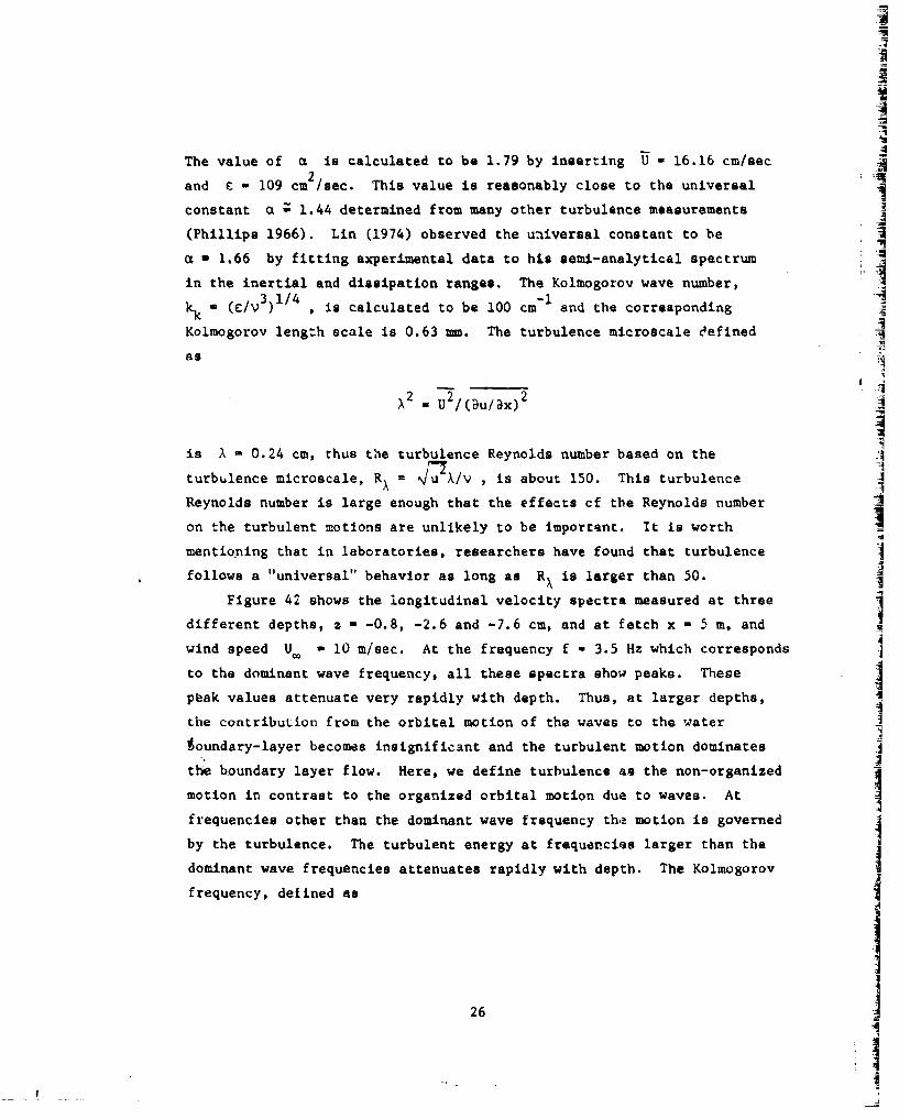
as

2 2 2X U /(au/ax)2M

is X a 0.24 cm, thus the turbulence Reynolds number based on the *1

turbulence microscale, R 4u X/v , is about 150. This turbulence A

Reynolds number is large enough that the effects cf the Reynolds number

on the turbulent motions are unlikely to be important. It is worth Imentioning that in laboratories, researchers have found that turbulence

follows a "universal" behavior as long as RX is larger than 50.

Figure 42 shows the longitudinal velocity spectra measured at three

different depths, z a -0.8, -2.6 and -7.6 cm, and at fetch x - 5 m, and

wind speed U. - 10 m/sec. At the frequency f - 3.5 Hz which corresponds

to the dominant wave frequency, all these spectra show peaks. These ]ptak values attenuate very rapidly with depth. Thus, at larger depths,

the contribuLion from the orbital motion of the waves to the water -i

toundary-layer becomes insignificant and the turbulent motion dominates

the boundary layer flow. Here, we define turbulence as the non-organized

motion in contrast to the organized orbital motion due to waves. At

frequencies other than the dominant wave frequency the motion is governed

by the turbulence. The turbulent energy at frequencies larger than the

dominant wave frequencies attenuates rapidly with depth. The Kolmogorov

frequency, defined as j261

IIi

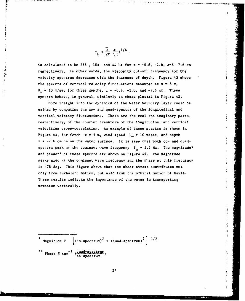
I.Ir.

I f~k 27 " 3 •

is celculated to be 256-, 104- and 44 Hz for z * -0.8, -2.6, and -7.6 cm

respectively. In other words, the viscosity cut-off frequency for the

velocity spectrum decreases with the increase of depth. Figure 43 shows

the spectra of vertical velocity fluctuations measured at x - 5 m,

U.- 10 rn/sec for three depths, z - -0.8, -2.0, and -7.6 cm. These

spectra behave, in general, similarly to those plotted in Figure 42.

More insight into the dynamics of the water boundary-layer could be

gained by computing the co- and quad-spectra of the longitudinal and

vertical velocity fluctuations. These are the real and imaginary parts,

respectively, of the Fourier transform of the longitudinal and vertical

velocities cross-correlation. An example of these spectra is shown in

Figure 44, for fetch x - 5 m, wind speed U - 10 m/sec, and depth

z - -2.6 cm below the water surface. It is seen that both co- and quad-

spectra peak at the dominant wave frequency fo 0 3.5 Hz. The magnitude*

and phase** of those spectra are shown on Figure 45. The magnitude

peaks also at the dominant wave frequency and the phase at this frequency

is -78 deg. This figure shows that the shear stress contributes not

only frcm turbulent motion, but also from the orbital motion of waves.

These results indicate the importance of the waves in transporting

momentum vertically.

Magnitude [(co-spectrum)2 + (quad-spectrum)2] 1/2

Phse -. (quad-spectrumco-spectrum

27

5. EFFECTS OF WAVES ON WATER MOTION

In this section, we present the experimental results concerning the

effects of waves on the water motion. For all the experiments, the wind

speed waA the same, U - 10 m/sec, and waves of three difierent heights

were generated by the wave maker. We measured the wave characteristics

of these waves. The surface drift velocity under these wave conditions

was measured, and the effect of wave steepness on the surface drift

velocity was determined. The water boundary-layer developed under the

action of wind and waves was visualized with dye, and the thickness of

the water boundary-layer was determined from the visualization results.

Vertical profiles of mean velocity and rms velocity fluctuations were

measured using the LDV. The velocity spectra were calculated from the

velocity fluctuations to determine the wave effect on the velocity field

and the basic turbulent characteristics.

5.1 Wave CharacteristIcs

The wave maker described in Section 2 was used to generate surface

waves. The oscillatory motion of the wave plunger was controlled by an

electronic wave generator operating at a frequency of about 1.6 Hz. The

voltages of the wave generator were selected to produce three different

strokes of the wave plunger, namely, H - 2.54-, 5.08- and 7.62 cm.0

Figure 46 (a) through (d) shows the pnotographs of the water surface for

H - 0-, 2.54-, 5.08- and 7.62 cm. All waves propagate from the left to

the right. The photographs were taken at a fetch of about x - 4 m. For

H° - 0 cm, there are no mechanically-generated waves. The waves are

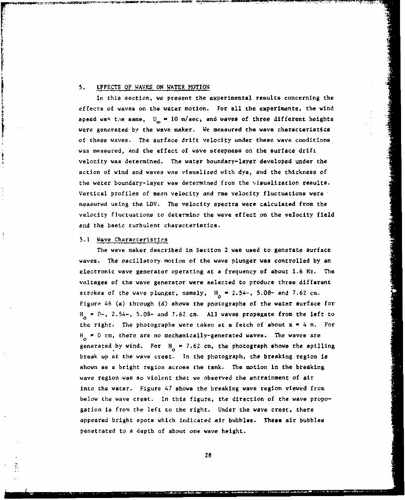
generated by wind. For H - 7.62 cm, the photograph shows the spilling

break up at the wave crest. In the photograph, the breaking region is

shown as a bright region across the tank. The motion in the breaking

wave region was so violent that we observed the entrainment of air

into the water. Figure 47 shows the breaking wave region viewed from

below the wave crest. In this figure, the direction of the wave propo-

gation is from the left to the right. Under the wave crest, there

appeared bright spots which indicated air bubbles. These air bubbles

penetrated to a depth of about one wave height.

28

'7

Figure 48 shows the wave energy spectra S(f) measured with a

capacitance probe at fetch x - 2 m and wind speed Urn - 10 m/sec. The

spectra peak at the dominant frequency f - 1.6 Hz and subsequent

higher harmonics. The strength of higher harmonic wave components

increases with H . For H. 0 7.62 cm, the spectral peaks at the

dominant wave frequency and higher harmonics have an envelope expressed

by S(f) - 1.46 x 1 2 f for fo0 <f< 0Hz.

The phase speed, C , of the dominant waves was measured with two

capacitance proben separated by a distance Ax - 1.02 cm apart. These

two capacitance probes were made of a thin copper wire coated with

teflon. We selected the teflon coated wire probe instead of the bare

stainless steel probe in order to minimize the possible cross talk

between two adjacent probes. To determine the value of Cp , we calculated

the cross correlation of the surface displacements measured with the two

capacitance probes. The time lag of the maximum correlation, AT , can

therefore be determined, and it should correspond to the time required

for the waves traveling over a distance Ax . Hence, the dominant phase

speed can be estimated as Cp- ax// . The dominant wave speeds are

108.4-, 108.4- and 121.1 cm/sec for H 1 2.54-, 5.08- and 7.62 cm respec-0

tively. Based on the measurements of C and f , we can estimate theo o

dominant wavelength X - C p/f as 65.3-, 65.3- and 73.0 cm for the

three respective values of H0

Based on the measurements of X , one can estimate the wave phase

speed by the linear wave theory. Comparison between the direct measure-

ment and the linear wave prediction could then indicate the nonlinear

effects on the wave propagation. Figure 49 ahows the plot of Cp/ fg-X/2R7

versus the wave steepness H/X . Here H is the wave height w 'ch can

be estimated from the rms wave amplitude by H =2 For comparison,

a solid line representing

21 + 2 I+I 1 (5-1)

29

I

is plotted (Kinsman, 1965). The last two terms in equation (5-1)

represent the nonlinear effect on the phase speed. The deviation of the

measurement points from the solid curve could partly be attributed to

the wind induced-surface drift. Figure 50.shows the variation of rms

wave amplitude 4`7 with fetch for three values of 11 . We used the photo-

diode wave gauge to measure the vertical displacement of the water A

surface because the wave height measurement by the capacitance probe

becomes inaccurate when the wave breaking occurs. Each data point was 3

calculated from a record of about 60 sec. The overall statistical error

is estimated to be about 10 percent. This error is mainly contributed by

a low-frequency modulation (having a period of about 20 sec) of the wave

field which is possibly caused by the return flow in the wave tank.

For H - 2.54- and 5.08 cm, the rms wave amplitude increases with

increasing fetch. For example, the wa'e energy per unit density, gn2 ,1

increases from 980 cm 3/sec2 at x " 2 m to 2509 cm 3/sec2 at x - 5 m forH - 2.54 cm. In section 4.2, we have presented the measurement of rmas

wave amplitude for the case without mechanically-generated waves, but

with wind only; the wave energy per unit density increases from prac-

tically zero at x - 2 m to 134 cm 3/sec2 at x - 5 m. This example shows

that when mechanically-generated waves are present, the energy Lransfer

from wind to waves appears to be more efficient than when mechanically-

generated waves are not present. This observation also applies to the

case of H M 5.08 cm. For M4 - 7.62 cm, however, the wave energy decreases0

with fetch. Apparently, the wai- breaking causes significant energy

dissipation by turbulence which overwhelms the energy transfer from wind.

Figure 51 shows the wave energy spectra measured at two fetches for

H 7.62 cm and U. 10 m/sec. The wave breaking reduces the energy0

content at the dominant wave frequency and increases the energy at

higher frequencies. For 6 Hz < f < 40 Hz , the wave energy spectrum

follows S(f) - 0.054 y2 3 f 7 / 3 . The energy gaps between higher harmonics

are filled in when wave breaking occurs. Figure 52 shows the wave

I3

S~~30A

energy spectra measured at x - 5 m for U . 10 m/sec and for various

conditions of mechanically-generated waves. In the capillary wave

regime, the energy increases with the value of H . In the graviLy wave

regime, there exists an envelope expressed by S(f) - 1.45 x 10-4 g2 i 5

for the dominant waves and their higher harmonics. This envelope could,

therefore, represent the saturated wave spectrum in the present investi-M

gation. Figure 53 shows the wave energy spectra measured at x - 5 m for

H - 7.62 cm and for three wind speeds. In the capillary wave regime,0

the wave energy increases with wind speed. In the gravity wave regime,

wave energy does not change appreciably, and the energy gaps between

higher harmonics fill in as wind speed increases.


The surface drift velocity was measured using a small paper disc

floating on the water surface. The paper discs were made the same way as

for the surface drift measurement described in Section 4.3. The drift

of the paper discs was recorded with a 16-mm movie camera. The

standard deviation of the drift velocity measurements was typically about

10 to 20 percent of the mean surface drift velocity. If breaking waves

appear, paper discs may not float well on the water surface. Frequently,

we did observe that paper discs were entrained into the breaking wave

region below the water surface. Consequently, these paper discs were A

discarded when making the drift velocity measurement. On the other I

hand, we also observed that the standard deviation in measuring the

surface drift velocity is large when breaking waves are present.

Figure 54 shows the mean surface drift velocity U plotted versus

fetch x . The mean surface drift velocity measured at x - 2 m are

plotted versus the wave steepness, H/X, in Figure 55. Also plotted is

the surface drift velocity measured in the wind waves at U,- 10 m/sec. I

This is a limiting case when the height of the mechanically-generated

waves approaches zero. The measurement points show that at H/I - 0.05, the

surface drift velocity is lower than that for the case when the mechan-

ically-generated waves are not present. For H/f > 0.05, the surface

drift velocity increases with the increase of the wave steepness.

31

I

The effect of wave steepness on the surface drift has been investi-

gated by Reisbig et al., (1973). In their laboratory experiments, the

wind speed ranged from 0- to 7 m/sec and the wave steepness varied from

0- to 0.069. Their experimental results show that the drift mechanisms

caused by wind and waves ere not simply additive. At low wind speeds,

the wave drift provides an augmentation to the wind drift, but at

higher wind speeds, the waves cause a net decrease in the coupled drift

velocity. This wave-induced diminishment increases as the wind speed

increases. In the present investigation, we covered a wider range of

H/X . Our data show a similar wave-induced decrease when H/X increases

from 0 to 0.05. For H/I > 0.05 the surface drift velocity increases

with wave steepness. In the following paragraphs, we will try to explain

the possible mechanisms which contribute to the complex behavior of the

surface drift due to the coupled wind and waves.

Jeffreys (1925) hypothesized the separation mechanism for energy

transfer from wind to waves. Recently, Chang et al., (1969) conducted a

series of laboratory measurements of mean and turbulent velocity in the

air flow region above wind-generated waves and their experimental results

tend to support the separation mechanism. Banner and Melville (1976)

conducted a flow visualization experiment to demonstrate that the air-

flow could separate from the water surface in the lee side of mechan-

ically-generated waves. Based on kinematic arguments, they hypothesized

that the separating flow would occur when waves break. More recently,

Weissman (1978) conducted laboratory experiments in the airflow over

mechanically-generated waves. His experimental results, both from smoke

visualization and from probe measurements, showed that the separating

flow in the air could occur even though wave breaking was not apparent.

In view of the separation mechanism described above, we expect that

in our experiment conducted for a wind speed of U - 10 m/sec over

mechanically-generated waves, the airflow could separate from the water

surface in the lee side of the waves. Although the presence of the air

separation could enhance tlhe energy transfer from wind to waves, the

32

effective shear stress exerted on the water by the wind is reduced.

This reduction is not difficult to imagine if we realize that the

separated flow would introduce a reverse flow region in which the shear

stress is exerted in a direction opposite to the wind. Now, if we

assume that the surface drift due to the wind should correspond to the

effective shear stress exerted on the water surface, we would therefore

expect that, for the case when mechanically-generated waves are present

and Zhe separation exists in the lee side of the waves, the surface

drift velocity would be lower than for the case without mechanically-

generated waves.

When the wave steepness increases further, additional mechanisms

other than the separation mechanism could influence the surface drift.

For example, the Stokes' drift (1847) on the water surface is expressed

by Phillips (1966) as

Ud 2 C (5-2)

where C is the wave speed and X is the wavelength. The Stokes'

drift would become important as the wave steepness and the wave speed

increase. Pottinger and Reisbig (1973) conducted an experimet.t to

determine the effect of waves on the drift of an oil slick. The waveswere generated mechanically by a wave maker. The wavelength ranged

from 25- to 50 cm and the wave steepness from 0.01 to 0.07. The oil

slick was, in essence, an oil lens of diameter 4.6- and 7.5 cm and thickness-4 -5varying from 10 to 10 of the wavelength. Their data indicate that

the oil slick drifted faster than that predicted by the Stokes' drift.They obtained an empirical relation to correlate their experimental

results.

"U U +Us d c

C + 0.445 C , for 0.01 < H/A < 0.07 (5-3)

and 25 < X < 50 cm,

where U is the correction term of the surface drift velocity.

33

k I

In the following, we will utilize the empirical result expressed in

equation (5-3) to help us understand our observation of the surface

drift caused by wind and waves. In Figure 55, we replot our data by

subtracting the surface drift velocity by the corresponding Stokes'

drift velocity, i.e., Us - Ud , and subsequently by the correction term

Uc, i.e., Us - id - Uc. It is interesting to point out that the datapoints of U - Ud - Uc does not show significant variation with wavesteepness and they have an average value of about 0.02 U which corresponds

to wind-induced current. This value is apparently lower than that

observed for the case when mechanically-generated waves are not present.

Therefore, we introduce an empirical formula for the surface drift

caused by wind and waves:

S 2 H'() 2 AI C (0.02 + + 0.445 ( (5-4)

for 0.05 < H/X < 0.10 , U. - 10 m/sec and 65 cm < X < 73 cm

A solid line is drawn in Figure 55 to represent equation (5-4) for

C/U. - 0.12 , and it can fairly approximate our measurements.

5.3 Water Boundary-Layer

The water boundary-layer was visualized with dye techniques. The

dye was introduced into the water by a vertical string 0.3 cm in diameter.

The string was located along the centerline of the tank. The string was

made of cotton and formed a closed loop with three point

supports. Part of the string was stretched vertically in the water and

part of it was exposed in the air. The part of string exposed in the

air was dyed with a fluorescent dye, and it was then lowered below the

water by sliding the string loop. The dye, washed sway from the string,

was initially vertical, and this vertical dye line was deformed and

dispersed by the motion in the water. Figure 56 is a photograph showing

the dye dispersion in the water for H - 7.62 cm and U 10 r/sec.0

Two flow regions are distinctly visible. In the top region about 15 cm

34

below the water surface, the dye disperses it the wind direction, and in

the bottom region below 15 cm from the water surface the dye disperses

in the reverse direction. The top region is apparently the boundary

layer of flow set up by wind and waves, and the bottom region corresponds

to the return flow due to the finite length of the tank. For the case

when waves are generated by wind only, we used a false bottom to channelthe return flow In-between the tank bottom and the false bottom, and

therefore we were able to control and minimize the reverse flow in the

region between the water surface and the false bottom. We tried to use

the same setup of the false bottom for the case when both wind and

mechanically-generated waves were present, but the reverse flow could

not be controlled as well a- when only wind-generated waves were present. A

* For lack of time to try to find a better way to control the reverse

flow, we decided not to use the false bottom for the case when both wind

and mechanically-generated waves were present.

The presence of the reverse flow could affect the water boundary-

layer. We are not in a position to estimate these effects due to the

reverse flow quantitatively, but, on the other hand, we expect that in

the region near the water surface and away from the reverse flow, the

flow characteristics should be most dominated by the local flow conditions

such as the break up of waves and the presence of strong shear. Figure

57 presents the thickness of the water boundary-layer measured from the

movie record of the dye dispersion in the water boundary-layer. We

define the thickness of the water boundary-layer as the depth measured

between the undisturbed water surface and the vertical position where

the local mean velocity was approximately zero. The data do not show

any consistent variation with fetch and wave height.

5.4 Mean Velocity

Figures 58 and 59 present the vertical profiles of longitudinal and

vertical mean velocities for H - 7.62- and 2.54 cm. In general, we0

experienced some difficulties in measuring mean velocity components

because of the unsteady nature of the return flow set up in the tank.

35

M W T - -. . . . . :. . .. . .- . . . .. ... . . ... .. .. . -. . . . . .

I

I

This unsteady flow apparently does not affect the measurement of velocity

fluctuations (Section 5.6), but it does affect the mean velocity component.

This unsteady phenomenon has a typical period of about 20 sec, but our

measurement period was about 40 sec. Thus, we do experience some

statistical uncertainty in measuring the mean velocity. Figure 58 shows A

that the mean velocity profile has a drift layer in the region about

15 cm below the undisturbed water surface, and a reverse flrw between

the depths of 15- and 25 cm. The drift layer does not appear as strong

as when the mechanically-generated waves are absent (Figure 32). This

result shows that in the presence of mechanically-generated waves, wind Iis no longer as effective in transferring energy into current as when

the mechanically-generated waves are absent. On the other hand, we have

observed that when mechanically-generated waves are present the energy

transfer from wind to waves appears to be more efficient than when

mechanically-generated waves are absent (Section 5.1). A systematic

measurement of both energetics in the air, water and wave fields is

needed to clarify how the energy is transferred from the air to the

drift current and to waves.

Figure 59 shows that in the top drift layer the vertical mean

velocity is small, while in the reverse flow region the vertical velocity

becomes significant when compared with the longitudinal velocity.

5.5 RNS Velocity Fluctuations

Figure 60 shows the vertical profile of rms longitudinal velocity

fluctuations, Jý measured for H - 7.62- and 2.54 cm. For0

H 0 7.62 cm, the data points are denoted by circles. At several depths,0

repeated measurements were made to examine the repeatability in the

measurement of rms velocity fluctuations. For H - 2.54 cm, repeated

measurements were also made in two series of experiments. This good

repeatability shows that the measurement of rms velocity fluctuations

does not appear to be significantly affected by the return flow.

Especially in the drift layer, the reverse flow should not appreciably

influence the velocity field. Comparison between Figures 58 and 60

"36

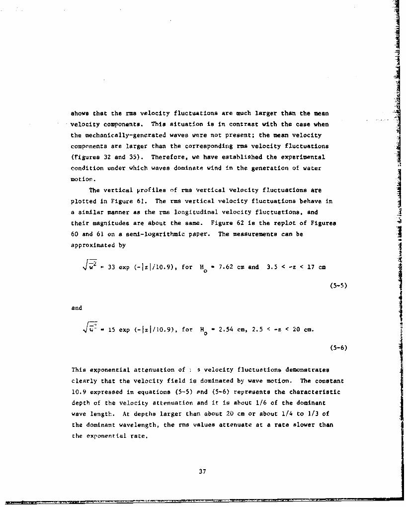
shows that the rms velocity fluctuations are much larger than the meanvelocity components. This situation is in contrast with the case when

the mechanically-generated waves were not present; the mean velocity

components are larger than the corresponding rms velocity fluctuations(Figures 32 and 35). Therefore, we have established the experimentalcondition under which waves dominate wind in the generation of water

motion.

The vertical profiles of rms vertical velocity fluctuations are

plotted in Figure 61. The rms vertical velocity fluctuations behave in

a similar manner as the rms longitudinal velocity fluctuations, and

their magnitudes are about the same. Figure 62 is the replot of Figures

60 and 61 on a semi-logarithmic paper. The measurements can be

approximated by

J• = 33 exp (-Izai10.9), for H° - 7.62 cm and 3.5 < -z < 17 cm

(5-5)

and

15 exp (-Izj/L0.9), for H 2.54 cm, 2.5 < -z < 20 cm.

(5-6)

This exponential attenuation of ; s velocity fluctuations demonstrates

clearly that the velocity field is dominated by wave motion. The constant

10.9 expressed in equations (5-5) ond (5-6) represents the characteristic

depth of the velocity attenuation and it is about 1/6 of the dominant

wave length. At depths larger than about 20 cm or about 1/4 to 1/3 of

the dominant wavelength, the rms values attenuate at a rate slower than

the exponential rate.

37

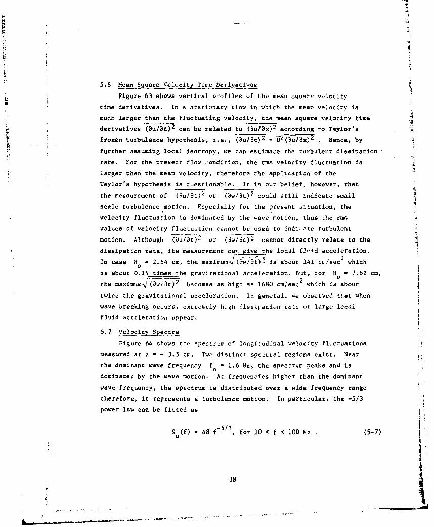
A

5.6 Mean Square Velocity Time Derivatives

Figure 63 shows vertical profiles of the mean aqtarc vtlocity

time derivatives. In a stationary flow in which the mean velocity is

much larger than the fluctuating velocity, the mean square velocity time

derivatives Zu/ t)2 can be related to (au/ax) 2 according to Taylor's

frozen turbulence hypothesis, i.e., (;u/at)2 - U-2 (Ou/ax)"2 . lience, by

further assuming local Isotropy, we can estimate the turbulent dissipation

rate. For the present flow condition, the rms velocity fluctuation is

larger than the mean velocity, therefore the application of the

Taylor's hypothesis is questionable. It is our belief, however, that

the measurement of (au/at) 2 or (aw/at) 2 could still indicate small

scale turbulence motion. Especially for the present situation, the

velocity fluctuation is dominated by the wave motion, thus the rms

values of velocity fluctuation cannot be used to indicAte turbulent

motion. Although (au/at)2 or (aw/at) 2 cannot directly relate to the

dissipation rate, its measurement can give the local flld acceleration.

In case H - 2.54 cm, the maximum (aw/gt)2 is about 141 ci,,/sec2 which

is about 0.14 times the gravitational acceleration. But, for He a 7.62 cm,

che maximuwý (awit) 2 becomes as high as 1680 cm/sec2 which is about

twice the gravitational acceleration. In general, we observed that when

wave breaking occurs, extremely high dissipation rate or large local

fluid acceleration appear.

5.7 Velocity Spectra

Figure 64 shows the spectrum of longitudinal velocity fluctuations

measured at z - - 3.5 cm. Two distinct spectral regions exist. Near

the dominant wave frequency f - 1.6 Hz, the spectrum peaks and iso

dominated by the wave motion. At frequencies higher than the dominant

wave frequency, the spectrum is distributed over a wide frequency range

therefore, it represents a turbulence motion. In particular, the -5/3

power law can be fitted as

S (f) -48 f- 5/3, for 10 < f < 100 Hz , (5-7)u

38

In Figure 65, the spectrum of vertical velocity fluctuations is

shown. It has a dominant peak and a second harmonic component which

does not appear in the spectrum of longitudinal velocity fluctuations.

For 2 < f < 10, the spectral density of the vertical velocity fluctu-

ations is higher than that of the horizontal velocity fluctuations. At

high frequencies, the spectrum in Figure 65 is fitted by

-5/3S (f) 66 f , for 4 < f < 100 Hz. (5-8)w

Comparison between Figures 64 and 65 indicates a possible generation

mechanism of turbulence in breaking waves. As will be shown in Section

6, the wave breaking introduces very strong vertical motion as a plume

injected downwards from the point where the wave breaking occurs. The

spectrum of this vertical motion corresponds to the energy excess in the

spectrum of vertical velocity fluctuations for 2 < f < 10. The spectrum

shown in Figure 65 is identical to that shown in Figure 64 for the

frequency range 1 < f < 2 Hz . The identical spectra for S (f) andU

S (f) shows unmistakably that in the frequency range 1 < f < 2 Hzw

the motion is caused by waves.

In the frequency range 2 < f < 4 Hz, S (f) is lower than S (f),U w

and the slope of S (f) is smaller than that of S (f). Based on theseu w

observations, we speculate that strong energy transfers from the verticsl

velocity component to the longitudinal velocity component. This spec-

ulation can readily be proven or disproven if the co- and quad-spectrum

of longitudinal and vertical velocity fluctuations car. simultaneously be

measured.

From equations (5-7) and (5-8), the ratio S (f)/S(f) is estimated

to be about 1.38, This value is very close to the value of 4/3 when the

turbulence is locally isotropic. Although we question the applicability

of Taylor's hypothesis to the turbulence in breaking waves, it is still

39

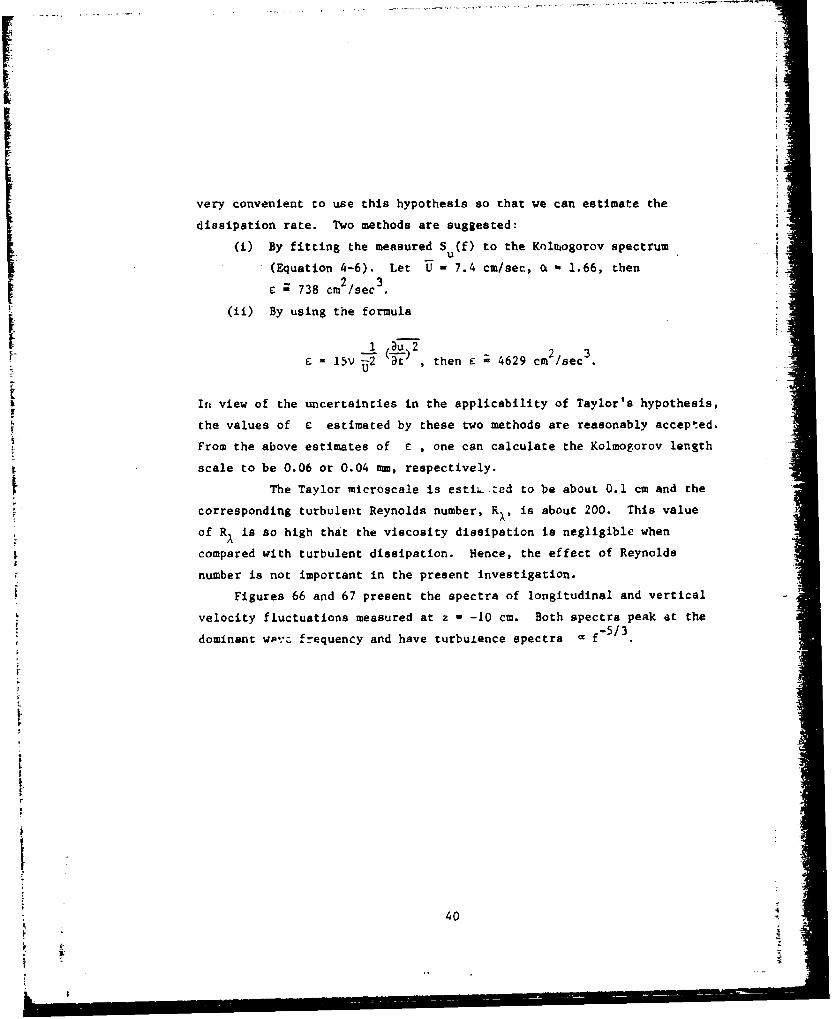
iI

very convenient to use this hypothesis so that we can estimate the

dissipation rate. Two methods are suggested:

(i) By fitting the measured S (f) to the Kolutogorov spectrumU

(Equation 4-6). Let U = 7.4 cm/sec, ac 1.66, then

c 738 cm2 sec 3

(ii) By using the formula

1 Du.215v -2 3 , then E 4629 cm /secU=

In view of the uncertainties in the applicability of Taylor's hypothesis,

the values of e estimated by these two methods are reasonably accepted.From the above estimates of C , one can calculate the Kolmogorov length

scale to be 0.06 or 0.04 m, respectively.

The Taylor microscale is estiL ted to be about 0.1 cm and the

corresponding turbulent Reynolds number, R,, is about 200. This value

of R is so high that the viscosity dissipation is negligible when

compared with turbulent dissipation. Hence, the effect of Reynolds

number is not important in the present investigation.

Figures 66 and 67 present the spectra of longitudinal and vertical

velocity fluctuations measured at z - -10 cm. Both spectra peak at the

dominant wpv: frequency and have turbulence spectra f-5/3

4

40

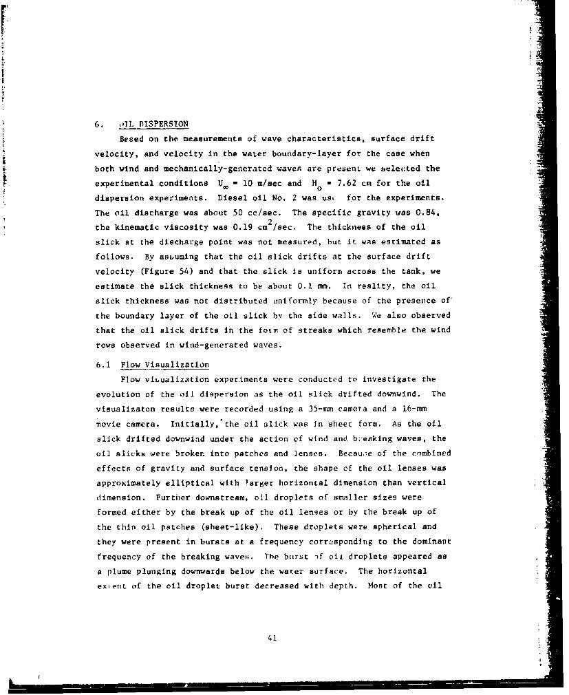
6. ,i1L DISPERSIONBesed on the measurements of wave characteristics, surface drift

velocity, and velocity in the water boundary-layer for the case when

both wind and mechanically-generated waves are presenL we selected the

experimental conditions U, - 10 m/sec and H - 7.62 cm for the oil

dispersion experiments. Diesel oil No. 2 was ust for the experiments.

The oil discharge was about 50 cc/sec. The specific gravity was 0.84,

the kinematic viscosity was 0.19 cm 2/sec. The thickness of the oil

slick at the discharge point was not measured, but It was estimated as

follows. By assuming that the oil slick drifts at the surface drift

velocity (Figure 54) and that the slick is uniform across the tank, we

estimate the slick thickness to be about 0.1 rmm. In reality, the oil

slick thickness was not distributed uniformly because of the presence of-

the boundary layer of the oil slick by the side walls. We also observed

that the oil slick drifts in the fotm of streaks which resemble the wind

rows observed in wind-generated waves.

6.1 Flow Visualization

Flow viuualization experiments were conducted to investigate the

evolution of the oil dispersion as the oil slick drifted downwind. The

visualizaton results were recorded using a 35-mm camera and a 16-mm

movie camera. Initially,'the oil slick was in sheet form. As the oil

slick drifted downwind under the action of wind and br-eaking waves, the

oil slicks were broken into patches and lenses. Becau.1e of the combined

effects of gravity and surface tension, the shape of the oil lenses was

approximately elliptical with larger horizontal dimension than vertical

dimension. Further downstream, o1l droplets of smaller sizes were

formed either by the break up of the oil lenses or by the break up of

the thin oil patches (sheet-like). These droplets were spherical and

they were present in bursts at a frequency corre-spondlng to the dominant

frequency of the breaking waves. The burst if oil droplets appeared as

a plume plunging downwards below the water surface. The horizontal

extent of the oil droplet burst decreased with depth. Most of the oil

41

droplets resurfaced very rapidly, and oil droplets of small sizes stayed

in the water boundary-layer and convected downwind by the drift currents.

From time to tiwe, we observed droplets having sizes of about 0.5-to 1 cm drifting very freely in the water as'if they were nearlyneutrally buoyant. We speculated that these droplets were, in essence,

a water droplet coated with a thin oil film. We further observed that

the oil film on the water droplet was not uniform in thickness. Near

the top of the droplet, the oil film appeared thicker than that near the

bottom due to the buoyancy of the oil in water. We called these droplets

"oil bubbles" because of their resemblance to soap bubbles in the air.

It must be reminded that the soap bubble has a thicker film near the

bottom of the bubble. Sometimes we observed that these "oil bubbles"

were attached to one or several air bubbles. These air bubbles were

entrained into water by the breaking waves. The conglomerate of the oil

and air bubble resurfaces very rapidly because of the additional buoyancy

of the air bubble.

6.2 Oil Concentration

We used the photographic technique to measure the vertical profile

of oil concentration in the water boundary-layer. The sample volume for

oil concEntration measurements was selected at fetch x - 4 m. The

sample volume was defined between the side (glass) wall and a black

colored vertical plate. The plate was about 30 cm high, 2 cm long and

0.2 cm thick and was positioned 1.65 cm away from and parallel to the

side wall. The total sample volume was a rectangular column, 30 cm

high, 2 cm long and 1.65 cm thick. Flood lamps projected light from

above `or illumination. The oil droplets existing in this sample volumec

were recorded by a polaroid camera standing about 30 cm away from the

side of the tank. To determine the volume occupied by the oil droplets,

their size was measured and their number was counted under a microscope.

Tht_ volume measurements were made at vertical increments of 1.25 cm. At

each increment, the oil concentration waa determined by dividing the oil

42 IL

l3

volume to the total volume of the increment, 4.1 cm3 . The oil droplets

observed in this figure are approximately spherical in shape, thus by

measuring the diameters (size) of the oil droplets, one can calculate

the volume accordingly. Identifying the oil droplets in this figure is

by no means a trivial task. Under these light conditions, an oil droplet

is accompanied by two bright spots, one on the top and one on the

bottom of the droplet. The top bright spot results from the light H

reflection from the top surface of the oil droplet, and the bottom

bright spot results from the light passing through and refracting out of Ithe oil droplet.

The vertical profile of instantaneous concentration is plotted in

Figure 68. This vertical profile shows that the maximum volume concen-

tration is about 0.009 and that the oil can penetrate as deep as about H20 cm (2.6 H ). To obtain 6tatistics of oil concentration, such as mean

and rms, we used seven vertical profiles of instantaneous oil concen-

tration. These profiles were measured from photographs which were Vsequentially taken at time increments of about 10 sec. Hence, eachphotograph could be treated as an independent observation. Figure 69

shows the vertical profiles of mean and rms oil volume concentration,

and Vc2 . The rms oil concentration was measured by calculating thesrandard deviation of the seven instantaneous concentration profiles,

thus it includes both wave-induced and turbulent fluctuations. The ruas

oil concentration is comparable to the mean value.

The vertical profile of the mean oil concentratiou is replotted on

a semi-logarithmic graph in Figure 70. The profile can be approximated

by

C = 0.015 exp (-Izi/7.9), for 5 cm < -z < 20 cm. (6-1)

The constant in the exponent of equation (6-1) is a characteristic

depth 7.9 cm for the oil concentration. This characteristic depth is

comparable to that observed from the vertical profile of -ms velocity

fluctuations (Section 5.5).

43

|I

I

I

From the seven photographs aforementioned, we obtained the size

distribution of oil droplets for U, - 10 m/sec and x - 4 m. For each

photograph, we counted the total number of oil droplets. The oil

droplets were thus grouped according to their sizes. The smallest size

of oil droplets which could be resolved photographically was 0.5 mm, and

the size increment was 0.25 mm. For each size group, we obtained the a

number of oil droplets. By dividing this number by the total number of

oil droplets, we can then obtain the percentage frequency for that size

of oil droplets; therefore, the size distribution of oil droplets for

this photograph is determined. From the seven photographs, we cani a

further obtain the average percentage frequency for a specific size.

Figure 71 is the size distribution of oil droplets. The average oil

droplet size is atout 1.1 mmu and the most frequently observed size is

0.75 mm for the present investigation.

A

44!

I

IIIIJ

II

44i1

3

i7. CONCLUSIONS

7.1 Turbulence and Wave-Induced Motion

Based on the experimental data obtained in the present research

study, we conclude that the turbulence structure in surface waters

depends strongly on its generating mechanisms. For the present interest,

two mechanisms, namely wind and waves, were considered. The important

findings are summarized in the following:

(i) When wind dominates the turbulence generation, the water

boundary-layer behaves very similar to the turbulent boundary-

layer over a rough surface. The mean velocity has a logarithmic

region. The water boundary-layer thickness 6w grows with

fetch and is approximated by

S- 0.025 (L)4/5 , for 0.2 < < 322 U2

Uu00

The profile of turbulence intensity also resembles that which Ihas been observed in the turbulent boundary-layer over a rough

surface. The maximum turbulence intensity is about 0.7 percent

of wind speed or 20 percent of the surface drift velocity.

The contribution of wave motion to the turbulence intensity

measurement is not negligible. The velocity spectrum shows a

peak at the dominant wave period and a modest range of f law.(ii) When waves dominate the turbulence generation, the water flow

does not resemble the boundary-layer flow. The water motion

is mainly governed by waves. The wave induced motion, such as

the rms velocity fluctuation attenuates exponentially with

depth. The turbulent motion is predominately introduced by

the wave breaking. The wave breaking introduces a strong

vertical burst motion like a plume plunging downwards below

the water surface. The penetration of tiviB burst motion is

about one wave height. The spectrum show a dominant peak

representing the wave-induced motion and an extensive

Kolmogorov spectrum f-5/3 for almost two decadles of frequencies.

45

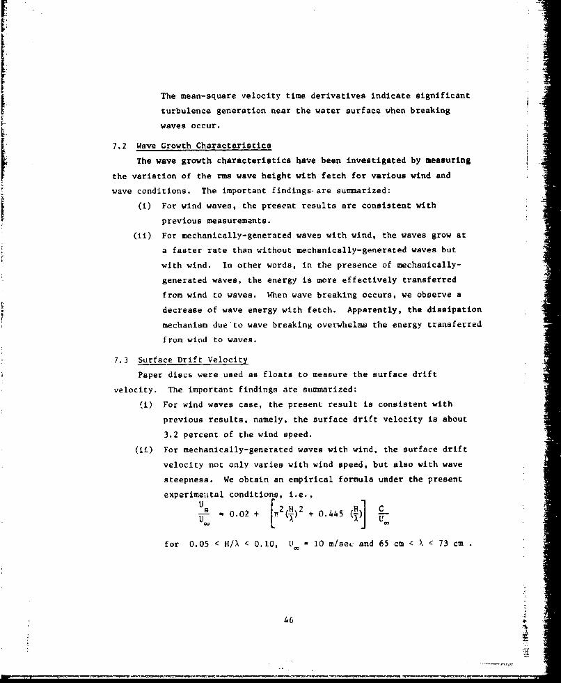
F7

The mean-square velocity time derivatives indicate significant

turbulence generation near the water surface when breaking

waves occur.

7.2 Wave Growth Characteristics

The wave growth characteristics have been investigated by measuring

the variation of the rms wave height with fetch for various wind and

wave conditions. The important findings, are summarized:

(I) For wind waves, the present results are consistent with

previous measurements.

(ii) For mechanically-generated waves with wind, the waves grow at

a faster rate than without mechanically-generated waves but

with wind. In other words, in the presence of mechanically-

generated waves, the energy is more effectively transferred

from wind to waves. When wave breaking occurs, we observe a

decrease of wave energy with fetch. Apparently, the dissipation

mechanism due'to wave breaking overwhelms the energy transferred

from wind to waves.


Paper discs were used as floats to measure the surface drift

velocity. The important findings are summarized:

(i) For wind waves case, the present result is consistent with

previous results, namely, the surface drift velocity is about

3.2 percent of the wind speed.

(ii) For mechanically-generated waves with wind, the surface drift

velocity not only varies with wind speed, but also with wave

steepness. We obtain an empirical formula under the present

experimeutal conditions, i.e.,U

-A 0.02 + [2 ~2 + 0. 445 d

for 0.05 < H/X 0 0, U = 10 m/sec and 65 cm < X < 73 cm

46

7.4 Oil Dispersion

Oil dispersion was investigated under conditions when breaking

waves occur. As the waves break, strong vertical motion is introduced

and the oil slick is broken into oil droplets. We measured the oil

concentration by using the photographic technique. For the particular

parameters uned in the present experiment, the mean oil concentration

decreases exponentially as

I

Z= 0.015 exp (-Izl/7.9), for 5 cm < - z < 20 cm ,

U, - 10 m/sec and H - 7.62 cm0

The rms oil concentration has values comparable to the mean oil concen-

tration. The size distribution of oil droplets was determined photo-

graphically. The average size is about 1.I mm.

4

47

I

II

AA

8. RECOMMENDATIONS FOR FUTURE RESEARCH

Before we initiated this research study, very little was known con-

cerning the turbulent motion in surface waters and the effect of tur-

bulence on oil dispersion. The present study. provides some important

information necessary for understanding the turbulent dispersion of oil

slicks, and it also calls for additional research effort.

8.1 Surface Drift VelociLt

In Section 5.3, we have shown the complicated coupling effects of

wind and waves on the surface drift velocity. Also, we have shown that

it is possible, empirically, to separate the effects of wind and waves

as expressed in equation (5-4). But, the expression is only for a

modest range of wave steepness under given winu speed and wavelength. .

It would, theiefore, be interesting to obtain, if possible, a similar

empirical formula for a variety of wind and wave conditions. This

formula could be used in numerical modeling for predicting the

horizontal spread of :*n oil slick due to the surface dr'ft.

8.2 Turbulent Motion Versus Wave-Induced Motion I

Measurements of both longitudinal and vertical velocity components

in wind waves and in mechanically-generated waves with wind show two

basic motions, namely, zurbulent motion and wave-induced motion. The

interaction between the turbulent motion aad che wave-induced motion is

not well understood. On the other hand, the updated turbulent theory

cannot inulude the wave-induced motion. The following approaches are

suggested:

(i) Separate the turbulent motion from the wave-induced motion by

the phase-averaging technique, and then investigate the

characteristics separately for either type of motion.

(ii) extend the present turbulence theory by including the wave-

induced motion. For the study of oil dispersion, we do not

recommend a complicated turbulent theory; instead, a theory

equivalent to the eddy iiscosity approximation could beconsidered.

48

L. -%

8.3 Taylor's Frozen Turbulence Hypothesis

Most of turbulence measvrements was done in time series. Taylor's

frozen turbulence hypothesis is frequently used to convert statistics

measured in the time domain into the spatial domain. For the case when

the mean velocity is much larger then the fluctuating component,

Taylor's hypothesis is valid. But, when the fluctuating velocity

component is larger than the mean velocity component, the validity of

Taylor's hypothesis is subject to doubt. Theoretical and experimental

studies are needed to investigate the validity of Taylor's hypothesis.

8.4 Oil Concentration Flux

Visualization techniques have been used to measure oil concen-

tration. The technique can further be used to determine the oil concen-

tration fluxes simply by multiplying the volume of the oil droplet by

its corresponding velcclty components. The oil concentration fluxes

could yield the important information such as eddy diffusivity of oil

dispersion.

49

--- -- -.-"---

REFERENCES

Aitken, J. (1884) "On the Effect of Oil on a Stormy Sea," Proc. Roy.

Soc., Edin. 12, pp. 56-75.

Baines, W. D. and Knapp, D. J. (1965) "Wind Driven Water Currents,"

J. Hyd. Div. A.S.C.E. 91, pp. 205-221.

Banke, E. G. and Smith, S. D. (1971) "Wind Stress Over Ice and Over Water

in the Beaufort Sea," J. Geophys. Res. 76, 7368.

Banner, M. L. and Phillips, 0. M. (1974) "On the Incipient Breaking of

Small Scale Waves," J. Fluid Mech. 65, pp. 647-656.

Banner, M. L. and Melville, W.K. (1976) "On the Separation of Air Flow over

Water Waves," J. Fluid Mech. 77, pp. 825-42.

Beebe, P. S. (1972) "TD'rbulent Flow Over a Wave Boundary," Ph.D. Thesis,

Colorado State University.

Boardman, G. and Dawson, F. (1972) "Process of Dispereing Oil Slicks,"

Official Gazette, U.S. Patent Office 895, no. 1, 255.

Bole, J. B. and Hsu, E. Y. (1967) "Response of Gravity Water Waves to

Wind Excitation," Dept. of Civil Engr. Tech. Rept. 79, Stanford

University.

Bye, J. A. T. (1965) "Wind-Driven Circulation in Unstratified Lakes,"

Limnol. Oceanogr. 10, pp. 451-458.

Canevari, G. P. (1969) "General Dispersant Theory," Proc. Jt. Conf. on

Prevention and Control of Oil Spills, New York City, pp. 171-177.

50

iL

Chang, P. C. (1969) "Laboratory Measurements of Air Flow Over Wind Waves

Following the Moving Water Surface," Ph.D. Thesis, Department of

Civil Engineering, Colorado State University.

Chang, P. C., Gorove, A., Atchley, B., and Plate, E. J. (1970) "A Self-

Adjusting Probe PosiLioner For Measuring Flow Fields in the Vicinity

of Wivd-Generated Water Surface Waves," Rev. Sci. Instrum. 41, 1544.

Chang, P. C. and Cheng, I. M. (1972) "Interaction Subrange Spectra of

Turbulent Wind Over the Air-Water Interface," J. Physical Ocean.

2, p. 273.

Colonell, J. M. (1966) "Laboratory Simulation of Sea Waves," Dept. of

Civil Engr. Tech. Report 65, Stanford University.

Davies, J. T., Qudwai, A. and Hansed, A. (1968) "Surface Stresses in

Ripple Formation Due to Low Velocity Air Passing Over a Water

Surface," Chem. Engng. Sci. 23, pp. 331-337.

Donelan, M. A. (1977) "White Caps and Momentum Transfer," NATO Symposium

on Turbulent Fluxes through the Sea Surface Wave PDnimics and

Prediction Marseille. France, Sept. 12-16.

Dreyer, A. A. (1973) "Study of Wind-Generated Seawaves in Shallow Sea,"

Thesis, USSR Academy of Sci., Shirshov Institute of Oceanography.

Eloubaidy, A. F. (1969) "Wind Waves and Reaeration Coefficient in Open

Channel Flow," Ph.D. Dissertation, Colorado State University.

Faller, A. (1963) "An Experimental Study of the Instability of the Laminar 4

Ekman Boundary Layer," J. Fluid Mech. 15, pp. 560-576.

51

Fannelop, T. K. and Waldman, G. D. (1972) "Dynamics of Oil Slicks," IAIAA Journal 10, No. 4, pp. 506-510.

Fay, J. A. (1969) "In Oil on the Sea," edited by D. P. Hoult, New York,

Plenum, pp. 53-63.

Fay, J. A. (1971) "Physical Processes in the Spread of Oil on a Water

Surface," Conference on Prevention and Control of Oil Spills,

Washington, D.C.

Fischer, H. B. (1967) "The Mechanics of Dispersion in Natural Streams,"

Proc. ASCE, J. of Hyd. Div. 93, No. HY6, pp. 187-216.

i

Fischer, H. B. (1969) "The Effect of Bends on Dispersion in Streams,"

Water Resources Research 5, No. 2, pp. 496-506.

Gad-el-Hak, M. and Lin, J. T. (1977) "Literature Survey of Turbulence

and Oil Dispersion in Surface Waters," Flow Research Note No. 111,

February.

Clover, R. E. (1964) "Dispersion of Dissolved or Suspended Materials in

Flowing Streams," U.S. Geol. Survey, Prof. Paper 433-B.

Grant, H. L., Moilliet, A., and Vogel, W. M. (1963) "'Turbulent Mixing in

the Thermocline," Pacific Naval Lab. preprint, Esquimalt, B.C.,

Canada.

Hoult, D. P. (1972) "Oil Spreading on the Sea," Annual Review of Fluid

Mech. 4, pp. 341-368.

Hidy, G. M. and Plate, E. J. (1966) "Wind Action on Water Standing in

a Laboratory Channel," J. Fluid Mech. 26, pp. 651-687.

52 A•. - -

Ichiye, T. (1967) "Upper Ocean Boundary-Layer Flow Determined by Dye

Diffusion," Phys. Fluids Suppl. S270-7.

Jeffreys, H. (1925) "On the Formation of Water Waves by Wind, 17"

Zrc. Rol. Soc. A107, pp. 189-206.

Jeffreys, H. (1926) "On the Formation of Water Waves by Wind," Proc.

Roy. Soc. London A 110, pp. 341-347.

Jobson, H. E. and Sayre, W. W. (1970a) "Vertical Transfer in Open Channel

Flow," Proc. ASCE, J. of Hyd. Div. 96, no. HY3, pp. 703-724.

Jobson, H. E. and Sayre, W. W. (1970b) "Predicting Concentration Profiles

in Open Channel," Proc. ASCE, J. of Hyd. Div. 96, No. HYI0,

pp. 1983-1996.

Karaki, S. and Hsu, E. Y. (1968) "An Experimental Investigation of the

Structure of a Turbulent Wind Over Water Waves," Dept. of Civil

Engr. Tech. Rept. 88, Stanford University.

Keulegan, G. H. (1951) "Wind Tides in Small Closed Channels," J. Res.

Nat. Bur. Stan. 46, pp. 358-381.

Kinner, P., Klemas, V., Leatham, W., Maurer, D., and Treasure, W. (1974)

"Dye and Drogue Studies of Spoil Disposal and Oil Dispersion,"

Journal of Water Pollution Control Federation 46, No. 8, 2026-2034.

Kinsman, B. (1965) Wind Waves -Their Generaton and Propagation on the

Ocean Surface, Prentice-Hall, Inc. Englewood Cliffs, N.J.

Kitaigorodskii, S. A. , Krasitskvi, V. P. and Zaslavskii, M. N. (1975)

"On Phillips' theory of Equilibrium Range in the Spectra of

Wind-Generated Waves," J. Phys. Oceanography 5, pp. 410-20.

53

Klemas, V., Davis, G., and Wang, H. (1975a) "Monitoring Estuarine

SCirculation and Ocean Waste Dispersion Using an Integrated Satellite-

Aircraft-Drogue Approach," NASA Larth Resources Survey Program.

Klemas, V., Davis, G., and Wang, H. (1975b) "Verification by Remote

Sensing of an Oil Slick Movement Prediction Model," NASA Earth

Resources Survey Program.

Klemas, V., Davis, G., and Kupferman, S. (1976) "The Influence of

Coastal Fronts on the Movement and Dispersion of Oil Slicks," NASA

Earth Resources Survey Program.

Kondo, J., Fujinawa, Y., and Naito, G. (1972) "Wave Induced Wind Fluctua-

tions Over the Sea," J. Fluid Mech. 51, p. 751.

Kullenberg, G. and Talbot, J. W., eds. (1974) "Physical Processes Res-

ponsible For Dispersal of Pollutants in the Sea With Special Ref-

erence to the Near-Shore Zone," Symp. on Phys. Processes Responsible

For Dispersal of Pollutants in the Sea With Specific Reference to

the Near-Shcre Zone, Denmark.

Langmuir, I. (1938) "Surface Motion of Water Induced by Wind," Science

87, pp. 119-123.

Leibovich, S. (1975a) "Natural Limit to the Containment and Removal of

Oil Spills at Sea," Ocean Eng. 3, No. 1, pp. 29-36.

Leibovich, S. (1975b) "Hydrodynamics Problems in Oil Spill Control and

Removal," Proc. of the 7th Annual Offshore Technology Conference,

Houston, Texas, pp. 527-544.

54

iI I I I I I 1 I I I I' i i i i i i

Lin, J. T. (1971) "Velocity Spectrum of Locally Isotropic Turbulence in

the Inertial and Dissipation Ranges," Phys. Fluids, 15 pp. 205-207.

Lin, J. T. and Veenhuizen, S. D. (1975) "The Fetch Effects on Wind Waves,"

Flow Research Note No. 58.

Lin, J. T. and Gad-el-Hak, M. (1977) "A Study To Conduct Experiaents

Concerning the Turbulent Dispersion of Oil Slicks - A Test Program

and Plan," Flow Research Note No. 110. January.

Lissauer, 1. M. (1974) "A Technique For Predicting the Movement of Oil

Spills in New York Harbor," Coast Guard Research and Development

Center, Report No. CGR/DC-8/74.

Lissauer, I. M. and Welsh, J. P. (1975) "Prellmii.ary Projections of Oil

Spill Movement for Three Potential Deepwater Sites in the Gulf of

Mexico," Coast Guard Research and Development Center, Report No.

CGR/DC.-34/75.

Liu, H. T., Lin, J. T., Delisi, P. P. and Robben, F. A. (1977) "Application

of a Flhorescence Technique to Dye Concentration Measurements in a

Turbulent Jet," Flow Measurement Symposium, National Bureau ol

Standards, Washington, D.C.

Long, S. R. and Hwang, N. Y. (1977) "On the Variation and Growth of Wave

Slope Spectra in the Capillary-Gravity Range with Increasing Wind,"

J. Fluid Mech.

Longuet-Higgins, M. S. (1953) "Mass Transport in Water Waves," Trans.

Camb. Phil. Soc. 245A, pp. 535-581.

55

iiLonguec-Higgins, M. S. (1969a) "A Nonlinear Mechanism for the Generation

of Sea Waves," Proc. Roy. Soc. A 311, pp. 371-389.

Longuet-Higgins, M. S. (1973) "A Model of Flow Separation at a Free

Surface,"' J. Fluid Mech. 57, pp. 1-20.

Longuet-Higgins, M. S. (1974) "An 'Entraining Plume' Model of a Spilling

Breaker," J. Fluid Mech. 63, No. 1, pp. 1-20.

Manton, M. J. (1972) "On the Generation of Sea Waves by a Turbulent

Wind," Boundary-Layer Meteorology , p. 348.

McNeely. W. 1 i1 "Oil Slick Dispersion Apparatus," Official Gazette,

U.S. r-ie,.c Office 883, No. 2, p. 604.

Miles, J. W. (1957) "On the Generation of Surface Waves by Shear Flows,"

J. Fluid Mech. 3, p. 185.

Miles, J. W. (1959a) "On the Generation of Surface Waves by Shear Flows,

Part 2," J. Fluid Mech. 6, p. 568.

Miles, J. W. (1959b) On the Generation of Surface Waves by Shear Flows,


Miles, J. W. (1962) "On the Generation of Surface Waves by Shear Flows,


Miles, J. W. (1967) "On the Generation of Surface Waves by Shear Flows,

Part 5," J. Fluid Mech. 30, ?. 163.

Murray, S. P., Smith, W. G. and Sonu, C. J. (1970) "oceanographif!

Observations and Theoretical Analysis of Ol1 Slicks During the

Chevron Spill," Louisiana State University, Report No. TR-87.

56

<1

Murray, S. P. (1972) "Turbulent Diffusion of Oil in the Ocean,"

Limnology and Oceanography 17, pp. 651-660.

Murray, S. P. (1975) "Wind and Current Effects on Large-Scale Oil

Slicks," Proc. of the 7th Annual Offshore Technology Conference,

Houston, Texas, pp. 523-533.

Phillips, 0. M. (1958) "On Some Properties of the Spectrum of Wind-

Generated Ocean Waves: J. Mar. Res. 19, pp. 231-245.

Phillips, 0. M. (1966) The Dynamics of the Upper Ocean, Cambridge

University Press. I

Phillips, 0. M. and Banner, M. L. (1975) "Wave Breaking in the Presence

of Wind Drift and Swell," J. Fluid Mech. 66, pp. 625-640.

Plate, E. J., Chang, I'. C. and Hidy, G. M. (1969) "Experiments on the

Generation of Small Water Waves by Winds," J. Fluid Mech. 35,

pp. 625-656.

Plate, F. J. (1970) "Water Surface Velocity Induced by Wind Shear,"

J. Engng. Mech. Div. A.S.C.E. 96, pp. 295-312.

Pott!nger, J. M. and Reisbig, R. L. (J973) "The Simulation of Deep Water

Waves for Oil Drift Studies," Proc. of the Missouri Acaderay of

Science, Columbia, Missouri, April. 1

Prych, F. A. (1970) "Effects of Density Differences on Lateral Mixing in

Open Channel Flows," California Institute of Technology, Report No.

KH-R-21. i

t '

I

57JA

I-!

Raj, P. (1977) "Theoretical Study to Determine the Sea State Limit for

the Survival of Oil Slicks on the Ocean," Arthur D. Little Rept.

No. 79299, February.

Reisbig, R. L., Alofs, D. J., Shah, R. C., and Banarjee, S. K. (1973)

"Measurement of Oil Spill Drift Caused by the Coupled Parallel

Effects of Wind and Waves," presented at Fifth Liege Colloquium on

Ocean Hydrodynamics Interactions at the Sea Boundaries, the Liege

Univ., Liege, Belgium, April 3-6, Vol 75, pp. 67-71.

Reisbig, R. L. (1973) "Oil Spill Drift Caused by the Coupled Effects

of Wind and Waves," Division of Engineering Research, Missouri

University at Rolla.

Ridgway, N. M. (1972) "Direction of Drift of Surface Oil With Wind and

Tide," New Zealand Journal of Marine and Freshwater Research 6,

Nos. 1 & 2, pp. 178-184.

Robben, F. (1975) "Wave SlopL and Height Measurement Techniques Using a

laser and Linear Diode Arrays," Flow Research Communication No. 57.

Robben, F. A., Lin, J. T., Delisi, D. P. and Liu, H. T. (1976) "Feasibility

Study of a Dye-Fluorescence Technique For Measuring Concentrations in

Fluids," Flow Research Note No. 91.

I

Sayre, W. W. and Chang, F. M. (1966) "A Laboratory Investigation of Open

Channel Dispersion Process For Dissolved, Suspended and Floating

Dispersants," U.S. Geol. Survey, Water Resources Div., Open File

Report.

Schwartzberg, H. C. (1970) "Spreading and Movement of Oil Spills," U.S.

Government Research and Development Reports 70, No. 17, p. 134.

58

Schwartzberg, H. C. (1971) "The Movement of Oil Spills," Joint Conference Ion Prevention and Control of Oil Spills, Washington, D.C. J

Shemdin, 0. H. (1972) "Wind-Generated Current and Phase Speed of Wind

Waves," J. Phys. Oceanogr. 2, pp. 411-419.

Shonting, D. H. (1968) "Autospectra of Observed Particle Motions in Wind A

Waves," J. Marine Research, 26, pp. 43-65. tI

Spencer, E. B. and Sorenson, R. M. (1970) "Set-up of Oil on Water by

Wind," Texas A&M University, Report No. 128-C.O.E.

Stewart, R. H. (1970) "Laboratory Studies of the Velocity Field Over

Deep-Water Waves," J. Fluid Mech. 42, p. 733.

Stewart, R. J. (1976) "The Interaction of Waves and Oil Spills,"

Massachusetts Institute of Technology, Report No. MITSG-75-22.

i

Stokes, G. G. (1847) "On the Theory of Oscillatory Waves," Trans. Camb.

Phil. Soc. 8,.pp. 441-55; represented in Math. Phys. Pap. 1, 314-26.

Sturm, G. V. And Sorrell, F. Y. (1973) "Optical Wave Measurement Technique

and Experimental Comparison with Conventional Wave Height Probe," i

Aippl. Optics, 12, pp. 1928-33.

Su, K. S. (1972) "Wind Waves and Diffusion in Open Channels," Ph.D.

Dissertation, Colorado State Universityf i

Takeuchi, K. (1976) private communication, University of Stanford.

Thorton, E. B. and Krapohl, R. F. (1974) "Water Particle Velocities 7

Measured under Ocean Waves" J. Geophy. Res. 79, pp. 847-52.

*159 S

J,

It

Thornton, E. B., Galvin, J. J., Bub, F. L., and Richardson, D. P. (1976)

"Kinematics of Breaking Waves," Proc. 15th Coastal Eng. Conf.,

Honolulu, Hawaii, July, pp. 461-476.

Thorton, E. B. (1977) "Rederivation of the Saturation Range in the

Frequency Spectrum of Wind-Generated Gravity Waves" J. Phys. Oceans.

7, 137-140.

Van Dorn, W. G. and Pazan, S. E. (1975) "Laboratory Investigation of

Wave Breaking, Part II: Deepwater Waves," Scripps Institute of

Oceanography University of California, San Diego.

Veenhuizen, S. D. and Karaki, S. (1973) "Turbulent Air Flow Over Wind

Excited Laboratory Water Waves," Department of Civil Engineering,

Colorado State University.

Veenhuizen, S. D., Yu, H. Y., Lin, J. T., and Pao, Y. H. (1975) "The

Design and Construction of a Wind-Wave Towing-Tank System," Flow

Research Report No. 38.

Waldman, G. D., Fannelop, T. K. and Johnson, R. A. (1972) "Spreading and

Transport of Oil Slicks on the Open Ocean," 4th Annual Offshore

Technology Conference, Houston, Texas, pp. 352-364.

Waldman, G. A., Johnson, R. A. and Smith, P. L. (1973) "The Spreading and

Transport of Oil Slicks on the Open Ocean in the Presence of Wind,

Waves, and Currents," AVCO Systems Division, Report No. AVSD-0068-72-RR.

Wang, S. and Hwang, L. (1974) "A Numerical Model For Simulation of Oil

Spreading and Transport and Its Application For Predicting Oil

Slick Movement in Bays," Tetra Tech, Inc., Report No. TT-P-345-74-1.

Weissman, M. (1978) Private communication.

60

rI

Wu, 3. (1968) "Laboratory Studies of Wind-Wave Interactions," J. Fluid

Mech. 34, pp. 91-112.

Wu, J. (1969) "An Estimation of Wind Zffects on Dispersion in Wide Channels,"

Water Resources Research 5, pp. 1097-1104.

Wu, J. (1975) "Wind Induced Drift Currents," J. Fluid Mech. 6-8, pp. 49-70.

Young, M. B. 0., Hsu, E. Y., and Street, R. L. (1973) "Air-Water

Interaction: The Nature of Turbulent Heat, Mass and Momentum

Transfer Mechanism in the Air Boundary-Layer," Technical Report

No. 163, Dept. of Civil Engineering, Stanford University.

Yu, H. Y. and Lin, J. T. (1975) "A Technique For Generating a Turbulent

Boundary Layer in a Wind-Wave Tank," Second U.S. National Conference

on Wined Engineering Research, Colorado State University.

611

F I2

I III

|I

I

I

|I

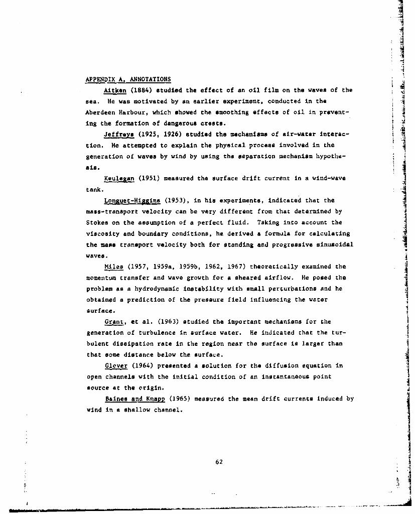
9

APPENDIX A. ANNOTATIONS

Aitken (1884) studied the effect of an oil film on the waves of the

sea. He was motivated by an earlier experiment, conducted in the

Aberdeen Harbour, which showed the smoothing effects of oil in prevent-

ing the formation of dangerous crests. -

Jeffreys (1925, 1926) studied the mechanisms of air-water interac-

tion. He attempted to explain the physical process involved in the

generation of waves by wind by using the separation mechanism hypothe-

sis.

Keulexan (1951) measured the surface drift current in a wind-wave

tank.

Longuet-Higsins (1953), in his experiments, indicated that the

mass-transport velocity can be very different from that determined by

Stokes on the assumption of a perfect fluid. Taking into account the

viscosity and boundary conditions, he derived a formula for calculating

the mass transport velocity both for standing and progressive sinusoidal

waves.

Miles (1957, 1959a, 1959b, 1962, 1967) theoretically examined themomentum transfer and wave growth for a sheared airflow. He posed the

problem as a hydrodynamic instability with small perturbations and he

obtained a prediction of the pressure field influencing the water

surface.

Grant, et al. (1963) studied the important mechanisms for the

generation of turbulence in surface water. He indicated that the tur-

bulent dissipation rate in the region near the surface is larger than

that some distance below the surface.

Glover (1964) presented a solution for the diffusion equation in

open channels with the initial condition of an instantaneous point

source at the origin.

Baines and Knapp (1965) measured the mean drift currents induced by

wind in a shallow channel.

iI

62

I

Bye (1965) studied wind-driven circulation in unstratified lakes.

Colonell (1966) showed experimentally that Miles's theory for the

momentum tranefer and wave growth of a sheared airflow under-predicts

the Erowth rates of the waves.

Hid• and Plate (1966) observed the effects of wind on water standing

in a laboratory channel.

Phillips (1966) reviewed state-of-the-art knowledge on wind waves

and the dynamics of the upper ocean.

Sayre and Chang (1966) reported a laboratory experiment on the

dispersion process for dissolved, suspended, and floating dispersants in

an open channel. They adopted Aria's moment distribution method to

solve the diffusion equation numerically.

Bole and Hsu (1967) conducted a laboratory experiment to determine

the response of waves to wind excitation. 1hey observed higher growth Irates for the waves than those predicted by Miles's theory.

Fischer (1967, 1969) studied the mechanics of dispersion in natural

streams and the effect of bends cn dispersion. He estimated the depth-

averaged lateral diffusion coefficient in curved channels, and he derived

an equation for predicting the longitudinal dispersion coefficient in

wide cpen channels by adopting Taylor's convective dispersion theory.

Davies, et al. (1968) studied the ripple formation caused by low- Ivelocity air flowing over water.

Karaki and Hsu (1968) conducted an experiment to investigate the

structure of a turbulent-wind boundary-layer over a water surface,

Shonting (1968) measured the vertical velocity fluctuations in wind

waves. The rms value of the vertical velocity fluctuations decreases __

exponentially with depth for the water region having depth less than 6M. The autospectrum of the vertical velocity fluctuations had a dominantpeak at a frequency corresponding to the spectral peak of the wave energy

spectrum.

63

63

I' I

IIWu (1968, 1969, 1975) in a series of reports studied wind-wave

interaction in a wind-wave tank. He measured the profile of the drift

current induced by wind and estimated the effect of the wind on disper-

s ion. He pointed out that waves do have a strong effect on the diffusion

process.

Canevari (1969) studied the mechanisms of and the basis for dis-

persing oil slicks with chemical dispersants.

Chaný (1969) investigated the detailed structure of airflow above

and between crests of progressing wind waves.

Eluaidy (1969) studied the diffusion process in open channels.

He noted that waves have a significant effect on the diffusion process.

Fay (1969, 1971) presented, for the first time, a systematic way to

predict how oil spreads in calm water.

Longuet-Higgins (1969a, 1969b, 1973, 1974) published a series of

F papers on the meci.wnisms of wave breaking. He proposed e. nonlinear

mechanism for the generation of sea waves and a model for flow separation

at the free surface.

Plate, et al. (1969) and Plate (1970) measured the drift velocity

at the water surface for two different wind friction velocities. They

observed that, over short fetches, the drift velocity increases according

to a power law, while, at fetches exceeding one meter, the drift velocity

maintains a constant ratio to the wind velocity.

Chan&, et al. (1970, 1972) developed a self-adjusting probe posi-

tioner (wave follower) to position a crossed-film sensor above the

instantaneous water surface and, thus, were 3ble to measure the wind

velocity field as near the instantaneous water surface as possible.

Jobson and Sayre (1970a, 1970b) conducted a series of experiments

in a large open channel by using a continuous line of dissolved dye

across the width of the channel. They measured the vertical diffusion

coefficient.

64

i i II I I I I I '

Murray, et al. (1970) and Murray (1972, 1975) discussed oceanographic

observations near the Chevron spilling well off the Mississippi Delta

and the relative roles of the various physical factors in the behavior

of oil slicks. They evaluated the role of large-scale turbulence and

the effects of surface tension in the control of oil diffusion. They

showed that the size and shape of a given oil slick can be predicted

with knowledge of the surface current, eddy diffusivity, and the rate of

oil discharge. Murray determined the relative effect of local winds and

near-surface currents on determining the movement of oil slicks in

coastal and shelf waters.

Prych (1970) examined the effect of density differences on lateral

mixing in open channels.

Schwartzberg (1970, 1971) investigated the movement and spreading

of oil spills on water. Spreading rates for small spills were measured

and correlated with spill volume, oil density, and water viscosity.

Field data indicated that these aspects of small spills cannot be scaled

up to large spill volumes.

Spencer and Sorenson (1970) analytically and experimentally studied

the setup cf oils having various densities and viscosities on a water

surface when subjected to wind. They showed that the setup of oil is a

functioa of wind stress and wind-generated wave action.

Stewart (1970) measured the velocity field over deep-water waves.

His measured spectra showed the presence of peaks caused by water waves.

Banks and Smith (1971) presented spectra of all three wind components

and co-spectra for the Reynolds stress and sensible heat flux over water

in the Beaufort Sea, in which wave effects were prescnt.

McNeely (1971) described au apparatus for measuri:ng oil slick dis-

persion.

Beebe (1972) measured the turbulent flow over a wave boundary.

Boardman and Dawson (1972) presented a new process for dispersing

an oil slick.

Fannelo2 and Waldman (1972) cot.sidered the spread of an oil slick

over calm water from a theoretical viewpoint. They presented a general

picture of the slick deve2lopment.

65

Hoult (1972) wrote, from an analytical viewpoint, an excellent

review article on oil spreading on the sea.

Kondo, et al. (1972) presented a spectrum for longitudinal fluctua-

tions near the air-sea interface which indicated that an influence of

the sea swell was present.

Manton (1972V modified Miles's wave theory to include the effects

of the turbulence present in the airflow. A particularly interesting

result was that the pressure leads the water surface elevation in space,

and the phase difference remains almost constant at 75 degrees.

Ridgway (1972) presented a mathematical analysis for predicting the

direction the surface oil drifts with the wind and the tide.

Shemdin (1972) measured the wind-induced current and the phase

speed of wind waves.

Su (1972) described a theoretical and experimental investigation of

the vertical and lateral mixing of tracer fluids in a straight, wide

open channel, with and without wind on the water surface. Vertical

mixing rates significantly increased when waves appeared on the water

surface.

Waldman, et al. (1972, 1973) presented an analysis of the spreading

and transport of oil slicks on the open ocean. They assessed the role

of turbulent diffusion as a transport mechanism and presented conclusions

regarding the applicability of the various analytical models.

Pottinger and Reisbig (1973) conducted laboratory experiments to

determine the effect of waves on oil spill drift. The data showed that

the drift velocity was greater than that predicted by Stoke's mass

transport theory.

Reisbig (1973) studied the effects of the wind and waves on oil

spill drift so that he could evaluate the importance of coupled wind

and wave drift mechanisms in computer simulations of the total drift.

Reisbig, at al. (1973) conducted laboratory experiments to determine

the surface drift speeds of an oil lens which was subjected to the

separated and coupled effects of wind waves. The results show that the

wind drift and wave drift mechanisms are not simply additive over all

66

A

regimes of wind speed. At low wind speeds the wave drift provides an

augmentation to the wind drift. At higher wind speeds, however, the

waves cause a net decrease in the coupled drift velocity.

Sturm and Sorrell (1973) developed an optical system to measure

wave slope. The measured slope was integrated to obtain wave height.

Wave height results obtained from this optical system were compared with

those from a capacitance wave height. The meniscus effect on the perfor-

mance of the capacitance wave probe was determined.

Veenhuizen and Karaki (1973) conducted an experimental study of

turbulent airflow over water waves. They found an organized wave motion

corresponding to the water wave in the turbulent airflow. This wave-

induced motion was apparent "p to four or five wave heights above the

wean water level.

Youg, et al. (1973) measured the turbulent heat, mass and momentum

transfer mechanisms in the air boundary-layer over wind waves.

Banner and Phillips (1974) investigated the incipient breaking of

small-scale waves. They presented P heuristic picture of the t, lent

motion in a breaking wave.

Kinner, et al. (1974) studied spoil disposal and oil dispersion

experimentally with dye.

Kullenberg and Talbot (1974) edited 31 papers on near-shore mixing

caused by waves and currents, dispersion over the continental shelf,

wind effects, oil slicks, and many other topics related to the physical

processes responsible for the dispersal of pollutants in the sea.

Lissauer (1974, 1975) projected the movement of oil slicks and

their impact locations along the shorelines of different states from

three potential deep-water port sites. He used average monthly wind

speeds and directions, and average monthly current patterns to predict

oil slick movement.

Thorton and Krapohl (1974) measured wave height and water particle

velocities in ocean waves. The measured wave-induced velocities were

comparable to those calculated by linear wave theory. At low frequencies,

the rotion was almost totally wave induced. At higher frequencies,

however, it was apparent that the motion was primarily turbulence.

67

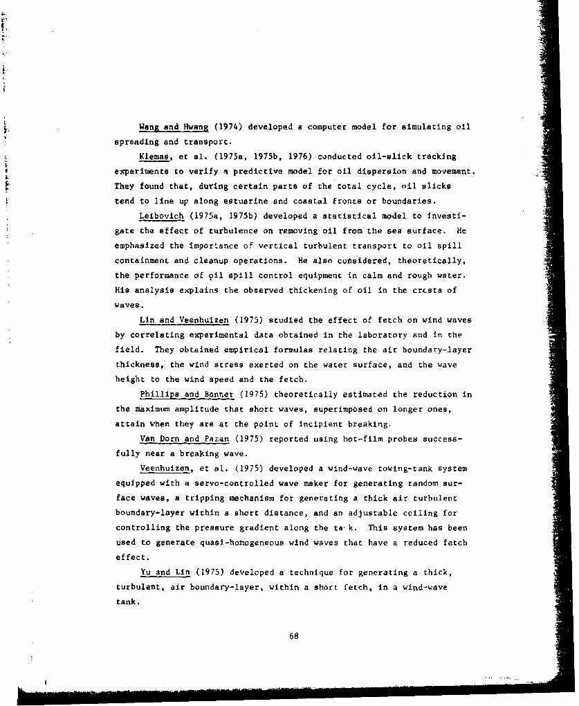
Wang and Hwang (1974) developed a computer model for simulating oil

spreading and transport.

Klemas, et al. (1975a, 1975b, 1976) conducted oil-slick tracking

experiments to verify n predictive model for oil dispersion and movement.

They found that, during certain parts of the total cycle, oil slicks

rend to line up along estuarine and coastal fronts or boundaries.

Leibovich (1975a, 1975b) developed a statistical model to Investi-

gate the effect of turbulence on removing oil from the sea surface. He

emphasized the importance of vertical turbulent transport to oil spill

containment and cleanup operations. He also considered, theoretically,

the performance of 9i1 spill control equipment in calm and rough water.

His analysis explains the observed thickening of oil in the cr~sts of

waves.

Lin and Veenhuizen (1975) studied the effect of fetch on wind waves

by correlating experimental data obtained in the laboratory and in the

field. They obtained empirical formulas relating the air boundary-layer

thickness, the wind stress exerted on the water surface, and the wave

height to the wind speed and the fetch.

Phillips and Banner (1975) theoretically estimated the reduction in

the maximum amplitude that short waves, superimposed on longer ones,

attain when they are at the point of incipient breaking.

Van Dorn and Pazan (1975) reported using hot-film probes success-

fully near a breaking wave.

Veenhuizen, et al. (1975) developed a wind-wave towing-tank system

equipped with a servo-controlled wave maker for generating random sur-

face waves, a tripping mechanism for generating a thick air turbulent

boundary-layer within a short distance, and an adjustable ceiling for

controlling the pressure gradient along the ta: k. This system has been

used to generate quasi-homogeneous wind waves that have a reduced fetch

effect.

Yu and Lin (1975) developed a technique for generating a thick,

turbulent, air boundary-layer, within a short fetch, in a wind-wave

tank.

68

!•k.•, : . . = • • -• • i- i I• i : l l

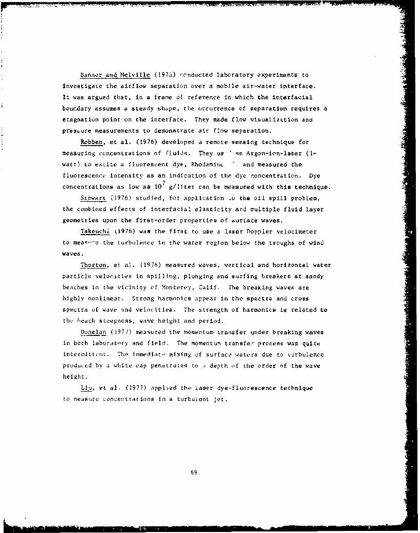
Banner and Melville (1973) cinducted laboratory experiments to

investigate the airflow separation over a mobile air-water interface.

It was argued that, in a frame of reference in which the interfacial

boundary assumes a steady shape, the occurrence of separation requires a

stagnation point on the interface. They made flow visualization and

presture measurements to demonstrate air flow separation.

Robben, et al. (1976) developed a remote sensing technique for

measuring ccncentrations of fluids. They us x n Argon-ion-laser (I-

watt) to excite a fluorescent dye, RhodaminL and measured the

fluorescence, intensity as an indication of the dye concentration. Dye7concentrations as low as 10 g/liter can be measured with this technique.

Stewart (1976) studied, for application .o the oil spill problem,

the combined effects of interfaclal elasticity and multiple fluid layer

geometries upon the first-order properties of •urface waves.

Takeuchi t1976) was the first to use a laser Doppler velocimeter

to mea•--e the turbulence in the water region below the troughs of wind

waves.

Thorton, et al. (1976) measured waves, vertical and horizontal water

particle velocities in spilling, plunging and surfing breakers at sandy

beaches in the vicinity of Monterey, Calif. the breaking waves are

highly nonlinear. Strong harmonics appear in the spectra and cross

spectra of wave and velocities. The strength of harmonics ia related to

the beach steepness, wave height and period.

Donelan (1977) measured the momentum transfer under breaking waves

in both laboratory and field. The momentum transfer process was quite

intermittL'nt. Thp immediato mixing of surface waters due to turbulcnce

produced by a white cap penetrate% to i depth of the order of the wave

height.

Liu, et al. (1977) applied the iaser dye-fluorescence technique

to measure concentrations in a turbuient jet.

69

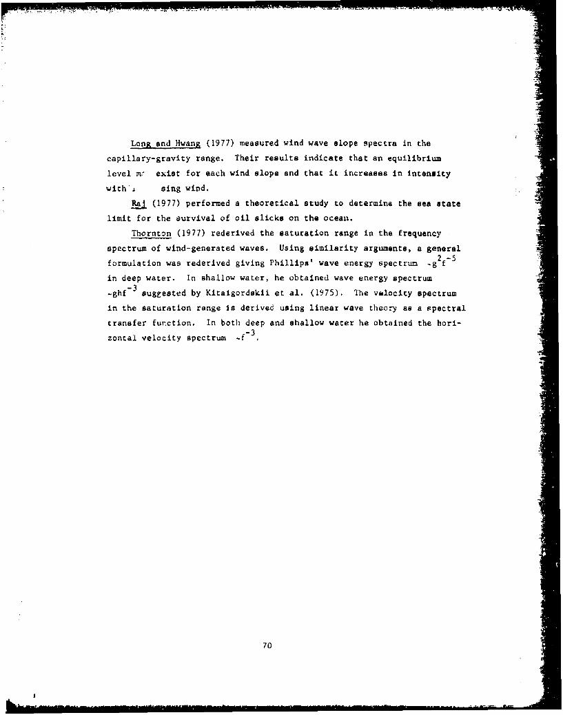
Long and Hwang (1977) measured wind wave slope spectra in the

capillary-gravity range. Their results indicate that an equilibrium

level m.r exist for each wind slope and that it increases in intensity

with'. sing wind.

jj(1977) performed a theoretical study to determine the sea state

limit for the survival of oil slicks on the ocean.

Thornton (1977) rederived the saturation range in the frequency

spectrum of wind-generated waves. Using similarity arguments, a general2 -5

formulation was rederived giving Phillips' wave energy spectrum _g f

in deep water. In shallow water, he obtained wave energy spectrum

-ghf- suggested by Kitaigordskii et al. (1975). The velocity spectrum

in the saturation range Is derived using linear wave theory as a spectral

transfer furction, In both deep and shallow water he obtained the hori-

-3.

zontal velocity spectrum esr 3.

70

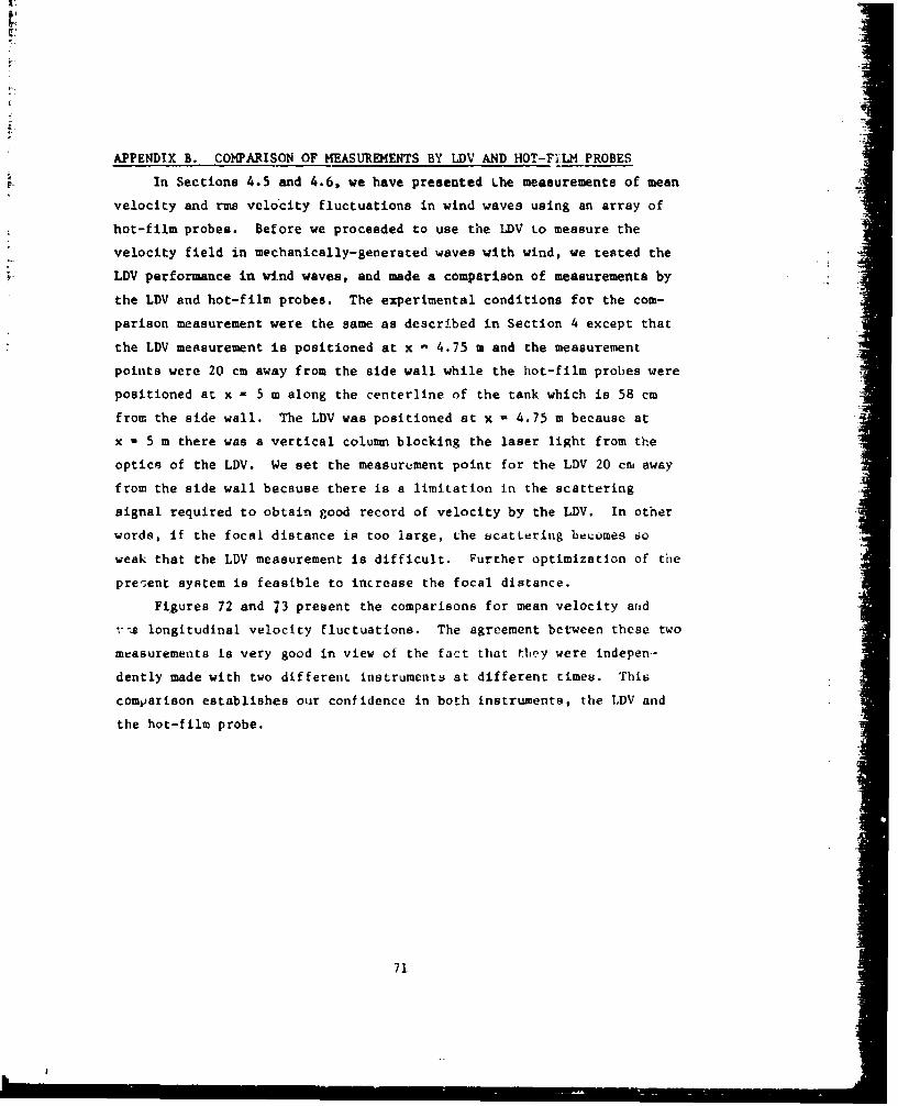
APPENDIX B. COMPARISON OF MEASUREMENTS BY LDV AND HOT-FiLM PROBES

In Sections 4.5 and 4.6, we have presented Lhe measurements of mean

velocity and rms velo'city fluctuations in wind waves using an array of

hot-film probes. Before we proceeded to use the IDV to measure the

velocity field in mechanically-generated waves with wind, we tested the

LDV performance in w.nd waves, and made a comparison of measurements by

the LDV and hot-film probes. The experimental conditions for the com-

parison measurement were the same as described in Section 4 except that

the LDV measurement is positioned at x - 4.75 m and the measurement

points were 20 cm away from the side wall while the hot-film probes were

positioned at x - 5 m along the centerline of the tank which is 58 cm

from the side wall. The LDV was positioned at x - 4.75 m because at

x - 5 m there was a vertical column blocking the laser light from the

optics of the LDV. We set the measurement point for the LDV 20 cm away

from the side wall because there is a limitation in the scattering

signal required to obtain good record of velocity by the LDV. In other

words, if the focal distance is too large, the bcatterluig becomes to

weak that the LDV measurement is difficult. Further optimization of tile

present system is feasible to increase the focal distance.

Figures 72 and 73 present the comparisons for mean velocity and

vi longitudinal velocity fluctuations. The agreement between these two

measurements is very good in view of the fact that tbey were indepen-

dently made with two different instruments at different times. This

comparison establishes our confidence in both instruments, the LDV and

the hot-film probe.

71

L

APPENDIX C. EFFECTS OF AN OIL SLICK ON WIND WAVES JExperiments were conducted to investigate the effecta of an oil

slick on wind waves for various wind speeds and at several fetches.

Diesel oil No. 2 was used in the experiments. It was fed onto the water

surface from the upstream end of the wave tank, and the discharge was

0.35 liter/sec. The specific gravity of the oil was 0.84 and the2

kinematic viscosity was 0.19 cm /sec.

The photodiode wave gauge was used to measure the vertical displace-

ment of the water surface with and without an oil slick present. The

gauge was positioned along the center line of the wave tank. In case an -.

oil slick was present, the intensity of the oil flourescence was strong 4

enough that the interface between the air and the oil could be detected -

with the photodiode wave gauge. In all the experiments reported here,

fluorescein disodium dye was added to the water so that the interface of

the water and the air could be detected when the oil slick. was absent.

For each experimental run, we first took data for tne ,:ase without an

oil slick. Then an oil slick was fed onto the water surface to investi-

gate its effects on wind waves.

Figure 74 shows a record of the vertical displf.cement of the water

or oil surface at a fetch x - 5 m for wind speed U. - 10 m/sec. Before

the oil slick reaches the measurement point, the record shows the timevariation of the vertical displacment of the water surface. As the oil

slick reaches the measurement point, the mean level of the air-oil

interface increases and the fluctuating vertical displacement decreases.

The tranuient stage lasts for about three to fouL winutes and a steady

stage reestablishes four minutes afterwards. The increase of the mean

level is partly due to the thickness of the oil slick and partly due tc

the fact that the setup of the water surface is altered by the presence

of the oil slick. After the steady stage is reached, another set of

data is recorded for the case when the oil slick is present. This set

of data could, therfore, be compared with data obtained without an oil

slick present in order to investigate the effects of oil slick on wind

waves.

72

r -i

C.1 Wave Profiles

Figure 75 shows wind-wave profiles without an oil slick present,

which were measured at fetch x a 4 m for three wind speeds, U - 4-, 7-,

and 10 m/sec. The wind-wave profiles are plotted as the time variation Aof the vertical displacement of the air-water interface. The amplitude

and period of dominant waves increase as wind speed increases and wave

packets are observed. These results are consistent with those presented

in Section 4.2.

Figure 76 shows the wind wave profiles when an oil slick is ipresent. Comparison between Figures 75 and 76 indicates that the

wind waves are significantly damped by the oil slick. In Figure 76(c), i

small scale fluctuations appear which indicate the break up of the oil

slick. Visually we have seen the formation of oil lenses floating on

the water surface for U - 10 m/sec.

C.2 RMS Wave Height

The rms values of the wave displacement are plotted versus wind

speed in Figure 77. When the oil slick is absent, the rms wave height

increases with wind speed and fetch, which is consistent with the results

presented in Section 4.2. For All wind speeds, the rms wave height for

the case with an oil slick present is smaller than that for the case

without an oil slick present. Thus, the damping effects of an oil slick

on wind waves are evident. When an oil slick is present, however, the

rms wnve height increases when going from 4- to 7 m/sec wind, but

decreases when going from 7- to 10 m/sec wind. It is worth mentioning

that for th" case of wind speed at 10 m/sec, oil lenses formed on the

water surface. We speculate that these oil lenses could transfer energy

from ale to water more effectively than a continuous sheet of oil slick

because the presence of oil lenses makes the water Burface rougher, and

the waves could be more effectively damped by them. Figure 78 shows the

variation of TMs wave height with fetch. For the case without an oil

slick, the rms values increase with fetch, which is consistent with the

results obtained in Section 2. When an oil slick is present, the rms

values do not vary appreciably with fetch.

73

C.3 Wave Energy Spectrum

Figure 79 presents the wave energy spectrum S(f) measured with the

photodiode wave gauge located at fetch x a 3.2 m for wind speed U - 10

m/sec without an oil slick present. Two distinct frequency regimes are

observed, namely, a gravity wave regime and a capillary wave regime.

The gravity waves have a peak spectrum at a frequency of about 4.7 Hz.

In the capillary wave regime, the wave energy spectrum follows

S(f) Y 8 2/3 f-7/3 , 7.5 Hz < f < 100 Hz,

where y is the surface tension per unit density and has a value of3 270 cm /sec for waeer, and 3 is a numerical constant having a value of

about 7.2 x 10-3 for this particular measurement. This -7/3 power law

was obtained based on dimensional arguments (Phillips, 1966), and it was

suggested originally by Hicks (See Phillips, 1958). To the knowledge of

the authors, the wave energy spectium presented in Figure 79 is the

first experimental verification of this power law. The measurement of

the wave energy spectrum at high frequencies is very important in under-

standing the characteristics of capillary waves. Since these capillary

waves act as roughness elements to wind, their characteristics would

influence the wind stress exerted on the water surface and, therefore, the

surface drift current. In Figure 79, there are two spectra calculated

from two independent records. The shaded area provides an estimate of

statistical error in measuring the wave energy spectrum.

The wave energy spectra measured at a fetch, x - 4w for three wind

speeds, V. - 4-, 7-, and 10 m/sec without an oil slick present are plot-

ted in Figcre 80. Each spectrum has two distinct wave regimes as

aforementioned. The value of B increases with wind speed. The dominant

frequency decreases with wind speed. Also, the frequency at which two

distinct wave regimes join decreases with wind speed. Thus the measure-

ments show that an wind speed increases the wave energy in both gravity

and capillary wave regimes increases. Long and Huang (1977) measured

"74

wind-wave slope spectra in the capillary and gravity ranges. Their

results indicate that an equilibrium level may exist for each wind

speed, and that it increases in intensity with increasing wind speed.

The present results are therefore consistent with theirs. It would be

interesting to investigate whether an asymptotic nature of the wave

energy spectrum exists in the capillary wave regime.

The effects of an oil slick on wind waves were also investigated

from measurements of wave energy spectra. Figure 81 shows the wave

energy spectra measured at fetch x - 4 m for wind speed U, - 4 m/atc,

with and without an oil slick present. The oil slick influences the

wave spectrum over all wave frequencies. In particular, the dominant

wave frequency for the case of an oil slick being present is higher than

that for the case without an oil slick. This result indicates that the

onset of the wind waves is delayed by the presence of an oil slick.

Figure 82 shows the wave energy spectra measured at x - 4 m for

U 7 m/sec. When an oil slick is present, the energy of the dominant

waves decreaReq, but the dominant wave frequency remains unchanged. At

higher frequencies, the effect of an oil slick is not as appreciable for

U - 4 m/sec. Comparison between Figures 81 and 82 9hows that the

effect of an oil slick depends on wind speed. Figure 83 shows a com-

parison of wave energy spectra measured with and without an oil alick

present for wind speed U - 10 m/sec. The spectral density at the

dominant wave frequency decreases significantly when the oil slick is

present. In the frequency range 6 Hz < f < 20 Hz , the spectral density

appears flat and it is possibly contributed by the presence of oil

lenses. lor frequencies f > 20 Hz , the oil slick effect is not

appreciable. From Figures 82 and 83, we conclude the following for the

present experimental conditions. For wind 9peed U. > 7 m/sec, the

effect of an oil slick on ~.;he generation of capillary waves is not

significant. TL.,e capillary waves most likely are generated locally by

wind and governed by surface tension. Therefore, the evolution of

.9i

capillary waves is expected to be different from that of gravity waves.

More research is needed to explore this evolution.

76

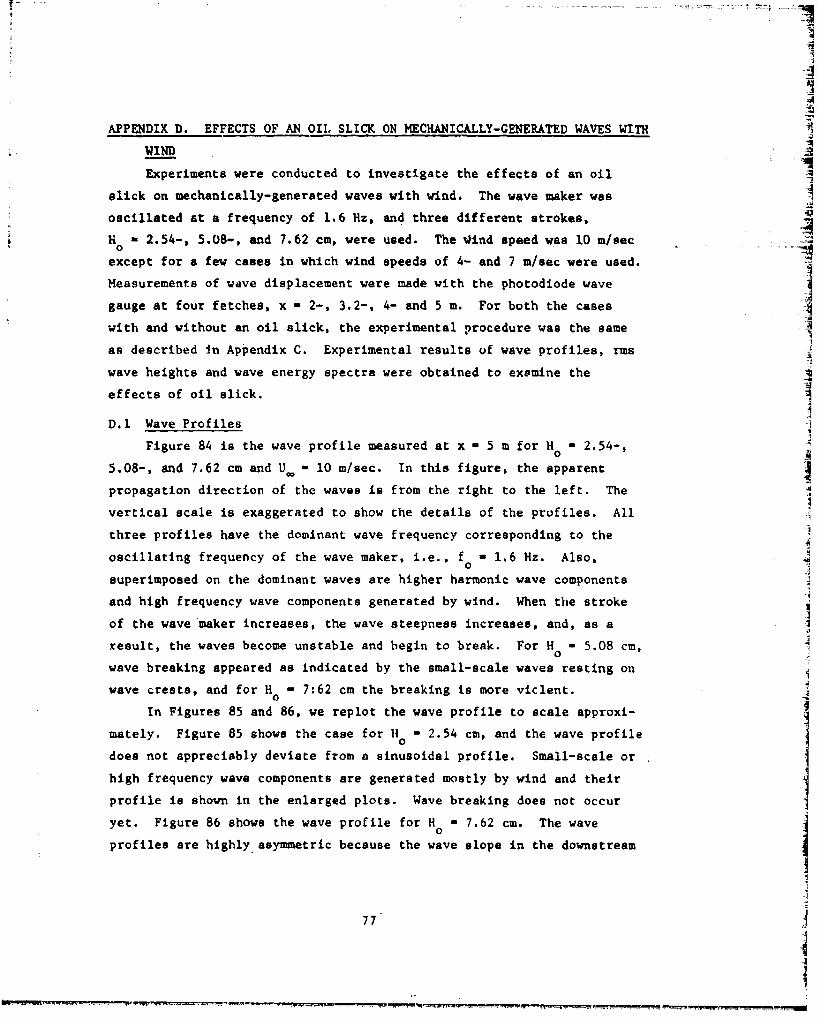
I

APPENDIX D. EFFECTS OF AN OIL SLICK ON MECHANICALLY-GENERATED WAVES WITH

WIND

Experiments were conducted to investigate the effects of an oil

slick on mechanically-generated waves with wind. The wave maker was

oscillated at a frequency of 1.6 Hz, and three different strokes,

_H - 2.54-, 5.08-, and 7.62 cm, were used. The Oind speed was 10 m/sec

except for a few cases in which wind speeds of 4- and 7 m/sec were used.

Measurements of wave displacement were made with the photodiode wave

gauge at four fetches, x - 2-, 3.2-, 4- and 5 m. For both the cases A

with and without an oil slick, the experimental procedure was the same

as described In Appendix C. Experimental results of wave profiles, rms

wave heights and wave energy spectra were obtained to examine the

effects of oil slick.

D.1 Wave Profiles

Figure 84 is the wave profile measured at x - 5 m for H° 2.54-,

5.08-, and 7.62 cm and U. 10 m/sec. In this figure, the apparent

propagation direction of the waves is from the right to the left. The

vertical scale is exaggerated to show the details of the profiles. All

three profiles have the dominant wave frequency corresponding to the

oscillating frequency of the wave maker, i.e., f a 1.6 Hz. Also,0

superimposed on the dominant waves are higher harmonic wave components

and high frequency wave components generated by wind. When the stroke

of the wave maker increases, the wave steepness increases, and, as a

result, the waves become unstable and begin to break. For H - 5.08 cm,0

wave breaking appeared as indicated by the small-scale waves resting on

wave crests, and for H - 7:62 cm the breaking is more viclent.0

In Figures 85 and 86, we replot the wave profile to scale approxi-

mately. Figure 85 shows the case for It - 2.54 cm, and the wave profile0

does not appreciably deviate from a sinusoidal profile. Small-scale or

high frequency wave components are generated mostly by wind and their

profile is shown in the enlarged plots. Wave breaking does not occur

yet. Figure 86 shows the wave profile for H - 7.62 cm. The waveo

profiles are highly asymmetric because the wave slope in the downstream

77

RIMS

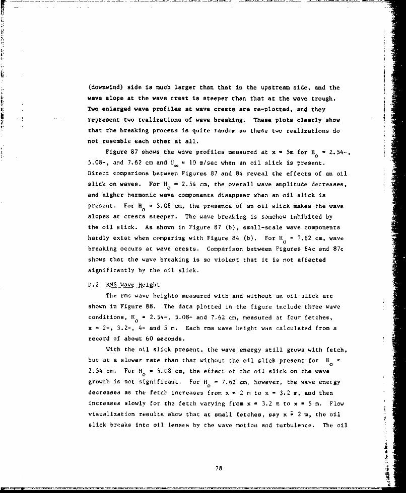
(downwind) side is much larger than that in the upstream side, and the

wave slope at the wave crest is steeper than that at the wave trough.

Two enlarged wave profiles at wave crests are re-plotted, and they

represent two realizations of wave breaking. These plots clearly show

that the breaking process is quite random as these two realizations do

not resemble each other at all.

Figure 87 shows the wave profiles measured at x -5m for H -2.54-,

5.08-, and 7.62 cm and U 1 - 0 m/sec when an oil slick is present.

Direct comparions between Figures 87 and 84 reveal the effects of an oil

slick on waves. For H 2.54 cm, the overall wave amplitude decreases,0

and higher harmonic wave components disappear when an oil slick is

present. For H - 5.08 cm, the presence of an oil slick makes the wave0

slopes at crests steeper. The wave breaking is somehow inhibited by

the oil slick. As shown in Figure 87 (b), small-scale wave components

hardly exist when comparing with Figure 84 (b). For H = 7.62 cm, wave

breaking occurs at wave crests. Comparison between Figures 84c and 87c

shows that the wave breaking is so violent that it is not affected

significantly by the oil slick.

D.2 RMS Wave Height

The rms wave heights measured with and without an oil slick are

shown in Figure 88. The data plotted in the figure include three wave

conditions, Ho = 2.54-, 5.08- and 7.62 cm, measured at four fetches,0

x - 2-, 3.2-, 4- and 5 m. Each rms wave height was calculated from a

record of about 60 seconds.

With the oil slick present, the wave energy still grows with fetch,

but at a slower rate than that without the oil slick present for H 0

2.54 cm. For H - 5.08 cm, the effect of the oil slick on the wave0

growth is not significaiiL. For Hi - 7.62 cm. however, the wave energy0

decreases as the fetch increases from x - 2 m to x = 3.2 m, and then

increases slowly for the fetch varying from x - 3.2 m to x - 5 m. Flow

visualization results show that at small fetches, say x ; 2 m, the oil

slick breaks into oil lenses by the wave motion and turbulence. The oil

7

78

----- , •• - : • ,7 _ ._=

lenses which float on the water surface could damp waves very effectively

(see Appendix C.2). Further downstream, the oil lenses are broken into

oil droplets which in turn disperse into the water column by the wave

motion and turbulence. Thus, the oil concentration near the water

surface becomes diluted, and the effect of the oil slick is no longer as

strong as at small fetches. The measurements of the rmw wave height are

plotted versus wind speed at x - 5 m for H° - 7.62 cm in Figure 89.

At UV - 4 and 7 m/sec the wave energy measured with the oil slick is

smaller than that measured without the oil slick. But, at U - 10 m/sec,

the effect of oil slick is not measureable, because under this condition

mosE of the oil slick is transported vertically below the water surface.

D.3 Wave Energy Spectrum

In this section, the wave energy spectra measured with and without

the oil slick are compared. Attempts are made to clarify further the

effects of an oil slick on mechanically-generated waves with wind.

In Figure 90, comparison of two spectra measured with and without

the oil slick for H 0 2.54 cm at x - 5 m is shown. The oil slick damps0cut considerably the wave components with f < 20 Hz

For H = 5.08 cm (Figure 91), the spectral density is higher at0

f - f 2f and 3f with the oil slick than without. This confirms thesteepening of the wave crests, which is observed in Figure 87, due to

the reduction in surface tension when the oil slick is present, As a

result, the rms wave height is enhanced slightly rather than damped.

With further increase of H 7.62 cm, no noticeable difference

between the two spectra is observed in Figure 92. Note that intensive

breaking is in progress in both cases. The oil slick is broken intosmall droplets and a great number of the droplets are transported into

the water column. As a result, the effect of the oil slick in wave

damping is insignificant. This result Ehows that for H - 7.62 cm, and

U M 10 m/sec, the oil slick could be treated as a passive medium as it

79iI

,I-'•' - . . 5 .. 'i .. -i -i i- ..... ¢

barely affects the wave structure. In other words, the effects of oil I :•viscosity and surface tension are unlikely to be important in the ••

present studyv. II•

AI

& I{I1II

- - - -' - - � �**�

I2 1

I

I

I-j-ii

'4

I¶1

I

I

Tables

Si

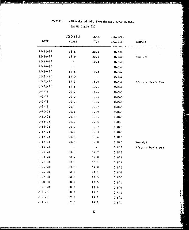
TABLE 1. -SUMMARY OF OIL PROPERTIES, ARCO DIESEL

(ASTM Grade 2D)

VISCOSITY TEMP. SPECIFIC

DATE (CPS) (0C) GRAVITY REMARK

12-12-77 18.8 20.2 0.838

12-14-77 18.9 20.1 0.840 New Oil12-15-77 - 19.8 0.840

12-16-77 - - 0.840

12-19-77 19.6 19.3 0.842

12-21-77 19.0 - 0.842

12-21-77 19.5 18.9 0.844 After a Day's Use

12-22-77 19.6 19.4 0.844

1-4-78 20.2 18.4 0.845

1-5-78 20.0 19.4 0.845

1-6-78 20.2 19.5 0.846

1-9-78 20.4 19.7 0.845

1-10-78 20.5 17.9 0.846

1-11-78 20.3 19.4 0.846

1-13-78 20.9 17.5 0.848

1-16-78 20.2 19.7 0.846

1-17-78 20.4 19.3 0.846

1-18-78 20.3 18.4 0.848

1-19-78 18.5 19.0 0.840 New Oil

1-19-78 - - 0.847 After a Day's Use

1-20-78 20.0 19.7 0.846

1-23-78 20.4 19.0 0.844

1-2L-78 18.8 19.1 0.844

1-25-78 19.0 19.0 0.842

1-26-78 18.9 19.1 0.840

1-27-78 18.8 17.5 0.840

1-30-78 18.9 18.3 0.841

1-31-78 18.5 18.9 0.840

2-1-78 18.8 18.2 0.842

2-2-78 19.0 19.1 0.841

2-3-78 19.2 19.1 0.841

8-

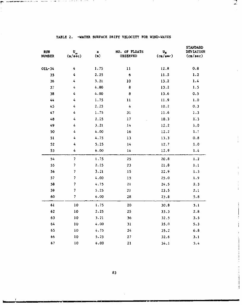
TABLE 2. -WATER SURFACE DRIFT VELOCITY FOR WIND-WAVES

STANDARDRUN U x NO. OF FLOATS Us DEVIATION

NUMBER (m/8ec) (m) OBSERVED (cm/sec) (cm/pec)

OIL-34 4 1.75 11 12.8 0.8

35 4 2.25 6 11.5 1.2

36 4 3.21 10 13.2 1.4

37 4 4.00 8 13.2 1.5

38 4 4.00 8 13.6 0.5

44 4 1.75 11 11.9 1.0

45 4 2.25 4 10.2 0.3

47 4 1.75 31 11.6 1.3

48 4 2.25 17 10.3 1.3

49 4 3.21 14 12.2 1.0

50 4 4.00 16 12.2 1.!

51 4 4.75 13 13.3 0.8

52 4 5.25 14 12.7 1.0

53 4 6.00 14 12.9 1.4

54 7 1.75 25 20.8 1.2

55 7 2.25 23 21.8 1.1

56 7 1.21 15 22.9 1.3

57 7 4.00 15 25.0 1.9

58 7 4.75 21 24.5 2.3

59 7 5.25 2) 23.5 2.1

60 7 6.00 28 23.8 5.8

61 10 1.75 20 30.8 3.1

62 10 2.25 25 33.3 2.8

63 10 3.21 36 32.5 3.5

64 10 4.00 31 35.0 5.3

65 10 4.75 24 35.2 6.8

66 10 5.25 27 32.6 3.1

67 10 6.00 21 34.1 3.4

83

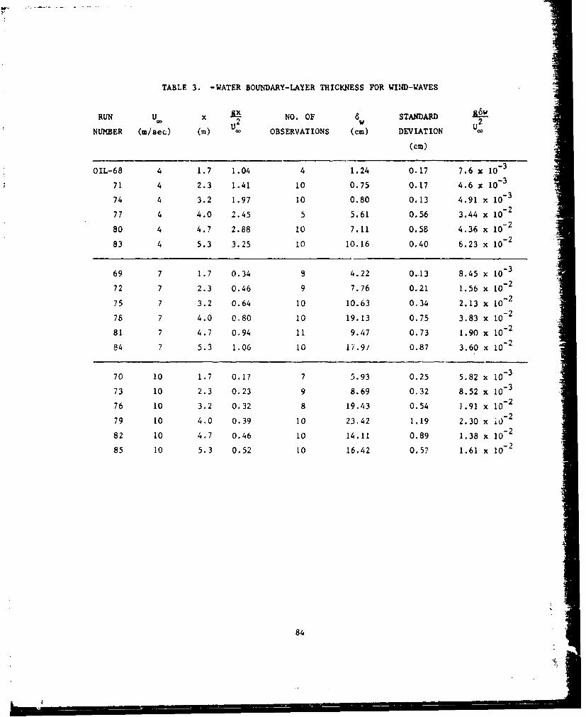
TABLE 3. -WATER BOUNDARY-LAYER THICKNESS FOR WIND-WAVES

RUN U_ x NO. OF 6 STANDARD 2

NUMBER (m/sec) (m) U: OBSERVATIONS (cm) DEVIATION oo

(cm)

OIL-68 4 1.7 1.04 4 1.24 0.17 7.6 x 10-3

71 4 2.3 1.41 10 0.75 0.17 4.6 x 10-3

74 4 3.2 1.97 10 0.80 0.13 4.91 x 10.3

77 4 4.0 2.45 5 5.61 0.56 3.44 x I0-2

80 4 4.7 2.88 10 7.11 0.58 4.36 x 10. 2

83 4 5.3 3.25 10 10.16 0.40 6.23 x I02

69 7 1.7 0.34 8 4.22 0.13 8.45 x 10-3

72 7 2.3 0.46 9 7.76 0.21 1.56 x I0-2

75 7 3.2 0.64 10 10.63 0.34 2.13 x 10 2

78 7 4.0 0.80 10 19.13 0.75 3.83 x 10-2

81 7 4.7 0.94 11 9.47 0.73 1.90 x I0- 2

84 7 5.3 1.06 10 17.9/ 0.87 3.60 x 10i.2

70 10 1.7 0.17 7 5.93 0.25 5.82 x 10-3

73 10 2.3 0.23 9 8.69 0.32 8.52 x 10-3"

76 10 3.2 0.32 8 19.43 0.54 1.91 x lo-2

79 10 4.0 0.39 10 23.42 1.19 2.30 x i0- 2

82 10 4.7 0.46 10 14.11 0.89 1.38 X 102

85 10 5.3 0.52 10 16.42 0.57 1.61 x 102

84

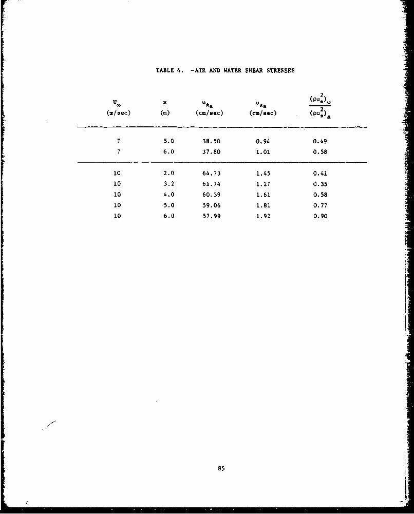
TABLE 4. -AIR AND WATER SHEAR STRESSES

2U. x u *a u *a p.)X2

(m/sec) (M) (cm/sec) (cm/sec) (pu2)

7 5.0 38.50 0.94 0.49

7 6.0 37.80 1.01 0.58

10 2.0 64.73 1.45 0.41

10 3.2 61.74 1.27 0.35

10 4.0 60.39 1.61 0.58

10 "5.0 59.06 1.81 0.77

10 6.0 57.99 1.92 0.90

85

rI

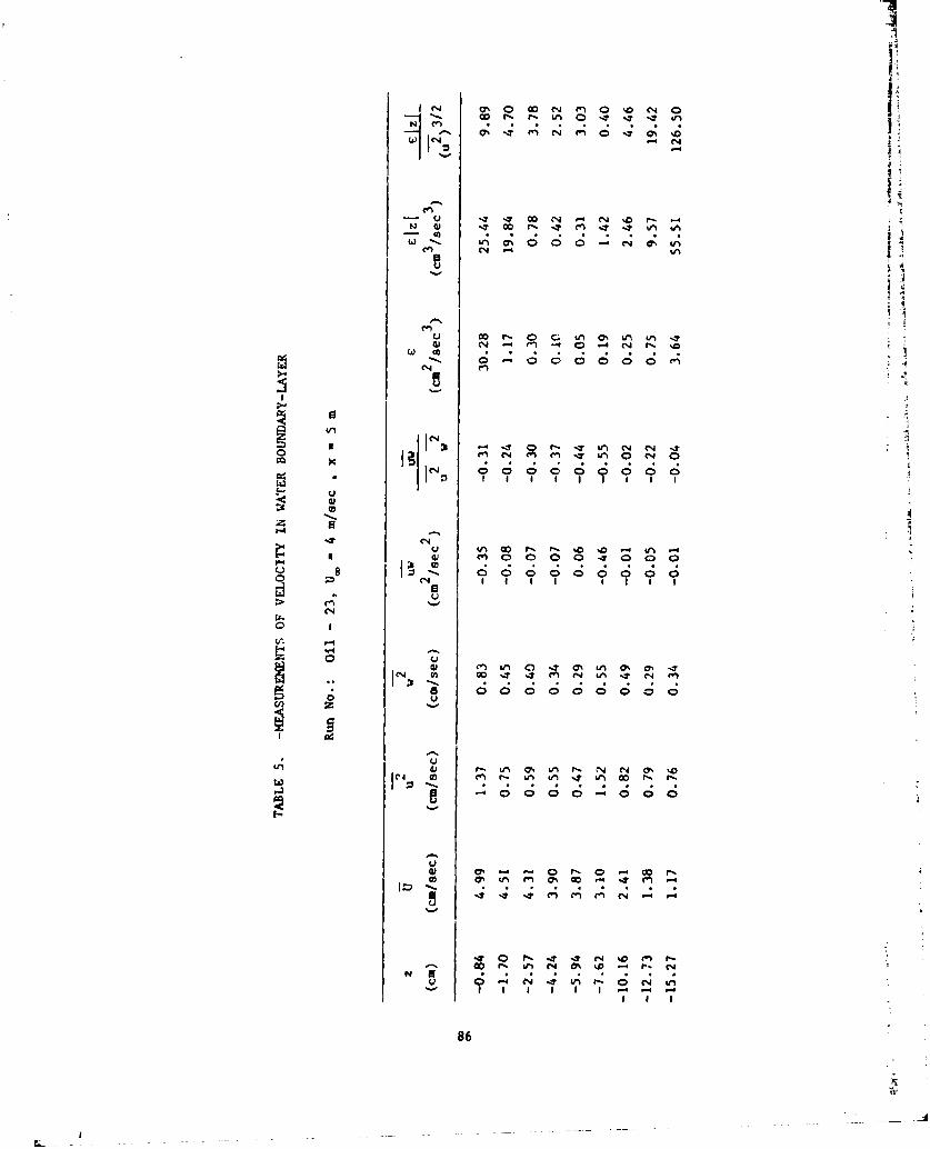
I~'i ' 0 (4 (n 0 .4D E 0

OD N fE i 0 0 '-I

- co

C'4-

C-)E C-4 en 4 4 4F'.

00 00 (n

CN

tn 0 It 0 n Na9) w~ IT m C4 Aa C

4A) - Ln 0 n rý N C% 1cg 3 M r n Ln : ) C ý r

I I I 1 1

86

CI C 4 C-4 C1 47N wa a

C- C4 -en

F. .J .-4 Le% .0 4 ao - co Na% .14w -4 0 0 0 0 0 0 0 0 q A

(n -4 ý

- Ao

OD OD U) 0 T.a - N u-4 U' 03 N-

I I00 0 00 0 0?

E-4 04 0 I

CA

G - N , f '.4

9 C9

M ' - '40 M3 M. 0 W0 M" C

'.0 C4 ( C4 1 1% 4- 0 s

-~0 I4 C') 0-4 0 (N 0 0

~ C'~I'~ '~ C) ' 1 u -I 4 C.-4

P 7

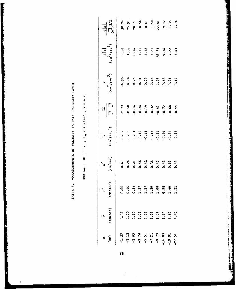
- ..J 0 -. -4~N 14 ' C 1 ' N - U' N - (S4

UV 14 0% %A l -4 (

r-" 1700 0 m %0 0

10*

00 1() 4 C% (N -4 C-4 CO -.?

I I i I I I I I

z

-I4 .. 7 -I al - % -

4) 0D 0 4cm.4 ( C 0

000 0

> ,

0 I

1-4

0w r- %0 -4 '0 (N ' C". r-1 MC4 C'

z

7 1C

C 00-4 -- m -. %D L 0 V -I

M) 0% 0 o 0 4 14 (n en -4 .7 0

-4 ( li ( 1 4 01 C'3 '0 t' 0% f'0I::C-4

88- ' N 4 -~ N (

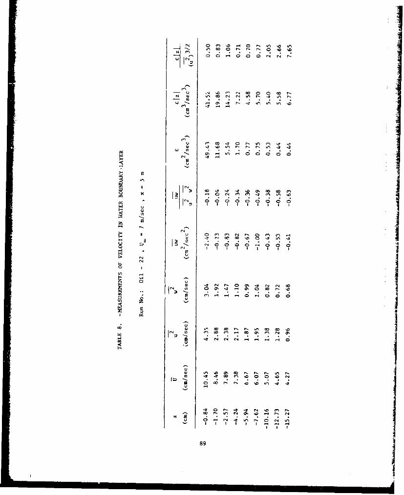
N 0 0 -.0 0 i0-

-~ ~ ~ 1 %n'r c r, r- r- 0 '

C-4

C-4 M. n1 -4 0 0 0 0 0

C 4 u m

C20 0 cc-4 0-0 a 04

I

CNN

Nw %OIC..-1ý

00

-4 -44

0 N0 '-. ~O. cc F'89 ~

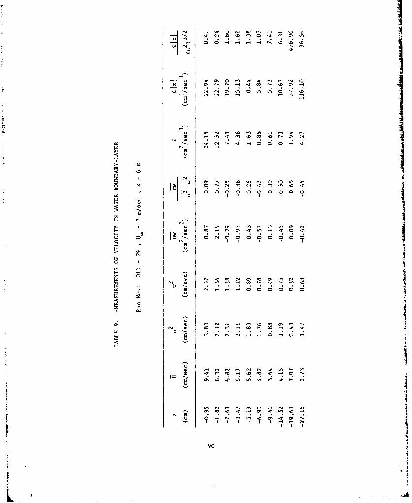
C1 (N i . r 0. 4 - 0 r-. `4 -4 CD 1

~6IN 0 1 0 7 NO env,-4 en4 - 4' r-.c

Go qJ r, 0 , '.0 tn '.4 e~'T

G) .4 -4 -7 4 '0 0 0 cn 0% (

cq r-. Lf) I-. fn( O

(n 0o 0 0o 0 04 0 0 ILn et r- (7, A *-4 C14 0 OD

0 90

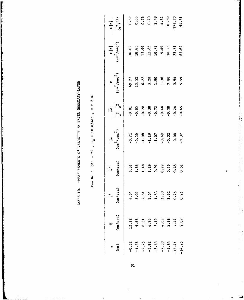
-n v (N -1 m% In C4 M% UiA r4 N'

m~ -4 - -1 14 M'* f-sO c

4;1 ( 4 IA (N (N; LAr~0 %U%0

z 0 N(0 ''7( N'

431

0 C-4

% 40 0 ON (- O% N 0l ( r'- 43 (N t'.3 0 -4 0% -.7 ('3 0 n

01 (Nf ý1- 0*

co VUC

0 .7 C" N cn V.4 P, ON CI0

91

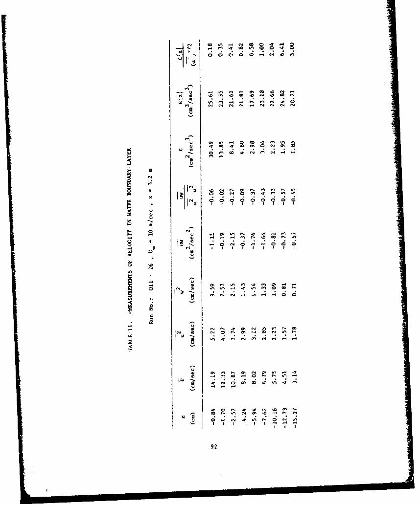
0 1 0 LA '.4 C4 .00 . .

-4A14 -4 C

Me U ' . .. . N -4= r N4 04

ON tn N - NN

-Z00 00 4 ' 0 00

~- 0 M'00 I (' " N n '4

NO

0 ~ ~ 01 N 0n L'I 4- ('4 m , 4

o - ON doC0 n

40 M~ C - 0 4 as% 4

0 -4 r C o o %* I

0 fn

~~~~~~a r- ~ U ~ ' 4 ~ '

924~ 4 (~I~'0 0 - U

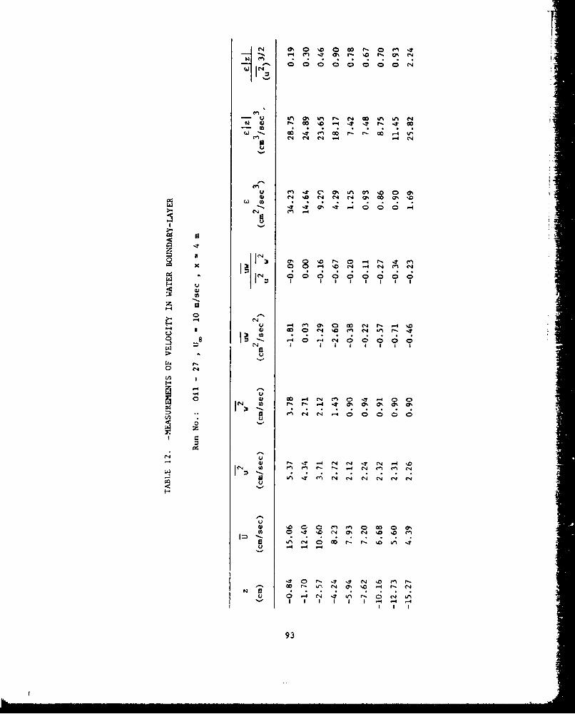
oo0000 0 0 C4

- ~ ~ ~ ~ ~ W Lf 'i - c i n e4

V --r C, CK 61% onI 0 0 0

CN -

4 kw

00-

04 4) g - C nto r, r-47 0% 0%~Nt. 4 '

en e4 C .4 NO 00 0

4)C C4 -

-4 -4 -

ci , 4 N, Nl 4, ) r4 '0N~~- -4 A-.4 N i e

93n 4 (~N

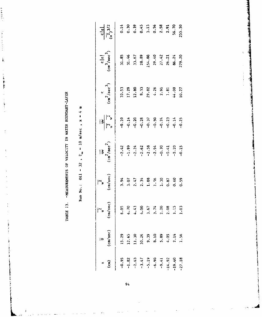
C% _ 0 0% 611 ( 00 r-4 0 0

t41 0 a - T (NC1

U 0V0 I N C4 C ~4 0 r-

0) I"' (l W m C (7 % m 0 C-

00 m N 0% 1 (N ) 0T

14 -4 -- C LNC4 " -4 -14

0) 0 1 -70 r- 0% .e 11 .4 '

* ~ ( 00 0 00 01m

C- 11. 6' -tq ( - 70 0 0~

-' 0% 'l (N '0 ON4 0 0%!* 1^- -4

LM C-4 MN (N (N N 0 0

c -j

-94

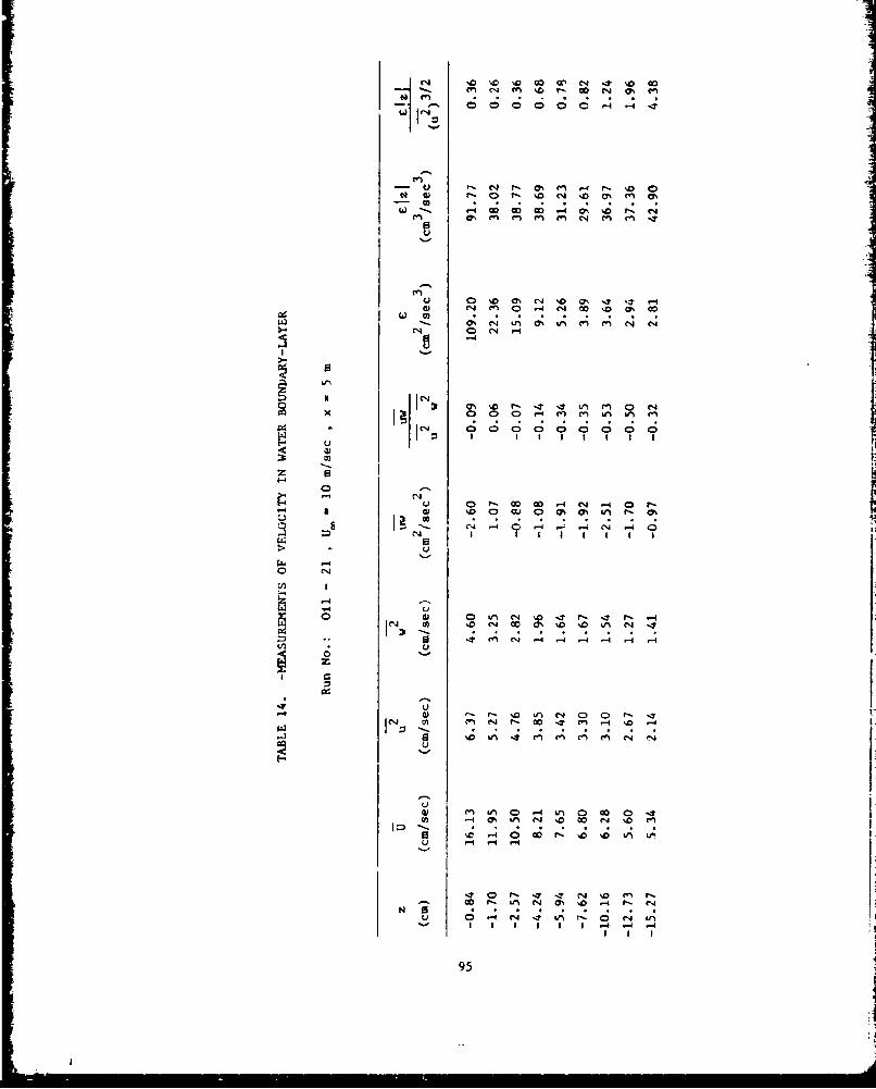
IzI- U P-ON M - 0fn m - '0

0 % s 0 Ch '.r4 0 % M 0

r- C.4 P N M 4

G)~-, NM M 0 0 ' 0

x o -P r 0% £I'P M N

z -

40 -

-l LA A 0 - 0 0 4 1N.4 A t

~1 -4 -4 04

95

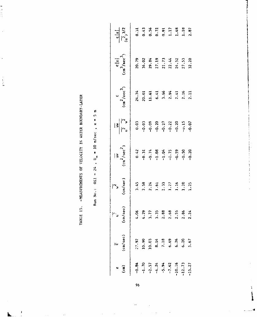
Q 0 .7 UN It a'e -. C4 m~ CDG

0) w. %( -70 fl -- WIN ('n 01

en C4 (N i (N( N( N m

U -7 - -4 -4 10 -P -4 %D -4

(0 Q r- 0 %D 1. 10 0% 7 ~-1 -4C14 (N4 (N -4

u CN P4 00 0.T

e4

U ~ ~ ~ O r- .- ' Q1 0 U l0% 0r4 C1 4 I

* U

0 0(1

0 4) I- 0 07 .0 Ln~. 0i~r14 (N 1 - .4-44 .4

10 1. r

8 -~ 4 ("I r-( ( N N

96

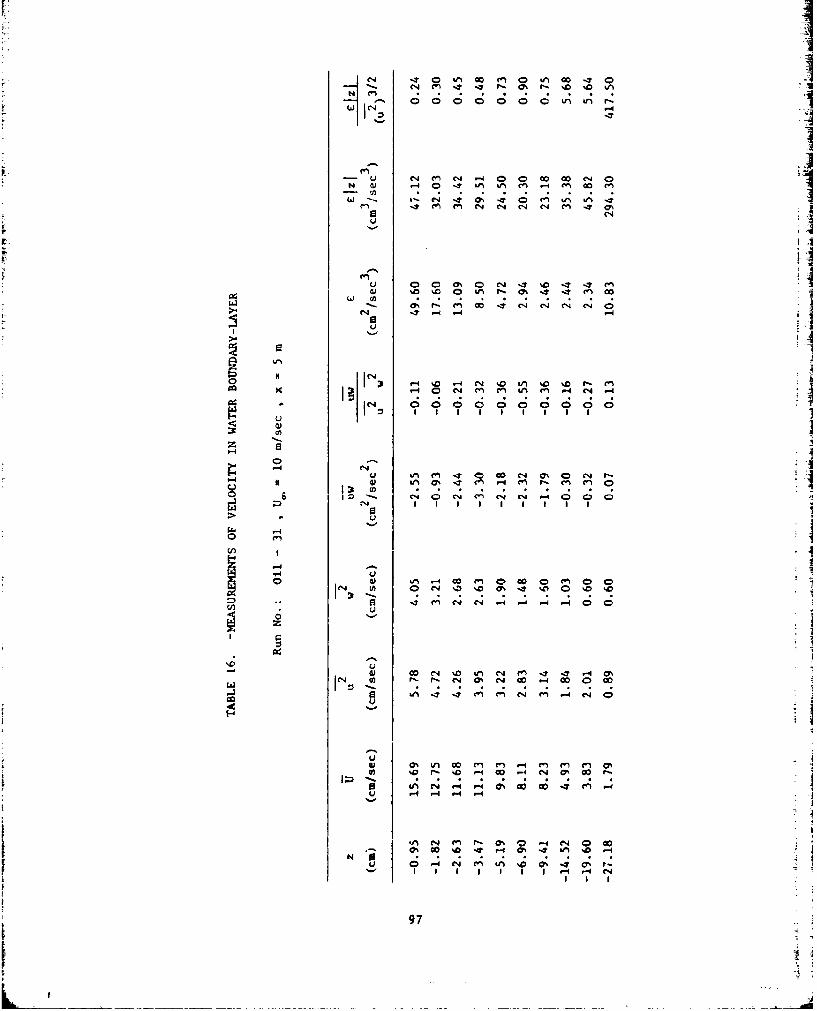
C14w000 00 C4C 1~-4

144

-10 C4- MN C4 0 0 (

N0 C 4 9 - U%D V' M- ',1 E. 0 %

-7 cO --4 CC 4- N ( c 0 00

U

0% 0n CID e .n M .4 M .M ON

sa LA 0% r4- r4 00- 436 (N (NN r-4 r- P-4 .-4

19I ! ' 2

04 C 0 '4 MN '. in~ 'B '0% 4--

97 ( -"' " -

- * w On- . -4 m~ '7 'C 0

(U No a%0 '0 4 Ln' W Lm 0% r- 'T

W% ccO 9' 0ý - rl: V; 'Cm* ( C ( .4 ~-4 (NO"

a N -4

v m~ a LM (N ON^0

(N4 mJ -4 .4 -4 -4

P-4~- 4) '7 'n U% c00

4 L^to

0j (N ' (10 0% p co mr l C4 ..jN 4 ' -t 1 % C4 0-n0 t. .-4

LA 4

&A eC n r- V 14 0 c

CN 19- Uý 1 i "!1 9

0 1-4 (N N (N) M 0D ON0 0 - t0

9U

IIII'1

Ii

ii

'1

'1

FigureB IiiI �

1I

II:

99

.1

WIND UNNI4V4

FIUR . WIND-TUNNELANK

100

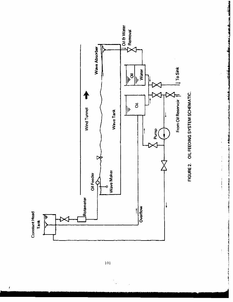
C) crIuiIXI

cc cI

C IDLIA

U.

LU-i

101

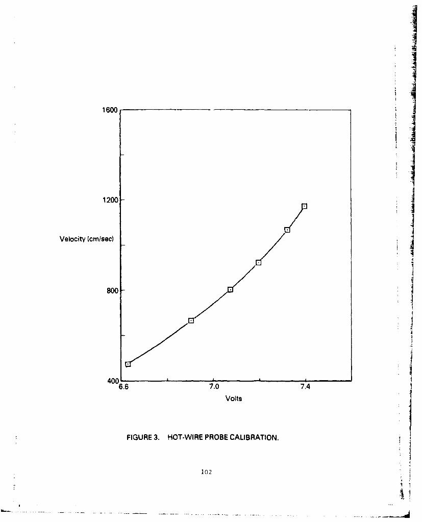
I

1600

iiI1200

Velocity (cm/sec) I I;800

11

JJ

40066 . ,,6. 7.0 7.4

Volts

FIGURE 3. HOT-WIRE PROBE CALIBRATION. j

102

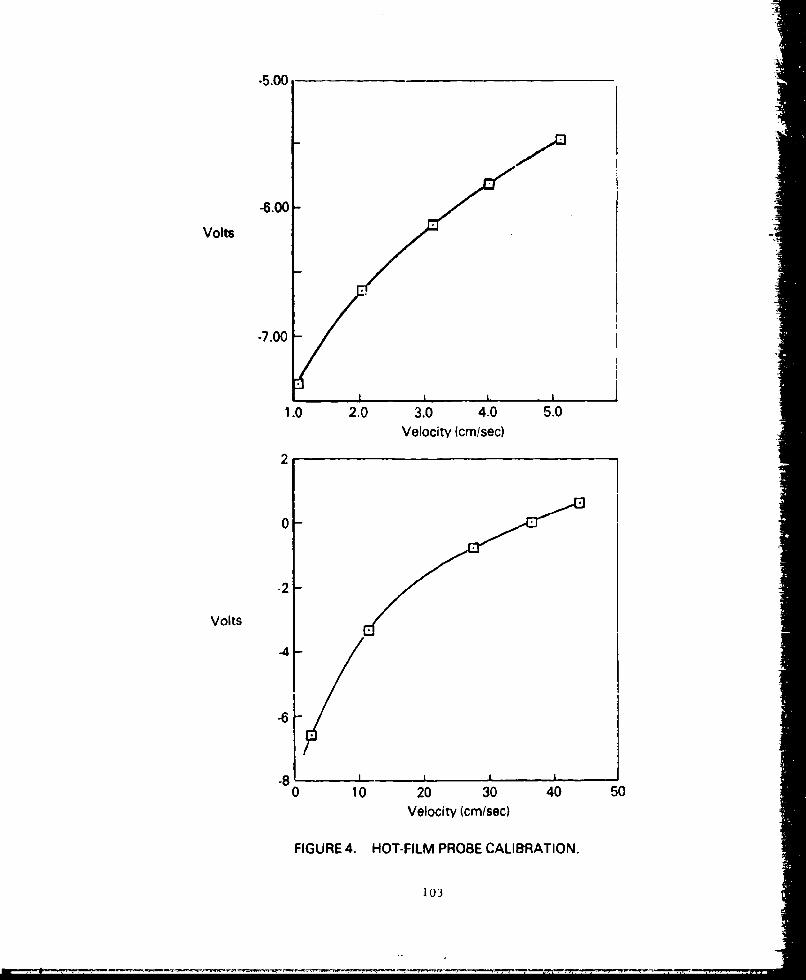
-5.00

-6.00-

Volts

-7.00

1.0 2.0 3.0 4.0 5.0Velocity (cm/sec)

2 -

0-

-2

Volts

-4-

0 10 20 30 40 50Velocity (cm/sec)

FIGURE 4. HOT-FILM PROBE CALIBRATION.

103

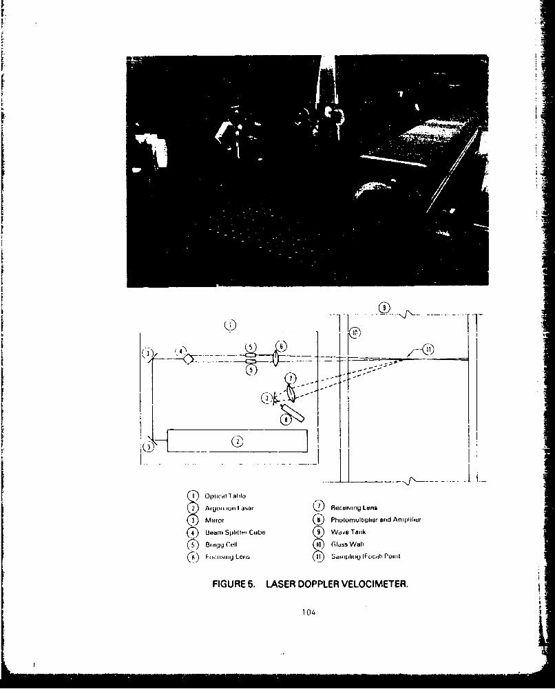
r09

I,6

4. ____________ Iil!1 ib 9 aeTn

( B fdqcj Cell ( CA)Glus Wall

( ) F-oc.1rsmirj Leritis11 Sd[1iiIriiy (FOC11) P0oint

FIGURE 5. LASER DOPPLER VELOCIMETER.

1.04

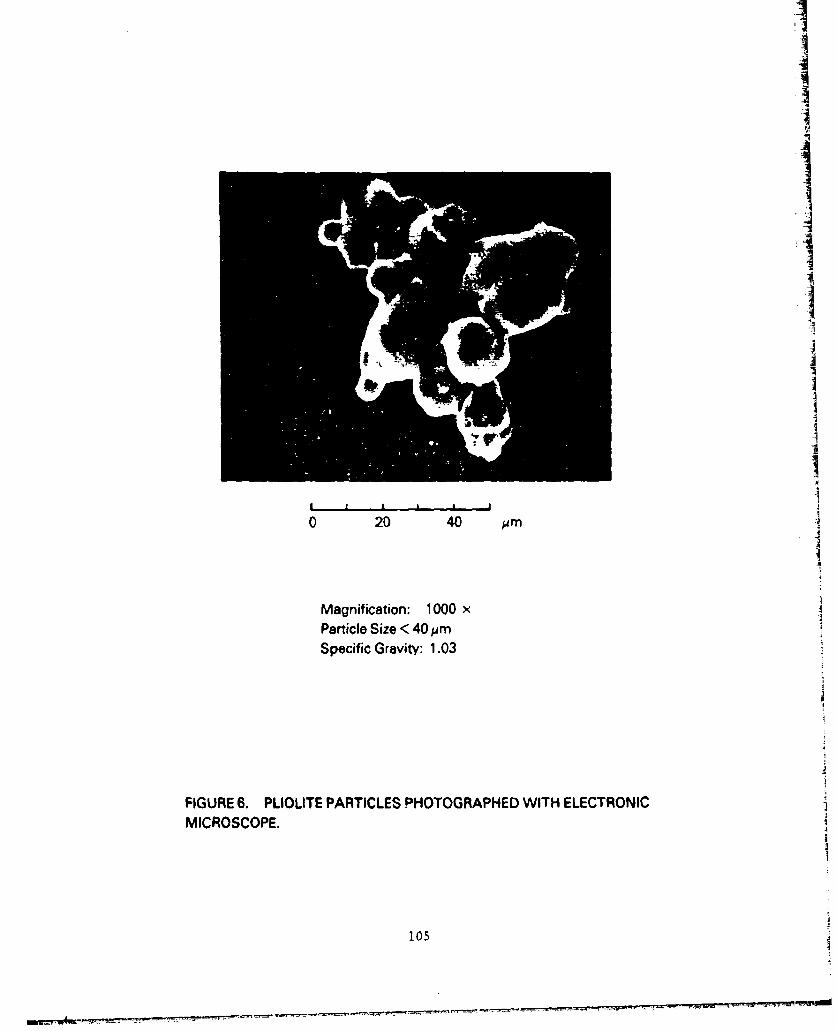
7t

0 20 0 JiMagniicaton: 000Partile Sze <40 ISpeciic Gavity 1.0

FIGUE6.PLILITEPARICLS PHTOGAPHD WIH EECTONIMICROCOPE

105

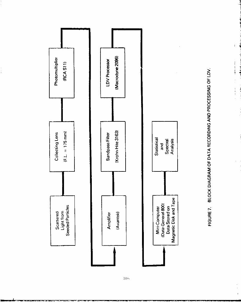
0)0-a-

4-- 0

z

E 0

.0 0U

U- r inm 0

U-0

cc0

0V))

CD

co w

FD 0E -C. C/)

10)

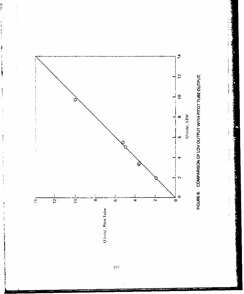
F-0

-F-

000

0-

-~Z I-0

0

-LC-

0

Izz

107

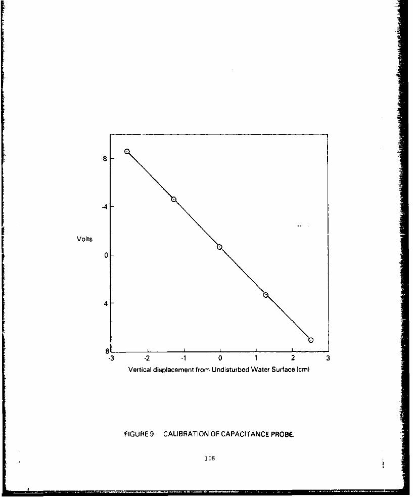
-8

4-

Volts

0-

4

8 I I I

-3 -2 -1 0 1 2 3Vertical displacement from Undisturbed Water Surface (cm)

FIGURE 9. CALIBRATION OF CAPACITANCE PROBE.

108

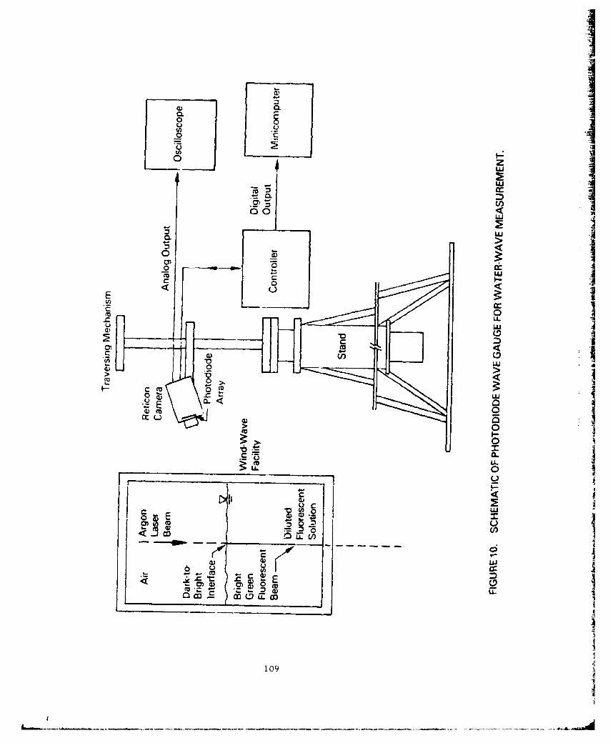
0.

0*Uz

00

I- -

E

V ccm 0

.~C 0 L

U w ID

_ m

Li.

0--

-CC

C-)

109U

FIGURE 11. PHOTODIODE WAVE GAUGE SETUP.

110

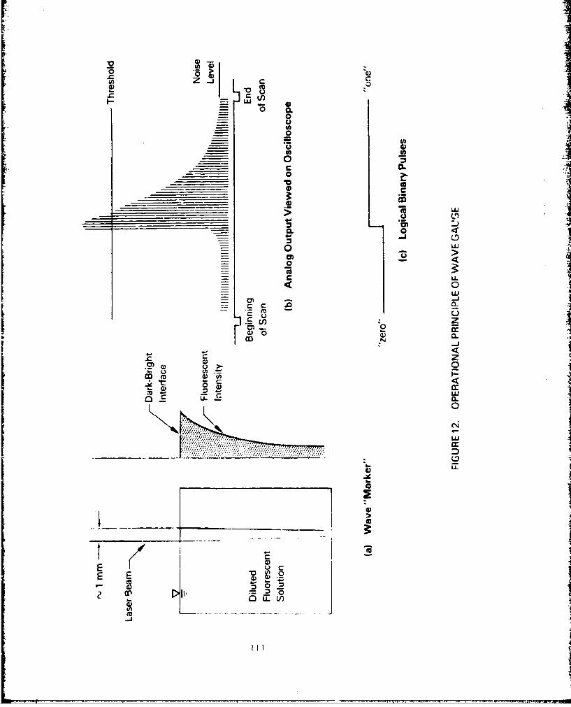
CC

0

= 0

UU'I))

__ _ 00

__ _ _ _ _0 <

0. 0 0

cI C a

- 00

C U.

c zW 0.

0 cc

-0 w-

/ 0.

0h.V ix

(/ a)2 I IX

E 2Qa, ~ i.

19I

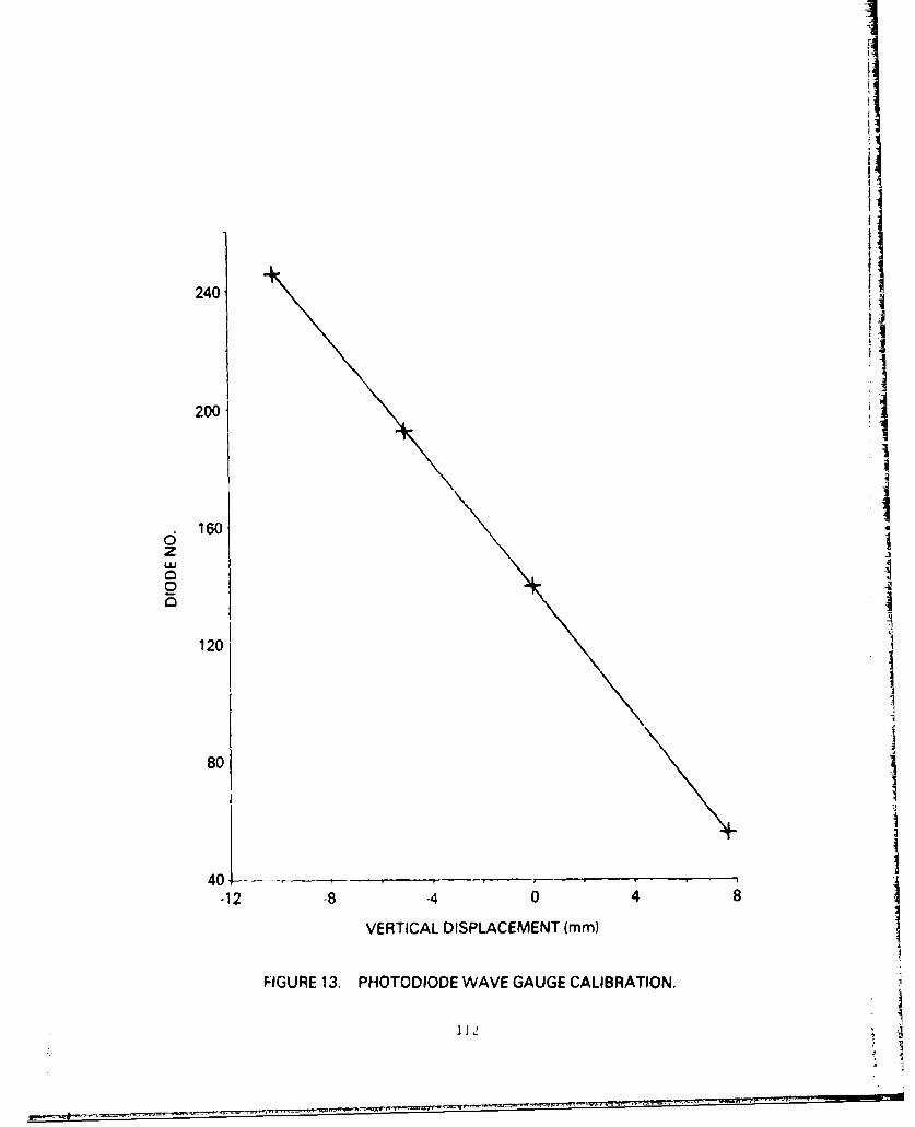
I

240 I

200 ]

d160S10

zw .a" -10

120

80

.12 -8 -4 0 4 8

VERTICAL DISPLACEMENT (mm)

FIGURE 13. PHOTODIODE WAVE GAUGE CALIBRATION.

S. .. . ... . •. •-112•

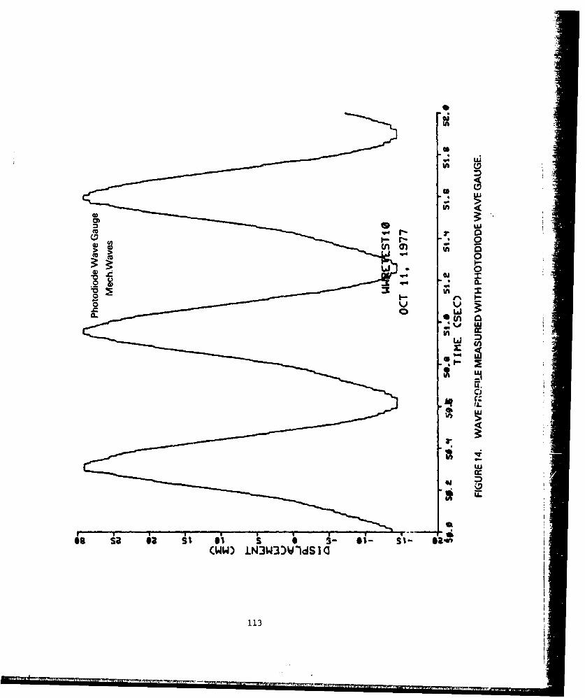
In <

CL

(UW)%. LNW)udI

113

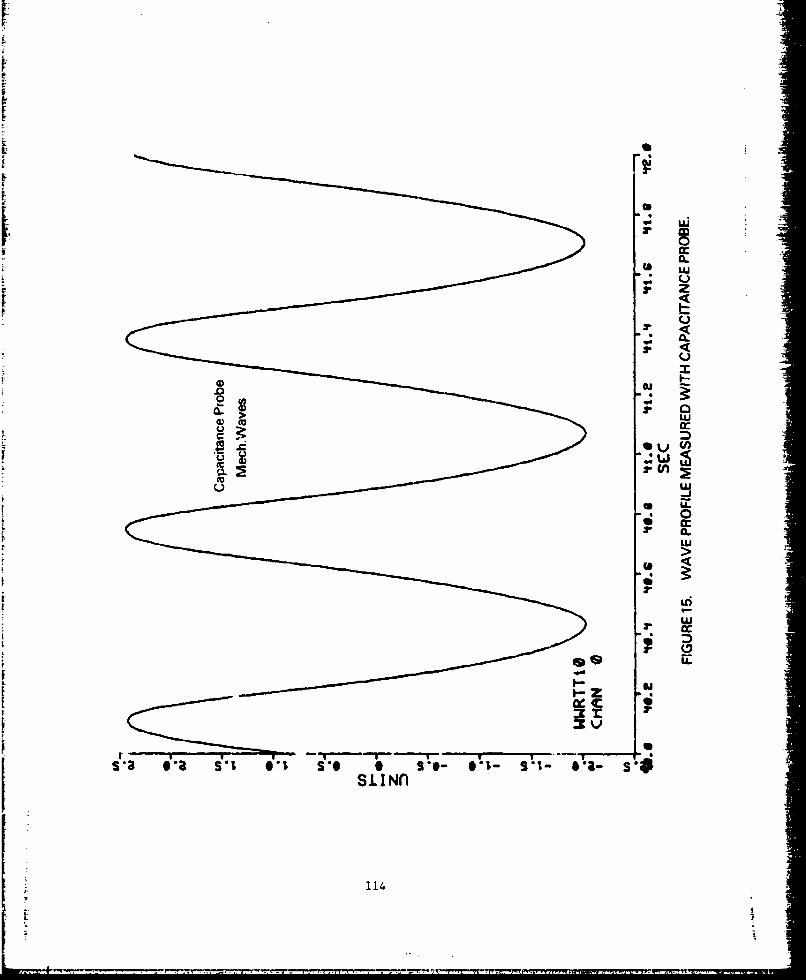
Ij.j

000.. wA

(L) cco

* 0.cc.

sCfL

S U.

F0wz

simni

114-

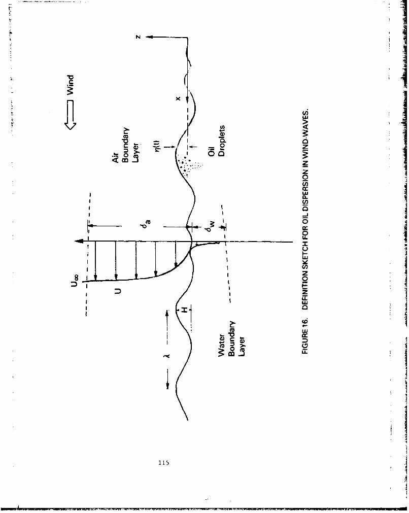
LU

0.

cc

0

z0:zi

w I

0L

MU(0"131

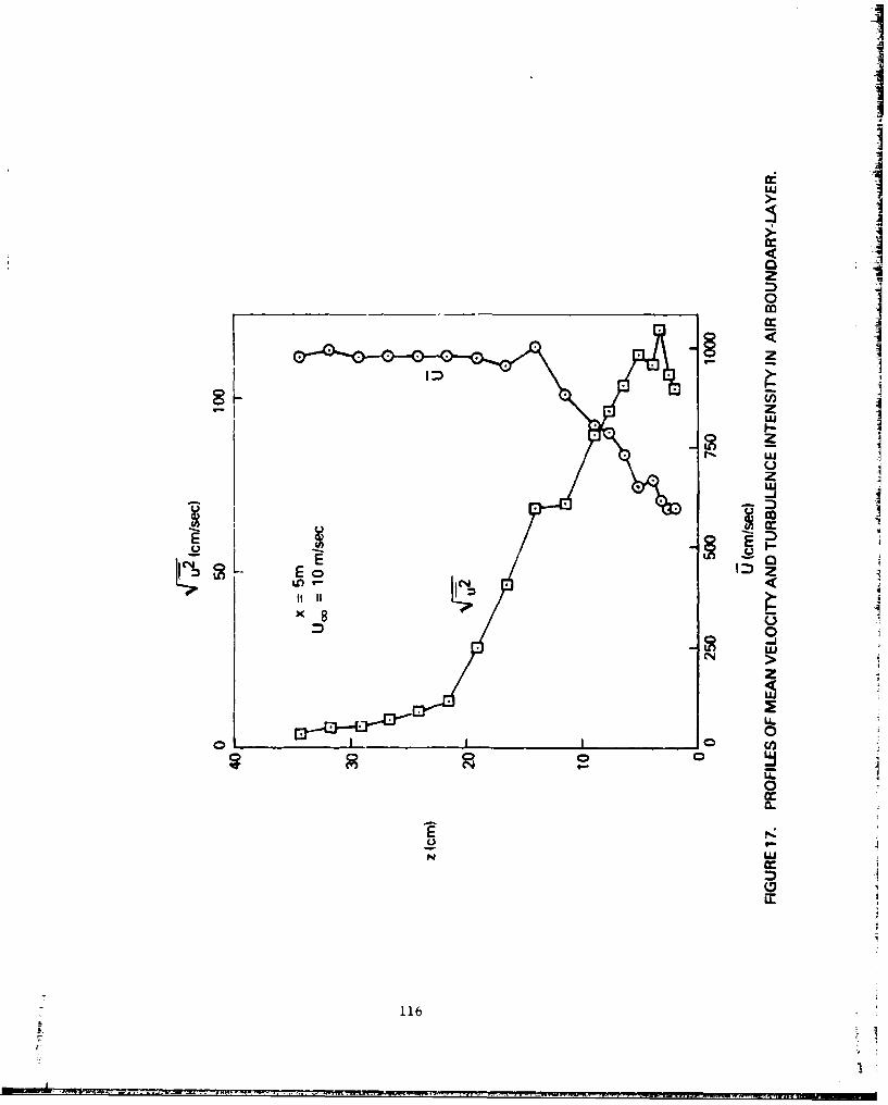
IMILUI

u 11

wUz

EoE

z

U-0 0

0

116

MUM"

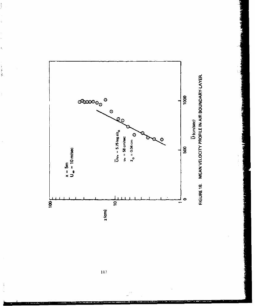
o 0

0D 0

10~

uiiu~u~ u

00

zigc

117

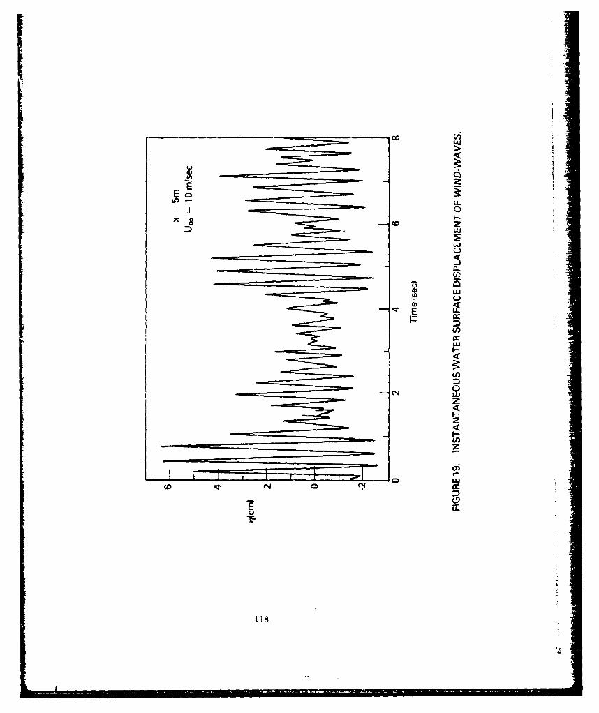
IO:U->

Lnw11wx-

LI)

(U <

E Uwzrcc-

00N 0U

z

C.,.

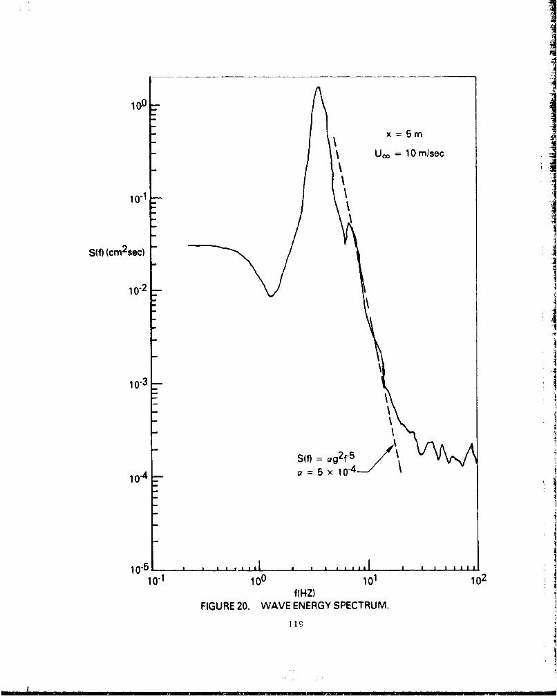
100-

- \ x=5mSUoo = 10in/sec

10.1_

2

S(f) (cm 2 sec)

10-2

10-3

Slf) a g12f-5\

10-4 Ia 5 x 10-4

10 5 aa Ial Al i a II

10-1 100 101 102

f (HZ)FIGURE 20. WAVE ENERGY SPECTRUM.

I 1c

II

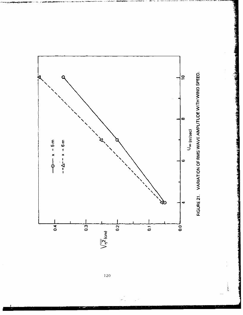
0-W

0-

LU

I Cc

LD (0

0

I lo -

1202

~inI fla n~ ba~ * *~ ~ * - . -,* ** ~ ** -* ui

L41

a-J

/ E

/ C D

/ ~z

LLI

// 004

/L

440

p I I pM

CDr (3ND

LU

o U-

z

I.-

U-

cc,

In m

122

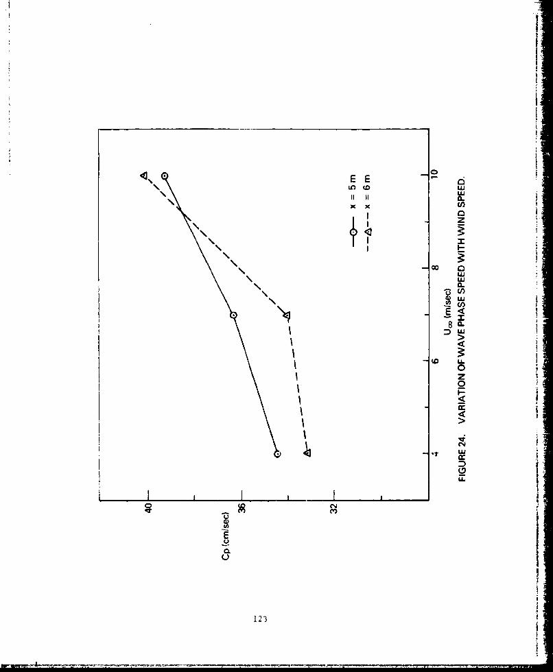
LAO coW

xxLU)0.1

z

000uJ0.

WW

8 0.

0z

C.,

LLI

0LA

123

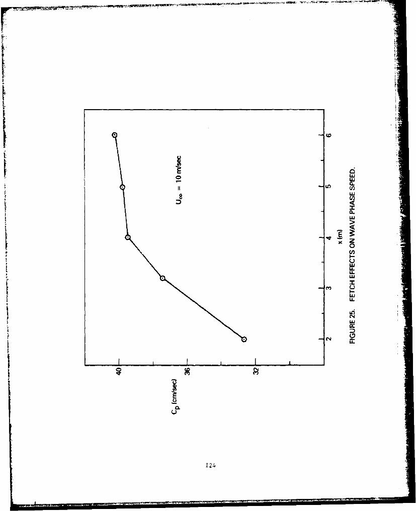
- - - .-. 7t

I CL0 LU

0~

LUJ

U.-

LLLLJ

ML)

CLU

124g

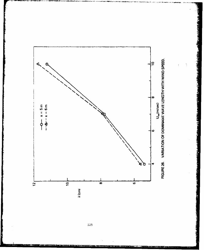
N coN N 3

N-Nu

EN

N ~ zN W

EE E

C14 co

iii IIp

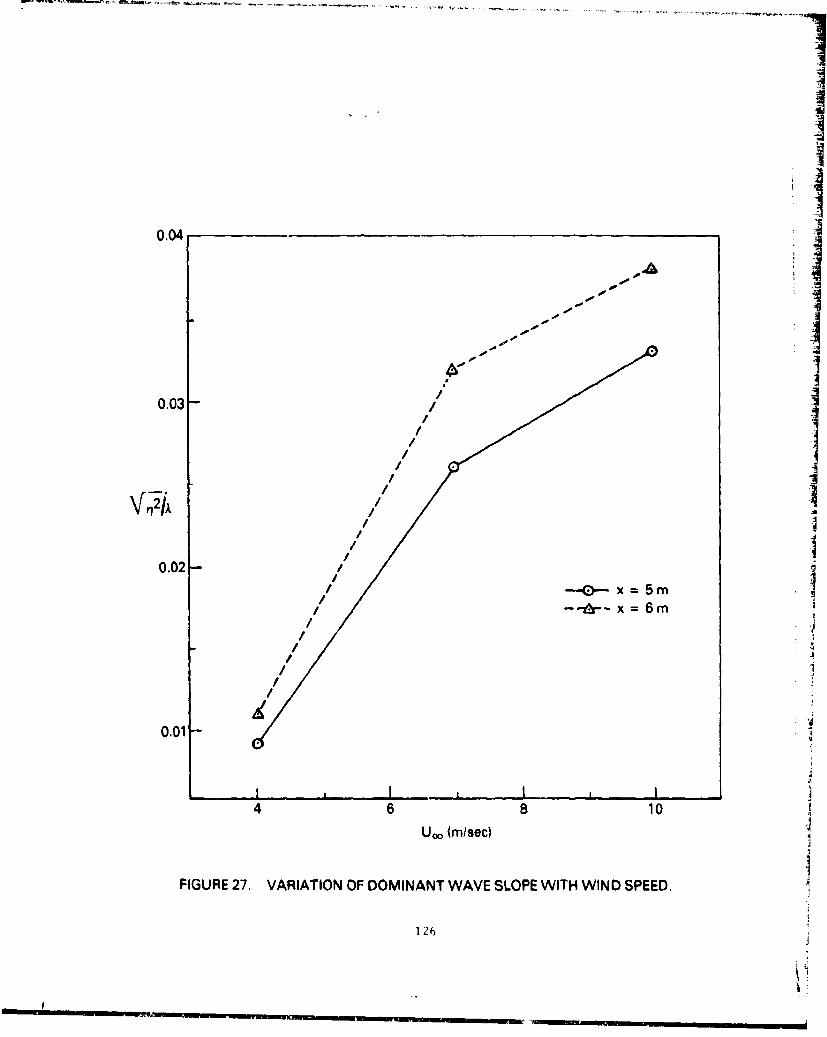
0.04

S4

,79

0.03-III/II

0.02-//

/ -m/ 6 m

0.01-

4 6 8 10

Uo (m/sec)

FIGURE 27. VARIATION OF DOMINANT WAVE SLOPE WITH WIND SPEED.

126

II I l i -- -- L I__ - . •

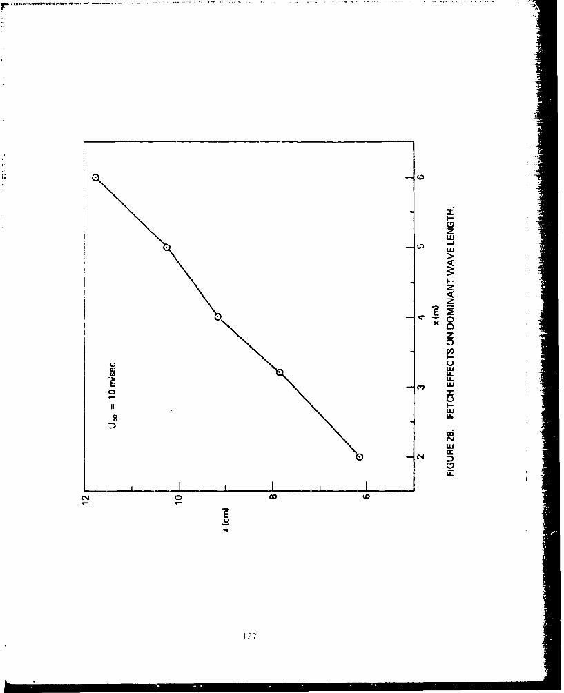
z<

z0

z

U-

IL

127

uif

L.I.

0 ho-0z

0U

C14~

EC

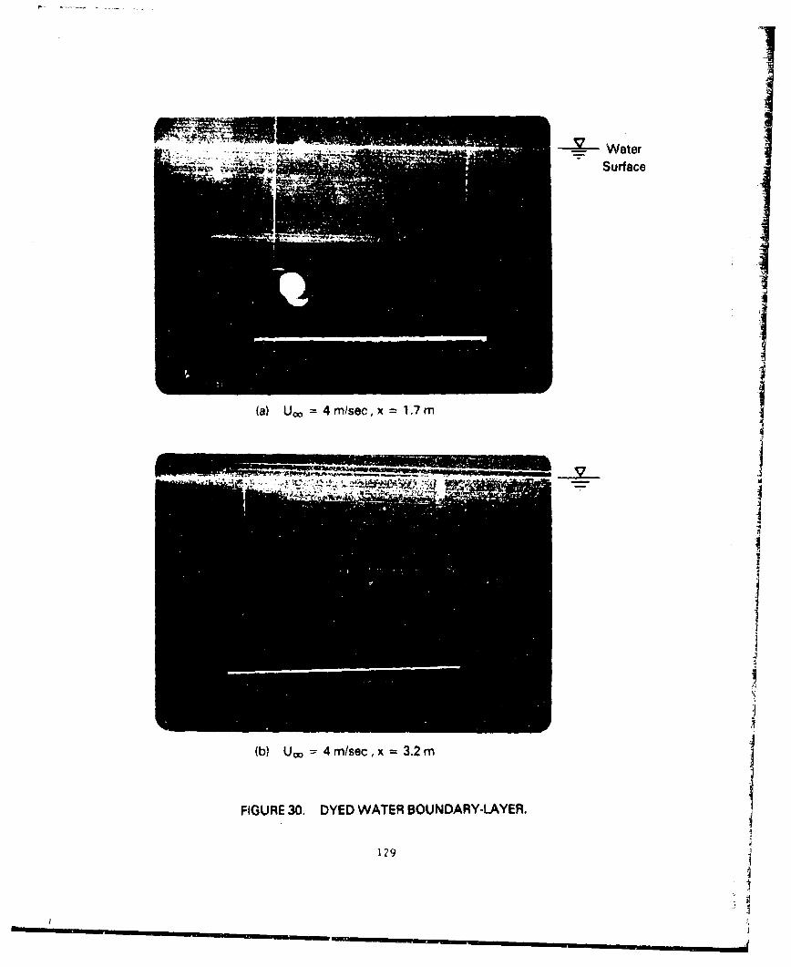
Ti

WaterfSurface

I

(a) Uo,= 4 m/sec, x =1.7 m

III

(b) U, 4 4m/sec, x= 3.2 m

FIGURE 30. DYED WATER BOUNDARY-LAYER.

129

WaterSurface I

(c) U = 7 m/sec,x = 1.7 m

II

(d) U = 7 m/sec,x = 3.2m

FIGURE 30. DYED WATER BOUNDARY-LA' "R. (CONT.)

130

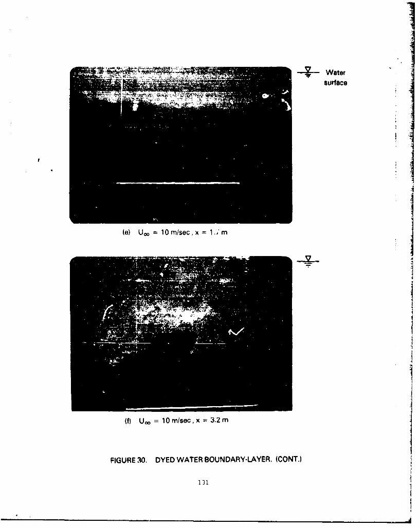
Water

surface

.13

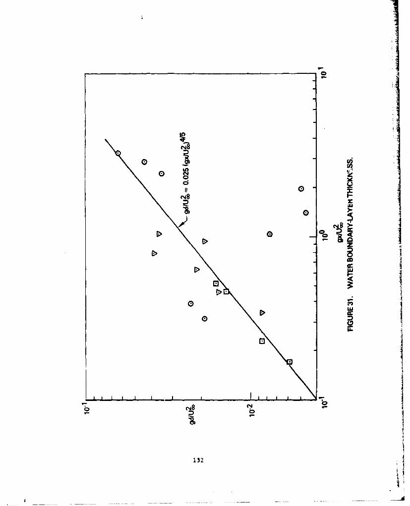
I-..

oo

0

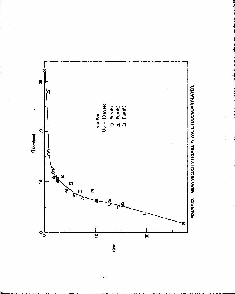
E ccccc

E oun q-. OCc-1

x 0 4Elc

0.

00~c

133

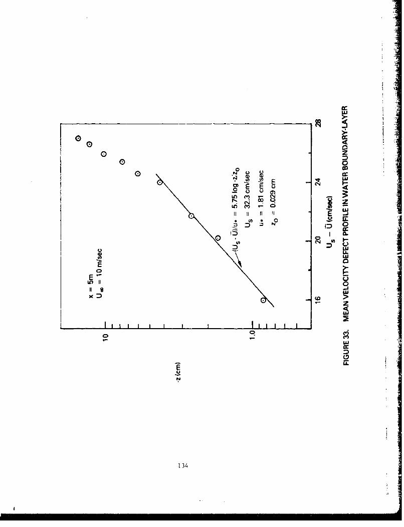
00

N

~Eu

C4

1340

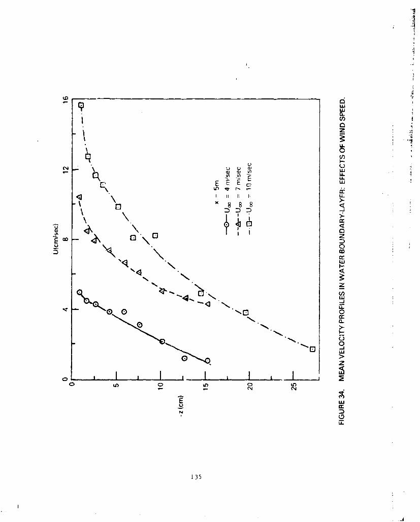
CL

LL0~

00

U-

I-

4))

tt 0 2\

ccLU

N z

0

Ul) LO

-LJa:

0D* zL

0 135

LU

0zo

zI.n

0

0-J

cl -J

z

OD

-jL-0

ueNr

136

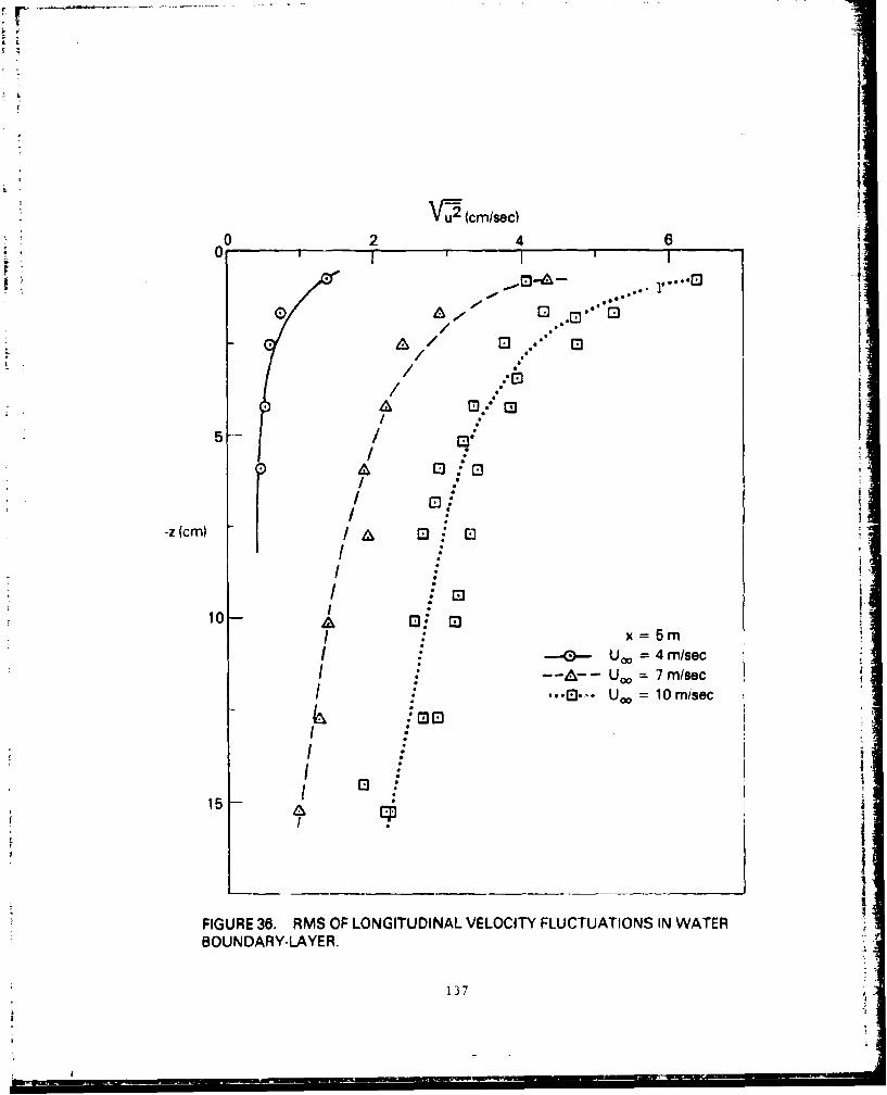
F

0' U2 (cmisec)

0 2 4 1

00

•/ ~ ~..E"D i

// E

PI o/

-z(cm) /I

10 -U:, 4 r/secII

I :x=Gm

hI **"fl Uo, = 4 mlsecS"----Ucoo- 7 m/sec

/.*.•. ,•• U 00 10 misec

15/I

FIGURE 36. RMS OF LONGITUDINAL VELOCITY FLUCTUATIONS IN WATER; BOUNDARY-LAYER.

i37

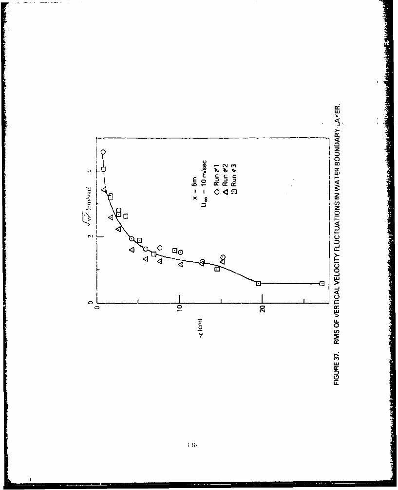
z

E cc cEo CCC c

K IIX8 zM z)

L) z<4

e" U

0

cc

w~

(D

w.

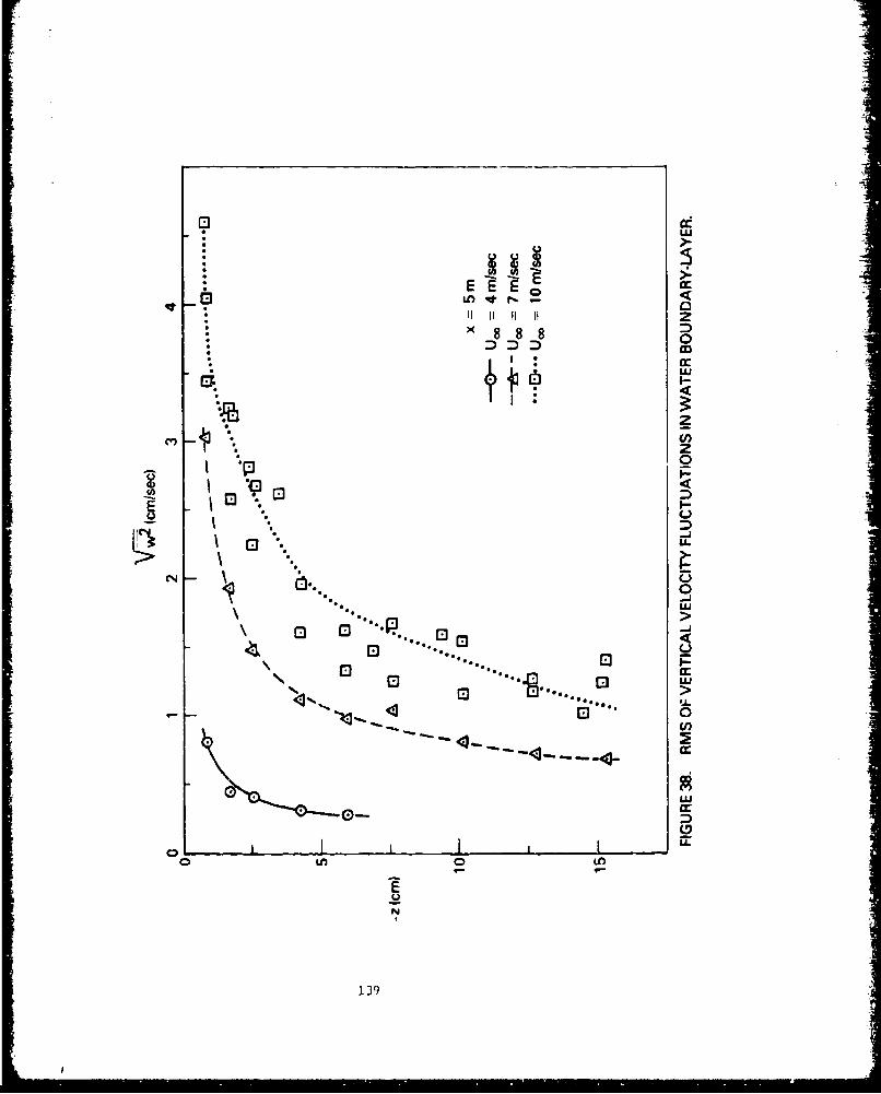
X*D DI I VI

* X888

ED D

3 L1L

(N S C)i..i

E.. 0

LUJ

Ln J 0 **c

139J

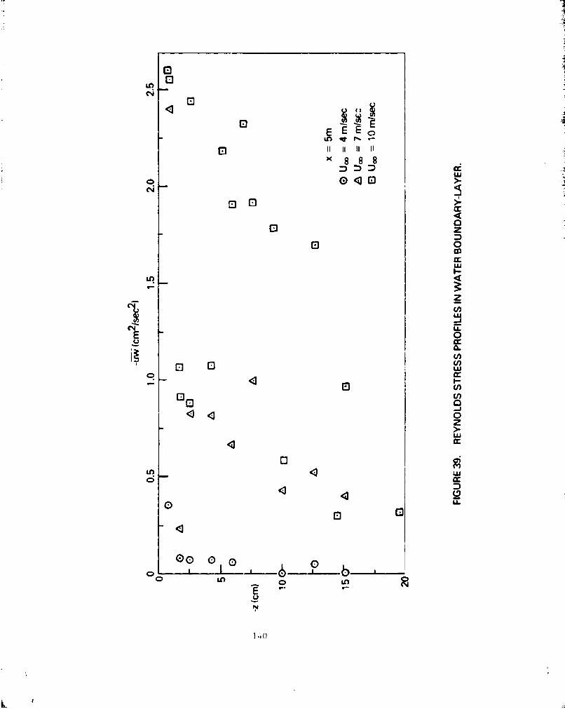
L)0

EE E

Ln v P1

D ccL-

0 >

z

El 0

UU

Lo

z

0(0

El '- LU

(n

0,

ini

000 0

0 i

E

N-1

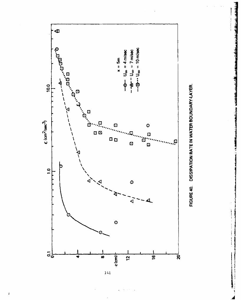
E E EE

xI I I i

2 100

LU

0c

0 4 .D

141

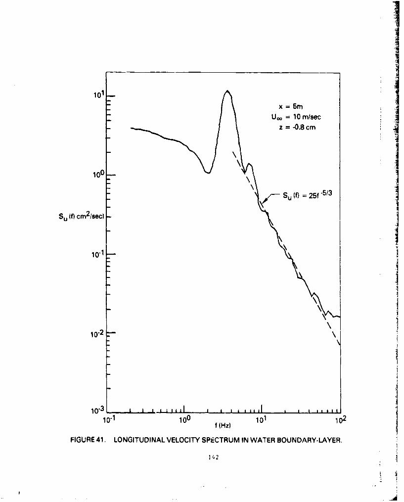
101Lx = 5m

U. = 10 m/secz = -0.8 cm

100-

"Su (f) = 25f -53

Su (f) cm2 /sec) -

mI

10-1

mI

mI

1 -

1023-

103 I 1*111 I~l I ii ,s*il . a a a*'*

10-1 100 f(Hz) 101 102

FIGURE 41. LONGITUDINAL VELOCITY SPECTRUM IN WATER BOUNDARY-LAYER.

142

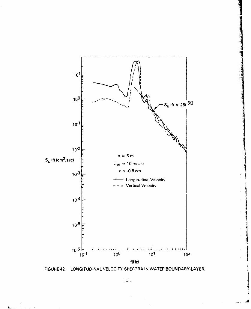
II

100 J

S"". .jl '•X• •,.._Ski (f) -- 25f.5/3

10-2

Su(f) (cm21sec)x 5r

LJoo 10 M/sec

10-3 - z -0.8 cm

; • Longitudinal VelocityS-Vertical Velocity

10-4

10-5

10-6 L -J I -A. ,I ,r t I I. ,

10"1 100 101 102

f(Hz)FIGURE 42. LONGITUDINAL VELOCITY SPECTRA IN WATER BOUNDARY-LAYER.

] 43

- - Verica VelcittI

|• __ =

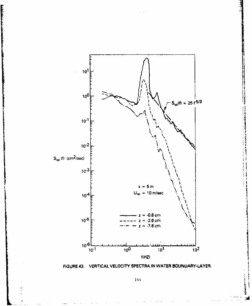
10-1

100 -

f) (cm /s

10-3 \ I1o•I ',i

12\ \ I*1:

x=5m

10-4 U0o = 10m/sec \ \I

-- z = -0.8cm10.5 z = -2.6cm

. z = -7.6 cm I

10-6 -. ,, J I , , , 11,,

10.1 100 -H01 102f (HZ)

FIGURE 43. VERTICAL VELOCITY SPECTRA IN WATER BOUNLARY-LAYER.

144

- =

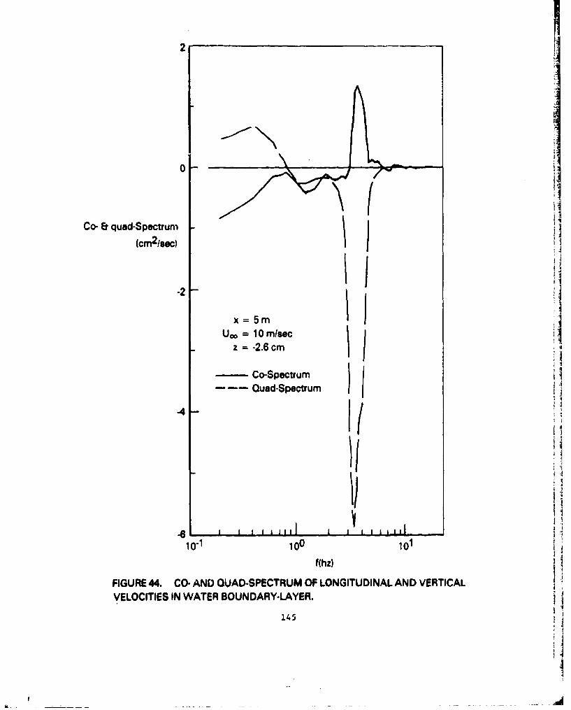
Co- & quad-Spectrum

(cm2lsec) II

"-2

x =5m

U= 10 m/secz =-2.6 cm

-- Co-Spectrum- u-- aSpectrum

-4-

-6 I" /"I

10-1 100 101

f(hz)

FIGURE44. CO- AND QUAD-SPECTRUM OF LONGITUDINAL AND VERTICALVELOCITIES IN WATER BOUNDARY-LAYER.

145

tI

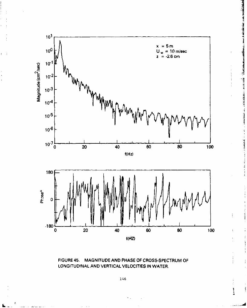
101

x =5m100 U - 10 m/sec

z =-2.6 cm

1-1 aE 10.1

.v 10-3

• 1043--5

10

10--5 _IJ

10-70i

20 40 60 80 100

f(Hz)

180-

0

S, ,0

-1800 20 40 60 80 100

f(HZ)

FIGURE 45. MAGNITUDE AND PHASE OF CROSS-SPECTRUM OFLONGITUDINAL AND VERTICAL VELOCITIES IN WATER.

146

L..I

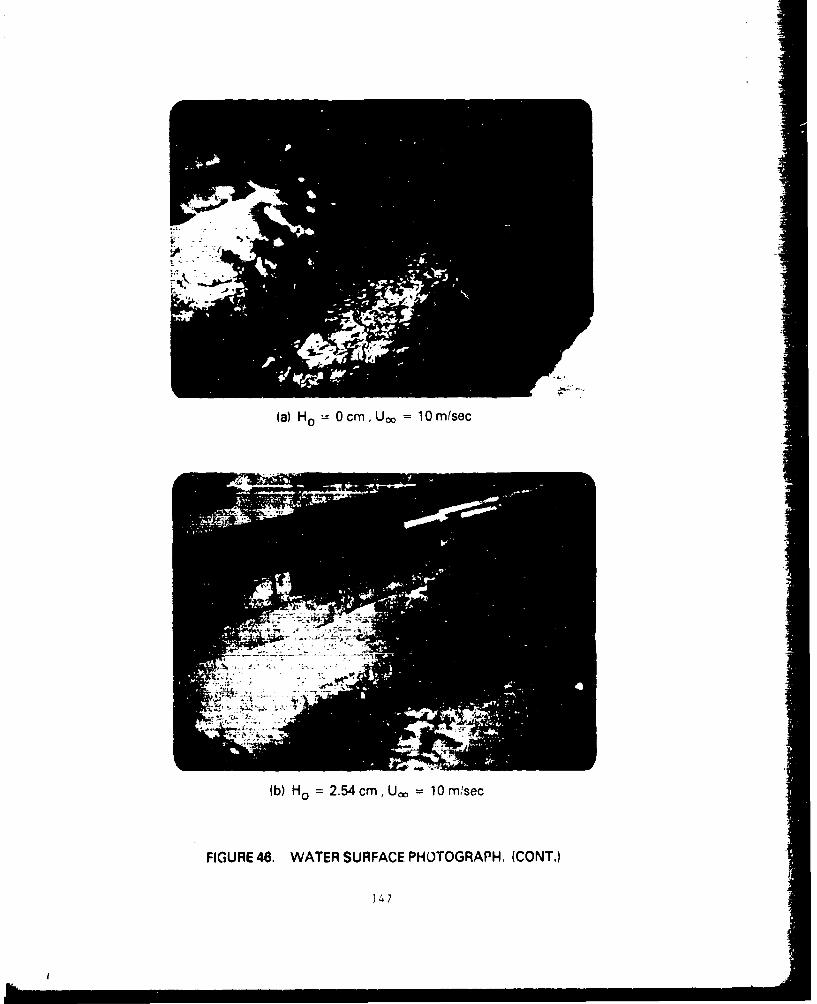
(a) Ho 0 Ocm.U, U 1 ml~sec

(b) H0 2.54cm Uo 1 mlinsec

FIGURE 46. WATER SURFACE PHOTOGRAPH, (CONT.)

1.4 7

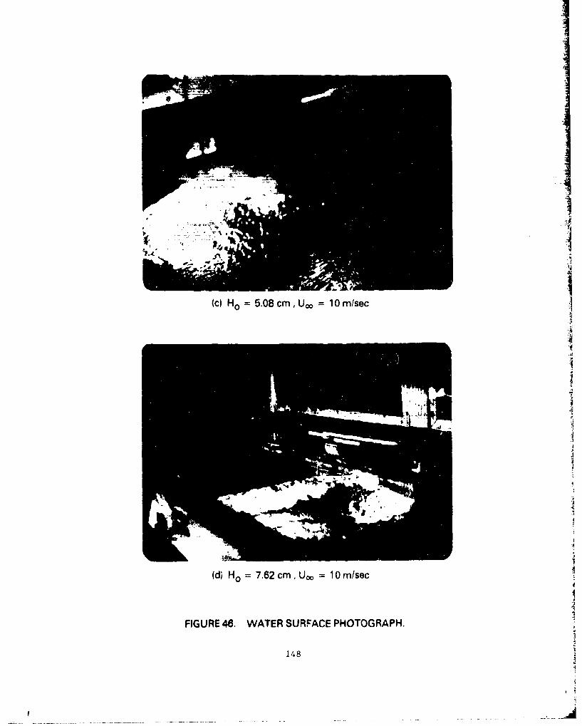
A(c) Ho = 5.08 cm, U = 10 mlsec

(d) Ho = 7.62 cm,eU, lOm/sec

FIGURE 46. WATER SURFACE PHOTOGRAPH.

148

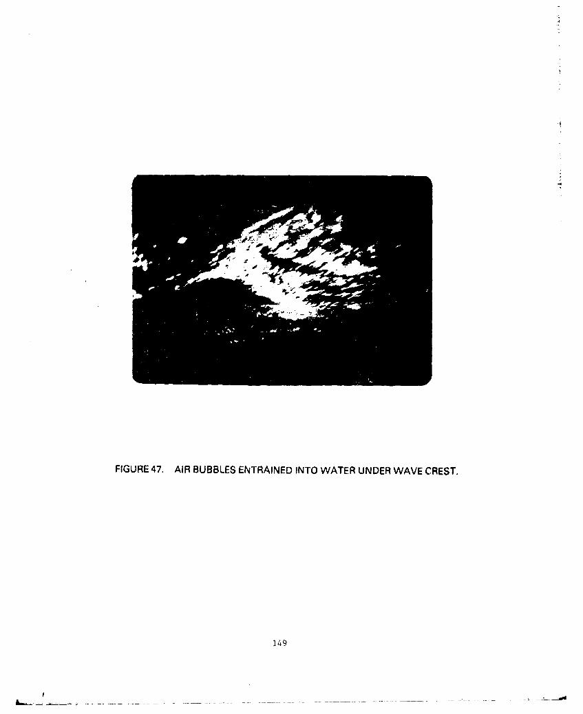
OvJ

FIGURE 47. AIR BUBBLES ENTRAINED INTO WATER UNDER WAVE CREST.

149

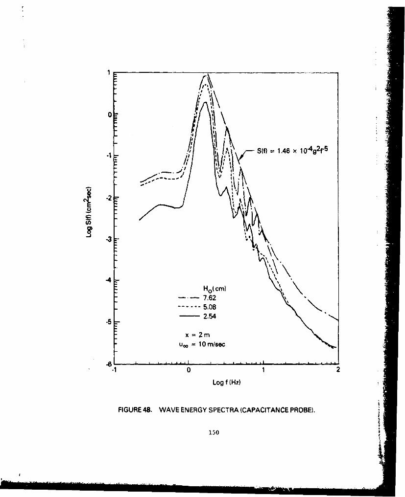
0C1 1

-1 / INSf 1.6xlgt

-3

-4Ho(cm)7.62

-5.08-- 2.54

x 2mU, =10 m/sec

-6 1 .A A I IIlI-1 0 1 2

Log f (Hz)

FIGURE 48. WAVE ENERGY SPECTRA (CAPACITANCE PROBE).

150

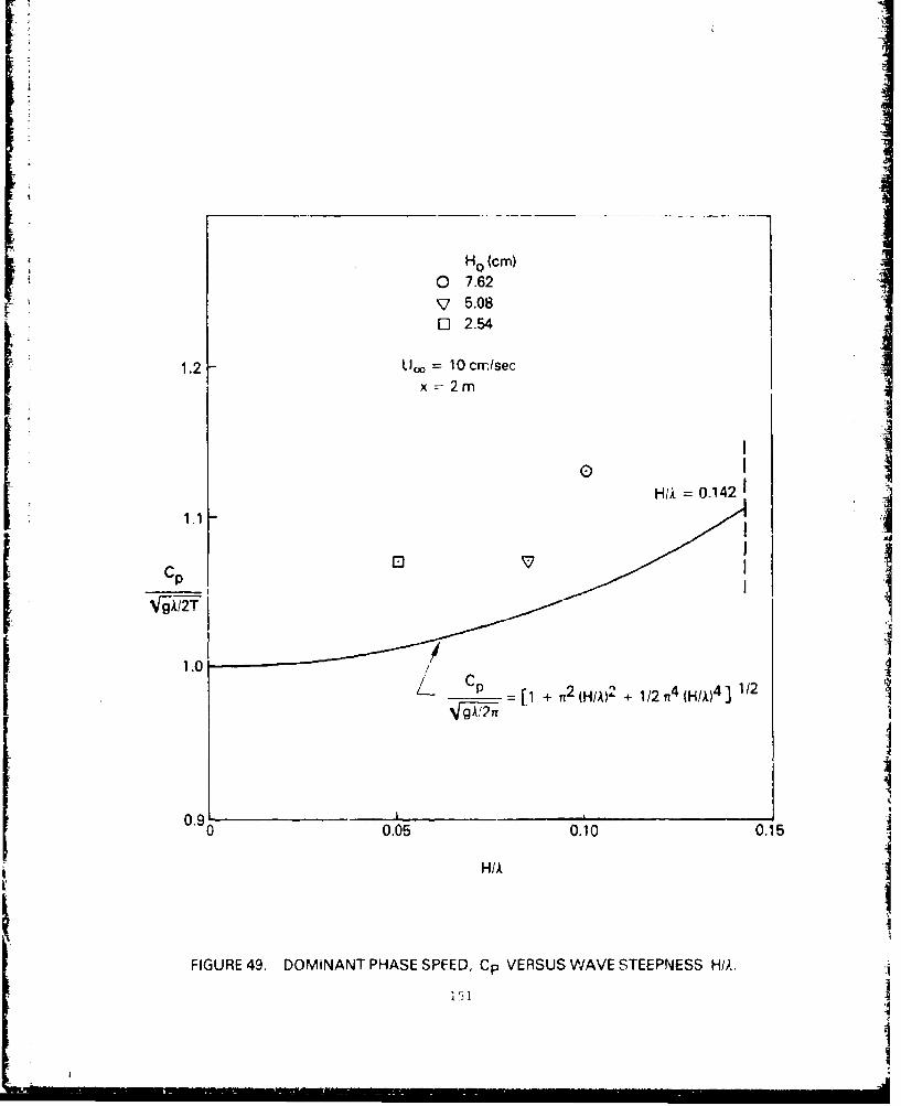
Ho (cm)o 7.62S, 5.08o 2.54

1.2 Ll,, 10 cm/secx 2- 2m

I *o I

NHl 0.142

[cp 0)•I

II

1_ = [1 + n2 (H/A) 2 + 1/2 n4 (H/A)4 ] 1/2N/"g -0'n

0.9' __,1-

0 0.05 0.10 0.15

IIFIGURE 49. DOMINANT PHASE SPEED, Cp VERSUS WAVE STEEPNESS H/A,

|i 151

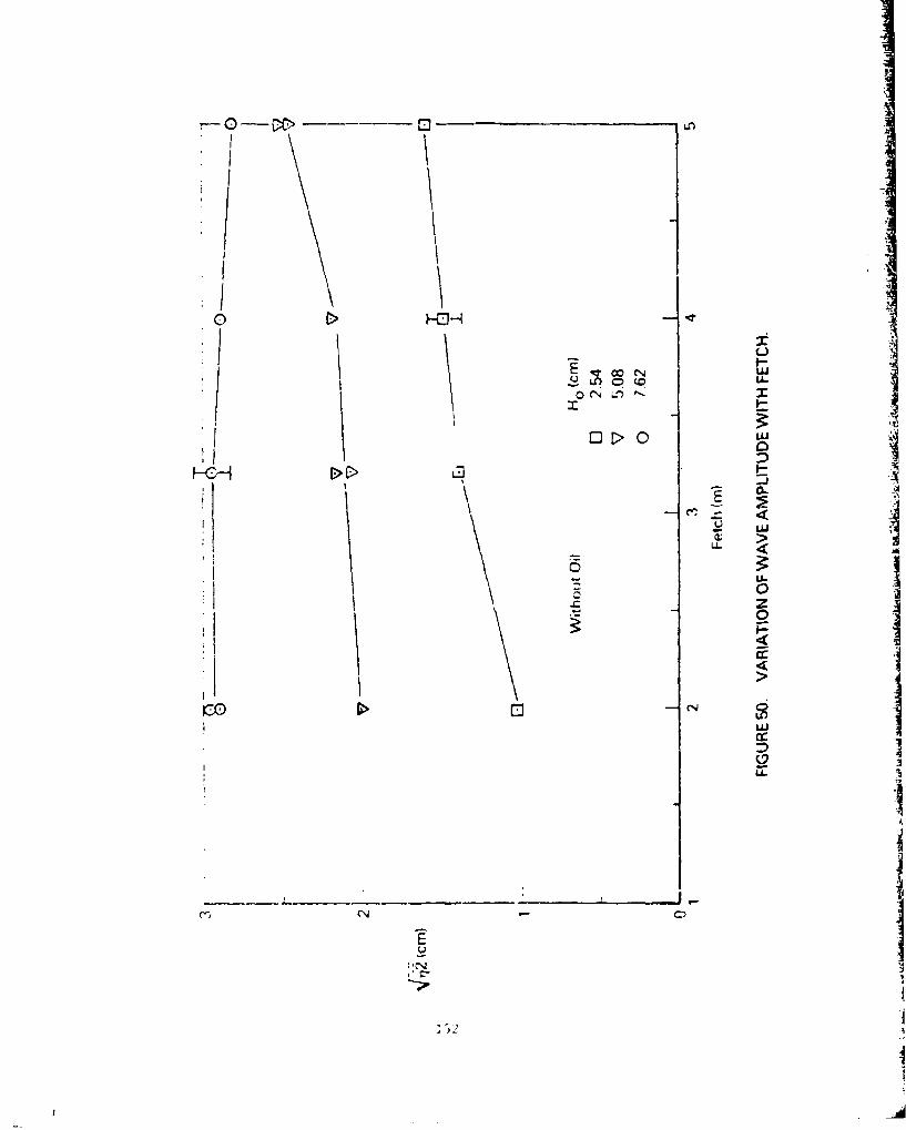
00

I Ij-

OV~'0I-0-

cc

V uiccI

CNI

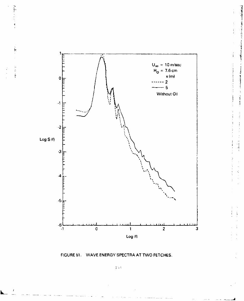
S 4 a

.Uco 10 mtsecHo = 7.6 cm

' ; x (M)

-25

Without Oil

.5 5

-2

Log S (f)

-3 '.N

-6

-1 0 1 2 3

Log (if)

FIGURE 51. WAVE ENERGY SPECTRA AT TWO FETCHES,

J ")

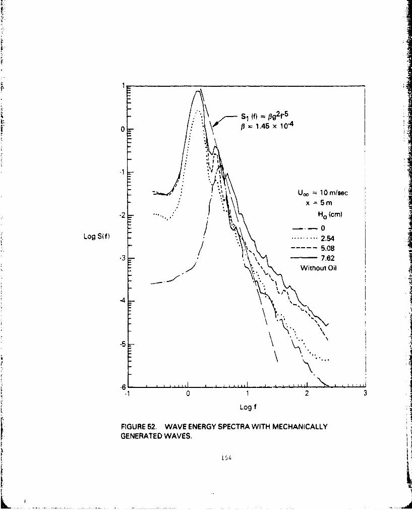
mI

\\f S1 (fl =Pg2f-5

0 p 1.45 x 10.40I

-1 _- "." : .

/ ;i,.,,U". 10 m/secI. I( .' x=5m

-2 H 0 (cm)

Log S(f) • .... 2.54

/ ." - 5.08-3 7.62

SWithout Oil

- ... \\

-4 \. \'...-4%

S-6 1-ii @ J

-1 0 1 2 3

Log f

FIGURE 52. WAVE ENERGY SPECTRA WITH MECHANICALLY

GENERATED WAVES.

154

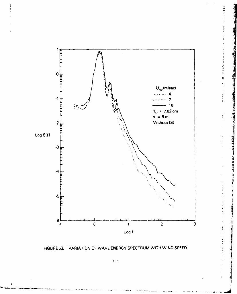
1.

0

U ,oU(mlsec)

*4

j -7/ 10

HO =7.62 cm

-2 -Without Oil

Log S(f)

-3

-4

- .1 1 L

.10 1 2 3

Log f

FIGURE 53. VARIATION OF WAVE ENERGY SPECTRUM WITH WIND SPFED.

155) - :

- : "•1

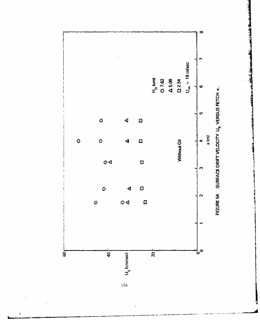
r.r.

LU~

0 u IILIcrI

Lu

CNN

i56

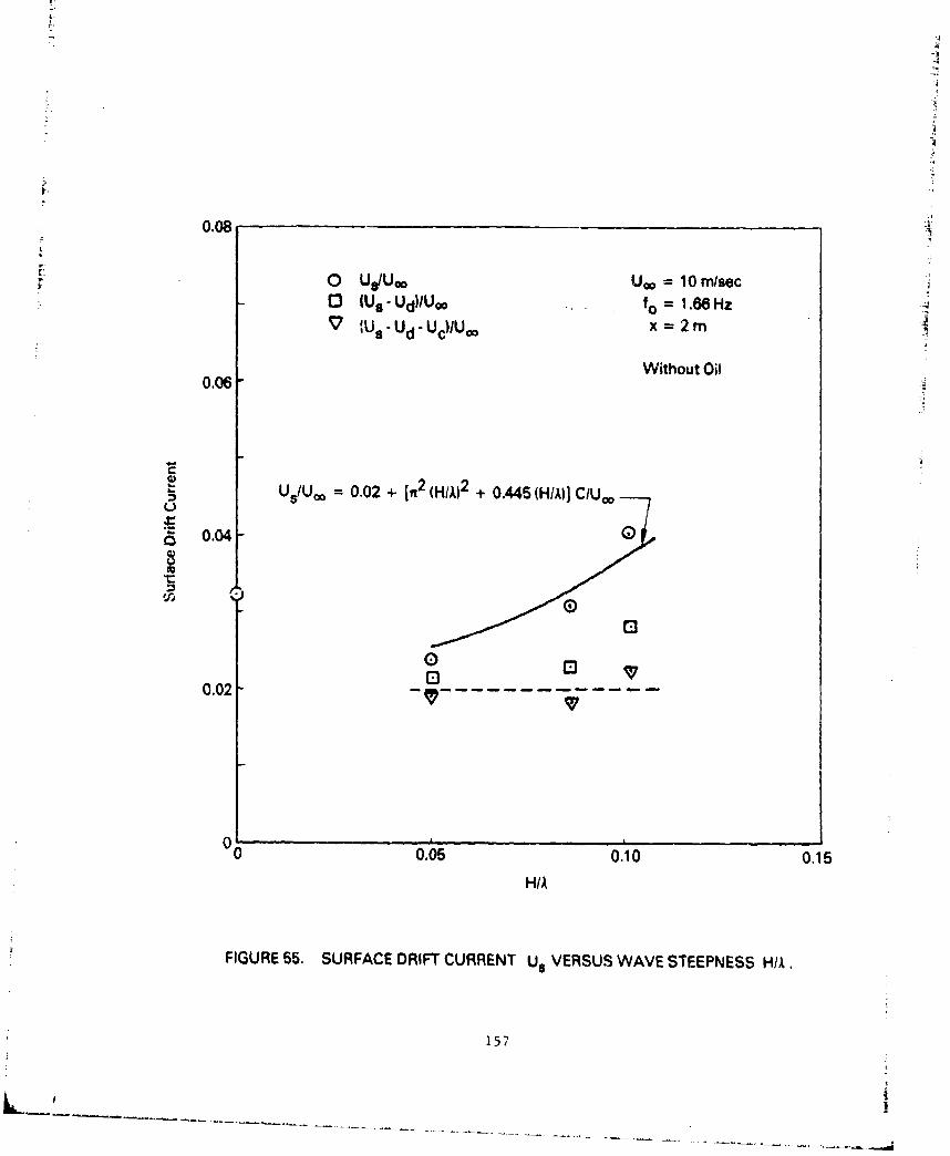
0.08

0 U/Uo UOO = 10 m/sec

0 (Us" Ud)/UoD fo 1.88 Hz 44"" Us.Ud. Uc)/U x 2 m

Without Oil0.06

Us/U,, 0.02 + [2 (Hik)2 + 0.445 (H/M)I C/Uo

0.04-

0-02-

00

0.05 0.10 0.15

H/A

FIGURE 55. SURFACE DRIFT CURRENT U8 VERSUS WAVE STEEPNESS H/k.

157

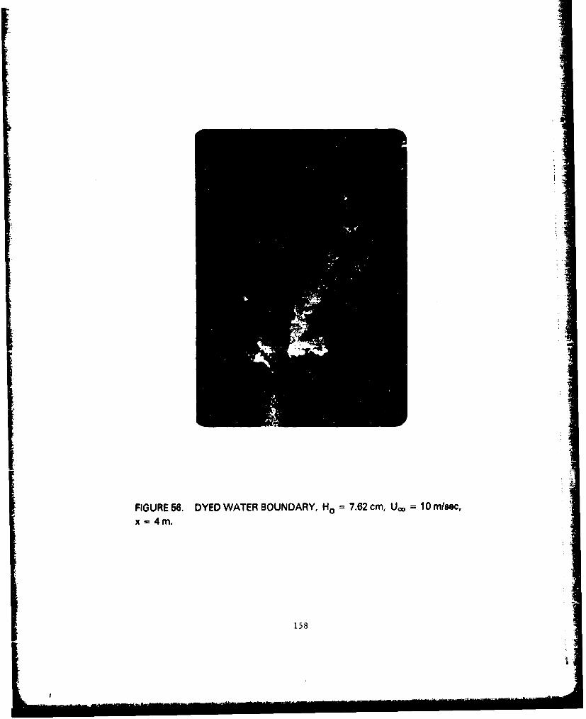
A

FIGURE 58. DYED WATER BOUNDARY, Ho 7.62 cm, U., = 0mr/secx 4m.

158

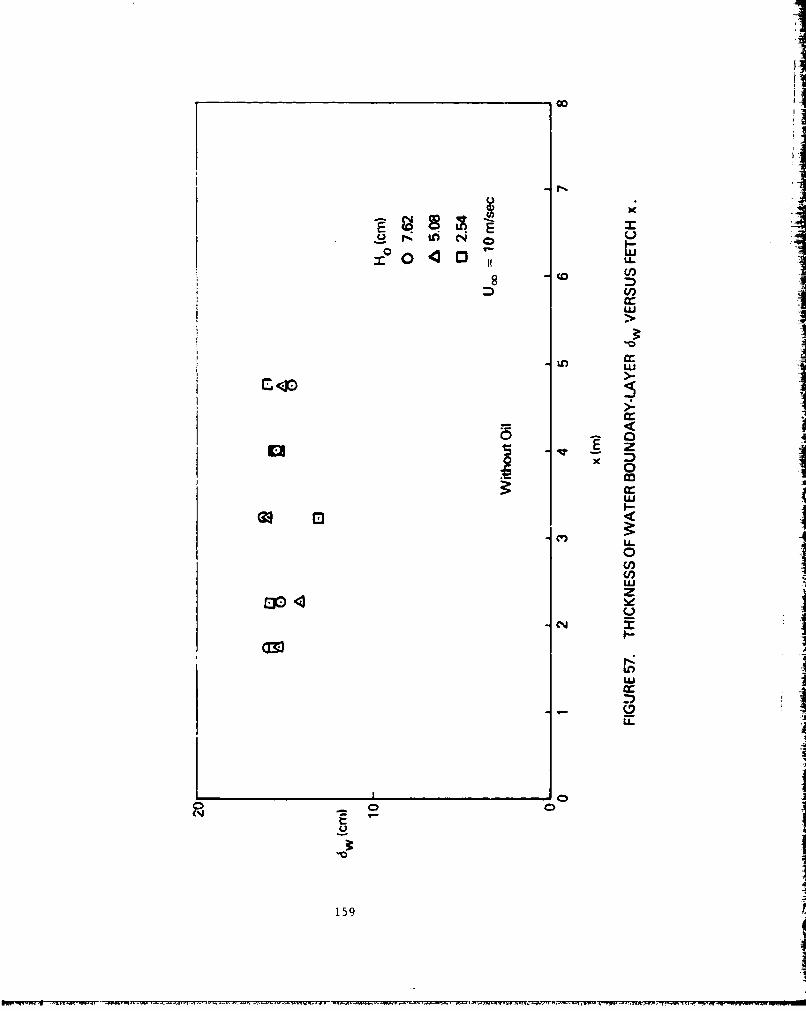
GoI

-E1_ _ _ _ _ _ _ _ _ _ _ _ _ _ _ _ __0

8 D0-~

LU I>A

0-

cioLU

0

LlUzCC.,

LU

159I

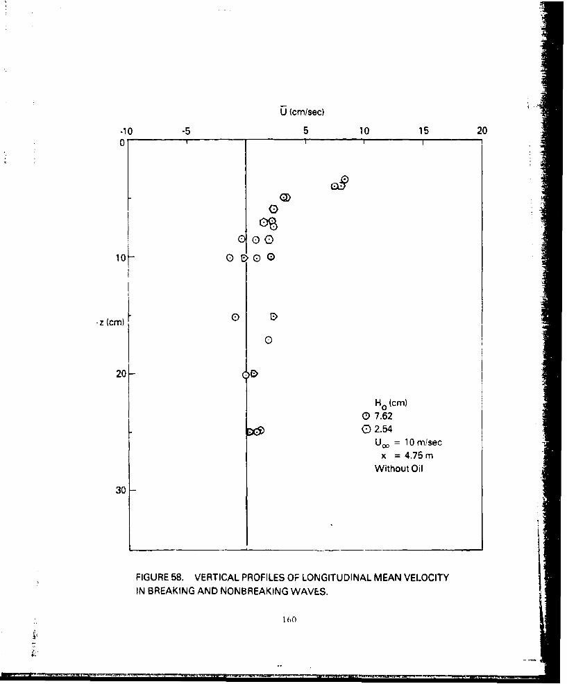
U fcm/sec)

-10 -5 5 10 15 200I I I

00

ilO- OE•OO

-z (cm) 0

0

20- D

Ho (cm)0 7.62

I. DO 02.54Uca= 10m/sec

x =4.75 mWithout Oil

30-

FIGURE 58. VERTICAL PROFILES OF LONGITUDINAL MEAN VELOCITYIN BREAKING AND NONBREAKING WAVES.

160

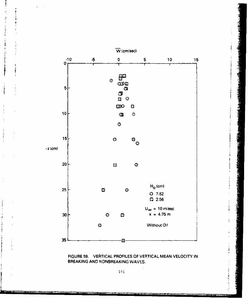
W (cmlsec)

-10 -5 0 5 10 15o I0Q

OEM-

5-

000) 0 "

103 El10- (D.

15- 0 13

- z (cm)

20 0D

25-Ho (cm)

0 7.62032.56

Uo = 10 mrsec30 0 Ell x = 4.75 m

0 Without Oil

35 1

FIGURE 59. VERTICAL PROFILES OF VERTICAL MEAN VELOCITY INBREAKING AND NONBREAKING WAVES,

• -l . I l I -I - ...Ii-

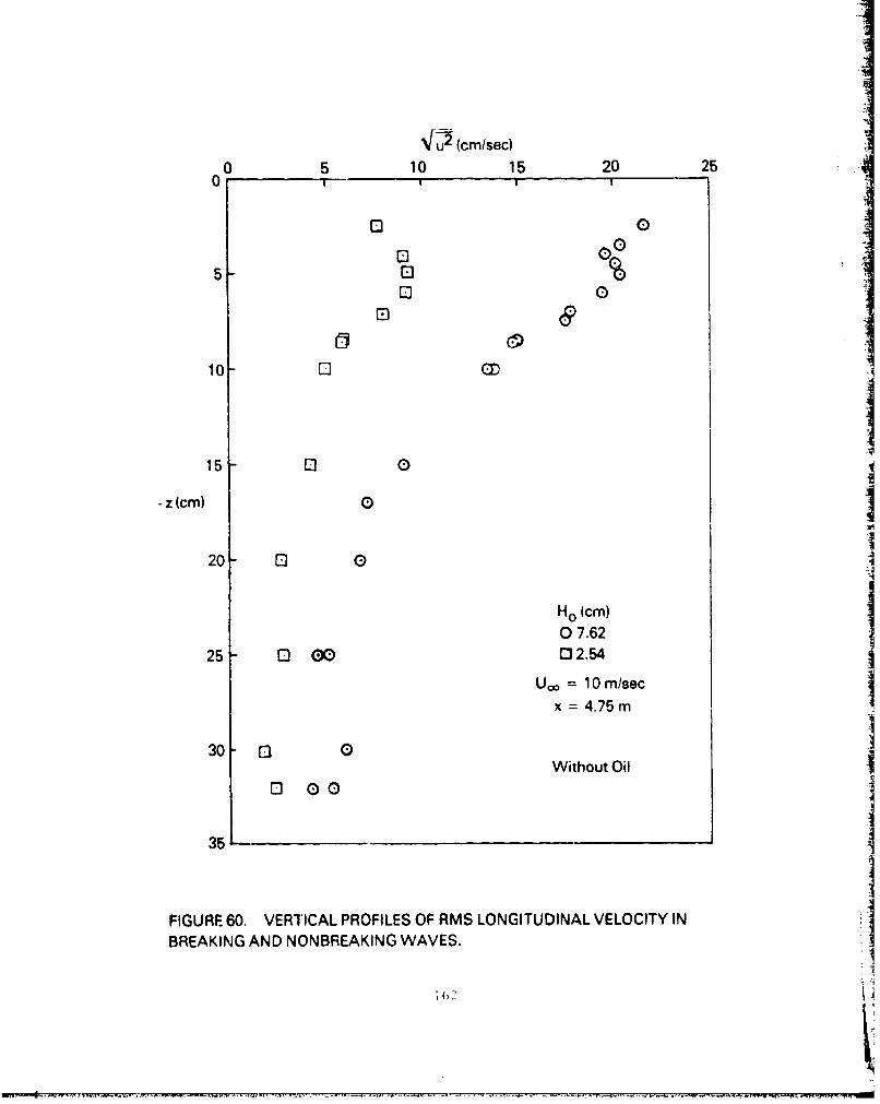
-u (cm/sec)

0 5 10 15 20 250 - ,,-- -

o 0

o05- 9

on 0

o &

10 00 I

15 0 0

z (cm) 0

20 03 0

Ho icm)07.62

25 0 0 00 02.54

Uo = 10 m/sec

x = 4.75 m

30 0 0Without Oil

0 00

35-

FIGURE 60. VERTICAL PROFILES OF RMS LONGITUDINAL VELOCITY INBREAKING AND NONBREAKING WAVES.

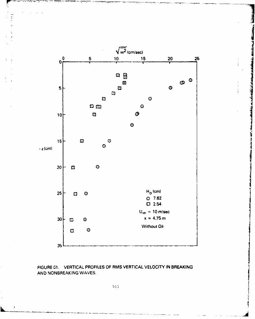
,*1iI

ýý•(cm/sec)

0 5 10 15 20 260 1 I

ID ID5 E0 0

0E 0

10

15- in 0

-z (cm) 0

20 - 013

I25 - I[ 0 Ho (cm)

O 7.620 2.54

U,,= 10 mlsec

30 - 0 x =4.75m IWithout Oil

351I

FIGURE G1. VERTICAL PROFILES OF RMS VERTICAL VELOCITY IN BREAKINGAND NONBREAKING WAVES.

I

I

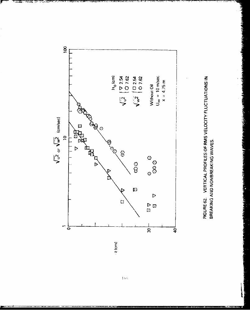
-5 - ,~

0Z8 x

I 0

iC)

I-

UU

0 leEr <

U 0

p0

UZ

IL

- LLL..~CC

0 0D

Uc

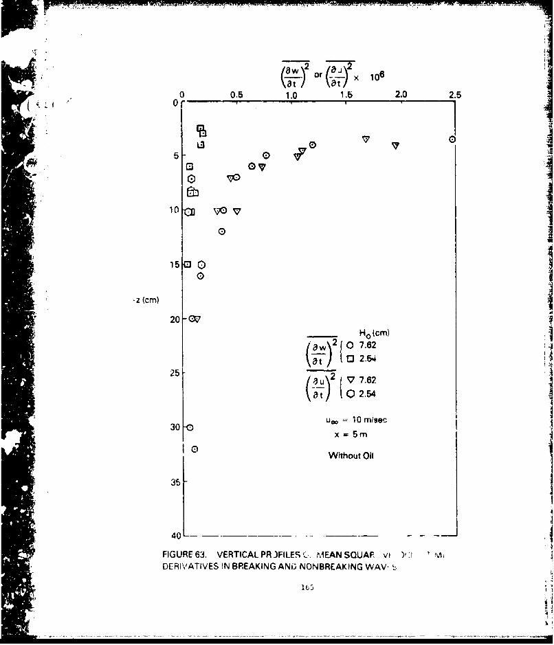
8w or x 106

0 0.5 1.0 1.5 2.0 2.5

0~

15 I

0

*Z fcm) 0I

* ~20 -CV7H0 lcm)

a w2

0 7.6

a 2t [3• 2.5

25 3u 2{ V 7.62

0at/ n2.54

u "o =10 Miserc

1 C) WIthout Oil .

35-

FI4Ro 6 -- .__-

FIGURE 63. VERTICAL PR.)FILES, MEAN SQUAFP vt )f- i ADERIVATIVES IN BREAKING ANW NONBREAKING WAV. t,

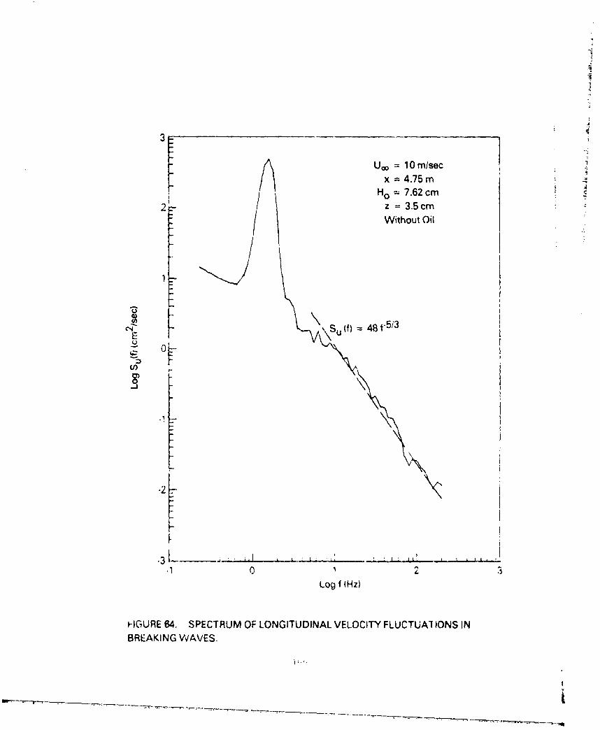
3I

LIM = 10 m/sec

x = 4.75mH = 7.62 cm

2 / z = 3.5 cmWithout Oil

1

C \u f 48 f-5i

".3'-

-2

.1 0 1 2

Log f( Hz)

HGURE 64. SPECTRUM OF LONGITUDINAL VELOCITY FLUCTUAI IONS IN

BREAKING WAVES.

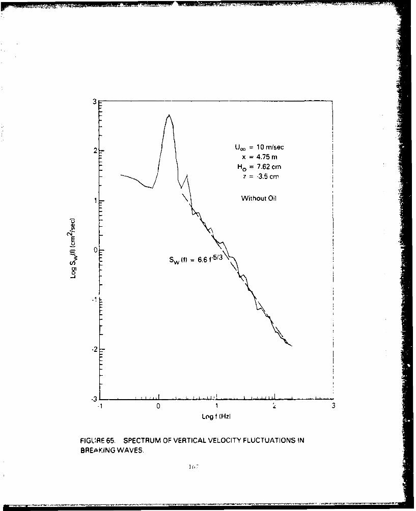
3

2 .U0 = 10 m/secx = 4.75 m

Ho = 7.62 cmz = -3.5cmrr.

1 •Without Oil

E0-

Sw (f) = 6.6 f

co

.2•

0 1 3

Log f (Hz)

FIGURE 65. SPECTRUM OF VERTICAL VELOCITY FLUCTUATIONS IN

BREAKING WAVES,I(:7

- -r.rr-r- -r-r, -- rw -- ---- rrcr~rr -tzrr~ .-

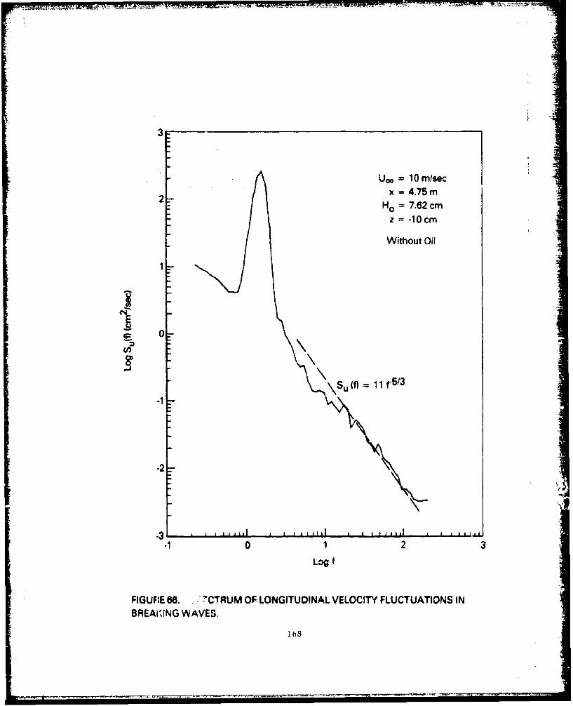
3

00= l0 m/secx = 4.75m

Ho = 7.62 cm

z = -10cm

Without Oil

-- 0

' I,

\Su ()0 11 f-5/3

-1

".2

0 2 3

Log f

FIGURE 88. "CTRUM OF LONGITUDINAL VELOCITY FLUCTUATIONS INBREAi'ING WAVES.

- --I-I I I I I Ir I- I

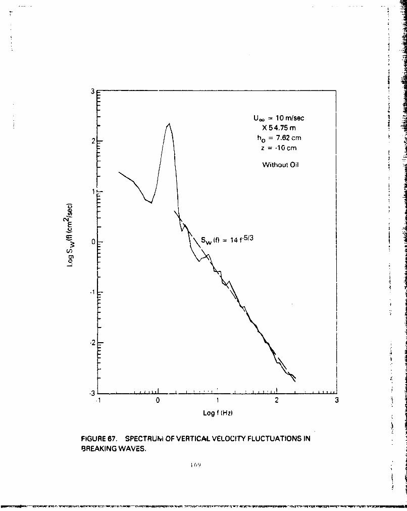
3 iU= 10 m/sec

X 54.75 mh = 7.62 cmz = -l0cm

Without Oil

CL4

E

S0 -- •\Sw (f) = 14 f-5/3

0n

-2--3

- 0 2 3Log f (Hz)

FIGURE 67. SPECTRUM OF VERTICAL VELOCITY FLUCTUATIONS INBREAKING WAVES.

I 69

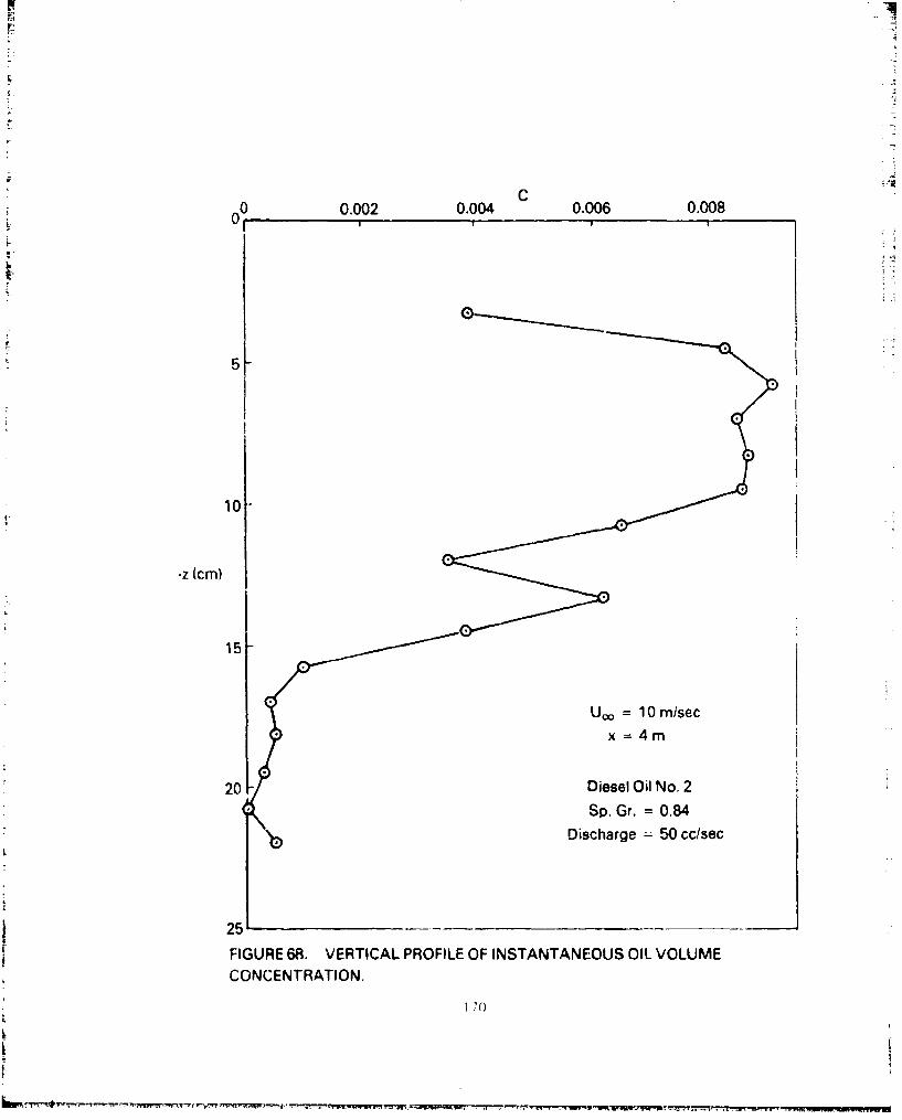
C0 0.002 0.004 0.006 0.00801'

10

-z (cm)

15-

U -10 m/secx=4m

20 Diesel Oil No. 2

Sp. Gr. = 0.84

Discharge = 50 cc/sec

25.

FIGURE 68. VERTICAL PROFILE OF INSTANTANEOUS OIL VOLUME

CONCENTRATION.

]710

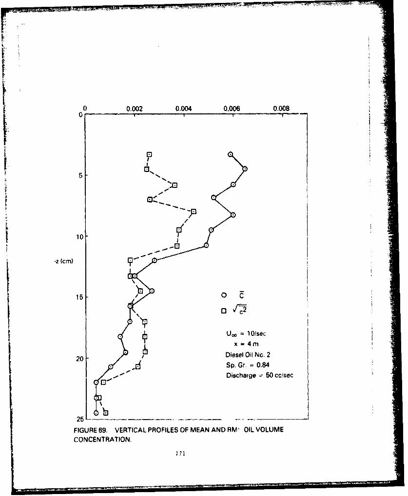
0 0.002 0.004 0.006 0.008

V0

5

10

-z (cm)

rI115 0\~ ~ ~

20 ":=220 ~Diesel Oil No.2

Sp. Gr. = 0.84

Discharge L 50 cc!sec

25 --- - .- - - _ _

FIGURE 69. VERTICAL PROFILES OF MEAN AND RM' OIL VOLUMECONCENTRATION,

171

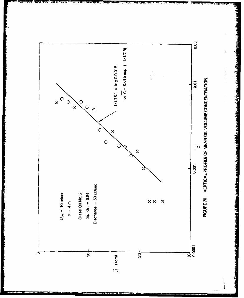
000

a; 0

N>

0 00

Iu j2-0

0

0 LU

E z 0 00 00

D

-J

I-

0l

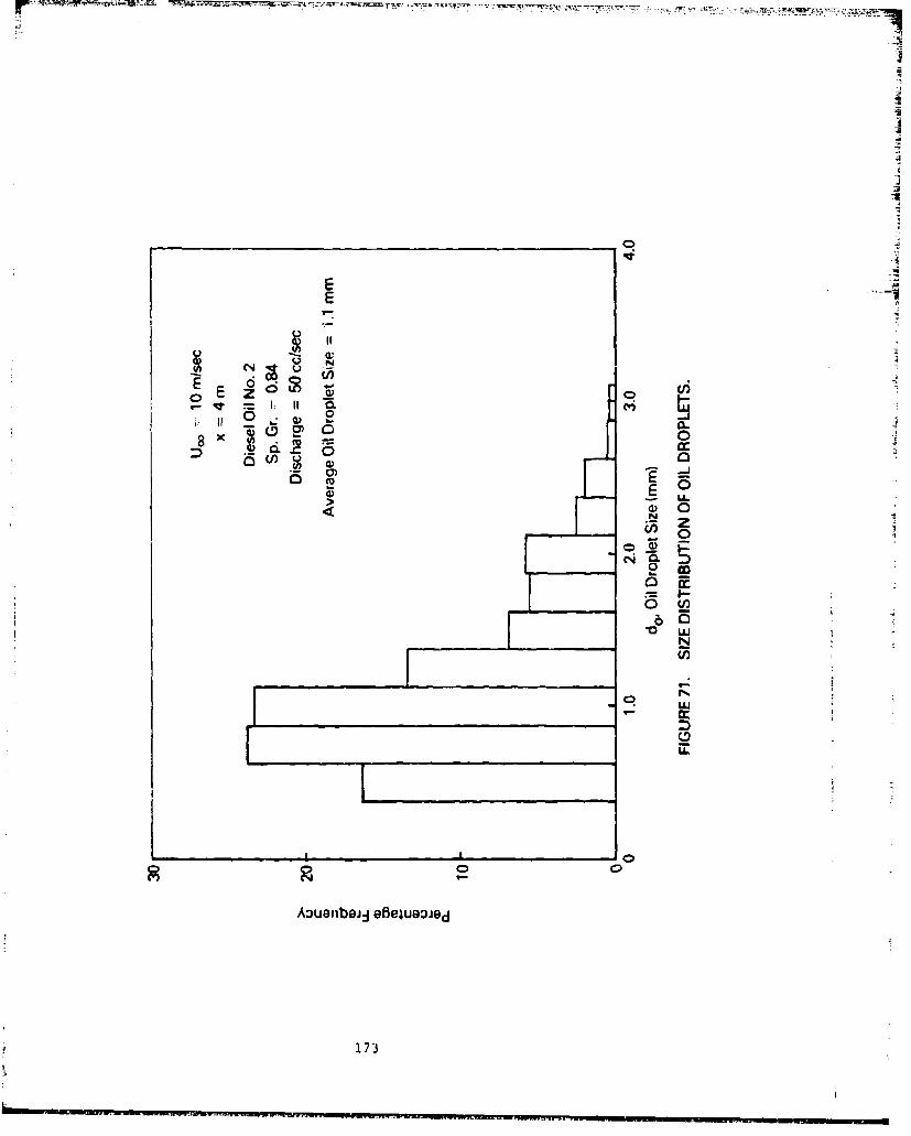
V7I

E z (n

0I

cz C

__ _ _ _ _ _ _ _ _ __ _ _ _ _ _ _ _ _ =0

U N0

Ez0 0 -J

00 (n

0)J

05

AouaibeiAOBBI90JN

173-

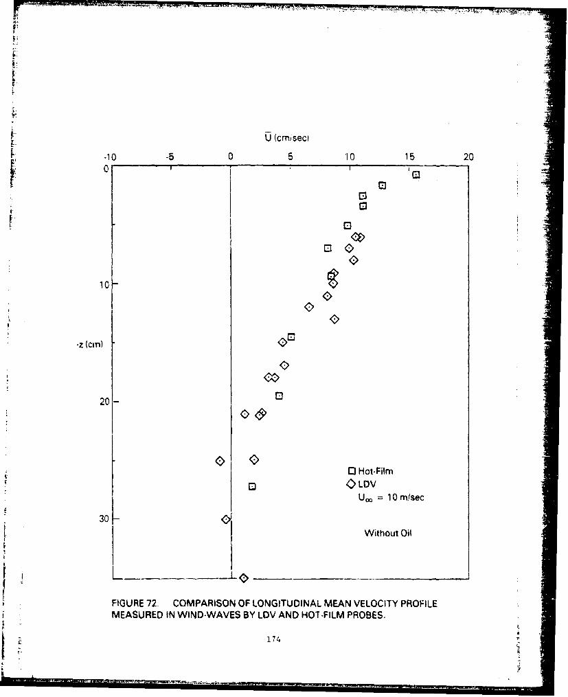
-- - v

U (cmisec

-10 -5 0 5 10 15 20

00

J0

rn00

0%:

10[

-z (on ) < > "

20- E

0 Hot-Film

0 • LDV

U,, = 10 m/sec

30 )Without Oil

FIGURE 72. COMPARISON OF LONGITUDINAL MEAN VELOCITY PROFILE

MEASURED IN WIND-WAVES BY LDV AND HOT-FILM PROBES.

F. 174

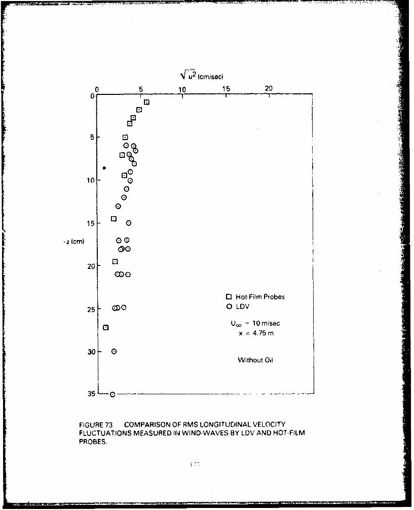
S(cmisec)

010 15 20

5 - n a)0

10 r-

00

15 - 0

-z (cm)

00

O0 -

C2DO

0 Hot-Film Probes

25 ¢ 0 LDV

SUo = 10 m/secx = 4.75m

30- 0Without Oil

35L0

FIGURE 73. COMPARISON OF RMS LONGITUDINAL VELOCITYFLUCTUATIONS MEASURED IN WIND-WAVES BY LDV AND HOT-FILMPROBES.

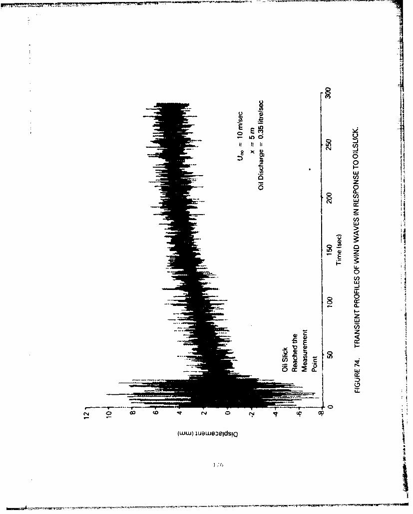
- ~~~~ ~ L -- -- _ - - - i

0 CN

00

z

cc,z4

>>

LL.

w

0r-J

C-

z

z

0A

U.

(Ww) juawooegdsio

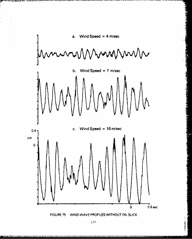
a. Wind Speed =4 m/sec

b. Wind Speed = 7 m/sec

0.41 c. Wind Speed =10 mlsec

cm

0

0 0.5 sec

FIGURE 75 WIND-WAVE PROFILES WITHOUT OIL SLICK.

177

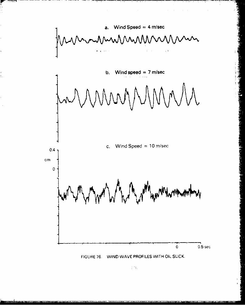
a. Wind Speed =4 rn/sec

b. Wind speed =7 rn/sec

0.4 -c. Wind Speed = 10mlsec.

cm

0 0.5 sec

FIGURE 76. WIND-WAVE PROFILES WITH OIL SLICK.

LLIPLIzI

CLn

II

zz

0.0

0 0

0;

~. IC

179 I

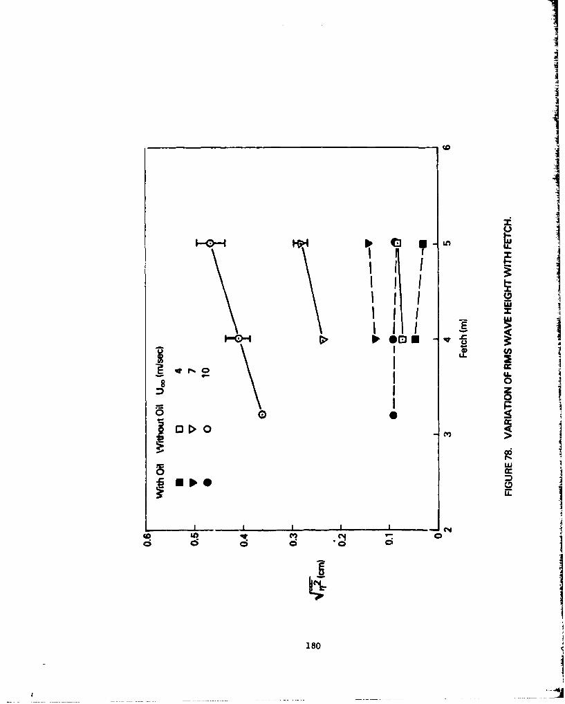
LnI

LLI0I

1801

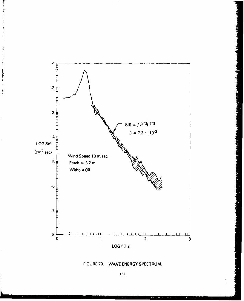
-2

-3

S(f) = fy2i3f-7/3

S=7.2 x 10-3

LOG S(f) -

(cm2 sec)

Wind Speed 10 m/sec.5 Fetch = 3.2 m

Without Oil

-6

-7

-8 '1 I j ilj . I ~ I 1111 I I I .1 1i m

0 1 2 3

LOG f (Hz)

FIGURE 79. WAVE ENERGY SPECTRUM.

181

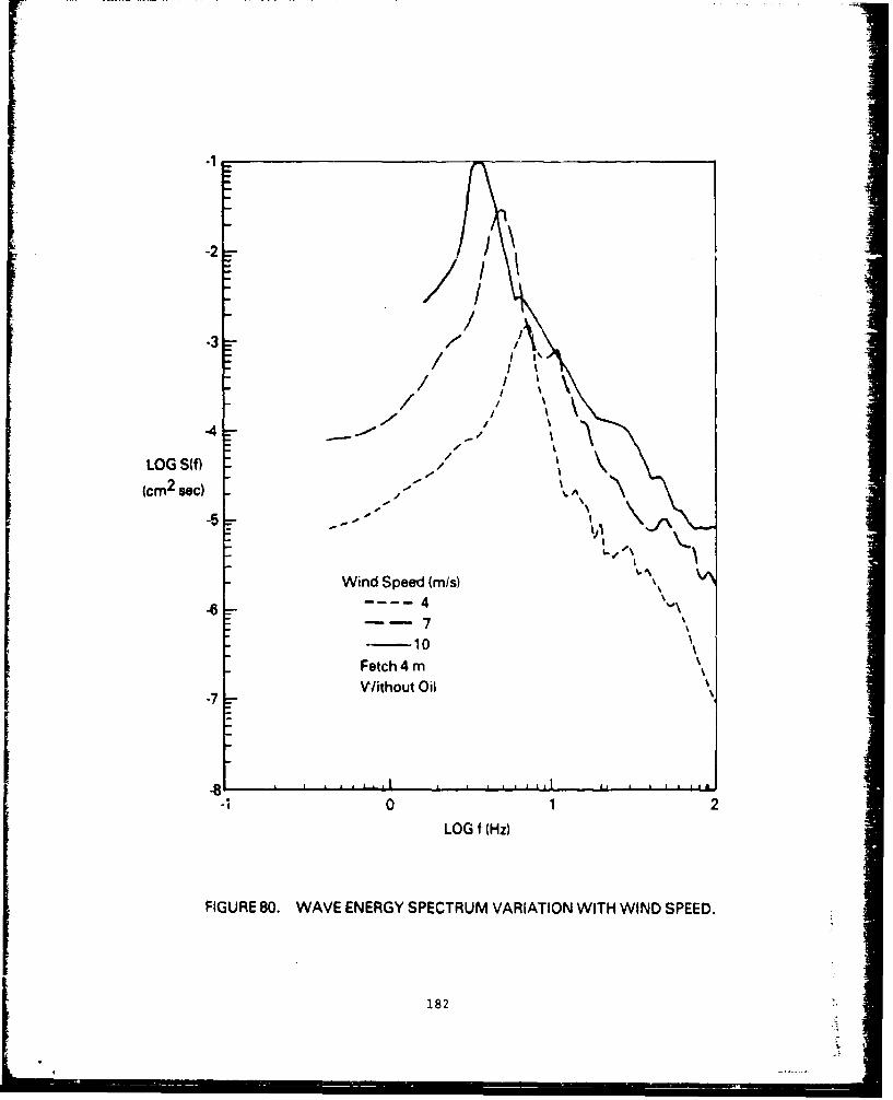
-1

-2

-3/ I

/ \/3 7/

//-4 ~'"*

LOG S(f) -

(cm 2 mec) .,

IA

Wind Speed (m/s)

-6 4-7

-10

Fetch 4 m

II

7 Without Oil

-8 ,, I. , . . u. . . .II 1 . I 1,1, 1 6 3

-I 0 1 2LOG f (Hz)

FIGURE 80. WAVE ENERGY SPECTRUM VARIATION WITH WIND SPEED.

182

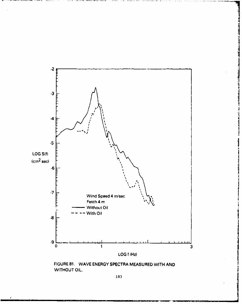
II

I iI

-2

II

-3

II- I

-5 "'I

LOG S(f) i(cm2 sec) '

-6- 1

-7 'Wind Speed 4 m/sec A \

Fetch4m 4 m

-- Without Oil-... With Oil

-89

0 1 3

LOG f (Hz)

FIGURE 81. WAVE ENERGY SPECTRA MEASURED WITH ANDWITHOUT OIL.

183

N • i • g III

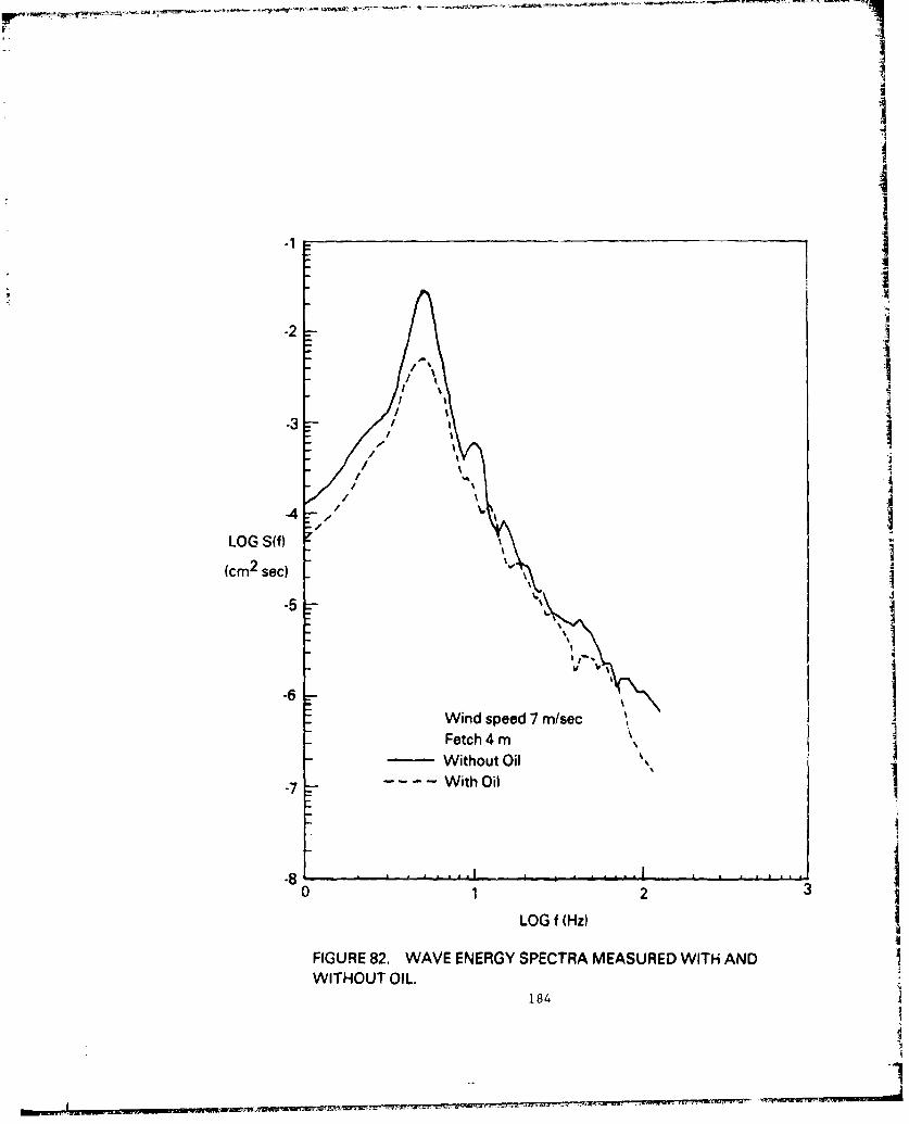
I

I

-2 _

(CM2 sec)

-5

I

-6Wind speed 7 m/seeSFetch 4 m \

•- -- Without Oil

-7 -- - -- - W i t h O i l

0 12 3

LOG f (Hz)

FIGURE 82. WAVE ENERGY SPECTRA MEASURED WITH ANDWITHOUT OIL.

184

A

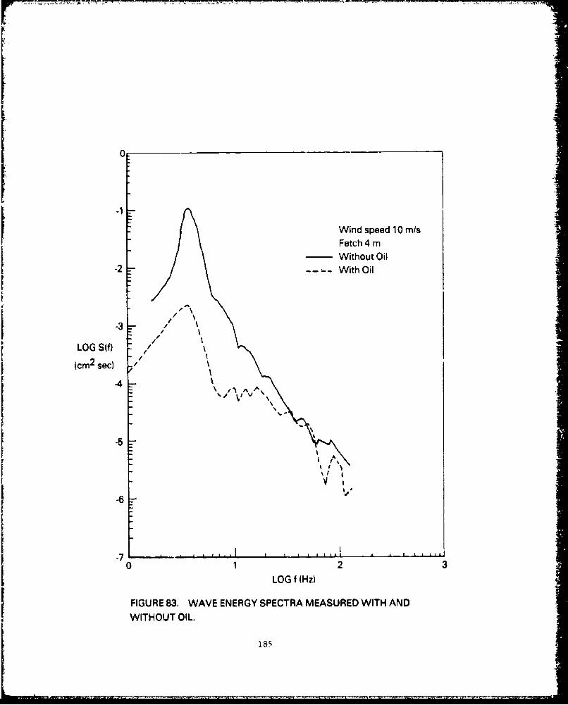
Z "-1

Wind speed 10 ml/sFetch4m

Without Oil-2 With Oil

-3-/!'

-3 - Ii

IJ(cm2 sec)

LOG /I AV AI\

-5

\I-6

-7, .. . I , •u , .I . . . .

LOG f (Hz)

FIGURE 83. WAVE ENERGY SPECTRA MEASURED WITH AND

WITHOUT OIL.

185

a. H. =2.54cm

1b. Ho = 5.08cm

// /

/T

c. Ho = 7.62 cm

Without OilTime

FIGURE 84. PROFILES OF MECHANICALLY GENERATED WAVES WITHWIND, VEHTICAL SCALE = 2 cm/DIV, HORIZONTAL SCALE = 0.5 sec/div.

i86

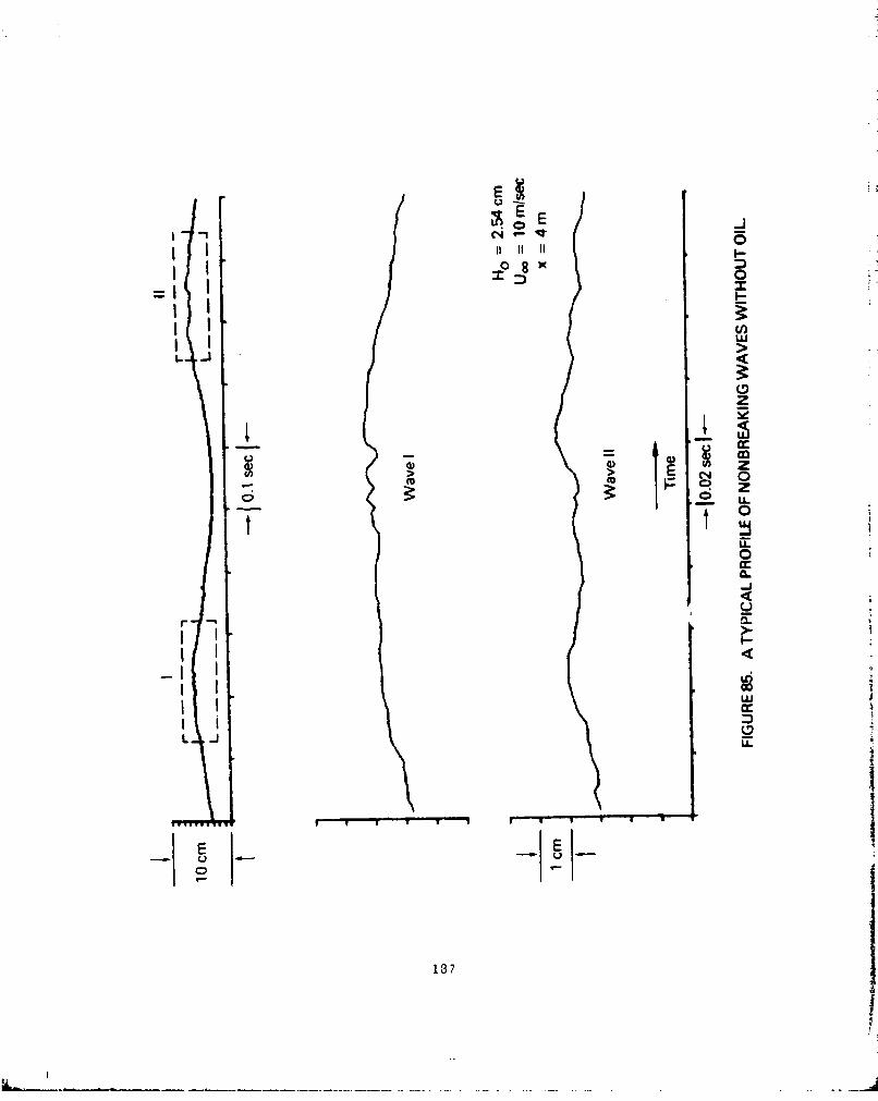
II U

II

LlaJ

IE

0 E

z

0)0oz

0

rI I

L J

I ~137

I mi

>~ -)

L. -'

I-

I-

oc£

0

U-

I~~ IF I I

-L)

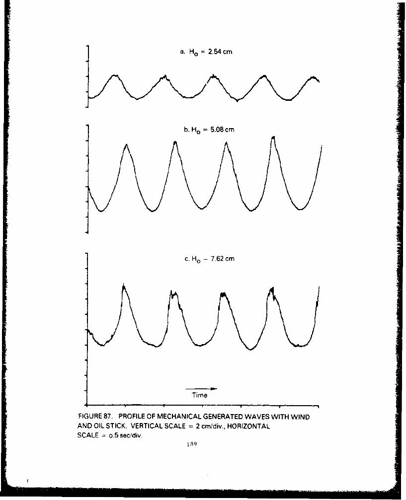
a. Ho =2.54cm

b. Ho = 5.08 cm

II

c. Ho= 7.62 cm

I Ii

Time

FIGURE 87. PROFILE OF MECHANICAL GENERATED WAVES WITH WINDAND OIL STICK. VERTICAL SCALE = 2 cm/div., HORIZONTALSCALE = o.5 sec/div.

*U

E 0ce -0-4

InZ u

8--- 0 >

0 IL0

C~z0 0N C 0

C-)N

IC4

190i

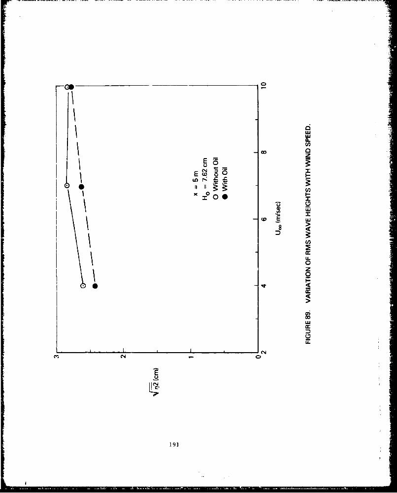
Go _ _ _ _ __ _ _ _ _ __ _ _ _ _

LU000

E =0 1wC.4

000zUm

U-

ev~ 0

191

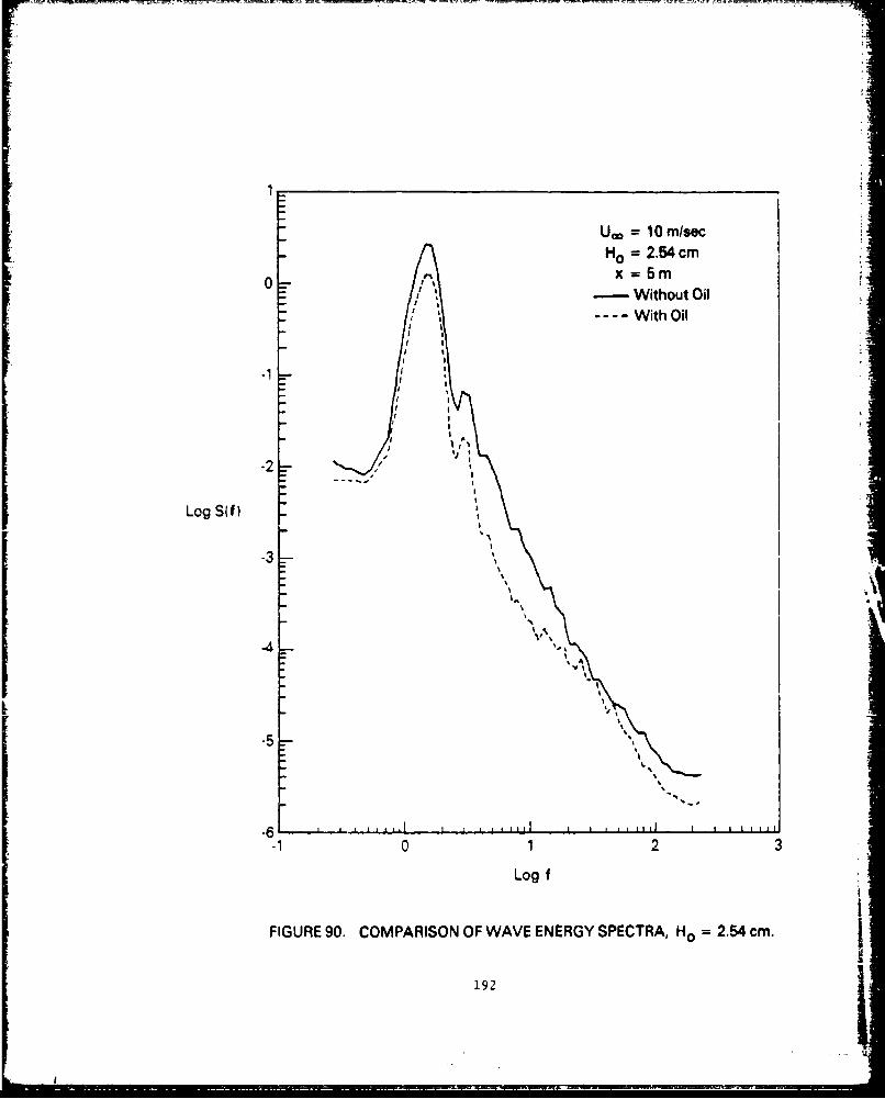
= 10 m/secH = 2.54 cm

x = 5 m/ - Without Oil

0- ---- With OilI S

Lo SSf

-1

II

-20

Log SLf)

I-

"I'

-10 1 2 3

Log f

FIGURE 90. COMPARISON OF WAVE ENERGY SPECTRA, Ho = 2.54 cm.

192

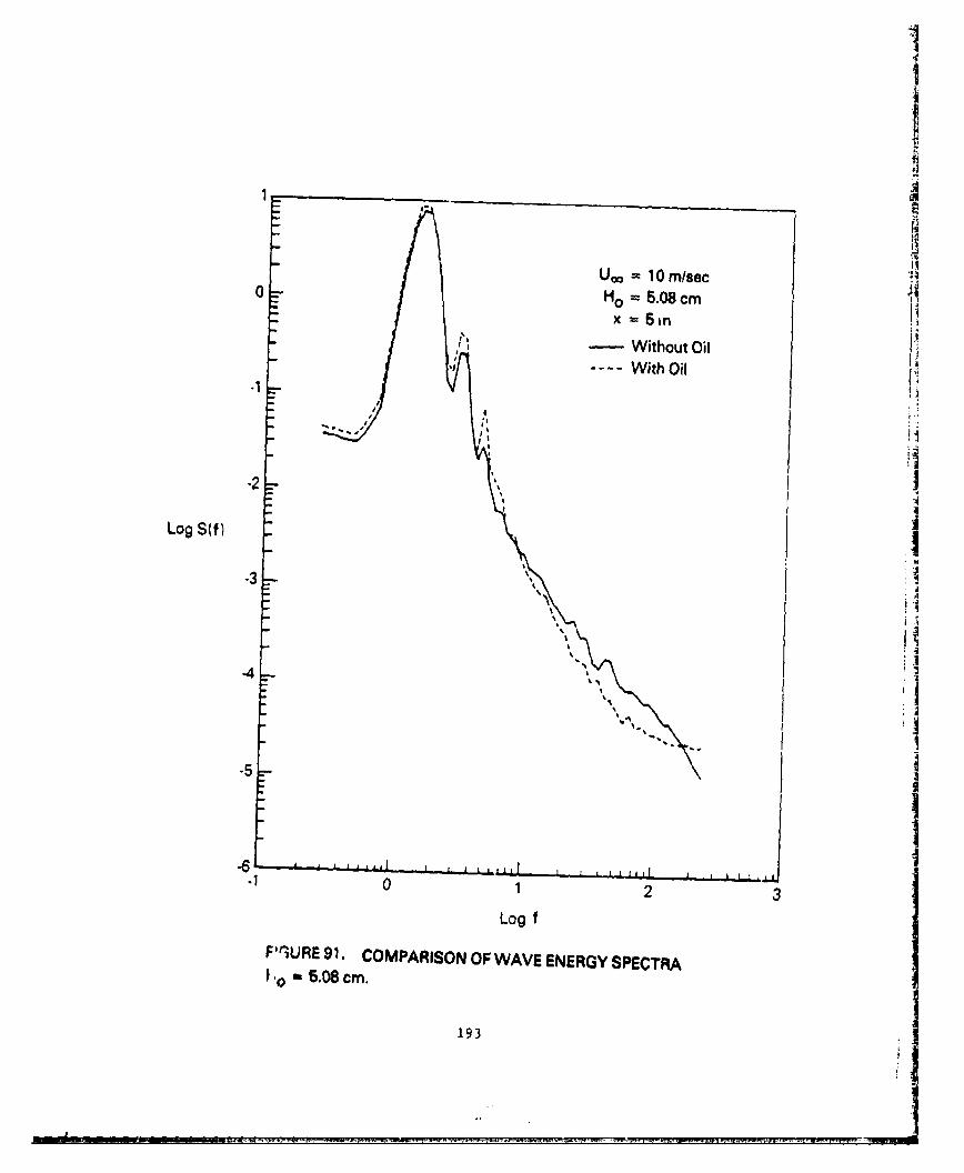
m- I !

Uoo = 10 m/sec" H° = 6.08cm I

"x x= in

Without Oil----- With Oil

Log S(f) .

- -

-4

S0 2 3

Log f

F'qURE 91. COMPARISON OF WAVE ENERGY SPECTRAt.o " 5.08 cm.

193

i

oI

_ .. !

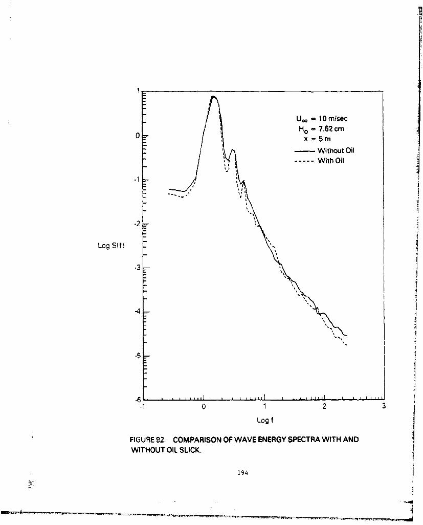
U00 = 10 m/secH0 = 7.62 cm

x=Sm

"-• Without Oil---- With Oil

.2IJN

-1 -,

Log S(f) -

-4

*5'

-2

i 2

LogLo Sf)

-49

' I ;

-1 0 1 2 3Log f j

FIGURE 92. COMPARISON OF WAVE ENERGY SPECTRA WITH AND

WITHOUT OIL SLICK.

194

UNITED STATES COAST GUMR - DTIC

Documents

Transcript of UNITED STATES COAST GUMR - DTIC