UNCLASSIFIED

AD NUMBER

AD886513

NEW LIMITATION CHANGE

TOApproved for public release, distributionunlimited

FROMDistribution authorized to U.S. Gov't.agencies only; Proprietary Information;JUL 1971. Other requests shall be referredto Weapon Systems Analysis Directorate[Army], Washington, DC.

AUTHORITY

USAEWS ltr, 3 Apr 1975

THIS PAGE IS UNCLASSIFIED

00 TECHNICAL I'ORT M-71-4

AN ANALYSIS OF GROUND MOBILITYMODELS (ANAMOB)

A. A. Rula, C. J. Nuttall, Jr. ~F F0D

CA-j T 4K 1AMI

JuyM7Sponoredby WaponSysems nalyis Drectrat

Office~~~~~~~~r of th AsistnieCifo tfU .Am4 4

N/

Conduted y U.Sposoe br y gne Wea ysEemnSaion Virc brgMat*p~/ c/6

Distribution limited to U. S. Government agencies only; proprietary information; Juns 1971. Oter requests

Unclassified,

ctDOCUMENT CONTROL DATA . R & D

(Security cl..lficetieo of title, body of .b. and inizing Annti must be entered whon t.overalI report Is clae.Wed)

I. OXIGI'dATING ACTIVITY (CopereN Au*W) S&e* REPORT SEC,.RITY CLASSIFICA TION

U. S. ArmyEngineer Waterways, Bper#iment Station I Unclassi'"iedVicksburg, Miss.I2" GROUP

S, REPORT TITLE

AN ANALYSIS OF GROUND M yILITE MODELS. (ANAMOB)

4. OESCRIPTIVZN NOTEK* S(1poeipatand InclulM dI a rtes)

Final reportS. AUTHOR(S) (Firt PsMe. nd dWe inilla, faet name)

Adam A. RulaClifford J. Nuttall, Jr.

S, REPORT DATE 7A. TOTAL NO. OF PAGES j7b. NO. Or

REFS

July 1971 321 144i40. CONTRACT ON GRANT NO. W..ORIGINATORS REPORT NUMI6KISI

Technical Report -71-4b. PROJECT NO.

C. Sb. OTHER REPORT NOte) (ARy oaer embW Met tMAy be elde11dhi "epen)

I0. DISTRIBUTION STATEMENT '

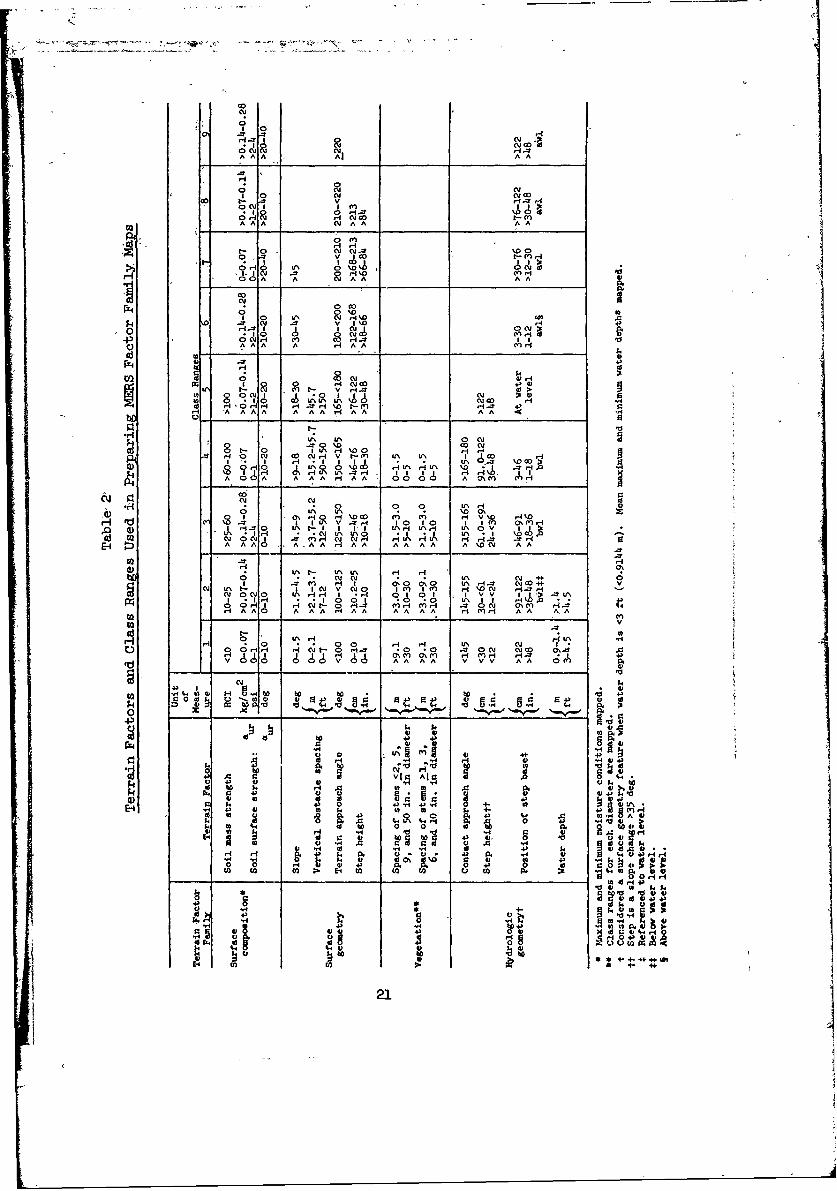
Distribution limited to U. S. Government agencies only; proprietary information; June 1971. Other requestsfor this document must be referred to U. S. Army Engineer Waterways Experiment Station (WESFS).

It- SUPPLEMENTARY NOTES 12. SPONSORING MILITARY ACTIVITY

Weapon Systems Analysis DirectorateOffice of the Assistant Vice Chief of Staff,U. S. Army

, _ __,_ ashington. D. C.IS. ASTRACTPractically every research effort and subsequent procurement of materiel for Army use is backed up with asystem effectiveness-cost effectiveness study. The development of good ground mobility models in support ofthese studies was of particular interest to the Office of the Assistant Vice Chief of Staff, U. S. Army, toassist in the construction of new models or in tle evaluation of existing models. As a first step, it washighly desirable to survey the existing models. With the need established, and with U. S. Army EngineerWaterways Experiment Station (WES) interest and technical capabilities in the field, a study aimed at theanalysis of existing ground mobility models was initiated by WES and WNRE, Inc., under contract to WES. The'objectives of the study were to analyze existing ground mobility models in order to: (a) determine theirgeneral level of usefulness and applicability to predicting cross-country-performance of ground vehicles inthe real world; (b) select the models that appear to be the more promising for this purpose and determine,their usefulness and applicability in more definitive terms; (c) point out iieas of the latter models inwhich additional researkh ee'i-" and (d) develop guidelines for future deirelopment of ground mobilitymodels. Various Army sources and unclassified literature were canvassed for cross-country performance modelsthat have been used or seriously proposed. Examination of these available sisnlations revealed a consider-able degree of fundamental commonality, despite initial differences in appearance. In light of the basicccmmonality, the available cross-country models were next-examined for the single-feature vehicle-terraininteraction models that they utilized. Those single-feature models found in the existing cross-countrymodels were identified. Each cross-country and single-feature model was then examined by a study-team mem-,ber familiar with the type of problem it dealt with. Each model was briefed, classified, and evaluated on,the basis 6f the degree of objective validation available and of subjective considerations as to adequacy,real-world verisimilitude, probable accuracy, etc. Models covering a given single-feature/vehicle inter-action were grouped and the characteristics, assumptions, and limitations that they shared were outlined.When data were available, checks of the prediction accuracy of the single-feature model were made. Detailsfor several classes of single,-feature models are presented in two appendixes to the report. Points of di-vergency were then examined for their significance, and (a) an overall judgment was made as to the mostadvanced existing model of the class, and its principal assumptions and 14mitations were evaluated;(b) modest suggestions were made for immediate improvements, as possible; (c)'from (a) and (P), recom-mendetions were formulated for the NOW model; and (d) specific further ,vork to improve the model wassuggested. In examining each type of model, modeling strategies available were (Continued)

DDt..mES.1473 :U 1.N. " A , 101c isDD OPMV41114 U glU Do rUnclassified

security Classlfication

Unclassified

Security Clasaifcatim14. LINK A LINK LINK C

KEY WOROSROLE WT ROLE. W? ROLE WT

Cross-countrymodels

Ground mobility models

Mobility

Off-road vehicles

Soil-vehicle interaction

LI

,,. ASSRACT (Continued)outlined in the broadest senss. This procedure facilitated classification of existing models and indicatedthe existence of alternatives that might not yet have-been explored. In general, the strategies consistedof a number of approaches 0' vach of several segments of the problem and a model was classed by the serialpath that it represented thiv ugh a matrix. It was found that, in general, the sequence of a rational pathdid not include successive steps that proceed from the more specific to the less. The study was conductedithin several constraints. Only those current models for cross-country operation that are functioning and

that offer the potential to do a simulation job now were considered. Ten cross-country models meeting mostof these criteria were selected for detailed examination. The study produced a compendium of existinggrouni mobility submodels and comprehensive cross-country vehicle performance models that have been used orhave a potential for future use. A structure for a NOW cross-country ground mobility model is suggested,

along with sme minor additions that do not require a great amount of effort. The study also presents alist of guidelines for the future development of ground mobility models along with plans for a future re-search program. This report consists of: a main text containing an introduction, a presentation and anal-ysis of single-feature models, a description and analysis of cross-country performance models, structurefor a NOW comprehensive cross-country model, and guidelines and plans for future development of ground mo-bility models; and two appendixes that preseit in detail the soil-vehicle models (Appendix A) and stream-crossing models Appendix 8) examined for this study.DD T',.147 RI~pi.A~l OQ P-- t411. I JAN "). WII"CN ofiltl,"MAIM 1

DD ,'"14 73 N U"hRm UnclassifiedUmocity Ciaoulat dea

A

TECHNICAL REPORT M-71-4

AN ANALYSIS OF GROUND MOBILITYMODELS (ANAMOB)

by J D CA. A. Rula, C. . Nutall, Jr. ___ m

~D

July 1971

Sponsored by Weapon Systems Analysis Directorate

Office of: the Assistant Vice Chief of Staff, U. S. Army

Conducted by U. S. Army Grngineer Waterways Gxperiment Station, Vicksburg, Mississippi. .39/1'

ARMY-MRC VICKSOURG, M3SS,

Distribution limited to U. S. Government agencies only; proprietary information; June 1971. Other requestsfor this document must be referred to U. S. Army Engineer Waterways Experiment Station (MESFS).

L0

THE CONTENTS OF THIS REPORT ARE NOT TO BE

USED FOR ADVERTISING, PUBLICATION, OR

PROMOTIONAL PURPOSES. CITATION OF TRADE

NAMES DOES NOT CONSTITUTE AN OFFICIAL EN-

DORSEMCT OR APPROVAL OF THE USE OF SUCH

COMMERCIAL PRODUCTS.

iii

Vm m

FOREWCRD

The analysis of ground mobility models reported herein was performed

by the U. S. Army 'Engineer Waterways Experiment Station (WES) for the

Weapon 'Systems Analysis Directorate, Office of the Assistant Vice Chief of

Staff, Department of the Army. The study was authorized by the Office,

Chief of Engineers, by 1st Ind dated 18 April 1969 to letter from the

Office, Chief of Staff, DA (CSAVCS-W-CS), dated 10 April 1969, subject:

Analysis of Ground Mobility Models (ANAMOB).

During the preparation of plans for executing the study, it became

apparent that to ensure a comprehensive and unbiased study, it would be ad-

vantageous to' utilize the services of a consulting firm that has been

closely associated with the experimental and theoretical programs related

to developing terrain-vehicle models of Government laboratories, universi-

ties, and industry. Accordingly, a contract was negotiated with WNRE, Inc.,

of Chestertown, Maryland, for participation in the study.

Acknowledgments are made to Mr. Hunter M. Woodall, Jr., Chief, Com-

bat Support Systems Group, and LTC Gerald E. Galloway, Weapon Systems Anal-

ysis Directorate, Office of the Chief of Staff, U. S. Army, for establish-

ing the need for the study and for preparing the outline for proposed study,

and to LTC A. J. Gow, Weapon Systems Analysis Directorate, Office of the

Assistant Vice Chief of Staff, Department of the Army, who monitored the

study and provided helpful suggestions.

Acknowledgment is also made to personnel of the U. S. Army Tank-

Automotive Command, Aberdeen Proving Ground, and Cornell Aeronautical Lab-

oratory for providing information and reports upon request, and to the fol-

lowing personnel and organizations for their cooperation in discussions,

correspondence, and reports furnished on modeling lunar vehicle performance:

v

Messrs. R. W. Wong and C. Kern,, The Bendix Corporation; J. P. Finelli,

General Motors Corporation; Mr. E. Markow, Gruman Aircraft Engineering

Corporation; and Mr. R. Love, National Aeronautical and Space Administra-

tion. Special recognition is given to Mr. B. D. Van Deusen, Chrysler Cor-

poration, for providing the results of Chrysler's vehicle dynamic response

prediction for a selected terrain.

This study consisted essentially of a review of pertinent unclassi-

fied literature that was readily available and information gathered from

discussions with personnel actively engaged in past and present. development

of ground mobility knowledge.

The information used in this report was prepared by the following

personnel:

Name Organization

D. D. Randolph Vehicle Studies Branch*C. A. Blackmon Vehicle Studies BranchE. S. Rush Vehicle Studies BranchA. A. Rula Vehicle Studies BranchJ. L. Smith Mobility Research Branch*M. E. Smith Mobility Research BranchA. S. Lessem Mobility Research BranchN. R. Murphy, Jr. Mobility Research BranchC. J. Nuttall, Jr. WNRE, Inc.

This study was. performed during 1969 and 1970 by the Vehicle Studies

Branch under the direction of Mr. Rula, Chief, and under the general super-

vision of Mr. S. J. Knight, Assistant Chief, Mobility and Environmental

(&E) Division, and Mr. W. G. Shockley. Chief, M&E Division. The material

for this report was assembled and analyzed by the various team members; the

report was written by Messrs. Rula and Nuttall.

Directors of the WES during this study and preparation of the report

wera COL L.vi Ai Brown, CE, and COL Ernest D. Peixotto, CE. Technical

Director was Mr. Frederick R. Brown.

* Mobility and Environmental (M&E) Division, WES.

vi

CONTENTS

FOREWORD . . . . . . ..... . . . . . . . . . . . . . . . ... . . .

CONVERSION FACTORS, BRITISH TO MTRIC -UNITS OF MEASUREMENT. . . .. xv

SUWARY ..................... xvii

PART I: INTRODUCTION... o .......................... 1

Objective ..... .. . .. ........ .1

Background. . . .. . . . . * . ......... .. . 1Perspective . . ...... ..... ........... 5Basic Concepts ........ .. ............. ......... 6

The vehicle o............. . . . ....... 7The driver. . . . . .. . ................ 7The terrain .................... . . . . . 8The model(s). . . . . . .. .. . . . . . ............. 11

Approach to the ANAMOB Study. . . . . . . . . . . . . . . 14Realism and Validation. . . . . . . .......... ... 18

Realism . . . ...................... 19Validation. . . . . . . . . . . . ........ . . 25

PART II: SINGLE-FEATURE MODELS .. ............. ... 27

Soil-Vehicle Models .... ................. 27Perspective . . . . . . . . . . . . . . . . . . . . 28General status. . . . . . .... . . . . . . . . . 30Strategies available . . . . . . .. . . . . . . . 31Soil models . . . . . . . . . . . . . . . . . . . . 33Vehicle models. . . . . . . . . . . . . . . . . . . . . . 45Soil-vehicle mdels *.... ............ .. 47Verification. . . . . . . . . . . . . . . . . . . . . . . 54

Obsta cleVle Models . ................. . 89Perspective . . . . . . . . . . . . . . . . . . ..... 91General status . . . . . . . . .. . . . ....... 95Strategies available . . . . . . . . . .. . . .... 98Vehicle ride dynamics model . ............... 100Slope models . . . . . . . . . . ' * * * * * 145Obstacle-vehicle geometry interference models ...... 150Obstacle-traction models ................. 152WES maneuver model . . . . . . . . . . . . ...... 154WES vegetation models .................. 157

vii

CONTENTS

Acceleration and deceleration models............. . 164Stream crossing models . . . .................. . .. . 167Water crossing model . .................. 168Ingress model ..................... . 169Egress models . . .................. ... 171

PART III: CROSS-COUNTRY PERFORMANCE MODELS . . . . . . . . . . . • 172

Elements -of a Cross-Country Performance Model . . ..... 173Model Uses . . . . . . . . . . ....... . . . . 174Operational Comprehensive Models ... . . . . . . . . . 177

Strategies available. . . . .... ................... . 178Common elements and differences . . . . . . . . . . 180Brief description of each model ........... . . . . 180

The NOW Model . . . . . . . . ........................ . . . 201Selection of NOW model ................ . 206Suggested additions to NOW model. . . . . ..... ..... 209

PART IV: GUIDELIN4ES FOR FUTURE DEVELOPMENT OF GROUND MOBILITYMODELS........ . . .......... . .. . . . . . . . . . 211

Past Accomplishments ...... ..................... . . 212Approach to Future Plans. . . . . .o......... . . . . 213AMC Ground-Mobility Research General Plan . . ...... 215

Phase I: Vehicle Performance . . . ... . .. . 216Phase II: Terrain Description. ... . . . .. . . 216

SELECTED BIBLIOGRAPHY . . . ........... . . . . . . . . . . . 227

APPENDIX A: SOIL-VEHICLE MODELS ......... .................. Al

Introduction .. . . . . . ............ AlWES VCI Model ........... . . . .. . ....... ............. .A2

Fine-grained soil and sands with fines, poorly drained. A5Coarse-grained soils. . . .. . . . . . . . . . . . . . A13

WES Mobility Numeric Model (Wheeled Vehicles Only). . . . .. A20Mobility numerics ............. ........ A23Fundamental relations .. .............. . A25

Bekker/LLD Soil-Vehicle Model . . . . . I .. . . . . . . . A28Soil parameters . . . . . . . 0 . . : . * . . • 1 A31Vehicle parameters, . . . . . . . A31Fundamental relations ........... A31Predictions . . . . . . . . . ..... . . . . . . A37Reece-modified Bekker LLD equations . . . . . . . . . . A37

Perloff Model . . . . . . . . . . . . . . . . . . . . . . .. A38

Fundamental relations . ................. A43Output values . . . . . . . . . . . . . . . . . . . . . . A46Predictions . . . . . . . . . . . . . . . . . . . . . . . A46

British Model . . . . . . . . . . 4 0 .. . .. . ... . . . A47APPENDIX B: STREAM-CROSSING MODELS ............ ... . Bl

viii

CONTENTS

Page

Introduction . . . . . . . . . ....... . . . ... . BlBackground ........................ . . . . BStrategies available ............... . . . .. . BlThe problem ......... . ... ................ .... B2

Description and Analysis of Stream-Crossing Models. . . . . . B5Description. .......... ........ . . . . . . ... B5Analysis of egress models... . . . . ..... B14

Simznary ....... . . . . . . . . . . . . . .. ... B17

LIST OF TABLES

Table Title Page

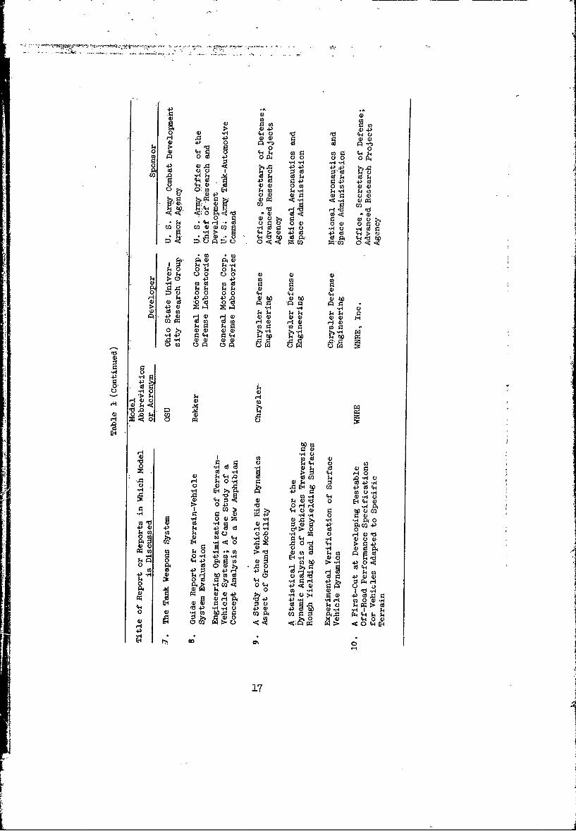
1 Models Used in ANAMOB Study 16

2 Terrain Factors and Class Ranges Used in Preparing MERS Factor 21Family Maps

3 MERS Factors Used to Describe Terrain for Ground Mobility 22

4 Soil and Soil-Material Properties 34

5 Compilation and Classification of Soil-Measuring Devices. 35

6 Pertinent Characteristics of Vehicles Used in the MEXA Field 59Test Program

7 Bekker/LLD Soil-Vehicle Models Evaluated in MEXA Program 61

8 Summary of Soil Data 64

9 MECA Data Used in Comparing Measured and Predicted First-Pass 65Go-No Go Performance

10 MEKA Data Used in Comparing Measured and Predicted Vehicle 68Cone Indexes

1 MEXA Data Used in Comparing Measured and Predicted First-Pass 74Optimum Drawbar Pull Coefficients

12 MEXA Data Used in Comparing Measured and Predicted First-Pass 76Towed Motion Resistance Coefficients

13 MEXA Data Used in Comparing Measured and Predicted First-Pass 82Sinkage

14 MEXA Data Used in Comparing Measured and Predicted Optimum 85Slip

15 MEXA Soil Data Used to Compare Measured Cone Index with Cone 88Index Predicted from Bevameter Parameters (kc, k1, and n)Using Equations Prepared by Janosi

16 Still-Water Speed of Floaters and Amphibians 170

ix

'4a

LIST OF TABLES (CONTINUED)

Table Title Page

17 Quantitative Comprehensive Operational Cross-Country 179Performance Models

18 Key to Single-Feature Models Used in Comprehensive Models 181

Examined

19 Comprehensive Model Components 183

20 Comprehensive Models Utilized for Design or Evaluation of 196Military Vehicles Through 1970

21 Single Feature Models for NOW Comprehensive Model 208

22 Outline of Plans for Phase I: Vehicle- Performance 218

23 Outline of Plans for Phase II: Terrain Description 224

Al Mobility Index Equation for Self-Propelled Tracked Vehicles A7(Equation A2)

A2 Mobility Index Equation for Self-Propelled Wheeled (All-Wheel A8Drive) Vehicles (Equation A3)

A3 Data Form for Computing Vehicle Cone Index (VCI') for Wheeled A16Vehicles in Sands (All-Wheel Drive) (Equation A5)

A4 Data Form for Computing Maximum Net Drawbar Pull (DBPmax) and A17Maximum Slope Negotiable (Smax) for Wheeled Vehicles in Sands

Bl Terrain and Vehicle Parameters -Used in Current Stream-Crossing B3

Models

B2 Vehicle Performance Output and Utilization of Current Stream- B4. Crossing Models

LIST OF ILLUSTRATIONS

.gue Title Page

1 Flow chart illustrating possible strategies for coupling soil 32and vehicle models to predict vehicle performance

2 Cone index profiles for different types of marginal surface 38materials

3 WES soil trafficability equipment 40

4 LLD portable bevameter 41

5 MEXA test beds 57

6 Military vehicles used in MEXA test program 58

x

LIST OF ILLUSTRATIONS -(COITINUED)

Figure Title Page

7 Comparison of measured and predicted vehicle cone indexes 69

8 Comparison of measured and predicted first-pass optimum draw- 71bar pulls for WES VCI models

9 Comparison of measured and predicted first-pass optimum draw- 72bar pulls for WES clay numeric models

10 Comparison of measured and predicted first-pass optimum draw- 73bar pulls for Bekker/LLD models

l Comparison of measured and predicted first-pass towed motion 77resistance coefficient for WES VCI models

12 Comparison of measured and predicted first-pass towed motion 78resistance coefficients for WES clay numeric model

13 Comparison of measured and predicted first-pass towed motion 79resistance coefficients for Bekker/LD models

14 Comparison of measured and predicted first-pass sinkage for 83Bekker/LLD models

15 Comparison of measured cone index and cone index predicted 87from bevameter parameters using equation prepared by Janosi

16 Flow chart illustrating possible strategies for coupling sur- 99face geometry, vegetation, vehicle, and driver models to pre-dict vehicle performance

17 Principal building blocks used in constructing vehicle ride 101dynamics models

18 U. S. Army Tank-Automotive Command ride dynamics model 103

19 Chrysler Corporation ride dynamics model 104

20 General Motors Corporation ride dynamics model 105

21 Ohio State University ride dynamics model 106

22 WES-FMC Corporat ion ride dynamics model 107

23 National Aeronautics Space Administration-General Motors 108Corporation ride dynamics model

24 National Aeronautics Space Administration-Brown Engineering 109ride dynamics model

25 Co-.nell Aeronautical Laboratory ride dynamics model 110

26 Calculation of correlation coefficient ll

27 The correlation function ll

28 Autocorrelation functions of several common waveforms 112

xi

LIST OF ILLUSTRATIONS (CONTINUED)

Figure Title Page

29 Examples of terrain pgwer spectra 115

30 Terrain and vehicle characteristics as a function of 1A7frequency

31 Force'-frequency vehicle response 118

32 Vehicle response-frequency relation 120

33 Idealized 4-degree-of-freedom model of vehicle 121

34 Vehicle model in displaced configuration for determining 122

forces

35 Forces acting on a vehicle at selected locations 126

36 Overview of terrain roughness test site near Carson Sink, 128

Nev.

37 M37, 4x, 3/4-ton cargo truck negotiating a rigid obstacle at 130

22 fps

38 Acceleration-time history; M37's front-axle response to 131

single obstacle at 15 mph

39 Acceleration-time history; M37's front-axle response to 133modified single obstacle shape at 15 mph

40 Acceleration-time history; M37's center-of-gravity response 134

on single obstacle at 15 mph

41 Pitch-time history; M37's center-of-gravity response on 135

single obstacle at 15 mph

42 Acceleration-time history; M37's center-of-gravity response 136

on cross-country course at 8 mph

43 Absorbed power-time history; M37's response on cross-country 137course at 8 mph

44 RMS vertical acceleration at driver's seat; M37's response 139on cross-country course at 8 mph

45 Schematic and circuit diagrams for calculation of absorbed 141

power

46 M37 driver's seat response to single 8-in.-high, half-round 142

obstacle at various speeds

47 M37 driver's seat response to single 8-in.-high obstacle with 142

30-deg face at various speeds

48 .137 driver's seat response to single 6-in.-high obstacle with 143

30-deg face at various speeds

xii

LIST OF ILLUSTRATIONS (CCVTINUED)

Figure Title Page

,49 Comparison of measured and- computed drawbar pulls on sloping 147surfaces

50 Effect of wheel load on drawbar pull performance on level 149

surfaces

51 Ground pressure distribution under tracked vehicle 150

52 Example of area denied computations for single obstacles 156

53 Force required to fail tree 159

54 Work required to override tree 161

55 Work required to fail tree 163

56 Graphical illustration of the WES method for predicting the 164average speed in terrains containing widely spaced discreteobstacles that are to be overridden

57 Flow diagram showing coupling of single-feature models used 184in WES comprehensive model

58 Primary coupling of single-feature models and arbitrary speed 185restrictions and time assessments in the TATAWS comprehensivemodel

59 Primary coupling of single-feature models, and feedback loops 186in OMEGA comprehensive model

60 Primary coupling of single-feature models, and feedback loops 187in CAL comprehensive model

61 Primary coupling of single-feature models used in Booz-Allen 188comprehensive model

62 Primary. coupling of single-feature models, and feedback loops 189used in McKenzie comprehensive model

63 Primary coupling of single-feature models in Ohio State Uni- 190versity comprehensive model

64 Design optimization procedure outlined by Bekker incorporates 191many single-feature terrain-vehicle relations that could bereadily used in a comprehensive cross-country vehicle per-formance model

65 Single-feature models and coupling in Chrysler comprehensive 192

model

66 Primary coupling and single-feature model used in WNRE go-no 193

go comprehensive terrain-vehicle performance models

xiii

LIST OF ILLUSTRATIONS (CONCLUDED)

Figur Title Page

67 Structure of WNRE go-no go model, illustrating types of 202terrain-vehicle-configurations tested and iterative testapproach used to develop diagnostic keys for immobilizations

68 Structure of WNRE go-no go model for linear terrain feature 204

69 Suggested primary couplings of single-feature models for the 207

NOW comprehensive model

70 General research plan, phase and task relations 217

Al Relation of MI to VCI -for self-propelled vehicles A9

A2 Relation of net maximum drawbar pull on level ground and A10maximum slope negotiable to ROI in excess of VC1

A3 Relation of towed motion resistance on. level ground to RCI AllA4 Net maximum dr&wbar pull, maximum slope negotiable-soil A12

strength- relations for tracked and wheeled vehicles oper-ating on fine-grained soils

A5 First-pass motion resistance-soil :strength relations for A13tracked and wheeled vehicles operating on fine.!grained soils

A6 Soil, vehicle-performance relations used in coarse-grained A15soil prediction analysis

A7 Performance of tracked vehicles in dry-to-moist sand A19

A8 Relations of performance coefficients for first pass of A24single wheel to clay mobility numeric

A9 Relation of pull, slope, and towed force coefficients to A26WES numeric for clay

A10 Relation of performance coefficients for first pass of A27single wheel to sand mobility numeric

All Shear stress (Txy) under center line of track as a function A40of depth for an applied strip shear loading

A12 Schematic representation of a tank in the soil A43

Bl Flow chart illustrating possible strategies for coupling B2stream-crossing models

B2 Go-no go test sequence for stream crossing B15

xiv

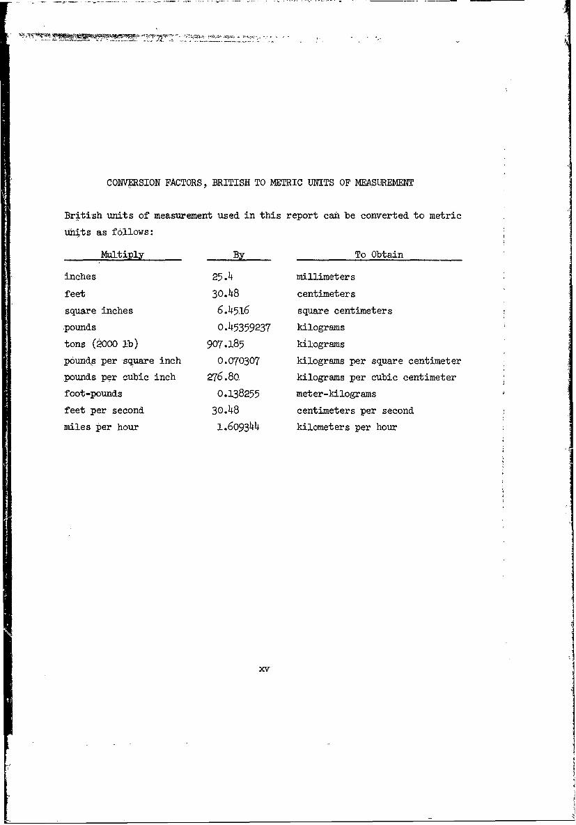
CONVERSION FACTORS, BRITISH TO METRIC UNITS OF MEASUREMENT

British units of measurement used in this report can be converted to metric

units as follows:

Multiply By To Obtain

inches 25.4 millimeters

feet 30.48 centimeters

square inches 6.45i6 square centimeters

pounds 0.45359237 kilograms

tons (2000 ib) 907.185 kilograms

pounds per square inch 0.070307 kilograms per square centimeter

pounds per cubic inch 276.80. kilograms per cubic centimeter

foot-pounds 0.138255 meter-kilograms

feet per second 30.48 centimeters per second

miles per hour 1.609344 kilometers per hour

xv

SUMMARY

Practically every research effort and subsequent procurement of mate-riel for Army use is backed up with a system effectiveness-cost effective-ness study. The development of good ground mobility models in support ofthese studies was of particular interest to the Office of the AssistantVice Chief of Staff, U. S. Army, to assist in the construction of new mod-els or in the evaluation of existing models. As a first step, it washighly desirable to survey the existing models. With the need established,and, with U. S. Army Engineer Waterways Experiment Station (WES) interestand technical capabilities in the field, a study aimed at the analysis ofexisting ground mobility models was initiated by WES d WIRE, Inc., Undercontract to WES.

A The objectives of the study were to analyze existing ground mobilitymodels in order to: ()' determine their generkl level of usefulness andapplicability to predicting cross-country performance of ground vehicles inthe real world; (b? select the models that appear to be the more promisingfor this purpose and determine their usefulness and applicability in moredefinitive terms; (&?point out areas of the latter models in which addi-tional research is needed; and (A)y develop guidelines for future develop-ment of ground mobility models. t

Various Army sources and unclassified literature were canvassed forcross-country performance models that have been used or seriously proposed.Examination of these available simulations revealed a considerable degreeof fundamental commonality, despite initial differenees in appearance. Inlight of the basic commonality, the available cross-country models werenext examined for the single-feature vehicle-terrain interaction modelsthat they utilized. Those single-feature models found in the existingcross-country models were identified. Each cross-country and single-feature model was then examined by a study-team member familiar with thetype of problem it dealt with. Each model was briefed, classified, andevaluated on the basis of the degree of objective validation available andof subjective considerations as to adequacy, real-world verisimilitude,probable accuracy, etc.

Models covering a given single-feature/vehicle interaction weregrouped and the characteristics, assumptions, and limitations that theyshared were outlined. When data were available, checks of the predictionaccuracy of the single-feature model were made. Details for severalclasses of single-feature models are presented in two appendixes to the

xvii

report. Points of divergency were then examined for their significance,and

a. An overall judgment was made as to the most advanced existingmodel of the class, and its principal assumptions and limita-

tions were evaluated.

b. Modest suggestions were made for immediate improvements, ai

possible.

c. From a and b, recommendations were formulated for the NOW

model.

d. Specific further work to improve the model was suggested.

In examining each type of model, modeling strategies available wereoutlined in the broadest sense. This procedure facilitated classificationof existing models and indicated the existence of alternat .ves that mightnot yet have been explored. In general, the strategies consisted of a num-ber of approaches to each of several segments of the problem and a modelwas classed by the serial path that it represented through a matrix. Itwas found that, in general, the sequence of a rational ,path did not includesuccessive steps that proceed from the more specific to the less..

The study.was conducted within several constraints. Only those cur-rent models for cross-country operation that are functioning and that offerthe potential to do a simulation job now were considered. Ten cross-country models meeting most of these- criteria were selected for detailedexamination.

The study produced a compendium of existing ground mobility submodelsand comprehensive cross-country vehicle performance models that have beenused or have a potential for future use. A structure for a NOW cross-country ground mobility model is suggested, along with some minor additionsthat do not require a great amount of effort. The study also presents alist of guidelines for the future development of ground mobility modelsalong with plans for a future research program.

This report consists of: a main text containing an introduction, apresentation and analysis of single-feature models, a -description and anal-ysis of cross-country performance models, structure for a NOW comprehensivecross-country model, and guidelines and plans for future development ofground mobility models; and two appendixes that present in detail the soil-vehicle models (Appendix A) and stream-crossing models (Appendix B) exam-ined for this study.

xviii

AN ANALYSIS OF GROU1ND MOBILITY MODELS (ANAMOB)

PART I: INTRODUCTION

Objective

1. The objectives of the study, "An Analysis of Ground Mobility

Models (ANAMOB)," were to analyze existing ground mobility models in order

to:

a. 'Determine their general level of usefulness and applicability

to predicting cross-country performance of ground vehicles in

the real world

b. Select the models that appear to be the more promising for

the purpose and determine their asefulness and applicability

in more definitive terms

c. Point out areas of the latter models in which additional re-

search is needed

d. Develop guidelines for future development of ground mobility

models.

Background

2. Recent growth in the sophistication and cost of weapons systems

has made it desirable to formalize procedures for making objective selec-

tions among them. The principal procedure developed has been cost-

effectiveness comparisons using increasingly complex or comprehensive corn-

puter programs.

3. To satisfy the requirements of a computer, all input informationmust be quantified, whether or not rational means exist for doing so. More-over, despite the most painstaking quantification, the basic concept of

large-scale cost-effectiveness computations ultimately involves comparison

among things that are so unlike that comparison seems irrational. These

fundamental difficulties may be greatly mitigated, but seldoi eliminated,

when cost-effectiveness comparisons are made between smaller systems that

S11

have, to the naked eye at least, a large-measure of similarity, such as be-

tween competing forms of ground vehicles in battlefield logi'stic support,

for example.

4. Notwithstanding,, to compare systems of whatever size, both cost

and effectiveness must be computed. Despite the usual gross simplifica-

tions (use of peacetime dollar values for wartime studies, assignment of no

intrinsic value to human life, etc.), even the cost element in such trade-

off relations has proven most elusive. From experience with the F-111, the

C-5A, and the MBT7O, all of which received the benediction of extensive

analyses, it appears increasingly difficult to estimate even the first cost

of a new machine with an error of much less than plus 100 percent.

5. Quantitative assessment of the effectiveness of a weapons system

presents even larger practical and philosophical problems, leading to the

suspicion that computed values for effectiveness indexes can hardly be more

reliable than their cost partners. Consider the case of a tank engagement.

Predicting behavior of each vehicle involved requires knowledge of:

a. Weapon reliaLility and accuracy.

b. Personnel behavior in acquiring targets, serving the weapon,

and operating the vehicle, all in an environment conditioned

by the battle, by the vehicle, and by the terrain.

c. Vehicle performance under the constraints of terrain, of mis-

sion, and of driver judgment.

In order to simulate* more than a simplistic one-on-one situation, projec-

tions must 63.so -be made of the ergonomic and technical performances of com-

munications systems, and of the interrelated responses of other man-weapon-

vehicle units, friendly and hostile, like and unlike. Finally, when, once

all the input parameters are given, the ensuing action can be predicted for

a reasonable time ahead, there- remains the crucial task of specifying real-

istic terrain inputs and initial conditions.

6. The ANAMOB study addresses itself to but a small part of this

broad picture and eschews entirely such formidable tasks as supplying

* In this report, simulation is defined as the act of representing some

aspect of the real world by numbers or symbols that can be easily manipu-lated to facilitate their study.

2

I

reasonable scenarios. ANAMOB examines only methods to predict the mobility

performance* of a single ground vehicle in a sequence of terrain conditions.

The outputs can be any measures of vehicle behavior that are desired. Even

this small part of the overall problem of simulating behavior of a vehicle

system in a given operational situation is extremely complex.

7. Despite the great utility of the helicopter in Southeast Asia,

requirements for increased ground mobility in our military vehicles con-

tinue. High-mobility ground vehicles support the general need in limited

warfare to amplify our manpower through the use of efficient machines, to

widen limited options, and to avoid piedictable channeling of traffic.

When they can be used, ground vehicles will usually prove less costly, and

sometimes less vulnerable, than helicopters. Helicopters and truly mobile

ground vehicles in combination offer a useful increase in operational flex-

ibility. Accordingly, between the continuing needs for ground vehicles and

for systems studies, it appears that cross-country traverse simulations

will be in use for some years to come. Such simulations must be as good as

possible if the entire systems study effort is to give meaningful results.

The ANAMOB study is addressed to the problem of improving cross-country

traverse simulation.

8. Current cross-country performance simulations are mostly ad hoc

models. Largely for this reason, a particular cross-country model will

sometimes, usually deliberately, be limited to the simulation of a part of

the overall problem only, that part specifically needed in the particular

larger simulation of which it is a subassembly. Limitations of this sort

are usually manifested in arbitrary restrictions on the terrain types

considered,;

9. The sponsor has recognized that further proliferation of ad hcc

model development not only leads to chaos (or at least the appearance

thereof), but also reduces the value of individual systems studies by

* Mobility performance in this context is defined as the ability of a

ground vehicle to move freely in a given terrain context. If predictionsare made by use of a comprehensive model, speed is usually used as theparameter to describe peirformance, whereas if the predictions are made byuse of a submodel such as a soil-vehicle submodel, drawbar pull and mo-tion resistance are usually the important performance parameters.

making them to a greater or lesser degree riot comparable with others. The

sponsor desires the promulgation of a complete, standard terrain-vehicle

interaction model of the best accuracy and highest degree of Validation cur-

rently possible, for regular and consistent use in more complete systems

simulations. This will be termed the "NOW" model.. The sponsor recognizes

that despite some 25 years of mobility research, the NOW model will still

leave much to be desired. Accordingly, development of a research and de-

velopment program to produce a significantly more accurate and more real-

istic model appears necessary..*

10. While one overall objective of ANP1M0B is to propose a NOW model

for uniform use in more complete system evaluation simulations, modeling

for less ambitious use (as part of engineering design optimization, for

mixed-mode comparisons in which the performance of a paper vehicle is com-

pared with that of existing machines, etc.), has also been lept in mind. As

a result, the NOW model recommended in Part III of this report is outlined

in a modular form, so that different relations may be used in some modules

according to the particular object of the model's use. A specific composi-

tion of each module is recommerded for each specific use of the NOW model.

In the design process it is not intended to restrict use of any method that

appeals to the designer,, but alternate methods must be used at his risk, be-

cause the controlling concept of ANAMOB is that all final evaluations will

be made using the NOW model in its evaluation configuration. The NOW model

proposed is recommended for operational use in evaluation simulations for

the immediate future (five years), irrespective of any minor improvements

that might be possible in the near future, so as to preserve internal con-

sistency among all studies in that time frame. Past experience indicates

that the rate of technical progress will be such that five years will be a

* This is not the first time in recent years that this general state of

affairs has been recognized, and stleps begun to rectify it. Two previousefforts in this direction were initiated by Advanced Research ProjectsAgency (ARPA) in 1964-66 (Mobility Environmental Research Study (MERS) at*the U. S. Army Engineer Waterways Experiment Station (WES)), and in 1967-63 (the Off-Road Mobility Research (ORMR) program at Cornell Aeronautical'Laboratory (CAL)). For reasons that have never appeared technically jus-tifiable, both programs were aborted just as they approached their payoffperiod.

4

minimum time increment for significant improvement. This is not to say,

however, that new elements should not be added to the model where it can be

demonstrated that they are necessary to give a radically different machine

a fair evaluation.

Perspective

11. Formal study of military mobility problems began during WorldWar II and was concerned initially with the failure of vehicles to negoti-

ate the muds and weak soils found in Italy, Germany, Okinawa, and other

battle areas. Research on the vehicle-soil relations that might explain

the failures and indicate ways to design vehicles less prone to soft-soil

immobilizations continued on a low-budget, essentially ad hoc basis into

the early 1950's. At that time, under the impetus of renewed tank immobili-

zations, this time in Korea, the problem was more formally recognized, and

there has been a modest but continuous program of research in this general

area under U. S. Army sponsorship ever since. Ground vehicle immobiliza-

tions are still with us, however, now in Southeast Asia. And despite the

fact that available vehicle-soft ground relations have generally clarified

some broad design and operational problems, and that they are fundamental

to the prediction of all ground vehicle operations, they are not yet en-

tirely satisfactory for many purposes.

12. In the early 1950's, Bekker expanded the purview of ground mo-

bility research from examination of vehicle-soil relations to study of more

general vehicle-terrain relations. Trees and hills and lumps and bumps

were recognized as elements contributing to the total impedance that a

ground vehicle encounters in a normal cross-country traverse. Other

researchers--partially despairing of advancing the solution of the soft-

soil problem, partially in recognition of the complexity of real terrain--

followed suit by tho end of the decade. Further impetus to treat the

complete terrain complex came from pressures at DOD level for cost-

effectiveness and/or systems studies in justification of new hardware pro-

posals. By the mid-1960's, a similar, systems approach was adopted in then-

beginning studies of possible moon vehicles.

5

13. In the mid-1950's, consideration was given to the interplay of

vehicle vibrations, or "ride," and speed, through the reaction of the

driver. A decade later, modest efforts were started to model the driver

and his vast influence upon actual performance more completely. Thus far,

progress has been slow, and no cross-country performance model in use today

incorporates the driver except as a vibration-visibility speed governor.

14. In a total systems approach, estimation of vehicle performance

in a particular situation is only one of several complex elements that re-

quire simulation. Under-the-gun for decision-fodder, the approach taken

over the past ten years to simulate cross-country performance has. generally

been to consult a limited number of research reports (of various vintage)

and Bekker's latest book, make a brief brainpicking tour of a few handy ex-

perts, add a lot of imagination (of various quality), and finally, erect

still another ad hoc model. And then the analyst moves on to the simula- Ition of the next element with a prayer that it will prove more tractable

and offer a more elegant solution. To some extent such almost casual inclu-

sion of terrain-vehicle interrelations may have been justified in the past

by the broad scope of the total simulations attempted. Individual vehicle

performance was but one of many elements affecting the final result. On

the other hand, the function of an army is to bring to bear on an enemy a

winning mix of firepower, armor, and mobility. In relation to ground vehi-

cles, then, one of the Army's major responsibilities is to understand vehi-

cle tactical mobility in order to optimize its fundamental three-way mix.

Any slighting of this critical element in a simulation upon which equipment

and doctrine decisions might be made is no longer defensible. Even simula-

tions that project reasonable, average performance in a "typical" terrain

only short-circuit the intention of those comparisons of new and/or exist-

ing equipment which include candidates having nonaverage performance

profiles.

Basic Concepts

15. Modeling of cross-country performance ideally involves four ma-

jor concepts: the vehicle, the driver, the terrain, and the model. While

it would seem that each is self-explanatory, some brief discussion at this

6

I1

point of the particular interpretations that are reflected in this study

may save some misunderstanding later on.

The vehicle

16. Of the four, the concept of the vehicle is essentially the most

straightforward. As noted earlier, the study is aimed primarily at ground

vehicles and at single vehicles- operating without appreciable engineer sup-

port to mitigate: terrain severity. In terms of army operations, this treat-

ment is to some degree unrealistic. Even reconnaissance operations will

usually involve a group of vehicles rather than only one, while most other

operations will involve many. In most cases, the single vehicle assumption

wi-ll be tconservative, but not always. In general, the larger the group of

vehicles in a given movement, the more likelihood of some organic engineer

support for bridging, bulldozing of trees and banks, etc. The operation of

a group of vehicles usually permits- more rapid recovery of individual vehi-

cles temporarily immobilized by terrain impedances, through towing rather

than winching, for example. As the number of vehicles involved increases,

the necessity for more than one vehicle to operate essentially in the

tracks left by the preceding vehicle increases. In some situations the im-

pedances of following vehicles operating in this manner will be reduced;

but where weak remolding soils are involved, the likelihood of a later vehi-

cle miring in the ruts of the preceding ones increases. If the vehicles

are such that they are not homogeneous in their general off-road perform-

ance and/or are not compatible in scale and destructiveness to the terrain,

the problems of following vehicles can be increased rather than decrease.

17. The degree of traffic channeling,, and its probable effects upon

movement of a group of vehicles, is of course a function of the number of

vehfhles, of the terrain, and of operational constraints. Either of the

latter two may force traffic channeling even where only a small number of

vehicles is involved and may, moreover, force such channeling where least

desired from a mobility viewpoint. Accordingly, the present treatment of

the vehicle proceeding solo must someday be expanded to properly reflect

terrain influences upon multiple vehicle operations.

The driver

18. The driver enters existing simulations, when at all, only as a

7

speed limiter in response to excessive ride vibrations or to reduced visi-

bility. His actual influence is often far greater. The general area of

driver decision (or cozmiander-and-driver decision, in the case of a tank)

in selecting a detailed- path through a given stretch of off-road terrain,

for example, is at the moment still unmodeled in practice. This, despite

the well-known fact that an experienced (and luckI.) driver can,/often get

through a given area by intelligent, on-the-spot, close-range route selec-

tion where an inexperienced driver would be constantly riding the winch

line. A complete model must eventually reflect the full impact of all

driver influences.

The terrain

19. The terrain component of the vehicle- driver relation is also a

familiar concept. Terrain is an area and in. the mi.itary sense denotes the

physical features of that area. In context of the present study, the fea-

tures of interest are those that specifically interact with a vehicle at-

tempting to traverse the area. These features are for the most part are-

ally distributed, even though a vehicle ultimately experiences terrain more

simply as a path. It is desirable in modeling cross-country operations to

incorporate terrain in its full areal scope so that vehicle paths may be

generated through realistic interaction of the capabilities of the Vehicle,

the requirements of the operation, and the configuration of the terra-in.

Simulation that does not permit this degree of flexibility cannot be ex-

pected to reflect the true differences in effectiveness among vehicles

whose overall mobility profiles are significantly different.

20. There is an overwhelming consensus that the primary terrain at-

tributes of interest to a cross-country vehicle operation are those that

describe in engineering terms the geometry of the surface and the strength

of the materials in it from place to place (in both cases including vegeta-

tion, streams, etc.). In this report, a single measurement of a single at-

tribute of the terrain will be called a factor. Gross slope, mean spacing

of trees of specified diameters, soil rating cone index, etc., are examples

of terrain factors.

21. Factors that describe the terrain segment of the environment are

of two kinds: those reflecting relatively stable, long-term attributes,

8

fI

and those reflecting the immediate state of elements subject to seasonal

and/or daily variation. A vehicle's performance is influenced by the geo-

metric and mechanical features and properties it finds point-by-point and

moment-by-moment in the terrain. These, in turn, reflect the combined ef-

fects of both kinds of factors.

22. Consider a slope of reasonable length and uniformity, extreme

but not impossible--say one having a 30 percent grade. Whether or not a

given, r elatively mobile vehicle can negotiate it depends on many factors

acting in concert with the slope. All may be considered, for the moment,

to be independent. It is readily apparent, for ekample, that the types of

soils involved, their stratification and moisture contents (and hence

strengths)", the extent of superimposed minor relief (microrelief), the sur-

face roughness (minirelief), and the kind qnd condition of vegetative cover

may each have some influence.

23. Slope (macrorelief), soil type and stratification, general vege-

tative cover, microrelief, and perhaps minirelief are relatively stable.

Soil moisture content and its stratification will usually vary from day to

day, the state of vegetation, from week to week. All will vary, more or

less, to some degree at different points in any given vehicle's path even

in a nominally homogeneous stretch of' terrain, and most will be altered to

some-' extent by the passage of a single vehicle.

,24. The long-term factors--those describing topography (macro-,

micro-, and mini-relief)j the general vegetative picture, soil types and

distributions, overall seasonal groundwater regime, semipermanent cultural

features, etc.--may for the most part be considered on the basis of rela-

tively large areal units. They may usefully be classified and analyzed es-

sentially within the framework of classical naturalistic studies. The vari-

able attributes must be treated on a time-dependent basis, reflecting tem-

poral variations in weather, cyclic influences of climate, the mechanics of

soil moisture and plant growth, and the onslaught of mankind.

25. In the aggregate, proper, long-term, broad classifications--in

terms of landform, geology, ecology, climate, etc.--with their interrela-

tions appear to constitute a sound base for predicting conditions to be

found in unsampled (and sometimes unsampleable) regional areas of the world,

9

4m.

and hence for predicting equipment performance (or, conversely, require-

ments) in such areas. The considerable environmental research that must be

done to develop this potential, via the correlation of the naturalistic

classification systems with the occurrence of geometric and mechanical ter-

rain features that directly affect the performance of military equipment,

appears to be one of the steps essential to the development of more ra-

tional terrain information.

26. Terrain features will, in general, be such things as a stream-

bank or a forest, described in terms of a number of factors. A streambank,

for example, might be described in terms of'a series of measurements defin-

ing its geometry in a single plane normal to the direction of the stream-

flow plus the location of the free waterline in relation to it; a forest,

in terms of frequency distributions of size and spacing of trees and in-

dexes of straight-line visibility and perhaps of effective strength of the

trees (functions of species). Although groupings of factors into features

are essentially arbitrary, there is a basic consensus, even here, following

lines of division laid down essentially by the prediction scheme employed.

27. To describe an actual section of terrain as a vehicle sees it,

it will normally be necessary to specify a combination of features. For

example, data on vegetation plus surface geometry plus surface composition

are needed to define a small piece of real estate that is significantly for-

ested. Vegetation occurs in a specific topographic situation and soil body,

and is often intermixed with deadfalls, stumps, and minor drainage features.

All in concert influence a vehicle's performance. A distinct combination

of factors that provide a relatively complete quantitative descriptipip of

terrain over an area (which may be quite small or very large) will be

termed a unit terrain.

28. In making vehicle performance predictions, unit terrains are gen-

erally assumed for practical purposes to be homogeneous; i.e., values for

each single factor measurement are considered to be constant, or to lie

within the same class range, or to be described by the same probability dis-

tribution. The number of discrete unit terrains necessary to describe an

area is obviously a function both of the number of factors used and of the

resolution with which each is defined. The problem is inescapably one of

10

Ii

• • m m u n

statistics. Actual terrain is endlessly variable and its "fall" descrip-

tion for vehicular purposes alone might conceivably run to the complete map-

ping of 30 or more measurements at a ,resolution of approximately 5 ft.*29. Clearly the cost of a truly precise set of maps in such terms,

even for a small area, would be prohibitive. Moreover, initial precision

would disappear with the passage of a few vehicles or a f&w rainstorms or a

few months. Accordingly, the practical description of terrain must accept

both considerably reduced resolution and extensive idealization of the ter-

rain geometry in order to keep the total number of factors manageable. The

tradeoff is not hopeless, but it does lead to uncertainty in any individual

result. The effects of this uncertainty upon most practical decision mak-

ing may average out in areas characterized by a large number of unit ter-

rains, but this remains to be objectively checked.30. Mapping terrain directly in terms of its factors, as in the cur- 1

rent generation of WES factor family maps, represents a straightforward in-

terpretation of the engineering numbers required to describe terrain. Some

experience has shown, however, that this apprbach may lead to the problems

just mentioned; i.e., reasonable, feasible, economical resolution results

in potential errors at any given point in the terrain. This- is not unex-

pected, of course. Mitigating this by squinting at the results through a

statistical filter is a suitable fix for some uses, as in design study, but

even here some desired Sensitivity must inevitably be lost.

The model(s)

31. A model for soimnldtiig cr6ss-country operation is- one or more ex-

pressions -and analytical processes that relate desired measures of vehicle

performance to quantitatively expressed vehicle, driver, terrain, and oper-

ational factors.** A complete cross-country performance model comprises

the follbwing basic elements:

* A table of factors for converting British units of measurement tometric units is presented on page xv.

** While ultimately any such model must be set up for computer use, notall current examples are fully computerized at this time. In some cases,possible geometric interference between the vehicle underside and theterrain is examined through the use of two-dimensional s',atic scalemod els-. This permits somewhat more complete representation of each, butat considerable obvious expense in computation time.

l11

r

a. Means to specify the vehicle in meaningful paiametric form.

b. Means to depict the terrain as a quantitative areal

phenomenon.

c. Criteria and procedures for generating and/or seledting paths

through the terrain (including, as an almost tr-ivial end

point, fully specifying a path a priori).

d. Means to quantify terrain factors for all segments of any

selected path.

e. Means to predict desired vehicle performance measures along

each segment of any selected path.

f. Rules for joining performances along individual segments into

a continuous traverse.

g. Means to aggregate predictions for individual route segments

into maps, totals, statistical-measures, etc., according to

the needs of the model user or of the larger simulation of

which the cross-country performance model is a part.

Elements a through d, which precede prediction of vehicle performance in a

given unit terrain, are considered to be preprocessing of the data; steps

I and g, which follow, are output processing. The logic and functioning of

both will be determined largely by the intended use of the complete model.

32. The heart of the model, however, is the calculation of vehicle

performance on a homogeneous path segment once all terrain factors perti-

nent to that segment are specified (element e). The resolution of terrain

data available, practical computing considerations, and terrain diversity

will together dictate the number of distinguishable homogeneous unit ter-

rains by which a given area will be represented. Thereafter, the validity

and resolution of the complete simulation is directly dependent upon the

adequacy and accuracy of the performance model per se.

33. As a result of the large number of vehicle and terrain parame-

ters involved, and of the true complexity of detailed relations among them,

most predictions of vehicle performance are presently done by computing in-

teractions of single terrain features with the vehicle, and subsequently

superimposing the results in various reasonable combinations and according

12

to several exclusivity rules. The currently accepted breakdown of real

vehicle-terrain interactions into manageable submodels--termed single-

feature models--is as follows.

a. A soil-vehicle model which, as -a function of quantitative

soil values, estimates (1) vehicle motion resistance due to

soil plastic and/or visco-plastic deformation and (2) net

traction available to overcome other impedances.

b. A soil-slope model which adds or subtracts gravity effects to

the soil-vehicle system. (These may include load transfer ef-

fects, reduced initial soil stability due to its sloped sur-

face, etc., as well as simple changes in net traction require-

ments.)

c. An obstacle interference model which searches for possible

geometric interferences during vehicle passage over an ob-

stacle, which may be deformable but generally is treated as

rigid.

d. An obstacle-surmounting traction model which projects torque

and traction required to override a vertical obstacle.

e. An obstacle-avoidance model in which is examined the possi-

bility of threading the vehicle through a planar array of in-

surmountable or especially troublesome obstacles, such as

large trees, stumps, and/or large boulders.

f. A vegetation override model which estimates traction and

torque required to maintain headway while overriding vegeta-

tion which cannot or may not be avoided.

g. A ride vibrations model which computes, as a function of ve-

hicle speed, the dynamic response of a vehicle to surface

roughness and compares this with personnel comfort, safety,

and performance tolerances, cargo tolerances, and/or vehicle

structural tolerances to establish a probable maximum speed

and corresponding average power expenditure.

h. A visijility model which forecasts the speed reduction which

will result, through driver election, from terrain-induced

reductions in the driver's view of the prospect before him.

13

i. A stream-crossing model which-examines vebicle ingress, swim-

ming, and egress as a static or dynamic mechanics problem.

In all except obstacle avoidance, the vehicle is tacitly assumed to be mov-

ing in essentially a straight line. Incremental effects of vehicle maneu-

vering on performance in the other terrain situations se sometimes esti-

mated and combined by further superposition.

34. Forces and torques calculated from several of tbe single-feature

models, in appropriate combinations, are transformed to estimates of speed,

fuel consumption, etc., using straightforward automotive engineering models

relating speed to v#ehicle engine and power train torque characteristics.

Approach to the ANAMOB Study

35. Various Army sources and unclassified literature* were canvassed

for cross-country performance models that have been used or seriously pro-

;posed. Exaination of these available simulations revealed a considerable

degree of fundamental commonality, despite initial differences in appear-

ance. All were conceived within the common framework of Newtonian mechan-

ics, and all consider at least a part of the overall vehicle-terrain inter-

relation. Differences and discrepancies arise (apart from degrees of com-

pleteness) largely in the idealizations or simplifications adopted in de-

scribing the vehicle, in describing the terrain, and in formulating the

equations relating the two.

36. in light of the basic conmonality, the available cr6ss-country

models were next examined for the single-feature vehicle-terrain interac-

tions models that they utilized. Those single-feature models found in the

existing cross-country models and those in practical use in less ambitious

computations were identified. Each cross-country and single-feature model

was then examined by a study team member familiar with the type of problem

it dealt with. -Each model was briefed, classified, and evaluated on the

basis of the degree of objective validation available and of subjective con-

siderati iis as to adequacy, real world verisimilitude, probable accuracy,etc.

* See Selected Bibliography.

14

37. Models covering a given single-feature/vehicle intei'action were

grouped and those characteristics, assumptions, and limitations that they

shared were outlined. Points of divergency kfere then -examined for their

significance, and

a-. An overall judg ent was made as to the most advanced exist-

ing model -qf the class, and its principal assumptions and

limitations were eyaluated.

b. Modest suggestions were made for immediate improvements, as

possible.

-c. Frm a and b, recommendations were formulated for the NOW

-model.

d. Specific further work to improve the modei in an approximatefive-year time frame was suggested.

38. In examining each type of model, modeling strategies available

were-outlined in the broadest sense. This procedure facilitated classifi-

cation of existing models and indicated the existence of alternatives that

might not yet have been explored. In general, the 'strategies consisted of

a number of approaches to each of several segments of the problem and a

model Was classed by the serial path that it represented through a matrix.

As will be seen later, some paths were not truly feasible and others would

simply be nonsense. It was found that, in general, the sequence of a ra-

tional path did not include successive steps that proceed from the more

specific t the less. This will become clearer once the strategy diagramsare presented. I

39. The study was conducted within several constraints-. As noted

earlier, only those current models for cross-country operation were consid-

ered that are functioning and that offer the potential to do a simulation

job now. Cross-country models meeting these criteria are listed in table 1.

40. Single-feature models considered are also essentially only those

presently in use, although a few promising paper candidates will be men-

tioned. The study is aimed at models dealing with ground vehicles only.

Extension of any model to cover surface effects vehicles (SEV's), however,

would not be difficult. Because SEV operation would not involve soil

15

4) 4) D

U)- *~ 0 A4

14)~ HH A-0 .-

03 4-4

P4 01) 4) 4)to t W 4L) U ~ Id: n It0 4' H 53 W) V4

m4),m ~ 4)

4)0i C.; a

W4, , to(0 PQ '0 *'4) C-1 I~ E-1 r. 0

k4 .~8 HH 4.) W~) ~ 04) X ID~ 1U) r- 2

(0 -4) 0 H 02-P~- r - 02 H14)4A &- 00 r-l t H 0, w~)

0,8U t- ) 00 0d .0 028 w r2

04 ) POQ m

00

00 *,- U

02 0

H) H 0) 4D 4

t E4 4) *1.44.H to 0 H

$4 'A ) $4 .43 p -1 1

00 10 U).) Ctopp 4) U) HU 4- 432 4)

0.r

ski to2. (04-2~ 4)0 4, t :;pi 34) 4) . 14 0 440 0 1 v 4)

to4 C4 'd .. >,42V4 q ,-U

43 W -0 4.'.44 4) H)4 -4Id0AU)~~ 0- 13f (4 U ~ 02 ' ~ *4)4) U E-4 x)4 u0 J.4 4 430

H

-4 H r4f2-

4-)>

4)4) 44)0) 4) 0iq4a rdI -

rH . ~ 4) 4)4 w : 5: 4)4p) 4 0 p 4)$4 rd't 0 00 4) 0H or, CH

0 a) 0 -4 0 4 0 JO

4) r.1 4) 0 44) 4

4- ( 0 0) 0 0 ( 4) 4)0 ~0:o &4 k4 $, $4ri E40

C) Q). 0 "O)

0 5

4) 4 d P

$4 0 0 ;q 0 04)44) r 4).0 0 0

;> co co) 00

00 )

0 40 004 0 44O) a) 4-0 0 0 ) 4) 4

4 - (D 4) 4

1 4)r ,

0d

0) -~ $4.4 $$ .4

0100 p~0 0 0

0.~

9: 4) 4

Ho -H41 -

H $4'~ 0 5:,1 0 4 : 1

a) 4- 'r4 4

H - : $40 s 4) 0 - Ha0 0o 4) ZF.4Mrlw*(-4 E-4C) .,I00,( I

07 0 Zi40" 0 H ~ OH 0Hr-5:d 0 U2i *d), Cr4 434- 0)) 144 0 0

4 $4 H)'1 H' o 0$40 0f c44 0,00'- rd P H 434) C) co4 pd 4 *- )

0 4- P, g~ .A o q 0C

04 0 P 0 4-440)$0 0 ~ to4 )0H 14 00 H0.v5:104 0 I'M 4)~.. 43 $40 4) 0Co 0 44 434)))

0~~~ 0 *,-IriQ> o 4)Cd4rS 44) fr1 *.10 04 ) .E-4 4)) r. 4 3a e) P >5, $4c4do00 '43 ,q.4 +) 4) 44) 4).r .- II0 , " o oP4 P4.Z 5~~-$$

> 041

17

strength relations* (unless the vehicle was a hybrid)', the terrain and

terrain-vehicle simulation would be simpler in many respects. Soil and

soil-vehicle models for inorganic soils only are examined--. Again, an exten-

sion to organic soils (muskeg, etc.) and to snows and snow-covered terrains

is entirely feasible, although the problem of validated "soil"-vehicle mod-

els in these cases is more severe; i.e., there is considerably less in the

way of available models and reliable supporting laboratory and/or field

tests.

41. The present study considers only the problem of a single vehicle

operating in unprepared terrain. Elaboration to include multiple vehicle

operation (the traffic problem) and various degrees of engineer support in

preparing the terrain for the vehicle remains largely for the future. Fi-

nally, while a complete model must, by general agreement, ultimately in-

clude a number of driver inputs, the present study considers only those

that have actually been modeled to date. There are but two. One is driver

reaction to more-or-less continuous vehicle vibrations (the ride problem),

in which the driver is presumed to alter the general level of his vibra-

tional environment to some tolerable level through speed adjustment. The

second -is the strong interrelation between the Vehicle and the terrain

through the mechanism of the driver, who adjusts his operating speed to

match the terrain information that he can identify (the visibility problem).

In many situations this will be the only impediment. The visibility prob-

lem, which is as yet fuzzy at best, is a good instance where poor simula-

tion of the vehicle-driver-terrain interactions could lead to seriously er-

roneous results. For example, without a good model for this important part

of the problem, the value of supplementary on-board sensing equipment, new

approaches to control, or even of advances in vehicle suspension capabili-

ties, obviously cannot be estimated intelligently.

Realism and Validation

42. Two important guiding criteria in the ANAMOB study are realism

* Such factors as dust, which are ignored as secondary in present groundvehicle modeling, would become primary, however.

18

and validation. The two are, of course, related but they are far from iden-

tical. To-,make a working distinction, validation of a model or submodel is

the extent to which its predictive accuracy has been demonstrated in reli-

able, relevant tests.

43. Realism in a model is the degree to which:

a. Parameters used to describe the vehicle do in fact describe

all of the functionally important features of real vehicles.

b. Parameters used to describe the terrain do in fact define

real terrain adequately as a vehicle sees it.

c. Vehicle behavior predicted on the basis of a and b agrees

with actual behavior of actual vehicles in actual terrains.

Note that a submodel may, by these special definitions, be valid, even

though it lacks realism. Ideally, of course, an overall model and all sub-

'models within it should be both realistic and validated. The nature of the

problem makes either requirement difficult to achieve.

Realism,

'44. Realism is a function both of the inputs to the model and of the

process by which the model predicts performance from them. The inputs in-

clude both vehicle and terrain parameters, but the latter are by far the

more troublesome. Realism of the inputs involves such questions as: "Are

the descriptors valid measures of relevant features? Do they, in the aggre-

gate, adequately describe the total situation? Is their combined resolu-

tion sufficient? How reliable are available values?" And finally, "What

is the true availability of reliable terrain data in terms of these meas-

ures at the present time and what are the prospects for the future?"

45. In describing simple terrains, the questions of data-- :ecision,

resolution, and reliability are paramount. For more complicated terrains,

the way in which complex situations are idealized and digested for presen-

tation also becomes important. In any system, there will be inherent lim-

its to realism at each level.

46. A large measure of idealization is necessary to describe both

the vehicle and the terrain quantitatively if an impossibly long list of

descriptors is to be avoided. Usual idealizations in vehicle specification

are to use simple straight-line and circle envelopes to describe the

19

vehicle geometry and to ignore (except in specifically dynamic situations)

changes of loading and geometry due to running gear and frame compliance.

In tracked vehicle representation, track and suspension details are fre-

quently omitted entirely and the track replaced by a simple flat plate with

idealized ground-gripping elements. Tire tread and deformation characteris-

tics, except in their crudest aspects, are normally ignored. By and large,

such simplifications presently have some justification, not only from a

practical computational viewpoint but also because the effects of these

simplifications appear to be generally well within the uncertainty band

associated with the assignment of associated terrain factor values.

47. Idealizations used to describe the terrain in manageable form

are potentially far more troublesome. Needless to say, real terrain is end-

lessly complex. There is no hope of dealing with it in any practical way,

as there might be for the vehicle itself, by simply increasing the number

of measurements used. While there is a barely tangible limit when such a

process is applied to any single vehicle, when applied to the terrain, it

implies rapidly increasing resolution whose end point is description in

terms of geometric and mechanical properties inch by inch in all directions.

Adequate terrain representation is clearly hopeless without a relatively

high degree of sophisticated simplification and classification.

48. The 1966 MERS exercise represents the most ambitious terrain

mapping exercise thus far attempted in relation to vehicle operations. The

general scheme for classifying terrain factors and the resolution attempted

are shuwn in table 2; Surface composition is described in terms of rating

cone indexes and the direct shear parameters, cohesion and angle of inter-

nal friction. Surface geometry is given in terms of gross slope, and ob-

stacle spacing, approach angle, and step height. Obstacle shaping is de-

scribed by a small number of straight-line segments and their intersection

angles. Vegetation is described by accumulation curves of stem density as

functions of increasing and decreasing stem diameters. These three classes

of factor families--surfac, composition, surface geometry, and vegetation--

describe the terrain on an areal basis. Values for some 17 factors (ta-

ble 3) are assigned for every point in a given land area to the resolution

indicated in table 2.

20

01 02

O.Cu Cu l-A AA A A

O o t. 0cu CU C

0 0l mu

AAACu A A A

AA

_ _i I.: 1_ _ _ _ _ _-p O-iA A

0 0 0 tou1- C UN2 V\ H\D t

I0 Cu

on 0 ~ i (nrIH A A A A All H A Al A ~ '

r74 __ _ )

o) 0 0 U\ , IA41to! U' 4-I A CII CD'% H~ A

'IA HI _z *uri ( 1 OH A A AA hAl H A A A l A AOP A l

*L4 IAr\ H H ~0 -IT in H0 OD 0. 00 iA . u

P.0Cu o IH W% *H 02 IV Vq

I - I I \0 0 co

00 ___ UNIo *- 0V110 I J o - 0 44d- 0 0 0\

*l 0 00icl c, 2 AJ :

A A AA AA All A Al 1V VM A A 01)p

-W P.% t- -l V\ H

to4 Hi V\,4 4C Co) 4* 0I0 cz o4 C\, t.4 rCO CJ kl

H ~ ~ ~ I I ,

0)4 q v 4+;- 0 11,\

P4 .4 ,4' I 41 A 1 ; ' AC ..:A)1 H AAA Aj A .P f q AA.

0 P. H q . R 4 0 ~ Hz) *0,0 0 4

c4 0 4 0 4)U10 4 0 40 4) 00 -H41)

0 A 404 4)J4IH H3 a45 p C) 1 . ' ) . +H

0% 41 +)5

A1 4c4 4CO COu0

C -A

-C ~ ~ -C Go vi a a.m

: 4; m am .1 -1B a * so &. SM - * S

o ~ ~ - OA = B 5 0 6 G4. -S m. I. C -4 * s. a .ca 0 a -0 04 6 a Cm a"mo ~ a CLA C LM M C M.5 .5G 060 .a am r

a6 We 0 CL min BL 0. a aC a~m054 0 0 Z 4. 401 .00,

ILI LI u 4 4 ~ M41 4w ) : .~ m m m .~

0 0a

H4 44D 20~ 0)- Ia - a a a aao-

fi) 'SI~- -m 5

0 . *a -CAI a a a

C 0 C5 C 05 55

40 CI C 40 &P -- - - -to9 -9 VI V!

.0 0 -0AC LO P4

0 0 4A

atU -CU =0 "

acv IA 0*00 V 3'

0 So

% . .

22

49. Watef courses, drainage features, and other major linear terrain

features are mapped. separately and treated as potential linear barriers.

Nine terrain factors* (table 3) are used to describe the geometry of typi-

cal ctoss sections of these obstacles, and the water depth, if any, ac-

counts for one more factor.

50. The 'MERS terrain description gives no precise positional infor-

mation about specific surface geometry and vegetational obstacles, no lca-

tions for Soil hard and soft spots within an area of a given class, and no

slope orientation information. Moreover, hydrologic feature description

does .not directly indicate the soils to be found' on the banks and in the

beds of streams, stream velocity, stream width, or the frequency with which

potential vehicle entrance and egress windows occur along the banks, whichis a critical feature of real life streams. These omissions were, for the

most part, made deliberately in order to make possible description of the

terrain in'what was considered a reasonable number of dimensions. Their

omission, however, and the idealizations involved in creating the measures

actually used both illustrate the terrain mapping dilemma.

51. Terrain quantification is further complicated by the question of

resolution in the 'classing of individual factors. The class intervals

shown in table 2 d6 -not appear unreasonably large, especially when it is

realized that inpractice they must be inferred largely from aerial photo-

graphs. Nonetheless, and,even presuming that the actual values on the

ground in fact lie in all cases within the stated class intervals, it has

been found that in combination these intervals can create an unacceptably

broad uncertainty band. For example, in a go-no go study of the Khon Kaen

map sheet No. EU, the performance of the M29C Weasel was computed to be

100 percent go across all areal features over the entire map if each fac-

tor was assumed to be at the lower severity bound within its assigned class,and was 99 percent no go when each factor was taken at its highest severity

bound.

52. Obviously, the probability that either of these extremes would

* After selection among multiple valu .s for some factors according toseason.

23'

II

prevail over the entire area is negligibly small. However, such wide

bounds are disappointing, to say the least. This result indicates that the

question of go or no go or of any more elaborate projection such as speeds,

can in fact only be realistically approached on a statistical basis. That

is, the proper description of go or no go or of. speed in a given unit ter-

rain is a statistical distribution. This immediately suggests that terrain

factors would better be expressed in terms of joint distributions (JPD)

among themselves. Such distributions would lend themselves to transforma-

tion to vehicle performance probabilities more-or-less directly by mathe-

matical methods. In turn, description of the terrain in terms of JPD's

suggests that statistically homogeneous terrain units might prove to belarger and far less numerous than would appear from the many different

unit terrains that arise in the discrete class-interval approach. The

consequences of this from an air-photo interpretation viewpoint, or from

the viewpoint of probabilities for automatized analysis of data from other

types of remote sensors, clearly would be beneficial.

53. Realism of terrain representation for vehicular mobility pur-

poses is fundamentally the most difficult problem in cross-country perform-

ance simulation. Indeed it is the keystone of realism for the entire oper-

ation. Accordingly, an unromantic estimate of the feasibility of improving

upon present capabilities to specify terrain should, to some degree, govern

objectives elsewhere in the total model. A high degree of accuracy in pre-

dicting vehicle behavior in a seriously unrealistic terrain, or in one that

is merely an imaginative abstraction of what is actually on the ground,

will for many purposes prove nearly useless.

54. The third leg of the stool supporting realism is the accuracy of

predictions when the inputs are accurately specified. Good representation

of the vehicle and of the terrain obviously does not of itself guarantee

realistic vehicle behavior predictions. Not only must the vehicle and ter-

rain inputs be correct, but the prediction model must also do the right

things with the input data. In further discussions of terrain-vehicle mod-

els, attention is directed largely to the latter problem. In this reduced

context, realism becomes more nearly akin to accuracy of prediction.

24

- -.-

Validatioh

55. Validation is defined in this report as the demonstration of

predictive accuracy of a model or submodel by reliable, relevant tests.

Validation also implies correct reasoning and solidity in the grounds upon

which a model is based. Note that since simulation involves the represen-

tation of reality by more convenient symbols, a model may be valid but lack

realism.56. Review of the literature shows that information pertinent to ve-

hicle performance prediction and testing is abundant, but that each set is

essentially relevant only to a specific single-feature model. Data to ver-

ify comprehensive cross-country models or to compare the prediction accu-

racy of two or more single-feature models intended to predict the same per-

formance parameters are almost nonexistent. Soil-vehicle model data pre-

dominate. They include soil performance tests conducted in the field with

full-scale vehicles and in the laboratory primarily with single wheels in

prepared soil bins. Both field and laboratory scale-model vehicle test

data are available. Performance parameters for which soil strength rela-

tions have been developed using full-size vehicles include drawbar pull,

motion resistance, slope climbing, speed, and minimum soil strength re-

quired to permit completion of a prescribed number of passes (usually one

pass and 50 passes). Laboratory tests of soil strength relations usuallyinclude drawbar pull, motion resistance, and torque measurements. Most of

the testing reported in the literature on soil-vehicle models is based on

the WES and Land Locomotion Division (ILD), TACOM, soil measurement systems.5.Although there are considerable full-scale vehicle test data in

a variety of soil conditions, most of these are not usable in model valida-

tion. Most of the field programs were planned for purposes other than val-

idation of any kind of model, with the result that their test results areof little value due to omission of data required by one or another (or all)

model(s). In some field exercises equipment used to obtain soil data was

inadequately specified. Published reports frequently do not include suffi-

cient of the basic data to perform independent analysis of measured vehicle

performance. Some that include both measured and predicted vehicle per-

formance fail to mention the specific version of the prediction system used,

25

LA

or to cite exact procedures and quantities used to make the predictions.

In still other cases, quoted predictions are made only after a prediction

system has been modified to reflect the test results to which they are sub-

sequently compared. Testing vehicles in the off-road er.vironment presents

many problems, and the state-of-the-art in standardized testing and data

collection must be improved before consistent, reliable, and relevant vali-

dation data will be available for ground mobility purposes. This does not

excuse sloppy reporting, however.

58. By comparison, reported laboratory test results are generally

complete. Differences between laboratory and field procedures preclude

their use interchangeably, however-. Laboratory tests are usually run in

homogeneous soils under closely controlled procedures with sophisticated

instrumentation. Field tests are usually run on comparatively nonhomoge-

neous surfaces containing variations in soil strength with depth, or along

the length of a test lane, or both, and in surface profile and Vegetation.

The accuracy and repeatability to which vehicle response measurements can

be made in the field are much less than are generally obtained under labo-

ratory conditions. Laboratory results provide a useful body of knowledge

to guide the interpretation of field data, but considerable effort is yet

required before laboratory results can duplicate field test results. Re-

lating laboratory soils to field soils and developing methods to translate

the performance of a single traction element to that of a full-scale multi-

element -vehicle still remain largely to be done.

26

PART II: SINGLE-FEATURE MODELS

59. Existing cross-country performance icdels all treat the terrain

as a' series of homogeneous, multifactored units, and treat the terrain-

vehicle relations in terms of combinations of single-feature interactions.

Differences arise in:

a. The parameters used to describe 'the terrain.

b. The details :of the single-feature interaction modeling.

c. The manner in which the effects on the vehicle of several

features in a single-unit terrain are combined.

d. The way in-which predictions for a series of unit terrains

are joined, to approximate the continuous motion of a vehicle.

Despite differences of these several types, there is still much in common

as to the specific single-feature models and rationale that are used in

formulating cross-country models. For this reason and because some results

of single-feature model testing are available for verification use, special

attention is given to single-feature models and they are discussed and eval-

uated before the comprehensive models are treated.

.6o. The terrain feature-vehicle models that were selected for de-

tailed comment include soil, obstacle, vegetation, and water crossing. The

obstacle and vegetation considerations are both static and dynamic. These

terrain-vehicle interactions are incorporated in most comprehensive models.

Soil-Vehicle Models

61. Organized research on the off-road performance of ground ve-

hicles began, under the impetus of World War II experience with vehicle

immobilizations in the muds of the world, with study of soil-vehicle inter-

relations. The soil-vehicle problem was and still is a first-order one,

Vehicles still can and too often do become immobilized on level surfaces

simply through excessive sinkage coupled with inadequate thrust. Not

only are obvious weak-soil immobilizations not yet behind us, but suc-

cess or failure in many more complex terrain situations, such as those

characterized by soil, slopes, and discrete obstacles, also depends upon

27

I

the soil-limited net traction that a vehicle can develop. Even in subcrit-

ical situations, the external motion resistance generated as aresult of

progressive soil failure under the moving vehicle is often a 'substantial

element in the energy absorption that ultimately determines power-limited

speed.*

62. All cross-country traverse models in current or recent-past use

are based largely upon applicable engineering mechanics; i.e., the behavior

of the vehicle is calculated primarily from the external forces acting upon

it. By and- large, the principal propelling forces and many of the imped-

ances experienced by a ground vehicle are developed at points and areas

where the vehicle contacts the terrain. Generally,, the off-road terrain

surface is soil (or snow, or muskeg, etc.) and the pertinent forces at any

time and place are accordingly dependent upon the stress-strain behavior of

that material, at that time and place. Thus, means to represent the soil

strength from point to point realistically, and reliable methods 'to calcu-

late interactions between any soil so depicted and the vehicle of interest

are central to the prediction of the vehicle's performance. Selection of a

suitable system for quantifying pertinent soil properties, and of related

means to predict soil forces on a vehicle, is clearly a most critical prob-

lem that must be resolved in constructing a meaningful cross-country per-

formance simulation. It will also be the most controversial. Soil-vehicle

interactions have occupied the energies and emotions of vehicle mobility

researchers for the 27 years there have been such workers.

Perspective

63. Study of the vehicle-soil relation began on an ad hoc basis in

Great Britain, the United States, and Canada in the early and mid-1940's.

The British work looked initially and primarily at vehicle flotation--at

Power consumption is of special interest in the design of lunar vehiclesbecause of stringent, nonnegotiable weight limitations for such vehicles.Electric motors and supporting energy systems must be selected with anabsolute minimum of overdesign. In this circumstance, it is embarrass-ing to acknowledge the uncertainty with which soil-related power consump-tion can in fact be calculated at present, even assuming that values forthe parameters used to describe lunar soil strengths are essentially cor-rect. Serious mistakes on the moon cannot be buried in a classified file.They will be broadcast immediately to a worldwide, prime-time TV audience.

28

m m m • • m • • •I

the prediction of vehicle sinkage and motion resistance when proceeding in

weak soils. The early work of Evans and others, simplified and extended in

the 1950's by Uffelmann, is the foundation for soil-vehicle interaction ex-

pressions currently used by the Fighting Vehicle Research and Development

Establishment (FvRDE)*i Soil-vehicle work in the United States began dur-

ing World War II with the problem of selecting optimal tires for off-road

military vehicles (Eklund, 1945), and with a study of tracked vehicle trac-

tion (Gross and Elliott, 1946). In 1945, development of means to predict

soil-vehicle interaction under traffic was undertaken by the U. S. Army

Corps of Engineers. Only the latter United States effort led directly to a

system of vehicle-soil relations that need enter present considerations,

but it generated two systems that -will be discussed--the WES VCI and the

WES mobility number systems. Canadian work began by treating the vehicle-

soil relation in terms of the combined loading that vehicle support and

traction placed on 'soil (Leggett and Bekker, 1948). This Viewpoint was

shortly eclipsed by the beginnings of the system of soil-vehicle inter-

action relations eclectically fathered by Bekker (1947 to 1953).** In the

years following, Bekker's proposals, elaborated and widely published, were

espoused by the U. S. Army Ordnance Corps and its successors, and are today

generally referred to almost interchangeably as the Bekker or the LID sys-

tem. The Bekker/LLD system has seen use in recent design efforts (ATAC,

NASA) and has invited a number of modifications (Firth, Janosi, Reece,

McRae, Perloff, etc.) aimed at improving its realism, accuracy, and/or

mathematical elegance. The most important of these has been the rational

reintroduction by Reece of the essential and fundamental concept of com-

bined soil loading under vehicle weight and traction; i.e., rejection of

the convenient simplifying assumption that these may be treated independ-

ently and subsequently simply superimposed. Reece's proposals will be

briefly treated, even though they currently lack the degree of development,

validation, or pragmatic acceptance postulated as part of the general

* 'Name recentl.y changed to Military Vehicles and Engineering Establish-ment (MVEE).

** More recent Canadian work by Dickson, Leger, Nicholson, et al. (1960to 1965) did not proceed far enough to warrant inclusion.

29

criterion for direct inclusion in the present survey of single-feature

models.

General status

64. Despite the efforts cited, there is today still no single agreed-

upon, reliable system of relations to predict the performance even of seem-

ingly simple soil-vehicle systems. Instead , there are several, largely em-

pirical procedures, each of which, when correctly applied to a problem

within its proper scope, will provide results generally within about +20

percent of the truth.

65. The reason the soil-vehicle interaction problem remains somewhat

controversial at this late date is essentially that it is exceedingly com-

plex, and has not yet in practice yielded to any manageable, fully theoret-

ical approach.

66. Consider a single tire- or track-suspension assembly simply pro-

pelling itself at a constant speed, in a straight horizontal line, over and

through a smooth, level, uniform homogeneous laboratory soil. Consider

further that after its passage, there remains an appreciable rut. Predic-

tion of such a seemingly elementary performance measure in this system as

the depth of that rut is a problem in three-dimensional, dynamic, failure

mechanics. The failing material, after deforming elastically, will compact

and/or flow, and its shear strength will in general, but in markedly vari-

able degree from soil to soil, be related (perhaps nonlinearly) to normal

stresses, to strains, and to rates of strain. The dynamically applied load

will be nonuniform and nonvertical. It will be applied to the soil through

a readily deformable, three-dimensional interface whose shape is complex,

and whose flexural responses to soil reactions are still more complex.

67. That is the laboratory situation. In the field, the soil will

often be neither entirely level nor have a smooth plane surface. It will

rarely be even nominally uniform with depth or for significant distances

along a traverse. Soil in the zone affected -by a vehicle will often ex-

hibit mechanical responses after a vehicle running gear unit passes which

differ from those it displayed as the unit first approached. The vehicle

will, of course, have more than one wheel and/or track, each probably carry-

ing different loads. Some vehicles will usually run in varying degrees in ]30

j

the ruts left by others. The vehicle will generally be accelerating, brak-

ing, and/or turning in some degree; sometimes bouncing; often proceeding

under the influence of other loads .generated by slopes, by pushed or

trailed devices, by the overriding of vegetation, and/or by the surmounting

of minor obstacles.

68. The situation is not hopeless, only nearly so. Needless to say,

however, considerable simplification and idealization of the total real

world pidture are requireld. And, as it has thus far resulted, even after

drastic pruning, the problem still requires an almost wholly empirical- approach.

Strategies available

69. Possible approaches to computing soil-vehicle interactions are

to:

a. Describe the overall situation in fundamental theoretical

terms, using equations of motion and a complete set of con-

stitutive equations for the soil material (along, of course,

with suitably precise boundary definitions).

b. Generalize sound, systematic test data from the laboratory

and the field in terms of proper nondimensional coefficients

(numerics).

c. Postulate a grossly simplified soil loading system whose re-

sponse is assumed to be analogous to that of a wheel and/or

track in the same soil, and to develop reasonable analytical

expressions relating the response of a real system to that

of the simplified system or analog.

d. Seek statistically reliable empiric correlations among var-

ious arrays of quantitative vehicle and soil parameters

without concern for underlying theoretical causes.

Possible variations among these strategies are illustrated in fig. 1. All

four strategies, sometimes mislabeled, have been attempted in some degree

at various times and places. Attempts at a respectably theoretical treat-

ment continue at several levels, on several computers, in several places,

but there is as yet no operational soil-vehicle interaction model that may

seriously be classed as theoretically founded. The development of such a

31

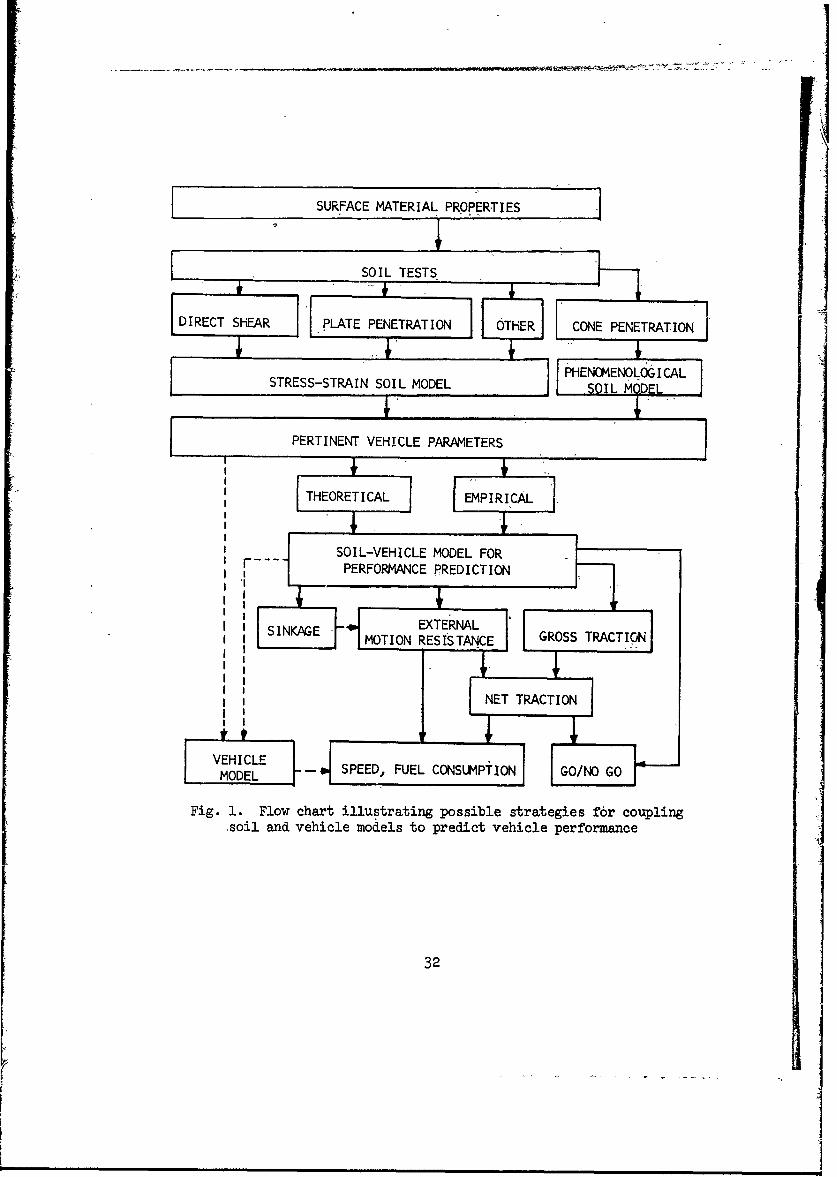
SURFACE MATERIAL PROPERTIES

SOIL TESTS

DIRECT SHEAR PLATE PENETRATION CONE PENETRATION

STRESS-STRAIN SOIL MODEL SH~~OILOEL

PERTINENT VEHICLE PARAMETERS

THEORETICAL EMPIRICAL

SOIL-VEHICLE MODEL FORS.. PERFORMANCE PREDICTION

! .

MONE- S FMOTION RESISTANCE GROSS TRACTION

Fig. 1. Flow chart illustrating possible strategies for coupling,soil and vehicle models to predict vehicle performance

32

I I

I 1

I 1I1 n I n n

model, finite-element and other powerful computer techniques notwithstand-

ing, awaits the statement and validation of suitable constitutive equations

for soils. Such wisdom will probably come, when it does, from more funda-

mental soils and mechanics studies than are now embraced by ongoing soil-

vehicle research.

70. In further discussions it is useful first to consider soil-

vehicle models in terms of the soil models and the vehicle models employed.

A soil model details a quantitative working concept of soil behavior under

load, defines, soil parameters by which to quantify soil strength within

this concept, and, if it is indeed a working model, it specifies procedures

to conduct and interpret tests on a given soil body by means of which

values may be assigned to the soils-system parameters used. Idealizations

and simplifications made in describing the vehicle, or its contact areas

with the soil and their loadings, constitute a vehicle model. Quantifica-

tions of vehicle characteristics that enter this model are the vehicle

parameters. A set of relations between measures of vehicle performance and

some combination of the soil and the vehicle parameters comprises a soil-

vehicle model.

Soil models

71. The common assumption of all soil models, whether explicit or

not, is that the controlling mass soil reaction in vehicle-related behavior

is the soil's shearing resistance, and that this in turn is related to soil

displacements. Freitag et al. summarized the current status of soil model-

ing from the vehicle viewpoint in a paper for the Fourth ASAE Symposium on

Similitude (1969). Tables 4 and 5 are reproduced from this paper. Table 4

lists soil properties and table 5 presents a compilation and classification

of soil-measuring devices. Table 4 includes a number of soil dynamic prop-

erties that are in fact not yet used in any soil-vehicle model, nor evenwidely measured in conjunction with related laboratory research. Principalamong the latter are coefficients reflecting rate dependent shear strength

or viscous behavior, which in most soils will clearly be non-Newtonian, and

probably nonlinear. In addition, viscous reactions may be expected to dif-

fer, sometimes radically, when strains are small and shear rates low, and

when large strains and high shear rates are involved. The dramatic example

33

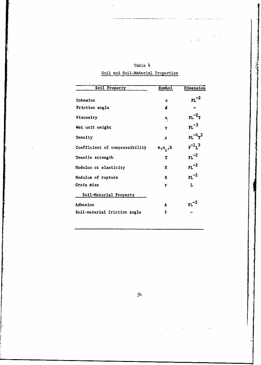
Table 4

Soil and Soil-Material Properties

Soil Property Symbol Dimension

Cohesion c FL 2

Friction angle -

Viscosity FL2 T

Wetunit weight FL 3

Density p FL-4 T2

Coefficient of compressibility m,n ,b F- L3

Tensile strength T FL 2

Modulus ot elasticity E FL- 2

Modulus of rupture: R FL 2

Grainbize r L

Soil-Material Property

Adhesion A FL 2

Soil-material friction angle 6 -

34

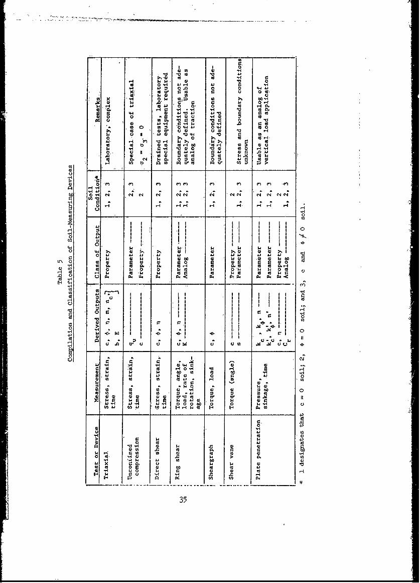
$4$4- ) V3 0i4 3 *0 0 0 4 4

cov r:c 93 0 cd14 0

4 to,- 4.

m x - 0. , A 0 0 41

.) 3 $.4 0~2 OH11-I Aid41 '0 0' 0 C3 1-C

0 0 4-4 @3) 4.O . r. cc@3 0 0 cc rW '1

V a) 0o *a 4- 0 0 3W3 Wa1 "4 CW H 4 " 0 tH

24 4) tr 41 4- 4) V0 >1 0 C, @3 OHU4.' en (3 rv-q 1'~ S.I$4 @3

$4 @H r. @3H "0 D0 10 4) -I 0 WO -O. u A -r Of4J 1v4 0~j- Ai. 4) .041

.0 3 0)3 C @3@ 4) 0C@C 3 cd p @32..co 0. C-4 S..0. 0 3 0 ~ 410 0)1

Clca0 0@ 0' C)a)

t o I

1

4 '4 1 ~ 4 e4 C4. 4 $4.l' $'J $4 1~'

(A -) __)_ -1 0 4)

41.0 m Id -2. Cd P.1 1 .I

A H 2 cc II 22 co I II d

L). 04' A40 04 N 4 2.'4... . 4341 43.1 41 41.

E-10 @3qH 30 @3 20 @02800 3 000 W 0 3

£V2

.r 00 I' I I 2 I

Hr I .0 a, uI u u c im4 cII

4 a -H 44 0 2 I

o: to 2- 0 -H V 14-I* 2 I 4'1 I- M- toa

H~~- a; a03a aaO. a 2.co 0 0' " V :1 0 3 0 .d .£.

@324) 2.4 6 80C) @3 80 mw F; .o A3 0) 4 4 r.

@3 "qa 9 000 £40 0) @34. a (Ha

@3~ ~~ 4- a a.4 2@

4-4

0v 4.@3l

0 cc 14 > 1.t-H 2,4 b44

M@3 0 e 3 4.3 00 dW) .H @3 0. w r.

f4 W- C)4 -H @3 H3 @ 3.00 .. 43 0 2.. W. o.

'v.6 ~ 42.' 4 a) 035

0 04) 0o o ci00)43 ..-

4 4 0 0 (41.' 29 0- 0) @ 0

$1V- (4 0 44 0

.5 ~0 41 V.)0 *-4S-s 0.0. (4,

a)0( 44-4 0-r43 @3-0 m

$4 .4J @3

0-( 0- 4.84 H

00.-H V34 +@3

4~ 4 Cd > 4 0 -0.-40)4-4U

,-0S a i a) C- aH r0r C' 4 04'J C4 l V' 04 e.I 10 W- -

H4 H) H tH -H r Hq H4

H H

0 ) 140 o 0$ 0. 0m 0. 0. 0 3@to (4( 14 0 $4 0 0 0 0 0 0 10Hq (4 04-( p -toi w -w .w -$4 00

L 40A4 40. P4 04 04 N- s~

H 41851

CLI@3

0(4 (H44)

______ ____ _ ____ @4) S-(

'V 'VI @34 10S (4 - asC: r4 (40 E ( 0( - 0 0

4)' 'Va S 0. "4 0 @30 ii (U ~ 4 cc H Si a 4 3 4 0..

04 0.4-44) to 4 (D (v 34) 0 to (4 US- S-o S1V3 C4 v 4( *a 5- w43 0 33J (4S- 0 S(.4(4 @ 034 U@3 0) (4.: 4" V)0(0( AiW 41' H 0 Si (4 U )

(4 4 r4 w to 0. C: Si Ho 10 u @ 044 p t 0$4 4w S-@0Sa3 p3- @3 .-4 (4 -H H) la SsH( t.d(C(

0 >4- 0 >06 w-a U) JO w 0 0 0 @3 @0'4 3.r4S04 54 4 U > N4 04 04

@3T 1 0 i

4 514 0 0 U@> M (4 W ~ @) 4-' 00 *,4 N 0

4) "qU @3@ d 01. 4w0 ( ~ i '4' I V 4)

S-4 605. W3Ss( - 0 0.0 c4S 0. 0 C: 0 S-s Is H %

&j @ S-i to 0H HJ 4) 03U 0Si 1-1 34 (4 r 41 H- y41 Si0) H@3 0. 0 4 H 0 CN SE4 p 0) .H (4 (4M

> on4 z tn 04 s 04

36

7I

of silicone putty, which flows under long-term gravity loads but shatters

on impact, may be onily an extreme illustration of the behavior of manysoils.

72. Pedologically, soils are bodies of material, one of whose most

striking features is stratification in essentially horizontal layers: the

A horizon, the B horizon, etc. In civil engineering work, the upper hori-

zons are normally removed and the assumption made, barring gross anomalies,

that the material is essentially uniform throughout the remainder of the

body. This assumption is not appropriate when considering vehicle perform-

ance. A Vehicle of anything like normal size will deal most of its life

with soils that are distinctly and noticeably stratified. This stratifica-

tion vwill not necessarily follow the pedologic definitions and will in most

cases be potentially more complex. Instead of two or three visibly dis-

cernible horizons, there will usually be considerable variation in strength

ith depth within the soil layers that the vehicle involves. Strength pro-

files will range from thin layers of weak, slippery materials over firm,

strong ones to relatively strong crusts over weak layers, with endless pos-

sible variations between. Some typical cone index profiles for different

types of marginal surface materials from the ground mobility standpoint are

shown in fig. 2. Accordingly, field descriptions "of soils for vehicle pur-

poses must in some way reflect the soil strength profile to a suitable

depth. The "suitable depth" will in general vary with the vehicle size and

weight, its running gear type, the mean level of soil strength, and the

shape of the soil stren-th profile. The profile effect may be incorporated

by presenting complete or idealized profiles or by using various averaging

rules. Field measurements must include sampling in some way over the depth

of interest.

73. The strength of a given soil material ill in general vary with

its water content and its state of compaction or density. It may be

largely affecte. also by its in situ microstructure. The reactions of a

body of this same soil material. in nature or in a system simulation in the

laboratory will, in addition, be affected by its geometry (its boundary

conditions or stratification). When the soil body is greatly disturbed, as

by the passage of a wheel leaving a rut, the boundary conditions are

37

Cone Index

0 10 20 30 40 50 0 50 - 1,0 150 200 250+

1' ______ _______

\ | 3 "° i1 . Padre Islan d , T ax .

2 Makua Beach, Hawaiilama 3 : Camp Vel flet, Mass.

ri. Appomattox RiVer, 7%. I . Yuma, Ai.3'2. Mo' Island, La.- 5 Suscinio Beach, rance..

303 Aihesale Lake, Miss.- 34: Carson Sink, Rev.

____ 5. Bnu._Tland F___ ____

Fine Greined Coarse GrainedInorcanic Soil.

0 5 0 5 200 25 0 0 10 20 30 0 50

1

7 en

1

'" 1 I. -m

rn Legend15 I0 25 Snow Greenlnd

1. Cap Hale, Colo. 1. DMO Sn ow, Greenland

2. Kapsukaain,, Canada 2 Moit 08, Greenland

3. Ft. Churchill, Canada Snow,

0. Houghton, Mich. 30r" 1 3

Subarctic Arctic

00 20 40 60 80 100+

- Legend\. ... 1. Minor Canal, La.

,, 2. Ft. Custer, Mich..3. Coap Petwaowa, Canada

', , . Camp Gagetown. Canada. 5. Farry Sound, Canada

\ SI"'-

0

2

0 IOrganic Soils

Fig. 2. Cone index profiles for different types ofmarginal surface materials

changed for the next wheel, and the in situ microstructure of the soil may

be disturbed to the degree that its strength is also changed. The impor-

tance of the latter effect, soil "remolding," to vehicle performance, espe-

ciaily in marginally weak soils, was demonstrated early in the WES traffic-

ability research. Realism in modeling soils dictates that this phenomenon

be reflected in some way. This is particularly important for the real

world case of a group of vehicles m&oving off-road where the tendency is in

fact to track one another even where terrain or other real constraints do

not force such channeling.

74. The ability of a soil to develop adequate bearing and traction

capacity under the traction elements of ground vehicles is primarily a

function of the shearing resistance of the soil. There are essentially two

methods of describing soil strength for groun mobility purposes and three

soil models that are currently in use in the United States. The soil

models are the WES vehicle cone index (VCI) method, the WES mobility number

method, and the Bekker/LLD method. Both WES methods use a cone penetrom-

eter (fig. 3) to obtain an index -of the shear strength of the soil in terms

of a single number, and the Bekker/LLD method uses a two-part bevameter

(fig. 4) consisting of a plate penetration and an annular ring shear device

for obtaining pressure-sinkage and surface shear strength data, respec-

tively, from which five soil parameters are currently derived.

75. WES VCI soil model. The WES VCI model is wholly empirical. The

surface body of material is described in terms of its general nature (fine-

grained or coarse-grained inorganic soil, organic soil, or snow) and its

profile of resistance to penetration by a small standardized cone (cone

index profile), corrected in soft, fine-grained inorganic soils for de-

creases in strength due to remolding as determined by a remolding test

(equipment is shoi-m in fig. 3). When the remolding test is used to obtain

a remolding index, the soil is described in rating cone index (RCI),* which

* The rating cone index is given by

RCIi = CI i x RIi

where CI= cone index for soil layer "i" and RI. 1.0= remoldingindex for that layer. 1

39

COMPACTION HAMMER

f '1 EMOLII4GTRAFICA. PILITYREMO LING, 0,11 I SAMPLER

A" ~ASE 1

3/8-IN. STAFF

CONE PENE-TROMETER

(S/a-IN. STAFF)

Fig. 3. WES soil trafficability equipment

is the product of the cone index and remolding index for the same soil

layer. While cone penetration resistance is assumed to be a function of

shear strength, no attempt is made to define the specific relation which is

different for the several soil Llasses. An average cone index (CI) over a

"critical layer" appropriate to the vehicle type and weight and the

strength profile of the soil and corrected for remolding as necessary is

usually used in place of the full profile. If the strength of the soil in-

creases with depth in the critical layer and the 6-in. layer below the crit-

ical layer, the standard procedure for determining the critical layer is

4o

*1

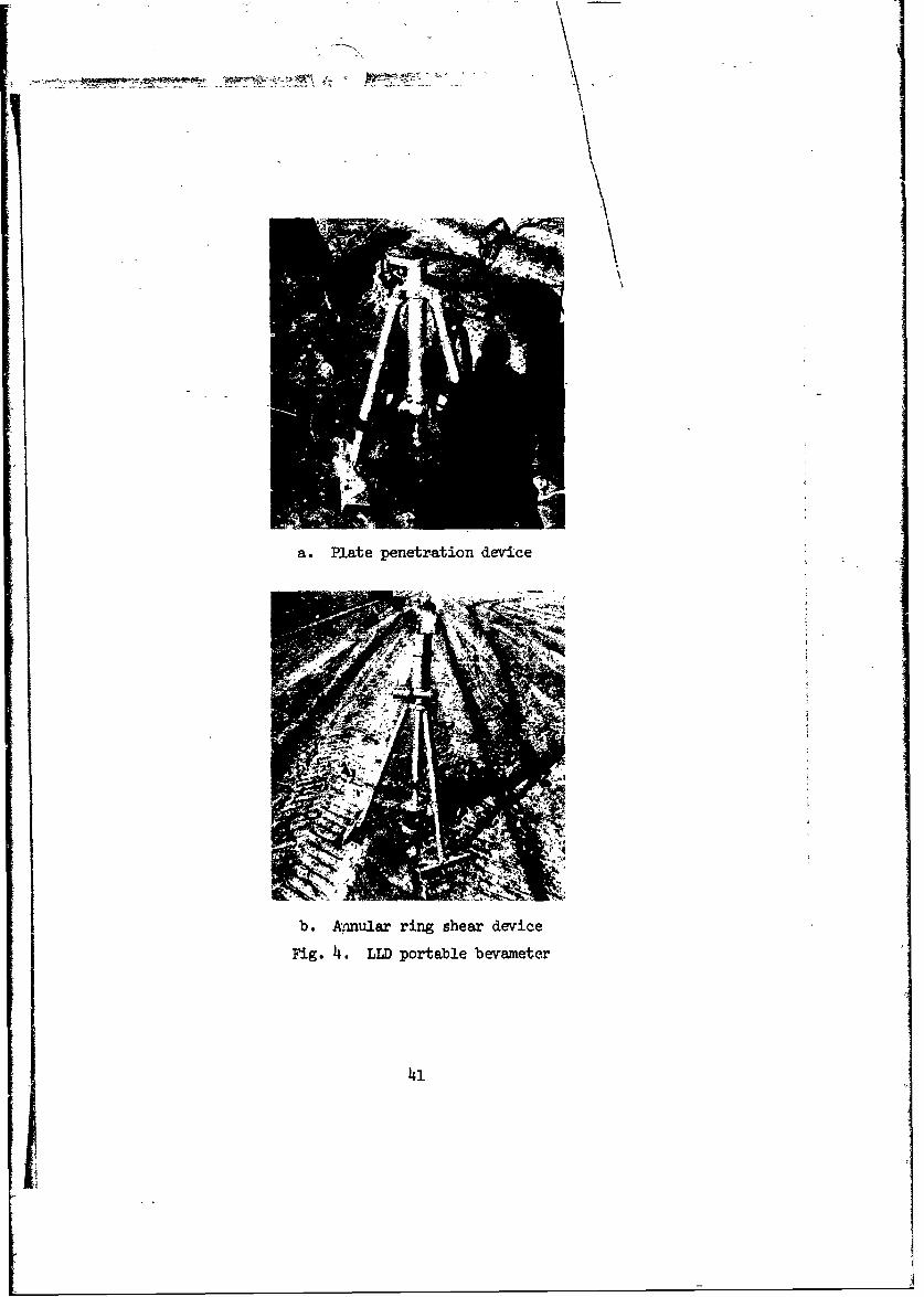
a. Plate penetration device

b.* Annular ring shear device

Fig. 4. LLD portable bevamete'r

used. However, if the 6-in. layer below the critical layer is weaker than

the normal critical layer, the deeper layer is considered to be the criti-

cal layer. In this way and with obvious, considerable loss of information,

the soil. strength at a given point may be expressed, and therefore easily

mapped, in terms of a single quantitative index, plus, as necessary, an in-

dication of the class of materials involved.

76. Considerable terrain mapping has been done on a worldwide basis

using the VCI method. Simplifying procedures have been developed for

crudely estimating changes in cone indexes due to various changes in soil

moisture or, more directly, due to rainfall, drainage, and dryingi Other

procedures have been developed for making reasonable estimates of on-the-

ground cone indexes through air-photo interpretation. An example of the

resolution that can be obtained from good quality, large-scale aerial pho-

tography is shown in table 2, which shows the pap units used in the MERS

study. The indicated level of resolution, which may in fact be even less

in practice, is still really only sufficient to distinguish-three levels of

soil strength for a given vehicle: strong enough, maybe, and too weak.

This is probably as much resolution as can be hoped for for some time to

come unless considerable advances are made in meaningful remote sensing,

and then exploited. More numbers might be added in order to play more elab-

orate games, but improvement in the results would be questionable at best.

77. Over the years considerable field data have been collected from

various parts of the world using the WES VCI method. These data have been

analyzed for the purpose of establishing a soil classificationi system and

procedures for estimating soil moisture content and strength in terms of CI

and RCI for the wet season only. The dry season wab not considered because

soils that undergo seasonal wetting and drying are normally trafficable in

the dry season. The classification system has been applied to soils in

temperate and tropical climates and separate reports have been published.

The classification system and the data available in the reports; have proved

useful in preparing tactical and strategic soil trafficability maps of re-

mote areas of the world.

78. WES mobility numeric soil model. The WES mobility numeric

model is also essentially empirical and, at this time, is applicable to

42

I'

pneumatic-tired vehicles. The mobility numelic model is based upon gen-

eralization of systematic single wheel tests on prepared homogeneous

(uniform strength profiles) laboratory soils through dimensional reason-

ing. Further work is required to improve procedures for predicting multi-

wheeled vehicle performance frum the single wheel results and in defining

soil descriptors for natural soil conditions equivalent to those used to

reduce laboratory results.

79. In sands, both in the laboratory and in the field, penetration-

resistance gradient* is used to characterize soil strength. In labora-

tory clay soil, CI** is used as an index of soil strength. In natural

clay soil, field test data indicate that prediction accuracy was slightly

better when RCI was used rather than CI.

80. Bekker/LLD soil model. This model describes soil responses to

loading in terms of three parameters that reflect soil deformation under

vertical loads, and three more (one of which is currently assumed to be

con:tant) that express the horizontal shearing resistance of the soil as a

function of mean normal pressure and horizontal deformation. The two sets

are treated independently. Horizontal shear parameters (c , , and K)

are extracted from tests with a small grousered annular ring-shear device

by best-fitting the results to a modified version of the Coulomb-

Micklethwait expression whose current form is:

* Penetration resistance gradient (G) is also obtained from tests with

the standard cone penetrometer. It is given by

CI- ci 0G= G= z/2

whereI

CIz = average cone index in the 0- to z-in. soil layer

CIO = cone index when z = 0

z = depth of penetration of the cone base into the soilsurfac e

** Cone index is obtained from tests with the same standard cone pene-

trometer used in the VCI method and is analogous to the ultimate bear-ing capacity of clay. In a clay homogeneous with depth, there is lit-tle change in cone penetration resistance after the base of the conepasses below the soil surface.

i 43

Fa

-r= (c + p tan#) (il-J " K) (e)

where

T = mean shear stress

p = mean ground pressure on shear area

J = horizontal travel of shear elements from initial position

The parameters c and are clearly analogous to soil cohesion and angle

of internal friction as used in engineering soil mechanics, but values.

measured by this method in a given soil do not duplicate those obtained bysuch more familiar soil mechanics procedures as the triaxiaL test. The

parameter K tends to give calculated curves of vehicle pull versus slip a

reasonable shape, but is erratic in practice, and is 'highly instrument-

dependent. In the most recent field correlation study, values of K de-

rived from actual ring-shear tests were not used, and K was instead as-

sumed constant and equal to one (inch)..

81. Vertical deformation parameters for a soil are derived by force-

fitting results from pressure-penetration tests with small flat plates of

two or more diameters to the equation, traceable to Bernstein via

Goriatchkin:

p= n (2)

where

p = average pressure

z = depth of plate penetration from the surface

k kc + k

r = plate radius

and kc k , and n are the soil response parameters. The plate tests

appear to give results that correlate with vehicle tests in the laboratory

but not in the field. This is probably due to variations in soil strength

profile with depth, which are always present in the field (and seldom in

well-run laboratories), whose influence upon a vehicle cannot properly be

sensed by small plates penetrating only a few inches below the soil surface.

82. Extensive publication of the Bekker/LLD soil value system has

44

I

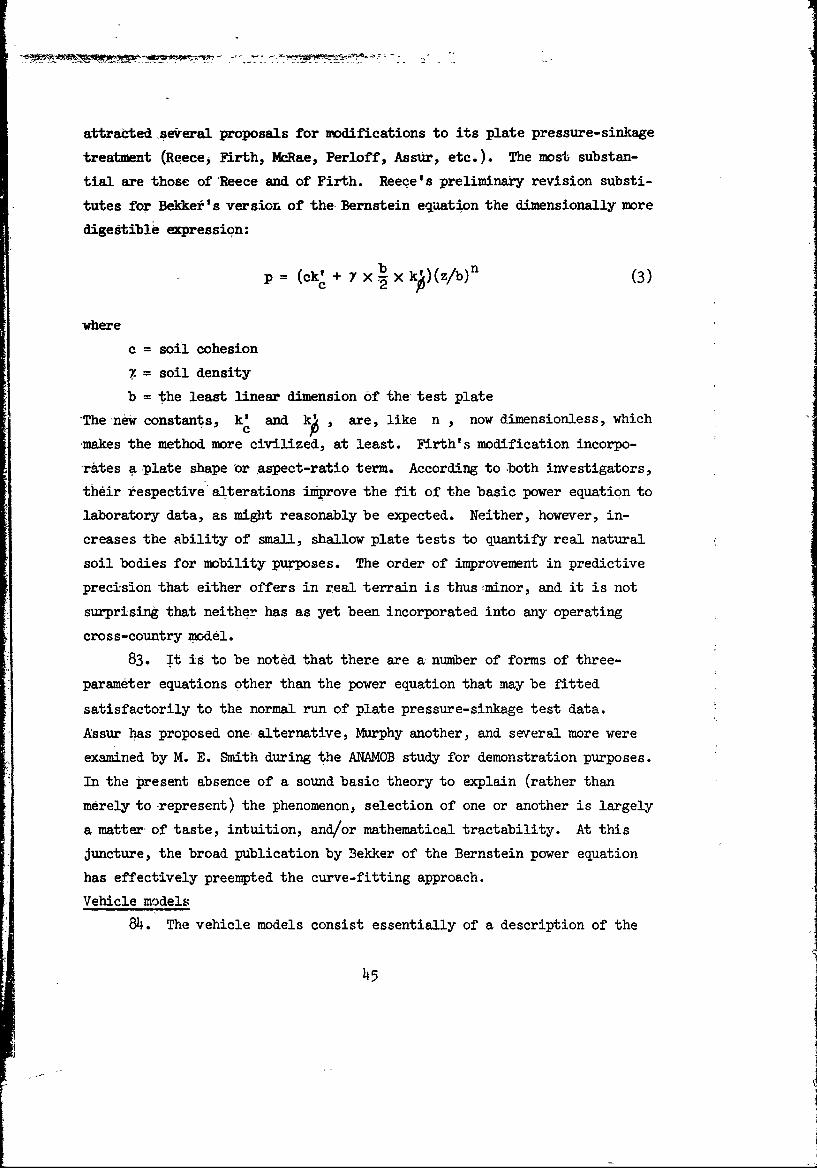
attracted several proposals for modifications to its plate pressure-sinkage

treatment (Reece, Firth, McRae, Perloff, Assur, etc.). The most substan-

tial are those of Reece and of Firth. Reece's preliminary revision substi-

tutes for Bekker's version of the Bernstein equation the dimensionally more

digestible expression:

p, +Yx k (z/bn (3)

where

c = soil cohesion

= soil density

b = the least linear dimension of the test plate'The new constants, k' and k' , are, like n , now dimensionless, whichc

makes the method more civilized, at least. Firth's modification incorpo-

rates a plate shape 'or aspect-ratio term. According to both investigators,their respective alterations improve the fit of the basic power equation tolaboratory data, as might reasonably be expected. Neither, however, in-

creases the ability of small, shallow plate tests to quantify real natural

soil bodies for mobility purposes. The order of improvement in predictive

precision that either offers in real terrain is thus minor, and it is not

surprising that neither has as yet been incorporated into any operating

cross-country model.

83. It is to be noted that there are a number of forms of three-

parameter equations other than the power equation that -may be fitted

satisfactorily to the normal run of plate pressure-sinkage test data.

Assur has proposed one alternative, Murphy another, and several more were

examined by M. E. Smith during the ANAMOB study for demonstration purposes.

In the present absence of a sound basic theory to explain (rather than

merely to represent) the phenomenon, selection of one or another is largely

a matter of taste, intuition, and/or mathematical tractability. At this

juncture, the broad publication by Bekker of the Bernstein power equation

has effectively preempted the curve-fitting approach.

Vehicle models

84. The vehicle models consist essentially of a description of the

45

vehicle design and potential contact areas with I .hw .il- and the', load-

ings, in an idealized and simplified form compatible w-vh a particular soil-

vehicle model. Thus, the vehicle characteristics used arb dictated from a

soil point of view. Most laboratory work has been with scale vehicle

models or with single traction elements, either scaled or prototype. TheBekker/LLD method has evolved prixiarily from small-scale laboratory tests,

the WES VCI method from prototype natural soil tests, and the WES mobility

number from laboratory single-pneumatic-wheel tests.

85. In a vehicle sense, a vehicle model also includes a straightfor-

ward automotive engineering model relating speed to vehicle engine and

power train-torque characteristics or to total traction available for pro-

pelling the vehicle. All comprehensive models incorporate such a submodel

as a base line from which terrain demands for traction force required to

overcome resisting forces are subtracted.

86. Data for speed-traction force models are- usually available for

all vehicles that have undergone engineering tests at Aberdeen Proving

Ground (APG). This test is run on a level, paved surface in all forward

gears.

87. If -performance test data are not available, a speed-traction

force model can be computed from engineering data in the form of a curve

relating transmission torque outnut to transmission rpm, output -provided by

the manufacturer. Traction coefficients and speeds can be computed for se-

lected transmission torque-speed output pairs using the following simple

equations:

Xf t x D gc RxW

where

T = traction force coefficientcI = overall power train efficiency

= transmission torque output, ft-lb

D = linal drive gear reduction ratiogRW = pitch radius of drive wheel or sprocket, ft

W = gross vehicle weight, lb

46

and

and=0.6818 x x C (5)

D

where

St = track or wheel speed, mph

rps = transmission output

C = circumference of drive wheel or sprocket, ftw

Maximum traction coefficient on a paved surface is usually limited to about

0.80, at which level tire or track slip will approach 15 percent. For

traction levels below about 0.60, slip is small, and track or wheel and

road speeds are considered to be equal.

Soil-vehicle models

88. The mechanics involved in coupling soil and vehicle models to

predict vehicle performance on a smooth, level soil surface are outlined in

fig,. I. All soil-vehicle models specify a set of surface material proper-

ties for which-soil tests are conducted to obtain the pertinent data, and

implicitly or otherwise, involve a soil model to arrive at the necessary

soil descriptors. The soil model is coupled with pertinent vehicle param-

eters. to form, theoretically or empirically, a soil-vehicle model from

which predictions are made. Go-no go performance may be predicted directly

from a soil-vehicle model or handled by comparing available traction to

total impedance. Vehicle speed is more usually computed by first determin-

ing external motion resistance and gross traction and subsequently adjust-

ing the traction to the level required to propel the vehicle. Details of

the soil-vehicle models discussed in the following paragraphs are presented

in Appendix A.

89. WES VCI soil-vehicle model. The WES VCI soil-vehicle model pre-

dicts the performance of a vehicle in terms of go or no go for a prescribed

number of passes (usually 1 and 50) over the same soil traveling in a

straight-line path. The model also predicts the maximum drawbar pull and

maximum slope negotiable, and motion resistance, for soils with strengths

above the minimum needed to just go. To be adequate for passage of a ve-

hicle, a soil must have sufficient bearing capacity to prevent the vehicle

47

from sinking too deeply and sufficient traction capacity to provide the

thrust needed to ovaxcome the motion resistance generated in rut formation,

slope climbing, obstacle negotiation, etc. Bearing and traction capacities

are both functions of the shear strength of soil. Traction failure can

occur on a soil having high bearing strength and with little vehicle sink-

age. Sinkage failure to the point of vehicle immobilization is always ac-

companied by traction failure.

90. Soil strength is measured empirically in terms. of cone index

(CI) and remolding index (RI), and when remolding index is used, soil

strength is expressed in terms of rating cone index (RCI). For coarse-

grained soils, organic soils, and snow, vehicle performance is related to

CI; and for fine-grained soils, it is related to RCI. Empirically derived

equations and graphs and' their use to relate strength of inorganic soils to

vehicle performance are given in Appendix A. The system has been used ex-

tensively by WES in conduct of mobility research programs. It has been

used in a number of studies including Swamp Fox I and II, REVAL WHEELS,

Wheeltrack, RAMS, 1/2-ton carrier developmient program, and RAC analysis of

Surface Cross-Country Vehicles in Vietnam. The system has also been used

to iescribe terrain conditions for QMR's and SDR's.

91. WES mobility numeric soil-vehicle model. The basic WES numeric

soil-vehicle model was developed frcu a dimensional analysis of results ob-

tained in single-wheel laboratory tests in hcmogeneous sand and clay soil.

The WES sand mobility numeric is

G (bd )3/2 8ITS= W Xh

where

G = average rate of increase of cone index with depth in sand

b = tire section width

d = tire diameter

W = load on tire

8 = tire deflection

h = tire section height

48

The original WES clay numeric was developed from test data with toroidal

tires only and took the form

IT = \Cb " 6 / 2 (7)

where C = average CI in the 0- to 6-in. layer. Analysis of later test

data showed that the performance of tires of a wide range of b/d values

*was Tpedicted best by

7 - (7a)

Performance* coefficients (pull/load and towed force/load) are each related

to the mobility numeric by curves derived from extensive laboratory tests.

92. An anlysis of data from prototype vehicle tests in natural clay

isoil showed that slightly better predictions were obtained using RCI rather

than CI. Therefore, the revised clay numeric used for prototype vehicles

on natural clay soil is

C Ib

The general curves and equations for vehicle performance in the field are

shown in fig. A8, Appendix A. The curves used in the design** of the NEXA

Vehicles shown in fig4 A9, Appendix A, were based on the original clay

numeric (the original numeric was the only one that existed at the time

the INEA vehicles were designed). The abscissa of these curves is the

reciprocal of the original clay numeric.

93. Several types of equations have been written to express the em-

pirical relation of performance to the clay mobility numeric. Two equa-

tions for rectangular hyperbola that reasonably approximate the experimental

relation of the pull coefficient and the towed coefficient to the sand mo-

bility numeric are given in fig. A10, Appendix A.

* In this model the optimum vehicle performance is considered to be in

the vicinity of 20 percent slip. While the approach and supporting datapermit predictions at other slips, predictions of pull, torque, andsinkage are usually made for the 20 percent slip point only.' The obvious reason for offsetting the curves was to have a "built-in"safety factor.

49

94. Bekker/LLD soil-vehicle.model(s)zi The Be er/LLD soil-vehicle

model assumes implicitly that the plates used in penetration tests are

simple analogs of the running gear of tracked vehicles and wheeled vehicles

equipped with relatively large, deflected tires. The mathematical model,

p = kzn , used to represent the results of plate penetration tests, be-

comes the basic mathematical model for tracks and large tires as well.

Solving the p-z relation for z , the uniform sinkage relation for

tracks and large tires is

z = ( -l.n (W/Ak)l/n (8)

where

z = sinkage

p = pressure

k = 1%/b k

n = exponent of sinkage

W = load per tractive element

A = bL for track: b = width, A = length;

for wheel: b* = maximum width of unloaded tire,= 2 V8(D - 8)

where D = diameter and 8 = deflection.

Motion resistance (R) per tractive element in all cases is the same and is

the sum of compaction resistance (Rc), gravitational resistance (R.), and

mechanical rolling resistance of suspension components (R ).** A bulldoz-

ing term, used at one time, is no longer applicable to R•

95. The Bekker/LLD soil-vehicle model assumes that the action re-

corded in ring-shear tests simulates the shearing action between the run-

ning gear of vehicles and the soil. The mathematical expression (eq 3-)

used to represent the results of a ring-shear test is accordingly consid-

ered to be the basic model for vehicle response. Equations- for vehicle

traction under various conditions that are derived from this expression are

listed in Appendix A. In its present form, the Bekker/LL soil-vehicle

* Sometimes b = minor axis of the ellipse representing the print of atire.

• R7 for an existing vehicle is usually obtained from the vehicle manu-facturer or APG engineering tests.

50

model relates gross traction and slip in the equation

KIH (Ac + W tan (9)- - -e

where

K = tangent modulus of deformation

s = slip ratio

c and X are soil cohesion and friction, respectively, as measuredby the ring-shear apparatus

96. Probably the greatest difficulty in using the Bekker/LLD model

arises in deciding what equations should be applied to a specific set of

conditions. For example, the equations used for predicting the performance

of rigid wheels differ from those used for predicting the performance of de-

flected wheels. Both are used on occasion for pneumatic tires. The diffi-

culty arises because a tire on a yielding surface may assume any shape be-

tween that of a rigid wheel and that of a deflecting wheel on a hard sur-

face, depending on the relative stiffness of the tire and the surface.* Pre-

sumably the true condition will be bounded by the two extreme assumptions.

However, in the absence of quantitative guidelines for making this selec-

tion, one investigator may select the rigid-wheel equations and another the

deflected-wheel equations for the same set of conditions and obtain signif-

icantly different prediction values from the same set of input data. This

may or may not be important when the model is used only to compare the per-

formance of a group of vehicles for a given soil condition, but becomes of

clear importance when actual performance of one vehicle must be predicted.

97. Reece modified the Bekker/LLD equation for total traction as re-

lated to slip by including an expression for frictional thrust from the

sides of a grousered track or wheel. Appendix A lists both equations.

98. WES-WNBE soil-vehicle model. The WES-WNRE soil-vehicle model

was developed basically along the lines of the WES VCI system, but solely

for one-pass performance predictions. In addition to computing go or no go,

* On an unyielding surface, only the tire yields to the pressure of the

load carried by the tire, whereas on a soil surface both the tire and thesoil yield. When a tire is operating in a soft soil, the yielding of thesoil may be sufficient to allow very little yielding of the tire. Inthis case, the shape of the tire is similar to that of a rigid tire.(See WES Technical Report No. 3-516, Report 3.)

51

the model includes an equation for predicting soil strength, in cone indexterms, required to permit one pass of a vehicle in unaccelerated, straight-

line motion over smooth, level soil, and the soil-generated component of

its motion resistance. These relations were developed empirically from

tests of a variety of medium and lightweight military vehicles in fine-

* grained soils. They have served as an interim basis for making first-pass

performance predictions and were adapted by WNRE to the needs of two subse-

quent vehicle go-no go mapping studies.

99. WNRE-CAL soil-vehicle model. This model was designed to utilize

soil strength data in the form given in the WES/ARPA MERS surface composi-

tion factor maps of selected areas in Thailand. In these maps soil mass

strength is presented in cone index terms, and surface tractive capacity by

values for the direct shear parameters c and • The WNRE-CAL model

joins the now-conventional Micklethwait-Coulomb assuniptions for gtoss trc s-

tion with the WNRE-WES projection of motion resistance (paragraph 98) to

predict vehicle net traction. It was first used in a computer program to

prepare go-no go maps for specific vehicles operating in terrain prescribedaccording to the quantitative descriptive system used in the MERS factorfamily maps. It was more recently adapted -for use in a conceptually simi-

lar go-no go study of lunar vehicles in lunar landscapes. There has been

no experimental verification of the reliability of the WNRE-CAL model.

100. Perloff soil-vehicle model. This model was developed to pro-

vide soft-soil mobility input to a digital computer simulation of tank-to-

tank combat intended for tank design evaluations. When this study began in

1960, Perloff concluded that neither the Bekker/LLD formulations for

tracked vehicle performance in soft soils nor then-extant procedures for

expanding scale-model results to full-size predictions were acceptable.

The new model he proposed as a result accepts one-dimensional pressure-

sinkage relations generalized from observations on small-scale models (or

from any other source) and by computer iteration determines a vehicle sink-

age and trim that satisfy its requirements plus those of static equilibrium,

including a slope component. Traction and slip are computed for the result-

ing equilibrium track sinkage and attitude on the- basis of an approximate

shear stress/strain relation derived from a traction oriented analysis of

52

soil direct shear test results. Despite its considerable complexity, the

Perloff model treats the effects of tractive and normal forces as independ-

ent within a two-dimensional static framework, which makes it fundamentally

as suspect as the less pretentious models it was intended to supplant.

Since there have been -o deminstrations of the predictive eccuracy of the

Perloff model, of the usefulness of the several elaborate new assumptions

it employs, or even of practical means to measure in the field the soil pa-

rameters involved, this model is not considered a serious candidate for use

in a complete vehicle cross-country performance simulation at this time.

Equations pertinent to the explanation of the system are listed in Appen-

dixA.

101. Lunar models. Several agencies and/or individuals have devel-

oped computer programs or models -for NASA lunar roving vehicle studies.

The soil-vehicle interaction used in these models in most instances is a

simplified version of one or another of the soil-vehicle models discussed.

For example, one study cites Assur's pressure-sinkage relations but a lin-

ear relation is actually used. In the other cases, the Bekker system is

frequently cited but not strictly adhered to. In no case prior to a modest

program begun by NASA at WES early in 1970 was any attempt made to validate

the soil-vehicle interaction part of the analytical model objectively. The

work of agencies that fall into this category are Chrysler, Brown Engineer-

ing, Bendix. Grumman, Cornell Aeronautical Laboratory, and Booz-Allen.

102. British s6il-vehicle model. Using essentially the classic soil

mechanics soil model, Uffelmann derived equations for maximum drawbar pull

for tracked vehicles and rigid wheels. These employed Micklethwait's equa-

tion for maximum tractive effort and include a corrention for slope angle

of the terrain. Uffelmann's equation for motion resistance for tracked ve-

hicles and rigid wheels in sand is derived by using Bekker's equation for

motion resistance to estimate an unknown power function which he postulated.

Equations for motion resistance and sinkage in clay of tracked vehicles as-

sume Evans' theory (1950). These and other equations are listed in Appen-

dix A. Laboratory verification of the wheeled vehicle relations on uniform

remolded clays is reported in the literature. Confirmatory field trials of

the Evans' tracked vehicle equations were reported.

53 i1

103. Other soil-vehicle models. The works of CARDE/Dickerson,

Eklund, and Kraft-LumingDayton were reviewed but are not included because

they are not pertinent to the discussions of the analytical models nor are

they complete models.

Verification

104. In conducting the literature review for this study, the litera-

ture that contained measured and predicted off.road prototype vehicle per-

formance and soil data that could be used in an objective evaluation of the

prediction accuracy of soil-vehicle models was sorted out for study. The

specific vehicle performance parameters of interest in the sorting process

were minimum soil strength requirements in terms of VCI, drawbar pull,

gradeability, motion resistance, and sinkage. Gradeability was included

because of its association with drawbar pull performance prediction; i.e.,

the tangent of the maximum slope angle negotiable can be -closely estimated

from the drawbar pull coefficient. In addition to the requirements Set

forth for vehicle performance and accompanying soil data, the- data were

also assembled as to the 'applicability of the model to vehicle and soil

types.

105. Selection of field test programs. The vehicle field test exer-

cises selected for preliminary study included Project Wheeltrack (1963),

Swamp Fox II (1964), MERS One-Pass Program (1965), Keeweenaw Tracked Ve-

hicle Speed Tests (1969), and Mobility Exercise A (1965-1970). A prelimi-

nary examination of the exercises revealed that except for the MEXA program,

only the Bekker/LLD and the WES VOI soil-vehicle models were employed end,

that several versions of the models were used in evaluating measured versus

selected predictic;.i performance parameters. With the advent of the MEXA

program, the WES mobility number models were used in the design phase and

later exposed to the prediction evaluation phase of the program.

106. At first glance, it appeared that the field exercises reviewed

contained considerable soil-vehicle test data to perform an appraisal of

soil-vehicle models cited, but when the data were organized in a manner re-

quired to produce a meaningful evaluation, the resultant data were minimal

for reasons stated in paragraphs 56 and 57. Similar difficulties were alro

expressed by Pleuthner (1969) in his recent report on a critique on the

54

performance of off-road vehicles, full-scale test results, and prediction

method evaluation. In the final analysis, it was decided to use only the

1MEXA data to conduct an evaluation of prediction accuracy of soil models

because the data met mbst of the evaluation objectives set forth. Of equal

importance was the fact that the MEXA data permitted checking the most re-

cent versions of three soil-vehicle performance prediction models (WES VCI,

WES mobility , number, and Bekker/L!D) used in current vehicle design and

evaluation studies.

107. Before discussing the MEXA program, some general comments are

presented regarding the limitations of past off-road vehicle testing and

reporting with the hope that these comments will help to improve future ve-

hice testing programs, at least to a point that the data produced will be

more reliable and useful for model verification. The test programs and re-

ports reviewed were not planned to permit an orderly assessment of the va-

lidity of the model or models used. Usually all the performance parameters

of a given model were not tested. Frequently, a field judgment was made by

the project leadier to collect only minimal data, thus allowing only a check

of a simplified or old version of the model. VCI and drawbar pull tests

are the most common performance parameters found in the literature. Motion

resistance and sinkage seldom accompany drawvar pull data for the same soil

condition. Some slope climbing and speed tests with accompanying soil data

are reported. Between and within exercises, testing procedures varied in

the number, type, and spacing of soil strength measurements made; in con-

ducting the vehicle test; and in recording and reducing vehicle response

measurements. Most field tests are reported in summary type reports and

are incomplete in detail of testing procedures, presentation of actual data

measurements, model used and any modification made, sample computations,

and a listing of all measured and predicted performance for comparative

purposes.

108. MEXA program. In 1964 the MEXA program was initiated by the

late R. R. Philippe and conducted at Vicksburg, Miss., to consider the var-

ious quantitative elements of the off-road ground mobility problem by a

group of experts in the field. The specific purpose of the program was to

design three vehicles capable of carrying a 2-1/2-ton payload with

55

approximately a 50 percent improvement in soft-soil performance over con-

ventional military vehicles. The design soil strength selected- was an RdI

of 7, which is just adequate for a man to walk on with some difficulty.

Methods of design based on research studies at WES and LID, TACOM, were em-

ployed to specify vehicle traction components that would yield the desired

soft-soil performance. The final configurations were two wheeled vehicle

concepts and one tracked vehicle concept that reflected chiefly the soft-

soil requirements, but other requirements such as obstacle- performande were

also considered in the design. One requirement was the development, of a

design that would utilize a minimum of new components.

109. After the test beds proposed in the NMEXA study were fabricated

and delivered, a second meeting of the expert group was held to design ind

implement a field program for testing the three vehicle test beds. The

primary purpose of the test program was to evaluate the methods used in the

design, compare the performance of the M]xk test beds with thst of approxi-

mately comparable conventional military vehicles on smooth, level surfaces,

and check or develop pertinent terrain-vehicle relations as required in

analytical modeling of vehicle performance in terms of speed. The MEA' and-

military vehicles used in the test program are shown in figs. 5 and 6, re-

spectively. Pertinent characteristics of these vehicles are given in

table 6.

110. Most of the field tests in soft soils were conducted at Carson

Sink and Four Mile Flat Playa areas near Fallon, Nev. Tests were run in

smooth, bare, level, soil--near ideal field soil conditions. The soil vas

a heavy clay, and the strength range was sufficient to determine no go and

a degree of go for the go conditions for all vehicles tested.

111. One object in the program was to examine the accuracy of the

several soil-vehicle performance calculation procedures originally used in

the preliminary design, and, if sufficient data were available, to modify

or refine the prediction procedures to achieve improvement in prediction

accuracy. Where revisions were made, they are identified as such in the

comparative analysis. In order to ensure that supporting soil measurements

and predictions were made in the most acceptable manner, personnel familiar

with each model were involved in the vehicle tests, in making the in situ

56

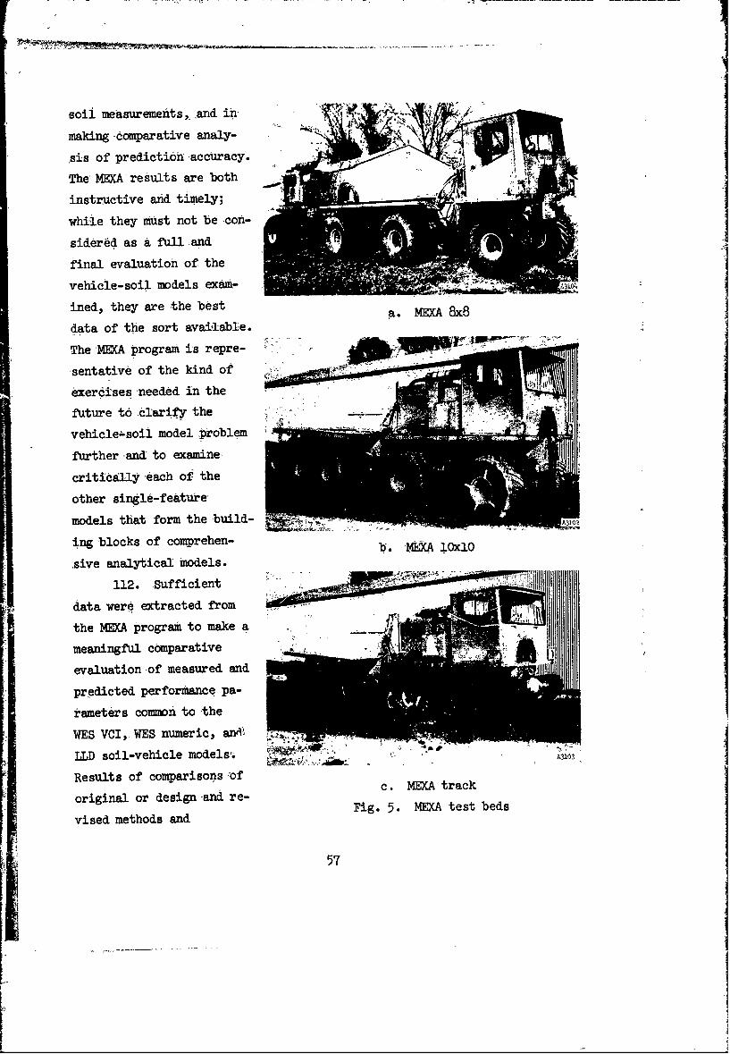
soil measurements,, and in-A

making -comparative analy-

sis of prediction accuracy.

TheF MEXA results are both

instructive and timely;

while they must not be -con-

sidered as a full and

final evaluation of the

vehicle-soil models exam-ined, they are the best a. mX M

data of the sort available.

The MEXA program is repre-

sentative of the kind of 0

exercises needed in the

future to clarify the

vehicle-soil model problem

further and to examine-

critically each of the

other single-feature

models that form the build- A 0

ing blocks of comprehen- b. *YA lOxlO

sive analytical models.

112. Sufficient 1111111data werei extracted from

the MEXA program to make a

meaningful comparative

evaluation of measured and

predicted performance pa-

rameters common to the

WES VCI, WES numeric, an&i

LLD soil-vehicle models. .. AV

Results of comparisons of c. MEXA track

original or design and re- Fig. 5. MEffDA test beds

vised methods and

57

comparisons of methods are

presented along with per-

tinent coments. In all

cases computations were

made using the final vehi-

cle characteristics and

(where appropriate) meas-

ured soil values in essen-

tially the same equations

utilized in developing the

preliminary designs as

a. XM4lOEI outlined in the first MEXA

report. Data from which

the graphical comparisons

Mof measured and predicted

results were prepared are

not presented in the re-

port; they are available

at the WES. The MEXA re-

sults have suggested some

refinements to each of the

models considered, both to

b. M35A2 those who have been work-

ing with each particular

system and to those who

have been looking over

their shoulders.

113. Evaluation of

soil-vehicle model perform-

ance parameters (NM~xdata). First-pass perform-

c. N13 ance parameters used in

Fig. 6. Military vehicles used in tEXA te soil-vehicle models

test program examined that were

58

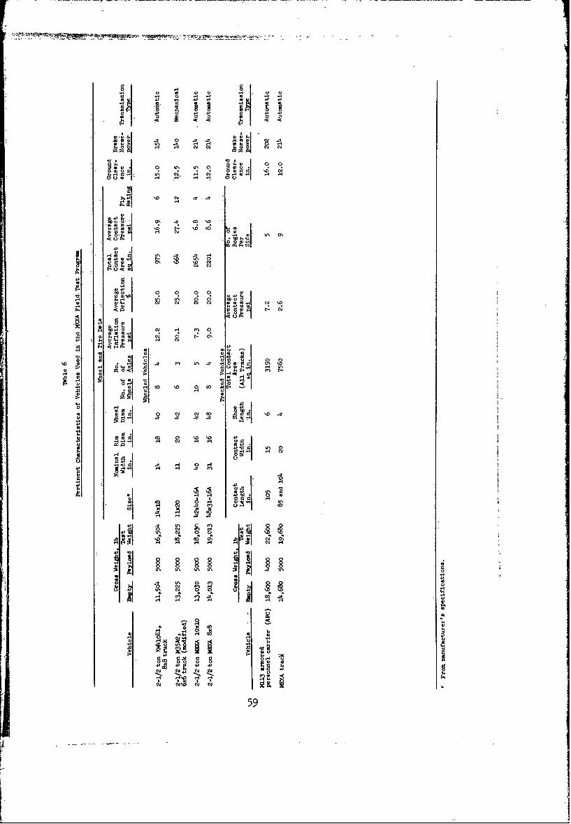
u -4

:r 0 so0 0

0 Lr 4,l

oo04, 04 14,,4

lo I cu I )a

1? 00 Q4 0 -C 001 N .

'A.~4 u% UN 0- H boS. 1 0 -:.04 0 u H l H v N 1 0 1

4

A 1 0 '00

0' x1.H0..-II.> IA N -4

o2 '0 Nv4 .

0' co \0 )co

4,~'. 0 v cv c ID T'

.1.4

~00 0 ' '0 N4

004.. N

N N N N o.

o 510 I 1

4,D 00j

.P 4. 4 1 H

o- .0 00o

0 0. 00 S.

'0. 0 01 H H4, .159

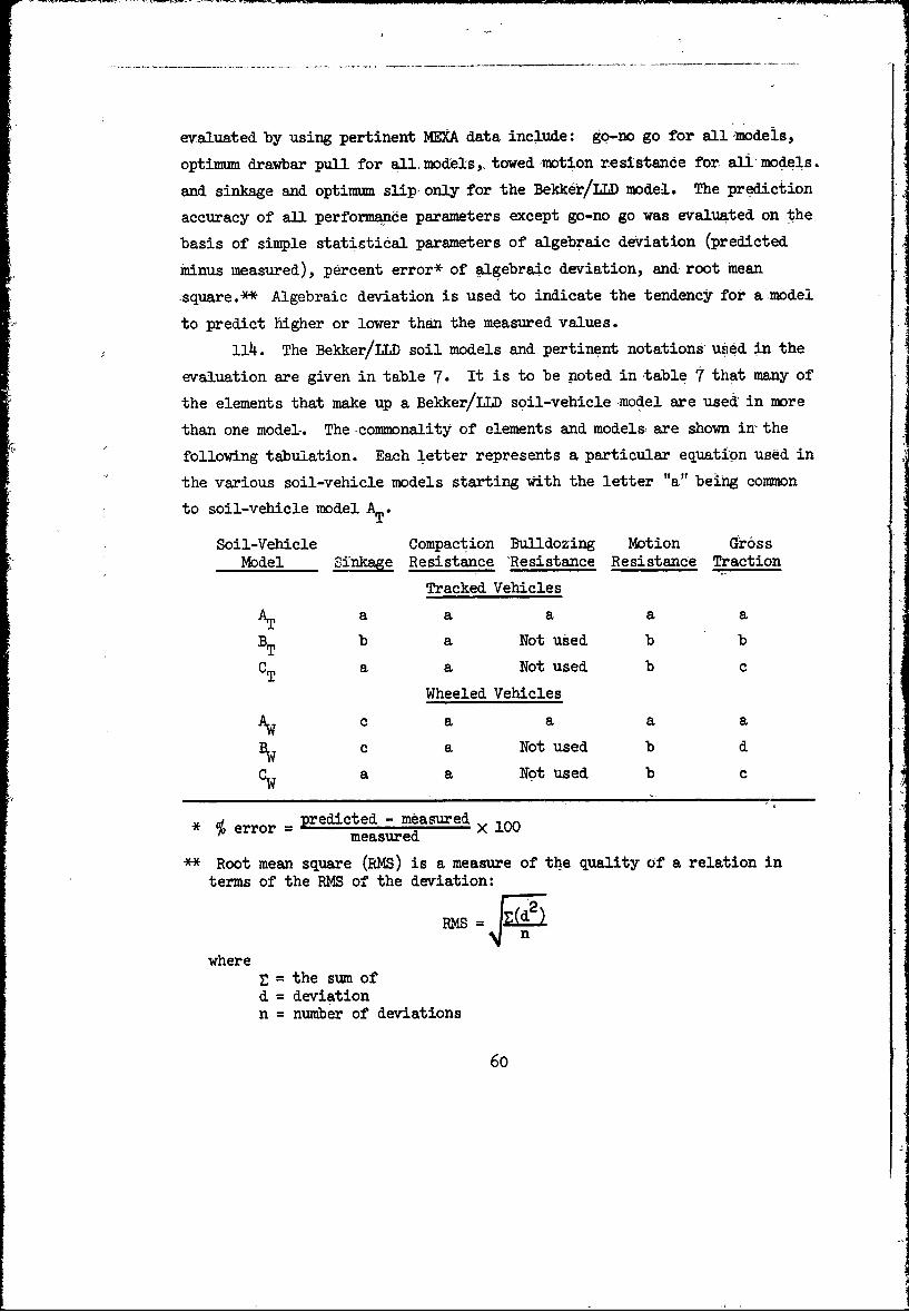
evaluated by using pertinent MEXA data include: go-no go for allmodels,

optimum drawbar pull for all. models,, towed ,motion resistance for a models.

and sinkage and optimum slip- only for the Bekker/LLD model. The prediction

accuracy of all performance parameters except go-no go was evaluated on the

basis of simple statistical parameters of algebraic deviation (predicted

minus measured), percent error* of algebraic deviation, and root mean

-square.** Algebraic deviation is used to indicate the tendency for a -model

to predict higher or lower than the measured values.

114. The Bekker/ILD soil models and pertinent notations u.ed in the

evaluation are given in table 7. It is to be noted in table 7 that many of

the elements that make up a Bekker/LLD soil-vehicle model are used in more

than one model. The -commonality of elements and models are shown in the

following tabulation. Each letter represents a particular equation used in

the various soil-vehicle models starting with the letter "a" being common

to soil-vehicle model AT.

Soil-Vehicle Compaction Bulldozing Motion GrossModel Sinkage Resistance 'Resistance Resistance Traction

Tracked Vehicles

AT a a a a a

BT b a Not used b b

CT a a Not used b c

Wheeled Vehicles

AW c a a a a

BW c a Not used b d

OW a a Not used b c

% error -predicted - measured X 100measured

** Root mean square (RMS) is a measure of the quality of a relation in

terms of the RMS of the deviation:

where= the sum of

d = deviationn = number of deviations

6o

Soil-Vehicle Compaction Bulldozing

Model Sinkage Resistance Resistance

1

AT Z R c z -)Rb =b (2zcKb.+YzK) K

z n + I)W k_ = n+l1 kn~ -i -

BT m Akl= n l ] Rc = (nL) m Not used

I) , -~ +l

CT z = n Rc njZ Not usedAk

Compaction BulldozingMethod Sinkage Resistance Resistance

2W ==bk~k =! n+1 b(2zc + yz2K

-__ __ __W___ 2n____ R c \n_ zb ~ + e

2_______2n+1 bk n+l

BW____ R a Zl- Not used-

I .(W fl Not Used

List of Symbols .

W = weight on the tractive element, lb 6 = tire deflec, 4

b = nominal tire width or tv'ack width, in. = bulk densit

9 a chord length..2 D-- 2 8 ) 8 for wheels or A = computed cd

track length ground contact p = computed gri_n a sinkage exponent, dimensionless z = sinkae, ir"

k = soil consistency, k -- c + k*, Ib/in. n+2 zm = naximun srt2 b R = compaction

o = cohesion, 4b/in. R = bulldozing• - angle of integral friction, deg

1% and coefficient of bulldozing resistance, dimensionless H = gotaciF.gross traci

K b .l r w a utangent modulus of deformation, in. D = drawbar p <K D = tire diamel

s = slip, dimensionless e = angle that

e- a Naperian logarithm (base '2.718), dimensionless

?

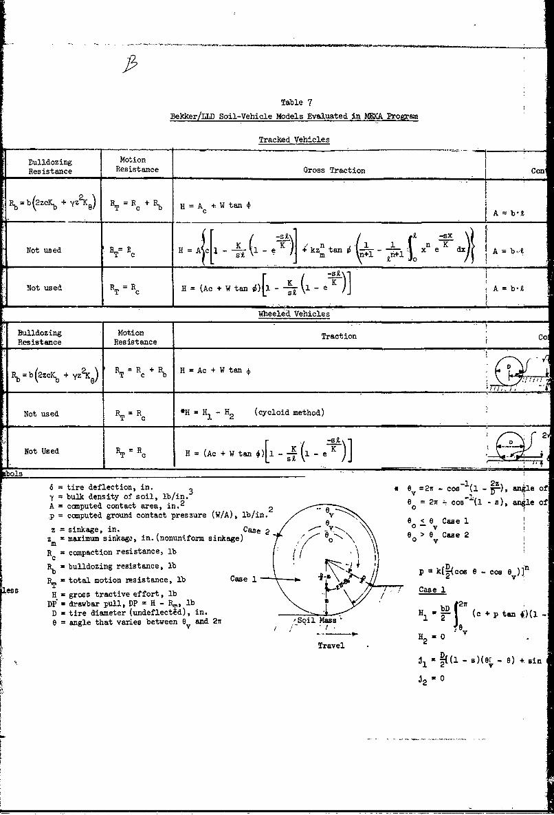
Table 7

Bekker/LLD Soil-Vehicle Models Evaluated in MEXA Program

Tracked Vehicles

.ulldozing Mo.ionResistance I Resistance Gross Traction Con

Rb=b(2zcKb + YAe) RT =Rc + Rb H= A +W tan A =b"

Not used RT- c H=4c[1 (1 e + kzn tan 1 en A =b-IS1m n P f+l 0

Not used R =R H = (Ac + W tan 0)[ K - - -A b-

Wheeled Vehicles

Bulldozing Motion Traction CResistance Resistance T

Rb=b(2zcKb + yz2 k9 ) RT = Rc + Rb H =Ac + W tan -

Not used RT Rc *H= H - H2 (cycloid method)

Not Used RT R c H (Ac + W tan ) [ - K

L

kbols ___"

6 = tire deflection, in. e =2r- cos (l -Z-), angle of

Y = bulk density of soil, lb/in. 3

A = computed contact area, in. 2 6o = 2w cos-"(l - a), angle of

p = computed ground contact pressure (W/A), lb/in. 2 Ca

z = sinkage, in. Case 2 0 vz = maximum sinkage, in. (nonuniform sinkage) "> C

Rc compaction resistance, lb

Rb = bulldozing resistance, lb p

RT = total motion resistance, lb Case I k[(co ev-csH = groes tractive effort, ib -- Caei:

Dl' -drawbar pull, DP = H - RT, lb bD 2n cD = tire diameter (undeflected), in. He = angle that varies between e and 2w ,Sil Ma )(iv ev

H2 =0 Travel

l - s)(8 - e) +sin

J2 0

MXA Program

Contact Area Remarks

A = b'k Zpe of sinkage_

i xn e K!A = b.I Type of sinkage

A b. Type of sinkage

Contact Area Remarks

Rigid wheels; H computed at

A =b/TD Z high slip only

Rigid wheel;

H computed at selected slip ,values

_2_T-6 Deflected tire;

1 . '( -66__ _ 4H computed at selected slip values

-A= 2b/F__

1 2z*0. =21 - cos- (1 - r-), angle of contact with original soil surface

e a 2w - cos- (1 - s), angle of slip0

e < 6 Case 1

8 0 > 6 Case 2

Case 2 2-

!,~o e vooo)n bD

Cae 2 v H1 = 2 c co 0 (c bD p tan f)(l1 e K o 6 de127r- -- 2e J

(c + P tan -)(- - e-K ocos e d H= =b (c + p tan 0 )(l e ) cos 0 de

H 'v 2 22 -"

J • (i - S)(e, - e) + sin 8 - s!n ] Jl = - s)(e0 - 0) + sin e - sin 6 ]3J2= 0 (2 = e - s)(8 -8) + sin sin6e]

61-62

From the tabulation on page 60 it can -be seen that three methods are used

to determine sinkage, one method is used to determine compaction resist-

ance, one method to determine bulldozing resistance in two models, two

methods to determine motion resistance, and four methods to determine gross

traction. Soil-vehicle models CT for tracked vehicles and CW for wheeled

vehicles are the same.

115. For each comparative analysis the data were selected on the

basis of the soil-vehicle model that had the least amount of complete data

so that the same measured performance data could be used to compare the

prediction accuracy of the models. The soil data used in the analysis are

shown in table 8.

a. Go-no go. The MEXA test items selected for making a com-

parison of measured and predicted first-pass go-no go per-

formance are given in table 9. Item numbers less than 100

designate VCI tests, and items 100 and greater designate

drawbar pull tests conducted in a soil strength range that

was near critical from the go-no go standpoint. Go-no go

performance for the Bekker/LLD model was made on the basis

of drawbar pull prediction. A go condition was assigned

for positive drawbar pull predictions and a no go for nega-

tive drawbar pull predictions. Data from 19 tests were

used for the wheeled vehicles; and the number of tests

ranged from 1 to 10 for the vehicles for which data were

available. Only five tests were available for the tracked

vehicles: two for the 'EXA track and three for the M113.

Information presented in table 9 is summarized below.

o Prediction Correct

Soil-Vehicle AllModel Wheeled Tracked Vehicles Remarks

WES-VCI

Original, 79 100 83VCI 1 (50)

Revised, 95 80 92VCI1

(Continued:)

63

Table 8Su"uiy of Soil Data

Avg CI RCI Sinkage0- to 0- to 6- to 12- to ParSaters $ear

Item 6-in. 6-in. 12- in. 18-in. k PParmeters,.,NO. Jle Layer Layer Layer C_ M _CV

X2M41OE1

89 48 37 35 19 19.7 9.0 0.55 0.28 30.9 1.090 48 37 35 19 19.7 9.0 0.55 0.28 30.9 1.091 34 24 21 18 10.4 12.4 0.37 0.23 32.3 1.092 34 24 21 18 10.4 12.A 0.37 0.23 32.3 1.0

M35A2, (Mod)

22 36 27 22 1 10.4 12.4 0.37 0.23 32.3 1.096 4*8 37 35 19 19.7 9.0 0.55 0.28 30.9 1.097 48 37 35 19 19.7 9.0 0.55 0.28 30.9 1.0

M113

40 19 11 14 14 0 3.8 0.17 0 11.2 1.041 15 8 13 17 0 3.8 0.17- 0 11.2 1.099 71 53 4o 31 20 10.1 0.58 0.28 30.9 1.0

100 71 53 40 31 20 10.1 0.58 0.28 30.9 1.0101 48 37 35 19 19.7 9.0 0.55 0.28 30.9 1.0102 48 37 35 19 19.7 9.0 0.55 0.28 3019 1.0103 34 24 21 18 io.4 12.1 0.37 0.23 32.3 1.0104 34 .1 21 18 1O. 12.4 0.37 0.23 32.3 1.0,105 29 18 21 26 0.8 5.3 0.,i 0 9.3 1.0106 27 18 18 19 0.5 6.8 0.155 0.17 13.8 1.0

MEXA ICIO

53 4 35 32 22 19.7 9.0 0.55 0.28 30.9 1.054 35 24 19 19 lO.* 12.4 0.37 0.23 32.3 1.055 14 6 10 13 0.8 5.3 0.14 0 9.3 1.057 10 5 11 17 0.8 5.3 0.14 0 9.3 1.058 11 6 11 17 0.8 5.3 O.1 0 9.3 1.059 15 8 14 20 0.8 5.3 o.12 0 9.3 1.0

108 46 35 30 17 1* 12.7 0.53 0.28 30.9 1;0109 46 35 30 17 10 18.0 0.53 0.28 30.9 1.0111 33 23 20 20 lO. 12.4 0.37 0.23 32.3 1.O112 33 ?3 20 20 10.4 12. 0.37 0.23 32.3 1.0115 20 13 13 17 0 3.8 0.17 0 11.2 1.0116 23 15 15 15 0 3.8 0.17 0 11.2 1.0118 23 17 18 23 0.5 6.8 0.155 0.17 13.8 1.0U19 22 16 20 23 0.5 6.8 0.155 0.17 13.8 1.0120 16 10 16 20 0 3.8 0.17 0 11.2 1.0121 18 11 1 18 0 3.8 0.17 0 11.2 1.0122 19 12 17 17 0 3.8 0.17 0 11.2 1.0

2ExA 8x8

69 12 6 8 16 0.8 5.3 o.14 0 9.3 1.070 18 10 10 1 0.8 5.3 0.14 0 9.3 1.072 34 7 13 16 0.8 5.3 0.14 0 9.3 1.0175 19 12 15 19 0.8 5.3 0.1 0 9.3 1.0

12 35 25 21 18 10. 12.4 0.37 0.23 32.3 1.0125 35 25 21, 18 10. 12. 0.37 0.23 32.3 1.0126 40 29 32 17 19.7 9.0 0.55 0.28 30.9 1.0127 20 29 32 17 19.7 9.0 0.55 0.28, 30.9 1.0129 21 13 15 17 0 3.8 0.17 0 11.2 1.0130 21 13 15 17 0 3.8 0.17 0 11.2 1.0131 23 14 22 21 0.5 6.8 0.155 0.17 13.8 1.0

ME)C Track

132 60 5? 38 34 20 10.1 0.58 0.29 35.3 1.0133 60 52 38 3 20 10.1 0.58 0.29 35.3 1.013 41 32 28 21 19.7 9.0 0.55 0.28 30.9 1.0135 2i 32 28 21 19.7 9.0 0.55 0.28 30.9 1.0136 33 23 20 19 1O. 12. 0.37 0.23 32.3 1.017 33 23 20 19 lO. 12.4 0.37 0.23 32.3 1.01210 69 *9 12 31 20 10.1 0.58 0.29 35.3 1.0141 69 49 42 31 20 10.1 0.58 0.29 35.3 1.0142 20 16 15 19 0.5 6.8 0.155 0.17 13.8 1.0143 18 9 14 17 0.5 6.8 0.155 0.17 13.8 1.01114 10 6 12 15 0.8 5.3 0.1* 0 9.3 1.0

64

T_

x I

aq4'

0190

XXx x

24 X H .x x x xx

d a 4 1

01 C)0 00 X XXXXY XX x 4'x

02 S.u 0d H 1H

C)0 H 4)

E 00

14 0

xX XXXX XX X244

4 ' E3 IdE-

HXIX 2442 x444 242 X

24 22444424X2424424 4 X

24 XXXXX x XXId0

H 0 0

.0 00 0

0V 0H H-g 0,, 43 -P

o~i 'g 0 .0t'a

c2 0

A- 0 0. 0 vi4) 4)

p1 HI H0 0 C

65

% Prediction CorrectSoil-Vehicle All

Model Wheeled Tracked Vehicles Remarks

WES numeric

Original 84 -- - T Tracked vehiclenumeric notavailable

Revised 84 'No revisions made

Bekker/LLD

Aw 42BW 42

CW 63AT 100

BT 80

CT 100

AW and AT 54 Aw and AT com-bined (most rep-resentative ofdesign method)

and CT 71 OW and CT ccmbined(revised method)

The tabulation above shows that for wheeled vehicles the

WES VCI models gave the highest prediction accuracy, with

the VCI1 model being best, the WES numeric method second,

and the Bekker/LLD models gave the lowest prediction accu-

racy. Of the three Bekker/LLD models, AW 3nd BW gave the

same results, and C was the most accurate. For tracked

vehicles, the Bekker/LLD AT and CT and the WES VCI1 (50 )

models gave the same and best prediction accuracy, the

WES VCI1 and Bekker/LLD BT models gave the same results

and were next best. On the basis of all vehicles, the

prediction accuracy for the WES VCI1 model was best, the

WES VCIl (50) was second, the Bekker/ILD CW and CT model

combination third, and the Bekker/LLD AW and AT combina-

tion model last.

b. VCI. A comparison of measured and predicted 50- and first-

66

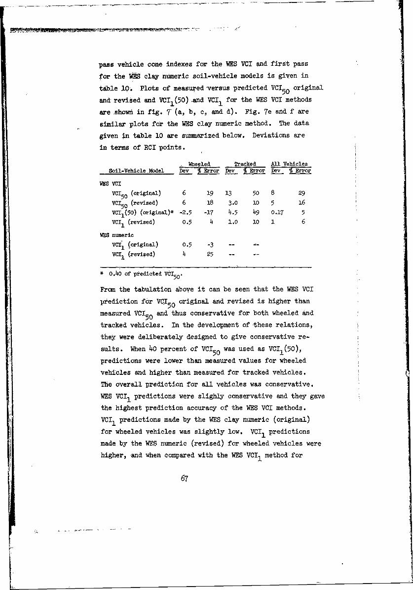
pass vehicle cone indexes for the WES VCI and first pass

for the WES clay numeric soil-vehicle models is given in

table 10,. Plots of measured versus predicted VCI 5 0 original

and revised and VCI,(50) .and VCI I for the WES VCI methods

are shown in fig. 7 (a, b, c, and d). Fig. 7e and f are

similar plots for the WES clay numeric method. The data

given in table 10 are summarized below. Deviations are

in terms of RCI points.

Wheeled Tracked All VehiclesSoil-Vehicle Model Lev %Error Dev I Error Dev % Error

WES VCI

VCI (original) 6 19 13 50 8 29

VCI5o (revised) 6 18 3.0 10 5 16

VCII(50) (original)* -2.5 -17 4.5 49 0.17 5

VCI 1 (revised) 0.5 4 1.0 10 1 6

WES numeric

VCfI (original) 0.5 -3 .. ..

VCI1 (revised) 4 25 . .-

* 0.40 of predicted Vo 50.

From the tabulation above it can be seen that the WES VCI

prediction for VC!50 original and revised is higher than

measured VCIo and thus conservative for both wheeled and50

tracked vehicles. In the development of these relations,

they were deliberately designed to give conservative re-

sults. When 40 percent of VCIo was used as VCI (50),501

predictions were lower than measured values for wheeled

vehicles and higher than measured for tracked vehicles.

The overall prediction for all vehicles was conservative.

WES VCI 1 predictions were slighly conservative and they gave

the highest prediction accuracy of the WES VCI methods.

VCI 1 predictions made by the WES clay numeric (original)

for wheeled vehicles was slightly low. VCI1 predictions

made by the WES numeric (revised) for wheeled vehicles were

higher, and when compared with the WES VCI 1 method for

67

I;.

1 .... .. H 1 ..... ..

44)

4) P

4)

0d 0)4

4)4

Q - o w t ot to z tO

H 4H

IV44)

f ~ j 01.0 (H cm-U 'i t- li -P

09 C N1 HOJ01 HO H

4) 4>

4)l 4)o0 ul- )

.0 liCW 01 A r-4,'- H) 4)).' .

4)H))H (a (a )

VH 4)i 4) C)00 H d Hj H 8 ag 00 4

4) Id 0) cm Id r4a

4 0 (Y)0 0 ~ -. 4 ~

001 00 ' ~ H

0 al 0

4r)

4) 40 COdfl s

00

to) o H w D a0 04) H 4)

Mo 4)'0l to I- N OIrq~Vu

W) -. m4 to AH 0- A-U c t M '

'A'

totoo to tot -0 v

H1 0

H c H 1 >.4 4

-1-LA x1 F. > t- H-H 42HN 0 cJ HH 0 1 H -4H14 E-4

(a C68

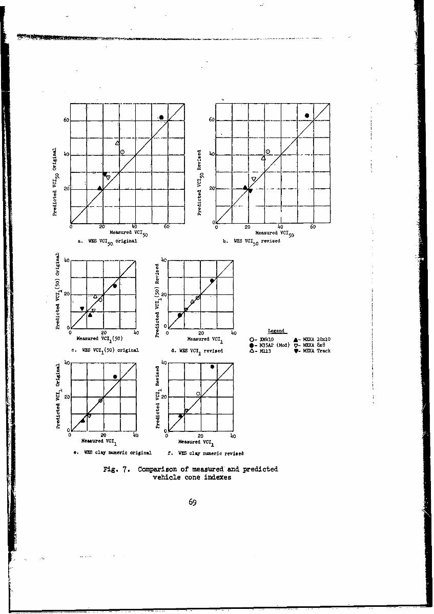
o -_ .60

, 1

4 40--

w0

200 20 O

44,

0 20' 40 ~ 0 20 40 6oMeasured VCI50 Measured VCI 50

a. WES VC1o50 original b. WES VCI 50 revised

0 -0--- -02

0

ot

o

20 - - o 0 - 20 40 L

I I.- M35A2 (Mo ) - xA Wc. WCES VCII1(50) original d. WES VCI 1I revised 6%- M113 V-MEXA Track

49 oZ

4o,

0 20 140 0 c 20 i 40dexson

Measured VC11(5I Measured VI 1 0-x.1o -MXlxO

e. WES clay umeri original . WES Vcanme revised -Ml Y-MATrc

-- 44

* a

Fig. 7. Comparison of measure& and predictedvehicle cone indexes

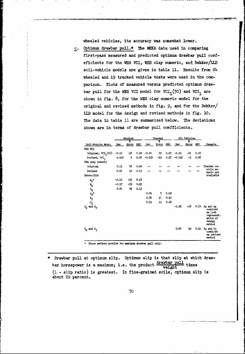
4

wheeled vehicles, its accuracy was somewhat lower.

c. Optimum drawbar pull.* The MEXA data used in comparing

first-pass measured and predicted optimum drawbar pull coef-

eficients for the WES VCI, WES clay numeric, and Bekker/LL)

soil-vehicle models are given in table 11. Results from 24

wheeled and 19 tracked vehicle tests were used in the com-

parison. Plots of measured versus predicted optimum draw-

bar pull for the WEB VCI model for VCII(50) and VCIl are

shown in fig. 8, for the .WES clay numeric model for the

original and revised methods in fig. 9, and for the Bekker/

LM model for the design and revised methods in fig. 10.

The. data in table 11 are summarized below. The deviations

shown are in terms of drawbar pull coefficients.

Wheeled Tracked All Vehicles

Soil-Vehicle Modei Dev Error RMS Dev Error DMB 0ev Error Rk; Remarks

WES VCI

Original, VC11(50) -0.15 -36 0.19 -0.24 55 0.25 -0.19 -45 0.22

Revised, VCIl 0.002 4 0.06 -0.034 -12 0.97 -0.016 -3 0.06WES clay numeric

Original 0.13 46 0.20 -- .. .. ... Tracked ve-

Revised 0.01 12 0.13 hicle nu-meric pot

Bekker/LLD availableA* -0.10 -35 o.18

-0.17 -59 0.21

cw o.4 25 0.13A* 0.01 5 0.12

BT o.6 14 0.10

0T 0.03 11 0.08AW and AT -0.06 -18 0.15 - andAT

combinedas =cstrepresent-ative ofdesignmethod

Cwand CT o.4 19' 0.11 OW and CTcombinedas revisedmethod

* These methods predict for maximum drawbar pull only.

* Drawbar pull at optimum slip. Optimum slip is that slip at which draw-drawbar p ulltiebar horsepower' is a maximum; i.e. the product wtimes

weight(1 - slip ratio) is greatest. In fine-grained soils, optimum slip isabout 20 percent.

7o

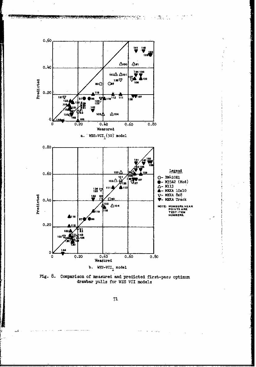
o

141 140

0.140i31 125

402A 42001 1 110V

1.2 124,

21 ' 14212

10' 103 &04

0 4. 143 106 ____ T___

0' 0.20 0.46 -0.60 0.,80'Measured

a. WES -VCI1(0)Y model

141 13

_______ Legend

125 0- M35A2 (Mod)124 -. 111 £12 M1125 A- EXA l~xlO

10142 90 VMEXA84)v 0.1) IV-MEXA Track

101 6104 NOTE: NUMBERSNEAR

tie; POINTS ARE

116 NUMBERS.

0.20 11Ails___

,1 222 4

300

1440~y~

0 0.20 0~ .'66 0.80Meaa'4 red

b. W-VCI1 model

Fig. 8. Comparison of measured and predicted first-pass optimumdrawbar p ulls for-WES VdI models

71

z

0 II- N11 43

A ri

0~ (N I

0~.

0 a z Id'

0~ 0 0A.H

0 0._ _ _ _ _ _

0 -~ to

H~ 0c00

-H

$4 0 0

00

4 14

"o**

01

00

H- Hi 0 0 0 0

P04OTpoid

72

112140 1410.8( -,- 1'- - l W s

ias 1 34 137 ,--1!03 Z

A 104

0.6 ' 102A 01 .

125V 124V ' -oWA A1onV V12

4J 0D92

4) 96

/ 970,142

106

V.20

1 122&115

Measured

a. Bekker/LLD Model - AW and AT

(These methods predict for maximum drawbar pull only)

0.80 -/Legend

141V o - XM41OEI13 0 0 - M35A2 (Mod)

100A 2j&- M1131"'VIs 'A - MEXA 10xlO

0o2a 1 ,4 V - MEXA 8x8

l24&12SV -Oj MMX Track

9I&921 127 NOTE: NUMBERS NEARPOINTS AREITEsT

0) ,ITEM NUMBERS.

97396 90 89 ____

143 V V142

11 1061s 1 18

122 12,-w " I ,129

A. O.105

0 0 4 00 oMeasured

b. Bekker/LLD model - W and CT

Fig. 10. Comparison of measu-ed and predicted first-pass optimumdrawbar pulls for Bekker/LLD models

73

*9*

t-\ U'. lI) 1.1 M3 H

It'. 0'. '.0 '0 '0 '0 0

i-i 81 - 0 -V

4 0

'-I .0

04 ON 0N %.c - \ IA. cu a)I C

4) 03 03 H 3 U' .4

H (0 0 Ho 0 , A* 4) 4

14 4)CD *Y 4) (

('3U 0 0 0U C 0 r4 .0p

I4 cc I 544)4 - 1

'01 4) 4000 03i 0~ .

0. 0

..- S. t43

.b: >H ) H UH x 14 > 0 9 1 1

H I4) 44 o 0 0 0) 0

~ '4

43' P4 *0 H

4) 4)

tA -0 0 'd

0 0A It'. t3 -t 04hI ~ ~ ~ c H 3 H -.II I

I a 74

For wheeled vehicles, all soil-vehicle model prediction ac-

curacies were greatly improved by the revised methods. On

the basis of the revised methods, the WES clay numeric,

WES VCI, and the Bekker/LLD OW methods, the predicted per-formance was higher than the measured performance. In

terms of RMS, the WES VCIl1 prediction method: was best, the

'Bekker/LLD CW methdd next best, and the WES clay numeric

last. As with wheeled vehicles, the revised tracked ve-

hicle methods improved prediction accuracy. The WES VCI 1

prediction method was conservative (predictions lower than

measured) whereas the Bekker/LLD C predictions were higherT

than measured results. For the WES VCI 1 and Bekker/LLD

tracked vehicle performance prediction methods, the predic-

tion accuracy was about the same (RMS of 0.07 versus 0.08).

For all types of vehicles, the RMS for the WES VCI, methodwas lower than that for the Bekker/LD and C combina-

tion method.

d. Towed motion resistance. The MEXA data used in the compara-

tive analysis of towel motion resistance coefficient for

the four WES and six* Bekker/LLD models are given in table

12. For the comparative analysis, data from 11 wheeled

and seven tracked vehicle tests were available. Plots of

measured versus predicted towed motion resistance coef-

ficients are shown for the WES VCI model for VCII(50) and

VCI 1 in fig. 11, for the WES clay numeric and revised

models in fig. 12, and for the Bekker/LLD models combining

AW and AT, and C and C in fig. 13. The data in table 12W Tare summarized on page 80. The deviations shown are in

terms of motion resistance coefficients. The WES VCI1(50)

prediction results were very conservative and very poor.

The particular soil strength-towed motion resistance

* Although two motion resistance equations are given in table 7, sinkage

used as an input is determined by three equations, giving six differentmethods for calculating motion resistance.

75

|I

i l tA% Cu 0 OD ON

0 0 0- OnI *

.0I % P .0

0 \ 0f o 6

0

0I H rH Ci+)C. f 0 Cj 0DG 0 0l 11

04 0 0 W4

0) H tH H Ho0\

o\ C\.4 c 0 CoCo C -

a0 0 w --H H 0 0 0 0

4> 411

t-.1 CO. CcU

S0 4,.-i H -4 0- H H 0 ,

C)*1m

H S.H

Id ~ 0 0 0) r 0 0j_:

to' od Vo I -

H)0 H .s 4

0 H 10 \ Ek

li -P a ;,4)

'o a ., Q -C

"I 14

0 000

H4 4

E-4 ~ . S.d Cua)- ~ 4 4

r-5 m1* --k E

0 00

r. .4 0 Mo Cu \0i ..obc kI Wt 4 4S

ciC ~ . HS 4 t- CH0

,I~ rE.J

tZ 0 0 76

0 ttA

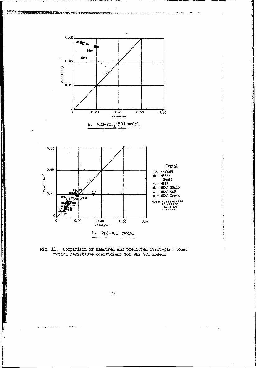
0.609

43a4

0.20

0 0.20 0.4.o 0.60 0.80Measured

a. WES-VCI,(50) model

0.60

Legend

* - Y35A2(Mod)

8 - M113-A - MEXA 10x1

1032 9/' l142 5-MX0.20 10 'NJAx1221 '1 131-MEXA Track

11 89 NOTE. NUMBERS NEAR9 134 POINTS ARE'

12:9 132,TEST ITEMNUMBERS.

108 lV Maue oe

0.20 0.4o 0.6o 0.8o

Fig. 11. Comparison of measured and~ predicted first-pass towedmotion resistance coefficient for WES VCI models

77

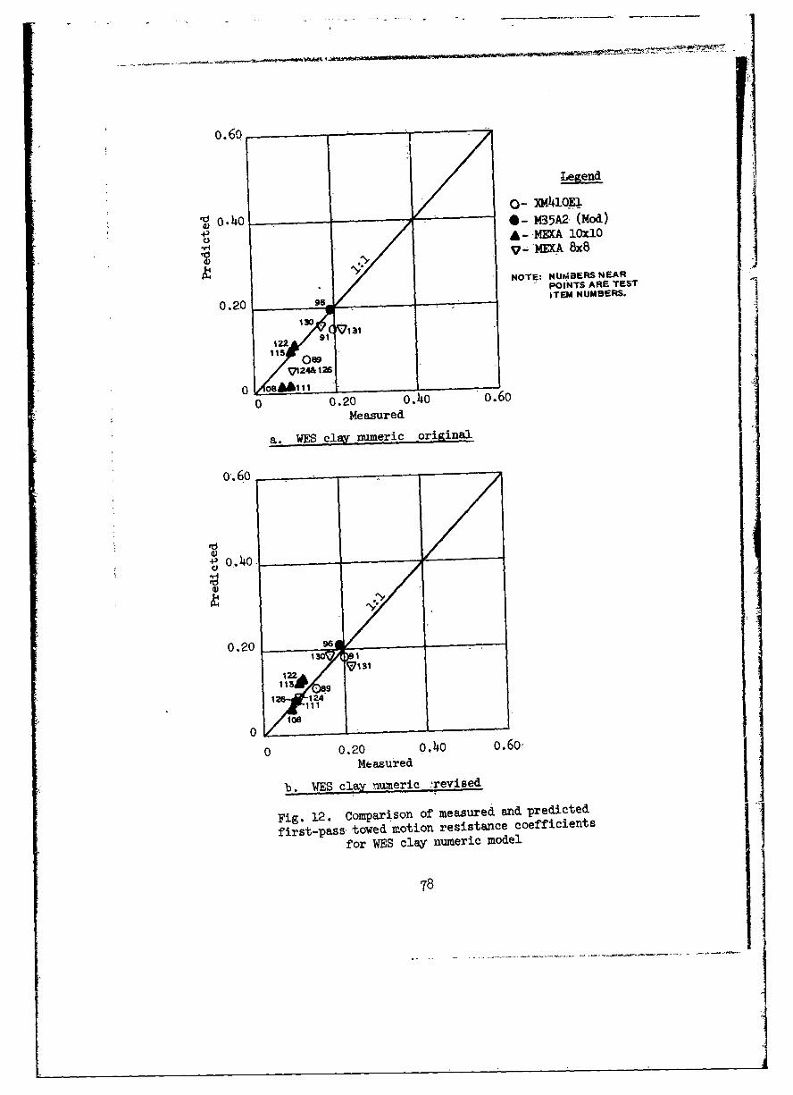
o.6o

Legend

0- XK4lQE4rd o.40 - M35A (Mod)4, A- -MEA 1Ox10

4)

NOTE: NUviERSNEAR• POINTS ARE TEST

0.20 96-/ . .. ITEM NUMBERS.

1, ,, OI122

115 089124& 126

0 0.20 o.4o 0.60Measured

a. ES clgZ numeric original

o,.60

C);9

0.20 96

130 I

00.20 0.4,o o.6o,Measured

b. ES l~ynumricrevised

Fig. 12. comparison of measured and predicted

first-pass towed :motion resistance coefficients

for WES clay numeric model

78

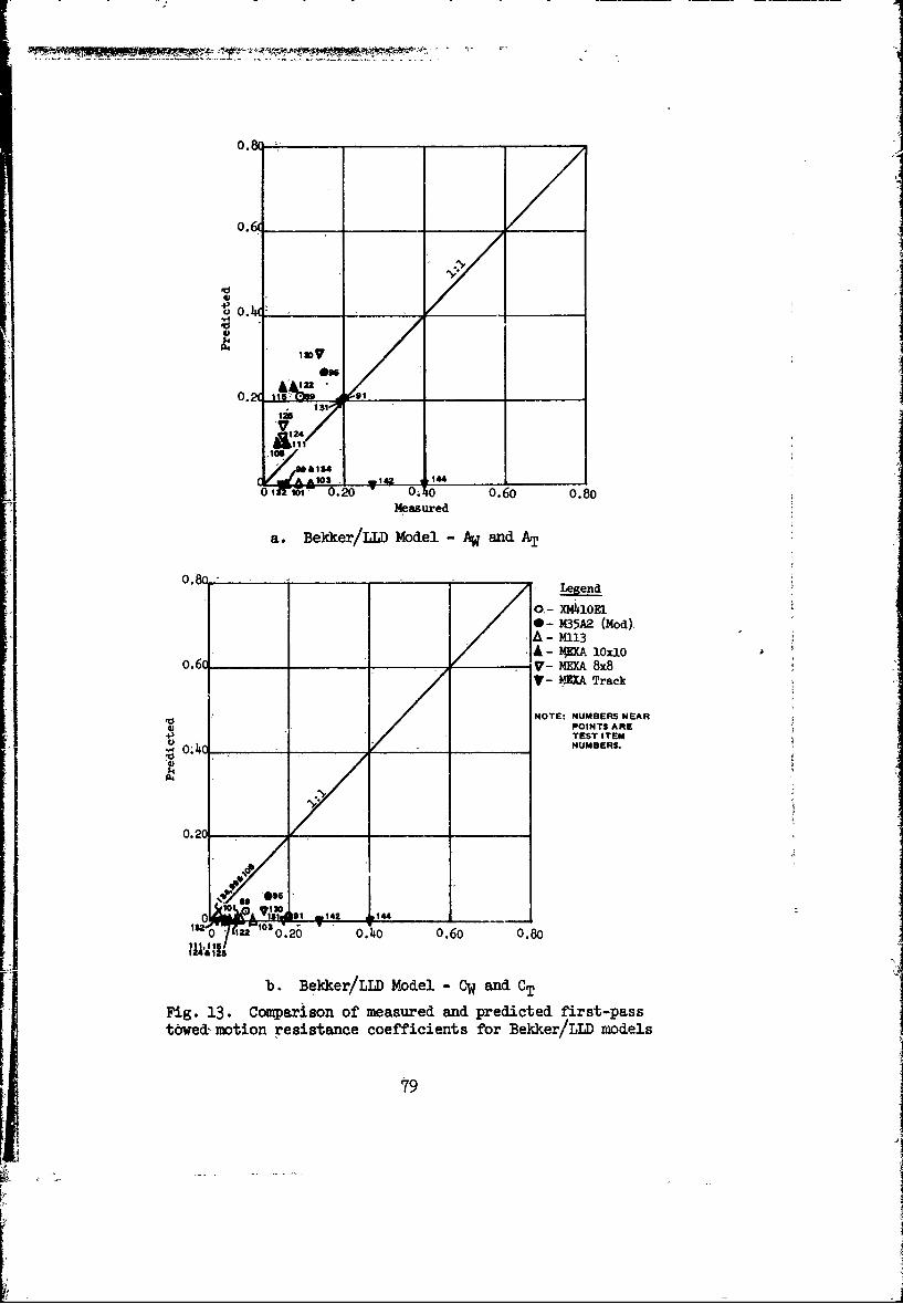
0.8

o.6_

4-1-

a o.4113DV

,mV

0 0 0 0.60 0.80Measured

a. Bekker/LLD Model - AW and AT

0.8 Legend

0- xm4ioEI0- M35A2 (Mod)A- 4130.6 _______ -NEJCAOxlOV- M 8x8V- EXA Track

NOTE: NUMBERS NEAR4POINTS AREIU TEST ITEM

0: o04 NUMBERS.

A-A

0.20 _____

9

10 30,

122 103 0.20 0.4o 0.60 0.80

b. Bekker/LLD Model - CW and CT

Fig. 13. Comparison of measured and predicted first-passtowed, motion resistance coefficients for Bekker/LLD models

79

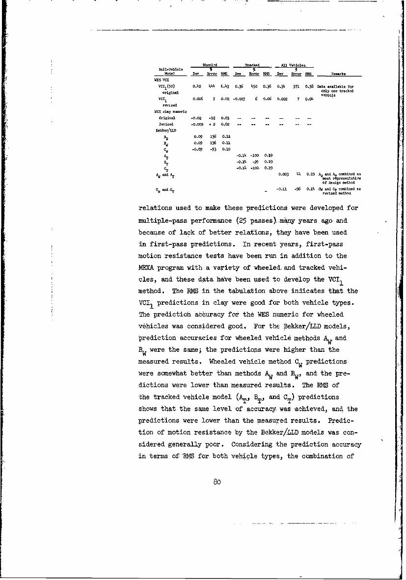
Wheelni Tracked All Vehicles.Soil-Vehicle

Model Dev Error RMS Dev Error RMS Dev Error RMS Remarks

WES VCI

VcI1 (50) 0.42 444 G.3 0.36 450 0.36 0.34 371 0.38 'Data available for

original oly one trackdvehicleVC I o.xc6 7 0.02 -0.007 6 0.06 o.002 7 0.04

revised

WES clay nmerie

Original -0.02 -12 0.03- - - - - - - -.

Aevised -0.009 + 2 0.02-- - --- - -.

Belker/LLD

AW 0.09 136 o.1

0.09 136 0.1

CW -0.09 -93 0.10

AT -o.14 -1oo 0.19

B, -0.14 -) 0.19

cT -0.14 -100, 0.19

and AT 0.003 44 0.15 AW and Av co bined asmost representativeof design method

C0 and -T -0.11 -96 o.14 Cw and CT combined asrevised method

relations used to make these predictions were developed for

multiple-pass performance (25 passes) many years ago and

because of lack of better relations, they have been used

in first-pass predictions. In recent years, first-pass

motion resistance tests have been run in addition to the

NEXA program with a variety of wheeled and tracked vehi-

cles, and these data have been used to develop the VCI 1

method. The RMS in the tabulation above indicates that the

VCI1 predictions in clay were good for both vehicle types.

The prediction accuracy for the WES numeric for wheeled

vehicles was considered good. For the Bekker/LLD models,

prediction accuracies for wheeled vehicle methods A. and

BW were the same; the predictions were higher than the

measured results. Wheeled vehicle method CW predictions

were somewhat better than methods A and BW, and the pre-

dictions were lower than measured results. The RMS of

the tracked vehicle model (AT, BT, and CT) predictions

shows that the same level of accuracy was achieved, and the

predictions were lower than the measured results. Predic-

tion of motion resistance by the Bekker/LLD models was con-

sidered generally poor. Considering the prediction accuracy

in terms of .RMS for both vehicle types, the combination of

8o

andC models gave slightly better results than the com-

bination of AW and AT models. The predictions for the com-

bination of AW and A were higher than measured results,

while the reverse was true for combinations of Cw and CT .

Of the WES and Bekker/LUD models examined, the WES VCI1

model was most accurate.

e. Sinkage. Of the soil-vehicle models examined in detail,

only the Bekker/LLD #-models are concerned with predicting

sinkage which is used as an input to the motion resistance

equations. The MEXA data used in the comparative analysis

of measured and predicted results are given in table 13.

Plots of -measured yersus predicted sinkage as used in the

various models are given in fig. 14. Results from 20

wheeled and 11 tracked vehicle tests were used in the com-

parative analysis. The--sinkage equations (table 7) were

used to predict sinkage for wheeled vehicles. The sinkage

equations for methods AW and BW are the same (table 7);

therefore, the Values shown for prediction .accuracy in

table 13 are the same. In terms of RMS, the method for

predicting sinkage for the AW and BW models gave more accu-

rate overall sinkage predictions than that for the CW model.

The sinkage predictions made for the CW model were lower

than the measured results, and the reverse was true for

sinkage predictions made for the AW and BW models. The

sinkage predictions for the tracked vehicles were much

poorer than those for the wheeled vehicles. The sinkage

equations for methods A and C are the same. SinkagesT -- T

predicted for the AT and B models are much less than theT

measured sinkages. Apparently the two methods used to pre-

dict sinkage of tracked vehicles are not sensitive to pre-

dicting sinkage of low-ground-pressure vehicles. In

fig. 14 it can be seen that little or no sinkage was pre-

dicted for the MEXA tracked vehicle, yet measured sinkage

ranged from about 2 to 10 in. For all types of vehicles,

81

Table. 13

MEXA Data Used in Comparing Measured and PredictedFirst-Pakss Sinkage

Bekker/LLD Models (See footnote for design and..revised methods)

Total or Bo BC orCNumber AT or Aw ____F_

of Algebraic Al ebraic AlgebraicTests Dev % Error RM Dev %.Error ___ Dev %:Error RIE

Wheeled VehiclesXM1410E1

3 -1.8 -34 2.4 T- -34 2.li --3.8 -87 4.1

M35A2 (Mod)2 -1. 4 -14 2.3 -1.4 -14 2.3 -4.1 -70 4.5

MEXA lOlO10 0.3 64 1.2 0.3 64 1.2 -1.3 -105 1.,

MEXA 8x85 -A4 -11 2.1 -0.11 -rli 2.1 -3.1 -92 3.1

All Wheeled Vehicles20 -0.4 23 1.8 -077 23 1.8 -2.1 -96 2.9

Tracked Vehicles

5 -3.8 -68 4.6 -0.5 -21 7.0 -3.8 -68 4.6

MEXA Track6 -4.0 -98 5.0 -4.o -97 5.0 -4.o -98 5.0

All Tracked Vehicles11 -3.9 -85 4.8 2.7 -62 6.0 -3.9 -85 1.8

All Wheeled and Tracked Vehicles31 -1.6* -15* 3.2* - - -3.0* -92** 3.7**

* Denotes combination of methods AW and 4. (original methods).

•* Denotes combination of methods CW anticT (revised methods).

82

20 ___-____

i051 2

10

-105

-5 130 VI29__ _

.i6,6

1 16

11 1 2 14 0 1 4

0-OIT ARE rbAE3ST

0 34 10 15 202 Measured, in.

a. Bekker/LLD - and A

2__sinkaefor_ Beer/_ models Legend---- X81

* - M35A2 (Mod)A - M113A - NExA loxloV- MEXA 8x8

1 __________ _____ - MEXA Track

NOTE. NUMBERS NEAR* POINTS ARE TEST

ITEM NUMBERS.

4) 0 __ _0. . . __1_-0 _ __ _

096

106 I 1 3 In

0 v . 6 1091 'S 144 _____

0 5, 712; 10 15 20its 30Measured, in.

b. Bekker/LLD :-. and CFig. 14. Comparison of measured and predicted first-pass

sinkage for Bekker/LLD models

83

the overall prediction accuracy obtained for the combina-

tion of AW and AT models was better than that obtained for

the combination of Cw and 0 T models.

f. Slip. All Bekker/ILD models except AW and AT use selected

slip values to compute gross traction. In this comparatiVe

analysis of measured and predicted slip, the evaluation is

made only for slip at optimum drawbar pull. The MEXA data

used for this comparison are given in table 14. The devia-

tions are in terms of percent slip. The wheeled vehicle

slip predictions for both methods were higher than measured

values. The predictions obtained with method B. were poor,

but the predictions obtained with method were very good.

In terms of RMS, the prediction accuracy for the tracked

vehicle was about the same for both methods. The predic-

tions were lower than measured results.

116. Summary discussion. Because of the importance that a soil-

vehicle model plays in the overall prediction accuracy of a comprehensive

ground mobility model for predicting speed performance, a few summary

statements are made to place the results of the soil-vehicle model verifi-

cation analysis in the proper perspective.

117. All comprehensive ground mobility models include a soil-vehicle

model to obtain net traction (DBP). Net traction is defined universally as

the tractive force developed at the vehicle drawbar when the vehicle is

traveling in a straight line on a level surface at a slow constant speed.

It is normally obtained as the difference between total or gross tioaction

(H) available and external motion resistance (R). The general equation is

H = DBP + R . Net traction is a function primarily of the soil strength,

the vertical load imposed by the vehicle on the soil, slippage between the

traction elements and the soil, and the vehicle speed. All of the soil-

vehicle models verified using the MEXA data accounted for all the factors

that affect net traction or drawbar pull in some form except vehicle speed,

which in all tests the speed of the traction elements was constant or

nearly so. Drawbar pull prediction by the WES VCI model is at the optimum

or maximum pull, and it is obtained from a set of curves relating excess

84

Table 14

MEXA Data Uded in Comparing-:Measured and Predicted Optimum Slip

Bekker/LLD Models (See footnote for design and revised methods)

Total -BT or BW CW orC- C _T

Number Al-ebraic Algebraic,of Tests Dev -Error, RM -Dev Error RMS

Wheeled Vehicles

XMI1OEI

6 21 110 21 0.33 2 2

M35A2 (Mod)

16 66 16 1 1

MEXA l~xlO

13 7 39 25 -0.08 -O.g 2

MEXA 8x89 7 46 20 1 6 3

All Wheeled; Vehicles

32 11 58, 22 0.38 3 2'

Tracked Vehicles

M1138 -8' -44 8 -6 -36 6

MEXA Track

11 -10 -37 16 -10 -36 17

All Tracked Vehicles

19 -9 -40 13 -9 -36 14

All Wheeled and Tracked Vehicles-3* -12* 8*

* Denotes combination of methods C and CT (revised methods).

85

soil strength to drawbar coefficient for different types of vehicles 6k

category of vehicles within a given type. A simple equation of dimension-

less form is used by the WES numeric (wheeled vehicles. only) to predict

drawbar pull at 20 percent slip. For most of the Bekker/LLD models, com-

plex equations are used to calculate &rawbar pull at selected slip values

from which a drawbar pull-slip curve is constructed. The discussion on

drawbar pull is also applicable to the prediction of motion resistance by

the various models.

118. An examination of the elements of each of the models verified

and the results obtained shows that the calculations required in predicting

drawbar and motion resistance by the WES methods are simple as compared to

the BekkerLD models. Furthermore, the WES models produced more accurate

predictions. The WES VCI and WES numeric (wheeled vehicles only) models

for predicting optimum drawbar pull coefficient have an RMS of 0.06 and

0.13, respectively. The RMS for motion resistance coefficient (wheeled ve-

hicles only) for the WES VCI was 0.02 ahd- for the WES numeric 0.02. The1combination of CV and CT considered as the Bekker/LLD revised model uses

the same equations for predicting gross traction and motion resistance.

For these models, sinkage is presumed to be uniform along the track length

and when applied to wheeled vehicles, the contact area is presumed to be

defined by the product of hard-surface contact length of the deflected tire

by the section width of the tire times the number of tires. An examination

of the Bekker/LLD revised method (CW and CT combination) prediction data

indicates that the prediction accuracy for all vehicles in terms of RMS was

0.11 for optimum drawbar pull coefficient, 0.14 for motion resistance coef-

ficient, 3.7 in. for sinkage, and 8 percent for slip. The predictions for

tracked vehicles were worse than those for wheeled vehicles.

ll9. The large deviations in sinkage are reflected in the predictionof motion resistance. The relatively low RMS obtained for the optimum draw-

bar pull suggests that the error in computing sinkage and motion resistance

must have been matched by compensating errors in computing traction. With

the extremely low sinkage predicted (see fig. 14b) as compared with the

measured results, approximately the same prediction accuracy for drawbar

pull would have resulted, with perhaps some modification to the traction

86

equation, had there been 300

no allowance ,made for

soil motion resistance at LegendSymbol Depth, in.

250 0 o to 6

120. In light of 0 6 to 12S12 to 18

the overall results

achieved by the Bekker/ 20o

LLD Cw and.C soil-Tvehicle models, it ap-

pears reasonable to con- x

sider using the Bekker/ 150

LID shear measurements

and tractive area assump- -

tions to compute avail- 100

able vehicle traction

without bothering with

the controversial and 50 0

worrisome problems of

,predicting sinkage and

motion resistance from 0

small plate tests. This 0 50 100 150 200Measured Cone Index

suggestion is further re-

inforced by examination Fig. 15. Comparison of measured cone index andcone index predicted from bevameter parameters

using equation prepared by Janosipares measured cone index

with cone index predicted from bevameter parameters using equations pro-

posed by Janosi for MEXA tests conducted at the Nevada test sites. The

data used in the comparison and the equation used are given in table 15.

The tendency to underestimate the strength of weaker materials and to over-

estimate the strength of stronger materials, seen in the vehicle test re-

sults, is repeated. If the penetration resistance of a -simple, rigid, asym-

metric cone of the same general scale as the test plates cannot be reliably

predicted from the plate penetration results, the chance for achieving ac-

ceptable estimates of the sinkage of the larger and more complex system

87

4-.1og uoC'j 0\ M 0 0 H

4) (V CY) H co cr4)

I \ CC)mY t- oC) S

Cq o I;o4'1 0 )CC) 0 .

4)\ 4.)() H

P- 1 0 0 0 0 0

H4, o o v

4)d 0 o

~O 0 n

00~

0) 0\ 0 0 --

r4 l H -\C1 H -- 0 CM'

4- 4.H _P +< + *r

- - S3 ,~ -<J i-4 +2-1 0- I c'

UN + 10.

r) U ol \D _t - 0$. \ 0i C'u .4 r

r- C)\ 00 L<HL- Ll0 1

+ 44

El ) 0 00.i O

> 4)) ~Ii I

0d r.- a ~ H \0 J 0 W4) 0 0C Y) 40$ *I ' (Y) ' UN ('J*- \ 0

4.'i

Hl Lr0 0 N +~0

O Ci2H ~ l+

HH

to ~ ~ O 0 0 f0 1 0 0H H1 H

0 U8

represented by a number of wheels or tracks is small. An extensive survey

of plate sinkage relations by Hvorslev (1969), including the bevameter

equations, concludes with

....the results of routine sinkage tests with small platescannot -be adequately represented by the sinkage equationsprepared by Bekker and others...

which

means that the sinkage of large plates cannot alwaysbe predicted with acceptable accuracy by means ofresults of sinkage tests with small plates and cur-rently available theories. Ability to do so is re-quired before the teAts and theories can be appliedwith confidence to the much -more complicated condi-tions encountered in the mobility of Vehicles [under-line added].

Obstacle-Vehicle Models

121. Surface configuration produces a profound effect on ground con-

tact vehicles whether they are operating on a prepared surface or natural

terrain. Exclusive of vehicle characteristics, vehicle road speed is de-

pendent on road alignment, grade, ,surface, roughness,. visibility, and traf-

fic. However, with current technology in roadway design and construction,

roadways can be constructed and maintained to yiele. a specified level of

performance in any type of terrain. On the other hand, military vehicles

are often required to perform missions on unimproved terrains in various

parts of the world. Terrain features occur in many sizes, shapes, and

spacings, producing an almost infinite number of combinations of surface

configurations; and their effects on vehicle performance range from immobi-

lizations caused by interference to reduction in speed caused by vehicle

vibration or obscuration of the surface by vegetal coven. Means to charac-

terize surface configuration (including discrete obstacles) and cover ade-

quately, and methods and techniques for predicting the interactions between

any surface configuration, visibility, and the vehicle and driver are thus

required as necessary inputs to any comprehensive model for predicting

cross-country vehicle performance with. some degree of realism. Compared

with soil-vehicle models, obstacle-vehicle models, including vehicle

89

Io

dynamics, are in the early stages of development.

122. Cross-country operation differs from on-road operation in es-

sentially four ways:

a. In off-road travel thepath is somewhat more freely selec-

ted by the driver.

b. The surface bearing capacity and traction characteristics

are more variable off-road than on, and frequently are very

low.

c. The surface will generally be much rougher in terms of

minor geometric anomalies and major slopes.

d. The selected path- will usually be strewn with obstacles, of

various sizes and shapes, ranging from linear features

(streams, ditches, etc.), discrete three-dimensional haz-

ards (rocks, deadfalls, etc.), to systems of clearly insur-

mountable, small area obstacles in planar array (large

trees).

123. The way in which a driver exploits the greater freedom avail-

able to him in selecting a path off-road has not yet been modeled. The ef-

fects of variations in strength *of the operating surface are the subject of

soil-vehicle modeling; minor surface anomalies are dealt with as a part of

the "ride" dynamic problem, and slopes in soil-slope modeling. All of

these have some analogs, however tenuous, in bn-road vehicle motion mechan-

ics. The obstacle problem, however, is essentially peculiar to off-road

cperations.

124. As previously stated, obstacles affect vehicle performance on

two levels. They may either reduce the potential operating speed of a ve-

hicle severely or totally immobilize it. While the latter, of course, is

merely the end point of the former, the distinction is useful because study

at the go-no go level can be adequately handled as a problem in static me-

chanics, whereas the speed problem should be treated as one in dynamics.

125. In this part of the report, obstacle-vehicle models are dis-

cussed separately according to the kind of feature and kind of terrain, ve-

hicle, and driver interaction exhibited. The models considered include

those that account for the effects of continuous, irregular terrain where

90

the profile includes small, irregular terrain features that produce vehicle

vibration or occasional shock; slope models that account for gravity ef-

fects; -discrete -obstacle models that account for geometric obstacle-vehicle

interference and if they can be overridden, the force required to override

them or when randomly spaced, the demands imposed by maneuvering;

Visibility models that account for the effects of recognition distance on

performance; and stream-crossing -models that account for the interaction a

vehicle -encounters when entering, crossing, and exiting a stream.

Perspective

126. Since the advent of the automobile (1920's), research by gov-

ernment and industry has been conducted on a continuing basis in various

countries of the world in highway design and construction, and vehicle de-

sign, particularly in the areas of steering, control, power train, and sus-pension. These areas are the principal contributors to the safety, effi-

ciency, and riding comfort of-on-road vehicles.

127. The speed- at which a driver of a vehicle will traverse obsta-

cles or continuous irregular terrain is controlled primarily by the level

of vibration activity that does not exceed his particular ride comfort

level. Vehicle vibration or ride is sensed by a driver or passenger

through sight, touch, and hearing in response to external stimuli, such as

motions, forces, and sounds. Whenever this sensation becomes too severe,

the driver will alter the vehicle's speed until the sensation reaches an

acceptable level. This sensation, therefore, is a significant factor in

determining the speed of a vehicle over a given terrain. The maximum vi-

bration activity may be limited:by the type of cargo or the structural ele-

ments of -a vehicle. Generally speaking, the driver or the cargo estab-

lishes the ride limits. The irregular terrain-vehicle problem is essen-

tially one of dynamics, and its solution must include the combined effects

of the surface- being traversed, the velicle, and the driver. Because of

the complexity of the problem and the desire to produce better riding ve-

hicles, considerable effort has been expended on modeling dynamic vehicle

response.

128. Because of the lack of mathematical, techniques required in

modeling suspension systems, much of the early work consisted of

91

V

* cut-and-try methods. The first significant contributions to an analytical

treatment of vehicle dynamics were made by Rowell,. Guest, and Olley in the

early 1920's and 30's. In 1922 Rowell made one of the first attempts to

analytically define the problem. This work was extended in 1926 by Pro-

fessor Guest and again in 1934 by Olley, who introduced an analytical

treatment of independent wheel suspension.

129. In 1941 a mechanical differential analyzer was built by Schil-

ling and Fuchs specifically for suspension analysis, and although it was

suited to only a single-degree-of-freedom system, it did permit the inclu-

sion of a nonlinear characteristic of shock absorbers. An important use of

this analyzer was the continuous determination of transient motions and

portrayal of the effect on motion by changes in the characteristics of the

shock absorber. This differential analyzer was the forerunner of today's

analog computer, and its capabilities led to rapid advances in suspension

analysis and design. By the 1950's, it was widely exploited by the automo-

tive industry.

130. In 1953, Jeska developed a 4-degree-of-freedom model that in-

cluded pitch and bounce of the body and vertical motions of the front and

rear wheels. The forcing function was an 'actual road wave measured by a

photographic technique. In 1955, Bodeau, Bollinger, and Lipkin of Ford

Motor Company developed a detailed ride analysis in which a 9-degree-of-

freedom model was.used to describe a passenger car. In 1960, Kohr of Gen-

eral Motors Corporation developed a mathematical simulation of automobile

ride. In his simulation, a measured road profile was recorded on magnetic

tape, and the tape was fed through an analog computer model of the vehicle

to predict the vehicle motions, i.e. pitch, bounce, and roll. The result-

ing motions were used to drive a vibration simulator, which was used as a

laboratory means of assessing the effect of the vibration on humans.131. Until about 1960, the analysis of ride had been concerned pri -

marily with the suspension system and means of improving the ride quality.

Although considerable work was done in the area of human tolerance to vi-

bration, a means for quantifying human tolerance to vibrations had not been

developed. Van Deusen has shown that very little of the research done ac-

tually pertains to the surface vehicle problem. Most experiments have been

92

devised to assess human response to sinusoidal motion in only one direction,

while the more complex ride comfort problem involves random vibrations in

various directions. The-most frequently used criteria have been those of

DieckMan and Janeway, who developed simple formulas for relating comfort

limits to amplitud, and frequency of vibration. There have been several

studies of "on-thes-road" measurements of ride comfort. For example, von

Eldik Thieme examined the Dieckman-Janeway criteria in the actual vehicle

environment, but he met with little success. Van Deusen and Versace used a

technique, referred to as cross modality, in which subjects received noise

signals through earphones and adjusted and matched their level to the sen-

sation level of ride vibration. A. statistical analysis showed favorable

correlations of the measured accelerations with ride sensation, and at

least indicated that correlations between ride sensation and vibration were

possible..

132. In the late 1950's the military began to recognize the signifi-

cance of vehicle vibration on off-road mobility and fire effectiveness.

This led to an extensive effort to quantify the vehicle vibration problem

and to correlate it with human response and terrain characteristics. In-

terest was shifted from deterministic to stochastic techniques. The latter

consists of classifying the terrain profiles by certain pertinent statis-

tics and analyzing the response statistically. The groundwork for this

type of analysis was begun in 1959 by Bogdanoff and Kozin, who described in

detail the statistical analysis of the responses of simple linear systems

to random terrain inputs. Although the vehicle models were simple and

idealized, the analyses provided a starting point and yielded much useful

information regarding fundamental relations between pertinent vehicle pa-

rameters and statistical terrain quantities. This study preceded those of

Bieniek (1960), Van Deusen (1962), and Bussman (1964), who followed essen-

tially the same approach as that described by Bogdanoff and Kozin. The one

notable exception was Van Deusen's introduction of a nonlinear vehicle sys-

tem into his statistical analysis.

133. In 1963, the U. S. Army Tank-Automotive Command began basic re-

search on the effects of vehicle vibration on human response. This work

was based on the results of past studies and so was oriented towards

i~93

quantifying the effects of random vibration on vehicle-driver performance.

Two performance parameters were developed to describe human response--"ac-

celeration density" and "absorbed power." Of the two performance parame-

ters, absorbed power is preferred in quantifying human response to vibra-

tion since it is a descriptor of the flow of energy from the vibrating ve-

hicle to the driver. During the 1960's the military sponsored several

studies in the development and application of ad hoc comprehensive cross-

country models in which V-ride was incorporated as a submodel.

134. In the early 1960's the sc6pe of WES mobility research was ex-

panded, and static and dynamic surface configuration-vehicle-driver inter-

action studies were initiated. In 1965, FMC Corporation conducted a study

for WES to determine the feasibility of using a digital computer to simu-

late the dynamic response of ground vehicles traveling .over unyielding ir-

regular terrain segments. This study resulted in the development of a gen-

eralized mathematical model of an n-axle vehicle which, within limits,, is

suitable for both wheeled and tracked vehicles. Recent efforts by WES have

produced improvements in vehicle dynamics modeling.

135. In 1966, CAL, under contract to ARPA,* began a comprehensive

study designed to augment knowledge of ground mobility and to refine meth-

ods available to planning, engineering, and field personnel for improving

it. One result of this study was the development of a comprehensiv-e ve-

hicle dynamics model that included both viscous and Coulomb damping proper-

ties of the suspensions. The model, although virtually untried, shows

promise for achieving a greater degree of realism than other models.

136. Recent events- in the United States space program have placed

even more emphasis on the dynamic behavior of ground vehicles. Several

studies of ride quality of extraterrestrial vehicles have already been con-

ducted by contractors for NASA. By their very nature, such studies require

a statistical analytical approach since cost and complexity preclude exper-

imental testing in extraterrestrial environment.

137. Organized discrete obstacle-vehicle research in the Western

* This program was terminated prior to the completion of the phases of the

program initially agreed to by ARPA.

94

J

world was given special attention as the result of World War II experiences.

Early United States military efforts were concerned with designing military

vehicles that- would reduce imobilizations by obstacle interference. Ob-

stacle test courses were constructed (APG) and tests on these courses have

become part of the overall vehicle engineering evaluation test program.

The results of these studies have led to the recent development of articu-

lated vehicles. 'United States discrete obstacle-vehicle research studies

gained more emphasis about the mid-1950's when terrain factors other than

soils were introduced as deterrents to off-road vehicle travel'and more at-

tention was given to obstacle geometry interference and the effects of dy-

namic response on vehicle performance. By the early 1960's these studies

produced several static and quasi-dynamic models which related, by simple

two-dimensional static mechanics, slope and obstacle geometry to go-no go

performance. A number of terrain-vehicle interactions not previously in-

vestigated were included in the MERS program. For example, the forc'$s in-

volved in overriding trees and obstacles, and the effects of obscuration or

recognition distance on vehicle performance were investigated. Special at-

tention has also been given by the British and Canadians to riverine cross-

ings, and several devices for aiding vehicles in crossing streams and riv-

ers have been developed. In addition to vehicle studies, research in the

United States and Britain has continued since World War II to develop ex-

pedients for bridging gaps and stabilizirg weak soils.

General status

138. Today's practice in modeling the effects of surface configura-

tion and vegetation on vehicle performance consistis essentially of two

types of analysis which are separated Onr the basis of the kind of vehicle

and/or driver interaction anticipated. Regardless of the analysis per-

formed, the terrain profile and associated di screte obstacles except vege-

tation are considered rigid. This consideration represents the worst con-

ditions from the standpoint of the vehicle's behavior. If a terrain unit

contains an irregular surface that can be easily overridden by a vehicle

without inducing frequent shock, vehicle performance is predicted 'by a dy-

namics model. In this case, the problem is commonly identified as surface

roughness, and the profile used is a statistically uniform surface profile.

95

If a terrain unit contains discrete obstacles larger than those included in

the rough terrain analysis and which are likelr to produce "mmobilizations,

it is assumed that traversing or circumventing the obstacles will be accom-

plished at a creep speed and the interactions are treated as static phenom-

ena. The models used in such terrain situations are thus static models.

The controlling factors in the relation of a static model are the geometry

of the obstacle and vehicle configuration. If the discrete obstacles that

the Vehicle must pass over (dikes) occur at wide spacings, and they can be

overridden at greater than creep speeds, a dynamic model is used to deter-

mine the maximum override speed. If a vehicle can override some obstacles-

and avoid some such as trees, override and avoidance models are used to se-

lect the optimum speed. For terrain units whose surfaces are obscured by

vegetation, namely grasses, a separate model is used to predict the effects

of recognition distance on vehicle speed.

139. Vehicle dynamic models simulate mathematically the dynamic re-

sponse of selected points within a vehicle (usually driver's seat or cargo

compartmdent) in traversing discrete obstacles or rough terrain. Perform-

ance is generally expressed in terms of relations between speed and zuch

quantities as absorbed power, RMS, or peak- acceleration, and referenced to

established horizontal and vertical acceleration and power limits. Most

dynamic models available are designed so that the motion of any generalized

rigid-body vehicle can be analyzed by one basic computer program. Most dy-

namic models predict vertical acceleration; however, they can easily be

modified to include horizontal acceleration. The mathematical techniques

and physical laws irnvolved in the formulation of dynamic models are common

to all models but differemices occur in the details of represonting the ter-

rain, vehicle, and driver limits, and the size of the comPuter required.

140. Mathenmatical descriptions of vehicle behavior in surmounting or

maneuvering around obstacles are essentially static models. Discrete ob-

stacles such as rocks, boulders, mounds, scarps, ditches, stumps, etc., are

usually first examined to detbrmine whether or not there will be spatial

interference between the obstacles and the nonpropalling vehicle structure.

This examination may proceed in either two or three dimensions: with or

without compliance of the vehicle running gearj suspension, or structure;

96

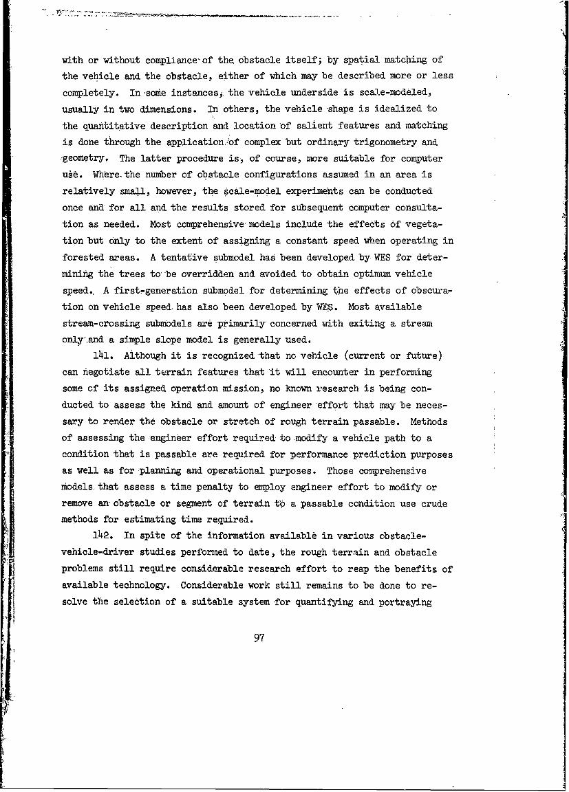
with or without compliance-of the, obstacle itself; by spatial matching of

the vehicle and the obstacle, either of which may be described more or less

completely,. In some instances, the vehicle underside is scale-modeled,

usually in two dimensions. In others, the vehicle shape is idealized to

the quantitative description and location of salient features and matching

is done through the application/of complex but ordinary trigonometry and

geometry. The latter procedure is, of course, more suitable for computer

use. Where-the number of obstacle configurations assumed in an area is

relatively small, however, the scale-model experiments can be conducted

once an for all and the results stored for subsequent computer consulta-

tion as needed. Most comprehensive models include the effects of vegeta-

tion but only to the extent of assigning a constant speed when operating in

forested areas. A tentative submodel has been developed by WES for deter-

mining the trees to- be overridden and avoided to obtain optimum vehicle

speed.. A first-generation submodel for determining the effects of obscura-

tion on vehicle speed has also been developed by V4S. Most available

stream-crossing submodels are primarily concerned with exiting a stream

only and a simple slope model is generally used.

141. Although it is recognized that no vehicle (current or future)

can negotiate all terrain features that 'it will encounter in performing

some cf its assigned operation mission, no known research is being con-

ducted to assess the kind and amount of engineer effort that may be neces-

sary to render the obstacle or stretch of rough terrain passable. Methods

of assessing the engineer effort required- to modify a vehicle path to a

condition that is passable are required for performance prediction purposes

as well as for planning and operational purposes. Those comprehensive

models. that assess a time penalty to employ engineer effort to modify or

remove an- obstacle or segment of terrain t6 a passable condition use crude

methods for estimating time required.

142. In spite of the information available in various obstacle-

vehicle-driver studies performed to date, the rough terrain and obstacle

problems still require considerable research effort to reap the benefits of

available technology. Considerable work still remains to be done to re-

solve the selection of a suitable system for quantifying and portraying

97

surface configuration for mobility purposes, develop means to predict

forces resulting from obstacle-vehicle interactions, and structure the in-

teraction modules pr subfriodels into manageable components so that a mean-

ingful cross-country performance prediction can be simulated by a compre-

hensive model., When this is accomplished, verification of the submodels

and the comprehensive model must be accomplished to obtain the level of

prediction accuracy that can be achieved in real terrains.

Strategies available

143. Possible approaches to computing terrain roughness and obstacle-

vehicle interactions are to:

a. Separate the overall problem into component parts on the

basis of dynamic or static interactions involved, using

equations of motion and mechanics and geometric and trigo-

nometric relations in matching obstacle-vehicle

interference.

b. Treat continuous irregular terrain surfaces and obstacles

as unyielding or yielding under a vehicle load, with un-

yielding representing the worst case of vehicle behavior.

c. Include a force or traction required in overriding or ma-

neuvering around individual obstacles.

d. Treat the terrain profile either as deterministic or sta-

tistical with probability statements.

e. Describe vegetation as a separate kind of obstacle, account-

ing for the forces involved in override and maneuver or a

combination of both, or assign a constant speed when a ve-

hicle operates in a forested area.

f. Assign a constant speed to areas where the surface is ob-

scured by vegetation or model the effects of obscuration or

visibility on vehicle performance.

144. A possible application of most of the above-listed strategies

is illustrated in fig. 16. Currently operating cross-country simulations

in'lude all the strategies outlined above, in one form or another. The

path selected through the strategy diagram to deal with terrain roughness

or particular types of obstacles can be, and frequently is, difficult even

98

nnm mu nnn mn ,, ,, m m ,, m ,,

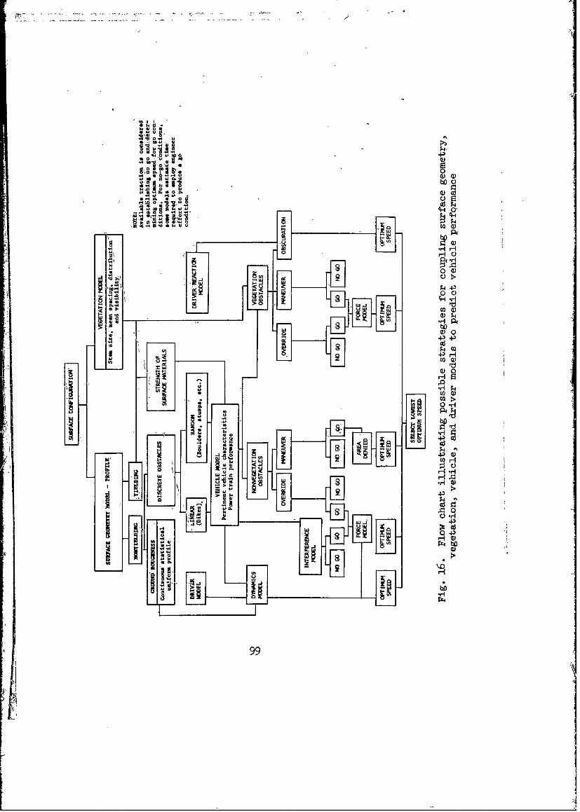
0

Un 00)

da0 .40

104 4-1

W0

14 Uw 4j.

- 1 4

go 00Q

l0a

C4 .

4,P

is j

--------------

0

99-

in a given overall simulation. This comes about, in part at least, because

of differences in form and availability of relevant terrain and vehicle

data. In its ultimate treatment, the surface configuration (surface geome-

try and vegetation) problem is a dynamic one in three dimensions involving

obstacles that may yield. Traction, inertia, and impedance forces in

equilibrium at all times will replace simple considerations of potential

geometric interferences. In many instances driver decision will determine

(both correctly and incorrectly) whether the problem is one of obstacle

avoidance or obstacle surmounting and, where terrain roughness is involved,

driver influence will enter again in selecting an acceptable speed on the

basis of subjective ride and vibration criteria.

145. In the next sections of this report, discussions are presented

on ride dynamic modeling of vehicle vibrations or the surface roughness

problem, negotiation or avoidance modeling of discrete obstacles (including

trees) on the basis of static relations, Visibility modeling, and stream-

crossing modeling.

Vehicle ride dynamics model

146. Eight vehicle ride dynamics models were examined in this study.

They are: (a) U. S. Army Tank-Automotive Command, (b) Chrysler Corporation

(Van Deusen), (c) General Motors Corporation (McKenzie), (d) Ohio State

University (Bussman), (e) WES-FMC Corporation (Smith), (f) NASA-GMC, (g)

National Aeronautical Space Administration-Brown Engineering, and (h)

Cornell Aeronautical Laboratory. Models (a), (b), and (e) have been par-

tially validated. No validation data are available for the others.

147. In reviewing the literature to select models for detailed study,

considerable commonality became apparent in the elements of building blocks

from which the models were constructed, whether intended for a specific or

a generalized vehicle. Because of this commonality in approaches to ride

dynamics modeling, and to avoid considerable repetition of information, a

general discussion on ride dynamics is first presented, and later differ-

ences in models are singled out for discussion.

148. The building blocks common to all of the ride dynamics models

examined in detail are shown in fig. 17. This figure shows the commonly

used choices in representing terrain, the vehicle, the terrain-vehicle

100

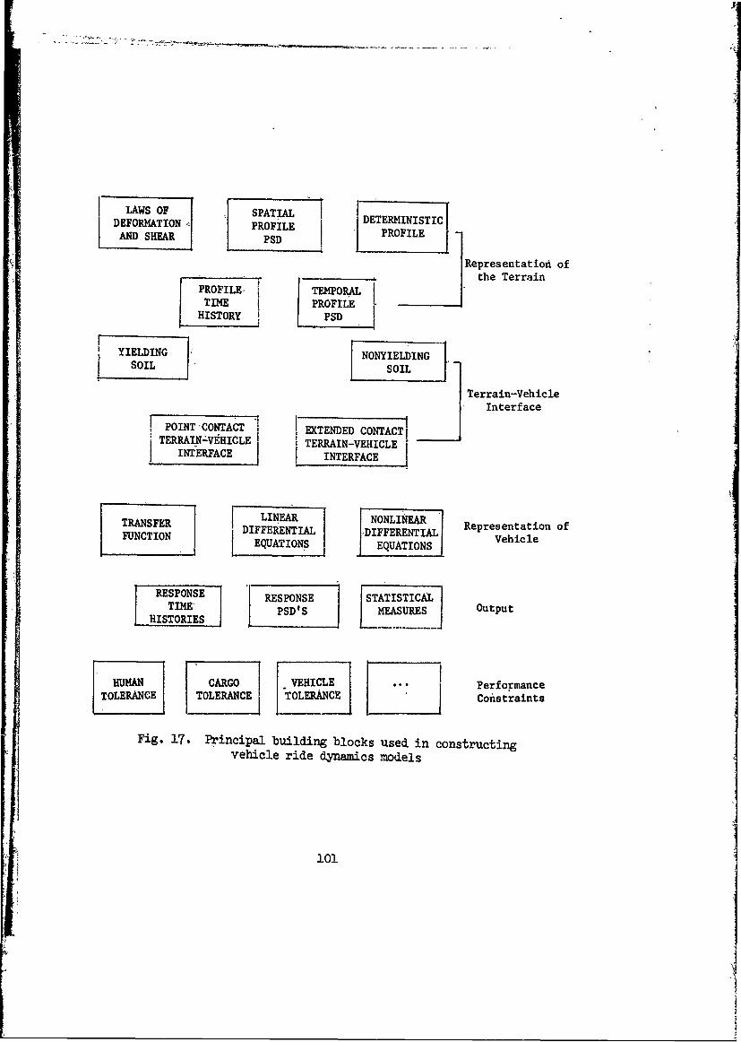
LAWS OF SPATIAL I IEEMNSIDEFORMATION PROFILE PROILEAND SHEAR PSD

Representationf ofthe Terrain

PROFILE- I TEMPORALTIME PROFILEHISTORY PSD

YIELDING NONYIELDINGSOIL SOIL

Terrain-VehicleInterface

POITCONTT EXTENDED CONTACTTERRAIN-49HICLE TERRAIN-VEHICLE

INTERFACE INTERFACE

TRNSFER ! LINEAR NONLINEARDIFFERENTIAL DIFFERENTIAL Representation ofFUNCTION EQUATIONS EQUATIONS

f RESoNs RESPONSE STATISTICATIME' PSD'S MEASURES OutputHISTORIES]L... .

HUMAN CARGO - VEHICLE PerformanceTOLERANCE TOLERANCE TOLERANCE Coistraints

Fig. 17. Principal building blocks used in constructingvehicle ride dynamics models

101

interface, performance constraints, and the output. In figs. '18-25, the

principal building blocks used in the construction of the several models

examined are indicated, and the manner in which the building blocks are

coupled is shown by the solid line connecting them. When a particular

model has more than one coupling approach, alternative couplings are shown

as dashed lines.

149. Representation of terrain. A vehicle oper: ring off-road en-

counters two types of hard-ground roughness. One type consists of discrete

obstacles such as boulders, tree stumps, logs, rice-field dikes, etc., to

which the driver tends to give individual attention. The other type con-

sists of continual more-or-less gradual variations in elevation that are

uniform over reasonably large areas and which the driver treats as an ele-

ment of the environment. The latter type, often referred to as stable

ground roughness, is characteristic of many virgin terrains and is of prin-

cipal interest in ride analysis. A distinction is made between these two

types, and they are generally treated separately in vehicle dynamics studies.

150. The simulation of rough stable ground is normally accomplished

by first measuring an actual terrain profile. The measurements, which con-

stitute an elevation-distance sequence for the area of interest, are trans-

ferred to magnetic tape, punched cards, or some other means suitable for

computer analysis.

151. Terrain profiles used in vehicle ride dynamics analyses may be

in either deterministic or statistical form. Selection of the form to be

used is dictated by the desired accuracy of the output and by the details

of available terrain data. A deterministic profile can be used as-recorded

in the form of a deterministic displacement-distance function to excite a

vehicle model passing over it. Vehicle response is then outputted in the

form of motion-time histories of various parts of the vehicle and generally

is not easy to interpret. As an alternate to the deterministic approach, a

terrain profile in statistical form can be used. In this form, the terrain

profile is expressed in terms of its frequency components.

152. A terrain profile can be converted to a statistical statement

of its frequency components. This is accomplished for a random stationary

segment of terrain by first computing the autocorrelation function. The

102

LAWS OFS

DEFORMATION SPATIAL DETERMINISTIC°PROFILE PROFILEAND SHEAR PSD

Representation ofthe Terrain

PROFILE TEMPORALTIME PROFILE

'HISTORY PSD

YIELDING NONYIELDING-]

SOIL SOI_

Terrain-VehicleInterface

1POINT CONTACT EXTENDED CONTACTTERRAIN-VEHICLE TERRAIN-VEHICLE

I INTERFACE INTERFACE

I '° 1T LINEAR, ANONLINEAR RRANSFER DIFFERENTIAL DIFFERENTIAL Representation of

FUNCTION EQUATIONS EQUATIONS Vehle

I I1RESPONSE STATISTICAL

TIME PSD'S MEASURES OutputHISTORIES

HUMAN CARGO VEHICLE.. PerformanceTOLERANCE TOLERANCE TOLERANCE Constraints

Fig. 18. U. S. Army Tank-Automotive Command ride dynamics model

103

r1

LAWS OF SPATIALL DFSHARION DETERMINISTICDEFO TION PROFILE oFLE -A N D SH EA R P SD P R" O F... .. IL ___E

Representation ofthe Terrain

PROFILE I TEMPORALTIME r PROFILE

HISTORY PSD

TIELDING LINEA j NONYIELDINSOIL SOIL

FTerrain-Vehicle

Interface

RESPOINT[ --- I Opu

CONTACT EXTENDED CONTACT1TERRAIN-VEHICLE T VEHICLEHer mnINTERFACE INTERFACE C

TRANSFER LIERNINA Representation ofFUNCTION DIF FERENTAL DFFERENTIALIVhil

EQUATIONS EQAIONSehcl

F RESPONSE RESPONSE STATISTICAL]HISTORIES PDS J 1 otu

HUMA CARGO IVEHICL] * PerformanceTOLERACE TOLERANCE2 TOLERANC Constraints

Fig. 19. Chrysler Corporation (Van Deusen) ride dynamics model

ro4

I LAWS OF 7PTASPAsoM L DETERINISTIC,

DEFORMATION PROFILE 'EEMNSIANDSHER 'PSD ___ L PROFILE -

Representation ofthe Terrain

PROFILE jTEMPORALTIME PROFILEHISTORY PSD

YIELDINGNONYIELDINGSOILL

Terrain-VehicleInterface

POINT-CONTACT !-E-TENDED CONTACT~TERRAIN-VEHICLE TERRAIN-VEHICLE

INTERFACE J INTERFACE

TRANSFER LINEAR NONLINEAR Representation ofDIFFERENTIAL IDIFFERENTIAL e e

FUNCTIONEQUATIONS E~UATIONSVeie

RESPONS RESPONLE STATISTICALTIME P'S AURS Output

HISTORIES ........ ......

HUMAN CARGO VEHICLETOLERANCE TOLERANCE TOLERANCE Performancej j Cons traints

Fig. 20. eneral Motors Corporation (McKenzie) ride d-nmics model

1105

LAWS OF FSPATIAL -EEMNSIDEFORMATION 1 PROFDTEMIISI

L AND SHEAR PROFFILEL. POILE

Representatiodt.ofthe Terrain

PROFILE I TEMPORALjTIME PROFILEHISTORY 'PSD

YIELDING LNxONYIELDINGSOIL SOIL

- - ---- Terrain-Vehicle

InterfacePOINT CONTACTETER -VEICLE TERRAIN-VEHICLEINTERFACE I INTERFACE j

I--TRANSFER LINEAR NONLINEAR Representation of

FUNCTION DERETIN IFFERNTIAL Vehicle

!!J "Tl TIMET OS

REPONSE RESPONSE ~ STATISTICALHISTIME S" IL MEASURES' Output

HITORIES'

E UMAN CARGO VEHICLE PerformanceTOLERANCE TOLERANCE TOLERANCE Constraints

Fig. 21. Ohio State University (Bussman) ride dynamics mdel

106

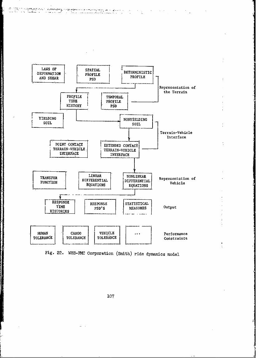
-&, iw -o -. i I

LAWS OFSPATIALDEFOMATON POFIE . DETERMINISTICsHEAR ROFILE PROFILE '

Representation of

the TerrainPROFILE j TEMPORALjTIME -PROFILE -

HISTORY [ tShD

YIELDING _ NONYIELDINGSOIL SOIL

Terrain-VehicleInterfacer, - t -__"_-

j POINT CONTACT I EXTENDED CONTACTTERRAIN-VEHICLE TERRAIN-VEHICLE

INTERFACE INTERFACET .... [ LINEAR F R

TRANSFER I NONLINEAR

DIFFERENTIAL DIFFERENTIAL Representation of

________________EQUATIONS rE1QbATIONS.

F RE'SPONSE RESPONSE STATISTICALTIME PSD'S ] MEASURES Output

HISTORIES , - .......

MANE TCARGO VEHICLE 7 PerformanceTOLERANC Coistraints

Fig. 22. WES-FMC Corporation (Smith) ride dynamics model

107

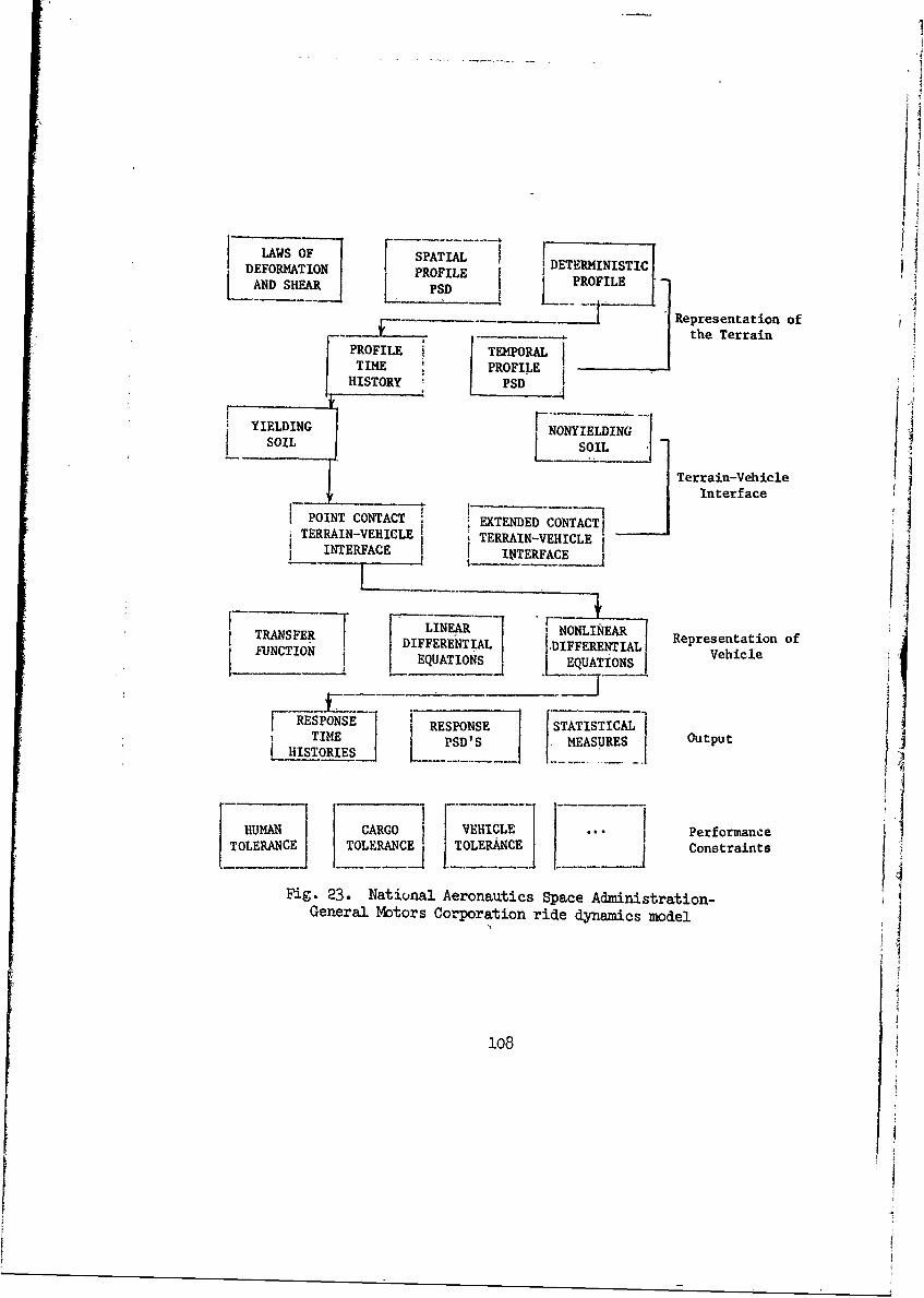
F iLAWS OF SPATIAL DETERMINISTIC

v~uIILu4PROFILE II PROIEISADSHEAR PSDPRFL

Representation ofthe Terrain

PROFILE i TEMPORAL

TIME : PROFILEHISTORY PSD

YIELDING NONYIELDING

SOIL NGSOIL

Terrain-Vehicle'/ Interface

, POINT CONTACT ETENED CONTACTfi TERRAIN-VEHICLE TERRAIN-VEHICLE

INTERFACE t ITERFACE

TRANSFER 7LINEAR 1OLNANTDIFFERENTIAL IDIFFERENTIAL Representation ofL EQUATIONSj [EQUATIONS Vehicle

R ONSE RESPONSE STATISTICALTIME PSD'S MEASURES 0I HISTORIESjPS' [ ..... -.... Otput

CARGO VEHICLE PerformanceTOLERANCE TOLERANCEj TOLERANCE Constraints

Fig. 23. National Aeronautics Space Administration-General Motors Corporation ride dynamics model

1O8

LAWS OF SPATIAL DETERMINISTICDEFORMATION PROFILE PROFILEAND SHEAR "PSD RFL

Representatiod ofthe Terrain

PROFILE TMIFORALTIME- PROFILE

-HISTORY PSD

SYIELDING NONYIELDINGSOIL SOIL

Terrain-Vehicle

Interface'POINT CONTACT EXTENDED CONTACT,,

TERRAIN-VEHICLE TERRAIN-VEHICLEINTERFACE INTERFACE .

LINEAR NONLINEAR Rpesnaino

DIFFERENTIAL DIFFERENTIAL e ceUNTON EQUATIONS EQUATIONS Vhce

RESPONSE RESPONSE STATISTICALTIMEMEASURES

OutputHISTORIES

EUMANC CARGO VEHICLE Performance

TOLERAC TOLERANCE TOLERANCE Conistraints

Fig. 24. National Aeronautics Space Administration-Brown Engineering ride dynamics model

109

LAWSOF ]SPATAL I DETERMINISTICDEFORMATION PROFIE PROFILE

ASHEA P

Reresentationl ofteTerrain

TIME PROFILE

YIELINGNONYIELDING

'Ter'rain-VehicleInterf ace

POINT CONTACT EXEDDCNATITERRAIN-V9HICLE CORA N TCTjINTERFACE I ERINE CE

TRNFRLINEAR,' NONLINEAR Representation ofFUNCIONDIFFERENTIAL DIFFERENTIAL Vh6.FUCINEQUATIONS -QAINSVhc.

HUMAN CARGO VEHICLE PerformanceTOLERANCE TOLERANCE TOLERANCE Cosrit

Fig. 25. Cornell Aeronautical Laboratory ride dyi~anics model

110

autocorrelation function is computed by taking two identical waveforms

(profiles), repeatedly shifting one with respect to the other, and then

calculating the correlation coefficient for each shift. The correlation

coefficient for a given shift is obtained by multiplying the elevations of

the two profiles at corresponding points on the horizontal scale and aver-I aging the products over a sufficiently long range, usually several periods

of the lowest frequency present, to provide a steady average. An example

is illustrated in fig. 26. The products a 1 1 a2 b 2 , a3 b3 , etc., are

computed, added together, and then ,divided by the total number of products

in-the sample. The correlation function is obtained from a plot of the

correlation coefficient as a function of the shift or lagged values

(fig. 27). The shift values may be in terms of time or distance, depending

IIb I b2 I

Fig. 26. Calculation of correlation coefficient. At corre-sponding points on horizontal scale, the ordinates of the twowaveforms are multiplied. The correlation coefficient is the

average of the aibi products

Shift

Fig. 27. The correlation function

ll

upon whether the original waveforms are functions of time or distance.

153. The autocorrelation function has a maximum value for zero shift,

w ich is equal to the mean square value of the waveform, and decreases to

zero if the mean value of the waveform is assumed to be zero for infinite

value of the shift unless the waveform contains periodic components. If

the waveform has periodic components, the autocorrelation function also has

periodic components of the same period. The autocorrelation functions for

several common waveforms are shown in fig. 28. The autocorrelation func-

tion of a discrete sequence is defined by

Rx(tl t1 + T) = i N (1

N kl Xk(t 1 ) X(t I +

where R (tl, tI + T) is the value of the autocorrelation function when

the lagged distance is T and Xkt) is the original sequence. The dis-

crete form of equation 11 is a direct translation of the autocorrelation

Signal Correlation Function

Ill',' __ ll_

0

:C

0

011112

function for a continuous and infinite sequence given by equation 12.

T

R W = -* Xk(t)Xk(t + .)dt (12)

This equation is true for a sequence that has an infinite length. However,

for sequences with finite length, consistent results require that the auto-

correlation function (equation 11) be modified to the form

Rx(t 1 ' t + ) N- Xk(tl)Xk(tl + ) (13)

k=l

This equation differs from equation 11 in that the quantity Xk(tl)Xk(tl

+ r) is averaged by dividing by the actual length over which Xk(tl) and

Xk(t I + T) are multiplied. For a random sample with a zero mean, the

autocorrelation function should approach zero and remain at zero as the lag

values increase, and the function should not be periodic. (See fig. 28 forrandom wave.) The extent to which the function fulfills these conditions

determines whether the waveform (terrain profile) is sufficiently random to

be described by this technique. However, an unsatisfactory autocorrelation

function can frequently be improved by performing a filtering operation

(detrending) on the original data to remove the influence of longer wave-

lengths. Another useful and very significant property of the autocorrela-

tion function is that it happens to be the Fourier transform of the power

spectral density (PSD) of a random, stationary waveform. Having obtained

the autocorrelation function, it is then possible to compute the power

spectral density function.

154. The PSD is a second moment or variance density spectrum. PSD

of a random, stationary function is defined as the Fourier transform of its

autocorrelation function as follows:

P(Q) = 2 J Rx(T)ei 2 rdr (14)

-w

where Rx(er) is the value of the correlation function for shift T , and

113

is the frequency in cycles per inch if is measured in inches and cy-

cles per second if T is measured in second.,* the _-*tegral .,ier the fre-

quency range 0 -+w of the PSD is the variance.-'

155. In the application of equation 14, a raw e-tirate .of the power

spectrum can be obtained by the following numerical method,:

m

(h -c R ( cos- h= o ,1 ,...m (15)

whererwh) = ower spectral estimate of series x at frequency,

Note: P(h) =

At = constant sampling interval (may be time or distance)

m = maximum lag

1/2 0= ,m

S ( T ) autocorrelation value of series x at lag v

The raw estimates are then customarily smoothed by using "smoothing" coef-

ficients. An accepted method of smoothing using "Hamming" coefficients. is

as follows:

sP(° ) - 0.54 P(o) + 0.4 p(1)x X X

sP(h) = 0.23 P(h-l) + 0,54 p(h) + 0.23 P(h+l) , 0 <h < m

SP(m ) = 0.54 p(m) + 0.46 p(m-1)

where SP( = smoothed power spectral estimate of series x at frequency

h,

mAt

Smoothing is necessary because the raw estimate is an inefficient estimate

of the true spectral density since a finite record length precludes

* This is true if the function has a zero mean. For functions with a zero

mean, the mean square and variance are the same.

14ll

-U ~, h. .

identifying f:requencies exactly and a more reliable statistical estimate

can be obtained by averaging over neighboring frequencies. Trial-and-error

methods such as the method developed by Hamming -have proved more useful in

obtaining sets of averaging coefficients that produce reliable spectral es-

timates than has any particular theory. There are several well-established

sets of coefficients avai-able, and in general, the Hamming method is quite

satisfactory.

156. A logarithmic plot of two terrain power spectra is shown in

fig. 29. The ordinate is in terms of inch2 per cycles per inch, and the

"Z 1.

. Profile A

Profile B

0.4

-Pr

Wavelength, Ln.0 20

.OPrf IA

0.02 0.05 0.1 1.0Spatial Frequency, 0, cycles/in.

Fig. 29. Examples of terrain Bower spectra

115

abscissa is in units of cycles per inch, the reciprocal of wavelength.

These spectra measure the rate of change of the average elevation with fre-

quency and are primarily geometric quantities that do not contain any units

of time. The area under each power spectrum represents the mean square

value of the total roughness for the respective profile. The area Under

the curve between any two selected wavelengths will indicate the contribu-

tion to the total roughness that this range of wavelengths produces. Thus,

from the terrain power spectrum curve, the wavelengths that make the great-

est contribution to the variation in the elevation measurements can be

determined.

157. The terrain elevation power spectrum can be used also with cer-

tain vehicle characteristics t 9 determine wavelengths and frequencies that

induce significant forces and motions if the velocity of the vehicle is in-

troduced. This is done by multiplying the abscissa of the terrain power

spectrum by the vehicle speed (inches per second) to obtain the frequency

cycles per second (cps), and by dividing the ordinate of the power spectrum2by the vehicle velocity to obtain the units of inch per cycles per second.

A different spectral curve obviously results for each velocity. This cal-

culation was performed on the terrain spectrum of profile A (fig. 30) to

represent vehicular speeds of 44 and 88 in./sec (2.5 and 5 mph, respec-

tively). It i.; seen that increasing the vehicle's velocity tends to shift

the spectrum to the right along the frequency axis and expand the frequency

range. For example, if a vehicle is excited by a sinusoidal exciter plat-

form with a controlled frequency, adjustable amplitude, and electronic

transducers to measure the resulting reaction forces and motions, a re-

sponse of the force ratio versus frequency (fig. 31) can be obtained by

systematically varying only the frequency. Similar relations can be ob-

tained for accelerations. For a linear system, this spectral relation is

referred to as the systems transfer function. Note in fig. 31 the two pre-

dominant frequencies at 2 and 15 cps. These are the basic natural frequen-

cies of the center of gravity and the axles, respectively. Variations in

the terrain profile that will excite frequencies of 2 and 15 cps will thus

generate large forces and motions between the vehicle and the terrain.

These frequencies are, therefore, of interest in determining the influence

116

A

88 in./sec ( '(Pr file-A PSD) ,

44 in.lsee] Vehic le requency

ResI nsq

I .J4 i0 -

S_---10--

;1 2

/

0.5 1.0 10.0 20 3o 4o

Frequency, cps

Fig- 30. Terrain and vehicle characteristics as a function

of frequency

117

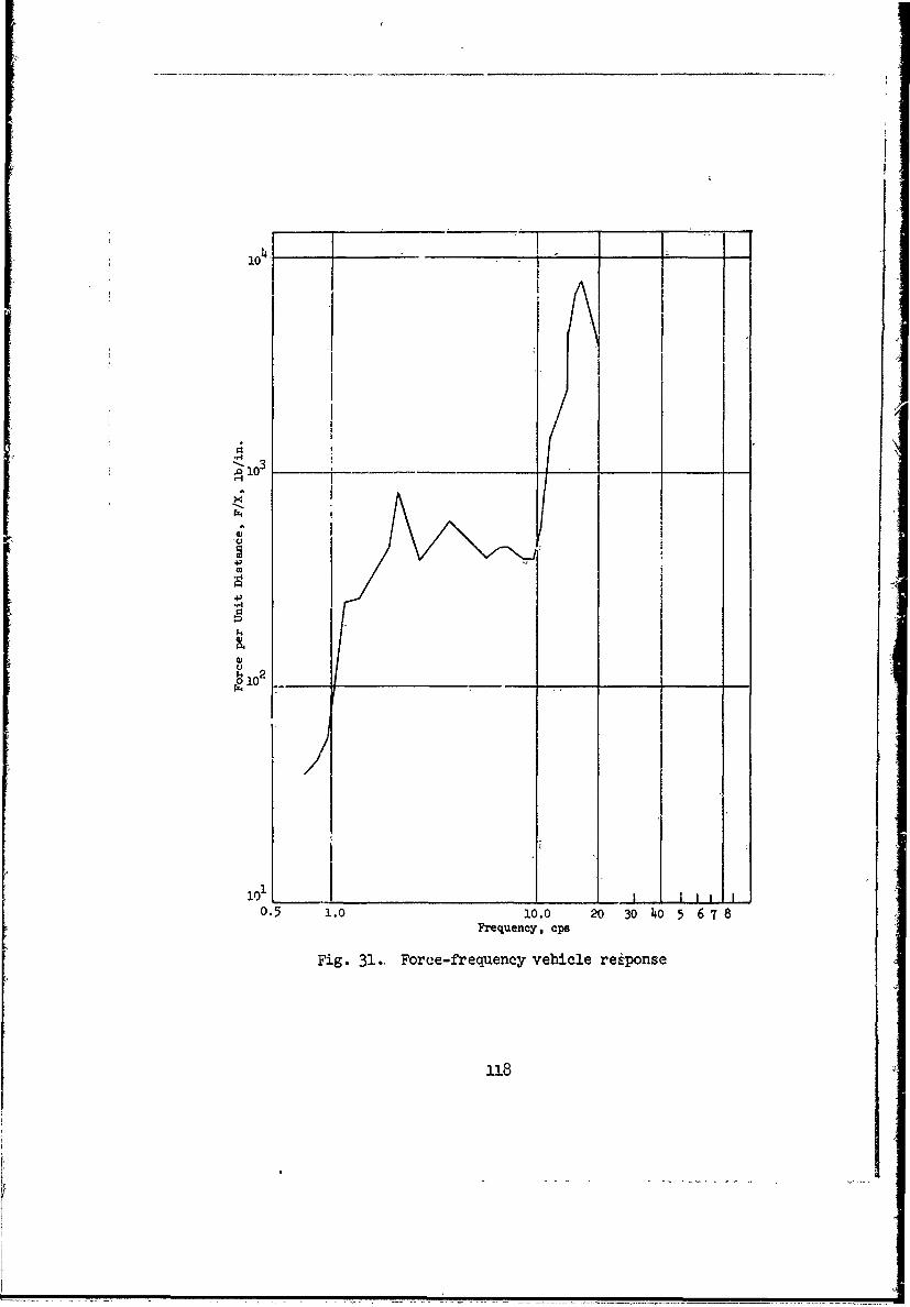
104,

II

103

,

010.,

o 102 ._ _ _ _ __ _ _ _ _ _ _ _

Ioi i- I t

0.5 1.0 10.0 20 30 4o 5 6 7 8Frequency, cps

Fig. 31. Force-frequency vehicle response

118

[5r lllIll

of the terrains on the reaction of the vehicle. This relation can now be

combined with the terrain power spectrum to obtain an estimate of the dy-

namic force or motion that the vehicle will exert on the terrain, and vice

versa. To do. this, the terrain spectrum must first be modified by intro-

ducing the vehicle velocity, as previously described. If this is done,

then to determine a power spectrum of the dynamic force that the vehicle

will exert on the terrain is simply a matter of multiplying the two spectra.

It is worth mentioning that the vehicle characteristics (fig. 31) must be

squared when this mathematical operation is performed to give the approxi-

mate units of pounds 2 per cycles per second (lb2/cps) on the ordinate of

the response spectrum. A typical result of these computations is shown

graphically in figs. 30 and 32 for the vehicle traversing profile A at a

speed of 44 in./sec. The influence of the vehicle's natural frequencies

(2 and 15 cps) is vividly portrayed by the dynamic response spectrum

(fig. 32). This response spectrum also has the same characteristics as

previous spectra, i.e. the area under the curve represents the mean square

value of the response. With this value, it is easy to determine the root

mean square (effective) value. This RMS value is the effective force that

the vehicle exerts on the terrain for that velocity. Such a spectral anal-

ysis provides a great deal of information on and insight into just how the

frequencies of the terrain influence a vehicle's response and further pin-

points critical speeds and terrain wavelengths. However, this analysis is

based on the fact that the vehicle is a linear system; that is, if the am-

plitude of the sinusoidal shaker is doubled, the only effect on the vehi-

cle's response is the doubling of the output for all frequencies. This,

however, is not the case for actual vehicles, which, unfortunately, are

nonlinear.

158. Most terrain models employ a nonyielding soil-vehicle interface.

No additional equations are required, and it is also reasonable since it

represents the worst case from a vehicle ride dynamics standpoint. Some

models, however, are more realistic and include yielding interfaces (Van

Deusen). A consideration of yielding surfaces increases the complexity of

the model, but permits a more realistic simulation of the real world ter-

rain situation.

ll9

10__ _ _ _ _ _ _ _ -- -

0

P4

4) 1

0.5 1.01 20 30 -

Frequency, cps

Fig. 32. Vehicle response-frequency relation

120

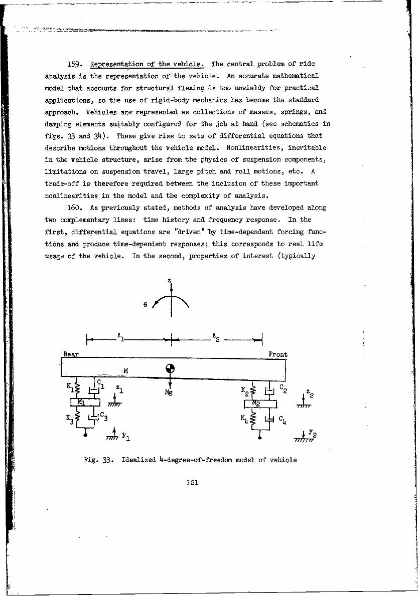
159. Representation of the vehicle. The central problem of ride

analysis is the representation of the vehicle. An accurate mathematical

model that accounts for structural flexing is too unwieldy for practical

applications, so the use of rigid-body mechanics has become the standard

approach. Vehicles are represented as collections of masses, springs, and

damping elements suitably configurcd for the job at hand (see schematics in

figs. 33 and 34). These give rise to sets of differential equations that

describe motions throughout the vehicle model. Nonlinearities, inevitable

in the vehicle structure, arise from the physics of suspension components,

limitations on suspension travel, large pitch and roll motions, etc. A

trade-off is therefore required between the inclusion of these important

nonlinearities in the model and the complexity of analysis.

160. As previously stated, methods of analysis have developed along

two complementary lines: time history and frequency response. In the

first, differential equations are "driven" by time-dependent forcing func-

tins and produce time-dependent responses; this corresponds to real life

usage of the vehicle. In the second, properties of interest (typically

z

e

Rear Front

K1 C1 z1K C2

K2

Fig. 33. Idealized k-degree-of-freeom model of vehicle

121

iI

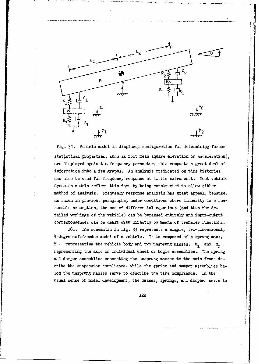
22

K CI

• K C

Fig. 34. Vehicle model in displaced configuration for determining forces

statistical properties, such as root mean square elevation or acceleration),

are displayed against a frequency parameter; this compacts a great deal of

information into a few graphs. An analysis predicated on time histories

can also be used for frequency response at little extra cost. Most vehicle

dynamics models reflect this fact by being constructed to allow either

method of analysis. Frequency response analysis has great appeal, because,

as shown in previous paragraphs, under conditions where linearity is a rea-

sonable assumption, the use of differential equations (and thus the de-

tailed workings of the vehicle) can be bypassed entirely and input-output

correspondences can be dealt with directly by means of transfer functions.

161. The schematic in fig. 33 represents a simple, two-dimensional,

4-d.egree-of-freedom model of a vehicle. It is composed of a sprung mass,

M , representing the vehicle body and two unsprung masses, M I and M2 ,

representing the axle or individual wheel or bogie assemblies. The spring

and damper assemblies connecting the unsprung masses to the main frame de-

cribe the suspension compliance, while the spring and damper assemblies be-

low the unsprung masses serve to describe the tire compliance. In the

usual sense of model development, the masses, springs, and dampers serve to

122

represent the bodyj, elasticity, and friction of the system, respectively.

The mass elements are assumed to be rigid bodies. The spring elements pos-

sess elasticity and are assumed to be of negligible mass. A spring force

exists only if the spring is deformed, such -as the extension or compression

of' a coil spring. Therefore, the spring force exists if there is a rela-

tive displacement between the two ends of the spring. The spring force-

deformation relation may be either linear or nonlinear. The damping ele-

ments have neither mass nor elasticity. Damping force exists only if there

is relative motion between the two ends of the damper. Many types of damp-

ing may be encountered in engineering systems, most of which are nonlinear.

However, there are but two. common types of damping occurring in vehicle

suspensions. One type is Coulomb damping, sometimes called frictional

damping, in which the damping force is a function of the normal force be-

tween the sliding b6dies as well as the materials involved. This type of

damping force occurs in suspension leaf springs and is assumed to be inde-

pendent of the relative velocity between the sliding bodies and dependent

on the direction of the- motion. The other type, which is used most often

in modeling, is that which is characterized by dashpot action in which the

damping force depends oxf the relative velocity of the deformations. This

type of damping occurs in shock absorbers. Some recent vehicle models have

included both types of damping in the suspension elements, but generally

the gross damping in suspensions is lumped in the latter type. All the

damping forces in the vehicle model in fig. 33 are assumed to be solely de-

pendent on relative velocity.

162. The number of degrees of freedom of any system is determined by

the number of independent coordinates required to describe the configura-

tion of each mass of the system.- For the model shown in fig. 33, two coor-

dinates are required to describe the configuration of the sprung mass--a

vertical motion of the center of gravity and a rotation about the center of

gravity. The axles are permitted to have motion in only the vertical di-

rection, thus requiring but a single coordinate to describe each axle's

configuration.

163. The differential equations describing the motion of the system

are arrived at through Newton's second law, F = ma . Determining the

123

equations of motion of any system first requires the establishment of a.co-

ordinate system and appropriate sign convention for each degree of freedom.

This coordinate system and sign convention are copletely arbitrary, but

once chosen, they must then be adhered to throughout the development of the

equations. Regarding the model in fig. 33, it is seen that all upward

translational motions and counterclockwise rotations are considered posi-

tive. Once the coordinate system and sign convention have been established,

the next step is to displace the model in a configuration such that all the

coordinates are affected, i.e. greater than or less than zero. For example,

assume that some arbitrarily positive displacements are applied to points

of contact of the front and rear tires displacing the system such that the

following conditions exist:

Y, > O y2 o y2 >Y 1

y1 > Z, :>z y>z 1 >

Y2 z 2 > z Y2 > z2 >

y2> 2?e O

where

YI, Y2 = vertical displacements of rear and front tires, respectively

zl, z2 = vertical displacements of rear and front axles, respectively

z. = vertical displacement of center of gravity of vehicla body

= rotation, in radians, of vehicle body about the center ofgravity

The terms with the dot notation denote time derivatives (velocities)of the appropriate coordinates.

This is a possible configuration for the system and is shcwn schematically

in fig. 34. In such a configuration, it is obvious that all the spring

elements are in compression. The amount of deformation for the front sus-

pension spring, A , is given by the relative vertical displacements of

the front axle and the point of attachment of the front spring to the

124

vehicle body i This deformation is denoted symbolically with reference to

the appropriate coordinates as:

= [z 2 - (z + 12 sine)]

Since z2 > z , the quantity in brackets is positive. Thus, positive de-

formations denote .spririg compressions and negative deformations denote ex-

tensions of the springs.

L64. -Similarly, the deformation of the rear suspension spring is:

= [z I - (z - A sin e)]

The quantities, A and A are the distances from the center of gravity1 2to the rear and front suspensions, respectively. The relative velocities

are obtained from the time derivatives of the deformations, e.g. for the

rear suspension

d (N)= [ t_ cos (16)

Assuming that the spring force-deformation and damper force-velocity rela-

tions are obtained for the suspension and tires through some means of meas-

urement, it is then possible to formulate functional relations, K(Al) and

C(ti) , that will allow for the calculation of spring and damper forces

due to variations in the tire and suspension deformations and relative ve-

locities. These relations may be in the form of tables, polynomials, or

piecewise linear segments. The suspension forces created by the configura-

tion in fig. 33 act upward on the vehicle body and downward with an equal

but opposite effect on the axles. The forces, generated by tire deflection

and damping act upward on the axles. The three masses, isolated into sepa-

rate free bodies with the appropriate forces applied to each mass, are

shown in fig. 35. The equations of motion, one equation for each degree of

freedom, are readily determined by summing the forces and moments acting on

each mass. They are as follows:

125

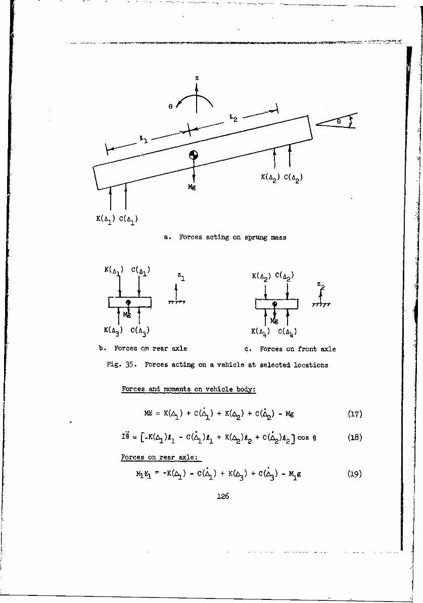
z

K(AI) c(A1)

a. Forces acting on sprung mass

K(A ) C(AI) z K(A2) C(A2)

K(A) C( A ) K(A) C( )

b. Forces on rear axle c. Forces on front axle

Fig. 35. Forces acting on a vehicle at selected locations

Forces and moments on vehicle body:

= K( ) + C( ) + + C( ) - mg (17)

A = [.K(Ll)t 1 - c( )I 1 + K(4) 2 + C(4)"2] cos 8 (18)

Forces on rear axle:

Mj1= -K(&,) - C(G) + K(%) + c(%) - Mg (19)

126

U ~-

Forces on front. axle:

= - c( 2 ) + K(A) + - M2 g (20)

where

and A. the deflections of the rear and front suspensions,respectively

A and j = the deflections of the rear and front tires, respectively

AI and L= the velocities of the rear and front suspensions,respectively

and A= the Velocities of the rear and front tires, respectively

165. The response to arbitrary inputs, Yl and Y2 , may be solved

using conventional methods for solving differential equations on either

digital or analog computers.

166. A two-dimensional model, although incorporating many nonlinear

features, is a simple representation of a vehicle. For example, the model

is restricted to motions in a plane. Expansion to a more general three-

dimensional model greatly increases the cost and complexity of analysis.

More degrees of freedom are introduced, thus increasing the number of equa-

tions, and the effects of independent and solid-axle suspensions become

more significant than with the two-dimensional model; and for travel other

than along straight paths, the concepts of space-fixed and body-fixed axes

and Euler angle references are required..

167. Representation of terrain-vehicle interface. Much of the work

involving mathematical modeling of vehicle dynamic performance uses a com-

mon representation of the vehicle traction element. When this element is a

pneumatic tire, .a spring and viscous damper are used to represent tire com-

pliance; when- the element is a track, the track pads are neglected and the

spring-damper representation is applied to the road wheels. The terrain is

represented as a vertical displacement input to each traction element,

hich, in turn, transmits vertical forces to the vehicle. The interface of

terrain and traction element is represented as a single point contact.

Such representations should yield generally satisfactory results where the

terrain is not too severe, i.e. where the radius of curvature of an

127

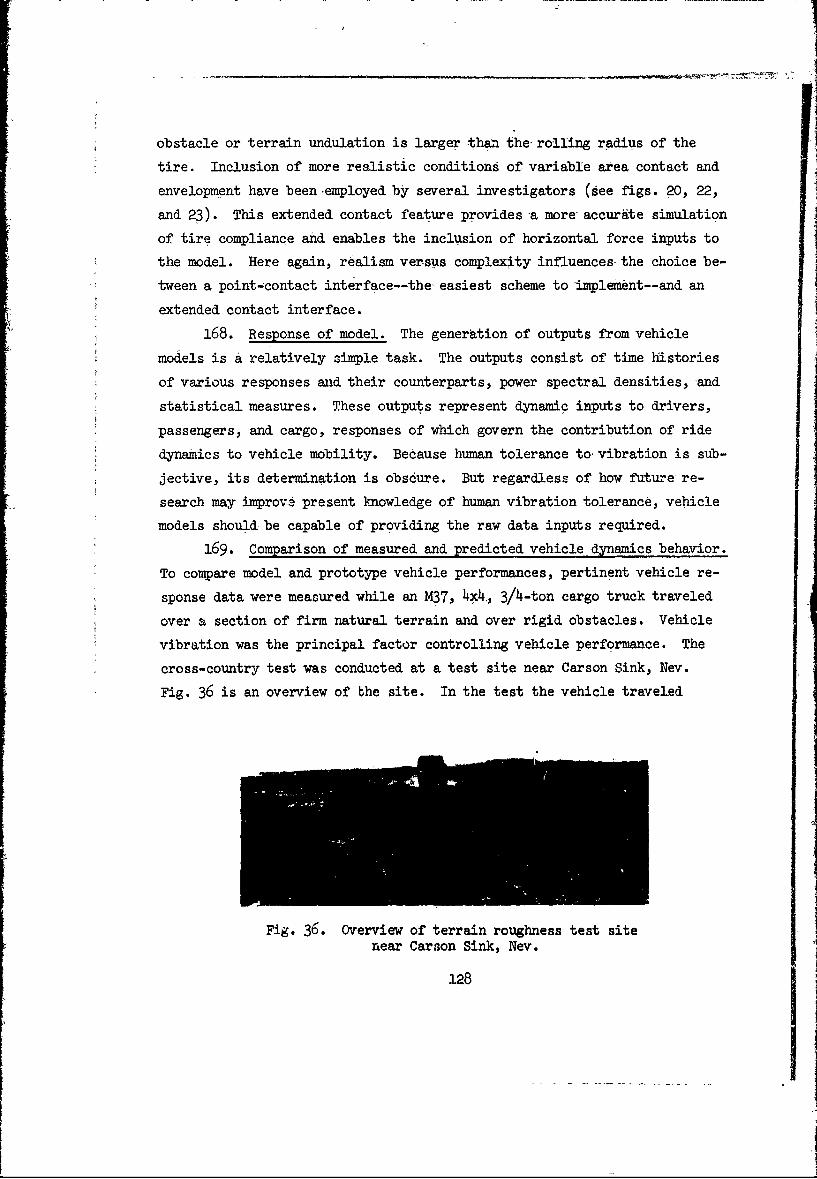
JI

obstacle or terrain undulation is larger than the. rolling radius of the

tire. Inclusion of more realistic conditions of variable area contact and

envelopment have been -employed by several investigators (see figs. 20, 22,

and 23). This extended contact feature provides a more accurate simulation

of tire compliance and enables the inclusion of horizontal force inputs to

the model. Here again, realism Versus complexity influences the choice be-

tween a point-contact interface--the easiest scheme to implement--and an

extended contact interface.

168. Response of model. The generation of outputs from vehicle

models is a relatively simple task. The outputs consist of time histories

of various responses and their counterparts, power spectral densities, and

statistical measures. These outputs represent dynamic inputs to drivers,

passengers, and cargo, responses of which govern the contribution of ride

dynamics to vehicle mobility. Because human tolerance to vibration is sub-

jective, its determination is obscure. But regardless of how future re-

search may improve present knowledge of human vibration tolerance, vehicle

models should be capable of providing the raw data inputs required.

169. Comparison of measured and predicted vehicle dynamics behavior.

To compare model and prototype vehicle performances, pertinent vehicle re-

sponse data were measured while an M37, 4x4., 3/4-ton cargo truck traveled

over a section of firm natural terrain and over rigid obstacles. Vehicle

vibration was the principal factor controlling vehicle performance. The

cross-country test was conducted at a test site near Carson Sink, Nev.

Fig. 36 is an overview of bhe site. In the test the vehicle traveled

Fig. 36. Overview of terrain roughness test sitenear Carson Sink, Nev.

128

over a 1000-ft-long, mildly undulating course at an almost constant speed

of 8 mph. The obstacle tests were conducted on: the WES obstacle test

course. In these tests the vehicle traveled at an average speed of 15 mph

in a path that was at a right -angle to the obstacle. The obstacle was a

nonyielding trian gular-shaped object, 6 in. high, with an approach angle

of 30 deg (-see fig. 37). The response data frca the cross-country and ob-

stacles tests were recorded on analog magnetic tape and processed on an

*analog computer. In addition, results from a previous study with the M37

were used to augment the analysis. Two mathematical models of the M37 were

used to simulate the actual tests, one using a point-contact interface for

the tire and terrain and linearized rotational motions, and the other using

an extended contact interface and nonlinear rotational motions.

a. Single obstacle test.

(1) The acceleration-time history of the response of the

vehicle's front axle to a single obstacle is shown in

fig. 38. The extended contact model yields the more

realistic motions, which very closely approximate the

measured motions in the initial portion. However,

this correspondence is of short duration, and the devi-

ations quickly increase to a significant level. The

nature of these deviations suggests that modeling of

the suspension damping may not be siifficiently accu-

rate. The shortcomings -of the point-contact model are

revealed by the extremely large accelerations occur-

ring during and just after the period of tire-obstacle

contact.. The adverse effects of the inability of the

point-contact model to simulate the envelopment char-

acteristics of the tire (see fig. 37) are accentuated

for cases such as- this when the input forcing function

contains significant discontinuities. An almost infi-

nite- negative acceleration occurred when the point of

contact became abruptly separated from the obstacle,

so that for a short time only negative downward forces

were applied to the axle.

129

II

Fig. 37. M37, 4A1 , 3/4-ton cargo truck negotiating arigid obstacle at 22 fps

130

~co

094

a U'l

C; 0$

4-1HI o

HIn0 M

4- 00i

0~ H)+

0 i 00

-- 0

0 LA 0

S'UO~oulaTaDDY TVDTVOA

131

(2) The tire envelopment characteristics can be included

to a certain degree in the point-contact model by mod-

ifying the obstacle shape in terms of the tire geome-

try. This is done by determining the vertical move-

ment of the axle as a tire (considered rigid) passes

over the obstacle. This movement then serves as the

modified displacement input to the point of contact.

Such a modification was made for the obstacle run, and

the response is compared with the original response in

fig. 39. In this case, the responses are not very

different.

(3) Little difference between the two models is noted when

the responses of the vehicle's center of gravity are

compared (fig. 40). The two distinct peaks, repre-

senting the contacts of the front and rear axles with

the obstacle, occur at about the same time as the

measured peaks, but the magnitudes for both models are

considerably smaller than the measured values.

(4) Generally, the essential features of the simulated

acceleration-time histories do not cbmpare well with

the measured waveforms.

(5) A noticeable difference occurs in the models in the

simulation of the vehicle's pitch motion. This dif-

ference is due largely to the different restrictions

placed on the rotational motions. The point-contact

model with the linearized rotational motions overpre-

dicts the pitch motions, and the extended contact

model underpredicts them (fig. 41).

b. Cross-country test.

(1) The results of the cross-country test are compared in

fig. 42 in the form of an RMS acceleration-time his-

tory at the vehicle's center of gravity and in fig. 43

in the form of an absorbed power-time history computed

from the accelerations at the driver's seat. The

132

02

0 P4

4) 0

Cd

0 ) <: p)

0 '4)

04)) H ~ I

V\ 01004-)

4~c 004(4 P

402

40 0 04

00

C;000 020

133

04I0

cc 00

0

; a)

01

Laa

134 4

- '-~-~-~ - --

4)

a,4) LC\

~,o \ H

4)4) a,

~0 H,4) C)

a,4)

H 04)

a,0 H

o

C4) I4)a, 0

o I ~2)o if CI,

4) LI\ 4)0

*r4 00 (1)

- 024) $4

H E-~ 4)

a,

- -.- -~. -~ -.-- -~

o 0

$4a,

1 4)a,-~ C)

0 -rz.-Cf~)I

U $40

4 c'J

5C

H 4)

'I;------------------------5

q H

~L . .5-Irx4

H 0 Ho 0

135

I

00

0~

0 4 0

0 E-

to0

0 5

o p4

COj

136

____ __ _ ____ ___ ___

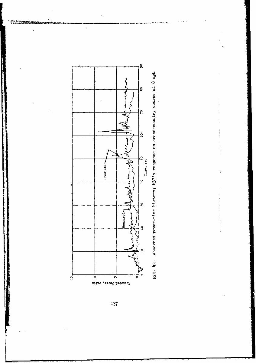
00

-0

+).

-4

4

0

0

0 U0ri0

n~vA zamoI paxo02

137O

predicted and measured RMS acceleration-time histories

are similar in form (fig. 42), but the model predic-

tions are both low by a factor of nearly 2.

(2) These results are the opposite of those from a similar

program reported by Van Deusen, in which the predicted

RMS vertical accexerations of the M37 were consist-

ently higher (by a factor of about 2) than measured

Values. This difference probably is due to the dif-

ferent methods for obtaining values of the vehicle pa-

rameters. Van Deusen obtained his values from shake-

table tests in which the entire vehicle was vibrated

over a selected range of frequencies, while those used

in the two models in this study were obtained by meas-

uring individual components while they were isolated

from the vehicle.

170. Problems associated With vehicle modeling. Determining accu-

rate and consistent values for the appropriate vehicle parameters is a

problem of tantamount importance in today's vehicle modeling. There are

others, however, that must be recognized, particularly when model and pro-

totype responses are compared. An example of a pertinent problem is shown

in fig. 44, where RMS vertical acceleration-time histories for differing

degrees of filtering are plotted. The unfiltered acceleration signal pro-

duces an RMS time history that is approximately twice the histories of the

three filtered signals. This is due to high-frequency vibrations transmit-

ted by the engine, flexural modes of the vehicle frame, anO. transducer pe-

culiarities, among others. When the acceleration is filtered with a 30-cps

filter, the RMS time history is reduced by nearly 50 percent of the unfil-

tered value. Filtering with 10- and 3-cps filters has only slight effects

on further reducing the magnitude. In fact, the 3-cps filter reduces the

RMS time history only 20 percent less than that obtained with the 30-cpsfilter. These filtered results, however, are still higher than those pro-

duced by the models. The models employing the concept of rigid-body me-

chanics are an assemblage of lumped masses, springs, and dashpots that have

discrete principal modes of vibration, usually not exceeding 20 to 25 cps.

138

do/

0

to

414

Jo 0

4.44

- - --

MiUiH1o; C;C

(YT'VITOO IVT4Q S

139p

Therefore, the models do not simulate the influence of engine vibrations,

bending modes of the vehicle frame, and other pigh-frequency components

that are present in the prototype response. Since these high-frequency mo-

tions are not bothersome to passengers and cargo, it is reasonable to fil-

ter out these effects when comparisons are made between model and prototype

responses. The measured RMS time history shown previously in fig. 42 was

processed with a lO-cps filter.

171. The modeled values of absorbed power (fig. 43) were generally

lower than the values that were computed from the vertical accelerations

recorded at the driver's seat. The computation was implemented on the ana-

log computer following the circuit diagrams (fig. 45) furnished by the Sci-

entific Computer Branch of the U. S. Army Tank-Automotive Command. A prob-

lem lies in the inability to reproduce the absorbed power-time history.

Each time the tape was processed a different time history was obtained.

This inconsistency is believed to be due to an open-loop, double integra-

tion in the absorbed power circuit.

172. Normally, models are validated by exciting them with simple,

well-defined inputs, such as a step function or sine wave, and comparing

the model response with that of a prototype vehicle driven over a course

with the same input configurations. Some criterion is chosen to determine

what is deemed a tolerable correspondence of the responses, and the model

is then adjusted until this degree of correspondence is met. The model is

then considered validated and, hence, representative of the vehicle. How-

ever, models validated in this manner to certain well-defined inputs are

generally valid only for those particular inputs. A vivid example of this

is illustrated in figs. 46, 47, and 48, which are plots of RMS vertical ac-

celeration at the driver's seat of the M37 versus speed for both measured

and predicted or modeled results for different sizes and shapes of single

obstacles. The model was "tuned" for the 8-in., half-round obstacle shape.

A close agreement exists between measured and modeled responses of the ve-

hicle to an 8-in. half-round obstacle (fig. 46). On the basis of these re-

sults, the model is considered truly representative of the vehicle. How-

ever, measured and modeled responses to an 8-in.-high obstacle with a 30-

deg face (fig. 47) deviate considerably. Furthermore, measured responses

14o

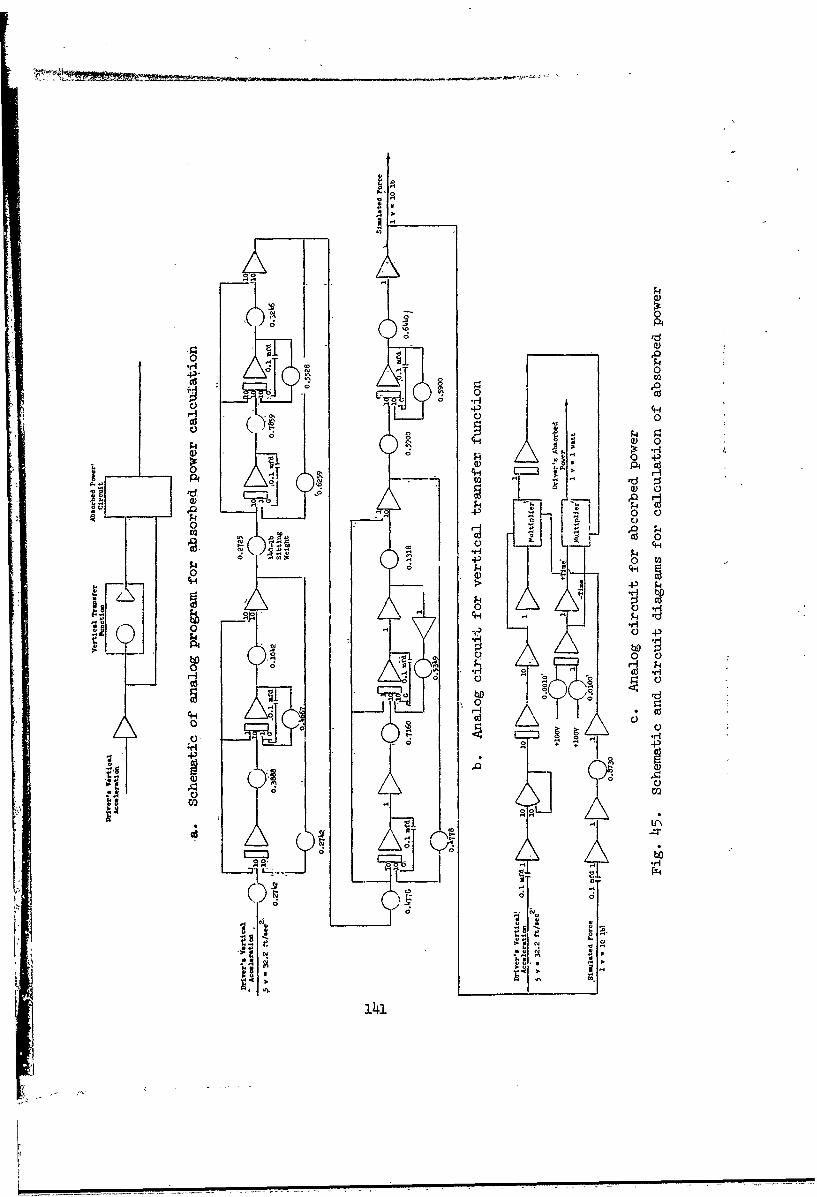
Q~F4

0

)- 0

$4

0) 0)

0o

0 -0 - "0

CHH

--- 0 .-4o2 0 .0-

00

114.4

t r

SI- aI

e' Q 0

Q0H

0 V

-H H

__ 0

1141

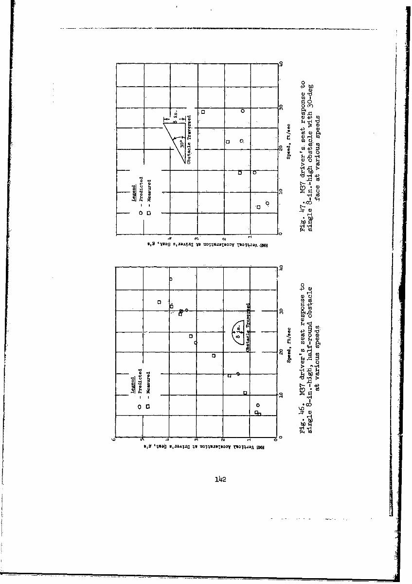
- 0

Q)

~0 0 (Y)

11 0) 43

on o cd, c

0G 00.

11 N j I_ 0

10 01

o 0

Sigi

0-P)

0 W0

d 0 a)4a)

0) 0

Lo bo C0G

0 c

81g 'os U,J&Ajzrj 4V UOT1JOSOoY TWO1144A SM)

14 2

CV)

-)

4I

00

H a)*r4 0 0 r )

03 A

op 0

______t 0~4_ _ _

H ~0 0

o co

I H02

UN~0

oM 0H

UOTIP~aTOOOV 020WA W

1430

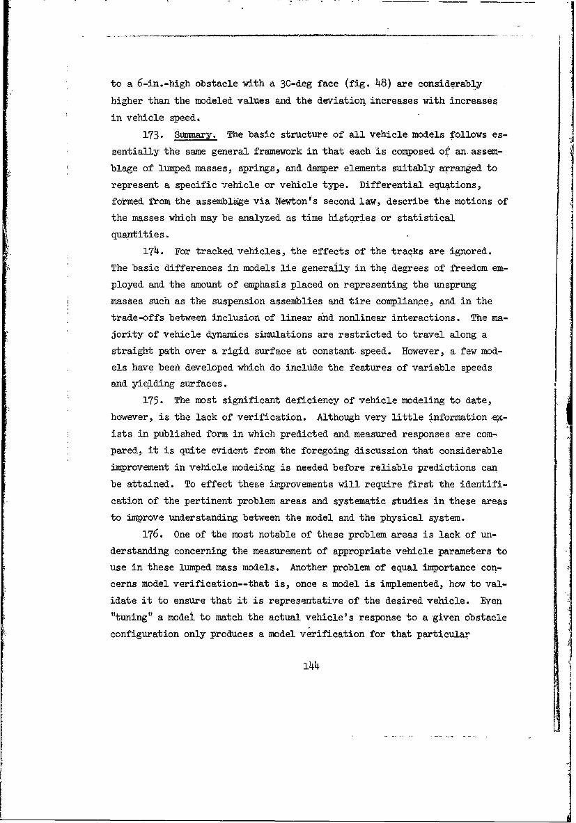
to a 6-in.-high obstacle with a 30-deg face (fig. 48) are considerably

higher than the modeled values and the deviation increases with increases

in vehicle speed.

173. Summary. The basic structure of all vehicle models follows es-

sentially the same general framework in that each is composed of an assem-

blage of lumped masses, springs, and damper elements suitably arranged torepresent a specific vehicle or vehicle type. Differential equations,formed from the assemblage via Newton's second law, describe the motions of

the masses which may be analyzed as time histories or statistical

quantities.

174. For tracked vehicles, the effects of the tracks are ignored.

The basic differences in models lie generally in the degrees of freedom em-

ployed and the amount of emphasis placed on representing the unsprung

masses such as the suspension assemblies and tire compliance, and in the

trade-offs between inclusion of linear and nonlinear interactions. The ma-

jority of vehicle dynamics simulations are restricted to travel along a

straight path over a rigid surface at constant speed. However, a few mod-

els have been developed which do include the features of variable speeds

and yielding surfaces.

175. The most significant deficiency of vehicle modeling to date,

however, is the lack of verification. Although very little information ex-

ists in published form in which predicted and measured responses are com-

pared, it is quite evident from the foregoing discussion that considerable

improvement in vehicle modeling is needed before reliable predictions can

be attained. To effect these improvements will require first the identifi-

cation of the pertinent problem areas and systematic studies in these areas

to improve understanding between the model and the physical system.

176. One of the most notable of these problem areas is lack of un-

derstanding concerning the measurement of appropriate vehicle parameters to

use in these lumped mass models. Another problem of equal importance con-

cerns model verification--that is, once a model is implemented, how to val-

idate it to ensure that it is representative of the desired vehicle. Even

"tuning" a modei to match the actual vehicle's response to a given obstacle

configuration only produces a model verification for that particular

144

r!

obstacle configuration. Since both the vehicle and the model responses are

frequency dependent, it seems more logical to validate a model by using as

input some general form of -random profile composed of many frequencies and

comparing the outputs in terms of their frequency response. Actual terrain

profiles of suitable length should ,serve this purpose.

177. Another problem that frequently causes significant differences

between the model prediction and vehicle measured responses is due to the

limited frequency range of the model as compared with the actual vehicle.

The contribution of the higher frequencies transmitted by the actual ve-

hicle can significantly affect the response, particularly so When evaluated

in terms of such statistical qu.tities as RMS, standard deviation, etc.

These high-frequency oscillations are negligible, however, with regard to

the ride problem and should be filtered from he measurements when making

comparison with model responses.

178. With these major problems in mind, it is apparent that consid-

erable study is needed in the area of vehicle dynamics modeling. However,

aii adequate correspondence between predicted and measured responses can

most likely 'be achieved with present modeling techniques through proper

filtering of the measured data and inclusion of accurate vehicle parameters.

Slope models

179. Many terrains contain slopes of sufficient magnitude that their

effects must be accounted for in the prediction of off-road vehicle per-

formance. Even when traction required to negotiate a slope does not exceed

the propelling force available, it will increase power required and fuel

consumption, reduce the margin of traction available to overcome further

impedances, and will usually decrease speed. Modeling vehicle and slope

interaction is thus a necessary element in any comprehensive model for pre-

dicting off-road vehicle performance. When a vehicle is operating on a

slope, there is an accompanying weight transfer and need for a margin of

excess traction to maintain steering control of the vehicle. In addition,

especially when side-sloping, a vehicle may overturn. Multipass operation

on slopes degrades or modifies the shape of the surface. In rough order of

magnitude of its effects on off-road vehicle operations generally, the

slope problem is probably second only to the soft-soil problem.

145

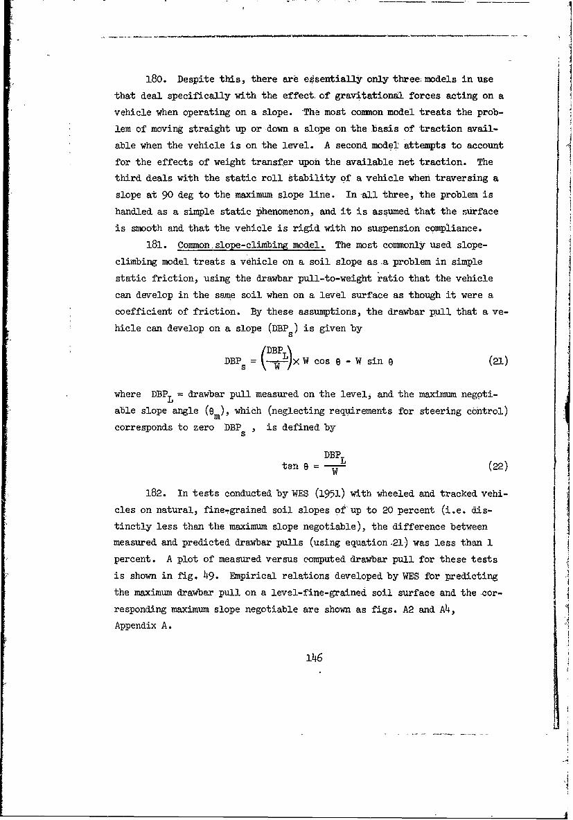
180. Despite this, there are e6,sentially only threemodels in use

that deal specifically with the effect of gravitational forces acting on a

vehicle when operating on a slope. -The most common model treats the prob-

lem of moving straight up or down a slope on the basis of traction avail-

able when the vehicle is on the level. A second model attempts to account

for the effects of weight transfer upon the available net traction. The

third deals with the static roll stability of a vehicle when traversing a

slope at 90 deg to the maximum slope line. In all three, the problem is

handled as a simple static phenomenon, and it is assumed that the surface

is smooth and that the vehicle is rigid with no suspension compliance.

181. Common slope-climbing model. The most commonly used slope-

climbing model treats a vehicle on a soil slope as a problem in simple

static friction, using the drawbar pull-to-weight ratio that the vehicle

can develop in the same soil when on a level surface as though it were a

coefficient of friction. By these assumptions, the drawbar pull that a ve-

hicle can develop on a slope (DBP ) is given by5

DBP = (- XW-xW cos o - W sin (21)

where DBPL = drawbar pull measured on the level, and the maximum negoti-

able slope angle (OMn), which (neglecting requirements for steering cohtrol)

corresponds to zero DBP , is defined by

DBP Ltan = -W (22)

182. In tests conducted by WES (1951) with wheeled and tracked vehi-

cles on natural, fine-grained soil slopes of up to 20 percent (i.e. dis-

tinctly less than the maximum slope negotiable), the difference between

measured and predicted drawbar pulls (using equation .21) was less than 1

percent. A plot of measured versus computed drawbar pull for these tests

is shown in fig. 49. Empirical relations developed by WES for predicting

the maximum drawbar pull on a level-fine-grained soil surface and the cor-

responding maximum slope negotiable are shown as figs. A2 and A4,

Appendix A.

146

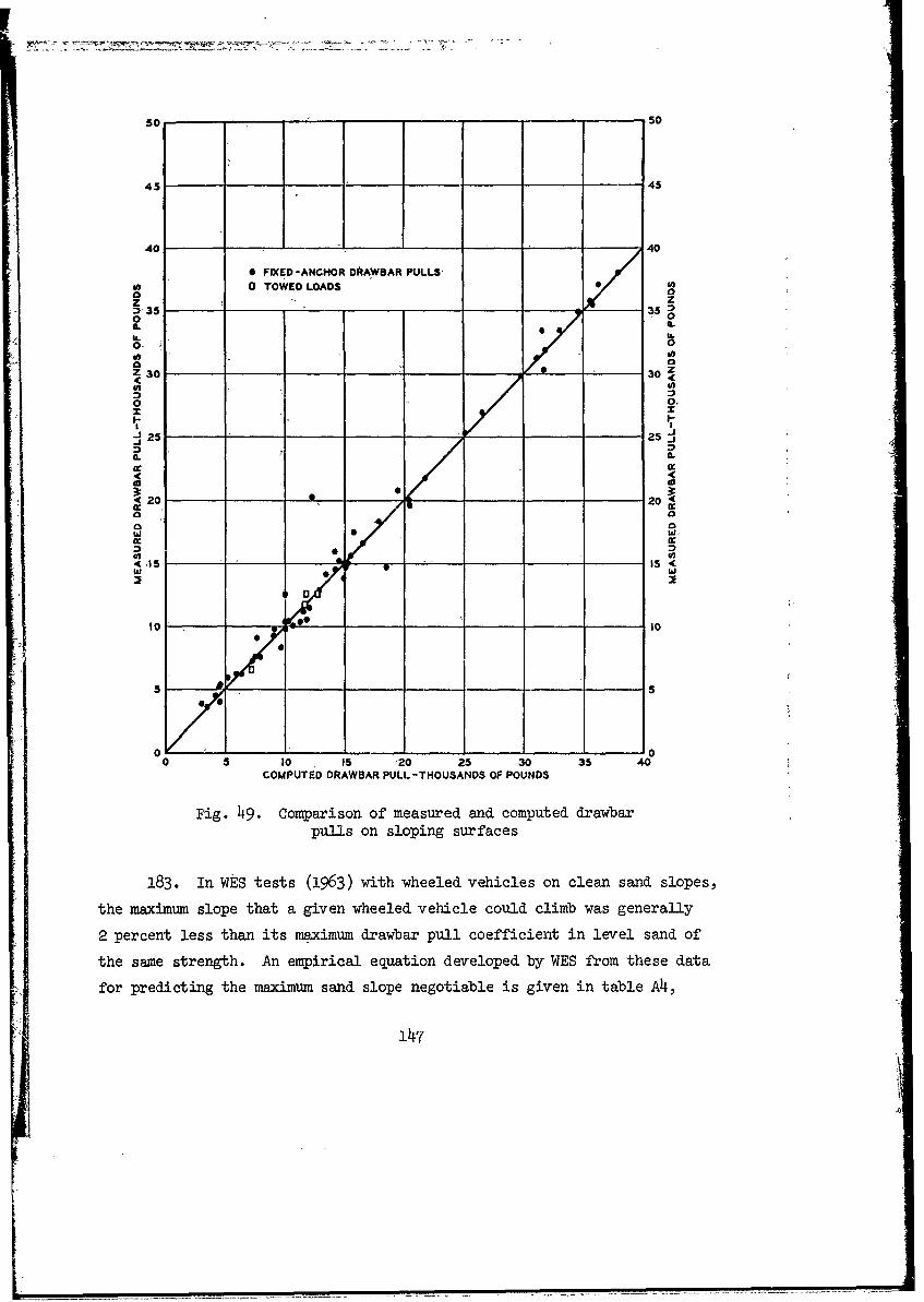
50 50

45 45

40 40

* FIXED-ANCHOR DAAWBAR PULLS'

0 TOWED LOADS 0

z z

0 0

/ .-Ena°

ao* " i

0o=.n.,o

0 0Z 30 __ 30z

I

I O .•

I -

0 I0

O25 25IL a.

-C20 ___ 20~

W W,

o W

COMPUTED DRAWBAR PULL -THOUSANDS OF POUNDS

Fig. 4. Comparison of measured and computed drawbar

pulls on sloping surfaces

183. In Ws tests (1963) with wheeled vehicles on clean sand slopes,

the maxim slope that a given wheeled vehicle could climb was generally

2 percent less than its maximum drawbar pull coefficient in level sand of

the same strength. An empirical equation developed by WES from these data

for predicting the maximum sand slope negotiable is given in table A,

147

0m

Appendix A. Measured maximum slope negotiable compared with values pre-

dicted from this regression equation yield ,a multiple correlation coeffi-2

cient (R ) of 0.96.

184. Laboratory wheel studies (cf. Smith 1969) show that the ratio

of drawbar pull to wheel load (DBPJW) decreases monotonically with in-

creasing load (fig. 50). This implies that predictions made with equation

21 should be slightly conservative insofar as the basic assumptions are ad-

equate. A recent lunar study by WES for NASA, reported by Freitag, Green,

and Melzer (1970), shows that for very light wheel loads, the relation

given by equation 21 is applicable, right up to maximum negotiable slopes.*

However, laboratory findings reported by Jones and Dewhirst (1964) with

model vehicles on sand and gravel slopes indicate that at somewhat higher

wheel loadings and high wheel slips the maximum grade predicted by °equation

22 was optimistic by as much as 20 percent.

185. LLD weight transfer model. When a vehicle is climbing a slope,

there is an effective transfer of weight from front to rear. Since ground

pressure is a primary determinant of tractive effort in soils, this weight

transfer should be accounted for in predicting vehicle slope operation.

LLD has recently published a model applicable to tracked vehicles which

makes some such allowances. This model assumes a trapezoidal ground pres-

sure distribution under a tracked vehicle when on a slope, as shown in

fig. 51. Values for contact pressure at-the front (a) and at the rear (b),

reflecting both the slope angle and the location of the vehicle center of

gravity, are then computed for two-dimensional static equilibrium. These

values are used somewhat inconsistently, with the basic Bernstein-Bekker

relation

z = (p/k)1/ n (23)

to calculate front and rear sinkage, and hence resistance generated by soil

compaction, and a slope resistance due to the vehicle trim in relation to

* Kloc, in "Vehicle Mobility Tests, Soft Soil Slopes," June 1970, purports

to show that this relation is not true at low loadings, but close analy-sis of his data does not support this conclusion.

148

00

IL-'

0P043 I Q-

4) $4 0 mA EAZ 0Ic

4*-P )

- 0C.) 0. H4 . 04) 1

C.))ca 0

0

0

01-4

00

0)0

-f 01J Hd

0,0

-P CMj

-HP

0 0H0 C0

co. CM

0 CH

H 0C0 0

qluaooj~ja0 TTncj .Qav~qx

14I

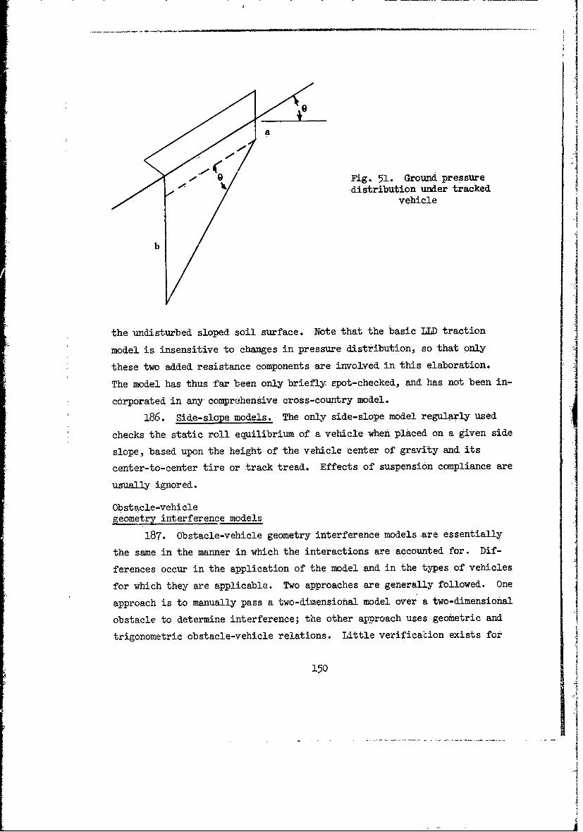
,Fig. 51. Ground pressure

L -distribution under tracked° vehicle

b

the undisturbed sloped soil surface. Note that the basic LID traction

model is insensitive to changes in pressure distribution, so that only

these two added resistance components are involved in this elaboration.

The model has thus far been only briefly spot-checked, and has not been in-

corporated in any comprehensive cross-country model.

186. Side-slope models. The only side-slope model regularly used

checks the static roll equilibrium of a vehicle when placed on a given side

slope, based upon the height of the vehicle -center of gravity and its

center-to-center tire or track tread. Effects of suspension compliance are

usually ignored.

Obstacle-vehicleZeomtry interference models

187. Obstacle-vehicle geometry interference models are essentially

the same in the manner in which the interactions are accounted for. Dif-

ferences occur in the application of the model and in the types of vehicles

for which they are applicable. Two approaches are generally followed. One

happroach is to manually pass a two-dimaensional model over a two-dimensional

obstacle to determine interference; the other approach uses geometric and

trigonometric obstacle-vehicle relations. Little verificat.ion exists for

~150

-

prototype vehicles except for standard rigid obstacles used in APG engi-

neering tests. Some scale-model verification results are available. Those

obstacle-vehicle geometry interference-models that are operational are dis-

cussed in the following paragraphs.

188. WESobstacle-Vehicle geometry model (GM or Chrysler or others).

These models manually test a two-dimensional vehicle scale model against

two-dimensional obstacles. Neither vehicle nor obstacle is considered to

have any compliance. The obstacle, but -not the vehicle, may be stylized.

The vehicle is presumed to approach the obstacle at 90 deg. Imnobilization

is usually assumed if there i s any {nterference at any time during the com-

plete- passage of the vehicle over an obstacle. If the vehicle can dross

othe obstacle or 6 section of irregular terrain, the WES model also deter-

mines the maximum attitude angle of tracked vehicles and the effective ob-

stacle angle for wheeled vehicles when crossing the obstacle. The effec-

tive obstacle angle for wheeled vehicles is the angle formed by a tangent

to -the point of tire-obstacle contact and a horizontal plane.

189. LLD obstacle-vehicle geometry model. The LLD model is a series

of computerized, two-dimensional comparisons between the vehicle and the

obstacle, both considerably idealized. This modeling is based upon equa-

tions published by Janosi in September 1968, which in turn, by way of manu-

script exchange, is due somewhat to suggestions subsequently published by

Bekker in 1969. The LLD model will handle four-wheeled vehicles and normal

skid-steered tracked vehicles. Obstacle shapes that can-be tested include

steps and vertical or V-walled ditches and crests, large and small. Possi-

bilities for interference are checked in- a series of critical vehicle/ter-

rain orientations and any interferences found are signaled. The assumption

is made that an interference equals an immobilization. These equations

were checked in a brief series of very slow-speed tests using three 4x4 ve-hicles and a few specially constructed concrete obstacles. Agreement was

good, as would be expected.

190. WMRE obstacle-vehicle geometry model. The WNRE model is phil-

osophically similar to the LID model except that the range of obstacle

shapes treated is more general and means are included for handling wheeled

vehicles with more than two axles. The -WNRE model is a small part

151

JI

integrated into a more elaborate go-no go program ,published in July 1968.,

It has since been furthei elaborated o handle articulate 6x6 vehicles and

still more complex shapes,as described in a July 1970 report of methods to

quantify lunar roving vehicle performance. In both cases, obstacle geome-

try is stylized in the general manner of the two-dimensional MERS terrain

map units and interference is considered tantamount to immobilization.

Obstacle-traction, models

191. When no geometric interferences are found, obstacle-traction

models determine whether or not sufficient traction can be developed to

surmount the obstacle. The soil-slope model may be considered as one pos-

sible member of this class but is usually treated separately. There are

two obstacle-traction models presently in the literature of complete cross-

country simulations; however, there has been no experimental verification

of these models.

192. WES obstacle-traction. model. In the WES obstacle-traction

model, determinations of the maximum force' required and the maximum force

that a vhicle can develop when at the maximum attitude -angle while cross-

ing an obstacle are made using the -following equations. For tracked

vehicles

F =W sin m(24)

where

F = maximum force ,required, lb

W = gross vehicle. weight, lb

amv = maximum attitude argle vehicle will attain in crossing obsta-

cles, deg

and

F d = DBP cos cmv (25)

where

Fmd = maximum force that can be developed, lb-

DBP = maximum drawbar pull on level surface, lb-

For wheeled vehicles, it is considered one axle at a time crosies the

152

obstacle, and W in equation 24- is replaced by - , where n is thena a

number of axles and ( is replaced by Oe as the effective obstacle-angle. If F mr , sufficient traction can be devel-

md is greater than It

oped for the vehicle to negotiate the obstacle.

193 . 'WNRE obstacle-tiaction model. The WNRE model computes, for

various critical positions of the vehicle on an obstacle, a .single coeffi-

cient of friction between the vehicle and the surface of the obstacle

needed for static equilibrium. This value is then compared with an effec-

tive coefficient of 'friction, taken as the vehicle net traction on level

ground divided by its weight, computed for soil having the given strength

characteristics. When effective coefficient of friction based on the ap-

propriate soil values is less than that required for equilibrium, the con-

dition is considered no go. There is obvious crudity in ignoring the re-

distribution of weight on the contact surfaces as it affects motion resist-

ance, tire deflection, actual single wheel traction, etc., for these may

seriously clter the magnitude of unit tractionf at each contact point. The

WNRE obstacle-traction model treats the problem as a quasi-static two-

dimensional one, with the vehicle approaching each discrete, linearized ob-

stacle at right angles. No vehicle "or obstacle compliance is allowed, ex-

cept '(in, the 1970,version) at the pitch joint of an articulated 6x6. How-

ever, the model will handle stylized wheeled and tracked vehicles of normal

configuration and a wide variety of obstacle sizes and Configurations. The

basic model, incorporated in a larger simulation published in July 1968,

has recently been :extended to cover two-dimensional, craterlike obstacles

and articulated, three-akle wheeled vehicles.

194. WES obstacle override speed model. In determining the speed at

which a vehicle can override an obstacle, the resisting force due to over-

ride is added to the other resisting forces acting on the vehicle. The

override force is determined by dividing the work required to override the

obstacle 'by the average distance between obstacles, or

Who0

F = (26)om. 12D)

0

153

where,

F = average force required to override obstacle, lbom

W = weight of vehicle, lb

h = height of obstacle, in.

D = average distance traveled between obstacles, ft

The average distance traveled between two obstacles is computed by convert-ing the area of the sample cell* to a rectangular area whose width is equal

to the vehicle width and dividing the length of the rectangular area by the

number of obstacles in the sample. The equation is12

D (27)

where

D = sample cell diameter, ft

w = vehicle width, ft

n = number of obstacles in sample

WES maneuver model

195. Abrupt nondeformable surface irregularities such as rock out-

crops, stumps, boulders, termite mounds, logs, etc., are deterrents to ve-

hicle performance and cause the vehicle to slow down to maneuver around

some and, perhaps override others. To account for the maneuvering effects

on speed, the WES maneuver -model uses semiempirical relations of percent

area denied and speed. By definition, "area denied" by a single obstacle

is the area encompassed by the obstacle itself plus one-half the vehiclewidth around the obstacle.

196. The equation for determining percent area denied is:

W + (t + wo)w + "] n= A X lO0 (28)

* The structural cell concept with its derivatives, mean tree spacing,

nearest neighbor distance, etc., has been explored with some intensity byWES. The concept is described in "Quantitative Physiognomic Analysis ofthe Vegetation of the Florida Everglades," by H. L. Mills, Contract Re-port No. 3-72, 1963, U. S. Army Engineer Waterways Exbperiment Station, CE,Vicksburg, Miss.; prepared by Marshall University, Huntington, W. Va.

154

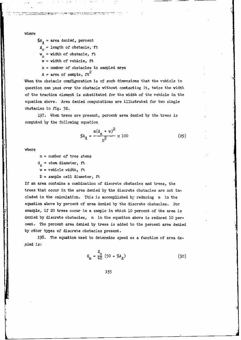
where

%A = area denied, percent

Ao = length of obstacle, ft

w 0- width of obstacle, ft0

w = width of vehicle, ft

n = number of obstacles in sampled area

A = area of sample, ft 2

-When the obstacle configuration is of such dimensions that the vehicle in

question dan pass over the obstacle without contacting it, twice the width

of the traction element is substituted for the width of the vehicle in the

equation above. -Area denrLed computations are illustrated for two single

obstacles in fig. 52.

197. When trees are present, percent area denied by the trees is

computed by the following equation

n(d + w)2d = 1 100 (29)

where

n = number of tree stems

d = stem diameter, fts

w = vehicle width, ft

D = sample cell diameter, ft

If an area contains a combination of discrete obstacles and trees, the

trees that occur in the area denied by the discrete obstacles are not in-

cluded in the calculation. This is accomplished by reducing n in the

equation above by percent of area denied by the discrete obstacles. For

example, if 20 trees occur in a sample in which 10 percent of the area is

denied by discrete obstacles, n in the equation above is reduced 10 per-

cent. The percent area denied by trees is added to the percent area denied

by other types of discrete obstacles present.

198. The equation used to determine speed as a function of area de-

,pied is:

SSm = 0 (50 - 5Ad) (30)

155

L

2

Area Denied- ( 8 +w

// Given:

d +w =0 \ Tree diameter, 2 ftVehicle width, 8 ft

Tree,

a. Tree

2Area Denied= w + (k + w)w 2 M-~

4 ft CJTven:Obstacle,, 2 ft wide

0 and 4 ft longjVehicle width, 8 ft

L-4f t w0

b. Obstacle

Fig. 52. Example of area denied computations for single obstacles

156

where

S = maneuver speed, mphm

S = maximum speed, mph, as controlled by soil, slope, dynatitic re-sponse, and visibility

199. It has been established by field tests that when the area de-

nied is less than 10 percent, the effect on vehicle speed is insignificant;

but when the area-denied is greater than 50 percent, the vehicle must over-

ride some trees or obstacles in order to traverse the -area.

WES vegetation models

200. Vegetation such as trees, bamboo clumps, brush, and grasses are

deterrents to vehicle performance since woody plants may cause the vehicle

to slow down to maneuver around or override single or multiple stems. In

addition to the maneuvering and overriding, problem, visibility restrictions

caused by vegetation alone may limit the vehicle's speed.

201. The WES vegetation model considers the effects- of vegetation in

terms of the maximum and average forces required to override trees and the

limits imposed by obscuration. Methods used in analyzing the separate ef-

fects of vegetation on vehicular movement are discussed in the following

paragraphs.

202. Vegetation impact model. A determination of the maximum forces

required to fail a single tree is used to establish whether or not the

strength of the leading edge of the vehicle and/or the driver's tolerance

to horizontal acceleration wili be exceeded.

203. In deriving the equation for maximum force required to fail a

single tree, a rational and an empirical approach were used. In the ra-

tional approach, it was assumed that a tree failed as a cantilever beam.

The fiber-stress equation for the resisting moment at -any cross section of

a beam is equal to the unit stress (Sm) times the moment of inertia of the

cross section with respect to the neutral axis divided by the distance from

the neutral axis to-the outermost fiber. In epplying this equation to a

tree, the resisting moment is the product of the horizontal pushbar force

and pushbar height (Fh X h ), the moment of inertia of a cross section of atree stem is nd4/64, and the distance from the neutral axis to the outer-

most fiber is ds/2; the equation is:

157

TTd s

h X h 67(31)p dS'

where

Z =stem diameter, in.

204. The ultimate unit- stress for-most trees -.ested was approxi-

mately 7500 psi. Using this value for unit stress and pushbar height as an

approximation of the length of the moment arm gave reasonable results wheh

compared mrith test results. Since unit stress and length of moment arm are

approximations, an empirical equation derived from test results is used to

determine maximum force required to override a single tree, as follows:

Fh= 0 - (32)

where

H = pushbar height, in.PAn example illustrating the quality of the relations established between

maximum horizontal pushbar force and stem diameter by equation 32 and line

of best visual fit is given in fig. 53.

205. To determine if the impact force will exceed the force that the

leading edge of the vehicle can withstand, the maximum force required to

override a single stem is compared with the strength of the leading edge,

as provided by the-vehicle manufaturer. If the information is not avail-

able, the bending strength of the leading edge is computed.

206. To determine whether or not the force of override will exceed

the driver's tolerance of 2-g horizontal acceleration, the maximum override

force is divided by twice the weight of the vehicle.

207. Vegetation override speed.,model. In order to determine the

speed at which a vehicle can override vegetation, the resisting force due

to override is added to the other resisting forces acting on the vehicle.

The override force is determined by dividing the work required to override

a single tree by the average distance between trees, or

158

100,000

ROATIONAL APPROACH '

~~rI~~ EQ FO# IE FBSVISUIAL FIT

co IO dIl

Z -SEMIRICAETR IN.

1059

101 0

F Wt (3

x

where

F =-average force required to override a single tree, lb0

Wt = work required to override single tree, ft-lb

D = average distance traveled between trees, ftx

The work required to override a single tree (vt) is determined by an empir-

ical equation derived from field work. The relation is shown in fig. 54

where work required per tree is plotted against stem diameter. The equa-

tion is

W = 100 d3

The average distance traveled between trees is computed by converting the

area of the sample cell to a rectangular area whose width is equal to the

vehicle width and dividing the length of the rectangular area by the number

of trees in the sample. The equation is the same as equation 27. When the

resisting force due to override is obtained,, it is added to the other re-

sisting forces acting on the vehicle, and a vehicle speed is determined

from the tractive force-speed curve.

208. Vegetation traction model. When a vegetation override speed

has been determined, a determination of the maximum tractive force required

to override a single tree is made. For a go condition the maximum tractive

force available must be greater than the force required to fail a tree

minus the kinetic energy at the override speed. The tractive force re-

quired is determined by the following equation

WTo= 2 x 5.8 (4

where

T = maximum tractive force required to override single tree, lb

W = work required to fail a tree, ft-lb

W = weight of vehicle, lb

160

1)000"000

-FT

F- 0

w 02

D 1010 -

3.

I-

w

(Li

ILI

)0 0 -1

I. L_10_10

STMDAETR N

LE-NA EGLINAF L.

0TIALEGEND

SPEED RANGE >0-3.9MPH

Fig. 54. Work required to override tree

161

g = gravitational const2ant,

V = vehicle velocity, fps

The work required to fail a tree is obtained from the empirical equation

illustrated in fig. 55. The force required to fail a tree is determined by

dividing the work required to fail the tree by the average distance the ve-

hicle travels to fail the tree, i.e. 5.8 ft or W15.8.

209. Visibility model. In some terrain situations visibility alone

can control off-road vehicle speed. The surface may be covered with

grasses or ferns of such height that surface features are completely ob-

scured, requiring the driver of a vehicle to reduce his speed to that of a

man walking ahead of the vehicle. In other situations, surface features

may be partially obscured by leaves or brush, or even by the arrangement of

stems and branches, with an accompanying, although lesser, effect on vehi-

cle speed. In any terrain situation, there is a very practical limit im-

posed upon the speed a vehicle may safely achieve--the vehicle should at no

time exceed that speed at which the driver can stop his vehicle in time to

avoid striking a damaging obstacle. This is, of course, equally true

whether the obscuration is occasioned by vegetation in a wooded area or by

fading light on a trail, or by fog on a superhighway. In each case, the

driver chooses a speed by integrating two factors: (a) the distance re-

quired to stop the vehicle, and (b) the distance that he can see and recog-

nize a significant obstacle. From the reaction time, braking force, and

recognition distance established for a specific set of conditions, the ve-

hicle speed as controlled by visibility is computed by the following

equation:

V =-at Va at 2,+2as (35)r r

where

V = speed controlled by visibility, fps(vehicle weight 32.2),

tr = reaction time, sec

s = recognition distance, ft

Reaction time is a function of the stimulus, the driver, and the vehicle

162

1 00,000,

I10,000

CL

W,_ W56.0d -,

irw

aL.

x0 10m

IdL

STEM DIAMETER, IN.

LEGENDA EGLIN, AFB FLA MAY 1965,

SPEED RANtE 56-3.9 MPHA EGLIN AFB, FLA., MAY 1965,

SPEED RANGE 4-12 MPH0 NASA MARSHALL SPACE FLIGHT

CENTER, MISS. AUG 1964,SPEED RANGE >0-3.9MPH

Fig. 55. Work required to ffail tree

163

characteristics. Tests have been conducted with a driver reaction simula-

tor; the results indicate that 0.5 sec is a reasonable estimate of reaction

time. Recognition distance is the maximum distance at which an obstacle of

mobility significance- can be recognized. Values of recognition distance

are obtained from field measurements. The braking force used to obtain de-

celeration is assumed to be equal to the maximum tractive force that can be

developed on the soil condition under consideration.

Acceleration and deceleration models

210. In negotiating terrain conditions that contain widely spaced

discrete obstacles that must be overridden (e.g. rice-field dikes), the

driver will accelerate after crossing an obstacle and decelerate before

striking the next obstacle. To account for the speedup and slowdown

processes, acceleration and deceleration models are used. The WES method

for predicting average speed in t~rrains containing widely spaced obstacles

that are to be overridden is illustrated in fig. 56. The acceleration and

deceleration models used by WES are discussed in the following paragraphs.

o20 DECELERATI

CISTANCEO FT

Fig. 56. Graphical illustration of the WES method for predicting theaverage speed in terrains containing widely spaced discrete obstacles

that are to be overridden

~21o Acceleration model. The effect of acceleration on average ve-

hicle speed is determined by the use of speed-distance relations and time.

Specific values of vehicle speed and drawbar pull are obtained from a draw-

bar pull-speed relation to develop the velocity-distance relation. Time is

computed from values obtained for accel~zation. The procedures used are

discussed below.

164+

I

iiig. 56. Grapica ilutnto of the~nl WEi-todfo reicigh

a. An increment for a velocity change is chosen on the drawbar

pull-speed curve* and the ,verage DBP and average velocity

for that increment are determined by the following

equations

DBP + DBP 2DBP - 2

V 1+ V21 22

where

V velocity, fps

b. The average acceleration a between V and V is com-

puted -as follows

a DB= (36)

where

W = vehicle weight, lb

g = acceleration of gravity, ft/sec2

c. The time t required to accelerate from V1 to V is1 2computed as follows

V2 -v 1t = (37)

a

d. The distance D traveled in time t is computed asfollows n

D =V x t (38)

This procedure is repeated for all increments between initial and final ve-

locities. If the vehicle is operating on a slope, the drawbar pull is

* Obtained by converting tractive force coefficient into tractiv 3orce

and subtracting motion resistance.

165

corrected for the effect of the slope

212. Deceleration model. The rationale and the method of predicting

the speed and distance traveled for a decelerating vehicle are as follows:V2 - VI

a. Rearranging equation 37, t - -a , the change in ve-

locity from V1 to V2 divided by the time required to

1 2effect that change is the deceleration when V 1 > V 2 .

b. The force required to produce this deceleration is equal to

the-mass W/g of the vehicle times the deceleration:

F = 2 (39)

c. The force available to produce this deceleration (braking

force is discussed in paragraph 213) is the motion resist-

ance, MR . Substituting into equation 39

w(v v)

V 2 V1

d. Again, from the basic equation = -a , -a may be

substituted into the equation above and the equation

rearranged

MRX g = -a

e. Or

MR -aW g

f. Speed at the end of any increment of velocity change may be

determined by the equation

V2 = V1 + at (40)

(a may be either positive or negative)

g. When V is equal to zero, equation 40 becomes:

166

V at =(NRXg) t

Or for any time increment from V = 0

V = at = x g) t

h. The distance d traveled during deceleration is predicted

by the general equation for distance while accelerating

from zero velocity:

d = 1 at 2 1 l × g t412 W IL

213. The computacidns made to determine the speed and distance trav-

eled when the vehicle is decelerating by braking are identical to those for

when the vehicle is rolling except that a braking force is used in lieu of

motion resistance as the force available to decelerate the vehicle. Brak-

ing force is assumed to be equal to the maximum tractive force the vehicle

could develop on the soil strength on which the vehicle is operating.

214. Average speed predictions. When a section of terrain is of

sufficient length for the vehicle under consideration to accelerate to its

maximum speed , the average speed is predicted by dividing the length of the

terrain section by the sum of the time required for acceleration to maximum

speed, the time traveled at the maximum speed, and the time required to de-

celerate from the maximum speed to the desired speed at the end of the ter-

rain section.

Stream crossing models

215. Crossing streams and rivers constitutes one of the most trouble-

some and hazardous operations in cross-country movement. Moreover, through-

out the humid climates of the world, it is a hazard that must be faced over

and again in any realistic traverse. AccQrdingly, full simulation requires

incorporation of a reasonable realistic river/stream crossing model, plus

proper relevant data on the configuration of streams in nature. Descrip- <

tion of a section of streambank for vehicle performance prediction requires

quantification not only of bank geometry, but also of bank soils--which

167

will often vary rapidly from the stream bottom up to the highest point of

the bank--and bank vegetation. Vegetation on the bank will frequently be

quite different from that just a few yards back due to levee formation, lo-

cal erosion, edge exposure of the forest, etc.

216. A typical stream crossing poses three separate problems. The

first is entrance to the stream or river over a bank, the ingress problem;

the second, swimming and/or fording the stream (or lake or river); the

third is exiting up the far bank (egress). Ingress and egress are essen-

tially obstacle surmounting problems with occasionally the added influence

of buoyancy, and perhaps hydrodynamic forces due to vehicle wave-making,

stream velocity, etc.

217. Negotiation of even a relatively minor drainage feature is al-

most invariably a critical maneuver. A principal difficulty in modeling

this realistically is to achieve, realism in the depiction of the stream it-

self. Even a small amount of conservatism can make a stream appear to be a

complete barrier to a vehicle where, in. fact, it might be negotiable in

many, many places. A feature of most streambahks, except where highly

channelized through the efforts of man,, is that they are highly variable as

to their severity from the point of view of vehicle negotiation. Short

stretches of a streambank can usually be found with some usable frequency

which present considerably less impedance to vehicle passage than do adja-,

cent sections that more nearly characterize tne bank on an average basis.

These may be termed entrance/exit "twindows." (Note that whether or not

these windows are in fact negotiable to a given vehicle is not part of the

present definition.) Proper description of rivers and streams for vehicle

crossing purposes must include statistics describing the configuration and

frequency of such windows.

Water crossing model

218. The effects of the water per se upon a vehicle transiting a

stream or river may be of several kinds. If the water is shallow enough,

and it usually is, the vehicle will cross between its ingress and egress

points by fording, even though it has inherent floating capability. In this

case, performance depends upon the bottom soils, the depth of water, ;and

the stream velocity. Where the stream velocity is appreciable, the stream

168

bottom will be hard. Sinkage will be small but traction may be limited by

water lubrication of, and reduced loading on, the contact surfaces--the

latter as a result of partial buoyancy. Partial buoyancy can be particu-

larly troublesome for vehicles with inherent floating capability when

stream depth approaches vehicle draft and stream velocity is high. In this

particular circumstance, the path across a stream may be totally out of ef-

fective driver control. Nonfloatirg vehicles often have an advantage in

these circumstances.

219. When water depth. exceeds the fording depth of the vehicle (with

or without special snorkeling arrangements), the vehicle must either havefloating capability, inherent or added, or the situation obviously becomes

no go for it.. Once free of the bottom a floating vehicle is simply a boat,

usually a very bad one. Modeling the primary performance of a floater

while fully afloat is accordingly a relatively straightforward problem in

hydrodynamics, complicated when in a swift current by the vehicle's rela-

tively slow still-water speed. Note that, because of the bank exit window

situation, the ability to land the vehicle at a precise point along the far

bank is of great importance to its effective egress capability.

220. Existing water-crossing models predict only still-water speed,

although this can readily be converted to speed-made-good across a stream

on a tacking course, of course. Modeling water-crossing performance, at

the moment, ignores serious potential control and stability problems which

beset these poor boats in a current. A reasonable estinate can be made of

the still-water speed of floaters aid amnphibians of the current general

style and performance, using the relation given in table 16.

Ingress model

221. In most instances, vehicle entrance into a stream is not con-

sidered critical, the presumption being that any stream that a vehicle can

get out of, it can more easily get into. By and large, this is a practical

simplification for mos; purposes, but cases where it would be of interest

to know that a vehicle might have difficulty entering a stream come readily

to mind. As one example, it might be desirable to enter a stream with the

purpose of using it as a trail for some distance, exiting miles away in a

totally different terrain situation.

169

~~1

~j-

Table 16Still-Water Speed of Floaters-and Amphibians

V K VL (HP/W), mph

where

K = value tabulated below

L = vehicle waterline length, ft

HP = gross installed power available for propulsion, hp

W = gross vehicle weight, short tons

Propulsion Hull K

Propeller Rough* 0.95

Propeller Clean* 1.10

Special tracks** Clean 0.95

Normal tracks** Clean 0.60

Wheels Clean 0.45

• "Rough" = hulls extensively cut up for

wheels, axles, drive lines, etc., as on theDUKW and its immediate successors.

"Clean" = similar to the 4x4 LARC's withfewer cutouts, fewer wheels, close-fittingwheel wells made possible by elimination ofthe suspension, etc.

** "Special tracks" = tracks designed specif-ically for effective water propulsion, as onthe LVT's.

"Normal tracKs" = land tracks as on theM113, M116, etc.

170

222. The principal factor that must be added to a downhill obstacle

model (incorporating vehicle stability model) to convert it to an ingress

model is the consideration of possible swamping. This will often be a dy-

namic splash situation, however, in which simple static waterline examina-

tion will prove conservative.

Egress models

223. There are three egress models in current use. All three pre-

dict either go or no go only.

224. WES egress model. The WES egress model simply applies the WES

soil-slope model, by using values for the soil cone index appropriate to

the bank soil conditions and the effective vehicle obstacle angle as deter-

mined by using the WES obstacle-geometry model.

225. LLD/Stevens Institute of Technology (SIT) model. The LID/SIT

model is essentially a regression equation relating observed and estimated

bank exiting performance of the 1113 to bank slope and height. It is

simple, but its rationale does not tempt one to use it for other vehicles.

226. WNRE egress model. The WERE egress model accepts bank geometry

in terms of the two-dimensional NERS linearizations and subsequently treats

the problem as an obstacle negotiation prediction, testing both for geomet-

ric interference and adequate traction. Static buoyancy at various points

in the exit regimen is considered in its effects upon nominal unit ground

pressure of the vehicle and hence its net traction. This model is totally

unsubstantiated by any tests.

227. Other egress model. A fourth model, still in an early state of

development, includes both some simple rigid-body dynamics and static buoy-

ancy in treating a two-dimensional vehicle exiting up a sloped bank. De-

velopment of this model, by Davidson Laboratory, ceased during 1968 at an

early stage and results from it are trivial at the moment. Accordingly, it

is not a candidate although its potential is considerable.

171

PART III: CROSS-COUNTRY PERFORMANCE MODELS

228. In this part of the study, comprehensive cross-country perform-

ance models that are currently operational are identified and analyzed.

Following the analyses, a single comprehensive model is outlined. This

model, termed the NOW model, utilizes the best of the currently available

single feature models in an optimal, fully computorized configuration. The

NOW model represents the current state-of-the-art of calculating off-road,

vehicle performance, and accordingly shares the limitations of the state-

of-the-art. The NOW model is thus incomplete in some important respects,

lacks realism in others, and. has not been fully validated in some parts

or as a whole. Despite this, the NOW model is considered to be useful

and usable in current and near-future simulations, provided only that

its basic limitations are not completely overlooked in the interpreta-

tion of final results.

229. By definition, the NOW model can be assembled without further

terrain-vehicle research, using only straightforward computer programming.

On the basis of the flow charts, details, and references given herein, the

critical portion of the NOW model that computes performance of a given ve-

hicle in a fully specified unit terrain can be programmed, in a user-

oriented language such as FORTRAN, and fully debugged well within a six

man-month effort.

230. A model for simulating cross-country operation is a series of

mathematical expressions and analytical processes such as the single fea-

ture models briefed in Part II which relate measures of vehicle performance

to quantitatively expressed vehicle, operational, and terrain factors. A

comprehensive cross-country performance model should be able to satisfy the

needs both of vehicle designers and of vehicle evaluators. To this end, it

must be able to predict reliably the performance of any vehicle operating

on any path in any properly described environment, and it should be suita-

ble for developing the characteristics of vehicles capable of achieving a

stated level of mobility performance within any specified environment.

231. Despite the use of ever larger computers, all models must for

practical purposes involve extensive simplifications of the vehicle and

172

terrain and of their interrelations. An optimal model for a given purpose

will be one that is no more detailed than necessary for that purpose. In

the present context, however, a good overall or general purpose model is

sought. By definition, such a model cannot in its completely general form,

be thus finely tuned to its usage. Accordingly, a good general purpose

model might be so structured that in its complete form it will yield the

highest available precisions, while by an orderly series of theoretical

simplifications and commensurate reductions in computational complexity it

may be made less precise to suit cases in which maximum precision is not

required, which may be often. As an alternative to a single "detunable"

model, it might prove easier to structure a series of alternate models,

each of which meets the special requirements of a more limited set of uses.

In this case, the overall model becomes essentially a chassis into which

detailed modules may be plugged according to the needs of the moment.

232. There are two essentially independent types of precision. In

design use, which implies inputting the vehicle entirely in parametric

fbrm, it is desirable that the model produce reliable relative performance

in various types of terrain with good sensitivity to design changes. Cur-

rent models reflecting the state-of-the-art in the terrain-vehicle research

are almost totally insensitive to a variety of relatively small design de-

tails that are known from field experience to be of critical importance in

specific, actual terrain situations. For evaluation purposes, it is more

important that the model produce results whose absolute accuracy correlates

well on a statistical basis with real world experience. The ideal model,

of course, would have both kinds of accuracy. In structuring the NOW model,

primary emphasis is placed on achieving maximum reliability in evaluating

vehicles in real world situations.

Elements of a Cross-Country Performance Model

233. A complete cross-country performance model comprises the fol-

lowing basic elements:

a. Means to specify the vehicle in meaningful parametric form.

b Means to depict the terrain as an areal phenomenon.

173

!'1

c. Criteria and procedures for generating and/or selecting

paths through the terrain (including, ts an almost trividl

end point, fully specifying a path).

d. Means to quantify terrain factors for all segments of any

selected path.

e. Means to predict desired vehicle performance measures along

each segment of any selected path.

f. Rules for joining performances along individual segments

into a continuous traverse.

g. Means to aggregate predictions for individual route seg-

ments into totals, statistical measures, maps, etc., ac-

cording to the needs of the model user or of the larger

simulation of which the model is a part.,

234. The heart of such a model is the calculation of vehicle per-

formance on a homogeneous path segment once all terrain factors pertinent

to that segment are specified. The resolution of terrain data available

and pragmatic computing considerations, plus terrain complexity, will dic-

tate the number of distinguishable homogeneous unit terrains by which a

given area will be represented in practice. Elements a through d above,

which precede prediction of vehicle performance in a given unit terrain,

are for present purposes considered as preprocessing of the data; steps f

and g which follow, as output processing. The logic and functioning of

both will be determined largely by the intended use of the complete model.

In the remainder of Part III, attention will be directed solely to the

structure of the central performance calculation: its completeness, the

adequacy of the single factor models it uses, and the rationale and logic

of couplings it uses to deal with multifactored terrain situations.

Model Uses

235. A total terrain-vehicle model can be used:

a. To analyze terrain in context of vehicle operations.

b. To optimize new vehicle configurations for stated missions

and terrains.

174

I

c. To assess the operational capability of new vehicle designs

or alterations to existing designs.

d. As part of a more comprehensive study, to make comparative

evaluations among a number of operational or mechanical

concepts that need not be closely related.

e. To generate "going" maps for use either at the strategic or

at the tactical level.

236. When a terrain-vehicle model is used to develop, from samples

of a given terrain, testable performance specifications for vehicles adap-

ted in various degrees to that terrain, it becomes in effect a terrain

analyzer, in Which vehicles function as "filters" or realistic terrain fac-

tor weighting devices. In this use the output is a specifications table

rather than the performance of a particular vehicle, and high precision in

predicting actual vehicle performance is not critical.

237. For use as a design tool, the model must be responsive to

"paper" changes in the vehicle. That is, it must provide means to calcu-

late realistically the results of changing vehicle dimensions, loads, pres-

sures, speeds, etc., entirely from the vehicle mechanical and dimensional

parameters. It should be sensitive to the order of design changes being

investigated (assuming these are themselves potentially significant) and

its indications of relative merit must be valid at least as to simple rank-

ing of competitive designs and preferably on a scalar ranking.

238. For vehicle and terrain evaluation and strategic planning, the

simulation should be sufficiently precise to discriminate among the per-formances of different vehicle and operational concepts in a wide variety

of terrains. Point-by-point absolute accuracy of prediction in the terrain

is not essential provided that, as in the design case, the vehicles are

properly ranked in each-,situation on a reasonably linear scale of merit.

In this application, the model may, if it improves overal precision, em-

ploy performance data measured during tests on existing vehicles. Such

data must still be generalized on a sound basis (as through the use of

validated nondimensional coefficients, and they do not eliminate the need

for rational coupling of simpler terrain-vehicle interactions) in order to

make realistic predictions for ccmplex terrain situations. The more usual

175

use for good performance data, which for practical reasons will always be

limited, will be to improve the overall realism and accuracy of the simu-

lation by fine-tuning single feature models and verifying particular com-

bining procedures.

239. Generation of tactical "going" maps for a given .group of vehi-

cles requires the greatest precision and realism. Ideally, all parts of

the performance model should be so precise that the quality of the output

is essentially dependent only on the resolution and reliability of the ter-

rain data used. The potential accuracy of computer-generated tactical maps-

based upon proper terrain-vehicle modeling, which conceivably might be pre-

pared on a daily or even hourly basis as terrain data are updated, is far

beyond that of the "going" maps with which the Army is presently living.

240. In each use, the most general form of the output will be in

terms of maps of individual vehicle performance measures, such as speed,

fuel consumption, go or no go, or no go diagnostics. Such maps may be ex-

pressed graphically or stored in a matrix that represents the maps as a dig-

itized network, and may ultimately be compressed into statistics of varying

degrees of sophistication. Alternatively, the output might be limited to

the tabulation of performance measures, segment by sement, along paths se-

lected by various criteria, and the accumulation of related statistics.

241. A route might be selected, for example, to minimize total

travel time between two points, to minimize fuel consumption, or to mini-

mize exposure to enemy hazards, all within further constraints such as a

specified maximum deviation from a straight-line course, or boundaries de-

fined by potential enemy reaction. Any route selection that does not re-

flect the extensive influence of moment-by-moment driver decision will be

unrealistic to some degree, however, because such a route will be selected

from a relatively omniscient viewpoint. Such omniscience may only be ap-

proached in practice, and then only where good terrain intelligence permits

close route selection prior to the operation and good navigation equipment

and good navigators are able to hew to the chosen course.

242. Route precelection in a tactical situation is not to be con-

fused with path specification when the problem is to evaluate one or more

vehicles. In the latter case, route specification may be tantamount to

176

preselection of the most suitable vehicle, because an arbitrarily specified

route, in effect, provides an arbitrary, fixed weighting of the relative

importance and frequency of various terrain factors. To treat real terrain

so simply is to risk nullifying the usefulness of the entire exercise. Ve-

bicles with different performance profiles, each optimally used, will each

see the same terrain in terms of quite different weightings of individual

and combined factors.

Operational Comprehensive Models

243. Published literature, including many U. S. Army and NASA re-

ports, was reviewed and various DOD agencies known to have used comprehen-

sive cross-country performance models in the past were surveyed to identify

significant, extant cross-country performance models.

244. In light of the objectives of ANAMOB, attention was concen-

trated upon those models meeting the following criteria:

a. The model should be fully quantitative; i.e. able to pre-

dict quantitative performance in specific, quantified ter-

rain situations.

b. It should be reasonably comprehensive; i.e. be structured

to predict vehicle performance in a variety of multi-

factored unit terrains.

c. It should be operational, i.e. developed to the point where

it is more-or-less immediately usable.*

Ten models were considered to meet these requirements. They are listed in

table 17.

245; Two other cross-country vehicle evaluation procedures in cur-

rent use which are not comprehensive performance models maybe mentioned.

The first of these is a computation used by USATECOM at APr to calculate a

single index of cross-country performance based upon a subjective weighting

of vehicle characteristics and measured performance. The second, REVAL

WEELS, places vehicles in various mobility categories on the basis of

* See second footnote, p 11.

177

.1

measured and/or computed go-no go, speed, and range limits in a small num-

ber of relatively simple situations involving soils, obstacle negotiatiln,

and obstacle avoidance. Terrain-vehicle relations used in the computations

are similar to those used in the other, truly comprehensive models. The

several incommensurate factors considered are combined by a standardized

but subjective scoring procedure, as in the APG calculations.

246. The design procedures proposed by Bekker, most recently in his

book Introduction to Terrain-Vehicle Systems, are treated in further dis-

cussions as a comprehensive performance model even though they -are not

organized into a functioning computer model for predictions in full multi-

featured terrain utits as defined herein. Most of the single factor models

required are available in his system, as is some of the coupling rationale

needed.

Strategies available

247. All of the models listedin table 17, except the WNRE model

(which treats only go or no go), predict vehicle performance in a unit

terrain primarily in terms of speed. Most predict

a. Maximum average speed due to available propelling force

and offsetting terrain impedances, Vprop

b. Maximum instantaneous speeds during longitudinal accelera-

tion and deceleration resulting from excess or deficit in

available propelling forces, or in presumed driver elec-

tion, Vaccdec

c. Maximum speed as limited by ride dynamics, Vride and/or

Vfire *

d. Maximum average speed, Vlimav

In addition, some models predict: maximum speed as limited by need for ob-

stacle avoidance, Vavoid ; as limited by driver vision, Vvis (Vdegraded

or Vnight); and/or while crossing streams, Vst . When the unit terrain

is such that more than one concurrent speed limit may be calculated (i.e.

both Vprop and Vride , for example), the assigned vehicle speed is

taken to be the least of these If, however, two or more calculated speed

maxima are mutually exclusive (speeds when overriding or avoiding the same

array of obstacles, for example), the optimum speed is sometimes selected.

178

Table 17

Ouantitative Comprehen.sive Operational Cross-Countrv

Performance Model s

Mode]Agency Designation Principal Peference

1. U.S. Army Engineer WES '"An Analytical Mode] for Predicting Cross-Waterways Experiment Country Vehicle Pnrformance," VSAWESStation Report No. 1-783 (8 vols.), 1969-1Q70.

2. U.S. Army Combat TATAYS "Tank, Antitank and Assault WeaponsDevelopments Command Pcquirements Study (1')," Dec l)69 (Final

Draft SECRET neport).

3. U.S. ArmyTank- OREGA "USATACOM Usitfg, lathematical Models forAutomotive Command Mobility Evaluation," Army Research anc,

Development Newsmagazine, Jan 1969, pp 20-21."Status ieport: Systems Analysis

Models at U.S. Army Tank-AutomotiveCommand," Technical Report No. 30308,Oct 1968, Warren, Mich.

4. Cornell Aeronautical CAL "Analysis and Simulation of DynamicalLaboratory-, Inc. Vehicle-Terrain iInteraction," Technical.

Memorandum V-J-2330-C-56, May 1969,Buffilo, N. Y.

5. Booz-Allen Applied Booz-Allen "Armored Reconnaissance Scout VehicleResearch, Inc. (XM800) Parametric Design/Cost Effective-ness Study (11)."

6. GM Defense Research McKenzie "Evaluation of-Cotnterinsurgency MobilityLaboratories in Relation to Environment," Final Report,

Jun 1966, Santa Barbara, California.

7. Ohio State University Ohio State Systems Research Group, "The Tank WeaponSystem," Annual Progress Report, ReportNo. RF-573 AR 65-1 (U), Jun 1965,Columbus, Ohio.

8. U.S. Army Tank- Bekker "Engineering Optimization of Terrain-Automotive Command Vehicle Systems, A ease Study of a Con-

cept Analysis of a New Amphibian," Tech-nical Report No. i0421, Feb 1969, Warren,Michigan.

Introduction to Terrain-Vehicle Systems,The University of Michigan Press,Ann Arbor, Mich. 1969.

9. Chrysler-Corporation Chrysler Test notes inclosed with letter dated 19Sept69 to Mr. A. A. Rula from Mr. B. 1).Van Deusen, Manager, Mobility Research,Chrysler Corporation.

10. WNRE, Inc. WNRE "A First-Cut at Developing Testable Off-Road Performance Specifications forVehicles Adapted to Specific Terrain,"Report No. 169-1, July1968, WNRE, Inc.,Chestertown, Maryland.

179

Common elements and differences

248. All ten of the full cross-country models analyzed employ a num-

ber of single feature models that in generas may be applied independently

or coupled together. Tables 18 and 19 identify the specific single-feature

models incorporated in each, and the flow charts given ii figs. 57-66 show

the basic logic and primary couplings involved. Note that several detailed

types of dynamic models are listed that occur only in the WES comprehensive

model (No. 1). Most of the other models shown to have a ride dynamics

single-feature model can handle such discrete obstacles as well, so that

lack of a citation means only that the published model does not include

specific inputs or speed limiting criteria for using the dynamic model in

these situations.

249. Input data requirements for each model listed in tables 18 and

19 are fully determined by the data needs of its several single-feature

models. All models studied require terrain inputs in deterministic form,

except for those used in "ride" computations where either deterministic or

probabilistic data usually may be used.

250. Driver modeling is in all cases limited essentially to the

driver using his discomfort as the primary determinant for maximum speed as

limited by continuous terrain roughness, or to estimate single Obstacle

negotiation speed. Driver reaction time is also included, explicitly or

implicitly, in some of the acceleration-deceleration models. None of the

models yet incorporate the effects of driver competence and judgment or the

influence upon mean performance of his detailed path selection.

251. The several comprehensive models differ among themselves pri-

marily in one or more of the following:

a. Number of single-feature models included.b. Specific single-feature model utilized.

c. Coupling involved.

d. Input required.

e. Output yielded.

Brief description of each model

252. Following is a brief description of each extant comprehensive

model based on information in the reports cited in table 17.

180

Table 18

Key to Single-Feature Models Used in Comrehensive Mndels Examined

References

Main Report Appendix

No. Identification Par. No. Fig. No. No. Par.

1.0 Soil Models

1.1 WES VCI 75-77

1.2 WES mobility numeric 78-79

.1.3 Bekker/LLD 80-83

1.4 Perloff

2.0 Vehicle Models

2.1 Automotive engineering 84-87

3.0 Soil-Vehicle Models

3.1 WES VCI 89-90 A 7-16

3.2 WES mobility numeric 91-93 A 22-25

3.3 Bekker/LLD 94-97 A 30-33

3.4 WES-WNRE 98

3.5 WNRE.-CAL 99

3.6 Perloff 100 A 40-43

4.0 Obstacle-Vehicle Models

4.1 Ride dynamic models

4.1.1 TACOM 18

4.1.2 Chrysler 19

4.1.3 GM (McKenzie) 20

4.1.4 Ohio State 21

4.1.5 WES-FMC 22

:4 1.6 CAL 25

41.2 Slope models 181-184

4.3 Obstacle-vehicle geome-try, interference models

4.3.1 WES, GM, Chrysler,, 188Others

4.3.2 LLD 189

(Continued)

181

III)

Table 18 (Concluded),

ReferencesMain Report Appendix

No. Identification Par. No. Fig. No. No. Par.

4.3.3 WNRE 190

4.4 Obstacle-traction models

4.4.1 WES 192

4.4.2 WNRE 193

4.5 Obstacle overridespeed models

4.5.1 WES 194

4.6 Maneuver models

4.6.1 4ES 195-199

4.7 Vegetation models

4.7.1 Impact models

4.7.1.1 WES 202-206

4.7.2 Override speed models

4.7.2.1 S 207

4.7.3 Traction model

4.7.3.1 WES 208

4.7.4 Visibility models

4.7.4.1 WES 209

5.0 Acceleration-Deceleration 211-213Models

6.0 Stream Crossing Models

6.1 Ingress models 221-222

6.2 Water crossing models 218-220

6.3 Egress models 223

6.3.1 WES 224 B 26-33

6.3.2 LLD/Stevens Insti- 225 B 13-25tute of Technology

6.3.3 W1NRE 226 B 34-43

6.3.4 Chrysler

7.0 Driver Decision (Exceptin Ride Dynamics)

182

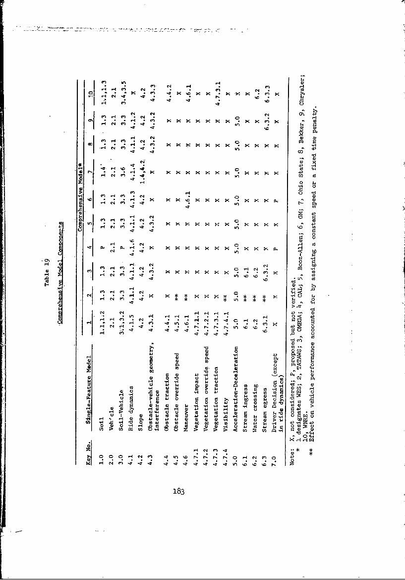
11 x H *

'0; C4C.)1 C

O\ 4

C C- 4 V! IA 5II~~6 -t - P 3 @

1; 4 Nn to V

.,- 0

C-4 0 Sto~~~~~.- 0C4 C D >4x x xX

Gig -t -

H ~ 0 r.** I-"0 )o

m. en -10)C4 .C 1C ,X 0

cnt H*.-C4

H- H m 0 -P4.5c 4i M q N C - m@3 C *H .4-5 X X X ~ xx C0

H ~ I H 4.5 *.t u .o ~0

C~06 Hi A4i *

*H *H 0 A 40 -

0 r. ;4I *N *r 0C0* 0 -4 N >0 N H1 .- C. . .c 4) r-i co r- I '

C.,*-t * - 4- cc -H

U 44 t3 u- ' 'y4 Co CO p4U4 ' 0 co@3 0 CO w5 to ca .

4j 4 1 -i4 ) 94')W 0

60 b e0 u ,W , 43 ' I

W3 t3 4j 5.. k C ii po43W- 4 4 tn4.- OH 1"4 Q)

0 CH1' P 3 ) s o .4 ' @

Ur Ci) 4-4@3 1. @ &OS @ 0 .C3 @ @3 r4 U ~$tn

@3 .- @3 1. > 1- o @3 .-1834-

w

W-i 0

zo Luut: 1 4,Cci)

tuE=Z UJI-Ofi w )WW :EV)H

aa. PEV0 ~ ct: L<",,3

0qr~jXLH

LULUO WO

-"o >-Lf j

18'E =)Kwa.L

0

4)pq 0

ol0

Cd ai)

0 0A

00

0

*r

0)

pr4 Cl)

00 E-00)

boW

EaI0

to40 a)

04-

00

E-~185

____ ___ ___ ____ ___ __ ___

_________

P 1-4__________

onI!2 J

r, LL4 I!A Id

_____ ____ ____ ___0

_____ ____ _____ ____ ___4

4-

r-I $4

c0

0

0)0

b0 W

L9r 0

E- 4 .,-4

HO HU

1864

Cd

I-I41

IrI a)

0

CH

00

W 94 0

t~ 187

'-4E

;> rd

0 0

00

$40PCI

*r-i

bD~

E-4 E-4

1,4

18

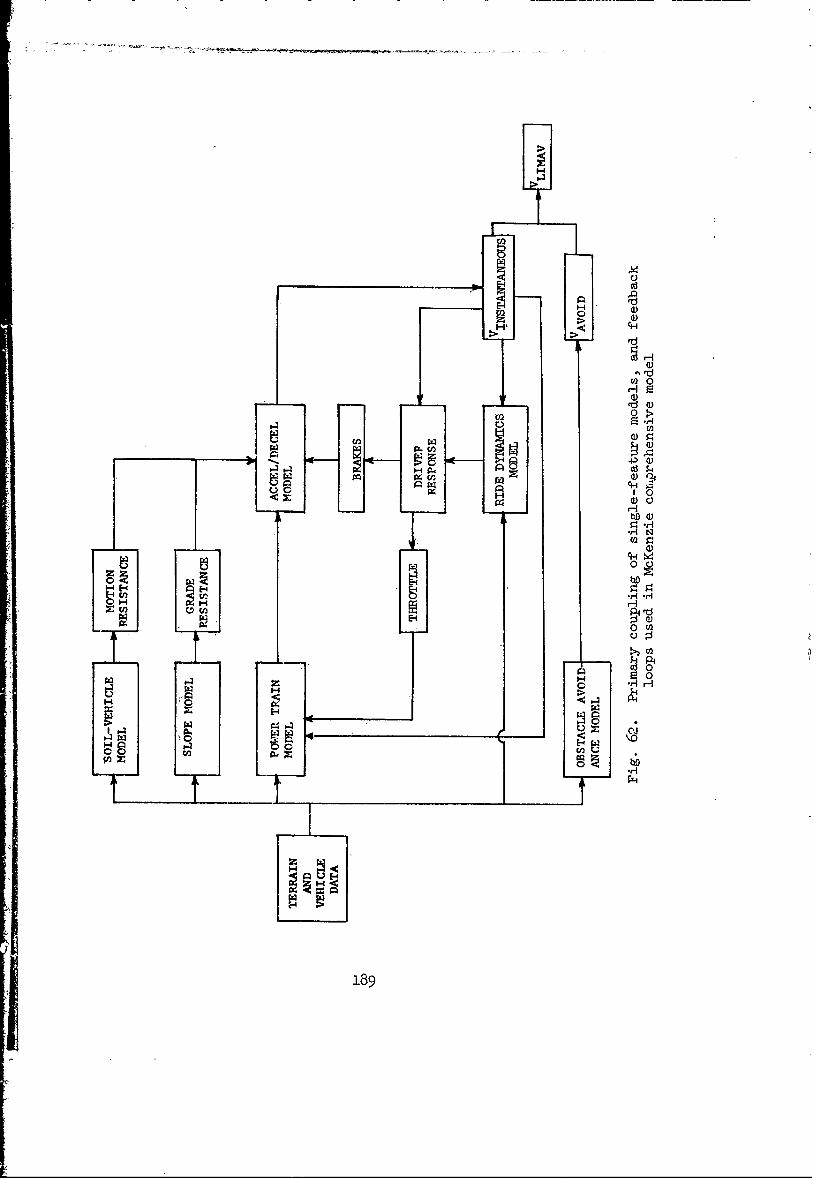
0

C)2

4-)

w '0

C-i

p 00

H-4 ~ - .

H Hfn I~d

1-41- 0__ _ _

E-44

189

E-1

ca3

co~ E-

p4-3

040

190

222

'm 2

w0d

0' z

ca 4 -

2.

r 119

-I,v* 'C)

*rrd

E-4

0

C-4,

0 ) r-'

~rd 0

0 $0)

U4-

0~ 0) 0-PH

H)

d-jcp'D

. ,I C

T4,

192

GO-NO~ ltKR.UNIT TERRAIN 7

04 0

040

Er' 0 0 C.

0Q 0

E-44 E-

43

0 0i 4

to P C4)0 20 pZ I

0

193

253. WES comprehensive model. The WES comprehensive cross-country

performance model (fig. 57) was designed specifically as a flexible proce-

dure to predict the performance of ground vehicles in any terrain confIigu-

ration. Its primary prediction is average vehicle speed in a discrete ter-

rain unit and in a traverse through a series of discrete units. Other

related outputs are fuel consumption rate and cargo delivery rate.

254. The WES model was formed by coupling together single- and

multiple-feature models schematically as shown in fig. 57. For an areal

terrain unit, the model computes an average speed. When crossing a linear

terrain feature, such as a -stream or a dry wash, time and distance are

computed. Whenever the computations indicate an immobilization (no go), an

arbitrary time penalty is assessed. Aggregating the unit terrain computa-

tions to predict an average speed along selected (sometimes several alter-

native) traverses through a variegated terrain is made manually by accumu-

lating transit times plus immobilization time penaltie for consecutive

path segments across mapped unit terrains or linear features.

255. The WES model will presently handle wheeled or tracked vehicles

in all terrain except muskeg (organic soils). At present, terrain data

suitable for direct use in the WES model are available in maps or on

punched cards for significant areas in Thailand, Canada, Germany, and the

United States.

256. At the time of this writing (1970) the WES model is approxi-

mately 80 percent programmed for a digital computer, but it is expected

that this figure will be raised to about 95 percent within the next year.

A more important limitation, however, is that it utilizes in several places

measured vehicle performance data, generalized on a simple regression basis

only. As a result, the WES model is not suitable to investigate the value

of new designs that involve unusual mobility characteristics. By the same

token, actual performance data on a particular vehicle in-being may readily

be incorporated, so that the model is particularly suited to evaluating new

machines in a broad range of terrain and mission situations, once a reason-

able amount of relevant, reliable performance data become available.

257.. The most fundamental deficiency of the WES model, which it

shares with all others presently in operation, is its lack of anything but

194

the most crude modeling of driver influences. Because this leads to omni-

scient path selection, point-to-point average speeds predicted by it must

be expected to be high.

258. Limited validation studies in which predicted- travel times were

subsequently compared with actual times of real vehicles in the same (but

real) terrain have indicated that the overall accuracy of the model is rea-

sonably good. Far more validation with a wider range of vehicle types in a

broader array of terrain types is evidently required before the true reli-

ability of the model can be assessed.

259. The WES comprehensive performance model has been used in sev-

eral studies to evaluate the cross-country capabilities of a variety of ve-

hicles. These studies are listed in table 20.

260. TATAWS (III) model. The TATAWS comprehensive mobility model

(fig. 58) was designed as part of an ad hoc tank combat simulation to pre-

dict the speed of tanks in selected terrains. It was formed by coupling

several of the single-feature models as snown in fig. 58. Specific single-

feature models included are identified in tables 18 and 19.

261. The TATAWS model determines limiting vehicle speed in a dis-

crete unit terrain -as the minimum of the following:

a. Speed as limited by propulsion, Vprop

b. Speed as limited by weapon firing, Vfire

c. Speed as limited by ride, Vride'd. Speed as limited by generally degraded visibility,

Vdegrade d

e. Speed as limited by night visibility pr.oblems, Vnight

V and V are determined separately by the TACOM ride dynamicride fire

single-feature model and form part of the input data for the main program.

Vand obstaclcrossing time delays are arbitrary re-Vdegraded I night ~adosa1 rsstrictions imposed on vehicle performance to make some allowance for miss-

ing single-feature models. Average speed for a traverse or a segment of a

traverse is determined using the limiting speed for individual traverse

segments adjusted for acceleration and deceleration, plus time de-ays

caused by obstacles or mission requirements.

262. The computed average speeds for each traverse segment and for

195

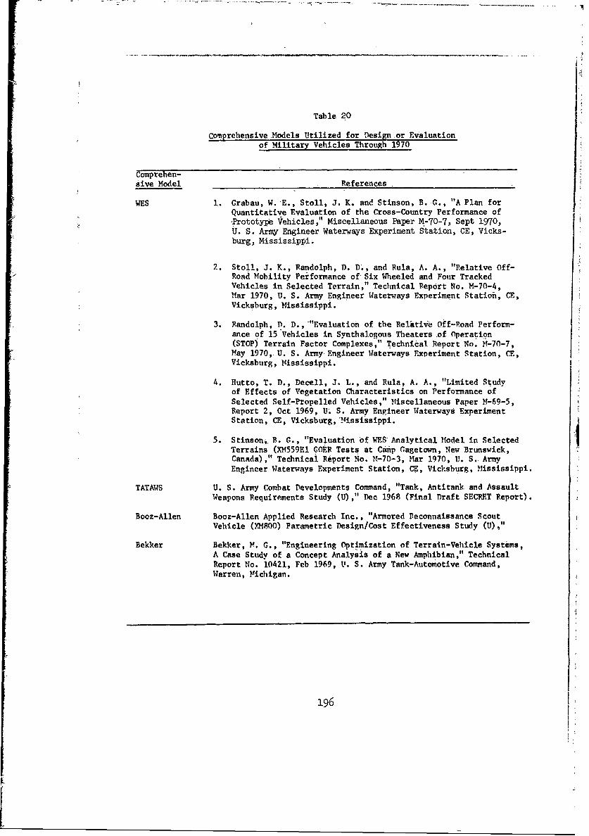
Table 20

Comprehensive Models Utilized for Design or Evaluationof Military Vehicles Through 1970

Comprehen-Sive Model References

WES 1. Crabau, W. E., Stoll, J. K. and Stinson, B. G., "A Plan forQuantitative Evaluation of the Cross-Country Performance ofPrototy] e Vehicles," Miscellaneous Paper M-70-7, Sept 1970,U. S. Army Engineer Waterways Experiment Station, CE, Vicks-burg, Mississippi;

2. Stoll, J. K., Randolph, D. D., and Rula, A. A., "Relative Off-Road Mobility Performance of Six Wheeled and Four TrackedVehicles in Selected Terrain," Technical Report No. M-70-4,Mar 1970, U. S. Army Engineer Waterways Experiment Station, CE,Vicksburg, Mississippi.

3. Randolph, D. D., "Evaluation of the Relktive Off-Road Perform-ance of 15 Vehicles in Synthalogous Theaters of Operation(STOP) Terrain Factor Complexes," Technical Report No. M-70-7,May 1970,- U. S. Army Engineer Waterways Experiment Station, CE,Vicksburg, Mississippi.

4. Hutto, T. D., Decell, J. L., and Rula, A. A., "Limited Studyof Effects of Vegetation Characteristics on Performance ofSelected Self-Propelled Vehicles," Miscellaneous Paper M-69-5,Report 2, Oct 1969, U. S. Army Engineer Waterways ExperimentStation, CE, Vicksburg, !ississippi.

5. Stinsoni, B. G., "Evaluation of WES Analytical Model in SelectedTerrains (XM559E1 GOER Tests at Camp Gagetown, New Brunswick,Canada)," Technical Report No. M-70-3, Mar 1970, U. S. ArmyEngineer Waterways Experiment Station, CE, Vicksburg, Mississippi.

TATAWS U. S. Army Combat Developments Command, "Tank, Antitank and AssaultWeapons Requirements Study (U)," Dec 1968 (Final Draft SECRET Report).

Booz-Allen Booz-Allen Applied Research Inc., "Armored Reconnaissance ScoutVehicle (M4800) Parametric Design/Cost Effectiveness Study (U),"

Bekker Bekker, M. G., "Engineering Optimization of Terrain-Vehicle Systems,A Case Study of a Concept Analysis of a New Amphibian," TechnicalReport No. 10421, Feb 1969, U. S. Army Tank-Automotive Command,Warren, Michigan.

196

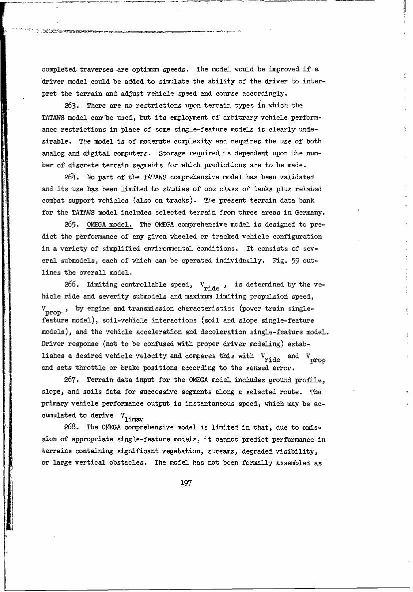
I

completed traverses are optimum speeds. The model would be improved if a

driver model could be added to simulate the ability of the driver to inter-

pret the terrain and adjust vehicle speed and course accordingly.

263. There are no restrictions upon terrain types in which the

TATAWS model can'be used, but its employment of arbitrary vehicle perform-

ance restrictions in place of some :single-feature models is clearly unde-

sirable. The model is of moderate complexity and requires the use of both

analog and digital computers. Storage required is dependent upon the num-

ber of discrete terrain segments for which predictions are to be made.

264. No part of the TATAWS comprehensive model has been validated

and its use has been limited to studies of one class of tanks plus related

combat support vehicles (also on tracks). The present terrain data bank

for the TATAWS model includes selected terrain from three areas in Germany.

265. OMEGA model. The OMEGA comprehensive model is designed to pre-

dict the performance of any given wheeled or tracked vehicle configuration

in a variety of simplified environmental conditions. It consists of sev-

eral submodels, each of which can be operated individually. Fig. 59 out-

lines the overall model.

266. Limiting controllable speed, V , is determined by the ve-ride

hicle ride and severity submodels and maximum limiting propulsion speed,

V , by engine and transmission characteristics (power train Single-prop. pwrtai ige

feature model), soil-vehicle interactions (soil and slope single-feature

models), and the vehicle acceleration and deceleration single-feature model.

Driver response (not to be confused with proper driver modeling) estab-

lishes a desired vehicle velocity and compares this with Vride and Vprop

and sets throttle or brake positions according to the sensed error.

267. Terrain- data input for the OMEGA model includes ground profile,

slope, and soils data for successive segments along a selected route. The

primary vehicle performance output is instantaneous speed, which may be ac-

cumulated to derive Vlimav268. The OMEGA comprehensive model is limited in that, due to omis-

sion of appropriate single-feature models, it cannot predict performance in

terrains containing significant vegetation, streams, degraded visibility,

or large vertical obstacles. The model has not been formally assembled as

197

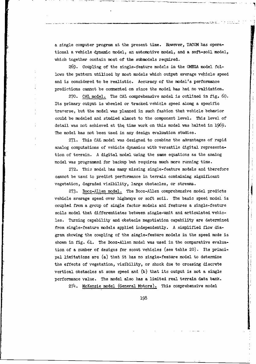
a single computer program at the present time. However, TACOM has opera-

tional a vehicle dynamic model, an automotive model, and a soft-soil model,

which together contain most of the submodels required.

269. Coupling of the single-feature models in the OMEGA model fol-

lows the pattern utilized by most models which output average vehicle speed

and is considered to be realistic. Accuracy of the model's performance

predictions cannot be commented on since the model has had no validation.

270. CAL model. The CAL comprehensive model is outlined in fig. 60.

Its primary output is wheeled or tracked vehicle speed along a specific

traverse, but the model was planned in such fashion that vehicle behavior

could be modeled and studied almost to the component level. This level of

detail was not achieved at thq time work on this model was halted in 1969.

The model has not been used in any design evaluation studies.

271. This CAL model was designed to combine the advantages of rapid

analog computations of vehicle dynamics with versatile digital representa-

tion of terrain. A digital model using the same equations as the analog

model was programmed for backup but requires much more running time.

272. This model has many missing single-feature models and therefore

cannot be used to predict performance in terrain containing significant

vegetation, degraded visibility, large obstacles, or streams.

273. Booz-Allen model. The Booz-Allen comprehensive model predicts

vehicle average speed over highways or soft soil. The basic speed model is

coupled from a group of single factor models and features a single-feature

soils model that differentiates between single-unit and articulated vehic-

les. Turning capability and obstacle negotiation capability are determined

from single-feature models applied independently. A simplified flow dia-

gram showing the coupling of the single-feature models in the speed mode is

shown in fig. 61. The Booz-Allen model was used in the comparative evalua-

tion of a number of designs for scout vehicles (see table 20). Its princi-

pal limitations are (a) that it has no single-feature model to determine

the effects of vegetation, visibility, or shock due to crossing discrete

vertical obstacles at some speed and (b) that its output is not a single

performance value. The model also has a limited real terrain data bank.

274. McKenzie model (General Motors). This comprehensive model

198

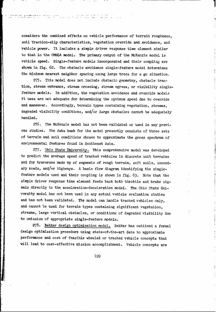
considers the combined effects on vehicle performance of terrain roughness,

soil traction-slip characteristics, vegetation override and avoidance, and

vehicle power. It includes a simple driver response time element similar

to that in the OMEGA model. The primary output of the McKenzie model is

vehicle speed. Single-feature models incorporated and their coupling are

shown in fig. 62. The obstacle avoidance single-feature model determines

the minimum nearest neighbor spacing -ncng large trees for a go situation.

275. This model does not include obstaclc -geometry, obstacle trac-

tion, stream entrance, stream crossing, stream egress, or visibility single-

feature models. In addition, the vegetation avoidance and override models

it uses. are not adequate for determining the optimum speed due to override

and maneuver. Accordingly, terrain types containing vegetation, streams,

degraded visibility conditions, and/or large obstacles cannot be adequately

handled.

276. The McKenzie model has not been validated or used in any previ-

ous studies. The data bank for the model presently consists of three sets

of terrain and soil conditions chosen to approximate the gross spectrum of

environmental features found in Southeast Asia.

277. Ohio State University. This comprehensive model was developed

to predict the average speed of tracked vehicles in discrete unit terrains

and for traverses made up of segments of rough terrain, soft soils, second-

ary roads, and/or highways. A basic flow diagram identifying the single-

feature models used and their coupling is shown in fig. 63. Note that the

simple driver response time element feeds back both throttle and brake sig-

nals directly to the acceleration-deceleration model. The Ohio State Uni-

versity modal has not been used in any actual vehicle evaluation studies

and has not been validated. The model can handle tracked vehicles only,

and cannot be used for terrain types containing significant vegetation,

streams, large vertical obstacles, or conditions of degraded visibility due

to omission of appropriate single-feature models.

278. Bekker design optimization model. Bekker has outlined a formal

design optimization procedure using state-of-the-art data to approximate

performance and cost of feasible wheeled or tracked vehicle concepts that

will lead to cost-effective mission accomplishment. Vehicle concepts are

199

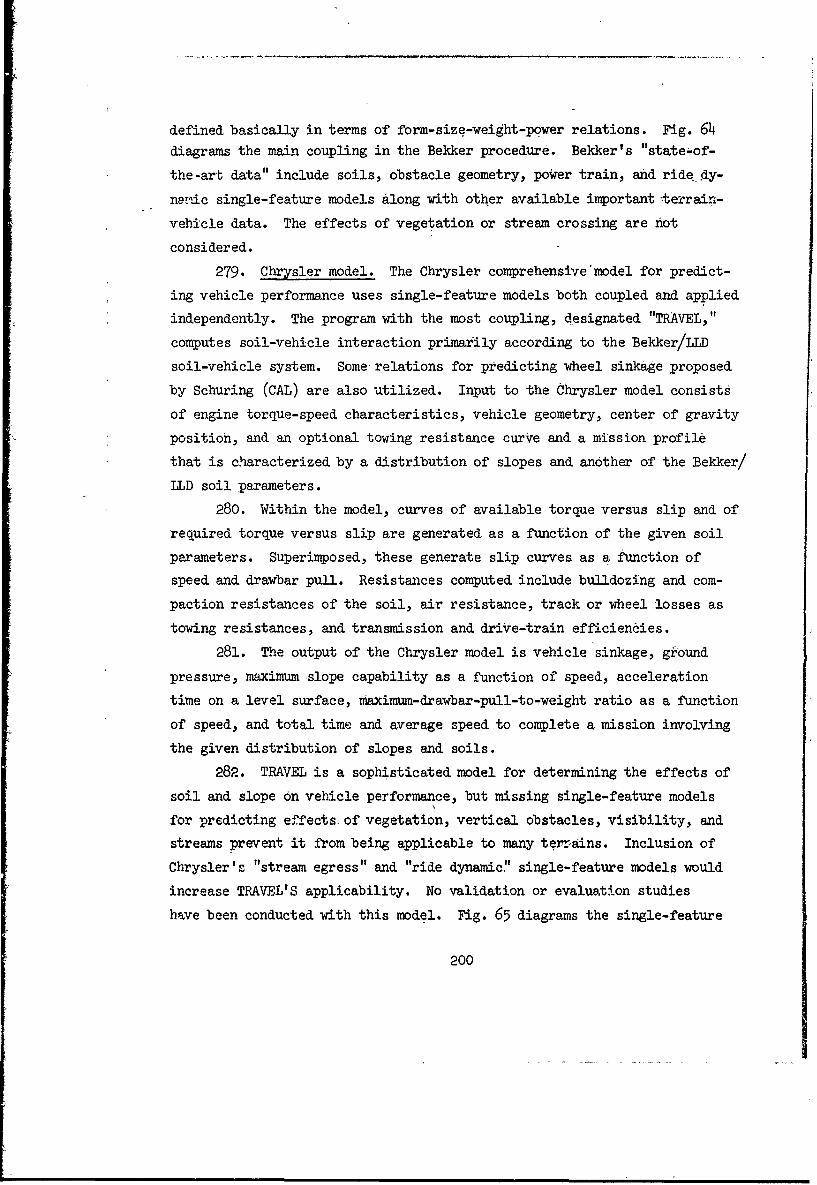
defined basically in terms of form-size-weight-power relations. Fig. 64

diagrams the main coupling in the Bekker procedure. Bekker's "state-of-

the-art data" include soils, obstacle geometry, power train, and ride dy-

neriic single-feature models along with other available important terrain-

vehicle data. The effects of vegetation or stream crossing are not

considered.

279. Chrysler model. The Chrysler comprehensive model for predict-

ing vehicle performance uses single-feature models both coupled and applied

independently. The program with the most coupling, designated "TRAVEL,"

computes soil-vehicle interaction primarily according to the Bekker/LLD

soil-vehicle system. Some- relations for predicting wheel sinkage proposed

by Schuring (CAL) are also utilized. Input to the Chrysler model consists

of engine torque-speed characteristics, vehicle geometry, center of gravity

position, and an optional towing resistance curve and a mission profile

that is characterized by a distribution of slopes and another of the Bekker/

LLD soil parameters.

280. Within the model, curves of available torque versus slip and of

required torque versus slip are generated as a function of the given soil

parameters. Superimposed, these generate slip curves as a function of

speed and drawbar pull. Resistances computed include bulldozing and com-

paction resistances of the soil, air resistance, track or wheel losses as

towing resistances, and transmission and drive-train efficiencies.

281. The output of the Chrysler model is vehicle sinkage, ground

pressure, maximum slope capability as a function of speed, acceleration

time on a level surface, maximum-drawbar-pull-to-weight ratio as a function

of speed, and total time and average speed to complete a mission involving

the given distribution of slopes and soils.

282. TRAVEL is a sophisticated model for determining the effects of

soil and slope on vehicle performance, but missing single-feature models

for predicting effects. of vegetation, vertical obstacles, visibility, and

streams prevent it from being applicable to many terrains. Inclusion of

Chrysler'- "stream egress" and "ride dynamic" single-feature models would

increase TRAVL'S applicability. No validation or evaluation studies

have been conducted with this model. Fig. 65 diagrams the single-feature

200

models and coupling in the -Chrysler comprehensive model.

283. WNRE model. The WNRE comprehensive model predicts go-no go ve-

hicle performance only and contains no dynamic simulation. The model uses

soil, slope, power train, vegetation override and avoidance, vertical ob-

stacle -ov(;rride and interference, stream crossing, and streambank egress

axid interference single-feature models. These single-feature models are

identified and their couplings shown in fig. 66.

284. Since this model predicts only go-no go, it has a relatively

simple structure. Lack of all dynamics limits the usefulness of this model

to the study of large areas for such purposes as vehicle oriented terrain

analysis. Figs. 67 and 68, which illustrate the range of terrain-vehicle

configurations examined in this simple static model only begin to suggest

the complexity of a-realist model for general purpose uses.

The NOW Model

285. The diagrams of the several comprehensive models presented in

figs. 57-66 reveal the considerable similarity in structure among all of

the models (except that of Bekker's whose objective is somewhat different).

This not unexpected broad consensus is useful at the present juncture.

286. The primary variation in structure is in the completeness with

which terrain is represented, reflected in the number of single-feature

models employed and in the selection of possible couplings among them.

This diversity is for the most part deliberate. In the several ad hoc mod-

els this arises either from the limits of the problem for which the model

was constructed and/or lack of available single-feature models at the time

the model was constructed. Clearly, the most complete comprehensive model

is that put together by WES, which has had the benefit of almost immediate

results from on-going research.

287. All of the models (except the WNRE go-no go model) consider

ride dynamics as an element of the problem, but two distinct approaches are

taken to develop a ride-limited speed. In one, vehicle responses for an

entire homogeneous terrain segment are accumiulated into one or another sta-

tistic describing the mean vibration environment before applying limiting

201

[ ____

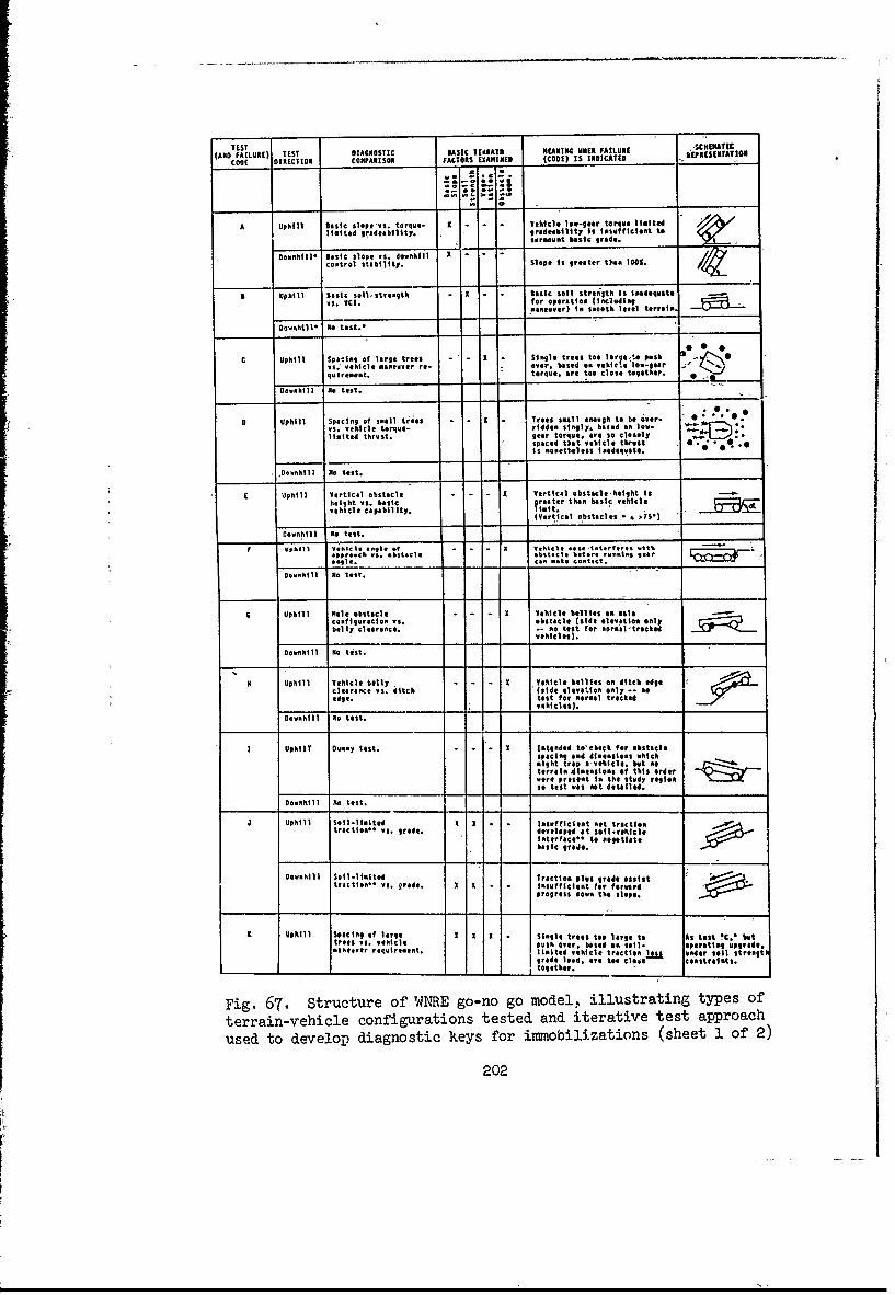
TEST HUI(ANDo FAILURE) "TEST OAUOSI 01eIC TESRAII ""AI"G mitE FAILORI CIUAZ

cooE IRECTIOM CUMNPARISON FACTOR AMIII (COO! I IICATES ERSETTO

8"I,. ";' I ty

limited gradeshliy I grdahltisiefesttsu.rmount basic trade.

goil'basic slope vs. dounthill X

0 coetII rol stability. Slope is greater than 1001.

S uphill ::sit sol'strngth A b asic soil stronith Is Inadequate ____

manever isoth leve terraim .~J-A

DvushLl Re test.-________

C Uphill Saigof large trees - x Single trees toe larg.-?. ob I -

vs. veI ma cver re- o ver, hosed en vehir'e low-ger *.

q.,srement. - torque. are too close together. I -

Downhill Am test.

0 Uphill SeI of Small trees - I Trees small enough to heI e-vs-' vehicle torque- ridden singly, basedc onlo-limited thrust, gear torque, are so clsl

spaced theat vhiclIe thrust 0 **. 0*Is nonetheless Inadequate. 4

Noshll R test.

Uphill lerticalsob stacle - Verticaltebutacle-height Is-height vs basIc grae tha aiChIlvehicle capability, lmt. osals(etcl'5

Noohll R test.

angle,. can eake contuct.

Downhill Re tout.

6 Uphill Mole obstacle A Vehicle belliesoen malebely claoe..ontt for :oeltrc1

Downhill No test.

8 Uphill Vehicle belly - - ehicle bellies on ditch edgec learance vs. ditch (sidef:lev4'IoR only -. oedge. test or eormal trached o

________ _____________ -vehicles).

Uonhill tNo test.

I Uphill' Dummy test. -- - x Intended to'choch fur obutacle

"Wocig and dimensien I whichnight trap a-vehicle. hut 00__htserr indimensions of this u rdewere present In the study ri;u

Ie test was eI detailad.

Downhill No test.

4 Uphill Soil-limited I I I nufficiest eet tractioatractionne vs. grade, developed at sgl-evehtcle

interface'0 to negotiate

basic grae*. 0

Downhill Saillimited Tractio pIls radeOsttrcin'VS. frade. S x I lo isffiin wu orwad

progress down the ulope.

K Uphill Spacing of large U I I igetestulret As test O!C * buttree s. eil po Ie bIfe on, re upertog raden.mane vr retoirem... 1.liited vehICle tracti n as s under soi Ist remg

-together. togae Catass

Fig. 67. Structure of WNRE go-no go model, illustrating types ofterrain-vehicle configurations tested and iterative test approachused to develop diagnostic keys for imobilizations (sheet 1 of 2)

202

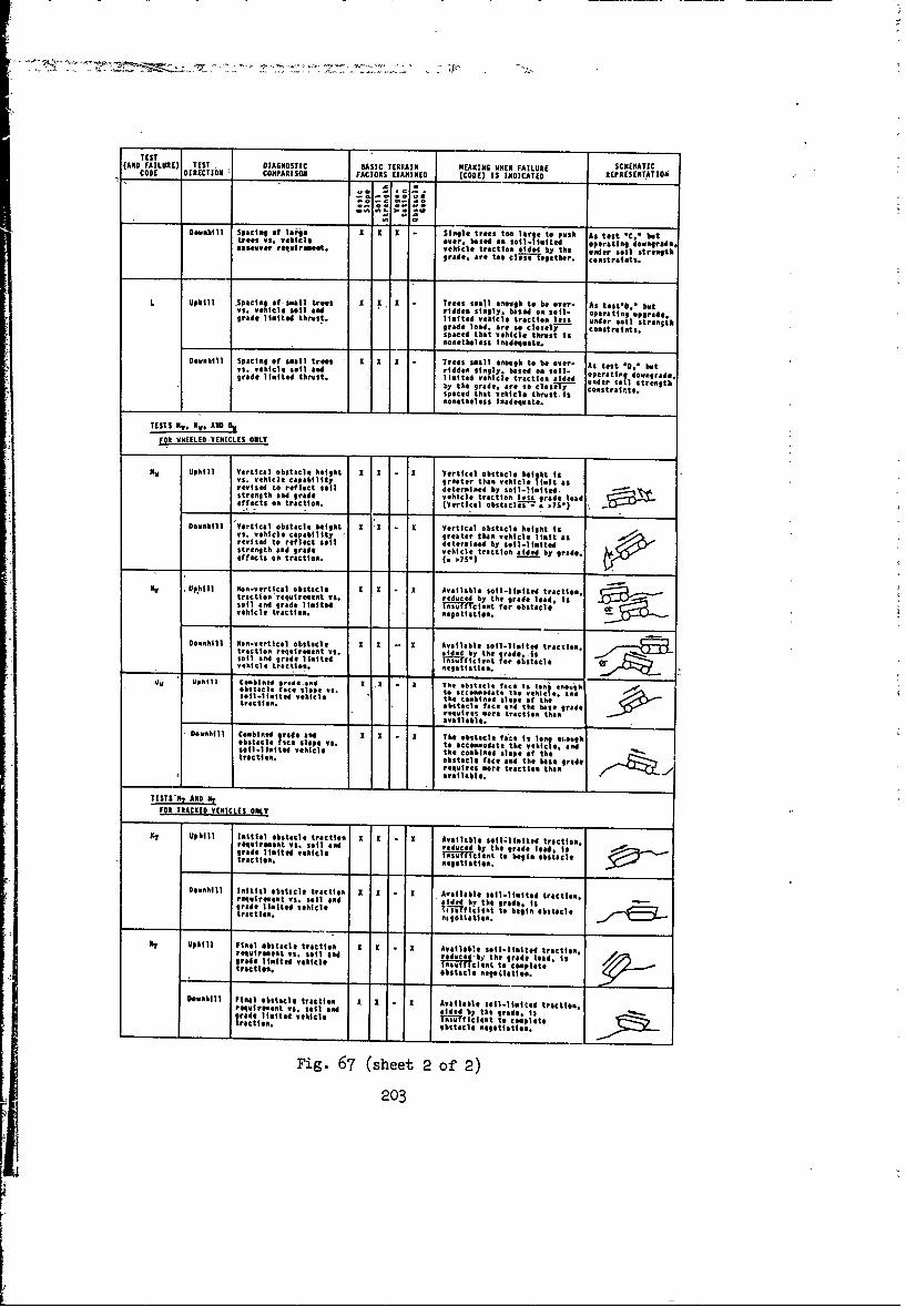
TEST(AND FAIURaE) TEST DIAGNOSTIC BASIC TERRAIN MEANING WHDEN FAILUREE SCEMIATIC

CODE DIRECTION COMDPARISON - FACTORS EXAMINED (CODE) IS INDICATED REPRESENTATION

Downhill Spacing of large I X X Slat'* trees too large to Push AN test *C atrees vs. vehicle ever, based om soil-limited oerating doLAisrade,Maneuver retoiromeot. vehicle trhctiom aided by the under %oil strength

grade. are too clo-se togther. Constraints.

L uphill ,Spacimg of-smallItree... X X X Tr.e. small anovgh to be over- As test's, hobtvs. eil I*l ad riddem slilily. based am sofl. OPeratieg aperade.grade limited thrust. limited vehicle traction less under soil strealth

grade load. are so closely t constraints.Spaced that Vehicle t hro t inoeetheless Inadeqoate.

Downhill Spacing of small trans I I I - Trans small eneobg to be over- As test .0,. hotvs. vehicle soil aed riddem sliily. hosed em soil- operative downgrade,grade limited thrust. limited v ehi cle traction aided ane sol trgtby the grade, are so c IIlry un c llstr ength.spaled that vehicle t hroSt is Cntansnonetheless Inadequate.

TESTS Mu, NV. ANDOiFOR VNEIESSVEHIClES ONLY

Me phll Vetialobct.,c:j*Ih I - Vertical obstacle height isVs ehicl capablity 1 ue hnvhcelmtarevised to reflect soil greter an vehsil-limit a

strength and grade v ehicle tractios l.:s grad" laeffects em traction. j(Vertical obstacls Ins)0

Downhill Vertical obs t he ight I X IX I Verticaltobsta Cliev het isvs. vehicler cpability greae them Veile Jlt asrevised to l relct sail determlsed by soil-imitedstrevgth and grade vehicle traction aided by grade.effects em traction. ( T'

N~ Ehill Nanvertical obstacle I Aalb e i-iie rcitation'reqairemeat vs. reduced bthgradelea IIssail and grade limited Tisaffic1 I fmr obstacloovehicle tractiom. negotiation.

Downhill Nmm-vertical obstacle I - Available sol-limitedl traccbom.tractien regairemeot vs. aided by the grode. -issoil and grade imite 1nafi n fo bsalvehicle traction. nmtfil t o ost.l

Qv uphill c~bin"d grade ama 'K li Tn bsicofc sle ao

srcoilmie Omilete combined slope Of thetractom.Obstacle facel and the base gradereqeires mare traction them

Downill CombneavaXilb.

Domohil , Com ined grade and a o h bstacle fate is jolgeoghObstcle fIcae slpevs to accommodate the vehicle. med1.il-ieitd vehicle thecoeimd slop*'Sf thetraction. obstacle fac and the base rd

available.

TESTS T AND NyFOR TRCKED VEICLES ONLY

NY Uphill I leitial Obstacl tractia I 0 I Available SOeI lmited tractiam.reqnireoeI vs. soil aold reoef yte rd edjgrde limited vehicle Ivscolb thague ostacltracton.Retiation.

Domehil loIitial obstacle tr4ctIOm1 X I X A-allobl* sol-limited tractiem.req ainment vOhio mIlaod a .oide by the grade. iv

vehicl Its~iln to begin obstacle

NT Uphill Filial obstacle traction X X X Available smil-limiged trci mreqeirament yin. soil meancd b~ h rd lea. i igrade limited vehicle uvafcet ocmlt

tractiom.obstacle mgotiatiom.L iDownhill Final obstacle traction I X I Available soil-limited traction,reqairemeet vs. Soil sew aided by h rdi

vehiostcle imvtiotiton.t

Fig. 67 (sheet 2 of' 2)

203

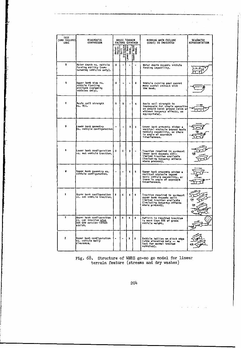
TEST(AND FAILURE DIAGNOSTIC BASIC TERRAIN MEANING WHEN FAILURE SChEMATIC

-CODE COMPARISON FACTORS EXAMINED (CODE) IS INDICATED REPRESENTATION

R Water depth vs. vehicle X Water depth exceeds vehicle _ _,-fording ability ,(non- fording capability.

~swimming vehicles only).

'S Upper bank step vs. X X Vehicle running gear cannotvehicle floating make useful contact with3ttitude (swimming the'bank.vehicles only).

7 Basic soil strength X X X Basic soil strength Is~~vs. VC1, inadequate for simple operattior --on smooth level ground (with oywithout buoyancy effects. asa ppropr ate)

U Lower bank geometry X X Lowercbank presents either avs. vehicle configuration vertic&I obstacle beond basic l

vehicle capability, or there OIL /-is angle of approachI nterference.

V Lower bank configuration X X X I- .Traction required to surmountvs. net vehicle traction. lower bank exceeds svehi ol

limited traction valableyn-----gcabit.(including buovncy effects

where p re s ent).

S Upper bank geometry vs. X X Upper bank presents either anvehicle configuration vertical obstacle beyondbasic vehicle capability or

there Is angle of approarhint e or ference g

X Upper bank configuration X X X X Traction required to surmount < ) -vs. net vehicle traction upper bank exceeds so pi

o smited traction available o(includtng buoyancy-effects swhere present).

Sppev hank configuration X X v X Deficit tn required trction

vs. C~et traction plus is more than 50% of gross50% GVW outsideAhrYst vehicle weight,isspst.

V Upper bank configuration X X Vehicle bellis en ditch edge

vs. vehicle belly (side elevation only - no

clearanceo test for normal trackedo

vehicles).

Fig. 68. Structure of WNtE go-no go model for linearterrain feature (streams and dry washes)

Uperbakcofiuaton I I I Trcio rqird2osuoon

criteria based upon driver, cargo, and/or weapon serving tolerances. In

the other, vibration based upon instantaneous speeds is continually moni-

tored by a tolerance criterion, and driver corrections are continuously fed

back in a loop to alter vehicle speed in response, usually through the

power train and/or acceleration/deceleration model. Driver reaction time

is usually incorporated in this feedback loop. This is probably an unwar-

ranted refinement at this time but it does serve to remind all that more

complete driver modeling is required.

288. At this stage, it is likely that most available, realistic ter-

rain roughness d&ta will be in terms of estimates of power spectral densi-

ties. Accordingly, ,a statistical input/output treatment appears most suit-

able even when the transfer operation involves the intermediate generation

of discrete input and output rather than a direct statistic-to-statistic

transfer fuhction. In the present absence of such a transfer function,

this obviously affects the manner in which the comprehensive models inter-

pret the ride dynamic data generated, rather than the ride dynamic model

itself.

289. Associated with this general difference in philosophy on ride

is a somewhat similar difference in the handling of soil-vehicle and power

train model interrelations. In some models, the relations are converted to

a pull-slip-speed relation for the particular soil and slope in a unit ter-

rain before proceeding to other parts of the program. In others, the pro-

gram continuously generates the information on a moment-by-moment basis.

The latter approach is appropriate where instantaneous speed values are

needed. In cases where there are a number of individual speed or go-no go

tests run before selecting a single controlling speed, as in the WES com-

prehensive model, the drawbar-slip-speed amalgamation appears more suitable.

290. While the WES model is the only one that specifically includes

a speed limit while crossing a discrete obstacle, such as a rice paddy dike,

any of the other :ide dynamic models could generate similar speed versus

acceleration information upon which selection of a possible maximum cross-

ing speed could be based.

291. At present, obstacle avoidance speeds, where used at all, are

based essentially upon a static viewpoint incorporated in regression

205

equations developed from limited test results. The present problem is one

of closely spaced insurmountable obstacles, such as large trees, and there

is no specific modeling of driver's route selection in real terrain. None

of the models attempt to account for driver route selection on any larger

scale.

292. In most areas of the world, stream crossing is a major impedi-

ment to off-road vehicle movement. Despite this, only four of the ten com-

prehensive models looked at included any modeling of this critical opera-

tion. Even these use modeling which is suspect, unrealistic, and/or to-

tally unvalidated. The consensus is that the bank egress problem is the

most critical for actual vehicles and is the most difficult to model. The

WES approach treats the streambank as a simple soil-slope problem. The

WIRE static model considers the bank as a complex, two-dimensional obstacle

upon which a vehicle may fail through geometric interference or lack of

sufficient traction at any one of several critical encounter points. A

first-order attempt to approximate transient contact forces during the time

when the vehicle is partially buoyant is included. In the Davidson Labora-

tory model, which is currently being elaborated by the University of De-

troit under a TACOM/LLD contract, vehicle momentum and buoyancy effects

upon ground contact pressure (and hence ground reaction) are being incor-

porated, but hydrodynamic wave forces will still be missing. However, this

appears to be an area where available or near available modeling from sev-

eral sources could be immediately combined to provide a substantial

improvement.

Selection of NOW model

293. The proposed NOW model is essentially the WES comprehensive

model as shown in fig. 69, with some suggested additions and changes in the

specific submodels that should be used. The numbers indicated in the

blocks in fig. 69 are the submodels suggested according to the listing

given in table 21.

294. The WES comprehensive model is proposed primarily because it

already makes provisions for the maximum array of single-feature and

multiple-feature terrain situations, which most of bhe comprehensive models

examined cannot handle at the present time without the expenditure of

206

UU u

m U C'

0. POLL 0 O

00

Z F-o

NJU~ D LA a. C L -C ' 4 C

.< 0 z ~ ~ ,~40~L

207

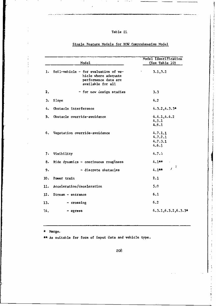
Table 21

Single Feature Models for NOW Comprehensive Model

Model Identification

Model (See Table 19)

1. Soil-vehicle - for evaluation of ye- 3.1,3.2hicle where adequateperformance data areavailable for all

2. - for new design studies 3.3

3. Slope 4.2

4. Obstacle interference 4.3.2,4.3.3*

5. Obstacle override-avoidance 4.4.1,4.4.24.5.14.'6. 1

6. Vegetation override-avoidance 4.7.1.14.7.2.14.7.3.14.6.1

7. Visibility 4.7.,1

8. Ride dynamics - continuous rougfiness 4.1*

9. - discrete obstacles 4.1"*

10. Power train 2.1

11. Acceleration/deceleration 5.0

12. Stream - entrance 6.1

13. - crossing 6.2

14. - egress 6.3.1,6.3.2,6.3.3*

* Merge.

** As suitable for form of input data and vehicle type.

2o8

F

considerable effort. Furthermore, WES terrain-vehicle submodels accounting

for the effects of soil, vegetation, and discrete obstacles were developed

from field test data, which makes them more realistic than if they were de-

rived from a purely theoretical standpoint. Preliminary pilot field tests

also indicate that predictions made with the WES comprehensive model are

reasonably accurate. Another factor that weighed heavily in selecting the

framework of the WES comprehensive model for the NOW model is the fact that

WES has developed a method for describing terrain for ground mobility pur-

poses that is geared to satisfy the terrain input requirement for the WES

cross-country model.

Suggested additions to NOW model

295. In addition to considering the dynamics effects of discrete and

continuous rough terrain on the driver, shock and vibration limits for

cargo and firing should also be included. For the moment, an arbitrary

limit should be assigned for cargo tolerance, and the shock and vibkation

limits established by TACOM and used in the OMEGA comprehensive model

should be used for ride tolerance while firing. The basic dynamic model

can be used to obtain the speed over specified terrain at which those lim-

its will be reached. The ride dynamic model used may be selected from many

others available according to what is most suitable for the form of input

data, the type of vehicle involved, etc.; however, once selected for a

given study, the same dynamic model should be used for making close inter-

nal comparison as in a design stu'y. This study did not deal critically

with the criteria upon which ride data developed by the dynamic models are

reduced to a speed level. Part of this problem is associated with the fact

that there is little evidence in the form of test data to arrive at an ob-

jective decision. The WES ride performance criteria are based upon verti-

cal and horizontal acceleration limits, and root mean square acceleration

at the driver's seat. The absorbed power criterion developed by TACOM for

driver and firing tolerances appears reasonable, and since an output of ab-

sorbed power can be obtained by modifying the WES dynamic model, it should

be included as a ride performance parameter.

296. For the NOW model, the WES manual operation for determining

obstacle-vehicle geometry interference should be replaced by the

209

computerized method proposed by TACOM and/or those incorporated in the 5TNRE

cross-country model, possibly including extension of these latter methods

contained in a more recent go-no go study in lunar terrain.

297. Particular attention should be given to the stream egress model

used in the NOW model. It is suggested that this be a reasonable merger of

the best features of the several available models, since no egress model by

itself represents the best that can be done at the present time.

1

210

PART IV: GUIDELINES FOR FUTURE DEVELOPMENTOF GROUND MOBILITY MODELS

298. As has been shown'in the previous sections of this report,

ground mobility models have been recently devised and most of them have

been developed for a particular abplication, used perhaps once, and have

remained dormant ever since. The comprehensive models reviewed usually

differed in objective, scope, application, submodels incorporated, and

level of sophistication.. It is also obvious that the information available

is limited insofar as the user is concerned in assisting him in evaluating,

selecting, or constructing a model that meets his requirements.

299. This study has not established any direct relations between the

comprehensive cross-country models examined and the reaw- orld because

model verification tests have not been run. On the other hand, a few rela-

tions have been established between several submodels thaz predict a partic-

ular kind and degree of terrain, vehicle, driver interaction. Furthermore,

it ,has been recognized during this study that without an analysis of exist-

ing models and related submodels and preparing a model for current use and

future development, development of comprehensive models would continue

along parallel or slowly converging paths. Moreover, without standardiza-

tion and continued use of an appropriate ground mobility model, it is not

likely that correlation between an acceptable comprehensive model and the

real world would be available any time soon. A unified approach is a ne-

cessity if stagnation in ground mobility modeling is to be prevented and a

means is to be provided for the user and the research community to communi-

cate in the solution of common problems.

300. Although the study has shown that considerable effort has been

spent in isobility research and that it is apparent that considerable effort

must be expended in the future before a comprehensive ground mobility model

will be available that will meet acceptable standards of accuracy, flexi-

bility, and realism for all T, .tential users, past research is only begin-

ning to pay off. The reason for the slow rate in payoff of ground mobility

knowledge can probably be attributed to the fact that what is known con-

cerning off-road ground mobility has not been organized in a form that

211

lends itself to straightforward application to common user pToblems. A,

aommon approach in defining requirements 'and missions is needed before

available knowledge can be arranged in a form that will produce timely di-

rect answers to questions frequently asked. Ongoing research must also be

geared to problem areas for which suitable answers are hot available.

Past Accomplishent s

301. Some of the knowledge available has been used in the design ana

evaluation of design and prototype combat vehicles that have -performed rea-

sonably well in most environments if the vehicle design and environmeht

were adequately described within the boundaries of' available knowledge.

Extrapolation to remote area envir6nments or quantifying the effects of ve-

hicle characteristics on performance, such as wagon steer employed in GOER

vehicles or limited slip differentials, has been less successful. Other

recent achievements are: the Army's adoption of standard tools and tech-

niques for the measurement of soil strength for mobility purposes; QM Is

for new vehicles are now beginning to include mobility specifications in

terms of an ability to operate in soil of a specific strength (rather than

in "deep soft mud"); vehicles have been designed and built to attain a

specified degree of mobility using mobility research findings and tests

have conclusively demonstrated the validity of' these- findings; AMC cost ef-

fectiveness personnel have been assisted in evaluation of the relative per-

formance of existing and proposed vehicles; a DOD-level ad hoc group, the

Intratheater Transportation Requirements Study Group, was recently rendered

assistance in its study of transportation requirements of the future; the

Army Materiel Systems Analysis Agency was significantly aided in its com-

parat:.ve evaluation of the MBT70 and M60 tanks; imaginative new velicle

concepts, e.g. walking machines, hiubless wheels, etc., have been proposed

for the consideration of Army planners; mobility research findings are cur-

rently being used in DASA studies of the effectiveness of craters as bar-

riers to ground vehicles; and mobility research engineers are serving as

consultants to NASA lunar trafficability panels and are engaged in test

programs to assist in the selection of the proper vehicles for lunar travel

212

(for NASA). The examples cited illustrate the useful achievements stemming

primarily from vehicle mobility research and the wide spectrum of military

purposes to, which the results of this research can, and undoubtedly will,

be put in the future.

302. A rapid catalysis of these products occurred mainly because of

a special project spons6red -and funded by ARPA . In 1963, ARPA, under its

Project AGILE, initiated a research program to determine the effects of the

various features of the physical environment on the performance of cross-

country ground vehicles and to provide data that could be used to improve

both the design and employment of such vehicles. A condition of the proj-

ect was that the data be interpretable in terms of vehicle requirements for

Southeast Asia. This program, called Mobility Environmental Research Study

(MERs), was begun in July 1963 following a preliminary study made in Thai-

land. This additional funding made it possible for the various mobility

research laboratories to pull together, synthesize, and partially validate

all relevant data and capabilities, and to conduct testing on obstacle

effects that might otherwise have not been conducted for several years.

Although circumstances forced ARPA to withdraw its support before the proj-

ect had been completed, the progress made before this occurred constituted

a quantum step in the scope of vehicle mobility research.

Approach to Future Plans

303. A more recent catalyzer of ground-mobility research has been

the demand by operations and cost effectiveness analysts for mobility eval-

uation performed by the application of a realistic comprehensive ground-

mobility model for predicting vehicle performance.

304. The general course for future mobility research is now quite

clear, namely, efforts should be directed toward the development of a com-

prehensive analytical model of vehicle performance. Such a model is now

generally envisaged as a coupling of appropriate terrain-vehicle-driver

interactions expressed in mathematical form to predict the performance of

any vehicle (in terms of go-no go, speed, fuel consumption, and cargo de-

livery capability) in any terrain. The component equations of the model

213

L=

may vary from purely theoretical to purely empirical. Fortunately, the

existence of objective statements of the relations existing between terrain

and vehicles makes it possible to test and validate those statements by

appropriately designed field experiments. Such experiments can obviously

progress from the simple to the complex, and this attribute makes it prac-

tical to identify a number of well-defined tasks. These tasks can then

be scheduled into a manageable sequence of activities and programs which

in sum constitute a comprehensive research program.

305. Development of a comprehensive model of vehicle performance

must be accompanied by a concurrent effort toward improving the current

ability to measure, describe, store, and retrieve terrain data. It is

axiomatic that these functions must be compatible with the vehicle per-

formance model. While considerable progress has been made in this subject

(again, fruition was hastened by special funding), much remains to be done.

306. To ensure continued usage of a model or submodels as a tool,,

the compilation of a complete set of instructions for Usihg them is a

necessity. The ideal model would be a complete simulation model defining

the interactions between terrain, vehicle, and driver. Complete validity

can be assured only when the effect of every significant component of the

vehicle, as well as of the terrain and driver, can be isolated and inde-

pendently examined. This means that vehicle inputs could be "modified,"

inserted in the general model, and the modified vehicle "tested" with the

model in such a way that the effect of the modification on performance

could be evaluated. It is apparent that an extension of this procedure

could be used to evaluate the almost limitless numbers of possible engineer-

ing trade-offs that might be madein any given conceptual vehicle. Thus,

the comprehensive mathematical simulation model becomes a basic and extra-

ordinarily powerful and flexible design and evaluation tool. It is clearly

the ultimate responsibility of the research community to provide the de-

sign and engineering community with appropriate instructions for using it

to maximum advantage. The consummation of this task must, however, await

the results of research to develop a comprehensive model of vehicle per-formance and improved terrain description methods. Once these two tasks

have been accomplished, or perhaps even after incomplete but substantial

214

r •i •m m

accomplishment, it should be a relatively simple matter to prepare a useful

instruction handbook.

307. The goals outlined are unquestionably worthy and every indica-

tion exi-sts 'that they can be accomplished. However, that accomplishment

can only result from systematic, continuous application of experienced per-

sonnel in a properly funded, carefully prepared, and executed research

program.

308. These goals for future ground mobility research have been re-

cently considered by the Research. Development and Engineering Directorate,

AMC, and mobility and terrain research programs conducted by various AMC

laboratories have been reprogrammed to ensure that a comprehensive ground-

mobility model will be compiled in the near future and that future research

has been geared to the improvement of the first-generation model. The

guidelines used in developing and implementing the AMC ground-mobility

research program are sound, and the plan satisfies the known requirements

for ground-mobility modeling. The plans presented herein are thus an

abbreviated form of the AMC program plan.

AMC Ground-Mobility Research General Plan

309. The AMC mobility research program has been designed with

several conditions in mind. OWe of the' conditions is that most of the

research will be accomplished and directed primarily by Army laboratories

at TACOM and WES, with assistance from the Natick and Cold Regions Research

and Engineering Laboratories as required. Another condition is the fact

that personnel of TACOM and WES have either made or contributed signifi-

cantly to most of the major advances in the state-of-the-art of mobility

research for the past several years. Since they are at the forefront of

the discipline, it seems most unlikely that any significant benefits could

accrue from further surveys of the state-of-the-art. Such studies would

inevitably consist primarily only of bringing the surveyors up to the

levels of sophistication already reached by the scientific and engineering

staffs of TACOM and WES. The general plan presumes that the state-of-the-

art is well known. The proposed research is designed only to extend .t;

215

no resources are devoted in the plan to surveys or similar excursions into

futility. The last condition is that scientific knowledge consists of

approximations; absolute truth or total reliability is never completely

reached. This is as true for knowledge about mobility as for any other

discipline. Thus, there will never be a "final" a-bsolutely complete and

totally reliable mathematical mobility simulation model. The general plan

is not premised on any such unattainable goal; however, it is based on the

firm conviction that a widely useful and acceptably reliable model can be

achieved within about five years. It will not be perfect, but it will

nevertheless be a powerful tool.

310. The AMC mobility research program consists of two phases

(Phase I: Vehicle Performance and Phase II: Terrain Description) that

will be prosecuted concurrently. If at the end of the first cycle, the

research program has not resulted in satisfactory solutions, the program

will be reevaluated and a new plan developed.

Phase I: Vehicle Performance

311. Phase I consists of five tasks, conducted largely but not com-

pletely in sequence (see fig. 70),. Task I consists of a consideration of

all the mathematical models of vehicle performance that are currently avail-

able and the compilation from the best of the submodels a general mobility

model. It is expected that the results of the present ANAMOB study will in

large measure fulfill the purposes of Task I., Upon completion of a first-

generation model, a set of experiments will be designed and conducted

(Task II) with the objective of revealing all deficiencies in the first-

generation model. Upon completion of the tests and analysis of the re-

sults, Task III can be initiated; it consists of an identification of all

of the research tasks required to deal with deficiencies revealed by the

field tests and the design of appropriate research programs for each. Task

IV consists of the conduct of those research tasks, and Task V completes

the cycle; it consists of the compilation of the second-generation simula-

tion model. The subtasks associated with each task are briefly described

in table 22.

Phase II: Terrain Description

312. Phase II consists of six tasks, one each to establish the

216

PHASE I: VEHICLE PERFORMANCE

COMPILE FIRST-GENERATION FIELD VALIDATION OFSIMULATION MODEL FIRST-GENERATION MODEL

(TASK I) (TASK II)

IDENTIFY ANDDESIGN RESEARCH

TASKS(TASK III)

IICOMPILE SECOND- CONDUCT RQID

GENERATION LONDUSEARC TASKSRESEARC TASKSSIMULATION MODEL (TASK IV)(T(TAS I)V)

(TASK V)

ItI

PHASE II:, TERRAIN DESCRIPTION

TASK I: SUBSTRATA CHARACTERISTICS

TASK II: SURFACE GEOMETRY CHARACTERISTICS TASK V:.- FACTOR COMPLEX

TASK III: VEGETATION STRUCTURE INTERRELATIONSCHARACTERISTICS

TASK IV: HYDROLOGIC GEOMETRYCHARACTERISTICS

TASK VI: INSTRUMENTATION SUPPORT

Fig. 70. General research plan, phase and task relations

217

Table 22

Outline of Plans for Phase I: Vehicle Performance

Task I: Completion of First-Generation Simulation Model

Purpose: Compile the most comprehensive and reliable mathematical simulation model,of terrain-vehicle-driver interactions possible from existing sources.

SubtaskNo. Title Brief Description of Work

A Examine Existing Models

1. Literature search Obtain and conduct literature search tofill knowledge gaps in existing U.S. andforeign ground~mobility models. Selectcomprehensive models worthy of furtherstudy. Group models into pertinentcategories.

2. Critical analysis Identify submodels or single-featureterrain vehicle relations that constitutethe building blocks of comprehensivemodels selected for further study. De-termine cormonality in single-feature sub-models. Identify assumptions, rationale,theory, or basis upon which submodel wasfounded. List input parameters, equations,and output nerformance parameters. Eval-uate existing test data and compare meas-ured and predicted performance results.Determine submodel applicability and

status of verification. Program submodelsfor analysis purposes if required. Iden-tify relationships between submodels.Establish common terminology. Prepare inhandbook form how each submodel is used,citing examples of computations, etc.(The handbook form will be used to preparetest plans for validation testing andinstructions for computer programmers.)

B Compile General Model

1. Develop flow chart Prepare flow chart of first-order analyt-and logic ical model and identify the submodels for

which the critical analysis revealed po-tentially usable submodels.

(Continued)

(1 of 5 sheets)

218

Table 22 (Continued)

SubtaskNo. Title Brief Description of Work

2. Write quantitative Develop procedures for compiling or inte-model grating submodels into necessary compu-

tational processes required to predictvehicle speed performance for off-roadoperation. Identify the submodels groupedtogether in each computational process.Establish common mathematical notations.

3. Program for computer Select computer which will be used tosolution obtain computer solutions. Program for

computer solutions the submodels acceptedas elements of the first-order analyticalmodel- and test for acceptable solutions.Debug model. Prepare report on computerprogram.

C Restructure ExistingIn-House Program

1. Identify programs to Evaluate TACOM/WES mobility research pro-be continued grams for relevance and application to

first-generation analytical model. Iden-tify those studies that Pre needed andcan be incorporated into the second-generation model.

2. Identify new prob- List new problems identified in preparinglem areas the first-generation model that require

research and can be completed in severalyears.

3. Prepare research Prepare research plans for each of theprograms problem areas identified in previous item.

Task II: Field Validation of First-Generation Model

Purpose: Validate both the general first-generation performance prediction modeland its component submodels or modules.

A, Design of Experiments

1. Identify testable Upon completion of critical analysismodel components (Task I, subtask A2) of a submodel or a

group of related submodels, examine inputrequirements and determine the measurementmethod and technique that will satisfy

the input requirements. If measurement of

(Continued)

(2 of 5 sheets)

219

Table 22 (Continued)

SubtaskNo. Title Brief Description of Work

input data is beyond current field test-ing capabilities, identify for furtherstudy,. Identify which submodel outputsare used as input to other submodels andwhich submodels must be: tested independ-ently and which related submQdels can begrouped and tested in a common test program.

2. Identify terrain, From critical analysis, identify range ofvehicle, and driver variation over which input parameters mayparameters- occur in nature, and identify the range of

each input parameter for which- predictionsare desired. This latter information is aprerequisite for validation testing. Forexample, soil strength of fine-grainedsoil has little or no effect on vehicletraction performance when-it exceedsjthevehicle cone index (VCI) about 60 points;therefore, most of the field testing shouldbe conducted in the VCI1 + 60 range. Pre-pare test specifications for each submodel.

3. Select test condi- Identify model to be tested singly andtions prepare testing procedures to be followed

in testing them. If testing is to beinitiated in laboratory with a vehicle com-ponent under controlled conditions, indi-cate the manner in which model verificationwill be achieved for prototype vehicles innatural terrain conditions. Prepare testingprocedures for the submodels that -will begrouped for testing in concert. Selecttest conditions necessary to meet aboverequirements.

4. Select and preparetest instrumentation Examine each submodel or group of submodels

to determine instrumentation requirementsfor verification testing. Determine forwhich submodels suitable instrumentation-is available. Prepare sketch plans identi-fying the instrumentation to be used for

testing each submodel or group of relatedsubmodels. Prepare designs for instrumen-tation not available to perform desiredtest procedures. Acquire component parts,assemble instrumentation system, and checkout system.

(Continued) (3 of 5 sheets)

220

r un u nm m nmmmu u unnu mnnnn • • •r

Table 22 (Continued)

SubtaskNo. .- Title Brief Description of Work

5. Write test plans Prepare test plans for validating eachsubmodel after relevant terrain, vehicle,and driver parameters have been specifiedand ins trientation requirements areknown. Select suitable test areas andprepare test schedule. Include in testplans test procedures and data analysisto be performed.

B Conduct Experiments

1. Mobilize for tests Mobilize for test and train teams intesting procedure,.utilization of instru-mentation and other measuring equipment,and reduction and preliminary analysisof data.

2. Execute tests: Conduct sufficient tests to validate in-dividual submodels or combinations ofsubmodels incorporated in the generalmodel. Identify gaps in knowledge foruse as-basis for conducting research pro-grams.

C Analysis for Deficiencies

1. Analysis Compare predicted and measured submodelresults for level of accuracy. If com-parative.results are poor, state why andwhether modification would improve pre-diction accuracy. Evaluate for consider-ation as a research task.

2. Report preparation Prepare interim report on each test pro-

,gram.

Task III- Identify and Define Research'Programs

Purpose: Identify and define research programs as required to improve to an accept-able level of reliability submodels and submodel combinations whi'h aretevealed as deficient by the test and validation program (Task II).

A Identify Deficiencies Identify, define, and prepare researchon Model programs as required to improve reliability

of submodels and coupling processes re-vealed deficient by tests.

(Continued)(4 of 5 sheets)

221

VI

Table 22 (Concluded)

SubtaekNo. Title. Brief Description of Work

B Write State-of-the-Art Prepare state-of-the-art of models andModels of Each Problem submodels to elucidate the relations ex-Area isting among some combinations of terrain,

vehicle, and driver factors and to insurethat the submodels are realistic and the

, interaction cana be described by mathiemati-

cal processes.

Task IV: Conduct Required Research Tasks

Purpose: Develop a basic understanding of terrain-vehicle-driver interactions insufficient detail to make- it possible to compile a highly reliable second--generation mathematical-performance prediction model.

A Design Research Programs Develop research plans for each task assoon as research requirements are identi-fied and defined. Establish research task-priorities.

B Conduct Research Programs Conduct research on updated programs whichwere being pursued prior to the initiationof the AMC ground mobility program and newresearch programs.

Task V: Compile Second-Generation General fodel

Purpose: Develop a reliable second-generation mathematical model for predictingthe performance of military ground-contact vehicles on a real-world com-bination of terrain conditions-

A Develop Flow Chart and Compile a complete and detailed flow chartLogic of the general comprehensive model logic.

B Write Quantitative Model Prepare quantitative mathematical expres-sions (or simulation routines) as requiredby the model logic.

C -Program for Computer Program comprehensive model for computerSolution solution and document for use.

(5 of 5 sheets)

222

L

characteristics .of substrates, surface geometry,. vegetation structure, and

hydrologic geometry, a fifth to consolidate these into a- total environment,

and a sixth on instrumentation support.

313. The tasks propose -research effort concentrated on providing the

detailed- terrain descriptiuns required by vehicle designers, vehicle test

agencies, evaluators, and planners who are preparing specifications for new

vehicle familie's. The proposed tasks do not incorporate any research

effort devoted expressly to those activities moce closely related to mili-

tary geographic intelligence, such as mapping significantly large areas in

terms of terrain descriptors for the purpose of constructing cross-country

locomotion maps, operations planning maps, and the like. Such activities

are primarily the responsibility of agencies other than AMC.

314. The plan is also based on the assumption that all six tasks

will be conducted simultaneously, so that information and experience gained

in work related to one can be imnediately transferred to the others.

315. It is further assumed that some effort in Phase I (Vehicle

Performance) will be devoted to terrain description in direct support of

those adtivities. For example, the test courses for the validation of per-

formance prediction models developed as a product of Phase I research will

have to be carefully described. These descriptions will be made using the

most sophisticated methods and techniques developed by Phase II research up

to that time, but such "production descriptions" will be obtained by

Phase I researchers. The subtasks to be pursued under each task are

briefly described in table 23.

223

Table 23

Outline of Plans for Phase II: Terrain ,escription

Task I: Substrata Characteristics

Purpose: Develop rapid, efficient, and reliable methods for acquiring data onsubstrata (soil, snow , muskeg, etc.) characteristics in a form usableby the mathematicatperformance prediction Submodels compiled ini Phase I,and to establish the significant ranges of variations of the relevantproperties of such material on a worldwide basis.

SubtaskNo. Title Brief Description of Work

A Identify Significant Examine submodels to be used and identifyDescriptors terrain factors as input.

B Establish Sampling -D1evelop and refine sampling theory; developTechniques methods of measuring the parameters or

factors required in above subtask.

C Establish Descriptor .Establish the ranges of variationson aVariations world scale by terrain descriptions re-

quired, both independently and in combi-nation.

Task II: Surface Geometry Characteristics

Purpose: Develop rapid, efficient, and reliable methods for acquiring data onsurface geometry characteristics in a form usable by the mathematicalperformance prediction submodels compiled as a product of Phase I research,and to establish the significant ranges of variations of surface geometryconfigurations on a worldwide basis.

A Identify Significant Examine submodels to.-be used to ensureDescriptors that all relevant properties of surface

geometry required are appropriately con-

sidered and described.

B Establish Sampling Develop and refine sampling theory.Techniques Improve data acquisition methods.

C Establish Descriptor Establish ranges of variation exhibitedTechniques on a world scale of surface geometry

features that affect vehicle locomotion.

(Continued)

(1 of 3 9heets)

224

Table 23 (Continued)

Task III: Vegetation Structure Characteristics

Purpose: Develop rapid- efficient, and reliable methods for acquiring data onvegetation structures in a form usable by the mathematical performanceprediction.models compiled in Phase I, and to establish the significantranges of variations of the relevant vegetation factors on a worldwidebasis.

SubtaskNo. Title Brief Description of Work

A Identify Significant Examine submodels to determine the vege-Descriptors tation structure factors required to

satisfy input requirements.

B Establish Sampling Develop adequate descriptors and fieldTechniques: procedures for making measurements rele-

vant to vegetation factors. Developmethods for rapidly acquiring vegetationdata.

C Establish Descriptor Establish--ranges of variations exhibited'Variations on a world scale by vegetation structure

factors and descriptions, both independ-ently and in combination.

Task IV: Hydrologic Geometry Characteristics

Purpose: Develop rapid, efficient,, and reliable methods for acquiring data on thecharacteristics of hydrologic features in a form usable by the mathematicalperformance prediction models compiled in Phase I, and to establish thesignificant ranges of variations of the relevant hydrologic geometry factorson a worldwide basis.

A Identify Significant Examine submodels and assemble the descrip-Descriptors tions relevant to the problem.

B Establish Sampling Develop methods of measuring the descrip-Techniques tors or factors relevant to entry, fording,

and exiting processes. Improve methods forrapid measurement. Develop and refinetheory of sampling.

C Establish Descriptor Establish ranges of variations on a worldVariations scale by the factors and descriptors used

in submodels.

(Continued)(2 of 3 sheets)

225

Table 23 (Concluded)

Task V: Factor Complex Interrelations

Purpose: Determine those combinations of factors and factor values that signifi-cantly affect vehicle performance, define their general geographic dis-tribution on aoworldwide scale,'and develop methods of describing suchfactor interrelations so that they may be readily used as input to themathematicaLperformance prediction models developed as a product ofPhase I research.

SubtaskNo. Title Brief Description of Work

A Data Compilation Assemble data collected in all programtasks into a single data store in a 'ormthat can be examined for a variety ofpurposes.

B identification of Signifi- Evaluate the effect produced by specificcant Factor Value Combina- combinations oh terrain factors to providetions insight as to which terraindescriptors

should be presented for utilization inother military activities.

(3 of 3 sheets)

226

SELECTED' BIBLIOGRAPHY

Aberdeen Proving Ground, "A Handbook of Ordnance Automotive Engineering,"(2 vols), 1945., Aberdeen Proving Ground, Md.

Assur, A., "Locomotion Over Soft Soil and Snow," Society of Automotive En-gineers Paper No. 782-F, Jan 1964, Automotive Engineering Congress, Detroit,Mich.

Baker, W. J., Sloss, D. A., and Miranda, C. F., "Stream Exiting Studies ofModel Amphibious Vehicles," Journal of Terramechanics, Vol 5, No. 4, 1968,

pp 33-55.

Bartlett, G. E. et al., "On the Prediction of Off-Road Vehicle System

Mobility," Jan 1969, International Automotive Engineering Congress, Detroit,

Mich.

Beckett, P. H. T. and Webster, R., "A Classification System for Terrain,"Report No. 872, Aug 1965, Military Engineering Experimental Establishment,Christchurch, Hampshire, England.

Bekker, M. G., "Engineering Optimization of Terrain-Vehicle Systems; ACase Study of a Concept Analysis of a New Amphibian," Technical Report No.

10421, Feb 1969, Land Locomotion Research Laboratory, U. S. Army Tank-Automotive Command, Warren, Mich.

, Introduction to Terrain-Vehicle Systems, University of MichiganPress, Ann Arbor, Mich., 1969.

_, Off-the-Road Locomotion; Research and Development in Terra-mechanics, University of Michigan Press, Ann Arbor, Mich., 1960.

, Theory of Land Locomotion; The Mechanics of Vehicle Mobility,University of Michigan Press, Ann Arbor, Mich., 1956.

Bendix Corporation, "Derivation of LSSM Vehicle Dynamic Equations," LVP-602, Mar 1969, Ann Arbor, Mich.

"Dynamic Response of Lunar Vehicles to Random Terrain," June1968, Ann Arbor, Mich.

, "Local Scientific Survey Module for Apollo Application Program,Final Report, Vol II, Book 5, Appendix D: Vehicle Analysis," BSR 1495,Feb 1967, Ann Arbor, Mich.

.... _, "LSSM 10-Degrees of Freedom Dynamic Simulation," LTM-005, June1957, Ann Arbor, Mich.

, "Lunar Roving Vehicle Six-Wheel Acceleration Equations.," Re-vised May 1969, Ann Arbor, Mich.

227

|A

Bieniek, M. P., "Suspension Dynamics," Automobile Engineer, Vol 50, No. 4,Apr 1960, pp 143-147.

Blackmon, C. A., "An Analytical Model for Predicting Cross-Country VehiclePerformance; Appendix C: Vertical Obstacles (Surface Geometry)," TechnicalReport No. 3-783 (in preparation), U. S. Army Engineer Waterways ExperimentStation, CE, Vicksburg, Miss.

Blackrnon, C. A. and Randolph, D. D., "An Analytical Model for PredictingCross-Country Vehicle Performance; Appendix B: Vehicle Performance inLateral and Longitudinal Obstacles (Vegetation), Vol II: LongitudinalObstacles," Technical Report No. 3-783, July 1968, U. S. Army EngineerWaterways Experiment Station, CE, Vicksburg, Miss.

Blackmon, C. A. and Stoll, J. K., "An Analytical Model for PredictingCross-Country Vehicle Performance; Appendix B: Vehicle Performance inLateral and Longitudinal Obstacles (Vegetation), Vol I: Lateral Obsta-cles," Technical Report No. 3-783, Dec 1968, U. S. Army Engineer Water-ways Experiment Station, CE, Vicksburg, Miss.

Blackmon, C. A., Stinson, B. G., and Stoll, J. K., "An Analytical Modelfor Predicting Cross-Country Vehicle Performance; Appendix D:, Performanceof Amphibious Vehicles in the Water-Land Interface (Hydrologic Geometry),"Technical Report No. 3-783, Dec 1969, U. S. Army Engineer Waterways Experi-ment Station, CE, Vicksburg, Miss.

Bodeau, A. C., Bollinger, R., and Lipkin, L., "Passenger Car SuspensionSystems," VM-117, 1953, University of Michigan, Ann Arbor, Mich.

Bogdanoff, J. L. and Kozin, F., "Behavior of a Linear One Degree of FreedomVehicle Moving with Constant Velocity on a Stationary Gaussian RandomTrack," Report No. 48, Feb 1959, Land Locomotion Research Laboratory, U. S.Army Ordnance Tank-Automotive Command, Center Line, Mich.

, "On the Behavior of a Linear Two Degree of Freedom Vehicle Mov-ing with Constant Velocity on a Track Whose Contour is a Stationary RandomProcess," Report No. 56, July 1959, Land Locomotion Research Laboratory,U. S. Army Ordnance Tank-Automotive Command, Center Line, Mich.

_ "On the Statistical Analysis of Linear Vehicle Dynamics," Re-port No. 7824, LL 73, Mar 1962, Land Locomotion Research Laboratory, U. S.Army Tank-Automotive Center, Center Line, Mich.

_ , "On the Statistical Analysis of the Motion of Some Simple Two-Dimensional Vehicles Moving on a Random Track," Report No. RR-19, LL-66,Apr 1960, Land Locomotion Research Laboratory, U. S. Army Ordnance Tank-Automotive Command, Center Line, Mich.

Booz-Allen Applied Research, Inc., "Armored Reconnaissance Scout Vehicle

228

(XM800) Parametric Design/Cost Effectiveness Study (U)_," (in 4 vols),Nov 1968, Bethesda', Md. SECRET.

Bussman, D. R., "Vibrations of a Multi-Wheeled Vehicle," Report No. RF 573-64-i, Aug 1964, U. S. Army Combat Development Command, Armor Agency, FortKnox, Ky.

Carlson, C. A. and Horton, J. S., "Forecasting Trafficability of Soils;Development and Testing of Some Average Relations for Predicting Soil

Moisture,"' Technical Memorandum No. 3-331, Report 5, June 1959, U. S.Army Engineer Waterways Experiment Station, CE, Vicksburg, Miss.

Cohron, G. T. el al., "Swamp Fox II, Republic of Panama, Vol III: Engi-neering Test," Apr 1964, Wilson, Nuttall, Raimond Engineers, Inc.,Chestertown, Md.

Cornell Aeronautical Laboratory, Inc., "Analysis and Simulation of Dynam-ical Vehicle-Terrain Interaction," Technical Memorandum VJ-2330-G-56,May 1969, Buffalo, N. Y.

Coulomb, C. A.., "Essai sur une Application des Regles de Maximis et Minimisa Certaines Problemes Relatifs a l'Architecture," Memoirs de l1 Academie desSciences, Sevants Etrangers, Vol 7, P 343.

Czako, T., "Methods of Vehicle Soft Soil Mobility Evaluations Based on theSoil Vehicle Interaction," Proceedings, First International Conference onVehicle Mechanics.

Departments of the Army and the Air Force, "Planning and Design of Roads,Airbases, and Heliports in the Theater of Operations," Part II, Chapter 9;and Appendix C, Technical Manual 5-330, Sept 1968, Washington, D. C.

Dickson, W. J., "Ground Vehicle Mobility on Soft Terrain," Journal, SoilMechanics and Foundations Division, American Society of Civil Engineers,Vol 88, No. SM4, Part 1, Aug 1962, pp 69-83.

, "Some Fundamental Soil/Vehicle Mechanics and a Method of Eval-uation of the Soil/Vehicle System," TM 621/21, 1961, Canadian ArmamentResearch and Development Establishment, Valcartier, Quebec.

Dieckman, D., "Einfluss Vertihaler Mechanischer Schwingungen auf denMenschen," Internat. Z. Angew Physol., 1947, p 16.

Doyle, G. L., "Lunar Surface Vehicle Dynamic Analysis and Analog Simula-tion," Interim Report SMS-PVEL-047, NASA/MSFC, Apr 1968, Brown EngineeringCo., Inc., Huntsville, Ala.

Dugoff, H., "Vehicle Egress from Streams - A Mathematical Model," Journalof Terramechanics, Vol 4, No. 4, 1967, pp 17-29.

229

Eklund, K. F., "The Influence of Load and Inflation on the Selection ofPneumatic Tires fo;. Military Vehicles,'" Report 922,. Apr 1945, U. S. ArmyEngineer Research and Development Laboratories, Fort Belvoir, Va.

Firth, B. W., "Resistance of Soils to Sinkage and Translation of RigidBodies: A Study by Means of Dimensional Analysis," Jan 1967, Universityof the Witwatersrand, Johannesburg,. South Africa.

FMC Corporation, San jose, Calif., "A Computer Analysis of Vehicle DynamicsWhile Traversing Hard Surface Terrain Profiles," prepared under contractfor U. S. Army Engineer Waterways Experiment Station, CE, Vicksburg, Miss.;published as Waterways Experiment Station Contract Report No. 3-155, Feb1966.

Freitag, D. R., "A Dimensional Analysis of the Performance of PneumaticTires on Soft Soils," Technical Report No. 3-688, Aug 1965, U. S. Army En-gineer Waterways Experiment Station, CE, Vicksburg, Miss.

Freitag, D. R., Green, A. J., and Melzer, K. J., "Performance Evaluationof Wheels for Lunar Vehicles (Summary Report)," Miscellaneous PaperM-70-4, May 1970, U. S. Army Engineer Waterways Experiment Station, CE,Vicksburg, Miss.

Freitag, D. R. and Knight, S. J., "A Technique for Estimating the Slope-Climbing Ability of Wheeled Vehicles in Sand," Miscellaneous Paper No.4-535, Aug 1962, U. S. Army Engineer Waterways Experiment Station, CE,Vicksburg, Miss.

Freitag, D. R., Schafer, R. L., and Wismer, R. D., "Similitude Studies ofSoils--Machine Systems," Journal of Terramechanics, Vol 7, No. 12, 1970,pp 25-59.

G4 Defense Research Laboratories, "Evaluation of Counterinsurgency Mobilityin Relation to Environment," Final Report, June 1966, Santa Barbara, Calif.

, "LSSM Mobility System, Preliminary Design Study of a LunarLocal Scientific Survey Module (LSSM)," Final Technical Report 66-17,July 1966, Santa Barbara, Calif.

"Specified LSSM Design Study, Vol I: Specified LSSM MobilitySubsystem," Final Technical Report 66-73, Nov 1966, Santa Barbara, Calif.

Grabau, W. E., Stoll, J. K., and Stinson, B. C., "A Plan for a QuantitativeEvaluation of the Cross-Country Performance of Prototype Vehicles," Pub-lished as Miscellaneous Paper M-70-7, Sept 1970, U. S. Army Engineer Water-ways Experiment Station, CE, Vicksburg, Miss.

Green, A. J., "Performance of Soils Under Tire Loads; Development and Eval-uation of Mobility Numbers for Coarse-Grained Soils," Technical Report No.3-666, Report 5, July 1967, U. S. Army Engineer Waterway- ExperimentStation, CE, Vicksburg, Miss.

230

~j

Grenke, W. C. and Nuttall, C. J., Jr., "Accessibility of Specific Areas onthe Lunar Surface as a Function of LRV Mobility Design Parameters," ReportNo. 201, June 1970, Wilson, Nuttall, Raimond Engineers, Inc., Chestertown,Md.

Guest, J. J., "The Main Free Vibrations of an Autocar," Proceedings, Societyof Automotive Engineers, Vol 25, 1925-26, pp 505-547.

Hegedus, E., "A Simplified Method for the Determination of Bulldozing Re-sistance," Report No. RR-22, LL-61, May 1960, Land Locomotion ResearchLaboratory, U. S. Army Ordnaice Tank-Automotive Command, Center Line, Mich.

Hughes, 1). C., Harrison, W. L., and Roger, P., "Project Tank Trap, A FieldEvaluaticn of Nuclear Terrain Barriers," Technical Report No. 17, June1969, Land Locomotion Research Laboratory, U. S. Army Tank-AutomotiveCommand, Warren, Mich.

Hutto, T. D., Decell, J. L., and Rula, A. A., "Utility Carrier DevelopmentProgram; Limited Study of Effects of Vegetation Characteristics on Perfor-mance of Selected Self-Propelled Vehicles," Miscellaneous Paper M-69-5,Report 2, Oct 1969, U. S. Army Engineer Waterways Experiment Station, CE,Vicksburg, Miss.

Hvorslev, M. J., "The Basic Sinkage Equations and Bearing Capacity Theo-ries," Technical Report M-70-1, Mar 1970, U. S. Army Engineer WaterwaysExperiment Station, CE, Vicksburg, Miss.

Janeway, R. N., "Vehicle Vibration Limits to Fit the Passenger," preliminarycopy of paper presented to Society of Automotive Engineers Passenger Carand Production Meeting, Detroit, Mich., Mar 1958.

Janosi, Z. J., "Obstacle Performance of Tracklayer Vehicles," Proceedings,Second International Conference, International Society for Terrain-VehicleSystems, Quebec City, Quebec, 1966) pp 40-60.

, "Performance Analysis of a Driven Non-deflecting Tire in Soil,"Report No. 8091, LL-84, June 1963, Land Locomotion Research Laboratory,U. S. Army Tank-Automotive Command, Warren, Mich.

, "Prediction of 'WES Cone Index' by Means of a Stress-StrainFunction of Soils," Report No. 46, Nov 1969, Land Locomotion ResearchLaboratory, U. S. Army Ordnance Tank-Automotive Command, Warren, Mich.

Janosi, Z. J. and Hanamoto, B., "An Analysis of the Drawbar Pull VersusSlip Relationship for Track Laying Vehicles," Report No. 69, 1961, LandLocomotion Research Laboratory, U. S. Army Tank-Automotive Command, CenterLine, Mich.

Jeska, R. D., "A Comparison of Real and Simulated Automobile SuspensionAnalysis," Society of Automotive Engineers Transactions, Vol 64, 1956,pp 273-283.

231

Jones, B. D. and Dewhirst, D. L., "Shear Strength of Soils on Slopes,"Society of Automotive Engineers Paper No. 782-H, Jan 1964, AutomotiveEngineering Congress, Detroit, Mich.

Kamm, W., Huber, L., and Wager, H., "Improvement of the Performance ofSnow Going Vehicles" (in German), FKFS No. 451, Stuttgart, 1943.

Kennedy, J. G., "Trafficability of Soils; A Summary of Coarse-Grained SoilsStudies Through 1970" (in preparation), U. S. Army Engineer WaterwaysExperiment Station, CE, Vicksburg, Miss.

Kennedy, J. G. and Rush, E. S., "Trafficability of Soils; Development ofRevised Mobility Index Formula for Self-Propelled Wheeled Vehicles in Fine-Grained Soils," Technical Memorandum No. 3-240, 18th Supplements, Mar 1968,U. S. Army Engineer Waterways Experiment Station, CE, Vicksburg, Miss.

Kerr, R. C., "Arabian American Oil Co. Motor Vehicle Design Studies: ADesign Guide for the Application of Pneumatic Tires to Vehicles Intendedfor Off-Road Service," Jan 1955, Arabian American Oil Co.

, "Automotive Transortation in Saudi Arabia," Society of Auto-motive Engineers Transactions, Vol 6, No. 1, Jan 1952, pp 73-82.

Kloc, I., "Vehicle Mobility Tests, Soft Soil Slopes," NASA-CR-109799, June1970, California Institute of Technology, Jet Propulsion Laboratory,Pasadena, Calif.

Knight, S. J., "Trafficability of Soils; A Summary of Trafficability StudiesThrough 1955," Technical Memorandum No. 3-240, 14th Supplement, Dec 1956,U. S. Army Engineer Waterways Experiment Station, CE, Vicksburg, Miss.

A "Vicksburg Mobility Exercise A, Vehicle Analysis for Remote-

Area Operation," Miscellaneous Paper No. 4-702, Feb 1965, U. S. Army Engi-neer Waterways Experiment Station, CE, Vicksburg, Miss.

Knight, S. J. and Freitag, D. R., "Measuring Soil Trafficability Charac-teristics," Miscellaneous Paper No. 4-462, Dec 1961, U. S. Army EngineerWaterways Experiment Station, CE, Vicksburg, Miss.

Knight, S. J. and Meyer, M. P., "Soil Trafficability Classification Scheme,"Miscellaneous Paper No. 4-442, Aug 1961, U. S. Army Engineer WaterwaysExperiment Station, CE, Vicksburg, Miss.

Knight, S. J. and Rula, A. A., "Measurement and Estimation of the Traffic-ability of Fine-Grained Soils," Miscellaneous Paper No. 4-441, Aug 1961,U. S. Army Engineer Waterways Experiment Station, CE, Vicksburg, Miss.

Kohr, R. H., "Analysis and Sinulation of Automobile Ride," Society of Auto-motive Engineers Journal, Vol 68, No. 4, 1960, pp 149, 151.

232

Kolifrath, M. G., Purvis, R. E., and Wachs, M., "Conceptual Framework of aTactical Logistic Vehicle Evaluation Methodology," Technical Memorandum No.12, July 1968, U. S. Army Materiel Systems Analysis Agency, Aberdeen Prov-ing Ground, Md.

Krait., D. C., "Development of Single Wheel Flotation Criteria," July 1969,University of Dayton Research Institute, Dayton, Ohio.

Kraft, D. C. and Luming, H., "Analytical Landing Gear - Soils Interaction;Phase II, Development of Initial Single Wheel Sinkage Prediction Techniquesand Computer Program," Jan 1969, University of Dayton Research Institute,Dayton, Ohio.

Leggett, R. F. and Bekker, M. G., "Fundamentals of Soil Action Under Vehi-cles," Technical Memorandum No. 6, Part I, Nov 1946, National ResearchCouncil of Canada, Associate Committee of Soil and Snow Mechanics, Ottawa.

Lins, W. F., "USATACOM Using Mathematical Models for Mobility Evaluation,"Army Research and Development Newsmagazine, Jan 1969, pp 20-21.

Liston, R. A. and Hanamoto, B., "The Drawbar Pull-Weight Ratio as a Measureof Vehicle Performance," Report No. 107, 1966, Land Locomotion Laboratory,U. S. Army Tank-Automotive Command, Warren, Mich.

Liston, R. A. and Martin, L. A., "Multi-pass Behavior of a Rigid Wheel inDeformable Soils," ASAE Paper No. 68-133, 1968*, American Society of Agri-cultural Engineers Annual Meeting.

Markow, E. G., "Predicted Behavior of Lunar Vehicles with MetalasticWheels," Society of Automotive Engineers Paper No. 632J,, Jan 1963, Auto-motive Engineering Congress, Detroit, Mich.

McKechnie, R. M., "VEH Digital Computer Program," Report 1968, Nov 1969,U. S. Army Mobility Equipment Research and Development Center, FortBelvoir, Va.

McLeod, J., Simulation, McGraw-Hill, New York, 1968, pp 5-12.

McRae, J. L., "Theory for Predicting Performance of a Wheel in Soft Soil,"Miscellaneous Paper No. 4-870, Feb 1967, U. S. Army Engineer WaterwaysExperiment Station, CE, Vicksburg, Miss.

Meyer, M. P. and Knight, S. J., "Trafficability of Soils; Soil Classifica-tion," Technical Memorandum No. 3-240, 16th Supplement, Aug 1961, U. S.Army-Engineer Waterways Experiment Station, CE, Vicksburg, Miss.

Murphy, N. R., Jr., "Measuring Soil Properties in Vehicle Mobility Research;An Evaluation of the Rectangular Hyperbola for Describing the Load-Deformation-Response of Soils," Technical Report No. 3-652, Report 2, Oct1965, U. S. Army Engineer Waterways Experiment Station, CE, Vicksburg, Miss.

233

Murphy, N. R., Jr.,, "Performance of Soils Under Tire Loads; Effects of TestTechniques on Wheel Performance," Technical Report No. 3-666, Report 6, Oct1967, U. S. Army Engineer Waterways Experiment Station, C10, Vicksburg,Miss.

Nuttall, C. J., Jr., "A Dimensionless Consolidation of WES Data on the Per-formance of Sand Under Tire Loads," Contract Report No. 3-130, Dec 1965,U. S. Army Engineer Waterways Experiment Station, CE, Vicksburg, Miss.

_"Ground-Crawling: 1966, The State-of-the-Art of Designing Off-Road Vehicles," Contract Report No. 3-162, May 1967, U. S. Army EngineerWaterways Experiment Station, CE, Vicksburg, Miss.

Nuttall, C. J., Jr., and Grenke, W. C., "A First-Cut at Developing TestableOff-Road Performance Specifications for Vehicles Adapted to Specific Ter-rains," Report No. 169-1, July 1968, Wilson, Nuttall, Raimond Engineers,Inc., Chestertown, Md.

Nuttall, C. J., Jr., Wilson, C. W., and Werner, R. A., "One-Pass Performanceof Vehicles on Fine-Grained Soils," Contract Report No. 3-152, July 1966,U. S. Army Engineer Waterways Experiment Station, CE, Vicksburg, Miss.

Olley, M., "Independent Wheel Suspensions - Its Why and Wherefore," Societyof Automotive Engineers Journal, Vol 34, No. 3, 1934, pp 73-81.

Ohio State University, "The Tank Weapon System," Annual Progress Report No.RF-573-AR-65-1(U), June 1965, Engineering Experiment Station, Systems Re-search Group, Columbus, Ohio.

Perloff, W. H., "A Critical Review of Selected Literature in the Field ofOff-the-Road Mobility of Tracked Vehicles," RF573WP-46(U), June 1963, OhioState University, Columbus, Ohio.

, "Mobility of Tracked Vehicles on Soft Soils," Aug 1966, PurdueUniversity, School of Civil Engineering, Lafayette, Ind.

Pleuthner, R. L., "A Critique on the Performance of Off-Road Vehicles, Full-Scale Test Results and Prediction Method Evaluation," Technical MemorandumNo. VJ-2330-G-54, Jan 1969, Cornell Aeronautical Laboratory, Inc., Buffalo,N. Y.

Pradko, F., Lee, R., and Kaluza, V., "Theory of Human Vibration Response,"Proceedings of the Army Science Conference, 1966, pp 215-228.

Prince, D. H., "Pitch Plane Dynamics of a Lunar Rover," Internal Publication,1963, Grumman Aircraft Engineering Corporation, Bethpage, N. Y.

Ramsey, B. J., "Status Report: Systems Analysis Models at U. S. Army Tank-Automotive Command," Technical Report No. 10308, Oct 1968, Land LocomotionResearch Laboratory, U. S. Army Tank-Automotive Command, Warren, Mich.

234

Lm ~ nmu{"

Randolph, D. D., "Evaluation of the Relative Off-Road Performance of 15Vehicles in Synthalogous Theaters of Operation (STOP) Terrain Factor Com-plexes,," Technical Report M-70-7 (Vols I and II), May 1970, U. S. Army En-gineer Waterways Experiment Station, CE, Vicksburg, Miss.

Randolph,. D. D. et al., "An Analytical Model for Predicting Cross-CountryVehicle Performance," Technical Report No. 3-783 (in preparation), U. S.Army Engineer Waterways Experiment Station, CE, Vicksburg, Miss.

Reece, A. R., "Principles of Soil-Vehicle Mechanics," Report No. 186, Oct1965, Fighting Vehicles Research and Development Establishment, Chertsey,Surrey, England.

" "The Effect of Grousers on Off-the-Road Vehicle Performance,"Journal of Agricultural Engineering Research, Vol 9, No. 4, 1964.

Roscoe, K. H., "An Apparatus for the Application of Simple Shear to SoilSamples," Proceedings of the Third International Conference on Soil Mechan-ics and Foundation Engineering, Switzerland, Vol'l, 1953.

Rowell, H. S., "Principles of Vehicle Suspension," Proceedings, Society ofAutomotive Engineers, Vol 17, 1922-23, pp 505-547.

Rula, A. A. et al., "Relative Off-Road Mobility of MBT7O and M6OAlE1 Tanksin Selected Terrains in West Germany (U)," Technical Report M-70-10, Apr1970, U. S. Army Engineer Waterways Experiment Station, CE, Vicksburg,Miss., CONFIDENTIAL.

Rula, A. A., Grabau, W. E., and Miles, R. D., "Forecasting Trafficabilityof Soils; Airphoto Approach," Technical Memorandum No. 3-331, Report 6(in 2 vols), June 1963, U. S. Army Engineer Waterways Experiment Station,CE, Vicksburg, Miss.

Rush, E., S., "Trafficability of Soils; Tests on Coarse-Grained Soils withSelf-Propelled and Towed Vehicles, 1956 and 1957," Technical MemorandumNo. 3-240, 15th Supplement, June 1959, U. S. Army Engineer Waterways Ex-periment Station, CE, Vicksburg, Miss.,

,. "Trafficability of Soils; Tests on Coarse-Grained Soils withSelf-Propelled and Towed Vehicles, 1958-1961," Technical Memorandum No.3-240, 17th Supplement, May 1963, U. S. Army Engineer Waterways ExperimentStation, CE, Vicksburg, Miss.

Schilling, R. and Fuchs, H., "Modern Passenger-Car Ride Characteristics,"Transactions, American Society of Mechanical Engineers, Vol 63, 1941, ppA59-A66.

Schreiner, B. G., "Mobility Exercise A (MEXA) Field Test Program; Pei.for-mance of the MEXA and Three Military Vehicles in Soft Soils," TechnicalReport M-70-11, Report 2, Mar 1971, U. S. Army Engineer Waterways Experi-ment Station, CE, Vicksburg, Miss.

235

'1 mn n nu nnnnn uu u~ n uuu ~o~a ~ nu a uum •

Schuring, D. and Belsdorf, M. R., "Analysis and Simulation of DynamicalVehicle-Terrain Interaction," Technical Memorandum V-J-2330-G-56, May 1969,Cornell Aeronautical Laboratory, Inc., Buffalo, N. Y., presented at theOff-Road Mobility Research Symposium sponsored by the Advanced ResearchProjects Agency, May 1966.

Scott, R. F., Principles of Soil Mechanics, Addison-Wesley, Reading, Mass.,1963.

Shamburger, J. H. and Grabau, W. E., "Mobility Environmental Research Study,A Quantative Method for Describing Terrain for Ground Mobility; Volume I:Summary," Technical Report No. 3-726, May 1968, U. S. Army Engineer Water-ways Experiment Station, CE, Vicksburg, Miss.

Sloss, D. A. et al., "Analysis of Estimated River Exiting Performance,"Technical Report No. 9689, LL 115, July 1967, Land Locomotion Division,b. S. Army Tank-Automotive Center, Components Research and DevelopmentLaboratories, Warren, Mich.

9

"A Study of River Magnitude and Frequency," Technical ReportNo. 9748, LL 116, Nov 1967, Land Locomotion Division, U. S. Army Tank-Automotive Center, Components Research and Development Laboratories,Warren, Mich.

Smith, M. E. and Freitag, D. R., "Deflection of Moving Tires; Center-LineDeflection Studies Through July 1963," Technical Report No. 3-516, May 1965iU. S. Army Engineer Waterways Experiment Station, CE, Vicksburg, Miss.

Stinson, B. (T., "Evaluation of WES Analytical Model in Selected Terrains(XM559E1 GOER Tests at Camp Gagetown, New Brunswick, Canada)," TechnicalReport M-70-3, Mar 1970, U. S. Army Eng.neer Waterways Experiment Station, hiCE, Vicksburg, Miss.

_ "Hydrostatic Forces Affecting the Water-to-Land Transition,"(unpublished), U. S. Army Engineer Waterways Experiment Station, CE,Vicksburg, Miss.

Stoll, J. K., Randolph, D. D.,, and Rula, A. A., "Relative Off-Road MobilityPerformance of Six Wheeled and Four Tracked Vehicles in Selected Terrain,"Technical Report M-70-4, Mar 1970, U. S. Army Engineer Waterways ExperimentStation, CE, Vicksburg, Miss.

Tolman, D. F., Doyle, G. L., and Harris, C. A., "Mobility Dynamics Analysisand Test of the Lunar Scientific Survey Module (LSSM)," Summary ProgressReport FIEL-19036-1, Mar 1967, Brown Engineering Co., Inc., Huntsville, Ala.

Turnbull, W. J. and Knight, S. J., "Properties of Surface Soils in the WetSeason," Miscellaneous Paper No. 4-447, Aug 1961, U. S. Army Engineer Water-ways Experiment Station, CE, Vicksburg, Miss.

236

U. S. Army Combat Developments Command, "Study, Tank, Antitank and AssaultWeapons Requirements Study (U)," Dec 1968, Armor Agency, Fort Knox, Ky.,SECRET.

U. S. Army Engineer Waterways Experiment Station, CE, "An Analytical Modelfor Predicting, Cross-Country Vehicle Performance," Technical Report No.3 783 (in 8 vols), 1969-1970, Vicksburg, Miss.

, "Mobility Environmental Research Study; A Quantitative Methodfor Describing Tdrrain for Ground Mobility, V'l VIII: Terrain Factor-Family Maps of Selected Areas," Technical Report No. 3-726, June 1966,Vicksburg, Miss.

"Trafficability of Soils, Slope Studies," Technical Memorandum3-240, 8th Supplement, May 1951, Vicksburg, Miss.

_, "Trafficability of Soils; Vehicle Classification," TechnicalMemorandum No. 3-240, 9th Supplement, May 1951, Vicksburg, Miss.

U. S. Army Materiel Command Ground Mobility Research Plan, Nov 1969(unpublished).

U. S. Army Tank-Automotive Command, "Research Report No. 6, "Technical Re-port No. 9560, Nov 1966, Components Research and Development Laboratories,Warren, Mich.

, "Status Report: Systems Analysis Models at U. S. Army Tank-Automotive Command," Technical Report No. 10308, Oct 1968, Warren, Mich.

, "Project I, Wheeltrack; A Joint Comparative Operational MobilityEvaluation," TCB-61-175-OE, 1962, Center Line, Mich.

Uffelmann, F. L., "The Performance of Rigid Cylindrical Wheels on Clay Soiland Proposed Developments to Produce a High Performance Under DifficultGoing Conditions," Report No. BR-157, Apr 1959, Fighting Vehicles Researchand Development Establishment, Chertsey, Surrey, England.

"The Relative Merits of Tracks and Wheels," Report No. BR-176,

May 19637Fighting Vehicles Research and Development Establishment, Chert-sey, Surrey, England.

Uffelmann, F. L., Evans, I., and Adams, J. E., "The Resistance to Motionin the Available Drawbar Pull of Tracked Vehicles on Soft Cohesive Soil,"Report No. BR-126, Oct 1954, Fighting Vehicles Research and DevelopmentEstablishment, Chertsey, Surrey, England.

Van Deusen, B. D., "Computing the Ride," Detroit Engineer, Mar 1962.

_. , "Ride Evaluation," Automobile Engineer, Vol 53, No. 13, DecT.9633

2.37

Van Deusen, B, D., "A Statistical Technique for the Dynamic Analysis of Ve-

hicles Traversing Rough Yielding and Non-Yielding Surfaces," Contract No.

NASW-1287, May 1966, Chrysler Corp., Detroit, Mich.

,_ _ "A Study of the Vehicle Ride Dynamics Aspect of Ground Mobility;Vol II: Human Response to Vehicle Vibration," Contract Report No. 3-114,Mar 1965, U. S. Army Engineer Waterways Experiment Station, CE, Vicksburg,Miss.

"Systems Analysis with Analog Computer Using Stochastic Proc-esses," Paper No. 453A, presented at Society of Automotive Engineers Meet-ing, Jan 1962.

Van Deusen, B. D., Sneyd, J. M., and Hoppe, C. H., "Dynamic Analysis ofHeavy Self-Propelled Guns," Contract No. DAAGi-69-C-0756, Vols I and II,.Dec 1969, U. S. Army Weapons Command, Chrysler Corp., Detroit, Mich.

Van Deusen, B. D. et al., "Experimental Verification of Surface VehicleDynamics," Contract No. NASW-1607, Sept 1968, Chrysler Corp., Detroit,Mich.

Van Eldik Thieme, H. C. A., "Passenger Ridling Comfort Criteria and Methodsof Analyzing Ride and Vibration Data," Paper No. 295A, presented at Societyof Automotive Engineers Meeting, Jan 1961.

Versace, J., "Measurement of Ride Comfort," Paper No. 638A, presented atSociety of Automotive Engineers Meeting, Jan 1963.

238

APPENDIX A: SOIL-VEHICLE MODELS

Introduction

1. The relations in this appendix, whether equations or graphs, are

shown in their current form without reference to prior evolutionary steps.

Assumptions, inputs, outputs, etc., involved in each model are presented

along with the explicit relations. Symbols common to all models are listed

immediately below. Definitions and symbols peculiar to a particular model

are given with the listings for that model.

W load on traction element, lb

b width of traction element contact; for tires, undeflectedsection width, in.

= length of traction element contact, in. (detailed definitionvaries in the several models, especially for wheels and tires)

d = unloaded tire diameter, in.

h = unloaded tire section height, in.

= tire deflection, in.

s = slip, ratio s - v

V = velocity of the vehicle, mphvVt = velocity of traction element, ft per sec

p = pressure, psi

z = sinkage or depth of penetration of traction elements, in.

A = area, sq in.

c = cohesion, psi (as defined by the instrument with which themeasurement is obtained)

= angle of internal friction, deg (as defined by the instrumentwith which the measurement is obtained)

Y = soil density, lb/in.3

= shear stress, psi

e = terrain-slope angle, deg

X = trim angle of running gear of vehicles, deg

N = number of major traction element assemblies supporting thevehicle

P = net traction (drawbar pull), lb

Al

WES VCI Model

2. The WES VCI model for predicting vehicle performance for fine-

and coarse-grained inorganic soils includes determination of minimum soil

strength requirements in terms of vehicle cone index (VCI), maximum towing

force, and towed motion resistance while a vehicle is traveling in a

straight line in unaccelerated motion on unobstructed level and sloping

soil surfaces. All of the performance parameters are related to rating

cone index (RCI) for fine-grained soils and cone index (CI) for coarse-

grained soils. The pertinent soil-vehicle performance relations were em-

pirically derived from field test data that included a range in vehicle

characteristics and soil strengths. Initially performance predictions in

fine-grained soils were for 50-pass traffic; however, subsequently a one-

pass performance prediction method was required. The VCI one-pass perform-

ance prediction scheme was developed by adapting techniques used in the 50-

pass prediction. For coarse-grained soils, one-pass performance only is

determined because tests have shown that the minimum soil strength for go

on the first pass is adequate for go on all subsequent passes as well.

3. Definitions peculiar to this model are listed below.

Critical layer. The layer of soil that is most pertinent to estab-

lishing relations between soil strength and vehicle performance. For 50-

pass performance in fine-grained soils and sands with fines, poorly drained,

it is usually the 6- to 12-in. layer; however, it varies with weight and

type of vehicle and with soil strength profile. For one-pass performance,

it is usually closer to the surface.

Fine-grained soil. A soil of 'which more than 50 percent of the

grains, by weight, will pass a No. 200 sieve (smaller than 0.74 mm in

diameter).

Coarse-grained soil. A soil of which more than 50 percent of the

grains, by weight, will be retained on a No. 200 sieve.

Sand. A coarse-grained soil with the greater percentage of the

coarse portion (larger than 0.74 mm) passing the No. 4 sieve (4.76 mm).

Sand with fines, poorly drained. A sand that contains some fines and

A2

layer" (between depths zI and z2), selected according

to vehicle weight and type, soil type, and cone index

profile character, adequately represents the full-CI

profile.

(2) There is no large discontinuity between mass soil

strength and surface soil strength.

(3) Nonwoody surface vegetation has no effect on performance.

(14) Soil stickiness has no effect on performance.

b. Vehicle.

(1) The vehicle moves only in straight, unaccelerated motion.

(2) Sufficient torque is available for self-propulsion in

all soil conditions.

(3) Individual tractive elements (tires or tracks) share the

gross load equally.

(4) All wheels in contact with the ground are powered.

(5) Tire deflection on self-propelled, wheeled vehicles is

assumed constant at the level determined by the infla-

tion pressure recommended for the vehicle in cross-

country operation.

5. Soil parameters used in this model are:

a. CI or RCI.

b. Gross slope.

c. Classification of soil (fine-grained, coarse-grained, or

organic).

d. Critical layer.

(1) It may vary with weight and type of vehicle and soil

strength profile.

(2, For freely draining or clean sands, it is usually the

0- to 6-in. layer.

(3) For fine-grained soils and sands with fines, poorly

drained, it is usually the 0- to 6-in. layer for one-

pass performance and the 6- to 12-in. layer for 50-pass

performance.

6. Vehicle parameters pertinent to this model are:

A4

6I

a. Tracked vehicles.

(1) Gross weight.

(2) Track width.

(3) Track ground contact area.

(4) Track pitch.

(5) Grouser height.

(6) Total number of bogies or road wheels for all tracks.

(7) Ground clearance to lowest point on hull.

(8) Engine horsepower.

(9) Transmission type (manual or automatic).

b. Wheeled vehicles.

(1) Gross weight.

(2) Number of tires.(3) Tire nominal wi-Ldth.(4) Undeflected tire outside diameter.

(5) Tire inflation pressure.

(6) Tire ply rating.

(7) Number of axles.

(8) Ground clearance to lowest point on chassis.

(9) Engine horsepower.(10) Transmission type (manual or automatic).

Fine-grained soil and

sands with fines, poorly drained

7. VCI, towed motion resistance, and drawbar pull performance curves

were derived from actual measurements in over 1600 tests run in prepared

and natural soil materials with self-propelled and towed wheeled and

tracked vehicles. The complete test data cover a wide range of vehicle

characteristics and types of fine-grained soils. Test vehicle weights

ranged from about 4000 lb to more than 100,000 lb; tire diameters ranged

from about 30 to 60 in.; and soil conditions included all fine-graincd soil

types, each in strengths ranging from unquestionable go to unquestionable

no go for each vehicle tested in it.

8. In fine-grained soils

A5

iI

j=OVCI RCI CI. RI. (Al)]

VCI= RI =n +- 1

j=n

where

CI before-traffic CI for soil at a depth z ;

z ~ (z 2 - z1 )I=l+ n

z1 and z2 = depth boundaries of the critical layer

RI. = RI at depth z

n = number of -equal divisions in critical layer used formeasurement purposes.

9. The fundamental relations and empirically derived equations and

graphs that are component parts of the WES VCI model are used for predict-

ing vehicle performance in fine-grained soils and are outlined below.

a. MI is determined from one of two equations, according to

whether the vehicle is tracked or wheeled. The equations

(A2 and A3) for self-propelled vehicles are given for the

appropriate vehicle type in tables Al and A2. Equations for

computing MI for towed wheeled and tracked trailers are avail-

able, 'but since they are not used in any analytical ground-

mobility model, they are not included herein.

b. VCI is a function of vehicle type, MI, and.the number of

passes to be completed. It is obtained from the curves in

fig. Al.

c. The net maximum drawbar pull coefficient on level ground and

the corresponding maximum slope negotiable are determined as

functions of the excess ROI over VCI (i.e., RCI - VCI),, clas-

sification of vehicle type, and number of passes to be com-

pleted. The relations used for 50- and one-pass traffic are

given in figs. A2 and A4,* respectively.

d. Towed motion resistance coefficient on level ground may be

Curves in fig. A4 are presently being tested and have not yet been vali-dated. They should be considered as preliminary and subject to somechanges as more data become available.

A6

• I

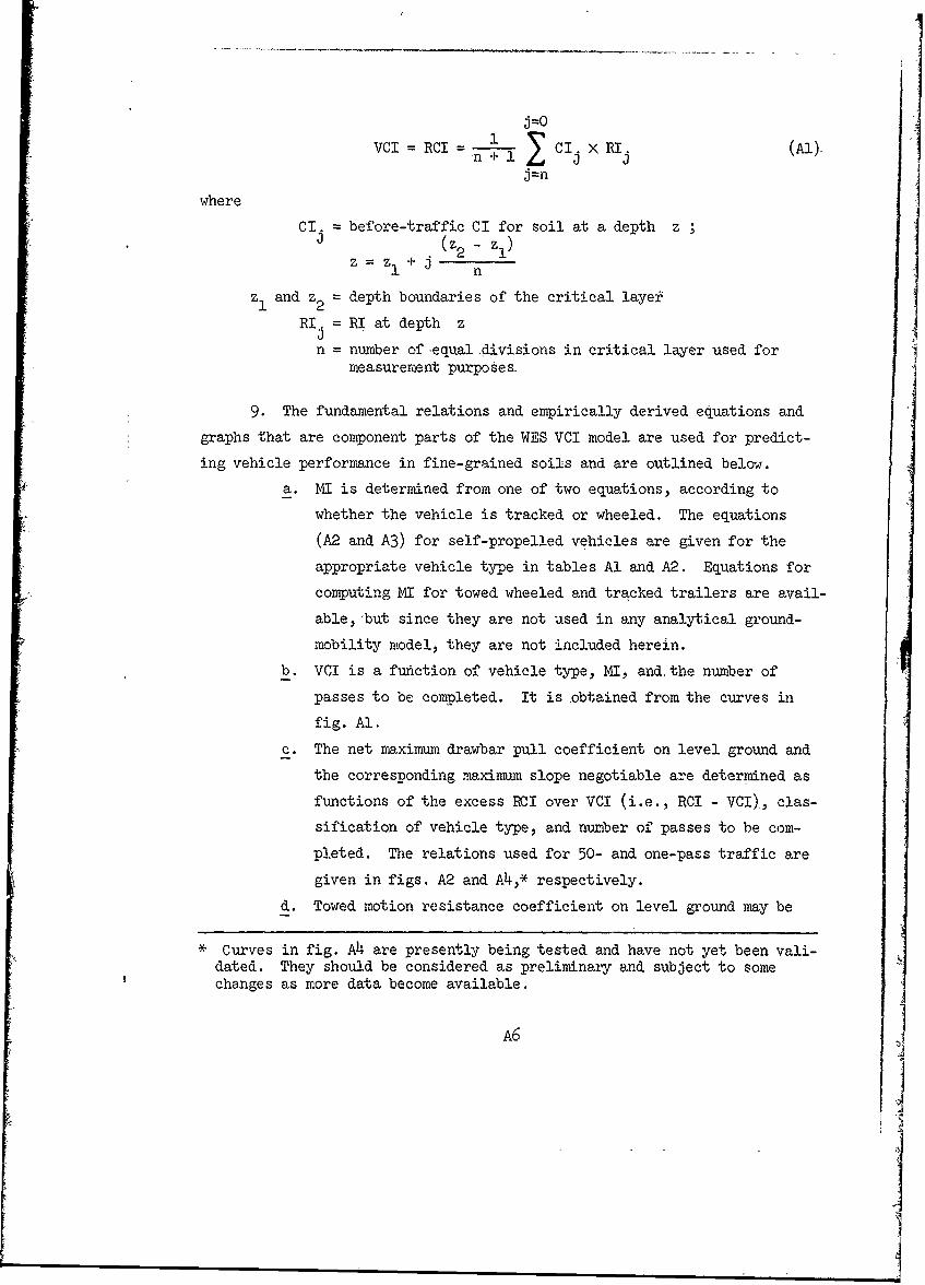
Table Al

Mobility Index Equation for Self-Propelled

Tracked Vehicles (Equation A2):

(contact/pressure X weightMobil- | factor factor bogie clear-

Strack tgrouser + r ance X engine X tranmissiontr •"I tr ck X qrmr ator fato eat co

index*, faetor factor fact factor factor

where

'Contactpressure g gross weight, lb

factor area of tracks in contact with ground, sq in.

Weight factor: Less than 50,000 lb = 1.050,006 to 69,999 lb - 1.270,000 to 99,999 lb - 1.4100,000 lb or greater- 1.8

Track factor - track width, in.100

Grouser factor: Grousers less than 1.5 in. high - 1.0

Grousers more than 1.5 in. high - 1.1

Bogie factor- gross weight, ib, divided by 10(total number of bogies on tracks in contactwith ground:) X (area, sq in., of 1 track shoe)

Clearance factor - clearance. in.• 10

Engine factor: 2!0 hp/ton of vehicle wt = 1.00<10 hp/ton of vehicle wt 1.05

Transmissionfactor: Automatic * 1.0; manual = 1.05

* The I index obtained is converted to VCI from the curves shown in

fig. Al.

A7

,!1

I.

Table A2

Mobility Index Equation for Self-Propelled Wheeled

(All-Wheel Drive) Vehicles, (Equation A3)

/contact weightMobil- (pressure X factor wheel

index* tire grouser l factor factor missionI XatO facatto\at factor factor/ factor

where

gross weittht..1'bContact pressure factor = outside dim

nos tire of tire,- in. X "No. ofwidth, in. X 2 tires

Weight FactorWeight Range, lb** Euationst

Weight <2000, Y - 0.553X 'factor: 2000 to 13,500 Y - 0.033X + 1.050

13,501 to 20,000 Y - 0.142X - 0.420'20,000 Y - 0.278X - 3.115

Tire factor: 10 + tire width, in.

Grouser factor: With chains - 1.05Without chains - 1.00

Wheel load factor: gross weight, kip'sNo. of axles/2

Clearance factor: clearance, in.10

Engine factor: k10 hp/ton - 1.00<10 hp/ton - 1.05

Transmission factor: Automatic = 1.00; manual = 1.05

* The MI obtained is converted to VCI from the curves shown in fig. Al.

** Gross weight, lbNo. of axles

t weight factor X gross weight, kips- Y =weiht fcto , X= -No. of axles

A8

-400Tracked Vehicles VCI

360 Wh I eI Tracked Vehicles VCI /

Wheeled-Vehicles VCI 1 -

320 J

280o __ __ __ __

240

-Pa200

Wheeled Vehicles VCl 50

:E 16o __ __ - _ -_ _

120 __ ______ _ _____ _ __ _

80

0 20 0 60 80 100 120 60 180 200Vehicle Cone Index

Tracked Vehicles

V. 1 7.0 + 0.2 MI- (MI + 6)MI +25.7

VCI = 19.27 + 0.43 MI - 125+7950 M .

Wheeled Vehicles 1 39.2 \VCIl 11.48 + 0.2 MI- I+3.7

VCI = 28.23 + 0.43 MI - (MI+ 367)

Fig. Al. Relation of MI to VCI for self-propelled vehicles

A9

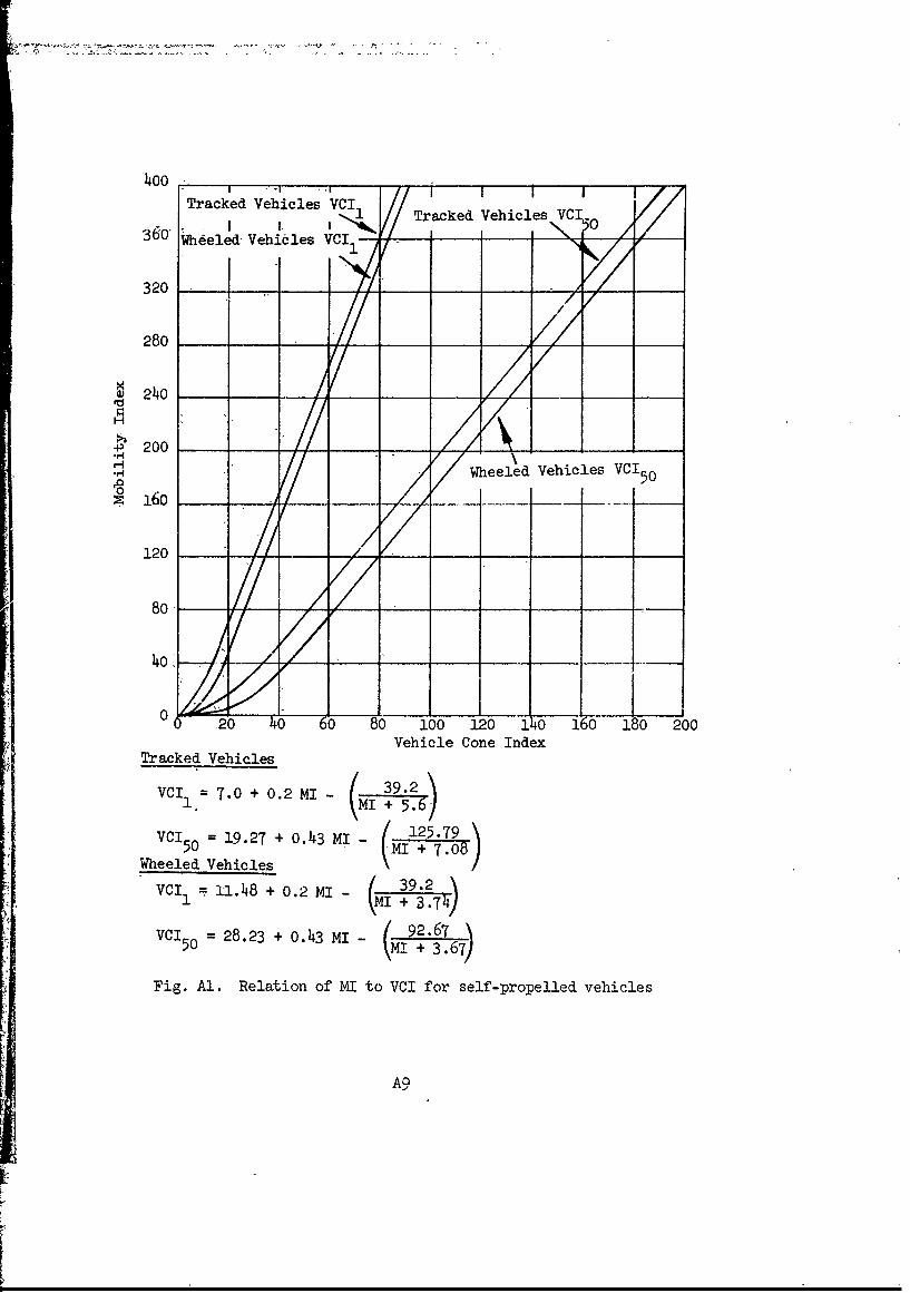
-=_ -~l6 .2 ~~l6 .2) ~ l ~ 2

Y = 0.0109X + 0.366 - V'(0.01146X + 0 .369 )z 0.01X (3)

.8

TRACKED VEHICLES WITHo .7c GROWSERS GREATER THANIIA

4) H

TRACKEDEO VEHILESCLES

0

9.0 - -0- 0 +0 +4 5 6 70 +0 +0 +0

RaigCn0ne-3it bv eiceCn ne x

Fig.~~~ A2 eaio f etcw mxu drwr pl nlve ru

and. ~ ~ GRUSR LEaximum slp1egtal-t112i xes f

.20O

50 passe

estimated from its relation to RCI or excess RCI, the classi-

fication of the vehicle by load and type, and- the number of

passes to be completed. The relations used for 25 passes and

one pass are shown in figs. A3 and A5,* respectively.

Y = 0.1858 - 0.01453X + /(0.1858 - 0.01453 7 - 0.00224X + 0.8623 ()

Y = 0.1609 - 0.00595X + /(0.1609 - 0.00595X)z - 0.001X + 0.2838 (2)

Y = 0.6 - o.oo885x + V(o.6 - o.oo885x) + o.ooX + 0.027 (3)

Y = 0.4167 -'0.01052X + 1(0.4167 - 0.01052X)z + 0.1886 (4)

o 5 .....

25 Passes2WHEE VEHICLES

*1 I00, 4 •

20

4)0

20 . ..........~10-

M TACKED VfIE$Ij

0 20 40 60 80 100 120 14o 160 18o 200

Rating Cone Index (X)

Fig. A3. Relation of towed motion resistance onlevel ground to RCI

• Curves in fig. A5 are presently being tested and have not yet been vali-dated. They should be considered as preliminary and subject to somechanges as more data become available.

All

I

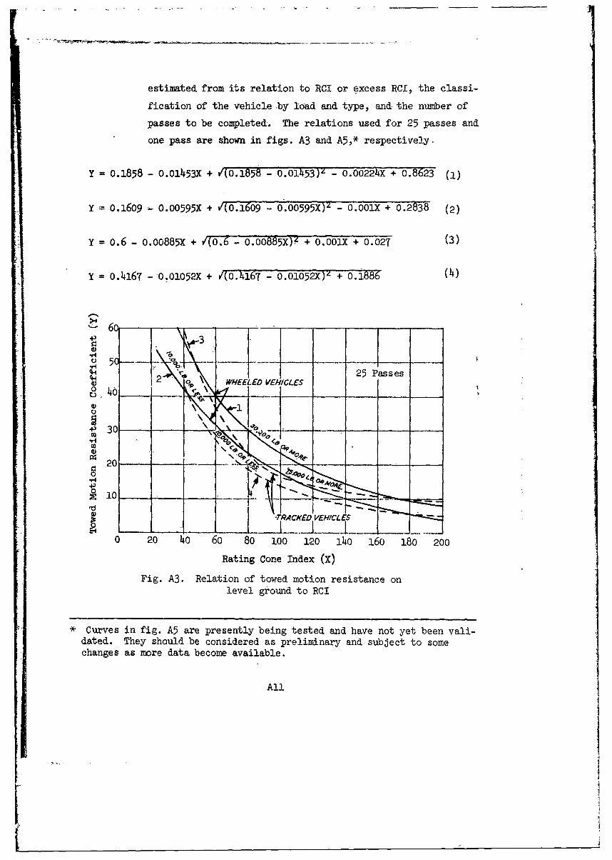
0.6

4,

0

oJ b/ .45 + 0.39 RCd1 - /(o.554+ 0.0392 RCx~

s-u-

0 Tracked Vehicles with GroundContact Pressure < 14 psiP4

HDW =05+0. .06 CI, V(0.544 + 0.0463 RCIx)z - 0.0702 RCI.

o 0 20 40 60 80 - 100

it Rating cone index -Points Above Vehicle Cone Index (RCI 1 )0

4,0.8

10

$4

z0.

~Wheeled Vehicles with Ground Contact Pressure 4 psi

0 D/W = 0.3 85 + 0.02 65 RCI -Yf1(39+0.319 +Cxz 0.0257 RCV

4, O - _L- I

Fig t. Ne'1 ri rwa plmx lp egtal-olsrntrelations Wheelaced andcle whe Grounde Conatpeating on fiegrie psi

DA-1

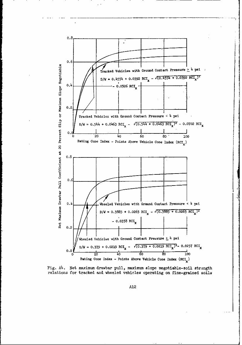
All Tracked Vehicles and Wheeled Vehicles with

Grouind Contact Pressur-e > 4# psi14R ,, 0.4 + 2.3075

~i0.3 RIX-+6_

Weeled Vehicle with Ground Contact Pressure < 4 psiMR0.861

__-0.035 + 086a, wRCI + 3.24i90 X

0.2

4

0.0

0.0 0"20 40. 80 100

Rating Cone Index - Points Above Vehicle Cone Index

Fig. A5. First-pass motion resistance-soil strength relations fortracked and wheeled vehicles operating on fine-grained soils

Coarse-grained soils

i10. The same basic soil and vehicle characteristics are used to pre-diet vehicle performance in coarse-grained soils in terms of VCI, towed

motion resistance, drawbar pull, and maximum slope negotiable for tracked

and wheeled vehicles. The relevant data were derived from some 1400 tests-of self-propelled wheeled vehicles (all-wheel drive) and about 200 tests ofseif-propelled tracked vehicles run mostly in natural sand conditions.

Test site data are characteristic of dry and moist sands commonly found in

inland deserts of the United States and of continental and river beaches

of the United States and foreign countries. Origins of the sands were

quartz, coral, and volcanic ash. The available test data represent a

reasonable range in vehicle and soil characteristics. The soil types

tested include sand and gravel, and sand and gravel mixtures. Wheeled

A13

vehicle test weights ranged from 2600 to 33,000 ib, tire diameters ranged-_

frcm about 30 to 65 in., and tire pressure ranged from- 10 to 60 psi.

Tracked vehicles tested included girderized and flexible tracks, and

weights ranged from 4500 to about 36,000 lb.

11. In clean sands

VCI 1I = CI (AM)

where

CI = average before-traffic cone index

Zl, 2 = depth boundaries of critical layer, usually 0- to 6-in. depth

12. Wheeled vehicles. From the individual tests, 352 separate em-

pirical soil-vehicle performance relations (see fig. A6a for examples) were

established for specific vehicles, and' data from these relat ions were input

to a statistical analysis to develop regression equations relating th6 lpr-

formance parameters to soil and vehicle factors. Multiple curvilinear re-

gression techniques were used to establish equations for predicting VCI,

maximum-drawbar pull, and maximum slope negotiable; and linear regression

techniques were used to develop an equation for towed motion resistance.

An example of the soil, vehicle-performance parameter relations used in the

analysis is shown in fig. A6. The Vehicle and soil characteristics used,

together with forms for computing performance, are given in tables A3

and A4.

13. The equations for vehicle performance in coarse-grained soil

resulting from this statistical analysis are as follows:

a. VCI 1 = antilogarithm* (-0.350X1 + 0.0526X2 + 0.0211X3

+ 1.5870). (A5)

b. Maximum net drawbar pull, percent of gross weight = (28.87X1

+ 10.lOX2 - 1.52X 3 - o.6lX4 - 43.82) + 100 . (A6)

c. Maximum slope negotiable, percent = (28.87X1 + 10.lOX2- 1.52X3 - 0.61X4 - 45.82) + 100 . (A7)

d. Towed motion resistance ={(22.20 + 0.92 x4)+ [(-88 -0.37 X X4) (log X) + 100. (A8)

* Logarithm to the base 10.

A14

/J

3C 30

420

o ISO 15200 250 300 350 4000 0- T0 1. C094.IOCX BEFOR YRAFfC

a- Effect of tire pressure on ve-0 hicle performance on dry-to-moist

. sand. M4 and M135, 2-1/2-ton,6x6 trucks; 11.00-20, 12-PR, _r4

NDCC tires 0

4X4

Fig. A6. Soi ~~l, il-pef c r elations.

20-80 -1 0

Vedinceas -ratned so10-PA pre tire

A15

Table A3

Data Form -for Computing Vehicle Cone Index (.V ) for. nieled

Vehices in Sands (All-Wheel Drive) (Equatioin A5)

Vehicle.Equation: Vehicle cone index (VCI ) = antilogarithm* (-0.350 (contact

area factor, XI) + 0 0526 (number of tires powered, X2)+ 0.0211 (-tire -oressre, X,) + 1.5870)

Vehicle and Soil Characteristics |

(1) Gross vehicle wt, lb

(2) Nominal tire width, in. =

(3) Rim diameter, in. =

(4) Number of tires powered = =

(5) Tire-ply rating =

(6) Tire pressure, psi = X3 =

Factors

Nominal tire width, in. 4; if >2., factor (7) = 2.0Rim diameter, in. if <2.4, factor (7) = 5.0

(8) Wheel diameter factor = (7)** x (2) + (3) == (7 -), X +

(9) Contact pressure 0.;607 x (6) + 1.35 (1170 X ()factor 4.93

o.607 X + 1.35 (117.0 X . ... 3-"_-) _.93 =

(10) Contact area factor = X log ( = log/. )

(11) Strength factor = -0.350 X (10) + 0.0526 x (4) + 0.0211 X (6)

+ 1.5870 = = -0.350 X + 0.0526 x

+ 0.0211 X + 1.5870

VehicPe cone index (VCII) = antilogarithm (11) = antilogarithm )

* Logarithmto the base 10.+* Number in parentheses indicates value assigned to that factor number.

A16

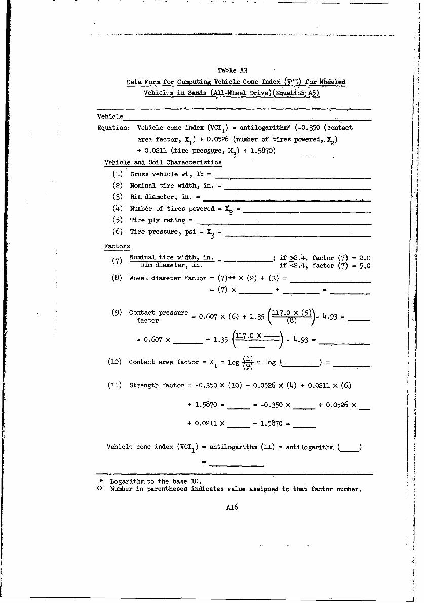
Table A4

Data Form for Computing Maximn Net Drawbar Pull (DBPmax) and Maximum

Slope Negotiable (S for Wheeled Vehicl.s in Sandsmx

Vehicle

Basic Equations

DBP N -of vehicle wt) .28,87Y +.-- m x -. .. ....... . . .. . . .'"-"3 v v A4 -:&5

s,,x(%) = 28.87x + l-OX2 - 1.52x 3 - o.6x4 - x6 =

Vehicle Characteristics and Cone Index

(1) Gross wt, lb __(2) Nominal tire width, in.

(3) Rim diameter, in. (4) No. of powered tires

(5) Tire ply rating (6) Tire inflation pr.-ssure, psi

(7) Cone index of 0- to 6-in. layer

X Factors

X1 = strength factor = log (.7)* =

= contact area factor = log =°a" /117.0 X (5)\

Xa = contact pressure factor = 0.607 X (6) + 1.35 ( (5Y 4.93 =

= wheel diameter factor = X7 X (2) + (3) =

x3 = same as (4)X3=

'4 = same as (6)

x5 = 43.82 for maximum net drawbar pull computations

X6 = 45.82 for maximum slope negotiable

X= Nominal tire width, in. if >2.4 factor (7) = 2.07 Rim diameter, in. if :2.4 factor (7) = 5.0

DBP = 28.87(_.___) + 10.10( ) - 1.52( ) - o.61( ) - 43.82

Smx= 28.87(-') + 10.10(-) - 1.52(_) - o.61( ) - 45.82 =

* Nubnber in parentheses indicates the vehicle characteristic, cone index,or X factor to use.

A17

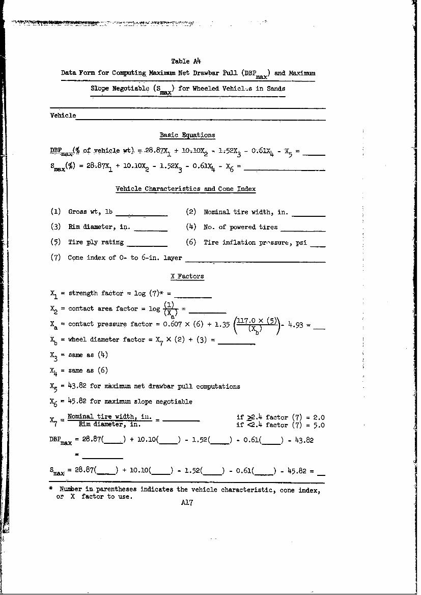
where for equations A5, A6, A7, and A8

X1 = slope, percent

X2 = log of estimated total contact area in square inches (see tablesA3 and A4)

X = number of tires powered

X4 = tire pressure, psi

X5 = log of cone index

45.82 and 43.82 = equation constants

14. The equations above were derived from available data, and after-

the-fact field tests have not been conducted to determine their predictionaccuracy. However, on the basis of the go and no go performance data fromwhich the relations were derived, the equations for maximum slope negoti-

able (equation A7) and VCI1 (equation A5) predicted vehicle performance

with an accuracy of 78 percent. The quality of the relations established,

in terms of absolute deviation,* was the same (0.02) for both maximum draw-

bar pull (equation A6) and towed motion resistance (equation A8).

15. Tracked vehicles. Data available on tracked vehicld performance

in coarse-grained soils indicate that tracked vehicles usually experience

little or no difficulty traversing level, clean sands. The effect of soil

strength and ground contact pressure on the performance (drawbar pull and

slope climbing) of a given tracked vehicle is small. Track type appears.

to be the principal factor influencing performance, as shown in fig. A7.

On the basis of these data, average drawbar pull values of 50 and 56 per-

cent of gross vehicle weight are used for prediction purposes for flexible

and girderized tracks, respectively. Motion resistance has not been well

defined. For the time being, however, the following equations are used.

Flexible tracks

MR 0.10W (A9)

Girderized tracks

NR5 0.074W (AlO)

* Without regard to algebraic signs.

A18

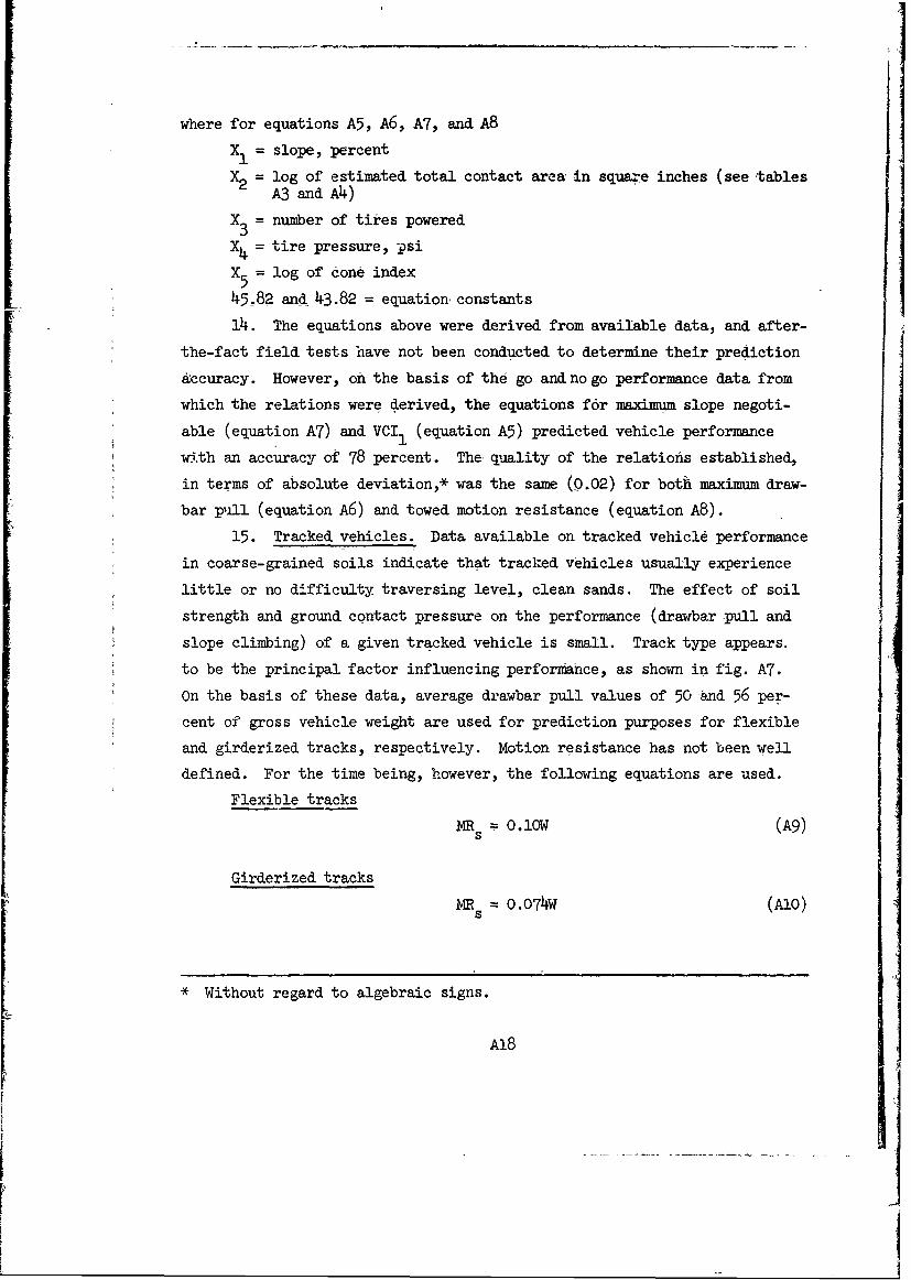
Id 60

fic DT0 t o D 6

50 A4. M C

eri

0 4o 80 ?.20 16o

0- to 6-in. Cone IndexBefore Traffic

0'-1

FeD7 an-.56oH Oi,00 ' ."

10,000 *-P =D4 .50Vo4

0 10,000 20,000 30,000 01,000

Test Weight, lb

Legend

D4,D6,&D7 Engineer Tractors (Girderized Tracks)M & M5A4 Hi-Speed Tractors} (Flexible Tracks)M290 Weasel

Fig. A7. Performance of tracked vehicles in dry-to-moist sand

where

iVs = towed motion resistance (soil), lb5

W = gross vehicle test weight, lb

16. Fundamental relations. The fundamental relations employed in

the WES VCI model for predicting performance of vehicles operating in

coarse-grained soils are summarized on the following page.

A19

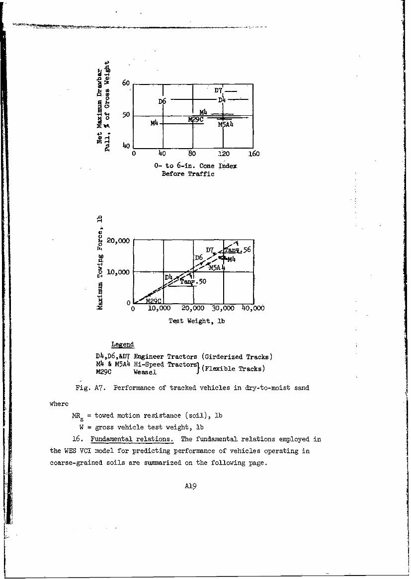
a. VCI for wheeled vehicles is determined using a regression

equation (equation A5) involving vehicle type, soil slope,

and vehicle characteristics. This equation is for dry-to-

moist sands only; investigations of wet and inundated sands,

which may present some problems for heavy vehicles because

of load- liquefaction, have not been completed.

b. Means for computing a VCI for tracked vehicles have not as

yet been developed.

c. The net maximum drawbar pull coefficient and the correspond-

ing maximum slope negotiable are determined from empirical

relations of CI and vehicle type classifications (equations

A6 and A7).

d. Motion resistance coefficient or percent of gross vehicle

weight on level ground may be estimated for a wheeled ve-

hicle by its relation to tire pressure and CI (equation A8)

and to track type for tracked vehicles (equations A9 and

AIO) .

WES Mobility Numeric Model (Wheeled Vehicles Only)

17. The WES mobility numeric model consists of one set of empirical

relations for predicting the performance of a single tire moving at 5 to 6

fps in a straight line in a fully remolded clay, and a second set for

performance in a dry sand. These relations were developed by the consoli-

dation of systematic laboratory test data by means of dimensional analysis,

extended by regression techniques. After the basic clay numeric wts de-

veloped, analysis of data from field tests with prototype wheeled vehicles

indicated that the use of RCI rather than CI would increase predictionaccuracy. Selected performance parameters (minimum soil strength requiredto complete the first pass--VCI1 , drawbar pull, input torque at 20 percent

slip, and towed motion resistance) are presented in proper dimensionless

form as unique functions of a "mobility numaeric," which is a dimensionlessload coefficient expressing the ratio of soil strength (in RCI terms) to a

nominal unit load exerted by the deflected tire upon the soil.

A20

18. The- basic mobility numeric relations were developed from labo-

Tatory results of more than 184 single-wheel tests in a heavy clay soil and

over 122 tests in sand. Each test involved soil strength and tire behavior

measurements during three to five passes of a wheel in the same path and

under a constant load. During each pass, the slip was slowly increased

linearly from -20 to 100 percent. In the remolded clay soil the drawbar

pull and torque of a wheel as related to slip: were essentially the same

from pass to pass, but differences were found in sand because its strength

may increase or decrease under the action of traffic, depending essentially

on. its before-traffic density.

19., The soil was so prepared in the laboratory that reasonably uni-

form soil conditions were achieved. The mass soil strength for the clay

soils in which tires were tested ranged from 7 to 45 CI (o- to 6-in. depth),

while sand strengths were from 8 to 77 CI (0- to 6-in. depth) or, in terms

of the strength gradient (G) over a depth equal to the tire width, were

from 2.6 to 25.7 psi/in.

20. Tires used in the development of the basic mobility numeric data

were treadless. The largest was 41.3 in. in diameter and the smallest was

8 in. Ratios of width to diameter ranged from 0.15 to 0.92.

21. Assumptions currently involved in this model are listed below.

a. General.

(1) The basic dimensional analysis of the tire-soil rela-

tion using a single cone index (C), rating cone index

(RCI), or cone index gradient (G) as the soil strength

parameter is valid and adequate.

(2) Contributions of soil dynamics and shear-rate-dependent

effects to net tire performance are negligible in the

soil-tire systems under study.

(3) Empirically determined relations accounting for changes

in tire proportions (b/d, 8/h, h/d), which enter the

final form of the mobility numeric, are generally ap-

plicable to similar soil-tire systems.

(4) The vehicle moves in equilibrium in a straight line on

A21

level soil at no more than normal vehicle speeds

off-road.

(5) The performance of a (multiwheeled) vehicle is the sum

of the performance (+) of its individual tires.

(6) It is adequate for design and simulation to represent a

slip-dependent relation in terms of performance at 20

percent slip, which is near optimum in terms of draw-

bar efficiency.

,b. Soil.

(1) The soil body is essentially uniform and is either

purely cohesive or entirely frictional (c/O soils

cannot yet be handled).

(2) The mean CI of a uniform clay soil body in the labora-

tory, measured -with standard cone penetrometer, ade-

quately describes those properties of the soil which

relate to vehicle performance.

(3) For field performance predictions in clay soils, mean

RCI within the critical layer, as defined by the WES

VCI method,is used in place of the laboratory mean CI

to calculate the controlling mobility numeric.

(4) There is no significant discontinuity between surface

and mass soil strengths.

(5) The gradient (G) of CI with penetration distance ade-

quately describes the properties of both natural and

laboratory beds of purely frictional soils as these

relate to slow-speed-vehicle performance.

c. Vehicle.

(1) Tire geometry is suitably described by measurements of

undeflected tire diameter, section width and section

height, plus, as an index of tire flexibility in the

soil, static -deflection under the test load, when on

an unyielding surface.

(2) The primary effects of tire pressure on performance are

fully accounted for by the deflection measurement.

A22

(3) Tread pattern has only a negligible influence on tire

,performance in uniform Soils.

d. Soil parameters,.

(1) For natL.al clay, RCI is the only soil parameter.

(2) For natural sand, CI gradient is the only soil

paraeter.

e. Vehicle parameters. Tire parameters are wheel load (W),

undeflected section width (b), unloaded diameter (d),

unloaded section height (h), and hard surface deflection(8).

Mobility numerics

22. Predictions are made from empirical relations of dimensionless

performance numbers (listed below) and dimensionless mobility numerics.

Py2V/* = drawbar pull coefficient

,PT,* = towed motion resistance coefficient

Z20d = sinkage coefficient

Two of the peiformance parameters measured during tests that relate to the

performance numbers listed above are pull (P 2 0 ) and pull required for a

free-rolling wheel (PT). When it is necessary to estimate motion resis-

tance at 20 percent slip, the towed force is used as a reasonable

approximation.

23. The WES clay _mobility nufneric for natural soil is

CIbd (61/2(l (All)W " +

where

RCI = rating cone index for the 0- to 6-in. depth

(See paragraph 1 for identification of other symbols.)

Relations of performance coefficients for the first pass of a single wheel

and revised clay mobility numeric are given in fig. A8. Relations of pull

* Subscript, 20, denotes slip, in percent.

A23

.....I-. 2 -- ---- ---

1.6o

o r1S 1.20+; /W 0 .8 - Q.1~2 P0l - --0.95

• 0.80

0

o~ A0.I40

H o

Clay Mobility Numeric

Cbd o OW h l+ b

a. Pull coefficient vs clay mobility numeric from field data

0.0

0 Note:

0 0.30 --.-.- - B -(RCI)bd6

0.30 1+ b

14 wo~~ 0.20 W hP 3 T9 i 1.35 2d0.20

0

F.-I

Clay MobilityNumeric

o ,~ ~ ~Cb 0.xB-(C~b()/op/W o 1~o+ b 13°( F

b. Towed force coefficient vs clay mobility numeric from field data

Fig. A8. Relations of performance coefficients for first passof single wheel to clay mobility numeric

A24

and towed force coefficients and the original WES numeric for clay are

given in fig. A9.

24. The WE sand mobility numeric is3~d, 12 x 1 (A12)

h

where

G = the slope of the curve of penetration resistance versus depth,averaged over a 6-in. depth. (See paragraph 1 for identificationof -other symbols.)

Relations of performance coefficients for the first pass of a single wheel,

slope negotiable,, and towed force and sand mobility numeric are given in

fig. AlO.

Fundamental relations

25. The fundamental relations pertinent to this model are as follows:

a. The clay -mobility numeric is determined from the soil and

"vehicle parameters and subsequently used in the relations

(fig. A9) to obtain performance coefficients for a single

wheel or wheeled vehicle. Actual wheel performance values

are calculated by multiplying the coefficients by W or Wd

for the wheel, as appropriate. The performance of a com-

plete vehicle is obtained by summing the performance of each

of its wheels (including a net motion resistance or negative

performance when a tire is not powered or has insufficient

net traction to propel itself). Performance measured in the.

laboratory during the second through fifth passes varied but

little from that during the first pass. Thus, although the

graphs were developed by the consolidation of first-pass

test results, they can be used to calculate pull, torque,

and towed force for every individual wheel on a vehicle, and

even several passes of the vehicle.

b. The sand mobility numeric, calculated from the soil and ve-

hicle parameters, is used to determine corresponding per-

formance coefficients from the curves shown in fig. AlO.

A25

r r

I

Vr4

43

o.4

-4

0.2 -""-

0.0

0 0.1 0.1 .2 0.3 o.4,-W .5Clay Mobility N erc,-

Fig. Ag. Relation of pull, slope, and towed force coefficients toWES numeric for clay

A26

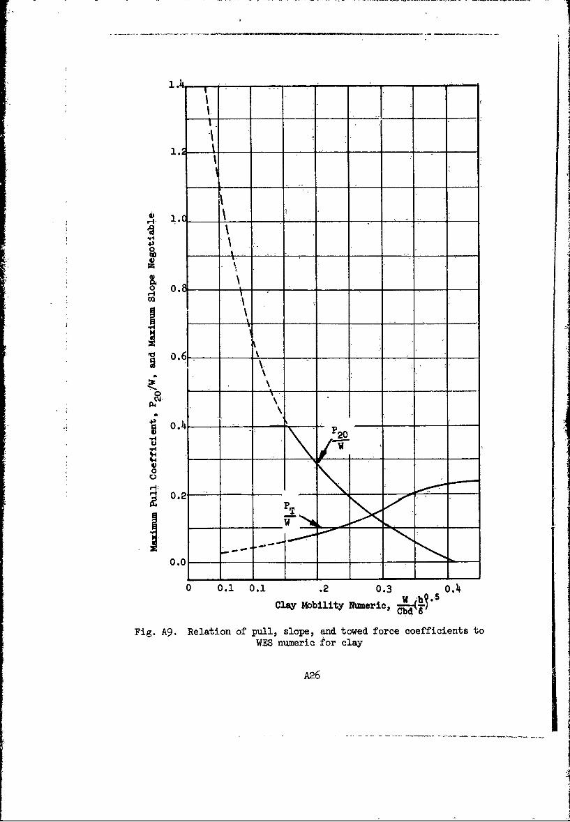
0.50.40

u 0.3

00

IW 00.

0 '20 ' 4b 6 80 100

Sand Mobility Numeric =

G(bd)3'2W h

a. Pull coefficient vs sand mobility numeric

0 .3 Not e;• O. G(bd)'/'Z 6S

0 xto -N.M

, -,,,_0.03850 + 0.48-10.- -0 - 2.58 6+ 0.025PT/ 0.85+ .8

0 20 4o 60 80 i0oSand Mobility Numeric =

-G(b) 31/2x 6W h

b. Towed force coefficient vs sand mobility numeric

Fig. A1O. Relation of performance coefficients for first pass ofsingle wheel to sand mobility numeric

A27

Bekker/LLD Soil-Vehicle Mcdel

26. The Bekker/LLD soil-vehicle model was first assembled by M. G.

Bekker and has subsequently been modified by U. S. Army Tank Automotive

Command (USATACOM) Land Locomotion Division (LL)- in. various minor ways on

the basis of experimental data. Still other refinements have been proposed

by other researchers (Reece, Firth, etc.). The model has both theoretical

and empirical aspects. It includes methods to predict Vehicle sinkage,

motion resistance, and drawbar pull versus slip in soft soils. In firm

soils, where motion resistance is small, it is usually neglected. Equa-

tions are available for predicting the performance of tracked- nd wheeled

vehicles, often in several forms. The forms differ according to the de-

tailed assumptions made, the level of mathematical treatment, and the over-

all framework within which the results are to be used.

27. Six soil values measured by means of a bevameter are employed in

the various equations. Values for soil cohesion (c), friction angle (s),and tangent modulus (K), used in the equation for gross tractive effort (H),

are determined from tests upon a small grousered annular ring loaded to

several normal loads. The ring is rotated under each load until the soil

beneath !.s cheared, and a record of torque versus angular deformation ob-

tained. c , , and K are computed from the records for several normal

loads. Three soil constants are used in the equations for track or wheel

sinkage: soil moduli of' cohesion (kc) and friction (k ), and n , an

exponent of sinkage. These are obtained by analysis of curves plotted for

results of pressure-sinkage tests with two or more small-diameter flat

plates forced vertically into the ground. Three further soil values are

used in a now little used equation for "bulldozing" resistance: two co-

efficients of bulldozing (Kg and Kb) and soil bulk density (7). Other

symbols used in various current equations are as follows:

s = slip ratio (dimensionles)

D = undeflected tire diameter, in.

zm = maximum sinkage, in.

= shear stress, psi

A28

28.' The Bekker/LID model was created by combining and amplifying

simple odels who'se beginnings 'may be traced to Bernstein (1913), Nichols

(1931), Goriatchdn "(1936), and Mickelthwaite (1944). Bekker consolidated

the earlier approximations into the first coherent engineering system for

calculating vehicle-soil interactions (1956). Since their first publica-

tion, Bekker".s equations have been more-or-less continuously modified in

various details, largely by LID, on the basis of data obtained from several

hundred scale-model vehicle tests conducted in the laboratory in several

soil types (clay, sand, and mixtures thereof) prepared to various consis-

tencies. Several hundred field tests in a number of different representa-tive soil conditions were also conducted with full-scale vehicles to verify

the predictions. Details of laboratory experiments and full-scale vehicle

tests are not well documented in the literature, however.

29. Assumptions pertinent to this model as currently used are listed

below.

a. General.

(1) Soil parameters derived from analyses of soil response

data obtained with the bevameter are soil invariants,

not significantly affected by instrument configuration.

(2) Values for the soil parameters at points disturbed by

the passage of a vehicle are unaffected.

(3) Pressure distributions under moving tires and tracks

are 'two-dimensional, are effectively analogous to the

axisymmetric pressure distributions under small circu-

lar plates, and are adequately represented at all

points by the power expression p = kzn

(4) Response of the soil body to vertical and horizontal

forces imposed on it by the vehicle may be calculated

independently and subsequently combined by simple

superposition; i.e., vehicle sinkage is independent

of track or wheel traction and slip.

(5) Gross vehicle traction is developed by shearing soil

along a surface defined by the instantaneous position

of wheel or tire grouser tips.

A29

1i

(6) Shear stress ('r)-developed at any point in the shear

failure surface can be expressed as a function of du-

mulative shear deformation- (j) along that surface by

the expression-

= (c + p tan-,O)(i - sA/ K )

(7-) A vehicle track is treated. as a rigid, flat plate,

whose sinkage is bounded between that calculated con-

sidering, sinkage to be uniform along the .nominal con-

tact length, and-,,sinkage calculated by considering

that it be zero at the front- of the contact area, in-

creasing linearly to a ma imum, at the rear.

(8) Pneumatic tire performance is bounded between- that of

a rigid, cylindrical wheel having the same overall

diameter and width as the undeflected tire, and that of

a short track whose length equals the contact length of

the, deflected tire on a hard surface-, and whose width

equals the undeflected tire section width.

(9) The gtound contact surface of a vehicle tire or track

is, defined by the assumed, running gear geometry con-

necting the point Where this intersects the undisturbed

soil level with the point 6f its greatest penetration

into the soil, and by overall width of the tire or

track.

(10) The vehicle moves in static equilibrium in a straight

line at a slow uniform speed on terrain with a plane

surface.

(11) Traction and support developed by track or tire con-

tact with rut sidewalls are negligible.

(12) Vehicle sinkage on sloped soil surfaces is identical

with that on level surfaces.

(13) The net traction of a (multiwheeled or multitracked)

vehicle is the algebraic sum of the net traction of

A30

all tires or tracks, each calculated as though operat-

ing in level soil unrutted by the prior passage of any

running gear ahead.

b. Soil. The soil mass is homogeneous and semi-infinite with

no hardpan at any depth from the surface less than twice

the maxiimum sinkage.

c. Vehicle.

(1) Slip of all wheels or tracks is the same.

(2) The weight distribution 6n the ground contact elements

does not change under applied external loads.

(3) Power train torque available at the running gear is

sufficient to ensure that soft-soil performance is

limited by soil-vehicl& interactions rather than avail-

able torque.

Soil parameters

30. Soil parameters obtained from results of tests with the beva-

meter are kc , k , n , c , , and k ,

where

kk = c =k

b smallest dimension (inches) of penetrating element (for a circu-

lar plate penetration test, b is the radius).

Vehicle parameters

31. Vehicle parameters are as follows:

a. Wheeled vehicle parameters are W , D , b , s ,and 6

b. Tracked vehicle parameters are W , I , s , and b

Fundamental relations

32. The fundamental relations pertinent to this model are as follows:

a. Resistance for all vehicle types.

(i) Compaction resistance.

bk n+l

131

,4"

(This equation is often written with one of the sinkage

expressions substituted for z , which changes its

appearance grossly without in any way altering its

actual meaning.)

(2) Gravity resistance.

R =W sin 0 (A1)

(3) Trim angle resistance.

R C1W [sin (9 + o) -sin,] (A15)

(4) Mechanical rolling resistance,.

Rr (A16)

(From manufacturer's data engineering tests or gen-

eralized handbook information.)

(5) Total motion resistance.

R+ + Ra + R (A17)

(6) Motion resistance coefficient.

-RR z + sin - + sin (e + a) - sin o +- (A18)W I(n + 1) W

b. Net traction for all vehicle types.

(1) Drawbar pull or net traction.

DBP = H - R (AI9)"

where

H = gross traction

A3-

(2) Traction coefficient..

DBP H R (2

c.Rigid wheels.

(1) Sinkage.

z r 3W5 (A21)

-(9) Gross traction for high slip only.

H =Ac + W tan (A22)

where

A = b

(3) Gross traction for any slip value (cycloid method).

H=H - H(A23)1 H2

where

ev = 2T- cos- 1 l- 2z/D)

~ 2Tr -cos- 1 - s)e = angle that varies between 0 and 2rT

e <e Casel10 - V

o V>0 Case 2

p- k (Cos e - Cos e)v]

Case 1: H =D f2 (c + p tan )(i -ej1/k) cos 0 dG

H2 0

A33

i D

= [(~ - s)(e - e) + sin 8 sin- ]

J2 = 0

'2 T

bD af j =/(c+Ptan )(1 e Kl)Case 2: HI =-2 C p ta e cos 0 de

ev

12 = f (c +-p tan - e " Kcos e dO'0

S [(I- s)(0- + sin 0 - sin 8o]

fu S) f. - ( - e) + sin e - si 0

d. Deflected tire and track that sinks uniformly.

(!) Sinkage.

z = (-)i/ (A24)

(2- Gross traction.

H = (Ac + W tanO)[l- (i- esK)]A25)

where

for wheel, A = 2-6(D- 6)

for track, I = length of contact area of track

A = bl

(3) Gross traction with grouser effects.

H {Ac (1 L+ + W tan [1 + 0.64hU cot-l i)]la K .(I - s/ (A26)

where

h = grouser height

A34

I

e. Track that sinks nonuniformly.

(1) Sinkage at rear of track.

(2 Glross traction.,L

[l.~~~(l'~ eL ) +k ta1 fn- s,K\+HkA ta jxe d x)(A28)

f. Power required (HP) to overcome compaction resistance..

n+l

N 550(l s) TI(n +1)(,bk)/n~

where

v = velocity, fps

= overall efficiency of power transfer betweenrunning gear and engine

9. Other. Relations that have been replaced or are sel~dom used

are given- below. These equations are included because they

were used in at least one of the comprehensive ground-

mobility models considered in the ANAMOB study.

(1) Bulldozing resistance Rb.

Rb =b(2K zc + Krz 2) (A30)

where

Kb =(N - tan )co2 (1 + cot, o tan ~

c

For wheels a cos7 1

A35

(2) Bulldozing resistance B

1co x.~ tan + cot xl[(cot~ ~ ~ ~~~[ - a ) +C ian x: ~ +)

Ex yz ct (x +) tan 0 a a x+(A1

where

=angle of' approach

x angle of' rupture plane

if'

then

c 2and,

1 2 2(o0B= yz tan (5+ + 2cz tan(40.

(3) Drawbar pull.

DBP =-H -(R C+ Rb + R) (A32)

where

R6 = Wsin 0

(4i) Bulldozing of' f'ront wheels.

p = k(z1 + z2'(A33)

where

Z= sinkage of' f'ront wheels

z= sinkage of' second. wheels relative toz

(5) Motion resistance of' rigid wheel.

2n+2

R0 3Wn2 2n+l (A34)2n22+ T

(3 -n) 2nl(n + l)(bk) 2n+.

A36

Predictions

33. Predictions are straightforward after the running gear of the

vehicles has been defined and the soil and vehicle parameters have been

determined.' One of the problem areas in this system is to differentiate

between rigid wheels and wheels mounted with pneumatic tires. A rigid

pneumatic tire is defined by any inflation pressure above the critical in-

flation pressure and the critical -inflation pressure is determined from the

following equation.

i (n + 1)w (A35)bic b Z(D- z)where

2

In the equation above, however, the determination of z requires the

assumption that the wheel is rigid.

Reece-modified Bekker/LLD eruations

34. Pressure-sinkaee relation. Reece's modification of the pressure-

sinkage relation, which he considers as tentative, is as follows:

p = (ck' + y k(A3)

where

k' k, and n = dimensionless soil constants

35. Gross traction of grousered track. The equation for gross

traction H proposed by Reece is:

H base + H side) + K- e- st -K (A37)

where

Hb2 cN+b2 +b2 NHbase bCc ca oHae= b N+ b caNa + b p0~

Hside = AChgt sin2 (45 + )+ 2yhg1Zm tan(45 + 0 cos(90 -

A37

I--

whereN=(1 -m)(!')

Nc=

c = adhesiona

WPo =(TL)

Nq =b tan

h = height of track grousergm = ratio of the area of the grouser tips to the total contact area

Reece hopes to replace K , a purely empirical constant, in the near

future. He also is working on a modification of the slip-sinkage relation.

Perloff Model

36. The Perloff model is essentially an unvalidated procedure for

predicting the effect of soil strength on the performance of tracked Vehi-

cles only. It is complex and any precision gained by the computation in-

volved has. not been demonstrated. The- oniy application- of the model has

been in a digital computer simulation of a tank engagement to predict tank

performance in soft soil from design characteristics. The output of the

complete simulation was intended to show the effect of individual design,

features, including mobility elements, on the overall effectiveness of

tank-weapon systems. Soil ,parameters used in the Perloff model are the

Mohr-Coulomb failure parameters c and , and shear stress/deformation

data measured in a standard direct shear test, and a pressure-sinkage

relation. Specific equipment and procedures that should be used to obtain

the pressure-sinkage relation to be used are not identified.

37. The model first finds, by a computer iterated process, vehicle

sinkage and trim, which satisfy the assumed pressture-sinkage assumptions,

plus static equilibrium equations which embrace terrain slope. It then

computes tractive force and track slip on the basis of some broad assunp-

tions relating soil displacement under a track to the unit shearing strain

experienced by the soil. By applying the shear stress/deformation data, a

distributiou of shear stress under the track is developed as a function of

A38

the track slip and integrated to obtain corresponding total and net trac-

tive efforts.

38. Then calculating track sinkage and attitude, the model assumes

the track to be a flat, rigid plate, plus a front ramp treated as a passive

earth pressure problem, and deals with it as a two-dimensional problem only.

In common with similar but less complex models, the unspecified pressure-

sinkage relation is taken to be independent of the size and shape of the

penetrating surface, and of the path of any part of that surface in reach-

ing a final sinkage. Again, as is commonly done, the effects of normal and

tangential loadings are computed separately and considered to be totally

independent. External motion resistance due to coil failure is considered

to be reflected completely in the final vehicle trim angle.

39. Assumptions and specific steps involved in calculating traction

(Perloff, 1966) are:

In 'order to relate the soil displacement at the surfaceto the unit strain experienced by the soil, the totalshear distortion is assumed linear with depth. It isfurther assumed that above some critical depth the soilis affected by the shear stresses, and below that depththe soil is unstressed. An estimate of this depth hasbeen obtained by analysis of an analogous elastic prob-lem. The result given by Scott (1963, p. 500) for theshear stress distribution due to a point shear force onthe surface of an elastic half space has been integratedtwice to yield the stress distribution due to an appliedstrip shear loading. The results of the analysis areshown as a plot of shear stress along the Center line ofthe tiack, Txz , as a function of the depth (Fig. All].Note that at a depth of twice the track width, the shearstress diminishes to 15 percent of the applied stress.Examination of'many stress-strain curves for soils indi-cates that the strains corresponding to a stress levelof 15 percent of the maximum shear stress are negligible.Therefore, a depth of twice the track width was chosenas the depth above which the soil is affected by theshear stress applied by the track, and below which thesoil remains undisturbed. Knowihg this depth, the unitshear strain is obtained by dividing, the soil displace-ment at the track surface by the depth of soil affected.

It is then necessary to know the relationship betweenshear stress and shear strain for each given soil. Thedirect shear test provided the closest analogy to theshearing effect produced by a tank track of all the

A39

0.0. 0.4 0.8 .

20

b/21.0

6.0

Fig. All. Shear stress (i ) under center line of track as a functionof depth for an applied strip shear loading

A140

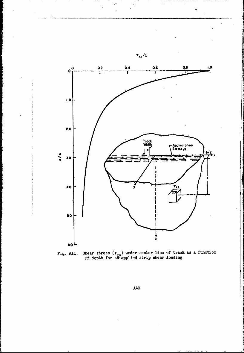
standard engineering tests on soils. Results presentedby Roscoe (1953) indicate that the shear strains in adirect shear test are distributed over approximatelythe middle one-quarter of the specimen. Assuming thestrains are uniformly distributed over this height,it is possible to determine the unit shear strain,and to relate the direct shear test results to theconditions under a tank track.

-For each value of sliP, the displacement at variouspoints under the track, d , is computed and convertedto the displacement, dds , in the direct shear testwhich corisponds to the same unit strain, i.e.,

dds = [A381

where TS is the thickness of the direct shear testspecimen,, and TT ,is the depth of soil affected bythe shear stresses imposed by the track (TT = 2b).

Computation of tractive effort is complicated by thefact that, in general, the shear stress in the soildepends not only upon the induced strain but also uponthe normal pressure. The results of direct shear testson a variety of soils suggest that the Coulomb (1776)equation can reasonably be approximated by:

r(,) = A(E) + B(e)an [A39]

where (r) is the shear stress at any strain, : . A(e)and B3e) are empirical parameters determined fromthe results of two or more direct shear tests at dif-ferent normal stresses, and an is the normal pressure.When the soil strength As fully utilized, equation[A39] reduces to the Coulomb equation for which A(C)=c and B(e) = tan$.

Direct shear test results for the soils being consideredare read into the computer in terms of A(e) and B(e) ,

from equation [A39j, for various values of sheardisplacement.

The values of A(e) and B(e) which correspond to thevarious dds at different points under the track aredetermined by Lagrange interpolation (Milne, 1949) be-tween the input data points.

Using the normal pressure distribution under the trackdetermined previously, and substituting into equation[A391, the shear stress distribution under the track iscomputed.

The total tractive force per unit track width is

A41

determined by numerically integrating the shear stressdistribution under the track by Simpson's rule (Milne,1949).

Input data

40. Vehicle and terrain data inputs -required for this. model are

listed below.

a. Tank. (A schematic representation of a tank in the soil is

given in fig. A12.,

(1) Weight, per unit of total track width, W1 .

(2) Location of center of gravity.

X = distance to front of track base

Y = distance =bove track base

(3) Length of track base in contact with ground, A

(4) Angle (A) between the track base plane and .the forward

inclined portion of tank track, A2

(5) Undercarriage clearance.

(6) Values of maximum power/torque limited velocity,

VI , on a rigid surface for various tank inclina-max

tions, a

(7) Track width, b

b. Terrain.

(1) Ground surface inclination, e

(2) Cohesive component of soil strength, c

(3) Angle of shearing resistance, .

(4) Unit weight of the soil, y

(5) Data points from the -assured pressure-sinkage relationfor the soil.*

(6) Data points from the expression for shear stress-displacement relation for the soil from direct sheartest results.

(7) Thickness of the direct shear test specimen.

* No generally accepted method for extrapolation of pressure-sinkage data

from small-scale models to prototype vehicles is currently available;therefore, the general shape of curves obtained experimentally from modelstudies have been assumed.

A42

wk.

Fig. A12. Schematic representation of a tank in the soil

Fundamental relations

41. The fundamental equations and general procedures used in this

model are as follows:

a. Sinkage (a rigid track is assumed).

(1) At any point,, x, along the track,, the sinkage, z ,

is expressed by

zf + s sin (a - (A4o)

where

zf =vertical sinkage at front of track base

a = total trim angle of track base lengthrelative to the horizon

(2) Trial values of zf and o are selected.

(3) Normal pressures along the track contact length are

determined to suit the resulting z = x line accord-

ing to the assumed input pressure-sinkage relation.

(4) Total normal force (V) per unit of trac& width is ob-

tained by integrating

v = Pv(X)dx (A41)0

A43

4 ,?

where

pv(x) = normal pressure at point x

(5) Trial values of z and a are tested by examining

whether or not the resulting force system is in static

equilibrium, i.e. whether or not

AISpP(x)dx wcos - Pe cos (A - sin (A42)

0

-(X)dX W1 os o + sin + P'O s 6 (A43) J

Ox X

where

W1 = weight per unit track width, lb

P = passive earth pressure, psie

The passive pressure force per unit width is determined by iteration for

each value of zf If equilibrium conditions are not satisfied, inclina-

tion, oy , is incremented and the process. repeated. Values of a are

increased until the rear end clearance of the track is reached before zf

is incremented to begin a new cycle. Iteration is continued until suitable

values of z and a are obtained or until the tank bellies out

VS = 1 - _-Z (A44)

where

V = actual forward speed of tank relative to theground

VT = velocity of track relative to tank hull

c. Slip velocity between track and soil.

Vs = VT - Vv (A45)

A44

d. Soil-displacement.

d=V t (A46)

e. Time.

t X (A47)VT

f. Actual soil, displacement at track rear.

dA sx (A4i8)

~.Maximum soil displacement at track-rear,.

dl- sA(A49)

i-Id" may be greater thand

h,. Shear stress.

i.. 'Thrust f'orce pet unit, width of track.

T f(d)dx (A51)

~.Tractive fordce required to just initiate or maintain motion.

T =W sin +P, sin (A -c'st (A52)req 1e f~~Y C sin (A + o

where.

~~' ~ . [+tan (A+ o) sin (A +)sieI~fsin (A + -e)

A4f5

k. Maximum available thrust.

T T at some optimum slip value'

1. Mobility factor.

Treq (-A53)

Tmax

m. Drawbar pull.

T m T =T k Tmax(1 k) (A54)

n. Maximum velocity.

Vma x =mVaxl -mi n ) A5

where

s. = minimum slip at which actu;§l thrust is equal

to required thrustV' = maximum velocity on hard surface for the slopemax angle, y , as determined by power and power

train characteristics

Output values

42. Output values obtained from this model are as follows:

a. Maximum track speed, V' , as limited by the soil at themax

point which is being studied.

b. Actual track speed.

c. The tractive force (thrust), T , per unit of track width

exerted between the soil -and the tank. When taken with

track speed and track width, corresponding horsepower out-

put and fuel consumption rate may be computed.

Predictions

43. To predict vehicle speed with the Perloff model involves a

large number of computations, each requiring many iterations. In a

A46

I"I

discussion of the application of the model in a computer simulation, Perloff

(1966) stated that

At this time it is difficult to assess the degree ofvalidity of the results of this analysis. As with thedevelopment of any model, many simplifying assumptions-were required. Although it is believed that the anal-ysis leads to results which are reasonable, and whichwill serve to distinguish the mobility characteristicsof tank design candidates, there is not yet any experi-mental verification of its predictive capability.

A part of the problem is to specify appropriate instruments and procedures

for obtaining the required pressure-sinkage relations. There is still no

generally accepted method for extrapolating to prototype vehicles pressure-

sinkage data from field tests of small plates or other track analogs.

British Model

44. British investigations of the general relation between off-road

performance of vehicles and the physical environment have been the respon-

sibility of the Fighting Vehicles Research and Development Establishment

(FVRDE). On several occasions research sponsored by the Ministry of De-

fense has been conducted by British universities. Generally, the work in

soil-vehicle research has been to improve a unified theory based on re-

lations developed using methods of soil mechanics and making appropriate

allowances or adjustments to account for soil-vehicle interactions in a

manner that would yield the best agreement with experimental test results

in the laboratory with running gear elements or in the field with prototype

vehicles. The basic types of vehicle running gear investigated are the

wheel and track, with special emphasis also given to wheel locomotion with

traction devices.

45. In the review of British literature, considerable attention was

given to a paper prepared as a basis for discussion at the Fourth Quadri-

partite Meeting of the Working Group on Ground Mobility held in Britian in

1963. The paper presents a summary of the past and recent British thinking

on the soil-vehicle relations required to predict the performance of ve-

hicle running gear operating in a variety of soil conditions. The

A47

I

information presented is a digest of British experiences gained through

comparing the application of theory to measured results for separate rela-

tions required to account for the total soil-vehicle interactions.* The

report also presents a method for predicting the effect of soil on the run-

ning gear of a vehicle by coupling the separate effects of sinkage, motion

resistance, slope resistance, and maximum net traction (drawbar pull).

Evidence of the quality of some of the single relations is available, butno results are available in the literature by which the prediction accuracy

for net traction, which is the resUltant, prediction of the separate rela-

tions coupling process, can be determined.

46. In the referenced paper,, it is apparent that different soil

descriptors are used as input to the various relations used to predict

an element of vehicle performance. For example, in the relation used to

predict motion resistance of wheeled and tracked vehicles operating on sand,

the Bekker/LLD soil parameters are used to obtain a value for one of the

unknowns, whereas the conventional soil mechanics parameters, c and ,

are used to predict sinkage of tracked vehicles.

47. The assumptions, soil and vehicle parameters, and fundamental

relations common to the British soil-vehicle model are listed below.

a. Assumptions.

(1) Plastic soil deformation without recovery.

(2) For small sinkages, the uniform pressure, q , is iden-

tified with the strip load bearing capacity of the <soil.

-(3) Soil is generally described in terms of conventional

soil mechanic parameters.

b. Fundamental relations.

(1) Sinkage in cohesive soils.

(a) Wheel (rigid).

d (wcbd")7 (A56)

* The referenced paper does not include soil-vehicle research contribu-tions made by Dr. A. R. Reece and Dr. B. M. D. Wills at the University ofNewcastle-upon-Tyne sponsored by the Ministrj of Defense. The contribu-tions made by Reece are discussed under the Bekker/LLD soil-vehicle model.

A48

where

C = mean value of shear strength measured

over the depth of disturbance

N = bearing capacity factorC

(b) Track.

z loge secB_ (A57)

where (q = bearing capacity of soil = 8C at deep

sinkagesW 1. WE 1/2

or - ,whichever is

smaller

n= number- of bogie stations per track

d = track pitch

E= elastic modulus for soil, 1000 psi

(2) Motion resistance.

-ia) Cohesive soils. Wheel (rigid) and track.

Rc : : s : nobl i:zo l , 1 0 sR qbz (A58)

(b ubscript c for cohesive soil.)(b) Loose, dry sand.

1. Wheel .(rigid).

= 0529 (W cos e)413 (A59)

2. Track.

R 0.0582 (W cos e)2 (A60)2

(Subscript s for sand.)

A49

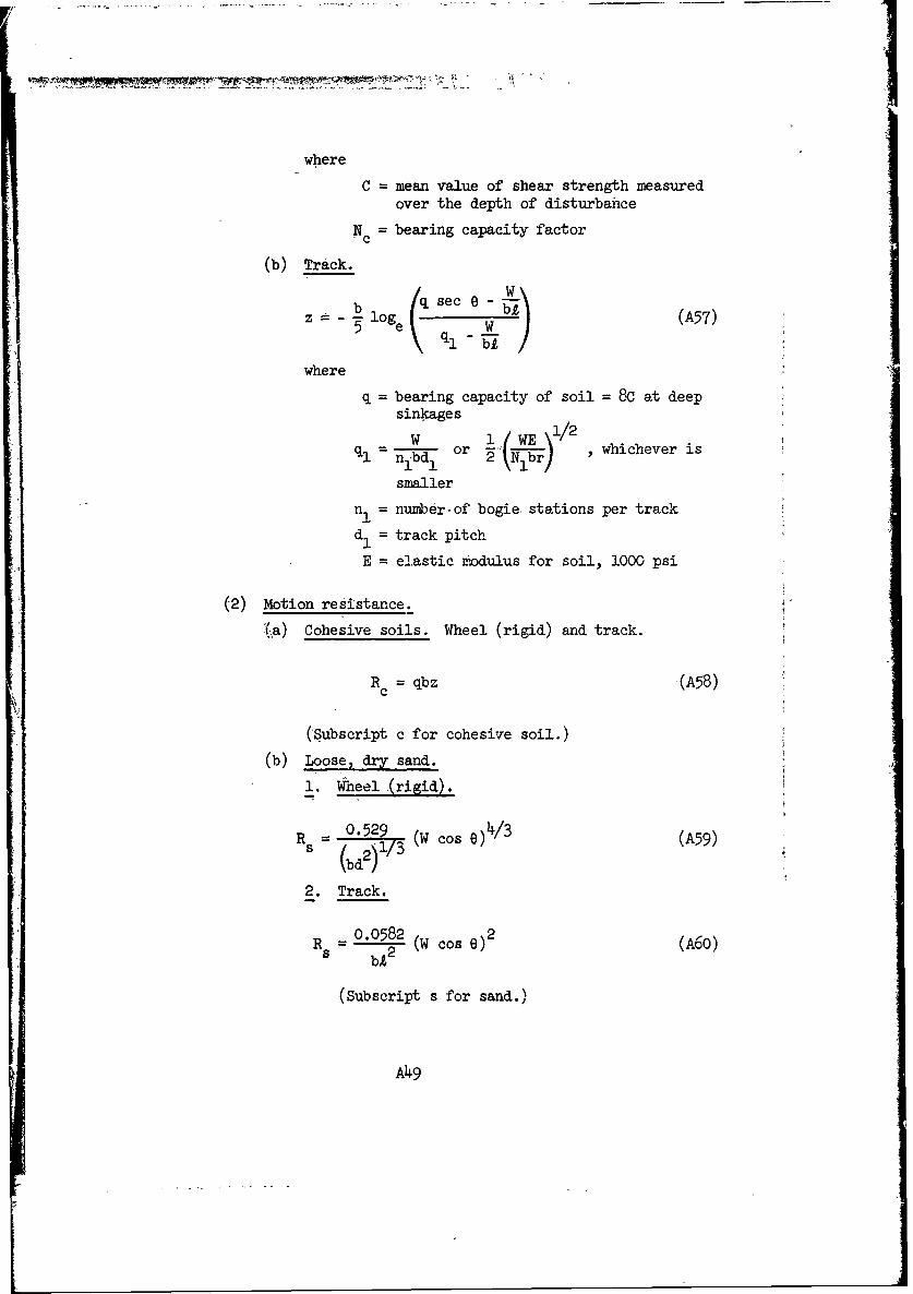
(3) Drawbar pull.

(a) Cohesive soils.

1. Wheel (rigid).

weCbd w - C and -=0.0077 (A61)'5-bd d

c

2. Track.

P = Ac - R (A62)

(b) Loose, dry sand.

i. Wheel (rigid).

P = W tan - R (A63)

2. Track.

P=Wtan 0"0582W2 (A64)b 2

(c) Firm, frictional slopes. Wheel (rigid) and track.

P = W tan (A65)

(4) Slope-climbing ability.

(a) Cohesive soils. Wheel (rigid) and track.

sin e = Ac - R (A66)• W

(b) Loose, dry sand.

1. Wheel (rigid).

tan e =[an e -0.529 (W Cos e )/](A67)t be2

A50

A]

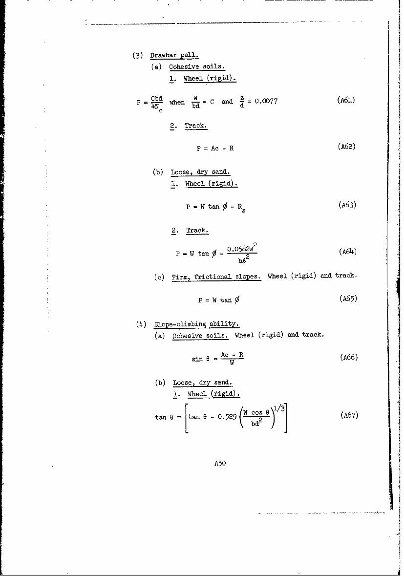
2. Trark.

tan 6 - [tan - 0.0582 (W '011 0)1(A)

(c) Firm, frictiona. slopes. Wheel (ri~id) and track's.

0 (A69)

A51

AJ*I-rN bLX 13: STJkA,., -c' il J( 0 E.,

introduction

Background

1. Of all terrain features, probably the least effort has been rk-

voted toward modeling vehicle performance in stream crossing. The reasz:.-:

for this are allied with the development of' amphibious vehicles, which

first made their appearance, in a military sense, during World War II. The

amphibious vehicles were originally intended to transport cargo and per-

sonnel from ship to shore, and early research efforts were devoted to in-

creasing water speed and cargo capacity. In the years following World

War III a new line of vehicles was developed, the DRAKE, LARC, and BARC.

This same period witnessed a quantum advance in off-road mobility, except

for the problem of stream crossings. For, while the performance of the

exotic amphibians in making the ship-to-shore transition was nothing short

of' spectacular, their stream-crossing capabilities left much to be desired.

The LLD began work on the stream-crossing problem in 1960 with the construc-

tion of a river simulator tank. The early work with this facility led to

the conclusion that the stream-crossing problem had not been adequately de-

fined. A program was initiated to evaluate the basic reasons for an am-

phibious vehicle's difficulty in negotiating streams, and field surveys

were made to develop basic river environment data. These studies indicated

that the primary cause of difficulty was the steep riverbank slopes and

they led to the development of two models for predicting performan..: in

stream exiting in go-no go terms.

2. Concurrently, through the MERS and MEGA programs WES was estab-

lishing a bank of basic stream data and conducting experiments with full-

size vehicles, which came to fruition with the development of empirical

relttions between maximum bank slope negotiable and soil strength.

Strategies available

3. The strategies available for predicting stream crossing all hinge

on the capability of the vehicle to negotiate the exit bank slope. The ap-

proaches have been either theoretical or empirical. The systems differ

131

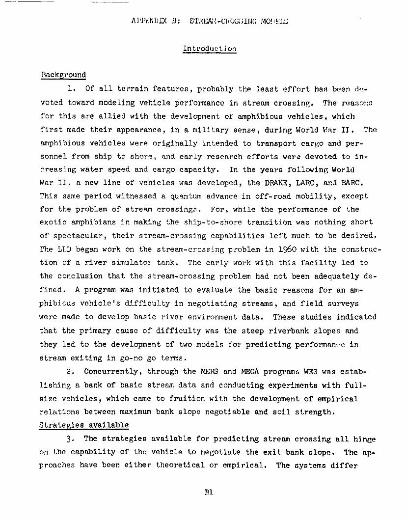
somewhat in the terrain and vehicle parameters used and in degree of so-

phistication. Fig. B1 graphically illustrates the main elements :of the

overall procedures. The terrain parameters used in each model and the

method of measurement are given in table B1; the vehicle parameters and

the vehicle types for which each model is applicable ar! also given in

table Bl. The vehicle performance output for each of the current models

is given in table B2, and the utilization of the current models and ap-

propriate references are also given.

The problem

4. The fundamental terrain conditions affecting the performance of a

vehicle attempting to cross a stream may be divided Into three general

categories--configuration, soil-conditions-, and Water -conditions--as-shown

in fig. B1. Any one of the three -may prevent passage of the vehicle, or,

I+ ICONFIGURATION SOIL WATER CONDITIONS

VEHICLE CHARACTERISTICS -

ITERRAIN-VEHICLE RELATIONS

TIHORETICAL EMIRICAL

FGO-NO GO

Fig. B. Flow chart illustrating possible strategiesfor coupling stream-crossing models

B2

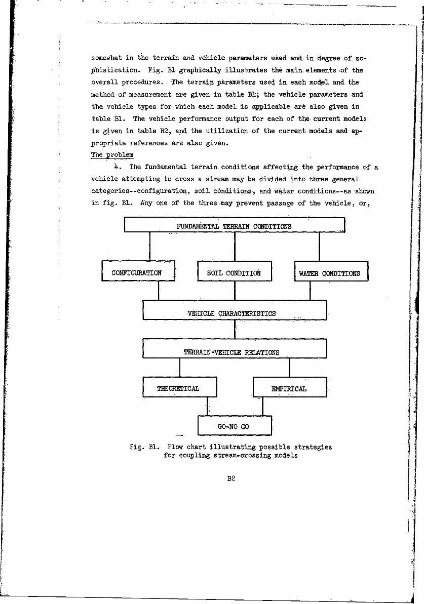
4'4 '

-H H1 H 0 0 0 1 -

9 4) .,04 .0 4 ( )1 Pr.g-I 44'rI d -

4) P4 -H H o 0 C30 0 ;q'

k' -H> H P $4. 0) -H C) *-i'd CHd4 qH 0d q-: 43 $.3 4; -4 C

% uqj 0 - ~ W 34 0' 0) 0 0 a 4 0 0 04as4

0H 0- r40 d r; I - -J:U i2 a qiP0 C 0AC) rI400 40 O0d w

02j ).i ~ 0 P 0 H9 0 ~ 002 04 :3, r. (D4 40

to $a4 - -1 P4 U00

4'

r.~ E-4

HP 0 4

a) rd 0 4 4' P 0' 04' 43 4,002 4) 2 :3 Id0

low ,-l 'd 0d5-i 44~ 0 0 v Ap r! P

02) EO P -I AlI r4I 0 Ar0 ad to 0 00 C) $i .a

4' to V2 $ 9i Pn P P0 0 P0 2 -iH H H 020 H- H

0 0 00 0 0P, 04'1 "4 *ri *ri ~ r

0 *14p$ 4 02H

4).~ ;3 , 44- 4 -S E-412 P P PrP.

00 0 0r0 0

Pq 0P.

,-4 4' -0 4 ' -' H ) 4 .

00 *,- tOr- r 0~ HO V-H wU 000 rr r4 02 bOdr bLH 0. t02'ri Q

0p. k 4S 0)P

0 4D' -

kr 4- ()44

02 $

4) 0 0'20

B3

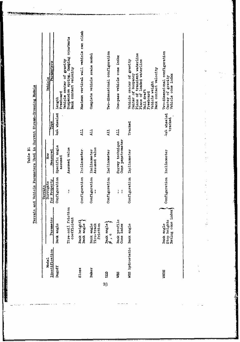
EO

a)

NH rAco $4 01

4.> a)

aY) H01 HA

-P ~0 (a 0) 00

0H

H- 4 0 C) (a 0 4'a1) 0(d to 4'1

04. 0 10

(a ) -A

0100 U-rI E019

ta -P' rd 0

45 0 00'Eri E-iE-

a) Ia)d I

C 4-) 4-1 4't'w 49>

CH.0

A 0 (

a) 4'a4( 4'F4'4

H 01 r4

a)(a) 044 :5 H0a 01 4

-P4 b'a 0 4-1-4d 0 Pia4 0 (mv

-H 0 4'9 HH 0 $3r.I4 01 a)q f+ a) j a

-P a) 44U- 0

Aa 01 a9a

~) H 60 W

4.1. k 4(a H r- '

8-0 0 CrI 4

4a HO ) p tjr a)0' (H 0 E 0 Pi> -- 14 aa b 0

a)* 4'ia0 0 N 0 ma "4aa) 0 .48'' 01 'd a)( *rH -- 04 *

0 r4- 0 0 w 0 *v. ;(4 0 A g, 0CHH4 P, 0O a a 10i P4 ri0 434 -

k0 4 0r 0r 0a ri -1 40

00r

0 4'rq 0co 0$' VI 014

4' 4'0

'd -v-4I C

+4 0

< . .

acting in concert, any combination may prevent passage. Moreover, when

acting individually, each category requires consideration of exclusive ve-

hicle parameters; hence it is apparent that a complete stream model must be

reasonably complex even to yield a simple go-no go answer. For example, if

the configuration of the streambank is such that the leading edge of the

vehicle strikes the face of the bank, the vehicle obviously cannot pass; if

the soil- permits excessive sinkage, the vehicle is immobilized, and if the

water depth exceeds fording depth (for nonamphibious vehicles) or if the

stream velocity exceeds the vehicle's water speed (for amphibians), the

stream is impassable. While the configuration of the stream may be ex-

pected to remain constant for : asonable periods of time, the water depth

and velocity-may be subject to rapid change in short periods of time as may

the soil conditions in certain soil types.

5. There are some redeeming factors, however. Streams that have ap-

preciable gradients lack soft soil banks and bottoms. And in areas where

the stream meanders, frequent "exit windows" may be found, which suggest

that reconnaissance .might change many a no go condition into a go con-

dition. In addition, some of the more recently developed vehicles have

positive erticulation, "inching capabilities," self-carried bridges,

underwater fording capabilities, and improved winching abilities for

self-recovery.

Description and Analysis of Stream-Crossing Models

Description

6. A complete model for predicting the stream-crossing capabilities

of ground vehicles is not available; however, various researchers have in-

vestigated various parts of the overall problem. The particular studies

reviewed are discussed in the following paragraphs and are identified ac-

cording to the researcher or agency. All the models discussed are egress

models.

7. Pgoff. This model determines the trajectory of an amphibious

vehicle making the transition from water to land. Equations are used to

account for the weight, buoyancy, auxiliary propulsion, wheel torque, and

B5

body-suspension interaction components. Two sets of equations represent

the tire-soil reaction at the bank. One set is based on the Bekker system

employing five soil parameters, and the other ,set is based- on the WES sys-

tem employing two soil parameters (neither set of equations has been pro-

grammed for use in the model at this time,)". Provision is made in the model

for the effects of auxiliary egress assistance (e.g. winches, rockets,

propellers, hydrojets, etc.).

8. At the present time, only a simplified version of the- model ihas,

been programmed for computer solution. The simplifications consist of a

restriction to nonyielding, purely frictional soil banks, and the assump-

tion that the vehicle body is a sealed rectangular parallelepiped. With

these simplifications, an egress trajectory of 10-sec duration required

about 4 hours computer time for the IBM 1130. Work is currently in pro-

gress to develop a more reasonable computer-to-real-time ratio.

9. The initial application of the model consisted of a study of a

4-wheeled, box-shaped vehicle in the approximate proportions of a 1

scale model of a lA-ton truck (jeep) egressing a uniform, rigid bank.

The following vehicle parameters were varied one value more and one value

less than the basic vehicle.

a. Vehicle length.

b. Freeboard.

c. Vertical center of gravity (CG).

d. Horizontal CG.

e. Suspension spring constants.

f. Suspension damping constants.

g. Initial velocity.

10. The bank-slope angle and the tire-bank coefficient of friction

were also varied within ranges so that:

Coefficient friction < tan e

Under this condition no vehicle, regardless of configuration or initial

velocity, could proceed indefinitely up the slope. Hence, for any set of

vehicle and bank parameters considered, the total distance traveled up

B6

the bank before stopping became an index of vehicle performance.

11. Using this performance index, the results of the computer runs

indicated the following minor changes in performance: (a) performance in-

creased with an increase in vehicle length, (b) performance decreased with

an increase in freeboard, and (c) performance increased with higher center

of gravity. Major effects on performance were as follows: (a) increase in

initial velocity increased performance, (b) increase in coefficient of

friction of bank incieased performance, and (c) increase in bank slope

angle decreased performance.

12. At the present time there is no verification for this model,, and

no serious attempt has been made to develop any empirical relations on the

basis of trajectory data. It is possible that this model may be of some

value to the vehicle designer, but it appears to require an exorbitant

amount of computer time in its early format, which admittedly is grossly

simplified. Nevertheless, it does represent a first small step toward the

ambitious goal of developing a general mathematical model describing the

egress maneuver, and the mere exercise of fabricating after-the-fact ex-

planations of the computer results has helped to define and establish

limits to'-the stream-crossing problem. If the results indicating minor

importance of some factors and major importance of other factors can be

confirmed with real vehicles in real stream egress tests, the way might be

shown toward a practical, realistic model based on only those factors of

significant value.

13. Sloss. This model estimates vehicle performance in exiting

streams by using a slope severity factor determined by reducing the bank

height by a trigonometric function of the bank slope angle. From examina-

tion of a number of cross-section profiles of riverbanks in the United

States, Sloss concluded that the bank configuration could be represented

by a series of slope angles and bank step heights, and that vehicle per-

formance could be qualitatively estimated by reducing the measured bank

height to account for the slope and comparing this computed value, termed

slope severity factor, to the height of vertical wall the vehicle can

climb. The functional static relation used to compute the slope severity

factor is

B7

-S = h -sin 2

where

S = slope severity factor

h = height of bank

= simple bank slope

Slope severity limits for the Mll-3 were qualitatively established as

follows:

Severity Factor Performance

0-2 Go, will negotiate all banks2-4 Marginal, will ne'gotiate some banks> 4 No go, will not negotiate any banks

14. In this model, the terrain and the vehicle inputs are grossly

oversimplified. The most important omission from terrain input is the

character of the bank. The prediction accuracy is as yet undetermined but

is probably low. The model is applicable only to tracked vehicles. The

go, marginalj and no go output has veiy limited uses.

15. Baker. Using a simple bank angle, , and a tire/track fric-

tion constant, f , Baker determi'.es the normal and tangential bank con-

tact forces as a function of bank angle and friction constant, and the dis-

tance traveled up the bank. The functional relations used are Archimedes'

Law, the general laws of static mechanics, and simple hydrostatic scaling.

16. The terrain inputs reflect the simplest possible geometry and

traction. The constant, f , used as a surrogate for true traction is not

really existent except on paved banks. The vehicle input is complete to

the extent that the scale model is complete. A scale model of any vehicle

is possible, and if the scale model is complete,, there can be neither

omissions nor assumptions of vehicle data.

17. The functional relations used are theoretical. Within the

limits tested, validation is 100 percent. At this time no further valida-

tion is needed as this is a simple matter of hydrostatics and static mo-

ment; by this same token, however, the static case may prove to be of

little value once the full dynamics are understood.

18. The principal limitations are the grossly oversimplified terrain

B8

input and the assumption that the vehicle always approaches the bank at

90 deg. The accuracy is limited to experimental accuracy only. The proce-

Adure is applicable to basically all vehicle types.

19. This procedure makes no specific vehicle performance predictions,

and is useful only as a part of a more complex model and only when scale

model results are available.

20. LLD. LLD's stream-exiting model grew out of the scale model

studies of amphibious vehicles by W. J. Baker, D. A. Sloss, and C. F.

Miranda. The fundamental philosophy was that any system of external forces

could' be reduced to one vertical force, one horizontal force, and a moment

acting at the center of gravity. The vertical downward force is gradually

transferred to the ground as the vehicle moves out of the water, and the

change in vertical ground reaction should then be equal to the change in

buoyancy between any two points. The horizontal force will directly affect

the motion of the vehicle and will act for or against the motion depending

on the direction of the net force and will occur only in the equation of

motion. The moment acting at the center of gravity of the vehicle will af-

fect the trim angle directly.

21., During egress the motion of the vehicle is assumed to be slow

(creeping) end all of the dynamic effects are ignored. Then the vertical

ground reaction, as a function of the distance traveled, can be related to

the vehicle parameters, the net vertical force, and the moment acting at

the center of gravity by the equations of statics. An equation of com-

patibility can be defined to relate the geometry of the ground to the num-

ber of wheels in contact to the trim angle. The equations are transcen-

dental in nature and are solved by trial and error. With the use of a

digital computer, values of the trim angle, , and values of the total

vertical reaction and reactions of each of the wheels are determined for

each incremental distance traveled. By iteration the resistance is com-

pared with the propelling forces to determine go or no go.

22. The vehicle input parameters assume an idealized box-shaped

vehicle.* The terrain input parameters reflect a simple bank angle and

* Wheels, axles, and obher appurtenances are considered as additional

boxes.

B9

an assumed angle of internal friction and cohesion for the soil.

23. The model yields a go-no go output, and in addition, the amount

of additional effort required in event a no go condition is indicated.

Nevertheless, there are some rather severe limitations inherent, especially

in any attempt to predict cross-country performance. Obtaining reliable

cohesion and angle of internal friction values for soil is LIffficult, per

se. Next, no provision is made for change in tire-soil friction under

traffic, and slip is excluded.

24. Nevertheless,, this model has considerable potential for develop-

ment. LLD plans to program the four LLD soil values, bank angle, and bank

length, and for any area use a statistical analysis based on random sam-

pling to generate a probability distribution curve. The evaluation of ve-

hicle performance would requfire a combination of the- environmental char-

acteristics that give rise to a no go condition. This wou'ldbe accom,

plished by repeated analysis for increasing bank angle until the no go con-

dition is reached. The combination of environmental factors giving rise to

a no go condition would then be compared with the probability distribution

curve to indicate the probability of a particular vehicle negotiating the

environmental1 conditions in the area.

25. Thus, it seems that the model shows promise for comparison of

vehicles, but only in a probablistic sense.

26. WES. This model relates bank slope negotiable to soil strength

in terms of the average cone index (CI) of the submerged portion of the

water-land interface. It was developed by empirical analysis of 40 water-

to-land transitions (or attempted transitions.) of three vehicles in the

United States and in Thailand. These tests were conducted as a part of the

WES MERS program. The terrain inputs are the simple bank angle, O , and

the average 0- to 6-in. CI for submerged banks. Vehicle input is VC11 , the

minimum soil strength required for a vehicle to complete one pass on a

level surface. The functional relations consist of curves relating maximum

slope negotiable to the average soil strength of the 0- to 6-in. soil layer

of that portion of the streambank that is submerged. If the bank angle is

greater than the maximum bank angle negotiable as shown by the curve, a

no go condition is indicated; if the bank angle is equal to or less than

BlO

J

the maximum slope negotiable shown -by the curve, a go condition is

indicated.

27. The use of the submerged soil strength implies the assumption

that the dry, i.e. above-waterline, portion of the bank is stronger than

the submerged portion--an assumption that can hardly be faulted. -The em-

pirical nature of the relation adequately accounts for all pertinent

vehicle parameters.

28. This model is considered to be adequately validated for three

vehicles: the M29C, the M113, and the XM561. Field tests are required to

establish the soil-slope or soil-drawbar pull curve for each vehicle of

interest, but there are indications that vehicles may be grouped into

classes, thus permitting a single curve for each class of vehicle.

29. The-procedures in using the model are very simple and it is well

adapted to field use. The prediction accuracy for the tests conducted to

date appears to be well within the limits of experimental error. The

growth potential for this model appears excellent. It may well turn out

that results from field tests with a few representative vehicles can be

extrapolated to represent all vehicles.

30. Another WES model uses equations for a simplified floating ve-

hicle to determine the maximum bank slope to which the vehicle will conform

as a result of vehicle momentum at the point of contact with the bank.

From the background of the WES water-land interface studies, Stinson con-

cluded that quite frequently the ability of an amphibious vehicle to nego-

tiate a streambank was dependent upon the assistance received from momentum

of the vehicle as it contacted the bank.

31. The terrain input is the simple bank angle, a . This implies

the assumptions of a hard bank, water depth such that the vehicle will

float until the bank slope is contacted by the vehicle, and no current.

The vehicle is assumed to have a rectangular receptacle shape that may be

described in the following terms:

Center of gravityCenter of buoyancy

Plane 6f transient waterlinePlane of loaded waterlineHull draft

Bll

FreeboardVehicle weightBank contact velocityLocation of center of front bogiewheel

The functional relations used are simplified dynamics allowing two degrees

of freedom. The graphical output presents the relation of pitch angle and

effective vehicle weight, the kinetic energy available at time of contact

with the bank, and the maximum bank angle the vehicle will conform to as .

result of kinetic energy.

32. The terrain input is grossly oversimplified; the vehicle shape

is admittedly simplified, but not to an unreasonable extent. However, the

assistance that the vehicle might receive from its water-propulsion ele-

ments is ignored. The functional relations are theoretically sound and di-

mensionally adequate within the limits considered, although there has been

no validation. Indeed, the model needs expanding before any validation is

attempted. The introduction of wave effects and a yielding soil might

change the general results.

33. The procedures involved in using this model are quite complex

and it is not, at this time, quitable for field use. The principal limi-

tations are the terrain oversimplification, the two-dimensional behavior,

and the omission of traction and water-propulsion assistance forces. The

prediction accuracy, as yet undetermined, is probably low. The development

of this model is static at this time.

34. WNRE. The WNPZ model treats bank egress as an obstacle problem

with soil strength constraints and possible buoyancy effects on vehicle at-

titude and net ground loading. Lower and upper slope angles with respec-

tive step heights define the bank profile. Soil strength is considered in

terms of rating cone index (RCI).

35. Essenttally, the go-no go criteria presuppose only two basic

independent reasons for immobilizations: geometric interference or lack

of adequate traction, usually due to soil shear limitation.

36. The potential for geometric interference is examined by geo-

metrically matching the parametrically described obstacle and vehicle (inside elevation only). Both the vehicle and the obstacle are assumed to be

B12

rigid in this encounter, and the bank is assumed to be defined by straight

lines with sharp, angular corners.

37. Calculation of bank-climbing ability is based upon a static

frictional model of a grossly simplified rigid vehicle on a rigid obstacle.

The vehicle is considered to approach this type of obstacle at right angles

only.

38. For most purposes,, all vehicles are treated as 4x's by making

appropriate adjustments to the center of gravity location and rear axle

treatment. For example, to determine whether a tracked vehicle could make

the initial start up an obstacle face, it is considered to be a 4x having

a like weight distribution relative to the ground contact length. However,

in testing its final negotiation of the obstacle, the 4x rear axle climb-

ing criterion is replaced by a test that treats vehicle attitude as the

moment the vertical-projection of its center of gravity crosses the upper

edge of the bank.

39. The equations used to estimate net traction- are given below:

D/W = COH/NUGP + TNP - RES

where

D = net available traction, lb

W = gross vehicle weight, lb

COH = apparent soil cohesion, psi

NUGP - ncminal unit ground pressure, psi

For wheeled vehicles:

wNJGP =

nb

where n = No. of tiresb = tire section width, in.d = tire outside diameter, in.

For tracked vehicles:

UGP = W

B13

where b = track width, in.= total length of track on

the ground (all tracks,both sides), in.

TNP = tangent of soil apparent angle of

internal frictionIS = 0.3 (VCl/RC) 3

For wheeled vehicles:

VCI = 3 + 3 X NUGP

For tracked vehicles:

VCI = 6 + 3 x NUGP

40. This model has been programmed for computer solution. An added

feature of the computer program is a printout of the reason for failure if

a no go prediction is made. An outline of the test sequence of the model

is given in fig. B2.

41. Because the bank egress, problem is intrinsically so severe, one

intermediate level of failure is calculated (test Y) that is intended con-

ceptually to indicate a conditional go when a reasonable degree (arbitrar-

ily set at 50 percent of gross vehicle weight) of winch or towing assis-

tance is utilized. Test Z was made the final test with the same assistance

potential implicit in case of failure.

42. The model has been used to predict performance of three military

vehicles across the streams occurring in -a small (18 x 27 km) area of

Thailand that had been previously mapped for mobility purposes as a part of

the MERS program. No validation has been attempted.

43. The growth potential of this model appears limited. The proce-

dures are too complex for field use, and the oversimplification of terrain

and vehicle input are not consistent with computer use. The procedures

used for estimating net traction are not well validated. The recent de-

velopment by WES of a VCI for one pass has superseded the former VCI as

used in this model.

Analysis of egress models

44. From tables BI and B2 it can be seen that the current

B14

TEST SHtAI(AND FAILURE: DIAGNOSTIC BASIC TERRAIt MEANING WHEN FAILURE SCHEtIATIC

CODE COMPARISON FACTORS EXAMINED (CODE),IS' INDICATED REPRESENTATION

R ater depth vs.-vehicle X 0 a e depth exceeds vehl e

fording ability (non- fording-capability.swimming vehic les only).o

oae

S Upper bank, step vs. X X vehicle running gear cannotvehicem floating ma ke ueful contact with,atti tude ,(switeming, the ban

T asic soel1 strength X X X I asic soil strength isVS. VCI-; iadequae for smpe operato

on smooth level ground (with ow tho.t buoyancy effects. as

appropriate).

U Lower bank geomer X X Lower bank,presents either a "-

vs. vehtl "ofiguration vertical obstacle beyond basicvehicle capability, or there Ott /is angle of approach

interference.

V Lower.bank configuration X X X * Traction required to surmount -

vsa net vehicle traction. lower bank exceeds soil- o .

Simit(d traction availablety.(inioding buoyancy effects

where present).

Upper bank geoetr vs. X - X Upperhlnk presents either a

1vehicla cofigation . m sflcnatwt

vehcle on vertical obstacle beyondbasicvehicle capability or -there.is, angle of approach _

interference.

X Upper bank configuration X X X _X Traction required to surmount . )vs. net vehicle traction. upper bank exceeds soil6

limited traction available(including buoyancy effects 0 :. _where present).

Y Upper bank configuration X x X X Deficit in required tractionvs. net traction, lig is more than 50 of gross60. GVW outside tWhrIt vehicle weight.assist.

z Upper bank configuration - X X Vehicle bellies on ditch edge

vs. vehicle belly (side elevation only -- no

clearance, test for normal trackedvehicles).

Fig. B2., Go-no go test sequence for str~eam crossing

B15

stream-crossing models share some similarity, yet have some significant

differences.. Both are discussed in the following paragraphs.

45. Terrain input. The terrain parameters used in the models, as

shown in table Bl, are quite similar, ranging from a simple bank angle to

a cohplete profile with soil strength measurements. Simplest is the WES's

hydrostatic model which uses only the bank angle and iicludes no soil con-

sideration. The dynamic trajectory model of Dugoff and the scale model

studies of Baker also use the bank angle as a surrogate for the configura-

tion of the streambank and assume a tire/soil and tire/track friction co-

efficient, respectively. The modified Baker model developed by LLD inputs

the bank angle of friction and soil cohesion. Sloss's slope severity

factor ignores the problem of yielding soil but considers the bank height

in addition to the bank angle. The WES model considers the cross-section

profile of the stream and uses the 0- to 6-in. average CI to account for

both traction and yieldifg soil. The WNRE model considers a break in the

bank slope to yield upper and lower approach angles and uses the RI with

some semiempirical equations to account for traction. For all models the

bank angle, bank height, or profile (as the case may be) is easily measured

without elaborate instrumentation. As regards the soil parameters, all ex-

cept the CI are somewhat difficult to secure.

46. Vehicle parameters. The vehicle parameters used in the current

models kas shown in table B2) range from WES's simple two-dimensional scale

model for obstacle interference to complete scale models (Baker) and even

complete vehicles (WES).

47. It may be noted that the Dugoff and WES hydrostatic models use

somewhat similar vehicle parameters, considering that Dugoff's dynamic tra-

jectory is limited to 4x4 wheeled vehicles and the WES's hydrostatic model

applies only to tracked vehicles. Baker's scale-model programs are of ]course applicable to any vehicle for which a complete sicale model is con-

structed; LLD's modification is applicable only to wheeled vehicles at this

time. The WNRE two-dimensional configuration is applicable to 4x4 wheeled

vehicles and single-unit tracked vehicles. The empirical models of Sloss

and WES apply to all vehicles.

48. Vehicle performance output. The vehicle performance outputs of

B16

J

the current stream-crossing models are listed in table B2. The outputs of

the Dugoff, WES hydrostatic, and Baker and LLD models are useful only as a

part of a more complex model and are not of themselves a meaningful pre-

diction of vehicle performance in stream egress. The output of Sloss's

slope-severity factor model in terms of go, no go, and marginal is indeed a

prediction of stream egress, but marginal is hardly acceptable. The WES

model and the LLD modification of Baker yield a straightforward go-no go

output that is a meaningful prediction and poses ho interface problems.

The added reason for no go as output from the WNRE go is a valuable aid in

cross-country predictions.

49. Utilization. From table B2 it can be seen that only three of

the stream-egress models have been used. Sloss's model was used to esti-

mate M113 performance at a total of 197 sites in the United States; how-

ever, no actual test results were available to evaluate the estimates.

This model was also used to estimate performance of three vehicles on four

bank slopes in Panama for which test results were available, and some in-

consistencies appeared in the evaluation. The WNRE model was used to esti-

mate performance in one small sector in Thailand; however, no actual test

results were available for comparison with the predictions. The WES model

was developed from 40 tests with real full-size vehicles.

Summary

50. Each of the stream-egress models has some disadvantages. The

Dugoff and WES hydrostatic models do not consider yielding soil, are re-

stricted to certain types of vehicles, do not of themselves yield a mean-

ingful prediction, and have no validation; thus these models are considered

as currently unacceptable. The Bekker and LLD scale-model programs can be

applied to any vehicle for which a complete scale model is available. Un-

fortunately, the results of scale-model tests pose difficult interface

problems, especially when soil is a factor; and frequently a large number

of tests with full-size vehicles are required before the scale-model test

results can be effectively used. LLD modification of the Baker equations

is interesting, but is lacking in validation. Sloss's slope severity

B17

iI

factor has no provision for soil characteristics and at best yields an in-

complete result. The WNRE model lacks validation, and relies upon equa-

tions using a VCI for 50 passes developed by WES that has been superseded

by a recently developed VCI for one pass. The WES model considers all

pertinent vehicle factoi's, and the CI has been repeatedly shown to °serve

as an adequate surrogate for soil characteristics important to mobility.

Admittedly, the empirical approach does require extensive testing with

full-size vehicles, but the answers are real answers in a real-world sit-

uation. It is judged that the WES model in its present form has perhaps

the greatest ability for field application.

B18

, 1- -N I

F:SUPPLEMENTARY~VL.

LI,-

- - - -. 1.777§17z tr

i.I

I

pp INFORMATION

'4?,-;

'\ \

I! DEPARTMENT OF THE ARMYWATERWAYS EXPERIMENT STATION. CORPS OF ENGINEERS

Id P. O. BOX 631

VICKSBURG. MISSISSIPPI 39180

I" RIPLY R1.F..o WESAR 27 July 1972

Errata Sheet

AlI ANALYSIS OF ',GROTJND MOBILITY MODELS (ANAMOB)

Technical Report M-71-4

July 1971

1. Please replace pages A8, A12, A24, and A26 with the revised pages A8,

A12, A24, and A26 attached hereto.

I

Table A2

Mobility Index Eauation for Self-Propelled Wheeled

(All-Wheel Drive) Vehicles (Equation A3)

contactontact weightMobil- |pressure xw h

ity | ffactor clearance engine trans-

inde* fire grouser fato atr middionffactor factor or fac factor

where L

Contact pressure factor = gross weight, lb

ii outside diamnom tire of tire, in. x No. of pwidth, in. 2 tires

Weight Factor

Weight Range, lb** EquationstWeight <2000 Y - 0.553X

factor: 2000 to 13,500 Y = 0.033X + 1.05013,501 to 20,000 Y = 0.142X - 0.420

>20,000 Y = 0.278X - 3.115

Tirefacor: 10 + tire width, in.100

Grouser factor: With chains = 1.05Without chains = 1.00

Wheel load factor: gross weight, KpsNo. of axles x 2

Clearance factor: clearance, in.

10

Engine factor: 10 hp/ton = 1.00<10 hp/ton - 1.05

Transmission factor: Automatic = 1.00; manual = 1.05

* The MI obtained is converted to VCI from the curves shown in fig. Al.

** Gross weight lbNo. of axles

=weightfactr , = gross weight, kipsNo. of axles

! A8 (revised)

'I

... ._ ___ _ __ ___ __ 1

0.8

i 0.6

• g Tracked Vehicles with Ground Contact Pressure I_ Psi

D/W =6.4554 + 0.0392 RCIx

A -(0.4554 + 0.0392 RCIx)E - 0.0526 RCI,

0 Tracked Vehicles with Ground Contact Pressure < 4 psi

H 1W D/w = 0.544 + o.o63 RCIx - /(0.544 + 0.0463 RCI )y - ,.0702 RCIx

Io c I II0 20 40 60 80 100

it Rating Cone Index - Points Above Vehicle Cone Index (RCIx

0°

.6

. Wheeled Vehicles with Ground Contact Pressure < 4 psi

/D/W = 0.3885 + 0.0265 RCIx

Z -. 3885 + 0.0265 RCIx)2 -0.0358 RCI x

Wheeled Vehicles with Ground Contact Pressuife > 4 p~si

ED/W = 0.379 + 0.021!? RCI x - J(0.379 + 0.0219 RCIx)z -0.0257 R~

0.0 x0 20 06080 1000 60

Rating Cone Index - Points Above Vehicle Cone Index (RCIx )

Fig. A4. First-pass net maximum drawbar pull, maximum slope negotiable-soil strength relations for tracked andwheeled vehicles operating onfine-grained soils

A12 (revised)

1.6o

0 . .20-o.8 1.31p2 -0.95

S0.8o -

,4 42 -

o 2; .4t 0

U .4

0 5 10 15 20 25

Clay Mobility Numeric

(RCI)bd xW- h 1+ bj

a. Pull coefficient vs clay mobility numeric from field data

S o.50

0 Note:

0.30 ___ -''I)bd( (i)o0.20 "Y-0" P /W= o.o4o + rTI a - 1.35

0.20

®0.10

0 5 10 15' 20 25Clay Mobility Numeric

(RCIbd x x

b. Towed force coefficient vs clay mobility numeric from field data

Fig. A8. Relations of performance coefficients for first passof single wheel to clay mobility numeri

!', A24 (revised)

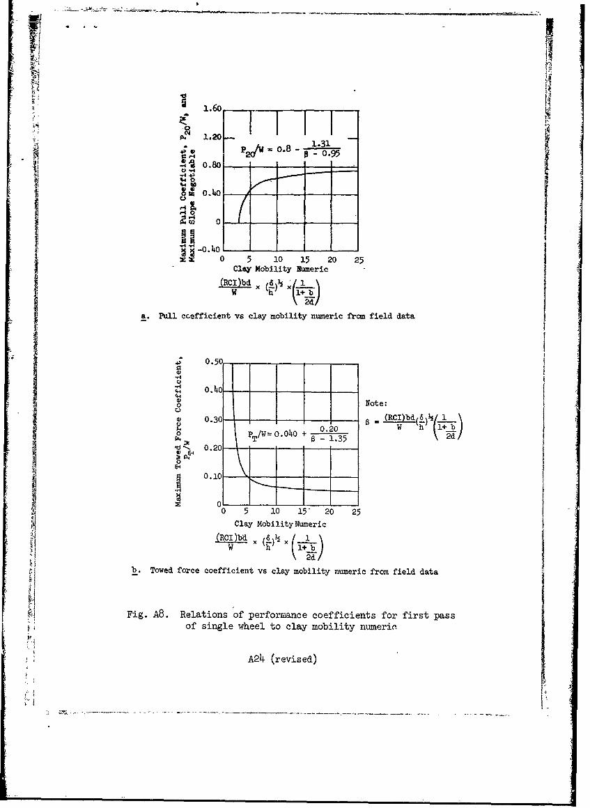
4

I\!

o .

0HfA I_ \

0.2- o --

" P T

yC"

0 I oo.i 0.1 0.2 o..3 o. 4.,, 0 .5

iClay Mobility Numeric,~~(RCI)bd

,, Fig. Ag. Relation of pull, slope, raid towed force coefficients to

/"I

__WE-S -u~i for clay

A K

H