AD-A286 731 - DTIC
493
i% AD-A286 731 PROCEEDINGS SECOND INTERNATIONAL CONGRESS ON RECENT DEVELOPMENTS IN AIR- AND STRUCTURE-BORNE SOUND AND VIBRATION MARCH 4-6, 1992 AUBURN UNIVERSITY, USA 95-01104 DTIIC 1111111 FB 281995 l l i ted by Malcolm J. Crocker P. K. Raju -.... " #[~T~UTION STA AEN Appoved for public rel 3t, , Volume 2
-
Upload
khangminh22 -
Category
Documents
-
view
4 -
download
0
Transcript of AD-A286 731 - DTIC
i%
AD-A286 731 PROCEEDINGS
SECOND INTERNATIONAL CONGRESS ONRECENT DEVELOPMENTS IN AIR- AND
STRUCTURE-BORNE SOUND AND VIBRATIONMARCH 4-6, 1992 AUBURN UNIVERSITY, USA
95-01104 DTIIC1111111 FB 281995
l l i ted by
Malcolm J. CrockerP. K. Raju -.... "
#[~T~UTION STA AEN
Appoved for public rel
3t, , Volume 2

PROCEEDINGS
DTICS•~ ~ ELECTEil
SECOND INTERNATIONAL CONGRESS ONRECENT DEVELOPMENTS IN AIR- AND
STRUCTURE-BORNE SOUND AND VIBRATIONMARCH 4-6, 1992 AUBURN UNIVERSITY, USA
PAIRAccesion For
NTIS CRA&IDTIC TABUnannounced
Edited by JustificationMooim J. rocr .......
P. K. Raju Distribution IAvailability Codes
Dist Avail and/orSpecial
THIBUIfON.STAf•,M A Volume 2
Approved for public release;
Distribution Unlimited j

Copyrigt @ 1992 Mchanica F~wrinueig Dqmutment, Auburn Universiy, A1, USAPrint in the United State of AmericaCover dinig by Malcolm J. Crocb and Wafy Ridgway
Clopin myw be medered fromIntenatonal Sound & Vilstin Congim wdtorsMoeW wem* Dw~nt202 RosHal
tbd permbon is obained from Ibauthos) and c*&udti given to the author(s) and thes ProcedinNoticatohn to the Editors o( thmg Procedng at Aubmn Univrsty a ago requir An author or hit
Nmarhomor, my rqtodii hit pqr in KI credtng thm procedow thit pemim ano~ t mtmpgal&e

SECOND INTERNATIONAL CONGRESSON RECENT DEVELOPMENTS IN
AIR- & STRUCTURE-BORNE
SOUND AND VIBRATION
MARCH 4-6, 1992
Auburn University
USA
Sponsored by AUBURN UNIVERSITY in cooperation with
THE INTERNATIONAL COMMISSION ON ACOUSTICS OF JUPAP
and with the following professional societies:
ACOUSTICAL SOCIETY OF AMERICA
ACOUSTICAL SOCIETY OF THE NETHERLANDS
ACOUSTICAL SOCIETY OF THE RUSSIAN FEDERATION
AMERICAN HELICOPTER SOCIETY
AMERICAN SOCIETY OF MECHANICAL ENGINEERSASSOCIATION BELGE DES ACOUSTICIENS
ASSOCIAZIONE ITALIANA dl ACUSTICA
AUSTRALIAN ACOUSTICAL SOCIETYTHE CANADIAN SOCIETY FOR MECHANICAL ENGINEERING
DEUTSCHE ARBEITSGEMEINSCHAFT FOR AKUSTIK (DAGA)
INSTITUTE OF ACOUSTICS, UNITED KINGDOM
INSTITUTE OF NOISE CONTROL ENGINEERING/JAPAN
INSTITUTE OF NOISE CONTROL ENGINEERING/USA
INSTITUTION FOR MECHANICAL ENGINEERS, UNITED KINGDOM
THE AMERICAN SOCIETY FOR NONDESTRUCTIVE TESTING, INC.
VEREIN DEUTSCHER INGENIRURE (VDI-EDV), GERMANY
THE SOUTH AFRICAN ACOUSTICS INSTITUTE
SOCIATI& FRAN(eAISE D'ACOUSTIQUE
SOVIET ACOUSTICAL ASSOCIATIONACOUSTICAL COMMISSION OF THE HUNGARIAN
ACADEMY OF SCIENCES
General Chairman-Malcolm J. Crocker, Mechanical Engineering Dqpartment
Program Chairman-P. K. Raju, Mhaikc Engineeing Dqmrtnmnt
liii tim , =•J QUALITy "'.t4[

scientific committeeAdnan Akay, Wayne State University, MichiganMichael Bockhoff, Centre Techniques Des Industries Mecaniques, FranceBrian L. Clarkson, University College of Swansea, United KingdomJ. E. Ffowcs-Williams, University of Cambridge, United KingdomRobert Hickling, National Center for Physical Acoustics, Mississippi
G. Krishnappa, National Research Council of CanadaLeonid M. Lyamsev Andreev Acoustics Institute, MoscowRichard H. Lyon, Massachusetts Institute of Technology, MassachusettsGideon Maidanik, David Taylor Research Center, MarylandM. L. Munjal, Indian Institute of Science, India
Alan Powell, University of Houston, TenClemans A. Powell, NASA Langley Research Center, VirginiaJ. N. Reddy, Virginia Polytechnic Institute & State University, VirginiaHerbert Oberall, Catholic University of America, D.C.
Eric Unger, Bolt Beranek and Newman, Massachusetts
V. V. Varadan, Pennsylvania State University, PennsylvaniaR. G. White, Institute of Sound and Vibration Research, United Kingdom
Organizing CommitteeJohn E. Cochran, Auburn University (Aerospace Engineering)Robert D. Collier, Tufts University (Mechanical Engineering)Malcolm J. Crocker, Auburn University (Mechanical Engineering)Malcolm A. Cutchins, Auburn University (Aerospace Engineering)Ken Hsueb, Ford Motor Co., Allen Park, Michigan
Gopal Mathur, McDonnell Douglas, Long Beach, CaliforniaM. G. Prasad, Stevens Institute of Technology (Mechanical Engineering)P. K. Raju, Auburn University (Mechanical Engineering)Mohan Rao, Michigan Technological University (Mechanical Engineering)Uday Shirahatti, Old Dominion University (Mechanical Engineering)
Financial SupportFinancial support for these international congresses has
been provided by:
National Science Foundation
Offic of Naval ResearchOfi.. of Naval Reearch-EuropeAlabama Space Grant Consortium
National Aeronautics and Spame Administration
College of Engineering (Auburn University)Departmnt of Mechanical Engineering (Auburn University)
iv

FOREWORD
This three-volume book of proceedings includes the written versions of thepapers presented at the Second International Congress on Recent Developmentsin Air- and Structure-Borne Sound and Vibration held at Auburn UniversityMarch 4-6, 1992. The Congress was sponsored by Auburn University in cooperationwith the International Commission on Acoustics of IUPAP and the 20 professionalsocieties in 14 countries listed at the beginning of each volume. The support ofthis Commission and the professional societies has been invaluable in ensuringa truly international congress with participation from 30 countries. This supportis gratefully acknowledged. In addition, the organizing committee would like tothank the National Science Foundation, the Office of Naval Research, the Officeof Naval Research-Europe, the Alabama Space Grant Consortium, NASA, theCollege of Engineering and the Department of Mechanical Engineering of AuburnUniversity for financial maistance.
Topics covered in the Proceedings include Sound Intensity, Structural Intensity,Modal Analysis and Synthesis, Statistical Energy Analysis and Energy Methods,Passive and Active Damping, Boundary Element Methods, Diagnostics and Con-dition Monitoring, Material Characterization and Non-Destructive Evaluation,Active Noise and Vibration Control, Sound Radiation and Scattering, and FiniteElement Analysis.
The order in which the 217 papers appear in these volumes is roughly thesame as they were presented at the Congress although the order is modifiedsomewhat so they can be grouped in the topics above. There are aso six keynotepapers, including Professor Sir James Lighthill on Aeroacoustics and AtmosphericSound, Professor Frank J. Fahy on Engineering Applications of Vibro-AcousticReciprocity;, Dr. Louis Dragonette on Underwater Acoustic Scattering, ProfessorRobert E. Green on Overview of Acoustical Technology for Non-DestructiveEvaluation, Professor David Brown on Future Trends in Modal Testing Technologyand Professor Lothar Gaul on Calculation and Measurement of Structure-borneSound. The papers in this book cover all major topics of interest to those concernedwith engineering acoustics and vibration problems in machines, aircraft, spacecraft,other vehicles and buildings.
In the last 30 years, improvements in computers have allowed rapid developmentsin both theoretical and experimental analysis of acoustics and vibration problems.In the early 1960s statistical energy analysis (SEA) was first applied to coupledsound and vibration problems. In the early 1970s the finite element method (FEM)was first used in acoustics problems. In recent years considerable progress hasbeen made with the boundary element method (BEM) in which discretization isconfined to two-dimensional surfaces instead of three-dimensional fields. Someof these approaches have been combined for instance in SEA-FEM. The 1980s,which have also seen rapid advances in improved measurement techniques, couldbe called the decade of sound intensity, as it can now be used for rapid meas-urements of the in-situ sound power of a machine, to rank noise sources anddetermine transmiion loss of structural partitions. Power flow in structures alsonow can be determined with the use of structural intensity measurements. Sound
v

and vibration signals are being used increasingly to diagnose the condition ofmachinery and to detect faults or to determine the properties of materials throughnon-destructive evaluation. There is also increased knowledge in sound radiationand scattering;, in particular advances have occurred in scattering theory and innumerical solution techniques.
The organization and hosting of a conference is a considerable undertaking,and this Congress is no different. We would firstly like to thank all the authorswho submitted their contributions promptly making publication of this bookbefore the Congress possible. We would also like to acknowledge the assistanceof the scientific committee and organizing committee who helped to completelyorganize some sessions. The staff of the Mechanical Engineering Department ofAuburn University also provided valuable assistance. Our special thanks areextended to Roew-Marne Zuk who worked untiringly and efficiently on all aspectsof the Congress program and this book, to Julia Shvetz who provided invaluIbleexpert assistance in all areas of Congress planning in particular with travelarrangements for foreign guests, and to Olga Riabova for her hard work onCongress communications.
Malcolm J. Crocker, General ChairmanP.K. Raju, Program Chairman
vi

TABLE OF CONTENTS
Page
FOREWORD . .v....... ......... ..... ooo.......... ..o ....... oDISTINGUIED LCURE SERIES ......................................... 1
]KEYNOTE ADDRESS ..................................................... 3A GENERAL INTRODUCTION TO AEROACOUSTICS ANDATMOSPHERIC SOUND .................................. ....................... 5
Sir James Lighthlll, University Colleg London, United Kingdom
AEROACOUSTICS ........................................................ 35
VORTEX SOUND INTERACTION .................................................. 37Ann Dowling, University of Cambridge, United Kingdom
NUMERICAL PREDICTIONS IN ACOUSTICS ......................................... 51Jay C. Hardin, NASA Langley Research Center, Virna
THE BROADBAND NOISE GENERATED BY VERY HIGH TEMPERATURE,HIGH VELOCITY EXHAUSTS .................. ............................... .59
SA. Mclnemy, California State University, California
FLOW-INDUCED NOISE AND VIBRATION OF CONFINED JETS ........................ 67Kamn W. Ng, Office of Naval Research, Virginia
STRUCTURAL-ACOUSTIC COUPLING IN AIRCRAFTFUSELAGE STRUCTURES ........................................................ 81
Gopal P. Mathur and Myles A. Simpson, Douglas Aircraft Company, California
RESPONSE VARIABILITY OBSERVED IN A REVERBERANT ACOUSTIC TEST OFA MODEL AEROSPACE STRUCTURE .............................................. 89
Robert E Powell, Cambridge Collaborative Inc, Massachusetts
RESPONSE OF LAUNCH PAD STRUCTURES TO RANDOM ACOUSTICEXCITATION ................................................................... 97
Ravi Margasahayam and Valentin Sepcenko, Boeing Aerospace Operations, Inc.Raoul Caimi, NASA Engineering Development, Florida
SONIC BOOM MINIMIZATION: MYTH OR REALITY ................................ 105Kenneth J. Plotkin, Wyle Laboratories, Virginia
CONTROL OF SUPERSONIC THROUGHFLOW TURBOMACHINES DISCRETEFREQUENCY NOISE GENERATION BY AERODYNAMIC DETUNING ................... 113
Sanford Fleter, Purdue University, Indiana
COMPARISON OF RADIATED NOISE FROM SHROUDED AND UNSHROUDEDPROPELLERS ................................................................... 121
Walter Eversman, University of Mmouri-Roila, Mimouri
vii

NOISE AND VIBRATION ANALYSIS IN PROPELLER AIRCRAFT BYADVANCED EXPERIMENTAL MODELING TECHNIQUES ............................. 129
Herman Van der Auwcrmer and Dirk Otte. LMS International, Belgium
AERODYNAMIC NOISE GENERATED BY CASCADED AIRFOILS ....................... 137Gerald C Lauchle and Lori Ann Perry, The Pennsylvania State University, Pennsylvatni
VIBRATION ISOLATION OF AVIATION POWER PLANTS TAKING INTO ACCOUNTREAL DYNAMIC CHARACTERISTICS OF ENGINE AND AIRCRAFT .................... 143
VS. Baklanov and V.M. Vul, AN. Tupolev Aviation Scienceand Technical Complex, Moscow, Russia
PASSIVE DAMPING ...................................................... 149
ANALYSIS OF CONSTRAINED-LAYER DAMPING OF FLEXURAL AND EXTENSIONALWAVES IN INFINITE, FLUID-LOADED PLATES ...................................... 151
Pieter S. Dubbelday, Naval Research Laboratory, Florida
EFFECT OF PARTIAL COVERAGE ON THE EFFECTIVENESS OF A CONSTRAINEDLAYER DAMPER ON A PLATE ................................................... 157
M.R. Garrison, R.N. Miles, J.Q. Sun, and W. Bao,State University of New York, New York
REDUCTION OF NOISE AT STEEL SHELLS WORKING BY USINGVIBRODAMPING COVERS OF MULTIPLE USE ...................................... 165
Victor F. Asminin, Sergey L Chotelev, and Yury P. Chepulsky,Voronezhsky Lesotechnichesky Institute, Russia
SIMULTANEOUS DESIGN OF ACTIVE VIBRATION CONTROLAND PASSIVE VISCOELASTIC DAMPING ........................................... 169
Michele LD. Gaudreault, Ronald L Bagley, and Brad S. Liebst,Air Force Institute of Technology, Ohio
A SUBRESONANT METHOD FOR MEASURING MATERIAL DAMPING IN LOWFREQUENCY UNIAXIAL VIBRATION .............................................. 177
George A. Lesieutre and Kiran M. Govindswamy,The Pennsylvania State University, Pennsylvania
PASSIVE DAMPING TECHNOLOGY ............................................. 181Eric M. Austin and Conor D. Johnson, CSA Engineering. Inc., California
RECENT APPLICATION OF THE PASSIVE DAMPING TECHNOLOGY ................... 189Ahid D. Nashif, Anatrol Corporation, California
MATERIAL AND STRUCTURAL DYNAMIC PROPERTIES OF WOOD ANDWOOD COMPOSITE PROFESSIONAL BASEBALL BATS ............................... 197
Robert D. Collier, Tufts University, Massachusetts
THE DAMPING EFFICIENCY OF METAL AND COMPOSITE PANELS ................... 205Richard M. Weyer, The Pennsylvania State University, PennsylvaniaRichard P. Szwerc, David Taylor Research Center, Maryland
viii

DAMAGE INDUCED DAMPING CHARACTR]STI(CS OF GLASS REINFORCEDEPOXY COMPOSITES ............................................................ 217
Max A. Gibbs and Mohan D. Rao, Michigan Technological Univernity, MichiganAnne B. Doucet, Louisiana State University, Louisiana
ON THE FLEXURAL DAMPING OF TWO MAGNESIUM ALLOYS AND A MAGNESIUMALLOYS AND A MAGNESIUM METAL-MATRIX COMPOSITE .......................... 223
Graeme G. Wren, Royal Australian Air Force, AustraliaVlkram K. Kinra, Texas A&M University, Tera
DAMPING IN AEROSPACE COMPOSITE MATERIALS ................................ 237A. Agneni, L Balis Crema, and A. Casteilani, University of Romse, Itsly
TRANSVERSE VIBRATION AND DAMPING ANALYSIS OFDOUBLE-STRAP JOINTS ......................................................... 249
Mohan D. Rao and Shulin He, Michigan Technological University, Michigan
DAMPED ADVANCED COMPOSITE PARTS ......................................... 257David John Barrett, Naval Air Development Center, PennsylvaniaChristopher A. Rotz, Brigham Young University, Utah
DAMPING OF LAMINATED COMPOSITE BEAMS wrrH MULTIPLEVISCOELASTIC LAYERS ......................................................... 265
Shuin He and Mohan D. Rao, Michigan Technological University, Michigan
FUNDAMENTAL STUDY ON DEVELOPMENT OF HIGH-DAMPINGS UCTURAL CABLE ........................................................... 271
Hiroki Yamaguchi and Rajesh Adhikari, Asian Institute of Technology, Thailand
VISCOUS DAMPING OF LAYERED BEAMS WITH MIXEDBOUNDARY CONDITIONS ....................................................... 279
Eugene T. Cottle, ASD/YZEE, Ohio
PASSIVE DAMPING APPLIED TO AIRCRAFT WING SKIN ............................. 287Vincent L Levraea, Jr. and Lynn C. Rogers, Wright-Patterson AFB, Ohio
MEASUREMENT OF DAMPING OF CONCRETE BEAMS:PASSIVE CONTROL OF PROPERTIES .............................................. 295
Richard Kohoutek, University of Wollongong, Australia
ACTIVE CONTROL AND DAMPING ........................................ 303
EXPERIMENTS ON THE ACTIVE CONTROL OF TRANSITIONALBOUNDARY LAYERS ............................................................ 305
P.A. Nelson, J.-L Rioual, and MJ. Fsher, Institute of Sound andVibration Research, United Kingdom
RECENT ADVANCES IN ACTIVE NOISE CONTROL .................................. 313D. Guicking University of (dttingen, Germany
STOCHASTIC ACTIVE NOISE CONTROL ......................................... 321AJ. Efron and D. Graupe, University of Illinois at Onicago, Illinois
lx

ACTIVE NOISE CONTROL WITH INDOOR POSITIONING SYSTEM ..................... 329Kenji Fukumizu, HKroo Kitagawa, and Masahidc Yoneyama, RICOH Co, Ltd., Japan
A NEW TECHNIQUE FOR THE ACTIVE CANCELLATION OF WIDE-BAND NOISEUSING MULTIPLE SENSORS ...................................................... 337
Felix Rosenthal, Naval Research Laboratory, Washington, D.C.
A GENERAL MULTI-CHANNEL FILTERED LMS ALGORITHMFOR 3-D ACTIVE NOISE CONTROL SYSTEMS ....................................... 345
Sen M. Kuo and Brian M. Finn, Northern Ilinois University, Ilinois
TIME AND FREQUENCY DOMAIN X-BLOCK LMS ALGORITHMS FORSINGLE CHANNEL ACTIVE NOISE CONTROL ....................................... 353
Qun Shen, Active Noise and Vibration Technologies, ArizonaAndrew Spanias, Arizona State University, Arizona
ENERGY BASED CONTROL OF THE SOUND FIELD IN ENCLOSURES .................. 361Scott D. S6mmerfeldt and Peter J. Nasif, The Pennsylvania State University, Pennsylvania
A PID CONTROLLER FOR FLEXIBLE SYSTEMS ..................................... 369A- Subbarao, University of Wismosin - Parkbide, WisconsinN.G. Creamer, Swales and Associates, Inc., MarylandM. Levenson, Naval Research Laboratory, Washington, D.C.
NUMERICAL SIMULATION OF ACTIVE STRUCTURAL-ACOUSTIC CONTROLFOR A FLUID-LOADED SPHERICAL SHELL ........................................ 377
C.E. Ruckman and C.R. Fuller, Virginia Polytechnic Institute and State University, Virginia
OPTIMUM LOCATION AND CONFIGURATION OF AN INTRA-STRUCTURAL FORCEACTUATOR FOR MODAL CONTROL .............................................. 387
Jeffrey S. Turcotte, Steven G. Webb, and Daniel J. Stech,U.S. Air Force Academy, Colorado
DEVELOPMENT OF AN ACTIVE VIBRATION CONTROLLERFOR AN ELASTIC STRUCTURE ................................................... 395
Douglas R. Browning and Raymond S. Medaugh, AT&T Bell Laboratoris, New Jersey
ACTIVE VIBRATION CONTROL OF FLEXIBLE STRUCTURESUSING THE SENUATOR .......................................................... 405
Shin Joon, Hahn Chang-Su, and Oh Jae-Eung, Hanyang Univernity, KoreaKim Do-Weon, Samsung Electronics, Korea
STRUCTURAL VIBRATION .............................................. 411
RADIAL IMPULSIVE EXCITATION OF FLUID-FILLED ELASTICCYLINDRICAL SHELLS ........................................................ 413
C.R. Fuller and B. Br6vart, Virginia Polytechnic Institute and State University, Virginia
ROTOR DYNAMIC IMPACT DAMPER TEST RESULTS FOR SYNCHRONOUS ANDSUBSYNCHRONOUS VIBRATION .................................................. 425
Tim A. Nale and Steven A. Kluman, Gneral Motors Corporation, Indiana
x

VIBRATION DESIGN OF SHAKERS LABORATORY OF THE NEW HONG KONGUNIVERSITY OF SCIENCE AND TECHNOLOGY ..................................... 435
Westwood K.W. Hong and Nicholas J. Boulter, Arup Acoustics, Hong Kong
KEYNOTE ADDRESS ..................................................... 443PROGRESS IN BOUNDARY ELEMENT CALCULATION ANDOPTOELECTRONIC MEASUREMENT OF STRUCTUREBORNE SOUND .................. 445
Lothar Gaul and Martin Schanz, University of the Federal Armed Forces Hamburg, GermanyMichael Plenge, JAFO Technology, Germany
SOUND-SMTUCITURE INTERACTION AND TRANSMISSION OFSOUND AND VIBRATION ................................................. 459
PLATE CHARACTERISTIC FUNCTIONS TO STUDYSOUND TRANSMISSION LOSS THROUGH PANELS .................................. 461
R.B. Bhat and G. Mundkur, Concordia University, Montreal, Canada
SOUND TRANSMISSION LOSS OF WALLBOARD PARTITIONS ......................... 469Junichi Yashimura, Kobayasi Institute of Physical Research, Japan
SOUND TRANSMISSION ANALYSIS BY COMPUTATIONAL MECHANICSUSING CHARACTERi! 1C IMPEDANCE DERIVED THROUGH A FINITEELEMENTAL PROCEDURE ....................................................... 477
Toru Otsuru, Oita University, Japan
NEW METHOD FOR CALCULATION AND DESIGN NOISEISOLATING ENCLOSURES ....................................................... 485
Ludmila Ph. Drozdova, Institute of Mechanics, Russia
EXPERIMENTAL RESEARCHES OF AIR- AND STRUCTURE-BORNE SOUND OFAGRICULTURAL MACHINES AND TRACTORS .................................... 493
Moissei A. Trakhtenbroit, VISKHOM Acoustic Laboratory, Russia
TIME DOMAIN APPROACH OF FLUID STRUCTURE INTERACTION PHENOMENAAPPUCATION TO SATELLITE STRUCrURES ...................................... 499
D. Vaucher de la Croix and C. Clerc, MEIRAVIB R.D.S., FranceJ.M. Parot, IMDYS, France
ACOUSTICS OF SHELLS WITH INTERNAL STRUCIRAL LOADING ................... 507Y.P. Guo, Massachusetts Institute of Technology, Massachusetts
LOW-FREQUENCY SOUND RADIATION AND INSULATION OF LIGHT PARTITIONSFILLING OPENINGS IN MASSIVE WALLS ........................................... 515
Roman Y. Vinokur, Lasko Metal Products, Inc., Pennsylvania
THE TRANSMISSION OF VIBRATION WAVES THROUGHSTRUCTURAL JUNCTIONS ....................................................... 523
Yan Tao, Defence Science and Technology Organization, Australia
THE SPATIAL-FREQUENCY CHARACTERISTICS OFSOUND INSULATION OF LAMINATED SHELLS .................................... 533
G.M- AviAova, N.N. Andreev Acoustics Institute, Russia
Al

STATISTICAL ENERGY ANALYSIS AND ENERGY M EOODS .................. 539
MODELING AND ESTIMATING THE ENERGETICS OF COMPLEXSTRUCTURAL SYSTEMS ......................................................... 541
G. Maidanik and J. Dickey, David Taylor Research Center, Maryland
AN ASSESSMENT OF THE MICROGRAVrTY AND ACOUSTIC ENVIRONMENTSIN SPACE STATION FREEDOM USING VAPEPS ..................................... 543
Thomas F. Bergen and Terry D. Scharton, Jet Propulsion Laboratory, CaliforniaGloria A. Badilla, SYSCON Corporation, California
APPLICATION OF VAPEPS TO A NON-STATIONARY PROBLEM ....................... 551LK. St-Cyr and J.T. Chon, Rockwell International, California
DEVELOPMENT OF ENERGY METHODS APPLIED FOR CALCULATIONS OFVIBRATIONS OF ENGINEERING STRUCTURES ..................................... 555
Sergei V. Budrin and Alexei S. Nikiforov, Krylov Shipbuilding Research Institute, Russia
THE STATISTICAL ENERGY ANALYSIS OF A CYLINDRICAL STRUCTURE .............. 561M. Blakemore and RJ.M. Myers, Topexpress Limited, United KingdomI. Woodhouse, University of Cambridge, United Kingdom
PREDICTION OF TRACKED VEHICLE NOISE USING SEA ANDFINITE ELEMENTS .............................................................. 569
David C. Rennison and Paul G. Bremner, Vibro-Acoustic Sciences Limited, Australia
MEASUREMENT OF ENERGY FLOW ALONG PIPES .................................. 577C.A.F. de Jong and J.W. Verheij, TNO Institute of Applied Physics, The Netherlands
COMPARISON OF MODE- £0-MODE POWER FLOW APPROXIMATION WVIHGLOBAL SOLUTION FOR STEPPED BEAMS ........................................ 585
Wu Ounli, Nanyang Technololical University, Singapore
RECIPROCITY METHOD FOR QUANTIFICATION OF AIRBORNE SOUND TRANSFERFROM MACHINERY ............................................................. 591
Jan W. Verheij, TNO Institute of Applied Physics, The Netherlands
VIBRATIONAL RESPONSE OF COUPLED COMPOSITE BEAMS ........................ 599C. Nataraj, Villanova University, PennsylvaniaP.K. Raju, Auburn University, Alabama
KEYNOTE ADDRESS ..................................................... 609THE RECIPROCITY PRINCIPLE AND APPLICATIONS IN VIBRO-ACOUSTICS ............. 611
FJ. Faby, Institute of Sound and Vibration, United Kingdom
GENERAL SOUND AND VIBRATION PROBLEM ............................. 619
FLOW-INDUCED VIBRATION PROBLEMS IN THE 01, GAS AND POWERGENERATION INDUSTRIES - IDENTIFICATION AND DIAGNOSIS ...................... 621
M.P. Norton, University of Western Australia, Western Australia
)di

IMPEDANCE OF A VISCOUS FLUID LAYER BET WEEN TWO PLATE T........... 633Michael A. Latcha, Oakland University, MichiganAdnian Akay, Wayne State University, Michigan
VIBRATION SUPPRESSION IN THE BUILDING FLOORS BY THE SYSTEMSWITH OXIDE-MAGNETS ....................................................... 641
Vilien P. Khomenko, Research Institute of Building Structures, UkraineLeonid N. Tulcbinsky, Institute for Material Science Problems of AS of the Ukraine, Ukraine
RECIPROCAL DETERMINATION OF VOLUME VELOCITY OF A SOURCEIN AN ENrALOSURE........................................................... 645
Bong-Ki Kim, Jin-Yeon Kim, and Jeong-Guon Ib. Korea Advanced Instituteof Science A Technolog, Korea
ANALYSIS OF FORCED ACOUSTIC FIELDS INSIDE STRUCTURALLYCOUPLED CAVITIES .......................................................... 651
Anzu Gdneng and Mehmet (;alilkan, Middle East Technical University, Turkey
THEORETICAL AND EXPERIMENTAL ASPECTS OF ACOUSTIC MODELING OFENGINE EXHAUST SYSTEMS WITH APPLICATIONS TO A VACUUM PUMP................659
B.S. Sridhara, Middle Tennessee State University, TennesseeMalcolm J. Crocker, Auburn University, Alabama
RUSSIAN CHURCH BELL ...................................................... 667Boris N. Njunin and Alexander S. Larucow, Moscow Automobile Plant (ZIL) Russia
A COMPARISON OF MEMBRANE, VACUUM, AND FLUID LOADED SPHERICALSHELL MODELS WITH EXACT RESULTS ........................ 675
Clean E. Dean, Stennis Space Center, Mississippi
EXPERIMENTAL STUDIES OF WAVE PROPAGATION IN A SUBMERGED, CAPPEDCYLINDRICAL SHELL ......................................................... 683
Earl G. Williams, Naval Research Laboratory, Washington, D.C.
SOUND ABSORBING DUCTS .................................................... 689Alan Cummings, University of Hull, United Kingdom
DUCT ACOUSTICS: JUNCTIONS AND LATrICES,APPLICATION TO PERFORATED TUBE MUFFLERS.................................. 697
Jean Kergomard, Laboratoire d'acoustique de l'Universit6 du Maine, France
EFFECTIVENESS OF IMPROVED METHOD AND TECHNIQUES FOR HVA DUCTSOUND ANALYSIS AND PREDICTION ............................................ 703
Michihito Terao, Kanagawa University, Japan
FLOW DUCT SILENCER PERFORMANCE .......................................... 711J.L- Bento Coelho, CAPS-Instituto Superior T~cnico, Portugal
MATRICES FOR PIPING ELEMENTS WITH FLOW.................................... 717K.K. Botros, NOVA HUSKY Research Corporation, Calgary, Canada
RESONANT FREQUENCIES OF THE LONG PIPES.................................... 725LN. Kijachko, LL Novikov, and IL~L Ustelencev, Noise and Vibration Control Laboratory, Russia
xii

GENERIC BUCKLING ANALYSIS OF ORTHOTROPIC PLATES WITH CLAMPED ANDSIMPLY SUPPORTED EDGES ...................................................... 729
S.D. Yu and W.L. Cleghorn, University of Toronto, Canada
SOUND AND VIBRATION CEASUREMENI r ................................. 737
A FREQUENCY DOMAIN IDENTIFICATION SCHEME FOR DAMPED DISTRIBUTEDPARAMETER SYSTEMS .......................................................... 739
R. Caander, Aerostructures, Inc., VirginiaM. Meqyap McDonnell Douglas Helicopter Co., ArizonaS. Hanagud, Georgia Institute of Technology Georgia
ELASTIC BEHAVIOR OF MIXED Ui-Zn AND Li-Cd FERRITES ........................... 745D. Ravinder, Osmania University, India
OBSERVATION OF ELASTIC WAVE LOCALIZATION ................................. 753Ling Ye, Geor Cody, Minyao Zhou, and Ping Sheng,Exxn Research & Engineering Co., New JerseyAndrew Norris, Rutgers University, New Jersey
FREE FIELD MEASUREMENT AT HIGH FREQUENCIES OF THEIMPEDANCE OF POROUS LAYERS ................................................ 759
Jean F. Allard and Denis Lafare Universitd du Maine, France
EVALUATION OF A DYNAMIC MECHANICAL APPARATUS ........................... 763Gilbert F. Lee, Naval Surface Warfare Center, Maryland
DETERMINING THE AMPLITUDE OF PROPAGATINO WAVES AS A FUNCTION OFPHASE SPEED AND ARRIVAL TIME ............................................... 771
J. Adin Mann III, Iowa State University, IowaEarl 0. WViliams, Naval Research Laboratory, Washington, D.C.
ISOLATING BUILDINGS FROM VIBRATION ......................................... 779David E. Newland, University of Cambridge, United Kingdom
LINEAR DYNAMIC BEHAVIOR OF VISCOUS COMPRESSIBLE FLUID LAYERS:APPLICATION OF A COMPLEX SQUEEZE NUMBER .................................. 787
T. Onsay, Michigan State University, Michigan
FUZZY COMPREHENSIVE EVALUATION OF SHOCK INTENSITY OFWARSHIP PROPULSIVE SYSTEM .................................................. 795
Pang Jian, Wuhan Ship Development and Design Institute, ChinaShen Rongying JiAo Tong University, China
ON THE EVALUATION OF NOISE OF THE CAM TYPE MECHANISMS .................. 803AJ. Chistiakov and N.L Suhanov, S.M. Kirov Institute of Teatile and light Industry, Russia
MULTIFUNCTIONAL CEILINGS ................................................... 807TJ. Galaktonova, Central Research and Design Institute of School Buildings, Russia
PHASE FEATURES OF MAN AND ANIMALS REACTION TO INFRASOUND EFFECT ....... 811BJ. Fraiman, Voronezh Electroiic Plaint, VoroaezhAS. Fauwv, Voronezh Medical Institute, VosonezhAN. Ivanniov and V.L Pavlov, Moscow State University, Russia
xdv

MEASURING OF THE TURBULENCE AND SOUND ABOVE THlE OC E AN......... 815AN. Ivannikov, SV Makeev, and V.I. Pavlov, Moince State University, Rumsi
COMPARISON TESTIS BETWEEN ACOUSTIC EMKISSION TRANSDUCERSFOR INDUSTRIAL APPLICATIONS ......................... 821
S.C Kerkyras.. PA Drakatos and YLI Tzanetos, University of Patras GreeceWILD. Borthwick CEC Brite DirectorateRIL. Reuben, Heriot-Wait University, United Kingdm
USING A CIRCUM[FERENTIIAL TRANSDUCER TO MEASURE INTERNALPRESSURES WITHIN A PIPE .................................................... 829
R.J. Pitinington and A. Briscoe, University of Southampton, England
CONDITION OF OLD MACHINES IN THE LIGHT OFVARIOUS VIBRATION STANDARDS .............................................. 8937
RLI. Murry, Regional Engineering College, India
PHOTOACOUSTIC METHOD OF THE DETER]MINATION OF AMPLITUDENON-RECIPROCALNESS IN GYROTROPIC MEDIA................................... 845
G.S. Mfityanich, V.P. Zelyony, V.V. Sviriova, and AN. Serdyukcw,Gomel State University, The Republic of Byekxwus
"A SOLUTION TO THE NOISE PREDICTION PROBLEM AT LOW FREQUENCIES ............ 847Yurii L. BobrovnitsKii lagonravov Institute of Enjgineering Research, Russia
"A PARALLEL PATH DIFFERENCE ON-LINE MODELLING ALGORITHM FORACTIVE NOISE CANCELLATION ................................................. 8951
Yong Yan and Sen K. Lao, Northern flinois University, Mlinosa
STUDIES OF THE BUILDING CONSTRUCTIONS BY MEANS OFNONLINEAR DIAGNOSTICS.....................................................8959
A.E. Ekirnov, I.I Kolodieva, and P1I Korotin, Academy of Sciences of the USSR, Russia
MEASUREMENT OF ACOUSTIC POWER OF FANS UNDER CONDITIONS OFREVERBERANT NOISE OF AERODYNAMI1C TEST RIG................................ 863
V3M Kazarov, V.G. Karadga. and A.S. Minakov,Central Aerohydrodynamics Institute (TSAGI), Russia
STATISTICS OF REVERBERANT TRANSFER FUNCTIONS ............................. 869Milki Tohyama and Tsunehlko Koike, NTT Human Interface Laboratories, JapanRichard I. Lyon. Massachusetts Institute of Technolog, Massachusetts
KEYNOTE ADDRESS ...................................................... 877OVERVIEW OF ACOUSTICAL TEJCHNOLOGY FOR NONDESTRUCTIVE EVALUATION .... 879
Robert E. Green, Jr., The Johns Hopkins University, Metyland
MATERIAL CHARACrERIZATION AND NON-DENTRUCTIWE EVALUA71ON .... 887
ANALYTICAL DETERM[INATION OF DYNAMIC STRESS ON PRACTICAL CEMENT]MILLS USING RANDOM VIBRATION CONCEPT ..................................... 889
V. Ramnazurti, University of Toledo, OhioC. Sujatha, Indian Institute of Technolog, India
xv

EVALUATION OF ACOUSTIC EMISSION SOURCE LOCATION FOR DIFFEENTTHREE-SENSOR ARRAY CONFIGURATIONS ..................... 897
Vmishbt Venkatesh and JR.. Houghton, Tennessee Technoloigical University, Tennessee
DEFECT'S DETECTION IN STRUCTURES AND CONSTRUCTI[ONS BY NOISESIGNALS DIAGNOSTIC'S METHODS............................................... 905
Vadim A. Robumman, Union *Electronics of Russia,* Riusia
TOOL FAILURE DETECTION USING VIBRATION DATA .............................. 909T.N. Moore, Queen a University, Knington, CanadaL. Pci, Stelco, Hamilton, Canada
PHOTOACOUSTIC METHOD APPLICATION QUALITY CONTROL OFULTRACLEAN WATER......................................................... 917
Alekse K. Brodnikovskii and Vladimi A. Sivolvk, Institute of Electronic Machinery. Russia
ULTRASONIC MEASUREMENTS ................................................. 919Vinay Drayi Iowa State University, Iowa
EVALUATION OF LAMINATED COMPOSITE STUCTURES USINGULTRASONIC ATrENUATION MEASUREMENT ..................................... 927
Peitao Shen and 3. Richard Houghton, Tennessee Technological University, Tennessee
EXPERT SYSTEM FOR ULTRASONIC FLAW DETECTOR.............................. 935A.N. Agarwal, S.C. Sun,ý and M.S. Bageshwar, Central Scientific Instrumenrts Orgnization. India
BOUNDARY EMEbORM AND FINME ELEMEOi'S............... ............... 943
RECENT APPLICATIONS OF BOUNDARY ELEMENT MODELING IN ACOUSTIC'S...........945A.F. Seybert, T.W. Wu., and G.C. Wan, University of Kentucky, Kentucky
NUMERICAL MODELING OF PERFORATED REACTIVE MUFFLERS..................... 957S.H Jia, A.R. Mohanty, and AF. Seybert, University of Kentucky, Kentucky
ON SELECI'1NG CHIEF POINTS TO OVERCOME THE NONUNIQUENESS PROBLEMIN BOUNDARY ELEMENT METHODS............................................. 965
Peter K. Juhl, Technical University of Denmark, Denmark
IMPLEMENTATION OF BOUNDARY ELEMENT METHOD FOR SOLVING ACOUSTICPROBLEMS ON A MASSIVELY PARALLEL MACHINE................................. 973
A. Dubey, K. Zubair, and U.S. Shirahatti, Old Dominion University, Virginia
SOUND RADIATION OF HEAVY-WOADED COMPLEX VIBRATORY STRUCTURESUSING BOUNDARY INTEGRAL EQUATION METHOD.............................. 3
Michael V. Bernblit, St. Petersburg Ocean Technologly University, Rusms
OBTAINING OF UNIQUE SOLUTI1ON OF A SOUND RADIATION AND SCATTERINGPROBLEM USING A BEM BASED OF THE HELMHOLTZ'S INTEGRAL.................... 969
LB. 'Tsukernikow, Scientific and Industry Amalgmation 'MIE Russia
ISOPARAMETRIC BOUNDARY ELEMENT MODELING OF ACOUSTICAL CRACKS .......... 993T.W. Wu and G.C. Wan, University of Kentucky, Kentucky
xvi

A SOLUTION METHOD FOR ACOUSTIC BOUNDARY ELEMENT EGENPROBLEMWITH SOUND ABSORPTION USING LANCZOS ALGORITHM .......................... I001
C. Rajakumar and Ashraf AS, Swanson Analysis Systems, Inc., Pennsylvani
THEORETICAL AND PRACTICAL CONSTRAINTS ON THE IMPLEMENTATION OFACTIVE ACOUSTIC BOUNDARY ELEMENTS ........................................ 1011
P. Darlington and 0GC. Nicholson, University of Salford, United Kingdom
BOUNDARY ELEMENT FORMULATIONS FOR ACOUSTIC SENSITIVITIES WITHRESPECF TO STRUCTURAL DESIGN VARIABLES AND ACOUSTIC IMPEDANCE ......... 1019
N•icolas Vlahopoulos, Automated Analysis Corporation, Mchi• n
MODELLING RADIATION FROM SUBMERGED STRUCTURES: A COMPARISONOF BOUNDARY ELEMENT AND FINITE ELEMENT TECHNIQUES ...................... 1027
Jean-Piere o. Coyette, Numerical Intration Techologiet, N.V, Begium
FINITE ELEMENT MODELING OF VISCOELASTIC DAMPERS ......................... 1037A. Gupta, MJ. Kim, and AR Marchertas, Northern Illinois University, Illinois
THE METHOD OF MODAL PARAMETERS TO DETERMINE THE BOUNDARYCONDITION OF FINITE ELEMENT MODEL ......................................... 1045
Wang Fengqua and Chen Shiyu, Southeast University, China
VIBRATION AND EIGENVALUE ANALYSIS USING FiNITE ELEMENTS .................. 1053Tirupathi R. Chandrupatla, OMI Engineering and Management Institute, MichiganAshok D. Belegundu, The Pennsylvania State University, Pennsylvania
DYNAMIC ANALYSIS OF PRACTICAL BLADED DISKS USING FEM AND CYCLICSYMMETRY TECHNIQUES ........................................................ 1061
AS. Panwalkar and A Rajamani, Bharat Heavy Electricals limited, IndiaV. Ramamurti, Indian Institute of Technology, India
KEYNOTB ADDRESS ..................................................... 1073UNDERWATER ACOUSTIC SCATTERING ........................................... 1075
Louis R. Dragonette, Naval Researh Laboratory, Washington, D.C.
SOUND PROPAGATION, RADIATION AND SCATTIERING ...................... 1085
SOUND BACKSCATrERING FROM OCEAN BOTTOM ................................ 1087Anatoly N. Ivakin, N. N. Andreev Acoustics Institute, Rumia
LABORATORY SIMULATION OF POINT MONOPOLE AND POINT DIPOLESOUND SOURCES ............................................................... 1093
K. KI Ahuja, Georgia Institute of Technoloy, Georgia
RECONSTRUCTION OF SURFACE ACOUSTIC FIELD FROM MEASUREMENTSOF PRESSURE OVER A LIMITED SURFACE ......................................... 1103
AnVe Sarkiessin, Charles F. Gumond, Ead 0. Williams, and Brien K Hoiston,Naval Research Laborato•y, Washington, D.C.
SCATTERING OF SOUND BY STRONG TURBULENCE AND CONDITIONSOF CHERENKOV RADIATION .................................................... 1111
Vadim L Pavov and Oleg A. Kharin Moscow State University, Russia
xvil

RECOGNITION OF UNDERWATER TARGETS BY MEANS OF RESONANCESIN THEIR SONAR ECHOES ....................................................... 1117
Guillmnmao C. Gaummud, Naval Suface Warfam. CednIteMrylandHam C. Sta^, National Defnme Rsarh Establkhment, Sweden
HmGH-FREQUENCY ELASTIC WAVES EXCITED w HNu THE STRUCTUREOF A SPHERICAL SHELL BY INCIDENT SOUND IN WATER .......................... 1125
Robert -ickling and Jlam F. Ban, University of Mhlsii Micssippi
ELEMENTS, EIGENFUNCrIONS AND INTEGRAL EQUATIONS INFLUID-STRUCIURE INTERACTION PROBLEM ..................................... 1133
Richard P. Shaw, S.U.N.Y. at Buffalo, New York
FAR-FIELD RADIATION FROM A LINE-DRIVEN FLUID-LWADED INFINITEFIAT PLATE WITH ATTACHED RIB STIFFENERS HAVING ADJUSTABLEATFACHMENT LOCATIONS ...................................................... 1141
Benjamin A. Cray, Naval Underwater Systems Center, Conneciu
THE EFFICIENCY OF LAYERED HOUSING WITH ARBITRARY SHAPE ................. 1149Samual A. Rybak, N. N. Andrew Acoustmi Institute, Russia
SOUND RADIATION BY STRUCTuRE WITH DISCONTINUITIES ...................... 1151P.L Koroti and A.V. Lebedev, Academy of Sciences of the USSR, Russia
A NEW APPROACH TO THE ANALYSIS OF SOUND RADIATION FROMFORCED VIBRATING STRUCTURES ............................................... 1157
TM. Tomilina, Bkgorao Institute of FEgeering Research, Russia
THE ASYMPTOTIC METHOD FOR PREDICrING ACOUSTIC RADIATION FROMA CYLINDRICAL SHELL OF FINITE LENGTH ....................................... 1163
A. V. Lebedev, Aculemy of Sciences of the USSR, Rumia
STRUCTURAL RESPONSE AND RADIATION OF FLUID-LOADED STRUCTURESDUE TO POINT-LOADS ........................................................... 1171
Chafic N. Hammoud and Per G. Reinhall, Universty of Washington, Wmanton
ACOUSTICAL IMAGES OF SCATrERmO MECHANISMIS FROMA CYLINDRICAL SHELL ......................................................... 1179
Chartes F. Gamood and Angm Sa'kiciaut, Naval Reeac Labortory Wash~t~on, D.C.
CALCULATION OF SOUND RADIATION FROM COMPLEX STRUCTURESUSING THE MULTIPOLE RADIATOR SYNTHESIS WITH OPTIMIZEDSOURCE LOCATIONS ............................................................ 1187
Martin Ochmann, Teclniscbe Fschhochschule Berlin, Gm
RADIATION AND SCATIERING AT OBLIQUE INCIDENCE FROMSUBMlERGED OBLONG ELASTIC BODIES .......................................... 1195
Herbert Oberall and X. L Ba%, Catbolic Univemity of America, Wahingtom, D.C.Rume D. Miller, NIKF Engineuin VirginiaMichae F. Waby, Stnmn Space Center, Mlissspp
RAY REPRESENTATIONS OF THE BACKSCATrERING OF TONE BURSTSBY SHELLS IN WATER. CALCULATIONS AND RELATED EXPERIMEN73 .............. 1203
Phiqp L Mastao, Lgung Z•,ng Nafha Sun, Org Kadudk and David IL HugmhWamhingtm State University, Wahnmgton
xvmi

VIBRATIONS, SOUND RADIATION AND SCATTERING BY SHELLSWrif ARBITRARY SHAPE ............................ 1211
Vadim V. Muzycenk, N. N. Andree Acoustuo Institute, Ruska
SOUND RADIATION AND PROPAGATION IN CENTRIFUGAL MACHINE PIPIN G ..... 1219Danielius Guzhas, Vilnius Technical University, Lkthani
SOUND RADIATION DY A SUBMERGED CYLINDRICAL SHELLCONTAINING INHOMOGENETTIES...............................................i122
Alehaander Klamuon and Joa Meisaveer, Talina Technical Univessity, Estonia
SPACE TIME ANALYSIS OF SOUND RADIATION AND SCATTERING .................... 1235C. Cler and D. Vaucher de Is Cmuiz METRAVIB LD.S., France
VIBRATIONAL AND ACOUSTIC RESPONSE OF A RIBBED INFINITE PLATEEXCITED BY A FORCE APPLIED TO THE RIB............................. 1243
Ten-Bin Juan& Anus L Pate, and Ahon B. Flatau, Ioma State University, Iowa
ANALYTICAL AND EXPERIMENTAL DETERMINATION OF TIE VIBRATIONAND PRESSURE RADIATION FROM A SUBM[ERGED. STIFFENED CYLINDRICALSHELL WrM TWO END PMATME ................................................ 1253
A. Harart and BME Sandman, Nava Undersea Warfare Center Divamo Rhode hilndJ-A. Zaldoak Westinghom Corporation, Pennsylvania
SPREADING LOSSES IN OUTDOOR SOUND PROPAGATION .......................... 1255Louw C. Sutherland, Rancho Pa"a Verdes, California
SOUND PROPAGATION........................................................ 1261Marinus b. Boone, Delf Univvxxity of Technology, The Netherlands
WEATHER EFFECTS ON SOUND PROPAGATION NEAR TIE GROUND .................. 1269Conny Lamsuon, UppaIa University, Sweden
PROPAGATION OF SOUND THROUGH TIE FLUCTUATING ATMOSPHERE .............. 1277D. Keith Wihon, The Pennsylani State Univeridty, Pennsylania
SOUND SHIELDING BY BARRIERS WITH CERTAIN SPECIAL TREATM4ENTS..............1235KW Fujwara, Kmusuhu Inttute of Daegn, Japan
SOUND DIFIMNY, STRUCIJRLAL MENS1W ANDSOUND FIELD SPATIAL TRANSFORMATION..................................1291
SOUND POWER DETERMINATION BY MANUAL SCANNING OFACOUSTIC INTENSITY......................................................... 1293
Michael Bokol CKFIIL FranceOndreqrfrice Technia University Prague, Ccechoslovakia
THE INFLUENCE OF ELECTRICAL NOISE OF MEASUREMENTOF SOUND INTENSTY ........................................................ 1299
Finn Jacobsen, Technical Universty of Denmark, Denmark
INTRFEEC EFFECTS IN SOUND INTENSITY FIELD OFSIMPlE SOURCES............................................................ 1307
G. proud and W.S. Kim, Stevens Institute of Technology, New Jersey
Adx

EXPERIMENTAL STUDY ON THE APPUCATION OF UNDERWATER ACOUSTICINTENSITY MEASUREMENTS ......................... 1315
E.• Stusnck and Michael . Luas, Wyle Laboratores, Virgina
INTENSITY MEASUREMENTS USING 4-MICROPHONE PROBE ........................ 1327LV. Lebedeva and S.P. Dragpn, Moscow State University, Russia
USE OF REFERENCES FOR INCLUSION AND EXCLUSION OF PARTIALSOUND SOURCES WITH THE 51SF TECHNIQUE .................................... 1331
Jorgen Haid, BrOd & Kjom Industr A/S, Denmark
IMPEDANCE-RELATED MEASUREMENTS USING INTENSITY TECHNIQUES ............ 1337Tapio Lahtk, Finnish Acoustics Centre Ltd., Finland
ENERGETIC DESCRIPTION OF THE SOUND FIELD AND DETEMMINATIONOF THE SOURCE'S PARAMETERS BY THE SPACE INTENSITY SENSOR ................ 1345
A.N. Ivannlkov, V.I Pavlov, and S.V. Holodova, Moscow State University, Russia
MEASUREMENT OF STRUCTURAL INTENSITY IN THIN PLATESUSING A FAR FIELD PROBE ...................................................... 1353
A. Mitjavila, S. Pauzin, and D. Biron, CERT ONERA DERMES, France
FREQUENCY-WAVENUMBER ANALYSIS OF STRUCTURAL INTENSITY ................ 1361.M. Cuschieri Florida Atlantic University, Florida
SOUND AND VIBRATION ANALYSIS ....................................... 1369
SEPARATION OF MULTIPLE DISPERSIVE STRUCTUREBORNETRANSMISSION PATHS USING TIME RECOMPRESSION .............................. 1371
Eric Hoenes and Alan Sorenen, Tracor Applied Sciences, Texs
DYNAMIC MECHANICAL PROPERTIES OF VISCOELASTIC MATERIALS ................ 1379Surendra N. Ganeriwala, Philip Morris Research Center, Virginia
A NEW APPROACH TO LOW FREQUENCY AEROACOUSTIC PROBLEMDECISIONS BASED ON THE VECTOR-PHASE METHODS ............................. 1387
V.A. Gordienko, B.L Goncharenko, and A.A. Koropchenko, Moscow State University, Russia
VIBRATION OF STEEL SHEETS OF THE SHEET-PILER ............................... 1395LN. Kljachko and LL Novikov, VNIrTBchermet, Russia
VIBRATION REDUCTION IN INDEXABLE DRILLING ................................ 1399W. Xuc and V.C. Venkatesh, Tennessee Technological University, Tennessee
FREE ASYMMETRIC VIBRATIONS OF LAYERED CONICAL SHELLSBY COLLOCATION WITH SPLINES ................................................ 1405
P.V. Navancethakrishnan, Anna University, India
ONE OF THE METHODS OF EXPRESS-CONTROL OF THESOUND-CAPACITY MACHINES .................................................... 1413
V. DWkovsky and P. Markelov, Kiev Politechnis, Ukraine
AUTOMOBILE DIAGNOSTIC EXPERT SYSTEM BY NOISE AND VIBRATION ............. 1419
Joon Shin and Jwe-Eung Oh, Hanyang University, Korea
xx

NOISE AND VIBRATION PROTECTION AT SOVIET COALMINING ENTERPRTSRS ........................................................... 1425
V.D. Pavelyev and Yu V. Flavitsky, Skochinsky Institute of Mining, Russia
ADVANCED TECHNIQUES FOR PUMP ACOUSTIC AND VIBRATIONALPERFORMANCE OrTIMIZATION .................................................. 1429
E. C;arletti and . Mik National Research Council of Italy, Italy
STATISTICAL ACOUSTICS THEORY APPLICATIONS FOR NOISE ANALYSISIN TRANSPORT VEHICLES ....................................................... 1437
Nickotay L Ivanov and eori M. Kurtzev, The Institute of Macbancim Rusi
AUTOMATED SYSTEM FOR CALCULATING THE LIMIT OF ADMISSIBLE NOISECHARACTERISTICS OF INDUSTRIAL EQUIPMENT .................................. 1445
LE. Tsukernikov and BA. Seliverstov, Scientific and Indust Amalgamation MIR, Russia
CALCULATION OF NOISE REDUCTION PROVIDED BY FLEXIBLE SCREENS(BARRIERS) FOR PRINTING MACHINES ........................................... 1449
Boris L Klimov and Natalia V. Sizova, Scientific - Research Instituteof Printing Machinery, Russia
ECONOMIC EVALUATION OF INDUSTRIAL NOISE SILENCERS ....................... 1455Olga A. Afonina and Natalya V. Dalmatova, Moscow Aviation Institute, Russia
SPECTRUM VARIATIONS DUE TO ARCHITECTURAL TREATMENT ANDITS RELATION TO NOISE CONTROL .............................................. 1459
OA. Alim and NA Zaki, Axandra University, Egypt
INTERNAL COMBUSTION ENGINE STRUCTURE NOISE DECREASE
OWING TO THE COEFFICIENT CHANGE OF NOISE RADIATIONOF ITS ELEMENTS .............................................................. 1465
Rudolf N. Starobisky, Polytechnical Institute, RussiaMichael L Fessina, Volga Automobile Associated Works, Russia
FORMULATION OF THE INTERIOR ACOUSTIC FIELDS FOR PASSENGERVEHICLE COMPARTMENTS ...................................................... 1475
ýadi Kopuz, Y. Samim Onlusy, and Mebmet q(ailkan,Midl East Technical University, Turkey
NOISE FROM LARGE WIND TURBINES:SOME RECENT SWEDISH DEVELOPMENTS ......................................... 1481
Sten Ljunggren, DNV INGEMANSSON AB, Sweden
NOISE FROM WIND TURBINES, A REVIEW ...................................... 1489H.W. Jones, Hugh Jones & Associates Limited, Tantallon, Canada
SOUND POWER DETERMINATION OF FANS BY TWO SURFACE METHOD ............. 1497Kalman Szab6, Gyula Hetenyi, and Laszlo Schmidt, Ventilation Works, Hungary
ACOUSTIC RADIATION FROM FLAT PLATES WITH CUTOUTTHROUGH FE ANALYSIS ........................................................ 1505
P Rasuma Murt; JNTIU Universly, IndiaV hujangp Rao and PVS Gamesh Kumar, N.S.T.L, India
xxi

ILLUSTRATIONS OF NUMERICAL PREDICTION OF SOUND FIELDS .......... 1513G. Rowenhouse, Tlechniou Isarel Institute of Technology, Haifa
ASPECTS REGARDING CAVITATION OCCURRENCE DURING THENORMAL OPERATION OF CENTRIFUGAL PUMPS .................................. 1521
L. Cominemen, INCERC-Amoustic Laboratory, RomaniaA. Stan, Academia Romani, Romania
A SIMPLE LASER DEVICE FOR NONCONTACT VIBRATIONAL AMPLITUDEMEASUREMENT OF SOLIDS ...................................... 1525
Alee M.E Brodnlkavsii R&D Cete raktik, Ruisis
THE OPTIMIZATION OF NONLINEAR VEHICLE SYSTEMS USINGRANDOM ANALYSIS............................................. 1527
Fanuing Sun, Coengde Li, Jianun Gao, and Pamela Danks-Lee,North Carolina State University, North Carolina
THE TRANSMISSION OF ARDNMCLYEEATDNOISETHROUGH PANELS IN AUTOMOBILES . ................... ........... 1535
John R. Callister, General Motors Proving Ground, MichiganAlbert R. George, Cornell Uniieusity, New York
EXPERIMENTAL STUDY OF: TRANSFER FUNCTION MEASUREMENTS USINGLEASTMEAN-SQUARE ADAPTIVE APPROACH..................................... 1543
Jiawei Lu, United Technlogies Carrier, New YorkMalolm J. Crocker and P.K. Rajn, Auburn University, Alabama
KEYNOTE ADDRESS..................................................... 1553FUTIURE DEVELOPMENTS IN EXPERIMENTAL MODAL ANALYSIS .................... 1555
David Brown, University of Cincinnati Ohio
MODAL ANALYSIS AND SYNTHESIS.........................................1565
DIRECT UPDATING OF NONCONSERVATIVE FINITE ELEMENT MODELSUSING MEASURED INPUT-OUTPUT.............................................. 1567
S.R. Ibrabini, Old Dominion University, VirgniW. DAmbrogio, P. Salvini, and A. Sestieri, Universiti di Roma, Italy
CURVATURE EFFECTS ON STRUCTURAL VIBRATION:MODAL LATTICE DOMAIN APPROACH........................................... 1581
Jeung-tae Kim, Korea Standards Research Institute, Korea
THE EFFECT OF HEAVY FLUID WADING ON EIGENVALUE LOCIVEERING AND MODE LOCALIZATION PHENOMENA............................... 1597
Jerry It Ginsberg Georgi Institute of Technology, Georgi
MODAL ANALYSIS OF GYROSCOPICALLY COUPLED SOUND-STRUCTUREINTERACTION PROBLEMS.....................................................1595
Vqay B. Bokil and U.S Shirahatti, Old Dominion Unwivesity, Virgina
A SIMPLE METHOD OF STRUCTURAL PARAMETE MODIFICATIONFOR A MDOF SYSTEM.......................................................... 1603
Q. Chen and C. Levy, Florida Interatonal University, Florida
xxdi

IL
APPLICATION OF LOCALIZED MODES IN VIBRATION CONTROL ..................... 1611Daryoiuh Allaci, QRDC, Inc., Mississippi
MODAL ANALYSIS AND SYNTHESIS OF CHAMBER MUFFLERS ....................... 1619Rudolf N. Starobianky, Togliatti Polytechnical Institute, Russia
LATE PAPERS .......................................................... 1625
EVALUATION OF ADAPTIVE FILTERING TECHNIQUES FORACTIVE NOISE CONTROL ........................................................ 1627
J.C. Stevens and K.K. Ahuja, Georgia Institute of Technology, Georgia
EFFECT OF CYIJNDER LENGTH ON VORTEX SHEDDING SOUNDIN THE NEAR FIELD ....................................................... 1637
J.T. Martin and KK. Ahuja, Georgia Institute of Technology, Georgia
SCATITERING FROM INHOMOGENEOUS PLANAR STRUCTURES ...................... 1647William X. Blake and David Feit, Naval Surface Warfare Center, Maryland
AN INFERENTIAL TREATMENT OF RESONANCE SCATrERINGFROM ELASTIC SHELLS .......................................................... 1653
M.F. Werby, Stennis Space Center, MississippiH. Oberall, Catholic University of America, Washington, D.C.
SOUND POWER DETERMINATION OF A MULTINOISE SOURCE SYSTEMUSING SOUND INTENSITY TECHNIQUE .......................................... 1661
Mirko Cudina, University of Ljubljana, Slovenia
CALCULATION METHOD OF SOUND FIELDS IN INDUSTRIAL HALLS .................. 1669V.L Ledenyov and A.L Antonov, Tambov Institute of Chemical Machine Building, Russia
AN APPROXIMATE MODAL POWER FLOW FORMULATION FORLINE-COUPLED STRUCTURES .................................................... 1673
Paul G. Bremner, Paris Constantine and David C. Rennison,Vibro-Acoustic'Sciences Limited, Australia
NONDESTRUCTIVE EVALUATION OF CARBON-CARBON COMPOSITES ................ 1681U.K Vaidya, P.K. Raju, MJ. Crocker and J.R. Patel, Auburn University, Alabama
ACOUSTIC WAVES EMISSION AND AMPLIFICATION IN FERROELECIRICCERAMIC LAYER WITH NONSTATIONARY ANISOTROIP' INDUCED BY THEROTATING ELECTRIC FIELD ..................................................... 1687
LV. Semcbenko, A.N. Serdyukov and S.A. Khakhomov, Gomel State University,The Republic of Byelau
AU31OR INDEX
m~itt

I
x�dv
KEYNOTE ADDRESSES PAGE
1. Sit James LighthillA GENERAL INTRODUCTION TO AEROACOUSTICSAND ATMOSPHERIC SOUND ................................................ 5
2. Lothar Gaul. Martin Schanz and Mihae PlengePROGRESS IN BOUNDARY ELEMENT CALCULATION AND OPTOELECTRONICMEASUREMENT OF STRUCIJREBORNE SOUND .............................. 445
3. Frank J. FahyTHE RECIPROCITY PRINCIPLE AND APPUCAT7ONS IN VIBRO- ACOUST7CS ...... 611
4. Robert E. Green, Jr.OVERVIEW OF ACOUSTICAL TECHNOLOGY FORNONDESTRUCTIVE EVALUATION ........................................... 879
5. Louis R. DragonetteUNDERWATER ACOUSTIC SCATFERING ..................................... 1075
6. David BrownFUTURE DEVELOPMENTS IN EXPERIMENTAL MODAL ANALYSIS ............... 1555
607

608

THE RECIPROCITY PRINCIPLE AND APPUCATIONS IN VIBRO-ACOUSTICS
Frank J. Faby
609

610

SECOND INTERNATIONAL CONGRESS ONRECENT DEVELOPMENTS IN AIR- AND
STRUCTURE-BORNE SOUND AND VIBRATIONMARCH 4-6. 1992 AUBURN UNIVERETY. USA
THE RECIPROCITY PRINCIPLEAND APPLICATIONS IN VIBRO-ACOUSTICS
F J FahyInstitute of Sound & Vibration Research
University of SouthamptonEngland
ABSTRACT
Lord Rayleigh postulated the general theory of vibro-acoustic reciprocity in 1873, and in 1959Lyamshev confirmed and elaborated it in application to vibrational interaction between elasticshells and compressible fluids. In many cases of sound radiation from vibrating structures,and of structural response to incident sound, reciprocal measurements of transfer functions areoften cheaper, less labour intensive, more convenient and more accurate than the equivalentdirect measurements. This paper summarizes the basic principles of vibro-acoustic reciprocityand illustrates its benefits by application to a wide range of practical problems.
1. INTRODUCTION
In its most general sense, the principle of reciprocity states that the vibrational response of alinear system to a time-harmonic disturbance which is applied at some point by an externalagent, is invariant with respect to exchange of the points of input and observed response.
The Hon. J W Strutt (Lord Rayleigh) presented the most comprehensive proposition of the
e.ral principle of reciprocity for vibrating systems in a paper read before the Mathematicaliety of London in 1873. However, it was the great German scientist Hermann von
Helmholtz, who first asserted that acoustic fields exhibited reciprocity, in a paper of 1860 onthe acoustic behaviour of open-ended pipes. He subsequently formalised his expression ofthe principle as applying to simple sources (point volumetric monopoles) and field pointpressures, in the presence of an arbitrary number and form of rigid scatterers in the fluid.
In a development of crucial significance for the practical application of reciprocity, Rayleighdemonstrated that the principle can be extended to harmonic vibration of all non-conservaive(dissipative) vibrating systems in which the dissipative forces are linearly dependent upon thevelocities, or relative velocities, of the system elements. He concluded his 1873 paper bystating, in relation to acoustic reciprocity, that "we are now in a position to assert that(acoustic)reciprocity will not be interfered with, whatever the number of strings, membranes,forks, etc. may be present, even though they are subject to damping". Rayleigh was awarethat his reciprocity theorem 'on account of its extreme generality, may appear vague'. In thishe was indeed prescient. It was not until 1959 that the Russian scientist L M Lyamshevpublished a formal proof of the correctness of this supposition, and paved the way for manyof the modem applications of the principle of reciprocity to vibro-acoustic problems, asdescribed below.
2. RAYLEIGH AND RECIPROCITY
2.1 Vibrational RecinrocityIn the 'Acoustician's Bible', The Theory of Sound, Rayleigh presents explicit exampleswhich clarify the ".nrplications of his theory. These are important, because they demonstrateapplications in which forces and couples, and translational and rotational displacements areinvolved. The cases are illustrated in Fig 1, in which the tilde indicates complex amplitude ofa harmonically varying quantity.
611

Dived CRoa~cai
(a)
(b)
M, 0,
Figure 1. Various realisations of Rayleigh's reciprocity principle[- indicates complex amplitude of a time-harmonic quantity).
Reciprocity for transient or non-periodic, events is not satisifed for mechanical systems witharbitrary distributions of non-velocity-dependent damping, such as the hysteretic loss model,often ass~umed to represent structural damping.
2.2 Acoustic ReciprEltyA homogeneous fluid at rest behaves like a linear elastic medium in response to small applieddisturbances. In air, energy dissipation arises from visco-thermal, and molecular relaxationmechanisms, but, in cases of practical interest in the field of vibro-acoustics, dissipativeeffects are weak, and reciprocty IS found to apply. The physical cases of prinmary practicalinterest are, however, rather different in the case of fluids and solid structures. In a fluid, itis difficult to generate a known force in a known direction, and also difficult to measureparticle velocity (at least it used to be). On the other hand, the fundamental acoustic source(the point monopole) displaces fluid at a rate described by its volume velocity Q, and the most
co .o form of acoustic transducer, the pressur microphone, transduces the force F appliedbythe fluid to its diaphragm. Hence, provided that this force is not significantly altered bydiaphrag motion, and that the microphone diaphragm is small compared with an acoustic
wavelength (omnini-irectional), this system should exhibit reciprocal behaviour in the ratioFIQ, according to Rayleigh's principle. In fact, Rayleigh also extended thereioctrelainship to acoustic dipoles and prticl velocities in the resulting sound filds Ince apoint dipole can also be represented bvy a point force applied to a fluid, this should not causeany surprise. This late for of acoustic reciprocity does not seem to have found muchpractical appliain but readers who can think of some night wish to communicate with theauthor. The basic cases of acoustic reciprocity in fluids are illustrated by Fig 2.
(b) d G i
Figure 2. Acousuic reciprocity in fluids (a) monopole son=e (b) dipole source
612

3. FLUID BOUNDARIES
The 9uestioo of the influence of the dynamic behaviour of the boundaries of a fluid on thevalidity of dhe acoustic reciprocity principle has exercised the minds of many scientists [SeeRf.). Rayleigh and uimplied that the presence ofocaly h reac bouaries, or,inpmaderprlamce, eda boundaries, does nt invalidatenr t. Lat, Skukazyk[1] confirmed the correctness of thei conclusion. It womld apeoh the abv nedconfined their analyses to locally reacting sufoes býcamse th a ted impedance boundaycondition can readiy incorporated into the acoustc e However. thb implication ofRayleigh's general reciprocity principle is that all components taking pat in the dynaicbehaviour can be incorporated into the total system, sublc to the proviso that Jntcpotential and dissipational energy functions are yeidefinite quadratic functions ofvelocity. The practical implications for the app of reciprocity to vilro-acoustic
prblms pr ofoun It is supiig that it was nearly at hundred yeasn before Lyanubev
y demonstrated that elastic structures which are contiguous with a fluid may bein c o r p o rte d in to . .t h e.to t a l, d y n a m ic s y s te m to w h i c h re c ipr. . o ci .ty [ 5 .6 ] . V i b r o sc o us ti
as applied to elastic systems such as plates and shells is illustrated by Fig 3.
air.)
00
F7r,)
Figure 3. Lyamshev reciprocity relationship for elastic structures excited by a point force.
4. DISSIPATIVE BOUNDARIES AND SOUND ABSORBERS
The question of the validity of the vibro-acoustic reciprocity principle in the presence ofdissipative mechanisms of the type exhibited by porous sound absorbers is a vexed one.Jannssen (151 concluded that the presence of gyrostatic terms in the governing equations ofporous sound absorbers invalidates reciprocity: but ten Wolde [13] discounts this conclusionas an artefact of the model selected, which is pnomenological, and therefore inexact In TheTheory ofSound, Rayleigh argues that even dissipation due to thermal conduction or radiationis not expected to invalidate reciprocity under conditions of harmonc excitation, tentativelysuggesting that "the theorem is perhaps sufficiently general to cover the whole field ofdissipative forces." The theoretical arguements could continue indefinitely, but the ratherlimited amount of experimental evidence published to date suggests that reciprocity holdsexcept where dissipation derives from the generation of turbulent flows (eg in IC engineexhaust silencers), and/or where non-linear fluid dynanic mechanisms operate (eg in aircraftengine intake absorbers operating at extremely high sound levels). Perhaps some readersmight like to contribute new experimental evidence relevant to this problem.
S. MODERN APPLICATIONS IN VIBRO-ACOUSTICS
S-1 Somind Rsdiation from Vibali StnatnrPrediction of the sound field radiated by a vibrating body is a problem shared by manytheoreticians and practitioners in the field ofgneering acoustic, including the designers ofactive sonar transducers, submarine hulls, car engines and loudspeaker cabinets. Analyicalestimates are largely limited to bodies of regular geometry which can be modelled as rigidly
613

baffled flat plates or cylindrical shells. In cases of bodies of irregular geometry, thet heoreI requirement is to determine the Green fmcdon which relates surface normalvibrational acceleration to the sound pressure in the radiated field. impumtoalechnquessuch as finite element and boundary element analysis we now available for tutng radiationfrom bodies or 'iryy-meuy. They employ the free-space Green function whichmeans that the radiated is expressed in the disution of bo normal scceleation andpressure over the surface of the vibrating body. Because the field pressure is the variablesought, iterative solutions ae necessary; these can be costly and time consuming to apply ifthe bodies large and highly irregular. The influence on the radiated field of geometricallyand materially complex scatterers and absorbers, such as those present in the factoryenvioment, n represented within the limits of practical cost constraints.
An alrive empirical method of determining the appropriate Green function is offerd bythe reci-pcty incipe, as illustrated by Fig 4. An elemental area of a vibrating surface may
d a monopole source: acting at the surface of the otherwise motonles body."Me transfer function between source and receiver poit i identical with dtt generted o thesurface of the rigid body by a monopole at the original receiver point, irrespective of theaounstical environment (provided it is linear and has time-in t physical p r ). TheIDl field generated by a continuous disuibutio of normal acceleaio over e surface of thebody may be represented by a discrete array of surface monopoles of appropriate amplitudeand phase. Hence, the total field at a receiver point may be estimated by summing the productof measured (or calculated) surface accelerations, sampled at a set of discrete points on dtesurface, with the corresponding Green functions. The latter are measured by insonifying therigid body with an omm-directuonal point source of known strength and measuring the soundpressures on the surface of the body with a small, omnindirectional roving microphone placedclose 10 the surface. Naturally, the acoustic environment should be the same for the reciprocalmeasurement as for the required estimation.
A fundamental problem in attempting to apply the reciprocity principle as described above isthe experimental characterization of the surface vibration field. Adequate criteria fordiscretization of a surface have not yet been developed, particularly in cases where thestructure is highly non-uniform in stiffness or mass distribution. It is clear that it is onlynecessary to acquire data which will produce a reasonably accurate estimate of the supersonicwavenumber components (k, < k) of the surface vibration, because the subsonic components(ks > k) don't radiate. Unfortunately, it is not simple to avoid spatial frequency aliassing,since a spatial equivalent of the anti-aliassing filter is not readily available. However, ISVRhas developed one form of such a filter as desribed later in relation to sound transmissionthrough aircraft fuselage models.
~eiIdt' -'9;
Ni) (ill
Figure 4. Reciprocal measurement of the Green Function.
Sound radiation from structures subject to localized input forces is of considerable practicalinterest for example, vibrational sources mounted on resilient isolators em often modelled asforce sources acting on the support structure. LyamsheVs form of the reciprocity principlecan usefully be applied to such problem. An omni-directional source is placed at the receiver
614

Ir
poi=no interet and die vibrational velocity induced at the position of form application is(as in Fq.3). The validity of this principle has recently been demonstrated in an
application to caft structues [J]. Ealie, many succesul applicato were made tosound radiation firoit ship stuctures by engineers at T flOin Def [131. Ten Wolde alsodetermined transfr functions between machinery induced structura vibration velocities andsound field pressures by exciting the stuctures with a point-acoustic sourc, andmeasuringdie blocked reaction forces/moments on the structure at the points of interest. Similarmeasuremets could be made in land vehicles, with the source e in the occupants' headpositions. Such reciprocal tess are far simpler, less costly and less time-consuming thandirect tests which equr the placement of vibrational sources by vibration generators,particularly since it is very difl to restrict vibrational force input to a specified direction.
5.2 Acnuatieaflv.Indned VibrationThe response of sactures to incident sound is of pwrula concern to us in the aero-spceindustry because of the combination of high noise levels and lightweight structures, whichsuffer fati•pe damage. Acoustic fatigue has also been a problem in nuclear, gas andpetrohenical industries [3, 91. In the early 1969Ys, P W Smith demonsuatved that the pointreciprocity principle could be extended to deive a very useful reciprocal relationship betweenthe radiation charactristics of an individual vibration mode of a structure, and the response ofthat mode to incident sound [12]. It is, in general, easier to solve a radiation problem thandiffraction problem, and considerable modal radiation data exists. Modal reciprocity analysishas been applied to many practical engineering problems, including that of the response ofgas-cooled nuclear reactor structures to excitation by the very high level sound (160-1700B)generated by the gas circulators in CO2 at 30 bar [101 and the response of the Ariane Vsatellite faring to launch nois.
A particularly valuable result of modal reciprocity analysis is that it clearly indicates theminimum mmount of extra damping that it is necessary to apply to a structure to reduce itsacoustically-induced response by a significant amount. To be effective, the mechanicaldamping must substantially exceed the radiation damping: this is particularly difficult toachieve in structures which radiate into water. Somewhat surprisingly, the acoustically-induced vibration of modem stiff, lightweight, sandwich panels used in aeropa sis also contrl principally by acoustic radiation damping, and not by mechanical damping.because their radiaton loss factors are so high.
53 Airborne Sound TransmimsioThe process of transmission of sound from one fluid volume to another via an interveningsolid partition involves both the phenomena discussed above; namely, a•custically-inducedresponse, and radiation from vibrating structures. The term airbome sound tansmission willbe used, although the principles described apply to any combinations of fluid media. TheSpecific applitcaion described below is t ainiuselage str s subject to propeller noise,but the measurement principle and the practical implementation could be applied to anyairborne sound transmission problem. A technique based upon exploitation of the Lyamshevreciprocity principle has been developed by ISVR and validated on 1/4 scale fuselagestructures, both bare and insulated[7, 81.
The transfe function of concern is that between a point forc acting on the external surface ofa fuselag and the sound Pressure e aWd at a point in the cabin space. Because a fuselagestructure takes the form of a shell stiffened by frames and stringer, and it also containswindows and doo,, the response of the structu and hence the acoustic transfer function,will vary markedly with location of the force: no single point is 'typical' . 1his poses adilemma mn attempting experimentally so characerise dynamic behaviour in nt o traunsfefunctions. Howev, because a forcing perians field has a continuous distribution, it may berepresented by an array of discrete, contiguous patches' of uniform pressure, provided thatthe dimensions of each patch ae suitable small On the basis that awl a distribution may berPr-ewend by adense distribution of uniform point force actin on each patch, it is possibleto extend Lyarinhev's reciparocity principle, asillustrated in Fig 5
615

igure 5. Extension of Lyrnshxe's relationship.
The vital innovation is dhat die surface vibration velocity created by the nmonopoie sou in threceiver space is spatially integrated over each pac by a capacitave transducer to genrae asignal proponiouala diohe surface volume velocity. A major advantages of such a trasducer isthat it acts as a spatial frequency (wavenumber) filter, thereby avoiding the aliassing problemencountered when makig point measuremn~ts with the acceelrometess
A set of transfer functions between a source at a receiver point in the cabin and the surfacevolume velocities represents a unique, once-for-all calibration ofr the fuselage ats a pressuretrunsducer. The sound F...erated at that receiver point by any externally applied ptressu fieldwhich saisfies the spatial discreisati'on criterion (1/8 wavelength) may he computed. Hence,the response to theoretically modelled prop~eller fields, plane waves, diffuse fields,concentrated presur fields, etc. may he compared. Propelle and flight parmnetersnay alsobe varied to study their influence on cabin noise. There appears to be noreason why themethod should not be applied to full-scale static: structures, with and without side-wallinsulation, furnishinps, etc., to provide rank-ordered performance data. Of course the|prcedure may be repeated at a number of receiver point to obtain a 'spaial-average' estmateo mean squre presure5. An example of the result of the validation exercise ae shown inFlg. 6.
I! 'kQ'gYS400 600 800 1000 1200
t a sFrequency (lHuZ)Fvgure 6. Validation of the extended Ly reciprocity technique on a model fuselages
T616
whc aife h pta icaiainciein(/ aeegh a ecmue.Hneth epnewtertclymdle rpelrfedpaewvs ifs ils

S.4 goree CharacterizationExp me.n ! techniques based on reciprocity may be used to characterize sources of soundand vibration. Since reciprocity relates to point input and output quantities, the resultingcharacterization necessarily takes the form of an 'equivalent point soutce, even if its action isnot physically concentrated in space. An examples is shown in Fig.7 based on the work atTPD-TNO in the Netherlands. A mechanical source of vibration mounted in a building on anumber of feet generates an open-circuit voltage in a loudspeaker (proportional to theinduced coil velocity) in another part of the building. Lyamshev reciprocity,whichincorporates the loudspeaker structure as part of the total dynamic system, shows that thetrnsfe fuction between the vibration velocity generated at a (receiver) point on at the floounder the machine by the action of the loudspeaker, and the current through the coil, allowsthe equivalent point foce acting at the receiver point to be evaluated. Unless the source isenclosed to minimise airborne sound radiation, the equivalent source will also account for thiscomponent of transmitted noise, Note that the loudspeaker does not have to approximat to apoint monopole source: it must simply behave as a linear, anti-reciprocal, electroacoustictransducer.
I I: I:
(a)(b
of recirocty (,a) machine operatng-, buddpeae open circut; (b) lodpae drvn;machine pasv (aftro te Wolde).
6. CONCLUSION
The vibro-acoustic reciproit principle may be exploited in mnuy cams of r•tca inters.t toprvd infomation in a simpler, faster and cheapw manner than by diec tests methods.Futerrsearch is necessary to establish die accuracy and reliability of reciprocal testld i e•ei•, y with regad to non-linear behaviour, sound absopve element a d
dascrw smnpling of vibrationa fields.
617

REFERENCES
1. Belousov, Yu. L and Rimskii-Korsakov, A.V. The reciprocity principle in acoustics andits application to the calculation of the sound fields of bodies. Soviet Physics Acoustics 21(2).(1975) 103-109.2. Cremer, L., Heck], M. and Ungar, E. Springer-Verlag, Berlin. Structure-borne Sound(2nd Edition). (1987).3. Fahry, F I. Noise and vibration in nuclear reactor systems. Journal of Sound andVibration 21 (3), (1973) 505-512.4. Fahy, F J. Sound and Structural Vibration - a Review. Proceedings of Intemoise '86,(1986) 17-38.5. Lyamshev, L M. A question in connection with the principle of reciprocity in acoustics.Soviet Physics Doklady 4., (1959a), 406.6. Lyamshev L M. A method for solving the problem of sound radiation by thin elasticshells and plates. Soviet Physics Acoustics I (1959b), 122-124.7. Fahy, F J and Mason J M. Measurements of the Sound Transmission Characteristics ofModel Aircraft Fuselages Using a Reciprocity Technique. Noise Control EngineeringJournal. 37(l), (1990), 19-29.8. Mason, J M. A reciprocity technique for the characterisation of sound transmission intoaircraft fuselages. University of Southampton PhD Thesis, (1990).9. Norton, M P and Fahy, F J. Experiments on the correlation of dynamic stress and strainwith pipe wall vibrations for statistical energy analysis applications. Noise ControlEngineering Journal 3(3), (1988), 107-118.10. Rivenaes, U. Design and acoustics tests of a dynamically scaled nuclear reactor structure.Ph.D. thesis, University of Southampton. (1972).11. Skudrzyk, E. Die Grundlagen derAkustik., Springer-Verlag, Vienna. (1954).12. Smith, P W. Response and radiation of structures excited by sound. Journal of theAcoustical Society of America .(5), (1962), 640-647.13. Ten Wolde, T. On the validity and application of reciprocity in acoustical, mechano-acoustical and other dynamical systems. Acustica 2L (1973), 23-32.14. Vir, 1L. Some uses of reciprocity in acoustic measurements and diagnosis. Internoise'85, Proc., 1311-1314.15. Janssen, J M. A note on reciprocity in linear passive acoustical systems. Acustica 8(6),(1958).
618

GENERAL SOUND AND VIBRATION PROBLEMS
619

620

SECOND INTERNATIONAL CONGIE•SS ONRECENT DEVELOPMENTS IN AIR- AND
STRUCTURE-BORNE SOUND AND VIBRATIONMA•CH4-o. 19W2 AUBURN UNIVEWITY. USA
FLOW-INDUCED VIBRATION PROBLEMS IN THE OIL, GAS AND POWERGENERATION INDUSTRIES - IDENTIFICATION AND DIAGNOSIS
M.P. NORTONDepartment of Mechanical Engineering
University of Western AustraliaNedlands 6009
Western Australia
ABSTRACTFlow induced vibration med Wise is of considerable interest to the proces and power generation industries - it relates not only to
occupational health and sofy but also to condition monitoring, maintenance, structural fatigue and failure. There we many recordedinstances of catastrophic failure assodated with vibration med acoustic fatigue; in particular, high capacity gas and steam pressurereducing systems are sometimes, pom to failure via acoustically induced fatigue. As such, flow induced vibration and noise in highcapacity pressure reducing systems is a tpical subject with designers of new offshore plaforms and power stations and upgrades ofexisting installations. The subject is also of interest to Iluid natural gas and petroleum refineries.
The• we numerous flow-induced sources of vibration and noiae in industrial installations. Three saw= are generally the lest welldefmed in the literatue and lik the me wall deflind mechanical sources, they pertain not only to unacceptable vibration and noiselevels but abo to vibration induced and acoustic induced fatiue and f .ailure Typical flow-induced sources of vibration and noiseinclude acoustic pulsations, acoustic reso• nces, cavity resonance&, turbulence, propeagatn acoustic waves, valves, bends, orificeplates, vortex: shedding, cavitation, rotating bladesc.10
Typical practical situations where flow- and mechanically-induced vibration and noise problems have arien include pressure reliefvalves in a wide variety of pas and steam flow systems, glycol pump lines on offshore platforms, high pressurlow pressure flaresystems, turbine exhausts, lmg redfigsernt (propare) circuits in LNG phlt compee pipg circuits, wellhead flow lines. Thespecific problem sorces have included pressur pulsatious, acoustic resona.nes, cavity resnaces, turbulence, propagatuin acousticwaves, vortex shdding, cavitation, cocindemce between acoustic mid structural modes etc.
INTRODUCTIONThis paper adrese a wide rnge of flow induced vibratio and noise problems with particular emphasis being placed on the oil andps and power generation Indusoies. Both mechanically-induced vibration and noise, and flow-induced vibration and noise areconsidered froen (i) - occupational health and aety, (ii) a condition moniting and maintenance, and (iii) a structural fatigue andfalur viewpoin
occupational health and safety as s of flow induced vibra•on and nore include general vibeation and noise criteris, whole bodyvibration, med speech interference particularly on platforms and in refineries. Condition monitoring and maintoenace aspects includethe mmgemat of rotating and reciprocating machinery, valves, and piping. Structural fatigue and failure aspects include vibrationand noi source Identification, buckling and stabilityanalysis, prediction models faor te asloon ofr dynamk sse and Man, sodprcia desi~gr considered-
As a general background to flow induced vibration and noie in the oil and Sao md power generation industries, aed in particular highcapacity presage reducing , sme typical problems dat can occur we now summar•sed. They include:
wave oicidme e structural flexwal pipe modrs and lahmel acoustic modes in pipingpeodhig high noise asdvibration levels&Wienda vorrtex shddlo n cavity
- amellag acoustic wae (acoustic resonances) faidde various sections. of pipewor* turbulenoe excitation of the pipe wall at region in proximity to hands, valves eec
p - Inishinty (staic instatblity (becidlivX flar sad other n ic l "Asbtse) re ig forontflow-ho dvibrationssandflow -wdos
621

high dynamic stress levels, overtressing of vessel nozzles, and acoustic fatigue as a result of the phenomena listed sboveand/or as a result of excesaive pressure drope at presusre reduction devicese;piping vibration and noie associated with reciprocating and rotating machinay,agravation of problems due to inadequate and/•r lnppropriae pipe support location;fatigue failure at regiows in proximity to small fittings, appendages, branch connections and other asymmetric flowdiscontinuities with regions of high strews concentration such as tes and poor quality welded connections (weld undercuttingetc.),
fatigue failure at connections (branches, restriction orifices, valves etc.) where the flow is sonic (i.e. at a supercritical pressuredrop).
Typical practical solutions to the preceding problems include:usage of suitable prediction models for optimising for low vibration, noise and stres at the design stage;reduce intenal acoustic enaegy at pressure reduction devices and flow discontioun•es;eliminate piping wealkn (add stiffnes•s, ma or damping where appropriate);control pressure drops via low noise valves and multi-stage restriction orifices;usage of pulation dampers, coincidence dampers, in-line silenoem, diffusr etc;eliminate/minimise all high stres concentration points at piping downstream of high capacity pressure reducing systems;give careful consideration to the design of items such as branch connections, support saddles, restraint attachments - i.e. allthese are possible fatigue failure points;where possible, use axisymmetric discontinuities in preference to asymmetric discontinuities - axisymmetric discontinuitiesare generally not potential fatigue failure points;ensure good quality full penetration welds with no undercut in flange, stiffener rings or welds;if asymmetric disturbances/discontinulfies are essential, mininise the abruptness of the discontinuity;use adequate wall thickness at piping near discontinuities and immediately downstream of pressure reducing devices;use welding tees or full wrap around reinforcements at all large branch connections.
From the discussion so far, it can be seen that the analysis and control of flow induced vibration and noise requires a workingknowledge of (i) the identification of excitation sources such as turbulence, standing acoustic waves, vortex shedding, cavityre.nanes, wave coincidences, buckling and associated pipe instabilities, reciprocation pumps, rotating blades, slug flows, cavitation,acoustic pulsations, valves, orifices and bends, (ii) prediction models (such as normal mode models, statistical energy analysis models,finite element models etc.) for vibration, noise and dynamic stress levels, and (iii) practical design considerations for items such aspulsation dampers, coincidence dampers, low noise valves, multi-stage restriction orifices, in-line silencers, diffusers, Helmholtzresonators, and pipe supports. In addition, field experience and a clear understanding of the flow process is essential to identifypossible problem areas.
SOURCES OF AND FUNDAMENTAL CONSIDERATIONS IN VIBRATION AND NOISEIt is useful to consider the two separately, even though there ae numerous sources which contribute to both vibration and noise.Industrial vibration and noise can be either mechanically- or flow-induced, and this vibration and noise can result in (i) unacceptablevibration levels, (li) unacceptable radiated noise levels, and (ill) vibration or acoustic induced fatigue and failure.
Vibration relates to oscillatory motion in solids whereas noise relates to oscillatory motion in fluids. Both vibration and noise can begenerated by either mechanical- or flow-induced sources or a combination of both - a flow-induced acoustic excitation can cause astructure to vibrate and radiate noise just like a mechanically driven unit such as a motor can; altematively, the vibrational energyfrom a machine can be converted into sound just like pressure fluctuations in a liquid or gsa can. In general terms, vibration will causenoise and noise will cause vibration! Therefore, it is desirable to consider the two in tandem in any analysis although the relationshipbetween vibration and noise is not necessarily linear.
Typical mechanical sources of vibration include unbalance associated with reciprocating and rotating machinery (turbines,compressors, pumps, fans, electric motors etc.), periodic variation of fluid pressures and acceleration of masses within reciprocatingdevices, branch connections, support saddles, restraint attachments and a variety of asymmetric discontinuities. With the exception ofreciprocating and rotating machinery, most mechanical sources are eimply associated with the amplified oscillations of asymmetricinertial masses - fluid forces at asymmetric discontinuities provide the excitation input to the piping systems which can be modelledas beam type elements with lumped inertial masses for the first few natural frequencies. Effects such as variable stiffness, variablemass, end constraints and the effects of axial bending, torsion and circumferential flexure have to be accounted for. Whilst theexcitation sources me generally of the forced steady-state type, transient excitation sources can also be present
Typical mechanical sources of noise include reciprocating and rotating machinery (turbnes, compressors, pumps, fans, electric motoetc.), and the etructure-bome transmission of vibrational energy from these soures to sections with large radiating arie. Any form ofmechanically induced vibrational energy within the frequency range 25 Hz to 20000 Hz will manifest itself very efficiently as noise ifit is transmitted to large radiating surface areas such as shells and plates. As a general rule, however, with the exception of regions inclose proximity to reciprocating and rotating machinery, the dominant sources of piping noise are not mechanical but flow-induced.
There are numerous flow-induced sources of vibration and noise in industrial installations. These sources are generally the least welldefined in the lifteraur and like the more well definedi mechanical sources, they pertain not only to unacceptable vibration and noiselevels but also to vibration induced and acoustic induced fatigue and failure. Typical flow-induced sources of vibration and noiseinclude acoustic pulsations, acoustic resonancer, cavity resonances, turbulence, propagating acoustic waves, valves, bends, orificeplates, vortex shedding, cavitation, rotating blades etc.
Figure I is a flow chart which summarises the primary sources and the fundamental considerations in industrial vilbatio and noieThe main difference between fundamental considerations for vibration and noise that vibration (mechanical- or flow-induced) isgenerally pertinent to condition monitoring and , dynamic msa amnd fatigue, and whole body vibration, whereas snise(mechanical- or flow-Induced) is primarily pertinent to occupational health and safety amid to environmental considerations. However,
622

becaume vibralion cauass noise and noise causes vibration (remsumber that the relatliosip is not mascemily linter) am ca usevibration to quantify the effects of noise or visa versa. The primary emphlas in tins peper isoa diagnosics with a view to avoiingstructural fatigue and fsilure. A thorough understanding of the physics of flow- and mnasnhoically-lnduced vibration and noise and itsrole in struct•ral fatigue and failure provides for mare cost effective design and eance more cost effective occupational health andsafety, and condition monitoring and maintenance Figure 1 illustrates this Important point.
Major sources of flow- and mechaniaclly-lnduced vibration sand poise, prediction models, experimental techliques for parametemeasurement, practical des considerations and some specific practical examples re outlined in the flow chart in Figure 1.Predicion models are avsilable for the prediction of vibration, noise and dynamic stres using normal mode analysis techiques,statiaticad energy analysis techniques, finite element analysis techniques, boundary element analysis technaiqes, and of counse a wide
ange of empirical and semi-empiricai techniques. Experimental techniques for parameter measurement include mound power, soundintensity and pressure fluctuation msasumment procedures for scur idemtification and ranking vibration intensity and vibrationalpower flow for dynamic stress analysis, and modal density, damping and modal analysis for identifying structural dynamiccharacteristics. Practical design options for reducing both flow- and mechanically-induced vibration and noise include pulsationdampers, low noise valves, multi-stage restriction orifices, in-line silencers, diffuses, Helmholtz rona•ors, piping supports atappropriate locations, optimising flow conditions and optimising geometrical permeers
Typical practical situations where flow- and mechanically-induced vibration and noise problems have arisen include preanure reliefvalves in a wide variety of gas and steam flow systems, glycol pump lines on offshore platforms, high pressuretow pressure flaresystems, turbine exhausts, lrge refrigerant (propane) circuits in LNG plants, compressor piping circuits, wellhead flow lines. Thespecific problem have included pr-ess pulstions, acoustic resonances, cavity resonances, turbulence, propagating acoustiwaves, vortex shedding, cavitation, coui dence between acoustic and structural modes etc.
The flowchart in Figue 2 serves as an example of how one should go about analysing a typical piping vibration and noise problem.The problem relates specifically to the effects of internal flow disturbances an the vibration response of and the acoustic radiation finmhigh eed gas flows in piping systems, and the flowchart summrises; the various technical aspects that one hes to consider whendealing with the problem. Three primary issues need to be addressed. They we: (i) identifikaion of the mechrans of vibration andnoise generation; (Hi) the development of prediction models; and, (iii) practical design considerations for optimum reduction in
GAS AND LIQUID FLOWSFluid flow can be categorised into gas flows, liquid flows and two-phase flows, and as one would intuitively expect, the vibration andnoise characteristics and the system dynamics are very different for each of thee csae. The primary difference between gas flows andliquidtwo-phase flows is that the latter two cues fluid load the structum. In addition, fluid loading can be categorized into two cases -small amplitude motion and lageo amplitude motions. Tih former does na affect the excitation forces wherea th inner ledai tovarious forms of dynamic instabilities. These two cases have to be treated separately.
Fluid loading hba two main effects on vibrating structures. Firstly, the fluid mass-loads the structure, and this alters the structuralneural freuencies. Secondly, the fluid medlium provides acoustic radiation damping, and this affects the sound radiation characteristicsof the structure. When the fluid medium is a gas, the ma- loading effects of the fluid we generally of a s•ond order since fluid forceswe proportional to density. Dene fluids (e.g. liquilditwo-phase flows) have sligificant effects on the vibrational sad sound radiationcharacteristics of structures. When the fluid volume is unbounded (e.g. a vibrating plate submerged in a large volume of fluid) itcannot sustain standlin waves and it simply mas-loads the structure, and provides acoustic radiation damping; when the fluid volumeis bounded (e.g. denae liquids contained within cylindrical shells), the peoblem is more complex because now both the structure andthe fluid can sustain standing waves and natural frequencies, and there is feedback between the structure and the flud. When thisthe system is referred to us being strongly coupled. Whilst only dense fluids muas-load structures, all fluids (including air) possessacoustic radiation damping characteristics - emne, is dissipated from the vibating dructure in the form of radiated sound.
In summary, fluid loading has the following general effects on vibrating trusctures(1) The natural frequencies of the structure me altered - this isamociated with the fluid -ms loading effects. The greatest effects
occur at low wavenumbers.(2) The acoustic radiation damping associated with sound waves radiating from the structure varies with the fluid density-
radiation damping is also important in light fluid moed(3) When the fluid volume is confined, the poesibility of strong coupling between fluid and structural modes exists.(4) The impedance of the structure is altered - numerous relationships are available for point and line forces and moments for
pla and shells.(5) The directivity and source cuhracteristics of fluid-loaded mdiatlos a modified.
The vibration and noise characteristics of fluid flows are summarised in Figure 3. The various sources (flow- and mechanically-induced) of vibration and noise (i.e. turbulence, standing acoustic waves, vortex shedding, cavity resonances, wave coincidences,acoustic puisations, valves, orifices and bands etcw) e also found in liquid and two-phase syatem The later ha additionsouwhich indude cavitation, stant instabilities (buckling), dynamic instabilities (flutter, parametric resonance and combinationresonance), pipe whip (i.e. the dynamic response of a pipeline tom instmantneou rupture), and of course mass loading.
Cavitation is peculiar to liquids and is associated with the generation of small, microscopic, unstable vanum cavities which collapse(Implode) very rapidly due to Insfficient liquid entering a volume spei. The continuing arle of imipoeons i due to high frequencyalternating pressures within the liquid - the bubbles grow to a particular size and thn collapse causing very h I nstantaneouspremnes and temperatmus. This continuous implosion primce cam pdu siganicant dmae, and the moadaced noi• and vibionis rI and Ibr d.i d.
623

Staleicnstabililty is ausied by fluid stliffami fortes - buddking of s ielast pipe plened at both end nad roamnveg a iftsdy liquid flowis cancecl examnpls of static instability. The psnaersoie tha control the degree Of s Ctatcensability m &U kv ircu irilins., flWi
Houser is a dynamnic instability that atias. becames tho fluid dynamic f-oreds nat egative damping - Le-. th structural velockYity Iaplain with the fluid dynamic forces, Single-modet flutte 12 a fll-amlgcotol b ntbility mad cupled-mod. flutter is a fluid-stiluns.s-rauuousd instability. Parametuic reaomcei mid combination rrs~oncs we dynmic instabilities. asnocuriad with tim-vivyingflow prmanarer - they usually predominate when the flow is pulseting (iLe. a periodic foructiom of times) or when the fluid piningthrough ths piping is inaths two-phase flow regime (L~e. the density is tims-varying). Pwarambki resonance is a dynamic inistbilitywhich occuns when the flow patte is a mulipl of ane of the natural frequencies of the cylinder. Comnbination resommi is a dynamicinstability which occurs when the peried of the flow is equal to the mm or difference end associated infege nab-Aermonics of thenatural f~requencies of a cylinder. The parameters that control the degree of dymnami intambility we structural stiffuses., fluid stiffiaess,stmuctural denping, fluid denping, structural man id fluid maus.
QUANTIFYING FLOW-INDUCED VIBRATIONThisaer is primarily concerned with reviewing various techniques for identifying and quantifying flow induced vibrations which ancommon in the oil, gas sanl power generation industries. The case is best presented by considering one of the mfost common targetuse - Piping systsms
Flow induced vibration end noise associated with high capacity prnesue reducing piping systems can remilt in (i) unacceptable pipevibration levels, 0ii) unacceptable radiated noise levels, and (iii) acoustic fatigue (due to excessive vibration generated via internal flowdisturbane).
Typical excitation soresa and associated problems that can occur have been reviewed in the general introduction. They include wavecoincidence, internal vortex shedding and cavity resonances, standing scouatic waves (acoustic resonances),turbulence excitation,cavitation, pipe instability (satfic insftability (buckling), flutter and other dynamic instabilities) resulting froan flow-induced vibrationssand flow pulsations, high dynamic stress levels, overstressing of vend nozzies, sand acoustic fatigue as a result of the phenomenalisted above and/or ass result of excessive pressure drops at premssue reduction devices, piping vibration and noise associaed withreciprocating and rotating machinery, aggravation of problems due to inadsquaie and/oir inapiropriate pipe support location, fatiguefailure at regions in proximity to small fitings, appendages, branch connections and other asymmetric flow discontinuities withreg~ions of high stress concentration such as tees and poor quality welded connections (wield undercutting etc.), fatigue failure atconnections (branches, restriction orifices, valves etc.) where the flow is soinic (i.e. at a supercritical pr-en dro).
In general, pomsble problem area of acoustic fatigue aon be quantified via sound powe emitted at regions of pressure reduction, pipeWall vibration levels, wall thiciness, pipe diameter, flow quantity, Mach number, pipe support conlitions, weld conditions at fitting,and flow discontinuities particularly asymmetric discontinuities. problem maes relating to noise generally coversa much widerscpand include wave coincdence cavity reso ancs standing acoustic waves, vortex shedding, propagating acoustic waves, tisbealince,Cet.
The followinkg analysis procedure is recommended for analysing hig capacity preiar reducing systems soch as; that illustrated inFigur 4.
i. Study all drawings & data sheets end identify
pipe diameterspipe wall thickneassis- seritr
pipe linmts bite- supportssuapport conditions (clamped, fixed, simply supported etc.)flowaperSadeifpa moleasler weightpatenyeatnumpaspecilic hedatioti
intrnalH . Evalluateo- of sounid and Mfach number at various locations in the flowinocess, taking temperatsre end density variations
LnOD -~ufill. Analyse critical preseae reducing points and atablillh *emin power and acousic Wongs criteriaiv. Evaluate possible combinations; of acoustic ronme (standing waves) mauds critical sections of the pipingv. Evaluate possible wave coincidences between structural flexural pipe mods; end intuuel scoustic modes at critical sections of
vi. Identify waormssof inaenal vorfte shedding aid cavityasemsvii. Identify posdbl .ra of possible pipe instability (buklng reuting been flowInduced vibratmios and flow pulsationsviii. Recommend solustions where end if possible to minioise tho eflectsat dthena-oveix. Predict vibeation levels for a variety of flow conditions by oftn either coqa. models or memored pipe vibration velocity
levels an existing 3 - at nmeroues sections of the pipe soeas OD dels dhe spatial variation of the vibration spectr alongths pips. lids con bedone at sey flow spued provided diot the flow sped mod condition Is identifled - levels at ther flow
1. Calcubo ~sumss levels fhem the vibsinonal velocity server displacement levelsId. Us. raildiation" aI*os to set atds the f mols ffet for .eneatingeleeam.
624

PANPulmyeduuredelinsiceamumordvealwas uanfd alodm UlS"pcom docrinsticaldmpensionuse t bbe asalysd end sound pow ad acoustic fatigue alolk e lsbdmLh Mhisa pest of th stody Is usually tho moat ingmotmot seIt establishes wheth1 or not there is the possibility of asnobspuise II acouswetie fudip. -ubIaI a Maob number problem (La.Mach number too high) inadequate pipe wal tiichea end a piping uepteoi m The mmd pee. ~levlat secfic distenofroem the various pým redaction devices cam also be H -Ads
Mth computatonal procedure for anomalies the possibility of acoustic fatigue due, So a pnm reduction device (e~g. the, valves MnFIX=n 4) is uamnmrlaed.
1. Pte drope -cm the vuoariu aiedintical rreducing polinsamasstablimbs&ii. Sound peenn level associated with the prn drop, Ap, inacompiled.iii. A acound pses level correction for valve at*l amd pnem.. atio is established.lv. A esetd prenr level coued=cio for the gas sizing coofficls is establishedi (finictions of flow iato).V. 71e namend powe for the presure reduction device is compseds from the adjead somund preer level. Mthi piovides a
quantative ensw of the intensity of the acoustic env egynsde the pipe.vi. The sound powa is scaele onto a desige chwit (Figursim ) for establaIshng the safe dodeig lihit of acoustically induced piping
vibrations - this design chat is besed an numerous teat casesad proavides a qualitative essea.m of the lIkellmod of a
vii. Bondoan tdo locatoio of the particular preser reducing point on the design chart, an asem eetu is maede oanths possibilityof a noise problelm, an acoustic fatigue problem, a Mach number problem (i~e. Mach number too hlgb), an Inadequate pipewell ticlumem, and a piping support problem.
To wasses the possibilt of acoustic fatigue, asscae with pressure, reducing devices, the following information is required:
- Item description + piping layoutAP Pacroessthe device
- Downstream pým (dynamic mmd sbatc)* Upaten p -r (dynameic mmd static)- Temperature (up*tramnd dmomsrmn)- Flow rate,
% %liquid welg
- Vapour oleculrweight
- Exit pipe dimensions- Mach neuber
CASE STUDIESSeveral case studies we simmumsed in this poapr.
Coincidence between, highier ceder acoustic modes Inside a cylindrical sled! and pipe wall structural modes is a donimmt ecenafor the smeisdatn of flow-Induced noiese and vibration in pipeines. Scen field data relating; toa paspipeine Installatooniwhee thisisthe case is presented herm Figure 6 Illustrates typical piping layouts, Figure 7(s) sclienwifically illustrates; various sources of POpNgvibration sand noise and Figur 7(b) Illustrates typical vibration amd noise messreento rIpeu
Excessive noise and vibration levels were experienced at the pa pipel ieInstallations, It was observe that the noise amd vibrationoriginated from various tee-junction intersectiones, and that it propagated for large disimmoes along stralight rame of pipeline. A typicalpipe wall acceleration spectra is prsete 'in FigreS, end the corresponding externally radiating soend pressure level spectra at soeneappropriate radial distance from the pa pipeline is presented in Figure9. The iaternal diameter of the steal poipeie is 0.914 es, thespeed of sound in the internal pas is - 385 nt/s, md the mes flow Mach nediber is - 0. 1. The precise details of the measurementlocations are not directly relievanst to this teat case as one is only cnendwith identifying the mecbhlnu of Dnos end vibration
From Figures Seand 9, it is very evident that there we large Increases in pipe wall vibration amd externelly radiated manis at certala,&Kdiscrt frequencies. Also, there is a one to one correlation between the vibration discrete frequencies and the radiated noise disrefrequenies. A dose examination of Figues 8 mmd 9 reveals that thefw firt thre domina peekemeat 275 Hz, 461 Hz mmd 676 Hza.
Coincidence is a possible source of the dominant peab at 275 Hz, 461 Hzt mmd 676 He. lbs cut-off frequencies; of the various higherorder acoustic mnodes can be evaluated from the equation below, sad Tabile 1. lbs cut-off frequmise we given by
xcopq- irpqcý(l -Mý1/
where cj is the ma of sound inside the pips, M is the mum Raow Mach mimber, a1 is the instead pipe radius, mmd the wxoj'e weobtained from Table 1. The coincidence frequency, le, is usaslly highier dutu the cust-off frequency, fco, of the relevse highe orderacoustic mode. Hoens, if coincidence is the dondenist mechaism for ths viration and ndoie spea In Figure 4 endS5 respectively,thanoneweuld exec that the measured coincident peeks mrin dose proximity toa nd pmselly higer t . the rmespecutie-offfrequencies a( the wpwropet latshihr order acoustic modes. The calculatsd cat-off frequencies for the relvu higher oerderaow~
mds(esoban d from the shov equation) end the exprmerhully doesd doolbas speciral peub aprestdinTle2
6 25

p q p q Sti1 q
0 1.8412 5 0 6.41560 3.0542 2 1 6.70611 3.8317 0 2 7.01560 4.2012 6 0 7.5013
4 0 5.3175 3 1 8.01521 1 5.3314 1 2 8.5363
Table I Solutions to J'p(Kpui) - 0
Higher order mode Measured spectral pea Cacuhedf do
1,0 275 2452,0 461 4070,1 - 5113,0 676 5604,0 709
Table 2 Mulared spectal peaks and calculaWd ct-off frequencies
it is clear from the table that the measured spectral peaks are both higher than and in dlos proximity to the calculated cut-offfrsquencies for certain higher order acoustic modes. It can thus be concluded that the spectral peaks at 275 Hz, 461 Hz and 676 Hzassocided with coincidence between the (1,0), (2,0), and (3,0) higher oeder acoustic modes and apr Iate structural pipe modes. Thefourth dominiau measured peak at - 1022 Hz is due to a higher acoustic mode such as the (5,0) or the (2,1) modes - as one goeshigher up in frequency it becomes harder to identify the specific higher oider acoustic modes asso with coincidence.
Thus, the msain conclusion to resuit from this teat case is that the dominant source of pipeline vibration and externally radiated anoisefrom the gas pipeline as coincidence between the higher order acoustic modes insid the pipeline and the pipe wall structural modes.
Identificatio of flow-induced vibration sources an presure relief valve onoiai acuits
A pressure relief valve for a filter sepsrator unit in an LNG plant vibrated very severely each time the valve lifted from its seat. Aschematic arrangement of the valve and its associated piping is presented in Figure 10. The vibration levels were so severe that thepipin and it support base experienced crking.
A Ample analysis indicated that the mass-spring natural frequency of the free-floating piston arrangement coincided with thefundamental acoustic stauding wave in the riser piping. The solution was to vary the air-spring stiffness by introducing a gas volumewith a pilot valve.
Identfication of flow- hiducel vibration sources in boiler-food nm
Classical rotordynamic instabilities produce a whirl velocity equal to slightly less thin half of rotor speed - hence rotordynamicinstabilities generally produce a characteristic vibration at 42 - 48% of shaft speed.
It was established that a cetain type of boiler feed pump sub-syncsronoms vibration which consistently ocntred at S0 -95% of shaftnning speeid was not due to classical rotordynamic instabilities but was due to excessive flow-induced vibration.
The boiler feed pump (Figure 11) has a double volute suction inlet - this causes additional flow disturbances and subsequently morefluid dynamic exciting forces than single entry suction inlets. In addition, wear rin grooves and spacing encourage localised flowirregularities uud the uoclated unwanted flow pattems at the impeller soaud
Hence, there are two primary sources of aerodynamically Induced disturbed flow at the suction inlet - rotaft, non-axisymmetricpessure fels at the impeller suction producing destabalising forces on the diffuser blades and pre-ntabou of the fluid prior to entryinio the clearances.
The combination of these fluid dynamic disturbances provides radial excittion of the sheft. A flexible shaft/stiffnes analyss indicatedthat the shaft is not rigid at running speed because of its ong length to diameter ratio. However, the shaft was only balanceddynmmically se a rigid shaft and not a a flexible shf by the owner. Hence, forced dor ronant vibrations we readily induced - i.ea flexible and unbalanced shaft excited by pImary sources of aerodynermlclly induced disturbed flow induce a forced or a resonantvibration which ultimately leads to impeller rub and subsequent failure. Te mechanisms leading to aubeynchronous vibration andsubsequent fallure we summarised in Fiue 12 and proposed means of reduchin the vibration are mmmaae in Figure 13.
Flow-inducad non JUNd vibrto associt~ed with a racin slowThis test cue Mlustrais how ame can sometmes Identify souces of noin and/or vibration onedGly wit a goo fudmna
knowledge of the subject and without the requirement for any sophisticated meauremiet histrumentalloalA Atation anos whom the manufsactrers of& prototype 10m alumnilum hulled racing sloop (yacht) wets faced with a excessivelow fequency (- 100-200 Hz) nise and vibration problem at ceetabi speeds. Unfoetunatly, the sn and vibration levels peaked at asped of- 10knots wd • c d to lsing speed o.1the yacht.
626

Because the problem -an -a rebated. it was mmeiWsl mosiad the, ad-s and vibration was psohebly flow-bindwed and iparticular ptobably, amoodabid with vomte shadding. -AN. it wa highly - baIs " dotoe vshaeddin~g frequenocy coincided with ainisor structural resooms Furthermnore, since the yacht was condruudud out of alumbdum which is very lightly damped the prblemawasmplifled
Some simple field trials allowed for a fopid Idenification of the suce of the problemo. Thue poesible primary seasoneof the vouteshedding were the mooand the keel. Towing the yach forwards (at the 10 landt cruising spee) withowtth dismod not elimainate thenoam and vibration. This suggestd thot the kid was tdo isobable smore. Towing the yacht backwards (11) at 10 knsoft readiled In thecomplee eliinadidon of the offanding naise and vitirialonil Wei proved brerond way doubthat the oms they poIlo mvostaxasidding froam the Intel - the flow p- -r awound the keloa dawad whenthesyachtwastwed badkwilada ths eiubimntesd mdu thevortex iseding. The -orc of the prblain mis confirmed yet amain by inmporafly attaching somn disposal boundary laow hrip wheto the keel and salling the yacht in its normal me at its cruising piesaL As expected, the boundary layer trip whree uncorielated thevortex shedding p aten d this in turn elliminsats the noiss and vibration. Vorice only produce, excesive structural vibrationa whentheymar well correlated along the length of a stucture - they oscillate in synipahy with eacwhaothe and this set up a tool excItation.When they wea unoamsleatd they do not msusla the tonal excitation.
Thus, the source of the excesiv noise and vibration on the yacht was Identified without the need to obtain any quantitative
Additional case studies on (i) identification of flow-induced vibrcation sources on liquid reciprocating pump piping circuits, 0II)idantification of flow-induced vibration sources in burneraiurnaes, and (fil) identification of flow-induced vibration saunaes in lispeIndustrial air nipply systemus will he discussed during the presentation.
REFERENCESI . Fundeanentals of Noise and Vibration Analysis for Engineers, M.lP. Norton, Camnbridge University Press (1989)2. Piping Vibration and Noise, M.P. Norton, Ensvier Applied Science Pubilislers (To be published in 1992)3. Flow Induced Vibrationsm, L-D. DlevimVan Nostrand Reinhold (1990)
DUAMEWU sa. sAM~n MWM55TY-
arise -6MAM nwsssn acl"11 O ETWO cuoum soup. aise? lowN ý Vq~m uassaam~s'SOunsaei SU5 L~lA~U nY~Yo .M MI
yscm~ vias~lul .uusr. amapons oenuu
STUAME i~hi~ P5Am ~ BZAM15i5 PI
DYNATIC DUTASEIII
AI;=TIC UN fJL5ATI.ra galgauVALVISCM VIBRTIO emanenxQWW- cc
VION PtuAy oles. PON = FLOW:ets coniea. fi piphg vnso a ow soas
627I! TA rl"Com pw

-ffmll VAIM -X mu IMOA
CVLUI~~mCAA mANCOM IWIOMIDNA AR"mEI
as DW To AM VIAT" M.U01,16m ý = 76 orm osoom. AVEr NONKMM-
Y*LVVU USFm UUcA~wA1F
1"PAMANOTmmmmmmumm
-ifpif
W(MZ .A. I~ 4I~3S o.
W a d ac m OFM MkAM Mn
ACOM" POLATIO~'626

190
ISO-
J 170 '~
ISO0 l00 400 600 800 1000
Mu immmame Dedo tb* for Amask Paft
bfrm III~I w~,* 0
go C.: In ac I~l
r0 3n o 0C a, o l.ac .0
4 fl.CawaCkA-a " (rm oe
L-uflr~ ---.
PmcdUgu trn saceI2
I"O WALLj
'-' MECHANICAL FLOW NOISE GENERATION
SHUNT 10 VALV PIPE FLOROOM WALL jNOLE DI
ACOUSTIC ACOUSTIC 100111/4SURFACE EDGEMODES MODE&I
SOUND RADIATION
PIM WALLVIONATIDEI
FW= 7a S~cimm(,mm imm Iagmmaso( vantmm rd ~fmum~tnu
629

6W4. ULO
S - First coincidence frequency (~ 275 Hz).90. nnn .
n. Frequency (kllz) 6. 0000
Flotw 8 Tyca piewDarm pe magsppline (speed of wouad - 3$.'s .vg.meaiiflolIw IMaslt neanbe -0O.1; maloral• dian1seler -09,1I4 ms)
,0. = aobr-io ~ &,P; .1
4-- First coincidence frequency 1- 275 Hz)
20. 000-
0.0 Frequency (kHz) g 01,, j
Fiva 9 Trjlalunafledtu:-ied pass los or a a ieie(speed of -Mn
-ie3nnVs n mlow Mac. mader -. I; inael.4ldimner -. 914m)
F~mlo m,,o p euu~
Nouawab aN - Pi- loaft
FJOUX u 2OPuu dsfwv p1
2000

.]'- Flueli Typiclaael, ob ree~sd umg
MECHANICMS LEADING TO SUBSYNCIIRONOUSVIBRATION AND SUBSEQUENT FAILURE
P&.Wat - ofamdVunI-fy lu&sca &s,&bw flo.
Double vobmt suctloo imle imutmes o-amiWpresmu damutdbmd - Mate noa4xiryfhlnetrPromoe filds at inyefler Wfcion
West ft~ roat and *ofctn -ew4eW Ulsud flow lrnvregaatla - pre-osima offln xow 0" o emuy Into wear ftn clat.=e
Satflexible - b~a~ncaing v 0 01)O spm me madP` ag Ved joout
6 000 rpm)
Fbexble and unbalanced shaf exie ypiuyl a of sanrdynssamly w&..cd
distumbed flow - a forced or a =umm vibstma (bendin or rows -II or both) is Inbsced
l -Mmbllney leds to W*4eflr sb Wa &.wmqa Afalure
Figure 12
631

PROPOSED MEANS, OP REDICXINQ SUBSYNCHRONOUSVIBRATION
j b=lia do&ia onin sp@d
bateso wow sola gMWAW- eoasqualr sal din 2= p.::ply a plai
Lhmdocalmk a ta possom amasgbollet feid pm so acaltee india
pr-m bacsaims and shaf - Iavbialekafte asdifclabms an
wesaci step wow dptouiduefw slsUnidertake a wat psqp as a do&l ballet feid pimp to mtitat
macdo.psuase fisaasidas madshaf bd vibratidon levelsafte niaiflemas te lsplaeudaamblish life exttesslan
Uindisialsce a sow progrnm ona sdo&l ballet fird psp tosonstotarmusde peasas fhsctmdamon and dhaft haulinvibratione level after modifluicain ame isoleminsid.
assamml life Messenam
Iane" sasltdrosa ltob n ss Inward sublef mid axiallyto mawtda stW -a dsp modananb ft25sW of lospeler
eyes of vadoss saga to aaldaieflo roatidon
Undesiske a rest prograrnan0 a uAnuj baller foid pang somocutor owsdon praue fluctuations sad shaft bmksgvibsuglon levels aftet asnGllmlma we tropleummssid
estobihA life comsita
Figure 13
632

SECOND INTERNATIONAL CONGRESS ONRECENT DEVELOPMENTS IN AIR- AND
STRUCTURE-BORNE SOUND AND VIBRATIONMARCH 4-6. 1992 AUBURN UNIVEIIY. USA
IMPEDANCE OF A VISCOUS FLUID LAYER BETWEEN TWO PLATES
Michael A. Latcha Adnan AkayDepartment of Mechanical Engineering Department of Mechanical Engineering
Oakland University Wayne State UniversityRochester, Michigan 48309 Detroit, Michigan 48202
U.S.A. U.S.A.
ABSTRACT
The impedance of a fluid layer separating two plates is obtained through a rigorous solution of thelinearized Navier-Stokes equations for viscous fluids. The results are given for infinite and finite rigidand flexible plates and reduced to the well-known results for lossless fluids. It is also shown that in thecase of thin layers of viscous fluids between rigid surfaces, the results reduce to those given in squeezefilm studies.
INTRODUCTION
The ability of thin fluid layers to sustain pressure and to develop internal friction allows them tobe used both as bearings to carry loads and to provide damping to vibrating structures [11. Commonapplications of fluid layer damping are seen in rotating devices, such as journal bearings, sphericalbearings, rotating disks, and in translating devices, such as bands and tapes.
Most squeeze film studies start from the Reynolds equation for thin films, which assumes thatgravitational and inertial effects are negligible and the fluid is Newtonian and incompressible. Veryfew studies have considered the effect of compressibility on thin film dynamics and on the pressure anddamping of squeeze film bearings [2-7].
In the present paper, we develop general expressions to describe the dynamics of a fluid layer be-tween two surfaces. We start with the Navier-Stokes equations for acoustic perturbations and considerthe linearized solutions for pressure and particle velocity in a medium with viscous losses. Expressionsfor the pressure and particle velocity in the fluid are derived for infinite and finite, flexible and rigidsurfaces separated by the fluid layer and the results are given in terms of impedances. When thesurfaces are rigid and in close proximity, the results reduce to those of squeeze films.
PROBLEM FORMULATION
Consider two thin plates located at y = 0 and y = d and parallel to the z - z plane. The platesare described by their normalized impedances, Z,1 and Zp2
Z= = -i2fl(w/-.)t1 - (w,4sc)9(kzc/w) 4 ] (1)
where P = wcm/2pc, m is the mass per unit area of the plate, w. = c2vf V/(vph), vp is the longitudinal
633

wave speed in the plate material, and h is the thickness of the plate.
Considering bending wave motion of the plates only in the r-direction, the equations of motioncan be written as
pcZ, rh = F(z,w) +p(zd,w) (2)pcZ,2q2 -P(Z,0, -)
where p(z,y, w) is the pressure in the layer between the plates. In the case of two infinite plates, werepresent the forcing function, F(z, o), as a travelling wave, or a Fourier component of an arbitraryforcing function, as Fo exp(iktx). The x-dependence of the pressure in the layer is the same. As weshall see later, in the case of plates of finite length, the x-dependence of the pressure in the layer isinfluenced by the boundary conditions on either end of the layer.
The acoustic field in a fluid with viscous losses can be described to the first order by two coupleddifferential equations [7+
V 2 4p + k0 iO (3)V2d + k2,.d 0()
wherek2 = k2 (1 + ikl,) k2, = ik/4, 1. = p/pc r, = (4p/3pc)(1 + 3 a/ 4pu)
where p and a are the coefficients of shear and bulk viscosity in the fluid, respectively. Viscous effectsare expressed in terms of characteristics lengths 1, and I',. The density of the fluid is p, c is the speedof sound, and k = w/c.
The velocity potential 4, represents the propagational or longitudinal mode of the wave, and thevector potential d describes the transverse or rotational diffusive shear waves.
The particle velocity and the acoustic pressure are obtained from the potentials as
ii =14,+ 10X d(4)p = iw,•l + ike;)4, (5)
The relationships between the wavenumbers in the z and y direction are given as follows:
k2 = k k2 k2' =k. - k. k, = k ,,s=
Using Eqs. (3-6), expressions for the pressure and particle velocity for the waves travelling across thelayer can be used to obtain the total impedance of two infinite plates separated by a fluid layer as
Z (Z,1 + Z,2 )(1 + b) - (ikp/k,,,)tan(kpid) - iZiZ,2(k,,/k.)tan(kd)(1 + a)PC (1 + b) - i(k,,/k,) tan(k,,d)Z,2 (1 + a) (7)
whereb = (r) tan(k,,d) cot(k,,a
a (r') + (2r) I - cos(k,,d) cos(k,,d)sin(k,,d) sn(k,,d)with k' = (w/c)(1 + ikl,) and r =k,,It,,t.,.
When viscous losses are negligible, r = 0, a = b = 0, and k, = k', = w/c and the impedance of thetwo plate system, Eq. (7), reduces to the well-known result
Z = Z,1 + Z. 2 - (i-/Icc) tan-•( d) - iZsZ,2(k,,c/,o) tan(k,,d) (8)PC 1 - iZ, 2 (k, 1 C/W)tan(ktd)
634

When the impedance of the backing plate is much larger than the impedances of the layer and theforced plate, the system impedance, Eq. (7), can be written as
Z _ (1 + b) - iZp(kp/1k')tan(k,,d)(1 + a) (9)
Pc -i(kl/LW,) tan(k,,d)(l + a)
When the viscous losses are neglected for the cae of rigid backing plate, Eq. (9) reduces to
Z Z = i + Zi(k,,c/w) tan(k,,d) (10)
pc (k,,c/lw) tan(k,,d)
Rizid Plates
In the case of infinite, fiat and rigid plates, there is no longer an x-dependent excitation. Conse-quently, the acoustic field in the layer is independent of z. Then, kJ, = 0 and k == kp. Now, sincer = k,2/kpnk,,, r, a, and b are all zero. In other words, when the infinite plates axe rigid, viscouseffects in the layer are confined only to the y-direction (through k,, and k,) and are small.
(Z' -Z ' (ik'/k,,) tan(k,,d)- iZp'Z2 (k,,I/kp)tan(kAd) (11)
PC 1 -- eZ 2 (k ,,1/k ) tan(k ,,d)
where Z 1 and Z,2 are obtained by setting k, = 0 in the plate impedance equation (1).
In the case of finite length plates, the spatial dependence of the acoustic field in the layer isdetermined not only by the force distribution on the plate(s) but also by the boundary conditions atthe ends of the layer.
Finite Rigid Plates
Consider two parallel plates of length L separated by a distance d. Assume the coordinate systemto be centered on the top surface of the lower plate. The pressure fluctuations in the layer must besymmetric with respect to its center and are assumed to vanish at its ends.
The pressure field in the layer can be expressed as
pp(x, y) = Ep. cos(kp.). {sin[(k,,).y] + e. cos[(kp,).yl} (12)
with the boundary conditions
p(+L/2,y) 0 -' = 0
where (k,.). = (2n + 1)r/L and (k,,)? =k k'2 (k,)..2
The boundary conditious in the y direction of the particle velo.. -ies are the same as before, exceptthat the x-dependence of the acoustic field is now determined through the flat rigid plate and theboundary conditions imposed on the acoustic pressure. Application of the boundary conditions gives
iWP 6.V.
(kx)n pn
V P. (k,,).(k.,)n =- (tp).p (k,.). swpr.
6 3F,

sn= i[(k.,).d] + r. sin[(k,,).d]co[(k,1).d] - coe(k.,).d]
where r. = (k,.) 2 (k,1 ).(k.,)..
Modal pressure amplitude p. is obtained by expanding the normal velocity Uo of the top plate inFourier cosine series as (-1)"4Uo (3
Uo = U. o [(k,.).z], U. = (2n+-1)i (13)
which gives_ [(-1)"4U0 l[ iwp 1 1
P (2= PJ I (k,),).J{cos[(k,).d] - cos[(k.,).d]} (1+6n6) (14)
wheresin[(k,,),d]/T'n + sinf(k.,).d]
c-= [(k,,).d] - cs(k.,)ndl
The impedance that the top plate surface sees is obtained by integrating the pressure distributionin the x-direction, yielding
• W [8L 1 cos[(k,,),d] cos[(k.,).d] {tan[(k.,).aj/rn + tan[(k,,)and}. = ( k,)n(2n+1)2;r2] (1 + 6b6n) {cos[(k,,).dI - cos[(k.,).d]12
which can be rewritten to separate the viscous effects as
Z E [-iWp 8L 1 1 1+b
[(k,,,)n (2n + 1)2T2 tan[(k,,).d] 1 + a
Squeeze Films
In cases where the thickness of the fluid layer is much smaller than the viscous boundary layerd., such that d/d > 1, the problem reduces to that of a squeeze-film bearing. Applying appropriateapproximations in Eq. (14), the pressure in the thin layer can be written as
,(z) = Pc04(-l)"+'(wl/c) co ( % --- , (16)PcUo( 2n + 1)f-(d/L) L
where a iE .alled the squeeze number defined as
12pL2
a = PC2 d2
It is clear that in squeeze films pressure waves travel with a complex wavenumber which can be expressed
in terms of the non dimen onal squeeze number.
DISCUSSION
The primary role of a fluid layer is to provide a coupling between the two plates. The strengthof the coupling is determined primarily by the viscosity of the fluid and the thickness of the layer.Considering the fluid layer properties in terms of its impedance in the normal direction to the plates,it is dear that the layer impedance also depends on the impedances of the two plates bounding it. Theimpedances of the plates contribute to the overall resistance and reactance of the layer.
636

3m.0
A d= ./110:Jd -10d.. d d d,
kAXFigure 1. - Imaginary part of the impedance from Eq. (9) for analuminum plate (h=1 mm) separated from a rigid backplate byair.
d= 4/o0
U.. -O• •0" : .° •
lkX
Figure 2. - Real part of the impedance from Eq. (9) for an alu-minum plate (h=-1 mm) separated from a rigid backplate by air.
In the absence of viscous losses in the fluid and neglecting radiation into the surrounding medium,radiation from the plate into the layer contributes to the resistive part of the overall impedance. At thecoincidence frequency of the forced plate, the direction of radiation in the layer is (presumably) parallelto the plates, and we can expect it to provide a source of damping. Above the coincidence frequency,however, the radiation into the layer is no longer parallel to the plates. In the absence of the secondplate, again, radiation damping would be expected, though to a lesser degree than at coincidence.However, the second plate reflects some or all of the radiated energy back. Thus, depending on theparameters of the layer and the plates, the effect of radiation into the fluid layer can have resistive and
637

reactive components, and that the reactance can be mass- or spring-like depending on the frequencyregime.
The effects of the viscous properties of the layer are reflected through the wavenumbers k, andk,. The wavenumber, k, of the longitudinal waves has a relatively small imaginary component. Itseffects are more significant at longer wavelengths. The wavenutmber k, of the shear waves has a largeimaginary component and is dominant within the viscous boundary layers. In cases where the layerthickness is of the order of the boundary layer thickness, the damping due to shear waves doniinates.
d =d, d1O
d ddd,
... .. .'. . .
I..I
Figure 3. - Magnitude of the plate displacement.
The plates and the fluid layer form a coupled system of three elastic continua. In the case ofinfinite plates, we consider a "spatial" resonance of the plate in vacuo when the phase velocity of theexcitation force equals the free bending wave speed of the plate. A similar resonance occurs betweenthe plate and the fluid at the frequency where the bending wave speed and the speed of sound in thefluid are equal, i.e. the coincidence frequency. The properties of the fluid layer modify these resonantfrequencies depending on the strength of the coupling it forms. The imaginary part of the impedance,given in Eq. (9), vanishes at the spatial resonances. As the layer thickness is decreased the frequencyof the spatial resonance increases as a result of an increase in the stiffness of the system, as shown inFig. 1. There are also resonances across the fluid layer thickness at relatively high frequencies.
The overall damping of the system depends on the layer thickness nonlinearly [7]. At very smalllayer thicknesses, although there is damping, stiffness dominates. Viscous damping attains a maximumas the layer thickness is of the order of boundary layer thickness [4]. At larger values of layer thickness,however, radiation from the plate into the layer becomes the dominant damping mechanism aroundthe coincidence frequency, as shown in Fig. 2.
The resonant effects and the influence of the fluid layer are also seen in Fig. 3, where the magnitudeof displacement of an infinite plate is plotted for different layer thicknesses. The damping effects offluid layers are more prevalent at lower frequencies. However, the effect of layer thickness on dampinghas a dual role. Although small layer thicknesses provide higher damping, they also provide a higherstiffness thus shifting the resonant frequencies of the plate upward, away from the effective regime oflayer damping, as shown in Fig. 2.
638

ACKNOWLEDGEMENT
This work was sponsored by a grant from the National Science Foundation.
REFERENCES
1. W. A. Gross, Gas Film Lubrication, Wiley, New York, N. Y., (1962).
2. W. E. Langlois, "Isothermal squeeze films," Q. Appl. Math., 20 (1962), pp. 131-150.
3. W. S. Griffin, H. H. Richardson, and S. Yananami, "A study of fluid squeeze-film damping," ASME
J. Basic Eng., 88 (1966), pp. 451-456.
4. M. J. H. Fox and P. N. Whitton, "The damping of structural vibration by thin gas films," J. Sound
and Vibration, 73 (1980), pp. 279-295.
5. J. J. Blech, "On isothermal squeeze films," J. Lubrication Technology, 105 (1983), pp. 615-620.
6. L. C. Chow and R. J. Pinnington, "Practical industrial method of increasing structural damping in
machinery, I: Squeeze-film damping with air," J. Sound and Vibration, 118 (1987), pp. 123-139.
7. P. M. Morse and K. U. Ingard, Theoretical Acoustics, Princeton University Press, Princeton, NJ
(1986).
8. K. U. Ingard and A. Akay, "On the vibration damping of a plate by means of a viscous fluid layer,"
J. Acoustics, Vibrations, Stress and Reliability in Design, (1987), pp. 178-184.
639

640

SECOND INTERNATIONAL CONGRESS ONRECENT DEVELOPMENTS IN AIR- AND
STRUCTURE-BORNE SOUND AND VIBRATIONMARCH 4-6. 1992 AUBURN UNIVERSITY. USA
VIBRATION SUPRESSION IN THE BUILDINGFLOORS BY THE SYSTEMS WITH OXIDE-MAGNETES
Villen P. Khomenko Leonid N. TulchinskyLaboratory for Investigation Laboratory for Magnetic Materi-of the Structures Service Features alsResearch Institute of Building Institute for Material ScienceStructures (NIISK) Problems of AS of the Ukraine
252037 Kiev, Ukraine 252142 Kiev, Ukraine
ABSTRACT
Systems using permanent magnets and magnetic liquids for supressionof vibrations from various machines and mechanisms are well known in theworld practice. Still they have some drawbacks that significantly limittheir application area. Adoption of oxide magnetes having high specificpower provides creation of reliable machines for vibration supression inthe building floors. The repulsion force between the magnetic units madeof strontium ferrite in a closed system can reach 3 UN that provides vi-bration damping from machines, large power-engines and other mechanismsand devices. The level of noise and vibrations from the above machinesdrops significantly as compared to the cases of traditional solutions.Corrosion resistance of oxide magnetes under conditions of high humiditycontributes to reliability of the magnetic dampers.
INTRODUCTION
Vibration accompanies operation of almost any machine and technolo-gical equipment. It harmfully effects the very machines, the buildingsthey are located in, as well as the operator. It also limits a furtherimprovement of these machines and mechanisms. Thus, effective vibro-pro-tective means have become a must for further development of engineeringand technology.
Traditional means (on rubber, with springs, etc.) have a number oflimitations: low efficiency, inadequate durability and reliability, espe-cially under conditions of aggressive medium (high humidity and a widetemperature range).
Prom practice, one of the effective techniques for vibration dampingin buildings and structures is employment of special-purpose devices onmagnetic and magnetic-active materials, e.g., devices utilizing permanentmagnets for oscillations d' ing.
In the devices of r1-T , the amortization effect is reached due tothe pull of two magneteL surrounded by magnetic liquid layers and dividedby the movable non-magnetic partitions. Fig. 1 shows a peculiar enginee-ring solution used in Japan (6j . Fig. 2 illustrates the one used in theUSSR J71
clbearing capacity of the above systems is not high, and their du-rability is determined by the velocity of liquid evaporation. The abovedevices employ not only permanent magnetes but liquid magnetes as well,and it considerably limits their- area of application, especially in thetemperature range, and it results in the cost rise since high-quality
641
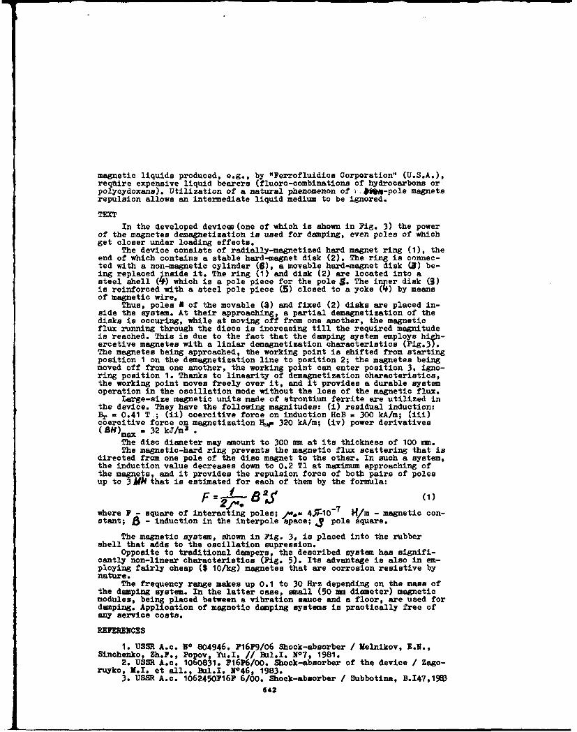
magnetic liquids produced, e.g., by "Ferrofluidice Corporation" (U.S.A.),requdire expensive liquid bearers (fluoro-combinations of hydrocarbons orpolycydoxans). Utilization of a natural phenomenon of *&If6-pole magnetsrepulsion allows an intermediate liquid medium to be ignored.
TEXTIn the developed devices (one of which is shown in Fig. 3) the power
of the magnetes demagnetization is used for damping, even poles of whichget closer under loading effects.
The device consists of radially-magnetized hard magnet ring (I), theend of which contains a stable hard-magnet disk (2). The ring is connec-ted with a non-magnetic cylinder (6), a movable hard-magnet disk (3) be-ing replaced inside it. The ring (1) and disk (2) are located into asteel shell (1#) which is a pole piece for the pole 9. The inper disk (3)is reinforced with a steel pole piece (5) closed to a yoke (4) by meansof magnetic wire.
Thus, poles I of the movable (3) and fixed (2) disks are placed in-side the system. At their approaching, a partial demagnetization of thedisks is occuring, while at moving off from one another, the magneticflux running through the discs is increasing till the required magnitudeis reached. This is due to the fact that the damping system employs high-ercetive magnetes with a liniar demagnetization characteristics (Fig.3).The magnetes being approached, the working point is shifted from startingposition 1 on the demagnetization line to position 2; the magnetes beingmoved off from one another, the working point can enter position 3, igno-ring position 1. Thanks to linearity of demagnetization characteristics,the working point moves freely over it, and it provides a durable systemoperation in the oscillation mode without the loss of the magnetic flux.
Large-size magnetic units made of strontium ferrite are utilized inthe device. They have the following magnitudes: (i) residual induction:Br - 0.41 T ; (ii) coercitive force on induction HoB a 300 kA/m; (iii)coercitive force on magnetization H16 320 kA/m; (iv) power derivatives
WBH0.=x = 32 kJ/m3 .The disc diameter may amount to 300 mm at its thickness of 100 mam.The magnetic-hard ring prevents the magnetic flux scattering that is
directed from one pole of the disc magnet to the other. In such a system,the induction value decreases down to 0.2 TI at maximum approaching ofthe magnets, and it provides the repulsion force of both pairs of polesup to 3 MY that is estimated for each of them by the formula:ajt 2/1.
2Y4.where P - square of interacting poles; ./,= 4p10- 7 H/m - magnetic con-stant; 5 - induction in the interpole space; J pole square.
The magnetic system, shown in Fig. 3, is placed into the rubbershell that adds to the oscillation supression.
Opposite to traditional dampers, the described system has signifi-cantly non-linear characteristics (Fig. 5). Its advantage is also in em-ploying fairly cheap ($ 10/kg) magnetes that are corrosion resistive bynature.
The frequency range makes up 0.1 to 30 Hrz depending on the mass ofthe damping system. In the latter case, small (50 mm diameter) magneticmodules, being placed between a vibration sauce and a floor, are used fordamping. Application of magnetic damping systems is practically free ofany service costs.
REPRENCES
1. USSR A.c. NO 804946. P16F9/o6 Shock-absorber / Melnikov, E.N.,Sinchenko, Zh.F., Popov, Yu.I. // Bul.I. N0 7, 1981.
2. USSR A.c. 1060831. P16P6/00. Shock-absorber of the device / Zago-ruyko, 3.I. et all., &ul.I. N46, 1983.
3. USSR A.c. 1062450P16P 6/00. Shook-absorber / Subbotina, B.I47,19$
642

4. USSR A.c. NO 1178982, F1679/02. Air shock-absorber / Boguslavs-ky, V.A. /1 Bul.1. NO34, 1985.
5. USSR A.c. NO 1157293, P16P6/oo. Shock-absorber / Rodionov, V.A.,et all., Bul. NO 19, 1985.
6. Application NO 55-41370. Japan. Shock-absorber. Published 1980.7. USSR A.c. NO 1213283, P16F6/00. A technique for magnetic-liquid
shock-absorbing // Rodionov, V.A., et all 1/ Bul.1. NO 7, 1986.
4
Figure 2--Damping system on peryaa-Figure 1-- Liquid-spring shock- nent magnetes using magnetic liquidabsorber of levetizing type 6 7 . 1-base; 2-shifted elements;1-rod; 2-piston; 3-permanent 3-permanent magnet; 4-magnetic liq-magnet; 4-magnetic liquid; 5-body. uid; 5-partitions.
Figure 3--Damping module on oxidemagnetes. 1-magnetic cylinder; 2-fixed magnetic disc; 3-shifted mag-netic disc; 4-magnetic yoke; 5-polepiece of the movable system; 6-non-magnetic supressing cylinder; 7-an-chor bolt for fixing the vibrationsource.
N
N
643

Figure 4--Demagnetization cha-racteristics for the high energy
-, MT oxide magnete.A working point of the magnetsystem: 1 - at the starting sta-te; 2 - at maximum loading;
& • 3 - at complete disloading.-- 20O
-// , - Figure 5--Loading characteris-tics of the damping module.
02' 4 a1 At, I MM
644

SECOND INTERNATIONAL CONGRESS ONRECENT DEVELOPMENTS IN AIR- AND
STRUCTURE-BORNE SOUND AND VIBRATIONMARCH 4-6 1992 AUBURN UNtVERSITY. USA
RECIPROCAL DETERMINATION OF VOLUME VELOCITYOF A SOURCE IN AN ENCLOSURE
Bong-Ki Kim, Jin-Yeon Kim, Jeong-Guon Ih
Department of Mechanical Engineering
Korea Advanced Institute of Science & Technology
Abetrct
Volume velocity of an acoustic source can be widely used in detennining the vibro-acoustic transfer
functions, in measuring the acoustic transfer impedances and in finding the generated power of a source.Several techniques have been proposed for this purpose, such as the laser velocimetry, the internal pressuremeasurement and the face-to-face electro-acoustic measurement. However, for a source in an enclosurewith flexible walls, acougto-structural coupling should be considered. Present method using an acousto-structural reciprocity principle results a good vibro-acoustic transfer impedance and can be used indetermining the volume velocity of a source in-situ.
1. Introduction
The volume velocity of an acoustic source is useful in characterising the vibro-acoustic transferfunctions, in measuring the acoustic transfer impedances and in determining the generated source power.For the study of these acoustic parameters, moving-coil type loudspeakers are popularly utilised as acoustic
sources due to its ease of control and cheap price. Several methods have been proposed to estimate theacoustic volume velocity of a loudspeaker. Among them, the following three methods have been suggestedfor practical measurements : the laser velocimetry, the internal pressure method and the electro-acousticreciprocity method. These methods require idealised environments or test rigs. In this paper , we propose anew technique for estimating the volume velocity of an acoustic source, in-situ. A reciprocity method usinga sructural-acoustic transfer function is adopted and the results are compared with other methods.
2. Determilnaton of volume velocity using an acousto-Wuctural reciprocity
Vibration and acoustic field in the flexible boundary, like shells or plates , which should be linear havethe reciprocal relationship. When we consider two situations, shown in Fig. I , the situation 1 is that themechanical force at A is active and the acoustic pressure at B is measured , and, reciprocally, the situation
645

2 is that the acoustic source at B is active and the vibrational velocity at A is measured. Then, from the
acoustic reciprocity principle we can find the following relationship"i:
vtl(rA) P(2)(r)=) (1)
Q1(TB),• F(2)(rA)
where F(r) is the point excited force at i = ;, and Q() is the volume velocity of a monopole source at =
Here v(r) is the vibrational velocity and P(r) means the acoustic pressure. This principle states that if in an
unchanged environment the locations of a small source and a small receiver are interchanged . the transfer
function between point A and B will remain the same. Therefore, the acoustic volume velocity, Q , as a
function of frequency can he given by
Q(f) = V(-•l' (2)
where the source should be considered as a monopole one. If the acoustic source can be assumed as a
monopole , it is not necessary to consider the shape of source in this method. This fact is powerful in
estimating the acoustic volume velocity of sources with irregular geometries'21 .
3. Comparison with other measurement methods
3.1. Laser velocimetry
Using the laser velocimetry one can directly measure the velocity, u, of a point on the diaphgram of a
loudspeaker. With this measured velocity the volume velocity of a source can be easily measured using QL =
;. - S where i is the surface normal vector and S is the effective area of diaphgram. For this measurement
the source is assumed to be a baffled rigid piston. In many cases at low frequencies a loudspeaker
diaphragm is often considered "pistonlike" one. When using the monopole source assumption, the condition
of ka << 1 should be satisfied where k is the wave number and a is the characteristic dimension of the
loudspeaker. At higher frequencies, however, the motion of different parts of the loudspeaker diaphragm
modes are excited. Under these conditions the loudspeaker will not behave as a monopole source. In this
paper, we have a loudspeaker of 100 mm in diameter and interested in the low frequencies below 400 Hz
where this problem can be considered as minimally affecting'I. The laser displacement meter ( KEYENCE,
LC-2310 ) was used in this experiment . The output signal from the lasr displacement meter was
differentiated to obtain the velocity.
3.2 Intermal pressure method
Loudspeaker diaphgram housed in an acoustically sealed cylinder vibrates like a piston. The cylinder was
made of PVC pipe of 650 mm in length, 100 mm in radius and 10 mm in thickness. As the piston vibrates,
it causes changes in the total internal pressure P and volume V. For perfect gases the relationship between a
small change in cavity pressure due to a small change in its volume can be given by131
2
P(M) M -C Q (3)
646

From this, one can determine the acoustic volume velocity by measuring only the acoustic pressure as
follows:
Q1PM = -j(V P(o) (4)
where p is the air density , c is the speed of sound, V is the volume of enclosure, and P(wo) is the pressure
fluctuation in the box. The wavelength should be larger than the characteristic dimensions of the enclosure.
If the wavelength is small compare to any of the internal dimensions, the pressure will also be governed by
a frequency-dependent spatial function"'. In this case , the error in estimating the acoustic volume velocity
would occur. However, we are interested in the low frequency range below 400 Hz, in which this problem
need not to be considered.
The laser velocimetiy method was used to be taken as a reference measurement of the acoustic volume
velocity for other methods. The comparison is made in Fig.2 and 3 between the acoustic volume velocity
using the internal pressure method and the laser velocimetry, Qn,(f) / QL(f). Internal pressure measurement
method underestimates the acoustic volume velocity by about 0.4 dB. Inaccuracies in the estimate of
internal pressure measurement may be caused by the vibrations of box plate or due to some bias errors.
3.3 Acousto-structural reciprocity method
To implement and prove the method mentioned in section 2 , an irregularly shaped chamber as illustrated
in Fig.4 is constructed using steel plates of lmm in thickness. The dotted line in Fig.5 is the result of the
acousto-structural reciprocity method between the points, say , A, and B. A large amount of deviations
from Fig.2 can be observed. Large peaks and troughs in the figure is caused by the inverse of the structure-
acoustic transfer function ( P/F ) and multiplicating it with the measured velocity. This fact means that the
peaky curves are due to errors in handling the peaky velocity and the inverse of transfer function data. For
these peaks , one needs a number of data points to average. If we choose several points on the boundary as
shown in Fig.6, the averaged acoustic volume velocity is given by
Q-ý1 i•n V (i (f (5)
Fig.7 shows a comparison between the acoustic volume velocity derived from the reciprocal method and
the laser velocimetry , QR(f) / QL(f), where QR(f) was determined by a reciprocal measurement when the
number of averaging points is 5. This would become larger as the frequency goes up to higher frequencies
due to the failure of the monopole source assumption. The acoustic volume velocity is influenced by the
environment where acoustic source is placed and by the electrical source input as well. The interaction
between the source and the flexible panels causes the change of radiation impedance of acoustic source.
This means that the acoustic volume velocity will be changed due to the boundary effects. Another problem
in these methods is irregular source shape. If the dimensions of a source are much smaller than the
wavelength of the sound being radiated, as a monople source, then the details of the surface motion are not
important and it will radiate exactly the same sound as any other simple source with the same acoustic
volume velocity. In spite of this advantage, established methods cannot find the acoustic volume velocity if
the shape of the source is complex. The acoustic reciprocity method which is introduced in this paper
"647

overcomes this problem, because it is not necessary for this method to consider the motion of vibrating
surfces,
4. Predict[o of interior mound fieldIf the system, illustrated in Fig.4, is linear, P/F and V/Q represent the same transfer function between
point A and B. When we consider two points or more on the flexible boundary .the pressure at point A willbe given by
A FJ(Y) (6)
If the transfer functions of all points are found and the input forces are known , the interior acoustic
pressure in the enclosure can be predicted. The two points on the panel, shown in Fig.4 , are selected asmechanical measuring points. The transfer functions , V/Q and P/F of A, to B and A2 to B are measured.
From Fig.? , we can find that averaged volume velocity when n=5, results more accurate transfer function
than that from direct measurement. The interior sound pressure in an enclosure can be predicted by using the
transfer functions , ( P/F ) and ( v/Q ). The measured pressures are shown in Fig.8-(a) and (b). If the systemis linear and if we can estimate the acoustic volume velocity accurately, the vibration and acoustic fields
will be in reciprocal relationship. Then, the two results from (P/F) and (v/Q) will coincide with each other
in all frequency ranges. As depicted in the figure, the acousto-structural reciprocity method predicts the
interior pressure very reasonably in all frequency ranges. Another complex situation considered is the
chamber consisting of double panels and containing sound absorbing materials in the enclosed space. Fig.9shows the comparison between the predicted and actually measured interior sound. Another good agreement
can be observed.
6. ConclusionA new method of measuring the volume velocity of an acoustic source is presented using the acousto-
structural reciprocity. Acousto-structunal reciprocity method overcome the problems of flexible boundary
effects and indeterminable source shapes. This method was applied to the prediction of interior sound
pressure due to the structural excitation and the result was in good agreement with the practically measuredone.
REFERENCE[1] L. M. Lyamshev ," A Question in Connection with the Principle of Reciprocity in Acoustics" , Soy.
Phy. Acoust. ,vol.5, pp. 406-409 (1960).[21 L E. Kinsler et al., " Fundamentals of Acoustics ", 3rd ed.Wiley , NewYork (1982).
[3) D. K. Anthony and S. J. Elliott, "A Comparison of Three Methods of Measuring the Volume Velocity
of an Acoustic Source ", J. Audio Eng. Soc., vol.39 (1991).
(41 J. M. Mason and F. J. Fahy, "Development of a Reciprocity Technique for the Prediction of PropellerNoise Transmission through Aircraft Fuselages" J. Noise Control Eng. .vol.34, pp. 43-52 (1990).
[51 T. Salava, " Sources of the Constant Volume Velocity and Their Use for Acoustic Measurements "1.
Audio Eng. Soc. .vol.22, pp. 146-153 (1974).
[6] Lord Rayleigh, "The Theory of Sound ", 2nd ed vol.11, Dover, NewYork (1945).
648

Leei Box
-•. .(/t." \B B
A AZ
(a) (b)
Fig.1. Reciprocal relationships between vibration Fig.4. Transfer functions between boundary poL-its, A,
and acoustic fields in flexible enclosures, and interior field point, B , in an enclosure.
S 0.2 0.2
o-; I ": i.!0.2 it11
I It
30I
100 150 200 2210 200 -320 "Co oo 130 200 250 200 300 400Frequency (Hz) Frequency (Hz)
Fig.2. Acoustic volume-velocity. -Fig.5. Acoustic volume velocity using reciprocalLaser velocimetry I - PM) method. (---:n1 , n=5)
-2
100 150 200 250 300 350 400 100 150 200 250 300 350 400Frequency (Hz) Frequency (Hz)
Fig.3. Comparison of measured volume velocity Fig.6. Coimparison of measured volume velocity
using 1PM and laser velocimetry using reciprocity and laser velocimetry.
649
'Ir! i

10 t ot
2•- 0.01 - 0.01 ''
100 1 zoo 250 300 350 400 100 ISO 200 ZOO 300 3 C3 -. O
Frequency (Hz) Frequency (Hz)
(a) (b)
Fig.7. Transfer function at a point: volume velocity is obtained
(a) by averaging those of 5 points (b) by measuring only one point.
(-:P/F v/Q).
80 1.
-I -
CO 050 O00 250 zoo 353 to co 0 :O 0 100 2-0 300 33 -
7rCt-nC'. Freauerncy (tz)
1a; (b)
Fig.8. Prediction of interior sound pressure at a point in an enclosure with simple
bare steel panels
(a) using the transfer function of P/F , (b) using the transfer function of v/Q.
( - : predicted - - - : measured)
3000
7 0 t0I
30 30 0
00 , ' t '( I
20 20
100 150g.00 250 300 350 a0O 0000 10 ISO zOO 300 50 -coFrequency (Hz) Frequency (H--)
(a) (b)
Fig.9. Prediction of interior sound pressure in case of complex system consisting of
double panels and absorption materials in the enclosed space
(a) using the transfer function of P/F , (b) using the transfer function of v/Q.
- : predicted : measured)
650

SECOND INTERNATIONAL CONGRESS ONRECENT DEVELOPMENTS IN AIR- AND
STRUCTURE-BORNE SOUND AND VIBRATIONMARCH 4-6, 1992 AUBURN UNIVERSITY. USA
ANALYSIS OF FORCED ACOUSTIC FIELDSINSIDE
STRUCTURALLY COUPLED CAVITIES
Arzu GONENC-SORGUC and Mehmot CALIýKANMechanical Engineering DepartmentMiddle East Technical University
06531 Ankara, Turkey
fABSTRACT
Dynamic response characteristics of structurally coupled multicavity systems arestudied. Acoustoelasticity method is used to model the structural-acoustical interactionunder externally applied harmonic forcing.
It is demonstrated that effects of structural-acoustical interaction are morepronounced when excitation frequencies are close to in-vacuo acoustical and structuralnatural frequencies. When excitation frequency is near the cavity resonant frequency, thecavity acts like a vibration absorber for the structural wall and the natural frequency ofthe coupled system almost coincides with cavity resonant frequencies. When the coupledfrequency is well separated from in-vacuo structural and acoustical frequencies, theinteraction is found to dominate the response at this coupled natural frequency.
NOMENCLATUREc0 speed of sound P# n'th acoustical modal pressureE Young's Modulus q m'th structural modal coordinateh wall thickness [0] coupled system matrixLob acoustoelastic coupling coefficient Q' m'th external structural generalized forcem structural mode index V volume
n'th acoustical generalized mass v Poisson'L ratio for partitioninq wallM• m' th structural generalized mass to equilibrium density of fluid1W acoustical mode index 03 (n'th st'ructural natural frequencyN total number of subcavlties uJk n'th acoustical natural irequency
IRODLCFIONA structure vibrating in contact witn a fluid of comparable density experiences
radiation loading comparable to its inertiel and elastic forces. Radiation loading thus:aodifies the forces acting on the structure since tile acoustic pressure depends on thevelocity. Hence, a feedback coupling between the fluid and structure exists. Here, thestructural and acoustical problems must be solved simultaneously [1].
Structural-acoustical coupling is pronounced in the dynamic analysis of totallyenclosed spaces with flexible walls. Submarines, aircraft and passenger car cabins aretypical examples of this type of coupling, commonly termed as gyroscopical coupling sincethe pressure in the vicinity of a flexible partition can be expressed in terms of theacceleration of the panel. Consequently, the dynamic behavior of the coupled system deviatesfrom those of its in-vacuo constituents. The degree of deviation depends on the level ofcoupling.
In technical literature several methods of analysis have been described. Among these,the acoustoelasticity method is found to be a very popular and effective approach at lowfrequencies [2,3].
651

In the acoustoelasticity metnod, pressure is expanded in terms of the normal modes ofrigid - walled cavity. The results are given in the form of linear ordinary differentialaquations for the response of each normal modes. The equations of motion of the flexible wallin terms of its structural modes are also expressed. Consequently, the coupled fluid -structural equations of motion are then obtained tr the acoustical naturalfrequencies and the corresponding modes (3].
In this study, acoustoelasticity method is employ_ --uy the acoustoelastic fieldresulted from the interaction between isotropic structural wall and interior acoustic fielduraer an external harmonic Forcing in three dimensional spaces. Acoustical naturalfrequencies, structural natural frequencies and coupled natural frequencies are found. Soundpressure levels inside cavities in a specified frequency band are determined.
ACOUSTOELASTICITY METHODIn ,)vdor to apply the ;ac:rutnelasticity method, it is assumed that the first suocavity
nas the isotropic flexible walis oln its right side while the other subcavities have flexiblewalis on both sides. Rectargular, three dimhnsional subcavities are chosen for convenience.A multi-cavity system and the relateo terminology are illustrated in Figure 1.
i~ =z j=N-2 j=N-1 j =N
p EeJWEt
_ /__•=1 i2 i=3 i=]N-I i=N
Figure I A Complex Shaped 3-0 Cavity witn an uucsloe -texiDle Wall
Acroustical SystemAcoustic fields in a general three dimensional cavity dividea into N subcavities by
isotrcpic flexible partitions is studied under external forcing. The wave equation istransformed into a set of ordinary differential equations by applying appropriate boundaryconditions and Green's Theorem. Hence modal equations of motion for the acoustic pressurecan be written as A11
)C (I) _)A__
"A P ____ for i.1i
A11 (Ji]•ll j-z
Alx
- 4 fox <s
dhere i repre•nts the subcavit,- numoer, e ,(i) is the a9.ustical natural frequency of the ithsubcavity, A,1 is the area of the flexible•.'wall, and V" is the volume of the i subcavityL denotes th• acoustoelastic c.uuplojng coefficient between the n acoustic mode of ithsutcavity and m structural mode of jt' Flexibie wall.
Structural SystemPartitions formed by isotropic plates simply supported along four edges are considered
in the analysis. Structural in, - vaeso normal modes used in expressing the flexible walldeflection by modal expansion are s ecIfied by boundary conditions on the flexible wall area.Then the modal equations for the i't structurei wall can be expressed explicitly as
652
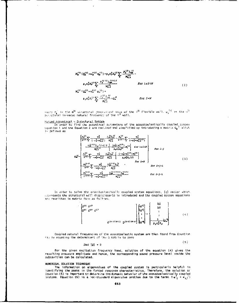
p ) .) _J for 1:91 (2)
2(2)
PQ ,A i•,-• ••,,. foZ i -.
M t e pm s~tucti:*.1Il .rer•-iu *Ld u,•,s of the ilh flexible wall iý theIz,. ý,- iJ. in-vacuc natura2 f;ten- ! the i' wall.
orcec /coust ica - ScructuraL Syste•,In order to fi!,d ,he .acoustical pcr.mmeters of the acoustoelastically coupled+ oyscer
Equation I and tne Equation 2 are comi.ined and simplified by introducing a matrix rll w-zi,;limi defined as
for i-N41)I j J .- j) 1) (1
11• L.. (-'+. )N,; I i
. _I ___ -. for I-J-1
In order to solve th:a o;tceI~sticailv coupled system equations, (q) vector which-. :,resents the structural wal': d1SlP'&-7ec.er-ts is introduced and the coupled system equationsar•., rewritten in matrix fo-i:n os fa.s.wc-
0Q12 r"12 q
II Pj 0' C:A
Coupled natural frequencies of Lhe acoustoelastic system are then found from Eouation(4;} by equating the determirart cf th, ,i matix to zero
(5jDer !Q] = 0
For the given excitation freque.ncy band, solution of the equation (4) gives theresulting pressure amplitude and hence, the corresponding sound pressure level inside thesubcavities can be calculated.
NUMERICAL SOLUTION TECHNIQUEThe information on eigenvalues of the coupled system is particularly helpful in
identifying the peaks in the forced r-esponse characteristics. Therefore, the solution o0Equatton (5) is important tv detai-mine th3 dynamic behavior cf the acoustoelastically coupled3ystams. Equatioa t5) is a :,or,-strndard eigenvalue protlem due to the terms (-a + -,a")
653

appearing in the denominator of each term of the Q matrix. In order to solve this nonstandardeigenvalue problem, an iteraLive solution technique is adopted. The technique involves thedetermination of the sign of the determinant as a function of the frequencyQ,. If the signof the determinant of the Q matrix found from two successive trial values of m'changes, t1henit is understood that there is a natural frequency lying between these tuo trial CE's. Oncetine interval is determined, the welI known Bisection Method is applied with a prespec, riedaccuracy to find the coupled natural frequency.
Acoustic pressure distributions inside cavities are determined from the solution ofEquation (4) by employing Gauss Elimination Method which gives the modal vectors (q} of thecoupled systems. Acoustical modal pressure amplitudes, and finally total acoustic pressureamplitudes are also determined in the specified frequency band.
CASE STUDIES"Case study I
In this case study, the forcnd response of a three dimensional sirgle cavity .sexamined in the frequency band of 0-200 Hz.
PEe1wE
Figure 2 Case Study 1
The cavity given in Figure 2 is believed as a typical representation of cabins of twin--engine general aviation aircraft [4]. Thu cabin noise levels in such kinds of aircraft arereported to be very high. It is assumed that noise entered into the enclosed space by theairbcrne path only through the structural wall with no leakage. Noise generation inside thenabin was totally ruled out. The following baseline parameters were used in the foregoinganalysis:
1. Rectangular cavityworking fluid : airspeed of sound : 340.46 m/sdensity 1.22 kg/midimensions - 1.22 m x 1.27 m x 3.61 m
2. Structural wallboundary conditions :simply noorted at
all edgeslocation : center- of y-z planedimensions 0.27 m x 0.7 ithickness (h) 0.00356 mmodulus of elasticity (E) (6.9) 1 0qi Pasurface density (a) : 9.6 kg/m2Poisson's ratio (v) : 0.33
3. Receiver Position : P(O.304, 0.914,1.215) m4. Excitation Force Amplitude 0.1 PaDamping characteristics of the structural wall and sound absorbing properties of rigid
alls were neglected in the present analysis.For the in--vacuo acoustical nturPl modes, n,, nf, and n, were taken from zero to 4.
3tructural in-vacuo natural mcdes, , ,smn, .ere retained from I t6 3. The present analysis war)erfarmed in the fr4equency band of (Y-206 Hz. Tables 1 and 2 present the in-vacuo acoustical
654

and structural irequencles ot linrct•pIed systtms, re-;pectively, calculated by the software.The coupled natural frequencies are tabulated in Table 3.
Taole I In-vacuo Acoustical Natural Frequencies
rn, - -_Z1 f (Hz]
0 0 1 47.16
0 0 2 94.31
0 0 3 141.47
0 0 4 188.62
0 1 0 134.04
0 1 1 142.09
0 1 2 163.89
0 1 3 194.88
S 0 139.53
.. .5 1_ 147.29
r)'__ 2 168.42
3 3 198.70'-I *----193.48
T•tble 2 In-vacuo Structural Natj,'al Freo'encies
if 2 212 3 3 3
1 22 3 1 2 3
f H) 136.31 169.27 217..54 J423 553 632.5 1085.6 1138.6 12.
Table 3 Coupled Natural Frequencies
fif , [Hz] 4 167., 7I 186.23J
In the case of weak coupling b etween the acoustic cavity and the structural wall, whenthe excitation frequency is near a structural or a cavity resonant frequency then the largestresponse will occur at these in-vacuo natural frequencies. On the other hand, when thecoujplins is strong, the contr:bution of the coupling into the response cannot be neglected.
Contributions by structural wall and cavity resonant frequencies into the response ofthe system are demonstrated in Figure 3 as well as the contributions of coupled frequencies.As 6epicted by the theory of acoustoelasticity, when the excitation frequency is wellseparated both from the structural and cavity in-vacuo natural frequencies, there may notbe a single dominant structural and/or acoustical cavity natural frequency in the response[23. For such a case, dominant peaks ir. the response are observed at the coupled frequencies.The peak at coupled frequency of 59.53 Hz seen in Figure 3 was associated with thisphenomenon. The sound pressure lev9e c-,rresponding to this peak was found to be 135 dB [5].
According to the Lheory, when the excitation frequency is close to a cavity resonantfrequency, the cavity acts like a v'brai;ion absorber for the structural wall. In such a case,ccupled frequencies either coincide with the :av
4ty natural frequencies or come very close
to these frequenci{s. In The present analysis, the in-vacuo acoustical ný)* frequency at94.31 Hz is shifted to 94.72 rlz while the acoustical natural frequency a Hz shifteddown r.o the coupled freouency- f 107.'9 Hz. Figure 3 iliustrates peaks • ding to thecavity resonant frequencies and the coupled frequencies of the structura ýical system[5)
WIhen the structural and ac-.-utlcal in-vacuo natural frequencies are close, the effectof the coupl ing is also -ronouncud ii the h ',,stonu response [3]. The acoustic natural frequency
655
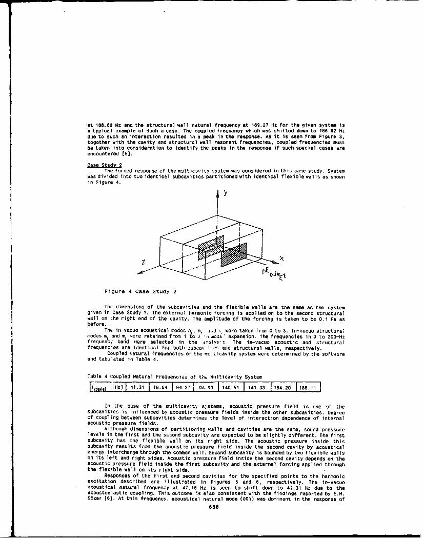
at 188.62 Hz and the structural wall natural frequency at 189.27 Hz for the given system isa typical example of such a case. The coupled frequency which was shifted down to 186.62 Hzdue to such an interaction resulted In a peak in the response. As it is seen from Figure 3,together with the cavity and structural wall resonant frequencies, coupled frequencies mustbe taken into consideration to identify the peaks in the response if such special cases areencountered [5].
Case Study 2The forced response of the multic¢vity system was considered in this case study. System
was divided into two identical subcavities partitioned with identical flexible wal Is as shownin Figure 4.
Figure 4 Case Study 2
The dimensions of the subcavities and the flexible walls are the same as the systemgiven in Case Study 1. The external harmonic forcing is applied on to the second structuralwall on the right end of the cavity. The aimplitude of the forcing is taken to be 0.1 Pa asbefore.
The in-vacuo acoustical modes n,, n, 1
j ,, were taken from 0 to 3. In-vacuo structuralmodes m. and rý "ere retained from 1 to 3 r) moaot' expansion. The frequencies in 0 to 200-Hzfrequency band were selected in the inalys-s The in-vacuo acoustic and structuralfrequencies are identical for both subcav 'j- and structural walls, respectively.
Coupled natural frequencies of the mriticavity system were determined by the softwareand tabu~ated in Table 4.
Table 4 Coupled Natural Frequencies of thb Milticavlty System
I 2cuoed [Hz] 1 41.31 1 78.64 1 94.37 194.93 f 140.51 1141.33 r184.20 1188.11
In the case of the multicavity systems, acoustic pressure field in one of thesubcavities is influenced by acoustic pressure fields inside the other subcavities. Degreeof coupling between subcavities determines the level of interaction dependence of internalacoustic pressure fields.
Although dimensions of partitioning walls and cavities are the same, sound pressurelevels in the first and the second subcav~ty are expected to be slightly different. The firstsubcavity has one flexible wall on its right side. The acoustic pressure inside thissubcavity results from the acoustic pressure field inside the second cavity by acousticalenergy interchange through the common wall. Second subcavity is bounded by two flexible wallson its left and right sides. Acoustic pressure field inside the second cavity depends on theacoustic pressure field inside the first subcavity and the external forcing applied throughthe flexible wall on its right side.
Responses of the first and second cavities for the specified points to the harmonicexcitation described are illustrated in Figures 5 and 6, respectively. The in-vacuoacoustical natural frequency at 47.16 Hz is seen to shift down to 41.31 Hz due to theacoustoelastic coupling. This outcome is also consistent with the findings reported by E.H.Sbzer (6]. At this frequency, acoustical natural mode (001) was dominant in the response of
656

the both cavities. The peal( obse'vea at the coupled frequency 78.64 Hz was also singled out¶ as a distinct peak since the excitation frequency is well separated from the in-vacudacoustical and structural natural frequencies as discussed in the previous case study. IIsuch a case, the response Deaks out at the ccupled frequency in the vicinity of acoustical,and/or structural natural frequencies while these frequencies do not appear in the responseany more. On the other hand, the in-vacuo natural frequency at 94.31 Hz was seen to becoupled resulting in two closely coupled natural frequencies at 94.63 Hz and 94.93 Hz dueto interactions between two subcavitles. This type of coupling experienced between twosubcavities can be termed as cavity coupling. The peak at this frequency in the secondsubcavity was observed to be higher than the one in the first subcavity. The sae discussionalso applies to the coupled natural frequencies of 140.51 Hz and 141.33 Hz resulting fromthe coupling of the in-vacua acoustical natural frequency at 141.47 Hz. The in-vacucstructural natural frequency at 189.27 Hz was coupled by shifting down, givipg two couplednatural frequencies at 184.20 Hz and at 188.11 Hz. The magnitude of the peak at 184.20 Hzin the second subcavity was higher than the one observed in the other subcavity. Converseiy,the opposite was observed at 188.11 HZ [5].
When Figures 5 and 6 are compared to Figure 3, it can be concluded that when theacoustical system is partitioned by flexible walls to form multicavities one, the couplednatural frequencies rather than the in-vacuo acoustical or structural natural frequenciesdominate the response. Special care should be exercised when identifying peaks in theresponse if the system to be analyzed is made up of multicavities [5].
CONCLUSIONSThe main conclusions reacned after the case studies can be outlined as follows:1. When the excitation frequency is well separated from in-vacuo acoustical and
structural natural frequencies, there is no single dominant structural-cavity naturalfrequency, structural-acoustical interactions cannot be neglected, and the dominant peaksin the response are observed at coupled natural frequencies.
2. When the excitation frequency Is near the cavity resonant frequency, cavity actslike a vibration absorber for the structural wall and the coupled frequency coincides withcavity resonant frequencies or come close to these frequencies.
3. If the in-vacuo acoustical and structural frequencies and the excitation frequencyare close to each other, then structural--acoustical interaction is pronounced in the systemresponse. The coupled frequency of the system happens to be close to these frequencies.
4. The accuracy of the present analysis depends on the number of acoustical andstructural in-vacuo modes. The higher the number of acoustical and structural modes, the moreaccurate the results obtained wbuld be.
5. The method is particularly applicable in the cases of low modal density. For thisreason, it can be successfully emploved to stucy structurally coupled interior acousticfields with or without absorption.
6. Care should be exercised in specifying the frequency increment when the excitationfrequency is near to in-vacuo acousical-natural frequencies to avoid the trivial solutions.
7. For structural in-vacuo modes, simple trigonometric functions have employed in theanalysis due to simply supported boundary conditions assumed for the partitions. One shouldbe careful when interpreting the results in practical applications since partitioning wallsare rarely simply supported. However, it is possible to adopt other orthogonal functions inmodal expansion to account for real-life boundary conditions.
REFERENCES1. Junger, C.J., Feit, D., 1986, "Sound Structure and Their Interaction", The MIT Press
Cabridge. Massachusetts, London, England.2. Sestieri, A., Del Vescove, D., Lucibello, P., 1984, "Structural-Acoustic Coupling in
Complex Shaped Cavities", Journal of Sound and Vibration, vol. 96(2), pp. 219-233.3. Dowell, E.H., Gorman, G.F., Smith, D.A., 1977, "Acoustoelasticity: General Theory,
Acoustic Natural Modes and Forced Response to Sinusoidal Excitation, IncludingComparisons With Experiment", Jrnal of Sound and Vibration, vol. 52(4), pp. 519-542.
4. Chao, C.F.B., 1981, "Modal Analysis of InLerior Noise Fields", Finite ElementApplications in Acoustics. Pp. 29-5:.
5. G~nenc-Sorgu,., A., 1991, "Act.ive Minimi:,ation of Acoustic Potential Energy Tnside theStructurally Coupled Fnc!osed Suaces", M.Sc. Thesis, M.E.T.U., July 1991.
6. S~zer, M., 1989, "Analysis ;:f Scructurally Coupled Interior Acoustic Fields byAcoustoelasticity Method", M.Sc. ihasis_.M.E.T.U., February 1989.
657

II o. 12. SoP
Figure 3 Lp vs External Exciting Frequency for Case Study 1
) (dlii
...........
I........... ......... .... ....
L L _ _ ... ._ _ -......
r k1TZ
~~CIr( L; v XC,2jiI.6 i... F1. !.ýi...M~cv foir the Second SuL'cav ity o-F C.aSE StLu•2v 2
656

SECOND INTERNATIONAL CONGRESS ONRECENT DEVELOPMENTS IN AIR- AND
STRUCTURE-BORNE SOUND AND VIBRATIONMARCH 4-. 1992 AUBURN UNIVERSITY. USA
THEORETICAL AND EXPERIMENTAL ASPECTS OF ACOUSTIC MODELING OF ENGINEEXHAUST SYSTEMS WITH APPLICATIONS TO A VACUUM PUMP
B. S. SrldharaIndustrial Studies Department. Middle Tennessee State University
Murfreesboro, Tennessee 37132
and
Malcolm J. CrockerMechanical Engineering Department, Auburn University, Auburn, Alabama 36849
ABSTRACT
The engine exhaust system was modeled as a lumpedsource-muffler-terminations system. An expression for the predicted soundpressure was derived In terms of the source and termination Impedances, andthe muffler geometry. The developed prediction scheme is very efficient fromcomputation point of view. Also, the predicted sound pressure can becalculated without computing the source pressure or the source velocityalthough these quantities can be calculated if necessary. The formulation wasverified through a series of experiments. The source impedance was measuredusing the direct method. Sound pressure level measurements for the predictionscheme were made for several source-muffler and source-straight pipecombinations. In all cases, correlation of the experimental results and thosepredicted by the developed expressions was good.
INTRODUCTION
In an Internal combustion engine, the engine is the noise source and theexhaust pipe Is the main transmitter of noise from the source to the open endof the pipe. The open end of the exhaust pipe itself acts as a source andradiates the engine noise to the surroundings. The primary function of noisecontrol devices used In the engine-exhaust pipe system should be to reducethe amount of sound energy radiated from the open end of the exhaust pipe tothe surroundings. A series of experiments could be conducted on severalmufflers Installed in the exhaust pipe to achieve the desired reduction in theexhaust noise. But this is not a very efficient way of reducing the amount ofsound energy radiated from the engine exhaust to the surroundings as thefabrication of mufflers and experimental work Involve a great deal of time,effort and cost. Alternatively, if one can develop a method to predict theradiated sound pressure at a specified distance from the open end of theexhaust pipe so that the prediction scheme Involves only a few measurements,then much of the laborious experimental work Involved In muffler design can beavoided.
In order to reduce noise levels one should have a good knowledge of thesound source characteristics and the manner In which the sound is propagated.If the sound is propagated from the open end of a pipe, then the radiatedsound pressure can be predicted at a particular location from the open end by
659
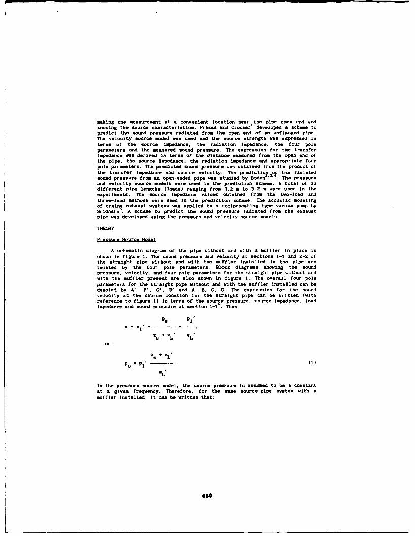
making one measurement at a convenient location near the pipe open end andknowing the source characteristics. Prasad and Crocker developed a scheme topredict the sound pressure radiated from the open end of an unflanged pipe.The velocity source model was used and the source strength was expressed interms of the source Impedance, the radiation impedance, the four poleparameters and the measured sound pressure. The expression for the transferImpedance was derived In terms of the distance measured from the open end ofthe pipe, the source Impedance, the radiation impedance and appropriate fourpole parameters. The predicted sound pressure was obtained from the product ofthe transfer impedance and source velocity. The predictio i 3o1 the radiatedsound pressure from an open-ended pipe was studied by Boden ' . The pressureand velocity source models were used In the prediction scheme. A total of 23different pipe lengths (loads) ranging from 0.2 a to 3.2 a were used In theexperiments. The source Impedance values obtained from the two-load andthree-load methods were used In the prediction scheme. The acoustic modelingof engin? exhaust systems was applied to a reciprocating type vacuum pump bySrldhara . A scheme to predict the sound pressure radiated from the exhaustpipe was developed using the pressure and velocity source models.
THEORY
Pressure Source Model
A schematic diagram of the pipe without and with a muffler In place isshown In figure 1. The sound pressure and velocity at sections 1-1 and 2-2 ofthe straight pipe without and with the muffler Installed In the pipe arerelated by the fou7- pole parameters. Block diagrams showing the soundpressure, velocity, and four pole parameters for the straight pipe without andwith the muffler present are also shown In figure 1. The overall four poleparameters for the straight pipe without and with the muffler installed can bedenoted by A', B', C', D' and A, B, C, D. The expression for the soundvelocity at the source location for the straight pipe can be written (withreference to figure 1) in terms of the sourge pressure, source impedance, loadImpedance and sound pressure at section 1-1 . Thus
V ,= V 1 I = __ -
Z+ZL' L'
or
zs + Zl.
Ps P1 ' (1)
7L'
In the pressure source model, the source pressure Is assumed to be a constantat a given frequency. Therefore, for the same source-pipe system with amuffler Installed, It can be written that:
$66*

XsXLPs . P, •(2)
It can be shown from equations (1) and (2) that
z+ZLZS S+ .
Pl, - P p(3)ZL' zL
Substituting for p,' and p, in terms of the radiation impedance, four pole
parameters and the sound pressure at section 2-2 (figure 1. cases i andii) equation (3) can be written as
p2' A zr + B Zs +zL zL,
S- -_____(4)P2 A' z+r Zs + Z L' ZL
In equations (1) through (4). the impedances zL' and ZL are the load
impedances corresponding to the cases without and with the muffler Installed.
MonoDole Radiation Model
The open end of an unflanged pipe can be modeled as a monopole or pointsound source for small values of the ratio of pipe diameter (at the open end)to the wavelength. In such a case, there will be plane and spherical wavepropagation to the left and right of the exit plane of the pipe. The soundpower transmitted through the open end of a pipe should be equal to the soundpower radiated from the open end of the same pipe modeled as a monopole whenthere Is no loss of energy.
The sound power transmitted through the exit plane of an open-ended pipeis given by the sound power incident on the exit plane minus the sound powerreflected at the exit plane. It can be shown that at the exit plane of thepipe:
1 S' 1 'pr' 2
- - (Jpz2'+ - Jp 2 ' 1 - - G'. (5)
2 Po co 2 Po co
In equation (5), Iprl is the pressure amplitude of the spherical wave at a
given radius, the cross sectional area of the pipe is denoted by S'. thesurface area of the imaginary sphere is represented by G' and other symbolshave their usual meaning. Equation (S) can be written as
661

IS' IP2,+l 2 ( I R- 12 l' r' 1 2 G' * (6)
where R' = ( P2 / ) is the complex reflection coefficient at the open
end of the pipe. The sound pressure can be written at the exit plane of thepipe in terms of its two components as
P2 ' = P2 '+ + P2'- = IP 2 '+ 11 R'I (7)
Solving for jp2'+1 in equation (7) and substituting into equation (6), it can
be shown that
IP2 'I = + R'j 2 ' ]1/2 1Pr', (8)
(1 - IR'l 2) s,
In a similar way, a relation between the sound pressures p2 and pr can be
established for the straight pipe in which a muffler is installed. Thus withreference to figure 1
( 1 - JRl2) s
IPrl = I[ -] 1/2 IP21 (9)
I1 + RI2 G
where the symbols have their usual meaning.
Prediction Scheme
Combining equations (4), (8) and (9) It can be shown that when there isno flow through the pipe and R = R' (for S = S'), the predicted soundpressure level is given by
JA' Zr + Bw Izs + ZL'! 1ZL I
Lp Lp 20log10
IA Zr + BI 1zs + ZLI IzL'I
+ 20 log10 ( r' / r ) . (10)
The terms L and L ' in equation (10) represent the predicted andp pmeasured values of the sound pressure level at distances r and r' from theopen end of the pipes of lengths L and L'. L is given by the sum of the threepquantities on the right hand side of equation (10). The first one Is ameasured quantity, the second term is derived from plane wave theory, and thethird quantity is based on the monopole radiation model used at the open endof the pipe. Expressions for the predicted value of the sound pressure level
662

L can be derived from a suitable combination of equations (4). (8) and (9)P
for special cases such as
(r' = 0, r > 0), (r' > 0, r = 0), (r' - 0. r = 0). when L * L' and L = L'.
EXPERIMENT
Several experiments were conducted and the radiated sound pressure levelwas predicted for different source-straight pipe and source-muffler-straightpipe combinations. A reciprocating type vacuum pump was the source used duringthe experiment. The experimental set up is shown in figure 2. A simpleexpansion chamber was the muffler element installed in the pipe. The sourceimpedance was measured using the direct method. The radiated sound pressurelevel was predicted using equation (10). Experiments were conducted in an openspace with the ground below the open end of the pipe covered with an acousticmaterial to minimize the ground reflections. A frequency range from 0 to 3200Hz was selected during the measurements to ensure only plane wave propagationin the pipe. A B&K type 2032 FFT analyzer and 0.006 m diameter microphoneswere used during the experiments.
Because of the size and weight of the vacuum pump and electric motor,measurements were made with tie experimental set up mounted on a horizontaltable. The sound pressure level measurements were made at a distance of 0.05 mfrom the open end of the pipe in order to maintain a 10 dB difference betweenthe signal and electrical noise. Although several experiments were conductedonly three plots are presented In this paper (figure 3 ).
RESULTS AND DISCUSSIONS
There are no theoretical methods to calculate the source impedance. Theschemes used to predict the source impedance are complicated and are still tobe proven. The accuracy of the measured values of the source impedance shouldbe verified by experimental means. The reliability of the random excitationand transfer function methods of source impedance measurement can be testedagainst known theoretical cases such as open and rigid terminations of a pipe.The accuracy of the predicted values of the radiated sound pressure level canbe determined by comparing the predicted quantities with the correspondingmeasured quantities. However, it should be remembered here that the predictedvalues of the radiated sound pressure level are functions of the measuredvalues of the source impedance, theoretical source models and computed valuesof the radiation impedance. It should also be noted that the predicted valuesof the radiated sound pressure level depend on the monopole radiation model.Therefore, the results presented in this paper should be examined keeping allof these factors in mind.
The reliability of the computed value of the radiation impedance has beenestablished in pipe acoustics7
. The monopole radiation theory is valid forsmall values of the pipe end diameter to wavelength ratio. Thus the accuracyof the prediction scheme depends mainly on the accuracy of the measured valuesof the source impedance. Also, the prediction scheme can be used to verify thecorrectness of the source impedance values. Although the sound pressure levelmeasurements were made at distances r' and r (figure 1) equal to 0.05 m it
663
_______________________________

has been establlshgd that the prediction scheme works well for small and largevalues of r' and r .
Referring to figure 3, the predicted values of the sound pressure levelshown in case I were obtained using the source impedance measured when thepump was operating. In this se, It Is seen that the predicted and measuredvalues of the sound pressure level agree well below 1200 Hz and above 2400 Hz.The disagreement above 1200 Hz can be attributed to the Increasing pipediameter to wavelength ratio at the open end of the pipe, whereas the reasonfor the good agreement between the predicted and measured values from 2400 to3200 Hz is not known. The sound pressure levels plotted in cases 1i and IIi(figure 3) correspond to the cases In which the source impedance was measuredwhen the pump was operating and stationary. The agreement between the predictedand measured values is seen to be good below 1200 Hz except In the range from100 to 250 Hz. A slignt frequency shift between the predicted and measuredvalues of the sound pressure level is seen in this case.
The acoustic model of an engine exhaust system is a powerful tool Inpredicting the behavior of a source- muffler-termination system. The model hasbeen found lo work well in the case of a system with a simple source such as aloudspeaker , and an actual source like the vacuum pump. It should be possibleto extend the acoustic modeling to systems with more complicated sources thanthat covered in this article.
REFERENCES
1. M. G. Prasad and M. J. Crocker, "A Scheme to Predict the Sound PressureRadiated from an Automotive Exhaust System," J. Acoust. Soc. Am.,70(5), 1345-1352 (1981).
2. H. Boden, "The Multiple Load Method for Measuring the SourceCharacteristics of Time Variant Sources," Summary of Paper 4. Ph. D.Thesis, Royal Institute of Technology, Sweden, 64 Pages (1989).
3. H. Boden, "Characterization of a Pneumatic Sliding Vane Motor as a Sourceof Fluid Borne Noise," S~umary of Paper 5. Ph. D. Thesis,Royal Instituteof Technology, Sweden, 34 Pages (1989).
4. H. Boden, "Characterization of a Multi-Cylinder Internal Combustion EngineSource of Fluid Borne Noise," Summary of Paper 6, Ph. D. Thesis,Royal Institute of Technology, Sweden, 40 Pages (1989).
5. B. S. Srldhara, "Theoretical and Experimental Aspects of Acoustic Modelingof Engine Exhaust Systems with Applications to a Vacuum Pump," Ph. D.Thesis, Auburn University, (1991).
6. M. J. Crocker, "Internal Engine Exhaust Muffling," Proceedings ofNOISE-CON 77, 331-357 (1977).
7. A. F. Seybert and D. F. Ross, "Experimental Determination of AcousticProperties Using a Two-Microphone Random-Noise Technique," J.Acoust Soc.Am., 65(1), 1362-1370 (1977).
664

I
PUPS ~souiczOR
7=U -POL WCl E MOO-t ý-OP
p-PtI*p Z L) . P",A'P l"Vsi LVw. L.OWh P. PI MZ. +IZoI PA NAPf.SVt Lm..V LV 1' C'Pz' OVj V1 -O P-,O V2V1.~ aowr,,,loCP.v,
Case i Case ii
Figure 1--Schematic diagram and equivalent electrical circuits for the scheme topredict the sound pressure radiated from the open end of a pipe. Case i. Withoutthe muffler installed. Case ii. With the muffler installed.
Figure 2-- Experimental set up for the vacuum pump.
665

z z0 - 0
nAo ,... ... . . o".. .. . .
FREUECY(z)FRQUECYHz
LL's WiJ
WJ0 0r
wr W
Case i Case ii
I I •I Figure 3--Predicted and measured valuesS~of the radiated sound pressure level.o - Vacuum pump data. r' = r = 0.05 m,-= 1.22 , L = 1.83 m;_
(••measured,---- ---- predicted.w•.. ll IThe pump impedance was measured when•(.J70 -! _____ ____ -• the pump was operating in cases i and
Si ii. A simle expansion chamber wasinstalled in the pipe in cases ii and
-J : '• 'iii.
0-
LI.I
1000 2000 3000FREQUENCY(Hz)
Case iii
666
z iue3-rdce n esrdvle

I
SECOND INTERNATIONAL CONGRESS ONRECENT DEVELOPMENTS IN AIR- AND
STRUCTURE-BORNE SOUND AND VIBRATIONMARCH 4-6, 1992 AUBURN UNIVERSITY. USA
Russian church bell.
Boris N. Njunin, Alexander S. LarucowNoise and Vibration laboratoryMoscow Automobile Plant (ZIL)
MoscowUSSR.
ABSTRACT.
The experimental studies of Russian church bell characteristics(eigenfrequencies, mode shapes, sound intensity vector mapping, etc.)were made using modal analysis and sound intensimetry methods.Experimental studies served as basis for the bell finite element modeldevelopment and identification. The finite element model of a bellallows, by optimization of profile, weight, dimensions and material, onthe stage of projection to obtain the design of a bell with requiredcharacteristics. As a result the church bells were manufactured usingmodern technology with "voice" similar to that of ancient Russian bells.
INTRODUCTION.
It's well known that as well as the most huge and the most remarkablein sound bells were only in Russia. Unfortunately, the secrets of artof casting of Russian church bells practically have been lost. The goalof our work is to tongue the sound of Russian church bell using modernresearch methods of sound sources acoustic parameters and modern castingtechnics. On the first stage of researches the experimentalinvestigation of acoustic and vibration characteristics of ancientRussian church bell of Samgin company was done. The finite elementmodel of this bell was developed and identified on the base of thisexperiments. This model was used for optimization of bell profile,dimensions, weight and material to obtain the bell design that closelyapproaches in sound to prototype (Samgin bell).
EXPERIMENTAL STUDIES.
Experimental studies of acoustic and vibration bell characteristicswere made in unecho chamber. Samgin bell (dimensions : 550 mm high,513 mm in max. diameter; weight - 83 kg) was suspended in the center ofunecho chamber. In the course of experimental studies the followingcharacteristics were determined :- vibration acceleration and sound pressure spectrum;- basic eigenfrequencies and eigenmodes, mode damping coefficients:- sound active intensity map;- bell surface zones that have most contribution to sound emission.
Measuremznt setup is shown on fig. 1. Excitation of bell vibrationwas done by the tongue of the bell. The mechanical arm was designed toinsure the cor-tant force of the stroke. Modal analysis of bellvibration were done using 126 measurement points (in each pointacceleration spectra were measured in three directions) and referencepoint on the tingue was chosen. In excitation and measurement channels
667

B&K3519 B&K
7 -JI 4344
IF<m
I I
B&K0 2624 0
7 F B&K 2034
IIN
ai
Fig.l. Measurement setup.
special type of windows were chosen to insure optimal Fourie analysis oftransient vibration signal. Modal parameters extraction was made usingmodal analysis package of L14S company (Belgium). while study of mostactive emitting bell surface zones the spatial vector of active soundintensity was measured at 30 mm distance from bell surface relative thepoints of acceleration spectra measurements in modal analysis. Usingintensity measurement package of 12S company measurement results werepresented as intensity vector and amplitude maps. On fig. 2. thesound pressure spectrum of the bell is shown. Measurement was done on 1m distance from the bell axe. Spectrum is composed of many discretepeaks. Time evolution of sound pressure spectrum shows that at thestroke moment sound spectrum is reach but in 1-1.5 seconds the spectrumis reduced to four basic discreet frequencies : 336 Hz, 652 Hz, 787 Hz,1064 Hz, which form the bell "voice". Experimental modal analysis ofthe bell were done in frequency range 50-3000 Hz. In this frequencyrange was determined 14 modes. The first mode is the most active, ithas frequency of 337 Hz (fig. 3). Information about bell mode shapesallowed to determine bell surface zones which were used for bell tuningon the finite element model on the design stage as well as tuning thebell after casting. Active sound intensity vector maps were studied forevery bell mode shape. Analysis
668
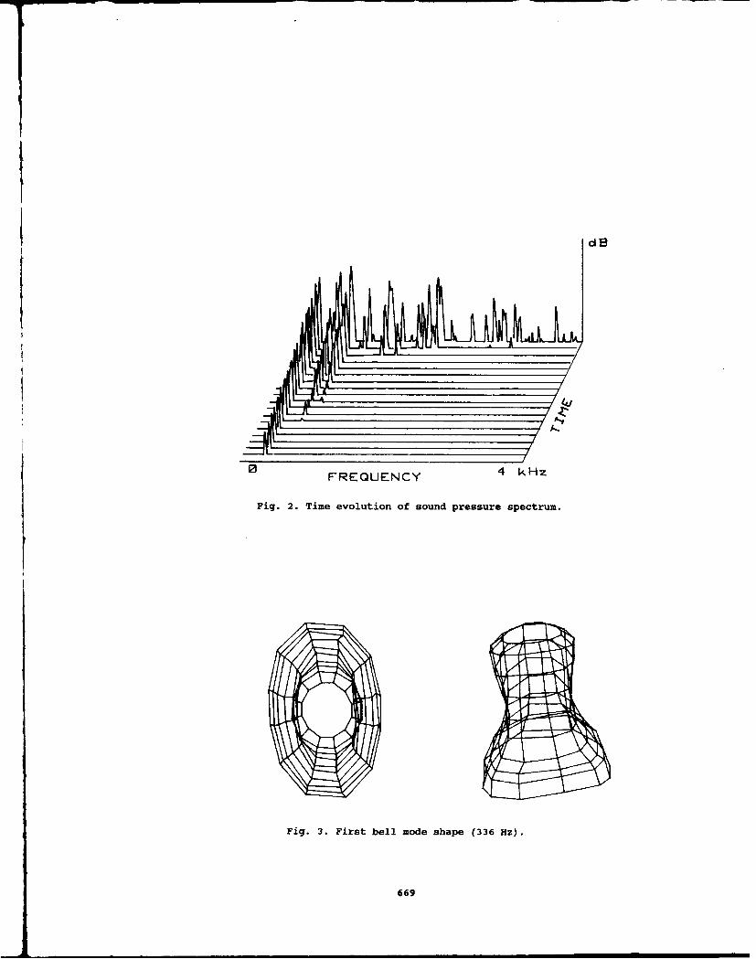
dB
4-1
0 FREQUENCY 4 kHz
Fig. 2. Time evolution of sound pressure spectrum.
Fig. 3. First bell mode shape (336 Hz).
669

of active sound intensity amplitude and vector maps (fig. 4) allows toconclude that bell surface maximum deformation zones make maximum
Fig. 4. Active intensity map (336 Hz).
contribution to sound emission. These zones could change their locationon the bell in dependence on excitation point location (point of tonguestroke).
THEORETICAL STUDIES.
The goal of theoretical studies was to investigate dependence ofbell eigenfrequencies and mode shapes on it's design (profile shape),alloy characteristics (elasticity module, specific density, Poisoncoefficient, etc.). Bell finite element model was developed composed ofvolume elements (8800 degrees of freedom, see fig. 5), which was usedto compute eigenfrequencies and mode shapes. Computations were done onHP workstation model 350 . Optimal number of degrees of freedom waschosen which insured 1% of accuracy in eigenfrequencies calculationassuming frequency range of first four eigenfrequencies (up to 2000 Hz)which form the bell "voice".This bell finite element model was identified using experimental modalanalysis. Experimental and computed eigenfrequencies are shown in table1. Correlation between experiment and computations is good enough.Finite element model identification also was done on the mode shapes andgood correspondence was obtained. On fig. 5 first mode shape is shown,this mode shape corresponds to that from experimental modal analysis.This model was used for studies of influence of natural variation ofPoison coefficient and elasticity coefficient on eigenfrequency
670
_____________________________

0 a,
Cu
'ata
0
44
671u

variation. Variation of these coefficient in 2-3 percent range causesthe variation of eigenfrequencies in 1-2 percent range. This finiteelement model was also used to develop methods of tuning the bell sound.Thus, developed bell finite element model allows on the stage of designto obtain bell design features(dimensions, weight, profile, alloy Table 1. Experimental andcomponents) which provide the computed bell eigenfrequencies.required sound characteristics ofthe bell. This design methodallows to obtain drawings of bell I Experiment I Computationjensembles to compose bellfrieswhich conforms to ancient Russian 336 Hz 336 Hzsound harmonic raw. Now we have 652 Hz 654 Hzdesigns of bell ensembles with 780 Hz 807 Hzweight from 8 to 1600 kg, which 1064 Hz 1063 Hzproduce sound within the range of 3octaves.
FIRST RESULTS.
Using developed drawings of 83 kg bells a number of bells weremanufactured and their acoustic characteristics were studied. In table2 eigenfrequencies and damping ratio one of these bells and the sameparameters of Samgin bell are shown.
Table 2. Eigenfrequencies anddamping ratio of new and Samginbells.
SNew bell I Samgin bell I
I Eigenfr. I Damping I Eigenfr.- Damping I
327 Hz 0.0010 336 Hz 0.0021664 Hz 0.0015 652 Hz 0.0017725 Hz 0.0011 780 Hz 0.0018
The new bell surpasses Samgin bell in continuance of sound especially onthe first tone. Eigenfrequencies of the new and Samgin bell are closeenough. On the subjective estimation of specialists "voices" ofmentioned above bells are very similar.
CONCLUSION.
The first stage in the bell sound research was implemented whichconsists of :1. the acoustic characteristics of Russian ancient Samgin bell werestudied;2. the finite element model of a bell was developed and identified onthe basis of experimental research;3. using finite element model the methods of bell tuning were developedand the dependence of "voice" of the bell from alloy components,dimensions and profile geometry was studied;4. the new bronze bell was manufactured which "voice" is similar tothat of Samgin bell;5. the drawings of bell ensemble weighting from a to 1600 kg whichproduce sound within the range of 3 octaves were obtained.
672

I
The following is assumed on the next stages of:1. to simulate on the computer the real bell excitation (tonguestroke);2. to study the stress distribution pattern of a bell to optimize thebell weight;3. to study the bell sound emission process using the boundary elementmethod;4. to create a data base on "voices" of ancient Russian bells whichcould be find in Russia.
ACKNOWLEDGEMENTS.
The authors would like to express their gratitude to Mr. A.N.Shatow of editorial department of Moscow episcopate for support in thisprogram.
673

674

SECOND INTERNATIONAL CONGRESS ONRECENT DEVELOPMENTS IN AIR- AND
STRUCTURE-BORNE SOUND AND VIBRATIONMARCH 4-6. 1992 AUBURN UNIVERSITY. USA
A COMPARISON OF MEMBRANE, VACUUM, AND FLUID LOADED SPHERICAL SHELL MODELSWITH EXACT RESULTS
Cleon E. DeanNaval Oceanographic and Atmospheric Research Laboratory
Numerical Modeling Division, Building 1100Stennis Space Center, MS 39529-5004
USA
ABSTRACT
A new set of spherical shell theories is presented with differing degrees of physicality, varying from asimple membrane model up to a fluid loaded shell theory that includes translational motion, rotary inertia, andtransverse shearing-stress. Numerical results from these theories are compared with exact results fromelastodynamic theory. The motivation of this study is to overcome the limitations of both modal analysisapproaches and of the somewhat more general Extended Boundary Condition (EBC) method due to Waterman,sometimes called the T-matrix method. The spherical shell is studied with an eye towards generalizing the resultsobtained to spheroids. The aim of the present research is to yield a better understanding of the scattering event byemploying more general and more physical shell theories.
INTRODUCTION
So-called "shell theories" simplify the calculations of the motion of thin elastic shells by makingassumptions about the scatterer and its movements. We use the standard assumptions of shell theory asformulated by A. E. H. Love [1] and which are as follows: first the thickness of a shell is small compared with thesmallest radius of curvature of the shell; second the displacement is small in comparison with the shell thickness;third the transverse normal stress acting on planes parallel to the shell middle surface is negligible; and finally thefibers of the shell normal to the middle surface remain so after deformation and are themselves not subject toelongation. These assumptions are used in the development of a shell theory for an elastic spherical shell in thespirit of Timoshenko-Mindlin[2,3] plate theory.
DERIVATION OF THE EQUATIONS OF MOTION
In spherical shells membrane saresses (proportional to P3) predominate over flexural stresses (proportional top32) where
I h
We differ from the standard derivation for the sphere [4] by retaining all terms of order pl2in both the kinetic and
potential energy parts of the Lagrangian and by considering the resonance frequencies for the fluid loaded case tobe complex. We note that this level of approximation will allow us to include the effects of rotary inertia and sheardistortion in our shell theory, as well as damping by fluid loading. The parameter ft itself is proportional to theradius of gyration of a differential element of the shell and arises from integration through the thickness of theshell in a radial direction. We will use an implicit harmonic time variation of the form exp(-iox). We begin ourderivation by considering a u,v,w axis system on the middle surface of a spherical shell of radius a (measured tomid-shell) with thickness h, as shown in Fig. 1.
675

%0
ey
Fig. 1. --- Spherical shell showing coordinates used. The ,, v, iv - coordinate system is somewhere on the mid-surface.
Lagranian vaiiational analysisThe Lagrangian, L, is
L = T - V + W, (2)
where T is the kinetic energy, V is the potential energy, and W is the work due to the pressure at the surface.The kinetic energy is given by
1 r2* rA12 -
T -2A2w Jo Jo- (.2( + wi2)(a + x) 2sin Odxd~do. (3)
where the surface displacements are taken to be linear as in Timoshenko-Mindlin plate theory:
a. = (I+a-)a• -- , (4)a a do
and
,= w. (5)
The motion of the spherical shell is axisymmetric sirice the sound field is torsionless. Thus there is no motion inthe v-direction. Substitution of Eqs. (4) and (5) into Eq. (3) yields, after integration over x and 0,
" .= hs It + 2 ihs h3 , d . h_ + h3 ,. h3 2sin -2( + -)a-+(-2 _X_)2 + (T+ ha ]do, (6)
or, in terms of 4,
T -- ,,p• '[(1.8,64 + 6P2 + j)li2 - (3.664 + 6#2 )iX +(1.8#4 +p)(- ) + (# 2 + l),s2jsin odg, (7)
whete the first and last terms in square brackets in Eq. (7) am associated with linear translational kinetic energiesand the middle two terms are associated with rotational kinetic energies of an element of the shell.
The potential energy of the shell is
V = ojj_,,2 . + a.sXx+a) sin odxdodo, (8)
676

where the nonvanishing components of the swain are
W a, d ) + 39 d82 f (9)
and
eft =(cotOu+w)+-+j-coc u- (10)a a 2 d
and where the nonzero stress components are
E(FRO = E_-2-( Ell + ref), (11)
and
E-r =•_v (E00 + vE"), (2
CIOO ý(12)
where E is Young's modulus. By substitution the potential energy becomes
v=!yJ 2'J 0 -f---- a 2 Iad200 ~ -.. IL jZx +a) a do ajO a ad
x -x du xdw 2-+2vfcotOf[(1+:-)u -- 1 l-) -w wJ (x+a{srnO[ fdOXa (13)
which after integration is
rEh du du1 V2- ((w+_) +(w+ucotO)2 +2v(w+-)(w+ucotO)
+fl2[ O_Ow d2) ot ( _.ýf2 Ow d'u -~ " Od d(92)cot O(u -) 2 +2votO(u---o)(-o-,-9)sm O. (14)
Terms in the potential energy proportional to 02 are due to bending stresses.And finally, the work done by the pressure of the surrounding fluid on the spherical shell is given by
S= 2Xa2 'p.wsin OdO, (15)
where p. is the pressure at the surface.
The Lagangjian density and its equations of motionA Lagrangian density must be used instead of the Lagrangian since the integration along the polar angle is
intrinsic to the problem. The Lagrangian density is
677

(6# +3. fl4e di du_,2
pha2[(I+ 6p2 + 1.8304),i2 ',-( 6+ 3 ) + (2 + 1.84)(-
'[do a o'J'do 3 do2
+(I + v2)V+,2 ]sin 0 - aE2._ (w + 46)2 + (W + ucot 0)2 +32v(w2+ -)(w + ucot 0)V2 - do"l8 do
+2 ia 2p.w sin 0, (16)
with corresponding differential equations of motion
d L d dL d 0Ld= Ouddu, dt du,'(7
and
( )dL d dL d uL+ d2 22 dc (18.,0-dw- dO 'w, -dtw -dn +dOdt 5;9 + dO2 0w"a(8
where subscripts denote differentiation of the variable with respect to the subscript.
By substitution ofEqs. (17) and (18) into (16) we obtain
O = (1l +2 fL- + cot2 O-U_ -(V + cotv O)u-2 ' -2f/ Cot a -W
+[(1+ V)+32(+ v+cot2O)] -2(4 p2 + 1) o2U )264(1+ vdo C2+6 ) t -(1.83 +3.2 )2---•t, (19)
and
(-. (IV2)a 2 = 2 d'u+ 2pCo 0 2 dU-[I+V)(l+.82) + 2 Cot2 9)1du
p.f i-23 cot 0(2--t !ý -2(l+v
doa+ 2
p42 U 2 ^d2U
T- --1. + 3 C_5U0
p+p2_d 4W2 d'W ,d 2 W
0 12 O dIW 2+Cot t(20)•.__(~~+3(1.+3 ~3) V+C 2 +)--1.-8-3+ / t (20)
These differential equations of motion (19) and (20) have solutions of the form
u7)=X 1- 1 2)1/2 dp.U07) .(l -71 -(21)
and
S+7)= )W.•-•',to (22).78
6781

where 17 = cos0 and P,(7/) are the Legendre polynomials of the first kind of order n. When the differentialequations of motion (19) and (20) are expanded ir. terms of Eqs. (21) and (22). we obtain a set of linear equations
in terms of U. and W., whose determinant must vanish. We shall consider two cases: with and without fluidloading.
The vacuum caseThe vacuum case is the simpler problem that occurs when the spherical shell is surrounded by a vacuum
such that there is no damping. Thus, the pressure at the surface vanishes: p. = 0. The set of linear equations theexpansion coefficients must satisfy are
0 =[ (I + 66l2 + 1.8p4) -(I +l 2 )K]U. + [p2 (3P32 + 1.8fl4)-_1 2•_-(1 + v•1]W, (23)
and
0 = -. [f(ic - 3)p32 - 1.8134 + I + vJU. + [C2 (I + 212 + 1.8#34) -2(1 + V) -_32 Kj. ]W., (24)
where Q = aoa / c, K = v + A. - 1, and A. = n(n + 1). In order for Eqs. (23) and (24) to be satisfiedsimultaneously with a non-trivial solution the determinant of the system must vanish:
0 = C14(1+ 6P2 + 1.8 .')(l + 2fl2 + l.813 4)+fl 2 ((31 2 + 1.8364)A, [(r - 3)p2 _ 1.8p4+ + v]
-[2(1 + v) + P12 . ](I + 6p32 + 1.8p4 ) - (I + 3 2
) K(1 + 2p2 + 1.8#4))
+(I + 12),[2(l + v) + fl3 2 d. ] - A. [(K - 3)p 2 - 1.8p34 +1 + v](3 2 + I + V). (25)
Since there are no damping terms, the shell vibrates theoretically forever. Thus, the normalized frequency12 can be taken to be real. Equation (25) is quadratic in C2l, thus we expect two real roots to (25) and thus twomodes for the motion of the shell. They are the symmetric and antisymmetric Lamb modes.
The fluid loaded caseThe fluid loaded case requires that we consider a modal expansion of the surface pressure in terms of the
specific acoustic impedance z,. In its most general form this is
p(a, 9, 0) = i Xz.W.iv '(cos O)cosmO, (26)~0-0
where
• K(ka)z.=zc•-• (27)
The specific acoustic impedance z. can be split into real and imaginary parts:
Z. = r. - io. n., (28)
where
r. =pcR¢{.A--•a, (29)
679

and
M., = PEIMI ah(ka)}1 (30)
For the case of axisymmetric motion we are considering, the surface pressure is
p.(O) = -. z.W.P,.(cosO), (31)
or by substitution,P, (O) = -i ( -coW., - 0),W.m, )P,(cos 0). (32 )
-0
Use of Eq. (32) in our set of differential equations of motion (19) and (20) yields the following set of linearequations for the expansion coefficients in the case of a fluid loaded spherical shell:
0 = [0j2(1 + 6p2 + L 8,4) - (1 + p2),C]U. + [Q2 (3fi2 + 1.8p 4) - p2 K _ (1 + v)]W,, (33)
and
0 K- ,[(xc- 3)fl2 - 1.8P4 + 1 + vyJ].+[0 2 (1 + a + 2P 2 + 1.8p4) - 2(1 + v) + Oy _p -2 KA.]W.. (34)
where
a m (35)ph
and
(36)h p,c,
Again the determinant of Eqs. (33) and (34) must vanish. However, in this instance the value of 0 must be takento be complex; the resonances have a width that depends on the damping. The result of setting this determinant tozero is
0 = o 4 (1 + 6p2 + 1.8fi4)(I + a + 2p2 + 1.8p')+01 iy(1 + 6ft2 + 1.8 gs) +0 2{(3p2 + 1.89),t,.[(K - 3)p2 - 1.8,6 + 1 + vI
-[2(1+ v) +.82 r. ](1 + 6P2 + 1.8P4) - (1 + p2 ) w(1 + a + 2P2 + L 8p4)) +r4-_Y(1 + p2) KI
+(1 + p2) K[2(1 + v) +P2 rK.] - A.[(w- 3)P2 - 1.8p4 + I + v](p 2 + I + v). (37)
Equation (37) has at least four complex roots. From work with an exact modal solution to the problem, weexpect two roots to be associated with the symmetric and antisymmetric modes of the shell. We expect the othertwo roots to be associated with a water-borne pseudo-Stoneley wave.
CONCLUSIONS
The next step is to plot the roots of Eqs. (25) and (37) to compare the resonances predicted by these modelswith those given by exact modal expansion solutions. By suppressing a and ?, the model associated with Eq.(37) reverts to the vacuum case model associated with Eq. (25). Similarly suppression of factors of P in Eq. (25)will result in a reversion to a previously derived solution (Junger and Feit, 1986). We may then rank the threedifferent models according to their degree of physicality and compare their results for various relative shellthicknesses against each other and against the exact results of the modal expansion model. We may also considerthe limitations of each of the models including the exact solution, as well as those of shell models in general.
680

By setting the values of a and y in Eq. (37) to zero, we revert the shell theory model to one without fluidloading. Similarly, by setting P3 to zero as well, the model reverts to a membrane model. These models, fluidloaded, vacuo case, and membrane, are successively less physically sophisticated and give successively less goodcomparison with exact (modal expansion) results. Starting with the least sophisticated model, we see in Fig. 2thick spherical steel shell dilatational (symmetric) and flexural (antisynimetric) mode resonances calculated by themembrane model. Here and in the succeeding figures thick means h/a =0.1; thin means h/a=0.01. The shell
material is a generic steel with density p, = 7.7 times that of water, shear velocityv; = 3.24 km/s, and longitudinal
velocity v, = 5.95 km/s. The surrounding fluid is taken to be water with density p = 1000 kg/m 3 and sound
velocityc., = 1.4825 km/s. The symmetric mode shows a good comparison between exact and shell theorypredictions, but the antisymmetric shell theory results for this approximation compare poorly with the exactflexural results. Note that some symmetric mode resonances were not found by our exact theory algorithm. InFig. 3 we see thin spherical steel shell dilatational (symmetric) and flexural (antisymmetric) mode resonancescalculated by the membrane model. Again there is good comparison between dilatational (symmetric) moderesonances calculated by the two methods, except for the first couple of resonances. Only a few exact flexuralresonances were picked up by our algorithm. And again the shell theory flexural (antisymmetric) moderesonances show the do not asymptote properly with increasing order. In Fig. 4 we have thick spherical steelshell dilatational (symmetric) and flexural (antisymmetric) mode resonances calculated by shell theory withoutfluid loading (vacuum). As in the membrane model the shell theory and exact calculations compare well for thedilatational (symmetric) mode resonances. In contrast with the membrane model, hcwever, the exact and shelltheory calculations for this model show much better agreement for the flexural (antisymmetric) mode resonances.This model does not include fluid loading, but does include the effects of shear distortion and rotary inertia. Thevacuum shell theory flexural mode resonances do not asymptote for large size parameter ka to the exact results,however. In Fig. 5 we see thin spherical steel shell dilatational (symmetric) and flexural (antisynms-'-' moderesonances calculated by shell theory without fluid loading (vacuum). As in the membrane model y . •/and exact calculations compare well for the dilatational (symmetric) mode resonarxces except for the Yresonances. This vacuum model does not have fluid loading, and has insufficient damping for todilatational (symmetric) mode resonances. Again, the flexural (symmetric) mode resonances show. ., :hecorrect behavior, but it is not possible to tell what the asymptotic value of the phase velocity would be tor largesize parameter on this scale. Next in Fig. 6 we have a plot of thick spherical steel shell dilatational (symisatnmc)and flexural (antisymmetric) mode resonances calculated by shell theory with fluid loading. As in the vacuumcase as well as for the membrane model, the dilatational (symmetric) mode resonances compare well for exact andshell theory methods. The flexural (antisymmetric) mode resonances, as calculated by shell theory with fluidloading, do not appear to have the correct asymptotic limit for large size parameter, although they do exhibitroughly the correct behavior for lower values of ka. Finally, in Fig. 7 we see thin spherical steel shell dilatational(symmetric) and flexural (antisymmetric) mode resonances calculated by shell theory with fluid loading. Theexact and shell theory calculations agree well for the dilatational (symmetric) resonances and exhibit a markedimprovement for the first several shell theory symmetric mode resonances. This is due to the inclusion of fluidloading in the modeL The flexural (antisymmetric) mode resonances show the appropriate behavior on this ratherlimited size parameter scale.
ACKNOWLEDGMENTS
We wish to thank the Office of Naval Research, the Office of Naval Technology, and NOARL managementincluding Drs. Chin-Bing, Franchi, and Moseley. Dr. Dean is at NOARL on an ONT Fellowship. This workwas funded by NOARL Program Element 61153N, G. Car, Program Manager.
REFERENCES
I. Love, A. E. H., A Treatise on the Mathematical Theory of Elasticity. 4th ed., Dover, New York, 1944, pp.515-537.
2. Timoshenko, S., On the correction for shear of the differential equation for transverse vibrations of prismaticbars, Phil. Mag. 41, 744-746, 1921.
3. Mindlin, R. D., Influence of rotary inertia and shear on flexural motions of isotropic elastic plates, J. Appl.Mech., 18, 31-38, 1951.
4. Junger, M. C. and D. Feit, Sound, Structures, and Their Interaction, 2nd ed., MIT Press, Cambridge, Mass.,1986, pp. 245-251.
681

020 200
-Z! 16.- 16. *
- ym eetricA Ea Sy r c A Ux At
8 x
S4 4.
0 .+ .. 00 10 20 30 40 50 60 70 80 0 10 20 30 40 50 60 70 80
Size Parameter Size ParameterFig. 2. Thick steel shell, membrane model (h/a = 0.1). Fig. 3. Thin steel shell, membrane model (h/a =0.01).
20- 20-
16--°---- -16+0 2hI Th She S ., 2h Thei
12- P-e. A 12 _ + S Tb-5 + -eti -
i2 x :e ic x En v"etI m 4 4 '+
0 0
0 10 20 30 40 50 60 70 80 0 10 20 30 40 50 60 70 80Size Parameter Size Parameter
Fig. 4. Thick steel shell, vacuum model (h/a = 0.1). Fig. 5. Thin steel shell, vacuum model (h/a =0.01).
20. 8.
416- - - -lbn • 7--aShe T~he A sy c 6 -- K
S.. - et5i .. ..12 T x. EX&(~ Th s_g 4----
7 0 10 20 30 40 50 60 7 0 0 10 20 30 40 50 60 70 80
_Size Parameter Size ParmeterFig. 6. Thick steel shell, fluid loaded (h/a = 0.1). Fig. 7. Thin steel shell, fluid loaded (h/la =0.01).
682
CL
0 % 00 02 04 06 09 02 04 06 09

SECOND INTERNATIONAL CONGRESS ONRECENT DEVELOPMENTS IN AIR- AND
STRUCTURE-BORNE SOUND AND VIBRATIONMARCH 4-6. 1992 AUBURN UNIVERSITY, USA
EXPERIMENTAL STUDIES OF WAVE PROPAGATIONIN A SUBMERGED, CAPPED CYLINDRICAL SHELL
Earl G. WilliamsNaval Research Laboratory, CODE 5137, Washington D.C. 20375USA
ABSTRACT
Experimental measurements on point-driven, fluid-loaded cylindrical shells in the fre-quency region 0 < ka < 10 are processed using nearfield acoustical holography and wavevector filtering in order to expose the details of wave motion on the structure. Gabortransform tools along with the creation of various filters in the k-w space domain are usedto study impulsive wave packets as a function of space and time excited by a point driveinside the shcll. This technique provides a very powerful tool for the study of expcjrimentaldata. In particular, we are able to visualize the difference between phase and group veloci-ties for helical waves traveling on the shell. Of particular note is the ability to display waveconversion at discontinuities, such as the ends of the shell. This wave conversion consistsof flexural to longitudinal, longitudinal to flexural, and conversion into radiated pressure.Similar conversions occur with shear waves, which are shown to be excited by a normalpoint force in the frequency region ka > 2.
INTRODUCTION
It is the objective of this work to uncover basic mechanisms of wave propagation on,and radiation from simple shell structures through the use of signal processing techniques.One of the simplest shell structures is a cylindrical shell with spherical-like endcaps, driveninto vibration by a point force inside. Although simple in structure, this vibrator is rich isbasic physics. To study this simple structure, the Naval Research Laboratory has severaladvanced research, large pool facilities. Robotic scanners under computer control trackpredefined contours and measure the pressure fields generated from the vibrator very closeto the shell. These contours are either cylindrical or conformal. Using nearfield acousticalholography (NAH)[I1 this information is processed to yield the normal velocity on thesurface of the shell as well as the surface pressure. At this point wave vector filtering(WVF) techniques are applied to provide an experimental dispersion analysis (free wavesof propagation) of the shell. We will discuss in this paper the processing steps which aretaken in WVF leading to the final result: the impulse response of the structure in the timedomain.
683

DESCRIPTION OF PROCESSING
Figure 1 shows a typical measurement grid for the nearfield pressure created by thev-brations of a point-driven shell. The point driver located inside the shell is excitedwith a chirp signal so that a broad range of frequencies can be covered with a singleexperiment.[1] The radial surface velocity is reconstructed using NAH on a grid concentricto the measurement grid at a radius equal to that of the shell. Where this grid coincideswith the surface of the shell, the radial surface velocity is reconstructed.
MeasurementGrid Point-Driven Shell
Figure 1- A computer controlled, robotic scanner measures the pressure over the grid shown(128x64) axial x circumferential points. The point-driven shell is excited by a chiptime signal.
Kz
Ssurh Velociy
(pw Unit Fares) Hlc Wuvam ci BuCg wanv Dqe su
IFFTKz->z
•r
14 I"nePulte RIqxn 14 stn->g Wm
Figure 2- Flowchart of the wave vector filtering process. The various Fourier transforms areindicated which take us through the flow chart in the clockwise direction.
684

The processing steps of WVF are shown in fig. 2. Note that the reconstructed surfacevelocity is normalized by the driving force generated by the point driver. The same normal-ization is applied to the measured pressure, creating transfer functions which provide theinput to WVF. These transfer functions are Fourier transformed to the frequency domainto provide the first box in the flow chart in fig. 2. The three-dimensional coordinate systemindicates that a cube of data exists, with two-dimensional slices displayed in the figure. Atypical data set consists of 128x64x512 points corresponding to the triplet (z, 0, W).
The first processing step takes spatial Fourier transforms in the circumferential andaxial directions. Thus vp(z, 0,w) --, Vp(k,, k#,w). The second box in figure 2 demon-strates this process and displays the magnitude of VF for a particular frequency. Themagnitude of Vp forms a 'figure 8" locus (the DC wavenumber is at the center of the "8").This locus is produced by the quasi-bending free waves which are excited on the shell andare discussed at length in a recent paper. (2]
The third panel in figure 2 represents an important processing step in which the wand k# axes have been interchanged. This plot shows the magnitude of VF for a particula-circumferential harmonic, k# = n. This plot is called an experimental dispersion curve,and provides the dispersion character of the n'th harmonic. The origin is at the center ofthe k. axis (not as shown) so that the right bianch indicates free waves traveling to theright on the shell, and the left branch waves to the left. As usual the slope of the curve atany point provides the axial group velocity of this wave. Note that the axial phase velocityis given by c. = w/k,.
The fourth panel in fig. 2 is derived from an inverse FFT on k,. Thus we haveVF(z, n, w). This plot is called a standing wave plot as it shows the distribution of nodes andantinodes as a function of frequency for a given value of n. (The gray scale representationhas been reversed in this plot so that the light areas represent the largest magnitude.)One can see the number of antinodes increasing with frequency (the slow quasi-bendingwave) until the rapid oscillation gives way to a much longer wavelength wave (the fastshear wave) about midway up the frequency axis.
The final step in the WVF flowchart is an inverse FFT in w to yield vF(z, n, 1). Thisis called the radial velocity, impulse response. Since all quantities are normalized to thedriving force (in the frequency domain), this inverse transform simulates the response ofthe system to a impulsive force in time. This is a band-limited impulse since generally alimited band of frequencies is selected from the standing wave data before the inverse FFTis applied. The actual location of the driver is just to the right of the displayed origin infig. 2. The dark areas represent the tracks of the impu!se as the wave travels down theshell, reflecting off of the endcaps to travel in the opposite direction. The slope of thesetracks provides the group velocity of the wave. Further processing can be applied to thistype of display to uncover the reflection coefficients of these waves at the ends of the shell,presented in another paper in these proceedings.[3J
Figure 3 illustrates some other processing schemes of the WVF approach used in thestudy of wave propagation in shells. The wave dispersion data (panel 3 in fig. 2) can beused as a starting point of three different filtering schemes. We will discuss the secondscheme in this paper. In this case the wave dispersion data is filtered by zeroing out thenegative part of the k, spectrum (illustrated by the stop band in the figure). A Tukeywindow is used in the transition region to smooth the data. Proceeding with the processingas shown in the last two panels of figure 2 one then arrives at the impulse response withwaves traveling only to the right in the shell, as shown in the center plot of figure 4. Ifone zeros out the right half of the k. spectrum, then waves traveling only to the left areobtained as shown in fig. 4. In this way the tracks of the waves can be analyzed better, andreflections more clearly studied. For example, the left-going waves in fig. 4 indicate wavesemanating from the center of the shell, corresponding to an internal ring discontinuity inthe shell. This discontinuity was extremely small, and was not detectable in the surfacevelocity plots (vF(z, 4.) at a given frequency). Unfortunately the gray scale rendition ofthe wave tracks obscures a lot of the details, which are much clearer shown in the colorviewgraphs presented in the talk corresponding to this paper.
685

=Stop Band
SuperSonic- __"_Impulse"
Response
•Kz /tzWave Dispersion K_
Right-GoingWaves
' Kz Z
Wave Dispersion _ _ _ _V - FrequencyS~Band-Limited
• Response
Kz /K Wave Dispersion Ký
Figure 3- A example of the three kinds of filters which are applied to the data in the "wave
dispersion domain". The center filter provides waves traveling only to the right, asshown in the center plot of fig. 4.
Another observation from fig. 4 is the left-going wave which appears at the very
bottom right of the 3rd panel. There does not appear to be any right-going wave which
causes it. Further processing uncovered a fast longitudinal wave launched at t = 0 fromthe point driver and traveling to the right with a nearly horizontal slope (about 5000 m/s).
When this wave struck the right end of the shell, it apparently was converted into the slow
quasi-flexural wave shown in fig. 4. The details of the fast waves are easily studied from
the impulse response of the pressure recorded on the measurement contour (fig. 1), as will
be shown in the lecture. This phenomenon of wave conversion at the ends of the shell is a
significant one, especially in light of the fact that the slow wave is subsonic, as thus is a
poor radiator, whereas the fast wave is supersonic and an efficient radiator.
686

Total Response Right-Going Left-Going
9.2
•42
9.8
2.4
9.0
7377.2
&2aa24
42.
1 61.40.80
ZL u1I~n-O Z Lae: n-O
I L M#:n ..O
Figure 4- Normal surface velocity as a function of (z, t) for the n = 0 circumferential harmonic.
The drive point is at t = 0, Z Lat = 40. The filter shown in the middle of fig. 3 is
applied to expose waves traveling to the right (center panel) and a similar filter to
provide waves traveling to the left (right panel). The dark lines ima' •ate wave tracks
of the quasi-fiexural wave. Slight widening of the tracks is the result ,f dispersion.
ACKN OWLEDGMENTS
This work is supported under a contract with the Office of Naval Research.
REFERENCES
1. E.G. Williams, B. Houston, and .1. Bucaro, "Broadband nearfield acoustical hologra-
phy for vibrating cylinders", J. Acoust. Soc. Am. 86, 674-679 (1989).
2. E.G. Williams, B. Houston, and J. Bucaro, "Experimental investigation of the wave
propagation on a point-driven, submerged capped cylinder using I(-space analysis",
3. Acoust. Soc. Am. 87, 513-522 (1990).
3. J.A. Mann III and E.G. Williams, "Determining the amplitude of propagating waves
as a function of phase speed and arrival time", 2nd International Congress on Recent
Developments in Air- &z Structure-borne Sound and Vibration, Auburn University,
(1992).
687
2.4 mm m m m l m mm

688

T
SECOND INTERNATIONAL CONGRESS ONRECENT DEVELOPMENTS IN AIR- AND
STRUCTURE-BORNE SOUND AND VIBRATIONMARCH 4-6. 1992 AUBURN UNIVERSITY. USA
SOUND ABSORBING DUCTS
Alan CummingsDepartment of Engineering Design and Manufacture
University of HullHull, N. Humberside HU6 7RX
U.K.
ABSTRACT
Some examples of epproximate variational solutions to problems involvingsound absorbi, ducts are given. More or less simple Rayleigh-Ritz typeformulations are applied to sound transmission in ducts - of variouscross-sections - having porous bulk-reacting liners, and to sound propagationin capillary tubes. Comparisons are made between these approximate solutions,exact solutions and experimental data (where these are available).
INTRODUCTION
Exact solutions to physical problems may, in some cases, not exist or (inothers) may involve higher functions that are difficult to compute. In suchcircumstances, purely numerical solutions to the governing equations of theproblem may be sought, finite element (FE), boundary element (BE) and finitedifference (FD) techniques being examples of methods that are fairly widelyused. In most cases, the implementation of these solutions would involvecomputer software packages or else computer codes that were specially writtenfor the purpose. In either case, considerable effort is likely to be expendedon the solution, and in some cases the use of numerical methods can result ina certain loss of "feel" for the physics of the problem. Examples of numericalstudies in duct acoustics are the work of Astley and Eversman [1W, who haveapplied a FE technique to sound propagation in flow ducts withlocally-reacting liners, and that of Chang and Cummings 121, who utilized a Dmethod in perforated tube flow duct silencers with hydrodynamicnonlinearities. There is a large body of published work describing theapplication of various types of numerical technique in both acoustics andvibration.
An alternative to FE methods is the use of simpler variationalformulations such as the Rayleigh-Ritz technique, which is closely related inits basic principles to FE methods, but is generally much less demanding interms of computational effort. Indeed, the least complicated Rayleigh-Rit?approaches can yield approximate solutions in exp- cit form (see, for exam-le,the paper by Astley [31), which can perw.it fairly easy physicalinterpretations of the results. There are many problems which lend themselvesreadily to this type of treatment, and we discuss some of them in this paper.
GENERAL FORMULATION
One of the attractive features of a 'ariational formulation is that thegoverning differential ejuations and most for all) of the boundary conditions
689

(b.c.s) in t 1,e i,.o ,L1-m ire implicit in a single equatloin. It the tiý id,ai iab le (which may be the acoustic pressure, the temperature perturbat ti, ora particle velocity component) is denoted q,, and the prolnlem istwo-dimensional in the (y,z) plane, with v being defined in the e-gion R, thi-na functional F(W) may be defined,
F(w) = Rf(J , ,4 ),dR, 1)2 2 2 2
where f( I is a function of 1, l 2p/ay ,2, 2qt/dz2, that could I in principle) alsoinclude derivatives such as )W/ay et cetera. If F is minimized w.r.t. yi, then
6F = 0. (2)
This equation gives rise to Euler equations, which embody the •overnin:differential equations and the natural b.c.s (which may or may not be the sameas the physical b.c.s). The function f( ) may be chosen to yield the desiredEuler equations and natural b.c.s. In the Rayleigh-Ritz (R-R) method, a trialfunction 0 is employed,
= .a P (y,z), (3)n n
where a are arbitrary coefficients and the functions 0 are chosen so thatnnthey satisfy the physical b.c.s on C, the boundary of R; we note that tp and iare different functions, unless VJ happens to be an exact solution to thegoverning differential equations, subject to the prevailing b.c.s. Equation(2) requires F(0) to be minimized w.r.t. the a , that is
aF/s3a = 0 (n = 1,2. .......... N). (4)n
Equation (4) yields a series of N simultaneous, homogeneous or inhomogeneous,linear equations in the cases (respectively) of homogeneous and inhomogeneousgoverning differential equations. In the first case, an eigenproblem results,from which the relative values of the a may be found, and in the second
instance, the absolute values of the a are determined. In either case, the
approximate solution W is found and the accuracy of the approximatioin usuallyimproves as N is increased.
A RECTANGULAR FLOW DUCT WITH AN ANISOTROPIC BULK LINER
Our first example of the use of Rayleigh-Ritz methods in sound absorbingducts is a two-dimensional planar sound field in a rectangular duct with ananisotropic, porous, bulk liner placed against one wall. A uniform airflow
ABSORBENT . Y2 2.
MACH " " RIGID WALLS
NUMBER M
xFigure 1. A rectangular flow duct
passes along the duct as shown in Figure 1. A fairly simple exact solution
exists in this case (see the more general analysis of Sormaz and Cummings[41), and we may compare our approximate solutions to the exact result. Weseek modal solutions of the form
p(x,y;t) = exp(iwt) A i Yi(y) exp(-iaikx), (5)I-1
w being the radian frequency, k the acoustic wavenumber and a. a dimensionless
690

I
axial wavenumber. If we choose
h1)h 2 2 , IM 2_ j2
F(Y) = [1/2(1-_M)JbfO ty2 - k2HllcgM) -uJY )dy
h+a+ (P/2P)b~f H1y ;) 2
- k'( _.2/.,:)Il y
2 Idy, (6)y h y 2
where b is the depth of the duct and py, 1., -y are the complex effective
density of the fluid in the absorbent in the y direction, and the propagationcoefficients (in units of ik) in the x and y directions respectively, theEuler equations of this functional are: (i) the convected wave equation inregion 1, (ii) the wave equation in the absorbent, (iii), (iv) the hard-wallb.c.s at the duct wall, (v) the b.c. of continuity of normal particledisplacement at the interface between absorbent and airflow passage. Boundaryconditions (iii)-(v) are the natural b.c.s, and constitute all but one of thephysical b.c.s. The remaining b.c. is that of continuity of pressure at theinterface, and we satisfy this by choosing a trial function that is continuousat y = h. The choice of the trial function is to some extent determined by theprior knowledge that Y(y) (for a pearticular mode) is a sinuous function (thisis apparent from the exact solution, which involves sine and cosinefunctions). Even without this information, we would have guessed as much, andtherefore trigonometric functions are appropriate for the c . While it is
perfectly possible to choose 0 = cos[nny/(h+a)], we note from b.c. (v) that
there is a discontinuity in Y' at y = h which cannot be accommodated by afinite number of terms in the summation, so it is more satisfactory to selectseparate trial functions for regions 1 and 2, viz.
Y, A + Bn sinniy 1 /2h), Y2 = A + C sin~niy 2 /2a), (7a,b),. Z,3, . . n1-,, .
where A, B , C are complex coefficients. Equations (4), (6) and (7) give rise
to an eigenproblem from which ai may be found. The modal attenuation rate is
then A = -8.6858 Im(k ) dB/m (if SI units are used); the axial phase speed is
given by c = w/Re(ka ) m/s.p
100.
(dB/m)
10
(a) C~b)
1 t . . . . .. . 1
200 Ik FREQUENCY (Hz) 1k 8k
Figure 2. Comparison between A for the exact solution, X , and single,------ 0o, three, o--------- , and seven, -- , d.o.f. R-R solutions for the
fundamental (i=1) mode in a duct with a fibrous absorbent having steady flowresistivities of 104 and 2x10⁴ SI rayl/m parallel and normal (respectively) tothe laminae of fibres; a = h = 100 mm; (a), M = 0.1, (b), M = -0.1.
691

The simplest solution involves a single degree of freedom (d.o.f.), witha uniform pressure trial function, and is found by putting B , C = 0. A
quartic equation must be solved to find a if there is mean flow, but thisequation becomes quadratic if H = 0, and an explicit expression may thereforebe obtained for a. Solutions with more degrees of freedom may be found and insuch cases, we may cast the problem either in the form of a determinantaleigenproblem (which may be solved by an iterative procedure such as Newton'sor Muller's method) or a generalized matrix eigenvalue problem (which may besolved by a standard routine). Each method has its advantages and drawbacks,but in the computations presented here, Newton's method was utilized.
In Figure 2, comparison is made between the exact solution and three R-Rsolutions for the attenuation rate of the fundamental mode in a rectangularduct. In the case of downstream propagation (M = 0.1), the uniform-pressureR-R model gives poor predictions even at low frequencies, while the threed.o.f. model yields acceptable predictions up to 1.8 kHz, beyond which thepredictions become increasingly inaccurate as the frequency rises. The sevend.o.f. model gives quite good results up to about 3-4 kHz. For upstreampropagation, the R-R predictions are generally better (because the transversepressure distribution is more uniform), although the one d.o.f. curve is stillnot adequate. The three d.o.f. model gives sensible predictions, even up to 8kHz, and the seven d.o.f. solution yields good accuracy up to 8 kHz. Otherdata (not shown here) indicate that the simplest, single d.o.f., R-R modelgives its best predictions for ducts with either large or small a/h ratios,for absorbents of low flow resistivity and at low frequencies, that is, wherethe actual transverse acoustic pressure profile is at its most uniform. Thegeneral trend is for more d.o.f. to produce more accurate results. Inpractical terms, there is no reason for one to use a R-R type solution for arectangular duct, since the exact solution may readily be calculated, but inthe case of (for example) a circular duct, there may be some advantage, sinceBessel and Neumann functions are more time-consuming to compute* than circularfunctions. We next discuss the case of a circular geometry.
A CIRCULAR FLOW DUCT WITH AN ISOTROPIC BULK LINER
To avoid excessive complication in turning to a circular geometry, weexamine a duct with an isotropic bulk liner, placed against the wall; theanalysis follows that of the rectangular duct very closely. The trial functionis essentially similar and so is the expression for the functional, though0/By is replaced by 0/Br and the integrals over the areas of regions 1 and 2take on a somewhat different form. Figure 3 shows a comparison between axialattenuation rates of the fundamental mode in a duct with a liner consisting ofan open-celled polyether foam with a steady flow resistivity of 5 430 SI
(dB/m,0-
Ik FREQUENCY (Hz) 2k
Figure 3. Comparison between the exact solution (w==--=c, M -0.197, X------4,H = 0, w----- , H = 0.197), single d.o.f. (O---0, M -0.197, 0-------O, M =0, O-- - -- , M = 0.197) and three d.o.f. (,&-----&, H = -0.197, b-- , M = 0,
- H = 0.197) R-R solutions for a in the fundamental (i=l) mode in acircular duct with a polyether foam liner; inner radius = 19.8 mm, outerradius = 38 mm; *, experimental data for M = 0.
692

rayl/m, predicted from the exact theory (which involves Bessel functions of
the first and second kinds) and from one and three. d.o.f. R-R formulations.
Numerical data are shown for three mean flow Mach numbers: 0, -0.197 and
0.197; experimental data are also shown, for zero flow.It is clear from Figure 3 that even the single d.o.f. R-R solution gives
generally quite fair predictions of A, though for H = 0.197 the accuracydeteriorates above about 1.5 kHz. The three d.o.f. R-R solution yields resultsthat are indistinguishable from the exact solution at all frequencies and forall three Mach numbers; predicted and experimental data for M = 0 agree well.The more favourable performance of the simpler R-R solutions in this caseresults partly from the lower flow resistivity of the foam as compared to thefibrous material and partly from the lower frequency range, smaller percentflow area and smaller duct width in this example.
AN APPROXIMATELY ELLIPTICAL FLOW DUCT WITH A CIRCULAR GAS FLOW PASSAGE AND ANINHOMOGENEOUS ABSORBENT
1 JK -(Di 125 mmR
220 mm
(a) (b)
Figure 4. The SAAB silencer: (a) cross-sectional geometry, (b) subdivision ofabsorbent in the R-R formulation.
This is the practical case of a SAAB automobile silencer, and is the mostdemanding of those discussed so far, in view of its awkward geometry and theinhomogeneity of the absorbent. Whereas in the previous two cases, exact
solutions have been available, this is not the case here; partly because ofthe geometry, and partly because of the inhomogeneous nature of the porousmedium, we cannot find analytical solutions to the present problem. Thecross-sectional geometry of the silencer is shown in Figure 4(a); the flowpassage occupies 18% of the total cross-sectional area. The casing isapproximately elliptical in cross-section and the flow passage is circular.Though there is a layer of very coarse stainless steel wool and a perforatedtube immediately within the periphery of the flow passage, the presence ofthese is ignored since they would be expected to present little impediment tothe passage of sound waves. The absorbent (a basalt wool) was found to have arelatively high steady flow resistivity (about 24 000 SI rayl/m) where it wasthinnest, but a low flow resistivity (about 8 000 SI rayl/m) at the thickestpoints. The flow resistivity was relatively insensitive to the coordinatedirection, and so the acoustic properties were taken to be isotropic. Becauseof the inhomogeneity, however, the absorbent was subdivided into regions ofconstant properties. Figure 4(b) illustrates how this was done. Provided wetake a sufficient number of these regions, the effects of inhomogeneity willbe adequately taken into account.
For the purposes of a R-R formulation, the sound field in region R0(which is circular), may be assumed to be axisymmetric if only the fundamentalmode is of interest, but in regions Rt, R2,... it should be allowed to vary
both radially and perimetrally. These regions were chosen to be radialsegments, and a radial variation in the trial function for sound pressure waspermitted, though the perimetral variation was suppressed. The trial functionwas axisymmetric - with two d.o.f. and a form similar to that in equation (7V- in R0, and continuous at the interface between flow passage and absorbent.
693

Separate two d.o.f. trial functions (like those in equation (7b)) were allowedin the sub-regions of absorbent; the coefficient A was common to all regions(including the flow passage), ensuring continuity of sound pressure at theinterface, but the coefficients of the quarter-sine function differed betweensegments. Because a perimetral pressure discontinuity existed between segmentsin the trial functions, natural b.c.s of continuity of pressure and normalparticle displacement between segments were required, in addition to thenatural b.c.s of the rectangular duct problem. A more complicated functionalis required here, and has the form
0R[tp _ 22 •2
+ - k 2(,-u.) IdRB + Pu2 (p -p Wit (8)i i
where y is, a priori, the dimensionless propagation coefficient (the same in
all coordinate directions in this problem), V is the two-dimensional
Laplacian operator on the duct's cross-section, p is the effective density, p
is the transverse spatial factor in the sound pressure field and E is theacoustic particle displacement normal to the boundaries between segments. Thisfunctional has all the required natural b.c.s. Because k appears in thefunctional together with p, it too has to be allotted a trial function in eachsegment, and a single quarter-sine curve (zero at the interface and maximum atthe wall) was chosen; the arbitrary coefficients appearing in these trialfunctions differed between segments. It should be noted that the pressuretrial function does not satisfy the hard-wall boundary condition, but this isunimportant, since this requirement is catered for by one of the naturalb.c.s. For the fundamental mode, symmetry permits the solution of onlyone-quarter of the sound field in the duct, the natural b.c. of zero normalpressure gradient along the dividing lines between this region and the other
three being physically correct. There are N segments of absorbent, and thetotal number of d.o.f. in the problem is 2N+1. The actual formulation wascarried out for an anisotropic, inhomogeneous liner, though the former featurehas so far proved to be unnecessary in this particular problem. For higherorder modes to be resolved accurately by the above formulation, subdivision ofthe flow area into segments (as with the absorbent in this case), togetherwith more degrees of freedom per segment, would prove necessary.
100 . "
A 5 "". 5
(dB/m)
(a) (b)
101100 1k FREQUENCY (Hz) 1k
Figure 5. The SAAB silencer: predicted and measured A; (a), M=0, (b), M=0.13;
i o--- &-..- t, 1, 13, d.o.f. R-R formulations; 0, measured data.
Single d.o.f. (with a uniform trial function for p only) and 13 d.o.f.R-R predictions for A of the fundamental mode in the SAAB silencer are shownin Figure 5, for two flow Mach numbers. No exact solution can be plotted, butexperimental data are shown instead. Agreement between the 13 d.o.f. curves
694

and measurements is good. The I d.o.f prediction for zero flow is fair becauseof the small open area fraction, but rather poor for M=0.13 because of theless uniform sound pressure profile in this case.
SOUND PROPAGATION IN A CAPILLARY TUBE OF ARBITRARY CROSS-SECTION
Here we consider a uniform narrow tube of arbitrary cross-section,containing a viscous, heat-conducting fluid. In the simplified, uncoupled,problem, the linearized Navier-Stokes (N-S) equation for parallel flow and thelinearized energy equations turn out to be isomorphic (see Stinson 15]), withthe form
(72- iW/r)w = -iw/rl, (9)
where = (wp/kp)u, q = v in the N-S equation, W = IpC /p)T, r) = P/Pr in theenergy equation, p is the sound pressure (assumed uniform). X the axialwavenumber, u the velocity perturbation, C the specific heat ratio, V the
pkinematic viscosity, Pr the Prandtl number and T the temperature perturbation.The b.c. in both the thermal and viscous problems is ip = 0 on C (the boundaryof R, the cross-section). A variational functional,
F)=(/)JJR IVtwtw + (iu/flW 2- ( i2w/rj))JdR, (10)may be defined, and has equation (9) as one of the Euler equations, though theother is the natural b.c. oV/an = 0 on C (n being the normal to C), which isnot the physical b.c. A forced b.c. is imposed by ensuring that the trialfunction has 0 = 0 on C, in which case &W = 0 on C. The cross-section may besplit up into triangular elements, all with one vertex at a central point inthe tube, C thereby being approximated by a series of line segments. In eachelement, a coordinate is specified, running from the centre normally to theopposite side and ip is assumed to vary (within the element) only in thisdirection. Clearly, jp must have the same value in all elements at the centre,and be zero at the wall. At low frequencies, a single d.o.f. parabolic trialfunction may be employed, ý = A(I-C ) (C being the dimensionless coordinate);at high frequencies, ý is put equal to the constant A for 0ssl-6/L, 6 beingthe viscous or thermal boundary-layer thickness (as appropriate) and L thedistance from the central point to the base of the triangular element, and isgiven a linear fall-off to zero for 1-6/LSCSI.
100
(dB/m)
10 100 1kFREQUENCY (Hz)
Figure 6. a in a square section tube of side 0.2 mm: )-=-, exact solution;.--- ==& , O------, low, high frequency 1 d.o.f. R-R solutions; ,-..=., Craggs'
and Hildebrandt's isothermal FE solution 16].
In Figure 6, the low and high frequency R-R predictions for a squar-section tube are compared' to the exact solution (see reference [51) and toan FE solution to the viscous problem by Craggs and Hildebrandt [6J (in whichthe assumption of an isothermal process was made). The R-R data compare
695

favourably to the exact result; the FE predictions agree well with the exactsolution at low frequencies (where the isothermal solution would be valid),but - as expected - are in error at higher frequencies. The I d.o.f. R-Rmethod produces simple explicit expressions for A both at low and highfrequencies, even for cross-sectional geometries that do not permit analyticalsolutions.
DISCUSSION
It has been shown that even quite simple R-R solutions to sound fields indissipative ducts can yield results that are sufficiently accurate forpractical purposes. The method is attractive because of its considerableversatility; it can be used on awkward geometries where analytical solutionsare impossible, and is used to best advantage with relatively few d.o.f.,since excessive complication would render a full FE solution more appropriatein many cases.
ACKNOWLEDGEMENTS
Research on the SAAB silencer forms a part of a project, based in theDepartment of Technical Acoustics at the Royal Institute of Technology,Stockholm, Sweden, and supported by the Swedish National Board forTechnological Development. Investigations on rectangular arid circular ductsare being carried out with support from the Science and Engineering ResearchCouncil, under Research Grant GR/F!59407, and from Sound Attenuators Ltd., ofColchester.
REFERENCES
1. Astley, R.J. and Eversman, W., A finite element formulation of theeigenvalue problem in lined ducts with flow. Journal of Sound and Vibration 6511979], 61-74.
2. Chang, I.-J. and Cummings, A., A time domain solution for the attenuation,at high amplitudes, of perforated tube silencers and comparison withexperiment. Journal of Sound and Vibration 122 [1988], 243-259.
3. Astley, R.J., Acoustical modes in lined ducts with flexible walls: avariational approach. Proceedings, Inter-Noise 90 Conference 119901, 575-578.
4. Sormaz, N. and Cummings, A., Acoustic attenuation in dissipative splittersilencers containing mean fluid flow. Proceedings, Institute of Acoustics13 [19911, 443-452.
5. Stinson, M.R., The propagation of plane sound waves in narrow and widecircular tubes, and generalisation to uniform tubes of arbitrarycross-sectional shape. Journal of the Acoustical Society of America 89 [1991],550-558.
6. Craggs, A. and Hildebrandt. J.G., Effective densities and resistivities foracoustic propagation in narrow tubes. Journal of Sound and Vibration 9211984J, 321-331.
696

SECOND INTERNATIONAL CONGRESS ONRECENT DEVELOPMENTS IN AIR- AND
STRUCTURE-BORNE SOUND AND VIBRATIONMARCH 4-6. 1992 AUBURN UNIVERSITY. USA
Duct acoustics: junctions and lattices,application to perforated tube mufflers
Jean KergommrdLaboratoire d'acoustique de l'UniversIt6 du Maine
Av. Olivier M4esslaen B.P. 53572017 Le Mans Cedex
FRANCE
ABSTRACT
Complete solutions for junctions between several guides can befound by using modal expansion and matricial formalism. Thus exact analysisof modes of an acoustic lattice can be made. In the case of a perforatetube muffler, this approach leads in two steps (calculation of junction andlattice analysis) to physical interpretation of practical interest.
INTRODUCTION
Propagation of acoustic waves in ducts of simple shape Is wellknown, even when dissipation or mean flow occurs. Nevertheless, propagationIn a lattice, or network, of ducts is a relatively new topics for research.The analysis of this problem can be divided into two parts: the calculationof the effect of junctions of tubes, and the study of the properties of thelattice. The problem of a general lattice can be considered and solved .using for example methods of condensed matter physics (see e.g. ref [1]).Here the discussion is restricted to a problem of great practical Interest,i.e. the perforated tube muffler. Our Interest lies both in a precisedescription of perforations and in a physical interpretation of thepropagation in such a muffler.
Several approaches have been used for solving the problem: in
general the effect of the perforation is assumed to be described by a shuntinductance (at low levels), but this Inductance is not calculated. We showthat a complete solution of the Helmholtz equation by using modal expansionallows to calculate this Inductance, to show that there is another (series)Inductance and to obtain the result in a form leading to a simpleinterpretation of the lattice modes.
MOELLING A JUNCTION USING MODAL THEORY: GENERAL APPROACH
Classically a perforation or a diaphragm or zero thickness can be
regarded as a guide of zero length. Thus modal decomposition can bemade both In the perforations and in the guides (the internal and theexternal ones): problems occur with the truncation of matrices (see e.g.Nittra and Lee [21 or Vassallo (31), but the method can be very useful.
Consider a junction between several guides (see fig.1)
697

Fig.l: junction betweenseveral guides
The junction can be firstly described as an n.m(i) port network,where m(l) Is the number of modes considered In guide I (see e.g. Jones[4] or Kergomard (5)). If the junction is sufficiently far fromdiscontinuities , or sources, in each guide, the termination of the portscorresponding to evanescent modes is closed on their characteristicimpedance. The distance condition is that the ratio V/d is sufficientlylarge, where I and d are the length and the transverse dimension of theguide, respectively. Thus it is possible to reduce the order of the networkto n.p(i), where p is the number of propagating modes in guide I at theconsidered frequency.
The junction being passive, the most simple method In order toobtain the impedance matrix (see e.g. Cotte [6]) of the n.m port-network isto use the wave equation in its integral form, thus:
P = Z U (1)
where P and U are pressure and velocity (multiplied by the area'S) vectors,respectively, (of dimension n.m), considered the output surface of theguides and Z the impedance block-matrix given by:
= -J IJj * (rl) G(ri,r) tj0(rý) dS1 dS•z ij I Si
where Z Ij is a matrix of order (m(i), m(j)), G is the Green function of the
closed cavity, limited by the output surfaces of the guides , and 0 thedimensionless eigenmodes vector defined as follows:
J 0 t@ dS = S 1.S
Here I is the unit matrix . w is the angular frequency, and p thegas density. At low frequencies, only the plane mode propagates in eachguide, the characteristic impedance of the evanescent modes Is inductive,and the problem is solved by the determination of the square matrix of thejunction, of order n. By decomposing the Green function on the eigenmodesof the cavity, one can show that this matrix involves a capacitance,corresponding to the compressibility of the gas contained in the cavity,I.e. to the uniform mode of the cavity, and inductances, corresponding tothe coupling between the higher modes of the cavity and both the planemodes and the evanescent modes of the guides (by neglecting the evanescentmodes one obtains the classical plane piston approximation: see e.g. forthe case of an expansion chamber Ih and Lee [71).
698

MODELLING THE JUNCTION: THE CASE OF THE PERFORATION IN A MUFFLER
L La a
S $
Fig.2: shema of a perforation Fig.3: equivalent circuitbetween two guides for the (ABCD) matrix
In figure 2 is shown a simplified schema for perforation in aperforated tube muffler. The first step of the calculation is concernedwith the junction between one guide (left and right sides) and the hole.This junction is a particular case of a junction between three guides. Thisproblem is classical and was solved by some authors. The above describedmethod is not well adapted, It is more simple to use the Green function ofthe Infinite tube. Of course the integral formulation is modified: Lapin[8] or Keefe [9] used the Integral equation by considering the plane modeexisting without branch as a volume source. Leppington [10] prefered toconsider the plane modes on the two sides of the hole as boundary sources.With the same idea, we solved the problem of the junction between threeguides and obtained the general shape of the equivalent circuit at lowfrequencies [11]. The circuit involves five lumped elements and atransformer.
It Is possible to apply the same method for a perforation betweentwo guides. If one notes pIL' P2L' PIR' p 2 R the plane mode pressures on the
left and right sides of the hole, respectively, and vlL, v 2 , vIR, V2R the
the plane mode velocities, one obtains the two following equations:
SI+S 2 S I + S2 2• 2
I VIL 2 2L 1 IR 2 2 (S + S 0 S +$S1 2 1 2
VI L V2L C D V I• 222
In these equations, the plane mode quantities are considered inthe abcissa corresponding to the center of the hole. The elements A, B, C,D, correspond to the equivalent T-circuit shown in figure 3, where theinductances L and L are given by the following expressions:
699

S +S1 I 2 222 -1JuL, = 2 S P-' =(Z 1 + Z)- 0
12JwL =- 1 JwLa + JwLs (3)
S + $ t
I/JWLs a SI 2t a (Z I+ Z) 2
The vectors a and 0 and the matrices Z and Z2 are given by thefolilwing formulae:
a cos k, J dS sin kz 0 dS
(4)
Z1. (s I' 0(r) Re(G,(r'r')) t*(r') dS dS'.
S Is the area of the perforation, 0 the elgenmodes vector of theperforation. I - 1 or 2, Re(G) the real part of the Green function of theinfinite guides, and z the longitudinal coordinate. The Green function canbe easily calculated by using a decomposition on the elgenmodes of theInfinite guides. In these expressions, we assume for simplicity that thehole is symmetrical with respect to a plane perpendicular to the z-axes ofthe guides. Thus the two indices a and s correspond to the two kinds ofmodes in the hole: the antisymmetrical modes, and the symmetrical modes(including the plane one), respectively.
We notice that the classical modelling of perforate tube muffler[12] omits the antisymmetrical term. Keefe [91 remarked that theinductance L is negative. Concerning the calculation of the inverse
matrix of ( Z1 and Z ), a variational calculation is often sufficient
(see Schwinger and Saxon (131 or Keefe [9]). Nevertheless, by consideringthe hole as a limit of a guide of finite length, it is possible tocalculate this matrix by using a double perturbation, the zeroth order termbeing the plane piston appoximation, the first perturbation is the resultfor a guide of Infinite length, and the second the result for a guide ofzero length. This method was used for the calculation of the inductance ofa diaphragm of zero thickness in a guide (see ref. 5).
Of course, the modal decomposition is possible only for particulargeometries. As an example, using the two kinds of Bessel functions, theexact calculation for a concentric perforated tube muffler Is possible.Nevertheless, the power of the present method is to obtain an exact form ofthe equivalent circuit for any geometry, even when frequency increases.The elements of the circuit can be determined by numerical computation(e.g. F.E.M.) or by experiment.
LATTICE ANALYSIS: THE CASE OF A PERFORATED TUBE MUFFLER
With the above results, it is now possible to analyse the wavepropagation in a given lattice. Some authors (see e.g. Peat [141, MunJal[15]) tried to obtain a decoupled approach of the perforate tube mufflers,by using the simple model ignoring the antisymmetrical modes, bycalculating the diagonal matrix of fourth order . We see here that themodal calculation leads directly to this decoupled approach, even forIrregular perforations. As a matter of fact, the two above matricial
700

equations ( 2). are the two submatrices of the required fourth ordermatrix . The diagonal matrix is unnecessary, the form (2) defines directlythe two lattice modes, and are easily extended to a portion of mufflerwith several perforations. Between two successive perforations, the planemode transfer matrices are Identical for the two lattice modes, they are:
cos kf pcj sin kt
((pc) 'j sinkt cos k1 I
Here f Is the distance between two perforations .The condition ofvalidity of this matrix for both modes Is that the propagation constant isthe same in the two guides, I.e. the temperature Is the same. Thus theInterpretation of the lattice modes Is very clear: the first one is theplane mode which exists without perforation, and can be called the"expansion chamber mode" . The second one Is a mode in a cylindrical tubewith perforations, like a musical wind Instrument with open side holes.This mode can be called the "flute" mode. In the case of regularperforations, Benade (16] showed that this mode is evanescent at lowfrequencies, and propagating and high frequencies, above a certain cutofffrequency.
CONCLUSION: TRANSMISSION THROUGH A PERFORATED TUBE MUFFLER
It remains to analyse the transmission through a perforate tubeexpansion chamber. Below the cutoff of the flute mode, the effect of thismode is only a kind of length correction to the input and output of theexpansion chamber, I.e. a small shift in the resonance frequencies. Thecutoff increasing when the perforations become nearer, one understands whythe effect of the perforated tube In the muffler Is very small at lowfrequencies, as it is well kwown by engineers. Above cutoff, the effect ofthe flute mode is very Important, and ignoring the perforate tube Isimpossible. We notive that for a small number of perforations, the effectof the flute mode can be important even below cutoff: this effect Is the•well known tunneling effect.
As a conclusion, modal theory with matricial formalism allows toobtain both the most simple exact description of a perforation between twoguides and the interpretation of the properties of a perforated tubesilencer in terms of lattice modes. This practical result can be extendedIn order to take into account the effect of losses. Concerning the effectof mean flow, the modal analysis of the junction Is valid, but thepropagation constant can be different In the two guides, then theinterpretation of the lattice modes Is less simple. Nevertheless, for smallMach numbers, a perturbation calculation allows to use the above results aszeroth order results, and the interpretation remains valid at least In aqualitative sense. Concerning the interaction of close spaced perforationsthrough evanescent guide modes, a further investigation Is needed.
Finally, at our mind, this analytical approach is very useful forphysical interpretation. An alternative method leading to relatively simplenumerical computation is the method of Stredulinsky et al 17] or Eversman[181, mixing FEN for junctions and transfer matrices for simple pipes.Moreover, our analysis Is.limited to linear cases, we notice that nonlinearmethods exist, e.g. the method of Chang and Cummings [19], or the method ofMorel et al f201
701

REFERENCES
[I] Depollier C., Kergomard J., Lesueur J.C., J. Sound Vib.142, 1990,153-170.
[2] Mittra R. and Lee S.W., Analytical techniques in the theory of guidedwaves (Macmillan, New York) 1971.
[31 Vassallo C., Th6orie des guides d'ondes 6lectromagnttiques, Tome 2(Eyrolles, Paris) 1985.
[4] Jones D.S., Acoustic and electromagnetic waves (Clarendon Press,Oxford) 1986.
(5] Kergomard J., J.Acoustique 4, 1991, 111-138.[6] Cotte-Dunajewski T. Contribution A l'6tude des r~sonateurs. These de
sp6cialit6 en acoustique. Aix-Marseille 1, 1977.[7] lh J.G. and Lee B.H., J.Acoust.Soc.AAm. 77, 1985,1377-1388.[8] Lapin, A.D., Soviet Phys. Acoust. 7, 1961, 77-79.[9] Keefe, D.H., J.Acoust.Soc. Am. 72, 1982, 676-687.[10] Leppington F.G., J. Sound Vib.83, 1982, 526-532.[11] Kergomard J., Khettabi A., 2e Congrds Franqals d'Acoustique, Arcachon
(France), 1992.[12] Sullivan J.W., J.Acoust.Soc.Am. 66, 1979, 772-778.[13] Schwinger J. and Saxon D.S., Discontinuities in waveguides (Gordon and
Breach, New York) 1968.[14) Peat K.S., J.Sound Vib. 123, 1988, 199.[15] Munjal M.L., Acoustics of ducts and mufflers (Wiley, New York) 1987.[161 Benade A.H., J.Acoust.Soc.Am.32,1960, 1591-1608.[17] Stredulinsky D.C., Craggs A., Faulkner M.G., Canadian Acoustics 15,
1987, 3-14.[181 Eversman W., Transactions of the ASME, J. of Vibration, Acoustics,
Stress and Reliability in Design, 109, 1987, 168-177.[191 Chang I.J. and Cummings A., J.Sound Vib. 122 1988, 243.[20] Morel T., Morel J., Blaser D.A., SAE technical paper series n° 910072,
February-March 1991.
702

SECOND INTERNATIONAL CONGRESS ONRECENT DEVELOPMENTS IN AIR- AND
STRUCTURE-BORNE SOUND AND VIBRATIONMARCH 4-6 1992 AUBURN UNIVERSITY. USA
EFFECTIVENESS OF IMPROVED METHOD AND TECHNIQUESFOR HVAC DUCT SOUND ANALYSIS AND PREDICTION
Michihito TeraoDepartment of Architecture,
Kanagawa University,Kanagawa-ku, Yokohama-shi, 221,
Japan
ABSTRACT
To include reflected wave contributions in the sound pressure level prediction of air ducts atlower frequencies, the acoustic driving wave pressure amplitude of each port and the coherencebetween them as the acoustic active properties I-esides the complex pressure reflection andtransmission factors for each port as the passive properties of a component are employed.Experimental and numerical determination methods and their application results to a ductnetwork are presented. Especially a two-step determination method and undesired microphonesignal suppression techniques under airflow has been developed.
INTRODUCTION
In HVAC sound prediction for frequencies below few hundreds Hz is most important in thebuilding space design stage, because of its large space requirement of roughly a half wave lengthdimensions for sound treatment whose installation cannot be allowed after this design stage. Thecalculation method which is most widely used in the area is of ASHRAE [1] by means of theenergy transmission loss summation of the components in series trom the source towards the
Shr6der phased signa - e ..... E" " --I'T s, i~nl ei " • . ... ... .................... .
Tes sina eI P(l Test signal C a
I • i7 ... I, - -- .... • - --- -- S---- --- ---- -----P4P ' PF-ý1pap. 1 . -3 (m
', s a
o n
dtriaP io f didt
SP;S Stbuigkhuin dw I.. straght d=c
Fig. I. Test arrangement and definitions for two-step acoustic propertydetermination of a duct component.
103

location of interest. This method disregards the reflected wave contributions of everycomponents and frequently gives under-estimation by about 10 dB in octave band SPL. Recentdevelopments of computers and signal processing techniques have ability to realize toimplement the complex sound pressure calculation instead of the sound energy calculation toregain the reliability of the prediction. In this line, a semi-complex sound pressure expression of asound source component, improved determination methods and a synthesis method of thecomponent properties, and some realistic applications of them are presented.
ACOUSTIC EXPRESSIONS OF A DUCT COMPONENT
Interface Acoustic Expressions for a ComponentTaking a interface in a plane wave region of every straight duct as shown in Fig.1 for a two-
port (K=I, II) coherent source, the relationships between the complex pressure amplitudes of
outgoing and incoming waves, PK and PK, the characteristic reflection and transmission factor, P v
and xK 1, and transmission factor, the driving wave pressure. f are given [2,3] as;
+P; T" P' P, - 1~ '~'i P- 1 [f+1
Load-side Reflection FactorThe the outgoing and incoming waves of the wave number of k can be detected through the
load-side reflection factor, RK , by measuring the transfer function, HK , of two locations, xK
and xK., as shown in Fig.l., by using following relationships [4];
pK=pK/(I+RK), and p-=Rp+ (2)
RK= [exp (-jk(x.- xK)) - HKK. ] / [HKK'.- exp (jk(xK.-xKv))] (3)
Ensemble Average Expression of a Source ComponentTaking the ensemble average of Eq.(1) to include partial coherent sources, we have
a pair of semi-complex sound pressure expressions as;
ifj 2 2 i2 2' * *I 2 2 2 IP1 +I;il = 'i I h IPIII2J + PJIPl 0. (1 p
iT hu'huJ I l~ I1~ h fal J 11,11 T11 ] (4)
12 1 12 21 2I P+1 I I' I i" a [,1 1I~ T,1, f.I +2 I , I [ 2 * *, ISpIN 2~o 1*11 f+I 1'n12
*7 711 -I1? (f+~(P I - T1 , I T 11T 1 1 1 Ou i l I
where the following property expression and complex coherence factors are introduced;
7h 1=1-piRi, Tij= 1n-p1RI Tj1=-,cIR•, %,l=-% 1 R1 and T1o=1llt111-Tl11ltl
704

Ji ll f>(Iflf 1 and + p)>/(Ip,1Ip.1) (6)
The absolute symbol( I I) and angle bracket(>) attached values are of ensemble averaged. Byusing Eq.(2), we have
Ip.= -Ip/ 11 + Rx (8)9•('p')= {111 + R, I /(1 + R,)*) } 11 + R, I /(1 + R,) }I) (9)
g W) = <(P .)* P j >/ (]p, HP g 1) = 2 SJV / (1pi ll m [) (10)
EXPERIMENTAL DETERMINATION OF ACOUSTIC PROPERTIES OF A COMPONENT
A two-step determination method [2,31 of the characteristic passive and active acousticproperties of a sound source component under air stream have been introduced instead of theanechoic termination method [5] and the multiple-load methods 16,7].
Passive Acoustic Property Determination_
The passive property is determined first. Superposing an external test signal el ( from J-thport side, for J= I and II in turn) incoherent with the primary sound source, the outgoing and
p(eJ)+ ~(e,)-incoming plane wave pressures, + and PK , coherent with the signal el , can be observed.The unknown passive properties can be determined by solving Eq.(1), which can be derived
from Eq.(1) disregarding the driving pressure terms incoherent with the test signal el;
p j P, i+Pj j, J=I,= T(e i Pi e9
(1P)P~ ep ( e (e ?
To extract the acoustic pressures, and PI, from the microphone pressures, PK and
PC(e,)pK , contaminated by the the primary source and flow induced noise, Eq.(12) was employed;(q (e) (ep (epO / S (el)J=II
pe) = 2 S.;,'/lell , and -. -- soy,, (12)
where oK K "% /2is the cross-spectrum between eJ and contaminated pressure PI(ep .(e l)
By replacing RK and HKK' by P. and HKK' in Eqs.(2) and (3), RK, PaK •and PIC can be observed.
\-/V-•''v•Vv"-•-Y" _ -0. ____ __ _ _
1 -FrequencytcyHH
a) Magnitude Feuny zb) Phase Fruey.HSFig. 2. Flow induced microphone noise suppression by an indirect cross-
i spectnum measurement6705

Active Acoustic Property Determination
In this stage, removing the externally superposed test sound in the Fig.1., the magnitude and
cross-spectrum, 11pK and I A, of both port pressures originated from the primary source is
observed. Applying the previously determined passive properties and the reflection factors,R ,
the active properties If I I and ) can be determined explicitly by using Eqs.(4),(8), (9) and (10).To suppress the flow induced microphone noise in measuring the pressure magnitude, an
indirect power spectral measurement by means of Eq.(13) have been introduced;Ip- =(25 S , K=1, (13)
In which the two additional microphones, numbered 3 and 4 are employed as shown inFig.l.These additional microphones are positioned far from each other in comparison with thecorrelation length of the turbulence. As seen in.Fig.2, the difference between the indirectlyextracted pressure and the acoustic pressure is within a few dB when the acoustic pressure is lessthan the flow induced fluctuation pressure by 10 dB [2].
Acoustic Properties by Two-Step ExperimentFig .3 and 4. shows the acoustic properties of fans under operation determined by the two-
step method by using the experimental setup illustrated in Fig.1. The properties are evaluated at
the source side discontinuity, x 1K] , of the straight duct, extending the data from that at themeasured stations, by using the loss free plane wave model.
For the mixed flow fan (Fig.3), the transmission factors under operation (Mach number of0.01) are still reciprocal in magnitude. For the centrifugal blower (Fig.4), the reciprocity of thetransmission factor under operation (Mach number of 0.05) does not hold. For both fans tested,
the driving wave pressure magnitudes towards both sides are roughly similar., 1fj-l- If, I
1.2
""1. %
S /.s60
" " tIi I .....I~pI
.0.4 . . .so
0.24
0 200 400 600 600 1000 1200 1400 1600 0 200 400 600 800 1000 1200
Frequency, Hz Frequency, Hz
a) Magnitude of the passive properties. c) Magnitude of the driving wave pressures.
10 .0 360
I 5ý ZPI 0.I8 )-l 270
so Iso90
"-. ... 0.......•" ," -e
-. e ... 0. 4 [Ifni -9801200'100
0 200 400 600 600 1000 1200 1400 1600 0 200 400 600 600 1000 1200Frequency, Hz Frequency, Hz
b) Phase of the passive properties. d) Coherence between the driving wave pressures.
Fig. 3. Acoustic properties of a semi-axial fan in operation, at mean airflowvelocity of 3.8 m/s.
706

0.. 2
i)~Oerto ONraio Oprto FrqecOFFi)Oeainof rqec.H
a) Magntud ofteIfetinfco
1 0.4 8 ' 3ia ' I
0.2 pil, 0.2 T t' I
00 200 400 600 800 1000 1200 1400 1I0u 20 40 60 0 00 1 400 100
i) Operation on Frequency, Hz ii) Operation Off Frequency. Hz
a) Magnitude of the transmision factors.
Operation ~ Oeraio ONON 1 peainOF'
1i0 OperatinonF
S~xru[~ ~000
20 00 60 80 00 20 40 600 200 400 600 600 1000 1200 1400 I~
i) Oeraion n FequncyHz i) peraionoff Frequency, Hz
d)~~~~~~b Centrifuga blwe tesed e)nmiso Magntueofrs.rvigwv pesrs
3ig.0 Acu3cpoeriso60etrfglboe
at opraio on(a enarlwvlct f 6 )ada prto fb(n flow).36
707

NUMERICAL DETERMINATION OF PASSIVE ACOUSTIC PROPERTIES
For few HVAC duct components, their characteristic reflection and transmission factors areavailable for both acoustically passive and active components. Fortunately most passive propertyof HVAC duct components will be determined by using the numerical approaches such as FEMand BEM, as far as the stream effects can be negligible.
StrgAiht Section Length for Plane Wave InterfaceThe transmission losses of the double elbows are shown in Fig.5. CPM stands for the the
semi-complex sound pressure method in which the active property terms are omitted in Eq.(4),instead EGM stands for the energy transmission loss method in which both the active propertyand interference terms are omitted in Eq.(4). There is some upper limit in the Helmholtz number, kW/x, to be able to obtain a combined section property from its sub-divided componentproperties. To apply plane wave approximation, there must be some region of section withuniform pressure. To achieve this up to the Helmholtz number of 0.95 beneath the first cross-mode cut on of the the straight section between two sub-divided components, the straight ductlength is required longer than roughly four times its cross sectional dimension[8,91.
Branch TakeoffsFor branch takeoffs, the transmission coefficient is dealt equal to the ratio of the sectional area
of the particular branch to that of all the branches and the reflection factors are zero in ASHRAE.As seen from Fig.6. [9], this may leads to a large error since grate many branch takeoffs are usuallyinstalled in a HVAC duct network.
A CompOnent Including Sound Absorbent MaterialsFig.7 shows the transmission loss of an expansion chamber which include absorbent
materials. BEM combined with the sub-structure procedure and the characteristic properties in
so ~~o 0. t b S R E i 4
40 0.6 --L a 0.""
- 0.06
" ;0.0 0.2 0.4 " 0"6 E 0m 1.0 0.0 0.2 0.4 0.6 0.8 1.0Wave number paraimete, kw/t kwft
a) Transmission loss a) Magnitude
2060 o602060 I0~o 60 •o ks 8" -- c •......
20 U'iii..
0.
=0.788•" .-. 20 ',
0.0 0.2 0.'4 0.6 0.8 1.0
"-W-ve number param , ", "kw
a).6 Trenlectioo ands trnais) factorsd
i ,,,,,,,.,.............. ... ,
10 2 5 0 -20
-07 .. . 00 0. 00 . .
Fig.5. Acoustic properties of a double elbow, of ai nanguisr T-shaped takeoff, by FEM.708

eolim T..d
C4 (Makeia region) 41: k-th ubregion 13 lc"w
- -: ierucee1
IRngnzrigid wall aj i
a)9 susJcure mo2Del.4
.0. M(C Aloo*i a) A115 scale modelon O.x. Tc~~m 2 of a HVAC duct network.
40 sooulS Material
30 4
20t
0 IGO 300 500 700 900 1100 1300 1500 1700Firequency, Hz 40A0 A 40 on J00 imn Jew
b) Transmission factor. Frequency. Hz
Fig. 7. A BEM substructure model b) 5Hz band PWL of arriving wave at terminal IV.of an expansion chamber with urethane-foam. Fig. 8. Sound predictions of a duct network.
terms of the effective sound velocity and the effective density of the acoustic material, Pe and Ce
[10 ,11], gives good results in contrast to the analysis by the normal impedance., zn.
ACOUSTIC PREDICTION OF A HVAC DUCT NETWORK
load-Side Relcn Factor Calculation
To calculate the sound pressure level at a desired position using the acoustic properties ofthe sub-divided components, a classic but simple synthesis procedure [91 is presented here.
For the j-th acoustically passive component in the load-side duct network of an activecomponent port, an expression (14) and its explicit solutions (15), (16) and (17) introducing the
source-side reflection factor Iand load-coupled transmission factors, TI"an T , defined
as Eq. (18), is given for a three-port component instead of Eq.(l) for general explanation, as;
Pt g r' .'rg. " p~j P
p Ir+ e 44I *.*jI' I'I pM' L a~ ~~ (14)Rl' P1' +1,T~R~IJOTai +'CJ'4ý (15)
T1 (I = p ejRv a I ~ p 'p and 1~~/~ (17)
709

Giving the terminal side reflection factors, R 1 'and R J , from the terminal towards the
source component in turn, R 1 '', Tj'and TJ'j of every component can be determined by usingEqs.(15), (16) and (17).
Acoustic Connection of A Source Component to Its Loads
Using the load-side reflection factor, RK, determined above and the active and passive
acoustic properties of the source component, the traveling wave pressure magnitude Kp~l ofevery port of the source component can be obtained by applying Eq.(5). Then the sound pressure
magnitude of a given location can be calculated applying T' 'and T"' of Eq.(18) from the sourcetowards the terminal in turn.
Predicted and Experimental resultsFig.8 shows the 5 Hz band power level, PWL(5), of the arriving wave at the terminal IV of an
1/5 scale model of a middle scale duct network as shown in the figure. The semi-axial fan shownin the previous section was used as the source component. The active property of this fan underoperation was measured again directly in this duct network. For the passive properties, thenumerically determined properties were used in the semi-complex pressure coupling method(CPM), instead the data of ASHRAE were used [1] in the sound energy transmission method(EGM-ASHRAE). The agreement of the present method (CPM) with measurement is good.
SUMMARY
For acoustic predictions of HVAC duct networks, fundamental effectiveness of a two-stepmethod for the passive and active acoustic property determination, FEM and BEM approaches forthe passive property determination of an air-duct component and a semi-complex soundpressure synthesis method for a duct network acoustic prediction has been presented.By applyingthese methods and properties to an about 1/5 scale model of a middle scale duct network, thesound pressure prediction agrees fairly well with measurement.
REFERENCES
[1]ASHRAE HANDBOOKSystemsChapter32,Sound and vibration control,(1984).[2] M.Terao and H.Sekine:In-duct Pressure measurements to determine sound generation,
characteristic reflection and transmission factors of an air moving device in air-flowInter-noise89,(1989),143-146.
(3] M.Terao,R.J.BernhardN.L.Denton and H.Sekine:Sound source strength sensitivity to loadimpedances in an air-duct system,Inter-noise 90,(1990),591-594.
[4] ASTM,E1050,Standard test method for impedance and absorption of acoustical materials usinga tube, two microphones, and a digital frequency analysis system,1985.
[5]W.Neise,F.Holste and G.Hoppe,Experimental comparison of standard sound powermeasurement procedures for fans,Inter-noise 88,Vol.2,(1988),1097-1100.
[61 M.G.Prasad and M.J.Crocker:On the measurement of the internal source impedance of a multi-cylinder engine exhaust system,J. Sound and Vibration 90,(1983),479-490.
[7] M.L.Munjal and A.G.Doige:On uniqueness,transfer and combination of acoustic sources inone-dimensional systemsJ.Sound and Vibration 121(1),(1988),25-35.
[8] M.Terao and H.Sekine:A method to detect separately sound of traveling wave in each directionat a point in air-moving system,Inter-noise 88,89-92(1988).
[9] M.Terao:A method to estimate sound transmission losses in air-duct network including thecontribution of reflected-waves from discontinuities,Inter-noise 86,Vol.1,(1986),571-576.
[10] M.Terao and H.Sekine:On substructure boundary element techniques to analyze acousticproperties of air-duct componentsInter-noise 87,(1987),1523-1526.
(I IJH.Utuno T.Tanaka, T.Fujikawa and A.F.Sybert:Transfer function method for measuringcharacteristic impedance and propagation constant of porous materials,J.Acoust.Soc.Am.86(2),(1989),637-643. 710

SECOND INTERNATIONAL CONGRESS ONRECENT DEVELOPMENTS IN AIR- AND
STRUCTURE-BORNE SOUND AND VIBRATIONMARCH 4-6, 1992 AUBURN UNIVER9STY. USA
FLOW DUCT SILENCER PERFORMANCE
J. L Bento CoelhoCAPS- Instituto Superior Tdcnico
1096 ULsboa CodexPORTUGAL
Flow ducts are widely used in industrial plants and internal combustion engine exhausts.High levels of acoustic energy may propagate inside the duct system, owing to existing noisesources and to internally generated noise, which might be undesirable to the environment and tothe duct structure. Silencers are employed, of which the straight-through resonator chamber is atypical configuration where the interference of geometry with the flow is kept to a minimum.Modelling techniques are available to a great degree of accuracy. Testing procedures arestraightforward and can be easily implemented on site. Although most design work is based onlinear conditions, these may not actually apply in many real situations. The silencer performancemay then significantly deviate from predictions, depending strongly on acoustic and flowconditions.
INTRODUCTION
Industrial fluid distribution systems as well as internal combustion engine exhausts make useof flow ducts which in some cases carry high levels of sound energy generated at noise sourceslike engines, pumps or other. Duct geometry changes, which may occur frequently in industrialarrangements and can be rather complex owing to needs for fluid distribution and control, mayalso be responsible for intemally generated noise. Various duct elements that disturb the flow andthe acoustic field may be considered, like side branches, orifices, valves, sudden constrictions orenlargements on any cross section area changes. These may act as secondary noise sources withthe energy generated locally being radiated both up and downstream. The noise carried by theflow inside the duct is radiated to the outside from apertures or exhausts or by the duct structureitself, causing a negative impact on the environment. Noise enhanced fluid-structure interactionmay also have destructive effects on the supporting structure causing material fatigue anddegrading reliability and performance of the system.
Design of a complete piping system is, usually, a very complex task. Each element isselected by considering its particular performance, cost and also the interaction with the wholesystem and the corresponding effects on the overall system performance or reliability. Noise is afactor which plays a major role, in some cases. A particular duct component may interfere witheither the acoustic field and its propagaion or, most especially, with the flow which, eventually,increases the noise levels inside the duct, becoming a secondary noise source. Insertion ofsilencing elements may then be essential. Good performance of duct silencers can be achievedwith high levels of attenuation resulting for selected frequency bands. The silencer Itself may,however, represent a further disturbance on the flow, thereby requiring a careful design where therelevant physical mechanisms are dully accounted for. Translation of all the complex physics
711

involved in sound propagation inside a flow duct can be difficult, but in the current state of the artrepresents a good understanding of the process is achieved. That is not exactly the one for thephenomena of interaction of the sound field with the low, and, especially, the secondlary soundgeneration at duct discontinuities owing to Interchanges between acoustic and mechanicalenergies where rather complex physical mechanisms, strongly dependent on geometry and onacoustic and flow conditions, are present.
These subjects have been studied In the last decades in many countries since they combineneeds for understanding of the physical phenomena and for technological advance towardsreduction in costs and noise pollution. An European project [1) which involves Portugal, France,Gt. Britain and Denmark is currently developing and assembling a great deal of work on pipingsystems whore a further insight on sound propagation and generation inside a duct system isbeing investiated.
SILENCER DESIGN
A good silencer design procedure should use reliable prediction methods and efficienttesting techniques for effective cost and performance minded quality control. Computerimplemented mathematical modelling has been presented in the literature [2-6, for example]based on analytical or parametric descriptions of the silencer chamber. The complexity of themodels vary from the very simple to rather complicated ones. Mathematical complexity is usuallylinked to complexity in geometry and to flow effects. Some of these may be overlooked forsimplicity sake in well controlled situations where linear plane wave conditions apply and secondorder mechanisms play minor roles.
Consider a straight-through resonator chamber, as sketched in Fig. 1, a commonconfiguration in many applications bearing the advantage of causing minimum disturbance to thefluid flow in the duct. A perforated bridge is most frequently used between the side branches inorder to minimise vortex formation at discontinuities and Its Interaction with the acoustic waves, byeliminating the free shear layer that would exist in the otherwise open chamber, and to takeadvantage of the further attenuation provided by the perforated wall, owing to dissipative and toreactive effects that after the acoustic coupling between the main duct and the resonating cavity.
Figure 1 - Straight-through silencer chamber.
In this simple geometry, the wave equations may be separately applied to all the elementaryregions which the chamber can be assumed to be composed of. Equations of continuity ofpressure and velocity are then applied as bound~ary conditions at the interfaces between thoseregions. By maimning plane wave propagation and a uniform mean flow inside the main pipe, theacoustic pressure in the perforated region results from
[IM2& t _M I ia , 2DuaX2 C ý2 DI(1)
where M (M..VIc, with V the mewn flow velocity and c the speed of sound In the fluid) is the Machnumber, R is the main pipe radius. p is the acoustic pressure inside the duct and u is the radialvelocity. Continuity of the particle velocity is asumed 49 the perforated wall. This has been shown[7] to provide a more realistic model for the actual behaviour of the perforated wall than a particledisplacement continufty condition, both from physicsl considerations (the perforate does not act asan impervious membrane and in most applications where 1.6.1 spatial disturbances at thecuflsrent locations of the boundiary are expected to be unoorretated) and from fits to experimentaldata. This velocity is given by
712

u (2)
where Pc is the pressure in the resonator region and Z is the perforate wall impedance. Byapplying the wave equation to this region and combining with Eqs. (1) and (2), the pressure p maybe obtained from:
p , C nPnce'rF
where
En k (k2 n )
where s, pc/Z, p is the fluid density and y are the roots of the complex polynomial equation
coD4 + clD3 + c2D2 + c3D + C4 = 0
with b, co, cl, c2, c3 and c4 being complex numbers depending on chamber radial geometry,convection effects (Mach number), fluid conditions (density, temperature), acoustic frequency andliner wall impedance, k.2x&. is the wave number, i,64d-1 and the coefficients Pn are determined byapplication of the pressure and velocity continuity conditions at the boundaries of the sections ofthe chamber.
Computation of this model is fairly straightforward and fast. Although the major physicalmechanisms were included in the mathematics, three-dimensional effects at discontinuities ornon-linear behaviour can not be accounted for. The latter can, however, be included, up to a point,in the model of the perforated wall.
The perforate wall impedance, Z, R+iX, should be considered for different regimes ofoperation and the appropriate description be adopted in each one. These regimes are essentiallydetermined by the amplitudes of the mean flow velocity and of the acoustic pressure inside theduct. For low pressure amplitudes, with the fluid at rest, the liner impedance is given by
where o is the open to total area ratio of the perforate, d is the length of the orifice, 0 is its diameter,v is the gas kinematic viscosity and w-2sxf.
For values of M larger than 0.05, Z becomes
Z03c M+iwP-[48`v-T*(1+d4)+d + 8 #(-0.74i)(1+305M3)"
An intermediate grazing flow regime, for 0.025 < M < 0.05, can be considered where the
resistance is given by 0.6 pc (M-0.025) (IGW - 40Ro(M-.0-0), with RO being the resistance forM,0.0, and the reactance Is given by the same expression for M > 0.05. The above expressionsquantify viscosity, inertial and grazing flow effects as well as those of orifice interaction. All theseeffects contribute to the overall silencing performance.
Another more powerful and comprehensive approach [4,5J considers the discontinuities ofthe boundary wall (any finite Impedance wall) of the main pipe to be a disturbance of the otherwiserigid wall. They are, then, replaced by equivalent virtual sources understood to be responsible forthe generation of superimposed pressure fields.The acoustic pressure field inside the duct maythen be assumed to be composed of a pressure field generated upstream and propagating in astraight pipe plus a perturbation field generated by a distribution of virtual sources located at thediscontinuities. In the presently considered stralgh-through configuration, these would replacethe perforated brlege. This would be considered as a set of elementary ring sources, for whichsimple mathematlcei solutions am known and can be applied.
713

All the major phenomena can be included in the mathematical formulation. By making use ofappropriate Green's functions, a complete description of the 3-D pressure distribution inside theduct can be obtained and computed.
The pressure field inside the main duct can thereby be derived from
P == _ pc2S (e'ix/(1+4 + i",kx/l1-14 -pk2c2 if G (1- i -- )zdx
The first term represents the acoustic pressure inside the duct in the absence of the silencer,where S is a non-dimensional amplitude, W accounts for an end reflection (open end at anexhaust), x is the longitudinal coordinate and the other quantities have already been defined. Thesecond term represents the contributions of the various perturbations of the boundary wall, interms of elementary sources of length Aj, where GI describes the pressure field generated by animpulsive ring source and z is a displacement function normal to the wall (the operator of zrepresents the interaction between the acoustic wave field and the moving fluid).
Although this might appear to be much more complex than the previously mentionedtechnique, that is not so. Various effects, like those of higher order modes or high pressureamplitudes, can be accounted for where required, which is not possible in a 1 -D model.
This model allows a segmentation of the silencer chamber along its axis with each segmentbeing assigned a different wall impedance, thereby accounting for its pressure dependence. Italso accounts for the presence of evanescent higher order modes. This was seen to be of arelative influence in certain cases, especially on the location of the resonant frequencies and onthe values of the larger attenuations. It is a highly power and flexible model, although it mayrequire some computation time depending on the number of the elementary virtual sources whichis related to the length of the discontinuity (perforate bridge).
SILENCER ATTENUATION
Figure 2 depicts typical attenuation curves of a silencer chamber of 0.392 m length, mainpipe radius of 0.019 m and outer/inner diameter ratio of 2.6, with a perforated liner of 15.7% openarea ratio, for two conditions of mean flow. The curves represent Insertion Loss, which can be
dB Insertion Loss M=0.O5040-
30 -
20
10
0
71440 ,80oa0nn~mm z 1.2 I 6k 2!7 2.4 ' iro n l nllt

1.50 U-. I."o Kz (P)1,25 .9-s.7% f.6o Hz (m)
1,00
0,75-
0150
0.25
0,00 0 -100 110 120 130 140 150 160 170 1;0
P (do)
20. ,,o f-1.5 Id4Z (P)
15- 0 f-1.5 kz(
10.5.
0 ~100 110 120 130 140 150 160 170 18o
P (do)
4. - .1 WkHz (P)
j* 3 22 W- kHz(M)
2
100 110 120 130 140 ISO 16O 170 18O
P (dlB)
1,50U4 46.f-00Hz(P
1,25- a=15.7 %-SooIlz(P)* • $ f=50 Hz (M)
1,00-
0,75
0,50
0,25
0,00 F'• , .. -
100 110 120 130 140 150 160 170 180
P (dB)
Figure 3. Measured (M) and predicted (P) changes in Insertion Loss for various conditions.
715
assessed from IL- 20 loglo p+U po,8 where p+u and pO me the potive going waves upstemand downstream of the silencer, respectively, under the assumption of a nongreflecting source,
which seems good enough.
Although the above models assume linear operating conditions, as do most theoreticaldevelopments, that might not be the case in many applicallons where high pressure amplitudesare present and non-linear effects are expected to play a significant role.
Figure 3 shows comparisons of changes in Insertion Loss, relative to the linear value (valuesof P below 100 dB), as function of duct pressure amplitude, from experimental tests and fromattempts to model the silencer chamber by using a pressure amplitude dependent model for theperforate wall impedance. Different frequencies, liner open area ratio and mean flow velocitiesare considered.
In this model, the resistance is given by 12 p( 1-2) 1 0 (2.2+°001P, where P is the
pressure amplitude, and the reactance is given by the previous expression with the last factor
multiplied by(1 + 5.103 M2)/(1 + 104 M2) where Mo'[0.5pc 2 (1 -02)]"¶/2 10 ('2."'O.O2P)
This model is applied for values of pressure P > 193 + 40 loglo M dB (this limit is differentwhen no mean flow is present or its velocity is very low). When the operating regime is notpressure amplitude or mean flow controlled, that is, the value of P is lower than the above limit butP > 175 + 40 log10 M dB, an intermediate regime may be defined where the reactance isdetermined by the mean flow and the resistance is the geometric mean value of the pressureamplitude and the grazing flow resistances.
Although this model was observed to yield good fits to a large number of experimentalmeasurements of perforate impedances reported in the literature, the mathematical description ofthe silencer performance does not lead to good fits to measured silencer attenuation, as thefigures illustrate. Similar trends in the variation of Insertion Loss with pressure amplitudes above100 dB are observed, however, in the comparisons. Results seem to suggest that the linear wavepropagation laws, which were assumed in the prediction, do not correctly apply. •
The results of the experimental tests have shown a generally increase of the silencerattenuation with pressure amplitude, although some decreases were occasionally observed.These variations may be explained by jetting and vortex formation and disintegration aboveorifices, vortex-acoustic wave interaction and to alteration of the acoustic coupling between thechamber regions. The efficiency of these mechanisms is reduced by the convection of theacoustic wave by the mean flow, thereby resulting a balance of those major physical mechanisms.
This field seems yet to be quite open for research in order to fully understand andmathematically describe all the physical phenomena taking place inside a flow duct, so that theperformance of duct silencers can be well predicted for the different conditions found in practicalsituations.
REFERENCES
[1] "Decision Support Environment for the Design of Piping and Flow Systems", CEC Brite ProjectBREU-0109-C.[2] Sullivan, J. W. and Crocker, M. J., Analysis of Concentric-Tube Resonator Having UnpartitionedCavities, JASA, 64 (1), 1978, 207-215.[3] Sullivan, J. W., A Method for Modelling Perforated Tube Muffler Components. I. Theory, JASA,66 (3), 1979, 772-778.[4] Bento Coelho, J. L., and Davies, P. 0. A. L., Prediction of the Acoustical Performance of CavityBacked Perforate Liners in Flow Ducts, Proc. 11th ICA, Vol. 5, 1983, 317-320.[5] Bento Coelho, J. L., Modelling of Cavity Backed Perforate Liners in Flow Ducts, Proc. NelsonAcoustics Conf., 1984.[6] Munjal, M. L., Rao, K. N. and Sahasrabudhe, A. D., Aeroacoustic Analysis of Perforated MufflerComponents, J. Sound and Vib. 114(2), 1987, 173-188.[7] Bento Coelho, J. L., Acoustic Characteristics of Perforate Liners in Expansion Chambers, ISVRPhD Thesis, 1983.
716

SECOND INTERNATIONAL CONGRESS ONRECENT DEVELOPMENTS IN AIR- AND
STRUCTURE-BORNE SOUND AND VIBRATIONMARCH 4-6. 1992 AUBURN UNIVERSITY USA
TRANSFER MATRICES FOR PIPING ELEMENTS WITH FLOW
K.K. BotrosNOVA HUSKY Research Corporation
2928 - 16th Street N.E.Calgary, Alberta, Canada
T2E 7V(7
ABSTRACT
The influence of local flow phenomena such as velocity gradients, flow separation, and shear layers on thepulsation propagation through piping elements is accounted for by the developing of a pressure loss transfermatrix. This matrix is derived for compressible, adiabatic flow through the element, and is coupled with thepure acoustic transfer matrix describing the inertial effects without flow, to delineate the overall transfer matrix(TM) for the element. For geometrically simple elements such as orifice plates and ball valves, the overall TM isobtained by direct multiplication of the two matrices. For more complicated elements (e.g. globe valve) suchseparation of effects is not possible and the overall TM was found to contain mixed terms resembling bothettects. Semi-empirical models to describe the transmission characteristics of acoustic waves through the aboveelements were developed, based on measurements of the overall TM and fitting the data to a prescribed model.
NOMENCLATURE
A- areaBa - inertial parameter matrixBp - mean flow parameter matrixco - speed of sound
Cp - specific heat at constant pressureD- diameterfi- defined factorsi- square root of (-1)
t, L - acoustic equivalent lengthsMo - Mach number
P- pressureR - wave number = oWcT - temperaturet- time
Ta - acoustic transfer matrixTp - pressure loss transfer matrixU - mean flow velocityx - space dimensionY - state vector
Zc - characteristic impedence = pc/A
GREEK LETTERS
S- valve opening, or dimensionless coefficientS- dimensionless coefficientsy- isentropic exponent
717

X0 - pressure loss coefficientp - density(- frequency
- pressure loss coefficient
INTRODUCTION
The influence of local flow phenomena such as flow velocity gradients, flow separation and shear layers on thepulsation transmission is often overlooked and not accounted for. in many instances, discrepancies areencountered between pulsation thus predicted and that measured in the presence of fluid flowing through theinstallation. The main reason for this problem is the fact that the plane wave theory, though useful whenapplied to pulsation propagation in long pipes, failes to describe the refraction/deflection of acoustic waves atthe shear layers caused by flow separation. In the literature there are several basic studies dealing with pulsationtransmission in internal flow systems or particular piping elements [1,2,31. A time domain solution for thetransmission of intense sound waves through the orifice plate was derived from fairly simple flow model [11l,accounting for the effect of irreversible pressure drop on the wave transmission. Propagation of pressure wavethrough a sudden pipe enlargement has been solved by the multiplication of a pure acoustic transfer matrix, amatrix related to pressure loss 121 and an adjusted coupling matrix 131.
More recently, some efforts have been made to develop more precise and consistent models of pressurepulsation transmission through various piping elements 14,5,6,71. the motivation was to be able to describe theoverall transmission characteristics of an element, despite that it is 3-dimensional in nature, by a simple butaccurate enough one-dimensional model. This can conveniently be incorporated into a general tool utilizingthe plane wave theory for the entire network of piping. This concept was driven from the fact that whatevercomplex phenomenon takes place within the element, the net effect is a plane wave transmitting both upstreamand downstream of it in a one-dimensional mode (if the frequency of propagation is below the cut-off frequencyof the pipe). These models are based on the transfer matrix (TM) approach and a concept of accounting formean flow effects. Some sort of coupling between the pure acoustic transfer matrix (Ta) without flow, andanother transfer matrix (T ) describing the effects of flow recounted only by the unrecovered pressure dropacross the element, is the iain feature of these new developments.
The manner by which these two matrices are coupled is governed by the type of element under examination.The developed overall TM takes into account interactions between the acoustic field and the highly non-uniformflow downstream of an element where a shear layer, recirculation, flow reattachment and pressure recoveryexist.
In this paper, the concept of the dependence of the overall TM on the two effects is laid out followed by aderivation of the pressure loss transfer matrix T for a compressible, adiabatic flow through an element. Basedon this concept, semi-empirical models of ag orifice plate, ball valves and globe valves were developedcontaining characteristic parameters which were obtained by flow-acoustic measurements. Experiments werecarried out on two facilities with air (90 kPa) and natural gas (600 kPa) 141. Basically, the method used indetermining experimentally the four components of TM of a piping element was either the two-load (2L) method[8,91 or the two-source (2S) method 1101. it is shown that fur relatively geometrically simple elemetits (such asthe orifice plates and the ball valves) separation of the two matrices Ta and TP was possible, and the overall TMresults from simple multiplication of Ta and Tp in a proper order [4].
For more geometrically complicated elements, such as the globe valves, the inherent complication of theinteraction between local flow phenomena, internal flow passages, wall reflection and acoustic waves make thisseparation of the two matrices impossible. The paper presents results nf the tranqrmission characteristics of theabove three elements as examples of both separable and inseparable transfer matriccs, for the range of flowMach number permitted by the experimental facilities.
CONCEPT OF TRANSFER MATRIX WITH FLOW
The complicated flow through an element of complex geometry can be modelled by a stream tube of varyingcross-sectional area following the development of Miles 1111. The pertinent conservation equations describingthe flow-acoustic phenomena are as follows:
a(pA) + c(pUA) (1)at + 0
718

a(pUA) + -(pU-A) A +P.U. (2)0t '1 N D 2
pTA = DpoU! /2 (3)
and P=Po(X)+P°(x,t) , U=U.(x)+U'(x,t) , p=po(X)+p'(x,t) (4)
where losses are accounted for by the pressure loss parameter )L(X). When the above equations are linearized,the set of equations for the perturbations transformed to the frequency domain 111 can be written in thefollowing matrix form:
dx = (B. + B,)Y (5)
where Y(x,(O) = |P'(m) (6)
B. :=ik , -M. -PC1 ; B=GA[-oM 2M~p.c+ ] (7)B.=ik . co) M: 0B0=M!
=( nx-. (l_]td
2 .)] kM=k/(1-M'.) (8)
The matrix B above contains the inertial effects while matrix Bo contains the effects of mean flow parametersand their gralients through the element. In general, it is not possible to retain such a clear separation of thesetwo effects in the integration of Eq. (5) since the two matrices Ba and Ba do not commute, i.e., B 8. * B4 B,.Additionally, integration of Eq. (5) requires solution of the mean flow parameters W(x), Po(x), po(X), co(x) whichare affected by the complicated geometry of the transmission element (e.g. a glohe valve). Flow separation,circulation and non-uniformities clearly add to the complication. Therefore, a closed form (analytical) solutionof Eq. (5) is only posible for simple geometry elements such as pipes 12,31 where the two matrices Ba and Bp areconstant along x, and also for area discontinuities 14,5,61.
For geometrically complicated element, a rather heuristic approach is adopted to overcome this problem. Theapproach stipulates that a general solution of Eq. (5) should take the form:
Y, = T(B.,B'p)Y, (9)
where T(B.,BP') is the transfer matrix, subscripts 1 and 2 are stations at the element boundaries: inlet andoutlet, and B'.11 are average representations of the inertial and mean flow effects, respectively. GenerallyTI(B'.,B,) i"Ti)B• -T(B'P), however, two limiting cases are obvious:
1. No mean flow, GM = 0 (i.e. pure acoustic)2. With mean flow effects much higher than inertial effects.
In the first case T --+ T = T(B.), while in the second case T -+ TP * TB,). The two matrices T" and T1 arecalled the acoustic and pressure loss transfer matrices [71, respectively. The first (acoustic) transfer matrix can beobtained by direct measurements utilizing the concept of the two-load [8,91 or two-source methods [101, whenthere is no flow through the element. Semiempirical parameters are commonly introduced to fit the dataobtained by either method above. The second (pressure loss) matrix is derived from simple considerations basedon the compressible flow through the element with known pressure loss coefficient t and takes the followingform:
iP T.22 (10)
which will be derived in the following section.
The overall transfer matrix for the element with flow is obtained by utilization of the above two matrices, T" andT to fit the data obtained from direct measurements of transmission characteristics with flow by either the two-load of the two-source method. In less complicated elements, such as orifice paltes and ball valves, direct
719

multiplicationof these two matrices fit the data quite well, while in more complex geometry such as a globevalve, the two matrices' parameters are imbedded in the overall matrix suggesting that the two effects (inertialand mean flow) are inseparable, as will be seen later.
PRESSURE LOSS TRANSFER MATRIX
The pressure loss transfer matrix for incompressible flow was derived in 151 which is applicable to liquid pipingnetworks or low Mach number flows. The same concept can be extended to compressible flow through pipingelements.
Consider the general element shown in Fig. 1 where compressible fluid is flowing from station 1 to station 2 ofdifferent areas, and a source of pulsation is placed upstream. The following pertinent gas dynamics equationsfor adiabatic flow with losses can be written:
continuity: p1A1 U1 = p2A2U2 (11)
energy: CPT, + 1U = CJT +1u2 (12)
1 2
pressure loss: difference in stagnation pressures = -EpU 1, i.e.
U2 7-1 Y -1
P r+ 2l _+ U I_ 1,UI 2C ,TJ L C T 2c,,(13)Perturbing the above equations (11, 12 and 13), utilizing the following isentropic perturbation relation at thesource (Station 1):
l = _1fl and , -l (14)
p, yP Ti 1 Y P.
while on the other side, the following general relation between perturbed parameters:
8PL 8N 8T2(15)P2 p2 T2
the following relationship between upstream and downstream perturbations of pressures and velocities isobtained:
8P [-LT1 T•,j][ ] (16)[&JI IT: TL8U2J
where:
T", = M, - fAr , P 2X= f f, _ f2 fs
T M.=' - fT , MT = f2f
f, = f,
and: I ±+ "t'f,]f, = E, _.1_ + V.I.b, _,, 4~e,1e 'y- 2CT, 2PC,T22 "P,i/s, + 2 f,=MAU, + Irp, uiu ou
+CT2 U 1 (y - 1)CT, + 2(y - 1)C2T2
C172U IU, uP=u ÷ 4, = PT
CfT2 *U (yU- 1)CT 2 2(y - P)CT,
720
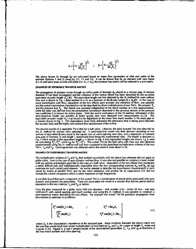
The above factors (fI through f8) are calculated based on mean flow parameters at inlet and outlet of theelement (Stations 1 and 2) using Eq. (11, 12 and 13). It can be shown that for an element with zero losses(4 = 0) and same areas at inlet and outlet (i.e. A1 = A2 ), the pressure loss matrix will be reduced to a unit matrix.
EXAMPLES OF SEPARABLE TRANSFER MATRIX
The propagation of pressure waves through an orifice plate of diameter do placed in a circular pipe of internaldiameter D has been investigated and the influence of the inertial effects has been described by the so-calledequivalent acoustic length (V ) 161. This equivalent length was first obtained by the 2L method for cases withoutflow and is shown in Fig. 2 (plot marked M = 0), as a function of the 0-ratio (where p = do//D). In the case ofwave transmission with flow, separation of the two effects; pure acoustic and influence of flow, was possibleand the overal transmission chracteristics can be described by direct multiplication of two TM's: the acoustic T.and the pressure loss TI. The former was assumed independent of the Mach number as a first approximation,while the latter was derived from the perturbation formulation described in the previous section as the pressureloss coefficient 4 is known for orifice plates. With the recent evolvement of the 2S method, refinement of thissemi-empirical model was possible as better quality data were obtained from measurements 16,101. Theequivalent acoustic length V ) was found to be dependent on the mean flow Mach number in the main pipe ina manner shown in Fig. 2. This dependence most likely delineates the interaction that is taking place betweenthe acoustic field and the highly non-uniform flow downstream of the orifice.
The second examle of a separable TM is that for a ball valve. Likewise, the pure acoustic TM was obtained bythe 2L method for various valve openings (oc). A semi-empirical model was then devised consisting of twoorifices of equivalent P-ratio equal to the square root of valve opening area ratio, and a separation of constantarea pipe of diameter D and length L determined from fitting the experimental data. The model is depicted inFig. 3 while results of the equivalent length L is shown in Fig. 4 (two equivalent lengths are shown, LA is usedfor calculating T.",T 22, while LR for T ,Tl). The overall TM for the ball valve with flow was also obtainedexperimentally using the 2L method an was then compared to the postulated multiplication scheme of the twoTM's: Ta and Tp. Good agreement was obtained and is discussed in more detail in 141.
EXAMPLE OF INSEPARABLE TRANSFER MATRIX
The multiplication scheme of T and T that worked successfully with the above two elements did not apply toglobe valve. Even in the case o4 pure -coustic without flow, it was also not possible to construct a basic modelwith say orifices and straight pipes like in the case of a ball valve. Separation of the two effects thus constitutesa rather difficult task and mathematically impossible since the two corresponding matrices Ba and B do notcommute for such complicated element. An earlier attempt to describe the transmission characteristicL of suchvalves by means of parallel TM's; one for the valve resistance, and another for its capacitance [151 did notinclude the inertial component which is rather important at high frequencies
It was then found that each component of the overall TM is a combination of mixed terms associated with pureacoustic and pressure loss parameters. These two parameters are mixed in a manner that did not permit distinctseparation to the two matrices Ta and Tp as before.
From the data measured for a globe valve (100 mm diameter - trim number 2.62 - stroke 50 mm - seat area3490 mm 2 ) with varied opening and Mach number, and using the 2L method, it was possible to construct asemi-empirical matrix describing the two effects. For example the overall TM for pulsation propagation fromdownstream to upstream is as follows:
T: 1cos(kt )+ikLA TV2 +ikL.Zc
[ Il sin(kt) T2cos(ko)+ikLA I
where 4 is the characteristic impedence of the attached pipe. Some similarity between the above matrix andthe one that would result from direct multiplication of two matrices T0 and Ta for a pipe of length t exists andis given in 171. Figures 5, 6 and 7 present results of the characteristi parameters I., LA and L6 as inctions ofthe flow Mach number and valve opening.
721

CONCLUSION
Transrr of pressure pulsation through piping elements is controlled by the inertial effects caused by theintern letry of the element, and aIso by local flow phenomena such as flow velocity gradients, flowsepar. ,nd shear layers. Generally, the interaction between the two effects is so complex to permitseparation of their respective contribution to the transmission characteristics of the element. However, for someelements, some sort of coupling between the pure acoustic transfer matrix without flow, and another transfermatrix describing the effects of flow recounted only by the unrecovered pressure drop across the element, exists.Full description of the overall TM for an element contains these two matrices coupled in a manner depending onthe complexity of the element. For example, simple multiplication of the two matrices matched the measureddata for an orifice plate and a ball valve, quite well. Such multiplication was not possible, however, in the caseof a globe valve. Semi-empirical modesl were developed for the above elements which are practical and usefulfor incorporation into prediction models for the propagation of pressure pulsation through piping networks.
It is important to emphasize that the above approach though works for certain elements, it has some limitationsin that identification of parameters containing either effects is not always possible without extensive flow-acoustic measurements. Also, even in case of separable TM, the pure acoustic transfer matrix may containparameters that are dependent on mean flow (e.g., the acoustic length to in the case of orifice plate). Thechallenge for future work in this area is to develop models based on a one-dimensional approach to quantifyand resemble the three effects: inertial, resistive and capacitive, in a more distinct, separable and consistentmanner.
ACKNOWLEDGEMENT
The work presented here is part of a research program sponsored by NOVA CORPORATION OF ALBERTA. Theauthor wishes to acknowledge the contribution of two of his colleagues towards this program:Dr. W.M. Jungowski and Dr. W. Studzinski, whose work are cited in the reference section.
REFERENCES
1. Cummings, A. and Chang, I.J., 'The Transmission of Intense Transient and Multiple Frequency SoundWaves Through Orifice Plates with Mean Flows", Rev. Phys. Appl., 21, 1986, 151-161.
2. Parrott, T., "Improved Method for Design of Expansion Chamber Mufflers with Application to anOperational Helicopter", NASA-TND7309, 1973.
3. Lambert, R.F., and Steinbrueck, E.A., "Acoustic Synthesis of a Flowduct Area Discontinuity", J. Acoust.Soc. Am., 67 (1), 1980, 59-64.
4. jungowski, W.M., Botros, K.K., Studzinski, W. and Szabo, J.L., "Measuring the TransmissionCharacteristics of Pulsating Flows Through Orifice Plates and a Ball Valve", Measuring and Metering ofUnsteady Flows, FED-Vol 40, ASME, New York, 1986, 21-32.
5. Jungowski, W.M., Botros, K.K. and Studzinski, W., "Generation of Pressure Pulsations at the Ball Valve",NOISE CON 87, The Pennsylvania State University, State College, Pennsylvania, June 8-10, 1989, 65-69.
6. Botros, K.K., Jungowski, W.M., and Studzinski, W., "On the Transfer Matrix of Orifice Plate with Flow",NOISE-CON 88, Purdue University, West Lafayette, Indiana, June 20-22, 1988, 475-480.
7. Botros, K.K., Jungowski, W.M., Studzinski, W., and MacLeod, J., "Influence of Flow in PulsatingSimulation of Gas Pipeline Installations", Proceedings of Gas and Liquid Pulsations in Piping Systems -Prediction and Control, Institute of Mechanical Engineers, London, UK, December 1-2, 1988, 89-96.
8. To, C.W.S., and Doige, A.G., "A Transient Testing Technique for the Determination of Matrix Parametersof Acoustic Systems", J. Sound & Vib., 62, 1979, 207-233.
9. Lung, T.Y., and Doige, A.G., "A Time-Averaging Transient Testing Method for Acoustic Properties ofPiping Systems and Mufflers with Flow", J. Acoust. Soc. Am. 73 (3), 1983, 867-876.
10. Doige, A.G., Munjal, M.L., and Alves, H.S., "An Improved Experimental Method for Determining TransferMatrices of Pipeline Elements with Flow", NOISE-CON 88, Purdue University, West Lafayette, Indiana,June 20-22, 1988, 481-486.
11. Miles, J.H., "Acoustic Transmission Matrix of a Variable Area Duct or Nozzle Carrying a CompressibleSubsonic Flow", J. Acoust. Soc. Am. 69 (6), June 1981, 1577-1586.
722

12. Munjal, M.L., "Acoustics of Ducts and Mufflers", Wiley, New York, 1987.
13. Ingard, U. and Singhal, U.K., "Sound Attenuation in Turbulent Pipe Flow', j. Acoust. Soc. Am., 55 (3),1974, 535-538.
14. Cummings, A., and Eversman, W., "High Amplitude Acoustic Transmission Through Duct Termination:Theory", J. Sound. Vibr., 91 (3), 1983, 503-518.
15. Johnston, D.N. and Edge, K.A., "Simulation of the Pressure Ripple Characteristics of Hydraulic Circuits",Proceedings of Gas and Liquid Pulsations in Piping Systems - Prediction and Control, Institute ofMechanical Engineers, London, UK, December 1-2, 1988,13-22.
1 2
PulsationSource
Flow
Fig. 1 Schematic of a Piping Element With Flow
I0 / do
LEGEND
0.8~I 1 O.O.8 I0. 0.00
0.6~ET 1 A13.0
0 .4 o -, : ' ,. , .. . . -
0.2 . 1
0.00 0.10 0.20 0.30 0.40 0.50 0.60 0.70 0.80 0.90 1.00
BETA - 0•
Fig. 2 Dimensionless Acoustic Equivalent Length for Orifice Plate With Flow
723

iS
35%
40%
50 %SFLOW r•50%
S. ... ....... ..... 0 a
1 o% 100 % Stroke
(ulopen)
~~~~ 1 ý FLOW , , , , ,
F 0.01 0.02 0.03 0.04 0.05 0.06 0.01.L__ L -- 1 Mach Number
Fig. 5 Dimensionless Acoustic Equivalent Lengthfor Globe Valve With Flow
Fig. 3 Acoustic Model for a Full-bore Ball Valve
10035 %40 %10 50%
605%
0.1
1A . 10L% Stroke (full open)
LB -0 0.01 0.02 0.03 0.04 0.06 006 007
Mach Number
- - " Fig. 6 Dimensionless Acoustic Parameter LA forGlobe Valve
0 Is n n a IS a II a U __v*.LWWUU - O6~ll
5 6%/L40 %
Fig. 4 Dimensionless Acoustic Equivalent Lengths e 60%
For a Ball ValveCC~ 3 6
,5% 100% Stroke5- /(full opus
0 0.01 0.0 0.03 0.04 0.06 0.06 0.07
Mach Number
Fig. 7 Dimensionless Acoustic Parameter LB for
Globe Valve
724

SECOND INTERNATIONAL CONGRESS ON
RECENT DEVELOPMENTS IN AIR- ANDSTRUCTURE-BORNE SOUND AND VIBRATION
MARCH 4-6, 1992 AUBURN UtJVErn,. USA
RESONANT FREQUENCIES OF THE LONG PIPES
L.N.Kljach•q I.I.Novikov, L.I.UstelencevNoise and Vibration Control Laboratory
VNllTBchermetChelyabinsk, USSR
ABSTRACT
Vibration and resonant frequencies of the long pipes are considered.The resonant frequency formula is sugested, which is in good correlationwith experimental data. On the basis of this consideration, a construc-tion for the long pipes noise reduction was designed. Sound pressure le-vel was reduced b7 14 dB.
The sound radiation from long pipes is a common situation for thenoise control problems. In most cases this radiation is caused by reso-nant vibration of pipes. For example, at a weld pipes production shopthe pipe, under heat treatmeht of the seam, radiated sound with 100 -110 dBA pressure levels at 1 m distance. After investigation it turnedout, that there were coincidence between the first resonant frequency ofthe pipe and the working frequency of heating indictors, both were about950 Hz. The resonant peak was rather narrow, its width approximately20 Hz. It is obvious, that to prevent such a coincidence, one has tocalculate the pipe resonant frequencies very accurately.
Formulae, usually recommended for this calculations, are derived intwo ways. Firstly, the pipe oscillations are supposed to be of the beam-type, with undeformable cross-section. But in this case the resonantfrequencies tend to zero when pipe length tends to infinity. Hence, thisway is unsuitable.Secondly, the pipe is considered as a thin cylindricalshell. The well-known result is [1]
where Wnmtt- resonant frequency of the (tm,n) - mode, C - velocity oflongitudinal wave in material of the shell, h.- shell wall thickness,
k,, xm/t , kit/ , t - shell length, R - shell radius,ko % - Poisson's ratio, n. - axial mode number,
T - circumferential mode number, 1t) 2 in Eq.(1). For infinitely long"shell,. -ca and Eq.(1) becomes
Wn = F TTT(2)
725

But the value of the first ( = 2) resonant frequency calculatedfrom Eq.(2) was 1,5 times as much as mesured value. The reason for suchdifference is neglect of the tangential inertia forces when obtainingEq.(1).
To get more accurate results consider shell equations of free moti-on
~L*.L 4 t2,4 (3)
where tt1 , U 2 and U3 are the axial, circumferential and radial dis -placements of cylindrical shell; they are functions of axial coordinate
M(0-4-<4) , circumferential coordinate 'Y(Oyf<23R) and time tThe LU 's are differential operators in OC and y , their forms aredependent on the shell theory assumptions.
The solution of Eq.(3) may be written as
U1 = Ai e ýt (km, X)cos kn,U2=A e eit • 2 (kmX)sin kn,
A,= e jfjtk.3JcoSk.,y , (4)A,, A2 and A3 are displacement's amplitudes, W. - frequency, (f ,and Y,-- trigonometric functions, determianed from boundary conditionsat XO and m=t .
After substituting Eqs.(4) in Eqs.(3), one obtains a sistem of 3algebraic equations with determinant A(•). For each (tm,n) there is aset of roots of equation A(&))=O , the lowest of the roots is the mainresonant frequency C.tn. of the (tt,.n) - mode.
In particular case when (9nn1 s are determined by Eq.(1), they ha-
ve following property. For each integer In exists such integer p , that
t= I• it{W }. This P is a function of C and CAiM(P/e)=0O
Assume, that this property is conserved in general case. Tables forfrequencies of free vibration of cylindrical shells in paper by Baronand Bleich [21 confirm validity of this assumption. Then to obtain theresonant frequencies of infinitely long pipes (C-- .ý) , it is correctbo put•kt-O 0 in Zqs. (4) from the beginning. This operation, after omit-
ting terms, negligable in comparision with W1A120 , results in
Ch tt (m- i) (5)('3- r fT
It should be noted, that the same result is oftained for some an-other forms of the operators L- . For t%- ' , Eq.(5) gives the firstresonant frequency , equals 2/3 of the fr from
Eq (2).29 zr For comparision, a shell with h/R--/30 , kVR•10/Jt in paper
[23 has the exact resonant frequency (after slight arithmetical trans-form) WOe -O0,0354- , here, from Eq.(5), w 0.02S8--C--.
Rm RThis analysis turned out to be necessary to reduce noise at the
above-mentioned shop. The pipe moved continuously, so it was impossibleto compress it by the dampers on the finite area, only point-touchingdampers were applicable. Besides, to avoid any skewness in pipe, dam-pers should be located symmetrically around the pipe. The number of thedampers was determined in following way.
For steel pipe, C = 5300 m/s, pipe wall thickness it - 0,008 m,ra-
726

dius R = 0,074 m, then f = 955 Hz, while mesured value was 930 Hz.This meant, that the sound was generated by the mode with ti = 2, that isby the wave with 4 nodes along circumference. For example, when in expe-rimental set-up 4 dampers were applied, the resonant mode turned aroundthe pipe's axis (from the theoretical point of view it meant, that k,, inEqs.C4) became very small, but not zero) and the nodes matched with thedampers. Sound remained at the same level. To elaborate an effectivedamper construction, an analogous pipe was investigated in laboratory.Thelength of the pipe was 5 m and it was enough bo consider it as infinite.Two different damper construction were worked out. DMechanical one consis-ted of 8 dampers, symmetrically located at an angle 450 from each other.Each damper was a bearing, which rotated with pipe's movement and trans-mitted vibration energy to the elastic base, were energy was absorbed.Electromagnetic damper was mounted with 5 mm space from the pipe, wichworked ar a core for it. In both cases noise level reduction equaled14-15 dB at the 1000 Hz octave band.
REFERENCES
1.Vibration in Engineering. Handbook. Moskow: "Mashinostroenie",v.1, 1978, p. 2 2 1 ( in Russian).
2.M.L.Baron, H.H.Bleich Tables for Frequencies and Modes of FreeVibration of Infinitely Long Thin Cylindrical shells. Journal of AppliedMechanics. 1954, v.21, N 2, p.178- 184.
7
m 727

728

SECOND INTERNATIONAL CONGRESS ONRECENT DEVELOPMENTS IN AIR- AND
STRUC"URE-BORNE SOUND AND VIBRATIONMARCH 4-6. 1992 AUBURN UNIVERSITY. USA
GENERIC BUCKLING ANALYSIS OF ORTHOTROPIC PLATESWITH CLAMPED AND SIMPLY SUPPORTED EDGES
S.D. Yu and W.L. Cleghorn
Department of Mechanical EngineeringUniversity of Toronto
Toronto, OntarioCanada M5S 1A4
ABSTRACT
Buckling problem of orthotropic rectangular plates with clamped and simply supported boundary conditions isinvestigated by the method of superposition. Bidirectional compression loads are considered in the analysis. Accuratebuckling coefficients with four digits of accuracy are tabulated for various load and material parameters along with anumber of plate geometries. This work may be extended to plates with other boundary conditions by simply changing thegenerating functions utilized in this paper.
NOMENCLATURE
a, b plate dimension in x and y directions, respectivelyD II,D 12,D22,D orthotropic plate flexural rigidity parametersD generalized rigidity parameter = (D 12 + 2D 66) / [(D 11D 22)"t2]K number of terms used in analytical solutionk. buckling coefficient = Pb2 / [/2(O nID22)t/
21N, compression load in x direction = -PN compression load in y direction --.-
plate lateral displacement divided by side length ax. y real space plate co-ordinatesXo, Yo plate affine coordinatesa load ratio = NX / N.0.6 affine load ratio= Ny. / N,E generalized Poisson's ratio = D I1/(D 12 + 2D66)"1q nondimensional distance = y 0lbo
eigenvalue = (oa2 p/-p'Dnondimensional distance = xola,
p mass per unit area* plate aspect ratio = b/a00 plate affine aspect ratio = b./a,
INTRODUCTION
Since plates of anisotropic materials are extensively used in enginering structures, the accurate knowledge of criticalbuckling loads and associated buckling modes is essential for reliable and lightweight structural design. However, accu-rate results for orthotropic rectangular plates are few in the literature. As is indicated by Leissa [1], buckling of isotropic,homogeneous plates is already complicated, not to mention the orthotropic plates. Because of this, energy methods, suchas Rayleigh-Ritz method, and finite element method, are commonly used in obtaining approximate solutions for freevibration and buckling of plates.
Accurate buckling results are typically available for two types of plates, i.e., simply supported plates and plates withone pair of edges simply supported. Fourier series may be used to find accurate solutions for simply supported plates.Analytical solutions for plates with one pair of edges simply supported may be obtained by using the Levy method.
729

In order to extend analytical type solutions for free vibration to plates with arbitrary classical boundary conditions,Gomian [2] introduced the superposition method. Now with this method one may obtain accurate results of free vibrationfor all classically-supported isotropic and orthotropic thin rectangular plates. A number of complicated supports, such aspoint supports, line supports, concentrated masses, distributed elasticity may also be handled by this method. In additionto rectangular plates, the superposition method is applicable to triangular and parallelogram plates. Recently, Yu andCleghom [3,4] investigated the buckling and vibration of in-plane stressed rectangular plates. A sum of publications usingthe method of superposition is estimated on the order of one hundred in the technical literature. Interested readers areinvited to refer to these publications by Gorman, Saliba, and the authors.
Generic buckling was proposed by Brunelle and Oyibo [5) in investigating buckling of orthotropic plates. By intro-cIucing a simple affine transformation, the rigidity parameters are replaced by a generalized rigidity parameter D , and ageneralized Poisson ratio F_ The advantage of this transformation is that it reduces the two independent rigidity parame-ters into one single generalized rigidity parameter because the generalized Poisson ratio has no effect on free flexuralvibration of plates with clamped and simply supported edges. This will result in a dramatic storage save in tabulating thecumputed ,buckling coefficients. For plates with free edges, the storage requirement may also reduced considering thatlimits of D and e for all composite materials fall in the following range [6,71: 0 < D * 1.0 and 0.12 ! E 50.65.
In this paper, the generic buckling of orthotropic rectangular plates with clamped and simply supported edges isinvestigated using the method of superposition. The results presented am accurate because our solutions satisfy both thegoverning differential equation and the boundary conditions.
GOVERNING DIFFERENTIAL EQUATIONS
The governing equation for plate buckling may be obtained by considering the equilibrium of an infinitesimal plateelement, or by simply letting the eigenvalue be zero in the equation for free vibration of in-plane stressed plates. Sincecritical buckling and zero frequency problems for a statically stable plate are mathematically equivalent, a buckling modemust coincide with a certain vibration mode in which the corresponding eigenvalue vanishes due to the in-plane loads.The governing equation for buckling of specially orthotropic plates is written as:
D Lw 8_2(D2w +D86w N2w N w (1)
To reduce the number of rigidity parameters used for orthotropic plates, the transformation is introduced:
x =(D11 )" 4xo a =(D11 )" 4 a, o=(D22 /D11)t1206 N. =(D1 1 )IrlNM, M. =(D 1)112M4
y =(D22)t 1 4yo b =(D 22)"14 b. *=(DiIID 22) 114,0. N = (D22) "2N, My = (D22)t2My (2)
Substituting the above relations into Eqn.(l), we obtain
j)4W a4.,, 24. • 1a2w + 2Wl- +w2W __w 84+ ký()2f w 82w]-0 (3)&x4 M2 2+-- +• ý-- X2. + o06 {=0O
ox xo8Yo 8'yo o L 8xo GC oy
where parameters that appear in above equations are defined in the Nomenclature. For buckling analysis of plates withclamped and simply supported edges, one needs to find the expressions for the bending moments transformed into theaffine plane. Considering the transformation in Eqn.(2). these expressions may be written as
12w
ED*}[~ eI{.I j} (4)
In order for the results to be valid for all orthotropic plates, it is advantageous to introduce the nondimensionaltransformation:
x.=aoE , yo=bTj . w=aW=(Di1 )" 4a.W (5)
One further rewrites the governing equation as:
+2*W 2 eW 4 84 W + 1 6
84 W 2D" 0W I a4 W Xrk_ [,2w . !iw
.t4 2 q2] (6b)
730

The nondimensional bending moments consequently become
M . a, a 2zW [, C)Wa M ,ob2 a 2W ED ' a W ) (7)
(Dn1 )114 = (Dn -)t14a. -W +o v.
SOLU OlON TECHNIQUE
The superposition method is based on the linearity of the governing differential equations The mathematical treat-ment draws the inference from the Levy method. Since rotations of plate normals about x, or y axis are due to the bendingmorients, M, and M, may be chosen to fulfill the superposition procedure. For a rectangular plate without simply sup-ported edges, one needs to construct four building blocks. Along each edge of the four building blo•cks. one of the ,- oboundary conditions, i.e., zero lateral displacement, is satisfied. The second boundary condition is associated with thedriving bending moments.
For clarity, four edges of a rectangular plate are denoted by i, and building blocks correspo.iding to the rectangularplate are denoted by j. For plates without simply supported edges, i,j = 1,2,3,4; for plates involving simply supportededges, j = 4 - N, where N, is the number of simply supported edges. For consistence, the edge number i is counted coun-terclockwise from the bottom edge; and the j-th building block is the one whose j-th edge is driven by a distributed bend-ing moment. A clamped edge i of a plate is treated as the simply supported edge in the j-th building block (i * j). Fori =j, the edge is subjected to a bending moment Mi.
Levy type solutions for each of the so-constructed building blocks may be readily obtained because there are a pairof opposite edges simply supported in all four building blocks. For reference, a summary of Levy type solutions and theboundary conditions along the other two edges for the employed building blocks is shown in Table 1. A solution to theoriginal plate may then be found by superimposing four sets of solutions and requiring the released boundary conditionsto be satisfied. This will iesult in a number of algebraic equations relating the bending moment expansion coefficients.Buckling loads may be obtained by searching those k, which cause the determinant of the coefficient matrix of the alge-braic equations to vanish.
Table t Levy type solutions for all four building block
Building Blocks Lateral Displacement Bending Moment Boundary Conditions
K• M1l b KrFirst Wt=ZY.,(il)sinmxt D - Y= E..sinm- W1(&,O)=Wi(tI)=Mq(t.O)=•, M, 1(k,l)=M1 (k)
Kc M 2a K•Second W2='.A)sinn,ni -~-5-Z=I_,sinni W2(o0,)W2 (t.1)--M0,11)---. Mt2Cl.1)=Mi(Ii)
K M30b KThird W3=YYQ())sinpnX4 =ZEsigonrk W,,0)=W(•,l)=Mr (4,l).O, MI,(FO)=MA(g)
X M4a =KFourth W 4 =•Y,(4)sinqnTq -- ;= lainqn1 W 4(0,1)=W4 (l.s1)=M4(l1,n)=O, Mk4(0,4)=M4 (1)
Solutions for the First Building BlockSubstituting the Levy type solutions given in Table I into Eqn.(6a), one obtains the following ordinary differential
equations:
Y: - 28mY. + A,,, = 0 (m = 1,2, F) (8)
where Roman superscripts indicate the order of differentiation with respect to TI, and the coefficients 8,. and A. are givenby
6,,, = D (mit/o.)2 - 0.5,•k~a, 4, M = (mil,,)2 -
Three families of solutions to Eqn.(8) may be written as:
Y,. = Asirfhl•,,, sinyll + B,,,sinh%,,rl cosy,,,l + Cmcoshl•,,r1 sinrryil + D,,,cosh, Cosy,,Tr (9)
Y. = Asinhpirl + B,,,cosh,,r.r +- C.ny.;;nry + D,,cos,,'mTl (10)
731

Y1 = A,,,sinhf3,,tri + BcoshI3,,,i1 + C,,siny,,,rl + D,,.cosyT,,s1 (II)
where P3,, and P3,,, are the known constants in terms of 8,, and A.. Constants Am. B_, C, and D,, may be found by consid-ering the boundary conditions shown in Table 1. After determining the four sets of constants, the lateral displacement forthe first building block is written as
Wj= [sinhE 1 l cos-,y.r coshf3,,.l " iI sinhf,,, cosy,,. cosho3,, sinry,.
+ I Em,.02 , sinhot,.s sinhy,.11 simit E EO sinho3,,r siny,,.i sinmtniz (12)[ef 1sinhp3,r sinhy•.n sinhl3,; sinyt,,l.
where
coshb ,,, siny,, 0 .,,O -1 -I
sinhj3, cosym 0 = 23,.ym(l + 06,) - 23• - y2) p' 2 = 1, + yý)
Solution for the Second Building Block
Substitution of the Levy type solutions for the second building block into Eqn.(6b) gives
Y'T - 2 Y"' +A,_Y_-=o (13)
where
5n = [D'(n.)' -O0.5k~ic j0' , A,, = [(n TC)4 (rtk,[i2(nit)24.
Similarly, one may obtain the lateral displaccment for the second building building block. It is written as
W sinhp3,, cosyt coshPA, siny.4i.
W E,,O,{ sinh--,,n, cosy,, coshp3,, sInysj
+ E sinho3. sinhy, lnrtil + n EnO3 n sinh,. si inn M (14)
Solutions for the Third and Fourth Building Blocks
Derivation of solutions for the third and fourth building blocks is not necessary. Solutions for the third and fourthbuilding blocks may be inferred from solutions for the first and second building blocks, respectively. Solution for thethird building block is obtained by replacing i1 with I - ri, and m with p in Eqn.(12). Similarly, solution for the fourthbuilding block is obtained by replacing t with I - t, and n with q in Eqn. (14).
Formutlif, n of Algebraic Equations
Solutions for the four building blocks, which satisfy the imposed boundary conditions, are now available. A solu-tion to the clamped plate may be obtained by simply superimposing the four solutions. However, the so-superimposedsolution does not satisfy boundary conditions for the clamped edges. In order for the solution to satify the boundary con-ditions, it is required the released boundary condition along each of the four rectilinear edges be exactly satisfied. Four-tunately, one notices that there are four sets of unknown constants appearing in expressions for the displacements. Byforcing the zero slope condit -is to be satisfied, we obtain a system of 4K linear algebraic equations relating the constantsE,, ,E,, E, and Eq. Buckling ;,ads are sought for values of k, which cause the determinant of the coefficient matrix of thealgebraic equations. Buckling modes may be found by simply solving the linear algebraic equations. To quantitativelydetermine lateral defelection of a plate which is in post-buckling mode, one needs to consider nonlinear factors.
Algebraic Equations for Plates with Simply Supported Edges
It is noticed that in all building blocks three of the four edges are simply supported. The remaining edge is con-sidered as simply supported when the driving moment vanishes. Therefore, solutions for the plates with simply supportededges may be obtained by eliminating contributions of appropriate building blocks. This indicates that analysis for platesinvolving simply supported edges is simpler.
PRESENTATION OF COMPUTED RESULTS
A Fortran code is developed to handle the numerical calculation of buckling coefficient for various geometries,
732

loading cases and rigidities. In running the program, it is found that convergence of buckling coefficient for all interestedcases is very rapid. Four digits of accuracy may be obtained by using only ten terms in the truncated series expressions.
Before presenting the results, we wish to make comparison with those by Wong and Bettess. They studied bucklingof isotropic rectangular plates clamped on all four edges using the Taylor's theory. Since the generalized Poisson ratiodoes not affect vibrational characteristics of oflhotropic plates with clamped and simply supported edges, bucklingcoefficients for an orthotropic plate with D0 = I should be the same as those for the isotropic plate, provided that theloading and geometry for the two types of plates are the same. Results of present paper and Wong and Bettess are tabu-lated in Table 2. Excellent agreement is encountered.
Table 2 Comparison of buckling coefficients for isotropic CCCC plates
D' aý0 0 Wong & Bettess Present paper
1.0 0.0 1.0 10.0738 10.071.6 8.2050 8.2012.0 7.8674 7.8672.4 7.5812 7.5813.0 7.3608 7.359
1.0 0.2 1.0 8.6382 8.6381.6 7.3486 7.3422.0 7.0692 7.0632.4 6.7650 6.7653.0 6.6102 6.606
1.0 1.0 1.0 5.3035 5.3041.6 4.0507 4.0512.0 3.9234 3.9232.4 3.8950 3.8953.0 3.8604 3.861
To decide how the tabulation of computed buckling coefficients for plates with different supports, a relationshipbetween the buckling coefficient and the generalized rigidity parameter for the given load ratio and aspect ratio is shownin Fig. 1. By examining the figure, one may quickly conclude that the buckling coefficient changes linearly with the gen-eralized rigidity parameter in the interval [0,1 ]. This indicates that only two values of D* need to be considered in tabula-tion. As a result, the storage space is dramatically reduced. Buckling coefficients for any other values of D* may beobtained with great accuracy by interpolation. This result may be significant in optimal design of composite plates.
10- C = 0.0
ac = 0.28- I
ko = 0.4
-- o = 0.6
6- ac = 0.8
OE = 1.0
4 -
2
-0 0.5;~D"
Fig. I BucKling coefficient k. of CCCC plates versus D'.
733

Table 3 shows buckling coefficients for the the camped orthotropic plates with D*=l.0 and 0.5, respectively. Buck-
ling coefficients for plates with one simply supported edge and two adjacent edges simply supported are presented inTable 4 and 5. All computed data given in this paper possess four digits of accuracy.
Table 3a Buckling coefficients of CCCC plates (D' = 1.0)
load ratio a.aspect ratio , 0.0 0.2 0.4 0.6 0.8 1.0 1.2 1.4 1.6 1.8 2.0
0.4 27.81 26.86 26.49 25.78 25.07 24.33 23.04 21.47 20.07 18.80 17.660.6 14.89 14.00 13.19 12.45 11.78 11.15 10.58 10.04 9.528 9.051 8.5490.8 11.09 9.970 9.028 8.231 7.550 6.964 6.455 6.011 5.619 5.273 4.9641.0 10.07 8.638 7.505 6.608 5.889 5.304 4.819 4.413 4.068 3.772 3.5151.2 9.581 8.316 6.973 5.954 5.175 4.569 4.085 3.692 3.366 3.093 2.7701.4 8.605 7.878 6.841 5.704 4.859 4.221 3.727 3.334 3.015 2.751 2.5301.6 8.201 7.342 6.619 5.627 4.721 4.051 3.542 3.144 2.826 2.565 2.3481-8 8.102 7.119 6.295 5.615 4.666 3.966 3.441 3.037 2.716 2.457 2.2412.0 7.867 7.063 6.149 5.402 4.649 3.923 3.385 2.973 2.650 2.389 2.1772.2 7.657 6.914 6.103 5.292 4.644 3.903 3.352 2.934 2.608 2.346 2.1322.4 7.581 6.765 6.059 5.244 4.555 3.895 3.333 2.909 2.580 2.317 2.1022.6 7.541 6.703 5.942 5.231 4.505 3.892 3.322 2.893 2.560 2.296 2.0812.8 7.416 6.690 5.883 5.196 4.482 3.890 3.316 2.882 2.547 2.281 2.0663.0 7.359 6.606 5.861 5.138 4.472 3.861 3.312 2.874 2.537 2.270 2.054
Table 3b Buckling coefficients of CCCC plates (D* = 0.5)
load ratio c 0aspectratio 0.0 0.2 0.4 0.6 0.8 1.0 1.2 1.4 1.6 1.8 2.0
0.4 26.36 26.07 25.34 24.59 23.54 21.71 20.10 18.67 17.38 16.22 15.180.6 13.70 12.85 12.07 11.33 10.61 10.16 9.604 9.079 8.533 7.850 7.2670.8 9.896 8.879 8.028 7.310 6.698 6.172 5.716 5,318 4.969 4.660 4.3841.0 8,872 7.595 6.594 5.804 5.172 4.658 4.233 3.876 3.574 3.314 3.0881.2 8.395 7.314 6.142 5.251 4.570 4.037 3.612 3.266 2.980 2.738 2.5331.4 7.410 6.773 6.063 5.081 4.341 3.779 3.341 2.991 2.707 2.471 2.2731.6 7.000 6.256 5.635 5.054 4.269 3.676 3.202 2.850 2.566 2.332 2.1371.8 6.899 6.053 5.351 4.776 4.257 3.640 3.169 2.802 2.458 2.237 2.0502.0 6.670 6.011 5.241 4.611 4.101 3.634 3.150 2.774 2.476 2.235 2.0362.2 6.456 5.821 5.219 4.545 3.999 3.560 3.145 2.762 2.459 2.215 2.0142.4 6.377 5.682 5.091 4.529 3.954 3.493 3.122 2.758 2.451 2.204 2.0022.6 6.342 5.631 4.994 4.460 3.941 3.461 3.075 2.757 2.448 2.198 1.9942.8 6.215 5.614 4.955 4.389 3.919 3.448 3.051 2.730 2.447 2.195 1.9903.0 6.155 5.518 4.947 4.356 3.940 3.446 3.039 2.711 2.444 2.194 1.987
Table 4a Buckling coefficients of CCCS plates (D" = 1.0)
load ratio c.4aspect ratio *0 0.0 0.2 0.4 0.6 0.8 1.0 1.2 1.4 1.6 1.8 2.0
0.4 15.81 15.35 14.91 14.49 14.09 13.70 13.33 12.96 12.60 12.25 11.890.6 9.581 8.968 8.419 7.925 7.480 7.076 6.710 6.375 6.069 5.787 5.5280.8 8.201 7.342 6.619 6.011 5.497 5.058 4.681 4.353 4.066 3.813 3.5891.0 8.087 7.063 6.149 5.402 4.800 4.311 3.908 3.572 3.288 3.045 2.8341.2 7.737 6.988 6.097 5.244 4.555 4,011 3.579 3.228 3.938 2.704 2.4901.4 7.416 6.707 6.017 5.229 4.482 3.890 3.428 3.061 2.764 2.519 2.3131.6 7.347 6.551 5.849 5.189 4.470 3.843 3.356 2.974 2.669 2.421 2.2141.8 7.313 6.528 5.764 5.098 4.464 3.828 3.321 2.927 2.615 2.362 2.1542.0 7.208 6.497 5.751 5.042 4.431 3.826 3.303 2.899 2.581 2.325 2.1152.2 7.161 6.427 5.736 5.027 4.393 3.825 3.296 2.882 2.559 2.300 2.0892.4 7.155 6.394 5.693 5.025 4.373 3.816 3.292 2.872 2.545 2,284 2.0712.6 7.119 6.391 5.664 5.008 4.368 3.802 3.292 2,866 2.535 2.272 2.0582.8 7.088 6.371 5.659 4.985 4.367 3.791 3.291 2.862 2.527 2.263 2.0483.0 7.083 6.345 5.654 4.972 4.361 3.785 3.291 2.859 2.522 2.256 2.040
734

Table 4b Buckling coefficients of CCCS plates (D" = 0.5)
load ratio o6aspect ratio *0 0.0 0.2 0.4 0.6 0.8 1.0 1.2 1.4 1.6 1.8 2.0
0.4 14.63 14.17 13.73 13.27 13.00 12.61 12.22 11.83 11.27 10.57 9.9600.6 8.395 7.846 7.356 6.915 6.517 6.157 5.830 5.532 5.261 5.010 4.7800.8 7.000 6.256 5.635 5.113 4.673 4.299 3.976 3.697 3.453 3.238 3.0471.0 6.887 6.011 5.241 4.611 4.101 3.689 3.345 3.053 2.809 2.602 2.4231.2 6.541 5.912 5.213 4.529 3.954 3.493 3.122 2.819 2.486 2.298 2.1331.4 6.215 5.614 5.063 4.505 3.940 3.448 3.051 2.730 2.469 2.252 2.0701.6 6.142 5.470 4.888 4.383 3.911 3.445 3.036 2.701 2.429 2.205 2.0191.8 6.111 5.454 4.828 4.289 3.831 3.423 3.034 2.694 2.413 2.183 1.9932.0 6.005 5.411 4.823 4.262 3.780 3.375 3.021 2.694 2.411 2.177 1.9832.2 5.956 5.339 4.786 4.259 3.765 3.345 2.993 2.688 2.411 2.174 1.9782.4 5.951 5.312 4.739 4.234 3.764 3.335 2.975 2.664 2.408 2.174 1.9752.6 5.916 5.309 4.722 4.202 3.750 3.334 2.967 2.661 2.403 2.174 1.9752.8 5.883 5.283 4.720 4.189 3.729 3.329 2.966 2.654 2.395 2.172 1.9753.0 5.878 5.259 4.704 4.188 3.717 3.316 2.965 2.652 2.389 2.168 1.975
Table 5a Buckling coefficients of CCSS plates (D = 1.0)
load ratio a.aspect ratio o 0.0 0.2 0.4 0.6 0.8 1.0 1.2 1.4 1.6 1.8 2.0
0.4 15.19 14.89 14.49 14.11 13.74 13.39 13.04 12.70 12.34 11.90 11.340.6 8.638 8.119 7.650 7.226 6.841 6.491 6.170 5.875 5.602 5.349 5.1110.8 6.719 6.030 5.457 4.974 4.565 4.214 3.910 3.645 3.412 3.205 3.0211.0 6.223 5.315 4.605 4.049 3.607 3.248 2.951 2.703 2.493 2.312 2.1551.2 6.180 5.123 4.266 3.628 3.147 2.775 2.480 2.241 2.043 1.877 1.7351.4 5.996 5.106 4.146 3.426 2.907 2.520 2.223 1.987 1.797 1.639 1.5071.6 5.773 5.030 4.119 3.329 2.773 2.372 2.071 1.837 1.650 1.500 1.3711.8 5.679 4.902 4.115 3.283 2.695 2.281 1.975 1.741 1.557 1.408 1.2842.0 5.668 4.827 4.085 3.264 2.647 2.221 1.912 1.678 1.494 1.347 1.2262.2 5.636 4.806 4.035 3.257 2.618 2.181 1.868 1.633 1.451 1.305 1.1852.4 5.575 4.803 4.000 3.256 2.598 2.153 1.837 1.601 1.419 1.274 1.1562.6 5.543 4.780 3.984 3.255 2.585 2.132 1.813 1.577 1.395 1.251 1.1332.8 5.539 4.748 3.982 3.250 2.577 2.117 1.796 1.559 1.377 1.233 1.1173.0 5.528 4.730 3.980 3.241 2.571 2.105 1.782 1.544 1.363 1.219 1.103
Table 5b Buckling coefficients of CCSS plates (D" 0.5)
load ratio o6aspectratioO•, 0.0 0.2 0.4 0.6 0.8 1.0 1.2 1.4 1.6 1.8 2.0
0.4 14.22 13.82 13.44 13.06 12.71 12.32 11.83 11.16 10.49 9.869 9.3080.6 7.506 7.025 6.582 6.273 5.929 5.613 5.322 5.051 4.798 5.558 4.3300.8 5.595 5.011 4.528 4.125 3.783 3.488 3.237 3.011 2.816 2.644 2.4901.0 5.094 4.343 3.762 3.307 2.946 2.652 2.410 2.208 2.036 1.888 1.7601.2 5.051 4.192 3.500 2.983 2.591 2.287 2.045 1.849 1.686 1.550( 1.4331.4 4.871 4.176 3.443 2.864 2.438 2.117 1.862 1.667 1.508 1.377 1.2671.6 4.645 4.058 3.437 2.832 2.374 2.037 1.781 1.582 1.402 1.276 1.1701.8 4.548 3.925 3.384 2.829 2.352 1.998 1.734 1.531 1.370 1.239 1.1312.0 4.536 3.863 3.307 2.818 2.346 1.981 1.709 1.502 1.339 1.208 1.1002.2 4.507 3.854 3.261 2.783 2.346 1.974 1.695 1.484 1.319 1.187 1.0792.4 4.445 3.844 3.248 2.750 2.340 1.972 1.688 1.473 1.306 1.174 1.0652.6 4.412 3.808 3.247 2.733 2.327 1.971 1.684 1.467 1.299 1.163 1.0552.8 4.407 3.778 3.236 2.728 2.312 1.971 1.683 1.463 1.294 1.159 1.0503.0 4.397 3.768 3.215 2.728 2.303 1.968 1.682 1.460 1.290 1.154 1.045
CONCLUSION
This paper investigated generic buckling of orthotropic rectangular plates with combination of clamped and simplysupported edges by studying a clamped plate. Results obtained by the superposition method are accurate, and the pr-cedure itself is analytical. The method may be employed to solve buckling of plates involving free edges by modifyinggenerating functions used for the clamped plates.
735

REFERENCES
[1] A.W. Leissa. Buckling of composite materials, Composite Structures, Vol.] (1983), 51-66.
[2] D.J. Gorman, Free Vibration Analysis of Rectangular Plates, New York: Elsevier North Holland, 1982.
[3] Yu,S.D., Cleghorn, W.L., Free Vibration Analysis of Clamped Orthotropic Rectangular Plates Subjected to Con-stant In-Plane Loads", presented at 1991 ASME Presure Vessels and Piping Conference, San Diego. California,published in Piping Components Analysis: Piping and Structural Dynamics, PVP-Vol. 218 (1991), 113-119.
[4] W.L. Cleghom and S.D. Yu, Analysis of buckling of rectangular plates using the method of superposition, to appearin Transactions of Canadian Society for Mechanical Engineering, Vol.15, No.4, 1991.
[5] E.J. Brunelle and G.A. Oyibo, Generic buckling curves for specially orhotropic rectangular plates. AJAA Journal,Vol.21 (1983), 1150-1156.
[6] E.J. Brunelle, The fundamental constants of orthotropic affine plate/slab equations, AIAA J., Vol.23 (1985), 1957-
[7] l.H. Yang and W.S. Kuo, The global constants of in orthotropic affine space, J. CSME, Vol.7 (1986), 355-
[81 P.M. Wang and P. Bettess, Elastic buckling of rectangular clamped plates, Int. J. Solids Structure, Vol.15 (1979).457-466.
736

SOUND AND VIBRATION MEASUREMENTS
737

738

SECOND INTERNATIONAL CONGRESS ONRECENT DEVELOPMENTS IN AIR- AND
STRUCTURE-BORNE SOUND AND VIBRATIONMARCH 4-6. 1992 AUBURN UNIVERSITY, USA
A FREQU3ENCY D06S.XN IDENTrIFICATION SCHEME FOR DAMPEDDISTRIBUTED PARAMTER SYSTEM
R. ChanderAerostructures, Inc., Arlington, Virginia, USA
M. MeyyppMcDonnell Douglas Helicopter Co., Mesa, Arizona, USA
S. Hanagud
Georgia Institute of Technology, Atlanta, Georgia, USA
ABSTRACT
A parameter identification technique in the frequency domain is discussed. For
this purpose, a distributed parameter model of a dynamic system within the framework ofEuler-Bernoulli beam theory is assumed to be known. Internal material damping and
external viscous damping are included in the model. The parameters are approximatedusing cubic cardinal splines, and their derivatives are evaluated from suchapproximations. For a given input, the response is assumed to be measured at discrete
locations in the system. Quintic B-splines are used to obtain approximate spatialrepresentations of the response and its derivatives from these measurements. AGalerkin-type approach in conjunction with an equation error technique is used toestimate the unknown parameters. Numerically simulated responses obtained from anindependent finite element model of an Euler-Bernoulli beam is used to validate theidentification technique. Estimated values of the mass, stiffness and dampingdistributions are discussed.
INTRODUCTION
For structures that can be modelled as continuous systems, discretization reducesmodeling accuracy. In such cases, if the form of the governing differential equationis known along with the initial and boundary conditions, the actual distributed systemitself can be considered for parameter identification without resorting to approximatemodels. A distributed representation of the system thus identified is likely to yieldmore accurate prediction of the system behavior. Also, the identified values can beused to reconstruct the response, which can be compared with the measured response tocheck the validity of the physical representation of the system itself. In the recentpast, several identification techniques suitable for distributed structural dynamicsystems have been reported (1-4].
At present, there are few techniques available to identify the unknown parametersof distributed structural dynamic systems in the presence of damping. Among these, thefinite element and spline-based techniques have received considerable attention. Thefinite element techniques are primarily concerned with the identification of systemsthat include proportional or general viscous damping. The spline-besed techniquesinvolve using time domain data for systems with constant or spatially varyingparameters, and include different types of damping models.
Damping is present in virtually all types of structures and materials encounteredin practice. Characterization and understanding of the daming behavior becomes even
more critical if, in addition to vibration, noise control problems are also addressed.In such cases, the material (internal or structural) damping should also be includedalong with the external damping of the system. In this vein, an identification scheme
739

suitable for one-dimansional systems, including both types of system dampings, isdiscussed in this paper.
The identification scheme uses data in the frequency domain, and a model of adistributed dynamic system within the framework of the Euler-Bernoulli beam theory.The parameters of the system, such as mass, damping and stiffness, are assumed to beuniformly varying along the length of th.e beam. The external and internal dampings areincluded by using the linear viscous and viscoelastic models respectively. Thespatially varying parameters are approximated using cubic cardinal splines, and theirderivatives are obtained from such approximations. For a given input, the responsechosen to be acceleration, is assumed to be known at discrete locations along the beam.Quintic B-splines are then used to obtain approximate spatial representations of theresponse and its derivatives from these discrete measurements.
A Galerkin-type approach in conjunction with an equation error technique is thenused to estimate the unknown parameters, which are values of the parameter splines atthe knot locations. Numerically simulated responses obtained from an independentfinite element model of an Euler-Bernoulli beam are used to validate the identificationtechnique. Estimated values of the mass, stiffness and damping distributions arepresented.
PHYSICAL SYSTEM NDDEL
The physical system is assumed to be modeled within the framework of the Euler-Bernoulli beam theory. The effects of internal and external dampings are includedusing the linear viscoelastic and viscous damping models, respectively. A modelgoverning the behavior o! such beams is assumed to be known a priori in the frequencydomain, and is taken to be as follows.
d2/dx
2 E(EI(x)+jC 5I(x))d
2a*(x,w)/dx
2)+
[jWC,(x)W-w2 pA(x)]a* (x,w) = -w2 F(x,w) (1)
where a*(x,w) is the acceleration response caused by the known forcing function F(x,w),x is the distance along the beam, and w is the frequency in radians/second. The beamis assumed to be fixed at x.0, and free at x=L, where L is the length of beam. EI andpA are stiffness and mass distributions respectively. C. and Cv correspond to theinternal and external damping coefficients respectively. The above parameters areassumed to be continuous functions of x, and are the unknown parameters to beidentified. in eq. (1), the initial conditions were assumed to be equal to zero.
For identification purposes, it is assumed that the acceleration is known at asmany frequencies as required, at a number of discrete locations. From this data anapproximation to the continuous response is constructed using quintic B-splines. Eachof the parameters appearing in eq. (1) is approximated in the identification process bycardinal cubic splines. The task of identifying the unknown parameters then reduces toestimating the values at the knot locations of these parameter splines. To accomplishthis, a Galerkin type weighted residual procedure in conjunction with an equation errorapproach is used.
SPLINE APPROXIMATIONS
Cubic cardinal splines and quintic B-splines were chosen as the approximatingfunctions for the parameters end response respectively.
Response Representation: The acceleration response is represented as follows.
Na (x,w) Z • ai(w) Oi(x) (2)
i=O
where #i(x) are the basis functions that satisfy appropriate boundary conditions, andai(W) are constants to be determined at each frequency. The functions #i(x) areconstructed using the quintic B-spline basis functions [51, so as to satisfy the givenboundary conditions.
Though many such combinations are possible, the following is used in this paper.
740

0 W)= -B1 (5) - (9/4)B1(5) Wx) + (65/2)B2(5) Wx)
0 2(3c) "- 82 (x) - (l/8)B 1(5) (x) + (9/4)B-2(5) (x)
ON(X) - 3()(x) + (3/2)BN+I(S)(x) + 3BN+2(5) (x)
O 3 1 Cx) - E%.1(5) (x) - 2B+25 (x)
ON.2(x) - D-2(5) (x) - 0.5 8 N+z (Cx)
Oi(x) = Bi(5) W, i.3,4 ...... N-3 (3)
where
Ci(Bi( x) . 1/hS[(x-xi. 3 )+5
- 6(x-xi. 2 )+5 + 15(x-xi-l)+5
-20(x-xi)+5 + 15(x-xi+}+5 - 6(x-xi+2 )+5 + (x-xi+3 )+5
X.3 < x-2 < x. 1 < x0 and xN+3 > XN+2 > XN+1 > xN
and
(x-xi)+5 = (x-xi)5, if x >_ xiS=0 if x < xi
For a given set of measured response at the knot locations i=0,l,2, . N, at a givenfrequency, the coefficients ai(w) in eq. (2) can be uniquely obtained. The responsederivatives required in eq. (1) can be calculated by differentiating eq. (2) as manytimes as necessary.
Parameter Snlines: The unknown structural parameters are expressed in terms of basisfunctions as follows.
rN
OP(x) = S ip Ci(x), p = 1,2 3 and 4 (4)i=0
where 9(l), 0(2) 0 (3) and 9(4) represent EI, COI, Cv and pA, an-1 Oi(l), 0i(2) 8i(3)and 9i(4) represent the coefficients corresponding to these parameters respectively.The values of N depend on the number of locations at which the parameters are to beidentified. The basis functions Ci(x) are taken as cubic cardinal splines [6] havingthe following characteristics.
Cj(xi) = 6
ij, C j(x 0 ) = C j(xN) = 0 ij = 0,1 ....... N
CN+ l (xi) - CN+ 2 (xi) = 0, C N+l(xO) = C N+2 (xN) = 1
C N+1 (XN) - C 3 +2(x 0 ) = 0 (5)
where 0)' represents differentiation with respect to x. Also, it has been assumed thatthe parameter knots coincide with the knots used for the response. In this case N=N+2.
N+2eP(x) 1: 01 P Ci(x) (6)
i-0
Due to the manner the cardinal splines are defined, Oip, i-0,1, .. ,N are the values ofthe parameters OP at the knots xi, and OPN+1 and OPN+2 are the derivatives of OP at x.0and x-L respectively. The identification procedure now involves computing thecoefficients OiP for p-1,2, 3 and 4.
741

IDENTIFXCATIO' S4HZM
Substituting eqs. (2) and (6) into eq. (1) and regrouping, the following set ofequations is obtained.
[ 2[Ok (1).jik (1)]Ck(X) [ 0ak( k.... (x) 3
+ 2 [ :(C[k()+jek (1) ]Ck'(x)3 [ k•0ak)k' (x)3
+ I[ oVk kl) jk (1Ck Cx) [ k!Ok )k (x( 3
+ [ :• (jw (2) -W29()Ck(X) 3 [ (30ak(w)•k(x) + 02 F(xW) = 0 (7)
At this stage, the coefficients ak and the excitation F are known complexquantities at any given frequency and can be written as
ak(w) = ak RC) + jak I(M
F(x,w) = R(x,W) + jFC(x,W) (8)
The number of unknowns Ok in eq. (7) equals 4 (N+3), corresponding to the values of(N+1) knot locations and also the derivatives at end points of each of the parameters.If an arbitrary number of equations is used in solving these unknowns in eq. (7), theresulting equation will not be equal to zero, but will result in some error. Theidentification procedure involves orthogonalizing this error with respect to each ofthe basis functions used in the parameter splines and computing the unknowns from theresulting equations. Thus, a set of equations is obtained for each frequency used inidentification. By combining these sets of equations for many frequencies, anoverdetermined system can be generated, a least squares solution of which yieldsestimates for the unknowns. The equations involved in this procedure are summarizedbelow. The following matrices are defined for convenience.
L
Rl, 2 = f [{C){0'"..)T{.aRI){C}T + 2{C}f0''T{aR'I}{c'}T
0
+ (c){0 ')T{aRI)(C'')T ]
L L
R3, 4 = J {C}(#)TfafRI}{C)Tdx FOR,, - f FR' 1 {C) dx (9)
0 0
Incorporating eqs. (8) and (9) into the weighted residual procedure, the followingequations involving coefficients of the unknown parameters is obtained.
Rft -Rt2 -wR4 -(02 R3 $Mi
R2 -Rf1 wR3 -w 2R4 e0 (4 ) (F I)(
742

Eq. (10) is obtained for a single frequency. Similar set. of equations can be writtenat other frequencies. Combining the different sets at various frequencies leads to anequation of the form
[CO] (0) -Fe} (11)
in which [CC] is a coefficient matrix of the order 2(N+3)n times 4(N+3), where n is thenumber of frequencies used in the estimation. Elements of this matrix are made up ofthe elements of matrices defined in eq. (9) evaluated at different frequencies. (9)and (F9) are the parameters and force vectors of length 4(N+3). Using the ordinaryleast squares technique, a solution {0*) to eq. (11) can be written as,
C9") = cOT CO-1 cOT FO (12)
NUMERICAL RESULTS
The identification scheme discussed in the previous sections is demonstrated inthis section using simulated data for a cantilever beam with the following properties.
L = 0.61m;EI(x) = 18.01*102 El-(x 2L)]
4 N-m2 ; C I(x) = 5.51 [l-(x/2L)]4 N-m
2
pA(x) . 4.22 [l-(x/2L)] N/m; Cv(x) = 17.3 [1-(x/2L)]2
N-sec/m2
The beam was subdivided into 6 regions (N=6), and an independent finite element programwas used to calculate the response at the resulting 7 knots. In the identification,the frequency response data in the following frequency bandwidths at 1Hz intervals wasused: 25-34Hz and 39-48Hz (around first mode), 144-153Hz and 158-167Hz (around secondmode), and 376-385Hz and 390-399Hz (around third mode).
The regions in the immediate vicinity of the modal peaks were omitted. This isbecause, less accurate estimates were obtained, if these areas were included especiallyfor viscous damping. The elements in the coefficient matrix [Cp] are integral termsinvolving products of polynomials. A sixth order Gauss-Legendre numerical procedure[7] was used to compute the elements in the matrix. A total of 36 parameters wereestimated, viz., the values at the 7 knot locations and the derivatives at the ends forstiffness, damping and mass distributions. Computed values for these unknowns at theassumed knot locations are presented in Figures 1-4. It can be seen from these figuresthat the estimated values are in good agreement with the actual values used ingenerating the frequency response functions at all the interior knots.
SUMMARY AND CONCLUSIONS
A spline based identification technique in the frequency domain that is suitablefor damped distributed structural dynamic systems was developed. A uniformly taperedbeam whose behavior can be modeled within the framework of the Euler-Bernoulli beamtheory was considered for the identification scheme. The infinite-dimensional responseand parameter spaces were approximated by quintic B-splines and cubic cardinal splinesrespectively. A Galerkin type weighted residual procedure was used to estimate theunknown parameters. Simulated acceleration frequency response data around the firstthree modes, for an applied impulse, was used to validate the technique. None of theparameters was assumed to be known a priori. The estimated results showed goodagreement with the actual values at all the interior locations of the beam.
REFERENCES
1. Banks, H.T. and Crawley, J.H., "Parameter Identification in Continuum Models,"Proceedings of the 1983 American Control Conference, San Francisco, California, 1983.2. Banks, H.T., Fabiano, R.H., Wang, Y., Inman, D.J., and Cudney, H., "SpatialVersus Time Hysteresis in Damping Mechanisms," Proceedings of the 27th IEEE Conferenceon Decision and Control, 1988, pp 1674-1677.3. Baruch, H. and Meirovitch, L., "Parameter Identification of Distributed Systems,"Journal of Sound and Vibration, 1985, pp 551-564.4. Meirovitch, L. and Norris, P., 'Parameter Identification in DistributedSpacecraft Structures," Journal of the Astronautical Sciences, 1986, pp 341-352.5. Prenter, R.M., "Splines and Variational Methods," Wiley Interscience, 1975.6. Shultz, N.H. "Spline Analysis," Prentice Hall, 1973.
743

7. Zienkievicx, D.C., -The Finite Element Method,- McGraw Hill Book Company, 1977.
2 2-5
-Z15
tol
1 &5 0.5
0
0 .. 0 0.16 0.33 0.5 0.66 0.830 0.16 0.33 0.5 0.66 0.83 Beam Location (x/L)
Beam Location (x/L) ,Actual .Estimated.Actual .Estimated Figure 2 Damping Estimates
Figure I Stiffness Estimates (Internal)
4 18
3.5 16
,3 14
S2.5 •12
2<" 10
1 .
0.5 4 14
0 0.16 0.33 0.5 0.66 0.83 0 0.16 0.33 0.5 0.66 0.83Beam Location (Y/L) Beam Location (x/L)
.Actual +Estimated ,Actual .Estimated
Figure 3 Mass Estimates Figure 4 Damping Estimates
744

SECOND INTERNATIONAL CONGRESS ONRECENT DEVELOPMENTS IN AIR- AND
STRUCTURE-BORNE SOUND AND VIBRATIONMARCH 4-6, 1992 AUBURN UNIVESITY. USA
ELASTIC BE1AVYOUR OF MIXED Li-Zn AND Li-Cd FERRITES
D.RavinderDepartment of Physics
Post Graduate College of ScienceSailabad
Osmania University, Hyderabad-500 004INDIA.
ABSTRACT
Polycrystalline samples of mixed ferrite systems having the chemical formulaLi0.5-x/ 2 MxFe2.5-x/20 4 (M = Zn or Cd) where x = 0.2, 0.4, 0.6, 0.8 and 1.0 were prepared
by conventional double sintering method. The final sintering temperature was done at 1250°C.The ultrasonic compressional (V1) and shear (Vs) velocities at room temperature of all the
mixed Li-Zn and Li-Cd ferrites were determined by the ultrasonic pulse transmission technique.The elastic moduli of the specimens have been computed and corrected to zero porosity.The corrected values of the elastic moduli and the Debye temperatures are presented.Lithium-Zinc ferrite with x = 0.6 is found to have minimum Young's and rigidity moduli.But in the case of mixed Li-Cd ferrite with x z 0.4 is found to have maximum Young'sand rigidity moduli .
The values of E, n, E0 , no and K of the mixed Li-Zn ferrites are found to decrease
with increasing zinc content (x = 0.6 mole). Beyond x=0.6 mole, these paramenters, showan increase for further addition of zinc. They, however, decrease once again for zinc ferriteswith 100% Zn. But in the case of Lithium-Cadmium ferrites the values of E, n, Eo, no and
K are found to increase with increasing cadmium content (x=0.4 mole). Beyond x=0.4 mole
these parameters show an decrease for further addition of cadmium. In both cases Poisson'sratio remains constan*. The variation of elastic moduli with composition may be interpretedin terms of binding forces between the atoms.
INTRODUCTION
A study of the elastic behaviour of solids is of great significance in understandingthe nature of interatomic and interionic forces in solids. The elastic properties of ferritespossessing the spinel structure have not been studied so systematically as their magnetic andelectrical properties. Moreover, there is a need for a thorough study of the elastic behaviourof these ferrites with new compositions possessing certain desired elastic properties in viewof their extensive applications in computers as memory cores and in several microwavedevices like isolators, circulators, gyrators, phase shifters, etc. It is with this view that
745

Ravinder,D., 2
a systematic study of the elastic behaviour of polycrystalline Li-Zn and Li-Cd ferrites hasbeen undertaken at room temperature.
EXPERIMENTAL DETAILS
Mixed Li-Zn and Li-Cd ferrites having the chemical formula Li0.5-x/2 x 2.5-x/204
where x = 0.2, 0.4, 0.6, 0.8 and 1.0 were prepared by conventional double sintering processwith a final sintering temperature 1250'C. The details of the method of preparation havebeen given in an earlier publications [1,2]. X-ray diffractometer studies of the samplesusing Cu (,L radiation confirmed the spinal formation. From the diffraction data, latticeparameter values and hence the values of X-ray densities have also been calculated andare given in Table-I.
TABLE-I Ambient elastic data (uncorrected) on Lithium-Zinc and Lithium-Cadmium ferrites
Ferrite Bulk X-ray Per- V Vs E nComposition density density cen-
0 3 K -3 10 3 K -3 tage ) 1 2 10 -2103Kgm- 103Kgm Poro- (m.S-) (m.S-) (xlO0 Nm 2 (x00Nm-
sity(%)
Li 0.4Zn 0.2Fe2. 4 0 4 4.66 4.86 4.1 6243 3806 16.25 6.75
Li .3Zn .4Fe 2.304 4.81 4.98 3.3 6131 3967 15.26 5.57
Lio.2Zno.6Fe2. 2 0 4 4.97 5.09 2.4 5200 2737 9.74 3.72
Li0.1 Zn .gFe 2.0 4 5.14 5.22 1.6 6281 4023 19.16 8.31
ZnFe204 5.30 5.32 0.5 4934 3028 11.64 4.86
Li0. 4 Cd 0 . 2 Fe 2 . 4 0 4 4.58 4.64 1.3 5751 3502 13.54 5.62
Li0 .3Cd0.4Fe2. 3 0 4 4.87 4.94 1.4 8962 5333 33.96 I 3.85
Li 0.2Cd 0.6Fe 2.204 5.16 5.24 1.4 5580 3988 21.81 8.68
Li 0.1Cd 0.Fe 2.104 5.46 5.53 1.3 5560 3271 13.67 5.52
CdFe 2O,4 5.75 5.82 1.1 4267 2300 7.88 3.04
The compressional (V1) and shear (Vs) velocities at room temperature of all the mixed
ferrites were determined by the ultrasonic pulse transmission technique [3]. but modifiedand improved by using a digital Textronic 2230 oscilloscope and utilising curser movementfor travel time measurements [4]. The error in the measurement of velocities is less than- 0.5%
746

Ravinder,D., 3
RESULTS AND DISCUSSIONS
The measured values of the compressional (V]) and shear (V ) velocities, along with
the computed values of the Young's modulus (E), and rigidity modulus (n), are in Table-I.Since the ferrites under investigation are porous (porosity ranging from 4.1 to 0.5%), theelastic moduli have been corrected to zero porosity using McKenzie's formula [5]. Thecorrected values of Eo, no, K and o% are in Table-Il.
17ABLE-ll Elastic data of Li-Zn and Li-Cd ferrites corrected to zero porosity
( x 101 0 Nm- 2)Ferrite oo_______________________0
Composition E n KO 0 0
Li0.4 Zn0.2Fe2.404 17.69 7.37 9.83 0.20
Li0 .3 Zn 0 .4 Fe2.304 15.76 5.73 8.89 0.21
Li0.2Zn0.6Fe2.204 Z10.19 4.35 5.16 0.17
Li0.1 Z Zi0.8Fe2. 1 0 4 19.98 8.26 11.46 0.21
ZnFe 2 0 4 11.75 4.90 6.53 0.20
Li 0.4Cd 0.2Fe 2.404 13.53 5.79 6.80 0.17
Li0.3Cd0.4Fe2. 3 0 4 33.84 14.57 16.75 0.16
Li0.2Cd0.6Fe2.20 4 22.26 9.37 11.87 0.16
Li0.1 d 0 .8 Fe 2 . 10 4 13.60 5.87 6.64 0.19
CdFe 20 4 8.02 3.41 4.15 0.18
It can be seen from Tables-I and II that the values of E, n, Eo, no and K of the
mixed Li-Zn ferrites are found to decrease with increasing zinc content (x=0.6 mole). Beyondx=0.6 mole, these parameters, show an increase for further addition of zinc. They, however,decrease once again for zinc ferrite with 100% Zn. From Table 11, it can further be seenthat the Poisson's ratio remains constant. Following Wooster's work (61, the variation ofelastic moduli with composition may be interpreted in terms of binding forces betweenthe atoms. As such, it can be understood from the experimental values of Eo and no (Table-Il)
that the atomic binding between the ions of Li-Zn mixed ferrites, decreases with increasingzinc content upto x=0.6 mole. Beyond x=0.6 mole, the binding forces show an increasefor further addition of zinc. They, however, once again decrease for zinc ferrite. Butin the case of Li-Cd ferrites the values of E, n, E0 , no, and K of the mixed Li-Cd ferrites
are found to increase with increasing cadmium content (xz0.4 mole). Beyond x=0.4 mole,
747

Ravinder,D., 4
these parameters show decrease for further addition of cadmium. From Table-li, it canfurther be seen that the Poission's ratio remains constant. Following Wooster's work [6],the variation of elastic moduli with composition may be interpreted in terms of bindingforces between the atoms. As such, it can be understood from the experimental valuesof E and n0 (Table-Il) that the atomic binding bet ns of mixed Li-Cd ferrites,
increases with increasing cadmium content upto x=(,. ,yond x=0.4 mole the bindingforces show decrease for further addition of cadmium. I•is composition variation of elasticmoduli in the case of Li-Zn and Li-Cd ferrites is similar to what has been observed inseveral other ferrites like Co-Zn [7] and Li-Ni [8] studied earlier.
Debye temperature (ED) for the mixed Li-Cd ferrites have been calculated using
the simple method given by Anderson [91
% t .--. V
where
h plank's constant
K Boltzmann's constant
N = Avogadro's Number
M = Molecular weight of the specimen
q Number of atoms in a molecule
P density of the specimen, and
Vm Average sound velocity
given by i
V m 3 " V s"- 3+ I
From the values of compressional (Vl) and shear (V ) velocities and X-ray density,
VI/P and Vs/P are calculated and are shown in Table-Ill. The mean atomic weight m/q
of the ferrite under investigation, calculated from the molecular weight m and the numberof atoms q in the chemical fromula are also included in Tble-Ill. The values of 0D and
Vm thus obtained are also given in Table-Ill.
748

Ravinder,D., 5
TABLE-Ill Reltionship between atomic weights and velocites
Ferrite mp V V/ eDComposition mqs (M.S-) (K)
Li 0 .4Zn 0 .2Fe2.40 4 30.55 1274 783 4204 564
Li0.3Zn0.4Fe2.30 4 31.53 1231 797 4353 584
Li0.2Zn0.6Fe2.20 4 32.50 1022 538 3060 411
Li0. IZn 0 .Fe 2 . 104 33.54 1203 771 4420 594
ZnFe 2 0 4 34.44 927 569 3342 450
Li0.4 Cd0.2Fe2.40 4 31.90 1239 755 3868 509
Li0.3 Cd0.4 e2.30 4 34.21 1824 1080 5904 780
Li0.2Cd0.6Fe2. 2 0 4 36.53 1065 761 4316 564
Li0. 1 Cd0. 8 Fe2.1 O 4 38.64 1005 592 3626 475
CdFe2 04 41.16 733 395 2568 335
It cn be seen from the tble that there is a continuous increase in the vlue of meanatomic weight with increasing zinc and cadmium contents.
In the case of Li-Cd ferrites, the values of VI/P , V s /P Vm and eD are also increasescontinuously with increasing cadmium content upto x=0.4 mole. Beyond x=0.4 mole the
above values show a decrease for further addition of cadmium. Plot of ED against Vm
is shown in Fig.l. It is interesting to note from the figure eD varies linearly with Vm-
A similar variation of E0D with Vm was reported by Narayana and Swamy [10,22] in the
case of rare eaarth and noble metals, and Reddy et al., in the case of Li-Ti [12] mixedferrites.
ACKNOWLEDGEMENTS
The author is grateful to Prof.Anwar Kamal, Head of the Department of Physics,Osmania University, Hyderabd, for his interest in this work. The author also thank theProf.T.Seshagiri Rao, Prof.K.Shankariah, Principal, Principal and Prof.U.V.Subbaa Rao, Headof the Department of Physics, Post Graduate College of Science (O.U.), Saifabad, Hyderabdfor their cooperation.
749

Ravinder,D., 6
Fig.I Plot of Debye tempeature (e0 ) against the avetage sound velocity (Vm)
for the Li-Zn and Li-Cd mixed lerrites.
X Li-Zn
0 Li-Cd
800
700
500
400
3001 I I 1 I 1
2500 2900 3300 3700 4100 4500 4900 5300 5700 6100
Vm (m SCE-)
750

Ravinder,D., 7
REFERENCES
1. RAVINDER,D. and SESHAGIRI RAO,T.
Cryst.Res.Technol. 25 (1990) 1079.
2. RAVINDER,D. and SESHAGIRI RAO,T.
Cryst.Res.Technot. 25 (1990) 963.
3. RAMANA, ý'.V.
Int.J.Roc.Mech.Mjn.Sci. 6 (1969) 191.
4. RAMANAY.V. and REDDY,P.V.
Acoustics Letters Vol.13, No.5 (1989) 83.
5. McKENZIE,J.K.
Proc.Phys.Soc.(Lond) 563 (1950) 2.
6. WOOSTER,W.A.
Rep.Prog.Phy. 16 (1953) 62.
7. REVATH-I,B. and SESHAGIRI RAO,T.
J.Less Comm.Met. 34 (1974) 91.
8. VENUGOPAL REDD),P., SESHAiGIRi RAO,T. and RAMANA,Y.V.
Solid St.Commun. 56 0'985) 985.
9. ANDERSON,O.L.
Physical Acoustics-Ill p.43,(Edited by W.P.Mason) Academic Press, New York, 1965.
10. NARAYANA,K.L. and SWAMY,K.M.
Material Sci.Eng., 18 (1975) 157.
11. NARAYANAK.L. and SWAMY,K.M.
Acoustica 39 (1978) 336.
12. REDDY,P.V., REDDY,M.B., MULEY,V.N., REDDY,K.B. and RAMANA,Y.V.
I Mater.3ci. Lett. 7 (1988) 1243.
751

752

SECOND INTERNATIONAL CONGRESS ONRECENT DEVELOPMENTS IN AIR- AND
STRUCTURE-BORNE SOUND AND VIBRATIONMARCH4-6. 1992 AUBURN UNIVERSiTY USA
OBSERVATION OF ELASTIC WAVE LOCALIZATION
Ung Ye, George Cody, Minyao Zhou, Ping ShengExxon Research & Engineering Co.
Annandale, NJ 08801
Andrew NorrisDepartment of Mechanical & Aerospace Engineering
Rutgers UniversityPiscataway, NJ 08855
U.S.A.
ABSTRACT
Spatial localization of bending waves was observed on a steel plate (72"X72"Xl") decorated withlucite blocks (3.5*X3.5"X3") arranged in either a periodic or a random array. The exponential decaylength of the localized modes was found to be as short as 12 cm at 2.8 kHz, and increased withfrequency as (fo - f)-1 , where fo = 3.5 kHz is a quasi-mobility edge. The experimental data and finite-element calculations suggest that the observed localization of bending waves is due to the strongresonant scattering of bending waves by the shear modes of the lucite/steel system. The genericnature of this localization phenomenon suggests its potential use as an attenuation mechanism forbending waves.
The bending wave[1.21 is a special type of wave which propagates only in plates, but whichincludes both longitudinal and transverse displacements and is dispersive. The bending wave isgenerated by acoustic waves obeying the full compressional and shear wave equations,[3] but itsproperties can also be derived by simple mechanical models when the plate thickness isconsiderably smaller than the bending wavelength. Although the propagation of bending waves insmooth plates has been extensively studied,!4] scientific questions remain about the propagation ofbending waves in non-uniform composite plates. Recent experimental data[5] on inhomogeneoussteel-refractory, composite walls do not agree with theoretical calculationl6] in either the shape ofthe transfer function or its spatial dependence. The resolution of this discrepancy was onemotivation for this study, another was to explore the possibility of Anderson localizationlTl of elasticwaves in a two-dimensional system.
The concept of wave localization was first proposed by AndersonM in 1958 in the context ofelectronic transport in disordered materials, and since then the importance of the localizationconcept in the physics of electronic transport and the metal-insulator transition has been extensivelydocumentedi$l. However, Anderson localization has eluded direct observation in electronic systemsdue to inherent difficulties in mapping electronic wave functions as well as distinguishing Andersonlocalization from electron-electron interactions and many-body phenomena. The fact that thesecomplexities are absent in classical wave systems is one reason for the current interest in bothelastic wave and light localization.!9-1']
753

The spatial dimensionality of the system is a critical parameter in the study of wave localization.In the Anderson theory, waves in one- or two-dimensional systems exhibit localization for anydegree of disorder.1121 In three dimensions, waves can be localized in some frequency regimes butdelocalized in others, and the frequency separating the regimes is denoted as the "mobility edge".
The subject of this paper is the first examination of the propagation of bending waves in randomlyor periodically inhomogeneous (rough) composite plates. We have discovered a strong resonantscattering of the bending waves which leads to spatial localization of the bending wave over abroad frequency range and where the localization phenomenon exhibits a "quasi-mobility edge* infrequency, characteristic of 3D-localization. This experimental observation confirms both theresonance frequencies and the resonance eigenstates calculated by a finite-element calculation. A1 D modal calculation[ 131 of reflection coefficient for bending waves reflected by a single block masswith internal resonances also gives a pronounce reflection peak at the block resonance frequency,which supports the measurement results.
The experimental system consists of at.83mx1.83mx2.54cm steel plate set on fourvibration-isolation supports. Edge reflections ___
have been reduced, but not eliminated, by no edge attenuationgluing a glass bar around four sides of the -.plate and sealing with a flexible viscoelastic -"damping materiall14l. This treatment reduces .
the edge reflection coefficient for f > 2 kHz to --0.5, estimated from the quality factor of the i.plate modes, as displayed in Fig. 1. Twohundred 8.89cm x 8.89cm x 7.62cm lucite 1W,blocks are bonded to the steel plate in eithera periodic, checkerboard or a random __-__. . . ..pattern. The contact material is "salolr, which 1 2has a melting point of 45 C. Due to the poor Frequency (kHz)wetting of salol on steel, even the periodicarrangement of blocks has significant Figure 1.randomness introduced from the steel-lucitecontacts. The excitation source used is a A comparison of the square of the magnitudeforce transducer, (B&K 8203) which of velocity transfer function for the infinite and finiteproduces a pulse 0.025-0.04 ms in duration selpae( .4m ihwtoteg
in an area less than 1 mm2. h rqec steel plate (d = 2.54cm) with/without edgen . The frequency attenuation. The flat solid line is theoreticalcontent of the pulse is flat within 10% from 0 calculation for infinite plate using bending waveto 6 kHz. The detector is an accelerometer approximation.(B&K 4384), which is magnetically attachedto the plate and measures the local vertical acceleration. The highly polished contact surfaces of theaccelerometer magnet and the plate shifts any mounting resonance above 25 kHz. The signals fromboth the force transducer and the accelerometer are analyzed with a Dual Channel SignalProcessor (B&K 2032), whose output is the transfer, or Green's, function H(f) = <a(f*F(f)>/<F(f)*F(f)>, where a(f) denotes the Fourier transform of measured acceleration, F(f) is the Fouriertransform of the excitation force, * denotes complex conjugation, and the angular brackets denoteaveraging over repeated excitation-detection measurements under identical conditions. In general,the averaging process reduces both electronic noise and transient signals from edge reflections.
Excitations of an elastic platel4l. of thickness, d, can generally be divided into two frequencyregimes - a low frequency range where the propagating modes are two dimensional, and a highfrequency range with a three dimensional character. The critical frequency separating theseregimes is C/2d, where Cs is the shear velocity. For the steel plate of d = 2.54cm, f - 65 kHz. In thefrequency range of interest, 0-6 kHz, while three propagating modes are possible along the plate(longitudinal, transverse and the bending mode) only the bending mode is excited and detected.The wavelength of the dispersive bending wave in meters, XB, is given by X8 = 15.7/4f-and hence inthis frequency range d<< Ae as well. Comparison of the experimental spatial intensity distribution ofthe plate excitation at 1.5 kHz is in excellent agreement with calculation[ 51 (a changed boundarycondition Is used) including the separation between intensity maxima of 39 cm.
"754

Figure 2 displays the frequency spectrum of the square magnitude of the velocity transfer functionfor the composite system with the lucite blocks arranged in a checkerboard pattern. Excitation anddetection are along lines parallel to the edge of the plate and separated by a distance of 160cm.There are three frequency regimes in Fig. 2: (1), for f < 2 kHz, the response is characterized bynumerous sharp resonance peaks of the modes of the plate; (2), for f > 3.5 kHz, there is a broadfrequency response with broadened modal peaks due to damping of edge reflections; (3), for 2 kHz< f < 3.5 kHz, the square of the magnitude of the velocity transfer function is roughly three orders ofmagnitude smaller (basically indistinguishable from noise) from the response in the other tworegimes. In this gap regime Xe is of the order of two to four lucite blocks. The same frequency gap isfound when the source-detector lines are rotated 450, which indicates the gap is isotropic, and is notdue to the Brillouin zone effects.
Figure 2.
The square of the displacement velocity transferfunction, expressed as IH12 (f)/f 2 , for the line source-line detector configuration at a separation of 160 cm. --Two hundred lucite blocks are glued on the steel :-plate in a checkerboard pattern. The spatialdependence of IH12 (f)/f2 at five different frequenciesare mapped at a fine mesh of detector locations by .1using a fixed point source. Localization is clearly o.seen In the frequency gap extending from 2 kHz to3 .5 k H . 0. 0 0 1
The spatial intensity distributions of the velocitytransfer function at five different frequencies are alsoshown in Figure 2. The spatial distributions weremapped with a fine mesh of detector locations forexcitation at a fixed point on the plate. For f = 1.5 kHzand f = 4.4 kHz, the spatial modes are essentiallyidentical to those of the bare steel plate. In contrast,for the gap regime the responses are localized, andcharacterized by high peaks for each frequency with a rapid decay. The position of the peak isindependent of the source position as long as the source remains inside the spatial domain wherethe mode has significant amplitude, with an exponential decay of the envelope. At 2.8 kHz, thedecay length is as small as 12 cm, of the order of the lucite block diagonal. This surprisingly smalllocalization length, 40% of X. at 2.8 kHz, can only be understood on the basis of a strong interactionbetween lucite blocks and the steel plate which has completely altered the character of the bendingwave. Indeed, the excitation of the plate outside the localized domain exhibits a "quiescent state"which is characterized by both vertical and horizontal displacements (as measured by detectorsplaced on the sides of the lucite blocks) falling below background and system noise.
Figure 3.
The spatial dependence of IH12 (f)/f 2 at thefrequency of 2.8 kHz measured from the centerarea (80cm x 80cm) of the steel plate, whichshows the spatial orthogonality property of thelocalized mode. The left was measured with thepoint source located in the center of the platewhich has four lucite blocks bonded to it, asindicated by the caption at left corner. The spatialdependence of jH12(f)/f2 at the right was measuredas the point source located in the center of sixteenblocks bonded on the plate.
755

Localized modes should be insensitive to the conditions outside the localization length. Thishypothesis was verified in a separate experiment by removing successive layers from a squarearray of two hundred lucite blocks centered at the intensity peak of the spatially localized mode. It isfound that the mode at f = 2.8 kHz does not after its configuration up to the removal of the third layerof 6x6 blocks from the center. Placing the source on the steel plate outside the third layer does notexcite the localized mode, as expected from the spatial orthogonality property of a localized mode.Spatial orthogonality of this mode is also strikingly illustrated by the fact that the excitation spreadsaround the domain of the localized state, leaving it an island of quietitude, as shown in the left ofFig. 3. However, with the removal of the third layer the intensity peak drops abruptly (by 40%),together with the appearance of plate response everywhere on the plate, which is indicated on theright part in Fig. 3. This last observation confirms that the localization is not due to local dissipation(within the blocks or at the contact area) because dissipation is local in nature, and thus can not bethe cause of the observed large non-local effect.
Figure 4.
The left: the bare plate mode at 2.8 kHz. TheLdgbl the square of the difference of the spatialvelocity transfer function with/without a singlelucite block bonded on the center of the steel platefor f = 2.8 kHz, which shows the effect of a bondedlucite block to the bending wave at the blockresonant frequency range. The plate was excitedby a point source located near the edge of theplate, and the spatial dependence of the velocitytransfer function was mapped with a fine mesh ofdetector locations.
Indeed, no localization can be found for a single block where multiple scattering is absent. Figure4 displays the effect of bending wave scattered by a single lucite block bonded on the steel plate.The spatial difference of the intensity distribution of the velocity transfer function at 2.8 kHzwith/without the lucite block is plotted on the right of Fig. 4, and a comparison is made by the bareplate mode at 2.8 kHz shown at the left.
Figure 5.
The solid line denotes the square of the 3 0.3displacement velocity transfer function, 1H12 (f)/f 2 , ' ifor point source point detector configuration with aseparation of 160 cm. The dashed line denotes 0 2 0.2-
the square of the displacement velocity transfer .
function when the source is present on the steel - fo'
plate and the detector is attached to the side of a 0.1 -~
lucite block with a separation between the sourceand the detector 80 cm. The three peaks " . ......delineated by the dashed line represent 0 2 3 4resonance modes of the lucite block. The vertical 1 Fro*a3 (KNz)
arrows indicate the frequency positions of finiteelement calculation of block shear resonances.
Measurements were repeated for a random arrangement of lucite blocks in a square array. Apoint source/point detector configuration was used. As shown in Fig. 5, the velocity transfer fun" :nexhibits a frequency gap between 2 kHz and 3.5 kHz. Figure 5 also shows the frequency responseof a lucite block bonded on the steel olate with an accelerometer attached on the side of the block.We draw several conclusions from both Fig. 2 and Fig. 5. First, coherent scattering due to periodicmass-loading isLrt the source of the observed frequency gap between 2 kHz and 3.5 kHz. Finiteelement calculations for an infinite steel plate of uniform d = 2.54 cm thickness, where the mass ofthe lucite blocks is modeled as a periodic modulation of density, show that the induced gap in the
756

velocity transfer function is smaller than 100 Hz, aiid also strongly dependent on direction, with itscenter frequency varying from -2 kHZ In (10) direction to -4 kHz in p11) direction. Thesuperimposed power spectrum of the shear response of the lucite block coincides precisely with thegap and Indicates that strong resonant coupling of bending waves to a lucite/plate shear mode isresponsible for the observed frequency gap of Fig. 2 (and Fig.5.) The role of resonant scattering Inenhancing localization has been predicted by numerous theoretical calculatdonsl 12.161 and Fig. 5strongly supports this view.
Figure 6. A -- - - - - - - -
The configurations of three shear resonance 2363HZ 283Hszmodes calculated by the finite element method.For f . 2.36 and 2.48 kHz, the dominant motion isrepresented by the relative shear of the upper_ I!-479HZlucite block surface relative to the steel plate alongthe diagonal direction, accompanied by a slightrelative vertical shift of the two corners. One of or Athese two degenerate, purely shear, modes hasmotion along the {10) direction, and the other 'along the (01) direction. The vertical displacement .is plotted, in arbitrary units, along the line AA. The A'configuration of the higher frequency mode at 3.28 Vertial mftpe*.W "Oaboam Dis•e s•kHz clearly indicates it as a torsional mode.
To explore the effect of resonance scattering in enhancing localization, a finite elementcalculation was carred out by dividing a single lucite block into 8x8x9 elements, with traction-freeboundary conditions on five sides and the sixth, 8.89cm x 8.89cm, side joined on to a 8.89cm x8.89xm x 2.54cm steel plate,.with the bottom of the steel plate fixed at four corners. The steel plate isdivided into 8x8x3 elements. The three lowest vibrational eigenstates obtained have the characterof shear and torsional resonances with the frequencies of 2.36, 2.48 and 3.28 kHz, as indicated bythe arrows in Fig. 5. These modes are separated by more than I kHz from the next higherresonance mode and span the observed frequency gap between 2 and 3.5 kHz. The configurationof the three shear resonance modes are plotted in Fig. 6. It is seen that whereas the two lower-frequency modes involve the relative shear of the upper block surface with respect to the bottom inthe diagonal directions, the higher-frequency mode is torsional in character. Since for a givendisplacement the relative shear in these modes should increase as the block height is decreased, itis expected that the restoring force, and hence the resonance frequency, should vary inversely withthe block height. A check with both the measurement of shear resonances for a single block bondedon the steel plate and the finite-element calculation show this is indeed the case.
Figure 7.
The inverse exponential decay length, 1lid,, 0.1for the amplitude plotted as a function offrequency. The decay length is measured by the 0.08line-source-line detector configuration through .
E o.oethe variation of the source-detector separation. 0.0The solid line is linear fit by Id'l= 0.09(f-f0 ), 'Zo.04where fo = 3.5 kHz, f is in units of kHz, and Id is -in units of cm. oo: .0
2.6 2.8 3 3.2 3.4 f. 3.6Frequency (KHz)
The transition between the localized and the
more extended states of the lucite block andsteel plate system is also of theoreticalinterest.[17- 101 In two dimensions, waves of every frequency are localized in the presence of anydisorder, and there can not be a true mobility edge. Nevertheless, it has been conjectured that therecould be "quasi mobility edge(s)" in a two-dimensional disordered system[ 17,18 ,201 which separatestrongly localized states from those whose localization lengths may be transcendentally large or
757
even power-law localized instead of exponentially localized.
We have measured the exponential decay length of the intensity as a function of frequency inboth source-detector configurations, and found it to increase rapidly as the edge of the frequencygap is approached. In Fig. 7, the inverse of the measured amplitude decay length, 1/1d, is plotted asa function of frequency. A linear relationship is seen up to Id-100 cm, which is about half the size ofthe total system. A linear fit to the data yield Id- 11 (f0-f)-l cm, where f and to are expressed in kHz,and fo - 3.5 kHz. This behavior is suggestive of a "quasi mobility edge" at f = fo, Due to the finite sizeof the system, the true nature of the states for f > fo, and whether they are power-law orexponentially localized, is impossible to determine in this experiment.
In conclusion, we have observed the first spatial localization of bending waves in a compositesystem over the relatively broad frequency range from 2 - 3.5 kHz. The physical mechanism for thelocalization is resonant scattering of bending waves by three shear resonances of the coupled luciteblock/plate system. The minimum attenuation length is 12 cm, which is in the order of a blockdiagonal and about 40% of the wavelength of the bending wave. The significant attenuation ofbending waves by the relatively light mass suggests that the mechanism may have practicalapplications for broad band attenuation of solid borne sound in structures.
The authors are grateful to G. V. Storch and D. J. Goldfarb for their technical support, and to P. K.Dixon for the helpful suggestion of using "salol" as bonding material.
REFERENCES
[1]. L. Rayleigh, Proc. Lond. Math. Soc. 17,4 (1887).[21. H. Lamb, Phil. Trans. R. Soc. A203, 1 (1904).[3]. L. Cremer and M. Heckl, Structure-Borne Sound (Spring-Verlag, Berlin, 1988).[4]. R. L. Weaver and Y. H. Pao, J. Appl. Mech. 49, 821 (1982).[5]. George Cody, to be published.[6]. Andrew Norris, to be published.[7]. P. W. Anderson, Phys. Rev. IM, 1492 (1958).[81. P. A. Lee and T. V. Ramakrishnan, Rev. Mod. Phys. 51,287 (1985).191. S. He and J. D. Maynard, Phys. Rev. Lett. 37, 3171 (1986).[10]. R. L Weaver, Wave Motion, 12, 129 (1990).[1 1]. For light localization, see B. Levi in Physics Today, 17, June 1991, andreferences therein.[12]. P. Sheng, Ed., Scattering and Localization of Classical Waves in Random Mediaw (WorldScientific Publishing Co., Singapore, 1990).[13]. Andrew Norris, ASA fall meeting, Houston (1991).[14]. They are manufactured by SoundCoat as product GP-3.[15]. L. D. Landau and E. M. Lifshitz, Th 2Lgyo ltiQ, 3rd Edition (Pergamon Press, 1986), p. 103.Also, see G. B. Warburton, The Dynamical Behaviour of Structures, 2rd Edition (Pergamon Press,1976).[16]. P. Sheng and Z. 0. Zhang, Phys. Rev. Lett. 57, 1879 (1986).[17]. y. Meir, A. Aharony and A. B. Harris, Europhys. Lett. 10, 275 (1989).[18]. M. Kaveh, Phil. Mag. B52, 521 (1985).[191. C. M. Soukoulis and G. S. Grest, Phys. Rev. B44, 4685 (1991).[20 I.The Koslowski and W. von Niessen, Phys. Rev. B42, 10342 (1990).
758

SECOND INTERNATIONAL CONGRESS ONRECENT DEVELOPMENTS IN AIR- AND
STRUCTURE-BORNE SOUND AND VIBRATIONMARCH 4-6. 1992 AUBURN UNIVERSITY USA
FREE FIELD MEASUREMNT AT HIGH FREQUENCIESOF THE IMPEDANCE OF POROUS LAYER
Jean F. Allard. Denis LafargeLaboratoire d'Acoustique - URA 1101 O1RS
UnIvers1t& du Maine - Avenue Olivier NessiaenBP 535 - 72017 Le Mans Cedex
France
ABSTRACT
A method of measuring the surface impedance in a free field ispresented. New measurements at frequencies up to 10 kHz pre compared withpredictions obtained by the use of the characteristic dimen.ions.
INTRODUCTION
The Kundt tube method cannot be used at oblique incidence and offerssome drawbacks. The high frequency range can be reached only if the tubehas a small diameter, and the preparation of homogeneous samples can bedifficult for these geometries. A method previously described in Ref. [I Iis set out, and the accuracy of the method Is verified at high frequencies,In a frequency range where the acoustical properties of the studiedmaterial can be predicted with no adjustable parameters.
THE METHOD
A sketch of the measurement set up is represented In Figure 1.
Two small electret microphones areset at M1 and M2 above a sample of
2porous material of several mTypically, MI is located 0.5 cm and
M 1. 5 cm from the material. The2
• I -x source S is located several metersfrom the microphones. If the
. distance from the source to the
microphones, and the area of thematerial is large enough, the
'3 acoustic field around themicrophones is not noticeablydifferent from the acoustic field
Figure 1 - Free field measurement induced by a plane incident waveof the surface Impedance above a porous layer of infinite
lateral dimensions. The angle ofincidence is 0. Let p,v 3 and p',vv be the pressure and the x3 component ofvelocity for the incident and the reflected wave respectively
759

p(x IX = a exp (J(- kx1 sine - kx 3 cosO)) ()
v (xx) = acos- exp (j (- kxsino - kxcos•)). (2)
p' (xI 'x 3 )= R(6) a exp (J(- kxsinO - kx 3cosO)}), (3)
v' (xx 3 ) - -R(o) a c exp j (- kxsind + kx c ) (4)
where k and Z are the wave-number and the characteristic impedance in air.
The quantity R(O) is the reflection coefficient, which can berewritten :
exp(J kd co.,,) - exp(j kd cosO) p(MI) / p(M 2)(( 2 (5)
exp(j kd2 cosO) p(Ml)/p(M2) - exp(-jkdl cos5)
and the surface impedance is given by :
Z sin(kd coso) - sin(kd2 cos*) p(Ml) / p(M2)zCo) = j C 1 (6)
cos* cos (kd, coso) p(M )/p(M ) - cos(kd cosO)
As in the case of the Kundt tube, phase and amplitude mismatchesbetween the two signal channels have to be taken into account and a ,,eciserelative calibration must be performed.
VALIDATION OF THE METHOD AT HIGH FREQUENCIES
For a porous material having a rigid frame, the propagation constant
k and the characteristic impedance 2 of the waves propagating in the
material are given by :
k V (7)S K K
Z =VpK (8)c
where p and K are an effective mass which takes into account the viscousforces and the tortuosity, and K is the dynamic bulk modulus of the air inthe material. Johnson, Koplik, and Dashen [21 have shown that p at highfrequencies can be written :
760

7
p k[I (I]Jp = k() + (-J) ]
where 5 Is the viscous skin depth, k the tortuosity, and A a
characteristic dimension for the viscous forces. In the same way, Champouxand Allard [3] have shown tha. the bulk modulus K at high frequencies isgiven by
K = vP/ v-(v-1) [l-(l-J) •-- ] , (10)
where A' is a characteristic dimension for the thermal exchanges betweenthe frame and the air In the porous material, B the square root of thePrandtl number, P the atmospheric pressure, and 7 the ratio of the
specific heats of air,Slightly more complicated expressions of K and p aregiven in Refs. M] and [3] for the medium frequency range, which presentthe adequate asymptotic behavior.
r~2 ,2 -1K = 7Po/ 7-(7-1) 1 + 871 (1 + Jp o- j (12)I JA.2B2wjP 1
where p and 1q are the density and the viscosity of air, and a and 0 the
flow resistivity and the porosity of the material. It was shown by Allardand Champoux [4] that at normal incidence for the case of materials likeglass-wools made cup of cylindrical fibers of radius R lying In planarplanes, A and A' were given by
A = 1/(2nRL) , (13)
A' = 2A , (14)
where L is the total length of fibers per unit volume of material. Thesurface impedance Z was calculated for a glass wool having a tortuosity anda porosity close to one, and a, A, and A' equal to
. A -10A = •.*.t • , A' =•• i• ' =93,I0 I4•~.
The surface impedance Is given by
761

Z =-J Z cot& k e
where e is the thickness of the material, equal to i0LWC ,and Z , and k
are given by Eqs.(9) and (10).
A.z7 (P/V-')
-o •The predicted and the measuredsurface Impedances are representedin Figure 2. There is a goodV ^ agreement between prediction and
measurement. It may be noticed thatI .. at frequencies higher than 1000 Hz,
the measurement can be performedwith samll samples of material ofarea 0.4 x 0.4 m.
F~a
Figure 2 - The surface impedance atnormal incidence of a layer of glasswool at high frequencies.Measurement seePrediction by Eqs.(1l)-02)Prediction by the empirical laws ofDelany and Bazley
CONCLUSION
The method presented Is very simple, and does not offer the drawbacksof the Kundt tube. It is not destructive, and can be used in situ on smallsamples of material at high frequenries.
REFERENCES
[1] J.F. Allard, Y. Champoux, "In situ free field measurements of thesurface acoustic impedance of materials", Noise Control EngineeringJournal 32, 1989,
[2 D.L. Johnson, J. Koplik, R. Dashen, "Theory of dynamic permeability andtortuosity in fluid-saturated porous media", J. Fluid Mech. 176,379-402.
[31 Y. Champoux, J.F. Allard, "Dynamic tortuosity and bulk modulus in air-saturated porous media", Journal of Applied Physics 70, 1991,1975-1979.
14] J.F. Allard, Y. Champoux, "Empirical equations for sound propagation inrigid frame fibrous materials", to be published in J.A.S.A.
762

SECOND INTERNATIONAL CONGRESS ONRECENT DEVELOPMENTS IN AIR- AND
STRUCTURE-BORNE SOUND AND VIBRATIONMARCH 4-6, 1992 AUBURN UNIVERSITY, USA
EVALUATION OF A DYNAMIC MECHANICAL APPARATUS
Gilbert F. LeeNaval Surface Warfare Center
10901 New Hampshire AvenueSilver Spring, MD 20903-5000
U.S.A.
ABSTRACT
A dynamic mechanical apparatus (Seiko Instruments Model DMS 110) wasused to determine complex Young's modulus on a soft elastomeric material (apolyurethane), a rigid plastic (polymethylmethacrylate), and steel. Themodulus is determined by bending a beam. The ends of the beam are clamped,while the center of the beam is driven at fixed frequencies between 0.01and 100 Hz. It was found that the modulus measured on the soft materialvaried by 50 percent when the clamping pressure was varied by a factor oftwo. It was also found that the measured modulus varied up to 17 percentover a two hour period even though no changes were made to the instrument.The modulus of the rigid materials did not show as much variation as thesoft material. It is concluded that instruments of this type are verysensitive to clamping pressure.
INTRODUCTION
Dynamic mechanical techniques are used to characterize polymericmaterials for sound and vibration damping applications. There are manycommercial instruments [1] as well as apparatus that were developed inlaboratories (2] but are not sold commercially. Round robin testing [3]uomparing many of these instruments has shown that data from theseinstruments can differ from each other and that extreme care must be takenin obtaining accurate results. In many applications, accurate measurementsare needed in order to predict the damping performance of a polymericmaterial in a designed structure. In order to determine the accuracy andprecision of a new instrument, it is necessary to make measurements undercarefully controlled conditions.
A dynamic mechanical apparatus (Seiko Instruments Model DMS 110) wasevaluated. This paper will briefly describe the apparatus, present theresults on thLee different materials, discuss the effect of clampingpressure on the measurements, and determine the accuracy and precision ofthe apparatus.
EXPERIMEN'•T
The dynamic mechanical apparatus (Seiko Instruments Model DMS 110)
763

uses a forced vibration nonresonant method. The complex modulus isdetermined from the amplitude and phase difference between the appliedsinusoidal force and the strain induced in the sample. The apparatus canbe operated in a temperature range from -150 to 500"C and at 13 discretefrequencies between 0.01 to 100 Hz. A computer is used to automate themeasurements and analysis. A special function key is provided on thecomputer keyboard, which allows a quick determination of the modulus at onefrequency as opposed to using a programmed measurement. This function keywas used in most of the measurements reported here. A flexural testfixture is provided to determine the complex Young's modulus, while a sheartest fixture is provided to obtain complex shear modulus. The complexYoung's modulus is defined as Y* = YI + iY'I, where YI is the real part orstorage modulus, Y'' is the imaginary part or loss modulus, and i2 = -1.The loss factor is defined as Y''/Y'. The shear modulus can be alsodefined in a similar manner as the Young's modulus. In this paper, thestorage modulus will be referred to as Young's modulus.
Measurements were made using only the flexural test fixture, while theshear test fixture was not used. using the flexural test fixture, the endsand the center of the sample are clamped as shown in Figure 1. The centerof the sample is mechanically driven. The clamping pressure is adjusted bytightening the screws on the clamps. The instruction manual did not giveany recommendation on this pressure. It was found, as will be discussedlater in more detail, that the measured modulus is dependent on the appliedclamping pressure. For the measurements made here, a torque screwdriverwas used to apply a known clamping pressure. The same torque value wasused on each clamp.
For this test fixture, the manufacturer's specifications state thatmaterials with modulus between 10-1 and 106 MPa can be tested. Threematerials were selected to cover this range of modulus values. A softelastomeric material (polyurethane) was chosen for the low end of therecommended range, a rigid plastic (polymethylmethacrylate PMMA) was chosenfor the middle of the range, and steel was chosen for the high end of therange.
Three types of measurements were made. In the first measurement,Young's modulus was measured as a function of time at 23"C and 1 Hz usingtorque values ranging from 0.014 to 0.71 N-m for the three materials. Forthe polyurethane, torque values in the low end of this range were usedbecause at values greater than 0.14 N-m the sample was noticeably deformedby the clamps. For PMMA, higher torque values (0.07 to 0.56 N-m) wereused. For steel, the highest values were used (0.14 to 0.71 N-m). Aprocedure was devised such that only one sample of each material was used.This procedure was the following: 1) a sample was clamped in the fixturestarting with the lowest torque value to be tested, 2) Young's modulus wasmeasured as a function of time, using the function key, for at least onehour, 3) on the same sample, the clamping pressure was increased to thenext higher torque value and step 2 was repeated, 4) step 3 was repeated upto the highest torque value.
In the second measurement, Young's modulus and loss factor weredetermined as a function of temperature from 23 to 180"C at a programmedheating rate of l"C/min on two PMHA samples using two different torquevalues. These measurements were made at a frequency of 1 Hz. Thesemeasurements were in the program mode, not using the function key.
In the third measurement, Young's modulus was determined as a functionof sample thickness (0.20, 0.25, 0.38, and 0.52 mm) at 23'C, 1 Hz, and atorque value of 0.35 N-m for steel. The function key was also used in thismeasurement.
The length and width of the polyurethane and PMMA test samples werenominally 50 mm long and 10 mm wide. The length of the steel samples was76 mm with a width of 10 mm. The distance between either end clamp and thecenter clamp is 10 mm. Thus, the total length between the clamps was 20mm, which was used in the determination of modulus and loss factor. Thethickness for the polyurethane samples was about 2 mm and for PMMA was
764

about 1.5 mm. The steel thickness was already mentioned above.
RESULTS AND DISCUSSION
Young's modulus versus time for the polyurethane is shown Figure 2 fortwo different torque values at 1 Hz and 23'C. The modulus near time zero(about 30 seconds of elapsed time) is about seven percent lower than themodulus after two hours at a torque value of 0.07 N-m. Increasing thetorque by a factor of two, the modulus curve at 0.14 N-m is about 50percent lower than the curve at 0.07 N-m. Also the initial modulus isabout 17 percent less than the modulus after two hours at 0.14 N-m. Thechange in modulus as a function of time is unexpected, since no adjustmentswere made to the instrument at any time during the measurement. It isbelieved that the sample is creeping in the clamps. The clamping pressureis decreasing with time, which, as shown below, leads to an increase in themodulus.
To illustrate this point, Young's modulus for the polyurethane isplotted as a function of torque at 1 Hz, 23"C, and for a given time of 5minutes in Figure 3. A smooth curve is drawn through the data points.Interpolating between the data points, the modulus increases withdecreasing torque for the two torque values of 0.07 and 0.14 N-m. A broadmaximum occurs at a torque value of about 0.028 N-m with a modulus value of52 MPa. The lowest modulus value is about 32 MPa at 0.14 N-m. Thedifference between the highest and lowest value of the modulus is about 62percent.
An independent measurement of the modulus was made using the wellestablished resonance apparatus [2,4]. The operating principle of theresonance apparatus is based on producing resonances in a bar test sample.Measurements are made over 1.5 decades of frequency in the kHz region. Forthe polyurethane, measurements were made over a temperature range of 15 to70"C. Time-temperature superposition (5] was used to extend the data tofrequencies lower than actually measured. The resulting modulus from theresonance apparatus is 33 MPa at 30 Hz and room temperature. As shown inFigure 2, this modulus is in the middle of the range of values found in theSeiko instrument at 1 Hz as a function of time for a torque of 0.14 N-m.For a torque of 0.07 N-m, the Seiko value is higher than the resonancevalue by 50 percent. It was found by measuring two different polyurethanesamples that the precision of the Seiko measurements is about ±5 percentfor a given torque value.
Young's modulus versus time curves at 1 Hz, 23"C, and four differenttorque values (0.07, 0.14, 0.35, and 0.56 N-m) for PMMA are shown in Figure4. The modulus increases with increasing time, similar to thepolyurethane. However the difference between the initial modulus (30seconds of elapsed time) and the modulus after 1 hour is on average 5percent, which is a smaller increase than for the polyurethane. It ispossible to measure a modulus as low as 3 GPa (0.07 N-m) and as high as 4.9GPa (0.56 N-m), which is 60 percent difference. Nielsen [6] has reported ashear modulus determined by torsional pendulum on PMMA to be 1.] GPa atroom temperature. To convert shear modulus to Young's modulus, thePoisson's ratio must be known. Using estimates of Poisson's ratio between0.35 and 0.5, the estimated Young's modulus values are between 2.9 and 3.3GPa. From these estimated modulus values, the torque value one would usewith PMMA is 0.07 N-m. It was found by measuring two different PNMAsamples that the modulus is reproducible to within ±1 percent for a giventorque value. The agreement may be fortuitous, since the comparison wasdone only at room temperature. It is possible that the clamping pressuremay change with temperature due to the difference between the thermalexpansion of the sample and clamps. Then it may be difficult to separatethe effects of clamping pressure and temperature on the modulus.
To illustrate the effects of temperature and clamping pressure onmodulus and loss factor, two PMOA samples were measured as a function oftemperature at two different torque values. Data for the first sample was
765

obtained using a torque value of 0.35 N-m. The results are shown in Figure5. Data for the second sample was obtained by a different operator with anunspecified torque. A comparison of the two measurements will demonstratethe variability of results between two users. The percent difference inYoung's modulus and loss factor between the two measurements is shown inTable 1 at six different temperatures. The first three temperatures (22.8,
Table 1: Percent Difference in Young's Modulus and LossFactor Between Two Measurements on PMMA as a Function ofTemperature
TEMPERATURE PERCENT DIFFERENCE PERCENT DIFFERENCE(C) IN YOUNG'S MOIXJLUS IN LOSS FACTOR
22.8 27 -14
46.5 27 -23
74.6 18 -18
102 4 6
126 5 2
158 -8 -3
46.5, and 74.7"C) are in the glassy region of PMMA, the next two highertemperatures (102 and 126"C) are in the region of the glass transition, andthe final temperature (158"C) is in the melt region. The differences arelarge in the glassy region, the smallest in the glass transition, andbecoming large again in the melt region.
Young's modulus for steel at 1 Hz and 23"C increases with increasingtime for a given torque value, but the increase is only about 2 percent(Figure 6). A range of modulus values (216 to 246 GPa) can be obtaineddepending on the torque values (0.14 to 0.71 N-m) used. From theliterature (7], a value of Young's modulus was found to be 207 GPa, whichis within 4 percent of the lowest value measured here. It was found thatthe modulus can be reproduced to within ±1 percent for a given torquevalue.
Young's modulus at 0.35 N-m deceases with increasing steel thicknessas shown in Figure 6. The lowest modulus value for a thickness of 0.52 mmis 139 GPa and the highest modulus value for a thickness of 0.20 mm is 232GPa.
CONCLUSIONS
A dynamic mechanical apparatus (Seiko Instruments DMS 110) wasevaluated to determine the effects of clamping pressure, temperature, andsample thickness on Young's modulus and loss factor. Measurements weremade on three materials: a soft polyurethane, rigid PMMA, and steel. Basedon these measurements, the following conclusions were reached:
* Young's modulus increases with time when the samples are clamped inthe flexural test fixture. Young's modulus increases by as much as 17percent for the polyurethane, 5 percent for PMMA, and 2 percent for thesteel.
* Young's modulus is dependent on the torque used in clamping thesample. For polyurethane, the modulus is 32 MPa at a high torque value of0.14 N-m. However, at a low torque value of 0.028 N-m, the modulus is 52MPa. For PMMA, the modulus varies from 3.0 to 4.9 GPa using torque valuesranging from 0.07 to 0.56 N-m. For steel, the modulus varies 216 to 246GPa for torque values ranging from 0.14 to 0.71 N-m.
766

0 The effect of clamping pressure and temperature on the modulus andloss factor was determined by comparing measurements made on two PMMAsamples. Differences of 27 percent in modulus and 18 percent in lossfactor were found at temperatures in the glassy region. Differences of 5percent in modulus and 4 percent in loss factor were found in glasstransition region. In the melt region, differences of 8 percent in modulusand 3 percent in loss factor were found.
* Young's modulus deceases with increasing steel thickness at a torqueof 0.35 N-m. For a thickness of 0.20 mm, the modulus is 232 GPa and for athickness of 0.52 mm, the modulus is 139 GPa.
6 The precision is about ±5 percent for polyurethane and ±1 percentfor PMMA and steel. The accuracy depends on the clamping pressure used.
REFERENCES
1. Read, B. E., G. D. Dean, and J. C. Duncan, Physical Methods ofChemistry, vol. VII, Rossiter, B. W. and R. C. Baetzold, eds., JohnWiley & Sons, Inc.: New York, 2nd ed., ch. 1, 1991.
2. Dlubac, J. J., G. F. Lee, J. V. Duffy, R. J. Deigan, and J. D. Lee,Sound and Vibration Damping with Polymers, Corsaro, R. D. and L. H.Sperling, eds., American Chemical Society Symposium Series 424, ch. 3,1990.
3. Jones, D. I. G., Proceedings of Damping '91, WL-TR-91-3078, vol. II,1991.
4. Madigosky, W. M. and G. F. Lee, J. Acoust. Soc. Am., 1983, 73, 1374-1377.
5. Ferry, J. D., Viscoelastic Properties of Polymers, 3rd ed.; John Wileyand Sons, Inc.: New York, 1980.
FLEXURE CHUCK FLEXURE BASE
FLEXURE CLAMP 0 Q AML
0
KNURLED SCREW 0 0
0] 0
FLEXURE MODE
Fig. 1: Flexural Test Fixture
767

so
40
35 0.14N-rn
~300
25
0 20 40 60 80 100 120 140
TIME (MIN)
Fig. 2: Young's Modulus vs Timeat 1 Hz and 23"C for Two TorqueValues for Polyurethane
60
so
0 402
230
0
200 .04 .08 .12 .16
TORQUE (N-m)
Fig. 3: Young's Modulus vs Torqueat 1 Hz and 23°C for Polyurethane(5 Minute Values)
S0.56 N-m
W• • 0.35 N-m
I• •,0.14 N-ma
S3 00.07 N-m
2 0MM.-rni t ,0
210 20 40 60 6o 100 120
TIME (MI)
Fig. 4: Young's Modulus vs Timeat 1 Hz and 23"C for Four TorqueValues for POMA
768

1.50E + 10 1.500
1.100
5.0.700 30.
-U z0.300
1.00E +06 -0.100-5.0 45.0 95.0 145.0 195.0
TEMPERATURE (C)
Fig. 5: Young's Modulus and LossFactor vs Temperature For PMMA at1 Hz
280
- 2600.71 N-m
o 2400.35 N-m
0 0.14 N-m
200,0 20 40 60 s0
TIME (MIN)
Fig. 7: Young's Modulus vsThickness at 1 Hz, 23"C, and aTorque of 0.35 N-m for Steel
240
220IA
nJ 200
o 180
S160
o 140
120.1 .2 .3 A .5 .6
THICKNESS (mm)
Fig. 6: Young's Modulus vs Timeat 1 Hz and 23"C for Three TorqueValues for Steel
769

770

SECOND INTERNATIONAL CONGRESS ONRECENT DEVELOPMENTS IN AIR- AND
STRUCTURE-BORNE SOUND AND VIBRATIONMARCH 4-6. 1992 AUBURN UNIVERSITY. USA
Determining the Amplitude of Propagating Waves as a Function
of Phase Speed and Arrival Time
J. Adin Mann III Earl G. WilliamsDept. of Aerospace Eng. & Eng. Mechanics Code 5137Iowa State University Naval Research LaboratoryAmes, Iowa 50011 Washington, D.C. 20375-5000
ABSTRACT
A method will be presented which calculates the amplitude of waves propagating
through a region of a structure as a function of phase speed and time. The processingis carried out on synthetic data which models a one-dimensional wave incident on aboundary with subsequent reflected and transmitted waves. Both dispersive, non-dispersive, and frequency band limited waves are Investigated. Results show successfuldetermination of reflections coefficients. The process is also applied to measured datafrom a fluid-loaded, point-drlven, finite cylindrical shell. There are many waves
propagating in the shell that the filtering techniques help to distinguish and quantify.The results allow experimental estimations of the reflection coefficients of wavesincident on the shell ends.
INTRODUCTION
The filtering technique outlined here determines the amplitude of a wave propaga-ting with a specified phase speed and frequency. Similar work is abundant in the seis-
mology literature [1-6] and in the tomography literature [7]. The emphasis in theseismology literature is to determine the group speed of waves propagating In the earthcrust. The analysis used in such studies is equally valuable for applications of
studying wave propagation in vibrating structures. This is especially true for waveswith a finite time duration.
The application that this paper addresses is waves propagatirp ir cylindrical
shells. The broad goal of such work is to study the characteri.tics of waves propaga-ting in a structure so that the modeling of the phenomena can be simplified. The
specific end result we are worxing for In this paper Is a technique to experimentallyestimate the reflection coefficient at discontinuities in the shell. The results fromthe filtering techniques described here are for one-dimensional propagation.
FILTERING THEORY
Consider a wave of frequency w propagating at the speed c . This wave will have
the form
u(t,x) = cos[w (t-(x/c P)) + (0)
where 1 is the phase of the wave. The filter we use is
771

X c P2 CoS[(2(t-(X/Cp2)) 2 1 t<t<t X <X<X2 (2)0 else
where a2 is the frequency, c is the phase speed and *2 is the phase of the wave the2 ~p22filter is searching for. The filtering procedure involves multiplying the field (Eq. 1)
by the filter (Eq. 2) and integrating over space and time.
A(W2 cp2, t',x') =Jf u(t.x)W(txw 2, cp2 ) dXdT (3)
where t' = (t 2+t )/2 and x' = (x 2+x )/2. This integral will give the largest value when
0) = u21 cP1 = cp2, and #, = .2. If there are several waves propagating at several
frequencies and phase speeds this filter can be used to distinguish between the
different waves.
The filter is centered at a time t' and position x'. We can then view the resultof the filtering to give the wave amplitude propagating through a region centered at thepoint x' at time t'. If the filter is small (X = x 2 -x and T = t -t are small) the21 21
results begin to give the amplitude of waves propagating through the point. This Isimportant if we are going to use the filtering results to track waves as they propagateand interact with boundaries or other material discontinuities.
The results presented here come from centering the filter at one spatial positionand varying the time t' (the filter center) and the phase speed c of the filter. The
p2
result is the amplitude of waves propagating through a small area as a function of timeand phase speed. We refer to plots of this data as phase speed vs. time plots or cp-tplots. The time at which waves arrive or leave a point and the phase speed at whichthey are propagating can be determined from the resulting data. At boundaries ordiscontinuities this Information can be used to determine reflection coefficients.
K-SPACE VIEW
The effect of the filter size and the way in which the filter works can best beseen in wavenumber-frequency space (k-w space) The filtering process (Eq. 3) in k-cspace is
A(w c, cp',k') _ U(wk)W(W,k, w2,Cp2) dk dw (4)
where U(c,k) is the two-dimensional Fourier transform of the surface velocity u(t,x).Ihe filter in k-w space Is
F sin[T(w2-ca)] sin[X[w /Cp - k)]
W(wk,(, c ) = 8XT T( 24w) X(&),/c - k) +p 2W 2 p2
(5)sin[T(w 2+)] sin[X(w2/cp2 + k)]
T(w220) X(W /c + k)22p2
772

where X = x 2-x I and T = t 2-t are the spatial and time width of the filter. The filter
is a sinc function centered at the frequency and wavenumber of the filter (w 2 and
W /c ).2 p2
A wave of frequency w' propagating with the phase speed cp' will be a point in thek-w space centered at w=w' and k=w'/cp'. Thus all the waves propagating in the struc-ture represent a point in the k-w space spectrum. If the filter is going to distin-guish between the various waves then the filter must not have t~o large of a bandwidthin k-w space. Equation (5) shows that the larger the filter is in real space and time,the more focused the filter is in k-w space (the k-w bandwidth is small). Thus a largefilter in real space and in time distinguishes between different wave types moreaccurately. However, if the filter is too large in real space and time, then we losethe effect of knowing the wave amplitude at a specific point x' and time t'. Thefollowing simulations will show how the filter can distinguish between wave types.
SIMULATIONS
All the simulations are of one or two waves incident on a boundary. The boundaryhas a reflection coefficient of 0.5 and a transmission coefficient of 0.1. In all thesimulations a dispersion curve for the waves is used to create the real space and timedata (called x-t plots). In one case the full impulse response is used and in theother cases the frequencies will be limited. The frequency limitation is accomplishedby filtering the data with a Kaiser-Bessel filter. The Kaiser-Bessel filter has abandwidth from 7000Hz to 11000Hz and a filter parameter alpha of 7.865. In all theresults shown, the phase speed filter is spatially centered at the boundary and thefrequency is 9000Hz. The filter size is X = 0.31m and T = 1.24msec.
The first results are for a single wave with a linear dispersion relation. Thewave has a phase speed of 400m/s at all frequencies. The x-t plot is shown in Fig. la,anJ Fig. lb shows the cp-t plot of the right going (incident) waves, We see in Fig. lathat the phase speed and group speed are the same in this case. Fig, lh shows that thefilter successfully indicates a peak at the correct phase speed and time. With thisdata we should only have a peak in Fig. lb at the phase speed anid arrival time of ourwave. This figure shows how the finite filter size distorts the data.
0Z*_ 0037a bi
mMe ow" o
Se
0 - 0oM
020 -0 0270j o;6 o12 0o.7 1M , 1010 4WASM 060 60 o b24oli 12 2,1ML
posmion (m) phase speed (m/s)
Figure 1. Single non-dispersive wave propagating at 400m/s.a) real space and time plotb) phase speed vs. time plot
773

The next example is a single wave with a dispersion relation that Is not a linearfunction of frequency. The dispersion curve is for a cylindrical bending wave propa-gating down the axis of a fluid-loaded cylindrical shell. These results have beenbandlimited with the Kaiser-Bessel filter. Fig. 2a contains the x-t plot. Note thatthe wave changes shape as it propagates. Fig. 2b contains the cp-t plot for the rightgoing wave incident on the boundary. These results show more spreading of the peak inthe cp-t plot. The peak occurs at the correct phase speed (401.6m/s) and arrival timeis 0.029sec.
The final simulation uses two waves. The first Is a wave with the same dispersionrelation as In the previous example. The second wave is a wave with a linear dispersionrelation propagating at 5000m/s at all frequencies. This example is a simulation of abending wave and a longitudinal wave propagating down a fluid-loaded cylinder. The x-tresults are shown in Fig. 3a and the cp-t results are shown in Fig. 3b. Both waves canbe seen propagating down the cylinder In Fig. 3a. Figure 3b when compared to Fig. 2bshows that the presence of the fast second wave did not distort the results except for afaint shadow at early times In the cp-t plot (Fig. 3b).
t a b
M
S
positin (rn) .312phase speed (ms)
Figure 2. Single dispersive wave. The dispersion curve models a bending wavepropagating down a fluid-loaded cylinder.a) real space and time plotb) phase speed vs. time plot
We now look at this third simulation in k-c• space to see how the filter candistinguish between the different waves. Figure 4 is the k-c. space plot of the filterand the dispersion curves of the two waves. The filter is represented by the grey scaleplot and the dispersion curves are represented by solid lines. The straight linerepresents the fast (SOO0m/s) longitudinal wave and the other represents the bendingwave. The filter is set for a phase speed of 401.6m/s and a frequency of 9000Hz. Wecan see that the peak of the filter is centered on the bending wave dispersion curve.But we can also see how the filter has nonzero values at the shear wave dispersion curveand at other frequencies and wavenumbers of the bending wave.
Now use Fig. 4 to consider the case of a filter centered in the frequency range of2000Hz to 5000Hz. We can see that in this frequency range the filter centered on thebending wave will be greatly influenced by the shear wave dispersion curve, making itmore difficult to separate the different wave types. Thus there are some limitations tothe filtering technique for separating different wave types if their dispersion curvesare close in k-w sace.
Although cp-t plots for the reflected wave (the left going waves) were not shownfor any of the examples here tey were comprable to the incident wave results.
774
prpgtn onafudlae yidr

ta bin .
Me ODS ~ . 0. • .031.
e,.
ii ~ ~ C oo~ OOS0.02?-
0J2 -- 0.023-
A 0 W0 G2 0.4 1. tO M00 Mb I U1posmOn (M) phase spee s)
Figure 3. Two waves. The slower wave is the bending wave modeled in Fig. 2 and thefaster wave is a non-dispersive wave propagating at 5000m/s.a) real space and time plotb) phase speed vs. time plot
r
qUenCy
2S3OM
6.11 A 4 15 148 I 251! e2 T 14.162.1 1685 125
wavenumber
Figure 4. Wavenumber-frequency plot of the two waves from Fig. 3 (the solid lines)superimposed with the filter centered at 9000Hz and 401.6m/s.
775

ESTIMATING REFLECTION COEFFICIENTS
To calculate the reflection coefficient at a discontinuity we need to know theamplitude and phase of the wave incident on the discontinuity and the resultingreflected wave. The filtering technique demonstrated can be used to separate wave typesand directions. Thus we must search for waves of the same phase speed amplitude butopposite in sign. The waves with the positive phase speed propagate to the right andwaves with negative phase speed propagate to the left. These correspond to the incidentand reflected waves.
In the simulations there Is one boundary with a reflection coefficient of 0.5. Theresults from the third simulation (Fig. 3b) will be used as an example. We begin bylooking at the peak In both the incident wave cp-t plot (Fig. 3b) and the reflected wavecp-t plot. For the Incident wave the peak occurs at 401.59m/s and a time of 0.029secand for the reflected wave the peak is at -401.59m/s and a time of O.03sec. The ratioof the amplitude of the peak values Is 0.503. We are, however, interested in the effectof integrating about each peak in the cp-t plots. The cp-t data Is integrated over arectangle centered at the peak. The reflection coefficient Is calculated from the ratioof the two integrals. Table I gives the value for the calculated reflection coefficientas the Integration area is increased.
Table 1. Comparison of the Integration area for the estimation of reflectioncoefficients.
Integration Integration Reflection Coefficienttime Phase Speed Estimation
0.00 0.0 0.5030.00008 60.3 0.4980.00016 120.6 0.4930.00024 181.0 0.5030.00030 241.3 0.5080.00038 301.6 0.5100.00044 361.0 0.5090.00052 422.2 0.5120.00060 482.5 0.5180.00068 542.9 0.5330.00074 603.2 0.5370.00082 663.5 0.538
These results suggest that the most accurate estimate of the reflection coefficient Isobtained by integrating over a small area around the peak value. An integration time of0. O0030sec and integration phase speed of 241.3 in this case represents a 9x9 pointgrid.
EXPERIMENTAL RESULTS
Results from experimental data are shown In Figure 5. These are results from apoint-driven fluid-loaded finite shell. The velocity data Is obtained from NAH [8],then the wave of zero order in the circumferential direction is used. Thus the datathat the filter is applied to are symmetric bending and longitudinal cylindrical wavespropagating down the cylinder. The filter Is centered at one end of the cylinder. Thefilter width is 32 out of 128 points along the shell and T = 0.128msec. Figure 5 showsthe incident waves. From the simulations we can interpret 4 peaks indicating separatewaves incident on the end. From this plot we can determine the time they arrive andtheir phase speed.
776

'1121413
12
2030450 550 650phase speed (WnS)
Figure 5. Phase speed vs. time results from experimental data. The filter is centeredat one end of a finite fluid-loaded cylinder.
CONCLUSIONSThe simulation results indicate the accuracy that should be expected from the
filtering technique. As long as the dispersion curves of different waves are far apartIn k-.w space then the different wave types can be distinguished. We have also shownthat accurate estimations of reflection coefficients can be obtained from theprocessing.
This work is supported by a contract with the Office of Naval Research. The firstauthor acknowledges contract support by Dr. Earl Williams and the Naval ResearchLaboratory.
777

R•FERfCES
1. S. Bloch and A. L. Hales, "New Techniques for the Determination of Surface WavePhase Velocities." Bulletin of the Seismological Society of America, Vol. 58, No.3, pp. 1021-1034, June 1968.
2. M. Landisman, A. Dziewonski, and Y. Sato, "Recent Improvements in the Analysis ofSurface Wave Observations," Geophys. J. R. Astr. Soc., 17, 369-403, 1969.
3. A. Dziewonski, S. Bloch, and N. Landisman, "A Technique for the Analysis ofTransient Seismic Signals," Bulletin of the Seismological Society of America, Vol.59, No. 1, pp. 427-444, February, 1969.
4. A. Dziewonski, J. Mills, and S. Bloch, "Residual Dispersion Measurement - A NewMethod of Surface-Wave Analysis," Bulletin of the Seismological Society of America,Vol. 62, No. 1, pp. 129-139, February 1972.
5. H. J. Hwang and B. J. Hitchell, "Interstation Surface Wave Analysis by FrequencyDomain Wiener Deconvolution and Modal Isolation," Bulletin of the SeismologicalSociety of America, Vol. 76, No. 3, pp. 847-864, June 1986.
6. D. J. Buchanan and P. J. Jackson, "Dispersion Relation Extraction by Multi-TraceAnalysis," Bulletin of the Seismological Society of America, Vol. 73, No. 2, pp.391-404, April 1983.
7. Avinash C. Kar and Malcolm Slaney, Principles of Computerized Tomoaraphic ImasingIEEE Press, New York, NY, 1988.
8. E. G. Williams, H. D. Dardy, and K. B. Washburn, "Generalized nearfleld acousticalholography for cylindrical geometry: Theory and experiment," J. Acoust. Soc. Am.,81, 389-407, 1987.
778

SECOND INTERNATIONAL CONGRESS ONRECENT DEVELOPMENTS IN AIR- AND
STRUCTURE-BORNE SOUND AND VIBRATIONMARCH 4-6. 1992 AUBURN UNIVERSITY. USA
ISOLATING BUILDINGS FROM VIBRATION
David E NewlandDepartment of EngineeringUniversity of Cambridge
Trumpington StreetCambridge CB2 IPZ
England
ABSTRACT
This paper discusses recent calculations and measurements of vibration transmission in buildings as aresult of excitation from the ground. The objective is to find a reliable design method for estimating abuilding's total vibration environment when there is vibration transmission from roadi, railways ormachinery.
INTRODUCTION
Anyone who lives near a railway is likely to be aware of the low-frequency vibration that is transmittedwhen a train passes. If this occurs only occasionally, it may not be troublesome; but regular excitation fromfrequent trains on an underground railway, or from heavy road vehicles, or from nearby machinery, can bemost intrusive. To reduce transmitted vibration, buildings are isolated from their foundations by springs.Albany Court, a six-storey apartment block built over a railway in London in the late 1960s, was the firstbuilding in the UK to be mounted on rubber springs. Its vibration isolating performance was good [I]. Nowthere are many isolated buildings in the UK and elsewhere, particularly where underground railways exist,and more such buildings are under construction or planned.
The simplest dynamical model, which is sometimes still used for design calculations, represents thebuilding as a rigid mass on springs. In order to be effective, the natural frequencies of the mass/spring systemhave to be low compared with the frequency range of the excitation. This model is only reliable when thebuilding is sufficiently stiff; otherwise local structural resonances interact with the rigid body modes. Then thevibration response is more complicated than a rigid-body model suggests. A resiliently-mounted building isnow recognised to be a complex dynamical system in which the properties of the foundation, the method ofisolation and the flexibility and damping of the building all contribute to its dynamic response. More realisticmodels represent flexible columns and floors by finite elements and use a lumped-parameter or otherapproximate representation of the foundation. This paper describes research in progress at Cambridge to (i)develop more accurate vibration models of buildings and their foundations and (ii) validate these modelsagainst measured data from a major building development in London.
METHOD OF CONSTRUCTION
There are at present two main types of rubber springs. One has solid blocks of rubber bonded to steelplates; the other has laminated rubber pads. For the laminated pads, the inter-layers may be metal sheets orthey may be woven textile materials into which the rubber has been forced under pressure during processing.In both cases the isolators are mounted at base level, usually on top of foundation piles.
779

The building is constructed on a base framework or raft that is supported on the rubber bearings; theseprovide its only means of communication with the ground. Typically these bearings may be of plan area1/2 m x 1/2 m and thickness 1/4 m and they carry a static pressure when the building is complete of about10 MN/m 2 [2]. As construction proceeds, the load on the pads increases and therefore their deflectionincreases. The design must allow for this and must also ensure that the isolated structure is not "bridged" byconnecting pipework or substructures or by debris from building operations.
The Albany Court building was small. It was mounted on laminated rubber springs that were designedto give a vertical natural frequency of 7 Hz. The vibrations generated in a previous (unsprung) building on thesame site were said to be "fairly perceptible", and had vibration levels up to 1 mm/s rms. According tomeasurements taken after completion, the sprung building had vibration levels in the range 0.16 to 0.25 mrn/srms in a bandwidth of 3 to 30 Hz [3].
At the time it was concluded that the building was performing "substantially as a rigid body" and thatpredictions based on the theory of a rigid mass on springs agreed satisfactorily with theory. But as largerbuildings were mounted on springs, it became apparent that such a simplified theory was inadequate. Thiswas due to a number of factors. The Albany Court building was a small one; later buildings wereprogressively larger. The Albany Court frequency of 7 Hz led to constructional problems for larger buildings;their mounted frequency was increased up to 14 Hz. No narrow band vibration analyses were made at AlbanyCourt; much more sophisticated measurements are now possible. The upshot is that it is now understood thatthe dynamic response of a building must be included in response predictions.
This is illustrated in fig. I which shows the calculated transmissibility for a mass on a spring in verticalvibration [4]. The solid curve shows the response of a rigid mass when the spring is such that the verticalnatural frequency is 10 Hz and the damping ratio is 0.1. The other two dashed curves show the response forthe same spring when the mass is flexible and has the properties of an elastic column of height 30 m with thedensity an(! Young's modulus of concrete. The two dashed curves differ because different dampingassumptions are made; these will be described below. Because of the interaction between the properties of themounted mass and its suspension system, the attenuation achievable is very much reduced. Instead ofobtaining an attenuation of 30 dB at about 70 Hz, this may be only about 5 dB.
102 -
101
"o ~10e \ i'0 '
modulus .' /,,/'", ,,"L m E .... /il \ ----,-- ---10-2 ! , ." "-
y(t) 10-4
0 50 100 150 200
x(t) (b) Frequency / Hz
(a)
Fig. 1 Theoretical transmissibility curves for a 30 m concrete column on a rubber bearing
"780

PROPERTIES OF RUBBER ISOLATORS
The performance of rubber isolators depends on their dynamic stiffness for very small amplitudedeflections (1 mm/s at 10 Hz corresponds to an amplitude of 16 microns) while subjected to high staticpressures (7-10 MN/m2). Both natural and synthetic rubber are used for building applications and there isconsiderable skill in the selection and processing of the rubber to give low dynamic stiffness at the same timeas high static stiffness (to prevent large deflections occurring during building construction).
Dynamically testing sample bearings is difficult because of the high static loads that have to be appliedand the very small dynamic amplitudes that are needed. This means that a very stiff dynamic testing machineis required with very small amplitude load cycling possible. An alternative method involves simulating theactual loading conditions by a concrete or steel loading block and then measuring the natural frequencies anddamping of the mounted assembly. To prevent movement of the underside of the test bearing, this is mountedon a large concrete inertia block, as shown in fig. 2. Damping is measured from the width of the recordedresonant peak. In order to make measurements at fixed strain amplitude, the usual method of testing is toapply a variable-amplitude dynamic force to the loading block in order to give constant dynamic strainamplitude. The measured force amplitude gives an "upside down" resonance diagram from which the naturalfrequency (and therefore dynamic stiffness) and the damping can be extracted.
VibratorSpecimen -
Loading block
Massive isolated foundation
Fig. 2 Apparatus for the direct measurement of the dynamic properties of rubber bearings
MODEL EXPERIMENTS AT CAMBRIDGE
A realistic dynamic model of a building requires accurate data on damping. In order to obtainfundamental data on the damping properties of reinforced cc icrete columns, which are one of the principalcomponents of many large buildings, model experiments are being carried out in Cambridge. So far, threedifferent columns have been tested: (i) prestressed by a central rod, (ii) reinforced but not prestressed, (iii)reinforced and prestressed. Each column weighs about 700 kg and is 4 m long and 0.3 m diameter. Impulse-response tests have been carried out with the columns suspended in different ways [5,61.
Typical frequency-response curves for axial and bending vibration are shown in figs. 3a and b. Thesehave been derived from measured impulse responses taken with the beams suspended horizontally on axially-thin supports located as close as possible to the nodes of the fundamental bending mode. Fig. 3a shows theaxial modes, excited by lightly tapping the end of the columns; natural frequencies are spaced uniformly atintervals of about 500 Hz. Fig. 3b shows the bending modes, excited by tapping sideways at mid-span. Thebending natural frequencies should follow the sequence 32, 52, 72 ... , but it can be seen that even modes areabsent because the point of excitation at the middle of the columns is a nodal point for these modes. Theinteraction of the supports is responsible for the subsidiary peaks in fig. 3b and for the natural frequenciesdeviating from their theoretical values.
781

40 40dB dB •
20 20
00 1 2 3 4 5 0 250 5(00 750
Frequency/kHz FrequmcylHz
(a) Axial response (b) Bending response
Fig. 3 Calculated frequency-response functions for a reinforced concrete columnderived from laboratory measurements of its impulse response
Damping factors have been calculated for the columns by a method due to McIntyre and Woodhouse[7]. This involves calculating the spectra of adjacent short lengths of the decaying transient. For a givenmode, the decaying height of its spectral peak is monitored with time in order to estimate the rate of decay ofthe modal damping coefficient. This method has been found to work well except when there are two modesvery close together.
The conclusions are that the damping Q factors for the fundamental axial (500 Hz) and bending (65Hz) modes lie in the range 100 to 150 (damping ratios .005 to .0033). These do not appear to correlate withthe different constructions of the columns; also the damping coefficients appear to be similar in magnitude forhigher modes.
The sources and magnitude of damping found in full-scale buildings, and the best method of modellingdamping for calculations, are subjects of continuing study.
FULL-SCALE MEASUREMENTS AT GLOUCESTER ROAD
A major redevelopment project has been carried out at the Gloucester Road underground station site inLondon in the last few years and is now approaching completion. The old buildings have been demolishedand in their place a combined shopping and residential complex has been built. The shopping arcade is builton columns immediately above the three surface tracks of the District and Circle Line and close to the twotracks of the Piccadilly Line which pass underground and use the same station. The residential block is to theside of the surface tracks; it is a ten-storey structure, supported on piles that pass within a few metres of one ofthe Piccadilly Line's tunnels. The shopping arcade is mounted on a concrete raft that is partially isolated byresilient bearings on top of its supporting columns. The residential block is fully isolated by rubber bearingsabove each pile; its rigid-body design natural frequency is 10 Hz.
By arrangement with the site developers and their consulting engineers, access to the site for vibrationmeasurements has been possible at all stages of the construction; measurements have been taken when the sitewas cleared and at stages during the progressive construction of the buildings.
These measurements have been of two types: (i) ambient vibration records taken under variousconditions but mostly at weekends when construction had stopped and the principal source of groundvibration comes from passing trains, and (ii) impulse vibration response records obtained using a calibratedimpulse hammer and also taken mostly at weekends.
Typical spectra from acceleration recorded on the ground and first floors of the residential block areshown in fig. 4. Below the spectra, the computed transmissibility between these two records is plotted. If
782

x(t) denotes ground-floor acceleration and y(t) first-floor acceleration, and S, (w), Sy (0)) = S,, * (0)). Sy, ((o)are their direct and cross-spectra, the total transmissibility (solid line curve) is given by the formula [8)
Tt(oW() = (soo() / S.(to))"•2 (1)
and the direct transmissibility (dashed curve) by the formula
Tdi,,,(0) = 1S•y(cO)1/S,,() .(2)
The first formula is based on the total response at the first floor measuring point, regardless of itscorrelation with vibration at the ground floor measuring point. In contrast, the second formula is based onlyon that part of the response at the first floor measuring point which is correlated with vibration at the groundfloor measuring point.
Ground Floor Spectrum First Floor Spectrum'' 0.15• • ' 0.15
N
0.1- 0.1-
0.05- 0.05Ej
E 0 0-0 50 100 150 200 0 50 100 150 200
Frequency Hz Frequency Hz
102 Transmissibility from ground to first floor
101
• 100/,,
10-2
10-3
10-10 50 100 150 200
Frequency / Hz
Fig. 4 Vibration records taken on the ground and first floors atGloucester Road and the corresponding calculated transmissibility
It is evident from the two transmissibility curves in fig. 4 that there is a large proportion of vibrationreaching the first-floor measuring point that is not correlated with vibration at the ground floor measuringpoint. This is not surprising given the complex construction of the building and its multiple points of supportand therefore excitation.
783

In order to examine pile response, impulse tests were carried out on some of the piles before thestructure had been built on them. This was done by applying a calibrated vertical impulse to the pile head andmeasuring the pile's response [9,10]. Five consecutive pile impulses (force versus time) and the resultingaccelerations of the pile head are superimposed in figs. 5a and b. By averaging these records (to reduce theeffect of ambient noise), and then taking their Fourier transforms, the magnitude and phase of the pile cap'sfrequency-response function have been computed. The results are shown in figs. 5c aitd d as the solid curves.They are compared with corresponding theoretical results (the dashed curves) calculated using a pile model inwhich the pile/soil interaction is obtained by treating the soil as a series of infinitesimally-thin horizontal layersand using soil properties derived from site measurements.
kNF_20Vis(0 0.02 0.04 0.06 0.08 0.1 0 00 004 0 06 008 0 1
Time/s Time/s
(a) Applied force (b) Pile head acceleration
10-3ra
'0-10
to-20 20 40 60 80 100 120 140 160 180 200 0 20 40 60 80 100 120 140 160 180 200
Frequency/Hz Frequency/Hz
(c) Magnitude of frequency-response function (d) Phase of frequency-response function(solid - measured, dashed - theory) (solid - measured, dashed - theory)
Fig. 5 Pile response properties measured at Gloucester Road
Vibration data has now been measured throughout the completed buildings at Gloucester Road andfurther measurements will be made when the buildings are furnished and in use. This extensive data bank willbe used to validate the theoretical models of vibration transmission which are the subject of extensive furtherresearch [10].
DEVELOPMENT OF ANALYTICAL MODELS
Preliminary results on finite-element models have been reported already [11]. The conclusion fromthis work is that, in order to accurately model the higher frequencies (above 20 Hz) of realistic three-dimensional structures, it is necessary to include a very large number of elements. Our research in Cambridgeincludes the development of a more computationally-efficient numerical model. Instead of being composed ofvery many small finite-elements, it has relatively fewer macro-elements. For example, a building has its mainstructural framework, each length of which can be modelled as a beam. Each beam length is a macro-elementand its theoretically exact frequency response can be calculated analytically. A set of frequency-responsefunctions then represents the behaviour of that macro-element. Each floor slab and wall panel is a plate macro-element. A similar approach can be followed to develop a describing set of frequency-response functions,although these must now be stored numerically. All these macro-elements are joined together by appropriateequilibrium and compatibility conditions which allow the complete collection of macro-elements to beassembled into a numerical model for frequency-domain calculations. Preliminary results from this work will
784

be published shortly [101 and it appears that there is a good prospect that the vibrational behaviour of largebuildings can be approximated satisfactorily by this approach.
Work on pile response is currently based on idealisations of soil interaction either (i) as a layered two-dimensional medium or (ii) as a continuous three-dimensional elastic half-space. Calcuiations based on thefirst have successfully predicted the transient response of unloaded piles to vertical impulses, fig. 5. Researchis aimed at showing how the design of a building's foundation affects the transmission of vibration into thebuilding. This has three stages: (i) determination of the ground excitation at source, either by calculation orby measurement; (ii) calculation of the transmission of vibration through the ground from source to abuilding; and (iii) calculation of the combined response of the building/resilient interface/foundation assemblyto its ground excitation. Research at Cambridge has made progress on problems (i) and (ii) [12,13] andinterest at present centers on (iii). The objective is to be able to convert ground vibration conditions in thevicinity of a building into calculated pile head movements under the resilient seatings. In particular it isimportant to know how the excitation under adjacent seatings is correlated and how the response of thebuilding modifies the calculated excitation amplitudes.
Probably the most important design parameter is the damping. This includes soil damping, dampingof the pile movements, damping of the resilient seatings, damping of the building's skeleton, damping of floorand wall panels, and damping arising from fittings and furnishings. Damping affects not only the overall levelof vibration but also the spatial and frequency distribution of the total vibration environment. For example,from fig. 1 it can be seen that two different models of damping produce markedly different variations oftransmissibility with frequency. Both are viscous damping models. In damping model A, each (incremental)mass is assumed to be subjected to a damping force proportional to the velocity of the mass. In dampingmodel B, each (incremental) mass is assumed to be subjected to a damping force proportional to the relativevelocity of adjacent masses [4].
FUTURE RESEARCH
These are complicated computational problems. Work on modelling a complete building using macro-elements is well advanced and appears to offer good results. Calculations and measurements of groundvibration transmission as a result of excitation from continuous road traffic have been successful. Primitivemodelling of piles is complete but the inclusion of piles in a moving ground model is under continuingdevelopment. The most challenging and, so far, least understood subject, is damping. Although reliablelaboratory tests have been completed on concrete columns and on model concrete frames, the damping valuesextracted from these measurements do not apparently tally with those occurring in the field with typicalbuildings. The aim is to extend the modelling process so that a complete building, including its resilientseatings, foundations and ground conditions can be taken account of when estimating the building's vibrationenvironment. Although the completion of such an all-embracing model is still in the future, progress inshowing vibration transmission within buildings is good and it is already possible to demonstrate a modelbuilding's dynamic behaviour by animating its response to ground vibration. This is likely to become avaluable design tool in optimising the structural features of buildings during their design.
FUTURE BUILDING DEVELOPMENTS
The construction of isolated buildings continues to run ahead of detailed knowledge of their dynamicperformance. The small Albany Court building had a calculated 7 Hz vertical natural frequency; largerbuildings that followed it had considerably higher frequency suspensions (up to 14 Hz) and performedsatisfactorily according to the standards set at the time. But the increasing awareness of the environmentcombined with the pressure to build close to or on top of railways and roads, and still include high-performance lecture rooms, studios and residential accommodation, has meant that freqvwmcies demanded forvery large buildings are now as low as 5 Hz or less. This makes the design of the rem .ient elements moretaxing, and their long-term stability, freedom from creep, resistance to ageing, fire-resistance, low dynamicbut high static stiffness, all become increasingly difficult to achieve.
The demand for higher performance at an economical cost has led to design solutions in whichdifferent parts of a building are isolated in different ways. For example, part only of a building may beisolated; or the whole building may be isolated to a moderate specification while quiet spaces within the
785

building are additionally isolated by separate bearings to achieve a higher specification. The "box within abox" construction, traditionally used for studio design, is now reproduced on a larger scale for complete suitesof rooms or concert halls.
The lowest natural frequencies for elastomeric bearings have so far been achieved by using solidrubber block constructions, with rubber blocks bonded to steel spacers and end plates. Recently lower-frequency steel spring assemblies, usually incorporating mechanical dampers, have been receiving attentionand have been used in a number of applications. There is considerable interest in these and other methods ofisolating complete buildings, particularly when earthquake protection is also necessary. The task of achievinggood isolation of low-frequency ground vibration at the same time as reducing higher-frequency noisetransmission and, if necessary, protecting against large sudden ground movements remains a difficultengineering design problem.
ACKNOWLEDGEMENTS
I am grateful to my colleague Dr Hugh Hunt and to our doctoral students Atul Bhaskar and DavidCryer, who have contributed to or supplied data for this paper. More details of various aspects of the workdescribed here are given in reference [14]. We are indebted to Bickerdike Allen Partners, consulting acousticalengineers, and to Tiflex Ltd, resilient bearing manufacturers, for providing information about the GloucesterRoad development.
REFERENCES
1. Waller, R. A. Buildings on springs. Nature, 211 (5051), 1966, 794-796.2. Grootenhuis, P. Structural elastomeric bearings and resilient seatings, chapter 9 of Polymers and
polymer composites in construction. Thomas Telford, London, 1989.3. Waller, R. A Building on springs, International Series of Monographs in Civil Engineering,
Vol. 2, Pergamon Press, Oxford, 1969.4. Newland, D. E. Mechanicul vibration analysis and computation, Longman, Harlow and John Wiley,
New York, 1989.5. Bhaskar, A. Damping in mechan;cal vibrations: new methods of analysis and estimation, PhD thesis,
University of Cambridge, 1992.6. Bhaskar, A. Damped vibration of concrete bars and beams. Proc. Int. Conf. on Traffic effects on
structures and the environment, Slovak Academy of Sciences, The Low Tatras, Czechoslovakia,1991.
7. McIntyre, M. E. and Woodhouse, J. Acta Metall., 36, 6, 1988, 1397-1416.8. Newland, D. E. Random vibrations and spectral analysis, 2nd edition, Longman, Harlow and John
Wiley, New York, 1984.9. Hunt, H. E. M. and Cryer, D. P. Site and laboratory experiments on vibration transmission. Proc.
Inst. Acoustics Conf. Vibr. in Buildings, 12 (7), 1990, 39.10. Cryer, D. P. Vibration of Buildings (provisional title), PhD thesis, University of Cambridge,
1992/93.11. Newland, D. E. and Bhaskar, A. Calculation of vibration in structures. Proc. Inst. Acoustics Conf.
Vibr. in Buildings, 12, 7, 1990, 11.12. Hunt, H. E. M. Modelling of road vehicles for calculation of traffic-induced ground vibration as a
random process. J. Sound Vibr., 144 (1), 1991, 41-51.13. Hunt, H. E. M. Stochastic modelling of traffic-induced ground vibration. J. Sound Vibr., 144(l)
1991, 53-70.14. Newland, D. E. and Hunt, H. E. M. Isolation of buildings ftom ground vibration: a review of recent
progress. J. Mech. Engng Sci., Proc. Instn Mech. Engrs, 205, 1991, 39-52.
786

SECOND INTERNATIONAL CONGRESS ONRECENT DEVELOPMENTS IN AIR- AND
STRUCTURE-BORNE SOUND AND VIBRATIONMARCH 4-6. 1992 AUBURN UNIVERSITY, USA
LINEAR DYNAMIC BEHAVIOR OF VISCOUS COMPRESSIBLEFLUID LAYERS: APPLICATION OF A COMPLEX SQUEEZE NUMBER
T. OnsayMichigan State University
Department of Mechanical EngineeringEast Lansing, MI 48824
U.S.A.
ABSTRACT
Linear dynamic behavior of viscous compressible fluid layers is studied by considering the squeez-ing oscillations of the enclosing surfaces. A nondimensional complex squeeze number is introduced tocharacterize different dynamic regimes of a fluid layer. Free and forced vibrations of a rectangular ge-ometry fluid layer are determined by using modal analysis methods. The asymtotic forms of systemresponse are discussed by comparing the thickness of the fluid layer with the viscous boundary layerthickness. The surface impedance and the time-averaged power absorbed by the fluid layer are deter-mined. Application of the complex squeeze number is demonstrated on a rectangular fluid layer withconstant surface velocity distribution.
INTRODUCTION
A thin layer of fluid trapped between two vibrating surfaces has a well-known damping capacity.The squeezing vibrations of the enclosing surfaces pump the fluid back and forth in the layer, while theviscous shear forces resist the flow and dissipate the energy. This dissipative property of fluid layershas been utilized in varity of applications, such as damping of vibrations in rotor-bearing systems andattenuation of flexural vibrations of panels in enclosures of machineries.
The literature on dynamic behavior of fluid layers involves two groups of studies; squeeze films inbearings and fluid layers in structures, where some of the selected work are listed in references [1-9] and[10- 14], respectively. The major difference between the two groups of applications is the thickness of thefluid layer, which in part defines the dynamic regime. Other important parameters are the geometry,equilibrium properties of the fluid and the frequency and amplitude of vibrations of the enclosing surfaces.In squeeze film studies, the combined effects of parameters are represented by nondimensional ratios,such as the squeeze number and the bearing number [1-4]. The concept of squeeze number can be utilizedin the study of coupled plate-fluid layer systems, if its definition is based on a wider range of frequenciesand layer thicknesses.
In this study, the linear dynamic behavior of finite fluid layers is studied by introducing a complexsqueeze number. The new form of the squeeze number provides a more general description of the lineardynamic regimes of a fluid layer. In the following analysis, the equations governing the motion of thefluid layer are given in a nondimensional form by using the complex squeeze number. Then, the study isfocused on rectangular geometries, where the time-averaged vibrational power absorbed by the the fluidlayer is determined by defining a surface impedance.
GOVERNING EQUATIONS
Consider a viscous compressible fluid layer enclosed between two surfaces, as sketched in Figure1. The enclosing surfaces are vibrating with time harmonic oscillations of the form V(xz,w)e-i'. The
787

yI
.1Viscoum Comprusaibl FluidL
Figure 1. A rectangular geometry Auld layer.
squeezing motion of the boundaries generates pressure gradients in the fluid layer. The fluid is forcedback and forth in the layer parallel to the surfaces. Viscous shear forces resist the motion of the fluidand dissipate the vibrational energy. The dissipative effects of viscous shear forces are influenced by theequilibrium pressure, the frequency of oscillations and the thickness of the fluid layer.
In this study, narrow fluid layers are focused. The thickness of the fluid layer is consideredmuch smaller than the wave length of pressure fluctuations. In addition, the vibration amplitudes ofthe enclosing surfaces are considered much smaller than the average thickness of the layer. Under suchconditions, the acoustic motion in the fluid layer is represented by a set of linearized fist-order differentialequations which govern the continuity of the fluid mass flow and the fluid momentum density [15,16]. Asa result of the narrow fluid layer assumption, the fluid pressure gradients and the viscous shear forces arelimited to the plane of the layer [1,12,14]. The resulting governing relation for the pressure distributionis a Helmholtz equation with a source term on the right-hand side:
V2 p-+ kp = Kc& (V)
where V2 is a two-dimensional Laplacian operator defined in the plane of the layer. In equation (1), the
rate of variation of the layer thickness is represented by Ve = V1 - V2, where V1 and V2 correspond to thevelocity distributions of the upper and lower surfaces, respectively. In addition, the propagation and thecoupling constants are given as
I --iwPj -- i P, k2•k2 = kj2 I - F(xt) and & = (I - F(--dl w di (2)
where k, = w/c is the acoustic wave number with c representing the speed of sound in the fluid. Thecomplex function F(xi) appearing in equation (2) is defined as [15]
(I +i)xt, Xf <F(xt) =(I +i) xjtanh [(1- i)/(2X1)]=) • t• (3)
where the ratio xf = d./de represents a relative measure of the viscous boundary layer thickness, d. =
'2/j7~w, with respect to the average thickness of the layer, di.
COMPLEX SQUEEZE NUMBER
Equation (1) is restated in a non-dimensional form
V2 p+ +.P=-fe (4)
The non-dimensional parameters appearing in Eq. (4) are defined as
P = E = (f kl)2 L'78 (5)788

where Ye = Vu/(-iw) is the spatial distribution of the layer thickness, PA is the equilibrium pressure inthe fluid layer and f is a characteristic length of the layer geometry. The two-dimensional Laplacianoperator V2 appearing in Eq. (4) contains spatial coordinates which are normalized with respect to f.
A unique feature of Eq. (4) is that it contains a complex squeeze number, a. This new complexform of the squeeze number generalizes the classical real form, which is defined for an isothermal processas a' = 12,iufw/(Pg 4) (1-4]. As explained in the following analysis, under additional dynamic constraintsthe complex squeeze number can be simplified to the classical real form.
The real and imaginary parts of the normalized complex squeeze number are plotted in Figure 2with respect to the ratio xe. The real part of the complex squeeze number represents the reactive andthe imaginary part the resistive effects of forces in the fluid layer. In Figure 2, the magnitudes of thereal and the imaginary parts of the complex squeeze number a have an opposite relative significance atsmall and large values of xe, and they become equal to each other only at a unique value of xg = 0.444.This particular value of x, defines a borderline between the resistive and reactive dynamic behaviors ofthe fluid layer.
1000
0.1
:100
10.0
1.0
0.0010.01 0.1 1.0 10
Figure 2. Complex squeeze number. ( E .xact, - - - Approximation).
The borderline value of xt = 0.444 is utilized to define the asymtotic forms of the complex squeezenumber:
nt (k1) 2 (1 +ixX), x, <0.444
i 1.19 (t kz) 2 (I + i), xe = 0.4 44 (6)
(CkI) 2 (1.2 + i 6x2), x, > 0.444
where again ke = w/c with c = V'7Th for isothermal conditions.
The second limiting case in Eq. (6) can be approximated from the third case by using xt = 0.444.
In fact, for values of x, > 0.444, the asymptotic form of the squeeze number corresponding to xe > 0.444
in Eq. (6) gives results which are almost equivalent to the exact values obtained directly from Eq. (5).Therefore, the following definition is suggested as an approximate form:
a = 1.2(fki)' + ia' for xe> 0.4 44 (7)
where again a' is the classical squeeze number. A plot of this approximate form of the squeeze number isgiven by the dashed curves in Figure 2. Note that, this approximation starts to deviate from the exactvalues when the ratio x, is decreased below 0.444.
Further simplification of Eq. (7) is possible for 6x2 > 1.2 or equivalently for 12 p/4 > 1.2wpe. Undersuch conditions, the inertial effects which are represented by the real part of the squeeze number becomenegligibly small. Then, the complex squeeze number reduces to a i ia'. In squeeze-film bearing studies11-4], generally very small layer thicknesses are considered, and thus the use of the classical form ofthe squeeze number is justified. However, in the application of fluid layers to attenuation of bendingvibrations in plates [10-141, a wide range of layer thicknesses and frequencies may need to be considered.
For such applications, Eq. (4) provides a more comprehensive governing relation for the linear dynamic
789

behavior of viscous compressible fluid layers.
RECTANGULAR GEOMETRY FLUID LAYERS
In the following, the governing relation given in Eq. (4) is applied to a rectangular geometryfluid layer which has boundaries open to ambient conditions, as sketched in Figure 1. The dynamicbehavior of the rectangular geometry fluid layer is studied independent of the dynamic charateristicsof the enclosing surfaces. An arbitrary velocity distribution is assigned to the enclosing surfaces andthe corresponding pressure response of the fluid layer is determined. In the solution process, first theeigenvalues and the eigenfunctions of the corresponding homogenous problem are determined. Then, theforced response of the system is obtained by utilizing the orthonormal eigenfunctions in a Fourier seriesrepresentation of the system variables.
UNFORCED RESPONSE
In order to determine the eigenvalues and eigenfunctions of the rectangular fluid layer, the fol-lowing boundary value problem is considered:
02. 824
---- + + a+4=0, BCs: *(0,z)=4(1,z)=0(z,0)=4(r,•)=0 (8)
where O(z, z) represents the unforced pressure distribution in the layer, r = x/L and z = z/L are thenormalized coordinates and ,' = bIL is the aspect ratio. For the rectangular geometry, the characteristiclength is chosen as C = L.
The eigenvalues and the eigenfunctions of the homogenous problem are obtained as2
o--. = (mr/0)2 + (n~r)2
and *,,(Z, Z) = W sin(nh z) sin(mr z/0), m,n = 1,2,... (9)
Then, the characteristic equation for the modal frequencies of the fluid layer is given by
2 [ n W 2 1 -Z/('-]- - M,,, = ,: ,, , .... ( 1 0)where xe.. = xt(w,.,). Note that, due to dissipative viscous effects induced in the fluid layer, the naturalfrequencies w.. are complex valued. Therefore, the time dependence e---', considered earlier in thisstudy, implies standing waves with time-decaying amplitudes for each independent solution.
Since Eq. (10) is a complex transcendental equation, it is unlikely that it will allow a closed formsolution. The modal frequencies w,, can be determined by numerical methods. As an alternate solution,the asymptotic forms of Eq. (10) are considered to find approximate relations for the modal frequenciesof the fluid layer. In the following, limiting cases corresponding to x, < 0.444 and xj _ 0.444 are discussed.
Case x, < 0.444. The characteristic frequencies are approximated by
L ± [(nr)2 + (m./0)2 ] 1/2 m,n = 1,2.... (11)
For this particular case, viscous shear waves which are induced near the enclosing surfaces are not ableto penetrate towards the center of the fluid layer. Therefore, the dissipative viscous shear forces haveno effect on the main motion of the fluid. Since during the derivation of the governing equations thenarrow channel assumption was made, the viscous shear components other than the one parallel to theenclosing surfaces were neglected. Consequently, the characteristic frequencies given by Eq. (11) impliesnon-dissipative fluid motion.
Case x, > 0.444. In this regime, use of a mass-stiffness-damping (M-S-R) representation facilitatesthe analysis. For this case, the characteristic equation is given by
M,.. 4. + iR,..w.. - S,.. = 0, m, n =1,2.... (12)
where
.M,_ = 1.2p = Mo, RM. = 12p = RD, .. = [(7 + (90)2 (13)
790

These modal parameters MA,,, R.,, and S.,, represent the mass, damping and the stiffness of a rectangulargeometry fluid layer, where each is defined per unit volume of the fluid. Equation (13) implies sameconstant values Mo and Ro for each mode, while S., depends on the order (in, n) of a mode. Furtheranology with a lumped-parameter multi-degree of freedom system yields the undamped modal frequenciesw, = /3S,,,/Mo and the modal damping ratios C,,, = Ro/(2 v/W3-9ý--). Then, the characteristic equationtakes a more familiar form
WLn +t i 2(-nWmne.m0- - W2 n. = 0 (14)
which yields(11-),., = 'Im. [-i. Cý Q]2ý . 1, 2,..
The free vibration response of the fluid layer is determined by considering the separable form ofthe fluid pressure p(z, z, t) = 0(z, z, w) q(t). Since the time dependent part was represented by q() = e-,the complex modal frequencies, w.., and W,-,, give two independent solutions q9,,(t) = e---l' andq...(t) = e-i .. Then, the general unforced response of the fluid layer is obtained by forming a linearcombination of these independent solutions
I - . + Bme . sin(n+) sin(mxrz/0) (16)
where Wmn, = W-. V1- C,,, is the damped modal frequency. The constants A, and B-. are determinedfrom initial conditions. Equation (16) implies that each mode may contribute to the pressure responseof the fluid layer in one of two possible ways.
i) When (-, < 1 or equivalently Rg < 4 Mo S_, then the mnth mode performs harmonic os-cillations with an amplitude that decays in time. Since the rate of decay is governed byC,- W,,o = 6u/(1.2 p, d,), the response of the corresponding mode decays faster in time if the layeris made narrower.
ii) When C.. 2! 1 or equivalently R> ? 4 MO S-.,, then no oscillations are possible, and the fluid motioncan be given as a superposition of two exponential time-decaying functions.
Since the damping ratio, C,,, is inversely proportional to the order of a mode (mn, n), the case C.. 2! 1 ismore likely to happen for low-ordered modes. For a general set of initial conditions, the pressure responseof the fluid layer will be composed of modal contributions with different types of time-dependence; thelow-frequency modes will contribute with pure exponential time-decay, while the high-frequency modesperform sinusoidal oscillations with time-decaying amplitudes.
FORCED RESPONSE
In the forced response analysis, the squeezing vibrations of the enclosing surfaces are considered.The pressure induced in the fluid layer is determined by assigning an arbitrary space distribution,Vt(z, z, w), to the rate of layer thickness variation. The orthonormal eigenfunctions 0,..(Z, z) are utilizedin Fourier series representation of variables V,(x, z,w) and P(t, z, w):
Vt(rz,w)= Z t..,(V)-. M0-n(Z,z) and P(,z,w) = Z Pn(WO )0_(x,z) (17)00.f m,n
where the coefficients Vt.. (w) are given by
Vt..() = 2L V1(x, z,w) sin(nwrz) sin(mv z10) dz dc, re, n = 0,1,2,.... (18)
The pressure response of the fluid layer is obtained from Eq. (4) as
P(z,z,w) = em in(nv xx) sin(mrz/tt) (19)S,,,,,= [(M/,)2 + n2 - _/,,Twhere e.. = Yj../d1 . The pressure response of the fluid layer depends strongly on c,. and a whichdescribe the spatial distribution of the layer thickness and the dynamic regime of the fluid layer.
In order to represent the dynamic behavior of the fluid layer, a surface impedance is defined,791

gzz)=-p(z, z,w)/V1(z, z,w). Equations (17) and (19) are utilized in finding an explicit form for thesurface impedance:
SZin(n _ x) sin(M _ Z/0) (20)T (m- n t/) + n2 - 0,/W2•
The denominator of Eq. (20) implies that the resonances will occur when R{. fr=-: R. = (mW/0)2 + (nir)2.
At a resonance, the impedance of the fluid layer becomes infinitely large. Thus, the layer becomes verystiff as felt by the enclosing surfaces. This resonance behavior is just the opposite of what is observedcommonly in other mechanical systems, where at a resonance the impedance would go to zero.
The real part of this surface impedance can be utilized to determine the dissipative behavior ofthe fluid layer. The tim~e-averaged vibrational power flowing into the fluid layer through the oscillatingsurfaces is defined as:
(zz(., ,W) = < p(Z. Zt) v,(,, Z') > = f Z ',, s.{Zz,,w,)} (21)
Substituting Ze(z, z,w) from Eq. (20) and integrating Eq. (21) over the spatial domain gives the totaltime-averaged vibrational power absorbed by the fluid layer:
320Pg V'(r,z,w) - (M/p)2 +_2 4 (22).,nw (m n)2 (M/,0)2 + n2 - R.1 /X+ 4
where o = R, + i It. The denominator of Eq. (22) implies possible peaks in dissipated energy as thefrequency approaches the resonances of the fluid layer.
ASYMPTOTIC FORMS
The limiting forms of the complex squeeze number are utilized in the discusion of the followingasymptotic forms.
Case xt < 0.444. Since the transverse shear waves that are induced by the oscillations of theenclosing surfaces decay rapidly within distances in the order of d., this case corresponds to negligibledissipative effects in the fluid layer. The coupling constant K. becomes strongly inertia-controlled,since its part representing the viscous effects is inversely proportional to the third power of the layerthickness. Thus, the main motion of the fluid layer becomes inertially coupled to the motion of thesurfaces. This coupling behavior should not be confused with the actual motion of the fluid, where inaddition to the inertia, the compressibility of the fluid also plays an important role. For this specialcase, a, = L2W2 p,(t + ixc)/Pt and the fundamental resonance occurs at fl, = (1/2 L)[(1/fp 2 + 1) Pllp,1112 (Hz).For example, a 10 x 10 cm air layer at atmospheric equilibrium pressure gives fi, = 2850Hz.
Case x, >0.444. The complex squeeze number is given by a = (W Me +iRD)L w/Pj. Then, thesurface impedance of the fluid layer becomes
Zt(Z, ,W) = 16P1 W (-Ro + iw Mo) sin(n z) sin(mrz/•o) (23)r E (mn)(0o - S. + iWRO)
Since Ro = 12#/d,, the bandwidth of resonances increases as the layer is made narrower.
APPLICATION
The application of the above results are demonstrated on a rectangular fluid layer which hasconstant distribution of surface velocities, V,(z, z,w) = V(w). In literature, special cases of this problemhas been considered for gas bearings [2,3,6].
For this example, integration of the fluid pressure over the surface area yields a total reactionforce:
F -' P, (24)
S(mn)2 +( n /ri
where c = V(w)/(-iwd,). Under special limiting conditions, when the complex squeeze number is approx-imated by a, = W, Eq. (24) gives the same the results as given by Blech [3].
In this case, the dynamic behavior of the fluid layer can be described in terms of an effective
792

impedance ZT(W) = -F7(w)IV(w), which is given as:
-di + n2 - •/I2
) (25)
The normalized magnitude of the layer impedance is plotted in Figure 3 with respect to the real andthe imaginary parts of the complex squeeze number for an arbitrary value of the aspect ratio 0 = 0.7.According to Figure 3, when both R, and 1o have small values, the fluid layer has a low impedance.This case corresponds to relatively large layer thicknesses and low frequencies. Then, starting from thislow-end-corner in Figure 3 and increasing the frequency of vibrations or decreasing the thickness of thelayer increases the contribution of the inertial and the viscous effects in the response of the fluid layer.The net result is an increase in the impedance of the fluid layer. Again starting from the low-end-corner,if the frequency is kept constant and the layer thickness is decreased, then the resistance due to viscous
_50-
30
Sto-•
I -10
- 3 0
-
Figure 3. The normalized impedance of a rectangular geometry fluid layerwhich has a constant spatial distribution of the surface velocities.(R= R.+ 1.).
40-
I, -40.2 20
Figure 4. The normalized time-averaged power Gowing into a rectangulargeometry fluid layer which has a constant spatial distribution of
the surface velocities. (a = R. + i 1.).
793

forces, R0 = 12&/d,, increases, which raises the impedance of the fluid layer until it reaches a maximum.Then, any further decrease of the layer thickness causes a decrease in the impedance since the flowbecomes blocked due to increased stiffness of the layer [4].
In the other direction, if the viscous shear effects are kept relatively small and the inertial fluidforces are increased by increasing the frequency, then the layer impedance starts to shcw some peaksand valleys, which correspond to the resonances of the rectangular geometry fluid layer. In this example,the fundamental resonance occurs at R, = 30.0, which corresponds to logt0(R.) = 1.477. As observed fromFigure 3, this fundamental resonance has a sharp peak for small I., which corresponds rela*ively largelayer thicknesses. But, as the layer thickness is made smaller, then the peaks are smoothed out due tothe increased viscous dissipation in the fluid layer. A similar behavior is observed for the higher modesof the fluid layer.
In addition to the layer impedance, the dissipative behavior of the fluid layer is analyzed. Thenormalized time-averaged power absorbed by the fluid layer is plotted in Figure 4 with respect to real andimaginary parts of the squeeze number. In Figure 4, as a resonance of the fluid layer is approached, thetotal power absorbed by the fluid layer shows a sharp increase. Under such conditions, the contributionof the resonated mode to the totad power becomes inversely proportional to Re. Therefore, as observedfrom Figure 4, lowering the thickness of the layer has an inverse effect of decreasing the total powerflowing into the fluid layer. Away from resonances and at lower R, values, the total time-averaged powerflowing into the layer increases with decreasing layer thickness.
CONCLUSIONS
Consideration of a complex squeeze number resulted in an efficient representation of linear dy-namic behavior of viscous compressible fluid layers. Since the formulation of the problem was based ona general surface velocity distribution, the results presented in this study can be applied to any specialcase. The surface impedance of the fluid layer, given in this study, can be utilized in the analyis ofcoupled dynamic behavior of finite plate-fluid layer systems.
ACKNOWLEDGEMENTS
This research was conducted in the Department of Mechanical Engineering at Wayne State Univer-sity (WSU), Detroit. Financial support of the Institute of Manufacturing Research at WSU is gratefullyacknowledged.
REFERENCES
I. W.E.Langlois, "Isothermal Squeeze Films," Quarterly of Applied Mathematics, Voi. 20(2), 1962, 131-150.2. W.S.Griffin, H.H.Richardson and S.Yamanami, "A Study of Fluid Squeeze-Film Damping," Journal of Basic Engineering,
Transactions of the ASME, Vol. 88, 1966, 451-456.3. J.J.Blech, "On Isothermal Squeeze Films," Journal of Lubrication Technology, Vol. 105, 1983, 615-620.4. E.O.J.Salbu, "Compressible Squeeze Films and Squeeze Bearings," Journal of Basic Engineering, June 1964, 355-366.5. S.Ishizawa, "The Unsteady Laminar Flow Between Two Parallel Discs with Arbitrarily Varying Gap Width," Bulletin of
JSME, Vol. 9(35), 1966, 533-550.6. D.F.Hays "Squeeze Films for Rectangular Plates," Journal of Basic Engineering, 1963, 243-246.7. R.M.Terrill, "Flow Between Two Parallel Circular Disks, One of Which is Subject to a Normal Sinusoidal Oscillation,"
Journal of Lubrication Technology, 1969, 126-131.8. W.A.Gross, "Gas Bearings: A Survey," Wear, Vol. 6, 1963, 423-443.9. D.F.Moore, "A Review of Squeeze Films," Wear, Vol. 8, 1965, 245-263.
10. G.Maidanik "Energy Dissipation Associated with Gas-Pumping in Structural Joints," Journal of the Acoustical Societyof America, Vol. 40, 1966, 1064-1072.
11. E.E.Ungar and G.Maldanik, "High-Frequency Plate Damping Due to Gas Pumping in Riveted Joints," Journal of theAcoustical Society of America, Vol. 44, 1966, 292-295.
12. M.J.H.Fox and P.N.Whitton, "The Damping of Structural Vibrations by Thin Gas Films," Journal of Sound and Vibration,Vol. 73(2), 1980, 279-295.
13. L.C.Chow and R.J.Pinnington, "Practical Industrial Method of Increasing Structural Damping in Machinery, I : Squeeze-Film Damping with Air," Journal of Sound and Vibration, Vol. 118(1), 1987, 123-139.
14. K.U.Ingard and A.Akay, "On the Vibration Damping of a Plate by Means of a Viscous Fluid Layer," Journal of Vibratien,Acoustics, Stress, and Reliability in Design, Vol. 109, 1987, 178-184.
15. P.M.Morse and K.U.Ingard, Theoretical Acoustics, Princeton University Press, Princeton, New Jersey, 1968.16. S.Temkin, Elements of Acoustics, John Wiley and Sons, Inc., New York, 1981.
794

SECOND INTERNATIONAL CONGRESS ONRECENT DEVELOPMENTS IN AIR- AND
STRUCTURE-BORNE SOUND AND VIBRATIONMARCH 4-6. 1992 AUBURN UNIVErSTY USA
FUZZY COMPREHENSIVE EVALUATION OF SHOCK INTENSITY
OF WARSHIP PROPULSIVE SYSTEM
Pang Jian" Shen Rongying*"
* Dept. of Acoustic & Vibration, Wuhan Ship Dev. & Design Inst. Wuhan, 430064, Box 64291, China
** Institute of Vib., Shock & Noise Research, Jiao Tong University, Shanghai, 200030, China
ABSTRACT
This paper deals with shock intensity of warship propulsive system (WPS) and its fuzzy compre-
hensive evaluation. The level of shock intensity and the factor reference set which consists of all the
intensity evaluating factors are presented. The method of single and two stage multifactorial evalua-
tion is used to evaluate the shock intensity. This method is applied to analysing a damage problem of
WPS of a mine countermeasures vessel under explosion circumstances. The theoretical analysis result
is compared with experimental one and the agreement is encouraging.
INTRODUCTION
Warship Propulsive System (WPS) is the heart of a warship. Whether a warship can operate
normally or not, it mainly depends on the reliability of WPS. With the development of new vibration
isolation system on warship, more and more study has been done on its resisting shock function,
especially when WPS is exposed to shock circumstance caused by underwater non-contact explosion.
It is well known that shock evaluation is a very important subject in investigation of shock response.
How to determine an evaluation criterion is the key problem in analysis of a damage caused by shock.
So far the shock response magnitude has almost been adopted to be a criterion in most standards
and references. Generally, acceleration is used to be an evaluation criterion in shock measurement
and analysis, because it is easy to measure and has directly relation with force. Therefore shock
damage level of structure is supposed to be determined by acceleration. Acceleration spectrum and its
time history have also been widely used. Another criterion of shock evaluation is velocity response.
H.A.Gaberson analyzed transverse wave in rod and longitudinal wave in beam and concluded that795

modal stress has only relation with velocity function and independence of frequency11 . He also pointed
out that acceleration magnitude has not direct relation with shock damage level and modal velocity
should be chosen as shock evaluation criterion. In engineering design and measurement, shock velocity
spectrum, especially pseudo velocity spectrum is widely used. However, shock is very complicated,
so shock criterion should reflect such a complexity. Unfortunately, above evaluation criterion only
considered one aspect of shock, that has not included all the intensity evaluating factors. In this
paper shock intensity of WPS and its fuzzy comprehensive evaluation are presented. The level of shock
intensity and the factor reference set are established. The method of single and two stage multifactorial
evaluation is applied to analysing a damage problem of WPS of a mine countermeasures vessel under
explosion circumstances. The theoretical analysis result is compared with experimental one and the
agreement is good.
SHOCK INTENSITY
Shock damage is not only related to response magnitude, but also to shock resource, shock pulse
time, structure material, equipment arrangement, human reaction and etc. Therefore, in order to
entirely assess the damage level of structure or equipment caused by shock, all above factors must
be considered. Shock intensity presented in this paper includes all these factors. Shock intensity is
defined as follows: when structure or equipment is subjected to shock excitation, multi-factors, such
as response magnitude, shock resource and single element damage index, must be included to evaluate
structure or equipment damage level caused by shock.
SHOCK INTENSITY SET AND FACTOR SET
Under shock circumstance caused by non-contact underwater explosion, WPS may be subjected
to different damage: no damage basically, damage to some extent, complete damage and etc. Shock
intensity of WPS exposed to underwater explosion is classified into five levels as follows
in which
AI - normal operation.
I, - slight damage, but the system still maintain operating normally.
Is - damage to some extent that means structure or equipment of the system is damaged and
its function decreases greatly, but the system can still operate.
14 - damage heavily, serious malfunction happens in the system and its matching function
decreases greatly, but through emergency measures it can be operated for short time.
796

IAi
1.111 P12 P13 114 PI5
0.5 I-
0 ij i2 i3 i4 i5
Figure 1: Graphic membership function
Is - loss of survivability.
U - the shock intensity reference set, which is a discrete set.
Instead of a jump discrete point set, the shock intensity varies from one level to its adjacent level
gradually, which shows the fuzzy characteristics of definition of shock intensity.
Usually, it is easy to determine two situations of the system: normal operation 11 and loss of
survivability Is. Therefore, after determining boundary ii of I, and boundary i& of I&, the shock
intensity set becomes a closed interval on real-axis, i.e.
W= I ' IiE [0,6 51 [jo, 5] (2)
whereas each intensity level li(i =1.... ,5) in the discrete set U is a fuzzy subset in a continuous set,
i.e. a fuzzy interval in a closed interval [0, 51, its membership function #I, is given in figure 1.
Shock intensity level I is also a fuzzy interval and has to satisfy two characteristics:
(1) The membership level at midpoint of interval reaches a maximum and equals to 1;
(2) At a joining point of two intensities, both of two membership levels are the same and equal to 0.5.
There are two types of membership function: sinusoidal and normal. Sinusoidal membership
function is only extended to adjacent intensity level, whereas normal membership function can be
extended to every intensity level. Therefore normal membership function is more widely used than
sinusoidal one. In this paper normal membership function is adopted.
The factor reference set which consists of all the intensity evaluating factors, can be defined as
V=( V,, V., V., V. ) (3)
where, each Vi(j = 1,... ,4) represents a factor subset which means individually as follows
Subset I (Vi): damage index S for different kind of structure or equipment;
797

Subset 2 (Vs): base motion magnitude, such as vertical acceleration a_, horizontal ak, vertical
shock velocity v.;
Subset 3 (Vo): factors inflnencing on intensity that may be got partly, such as the deformation of
warship under explosion, relation between shock resource and warship;
Subset 4 (1.): intensity magnitude, which is very difficult to give out , such as human reaction.
For V, and V4 factor subset, it is difficult to get the real value of shock intensity. So fuzzy statistical
data or expert evaluation is inevitable to determine these factor levels, whereas for I I and V2 factor
subset, membership function can be set up, and single factor evaluation can be obtained based on
these function. Unfortunately, so far the shock test data is very limited, it is very difficult to establish
corresponding membership function which needs much more data and information on shock. Therefore,
membership function of V, and V2 established in this paper and evaluation matrix derived from these
functions are subjective to a certain extent. A large number of test is needed to check these functions.
Damage level of each equipment or structure is expressed by its shock damage value. 0 means
normal operation; I represents complete damage. Other damage level between these two extreme level
are divided into several levels listed in table 1.
Table 1
shock intensity it 12 is 14 Il
damage index S average 0 0.15 0.45 0.8 1.0
of equipment range 0 0-0.3 0.3-0.6 0.6-1.0 1.0
Due to complication of warship structure and different arrangement of equipment, the shock
damage level of structure or equipment is different. In this paper we consider shock intensity on the
foundation structure or equipment, and assume that structure or equipment are rigidly jointed with the
foundation. Therefore, both damage levels of structure or equipment and foundation may be considered
as the same. The acceleration and shock velocity of five shock intensity level are shown in table 2.
Table 2
shock intensity I 2 Is 1 14 Is
vertical acceleration average 60 140 180 220 00
a. (g) range 0-120 120-160 160-200 200-240 240-co
vertical shock velocity average 1.25 2.75 3.5 4.5 1 o
e. (m/s) range 0-2.5 2.5-3.0 3.0-4.0 4.0-5.0 5.0-oo
FUZZY COMPREHENSIVE EVALUATION OF SHOCK INTENSITY
798

Figure 2: Block diagram of evaluation process
There are many factors that may be considered in evaluating shock intensity. Here we use the
method of two-stage evaluation, whose steps are as follows.
Because each factor subset includes some sub-factors, first we have to evaluate every V, by using
single-stage evaluation. Second, based on the results of single-stage evaluation two-stage evaluation is
treated. Thus the two-stage fuzzy evaluation model is estabFl5hed1 I.
Single-stage comprehensive evaluation: each factor subset includes ri factors. In order to derive the
evaluation matrix R., weighting function Ai should be determined. Weighting function A, represents
the contribution of each factor in factor subset Vj. Assuming the evaluation matrix uf Vj to be as Rj,
the corresponding fuzzy level vector B, is obtained as follows
B,= A, x R, (4)
Two-stage comprehensive evaluation: Bj is the result of single-stage comprehensive evaluation
about Vj. Based on this result, we decide the total weighting function, which represents the contri-
butions of each factor subset in factor set V. The total evaluation matrix B consists of b,. The final
fuzzy vector is obtained as follows
B" = A x B (5)
Above process is shown in figure 2.
Before using the fuzzy comprehensive evaluation, it is necessary to determine membership function.
Here normal membership function is adopted, that is
799

P(X) = exp 0_• _ )2)
in which m and c are constants. The constant c may be obtained from the condition of
exp((ui+i iri) = 0.5 (7)2e
Then we can get
S= 0.6 ( xj+l- x,) (8)
where xj, zx+, (j = 1, ..,4) are the boundary values of intervals. The calculation results are given in
table 3.
According to Equation (6), each element of fuzzy relation Rj is obtained, i.e. ri = pij (i =
1. . .5, = 1, ..... 4)
r,,j(Vj) = Xp( V(_v - Mir)2) (9)cii
Table 3
factor S(V1 ) ai(V2) ah(V') V.(V 4 )intensity inmi ei, m e,1 rii e,1 - e
jý ~ ~ if~ Ca i4jj
4 0 0 60 72 36 36 1.25 1.5
12 0.15 0.18 140 24 84 12 2.75 0.3
Is 0.45 0.18 180 24 108 12 3.5 0.6
14 0.8 0.24 220 24 132 12 4.5 0.6
is 1.0 0 00 00 00 00 00 00
Based on rij, each fuzzy evaluation can be treated to each single factor of a practical problem,
and the evaluation results A- (i = 1,..., 4) can be obtained.
The fuzzy comprehensive evaluation is applied to checking a practical shock evaluation problem in
reference 131. Explosion test results give out factor values at foundation of a diesel engine : S(V1 ) = 0.7,
4.(V2) = 179, aA(Vs) = 107.4 and v,(V4 ) = 3.5. Fuzzy vector of its shock intensity is required to be
determined. Substituting Vj values and data listed in table 3 into equation (9), we can obtain
R,= [0.00, 0.00, 0.15, 0.84, 0.00
R=[ 0.03, 0.07, 1.00, 0.05, 0.37]
800

", = [0.02, 0.02, 1.00, 0.01, 0.37
R. = 0. 11, 0.0o, 1.00, 0.06, 0.37j
After single factor evaluation, vector Rj (j = 1,...,4) is obtained, single-stage comprehensive
evaluation can be calculated according to equation (4).
Only one factor is included in subset V1, i.e. damage value of equipment S(VY) = 0.7. Weighting
vector, A, = 11.01 is chosen because of only one factor. Therefore, we have
BI = A•• = 1[1.0 1[ 0.00, 0.00, 0.15, 0.84, 0.00 ] [0.00, 0.00, 0.15, 0.84, 0.00
Three factors, a., a, and v. are included in subset V2. Weighting vector A: is given according to
experience data, i.e. A, = 10.4,0.2,0.4). We obtain
0.03 0.07 1.00 0.05 0.37
B, =[o., 0.2, 0.41 0.02 0.02 1.00 0.01 0.37 0.06, 0.03, 1.00, 0.05, 0.37
0.11 0.00 1.00 0.06 0.37
So far the research on underwater explosion, the deformation of warship and human reaction are
very limited. Therefore it is hard to determine the evaluation factors of Vs and V4 . Here, comparing
the research result of earthquake with one of underwater explosion, single stage evaluation results of
fuzzy vector are obtained:
• B, [0.00, 0.36, 0.48, 0.32, 0.00
84 j0.00, 0.48, 0.50, 0.12, 0.00]
Determining total weighting vector, A = 10.3, 0.4, 0.15, 0.151, the two-stage comprehensive evalua-
tion is obtained
B'= 0.3, 0.4, 0.15, 0.15]
It is the final evaluation result. Analysing the membership level in intensity fhzzy vector B*, we
can conclude that main intensities are located in Is and 14, and this analysis is basically in agreement
with the explosion test result.
CONCLUSIONS
801

From above investigation, some conclusions may be drawn:
1. Shock intensity is a comprehensive index in analysing the damage of WPS equipment or
structure subjected to underwater explosion shock excitation, and includes shock response, structure
or equipment, explosion resource and etc. The method of single and two stage comprehensive evaluation
may be a suitable way for solving evaluation problem of shock intensity of WPS.
2. Basically, shock intensity set and factor set include almost all information of shock intensity
analysis. It is reasonable to evaluate shock intensity using two stage fuzzy comprehensive evaluation.
The theoretical analysis is basically in agreement with the experimental result.
3. It is an exploration to apply the method of fuzzy comprehensive evaluation into investigating
shock intensity of WPS. The concept and analysis methods presented in this paper should be further
improved.
REFERENCES
1. H.A.Gaberson, Modal velocity as a criterion of shock severity The Shock and Vibration Bulletin,
Dec. 1909.
2. Guang-Yuan Wang, Two-stale eomprehensive evaluation of earthquake intensity and application
Earthquake engineering and structural dynamics, Vol.13,No.l,1985.
3. The proceeding of underwater ezploeion teast on 0820 mine countermeasures vessel Technical
Report of Marine Design & Research Institute of China, Apr. 1982.
802

SECOND INTERNATIONAL CONGRESS ONRECENT DEVELOPMENTS IN AIR- AND
STRUCTURE-BORNE SOUND AND VIBRATIONMARCH 4-6. 1992 AUBURN UNIVERSITY. USA
ON THE EVALUATION OP NOISE OP THE CAM TYPE MECHANISMS
A.J.Chistiakov and N.L. SuhanovS.M.Kirov Institute of Textile and Light Industry
St.Petersburg,USSR
This paper presents the results of evaluation of sound radiation ofoom mechanisms.The terms for Energy Accounting Equation have been obtainedfor this kind of mechanisms. The equation of the radiation efficiency of ashaft with a finite lenght and flexural mode of vibration has beenobtained.
"The prediction of the level of noise of the cam mechanisms based onthe results of the investigations has been validated experimentally.
INTRODUCTION
In a first approximation a number of cam mechanisms could be modeledas a system with an elastic body impacting a metal cylindrical shaft. Thesolution of the problem of sound radiation from this system has been basedon the statistical energy method.
The level of the sound energy (A-weighted) radiated by an element ofthis system per one shock can be presented in the form of the EnergyAccounting Equation [i1:
Leq (A.fO.Af)=101glF'(fO)1 2 +1OlgRe[H (fo)/J ]+1 Olg(OradA/f 0 )+
+1Olg(Af/f 0 )-1Olgr)+1Olg(S/M)+101g(poCo/2yr 10-12) (0)
where F' (f )- is the force derivative spectrum;Hc(fof- is the structural response of the element;Grad - is the radiation efficiency of the element;
S -are the loss faotor,surface area and the mass of the element;'.if - is the band centre frequency and frequency band;Sp. C - are the density and speed of sound in air.
This Method has been used sucoesfully for prediction of machine noisein many cases (I ]. Thus,in this paper, Energy Accounting Equation has beenobtained for evaluation of noise of the cam type mechanisms.
For the mechpnisms under study the load is usually standard and isgiven by F=Fosin (•t/T). Then the value IF' (f)I 2 will be:
IF(f)I-=Fo02 in2 (wtf)/(1_(fT) 2 )2 (2)
803

where FoE - are the amplitude and duration of the shook;f - is the frequency.
The amplitude of the force could be determined from the properties ofthe mechanism:
Fo= 7WV/
where N - is the mass of the impacting body;V - is the impact velocity.
The value Re(He/J) of the shaft in the region of frequenciesabove the first resonance could be obtained using its characteristicimpedance[2]:
Re (HJ)=11[ f12r5/2 (29pj (Icl) 1/2)) (3)
where c1 ,r,p,-are longitudinal wave velocity, radius and dencity of theshaft.
The value Re(Hc/J) for the impacting body is equal to:
Re (H,/J)="1/1 (k-w 2 M) 2 +(klT) 2] (4)
where k,M,71 -are the assisting stiffness,mass and loss factor of the body.The radiation efficiency %of the impacting body can be assessed from
the formula[3]:
Cb= (koR) /(4+(koR)4) (5)
where R-is the equivalen radius of the impacting body(radius of the spherewith equivalent to impacting body surface area);k =2%f/c -is wave number in air.
Itohas begn determined experimentally that the assessment of theradiation efficiency of the shaft by presenting it as an infiniteosoilating cylinder leads to a great number of errors. That is why thetask of assessment of the radiation efficiency of a shaft with a finitelength and flexural mode of vibration has been put forward.
The radiation efficiency of an infinite shaft is equal to(3]:
o•=2/E-korIH( 2 )' (kor)I] 2 ,.[1+(2/%kO3 r 3 )2 ]- 0 , 5 (6)
It is known that the radiation efficiency of a linear group of ncorrect phase sources with their own efficiency 0o can be determined fromthe expression[4]:
n-10 r=o fI+(2/n)Z((n-I)sin(ikod)/(ikod))] (7)
i=1
where d - is the distance between the sources.When n - o and nd = 1 = const, after a number of tranarormations the
expression (7) can be rewritten in the form of:
G=ow[ (,./2)Si(kol)-(1./kol)sirn(kol/2) ],,w (I+(,./kol) 2 )- 0 ' 5 (8)
In the Eq. (8) the expression between the parentheses characterizesthe influence of the cylinder on its efficiency.
Taking into account Eq. (6),the expression (8) can be rewritten in theform of:
o-.+.(1+2/Eko3 r 3 ) 2 ] 0 . 5 [14+(e,/kol) 2 ]-0. 5 (9)
804

The expression (9) determines the radiation efficiency of theosoilat in cylinder of a finite length. When k4»z>, the expression cor-responds to an infinite osoilating cylinder, btit when kO1,kr«N, ,i.e. onlow frequencies, it corresponds to the dipole.
When the osoilations of the shaft take place on its own frequencies,its portions with a length of X /2-1/n are moving with thealternating phase (X, -is the length of t&e flexural wave in the shaft).
That is why let us consider a linear group of sources with thealternating phase.
The radiation efficiency of the group has been obtained in the formof:
n-iao=o0[1+(2/n)E ((-1 )'(n-i)sin(i kc~d)/ikod)] (10)
0 i=1
Finally. taking account of Eq. (9) and Eq. (10), radiation ef fioienoyof a finite cylinder oscilating in one of its own forms can be rewrittenin the form of:
n-1
(11)where n - is the number of the osoilation mode.
The expression of the denominator of the formula (12) reflectsthe interaction of the sections of the cylinder moving in the antiphaseand substantially diminishes the total radiation efficiency and more sowhen n-is even.
In the frequency band Af the average radiation efficiency is equal to:
nn. n=n
n=n1L n=n
where n, ,nu- are the lower and upper number of the mode of the oscilationsin the frequency band Af;f -is the n-resonance frequency of cylinder.
Ths analysis of the solution has shown that in a general case, thesound radiating system can be dominated both by the radiation of the shaftand by the radiation of the impacting body.
The Table 1 presents, as an example, the results of the calculationsof the sound energy radiated by a system for the following parameters ofthe system:
r=2-10 2 m R=310-2 m P1 _8. lO3 kg/M3 N=2. 10 2 kgk=1 07N/o r77=0O 3 T7(1)=-1 ) ( o)( 3 S
Table 1- The level of the sound energy of the system (dB re 1-o 1 2 J)
Octave band centre frequency, (KHz)Source Type Total(A)
0.5 1 2 4 8
The shaft 68 62 61 39 27 66
The impacting 56 63 64 56 46 69body
805

k
"The caloulation has shown that the noise of the meohanisms under studyis determined by the radiation of sound of the elastic body. The solutionhas made it possible to obtain the dependencies of the radiation of soundfrom meohanisms on the oharaoteristios of the system and, consequently,to predict the efficienoy of the construotional means of reduction ofnoise.
REFENMCES
1. E.I.Riohards: On the prediction of impact noise, 3: Accountancy inindustrial machines. Journal of Sound and Vibration, 1981 ,v 76, p.187-232.2.V.S.Nikiforov,S.V.Budrin: Prop tion and Absorbtion of Vibration onShips, Sudostroyenie,Leningrad,1968, 216p. (in Russian).3.E.Skudzyk: Simple and complex systems, The Pennsylvania State UniversityPress, University Park and London, 1968, 558p..4.V.N.Tjulin: Introduotion to the Theory of Radiation and Dispersion ofSound, Nauka, Moscow, 1976, 256p.(in Russian).
806
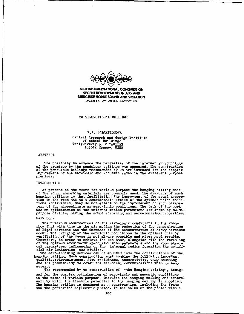
SECOND INTERNATIONAL CONGRESS ONRECENT DEVELOPMENTS IN AIR- AND
STRUCTURE-BORNE SOUND AND VIBRATIONMARCH 4-6. 1992 AUBURN UNIVERSITY. USA
MULTIFUNCTIONAL CEILINGS
TI. GALAKTIONOVA
Central Research-and design Instituteof school Buildings
Tretykovskiy p. 2 TsNIIEP103012 Lroscov, USSR
ABSTRACT
The possibity to advance the parameters of the internal surroundingsof the premises by the pendulous ceilings was appeared. The constructionof the pendulous ceilings recommended by us are intended for the compleximprovement of the aeroionic and acoustic rates in the different purposepremises.
INTRODUCTION
At present in the rcoms for various purpose the hanging ceiling madeof the sound absorbing materials are commonly used. The drawback of suchhanging ceilings is that facilitating the improvment of the sound absorp-tion in the room and to a considerable extent of the optimal noise condi-tions achievement, they do not effect on the improvement of such parame-ters of the microclimate as aero-ionic conditions. The task of the workwas an optimization of the internal medium parameters for rooms by multi-purpose devices, having the sound absorbing and aero-ionizing properties.L0AIN BODY
The numerous observations of the aero-ionic conditions in the roomsshow that with time in the air medium the reduction of the concentrationof light aeroions and the increase of the concentration of heavy aeroionsoccur. The bringing of the aeroionic conditions to the optimal ones byventilation of the rooms is not always possible and gives good results.Therefore, in order to achieve the set task, alongside with the revealingof the optimum architectural-construction parameters and the room physi-cal parameters, influencing on the internal medium formation the artifi-cial air ionization was studied.
The aero-ionizing devices can be mounted into the constructions of thehanging ceiling. Such construction must combine the following importantqualities:bioresistance, fire resistance, decorativity, easy mountingand the possibility to cover the technical communications with an easyaccess.
The recommended by us construction of "the Hanging ceiling", desig-ned for the complex optimization of aero-ionic and acoustic conditionsin the rooms of various purpose, includes the hanging ceiling and controlunit by which the electric potential to the hanging ceiling is supplied.The hanging ceiling is designed as a construction, including the frameand the perforated diplectric plates. In the holes of the plates with a
807

certain pitch the tapered metal elements-needles, connected with eachother, are located. Such plates, as it is known, absorb sound in variousfrequency bands depending on the applied material and in our case theycreate the concentration3 of light aerojons at the breathing level /1.0-1.5 m/ of order 3-5 .10 of aerions per 1 cm3 /Fig.l /.
The voltage of 30-40 KV from the control unit is supplied to themAetal interconnected needles. In this the autoelectron emission takesplace, which leads to the formation of light aeroions.
Simultaneously with the concentration of light aeroions the decreaseof the heavy aeroion concentration occurs due to their deposition underthe action of the electric field on thee floor surface.
In order to create the necessary micriclimate in the room we have al-so, developed "A sound absorbing device" for the hanging ceiling, inclu-ding a metal frame in the form of a grate with a face thickness of 3-5-4,installed with the clearance on the enclosing construction, providedwith a film,. located between the frame and the enclosing construction.The faces of the grate, turned inside th6 room, are tapered to naught.During the voltage of 30-40 kV supply from the control unit to the Zratethe autoelectron emission occurs, leading to the formation of light aero-
-ýons depends on the supplied voltage value and the sharpening extent ofthe elements. In order to create the necessary potential gradient theratio of the sharpened part to the non-sharpened one must be within 1:2-1:4 range at the ratio of the edge thickness to its height 1:10 - 1:5.The sound absorption coefficient of the construction under study is de-termined from the boundary conditions on the grate for the total fieldof the incident and reflected waves, as well as for the field, excitedin the intervals between the edges, where the film, which works as a me-mbrane; is located.
',e have measured the sound absorption coefficients of various versionsof proposed constructions in a small-size reverjeration chamber on thesamples, the area of which did not exceed 1.5 m and in a large reverbe-ration chamber. The results of the measurement are presented in thetable.
A'nother version of similar constructions can be an acoustical multi-cavity panel with a slit perforation. The acoustical factors of suchpanel, also, have been determined in the reverberation chambers.
The geometric parameters of the panel with the slit perforation, inwhich the needles for the air aeroionozation can be located, are givenin Fig.2 . Considering the geometry of the panel one can see that it canattributed to a physical model of the related resonance systems of Helm-holtz resonator type.
REFEOU3NCES
The results of the measurements have shown that the absorbing proper-ties of the panel with the links are 30-80f improved in comparison withthe smooth reinforced concrete plate and 20-60Z improved in comparisonwith the perforated plate.
The studies, performed in the small-size reverberation chamber, haveshown:
- the complex sound absorbing ceiling from "ickmigran" plates, perfora-ted for the aeroion radiators, has a broader sound absorption spectrumin comparison with the non-perforated "Akimigran" plate /Oc=0.9 - at 25OH7/
- the complex construction from the sheets of gypsum plaster board,perforated for the aeroion radiators, is a pronounced resonance construc..tion with maximum sound absorption coefficient at 250 Hz frequency;
- the optimum hei.ht from the breathing area of a man to the aeroionradiation source must not exceed - 2.5 m, and the total height of theroon from the floor to the hanging ceiling must not exceed 4 m.
Taking into account good sound absorbing properties and multifunc-tionality of the ceilings with aerolonization of air, these constructi-ons can be recommended for noise reduction in public buildings.
808
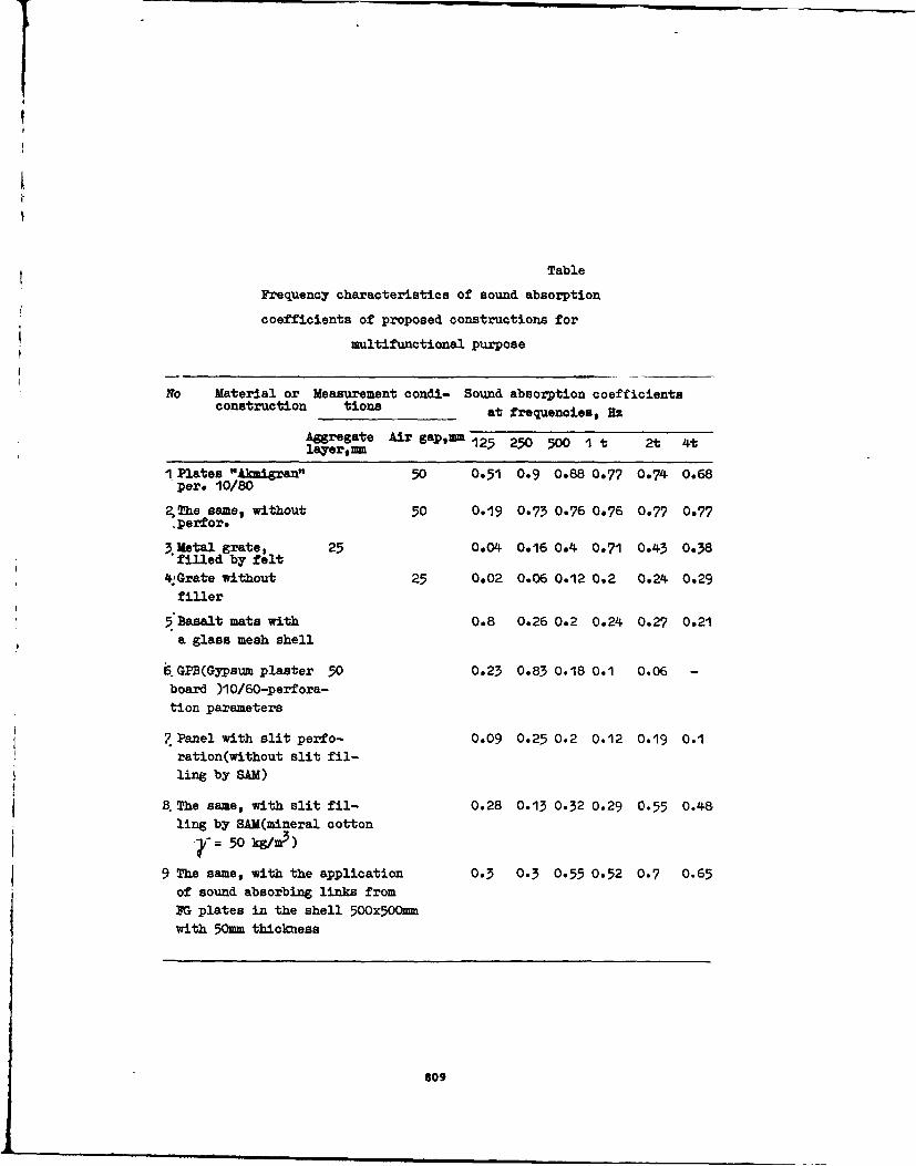
Table
Frequency characteristics of sound absorption
coefficients of proposed constructions for
multifunctional purpose
No Material or Measurement condi- Sound absorption coefficientsconstruction tions at frequencies, Hz
Aggregate Air gapM m 125 250 500 1 t 2t 4tlayer,u
I Plates "Ak-igran" 50 0.51 0.9 0.88 0.77 0.74 0.68per. 10/80
2ýThe same, without 50 0.19 0.73 0.76 0.76 0.77 0.77Sperfor.
3 Metal grate, 25 0.04 0.16 0.4 0.71 0.43 0.38"filled by felt
klGrate without 25 0.02 0.06 0.12 0.2 0.24 0.29filler
5 Basalt mats with 0.8 0.26 0.2 0.24 0.27 0.21a glass mesh shell
6.GPB(Gypsum plaster 50 0.23 0.83 0.18 0.1 0.06 -board )10/60-perfora-tion parameters
7 Panel with slit perfo- 0.09 0.25 0.2 0.12 0.19 0.1ration(without slit fil-ling by SAM)
B The same, with slit fil- 0.28 0.13 0.32 0.29 0.55 0.48
ling by SAM(mineral cotton?-= 50 kg/in)
9 The same, with the application 0.3 0.3 0.55 0.52 0.7 0.65of sound absorbing links fromPG plates in the shell 5OOx5OOmmwith 50mm thickness
809

A-,eedL'e , 2-p OaFe
Mass of areca:uxit, !:rtj2 ............
I-hic'cae-zc a slab, - U -.............. ZCU
Di.eoter of ope.ina7lr ........................ .C
Distance betr.eer o.eai~ns, ima ................... IE5
.idth of alit, -, . ............................... 5C-3 c
Fig.2
810

SECOND INTERNATIONAL CONGRESS ONRECENT DEVELOPMENTS IN AIR- AND
STRUCTURE-BORNE SOUND AND VIBRATIONMARCH 4-6, 992 AUBURN UNIVERSITY USA
PHASE FEATURES OF MAN AND ANIMALS REACTION TO INFRASOUND EFFECT
1 2 33D.J.Fraiman1. A.S.Faustov2. A.N.lvannikov , V.l.Pavlov
Medical Laboratory of Voronezh Electronics Plant, Dru2hinnikov 1, 394068 Voronezh
2 Voronezh Medical Institute, 394068 Voronezh
Department of Acoustics,Faculty of Physics, Moscow State University, 119899 MoscowRussia
ABSTRACT
Infrasound effect on biological systems is investigated by us within three main
positions.
INTRODUCTION
First, we have studied the development of the interaction process betweeninfrasound and human body within the time. Parameters of the functionality of thenervous and cardiovascular human and animal systems are studied according to ordinarytechniques. The investigation covered hemodynamics, hemocoagulation. oxygentransportation, histology and histochemistry of myocardium, vessels, adipose cellschanges, managerial function of the vegetative centers of the nervous system, andpsychophysiological functions of the man-operator. Traditional techniques are used. Inthis paper all techniques are used not to investigate human and animals functions, butonly to mark the direction of explored systems reaction to infrasound effect.
Secondly, the investigation was carried out within positions of physicalacoustics.We came from the following assumptions. Majority of all interactions betweeninfrasound and man takes place in official and domestic apartments. However, thedimensions of these apartments are comparable with a wavelength (at least, up to 100Hz). A man who is either by force of official duties, or domestic habits in one oranother part of the room, will interact with different energetic components of theacoustic field. In this connection various biological response at infrasound effect canbe expected (13.
Thirdly, we have come from the physiology of sensorysystems with rich actualmaterial, which allows to make a conclusion that ear added mechanism of interactionbetween man and infrasound should exist.
EXPERIMENTAL RESULTS
It is stated by an experiment that man and animals reaction on infrasound withinthe first seconds begins from activizatton ob the vegetative nervous system, starting upthe humoral channel of the human body function regulation within several minutes frombeginning of interaction. At the same time changes of the functional activity of thesubcortical structures and human efficiency level arise.
By the end of 4-6 hours from the beginning of the effect the reversible changes ofhemocoagulation and activity of respiratory myocardial ferments are being developed. Thenext phase is the phase of latent modifications which changes by 18-20 day of the effectwith preventive force consumption of the human body and arising of the morphologicalmodifications in the cardiovascular system.
811

The whole chain of the resoonse reactions develops when the object is in that dartof the laboratory where the vectors of active and reactive intensity are collinear (zone
D). It is found that starting-up point of the development of the response reaction chain
is the direct effect of acoustic wave and vascular system in D-zone which is cleared outby us (21.
All reactions investigated by us begin and go out in the determined time intervals
called by us the phases of the human body reaction on the infrasound E31.The person and animal reaction on the infrasound action begins from the reaction of
the nervous system. In the first minute the regulating activity of the sympathetic
section o; the vegetative nervous system is strengthened and the tension index of otherstructures of the central nervous system is increased.
Then to the twentieth minute of influence the activity of the subcorticalstructures of the brain becomes worse and the level of the person capacity for work is
reduced. At that time the indications of switching on of more plastic and longerfunctioning humoral channel of the person function regulation are appeared.
On the first day at the end of the fourth - sixth hour of everyday six hourinfluence of infrasound of the level 100 dl on frequency of 10 Hz the expressed reactionof increasing the coagulation activity of blood is developed. At that time the decreaseof oxygen consumption from blood is registered, oxygen content is increased in venousblood without changing its percent level in arterial blood.
On the third day of influence the increased activity of some ferments of heartmuscle respiratory cycle and activity oppression of other are clearly registered.
To the sixth day of influence the coagulation activity of blood is reduced to the
development of hypocoagulation.To the twelfth day of influence the oxygen content in arterial and venous blood is
normalized.The state of coagulation activity of blood, the activity of respiratoryferments of the myocardial don't differ from the initial data. The histological changesof the muscular cells of the heart in the first day have a reversible character.
To the twenty fourth day of influence the hypercoagulation of blood is appearingagain, the activity of respiratory ferments of the myocardial is diminished almost on 50Z. The destructive changes of the myocardial are appeared.
Particularly must be said about the reaction of the cells containing substance -protector geparin. At first labrozit content is changed, then their content per unit ofarea is gradually decreased maximal reducing to the twenty fourth day of influence.
DISCUSSION
All changes have a phase character. Under the phase of development we understandlimited spaces of development of human body - reaction on infrasound. So the primaryreaction of the nervous system is going out, the nervous centers get over a new level offunctionality directing the humoral reaction to the infrasound action. At first thisreaction has a time - serving character, the trustworthy changes from the 12th to the18th day of influence are not found, at least, by out methods. And only after the 18thday of influence the reserve oossibilities of human body are grown weak and visiblechanges in organs and systems can be seen. The second important moment, in our opinion,is the revealing of the ear added mechanism of the infrasound interaction and it isappeared that the infrasound can act directly on the wall of the blood vessel model. Theanalogous changes are registered from the vascular basin of persons and animals. Thereaction is developed instantly with the appearance of forced acoustic interaction and
disappears with the turning of the acoustic generator without decrement. The revealeddirect action of the infrasound on the vessels explains the instant development of thereciprocal reaction of the nervous system when the infrasound is actinggand the
development of all above stated functional and morphological changes in it.In addition, the revealing of direct mechanism of the interaction of the blood
vessel system and infrasounC explains the fact that practically in all publications
describing the morphological changes those or other changes in the vessels of theinvestigated organ or ischammic changes in it are pointed out.
All above stated biological changes are developed not in all places of laboratory
room but only in places where vectors of active and reactive intensity are collinear.Where the active sound intensity vector vortex is not equal to zero, the changes do notappear at all or has a character of the reactions developing in the conditions ofcomfort. And this is in spite of the same level of sound pressure.
The results clearly point out on the phase character of person and animals
reaction, on the interaction with the infrasound. The basic phase of this interaction
are:
812

1.The functional Phasea) a Primary reaction of the nervous system on interaction between infrasound and
vascular system,
b) a neurohumoral reaction,
c) a functional organs and tissue reaction on infrasound effect.2.The phase of the functional systems tension followed by the organs and systems
transfer on a new level of functioning in order to suppo-t a homoeothase.3.Functional system consumption phase.
4.Phase of the expressed morphofunctional modifications development.
CONCLUSION
The oossibility of the development of this phase of man and animal reaction oninteraction with infrasound depends on the place of their position in the space of theofficial apartment. More exactly, it depends on their interaction with one or anothercomponent of the acoustic field energetic structure (zone V and zone D according to ourterminology). An important conclusion follows from this. Under the equal sound pressurelevel experiments carried out in V zone caused development of reactions similar withthose ones as at the rest. It can lead into error the investigators and cause erroneous
conclusions.Besides, the application of non-adequate, not sensitive technioues either at
"short-term test', or "hits" of the time of material collection to the latent phase cancause erroneous conclusions even at position of the object in the zone D. And, a levelof sound pressure which influences upon reaction development rate may be so low that aduration of each phase can be estimated as an absence of orocess development oradaptation to it. In reality, the reaction develops since afferent vascular systemreceptors have very low limit of the sensibility.
To transfer to a higher limit of excitation these receptors need very powerful
irritant. With sound pressure level of 130 dl the receotors consumption appears very
quickly and the reaction may be weakly expressed as these is no signal of neurohumoralreaction starting-up. Whereas self-damaging of vessel walls quite protracted process
causing protracted hypocoagulation which does not cause any guarded reaction ofinvestigator.
So, phase development of man and animals reaction on infrasound in zone D must betaken into account in elaboration of the hygienic standards on infrasound.
We will present the above-described results in graphical forms. So, fig.l a)
,b),c), d) show:l.Nervous system reaction.
2.Humoral reaction.3.Reaction of hemocoagulation.4.axygen content in venous blood.
5.Level of person capacity for work.6.Activity of respiratory cycle ferments-7.Morphological changes of myocardial and cells-protectors.
REFERENCES
l.Fraiman 3.3.. ]vannikov A.N., Zhukov A.N. On the Influence of Infranoise Fields on
Humans. 6-th International Meeting on Low frequency Noise and Vibration.Leiden 1991,
p.4 9
-5 6
.
2.Zhukov A.N., lvannikov A.N., Pavlov V.I., Fraiman 3.3. Infranoise in closed Volumes,Fortschritte der Akustik, DAGA-91 Bochum, Teil A. s.385-388.
3.Zhukov A.N., Ivannikov A.N., Kravchenko D.1., Pavlov V.I. Distinctive features ofenergy fine structure of a sound field. Soy. Phys. Acoust. 1989, vol.35, no4, o.367-369.
813

lPhose tiU i daoy % Phase 1+7 day
+25
CL bl0{ N ,opýls 0 týc 13 4 5 ,dayjO 02 Q3 i 4 5o t"' ý6
-25 -- 25% 0/0
+25 *+5
i Phase 12-18 day W Phase 18 +24dao
3,4,6 3
13 7 ,
- 25 -25
814

SECOND INTERNATIONAL CONGRESS ONRECENT DEVELOPMENTS IN AIR- AND
STRUCTURE-BORNE SOUND AND VIBRATIONMARCH 4-6. 1992 AUBURN UNIVERSIT. USA
MEASURING OF THE TURBULENCE AND SOUND ABOVE THE OCEAN
A.N.lvannikov. S.V.Makeev, V.l.Pavlov
Department of Acoustics
Faculty of Physics
Moscou State UniversityMoscou, 119899
USSR.
ABSTRACT
In this paper the original results of the observation of low-frequency atmosphericpressure fluctuations are presented. The results have been obtained straight over the
Pacific Ocean surface during the 17-th expedition of the 'Academician Nesmejanov* ship.The theoretical expressions for the degree law of the amplitude spectrum decrease andits connection with the wind velocity were found. It was carried out the experimental
results analysis and its comparison with the proposed theoretical model of turbulence.The spikes on the background of fluctuation spectra have been discovered.
INTRODUCTION
There are a lot of publications concerning the atmospheric low frequency (less then20 hz) noise and most of them deal with a pressure fluctuation above a ground but not
upon water, because of experimental difficulties in the latter case. The measurements of
a pressure fluctuation above a ocean surface especially at far distances from a coastare very interest. The data of such experiment are analyzed in this work. The atmospherepressure fluctuations have been obtained above ocean surface during of the "Academician
Nesmejanov" scientific ship's expedition (October 1989 - February 1990). The ship's rou-
te lay in the west area of the Pacific Ocean from Vladivostok to New Zealand.
EXPERIMENTAL PROCEDURE
The atmosphere pressure fluctuations were registered by high sensitive microphone
carrier system type 2631 "B&K". During the measurements the microphone of carrier systemhas been removed at 2 a from ship board and 3 m from ocean surface by special bracket.
The frequency of acoustic signal above 100 Hz was cut by low-pass-filter 01013 'Robot-ron*. Then the signal was amplified by intrinsic amplifier of the indication block 02022"Robotron" and one was recorded to the FM channel of gauging tape recorder HAS-54 "Tele-
funken'.
Simultaneously with registration of acoustic signal the vibration of ship frame hasbeen recorded to other tape recorder channel. It was made to except the *psevdoinfraso-undf caused by the ship's vibrations. At the same time the coordinates of the ship, itsvelocity and course, the direction and velocity of wind, atmospheric pressure have beenfixed too. Frequency analysis of recorded analog signals was carried out with the help
of FFT-analyzer CF-300 ONO SOKKI in the range 0-20 Hz by means of linear average of 512instant amplitude spectra. The duration of signal analysis was about seven minutes.
The typical averaged frequency spectrum in log-log scale is presented in Fig.l. Co-rresponding record was made 9 February 1990 in the Pacific Ocean's region removed morethen 1500 km from New Guinea coast to North-West. The analysis of obtained spectrum
815
_ _ _ _

shows that in the investigated frequency band 0,5-20 Hz there is monotone decrease ofamplitude spectra of pressure fluctuations with respect to frequency. Linear dependencein range 0,8-20 Hz is good observed too. It testifies of the degree law of decrease ofamplitude spectrum with respect to frequency. The fall of spectrum at frequency 0,5 Hzand below is caused by the low frequency rolloff of gauging channel. It is necessary tonote that about 10-15% spectra differ considerably from one shown in Fig.l. The connec-tion of this phenomenon is not revealed yet.
THEORETICAL MODEL
Let assume the atmosphere pressure field p(X.t) to be described by the expression
p(X.t) ý P 0 V'u(X.t) (1)
where P0 is the air density, V is the velocity of the air flow, U(X.t) is the field of
the velocity fluctuations. Then the correlation function is
(p(1 1 t 1 )p(X 2 t 2)) = B!. -n 2 ,t(-t 2 ) I .OiI A) .t lu( . t )-n 2)
The brackets mean the average procedure. ni= V. /Ivi. Following the hypothesis of 'fro-
zen" turbulence IlI we can write:
<Ui(X1.t )U (X2 t 2) =)Dij J( W - l ezp[_ t 1 - ) + (t 2
Here . = Xnf is circular freouency, k is wave vector, tensor D. 6. ý Ai aco kn2
the medium's incompressibility, i.e. the condition dit; U = 0 is satisfied. The quantityE(k) is spectral density of the turbulence fluctuations energy normed by condition:
00<U 2(w.t.) = 2f k B(h)(4
0
For the calculations it is convenient to use spherical frame with Z-axis along of thevector V = Vfl. Taking account of the properties of the 6-function we have:
<p(X. t )p(I.t )), +Ke-( t is2 _- Jdh [ - Vh 3 (5)
In the inertial interval of turbulence there is the condition "< - ll- <I where-V
and I are external and internal scale of turbulence correspondingly, the quantity E(k) =
IF A.71 . Here le- K- 2/3, K and P are constants, S defines the average dissipation of en-
ergy per time unit and per mass unit of the medium.Then we obtain:
0
e1d

LAdB
10 0
80
1 10 Hz
Figure 1--The tyD'Cdl averaged soectruft.
0-
-15- 6
-45-
- 60 4 8 12 16 20 HzFioure 2--The svetra in different daVS: 1 - Feb.2. 2 -Fob.5. 3 -Feb.8. 4 -Feb.11.
5 - eb.4. 6 - Feb.17. 1990.
8J17

22Here the coefficient is C = . The exoression in square brackets is IPrW)li. (4.41 )(4.43)
where Ipv s the amolitude spectrum of pressure fluctuations. It yields
1/2 PI4 - ALOPp.j =C poR V 2 . 2 (7)
It was these fluctuations that were measured in the experiments and their amplitude spe-ctruo va- determined as the result of analysis of data tape records. For comparison of
the experimental results and theoretical model we represent Eq.(7) in log-log scale:
L(f) = A 4 B lgY - C Zgf (8)
1/2 P0R B - j ; O5HereA=201B=20 ; C=20 2 p,=" 10 Pa is base level
of sound pressure. L(f) is the level of amplitude spectrum component in dl. For Kolmogo-roy's isotrooic turbulence P= 513 (1]. Therefore, the dependencies L - 26.6 lgV at thefixed frequency and L -v 16.7 lgf at the constant wind velocity will to confirm the Kol-mogorov-Obuchov theory.
EXPERIMENTAL RESULTS
To our opinion the part of the way from the New Hebrides to Japan is of the mostinterest (02 February to 17 February 1990), where the ship sailed to NorthvNest with the
approximately constant velocity of 12-13 knots. Total path of the way in the west areaof the Pacific ocean was more than 9000 ke and it took 16 days. The most distance fromcoasts was 1500 km. On the whole the way the fluctuations spectra were similar to theone shown in Fig.l. In Fig.2. one shown the dynamics of the spectra in this time periodin linear frequency scale. In different days the averaged spectra were processed by the
least squares method on PC.It is interesting to consider the connection of atmospheric pressure fluctuations
and the infrasound with the oceanic and atmospheric parameters to examine the suggestedtheoretical model. The dependence of the typical parameters of the fluctuations spectra
from the wind velocity is of the most important. In Fig.3. the dependence nfl f ) is
where V e, is the module of the vector sum of the wind and the ship's velocities. The
line in Fic.3. is described by formula:
n = 1.01 - 7.94- 10 3Yf (9)
i.e. there is a weak trend to decrease n with respect to the effective wind velocity. Inthis period the average value of n = 0.92 : 0.08 that correlate good with the theoreti-cal value of n = 5/5 = 0.83. The similar situation exists for dependence of n from a ro-ughness of the ocean's surface. Though in this case one has to account the connectionbetween the wind velocity and the ocean's roughness.
It results from Eq.(8) that an amplitude of spectral components is a linear functi-on of I-. The integral sound level Lint in a fixed frequency range is proportional to
19V. The dependence int in range 0-20 Hz of ZCV is shown in Fig.4. (points on the
chart). There is an increasing of the pressure fluctuations level though the experimen-tal value of the coefficient B turns out smaller than the theoretical one.
DISCUSSION OF THE SPIKES OF SPECTRUM
The obtained results contain often spikes on the background of almost monotonousdecreasing of the fluctuation spectrum. Perhaps it is infrasound. For example analysisof the fluctuation record on the way from the New Hebrides to Japan reveals spikes inrange 3.5-4.0 Hz. The exceeding of these spectral components over background is 4-10 di.The notable spike at frequency 3.9 Hz and the exceeding above the background of 7 dl is
818

n
1.0
0.8 °
0.6I !I
0 5 10 Veff, nm/c
Figure 3--Exoerlmental value of the coefficient n.
LdB120
100 - 00 0
80080 -• 0o
, I I I i I
0.4 0.8 1.2 LgV
Figure 4
-- InteoraI sound level booints) and infrasound level (circles).
819

shown in Fig.l.The level of infrasound in this ties period was fluctuated from 80 to 100 ds, i.e.
the value of the sound pressure of infrasound wave was approximately P - IPa. Infrasoundlevels reach maxima in the period of February 7-11. It is necessary to note that the ob-
served invariability of the spikes frequency and the relative narrowness of their spec-
tra are similar to peculiarity of "marine voice" [2]. This allows to sake a supposition
about their similar origin. Naturally it appears the question about origin of this in-frasound. Unfortunately our data do not allow to give correct answer.
The dependence of an infrasound level on wind velocity at frequency 3.5-4.0 Hz isshown in Fig.4. (circles on the chart). One can to see the weak trend to its increasing
at great wind velocities. In spite of the considered data do not allow to make correctconclusion about the oceanic infrasound's origin, we may suppose the one described inE2].
CONCLUSION
During the three months of the expedition the ship sailed more than 30,000 km inthe Pacific Ocean. It gave exceptional observations of the atmospheric turbulence andthe infrasound at large distances in the wide band of infrasonic frequencies (more thanfive octaves). The experimental investigations were carried out in the frequency band of
0.5-20 Hz.The spectra of the atmospheric pressure fluctuations were shown to decrease propor-
tionally to (dn. The index n "as determined. Its dependence on the wind velocity was es-tablished. Also the spikes on the background of the fluctuations spectra were discove-red. They are expected to be connected with the infrasonic waves. It was offered a theo-retical model of a description of pressure fluctuations and its comparison with the ex-
perimental results.
REFERENCES
1. S.K.Satchelor. The theory of homogeneous turbulence. Cambridge, 1953.
2. Pavlov V.I.. Sukhorukov A.I. Infrasound radiation into atmosphere by an eddy inhomo-geneity located near the ocean surface. Acad. Sod. USSR, Atoos & Oceanic Phys.(USA),vol.20, no.8, 1984, p.674-681.
IV20

SECOND INTERNATIONAL CONGRESS ONRECENT DEVELOPMENTS IN AIR- AND
STRUCTURE-BORNE SOUND AND VIBRATIONMARCH 4-6, 1992 AUBURN UNIVE&SJTY USA
COMPARISON TESTS BETWEE ACOUSTIC EMISSIONTRANSDUCERS FOR INDUSTRIAL APPLICATIONS
S.C. KERKYRAS*, W.K.D. BORTHWICK*, R.L. REUBEN•.
P.A. DRAKATOS" and K.L. TZANETOS*
* DEPARTMENT OF MECHANICAL ENGINEERING, UNIVERSITY OF PATRAS, GREECE.
* DEPARTMENT OF MECHANICAL ENGINEEING,HERIOT-WATT UNIVERSITY, EDINBURGH, U.K.
0 Present Address: CEC BRITE DIRECTORATE.
1. ABSTRA
In this work the response of some commercial PZT Acoustic Emission (AE)transducers is examined under a set of controlled conditions in order toIsolate the resulting effects of surface excitation (controlled by wavepropagation conditions) and characteristics of the sensor Itself (i.e.resonances). The behaviour of the two commercial transducers is compared withan experimental transducer based on PVdF film.
2. INTRODUCTION
The increasing interest in Improving the productivity of manufacturingprocesses has naturally emphasised the role of automation of these processes.The successful automation of manufacturing operations requires continuousknowledge of the state of the operation. The control of manufacturingprocesses also requires on-line information on the behaviour of themanufacturing systems. In this light, Acoustic Emission (i.e. stress waveemissions from materials undergoing deformation, fracture, or other internalmechanisms releasing energy) has great potential as a technique to monitorsuch processes. It has therefore become very important to investigate thefactors that influence the responses of commercial AE sensors and to comparethese responses with those obtained by some non-commercial, high fidelity AEtransducers.
3. REVIEW ON SOME TYPES OF AE TRANSpUCERS
In this work, two different types of AE sensor are compared. AE can bemeasured using plezoactive, capacitive, electromagnetic methods. Thefollowing brief review describes the two types relevant to this work and alsoan optical sensor against which the PVdF sensor has already been compared Il].
1) Comercial Piezoelectric AE sensors
The majority of the commercial AE sensors belong in this category. Thepiezoelectric active element is lead-zirconate-titanate (PZT) and thesesensors may be "broadband" or "resonant" devices. The large aperture (phaseinterference effects due to large contact surface) of the commerciallyavailable devices (shoe sizes are typically of the order 10 to 20 mm) restrict
621

the response to the different wave modes. The directlonality depends oncrystal geometry and polarization. Normally commercial sensors areomni-directional.
iI) The PVdF displacement transducer
The semi-crystalline polymer polyvinylidene fluoride (PVdF) processespiezoelectric properties. It is flexible and compliant and has excellentbandwidth and sensitivity. PVdF has been successfully used in astrain-gauge-like application as an AE transducer for monitoring composites[2]. Scott and Carlyle (3] indicate that PVdF transducers suffer much lessfrom ringing than commercial broadband devices and are capable of a flatfrequency response over a wide range. Chang and Sun [4] have developed a PVdFtransducer which, depending on the backing geometry, may be used either as adisplacement or a velocity transducer. For displacement measurements a brassbacking with a conical extension is pressed against the PVdF film and onto thesurface being monitored. The use of a long acrylic rod as backingsignificantly changes the response to being more like that of a velocitytransducer.
A PVdF displacement transducer with brass backing has been used to monitor aturning operation on a lathe (Kerkyras et al (5]), and Its frequency responseappeared to be very promising for power spectrum diagnosis of AE signals,something which has proven very difficult using commercial AE devices. Thebasic conclusion from this work was that this AE sensor showed high fidelity,mode separation and had a broadband response free from resonances. Thesecharacteristics, together with its low cost make it a potentially very usefuldevice.
Ili) The Fibre Optic Interferomter
Optical trandsucers for AE monitoring are attractive because of thepossibility of using both contacting and non-contacting probes and because oftheir flat frequency response over a very large bandwidth.
It has been shown that fibre optic techniques can be used to reallse robustInterferometers with a wide range of applications in physical sensing. Inparticular, fibres have been used effectively as displacement and velocitytransducers [6].
4. EXPERIMENTAL SET-UP
The transducers studied In this work were tested using a range of propagationmedia and their response was analysed by using standard signal processingmethods. The sensors used were the Dunegan S9204 and D9201A and theexperimental PVdF displacement transducer. A standard AE source, the Nielsenpencil lead break, was used as excitation. Fig.1 shows a block diagram of theinstrumentation used in the experiments.
The three propagation media that were evaluated were:
a) A large cylindrical steel block of height 19 cm and diameter 18 cm, welllapped on both flat surfaces.
This structure was used as a propagation medium in an attempt toeliminate reflections as far as possible. In order to achieve this thehighest available sampling rate (40 or 20 MHz) was used to acquire AEdata.
b) A steel plate of dimensions 54 x 28.2 x 0.65 cm.
The reason this structure was chosen as a propagation medium was theavailability of analytical solutions which can provide a comparisonbetween measured and calculated responses (e.g. Ceranoglu and Pao [71).
c) A long steel bar of rectangular cross-section having dimensions
177 x 7.5 x 1.3 cm.
822

This structure was proposed by Kerkyras et &1 18] as a simple propagationmedium in order to increase the number of reflections of bulk waves atthe free surfaces and In this way to minimlee their Influence on thereceived signal by placing the sensor at a long distance from the source.In thIs way it was expected that the dominant wave mode captured by thesensors would be surface waves. Fig.2 shows these three differencepropagation media schematically.
5. RESULTS AND DISCUSSION
In all experiments a 40dB gain pre-amplifler was used. The first 4096 datapoints were stored In the computer memory. These data were then averaged overat least 8 pencil lead breaks in each case. The data were normalized and anFM was performed. It should be noted that amplitudes In the obtained plotsare affected by gain and trigger level settings which were chosen to give thebest reliability of data capture. Furthermore the data were ranged to ensuremaximum resolution within the window. This means that amplitudes in thefrequency domain are relative only but the visual content of the graphs ismaximised.
Figures 3 to 7 and 9 to 13 show frequency domain responses for the variouspropagation media for the D9201A and S9204 sensors respectively. Also,Figures 8 and 14 show time domain responses for these two sensors obtained onthe steel plate propagation medium. Finally, figures 15 and 16 show.respectively, time- and frequency-domain responses for the PVdF basedtransducer to excitation on the cylindrical steel block.
By comparing Figures 9-13 with Figures 3-7 It can be seen that the D9201Asensor is sensitive to surface waves with broad frequency responses in therange of 0. 1 to IHHz whereas the S9204 sensor is sensitive In the frequencyrange of 50 to 450 kHz. Also, both sensors showed similar sensitivity both Insurface and compression waves. The influence of the three differentpropagation media on the transducers' response Is quite obvious in thefrequency domain. Furthermore, epicentral excitations changed the frequencyresponses significantly.. The steel block gave the clearest results, the datafrom the steel plate and the rectangular bar being influenced by multiplereflections as indicated by the decaying higher frequencies.
According to the manufacturer, both transducers should respond to the surfacevelocity. However, as can be seen from Figures 8 and 14 the time-responses ofthese commercial AE transducers are dominated by the basic resonances of thesensor (ringing). This means that the output of such sensors is not theaveraged velocity of the area on which they have been placed but Is dominatedby the characteristics of the sensor. Furthermore, It has been shownelsewhere (91 that integrated time domain responses (considering the sensorsas velocity transducers) did not give the type of trend predicted by the RayTheory of Ceranoglu et al [7].
Concerning the selection of the appropriate propagation medium for sensorcalibration, it is obvious that this will depend on the specific requirementsfor each test. The massive steel block gives results which correspond closelyto the calibration data for Rayleigh waves although reflections were nottotally avoided because of Its limited size. More massive structures andhigher sampling rates give a good solution to the problem but the expense ofsuch structures for propagation media is quite high. The steel plate waschosen as a possible propagation medium because of the availability of ananalytical solution and because steel plate of the required dimensions isreadily obtained.
Finally the long rectangular bar showed frequency responses which could be dueto Rayleigh excitation merely because of the rapid decay of bulk waves withdistance from the source, a factor that does not affect Rayleigh waves asmuch.
The time- and frequency-domain responses of the PVdF transducer on thecylindrical block are shown In Figures 15 and 16. The time domain response is
6423

typical of that expected of a normal surface response for an infinitehalf-space [7] and back-to-back tests with an interferometric sensor haveshown a striking agreement In response (11. A comparison of the frequencydomain response (Figure 16) with those obtained under similar conditions forthe two commercial transducers (Figures 3 and 9) illustrates how theinformation from these latter two sensors Is dominated by their own resonance.This is especially important if one seans to analyse the frequency content ofacoustic emission signals and suggests that either a careful calibrationagainst a flat response transducer or the direct use of such a transducer isrequired for such applications.
6. CONCLUSIONS
The comparison of two commercial transducers with one experimental transducerbased on brass-backed PVdF film has highlighted the effect of crystalresonances on the response of the former type.
The use of a variety of propagation media has further Illustrated that wavepropagation effects can also Influence the frequency contact of the responseto a white noise source.
REFERENCES
I. KERKYRAS, S.C., BORTHWICK, W.K.D., REUBEN, R.L., McBRIDE, R.,BARTON, J.S. and JONES, J.D.C.: work to be published.
2. STIFFLER, R. and HENNEXE, E.G., J. Evaluation. vol.42, pp 956-960,Jul. 1983.
3. SCOTT, W.R. and CARLYLE, J.M., Naval Air Development Centre Report IR,Task No. 2R011088, 1976, Warminster, Pa.
4. CHANG, C. and SUN, C.T., J. Acoustic Emission. vol.7, pp 21-29. 1988.
5. KERKYRAS, S.C., WILCOX, S.J., BORTHWICK, W.K.D. and REUBEN, R.L.,Proceedings of 4th World Meeting on Acoustic Emission, Boston,Sept. 15-18, 1991.
6. McBRIDE, R., BARTON, J.S., JONES. J.D.C. and BORTHWICL, W.K.D.,Electro-Optics and Laser International Conference, Birmingham.March 20-22, 1990.
7. CERANOGLU, A.N. and PAO, Y.H., J. of Applied Mechanics, vol.48,Mar. 1981.
8. KERKYRAS, S.C., REUBEN, R.L. and BORTHWICK, W.K.D., Non-DestructiveTesting and Evaluation. To be published.
9. KERKYRAS, S.C., M.Phil. Thesis, Herlot-Watt University, Edinburgh.1991.
824

P with omtn
Figur L: 81oft diagr or sqimentil aetup
(b)" nml
(a)
FV1We 23 Me paa pluatim ameda aend(a) l• itne"l aai bla
(0) 1Un Utl Nw2
825

9 I6
Ia vii ii i
16a Iii I'826

S- -- |,;
U - U
* IiiU 0
1iii

_ _ _" .
ii !
4 U
828i

T
SECOND INTERNATIONAL CONGRESS ONRECENT DEVELOPMENTS IN AIR- AND
STRUCTURE-BORNE SOUND AND VIBRATIONMARCH 4-6& 1992 AUBURN UNIVERSITY, USA
USING A CIRCUMFERENTIAL TRANSDUCER TO MEASUREINTERNAL PRESSURES WITHIN A PIPE
R.J. Pinnington and A.. Briscoeliinitute of Sound and Vibration Research
University of SouthamptonSouthampton, S09 5NH
England
ABSTRACT
A circumferential transducer has been devised which measured the dynamic pressure of gas or fluidwithin a pipe. The transducer consists of a piezoelectric wire wrapped circumferentially around the pipe wall.Such an arrangement ensures only sensitivity to axi-symmetric waves as waves with more than onecircumferential half wave length will not be detected. The transducer is therefore only sensitive to thepredominantly, fluid-borne wave and the predominantly compressional wave in the pipe wall. The sensitivityto these two wave types is calculated and approximate expressions given. The applicability of the method isassessed for soft and hard pipes containing water. Some measurements are presented for a perspex pipe filledwith water.
1.0 INTRODUCTION
Fluid-filled pipes can represent a significant vibration path, in both the fluid and pipe wall, from amachine to the supporting structure. To assess this problem a non-intrusive pressure sensor has been devisedwhich involves an integral number of turns of a piezoelectric sensor around the pipe wall. The device istherefore only sensitive to n = 0 axisymmetric waves as others have equal positive and negative radial motionsand cancel.
There are two n = 0 waves; a predominantly fluid based wave termed s = 1, and the s = 2 wave whichis predominantly longitudinal motion in the pipe wall [1. The s = I wave is the main contributor to thepressure and radial wall motion, and their relationship gives the sensitivity of the transducer. Unfortunatelythe s = 2 wave also has small pressure and radial motion contributions which disturb the accuracy ofmeasurement of pressure. The sensitivity of the radial wall motion to both wave types is calculated here andcomparisons made on a perspex pipe, with and without water.
The calculations involved approximate values for the wavenumbers for the n = 0; s = I and s = 2waves.
2.0 THEORY
2.1 The eguations of motion
With reference to Figure 1 the shell displacements are u and w in the axial and radial directions. a., N0refer to axial and circumferential stress. The fluid pressure is p and axial displacement uf. The followingequations are simplified forms of Kennard's equations [2].
Equilibrium of forces in the axial direction gives
829
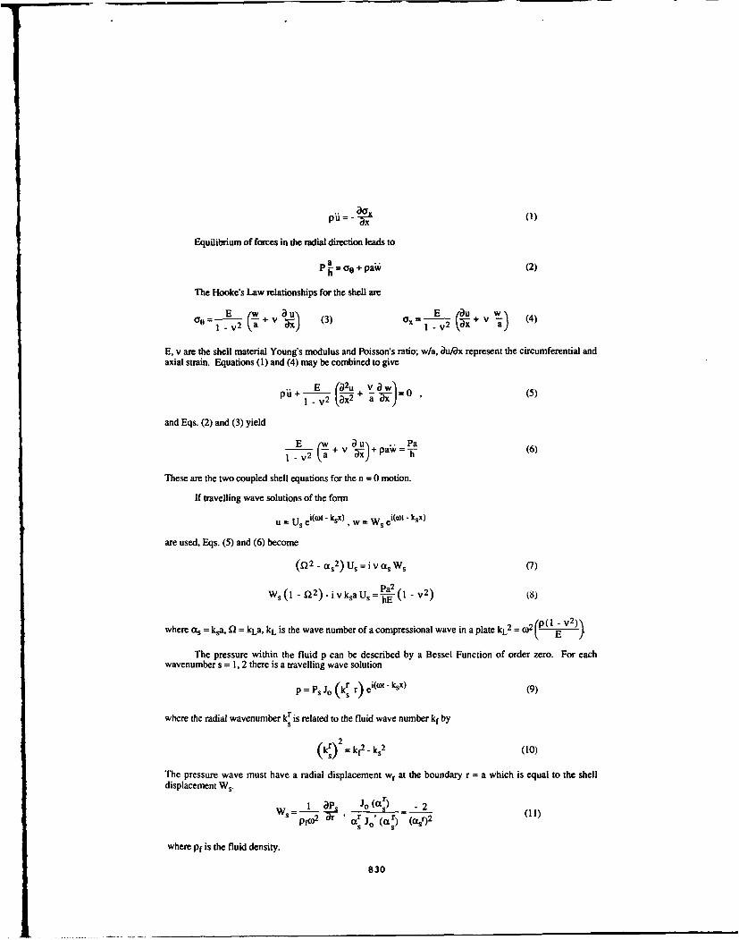
pi= - (1)
Equilibrium of forces in the radial direction leads to
P =ao + pawk (2)
The Hooke's Law relationships for the shell are
a E C) u (3) Ex au+ (4)1 - v2 -X I - V2C;. a
E, v are the shell material Young's modulus and Poisson's ratio; w/a, au'ux represent the circumferential andaxial strain. Equations (1) and (4) may be combined to give
1-v+ (c 2u yawl 0 (5)
and Eqs. (2) and (3) yield
E Pa(6_i + V ) + pa;w = -f-(6)1 - V2 -
These are the two coupled shell equations for the n = 0 motion.
If travelling wave solutions of the form
u = Us ei(wot ksx), W = Ws ei(Ct- tksx)
are used, Eqs. (5) and (6) become
(0 2 -Oas 2 )Us=iVasWs (7)
pa2 ( 2 8WS(l - )ivkaUs= - -V 2) 8)
where as = ksa, Q2 = kLa, kL is the wave number of a compressional wave in a plate kL2 = V(
The pressure within the fluid p can be described by a Bessel Function of order zero. For eachwavenumber s = 1, 2 there is a travelling wave solution
p = Ps JO (k: r) ei(t - ksx) (9)
where the radial wavenumber kr is related to the fluid wave number kf by
kr) = k - ks2(10)
The pressure wave must have a radial displacement wr at the boundary r = a which is equal to the shelldisplacement Ws.
1 = P Jo (t, -2W =p- -. r S (I)f(0 st J'( (IS) "(ar)2 (1
where pf is the fluid density.
830

Using the small argument identity the pressure becomes
Ps -2B s= 1,2 (12)
where xf = kfa, B is the Bulk Modulus of the fluid.Equations (7), (8) and (12) may now be used to find the wave numbers s = 1, 2 and then all the
sensitivities or cross-sensitivities.
2.2 The wave numbers s = 1. s = 2
Substitution of Eq. (12) into (6) gives a relationship in ks,
-n2=-1( k12 2 vS_ kL 2 " k 2) (13)
It is known that one value of ks, s = 1 is always less than kL and kf. Thus assuming ks > kL2 , Eq. (13)becomes
1 -fj 2 -V2 =-P (ký'k2 (14)
The solution for the wave number k., s = 1 is
I+ V2 - J2- 2'~(5k12 = kr 1- V2 - f2 _(15)
where the fluid loading term 0 is
Ba- (I _ v 2) (16)
The fluid wave in the pipe k, is therefore always slower than the wave in an infinite medium kf. The wave s =1 decreases in speed with decreasing wall stiffness (increasing II).
The approximate solution to the second wave number ks, s = 2 is obtained with the knowledge that it isalways smaller than the fluid wave number kf. This means that the wave length in the pipe shell is greater thanin the fluid. The fluid is experienced as a stiffness (controlled by the fluid bulk modulus) by the shell wall.Equation (12), on setting k, a kf is
I _ D 2 + = .V2 k (17
kL2 - ks 2 (17)
which on rearranging becomes
k 2 =kL2 (l1 -0 2+ ) (18)22k2 1 + p3 - C12 -V2
If there is no contained fluid I = 0
k 22=kL2 I - 122 (19)
831

At low frequencies Q2 Icl and k7= to ' , i.e. the cylinder behaves as a rod. Setting G1 =0 in Eq.(3) (on account of the empty pipe) indicates thk'ahe radial motion is just controlled by the Poisson's ratio, asfor a rod.
W aua =- va (20)
As the frequency increases such that C12 * v2 the radial wall motion is constrained by inertia effects andthe wave number k 2 becomes slightly lower, i.e. that of a plate kL.
k 2 = kL=o = 0) (21)E
The effect of the contained fluid, as described by 0, is to restrict radial wall motion, causing axial wavenumber k2 to tend to that of the plate. This implies that these waves should not have large radial motions,making them relatively insensitive to a radial motion transducer.
2.3 The relationship between internal oressure and radial wall motion for the two wave toes
The relationship between fluid pressure and radial wall motion for both wave types s = 1, 2 is availableby substitution in turn of Eqs. (15) and (18) into (12).
P2a
W2 "2" s = 2 (23)
The negative sign for W2 indicates that for this wave most energy is within the shell. The shell motion drivesthe fluid, hence an increasing shell radius w causes a rarefaction in the fluid. Note that the fluid pressure isonly controlled by the Bulk Modulus, i.e. the fluid acts as a spring for s = 2. Equations (22) and (23) lead tothe general relationship
W2 = PY I -[v2- 2]a 1 P() (24)Wl PI 1 0 -7 PI
The radial and axial displacements are related by Eq. (7), substitution of the two wave numbers kI andk2 yields
- I Is=1 (25)
k1a
because kL2 v k12 .
U 2 . i W2 (I + C 2 ) s=2 (26)v kLa
Division of these two expressions leads to the general relationship
U 2Xla I + f " £ 2'C 2 ) -- (27)U1 I-- Wl V2 )k2 XWI(
The axial stress given from Eqs. (4) and (7) can be written
o W rkL EvC a [kL2 -ks2 JI - v 2 s = 1,2 (28)
832

2.4 The radial wall motion for shell axial excitation
If at a boundary x = 0 there is a free surface, but an imposed axial wall stress, the two pressuresPI + P2 = 0.
Therefore the ratio of the two wall motions becomes from Eq. (24)
W2/W1 = I/y . (29)
For a steel pipe a/h = 10, with water inside y - 0.2 and the radial motion is dominated by the shellwave giving W2 /W1 = 5. The radial sensor would be inaccurate using Eq. (22); in fact Eq. (23) would beappropriate if there was no fluid excitation.
For a rubber pipe of the same a/h ratio y - 20 and W2/Wj1 = 0.05. The radial wall sensor would give
accurate pressure measurements from Eq. (22).
2.5 The radial wall motion for fluid excitation
If at a boundary x = 0 the axial stress was zero, but a pressure was imposed on the fluid, the sum ofthe axial stresses 0 1x + a2x = 0, there from Eq. (28)
W2/W _ =- 2 X (30)
For this case for hard or soft shells the radial stress W2 associated with the shell wave is negligible and
so Eq. (22) can be used to measure the pressure.
3.0 EXPERIMENTAL WORK
Some experimental work was carried out on a vertical perspex pipe shown in Figure 2. The pipe was1.9 m tall, with a 69 mm internal radius and 6 mm wall thickness. The fluid inside the pipe was excited usinga honeycomb piston at the base. Longitudinal structural excitation was applied at the top of the pipe using aB&K mini-shaker upon a honeycomb disc. The shaker was centred to excite predominantly n = 0 shell waves(s = 2).
A B&K hydrophone was hung vertically to monitor internal pressure at any point. A PVDF wire withthree turns was located towards the pipe mid height position. This sensor detects only pipe radial motion inthe n = 0 mode. Four piezo-resistive strain gauges, of gauge factor 50 were located at 900 intervals around thecircumference. These were also employed to detect the longitudinal strain, largely associated with the s = 2wave.
3.1 Measurements of lonvitudinal and radial motion on the empty pine
The pipe was excited axially on the empty shell using the top vertical shaker. The input accelerance atthe top honeycomb cap is given in Figure 3. This displays a series of resonances superimposed upon a
stiffness characteristic below 1 kHz, and a mass characteristic above 1 kHz. It is likely that thesecharacteristic lines correspond to the properties of the honeycomb cap, the separating resonance occurring atabout I kHz. The resonances below 1 kHz are associated with the tube longitudinal motion and the supportplate at the tube base.
Figure 4 displays the radial displacement W divided by the axial strain at the monitoring position.Below about 400 Hz the result is quite ck•., to the theoretical expectation of Eq. (26). • =0 for an emptypipe, v = 0.4 for perspex.
The measurement is close enough at low frequencies to suggest that the PVDF is useful formeasurement of the pipe longitudinal motion for the n = 0 structural wave, as well as the n = 0 fluid wave forwhich it was originally intended.
3.2 Measurements of longitudinal and radial motion on a water filled pipe
The pipe was filled with water. An air gap of one centimetre was left between the fluid surface and thetop honeycomb cap.
833

The fluid column was excited with the honeycomb piston at the base. A hydrophone suspended justabove the piston monitored the generated fluid pressure. The piston acceleration was monitored by a centrallymounted accelerometer.
Figure 5 gives the modulus of the acceleration per unit pressure at the base of the fluid column. Themain features of interest are the resonance frequencies of the fluid column which occurred at intervals of 110Hz, as integral numbers of half wave lengths within the fluid.
The fluid filled pipe was then excited axially on the shell from the top as had been done with the emptyshell. The input accelerance at the shell cap is compared in Figure 3 with that of the empty pipe. Mostresonances increase by about 10% with the water present. The reason for this is seen in Eq. (18). 0 is zerofor the empty pipe, and about 12.4 for the full pipe. The presence of the water suppresses the Poisson's ratiomotion of the pipe wall causing the axial shell wave speed c2 to increase.
The hydrophone was located adjacent to the piezoelectric ring and the pressure was measured using theconstant form from Eq. (22). The two pressure estimates are plotted as a ratio in Figure 6. Below I kHz thevalue is close to unity suggesting an accurate result. As the ring frequency is approached (4 kHz) thepiezoelectric ring tends to over estimate because of the frequency dependence of the denominator in Eq. (22).
4.0 CONCLUSIONS
(1) The s = I and s = 2 shell and fluid wave numbers and wave speeds have been derived and confirmedby measurement.
(2) The radial wall motion for the s = I fluid wave has been calculated. This is the basic sensitivity of thePVDF sensor.
(3) The radial wall motion for the s - 2 shell based wave has been calculated for any material.
(4) This wall motion (3) is negligible for perspex or rubber pipes, which means that the radial sensor willaccurately measure the fluid pressure in the presence of wall vibration.
(5) The radial wall motion for the s = 2 shell wave is similar for a steel water filled pipe as for a pipe invacuo. The radial motion is controlled by the Poisson's ratio. A radial motion sensor will thereforepick up contributions from both s = I and s = 2 waves, and would be inaccurate.
(6) For fluid based excitation, from a pump on a steel pipe, the main wall motion is attributed to the s = Ifluid wave. A radial sensor will be accurate in magnitude and phase.
5.0 REFERENCES
Ill C.R. Fuller and F.J. Fahy. (1981) Characteristics of wave propagation and energy distributions incylindrical elastic shells filled with fluid. Journal of Sound and Vibration, 81(4), 501-508.
[21 A.W. Leissa. (1973) Vibrations of shells. NASA SP-288, Scientific and Technical InformationOffice, NASA, Washington D.C.
Figure 1 Coordinate system, displacements and geometry.
834

Figure 2 Rnc mlSerup
Ee Ridyndii
Ruler
Fluid
Hydwphone
Perpex pipe Stam gauges
Aluminium coated rape
| PVDF wire
(inside pipe)
Alunminum Rings
Rubber Inner Tube Piston
3D
20
10
S,%///
o -20 water filled
S- e umpt y
-40
..2k . 4k 0. 0k D. 8k 1. Ok .22k 1. 4k
Frequency liz
Figure 3 Input accelerance on the tube cap.
835
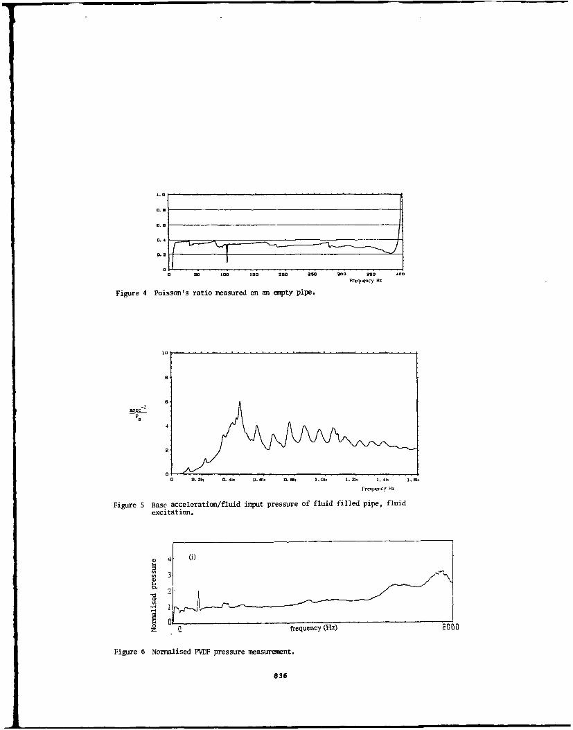
11.
0.4
0.2
00 50 100 150 200 250 300 350 400
Freqency Hz
Figure 4 Poisson's ratio measured on an empty pipe.
me-2pa 8
2
a 0.2k 0.4k 0.5k, 0. 6k 1. 0' 2.2k 41 , .5k
Frequency Hz
Figure 5 Base acceleration/fluid input pressure of fluid filled pipe, fluidexcitation.
S3
o frequency (I1z)
Figure 6 Normalised PVDF pressure measurement.
836

SECOND INTERNATIONAL CONGRESS ONRECENT DEVELOPMENTS IN AIR- AND
STRUCTURE-BORNE SOUND AND VIBRATIONMARCH 4-6. 1992 AUBURN UNIVERSITY. USA
CONDITION OF OLD MACHINES IN THE LIGHT OF
VARIOUS VIBRATION STANDARDS
R.L.MurtyHead of Production Engineering
Regional Engineering CollegeWarangal - 506 004
INDIA
ABSTRACT:
Vibrations are accepted as an indicator of the health of a machine. In the earliesttimes, the subjective method of human feel was adopted to judge the severity of vibration.This led to disputes of all kinds and over the last 100 years, many attempts have beenmade to set "acceptance standards". The important ones are as follows: I) Goldman's chart2) Rathbone's tolerance chart, 3) Federna's chart, 4) General machinery vibration severitychart, 5) Polacek's recommendations 6) Recommendations of Central Machine Tool Institute(CMTI), Bangalore, India. In the present work, the existing standards have been reviewedand the vibrations of a large number of used machine tools were measured. The quality ofthese machine tools was assessed in the light of various standards.
INTRODUCTION:
Vibration has been a guage of performance of a machine since the beginning of the indus-trial age. When measurement of vibration was difficult, people adopted the subjectivemethod of human feel. This led to disputes and some kind of measurement was invented inthe middle of 19th century. It is now felt that vibration like temperature and noise can bean acceptable indicator or parameter for gauging machinery. In this paper important litera-ture on the subject has been reviewed. At the end, some examples based upon a number ofcase studies conducted under the guidance of the author are presented.
The scope of vibration in the present study is concerned only with severity of themechanical vibration of individual machines and not individual parts of a machine. Theidea is to evaluate vibrations with respect to reliability, safety and human perception andto use vibration as a criterion for acceptance, maintenance, quality control, inspection andinstallation of machinery.
EVALUATION OF VIBRATION INTENSITY:
Vibration may be defined by two important factors or parameters:I) amplitude, 2) thepeak or R.M.S value of velocity, these factors are to be evaluated over a band of frequen-cies. Most existing standards on vibration adopt these two parameters.
Double Amplitude:
Double amplitude of vibration is the peak to peak value of particle displacement andis a very useful vibration parameter as it can cover sinusoidal as well as non-sinusoidalvibrations. When one is concerned with the degree of imbalance and relative deflections,amplitude is the relevant factor.
837

2
504I4 _______ !______ ,_____________
50.4x10
1-50.Ax.10- INTOLERD&Ez
INTUNLEASANT
SOAx1lO'
50.4x-
5.0 • • RF"
o. J I
2 5 20 50 100FREQUENCY - C/S
Fig. I Human Response to Vibration (Goldman)
Vertical vibrations limits for passenger comfort - Janeway)
200
S20
1 10 1 o o 10FRUMEJCY IN C/S
Fig.2 Threshold of perception of Tangential vibration applied to fingertip
(after Bekesy)
838

3
I I ! II* I IIi | i | It|!'
1000
2500
250
CORRECT D0EIATEY
ROUG;H -2 NED CORRECTION
FAIR
VERY GO2.5 t
1 2 3 4 6 0 20 100
FREQUENCY IN C/S
Fig. 3: Rathbone chart of Vibration Severity.
200
100
4020 0 0 •10
FREQUlENC IN C/S
Fig. 4. Federna's recommendations on vibration.
839
z44

4
2
1 2 10 100 1000
FREWNCY IN C/S.
Fig. 5: Russian standard on vibration (I - 200 - 54)
250
2.05
j1.5
0.25
100 200 300 1000 10000 1OO
VIBRATION FREULENCY IN CYaES PER MINUTE(RP9)
Fig. 6: General machinery vibration severity chart.
840

Velocity:
When one is concerned with irsiernal wear and machine failure, velocity measurementis important. The energy cf vibration is proportional to the square of the mean velocity.As the velocity directly affects wear, it is a valuable parameter when vibration is used formaintenance purposes. Vibrations with the same RMS velocity in the frequency band 10 to1000 are generally considered to be of equal severity. Succeeding ranges of the evaluationclassifications have a ratio of J.6 giving a step of 4 dB between severity levels.
IMPORTANT STANDARDS:
The first human response curves for vibration were obtained during 1920-1950 by U.S.Navy Scientists.
Goldman's Chart of Human Response:
Goldmann's human response curves are shown in Fig.1. These are very important fortravelling in automobiles, ships etc. The response values were obtained by statisticalmethods and are valid for the majority of peopie.
The threshold perception of tangential vibration applied to the finger tip is given inFig.2.
Rathbone's tolerance chart:
This was given in 1939 and was prepared for the sake of safety and insurance ratherthan maintenance. Fig.3.
Federna's tolerance chart: (DIN 4150) (Fig.4)
These are based upon constant velocity curves following preferred series R.5. Federna'srecommendations seen to cover only low speed machines.
Russian Standards:
The Russian standard on vibration covers a speed range of 600 to 6000 RPM. Thecurves in the Russian standards are steeper than Federna's curves.
General Machinery Vibration Severity Chart:
This chart is given in Fig.6. The curves in this chart provide a guide to establishvibration tolerances for machinery running at speeds upto 100,000 RPM.
German Standard:
This is given in Fig.7. This is similar to the chart shown in Fig.6.
There are other less known or rather similar standards and recommendations which areskipped in this paper.
RECOMMENDATIONS FOR MACHINE TOOLS:
Machine tools are mother machines and their accuracy and performance affect themanufacturing quality of all other machines. Comprehensive recommendations regardingvibrational tolerance limits for machine tools were first proposed by Polacek. In the morerecent times recommendations have also been made by the Central Machine Tool Institute,India. These recommendations for 4 types of commonly used machine tools are summarisedin Table 1. It may be seen that vibrational amplitudes are required to be measured uptospeeds of 600 RPM, whereas velocities are to be measured at speeds of 600 RPM and above.
It may be seen that the recommendations made by CMTI allow higher amplitudes andlower velocities for the same vibrational severity description in comparison with the recom-mendations of Polacek. From this it may be said that Polacek's recommendations are moresuitable for acceptance purposes, whereas CMTI recommendations are more relevant formaintenance purposes.
EXAMPLES OF CASE STUDIES CONDUCTED:
Extensive data on vibrational amplitudes and velocities was obtained on a large numberof machine tools using the Bruel & Kjaer Piezo-electric vibration meter (type 2511). Twoexamples only are presented here.
841

6
150 -._ _ _ _ _ _ _ _ _
E :,2.5
N 16
,1025 MOTOR CAR RIMS, Et c -10
ROTORS, WC, 14/CR OTA T I NG ANC CTOOL DRIVES N . - -- - --- •. . . . "- -TCX1 (I~~IVESOSCLLATING r'--
MTRPARTS 1. <: 1163
GRINDEP, PRECISION
MACH•NE TOOLS LER . ASHAFTS (.A
2.5 - HIGH PRECISION -- -- - - -
Etc.
0.4 1 2.50.4 --- • -'-' ___ N
1.6
1.0
150 300 1500 300 15000 60000
SPEED IN t4 (8.P B)
Fig.8.1. Vibrational behaviour of aspecific lathe judged by
Fig.7 Limit zone of vibrations: (VDI -205-210) Polacek's recommendations.
32 1.8
NNS- _ _ __ !"1.15
P M12.j • 0.7
- 8 0.45
HP HP
(8.2 A) (8.2 B)Fig.8.2. Vibrational behaviour of the same lathe as in Fig.8.l judged by CMTI recoru dations
842

7
10N
6 -3
4.0 1.0* N
- -4,
P .4
(9.1 A) (9.1 B)
Fig. 9.1. Vibrational behaviour of a specific Milling Machine judged by Polacek's
recommendations.
20
N
M12.50
80.7
N- 0.45
0.28
S.•. .. .. -• - -'-"T P'' r- . .. . .:
(9.2 A) (9.2 B)
Fig. 9.2. Vibrational behaviour of the same milling machine as in Fig. 9.1
judged by CMTI recommendations.
843

Table I
Polacek
Double Peak velocity Double i1b Description
Machine amplitude (mn/sec) arplitude velocity of vibration(p m) (P m) (nlm/sec) severity
(frequency (frequency (frequency (frequency,4 10 Hbe) > 10 H~z) 10 HO) 10-1000 Hz)
Lathe 25 2.5 32 1.8 Nom-el(N)
16 1.6 20 1.15 Med i Lm (M)
10 1.0 12.5 0.7 Precision(P)
- - 8 0.45 High Preci-sion (HP)
Milling 10 1.0 20 0.7 N
Machine 6.3 0.63 12.5 0.45 M
4.0 0.4 8 0.28 P
Table 1: Recoauendations on limits of vibrational severity of PWc tools.
Figures 8 and 9 are typical charts showing double amplitude/peak velocity/RMS velo-city at various speeds for a lathe and milling machine respectively. Figures 8.1 A, 8.1B,9.1A and 9.1B correspond to Polacek's recommendations. Figures 8.2A, 8.2B, 9.2A and 9.2Bcorrespond to CMTI recommendations. It may be seen that in general, amplitudes of vibra-tion are within limits of P,M, or N up to speeds of 600 RPM. At speeds higher than600 RPM the amplitude may exceed the P-M-N range. The milling machine under questionhas its vibrational amplitudes as well as velocities exceeding the P-M-N range. It is interest-ing to note that these three machines are roughly of the same age. However, the higheramplitudes for the milling machine seems to be not due to its original design or quality butits higher rate of bear. It is common knowledge that milling machines are continuouslysubjected to oscillating loads and so wear more rapidly than other machine tools.
CONCLUSION:
The various recommendations on vibrational limits are very useful for accuratelyassessing the condition of old machine tools which are expensive.
It is necessary to establish proper vibrational standards for precisiorn and high precisionmachines and vital drive components going into them. The auther has initiated work in thisdirection.
REFERENCES:
1) "Specifications and Tests of Metal Cutting Machine Tools," Vol.1 & 2, Proceedings of the
conference 19th and 20 Feb. 1970. The U.M.I.S.T.
2) "Machine Tool Design", Vol.1,2, & 3, by N.Acherkan, et al, MIR Publishers, 1969.
3) "Machine Tool Design" hand book, published by Central Machine Tool Institute, Bangalore,India, 1978.
4) Francis S.Tse, Ivan E.Morse, Rolland T.Hinkle, "Mechanical Vibrations", CBS Publishersand Distributors, New Delhi, 1983.
5) ISO Standard 2372 on Mechanical Vibrations of Machines.
844
SECOND INTERNATIONAL CONGRESS ONRECENT DEVELOPMENTS IN AIR- AND
STRUCTURE-BORNE SOUND AND VIBRATIONMARCH 4-6. 1992 AUBURN UNIVERSITY. USA
PHOTOACOUSTIC METHOD OF THE DETERMINATION OF AMPLITUDENON-RECIPROCALNESS IN GYROTROPIC MEDIA
Mityurich G.S.. Zelyony V.P., Sviridova V.V., Serdyvuk-v A.N.Department of Physics
Gomel State UniversitySoviet. st..104. 246699, Gomel
The Republic Df Byelorus
There is investigated a possibility of measuring the amount ofamplitude ldichroic) non-reciprocalness in gyrotropic media put inexternal field using the method of photoacoustic (PA)spectroscopy. We getthe expressions for the amplitude and phase characteristics of PA -signal corresponding to the orthogonally polarized isonormal waves inopposite directions. We suggest a way of determination of amplitudenon-reciprocalness of ring laser resonators, containing elements withnatural and magnetic dichroism measuring the difference of amplitudes andphases of PA signals due to the different absorption of waves propagatingin direct and reverse directions.
It follows from some studies [1-33 that the effects of opticalnon-reciprocalness take place in g-rotropic crystals under the action ofexternal magnetic field. Irreversibility of light propagation is due tothe difference in phase velocities of isonormal waves propagation in theopposite directions. There is also a polar non-reciprccalness of forwardand reverse wave [3] due to different ellipticity of intrinsic waves. Asa 87rotropic crystal, put in external magnetic field, is characterized byabsorption that it is obvious that one more similar effect can takeplace, i.e. dichroic non-reciprocalness of direct and reverse waves dueto different absorption of orthogonally polarized isonormal waves.
The given effect has important practical implementation, forexample, for the realization of one directed generation of opticalradiation of ring laser in which the resonator is used with amplitudenon-reciprocalness containing the elements with magnetic and(or) naturalcircular dichoism [4].
In this study we investigate a possibility of using the method ofphotoacoustic (PA) spectroscopy for measuring the amount of amplitude(dichroic) non-reciprocalness in gyrotropic media.
We shall discuss the subject on the basis [1) of
D =[E + t UY hiX E + ta H,
that describe naturally activity media with applied external magnetic
field. In (1) 7 -antisymmetric tensor of the 2-nd range, dual to the
845

magnetic gyration vector 'Y , the imaginary part of which. I" . relatesto the magnetic circular dichroism. O. = OL' + t OL" . with Lt" -thenatural circular dichroism. H - the external magnetic field.
Solving the equation for normals. on the basis of (1 an d Maxwellequations cm Ei = B. [m H]= - D. we get the refractive indexes for
circulary polarized waves [1]. imaginar7 part of which, calculated up tothe 1-st order of magnitude of gyration parameters, is of the form:
0 E Fý + 0)
where n is the unit vector of a wave normal and parameters E 'a-
' correspond to the isotropic media without the inversion center. n h= = ;h COS(O), 8 - angle between vector n and direction of the externalmagnetic field.
In our case the sample under consideration is located ingas-microphone rotating cell for measuring in transmittance mode [5]: tothe cell being in the external magnetic field . Selecting the optimalcondition of thermally thick optically thin sample, we can write thebellow expressions for the PA signal amplitude:
1q+ = A G . = 411 n:_/X, (3)
where 0 the modulation frequency of incident light beam, A - value,determined by parameters of the media and PA cell. Taking into account'2) and (3), and determining the difference of PA signal amplitudes forthe direct and reverse waves we can derive 6ql12= lq+- q_1 1.2
-cit + r" n h-1.2 ' -1 0 --
from which we conclude that the resulting signal, measured in forward(8q,) and reverse taq2 ) directions differs by the magnitude that isproportional to the doubled value of magnetic circular dichroismparameter 7° . It is obvious that the difference of the PA phases forleft/right-polarized waves A(D = 10 - 01 = al"Ctg((X-y))/i(+Xy)),where X 2 & ). y =1 - 2w2_ - 2_) ae+=_ /l_+.measured in
whrex 1 + +1 .- a -(opposite directions, differ by 2Y' multiplied f(sa_). (where f - is
function of optical and thermal parameters of a medium).Therefore, measuring the amplitude and phase characteristics of PA
signal, corresponding to circulary-polarizes of incident light, let usdetermination the magnitude of the dichroic non-reciprocalness of gyro-tropic media or amplitude non-reciprocalness of resonators ring lasers.
References
1. Belyi V.N.. Serdyukov A.N.//Crystallography. 1974, V.19, N6. p.1279.2. Markelov V.A., Novikov M.A.. Turkin A.A. //Letters ZFTF. 1977, V.25,
N9. p.404.3. Mityurich G.S.. Filipov V.V.//Crystallography, 1984, V.29, N.5. p.837.4. Voitovich A.P., Severinov V.A. Lasers in anisotropic resonators. Minsk
"Science and Technique". 1988, p.270.5. Cahen D. //Rev.Sci.Instrum., 1981. V.52, N.9, p.1306.
846

SECOND INTERNATIONAL CONGRESS ONRECENT DEVELOPMENTS IN AIR- AND
STRUCTURE-BORNE SOUND AND VIBRATIONMARCH 4-6, 1992 AUIBURN UNIVER•'7Y. USA
A SOLUTION TO THE NOISE PREDICTION PROBLEM AT LOW FREQUENCIES.
Yurii I .Bobrovnitaldi
Machinery acoustics laboratoryBlagonravov Institute of Engineering Research,
Griboedov mt., 4, Moscow 101830, USSR.
ABSTRACTAn approach to the noise prediction problem for a complicated source (e.g., a machine) in a complicated
room is presented fbr the frequency range where sound wavelongth is greater or comparable to the sourceand room dimensions. Solution obtained to the problem ;s expressed through a finite number of parametersof rigorously defined models of the 6aund source and room which can be measured experimentally.
A sound source is modeled by an ensemble of secondary point sources (monopoles and dipoles locatedat an enveloping surface) which correspond to radiation in the free space. Sound scattering by the sourcebody is taken into account as a matrix of scattering coefficients. A method of experimental identificationof these model parameters in arbitrary dosed room is proposed. The method is based on the propertiesof Helmholts integral operator and on the two-microphone measurement techniques.
Acoustic model of a room is defined, in the approach, by a matrix of integral coefficients of soundreflection from the room walls. The coeffcients may also be measured experimentally.
A number of laboratory experiments has been carried out which prove practical validity of the sourcemodel as well as the experimental method of identification of its parameters.
1 INTRODUCTION
Of great interest in noise 7.ontrol engineering is the problem of predicting sound field radiated hoam a sourcein an enclosed space. In fact, the prediction problem is the central problem in general field theory, andthere is a large body of literature on the subject, especially in electrodynamics and underwater acoustics.In machinary acoustics, the problem is distinguished by the extreme geometric and physical complexityof sound sources (machines and other operating equipment) and rooms (such as manufacturing hals orvehicle compartments). Here the problem has solutions in limiting cases of very low and high frequencies.In wide frequency range where the sound wave length is comparable to the source and room dimentionsthe problem cannot be considered as solved. There are a number of attempts to treat it (see, e.g. (I-4]),but a solution practically acceptable in this frequency range seems possible only on the experimental basis
(5].It is the purpose of this paper to present a new approach to the problem whi, rovide such
solution to a large class of comaplicated sources and rooms. The key point of the approach ae theory inwhich the sound field is expressed via a finite number of parameters of the sources and roonm. Starting fromthe theory, formal acoustic models of a sound source and a room are rigorously defined, and experimentalprocedures are proposed for identifying their parameters. The model parameters of given room and sourcemay be measured separately in rather arbitrary acoustic conditions. Knowledge of these parameters allows
847
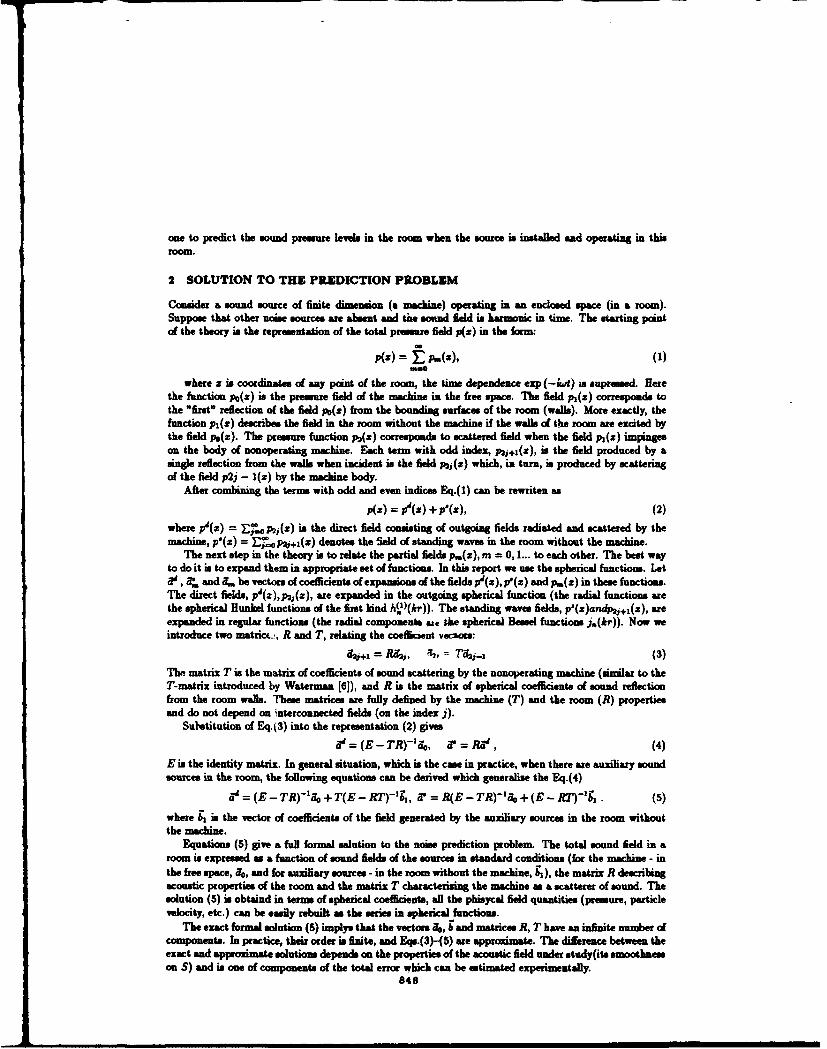
one to predict the sound pressure levels in the room when the soure is installed and operating in this
room.
2 SOLUTION TO THE PREDICTION PROBLEM
Consider asound source of finite dimension (a machine) operating in an enclosed space (in a room).Suppose that other noise sources ae absent and tne sound field is harmonic in time. The starting pointof the theory is the representation of the total pressure field p(r) in the form:
p(A) = • p,.(), (1)m.0
where z is coordinates of any point of the room, the time dependence exp (-L4t) in supressed. Herethe function po(z) is the pressure field of the machi in the free space. The field p1(z) corresponds tothe 'first' reflection of the field p0(r) from the bounding surfaces of the room (walls). More exactly, thefunction pl(z) describes the field in the room without the machine if the walls of the room are excited bythe field p,(x). The pressure function p2(z) corresponds to scattered field when the field pl(x) impingeson the body of nonoperating machine. Each term with odd index, p2j+3(z), is the field produced by asingle reflection from the walls when incident is the field pj,(z) which, in turn, is produced by scatteringof the field p2j - 1(z) by the machine body.
After combining the terms with odd and even indices Eq.(1) can be rewriten as
p(W) = AX() + (Z), (2)where pV(z) = E op2,j(z) is the direct field consisting of outgoing fields radiated and scattered by themachine, p'(z) = Efpz+i(z) denotes the Seld of standing waves in the room without the machine.
The next step in the theory is to relate the partia fields pk.(z), m = 0,1... to each other. The best wayto do it is to expand them in appropriate set of functions. In this report we use the spherical functions. Leta, 96. and a ýn be vectors of coefficients of expansions of the fieldsp (z), p(x) and p.(x) in these functions.The direct fields, pa(z),p r(z), re expanded in the outgoing spherical function (the radial functions arethe spherical Hunkel functions of the first hind h( )(kr)). The standing waves fields, p°(x)andp2.÷1 (z), areexpanded in regular functions (the radial componenis ate the spherical Bessel functions jý(kr)). Now weintroduce two matrict.., R and T, relating the coefficient veaor:
• • = RI•,, 42, = rZ_• (3)The matrix T is the matrix of coefficients of sound scattering by the nonoperating machine (similar to theT-matrix introduced by Waterman [6]), and R is the matrix of spherical coefficients of sound reflectionfrom the room walls. These matrices are fully defined by the machine (T) and the room (R) propertiesand do not depend on interconnected fields (on the index j).
Sutstitution of Eq.(3) into the representation (2) gives
ad = (E - TR)-'i,, a@ = Ad, (4)E is the identity matrix. In general situation, which is the case in practice, when there are auxiliary soundsources in the room, the following equations can be derived which generalize the Eq.(4)
ad = (E- TR)-'1 O + T(E- RT)-I, a- = R(E - TR)-1'5 + (E- RT-1, . (5)
where b1 is the vector of coefficients of the field generated by the auxiliary sources in the room withoutthe machine.
Equations (5) give a full formal salution to the noise prediction problem. The total sound field in aroom is expressed as a function of sound fields of the sources in standard conditions (for the machine - inthe free space, 3o, and for auxiliary sources - in the room without the machine, ý), the matrix R describingacoustic properties of the room and the matrix T characterizing the machine s a scatterer of sound. Thesolution (5) is obtaind in terms of spherical coefficients, all the phisycal field quantities (pressure, particlevelocity, etc.) can be easily rebuilt as the series in spherical functions.
The exact formal solution (5) implys that the vectors a6, C and matrices A T have an infinite number ofcomponents. In practice, their order is finite, and Eqs.(3)-(5) are approximate. The difference between theexact and approximate solutions depends on the properties of the acoustic field under study(its smoothnesson S) and is one of components of the total error which can be estimated experimentally.
848

3 DEFINITION OF THE MODELS
It is men fom the solution (5) that the mound socm under study (the machine) is modded by its soundfield in the free space, a6 and by the scattering matrix T, The relecting matrix R is in this ca theacoustic model of the room.
It should be noted that the vector parameters of the source model, a6, may be replaced by more physicalparameters, namely, by two vectors, o70 = pe(si),...,pe(sjt) and go = t'(s 1) ...= tvs(sr), which describe thepressure and particle velocity distributions on the hemisphere S enveloping the machine, in the free spaceconditions (ai,, = 1,.., N, ae the grid points on 5). The machine in this case is modeled by an assemblyof the secondary point sources - N monopoles and N dipoles located on the enveloping surface S. It isapparent that model parameters 30 and parameters 6, t; are equivalent, they are linearly interconnectedvia spherical harmonica.
4 FIELD FACTORIZATION
One of the main points of the approach presented here is the field factorisation, ie. presentatiou of thefield as a sum of outgoing and standing waves (mee Eq.(2)). We use for the purpose the Helmholts integraloperator
H(p, v) = JJ[p(.)8g(z, .)10. - apt( .gz )dS, (6)
where S is a closed surface, g(x, s) = exp(skr)/4wr is the Green function of the free space, p(s) and v(s)are values of the sound pressure and particle velocity on S, a E S, it is the outward normal vector, z isa space point,r = Is-usi. According to the basic property of the operator[7) we have H(P, v) =pd(z)for z outside S, and H(p, v) = -pa(z) for z inside S. In other words, when the H-operator acts onarbitrary sound field, measured at the surface S, it gives: in the exterior region of S - the field componentpI generated by sources placed inside S; sad in the interior region of S - the field component p' generatedby sources operating outside S. Contrary to the commonly used method [8], this method of factorizationis valid at all frequencies and is applicable to any dosed surface S.
In practical application of the method, we calculated the integral operator (6) replaced by its discreteanalogue. Measurements of the total presure and particle velocity, p and v, on the surface S were performed,in this work, using the two-microphone technique.
5 IDENTIFICATION OF THE MODEL PARAMETERS
Here it will be shown how the parameters of the source model, 20 and T, and the parameters of the roommodel, R, can be obtained experimentally in rather arbitrary acoustic conditions, using convensionalmeasuring techniques.
The vector parameters of the source model, co or 1% ,io, can be obtained by direct measurements inan anechoic room. However, many sources cannot be installed in anechoic rooms. Besides, the frequencyrange considered here includes low freguences at which it is not simple to simulate free-space conditions.Therefore experiment procedure is proposed for parameter identification in arbitrary dosed room. Theidea of the procedure follows directly from Eqs.(5): multiplying the second Eq.(5) by the matrix T andsubstracting it from the first Eq.(5) yield
6 = a4 - Ti. (7)
This equation shows that the parameters of the source model (47) can be extracted from experimentallymeasured total field in a room, if the scattering matrix T is known and if the total field is factorizedaccording to Eq (2).
The matrix T of the scattering coefficients can be determined in the following experiment. Let thenonoperating machine be installed in any room and subjected to sound radiation from a small probe sourcelocated outside a hemisphere S enveloping the machine. Measuring the sound fields on S, factorizing itand expanding into the spherical functions one can obtain vectors V and a', which are interecounectedby the equation a' = Tir, which strictly follows from Eq.(5) for d6 = 0. Having done the procedure forseveral sites of the probe source outside S, one can obtain the matrix T. C Fig.)
849
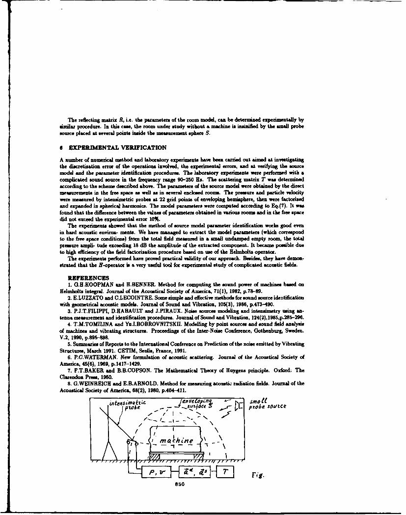
The reflecting matrix R, i.e. the paameters of the room model, can be determined experimentally bysimilar procedure. In this case, the room under study without a machine is insinified by the small probesource placed at several points inside the measurement sphere S.
6 EXPERIMENTAL VERIFICATION
A number of numerical method and laboratory experiments have been carried out aimed at investigatingthe discretisation error of the operations involved, the experimental errors, and at verifying the sourcemodel and the parameter identification procedures. The laboratory experiments were performed with acomplicated sound source in the frequency range 90-250 Hs. The scattering matrix T was determinedaccording to the scheme described above. The parameters of the source model were obtained by the directmeasurements in the free space as well as in several enclosed rooms. The pressure and particle velocitywere measured by intensimetric probes at 22 grid points of enveloping hemisphere, then were factorizedand expanded in spherical harmonics. The model parameters were computed according to Eq.(7). It wasfound that the difference between the values of parameters obtained in various rooms and in the free spacedid not exceed the experimental error 10%.
The experiments showed that the method of source model parameter identification works good evenin hard acoustic environ- ments. We have managed to extract the model parameters (which correspondto the free space conditions) from the total field measured in a small undamped empty room, the totalpressure ampli- tude exceeding 18 dB the amplitude of the extracted component. It became possible dueto high efficiency of the field factorisation procedure based on use of the Helmholts operator.
The experiments performed have proved practical validity of our approach. Besides, they have demon-strated that the H-operator is a very useful tool for experimental study of complicated acoustic fields.
REFERENCES1. G.H.KOOPMAN and H.BENNER. Method for computing the sound power of machines based on
Helmholts integral. Journal of the Acoustical Society of America, 71(1), 1982, p.78- 8 9.2. E.LUZZATO and C.LECOINTRE. Some simple and effective methods for sound source identification
with geometrical acoustic models. Journal of Sound and Vibration, 105(3), 1986, p.473-490.3. P.J.T.FILIPPI, D.HABAULT and J.PIRAUX. Noise sources modeling and intensimetry using an-
tenna measurement and identification procedures. Journal of Sound and Vibration, 124(2),1985,p.285-2 96.4. T.M.TOMILINA and Yu.I.BOBROVNITSKII. Modelling by point sources and sound field analysis
of machines and vibrating structures. Proceedings of the Inter-Noise Conference, Gothenburg, Sweden.V.2, 1990, p.895-898.
5. Summaries of Reports to the International Conference on Prediction of the noise emitted by VibratingStructures, March 1991. CETIM, Senlis, France, 1991.
6. P.C.WATERMAN. New formulation of acoustic scattering. Journal of the Acoustical Society ofAmerica, 45(6), 1969, p. 1417-1429.
7. F.T.BAKER and B.B.COPSON. The Mathematical Theory of Huygens principle. Oxford: TheClarendon Pres, 1950.
8. G.WEINREICH and E.B.ARNOLD. Method for measuring acousti. radiation fields. Journal of theAcoustical Society of America, 88(2), 1980, p.404-411.
p•L ." J_7 .. syrv, pzobe sOcace/ / 1 N 5
IIP,-. Ir i i s
p, a ~ 4' -E ] Fig.850

SECOND INTERNATIONAL CONGRESS ONRECENT DEVELOPMENTS IN AIR- AND
STRUCTURE-BORNE SOUND AND VIBRATIONMARCH 4-6. 1992 AUBURN UNIVERSITY USA
A PARALLEL PATH DIFFERENCE ON-LINE MODELLING ALGORITHMFOR ACTIVE NOISE CANCELLATION
Yong Yan and Sen M. KuoDepartment of Electrical Engineering
Northern Illinois UniversityDeKalb, IL 60115
815-753-9967
ABSTRACT
In the commonly used active noise cancellation configuration, on-line system identification of the auxiliarypath and error path has been a difficult problem. The algorithms already proposed are not satisfactory. A newalgorithm, using a "parallel path difference" scheme, is developed theoretically. Simulation results successfullyproved the validity of the theory and the feasibility of the new algorithm. Steady state and dynamic performanceis analyzed.
I. INTRODUCTION:
In the commonly used active noise cancellationconfiguration (Fig.l), a copy of the transfer functionproducts Hs(z)He(z) is needed for the filtered-X [1] orfiltered-U [2] algorithms. On-line system identification of 1. ÷ ,+Hs(z)He(z) is preferred to accommodate the changingenvironment, thus the changing parameters of Hs(z)and/or He(z). This is a difficult task since the signalpicked up by the error microphone, e"(n), is always amixture of signals from P(z) and Hs(z) and we have noway of distinguishing the two. From another point ofview, if we use an adaptive filter T(z) to identifyHs(z)He(z) (Fig. 2) [1], the disturbance in the modellingscheme is closely correlated with the input signal to T(z),resulting in a biased optimal solution of T(z), asdescribed by the following mathematical deduction. Figure 1 Commonly used active noise
From Fig. 2, when adaptive filter T(z) converges, the control configurationZ-transform of the error sequence e(n), according toMason's law, is:
E(z) = (P(z)He(z) + A(z)HsWz)He(z) - A(z) T(z)) * V(z) (1)
if e(n)=O, then E(z)=O, we have :
851

T(z) -Hs(z)He(z) + P(z)He(z) (2)ACz)
therefore T(z) is niot the desired Hs(z)He(z), instead,
it is biased by an unknown part P(z)He(z)A(z)
I1 NEW PARALLEL PATH DIFFERENCE + -ALGORITHM:
The algorithms already proposed to solve the aboveproblem are analyzed and found unsatisfactory[2][3][4][51. To meet the need for better algorithms toidentify Hs(z)He(z), a parallel path difference algorithmis proposed in this research (Fig.3). There are three keypoints:
a) We separate the pwcssof identifying Hs(z)He(z) Figure 2 Identification ofand that of reducing noise, because unless we get the Hs(z)He(z) with T(z)right copy of Hs(z)He(z), the effort of trying to reducethe noise will be in vain. Therefore we use software to detect the change of Hs(z)He(z) by detecting the trendof el"(n) and e2"(n). Once change detected, the software will go to a routine in which it fixes the noisecanceling filters and tracks the new Hs(z)He(z), then it adapts the filters to cancel the noise.
b) In the process of modelling Hs(z)He(z), we do not model Hs(z)He(z) directly. Instead, we use twoparallel paths and split the input sequence into odd-numbered and even-numbered sequences to drive the twoadaptive paths alternately. After the two adaptive filters both converge, we use the optimal coefficients of thetwo filters to CALCULATE Hs(z)He(z), i.e. the information about Hs(z)He(z) is extracted from the differenceof the two paths. The switching between the two paths is accomplished by software.
c) Software detectors to detect the convergence conditions are crucial in this algorithm.There are two detectors involved here. One is
the detector to detect the change of Hs(z)He(z).This can be easily done by detecting the changing ,(n +
trend of e"'(n). In normal mode, the main path is Psused. (Fig. 2) If Hs(z)He(z) has not changed, wehave the right copy in the filtered-X path, e"2 (n)should be going down. If Hs(z)He(z) has changed 2
so much that the copy we had can no longer beused as an approximation of the real Hs(z)He(z), A Tit.% I
e"2(n) will be going up(tending to diverge). Thusby detecting the trend of e" 2(n), we can detectthe change of Hs(z)He(z), then the software willgo to a routine in which it switches the input U
between the two paths to determine the newHs(z)He(z). The second detector is the one todetect the convergence of the two switchingpaths. This one is even more crucial and may be algorithm, no feedback casemore difficult to implement Only when the twoswitching paths have converged(i.e. Tl(z) &T2(z) have converged), can we calculate the new Hs(z)He(z) by the following method. More of this point willbe discussed near the end of this paper.
After convergence of the two switching paths, Hs(z)He(z) can be calculated as follows:1. The case without feedback:
In the system diagram shown in Fig. 3, when the filters Tl(z) and 72(z) converge, we have:
852

El(z) P ( ZP()He(z) +A1(z)He(z)He(z) -Al(z)T (z)) * Vow(z) (3)
E2(z) P (P(z)He(z) + A2(z)Hs(z)He(z) -A2(z)T2(z) ) * Vm(Z) (4)
When Tl(z) and T2(z) have enough coefficients:
E1(z) - E2(z) = 0 (5)
we can asmum:
V.W (z) - V .(z) (6)
subtract the two equations and solve for Hs(z)He(z). we have:
Hs(z)He(z) - Al(z)T1(z) - A2(z)T2(z) (7)Al (z) - A2(z)
This is a significant result compared with [Equ.2J since the unknown term P(z)Hc(z) is canceled, thus theerror path Hs(z)le(z) can be estimated correctly.
During the modelling process, we can let A2(z) and Al(z) have a fixed relation such as: A2(z)=m*Al(z)where m is an adjustable constant, then the above equation becomes:
Hs(z)He(z) T Ti (z) -m * 2(z) (8)1 -r
so we calculate Hs(z)He(z) from the final coefficients of Tl(z) and T2(z).2. The case with feedback:
v~n) + ella)el'(n) or e2"jn)
+ + " 2 +
Figure 4 Parallel Path Difference algorithm, with feedback
The system diagram is shown i Fg.4. When e fi Tl(z) and 2(z) convege, w have:
653

El (z) P(z)He(z) + A1z(z)He(z)He-(z)-Al(z)T1(z) (9)Vow~z) 1 - B (z) + Al (z) He (z) F(z)()
E2(Z) P (z)He(z) + A2(z)Hs(z)He(z) - A2(z) T2(z) (10)1"V. (Z) 1 - B(z) + A2(z) Hs(z) F(z)
Since F(z) is the feedback, we can use a directional speaker at the canceling point and a directionalmicrophone at the input point to make sure that feedback is weak, in other words, the coefficients of F(z) aremuch smaller than those of He(z). Then if we let: A2(z)=m*Al(z) and choose m close to 1, e.g. m=0.99,it is reasonable to assume that the two denominators are equal while Al(z)Hs(z)He(z) and A2(z)Hs(z)He(z) arenot (we need the difference between the two).
Solve for Hs(z)He(z), we have the same result:
Hs(z)He(z) = TI(z) -m * T2(z) (11)
M. STEADY STATE ANALYSIS IN TIMEDOMAIN:
To demonstrate the inner workings of the system in ,w +
more detail, we now use the more classical approach toderive the mean square error function in time domain, toget the Wiener solution and to compare it with the above AN *1 A_
results obtained using Mason's law. To simplify theexpressions, we can combine He(z) into P(z) and Hs(z) a"[2], obtaining the equivalent system block diagram in Fig Vat5. If the impulse responses of the plant and the error pathare P = [po,pl ..... ',-1_] T and
Ha = [hso,hs1, ... .hse,,,] , respectively, and thecoefficients of the adaptive filters A and T at the same Figure 5 Combining He(z) into P(z)
instant are A. = (a, (n) , a, (n) ..... a,, (n) ]*
and T, ( t. (n), t, (n) ..... t,.t (n) ] rrespectively, then we have: (capital letters denote vectors and matrices while lower case letters denote scalars,for vectors, we use subscripts to denote time index while for scalars we use function convention,Le. f(n))
x, (n) = x4'P and x, (n) =X4.A. (12)
where X. = [x(n) ,x(n-1) .... x(n-N+1) ] TDefine:
x 2 ((n) x(n) x(n-1) ... x(n-N+1)x 2 (n-1) x(n-1) x(n-2) ... x(n-N)
X2. --- An = S. A•. (13)
x 2 (n-N+l) -x(n-N+1) .... ... x(n-2N+2)
where S. is used to designate the matrix and is obviously symmetric. Then:
854

x 3 (n) - X.` H, = A, S. H. (14)
x. (n) = x, (n) + x3 (n) = X4 P + A.D7 S Hg (15)
xs(n) = X 2 .T Ta _ A.- S. T. (16)
e(n) = x,(n) - xs(n) (17)
=AT S( H. - T,) + X(17P
therefore:
E[ e (n)] E~e (n)e(n)] El( H:-T.;) SA. + PT X.] [A.7 Sh (H.-T.) +X.7 P) I (18)
-E[(T.- H.) Sn A. A.T S. (T. - fH)] - 2E[ (T.7-H;) Sn An X.7 P ]+ E[P T Xn X.:PA
a) For the modelling Drocess. in which A is fixed and T adapts, let VT = 0, we have:
VTM2 E(S. A AT Sn ) (Tn-H,) -2E( Sn A X.7) P = 0 (19)
if [E(Sn A A T S)] - exists, then we have:
T" = HS + [E(S, AAT S")]-1 E[S.A X;] P (20)
This result is comparable with the previous one obtained using Mason's law [Equ.21, that is, the Wienersolution of T is biased from Hs by an unknown part related with P. The corresponding minimum MSE is:
E(e 2 (n) ]I.,,= E[ (PPTn) 2 E(PTXA•TS,] [E(SAA TSn) -1E[SAXP] (21)
the coefficient updating equation is :T- e 2 (n) = Tn-p2e(n) de(n)
T.,l=Tn-PVT= T 8P-T aj~en T (22)
=T.+p2e(n) S.A
which is the normal LMS algorithm, with input signal sequence to T as SAb) For the noise control process, in which A adapts, the error signal is:
e'(n) =x, (n) 'AnTSnHS+XnTP (23)
therefore, the mean square error is:
E[e2 (n)] =EI[e(n) e T (n) ] =E[ (A.TSH,+X.;P) (H.lSA.,+PTXn) ] (24)=E[A.TSH.H.S.A.] +2R[X"PHrS,,A] +E[ x;PF TX.]
This is a quadratic function about A, the global minimum is determined by:
VA=2E([S".HTHS-]A+2E(SfHP TX] =0 (25)
so the Wiener solution for A is:
855

A*= [E(S.H,4S.) ] -1E[S",HP TX.] (26)
the coefficient updating equation is :
'-A 9. e9 (n)A.*="•V - A- (27)
=A.-i2e (n) Sq.i
which is the filtered-X LMS algorithm. We see here the need for the identification of Hs(z).
IV. DYNAMIC PERFORMANCE ANALYSIS IN FREQUENCY DOMAIN:
To analyze the dynamic performance of the system, we use the approach developed by Clarkson [61, whichdescribes the LMS adaptive filter by a transfer function. In general case, this is only an approximation, sincean adaptive system is time varying thus can not be described by a transfer function. For some special cases,including the periodic input case, however, the Z-transforms of the input and output signal become independentof time, therefore the adaptive system can be described by an equivalent transfer function. From this function,we can study the stability and convergence properties of the adaptive process. In this paper, we will give thesalient points of this approach used in our case for periodic input signals.
Referring to Fig.5, for the identification process, in which A is fixed and T adapts, the updating equationfor T,= [t, (n) , t, (n). tN- (n) ] T is:
" ",=T.,.+pe (n-1) xe,,.,. (28)
using the above equation iteratively and assuming T(O)=O, we have:r.-1
Tn=P r• e (i) x=, (29)
so we have:n-1 n-1 N-
x5 (n) =fT7X2 = P N. e(i)=X2TX2 f=P ?: [e(il) N x(i-j)x(n-j)l
fl-i
=IL T. [e(i) Nrj]
where r, is an autocorrelation estimate, N is the order of filter. As N--,, r,,, will be the actualautocorrelation, for which rn=r,,- for periouic signals. So if the filter length is long enough, we have:
fl-ix, (n) =LNF. oei) r._I (31)
.-C
and:
e(n) =x 4 (n) -x, (n) = x1 (n) -x 3 (n) -x, (n)n-1
=x(n) * P - x(n)* A * H _ - LN5 e(i)rn 1 (32)n
=x(n)* P -x(n) *A * H, -_sNF e(i) r-.+ ILNroe(n)
where "*" denotes convolution. Rearranging terms and taking Z-transform of the equation, we get:
856

(z) P(z) -A(z) Hs(z) (33)X(z) 1-isNr0 ÷+WIR•(z)
where R(z) is the Z-transform of the autocorrelation sequence R = [r0 ,ri..... r,_.].This is a very important result, since it describes the whole adaptation process, the dynamic state as well
as the steady state. At first sight, it appears contradictory to the result we got previously [Equ.l]. The reasonfor the difference is that the former one is the Z-transform of the error sequence at the steady state, while thecurrent one is the Z-transfonn of the whole error sequence starting from the beginning of the adaptation process.
Using this result, we can study the stability propty of the system by studying the root loci as IL changes,given input signal (thus given R(z)). We can also study the convergence property of the system byapproximating the denominator to a second order polynomial of Z -1 and relating the damping property of MSEto the pole locations.
Using the final value theorem of Z-transform, it is easy to see that e(-) =0. So for periodic input signal,there is no excess mean square error for both paths. This is ideal for the parallel path difference algorithm.
To analyze the effects of error in estimating Hs(z), we use the results from Elliott[7]. To further simplifythe problem, Elliott et al used a sinusoidal signal for the input, so that the effects of the estimated Hs(z) canbe specified by AeA. After some involved derivation, the following result is obtained:
E(z) - P(z) [ 1-2z cOSwo+Z 2] (34)X(z) 1-2z CosW0 +z2+04 H z (z) (Zcos(Wo-4 )-cos4i)(
From this equation, we can determine the effects ofthe estimation error of Hs(z) on the total system i-gm-5 W KW .hen -t tr-ld,
performance. - s.).(:) at ^H
V. SIMULATIONS AND DISCUSSIONS:
Simulations of this algorithm for nonfeedback and H.- - fIk
feedback-present cases are performed with some simple filmtransfer functions. We let the initial state of the system , - -
be at optimal state so that the noise is perfectly canceled. ""Then we changed Hs(z) to a totally different one and , 1. sift i ftobserved the performance of the system. When we do not tIetrack Hs(z)He(z) at all, the MSE of error signal e'(n)diverges as in Fig.6. When we use PPD algorithm, rigure 6 If not tracking Hs(z)He(z)tracking of Hs(z)He(z) has been observed in all but largefeedback cases. Fig. 7 shows a result with no feedback inwhich Hs(z) changed to another function such that weknew our 5th-order adaptive filters Tl(z) and T2(z) couldstill identify with zero MSE. The cases with feedback arm f, . HI
shown in Fig.8 and Fig.9. When tracking of Hs(z)He(z)is not ideal, i.e. when Tl(z) and T2(z) are not flexible Ienough to adapt themselves to make MSE's of el(n) and -
e2(n) zero, the error signal e'(n) will perform as inFig. 10.
Simulations of the algorithm using measured real --
world transfer functions have also been done. The resultsare similar to those with simple transfer functions exceptthat the excess MSE's are not zero. ,g. . -_
From the simulation results, we can see that thealgorithm works very well for nonfeedback case and Figure 7 Using PPD to trackworks fine for weak feedback (less than 5%). When the Hs(z)He(z), with no feedback
857

feedback is larger than 5%, however, it does not workvery well. This is because when we derived the equation .f.a ,to calculate Hs(z)He(z), we assumed that F(z) was very __I
small by using a directional speaker at the cancelingi-lpoint and a directional microphone at the inputpoinL(otherwise it is difficult to separate the unknownA(z)Hs(z)F(z) term.) If F(z) is large, we need to derivesome other equation to calculate Hs(z)He(z), which is noteasy.
VI. CONCLUSION: .
This paper proposed a new algorithm to identify theerror path for filtered-X algorithm in active noise Figure 8 PPD with small feedbackcancellation. This parallel path difference algorithm canbe used in a more general system identification contextwhen the plant noise is closely correlated with the input C •of I=h- t- .Hesignal to the adaptive filter. w
REFERENCES:
1. B. Widrow and S.D. Stearns, Adaptive SignalProcessing, Prentice-Hall, Englewood Cliffs, NJ,1985;
2. L.J. Eriksson, "Active Sound Attenuation UsingAdaptive Digital Signal Processing Techniques", .=-.-,
Ph.D. Thesis, University of Wisconsin-Madison,
August, 1985;3. LJ. Eriksson, M.C. Allie and R.A. Greiner, "A New Figure 9 PPD with larger feedback
Approach to Active Attenuation in Ducts", Paper C5-2 in Proceedings of 12th International Congress onAcoustics, Toronto, Ontario, Canada, 24-31 July,1986 ( Canadian Acoustical Association, trski oH sHe. by PMP aIth=
Toronto, 1986);4. L.J. Eriksson and M.C. Allie, "Use of random noise
for on-line transducer modeling in an adaptiveattenuation system", J.Acoust. Soc. Am., 85.797-802(1989);
5. L.J. Eriksson, "Development of the filtered-Ualgorithm for active noise control", J.Acoust. Soc.Am., 89(1) 257-265, (Jan. 1991).
6. P.M. Clarkson and P.R. White, "Simplified Analysis ,_ I-
of the LMS Adaptive Filter Using a TransferFunction Approximation", IEEE Transactions on Figure 10 Non-ideal Hs(z)He(z)Acoustics, Speech, and Signal Processing, Vol. tracking due to finite T(z) lengthASSP-35, No.7, July 1987;
7. S.J. Elliott, I.M. Stothers and P.A. Nelson, "A Multiple Error LMS Algorithm and Its Application to theActive Control of Sound and Vibration", IEEE Transactions on Acoustics, Speech, and Signal Processing,Vol. ASSP-35, No.10, October 1987.
858

SECOND INTERNATIONAL CONGRESS ONRECENT DEVELOPMENTS IN AIR- AND
STRUCTURE-BORNE SOUND AND VIBRATIONMARCH 4-6. 1992 AUBURN UNIVErSITY, USA
STUDIES OF THE BUILDING CONSTRUCTIONS BY MEANS OFNONLINEAR DIAGNOSTICS
Ekimov A.E.,Kolodieva I.I., Korotin P.I.Institute of Applied Physics Academy of Sciences of the USSR,
60300, N. Novgorod, USSR.
ABSTRACT
In diagnostics of constructions with broken integrity (cracks,adhesion failures, etc. ) the methods using nonlinear phenomena find anincreasingly frequent practical application. The second harmonicgeneration mechanisms are best investigated but the real processes aremore diversified. In this communication we report on the experimentalinvestigation of the turbo-set bearer where subharmonics were observedalong with the fundamental frequency harmonics. This allowed theturbo-set having a polyharmonic vibration spectrum to be used for crackdiagnostics of the bearer.
INTRODUCTION
The crack-type defects in building constructions such as machinebearers can appear both at the building stage and when operated becauseof the large vibration load. Such defects can strongly modify thestrength characteristics of the bearers and increase their damage in somecases. Therefore, the timely diagnostics is the first element in thesystem of preventive measures for longer service of building and otherconstructions. As a rule, with any arbitrary method of control, thedefects are revealed by indirect signs (for example, by time delay in thepulsed procedure). The task of the researcher is to choose the set ofindirect signs with high noise protection, which are best suited to aparticular object subject to control.
In this communication we report on the vibration test of theturbo-set bearer used in the N. Novgorod heat-and-power station. In thelong-term service (over 30 years), when the vibration load was large,extenided cracks formed in the bearer interier which were stopped bysealing with a synthet-¢ binder. Meanwhile, atter a decade since thecracks were sealed the increased vibrations at some sites of the bearermade !t necessary to control the sealing quality and the possible crackdevel'opment. To answer these questions we carried out a series ofvibratlonal tests o~f the bearer. It was found that the cracks in thebearer have produce. the nonlinear phenomena which can be used as cracksattributes for tha diagnostic purposes,
859

EXPERIMENTAL PROCEDURE
The vibrations of a bearer (20 m in length, 6 a in width and 8 m inheight ) were investigated both when the turb6-set (25 MW) was operatedand run-out and when the bearer vibrations were excited (with theturbo-set switched off), successively at several points, by a linearlytunable harmonic forse (50 newtons) produced by an electrodynamicvibrator.
Figure 1.
Figure 1 shows the scheme of a bearer with vibration receivers(accelerometers) mounted at fixed points; the signals from the vibrationreceivers were processed cogerently. In the case of artifical excitationwe determined the induced vibration Vk,, where Vk, is the vibrationalvelocity at point I from an external forse F applied to point k (V and Fare complex quantities). The matrix of transfer functions Y. wascalculated in the frequency range 20-150 Hz (n is the number of thereceiver and m is the number of the excitation point). The components ofthe Yn. matrix are given by
Yk, = Vki/Fk , (1)where Yk1 is the transfer admittance. The external force frequency (•)was varied linearly
S= ws + q't (2)Here q is the proportionality coefficient that describes the rate
of frequency variation, w, is the initial frequency of the operatingrange and t is time.
When the monolithic part of the bearer (the domain far from thecracks), the vibrovelocity spectrum Vkk coincided with the spectrum ofthe driving force Fk (Figs. 2a,b). At other points of the construction,at a given Fk the vibrosignals were insufficient to be detected againstthe noise background.
When the point at which the external force was applied wastransferred from the monolithic part of the bearer to a domain containingcracks, the admittance Yt increased and the spectrum composition of thevibrations was enriched at point 1 and other points of the construction,where the signal was distinguished against the noise background. As aresult, harmonics appeared In the vibrosignal spectrum; the harmonicgeneration effect is used in the nonlinear diagnostics, for crack
860

I0
ta) 4lb 0t-?
A) 300 "•Z
00 HZ) b) far off crack
AS.)
150
t.. - -- .....
"c) near by crack
Figure 2
861

detection for example. Moreover, in the vibrosignal spectra of thesensors located near the cracks we observed the appearance ofsubharmonics as the excitation frequency approached the resonancefrequencies of the construction (Fig. 2c). The localization ofsubharmonics near the cracks indicated that the excitation ofsubharmonics is stimulated and the resonances of the construction enhancethe effect.
From Fig. 2c it follows that the subharmonic level is sufficient touse this effect as a diagnostic sign of presence and localization ofcracks.
The use of the appearance of subharmonics in the vibroresponsespectrum as a diagnostic sign makes it possible to use polyharmonicsources for the excitation, for example, the turbo-set itself in therun-out regime. Besides, the dynamic force from the turbo-set is mostlysufficient for this effect to be manifested in the bearer irrespective ofthe crack location. As an illustration, Fig.3 shows the spectrum of thebearer vibrations in the crack region, which was obtained during therun-out of the turbo-set. Figure 3 clearly shows the vibrations in thefrequency range v=312,w, where w9 is the lower frequency of thevibration source.
The assumption of the parametric nature of the vibration spectrumenrichment has made it possible to define the characteristic thickness ofthe cracks from the time the nonlinear henomena appear in the vibrationresponse when the exciting force level zs changed.
Figure 3.
SUMMARY
1. Analysis of the transfer matrix on the basis of the subharmonicgeneration effect permitted to reveal the crack and localization in thebearer interior, and the excitation levels at which the nonlineardistortion appeared in the response permitted the defects to be measured.
2. The possibility of using the vibroactivity of the mechanisms,when operated, for monitoring the state of the building construction(bearers, clikes, bridgesetc.) on the basis of the subharmonicgeneration effect is demonstrated in practice.
862

SECOND INTERNATIONAL CONGRESS ONRECENT DEVELOPMENTS IN AIR- AND
STRUCTURE-BORNE SOUND AND VIBRATIONMARCH 4-6. 1992 AUBURN UNIVERS17Y. USA
M.EASUREM4ENT OF ACOUSTIC POWER OF FAN'S UNDER CONDITIONSOF REVERBERAN~T NjITSF OF AERODYNAM1IC TEST RIG,
V.M. Knznrqv. Dr. V.C,,Karadqi, Dr. A.S.M'irsknvC-ntrai Aermoiydrodynnmics Instjtitut (TSACI ),
Moscow Brinch, A,-omt ir Division, SSRR
ABSTRACT
-Acoos ti c ,-hnrartoriar is of falls "Along it 111 f fw r- I 'ehamrsttorist ic srn eqsent iaI factors that dotermino 'oi r hi~h,~~~p#,frormnnrk . Aeutir nnd Rerodynamir t 't sts a o~m1v-te~te -,ill fo'It ( Iirot spejiallized -mind-1-fI 'Xlnlesilring r-ah-nemir.
A'-hievpmmit a inl sokit~ntitrat''u'" me-ke it posstlihIn meak,,ro a,cw,fsirpowpr directly on t h'ý,i s rtv, uynder cond~ition, of ,vorhornnt na
In fbi" in''' t '#'- ho'I ioehiij:1m,.ofV m--roaontt o' ,,,r', Ic vocer of Urnsk'- P7-'trrm orarrrl-rr it" rrrý r lca,' ioOl .r'n r,,vurt-i
T 1 0l 'srqi]: "r at rrmti - p-- -, roar~m~-n pvd sril ~ o r-'"'-- sor rc or -.oo r
rf~~~ ~~ ano-f i' a n hat'k,'r-rtnw ota- n' c rea'rrhker.-nt itoisa in tire rrra-11
I cow- irerrrrr nj as
I = 'l' I ,ri) - Sorird irrtr'rri t X.1,"veI ;.d1B*
I ltllg(W./Wrr) - Sorind pow,ýr lc~veI,dB;L I I/N *1 tpL - Momea asoiri pressnre level ,dB;Xa Nlimhbr of mensrirag points;p q0~tln 1 . N0r-f ;
Po -I10 v/ml - Reference (piantity of snnnd pressilre;
-Root -meirn-varrre or sournd prpssnrýr,N/M7.,X (t d)fi;
M -rcrrremenr surtr'cv,mgrt Timnu, a;I Pirticlp 1-oloity,mu/s;
W - Snurnd pnrwer,w;Wo 10"w - Reference qrarnt ity of stiund power;C5, V11N Lt( Lp~U -L R-oo-meon-square di.spergion of sound pressure level,dB;
i-Current number of mensurement;n -Component normal to thp *r-asnrprmeni suirface;
4 (njiigauta valtie.
863
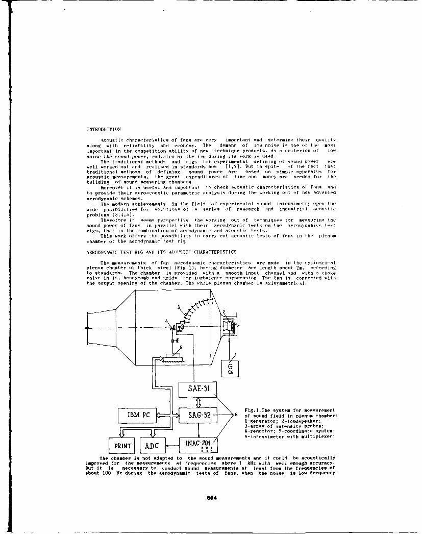
I NTRODIJCT ION
Acoustic characteristics of fans are very important and d-termine their qualityalong with reliability and economy. The demand of low noise is one of the mostimportant in the competition ability of new technique products. As a criterion of lownoise the sound power, radiated b) the fan during its work is used.
The traditional methods and rigs for experimental defining of sound power arewell worked out and real ised in standards now f1,21. But in spite of the fact thattraditional methods of defining sound power are based on simple npparatuis foracoustic measurements, the great expenditures of time 7,nd money are needed for thetbuilding of sound measuring chambers.
Moreover it is useful and important to check acoustic characteristics of f.urns anoto provide their aerocroustic parametric antalysis during the working out of new advanced
aerodynamic schemes.The modern achievements in the fielt of experimental sound intensimetry open the
wide posibilities for sol,,tions of n serips of research and industrial avou,,ticproblems [3,4,5].
Therefore it seems perspective the working out of techniques for measuring thesound power of fans in parallel with their aerodynamic tests on the aerodynamics testrigs, that is the comhination of aerodynamic and acoustic tests.
This work offers the possihility to carry out acoustic tosts of fans in the plenumchamber of the aerodynamic test rig.
AERODYNAMIC TEST RIG AND ITS ACOUSTIC CHARACTERISTICS
The meaqiiremPntg ot fan aerodynamic characteristics are made in the cylindriralplenuim chamber of thick steel (Fig.l), havi.ng diameter and length about ?m, accordingto standards. The chamber is provided with a smooth input channel and with n chokevalve in it, honeycomb and grids for turbutlence surpression. The fan is connected withthe output opening of the chamber. Tho whole plenum chamber is axisymmetrical.
32
of d e h
Fig.l.The system for measurement
ThM PC SA -32 16 of sound field in plenum chamber:1-generator; 2-loudspeaker;3-array of intensity probes;4-reductnr; 5-coordinate system;
fi-intenaimeter with multiplexer;
The chamber is not adapted to the sound measurements and it could be acousticallyimproved for the measurements at frequencies above I kHz with well enough accuracy.But it is necessary to conduct sound measurements at least from the frequencies ofabout 100 Hz during the aerodynamic tests of fans, when the noise is low frequency
864

I
one in the main.The standard sound power measurement techniques suppose the placing of checked
sound source tested into the anechoic chamber (free field) or reverberant chmber(diffused field). The choice of measurement technique is determined by the fieldcharacteristics.
The investigations were carried out for clearing up the correspondence of plenumchamber sound field to reverberant or free field conditions where conducted.
A wide band noise source was installed at the chamber in place of the fan (Fig.1),and sound pressure measurements were conducted in the octave frequency bands at thepoints on the halfsphere surface with the radius 2-0.75 s,centered by a loudspeaker. Thenumber of measurement points was N=200 for every frequency band.
The statictical analyses of measurement results gave mean Lp and root-mean-squarepressure levels in octave frequency bands, and also gave the bargraphs of pressuredistribution onto the measurement surface of halfsphere (Fig.2). The bargrapha aremade with the method of rectangular "contributions."
.33
Fig.2. Statistical andtheoretical distribution densityfor sound pressure on the surfaceof measuring sphere in the plenumchamber.Central octave frequency
0 .N . 500 Hz
The theoretical and statictical distribution from the point of view of theirsmoothing was performed according to Romanovsky rule (61 showed a good agreement with thitype I distribution for minimum values [7]:
f(Lp)" 1/0,. ez.p{[(Lp-Mi)/O]i - expf(Lp-M,)/0]} . (1)
where (5 4/O.283;W 5p*077"i - the distribution parameters.The character of distributions confirms a significant pressure level dispersion on
the surface of measurement sphere in the plenum chamber for all octave frequency bands.Thus, the root-sean-square dispersion of pressure level is within the limits of 3 - 5.6dB for different octave bands. The root-mean-square dispersion should not exceed 1.5 dBfor the reflected field. At the same time the character of chamber space pressuredistribution shows the presence of reflected waves and cannot be explained from thepoint of view of a free field sound source.
Hence, the measurements of plenum chamber sound field and the consequentresult analysis show, that the chamber field is neither free nor reverberant. Theapplication of standard methods of fan sound power measurements in the plenumchamber is impossible without its special modernization.
EXPERIMENTAL TECHNIQUE AND MEASUREMENT SYSTEM
The vector of sound intensity characterizes the rate of sound energy flow at a poninof space. Therefore it is necessary to know the distribution of the normal component ofacoustic intensity vector active part on the surface, enclosing the source, in order todetermine its sound power [5]. Then the sound power of the source inside the measurementsurface is
W " Re(I.) dS .(2)
where ]nI pV .
The intensity method of sound power measurement has some advantaes the main of whichare the possibilities of making measurements at the place of utilization of the studiedsound source (in situ) and in the presence of significant background noise, exceeding
865

the •seful source level. The important advantage of this method consists in itssimplicity.
The posibility of using intencity method for measurements power of sound source inthe presence of high levels of background noise is due to the energy flux throw thesurface. The integral of the normal component of sound intensity throw the surface Swithout any sound sources inside is equal to
P e(In)dSO (3
The expression is true if there is no power absorption inside the measurement surface.Expressions (2) and (3) are also true if the sound source is on an ideally
reflecting surface and is surrounded by the measurement surface closing on it.To define practical application possibilities or this method it was necessary to
clear out its abilities under plenum chamber conditions on a specific measurementsystem and to evaluate the measurement accuracy.
The measurement system was based on a two microphones intensimetry probe and afinite difference scheme for practical velocity definition.
in 'P+z)X NP,-pl) dtIn 2 T{ (4)
It consisted (Fig.l) of 8 - 10 intensity probes array in the form of 1/4 part of circlewith the radius of .75 m connected through a multiplexer with an analogue intensimeter,type INAC-201 Metravib company (France). A traverse device provided antenna rotationaround the system symmetry axis for obtaining the measurement half shere. A personalcomputer provided the traverse device control, cyclic probe switching at the continuoustraverse device movement, information aqusition from the intensimeter, its secondaryprocessing and measurement results display.
The measurements were performed in octave bands of 125,250,500,1000,2000,4000 Hzcentral frequency.
In the course of measurements every intensity probe moved along its own circle.If the movement trajectories are central lines of sphere segments the surface areas ofwihich are equal and the intensity measurements by each probe are carried outdiscreately, then:
W= IndS --Z InL AS T -In, (5)S L-i L-i
)= 2V r"/ N - surface area of the measurement sphere with radius - r for onediscrete intensity measurement.
MEASUREMENT RESULTS
The measurements were performed in two stages. First the accuracy was evaluatedusing model sound sources. Fig.3 presents the results characterizing sensitivity ofthe intensimetry method of acoustic source power measurements to the backgroundnoise effects. The measurements were carried out in an anechoic chamber with thehelp of intensity measurement system (Fig.1).
dB
Fig.3. The error of sound power-I •measurements using intensity
method
-2
The source power was defined according to the expression (5) . Abscissaexpresses relations of the noise pressure %w and the useful signal Nc in themeasurement point (Fig.4), ordinate axis shows the difference A Lw between the.power level IL. measured under background noise conditions rnd the power levelLow - without noise, i.e.
LLw- Low()
866

method of sound power measurement: 1-generator; 2-power a<plyfier
3,4-loudspeakers; 5-measurement system (Fig.l1)
According to data in Fig.3 the intensimetry method gives the possibility to definethe acoustic source power in presence of background noise exceeding the useful
signal by 10 - 15 dB with sufficient accuracy.Fig.5 gives the results of acoustic power measurements of a model noise source
in an anechoic chamber and in a plenum chamber of aerodynamic rig using theintensimetry method. The electrical power supplied to the sound source during thesemeasurements was controlled and kept fixed. Acoustic conditions in the anechoicchamberand plenum chamber were essentially different. Thus in Fig.6 there are givenmean Lp and root-mean-square values of the sound pressire diring i hemeasurements in the anechoic chamber and plenum chamber for octave handq of theanalysis. These data indicate an essent ial exredence of fhe inind pr, 'err' ii, thr.plenum chamber over the sound pr-sure in i he" q,' h'ir ,hamll-r. Rt,,'it--,".-,,- r(,
dispersion of pressure distrihut ionv iti the p i . -.I... I Ti, t tn --e j
pressure qnali7atinn in tho, np1,iim ,h.mhrr im'. '....,, .,'f r+', , f'rs thehard walls.
Lw,
doa90-
0.08
80 _ _
V76 3514 707 Wa5 Z50 f, H
Fig.". The -'osirn~.rI 1, 1 -.,od
T7:__ -; t j IIv~'90 ______
415 250 500 1k 2k 4k fHz--
867
I

measurement results differs not more than by 1.5 dB (Fig.5) and this pro%- highaccuracy of intensity measurements.
The measurements in the plenum chamber showed that the sound field pressure -intensity index Lp - LI on the measurement surface for all the octave bands doesnot exceed 10 -13 dB. This fact confirms the possibility of the intensimetry methodapplication in this case.
Fig.7 gives the acoustic power measurement results for a centrifugal fan U14-46in the plenum chamber at the revolution number n1=600 rev/min and n2=700 rev/min.The character of the variation of the acoustic power level radiated by the fan withthe variation of the revolution number of the fan impeller corresponds well enoughto the data of [K] where criterial equations of the acoustic power of fans arepresented.For comparison, Fig.7 gives the experimental results of fan 014-46 noiseinvestigations for the revolution number 700 rev/min from the work [9]. Theagreement seems satisfactory.
?0
Fig.7. Octave bands acoustic power- - of centrifugal fan 014-46.
Intensimetry methodS......_ -work [9]
it 176 M 71 1446 8sc0 fHz
The investigations described in this work permitted to draw the followingconclusions:1. The statistical analysis of pressure level distibutions in the plenum chamber ofthe aerodynamic rig at the radiation of broad-band noise into it showed that theacoustic field of the chamber is not free and reverberant therefore thestandardized methods of fans acoustic power measurements in the plenumchamber of the aerodynamic rig proves to be impossible.2. The intensimetry method provides acoustic power measurements of the source underconditions of the aerodynamic rig in the low frequency range beginning from theoctave band 125 Hz in the presence of background noises exceeding the useful signalby 10 - 15 dB. The measurement accuracy is within 1.5 dB.3. The developed method and automatized measurement system provide the combinationof aerodynamic and acoustic measurements in the course of tests in the aerodynamicrig.
REFERENCES
1.1iuc' 12.1.024-81. If'M. OnpeAnJleuae uLWtba xdpaaKrepkt•'rwk HCU'r0qHMKuU tWW%aadl'Jfyuf*eo• KdNrpe.
2.I'CI 12. 1.027-80. UD'M. 0I1peuAeJIeue UtvWAv3b Xapd"I'epktL:'lK C'IV4,HKUb UgbM% U
•:sIupeepANuuHHUM UIUWLIU4KW.
3.Intensity Measurements. The analysis technique of the ninties. "Bruel & Kjer",December 1988.4.F'ruOAKU H TerxHuHI "Unr W'r pH4eUKMx HhWapenHA k dUhlUMUMOuA UayC'VKme. COUPHMpjmu'ur Cuue-ru MIuiui u tmmiuuktyw.WcMuan,17-18 rup'ra 1987r.5.1ImuapeuUSNA H.H. ,Kdypu~d H.4,. t&upJ4waK H,A. WT4uAHatiU H TexHUU "aw~em" 3"~,YMUUANVU"tUUrbt MCUIU4HH UkIYU M 0O3up OHI14 0MM, N 696,1989r.6•M'IrpuLIu•uib/awA A.K. 'eXnHNKU cTirTHU''HUeUKHX 8bHHUJIkeHIA. M.,"Haya&' ,1971r",7,XdmH 1'. , U61impu C. Crr•T'Tucawe MJAeJ|n a Hii0HftWHptb3. aiAdawax. M, "ft&p",1969'.8. Co,,usxusu T . C. Uenwrpu em•. ase',w,'riupM. M., "bt1uauerpoeHw'e",1975a.9.L wAmHE H. Wpb~ii u UW'avM Nil IUHIpU~suurkse. CIIPdBu4HftK. M. , "WumNauwipuemume" 91985r.
"a5

SECOND INTERNATIONAL CONGRESS ONRECENT DEVELOPMENTS IN AIR- AND
STRUCTURE-BORNE SOUND AND VIBRATIONMARCH 4-6. 1992 AUBURN UNIVERS1TY USA
STATISTICS ON REVERBERANT TRANSFER FUNCTIONS
Mikio Tohyaima'), Richard H. Lyon2 l, and Tsunehiko Koike)
'NTT Human Interface Laboratories, #3-9-11, Midoricho, Musashino-shi, Tokyo, 180 Japan4Department of Mechanical Engineering, Massachusetts Institute of Technology, U.S.A.
'N"In Advanced Technology, Tokyo, 167 Japan
ABSTRACTThe transfer function (IF) can be thought of as a stochastic process on the frequency axis due to
random occurrences of poles and zeros in the complex frequency plane. This paper describes thepole-..;pacing statistics of the TFs based on the random matrix theory, and shows that the zerosdistribute following a Cauchy distribution in the complex frequency plane. The trend and fluctuations ofthe accumulated phase is also analyzed using the group delay which is the first derivative of the phase.Inverse filtering for waveform recovery in a reverberant space is mentioned as an important example onmachinery diagnostics based on the IF statistics.
1. INTRODUCTION
The control of acoustical systems require signal processing methods that take the complexity andvariability of their transfer fimctions(TFs) into account. We look for certain stable characteristics in the
statistical properties of the TFs, which may be represented by thousands of poles and zeros[l ].The IF can be thought of as a stochastic process due to random occurrences of both the poles and
zerosofaTF[l](21[31. Schroederf4][5] measured the normal-frequency spacing distribution of arectangularelectromagnetic cavity. For large normal-frequency separations, the exponential Poisson distribution
appears to be adeqate; however for smaller aepawdom his rtsew did not give an eixnential dectease, butrather a distribution with a maximum at a frequency spacing that was different from zero.
Work since the early 195(ls on the distribution of energy levels in complex nuclei has a bearing on
discussions of normal-frequency spacing statistics in acoustics[31. In 1957, Wigner[6l showed theoretically
that 2 * 2 matrices had eigenvalue separation following Rayleigh distribution rather than Poissondistribution. And, reently, Davy [7] and Weaver [81 experimentally confirmed that the resonance-frequencyspacing follows the Rayleigh distribution in a large reverberation room and in elastic vibrations,respectively. The authors illustrate the transition from the Poisson- to Rayleigh distribution of the spacingsbased on the Wigner's random matrix theory [9].
The poles are distributed along the pole-line following a Poisson-like distribution; however, the "cloud"
of zeros is distributed two-dimensionally throughout the complex frequency plane. In this paper, the
authors introduce a Cauchy distribution function into the cloud of zeros, and we analyze the statisticalproperties of the accumulated phmeslO,11 II nvase fibeft in a reverseant emceis dlsman idlned, sime
source waveform recovery is an important issue on machinery diagnostics based on the TFstatistics(l].
869

2. POLE-SPACING STATISTICS
Perhaps Wantes papert 121 is the earliest scientific report in which dhe transmission irregularity in Aroom was considered as a statistical process[3J. Boltf2J expressed the transmission irregularity introducinga Poisson model which is an exponential distribution into the nornal-frequency spacig statistics- Theeigar frequences(poles) of a recangujar room (Lx, Ly. Lz ) with rigid boundaries is given by
wb.=(ex.1L)-!(1 IaP+(rm IbP+.(n Ic02 (rad/s) (1)
where c denotes the sound speed (mls), I. m, amar intege numbers the length of the sides(in) areUx = aL, Ly =;bL, Laz = cL, and a, b, c shows the ratio of the lengths. The pole occurring Processis not stationary, since the density of the poles in a unit frequency interval n, (a) ) (- lID, D :averagepole-separation) increases in proportion to the square of the frequiency. Thus, we norma~lize the Poledistribution by the pole density in every frequency interval of interest. The frequency interval becomesshort, as the frequency increases, so that all the intervals of interest have an equal number of poles.
Figure I illustrates the histogram for the pole-spacing distributions. We can clearly see theexponential distributioni. Thbe upper part of the graph shows an ensemble average over 16 frequencyintervals all of which contain 200 poles. The lower data are samples for the distributions obtained inseveral frequency intervals.
Schroeder's experimental daia[41 in an electromagnetic cavity, however, illustrated that the Poissondistribution is not adequate for small frequency separations. The tendency for the small frequencyseparations to be less probable can perhaps be explained by considering effects of perturbationst3].Groups of modes that may have degenerate cigen frequencies will suffer a splitting of the eigenfrequencies In the presence of perturbations in practical acoustical spaces and structures( 131.
The effects of the perturbations on the modal spacings can he approximately estimated by coupledmechanical osciflators[3J. With reference to Flg2, the masses and spring constants of the two oscillatorsare Mi, M, and K1, K, respectively, and the coupling spring constant is K11, The "eigen matrix E " forthe eigen frequencies is written as
(E) -(E.) +(Ep) 01 b2 -,, 2) (2)
where .0=V17- K79, wor =fgkjTJr, b- = K12 /MlI, van c = K12/Ul 2. In Eq.(2) above, matrix E.hos the eMen frequencies of two "independent- oscillatos and matrix E, represents the coupling effcts
IThe eage frequencies of the coupled oscillators are given by positive square roots of the cigenvalues 11 and 12 of the matrix E. We ar now interested in the statistics of the spacings. This isbecause the perturbation caused in a practical acoustic space like an irregularly shaped room results inthe random coupling between adjacent modes[141. We can assume tha the modal coupling randomlyvaries as the frequency changes. Following Wigner's random -marix ftory(6,9), suppose that theelements b and c of matrix E, we mutually independent Gaussian variables which have standarddeviation of a. The spacing of the two elgen frequencies, S= A w= 41i -412, can be written by
S2 =(Am?. = t2 + eazl+b 2 +C2 -2- 01r2 +b 2 )(asz2+-c2T)-bT-2 w -b 2 + C2 (3)
as 0 bc menuch large tha mi and min. 7he randoim variale of 4m is a positive square root of thesqumd sum of the two independent Gaussian variables. Canaequuntly, fth spacing between two ienm'requencles is disartiaed following a Rayleigh disribuio~n as the pesturbalon becomes large.
Figure 2 lmruan due trinultien of die splacing histogrnam from a Poisson distribution to a Rayleighdlsaulbinon. We proftaed randomly SOW puirs of two elgen frequencies whose spacings follow thePolusion dbasrlobwl, when the coupfin effst Is nodalng The random coupling parameters b and cbodk of which have um mea value 3e conruolled by dhamagng the imdud eation 0 . We asummedthat a beI e lairge, as dke effects of the coupling is strong. We can see that the modal spacing11 0b1e following dhe Rayleig distribution, as the~nroda coupilingt becromes large.
670

3. THE DENSITY FUNCTION FOR THE CLOUD OF ZEROS AND PHASE TREND
3.1 Modal ERmnion of a TFThe modal expansion of a transfr function with source at X and observer X 0 is given by
H (w) = const Y, 4`6o (xs) WFro (x°) (4)
m (0)- oin- j8m)(0+ Om- J 54)
where W. are mode shapes, w= 2 g f, f is the frequency in Hz, a) . are the undamped resonance(radian) frequencies. The poles of this function are at w=+± o+j 8. If we assume that thereverberation time T, =6.9 / . is the same for all modes (&---8o). then the poles lie along a straightline at a distance 8 0 = 6.9/T. above the rea frequency line (Fig. 3).
The poles distribute on the pole-line following a Poisson-like distribution as stated in the previoussection; however, the zeros lie two dimensionally throughout the complex frequency plane. When theobserver is in the reverberant field, the number of zeros on the pole-line is about half the number ofpoles[15, 161. If the mode shape functions are real, and the pole-line is as shown in Fig.3, then bysymmetry the remaining zeros are evenly distributed above and below the pole-line, which means that1/4 of them are below the pole line. The portion of these zeros below the pole-line that are also belowthe real frequency axis me non-minimum phase zeros, and these zeros generate the reverberant phase partof the total phase delay between source and observer.
3.2 The Density Function for the Cloud of Zeros fI10We will consider the TF for a reverberant field to be a random process in the complex frequency
domain[3]. Following Rice's random noise theory[171 and Schroeder's "Frequency Auto-correlationFunction" of a TF[18], if the real and imaginary parts of a TF can be considered statisticallyindependent, then the density of the TF zeros should be proportional to the squared inverse of thedistance bt from the pole-line in the complex-frequency domain. Such a hyperbolic type of density function,however, cannot give the total number of zeros, because such a distribution function will diverge close tothe pole-line. We therefore postulate that the zeros are distributed in a cloud around the pole-line with adependence on the distance normal to the line defined by
P(P)= 4/x 2(5)
1 +4fi 2
where 6-=6t/ D, D - l / n (o ) is the averaged pot. spacing, and n A( ) is the modal density.In order to test the ideas presented above, we have carried out a series of measurements of the TF
of an 86 Wn room with a reverberation time 1.8 sec. in the 500 Hz octave band. The measurementswere performed at different distances of the microphone from the loudspeaker, and we have calculated the"averaged" number of zeros in 4TFs in the reverberant fields. The method for zero counting is explainedin Ref.[101. Figure 4 shows the experimental arrangements for the impulse response measurements. Theaveraged number of zeros below the test-frequency-line in the lower half plane is illustrated in Figure 5. Theresult clearly demonstrates that the distribution of zeros follows the solid line which decreases followingCauchy distribution by Eq.(5). The total number of non-minimum phase zeros below the real frequencyaxis is 48 at 500 Hz octave band following Eq.(5).
3.3 Accumulated Reverberant PhaserlS. 161The accumulated phase can be determined by both the poles and zeros. Minimum phase zeros cancel
the effects of the poles on the TF phase, while non-minimum phme zeros and the poles both increasethe phase-lag of a TF. Thus, the reverberant phase is #ev = - 2xNt. The number of the non-minimumphase zero. V can be estimated following the Cauchy distrbution. Figure 6 illustrates samples ofTFs along different test frequency lines. The global phase bund is estimated (by # p in the graph) fromthe number of zeros. The accumulated phase, however, has a large variability from the theoreticaltrend[l]. Therefore, we investigate the local statistical properties of the phase in a frequency intervalusing the group delay.
871

4. POWER SPECTRUM AND VARIANCES OF THE GROUP DELAY FOR A TF[ll]
We take the general fonn of the TF and the group delay as
H (w)=K (0-a)(- .. * = (o -ar( ) +arg(oW-ab).... + arg(o0-) )- arg(0-oai)...
arg(o)-),=O.tanL -JI( ~ - ~ (6)
where the poles and zeros form a Pattern in the complex frequency plane as shown in Fig. 3, a . = ±1,orm=a +j S.(complexsingularities, polesand zeros of H), and C, =(ow -o0)L)I/ & The values of a .are determined from the steps in the phase of TF. The positive group delay pulses are due to zerosabove the test frequency line, and the negative pulses are due to the zeros below the line.
Fig.7a shows a sample for the group delay of the reverberant TF. We produce a "power spectrum" ofthe "random pulse process" of the group delay T = r. for each 6 - stzip(Fig.3). The Fourier transform
m
of rm) (w -4x, .m=8 on a 5 -strip) is
Tm(x ) = -L r(i)exp(-jowx)do = (a.12)exp(-8 x) (7)
According to the density of the zero cloud, the strip off the pole-line has a number of singularities per
unit-frequency interval[15,16] (here, 8 is a delta-function),
dn (zero~clond)(Co))=(n p(m) / 4) p(J ) dfi, dn (pole-line) (o) = (3/2)n POO) 8(P -ADo) d (8)
since there ae n, singularities due to poles (a.==-1) and (1I/2)np singularities (a.= +1) due to the zeroson the pole-line. Consequently, using an integration over all the 6- strip with the density of singularities,the total power spectrum of the group delay due to all the singularities is approximately written at a testfrequency line by,
Ps, total (x )'=Ps,pole-line(x)+ Ps, zero-cloud(X)" -n,,exp(-2x t) +(9)16zx+t2 I
as x 5 becomes large.
The power spectrum of the group delay has the trend of l/(x 8 2 . Fig.7b demonstrates the powerspectrum of the group delay. We can clearly see a tendency towards the "lIx" type of spectrum, asx 8 becomes large. Fig.7c shows the variances of the group delay which is calculated by the totalenergy of the power spectrum density by Eq.(9) above. The variances decrease squared inversely, as 6,becomes large; the phase fluctuations decrease independent of frequency, as the damping increases.
S. WAVEFORM RECOVERY IN A REVERBERANT SPACE
Inverse filtering and source waveform recovery are important issues for sound and vibrationcontrol[l]. Inverse filtering, however, is not a stable process, since the TF generally has non-minimumphase zeros[ 191. We propose a method for the pulse-like source waveform recovery that takes the
absolute value of the group delay and inversely filters the minimum phase components of a TF.
5.1 Minimum Extraction and Inverse FA'TF of a non-minimum phase system is always written as the product of a minimum-phase TF and
an all-pus TF as shown by Fig.8 [1). If the source waveform is itself minimum-phase, it is completelyrecovered by the inverse filtering only for the minimum phase part of the TF. The authors propose a newmethod for the minimum phase decomposition that takes the absolute value of the group delay of a TF.
872

The signal processing procedure is explained in the Appendix. We take a TF for a "reference"obtained from an impuleresponse-like record having a finite data length. Thus, the TF has only zerosin the discrete frequency plane; all of the polynomial poles of the TF are located at the origin of thediscrete frequency plane. When the source waveform is non-minimum phase, the non-minimum phasecomponent is approximately recovered by "reversing the phase lag of the all-pass part" using a delayedprocess[201. The inverse filtering for non-minimum phase TFs, however, becomes completely possibleusing the TF data obtained by multi-charnel observaion[211.
5.2 Samples of Recovered Waveforms in a Reverberant SoaceWe have carried out a series of measurements concerning the reverberant responses to a train of
pulse waveform source signalSWo: 500 Hz) in an 86 m3 room under the similar conditions to those inFig.4. Figure 9b shows the recovered waveform from the response data (Fig.9a) observed at MI. Wecan clearly see that a pulse-like source waveform is extracted from the reverberant response.
Figure 10 are examples of waveforms at M2a and M2b recovered by the inverse filter for M2 usingan exponential time window[20, 221 and smoothing average in the frequency domain of the TF. Therecovery process becomes more "robust" to the unpredictable changes of the TFs. This is partlybecause the density of the zeros closely located to the test frequency line decreases by the exponentialwindowing or the smoothing average[23] following the statistical properties of the rev-' TFs.
6.CONCLUSION
We have investigated the distribution of zeros of TFs theoretically and numerically bý ,os.g impulseresponse data obtained from measurements in a reverberant space. The distribution of zeros ronnkl to thepole-line is the Cauchy distribution. The number of non-minimum phase zeros and the accumulawtd phaseinversely decrease, as the damping (or the modal overlap) of the vibrating system increases. We havealso formulated the fluctuations in the phase, and confirmed the results using measured TFs.
A source waveform recovery in a reverberant space has been demonstrated. A pulse-like waveformcan be recovered by inverse filtering which uses the minimum phase part obtained from the reverberantTF by taking the absolute value of group delay. We recommend the exponential windowing andsmoothing TFs for robust waveform recovery, since such the procedures make the recovery process lesssensitive to changes of the reverberant conditions over time. The authors thank to the NTT ComputingCenter for consulting of inverse filtering calculation by CRAY-ft
REFERENCES
[1M R.Lyon, "Machinery Noise and Diagnostics," Butterworths (1987)[2] R. Bolt, J. Acoust. Soc. Am. 19, 79-90 (1947)[3] R.Lyon, J. Acoust. Soc. Am. 45,545 - 565 (1969)[41 M. Schroeder, Acustica 4, 594-600 (1954)[51 M. Schroeder, J. Audio Eng. Soc., 37, 795-808 (1989)[61 E. Wigner, Statistical Theories of Spectra: Fluctuations (Ed. C. Porter) Academic Press Inc., 188-198(1965)[71J. Davy, Inter-Noise '90, 159-164(1990)[8] R. Weaver, J. Acoust. Soc. Am. 85, 1005-1013 (1989)[9] T. Brody et asll, Rev. Mod. Physics 53 385-479 (1981)1101 M.Tohyama, R.Lyon, and T. Koike, J. Acoust. Soc. Am., 1701-1707 (1991)[11 M.Tohyama, R.Lyon, and T. Koike, Int. Conf. Noise in Phy. Sys. and 1/f Fluctuations, 567-570 (1991)[121 E. Wente, J. Acoust. Soc. Am. 7, 123-126 (1935)1131 K.Sato and M.Koyasu, J. Acoust. Soc. Jpn 13 231-241 (1957)[141 P. Morse and R. Bolt, Rev. Mod. Phy. 16,69-150 (1944)[15] R.Lyon, J. Acoust. Soc. Am. 73 1223-1228 (1983)161 R.Lyon, J. Acoust. Soc. Am. 76, 1433-1437 (1984)171 S. Rice, Bell Sys.Tech. J. 24,46- 108 (1945)181 M. Schroeder, J. Acout.Soc.Am. 34, 1819- 1823(1962)
[19) S. Neely and J. Allen, J. Acoust. Soc. Am. 66, 165 - 169 (1979)120YJ. MourJopouios, P.M. Clarkson, and J.K. Hammond, Proc. of ICASSP'82, 1858-1861 (1982)[211 M. Miyoshi and Y. Kaneda, IEEE ASSP-36, 145-152(1988)[221 M.Tohyama and R. Lyon, J. Acoust. Soc. Am. 86, 2025 - 2029 (1989)(231 J. Mourjopoulos, J. Sound & Vib. 102, 217-228 (1985)
873

7D Averag Spacing At O==5- rrenibeswe P= :8W W
In *12 42 a :~~ ~ Lz:Ly .r1: :2':J(Piso Disribtio) A- b WWI/M, C k,2/M2 :3100.7 Ense-fte, Average 7 xe"11
7:over .16 Frequency Int-arvls, 5 a d
7ýSa~,e *0. a 0Seveal intervals 1
To 00 , &A &O a standard deviation S
1A V Vale 10 *U~~ of b, c7_
7 SID
Fig.1 Pole-spacing distributions of a TF in a Fig.2 Pole-spacing of randomly coupledrectangular room mechanical springs
+ j8 ,1/10oc.a, =+1 nus Band-pass Arm.
0Generator Fitter
50 ----- ~ ----------- -- pole I o W e6m 10a 1,~ Loudspeaker
MilI i M6KG., =-1 Test Frequency Line M '<ao: Zero above the test frequency line Ov.=I+ l
-j 0:zero below the test frequency line a~, -1 M4Mcohnx pole a.- -1 6.74: mico h
Fig.3 Pole-zero locations of a TF in the complex Fig.4 Exponential set-up in a reverberantfrequency plane and a 8-strip for die group space. The distance between M2a,b:0.68mdelay singularities
100Frequeny (Hz)70500Hz(I/1 act.Y 70 1000Hz- 3Wo ______ 700
20 20 0
50 10 c%42
30 30
0 C;20- 71 20 0 - V%71 20014__ __ _ _ _ 4
Fig.S, The nubroWeo oae eo h et Fi. mltd n hs fteTsafrqunc lie h oi iei etmtd0o ifrntt rqec ie
7 7 0 )5-874

= 4.0 30 3.5 dB 10tog(6/4)2
350Hz 525Hz 700Hz 4=4
t,,= tL.J. •- -, .- . .... - .: -
0ý 10.6 dB 1301.53./4 , ,_,
. f + _'i, k 5Ut3 5 7 10 3
--- x
Fig.7a A group delay sample for the TF Fig.7b Power spectrum of the group delayat different test frequency lines
100 (
IY2 lo73 -- I 1~(GG 5 •@1000Hz j
G 5- 500Transfer30 :--208 ------. .-- function
A25 if CL
10 0 0 Minimum
5
3 A X
" 2 All-pass
107 o: minimum phase zero
*: non-minimum phase zero
3 35 105,x: pole
Fig.7c Variances of the group delay samples Fig.8 Decomposition of a TF into all-pass
and minimum phase components
+17 +5Recovered at M2a
512
0 - 512 0
N
-1 t =N11 414 (S) -
-1 7 -5
+5 +5at M2b
S, 11 1, 512• -
5251
] .• -5
Fig.9 Reverberant response and recovered Fig.10 Recovery at M2a and M2b by the inverse
source waveform at MI filter for the TF at M2. A smoothing average
(within 60 Hz) and an exponential window
(reduced effective T3 :0.36s) is applied.
875

Appendix: Source Waveform Recovery Procedure
Inverse Filter Creation Source Waveform Recovery
4 "~ Referance Response .. Test Response
me-windowed time-windowed
Li " WMinimum Phase~Or Creation
" I0Phase F
'0 limination 'A AWJ) ejot~(
1,1 .lroup_______ _I D -o) Delay jomi( Filtering(GO) AA
A-I L I t
Absolute Value T
11 1 GDr Recovered
I. DJ i oD liSource Waveform
I min W) 4
w Minimum
2---,l-l'---A(Wle.;n/n(") IInverse Filter
876

KEYNOTE ADDRESS
OVERVIEW OF ACOUSTICAL TECHNOLOGY FOR NONDESTRUCTIVE EVALUATION
Robert E. Green, Jr.
877
ILd a l iim ~ imI

878

SECOND INTERNATIONAL CONGRESS ONRECENT DEVELOPMENTS IN AIR- AND
STRUCTURE-BORNE SOUND AND VIBRATIONMARCH 4-6. 1992 AUBURN UNIVERSITY. USA
OVERVIEW OF ACOUSTICAL TECHNOLOGY FORNONDESTRUCTIVE EVALUATION
Robert E. Green, Jr.Center for Nondestructive Evaluation
The Johns Hopkins UniversityBaltimore, MD 21218
U.S.A.
ABSTRACT
A brief overview is presented of acoustical techniques fornondestructive evaluation of materials and structures. Among thegeneral topics covered are modes of elastic wave propagation in solidmaterials, energy flux vector, and nonlinear effects. Included in thesection on ultrasonic measurements are ultrasonic attenuation, laserultrasonics, full-field imaging of acoustic displacements, opticaldetection of acoustic emission, acousto-ultrasonics, acousticmicroscopy, ultrasonic tomographic imaging, thermal-wave and electron-acoustic waves, and the use of low-power ultrasound to probe the effectof high-power ultrasound on materials.
INTRODUCTION
Acoustical techniques, particularly ultrasonics play a prominentrole in nondestructive testing because they afford very useful andversatile nondestructive methods for evaluating the microstructures,associated mechanical properties, as well as micro- and macroscopicflaws in solid materials. This offers definite advantages over othertechniques which rely on surface measurements alone, since it is wellknown that many properties exhibited by the surface layer of a solid arenot identical with the behavior of the bulk material. Surfaceultrasonic waves may also be used to advantage, however, to probe thesurface layer. Interrogation can be performed at various depths intothe material, since the penetration depth of such waves increases withdecreasing frequency. Moreover, a variety of guided waves are findingincreased usefulness for probing interfaces between different materials.
Since in nondestructive evaluation applications it is not desirablefor the ultrasonic waves to alter the material through which they pass,it is necessary to work with very low amplitude waves, which normallyare regarded to obey linear elasticity theory. Although most practicaluses of ultrasonics are applied to solid materials which arepolycrystalline aggregates and therefore assumed to be isotropic, withreal crystalline solids the condition of ideal isotropy is extremelydifficult, if not impossible, to attain. In the case of compositematerials the presence of anisotropy may be even more pronounced than incrystalline metals and ceramics because of the particular lay-up orfilament placement processes involved. Since in the case of fairly thincomposites panels as used in aerospace structures anisotropy exerts onlya minor influence on ultrasonic wave propagation along the thicknessdirection, the effect of this anisotropy has also been generallyignored. However, as more applications are found for increasinglythicker composites there is an increased awareness of the need to
879

account for anisotropy effects in ultrasonic wave propagation and the
associated nondestructive evaluation techniques.
MODES OF WAVE PROPAGATION
In order to determine precisely what type of waves will propagatein a given direction in a specific anisotropic material, the density andelastic moduli of the material must be known and the eigenvalues (wavespeeds) and the eigenvectors (particle displacements) determined fromsolution of the equation of motion. Three different linear elasticwaves may propagate along any given direction in an anisotropicmaterial. These three waves are usually not pure modes since each wavegenerally has particle displacement components both parallel andperpendicular to the wave normal. However, one of these components isusually much larger than the other; the wave with a large parallelparticle displacement component is called quasi-longitudinal, while thetwo waves with large perpendicular particle displacement components arecalled quasi-shear. In the event that the material is isotropic, thenall modes become pure modes, i.e. the particle displacements are eitherparallel or perpendicular to the wave normal, and the two quasi-shearmodes degenerate into one pure shear mode (1].
Eneruv Flux Vector
Also of great practical importance to elastic wave propagation inanisotropic materials is the fact that the direction of the flow ofenergy per unit time per unit area, the energy-flux vector, does not ingeneral coincide with the wave normal as it does in the isotropic case,i.e. the ultrasonic beam exhibits refraction even for normal incidence[1]. An example as to how disregard for energy flux vector deviation inthick anisotropic materials can cause errors in nondestructive detectionof cracks or delaminations is shown in Fig. 1. If the degree of energyflux vector deviation was not determined prior to this test and theassumption made that no deviation occurred, subsequent investigationwould not reveal the crack in the calculated position beneath thetransducer, while the real crack location would not be identified.
Nonlinear Effects
Nonlinear effects associated with ultrasonic wave propagation mayalso be used to advantage for nondestructive materials characterization.Nonlinear effects in elastic wave propagation may arise from severaldifferent causes. First, the amplitude of the elastic wave may besufficiently large so that finite strains arise. Second, a material,which in its undeformed state behaves in a linear fashion, may behave ina nonlinear fashion when infinitesimal ultrasonic waves are propagated,provided that a sufficient amount of external static stress or internalresidual stress is superimposed. Finally, the material itself maycontain various energy absorbing mechanisms such that it is locallynonlinear, e.g. the defects enumerated previously [1].
ULTRASONIC MEASUREMENTS
Two features of ultrasonic waves are primarily used for obtaininginformation about the microstructure and associated mechanicalproperties of materials, namely, velocity and attenuation. Ultrasonicvelocity measurements permit determination of thickness, crack location,and bulk residual stress (strain). Ultrasonic attenuation measurementsserve as a very sensitive indicator of internal loss mechanisms arisingfrom microstructure and microstructural alterations in the material.
880

Ultrasonic Attenuation
Although geometrical effects can cause energy to be lost from theultrasonic beam, such losses are not indicative of intrinsic lossmechanisms associated with the microstructure. Once proper precautionsare taken to either eliminate or control these geometrical effects,ultrasonic attenuation measurements serve as a very sensitive indicatorof internal loss mechanisms in the material. This sensitivity derivesfrom the ability of ultrasonic waves of the appropriate frequency tointeract with a variety of defects including cracks, microcracks,foreign particles, precipitates, porosity, fiber breaks, delaminations,disbonds, voids, grain boundaries, interphase boundaries, magneticdomain walls, and even dislocations (2].
Laser Generation/Detection of Ultrasound
Although piezoelectric crystals have been predominantly used asultrasonic transducer materials, a major problem associated with theiruse is the requirement that both the generating and receivingtransducers be acoustically bonded to the test material with some sortof acoustical impedance matching coupling medium such as water, oil, orgrease. In addition to modification of the ultrasonic signal andpotential harm to the test structure by the coupling medium, therequirement of physical contact between transducer and test structureplaces additional limitations on ultrasonic testing. Although bothcapacitive pick-ups and electro-magnetic acoustic tranducers (EKAT's)are presently available, the only universally useful non-contacttec>-,ique is laser beam generators and detectors. Laser beam probesaffuid the opportunity to make truly non-contact ultrasonic measurementsin both electrically conducting and non-conducting materials, inmaterials at elevated temperatures, in corrosive and other hostileenvironments, in geometrically difficult to reach locations, in outerspace, and do all of this at relatively large distances, i.e. meters,from the test structure surface. Incorporation of scanning techniquesor full-field imaging greatly increase the capability of testing largestructures without the present necessity of either immersing the testobject in a water tank of using water squirter coupling (3-4].
Full-Field Holographic Imaging of Acoustic Displacements
Figure 2 shows the results of a holographic interferometrytechnique which permits full-field imaging of surface displacements dueto ultrasonic wave propagation [5]. A laser pulse was used to record aholographic image of a graphite/epoxy composite plate. Subsequently, asecond laser pulse was incident on the center of the plate (oppositeside than shown in figure) and, after sufficient time for the resultingultrasonic wave to travel to the opposite surface of the plate (sideishown in figure), a third laser pulse was used to re-expose theholographic plate. The resulting interference pattern shows theultrasonic wavefront traveling outward from the source with theinfluence of the anisotropic character of the plate clearly evident. Analteration in the holographic image is also evident in the left lobe ofthe figure probably caused by a delamination between one of the Internalcomposite layers.
881

Optical Acoustic Emission Detection
The importance of acoustic emission monitoring is that properdetection and analysis of acoustic emission signals can permit remoteidentification of source mechanisms and the associated microstructuralalteration of the material. Several non-contact optical interferometricdetectors have been used to record acoustic emissions from a variety ofmetal specimens [6]. In several series of tensile tests, the dimensionsof the specimens the gauge sections were chosen to be very small s" thatany microstructural alteration would be visible on the gauge sectionsurface and could be examined in detail using both optical and scanningelectron microscopy. Because of the large flat frequency bandwidth (0 -60 MHz) of the optical probe, acoustic emission signals were obtained ina frequency regime not normally detected with conventional transducers.Tests run on a series of stainless steel specimens revealed a largenumber of acoustic emission signals at 9 - 10 MHz prior to fracture.Scanning electron microscopic examination of the fracture surfaceresulted in a one-to-one correspondence between these high frequencysignals and the fracture of intermetallic particles in the steel.
Acousto-Ultrasonics
Originally, the acousto-ultrasonic method used a conventionalultrasonic transducer operating in the 1-10 MHz regime as a generator,while the receiver transducer was a conventional acoustic emissiontransducer operating in the 100-150 kHz regime. Acousto-ultrasonictests are now run with various types of transducers, such as broadbandones, and the receiving transducers are no longer limited to the100-150 kHz regime. In a few examples, through transmission has beenreported, but the majority of acousto-ultrasonic tests are run withboth the generating and receiving transducers coupled to the sameside of the matrial under test. The received signals are more complexthan those normally obtained with conventional pulse-echo testing,and, therefore, require more elaborate electronic processing. Recentlypulsed lasers have been used for generating acousto-ultrasonicsignals and laser interferometers have been used as detectors. Alaser acousto-ultrasonic system has been recently used to obtainwaveforms from composite materials (7].
Acoustic Microscopy
In recent years scanning acoustic microscopy has developed to theextent that it possesses spatial resolution comparable with opticalmicroscopes. Instruments have operated at room temperature withfrequencies as high as 3.5 GHz possessing wavelengths down to 400 nm.Cryogenic and high pressure instruments have worked with wavelengthsless than 250 nm. Since the contrast mechanisms depend on the elasticproperties of the materials under examination, these instruments providea valuable tool for materials characterization not obtainable in anyother manner. A particularly exciting acoustic microscope systempermits evaluation of materials and processes on a practical scale [8].Images are formed directly by displaying the amplitude of broadbandacoustic pulses possessing center frequencies from 10 to 100 MHz.Figure 3 shows an example of the use of this system to investigate asolder bond between two silicon wafers. Note that not only are thevoids in the solder bond easily detected, but the grains in the largersilicon wafer are visualized without the need for chemical etching.
882

Ultrasonic Tomogranhic imaging
X-ray tomography has proven to be an extremely usefulnondestructive evaluation technique. However, the experimentalapparatus is sophisticated, expensive and poses an inherent radiationhazard. On the other hand, x-rays travel in straight lines or fan beamsas desired and are not refracted by any anisotropy in the materialthrough which they pass. The equipment for ultrasonic tomography isrelatively simple, inexpensive, and extremely safe. However, ultrasonictomography has only met with limited success, primarily with medicalimaging, because the human body is very nearly isotropic as far asdensity and elastic properties are concerned. The complicationsintroduced by anisotropic in industrially important metals has preventedsuccessful implementation of ultrasonic tomography in these materials.Unfortunately, there is no simple nondestructive method of determiningthe texture of bulk metals a priori.
On the other hand, the anisotropy of composite materials can bedetermined a priori because the particular lay-up or fiber placement ofcomposite materials is controlled during the manufacturing process.Moreover, the anisotropy of composite materials generally mimics that ofsingle crystals for which the general ultrasonic propagationcharacteristics are well known. Therefore, it is highly probable thatultrasonic tomography will be easier to implement in composite materialsthan in metals. Research is currently underway to make full use of allinformation with regard to ultrasonic wave propagation in anisotropicmaterials in order to develop an ultrasonic tomography technique fordefect imaging in anisotropic materials, particularly composites (9].
Thermal-Wave and Electron-Acoustic Wave Imaging
As initially developed thermal-wave imaging used laser beamscanning of a test object placed in a closed gas-filled container tocause changes in the gas pressure in direct proportion to thermalproperty changes in the surface layers of the test object. More recentdevelopments have permitted elimination of the gas-filled container byuse of a second probe laser beam which either detects surfacedisplacements of the test object due to localized thermal expansion orchanges in the refractive index of the air just above the samplesurface. Thermal-acoustic imaging describes a modification where thelaser beam introduces heat locally and periodically onto one surface ofa specimen and the elastic wave resulting from local thermoelasticexpansion of the sample is measured, usually with a piezoelectrictransducer coupled to the other surface of the specimen.
Another modification uses a chopped electron beam in a scanningelectron microscope to excite thermal and elastic waves at the topsurface of a test object. The elastic waves are detected by either apiezoelectric transducer coupled to the bottom surface of the testobject or an optical interferometric displacement probe. By displayingand recording the output of the detector as a function of position ofthe scanning electron beam an "electron-acoustic" image of the testobject can be obtained, Fig. 4, [10].
883

High-Power Ultrasonic Waves
High-intensity ultrasound has found practical application inwelding, machining, drawing, forming, grain refinement duringsolidification, diffusion enhancement, accelerated fatigue testing, andstress relieving. However, the mechanism by which high-intensityultrasound influences the mechanical deformation of metals is stillunknown. A multiparameter system which permitted simultaneousmeasurement of a number of quantities to test the proposed mechanismsfor the influence of high-intensity ultrasound on the mechanicalproperties of metals [11]. An 8 MHz x-cut quartz transducer wasacoustically coupled to the flat upper end of a test specimen, while a20kHz ultrasonic horn was coupled to the lower end. The x-cuttransducer was electrically connected through an impedance matchingnetwork to an ultrasonic pulse-echo system. The insonation period ofthe high-intensity ultrasonic unit was controlled by a timing circuitwhich permitted the insonation period to be continuously varied.Measurements of elastic wave velocity directly yielded information onthe variation of the effective Young's modulus as a function ofapplication of high-intensity ultrasound. The same system permittedsimultaneous measurement of ultrasonic attenuation, which served as amonitor of dislocation motion.
CONCLUSIONS
In this paper, a brief overview has been presented of acousticaltechniques for nondestructive evaluation of materials and structures.Unfortunately, because of space limitations all currently used anddeveloping techniques have not been covered. There is still much workto be done in developing a complete understanding of ultrasonic wavepropagation in anisotropic and inhomogeneous materials. Three-dimensional imaging of defects in industrially important metals andceramics and in thick composites using ultrasonic techniques is not yeta reality. These developments will finally bring to fruition theability of ultrasonics to successfully be classified as a quantitativeNDE technique.
REFERENCES
[1] R.E. Green, Jr., Ultrasonic Investigation of Mechanical Properties,Treatise on Materials Science and Technology, Vol. III, AcademicPress, New York (1973).
[2] R.E. Green, Jr., "Effect of Metallic Microstructure on UltrasonicAttenuation in Nondestructive Evaluation: MicrostructuralCharacterization and Reliability Strategies. Otto Buck and StanleyM. Wolf (eds.), Metallurgical Society of AIME, Warrendale, Pa, pp.115-132, (1981).
(3] D.A. Hutchins, "Ultrasonic Generation by Pulsed Lasers", PhysicalAcoustics, W.P. Mason and R.N. Thurston (Eds.), Vol. 18, pp.21-123,Academic Press, NY (1988).
[4] J.W. Wagner, "Optical Detection of Ultrasound", PhysicalAcoustics, W.P. Mason and R.N. Thurston (Eds.), Vol. 19, pp.201-266Academic Press, NY (1990).
884

Figure 3. Acoustic microscope image of solder bond betweentwo silicon wafers [7].
(a) (b)
(C) (d)
Figure 4. Scanning electron microscope and electron-acousticimages of integrated circuit (9]:5 key (a) SEM, (b) electron-acoustic30 keV (c) SEM, (d) electron-acoustic
885

(5] M.J. Ehrlich and J.W. Wagner, "Anisotropy Measurements andIndication of Ply Orientations in Composite Materials UsingHolographic Mapping of Large Amplitude Acoustic Waves", inNondestructive Characterization of Materials, P. Holler etal.(Eds.), Springer-Verlag, New York, 99-106 (1989).
[6] J. Murphy, J.T. Glass, S. Majerowica, and R.E. Green, Jr., "LaserInterferometric Probe for Detection of Acoustic Emission", MaterialsEvaluation 1A, 714-720 (1990).
[7] R.D. Huber and R.E. Green, Jr., "Noncontact Acousto-UltrasonicsUsing Laser Generation and Laser Interferometric Detection",Materials Evaluation A2, 613-618 (1991).
(8] R.S. Gilmore, K.C. Tam, and D.R. Howard, "Acoustic Microscopy from10 to 100 1Hz for Industrial Applications", General Electric ReportNo. 86CRD015, General Electric Corporate Research and Development,Schenectady, NY (1986)
(9] X. Teng, E. Bolz and R.E. Green, Jr., "Ultrasonic Tomography ofAnisotropic Materials", to be published in Proceedinas of 14 thInternational Congress on Acoustics, September 3-10, 1992, Beijing,China.
[10] J.C. Murphy, J.W. Maclachlan, and L.C. Aamodt, "Image ContrastProcesses in Thermal and Thermoacoustic Imaging", IEEE Transactionson Ultrasonics, Ferroelectrics, and Frequency Control, UFFC-33,529-541 (1986).
(11] R.B. Mignogna and R.E. Green, Jr., "Multiparameter System forInvestigation of the Effects of High-Power Ultrasound on Metals",Rev. Sci. Instrum. U, 1274-1277 (1979).
Fig. 1. Ilustration of energy- Figure 2. Holographic full-fieldflux vector deviation (refraction) imaging of ultrasonic waves oncausing misjudgement of crack surface of graphite/epoxy compositelocation in anisotropic solid. [4].
886

MATERIAL CHARACT7ERIZATION ANDNON-DESTRUCTIVE EVALUATION
887

see

SECOND INTERNATIONAL CONGRESS ONRECENT DEVELOPMENTS IN AIR- AND
STRUCTURE-BORNE SOUND AND VIBRATIONMARCH 4-6. 1992 AUBURN UNIVERSITY. USA
MALNlALM VE IWIQIO OF DYNM1C STMSO
V.Ranmmurti C.SujathaDistinguished Visiting Professor Senior Scientific Officer
Department of Mechanical Fhgieering and Department of Applied MechanicsUniversity of Toledo, U.S.A. Indian Institute of Technology
Madras, INDIA
ABSTRACT
The dynamic stresses experienced by the skin of cement mills is essentially dueto the impact of the freely falling balls and cylpebs inside the rotating mill. Thedetermination of the magnitude of the forces acting on the surface of the mill andconsequently the associated stresses is a complicated exercise. Random vibrationconcept in ccjuntction with cyclic symmetry is used to present a method to hendle sucha problem in this paper.
KEYWORDS:- Stress analysis, Cement mill analysis, FEM technique, Random vibrationanalysis.
1. INTRODUCTION
Tumbling mills (11 are used for grinding in most of the plants where ncnmetallicminerals are processed. The operation can be in a wet or dry medium. In the majorityof tumbling mills the rotating container is a cylindrical shell mounted with axishorizontal, and provided with openings through the heads for feed and discharge ofmaterial respectively. The differences between various mills lie in the shellproportions, nature of tumbling bodies and the method of discharge. The mill istypically a combination of cylindrical and conical shells as can be seen in Fig.l.The end plates of the mill heads are bolted to the shell flanges. The inlet andoutlet heads of the mill are generally of cast steel with integral hollow truraionsthe trumnion corresponding to the gear end is provided with a collar, whereas thetrumnion at the other end of the mill forms a plain Journal.
1.1 Stresses due to dead load
Typical industrial mills vary in diameter from 1.2 to 3.6 m with lengths of thecylindrical portion varying from 5.4 to 16.2 m as shoawn in Table 1 [2]. Typical shellthicknesses are also indicated in the Table. Liner thicknesses are normally around1.6 times the main shell thickness. The semi-cone angles (O) are typically 60, 72 Cr85 . Fbr the rorial loading encoumtered (40% of the volume of the shell) stressesintroduced by the asymet.tc bending of the dead load due to the charge inside arenormally less than 30 N/mm with peak values around the Junction of the cone and thecylinder even when the liner thickness is ignored [3]. But this sort of estimation ofstress does not take into account the dyramic stress introduced by the freely fallingsteel balls/cylpebs when the mill is run. These mills generally run at speeds ofabout 60% of their critical speeds ensuring the free fall of these balls from asubstantial height. This introduces a considerable magnitude of dynamic stress on the
889

shell and this has, hitherto, not been taken into account in reported literature (4].
The present investigtion aims at determining the darmmic strains due to the randomloading of the steel balls on the skin of the shell. The three parameters whichinfluence the dynamic loading are the diameter of the shell, the speed of operation ofthe mill and the size and weight of the clarge inside the mill.
1.2 Mechanism of Tumbling
The tumbling mill has overall variability not only in size but also in shape, intotal weight and the motion of the tumbling media. It has been observed that the motionof these bodies within the cylinder comprises two distinct varieties (i) rotation of therods around their own axes lying parallel to the mill axis and (ii) cascading (rollingdown the surface of the load) or cataracting (parabolic free fall above the mass).
Fig.2 is an idealized representation of the action in a mill operating at a speedresulting in cataracting. Shown alongside is the actual flow pattern inside a tumblingmill. In the lower part of the mill, balls are in irregular layers concentric with themill shell. The layer in contact with the shell itself is moving at substantially thesame rate as the shell; the rougher the mill lining, the less the slip. Any ball inthis layer between lines a-a and b-b, is subjected to two sets of forces, one applied atthe point of contact with the mill shell, in a direction tangential to the shell (asshown in Fig.2) and clockwise; the other applied on the opposite side of the ball andoppositely directed. This pair of forces acting on any one ball constitutes a coupleand since the ball is constrained by contact with the shell and its neighbours, itrotates about an axis. Thus every ball In the zone between a-a and b-b has similarrotation under the action of similar couple. The result is sliding of cataractlngsurfaces across each other under pressure. Particles nipped and passed between areground by abrasion.
In the zone from b-b to a-a, reckoning clockwise, in a mill operating atcataracting speeds, there is substantial free fall of balls out of contact with eachother and no grinding or breaking action whatever. At the surface c-c there is crushingby impact between the falling bells and the balls below the surface, which are supportedby the mill shell. In the zone a-c, c-c, d-d, there is most intense and turbulentmotion, consisting of violent tumbling in the region above the heavy dotted line andrapid shear of the mass along the dotted line with the portion of the balls below theline moving rapidly with the mill shell and those above appearing as a mass, to bestationary, although each individual in this mass is in rapid motion with respect to itsneighbours.
2. DE•E•MINATION OF DYNAMIC STRESS
The freely fallIg cylpebs produce an enormous amount of dynamic load on the skinof the shell. The intensity of this loading is a function of the diameter of the ball,speed of the mill and height of fall (diameter of the shell). The centrifugal effect ofthe rotating shell is normally of small magnitude [51, since speeds encountered fortypical mills are in the range 17-22 rpm [4).
Fran the experiments conducted [6] on an aluminium model of a mill (Fig.3), it isassumed that radial pressure varies as the square of the speed while the circumferentialpressure varies linearly as the operating speed. It is also assumed that the rmspressures both in the radial and the circumferential directions are roughly proporticoalto the diameter of the ball. Based on these assumptions the rms pressures for typicalball mills have been predicted for 40% charge and are shown in Table 2.
3. FINITE ELREM IDEAUIZATION
For the analytical solution of the problem, the ball mill (Figs.4 and 5) has beentreated as a cyclic symmetric structure with asymmetric lcading [7]. Thoughrotationally synmetric, the concept of cyclic symmetry has been adopted to allow for theintroductiai of ribs if necessary and to reduce the size of the problem. If one isinterested in discretising the whole structure, the core and time needed would bee nor m o u s .
89

IL
The ideal finite elements for solving problems under this category are triangularshell elements [8] with six degrees of freedom at each node. The stiffness and massmatrices formulated in Cartesian co-ordinates are to be transformed to polar formresulting in displacements along radial, circumferential and axial directions.
The mathematical modelling of a cyclic symmetric structure for static analysisunder generalised loading is given by one of the authors [7]. Let us consider a cyclicsymmetric structure with N identical repeating sectors. The force acting on thestructure is expressed as a sum of several Fourier canphinents. The number of suchharmnnics is finite (N). Thus for each harmonic, analysis of a single repeating sectoris possible. This is in fact an extension of the standard practice of analysis for anaxisymmetric structure under arbitrary loading. The forces and the correspondingdisplacements are expressed in terms of a corresponding Fourier series. The totalresponse is obtained as a sum of the individual Fourier heamonic responses.
4. DYNAMIC ANALYSIS WITH ASYMMETRIC LOAD
The dynamic problem considered here involves computation of transfer function forunit load (varying hermonically with time) at frequencies in the range of excitation.The solution to the steady-state vibration problem with harmonic forcing function sineXwith maximum intensity unity involves modifying the principal diagonals of the stiffnessmatrix by adding appropriate Met terms (inertia forces) and using the same solutiontechnique as for static analysis. This is valid only when damping in the system isignored. From the experimentally arrived at values of power spectral density of dynamicpressures [61, it is seen that the highest forcing frequency for which the powerspectral density value is of measurable magnitude is around 10 Hz. Fram what follows inthe next section, it is seen that the lowest natural frequencies of practical mills aremuch higher then the highest forcing frequencies. Hence, the chances of the millgetting excited at any of its natural frequencies is remote. Therefore, for thesubsequent dynamic analysis, damping is ignored and the frequencies of excitation usedfor camputing the transfer function vary from 0 Hz to the frequency corresponding to thetenth harmonic of t!• running speed. In subsequent computations, it is found that thecontribution from M*T terms to the modified stiffness matrix is negligibly small.
Fig.6 shows the variation of displacement due to unit dynamic line load sinb4t for amill without liner. The displacements of the sector in which the load is applied andthe adjoining sectors all around the circumference have been plotted. Fig.7 shows thecorresponding variation of stresses around the circumference. It is observed that thedecay rate around the circumference is not fast for mills with liners. Table 3 showsthe cnmputation time for the dynamic response due to load sinult. The computations weremade on a computer which takes 6ps for multiplication.
5. NATURAL FREQUENCY DEThE.1INATION
The governing equation for free vibration can be written as
where [K] is the stiffness matrix,t•J the displacement vector and [M) the mass matrix.Since the eigen vector {uiJ of a repeated sector is connected to the (i + l)th vector bythe relationship
{ ui+l = ei•uiJ (2)
the stiffness matrix of any cyclically symmetric structure will be Hermitian [7]. Hencefor N even, Eq..(1) has to be solved for (N/2 + 1) values of 9 and N odd calls forsolution of (N + 1)/2 values of 9 to get all the eigen values of the entire structure.
Table 4 gives the lowest natural frequencies of typical industrial ball millsmentioned in Table 1. Also shown in the Table are recommended operating speeds forthese mills. It is seen that the fundamental frequencies are much higher then theoperating speeds (at least 20 times). These values are obtained for mills of the typeshown in Fig.3. The forcing frequency (the dominant pressure frequency corresponding tothe rurning speed) and its 10 haronnics thus lie in a range far below the natural
891

frequencies. Hence while doing the steady state analysis one is Justified in neglecting
the damping.
6. RANDOM V TION CONCEPr
To determine the spectral density of the response of a system (9] to a singlerandamly varying force, it is only necessary to know the spectral density of theexciting force, and the relevant receptance of the system. In cases where a number offorces act together, complication arises not simply from the larger numbers, but fromthe possibility that the different forces are in same way related, so that theircross-correlations are to be taken into account. The response of a system to a singleinput is given by the equation
Sx(f) = IC(if)12 Sp(f) (3)
where S (f) is the power spectral density of the output respocse, S (f) the powerspectralxdensity of the input force and a(if) the transfer function. p
Eq.3 hes been extended to the case of multiple loads. It has also been assumedthat the radial and circumferential pressure inputs are uncorrelated.
6.1 Response to multiple loads
When more than two random forces act together, the analysis may be extended withoutdifficulty, although, of course, the number of cross-correlation terms is greatlyincreased, and equations get lengthier.
Consider, e.g., the response x(t), of a system, in a given direction, to threerandom loadings P(t), Q(t), R(t), acting simultaneously. We can obtain an expressiongiving the auto-correlation function R() in terms of the auto-correlation functionsRp('), RQ(T), RR(-r) and the cross-correlation functions RNQ(r), RFQ (r), FQRr), IRQ(r),
oRpu(-) and R(C) and this result can be used to express the spectral density S(f) ofut x(t) h terms of the spectral densities and cross-spectral densities of the
loadings. Proceeding in this way we obtain
OC. 4cxps(f) -O d* f +C*x xPpxRPRff
Sx(f) = + OxQCxQ SQ(f) +OXQOXRSW(f) +,XQCXPSW,(f) (4)
L 4 xRO xR SR(f) +Oa kxpP(f) + O xROQSR(f) _
Where there are n forces PIP 2 , ... Pn acting, a general result having the form
n nSX (f ) = : X CC XP 0C xP P (f)(5xr.1 s=l r s r s
obviously applies, where Sp r pr(f) is to be interpreted as SPr(f).
Fbr the finite element model of the mill considered, there are 12 repeating sectorswith 6 partitions per sctor. Hence 72 line loads with a time lag of r. between succes-sive loads have been considered. Hence in the present analysis n = 72.
Since adjacent forces Pr and P, for the bell mill are such that
Pr(X,t) = Ps(x,t +zo) (6)
892

it follows that
12?Te i7f'r p f (7)Sr Ps(f e 0 r
Here 2vTfr° = 27n/72 (8)
where f is the frequency corresponding to the operating speed of the mill. HenceEq.5 may be simplified as
n nl * ei2Vt(s-r)/72
F, ZC IoCC e sFr(f) (9)r=l s=l xPr xPs
Since the effect of damping is ignored as mentioned earlier, the transfer functionsof displacement and stress are real quantities. Besides, the contribution from mtterms to the modified stiffness matrix being negligible, the simplification shown inFq.lO could be made.
=x _A IXCrXc e i2L(sr)/72] Pr (10)
It is this equation which has been made use of to predict the rms values of stresses foractual mills from the predicted rms values of pressure.
7. COMPUTATIONAL PROCEDURE
The ball mill has been assumed to have 12 repeated structures each subtending 300at the centre. Let the first of such structures consist of 6 partitions, eachsubtending 5 at the centre as shown in Fig.4. In the finite element model of theactual mill shown only one half-length of the mill has been considered assumingsymmetry. Each structure consists of 112 nodes and 180 triangular plate elements. Eachplate element has six degrees of freedom at each of its nodes. Since the mill can bethought of as being simply supported at both ends, all degrees of freedom correspondingto the three translational modes have been suppressed at all nodes at the support end.Since the mill has been assumed to be symmetric about the middle of the longitudinalaxis, all degrees of freedom corresponding to the translatory motion z and therotational motions corresponding to r and 8 for all nodes at mid-span have beensuppressed giving rise to a problem of size 5
110xl08 for each structure.
For the finite element model of the mill 72 line loads have been considered. Aline load with components of uniform intensity in the radial and circumferentialdirections has been assumed to act along a meridicnal line including the conical portionand the cylindrical portion of larger diameter. Fbr the actual mills mentioned in Table1, the analysis has been done considering a liner, the thickness of which is twice thatof the shell. The output displacements and stresses have been computed on the basisthat the radial and circumferential inputs are uncorrelated.
Many of the actual mills do not have diaphragms. But there are quite a few withdiaptwagms (2]. The diaphragm are annular circular plates typically at 20% and 50% ofthe length of the mill dividing it into three compartments. The first compartment bhacylpebs of mean diameter 65 sm , the second 45 am and the third 35 imm, so that theeffective diameter works out to 45 imm. For the present analysis, a diaphrag has beenassumed to exist at 1/3 span of the cylindrical portion and its effect has beensimulated by arresting displacements in all three mutual perpendicular directions. Thissimplifying assumption need not necessarily be true.
Fig.8 show the variation of stress along the length of the mill for one of theactual mills mentioned in Table 1. Steel balls of 47 mm dia. have been assumed for the
093

calculations. These stress values have been plotted for the cases of diaphrapn presentand absent.
8. CONCLUSION
The circumferential and the meridional stresses computed by considering the static
asymmetric lcio of the grinding media are found not to exceed a maximum value ofaround 30 N/m even for the largst mill [31 assuming the main shell alone to take theload. Since the liner which is concentric with the shell also contributes to the
strength, its thickness should also be accounted for in the analysis. If this istaken Litc account, it is likely that the maximun stress level may go down by about
cne-sixth of the original value (inversely prgportional to the square of the effectivethickness) and this will then be around 5 N/mn . This value gives an impression of themill being grossly overdesigned. But from Fig.8 it is observed that the maximum dynamic
stress computed due to the rn.,_ loading when the mill does not have diaphragms canreach a value as high as 115 N/mn . However, many practical mills of large spans haved-aphragfs. The introduction2 of diaphragms as seen from the same figure brings down thevalues substantially (30 N/m ). However, introduction of the diaphrajips has been assured to result in zero deformation in all the three directions mutually at right angles.Probably this is an over simplification of what is really happening in practice. This,
in the authors' opinion, is to be re-exm.ned.
1. Tagrt, Handbook of MLneral Processing, John Wiley, New York, 1954.2. Labahn, 0., Cement Engineers' Handbook, 3rd Edn. Bauverlag, GmBH, Wiesbaden, 1971.3. amnamurti, V., Siva Prasad, N. and Rayudu G.V.N. Stress analysis of mill heads of
large tube mills, Zement Kalk Gips, V 36, n 11, 1983, pp 633-638.4. F•amsmurti, V. and Alwar, R.S., Stress Analysis of a tube mill, J1. Strain Analy-
V.8, n 3, 1973, Pp 200-208.5. Iemamurti, V. and Omprakash, V. Failure analysis of semi-autogeneous grinding mills,
Zement Kalk Gips, v 21, n 2, 1988, pp 87-90.6. HFaamurti, V., Sujatha, C. and Irretier, H. Dynamic strain measurement on a model of
a cement mill, Zement Kalk Gips, v 44, n 2, 1991, pp 123-126.7. Iaiamurti, V. Computer Aided Desig in Mechianical Ebgineering, Tata McGraw Hill,New Delhi:1985S. Zienktiewricz, 0.6., The Finite Element Method in Engineering Science, Mc-Graw Hill,
New York, 1971.9. Robson, J.D., An Introduction to Random Vibration, Elsevier Pub.Co., Lo~ndon, 1964.
TABLE I TAKLE 3
DIMENSIONS OF TYPICAL BALL MILLS (mm.) COMPUTATION TIME FOR DYNAMIC RESPONSETO UNIT LOAD SIN 4t
Type r 11 r2 12 t Size or No. o r Time1_ __ 1 2the sectors (CPU
1 185 225 608 5400 16 problem considered sec)
2 295 330 910 8000 24a3 47o 46o 1217 1o8oo 3 Actual mill 56oxl8 6 4204 658 610 1522 13500 4 Modelmill 360x78 3 1555 750 800 1825 16200 50 TABLE 4
TABLE 2 NATURAL ]FREQUENCIES OF TYPICALINDUSTRIAL BALL MILLS
PEEDICTE PRESSURES FOR TYPICAL Remc-i-nded Natural OperatingINDUSTRIAL MILLS ~rpe ¶Sp Operating fre7. freq./Na-
(rm) speed (rpm) (Hz tural freq.
Predicted rms 0~ 00Mill Recammended pressure fr4 ~ 'S 21
TyeSpn orat m balls (N/ I0 2 00 1.1ferential 5 1 17. 15.1190 .O 51
5* 162oo 17.2 22.39 0.01280
894

~iI~ilimits in oration
FIO. I 61111,11IWC MILL F10.2 WILL WITH SIALLS INSIDE
Thickness of the shell 1.2S
All dimensOions in mm
pFo.1 DETAILS OF THE ALUM~IP"# SMELL
For G smgFWctwO:ftlfrtitans.0* Modes. IfZ Etjnfts.Itoo Equations.54O, Boxfdwidth. 10111
FIG.A FINITE ELE0ENT MODEL OF mALL MILL
895
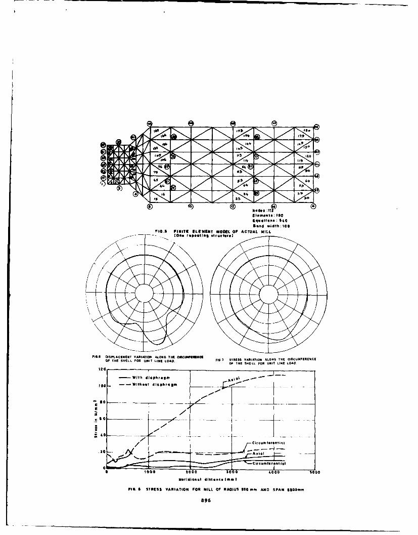
its Ilib $A'S I44
lowulos i'.s
- 5 ~ w i t h I O
P10. FINTE LEMET NOEL F ATUALJIL
- Wbond icdII;106FI.S FNIEELMNTMDE F CUA IL
100 ~ ~ ~ ~ (R -- Without structmure)_ _____
Fl. IPAISIVRAIO LN H ICMEEC
Metoofa -- Witanue dimmrag
FIsoTESVRAIN O ILO AISSC mADSA 60m
to9

SECOND INTERNATIONAL CONGRESS ONRECENT DEVELOPMENTS IN AIR- AND
STRUCTURE-BORNE SOUND AND VIBRATIONMARCH 4-6, 1992 AUBURN UNIVERSITY• USA
ZVALWtTXON OF ACOUSTZC MISSION SOURCZ LOCATION FORDXIIUZNT TBRZZ-SRNSOR hARk! CO"1IGUMPTIONS
Vasisht Venkatesh and Professor J.R. BoughtonDepartment of Mechanical EngineeringTennessee Technological University
Cookeville, TH 38505, U.S.A
ABSTRACT
A common method of detecting a discrete acoustic emission source is bycomputing the time difference between each sensor arrival time. A threesensor equilateral triangular array is often used to locate sources in twodimensional cases. However, this arrangement can create false sourcelocations.
Experiments were carried out to find a possible sensor arrayconfiguration, that would reduce the ambiguity in source location. Variousthree sensor array configurations were used, while keeping the sampling rate,trigger level and gain constant.
Results indicated that a scalene (having unequal sides) triangular arrayconfiguration provided accurate locations with the least amount of ambiguityand no false source locations.
INTRODUCTION
The acoustic emission (AE) technique, of nondestructive testing, detectsstress waves which have been emitted within or on the material surface. TheAE technique has many advantages , since it is capable of detecting dynamicprocesses[I]. The source of energy released is within the test object anddoes not need to be supplied. Acoustic emission sensor arrays can also detectsources from any direction on the test object without depending on priorknowledge of probable location.
In order to be able to locate acoustic emission sources an array ofsensors are placed on the surface of the test object to form a monitoringregion. The arrival times of stress waves at each sensor is noted, and thesource is located by the difference in arrival times. At least three sensorsare required to locate sources in a two dimensional case. Additional sensorscan be added to reduce the ambiguity in source location, however increasingpart and instrumentation costs. Only the three-sensor array is discussed inthis paper.
897

The ability to accurately locate acoustic emission sources is animportant area of nondestructive evaluation. The NDE methods need to beimproved to lower the margin of error and the false locations. The majoradditional problem today is source location in non-isotropic materials suchas engineering composites structures. This paper provides results toexperiments, with three sensor array configurations as shown in Fig. 1, whichwere conducted to find configurations that provide the least number falsesource locations.
THEORY
Consider three sensors on a plate as shown in Fig.2. Assume isotropicconditions where the shear wave from an acoustic emission source travels ata constant velocity,/'. Where G is the shear modulus of elasticity and Pisthe mass density. The sensor arrival sequence is marked 1,2,3 as shown inFig.2. The respective distances between sensors and sources, and the anglesare also noted. The time difference measurements would be between second andfirst sensors and third and first sensors (Eqs.l and 2). Figure 3 showstypical signals and the respective arrival times.
A t2= t- ti (1)
t2=t- tI (2)
(a) (b) (c) (d) (e)
Fig.l Triangular sensor configurations used, (a) equilateral,(b) 30' isosceles, (c) 1T isosceles, (d) 120 isosceles, (e)scalene.
0,i/ , •.AC(f
I 2.
Fig.2 Generic sensor configuration. (1]
898
• • ! ! Sow(

The distance from source to reference sensor, S , is given by thefollowing equations [1]
V? _.&t,2 V2"L (source tOS) "-2= 2 ( &tj V+D1 COSINE (e- 1)) (3)
L (source tOS 1 )1 . 3= 2 At V÷D COSxNE(e 3-e) (4)
where, V is the velocity of the shear wave, determined experimentally.
Equations(3) and (4) are equations of a hyperbola and can be solved
simultaneously to find the source location from the first hit sensor. The
solutions to these equations very often provides two solutions (Fig. 4), both
of which satisfy the input conditions. It is not possible to distinguish the
true source from the false source without further information.
-" - -u•.w S-m,. " -" * " *.=
Fig.3 Typical signals showing arrival times.
FALSE SOURCE
HYPERBOLA -22
HYPERBOLA 1-3 C\TRUEE SOURCE
/
2 3Fig.4. Intersection of hyperbolae giving rise to two sourcelocations.
899

In determining the time difference measurements in Eqs. (1) and (2) it ispossible to use sensors 2 and 3 as the first hit sensors instead of sensor 1.This would require changing the input data (angles and distances) inequations (3) and (4). For example by using sensor 2 as the reference sensorEqs. (1) and (2) become
At 1=tL- t2 (5)
A t2 = 3 - 2 (6)
The arrival times used in these equations are the same as those used Eqs. (1)and (2). It can, therefore, be seen that for a given acoustic emission (3arrival times) Eqs.(3) and (4) can be solved three separate times, yieldingthree possible source locations. This method, as wil be seen, improves theaccuracy of source location for scalene sensor array configurations.
EXPEZRZINTExperiments were carried out on a 1219.2 X 457.2 mm aluminum plate. Four
Valpey-Fisher, VP-1093, pinducers were used in the experiments. One waslocated next to the AE source as a trigger sensor to activate the signalanalyzer. The pinducers used were broadband transducers with a flat frequencyresponse to 1.4 MHz. These transducers were mounted on the aluminum plate bycoupling wax. A 4-channel Data Precision, Data 6100, waveform analyzer wasset at 25,000 samples per second sampling rate. A Tektronix, model AM 502,amplifier was set at a 23 dB gain. See Fig.5 for experimental set-up.
An artificial acoustic emission source was used to carry out the sourcelocation tests. A brittle fracture or pencil lead (Hsu-Nielson) [3] source wasused with a 0.3 mm diameter, and HB hardness lead. This pencil lead sourcewas usd because it provided an easily reproducable signal.
The various sensor array configurations, in Fig.l, were set up andpencil lead breaks were performed at different points on the aluminum plate.These lead break points were mapped and the arrival times at the threesensors were recorded. These arrival times along with the angle and distancedata are input into an iterative computer program, that iterates Eqs.(3) and(4) until the absolute difference between them is under a tolerance of 1.0
mm. If this tolerance limit is not satisfied, then no solution is found forthe input arrival times. The output data is then mapped to determine theaccuracy of the solutions
S- | ~Amplifier ISI I _ • Waveform Plotter
Fig.5 Experimental setup
900

RZSULT8 AND COOUCWZOU
As can be seen from Fig.3 the arrival times of the signals are fairlyeasy to find, however with a sampling rate of only 25 KS/s the possible erroris 40 us[l3. This error is rather large and could produce upto a 90 mm error.It is interesting to note that the experimental errors were much less than 90mm for the scalene triangle. This error should be reduced by using systemswith higher sampling rates.
The results of some of the experiments are shown in Table 1. and Fig.6.These results show that the equilateral, 100and 30'isoceles triangluar arrayslocated two sources within 4 mm, however these same good results producedfalse sources. All initial source locations for the equilateral, W0and 3cPisosceles triangular arrays, were found using sensor 1 as the referencesensor as shown in Fig.6. When the reference sensor was changed to sensor 2and 3 very few solutions were achieved, for the isosceles triangularconfiguration, by the iterative program. The solutions were mapped and thearea where source locations were within 50 mm from the actual source werefound. This area as shown in Fig.7 is the effective source location area. Asthe arrays were changed from the equilateral to the 30' and 10 isocelesconfigurations the effective source location area got thinner, but strechedfurther away from sensor 1 as shown in Fig. 7.
Table 1. A few of the actual and calculated sources with anequilateral sensor array configuration. This table shows the twohyperbolae intersections as source I and source 2. Refer to Fig.6.
Sample Actual values Source 1 Source 2No. from REF at (False Source)
Sensor ADistan- Angles, Distan- Angles, Distan- Angles,ce, ce, ce,cmm degrees mm degrees mm degrees
1. 129.40 90 107.44 104.85 113.23 107.712. 219.96 90 219.71 90.52 96.77 270.313. 279.40 90 283.46 90.01 157.73 270.014. 127.0 35 183.64 44.11 - -
5. 203.20 70 275.60 79.64 - -
--- -- R -L-I-
si
Fig.6 Source location of equilateral sensor array from Table1. True and false sources are shown for the solutions.
901
U" S.I!

S, 5
Zone
(a) (b) (c)
Fig.7 Effective source location area for (a) equilateral, (b)30 isosceles and (c) 10 isosceles triangular configurations.
The scalene triangular array provided different results from theequilateral or the isoceles arrays. Although the scalene configurationlocated sources from 20 to 70 mm of the actual source, it did not produce anyfalse sours.. (see Table 2. and Fig.8). The scalene array configuration alsoprovided three sets of solutions (A,B,C) for every source by chanqinq thereference sensor, as seen in Table 2. It can be seen from Fig.8 that thethree solutions generally formed close groups. The actual source wouldgenerally be close to the average distance of the three solutions. There are,however, places of uncertainity where the three solutions are widelyseperated (5a,5b,5c).
Table 2. This table shows some of the actual and calculated sourcelocations calculated for the scalene configuration with referencesensor A. Refer to Fig.8.
Sample Actual values Experimental Absolute errorNo. from REF sensor values from REF in source
A A locationDistan- Angle, Distan- Angle, R - R esce, R. ce, R, E S
mm Deg mm Deg
1A 152.4 120.0 180.09 146.7 27.7 26.71B 152.4 120.0 185.4 150.0 33.0 30.01C 152.4 120.0 190.5 146.0 38.1 26.0
2A 203.2 110.0 271.8 104.8 68.6 5.22B 203.2 110.0 236.2 118.0 33.0 8.02C 203.2 110.0 279.4 109.0 76.2 1.0
3A 304.8 110.0 271.8 104.8 33.0 5.23B 304.8 110.0 266.7 108.0 38.1 2.03C 304.8 110.0 279.4 109.0 25.4 1.0
4A 431.8 110.0 455.9 113.4 24.1 3.44B 431.8 110.0 457.2 114.0 25.4 4.04C 431.8 110.0 477.5 114.0 45.7 4.0
5A 254.0 60.0 272.8 104.8 18.8 44.85B 254.0 60.0 261.6 107.0 7.6 47.05c 254.0 60.0 279J4 109.0 25.4 49.0
902

A 'IPE bA
Fig.8 Source location of scalene s sor array from Table 2.Solutions for each reference sensor are shown.
The 1260isosceles array configuration tests provided ambiguous results,since the configuration approaches a linear configuration. It was also notedthat all configurations produce ambiguous results when the sources werewithin 70 mm from any sensor.
In summary although, the equilateral 300and leisosceles array3 producedaccurate results within the zone location area, false sources are alsolocated. The scalene triangular array on the other hand, had source locationsthat were not very accurate, but did not produce false sources. The sourcelocation can, however be improved by using an analyzer with a faster samplingrate. A sampling rate around 100 KHz could significantly improve the accuracyof the scalene configuration to within a 10 mm circle of uncertainity.
RZPUZN3SS
[1] Ronnie K. Miller and Paul McIntire, "Nondestructive Testing Handbook",Amerinan Society for Nondestructive Testing, Vol.5, 1987.
[2] Dong-Jin Yoon, Young H. Kim and Oh-Yang Kwon, "New Algorithm for AcousticEmission Source Location in Cylindrical Structures", Journal of AcousticEmission, Vol.9,No.4/October 1990.
[3] Michael R. Gorman and William H. Prosser, "AE Source Orientation by PlateWave Analysis", Journal of Acoustic Emission, Vol.9,No.4/October 1990.
903

904

I
SECOND INTERNATIONAL CONGRESS ONRECENT DEVELOPMENTS IN AIR- AND
STRUCTURE-BORNE SOUND AND VIBRATIONMARCH 4-6. 1992 AUBURN UNIVERSITY. USA
DEFECTS DETECTION IN STRUCTURES AND CONSTRUCTIONSBY NOISE SIGNALS DIAGNOSTICS NETHODS
Uadim A. RobsnanUnion "Electronics of Russia"
2 Krasnopresnenskaya nab.Noscow. 103274, USSR
ABSTRACT
In the course of engineering structures maintenance noise signals mayoccur as a consequence of technological equipment loading, or signals.emitted by special generators -gauges. Generation and propagation ofmicrodefects in the form of cracks and disruption of elements connectingcontacts in structural units are possible in the caurse of dynamicloading.
Identification algorithms are based on usage of noise signalsmultiparametric analysis. The signals could be classified into 2 groups:signals, generated by outer noise sources, and signals, emitted by defectsand damages themselves. The experiments proved, that various non-lineareffects and transformations of noise signals and their spectrum, detectedin separate space and time points, are very important.
Irreversible structure modifications processes and brittle failure instructurl materials take place as a result of local defects accumulation.Such processes generate at the starting stage of plastic deformation anddevelope together with micro- and macrocracks complex propagation, endingabruptly by catastrophic failure. Such phenomena investigation is of someinterest from the acoustic point of view, as various structural defects inmaterial produce different nonlinear effects in acoustic uaves propagationin solid deformed medium. Besides, defects generation and accumulationzones in medium also demonstrate themselves as inner sources of acousticnoise - acoustic emission (AE). Defected zones generation and propagationin material, produced by outer loads, have stochastic nature, which iscorrespondingly reflected in statistical regularities of acousticdetection and ranging signals parametric changes. Both statisticalparameters and acoustic non-linearity effects are identification featuresfor margins betveen faults development stages.
The performed investigations contain methods and results for thefollowing problems solution:
- spectrum distortion degree comparsion for active detection and
905

ranging of deformed media by regular and noise acoustic signals;- interaction of acoustic waves with various spectral characteristics
alongside with non-linear deformation propagation;- cracks acoustic emission probabalistic characteristics at deformed
medium failure stages:- acoustic emission signals spectrum change analysis at vaious stages
of non-linear deformation and failure propagation:- defects detection in structures for failure conditions prevention.The experimental researches have been carried out using special
laboratory testing beds, as well as in situ. The insitu experiments havebeen carried out on soil masses and engineering structures and structuralelements, failed in the course of the Spitak earthquake in Armenia.Diagnostics of structures, failed during the earthquake, covered masonrydwellings and industrial buildings made of precast reinforced concrete andmetal elements.
The first experimental series contains materials investigation underthe conditions of rather low level of non-linear deformation; it wasconnected with non-linear acoustic effects analysis in plasticallydeformed materials. These researches allowed to ascertain that in thecourse of plastic deformation propagation advancing dislocations stimulategeneration of AE signals stationary flow in the form of narrow -band noisepulses complex, parameters of which do not have considerable fluctuations.And by the AE signals appearance moment discreteness it could be concludedthat dislocational movement is abrupt, but not in the form of smoothcontinuous displasement. The other experimental series was dedicated tothe investigation of additional ultrasonic action influence effect on non-linearly deformed material. This stimulated dislocational movementactivization. The abnormal acoustic phenomena investigations were carriedout under the conditions of various spectral characteristics of outerultrasonic transducers and non-linear deformation levels. So. for example.considerably powerfull narrow -banded noise pulses action on plasticallydeformed materials produced non-linear spectrum distortion in the form ofits maximum displacement to the region of lower frequencies and irregularpower redistribution to both spectrum wings. The influence of outer staticloading and acoustic influence were studied within dislocation model ofFrenkel-Kontorova. At the beginning so far as outer acoustic actionoscillation is increased, oscillators networks undergo non-lineardistortions, the spectrum is enriched by the highest harmonics, but theprocess remains periodical. Then the periodicity is disturbed by atomsmigration from one potential field into another; new spectrum componentsare generated. At last subharmonics mass generation takes place, as wellas all possible heterodyne frequencies, that is a transition into therandom frequencies mode is observed.
Acoustic phenomena investigations in metal and reinforced concretestructures were carried out under static and dynamic loading applied up tocomplete failure stage. The experiments provided for organization ofmultichannel monitoring of acoustic signals in tensile and compressivestressed zone, as well as for differences definition of acoustic spectranon -linear transformation zones.
Even at the starting stages of non-linear deformations, correspondingto not less than 15 e of breaking load, narrowbanded noise signals ofactive detection and grading were monitored, which had the amplitude andspectral lines width of high-frequency harmonics higher, than of the firstone. But such widening was limited by the distance to the transducer of no
906

sore than I a. Kith further increase of non -linear deformation thesimilar effect was observed in the compressed zone at 0. 5 - 0.? adistance, and there was a 20 - 25 Z increase of the second harmonics powerin the limited frequency band. But in tensile zone the second harmonicspower increase did not exceed P? - 20 Z. When the loading reached 60 - 65X of the breaking one, the second harmonics power increased 2.7 - 3 timescompared to 10 - 15 Z of breaking load power level.
In the course of reinforced concrete beam detection and ranging bywide -band noise there is irregular power redistribution from the centralpart of the spectrum to the region of low and high frequences depending onthe sign and non-linear deformation obsolute value, as veil as distance tothe transducer. When the distance to the transducer is increased, there isdecrease and redistribution of power in spectrum high- and low-frequencyzones. On compressed parts of the material the power of the spectrum high-frequency wing is t.6 - 1.8 times greater than of signal spectrum in thetensile part. Besides, some frequency range narrowing of wide-band noisesignals spectrum was observed in material's parts under tensile stresses.
The experiments on non-linearly deformed reinforced concrete beamalso shoved that under interaction of regular waves and noise, generatedin one direction by two parallel transducers, power redistribution to thehigher-frequency zone takes place simultaneously with new spectrum zonesformation and power decrease in monoharmonic component of the spectrum. Innoise component there is also power redistribution to lou-frequency andhigh -frequency zones when the distance to the transducer Increases. Theincrease of the distance to the transducer is accompanied by powerdispersion In the spectrum with high-frequency component increase only incompressed zone. In tensile stress zone there is a spectrum maximum shiftto the lower frequencies zone together with power decrease, which alsodepends on relative deformation level.
Non-linearly deformed solid media evolution could be represented assuccessive stages of irreversible destructive processes, with acousticemission (AE) signals as indications of their development. Such processand margins between its separate stages could be analized by theappearance of characteristic non-linear transformations in emissionsignals spectra. In RE signals spectra there are non-linear distortions inthe form of local extremes on subharmonic frequencies with their doublingeffect and the following spectrum reorganization into the noise one in thelow-frequency wing before abrupt failure. In all cases extremes appearanceon new frequencies was connected with the beginning of the local defectsinteraction stage, and the noise spectrum formation identified the abruptfailure start. Non-linear spectra transformations, found in the course ofexperiments, allowed to suppose that in the emission process developmentthere is a certain analogy with bifurcational transition to random stageaccourding to Feigenbaum pattern or combinatorial subharmonic componentsformation in the spectrum. The RE pulses flow could be simulated as randomtransition process complex in connected non-linear oscillations. Thecomputer-aided experiments using this model proved random transition modein the form of bifurcations stage.
The investigations allowed to establish acoustic spectra nonlineartransformations not only by active medium detection and ranging, but alsofRE signals, emitted by growing defects. Non-linear spectral distortionsobserved in the course of physical experiments and computeraidedsimulations recognize quantitative differences in failure stages. Thisprovides for identification of destructive processes separate stages inorder to prevent failure catastrophic stages.
907

908s

SECOND INTERNATIONAL CONGRESS ONRECENT DEVELOPMENTS IN AIR- AND
STRUCTURE-BORNE SOUND AND VIBRATIONMARCH 4-6 1992 AUBURN JNIVEPSII. USA
TOOL FAILURE DETECTION USING VIBRATION DATA
T.N. Moore J. PeiAssociate Professor Research Engineer
Department of Mechanical Engineering Technical Services DivisionQueen's University Stelco
Kingston, Ontario, CANADA Hamilton, Ontario, CANADA
ABSTRACTThis paper investigates the possibility of using vibration signals to
detect failure of a multi-insert face mill. Tests were performed using athree-insert face mill to machine a standard workpiece. Cutting inserts withknown amounts of edge fracture or wear were used, in various combinations,during the milling process. The resulting vibration signals, obtained both onthe workpiece and the clamping fixture, were analysed to determine both thetype and severity of insert failure that can be recognized using varioussignal analysis methods. It is shown that both edge fracture and wear can bedetected, albeit with varying degrees of confidence.
INTRODUCTION
A major component of any effort to develop intelligent and flexibleautomation systems must be the concurrent development of automated,diagnostic systems to handle machinery maintenance and process controlfunctions. In the short term such systems promise major gains in productivityand product quality. In the longer term, such diagnostic systems are one ofthe enabling technologies for the "lights out" factory.
An important element of the automated process control function is thereal-time detecti n of cutting tool failure, including both wear and fracturemechanisms. The ability to detect such failures "on-line" would allowremedial action to be undertaken in a timely fashion, thus ensuringconsistently high product quality and preventing potential damage to theprocess machinery. Of all the metal removal processes employed in industry,by far the most prevelant are those of drilling and milling.
A number of researchers [1,2] have investigated the potential foron-line diagnosis of drill failure (particularly drill breakage) and severalcommercial systems are, in fact, presently available.
However, far less emphasis has been placed on the real-time detection ofmilling cutter failure. For this reason the present study will focus onmilling operations, particularly that of face-milling.
The basic premise of any automated, real-time tool condition monitoringsystem is that there exists either a directly measurable, or a derivedparameter, which can be related to advancing tool wear and/or breakage.Obviously the most desirable monitoring system would be capable nf detectingboth types of failure successfully.
In the ideal case, the system should be able to detect levels of wearwell below those at which the tool would have to be replaced, and should alsobe sensitive to relatively small changes in the level of wear. The lattercharacteristic would provide the system with the potential to "trend" the
909

wear pattern and predict the amount of useful life left in the tool(allowable wear limit reached).
With respect to tool fracture, the system should be able to detect bothsmall fractures, "chipping" phenomena, and catastrophic failure of a tool.Although prediction of such failures would be desirable, it is problematicwhether this is a practical goal, at least in the near future. 'he number ofvariables which determine the actual occurrence of tool fracture togetherwith their complex interactions, and in many instances their underlyingstochastic nature, make reliable prediction capabilities, at best, along-term prospect in tool monitoring systems.
A number of parameters have been studied to determine their suitabilityas indicators of cutting tool failure including cutting forces [3,4], spindlemotor current [5], acoustic emissions [6], and noise [7]. These methods haveachieved varying degrees of success.
An additional parameter which has a number of practical advantages isvibration. Accelerometers, the transducers most often used for the vibrationmeasuring task, are small, rugged, reasonably inexpensive, and easily mountednear the cutting process. In addition, they are available with varioussensitivities and frequency response ranges.
Research carried out by Mehta, Pandey and Chakravarti [83 andGrieshaber, Ramalingam and Frohrib (9) has indicated that vibration signalscertainly could form the basis of a tool condition monitoring system forface-milling operations. However, this work was carried out for asingle-tooth mill which is not particularly representative of themulti-insert face-mills actually employed in industry.
OBJECTIVE
The objective of the present study, then, is to investigate thepossibility of using vibration signals generated during interruptedface-milling to detect tool failure on multi-insert milling cutters.
This paper will report on the methodology and initial results of cuttingtests employing inserts with known degrees of wear or breakage. Preliminaryanalyses of these signals in the time and frequency domains will also bepresented. The results of more involved analyses and the development ofstrategies for automated recognition of these failure signals will bepresented in future work.
METHODOLOGY
The experimental studies were carried out using a 3hp vertical millingmachine. The cutting tool was a 3.81cm diameter, three insert, face-millemploying Carboloy TPG-322E grade 370 tungsten carbide cutting inserts. The"standard" workpiece was a mild steel plate with a length of 30.5cm, a heightof 15.2cm, and a width of 1.3cm.
While cutting, the mill traversed the length of the workpiece performingan interrupted, symmetric cut. See Figure 1. The actual cutting conditionsused are shown in Table 1.
The vibration generated during milling was measured at two locations: onthe workpiece itself, and on the workpiece clamp (the more practical locationfrom an industrial application point of view). The location of eachaccelerometer and its measurement axis is shown in Figure 2. The vibrationsignals were tape recorded for later analysis in the laboratory.
Recognizing that changes in the structural dynamic characteristics ofthe machine-tool-workpiece system (MTWS) would also result in changes to thevibration signal generated during millinq, it was decided to minimize thiseffect as much as possible during the cutting experiments. This was done byfixing the three dimensions shown in Figure 3. Thus the tool-spindleprojection, H1, the height of the table above the machine base, H2, and theheight of the workpiece above the clamp, H3, were kept fixed during each cut.This approach is consistent with the "real life", high volume, productionmachining situation since, in this instance, the structural dynamiccharacteristics of the MTWS would not be expected to change significantlyduring the milling cycle on each new (nominally identical) workpiece.
Since it was desired to determine the potential for recognizing bothwear and fracture failures of the milling inserts, two sets of tests wererun.
910

TOEW FEEDDIRECTION
-'*i~ ACCELERONATEN
/ MILLNG CUTTER 'C
38-1 OIAM/ \/H3 , CLAM W
WORKPIECE
127 WIDE NCC
Figure 1. Schematic of interrupted ,,symmetric milling cut.
SPINDLE Figure 2. Test set-up
LAMP Table 1. Cutting conditions usedTABLEin milling tests.
Depth of Cut: i. 0m
H2 Fee Rate: 0.18mm/toothCutting Speed: 180M/Min.
Figure 3. Dimensions fixed during Engagement Angle: 39.8*
all milling tests.
The first series of tests consisted of milling cuts made using variouscombinations of worn and sharp inserts in the three-insert cutter. The worninserts were obtained by machining a "wear block" under very light, andnon-interrupted, machining conditions, thus achieving a slowly increasingamount of wear (flank wear on the insert) with minimal chance for edgechipping. If chipping did occur on an insert it was discarded. Once thedesired flank wear had been obtained, the insert was put aside to be usedsubsequently in the actual interrupted face-milling tests performed on thestandard workpiece.
In the second series of tests milling cuts were made using variouscombinations of "fractured" and sharp inserts in the three-insert cutter. Dueto the difficulty in obtaining controlled amounts of edge fracture duringnormal machining operations, it was decided to simulate fracture of theinsert using electrical discharge machining to remove a controlled amount ofthe insert cutting edge. This is shown in Figure 4. The dimension, L, is usedin thls study to quantify the magnitude of the edge fracture.
911
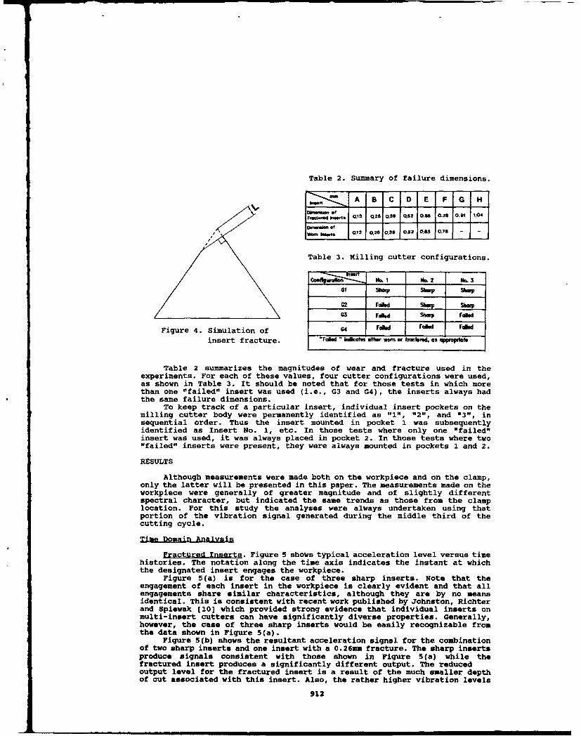
Table 2. Summary of failure dimensions.
A B C D E F G H
FalctOd Worts Q13 Q21 039 052 0 0.6 0 10.I6
4 W Wo I O f Q 1 0 .2 0 0 .30 0 .8 2 0 5 0.6 0 - -
Table 3. Milling cutter configurations.
Co-fl No.I Me.2 No. 3
____1__ Shop~ ShinP Shwp
G2 rawd ShWp Sh-G3 rVad SIWP fdai
Figure 4. Simulation of Gl FWa raw IVald
insert fracture. Fd "lkaNs .t wonm frc. asa
Table 2 summarizes the magnitudes of wear and fracture used in theexperiments. For each of these values, four cutter configurations were used,as shown in Table 3. It should be noted that for those tests in which morethan one "failed" insert was used (i.e., G3 and G4), the inserts always hadthe same failure dimensions.
To keep track of a particular insert, individual insert pockets on themilling cutter body were permanently identified as "1", "2", and "3", insequential order. Thus the insert mounted in pocket 1 was subsequentlyidentified as Insert No. 1, etc. In those tests where only one "failed"insert was used, it was always placed in pocket 2. In those tests where two"failed" inserts were present, they were always mounted in pockets 1 and 2.
RESULTS
Although measurements were made both on the workpiece and on the clamp,only the latter will be presented in this paper. The measurements made on theworkpiece were generally of greater magnitude and of slightly differentspectral character, but indicated the same trends as those from the clamplocation. For this study the analyses were always undertaken using thatportion of the vibration signal generated during the middle third of thecutting cycle.
Time Domain Analysis
Fractured Inserts. Figure 5 shows typical acceleration level versus timehistories. The notation along the time axis indicates the instant at whichthe designated insert engages the workpiece.
Figure 5(a) is for the case of three sharp inserts. Note that theengagement of each insert in the workpiece is clearly evident and that allengagements share similar characteristics, although they are by no meansidentical. This is consistent with recent work published by Johnston, Richterand Spiewak [10] which provided strong evidence that individual inserts onmulti-insert cutters can have significantly diverse properties. Generally,however, the case of three sharp inserts would be easily recognizable fromthe data shown in Figure 5(a).
Figure 5(b) shows the resultant acceleration signal for the combinationof two sharp inserts and one insert with a 0.26mm fracture. The sharp insertsproduce signals consistent with those shown in Figure 5(a) while thefractured insert produces a significantly different output. The reducedoutput level for the fractured insert is a result of the much smaller depthof cut associated with this insert. Also, the rather higher vibration levels
912

associated with the insert following the fractured insert is apparent. Themuch higher vibration level associated with the insert's disengagement fromthe workpiece is particularly noticeable. These features are due to theincreased "effective" depth of cut associated with this insert.
The results for other magnitudes of fracture and numbers of fracturedinserts are basically the same. The presence of a fracture is readilydetectable. It would seem from the time domain data available, that the useof either an "envelope detection" or a wthreshold crossing" scheme wouldprovide the ability to automate the detection of tool fracture in amulti-insert milling operation. However, it is not yet clear whether the timedomain signal, on its own, can be used to reliably classify the actualmagnitude of the fracture. This work remains to be done.
Worn Inserts. The acceleration-time histories for the worn inserts donot, in general, produce the noticeably different engagement signals evidentin the case of fracture. However, by processing the data in a slightlydifferent manner it is possible to detect evidence of tool wear.
Figure 6 shows the amplitude probability density (APD) for several toolconditions. This distribution shows the percent of time a given level waspresent within the sample period. The data shown is for eight ensembleaverages.
Figure 6(a) is for three sharp inserts. Note the essentially symmetriddistribution. For the combination of two sharp inserts and one with 0.65m-flank wear, see Figure 6(b), the APD is skewed to the left and its peak valuejis also shifted noticeably from its position for three sharp inserts. Figure6(c) shows the results for three inserts with 0.65mm flank wear. In this cas•the peak has decreased and shifted to the left and broadened significantly..
It thus seems possible that insert wear could be detected using suchfeatures as the location of the peak in the APD, the magnitude of the peak,and the area under specific segments of the distribution. This techniquewould also seem to hold promise for fractured inserts.
Frequencv Domain AnalysisFrequency spectra were obtained for the various tool conditions. All
spectra were generated using eight ensemble averages and were calculated overa bandwidth of 0 to 20kHz using 800 lines of resolution.
In many cases it was observed that the level of the spectral peakswithin the the frequency range 12 to 18kHz was affected by the toolcondition. However a review of all the available spectra data indicated thatthis change in spectral level did not always occur and that the change whichdid occur was not consistently related to the known change in insertcondition. That is, an increase in fracture dimension, or wear, did notalways result in a consistent increase (or decrease) in a particularfrequency band. Thus, although such frequency spectra may well provide someindication of tool failure under most conditions, it seems very unlikely that
I 3S4AW
• E-GAG2 .. ...
TIi IMIm) I ....
'IIT
t -4 -4
491-0 go 1 20 IO 4 0 60 120 60 40
Figure 5. Time domain data - insert fracture. - 0 ..ACCELERATION (g)
Figure 6. Amplitude probabilitydensity - insert wear.
913

they would ever be able to provide a reliable indication of the particularmagnitude of the failure.
It was recognized that one reason for such inconsistent results could bethe lack of synchronous averaging when acquiring the data signal to befrequency transformed.
To circumvent this problem an external trigger system was built. Itgenerated trigger pulses which were keyed to the engagement of each of thethree inserts with the workpiece. The trigger pulses generated for eachinsert were recorded on separate tape tracks. In this manner a given pulsetrack could be used to acquire the vibration data associated with a specificinsert engagement and to ensure that the vibration signal was completely andconsistently captured within the data window of the FFT analyzer. All thefrequency spectra discussed in this section employ the synchronous averagingtechnique.
Fractured Inserts. Figure 7 presents an example of the synchronouslyaveraged spectra obtained for the combination of one fractured and two sharpinserts. In this case Insert 2 was fractured and the figure presents thespectra obtained for each of the eight fracture magnitudes tested, rangingfrom 0.13 mm to 1.04 mm. Recall that due to the use of synchronous averaging,the spectra shown in Figure 7(a) (triggered on Insert 1 engagement) areobtained from the vibration signal generated only by Insert 1 engagement. Inthe same manner, Figure 7(b) represents only the Insert 2 vibration signaland Figure 7(c) represents only the Insert 3 vibration signal.
TRIGGERED ON INSERT 1 TRIGGERED ON INSERT 2 TRIGGERED ON INSERT 3 Fracture"(a)" '(b). .. .(c)"
1.04 mm
0.91mm
2 0.78mm
0-65mm
.j 0 0.52 mm
C) 0.39 mm
0.26mm
0.13mm
0 200ooFREQUENCY (Hz)
Figure 7. Frequency domain data - insert fracture.
Comparing the results presented in these figures, the presence of insertfracture is readily apparent. The spectra associated with the fracturedinsert are significantly different from those obtained from the two sharpinserts.
Interestingly, for small fracture dimension (0.13mm and 0.26mm) thespectral magnitude increases in the range 15 to 18kHz. This is likely theresult of the specific insert geometry causing significantly more energy tobe generated in the cutting zone at these high frequencies. Such frequenciesare known to be associated with metal deformation/shearing processes. Thecombination of an increase in energy a these high frequencies and a reductionin energy level at lower frequencies, could serve as a very sensitiveindicator of insert "chipping" (loss of a small amount of the cutting edge).
The spectra for Insert 1 and Insert 3 (both sharp) share the samegeneral characteristics. However since Insert 3 follows Insert 2 (the
914

fractured Insert) in the cutting cycle (see Figure 5), and thus has a greatereffective depth of cut than Insert 1, the spectra associated with Insert 3have generally greater magnitude than for Insert 1.
The results for the combination of two fractured and one sharp insertare similar, with the fracture condition readily apparent. The distinctdifferences between the "sharp" and "fractured" spectra leave little doubtthat the presence of fracture can be reliably detected. However, the questionremains whether a method can be found to use this data to reliably quantifythe magnitude (determine the severity) of the fracture.
Worn Inserts. Figure 8 presents the results obtained for the combinationof two worn and one sharp insert. To begin, notice that the frequency spectraassociated with the sharp insert, Figure 8(c), remain consistent with thoseseen earlier during the fracture tests (see for example Figures 7(a) and(c)). The sharp insert spectra are also basically unchanged for increasingwear dimensions on Inserts 1 and 2.
The worn insert spectra are noticeably different from the sharp insertspectra. The worn insert spectra decrease in magnitude at lower frequencies(0 to 4 kHz) with increasing flank wear, and tend to increase in magnitude atthe higher frequencies (15 to 18kHz) with increasing wear. Thus it would seemlikely that such spectral data could be used not only to provide anindication that flank wear is present, but also the relative magnitude ofthat wear.
TRIGGERED ON INSERT 1 TRIGGERED ON INSERT 2 TRIGGERED ON INSERT 3 WEAR0) I , ý A 1&2)(a) . .. ) 078mm
O 065mm
OL52-mm
luJ 0.390mm
66
FREQUENCY(Hz)Figure 8. Frequency domain data - insert wear.
Quantitative Fault Features. The results presented earlier indicate thatboth insert fracture and wear could be recognized from changes in thespectral data associated with insert engagement vibration signals. If such atechnique were to be applied in an automated (computer controlled) diagnosticsystem it would be necessary to obtain quantifiable "features" associatedwith these spectra, that could then be manipulated by the computer in such amanner as to provide a decision making mechanism.
One such "feature" might be the area under the spectrum within aparticular range of frequencies. The change in this area (or areas, if morethan one range of frequencies is employed) could then be related to the wear(or fracture) dimension on the insert.
For this particular exercise it was decided to limit the featuresobtained to the area under the spectrum within the 15 to 18 kHz frequencyrange. This was called the Wear Identification Area (Fracture IdentificationArea for the case of fracture). Figure 9 shows the Wear Identification Area(WIA) curve that results when using the average of the WIA values obtainedfor the wear test series described in this study.
The average WIA curve shows a relatively rapid increase in value untilapproximately 0.5mm flank wear (at which point the WIA has reachedapproximately three times the value for a sharp insert) after which it beginsto decrease. This type of relationship could be used by an automateddiagnostic system to quantify the magnitude of flank wear present on a giveninsert.
Of course it may well be possible to enhance the reliabiliity of such a
915

S240-
ISO
S60.
0 0ý OA Q8
FLANK WEAR (mm)Figure 9. Average WIA as a function of insert wear.
system by employing WIA values based on additional frequency ranges (such as0 to 4 kHz). The Fracture Identification Area (FIA) curve could be generatedand used in a similar manner.
CONCLUSIONS
This perer has presented preliminary results from a study undertaken todetermine if vibration signals could be used to detect the failure (edge wearand fracture) of cutting inserts on a multi-insert face milling cutter.
It was shown that evidence of both tool fracture and flank wear can befound in both time and frequency domain analyses. However, it is also notedthat when employing the simple analysis methods described in this paper, itis not possible to reliably determine the actual magnitude of the toolfailure nor to distinguish between the type of failure (wear or fracture)that has occurred.
Future work will attempt to identify processing methods which producefeature vectors capable of providing both quantitative measures of toolfailure and unambiguous indication of the type of failure.
REFERENCES
1. Braun, S. et. al., "Signature Analysis Applied to Drilling", ASME J.of Mechanical Design, Vol. 104, pp. 258-276, 1982.
2. Moore, T.N. and Reif, Z.F., "Detection of Tool Breakage Using VibrationData", Society of Manufacturing Engineers, Manufacturing EngineeringTransactions, pp. 45-50, 1985.
3. Altintas, Y., Yellowley, I. and Tlusty, J., "The Detection of ToolBreakage in Milling Operations", Journal of Engineering for Industry,Vol. 110, pp. 271-277, 1988.
4. Richter, F. and Spiewak, S.A., "A System for On-Line Detection andPrediction of Catastrophic Tool Failure in Milling", Proceedings of NAMRCXVII, pp. 137-143, 1989.
5. Matsushima, K., Bertok, P. and Sata, T., "In-Process Detection of ToolBreakage by Monitoring the Spindle Current of a Machine Tool", ASNEWinter Annual Meeting, Measurement and Control for BatchManufacturing, pp. 145-154, 1982.
6. Diei, E.N. and Dornfeld, D.A., "Acoustic Emission Sensing of Tool Wear inFace Milling", ASME J. of Engineering for Industry, Vol. 109, pp.227-233, 1987.
7. Lee, L.C., "A Study of Noise Emission for Tool Failure Prediction", J.Machine Tool Design and Research, Vol. 26, No. 2, pp. 205-215, 1986.
8. Mehta, N.K., Pandey, P.C. and Chakravarti, G., "An Investigation of ToolWear and the Vibration Spectrum in Milling", Wear, Vol.91, pp. 219-234,1983.
9. Grieshaber, D., Ramalingam, S. and Frohrib, D., "On Real-Time ToolFracture Monitoring in Milling", Proceedings of NAMRC XV, pp. 477-484,1987.
10. Johnston, C.M., Richter, F. and Spiewak, S.A., " A Comprehensive Model ofthe Milling Process for On-Live Tool Condition Monitoring", Proceedingsof NAMRC XVI, pp. 178-197, 1988.
916

SECOND INTERNATIONAL CONGRESS ONRECENT DEVELOPMENTS IN AIR- AND
STRUCTURE-BORNE SOUND AND VIBRATIONMARCH 4-6. 1992 AUBURN UNIVERSITY. USA
PHOTOACOUSTIC METHOD APPUCATION QUAUTYCONTROL OF ULTRACLEAN WATER
Aleksei M. Brodnikovskii, Vladimir A. SivovolovR&D Center "Praktik"
Institute of Electronic MachineryMoscow 103498, Russia
ABSTRACT
The report is about laser photoacoustic device development and testing for ultracleanwater organic pollutants used in microelectronics. The fourth harmonic Nd:YAG laser(energy in pulse 2 nl) is used as a radiation source for optoacoustic signal excitation. Thedetection limit is about 20 ppb. Also the device can detect microparticles in liquids (one micronsize and larger).
Organic pollutants water control is the very important problem from microelectronictechnique point of view. Laser UV excitation fluorescent spectroscopy is one of the mostsensitive method of control. But there is the whole number of organic compounds which havethe low quantum fluorescent efficiency.
The laser device based on photoacoustic effect was developed for non-fluorescent pollu-tants control. When part of the laser radiation energy is selectively absorbed by pollutantsthe acoustic pulses are appeared in control medium registered by sensitive piezoceramicsensor. The fourth harmonic Nd:YAG laser is used as a radiation source. Pulse radiationenergy is 2 m J, wavelength is 266 nm, pulse duration - 15 - 20 ns.
The radiation is directed to thermostabilized photoacoustic cell through which testedwater pumped.
The cell's construction permits to register photoacoustic and fluorescence signals simul-taneously (set-up is shown on Fig. 1). Acoustic pulses are detected by sensitive piezoelementceramic PZT-19 cylinder. Further the electric signal is amplified by low noise preamplifierand amplifier (the total amplifier coefficient K - 2000). The boxcar integrator permits tosuppress the outside acoustic noise and parasitic signal noise due to radiation absorption incells windows.
917

2 3 41PA(fa."J)
5 4 0
3 0
00II 2 0
8 o
1210 20 30 40 SO2(PPB I
Fig. 1. Experimental set-up. I - Nd:YAG laser. 2, Fig. 2. Experimental results. PA signal vs concen-3- doubling crystals; 4 - selective miror; 5 - filter; 6 tration of added pollutant - KHP (dissolved in water).- focusing lens; 7 - photoacoustic cell; g - piezoelec- Zero level of PA signal corresponds with absorption oftric elementand preamplifier; 9 - fluorescense channel; laser radiation in water.10 - powermeter; I I - boxcar Integrator; 12 - plotter.
This set-up can register the energy absorbed inside the cell as small us 2x0"7 J. Todetermine the limits for device analytic possibilities the measurements of PA signal depend-ance on KHP concentration were made.
The test results show the minimum detectable concentration of organic pollutants (KHP)
is about 5 ppb with S/N-3 (Fig. 2). This set-up permits to detect the presence of microparti-des (size more than 1 , m) in liquids and to conduct the photochemical dynamics reactionsresearch work also.
91'

SECOND INTERNAT1ONAL CONGRESS ONRECENT DEVELOPMENTS IN AIR- AND
STRUCTURE-BORNE SOUND AND VIBRATIONMARCH 4-6,. 1992 AUBURN UNIVERSITY USA
ULTRASOMC MEASUREMENTS
Vinay Dayal
Assistant Professor. Aerospace Eng. and Eng. Mechanics Dept., andFaculty Associate, Center for Non-Destructive Evaluation,
Iowa State University. Ames, Iowa, 50011.USA
ABSTRACT
A travelling wave can basically be defined by two basic ultrasonic parameters: Wave Velocity,and Attenuation. The measurement of these parameters has been done by the conventional time-of-flight techniques. These techniques breakdown when the medium In which the waves are travelling arethin, or, the wave velocity Is dependent on the signal frequency. All the limitations of the time-of-flightmethod can be eliminated by the use of Fourier transformation techniques. The development of a frequen-cy based measurement and it's automation are described here, and results are presented to show theaccuracy and precision of the method applied to metallic and composite materials of various thickness.
INTRODUCTION
The measurement of wave speed of an ultrasonic wave in materials has been performed for a verylong time. The purpose, In general, has been Non-destructive Testing. and material properties evalua-tion. The velocity of the wave can be related to the stiffness of the sample [11. There are many excellenttechniques developed for the measurement of wave velocity and attenuation. Very briefly, the techniquecan be described as follows. An ultrasonic wave Is passed through the material and the time takenfor the wave to travel through the specimen Is measured using an accurate oscilloscope. A series ofpulses are obtained and the time Interval between the two received pulses is twice the time taken forthe wave to travel across the width of the specimen. An observer measures the time between anytwo peaks In the received signal and If the thickness of the specimen Is known the wavespeed can becalculated by v = 2* (thickness)/time. The attenuation is measured by measuring the decreasing ampli-tude of a series of pulses. The limitations of this technique are: (1) the thickness of the specimen shouldbe accurately known before the can be reliably measured, (2) though each and every point In the signalhas gone through the specimen and hence obviously contains the Information about the wave speed.only one point is picked disregarding the information contained at all other points, (3) human judgementIs required so as to Identify the exact location of the peak of the signal which Introduces some subjectivtyto the measurement. McSkimin[2] Improved this technique by using a copy of the same wdve translatedin time so that the two pulses could be overlapped and a better match of the signals could be achieved.Papadakis[31 used pulse echo overlap for Increasing the accuracy of measurements. But again thiswas more of a judgement measurement and works very well If the material Is non dispersive and thepulse is not distorted as it passes through the s. 3cimen. If the material is dispersive, or the attenuationis dependent on the signal frequency, then a variation of the time-of-flight method, called tone-burstmethod, could be used. Here a burst of signal, about ten cycles long of a single frequency Is used,but the measurement technique remains the same. This helps In Identifying the frequency at which thewave velocity and attenuation are measured. The measurement of time-of-flight Is possible only If thereflections from the two surfaces of the specimen can be clearly separated In time domain. This isobviously a big draw back and restricts the use of the ultrasonic methods to relatively thick samples.
919

Kinra and Dayal[4] developed a new technique for the measurement based on the Fourier transforma-dion of the signal from time domain to frequency domain. The Fourier transformation of the first andthe second pulse in the signal Is obtained and the slope of the phase vs. frequency curve is calculated.Now, If the thickness of the specimen Is known, the wave speed can be calculated and if the wavespeedis known then the thickness can be calculated. This technique can be used for automation If the thicknessof the plate is constant and the changes in wave speed are to be measured. In cases where therethe thickness Is not known very accurately or if there is local variation In thickness, then the results willbe in error. This technique, with a slight variation could be applied to samples where the Individual pulsescould not be separated, which has increased the range of measurement of the ultrasonic method.
The above mentioned methods worked if the thickness of the samples was measured beforehand.Now for the purpose of Non-Destructive Evaluation, where a large number of measurements are required,the above techniques become extremely slow. First, the thickness has to be measured at all the pointswhere the velocity Is required and then the ultrasonic measurement could be made. Dayal[5] has devel-oped a new computer controlled variation of the Frequency domain technique where both the wavevelocity and the thickness of the sample can be measured. The technique is based on the transformationof the signal from time domain to frequency domain and the whole process Is possible only with thehelp of computers.
The development of the ultrasonic measurement of wave velocity by the Fourier Transformationtechnique and the automation are outlined here. These methods make the measurement precise andautomated.
ULTRASONIC MEASUREMENT METHODS
"Time of Flight method
A typical signal as reflected from an aluminum plate is shown in Fig.(1). The time, t, for a completetravel of the signal from the front surface to the rear surface and back is show on the figure. If thesample thickness, h, is known, then the wave velocity, v, can be written as,
v = 2*h/t (1)
Attenuation coefficient, k2 , is defined as the decrease in the signal amplitude as the wave travelsthrough the sample. This decay is exponential and hence the signal amplitude is measured over anumber of pulses and fitted to exp(-k 2 x ) curve and an average value of k2 is obtained.
2
iiU
TIME IN pe
Fig. 1 Various pulses reflected from an aluminum plate of thickness 4.7 mm.
Frequency Domain method for thick samples
The technique works both for the reflection and transmission mode of wave propagation. Due topaucity of space. only the reflection mode of measurement will be described. Interested reader is referredto [41 for the transmission mode of measurement. In this mode of wave propagation. only one transducer
920
ILa

6Water
4S
1- Water
Transmitter Sample
Fig. 2. Wave propagation through the specimen in reflection mode.
acts both as the transmitter and receiver. A typical experimental setup is as shown in Fig. (2).
Let U, (t) = fo(wt-kox) be the wave produced by the transmitter. If a is the distance of the front
surface from the transducer, the reflection from the front surface of the specimen is.
U2 (t) Ro0 fo(wjt-2ako). (2)
where w is the circular frequency ot he signal, k. to./co is the wave number in water, and co is thewave velocity in water.
The reflection from the back surface is,
U4(t) = To0 R 1oT10fo(0 t-2ako-2hk), (3)
where h is the plate thickness and k is the wavenumber in water.
In the above equations, the reflection coefficients R11 and transmission coefficients T11 are definedas,
Rq. (pc - pjc•)/(pc +pjct), and
T11 = 2pAc/(pjcn + p1c). (4)
where subscript i defines the medium from which the wave is incoming and hitting the interface betweenmedium i and medium j.
The Fourier transform is defined as.
F(wo) ,- FFTpf(t)] - fte4d co- < w, < 0, (5)
Using the Fourier transformation, Eq.(2&3) give.
A2 (ou) = Rol e-1'2 Po (wo), (6)
F'4 (w) = TolR1 oT1 o e-"* 14e-7k • (w), (7)
Now a combination of Eq.(6) and Eq.(7) gives,
( 14iA4) = T0 Rol T1 (8)ToIR IoTIo
It should be noted that in the above equation the wave number k for the material can be real for
921

elastic materials and complex for linear viscoelastic materials. Thus Eq. (8) Is valid for linear viscoelastic
materials If the damping Is small. Then k can be written as, k = k, + i k2, and k2 / k, <<1.
Now, equating the real and imaginary parts on the two sides of Eq. (8) one obtains.
k, (w) = -•/2h, and
k2(w) - In(F*F) /2h (9)here k2 Is the attenuation coefficient for the material.
These equations are useful if various pulses can be separated in time domain. The advantage overthe time of flight is that the wave velocity and attenuation can be determined as a function of frequency.They breakdown If the sample width is such that the pulses cannot be separated in time domain. Inthat case following analysis can be performed.
Frequencv domain method for thin comosites
Referring to Fig. (2) the Fourier transform of pulses labeled (6) can be written as
P6 - TR31 0T1o e-ei ro (w), (10)
Since pulse (2) cannot be separated a new reference pulse is obtained. This is done by replacingthe thin sample by a thick coupon with the front surface precisely at x=a. The Fourier transform of thisreference signal then is,
F (w) = R0 1 e-C2t" Fo (w), (11)
The series of pulses 2,4,6.... are added as follows,
G" (w) - P (w) + TolRwTio 1 R0m-)I()).e+I•'hJ (12)M=1
Now if
Z = R0--m with IZI < 1 (13)
Then 7T10 (14)
Since IZI < 1 and (l-Z)-1 = 1 + Z + Z2 + Z4 ... •, and If
ToTIro (F'(co) (15)
one obtains Z = 13 / ( 1 + 13). The complex valued wave number, k, can easily be obtained from Z.This summation of the infinite series is easier done for the transmitted field and in that case the problemof the replacement of the block does not arise. In this case one can derive the following relation,
G =u TolToie -(k~e)F'((0) TIT1-R 2-jM
1- e (16)
This equation can be reduced to,
Z1+ ZY - Do = 0, (17)
where Y = RToZo G*(o) Zo = exp (-ihko) and Do = 1 IR 2
922

For the details of the solution of these equations the interested reader is referred to [4]
Simultaneous measurement of wave speed and Attenuation
The set up for this method is shown in Fig. 3. Here a reflector is placed at some distance at theback of the sample.
Water Water
Transmitter SampleI
Reflector
Fig. 3. Wave propagation through the specimen in reflection mode.
The Fourier Transform of the pulse reflected from the reflector surface and received by the transducer,when no specimen Is present. is
d (w) = R02 e-0. ((w), (18)
The transform of the front surface reflection (2) . the back surface reflection (4) and the wave (r)which is transmitted through the specimen, reflected from the reflector and again travelling through thespecimen is received by the transducer, are
F2 (w) = R01 e-'-- ro ((u), (19)
F4 (=) f To1RloT1 o e-46e-a'h Fo (w), and (20)
] = () R220e (u). (21)
A combination of Eqs. 18,19.20 and 21 gives.
(-, TOiTiOROl -i hko. (22)
Comparing the phase of both sides of Eq.22. the following relation is obtained,
phase I Pd rr2koh. or
h= S-(,,/J) (23)4x
Now,
44) = Ol24)
923

The phase of both sides of Eq. 24 is compared and the wave speed can be calculated from.
4xh =(25)
RESULTS AND DISCUSSION
A special test specimen Is prepared for implementing the various methods for thick compositesfor comparison purposes. The sample is as shown in Fig. 4.
Steel
Copper Ste Brass
Aluminum plate
Fig.4 Test sample.
A 9.4 mm aluminum plate is prepared with holes drilled at three locations. These holes were thenfilled with three Inserts of copper, brass, and steel. Thus, we have a sample with roughly the samethickness but very different materials. Various results obtained are shown in the Table.
Table I: Comparison of three measurement methods.
Technique Aluminum Brass Steel Copper
c c d c d c d1. 6.375 9.5 4.234 9.4 5.732 9.4 4.696 9.32. 6.372 9.5 4.241 9.4 5.713 9.4 4.704 9.33. 6.347 9.421 4.218 9.35" 5.702 9.363 4.363 9.352
1. Time of Flight / physical measurement of thickness.2. Frequency domain method / physical measurement of thickness.3. Simultaneous measurement reflection modec: wave velocity in mm/gi secd: specimen thickness in mm.
In this table the results are in the following order. First, the physical dimensions of the sample andthe wave velocity as measured by the time of flight method, are recorded. Next, the wave velocitiesas obtained by the technique developed by Kinra and Dayal3 and outlined above as the Frequency do-main method for thick samples. The schematic of the method is as shown in Fig. 2. Note here that inthis technique the experimenter has to provide the thickness of the sample and hence thickness is physi-cally measured and wave speed is calculated by computer. Next, we present the results obtained bythe reflection mode. The schematic of this setup is shown in Fig. 3. Here both the wave speed andthickr ss are estimated by the computer. The input for this technique is the wave speed in water whichis accurately determined. The results for the computerized tests are averaged over 25 points and thestandard deviation of the measurement for all the values was less than 0.1 %. It is seen that the techniquedeveloped here is capable of measuring the thickness and wave speed of the material quickly and pre-cisely.
The technique described under the method for thin specimen, is applied to an aluminum plate. Thewave speed was measured in an aluminum plate and the plate was gradually machined to reduce thethickness. The results are shown In Table I1. In this table the first measurement is for an aluminumplate 2.807 mm thick with the tone-burst method, Then the same plate is analyzed by the method forthe thin plates and the results are shown. Next, the plate Is gradually machined to 0.258 mm and theresults are presented. For comparison purposes the ratio of the sample thickness to the signal wave-length, X, is also listed. It can be observed that even when the plate thicknes', is less than half of thewave length the method provides with an accurate wave speed. All the measurements were made tentimes and the standard deviation of ± .14 % shows the repeatability of the measurement.
924

Table II Results for a thin aluminum sample.
h hIX c (7/C Techniquemm mm/,* sec %
2.807 4.4 6.3572 0.013 Tone Burst2.807 4.4 6.3275 0.010 Thin sample1.686 2.7 6.3461 0.040 Thin sample1.001 1.6 6.3538 0.030 Thin sample.613 0.96 6.3594 0.130 Thin sample.258 0.40 6.3231 0.140 Thin sam[le
Sample: Aluminum Frequency: 10 MHz. Mode: Transmission
Now some results from the automation of the simultaneous measurement technique will be presented.A Stepped plexi-glass sample was prepared for testing and a line scan of the wave velocity and thicknessis made. The results are as shown in Fig. 4. It is observed that the thickness of the sample is veryprecisely measured and the wave velocity remains constant over the entire measurement range.
5.3
Z 2.S- 2.3t .. 2.0 r
1.0- • kwf by Uftrmmd(as m) 1.0 •
5- W. Spd ,5
+ 3.0
1.0 - I, b . oa.0mm
0 15 30 45 6o 76 90 106 120 135 10
LOCATION ON SAMPLEFig. 4 Wave velocity and thickness scan of a stepped plexi-glass sample.
Next, a Graphite/Epoxy composite specimen was specially made for proving the usefulness of thetechnique. The specimen has a step variation in thickness in the middle. The specimen is as shownIn Fig. 5, and was subjected to the computerized thickness-velocity scan. The results show that thetechnique presented here very efficiently measures the change In thickness while the wave velocity re-mains essentially constant. Notice also that the thickness scan shows some scatter of values at theedge. This is because when the transducer is on the step, part of the wave is reflected from the uppersurface and part from the lower surface. This obviously cannot be differentiated and results In wrongvalues.
The limitation of the automated technique Is that both the sides of the specimen should be accessible.In the reflection mode though only one transducer is needed on one side of the specimen, a reflectionplate has to be provided. In transmission mode transducers have to be placed on both sides of thespecimen. The advantages are the precision of measurement, speed of data collection and very special-ly, if the specimen has varying thickness, the technique will provide with the thickness and wave speedautomatically.
CONCLUSIONS
The conventional time-of-flight method of measuring the acoustic parameters is good if the sampleIs thick and thickness Is accurately known. Transformation of signal Into frequency domain improves
925

the precision of the technique. If the sample Is thin and the individual signal pulses cannot be separatedthen the frequency domain analysis Is the only method of measurement. For a large number of measure-ments over a sample which Is not accurately measured, the automated method of simultaneous measure-ment of wave velocity and thickness can be used. The use of computational methods Increase thereliability and precision of the measurement.
3.5- 9 -
E 0.5-
Fig. 5 Wave velocity and thickness scan of a stepped Gr.Ep composite sample.
REFERENCES
1. V.K. Kinra and V. Dayal, " Acoustic Methods of Evaluating Elastic Properties, or, Will the Real YoungsModulus Please stand up ?" Manual on Experimental Methods for Mechanical Testing of Composites,Ed. R.L. Pendleton and M.E. Tuttle. published by the Society of Experimental Mechanics.
2. M.J. McSkimln, " Pulse Superposition method for measuring Ultrasonic Wave Velocity in Solids," J.Acoust. Soc. Am. 33(1),12 (1961).
3. EP.P Papadakis, "Ultrasonic Phase Velocity by the Pulse-Echo overlap method incorporating DiffractionPhase Correction." J. Acoust. Soc. Am.. 42(5). (1967).
4. VK.Kinra, and V. Dayal, "A New Technique for Ultrasonic-Nondestructive Evaluation of ThinSpecimens." Expt. Mech., 28(3). (1988).
926
.,am -- ~ ~.5n,,m m m u a a I I u N

SECOND INTERNATIONAL CONGRESS ONRECENT DEVELOPMENTS IN AIR- AND
STRUCTURE-BORNE SOUND AND VIBRATIONMARCH 4-6. 1992 AUBURN UNIVERSITY. USA
EVALUATION OF LAMINATED COMPOSITE STRUCTURES USINGULTRASONIC ATTENUATION MEASUREMENT
Peitao Shen and J. Richard HoughtonDepartment of Mechanical EngineeringTennessee Technological University
Cookeville, TN 38505
ABSTRACT
The existence of delamination and porosity in laminated composite structures will degrade the strengthof the structures. The detection of delamination can be easily obtained using ultrasonic C-scan or A-scanmethods. But, the detection of porosity in laminated structures has been a difficult task for years, especiallyin production condition. This paper will analytically evaluate the current techniques used in industry, anddevelop accurate attenuation measurement methods for the evaluation of porosity. The test samples, whichare used in the laminated structures of the German airbus by Textron Aerostructures, Inc, will be tested usingultrasonic C-scan and grid-based A-scan methods. The digitized waveforms are stored and analyzed usingdifferent attenuation measurement algorithms. The volume of porosity are calculated using digital imaginganalysis. Finally, the correlation between ultrasonic attenuation and the volume fraction of porosity arecalculated and analyzed.
INTRODUCTIONThe existence of delamination and porosity in graphite-epoxy composite materials will degrade the
strength of structures. The ultrasonic nondestructive inspection in aircraft wing structures made by graphite-epoxy composite materials is a required quality assurance procedure in the aircraft industry. The regularprocedure is first to inspect the parts using ultrasonic C-scan through-transmission testing method. From theC-scan results, it is usually quite easy to locate the regions with delamination according to some recommendedindustrial C-scan testing standards. But, however, the detection and quantization of porosity is a difficult task.The difficulties of evaluating porosity come mainly from the following factors: (i) The lack of theoreticalresults about sound property in porous laminated composite materials; (ii) The lack of acceptable measurementtechniques for porosity evaluations.
According to some reported literatures, the early study on the relationship between porosity andultrasonic attenuation coefficient in isotropic materials was carried out by Gubernatis and Domany 11,21. Theydeveloped approximate expressions for ultrasonic attenuation in porous media with finite-sized pores. Adleret al. successfully applied Gubematis and Domany's results to the characterization of the porosity in aluminumalloy castings [3]. The porosities in aluminum castings are dominated by spherical pores with a Gaussian typeof peak size distribution in the diameter of the pores. On the basis of Adler's experimental results andGubernatis and Domany's theory, Nair and Hsu et al. made a study on the estimation of porosities usingfrequency-dependent attenuation measurements [4,5]. Instead of directly using Gubernatis and Domany'sapproximation, they developed an attenuation slope algorithm which was felt to be more suitable for thecylindrical pores which typically exist in composite materials.
Although laboratorial research has been applied to evaluation of porosity in graphite-epoxy composites,the understanding and testing techniques are still inadequate for application in industry. Based on the testingtechniques currently used in industry, this paper will present practical ultrasonic attenuation measurement
927

algorithms, conduct ultrasonic attenuation measurement and porosity analysis experiments, and correlate thevolume of porosity with ultrasonic attenuation coefficients.
ULTRASONIC ATTENUATION MEASUREMENT METHODSThe attenuation of sound in test materials may not have many direct interests to engineers. But, the
change of attenuation is often a result of some physical or chemical change related to the property of the testmaterials. Thus, the use of ultrasonic attenuation measurement technique to characterize material property hasbecome an important subject for NDE engineers. Papadakis did a series of research work on absoluteattenuation measurement which focused on the beam diffraction correction [6]. Other research on quantitativeattenuation measurement has been reported by Simpson et al. [7]. In this study, the investigation of attenuationmeasurement will be based on current measurement techniques used in industry. The equations for thecalculation of ultrasonic attenuation using contact pulse-echo and through transmission testing methods willbe introduced.
Ultrasonic- attenuation can be defined as the rate of decay of mechanical radiation at ultrasonicfrequency as it propagates through a material. For a plane wave, which should be the case in the far fieldmeasurement, the attenuated wave in space is expressed as
where Po and P are the amplitudes of wave pressures at the beginning and the end respectively, and a is theattenuation of the wave travelling in the z-direction of the test materials. The attenuation a is measured innepers per unit length or in decibels per unit length.
Figure 1 is a diagram of wave propagation indicating both pulse-echo testing and through transmissiontesting -••,thods. The ultrasonic transducer first sends the longitudinal waves to medium 1 (delay line or waterpath), and then the waves propagate through medium 2 and medium 3. For through transmission testingmethcd, medium 2 is usually the test specimen, medium 3 is usually the same as medium 1. Water is usuallythe couplant medium. In the case of contact pulse-echo testing with a solid delay line, medium I is the delayline and medium 3 is air which would not transmit ultrasonic wave.
I L
as
I .,edim 2Tit.,ta hrough rnniso
fme
Figure 1. Diagram of wave propagation and A-scan presentation
Methods available for calculation of the ultrasonic attenuation based on the A-scan presentation is verydiversified. One method used in industry only makes use of the echo B from the back-wall. In this method,the echo B. is initially set at 80% of full scale on the display at some reference location which is assumed bythe operator to be a good area without porosity. The attenuation at another location is calculated by comparinga new Bb value with the B, value obtained at the reference location. For through transmission testing method,only the wave pressure H is used for attenuation measurement. In this section, equations for ultrasonicattenuation measurement using contact pulse-echo and through transmission testing methods will be introduced.The testing methods used in industry can then be evaluated analytically.
92S

S~Ultrasonic Attenuation Measured by Pulse-echo MethodFrom the wave propagation relationship shown in Figure 1, the following equations are derived [6,81,
and
or
R,- A (4)
where a2 is the attenuation coefficient in medium 2, A, B, and C are echoes defined in Figure 1, R, is the
reflection coefficient between medium 1 and medium 2, and Ao is the echo from the delay line bottom surfacewhen it is not coupled to the test specimen. For normal attenuation measurements, Equation (3) isrecommended to measure R1. But in the case that the echo C is not visible, which is very possible in areas withthe existence of porosity, Equation (4) is an alternative measure of R,. Determining the experimental R, isextremely important for accurate attenuation measurement. In using the above equations, one must considerthe possibility of a phase inversion at the reflection surface.
The attenuation given by Equation (2) is in nepers per unit length. It is common to transfer nepers intodecibel ( I nepers = 8.686 dB). In the measurement of porosity vs. attenuation, one first calculates theattenuation in good areas (without porosity) at, and then the attenuation in bad areas (with porosity) ot. Theattenuation caused by porosity will be the difference of these attenuations.
Considering the change of reflection coefficient because of good and bad areas, the attenuationcoefficients for good and bad areas are
1 0 ( -R,2) A,]
a =-4- " (5)'2L 2 BTa
and
1)! 0 A6)Asl6
The difference between these is
a ,-Czs=- - 1 -(7)2 (JR(I_ 2 Bb4e
Equation (7) is an accurate expression for relative attenuation measurement. If one assumes that Rib = R,, andA, = A, then one has
929

uB
,.ajln- 1 .* (8)
Equation (8) is the expression for attenuation measurement only using the echo B, and is the approximateattenuation measurement method used in industry. It is obviously the most convenient method for theultrasonic inspector.
Ultrasonic Attenuation Measured by Through Transmission MethodSimilarly, from the wave propagation relationship shown in Figure 1, one can find 19],
H=etO -- qe -16A2". (9)
where ct2 is the attenuation coefficient in medium 2, R, is the reflection coefficient between medium I andmedium 2.
Next, the question is to find the actual attenuation caused by porosity. From Equation (9), one can findthe amplitudes for both good and bad areas
HP(- ~~~2L(10)
and
H.=p-(1-II2')e 4-'e -2aL (13)
The difference of attenuation between bad and good areas is
a a,.I (12).2 1 1 _R1 2,(12)
In this equation, the first term on the right side of the equation is the measured attenuation using H, the (a2u-c 2Q) is the actual attenuation caused by porosity, and the second term on the right side is the error caused bychanges in the reflection coefficient at different surfaces. In reality, the reflection coefficients change fromspecimen to specimen, the error caused by the reflection coefficients can be very significant. One solution isto determine an H, measurement on each new surface before searching that surface. From Equations (7) and(12), one can see that the measured attenuation using contact pulse-echo and through transmission methodsare theoretically not correlated.
If surface conditions are assumed to be the same for the both sides of the test specimen, from Equation(12), one can get
,I Hba -a -a InL (13)
This is really the equation for attenuation measurement using through transmission method. Thus, by referringto Figure 1, the procedure to calculate attenuation is: (i) measure H at good areas (without porosity), H,; (ii)measure H at any other areas H1; (iii) calculate attenuation using Equation (13). Under the condition of abovesimplification, the attenuation measured by through transmission method is half of that measured by pulse-echomethod.
930

ULTRASONIC ATTENUATION MEASUREMENT AND POROSITY ANALYSISThe ultrasonic A-scan tests using both contact pulse-echo and through transmission testing methods
were carried out on some graphite-epoxy composite test specimens with different thickness. These specimensare constructed from one to four books. While, each book has a lay-up configuration of (0/45/-45/90/45/45/%).The attenuation coefficients were calculated using both the developed accurate method and the industrialapproximate method (only use the echo B). The ultrasonic C-scan testing was also conducted. The areas withindications of porosity were marked with grid patterns. The A-scan waveforms were digitized on each grid,and stored for attenuation analysis. The size and volume of porosity were analyzed by destructive cutting andimaging analysis. These results will then be correlated with ultrasonic attenuation coefficients.
Comparison of two ultrasonic attenuation measurement methodsIn this test, the test specimens are those with different thicknesses but the same book lay-up. Because
of the manufacturing process, the surface roughness of these specimen is different. Table I lists the surfaceroughness and specimen thicknesses of the test specimens.
Table 1. Test Specimens
No. T"ick,,eMm) R ,A,,)
2 5.055 8.51
3 3.759 0.940
4 5.004 5.51
5 2.972 10.24 tet specime
6 4.902 224
7 • 0.914 ---
Figure 2. A-scan testing system
20 20
is Ia16 0: usu the 1at mlethod 16 0: use the Ist method
.1 y0.73+1.62x y.l.56+l.IX
2 use the 2d method a 1 2 0: use the 2nd method10y=O .36+1.72x CI Y 1 0 .0+.3
.10 r=0.652 .2 r--0.01 1
0 06 00 .1 6
2 2
0- -- -- -- ----- --------------2 -2 %1 2 3 ,4 5s 7 a 2 3 4. s 6s
itkn"Ss (mm) thickness (mm)
(a) 5 MHz transducer (b) 2.25 MHz transducerFigure 3. Attenuation results from specimens with different thickness and surface roughness
Figure 2 is the testing system for ultrasonic attenuation measurement using the two methods. The RFwaveform from the ultrasonic pulse/receiver (Panametrics 5052PRX) is displayed on the LeCroy digitaloscilloscope. The echoes A, B and C shown in Figure 1 are recorded for ultrasonic attenuation measurement.Because the test areas selected for the comparison of attenuation measurement methods are defects-free, theecho C is possible to measure. Thus, Equation (3) can be employed in calculating reflection coefficients. Inthis test, because the attenuation is only caused by the change of specimen thickness, thus the attenuation for
931

good area is marked on the specimen with smallest thickness. Figure 3 is the attenuation measurement resultsfrom the test specimens with different surface conditions. The first method is an exact attenuation measurementmethod shown in Equation (7), and the second is an approximate method expressed by Equations (8). The firstmethod provides good correlation results using ultrasonic transducers of 5 and 2.25 MHz. The correlationbetween attenuation and thickness using the second method is not good at all. One can conclude that thesecond method is very sensitive to the surface and coupling conditions, while the first method is moreapplicable to the different surface condition.
Ultrasonic C-scan Testing
324
I. Transducer: Paoametrcs W201 5.0/0.25
2. PC-3M comouter with C-scan and attenuation calculation program3. X,Y.Z-axis anpulator4. Immersion tan5. Panametrics 5M2PRX50 Pulser/Receiver6.l HP Paintiet P color printer7. Motor con rol er
Figure 4. PC-based ultrasonic testing system
In a manufacturing environment quality assurance procedure of composite structure, the C-scan throughtransmission testing is first carried out covering all the accessible sections of the structures. The areas withdelamination indications are first sorted out. Then for some suspicious areas, mostly the areas with existenceof porosity, the A-scan testing is further manually conducted. The areas with porosity are marked. The finaldecision will be made according to the industry accept/reject criterion. So far, the identification of porosityis mainly made based on the attenuation corresponding to the echo B. The manufacturers' objective is todetermine what the relationship is between ultrasonic attenuation and porosity.
In this laboratory study, the C-scan testing was performed to show the flaw distribution on the testspecimens using a laboratorial PC-based ultrasonic testing system as shown in Figure 4. This system wasconsisted of a 100 MHz A/D board, Panametrics 5052X pulse/receiver, and Sonix ultrasonic testing software.Figure 5 shows the C-scan image of test specimen No.5.
F it.: Data airt .I=i
.2 -Specimen No.5
0.... , • -marked area
72...S6.35x6.35
-. 1113
86
Figure 5. C-scan of test specimen No.5 Figure 6. Marked area for porosity analysis
932
LB I I Ii /IlllIe

From the image shown in Figure 5, the darker regions indicate defects. The information about thedefects in the transition region was not well defined. For this study, the area which shows porosity wereverified by manual A-scan testing method, and marked as shown in Figure 6.
Ultrasonic A-scan TestingThe RF waveforms were digitized and stored from each grid of the marked area. As rule of thumb, if
there exist echoes between the front and the back wall echoes, and also with the existence of the back wallecho, this indicates the existence of porosity. If the back wall echo disappears, this indicates the existence ofdelamination. Thus, the selection of the area for porosity analysis follows this rule. The contact throughtransmission testing were also conducted in the marked area. The ultrasonic attenuation measurement wascalculated using the two methods for contact pulse-echo testing and through transmission method expressedby Equation (13).
Porosity AnalysisAfter the A-scan testing, the marked area shown in Figure 6 was first cut by a diamond blade, the area
was cut into thin slices by a diamond wafer blade. These thin slices were first photographed at 5xmagnification, and the resulting pictures were processed with a digital-imaging analysis system. The contourfor each individual porosity cross section was traced automatically by the software, and then the area of eachporosity was calculated. The volume fraction of porosity was obtained considering the volume of porosity ineach slice and the volume of each grid. Figure 7 shows an example of porosity analysis.
- - - ~ ' '~ '" "'
4 S-~' 6- T
r Porosity size (mm2 )
1. 0.106 2. 0.080 4. 0.082 }5. 0.0953. 0.184 16. 0.045
7~. 0.039j8._0.132
Figure 7. An example of porosity analysis
Correlation between Ultrasonic Attenuation and Porosity
20 2018 5 MHz transducer (M201) 18 t16 05; use thei dcr (Ixmt43s)
60:u,,+7.51x 16 Contact through transmission-14 .14 y:--.
0 2+5.OO8
A; use the 2nd method r-0.887
Z.12 yl 1.$ao+7.492x - 12[
212
0-0C 6
0 .0
2 '-2
0.0 0.2 0.4 0.6 0.i 1.0 1.2 1.4 1 .6 0.0 0.2 0.4 0.6 0.8 1.0 1.2 1.4 t.6porosity volume fraction (X) Porosity volume fraction M•
(a) (b)
Figure 8. Ultrasonic attenuation vs. porosity volume fraction
933

The correlation between ultrasonic attenuation and porosity volume fraction was calculated using linearleast square fit analysis. Figure 8 shows the results using contact pulse-echo and through transmission testingmethods. In Figure 8(a), the results obtained from the two methods using Equations (7) and (8) are seen tobe quite similar. The reason for this is that the reflection coefficient R, was calculated from Equation (4), andthe good area for attenuation calculation was measured on the same test specimen. Thus, the surface conditionsbetween the good and the bad areas are the same. This also indicates that the approximate method can producegood results if the test specimens have nearly the same surface condition. The correlation coefficients areshown in the figures as 0.815 and 0.887 respectively for the pulse-echo method Figure 8(a) and throughtransmission method Figure 8(b).
CONCLUSIONSAs a result of this study, the following conclusions can be made.(i). The exact equations of attenuation measurement for pulse-echo and through transmission testingmethods are derived. The result indicates that the conventional equations for attenuation measurementare approximations, and the relative attenuation measurements have a higher reliability using Equation(7) or (12).(ii). The method expressed by Equation (8) is an approximate attenuation measurement method.Analytical investigation shows that it can provide good approximate if the reflection coefficientsbetween the test point and the reference point are similar.(iii). There exists a linear relationship between ultrasonic attenuation and porosity volume fraction. Inusing contact testing methods, the correlation coefficients obtained in this study are 0.815 and 0.887using pulse-echo and through transmission testing methods respectively.
REFERENCES[1] Gubernatis, J. E., E. Domany and J. A. Krumhansl, 1977, " Formal Aspects of the Theory of theScattering of Ultrasound by Flaws in Elastic Materials", Journal of Applied Physics, Vol.48, No.7, pp.2048-2811.[2] Gubernatis, J E. and E. Domany, 1983, " Effects of Microstructure on the Speed and Attenuationof Elastic waves: Formal Theory and Simple Approximation", Review of Progress in QuantitativeNondestructive Evaluation, D. 0. Thompson and D. E. Chimenti, eds (Plennum, New York, 1983),Vol.2A, pp. 833-850.[3] Adler, L, J. H. Rose and C. Mobley, 1986, " Ultrasonic Method to Determine Gas Porosity inAluminum Alloy Castings: Theory and Experiment", Journal of Applied Physics, Vol.59, pp. 336-347.[4] Nair, S. M., D. H. Hsu and J. H. Rose, 1989, " Porosity Estimation Using the FrequencyDependence of the Ultrasonic Attenuation", Journal of Nondestructive Evaluation, Vol.8, No.1, pp.13-26.[5] Hsu, D. K. and K. M. Uhl, 1987, "A Morphological Study Of Porosity in Graphite-EpoxyComposites," Review of Progress in Quantitative Nondestructive Evaluation, Vol.6B, pp. 1175-84.(6] Papadakis, Emmanuel P., 1990, "The Measurement of Ultrasonic Attenuation," UltrasonicMeasurement Methods," Ultrasonic Measurement Methods, Physical Acoustics XIX, edited by R. N.Thurston and Allan D. Pierce, Academic Press, Inc., 1990, pp. 108-154.[7] Simpson, W. A. and R. W. McClung, " Quantitative Attenuation Technique for MaterialsCharacterization," Materials Evaluations, Vol.49, pp1409-1413.[8] Lynnworth, L C., 1973, "Attenuation Measurements Using the Pulse-Echo AB method, WithoutMultiple Echo Reverberations in Specimen," Materials Evaluations, Vol.30, pp. 6-16.[9] Houghton, J. R. and P. Shen, "A Study on Porosity Content of Laminate Structures of GermanAirbus Using Ultrasonic Attenuation Measurement Method," Technical Report: No. MC7R1191-02, toTextron Aerostructures, Inc, Tennessee Technological University, October, 1991.
934

SECOND INTERNATIONAL CONGRESS ONRECENT DEVELOPMENTS IN AIR- AND
STRUCTURE-BORNE SOUND AND VIBRATIONMARCH 4-6. 1992 AUBURN UNIVERSITY USA
F.XPERT SYSTEM FOR ULTRASONIC FLAW DETECTOR
A.U.Agarwal, S.C.Suri, N.S.BageshwarCentral Scientific Instruments Organisation
S&M Centre, CSIR Complex, NPL Campus, Hillside RoadNew Delhi-lIO 012
INDIA
ABSTRACT
Ultrasonic flaw detectors are being increasingly employed for non-destructivetesting and inspection of materials, in wide ranging fields. Due to paucity of suitableexpertise and infrastructure, instruments remain unattended, and become faulty, resultingin shut-downs, causing a drain on national economy. Effecient utilisation ofinstrumentation resources in a country is basic requirement for development of advancedtechniques so as to contribute substantially for its technical, industrial, and economicgrowth. With latest research techniques being incorporated in design of sophisticatedinstruments, challanges of installation, operation, and repair can be met by adoptingrecent techniques like Artificial Intelligence/ Expert System, for equipment diagnosisand maintenance management. The paper discusses design of expert system which shall provebeneficial in enhancing equipment utilisation, substantially reducing shut-downsbesides contributing towards development of human resources.
INTROUJCTION
Ultrasonic equipment are being extensively employed in non-destructive testing,study of material properties besides medical diagnosis and therapy. Due to rapidindustrialisation of developing countries, there has been even more rapid increase intheir applications in diverse fields of research, education, health care, and industry.Ultrasonic flaw detector is a sophisticated equipment, which permits wide coverage ofnon-destructive tests and thickness gauging in materials with the help of different typesof probes. It is generally used to detect blows in castings, cracks caused by fatigueand flaws in metallic materials. It can also be utilised for assessing the physical andmetallurgical characteristics of a material through measurements of velocity and itsattenuation properties. Depending upon use, storage, environment, handling, stability ofline voltage and life of components, instruments may go out of order during their normaloperation. These instruments also need recalibration at regular intervals, so that theirworking do not deviate from set standards and uses. The techniques of installation,operation, maintenance and calibration of such instruments being relatively complex,skilled, and trained personnel are not available in sufficient numbers, especailly, indeveloping countries. As these instruments represent sizable investment, it is importantto develop precision instrumentation techniques, so that wastage of limited nationalresources and draining of foreign exchange are avoided.
Computers have affected profoundly our life and their applications I]) are becomingindispensable in development of instrumentation techniques. For computer scientists,artificial intelligence (Al) represents an attempt to set up algorithmic principles forsimulating thinking process of the brain, to develop some sort of general problem solvingor human like intelligence behaviour. Expert system (ES) and knowledge engineering are
935

amongst the most important areas of application of Al. Applications of expert systeminclude non-destructive testing and inspection, manufacturing, and optimal routing tofault-diagnosis. At various UNIDO workshops discussing instrument related problems, oneof the important recommendations include development of expert system for fault-diagnosis, repair, and maintenance, so that suitable maintenance facilities and relatedhuman resources are available to meet challanges of advancing technology. The concepts ofexpert system act as a modern tool for efficient operation, maintenance, and fault-diagnosis of ultrasonic equipment [2]. Development of expert system is also helpful tohave computer aided instruction packages for training of instrument operators and repairpersonnel.
cP3•VR SYSTEM
The expert system is a branch of Al that makes extensive use of specialisedknowledge to solve problems at the level of a human expert. An expert system is regardedas a com-uter programme that embodies the expertise of one or more experts in some domainand apples this knowledge to make useful inferences for user of the system [3]. It makesextensive use of specialised knowledge available from books, magazines, journals,instrumets manuals, and knowledgeable persons to solve problems, much more effeciently,at the level of a human expert. An expert is a person who has expertise in a certainarea, that is not known or avialable to most people. ES is often applied today to anysystem which uses expert system technology. This may include special expert systemlanguages, programmes, and hardware designed to aid in the development and execution ofexpert system.
INFERENCE , _ _ _ _ , KNOWLEDGEENGINE * BASE
EXPLANATIONFACILITY
DATA USERINTERFACE :INTERFACE:
DATA: USER HUMAN
FILES: EXPERT(S)
BOOKSJOURNALS
MAGAZINES
Figure I--Expert system block diagram
The expert system consists of four main elements called ES-Shells :i) Knowledgebase; ii) Inference engine; iii) Data interface; and iv) ITeer interface. The basicconcepts of a knowledge based expert system are shown in figure 1. The expert's knowledgeabout solving specific problems is called the knowledge domain and is entirely includedwithin the problem domain. The knowledge of an ES may be represented in a number of-ways.One commonly used method of representing knowledge is in the form IF, THEN type rules. Awide range of knowledge based ES have been built, now a days. The process of building anES is called knowledge engineering, which refers to the acquisition of knowledge from ahuman expert or other sources and its coding in the expert system. Rule based system has
936

been preferred for o, r problem because rules and facts are input directly into the expertsystem. The procedural programming relates to a conventional programme starting at apoint 'xl', and Zhen a series of sequential procedures are defined, which upon completiongive the answer at point x2'. The expert system starts by asking what is the answer atpoint 'x2' and then by examining the facts and rules in the knowledge base, it dttermineswhich data is required to derive the answer. The means Oy which the system carries outthese operativns is called the Inference engine.
As in most of expert sytems, in our case also, both data and user interface are oneand same thing, since the user is required to input data after inspecting the sub-system/equipment into expert system by answering its questions. This is termed fully Interactivesystem. However, sophisticated expert system is able to determine answers to many oftheir questions by accessing data stored on computer. Some of the important features [21are i) increased availability; ii) multiple expertise; iii) reduced cost; iv) permanence;v) increased reliability; vi) explanation facility; vii) fast response; viii) steady,unemotional, and complete response at all times; ix) intelligent guide; and x)intelligent data-base. There is also indirect advantage as the knowledge being explicitlyknown, it can be examined for correctness, consistency, and completeness.
For development of an expert system, knowledge engineer first establishes contactswith the human expert(s) in order to explicit the expert knowledge, and then codes itexplicitly in the knowledge base. The expert after evaluation gives a critique toknowledge engineer and process iterates until system's performance is judged to besatisfactory by the expert(s). It must be of high quality otherwise it may become proneto bugs. It is generally designed very different from conventional programmes, becausethe problem usually has no algorithmic solution but relies only on inferences and it mustbe able to explain its reasoning so that same can be checked. An explanation facility isan integral part of sophisticated expert system and may be designed to allow the user toexplore multiple lines of WHAT, IF... type questions, called hypothetical reasoning andeven translate natural languages into rules. Expert system has been very successful indealing with real-world problems that conventional programming methodologies have beenunable to solve, especially those dealing with uncertain or incomplete information. It isdesigned to have general charateristics [2] like i) high performance; ii) adequateresponse time; iii) good reliability; iv) understandable; v) flexibility; and vi) simpleexplanation facility. In a rule based system, knowledge can easily grow incrementally, sothat its performance and correctness can be continually checked. Expert system has beenapplied to almost every field of knowledge and hundreds have been built and reported incomputer journals, books, and conferences.
Basically, depending upon whether the problem is knowledge or intelligenceintensive, suitable language can be choosen. Experi. system rely, to a great extent, onspecialised knowledge or expertise, to solve a problem and on a pattern matching within arestricted knowledge domain to guide. Now a days, dozens of languages are available andterminology includes tools, shells or integrated environments. Expert system language,in addition to its being a translator of connrands written in a specific syntax, alsoprovides an inference engine to execute statements of language. Primary considerationsfor selecting a language are portability, running time, convenience of access, ease ofreading, ease of maintaining and updating, flexibility, interfacing with other languages,familiarity of the programmer with the language. The most commonly used languages inwriting of expert system are LISP and PROLOG. These languages are symbolically orientedi.e., designed particularly to work with word symbols rather than numerical calculationsand analytical algorithms. Other features are recursion and facility of dynamic memoryallocation [4]. PROLOG, especially has a number of advantages for diagnostic systemsbecause it is specially designed for logic expressions (IF/THEN), contains a specialprocedure for solving systems of logic expressions, and built-in backward chaining. It ismore coovenient and effecient to built large expert system with shells and utilityprogrammes, specifically designed for their building.
We feel that scientists and engineers should write their own expert •ystem i.e.,special knowledge engineers are not required. The commercially available softwarepackages (shells) and special languages LISP and PROLOG are unnecessary and evenundesirable (41. Most of us are conversant with a procedural high level language, such asFORTRAN, BASIC, PASCAL, or C. All of these do an excellent job on codifying expertsystems. Features like recursion and dynamic memory allocation are available in PASCALbut for FORTRAN 77, these can be done quite easily by indirect means and using datamanagement in the coding using linked list. Also, the engineer is an expert on theengineering procedure, as well as being specialist, or near specialist, in some phase ofengineering. The engineer has an almost unique training and experience in intuitivedecision making, which is the whole basis of expert system. Finally, engineers are highly
937

creative, and can cope with the creativity requirements of designing expert systems. Theexpertise, combined with the rigorous training in logical thinking that all engineerspossess, make them uniquely well qualified to develop expert systems.
ULTFD EXPERT SYSTDE
The designed expert system is equipped with following four main knowledge baseutilities:I. Equipment knowledge utility (EK-Utility)2. Test & auxillary equipment utility (TAE-Utility)3. Equipment maintenance utility (EM-Utility)4. Equipment fault-diagnosis utility (FD-Utility)
While entering ULTFD expert system, computer will display:
Utility Code Page No.
Equipment Knowledge IMaintenance 2
Fault-diagnosis 3EXIT 4
PLEASE ENTER DESIRE CODE @
and ask now to enter a desired code. On entering code I, expert system starts displayingEK-text, page by page, on user Intervention. One may quit a sub-utility or utility byusing control commands. On completion or quit, page No. * will be again displayed onmonitor. On entering code 2, the expert system asks user regarding availability of tools,test and measuring equipment, and chemicals required for maintenance of equipment withhim. On positive response, expert system starts describing, step by step *procedure formaintenance of the equipment. On pressing code 3, expert system first asks availabilityof items required for fault-diagnosis using TAE-utility. On positive response, a blockdiagram of electronic circuit of equipment will be displayed on video display unit (VDU).Expert system then asks user to measure various technical parameters at various testpoints of equipment. In response utilising internal knowledge base contained in FD-utility, it will suggest fault(s) on VDU. Again, expert system will instruct user tomeasure the parameters at various test points. On user feed-back, expert system willdisplay the faulty components(s).
EK-utilityThe utility of expert system provides user, detailed general operating instructions
with video presentations, examples, precautions, and warnings, about working of the'equipment. It consists of following fifteen EK-sub-utilities:EK-l: General layout of the equipmentEK-2: Specifications/ technical data of equipmentEK-3: Accessories supplied with the equipmentEK-4: Operating controls, their function & locationEK-5: Installation procedure near test spotEK-6: Adjustment of operating voltage at-siteEK-1: Fuses and their locationsEK-8: Connection of probes in various modesEK-9: Principle of operationEK-1O: Adjustment of operating controlsEK-I1: Preparation of test surface and precautions for optimum resultsEK-12: Selection of probe for a particular applicationEK-13: Operating procedure depending upon specific problem, preliminary
controls setting and checks for optimum operationEK-14: Flaw alarm, adjustment of gate position and widthEK-15: Inspection techniques
For example, EK-2 Sub-utility describes detailed knowledge about equipmentparameters and functions viz., operating mode, measurement range, test frequency,accuracy, pulse repetition tate, sweep linearity, dead zone, pulse delay, calibratedattenuation, selective scale expansion, receiver gain, monitor gate position, monitorwidth, monitor level! sensitivity, alarm indications, CRT, operating tempertaure range,dimensions and weigbt of the equipment. EK-4 Sub-utility describes function of equipment,monitor operating controls on front panel (25 Nos.) ind side panels (left-2Nos. and
938
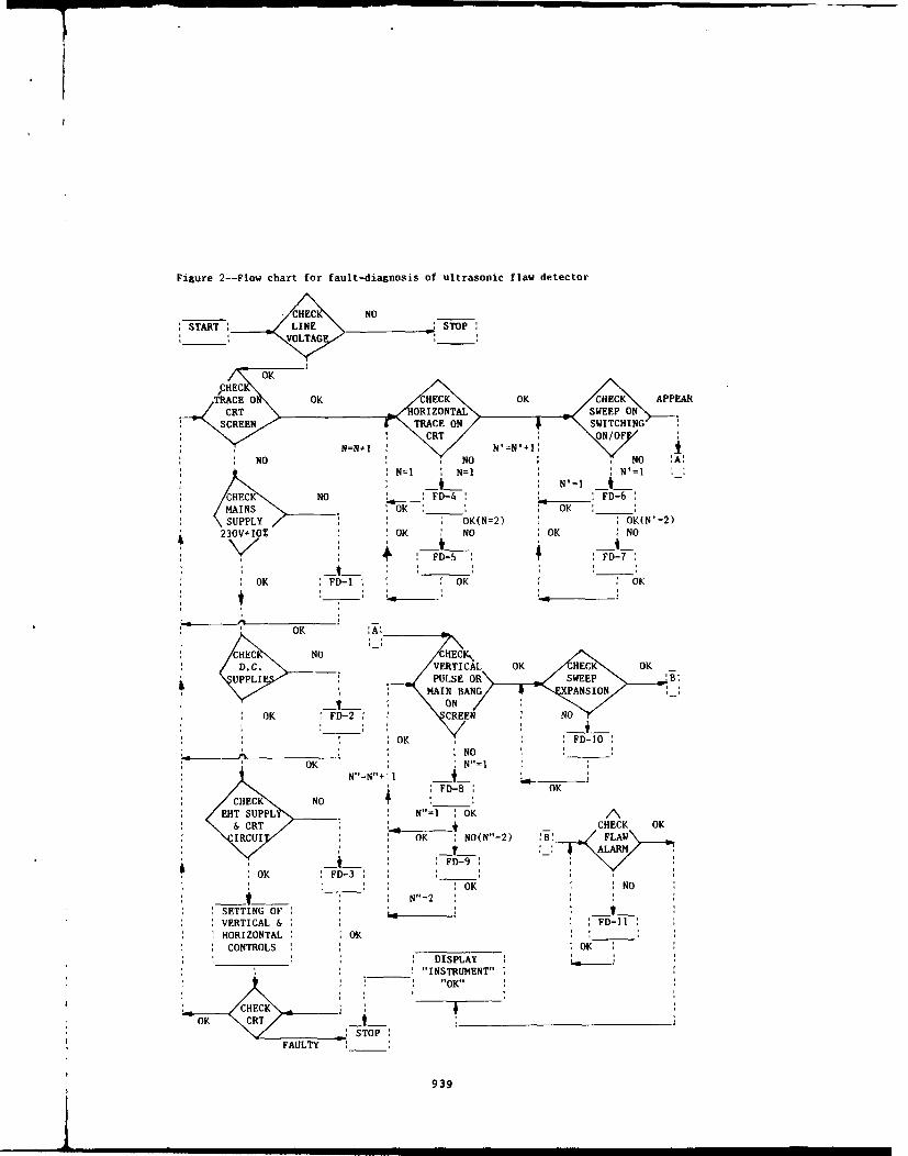
Figure 2--Flow chart for fault-diagnosis of ultrasonic flaw detector
CHEC NOSTART LINE _ STOP
_______ OLTAG
COC K HC APA
_LN'=I *L '-CHECKFD-4 FD-6
MAINS oK OK ___
SUPPLY, OK(N=2) OK(N' =2)230V+10• : OK NO OK NO
q , :, D-5: €FD-7
:0, K ',FD-l: ', 'OK : OK
S OK A:•
CE NO HEC OK
D..VERTICAL OK CH~tECK O
SC U>LEP L E O SE P' :
ON ON
OK EFD-2 T CREEN NOWTI
C OKF-I-OF
OK FD- F OK lNO : :
I~ N= N'=l___
CHECK NO FD-8 OK-
SUPPL: N" : OK AC K : F 7 cHECK OK
IRCI, OK : NO(N"=2) :B: FPLAW• ___.4 ALARM
* _ ', ' PD-9 ':0OK : FD-3:' : : __
_IO NO
._ ._ _ N'=2SETTING OF : : : ___JD-_VERTICAL & H OK
HORIZONTAL : ,OK _____CONTROLS > I I K
P, D I PULSE R SWEP "B
I'N BINSTRUMENT""OK"
* CHE CK:N
EH STOP O
FAULTY ______
D939

right-4Nos.). It also shows the broad view of each control knob individually and theirlocation on the equipment. EK-8 Sub-uti'' A-ribes connections of probes in single anddouble transducer mode. EK-12 Sub-u' es efficient utilisation of straight,angular, and surface wave probes for -. application. It also instructs aboutavailability of probe for immersion techniques used for testing of material of peculiarshape which otherwise is difficult to detect using either a straight or angular probe, orwhere test surface is rough and gritty. EK-15 Sub-utility explains inspection techniquesfor detection and thickness gauging of flaw, employing single and double transducerapproach.
TAE-utilityThis utility of expert system provides users, list of test and auxiliary equipment,
tools, and chemicals with complete specifications/ technical details required formaintenance, as well as, fault-diagnosis of flaw detector. The list mainly includesdigital and analog multimeters, two channel oscilloscope (20MHz), high tension test set,adjustable transformer (5V ...... 250V, IA), signal generators, sine wave generator(0.... 12MNHz), adapter board amplifier and trigger, recorder and amplifier dummy, steelreferences, stepped reference steel blocks, probes, screw driver set, pliers, and carbontetrachloride.
EK-utilityThis utility of expert system consists of five packages and provides detailed
instructions alongwith video presentations regarding:EM-I: Checking of cables, operating voltage, fuses, movement of controls, cleaning of
joints, and removal of dust from equipmentEM-2: Preventive maintenance programmesEM-3: List and location of PCB'sEM-4: Dismounting and assembly of PCB'sEM-5: Calibration of equipment
These packages describe step by step procedure by intervention with user, by askingquestions from him. It also instructs him about various warnings and precautions to beobserved at respective stages. As an example, EM-3 Sub-utility describes the mosteffective way of reducing the number of failures and increasing instrument useful life.It reduces breakdowns during operation by repairing minor faults before they give rise toserious troubles. It also stresses the advantage in maintenance of history sheets andmaintenance schedules. EM-4 Sub-utility describes for the users, the systematic way ofassembly and disassembly of various PCB's from chasis by using required tool(s) in aproper manner by observing instructions on monitor. Calibration of the equipment bytaking measurements of standard samples with flaws at specified distances by usingvarious control knobs is described in EM-5 Sub-utility.
FD-utilityFor fault-diagnosis [51, the user should have good grasp of basic electronics, test
and measuring equipment, and should be well conversant with the localising and pin-pointing the source of trouble, There may be many reasons for the trouble and to localisethe fault, it is essential to eliminate the other sources in proper sequence byscientific experimentation and proper checks. It is known that faults due to componentdeterioration, dry solder, and intermittent contacts are difficult to diagnose andrepair. By using test points voltage data and principle of operation of circuits, fault-diagnosis can be systematically carried out. FD-Utility helps users in fault-finding ofthe instruments. Brief flow-chart for fault-diagnosis is given in figure 2. It is mainlyassociated with following eleven sub-utilities:FD-I: Fault-diagnosis of main supplyFD-2: Fault-diagnosis of power supplies (tIOOV, t20V & 40OV)FD-3: Fault-diagnosis of EHT supply & CRT circuitsFD-4: Fault-diagnosis of clock circuitFD-5: Fault-diagnosis of sweep amplification circuitFD-6: Fault-diagnosis of unblanking circuitFD-7: Fault-diagnosis of Z-axis amplification circuitFD-8: Fault-diagnosis of main bang delay circuitFD-9: Fault-diagnosis of transmitter, receiver, & TCG circuitsFD-I: Fault-diagnosis of selective/ sweep expansion circuitFD-I: Fault-diagnosis of flaw alarm circuit
From flow chart, it is observed that if horizontal trace and sweep appear on CRT onswitching ON/OFF, FD-utility bypasses sub-utilities FD-I to FD-7. If, however, slope of
940
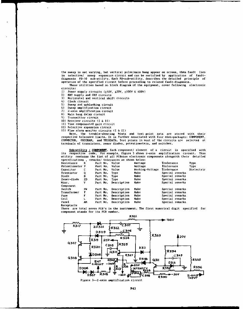
the sweep is not varying, but vertical pulse/main bang appear on screen, then fault liesin selective/ sweep expansion circuit and can be rectified by application of fault-diagnosis FD-IO sub-utility. Each FD-sub-utility, describes the detailed principle ofoperation of the specified circuit before proceeding to related fault-diagnosis.
These utilities based on block diagram of the equipment, cover following electroniccircuits:I) Power supply circuits (±IOV, ±20V, ±IOOV & 40oV)2) EHT supply and CRT circuits3) Horizontal and vertical shift circuits4) Clock circuit5) Sweep and unblanking circuit6) Sweep amplification circuit7) Z-axis amplification circuit
8) Main bang delay circuit9) Transmitter circuit10) Receiver circuits (I & II)11) Time compensated gain circuit12) Selective expansion circuit13) Flaw alarm monitor circuits (I & II)
Here, the trouble-shooting hints and test point sets are stored with theirrespective tolerance limits. It is further associated with four mini-packages: COMPONENT,CONNECTOR, OSCGRAM, and TECHDATA. Test points in most of the circuits are selected atterminals of transistors, zener diodes, potentiometers, and switches.
Sub-utility : COMPONENT. Each component/ element of a circuit is specified withits respective code. For example, figure 3 shows z-axis amplification circuit. Thisutility contains the list of all PCBwise electronic components alongwith their detailedspecifications , remarks/ tolerances as shown below:Resistance R Part No. Value Wattage %tolerance TypePotentiometer P Part No. Value Wattage %tolernace TypeCapacitor C Part No. Value Working-Voltage %tolernace DielectricTransistor Q Part No. Type Make Special remarksDiode D Part No. Type Make Special remarksZener-diode ZD Part No. Type Make Special remarksMisc. V Part No. Description Make Special remarksComponentSwitch SW Part No. Description Make Special remarksTransformer T Part No. Description Make Special remarksFuse F Part No. Description Make Special remarksCoil L Part No. Description Make Special remarksPanel AM Part No. Description Make Special remarksReceptacleThere are total seven PCB's in the instrument. The first numerical digit specified forcomponent stands for its PCB number.
R321
0309 C 6 -v f 9 2i0Q 3079
Figure 3--Z-axis amplification circuit
942.
•~~~~~ ~ ~ 319mm 20V n ll m m

Sub-utility : CONCTOR. This utility describes the connector-wiring plan andsemiconductor elements connections.
Sub-utility : OSCGRAM. This utility contains the part-numberwise oscillograms atvarious test points at base, emitter and/or collector of transistors. For example, figure4 shows oscillograms observed at collector of transistors used in z-axis amplificationcircuit. The oscillogram at any test point may be displayed at any stage of fault-diagnosis by user intervention.
Sub-utility : TECHDATA. This utility contains the part-numbernise voltage levels atvarious test points at transistors (emitter, base and collector); and voltage acrosszener-diodes. Table I shows voltage data at various test levels in z-axis amplificationcircuit for reference. The data may be recalled at any stage during fault-diagnosis byuser intervention. Volatge data at various test points in flaw alarm circuit are given,both, with and without Alarm ON & off position.
Table I--Voltage levels at various test 72Vpoints in z-axis amplification circuit Q307 15Vfor ready reference Vc _____ --__- _
38V:Transistor:Fmitter: Base Collector Q308 lOV
Code Vc _----_.-__
Q307 72 72 73 Q309 16 &15 3•6•Vvc -- •L-• lOV
Q308 32 33 72
Q309 .2 .8 33 Q310 8.2V
Vc _-Q310 .8 1.5 3
7tl5ý 2V
Q311 -.1 .5 2 at Q311 "V 1.5Vinter min Vc _ _ _ _ ____1_
or maxFigure 4--Oscillograms at different testpoints in z-axis amplification circuit
CONCLUSION
The expert system designed is expected to be highly advantageous for instrumentusers for proper installation, efficient operation, and calibration. It shall also helpto curtail down-time of the instruments by providing expertise in preventive maintenance;fault-diagnosis; and repair, even when experts or relevent technical literature, ormaterial are not easily accessible. The expert system designed and being developed shallnot only open new vistas of creating expert human resources in developing countries, inthis specialised field but also save valuable national resources, and foreign exchangeinvolved in procurement of equipment. It will also contribute towards increasingindustrial and economic progress of the country. The authors are thankful to Dr. K.R.Sharma, Director, CSIO, Chandigarh for kind permission to express our views.
REFENCES
1. A.N. Agarwal, S.C. Suri, H.S. Bageshwar; Use of computer in management andmaintenance of ultrasonic equipment; Proceedings of national symposium onultrasonics; 1989.
2. A.N. Agarwal, S.C. Suri, M.S. Bageshwar; Expert system for maintenance and fault-diagnosis of ultrasonic equipment; Proceedings of international congress onultrasonics; 1990; A30-35.
3. R. Jackson; Introduction to expert systems; Addision-Wesley, Reading, Mass; 1986.4. James N. Siddal; Expert system for engineers; Marcel Dekker, Inc., New York; 1990.5. S. C. Suri; Expert system for maintenance of ultrasonic flaw detector; H.S. Thesi.,
BITS, Pilani; 1991
942

BOUNDARY ELEMENTS AND FINITE ELEMENTS
943

944

SECOND INTERNATIONAL CONGRESS ONRECENT DEVELOPMENTS IN AIR- AND
STRUCTURE-BORNE SOUND AND VIBRATIONMARCH 4-6. 1992 AUBURN UNIVERSITY. USA
RECENT APPLICATIONS OF
BOUNDARY ELEMENT MODELING IN ACOUSTICS
A. F. Seybert, T. W. Wu and G. C. Wan
Deparmnent of Mechanical EngineeringUniversity of Kentucky
Lexington, KY 40506-0046U.S.A.
ABSTRACTThis paper discusses recent applications and advances in using the boundary element method (BEM) in
acoustics. A brief review of the BEM theory is followed by several illustrative examples in various areas ofapplication. These include: radiation and scattering of sound from elastic structures, muffler and silencerperformance prediction, evaluation of partial enclosures for noise control, and prediction of sound radiationefficiency. The paper also reports some recent progress in overcoming the nonuniqueness problem, thin-bodyradiation and scattering, and frequency interpolation.
REVIEW OF THE BEM THEORYConsider a body with boundary surface S submerged in an infmite acoustic medium fi of mean density
P0 and speed of sound c. The body may be either set in vibration in a radiation problem or subject to an incidentwave velocity potential 4)i in a scattering problem. In linear acoustics with time-harmonic excitations of angularfrequency w, the particle velocity v and the sound pressure p are related to the velocity potential i) by v = -Mt,and p = ikz4A, respectively, where i = r-I, k-Wc, and zo-p 0 c. The normal vector n is defined as the unitnormal on S directed away from the acoustic medium Q. The boundary value problem can be reformulated interms of the Helmholtz integral equation as follows I 1:
C(PM P)= - is [P Q)•--(Q)" W(PQ) 4Q)]dS(Q) + 44•r(P) (I)
where ip = e-ik/r (r = IQ - Pt) is the free-space Green function due to a time-harmonic point source at P. C(P) isa constant that depends on the location of P.
A numerical solution to the Helmholtz integral equation [Eq. (1)] can be achieved by discretizing theboundary surface S into a number of surface elements and nodes. Quadratic isoparametric elements (six-nodetriangles and eight-node quads) have been widely used in recent years so that both the acoustic variables and theboundary geometry can be more accurately modeled. The global Cartesian coordinates Xi (i- 1, 2, 3) of anypoint on an element are assumed to be related to the nodal coordinates Xicz by
Xi(" E NQ)XiQ , = - ...... 6 or 8 (2)
a
in which N. are second-order shape functions of the local coordinates (Q,rl). The same set of quadratic shape
functions is used to interpolate the velocity potential *on each element, that is,
945

(3)a
where 4 a are the nodal values of the velocity potential. The normal velocity ab% on each element is also
obtained by the same interpolation of the nodal values ofJaL.Discretizing Eq. (1) and putting point P at each nod result in a system of equations as follows [ 11:
[C) fx)- - b) (4)
where [C1 is a square coefficient matrix, {bI is the right hand side vector and 1x) contains the unknowns (4% or
cWOn) on the boundary S.
COUPLED FEM/BEM FOR FLUID-SOLID INTERACTION PROBLEMSWhen an elastic stnucture is submerged in a heavy fluid such as sea water, the vibration of the structure
will be affected by the surrounding fluid, and the whole system becomes a coupled structural acoustic problem.A coupled technique, using the finite element method (FEM) for the structure and the BEM for the fluid, is anatural choice for numerical solution of fluid-structure interaction problems. Combining the FEM and the BEMequations and enforcing continuity conditions on the fluid-solid interface (the "wet" surface) lead to thefollowing coupled structure acoustic equations 121:
-B A [ ] [up] - [4pi
where p, u, and pl are the nodal value vectors of the sound pressure, displacement, and incident sound pressure,respectively, and fm is the mechanical load vector. The top part of Eq. (5) is from the FEM and the acousticload is represented by -[LI{p). The bottom part of Eq. (5) is from the BEM. Equation (5) can be solved forboth the displacement and pressure simultaneously. The dimension of the final system of equations may bereduced by expressing the structural displacement as a linear combination of either Ritz vectors or eigenvectors[3].
An example problem is given to demonstrate the coupled FEM/BEM approach. Consider an aluminumcylindrical shell with both ends being excited internally by a uniform pressure p0 . The length of the cylinder is4a and the thickness is Wa4 where a is the mean radius. Figure I shows the pressure directivity for ka - I at aradius 50a from the cylinder. It is also shown that for this example the Ritz vector synthesis converges fasterthan the modal synthesis.
BEM FORMULATION FOR MULTIPLE DOMAINSIn many industrial noise problems, the domains and boundaries are quite complex. In an industrial
silencer, for example, the interior domain may be partially subdivided by baffles and other surfaces. In suchcases, the single-domain BEM formulation is cumbersome to use and may not be computationally attractive.However, by subdividing the original domain into subdomains and matching appropriate continuity conditionsat interfaces, it is possible to solve the problems by using the BEM 141. To illustrate the application of the multi-domain BEM, two problems in industrial noise control are shown in the following: transmission loss ofsilencers [41 and radiation from a source within a partial enclosure 15, 61.
Transmission loss of silencersA simple expansion chamber with an extended inlet tube is shown in Fig. 2a. From the modeling
standpoint, the extended tube is viewzd as a thin projecting surface extending into the acoustic field for which asingularity arises when the single-domain BEM is used. Using the multi-domain BEM, the interior region oftheexpansion chamber is divided into two subdomains, as shown in Fig. 2a. Figure 3 shows the comparison ofthe transmiasion lotw (TL) calculated by the BEM and an axisymmetric FEM for the cme In Fig. 2a. The FEMmodel consisted of 166 four-node linear elements with a total of 206 nodes, whereas the BEM model consistedof only 17 quadratic line elements with a total of 36 nodes. As shown in Fig. 3, the TL varies considerably withfrequency kL. In addition to the classic expansion humps at odd multiples of quarter-wavelength, the verynarrow peaks which increase the TL values abruptly are the results of resonance and side-branch effects due tothe extension tube. Excellent agreement between the boundary element solution and the finite element solution isobserved.
As a second example, consider the double-expansion chamber with an internal connecting tube shown inFig. 2b. The BEM solution and the axlsymmetrlc FEM solution are compared in Fig. 4. The FEM meshconsisted of 318 four-node linear quadrilateral elements with 388 nodes. The BEM mesh consisted of 30quadratic line elements with 63 nodes. Good agreement between the BEM and the FEM solutions is obtained.
946

SFull expanslce• n-( 'a 40 Ritz VeCtOS I e -
8 a 100 CiieVCIM
6
4-
2
I * I * I * * *
0 3 6 9 12 15 18X10-3
Figure 1. Normalized pressure magnitude at a distance of 50a from the center of the cylindrical shell.
Ic--IL
(a)171LISI Sl Si
(b)
Figure 2. Silencer geometry and multi-domain BEM model of each: (a) expansion chamber with extended
inlet, (b) double expansion chamber with internal connecting tube.
947
.•~~~ S'1 l.,.,.m.- mmmi ml lml/m•m

70
60 - - OEM Soluti.o
0 FetM Solution
C 50V
o 40
0
C2 20
I-
l0
0.0 0.6 1.2 1.8 2.4 3.0 3.6 4.2 4.8
kL
Figure 3. Transmission loss versus kL for the silencer in Fig. 2a.
140
- BEM solution
120 0 FEM solution
1 I00
00
-J 80
40
20
20
0.0 0.6 1.2 1.8 2.4 3.0 3.6 4,2 4.8
kL
Figure 4. Transmission loss versus kL for the silencer in Fig. 2b.
Radiation from a source within a nartial enclosureFigure 5 shows a spherical source at the center of a cubical enclosure with two -4uare openings. The
radius of the source is 0. 1 m, the length of each edge of the enclosure is 0.5 m and the size of the openings is0. 1 m square. The enclosure is rigid. The boundary condition on the spherical source is a unifonn normalvelocity of 0.2 m/s, and the boundary condition on both the inside and outside surfaces of the enclosure isnormal velocity of zero.
948

Sozurce
Opening
Figure 5. Radiation from a spherical source within a partial enclosure. The grid on the right side of theenclosure is the BEM mesh used on the inside and outside surfaces of the enclosure.
Two approaches are used. In the first approach, the multi-domain (coupled interior/exterior) BEM isused to determine the sound field inside and outside of the enclosure simultaneously. The mesh used is shownin Fig. 5. The second approach is an approximate "two-step" method used for comparison purpose only. Inthis approach, the interior and exterior sound fields are decoupled by assuming a radiation impedance zr at theopenings. If the frequency range is sufficiently low such that the sound pressure and particle velocity at theopenings are approximately uniform, a reasonable approximation of the radiation impedance is
zr - 0.5 (ka)2 poc + j (0.85 ka) p 0 c, (6)
where a is the radius of an equivalent circular, baffled piston. Using the radiation impedance boundarycondition on the openings, the interior sound field may be determined using the interior BEM. The exteriorsound field is then found by solving the exterior problem using the exterior BEM. The boundary condition onthe openings for the exterior problem is the normal velocity (or sound pressure) determined from solving theinterior sound field.
Figure 6 shows the sound pressure level (dB re 20pJPa) as a function of frequency at the center of theopening, as calculated by both methods. The frequency range in Fig. 6 has been restricted to less than 1000 Hzwhere the approximate solution is valid. Figure 7 shows the sound pressure level at 790 Hz (a resonancefrequency of the interior of the enclosure) at a distance of 5m from the center of a plane parallel to the side of theenclosure and passing through the openings. The two sets ofdata in Fig. 7 correspond to the case in which theenclosure is rigid, and the case in which the interior surfaces of the enclosure are lined with a sound absorbingmaterial having a normal acoustical impedance z - 208 + j2"8, i.e., a normal incidence absorption coefficient of0.8. Also shown for reference in Fig. 7 is the sound pressure level that would be present when the enclosure isabsent.
The multi-domain BEM can help a noise control engineer determine the effect of the size and location ofopenings and select the best absorbing material for a partial enclosure design.
949

160o Coupled Method
-- a-- Approximate Methodm150
140
•120
U)
a-
U)0~
100 ,
0 200 400 600 800 1000Frequency (Hz)
Figure 6. Sound pressure level at the center of the opening.
"-- Without A~ortplon-6- With Abso"oi
No Enclkmte
Figure 7. Sound pressure level at a distance of 5m from center of a plane passing through the openings of
the enclosure.
950

PREDICTION OF SOUND RADIATION EFFICIENCYDirect sound radiation from a vibrating structure is a function of the exciting force applied to the
structure, the structural properties, and the sound radiation efficiency of the structure. The vibrational responseof a structure may be described by a superposition of its vibrational modes. It is, therefore, important to knowthe modes of vibration and the radiation efficiency of these modes. The radiation emciency is a function of themode shape and the frequency of vibration. Although a mode shape is a normalized vibration, the radiationefficiency is an absolute value; it is a property of the mode. Therefore, the radition efficiency an be used tocompare the sound radiating chracterstics of different strucural modes.
Alter applying the BEM to solve for the unknown (sound pressr or normal velocity) at every node onthe surface of a structure, the sound intensity at each node can be calculated. By integrating the sound intensityover the whole surface, the total sound power W radiated by the structure is determined. The radiationefficiency a is the ratio of the sound power radiated by a vibrating structure, to the sound power that would beradiated by an equivalent flat piston vibrating in an infinite baffle:
W (7)p0cS<v2>
where -v2> is the mean square velocity of the surface S.The following is an example to illustrate how the analysis of the radiation efficiency can be accomplished
by the BEM [71. Figure 8 shows a gearbox with its BEM mesh. The vibration data of the gearbox, includingeight modes in the frequency range from 500 to 3,000 Hz, was obtained from modal analysis experiments. Thevibration of the gearbox (normal velocity on the surface) is used as the boundary condition in the HEM. Theradiation efficiencies of the eight modes are calculated by the BEM and shown in Fig. 9. As seen in Fig. 9, allof the modes are very efficient radiators of sound. These results can be checked by using Wallace's plateradiation theory [SI to make an approximate analysis. This theory is strictly valid only for simply supportedplates in an infinite baffle, and is based on /'kb, the ratio of the acoustic-to-bending wave numbers. In Fig. 10the radiation efficiencies of the seven of the eight modes are compared to the radiation efficiencies of arectangular plate having the same dimensions as the top surface of the box, as determined by Wallace's theory.The mode at 2000 Hz is not shown since it does not exhibit a d-. nant plate mode on the top surface. Thediscrepancies observed in Fig. 10 are due to that the top surface of the box is not baffled and there is radiationfrom the other surfaces.
t. v(O)
Figure 8. BEM mesh of the gearbox.
953.
• ---- .----- == ===. •m,,,,.•'•"- m • n

b
S" " I I
1.0
0 I I I I I50 1000 1500 2000 2500 3000
Naturai frequency, Hz
Figure 9. Radiation efficiencies of the eight transmission housing modes.
2.o
(2. 3)
1.5(41 (13b
S/ -(4.1)
0 1.0 (
CO
.r
.5 0 Baffled plateA Gearbox
01 I I.50 .75 1.00 1.25 1.50
Wave number ratio, k/kb
Figure tO. Radiation efficiencie, ,alculated by the BEM and plate theory, respectively.
952

Structural modification of the gearbox is a logical method to control its sound radiation. In general, thespectrum of the forces which excite a structure is dominated by relatively low frequency components.Modifications which stiffen a structure tend to push the vibrational modes to higher frequencies where theseforces are weaker-an effect that reduces vibration. However, this simplistic approach ignores the effect ofradiation efficiency on the radiation of sound. Equation (7) shows that the sound power is directly proportionalto the radiation efficiency. Thus, while modification of the structure may reduce the mean-square vibration, itmay also increase the radiation efficiency.
Consider the effect of a straightforward modification to the thickness of the gearbox's surface plates.This alternation would change the natural frequencies of the modes without materially altering the mode shapes.To see the effect of such a modification, the radiation efficiency of each mode was determined at frequenciesabove and below the measured value. These data are plotted in Figs. 11 and 12 for the 658- and 2722-Hzmodes, respectively. The actual measured natural frequency of each mode is represented by the filled datasymbol.
The radiation efficiency of the 658-Hz mode increases with frequency, as shown in Fig. 11. Thus, athicker gearbox will radiate more noise if the reduction in vibration does not offset the increase in radiationefficiency. It is also possible that making the gearbox thicker may cause a mode with a high radiation efficiencyto move from a frequency where it is not excited to a new frequency (e.g. a gear mesh frequency) where itradiates considerably more sound energy.
By contrast, the radiation efficiency of the 2722-Hz mode is almost independent of frequency, as see inFig. 12. Thickening of the box will not increase the radiation efficiency of this mode, and unless the newfrequency coincides with a gear mesh frequency, the sound energy radiated by this mode will decrease.
THE NONUNIQUENESS PROBLEMOne potential shortcoming of the BEM in acoustics is that the exterior boundary integral formulation
shares the difficulty of nonuniqueness of solution at resonance frequencies of the associated interior problem[9]. Several modified integral formulations have been proposed to overcome the nonuniqueness problem. Themost commonly used one is the Combined Helmholtz Integral Equation Formulation (CHIEF) proposed bySchenck 191. This formulation uses the Helmholtz integral equation with points (CHIEF points) inside of thebody (where C(P) - 0) as a constraint that must be satisPed along with the usual Helmholtz integral equation onthe surface. The resulting over-determined system wnay then be solved by a least-squares procedure. If aCHIEF point falls on any nodal surface of the related (auxiliary) interior problem, it becomes useless. Recently,Wu and Seybert proposed two different enhanced CHIEF formulations, the "Enhanced" CHIEF method [ 10]and the "Weighted Residual" CHIEF [Il] method, to partially remedy this difficulty. The "Enhanced" CHIEFmethod includes the derivatives of the CHIEF equations in three coordinate directions as three additionalconstraint equations that must be satisfied along with the original CHIEF system. Therefore, there will be a totalof four constraint equations at each CHIEF point. To further improve the CHIEF method, the "WeightedResidual" CHIEF method in which the "Enhanced" CHIEF equations are weakly satisfied in a volume, insteadof CHIEF points, inside of the body.
Another formulation to overcome the nonuniqueness problem is the method proposed by Burton andMiller 1 12]. This approach consists of a linear combination of the Helmholtz integral equation and its normalderivative equation. It has been proved that the linear combination of these two equations will yield a uniquesolution for all frequencies if the multiplicative constant of the derivative equation is appropriately chosen.However, the major difficulty in this formulation is that the normal derivative of the Helmholtz integral equationcontains a hyper-singular integral. Procedures to integrate the hypersingular integrals for three-dimensionalproblems with curved boundary surfaces have recently been reported [13, 14, 15].
FREQUENCY INTERPOLATION TECHNIQUEAlthough the BEM is a very efficient numerical technique for acoustic analysis at a few frequencies, it
may be impractical for multi-frequency applications. The main reason is that the integral in the Helmholtzintegral equation is frequency dependent. For each frequency, all of the components in the coefficient matrix[C] and the right-hand side vector (b) in Eq. (4) need to be recalculated. The procedure is very time consumingifsolutions for a wide frequency spectrum are required.
A frequency interpolation technique has been successfully applied to multi-frequency analysis bySchenck and Benthien using constant elements [ 161. The concept has been extended to quadratic isoparametricelements ( 17, 181 and will be described briefly here. It is known that the integral of the Helmhotz integralequation may vary rapidly with frequency due to the fluctuating term c-ikr in the Green's function. The rapidvariation with frequency can be neutralized by multiplying the integral by a "counteracting" wave. Neutralizedintegrals can be calculated at a set of reasonably spaced "key" frequencies. The integral at a certain frequencycan then be formulated by interpolating the integrals at adjacent "key" frequencies.
An example of the use of frequency interpolation is shown in the following problem. Consider therectangular duct shown in Fig. 13. The left end of the duct is driven by a piston with a velocity equal to Ini/sec. The right end of the duct is rigid. Figure 14 shows the sound pr,'sure level on the middle cross sectionof the duct (X - 1/2) in a frequency range up to kL = 14. Note the guod agreement between the analyticalsolution and the values predicted by the BEM with and without frequency interpolation. Two key frequencies atkL = 0.458 and 11.9 were used for this frequency interpolation run. This test case was run on the IBM3090
953
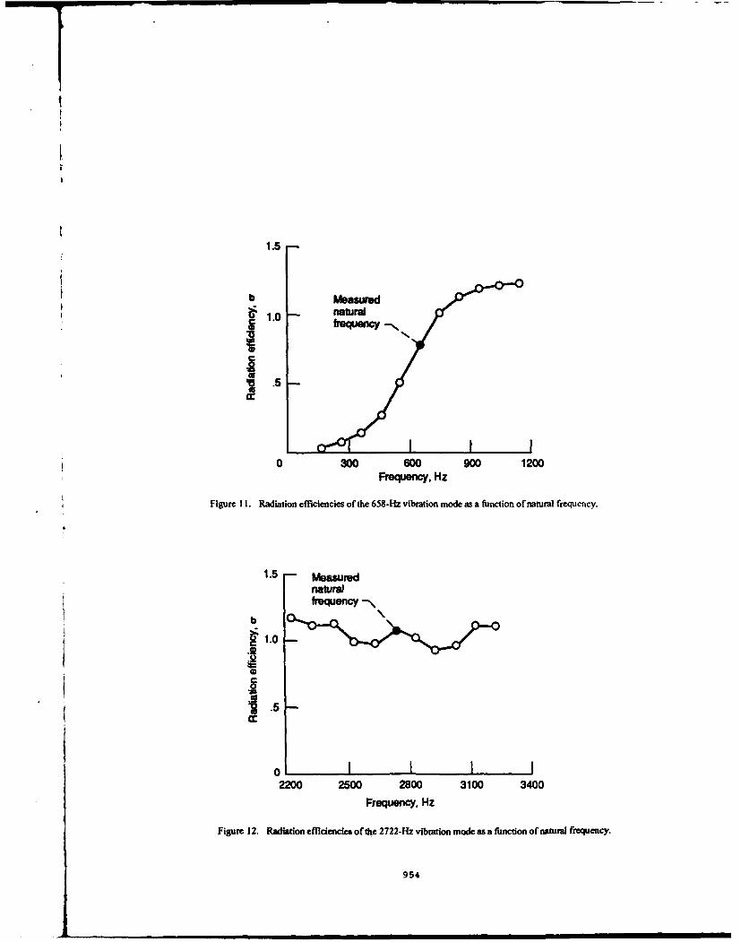
1.5
b LMeasuffd
S1.0 naturalfrequency-%"oI
.345 .5
0 300 600 900 1200Frequency, Hz
Figure 11. Radiation efficiencies of the 658-Hz vibration mode as a function of naturai frequency.
1.5 Measurednaturalfrequency-•
:1.
78.5
0-
0 I I2200 2500 2800 3100 3400
Frequency, Hz
Figure 12. Radiation effciencies of the 2722-Hz vibration mode as a function of natund frequency.
954

Y
SL -. x
Figure 13. BEM mesh of the rectangular duct.
170
S150 1
103
10
13U aCL 13.
Z 140 t2
010
130
0 2 4 6 8 to 12 14
KL
Figure 14. Sound pressure level on the middle cross section of the duct: solid line, analytical solution;circles, direct BEM solution; squares, BEM solution with frequency interpolation technique.
supercomputer under vector mode[ 171. The CPU time for this frequency interpolation run is slightly less than50% of the CPU time for the corresponding direct solution run.
THIN-BODY RADIATION AND SCATTERINGSound radiation and scattering from thin bodies has many important applications (such as transducers
and fins) in acoustics. It has been known that the conventional boundary element method (BEM) using theHelmholtz integral equation is not suitable for problems involving thin bodies. The major difficulty is due to thefact that the mesh on one side of a thin body is too close to the mesh on the opposite side. Therefore, extremelyfine meshes have to be used and nearly singular behavior may occur in the integral equation. Recently, a normalderivative integral equation that converges in the Cauchy principal value sense has been successfullyimplemented in a quadratic isoparametric element environment to solve the thin-body problem 119, 201.
955

SUMMARYThis paper briefly reviews recent progress in the BEM research in acoustics and noise control at the
University of Kentucky. Detailed discussion of each of the individual topics can be found in the references.The results have shown promising future of the application of the BEM to practical engineering problems.
REFERENCESI. A. F. Seybert, B. Soenarko, F. J. Rizzo and D. J. Shippy, "An Advanced Computational Method for
Radiation and Scattering of Acoustic Waves in Three Dimensions," J. Acoust. Soc. Am.. Vol. 77, No.2, pp. 362-368, 1985.
2. T. W. Wu, A. F. Seybert and W. L. Li, "Applications of the Coupled FEM/BEM Technique toStructural Acoustics Using Consistent Isoparametric Elements," ASME Vibration Control Mechanical.Structural. and Fluid-Structural Systems K. W. Matta and M. K. Au-Yang (Eds.), PVP-Vol. 202, pp.25-30, 1990.
3. A. F. Seybert, T. W. Wu and W. L. Li, "A Coupled FEM/BEM Solution for Structural AcousticProblems Using Ritz Vectors and Eigenvectors,"ASME Structural Acoustics R. F. Keltie, et al. (Eds.), NCA-Vol. 12/AMD-Vol. 128, pp. 171-178, 1991; also to appear in ASME Transactions J. Vib.
4. C. Y. R. Cheng, A. F. Seybert and T. W. Wu, "A Multi-domain Boundary Element Solution forSilencer and Muffler Performance Prediction," J. Sound Vib., Vol. 15 1, pp. 119-129, 1991.
5. A. F. Seybert, C. Y. R. Cheng and T. W. Wu, "The Solution of Coupled Interior/Exterior ProblemsUsing the Boundary Element Method, J. Acoust. Soc. Am., Vol. 88, pp. 1612-1618, 1990.
6. A. F. Seybert, T. W. Wu and W. L. Li, "Analysis of Noise Radiated by a Source within a PartialEnclosure Using the Boundary Element Method", Proceedings of the Inter-Noise 89, pp. 1225-1228,Newport Beach, California, 1989.
7. A. F. Seybert, T. W. Wu, X. F. Wu and F. B. Oswald, "Acoustical Analysis of Gear HousingVibration," NASA Technical Memorandum 103691, 1991.
8. C. E. Wallace, "Radiation Resistance of a Rectangular Panel," J. Acoust. Soc. Am., Vol. 51, No. 3,pp. 946-952, 1972.
9. H. A. Schenck, "Improved Integral Formulation for Acoustic Radiation Problems," J. Acoust. Soc.Am., Vol. 44, pp. 41-58, 1968.
10. T. W. Wu and A. F. Seybert, "Acoustic Radiation and Scattering," Boundary Element Methods inAcoustics, Chap. 3, R. D. Ciskowski and C. A. Brebbia (Eds.), Computational MechanicsPublications, Southampton, UK, 1991.
11. T. W. Wu and A. F. Seybert, "A Weighted Residual Formulation for the CHIEF method in acoustics,"J. Acoust. Soc. Am., Vol. 90, No. 3, pp. 1608-1614, 1991.
12. A. J. Burton and G. F. Miller, "The Application of Integral Equation Methods to the NumericalSolutions of Some Exterior Boundary Value Problems," Proc. Roy. Soc. Lond., A 323, 201-210,1971.
13. G. Krishnasamy, L. W. Schmerr, T. J. Rudolphi and F. J. Rizzo, "Hypersingular Boundary IntegralEquations: Some Applications in Acoustic and Elastic Wave Scattering," ASME J. Atm. M 57,404-414, 1990.
14. T. W. Wu, A. F. Seybert and G. C. Wan, "On the Numerical Implementation of a Cauchy PrincipalValue Integral to Insure a Unique Solution for Acoustic Radiation and Scattering," J. Acoust. Soc. Am.Vol. 90, 554-560, 1990.
15. C. C. Chien, H. Rajiyah and S. N. Atluri, "An Effective Method for Solving the Hypersingular IntegralEquations in 3-D Acoustics," J. Acoust. Soc. Am., Vol. 88, pp. 918-937, 1990.
16. H. A. Schenck and G. W. Benthien, "The Application of a Coupled Finite-Element Boundary-ElementTechnique to Large-Scale Structural Acoustic Problems," Advances in Boundary Elements, Vol. 2, pp.309-319, C. A. Brebbia and J. J. Connor (Eds.), Computational Mechanics Publications,Southampton, UK, 1989.
17. T. W. Wu, A. F. Seybert, G. C. Wan and R. Ciscowski, "Vectorization and Parallelization of theBEMAP program on the IBM 3090," Proceedings of Interational Conges on Recent Developments inAir and Structure Borne Sound and Vibration, pp. 489-498, Auburn University, Auburn, Alabama,1990.
18. A. F. Seybert and T. W. Wu, "Application in Industrial Noise Control," Boundary Element Methods inAcoustics, Chap. 9, R. D. Ciskowski and C. A. Brebbia (Eds.), Computational MechanicsPublications, Southampton, UK, 1991.
19. T. W. Wu and G. C. Wan, "Numerical Modeling of Acoustic Radiation and Scattering from ThinBodies Using a Cauchy Principal Integral Equation," submitted to J. Acoust. Soc. Am., 1991.
20. T. W. Wu and G. C. Wan, "Isoparametric Boundary Element Modeling of Acoustical Cracks," to bepresented at the Second International Congress on Recent Developments in Air- & Structure-BorneSound & Vibration, Auburn University, Alabama, March 4-6, 1992.
956

SECOND INTERNATIONAL CONGRESS ONRECENT DEVELOPMENTS IN AIR- AND
STRUCTURE-BORNE SOUND AND VIBRATIONMARCH 4-6. 1992 AUBURN UNIVERSITY. USA
NUMERICAL MODELING OF PERFORATED REACTIVE MUFFLERS
Z. H. Jia, A. R. Mohanty and A. F. SeybertDepartment of Mechanical Engineering
University of KentuckyLexington, Kentucky 40506
ABSTRACT
In this work, a multidomain boundary element approach is used to model both three-dimensional and axisymmetric perforated structures and solve for the acoustical parame-ters. Impedance on the perforated plate is assumed known and equals the ratio of pressuredrop across the perforation to particle velocity there. Three numerical examples are con-sidered. The first two involve simple geometry and boundary conditions, and the numericalresults obtained are accurate in comparison with exact solutions. The third example treatsa plug muffler. Transmission loss from several different porosities are obtained and are seento agree favorably with available experimental results.
INTRODUCTION
Mufflers are an important noise control device used in the automotive and otherindustries. One effective strategy in reactive muffler design to obtain maximum sound at-tenuation at relatively high frequencies is to use perforated components. The introductionof perforated baffle plates, tubes and other perforated structures enhances the performanceof a muffler in a desired frequency range.
A number of researchers in the past have developed various prototypes for experimen-tal and analytical verifications. A state-of-art review of muffler design has been given byMunjal [I]. Using a one-dimensional model, Igarashi and Toyama [2] demonstrated theeffect of perforation in mufflers both analytically and experimentally. Sullivan and Crocker
[3] derived a one-dimensional model for a perforated concentric-tube muffler with meanflow. Sullivan [4,5] improved their method by including a varying perforation impedancealong the axial direction. Nonlinear effects due to the changing impedance and highsound-pressures were also considered. A numerical decoupling technique was presentedby Krishnamurthy and Yam [6] and Peat [7], but their approach may not be applied to
957

nonlinear cases such as treated by sullivan [4,5], although it works well in linear cases. Atime domain approach for perforated mufflers was presented by Chang and Cummings [8];the extra computational time required in their study remains a question. The aforemen-tione,1 work are all analytical or experimental in nature, and deal with somewhat simplifiedgeometry.
For problems involving complex geometry, numerical results are also available. Roms[9], for instance, presented a finite element solution to a complex three-dimensional mufflerwith perforated structures. He treated the perforated tube as a flexible membrane, andassumed that the acoustical particle velocity to be the same on both sides of the membrane.Another powerful and perhaps a more effective numerical method for acoustic problems,the boundary element method (BEM), has been used extensively in modeling acousticradiation ond scattering problems, including muffler problems. Seybert and Cheng [10]presented results for transmission loss of simple mufflers, using the BEM. Work by Tanakaet al. [11] and Kipp and Bernhard [12] also used the boundary element technique.
Despite numerous work in solving acoustic problems using the BEM, modeling ofthe perforated structures with the BEM has not been done. In this study, we presenta boundary element approach to solve problems involving three-dimensional perforatedstructures. In our analysis, a complex muffler is partitioned into subdomains betweenwhich impedance boundary conditions [3]
P - P2 =poCu (1)
are specified, where p1, and p2 are the acoustic pressures at each side of a perforatedinterface po and c are density and the speed of sound, respectively, u. is the normalparticle velocity and C is the nondimensional specific acoustic impedance which may beobtained by experiments [4,5].
An arbitrary-shaped muffler with complex internal structures can be modeled usingthe current method by modifying the existing multidomain boundary element formulation[13,141 into one which considers perforation at interfaces of subdomains. Unlike the exist-ing formulation [13,14] in which the interfaces are artificial, the perforated interfaces arephysically real. This requires that the interface conditions (1) be included in the integralequations. One may also view Eq. (1) as an extra constraint. The current formulationconsiders only zero-mean-flow cases. For cases involving mean flow, further modificationsare required and such problems will be considered in future studies.
Three numerical examples are presented. The first two are simple problems with exactsolutions. In the third problem, the transmission loss of a plug muffler is compared to theexperimental result by Sullivan [5].
FORMULATION
Considering a structure with internal perforated partitions shown in Fig.l, the entireacoustic volume enclosed by boundary SE can be treated as a group of subdomains Biconnected by a common interface S1 (For convenience, only two domains are shown). For
958

a typical subdomain Bj, the governing differential equation in a time-harmonic acousticwave field is the Helmholtz equation
V2 pU) + k2p)j) = 0. (2)
In Eq. (2), pO() is the acoustic pressure in domain Bj, k = w/c is the wave number, w isthe angular frequency, and c is the speed of sound.
S,n
Fig. I - A structure with internal perforated partitions.
The boundary integral formulation of the Helmholtz equation governing the acousticfield in subdomain B, [i.e. Eq. (2)] can be expressed as
SO U) (X (yo)
'C(x)p(i)(x) = J (O(x,y)--A (y) - p()(y)L(x,y)) ds(y), (3)
where & - e-IkR/R is the free-space Green's function in which R = Ix - yl, x and y areposition vectors of a collocation point and the integration point, respectively, and n is theunit outward normal on the boundary OBj of domain Bj, (OB, consists of both externalboundary SE and interfaces SI), and i = V-1 The leading coefficient C*(x) is given by
C*(x) = - "B ( 1 )ds(y). (4)
In Eq. (3), tlie normal derivative of pIC) with respect to n is related the normal particlevelocity uO') by
n :-iwp~uO1 ), (5)
where Po is the fluid density at equilibrium.
Substituting Eq. (5) into (3) and performing discretization via boundary elements,we convert Eq. (3) into a set of linear algebraic equations. In matrix form, the equationsfor subdomain Bi may be expressed as
959

/ 2A(W' 1J) l+ [(j 1 B) ] uE = ' (6)1 2 E2 2 1
where A(n.'2 and B(n.) are submatrices generated by numerically integrating the kernels ofthe integral equations. p) and p are the sound pressure at SE and Si, respectively,and uW) and ui) are the particle velocity at the corresponding boundaries. Bold lettersare used here because both quantities contain multiple discretized values.
Without loss of generality, we assume that u•) and u() are known at SE for a two-domain structure as in Fig.1. By moving the known quantities to the right-hand-side ofEq. (6), the equations for domain B, and B2 become
(I,) A() B,,,) IBP(El/l=(1,[ A¶ . . B¶;) :-_P)/{ut )}, (7)A•)A21 22 UI 'B21J
and(2) A (2) B (2 (E(2)All •12 •12 (2 _ Bil ) ]u()
A() A(2) B,(2) P, P( 2) U
2 A 2 2 22 (2 21
It is obvious that neither Eq. (7) nor (8) can be solved independently since the numberof unknowns is greater than that of the equations. However, by considering the continuityof velocity across the interface Sj expressible as
.(I) = (2). (9)
and using Eq. (1), p) and ul can, be eliminated from Eq. (8). A combined system ofequations involving the entire structure is expressed as:
Al 11 12 32 0 pf! I (B 1~ (1)A 2') "() B22 0 ! B(,I B .'u2~ 2~( 1) = - (2) (10)
0 AM D(2) A.(2) u(1) B (2) U(2)12 12 11A 11 E
A(2) D(2) A (2) (2) B(2) (2)•22 •22 .. 21. I PE J21 tE
where D(m2) -•( 2 ) pc(cAM.
Gaussian elimination is employed to solve the system simultaneously for the unknownsat both SE and S1. Values of p(i and u( can be recovered from Eq. (1) and (9),respectively.
960

NUMERICAL EXAMPLES
The first example is a perforated sphere with a point source at its center (Fig.2). Theinterface impedance on the perforation is assumed known. Four different three-dimensionalmeshes are used to model this interior/exterior coupling problem. Exact solution for thisproblem is derived for comparison. The results of boundary pressure P, (inside) and p2
(outside) are listed in Table 1.
2--V
Fig. 2 - A perforated sphere with a point Fig. 3 - Cirular duct with a perfotredsource at the center. partition at the center.
Table 1. Boundary pressure for perforated sphere (( = 1, k = 1)
# of ele. p 1/(po.w)(BEM) p,/(ipow)(exact) p2/(ip. w)(BEM) p2/(ipow)(exact)8 -0.466 -1.944 -0.488 -1.852 0.215 -0.856 0.171 -0.838
24 -0.486 -1.862 -0.488 -1.852 0.179 -0.840 0.171 -0.83896 -0.488 -1.853 -0.488 -1.852 0.176 -0.838 0.171 -0.838
128 -0.488 -1.853 -0.488 -1.8,52 0.175 -0.838 0.171 -0.838
It is clear that the numerical results in Table 1 converge rapidly with mesh refinement.Different values of C (from I to 100) and k (from I to 10) were also considered. The resultsare similar to those in Table 1 and hence are not presented here.
The second example involves a circular-cross-section duct with a perforated plate as apartition in the middle (Fig.3). The particle velocity at one end is specified as u = lm/s.Numerical results are shown in Table 2, where P, and p2 are sound pressures on each sideof the partition.
Table 2. Boundary pressure for circular duct (C = 1, k = 1)
# of ele. pi /(ip0 w)(BEM) pi /(ip.w)(exact) p2/(ip.-)(BEM) p2 /(ipow)(exact)16 0.817 0.267 0.818 0.288 0.381 -0.358 0.370 -0.28832 0.816 0.255 0.818 0.288 0.369 -0.335 0.370 -0.28858 0.821 0.264 0.818 0.288 0.365 -0.330 0.370 -0.288
100 0.821 0.275 0.818 0.288 0.364 -0.319 0.370 -0.288
961

As with the first example, the numerical results converge to the exat solution withan increasing mesh refinement, although with a somewhat slower rate.
Flow Plug
---------- 49.3 101.6
-d 257.2
Fig. 4 - Schematic of the Plug Muffler(all dimensions in mm)
In the third example, a plug muffler analyzed by Sullivan [5] and Krishnamurthy andYam [6] is considered. A schematic plot of the muffler and its dimensions are given in Fig.4.For the perforated interface, a nondimensional specific impedance obtained by Sullivan [5]is used:
C = (6.0 x 10⁻³ + i4.8 x 10-5 f)/&, (11)
where f is frequency in Hz and a, is the porosity of the perforated tube. An axisymmetricmodel with 156 elements (not shown) is used for this problem. For a = 0.039 and temper-ature at 22°C, the transmission loss is calculated from f = 0 to 3500 Hz. The computedtransmission loss (dB) is presented in Fig.5, together with the experimental results bySullivan [5]. A good agreement between these results can be seen in Fig.5.
40
S
Ii20 a
a a
0 500 1000 150o 2000 2500 3000 3.500
Fig. 5 - Transmission loss for Plug Muffler in fig. 4,-present method, a experimental ref [5).
962

In order to see the effect of changing the porosity, values of porosity ranging from 0.03to 0.07 are used to compute the transmission loss. The computed results are presented inFig.6. By examining the curves associated with different porosity, it becomes clear thatthe porosity does play an important role in noise reduction.
6s
50 0 -0.0340
=-. 5 0 .07 o O
0.05
030/20
10
00 500 1000 1500 2000 2500 3000 3.500
"rus•,y (Hz)
Fig. 6 - Transmission loss for varying porosities from 0.03 to 0.07
DISCUSSION
A boundary element formulation for acoustic structures with perforations was pre-sented. Satisfactory results were obtained. The current study does not include mean flow.The influence of the mean flow on the Transmission Loss of a muffler is an importantsubject which will be discussed in future studies, although at low Mach numbers (< 0.3,as in the case of automobile exhaust), its effect is limited. Dissipative mufflers can alsobe modeled with the current approach. Experimental work involving both mean flow anddissipative effects is under way.
ACKNOWLEDGMENT
This work was supported by NSF grant MSM-8810909.
REFERPENCES
1. M. L. Munjal, "State of the Art of Acoustics of Active and Passive Mufflers", Shockand Vibration Digest, 22, No. 2, (1990), 3 - 12.
2. J. Igarashi and M. Toyama, "Fundamentals of Acoustical Silencers (I)", Report No.339, Aeronaut. Res. Inst., Univ. of Tokyo, (1958), 223 - 241.
963

3. J. W. Sullivan and M. J. Crocker, "Analysis of Concentric-tube Resonators havingunpartitioned Cavities", J. Acoust. Soc. Am. 64, (1978), 207 - 215.
4. J. W. Sullivan, "A Method for Modeling Perforated Tube Muffler Components. I.Theory", J. Acoust. Soc. Am. 66, (1979), 772 - 778.
5. J. W. Sullivan, "A Method for Modeling Perforated Tube Muffler Components. II.Applications", J. Acout. Soc. Am. 66, (1979), 779 - 788.
6. J. Krishnamurthy and K. Yam, "Decoupling Approach to Modeling Perforated TubeMuffler Components," J. Acoust. Soc. Am., 69, (1981), 390 - 396.
7. K. S. Peat, "A Numerical Decoupling Analysis of Perforated Pipe Silencer Elements,"J. Sound Vib., 123, (1988), 199 - 212.
8. I. J. Chang and A. Cummings, "A Time Domain Solution for the Attenuation, atHigh Amplitudes, of Perforated Tube Silencers and Comparison with Experiment," J.Sound and Vib., 122, (1988), 243 - 259.
9. D. F. Ross, "A Finite Element Analysis of Perforated Component Acoustic Systems",J. Sound Vib. 79, (1981), 133 - 143.
10. A. F. Seybert and C. Y. R. Cheng, "Application of the Boundary Element Methodto Acoustic Cavity Response and Muffler Analysis", ASME J. Vib. Acoust. StreasRel. Dsgn. 109, (1987), 15 - 21.
11. T. Tanaka, T. Fujikawa, T. Abe and H. Utsuno, "A Method for the AnalyticalPrediction of Insertion Loss of a Two-dimensional Muffler Model Based on the TransferMatrix Method Derived from the Boundary Element Method", ASME J. Vib. Acoust.Stress Rel. Dsgn., 107, (1985), 86 - 91.
12. C. R. Kipp and R. J. Bernhard, -Prediction of Acoustic Behavior in Cavities Usingan Indirect Boundary Element Method", ASME J. Vib. Acoust. Stress Rel. Dsgn.,109, (1987), 22 - 28.
13. A. F. Seybert, C. Y. R. Cheng, and T. W. Wu, "The Solution of Coupled In-terior/exterior Acoustic Problems using the Boundary Element Method," J. Acou.t.Soc. Am., 88, (1990), 1612 - 1618.
14. A. F. Seybert, Z. H. Jia and T. W. Wu, "Solving Knife-edge Scattering Problemsusing Singular Boundary Elements," J. Aý--,ut. Soc. Am., Accepted for publication.
964

SECOND INTERNATIONAL CONGRESS ONRECENT DEVELOPMENTS IN AIR- AND
STRUCTURE-BORNE SOUND AND VIBRATIONMARCH 4-6 1992 AUBURN UNIVES1tY USA
ON SELECTING CHIEF POINTS TO OVERCOMETHE NONUNIQUENESS PROBLEM IN BOUNDARY ELEMENT METHODS
Peter M. JuhlThe Acoustics Laboratory
Technical University of DenmarkBuilding 352, DK.2800 Lyngby
Denmark
ABSTRACT
In this paper the problem of fictitious eigenfrequencies in acoustic ladiation andscattering problems is considered. A simple method to overcome the nonuniqueness problemis the Combined Helmholtz Integral Equation Formulation (CHIEF) proposed by Schenck[l].However, CHIEF points placed on or near a nodal surface of the corresponding interior problemdo not provide a linearly independent constraint. The problem of selecting 'good' CHIEFpoints is therefore still a major topic using CHIEF,
By using a rank revealing factorization of the BEM coefficient matrix it is shown thatthe necessary number of 'good' CHIEF points may be determined7 furthermore one may decidewhether a CHIEF point is 'good' or not.
This new approach is successfully tested on an axisymmetric BEM formulation using oneor several CHIEF points.
INTRODUCTION
Boundary Element Methods (BEM) have successfully been used for solving radiation andscattering problems in acoustics for some years. One of the most significant advantages ofBEN compared to the Finite Element Method (FEM) is that a three-dimensional problem may bedescribed by a two-dimensional integral equation so that only the boundary of the (e.g.exterior) domain has to be discretized. Not only does this solve the problem of handlingdomains of infinite extent, which obviously are difficult to deal with with FEM, but the workof discretizing a problem to obtain a numerical solution is reduced significantly.
One of the frequently addressed problems in BEM is the problem of fictitiouseigenfrequencies (or characteristic frequencies) in exterior boundary integral formulations.These fictitious eigenfrequencies are a result of the formulation into an integral equation(Fredholm integral equation of the second kind), and are the eigenfrequencies of acorresponding interior problem, but they have no physical meaning for the exterior problemunder consideration.
The nonuniqueness problem is numerically manifested in a rank deficiency of the BEMcoefficient matrix, and in order to obtain the unique solution that is known to exist severalmodified integral equation formulations that provide additional constraints to the systemof equations have been proposed. As the space given here does not allow for a summary of thedifferent formulations and their advantages/disadvantages (such a summary is given in arecent article by Wu and Seybert [2]), suffice it to say that a theoretically robustformulation suffers from being complicated and/or computationally inefficient. On the otherhand, a simple formulation easy to implement, like the CHIEF proposed by Schenck [1], leavesthe user without the insurance of having obtained the correct solution.
The CHIEF formulation proposed by Schenck (I] uses the Helmholtz Integral Equationfor exterior problems with interior points (CHIEF points) to produce the necessary constraint
915

to obtain an unique solution, when the constraint is satisfied along with the HelmholtzIntegral Equation with points on the surface. This formulation has the drawback that pointsplaced on a nodal surface of the corresponding interior problem do not provide a linearlyindependent constraint and are therefore useless ('bad' CHIEF points). The term 'good' CHIEFpoints is used for points that do provide a linearly independent constraint. Another problemusing CHIEF is how to determine how many 'good' CHIEF points that are needed to obtain thecorrect solution - recently it has been reported [2] that the use of only one 'good' CHIEFpoint is not in general sufficient at higher characteristic frequencies.
The problem of characteristic frequencies and interior nodal surfaces is of practicalimportance due to the numerical treatment: When dicretizing the problem bad solutions occurnot only at the characteristic frequencies but in a range of frequencies near thecharacteristic frequencies - likewise are CHIEF points placed near (and not only on) theinterior nodal surfaces 'bad' CHIEF points. The 'bandwidth' of the zone leading to falsesolutions depends on: the frequency, the sophistication of the method (the order of thepolynomials used to approximate the geometry and the acoustic variables), and of the used'fineness' of the mesh. Since it is unlikely that one should chose a frequency exactly equalto a characteristic frequency it is always (at least in theory) possible to circumvent thenon-uniqueness problem by making the mesh finer. However, this is a strategy that leads toan enormous amount of computational work and storage required. According to this point ofview the use of CHIEF and other methods to circumvent nonuniqueness may be regarded asmethods to enable the user to maintain a mesh as coarse as possible to obtain a given accura-cy when the problem of nonuniqueness is neglected (a rule of thumb is to chose the mesh sizeto be half a wavelength). The computational work of a formulation to circumvent nonuniquenessis therefore an important parameter to be considered.
FORMULATION
Assuming time-harmonic waves and omitting the time factor eoit the general Helmholtzintegral formula [3) can be expressed in terms of the complex pressure p:
C(P).(P) = f, (P(O) n÷-+ikzov(O)G(R))dS÷ 4,ip(P). (1)
This formula is valid in an infinite homogeneous medium (e.g. air) outside a closed body Bwith a surface S. In the medium p satisfies Vlpek
2p - 0 . Q is a point on the surface S, and
P is a point either inside, on the surface of, or outside the body B. R-iP-QI is the distancebetween P and Q, and G(R) -e'i/R is the free-space Green's function; k-w/c is thewavenumber, where w is the circular frequency and c is the speed of sound; i is the imaginaryunit and zo is the characteristic impedance of the medium; n is the unit normal to thesurface S at the point Q directed away from the body, and v is the (complex) surface velocitynormal to the body. The quantity C(P) has the value 0 for P inside B and 4* for P outsideB. In the case of P on the surface S, C(P) equals the solid angle measured from the medium(-2s for a smooth surface) [4]. In order to solve Eq.(l) numerically a mesh is used todiscretizise the body B. The acoustic variables p and v are then supposed to follow aspecific shape (e.g. quadratic) between then nodes of the mesh. In this way the geometry andthe acoustic variables of the problem are defined by the values on a finite number (N) ofnodes. In most problems the values of v are known or may be expressed in terms of p by animpedance relation: p(Q)-z(Q)v(Q) (note however that this formula is valid only for a locallyreacting surface). In order to obtain N equations matching the N unknown values of thepressure p the point P is placed on the N nodes of the surface S. The resulting equationsmay then be expressed in matrix form:
Dp-Mv.p , (2)
where capital bold letters denote matrices and minor bold letters denote vectors. Using theboundary conditions with Eq.(2) reduces Eq.(2) to:
Cz y, (3)
where x is the unknown vector and y is the known vector. For the problem of scattering froma rigid surface C equals D and y equals pX, and for a radiation problem where v is known Cequals D and y equals Xv.
SINGULAR VALUE DECOMPOSITION
As the frequency approaches a characteristic frequency the matrix C becomes ill-conditioned. The condition number x may roughly be described as the factor a disturbance of
966

an element in the matrix C or the righthand-side y is multiplied with in the solution vectorx. As the elements of C are a result of approximations (discretization and numerical integra-tion) the uncertainty of these elements are usually larger than the machine epsilon (theaccuracy in which the numbers are represented internally in the computer). The problem ofcharacteristic frequencies is reflected in a large condition number.
In handling singular matrices the Singular Jalue Decomposition (SVD) often isconsidered the ultimate tool (see e.g. Press et al.[5)). The Singular Value Decompositionof a square NxN matrix A is defined as
A - UTVT, (4)
where VT denotes the transposed of the matrix V. This decomposition is always possible[5],and programs to preform the SVD are available both for main-frames and for PC's (routinesare listed e.g. in Press et al.[5]). The matrices U and V are each orthogonal i.e.:
I LiksNUkUn ' 6k •25 (5a)
lsksM (5b)
•Vjk Vj= ' kn (5b)
where ujk denotes the element in row i column k, and 6 is the Kronecker delta. V is adiagonal matrix, and the values wj in the diagonal of V are called the singular values.Without loss of generality the columns of the matrices U, V, and W may be arranged in orderof descending Vj's so that w, is the largest element and wv is the smallest. Since U and Vare orthogonal their inverses equal their transposes, and the inverse of A is
A-' - V. [diag(l/wv) ]I UT . (6)
Analytically this formula behaves well if none of the wj's are zero, but numerical problemsarise if one or several of the vj's are small compared to the accuracy of the elements of A.The condition number x of a matrix is defined as the ratio wv/wM, and the matrix is said tobe ill-conditioned/singular if this ratio is large/infinite.
In order to investigate the properties of the SVD further it is convenient to regardA as the 'atrix of a linear mapping:
y - Ai, (7)
i.e. the vector x is mapped onto the vector y by Eq.(7). The columns in U and V calculatedby a SVD are connected by the simple relation:
Av, - wju. (8)
Any vector xe! may be expressed by the columns of V:X - C *v , *. . * .- (9)
and the vector y onto which x is mapped by Eq.(7) may be expressed using Eq.(8) and Eq.(9):
Sw .( 1 0 )J-1
In this way (considering Eq.(8)) the wj's may be regarded as the magnification of the v4'swhen mapped onto the corresponding uj's (in some sense similar to a 'transfer-function'). IfA is regular (non-singular) then when x goes through all possible combinations of the columnsof V (by Eq.(9)) y will go through all possible combinations of the columns of U. Consequ-ently the columns in V spans a orthogonal basis for the solution space of A, and the columnsof U spans a orthogonal basis for the range of A (range refers to 'what may be 'reached' byA').
If A is singular then one or several of the wj's are zero (say the last N-R ones, R<N)and the corresponding last column(s) of V are called singular vectors and are by Eq.(8)mapped into the zero-vector:
AvS - 0. (11)
In this case A is said to be rank deficient (the rank of A is R), and two additionalsubspaces are needed in the discussion of the mapping: The last N-R columns of V are calledthe null space of A (since they are mapped into the zero vector), and the corresponding (lastN-R) columns of U are called the orthogonal complement of A (since this vector space may notbe 'reached' by A). The solution space of A is then spanned by the first R columns of V, andthe range of A by the first R columns of U. These properties are summarized in table 1:
967

Table 1: The connection between the four fundamental subspaces and the SVD.
name basis vectors dimension
range u1 ,u,. . ,u R
orthog. compl, u+1 ,...,U N-R
solution space v 1 ,v 2 . - R
null space Vk+,..., N-R
If A is the coefficient matrix of a system of equations to be solved for a known
right-hand side b i.e.:
Ax- b, (12)
a singular matrix corresponds to one of two alternatives: Either the system of equations has
no solution (b is not in the range of A) or the system of equations has one or severalinfinities of solutions (b is in the range of A, and may be expressed as a linear combinationof the first R columns of A), since in this case any combination of the zero-vectors(vR+ 1 ... ,vM) may be added to a specific solution. In contrast to e.g. the simple source
formulationl1] a solution is known to exist at characteristic frequencies, and the latteralternative is therefore the actual one. The number of zero wj elements is as previously
stated the rank deficiency of the matrix A and is the number of missing linearly independentequations that must be added in order to maintain a system where the number of equations
equals the number of unknowns. The problem is therefore to add additional constraints to thesystem of equations in order to obtain an unique solution (or in other words in order to pick
out the correct combination of the singular vector(s)).Numerically an exact singular matrix seldom occurs, but the situation described above
is manifested in an ill-conditioned matrix. The numerical rank of a matrix, may be definedas the number of wj's under a certain value (corresponding to a maximal condition number K,
chosen with regard to the approximations made or with regard to experience). If Eq.(6) is
used without modifications at a characteristic frequency the solution vector may be drawntowards infinity in a direction that is almost a singular vector or in the case of a rankdeficiency higher than one: a combination of the singular vectors (the solution is pollutedwith a constant times the singular vector(s)) due to approximations made and/or round-offerrors. (As previously stated round-off errors are mostly negligible compared to theapproximations made.)
USING SVD IN BEH
The CHIEF approach uses the Helmholtz integral equation with interior points in orderto produce these linearly independent equations [1]. However, a CHIEF point placed on or near
a nodal surface of the corresponding interior problem does not provide a linearly independent
constraint and is useless [21 (or sometimes even more corrupting to the solution than doingnothing). An approach is to distribute a number of CHIEF points hoping that a sufficient
number of CHIEF points do not fall on or near a nodal surface. The resulting overdeterminedsystem of equations is then solved by means of a least-squares procedure. Note that the SVD
may also be used in the case of a MxN matrix (N>N). In this case U is a MxN column-orthogonal
matrix, and the matrices V and W are both NxN. The (generalized) condition number is still
defined as the ratio wv/sw. In terms of accuracy the SVD is more favourable than the normalleast-squares procedure using ATA since the matrix A
TA has the condition number x
2, if the
rectangular matrix A has the condition number x.
The theory in the last paragraph was discussed for the case of a real matrix A.Handling the complex BEM coefficient matrix in Eq.(3) may be done either by a complex SVD
routine or by rewriting the complex system of equations in Eq.(3) to a real system of
equations: With C-A+iB, z-xt+ix', and y-y9+iy one may rewrite Eq.(3):
If z.w-*rs+ix0x is a singular vector:
A 0 (14)
then it immediately follows that -xeI+ige' is a singular vector as well, and this vector is
evidently orthogonal to xe-*ga+izx0. It can be shown that the singular values of the matrix
968

in Eq.(12) always are pairs of same value due to the special structure of the 2Nx2N matrix,and that the two columns in U and V corresponding to the two identical wj's have the abovementioned property. In the following examples only one value of the pair of wj's is shown.In order to investigate the behaviour of the singular values (the vj's) near a fictitiouseigenfrequency, SVD has been preformed on the square BEN coefficient matrix in the case ofa rigid sphere. The axisymmetry of the geometries in the presented examples has been madeuse of, and hence the test case is made on an axisymmetric BEM formulation where only thegenerator of the bodies is discretizied. The generator of the sphere was divided into 19 linesegments and 20 nodes, and p was assumed to follow a linear variation between the nodalvalues (v is zero).
JE-02
it'
I *m 93 Tmiil~m
wW I3.1 13174
- K3 .3 -•.
I-02
C 1243 678 01O1 2 i3 1 4 15 14 1 1; ; 20)
ka=3.0 E ka=3.1415 - k73.3
Figure 1: The singular values at three frequencies nearthe first fictitious eigenfrequency ka-r. The last singu-lar. value becomes very small at ka-w, whereas the othersingular values are practically identical in the range3<ka<3.3. This behaviour is directly reflected in thecondition number x-vwl/w, which becomes large at ka-3.1415.
One of the important properties of the SVD can be deduced from figure 1, which showsthe singular values of the BEN coefficient matrix at the frequencies ka-3, 3.1415, and 3.3.In the cases ka-3 and ka-3.3 all the singular values are of same magnitude, and the conditionnumber x is small and the solution produced by the normal BEM formulation is good. In thecase ka-3.1415 (very close at ka-w) the last singular value becomes very small, and thereforethe condition number becomes large. Hence the solution produced by solving the square systemof equations is bad (useless). Since only one singular value becomes small at ka-3.1415 onlyone good CHIEF point is needed to add sufficient constraint to the system of equations, andthe condition number calculated by the SVD for the overdetermined system of equationsproduced by the BEN coefficient matrix with a CHIEF point in the centre of the sphere isx-2.6. Note that the condition number for the overdetermined system at the first fictitiouseigenfrequency is less than the condition number at the two nearby frequencies (ka-3 andka-3.3); this indicates that at these frequencies the problem of fictitious eigenfrequenciesis already detected by the SVD due to the 'bandwidth' of the fictitious eigenfrequencies,but is not at this distance to the fictitious eigenfrequency so severe that a bad solutionis obtained.
ADDING A CHIEF POINT
Once one by inspecting the singular values of the BEN coefficient matrix has decidedthe number of good CHIEF points needed to pick out the correct solution to the problem itbecomes important to be able to estimate the quality of the CHIEF point. Note that if thecomplex system of equations has been translated to a real system by Eq.(13) a CHIEF pointprovides two independent equations to be satisfied along with the normal BEN coefficientmatrix corresponding to the two singular vectors shown to exist in the previous section forthe two identical singular values.
The SVD provides a very good tool for deciding whether a CHIEF point is good: Thesingular vectors. When a matrix A is rank-one deficient any constant times the singular
969
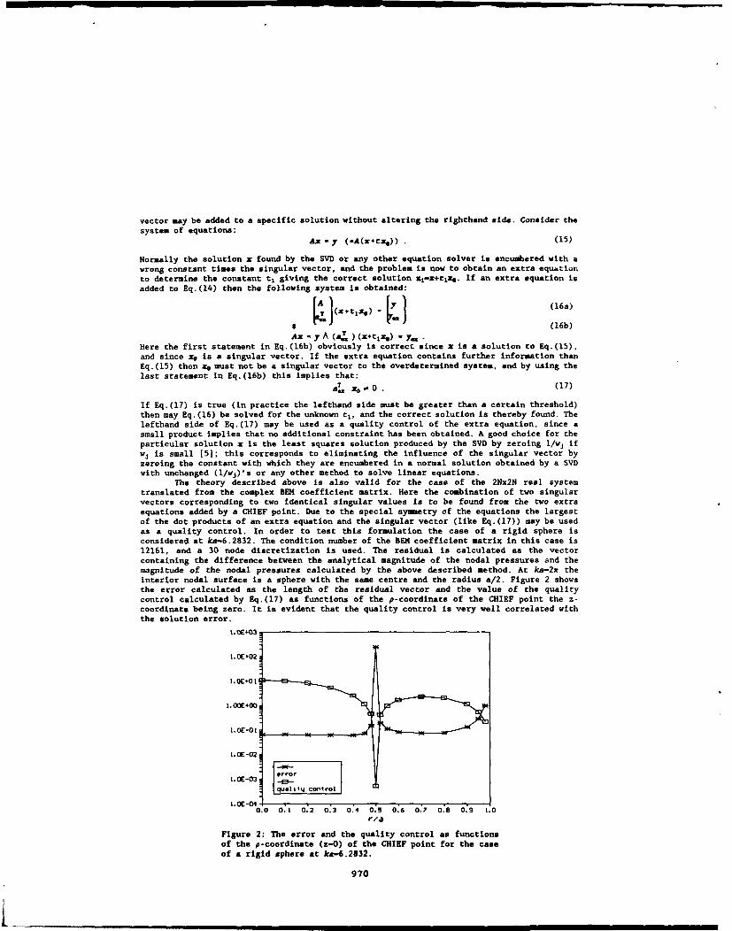
vector may be added to a specific solution without altering the righthand side. Consider thesystem of equations:
Ax - y (-A(x+txo)) (15)
Normally the solution x found by the SVD or any other equation solver is encumbered with awrong constant times the singular vector, and the problem is now to obtain an extra equationto determine the constant t1 giving the correct solution xl-x+trlx. If an extra equation isadded to Eq.(14) then the following system is obtained:
(x~tizo) (16a)
$ -(16b)
Ax = y A (4., ) (x+tlxe) y=Here the first statement in Eq.(16b) obviously is correct since x is a solution to Eq.(15),and since xv is a singular vector. If the extra equation contains further information thanEq. (15) then x0 must not be a singular vector to the overdetermined system, and by using thelast statement in Eq.(16b) this implies that:
aT= x 0. (17)
If Eq.(17) is true (in practice the lefthand side must be greater than a certain threshold)then may Eq.(16) be solved for the unknown tj, and the correct solution is thereby found. Thelefthand side of Eq. (17) may be used as a quality control of the extra equation, since asmall product implies that no additional constraint has been obtained. A good choice for theparticular solution x is the least squares solution produced by the SVD by zeroing l/wj ifwj is small [5]; this corresponds to eliminating the influence of the singular vector byzeroing the constant with which they are encumbered in a normal solution obtained by a SVDwith unchanged (1/vj)'s or any other method to solve linear equations.
The theory described above is also valid for the case of the 2Nx2N real systemtranslated from the complex BEM coefficient matrix. Here the combination of two singularvectors corresponding to two identical singular values Is to be found from the two extraequations added by a CHIEF point. Due to the special symmetry of the equations the largestof the dot products of an extra equation and the singular vector (like Eq.(17)) may be usedas a quality control. In order to test this formulation the case of a rigid sphere isconsidered at ka-6.2832. The condition number of the BEK coefficient matrix in this case is12161, and a 30 node discretization is used. The residual is calculated as the vectorcontaining the difference between the analytical magnitude of the nodal pressures and themagnitude of the nodal pressures calculated by the above described method. At ka-2W theinterior nodal surface is a sphere with the same centre and the radius a/2. Figure 2 showsthe error calculated as the length of the residual vector and the value of the qualitycontrol calculated by Eq. (17) as functions of the p-coordinate of the CHIEF point the z-coordinate being zero. It is evident that the quality control is very well correlated withthe solution error.
1. UE+03
t. 0£+02
I.OE+O|
I.OOE+O0
t.OE-02
aOE 0.o o;A 0.2 0.3 0:4 0.5 0:6 0:7 O.' 0.o9 1.0r~a
Figure 2: The error and the quality control as functionsof the p-coordinate (z-0) of the CHIEF point for the caseof a rigid sphere at ke-6.2832.
970

SVD AT HIGHER FREQUENCIES
At higher frequencies the nonuniqueness problem becomes more severe due to the closespacing and to the 'bandwidth' of the characteristic frequencies. One may very well encounterthe situation where the bands of bad solutions no longer are disjunct and the solution iscorrupted by two or more characteristic frequencies near any chosen frequency. This situationis reflected in two or more small singular values calculated by the SVD with correspondingsingular vectors, and the (numerical) rank deficiency of the BEE coefficient matrix isgreater than one. The number of required good CHIEF points equals the number of smallsingular values, and they must be chosen so that the quality control is fulfilled for allsingular vectors for at least one CHIEF point (but a single CHIEF point does not need tofulfil the quality control for all singular vectors). Note that the method of quality controland finding the right combination of singular vectors are valid also when the wj's are notexactly zero but less than a threshold decided by the user. In this way one may at any higherfrequency benefit from adding CHIEF points selected by inspection of the quality controlindicators.
2.50 C
02.25 0
0L4 2. 009
41 C3 CHEFpo
o 1.50-
31.25- 0
c1.100-
*0.75-S < P,50.50 - C
0.00- =
0 20 40 60 80 100 120 140 160 190angle S (degrees)
Figure 3: Scattering by a sphere for ka-15.0397. Two CHIEFpoints are needed to obtain an accurate solution.
In order to provoke a higher rank deficiency, scattering of a plane wave withmagnitude one from a rigid sphere for ka-15.0397 is considered. The generator of the sphereis discretizied in 79 elements and 80 nodes. In this case two singular values become verysmall due to the presence of another fictitious eigenfrequency at ka-15.0335 (M-wI/wr-2466;wl/vm-1-310;
W1 /w5X 2-9.7), and the rank deficiency of the BEM coefficient matrix is two. Figure 3 showsthe magnitude of the pressure on the surface as a function of the angle defined in the smallinset in the figure. It is evident that in this case two 'good' CHIEF points are requiredto obtain an accurate solution. The CHIEF points are selected with respect to the qualitycontrol.
DISCUSSION
The two important features of the SVD are:1) The singular values, which allow the user to decide how many CHIEF points are
needed (if any).2) The singular vectors, which provide an excellent tool to check the quality of
the CHIEF points.The main disadvantages of the SVD are its great complexity and the fact that
calculating the SVD is quite time consuming compared to other methods. However, in BEM thetime consumed by setting up the equations is in most cases still much larger than the timeused to solve the system of equations.
Recently another method to estimate the singular values and the singular vectors -therank revealing QR factorization (RRQR)- has been discovered[6]. The RRQR is far moreefficient (in terms of consumed time and storage) than the SVD.
In many cases it would be more advantageous to solve the overdetermined system of
971
equations arising from the BEN coefficient matrix and from the CHIEF points rather thanfinding the right combination of singular vectors (by solving a small system of equationsfor the unknown ti's). Using the SVD this probably means that a new SVD must be calculatedfor the resulting overdetermined system of equations, but using the RRQR factorization itis possible to update the factorization when extra equations are added to the originalsystem(
71.
Note that the attempt described in this paper is valid for any kind of extra equationsone may wish to add to the original BEN coefficient matrix. This attempt may therefore beused in more advanced formulations to circumvent the nonuniqueness problem like SuperCHIEFor CHIEF-block (see [2] and the references therein). The extra equations obtained by any ofthese advanced CHIEF methods may be checked in the same way as the ordinary CHIEF points.Since these formulations often offer more equations than the rank deficiency of the BENcoefficient matrix, the resulting overdetermined set of equations must be solved in leastsquares since - e.g. by the use of a RRQR factorization.
It must be emphasized that the test cases presented in this paper concerns anaxisymmetric model where the rank deficiency problem is less severe than in a general three-dimensional formulation, but this method is valid for general three-dimension l formulationsas well.
Finally it should be mentioned that the approach proposed by Burton and Miller andused in (4] also can be expected to fail when the frequency get so high that the bands ofbad solutions from the Helmholtz Integral Equation and its normal derivative no longer aredisjunct.
CONCLUS IONS
In this paper it has been shown that the rank deficiency of the BEM coefficient matrixat characteristic frequencies may be revealed by a singular value decomposition (SVD).
It has been shown that due to the 'bandwidth' of the characteristic frequencies therank deficiency of the BEN coefficient matrix may be greater than one when two or severalcharacteristic frequencies are near the frequency in interest.
The number of 'good' CHIEF points needed to obtain an unique solution equals the rankdeficiency of the BEN coefficient matrix, and it has been shown that by making use of thesingular vectors obtained by the SVD the quality of the CHIEF points can be evaluatedreliably.
This formulation may also be applied to more advanced methods to overcome the non-uniqueness problem.
The author believes that this formulation provides a useful tool not only for solvingthe nonuniqueness problem, but also for maintaining a mesh as coarse as possible for a givenaccuracy. This latter feature becomes very significant when modelling complex structures athigher frequencies, and the author believes that by the use of this formulation it ispossible to apply BEN to a larger category of problems than up to the present.
REFERENCES
1. H.A.Schenck, "Improved Integral Formulation for Acoustic Radiation Problems",J. Acoust. Soc. Am. 44,41-58 (1968).
2. T.V.Wu and A.F.Seybert, "A weighted residual formulation for the CHIEF method inacoustics", J. Acoust. Soc. Am. 90,1608-1614 (1991).
3. B.B.Baker and E.T.Copson "The mathematical Theory of Huygens' Principle", 2nd EditionOxford University Press, 1-32 (1953).
4. C.C.Chien,H.Rajiyah and S.N.Atluri,"An Effective Method for Solving the HypersingularIntegral Equations in 3-D Acoustics", J. Acoust. Soc. Am. 88, 918-937 (1991).
5. W.H.Press et al. "Numerical Recipes", Cambridge University Press, 52-64 (1986).
6. T.F.Chan, "Rank revealing QR factorizations", Lin.Alg.Appl. 88/89 (1987), 67-82.
7. G.H.Golub and C.F.Van Loan, "Matrix Computations', 2nd Edition, The John HopkinsUniversity Press 592-600 (1989).
972

SECOND INTERNATIONAL CONGRESS ONRECENT DEVELOPMENTS IN AIR- AND
STRUCTURE-BORNE SOUND AND VIBRATIONMARCH 4-6, 1992 AUBURN UNIVERSIIY. USA
Implementation of Boundary Element Method forSolving Acoustic Problems on a Massively Parallel
Machine
A. Dubey, M. Zubair, and U.S. Shirahatti$
Abstract
Boundary Element Method (BEM) has found increasing use in thesolution and analysis of acoustic field problems. The BEM requiresleass grid generation and is ideal for solving infinite domain problems.The BEM is computationally intensive and is suitable for parallel im-plementation. The three major tasks in the implementation of BEMare:
"* Computation of H and G action matrices using numerical in-tegration. The elements of these matrices can be computed inParallel.
" Rearrangement of H and G matrices into [A] {X) = (B) form.On a parallel machine this essentially means redistribution ofdata. To minimize redistributioa cost it is desirable to map theproblem intelligently on the parallel machine.
"* Solving for the unknown X on the boundaries and at the requiredfield points in the interior of the domain. Here, parallelism canbe exploited both for computing X at the boundaries and in theinterior.
In this paper we look at the implementation of BEM on a hypercubebased parallel machine, the Intel iPSC-860. The example problemwhich we consider is the solution of Helmholtz equation inside a three-dimensional rectangular acoustic duct.
"Department of Computer Science, Old Dominion University, Norfolk, VAtfDepartment of Computer Science, Old Dominion Universty, Norfolk, VAtDepartment of Mechanical Engineering and Mechanics, Old Dominion University, Nor-
folk, VA
973
L... ... . . . - m m. m i m im l m

1 Introduction
The numerical solution of acoustic field problems has attracted considerableattention in recent years. The numerical solutions have been proposed us-ing the finite difference, the finite element or the boundary element method(BEM) [I]. The HEM is computationally intensive and is suitable for par-allel implementation. In implementing BEM one can exploit parallelism attwo phases. One while computing the unknown quantities at the bound-ary elements and the second while computing the field values inside thedomain. Major part of computations in both the phases involve evaluationof mutually independent surface integrals which is ideally suited for parallelenvironment. The other major computation is parallel solution of a systemof linear equations, which has been extensively studied by researchers inpast, e.g. t2, 31
In this paper we look at the implementation of BEM on a hypercubebased parallel machine, the Intel iPSC-860. The example problem ib thecomputation of acoustic field inside a three-dimensional rectangular ductwith various boundary conditions prescribed on the surface. The equationgoverning the acoustic field quantities is the three-dimensional wave equa-tion.
2 Boundary Element Formulation
The acoustic field in a duct is governed by the wave equation,
_2 -) OP (1)
where, c represents the speed of sound in the fluid. The Laplacian, V, incartesian coordinates for three-dimensions, is
ar2 -- y- + 8z2 (2)
By assuming the pressure in the form,
(px, Y, Z't) = p (X, Y,Z) C-tw, (3)
the wave equation is reduced to the Helmholtz equation,
V 2p + k
2p = O, in the domain fl (4)
974

where k is defined as the wave number (k = w/c). The symbol p representsthe pressure distribution and q is defined by,
q= (.5)
where n is the unit normal on the boundary.Now consider the following boundary conditions,
p = p on r, Essential Condition
q = 4 on 172 Natural Condition (6)
where the total boundary of the domain Q1 is f = rI + 72 .The boundary conditions basically consist of two types of known values.
Either the pressure or the normal derivative of the pressure is known at theboundary as seen in Eq(6).
The method of weighted residuals statement of the Helmholtz equationis
f, (v~p..+ k2p)p'dil =0 (7)
where the fundamental solution,p, or Green's function for the Helmh Itzequation satisfies
V2p* + k
2p" + A -0 (8)
and Ai is the Dirac delta function. The fundamental solution in three-dimensional spare is
-= ik,,p"
and
, rwhere r is the distance between the source point and the observation point.
Integrating Eq.(7) by parts twice, we get
In(V2 P + k2p-) p df? I qp~dl + fjpldr. (1
975

The term, fa (V2p + k2p) p dO in Eq.(10) can be shown to reduce to-cip,. The expression ci is considered constant for each boundary elementand is defined as
ci = 0 outside the boundary
.= = on a smooth boundary (r)
ci = 1 inside the boundary(f)) (12)
The boundary element governing equation becomes
N NCýp, + F f qpd'r = r- j p qdr, (13)
.j=1 ." j=i Ir
where N is the total number of elements. Eq.(13) is applied to each elementto form a set of equations with p or q unknown in each element. Substitut-ing the fundamental solution, Eq.(9), into the boundary element governingequation, Eq.(13), gives
N N
cipj~+Z pf(i/4.f)(-hr +ik) eik~dr=FJ q [(ui4-xr) e-k' dr.(14)
If constant elements are used, p and q are assumed constant over eachelement. Therefore, p and q can be extracted from the integrals in Eq.( 14).
System of equations.By applying the governing equation to each element, a set of equations isformed which can be represented in matrix form. The integrals in Equations
(13) and (14) can be written as
I, q'dF, Gj = ,dr (15)
for constant elements. The integrals in Eq.(15) are solved using a four-pointGauss quadrature technique. The system of equations becomes
cpj + fI- pi = CIAq,. (16)
The cip. term can be combined with the RiH term to form a new matrix Hj,
#ij + ci i-7j (17)
976

Therefore, the system of equations in matrix form is
[H] {P) = [G]{Q} (1Q)
Both {P) and {Q) vectors contain known and unknown values of p andq. To solve Eq.(18), the matrices will be transformed into a new mnatriXequation
[A] {X) = {B); (19)
where all the unknowns axe in {X}. After solving the system of equations,all the p and q terms axe known at the boundary. If any values of internalpoints are required, they can be found only after the boundary values havebeen calculated.
3 Parallel Implementation
3.1 Intel iPSC-860
The Intel iPSC-860 is a large-scale parallel supercomputer with a MultipleInstruction Multiple Data distributed memory architecture. Computationis carried out in physically independent processors referred to as nodes. Thenodes are physically connected in a multidimensional hypercube topology.A hypercube of dimension d has 2d processors labeled 0 to 2d - 1, with aconnection between two processors if and only if the binary representations
of the labels of these processors differ in exactly one bit. The interconnectionnetwork of a 16 node hypercube is shown in Figure 1.
A single node of an Intel iPSC-860 is a fully functional computer systemcontaining an i860 microprocessor with I/O facilities. The Intel 1860 mi-croprocessor uses an advanced architecture to deliver balanced integer andfloating-point performance. The iPSC-860 systems are scalable from 8 pro-cessors to 128 processors, with peak performance ranging from 480 MFLOPS
for an 8 processor system to 7.6 GFLOPS for a system with 128 processors.Each processing node can have 8 to 64 MBytes providing total system mem-ory ranging from 64 MBytes to 8 GBytes. Communication among nodes isa critical performance element for parallel processing computers. The InteliPSC-860 nodes communicate via Intel's proprietary Direct-connect internalnetwork, a message passing system that dynamically creates communicationcircuits between communication nodes. When two nodes wish to communi-
cate, the network builds a communication channel between them for as long
977

as the communication lasts and transmits the message at a bi-directionalrate of 5.6 MBytes/sec. Total communication bandwidth scales with thenumber of computing nodes.
3.2 Parallel Implementation of BEM
An informal description of a parallel implementation of BEM on the InteliPSC-860 is as follows.Step 1. Distribute geometry information about the physical domain in-cluding the elements details to all the p nodes of the iPSC-860 system.Step2. Assign k = N/p distinct elements to each node, where n is the totalnumber of elements. Each node then computes 2k(n- 1) integral expressionsusing gauss quadrature. After this step we have all the elements of actionmatrices H and G distributed over various nodes of the system.Step 3. Redistribute and combine the elements of H, G, P, and Q soas to get the AX = B form. The redistribution is such that contiguouscolumns of A are mapped to a node. We have opted for this distributionbecause we intend to use the system solver package developed by Dongarraand Ostrouchov [21.Step 4. Solve for X using an the package described in [21. After this stepwe have all the information about the boundary points which is distributedto all the nodes of the system.Step 5. Let Nd be the total number of points of interest in the interiordomain. Assign Nd/p points to a node of the iPSC-860 system. Each nodethen computes field values for Nd/P points by evaluating surface integralsusing Gauss quadrature.
To illustrate these steps in some detail, let us consider an example wherethe problem domain is divided into 24 boundary elements, as shown in Fig-ures 2-3 ( four elements per face of the duct). The hypercube chosen for thisexample has a dimension 2. In the first step we distribute the geometry in-formation (consisting of the coordinates of end points and mid point of eachelement) of the entire domain to all four nodes of the hypercube. Figure4 shows the distribution of these 24 elements to the nodes of the hyper-cube. Figure 5 indicates the generation of the columns of G and H matricescorresponding to the elements napped onto each node. For example, nodePEo generates first six columns of G and H. Generation of a column ofG or H involves 23 surface integrals (Note that the diagonal element whichcorresponds to the singularity is analytically obtained.). The rearrangementstep basically involves (i) a local sub-matrix into vector operation resulting
978

in bi's, and (ii) movement of b's across the nodes. This is illustrated inFigures 6-8. The implementation of Step 5 is similar to that of Step 2.
4 Preliminary Study
Our preliminary study is for a rectangular duct, the surface of which has beenmodeled using constant quadrilateral elements. The boundary conditions on
the rectangular duct would be as rigid walls on four of longer faces. We willincorporate a harmonic tCme dependent forcing function on one of the smallerfaces. The boundary condition on the opposite small face will consist of (i)rigid wall, (ii) pc termination, and (iii) impedance termination. Preliminaryresults will be presented.
References
[11 C.A. Brebbia, J.C.F. Telles, and L.C. Wrobel, Boundary ElementTechniques, Springer Verlag, 1984.
[2] J. Dongarra and S. Ostrouchov, LAPACK block factorization algo.
rithms on the Intel iPSC-860, LAPACK Working Note 24, Tech-nical Report CS-90-115, University of Tennessee, Oct.1990.
(3] K.A. Gallivan et al., Parallel algorithms for matriz computationsSIAM, 1990.
979

z
h
g•g
a "4 y
Mbi
x
Figure 1. Interconnection network for a Figure 2. A rectangular duct.sixteen node hypercube.
Ses el6 e - e6 e7-e2
b c : 7 el PEg PE,
h e e afi9 lflea3 em4
fil l el$ el6
ae b f 2PE PE3e17/ ell e21 en L
ejq C20 e23 e2%
dh c g
Figure 3. Division of the six faces of the rectangular Figure 4. Boundary elements mapping onduct into boundary elements. a 2-dimensional hypercube.
980

G Q H p
jGIJ G2 G, G4 fMH, H2 H, Hi4 - P,
6I L2 6 P2Li PPPR. PE, PA PFA PE. PE, PE2 PE,
Figure 5. Assignment of Processors for computing matrix coefficients. (the shaded regions
indicate known values and the unshaded regions indicate unknown values).
FA, A,l A3~ Aý [ Pi- 1Ii P2
A X B
Figure 6. Rearrangement of G and H matrices. (Note that b- = GQ•,, 6' = G2Q2. b1 HP3. b= HP)
A,=H,. bW P PE, A2=H 2 b2
A,=G, I Py P A04-=G4 , b
Figure 7. Distribution of matrix-A, and vector-b-pardta-sum on a 2-dimensional hypercube.
bl+ b b=b + +e+& b=bl'+b1 +b'+b
P2PPRI PRI
be++b bl~ +b2 +be+VP b=b'+b2 +b3+b 4
Figure 8. Algorithm for computing partial sums of b and its distribution to all the nodes.
981

I 92
962

SECOND INTIERNATIONAL CONGRESS ONRECENT DEVELOPMENTS IN AIR- AND
STRUCTURE-BORNE SOUND AND VIBRATIONMARCH 4-, 1992 AUBURN UNIVERSITY. USA
SOUND RADIATION OF HEAVY-LOADED COMPLEX VIBRATORYSTRUCTURES USING BOUNDARY INTEGRAL EQUATION METHOD
Michael V. BernblitDepartment of Electronics and Controls.¶St.-Petersburg Ocean Technology University.
St.-Petersburg, 190008.U.S.S.R.
The computational method for calculating of Complex Vibratory struct-ures' Sound Radiation into an infinite acoustical medium is developed usinga modified Boundary Integral Equation (BIE) technique. The two-level proce-dure is presented as the computational shell for Sound Radiation of heavy-loaded structures when their vibration in air is numerically predicted.The method is compared to the conventional modal analysis approach. Numeri-cal results are presented for the normal point-force driven free-free beamin water.
The radiation field of a complex structure vibrating with a speciefieddistribution of the normal velocity Vn(3) at its surface S can be calcula-ted using Boundary Integral Equation [1-3]
0.5 p(T)+ \p(T).g(f,,r)dS = -Jw\Vn(•).gg(r.,) dS , (1)
where p(l) is a surface pressure to be computed; -1,1 are the source andsurface field points; • is the density of the acoustic medium; a =2-1.f;g,(zx)=exp(jkr)/4= r Is a free-space Green function for the infinite aco-ustic medium; k= W/c-wavenumber; g = age/an is the Green function's nor-mal derivative. After p(C) is calculated from Eq.l Sound Field at any ar-bitrary point can be computed using Helmholz integral. More over, Sound In-tensity mapping can be added to observe acoustic energy distribution. To-tal radiated power and radiation efficiency also can be derived numerical-ly. So using BIE technique the compete solution of the Sound Radiation Pro-blem can be obtained.
Unfortunatly, when the normal component of the surface velocity Vn(1)is not specified, it should be derived from the matrix equation of the bo-dy-motion
[M] {) [R) ({) [k] (x) = (Q)-(P) , (2)
where [M], [R]. [k] are the mass, damping and stiffness matrices; (x) and(Q) are the vectors of the surface displacements and the intensity of theapplied forces; (P)7={O,O,p) is the acoustic radiation loading. In caseof "light" acoustic medium (in air) the surface pressure loading (P) inEq.2 can be ignored and Vn(f) Is easily computed (any commercial Finite
963

Element or Modal Analysis software can be used). But when the acoustic lo-ading is heavy (in liquids) Eq.1 and 2 must be treated simultaneously, be-cause Vn(1) depends on the unknown distribution of the surface pressure.Many efforts has been done to combine BIE with the conventional eigenvalueanalysis, but all of them couldn't provide the exact solution, because ofthe Modal Coupling problem in Sound-Structure's Interaction.
Nevertheless such a solution can be obtained using a definition of thedisplacement vector (x) as a convolution of the structural Green functionG(x.y) with the intensity of the applied forces [4]:
IX) = I (G(1,`) ]-.({(oi) + (P(cV)) ) dS.
Thus the displasement of a fluid-loaded surface is presented as a sumof that one (X}ofor the unloaded structure and a convolution of its Greenfunction and the surface presure p(y)
(x} = {x) + G ( p,).p(7) dS (3)
where G3 (3',*)= z_ G is the normal component of the N-dimensioned compl-iant matrix. L-L
Substituting Eq.3 into Eq.1 one can obtain the modified BIE
0.5 p(T) + 1 P(7).g(y,-) dS= J \ a ng (37,1) dS, (4)
where =- CO . [x) is the normal surface acceleration; the kernel
gpv (7,37) = gv (Y 'g) - r 7A g G?( 7A(3t') dS
contains the additional member which is the convolution of the structuralG()= - C4GZ and medium gp Green functions.
Thus the two-level procedure of BIE method is presented for the acous-tically loaded structures. At first the fluid loading is ignored and thein-vacuo acceleration a() and the Structural Green function is calculatedusing any available software. Then the surface pressure distribution iscomputed from Eq.4. At second the vibration of the loaded structure is de-rived from Eq.3. As a result, Helmholz integral formula predicts the pres-sure at any arbitrary field point.
The numerical solution of 3d Helmholz integral eqation and the problemof its uniqueness were discussed in various publications.The Combined Hel-mholz Integral Equation Formulation (CHIEF) [3] was prefered. The bodysurface S was devided into N planar elements assuming that the velocityand pressure distribution were iniform over each of the surface element&S. For this case Eq.4 can be rewritten in the matrix form
[I] + [DI ) (p) = [Q] (an} , (5)
where Dt= 2 g(rqg).dS and QqS= 2.? ý g,(rq).dS are coefficients,related the contribution of the dipole and monopole elementary sources.This coefficients are calculated numerically [5]; [I] is the Unit matrix.
It is interesting to compare the modified BIE procedure with the ap-proach, based on the conventional modal analysis, previously developed in
Sund-Structure's interaction problem. For this purpose the in-vacuoa%(y) and fluid-loaded an(V) surface acceleration can be given in series
aa,~( y)=L Ag (7) . (6)
where AV and AV are modal complex amplitudes, V@ (?) is the In-vacuo
984

orthonormal modal functions.The structural in-vacua Green function has a well known representation
(6)
c.~l Co )4 (7)V#
where m. is the modal (per unit area) mass; cOt= C~)a *(1
-j%); Q3,isthe natural frequency of the V -mode; 1 is the corresponding in-vacuo lossfactor. Neglecting the influence of the surface dipole sources, p(r) isrepresented by
p(x) = 2p .(-y) g(1.1) dS . (8)
Substituting (6-8) into Eq.4 one can derive the infinite system
(1- FA m (1] 0 A (9)
wheree e -2 p •. •%(.) - Y, (x)g(g',) dSxdS is the complex modalentrained mas. S
If the modal coupling Is not considered, then from Eq.9
S= .z¥a
-8A& 7- j + Ysa3-I( +(10)
where S.4 = C.' / * 11' is the resonant frequency of the fluid loadedstructure; T is the entrained mass coefficient for the V - mode; L=
ycd o / Ca mois the sound radiation loss factor; fi•p= mj( + iZ'is the complex entrained mass of the ) -mode which radiation efficiency is
Thus one can notice that the eigenvalue approach can be derived fromthe BIE method which provides the most efficient instrumentation to solvethe modal coupling interaction problem for the fluid-loaded structures.
The numerical results were recieved for a normal point force drivenfree-free thin beam. The exact solution for the Structural Green functionis given in (7], using Krilov's functions VL(.y x/L), i=l,...4
G(x/x' AI x/L+V [(x-x')/L]H)cos(V-j'
where J4 =k,&L(1-j 2/4); kb is the in-vacuo bending wave-number; Lis the beam's length; M is it's in-vacua total mass; (x,%9 ) -cylindricalcoordinates; H=1, if x > x', else H=O;
a - - V, ,)&V 3- )V a(,y T) V Qf J, V1 j)\.(l - x/)
The modified BIE method was used in the low frequency band kr < 1,where kr, is the beam's wave-radius. The in-vacuo loss factor L=Z.Ol.
985
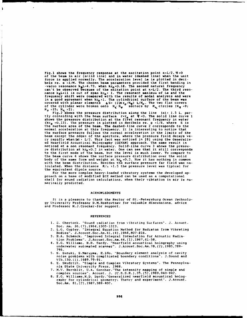
Fig.1 shows the frequency response at the excitation point x=L/2. 4=0of the beam in air (s-lid line) and in water (dashed line) when the unitforce is applied normally. The acceleration level La is plotted in deci-bels re. a =1/M. The chosen beam parameters provided the first bending in-vacuo resonance kLL=4.73, when kro=O.18. The second natural frequencycan't be observed because of the exitation point at x=L/2. The third reso-nance k&L=ll is out of span kro< 1. The resonant maximum of La and thefrequency shift were compared with the results of modal analysis and werein a good agreement when kro<l. The cylindrical surface of the beam wascovered with planar elements aS= (2s•rr/Nq) L/N,. The two flat coversof the cylinder were broken onto Ne NT sectors by N., circles (NK =9;NX =15; N.L =2).
Fig.2 shows the pressure distribution along the line 1xl< 1.5 L, par-tly coinsiding with the beam surface r=ro at %P=O. The solid line curve 1shows the pressure distribution at the first resonant frequency in water(kr, =0.13). The pressure is plotted in decibels re. p =1/S, where S isthe surface area of the beam. The dashed-line curve 2 corresponds to thenormal acceleration at this frequency. It is interesting to notice thatthe surface pressure follows the normal acceleration in the limits of thebeam except the edges of the aperture, where the pressure field decays ve-ry rapidly when a| > L/2. This fact was noticed in [8] using the Generalis-ed Nearfield Acoustical Holography (GENAH) approach. The same result isnoticed at a non resonant frequency. Solid-line curve 3 shows the pressu-re distribution at krg=O.2 in water. One can see that it still correspondsto the first mode of the beam, but the level is much lower. To compare tothe beam curve 4 shows the surface pressure distribution over the solidbody of the same form and weight at kr,=O.2. Now it has nothing in commonwith the beam distribution. Besides the surface pressure far field was ca-lculated. When the distance R/L >1.5 the pressure level was tipical forthe equivalent dipole source.
For the more complex heavy-loaded vibratory systems the developed ap-proach on a base of modified BIE method can be used as a computationalshell for sound radiation calculations, when their vibtation in air is nu-merically predicted.
ACKNOWLEDGMENTS
It is a pleasure to thank the Rector of St.-Petersburg Ocean rechnolo-gy University Professor D.M.Rostovtsev for valuable discussions, adviceand Professor M.J.Crocker-for support.
REFERENCES
1. G. Chertock. "Sound radiation from vibrating Surfaces". J. Acoust.Soc. Am. 36,(7),1964,1305-1313.
2. L.G. Copley. "Integral Equation Method for Radiaton from VibratingBodies". J.Acoust.Soc.Am.41,(4),1966,807-816.
3. H.A. Schenck. "Improved Integral formulation for Acoustic Radia-tion Problems". J.Acoust.Soc.Am.44,(l),1967,41-58.
4. E.G. Williams, H.D. Dardy. "Nearfield acoustical holography usingunderwater automated scanner". J.Acoust.Soc.Am.78,(2),1985,789-798.
5. S. Suzuki, S.Maruyma, H.Ido. "Boundary element analysis of cavitynoise problems with complicated boundary conditions". J.Sound andVib.130,(l),1989,79-91.
6. E. Skudrzik. "Simple and Complex Vibratory Systems". The Pennsylva-nia State University Press, 1965.
7. M.V. Bernblit, U.A. Gonchar."The intensity mapping of simple andcomplex sources". Acoust. J. (U.S.S.R.),35,(5),1989,940-942.
8. E.G. Williams,H.D. Dardy."Generalized nearfield acoustical holog-raphy for cylindrical geometry: Theory and experiment". J.Acoust.Soc.Am. 81,(2),1987,389-407.
986

I'
,o -%'
-20
0.• 01. 02. QDA 0.6 03
Figure 1--Beam normal surface acceleration distribution in airand in water
Lp, A c1640
ZO 30
0 #o
-20 / . ; -\
-30
-i." -LO -0.5 0 0.5 1.0 i.5
Figure 2-- Beau surface pressure distribution
987

988

SECOND INTERNATIONAL CONGRESS ONRECENT DEVELOPMENTS IN AIR- AND
STRUCTURE-BORNE SOUND AND VIBRATIONMARCH 4-6. 1992 AUBURN UNIVERSITY, USA
OBTAINING OF UNIQUE SOLUTION OF A SOUND RADIATION AND SCATTERING PROBLEMUSING A BEM BASED OF THE HERMHOLTZ'S INTEGRAL
I.E.TsukernikovScientific and Industry Amalgamation "Mir"
MoscowUSSR
A version of the boundary element method isconsidered. The external boundary- value problem is broughtto surface integral of the first kind for an unknown surface characteristic of sound field: pressure if the Neumann'sproblem is considered or normal velofity for the Dirichlet's problem. It is shown that the fundamental solutionsof the integral equation are the boundary values of standing waves existing in the interior region at the character-istic frequencies and so the nonunique solvability of the integral equation is not transfered to the external problemsolution writted by the Helmholtz's integral. The merit of the method is illustrated on the example of calcula-ting the sound field of the pulsating sphere.
A method of boundary elements is widely used for numerical solution of sound radiation and scatteringproblems. The solution is presented in an integral form and the problem comes to an integral equation relativelyto an unknown field characteristic (sound pressure or normal component of vibrating velocity) on the boundarysurface.
The most difficult is the task of selecting and solving an integral equation because it is connected withnonunique solvability of equations at Dirichlet's or Neumann's eigenfrequences of the interior region determinedby the boundary surface E11. To overcome the obstacle at present the most widely used are two methods [2,31:the method offered by Schenk [4] in which the problem is brought to an overdetermined system of equations andthe method of Burton and Miller [5] in which a combined integral equation is used. Under certain constraintsboth methods make it possible to attain unique solution of the equations and problem.
If the final task is calculating of field characteristics outside of the boundary surface, there exists a versionof the method of boundary elements which does not require a unique solution of the integral equation. The prob-lem is brought to an integral equation of the first kind nonunique solvability of which due to specific propertiesof eigenfunctions of a homogenious equation does not transfer to the solution of the exterior problem expressedby the Helmholtz's integral. In the case of the Dirichlat's problem that result was obtained in the work (6]. Inthe present article it is transfered on the case of the Neumann's exterior problem. It makes it true for all problemsof sound radiation and scattering in which the question of nonunique solvability is present.
Let us consider a problem of determining a radiation field of a body vibrating with a predeterminedvelocity v on its surface S. In a mathematical ense this problem is equivalent to a problem of sound scattering ona stiff obstacle and is formulated for harmonic time dependence as the Neumann's exterior problem for the homo-genious equation of Helmholtz. Let us put down a solutlon in the form of the Helmholtz's integral [7)
989

P(x) A{ Ply) - ikpcv(y)l glx, y)dS, (1)
S any
where P(x) and P(y) are sound pressures in the point x of the exterior region and in the point y located on the
surface S of the body; (a/any) is the derivative with respect to external normal to the surface S in the point y;
g(x, y) = exp(iklx-yl)/(4wrlx-y I) is the free space Green's function ; k is the wave number; p and c are the
medium density and the sound velocity in it.
Taking the derivative of Eq.(1) with respect to the exterior normal to S in the point Yo on S and tending
the point x to S(x -* yo + 0) due to the boundary condition ap/an = ikpcv we obtain an integral equation of the
first kind relatively to unknown distribution of pressure p(y) on S:
a ag(yo, y) v(y0 ) ag(yo, y)a f p(y) a ny dS = ikpc ---- + f v(y) any° dS (2)snv. S any 2 S an.,
The integral in the left-hand side of Eq.(2) should be understood in the sense of the Caushy's principal
value. Some methods of its regulation are examined in the works (2, 5].It is known (11 that the Eq.(2) has not a unique solution if the wave number coincides with an eigen
value ki(i - 1, 2 .... ) of the interior Neumann's problem.Let us determine the physical sense of characteristic solutions of the homogenious integral equation.
The solution pi of the homogenious interior Neumann's problem (with the boundary conditio.-, - (y)=0on S) written down with the Helmholtz's integral lookes like as follows:
pi(x) = - fpi(y) YTX ) dS for x inside S (3)s any
Let us differentiate Eq. (3) with respect to the exterior normal to the surface S in the point yo andtend the point x to S: x - yo - 0 . As the function pi(y) is continuous on S the potential of the double layer (3)has continuous normal derivative on S [1]. As a result satisfying the boundary condition of the problem we obtain
the equality
a ag(y 0, y)-- f pi(y) -- dS = 0,a)nYo S any
which coincides with the homogenious equation for Eq. (2) and shows that the solution of that equation is the
boundary value of the Neumann's interior problem solution.
Using the way identical to that applied in the work [6] it becomes possible to show that if the eigenvalue ki is degenerate of order n the boundary values pJ(y) (j 1, 2 .. , n) of principal solutions of the Neumann'sinterior problem form the basis of the eigen functions of Eq. (2), that is they are the only set of linearly independ-ent fundamental solutions of homogenious integral equation.
General solution of Eq. (2) should be written down as follows:n
ply) , pO My + j 2: 1 Cj p~i (y), (4)
where pO is the particular solution depending on the right.hand side part of the equation and constants cl mayhave any values.
From the mathematical property of the Helmholtz's integral it follows that for i (y) the next equalityis true:
ag x, y)f P!(Y) dS - 0 forx outsideS.
SJ an,In a physical sense it reflects the fact that the fundamental solutions of the integral equation, being
the boundary values of standing waves which exist inside S upon eigen values of the wave number, do not give
990

any contribute to the exterior field.As a result, substituting Eq.(4) in Eq.(1) we see that the required solution p(x) of the exterior problem
depends only on a particular solution of the integral equation, So, despite the fact that the solution of the in-
tegral equation is not a unique one found out with the help of the Helmholtz's integral (1 solution of the exterior
problem is a unique one. The considered method of boundary elements has an advantage over the version based
on an integral equation of the second kind [8] a nonunique solution of which is completely transfered to the
pressure of the exterior field written down with the help of Eq.(U1.
As an illustration, curves of dependence of the maximum relative error 6, % (in comparison with an
analitic solution) versus wave radius ka, obtained by calculation of the radiation field of a pulsating sphere with
the radius a using the above-mentioned method are shown in Fig. 1 (a). The calculations were carried out for the
range of wave numbers including the first two eigen values of the Neumsnn's interior problem for which ka=4.49
and ka = 7.25. The dash line corresponds to the error which appeared in the solution of the integral equation (2).
The solid line corresponds to the error of pressure in the radiation field in points of the sphere with the R = 1(a
calculated with the help of Eq,(1). Increasing of the error up to 100% in the solution of the integral equation in
the visinity of the characteristic frequences does not influence on the results of the radiation field calculation.
For comparison the analogues curves corresponding to the error appearing when the integral equation of the
second kind is used (81 are represented in Fig. 1(b). The error in the solution of the integral equation is fully
transfered to the results of the radiation field calculation.
REFERENCES
1. Kolton D., Kress R. Integral equations methods in scattering theory. - New York. Chichester. Bricbane. Toronto. Singapore:Wiley & Sons, 1983.
2. Akyol T.P. Schallabstrahlung von Rotationakorpem. - Acustica, b.61, No. 3, 1986, s. 200-212.3. Tobocman W. Extention of the Helmholtz integral equa, ion method to shorter wavelengths. - J. Acoust. Soc. Am., v. 80, No. 6,
1986, p. 1826-1837,4. Schenck H.A. Improved integral formulation for acoustic radiation problems. - J. Acoust. Soc. Am., a. 44, No. 1, 1968, p. 41- 58.5. Burton A.J., Miller G.F. The application integral equation methods to the numerical solution of some interior boundary-value
problems. - Proc, Royal Soc. London, v. A323, 1971, p, 201-220.6. Tsukemikov I.E. Numerical solution of the exterior Dirichlet problem by means of an integral equation of the first Vnd. -
U.S.S.R. Computational Mathematics and Mathematical Physics, v. 16, N 5, 1976, p. 267-273.7. B.B.Backer, E.I.Copson, The mathematical theory nf Huigens' principle. - Oxford, 1953.B. Chertock G. Sound radiation from vibrating surfaces. - J. Ac•ust. Soc. Am., v. 36, 1964, p. 1306-1313.
991
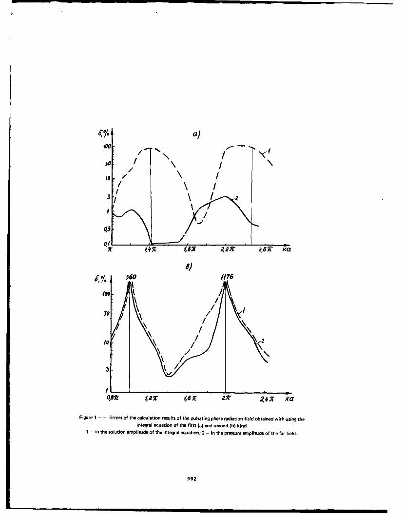
VO /ja)
001
//
30
10~ X
o/ --
%0e
v
qto
92 167 z 221 67, ka
I)
30 7 / ,
o // /
,\ /3!
Figure 1 - - Errors of the calculation results of the pulsating phere radiation field obtained with using theintegral equation of the first (a) and second (b) kind
1 - in the solution amplitude of the integral equation; 2 - in the pressure amplitude of the far field.
992

SECOND INTERNATIONAL CONGRESS ONRECENT DEVELOPMENTS IN AIR- AND
STRUCTURE-BORNE SOUND AND VIBRATIONMARCH 4-6. 1992 AUBURN UNIVERSITY. USA
ISOPARAMETRIC BOUNDARY ELEMENT MODELING OF ACOUSTICAL CRACKS
T. W. Wu and G. C. Wan
Department of Mechanical Engineering,University of Kentucky, Lexington, KY 40506,
U. S. A.
ABSTRACT
When a thin structure of infinitesimal thickness is submerged in an infinite acoustic medium, the acousticvelocity field contains a singularity at the knife edge of the thin structure. This problem resembles a crackproblem in fracture mechanics. In this paper, a boundary element formulation using a Cauchy principal integralequation is used to model this acoustical crack problem. Quadratic isoparametric elements are used in theformulation so that the knife-edge singularity can be easily modeled by the quarter-point technique.
INTRODUCTION
Sound radiation and scattering from thin bodies has many important applications (such as transducersand fins) in acoustics. It has been known that the conventional boundary element method (BEM) using theHelmholtz integral equation is not suitable for problems involving thin bodies. The major difficulty is due to thefact that the mesh on one side of a thin body is too close to the mesh on the opposite side. Therefore, extremelyfine meshes have to be used and nearly singular behavior may occur in the integral equation. This problem isvery similar to the crack problem in fracture mechanics. One way to solve a thin-body problem is to use themulti-domain BEM formulation [ 11. However, it requires a lot of preprocessing efforts and may also result in avery large system of equations because an imaginary interface surface has to be constructed and discretized.
A more elegant way to solve the thin-body problem is to use the normal derivative integral equation.However, it involves the evaluation of a hypersingular integral in the order of l/r3 , which is integrable only inthe finite-part sense. Several techniques have been proposed to regularize this hyper-singular integral [2-5. Inthis paper, we briefly review a recent BEM formulation to solve the thin-body problem 161. This formulationuses a less-singular normal derivative integral equation, originally derived by Maue 171 and laterby Mitzner 181using a different approach. The normal derivative integral equation by Mane is less singular because thesingularity is in the order of h/r2 only and it converges in the Cauchy principal value sense rather than only in thefinite-part sense. Numerical integration of the Cauchy principal singularity in Mane's equation can be achievedby subtracting a term at the singular point and then adding the term back (9].
It should be noted that the convergence of Mane's equation requires two continuity conditions 16,91.The first condition is that the sound pressure must be continuous everywhere. This requires the use of at leastthe CO continuous elements. The second condition is that the tangential derivatives of the sound pressure mustbe continuous at collocation points. This is the Ct continuity condition. The simplest way to satisfy both of theCO and Ct continuity conditions simultaneously is to use the regular CO isoparametric elements and putcollocation points inside each element. One important feature of using the CO isoparametric elements is that theresulting numerical model will be compatible with other analysis tools, such as the finite element method. Inaddition, the quadratic CO isoparametric elements will allow the use of the quarter-point technique (10,111 tomodel the W, singularity of the tangential velocities at the knife edge of a thin body (121.
Through a systematic collocation point genetation scheme, the number of collocation points will bealways greater than the number of nodalpoints. In other words, there will be more equations than unknowns.The overdetermined system is then solved by a lemt-sqares procedure. Numerical eAamples are given to verify
993
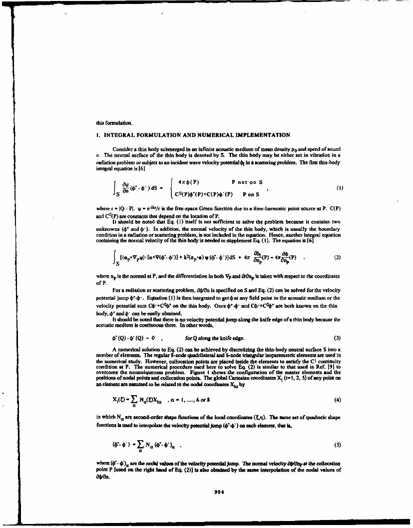
this formulation.
I. INTEGRAL FORMULATION AND NUMERICAL IMPLEMENTATION
Consider a thin body submerged in an infinite acoustic medium of mean density p0 and speed of soundc. The neutral surface of the thin body is denoted by S. The thin body may be either set in vibration in aradiation problem or subject to an incident wave velocity potential 1 in a scattering problem. The first thin-bodyintegral equation is [6]
f N{ 47r4(P) P not on SJ5 )÷t- O)ds - (i)S C°(P)4(P)+C(P)*b'(P) P on S
where r = IQ - P1. qr e-ikr/r is the free-space Green function due to a time-harmonic point source at P. C(P)
and C°(P) are constants that depend on the location of P.It should be noted that Eq. (1) itself is not sufficient to solve the problem because it contains two
unknowns (W and (ý'). In addition, the normal velocity of the thin body, which is usually the boundarycondition in a radiation or scattering problem, is not included in the equation. Hence, another integral equationcontaining the normal velocity of the thin body is needed to supplement Eq. (1). The equation is [6]
S((npxVpwr). [nxV($- (')] + k2(np-a) W (O-O)"dS + 41r -4P) - 41r-(2)
where np is the normal at P, and the differentiation in both Vp and 8/8nip is taken with respect to the coordinatesof P.
For a radiation or scattering problem, ft% is specified on S and Eq. (2) can be solved for the velocity
potential jump V+4-. Equation (!) is then integrated to get O at any field point in the acoustic medium or thevelocity potential sum CGf+C%+ on the thin body. Once 4-4- and C%-+C%+ are both known on the thin
body, (0+ and it" can be easily obtained.It should be noted that there is no velocity potential jump along the knife edge of a thin body because the
acoustic medium is continuous there. In other words,
V(Q) =("(Q) = 0 , forQ along the knife edge. (3)
A numerical solution to Eq. (2) can be achieved by discretizing the thin-body neutral surface S into anumber of elements. The regular 8-node quadrilateral and 6-node triangular isoparametric elements are used inthe numerical study. However, collocation points are placed inside the elements to satisfy the CI continuitycondition at P. The numerical procedure used here to solve Eq. (2) is similar to that used in Ref. [9] toovercome the nonuniqueness problem. Figure 1 shows the configuration of the master elements and thepositions of nodal points and collocation points. The global Cartesian coordinates Xi (= 1, 2, 3) of any point onan element are assumed to be related to the nodal coordinates )q by
Xj(V)= Na(t)Xi. a - I ...... 6 or 8 (4)
in which Na are second-order shape functions of the local coordinates (t,q). The same set of quadratic shape
functions is used to interpolate the velocity potential jump ($'4) on each element, that is,
W(0-) - N,(O-). (5)a
where (W- 4V), are the nodal values of the velocity potential jump. The normal velocity 5Jz0np at the collocationpoint P [used on the right hand of Eq. (2)1 is also obtained by the same interpolation of the nodal values of
994

10.S
W-.0)(,aO .0). 1 .4 3,.4 .4 5 , .45 , 1
1-.8,.S) (0,-.8 .a-a) (A.45,iJ,4-,0 0 (0,0- .1 (1,0,0)
O Nodal Points
* Collocation Points
Figure 1. Configuration of the master elements.
The integration of the kernel (npxVpw).[nxV().41)- in Eq. (2) should be performed in the Cauchyprincipal value sense. For each collocation position of P, there is only one element that contains the singularpoint P. This element is denoted by Se. Numerical integration on all the other elements are nonsingular and canbe carried out in the usual way. For integration on the singular element Se, a polar coordinate system (p,O) isused on the corresponding master element Sm as shown in Fig. 2. Numerical integration of(npxVpu).[nxV
W4i)-- on Se can be achieved by subtracting a term at the singular point and then adding the term back. Detaileddiscussion of this procedure can be found in Ref. (9]. The result is
j npx j-0- - 2wjR(O) F(p,O) - F(Oe) dp dO
Isn 0p'[x~p'd'IS Jo 0 P
f2w+ J F(0,0) InR(O)d0 , (6)
where R(0) is distance from P to the element boundary measured on the master element plane as shown inFig. 2 and
F(p,e)-=p2 (npxVpwp).[nxV(4•O- •)3 J I ,(7)
in which I J I is the Jacobian between Se and Sm.For the collocation scheme suggested in Fig. 1, the total number of collocation points is always greater
than the total number of nodal points. The overdetermined system is then solved by a least-squares procedure.In addition, 4V- (0' is also forced to be zero at all of the knife-edge nodes. This will reduce the total number ofunknowns in Eq. (2) even further. It is well known that the acoustic velocity field at the knife edge has asingularity in the order of lAIr, where r is measured from the knife edge [ 121. Unlike the multi-domain BEMapproach [ I1, the thin-body integral formulation does not require modeling of an imaginary interface, and hence,eliminates the need to model the singularity of the velocity field on the fluid side of the knife edge. In addition,since the normal velocity on the thin body is always given as a boundary condition, the !/ singularity existsonly in the tangential derivatives of g- 40'. As will be shown in the example problems, this singularity can beeasily modeled by moving the midside nodes of the elements adjacent to the knife edge to their quarter-point
995

P
1 '1 /P -
Singular Element So Corresponding Master Element Sm
Figure 2. Polar coordinate transformation.
positions [10, 1 1. After Eq. (2) Is solved for f)- 40' at every nodal point, Eq. (1) is then integrated to obtain
C4'+C%0. Note that Eq. (1) is only weakly singular and is integrable In the normal sense. Therefore, the
singular point P is collocated directly at each nodal point to get C4-+C+ there.
I. EXAMPLE PROBLEMS
The first example problem is the radiation from a vibrating circular plate of radius a The plate isclamped around its boundary and vibrating at its first axisymmetric mode with kn - i. The vibrating velocity isnormalized by setting the maximum velocity at the center to be 1. The neutral surface of the disk is discretizedby 24 eight-node quadrilateral elements and eight six-node triangular elements as shown in Fig. 3. Note that forall of the 8 quadrilateral elements adjacent to the knife edge, their midaide nodes on the elements' sides in theradial direction are moved from the regular middle-point positions to the quarter-point positions. This willimplicitly incorporate the ýrr behavior in the quadratic shape functions and consequently the 1r singularity inthe derivatives of the shape functions. Since this problem may not have an analytical solution, an axisymmetricmulti-domain BEM solution is used to verify the thin-body BEM solution. Therefore, also shown in Fig. 3 isthe axisymmetric multi-domain BEM mesh used for this problem. In the axisymmetric multi-domain BEMmodel, the circular plate is modeled by four line elements and six additional line elements are used to form aninterface. In addition, special singular elements [ 131 are used to model the knife-edge singularity. To verify theBEM solution, variation of the magnitude of the velocity potential W in the radial direction on one side of thecircular plate is compared to an axisymmetric multi-domain BEM solution in Fig. 4. Excellent agreement isobserved between the two BEM solutions. The importance of the !A singularity is also shown in Figs. 4 bythe solutions obtained when the quarter points are intentionally moved back to their regular middle-pointpositions. It is obvious that the quarter-point technique is very Important to the accuracy of the solution.
Xx
X,
r-real boundary surface
+
imaginary interface
(a) (b)
Figure 3. BEM meshes for the circular ph"e: (a) the thIn-body apprach; (b) the axisymmetrlc multi-domain
996

0.6
0.4
0.3
0.2
- MULTI-DOMAIN BEM0.1 * THIN-BODY APPROACH
WITH V4-POINT TECHINQUE
0.0 13 THIN-BODY APPROACHWITHOUTr /4-POINT TECHNIQUE
-0.1
-0.2 0.0 0.2 0.4 0.6 0.8 1.0 1.2
r
Figure 4. Magnitude of the velocity potential on one side of the circular plate as a function of the distancefrom the center.
The second example problem is the scattering of an incident plane wave from a rigid thin-walledhemisphere with radius a Two BEM meshes used to model this hemisphere are shown in Fig. 5. Note thatquarter points rather than middle points are used for the elements adjacent to the knife edge. The incident planewave has a velocity potential of unit amplitude and is traveling in the -X3 direction. Again, this problem is alsosolved by the axisymmetric multi-domain BEM with special singular elements being used to model the knife-edge singularity. The comparison between these two BEM solutions for the scattered velocity potentials on bothsides (exterior and interior) of the cylindrical surface is given in Figs. 6 and 7. Figure 6 shows the real part ofthe scattered velocity potentials and Fig. 7 shows the corresponding imaginary prt Again, very goodagreement is observed.
13 13
JI-- --.. ---.-...X2 2
Xl X(a) (b)
Figure 5. BEM meshes for the hemisphere: (a) 109-node mesh; (b) 30 1-node mesh.
997

t.
1.6"
1.0
4ON INTERIOR SURFACE:'j 0.-5 - MULTI-DOMAIN BEM
0 THIN-BODY APPROACH (109 NODES)D THI-BODY APPROACH (301 NODES)
ON EXTERIOR SURFACE:-- - MULTI-DOMAIN BEM
0.0 A THIN-BODY APPROACH (109 NODES)(> THIN-BODY APPROACH (301 NODES) - 6
A• . .. .. .6 .o-"-- ...
-0 .5 . .. . .. .
-10 0 10 80 30 40 5w 80 70 80 90 100
O(deg.)Figure 6, Real part of the scattered velocity potentials on the Interior and exterior surfs= f the hemisphere
as a function ofthe angle measured from the X3-axis.
01
ON INTERIOR SURFACE: "6
-MULTI-DOMAIN BEM. THIN-BODY APPROACH (109 NODES)
o THIN-BODY APPROACH (301 NODES)
ON EXTERIOR SURFACE:---
MULTI-DOMAIN BEM
A THIN-BODY APPROACH (109 NODES)STHIN-BODY APPROACH (301 NODES)
-2 'Dr001
310
-10 0 10 20 30 40 80 60 70 80 90 100
0(deg.)
Figure 7. Imaginary part of the scattered velocity potentials on the interior and exterior surfaces of thehemisphere as a function of the angle measured from the X3 -axis.
998

111. CONCLUSIONS
The normal derivative integral equation originally derived by Mane is applied to the BEM solution of thinbodies (or acoustic cricks). This normal derivative integral equation converges in the Cauchy principal valuesense rather than only in the finite-pan sense. The formulation is implemented in an isopammetric elementenvironment. The quarter-point technique is used to model the I/• singularity associated with the tangentialvelocities at the knife edge. The BEM results compare very well with axisymmetric multi-domain BEMsolutions.
REFERENCES
I. A. F. Seybert, C. Y. R. Cheng and T. W. Wu, "The Solution of Coupled Interior/Exterior AcousticProblems Using the Boundary Element Method," . Acoust. Soc. Am. 88, 1612-1618 (1990).
2. A. J. Butoan and G. F. Miller, "The Application of Integral Equation Methods to the Numerical Solutionsof Some Exterior Boundary Value Problems," Proc. Roa. Sc. A 323, 201-210 (1971).
3. T. Tend, "On Calculation of Sound Fields Around Three-Dimensional Objects by Integral EquationMethods," J. Sound VY. 69, 71-100 (1980).
4. J. B. Mariem and M. A. Handi, -A New Boundary Finite Element Method for Fluid-Structure InteractionProblems," Int. J. Num. Methods Eaw 24, 1251-1267 (1987).
5. G. Krishnasamy, L. W. Schmerr, T. J. Rudolphi and F. J. Rizzo, "Hypersingular Boundary IntegralEquations: Some Applications in Acoustic and Elastic Wave Scattering," ASME J. An. Mech 57,404.414 (1990).
6. T. W. Wu and G. C. Wan, "Numerical Modeling of Acoustic Radiation and Scattering from Thin BodiesUsing a Cauchy Principal Integral Equation," submitted to . Acoust. Soc, Am. (1991).
7. A. W. Mane, "Zur Formulierng eines allgemeinen Beugungsproblems dutch eine Integralglcichung," Z.Phy. 126, 601-618 (1949).
8. K. M. Mitzner, "Acoustic Scattering from an Interface Between Media of Greatly Different Density," L.Math. Phys. 7, 2053-2060 (1966).
9. T. W. Wu, A. F. Seybert and G. C. Wan, 'On the Numerical Implementation ofa Cauchy Principal ValueIntegral to Insure a Unique Solution for Acoustic Radiation and Scattering," J. Acoust. Soc. Am. 90,554-560 (1990).
10. D. Henshell, "Crack Tip Finite Elements Are Unnecessary," Int. J. Num. Methods Eng. 9, 495-507(1975).
11. R. Barsoum, "On the Use of Isoparametric Finite Elements in Linear Fracture Mechanics," Int. J. Num.
Mehds !En 10, 25-37 (1976).
12. P. M. Morse and K. U. Ingard, Theoretical Acoustics (McGraw-Hill, New York, 1968), Chap. 8.
13. A. F. Seybert, Z. H. Jia and T. W. Wu, "Solving Knife-edge Scattering Problems Using SingularBoundary Elements," to appear in J. Acoust. Soc. Am.
999

1000

SECOND INTERNATIONAL CONGRESS ONRECENT DEVELOPMENTS IN AIR- AND
STRUCTURE-BORNE SOUND AND VIBRATIONMARCH 4-6. 1992 AUBURN UNIVERIY, USA
A SOLUTION MErHOD FOR ACOUSTICBOUNDARY ELEMENT EIGENPROBLZM Wirh SOUND ABSORPITION
USING LANCZOS ALGORITHMby
C. Rajakumar and Aftraf AliSwanson Analysis Systems, Inc.
Houston, PA 15342
ABSTRACT
A damped system elgenvalue analysis of acoustical cavities using the boundary element method ispresented. The acousticbound. eeamenrigaiproblem formulution presented byBanerjee etal. [I) is extendedto include sound absorption in acoustical cavities. A dissiative term is included in the eigenvalue matriequation to account for boundary absorption. The resulting damped system eigenrvalue problem is "Ived usinga new approach of applying the L.anczos subspace algorithm to quadratic eigemproblenis. Since the boundaryelement matrices are unsymmnetric, the Lanczos algorithm presented is in its most general form for unsynunetricquadratic cigenproblems. Examples are presented to show the application of the method to find thecigaifrequencies of acoustic cavities with sound absorption.
INT`RODUcrION
Computation of the acoustic cavity resonant frequencies is an essential paut in the design of automobilepassenger cabins. Finite element modeling of the acoustical problem is routinely camred out where thediacretized wave equation is set up as an eigenrvalue problem and the resonant frequencies and mode shapecomputed. Employing the boundary element method, the acoustical cavity resonance problem was set up as analgebraic eigenvalue problem by Banerjee et al. [11. Although the boundary element matrices ane analler in sizethan the finite element matrices, they are unsymmetric. Therefore, the use of boundary element eigenvalueanalysis requires an efficient eigenvalue extraction method for tansymmnetic matrices. In the paper byRajakuma r e al. [2] the Lanczos solution algorithm for the unsynuetwric generalized elgenvalue problem wasapplied to the acoustic boundary element eigenanalysis.
In the present work, the Lanczos algorithmo is applied to the damped system eigenvalue problemformulated by the boundary denawt discretization of acoustic caviie with sound absorption. The algorithmpresented is unique, in that, it does not use ohe method of matrix augmentation to linearize the quadraticeigenvalue problemrsng iwn damped dynamic systems. In order to wrea unsynunetric stiffiwssW mass, anddamping matrices, the algorithmn is kept general enough and thereforeinsquite suitable forthe absorptive acousticboundary element eigettproblem.
A brief outline of the paper is as follows: first, we set up the acoustic boundary element eigetiproblemas shown in the paper by Banrmjee et al. [1]. Then, a simple method of incorporating the boundary absorptioninto the boundary delmnw formulation is shown. Finally, the resulting quadratic eigenivalue problm is solvedusing a new ap;proA of applying the L~amcns algorithmn which eliminates the need for dealing with doubledsize matrices 9f the matrix augmentatio method. The Lancun algorithm and ftimpemnato details inInclude&.
ACOUSTIC B3OUNDARY ELEMdENT OENFROBLAM
Mwe acoustic wave equation governing the acoustic pineare p in a fluid is given by:
1001
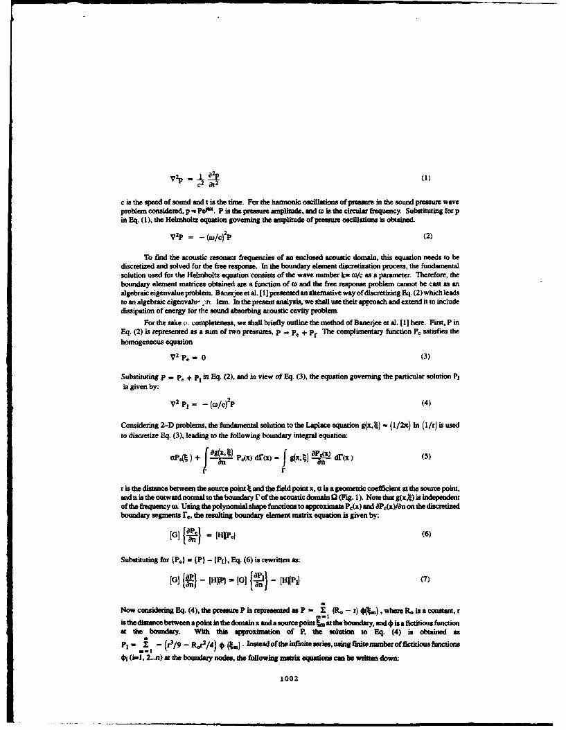
c is the speed of sound and tis the time. For the harmonic oscillations of pressure in the sound pressure waveproblem considered, p -PeiM2. P is the pressure amplitude, and o) is the circular frequency. Substituting for pin Eq. (1), the Helmholtz equation governing the amplitude of pressure oscillations is obtained.
V2p _ _ (0)/C)2p (2)
To find the acoustic resonant frequencies of an enclosed acoustic domain, this equation needs to bediscretized and solved for the free response. In the boundary element discreiation process, the fundarmentalsolution used for the Helmholtz equation consists of the wave number k- 0o/c as a parameter. Therefore, theboundary element matrices obtained are a function of w1 and the free response problem cannot be cast as analgebraic cigenvalueproblern. Banerjee et a1. [11 presented analternative way of discretizing Eq. (2) which leadsto an algebraic eigenvalu-,-*rc lem. In the present analysis, we"sal use their approach and extend it to includedissipation of energy for the sound absorbing acoustic cavity problem.
For the sake o. completeness, we shsll briefly outline the method of Banerjee et al. [11 here. First, P inEq. (2) is represented as a sum of two pressures, p - Fr. + pr The complimentary function Pc, satisfies thehomogeneous equation
V2 pC 0 (3)
,Substituting p - p,ý + p, in Eq. (2), and in view of Eq. (3), the equation governing the particular solution PIis given by:
V2 p, (O/C) 2 P (4)
Considering 2-D problems, the fundamrental solution to the Laplace equation g(x,) (I (/23t) In (I /r) is usedto discretize Eq. (3), leading to the following boundary integral equation:
r r
r is the distance between the source point t and the field point x, cz is a geometric coefficient at the source point,and n is the outward normal to the boundary r of the acoustic domain Q (Fig. 1). Note that g(xt) is independentof the frequency o) Using the polynomial shape functions to approximate P,(x) and aPc(x)/O~n on the discretizedboundary segments r., the resulting boundary element mat&i equation is given by:
[G] [Hc = IHP.) (6)
Substituting for (P.) = (P) - (PI), Eq. (6) is rewritten as:
to] If} - [Wj) - [G] {I -1 [HJ(P1] (7)
Now considering Eq. (4), the pressure P is represented as P 1 Rt. - r) *%.a) , where RO is a constant, r
is the distance between apoint in the domain x and a source point tLnat die boundary, and 4 is a fictitious funictionat the boundary. With this approximation of P, the solution to Eq. (4) is obtained as
P,, 1 - (0/19 - Ror2/4) io (4,). histead ofthe infinite series, using finite number of fictitious functions4k. 0n-1. 2...n) at the boundary nodes, the following matrix equations can be written down
1002

(PI - [AIM, (P4J - [Dj*I, {Ofn [B1+1()I an-
Substituting for (PI and (OPitan I into Eq. (7), and defining (M] ((0](B] - [HilDI) arid
the boundary element equation for the acoustic problem is obtained.
[GoQI - [HPI - (w/c) 2 [M( *1 (10)
Banerjee et al. [1] used J+} = [A]-rIP} in Eq. (10) to formulate the algebraic eigeproblem. In the referenceby Ali et al. [3], (P) was replaced by [A]{*} to form the eigenproblem with *} as the eigenvector, therebyavoiding the inversion of [A]. When the boundary of the acoustic domain is hard, (Q)-0, and the algebraiceigenproblem can be written as:
[Kw, -j - )i M
where, [K] - [H41 [A, k. - (owdc)1
The boundary element matrices [K] and [M] are independent of the frequency o) and Eq. (11) is ageneralized eigenvalue problem. The eigenpairs ki, I+. I represent the resonant frequencies and mode shapesof a non-absorbing acoustic cavity. Starting from Eq. (10), a method of incorporating a dissipation term toaccount for sound absorption at the boundaries of an acoustic cavity is shown next.
SOUND ABSORPTION AT THE BOUNDARY
Invariably, some amount of energy is dissipated due to the absorption of sound at the boundaries of anacoustic domain. In order to account for the dissipated energy, Craggs [4] has presented a damped form ofHelmholtz Eq. (2). For the absorption of sound at the boundaries of an acoustic cavity, we employ a similarapproach by considering tie linear momentum equation that relates the fluid pressure gradient and the velocityat the boundary
Op N 0 (12)
where, Q is the fluid density, V is the velocity vector, and n is the outward normal. To account for the energydissipated at the boundaries, an absorption term is introduced on the right-hand side of Eq. (12):
Op 8V .ff +RV-V (13)
In the absorption term, the reason for using the velocity divergence V • v ao pposed to V as in Cragg's papercomes from the consideration of the consistency of units, when the acoustic resistance R is in myl (n-4e/m).Furthermore, Zenkiewicz and Newton [51 have shown the relationship Op/On - - (1/c) Op/Otto wount forthe energy loss due to the out bound pressure waves at an open boundary for plane wave siuatiors. Since opvatis related to V. V via the conservation of mass equation
V.V- -• T(14)
of a compressible fluid, the boundary absorption term used in Eq. (13) would be appropriate. So, substitingfor V. v from Eq. (14) into Eq. (13) the pressure gradient at an absorbing boundary is written as
1003
I •

aR/gc is the nondirnansional absorption coefficient of the sound absorbing aulalW at *he boundarY. Theacoustic resistance R for foam and fibrous type mate-i am gwin ma function of fisquency by Cm9P [4].
For the harmonic oscillaons in acoustical Problems, the boundary presure "nd velocity in Eq. (15) arerepresmted in complex exponential form a p a ,elt and v - Ve*, recovey. In the present p aper theboundary velocity is not used W=ce the fluid-structure interface boundary is massund to be stationary. Theboundary pressure gradient at a sound absorbing boundary is, then obtained haom Eq. (15) as
f. - -jw 0Pp (16)
ABSORTION TERM IN THE BOUNDARY ELEMENT MATRIX EQUATION
Using the relationship inEq. (16), the absorption in an acoustic cavity can be incorporated in thediscretized boundary element Eq. (10). Eq. (16) is rewritten in term of the nodal pressure gradwift a follows.
IQ) - - i (40/0 0 (P (17)
When absorption material is used on a part of the boundary rI, Eq. (10) is written down in partitioned form as:
G1]O2 Q,[:11 oj ~ - HJ~j =(o)c)
2Im*118
Pressure gradients at the absorbing end non-absorbing boundary nodes ar denoted by MQ and IQ2),respectively. Then, substituting from Eq. (17) into Eq. (18)
I - Wr/. P _ - (0/c )2 Thl 40 (19)
For the part of the boundary where there is no absorption, we assume acoustically hard boundary conditionIQ2}=o. Partitioning the mtrix (A] inmEq. (8), we substitute for IPIJ - fA=A1(*Ij + (AL2 ](421 in Eq. (19).
[GIIAII,, G1IAII (os) (OC2M ,
.G21A12j '02
Taking the coefficient -4 into the matrix, end denoting the absorption matrix as [C] end (K1a -HIfAL, Eq. (20)is rewritten a:
j ()/c) [C1I* + [KIOI _ (CO/c):2Ml~M (21)
Eq. (21) is the eigenvalue problem for the acoustic cavity with sound absorption. Defining the eigenvalues as)l =j (to/c), and the eigenvectors (xi) = I*f, the quadratic eigzproblem to be olved is
Iixl• + {MCjxj + )42M1xII - 0 (22)
LANCZOS AWORMIM FOR QUADRATIC EIGENVALUE PROBLEMS
The successful Implementation of the boundary element acoustic geiguproblanu formulation presenteddepends upon the availability of an efficient method of solving the quadratic eigenproblem posed in Eq. (22).
1004

The systemn stiffnress, damping. end mass matie [K]. [C], and (Mrespectively. are unsymunetric and fullypopulated and are of anm n x n. For large acoustic cavity resonance problems usually only the first few
aiefeuncues are of hetout of the 2n cigenfrequencies of the eigenproblem. Iberefore, we choose asubpacetechnique. Further, the Lanczoesuabseace method Is specifically choseribecauase the Lanczoe urbspecematrix is tridlagonal whose eigenpair can be extracted very efficiantly.
in order to solve Eq. (22). the 'jsual approach is the method of matrix augmentation, leading to a linearcigenvalue problem. This method doubles the siz of system matrices to 2n and is undewrsi raoehm the pointof computer storage requirements. In the present approach, the Lanczoe algorithm is applied to the quadraticeigeniprobletn directly, eliminating the need for matrix augmentation. In reference (6], Mheng et al. presencedan inverse Iteration method of solving quadratic eigenprobleuns without augmentation. Pursuing along theirapproach, here we seek to set up fth Lanczoe algorithm to solve Eq. (22). For the quadratic eigenproblem, matrixR of size n x mn and matrix T of size m x mnare defined as the characteristic matrix and eigenvalue square matrix,respectively, if they satisfy
M [R)]+(C] [R]P1 +[(KI[R] rr -0 (23)
and rank (T)m. Then the cigenvalues of the standard eigenproblem
M (yJ - Pi (yJ (24)
will approximaute die cigenvalues of the original problem in Eq. (22), i 1/L.A recursion scheme thatgenerates the Lanczos vectors lr1 I, j=1. 2 ...mi (m•!2n), which are the columns of the characteristic matrix (R],needs to be set up in order to transform Eq. (22) into Eq. (24) in the subseace Y1 mnx mi. The Lanczos recursionfor the unsymmetric genrmalized eigenvalue problem, given by [M - 0 in Eq. (22), was presented by Rajakumarand Rogers [7]. Extending this work, a complete derivation of the Lanczos algorithm for the quadraticcigenprobleni, along with proofs are shown in the reference by Rajakunar [8]. Here we shall present the Lanczosrecursion without the detailed derivationis and proofs.
For symmetric matrices, the single-sided Lanczos recursion scheme for the generalized eigenvalueproblem is well known [91. Since the matrices in Eq. (22) are unsymmetric, we seek to formulate the Lanczostwo-sided recursion where the transposed eigenproblemi
[Kflrlzd + f)X~Cfz~j + X2 [M~(j- - 0 (25)
is considered, along with the original problem. It can be shown that the eigenvalues of Eq. (25) are the sameas that of Eq. (22) 1 xi) and Izi) are called the right anod left-hand cigenvectors, respectively. They arebiorthogonal since they satisf the generalized biorthogonalit condition
IZjT CIxjd + Iij) [M"xi + (ziI T My~Ji - 0(26)
when iq~j. (IIJ - )q IxJ. and Ii)- Xj fzj) are defined as the dependent right and left-hand eigenvectors,
respectively . In the Lanczos two-sided recursion given below, two primary and two secondary sequence ofVectors IV] - IVI V2 ... vM, JIM - [WI W2 ... w.]j and [R] - [r, r2. .r. ,(IS] - LSt s2 ---s.J, respectivelyare generated. The primary and secondary Lanczos vectors will map the independent and dependenteigenvectors, respectively.
Two sets of arbitrarily chosen vectors [ý) 1*,4 and (f,). 11,) we normalized such that
(wtIN[C lvi) + IslIT[IA lvi) + (wjlýM] (r1 - 1 to get the starting set of primary and secondary Lanczosvectors Iv1 I, (w~l and (r,), IsJ). Weset 101- 1*.) and (i.) - (I,)in our implemeritationisince thenevectorsare arbitrarily chosen. Forj-l,2 ... i, (m•52n)
- -+1 [K]F 1(lCijvjj + 4rjl~) -, ujlv - Pjdvj...i (27)
1005

{w1.v1- [KjFT([C(cjIT~ + k~T(,1jl) -ajwj-j - 86-j1{w.. (28)
{i l , -j - 1 I I9
{, - {i - - at (S4 - 6bjlj-} (30)
(when j = 1, 1 vo = o = 8 1wo - 86so = 0)- ({I Tci + T) - ([CIjv + MIr1}) + {Wj[l IM j (1
Aj+ (j~I T1C(V +1 + I+ 1 TMI 1 1, + IwJ+l IT[mI {rj+i (32)
8j+ I Aj+11",/ (33)
P 61 j+1 sign (Aj+1) (34)
{w .,,} I {. .+1) (35)6j+ J
-j+1) {Wj+ 11 (36)
{,•+i} , {,•+1} (38)
The Lanczos vectors generated in the recursion presented above satisfy the generalized biorthogonalitycondition given by
twfCIl [iM + ts]TM M + Wti (MRI - RI (39)
In finite precision computations, they loose their biorthogonality [91, and the following reorthogonalizationscheme is used in our implementation.
The (j+1)s vectors computed in Eqs. (35) thin (38) ae checked for their biorhogonality with respectto each of the j vectors by computing the coefficients 0, and 4k as follows:
01 - ({w-fIC] {vj+lI + I-SM] {vj+,I + -w_ T[ I {rj+ 1 (40)
.- {W,+} 17c] 1vj + {sj. I+fM N + {wj+II[ TM I(r (41)
1006

If the magnitude of any of the coefficients, say thekthcoefflcient, istgreater than apredetermiined smnaUl number,E. then the reorthogonalizing step are given by
{Vj+l11-41{V+l -) k-k (42)
(ri+i} - (rj+iJ - Okrk (44)
In the present implementation, ea = 104 is used.
The two-sided Lanczos recursion presented in Eqs. (27) dint (38) results in a biorthogonultransforrmaton of the quadratic eigenproblem into the standard eigenvalue problem given in Eq. (24). Thecigenvectors are related by
1xi) - (Vilyi,)11. jj y (46)
Using the recursion equations (27) and (29), it can be shown that 18] matrices [Rit and M satisfy the characteristicequation (23), and that MT is a tridiagonal matrix formed by the Lanczos recursion coefficients.
at p2 0
rn 2 CE 1 (47)0 6. am
The eigenvalues p = (IQj of the standard cigenvalue problem in E~q. (24) are extracted by a QR algorithm [10]designed to extract complex eigenvalues. With an incresasing number of recursion steps, the subspace size mnincreases aid the eigenivalues at the lower end of the eigenivalue magnitude spectrum quickly converge to yieldthe kit's of the original problem. In the present application , the fmrs k eigenvalues converged usually w~ihin asubspace size of m-k+ 16. To compute the eigenvectors of the original problem. Eq. (46) is used. Bigenvectors{yi) are computed by inverse iterations of the M matrix.EXAMPLES
Thiree simple examples are shown to validate the incorporationt of sound absorption in the acousticboundary element eigenproblem. The boundary absorption method presented haes also been fimplemented in theacoustic finite element eigenproblemn in the ANSYSO general purpose program (11]. Therefore, the boundaryelement results are compared with the finite element results in these examples.
A square cavity shown in Fig. 2 is considered. The absorption free eigenfrequencies for this problem
are ft (c/2) [(ez/L.) 2 + (e y/Lyf)12]. ex I ey w-0, 1, 2... w. Lx and Lyme the length and width ofthe
domain, respectively. We usoe tfhdis eapeto validat theLanczoselgenvaluecomputationagorithmpreaented.The absorption coefficients at the absorption layer and at the walls 0, and 16, respectively, are set to zero. Forthe boundary element discretization, 36 boundary nodes and 14 intemnal nodes are used. Te need for internalnodes to improve the accuracy of computed frequencies was pointed out in reference (3]. Thfe lquencies shownin Table 1 include the theoretical and a l0 x 10 mesh finite element (11] results for comparison with the boundaryelement solution. The acoustic remsoati frequencies are the positive imaginary parts of the conjugate pair of
1007

eigenvalues computed. The five eigermode frequencies from the boundary element method compare favorablywith the finite element solution in coming close to the theoretical feaquencies.
The square cavity problem is solved with uniform boundary absorption by taig pf - Pb, - 0.2. Table2 shows the frequencies computed by the boundary and finite element methods using the same discreization uin Example I. The eigenvalues )i - oi, * j (0j, now have a nonzero real part. The imaginary pan gives thedamped resonant fteluency fl - 0i /27c. Compared to the nonabsorption case, the frequencies have slightlyreduced for modes 3-8. Mode 2 shows a nonoscillatory exponential decay response. The boundary elementresults compare well with the finite element results at the lower modes. With an increasing number of internalpoints, the boundary element results will improve. The mode shapes 2 and 4 obtained from the finite elementresults are plotted in Fig. 3.
Here the absorption is nonuniform, N = 0.9 and Pb = 0. Table 3 shows the ftequency results. Modes3-10 show an increase from the undamped frequencies. Mode 2 again shows a nonoscillating decay. The plotof mode shapes 2 and 4 obtained from the finite element analysis are shown in Fig. 4. It is interesting to notethe concentration of contours near the absorption layer in these plots.
CONCLUSIONS
A method of incorporating boundary absorption in the eigenvalue analysis of acoustic cavities using theboundary element technique has been validated. Since the damping matr is obtained from the discretizedboundary element matrix, the implementation of the method is simple. Using the experimentaily correlatedabsorption coefficients of fibrous and foam type material found in reference [4], the damped system resonantmodes of acoustic cavities, such as the automobile passenger cabin, can be computed. The Lanczos algrithmnfor quadratic eigenproblem employed is found to be quite efficient since it does not require augmentation of thesystem matrices. When only a few eigenvalues of a large dynamic system is needed the Lanczos subspacemethod is quite effective, both in speed of computation and in accuracy. However, when the number ofeigenvalues needed is Imle, say >50, the total reorthogonalization scheme used will slow down the computationand a selective reorthogonalization [9] would improve the situation. Finally, the absorption in cavities affectthe eigenmode pressure distribution quite appreciably, even though the damped system frequencies are not veryfar away from the undamped frequencies.
ACKNOWLEDGEMENTS
The authors thank Swanson Analysis Systems, Inc. for the support of this work. Contributions ofJackie Williamson and Charmaine Grunick in the preparation of the manuscript is acknowledged.
REFERENCES
I. P. K. Banerjee, S. Ahmad and H. C. Wang, 'A new BEM formulation for acoustic aigentfrquercyanalysis', Int. J. Numer. Methods Eng., 26,1988,1299-1309.
2. C. Rajakunmar, A. Ali and S. M. Yunus, 'Lanczos algorithm for acoustic boundary element eigenvalueproblems', J. Acoust. Soc. Am., to appear, 1992.
3. A. Ali, C. Rajakumar andIS. M. Yunus, 'On the formulation of the acoustic boundary element eigenvalueproblems', Int. J. Numer. Methods Eng., 31, 1991, 1271-1282.
4. A. Craggs, 'A finite element model for acoustically lined small rooms', J. Sound Vib., 108(2), 1986,327-337.
5. 0. C. Zienkiewicz and R. E. Newton, 'Coupled vibrations of a structure submerged in a compressible
fluid', Proc. Int. Symp. on Finite Element Techdiques, Stuttgart, 1969, pp. 359-379.
6. T-S Zheng, W. M. Lin and Z. B. Cai, 'A generalized inverse iteration method for solution of quadraticeigenvalue problems in structural dynamic analysis', Computers & Structures, 33, 1989,1139-1143.
7. C.RajdaumarandC.R. Rojer, 'TeLanczosalridu appltoun an geneaind eigvaueproblem', Int. J. Numer. Method Eng., 32,1991, 1009-1026.
S. C. Rajakunar, 'Lanczos algorthm for the "amdc eigurvalue problem in engineering applicatio'.Computer Meth. App. Mech. and Eag., submitted for possible publication.
1000
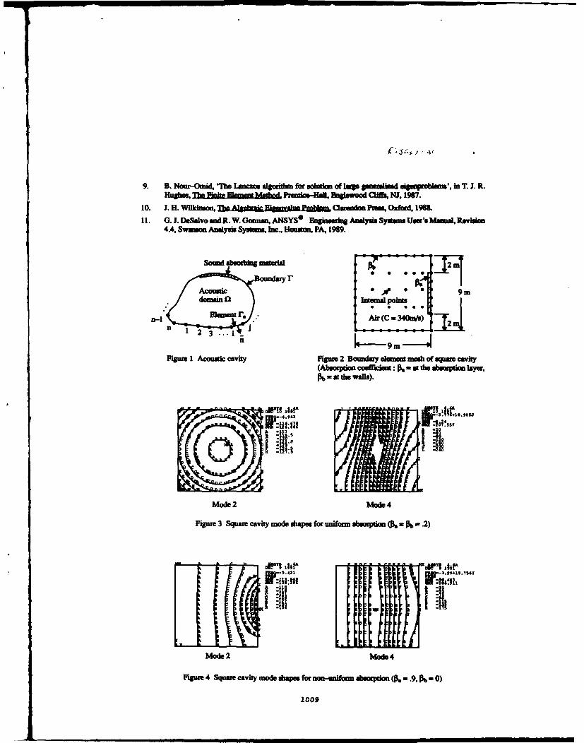
9. B. Nour-Omid, 7W Lammao algoidumi for ucila of large guesralked ulgsqublowu', in T. J. R.
10. J. H. Wilkinson Zmi Oarmulo Pm.., Oxford, 196.
11. 0. J. De~avo ad R. W. Goamn, ANSYSO Bnginsdg AnalsisSyimnaUs'ersMumalRaVisi4A. Swmua. Analysis Systans Inc.. Houmon, PA, 1969.
sound abbng mterWa
mbý PbBoundary r
Acoustic *9mdomain CA himenal points
3 .. I
Figure 1 Acoustic cavity Fgure 2 Boundary a]mu mesh of square cavity(Absorpio couffcint: P.-at the absoption laerPb -at dig walk).OARTS 116f1
Mode 2 Wo&e4
Figur 3 Square cavity mode diao for unifomo as~osptio (ft . Pb . .2)
1 :1121 -3, 41,75
Mode 2 Mlode 4
Figur 4 Square cavity mode diapes for nmqon-unifoa absrption (p6 .9, pb .-0)
1009

Table 1 Acoustic resonanice ftetleencies of cavity with zwo absorption (Ni - b- 0)
No. Thogatical1nilowices (Hz) Dmudwy Dunwt inife ULUIm
I0.900947059-05 -0.16W53645-05J -0.730307435-04 -0.98103W096406J
2 0 -0.900969153.-0 0.160519183-0J 0.730519423-04 0.931571645-06 J
3 - 0.000000003.00 -19.0315385J 0.000000006+00 -18.984927.14 18.6889 0.000000005.00 19.031585 J 0.23827455E-06 13.964927.JS - -0.19916942E-06 -19.1277081 0.290674743-06 -13.964928J
6 18.883 0.000000005.00 19.1277081 0.29079153-06 18.984928.1
7 - 0L00000000E400 -26.97142.J 0.000000003.00 -26.38742J
8 26.7129 0.000000005.00 26.9721421J 0.000000006+00 26.8487421J
9 - 0.000000005.00 -39.2140771J 0.000000003.00 -38.-48881
10 137.7778 0 .000000005.00 39.2140771 0.000000005.00 38.-48881J
Table 2 Acoustic resonance frequencies of cavity with uniform absorption (0, - P= 0.2)
Computed Phequendes
No. Boundary Elemen Finite Sleiemen
1 -0.69521872S410 -0-32956126E-091i 0.537121615-.09 0.514978405-091J2 -4.8788196 0.000000005.00 J1 -4.9431474 0.000000005.0013 -3.8496925 -18.905690 -3.7763896 -18.905246 J
4 -3.8496M2 18.9056901 -3.7763896 18.905246J5 -3.924848 -18.9736771J -3.776389 -18.9052471J
6 -3.9248480 18.9736781 -3.7763897 18.905247J
7 -5.3478454 -26.783942.J -5.1516059 -26.823973.J8 -5.3478454 26.7839421J -5.1516060 26.8239731J9 -4.5679968 -39.2112401J -3.9654993 -38.695021
110 1-4.3679969 39.2112401 J -3.9654994 38.695024
Table 3 Acoustic resonance fr-equencies of cavity with non-uniform absorption (Pa. - 0.9, O = 0)
Com utdRqecs
No. Boumday mement Finite Eksume
1 -0.322777923-07 -0.312459745-071J 0.707427675-06 -037968327E4-06J2 -3.3779687 0.000000005.001J -3.4207326 0.00000OE000500
3 -0.61991593 -193722901J -0.61317013 -19.236889J
4 -0.61991592 19.3722901J -0.61317014 19.23688915 -3.3924172 -19.7935521J -3.2896905 -19.75558316 -3.3924172 19.7935521J -3.2896902 19.7355531J7 -13665337 -27.3446341J -1.3564M9 -27.252889J
8 -13665337 27.3446341J -1.3564100 27.252889J9 -0.39190014 -39.4271601J -0.32248800 -38.7215211J
110 1-0.039190016 39A271601 J -0.32248W4 38.7215221J
1010

SECOND INTERNATIONAL CONGRESS ONRECENT DEVELOPMENTS IN AIR- AND
STRUCTURE-BORNE SOUND AND VIBRATIONMARCH 4-6. 1992 AUBURN UNIVERSITY USA
THEORETICAL AND PRACTICAL CONSTRAINTS ON THE MPLEMENTATION OFACTIVE ACOUSTIC BOUNDARY ELEMENTS
P. Darlington G.C. Nicholson
Department of Applied AcousticsUniversity of SallordSafford MS 4WT UK
ABSTRACTThe reflection of normally Incident plane acoustic waves from a plane impervious boundary can becontrolled by actively modifying the mechanical Impedance of the boundary suspension. Thisapplication of active control techniques motivates the study of active absorbers. The performance ofsuch active boundaries Is limited by both physical constraints on the transducers and controllingfilters and by the behaviour of adaptive signal processing algorithms which are used to design thecontrollers. This paper details some operational constraints imposed by the properties of thesuspension and forcing actuator used in the device and by the practical requirements of stabilityand causality in the system. The constraints are Illustrated in the context of an attempt to Implementa broadband active acoustic absorber.
NOMENCLATURE
c speed of sound (mIs) ZE voice coil blocked impedance (92)d distance (cone to microphone) (m) Zd desired spec. acoustic ImpedanceF total force on cone (N) (Ns/m3)i voice coil current (A) zm mechanical impedance (Ns/m)j 4-1m moving mass (kg) 0 transformation factor (N/A)p acoustic pressure (Pa) po equilibrium mass density (kg/m3)P power (Watts) c delay (s)R mechanical damping (Ns/m) 0) angular velocity (rad/s)S cone area (mW)T controller delay (s) Sbscript..u cone velocity (m/s)V controller output voltage (V) c at surface of coneW control filter i incident componentX cone displacement (m) r reflected component
I INTRODUCTION
It a plans impervious rigid plate, suspended with respect to mechanical ground by linear springs anddamping elements, is excited by a normally incident plane wave, it will be forced into motion. Thesuspension elements can be arranged so as to allow uniform motion over the entire surface. Under
1011

this condifion, the analytros of the r eflectioc wave, absorption of ancidenyacoustic energy by the surace and trawsmu ion of the acoustic dwokurbance Into a compresot blemedoum bansing the plate o a simple problem found in many acouertes textbooks. The behavlour omthe system can be characterized In terms of the rativ of the charactelstsc Impedance(s) of theflui(e) on either sxte of the plate and the lemant •mingednce of toe m utpended plate, a tiwacaunical Impedance tieng determined by the plates wurface mass fenscy and the paramete. ofthe suspension elements. N an addrtional foreng term is addpe to the equation of motion of theplate, it Is possible to actively modify the rmechanical Impedance of the struicture and so modify thereflection, absorblion or tranmission of sound.
Such an "Active Acoustic Boundary" has b eln the bubjea oo conviderble reserh effort, includingwork performed at Gottingen a1 lo and considerable research as Virginia Polytechnic Institute [3,4t.The German work has focussed upon the polaron of the imperion and asurfcb( on of an acinelycontssled bouncltry element, whit much ou the Ame)can work has concentrated upon the controlof transmission of acoustic energy over a pcrtition. Thlds paper dascrhbes some fundamenmal vimicswhich define an operating envelope for practical acnive boundary elements, presented In thesimplified context of a small active boundary element forming the termination of an acosi
wavaguers, operating at frequencies below the ne vlan be "cut-ordc frequency.
2 MODEL PROBLEM - THE ELECTRODYNAMIC ACTIVE ACOUSTIC ABSORBER
The discussions and expedmentai results presented in this paper are based upon animplementation of the oActive Acoustic Boundary Bement" concept bualt around a conventionaldThect radiating electrodynamfc loudspeaker. Using a loudspeaker as the bounvauy element hasseveral advantages - It has an (approximately) plans Impervious surface (the corne) which Is linearly
suspended with ospert to mechanicsl ground (the frarie) by a sut enswon ldesigned to permituniform ipiston-like" displacement of the cons. The loudspeaker also has a motor system via whichcontrolling forces can be apcived to the cone. To instrumei u the surface Impedance, c miniaturepressure microphone was fixed on the moving cone, In such an orientation as to minkmise thetraneducer't acceleration response. The coIn velocity can be trareduced by several e: ans - theresults presented In this paper use velocit measures derived from a miniature accelerometer fixedon the cone, the output of which wans integrated elecronicaly.
The control required to force the surface Impedance to some prepecified value is obtained by a
hnear filtering operation on meodufes of an acoustic variable in the waveguide. In the systemstudied In this cnper, the ptesrure at the cone of the loudspeakerf or et a point in the wmvegutdosome distance from the active termination, Is the vasable used as the input to the controlling filter.
2.10ptimal Controller Configuration
If the active Impedance device Illustrated In Fig. I Is achieving a desired Impedance:
u
then it Is possible to Identify the optimal configuration of the controlling filter, W.O. by solving theequation of motion of the cone. The total force on the cone Is a sum of the force due to the motorsystem, the acoustic reaction, and the silliness and damping of the supnsion:
F -(V -_W) - p.S - Ru -!Iu (2)
Subsiung the total force defined in equation 2 into the equation of motion of the cone gives:
1012

Figure 1 Experimental Electrodynemleo A*&*v Abeorber
*Y O-paS- Ru -ku mjnu (3)
which, recalinig that the loudspeaker voltage Is obtained by passing the pressure at the conethrough the controller (see Fig. 1):
V - -0
and substituinig for pN from equation 1, gives the optimum filter:
W-M Z' (Zu + ) +SZE(4)
Equation 4 phows that the filter required to force the surface acoustic impedance at the cone of theloudspeaker to the desired value of z. has two additive terms. The first term is proportiona to theInverse of the desired kimpedance, whilst the second term, SzEJ#, Is Independent of the requiredimpedance. (This second term Is actually the filler required to hold the cone of the loudspeakerperfectly still. Implementing an Wninke kimpedance, zd - -). In order for the optimum filter to berealizable, the desired surface Impedance should have a causally stable Inverse (as zgs Is a factor ofthe first term of the right hand skide of (4)). The only other potential problem In specifying the filterW~o are the singularities In the mechanical Impedance at the loudspeaker, za, at zero and hifinkefrequencies. ?Z has hIfinke magnitude at d.c. due to the suspension stiffness - this would requirethat W.01 should have Winksft d.c. gain, which Is, clearly, Irnpractical. Fortunately, practicalImplementations of active Impedances are banripass lmited (at low frequencies by the linearexcursion of the suspension, see section 3.1, and at high frequencies by the plane wave 'cut-off" ofthe wave grid) so the singularktles in the Ideal filter solution, (4), are never required.
2.2 Optimum Controller Using Upstream Preissure Signal.
if the Input to the controllng filter Is derived from a microphone located hIn the wavegulde somedistance from the surface of the cone (changing the position of the switch in Fig. 1) then theoptimum controller solution becomes significanitly more complicated. If the wavegulde Is lossless,such that the transfer function between the component of pressure due to rlghtwarde propagatingwaves at the upstream microphone location and the cone can be described by a pure delay,
1013

the optimal controller is given by:
+- S
WO r =-,7-eý
Wop + F 2" P )] (5)
where zr is the effecive mechanical impedance and F is the delay term:
ZT - Z++*2I/z F-ei00
Equation (5) reduces to equation (4) when F-1.
3 OPERATIONAL CONSTRAINTS OF PRACTICAL ELECTRODYNAMIC ACTUATORS
The optimal solutions developed above assume that the loudspeaker system used as the basis ofthe active termination has Ideal behaviour, characterized fully by a linear equation of motion, suchas (3). Real loudspeakers depart from this Ideal in two important respects; they have nonlinearsuspensions and motor systems and the voice coll can handle only a finite power. Both of thesenon-Ideal properties define edges of the operational envelope of adaptive Impedances built aroundeiectrodynamic actuators, which are discussed below.
3.1 Suspenlion Nonlinearlty
The suspension of a practical electrodynamic actuator does not have a linear compliance (anddamping) term, rather the compiance reduces as the cone Is displaced further from equilibrium - thesuspension stiffness hardens. There is, therefore, an absolute limit on the cone excursion. Wellbefore this fracture limit is reached, the suspension will become significantly nonlinear and it isappropriate to define an limit of (approximately) linear cone excursion. This limit of linearexcursion, I X , defines a frequency dependent limit of maximum linear velocity. I ulm,:
uI.., - o1X Ix., (8)
Note that the transducer has a velocity zero at d.c., as a consequence of the displacement limit.Given this zero In the practical transducers response, it Is never necessary to attempt to Implementthe dcc. pole in the Ideal optimal filter solution, (4). If, as shown in equation (6), the velocity of thecone of an actively controlbld Impedance is limited, then it is possible to define a maximum pressurethat can exist at the cone when the system is implementing a desired Impedance:
IplU lul,. IZI (7)
An example of this imitation on the pressure at the cone is presented in section 3.3.
3.2 Actuator Power Hand"l"g
The motor system of an electrodynamic loudspeaker has a finite electrical power handing capacity,which limits the voice coil current and resulting electrical force applied to the cone. This forceimposes a second Emit to the cone velocity, when the Impedance at the cone is held by thecontroller to the desired value of zd. If the maximum power handling of the voice coil is P Watts, thenthe maximum voice col current is:
IMM - '4 P/S*Ze~)
which, assuming the active Impedance is successfully Implementing the desired Impedance
1014

(equation 1) can be subetlbAsd Iito the equaIon ofimaont (3) to defin the maximinu velocity:
U. - I- I- 14P1!WZs)(8(Z.+SZd)
As described for eq"Ion (6), the velocity limit defined by (8) can be used either to specify the themaximumn pressure permissible for a given z (seee section 3.3), Or mnimnUM Zd for a specifiemaximum pressure.
3.3 Example
The cone velocity Ilmimb Imposed by the maximum cone linear excursion and the motor voice coilpower handling can be evaluated given the desird impedance, and the specifications of theactuator used. The experimental fig developed at the University of Safford uses 8200A drive units,manufactured by KEF Electronics Unmited, Tovil, Maidstone. England, having a 6.3mm (peak topeak) linear cone excursion, 50 Watts (programme) power handing and 8 Ohm nominal Impedance.Nf this loudspeaker is controled, such that the specific acoustic Impedance at Its cone is 416 Rayls.then the velocity limit are shown In Figure 2.
Figure 2 Velocity and Preesure Limits for the Eleatrodynamlo Acti* Absorber( Zda 415Rayle.) ___________________
S0 -, *1 3
1 ______ ______ 143 -_____a.
u V
a.) = -.- ý-- 133 E
> D
0 0.1 _____ __ __1230U _ _ _ _
113
0 200 400 600 800Frequency Hz
The actual velocity limit is defined by the smallest of equations (6 & 8) at any frequency - the conedisplacement limt dominates at low freqiuencies, whil st t frequencies above approximately 100 Hz.the velocity of the cone Is limited by the power handlng capability of the coil. As the Impedance atthe surf ace of the cone Is known to be zd - 415 Rayls, the maximum velocity dafta can be easilyscaled to give the maximum pressure which ce-i be sustained at the cone of this active absorber -this maximum pressure Is also shown In Figure 2.
4 CONSTRAINTS INTRODUCED BY THE 'FEEDBACK CONTROL TOPOLOGY
hlast of the previous work on the active control of surface acoustic Impedance (for example [1 -41)has been characerized by the wse of a "fefrad controller architecture. That Is to say theconr~olling filter soene the Input acoustic pressure incident on the active terminatrio and uses thissignal to deriv the control force required to dive the active boundary. The workc described In thispaper wsee a fundamentally different architecture, In which the controllr observes one componentof the system response (the cone pressur) and woes this signal to derive the control force. Thisapproach Is (aitost) a lseodbaciC control topology, In which, as the name suggests, a feedback

path exists from the plant response to the controler input. In the active termInation system describedIn this paper, the feedback path Is from the cone velocity (system output) to the pressure at the cone(controller Input) - any component of cone velocity caused by the electrical forcing term In theequation of motion (3) changes the pressure at the cone.
Using this feedback control approach Introduces several complications. including the potential forloop instability, which must be avoided If the system is to be practically useful. The incident andreflected pressure components at the cone may be related through an equation derived fromcontinuily of velocity:
Pr IP1- poc..u
which allows the system to be represented In terms of the block diagram of Figure 3 The figuredearly shows a feedback path around the controled termination, generating the reflected pressurecomponent of the acoustic pressure at the cone, pc. In order for the loop to be stable, Its magnitudetransfer function should be smaller than unity:
I z P'C I (1
which can be rearranged to give a lower Imit on the impedance which can be Implemented by acontroller In the presence of the feedback path:
I z1 > pc (9)
Note that a further potential feedback path exists, In which the reflected pressure propagates awayfrom the actively controled termination and is again reflected, to form a component of the Incidentpressure. In a practical duct this feedback path has magnitude gain equal to or smaller than thedrect path described above and does not usually significantly after the stable bound (9).
Equation (9) shows that it Is Impossible to implement an active ideal absorber (zd- p•c) using a purefeedback architecture. The system studied at the University of SalWord includes an electrical"feedback canceling" path which subtracts an estimate of the feedback components of pe from theInput of the controlling fIlter. The transfer function of the feedback cancelling filter is automaticallyestimated before the system Is operated, and attempts to cancel both the "drect" reflected pressurecomponent and any component of the Incident pressure due to feedback. Using this feedback
Figure 3 Block Diagram of the Feedback Controlled Active Absorber
+
1016
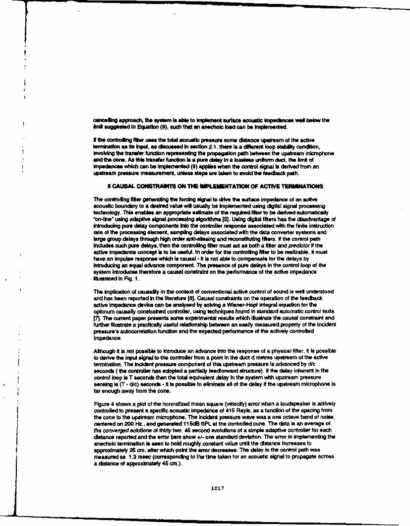
canceling approach, the system Is able to Implement surace acoustic impedances wel below theimit suggested In Equation (9). such that an anechoic load can be implemented.
if the controling filter.uses the total acoustic pressure some distance upstream of the activetermination as ft input, as dicuessed In section 2.1. there Is a diflerent loop stability condition,involving the transfer function representing the propagation path between the upstream microphoneand the cone. As this trander fuiction Is a pure delay In a lossless unfuorm duct, the imit ofImpedances which can be Implemented (9) applies when the control signal is derived from anupstream pressure measurement, unless steps are taken to avoid the feedback path.
5 CAUSAL CONSTRAINTS ON THE IMPLEMENTATION OF ACTIVE TERMINATIONS
The controlling filter generating the forcing signal to drive the surface impedance of an activeacoustic boundary to a desired value will usually be Implemented using digital signal processingtechnology. This enables an appropriate estimate of the required filter to be derived automatically"on-line" using adaptive signal processing algorithms [5]. Using digital filters has the disadvantage ofintroducing pure delay components into the controller response associated with the finite instructionrate of the processing element, sampling delays associated with the data converter systems andlarge group delays through high order anti-allasing and reconstituting filters. If the control pathincludes such pure delays, then the controlling filter must act as both a filter and predkctor I theactive Impedance concept is to be useful. In order for the controling filer to be realizable, it musthave an Impulse response which Is causal - it Is not able to compensate for the delays byintroducing an equal advance component. The presence of pure delays in the control loop of thesystem introduces therefore a causal constraint on the performance of the active Impedanceillustrated in Fig. 1.
The Implication of causality In the context of conventional active control of sound is well understoodand has been reported In the literature [8]. Causal constraints on the operation of the feedbackactive Impedance device can be analysed by solving a Wiener-Hopi integral equation for theoptimum causally constrained controller, using techniques found In standard automatic control textsM7J. The current paper presents some experimental results which illustrate the causal constraint andfurther illustrate a practically useful relatlonship between an easily measured property of the Incidentpressure's autocorrelation function and the expected performance of the actively controledImpedance.
Although it Is not possible to Introduce an advance into the response of a physical filter, it Is possibleto derive the input signal to the controller from a point in the duct d metres upstream of the activetermination. The Incident pressure component of this upstream pressure Is advanced by d/cseconds (the controller has adopted a partially feedorward structure). if the delay inherent in thecontrol loop Is T seconds then the total equivalent delay In the system with upstream pressuresensing is (T - d/c) seconds - it is possible to eliminate all of the delay if the upstream microphone isfar enough away from the cone.
Figure 4 shows a plot of the normalized mean square (velocity) error when a loudspeaker Is activelycontrolled to present a specific acoustic impedance of 415 Rayls, as a function of the spacing fromthe cone to the upstream microphone. The Incdent pressure wave was a one octave band of noise,centered on 200 Hz., and generated 115dB SPL at the controlled cone. The data is an average ofthe converged solutions of thirty two, 46 second evolutions of a simple adaptive controller for eachdistance reported and the error bars show +1- one standard deviation. The error in implementing theanechoic termination is seen to hold roughly constant value until the distance Increases toapproximately 26 cm, after which point the error decreases. The delay in the control path wasmeasured as 1.3 msec (corresponding to the tIme taken for an acoustic signal to propagate acrossa distance of approximately 45 cm.).
1017

Figure 4 Converged Nomalized US Veloolty Error and Max { q r,,(c) I) (r.&o for theAdaptive Absorber (z4415) with Upstream Pressure Detection. (Error bare show a4. o)
0.30
.0
E 0.9N0
V
•02 10.80
00
Z 0.00 1.. .. .. .. .. .. .. .. .. .. . .7000 20.0 40.0 600
Distance cm
Also shown In Fig. 4 Is the maximum absolute value of the incident pressure's autocorrelatlonfunction for lag greater than the effective delay (T-dic). Experience has shown this parameter to bereasonably well correlated with the norm of the optimum controller's Impulse response vector and,consequently, with the coherence between the actual and predicted cone velocities. According tothis empirically observed relationship, the optimum mean squared error In the Implementation of adesired Impedance Is proportional to:
E[se _ I- MX r(C1 ))2 (10)t > (1"dc)
Equation 10 shows that the causal constraint can be effectively removed by Increasingd, when the system becomes a pure feedforward controller. Equation 10 also reveals that a purefeedback system (d-0) can estimate a desired Impedance to an accuracy which can be predicted Ifthe autocorrelation function of the Incident pressure signal Is known.
CONCLUDING REMARKS
This paper has demonstrated that physical properties of a conventional electrodynamic loudspeakerused as the basis of an active acoustic boundary element Impose limits upon the range of specificacoustic Impedances which can be Implemented. Further constraints are Imposed by the physicalrequirements of controller stability and causality. Despite these constraints It Is possible to constructactive acoustic ioads using feedback control which will approximate desired surface specificacoustic Impedances to a predictable degree of accuracy for a defined Incident pressure signal.
REFERENCES
[11 Guicldng, D., KarcherK. & Rolwag, M. "Coherent Vlllralllon I•ut : An Ex.Jqaw• ComlparieWActive M -IIIoa for use in Rowm Aoom~•;' JASA J.Sound Vi v145(2) pp19 - 215v78(4) 1985 ppl1426 - 1434 R5" Nk~holson, G.C. & Darwon, P. "Sgmmt Subs for[2] Wenzel. IA a Guldfng D l •t&os und Budk AcouNW Pro.• I l 3. ple.1 991 .ppEx mermoe xur Adepiwll skier aidlvsm Sd~lmdkW mot 155-164dine brfen• voeel Wentlbpedee, PI] Nelson. PA•, Hamnmond, J.K 9 Elliott. S.J.F FF~shrlte der AkIt•k DAGA '01990 pp 899 - 902 "Casa Co ý oan go Active C.onlrol of SoumrfP3] Fufler, 0. -"Aoe Coarll Soun 0d Tr.nanisdon Pro;. ICASSP.1987, pp 145-148
R•Ld from Ellesto Plstle by VibraMl• In~ bu: L ['/Laning, JAH & Baft.n R.H. "Randont Proossess In,•/WJm* nd • .0v36 1990 pp 1-15 ,Aullosc Contro', lMcGraw-HI111, 1966, (Chapter 7)R4] Ritter. C. "Active Carol of Sound Radoialon from awiring Rangta Panel by Sound Sources and
1010
S• • - • • i am ll Il I . ..... mi • •z

SECOND INTERNATIONAL CONGRESS ONRECENT DEVELOPMENTS IN AIR- AND
'STRUCTURE-BORNE SOUND AND VIBRATIONMARCH 4-6. 1992 AUBURN UNIVERSITY. USA
BOUNDARY ELEMENT FORMULATIONS FOR ACOUSTIC SENSITIVITIES WITH RESPECT TOSTRUCTURAL DESIGN VARIABLES, AND ACOUSTIC IMPEDANCE
Nickolas VlahopoulosAutomated Analysis Corporation
2805 South Industrial, Suite 100, Ann Arbor, MI
ABSTRACT
The concept of acoustic optimization for structure - borne noise (i.e. modifying the vibrating structure inorder to reduce the emitted noise) is closely related with the derivation of acoustic sensitivities. In this paperthe principles of acoustic optimization are discussed initially, and two algorithms for acoustic sensitivities aredeveloped. (i) Acoustic sensitivities with respect to structural sizing design variables, where physicalproperties of the structure are used as design variables. These can be readily used in an automated optimizationprocess. This methodology is applicable to both interior and exterior problems. (ii) Acoustic sensitivities withrespect to acoustic impedance. The property of the absorbing material used as treatment is the design variablein this formulation. These sensitivities can indicate the optimum distribution of absorbing material.
I. INTRODUCTION
Two type of analyses are associated with analytical structure - borne noise prediction (FIgure 1). The FiniteElement Method (FEM) is commonly used to compute the vibration of the structure emitting noise [1], [2], andthe Bonnday Element Method (BEM) can be used topredict the generated noise (3]. Tberefolre, the smrucnalanalysis is performed by FEM and the acoustc analysis by BEM. Other methds for acoustic prediction amealso available (finite element method (4], statistical energy analysis [51) but in this paper the focus will be onthe BEM. The scope of an acoustc optimization process is to reduthe he strctr - borne noise by modifyingthe noise source, i.the he structure. Design itrions can be performed by the designer based on practicalexperience, but this is not the most efficient method. An automated optimization process can be developed(Figure 2) with the stctual and the acoustc analysis as integra parts of the optimization. Within each loopthe FEM analysis computes the response of the structure, and the BEM analysis predicts the generated sound.The optimizer changes the values of the structural design variables, the finite element structural model isupdated, and the next optimizatim loop begins. The process is continued until convergence, or an acceptablenoise reduction is achieved. In an optimization scheme it is inpbrutant to have available the gradients(sensitivities) o: the objective function and the constraints, ith respect to the design variables in order to guidethe solution (61. Formulation of acoustic sensitivities is te first step in crating an acoustic optimizationprocess, and the scope of this paper is to develop formulations that can readily be used within an automatedprocess. Two algorithms for acoustic sensitivities aem developed in this paper(i) Acoustic sensitivities with respect to sizing design variables.
The physical properties of the structure are used as design variables. This methodology can be applied toboth interior and exterior problems lor noise reduction.
(ii) Acoustic sensitivities with respect to acoustic impedfce.The acoustic impedance of the absorbing material used as treatment is the design variable in thisformulation.
10.9

Previous work has been done in deriving hape sensitivities in the BEM [7], [81. However, there are twoproblems asociated with actually implementingem in an au,-amtd optimization procss:(i) It is expensive to obtain good shape sensitivities, and general purpose finite element programs do not in
general have available such a feature.(ii) It is difficult to update the finite element model within an automated process at the beginning of each
iteration, when shape modifications must be implemented [9]. Simple modification rules for deformingthe initial mesh often run into problems, and general purpose software packages performing adaptive meshrefinement art not yet available.
In this paper the effort is concentrated on formulating sensitivities with respect to sizing design variables, thatcan be used in an automated process.
Efforts have also been made to use sensitivity analysis and optimization concepts with other acousticprediction methods. Specifically a finite element procedure for design of cavity acoustical treatments wasdeveloped [101. Acoustic optimization using the finite element method for acoustic prediction was performedfor a car interior [11], and an optimization method selecting the damping treatment was developed [ 12] usingthe statistical energy analysis method.
In Section II of this paper the formulation of acoustic sensitivities with respect to sizing design variables isderived, and areas of applicability are identified. Section III contains the formulation with respect to acousticimpedance and the potential applications. Finally, Section IV contains the plans for utilization of this research,and further developments.
II. ACOUSTIC SENSITIVITIES WITH RESPECT TO STRUCTURAL SIZING DESIGN VARIABLES
The numerical implementation of the Boundary Element Method in acoustics is a two step process. First thesystem of equations:
[A] fp) - [B] (u.) = (0) (1)
is solved on the boundary surface. (p) = vector of acoustic pressure on the surface, (un) = the vector ofnormal velocities on the structural boundary, [A] and [B] =t full matrices depending only on the geometry ofthe surface and the frequency of excitation. Once (p) and {un) are computed the acoustic pressum at any fieldpoint can be computed:
p,= {A IT(pj - (Bo)T un) (2)
where subscript "o" indicates a field point and the vectors {Ao), {Bo) depend only on the geometry of theproblem and the frequency of excitation.
•poThe scope of this formulation is to derive the acoustic sensitivity -•- where Po = acoustic Pressure at the
field por -" and h = structural sizing design variable. The term sizing indicates that the change in the physicalproprty does not influence the shape and the geometry of the structure. The design variable h can be forexample the thickness of a plate, the stiffness of a spring, the cross sectional area of a beam, a materialproperty etc. In this formulation we will consider only velocity boundary conditions for the acoustic problem.This, however, does not impose any restriction in the formulation, since condensation can be used to reducethe system in the section with only velocities as boundary conditions. The algebra involved, however, is moretedious and therefore not presented in this paper.
By using the chain rule, -c- can be written:
op. ± apo )
(3)
1020

where uni = nonmal velocity of the ith element, and I toWi number of boundary elements used in the model.
apoIn this manner the acoustic sensitivity is decomposed in two pars, t-- which can be calculated firm the BEM
au.~
acoustic analysis, and ) which can be calculated by the FEM structural analysis. The first part indicates
how the acoustic j-ssure changes with respect to the boundary conditions (acoustic part), and the second howthe boundary conditions change with respect to the design variables (structural part). By differentiating Eq. (1)with respect to the ith element normal velocity uni:
,Aaup aia u } • =o(p) {P+ [A alpn a'O fn) -[1B (]
•u n, &.' O(4)
In this equation -a] a_] = 0, because [A] and [B] are only geometry dependant, and change of thealu. flu
velocity unl does not imply changes in the geometry, since only sizing variables are considered in thisformulation. Therefore from Eq. (4):
'Ip} = [A]-'[B] (Id}aun, (5)
where (Ii) = unit vector with only one non - zero component in the ith position. For a field pointdifferentiating Eq. (2) with respect to uni results in:
(0 A 'T{p)., (A.) (B0)T I (6)
T a{Bo}T
Where terms an are neglected. Substituting Eq. (5) into (6) results in:
"0P-Z =((A Ao T[A]"1 UB] -[Bo}T} {liJ
ap 0 (BC(7)
apoThis constitutes Jte derivation of the acoustic part of the acoustic sensitivity --. he terms in the right hand
side of Eq. (7) can be readily available firom the solution of the BEM analysis for the acoustic pressure. Theadditional computational effort in solving Eq. (7) is negligible if a solution for the acoustic problem exists. For
*apo,all the optimization itatioms a. will not change since all the terms in the right hand side of Eq. (7) depend
on the geometry only. Therefore, in an acoustic optimization process with structural sizing design variables
apo 4.need to be calculated only during the first iteration. • constitutes the acoustic part of the acoustic
sensitivities.
1021

aunlThe second part of the acoustic sensitivities is T- and can be calculated during the finite element analysis
of the structure. When the femquency response analysis is performed using the direct approach the solution iscomputed in the frequency domain by:
- (o02k ] {(x} + i (0 [CS] {,Xj + (K] (x) -- (F.1 (8)
where [M], [CS], [K] = mass, damping, and stiffness matrix, (Fol = forcing vector, Ixo) = responsedisplacement, and to = frequency of excitation. Eq. (8) can be written as:
is] (xe) = IF.) (9)
where [S] =- 2 [M] + i o [C] +[K] ). By differentiating Eq. (9) with respect to a sizing design variable hresults in:
a[S] (0)Sfx + [S] + = (0)
{xo} a[S]) -Xo
(1h - [S(10)
hrS] e2 [ 2A[M] . A[C] A[K]]
where - + 0 +- ]. Fro Eq. (10), considering that the solution is obtained in
the frequency doman, i can be derived from L and accounting for the geometry -•- can becomputed. This is the structural part, of the acoustic sensitivities and it can be computed within the structuralanalysis. Unlike the acoustic part it must be computed within each iteration loop. If the modal method is usedfor frequency analysis the structural part of the acoustic sensitivities can be computed using information fromthe eigenvalue and eigenvector derivatives.
In this section the acoustic sensitivities with respect to structural sizing design variables am derived. Theformulation for the acoustic part can be readily implemented in an acoustic code based on the BEM, and it isintended to be implemented in SYSNOISE, a general purpose acoustic code [131. The structural part can becomputed either externally from a general purpose finite element code using data extracted from the code, orinternally if the code has a capability for the user to modify the solution sequence (for example DMAPprogramming in MSC/NASTRAN). The developed methodology can be used in all the areas where acousticprediction through the BEM is applicable. It can be used for both interior and exterior noise problems. In theautomotive and the construction equipment industry it can be used in reducing the interior passenger cabinnoise (see Figure 3), or the exterior noise emitted from vibrating components (engine blocks, transmissionetc). Aerospace application can be the reduction of the passenger cabin noise. Finally, it can have significantmilitary applications, contributing in reducing the noise emitted from structural components of militaryvehicles. This is important because their survivability depends on the acoustic signature they emit.
III. ACOUSTIC SENSITIVITIES WITH RESPECT TO ACOUSTIC IMPEDANCE
For this development Eq. (1) and (2) of the two step BEM solution process are used. By considering eithervelocity or impedance boundary condition, and denoting them with subscript "1" and "2" respectively, Eq. (1)and (2) become:
AIfA1 PiH) B1iB12i uni)=1 0 1A2 A22 ýP2 1B21B22] Un2) (11
and
1022

For area "2", (p2) } ffi [ un2), where [C] diagonal acoustic impedance matrix. Substituting in Eq. (11)
results:
AIIA1 Pi IIB1 (0) (a)
A21 A22 [C] { u .2) ) -[B21B22]UU:2')= (b) (3)
In order to condense this equation to variables of the area "I" only, fir Iun2} is expressed in terms of (Pl)and {Unl } from Eq. (13b), and then it is substitutedA in Eq. (13a). This results in:
(U.2) ----[D] [B21] {Unl}- [A211 {POl}14
and
[AC] (p1) -[• ] Pt}) = u 0) (15)
where PII = [[A22] [C] - []B22]] , and
[AC] =[[All] - [AI7J [CI PD] A21] + [BI] [I] IA21]1 16
[BC] =[[Bll] - [AI2] [C] PDI [B21] + IBI PI] D [B21] (7
By considering the impedance value of an element as design variable, or an entire area of elements with a
common value for acoustic impedance and denoting it by ci, differentiation of Eq. (15) results in:
[AC3 clip') +[AC-] {PI}- [BC] a_.• 14[ +IDBC] {un} = (03a• &ji (18)
where
a[C] A[C] BIp] ý AID].3ci Acj &ci Aci (19)
PAC a[AC] [DBC] = a[BC'acj acj(20)
In deriving Eq. (18), (19) and (20) matrices [A] and [B] are independent from the acoustic impedance used asdesign variable. In Eq. (18) (Unl I is independent of ci, therefore:
[AC] alp') [DAC] {Pl} - [DBC] (u.1) = {DF}
kj (21)
alp,)i can be computed from Eq. (21), and -!i2 from Eq. (14) as:
1023
S ... . . . . • .---- ,,----- • ,,,• m, m mnu m Il.. mu u I I !OWN

a~un•=.•][[B2] {nl}- A211 pl}l]- PD] [A21]a{
ac, &j [ NO(22)
Then for a field point Eq. (12) results in:
= (f aPia_•_0 Un2c + (u [q3
U_ B. (23)
In this type of acoustic optimization the structural analysis determining the velocities Junl) need to beperformed only during the first iteration, since the structural vibration is not considered to be affected from theabsorbing material used as acoustic treatment. Only the acoustic analysis will be performed within eachiteration (see Figure 2). This methodology can be applied in the automotive and aerospace industry to optimizethe distribution of the absorbing material used as treatment in passenger compartments.
IV. FUTURE APPLICATIONS
The two formulations for acoustic sensitivities, developed in this paper, can be implemented in the generalpurpose acoustic code SYSNOISE. They are based on the collocation boundary element method, uncoupledsolution (i.e. only the effect of the structure on the fluid is considered). Since SYSNOISE also includes thevariational formulation and a coupled solution sequence, effort will be made to further expand the algorithmsdeveloped in this paper for the variational BEM method, and for coupled problems.
V. ACKNOWLEDGEMENTS
I would like to express my gratitude to Automated Analysis Corporation for the availability of the ourcesthat allowed completion of this research effort, and to Numerical Integration Technologies ior theirencouragement in pursuing this development.
REFERENCES
1. Hughes, T.J.R., "The Finite Element Method, Linear Static and Dynamic Finite Element Analysis,"Prentice - Hall, 1987.
2. Meirovitch, L, "Computational Methods in Structural Dynamics," Sijthoff and Nordhoff, 1980.
3. Fyfe, K.R., and Coyette, J.P., "Acoustical Design Using the Boundary Element Method," SecondInternational Conference on Methodology and Innovations in Automotive Experimentation, Florence, Italy,November 22 - 25, 1988, pp. 102 - 116.
4. Coyette, J.P., and Guisset, P., "Finite Element Methods for Interior Acoustics," Second InternationalConference Methodology and Innovations in Automotive Experimentations, Florence, November 22 - 25,1988, pp. 138 - 154.
5. Lyon, R.H., "Statistical Energy Analysis of Dynamical Systems: Theory and Applications," The MITPress, 1975.
6. Haftka, R.T., and Kamal, M.P., "Elements of Structural Optimization," Martinus Nijhoff Publishers,1985.
7. Smith, D.C., and Bernhard, R.J., "Computation of Acoustic Shape Design Sensitivity Using a BoundaryElement Method," Numerical Techniques in Acoustic Radiation, Winter Annual Meeting of ASME, SanFrancisco, California, December 10-15, 1989, pp. 109 -116.
8. Kane, J.H., Mao, S., and Everstine, G.C., "A Boundary Element Formulation for Acoustic ShapeSensitivity Analysis," Journal of the Acoustical Society of America, Vol.90, July 1991, pp. 561 -573.
1024

_ _ _- - :- ..
9. Haftka, R.T., and Grandhi, R.V., "Smtctural Shape Optimization - A Survey," Computer Methods inApplied Mechanics and Engineering, vol. 57, 1986, pp. 91 - 106.
10. Bernhard, RI., and Takeo, S., "A Finite Element Procedure for Design of Cavity Acoustical Treamnents,"Journal of the Acoustical Society of America, Vol 83, June 1988, pp. 2224 - 2232.
11. Nagabuchi, K., Hagiwara, I., and Arai, A., "Application of MSCINASTRAN Sensitivity Analysis atNissan Motor Company," 1989 MSC World Users Conference Proceedings, March 15 - 17, 1989.
12. Lu, L.K.IL, "Optimum Damping Selection by Statistical Energy Analysis," Statistical Energy Analysis,Winter Annual ASME Meeting, December 13 - 18,1987, Boston, Mass, pp. 9 - 14.
13. Coyette, J.P., "Numerical Acoustic Analysis in Automotive Design Using SYSNOISE," NAG NededandsAkoestisch Genootschap, Journal 99, September 1990, pp.2 9 -42.
StructuralFEA Vibration
Vibration FEA _BEM ,
Figure 1. Analyses associated with noise prediction
1025

S (Optimilze~r- -
r. I0 Stutua AcousticsEAVibr~ationý FEA Noise]
FEA BEM
L SStructural
AnalysisAcoustic Analysis
Figure 2. Flowchart of an acoustic optimization process
Thickness of panel usedas design variable
Figure 3. Example of a sizing design variable for an automobilecompartment
1026

SECOND INTERNATIONAL CONGRESS ONRECENT DEVELOPMENTS IN AIR- AND
STRUCTURE-BORNE SOUND AND VIBRATIONMARCH 4-6. 1992 AUBURN UNIVERSITY. USA
MODELLING RADIATION FROM SUBMERGED STRUCTURESA COMPARISON OF BOUNDARY ELEMENT AND FINITE ELEMENT TECHNIQUES
Jean-Pierre G. CoyetteNumerical Integration Technologies N.V.
Ambachtenlaan, 29B3,601 Heverlee
(Belgium)
ABSTRACT
Various computational strategies are available for modellingradiation from submerged structures. The most usual way consists touse a coupled procedure where the unbounded acoustic medium ismodelled using boundary elements while finite elements are selectedfor the structure.
An alternative is offered by selecting both acoustic and structuralfinite elements. In this case, the near field is modelled usingconventional acoustic finite elements while the far field isdicretized into infinite elements. These infinite elements containappropriate interpolation functions in order to describe the farfield behaviour. The so-called 'wave envelope' approach can beselected in order to speed up the generation of element matrices.
These two approaches are reviewed and compared in this paper. Bothformal aspects are described but also specific application toradiation from submerged structures.
INTRODUCTION
Modelling of radiation from submerged structure usually involvecoupled models where reciprocical fluid-structure interactioneffects are taken into account : structural displacements act asboundary conditions for the fluid while fluid pressures generateadditional loads on the structure.
The effective consideration of these effects require selection ofappropriate models. The unbounded character of the fluid domain is adifficulty which can be overcome using a boundary integralformulation. The dimensionality of the problem is reduced so thatonly a boundary discretization is required. The direct boundaryintegral representation usually selected involves surface pressuresand normal velocities.
1027

Reciprocical effects can easily be handled using a couplingprocedure converting, on one hand, structural displacements intoboundary normal velocities and, on the other hand, fluid pressuresinto mechanical loads. This approach has been described by WILTON[81 and will be summarized below.
An alternative procedure consists to use both acoustic andstructural finite elements. The unbounded character of the fluiddomain is not well suited for a finite element approach. The problemcan however be handled by defining some radiation impedance boundarycondition on a fictive surface located at a finite distance from thestructure. Difficulties of locating this fictive boundary andassigning suitable boundary condition can be overcome by usingacoustic infinite elements for the far field. These elements allowto map a region of infinite extension and use appropriateinterpolation functions in order to reproduce the expected far fieldbehaviour.
These elements have been introduced by BETTESS [1] some years agoand have been successfully refined recently by ASTLEY and COYETTE[4,5] through application of a 'wave envelope' process allowing tosimplify generation of related element matrices.These two concarrent approaches are presented below. Application toa submerged structure is then described.
MIXED FINITE ELEMENT/BOUNDARY ELEMENT APPROACH
As stated before, this approach relies on the use of a conventionalfinite element model for the structure while a direct boundaryintegral representation sustains the development of the acousticboundary element model.
Acoustic boundary element representation. In the frequencydomain (assuming a time dependence like exp(+iwt)), the basis forsuch an approach is the Helmholtz surface integral equation linkingsurface pressure p and normal velocity vn :
c(x)p(x) - p,(x)+ (y) G(xy + iwpv. (Y)G(xY) dS(y) (1)
where x and y are points located on boundary surface S, ny is thelocal normal to S at boundary point y (assumed to be directed intothe fluid medium) and Pi is the incident field pressure.
In the above expression, G(x,y) is the usual Green function(fundamental solution of 3-D Helmholtz equation for a point sourcelocated at y point) given by
G(xy) _ exp(-ikR(x,y)) (2)4HR(x,y)
where R is the distance between x and y points while k is thewavenumber.
The numerical procedure relies on discretization of boundary surfaceS and selection of interpolation functions for both surface pressureand normal velocity.
1028

Collocation of the discrete form of Eq. (1) at each boundary node inturn allows to set up a relation between nodal pressure vector P andnodal normal velocity iector V
[A](P) - (P,) + [(B(V) (3)
where A and B are frequency dependent matrices while Pi is thevector of nodal incident pressures.
In a coupled model, the normal velocity vector V is related to thestructural displacement vector U through
(v) - iW[T](U) (4)
where the matrix T contains normal components at boundary nodes.
Structural finite element model. The structural model is basedon a displacement finite element model and is characterized, in thefrequency domain, by :
(zJ1u) - (F.) - (&1](P) (5J
where C is the geometrical coupling matrix allowing to convert fluidpressures into mechanical loads while ZS is the structural impedancematrix given by :
(Z5, - [K.] + iw[D.] - -2[1] (6)
where KS, MS and DS are the usual stiffness, mass and dampingmatrices.
Coupled model and solution strategy. The coupled model resultsfrom merging Eq. (5) and (3) using the kinematical continuityrequirement expressed by Eq. (4). The resulting coupled systemappears as
lu)BT A]( P (P (7Alternatively this system can be written using a modal descriptionfor the structure. In this case, the structural displacement vectorU is expressed as a combination of structural modes through
(U) - [(D](X) (8)
where 4P is the modal matrix while X is the vector of modalparticipation factors.
System (7) can be rewritten as
1(X) P, (9)
1029

where
r] - [c][j]
are the so-called modal impedance matrix, modal load vector, modalcoupling matrix and modal normal matrix, respectively.
Solution of either system (7) or (9) is performed using an efficientfluid methodology where structural unknowns are first eliminated(taking into account sparseness and symmetry of structural matricesand specific properties of C and T matrices). The resulting updatedfluid set of equations is then solved for nodal pressures. Recoveryof structural displacements results from solution of system (5).
It must be stressed that the direct boundary integral formulationsuffers from non-uniqueness of the solution at critical frequencies(eigenfrequencies of related Dirichlet interior problem). The so-called 'CHIEF' procedure [10] has been selected to remove thisproblem.
The above procedure has been implemented in SYSNOISE 4.4 (6) whichallows to import either structural matrices or a modal basis fromstructural packages in order to set up the structural model and tosolve the coupled problem.
FINITE ELEMENT/INFINITE 'WAVE ENVELOPE' ELEMENT APPROACH
This alternative procedure makes use of structural finite elementscomobined with (volumic) acoustic finite elements for the near fieldwhile infinite 'wave envelope' acoustic elements are selected forthe far field.
Acoustic finite elements are iso-parametric elements with unknownnodal pressures. Infinite 'wave envelope' elements are based onmapped infinite elements (as described in [21) and make use ofspecial interpolation functions combining polynomial and harmonicexpansions.
Weichted residual statement. Solution of Helmholtz equation inan infinite domain V is based on application of a weighted residualstatement incorporating field and boundary residuals.
Considering only velocity boundary conditions on surface S
ap/an - -ipwv. on S (II)
and the equivalent finite approximation for the radiation conditionon a far field boundary Sm
ap[an - -ikp on S. (12)
the weighted residual statement is formulated as
J(VW, - Vp + k-vWp)dV + JI pw W, v. dS - Jik , p dS - 0 (13)V S
1030

where Wi are weighting functions.
If acoustic pressure p(x) is written as a trial expansion of knownbasis functions Ni(x) and unknown coefficients qi, correspondingstiffness, mass and damping matrices are
V
-.1 f (W, ujcni (14)V
D -I J (PN,) NdSS.
and the acoustical loading vector is
F,- ip- f ( W, v. )dS (15)
The unknown coefficient vector Q (containing nodal pressures qi) isgiven by solution of equations
[Ka + ikD. - k-2 N.](Q) - (F.) (16)
infinite element mapping. The existence of the infinite domainrequires to subdivide exterior region into inner and outersubregions. The inner region lies close to the radiating surfacewhile the outer region extends to S.2
A conventional finite element mesh is constructed within the innerregion and usual shape functions are selected for both Ni and Wifunctions.
The outer region is subdivided into a single layer of infinite waveenvelope elements matched to the conventional mesh at an arbitraryinterface.
The mapping and interpolation functions related to these three-dimensional elements are based on reference [21
Polynomial expansions Fi in local coordinates (~',)are selectedsuch that the expected far field behaviour (1/r for 3-D problems) iswell reproduced along local infinite direction
The wavelike behaviour of the solution is also approximated by theexponential factor. Moreever since the near field/far fieldinterface is located at r-a, compatibility with conventionalacoustic finite elements is ensured.
Wave envelope weighting scheme. The wave envelope approachintroduced by ASTLEY (3] for large but finite elements has beenextended to infinite elments by ASTLEY and COYETTE [4,51 andinvolves weighting functions defined as the complex conjugates ofthe basis functions Ni multiplied by a factor (air)2 ensuring thatmass and stiffness integrals are finite and that radiation integralvanishes as the outer boundary approaches infinity
1031

S- (a1r)2 A (18)
The use of above interpolation and weighting functions allows to setup element mass and stiffness matrices which can be assembled in theusual way to form global mass and stiffness matrices.
A key feature of these element matrices is the cancellation of theexponential factors within each integrand and the boundedness of allresulting integrals as the element volume becomes infinite. Allintegrands can therefore be transformed to a finite region of theparent space and integrated numerically using standard Gauss-Legendre quadratures.
This is a major advantage over conventional infinite elements whichrequire the more complex Gauss-Laguerre quadrature scheme. Anadditional interest results from the fact that related elementmatrices are frequency independent so that far field mesh usuallydoesn't need to be refined as frequency increases.
Extension to coupled problem. Extension of above approach tocoupled problems is straightforward. The discrete structural modelbased on finite elements can easily be coupled to the above acousticfinite element/infinite 'wave envelope' element model following theprocedure described for coupling structuzal finite elements andacoustic boundary elements. This operation leads to the system
[ . _W2M2 K. - •k . ( = (19)
Various solution strategies can be selected for solving Eq. (19).The fluid methodology is based on elimination of structural degreesof freedom and solution of related (updated) fluid problem.Conventional modal approach can also be used for the structuralmodel while Ritz vector approach [7] appears as a promising tool forthis kind of problem.
APPLICATION
The problem of a submerged spherical shell is considered [9]. Inthis problem, a thin-walled spherical shell is submerged in a liquidand driven internally with a point load. The shell has a radius a =5m, a uniform thickness h = 0.15m while the constitutive materialhas a Young's modulus of 2.07x101 1 Pa, a Poisson's ratio of 0.3 anda density of 7669 kg/m3 . The fluid is water with a density of 1000kg/M3 and a sound speed of 1524 m/sec. A load of 1 N is applied atone pole and solution is computed at ka=l and 1.5 .
Due to symmetry, only one fourth of the actual structure has beenmodelled. The structural finite element mesh is shown at Figure 1(241 nodes, 216 elements). This mesh is also the boundary elementmesh used for coupled FEM/BEM computations. The acoustic finiteelement mesh used for the near field is represented at Figure 2 (864brick elements). Far field is modelled using 241 infinite waveenvelope elements with linear interpolation functions Fi alonginfinite direction.
Surface pressures along a meridian line are represented at Figures 3and 4 for ka=1 and 1.5, respectively.
1032

From these surface results, far field pressures can be computedusing the discrete form of Eq. (1). Directivity diagram in symmetryplane x = 0, at a distance d=20a from shell's center has beencomputed using surface pressures and normal velocities obtained fromthe two models. Magnitude of far field pressures is represented atFigures 5 and 6 for ka=l and 1.5, respectively.As it can be seen from these figures, the two models give similarresults.
CONCLUSIONS
Two alternative procedures for handling acousto-structural problemshave been presented.
The mixed boundary element/finite element technique allows to reducethe dimensionality of the problem. Acoustic matrices A and B arehowever full, complex, unsymmetric matrices.
The number of degrees of freedom involved in the wave envelopesolution is generally much large than an equivalent boundary elementsolution and mesh generation is more time consuming but theresulting equations are more sparse so that the solution time is notnecessarly much greater than for the boundary element solution.Additionally the non-uniqueness nroblems which cause difficulty withsome boundary element formulations are entirely absent.
REFERENCES
[1] P. BETTESS and O.C. ZIENKIEWICZ, 'Diffraction and refraction ofsurface waves using finite and infinite elements', Int. J. Num.Meth. Eng., 11, 1271-1290, 1977.
[2] O.C. ZIENKIEWICZ, K. BANDO, P. BETTESS and T.C. CHIAM, 'Mappedinfinite elements for exterior wave problems', Int. J. Num. Meth.Eng., 21, 1229-1251, 1985.
[31 R.J. ASTLEY and W. EVERSMAN, 'A note on the utility of a waveenvelope approach in finite element duct transmission studies',Journal of Sound and Vibrationi 1k, 595-601, 1981.
[4] R.J. ASTLEY and J.P. COYETTE, 'Mapped wave envelope elements ofinfinite extent : applications to acousto-structural scattering',International Conference on Recent Advances in Structural Dynamics,Southampton, July 15-18, i991 (Additional Papers Volume, 1-10).
[5] R.J. ASTLEY, J:P. COYETTE and G.J. MACAULAY, 'Mapped waveenvelope elements for acoustical radiation and scattering',submitted to Journal of Sound and Vibration, 1991.
[6] SYSNOISE User's Manual Version 4.4, Numerical IntegrationTechnologies, 1991.
[7] J.P. COYETTE, 'Ritz vectors synthesis versus modal synthesis forfluid-structure interaction modeling', Proceedings Int. Conferenceon Recent Developments in Air- and Structure-Borne Sound andVibration, Auburn, Eds. M.J. CROCKER, Vol. 1, 115-126, 1990.
[8] D.T. WILTON, 'Acoustic radiation and scattering from elasticstructures', Int. J. Num. Meth. Eng., 13, 123-138, 1978.
[9] G.C. EVERSTINE and F.M. HENDERSON, 'Coupled finiteelement/boundary element approach for fluid-structure interaction',J. Acoust. Soc. Am., AZ, 1938-1947, 1990.
[!01 H.A. SCHENCK, 'Improved integral formulation for acousticradiation problems', J. Acoust. Soc. Am., 1j, 41-58, 1968.
1033

Figure 1 Structural FE Mesh. Figure 2 Acoustic FE Meshfor the Near Field.
BEM Solut. BEM Solut.
p WEEEESoSol.t. -•--
WEFM Solut. EMSlt
F 3
C C
/
- I/
Figure 3 Surface Pressure along Figure 4 Surface Pressure along
a meridian line at ka=l. a meridian line at ka=l.5.
1034

for kai dBvluerfrne .05P)
Figure 5 Directivity Diagrams for Pressure at d=20afor ka=l. (dB value, reference 2.10-5 Pa).
103
: _& :
BE ou
WEE Sout
Figure 6 Directivity Diagrams for Pressure at d=20afor ka=1. (dB value, reference 2.10-5 Pa).
1035

1036

SECOND INTERNATIONAL CONGRESS ONRECENT DEVELOPMENTS IN AIR- AND
STRUCTURE-BORNE SOUND AND VIBRATIONMARCH 4-6 1992 AUBURN UNIVERSITY USA
FINITE ELEMENT MODELING OF VISCOELASTIC DAMPERS
A. Gupta, M.J. KIm, and A.H. MarchertasDepartment of Mechanical Engineering
Northern Ilinois UniversityDeKalb, IllInols 60115
ABSTRACT
Behavior of Isolation bearings used for supports of nuclear reactors Is "tudled in this paper. These selamLIsolation bearings have very high vertical stiffness to support the weight of the structure whie having very la*horizontal stiffness for Isolation purpose. The pasv damping provided by these bearings Is of inerestw A n11telement model of 3-0 constitutive relation of these vlscoelastic materials is developed. Hysteresis loops ae druwrfor different maximum strains at a particular frequency, and the process Is repeated for various frequencies. Thearea under the hysteresis loop Is computed In order to olbaln damping properties.
INTRODUCTION
Environmenwal safety of nuclear reactors Is always of concern and present global environmentalconsioumne makes It even more important. Isolation bearings placed between the structure and the ground wouldgreatly enhance the safety of the reactors from seismic effects. These bearings have many desirable properties suchas a very high vertical stiffness and very low horizontal stiffness, durab•lity, corrosion resistance, and relatively highdamping capacity.
A 3-1) consmttullve model predicting the behavior of such material Is essential for reliable design. SufficientIntemal damping of these bearings would eliminate the need for an active vibration control system. In this paperdamping properties of materials used for such bearings are studied.
THEORY FORMULATION
The following outline describes the comlputational steps performed in order to evaluate stresses from givennodal displacements. The constitutive relations are based on work by Simo and Taylor [1-31. For given nodaldisplacements at time a, the deformation gradient f Is first computed, then the right Cauchy Green tensor Isevaluated as
Next,
S-J'3
Q wheeJ -dotF
making dotQ= I•. The devistoric sUess becomes
dew r (s) = r (a) - 1 (ii Q (s)1 g3
1037

whereG Is metric tensor in the reference configuration. if rectanglar Cartesian coordinates are used,. = f (secondorder unit tensor). The Eudedlan norm
I dev r (s) I =(•(s) :(•)]I
Is used to evaluate the damage function which is assumed [21
S-maxI devre(s) I. sl c
The effective devistoric Lagranglan stain Is
3 (s) - 1 (Yq) dev . (s),
whwe I (.) /s a funcdon of damage vadsble 7, defined as
7(X) -p0 + 0(!- CL 6e 0 a.j * 0 e~ 10))- +( - .-----,, af.x/4
Here a nd p are Input parameters, a being the damage exponent and p being the damage IklkL
The stress tensor Is taken as:
g + K In JI ( fIG. + (Go -G. ) ea6l : (s)ds
wher K Is the bulk modulus. Is the relaxation time constant, Go corresponds to the short term sher modijus, and
G. to the long germ shear modulus. The dot denotes the derkva with respect to time.
The stress tensor Is updated through Incrementa steps based on the following derivation:
S- +f [G. + (G. - GJ)e-"- "']* (s) ds- f, [G. + (Go Gje J-'n *(s) ds
- K In J,.,! + .f Jfl[G. + (Go-G.)e'1" (s) da
- K In J. !,(n J-- l'riG.,(Go-Gj .- O), )"" J)cs
*f'"'G.+(G0-Gje -'1-i(s)ds-f'n(GA-G0 -G*4 d''~s)dl
K KIn 4, IJ"~[G..(G, &''o -%- .1~~d-±!-'J.-
1038

__ -44 -X
71W.
+e-1)~(Go -Gje0 -- (a A toet
~ sAt 1U
m(G0 -O..) (1 -M.) -
ThUS .1- 4K A 4 +GO .1
where the hiato.-y varlable H. and Az, are de~ne as
1039

Finaly the dreaw ca~n be expressed In Incremental fom as
where
RESULTS
Sinc thaes Isolation bearings are used to protect thre reactors from esathquakae the frequency range theIs of interest Is wustay vey low. First the beairing IB sublected to a loading frequency of 0.05 HL~ Msdmtmn strainsof 30, 60, 90, 120, 150, 120.,go,60, anid 30%. three cycles each, we specilled for the Input. The loading history isshow~n In Figure 1. The correspondinig stress-strain plots are plte hin Fgur 2. the tracee of decreasing OVApitdebeing Indidcated hIn dotted line&. The next loading IrWt Is sky"a to the WreAous a wone ocp that the new frequencyIs 0.5 Hrr
The damping ratio I Is measured from the deiildon C = 42uA. where Ah Is the ware of the hysteresis loopand A. Is the elastic strain energy or the hysteresis loop. The numrneica vauses of damping railos for the two loadhihistories are presented In Table 1.
Ned the specimen Is subjected to an offset cyclic loading as shown hin Fogxe 3. The shee specimen wasloaded to 100% straining (3 1/2 cycles) f1ollowed by two full cycles from 50% to 00% sgrain and then back to theprevious loading of 100% strain. The response of the specimen Is shown in Figure 4. Dotte linesdicate thereceding ampliftude Ioadir%
The specinen is subjcte to some more loading histories with maximeim strain rangin from 25% to 150%.The varislo of damping ratito an frequency Is plotted In FgRem 5. Sknerly Figure 6 displays variation of dampingratio with maximum strains kw ursoauencles ranging from 0.06 Hz to 1 Hz.
CONCLUDING REMARKS
The results show that damping decreases with increasing frequency. This Is hin agreement with Stelde [43lIXA not with, Tau~la~n [5]. Damping decreases sightly with Increasing strain I only 1et cycle Is considered but 2ndcycle onwards damping Is Independent of maximum strain. Futherw Investigation Is needed to correlate the ane~clytcand axperimental resti.
REFERENCES
I1. SImo, J.C., and Taylor, R.L., 'A Simple Three-Dimnensional Viscoelastic Modal Accouftin for DamageEffects".
2. S~m. J.C., and Taylor R.L., 'A Three-Dimensionall Finite Defiormastion Viscoelastic Model Accouinting forDamage Effects,' UCS/SESM/850. SESM, V.C. Berkeley, 1965.
3. Skmo, J.C., 'On a Ftily Three-Dnenslouul Finks-Strain Viscoelastic Damage Model: Fornmiastlon andConnptainonal Aapecfs. Comp. Meths. Appi. MachL Engr., 60. 1987, Pp. 153-173.
4. Steldel. R.E., An Introduction to Mechanical Vibrations, 3rd Editkon John Wiley & Sons, 1969.
5. Tajhisn, F.F., and Kelly, T.M., -tesftn of Seismnic Isolation Bearings for Advanced Uquld Metal ReactorPrism,' Seismic. Shock and Vibration Isolation, ASME PVP - Vol. 147, 1968.
1040

- Nii - -
Cj
so 2oj •oo WW%a.
4)
(Nj0 200 400 00
time (sec)
Foreo 1. Tkme History of 0.06 Hz Loading
CC
- increasing amplitude-- decr.easing amonit•w-e
0.a
"7-.5 0.0 1.5
shear strain (in/in)
POM 2- Seec of Hyesi IPk•s due to LJoading in FIW 1
11041

Table 1. Damping In Hytereesi Loops wih Increting & Deceasing Sralin
Cycles Damping adn FrequenciSrain In/in
0.05 Hz 0.5 Hz
lt 0.1517 0.11962nd 0.3 0.1429 0.10683rd 0.1429 0.1074
iet 0.1500 0.11562nd 0.6 0.1429 0.10723rd 0.1429 0.1074
lot 0.1460 0.11112nd 0.9 0.1429 0.10733rd 0.1429 0.1074
lst 0.1444 0.*1002nd 1.2 0.1429 0.10733rd 0.1429 0.1074
lot 0.1436 0.10562nd 1.5 " 0.1429 0.10733rd 0.1429 0.1074
let 0.1456 0.10912nd 1.2 0.1429 0.10763rd 0.1429 0.1074
let 0.1466 0.10962nd 0.9 0.1429 0.10763rd 0.1429 0.1074
lot 0.1483 0.11062nd 0.6 0.1429 0.10773rd 0.1429 0.1074
lot 0.1536 0.11372nd 0.3 0.1429 0.10793rd 0.1429 0.1075
1042

4)
UUu'I
I0 ' 'J
0 8 16
time (sec)
Four 3. Tme HHItory of OOst LoadkIg
0
- increasing amplitude- decr'eeasng amplitude
0
ýL-I .0 0 i .0
shear str'ain (in/in)
Fkpe 4. Seq~enee of Hydereel Forn due to LOKdV In FOM 3
1043
• ......... ... -..- rammmmmmmm m

Cý
0o 25% ms~u train0 50 m~~m~mstrin
o01 I:MZ. str:~
SiOO% maximum sttraln
°0 o.6 1.2
frenquency (Hz)
Rgr 5, Voradlon of Damlping with Frequency fob' Dilloelnt Values d Strain
O 0.25 HZ frequ0ncy0 0.50 HZ f1.Qu2ncy
f0q75 Hz frqzuency
0 1.00 HZ frequency
9 ----- G- O --
h 0 HZ a- -- ----
O 0 05 1 .0 1 .5
maximum strain (in/in)
Figure 6. Valedeon d Damping wth Mwdnum Smaln for DIkrt Values of FreuecyU
1044
• ' I I I

SECOND INTERNATIONAL CONGRESS ONRECENT DEVELOPMENTS IN AIR- AND
STRUCTURE-BORNE SOUND AND VIBRATIONMARCH 4-6, 1992 AUBURN UNIVErSTY. USA
THE METHOD OF MODAL PARAMETERS TO DETERMINE
THE BOUNDARY CONDITION OF FINITE ELEMENT MODEL
Waq Famisaa, Cbma SUM Prsoeni
Dep m elfMthematde Meeafra
Soebeast Unieusky, NmJjism P.R.Cbha
ABSTRA.CT
In this paper, a method used to determine the boundary condition of Finite Element Model with struc-
ture modal parameters is presented. On deriving the method, the theory of Finite Element Modal for dy-
namic calculating is used. Combined with the modal parameters got from experiment, a FEM-Modal
Parameter equation to determine the boundary condition is put forward. For solving the equation, three
methods are given. The first is the accurate method. The second is the full mode computation method by
means of generlized inverse matrix. The third is the interpolation method of frequency. An applied example
is given and the results of calculation fully verify the effectiveness of the method offered.
NOMENCLATURE
[KAj= Stiffness matrix of the FEM
[K] *I Unknown bound stiffness matrix
L = The mumber of unknown bound
(M A] = Mass matrix of the FEM
{x} = Displacement vector
{W } = Acceleration vector
{OA} = The i-th eigenvector
{(o,} = Thei--th tested modal vector
w• - The i-th eigenfrequency
Oj = The i-th tested natural frequency
INTRODUCTION
Before the structure dynamic calculation of Finite Element Model, it is very important to determine the
boundary condition accurately. In fact, the boundary condition of a large number of structures cann't be
simplilied as ideal boundary condition. For example, the bearing supporter of rotor machine, the joint of
machine element, and the installing and fixing point of a structure, cann't be described as a ideal boundary
condition. Because of this, it is very significant to determine the boundary condition of a structure before
the structure dynamic computation.
Based on the Finite Element Model and structure modal parameters got from experiment, a method
1045
I ...

used to detemine the boundary condition of Finite Element Model is presented.
FEM-MODAL PATAMETER EQUATION
For a undamped structure, the equation of motion for the structure Finite Element Model is[M1 ) {W") + [E {x}-0 (-)
Where: EMpjis the mass matrix of the FEM of order N by N, [Kj is the stiffness matrix of the FEM of or-der N by N, and {x) and (1r' ar the displacement ( including the translational displacement and the
rotational displacement) and acceleration vectors of order N.
The eigenfrequency and eigenvector of equation (I) are obtained from the solution ofo% [UD~e, - 0(2)
For each i, we have a vector (M)A,({j}i -= 1,2,---,n), and these vectors constitute a full mode group.
In fact, the boundary condition of a large number of structures cann't be simplified as ideal boundary
condition and it is called unideal boundary condition. Suppose there are some unknown elastic bounds in
some given FEM nodes in some given direction. Then, all of the bound stiffness of the unknown elasticbound constitute a bound stiffness matrix [K'], and the matrix [K *] is a diagonal matrix. Therefore, the
unknown elastic bounds supply a bound force -[K'] (x}, which is opposite to the displacement.
In that case, equation (1) changes into
(MA]{f'} + (KL,(x} - - (K' J{x} (3)
Equation (3) is called the dynamic equation of the Finite Element Model with unideal boundary
bound.
If the accurate modal parameters oi and (0j, (i = 1,2,...,m) are got from modal testing, for the r-th
eigenfrequency,we have-'[ o, r,]{0), + [K,,1]{01, - - [K" * ](0,
i - 1,2,---,m (4)
where 0, - containing the tested modal vector and the untested modal vector.
Equation (4) is called the FEM-Modal Parameter equation used to determine the boundary condition of
structure Finite Element Model.
By solving equation (4), we can get the unknown boundary bound stiffness K,, K 2,-.., KL(L is defined
as the numder of unknown bound).
THE ACCURATE METHOD
If all the tested mode on the node of the FEM of a structure are full mode (containing the mode branch
of rotational direction of order N, and {O(}0 is the i-th column of the tested modal matrix. Substitute({j}into equation (4). For each i, a set of KiK,,,--.,KU(L < n) can be got (i = 1,2,--.,m). So, we get m sets of
unknown boundary bound stiffness solution.
By using the method of the least squares, a solution of unknown boundary condition with minimum
variance can be got, that is:
0I K
1046

S............ (5)
The accurate method is used only in the case that the measured mode is a full mode.
The solution of this method is accurate and satisfying, but, as all known, it is difficuty to zest
rotational modal branch.
FULL MODE COMPUTATION METHOD BY MEANS OF GENERLIZED INVERSE
MATRIX
The eigenfrequency and eigenvector of equation (3) can be got from
( [c, +I K'I-,.'[M,]){}(0 - (6)
For the i-th. eigenvaluc, equation (6) can be written into
I~~~ MTM f
(-,:i '-,r IF.I-oi = 1,2,---..m (7)
where [Ku] contains [K" ], subscript c and f is regard as testing degree and untesting degree. From
equation (7), we get
i = 1,2,---...n(8)
There are a lot of solution to equation (8), By leading in an additional constrain condition.
{Oti,} I, = min (9)
then, only a solution of equation (8) which has the minimum Frobenius norm can be got
), _- ([K" _- w[Mtj [I~ .[Ml ]l(."
i= 1,2 ......i(10)
From equation (10), we get the i-th aigenvector
t0
Equation (10), (II) is called the full mode computation method by means of generlized inverse matrix.
When the rotational mode branch has not been tested, the rotational mode branch can be got from the
translational mode with this method. Substituting the full mode into equation (4), we can get an approxi-
mate solution of [9: ). A computation example can be seen later in this paper.
THE INTERPOLATION METHOD OF FREQUENCY
Before solving equation (4), two sets of modal parameter are ealculated with finite element model in
1047

two ec+; First, let all the unknown boundary bound be free. ( i.e, all equal to zero). Second. let all the
unknc qn boundary bound be fixed end.
For solving equation (4), there are two interpolation method. One method use the restrained stiffness,
the other use the restrained mode branch.
L.THE INTERPOLATION METHOD WITH RESTRAINED STIFFNESS
If the eigenfrequency of the finite element model of the structure when all the unknown boundary
bound be let free is ao'(i = i1,2,--,m), and tne eigenvector are I, FI (i = 1,2,- ,m). The eigenfrequen yLnF X III
of the finite clement model of the structure when all the unknown boundary bound be fixed end is c4i'(i - 1,2,
-..,m), and the eigenvector are 1 1 (i 1,2,---,m). c,(i = 1,2,--.,m) is the tested modal parameter(nS X 11
of the structure. SuppGu wo(i = 1,2,-.. ,m) is the calculated modal parameter when the bounadry bound
stiffness are . and
o <a) <a), i--1,2,-..,m (12)
Then, the boundary bo'nd stiffness can be got with interpolation method, it isF
K,'=0 - 0"I-FK:,, - K 0),
(1 1h-e teK (13)
K,' K - (141L .i 0°.1
oa -a)KL
where i may be anyone of 1,2,,--,m.
As a general rule, the unknown boundary hound stiffness affect the lower eigenfrequency most. So, for
the interpolating of equation (13), the first eiger frequency will often be used, we have
K , --- :KI, j =1,2,...,L (14)I1 -- I
After the bound stiffness Kf(j= 1,2,---,L) is got from equation (14), we calculate the eigenfrequency
ot) and eigenvector in that case. Then, we continue to interpolate with the calculated eigenfrequancy and
bound stiffness until the satisfying result of eigenfrequency and eigenvector which are equal to the tested
modal parameters are got.
2. THE INTERPOLATION METHOD OF BOUNDARY BOUND MODE
BRANCH
If {(O}, is the i-th branch of the i-th eigenvector of the finite clement model of the structure when
all the unknown boundary bound be let free, and {(0}, is the j-th branch of the i-th eigenvector of the
finite element mode! of the structure when all the unknown boundary bound be fixed end. Then, the inter-
1048
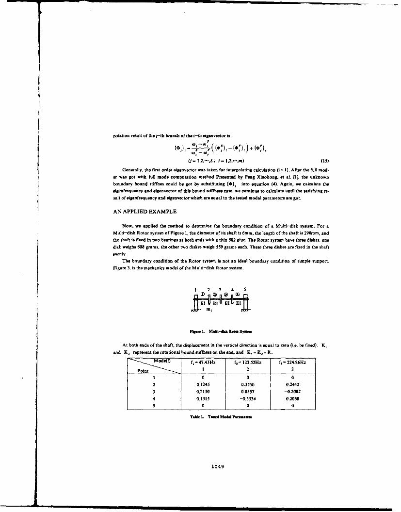
polation result of the j-th branch of the i-th eigenvoctor is
= I W,(~ .',(J-l1,2,...,L, l= l,2,...m) (15)
Generally, the first order eigenvector was taken for interpolating calculation (i= I). After the full meod-
er was got with full mode computation method Presented by Peng Xiaohong, et al. [1], the unknown
boundary bound stiffnes could be got by substituting (V), into equation (4). Again, we calculate theeigenfrequency and eigenvector of this bound stiffness case, we continue to calculate until the satisfying re-
sult of eigenfrequency and eigenvector which are equal to the tested modal parameters are got.
AN APPLIED EXAMPLE
Now, we applied the method to determine the boundary condition of a Multi-disk system. For a
Multi-disk Rotor system of Figure 1, the diameter of its shaft is 6mm, the length of the shaft is 290mm, and
the shaft is fixed in two bearings at both ends with a thin 502 glue. The Rotor system have three diskes. one
disk weighs 608 grams, the other two diskes weigh 559 gram-, each. These three diskes are fixed in the shaft
evenly.
The boundary condition of the Rotor system is not an ideal boundary condition of simple support.
Figure 3. is the mechanics model of the Multi-disk Rotor system.
1 2 3 4 5
El 9El UEl f E l )
Figure 1. Mslti-d1k Rotor System
At both ends of the shaft, the displacement in the vertical direction is equal to zero (ie. be fixed). K,
and Kz represent the rotational bound stiffness on the end, and K, K2= K.
Mf, =47.43Hz f2 = 123.52Hz f3 - 224.86Hz
1 2 3
1 0 0 0
2 0.1245 0.3550 0.2442
3 0.2150 0.0357 '-0.2082
4 0.1315 -0.3534 0.2068
5 0 0 0
Table 1. Tested Modal Parametets
1049

Simple Support at Both Ends Fixed End at Both Ends
Mode Consider The Do Not Consider Consider The Do Not ConsiderRotational Inertia The Rotational Rotational Inertia The Rotational
of The Diskes Inertia ofThe Diskes Inertia
I 23.47Hz 23.73Hz 52.95Hz 54.26Hz
2 90.59Hz 94.17Hz 134.IIHz 142.68Hz
3 191.42Hz 202.93Hz 232.72Hz 237.58Hz
Table. TbeElgeufreqeeaey ofFEM of TeMund-tik Rotoe Systs to TwoBounadary Ceadlteo Cae
The mode of the Multi-disk Rotor system was excited with random excitation method (by using an
untounched BJ-U type broad band electric exciter). After modal analysis and parameter identification, the
tested modal parameters are got as table I. The synthesized amplitude-frequency characteristic and first 3
mode are shown in Figure 2. The unknown boundary condition need to be determined with the method we
put forward.
All the eigenfrequency of the two Finite Element Models are listed in Table 2. The first Finite Element
Model has an assumed boundary condition of simple support at both ends, the other has an assumed
boundary condition of fixed end at both ends. ( Ii: The rotational inertia of the diskes) The unknown
boundary bound stiffness KA,K2 was determined with the method we presentd. Figure 3 is the Mechanics
Model of the Multi-disk Rotor System.
First, with the interpolation method of frequency, the unknown bound stiffness is determined to be:
K= K 2= 1472.41N •m
o 123.52Hz
47.43 224.86
Hz Hz
Frequency (c) Mode 2
(a) Synthesized Amplitude-Frequency
Response Characteristic
(b) Mode I (d) Mode 3
re 2. Syasneslied Frequsecy Reemq ýFondle. of The Multi-disk Rotor Systm
1050
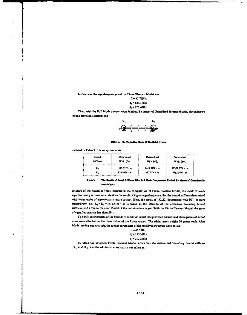
t
In this case, the eigenfrequencyes of the Finite Element Model are:
f, - 47.72Hz,
f2 = 123.31Hz,f,= 220.40Hz,
Then, with the Full Mode computation Method By means of Generlized Inveorc Matrix, the unknown
bound stiffness is determined
K, K2
Ftpure 3. The Mediansa Maid effbe Raeim Systems
as listed in Table 3. It is an approximate
Bound Determined Determined Determined
Stiffness With {(}) With (0)2 With (0)3
K, 11 19.22N • m 1411.59N • m 22977.63N • in
K, 933.43N. in 377.03N • m 4062.56N in
Table 3. The Results of Bead Siffem With Full Made Compstatid Methed By Mem of Gestdgmd b-.
vere Matrix
solution of the bound stiffness. Because in the computation of Finite Element Model, the result of lower
sigenfrequency is more accurate than the result of higher aigenfrequency. So, the bound stiffness determinedwith lower order of eigenvector is more correct. Here, the result of K,,K 2 determined with ({}, is moretrustworthy. So, K, = K 2 = 1472.41N * m is taken as the solution of the unknown boundary bound
stiffness, and a Finite Element Model of the real structure is got. With the Finite Element Model, the errorof eigenfrequency is less than 2%.
To verify the rightness of the boundary condition which has just been determined, three pieces of added
mass were attached to the three diskes of the Rotor system. The added man weighs 54 grams each. After
Modal testing and analysis, the modal parameters of the modifyod structure were got as:
f, - 45.70Hz,
f2 = 115.30Hz
f3 = 212.20HzBy using the structure Finite Element Model which has the determined boundary bound stiffntess
KI and K 2, and the additional mass matrix was taken as:
1051

"00.054
0
0.054
0
0.054
0
0
three eigenfrequency of FEM of the modifyed structure were calculated as:
f, = 45.73Hz,
f2 = 118.64HZ,f3 = 211.54Hz,
The value of eigenfrequency calculated with the FEM of the modifyed structure is consistent with the
tested modal parameters of the modifyed structure. From this result, it clearly shows the boundary boundstiffness determened with the method we presented can be taken as the real boundary bound stiffness which
are used for the dynamic computation and analysis of the structure.
ACKNOWLEDGEMENT:
The author would like to thank the research associate Wu Xuixing for hers support and assistence in
doing experiment.
REFERENCES:
I. Peng Xiaohong. 'To Correct the Finite Element Model of a Structure With Tested Modal Paramet-
er', Vibration and Shock, No. 3, 1984.2. Xu Wanli; Xia Yilin, 'Mass Matrix and Stiffness Matrix Correction Using Generlized Inverse Ma-
trix', Proceedings of the 5rd National Modal Analysis and vibration testing conferarce, P. R.China,
1988, pp. 858-866.3. Baruch, M. 'Optimazation Procedure to Correct Stiffness and Flexibility Matrix Using Vibration
Tests' AIAA J. Vol. 16. No. 1i, Nov. 1978, pp. 1208-1210.
4. Berman, A. 'Mass Matrix Correction Using an Incomplete Set of Measured Modes'. AIAA J. Vol.
17, No. 10, Oct. 1979, pp. 1147-1148.5. Lu Zhenhua, Feng Zbendong, 'The Optimal Structural Modification Principle for the Maximum
Shifts of Natural Vibration Frequencies' Proceedings of the 6rd International Modal Analysis Con-
ference, 1988, pp. 1107-1111.
1052

SECOND INTERNATIONAL CONGRESS ONRECENT DEVELOPMENTS IN AIR- AND
STRUCTURE-BORNE SOUND AND VIBRATIONMARCH4-. 1992 AUBURN UNIVERSITY. USA
VIBRATION AND EIGENVALUE ANALYSIS USING FINITE ELE•ENTS
Tirupathi R. ChandrupatlaMechanical Engineering Department
GMI Engineering and Management InstituteFlint, MI 48504
U.S.A.
and
Ashok D. BelegunduMechanical Engineering DepartmentThe Pennsylvania State University
University Park, PA 16802U.S.A.
ABSTRACT
The paper presents the steps involved in the use of finite elements for
the analysis of vibration problems. Formation of stiffness and mass matricesis followed by discussion of techniques of reducing the size of the matrices.Characteristic polynomial, vector iteration, and transformation methods ofeigenvalue and eigenvector evaluation for free vibrations of structures arepresented. Damping aspects are discussed for the special case of Raleighdamping.
INTRODUCTION
A structure vibrates when forces of variable nature are applied on it.Sudden application or sudden release of forces also cause the structure tooscillate in a cyclic manner about its equilibrium position. If anelastically deformed structure is suddenly released, the resultingoscillations are referred to as natural vibration. A structure modeled as amass-spring system tends to oscillate indefinitely. The frequency ofoscillation is called the natural frequency. For variable forces, if thedisturbing frequency is less than one third of the lowest natural frequency,the structure may be treated as static and mass effects need not beconsidered [U1. Vibration in real structures subsides with time due todamping action. Damping in structures may be due to internal materialcondition, friction in joints, or external dampers introduced to absorbvibration.
It is clear from the discussion above that evaluation of the lowestnatural frequencies is necessary to predict the dynamic behavior of thestructure. This is accomplished by considering the stiffness and masseffects using finite elements. The vibration control aspects requireconsideration of damping in the system. The purpose of this paper is to givean overview of the use of finite elements for the analyses. First, theformation of stiffness and mass matrices is considered. Techniques of matrixsize reduction are discussed. Methods of evaluating natural frequencies or
1053

equivalently the eigenvalues are presented. Strategies for consideringdamping effects are developed.
STIFFNESS, MASS, AND MATRIX REDUCTION
In the finite element analysis, a structure is divided into elementswhich are connected at nodes. Consider the structure shown in Fig. 1. Thenodal displacements referred to as global degrees of freedom are denoted Q),Q2. Q3..... ... It is convenient to consider the energy in the structure byconsidering the energy contributed by each element. A typical element isillustrated in Fig. 2. The nodal displacements of the element are denotedqt, q, .. . . . . . These may be referred to as the local degrees of freedom. Thefinite element model expresses the displacement field in the element in termsof the nodal'displacements of the element.
y
22 6 64 A
1 S
Q~z-2i J~ i
z GLOBAL DOF / LOCAL DOF
Figure 1 Structure Figure 2 Element
The total strain energy in the structure is obtained as the summation ofstrain energy in the elements. The result of these steps is represented asfollows:
2 Q2
Noting that in dynamic problems, the nodal displacements are functionsof time, the total kinetic energy is also obtained through element kineticenergy.
KA 0MG OTMO(2)2 2
1054

On developing the Lagrange's equations of motion, the finite element
representation becomes:
MO + KQ-o (31
On setting
Q - U aMiat (4)
where 0 is the circular frequency 1= 25 f, f Hz) and U is cal.led theeigenvector representing the corresponding mode shape. Denoting A o, whereX is called the eigenvalue, we have,
KU- IMU (5)
Stiffness and mass matrices for various structural elements are presented inf2, 31.
Stiffness and mass matrices formed above are square matrices of sizegiven by the number of degrees of freedom. Generally these matrices arebanded. Some techniques of eienvalue analysis make use of the banded natureof the matrices. There are other methods which work with full size matrices.In these cases, it will be of interest to reduce the size of the matrices.This helps in handling large scale problems while retaining the possibilityof calculating significant modes of vibration. A technique commonly used iscalled Guyan Reduction (41.
Guvan ReductionThe key here is to identify master and slave degrees of freedom [fI.
The master degrees of freedom control the eigenvalues and modes desired andslave degrees of freedom are those which have minimal inertia contribution.In a beam bending problem, the rotational degrees of freedom are typicalslave degrees of freedom. If U and U. are identified as master and slavedegrees of freedom respectively, we partition the stiffness and mass matricesas follows:
The slave degrees of freedom are eliminated using
U.,- - K.ý KMU. 7
In the computatipne, the inversion need not be explicitly carried out. Theproduct T = K28 can be obtained by applying Gauss elimination on KHz
1055

together with each column of K, as the right hand side, and thenbacksubstituting for each column. Denoting the reduced matrices as K. and Mrrespectively, we get
T 1; K.ý'gK,- K - K. (8)
M- - MT - T MT T TTM T
The reduced problem is given by
glU. - X.MU. (9)
Various strategies can be used for identifying the slave degrees of freedom.The idea is to look for the ratio of diagonal element of K and thecorresponding diagonal element of M. The degrees of freedom with largestratios are candidates for slave DOF. For a detailed account see fl, 5, 61.We also note here that if elements of M and M0 are all zero, the Guyanreduction is precisely static condensation. A bound algorithm for thereduction has been presented by Wright and Miles [61. The stage is now setfor discussing the techniques of finding the eigenvalues and eigenvectors.
EIGENVALUES AND EIGENVECTORS
The eigenvalue-eigenvector evaluation procedures fall into the broadcategories of characteristic polynomial, vector iteration, andtransformation methods. Main characteristics of these techniques arediscussed below.
Characteristic Polynomial TechniqueSolution of the problem posed by (5) or (9) is equivalent to determining
zeroes of the polynomial in A given by
d(K - LM) - 0 (10)
The eigenvector corresponding to each eigenvalue is then evaluated. Thistechnique is quite efficient for small problems. The technique is alsoreferred to as determinant search method 181.
Vector Iteration MethodsChief among the vector iteration methods is the inverse iteration
method. The method uses properties of the Rayleigh quotient. We start witha trial vector u 1 . Then for steps k = 1,2,..., we determine u2 , u3 ....
'i., - m1 k
1056

The inverse iteration converges to the lowest eigenvalue. It is necessaryhere that the boundary conditions are applied to modify the stiffness to makeit positive definite. We also note that the banded nature of the stiffnessand mass matrices can be effectively used in this method. Higher eigenvaluesare obtained efficiently by excluding the space spanned by the eigenvectorsalready evaluated using the Gram-Schmidt Orthogonalization. Subspaceiteration algorithm proposed by Bathe 191 involves iteration in a subspace ofdimension determined by the number of eigenvalues desired.
Transformation MethodsA transformation method that is quite efficient for small scale problems
is the Generalized Jacobi Method. A series of transformations P,, P1,*..,I 1
are used such that if P represents the product
P -PP 2 ...P. (12)
then the off diagonal terms of P.EP and VMP are simultaneously, zero. Inpractice, the limits on off diagonal terms may be se. as 1O'-x(smallestdiagonal stiffness element) for stiffness matrix, and 10"x(largest diagonalmass element) for mass matrix. The zero check is more efficiently performedby checking elements farthest from the diagonal to the diagonal in the order(l,n), (1,n-1), 12,n), 41,n-2) ..... .Since initial matrices are banded, thisapproach saves computational effort. In this approach, full matrices areused. Both stiffness and mass matrices need not be positive definite.
There are other transformation methods where the generalized eigenvalueproblem is first turned into a standard form
K'MU -1• (13)A
The matrix K'1
M is then tridiagonalized using various transformation methodssuch as Householder method or Lanczos method. Required eigenvalues are thendetermined using inverse iteration. QR iteration may be used to determineall eigenvalues. Lanczos method is becoming popular for large scale systems.
Lanczos Method. In the tridiagonalization process, matrix X of Lanczosvectors x), X2, x3,.. . represented by
x -[ .... (14)
is chosen such that
XTMX-I (15)
XTMK 'MX - T
1057

where I is the identity matrix and T is a tridiagonal matrix. The eigenvalueproblem in the tridiagonal form is represented by
U -X0
I.
For details of computations for the formation of Lanezos vectors refer to(5,8,91. Recently considerable research has been devoted to the developmentof the Lanczos method. Several FEA software vendors have implemented thismethod in their codes. The main problems involved are in overcoming therounding off errors in computations.
DAMPING CONSIDERATIONS
With damping, the equations of motions for free response are
MO + CO + KQ - 0 (171
The damping matrix C is rarely developed from element level. A commonapproach is to assume that C is a linear combination of K and N. Thus
C- aK + PM (18)
where C and P are scalars. This case is referred to as Raleigh damping(9,101. We now assume the steady state solution to (17) is of the form
Q - Ue" 419)
Where U is a mode shape. Substituting int (17), and noting Eq.(18}, we have
KU - S +. 32 MU (20)1 + as)
Comparing the above equation to Eq.(5), we see that the mode shapes of theundamped and the proportionally damped system are the same. Further thequantity within brackets is simply equal to square os the undamped naturalfrequency 0. Thus
1058

AS- - B (21)i a sa
Solving for s, we get
S - - * ~- + (22)
(ad "i |- c2
where C is the damping ratio and 0 is the damped circular frequency for themode corresponding to natural Prequency 6. Above equation helps indetermining the a and p experimentally for a given dynamic structure or inthe determination of their values for given damping ratios 111).
DISCUSSION AND CONCLUSIONS
Several aspects of vibration analysis have been presented in this paper.Finite element formulation of stiffness and mass matrices is followed byeigenvalue and mode shape determination. Forced vibrations have not beenconsidered in this presentation. We have discussed Raleigh damping, butthere are several other aspects of general damping have not been consideredhere. Hysteritic damping and damping considerations in viscoelasticmaterials f121 pose challenging problems.
BIBLIOGRAPHIC REFERENCES
1. COOK, R.D., Concepts and Applications of Finite Element Analysis. JohnWiley & Sons, New York, 1981
2. PRZMIENIECKI, J.S., Theory of Matrix Structural Analysis, McGraw-Hill.New York, 1968
3. CHANDRUPATLA, T.R.. and A.D. BELEGUNDU, Introduction to Finite Elementsin Engineering, Prentice Hall, Englewood Cliffs, New Jersey, 1991
4. GUYAN, R.J., "Reduction of Stiffness and Mass Matrices." AIAA Journal,3 f1965), 380.
5. HUGHES, T.J.R., The Finite Element Method - Linear Static and DynamicFinite Element Analysis, Prentice Hall, Englewood Cliffs. New Jersey.1987
6. HENSHELL, R.D., and J.H. Ong, "Automatic Masters for EigenvalueEconomization," Earthquake Engineering and Structural Dynamics, 3(1975), 375-383
7. WRIGHT. G.C., and G.A. MILES, "An Economical Method for Determining theSmallest Eigenvalues of Large Linear Systems," Int. J. for N'umericalMethods in Engineering, 3 (1971), 25-33
1059

8. HUMAR, J.L., Dynamics of Structures, Prentice Hall, Enrlewood Cliffs,New Jersey, 1990
9. BATHE, K.J., Finite Element Procedures in Engineering analysis, PrenticeHall, Englewood Cliffs. New Jersey, 1982
10. INMAN, D.J., Vibration with Control, Measurement, and Stability,Prentice Hall, Englewood Cliffs, New Jersey, 1989
11. EWINS, D.J., Modal Testing : Theory and Practice, Research StudiesPress, 1984
12. SEGALMAN, D.J., "Calculation of Damping Matrices for LinearlyViscoelastic structures", Journal of Applied Mechanics, 54 (1987), 585-588
1060

SECOND INTERNATIONAL CONGRESS ONRECENT DEVELOPMENTS IN AIR- AND
STRUCTURE-BORNE SOUND AND VIBRATIONMAPCH 4-6 1992 AUBURN UNIVERSITY. USA
DYNAMIC ANALYSIS OF PRACTICAL BLADED DISKS USING FEM ANDCYCLIC SYMETRI TECHNIQUES
A.S.Panwalkar*V.Ramamurti**A.Rajamani*
*Vibration Laboratory,
Corporate Research and Development Division,Bharat Heavy Electricals Limited,
Vikasnagar, Hyderabad, 500593, India
**Department of Applied Mechanics.Indian Institute of Technology. Madras, 600036, India
ABSTRACT
Coupled free vibration characteristics of practical bladed disks are computedusing triangular shell element and cyclic symmetry. Potters' method is used forsolution of the eigenvalue problem. Blade-disk joint constraints are applied based onLove-Kirchhoff hypothesis. Blade to blade variation of looseness at the blade-diskjoint is also considered. Results of three practical bladed disks with different bladeaspect ratios and having approximately the same disk radii ratio are presented. Forlarge aspect ratio of blades, the bladed disk vibration behaviour is simple. For themedium and small aspect ratio blades, complex mode behaviour is observed.
INTRODUCTION
The bladed disk assemblies in general are flexible and have to withstand severeoperating conditions such as large centrifugal force loading, higher operatingtemperatures, flow induced dynamic loads etc. Therefore, it is very essential todetermine the vibration behaviour pattern of the bladed disk from design point of viewfor long time trouble free operation of the machine [I]. A typical turbine bladed diskconstitutes a dynamic system in which different flexibilities of its components such asdisk, blades, shrouds etc., dynamically interact with each other. Kuo [2] illustratedthe influence of blades and shrouds upon the natural frequencies. Omprakash andRamamurti [3] made a parametric study of the coupled free vibration characteristics ofrotating bladed disks. Irretier and Schmidt [4] used receptance techniques andcomponent mode synthesis. They emphasized the use of component mode synthesis to solvethe problem of mistuning. Ewins [5,6] has done a detailed study to understand vibrationbehaviour of bladed disks and addressed to the problem of mistuning. Ewins andImregun [7] made studies on the bladed disks with packeted blades. Griffin andHoosac [8] considered mistuning using spring and mass constants as the random variablesfor blades. Pierre and Cha [91 and Wei and Pierre [10] used perturbation approach toexplain mode localization phenomena in a mistuned bladed disk. Afolabi [11] useseigenvalue spectrum method as suggested by Ewins [6] and he classifies [121 thevibration behaviour of mistuned bladed disk. Finbow and Watson [13] presented practicalexperiences on the working bladed disks.
The aim of this paper is to study the vibration behaviour pattern of practicalcases of steam turbine bladed disks whi:h are in operation. A triangular shell elementis used for both disk and blades. The attachment of blades to the disk is maintained bya set of constraint equations derived from Love-Kirchhoff's hypothesis. Potters' schemeand cyclic symmetry [14] are used to solve the equations. The bladed disks which areconsidered for the analysis have blade aspect ratios of 2.23, 3.1 and 4.4 with disk
1061
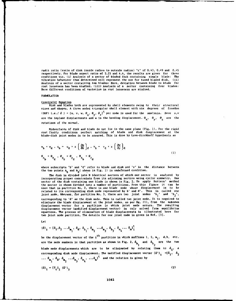
radii ratio (ratio of disk inside radius to outside radius) 'E' of 0.43. 0.49 and 0.45respectively. For blade aspect ratio of 2.23 and 4.4, the results are given for threeconditions viz. (i) Analysis of a sector of bladed disk containing single blade: Thevibration behaviour thus determined will represent the one for tuned bladed disk. (ii)Analysis of a sector containing two blades: Here, deviation between blade to blade forroot looseness has been studied. (iii) Analysis of a sector containing four blades:Here different conditions of variation in root looseness are studied.
FORMULATION
Constraint EquatioDisk and blades both are represented by shell elements owing to their structural
sizes and shapes. A three noded triangular shell element with six degrees of freedom
(001F) i.e.{ 6 } = [u. v, w, 0x, ey, azIt per node is used for the analysis. Here uv
are the inplane displacements and w is the bending displacement. e * 6
y, ez are the
rotations of the normal.
Midsurfaces of disk and blade do not lie in the same plane (Fig. 1). For the rigidroot fixity conditions perfect matching of blade and disk displacement at theblade-disk joint nodes is to be assured. This is done by Love-Kirchhoff hypothesis as
b db w ' =b ud +z d b d ' z d + -w I d
(1)
d 'd Ob Yd ' 8zb zd
where subscripts 'b' and 'd' refer to blade and disk and 'z' is the distance betweenthe two points Ab and Ad( shown in Fig. 1) in undeformed condition.
The disk is divided into N identical sectors of which one sector is analyzed byincorporating proper constraints from its adjoining sectors using cyclic symmetry. Onesector of the disk containing one blade is shown in Fig. 2. To apply Potters' methodthe sector is shown divided into a number of partitions. From this figure it can beseen that in partition No. 2, there is one blade node whose displacement is to berelated to its corresponding disk node represented by b' and d'. This is called onejoint node. Whereas, for partition No. 3, there are two joint nodes 'b,' and 'b 2 1'
corresponding to 'd' as the disk node. This is called two joint node. It is required toeliminate the blade displacement at the joint nodes, as per Eq. (1), from the unknowndisplacement vector for a partition in which joint node occurs. The resultingdisplacement vector (modified displacement vector) is only solved from equilibriumequations. The process of elimination of blade displacements is illustrated here fortwo joint node partition. The details for one joint node is given in Ref. [3].
Let
=(61.
6 6 6bIa
6 m2 "''6 m'
6b
6 m4 "" 6 m
1 i1}i ,2 ... mld' d" , 2t3b2' 4...
be the displacement vector of the ith partition in which suffixes 1, 2, mi, d,b, etc.
are the node numbers in that partition as shown in Fig. 2. 6 and 6 are the two
blade node displacements which are to be eliminated by relating them to 6d8 a
corresponding disk node displacement. The modified displacement vector W1 i =[611 62
... 6 d' 6 .6 .6 ... 6MIt and the relation is given by• .. dml in2 "'3 in4 , m
46)i -[Tcli 461)i (2)
1062

where ITc]i is the transformation matrix which is given by
[T] [ R2 ](2a)[Q 2 1
0R3
where, [R 1 ], [R 2] and (R 3 1 are the unit matrices of sizes [6(ml+l). 6(ml+1)],
[6(m 3 -m 2 +l). 6(m3 -m 2 +1)] and [6(m-m4 +1), 6(m-m4 +1)] respectively. [QI] and [Q2 ] are of
size (6, 6) and the terms of these matrices are obtained by using the constraintEq. (1) for blade nodes bI and b2 and disk node d. It may be noted that for one joint
node partition T1c' will contain the above matrices excluding [Q2 I and [R3 ]; the
resulting matrix (Tr will be same as that derived in Ref. 13).
Stiffness And Mass MatricesThe element stiffness is determined by triangular shell elements. Masses are
lumped for translational degrees of freedom equally at the three nodes. In Potters'scheme element matrices are assembled partition-wise and hence the matrix equation forthe eigen value '*' is written as (Ref. [14]).
B A 0 0 . . .0 0 Ak zk z1 I ni 1I
Aft B A 0 . . . 0 0 0 z z1 2 2 2 2
0 t B A 0 0 0 z3 23
0 0 0 0 . . . At z"n-2 Bn- An- Znl n-l
Ank 0 0 0 ... 0 A t B z z"n'2 n-l nn
where [Bi], [Ai] etc. are the elements of partitioned stiffness matrix, {z.} is the
partitioned eigenvector and [M] is dia (Mi. M2 , M3 ... MnI, Mn] with Mi as the
partitioned mass. Suffix 'i' represents partition number and there are (n+1) partitionspresent in one sector. It may be pointed out that the matrices [B], [A] are required to
be transformed using transformation matrix given by Eq. (2). This transformation is
explained in Ref. (3]. In Eq. (3), k 1 f e- and k2 - i; i = / and g is the wave
1 thpropagation constant which relates displacement vectors of k sector and its previous
sector i.e. (k-I) by the equation &. = e-Wj (A.5 ). The value of 'I' depends upon the
wave number or the number of nodal diametral mode 'n' to be analyzed such that
= 2xn (4)
1063

where N is the total number of sectors; 'n' can take following values
n 0 0, 1, 2 .... (N/2) for N evenn - 0, 1, 2 .... (N - 1)/2 for N odd
The solution of Eq. (3) yields modified displacement vector. The recovery ofactual displacement vector can be made by Eq. (2).
CONDITIONS OF BLADE ROOT FIXITY
In analyzing the bladed disk assemblies three root conditions which pertain todifferent blade root looseness are studied. Looseness is modeled as follows. There aresix nodes at the blade root which join with the disk nodes. Out of these six nodes, twonodes which appear in the third partition are released and the displacements aretreated as DOF's without any joint constraint. Whereas for a tight blade, jointconstraints are applied for all the nodes as described earlier. This way the differencebetween a loose blade and a tight blade is incorporated. The conditions considered are:I) Single blade in a sector without releasing the nodes. This is the case of tunedbladed disk with all blades attached tightly. 2) Two blades in a sector with firstblade tight and the second blade let loose. This means that there are alternate looseand tight blades attached to the disk. 3) Four blades in a sector with first and fourthblades tight whereas second and third blades have looseness. This means that every twotight blades are followed by two loose blades in succession.
ANALYSIS OF BLADED DISKS
The results obtained by the present method are compared for a circular diskconsidered by Salama [15] and for a typical Low Pressure (LP) turbine blade for whichresults have been obtained by using commercial packages PAFEC and VIPACK and byexperiments [161 for checking the computer program developed. The comparison is foundto be excellent. Three bladed disk assemblies which are in operation are considered.These assemblies have blade aspect ratios (i.e. ratio of blade length to chordwisewidth at the blade root profile) of 2.23, 4.4 and 3.1 with corresponding disk radiiratios of 0.43, 0.45 and 0.49.
Case I- Intermediate Pressure (IP) Turbine StageThis is a case of an IP stage of 110 NW steam turbine with 168 blades on the disk
and a blade aspect ratio of 2.23. Three conditions (as described above) are consideredfor analysis.
Condition 1. This condition represents a tuned bladed disk. A plot of naturalfrequency versus nodal diameter for the first three modes is given in Fig. 3. Vibrationmodes of cantilever blade corresponding to first flapwise bending (1B - tangential) andfirst edgewise bending (1EB - axial) are also shown in this figure. From this figure itis observed that 0 nodal circle axial mode frequency rises as nodal diameter increases.This curve crosses the frequency curve for tangential vibration around 10 nodaldiameters. Similarly 1 nodal circle axial mode frequency curve also crosses thefrequency curve for tangential vibration around 5 nodal diameter. At the cross overregion the mode shapes are highly coupled with tangential and axial displacements.Similar findings have been experimentally observed by Finbow and Watson [131. Thetangential vibration frequency curve has distortion in the cross over region. However,finally it settles down to a lower value and fairly remains unaffected by increase innodal diameter after 12. Omprakash and Ramamurti [3] have also reported severe couplingof blade and disk modes for small aspect ratio blades for a given c. It may be pointedout that the parameter c determines the flexibility of the disk. This flexibility canbe compared with the flexibility of the blades.
Condition 2. In this condition the second blade is deviated in its looseness atthe root. This is similar to a bladed disk with alternate blade having looseness. Itmay be noted that such kind of looseness may be prevailing in the bladed disk at thetime of assembling. The results under this condition are given in Fig. 4. It isobserved from the figure that the tangential mode splits into two curves. The lowercurve gives predominantly second blade tangential mode. Whereas upper curve is for thefirst blade. Again the tangential mode frequencies distort due to the cross over by 0nodal circle axial mode and 1 nodal circle axial mode. It is also observed that for 0
1064

nodal diameter the tangential modes are not split corresponding to first bladevibration or second blade vibration. Instead both blades vibrate tangentially in phasewith each other and also with disk (1117.97 Hz) or out of phase with each other(1431.21 Hz) or both blades tangential in phase with each other and out of phase withdisk (1917.96 Hz). This behaviour is quite peculiar. It is likely that severe couplingbetween disk and blades causes this behaviour. Hence it may be realized that simplespring and mass models are inadequate to bring out this type of behaviour. It may alsobe noted that deviation in the blade's root looseness has clearly isolated thefrequencies and, therefore it represents the practical case. Experimentally, quitevaried frequencies are observed for a practical case for which all blades may not getexcited for a given resonance frequency 1171.
Condition 3. This condition represents a bladed disk for which after every twoblades there are two consecutive loose blades. The mode shapes for this condition arehighly complex and it is difficult to categorize. Plotting of frequency curves giveconfusing trend if modes have not been correctly identified. Therefore, instead ofplotting, a table is given in which modes are approximately identified. Table - 4 showsvarious modes and their frequencies. The tangential mode frequencies are split. The inphase and out of phase motions with respect to each other are mentioned in the table.
Case 2- Low Pressure (LP) Turbine StageThis is a case of an LP stage of 110 MW steam turbine where there are 132 blades
on the disk with blade aspect ratio of 4.4. These blades are long and twisted. Theanalysis is done upto 10 nodal diameters for the three conditions.
Condition 1. A plot of natural frequencies for the first three modes versu,diameter is given in Fig. 5. Vibration modes of cantilever blade corresponding tflapwise bending (lB - tangential), first edgewise bending ( IEB - axial) andtorsional (IT) are also shown in this figure. Frequencies for axial vibrations in,with nodal diameter and the rise is controlled by the cantilever blade frequency asblades vibrate along with disk. Thus for higher nodal diameters there is no appreciabl'rise in frequency. For 0 nodal circle mode the frequency is below the edgewise bendingmode of the cantilever blade. One nodal circle mode is here combined with torsionalmode of the blade. This suggests that spring and mass models without admitting modalstiffness and modal masses for torsional modes will be inadequate to explain thisbehaviour. The I nodal circle mode at 10 nodal diameter is below the torsion mode ofcantilever blade.
Condition 2. The results of the analysis are given in Fig. 6. It is observed that0 nodal circle axial frequency behaves as in the previous case. The tangentialfrequency splits into two and both are marginally affected by increase in nodaldiameter. Whereas, combined torsion and I nodal circle mode frequency splits into two,one of which is for blade torsion alone. This frequency is considerably low inmagnitude and it is marginally affected by increase in nodal diameter. The second onewhich is similar to combined torsion and I nodal circle mode shows a similar trend asobserved in Fig. 5. The split in frequencies for the tangential and torsional mode isdue to the looseness created in the second blade.
Condition 3. The results of the analysis are given in Fig. 7. Here also the0 nodal circle axial mode frequency shows similar trend as obscrved in Figs. 5, 6.Tangential vibration mode splits into four frequencies - two for the tight blade andother two for the loose blades. So it forms two groups. In each group the twofrequencies are very close and at times it is very difficult to distinguish them on thegraph. In case of torsion mode also two groups are formed. The first group in whichonly one frequency is present is for combined blade torsion and 1 nodal circle mode.Whereas the second group has 3 close frequencies corresponding to blade torsion modeonly. The trend of these curves is very similar to those in Figs. 5 and 6.
The general observation from this analysis is that the axial mode of 0 nodalcircle does not split in spite of the root looseness. This mode crosses over tangentialvibration mode. There is little coupling between these two modes. This phenomena isalso seen for the long bladeb in Ref. [3]. Therefore, large aspect ratio blades whichbehave like beams can be represented by spring and mass models for bladed diskanalysis.
1065

Case 3- HijI Pressure (HP) Turbine StageThis is a case of a HP stage of 236 MW steam turbine where there are 94 blades on
the disk with blade aspect ratio of 3.10. In this case only condition no. I (i.e. thesector containing one blade) is considered. Conditions 2 and 3 have not been consideredas the trend due to blade root looseness variation has been obtained for the extremecases of blade aspect ratios given above. The analysis was done upto 45 nodaldiameters. For each diametral mode first three modes are obtained. The naturalfrequencies for these modes are plotted against nodal diameter as shown in Fig. 8.These modes depict both axial and tangential vibrations of blades. The coupled modesare observed around fifth nodal diameter. All these modes show general tendency ofincrease in frequency value with respect to nodal diameter from 0 to (approximately) 10and thereafter less significant change is observed with increase in nodal diameter.
CONCLUSIONS
The above Analysis shows behaviour of both axial and tangential modes of vibrationfor practical bladed disks. From the behaviour pattern of these bladed disks followingpoints have been concluded -
1. For small aspect ratio blades, the bladed disk modal behaviour is highlycoupled. Therefore, it is desirable to perform detailed analysis using FEM instead oflumped spring and mass models.
2. For large aspect ratio blades, the bladed disk behaviour is simple andinsignificant coupling of blades and disk is observed. Therefore, the lumped spring andmass models can be used adequately.
3. For large aspect ratio blades, the torsional mode is observed to be combinedwith one nodal circle mode.
4. The root looseness has no influence on the zero nodal circle mode for all thecases considered.
5. For medium aspect ratio of blades, the bla~es and disk modes tend to couple.
REFERENCES
1. A.S.PANWALKAR, A.RAJAMANI and V.RAMANURTI 'Turbomachinery blade dynamics - areview' Shock and Vibration Digest vol. 22, no. 12, 1990, pp 3-9.
2. P.S.KUO 'On the formulation of coupled /uncoupled dynamic analysis of bladed -disc assemblies' American Society of Mechanical Engineers, Paper No. 81-rFT-126,1981.
3. V.OMPRAKASH and V.RAMAMURTI 'Coupled free vibration characteristics of rotatingtuned bladed disk systems' Journal of Sound and Vibration, vol. 140, no. 3, 1990.pp 413-435
4. H.IRRETIER and K.J.SCHMIDT 'Mistuned bladed disks - dynamical behaviour andcomputation' International conference on Rotor Dynamic Problems in lower Plants,Rome, Italy, 1982, pp 215-226.
5. D.J.EWINS 'Vibration characteristics of bladed disk assemblies' Journal ofMechanical Engineering Science vol. 15, no. 3, 1973, pp 165-186.
6. D.J.EWINS 'Vibration modes of mistuned bladed disks' Transactions of the AmericanSociety of Mechanical Engineers, Journal of Engineering for Power, vol. 98. no. 3,1976. pp 349-355.
7. D.J.EWINS and M.IMREGUN 'Vibration modes of packeted bladed discs' Vibration ofBladed Disk Assemblies, American Society of Mechanical Engineers. 1983. pp 25-33.
1066

8. J.H.GPRkkIN and T.M.HOOSAC 'Model development and statistical investigation ofturbine blade mistuning' Transactions of the American Society of MechanicalEngineers, Journal of Vibration, Acoustics, Stress and Reliability in Design.vol. 106. no. 2, 1984, pp 204-210.
9. C.PIERRE and P.D.CHA 'Strong mode localization in nearly periodic disorderedstructures' AIAA Journal, vol. 27, no. 2, 1989, pp 227-241.
I0. S.T.WEI and C.PIERRE 'Localization phenomena in mistuned assemblies with cyclicsymmetry part I: free vibrations' Transactions of the American Society ofMechanical Engineers, Journal of Vibration, Acoustics, Stress and Reliability inDesign, vol. 110, no. 4. 1988. pp 429-438.
11. D.AFOLABI 'The eigenvalue spectrum of a mistuned bladed disk' Vibrations of Bladesand Bladed Disk Assemblies, American Society of Mechanical Engineers, 1985.pp 23-30,
12. D.AFOLABI 'The frequency response of mistuned bladed disk assemblies' Vibrationsof Blades and Bladed Disk Assemblies, American Society of Mechanical Engineers.1985. pp 15-21.
13. I.FINBOW and S.J.WATSON 'Experimental verification of turbine blade vibrationcharacteristics' IMechE paper C 196/79, 1979, pp 163-172.
14. V.RAMAMURTI 'Computer Aided Design in Mechanical Engineering' New Delhi: Tata
McGraw-Hill, 1989.
15. A.K.SALAMA 'Finite Element Dynamic Analysis of Blade Packets and Bladed DiscAssemblies' Ph.D. Thesis, Institute of Sound and Vibration Research, TheUniversity of Southampton. 1976.
16. O.P.SHARMA 'Generation of Campbell diagram for last stage LP moving blades of 500MW steam turbines' Steam Turbine Engineering and Development Centre, Bharat HeavyElectricals Limited, Hardwar, India, Rep. No. TB-002-0-DL, 1989.
17. A.S.PANWALKAR, A.RAJAIANI AND V.RAMAMURTI 'Free vibration studies on turbine stageusing cyclic symmetry' Presented at the International Conference on EngineeringSoftware held at TIT New Delhi, India Dec. 4-7 1989. Engineering Software, NarosaPublishing House. Editors C.V.Ramakrishnan et. al.. 1989, pp 459-466.
Z AXIS
ONE SECTOR OFDK DISK
B. , LADEMIDSURFACE
b
DISKMIDSURFACE BLADE
FIG 1. A SECTOR OF BLADED DISKCONTAINING ONE BLADE
1067

TABLE 1 NATURAL FREQUENCIES IN Hz FOR CASE NO.1.CONDITION NO. 3
Nodal 0 Nodal Tangential motion Tangential motion I Nodal
Dia. Circle for 2 ndand 3 Ablades for Stand 4 thblades circle
In phaseI Out of In phase Out ofI phase phase
0 242.332 269.26 1287.11 1285.15 1622.23 1644.53 1370.205 557.94 1291.91 1288.01 1703.14 1707.71 1731.687 931.34 1296.46 1288.09 1647.30 1646.57 2398.278 1190.48 1304.53 1288.40 1649.37 1646.58 2687.319 1275.79* 1382.03 1293.48 1652.27 1647.27 -
10 1433.14* 1285.37 1391.66 1666.09 1649.65 -
15 2345.41 1290.41 1384.93 1645.97** - -
1489.9120 2615.13 1290.93 1408.12 1646.47* - -
1462.77
For 0 nodal diameter following frequencies are observed whichcould not be put in the categories mentioned above:1) 1113.58 Hz - All blades tangential motion in phase with disk
2) 1277.74 Hz - Ist and 4th blades axial with I nodal circle and
2nd and 3 rd blades strong tangential motion
3) 1282.34 Hz - Ist and 4 th blades axial with I nodal circle and
2 nd blade strong tangential motion
4) 1643.83 Hz - Ist and 4th blade tangential out of phase with each other
5) 1434.50 Hz - 2 nd and 3 rd blade strong tangential motion6) 1920.88 Hz - All blades tangential motion out of phase with disk
SThis mode is mixed with 2 nd and 3 rd blade in tangential motion
* This mode gives tangential motion for Ist blade only
"".0 0 CIm"
z Is
S....... i~ iLM:&T -•,-m• : : • ,I,.,.lse e
PARTITION NO.3 too
KADE ELEMENTS , ,
FIG 2. PARTITIONED SECTOR OF 14 '""'
BLADED DISK ,, fJTMUAL FRUIENCIS FO0 CAS I.CNOITM "01
1068

116081300
12 00 1 T
"do sme. w~eft"1* obe se, Wi Nodal circle axial.st be" o of 'saTo rsion
* bs sitWr 0
mod"e .sneme Nodr duo.ft
luhe
Igo V so mo tooomdal clcl aadl crc.Toox ial
Nvrco
1106111 ~Ns dinie.Nda da
FIAMTRA FEUECISFO AS ICMOTMPl2 FO. 5 NATURAL FREQUENCIES FORCASE-I, CONNOIIOiO-2
12001069

1200-
1Nodal circle
Torsion for bad
so-
3 ~3 Curvyes of blad. tarsion
ON 0 Nedol circlo axial
£00s
400 2 C u rve of tangential
30A L02 to 1
Nodal dia.FIG. 7 NATURAL FREQUENCIES FOR C ASE-2
CONDITIJON -3
1300
Hle@
300
IGO
"NoW. O"MMEINFIG.$ NATURAL FREQUENCIES FOR CASE- 3
1070

AUTHOR INDEX
Adhikari, Rajesh, 271 Browning, Douglas R., 395Afonina, Olga A., 1455 Budrin, Sergei V., 555Agarwal, A.N., 935 Caimi, Raoul, 97Agneni, A., 237 Calikan, Mehmet, 651, 1475
Ahuja, K.K., 1093, 1627, 1637 Callfster, John R., 1535
Akay, Adnan, 633 Carletti, E., 1429Ali, Ashraf, 1001 Casteliani, A., 237
Alim, O.A., 1459 Chander, R., 739
Allaei, Daryoush, 1611 Chandrupatla, Tirupathi R., 1053
Allard, Jean F., 759 Chang-Su, Hahn, 405
Antonov, A.I., 1669 Chen, Q., 1603Asminin, Victor F., 165 Chepulsky, Yury P., 165
Austin, Eric M., 181 Chistiakov, A.J., 803
Avilova, G.M., 533 Chon, J.T., 551
Badilla, Gloria A., 543 Chotelev, Sergey L., 165
Bageshwar, M.S., 935 Cleghorn, W.L, 729
Bagley, Ronald L, 169 Clerc, C., 499, 1235Baklanov, V.S., 143 Cody, George, 753
Ball, James F., 1125 Coelho, J.L Bento, 711
Banks-Lee, Pamela, 1527 Collier, Robert .. , 197
Bao, W., 157 ComAnescu, L, 1j21
Bao, X.L, 1195 Constantine, Paris, 1673
Barrett, David John, 257 Cottle, Eugene T., 279
Belegundu, Ashok D., 1053 Coyette, Jean-Pierre G., 10221
Bergen, Thomas F., 543 Cray, Benjamin A., 1141
Bernblit, Michael V., 983 Creamer, N.G., 369
Bhat, R.B., 461 Crema, L Balis, 237
Biron, D., 1353 Crocker, Malcolm J., 659, 1543, 1681
Blake, William K., 1647 Cildina, Mirko, 1661
Blakemore, M., 561 Cummings, Alan 689
Bobrovnitskii, Yurii I., 847 Cuschieri, J.M., 1361
Bockhoff, Michael, 1293 D'Ambrogio, W., 1567Bokil, Vijay B., 1595 Dalmatova, Natalya V., 1455
Boone, Marinus M., 1261 Darlington, P., 1011Borthwick, W.K.D., 821 Dayal, Vinay, 919
Botros, K.K., 717 de la Croix, D. Vaucher, 499, 1235
Boulter, Nicholas J., 435 de Jong, C.A.F., 577
Bremner, Paul G., 569, 1673 Dean, Cleon E., 675
Br6vart, B., 413 Dickey, J., 541Briscoe, A., 829 Didkovsky, V., 1413
Brodnikovskii, Aleksei M., 917, 1525 Doucet, Anne B., 217
Brown, David, 1555 Dowling, Ann, 37

Dragan, 5.P., 1327 Hickling, Robert, 1125Dragonette, Louis R., 1075 Hoenes, Eric, 1371Drakatos, P.A., 821 Holodova, S.V., 1345Drozdova, Ludmila Ph., 485 Hong, Westwood L.W., 435Dubbelday, Pieter S., 151 Houghton, J.R., 897, 927Dubey, A., 973 Houston, Brian H., 1103Efron, ANJ., 321 Hughes, David H., 1203Ekiniov, A.E., 859 Ibrahim, S.R., 1567Eversman, Wlater, 121 Ih, Jeong-Guon, 645Fahy, F.J., 611 Ivakin, Anatoly N., 1087Faustov, A.S., 811 Ivannikov, AN., 811, 815, 1345Feit, David, 1647 Ivanov, Nickolay 1., 1437Fengquan, Wang, 1045 Jacobsen, Finn, 1299Fessina, Micahel 1., 1465 Jia, S.H., 957Finn, Brian M., 345 Jian, Pang, 795Fisher, M.J., 305 Jiricek, Ondreij, 1293Flatau, Alison B., 1243 Johnson, Conor D., 181Flavitsky, Yu V., 1425 Jones, H.W., 1489Fleeter, Sanford, 113 Joan, Shin, 405Fraiinan, B.J., 811 Juang, Ten-Bin, 1243Fujiwara, Kyoji, 1285 JuhN, Peter M., 965Fukumizu, Kenji, 329 Kaduchak, Greg, 1203Fuller, C.R., 377, 413 Karadgi, V.G., 863Galaktionova, T.I., 807 Kazarov, V.M., 863Ganeriwala, Surendra N., 1379 Kergomard, Jean, 697Gao, Jianjun, 1527 Kerkyras, S.C., 821Garrison, M.R., 157 Kharin, Oleg A., 1111Gaudreault, Michele L.D., 169 Khomenko, Villen P., 641Gaul, Lothar, 445 Kim, Bong-Ki, 645Gaumond, Charles F., 1103, 1179 Kim, Jeung-tae, 1581Gaunaurd, Guillermo C., 1117 Kim, M.J., 1037George, Albert R., 1535 Kim, Jin-Yeon, 645Gibbs, Max A., 217 Kim, W.S., 1307Ginsberg, Jerry H., 1587 Kinra, Vikrami K., 223Goncharenko, B.I., 1387 Kitagawa, Hiroo, 329G~nenq, Arzu, 651 Klauson, Aleksander, 1227Gordienko, V.A., 1387 Klimov, Boris 1., 1449Govindswamy, Kiran M., 177 Kijachko, LN., 725, 1395Graupe, D., 321 Klusman, Steven A., 425Green, Robert E., 879 Kohoutek, Richard, 295Guicking, D., 313 Koike, Tsunehiko, 869Guo, Y.P., 507 Kolodieva, 1.1., 859Gupta, A., 1037 Koropchenko, A.A., 1387Guzhas, Danielius, 1219 Korotin, P.1., 859Hald, Jorgen, 1331 Korotin, P.1., 1151Hammoud, Chafic M., 1171 Kumar, PVS Ganesh, 1505Hanagud, S., 739 Kuo, Sen M., 345, 851Harari, A., 1253 Kurtzev, Georgiy M., 1437Hardin, Jay C., 51 Lafarge, Denis, 759He, Shulin, 249, 265 Lahti, Tapia, 1337Hetenyi, Gyula, 1497 Larsson, Canny, 1269

Larucow, Alexander S., 667 Ng, Kam W., 67
Latcha, Michael A., 633 Nicholson, G.C., 1011
Lauchle, Gerald C., 137 Nikiforov, Alexei S, 555
Lebedev, A.V., 1151, 1163 Njunin, Boris N., 667
Lebedeva, I.V., 1327 Norris, Andrew, 753Ledenyov, V.I., 1669 Norton, M.P., 621
Lee, Gilbert F., 763 Novikov, 1.1., 725, 1395
Lesieutre, George A., 177 Ochmann, Martin, 1187
Levenson, M., 369 Oh, Jae-Eung, 405, 1419
Levraea, Vincent J., 287 Onsay, T., 787Levy, C., 1603 Otsuru, Toru, 477
Li, Chengde, 1527 Otte, Dirk, 129Liebst, Brad S., 169 Panwalkar, A.S., 1061Lighthill, Sir James, 5 Parot, J.M., 499Ljunggren, Sten, 1481 Pate, Anna L, 1243
Lu, Jiawei, 1543 Patel, J.R., 1681Lucas, Michael J., 1315 Pauzin, S., 1353Lyon, Richard H., 869 Pavelyev, V.B., 1425
Maidanik, G., 541 Pavlov, V.I., 811, 815, 1111, 1345
Makeev, S.V., 815 Pei, J., 909Mann, J. Adin, 771 Perry, Lori Ann, 137Marchertas, A.H., 1037 Pinnington, R.J., 829
Margasahayam, Ravi, 97 Plenge, Michael, 445
Markelov, P., 1413 Plotkin, Kenneth J., 105Marston, Philip L, 1203 Powell, Robert E., 89
Martin, J.T., 1637 Prasad, M.G., 1307Mathur, Gopal P., 81 Qunli, Wu, 585McInerny, S.A., 59 Rajakumar, C., 1001Medaugh, Raymond S., 395 Rajamani, A., 1061Metsaveer, Jaan, 1227 Raju, P.K., 599, 1543, 1681
Meyyappa, M., 739 Ramamurti, V., 889, 1061
Miccoli, G., 1429 Rao, Mohan D., 217, 249, 265
Miles, R.N., 157 Rao, V Bhujanga, 1505Miller, Russel D., 1195 Ravinder, D., 745Mirskov, A.S., 863 Reinhall, Per G., 1171
Mitjavila, A., 1353 Rennison, David C., 569, 1673Mityurich, G.S., 845 Reuben, R.L, 821Mohanty, A.R., 957 Rioual, J.-L, 305Moore, T.N., 909 Robsman, Vadim A., 905
Mundkur, G., 461 Rogers, Lynn C., 287Murti, PV Ramana, 1505 Rongying, Shen, 795Murty, R.L., 837 Rosenhouse, G., 1513Muzychenko, Vadim V., 1211 Rosenthal, Felix, 337
Myers, RJ.M., 561 Rotz, Christopher A., 257Nale, Tim A., 425 Ruckman, C.E, 377Nashif Ahid D. 189 Rybak, Samual A., 1149Nashif, Peter J., 361 Salvini, P., 1567Nataraj, C., 599 Sandman, B.E., 1253Navaneethakrishnan, P.V., 1405 Sarkissian, I ,gie, 1103, 1179
Nelson, P.A., 305 Schanz, Mm in, 445Newland, David E., 779 Scharton, Terry D., 543
Schmidt, Laszlo, 1497 Van der Auweraer, Herman, 129Seliverstov, B.A., 1445 Venkatesh, Vasisht, 897, 1399Sepcenko, Valentin, 97 Verheij, J.W., 577, 591Serdyukov, A.N., 845 Vinokur, Roman Y., 515Sestieri, A., 1567 Vlahopouios, Nickolas, 1019Seybert, A.F., 945, 957 Vul, V.M., 143Shaw, Richard P., 1133 Wan, G.C., 945, 993Shen, Qun, 353 Webb, Steven G., 387Shen, Peitao, 927 Werby, Michael F., 1195, 1653Sheng, Ping, 753 Weyer, Richard M., 205Shin, Joon, 1419 Williams, Earl G., 683, 771, 1103Shirahatti, U.S., 973, 1595 Wilson, D. Keith, 1277Shiyu, Chen, 1045 Woodhouse, J., 561Simpson, Myles A., 81 Wren, Graeme G., 223Sivovolov, Vladimir A., 917 Wu, T.W., 945, 993Sizova, Natalia V., 1449 Xue, W., 1399Sommerfeldt, Scott D., 361 Yamaguchi, Hiroki, 271Sorensen, Alan, 1371 Yan, Yong, 851Spanias, Andreas, 353 Ye, Ling, 753Sridhara, B.S., 659 Yoneyama, Masahide, 329St-Cyr, LK., 551 Yoshimura, Junichi, 469Stan, A., 1521 Yu, S.D., 729Starobinsky, Rudolf N., 1465, 1619 Zald, N.A., 1459Stech, Daniel J., 387 Zaldonis, J.A., 1253Stevens, J.C., 1627 Zelyony, V.P., 845Strifors, Hans C., 1117 Zhang, Ligang, 1203Stusnick, Eric, 1315 Zhou, Minyao, 753Subbarao, A., 369 Zubair, M., 973Suhanov, N.L, 803Sujatha, C., 889Sun, Naihua, 1203Sun, Fangning, 1527Sun, J.Q., 157Suri, S.C., 935Sutherland, Louis C., 1255Sviridova, V.V., 845Szab6, Kalman, 1497Szwerc, Richard P., 205Terao, Michihito, 703Tohyama, Mikio, 869Tomilina, T.M., 1157Trakhtenbroit, Moissei A., 493Tso, Yan, 523Tsukernikov, I.E., 989, 1445Tulchinsky, Leonid N., 641Turcotte, Jeffrey S., 387Tzanetos, K.L, 821Cberall, Herbert, 1195, 1653Onlfisoy, Y. Samim, 1475Ustelencev, L.I., 725Vaidya, U.K., 1681