UNCLASSIFIED

AD 296 179

ARMED SERVICES TECHNICAL INRMAI ONARImN HALL STATIARLIMMI 12, VIRGINIA

UNCLASSIFIED

NOTICE: lThen goverment or other dravings, speci-fications or other data are used for any purposeother than in connection with a definitely relatedgoverment procurumat operation, the U. S.Government thereby incurs no responsibility, nor anyobligation hatsoever; and the fact that the Govern-ment may have fozmulated, furnished, or in any waysupplied the said dravings, specifications, or otherdata is not to be regarded by implication or other-vise as in any manner licensing the holder or anyother person or corporation, or conveying any rightsor permission to manufacture, use or sell anypatented invention that may in any way be relatedthereto.

NOTES ON THE THEORY OF0 ECONOMIC PLANNING

'ROY RADNER

TECHNICAI. REPORTNO. 9.JANUARY 1963

PREPARED UNDER COW4RACT Nonr.222 (77)

FOROFFICE OF NAVAL RESEARCH

This research was supported In part by the Ofie of Naval Research under Contract ONR222.(77) With the University of California., Reproduction In whole or in part is permitted forany purpose of the United States Governnmt

CENTER FOR RESEARCH IN MANAGEMENT SCIENCE

c m UNIVERSITY OF CALIFORNIA

______ rk~ley 4, California

C"4

NOTES ON THE THEORY OFECONOMIC PLANNING

BYROY RADNER

TECHNICAL REPORT NO. 9JANUARY 1963

PREPARED UNDER CONTRACT Nonr-2fl (77)

(NR.047-029)

FOR

OFFICE OF NAVAL RESEARCH

This resarch was supported in part by the Offi1ce of Naval Research under Contract ONR22 (77) with the Univerity of California. Reproduction In whole or in part Is permitted forany purpose of the United Siame Government

CENTER FOR RESEARCH IN MANAGEMENT SCIENCE

UNIVERSITY OF CALIFORNIA

Berkeley 4, California

ACKNOWLEDGMENTS

This report has been prepared in connection with the

research project "Economics of Information and Organization,"

supported by the Office of Naval Research under Contract

Nonr-222(77) (NR-047-029) with the University of California,

Berkeley. Reproduction of these notes in whole or in part is

permitted for any purpose of the United States Government.

Most of the work was done while I was a Fellow of the Guggen-

heim Foundation, whose support I also gratefully acknowledge.

I thank the Center of Economic Research, Athens, Greece,

and its Director, Professor A. G. Papandreou, for giving me

the opportunity of presenting this material in a series of

lectures during the summer of 1962.

Finally, Professor C. B. McGuire helped me a great deal

with his comments on the manuscript.

TABLE OF CONTENTS

CHAPTER I. Description of an Economic System in Time

Section 1. Introduction

2. Commodities

3. Production and Consumption Possibilities

4. Economic Programs

5. Linear Activity Analysis Model of Production

Possibilities

6. Dynamic Input-Output Model (Leontieff)

7. Linear-Logarithmic Production Functions

(Cobb-Douglas)

8. Constant Elasticity of Substitution Production

Function (Arrow-Chenery-Minhas-Solow)

9. Technical Change

CHAPTER II. Basic Criteria for Choosing among Economic Programs

Section 1. What is Important about an Economic Program?

2. Efficiency

3. Social Welfare Functions and Social Time

Preference

CHAPTER III. Derived Criteria

Section 1. Present Value

2. The Rate of Return

3. The Benefit-Cost Ratio

CHAPTER IV. Calculation of Optimal Programs: An Example

Section 1. Introduction

2. The Case of One Commodity

3. The Case of Two Commodities, Produced and Primary

4. Multicommodity Case: No Primary Resources

5. Multicommodity Case with Primary Resources

9CHAPTER V. Proportional Growth Programs

Section 1. Introduction

2. Fastest Growing Proportional Growth Without

Consumption

3. Interest Rates for Efficient Proportional Growth

Programs with Consumption

4. Do Optimal Programs Tend Towards Proportional

Growth in the Long Run?

$

INTRODUCTION

The aim of these notes is to introduce the reader to some

mathematical models of economic planning on a national scale,

and to a number of theoretical results on the properties of

optimal economic programs.

In addition to describing a fairly general framework for the

mathematical analysis of economic planning, I describe a number

of special models (Chapters I and II). These models have in com-

mon the following features:

(1) They either have been used in applications, or appear

to have promise of applicability.

(2) Planning is formulated in terms of real goods and ser-

vices, or index numbers of real quantities, rather than

in terms of financial magnitudes.

(3) The models can, in principle, be used with a relatively

high degree of disaggregation by commodities.

The theoretical results presented are of two types. First,

I review some of the literature concerning the properties of

optimal paths of economic growth. In this literature, an impor-

tant topic is the role of shadow prices and interest rates as

indicators of optimality (Chapters III and V). Much attention

has also been given to proportional (balanced) growth, and the

tendency of optimal programs to approximate proportional growth

(Chapter V).

The second group of results, which have not been previously

published, concern a rather special model - special with regard

to both the description of production possibilities and the cri-

terion of optimality. For this model I discuss in some detail

the properties of optimal programs (Chapter IV). For both finite

and infinite planning horizons, I give formulas for optimal time

sequences of consumption, investment, and allocation of resources.

The long-run growth rates, directions of growth, and shadow inter-

est rates are also given. Using these results one can study the

way in which the optimal path depends upon the various parameters

2

of the technology and of the preference criterion. In particular,

one can get some interesting results about the influence of time

preference.

The results for this special case illustrate the various

general theorems mentioned above. In addition, the special case

is general enough, and the computations required to determine the

optimal programs are simple enough, to make the model appear

attractive for applied work.

I have tried to present the various theorems in a fairlyprecise fashion, and therefore have adopted a mathematical pre-

sentation. On the other hand, I have included proofs in only a

few of the simplest cases. This limitation was a consequence ofthe time limits of the lectures for which these notes were writ-

ten, and of the interests of the audience.+ Readers who are in-

terested in proofs can follow up the references to the literature,

except in the case of Chapter IV. In that chapter I have givensome indications of the method of solution, since I use the tech-

nique of "dynamic programming", and this technique is relatively

new to the theory of economic planning. (A paper giving completeproofs of the results in Chapter IV will be available soon.)

Limitations on the Scope of the Theory Presented

The literature on the theory of economic planning, though

primitive in many respects, still covers a wide field of topics,

of which only a few are included in these notes. I should try to

make clear at the beginning the limitations that have been im-

posed, again by lack of time, and also by the limits of my own

competence.

(1) The theories presented are intended to apply primarily

to planning on a national scale.

(2) The planning considered is "technological" in the sense

that the planning takes place within technological, but not be-havioristic or financial, constraints. Thus, I do not explicitly

consider models of autonomous determination of the behavior of

+An elementary knowledge of the differential calculus and matrix

algebra should enable the reader to follow these notes.

3

economic agents such as consumers and investors. It is difficult,

of course, to make a sharp distinction between technological and

behavioristic determinants in the economy; for example, whether

one treats the consumption of food as a planned input into the

activity of producing labor, or as determined by a demand func-

tion for food, will depend upon institutional features of the

particular problem being considered. Even in a free market econ-

omy, however, there is some interest in comparing the hypothetical

results of a technologically planned program with the historical

or projected development of the economy.

(3) The models considered are aggregate in terms of indi-

viduals (consumers, firms). Planning is discussed in terms of

total consumption or total production of the various commodities.

(4) There is no discussion of techniques for decentralizing

the planning process or the process of carrying out the plan.

(However, one result of Chapter III, Section l, bears on this

point, and I also give some references to the literature on the

subject.)

(5) There is no discussion of uncertainty. Indeed, there

has been practically no theoretical investigation of uncertainty

in economic planning.+

Plan of the Notes

A necessary step in the mathematical analysis of a planning

problem is, of course, a precise formulation of the problem. In

the approach that I have followed, the specification of the prob-

lem can be divided into two parts, a specification of the set of

programs that are technologically feasible, and a specification

of the criterion to be used in comparing alternative programs.

These two tasks are interrelated in so far as the type of cri-

terion used is limited by the terms in which one describes the

programs. For example, if consumption is described only in terms

of total consumption of each commodity, then one cannot compare

+ See, however, J. Mirlees, "The influence of uncertainty on the

optimum rate of Investment," Ph.D. Dissertation, Cambridge Uni-versity, Cambridge, England, 1962.

4

programs on the basis of the distribution of consumption among

individual consumers. Chapter I presents a general framework for

the description of technological possibilities, in a dynamic con-

text, together with a number of special cases, including linear

activity analysis, the dynamic input-output model, and certain

special production functions. Chapter II discusses an array of

alternative criteria for comparing programs. In particular, some

attention is given to the problem of defining criteria for pro-

grams with an infinite horizon.

Certain criteria are of interest, not because they directly

express value judgments about an economic program, but because it

is hoped that their use will lead to the selection of programs

that are preferred in some more basic sense. I have in mind here

such criteria as present value, rate of return, and the benefit-

cost ratio. In Chapter III, under the heading "Derived Criteria",

I discuss the rationale, or lack of rationale, for the use of

these criteria.

In Chapter IV I fit together various elements introduced in

Chapters I and II in the form of a complete, but special, model,

and I discuss in some detail the calculation and properties of

optimal programs for this special case.

Much of the recent literature on the theory of optimal eco-

nomic growth deals with proportional growth, and in particular

with the following two questions: (1) What is the relation between

the rate of growth and the shadow rate of interest in an optimal

proportional growth program? (2) Is there any tendency for optimal

economic programs to approximate proportional growth programs in

the long run? Our current knowledge of the answers to these ques-

tions is far from complete; the results reviewed in Chapter V

would suggest the following tentative conclusions: (1) For an op-

timal proportional growth program, the shadow rate of interest

will be at least as large as the rate of growth. (2) An optimal

program will typically tend towards proportional growth in the

long run, provided there are no primary resources in the economy,

or provided all primary resources grow at the same (constant) rate.

It should be emphasized that so far theorems of this type have been

proved only under fairly special assumptions, including the assump-

tions of constant returns to scale, and constant technology.

I-i

I. DESCRIPTION OF AN ECONOMIC SYSTEM IN TIME

1. Introductiona

Any precise discussion of economic planning must take place

in a context in which the alternative paths of economic develop-

ment are precisely described. Therefore this first chapter is

devoted to a review of some of the more important theoretical

models of an economy in time. The emphasis will be on describing

the production and consumption possibilities, especially the

former. Consumption will be discussed again in the next chapter,

which is devoted to the problem of describing preferences among

alternative economic programs.

A model of an economy in time should be capable of describing,

in addition to the usual features of a static model, such phenom-

ena as' durability, aging, storage, waiting, as well as the sequen-

tial aspects of production, from raw materials and labor, through

investment goods and intermediate goods, to consumption goods. A

* special case of importance is thatof education.

In my opinion, the most general and potentially useful frame-

work is the one in which one tries to describe the possibilities

of transforming the economy from one period to the next. This

approach has a minimum of conceptual problems, and lends itself

most easily to technical measurement. Other models, based upon

the ideas of "waiting" or "gestation" have, for me, an element of

mystery, unless based in turn upon a model of technological trans-

formation.

Finally, one wants to be able to describe technological

change and learning. In other words, having described the tech-

nological possibilities for the evolution of an economy, one may

go a step further and try to describe the ways in which these

technological "laws" change in time.

One technical point to be mentioned is that I have chosen

the discrete time - or period analysis - approach in these notes,

as opposed to the use of continuous time. The former is concep-

tually simpler, and can also be used with more elementary mathe-

matical tools.

1-2

2. Commodities

We start with a fixed list of commodities, numbered 1 to M.

The concept of "commodity" is to be interpreted rather generally,

including capital goods, intermediate goods, consumer goods (in

so far as these distinctions make sense), land of different types,

and labor of different types and skills. Goods are to be distin-

guished by their physical qualities, including age and location.

Indeed, all distinctions that could be important from the point

of view of production, consumption and'trade are, in principle,

to be embodied in the classification used.

It should be pointed out that the assumption of a finite

list of commodities implies that if the other physical qualities

of a commodity change with age, then that commodity cannot last

forever. It should also be mentioned that certain models of

technological change require, in essence, an infinite list of

commodities.

3. Production and Consumption Possibilities

Suppose that at the beginning of any given period, there is

available a stock zi of commodity i. A certain quantity, ci , is

devoted to consumption, and the rest, xi, is used as an input

into the productive process (including use as inventory, stock of

machines, etc.). Given zi , one must of course have

ci + xi = zi , ci k 0, xi 0.

If c denotes the vector with components ci, etc., then one can

rewrite the above as

(3.1) C + x = Z , C= O, x k 0.

Given the input vector x, i.e. having determined the gross

allocation between consumption and production, it remains to de-

termine how to use x in the productive process. The outcome or

result of the productive process, at the end of the period in

question, will be some vector y of quantities of commodities, the

output vector.

'-3

To the output vector y may possibly be added a vector q of

quantities of commodities made available exogenously (primary re-

sources, grants from outside the economy, etc.). The resulting

sum (y+q) is then available as the new initial stock vector for

the succeeding period.

Given any input x, only certain outputs y are technologically

possible. One says that an input-output pair (x,y) is feasible if

it is possible to produce y from x in one period. We may denote

the set of all feasible input-output pairs by the symbol ,T. The

set 7 is sometimes called the technological transformation set or

production possibility set.

The concept "production" is to be interpreted very generally,

including in principle all transitions of the state of the system

that are economically interesting. In particular, it includes the

phenomena of storage and aging, with or without associated physical

changes.

Indeed, for certain purposes it may be useful to treat "con-

sumption" itself as part of the productive process, just as we

treat the consumption of corn by hogs. However, in most present-

day societies a purely technological treatment of consumption

would not seem appropriate.

At the other extreme, one often divides goods into "consumer

goods" and "investment and production goods", so that in such an

approach many components of the vectors c and x would be zero

(and not the same onest). However, in principle, any commodity

can be used for both consumption and production (e.g. automobiles).

4. Economic Programs

We consider now a sequence of periods t = 1, 2, ..., T (where

T may be finite or infinite), with a given initial stock vector

z(l). Also, in every period t ! 2, a vector q(t) t 0 is fed into

the system exogenously.

A feasible program is a sequence of T quadruples

sz(t), chi, x n y a ns i

satisfying the technological and accounting constraints:

I-4

c(t) + x(t) = z(t),

c(t) and x(t) 0, t = l, ... , T,

[x(t),y(t)] in T,and

z(t) = y(t-1) + q(t), t = 2, ... , T.

An economic program may be wholly or partly planned, or

wholly determined by autonomous behavior. For example, consump-

tion c(t) may be determined as a function of z(t) by a free mar-

ket system (as described by demand functions, Engel curves, con-

sumption functions, etc.), whereas production y(t) may be cen-

trally planned, as a function of x(t) = z(t) - c(t).

In the following sections I review some special models of

production possibilities.

, 5. Linear Activity Analysis Model of Production Possibilities+

Suppose that there are N production activities j = 1,... ,N,

and denote the "level" of activity j by aj k 0. Both input and

output vectors are linear transformations of the activity vector

a, thus:

NXl = Z rijaj

J=lria

Nyi= J= Pijaj

In matrix notation we have

x = Ra,

(5.2)y = Pa.

+See KOOPMANS, 1951, 1957. A list of references is placed at theend of each chapter, and a combined list is placed at the end ofthe book.

1-5

It is usual to take account of the possibilities of "throwing

away" goods, or of unemployment, by replacing the equality signs

in (5.2) by inequality signs:

x 2 Ra,

(5.3)y f Pa.

The coefficients rij and Pij are assumed to be k 0. The coeffi-

cient rj is the input of commodity i required to operate activity

J at unit level. The coefficient PiJ is the output of commodity i

when activity j is operated at unit level.

The set ,7 of feasible input-output pairs is the set of pairs

(x,y) that satisfy (5.3) for some non-negative vector a of activ-

ity levels.

Condition (5.3) implies, but is not implied by, the following

* condition:

(5.4) y : x + (P-R)a.

For example, if all of the elements of (P-R) were non-negative,

and some were positive, then (5.4) could be sat. isfied by a posi-

tive output vector y, with a zero input vector x. The economic

interpretation of the sense in which (5.3) is stronger than (5.4)

is that the inputs x t Ra must be available at the beginning of

the period in which the output y 5 Pa is produced.

The Linear Activity Analysis (LAA) model is a very general

one, except for the finiteness of the number of activities. It

is well adapted to statistical measurement, and in the computation

of economic programs one is led to the techniques of linear pro-

gramming.

The following example is meant for expository purposes only.

Example: "Shoe Production"

Suppose there are 5 commodities: labor, leather, shoes, new

machines, and second-hand machines. A machine lasts for only two

periods. Let activity 1 be the production of shoes using new

machines.

1-6

Input OutputCommodity Coefficientsril Coefficients Pil

1. Labor r11 =2 Pl= 0

2. Leather r21= 1000 P21 0

3. Shoes r31 =0 P3 1 =500

4. New Machines r41= 1 P4 1 = 0

5. Second-hand Machines r5 1 = 0 P51 = 1

Let activity 2 be production of shoes using second-hand

machines.

Input OutputCommodity Coefficients r12 Coefficients Pi2

1. Labor 3 0

2. Leather 1000 0

3. Shoes 0 400

4. New Machines 0 0

5. Second-hand Machines 1 0

If two new machines were provided every year, one could have

two new and two used machines in every period, so that in every

period one could use the activity vector (2). Then inputs would

be

/ 2 310

/1000 100 4000io ioo oKo0Ra = 1() 0

1 0/ 2

0 1

and outputs would be

0 0 0

0 0 (2 0Pa= 500 400 () = 1800

0 0 0

1 0 2

1-7

Unless labor, leather, and new machines were provided exoge-

nously, column vectors describing their production would have to

be added to the input and output matrices R and P.

Note that for convenience I have chosen to measure each

* activity by the number of machines used. This Ras arbitrary. I

might just as well have chosen any other unit, e.g., number of

shoes produced.

The LAA model easily expresses joint production.

Example: "Meat Packing"

Commodity Input Coefficients Output Coefficients

1. Labor 1 0

2. Cattle 5 0

3. Meat 0 2500

4. Hides 0 10

5. Bone 0 50

In this example there is only one activity, so that R and P are

each (5 x 1).

Storage of a commodity can be expressed by an activity with

identical input and output coefficients:

input output

1 aI

0o 0

or, if there were 5 percent loss in storage, one would have

input output

1 0.950 00 0

0 0

The LAA model has the property of constant returns to scale;

i.e., if (x,y) is a feasible input-output pair, then so is (>x,y)

for any non-negative number X. This is, of course, achieved by

multiplying all activity levels by X.

1-8

In many cases, one may only be able to multiply by scale factors

X that are whole numbers. This would presumably be the case in

the example "Shoe Production", in which the number of machines

used must typically be an integer, so that the activity levels

must be integers. However, even in such cases it may be conveni-

ent to make the approximation of assuming that any non-negative

number is a possible activity level.

The LAA model also has the property of convexity or non-

increasing marginal productivity; i.e., if (x,y) and (x, ) are

feasible input-output pairs, then so is

(ax + [1-au, ay + [,-a] )

for any a with 0 f a : 1. This is achieved, of course, by using

the activity level vector aa + (1-a)i, where a and a are the ac-

tivity level vectors corresponding to (x,y) and (xj), respectively.

Exercise. Construct a hypothetical LAA model with the following

properties:

* Commodities: land, labor, machine tools, agricultural machin-

ery, food. Assume that machine tools last 3 periods, and that ag-

ricultural machinery lasts 2 periods. Assume that

a) machine tools are produced from labor,

b) agricultural machinery is produced from labor and

machine tools,

c) food is produced from land and labor, or from land,

labor, and agricultural machinery.

Provide two alternative activity vectors for the production of

food from land, labor, and agricultural machinery.

If land and labor are given exogenously in each period, this

induces certain constraints on the possible activity levels; what

form do these constraints take?

6. Dynamic Input-Output Model (Leontieff)

The so-called Dynamic Input-Output (DIO) model is a special

case of the Linear Activity Analysis model presented in the last

section. In the DIO model there is a one-to-one correspondence

I-9

between commodities and activities, and each activity can be re-

garded as the activity of producing the corresponding commodity.

Thus the DIO model describes a situation in which there is no

joint production. Also, one says that there are fixed input

. proportions for the production of any one commodity.

Two kinds of input requirements are distinguished in the DIO

model: "flow" requirements and "stock" requirements. Although

stocks enter the model, durable goods are not distinguished

according to age, as is possible in the more general LAA model.

One can consider two alternative versions of the DIO model.

Version I.

To produce 1 unit of commodity j requires aij units of com-

modity i, which amount is used a in the production process during

the current period. One requires in addition bij units of commod-

ity i, which amount is not used up, but is conserved as a stock.

Thus:

R= A + B,

(6.1)

SP =I+ B,

where A = ((aij)), B = ((bij)), and I denotes the identity matrix.

The elements of B are called the "capital-output coefficients".

Version II.

In the second version, the flow requirements are entirely

met from current production, i.e. within the period in question,

so that

R = B,

(6.2)

P = I - A + B.

In both versions, if stocks suffer physical depreciation in

the form of loss (but not in the form of changed physical charac-

teristics), then this phenomenon can be described by replacing

the terms bij in the output matrices by the terms dij bij, where

I-10

dii represents the depreciation factor, per period, for commodity

i when used in the production of commodity J. In matrix notation,

let 1 = ((dijbij)); then one has

Version I R= A + B

P= I +

Version II R = BP =I - A +

7. Linear-Logarithmic Production Functions (Cobb-Douglas)

In the model to be described in this section, one retains

the assumption of no Joint production for new goods, but, on the

other hand, one allows for the possibility of variable input pro-

portions, and is able to describe the aging of durable goods.

The model is a multisector generalization of the model used by

Cobb and Douglas to describe the productivity of labor and capi-

tal. In particular, the logarithm of output of each new commodity

is a linear function of the logarithms of the inputs into that

industry.

Let the commodities be divided into two groups, new (i.e.

newly produced) (i = l,...,N), and second-hand (i = N+1,...,M).

Production of New Commodities. Let xii be the quantity of

commodity i devoted to the production of commodity J, and let yj

be the output of commodity J; then

M(7.1) log yj = Pj + 2 aij log xij, J = 1, ... , N.

i=l

Assume a j z 0. Further, the assumption of constant returns to

scale, if appropriate, can be expressed by

(7.2) Z aij = 1, J = 1, ... , N.i

I-il

If xi is the total amount of commodity i devoted to (all)

production, then

N(7.3) Z xij xi*" J=l

The production function (7.1) can be rewrittenM xiJ

(7.4) yj = (e J) 1 xa iJi=1

or, to take account of the possibility of disposal, with an in-

equality 5. Note that both new and second-hand inputs typically

enter as inputs into each function (7.4).

Aging and Depreciation. Assume that each commodity is used

up at a rate that depends upon the commodity and upon its age,

but not upon the use to which it is put. (In this model, commod-

ities can be distinguished by age.) If J represents a second-

hand commodity, then there is some other commodity in the list,

say J', that represents the same good of age one period less.

Assume that

yj (e )x ,

or

(7.5) log yj = PJ + log xi, J = N + 1, ... , M

Thus one can express an arbitrary age pattern of physical loss of

"durable" goods, in other words, an arbitrary distribution of

length of life.

Example: If commodity 4 is a new machine, and commodity 5 is a

1-period-old machine of the same type, then one might have

Y5 = (0. 6 )x4

expressing the fact that 60 percent of the new machines survive

to the second period (here p5 = log 0.6). Furthermore, if no

1-12

machines of age more than one period appear on the list, this

expresses the fact that no machines of this type last more than

two periods.

A Unified Notation. One can simplify the notation, and ex-press the production of new and old goods in a unified way as

follows.

Let

(7.6a) xij = fijxi, i = 1, ... , M, J = 1, ... , N,

and for J = N + 1, ... , M define

[1 if i is the predecessor of J from

(7.6b) fiJ = J= the point of view of age (i.e. i=J')

0 otherwise.

Also define+

Y log yj, XI = log xi

A =((alj))

i,J = 1, ... , Mf- ((fiQ))

(7.6c)711(f) 7 a log (f

X X Y

BM X M YM T M

where single brackets denote vectors and double brackets denote

matrices. Then the production of both new and old commodities is

expressed by

+To avoid indeterminacy, make the convention that O"log 0 = 0.

1-13

(7.7) Y = 1 + TI(f) + AIX

Note that fiJ is the proportion of the input of commodity i

that is devoted to production of commodity j (not to be confused

, with input proportions for a given industry!). Hence

N(7.8) fiJ k 0 , Z fiJ = , i = 1, ... , M

J=l

Note, too, that rj(f) = 0 for J = N + 1, ... , M, i.e. for

all of the second-hand commodities.

8. Constant Elasticity of Substitution Production Function

(Arrow-Chenery-Minhas-Solow)

In the production of any single commodity, the Dynamic Input-

Output model provides for no substitution of one input factor for

another. On the other hand, the Linear-Logarithmic production

function provides for substitution, but of a special form. For-

mally, the elasticity of substitution between any two inputs (see

* ALLEN, pp. 340-343) is zero in the DIO model, and one in the LL

production function. A general class of production functions has

recently been proposed with the property of an arbitrary constant

elasticity of substitution, and including the fixed-proportions

and linear-logarithmic production functions as special cases.

This more general function promises to be of interest, but

it has not yet been incorporated in any planning model, and so

will not be discussed here.

9. Technical Change

One may think of technical change as a change in the produc-

tion possibility set J, or, more generally, as a change in both

the list of commodities and 3.. In terms of the special models

discussed above, the first type of change would be expressed by

changes in the input and output coefficients, or by changes in

the parameters of the production functions. The second, more

1-14

extensive, type of change would involve the introduction of new

goods, new equipment, and new activities or production functions.

We typically think of technical change in terms of improve-

ment; e.g., this may take the form of a decrease in some input

coefficient or an increase in some output coefficient. Of course,

we also hear of examples of technical "decline", e.g., the so-

called "lost arts" of making fine swords or stained glass windows.

Neutral Technical Change. One calls technical change of the

first type neutral if, roughly speaking, it affects "equally" the

productivities of the various input factors. For example, if an

activity produces one output, and that output coefficient is in-

creased, whereas the input coefficients are left unchanged, then

the resulting technical change is neutral.

If one is using a production function model, let the produc-

tion function for a particular commodity be

(9.1) y = bg(Xl,..opxM);

then a change in b might be called neutral.

A more specific meaning of neutrality is the following.

Let x' ..., xM be the input quantities that minimize the cost of

producing a given quantity of output A, at given input prices

pi' ...' PM" Now consider a change in the production function,

and look for the new minimum cost inputs to produce the same

quantity y, with prices unchanged. The technical change is

called neutral if the new cost-minimizing input quantities are

proportional to the old ones.

If the production function in (9.1) exhibits constant returns

to scale, i.e., if the function f is homogeneous of degree 1, then

a change in the parameter b will be neutral in the more specific

sense just defined.

Improvement of Capital Equipment. Even without any change

in the list of consumption goods, the most widely held view cur-

rently is that advances in technical knowledge about the produc-

tion of consumer goods are largely embodied in new capital equip-

1-15

ment - and in the corresponding newly required labor skills.

This involves additions to the list of commodities, and corre-

sponding additions to the list of activities.

As an example, I sketch a model used by ARROW. Consider the

following "commodities":

aggregate output

labor

capital goods of type 1, 2, 3, etc., ad inf.

Imagine that capital goods of type t are built at time t, and

embody the "latest improvements" in technology. One unit of

capital of type t

a) requires L(t) units of labor input,

b) yields P(t) units of output,

c) has a given lifetime.

Technical improvement might be expressed by:

L(t) decreasing or constant,

P(t) increasing.

Arrow makes the special assumptions:

L(t) constant

P(t) = ,t-n

where p and n are positive constants. The assumption about P(t)

is suggested by some experience in the U.S. aircraft industry.

1-16

REFERENCES TO CHAPTER I

K. J. ARROW, "The economic implications of learning'by doing,"

Institute for Mathematical Studies in the Social Sciences,

Stanford University, ONR Technical Report No. 101, Dec. 7,

1961.

K. J. ARROW, H. B. CHENERY, B. S. MINHAS, and R. M. SOLOW,

"Capital-labor substitution and economic efficiency,"

Review of Economics and Statistics, 43 (1961), 225-250.

P. A. DOUGLAS, "Are there laws of production?" American Economic

Review, 38 (1948), 1-41.

L. JOHANSEN, A Multisectoral Model of Economic Growth, Amsterdam:

North - Holland, 1960.

L. JOHANSEN, "Substitution vs. fixed production coefficients in

the theory of economic growth: a synthesis," Econometrica,

27 (1959), 157-176.

T. C. KOOPMANS (ed.), Activity Analysis of Production and Allo-

cation, New York: Wiley, 1951.

T. C. KOOPMANS, Three Essays on the State of Economic Science,

Chapter I, New York: McGraw-Hill, 1957.

W. W. LEONTIEFF, Studies in the Structure of the American Economy,

Oxford: Oxford University Press, 1953.

E. MALINVAUD, "Capital accumulation and efficient allocation of

resources," Econometrica, 21 (1953), 233-268.

R. M. SOLOW, "Investment and technical progress" in Arrow, Karlin,

and Suppes (eds.), Mathematical Methods in the Social Sciences,

Stanford: Stanford University Press, 1960, pp. 89-104.

R. M. SOLOW, "Technical change and the aggregate production func-

tion," Review of Economics and Statistics, 39 (1957), 312-320.

J. VON NEUMANN, "A model of general economic equilibrium," Review

of Economic Studies, 13 (1945).

II-i

CHAPTER II

BASIC CRITERIA FOR CHOOSING AMONG ECONOMIC PROGRAMS

* 1. What is Important about an Economic Program?

In developing criteria for choice among alternative economic

programs, one may ask two questions:

1) What aspects of the program are to be looked at in

making a choice?

2) Having decided which are the important aspects, how

precisely are they to be combined and evaluated?

Current discussion of economic planning seems to concentrate

on the following basic aspects (basic from the point of view of

preference among programs):

I) Total or per-capita income

ii) Composition of income

Iii) Distribution of income

iv) Employment

One is, of course, concerned with the time pattern of all of these.

One might be tempted to include a fifth aspect when one is

discussing programs with a finite horizon, namely, the terminal

stocks that are to be carried forward at the end of the program.

This aspect is not basic, however, in the same sense as the above

four are, since the value attached to such terminal stocks is

typically derived from their power to produce income in the period

beyond the horizon.

Under aspects (i) and (ii), one looks at the sequence of vec-

tors of quantities of commodities designated for consumption in

each period (denoted by c(t) in Chapter I), with or without divid-

ing by the population number. If population is determined exoge-

nously, ice. is not affected by the choice of an economic plan,

thcn increasing total income and increasing per-capita income are

equivalent, But if population growth (or decline) depends upon

the program chosen, then population must typically enter the list

of "commodities", and maximizing total and per-capita income will

11-2

typically not be equivalent. Indeed, maximizing per-capita in-

come may lead to (possibly) socially unacceptable programs, in-

volving, for example, restricting births, or even killing a part

of the population'

The remaining sections of this chapter are devoted to an ex-

position of some means of describing or expressing preferences

among alternative sequences of consumption. However, a word

should be said here about a certain basic difficulty in arriving

at a satisfactory definition of consumption. The models described

in Chapter I have in common the feature that the activities of

consumption and production are in a certain sense independent -

from a mathematical point of view one might say they are additive.

More precisely, recall that the beginning-of-period stock zi of

each commodity is divided into two parts, ci and xi, the quantity

ci being "consumed", and the quantity xi being used as an input

into production. In particular, one has the accounting identity,

ci + xi = zi

It seems to me doubtful, however, that in every case one can

achieve such an algebraic separation of consumption and production.

F~r example, the consumption of food is valued in itself by many

consumers, but at the same time variations in the consumption of

food may well affect the productivity of labor, and therefore be

properly included in the vector x of inputs. In spite of this

type of difficulty, the assumption of the separability of consump-

tion and productive inputs will be retained in these notes, in

view of its consistency with conventional income accounting proce-

dures, and in the hope that the resulting errors are not too sig-

nificant.

Employment goals are typically connected with income distri-

bution goals. On the one hand, it is usual to find workers strug-

gling to obtain shorter working hours (for the same pay, of course).

On the other hand, it is very likely, in Western cultures at least,

that most people would want some employment, even if such employ-

ment were not necessary to obtain an acceptable income! If lei-

sure is regarded as non-productive consumption of a stock of

labor, then this last point is a special case of the preceding

paragraph.

11-3

However, in the present, far-from-Utopian state of the world,

unemployment is considered bad primarily because of the resulting

low incomes of the unemployed. Unemployment is also considered

bad because it is thought of as wasteful. But this evaluation is

"derived" rather than "basic" in the sense that there may be sit-

uations in which maximization of total income requires some unem-

ployment. In other words, whether or not unemployment is wasteful

depends upon the particular situation.

In the remainder of these notes (with the exception of Sec-

tion 2 of Chapter V) I will confine my attention to criteria that

compare alternative economic programs solely on the basis of com-

parisons of the corresponding sequences c(t) of vectors of total

consumption. This means, in particular, that I will be ignoring

explicit consideration of distribution or employment goals.

2. Efficiency

The criterion of efficiency is about the weakest (i.e. least

selective) useful criterion that is generally proposed for the

evaluation of economic programs. A program is efficient if con-

sumption of any commodity in any period cannot be increased with-

out decreasing the consumption of some other commodity in that

period, or decreasing the consumption of some commodity in some

other period.

Formally, if c and d are two vectors, write

c > d, if ci = di for all i;

(2.1) c > d, if c d but c / d;

c > d, if ci > di for all i.

A feasible program with a sequence of consumption vectors

c(l),...,c(T), is efficient is there is no other feasible program

with consumption vectors, say, c(l),...,c!(T) such that

c'(t) c(t) for all t, and

(2.2)

c'(t) c(t) for some t.

II-4

Typically, the class of efficient programs will be very

large, and some further criteria will be needed to arrive at a

choice among the efficient programs.

Since efficiency is a generally agreed-upon criterion, it is

not surprising that economic theorists have devoted a good deal

of attention to the problem of characterizing efficient programs.

Some of these results will be reviewed in Chapters III and IV.

3. Social Welfare Functions and Social Time Preference

In this section I describe some special formulations of pref-

erence among alternative time patterns of consumption, in terms of

numerical functions of the sequence of consumption vectors c(l),

•.., c(T). I will call a social welfare function any numerical

function U defined on the set of possible sequences c(l), ... ,

c(T) such that

U[C(1), ..., c(T)] > U[C(1), ..., c(T)]

expresses the fact that the sequence c(l), ..., c(T) is preferred

(e.g. by the planner) to the sequence c'(l), ..., c'(T).

One Period Welfare. The first special assumption that sug-

gests itself is that the social welfare that is derived from a

sequence of consumption vectors can be expressed as a function of

one-period welfares. In other words, suppose that in each period

t one can define the welfare (or "income") that is attributable

to the consumption c(t) in that period only, say

(3ol) vt = u tic(t)] ,

and suppose that the social welfare function for the sequence

c(1), ..., c(T) is defined in terms of the numbers vt , thus:

(3.2) U[c(l), ... , c(T)] = V(v I , ... , VT)

11-5

In this case, the function ut expresses how the quantities of dif-

ferent commodities consumed in period t are combined to provide a

single measure of welfare in that period, whereas the function V

describes the preferences among alternative time-patterns of one-

* period welfare.+

I first describe some special forms of one-period social

welfare functions.

(i) Linear Case. Suppose u has the form

M(3.3) u(c) = u(cl, .. , CM ) Wic •

i=l

This is the form taken by most index numbers. Thus the"weights" mi may be constant prices, to give an index of "real

income".

Note that a proportional change in all the components of c

results in an increase of welfare in the same proportion; i.e.,

u(kc) = ku(c) , for any number k.

(ii) Linear-Logarithmic Case. Suppose u has the form

M(3.4) u(c) W Z i log ci

i=l1

This is, of course, defined only if ci is positive for all i for

which wi is non-zero.++

A proportional change in all the components of c adds a con-

stant amount of welfare, thus

+ Note that a strictly increasing monotonic transformation of

the functions U and V does not change the order of preferenceamong sequences of consumption or one-period welfare. The sameis typically not true of monotonic transformations of the one-period welfare function u, since the numerical values taken bythe function u enter into the function V.

++Here, and elsewhere in these notes, I use the convention thatO.log 0 = 0.

11-6

u(kc) = Z w i log (kci)i

= Z Wi(log k + log c1 )i

= (Z wi)log k + Z Wi log Cii i

= (Z wi)log k + u(c)i

The linear-logarithmic welfare function exhibits decreasing

marginal welfare, since

6u(c) __

< ') CcI c 1

The linear-logarithmic function is the logarithm of a weighted

geometric mean of the consumptions of the individual commodities,M

in the case wi i 0 and Z = 1, since

eU(c) = M cI

i=l

(iii) Desired Proportions. Suppose that one wishes to maxi-

mize consumption, but in certain desired proportions, so that con-

sumption of any individual commodity in excess of the desired pro-

portions is not valued. Let i., ..., wm be the desired proportions

of the M commodities. If w > 0 for every i, then this one-period

welfare function can be expressed as

ci(3.5) u(c) = min ( )

i Wi

More generally, denoting by w the vector with coordinates ci,

if c 0, then

(3.6) u(c) = min f kc 2 kwI

11-7

The figure shows typical "iso-welfare" contours for the case of

two commodities.

Sc2

! !c

The dotted line in the figure indicates the set of consumption

pairs (C , C2 ) that are in the desired proportions.

This type of criterion function is often used in the Soviet

Union (see WARD).

Intertemporal Preference. Once having chosen a measure of

one-period welfare, it remains to choose a way of expressing

preference among alternative sequences vt of one-period welfare

values. In other words, it remains to choose a particular form

for the function V of equation (3.2), which might be called the

social intertemporal preference function.

The simplest function that suggests itself is a sum of one-

period welfares:

V(v I, v2 , ... ) = Z vt

t

More generally, one might consider a linear function of one-period

welfares:

(3.7) V(vl, v2 , ... ) = Z dtvtt

A special case of (3.7) that is of some appeal is produced by

taking

(3.8) dt = dt

11-8

where d is a given positive number; in this case (3.7) becomes

(3.9) V(v l, v2, ... ) - Z dtvt •t

* The number d is called the social time discount factor, or time

preference factor. If d < 1, this expresses a preference for

present as against future consumption; inversely, d > 1 expresses

a preference for future as against present consumption.

If the number of periods is infinite, the sums (3.7) and

(3.8) may not converge. In particular, if the sequence vt grows

at least as fast as the sequence (I/dt), then the sum (3.7) will

be infinite.

Other criteria focus on the long-run, or asymptotic, behavior

of the sequence vt. For example, one can take

(3.10) V(v l, v2, ... ) = lim vt

if this limit exists. This is essentially the criterion applied

when one looks for best stationary states.

In the typical economic growth problem, the sequence vt

grows without limit (even if vt represents per-capita income),

and the formulation (3.10) is not useful. In such a case one may

consider the rate of growth. The rate of growth rt of the sequence

vt at period t is defined as

(3.11) rt -() - 1 .Vt-1

(I am assuming that all of the vt are positive.) If

(3.12) r = lim rt

exists, it is called the asymptotic or long-run rate of growth.+

+ Note. If time is continuous, and vt is a differentiable function

of time, then the instantaneous growth rate of vt at time t isdvt b t

defined by -f-/vt . Thus the growth rate of vt = ae is b.

11-9

In exponential growth

vt = abt P

the growth rate is constant and equal to (b-i).

The asymptotic rate of growth of a sequence may be zero,

even though the sequence grows without limit, e.g. for

vt = t •

Two sequences may have the same asymptotic growth rate (or

same limit) and yet one be always larger than the other. More

troublesome is the case in which two sequences have the same

asymptotic growth rate, but the first is greater than the second

at some time periods, and smaller in others.

The last difficulty suggests a different type of criterion.

Instead of trying to assign a numerical value expressing "social

welfare" to every sequence, one may be satisfied with pair-wise

comparisons of sequences, for example by assigning a numerical

value to the sequence of differences.

Finally, one may combine several criteria hierarchically,

or one may try to maximize the value of one criterion, subject

to constraints on the value of another.

REFERENCES TO CHAPTER II

S. CHAKRAVARTY, "The existence of an optimum savings program,"

Econometrica, 30 (1962), 178-187.

A. G. PAPANDREOU, "Planning Resource Allocation for Economic

Development," Center of Economic Research, 1962.

B. WARD, "Kantorovich on economic calculation," Journal of

Political Economy, 68 (1960), 545-556.

CHAPTER III. DERIVED CRITERIA

l. Present Value

1.1 Introduction

Economists have long discussed the possible role of prices

in promoting efficient production and allocation in a market

economy. More recently, there has been considerable study of the

possibilities of using "imaginary prices" as aids in the calcula-

tion of good economic programs in cases in which the economic

decisions are not left to a market. In this section I will re-

view some of the theorems on the connection between economic

optima and such systems of imaginary prices - usually called

shadow prices in the technical literature.

Essentially, these theorems indicate how suitably chosen

shadow prices can be used to test an economic program for opti-

mality in the sense of some of the basic criteria discussed in

the last chapter. Given a shadow price pi(t) for each commodity

in each period, one can calculate the total "shadow value" of any

sequence of consumption vectors c(t) as

z Pi(t) ci(t)

i,t

One can also calculate the "shadow profit" for any input-output

pair [x(t),y(t)] as

z Pi(t+l) Yi(t) - 7 pi(t) xi(t)i i

and add up these shadow profits for any program of production.

If one interprets the shadow prices corresponding to future

periods as discounted prices (and it will be seen that this is

appropriate), then one can interpret a total value of the type

Just described as a present value. The three theorems I will

discuss are, roughly speaking:

111-2

(1) An economic program is optimal if and only if the corre-

sponding sequence of consumption has maximum present value among

all feasible consumption sequences, provided the present value is

calculated using suitably chosen shadow prices.

* (2) An economic program is optimal if and only if, for suit-

ably chosen shadow prices,

(a) no other consumption sequence (feasible or not)

with the same, or less, present value is pref-

erable, and

(b) no other feasible plan of production yields a

higher present value of total profits.

(3) If production can be divided into several sectors, with

no external economies or diseconomies between sectors, then result

(2) above can be extended to apply to separate profit calculations

by the individual sectors.

Naturally these theorems hold only under certain assumptions about

the production possibilities and about the criterion of optimality.

The theorems are interesting for at least two reasons. First,

they may be used to form the basis of a method of calculating op-

timal programs. Second, theorem (3) suggests a way to decentral-

ize the process of economic calculation or decision making.

1.2 An Example

For those who are not familiar with the concept of prices as

indicators of optimality, it may be useful to begin with a simple

example of calculating an optimal one-period production plan.

Suppose that two goods - labelled 1 and 2 - are to be pro-

duced, and that two other goods - call them "capital" and "labor"

- are used as inputs. Suppose further that the production func-

tion for good i is

(1.1) Yi (e )K i Li1,

111-3

where

Yi is the output of good i,

Ki is the quantity of capital devoted to the production

of good i,

Li is the quantity of labor devoted to the production of

good i,

and Pi and a. are parameters, with ai > 0. Let K and L be the

total amounts of capital and labor, respectively, that are avail-

able as inputs into production, so that

(1.2) K1+ K2 KL 1 + L2 L

Kik 0, Li k .

The set of feasible output pairs (yl,y2 ) is represented in

Figure 1 by the set of points bounded between the curve and the

two co-ordinate areas. The efficient output pairs lie on the

curve itself, which we may call the efficiency curve.

To illustrate result (1) of Section 1.1, consider the

efficient+ output pair (y1,y2 ) in Figure 2.y2.

Y2 Y2

0 Yl - - Yl

Figure 1 Figure 2

In Chapter II the criterion of efficiency was applied to con-sumption. It can be extended to production here in an obviousway, or alternatively the reader may imagine here that all ofthe output will be consumed.

111-4

Through the point (yl,y 2 ) draw a line tangent to the effi-

ciency curve (see Figure 2), and denote the equation of that liire

by

(1.3) plyl + p2Y2 = d.

The parameter d is, of course, given by

(1.4) d = pl l + P2 Y2

For the case shown in the figure, the parameters p1 and P2 will

be positive, so that d is also positive.

Call p1 and P2 the shadow prices of goods 1 and 2, respect--

fully, and for any output pair (ylY 2 ) (not necessarily on the

line (1.3)), call the value of

Plyl + P2Y2

the shadow value of the output pair. It is intuitively clear

from Figure 2 that of all the feasible output pairs, the givenA

efficient pair (yl,Y2 ) has the largest shadow value.

Furthermore, Figure 2 makes it plausible that if one were

to change the shadow prices and again search for the output pair-

that maximizes the shadow value, one would be led to another

efficient pair. Indeed, by giving the shadow prices all possibl.e

non-negative values, one is led in turn to all the efficient out--

put pairs.

Finally, suppose that the efficiency curve had the shape

shown in Figure 3 (this could be the case for some production

functions other than (1.1)). It would still be true that an out--

put pair with maximum shadow value - for any given non-negative

shadow prices - is efficient (e.g. the point y' in Figure 3), butt

there would now be efficient output pairs (e.g. the point y")

that could not be obtained by maximizing shadow value - for any

non-negative prices.

111-5

Y2

yy

yy Yl

Figure 3

Shadow prices can also be used to characterize output pairs

that are optimal in the sense of maximizing a social welfare

function, provided the function has a suitable form. For example,

suppose that the welfare function has the form

(1.5) u(YIY2) 1 i log yl + w2 log Y2

where w 1 and w 2 are given positive numbers (see Chapter II, Sec-

tion 3). A typical iso-welfare curve is shown in Figure 4.

Y2

) Y2

Figure 4

It is intuitively clear (see Figure 5) that the feasible output

pair with maximum welfare is the point y at which an iso-welfare

curve is tangent to the efficiency curve.

111-6

Y2

yA1

Figure 5

The dotted line that is tangent to both the efficiency curve and

the iso-welfare curve at the optimal point y determines again

shadow prices such that y has maximum value among all feasible

output pairs.

The particular configuration shown in Figure 5 is possible

because the production and welfare functions have certain specialproperties. In particular, the production function (1.1) exhibits

decreasing marginal productivity of the inputs, and the welfare

function (1.5) exhibits decreasing marginal welfare for each good.

Since the "price line" is tangent to the iso-welfare curve

as well as to the efficiency curve at the point y, it can be

shown that one can take as shadow prices any pair of numbers pro-

portional to the partial derivatives of the welfare function,

evaluated at y. Since in the present example

u(Y1 'Y2 ) i

one can take

(1.6) Pi =Yl

111-7

Thus pi can be interpreted as the increase in welfare that would

be achieved were one to be able to increase the optimal amount of

good i by one unit (without decreasing the amount of the other

good).

Figure 5 also illustrates part (a) of result (2) of Section

1.1, namely, that the output pair (y1 ,y2 ) gives the largest wel-

fare of all the points on the "price line" (or even below the

price line). Since all the points on the price line have the

same shadow value (and, of all the points below, a smaller value),

the pair (y,) is the best among all those that involve no

larger "expenditure" of units of shadow value.

To illustrate part (b) of the results of types (2) and (3)

(see Section 1.1) requires the explicit calculation of an optimal

output pair, which I will present using the linear-logarithmic

welfare function (1.5).

Taking the logarithm of the production functions (1.1), and

substituting (K-K1 ) for K2 and (L-L1 ) for L2, one obtains

log y1 = P1 + a1 log K, + (1-al) log L1

(1.7)

log Y2 = P2 + a2 log(K-K1 ) + (1-a2 ) log(L-LI)

The variables to be chosen are K1 and LI. Using the welfare

function (1.5), the welfare v obtained for any choice of K1 and

L1 is

(1.8) v = I[1I + a1 log K1 + (1-al) log LI]

+ w2 [P2 + a2 log (K-K1 ) + (1-a2 ) log (L-L1 )].

(It is assumed that 0 < K1 < K, 0 < L1 < L.) The optimum is ob-

tained by setting the partial derivatives of v with respect to

K1 and L1 equal to zero.

III-8.v olal wo2'2 0

(1.9)

v 1l(l-aI) -w 2 (k-a2 )

1 = L-L 0

This is easily solved to give

Ki= +K ,

(1. i0)

Li = (ll-_al) + w2 (i-a 2 )i•

Let p1 and P2 denote the shadow prices of goods 1 and 2

respectively, as before, and let r and s denote the shadow prices

of capital and labor; then the shadow profit derived from the

production of good i is

(1.11) piy i - rKi - sLi

Suppose that the prices Pi are given by (1.6), and the prices r

and s by

(1) r , + 2a 2 w(l-al ) + w 2 (l-a 2 )(1.12) r =, s=•K L

I will show that, with shadow prices so defined,

(a) the optimal allocations (1.10) yield zero shadow

profits, and

(b) any allocations that are not proportional to the

optimal ones yield negative shadow profits.

In particular, then, I will have shown that the optimal alloca-

tions maximize shadow profits in each production sector.

111-9

To demonstrate (a) above, substitute the given values of the

shadow prices, (1.6) and (1.12), and the optimal values of K. and

Li, (1.10), in the expression for profit, (1.11); this gives

(1.13) profit = w i - Wiai - Wi(l-ai) = 0.

Secondly, if (Ki,Li) is not proportional to (K±,Lii), and Yi

denotes the resulting output, then profit is

yI i

To show that the profit (1.14) is negative, it suffices to show

( 5 j (i .)+ (l-ci) (- L

Yi Ki Li

But from (1.7)

(Y Ki i 1i-a i KL(Y ( hi iLia <a IC ) + (l-ai) ~

Yi Ki Li Ki Li

which proves (1.15). (The last inequality follows from the well-

known fact that a weighted geometric mean is smaller than the

corresponding weighted arithmetic mean.)

One may give an interpretation to the shadow prices r and s

similar to that given to p1 and p2. First rewrite the expression

(1.8) for welfare directly in terms of Kl , K2 , L1 and L2

(1.16) v = wl[8 + a1 log K1 + (1-al) log L1 ]

+ a2102 + a2 log K2 + (1-a2 ) log L2].

The effect on v of a small change in K, (holding the other inputs

constant) is given by the partial derivative

III-10

(1.17) = .1

Substituting the optimal value (1.10) for K1 in (1.17) gives

v lal +w a2(1.18a) v 1122 r

KI=KI11 =K 1 K

Similarly, one easily verifies that

(l.18b) = rW2 2A

(1.19)= v =

1 =L 1 1 2L

Note that in (1.18) (in contrast to (1.9)), an increase in K1 is

not compensated by a corresponding decrease in K2 . Hence r can

be interpreted as the increase in welfare that would be achieved

if the total stock K of capital were increased by one unit. A

similar interpretation holds for s.

1.3 Shadow Prices, Present Value, and Optimality

Let Pi(t) denote the shadow price of commodity i in period t.

If one makes an analogy with a market economy, then pi(t) is to

be interpreted as the present value or discounted value of one

unit of commodity i made available, or used, at the beginning of

period t. The present value of a commodity vector c(t) is there-

fore

M(1.20) i, Pi(t)ci(t)

and the present value of a sequence c(l), ..., c(T) is

T M(1.21 x z Pi(t)ci(t)ot=l i=l

III-ii

It may be helpful to say a little about the relation between

formula (1.21) and the usual way of computing present value from

market prices and interest rates. Let pi(t) denote the market

price of commodity i that is current at the beginning of period

t, and let there be a single rate of interest r. Then the pres-

ent value of the commodity vector c(t) would be

(1.22) 1 7 P*(t)ci(t),(l+r)t-lI P

and the present value of the sequence c(l), c(2), ..., etc. would

be

(1.23) z 1 E i(t)ci(t).t (i+r)t- I

More generally, there would be a different rate of interest for

each interval of time from 1 to t (e.g. "long" and "short" term

interest rates). Let rt be the interest rate (per period) for

the time interval from the beginning of period 1 to the beginning

of period t; then the present value of sequence c(l), c(2), ... ,

etc. would be (compare with (1.23))

P 1(t)(1.24) 7 1 7,p*(t)ci(t ) = E 7 ... ci(t )t (l+rt)t': I t i (1+r t)t-1

By comparing (1.24) with (1.21) one sees that the shadow price

Pi(t) corresponds to the discounted market price

p."(t )

(1.25) ( t)(1+rt~-

It is important to note that the numbers (1.25) do not

uniquely determine the sequence of market prices and rates of

interest. Hence it is not possible to associate a unique sequence

of shadow rates of interest with a given sequence of shadow prices

pi(t"

111-12

Returning now to the shadow prices, one defines the shadow

profit associated with the input-output pair [x(t),y(t)] by

(1.26) z pj(t+l)yi(t) - I pi(t)xi(t ) .i i

Notice that the output yi(t) is evaluated using the price pi(t+l),

because that output is made available only at the beginning of

period (t+l). Summing (1.26) over t, one gets the total present

value of the profit associated with the entire production program[x(t),y(t)]:

(1.27) 7[z pi(t+l)Yi(t) - 7 Pi(t)xi(t)] •

ti i

If production is divided into "sectors", then there will be

an input-output pair [x(k)(t),y(k)(t)] for each sector k, with

(1.28) x(t) = z x(k)(t)k

(1.29) y(t) = Z y(k)(t)k

One can then calculate the shadow profit in each sector by for-

mulas analogous to (1.26) and (1.27).

Before giving precise statements of the theorems on shadow

prices and optimality, I must introduce some ideas concerning

consumption and production possibilities. First, there may be

constraints on consumption other than those imposed by limita-

tions on productivity and on the availability of natural resources.

For example, there may be some minimum consumption standards, de-

rived from either biological or political considerations. Or it

may be considered unacceptable for consumption to decrease at any

time. The set of consumption sequences that are considered accept-

ablea priori will be denoted by i. This set will typically dif-

fer from the set of feasible consumption sequences. The set of

consumption sequences that are both acceptable and feasible will

be denoted by,(6 . The set 4 then, depends upon the set k of

acceptable consumption sequences, upon the set J' of feasible

Input-output pairs, and on the sequence of natural resources q(t).

111-13

In the following statement of theorems on shadow prices and

optimality, I use the concepts of convexity and concavity as

applied to certain sets and functions.+ Roughly speaking,

(a) If the production possibility set 3' is convex, then

(globally) production has the properties of non-

increasing returns to scale and non-increasing margi-

nal productivity of the various factors.

(b) If the welfare function U is concave, then each com-

modity at each period has non-increasing marginal

welfare.

Let e- denote the set of consumption sequences {c(t)} that

correspond to the set of all feasible programs. It can be shown

that if r is convex, then so is AI.

I present the following theorems without proof.

(1) A "best"program has a maximum present value; i.e.,

(la) If for some positive shadow prices pi(t) a consumption

sequence has maximum present value in the set /1, then

it is efficient in/j..

(ib) Assume that J" is convex. If a consumption sequence is

efficient, in t , then for some suitably chosen non-

negative shadow prices, it has maximum present value in C.

(lc) Assume that J is convex, and that the welfare function

U is concave and continuous. If the consumption sequence

maximizes U on C, then for some suitably chosen shadow

prices it maximizes present value on 02.

One aspect of theorems (la) and (lb) is illustrated in the

following figure. c(2)

D B

" A

0 " / c(l)

+For an introduction to these concepts, see BERGE, Chapter VIII;or EGGLESTON; or HADLEY (on convex sets).

111-14

The figure represents a situation in which there is one com-

modity and two periods. The shaded region represents the set L.

Point A is an efficient consumption pair for which the correspond-

ing shadow prices are positive. Point B is an efficient pair for

which the shadow price of consumption in period 1 is zero. Point

D maximizes present value on Aif the shadow price of consumption

in period 1 is zero, but D is not efficient since point B provides

more consumption in period 1, and the same in period 2.

Other aspects of (la)-(lc) are illustrated by Figures 2-5 of

Section 1.2, with suitable relabelling of the axes.

(2) A "best" program produces the most welfare for the given"shadow expenditure", and the most shadow profit from

production.

Assume that 7is convex, that U is strictly+ concave and contin-

uous, and that there is a conceivable non-negative consumption se-

quence that is better than the best feasible consumption sequence.

A consumption sequence c(t) is best in A if and only if for some

suitably chosen shadow prices

(a) 4(t) is a best consumption sequence among all those non-

negative sequences whose present value is no greater

than that of 8(t);

(b) the sequence of input-output pairs [4(t),y(t)] associ-

ated with 8(t) has maximum shadow profit among all fea-

sible programs.

To the above assumptions must be added the proviso that the pres-

ent value of the sequence 8(t) is not the minimum possible in the

set 4 .

(3) Decentralization of the profit calculation.

Suppose that the production possibility set 'is what we shall

call a sum of setsK

k=l

+Roughly speaking, strictly decreasing marginal utility.

111-15

i.e., suppose that an input-output pair (x,y) is feasible if

and only if there is an input-output pair (x(k),y(k)) inj-k,

for each k, such that

(x,y) = Z (x(k),Y(k)).k

This assumption expresses what is sometimes called the absence of

external economies or diseconomies among sectors. If this assump-

tion is added to those of theorem (2) above, and if each set Zk

is convex, then conclusion (b) of result (2) holds for each of

the K sectors separately.

In the case of planning for an infinite number of time

periods, similar results can be obtained, but additional assump-

tions are needed (see DEBREU, 1954; MALINVAUD, 1953 and 1961a).

In some situations, not every non-negative consumption se-

quence may be considered acceptable from the point of view of the

planner. In other words, criteria other than the welfare func-

tion may be brought into the planning problem, in the form of

constraints on the set of consumption sequences from which a

choice is to be made. For example, there may be minimum require-

ments for certain commodities (food, housing) and maximum limits

on others (leisure). If the set of acceptable consumption se-

quences is convex, and if the set t above is redefined to be the

set of consumption sequences that are both feasible and acceptable,

then Theorems (M)-(0) above remain correct as stated, except for

the following change: in Theorem (2) one must assume that there

is an acceptable consumption sequence that is better than the

best feasible and acceptable consumption sequence.

111-16

1.4 Some Remarks on the Uses of Shadow Prices in Planning

The example given in Section 1.3 might give the impression

that shadow prices are useless for economic planning, since it

would appear that in order to calculate the correct shadow prices

corresponding to the solution of a planning problem, it is neces-

sary to calculate the solution of the problem!

Actually, the situation need not be as bad as this first

impression might indicate. First, the problem of finding the

appropriate prices might be easier computationally than the

original problem. This sometimes occurs in the case in which

the problem of finding an optimal program reduces to a linear

programming problem (as in the case of linear activity analysis).

Here, the prices are the so-called dual variables, and the dual

problem may be easier than the primal problem.

Secondly, computational schemes have been proposed in which

one successively adjusts the economic program, then the shadow

prices, then the program again, etc., with convergence towards

the optimal program and the correct prices [see ARROW and HURWICZ

(1957)(1960)]. In particular, in the case of several production

sectors, an iterative process that takes advantage of the "decom-

position" of the production set can achieve considerable reduc-

tion in computation, or suggest ways of decentralizing the com-

putation [see DANTZIG and WOLFE (1960), MALINVAUD (1961b), and

again ARROW and HURWICZ (1960)]. Thirdly, application of the

shadow price theorems may yield theoretical insights into the

structure of optimal programs.

I will not have the time to discuss points one and two on

computation, although they are important and interesting; I do

intend to return to point three later in these lectures.

Finally, I should point out one danger in the use - or rather

misuse - of shadow prices. If one cannot solve the computational

problem of determining an optimal program, one may be tempted to

guess at proper shadow prices and proceed from there. In partic-

ular, it is tempting to use observed market prices for this guess.

Of course, the market prices, when used as shadow prices, need

111-17

not lead to a feasible program; if they do, that program may be

far from optimal from the social point of view. The use of

shadow prices does not release the planner from the social respon-

sibility of formulating fairly definite criteria of social welfare.

When market prices are used as a basis for estimating correct

shadow prices, the hardest thing to determine is typically the

appropriate rate of interest (or rates of interest). Thus there

is typically much controversy on what rate of interest to use in

planning public investment in roads, hydroelectric plants, etc.

This is a backwards way to attack the programming problem; a more

sensible way is to determine a feasible program with a desirable

(if not optimal) consumption sequence, and then see whether there

is some set of interest rates (and other shadow prices) that

rationalizes the program in the sense of the above theorems. If

not, the program can be adjusted, perhaps using some of the iter-

ative techniques described in the above-mentioned references, and

the process of testing the program can be repeated. (Some proc-

esses of this kind would seem to be a feature of current French

planning; see MASSE.)

The problem is somewhat different if one is trying to choose

not an overall program but a change in, or addition to, some al-

ready determined overall program. An example would be the choice

of the best scale or location of a hydroelectric plant in a coun-

try that already has an overall economic plan. In this case it

would be reasonable to use the shadow prices (and, in particular,

the interest rates) that had already been used in the determina-

tion of the rest of the plan, provided the plan as a whole was

considered approximately optimal. I shall not, however, go into

this class of problems in these notes.

111-18

2. The Rate of Return

Although the criterion of rate of return has been much dis-

cussed, and often advocated, its usefulness is questionable. On

the one hand, in those cases in which the criterion of rate of

return gives correct results, the criterion of present value also

gives correct results, and is just as easy, if not easier, to

apply. On the other hand, the criterion can lead to incorrect

results, even under circumstances in which the criterion of

present value works well. Nevertheless, because of the widespread

use of the rate of return, some discussion of it seems desirable.

This criterion is typically used for choosing among individ-

ual investments, private or public, rather than among entire

national programs. However, in principle it can be applied as

well to national programs, provided one already has a numerical

measure of "income" in each period.

Suppose that one is considering a sequence of incomes, vI,

v2, ...y etc. These may be total incomes (in each period), or

they may be increments of income associated with a particular in-

vestment project under consideration. In the latter case, the

initial income (or incomes) in the sequence will typically be

negative, and the later incomes will typically be positive.

Before defining the rate of return in a general way, it may be

well to give two simple examples.

Example 1. v1 = -K, v2 = K + v, vt = 0 for t & 3.

In this example, one invests K in period 1, gets back K + v

in period 2, and that's the end of it. It is not unnatural here

to call the quantity (v/K) the rate of return.

Example 2. v1 = -K, vt = v for t 2 2.

In this second example one invests K in the first period, and

gets back v in every following period, ad infinitum. Such a

situation could arise if the investment opportunity of Example 1

were available in every period. Again, it is not unnatural to

call (v/K) the "rate of return".

111-19

In Example 1, suppose that the rate of interest were r; then

the present value of the income received in period 2 would be

(2.1) K +v.1+ r

Suppose further than r = v/K; then the present value (2.1) would

exactly equal K. In other words, the quantity (v/K) is exactly

that interest rate that makes the present value of future income

equal to the initial cost.

In Example 2, for a given rate of interest r, the present

value of future income (t > 2) is

(2°2) zv (v) ()t=2 (l+r)t-1 t0 +

= +r v/r •:1 -

0 Hence if r = (v/K), then again the present value of future income

equals the initial cost.

More generally, for any sequence of incomes vl, v2, ..., etc.,

the rate of return is defined as that rate of interest that would

make the present value of the income sequence equal zero. Formally,

given the sequence v(t), define the present value

v t(2.3) (r)= z

t=l (l+r)t - 1

The rate of return i is defined as the real-valued solution of

(2.4) 0(")= 0

It should be pointed out that, in general, (2.4) may have no

solution, or may have several solutions, so that the rate of re-

turn is not really defined for the entire class of all possible

income sequences. As a further restriction, a value for the rate

of return is usually not considered sensible unless it is > -1.

This is because one usually thinks of the discount factor (1/l+r)

as being > 0. In particular, if all of the vt are non-negative,

111-20

and some positive, including vl, then the discount factor would

have to be negative, if anything! (E.g., if v1 = v2 = 1, and

vt = 0 for t k 3, then i = 2.)It is often thought that the higher the rate of return, the

better is the income sequence. However, it is easy to construct

examples in which there is no monotonic relation between rate of

return and present value calculated at a given shadow interest

rate (see MASSE, pp. 23-24). In view of the intimate relation

between optimality and maximum present value (see Section 1 of

this chapter), this shows that maximizing the rate of return can

not be guaranteed to lead to optimal programs. A suitable example

can be constructed along the lines of the example at the end of

Section 3 of this chapter.

There are, however, three somewhat interesting results con-

necting the rate of return and optimality. Let r0 be a given

rate of interest, and call a program maximal if it yields an in-

come sequence that has maximum present value among the alternative

programs. I shall call the income sequence for the maximal pro-

gram maximal, too. The three results are as follows:

* (1) For "small" departures from a maximal program, the rate

of return on the marginal income sequence (the sequence of incre-

ments) equals the given interest rate r0 .

(2) If r 0 0, and all incomes are non-negative after the

first period, then for sequences whose rates of return are suffi-

ciently close to ro , those sequences with the higher rate of re-

turn will also have larger present value. In particular, if the

maximal sequence has a rate of return equal to r0 , then r0 is a

(local) maximum of the rate of return.

(3) If the set of alternative income sequences (i.e., the

sequences corresponding to alternative programs) exhibits constant

returns to scale, then a maximal program also has a maximum rate

of return.

To prove the above propositions, suppose that the set of

alternative income sequences (or programs) is indexed by a param-

eter 0. Modifying slightly the notation of (2.3), let O(r,e) de-

note the present value of a sequence {vt(e)}, if the rate of

interest is r, thus

111-21

E vt(e)0(r,e) = z ) -t=l (1+r) t -

Also, let Or and Oe denote the partial derivatives of 0 withrespect to r and e1 respectively.

Let r be a fixed interest rate, and let e be a maximalprogram; then

(2.6) Oe(ro,e) = 0

or, from (2.5),

(2.7) E = 0t=l (1+ro0

(assuming all the necessary properties of differentiability and

convergence). Hence ro is a rate of return for the sequence

v (A) , which proves result (1).

* For any e, suppose that ir(e) is the corresponding rate of

return; the function r(e) is defined implicitly by

(2.8) 0[-i(e),e] = o

Differentiating (2.8) with respect to e gives

(2.9) Or[r'(e),e]'(e) + e[r"(e),e] = o

Solving for r'(e):

Oe[r"(e),e](2.10) I,(e) = *r[i (e),e]

Under the assumptions of result (2), Cr is negative; hence i'(0)

and Oe[*(e),e] have the same sign. If 0 / e, and if 2'(e) is suf-

ficiently close to ', then Oe[(0),0] and Oe[ro,0] have the same

111-22

sign, and hence so do -'(e) and Oe[r ,e], which proves the firstpart of result (2). Furthermore, r( ) = one has

= 0

so that, by (2.10), r'(e) e 0, and r(e) has a local maximum at e4,which proves the second part of result (2).

If there are constant returns to scale, i.e., if the avail-

ability of the sequence {vd implies the availability of the se-

quence {kvtl for all k k 0, then any maximal program must have

present value zero (if a maximum exists at all). But in that

case the rate of return for the maximal program is equal to the

interest rate, so that result (2) applies.

3. The Benefit-Cost Ratio

Another criterion that is widely discussed, but unreliable,

is the so-called benefit-cost ratio. For any given sequence ofincomes vt, let B denote the present value of the positive incomes

. in the sequence, and (-K) the present value of the negative in-

comes; B is called the present value of benefits, and K the pres-

ent value of costs. The benefit-cost ratio is

(3.1) R = B/K

In terms of the present notation, the (net) present value of the

sequence {vt} is of course

(3.2) P = B- K .

Figure 6 shows the lines of constant benefit-cost ratio in the(KB) plane, and Figure 7 shows lines of constant present value.

111-23

B

* /

K K

Figure 6 Figure 7

The proposition that maximizing the benefit-cost ratio typically

does not lead to maximizing present value is, of course, equiva-

lent to the proposition that minimizing average cost typically

does not lead to maximum profit, and therefore probably needs no

explanation here. Figure 8 will help the reader to recall the

essential difficulty. In the figure, the shaded area represents

the feasible cost-benefit pairs. Point M is the feasible point

with maximum benefit-cost ratio, whereas point N has maximum pres-

ent value. As one moves along the boundary of the feasible set

from point L to point M, both R and P are increasing. Between M

and N, R is falling, but P is rising. Beyond N, both R and P are

falling.

By constructing figures similar to Figure 8, for Examples 1

and 2 of Section 2 of this chapter, one can easily see how maxi-

mizing the rate of return can lead to results that differ from

maximizing present value.

B

R=max P=max

K

L

Figure 8

III-24

REFERENCES FOR CHAPTER III

K. J. ARROW and L. HURWICZ, "Decentralization and computation in

resource allocation," Essays in Economics and Econometrics,

Chapel Hill, N.C.: University of N.C. Press, 1960, 34-104.

C. BERGE, Espaces Topologigues, Paris: Dunod, 1959.

G. B. DANTZIG and P. WOLFE, "The decomposition principle for

linear programs," Operations Research, 8 (1960), 101-111.

G. DEBREU, Theory of Value, New York: Wiley, 1959. (Cowles

Foundation Monograph 17)

G. DEBREU, "Valuation equilibrium and Pareto optimum," Proceedings

of the National Academy of Sciences of the U.S.A., 40 (1954),

588-592.

H. G. EGGLESTON, Convexity, Cambridge: The Cambridge University

Press, 1958.

G. HADLEY, Linear Algebra, Reading, Mass.: Addison-Wesley, 1961.

T. C. KOOPMANS, Three Essays on the State of Economic Science,

Chapter I, New York: McGraw-Hill, 1957.

E. MALINVAUD, "Capital accumulation and efficient allocation of

resources," Econometrica, 21 (1953), 233-268.

E. MALINVAUD, "Efficient capital accumulation: a corrigendum,"

Working Paper No. 28, Management Science Research Center,

University of California, Berkeley, June, 1961.

E. MALINVAUD, "L'interet comme indicateur de choix dans l'alloca-

tion des ressources," Association Internationale de Science

Economique, Colloque sur la Thgorie de l'Int~ret, Royaumont,

Mars, 1962 (mimeographed).

E. MALINVAUD, "On decentralization in national planning," Working

Paper No. 36, Management Science Research Center, University

of California, Berkeley, August, 1961.

E. MALINVAUD, "The analogy between atemporal and intertemporal

theories of resource allocation," Review of Economic Studies,

28 (1961).

P. MASSE, Le Choix des Investissements, Paris: Dunod, 1959.

CHAPTER IV

CALCULATION OF OPTIMAL PROGRAMS: AN EXAMPLE

1. Introduction

In this chapter I will bring together various elements intro-

duced in the first three chapters, in the context of an extended

example. For this example I will derive explicit formulas for

the optimal programs, both for finite and infinite horizons, and

show how certain aspects of these programs - e.g. the saving and

consumption coefficients and the rates of growth - depend upon

the various parameters of the production and social welfare func-

tions. I will also investigate the corresponding shadow prices.

For this example, I will assume:

(1) There are two types of commodities, produced and non-

produced (primary resources). The production and aging of the

produced commodities follows the linear-logarithmic model of

Chapter I, Section 3. The primary resources are made available

exogenously, i.e. in a sequence of quantities that does not de-

pend upon which program is adopted.

(2) Social welfare is a sum of discounted one-period wel-

fares, and the one-period welfare function is linear-logarithmic,

as in Chapter II, Section 3, Example (ii).

An important division of cases arises according to whether

or not primary resources (in the above sense) actually do enter

into the economy. In the special case of the absence of primary

resources, the optimal programs approach, in the long run, propor-

tional growth paths, i.e. paths in which the consumption, produc-

tion, and stocks of all commodities grow exponentially at the

same rate. This common growth factor is a product of two factors.

The first factor is a weighted geometric mean of the savings fac-

tors for the various commodities. The second factor is the growth

factor for production that would be achieved if there were no con-

sumption, but goods and services were allocated to production in

the same proportions as in the optimal program. This latter hypo-

thetical growth factor is in turn typically less than the maximum

IV-2

that is technologically possible, because the "direction" of

growth in the optimal program is pulled away from the direction

of technologically maximum growth by the tastes for current con-

sumption. In the limiting case of a social time discount factor

of unity (no discounting of future welfare), consumption is zero,

and production grows at the maximum rate that is technologically

feasible.

If primary resources are present (and necessary for produc-

tion), then the long-run behavior of output is determined by the

long-run pattern of the sequence of primary resources. In partic-

ular, if a constant quantity of each primary resource is available

each period, then output and consumption approach constants in the

long run; whereas, if the supplies of all primary resources grow

at the same rate, then asymptotically output and consumption also

grow at that rate. Even if the social time discount factor is

unity, consumption will typically be positive; indeed, the opti-

mal program in this case is the program that yields the highest

long-run level of welfare.

(In interpreting these results, it should be borne in mind

that "consumption" here consists of all quantities used up that

do not enter the productive process.)

Shadow prices can be calculated for the optimal programs in

all of these cases; furthermore, in the case of long-run propor-

tional growth, there will be a natural way of defining the asymp-

totic shadow interest rate. In all cases, the rate of interest

exceeds, or equals, the rate of growth, according as the social

time discount factor is less than, or equal to, unity.

I use the method of dynamic programming to derive these re-

sults. The essential idea of this method is to determine the

maximum welfare achievable at any time as a function of the cur-

rent stocks of commodities and of the number of periods remaining

in the program.

In order to make the exposition easier to follow, and to

bring out more clearly the various aspects of the problem, I give

first an example with a single commodity, followed by an example

with two commodities, one produced and the other a primary resource.

IV-3

The general multicommodity case is then discussed, with a division

into the two cases of absence and presence of primary resources.

2. The Case of One Commodity

Suppose there is only one commodity, whose production obeys

the relation

y = e3x, or

(2.1)log y = 0 + log x,

where x is the input, y is the output, and P is a given parameter.

If consumption in period t is denoted by c(t), then the social

welfare for the (T+l) periods 0, ..., T is assumed to be+

T(2.2) v = z 5 log c(t),

t=O

where 6 is a positive parameter, the social time discount factor.

In each period t, one must decide how to divide the beginning-

of-period stock z(t) into consumption c(t) and input x(t). Thus

one has

c(t) + x(t) f z(t) , t = 0, ... , T ;

(2.3) c(t) 0 0, x(t) g 0 ,

z(t+l) = epx(t) , t = 0, ... , T-1

The problem is to maximize welfare v, as given by (2.2) subject

to (2.3), and given z(O) and T.

+For convenience, I start counting time at t = 0 here, instead of

t = 1.

IV-4

The Dynamic Programming Valuation Function

The problem will be solved by determining, recursively, a

function GT(z) that gives the maximum possible welfare for a given

initial stock z(O) = z in a program (T+l) periods long.+Consider first the case T = 0. The best program is clearly

the one in which all of the initial stock is consumed. Hence

(2.4) GO(Z) = log z

Now consider the case T = 1. If c(O) is consumed in period

0, the initial stock in period 1 will be, by (2.3),

z(l) = e[z(o) - c(o)] , or

(2.5) log z(l) = 0 + log[z(O) - c(O)]

But since period 1 is the last period, all of z(l) will be con-

sumed, so that total welfare will be

(2.6) v = log c(O) + 5 log z(l) = log c(0) + 5(P + log[z(O)-c(O)]).

To maximize v, set the derivative of v with respect to c(O) equal

to zero

'737T z (o) - c (o) =o

which yields

(2.7) c(O) = (T )z(O)

x(O) = )z(o)

+For the one-commodity case, a direct rather than recursive

attack on the problem is probably simpler, but the aim here isto introduce the recursive method in a simple context.

IV-5

The maximum value of welfare is therefore (substituting (2.7) in

(2.6)

(2.8) G1 jz(o)] = log ( WO)z(o) + 5[ + log ( )o

or, after some rearrangement,

(2.9) G [z(O)] = (1+5) log z(O) + log )+6 log (5)+5f.

Note that from (2.6) one could have written

(2.10) G1 [z(0)] = max [log c(0) + 6G0 (e [z(O) - c(0)].c (o)

Similarly, at the beginning of period 1 in a program with horizon

T (i.e. a program with (T+l) periods) one faces a remaining pro-

gram of T periods, but with an initial stock of z(l), instead of

z(0). Hence GT is related to GT I by

(2.11) aT[z(o)] = max [log c(o) + 6GTj (ez(o) - c(u)])J..c (0) -1

I will shortly show that GT is given by

(2.12) GT(Z) = (Q T log Z +

where KT is a quantity that depends upon T, but not upon z. The

formula for KT is given below, but is not important for the time

being.

The significance of the particular form (2.12) of GT is re-

called by going back to the recursive relation (2.11). In order

to determine what to do in the first period of a program with

horizon T, we must maximize

log c(O) + 6GT_I[z(l)]

From (2.12), this is equal to

IV-6

log c(O) + 5 TZ log z(l) + KT lLt=O

Tlog c(O) + ( 5 5t) log z(1) + KT _I

t=1

To maximize this last quantity, it is sufficient to maximize

Tlog c(O) + ( Z 6t) log Z(l)

t=1

since KT l is independent of c(O) and z(l). A comparison of this

last quantity with (2.6) shows that this maximization problem is

formally the same as that for the case T = 1, except that § hasT t

been replaced by ( Z 6t=1

What is more, the problem of determining what to do in

period t of a program with horizon T is equivalent to a problem

of determining the first step of a program with horizon (T-t),

. and according to the remarks just made, this latter problem has

the same form as a problem with horizon 1. Hence the problem of

determining any single step of a program with arbitrary (finite)

horizon can be transformed into an "equivalent" problem of deter-

mining the first step of a program with horizon 1.I now prove (2.12), and the proof will show, incidentally,

that K is determined recursively by

(2.13) Z t 6t) Z.to(t 6t) log 2 6t)

T+ Z t + 8 KT- '

1

K0 =0.

IV-7

The proof is by induction. It has already been shown that (2.12)

and (2.13) hold for T = 0. Suppose now that it holds for all

horizons up to and including (T-l). Then from (2.11) one has

(2.14) GT[z(O)] = max log c(O) + E5( T (1+log[z(0)-c(O)])c(o)l

+ 5KT_1]•

Performing the indicated maximization, one gets

T-1

1 0

0m 0,or

c(o)- z ,

(2.15) oT

x(O) = z(o) - c(O) t )z(°)

0

Substituting (2.15) in (2.14), one easily verifies the desired

results.

Consumption and Saving Coefficients

According to the principle already used in relating GT to

GTl (see (2.11)), one obtains immediately from (2.15) the opti-

mal consumption and saving in period t for a program with horizon

T, since one starts period t with a stock z(t), and there are

(T-t) periods remaining ir the program after the current period t.

Thus,

iv-8c(t) =T-t Zt

E 6k

(2.16) k=O

x(t) T zt -tk=l k=O

Notice that the ratios of c(t) and x(t) to z(t) depend upon t and

T, but not on z(t).

Infinite Programs

For the rest of this section, the discussion will be limited

to the case of an infinite horizon. Letting T - in (2.16), for

fixed t, one obtains for the case 6 < 1

c(t) = (l-6)z(t)

(2.17)

x(t) = z(t)

Thus one has a constant saving factor, equal to the social time

discount factor in all periods.

Since the sum in (2.12) does not converge for 6 = 1, we can

not strictly speak of the optimal infinite program for this case.

Nevertheless, we see that as 6 -4 1, for fixed t, consumption

approaches 0 and "saving" (input) approaches z(t).

Returning to the case 6 < 1, one easily computes the evolu-

tion of output z(t) in time as

z(t) = 6epz(t-l) •

The solution of this difference equation is

(2.18) z(t) = (5ep)t z(O) •

Hence output, and therefore consumption, grows exponentially,

with growth factor 6eO (the growth rate is 6e-l). The maximum

IV-9

growth rate for output is achieved if 5 = 1, but in this case

there is no consumption! If ' 8 " 1 1, and 5'eO > 1, then the

optimal program corresponding to 6' will start with higher con-

sumption than the optimal program corresponding to 5", but even-

tually consumption in the second program will surpass that of the

first, since it is growing exponentially at a larger rate.

The Interest Rate for an Infinite Program

There is only one commodity, so that the only shadow prices

associated with an optimal program correspond to rates of interest.

Indeed, since growth occurs at a constant rate, the shadow rate

of interest must be constant. I will show that it equals (e-1)

for all optimal plans; this corresponds to a shadow discount fac-

tor of e- P. In particular, the shadow rate of interest exceeds

the rate of growth if 8 < 1.

To show that the rate of interest is (eB-1), it suffices to

show that, using this rate (and this rate only), shadow profit is

maximum for the production plan of the optimal program.

For a rate of interest r, the present value of profit for

period t is

_y(t) _ x(t)

(l+r)t + (l+r) t

or, using the production relation (2.1),

(219) ex(t x(tt x(t (e_l-r)(l+r) t + l (l+r)t (1+r)t+ l

Three cases arise:

(i) If eO-l-r 0 0, then profit could be made arbitrarily

large by making x(t) sufficiently large.

(ii) If eO-l-r 0 0, then maximum profit (zero) is achieved

by making x(t) = 0, i.e. by not producing.

(iii) If e-l-r = 0, then profit is zero for all production

plans.

IV-IO

Hence the only interest rate for which an optimal plan gives

maximum profit is r = ep-1 (case (iii)).

It is of some interest to note what happens when a linear

welfare function is used instead of a logarithmic-linear one.

Suppose that in place of (2.2) one has the welfare function

T(2.20) v = 6 5tc(t).

t=O

It is easy to show that two cases arise in classifying the opti-

mal programs:

(i) If e -< 1, then all of the initial stock z(O) is con-

sumed in period 0, and consumption is zero for the rest

of the program.

(ii) If 50 > 1, then consumption is zero until the final

period T, at which time the stock z(T) = eToz(O) is

consumed.

In the boundary case 5eO = 1, all programs are equally good

(provided nothing is thrown away).

. Even this simple example indicates how the use of a purely

* linear welfare function can possibly lead to extreme - and absurd -

results.

Exercise 1.

Verify part (a) of result (2), Section 1.1, Chapter III, for

optimal infinite programs. [Hint: take the shadow "budget" to be

equal to z(O), the value of the initial stock, and treat the con-

strained maximum problem in the usual way, ignoring the fact that

there are an infinite number of "unknowns" c(t).]

Exercise 2.

Find the shadow interest rates for optimum programs with

finite horizon T.

IV-ll

3. The Case of Two Commodities, Produced and Primary

Suppose that there are only two commodities, of which the

first is produced from inputs of both, according to a linear-

logarithmic production function, and the second is a primary

resource (see Section 1). More precisely, if in any period the

inputs of the two commodities are x and x2, respectively, then

the output of good 1 is

(3.1) Yl = eox 1 x2 2 or

log Yl = P + a1 log x1 + a2 log x2

where P, a1 , a2 are given parameters, and a1 and a2 are positive.

I shall also have occasion to use the assumption of constant

returns to scale,

(3.2) a = .

As far as commodity 2 goes, a quantity q(t) is exogenously made

available at the beginning of each period t.

Suppose further that the social welfare function is given by

T(3.3) v = 6 [Wl log el(t ) + w2 log c2 (t)],t=

where 6, wl, and w2 are positive parameters, with

(3.4) "UI + 2 = ,

and ci(t) is, as usual, the consumption of commodity i in period t.

The programming problem is to choose the consumptions ci(t)

and the inputs xi(t) to maximize the welfare (3.3) subject to (3.1)

and

IV- 12

(3.5) ci(t) + xi(t) 9 zi(t) i = 1, 2,

ci(t), xi(t) ? 0 J t = 0, ... , T,

zl(t+l) = Yl(t) t = l,., T,

* z2 (t) = q(t) t = 1, ... , T,

where zl(0), z2 (0), and q(l), ... , q(T) are given.

Notice that since only one good is produced, there is still

no problem of allocation of inputs among alternative uses, but

only the problem of allocating the stocks zi(t) between consump-

tion and production.

The Dynamic Programming Valuation Function

Again, I use the dynamic programming technique, determining

recursively a function GT that gives the maximum possible welfare

* for a given horizon T, a given initial stock z(0)= kz(O) , and a

given sequence of primary resources q(l), ... , q(T).

For T = 0, all initial stocks are consumed, so that

(3.6) GO[z(0)] = wl log zl(0) + w2 log z2 (O).

Now consider T = 1. The welfare is

(3.7) v = Ci1 log cl(O) + w2 log c2 (0)

+ 6[l(O1[a 1 log xl(0) a2 log x2 (0)]c 2 log q(l)],

since all the stock in the final period (t = 1) will be consumed.

The partial derivatives of v with respect to the various unknowns

are

(v i v 5 Wlai(3.8) rej --,' = ' i = 1, 2.

Because of the constraints (3.5) on available stock, one must have

IV-13v v

(3.9) x , 1 1, 2,

or, from (3.8),

C I 5wlal(3.10) =1, 2.

The solution of (3.10) is

Cl(O)-- ( 1)Zl(O) ,Xl(O) 5a r 1 )zl(o),= +F~ 1+a

(3.11)

= w2 22 l zc2(0 ) = (cO2+Sa~la2)z2(O)' x2(O) ( (i25~c~2(O)•

Substitution of (3.11) in expression (3.7) for welfare gives

(3.12) Gl[z(O),q(l)] = (1 + 5a1)WI log zl(0)

• + (5a2i + c02) log z2(0) + Kl[q(1)],

where K1 does not depend upon z(O). Equation (3.12) can be re-

written:

(3.13) Ol[z(O),q(l)] - wl(1) log zl(0) + w2(l) log z2 (O)

+ Kl[q(1)],

where

(3.14) w1(l) = (1 + 6a1) 1

c2 (1) = 2wl + w2

Note that GI is similar to Go , except that the "weights" aI are

replaced by new weights wi(l), and a term independent of z(O)

has been added. Note, too, that the new weights are linear func-

tions of the old ones. These are the key features that will en-

able us to go easily from a problem with horizon (T-l) to a prob-

lem with horizon T.

iv-14

In general, one has the following relation between GT and

GT-:

(3.15) GT[z(O),q(l),...,q(T)] = max{l log cl(O)

+ w2 log c2 (0)

+ 6GT_l[z(l),q(2),...,q(T)

where the maximum is subject to (3.5).

Using an argument by induction similar to that used to ob-

tain GI, one can show without much trouble that

(3.16) GT[z(O),q(l),...,q(T)] = wl(T) log zl(O)

+ w2 (T) log z2 (o)

+ KT[q(l),.. .,q(T)],

where

Wl(T) = W1 + 6al l(T-1),

(3.17) w2 (T) = w2 + 6a2el(T-1),

el(O ) = ii , = 1, 2.

Equations (3.17) can be solved to give

T-1Wl(T) = z (6al1te 1 ,0

(3.18)T-2

w2 (T) = w2 + 6a2 2 (Sal)tw1 .0

As in the case of Section 2, the formula for KT is irrelevant

for the determination of the optimal policy, but for complete-

ness I give it anyway.

IV-15

(3.19) KT[q(l),...,q(T)] =

W 1 log u I + W2 log w2 + 5alwl(T-l) log alcul(T-l)

+ 6a2 fl(T-l)log 6a2wI(T-1) -wl(T)log wI(T)-w 2 (T)logc2 (T)

+ 5[wI(T-I)k 2 (T-l)q(l)] +SKT _I[q(2),...,q(T)],

K0 = 0.

Consumption and Saving

In deriving (3.16)-(3.18), the optimal consumptions and in-

puts in period 0 will be found to be:

cl(o) = zl(o), xl(o) = [ l(T)w ] zl(O)'

(3.20)

' e~2 ] w2(Tl-w21,2T) 0

o2(0) - ] z 2(0) x2(o) w(T)] z 2().

Hence, the optimal consumptions and inputs in period t of a pro-

gram with horizon T will be

cl(t) = [wlT3zl(t), xl(t) = . Zl(t ) ,

(3.21)

c w2 ] we2(T-t)-w2-zc2 (t) = F°w2(T-t)'z 2 (t)' x2 (t) = w2kT-t) 2 ( t ) "

Infinite Programs

If 6aI < 1, then the sums in (3.18) converge as T-, f, and

*i(T) converges to, say, 'i, given by

(3.22)

w2 7 1)wI + '2 .

iv- 16

Hence consumptions and inputs in every period will be

cl(t) = (l-6al)zl(t) - Y1zl(t)

xl(t) = 5a 1 lZ(t) 1 alzl(t)(3 .2 3 ) 2

c2 (t) = [wi5a 2 + W2(i-5al) z2 (t) -- 2z 2 ( t )

x2 (t) = W1 a2 + 2('1-5a) ]z2 (t) a2 z2 (t).

Notice that the consumption and saving coefficien:s do not depend

on the sequence q(t) of primary resources. Notice also that the

consumption and saving coefficients -1 and a, for commodity 1 do

not depend upon the weights w1 and w2 in the welfare function.

The saving coefficient a2 for commodity 2 is an increasing func-

tion of the social time discount factor.

For 6 = 1, we have

(324)

a2 - 1 *

For 6 close to 1 we have the approximation

(3.25) a2 + al[l-(1-)(1 + -

Consumption of both commodities approaches zero as 6 -, (1/al).

I turn now to a discussion of the time pattern of output of

commodity 1 for optimal infinite programs. Let

(3.26) ei = log ai

so that

(3.27) log xi(t) = i + log zi(t)

IV-17

(note that < 0); and let

(3.28) = + a l + a 2 2

I will show that, for an optimal infinite program,

(3.29) log zl(t) = at log z(O) + (7 kl)0t-l

+a 2 a1 log q(t-l-k).+ 2k=O

(We have also, of course, z2 (t) = q(t).)

The first term on the right side of (3.29) converges to 0.

The second converges to

C.g = C_.1-a1 a2

* The third term depends upon the behavior of q(t).

Consider the special case in which q(t) grows (or declines)

at a constant rate:

(3.30) q(t) - q(0)qt.

This includes the special case of constant q(t). It can be

shown that the third term now will be asymptotically t log q,

so that

(3 31) zl(t) - hqt ,

where h is some constant depending on the various parameters.+

In particular, if q(t) is constant (q = 1), then

(3-32) lim zl(t) = q(O) exp ( ).t a2

+For two functions f(t) and g(t) of t, f(t) -g(t) means that

lim = 1.t-. 9t

Iv- 18

Hence, for exponential growth of q(t), the optimal program

approaches asymptotically a proportional growth path in which

output of commodity 1, consumption of both commodities, and inputs

of both commodities are all growing at the same rate as q(t). In

particular, consumption will be asymptotically

(3.33) c(t) , kiqt,

for some constants ki. The one period welfare in period t will

then be approximately

(3.34) VMt M't)

where

(3.35) v(t) w I log kI + W2 log k2 + t log q.

The precise meaning of (3.34) is that

* (3.36) lim [v(t) - 7(t)] = 0,

even though v(t) and v(t) may be increasing without limit.

One can show that the constant

(3.37) ul log k, + w2 log k2

is maximum when 5 = 1 (see Exercise 1 at the end of this section).

To complete this section I will derive formula (3.29) for the

output zl(t) of commodity 1. From (3.27), (3.1) and (3.5) we have

(3.38) log zl(t+l) = 0 + al[e 1 + log zl(t)] + a2[i2 + log z2 (t)].

Using (3.28) and the fact that z2 (t) = q(t), we can rewrite (3.38)

as

(3.39) log zl(t~l) = { + a1 log zl(t) + a2 log q(t).

IV- 19

It is not hard to verify that (3.29) is the solution of the

difference equation (3°39).

Exercise 1. In the case of constant q(t) = q, write the equa-

tions for a stationary state for given consumption and savings

coefficients yi and ai. Find the values of these coefficients

that maximize the (constant) one-period welfare

W1 log ci + 2 log c2 ,

and verify that the resulting stationary state is the limit as

t- ;P of the optimal program for 5 = 1.

Exercise 2. Let g = q-1 be the (constant) rate of growth of

q(t), and let r be the asymptotic shadow interest rate. Show

that1

l+r 'l -+ W1 a2S=1 + 0 ) 2 a 2 2 [ w ) +

'Y2 'Y27 _Y

and hence that r > g for 6 l 1, and r = g for 6 = 1.

4. Multicommodity Case: No Primary Resources

In this section I discuss the case in which there are two

groups of commodities:

(a) new, which are produced according to linear-logarithmic

production functions, and

(b) second-hand, which are classified according to age as

well as other physical characteristics, and which are

used up according to given distributions of lifetime

(which may have any form).

This model of production was discussed fully in Chapter I,

Section 7. Since the introduction of primary resources into the

system leads to results that are qualitatively different in some

respects, I defer that case to the next section.

IV-20

The present case may be regarded as a multicommodity general-

ization of the one-commodity case discussed in Section 2. One

must now determine in each period, not only the optimal alloca-

tion of the stock of each commodity between consumption and input

into production, but one must also allocate the total input of a

commodity among the several production sectors (each of which

produces a single "new" commodity).

The results for this case were described qualitatively in

Section 1 of this chapter. Here I will give a more detailed and

mathematical description of the results, but without proof. The

proof combines the dynamic programming technique of the previous

two sections with the type of calculation used in Chapter III,

Section 1.2.

For the convenience of the reader, let me first restate the

production model as compactly as possible (see Chapter I, Section

7, equations (7.6)-(7.9)).

, Let there be M different commodities altogether, the first

* N of them being the newly produced ones. Let xi and Yi' respec-

tively, be the input and output of commodity i (i = 1, ... ,

and define

Xi = log xi i= log Yi

(4.1)

YMYX1

XM Y

The "production function", for all commodities, is

(4.2) Y = + q(f) + A'X

where 0 is a vector of parameters, A is an MxM matrix ((aij)) of

parameters, f is an MxN matrix ((fij)), and q is a certain vector-

valued function of f.

For 1 f i : M and 1 5 J 5 N, aij is the non-negative elas-

ticity of production of commodity J with resrect to good i. For

N + 1 f J 5 M, aij is 1 if j is the "same" commodity as i, but

IV-21

one period older; otherwise a i = 0. We have a j ? 0 for all

i, J. I assume that the production of new goods exhibits non-

increasing returns to scale. Mathematically, the important

implications of these various remarks about the aij can be sum-

marized by

M(4.3) aiJ = 0,kZ I akJ 5 , all i and J.

For 1 : i s M and 1 s J :5 N, fij is the proportion of the

total input xi of commodity i that is devoted to the production

of commodity J. Thus the f i are production allocation variables

to be determined in the program. By definition,

N(4.4) f > 0, Z f j = 1.

k=l

The function n is defined by+

MZ i ij log fiJ' 1 f j N,

qj~f = <i=l

0, N+ 1 < J 5M,

(4.5)

Ti1

71M

For a social welfare function, I take the linear-logarithmic

form, with time discounting, of Chapter II, Section 3. Let c(t)

be as usual the consumption vector for period t, and define

(4.7) Oi(t) = log ci(t),

el(t)

(4.8) c(t) :( ) •

CM(t)

+The convention that 0 log 0 = 0 is to be understood here.

IV-22

Let w be a vector of M non-negative components wi' and let 5 be

the social time discount factor; then the social welfare function

is assumed to be of the form

T(4.9) Z t 'o(t), with 6 < 1.

t=O

An optimal program is one that maximizes the welfare (4.9),

given the initial stock vector z(0), subject to+

Z(t+l) = + 'rf(t)] + A'X(t) , 0 < t < T-1

(4.10) c(t) + x(t) s z(t)

c(t) 2 0, x(t) 2 0, 0 < t s T,

and to condition (4.4) on the fij(t).

To describe the optimal program, let GT[Z(O)] denote the

maximum welfare possible for a program with horizon T, given the

* initial stock z(O). Then it can be shown that

* (4-11) GT[z(O)] = w(T)'Z(a) +

where

t(4.12) w(t) = Z (6A)kw,

k=O

and KT is a quantity that depends upon T but not upon z(O). In

particular, K0 = 0. Note that G0 [z(O)] = w'Z(O), which is ob-

vious since for T = 0 all the initial stock will be consumed.

It can also be shown that in an optimal program with horizon

T, consumption, inputs, and input allocation are determined by

(4.13) xi(t) [Wi(T-t) -wi zi(t),

(4.14) ci(t) i zi(t),

+ Again, Zi(t) = log zi(t).

IV-23

(4.15) fiJ(t) = a w (T-l-t)

Z a ikw k(T-l-t)k=l

Notice that the optimal production proportions in (4.13)-(4.15)

do not depend upon current stocks.

Programs with Infinite Horizons. If the horizon T is in-

creased without bound, equations (4.11) and (4.12) approach

limits, which characterize the optimal program for an infinite

horizon. Define

A Z A

(4.16) k=Oe = A.

The optimal program for an infinite horizon is determined by

(4.17) xi(t) 051w zi(t) aizi(t),

(4.18) ci(t) = zi(t) " izi(t),

(4.19) fiJ(t) N ¢jJ

E aik " kk=i

Notice that the optimal proportions ai, Yj, and ¢iJ are constant.

Define

(4.20) ei = log ai' l = )

(4.21) C = 1+ 71(0) + A'.

IV-24

It follows from (4.1o) that, for the optimal program, Z(t) is

given in terms of Z(t-1) by

(4.2 2 ) Z(t) = C + A'Z(t-1), t 1.

The solution of this difference equation is

t-1

(4.23) Z(t) = Z (A')k + (AI)tz(o).k=0

The sequence Z(t) may converge or diverge as t gets large; i.e.,

the sequence of stocks zi(t) may converge to a non-zero limit,

diverge, or converge to zerv. However, if the matrix A of coef-

ficients aiJ satisfies certain further conditions, then the rela-

tive proportions of the quantities zi(t) do tend towards limits

as t increases; indeed, z(t) approaches a proportional growth

path with a constant rate of growth.

The mathematical conditions that I have in mind have the

following economic interpretation:

(a) There are constant returns to scale in the production

of each commodity J = 1, ..., N.(b) The economy cannot be decomposed into independent sub-

economies.

(c) Production is acyclic in the sense that one cannot

partition the commodities into groups B l, ..., BK such that com-

modities in group B2 can be produced from commodities in group B1only, commodities in B3 can be produced from commodities in B2only, ..., etc., and commodities in B1 can be produced from com-

modities in BK only.

Mathematically, conditions (a)-(c) are expressed by

M(a') aij = 1, all Ji=l l

(this corresponds to (a) above).

(b') A is fully regular+ (this corresponds to (b) and (c)).

+ See GANTMACHER, Vol. 2, p. 88.

IV-25

As a consequence of conditions (a') and (b"), the limit

(4.24) A = lir Akk

exists; furthermore, all of the columns of A are identical, sayequal to the (non-negative) vector a, and ii = 1. The asymp-

totic growth factor of the optimal program is

(4.25) (1 + g) = e ,

g being the asymptotic growth rate. The growth factor (1 + g)

can also be expressed as a product of two factors:

(4.26) (1 + g) = I CTi [ea'p+a' (O)[i=lIThe first factor is a geometric mean of the "saving coefficients"

ai of the several commodities (see (4.17)). The second factor is

the growth factor that would be realized if consumption were re-

duced to zero, but the same allocation coefficients 0 were used' iJ

(see (4.18)). Equation (4.26) corresponds to equation (2.18) of

Section 2 for the one-commodity case, with the first factor of

(4.26) corresponding to the saving coefficient 6 in (2.18), and

the second factor in (4.26) corresponding to e1 .

As the social time discount factor 6 approaches 1, the con-

sumption coefficients -i in (4.18) approach 0, and the saving

coefficients ai approach 1. Furthermore, the allocation coeffi-

cients OiJ approach the values

(4.27) lim 0 1 j

ai

Notice that in this limiting case the consumption, saving, and

allocation coefficients depend only upon technological parameters,

and not upon the weights wi in the social welfare function.

IV-26

Further light on this point is obtained by looking at what hap-

pens to the weights cW' as 5 approaches 1. Looking at (4.16), we

see that the sum defining A diverges for 5 = 1, so that W is not

defined in this case. However, it can be shown that

(4.28) lim (1-6) Z (sA)k = ,

5 1 0

and also+

(4.29) Aa = a,

so that, for 5 close to 1, W is approximately proportional to i.

Hence for 5 close to 1, the "dynamic programming valuation func-

tion" GQ, (see (4.11)) evaluates current stocks with weights Wfi

that are approximately proportional to the i, i.e. with weights

that are approximately independent of the original weights wi in

the social welfare function.

It can also be shown that as 5 approaches 1 the asymptotic

rate of growth in (4.25) approaches the maximum possible rateof growth of output. This case thus provides an example of the

so-called "turnpike theorem" (see Chapter V). It should be em-

phasized that this maximal growth factor is typically larger

than the second factor in (4.26).

Now I consider the long-run direction of the optimal path,

i.e., the long-run relative proportions of the commodities.

Define

(4.30) *= T (A'-At')k , p = e ;

0J

then, in the long run, the stocks z3 (t) are in the same relative

proportions as the quantities n J. To be precise, let g be the

asymptotic growth rate of the optimal program, as given by (4.25),

and define

(4.31) log h0 = a'Z(O).

+Note that Av = a for any vector v such that Z vi = 1.i

IV-27

It can be shown that

(4.2) zj(t)-h o (l + g)tij, J =l,... M.

Note that the long-run proportions El depend upon the vari-

ous parameters of the problem. In particular, as 5 approaches 1,

the I I approach the proportions along the path of proportional

growth with the highest rate of growth (again, see the discussion

of the "turnpike theorem" in Chapter V).

Finally, one can show that the asymptotic shadow interest

rate is greater than the asymptotic growth rate if 5 < 1, and

equals the growth rate if 5 = 1.

5. Multicommodity Case with Primary Resources

In this section I expand the model of the previous section

to include a third group of commodities, primary resourcen.

These are commodities that are not produced, but whose stocks

are determined exogenously in each period, this sequence of

stocks being independent of the program chosen. Whether or not

a particular commodity should be classified as a primary resource

will typically depend upon the circumstances of the problem. For

example, in a very poor country the population growth (or decline)

may depend upon which economic program is chosen, whereas in a

rich country the population might well be taken to be a primary

resource, at least as a good approximation. Land should typically

be treated as a primary resource, unless the economic programs

considered involve possible long-run changes in the fertility of

the soil, etc.

The formulas describing the optimal programs for this case

are similar to those for the case of no primary resources. How-

ever, the evolution of the output of the produced (i.e. non-

primary) resources will depend upon the availability of primary

resources. For example, if the supply of primary resources is

constant, then in an optimal program all outputs, consumption,

etc. will approach constant levels in the long run. On the other

IV-28

hand, if the various primary resources are growing exponentially,

then output and consumption in the various sectors will also be

asymptotically exponential, with possibly different rates for

different sectors.

Suppose now that to the list of M newly produced and second-

hand commodities, we add P commodities, called primary resources,

which enter into the production of the new commodities, but whichare themselves exogenously supplied. Let z(l)(t) denote the vec-

tor of stocks of the produced commodities (1 to M), and z(2 )(t)

denote the vector of stocks of primary resources (M+l to M+P), at

the beginning of period t. Let Z(1 )(t) and Z(2 )(t) denote the

corresponding vectors of logarithms. Using the notation of Sec-

tion 4, I assume

(5.1) Z(1 )(t) = + rI(f[t]) + A'X(t).

, Note, however, that here the matrix A has (M+P) rows and M

columns and the matrix f[t] = ((fij[t])) of allocation coeffi-

cients has (M+P) rows and N columns. Conditions (4.3) and (4.4)

are still satisfied (with the appropriate minor modifications

due to the change in the number of commodities).

By definition, the stock of primary resources is determined

by

(5.2) Z(2 )(t) = Q't),

where Q(t) is a given sequence.

It can be shown that the maximum welfare obtainable, given

the initial stocks z(O) and the primary resource sequence q(l),

q(2), etc., is

(5.3) QT[z(O),q(l),...,q(T)] = w(1)(T)'Z(1 )(0)

+ a(2 )(T)'Z(2)(O)

+KIql)..(T1

IV-29

where KT is independent of z(O) (I omit the lengthy formula for

KT), and w(1)(T) and w(2 )(T) are given by

a)(1 )(T) = o(i) + 5Al0'(1)(T-1),

* (5.4) w(2 )(T) = (2) + §A2 w(1 )(T-1 ),

*(i) (0 ) = (1)

and

( : w(2) - : '(Dv M+P

A1 =J=l,.. .,M

(5.5)A2 ((aj))i.M+,...,M+P

SJ=l,. . .,M.

Equations (5.4) can be solved to give

T10( 1 )(T) Z (EAl)ko My

k=O

(5.6)T-1

( 2 )(T) = '(2) + 6A 2 Z (6A1) "(1),

If we define the vector w(t) by

(5.7) W(t) = (J( 1 )(t)

then the optimal program is given by equations (4..13)-(4.15) of

Section 4, using, however, the formulas (5.6) and (5.7) for the

vector w(t) (instead of the formula (4.12) of Section 4).

Iv-3o

Programs with Infinite Horizons. If the horizon T increases

without bound, the sums in (5.6) will converge for all values of

5 less than some value S. Typically, if there are non-increasing

returns to scale, then 5 will be greater than unity. Of course,

if A2 = 0, then primary resources do not enter into the produc-

tion of the produced commodities, and one is essentially back in

the special case of Section 4.

Letting w denote the limit of w(T) as T gets large, one has

from (5.6)

G k(I) = Z (5A 1 )

k=0(5.8)

= '(2) + 5A2 kE ( A1) )k=O

With W" as given by (5.8), one can now use equations (4.17)-

(4.19 ) to describe the optimal program for the case of an infi-

nite horizon. Note that again the proportion of stocks that go

to production and consumption are constant in time (but typically

different for different commodities).

Defining C as in (4.20) and (4.21), the evolution of the

beginning-of-period stocks of commodities 1 through M is deter-

mined by

(5.9) Z(1 )(t) = ( + Ai Z(1 )(t-l) + A' Q(t-1).

The solution of this difference equation is

t-1I t-1(A )Qt--)(5.10) Z(1 )(t) = t (A,)k + (A')tz(1)(O)+ A '

0 0

These last two equations correspond to equations (4.22) and (4.23)

of Section 4; they are also the generalizations to the multicom-

modity case of equations (3.38) and (3.29) of Section 3.

Assume again that constant returns to scale prevail, + and

+The results that follow typically hold even if there are some,but not too strong, increasing returns to scale. What is re-quired is that the largest root of A1 be less than unity.

IV-31

that A1 is fully regular (see the discussion preceding equation

(4.24) in Section 4). Then the first term on the right side of

(5.10) will converge to a constant vector, and the second term

will converge to zero. The behavior of the third term depends

upon the behavior of the sequence Q(t).

Suppose that the supply of each primary resource grows at

a constant rate; i.e., suppose that

(5.11) qi(t) =qi(O)q

or

(5.12) Q(t) Q(0) + tQ.

Then it can be shown that the third term of (5.10) equals

(5.13) [t A2 A 1 q(O) - [A2 (I-A 1 ) I -A-A)A 1 'Q+t[A2 (I-A 1 )- 1 ]'Q.

As t gets large, the first two terms of (5.13) approach constant

vectors. The third term is of course proportional to t. Define

(5.14) S = [A2 (I-Ay 1) - l ] Q.

One may summarize the situation by saying that

(5.15) lim (Z(1)(t) - tS) = H,

where H is some constant vector. Define

Hi S

(5.16) hi = e , si = e , M;

then (5.15) can be rewritten

(5.17) zi(t) , his •

IV-32

In other words, in the long run the beginning-of-period

stock of each conmmodity - and therefore consumption, too - will

tend to grow exponentiallY. The asymptotic growth rates for

different commodities will typically be different. However, if

all of the primary resources grow at the same rate, then in the

long run all of the produced commodities will grow at the same

rate, too. [This last point follows from the fact that

A2 (I-A1)-l is a non-negative matrix with all of its column sums

equal to unity.]

REFERENCES FOR CHAPTER IV

F. R. GANTMACHER, The Theory of Matrices, 2 vols., New York:

Chelsea, 1960.

V-1

CHAPTER V

PROPORTIONAL GROWTH PROGRAMS

1. Introduction

A proportional growth program is a feasible program in

which all beginning-of-period stocks, consumption, and inputs

grow exponentially at the same rate. In such a program, the

relative proportions of the stocks, consumption, and inputs

remain constant, even though the absolute magnitudes are in-

creasing. Proportional growth (sometimes called "balanced

growth") is a natural generalization of the stationary state.

If we are interested in growing as "fast" as possible, while

maintaining some desirable proportions among the various com-

modities, then it may appear useful to concentrate on the study

of proportional growth, even though in principle the more logical

approach would be to search for optimal programs using the

"desired proportions" welfare function of Chapter II, Section 3.

Finally, theoretical research to date indicates that there may

be many circumstances in which efficient or optimal programs

tend towards proportional growth in the long run.

Formally, a program 4z(t), c(t), x(t)j is a proportional

growth program (PGP) if, for some non-negative vectors z, c,

and x, and some number g > -1,

z(t) = (i + g)tz

(1.1) c(t) = (1 + g)tc t = 0, 1, 2, etc.

x(t) = (1 + g)tx

and

C + x= Z(1.2)

[(1 + g)tx, (1 + g)t+iz] is in '-', t = 0, 1, etc.,

where 'is the production possibility set.

V-2

Equations (1.1) express the proportional growth of the program,

and conditions (1.2) its feasibility (see Chapter I, Section 3).

The number g is called the growth rate of the program. I will

denote a PGP determined as in (1.1)-(1.2) by the quadruple

(z, c, x, g).

To be precise, a program described by (1.1) and (1.2)

should be called a constant rate PGP, since the relative pro-

portions of the commodities would also remain the same if the

factor (1 + g)t were replaced by any other function of time.

However, in these notes I will consider only constant rate PGP

so that the qualifying phrase "constant rate" will not be used.+

In this chapter I summarize three theoretical propositions

about PGP's. The first two of these concern the rate of interest

for "best" PGP's. The first states that for the fastest growing

PGP without (non-technological) consumption, the interest rate

equals the growth rate. The second states that for an efficient

PGP with consumption, the interest rate exceeds the growth rate.

The third result describes a situation in which all consump-

tionless programs that are "optimal" in a certain sense tend

toward the fastest growing PGP (this is the so-called "turnpike

theorem").

2. Fastest Growing Proportional Growth Without Consumption

The earliest mathematical study of the relation between the

shadow interest rate and the rate of growth in "best" PGP's was

that of VON NEUMANN, who studied the case of consumptionless pro-

grams; that is, programs in which c(t) = 0. It should be empha-

sized that this does not exclude "technological consumption",

e.g. the consumption of food necessary to produce labor (see

Chapter II, Section 1).

If we follow the approach used thus far in these notes, we

are not prepared to choose among programs with zero consumption.

Implicit in von Neumann's treatment of the problem was the idea

+ Indeed, as far as I am aware, the use of the terms "proportional"

or "balanced" growth always has referred to the constant ratecase.

V-3

that of two consumptionless PGP's, the one with the higher rate

of growth of output is the better. Such a point of view might be

appropriate in a "crash program" of development in which one re-

duces consumption to the subsistence level and tries to achieve

some given output targets as quickly as possible. Of course, the

consumptionless PGP with the highest rate of growth might have

outputs in "undesirable" proportions. The proposition that this

last problem may not arise for a sufficiently long crash program

is the subject of Section 4.

Before stating von Neumann's result, we need some definitions.

An input vector x is called balanced if for some number g > -1

the input-output pair (x, [1 + g]x) is feasible. The largest num-

ber g for which (x, [1 + g]x) is feasible is called the growth

rate associated with x (in principle g may be infinite). It is

obvious that a PGP must use a balanced input vector.

For input-output pairs that are not proportional, the follow-

ing concept is a generalization of the growth rate. If (x,y) is

an input-output pair, the coefficient of expansion R(x,y) is de-

fined by

(2.1) R(x,y) = max kly . kx} •

(The reader has already met the coefficient of expansion under

another name in the "desired proportions" welfare function of

Chapter II, Section 3.) For a balanced input vector x, with out-

put (1 + g)x, the coefficient of expansion is of course equal to

1 + g, i.e.

R(x, [1 + g]x) = 1 + g.

A consumptionless PGP is called fastest growing if it has

the maximum growth rate possible among all feasible consumption-

less PGP's. Von Neumann was concerned not only with demonstrating

the existence of fastest growing consumptionless PGP's, but also

of characterizing them in terms of shadow prices. A vector p of

v-4

prices together with a number r is called an equilibrium price-

interest pair+ if

p ? 0, r > -i(2.2)

P2+2- x) : 0 for all (x,y) in J.

Von Neumann showed that under certain conditions on the pro-

duction possibility set J, one has the following proposition:

There exist x, g, and p such that

(a) x is balanced, with growth rate g

(b) (p,g) is an equilibriin price-interest pair

(c) 1 + g = max R(x,y).(x,y)ET

Thus (a) and (c) assert the existence of a fastest growing PGP,

and (b) states that for the corresponding system of shadow prices

the interest rate equals the maximum growth rate.

One set of conditions under which von Neumann's proposition

" is valid is described below; this set is more general than the

* set originally used by von Neumann himself.

The assumptions are:

(i) Constant returns to scale. If (x,y) is in ZP, then so

is (kx,ky) for any non-negative number k.

(ii) Additivity. If (x,y) and (i,y) are in ", then so is

(x + i, y +

(iii) Continuity. If every one of a sequence (xnyn) of

input-output pairs is in 4_, and if

x= lim X y = lim Yn,n n n

then (x,y) is in

+ See Section 3 of this chapter for a further discussion of the

shadow-price interpretation of an equilibrium price-interestpair.

V-5

(iv) Nothing from nothing. There is no feasible pair (0,y)

with y • 0.

(v) Free disposal, If (x,y) is feasible, and if R k x and

y f y, then (R,-) is also feasible.

(vi) Every commodity can be produced. For every i=l,...,M

there is a feasible pair (x,y) for which the i-th co-

ordinate of y is positive.

For proofs of von Neumann's proposition under assumptions

(i)-(vi), see KARLIN, Chapter 9, and GALE.

3. Interest Rates for Efficient Proportional Growth Programs

with Consumption

I turn now to the consideration of proportional growth pro-

grams with consumption, and in particular to a characterization of

efficient PGP's with consumption (see Chapter II, Section 2 for

the definition of efficiency).

A shadow interest rate is said to belong to a PGP if, for

some non-negative price vector, profit is at a maximum using the

given program. To be precise, let r and p denote some interest

rate and price vector, respectively, and let (z, c, x, g) be a

PGP. The profit is proportional to

(3.1) (l + g)pzkl+r) -px

since (1 + g)z is the output corresponding to the input x. An

interest rate r is said to belong to the PGP (i, c, i, g) if

there is some non-negative price vector p such that

(3.2) (i+g_ (i+ g)r'z = rl+r

for all PGP's (z, c, x, g). A PGP may have more than one in-

terest rate belonging to it, or none.

Condition (3.2) can be reformulated as follows, if there

are constant returns to scale. The left side of (3.2) must be

non-positive, for every program different from the given program,

v-6

because, if it were positive, then it could be made arbitrarily

large by increasing the scale of production. By continuity, the

right side must therefore also be non-positive. On the other

hand, if the right side of (3.2) were strictly negative, then it

could be increased (algebraically) by decreasing the scale of

production. Hence the right side of (3.2), i.e. the profit for

the given program, must be zero. Condition (3.2) can now be re-

formulated

(1 + _ o

(3.3)(i + g) 'z - o.

i+

We see, in particular, that r is an interest rate belonging

to some PGP, if and only if (p,i) is an equilibrium price-

interest pair, and the PGP to which it belongs gives zero profit

[see (2.2)].

Suppose that the production possibility set j is defined

by the Linear Activity Analysis model of Chapter I, Section 5,

which, incidentally, satisfies assumptions (i)-(vi) of Section 2

of the present chapter. MALINVAUD has shown that, in this case,

if an efficient PGP has an input vector x with all positive co-

ordinates (x > 0), then the largest rate of interest belonging

to the program is greater than the growth rate of the program.

It is of some interest to compare the present theorem with

the von Neumann theorem described in the previous section. In

the von Neumann case the rate of growth of the fastest growing

PGP is an interest rate belonging to it and typically the only

one, i.e., the largest interest rate equals the rate of growth.

However, this does not contradict the present result, because in

the von Neumann case consumption c is zero although some stocks

zi are positive, so that the von Neumann PGP is not efficient in

the sense used in this section.

V-7

4. Do Optimal Programs Tend Towards Proportional Growth

in the Long Run?

One may say that the program 4z(t), c(t), x(t)} tends

towards the non-zero proportional growth program (z, c, x, g)

in the long run, if

lim zWt, z

t 0 (1 + g)t

(4.1) lim c(t) = ct -> (1 + g)t

lim x(t) = x.t->c (1 + g)t

In this case g is the long-run, or asymptotic, growth rate of

the program.

In Chapter IV we saw that the optimal programs for that

somewhat special model could tend towards PGP's under certain

conditions. The question arises whether this phenomenon general-

izes to other models. To my knowledge, theorems of this type for

fairly general production possibility sets have been obtained

only in the case of consumptionless programs, although the theo-

rems of Chapter IV suggest that the phenomenon is more general.

It would appear, however, that the condition of constant returns

to scale is crucial here, at least for asymptotic proportional

growth at a constant rate.

I will present one theorem along these lines (see RADNER).

For other theorems the reader should consult MORISHIMA, McKENZIE,

and the papers referred to there. In all of these theorems on

consumptionless programs, the PGP to which the optimal programs

tend is (or is related to) the fastest growing PGP of the von

Neumann theorem. Because of this, such results have been called

"turnpike theorems", the "turnpike" being the expansion path of

the von Neumann PGP.

I have already noted that the concepts of efficiency and

optimality introduced in Chapter II cannot be directly applied

v-8

to choices among consumptionless programs. However, the same

criteria can be defined in terms of final stocks z(T) at the

horizon T, instead of in terms of consumption. For example, I

will say that a feasible consumptionless program i(O),.. .,(T)

is efficient for final stocks, given the initial stock z(O), if

there is no other feasible program z(O),...,z(T) such that

z(O) f i(0),

(4.2)

z(T) ? (T).

Let X be the input vector for the fastest growing PGP (which

I will suppose here to be unique up to multiplication by positive

numbers), and call the set of all non-negative multiples of x the

von Neumann ray.+ The fastest growing PGP will expand along the

von Neumann ray. The "turnpike theorem" to be presented here

states that, roughly speaking, if the horizon T is sufficiently

far away, then the path of outputs for any program that is effi-

cient for final stocks will spend most of the time near the von

Neumann ray. This situation is depicted in Figure 1, for the

case of two commodities.

2

-z(T)

Figure 1

In the figure, the line through the point X is the von

Neumann ray, and the curved path from z(O) to z(T) represents

an efficient program starting from z(0).

+This is indeed the ray from the origin passing through x inthe M-dimensional "commodity space".

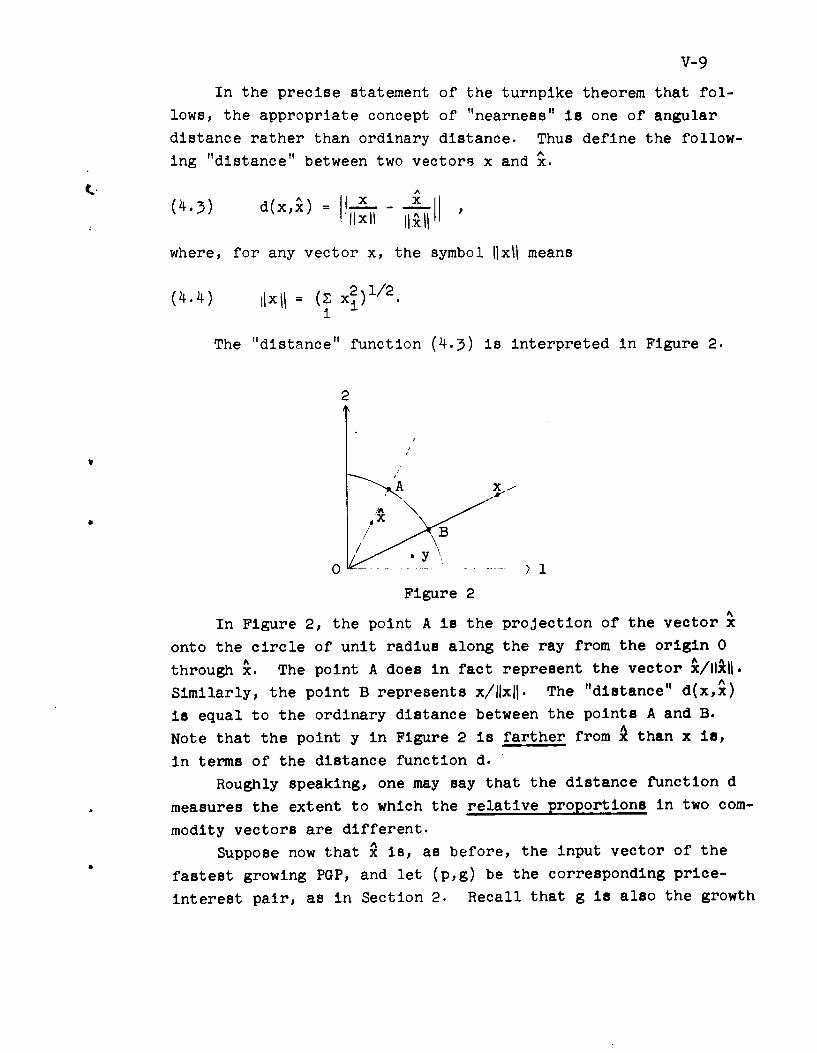
V-9

In the precise statement of the turnpike theorem that fol-

lows, the appropriate concept of "nearness" is one of angular

distance rather than ordinary distance. Thus define the follow-Aing "distance" between two vectors5 x and x.

(43) d(xx) = x xlix II JI, 11

where, for any vector x, the symbol lix1U means

(4.4) Jix = ( 2)1/2.

The "distance" function (4.3) is interpreted in Figure 2.

2

/ BXX

/

Figure 2

In Figure 2, the point A is the projection of the vector x

onto the circle of unit radius along the ray from the origin 0

Athrough x. The point A does in fact represent the vector x/II~l.

Similarly, the point B represents x/IxJJ. The "distance" d(x,x)

is equal to the ordinary distance between the points A and B.

Note that the point y in Figure 2 is farther from A than x is,

in terms of the distance function d.

Roughly speaking, one may say that the distance function d

measures the extent to which the relative proportions in two com-

modity vectors are different.

Suppose now that x is, as before, the input vector of the

fastest growing PGP, and let (p,g) be the corresponding price-

interest pair, as in Section 2. Recall that g is also the growth

V- 10

rate. In addition to the technological assumptions (i)-(vi) of

Section 2, suppose that the following conditions are satisfied:+

(vii) p > 0

(viii) If an input-output pair (x,y) is not proportional

to (x, (1 + g)x), then it yields negative profit,i.e.,

t+g- pyx < 0.

(ix) From the initial stock vector x(O) one can get onto

the von Neumann ray, i.e., for some number k > 0,

(z(O), k!) is in ".

One knows, from considerations similar to those discussed in

Chapter III, Section 1, that if a program is efficient for final

stocks, given z(O), then for some non-negative vector w 0, the

program maximizes w'z(T) in the set of all feasible programs

starting from z(O). Suppose then that such a vector a 7 0 is

given, such that 'c > 0.

Turnpike Theorem. Given z(O), for any E > 0 there is a num-

ber S such that for any horizon T, and any feasible program {z(t)

starting from the given z(O) that maximizes w'z(T), the number of

periods in which d(z[t],) 2 e cannot exceed S.

It should be noted that the number S is independent of the

horizon T. A formula for S can also be given (see the original

reference).

Finally, I should point out that the turnpike theorem does

not hold in general if some assumptions about the technology are

not made in addition to (i)-(vi) of Section 2.

+The result in RADNER is proved under somewhat more general con-

ditions than those given here, and also for a somewhat moregeneral concept of optimality.

V-ll

REFERENCES FOR CHAPTER V

D. GALE, "The closed linear model of production," in Kuhn and

Tucker (eds.), Linear Inequalities and Related Systems,

Annals of Math. Study No. 38, Princeton N.J.: Princeton

University Press, 1956, pp. 285-303.

S. KARLIN, Mathematical Methods and Theory in Games, Programming

and Economics, Vol. 1, Reading, Mass.: Addison-Wesley, 1959.

E. MALINVAUD, "On the rate of interest of proportional growth

programs," Working Paper No. 32, Management Science Research

Center, University of California, Berkeley, August, 1961

(dittoed).

M. MORISHIMA, "Proof of a turnpike theorem, the no Joint produc-

tion case," Review of Economic Studies, Vol. 28 (1961).

L. McKENZIE, "The turnpike theorem for a generalized Leontieff

model," Econometrica, 1963 (forthcoming).

R. RADNER, "Paths of economic growth that are optimal with regard

only to final states: A turnpike theorem," Review of Eco-

nomic Studies, Vol. 28 (1961), 98-lo4.

J. VON NEUMANN, "A model of general economic equilibrium," Review

of Economic Studies, Vol. 13 (1945-46), pp. 1-9.

BIBLIOGRAPHY

Chapter

K. J. ARROW, "The economic implications of learning I

by doing," Institute for Mathematical Studies

in the Social Sciences, Stanford University,

ONR Technical Report No. 101, Dec. 7, 1961.

K. J. ARROW, H. B. CHENERY, B. S. MINHAS, and I

R. M. SOLOW, "Capital - labor substitution and

economic efficiency," Review of Economics and

Statistics, V. 43 (1961), 225-250.

K. J. ARROW and L. HURWICZ, "Decentralization and III

computation in resource allocation," Essays in

Economics and Econometrics, Chapel Hill, N.C.:

University of North Carolina Press, 1960, 34-io4.

C. BERGE, Espaces Topologiques, Paris: Dunod, 1959. III

S. CHAKRAVARTY, "The existence of an optimum savings II

program," Econometrica, vol. 30 (1962), 178-87.

G. B. DANTZIG and P. WOLFE, "The decomposition princi- III

ple for linear programs," Operations Research,

Vol. 8 (1960), 101-111.

G. DEBREU, Theory of Value, New York: Wiley, 1959). III

(Cowles Foundation Monograph 17)

G. DEBREU, "Valuation equilibrium and Pareto optimum," III

Proceedings of the National Academy of Sciences

of the U.S.A., Vol. 40 (1954), 588-592.

P. A. DOUGLAS, "Are there laws of production?" American I

Economic Review, Vol. 38 (1948), 1-41.

H. G. EGGLESTON, Convexity, Cambridge: The Cambridge III

University Press, 1958.

B-i

Chapter

D. GALE, "The closed linear model of production," in V

Kuhn and Tucker (eds.), Linear Inequalities and

Related Systems, Annals of Math. Study No. 38,

Princeton N.J.: Princeton University Press,

1956, pp. 285-303.

F. R. GANTMACHER, The Theory of Matrices, 2 vols., IV

New York: Chelsea, 1960.

G. HADLEY, Linear Algebra, Reading, Mass.: Addison- III

Wesley, 1961.

L. JOHANSEN, A Multisectoral Model of Economic Growth, I

Amsterdam: North-Holland, 1960.

L. JOHANSEN, "Substitution vs. fixed production coeffi- I

cients in the theory of economic growth: a syn-

thesis," Econometrica, Vol. 27 (1959), 157-176.

S. KARLIN, Mathematical Methods and Theory in Games, V

Programming and Economics, Vol. 1, Reading,

Mass.: Addison-Wesley, 1959.

T. C. KOOPMANS (ed.), Activity Analysis of Production I

and Allocation, New York: Wiley, 1951.

T. C. KOOPMANS, Three Essays on the State of Economic I,111

Science, Chapter I, New York: McGraw-Hill, 1957.

W. W. LEONTIEFF, Studies in the Structure of the Ameri- I

can Economy, Oxford: Oxford Uriversity Press, 1953.

E. MALINVAUD, "The analogy between atemporal and inter- III

temporal theories of resource allocation,"

Review of Economic Studies, Vol. 28 (1961).

E. MALINVAUD, "Capital accumulation and efficient allo- I,IIIcation of resources," Econometrica, Vol. 21

(1953), 233-268.

B-ii

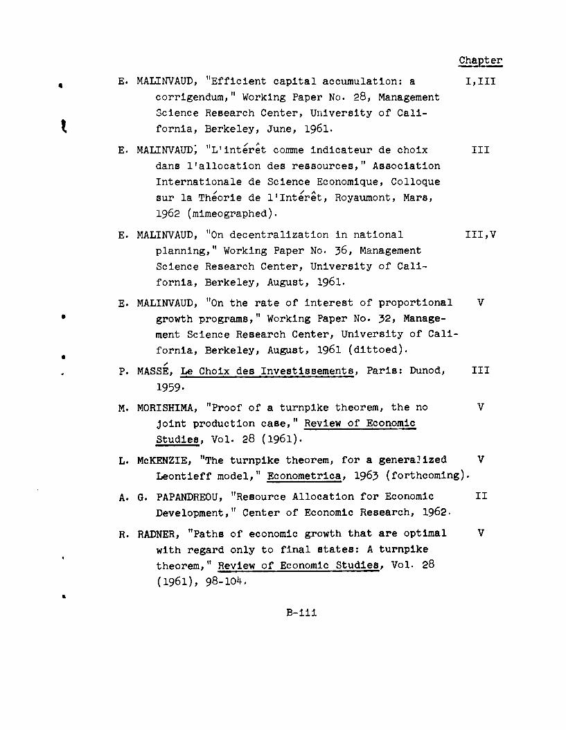
Chapter

E. MALINVAUD, "Efficient capital accumulation: a IIII

corrigendum," Working Paper No. 28, Management

Science Research Center, University of Cali-

tfornia, Berkeley, June, 1961.

E. MALINVAUD; "L'interet comme indicateur de choix III

dans l'allocation des ressources," Association

Internationale de Science Economique, Colloque

sur la Theorie de l'Interet, Royaumont, Mars,

1962 (mimeographed).

E. MALINVAUD, "On decentralization in national III,V

planning," Working Paper No. 36, Management

Science Research Center, University of Cali-

fornia, Berkeley, August, 1961.

E. MALINVAUD, "On the rate of interest of proportional V

growth programs," Working Paper No. 32, Manage-

ment Science Research Center, University of Cali-

fornia, Berkeley, August, 1961 (dittoed).g

P. MASSE, Le Choix des Investissements, Paris: Dunod, III

1959.

M. MORISHIMA, "Proof of a turnpike theorem, the no V

Joint production case," Review of Economic

Studies, Vol. 28 (1961).

L. McKENZIE, "The turnpike theorem, for a generalized V

Leontieff model," Econometrica, 1963 (forthcoming).

A. G. PAPANDREOU, "Resource Allocation for Economic II

Development," Center of Economic Research, 1962.

R. RADNER, "Paths of economic growth that are optimal V

with regard only to final states: A turnpike

theorem," Review of Economic Studies, Vol. 28

(1961), 98-lo4.

B-iii

Chapter

R. M. SOLOW, "Investment and technical progress," in I

Arrow, Karlin, and Suppes (eds.), MathematicalMethods in the Social Sciences, Stanford:

Stanford University Press, 1960, pp. 89-104.

R. M. SOLOW, "Technical change and the aggregate I

production function," Review of Economics and

Statistics, Vol. 39 (1957), 312-320.

J. VON NEUMANN, "A model of general economic equi- I,V

librium," Review of Economic Studies, Vol. 13

(1945).

B. WARD, "Kantorovich on economic calculation," Journal II

of Political Economy, Vol. 68 (1960), 545-556.

B-iv

BASIC DISTRIBUTION LIST

Nonr-222(77), NR-047-029

* University of California

University of Chicago Columbia UniversityStatistical Research Center Dept. of Industrial EngineeringChicago, Illinois New York 27, New YorkAttn: Prof. Paul Meier Attn: Prof. Cyrus Derman

Stanford University University of MinnesotaApplied Math. and Stat. Lab. Dept. of StatisticsStanford, California Minneapolis, MinnesotaAttn: Prof. G. J. Lieberman Attn: Prof. Ingram 01kin

University of Minnesota Columbia UniversityDept. of Statistics Dept. of MathematicsMinneapolis, Minnesota New York 27, New YorkAttn: Prof. I. R. Savage Attn: Prof. H. Robbins

Florida State University New York UniversityDept. of Statistics Institute of Mathematical SciencesTallahassee, Florida New York 3, New YorkAttn: Dr. R. A. Bradley Attn: Prof. W. M. Hirsch

Princeton University Cornell UniversityDept. of Mathematics Dept. of Plant BreedingPrinceton, New Jersey Biometrics UnitAttn: Prof. S. S. Wilks Ithaca, New York

Attn: Walter T. FedererColumbia UniversityDept. of Mathematical University of North Carolina

Statistics Statistics DepartmentNew York 27, New York Chapel Hill, North CarolinaAttn: Prof. T.W. Anderson Attn: Prof. Walter L. Smith

University of California Rutgers - The State UniversityDept. of Statistics Statistics CenterBerkeley 4, California New Brunswick, New JerseyAttn: Prof. J. Neyman Attn: Prof. Martin B. Wilk

University of Washington Michigan State UniversityDept. of Mathematics Dept. of StatisticsSeattle 5, Washington East Lansing, MichiganAttn: Prof. Z. W. Birnbaum Attn: Prof. Herman Rubin

Cornell University Brown UniversityDept. of Mathematics Division of Applied MathematicsIthaca, New York Providence 12, Rhode IslandAttn: Prof. J. Wolfowitz Attn: Prof. M. Rosenblatt

ii

Harvard University Cornell UniversityDept. of Statistics Industrial and EngineeringCambridge, Massachusetts AdministrationAttn: Prof. W. G. Cochran Ithaca, New YorkUAttn: Prof. Henry P. GoodeUniversity of CaliforniaManagement Sciences University of Wisconsin

Research Project Dept. of StatisticsLos Angeles 24, Calif. Madison, WisconsinAttn: Dr. J. R. Jackson Attn: Prof. G.E.P. Box

The Research Triangle Inst. Stanford UniversityStat. Research Division Dept. of Economics505 West Chapel Hill St. Stanford, CaliforniaDurham, North Carolina Attn: Prof. K. J. ArrowAttn: Dr. M.R. Leadbetter

Institute of MathematicalColumbia University StatisticsDept. of Indust. Engr. University of CopenhageNew York 27, New York Copenhagen, DenmarkAttn: Prof. S.B. Littauer Attn: Prof. Anders Hald

University of Michigan Cowles Commission for ResearchDept. of Mathematics in EconomicsAnn Arbor, Michigan Yale UniversityAttn: Prof. L. J. Savage New Haven, Connecticut

Attn: Prof. T. C. Koopmans

Carnegie Inst. of Technology

Grad. Sch. of Ind. Admn. Mass. Inst. of TechnologySchenley Park Cambridge, MassachusettsPittsburgh 13, Penn. Attn: Dr. R. A. HowardAttn: Prof. G.L. Thompson

Brown UniversityThe George Washington Univ. Dept. of MathematicsDept. of Statistics Providence 12, Rhode IslandWashington, D.C. Attn: Prof. David GaleAttn: Prof. Harold Bright

The John Hopkins UniversityStanford University Dept. of Math. StatisticsDept. of Mathematics 34th and Charles StreetsStanford, California Baltimore 18, MarylandAttn: Prof. S. Karlin Attn: Prof. Geoffrey S. Watson

Stanford University Northwestern UniversityDept. of Statistics Dept. of MathematicsStanford, California Evanston, IllinoisAttn: Prof. C. Stein Attn: Dr. A. Charnes

Logistics Research Project Purdue UniversityThe George Washington Univ. Dept. of Economics707 22nd St, N.W. Lafayette, IndianaWashington 7, D.C. Attn: Dr. Stanley ReiterAttn: Dr. W. H. Marlow

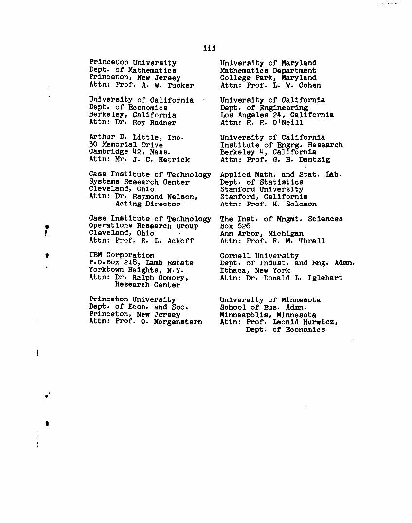
iii

Princeton University University of MarylandDept. of Mathematics Mathematics DepartmentPrinceton, New Jersey College Park, MarylandAttn: Prof. A. W. Tucker Attn: Prof. L. W. Cohen

University of California University of CaliforniaDept. of Economics Dept. of EngineeringBerkeley, California Los Angeles 24, CaliforniaAttn: Dr. Roy Radner Attn: R. R. O'Neill

Arthur D. Little, Inc. University of California30 Memorial Drive Institute of Engrg. ResearchCambridge 42, Mass. Berkeley 4, CaliforniaAttn: Mr. J. C. Hetrick Attn: Prof. G. B. Dantzig

Case Institute of Technology Applied Math. and Stat. Lab.Systems Research Center Dept. of StatisticsCleveland, Ohio Stanford UniversityAttn: Dr. Raymond Nelson, Stanford, California

Acting Director Attn: Prof. H. Solomon

Case Institute of Technology The Inst. of Mngmt. SciencesOperations Research Group Box 626Cleveland, Ohio Ann Arbor, MichiganAttn: Prof. R. L. Ackoff Attn: Prof. R. M. Thrall

IBM Corporation Cornell UniversityP.O.Box 218, Lamb Estate Dept. of Indust. and Eng. Admn.Yorktown Heights, N.Y. Ithaca, New YorkAttn: Dr. Ralph Gomory, Attn: Dr. Donald L. Iglehart

Research Center

Princeton University University of MinnesotaDept. or Econ. and Soc. School of Bus. Admn.Princeton, New Jersey Minneapolis, MinnesotaAttn: Prof. 0. Morgenstern Attn: Prof. Leonid Hurwicz,

Dept. of Economics

S

iv

BASIC DISTRIBUTION LIST FOR UNCLASSIFIED TECHNICAL REPORTS

Head, Logistics and MathematicalStatistics Branch

Office of Naval ResearchWashington 25, D.C. 3 copies

Commanding OfficerOffice of Naval Research Branch OfficeNavy 100 Fleet Post OfficeNew York, New York 2 copies

ASTIA Document Service CenterArlington Hall StationArlington 12, Virginia 10 copies

Defense Logistics StudiesInformation Exchange

Army Logistics Management CenterFort Lee, VirginiaAttn: William B. Whichard 1 copy

Technical Information OfficerNaval Research Laboratory

$ Washington 25, D.C. 6 copies

Commanding OfficerOffice of Naval Research Branch Office346 BroadwayNew York 13, New YorkAttn: J. Laderman 1 copy

Commanding OfficerOffice of Naval Research Branch Office1030 East Green StreetPasadena 1, CaliforniaAttn: Dr. A. R. Laufer 1 copy

Bureau of Supplies and AccountsCode OWDepartment of the NavyWashington 25, D.C. 1 copy

Institute for Defense AnalysesCommunications Research Divisionvon Neumann HallPrinceton, New Jersey 1 copy