UNCLASSIFIED

AD NUMBER

AD876563

NEW LIMITATION CHANGE

TOApproved for public release, distributionunlimited

FROMDistribution authorized to U.S. Gov't.agencies only; Administrative/OperationalUse; 11 AUG 1970. Other requests shall bereferred to the Office of Naval Research,Attn: Code 466, Arlington, VA 22217.

AUTHORITY

ONR ltr, 29 Aug 1973

THIS PAGE IS UNCLASSIFIED

GENWI-AL DYNAMICS

*4444l Reproduction In who le er in

part is permitted for any pur-

p0 .,o- of the United Stat',s Govern-

PROCESSING OF DATAFROM SONAR SYSTEMS

Volume VII

Each transmittal of Ihis document out.dde the Axenrie% of theU.S. Government mr !t have prior approval s-f the Offire ofNaval R1 10li;. , 2__'

1This research was sponsored by the Office of

Naval Research under Contract N00014-68-C-0")!92 (O)NR Contrict Authority ldentificatlonNu>lu.r NIt--2SG-001-1) with General DynamicsCorporation, Electric Boat Division. The workwas performed unler subcontract by Yalel' iiversit '.

lranz 11. L'uteurJnhn II. Chang

\-cr.-ne Ft. MacDonald D,.:.• :,:,,•, o <,:m iv P . olr/a v) - r !• N v 1

, / ,.7 iltCS---Ex:::~ied:,~...2•' ~k z~_/NOY 13 1910

Appr-oved: 7FV)'efr6Pr. T l va'n Woerkom

.'•~llla; :of Sci(ientiffic ,. .,rd

1 :1 7-70-051Aul:•ibL lit 197€1

ABSTRACT

Volume VII deals with the following topics:

1. Optimum Detector for Nonisotrokic Noise

The previously obtained expression for the optimum detector when

signal and noise are zero-mean gaussian processes, and when the noise may

contain interference components are analyzed to determine the detailed

structure of the detector. The detector turns out to contain beam formers

that are aimed at the target signal and each interference, the signals

from the interference beams being passed through rather complex filters and

then subtracted from the target signal. The complexity of the optimum

filter relative to conventional systems is examined, and it is found that

the added complexity is quite moderate.

2. Adaptive Array Processing

The optimum detector discussed above is most easily constructed by

using transversal filters, consisting of a tapped delay line and adjustable

weights applied to the taps. Algorithms based on the method of stochastic

approximation for automatically adjusting these weights are considered in

this section and conditions for convergence and rate of convergence under

several different conditions are obtained.

3. Optimum Passive Bearing Estimation in a Spatially Coherent

Noise Environment

The Cramer-Rao lower bound is computed for the bearing estimator,

subject to the assumption that interference noise is present. The results

are compared wich those obtained for a modified split-beam tracker

employing simple interference nulling.

I

4. Space-Time Properties of Sonar Detection Models

The problem of optimizing array configurations is not a well-posed

problem unless it can be shown that an optimum actually exists. Many

c•on ly used models for sonar detection systems turn out to be singular

so that the optimum does not exiet i.e. it is infinite. A rigorous

examination of the problem of model singularity, using measure theoretic

considerations is undertaken in this section, and general criteria for

nonsingularity of models are developed.

iv

CONTENTS

"Report Title Page

Abstract iii

Foreword vii

I Introduction 1

11 The Optimum Detector For Nonisotropic Noise 1

III Adaptive Array Processing 3

IV Optimum Passive Bearing Estimation in a SpatiallyCoherent Noise Environment 7

V Space Time Properties of Sonar Detection Models 10

38 The Optimum Detector for Nonisotropic Noise A-i

39 Adaptive Array Processors B-I

40 Optimum Passive Bearing Estimation in a Spatially

Coherent Noise Environment C-1

41 Space-Time Properties of Sonar Detection Models D-i

4V

I|I

FORE WORD

This is the seventh in a series of reports describing work performed by Yale Univer-sitv uider a subcontract wNith Electric Boat division of General Dynamics, primecontract number N0•001.4-6s-C-0:392. The Office of Naval Research is sponsor forthis contract, LCDR J. F. Lvding is Project Officer for ONR. Mr. J. W. Herringis Project Engineer for Electric Boat division under the direction of Dr. A. J.vma Woerkom, Manager of Scientific Research.

i~vii

I. Introduction

This report is the first of two volumes dealing with work completed

Iuwder contract 8050-31-55001 between Yale University and the Electric Boat

Company during the period from July 1,-1968 to April 30, 1970. More

detailed discussions of the results are contained in the four progress

reports Nos. 38, 39, 40 and 41, which are svpended. The companion volume

(vol. WII of this series) covers work done during the same time period

and contains results submitted originally in progress reports No. 42 and 43.

Three of the topics contained in this volume are continuations of work

covered in earlier reportz. dealing with the effects of anisotropy of the

background noise field - also referred to as interference noise. The three

progress reports deal respectively with the form of the optimum detector,

with the behavior of adaptive detectors, and with bearing estimation under

these noise conditions. The fourth topic, which deals with the effect of

signal models and the various possibilities for singular detection is

entirely new and represents a substantial departure from work described in

previous reports.

II. The Optimum Detector for Nonlsotropic Noise

An expression for the optimum detector transfer function when the noise

contains one or more strong interference components was originally obtained

in Progress report No. 33, which is part of volume V of this series. The

implication of this expression on the detailed structure of the detector is

examined in Progress report No. 38.

The results of both reports are based on the assumptions that the

signal, noise, and interference are all sample functions of a zero-mean

gaussian random process, that the interference consists of a number of

isolated point sources and that the noise is otherwise isotropic and far-

t

field. Under these conditions the filter can be shown to separate into a

spatial part - essentially a set of beam formers - and a temporal part or -

Eckart filter. For the case of a single interference the spatial part,

which is also the significant part, takes the form:

HIP.[,K,,[e" JWr KI ( I() e-JW' M

where the are the signal delays, the 11) are the interference delays,

M is the number of hydrophb*s Ks Ye) is the ratio of interference spectral

density to ambient noise 4ensity, and GlO(w) is given by

M .•. (TO))G 10(w) -, I P__ k- k1 k-i

This result can be interpreted to mean that the filter contains a simple

beamformer aimed at the signal and a second beamformer aimed at the inter-

ference, and that the interference output is subtracted from the signal

output after being passed through a filter with the transfer function

given by the coefficient of the second bracketed term in the above

expression.

For more than one interference the result is basically similar - a

beam is aimed at each interference and the output is subtracted from that

of the main signal beam after passage through a compensating filter. The

complexity of these compensating filters increases with the number of the

interferences; in fact even for a single interference it is such that

automatic design by some sort of 4daptive mechanism would almost have to

be used. This point is considered further below.

A major difficulty in the design is that because of the need to form

several beams simultaneously, beam steering must be done by tapped delay- [2

A

lines. The number of taps and the tap spacing are largely a function of

array resolution, which in turn, can be related to array aperture. For

typical arrays the number of taps tends to be very large; however this is

true even if conventional or suboptimal instrumentations are used. The

added complexity required in the optimal instrumentation is, from this point

of view, quite modest.

II. Adaptive Array Processing

The automatic design of complicated filter transfer functions of the

sort mentioned above can be accomplished fairly easily by means of trans-

versal filters - filters produced by feeding a signal into a tapped delay

line and adding the weighted tap outputs to form the output. For a delay

line having M taps the output y(t) of such a filter has the form

My(t)- ci x(t-ri)

where x(t) is the input signal, and ct is the weight applied to the intput

delayed by the time Ti. If - - is small for all i - I...M this

expression is a discrete approximation of a convolution integral in which

the ci represent the impulse response of a filter at time ti* Since each

c can take on any arbitrary value, extremely complex filters are easily

synthesized in this way. It was shown in progress report No. 34 that the

adjustment of the ci subject to one of several criteria of optimality is

easily accomplished by means of algorithms based on the stochastic

approximation methodof Robbins and Monro.Progress report No. 39 is a

continuation and elaboration of the earlier report.

The basic assumptions used in the analysis are:

1) Target, interference, and ambient noise are zero mean gaussian processes

2) The sum of interferences, ambient noise, and local noise are regarded as

3

the effective noise, which is assumed to be statistically independent

of the target signal.

3) The target signal component s (t) observed at the output of the ith

hydrophone is a linear time invariant transformation of d(t), the

target-signal that would be observed at the output of an ideal isotropic

hydrophone located at the origin of coordinates. The autocorrelation

function of d(t) is assumed to be known.

4) The statistics of the noise field are unknown. It is not known whether

interferences are present, or where they are located.

5) The wave fronts of target and interference are assumed to be plane over

the dimensions of the receiving array.

It is assumed that the adaptive mechanism is to produce a filter

optimized in a given direction and designed to suppress interference signals

from other directions. By varying the azimuth for which the filter is

optimized the system produces a bearing response pattern which can be

examined by an operator t4J determine whetfier a target is present.

The space-time filter takes the form of a set of K hydrophones, each

connected to the input of the delay line of a transversal filter having

M' taps. (Note that this notation differs from that used in most of the

other reports in this series). The outputs of all the transversal filters

is summed to form the signal z(t), which after possible further filtering,

is squared and smoothed to yield the observed output. The adjusting

algorithm for the K(Mil) weights in all of the transversal filters then

takes the simple form:

_J+1 - j + 2Yj [Rdd - Zj ýj

where W is the vector of all of the tap weights suitably indexed, Yj is a

weighting parameter, R d4 is the input space-time autocorrelation function,

4

Lj is the output z(t), and i is a vector of delayed versions of the received

signal; all at the jth step in the iteration. The process converges for* aJ

of the form y j 3 with h < a < 1. Rd• can be computed if the target

signal direction and autocorrelation function are known; thus it contains the

information about desired target direction that is needed for the filter to

adjust itself.

General expressions for the convergence of the filter have been

obtained and are given by Eqs. 3.5 - 32 and 3.5 - 33 of progress report 39.

These expressions are too complicated to yield much insight. They can how-

ever be simplified by chosing specific expressions for the weighting

parameter y A particularly simple expression results from the choice

Y M) 2() l)i , where Am is the mth elgenvalue of the covariance matrix

of the received signal, and where the superscript (m) on yj implies that

different weights are used in different filters. In this case it is found

that the mean-square error at the (j+l)th step is given by

2 2 1___ 2 - T)aj4l (J+l) 2 emn + )2 - y (- p

where R is the covariance matrix of the received signal, and where ermiuY

is the irreducible error resulting from the fact that a continuous filter

is approximated by a discrete structure. If the second term is initially

larger than the first then this expression indicates an initial m.s. error

reduction at a rate j-2 ; however eventually the first term will always

dominate, with the result that convergence eventually takes place at a rate1-l"

As long as the noise environment is stationary the filter converges

to the optimum form discussed in previous progress reports (e.g. #38) in

which the interference noises are strongly suppressed. This is shown not

5

only analytically, but also by means of a computer simulation using real

data. If the noise environment is nonstationary, Partial results have

been obtained under the following conditions%

1. If the nonstationarity can be characterized by chanping parameters,

with the values of the parameters governed by a known dynamic relation

than the method of stochastic approximation can be modified by inclusion

of this dynamic relation. In fact the recursive Kalman filter method can

be applied to this case with results that converge to those obtained by

the method of stochastic approximation in the stationary case. In the

nonstationary case the weighting parameter y of the stochastic approxi-

mation algorithm is modified and takes the form y - Yj + B, where B is

a constant. For the case where the optimum gain parameter e is Riven by

the relation

hj+l a a ej + UP 0 < a < I

and where the desired filter output is given by

where 4a [

and where u and v are stationary independent, zero mean, scalar, white

noise processes, with variances q and * respectively, then

B =q/

For the stationary case q - 0 and a - 1, so that 8 - 0, but in general

the presence of a nonzero B prevents the gradual disappearance of the

Seightinp parameter yj, which would make trackin2 of a chsanging environ-

mr'ent impossible. On the other hand, the fact that y does not Po to zero

as j * has the effect that the filter does not converge in mean square,

which means that a small Jitter (proportional to 0) continues to exist in

the output.

2. If the nonatationarity is such that the optimum gain parameter e

satisfies a relation of the form

-Jjl - j + 15

i.e. the nonstationary is in a sense "temporary" and disappears with J

then the standard method of stochastic approximation converges as long as

the weighting factor yji has the form

YO

where Isc<ac<l

an S <

Other methods for dealing with nonstationary environments can be

envisioned, but have not yet been evaluated.

IV. Optimum Passive Bearing Estimation in a Spatially Coherent

Noise Environment

Report No. 40 is a continuation of report No. 37 which was included

in vol. V. The earlier report dealt with the Cramer-Rao lower bound for

determining the rms bearing error attainable in an isotropic noise field.

The present report extends this ta the case where interference is present.

As in the earlier report the analysis initially considers an arbitrary

number of hydraphones arbitrarily spaced on a linear array, and arbitrary

signal, ambient noise, and interference spectra. However, in order to get

results that are simple enouph to yield some insight into important

parameters, some of this generality is sacrified; in particular it is

7

assmd that the ambient noise power is much greater than the signal power;

signal, interference, and ambient noise spectra are taken to be identical In

form, and the hydrophone spacing in uniform. Additional important assumptions

are that the interference bearing is known and that the ambient noise is

independent from hydrophone to hydrophone. Also, as in the earlier report

the performance of the split-beam tracker is computed to provide a comparison

between the possibly unrealizable bound and a practical instrumentation.

Approximate expressions for the lower bound take on simple forms if

the target and interference separation is either very large or very small.

In each case limiting expressions have been obtained for the ambient-noise

dominated case (MI << N) and for the interference dominated case (MI >> N).

The parameter determining target and interference separation is y - (d/c)o

W (sin 6 - sin 0 ) where d is the hydrophone spacing, c is the soundmax

velocity wa is the maximum frequency, 6 is the target bearing and 4 is

the interference bearing. If the bias terms are neglected then for y >> 1

the respective lower bounds are approximately

36irc 2(N 2+11N8)Is2 (Ml << N)

TWT 3 d 2 coS2 e(M -N )([+Qf-2)I/N]max

- )2 >

22 2

36r c2 [N2+(M-I)NS]/$2 N)T 3 d 2cos2. M 2 - 8/5 M3 + 2M]

max

The lower bound for I - 0 (i.e. no interference) is the same as that

found in report No. 37. By comparing the denominators in the two

expressions above one can conclude that the effect of a remote interference

is equivalent to the loss of 2/5 of a hydrophone.

For near interference, such that y < l/M, the corresponding results

arT

361c (N2+MSN)/S <1 N)

36rc2 MI[N+(M-l)S]/S

T w d2 Cos2 8 (M 4 _M2 ) <<N

If the difference in denominators (which amounts to the previously mentioned

2/5 M) is discounted, the lower bound in the interference dominated case is

seen to be MI/N times as large as for large y.

A modified form of split-beam tracker employing simple interference

nulling ahead of the split-beam section was considered in progress report

No. 29. For this tracker the following results were obtained:

"967r c2 N2S2

T) 0 M 2 (M-2 )2(•_•2 ma

T_ T d cos O (MC-2) y M

The second of these expressions is invalid for y very near zero because

some of the approximations made to obtain it break down, however it is an

indication that the modified split-beam tracker cannot estimate bearings

extremely close to the interference bearing (since as a result of the

nulling there is no signal in this direction). In this respect the split-

beam tracker performance appears to fall considerable short of the Cramer-

Rao bound, which is finite for y = 0, albeit consideralby larger than for

large separation. The comparison between the split beam tracker and the

Cramer-Rao bound is facilitated by computing the ratio of the two error

variances, this is

9

2 2.67(1+2.4/M) y>> 1, M>> 1

11.-(1+8/M) 0 < y << 1, F>> 1y

The second of these expressions Is invalid for y * 0 as Indicated above.

Both expressions indicate that for sufficiently large M the split-beam

tracker performance is fairly close to the lower bound; but at the same

time they also suggest that some improvement might be achieved, particularly

for small separations between target and interference, by going to a

different implementation. Such implementations are currently being studied.

By plotting curves for the exact expressions rela:ing (9 - 9)2 to y

it is found that the large y approximation is good for separations between

target and interference bearing greater than the beam width of the array,

defined as the angle for which the signal output falls to one half its

maximum value. This is roughly true both for the C-R bound and the split-

beam tracker. Also, in both cases, for separation smaller than the beam-

width the performance deteriorates rapidly; however the deterioration is

considerably more rapid in the case of the split-beam tracker.

The error variance decreases with M4 for large separations in both

cases, and the C-P bound decreases with M3 for zero separation between

target and interference bearing. Thus theoretically the error can be made

arbitrarily small for both large and small separations by letting M become

sufficiently large. Here it must be noted however, that for a fixed size

array the assumption of zero ambient noise correlation between adjacent

hydrophones will become invalid for very large M.

V. Space Time Properties of Sonar Detection Models

In all previous work, and in most analyses of sonar in the literature

the array configurations are taken as given. In a good many of the analyses

10

reported in the previous volumes, in fact, the arrays have been assumed to

be linear and with equally spaced hydrophones. The question naturally

arises as to whether the performance of an array with a given number of

hydrophones might not be improved substantially by seeking an optimum

"configuration.

It turns out that the attempt to find algorithms for determining the

optimum placement of hydrophones involves searches through a 3K-dimensional

continuum. where K is the number of hydrophones. For the large values of K

that are of practical interest such a search is an extremely formidable

undertaking for which there is no guarantee of success. Hence it becomes

very desirable to obtain first some estimate for the ultimate performance

of which an array with a large number of arbitrarily spaced hydrophones is

capable. Such an estimate is, however, even conceptually possible only if

in the lin-it of continuous observation (i.e. as K + ") the signal model

remains nonsingular. Many commonly used models turn out, in fact, to be

singular; i.e. as K - it becomes possible to determine the presence or

absence of the signal with zero error even though both the array size and

observation times are finite. For this reason such models are physically

not completely realistic (which is not to say that they are not useful), and

it is desirable to obtain general conditions guaranteeing that a given model

be nonsingular. This is in essence what is done in report #41.

The approach taken is based on the realization that any communication/

detection (C/D) system can be represented as a series of mapping operations;

i.e. an encode operator e maps source characters from the space A of source

characters into the space W of channel signals which is in turn mapped by a

transmit operator t into a space V of receivable signals, etc. until the

final mapping produces an estimate a of the source character, which is an

element of the space A. The operators are stochasticallv determined, hence

" = ------ ="11

can be considered as being themselves elements of probability spaces E, T,

etc. The notation is generalized by denoting the space of source characters

by SI and the space of mappings of S2K-1 into 52K+. by S2K where K a 1,2,3...L.

A marginal probability measure Ui may then be defined on each of the spaces

Si where i - 1,2,4,6...2L. These measures will induce probability measures in

the remaining spaces S2K÷l, K - 1,2,3...L; furthermore they induce conditional

measures of the formV, the measure induced in Si conditioned on the trams-

mission of a signal a.

A class of models having particularly simple properties are the factor-

able models. In this class the probability measure V defined on the product

space S a S1 x S2 x 54 - S 2L is given by

This form of the measure implies that the stochastic operations of the model

are independent. Yost of the models used in the usual communication and

detection studies are factorable in this sense.

The central theoremes concerning the singularity of models are then

given by Corollary lof Theorem 9, and Theorem 10 of chapter 2:

If S - S 2L+ are countable with discrete metric, then the model Mis singular if and only if the conditional measures v r n L+, are

2L+l 2L4-

orthogonal for every pair of characters r and s in S1 for which P(r) > 0

and such that r 0 s.

If M is a factorable model then it is singular if and only if P2k+l

and U2k l are orthogonal for all k < L, and r 0 s.

The implication of these theorems is that for a factorable model to

be singular, singularity most be present in the first stage, and it must

be preserved by all subsequent transformations or mappings. Mile this

might appear to be a rather strong requirement which would have the effect

12

of making most practical models uonsingular, it turns out that many of the

usual encoding transformations considered in communications processes

preserve singularity, so that singular models are actually more comwon than

might be supposed. In particular, it is shown in Theorem 1 of chapter 3

that additive stages are usually singularity preserving. On the other hand

it is shown in Theorem 2 of this chapter that if stage k is such that the

support space of the measure u2k is a subspace of the previous apace (S 2 k -)

and if u2k is independent of U for all i < 2k then the model M is nonsingular.

LParticularly simple statements can be made if the conditional measures

11 rl are Gaussian. In this case one can use the fact that two Gaussian

measures are either orthogonal, or they are equivalent. Furthermore

according to Theorem 4 of chapter 3 two Gaussian distributions P and Q are

equivalent if and only if

1. m(-) E: H(r)2. r has a representation r (s,t) - X K ek(s) ek(t) where the set of

functions e k(t) is a complete orthonormal set in the reproducing

2kernel Hilbert space H(r ) and E(1-Xk) < -, and X > a > 0 for all k.Q k k

In this thteorem rP avd rQ are covariance of the distributions P and Q, with

mean functions m(') and 0 respectively. As a consequence of this theorem

singularity may occur when the mean function of the signal process lies

outside the space H(rQ); i.e. if P has a linear projection outside the support

space of Q; if this is not the case singularity may still occur if some noise

eigenvalues are zero or if the signal and noise processes do not put almost

the same energy into all but a finite number of dimensions (or eigenvalues).

Applications of this theory have been made to two simple sonar situations.

The first of these is one dimensional: a source is either to the right or to

the left of the observer, and the observer can determine the direction of wave

propagation. This situation is singular, even if the velocity of propagation

13

is random, if random noise is added, and if other random effects are present,

as long the randomess is not sufficient to make a right-going wave look

like a left going wave.

The more interesting problem of sonar In three-dimensions has also

been analyzed with the result that the usual model ý.n which the signal wave-

front isa deterministic function of the coordinates is also shown to be

singular. This explains the result of Vanderkulk that as the number of

hydrophones goes to infinity, the array gain becomes infinite and detection

becomes perfect. This result is shown to hold even if white noise is added

at each hydrophone; to produce a nonsingular model it is necessary to

introduce some perturbations into the wavefront. The affect of perturbed

wavefronts is currently being analyzed.

HI14

F _______

THE OPTIMUM DETECTOR FOR NONISOTROPIC NOISE

by

Franz B. Tuteur

Progress Report 'No. 38

G-2neral Dynamics/Electric Boat Rcsc~arch

September 1968

I)IF.P'AIKI MIN-L,\ E N ENGIN EE RIN(;

AND) APPLIEI) SCIENCE

YALE UNIVERSITY

Summary.

The feasibility of using tapped-delay-line filters to synthesize the

optimum processor is investigated in this report. It is found that the

most severe requirement that is placed on the delay lines arises from the

necessity of steering the arrav in steps that are commensurate with the

resolution of which the array is theoretically capable. If delay lines to

accomplish this can be fabricated then the additional comnlexity required

in the construction of an optimal filter is relatively minor; that is, it

requires delay lines of no greater complexity.

I!A-rI"

|A-

The Optimum Detector for Nonisotronic Noise

I. Introduction.

In Progress Report No. 33 (Ref.1) the effect of localized noise sources

on the performance of the optimum (likelihood-ratio) detector of directional

Gaussian sisaals was investigated. In the present report the structure of the

optimum catector is considered.

The nomenclnrure used it, this progress report is exactly the same as that

used in Ref. 1, which is assumed to be available to the reader.

11. General Form of the Optimum Detector

The oencral fcrm cf the nptzmum detector is contained in Eqs.(22) and (23)

A Ref. 1. If the output of the filter is designated by

u = log LR - C (1)

then the optimum detector structure has the form

WT T 12U=Z 1 Ili W(n)X)

he-()1 (n) rn(n) W - (3)N(n) /-i + S(n)G (n)/N(n)

'nd where th2 optimum array zain G (n) is defined by

GC0 (n) a V T(n)Q-I (n)V* (n) (4)

If thL time of observation T is large, the summation in (2) can be converted to

an integrral in the frequency variable fh hence the detector output U takes the

f orm,• ~u -- T . _T)_()2f(5)

whczre by direct analogcy with Eq.(3)

nS(f) / S(f 5 f ) f) V*(6)

-- - N(f) /4+ S(f)G(f)/N(f)0

A-2

IIn this expression S(f) and N(f) are, respectively the signal and noise spectral

densities, and Q(f) is the noise spectral matrix whose elements are the cross

spectral densities of the noise voltages received on the different hydrophones

of the array. 7(f) is the steering vector, given by

j2RfTI

(f' 1 (7)

1MjnTM

where the c1 are hydrophona gains and T the signal delays. Also, the array

gain becomes

G 0 (f) = (f (f) (f) (8)

If the bandwidth W is very large, Parseval's theorem can be used to con-

vert Eq. (5) into T

iZ W f(t) 2 dt (9)0

where z(t) is the inverse Fourier transforn of H (f)X(f). This innlias that

u can be obtained from a circuit of the form shown in Fig. 1.

-- No~f)--un- 1() -- rua

rer rS/

/

Figure 1. Likelihood-ratio Detector

In this figure H (f) is a filter containing the common frequency-sensitive

component in H(f), namely A-3

H c(f) . (o10C N (f)94-SC()d(f)/N(f)

The individual filters H 1(f), H2 (f)...H (f) are then respectively the first,

second, .... , 1i4h row of the matrix product 2.-(f)V (t).

III. LerailA Ytrr-jcture of the Filter with Directionyt Interferencc.

As in section IV of Ref. 1 we assume that the noise component consists of

an isoLropic part and a numbecr of point sources. Then the noise spectral

zatrix has the form

N (f) R T

'1(f) N t%(f) + E Kr(f)Vr*(f)V (f)] (11)r=l r

where K (f and where I (f) is the spectral density of the r noiser N () r

source.

Since the frequency weighting filter of Eq.(lO) is common to all channels,

the essential oneration performed by the processor is

H' (t) q-l(f)V*(f) (12)

The inversion of the spectral matrix in (12) can be accomplished by

means of Eq.(35) in Ref. 1. The result is

HI V %ý[/ fK V1 .v2 :AS*.QT-Wc1 -12 (13)N (f)0

where the dependence of %, V r, Kr, G, and £ on f has been suppressed for

convenience. The notation of Ref. 1 is used, with n replaced by f in all

cases. Note that the scalar multiplying factor N(f)/N (f) can be absorbed

into H (f) of Eq.(10) so that the essential oneration is that indicated by

thu expression in the braces, {...1.

To gain some insight into the implications of this result we consider some

Ainplc examples. In all cases we assume that %(f) - I, the unit matrix;

this implies that there is no interphone correlation of the isotropic noise

coAponent._ A -4

Suppose first that there is only a single interference. Then the ex-

pression inside the braces in Eq.(13) becomes

N 0 f)* KIo*U"(f - ~f)H (f) - V K1 1 V1

(f) (f) - -o vl +7K 4-l

-1 10-~ (1) 3(14)e e

where w - 2vf and where (1)

M j2irf(T k k (5G 0 lo f) e .rk)

k-i

The unsuperscripted T's are the signal delays, while the superscrioted T'S

are the interference delays. Thus Eq.(14) indicates that the filter forms

two beams, one steered on the signal and one on the interference, the outnut

of the interference beam is passed through a filter with transfer function

KIG M + KIM) and the result is subtracted from the signal beam output.

A possible system block diagram is shown in Figure 2. This system is quite

similar to that proposed by V.C. Anderson [4] and. reported on by Cox [5].

-T Signal Beam

H (fC

InterferenceBeam

M 4

outnutFigure 2. Optimum Filter for Single Interference.

A-o

This filter can be constructed using M tapped delay lines to generate the

delays T k and Tk(1) in each hydrophone channel, and two additional delay lines

to generate the filter functions H (f) and K (f)G 1 0 (f)/[14MK (f)]. The use

of tapped delay lines for the construction of variable filters is discussed

in detail in Refs.[2] and [3]. and it has the advantage that they permit

automatic adjustment by relatively simple adaptive algorithms.

It is clear that the delay lines used in each of the hydrophone channels

must have a sufficient number of taps and a sufficiently small inter-tap

spacing to permit steering to any one of the distinct beams that can be re-

solved by the array system. In this connection it should be noted that if

interference elimination were not a factor mechanical steering of the array

could be used to reduce the length of these delay lines. However, since

interferences may cone from any direction, interference elimination requires

that delay lines of the maximum length needed to steer the array through 360*

bi used in each channel.

A discussion of delay-line characteristics is given in Appendix B, and

it is shown there that the number of taps needed tends to be very large.

Specifically, for a linear array with M hydrophones spaced uniformly a

distance d apart the number of taps is given by

B d %TG'-1)

where B is the signal bandwidth and c the velocity of sound. Using typical

values of B = 2ir x 5000 rad/sec., d - 2ft, c = 5000 it/sec, and 14 = 100, this

works out to K - 26400 taps. Also, it is shown in Appendix B that the tap

increment under these conditions should be on the order of 1.551 sec. The

numbar of taps needed appears to be well beyond currently available hardware.

A-6

The function GC f) given in Eq.(15) is most easily constructed from am m• .(1) .delay line having at least M taps giving the delays Tk - k M l...M.

Since both target and Interference can be located anywhere in azimuth this

line must have the same resolution as that needed in the individual channels.

Furthermore, the maximum delay needed is at least twice that needed in the

channels. This is easily demonstrated by considering a linear array in which

I -•. k (sine 1 - sine)

where e1 is the interference direction and 6 the signal direction. The maximum

value of delay, obtained for k - M, 01 - -v/2 and 0 = w/ 2 is 2Md/c while the

minimum value is -2md/c. A delay line can only produce positive delays: the

effect of negative delays can be obtained by inserting a fixed delay line into

the line from the upper summing junction in Fig. 2, as discussed in Ref.5.

If this is done the range of delays needed in the tapped delay line under

consideration is 2Md/c compared to a maximum delay of (Q-l)d/c needed in the

channels.

The additional frequency weighting K(f)/[l + MYl(f)] is a relatively

minor modification in the filter characteristic. It can be imniemented by

applying different weights to the tap outputs before they are summed, as

explained in Refs.[2] and [3]. Thus the entire filter function

KICf)G1 0 (f)/[l + MKI(f)] can be constructed from a standard tapped delay line

filter using a delay lina with twice as many taps, hence twice as long, as

the delay lines used in the channel. It therefore involves no major additional

design problems.

Actually, it is possible to redraw the block diagram of Figure 2 in such

a way as to cut the length of the delay line needed to generate G1 0 (f) in

half; i.e. to make it no longer than the lines used in the individual channels

to steer the array. Such a block diagram is shown in Figure 3.

A-7

tI

(--)- _ ___ ___-T

• _C

+ 21

itl I 1+NK (f) 1 2

Delay Line

Figure 3: Modified Block Diagram for Single-Interference Filter.

it can be verified that this system produces the same output as Figure 2, but

the delay line at the lower right of the diagran, which is needed to generate

the function C10(f) has taps only at delays (1), 2(1), etc. rather than at

the delay differences TiI- 1 [i 2 T2 - T2* etc. Hence the maximum length

of this line needs to be no greater than the lines used in the individual

channels.

A-8

Finally, the function H (f) must be considered. Since this is a muchc

simpler function than G10 (f) it can be synthesized by means of a separate

tapped-delay-line filter with only a modest number of tars. Alternatively,

H ce(f) can be generated in each channel by summing some of the tap outputs

of the delay lines used for steering the array.

If the signal and noise spectra are similar in form and if the SNR

S(f)G0(f)/N(f) is small, Hc (f) can be omitted entirely.

Two Interferences

With two interferences the expression in the braces of Eq. (13) becomes

explicitly: [1+ 11 IE G'1 j4G 1

If it is again assumed that [ 1 2 12 thsbeoeHi r t-e ths ecme

H" - - AI(f)V1 - A2 (f)0 2 * (16)

whr A() Kl(f) [I÷MK2 (f)]G1 0 (f) " Kl(f)K2 (f)Sl 2 (f)C 2 0 (f)SI~+M[RI(f)+K 2 (f) ] + [M2- 1GI 2 (f) 12 ]K1 (f)K 2 (f)

K2(tf)+MKI(f) G20(f) - K (f)K2(f)G 6f)OG(f)and A2 (f) = 2 1 0 1 2 21 1 0 (18)

l+[K 1 (f)+K 2 (f)] + [M- IG 12 (f) 12 KI(f)K2 (f)

Thus the system takes the form shown in Figure 4. If It is large, and if the

interference sources are reasonably well separated it is shown in Ref.l that

122I i 12 (f)~ -2 M and can therefore be neglected relative to M. Under these

conditions the denominator factors giving

A (f K(f) K(f)K2 (f) 1 2 (f)G2 0 (f) (19)

1lf l(f Sl 0 (f) - (19f, ~~[I+MKI (f) ] [l+MK2 Mf)

andK (f) K (f)K 2 (f)G2 1 (f)G (f)2 1 2 221 10 (21))A 2 (f) l+MK2 (f) O20 (f) -[l+MKI(f)][l+MK

2 (f)]

A-9

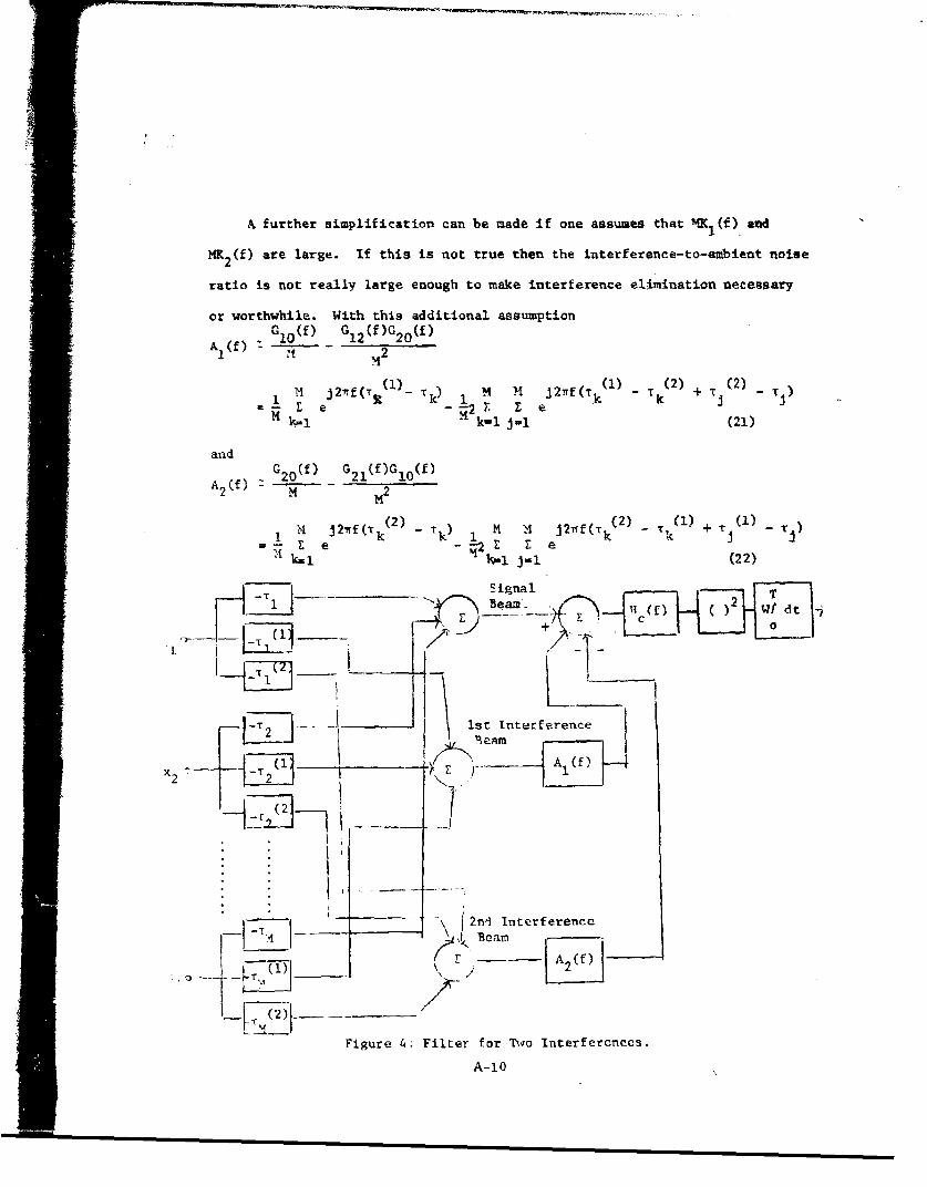
A further simplification can be made if one assumes that '-!K(f) and

M2(f) are large. If this is not true then the interference-to-ambient noise

ratio is not really large enough to make interference elimination nezessary

or worthwhile. With this additional assumptionC 1 0 (f) G1 2 (f)G 2 0 (f)

S(f) 2

j27f(T (1)_- 2 M( (1) (2) (2)

1 • e -q2 Z e +H k-i kiwi j-1 (21)

and

A(f) GG2 0 (f) G2 1 (f)G 1 0 (f)

I 2ff Tk(2) T -1M M, j21ff ( k(2) _Tk (1) + j (1) )

E ei21f(Tk - 2k) Z - (ik.14X- 1 - (22)

___ ---- "Signal - T_T L 2-

1•-- .. .1 st. eTht erf[rence-•.

_____ ___1_ (f)_ Af (

SI0

(0 -7

ýL2 2'id Interference

- -T 13 e am -

A (f)

Figure 4: Filter for Two Interferences.

A-10

It is easily seen that the filter functions A1 (f) and A2 (f) can be

constructed from tapped delay lines with weights applied to the tap outputs.

Since the single summation term has already been discussed, we consider only

the double summation. Again, it is clear that the resolution needed is the

same as in the delay lines used in the channels. Also, if one examines all

extreme values of T T (1) and T (2) one can show that for a linear arrayI kt 1k 9a kthe total delay can range from -2Md/c to 2Md/c. Since the delays required

by Al(f) may be the negative of those required by A2 (f) it is necessary to

use a fixed delay of 2Nd/c in the signal beam channel and tapped delay linesof length 4Md/c in each of the interference channels. Thus the tapped delay

lines must be four times as long as those used in the hydrophone channels.are N2

Since there are terms to be summed it might appear that at least

_ 2 taps would be needed on these delay lines. Although it is shown in

Appendix B that tapped delay lines used for linear or circular arrays should

have considerably more than M taps, this is not necessarily true in other

array geometries. However, if a line with sufficient resolution to resolve

distinct beams of the array system does not have enough taps, it simply

means that some of the terms in the double summation are identical, at least

to the accuracy of the delay increments. Hence these terms will be more

heavily weighted in the sum. Thus it appears that the delay line required

for the double summation needs to be no more complicated than that used for

the single summation. Note that it is just as easy to implement the exact forms

of A1 (f) and A2 (f) as the approximate ones given in Eqs.(21) and (22). If

the additional frequency weighting required by the exact function is reasonably

smooth it will call only for small changes in the weights applied to the tap

outputs. This is true even if the effect of jG12(f)12 i the denominator

of Eqs. (17) and (18) is taken into account, because the angess introduced

by this term are no more rapid .han those produced by the numerator terms.A-iI

Also the function c(f) may as well be combined with AI(f) and A2 (f). Thus

the optimum filter capable of handling two interference signals would con-

sist of M tapped delay lines of unit length and two delay lines of four times

this length. In addition a fixed-length delay line would be needed in the

signal-beam line as discussed in the previous example. The number of taps in

a unit-length tapped delay line is that given in Eq. (A-35) of Appendix B.

It is undoubtedly possible to rearrange the block diagram to make more

efficient use of the delay lines as was done in the previous example.

However, since such a procedure would not reduce the complexity of the delay

lines by any order of magnitude, this matter is not pursued here.

More than Two Interferences

If the assumption 9(f) - I is used in Eq.(13) the expression in braces

becomes:

--- lH"(f) - {V - /V ¾V V,'KV I[ + G) )o 1-1:'-2-12:"~--

M *. A *. A (23)1V - AI(f)V1 - A2 (f)V2 . -AR(f)VRwhere A (f) = (f) [rth element of [I + G

r r.

Since [I + G] is now an R dimensional matrix it is clear that instead of

double summations of the sort appearing in Eqs.(21) and (22) A (f) nowr

involves R-fold sur.mations. A typical form of such a summation is the three-

M M M j1T (-uk (1) k(2) + T (2) _Tj(3)_THi M M j2nf(T ~- rk + (2) - - r ).

fold summation I E E ek-i j-i %-I

Although it is somewhat difficult to examine all terms of this sort, it is

fairly clear that the maximum delay that can occur is twice the value

required to steer the array through 3600. Also, it is necessary to account

for the fact that these delays can be positive or negative. Thus each one

of thcý A r(f) [or H c(f) A r(f)] can be generated by a delay line of four unit

lengthq. The R-fold summation will, of course, require the addition of MR

terms, however as was noted in connection with the double summation, many of

A-12

these terms are identical, and therefore the variable weights applied to each

tap output should permit the filter functions to be generated without the

need for a larger than normal number of taps.

Assuming that a quadruple-length delay line can be constructed by

connecting four single-length lines in series we see that the total number

of tapped delay lines is 4R+M. In addition at least one fixed delay line

is needed to permit the generation of negative delays.

It will be noted that none of the block dia!rams presented so far are in

the form of Figure 1. Since the block diagrams suggested in Ref. 3 are of

this form, it is of some interest to consider the arrangement shown in

Figure 5, which is essentially in the form of Figure 1.

By inspection of this figure the transfer function .•(f) for k 1 1...m

is given by

Bk(f) - r + . eA (f) (24)

It is clear that a tapped-delay line filter that can implement Ar(f) forSr - 1 .... R will have sufficient flexibility to implement Rk(f). Furthermore,

the post-summation filter c(f) shown in Figs. 1 and 5 can be moved into

each of the hydrophone channels, and the delay line filter that can implement

(f) can also implement Hk(f)H (f). Thus it appears that a delay line of

four time unit length in each hydrophone channel, with adjustable weights

on each tap, should suffice to generate the optimum filter function. This

arrangement would therefore call for 4?4 unit-length lines, where unit length

refers to a line capable of providing all the delays needed to steer the

array through 3600. In Ref.[l] it was suggested that the numnber of single

interferences that can be eliminated by the kind of system discussed here

is on the order of &. Therefore, since for all M 5 2 4M > 4Ai + M the

block diagram of Fig.5 is less efficient in the use cf delay lines than that

of Fig.4. However, it is again true that no order-cf-magnitude difference is

involved.A-13

Conclusion

If correlation of the isotropic noise components between adjacent hydro-

phones is negligible then the optimum filter is shown to consist of an array

system capable of forming a signal beam and R additional beams that are

steered on each one of the interference sources. After passing through rather

complex filters these outputs are subtracted from the signal beam-former out-

put and the result is then passed through a post-sunmation filter, squared,

and averaged.

Filters of considerable complexity can be synthesized automatically by

use of tapped delay lines. The tap outputs are individually weighted and

then sumsmed to provide the filter output; the weighting can be accomplished

by a simple computer which implements an adptive algorithm. Such adaptive

filters have been considered by Luckey (2] and by Chang and Tuteur [3].

If tapped delay lines are used to generate the R + 1 beams that must be

formed by the system it is shown that the number of taps required is

2proportional to BD lcd where B is the signal bandwidth, D is the array size,

d 1.5 the interphone spacing and c is the valocity of sound. Typically, for

a linear array with 100 hydrophones the number of taps required is on the

order of 20000 or more; which appears to be well beyond current technology.

However, since this requirement arises primarily from the need to produce

several beams it is shared by suboptimum processors such as the simple

multiple beam former. In fact, it is also shown that the additional com-

plication needed to make a conventional system into an optimum one is

rocatively minor. For a system having 1 hydrophones, and capable of elimi-

nating R interference sources, the optimtm system would require 4R+M delay

linns, while the simple beam former would require M delay lines. The

A-14

conclusion seems to be therefore that if tapped delay lines can be built

to steer the array satisfactorily then the optimum processor can be built

fairly easily by the use of a few additional delay lines plus some

relatively simple associated circuitry.

List of References

1. F.B. Tuteur, "The Effect of Noise Anisotropy on Detectability in anOptimum Array Processor", General Dynamics/Electric Boat ResearchProgress Report No. 33 (September 1967).

2. R.W. Lucky, "Automatic Equalization for Digital Communication' BellSystem Technical Journal XLIV, No. 4, (Avril 1965), Dp.547-588.

3. J.H. Chang and F.B. Tuteur, "Methods of Stochastic ApDroximationApplied to the Analysis of Adaptive Tapped Delay Line Filters', GeneralDynamics/Electric Boat Research kept., No. 34 (October 1967).

4. V.C. Anderson, "Steerabla Null Processing", Proc. 23 Naval Symposiumon Underwater Acoustics 1965 (429-433).

5. H. Cox, "Array Processing Against Interference", Naval Ship SystemsCommand, Washington D.C., October 1967.

6. P.M. Woodward, "Probability and Information Theory with Applicationsto Radar", McGraw-Hill Book Company, Inc., New York, 1953, naga lnl.

A-j5

Appendix A

The Number of Distinct Beams Produced by an Array

Consider a conventional array having 14 hydrophones as shown in Figure Al.

For the sake of simplicity it is assumed that the only processing done is to

.- T s 2 t) 2 a() Integrator -4-

Figure AIl Conventional Array.

ixh; sh igna•i rouia ;xch hydrophone in order to steer the array, the delayed

,i•:n xl' "r,: Lh~n 3un.-lod, the result is squared, and averaged.

"T'h. rc:i~cved •igna! iS

Z~t)= S~) + ~t)A. 1

T

[(t) n 1 )..... k (t)]T

T

Fil h11r: Of this discussion we consider only s(t), which is

tsý5u-d to I,, expanded in a Fourier stries so that

WT J • t(t)s V(n) A.2

V(n) = gives the signal direction.

- rA-16

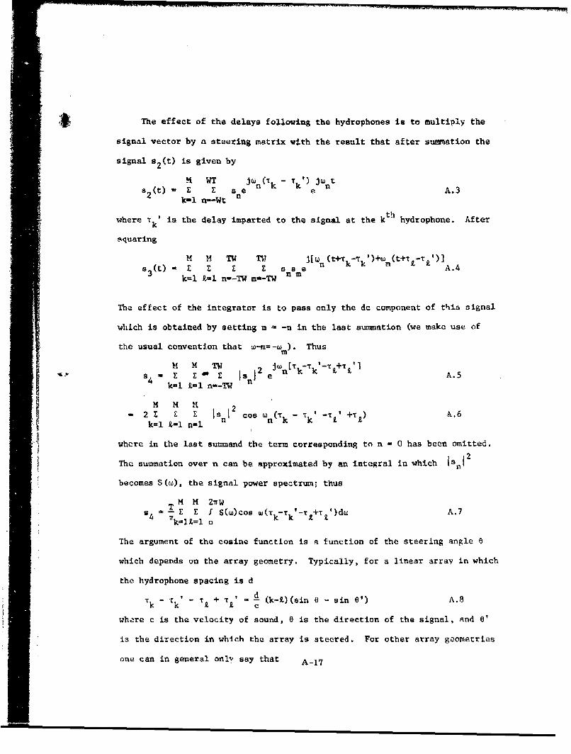
-i # The effect of the delays following the hydrophones is to multiply the

signal vector by a steering matrix with the result that after summation the

signal s 2 (t) is given by

M WT JW-(T k - Tk j) JUnts s2(t) - E E Sa n A.3

k-i n--Wt

where Tk' is the delay imparted to the signal at the kth hydrophone. After

squaring

M M TW TW J[Wn (t+tk-Tkf)+wM (t+t z-r)]S 3 W -E E S se A.4

k-1 9-l n--TW m-TW n1 m

The effect of the integrator is to pass only the dc component of this signal

which is obtained by setting m - -n in the last summation (we make use of

the usual convention that w-m=-w ). Thus

M M TW 2 w[Tk-Tz+-' L"a 0E i ej A.5

k-l t=1 n=-TW

M M K- 2 Is n£ cos Wn(Tk - Tk' -Tt +T ) A.6

•'i"! k=l Z,-1 n-l

where in the last summand the term corresponding to n 0 has been omitted.

The summation over n can be approximated by an integral in which isn1in

becomes S M), the signal power spectrum- thus

SM M 21TWE E I S(W)cos w(T -T k-T +T£i)dw A.7kl=l kk I

The argument of the cosine function is a function of the steering angle 8

which depends on the array geometry. Typically, for a linear array in which

the hydrophone spacing is d

Tk - Tkc T + U d - (k-1) (sin U - sin 0') A.8C

where c is the velocity of sound, 6 is the direction of the signal, and 8'

is the direction in which the array is steered. For other array geometries

one can in general only say that A-17

T f-kT T I D)A.9S- Tk' - T£ - f•k' a -- A,k k C

where D is some distance parameter (such as the diameter in a spherical array)

and where f(k,0,VG') is a dimensionless function having the following

properties

f(k,iS,) 0 for all k and IA.10

f(k,k,0,01) 0 for all 8 and e'

If the array is steered approximately in the signal direction

6' = 6 + AO, where Ae is small, then

-f'(kZ,) + - --- f"(k,1,8) + ... A.I1

where f(k,2,O) - f(k,k,a, 8 + AG) etc.

If AG is small, and if f'(k,t,8) is finite, only the first term of this series

needs to be retained, so that for small AG Eq.(A.7) becomes:

T I Z. 2rW D 4 (,~)0dS4(W) Z 1 f 3 M cos[D f' (k, 0)A 1dw A.12k-l=l o o

It is now also possible to expand s 4 in terms of 66 around A8 - 0. If only

terms up to second order are retained in this expansion, then in view of A.102 2D 2 M M 2

% A 7. .. . 2 E [ f ( , , ) }d w A . 1 3

o 2e k-l 21-

The ratio of output for &0 # 0 to that for 60 - 0 is

s 4 (A0) D2 B2I vAg) 2 , M M 2

(0 - 2 j=2 E E [f'(kj,O~)] A1

s4( 2 y) 2c M k='l X.=1

where 2 o A.115

f S(O)dw0

When the integrals in this expression converge for W + W B is frequently taken

1 a d.finition of the signal bandwidth [6]. It can, of course be evaluated

if an .xplicit form for Z(e) and a value for w are known.

A-18

If the beam is completely off target f(k,i,8') is presumably quite

large and therefore the integrand in A.7 is a rapidly oscillating function

for all k 0 Z. Significant contributions to s4 are therefore made only by

those terms for which k = Z, with the result that fo. the beam completely

off target 2A.s 4 = f S (f)dw

4

so thats 4 (off target) 1

a 4(0) MA1

The beam width can now be defined in terms cf the value of AG for which

s 4 (A6)/s 4 (0) takes on some specified value between Its maximum value ofI1 1iunity and its minimum value of - . We take this value to be -' this is a

satisfactory value for all M > 2. For large M the double summation in A.14

is a large number and therefore the value of AG required to produce a value1

of s 4 (AA)/S 4 (0) of 1 is small. Therefore the higher-order terms that were

omitted in A.11 should, in fact be negligible for suffirtentl, large '4.

Setting A.14 equal to - results in2

( 2 c2 A.19

D B ý-2 I E E [f'(k,z,o)]-k=lt=l

The beam width is defined to be equal to 26e; thus

Beam width = 2 = A.19S' 4 12

D EZ 2

JIk=1 =1

For simple array geometries the double summation appearing in this

expression can be evaluated in closed form. Thus consider a linear array

in which the hydrophone spacing is d. Then letting D equal thv nrrry length,

w- have D = (ti l)d, and we see from Eqs.A.8 and A.9 that1

f(k,1,O,6') = - (k-t)(sln 9 - sin 0'). Hence

A-19

f'(k,tO) ( k-I)cos 9

and MI H 2 cos2 2 cs 2 M4 M2

Z Sf'(kie) -- - Z 2t ( --)Sk-1 Z-1 M-) k- i L = M-1)2j 1

Hence for the linear array

2A6= 246c(K-l) . 2/'c A.20

.2DBVI2-1 cos ' MB d cos e

if M !> 1.

The fact that this expression becomes infinite for 0 - + is a reflection2

of the fact that in the end-fire direction the first-order term in A.Ml

vanishes, so that the quadratic term should be used. This is a peculiarity

of the linear array which does not occur with other arrays.

The number of distinct beams is most reasonably defined as

average beam width

However, in order to avoid the complication introduced by the infinity that

occus i EqA.20fore =+ 7Toccurs in Eq.A.20 for 8 - we obtain an estimate of N for the linear

array by use of

N = 2n (average reciprocal beam width)

Th2 average reciprocal beam width is the average of B(D/c)cos over the

interval - 2 < a < and it is equal to BD/c Thus for a linear array

2'~~~~~ for6iea ra

with hydrophone spacing d, the number of distinct beams is approximately

N = 2__1 d A.21Y/6 C

Typically, we can take d = 2 ft c = 5000 ft/sec and B = 2r x 5000 rad/sec.

giving N M Z IOM A.22

Another simple geometry for which A.19 can be put into a closed form is

thQ circular array with an even number of equally spaced hydrophones.

A-20

Assume that the nominal signal wavefront is perpendicular to one of the major

diameters and consider a small displacement AG away from this nominal

direction. Then if D is the major diameter it can be shown that

f'(k,t,O) - Isi. !r (k-Z)I cos " (k+1 -2)

M N

For sufficiently large M one can replace the double summation by a double

integration:

NM M 2 w1 22 w i n 2 2 ( 2

E E sin - (k-t)cos (k+t-2) - f If sin (x-y)cos (xy)dxdy

"k=1 t=l -- 0 0

A.22a

Thus Eq.A.21 becomes

2 4c A.23BD

This appears to be independent of M, however for constant interphone distance

D is a function of M; in fact for the circular array, with M large, : Md/rr.

(This follows since for large M, Md is approximately the circumference of

the circle). Hence Eq.A.23 becomes:

4wr2 _ A.24

BMdlc

and the number of distinct beams is

N BMd/c A.252

These expressions are very similar to the corresponding ones for the linear

array, Eqs. A.20 and A.21.

The dependence of N on M is seen to be a direct consequence of the

fact that both the linear and circular arrays are one-dimensional, so that

for constant interphone distance D is proportional to M. This dependence is

different for arrays in which the hydrophones are distributed over an area

or a volume,

The simplest example of an area distribution is an array in which the

hydrophones are equally distributed over a square. Such a distribution, for

A-21

M ' 9 in shown in Fig. A.2.

.4 d .

D

Figure A.2: Square hydrophone array.

M M2Evaluation of E I (f'(k,tG)] is somewhat tedious, but essentially

k-1 L-1

straight forward. It turns out, rather surprisingly, that the result does

not depend on 0, and is, in fact exactly equal to M2/6. Also, D - (vi-l)d.

Hence, by use of Eq. A.19 the beam width is given by

26 .c A.26DB (Ai-l)Bd

and therefore the number of beams is

nDB .s(ai-l)Bd A.-7

Note that in terms of D,H, and c this result is essentially the same as that

obtained for the linear array (Eq.A.20). Hence in going from a one-

dimensional to a two dimensional array the major change is in the denendence

of D on M.

From dimensional argumenta this conclusion can be extended to other

two dimensional arrays such as a spherical array with hydrophones only on

the surface. For all such arrays

2L%9 a -- A.28Mkd

where the dependence on i/NR is approximate and holds for large M. In additior

for a volume distribution it is expected that

2i0 - c A.29M 13Bd

Th-_ factor of proportionality in all of these cases appears to be on the order

of 10 or less.

A-22

Lippendix B

Characteristics of Delay Lines Required in Array Processors

In this appendix we examine the total time delay, number of taps, and

delay between taps of the tapped-delay lines required to steer the array

over 3600 in azimuth. We consider initially the linear array with uniform

spacing between hydrophones for the sake of mathematical simplicity; these

results are then extended to other arrays with suitable modifications.

Consider a simple array processor of the form showrn in Figure A.l. Lle

assume that the signal from each hydrophones is applied to a tapped delay

line and that the delays *-r1 it, T2 )**..TM' are obtained by taking the out-

put from the proper tap in each channel. We assume that the taps are

equally spaced along the line, that the time delay between adjacent taps is

AT and that the total number of taps is KC. Thus the maximum delay that can

be obtained from any line is KAT. It is assumed that all the M4 delay lines

are identical.

If a linear array is steered in the broad-side direction all the delays

are equal, and we may as well assume that the delays are zero, i.a. the

outputs of the first tap on each line are connected to the summer. Suppose

ith no tht e wiosh o steer oo th ary wa rom theroad-sie diecio bithe angle A8.,,e smlls value ,of 6a is oband by mknge thý delayp of

th- i tw hydrophone equal to (i-l)AT; i.e. on the first delay line we

connect to the first tap, on the second delay line to the second tap, etc.

For a linear array with uniform hydrophone spacing d the difference in

iiiii lin and thatthe delty - th' l2 ..- M r bandb ai•teo

time delay between the a and j c hydrophone is given by

T T~ = (1 - J) i sin 0 AX.30

A-23

7I

where c is the velocity of sound and 8 is the angle between the wave front and

the array axis. For small 0 near 0 - zro sin : e - 48. Thus, since for

adjacent hydrophones the minimum value of t- T is LT, we have

A dT A.31c m•m

The minimum value of 60 obtainable from a linear array with M hydrophones

is given by Eq. A.20 of Appendix A. It seems reasonable to design the system

in such a way that this minimum is matched to the minimum obtainable due to

the limitations imposed by the finite number of taps available on the tappec1

delay lines. Thus we get

A 2 - A.32BM

(Note that we are actually equating the ASmin of A.31 to 2A0 of Eq. A.20"

however this is consistent with the definition of the number of distinct beams

in Appendix A).

In order to steer the beam into the end-fire direction the delays betwe-n

dadjacent hydrophones must be made equal to -; thus the maximum amount of

daly, required at the last hydrophone, is (M - l)d/c. Therefore the number

of taps on each delay line must beK ,, ) B !!

K c A.33AT 2r6v

Using the same typical values as in Appendix A, i.e. B - 27x 5000, d 2,

c - 5000, we obtain

1.55xi0-4

M

and K - 2.67 M(M-l)

If M - 100, AT = 1.55 usec and K = 26400 taps.

For othe'r array geometries a relation such as A.31 will generally hold,

_xxpt that if the spacing is not uniform d should be the smallest inter-

'v ~rD•onc spacing. Then using Eq. A.19 we obtain in general

A- 24

I

2&13

il T ,2d A. 34S:' I 'A

BD/ Z [ f'(k,,e) 2-,, k~l£= I

Also, since the maximum delay required is in general- D/c, the nubr K. of

taps on the delay line must be

AT 2cL:1 A.35

As is shown in Appendix A the expression under thz square root is Renorallv

proportional to M 2;e.g., for the circular array it is '1 /4. Thus it a',vears

to be generally true that

BD2 A,36K 2cd "6

with the factor of proportionality probably on the order of unity. Vor one-

dime.nsional arrays, such as lines or circles, D is proportional to Md, hence

K is approximately proportional to 1M2 d/c. For two dimensional arrays D is

proportion al to ýId-, therefore K is proportional to 'nMd/c. For volumne

distributed arrays, K would be proportional to - Similarly, the

incremental delay ATr s inversely proportional to BM! for one-di'¶:nsional

arrays to BM• for two dim ensional arrays and to BMI3 for three-dimensional

arrays.

A-25

r -*-_

ADAPTIVE ARRAY PROCESSORS

by

John H. ChangFranz B. Tuteur

Progress Report No. 39

(;,,ncr-!L Dynvaic/Electric Boat Research

April 1969

i)IA!1.\I I\ilN F OF EN(;INEERING

ANI) APPLIEI) SCIENCE

YALE UNIVERSITY

SUWARY

This investisation is concer ed with the design and analysis ofan adaptive array processor in hich the individual filters consist oftapped-delay lines and adjustall Igains. Convergence propert>±J of theiterative procedures are con3ider2ed and the performances in f`tlerlngas well as in detection are deterained analytically.

Chapter I presents the background and description of the problemto be considered. Chapter 11 describes the structure of tapped-deity-line filters in an array. The effect of misadjustment and the relation-ship between mean squared error and the number of delay elements arediscussed.

In Chapter III the design of adaptive tapped-delay-line filtersis formulated. The method of stochastic approximation and mean-squared-error criterion are employed to adjust the gains automaticaliy.It is shown that it is not necessary that the desired signal generallyused to obtain the error function be available. Either signal or noisecorrelation functions will suffice to generate the error gradient.Problems basic to all adaptive processes such as the conditions forconvergence, rate of convergence, choice of the weighting sequenceare answered with explicit expressions. Adaptation in a nonstationaryenvironment is considered in Chapter IV using algorithms derived fromthe Kalman filtering techniques and dynamic stochastic approximationmethods.

L ~In Chapter V one approach Lo the cusesign, of an optimum adaptivearray detection svstxzn is considered. Use is made of the convergenceproperties of adaotive tapped-delay-line filters and the properties oflikelihocd-ratio detectors for the case of Gaussian input processes andlow input signal-to-noise ratios. This approach is especially usefulwhen the received waveterms are disturbed by strong but unknoun noisesources. The performances of the proposed adaptive detector are analyzedfor bandlimited processes. The output signal-to noise ratio anddirectivity patterns are evaluated and compared with those of thenonadaptive systems.

In Chapter VI results obtained from digital computer simulationsare presented to check the afore-mentioned analyses using both actualsonar signals ard data genr.cated from random numbers.

B-i

TABLE OF CONTENTS

SUMMARY

ACKNOWLEDGEMENT

LIST OF FIGURES ANM TABLES

CHAPTER ONE INTRODUCTION

1.1 The General Problem

1.2 Adaptive Filters, Detectors, and State of the Art

1..3 Problem Statement and Objectives

CHAPTER TWO GENERAL FORM OF THE ADAPTIVE PROCESSOR

2.1 Signal and Noise Models

2.2 The Structure of the Receiver

2.3 Tapped-Deiay-Line Filters in an Array

2.4 The Tapped-Delay-Line Filters and the wiener Filters

2.5 The Effect of Interference on the Processor Structure

CHAPTER THREE THE ADAPTIVE MECHANISM

3.1 Introduction

3.2 Methods of Stochastic Approximation

.3.3 The Design of Adaptive Tapped-Delay-Line Filters

3.4 Convergence Properties of the Adaptive Tapped-Delay-

Linu Filters

3.5 Further Remarks on the Operation of the Proposed System

CHAPTER FOUR .XP.ATION IN A NONSTATIONARY ENVIRONMENT

4.1 Introduction

4.2 Application of the Method of Dynamic Stochastic

Approximat ien

4.3 .,ppllnation of the Kalman Filtering Techniques

4.4 Nonstatlonarity and the Use of Ordinary Methods of

Stochastic Approximation

"l-kLi

CHAPTER FIVE PERFORMANCE ANALYSIS OP THE ADAPTIVE RECEIVER

5.1 Introduction and Assumptions

5.2 Statistics of an Array Processor

5.3 Initial Behavior

5.4 Final Behavior

5.5 Adaptive Behavior

CHAPTER SIX COMPUTER SIMULATIONS AND NUMERICAL EXAMPLES

6.1 Introduction

6.2 Computer Simulations

6.3 Experimental Results

6.4 Numerical Computations

CHAPTER SEVEN SUMMARY, CONCLUSION, AND SUGGESTIONS FOR FUTURE RESEARCH

7.1 Summary and Conclusion

7.2 Suggestions for Future Research

APPENDIX A THi OPTIMUM DETECTOR FOR DETECTION OF A GAUSSIAN SIGNAL

APPENDIX B PROOF OF THEOREM 1

APPENDIX C SOME PROPERTIES OF GAMMA FUNCTION

APPENDIX D EFFECT OF UNCERTAIN SIGNAL POWER ON THE FINAL VALUES

OF THE GAINS

APPENDIX E GENERAL DYNAMIC METHODS OF STOCHASTIC APPROXIMATION

APPENDIX F SUMMARY OF KALMAN FILTERING TECHNIQUES

REF ERENCES

B-iv

LIST OF FIGURES AND TABLES

Figure 1 Signal Model

Figure 2 Noise Model

Figure 3 General Array Processor

Figure 4 Tapped-Delay-Line Filters in an Array

Figure 5 Impulse Response of an Optimum Filter

Fitgur 6 Structure of Tapped-Delay-tine Filters

Figure 7 Adaptive Mechanism

Table 1 Comparison of Filter Coefficients

Figure 8 Variation of Mean-Squared Error

Figure 9 Variation of Filter Coefficients

Figure 10 Variation of Mean-Squared Error versus the

SWeighting Sequence

Figure: 11 T,1fcct of Uincertain Signal Power

A Figure 12 Comparison of the Pates of Convergence

Figure 13 Minimum Mean-Squared Error versus the Number

of Taps

Figure 14 Variation of Detector Output

Figure 15 Noise Correl]tion Functions

Fi',ure 16 Signal Correlation Function

ITIb1. 2 N2.' •ross-2rrr[1.tiun Coetticionts

Table 3 Exocrtc~ut:ul Vaults

Figure 17 Variantln of Normalized Output Signal-to-Noise Ratio

FlgurL 1> V'•ri .i Lir,:etivitv P tterns

13-v

CHAPTER ONE INTRODUCTION

*1.1 The General Problem

The problem of designing a linear device to eliminate noise or

to predict the future behavior of an incoming signal was considered

by Wiener [1] more than twenty-five years ago. Wiener filters are

optimal in the least square sense for stationary signals. More recent

work by Kalman and Bucy (2] has led to the design of optimal time-

variable linear filters for certain kind of non-stationary signals.

For such signals, Kalman-Bucy filters can deliver substantially better

performance than Wiener filters.

Both the Wiener and the Kalman-Bucy filters must be designed on

the basis of a priori or assumed knowledge about the statistics of the

input (useful signals and noises) to be processed. These filters are

optimum in practice only when the statistical properties of the actual

input signals match the a priori information on the basis of which the

filters were designed. When the a priori information is not known

perfectly, the filters will not deliver optimal performance. The

concept of adaptive filters has been developed to solve such problems.

An adaptive filter can adapt itself to changing operating conditions.

These changes may be due to variations in the input signals or the

internal structure of the filter. Adaptation is accomplished by ob-

sevation of the reaction of the filter to an external signal or to an

internal variatizon with subsequent goal-directed variation of the filter

parameters so that some quality criterion is minimized.

B-I

mm

ii

There are several criteria for optimization of a processor for

an array of sensors such as hydrophones. Farran and Hills [3] have

used the criterion of maxim~zation of array gains to design real

weightings for individual sensors. With a similar approach Mernoz 14]

has been concerned with the optimum utilization of an array for

separation of a signal of known waveform from noise. Wiener [(] used

the criterion of minimizing signal distortion to design filters. Burg

et al [5] developed a theory for spatial processing of seismometer arrays

based on the Wiener least-squared-error criterion. Bryn [6] used the

avaluation of the Neyman-Pearson likelihood ratio to minimize risk,

whereby a theory of optimum signal processing has been developed for

three-dimensional arrays operating on Gaussian signals and noises. All

of the above contributors were concerned with matrix-inversion techniques

for the optimum solution to the array processing problems. Edelblute,

Fisk, and Kinneson [71 have shown that the above criteria yield

equivalent results at a single frequency. Performance comparison between

optimum, suboptimum, and conventional detection systems under different

_-_ operating situations has been made recently by Schultheiss and Tuteur

• =• [8.9,10].

When the noise or signal distribution is not perfectly knoxn, the

afora-mentiuned detection methods present two major difficulties. If the

underliing statistics are unknown, the previous techniques cannot be

used, if they are incorrectly assumed, the consequent detector performance

can be absurd.

Since adaptive filters can be constructed with only partial

knowledge about the system and filters can be incorporated to realize

most detectioh systems, adaptive detectors can be designed in a similar

B-2

fashion. In this study one approach to the design of an optimum adaptive

array detection system is considered. Use is made of the convergence

properties of adaptive tapped-delay-line filters and the properties of

likelihood-ratio detectors for the cases of Gaussian input processes

and low signal-to-noise ratios. This approach is especially useful when

the received waveforms are disturbed by strong but unknown noise sources.

B-3

1.2 Adaptive Filters, Detectors, and State of the Art

Considerable interest has been expressed recently in the applica-

tion of adaptive filters to communication problems. Wlidrow (Ill and

Gabor, et al [121 have independently investigated and constructed systems

that "learn" or adjast themselves to stochastic signals in order to

minimize error rciwer. Both compare a filtered, noisy signal with a noise-

free signal to obtain the error. The mean-sqare error as a function

of certain of the filter parameters is a high-order narabolic surface.

These parameters are adjusted according to surface searching procedures

for minimum error. Gabor and Vidrow each have constructed their self-

orvanizing systems in the form of a highly specialized analog computer.

Bucy and Follin [31 suggested an adaptive filter which measures the

spectral densities of the imput signal and noise processes and adjusts

its band-pass to give optimum filtering in the Wiener sense.

Narendra and McBride [4] described an optimization tezhnique which

is applicable to filtering problems. The change in each parameter is

determined from an error gradient in parameter space computed by cross-

correlation methods which are independent of signal spectra and require

no test signal or parameter perturbation. This method -.orks if either

the noiseless si-nal is available or the signal soectrum is known. Some

averaginZ operat;..n is nerforned to obtain the parameter increments.

'lore recertlv Widrow, [15,161 analyzed an adaptive filter consisting

o'f rapped-delay-line and adjustable gains. The adaptive algorthm was

,btained throuoh heuristic reaionlni, rather thEn matheratical ri-.orous-

So. •-me apprexin.it,.: methods were given to estim&te the rate of

II aaptation,teffcct of .ir-adlustmenLs,etc. Po,.yever, a noise-free sipnal

n irulared signal is ruquired to adjust the gains.

H-.|

A number of authors have applied "adaptive" techniques to the

problems of detecting signals in the presence of noise. The problem of

designing an adaptive filter for a fixed waveform whose time arrival

is unknown has been considered by Glaser [18]. In his work a statistical

decision theory approach is used. Local waveform uncertainty is expressed

in terms ef an a priori probability density function but recurrence time

uncertainty is not. The epoch is instead detected on a local basis and

the assumption is made that epoch measurement is accurate.

Jakowatz, Shuey, and White (19] have proposed an adaptive filter

for detecting a recurrent fixed waveform. The basic operations are :

(1) comparison of a sample of the incoming waveform with an estimate

of the unknown signal, (2) correlation of these two, (3) on the basis

of the correlator output, guess whether or not a signal is contained

in the current sample of the incoming waveform, (4) at those times

when a signal is guessed to be present, form a new estimate of the

signal which consists of a weighted average of that sample of the input

with the prior estimate.

Although basic guidelines from signal detection theory are used in

the adaptive filter of Jakowatz and et al, the design approach is

not an optimum one as the authors indeed recognized. Two characteristic

features are apparent in this adaptive filter. First, a local detection

is required before any modification of the memory is made. Secondly,

the receiver memory is used to remember a single waveform. This is

undoubtedly an inadequate memory for the receiver to be optimum. Their

adaptive filter may be, however, a practical receiver when the local

waveform signal-to-noise ratio is large enough to permit good local

B-5

dettction. In such a case the simple implmentation of a receiver

with a single waveform memory may Justify its suboptimm detection

pertormance.

Daly [201 and Scuddcr (21] have considered a local detection

problem in which a fixed local waveform recurs in a synchronous

mannrer. In the local detection case the problem becomes that of

dctction where each of the local waveform recurrences are using all

th.- p-ist Infotmation. The approach is Bayesian and one of optimum

r•:;:•vcr dkŽtn. One central problem is common, however, and that

is the problem of implementing an optimum receiver which requires

in cxponuntially growing memory. As Scudder [211 pointed out, the

stand-ird nonsequentlal realization of tha optimum receiver is very

complex, grows exponentially with time, and the analysis of its

performance is close to impossible, even using present day computers.

In detection problems, the primary goal is to decide between

two hypotheses: presence of signal plus noise or noise alone. If

on,. •rcfere ccrrect decision to mistakes, Peterson, Birdsall, and

Fox f221 have shown that the optimum receiver is one Aihich realizes

the iiko.lihood ratio of the observation and this fact does not depend

on :.y specific quantity to be maximized or minimized.

S Tb lik,,!ihood ratlo plays z central role in the design of

.d w rL,'c¢r renlIzation as it did in the design of optimum

rec(.ive:• in cl.stc.1l detection theory. The adaptive receiver

realtzition in th-s report is obtained by constructing Wiener

. ftlr,- f r each qcn-or .tsut. c.iscadlng the sum of these filters

with thL inverse •ru7re root of the signal srectrum density, then

squ.1ring m d averaging. SItic :he Wiener filters are approximated

B-6B

Best Available Copy

by tapped-delay lines and realized adaptively, the detector

implementation is very simple and practical. For Gaussian

9processes and low signal-to-noise cases, the proposed system

will asymptotically form a likelihood ratio detector and at

the same time the output signal-to-noise ratio is maximized.

1.3 Problem statement and objectives

The problem considered in this study is the passive detection

of a noise-like signal waveform generated by a source located

in a known direction from the receiver. Typical applications of

this general problem can be found in sonar detection, seismic

detection and radio communications. The sonal application is the

one that primarily motivates this study, and examples will be

taken from the sonar area. In order to take advantage of the known

directivity of the target signal, a directional receiver in the

form of an array is employed to distinguish signal from noise. In

the sonar application, the receiver consists of an array of hydro-

phones, together with an appropriate processor. Generally speaking,

the processor consists of individual filters on each sensor output,

a summer, a post-summation filter, a square-law device and an

averaging filter. The output of the averaging filter is used to

indicate the presence of a target signal.

In the absence of a target signal the averaging filter output

is the result of noise waveforms ricked up by the array elements.

The noise is partly far-field noise and partly locally generated.

The far-field noise is often assumed to be directionally isotropic;

however, there may also be directional noise sources. These direc-

tional noise sources are referred to as interference sources; while

the directionally isotropic component is referred to as ambient

B-7

noise. In the absenc• cf interference noise, detection of a target

signal can be based sirplv on the presence of a directional compon-

eat in the received signal. However, if interference sources can

be expected to be present in the noise field, than it is necessary

to define the target in some way to distinguish it from the direc-

tional noise components.

The research described herein is concerned with developing a

system for processing the outputs of a passive array of hydrophones

tinder the following assumptionsi

1) Targut, interferences, ambient noise and local noise are assumed

to be Saussian random processes.

"2) The sum of interferences and ambient noise are regarded as the

effective noise, which is assumed to be statistically Independ-

ent of the target signal.

3) The target-signal component s (M observed at the output of

the Ith hydrophone is a linear time-invariant transformation

cf d(t), the target-signnl component observed at the output of

an ideal isotropic hydrophone located at the origin of the

coordinates. The target direction is known, together with its

autocorrelation function (but not necessarily its power level).

4) The statisticu of the noise field are completely unknown. Inter-

ferences may be present, but this is not known. If they are

present, their directions ;rc unknown.

5) The wavefronts of target ani interferences are regarded as

plan,- over the dimensions of the receiving array.

6) The proccsqor is a directional array whose gain is maximized

in the direction from which the target is expected to come.

Since the processor in to be designed in much a gay that It can b,

easily implemented and be able to operate veil in real time in the

t presence of unknown noise field, adaptive techniques mast be employed.

The system proposed here consists of an adaptive linear nultichannel

filter and algorithms for iterative adjustment of the filter coeffi-

cients on the tapped-delay lines. A new philosophy is introduced

here for designing adaptive algorithms using the methods of stochastic

approximation. This philosophy allows any given partial information-

e.g., the correlation functions between the wavref rent and various

delayed signals - to be incorporated directly into the weighnt-

adjustment procedure.

This information is completely specified once the spectrum and

the direction of the target are known. 'Since this term appears in

the adjustment formula, a space-time filter optimum in a predeter-

mined direction is produced. This filter is supposed to reduce

disturbances coming from other directions. When a signal appears

in the expected direction, a maximum response will show on a display

device. The average bearing response can be obtained from a plot

of the averaged squarer output versus the looking angle of the array-

In most practical situations a narrow peak is consi-dered to be the

target.

Convergence properties of these algorithms arc investigated both

¾ analytically and using simulation experiments as examples. The

variations of error variance, signal-to-noise ratio, and directivity

patterns during and atter the adaptation period are determined.

B-9

CHAPTER TWO

C.ENERAL FORM OF THE ADAPTIVE PROCESSOR

2.1 Signal and Noise Models

Let us consider an array of K omni-directional hydrophones. If both target

signal and noise are present at each hydrophone, the total signal received by the

ith hydrophone is

xi(t) W si(t) 8 ni(t) (2.1-1)

where s i(t) is the signal component and n (t) is the noise component. It is

assumed in all cases that the signal originates from a source sufficiently remote

from the hydrophone array so that the wavefront is essentially plane over the

dimensions of the array. This assumption also neglects distortions due to

surface scattering and other propagation effects. Let d(t) be the signal received

by a hypothetical hydrophone situated at an arbitrary reference point in the array.

d(t) is assumed to be a member function of a zero-mean gaussian random process.

If the array and its housing were acoustically transparent, the signal component

at the ith hydrophone is si(t) = d(t-Ti), where T represents the propagation

delay between the ith hydrophone and the reference point. Then the signals at all

hydrophones can be represented by the vector

is(t) = [dWt-T 1 ) d(t-T 2 )--- d(t-TK)] (2.1-2)

where K is a constant denoting the number of hydrophones in an array. If this

expression is Fourier transformed, there results

s w - D (w) a *T(w)

T jW 11 JWTKwhere T. ( e (2.1-3)

and where D(w) is the Fourier transform of d(t).

Let the spuctral density of the reference signal he 0d(w). Then the signal

field may be represented by the cross-spectral density matrix

( a *) aT() (2.1-4)

B-1O

"PROPAGATIONDELAYS

e J•l=aI u sI

d (t) ej__ _ _ =02 __)___ ___

REFERENCE (w) s2 (t)SIGNAL

eJwrK=aK (w) S K(t)

Figure 1. Signal Model

OTHERINTERFERENCE

e t n,(tejJI=(r ) (r•) --n

AMBIENTNOISE

Ir (t) (r)rTH jeP 2 b•b)(2) Wn 2 (t)

INTERFERENCE AMBIENTNOISE

AMBIENTNOISE

Figu,reý 2. NoisQ Model

B-11

The model used for generating the observed signals is shown in Fig. 1.

The noise background is also assumed to be gaussian and to consist of ambient

noise with power density matrix T (w) plus interferences with power spectral-O

density 4i(w), i - 1,2,---, L. Assuming that all the interferences are statis-

tically independent, the total noise background is then

L•n(o) = E( + i (l ( (2.1-5)

In case the ambient noise is independent from hydrophone to hydrophone and

has power spectral density + (0) at each hydrophone, and if there is only a

sinLgl= int.:rferonce present with spectral density tI(w) , then Eq. (2,1-5)

reduces to

= () ( + q)(w) b(w)b*T(•) (2.1-b)

where I is the unity matrix and

Ijot 1 jWQ 9b_(4 [a e M... (21-7)

is composed of the appropriate delay for each hydrophone to steer the array

conventionally at this single interference. The noise model is shown in Fig. 2.

2.2 The Structure of the Receiver

Receiving arrays consist of individual filters on each hydrophone output,

a post-summation filter, a square-law device, and an averaging filter. A

schematic diagram is shown in Fig. 3. They are commonly used in sonar systems

to increast the ratin of desired signal power received to undesired noise power

received from otb-Žr sources. The hydrophones ar, assumed to be omnidirectional

and to be passive, i.e., they receive 3ignals from the surrounding environment.

No signals are transmitted to the environment from the hydrophones.

The signal received by the array from the hydrophones are assumed to result

from two separate mechanisms:

1) One component produced by the target signal propagatingin the medium surroundtnp the hydrophones.

B-12

2) A second component produced by ambient noise and

interfering sources.

The total output signal from the hydrophone to the processor is the sum

of the signals described in the above if the target signal is present or just

the second component in the absence of the target signal. Normally, the signal

components from the individual hydrophones are related to each other through

some simple linear transformation (such as a pure delay), while the noise

components from these hydrophones are relatively less correlated unless some

interferences are present.

The principle of the array is that, by suitably adding the outputs of indivi-

dual hydrophones (perhaps after a linear transformation is appliad to each), the

signal components may be made to add up faster than the noise components. Then,

the ratio of signal power to noise power at the summing junction or array beam-

former output may be higher than at the individual hydrophone outputs. It is also

"true that array systems are essentially matched filters in space; a directional

signal is matched by a directional receiver. The directionality of an nrray is

obtained by properly delaying the target signal from each hydrophone and summing

the result. This addition is coherent for signals coming from the direction

corresponding the delays, but incoherent in other directions. Therefore, a

target signal can be distinguished from the noise becausu of its directivity and

a directional array is needed to detect it.

The Optimum Receiver

As shown in Fig. 3 the array processor consists of individual filter

Hi(w), i - 1,2,---,K , on each hydrophone, a vost-summ•ation filter G(w) , a

square-law device, and an averaging filter H av(c) . Alt'hough G(to) can be

included in the individual filters, it is considered separately for convenience.

There are several criteria of optimization of a processor for an array of

hydrophones. It has been shown by many authors [31 - [7] and very briefly in

B-13

0=~~

> C~j

w

III "N

ii

CYU))U

Ma-

iT 0

B-14

Appendix A that the optiuum Individual filters

! - IH I M 12(w)' H )2-

for the models described in Sect. 2.1 are of the form

- "-an a (2.2-2)

The form of the individual filters is found to be invariant under changes

of optimization criteria. Only the optimum post-summation filter G(w) needs

to be modified.

Assuming Gaussian statistics for both the signal and noise and using a

likelihood ratio test, G(w) is found to be11I *T -1

GL(w) M d + d T a] 2 (2.2-3)Sd -nn -

If one is interested in estimation and minimizes the mean squared error between

Iuthe target signal and summer output , the appropriate filter is

C M = C2 () (2.2-4)

If one maximizes the signal-to-noise ratio at the detector output G(M) is1

G-(w) ."/d (2.2-5)

An interesting simplification occurs for the case of small signal-to-noise ratio

at the input to the squarer, or when

a*T •-a << 1 (2.2-6)O -nn -

then

G) (w) G W 2(M (2.2-7)

and the detector structure is essentially the same regardless of the design

criteria either to use a likelihood ratio test cr to maximize the output signal-

to-noise.

1-This is really not what we intend to do, but Eq. (2.2-4) is included her%. for

reference.i~i| B-Ij

From Eqs. (2.2-2) and (2.2-7) we can alternatively write the optimum

filters as

H - d a 4 (2.2-8)-Op -n d --Tnn

and the post-summation filterI

G(t) - t -2 W) (2.2-9)d

appearing in Eq. (2.2-8), Is just the spectral vector between the refer-

ence signal and various signal components of the hydrophone outputs.

In any system which operates in a realistic noise field, the optimal filters

rmust be periodically revised. It is important, therefore, that these filters

assume a form that can readily be changed. The results concerning optima! filters

describtd by Eqs. (2.2-2) and (2.2-8) have assumed that the filters are arbitrary

without constraints and cannot be constructed without statistical knowledge about

both the signal and the noise. In the following section we shall examine the

rather practical situation in which filters in an array consist of weighted-

tapped-delay lines. This type of filters can approximate the physically unreali-

zabl; Wiuner filters such as Eq. (2.2-2) or (2.2-8) tn any desirable degree.

Furthermore, adaptive techniques can be applied to automatically adjust the

weights on these lines without using noise statistics. The relationships between

tapped-d•Ily-line filters and the Wiener filters are discussed very shortly. The

,daptive part will be treated in Chiapter Three.

2.3 rinpd-Dizlv-Linc Filters in an Array

W, shall first of all dscriba the structure of a tapped-delay-line multi-

ch-nnal filter processinf! the outputs of K hydrophones. The output of each

hvdrovhnn enters a tappcd-d~lay-line, and is picked off at various tr-ps(usually

.quilly ip-ccd) on the delay line, delayed in timL but unchanged in wave-shape.

Thc sinrn.l frco- each tpD is passed throuph an associated variable attenuator

(tiw wc~ht); all the attenuator output signals are then sunmied.

9-16

"DELAYS WEIGHTS--- I tos(t

1- 1

xi~t) w,& X WA))

SUMMER

XK(t)t- ejwA XK(t'A) K

0t.-JwmA I1Xl (t-MA) G •.,

Figure 4. T;app,.-cl- ,tl.,y-Lin,- Fl t-'l .r ill •ln A -rr-tY

B-I17

a) Notations and the Filter Output

It is seen in Fig. 4 that each delay line consists of (N+l) tap points lead-

ing to (M+1) weights c-... The tap points are separated by N ideal delays of A

seconds each. Note that each weight is indexed-by its tap point, and each tap

Point is identified by the index of the succeeding delay.

Define

C ik kth weight on the 1 th filter (2.3-1)

W-C (2.3-2)

n(t) (t-ka) (2.3-3)

(t) - (t-k) (2.3-4)(I-l)t4k 'v(") - n (t-k&) (2.3-5)

(•-l)M+k

where i - 1, 2,..., K , is the hydrophone index and k 0 0,l,2,...,M , is the tap

point indux. Using vector notation, the column vector of output signals n_ for

the entire hydrophone array may be written as the sum of delayed target signal

vector and a delayed noise vector v , or

, + (2.3-6)

where

S(t) r; 2(t) ... n(t) ] (2.37)

K(H+l)

L t 2(t) (t . C t) ] (2.3-8)K(M+l)

..[,~tv( .• ""V(t) ](2.3-9)1 2 K (M+l)

and n3 denotes the transpose of r If the weight vector W defined as

, ,,[w1 2 .. WK(K+l)] (2.3-10)

the filter output z(t) is then

vt) - W n(t) (2.3-11)

B-I8

Note that W and r are K(M+l)-dimensional vectors.

The equations given above express the continuous time notation for the

t variables used in this research. Uniform discrete-time samples of these quanti-

ties are also of interest and are expressed by using the discrete-time index J

Time samples are assumed to be taken at intervals of T seconds and, forsamp

notational simplicity, the values of the various parameters at the jth sampling

instant are expressed as

it r(t) T (2.3-12)

z. z(t) it samp (7 3-13)

Becaus the amp

Because the present work is concerned with iterative weight-adjustment pro-

th thcedures, the j sampling instant is associated with the j iteration of the

weight vector. Thus, the value of the K(M+l)-dimensional weight vector at the

thj iteration is W . Hence a weight parameterized by a discrete time index j

this interpreted as the j iterated value of the weight, while an unparameterized

weight, as In (2.3-2), is interpreted as a time-invariant quancity.

b) Autocorrelation Matrices of the Input

When both the target signal and the noise processes are described in terms

of their statistical properties, the performance of the system can be evaluated

f in terms of its average behavior. The quantity of most interest is the second

statistical moment. For the K-dimensional vector of array output signals, X(t),

the second moment becomes the (KxK)-dimensional autocorrelation matrix R (T)

given by

R (T) 6 E[X(t) XT(t-r)] (2.3-14)

where X (t) - [xi(t) x2(t) ... xK(t)]

E['] denotes "expected value",

Bl-19

and T is a running time-delay variable. For the K(M+1)-dimensional vector of

all the signals observed at the weights, n(t), the second moment is the

K(M+1) x K(M+1)-dimensional autocorrelation matrix R given by InIR n(T) - EtrDt) nT(t-)] (2.31-15)

Using Eq. (2.3-7) in Eq. (2.3-15) gives

R (T) - E :n (2.3-16) 1 in(t) K (14+1)

K(M+l)

and, using Eq. (2.3-14), the second moment R becomes

R(r) R (T+t) R (t+MA)

R (-r-6)

R (T) K - ) (2.3-17)

R-x (TM -x)

The above matrix is in the form of a Toeplitz matrix having equal matrix-valued

elements along any diagonal. Note that by the assumption of independence of

signal and noise components, we have

K (i) - R(i) + R (T) (2.3-18)

where R (z) and R (z) are, respectively, the K(M+l) x K(M+l)-dimensional signal

and noise autocorrelation matrices given by

Rg( l - [Kjr) jT(t-r)] (2.3-19)

TR (;) E[l(t) v (t-i)] (2.3-20)

Thesu matrices are also of the Touplitz form analogous to Eq. (2.3-17). The

advantage of the Toeplitz configuration is that the entire matrix can be con-

structed from the first row of thu submatrices - i.e., from the matrices R (T),

R (T+4), R (x+NL), in Eq. (2.3-14). Thus the K(M+1) x K(M+l)-diiacnsional auto-

B-20

correlation matrice can be stored as a K x K(1+1) -dimensional matrix:

c) Optimum Weights

The difference between the sumer output and the desired (reference) signal

is the error function

e(t) - d(t) - z(t) (2.3-21)

using the notation defined previously we can write the square of the error as

e2(t) A Q(e) a d2 - 2 dn Tw +WT W (2.3-22)

the mean value of which is

e Q(e) d -2 driw+w R W (2.3-23)

To obtain the optimum vector W which minimizes the mean-squared error, we take--op

the gradient of Eq. (2.3-23) and set the resulting form to zero,

V W e2 2 n+ 2 (RC + R)W 0 (2.3-24)

or

W = c(R ) + R (2.3-25)

where

RTZ [d(t)nl(t) . . . d(t)n(t)1 K (M+l)

-[d(t) ) d(t).(t) . (2.3-26)SK(M+l)

is determined completely by the signal correlation function Rd (T) and various

delays for independent signal and noises. Note that in Eq. (2.3-25) RK. R

and are shorthand for R (o) and R (o)

d) Effect of Non-0ptimum Gains

The effect of nun-optimum gains on the minimum mean-squared error is con-

sidered here. The absolutely minimum squared error achievable in using the

B-21

tapped-delay lines is obtained by substituting Eq. (2.3-25) into Eq. (2.3-23)

e 2 - d 2 dnT W + W T R Wmin --op --op .-.n -op

= d 2 _T W-c-op

2 _T -1- d %E R Rd (2.3-27)

Using Eq. (2.3-27) and Eq. (2.3-25), Eq. (2.3-23) can be expressed as for any

fixed W as

e 2 d -2 T W+W TR W

2 T T Temin + d --opW -2 W+TRW

e2 + W T R W - 2 W T R W + WT R W2 TTT

--op --n -op --op -n-

2 + (w - W ) R(W - ) (2.3-28)oin _ _Op - -DP

If we relate the arbitrary gain to the optimum one by

w - w + AW-- -- op -

then from Eq. (2.3-28) the difference in mean squared error due to non-optimum

values of W is

Ac 2 e 2 2 e2 (W - w )T R (W-" emin - --op -r - -op

T• K(M+I) K(M+l)(6W) R (LW) 6 iiw A, nh

-1 Y i1 h=1 1 ih .h

K2 (M+i)2 max IAwiIma xI " ' r, I T (2.3-29)all i all

i,h

B-22

Thus, the error due to non-optimum gains is bounded if the deviations of the

gains and the input correlation functions are bounded. Note especially that

for tapped-delay-line fi.ters max In lh I - R d (o) + R (o)all i,h

2.4 The Tapped-Delay Line Filters and the Wiener Filters

The multichannel Wiener filter which minimizes the mean-squared error

between the summer output in an array and the target signal is obtained by

combining Eqs. (2.2-2), (2.3-3) and (2.2-4). The individual filters in this

case become

,H M(• 1 *- a •-Im -Un -- *T a

+ ann• - d (2.4-1)

where X (w) is the input spectral matrix

xx-

and lds(w) is the spectral density vector between the desired signal and

various signal components of the hydrophone outputs.

Eq. (2.4-1) is the generalization of the single channel Wiener filter

H MOd(w) ejwa Od(w) e ja (2.4-3)Ha()) e+ ýn() x--)

for the case of long delay a - - T [1] he factor ejw is missing in

Eq. (2.4-1), but it is understood that Wiener filters of this type are -.nt

physically realizable. Although they cannot be constructed by RLC netwo.rks,

they can, however, be approximated by tapped-delay lines in practice. We

will first of all show that the tapped-delay-line filters with gains given by

Eq. (2.3-25) will approximate the continuous Wiener filter Eq. (2.4-1) in the

B-23

hi (t)

.\1/\

/\

/,

rI r2 ri-i r,- ri+1 TK-I TK

///t

SFiur•5. n-ipul-;c• responslle of an optimurnSFilter (no interference!)

S~B-24

LImean squared sense.

Consider a transfer function vector

H (W)= t•)•) (2.4-4)-1 -t= (w §-(w)

and the transfer function vector for the tapped-delay-line filters

M

1!2 - kiO k eJ•hkA (2.4-5)

where

T [ik C2k.... ckI , k = o,1,2,"-. M

Equating Eqs. (2.4-4) and (2.4-5) yields

IHk c e k (P w) ..ds(w) (2.4-6)

Premultiplying both sides of Eq. (2.4-6) by 0 gives

H.* (wk) = *() (2.4-7)

Multiplying the above equation by e JW2 and integrating in the frequency domain.

we have

1 dw 4 ( wel(L-k)A 1 jdw *,(w) edwit (2.4-8)

But the fxequency integrations are just correlation functions, i.e.,

1 d *weI Xll(E-kA) RXlxK (A-kb)

IT x*()(ju-•( .-. R - (LA-kA)

(2.4-9)

B-25

and

l_ l,,.•() "4 e

Rds ZA~j(2,4-10)

Thus Eq. (2,4-8) can be written as

M (2.4-11)

or

M K = Rds(i() (2.4-12)k.E- EI R X'- Mxy~ A 'IL) cik = Rd 2&k- i i h

for Z 0,l,2,-,M; h - 1,2,''-, K . Using the definitions of various

correlation matrices we see that Eq. (2.4-12) is equivalent to Eq. (2.3-25).

11(w) is approximated by E 2 ((w) in the sense of minimizing the mean

squared error in the frequency domain. For the sake of simplicity, let us

first treat the case of a single filter.

If the transfer function H(w) can be regarded as being band limited to

(_, < w < w then by simple Fourier expansion we haveo c

Ck -JwkAw (2.4-13)

where

1 (2.4-14)

and the c's are Fourier coefficients

ck ( Jk d(-- e Jkg d -2 (2.4-15)

CB

B-26

The Impulse response of the Wiener filter Eq. (2.4-3) generally takes the

form shown in Fig. 5; i.e., it has a peak value at T - Q , and h(r)- ,- 0 as

IT - l - -. The memory of the filter can therefore be defined as the value

of T for which the ratio Ih(T)I/Ih max(T) has some predetermined small value

that is not exceeded for T > T on the positive side and T < 0 on the negative

side. If the noise spectrum is relatively flat the filter memory is proportional

to the correlation time T of the signal.

For a filter having a finite memory ck -- 0 for sufficiently large k. In

general. c_ M ck* and hence if c1 - 0 so does ck . The infinite series of

Eq. (2.4-13) can therefore be truncated to a finite series running from

k - - M/2 to M/2 (where, for simplicity, M is assumed to be an even number).

and the resulting finite sum will approximate R(w) as closely as is derived by

making 1441, the number of taps, large enough. Then

M/2 M

( ki--M/2Ck -kO cl-M/2

. jejAM/2 M , e-JAW (2.4-16)

where I. k + M/2 and c' C _M/2

It is readily seen that the summation terms in Eq. (2.4-16) can be constructed

using weighted-tapped delay lines. The middle of the delay line corresponds to

the term k - 0.

The minimum mean squared error resulting from the process of approximating

4M/2 -JwkLH(M) by L C. e is obtained by choosing the coefficiei~ts in accordance

k-=M/2k

with Eq. (2.4-15)

B-27

- 2tw) x /2E1 2 I H(W) - k-wM/2 k e 12 du

• -2ww•0

- 20I

2 1 ( 1/22 I11i(,412, da - 2 kZ.O •"II'

k-"1/2+ k (2.4-17): 2

Thus M is determined by the maximum possible value of e . Since ICkI + 0 for

values of k such that k A » T , the signal correlation time, it also followsC

that M is proportional to T c/A with the proportionality constant chosen to

produce in acceptable mean square error. A typical value of M might be4 T/

The extension of this argument to arrays of filters such as in Figure 3 is

immediate except that in general the filters must introduce additional delays

in order to steer the array. Hence the impulse response of hi(t), the ith

filter, peaks at t = Ti and diminishes for values of t away from Ti . If all

the filters consist of delay lines having M+1 taps, then by reference to Eq.

2.4-16 one can make

4M/2 _jj(k+kiSHiG) - kM/2 eke

_e(./2_kL) M j (2.4-18)

Z=O tZ

where, as in Eq. (2.4-16), X = k+%M/2 c' ad where in additionz Ck_/2,anwhr nadto

k T . The value of k for which c' in maximum is then given by

B-28

L - M/2 - ki . Also, if the maximum delay Ti in such that k k i thenmax

M must clearly be increased by ki - over the value needed for a single filtermaX

applied to the same signal spectrum, i.e., typically M might be

4TM C + (2.4-19)

max

2.5 The Effect of Interferences on the Processor Structure

In this section we consider the effect of interferences on the processor

qtructure under the assumptions that

1) The input spectra are identical in shape (but notin power levels) over the frequency range (O,w)where most of the input power is concentrated.0

2) The directions of the interferences are knownexactly and th 0 tap sparing are set to thedesirable amount.

The optimum individual filters in a general array configuration are re-

.ritten here for convenience

H a ?*-1d a (2.5-1)-op --nn -

where the noise spectral matrix are given by Eq. (2.1-5)

L

In the above V's are understood to be function of w ; - is the ambient

noise spectral matrix, and the t(ii 1, 2,--L) are the interference spectral

matrices. The signal and noise models shown in Fig. 1 and 2 are used here.

When necessary, a superscript will be used to indicate various interferences.

For example, the i interference delay is defined as

b1 T• jWPI M(J) JLeO2(I) .. .j 'L

- e 2 " e • J i = 1,,'' L•

a) No interference

If there is no interference, the general noise spectral matrix reduces to

B-29

DELAY-•"••• xl) I M•

X K (t)

(a) NO INTERFERENCE CORRELATED NOISE

X, (t) T

Z(t)

(b) NO INTERFERENCE UNCORRELATED NOISE

ig, •. Structure of Tapped -Delay-Line Filters

-B-30

the ambient noise spectral matrix. Let

t~ ( l1 k12 ... A

f Kl " KK

The optimum filters defined in Eq. (2.2-8) become, K -Jw-[m

a- (2.5-5)- d-o -

where

T-m f qlm q2m -' qKM.

and

ithi-h element of L

2Ince the input spectra are assumed to be similar, the term 'h/iW will be a

constant for i - 1,2,--,K ; h - 1,2,--,K , K being the number of hydrophones

in an array. The t optimal filter can be constructed using K taps with the

weights set at

c ik q ik (2.5-6)

for the input signal xi(t) delayed by xk seconds. The implementation is

shown in Fig. 6a.

If the ambient noise is independent from hydrophone to hydrophone, we then

have the simpler implementation shown in Fig. 6b. Here only a single gain

Ci M Td'•ii = ii is used to weigh the delayed input xi (t-Ti). This system

is similar to that studied by Schultheiss for likelihood ratio detection of

Gaussian signals with noise varying from element to element of the receiving

array [39]. Furthermore, if the ambient noise power is identical to all hVdro-

phones, a conventional beamformer is obtained. Thus the cost cf implementing

B-31

optimum filters depends largely on the degree of aoise correlation between

various hydrophones.

b) Single Interference

If there is only a single interference and the ambient noise is statistically

independent from hydrophone to hydrophone, the optimum filters are

-+ l d a (2.5-9)

and the ith row is just

jd -J•' eiJWP• K Jw(pm - i)H (W)O md mJ- (2.5-1.0)

If the input spectra are identical in shape, then

-JWT M jw I M- ¶ )S Si e - •mH (u)) e E+/ e (2.5-11)i KI K+N/I =-1

where S, N, and I are respectively the power levels of target, ambient noise,

and interference. Tlhe filter defined by Eq. (2.5-11) can be constructed by

setting the gains according to

c i1N/) (2.5-12)Cik N (ik - + K

at taps corresponding to time delays of

Aik - 'i - + tk (2.5-1k)

for i 1.2,---, K and k = 1,2,---, K . (6ik is the Kronecker 6). Hera

the number of taps on each individual filter is equal to the number of hydro-

phones in the array (M = K). The effect of interference appears in summation

terms of Eq. (2.5-11). The impulse response of the Ith filter under this

situation will consist of two narts. There is a positive spike of strengths I

(I at t = i and negative impulses of strength S 1 atK + N/IK +N1

;i -k + Tk

B-32

c) Two or More Interferences

In the presence of L interferences, the inverse of a general noise

spectral matrix has been Investigated by Tuteur (33). The results are

where C has elements

For independent ambient noise;

S - 4o I , I ff unity matrix

-TvUb

Eq. (2.5-14) reduces to

-l~ -171-r

--in -o ro2 K1 "'**[ ÷.I- (2.5-16)

where

ST b (2.5-15)

SSgib 41 Oh -i -%(.5JT

If two interferences are present, L ; 2 , the inverse of the corresponding noise

spectral matrix becomes

-l1 -I 4

4- = - -2E * T-nn a - D[IT, b v1 ) bL [-1

+(% + +2 )*2 T- -2 2 1 2 (b-L 2 (2.5-18)

where

OC• T

0(o + % K)(4O + 0 K) - ¢0 *2 IbT b*12 (2.5-19)

B1-33

For similar input spectra, the optimal individual filters are

H *-1 0-p -nn d-

s * SN t (N + KI )I b *b1 a*- - - --C+L) a

T a* 2+~ (N + K!2I 1jD ) a] (2.5-20)

where Ik for k - 1,2 is the power of the kth interference.

The ith individual filter is therefore

S )-JTi _ SN -jwp (1) K jw(p m t )ii- - e -D [(N+KII)Ile •Ie m •m

-JWP (2) K jw(0(2) -)

+ (N + KI 2 )I 2 e I E ei m -

-2 1 i K K jw~(2) _ pMo(l) + P (2) - ) (2.5-21)1 2 M Sel

.i Eq. (2.5-21) the first two terms inside the bracket can be realized using K

taps, but the last term would require K2 to produce the desired impulse response.

It is readily seen from Eq. (2.5-16) that in the presence of L interfering

sources KL taps would have to be used. Since the number of hydrophones in an

array may be large (in the order of 102 or more), the cost of implementing

optimal filters for several interferences could become extremely large.

A different point of view has been taken by Tuteur[45] who has consr&idred the

number of taps on the delay line required to realize the angular resolution of

which the array is capable. For the particular example 9f a linear array he has

found that thb tap spacing needed to match the angular resolution i on the order

of I/BK where B is the signal bandwidth in hertz. Since the maximum delay re-

quired to steer the array over 1890 in azimuth is 2(K-l)d/c , where d is the

hydrophone spacing and c the velocity of round in water, the number of taps

B-34

needed to provide all the possible signal delays required by the P's and T's in

Eq. (2.5-21) is

M - 2 BK(K -1)d/c (2.5-22)

Although for typical bandwidths and large array sizes this number is very large,

it is independent of the number of interferences. This is true since the argu-

ment based on angular resolution implies that many of the K L taps raq-"ircd to

implement Eq. (2.5-16) can, in fact be considered identical. Note that M as

given by Eq. (2.5-22) is on the order of K times as large as the value given in

Eq. (2.4-19). The very much larger estimate obtained here is a direft result of

"requiring the array to be able to resolve several sources at different angles

simultaneously. If delay lines with the smaller number of taps given by Eq.

(2.4-19) were used one would expect a performance degradation resulting from the

fact that the array could in general not be precisely steered in the various

aterference directions. The extent of this degradation has not been investigated.

B-35

CHAPTER TEMEE

THE ADAPTIVE ISCHANISM

3.1 Introduction

The previous chapter presented a means for determining the optimum values

of the gains provided that the statistical properties of both the desired signal

and the noise are known.

In the present chapter a method is developed for adjusting the gains auto-

matically when this information is only partially available. In particular, it

will be shown that adjustment is possible if only the correlation function of

the desired signal, or (not and) of the noise is available.

The adaptive filter described here bases its own design (its internal qjust-

able gains) upon estimated or measured statistical characteristics of input and

output signals. The statistics are not measured explicitly and then used to

design the filter; rather the design is accomplished in a single process by

recursive algorithm which updates the adjustments with the arrival of each new

data sample.

Two of the most commonly used iterative methods for making adjustments to

improve system performance are the relaxation method and the method of steepest

descent (or ascent). The relaxation method involves making a change in the value

of only one of the controller parameters and then re-evaluating the performance

measure. If the performance has been improved, a second change in the same

direction is made; otherwise, the first change is retracted and a change in the

opposite direction is made. This process is continued until no further improve-

ment in the performance measure can be accomplished by adjusting that particular

parameter; whereupon the same process is repeated for each of the remaining

controller parameters. After several iterations through the entire procedure,

the controller parameters tend toward that set of values which yields the optimum

performance measure.

B-36

The methods of steepest-descent (or ascent), referred as gradient techniques

are operated in a manner similar to the relaxation method, with the notable excep-

tion that all parameters are adjusted simultaneously rather than sequentially.

This is done by measuring the partial derivative of the performance measure with

respect to each of the controller parameters and then adjusting all the para-

meters in such a way that the net effect is the largest possible improvement in

the performance measure. A number of techniques have been developed for deter-

mining the partial derivatives.

The most straightforward method is to perturb each of the parameters sequen-

tially and measure the derivatives directly. This procedure, however, offers

little advantage over the relaxation method. A second technique is to perturb the

parameters simultaneously in such a manner that the effect of the perturbation of

each parameter on the performance measure will be distinguishable from the effects

of the perturbations of all the other parameters. Ways in which this may be done

include perturbation by independent random noise, distinguishing the individual

effects by correlation detection (14]; or perturbation by frequency-separated

sinusoids, distinguishing the effects by narrow-band detection [40].

Gradient techniques can be considered as the special case of the more gen-

eral method of stochastic approximation, by which either deterministic or random

problems can be solved with ease. In this chapter adaptive algorithms will be

derived to automatically adjust the weights on the tapped-delay lines described

in the previous chapter. The methods of stochastic approximation will be used

extensively in the remaining part of this research.

3.2 Methods of Stochastic Approximation

The methods of stochastic approximation were originally developed by Robbins

and Monro in 1951 [28]. Their purpose was to find the root of a function dis-

turbed by measuring noise. The term "stochastic" refers to the random character

of the experimental errors, while the term "approximation" refers to the con-

B-37

tinued use of past measurements to estimate the approximate position of the goal.

Kiefer and Wolfowitz [29] adapted the idea of stochastic approximation to the

problem of finding the maximum of a unimodal function obscured by noise, Blum

[301 used the gradient method to extend the above techniques to the multi-

dimensional case. Later on Dvorestzky [31] greatly generalized and unified the

whole theory and Kesten (41] derived some formulas to speed up the rate of con-

vergence in terms of the number of changes in sign before a certain step.

a) Basic Considerations

Stochastic approximation, much like ordinary successive approximation in the

absence of experimental error, involves two basic considerations--first choosing

a promising direction in which to search and selecting the distance to travel in

that direction. Picking a search direction is no more difficult for stochastic

than for deterministic approximations, for one simply behaves as if he believed

the experimental results, ignoring entirely the possibility of error. This means

of course that the experimenter will move away from his goal whenever he is mis-

led by the vagaries of chance error. It will be seen that such temporary set-

backs do not prevent ultimate convergence if the step sizes are chosen properly.

In both stochastic and deterministic schemes, the corrections are made

progressively small as the search proceeds so that the process will eventually

converge. To make this convergence rapid, one would like to shrink the step size

as speedily as possible. The main difference between stochastic and determinis-

tic procedures is in fact the speed with which the steps can be shortened. When

noise is totally absent one can reduce the steps very rapidly, but when there is

danger of an occasional jump in the wrong direction, shortening the steps too

rapidly could make it impossible to erase the long-run effects of a miszake. In

the latter case the process would still converge, but to the wrong vrlue.

b) The Ordinary Methods

Many problems in modern engineering systems design can be reduced to that of

B-3 8

finding the extre.a of functions of several variables

I mQ(c 1- '2,-' c) Q(C) (3.2-1)

where c - {cl, C 29"* c}n

Denoting the optimal values of c by c opand assuming that the extremum of interest

a to us is a minimum, we can obtain the solution of c *c by setting the gradientA Vp

of Q(c) equal to zero, i.e.,

7 QW . 0 (3.2-2)

aQýC) aQ(c)where V_~c .C ac

Generally a closed-form solution cannot be obtained for (3.2-2), so iteration

methods are required, especially the gradient method. The gradient method re-

lates the coordinates of a given point with the coordinates of the preceding

point and the gradient VQ(c) . The algorithm for determining -c. can be

written in the form

W C c V Q(C ( (3.2-3)

]IIJ~ whr ,,(1 2 c -:-

When Q(c) is not given analytically or is not differentiable, the gradient

VQ can be approximamtely determined with the formula

C a) -Q_(c a)2 (3.2-4)

where

Q. (c a) {Q(c a Q(e + a a (3.2-5)

and denotes the base vectors

.t (1, 0, ..., 01 , e - {0 r 0,..., 1) (3.2-6)

The corresponding algorithm Is then

Q• a -c a) . Q~ .

c cQ (3.2-7)

B-39

In the above we assumed that Q(c) is a deterministic function. If we

consider a function Q(xlc) , where x - {x 1 , x 2 ... , xu) is a vector of sta-

tionary random variables with distribution P(x) , it is natural to attempt to

find the extrema of the mathematical expectation:

1(c) - Q(4.c)P(x)dx - E(xjc) (3.2-8)

The condition for determining the optimal value c is of the form

SI(c) ={ Q.(xk)} w 0 (3.2-9)

We can apply the algorithms (3.2-3) aud (3.2-7) to (3.2-9) and functional

(3.2-8) only when the priori distribution P(x) is known and, consequently, the

mathematical expectation can be determined beforehand. Frequently, however, the

probability density function P(x) is unknown. Nonetheless, the optimal vector

c can still be determined by applying the gradient method using VcQ(Xlc)__• ~-op---

instead of E{f Q(xjc)} . This is one of the advantages of using the method of

stochastic approximation. With this method the algorithms for determir-ng c--op r

can be written in the form

C.-+ C- = C Q(x ' ) (3.2-10)Jc_-j-j

if Q(xjc) is analytic and differentiable, and

c+I = (cx {Q+(xIc , ) Q (xjc a (3.2-11)2a , a - _-+_- .7'

if 7J Q(xlc) dots not exist. Here y' determines the pitch of the algorithm

and generally depends on the index of the step and the function itself.

Algorithm (3.2-10) is a multivariate form of the Robbins-Monro procedure,

while algorithm (3.11) is a multivariate form of the Kiefer-Wclfowitz scheme.

The analogy between deterministic and stochastic algorithms is apparent. It

should bL emphasized however, that stochastic algorithms deal with stationary

rýnadn variables which may contain random noise in addition to the useful signal.

iB-40

c) Convergence Conditions and Their Geometrical Significances

We shall describe the conditions under which the above-mentioned algorithms

converge. Since the mean squared error is used throuFhout this study as the only

performance criterion, Q(xj[) is analytic and differentiable and we therefore

need to consider only algorithm (3.2-10).

Let c satisfy the equation--Vp

E{7c Q(Xllc') - 0 (3,2-12)

E{VcQ(xjc)) is a set of real measurable functions of real variables c such that

EfVeQ(xr 0 for c = c (3.2-13)-- - <- < -- op

where c p is a constant vector, and where c < c means c (<

for all i .

Theorem 1.: Let y1 * Y2 "'" be a sequence of positive numbers such that

(A 1) lim r0

(2)ill 'j = (3.2-13)

(A 3) 2

Let the following conditions be satisfied

Inf (c - COp )T E{V_ Q(x[c)} > 0 (3.2-14)

(B) opH-e H<> 0

(C•)E T I) VQ(l)) d(cT P op + cTT ) (3.2-15)

for all c in a bounded set and d > 0

Then the sequence c defined by (3.2-10) converges with probability one to

C-op

B-41

Proof: The above theorem has been proved by many authors. An outline is given

in Appendix B

We see that theie are several restrictions impused on the sequence {yj}

as well as on the behavior of the function CQ(xc) . These conditions not

only guarantee the convergence of the algorithms but also possess certain geometri-

cal meanings.

(i) yi > n . This is to assure that the corrections, on the average, are to be>3

aidp In thv right directions.

(2) yj -1 0 ns j ÷ . This is to assure that c calculated from algorithm

(3.2-10) will converge on some specific value. Suppose we let the measured

error gradient be VcQ(xlc) and tie averaged gradient be E{I Q(xIc)}.

Then

V Q(XICj) F _Q(x•lc )} + & ; - 1,2.... (3.2-16)

c _ -- ýj -

where •. is a zero-mean random variable.Thus, VQ(xlcj) is not necessarily zero even if c = c If the condi-

S_j - -1 --op

tion ýj * 0 as j - is satisfied, the random fluctuation h are reduced to

zero as j - , which permits c to converge.

2 2(3) jl YJ < • or iii YJ - 0 as j1-

This condition As needed to account for the cumulative effect of the fluctua-

tion % If Eq. (3.2-16) is substituted in Eq. (3.2-10), there results

Y- E{? Q(2Lc)} - (3.2-17)

Summing the above from I = J upward gives

c - L y E{V Q(xlcj)c - 7 y (3.2-18)_j j-- j j

B-42

which expresses the total variation in c from the j th step onward. The

variance of the random part of this variation is

E j (3.2i

It is assumed that observations on Q(xjc) are taken sufficiently far apart in

time so that the g are independent.

Hence the righ-hand side of (3.2-19) becomes j y0 2 2 }

Assuming that E[E] 2_ [• o l

E (jYj _,j~ EEC2] r (3.2-20)

Hence the requirement Z y2 7 0 assures that the variance and the total randomaj i

variation approach zero as J +

(4) "

Conditions (1) through (3) assure only that c converges to some value-1-

c . Condition (4) assures that c .c This follows from Eq. (3.2-18).-op

Taking expectations on both sides yields

E[c -g3r- E yj E(VQ(xlc)i (3.2-21)

-jjJ yj E{c -jc

Then, since condition (4) implies j = , if approaches any value other

than co , E{VQ(xc.)} will not be zero for any j J and therefore the total

corrective effort j~j Yj E{? Q(xIc )I becomes infinite.C - --j

The above four conditions state that the rate with which yj decreases must

be such that, on the one hand, the variance of performance index vanishes, and on

the other hand, the variation in yj over the variation period is large enough

for the law of large numbers to hold.

B-43

inf (c -Cc- ) Et{VQ(x1C}. - 0 for e > 0

(5)C 'S- c-II <p

The condition determines the behavior of the surface E{VcQ(xlc)} - y close to

the minimum and, consequently, the sign of the increments of c Actually, if:-j

the error criterion does have a unique minimum, the above condition is generally

satisfied.

(6) E{ýVcT Q(xWc) 7 .Q(xl )} < d (copT -op + cTc) for d > 0.

This condition requires that the mathematical expectation of the quadratic forms

E{V T Q(xlc) V ,(_x1)}

increase, as c increases, no faster than a quadratic paraboloid.

d) Modification of the Ordinary Methods

In this section we shall consider the algorithm

c - - -Y(VQ + VQ2 ) (3.2-22)

rather than the previous one

IJ+i , c j - Y(VQI + 7Q 2 ) (3.2-23)

where Q -+ Q2- Q is a function of the error, and the average of it is the per-

formance criterion to be minimized.

Comparing Eqs. (3.2-22) and (3.2-23) with the regular gradient method with

constant y

+ -c - Q(- -+ (3.2-24)

-j+l -j 2

we see that in Eq. (3.2-23) no average is taken while in Eq. (3.2-22) a partial

average is taken. i . the random component of the gradient

VQ = VQ +

is eliminated by the properly chosen sequence y

B-44

One would conclude therefore that the same y which eliminates the error

caused by the difference between (VQ1 + VQ2) and (VQ1 + VQ2 ) would also

eliminate that caused by the difference between (VQ I + VQ-2 ) and (7Q1 + VQ2)

This is stated precisely in Theorem 2.

Theorem 2 : Let y, Y2 .. • be a sequence of positive numbers such that

(A) lim 'j 0 • Y .0 < 2 (3.2-25)•_.:_ ,(A) lim Y '~ YJ i ' 1 Y

Let the following conditions be satisfied

inf (c-Co)T E I{V Q Q2 I > 0 (3.2-26)(B) op II-cl 1<c

E<1C-P c OPP <l

(C) E{(Q+ QT (VQ + 2 ) <d(cTT c + T c) (3.2-27)

where c > 0 , d > 0 p

Then the algorithm

, = .j Yj (VQ1 + VQ (3.2-28)

Min~imizingE{Q 1 (e) + Q2 (e)}

converges with probability one to c-op

Proof

Subtracting c from both sides of Eq. (3.2-28)--op

- cJ+1 -- cp -- c.• -- cop (VQ1 + ýQ2 (3.2-29)

and taking the inner product, we have

(c -c )T(c C (c C) T( -c )7-j+ - -op -7(j+l -op --j -p (--j -o p

- 2 Yj(cj - O )T(vQ1 + V-) + (VQ1 + "Q2 )T(VQ1 + -Q2 ) (3.2-30)

B-45

?I

Taking the conditional mathematical expectation for iven S 2 ,..., Ej yields

E[I-Ic•j 1 - c P112 h1 . 2_ 9 . .

u lie -c IP 12 2 -c TE{Q 1- -p ) i- 1 i (5op

:: : :,+ + E((9Q)(VQ 1 + } (3.2-31)

From condition (c) * Eq. (3.2-31) becomes

E~f c -c 112 c ,) T2 .-j----[l -o -1 -

Op -2- y -0 EI{Q_ +T0

+ yý d( c + T (3.2-32)I -op cc

Using condition (B), the above reduces to

iii -cii c__.--__> ~E < C lPj 1p 2 (l+1 y2.• S)+ Y Ia~Zo

c Ic1 - C 1 (l+y2 d) + 2y dcT c (3.2-33)I - op

From this point on, we can follow in exactly the same manner the steps leading

from (B-9) to (B-18) in Appendix B.

3.3 The Design of Ae½ptive Tapped-Delay-Line Filters

The adaptive algorithms used here are derived from the methods of stochastic

approximation stated in the previous sections. The quality criterion may be

represented in the form of the mathematical expectation of some strictly convex

function of the deviation of the output variation from the desired function. For

simplicity we shall use the mean-squared criteribn. Thus

I (c) = E{Q(d - z)} with O(e) = e2 (3.3-1)

For the tapped-delay-line filter shown schematically in Fig. 4 we know

x (t) S Ci(t) + ni(t) (3.3-2)

B-46

It is assumed for the moment that these functions are stationary random processes.

9 Nonstationary or time-varying systems will be considered in a later section.

As seen from Fig. 4 and the definition of d(t) given in Sect. 2.1 the error

function is

Te(t) - d(t) - d -W (3.3-3)

and its square is

Q(e) - e2 _ d 2 2 dT1T + WT n T (3.3-4)

The gradient of Q with respect to the weights becomes

V.. (e) - 2 da + 2 n nT W. 2 e n (3.3-5)

Upon using algorithm (3.2-10), the adaptive scheme to adjust the weights obtained

as

W W- + 2 yj • (dj zj) (3.3-6)t-j+l --j 2 tfj(~-

The above adjustment procedure requires the availability of the error

function as a real time function. This requirement is not convenient in dealing

with communication problems such as filtering and detection, and it must therefore

be removed.This is done by rewriting Q(e) as

2 2 ~t d2(t ~)ztQ(e) [d(t) - z(t)] z

2 2(M+)z2(t) + d(t) -2 d(t) kEl Wk [wk(t) + vk(t)] (3.3-7)

Let

1 2 (t) (3.3-8)

Q2 2 d2(t) 2 d(t) z(t) (3.3-9)

and note

=VQ = 2zVz 2 n_ z (3.3-10)

B-47

E{fQ 2} - - 2E(d411 A- 2 R (3.3-11)

where

-d d(t) a (t) " d(t)d(t+T 1 ) Rd(r 1)

i dC2 d(t) s 2 (t-A) d(t)d(t+T 1 -) Rd(TlA-)

Rd• E -E -E

d'+ d(t) a (t-M6) d(t)d(t+-r -MA) Rd(-lr-HA)!1

L',dEM+ d(t) SK(t-MA) d(t) d(t+TK-MA) Rd(-rK-MO)

(3.3-12)

In the above Rd(T) is just the autocorrelation function of the desired

signal d(t). Fvr any given number of taps and their spacings, together with the

knomwn signal dircction, ! can be completely specified if Rd(T) is given.

Substituting (3.3-10) and (3.3-11) into (3.2-20), we obtain the desired

algorithm to adjust the weight vector

w -2y +2- 2 (3.3-13)

-J+1- -;;j j j-0j + , dY

During the training period, the information required to adjust the weights

is just the signal autocorrelation function. z and n_ are available as real time

functions. Algorithm (3.3-13) will be used extensively in designing an array

processor. Its convergence properties are given in the next two sections. The

implementation of this adaptive mechanism is very simple.

T1(t) Rd ( i-kA) L (i-l)M+k

A rathor detailed structure is shown schematically ink Fig. 7.

B-48

I+x +

'CIM cli0~

5~ Hd0~

00

B-49

In comparing the formula for the optimum gains

W (R + R )-1RýC -V -zd4

with the recursive procedure

w -W+ 2yR 2yzn-j+i ýl i jzd i 2Y -ý41

we see several advantages in using adaptive tapped-delay-line filters over non-

adaptive tapped-delay-line filters:

(1) No ncise field m-asurements are required since the weights are adjusted in

the presence of normal hydrophone outputs.

(2) No sclutions of si-multaneous equations for the weights are required.

t(31 When the signal correlation functions are used in (3.3-13) the difficulty

oý generating some simulated signals as proposed by Widrow and et al [16] is

completely removed.

(4) It is not necessary to assume that the undesired interferences originate from

point sources. The noise can take any realistic forms.

3.4 Physical Interpretations of the Convergence Conditions

It has been shown that algorithm (3.3-13)

W -W - 2 y z R (3.4-1)-Lj+l -j i !!d E~+2''

is derived fUom (3.2-20) with c replaced by W , i.e.,

W -W - (V Q + 7") (3.4-2)

Although (3.4-2) converges both in mean square and in probability under certain

mathematical conditions, it is not clear whether these conditions can be met in

reality. These conditions are repeated here for convenience.

(A) Jim y -o Z = y 2 < 'j > 0

B-50

(B) inf (w - T v(VQ >

-op E

(C) E{(VQ1 + (VQ1 + VQ2)

d(T W + W) d > 0op -lop -

rhe choice of y which satisfies (A) is rather at our own disposal. We can

always set Y -Y- where Y > 0 and 1/2 < a < I to fulfill the require-

ments of (A). "the remainin~g conditions depend on the surface of the error

gradient, which in turn depends on the choice of error criterion and the physical

system under consideration.

We shall show in the f ,Ilow,.rng two lemmas that conditfons (B) and (C) are

• i.•irsfled If (1) the error functioa Q(e) is strictly convex; (2) the second

'..••vative of Q(e) with respect to e exists and is uniformly bounded; (3) all

sLgnals (useful signal, ambient noise and interferences) are generated from phys-

ical.ly realizable sources and thus their second order statistics are uniformly

bounded. The first two conditions are definitely satisfied because the perform-

2ance criterion employed here is just the mean squared error so that Q(e) - e

which is strictly convex and 92Q/.3e 2 - 2 is uniformly bounded. The third condi-

tion concerning the boundedness of the correlation functions of the input proc-

esses is also satisfied in most practical situations.

Consequently, we can conclude that all the convergence conditions can be met

in practice and the adaptive schemes should be operative in adjusting the weights

on the tapped-delay lines.2

Lemma 1 For the tapped delay line filters, if Q(e) = e then at the neighbor-

hood of W minimizing E[Q(e)} the following statement is true:--op

>i (W- T

-QR5 1 >

B-,51

Proof: Since I - E[Q] has a minimu,- at W - W w , e can write for

k- 1, 2, ... K(M+l)

_ 0 for W w(k) (3.4-3)k k<Cp

thus

w(k)) I(w -w () -- >L 0 for all k (3.4-4)k op ;w k

and

inf (W - •W)E Q1 +-Q 2} >0 (3.4-5)

E< kiw - W H < I

0op C

Lemma 2

2Let Q - Q1 + Q2 - e . If the second order statistics of the input

processes are hounded, then for the tapped-delay-line filters under study the

following condition is always satisfied:Ef((Q+ -2)T( 7 QI+.2q9 < kI (WT W +WT k > 0

--- -op -Wop

Proof

Using a Taylor series expansion about W = W , we have-- --op

VQ(W) - VQ(W) + j ( - Wup) (3.4-6)

--op -W Op

where J is the Jacobian having elements

k; I, - 1,2,..., KCQ ;+l) (3.4-7)Jik Z=" w3w k

Since the error function is

K(M+l)e(t) = d(t) - z(t) d(t) - Wk nk(t) (3.4-8)

we see that

t2 - A_ 2 = ;.a _ t (3.4-9)W ek aw k e k

B-52

and M 2 n (t)(3.4-10)aw kaw L B 2 fk~L ak' t

IL . 3

Therefore, the averaged value of the error gradient can be written in the follow-

lug form in view of the above expressions

S- V I + R (W -W o 2 R ( - ) (3.4-11)

_ -op

because VQ = 0 at the optimu point and R is the input correlation matrix

with elements nk(t)Wn£(t) for k, t - 1,2,..., K(M+I).

Note that

E{(VQI + +

•=:=" T VT< E{V Q1 + VQ 2) E(VQI + VQ2} (3.4-12)

and for real variables

a2 + b2 >-2 ab from (a + b) -> 0

(a - b) 2 = a2 + b2 < 2(a 2 + b 2) (3.4-13)

The desired result is obtained by substituting Eq. (3.4-12) into Eq.(3.4-11)

and setting a constant

k I sup nk(t)Y(t)I (3.4-14)all k,1

for all k and k . The constant k, defined above will be bounded if the second

order statistics of the input processes are bounded.

3.5 Convergence Properties of the Adaptive Tapped-Delay-Line Filters

Having found an algorithm which converges in some sense, we shall now

investigate how fast it converges. In other words, we would like to know how

fast the parameters approach to their values and the mean-squared-error at each

stage during the adaptation period. The effect of the input statistics on the

B-53

rate of convergence will be determined. The adaptive bet- vior adjusted in the

presence or absence of the target signal will also be studied.

Rewrite algorithm (3.3-13) here for convenience

+ W + 2 y R 2 y( z n 3.5-1)

Since the summer output is

- (3.5-2)

we have.

W (1 -2 ~ )W 1 + 2 y dý (353

Taking the mathematical expectation of (3.5-3) and diagonizing the input correla-

tion matrix R such that

R -P A P (3.5-4)

we obtain

E[W (-2y p- P)2 EW + 2"y (3.5-5)-1J+ jý -1 -d

where P is an orthonormal matrix and A is the corresponding eigenvalue matrix.

Some comments are in order

I) In Eq. (3.5-4) the input correlation matrix assumes different values

depending upon whether the input contains noise only or signal plus noise. When

both the target signal and the undesired noise are present, the output of the ith

hydrophone is

XI(t) = si(t) + n i(t) (3.5-6)

so that the various delayed inputs n k(t) contain signal components •k(t) as

well as noise com;)onents ý k(t)

(t) (t) + vk(t) , k 1, 2,..., K(M+I) (3.5-7)

B-54

and

Snz • + V) i+ V) T W (3.5-8)

E[_Zl] ElE[I + V-] E[W] ( +R) E[W]_ (3.5-9)

A and R are the input signal correlation and input noise correlation

matrices. Thus, it is important to keep in mind that

-'=R + R when xpt) = s (t) + ni(tW (3.5-10)

and

R R when xI(t) n n(t) (3.5-11)

2) In taking the average over Eq. (3.5-8) it is assumed that W is

statistically independent of n . Although W cannot affect n in any manner,

the increment of W at each stage is related to Dby Eq.(3.5-1). Since the incre-

ment is generally very small and the total effect involves addition of a large

number of small increments, we can assume E[Dn w] T Efn n T E[W] in a manner

similar to that used in the analysis of phase-locked loopsI.

Thus for large j (at later stages during the training period) there should be

little correlation between W and +

In returning to Eq. (3.5-5), let us define a new weight vector

WI - P W (.-2

and a new delayed input vector

T1' _ P_ (3.5-13)

m2

Since - R WP as seen from Eq. (2.3-25),

we transform Eq. (3.5-5) into

- (I -2Y )E[W + 2Y & W' (3.5-14)wj~ _j j --op

1See A. J. Viterbi, Principles of Coherent CommunicationMcGraw Hill Book Co., N. Y., 1966.

SThe optimum weight vector W assumes R R or R R depending on thetraining environment. oN -

SB~-55

or

-( W' -(1- 2y1 A) (MW' -WI (3.5-15)-Op -1 --p

Nov consider any particular component of WI and for clarity no subscript

or superscript denoting the component is used. Then we obtain a difference

equation for Ewi%] - l

; op

We shall. now calculate the mean square of the weights.

If we first take the outer product and then the mathematical expectation on

iI

both sides of Eq. (3.5-1), we can write after some algebraic manipulations ( 17]

- + 4 (

+4y - e, n -n )(3.5-iB)H[] l~ -op -

where {A)s5 denotes the symmetric part of matrix A and

B) 1(Ar T+EBA)T

For large j the following approximation can be made

e2 2 e (3.5-19)e whosen s ol u-i i

which can be viewed as a Taylor series expansion around the optimum point and

with higher order terms neglected.

I This is done by combining the following steps:

a. ot Tie W` Wq (+5-) we cy wie (W te n om Tleri + a4y2e2n plain slT7

T T T S

b.iC ( - i, + n )2{R (W -W)W Wi-iI -- i n-P -ýj -j

C. iwe is used to make the expression compact and the superscript can be

removed in dealing with diagonal terms of a squaee matrix.

B-56

Therefore, Eq. (3.5-18) becomes

T+1 * T + 4 y {R (W

2 2+4 ey R (3.5-20)

Using the transformation W' - P W defined in Eq. (3.5-12), we can express the

diagonal terms of the above matrix as, T D T.• TDTD

(w;I w;+1i -- w3 T? + 4 y { (•p- wI)w'T}

2 2+4y 2 (3.5-21)j emn _

while the outer product of Eq. (3.5-14) is

W1, W, T (1 -- 4 yi .W + 4 y 4 (3.5-22)

Let

V- (W! - W')(W T 3.523);-1 -j -i- - i- ;;-i

Subtracting the diagonal terms of Eq. (3.5-21) from those of Eq. (3.5-22)

yields

V D0 (1-4yAL) V D + 'jLy36 n (3.5-24)-j+l +4v 2 Ae mi

which has elements of the form ,2 -( 2

Thus, for any particular component of V , we have

(W+12) (I - 4 v + 4 y.2 X e*2 (3.5-25)

Iterating backward,

V v I --

Vj+l = VI kI. (1 - 4 yk X) + 4 X e min kEl Y' Z-2k+l (1 - 4 yAX) (3.5-26)

1B-57

But v1 - 0 because (wj) w! , so that

vj+ (w + + 2 4 i e2""v (w) a4 4-e 1 2 E Y2n+i(i - 4 y 1) (3.5-27)

Using Eqs. (3.5-17) and (3.5-27) we shall find the rate of convergence in terms

of weight variance and the mean squared error.

The weight variance is

K(M+)l- (m) w(M) 2 (3.5-28)

-J+1 -Op Wp-I 1+1 op

and the mean squared error at each stage of adaptation is from Eq. (2.3-28)

2 2e 2 e2 -VI W YR (W -W )J m+in --mp -+i -op .-i j+i -op

a (WI IW) (WI -w : 35-J+1 -Op) -ýj+1 -op,

where A and W' are defined by Eq. (3.5-4) and Eq. (3.5-12) respectively.

The expected difference between the mean squared error at each stage during the

training period and the minimum mean squared error is then

-- -• K(M+I)E~c - 2 E E- w() IMjI•1 mi mI m j+l Wop

!: (M+-I),(m w (m))2

(w w ) (3.5-30)mM! m (j-+l op

Since

(w+ ,o)2 2 . p:(W 0 = (w -+ (3.5-31)

i+1 - +~ ;+1+ J4)2

the weight variance is

K(M+1) -2 j j1W - w 1 12 E~1 4 A emmi i~ k~+ 4y

,(M) ,(m) (.-2

+ [(wi - w ) ii (I - 2 Yk ) (3.5-32)op k-k

B-58

and the mean squared error becomes

i W m mink ki + X

K(M+I) ''2 2+ UL)E 1 X ( m - wI (kl(l -2 ykXm)) (3.5-33)

Eqs. (3.5-32) and (3.5-33) are the desired expressions for the rate of convergence.

Although they appear to be quite complicated, simpler results can be achieved by

setting the weighting sequence y to some special forms.

a)17J - 2Q +1'.X-(3.5-34)II ~a) -

thThis really mea.:, that y is a diagonal matrix whose m element is

12(j+l)x for m - 1,2,...K(M+I). Eq. (3.5-34) is a legitimate choice as it

satisfies all the required conditions for convergence.

Since

" (1 - 2 y 0 (3.5-35)

and [see (C-8) of Appendix C]

i 1 2 (k+l). 2•:- =•+(1 - 4 Y X) = £kl(l - 7ý11) = (j+1)26k k+l' £ &+kAl (J+i)2

the mean squared error at ea.c~h stage is

-2 -2 KQ4+l) 2 + 1 K(m+)) (in) 2

e -e2 e + (w)j+l - emn -- mi mn (j+l)2 m-i m 1 op

V 1(11+1) %2n + 2 • E R (Wl- W )emin Q+)2 Jl 2 (-- 0 -- Wp)S(J+i) (j+l)-o -n 1-r

(3.5-37)

This is the optimum choice of yj whic h provides the fastest rate of con-

vergence and can be derived by making e1 a mininmum for each j-1,2......Simula-

tion results also confirm this argument. B-59

and the weight variance is

11 2_,.- K(M+l)

"ýJl --o '2 mi -1 X-"(J+l) m

+ 3j 2 W~OI- II2 (3.5-38)

The significance of the above expressions is apparent.

The initial error at time j - I is just the norm of the difference between the

initial and optimum gains in the parameter space, i.e.,

2 -2 Te -e ( - W OP) (3.5-39,eI emmr -l--o-¶-

The initial mean-squozed error will decrease at the rate of i/j2 , J being the

adartation time. However, the first term on the right-hand side of Eq. (3.5-37)

decreases at the rate of J/(j+l) 2 1/j and will definitely dominate the first

term during the later training period. It is proportional to the total number

of gains being adjuste.- ant the a',solutely obtainable mean-squared error using

that many taps. That is, for large J

-2 2 1 K (M+÷.': e (3.5-40)•'- J+1 - m•: min

It appears that more zraining time would be required to make ej approach to

Sem 2 if more weights [K(M+!) in number ] are to be adjusted. Actually, e 2

is a monotone decreasing func~tion of M . It was shown in Chapter I1 that

e 2 1 1H(w)I K(M+l) 2 (3.5-41)min 2r J- C m

-- 00

where H(w) is the continucus transfer function to be approximated. Since this

quantity does not decrease linearly with M , there is always compromise to be

madc between the training time and the accuracy of approximation. Therefore we

should kecp in mind that using too many taps may do more harm (longer training

3B-60

period) than good (smaller mean-squared error). That the mean squared error

decreases at the rate of -• for y - ( i) is a well-known fact in employing

the methods of stochastic approximation. Here, however, we have shown explicitly

the dependence of error rate on system parameters such as the number of hydro-

phones in an array, number of taps for each individual filter, and the input

statistics. As a simple illustration, suppose that we want to reduce the error

in a single filter to about 1Z of its minimum

2 2 )/ 2 0.01j+1- min min

then for .100 taps we need roughly J = 10,000 samples to adjust the weights or

equivaleerly about 10 seconds of real-time data for a sampling rate of 1,000

samples per second.

The time required to make this same adjustment in an array of filters need

not be much greater since the adjustment can be done in parallel processors

operating simultaneously. ?arallel processing is quite feasible here, since the

basic algorithm is so simple.

b) (3.5-42)) j 2(j+--l)

The choice of y defined in Eq. (3.5-34) requires some a priori knowledge

about the input statistics. If the noise correlation matr'x is unknown, an

assumption forcing us to apply adaptive techniques, the input correlation matrix

and thus the eigenvalues cannot be determined. Here we shall consider an arbi-

trary sequence y J i/2Cj+l).

Since (see Appendix C)

X _5-+23- ?) 1

k ( -J+-P (j+l)! r(2-0) r(2-_)(j+l)X (3.5-43)

for j >> I and j - a

B-61

and

2X (i+')21J (JIi) 2X (3.5-44)

Eq. (3.5-33) becomes

K(m+l) 12 e2 2X2 m min

ej+l - e mn-I 21 k (k+l)2isMa (j+l) (i

+ M 2 ( 1 r(2- ) 01 (3. 5-45)(j+l) 2m r(2-1m)

which of course reduces to Eq. (3.5-37) when 1 I 1 for m - 1,2,..., K(14+1).

c) y - y - constant (3.5-46)

The expressions for y defined by Eqs. (3.5-34) and (3.5-42) satisfy

the conditions for convergence as stated in Section 3.2. In these cases the

y's and thus the gain increment AW - W - W become smaller and smaller

as time j proceeds during the adaptation period. It is anticipated that the

rate of convergence will be increased if a small constant value is set for y

As shown by Comer [42], the algorithm with constant y has comparatively little

noise resistance. Furthermore, in the presence of measuring error with variance

2 , convergence in the usual sense does not occur, but

lir Hw .I.N l 2 W p(y , o2 ) (3.5-46)

and

F(y , o2) - 0 as Y - 0 (3.5-47)

We shall next study the rate of convergence when y is a constant.

From Eq. (3.5-17) we see that with y j constantJ3

W;+l (wi Wo'p) Hl (I - 2 YX) + w

2 1 -2 X)i (wj wo') + w, (3. 5-48)op

B-62

S ince

a + ay + a'2 + . + ay U-1 a(l - (35-92 -k. )(3.5-4,9)

We can obtain

1 (1 4YX)-k 1 [(1- 4 y1) -(J-)-l] (3.5-50)k-i 4yX

Thus,

k£l Yk2 0-'k+l (I- 4y,) - k1 y2 (I -4)

y y2 (i - 4y)x)J-i kl (1 - 4 •X)-k

Sy2J1 [. 1 (1 - 4•,)2 - (3.5-51)

and Eq. (3.5-27) becomes

(w - wT) e y El - (1 - 4yX)l)-] (3.5-52)

The mean-squared error is then

e - n e y I X (1 - (I - 4yX J-1J+1l emm min m=l n M)

(K (M+ (n)() 2 2 j

+• Xm (w() -wt i ••r+ ui m op m

(3.5-53)

It is seen from the above expression that if the error is to decrease at all, one

basic requirement should be met, i.e.,

0 < I - 4X m < 1 with y > 0 (3.5-54)

for m - 1, 2, ... ,K(M+I)

which implies

4-- (3.5-55)

max

X is the largest eigenvalue of the correlation matrix R * Thusmax "T)

constant cannot be set at will if stability of the adaptive loop is to be

maintained.

Conclusion

The adjustable gains under the operation of our proposed adaptive scheme

using signal correlation functions converge to two different sets of optimum

values depending on whether the input contains target signal or not durirg the

training period, i.e.,

lim W a (R + R R if x - S+nJ-1- J -V d

lim W = R-1 if x - n.4** _,. -j -v -ci.

The mean squared error decreases approximately as the first power of the adapta-

tion timc-. The rate of convergence is essentially indifferent to the number of

weights to be adjusted as our algorithm allows simultaneous adjustments. Tha

size of error, on the other hand, does depend on the total number of taps and

the difference bhtween the initial and the optimum values of the weights. It

is also of importance to note that the weighting sequence cannot be selected at

will. Although Y, a < I satisfies all the conditions for conver-

genc.. for any positive constant I , this coxnstant should not exceed ifmax

stability of the adaptive loop is to be maintained. This is especially important

during the earlq stages of adaptation. Simulation results are given in ChaDter

six.

3.6 Further Remarks on the Operations of the Proposed System

I a) Choice of the Initial Weights

Although the adjustable weights can be set to any values at the beginning of

the adaptive process, it is desirable to set them not too far from their optimum

B-64

by using whatever informmtion is available concerning the statistics of the noise

field. The formula for calculating the optimum gains can be utilized to start

the initial computaticn with Inaccurate noise statistics. This kind of choice

will shorten the adaptation period and thus ruduce the cost of operation, In

cases where-absolutely no such Information is known, the gains associated with

the input delayed by T (i - 1,2,...K) are set to I and the rest to zero so that

a square law detector is used at the starting moments. As the adaptive proceeds,

the whole system will gradually be transformed into an optimum one. Any target

signal not detectable during the early stages can probably be ferretted out at a

later time.

b) Problem of Signal Supprassion

In most adaptive detection systems such as those of Glaser [181, Jackowatz,

etc. [19) more errors are made as the input signal-to-noise ratio is decreased.

In fact, it has been hypothesized that if the signal-to-noise ratio is gradually

decreased, eventually a point is reached where instability occurs, with conse-

quent breakdown of the system. That is, for signal-to-noise ratios below a

certain level, the number of errors degrades the quality of the measurements to

the extent that the use of the erroneous measurements by the detection results

in even more errors. This, in turn, causes even poorer measurema'rts, and so on

until a complete collapse of the system performance to an error rate of one-half

occurs. In our system, however, adaptation always takes place regardless of the

presence of the target signal. It is therefore reasonable to anticipate that

there will be no signal suppression phenomenon.

c) Problem of Uncertain Signal Powrr

In designing most non-adaptive optimum deteation systems, complete :,tjtistA--

cal knowledge is required for both the signal and the noises. That is, their

spectral shapes as well as their power levels are assumed to be known. The

B -65

ii

proposed adaptive system assumes no information about the noise fields, which

represents one of major advantages in applying iterative procedures. Although

it is reasonable to assume that the general shape of signal spectrum is known,

signal power level may be in some cases uncertain before detection. To get more

insight about the operation of the proposed system one may ask how the uncertain

signal power affects the system performance. This can be answered by studying

what algorithm (3.5-1) converges to if signal is indeed present in the postulated

direction but nas a power level different from that assumed.

It is shown in Appendix D that if the assumed signal power differs from the

actual power by a multiplicative constant, the gains adjusted according to

algorithm (3.5-1) will converge in mean as well as in mean square to their opti-

mum values multiplied by the same constant. Consequently, the asymptotic struc-

ture of the proposed system will differ from the optimum one by a multiplicative

constant if incorrect signal power is assumed during the adaptation period. For

a fixed threshold the detectability of the detector, in terms of false alarm rate

and miss probability, will be degraded to an extent depending on how the constant

deviates from unity. The threshold should be adjusted around its normal operating

level as a function of the signal power. If, however, some kind of display device

is available as in most practical cases to observe the directivity pattern of the

array system, uncertain signal power will not affect the sensitivity of the pat-

tern. The output signal-to-noise ratio remains essentially unchanged.

1B-66

CHAPTER FOUR

ADAP'. 7ION IN A NONSTATIONARY ENVIRONMENTt4.1 Introduction

In Chapter III iterative procedures were derived which involve no noise

statistics and no explicit time-averaging. It is generally noted that the

optimum processor can do significantly better than the conventional prot•essor

for highly directional noise. However, highly directional noise fields are

likely to be nonstationary. For example, in the sonar array problem, the most

likely sources of directional noise or interference are ships, and ships may be

moving. Under this situation the input covariance matrix and hence the opthin,'

gains on the tapped-delay lines will be a function of time. It is obviously

desirable to modify the algorithms in such a way that adaptation can still be

accomplished in a nonstationary environment. Otherwise, if we still use the

same algorithm to estimate the gains, the actual optimum point in the parameter

space would have moved to some other place before a steady state is reached.

This is a very important problem frequently encountered in practice.

In this chapter we shall, consider several Ratrial solutions to this diffi-

cult problem. These solutios are partial because each one of them can be applied

to very restrictive cases under particular assumptions. If the law governing the

parameter variation is known completely, we can generalize the dynamic qtochastic

approximation method [36] to adjust the time-varying parameters. In case the

dynamics of parameter variations is generated by a special mechanism and some

pertinent statistics are available, we can then apply the Ralman filtering

techniques to this nonstationary problem. Cases mostly uncountered in practice

are nevertheless different from these two. We cannot expect to know the equation

of parameter varietion exactly, not do we have complete statistics. If all the

information we have about the noise fields is the rate of change, wu shall just

use the ordinary procedure and determine the tf fect of nonstationarity on its

-- [8-67

convergence properties.

4.2 Application of the Method of Dynamic Stochastic Approximation

When the random environment is nonstationary with time-varying statistics,

the optimum parameter set e - W becomes a function of time index j . Its--- op

value at time j will be denoted by 0 . It is assumed here that the law

governing the variation is known, although the sequence to be estimated is un-

known. In this case the generalized dynamic stochastic approximation method

developed in Appendix E can be applied to the design of adaptive tapped-delay

line filters. If the variation of 8 is governed by a known operator L such

that 1 - L(e,) then the desired algorithm i. given by (Eq. E-19)

W1j+l - L(,jW ) - Yj VQ(AIWj) (4.2-1)

where the C's are replaced by the W's. Upon using (4.2-1) the adjustment pro-

cadure for our delay line filters becomes

W ( + 2YR - 2yz (4.2-21'

The above formulation is restricted to the case where the dynamics of the opti-

mum set 0 are described by a homogeneous difference equation

a uL a (4.2-3)

-j+l --j4-l~j -7j

where L , not necessarily linear, may be assumed to be a state transition

matrix (if " is treated as the state of the system at t ) with the properties

L I unity matrix for all j

¾(~j L -L

and

I - L-V j,k

Thus, if the law governing the variation of the optimum set is completely known,

we can always take the time-varying effect into account and adjust the parameters

B-68

systematically to their optimum state. However, in most practical cases such as

sonar detection problems, this variation is random due to the random nature of the

9 unpredictable environments like thermal noise, surface agitation flow noise, cavi-

tation noise, moving interferences, etc. Then the time-varying trqnd can only be

described statistically by its measured or estimated frequency response or spec-

trum.

It seems likely that the well-known Wiener prediction theory can be applied

to estimate the variation. But there is a serious drawback in using this theory.

Since e is estimated from 0 and possibly other previous states, the prob-

lem at hand is similar to that of a random walk. The estimation error at each

step may be small, but the accumulated error can be (not necessarily) very large.

Convergence in mean square or in probability is not assured. In the next section

we shall modify the sequency y such that y' = y + a, in using the ordinary

.tochastic approximation method. The sequence y. satisfies the usual conditions

Y . • a < 1 and 5 is used to correct the time-varying effect. As a

limit Y A 0 when J -* ,but B, will converge to a small cunstant. Since

the optimum set is always moving, some adjustments should be made at all times.

4.3 Application of the Kalman Filtering Techniques

It has been shown in our previous developments that the adaptive tapped-delay

line filters designed via the methods of stochastic approximation using the current

input information can asymptotically converge to the Wiener filters. Sinc. Wiener

filters are designed for stationary processes and their extensions to the time-

varying case are the Kalman filters, we shall apply the Kalman filtering techniques

to the design of adaptive tapped-delay-line filters with the hope that more rapidly

convergent algorithms can be obtained and at thc same time adaptation in nonsta-

tionary environments can be achieved. Consider a discrete filter consisting of

tapped-delay-lines and K(M + 1) adjustable gains W . Let " be the tap spacing

1B-69

and Cik be the weight at the kth tap on the ith filter.

Referring to Fig. 4 and the notation of Section 2.3, the filter output is given

by

z(t) - wT n (4.3-1)

where W and n are K(M + 1)-dimensional vectors.

The perfurmance criterion to be minimized is the mean squared error at each stage

between the desired filter output d(t) and the actual filter output x(t).

l .I i T 2

J kmi 2d - kJD HW1 (4,3-2)

where D is a j-dimerional vector and H is a jx[(M+l)K]-dinensional matrix

defined respectively by

d l

D d- 2 (4.3-3)-j7.

For large j and stationary environment Eq. (4.3-2) is just the usual mean

squared error

J - er2 o d(t) - z(t)] 2 (4.3-4)

Suppose that at each time t there are available the-desired filter output D

which is related to the optimum gains e and additive measuring noise v

D - H e + (J.3-5)

The noise v is an additive random sequence with known statistics

E[Yjl - 0 for all j (4.3-6)

E [Lk •T 6jk (4.3-7)

B-70

The matrix is assumed to be non-negative-definite unless otherwise stated.

Let the optimum gains be generated by a source described by a first order dynamic

sys tern

a =a + U (4.3-8)

-1 j-i -i-

where the constant 0 < a < 1 is a scalar and u-1 is a vector random sequence

with known statistics

Ejis] 0 3 (4.3-9)

E[-u~ 4 ak 'jk (4.3-10)

The matrix (L is assumed to be nonnegative-definite, so it is possible that

I B J

uj - 0 . It is also assumed that the random sequences v and u are uncorre-

I. lated.

Kmploying the well-known Kalman filtering techniques (a sunmary is given in

Appendix F), the estimate of the optimum gains at stage (Q + 1) can be calcu-

lated from Its previous v e by

W =W + K (d -an TW (4.3-11a)I .-j+l --j -i j i

K. P .r.C (4.31b

Pj (a P-1 -1c

P 1 = (82 ;- + -+ - (4.3

i-i

It is to be noted that Eq. (4.3-8) is a rather particular model for which

the results presented in this section hold true. This assumption makes

the present approach a partial solution. For slowly varying 2 arameters,

the variance of the random sequence u , var [,I1 (1-a ) var [] , 4s

small and permits us to assume a 1 .

B-7 t

(4.3-lic) can be rewritten in a more convenient form for computational purposeP - (a2P +1,Ta? q

:-1 ;-j -1 _q2~ +;- -1 l _1) j Ja~.l + 1"

1j rý (a ? j~ (4.3-11d)

P is a K(M-41) x KQ4+l)-dimensional matrix.

Since we are at liberty to process new data only one at a time, and for slovly

time-varying case a =1 (37], we arrive at the following simpler formulation

for the iteration process

W W + r n (d - n2+T .j (4. 3-12a'w+ -i -1+1 - J+l +.

with

'p (4.3-12b)

(P+qj)_ (4. 3-12c)

i . -1+

where

Var (v oo(4.3-13)

q -Var (u) (4.3-14)

for stationary whiteŽ random sequences (v I )and fu I. Algorithm (4.3-12) will

| I| 2

be discussed for both stationary and nonstationary cases. its relationship to

the method of stochastic approximation will also be given.

a) Stationary Cade

In the stationary case the optimum gains are time invariant 30 that

B-72

" •-e for all j a -1 and u 0 Suppose that 4- 1 (3.6-15)

reduces to

W a w + r n (d fT w) (4.3-15a)-1+1 -:1_ -1+1 ;-1j+1 1+1 -1+1 71

f+1 " r (4.3-15b)-j+1 + -1+1 R1+1

'oubining Eq. (4.3-15a) and (4.3-15u) gives an aitkrnative expression

[H T H H 1 Th (D3--jj -j

which is just the solution of minimizing the error (4.3-4) by the least square

fit. The relationship between optimal filtering and least square fit has been

-ointed out by various authors [43, 441. The sequence W descrlbed by Eq.

(4.3-16) will be shown to converge to the optimum gains

6 --Rý ~n - R •[(4.3-17)

f-his is done by rewriting Eq. (4.3-16) in the form

W.• H T H ] -J-1 [ D(4.3-18)

Applying the strong law of large numbers and making use of tho fact that continu-

ous functions of convergent random sequences are also convergent, we can state

that

u T -1 T-1

-l] -l- {Ex [nn •R- (4.3-19)

SThis corresponds to the problem of mininizing .- H. 1i2 i_'utead of-- -3 -- -eD- - Ia H 1' used in Eq. (F-7). The weighting matrix R is requird

-- R•I

is required if the measuring noise v is GauGs 4 an distributed with zero mean-1

and covariance matrix R.. For details, see [44].

B-73

with probability one if R exists and Is positive definite. R al*ways meets

these requiTements because it is the correlation matrix of the delayed inputs.

By the same token we can state

L. H D lie[I E d (4.3-20)

J. 'i ý-1 jkr1 dk~ R:8n

with probability one if Rdn exists. Consequently one concludes that

].im(ý 1 R-1 . -Prob , R_- I (4.3-21)

and the limit 6 minimizes the mean squared error defined by Eq. (4.3-2). It

is noted that in using algorithm (4.3-15) the initial estimate of the parameters

is arbitrary and r-l is finite and positive definite. We can just set

0I WI =0 and r -I - unit matrix to start the iteration process. The connection

between algorithm (4.3-15) and the ordinary method of stochastic approximation

.,an be constructed as follows:

'iom Eq. (4.3-15b) we have

T I T

K I+ n " k•nl

I + J1 T (4.3-22)

which for large j converges to

hl r1 , I-I + j R (4.3-23):j -V --n

Thus the weighting matrix appearing in Eq. (4.3-15) approaches to

lim _ R-

and the corresponding algorithm becomes

SW + - R d -i I () (4.3-24)-1+1 -j j+-i -t+l 1+1 n-j+l -j

B-74

Eq. (4.3-24) is just the adjustment procedure derived from the ordinary method

of stochastic approximation

tT1 U -W+ Y1 (d -n W (4.3-25)

-+. -j 21+i -+l. *J+1 'Ij+1 ';-j

with

1 1• 1 (4.3-26)

Y-J+I is considered as a weighting matrix in this case and in the simplest case

is just +IY-- if R is a diagonal matrix and y- constant. In theY

1j+lj+l-

transformed parameter space where W' - P W , R - p/\P the optimum weighting

sequence is (k) - 1 Ak being the kth eigenvalue of R . ExplicitJ+l (j+l)A Ik

expressions for the rate of convergence have been derived in Section 3.5. Since

algorithms (4,3-15) and (4.3-25) minimize the same quadratic criterion in the

limit, it will be of interest to compare the convergence properties of the two

algorithms. It is to be expected that algorithm (4.3-15) will be more rapidly

convergent than algorithm (4.3-25) since at each stage of the iteration, algo-

rithm (4.3-15) uses information from the inputs of all past stages whereas algo-

rithm (4.3-25) only uses information from the input that is received at the currcnt

stage. The optimum sequence fyj I defined by Eq. (4.3-26) can be predetermined

only when we know the ccrrelation matrix P , which contradicts our motivation

of using adaptive techniques. That algorithm (4.3-15) converges faster than

algorithm (4.3-25) with arbitrary y'. -- < a < 1 , ran be further illus-3 a ' 2trated by comparing the methods of minimization embodied in each of the algorithms.

Algorithm (4.3-25) proceeds in the direction of the negative gradient of

(d - WT )2 at the j iteration stage. Algorithm (4.3-15), on the other hand,

is a second order algorithm that selects 4i which minimizes kll(d-k- ') I at

the jth iteration stage. On this basis, it seems plausible that algorithm

(4.3-15) should be more rapidly convergent than algorithm (4.3-25), a conjecture

B-75

that will be reinforced by the simulation results presented in Cbapter Six.

Thr requirevent that the desired filter output d(t) be available can be re-

moved using slnal correlation functions.

(b) Nonstationerv Case

In the general case where the optimum gains vary with time as a result of

=ffi=•the nonstationary noise fields, algorithm (4.3-12) will have to 6•e used to makeadaptation possible in nonatationary environments. If we are willing to adjust

the weighting matrix r at each stage during the adaptation period, algorithm

(4.3-12) is the desired procedure. If, however, we just want to modify the ordi-

nary mvthod of stochastic approximation such that

S- y 4• (4.3-27)

where

then n constant can be found in the following discussion to correct the time-

varying- effect. As a limit y j 0 when j - , but adjustments are made at

.ill timu due to the presence of 4

Consider the adjustment procedure

-1 TV, +- P-- I (d - W ) (4.3-28)i+ 1 I 1+1 2J+i 1+1 -j -j+i

where thc weighting matrix F in the stationary case is

-I + 1 T (4.3-29)i--J+1 J -1+l -j+l

and that in the ont,.tionarv case is

it =" ± +l~ . q I) + (4.3-30)

Following the arg=,ýne-• l:nding to Fq- (4,3-23), we can write from Eq. (4.3-29)

-_ . . , .( - - R ( 4 . 3 - 3 1 )

W-t

Sinct Eq. (4.3-30) is a nonlinear difference equation of the form

S-1 -lx - (x + a) + Y

j+1l I ~

whose explicit solution is not available, we shall only consider the asymptotlcl

behavior of Eq. (4.3-30) for large J such that

a.

b. T T < u' + a 1-KT %+l. -+q m-1+1 -1+l

C. I' << B-j+l -=-+l

If the above assumptions hold, one can obtain the steady state J as

lim B - q (4 3-32)

and the adjustment constant 8 defined in Eq. (4.3-27) has the form

% 5. (. 3-33)aa

Therefore, a simple iterative procedure te adjust the gains in nonstationary

environment is

W W- + 4(Y +) 7 (d W T n 43-4-::1+1 -1 j -1+1 j+ -i: -ý1+1' 4.-4

The quantity d r,.+i appearing In Eq. (4 3-34) can be replaced by the signal

correlation function

Simnsry - Let the actual target wavefront d and the summer outputrI

z r T W be related at time t by

d T, w. + v '4.3-35)

where the noise v is an additive random sequence with known statisticb

E[v 1 0 , Var (v.) =

"* See Appendix G for details

B-77

,et tht opt .e gaI= ins b-. described by a first order dynamic system

-1 +~ + (4.3-.36)

where the constant 0 < a < 1 Is a scalar and u. a vector random sequence vith--1J

known statistics Efu_ 1- 0 E[Efu u - q I. The algorithm to estimate the adjust-

able gains W which minimizes the mean squared error at each stage

.j k Z1 I[dk - ak -W_ (4.3-37)

can be written in the general form

W w -W +r~ [R -n (4.3-38)

The weighting sequence r assumes different expressions depending on the sta-ý-J

tionarity of process and on whether an optimum estimation procedure (fastest

convergence rate) is required. Four different choices of r are listed below:

I- . . ...tionarity•optinalty" - i stationary nonstationary

I I

optimum (r + n n -

y rInonioptimum +

where J 1 <

Sj 2 a

4.4 Nonstaticnarity and the use of Ordinary Methods of Stochastic Approximation

a) Notations

Recall that the adjustment procedure used very frequently in this study is

of thý, form

W.+ -2 R 2- z n (4.4-1)J B- -

B-7 8

which !s derived from the ordinary aanthod of stochastic approazlntlon

"1 i+," -V jQ (4.4-2)

The optimum gains for the multiple-sensor array

H- W - R + R ER (4.4-3)

are obtained by solving E[VQ] - 0

In order to illustrate the essential steps involved, we shall consider the

simplast case where only a single filter is designed by adjusting a single

gain constant. Extensions to the general case is reasonably straightforward.

The optimum gain in this case is then

C= [. s(0) + Rn (0)] - R (0) (4.4-4)

where R (T) and R (T) are respectively the signal and noise autocorrelation

functions. When the noise field is time-varying such that

R Rn(T,t) - Rn(r) [1 + f(t)] (4.4-5)

the optimum gain is also a function of time t

II--6(t) = Rs (0) + R n(0) [1 + f(t)] R S(0) (4.4-6)

whose value at time t = j will be denoted by 0

In the above f(t) is a time function and depends entirely on the nrnsta-

tionarity of noise fields. This function will be a constant in the stat!:ýnary

case.

At time t = j , the optimum gain can be written from Eq. (4.4-6) as

i 1 = a + F (4.4-7)

where

e - [R (0) + R (0)] R (0) (4.4-8)o n s

B-79

is the time-invariant optiumn gain and

F . 1 1 i ,.(0) + R(0)• - R (O)f+ R (0) + R ()1 2 R2 (O)f 2 +.j 0 n a n n1f

(4.4-9)

in the time-varying part resulting from a simple series expansion.

Thus, the optimum gain at any instant can be related to its previous value by

a j+l - 6 + Ae (4.4-10)

-_ A is the increment o 8 J at t - j and given by

Aij • Fj - Fj

ammm ( -i~(0 jj~l "j

-- t= Ea(fJ+.- f )Rn(0) -1 + [Rs(0) + R (0)] %(0)( + fj) +..o)j+ i n j+ j-(4.4-11)

Let the dominating part of A@ be denoted by 0(

j W

Then we have

a" ,, + O( (4.4-12)

Up to now we have not posed any restrictions on w so that Eq. (4.4-12) is

valid in general.

b) Assumptions and Analysis

It is assumed that in using the adjustment procedure

-= =J+1 - ci - Y VQj (4.4-13)

the following conditions hold

(i) There exist constants Kk and K such that

K._. CK - 1 < I -Vi < K u cI - 0j (4,4-14)

for all J . This simply says that the gradient is of bounded variation.

B-80

Note that

I A VQ(c)< 0 when c 8(4.4-15)

and

E"VQ k '*, cj] C (c - 8 )1 (4.4-16)

for som= I K < < Ku

(ii) The conditional variance of VQ is also bounded

Var [VQIC. ] < C2 < (4.4-17)

2 -2Since Var [x] x - x , we can write from Eqs. (4.4-16) and (4.4-17)

E((VQ) 21 '", "c Ij[ 1

2Var (VQ ic1i". Cj] + E[VO JIc -9" c PI

L 2 + c j2 2+ ( (4.4-18)

(iii) The weighting sequence is of the form

Y -Y > 0 , a < 1. (4.4-19)

Subtracting Eq. (4.4-13) by Eq. (4.4-12)

cj+ -%. cj- -% yj VQ1 -o0 (+) (4.4-20)

and squaring give

()cj+1 - e~ 2 2- ej) + Y(VQ + 0 21

I2-Y) VQ1 (c1 - a ) + 2y Vo 0(-)

j j

2( - 6 ) o(-) (4.4-21)

B-81

Taktni th. condttlonl exp-ectationm on bth .14k. of Eq. (4.4-21) yield.

E[( cj+1 -j+l) Cl,'. c,1

- (c - + y2 EE7Q l)2 "clg Cl] +

- 2 Y1(c1 - 8) E[VQ1 Ic 1 ... ,c]

+ 2 y O,---. Cl I

- 0 (4.4-22)C 'itj

From Eqs. (4.4-16) and (4.4-18) it follows that

E[(cj+1 - ej+l)2I cl,. -, cj]

2 2 [ 2 2+ 2_ K

Y1 (cj - 4)2 j y - 2)

2 (_)2c +- 2 o 0

+ 2 . °(4) 1 cS - aj

Ic j j2 K2 K32 K1

a-6 + 2+ 22 wIam4 I ''

cjj

S._ ej)2 + _L Ij e _jIj C j 01c jj

K+ It - 6 (4,4-23)

wj W

where the Ki's are constants.

We shall now consider several ranges of w relative to a.

Case 1. (, > a .

After enlarging the corresponding coefficients, the terms of lower order of

B-82

magnitudt. will include the term of highet order. Thus, for -

E . (4.4-23) become

,I •[(•+I- ej+1 )2l~l,. ,

.K 4 2 K2 K 6S< (1 - )(cj- 0j) + - + (4.4-24)

Now, we take (unconditional) expectations on both sides of Eq. (4.4-24). when

estimating E[Ic - 6j11 , we use the inequality [47]-I

E[Ixl] < e + e Fjx 2 (4.4-25)

The inequality (4.4-25) holds true for every c > 0 and every random variable

with finite variance.

If we set e -- for some small 6 > 0 , then the unconditional expectation

of Eq. (4.4-24) is

2 K2

KK K

K7 2 i 2

S(1 - K7 E(cj - 6j)2] + + -

j j2w- a 2a (4.4-26)

A lemma due to K. L. Chung will be used here.

Chung's lemma Let Vi , j = 1,2 ............ be real numbers suchi that for

j >J

V < (1- -)V + ]- (4.4-27)J+l .5 j t

Chung, K. L., "On a Stochastic Approximation Method,"Ann. Math. Statist. vol. 25, pp. 463-483, 1954.

B-83

Qhere 0 1 1 , - 0 . b -0 t real.

Then

lir sup j t-s V b (4.4-28)

This lemma remains true if the inequalities (4.4-27) and (4.4-28) are reversed

and simultaleou3ly, l1m sup is changed into lim inf.

Upon using Eqs. (4.4-27) and (4.4-28), we have

2 3E( - 99)2 Q_ (j-a) for w a

and

E[(cj - aj 7 • O(J-w+2 for a < w < 3() 2 (4.4-29)

Case 2. w < at

Under this situation Eq. (4.4-23) reduces to

E[cj+I -l +1) 2cl "C )

K4 2 K6 K1

(1 - -)(c - 0 ) + - + 2- (4.4-30)

If we take the unconditional expectations on both sides of Eq. (4.4-30) and

follow similar steps leading from Eq. (4.4-24) to Eq. (4.4-26), we obtain

2K 4 K7

E(c - z - ) E[c - j)2 + 7(44-31)E[cj i ( % + 2w-a (4.4-31)

Invoking Chung's lemma gives

E[(c - 0t)2 2 0(j-2a-2w) ,4.4-32)

Since, by assumption in this case w < a , we see that the sequence { c} I

j = 1,2 ....... , will diverge.

Case 3. w = a .

Following steps similar to the above two cases and letting e be a constant,

B-84

K J

+ 6cj - 1 (4.4-33)

andSK4 K1

E((c3 2 1 < (1 K4 We- 32] + K

SK6 -1 2jz

+ _ c + c E[(c -

U - K5 /j") E[(c - 2 + K6/jf

(4.4-34)

Chung's lemma gives

E[(e - 8j ) 2 O( 0 constant (4.4-35)

c) Conclusion

There are several points worth noting in the above analysis. All Lhz results

are intuitively reasonable. The inequality w > a indicates that the rate of

parameter variation is slower than the rate of convergence in the stationary case

(in the order of j-0). If the rate of time-variation is relatively slow

( , -) the ordinary method of stochastic approximation can be employed to

adjust the time-varying parameter without affecting the rate of convergence. On

the other hand, if the optimum parameters vary at a rate slower than but compa-

rable to the rate at which y decreases (a < w < - a), the actual rate of con-J 2

vergencu is reduced by an amount depending upon the difference (.-a). Suppose

that the rate of parameter variation is faster than that of convcrgence, we can

never expect to have the algorithm converge to the desired value at any time.

B-85

,-t ci .In short, the interrelatiooshiPs

of '., . a, and thu rat• ot convergence are

2+,++ +. v 3 (Cc, -

j V. -• constant

3 V,-O(j- -)2

B-836

t ~PERFOLMACE ANALYSIS OF TKE ADAPTIVE RECEIVER

5.1 Introduction and t/ssumpvions

In Chapter Two the rather practical situation in which filters in an array

consist of weighted-tapped-delay lines were considered. It is shown that tapped-

delay-line filters can approximate the continuous Wiener filters quite closely

with proper delays and proper weights. The method of stochastic approximation

and a mean square error criterion were employed in Chapter Three to derive

adjustment procedures using signal statistics.

An adaptive array receiver is formed by incorporating these adaptive tapped-

delay-line filters in an array as shown in Fig. 3. In this chapter we shall study

the performance of such a processor. The performance criteria to be evaluated

are the output signal-to-noise ratio and directivity patterns. These quantities

depend on a number of system parameters such as field (target, noise, inter-

ferences) properties, number of hydrophones in an array. number of taps and their

spacings on the tapped-delay lines, adaptation time, locatiuba of the target and

interferences, etc.

The following assumptions are used to simplify the analyses:

1) Target, interference and ambient noise are assumed to be

Gaussian random processes.

2) The receiving array is assumed to be linear and to consist of

K omnidirectional hydrophones.

3) The wavefronts of target sienal and interference are regarded

as plane over the dimensions of the receiving array.

4) The sum of interference and ambient noise is regarded as the

effective noise.

B3-87

5) The input spectra are identical in shapes (but not in levels)

over the frequency ranve (0, w) where most of their power is

concentrated. This situation closely resembles conditions

encountered in practice if one ignores periodic components of

the irput processes.

6) The noise consists of a single point interference and ambient

nois.,

7) The ambient noise is statistically independent from hydrophone

to hydrophone.

Mathematically, the above assunptions are equivalent to the following equations.

(1) Ratios of the input

¢d (ý.) l/ -, .w) - S/N

i£

Mi(•) I,•<) - N1

ti = I/S

for 0 < 0 , , Q is large. The spectra are zero elsewhere.

(2) Spectral Matrices

Signal € " (d *T

i (5.1-2)

Noise It no t + 1 _b b*T

With the aid of a matrix inversion formula (7]1

we have

1- 1. b ]T (5.1-3)--nn K - K+n

If £ exists and i _ is of rank 1.

B-88

where

T 1wr 1 JWTi 2 T1ar wle e ... e6W

A o e-W1jwP2 Jz

b T f e .oI. 2 ea ]-'K (5.1-4)

and for a linear array of equally spaced hydrophones,

"- h - , - �i - hl sin e (5.1-5)

together with the following definitions

d = hydrophone spacing

c M sound velocity in water

aT - target angle

0 - interference angle

I unity matrix

5.2 Statistics of an Array Receiver

It will be necessary for all cases to obtain expressions for the mean and

variance of the detector output. Some useful expressions for the related spectral

densities and stpectral matrice.s will be obtained first. Referring to Figs. 1 to

3. the beamformer output is

Kz(t) - Jl Yi(t) (5.2-1)

and, therefore, its autocorrelation function is

K KR z(T) - Etz(t) z(x+T)} W 14 E{yi(t) yk(x+u)}

K K_ i~l k=l R(¶ (5.2-2)

The power spectral density of z is consequently

K K K KSC(W-) () kl ( ' (5.2-3)

B-89

where * indicates the conjugate. If the transfer function vector H(w) is

defined by

[I 0W B, e2 (W) ... ()(5.2-4)

then Eq. •5.2-3) can be wri tten ccupact.y as

(W) (W'T~ (W) (5.2-5)

where H (w) is the tzanspos- of M(w) and

x1. x1'k

* X+'; N J (5.2-6)

is the input epectral matrix.

If the r,•ferenced signal d(t) and noise n. (t) are assuioed to be un-1

correlated fo all i , then

Rxik (t) * R (,n k . SR k (r)

ox ik(W) n nik(W) + 0S+k( (W)

and

-. + (5.2-7)-- 1Cx -so -nn

The O's are understood to be functions of w . ( and t are respectively

the Rignal and noise spectral matrices defined by Eqs. (2.1-3). One very useful

property of the spectral matrices is that they are Hermitian, i.e.,

I*T , - (5.2-8)

Assuming without loss of generality that the averaging filter has unity gain at

This assumes that the filter does not have any poles at w-0; i.e., does not

contain an integrator. Thus this assumption is not completely general, but inpractice integrators will always be of finite time. So it is not a very seriousloss of generality.

B-90

w 0 , the detector output will have an average

y h (T) ZX--Trrdr - -z H8 (W- 0)

2 2r 2I (W~' U (5.2-9)

I

But

a1 (,) - IG(u)1 2 *z(W) (5.2-10)

Hence, in the presence of signal, using Eq. (5.2-5)II

<Y> 2- G2 I-I i -xL dw (5.2-11)

in the absence of signal

<Y>N = -• 1 HT t H dw (5.2-12)

and the d.c. change of the output becomes

1 -N IG12 HT H* (5.2-13)Yd.c.0 <Y>S+N - -2--G -H - - dw 2-3

In order to obtain a convenient expression for the output variance, assume that

the averaging time T is long compared to the correlation time of z 1 (t) , orav

equivalently, that the bandwidth of the lowpass averaging filter H av(W) is much

narrower than the bandwidth of zI(t) . Then [23, 24]

Cy2 1 1 MT 2 d2

"1 IG14 -T + - d7 (5.2-14)

avT -- SS -nnlav B9

B-91 ,

where Tav is the averaging time defined by

l/T A r 2 (O)dT (5.2-15)

So far we have assumed that the individual filters in an array are con-

tinuous filters. If tapped-delay lines are used to replace them, then referring

to Fig. 4 the following expressions are obtained

Let the ith individual filter be

M -Jk

i(w) - kiO Cik e (5.2-16)

where Cik and &ik are the weight and spacing at the kth tap on the ith

filter.

The weights assume different values depending on the training environment.

The post-summation filter G(w) is fixed at all times by (2.2-9), i.e.,

I

G(w) - (O) (5.2-17)

Substituting Eq. (5.2-16) and (5.2-17) into Eqs. (5.2-9) through (5.2-14), we

obtain the following statistics

<Y>s+ " 2G1 H T t H dw

K K M M 1 -'- A

i-l h~l k1O ZIO Cik Chz J" Vd t e-" (5.2-18)

12 HT H

1 r t H du)Y>N 2= v i- -- --

K K M M 1 dw JW(h -hi Ai)

" i•l hil k-CO Zo1 Cik Ck Tit d enin h

(5.2-19)

B-92

id.c. - ->N G 1 HT * Hd

W K K H M j wd( ejA(T'-Th) Jw(Ahl" Aik)

-iil h-i ¶40 iO t ik CMht 2Jh) -(:((5.2-20)

52 IG1 fN {T ýI H*)2dwy riT Jv -U -

K K K K M M M HEi C"l hal h'E 1 k'0 k'O EO E E"O Cik Cilk' Chi Chvk?

1 Idw -2 n iwe, (fht + Ah'' - Ai'kt)av [ i% -Nik"itT W* d n n 8 (5.2-21)

where X (or * ) is the ijth element of the input (or noise) spectral

matrix and Eq. (2.2-21) is valid for the case of small signal-to-noise ratios.

It is readily seen that if every gain Cik (i = 1,2,...k and k - O,1,...M)

is multiplied by a constant such as the cese of uncertain signal 'power, the final

value of the cutput signal-to-noise ratio, defined as the change of dc level due

to the appearance of a target signal divided by the rms fluctuation of the output,

remains essentially unchanged.

5.3 Initial Behavior

Assuming the worst case where absolutely no information about the noise

field is known, the gains associated with the input delayed by Ti (i 1,2,...K)

are set to 1 and the rest to zero so that a square-law detector is used at the

starting moments. Here the output of each hydrophone is delayed to provide maxi-

IThe integral appearing in Eq. (5.2-20) will, in general, yield delta-functions

with infinite strength at certain instants. This difficulty does not arise in

practice since most processes are bandlimited and the range of integration is

W to w2 . where w 1 and w2 are finite numbers.

B-93

mum response in the signal direction, i.e.,

)- A (5.3-1)

The weights and spacings are simply

Cik ik

ik 1 i ik (5.3-2)

Substituting Eq. (5.3-2) into Eq. (5.2-20) gives the dc change of the output

due to the presence of target

-d.c( I d1r *

K K 1 eJ(Ti Th) e JW(Th- -ri)i-l hi- Li Chk

"o1_ dc -- "'-w-0(5.3-3)

The output variance is obtained by coubining Eqs. (5.3-1), (5.3-2) and (5.2-21)

(a()2 - .rd (,1 2 ~ )SY av -• - 1- n n-

fl

K K K K _W - jw(th+ t h'- r1--T.,)

av

o0

Ka) The Output Sigal-to-Noise Ratio

Dividing Eq. (5.3-3) by the square root of Eq. (5.3-4) gives the output signal-

to-noise ratio

B-94

SI

i [ opoW

* SNR1 0 2N{li. ~)dJ (5.3-5

*T U 1,T 1 ,) d

The term K2Tb1 appearing in the numerator of Eq. (5.3-5) is propor-

tional to the side lobe level in the direction of interference. For narrow band

systems which have pronounced side lobe structure, the signal to-noise ratio is

seen to depend on the side lobe level in the interference direction. This cer-

tainly agrees with our expectation.

We shall now evaluate the integral for the case of similar input spectra.

Note that

, K g w(P h- P) K Kjil.l E . ill h o (ph- o P-i)

K-1 KK 4+ 2 1iEI h.Ei+1 cos W (ph- Pi) (5.3-6)

The value of the double sum in Eq. (5.3-6) can be further evaluated for our case

of a linear array with equal spaced hydrophones. If such an array is steered

broadside; i.e., if the target is at a location perpendicular to the array axis,

then

0h 0i .Ih - il d sin 0 l h - ilp (5.3-7)h O

and the double sum in Eq. (5.3-6) can be replaced by a single sum

K K •w(Ph- 0£ K-l

igl h=l e K + 2 p1 (K - i) cos W i P (5.3-8)

13-95

Using Eq. (5.3-8), we have

N~(1 K - (l + 1 ab 2) dwy w-K

( 2 K jw-- w (I + I K K dJ P 2

iT- Uill h-i

Y av

2 fK 0 X-1&)S7- ( + i[K + 2 i,(K-i) CoB Wip j)2 dwj 10

I2 K-sinWip00 (K-i)(S) gvT N K g 2 ii w (ip

+ L2 K-1sin w ipi.2 K i (K-i)

N

2 K-1 K-1 sin w (i-h)p + sin w (i+h)P 1 )K2 i hE i 0 0+ 0d--4• W (i•h-

(5.3-9)

In most practical cases the maximum frequency processed is very high such that

W •0o >> I. Then the sums associated with p make negligible contribution

except for i - h and we have a simpler expreesion

(5--10

-t+ {I+ z_ l 2

o 1 2- + 12 (1 + -L ) K-1s. ,-,2

The output signal-to-noise ratio becomes

i 2 i~SNRI (a, o - 1 2 ( 1 2

2 2 (5.3-11)

N NH

For most cases of practical interest, the number of hydrophones in an array is

9 large K >> 1 so that for atbient-noise-domiuated environment

S N2 >>2 (. 2SN c a K (N) when (, I Y K (5.3-12)

and for interference-dominated environment-1

SNR a K2 (4 when ) K (5.3-13)

The results concerning the output signal-to-noise ratio have been previously

derived by Schulthiess [32] for a conventional power detector under the assump-

tions that the interference and ambient-noise are white over 0 < < w and-1

o

GM - 1 . In our case G(w) - 'd 2 and the input spectra are similar rather

than constant over the same frequency range. This is equivalent to inserting an

Eckart filter

JG (W1j2 - 1 (5.3-14)]GE(•) 2 d(W)

after the beamforming point in the absence of interference. The effect of in-

serting this filter has also been considered by Schultheiss and reported else-

where [39].

b) Directivity Patterns

The average output of the squarer, y , yields the so-called directivity

pattern which may be obtained by varying the electrical time delays and keeping

the physical orientation of the array fixed, or by keeping the electrical time

delays fixed and varying the physical orientation of the array relative to the

plane wave signal. It is a function of the target bearing relative to the bear-

ing angle of the major lobe of the array pattern.

-Let T and 6 be the target and interference bearings relative to the

broadside condition with the convention of signs that angles are measured clock-

B-97

wise from broadside.

Target

,/

" Interference

*1 |Array

Af we define the following terms for a linear array of equally spaced hydrophones,

o M A sin 8T (5.3-15)

o° " s8 in 1 (5.3-16)C2

d i e sin e (5.3-17)

d - hydrophone spacing

c = velocity of sound in water

ththen the signal and interference delays at the i phone in a linear array with

equal spaced hydrophones would be

P, = (K-i)P (5.3-19)0

and the steering angle

"a (K-i)T (5.3-20)

where 10 , the looking angle appearing in the individual filters, is the

independent variable of the dlirectivity pattern.

B-98

It is seen from Eq. (5.2-18) that the averaged output is

Yi ~dw _G12 (HI

y l l

J W•(P i- Ph) e ' ; h+-1e

K K i "O1 jwto) r

r -- dw~[e e

LE~~ I 1

I Jw(i-h)(po- -ro)+ ge

S I I

+ 2w-4• 0dw (5.3-21)

Upon using Eqs. (5.3-6) and (5.3-8) and carrying out the integration, we have

Uo N I

K-i sin Woi(To- To)+ Z (K-i)

W i(TO- xo)00 0

'i'" + Isin Wot(Po Tr

s 1 0 0 (5.3-22)i S Wol(Po" °

d d dIn the above po = s in 9,1 To sin , -r sin 0,6 being the independ-

0 C

ent variable In calculating the directivity pattern y(O). If target and inter-

ference are well separated in bearing, the directivity pattern will take the

general form shown below because of the plus signs appearing in Eq. (5.3-22).

e T B-99 01

In the signal direction I - 'o and for woP0 >> 1

W N I( - eT) -2 K + -)+ K l (5.3-23).1 T 21r

Similarly in the interference direction -I.. PO

W 0 N Iyl(e - 6l 1 •K [(I + S) + K , (5.3-24)

and in any other directionsI KI N I

y (a) N • + +I (5.3-25)

5.4 Final Behavior

a) Optimum Gains and Training Environment

The final form of our adaptive array processor is the one in which all the

gains are set at their optimum values. From the convergence properties of adap-

tive tapped-delay-line filters we know that the final values of the gains are

different under different training environment. They are

W(S+N) (R (+.4-I)1j -C -=di

Iw (N) R !ý- (5ý4-2)

where

WT - [110 C1 1 --- CiM C20---C 2M--CKO---CK]4

R - E[_ T

TTi a [s 1 (t) s1(t - K (t - MA)]

T ST [n1(t) n(t-) ... nK(t- MA)

as indicated in Fig. 4,

It has been shown i2n SEtt. 2,4 that for the tapped-delay-line filters, if

B-100

the gains are set according to Eq. (5.4-1) or (5.4-2), they are approximately

equivalent to the optimum filters

H (S+N) (0 *da (5.4-3)

H(N) *-l (5.4-4)-ai nn d

The accuracy of the above approximations depend on the number of taps used. For

the case of similar input spectra we shall see that filters defined by Eq.(5.4-3)

or (5.4-4) can be realized completely by tapped delay-lines with proper settings

and proper spacings.

Although the optimum gains are difficult to be expressed analytically using

Eq. (5.4-1) or (5.4-2), they can be computed in the frequency domain by

Cik " " H1 (m) i dw (5.4-5)-- •It kA

for the kth gain on the ith filter. HR(M) is Just the ih row of either Eq.

(5.4-3) or (5.4-4).

We shall first of all consider Eq. (5.4-4).

Since

(N) *- Od b b*H " [ a* (5.4-6)

- ~ -,nn 4 d~ Tn Elz- _ /- n z nI~i

its ith row isK ,

(N) d bi kl bk ak(5.47)On ýn4

so that the impulse response is

1 S d i 'J i K ejw(Pk Tk)

hi(t) I d le - K+4 + /4-i dt

LB-101

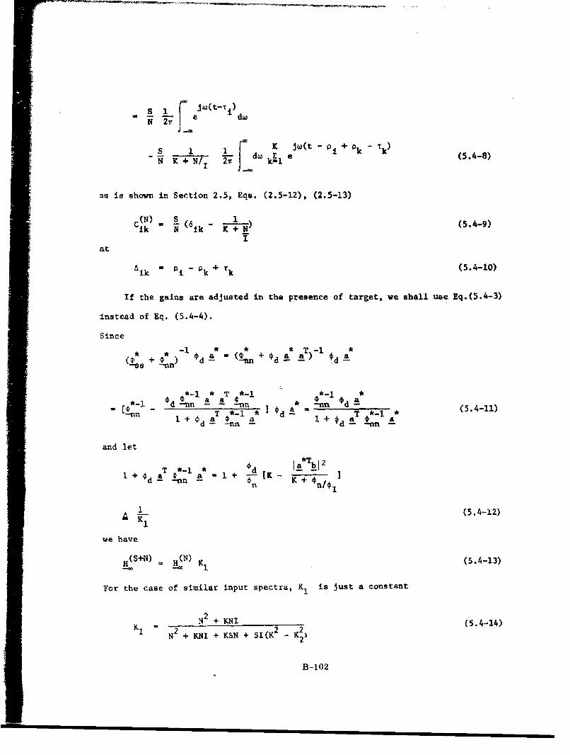
N 21 • d

s IGO K jW(t-1+ Pk-•k)s ~d ,L Ll w ew% i k k (5.4-8)

N K +N/1 2w) k-

as is shown in Section 2.5, Eqs. (2.5-12), (2.5-13)

C(N) S'}-)(5.4-9)Lk N 6 ik

yat

SAik m Pi - Qk + Tk (5.4-10)

If the gains are adjusted in the presence of target, we shall use Eq.(5.4-3)

instead of Eq. (5.4-4).

Since

*• -I * a * * (* t-l - *C(ts + ) d- (t +dn -d A- Ad

*- a* aT t * •*-Id dnn - * A -nn * -n d (5.4-11)

nr T-- T *-I*! I ~+ ý d- aT -nn*- _a - + f d- a- a

and let

T * * !d A*Tbh_21 + $d -- nn _a =I o n [K K+ O/

.i(5.4-12)

we have

(S+N) H(N) (5.4-13)H & K 54-3

For the case of similar input spectra, KI is just a constant

N2 + 2 2 (5.4-14)K N2 + KNI + KSN + SI(K2 K2)

B-102

where2 K

K2 IbTjj K' (5.4-15)

with equality when a - b or when target and interference are in the same direc-

tion.

Therefore

C 4(sN) , KlC () lot 1 - 1,2,..., K; k- 1, 2 .. ,K (5.4-16)

In other words, fo r similar input spectra the optimal gains trained under noise

alone differ from those under noise plus signal only by a multiplicative con-

stant K Thus, all the performance criteria (output signal-to-noise ratio,

and directivity pattern) remain essentially unchanged regardless of the training

environment. Of course, should the input spectra have distinctive shapes, Cik

and C(N) would assume different values. If the signal-to-noise ratio is smallik

at the input to the squarer

-T * -I a <<

the constant K1 is close to unity independent of the input spectral shapes.

In view of the above discussions we shall use the optimal gains defined by

Eq. (5.4-9) In analyzing the final behavior of our adaptive processor.

b) The Output Signal-to-noise Ratio

From Eqs. (5.4-9), (5.4-10) and (5.2-20L the dc change of the output is

_ ~TmYd.c Css H- M 1)dw

KK K K 1 5- 14 hE-l kE1 39!1 N ik K+N/,) N hih K+N/

II

od ejf (ph - - P+ k k (5.4-17)

B-103

For the sake of simplicity, we shall assume that the array it steered broadside.

Then T - 0 (1 - 1,2,..-,[) and the above expression reduces to

- 2 K K X K 11 Yd.C iE-i h-•l k4l Z11 ('ik - K+1I('ht " +

1 } dw ejw(Ph - PZ - P' + Pk)

00SS 2 w KK -1 sin W 0i

0N 2 K - JT7 K + 2 11_ (K-i) o °

K-I sin W 1 0+ - E[K + 4K l (K-i) - i0 I

(K+lN/1)2 , W 1Pi

K-i K-I sin w (i-h)po sin W (i+h)po+ 2 E1 hil (K-i)(K-h)( wo(i-h)p + 0 (i+ o)p ] (5.4-18)

or

W S K2 (K-1 + N/I)

27r N2(K + N/I)

4 K-I sin w i p

K(K- + N) ill W ip 0

2 K-1 K-i sin w (i-h)pa+ 2K 2 ( I2 h£ l (K-i)(K-h)[ 0 0

+ sin W (i+h)p 0I_] ( oih)o 5.4-19)w 0(i+h)p

Let us now consider the variance of the detector output. From Eqs. (5.4-9),

(5.4-10) and (5.2-2) we have

(o( ))2 L- l___ IG] {HT , H* 2 du-- °T y 12-

Y 7 av

B-104

K K K K K K K K

1- 1 -i h-l b-il k-i k- 1-1 X X-

* (•S ik " 1 - 1 h K N 1 ) ' , I

1 iw(pi -

dw *-2 6 + e i "he"-a d n ih Iav

"( %i'h' + T

Jw(oh- 0£ + T + 0 h, - P£, + TV, - Di + P itk - + k - Tk)

(5.4-20)

Rearranging, K°K K

2 K K K K K

S.J h -0 £ + s -0i w Pk - ____ i]2i-+ -

TT- aw I (6-e

i ll j i k~il h-El N v K4-N/ I

S (e- h K j(h - 0 + -)S + 0 i+N/ h-i e

N I h 9

•w P g + S + T

_rT a- dw i+-) __ K ip-N1 ' Yl 2

fo

Je I: +N/ E i i

(5.4-21)

B-105

For Ti 0, it reduces to

2 2 02 2 2K K K j -(p I phao I---,-,. (-) Idw K - E EeY -ffT Nv j/ KN 1 i-1 hi

0

Kii i K+ -(K-+N/) 2 C ill h1 e I

0 2 2 2K K-i sin w

-i 'd -K K K + 2 i1 (K-i) ]i7 av oI1

"2 K-i sin w i P* (K+N/ 1 ) 2 [K + 4K il1 (K-i) - w 0 0

K-i K-i sin w (i-h)p sin w (i+h)p j+ 2 Ey h•- (K-i)(K-h) ( 0 0 + 0)]) (5.4-22)

Dividing Eq. (5.4-19) by the square root of Eq. (5.4-22) yields the final form

o- the output signal-to-noise ratio

1

mN. T w 2 S K(K-i + N/ 1 )

SSNR ) N K + N/I

4 K-i sin w i P1_-" K(K-l + N/I) iJ1 (K-i) 0

2 K-I K-i+_E EK2 (K+N) ii hI (K-i)(K-h)

sin wo(i-h)p sin w (i+h)p 0 12

w o(i-h)p o+ (i+h)p (

If w p 1 then0 01

T w 2H1 av o (1S 1+N/(K-l)I 1 (K-1)(2K-1) 22SNR, = ( -) W (K-i) I+N/KI 23 K(K1-/1)2

1

72 (K-0) (5.4-24)

B-106

Eq. (5.4-23) or (5.4-24) gives the asymptotic performance of the adaptive array

processor. Since the training period is definitely of finite time, the actual

signal-to-noise ratio is lower than that given by Eq. (5.4-23) or (5.4-24). It

is to be noted that Eq. (5.4-23) is just the output signal-to-noise ratio of an

optimal (likelihood ratio) detector first investigated by Schultheiss [32] and

then by Tuteur 1331 from a simpler formulation inder the same assumption [similar

input spectra over (0, w0)]. This is no coincidence but stems from the fact that

adequately large number of taps is used (number of taps per hydrophone output

number of hydrophones in an array) and that for similar input spectra the con-

tinuous individual filters are just combinations of time delays and constants.

Therefore, it is reasonable to expect that in this special case the adaptive

array processor can, in principle, converge to the optimal processor after suffi-

ciently long period of adaptation.

In the absence of interference the behavior of the processor remains un-

altered throughout the training period because1

1 Ta •o2

SNE = SNR - v a for I - 0 (5.4-25)1 ~2 7t N ~ fraO(.-5

Without interference we do not take advantage of the reason why the optieum

detector is superior to the conventional detector:

1) It can combat noise correlation between hydrophones and

2) It can utilize variations in input signal-to-noise ratio over the processed

frequency band.

Since from Eqs. (5.4-19) and (5.4-21) we can write

Wo I a*Tb12 11FTS 2 -[ ) lab/ d- 2 (5.4-26)

SNR, I a"(K K+N/2 T J0'N 'I

we see in the above equation that in the absence of the interference or for verylarge values of N/I the side lobe factor j*aTt2 approaches zero and output

K+N/ I

signal-to-noise ratio depends linearly on the number of hydrophones K. For very

B-107

Wr b12

strong interference (N/I << 1), the same quantity anproaches to 1A --1 /K

The size of this side lobe in a fixed direction depends on frequency. In a narrow

band system large variations in this term may occur. That is, there will be dis-

tinct maxima and nulls in the side lobe pattern. In a broad band system the

magnitude of the side lobe is averaged over frequency.

c) Directivity Pattern

Using Eq. (5.2-18), (5.4-9) and (5.4-10), we have

y'.- H d.

K K K K 2 W 1- ~-) ik K+l/1 hk

i1l h-l k-i LilN-iN

•1 [ d- od E e + h n 6hh

2rJo d dni

Iw(pO - Ph MPh- P2 + - i + Pk k. o° *1 ' 2K [eSJ"i e- wr N K eL(Pk tk) k 2=i 2"" L•l i [e+-N-/I - kF=- e ]e ,

d+N/ kE1 e ]e (5.4-27)2Tr Jo N !+N/I1 k! I

The writing of the above expression is permissible because for

• I *H 0 •d a we have

jt * 1- ^ 1 *TIG12 H = - aT d n (naa +d )d-n a -d

-d 2 -- T- --- -n-Tn -i

(a*T a)2 + a D - a (5.4-28)-'nn d - -nn --

B-108

which is equivalent to the integrand appearing in Eq. (5.4-27).

Eq. (5.4-27) is further simplified to

--- 1 O 2 KL K j(h-i)(r- t)

2 K2jw(( i- T ) K K Jw(Th+ Ph k Y

K+N/I i -i e h-l ki• i

K jW(P- T) K Jw(Th- 0h)]21S--:+ 1 j . e h1l(K+N/I) 2 ii

K K K jw(i-h)(TO- po)+ d. (N) - ly ZJ, l 01 (5.4-29)

K K K JW(T i- T h + Ph- Pk + Tk

i-l h4l kzi e

SK K j(i-h)(To- T )

i-1 hil

K K K JW(Ti- i- Ih + Oh- k+ 'k)

i-i h-i k1is

h k k (5.4-30)

and

K 2K jw(p 1 - T ) K Jw( h- Ph

K K Jwl(i-h)(p 0- T ) K K jw(k-Z.)(T - po)

B-109

K-I[K+ 2 ill (K-i) cos W i(po- T)

K-i.[K + 2 h1I (K-h) cos w h(P- o)]

12 K-1

K + 2K il (K-i)cos W i(P - r0) + cos ' i.(To- PO

K-I 2+ 2 l (K-i) cos w i(io- o)

K-I K-i 1* 2 i Z1 hE1 (k-i)(K-h) i cos (ipo- iT+ 0 hho)

i-h

+Cos (1o0 -i0 -ha +h hpo)] (5.4-31)

We have

2 K-i sin w i(O- T-)s)I K + 2 ill (K-i)

. 2r -W i(o- To)

-+/ C-) i-

+ (41/I [K +2 + (K K- ( i Ct- -)

(K+NI) i2 ((p 0- T

0 0

sin C K-I sin w i(- T-+ 0 0 0) + 2 (K -i) 2 A Io)

0 (K+ (2 a- '00 i(-0o- 0 )

)• ([K(K-i+N/I) K- 1 2K i wi iit- p )

2r• N2/ 1(4KN/I 1 (K-i) a p (5.4-32)+ ~ ~ ~ ~ ~ ~ k TTj K,/) KNIip

0)

In the above the last terms on the right-hand sides of (5.4-30) and (5.4-31)

have been omitted because these terms always contribute very little upon integra-

B-If0

tion. They are divided by wU which is large to make B WO negligible.0

At an angle far away from both the signal and interference directions, we may

neglect all the oscillatory terms and get

2X2 (K-I+N/I) 2 W .• K(K-l)z- (R) /I) 2 2r N"

L o S K(K-L+N/I) (5.4-33)

T~ "- (K+N/I)

"T"i the signal direction, -C

-- So ( 2 K K2 (K-I+N/I)

2

T 2n (P (K + N/) 2

4 " (S• (K-1+N/I)2 1 (K-I) (2K-1)

27 I (K+N/I) 2 3 K(K-1+N/I)

"+ () K(K-l+N/I (5.4-34)+ (K) §K4N/1)

and in the interference direction, T -PO

ý S 22 K2KI+N/I)K(Kl+N/ 2-0 2S N (K+S/I) 2

- 2-'S" K(K-1) 2 V- (K-/-I)

S() (K-I) S S K(K-1)2 (K+N/K) 2 2n (N) (.4-NI3

Although exact shapes of the optimal directivity pattern given by Eq.

(5.4-32) cannot be plotted without assuming specific input power levels, they

will take the general form shown below by comparing Eqs. (5.4-33) through

B-Illl

(5.4-35). There is always a maximu in the signal direction and a minimum in the

interference direction. Specific results will be given in the next chapter.

• (o)

i t i

-,5 Adaptive Behavior

The behavior of a tapped delay line filter is completely determined once the

" " hts and spacings ar,. known. if Cek ax:d Aik are the weight and spacing at

t'Ae kth tap on the ith filter, then for an array of K hydrophones and M taps at

each sensor output, the impulse response vector of the pre-processor (from hydro-

phone outputs to the beamformer) is

hWC 6(t

hl(t) W C 6(t - AI.h2(t C2£6(t A2£(5.5-1)2 2XOh(t) E (

-=hK(t) C Z6tAi

and the transfer function vector

• ..() C2e12

K CKe

S~B-112

For the adaptive array processor the tap spacings are fixed throughout the

training period but the weights are adjusted according to

W -w - 2 nz+ 2 553

where rj determines the pitch of the algorithm and generally depends on the

time index j ; the n's are the delayed inputs and z is the summer output. The

variation of the weights during the training period will thus determine the ad~pt-

ivc behavior of the processor. The filtering problem was studied in the lest two

chapters where the variations of mean squared error as a function of time index

jand input statistics were expressed explicitly. Here we shall study the

V J.etection problem by examining the variations of the performance criteria during

the training period. Since the input is random, the weights expressed by (5.5-3)

;Tre random and only their expected values are of significance. It has been shown

- ect. 3.5, especially Eqs. (3.5-7), (3.5-35) and (3.5-43), that the expected

* diJes of W4 at any stage is related to their initial and final values by the

foarl Jrmula

I Pj q

where W - W(j-1) and W W(j=-) ;p~ and q are functions of j and depend

mii t

IlI

on the choice of the weighting sequence y For example, if Y tois chosen as

a weighting matrix such that

1 (~))I(+) (5.5-5)

Xe k k th eigenvalue of h , a 1,2, a e.,K(M+l)

then

1 (5.5-6)

P1 j+l

B-113

.q...+L (5.5-7)

If, however

1 2(1+1) I - unity matrix (5.5-8)

then they are of the form

r(j+2 - X max) r(J+2 -min)(5F (2_Xmax) (J+l) I "i P] ! (2_X min)(J+.l)i T559

qj - I - p (5.5-10)

where Xmin and k are the minimum and maximum eigenvalues of the input

correlation matrix R

Combining Eqs. (5.5-2) and (5.5-4) we can write

• p H 1 (w) + qJ M_.(u)* --- *

P a + qj n a (5.5-11)j- jnn d-

1I(w) and gw) denote respectively the initial and final forms of transfer

function vectors.

Since in all cases po " 1, qo = 0 and p, - 0. q. - 1, the adaptive processor

starts to be a square law detector and will be transformed gradually into an

optimal one. We can determine where the adaptive processor stands between these

bounds during the adaptation period by substituting Eq. (5.5-11) into the expres-

sions of various performance criteria.

Basically, we are required to evaluate the following three integrals

AJ+ IGI2 L- 1 G (p + q H-O)r- P (P) H + q H_) dw (5.5-12)

B-114

r (pj 1+ qj T (PJ + qj H )*} 2 dtw (5.5-13)

BJ~ 1 T -nnjGk )Ts(

cJ+ 1 * OIGt2 (PJ + q!i (pj P 1 + qj H)dw (5.5-14)

where in Eq. (5.5-14) the H's have steering vector a rather the signal delays

a in deriving the directivity patterns.

Since

(pj I1, + qj H )T I (p J1 + qH _)

2 T * 2T *-p - __1 +-- qj H $-1 .

T *+ 2 p -A, H_

we shall evaluate each one of the three integrals, Eqs. (5.5-12) through (5.5-14),

by using Eq. (5.5-15)., When the first two terms of Eq. (5.5-15) are used, the

results are already available from the previous two sections on the initial and

final behaviors.

Thus, we obtain A+(k) k - 1,2,3, when the kth term on the right-hand side of

Eq. (5.5-15) is substituted into Eq. (5.5-12)

A(1) 2 1 1I12 IT * 2 -- () (5.5-16)J+l "i " IG -- sI- i+s - PjR Yd.c

A (2) q2 2HT , * 2 -(-)j+l j 2 ,- -• -s - I Yd.c (5.5-17)

where ()is given by Eq. (5.3-3) and -) by Ea. (5.4-19)Yd. c is ad.c •

(3) 2IC12 T

A 2 p q1 f H dw

j+ 271 d _ "d -nn- -d

B-115

which for broadside condition becomes

K K Ja(pi- Ph)

A (3) 2 p qK i-i h4-i

p q A K-1+NýI

3+1 ~ " j 2r i [ K+N/I]d

2 K-1 sin W i0 1- 2 l ( -i) " (5.5-18)

if W p >> 1 , then

(3) O S q K-+N/I (5.5-19)

3ý K+N/I

We shall consider the second integral.

Note that

S(pj I + qj H )T ) (pi l + q IQ)*

" P. •I -i)+ qj H)p

'

+4 2 2(HT *2 2 2 Tpjq L~ -1-H + 4 pj q 3j 3* 1)

3 T T+ 2 p q3 ( j-1 QO _Ij j ..)

3 * T+ 2 p3 qj TH 1D jj (H3. (pALH (5.5-20)

Thus we obtain B(k), k - 1,2,'--,6, by substituting the kth term on the right-J+lhand side of Eq. (5.5-20) into Eq. (5.5-13)

(1) 4 1 * 2B ~l - Ij1T v IGI' (Hj '4 Hn ) d,

P4 (1) (5.5-21)=BPj y

B-116

(2) qJ4 • T 2Bj~j rrT 1 IG1

4 (R; 0n H.) dw

1 2q 4 0 )2 (5.5-22)S.- q j ( y

j y

"where (Oy1) is given by Eq. (5.3-9) and (a by Eq. (5.4-22).

B.(3) •4 2 q2 1 IJI4 G 1 - H-) dJ+lT -- u

av

4 pj2 qj2 1 -2 (a*T -1 2pTqav -- -nn -nn a dw

4 42 2 K2 0 (5.5-23)

7Tav

() 4 2 q2 1 IG14 (T 0 0*~J+- pj qj -nTa- 11 '' -1 F d

,IV

4 p 2 q22 - *T P 2 *T D-1 a)dw7Tav JO d n n

- 4 pj2 q 2 _1 W ( + I j *TbI 2)K - jibj2 5.5-24)

which becomes for broadside condition

2 K-1 sin o i poB() 4 pj 2 q 2 K2/N [K + E (K-i) W-I1j+1 qJP K+N i-1.1io:.

K-i sin j) i p+ _I/N [K2 + 4K (K-i) o - 0K+N/T 14 W

K-1 K-I sin w 0(i-h)w ap sin w0(i+h)p 0

+ 2 (K-t)(K-h)( o(i-h),,P 0 + :o(i+h p

(5.5-25)

B-117

Furthermore. if woo% >> 1, then

(4) 2 2 w a 2 K + I/N - 2

4J~ q + +K +124 2 TrT / I/N K2

pj2 qj 2 w 2 + [K' + K2+ 3(K-1(2-)](5.5-26)

3 1 G T T H*BJ 2 pj q 7Tavj-n H-)( Ql inn t

2p qa 3 1 J *T C- a)(a *T - a))dw

S2 pj q 3g NS (K - I dToW (5.5-27)

av 0

for '1, 0 , the above expression reduces to

. ~ K K- (-in w•+,I) i P0.(5) 2 jq3 S• K(K-'I+N )- 1 i-(K-l) - ?" -LL

2j+l 2pj q, 3 K (K-+N/1) K-i ( 0&V

3()T°2 K-1+N/I for ( > 1 C5.5-28)

2pj qjK0

B(6) - 2 pj (T T

'IIL - (H ý H )dwJ+1qj )av -1 _ =1,-"I -.-n

2 p-3 *T2Pj ¢ (a'- -- n a) (*_ _ dd

7T d ~ C -nndav

= 2 pj q (K + a*T b12 )ddTv J o

K~, K-i sin o 0o

2 p3 q• C ( N K + t [K+ 2 ' E( - ' ]

B-i18

for T 0 and

23 N

avfor p 2u Ku3 N I•c (5.5-29)for po• >> 1

thWe shall next consider the third integral. Using the k term on the right-hand

S•! ~~~(k) k, ,,side of Eq. (5.5-14) in evaluating Eq. (5.5-13), we have c k 1,2,3

.(1) 2 1 ^- cid2 jT (52-3r_,j• pj IG12' ji ý H1 w -pj yi (5.5-30)~J+l~ r~- XX :712 1

( 2 ) q IG2 d - q12- (5.5-31)cj+ i=~ 27- -A dw YO

where i1 is given by Eq. (5.3-22) and y. by Eq. (5.4-32).

-3 2 p q IG12 T dw-j+l j q 2n -- AX- -x d

p-q, 0 * a *T )-i.duT ad na- ann -

S•K+$[^*T !2 1 '*T *T *

Tr N K+N 1 (5.5-32)

Since

SK K jw(i-h) (r - - )a aj2 = . h.1 e (5.5-133

and

•*T *T *Ta a a b a

K K K JCw(Ti- Ti- Th + Ph- Pk- Tk)

iJ1 h-i ki-e

B-119

K X jw(i-h) (r - 0)

ili h-i

K K jw(i-k)(p - T )

ill kil

+ K K jw(k-h)(po- 0t)

h-l kl e

K K K JW( T- h + Qh- Pk- k)

iil h1l k•l

i ý h M( k (5.5-34)

Eq. (5.5-32) reduces to the following expression by omitting the contribution due

to the last term on the right-hand side of Eq. (5.5-34)

_(3) 0 [K + SK -K2 2K)]

J+1 Piq R N K+N/I -

0 S K-1 isin w i(o--T0

N 0l 0 0 +(- 0 T 0)(55K sin wo i(Po" To)0 sint Wo 0(- T

+ i( - T ).-50 i C-) o 00 0 0

Just as we did in expressions y and y. for three special cases, we shall also

evaluate C (3) in a similar fashion. When the array is steering in a direction

far away from that of target and interference, we neglect all the oscillatory

terms and get

-- • _(3) () pqj-"KI+S S I

+1 (J ) P i qN - N K+N/I (3K - 2)] (5.5-36)'|i .o L N N oo . =In the target direction, T T

(3) • S S 1 2(Cj+1 T- (K + K (7 i- - 3K - 2K)]

+ 2p qS 2K-IN/I K-12, K+N/ ill (K-i)

B-120

2Y. I +-S 2K -4K+2+0Ni'P j N K+(5537)

and in the interference direction

(3) (USJ q o S 1 -2 K)C e Pj qj [K + I N K+NKI (3

S e K K-1

+2p qj (jj) q E (K-i)

q K[p + S K[2_ 3K+2+NII(5

" PJ j �•N +/i -'N (5.5-38)

Now we are ready to express the performance variations during the training period.

(1) OutpLr signal-to-noise ratio

3W

SNR k-i 1+1 (5.5-39)J+l61/ 6 (k) }1

SkZl Bj+l

where the A's are given by Eqs. (5.5-16) through (5.5-19) and the B's by Eqs.

(5.5-21) through (5.5-29)

(2) Directivity Pattern

_ 3 c(k)Y+I=k- l (5.5-40)

l k-il J+l

where the C's are given by Eqs. (5.5-30), (5.5-31) and (5.5-35). For any parti-

cular steering direction Yj+l is readily computed from Eqs. (5.3-23) through

(5.3-25), (5.4-33) through (5.3-35), and (5.5-36) through (5.5-38). Various

computations are shown In Chapter Six.

B-121

CHAPTER SIX

COMPUTER SIMULATIONS AND NUMERICAL EXAMPLES

6.1 Introduction

A great deal of attention has been given to proving that iterative pro-

cedures described in previous chapters converge under certain conditions. Having

proved convergence of the adjustment schemes, our problem is to demonstrate that

the procedures are feasible; that is, solutions can be obtained by using the

adjustment proccdures in a reasonable amount of time. To establish this point,

computer studies were made to the design of adaptive tapped-delay-line filters

and detectors. Recall that the approach to adaptive receiver design has been an

optimal one. The adaptive design is a result of realizing the optimum receiver

in a sequential manner.

In this chapter we consider simulating an adaptive processor on a digital

computer for a rather specific case to observe how the processor performances

vary with time. Several examples have been worked out by digital computer simu-

lations to verify all the theoretical analyses presented in Chapter III.

Some computations have also been carried out to show the performances of

an adaptive detector described in Chapter V. These computations were done based

on theoretical analysis rather than simulation which, in this case, would require

too much computing time without providing any general conclusions. All these

numerical examples were worked out on the IBM 7094 11-7040 direct-coupled system

at the Yale Computer Center.

6.2 Computer Simulations

An arbitrr•v array processor was used here as an example to demonstrate the

properties of the two algorithms given in (3.3-6) and (3.3-13), i.e., the algo-

rithms using desired signal and signal correlation function, respectively.

A linear array of six uniformly spaced isotropic hydrophones was assumed to

B-122

be influenced by the following set of si Wale:

9 1. A planar target waveform incident from the broadside.

2. A single interfering planar noise waveform incident at

"angie 0, 1200

3. A "white" gaussian noise source at each hydrophone repre-

seating the ambient noise which is assumed to be uncorrelated

from hydrophone to hydrophone.

The hydrophones were spaced c/w 0 units apart, where c is the velocity of

propagation in the isotropic medium and w0 is the center frequency of the

target signal. The output of each sensor was processed using a tapped-delay

line containing ten multiplying weights and nine ideal time delay of (_! )2w0

seconds each, Because the target-signal waveform was incident from the broad-

side direction, the target signal arrived simultaneously -- i.e., in phase --

at the output of all six hydrophones.

The target signal and the interference were modeled as a broadband

gaussian random processes. At each hydrophone the ratio of target-signal vari-

ance to total noise variance is 0.01. All these properties were generated by

passing a pseudo-random gaussian sequence through an appropriately designed

digital filter. Signal, noise, and interferences were generated as sequences

of random numbers from random number generators. The sequences were then trans-

formed from rectangular distribution to normal distribution using existing

programs. Each simulation started with an initial weight vector having all con-

ponents associated with no-delays set to unity and the rest to zero. The weight

vector was then adapted using the appropriate iterative equations.Yo

Throughout the study the sequence yj was determined as yJ 2(J)

YO being a variable parameter. The behavior of the process depends critically

on the parameter y ; hence each case considered was carried out for a number

B-123

of values of Yo " As y was increased, the convergence of the process in-

creased steadily until a point was reached for which the process would break into

violent oscillations that took a long time to die out. This point was predicted

in Chapter III that y sLhuld satisfy

~< 3 < 14

max

for all j , especially at the starting moments. Since the largest eigenvalue

was not known a priori, the best weighting sequence y can only be chosenmax

by experiments.

As a check case, the optimum (mean-square sense) values of the coefficients

were found by correlation techniques, by averaginR the necessary values of the

correlation fuxnctions R s(T) and R (r) over an interval of 2000 samples. This

set of coafficientp is compared in Table 1 with the sets of coefficients obtained

by the approximation method for the two algorithms chosen. The average filtered

error as measured by the algorithms over the 2000-sample interval is plotted

against time index during the adaptation period. This is shown in Fig. 8 where

the minimum mean squared error with the optimum weight is denoted by a horizontal

line. The smooth curve indicates the mean squared error calculated by theoretical

analysis.

Fig. 9 shows how the weight vector approaches its optimum point independent

of the initial settings.

Figs. 10a and 10b show that faster rate of convergence can be obtained byYo

increasing o if Y, 2(J4l) but not too large to cause oscillation. When

constant weightitiv sequenc. was used (Fg,. 10a), the mean squared error at later

adaptation stages would oscillate around the minimum mse instead of approaching

it ,radually. For a single filter and known correlation functions, the relation-

shins bcrween the rate of convergence and the maximum eigenvalue are shown in

B-124

Fig. lob. As evidenced by Table 1 and Figs. 8 and 10, the filter designs for the

#. two algorithms are equivalent in the sense that they result in nearly equal values

of average filtered error. The average filtering errors as obtained by these two

algorithms over the 2000-sample interval were only a few percent greater than that

for the filter designed by correlation techniques. In view of the limitation on

the length of data available, this performance is entirely satisfactory.

The important point to be brought out is that the total computing time re-

quired by any one of the two adjustment procedures for finding the optimum set of

coefficients was no greater then the computing time required to measure the nec-

essary correlation functions and solve the associated set of simultaneous equa-

tions for the minimum mean-square error coefficients. Thus the adjustment methods

are no more trouble to apply than correlation techniques, yet they eliminated the

requirement of a priori statistics.

The effect of uncertain signal is shown in Fig. 11. We see that if the

assumed signal power differs from the actual power by a multiplicative constant.

the Rains adjusted according to algorithm (3.3-16) will converge to their opti-

mum values multiplied by the same constant.

An attempt was made to compare the rate of convergence for two different

approaches: the Kalman filtering technique using all the past information (see

Section 4.3) versus the ordinary method of stochastic approximation. As expected,

the Kalman technique gives a faster rate of convergence. Some of the reasons

were given in Section 4.3. See Fig. 12.

There is no general method to select the right number of taps so that a

predetermined accuracy can be achieved for any given system. S.veral runs were

made to plot the minimum mse versus the number of taps. It was found that by

properly adjusting the tap spacings, five or six taps could produce quite satis-

factory results. One plot is shown in Fig. 13.

B-125

i-

cc CD

ooI Ice

0° 00 0

- 0"I o 00 000

0 00 M 0 %-)

0 ° 0

or m '-,

00 0 l

S00.,q LO 0

o ,o

Lo~ ýv InH )

=_M

0

0 0c't Se> v U

0 00 00- 0 OD ~

C; 00 05 C

- " -4

5 00 0

ItI

C

00-

b4)

ii B,-126

I1 0 00IIHiiLf

mi0

NV

!CC0a

f I I

-4-

0 01-4

Tw --

(1) j

7 LOsOD

-0~

iii

'2 0o

1'r

SB-127

0'

0000

i~00

S~0

i ~0S-0

I

i I I

'I 0• "

II0

s ' I

-II • o- --.

B-128

OD

zI 0

0-0025 z "-

00000 0" tt* * *0

0 0 0 ma , 0

0-

i ',/'"

I Q

B-129

i0

1i.

i /LI _i

uJ

° 0)

00...--"" -- 0 0

000 -- -- 0 0nI " " •I I

_ I_ 0 +

0(.5

< to

'~~0 Co )/ -0

- -M Ill- 0S. .. -4

B-3

oo

= /-1'0-- =--- I mm/

9 �i3 IC)

o 0g�) t�)

00 0

0I 0

_ 0I 0

I-' � I

I0Q�0c'J

II II Ii 1 0 �1 I 0 �Irr a I d- �- - I SI I

* I wI I II S I 0�tc�o I II I (�)a I I.-.I UII I

0I II I I � tI II I I C) �

I I II: r4

I -I I 1a 1 1I I II I 10I

I II I I/ I

1�-�'-. - - CL)

-- - - - CT)-- - - -. - - -- -

,-- --- --- -- -

- - - -- -

----IŽiil �dj� LwL .�I ___C ( 0

B-131

000

0

-0

S-0 •El

/ 0 'o

"o0 "o

L-

o •

/ 4

/ -:0|

//" I

A.cI

11- 3'0

emin

1.5-

I.O

0.5-

1 3 5 7 9 II 13

NO. OF TAPS PER SENSOR OUTPUT

Figure 13. Minihuii NISQ vs. nivibcr of taps per hydruphonu output

B-133

LdJSso

-0

o

Or)0 0F- (0

(f)U0 0

LiJ(1.

0

0

- 0

0

10

- 0

oJo! jO

C>C ,CC) .7_

•

Best Available Copy

When this simulated array processor was used as a detector, the detector

output was examined. After 2000 samples of adaptation, the weight vector was

held fixed and the same 2000 samples were sent to the detector. The input con-

tained noise only at the beginning of this operation and contained bath signal

and noise starting from t - 1000. Fig. 14 shows clearly how to interpret the

detector output and decide the presence of a target.

6.3 Zxperimental Results

Sonar noise recorded at sea from a collection of 6 hydrophones has been used

to test the iterative rules described in previous sections. An IBM 1800 computer

was used to make data tapes compatible with an IBM 7094-7040 system which z~vs used

as the principal computational tool in the experiments.

The noise was a 2-second noise sampled every 1/8000 second. The total band-

width of the data was about 425 Hz to 2400 Hz. The hydrophones in a linear array

were separated by 7.5 inches.

Since the data were collected in actual sea water, the directionality of the

noise field was not known exactly. From the display of correlation functions of

several channels (See Fig. 15) there seemed to be some interfering source present

in addition to the ambient noise.

In order to show how the processor eliminates background noise, a target

signal was produced from a noise generator and passed through a filter. The

signal autocorrelation function is shown in Fig. 16. Three different signal

directions were tested, i.e., direction A (opposite to the assumed noise direc-

tion, direction B (perpendicular to the assumed noise direction), direction C

(similar to the assumed noise direction). After proper signal delays we obtained

three different noise correlation matrices whose cross-correlation coefficients

for the six channels are tabulated in Table 2.

It is seen from Table 2 that for direction B the actual noise correlation

"matrix consists of many oscillatory terns. If signal delay' were insertcrd to

B-135

align target coming from direction C, the interference was also in phase so that

all the cross-correlation coefficients are positive. On the other hand,ifsignal

delays vwre inserted to align the target coming from direction A, the noise field

was further do-correlated. Consequently, the array gain defined by

sliMal-to-noise ratio of the summer outputsignal-to-noise ratio at channel 1

was larpeit if the target came from direction A and least if both the target and

the noise came from the same direction. This is shown in the second row of Table

3. Note that the signal-to-noise ratio in this experiment has been defined as the

signal pover divided by the noise power, rather than the d.c. change of the output

due to th2 presence of the target divided by the rms fluctuation of the output.

The later definition is more meaningful for the detection problem and the former

definition is useful for the problem of signal extraction. Several cases were

studied on how our proposed adaptive array processor eliminated the undesired

noise. clmplete results are shown in Table 3, where SNR is the input signal-in

to-noise ratio at Channel 1, SNR.t is the output signal-to-noise ratio of the con-C

ventional processor, SNR6 is the final output signal-to-noise ratio of the adap-

tive processor after 2000 Iterative adjustments and using 6 taps in each individ-

ual filter, SNR1 2 is the same as SNR6 except that twelve ttps were used for each

individual filter. So far we have assumed that the reference or desired signal

d(t) is the same as the target signal, i.e., d(t) - 9(t). If d(t) is replaced

by some delayed version of s(t), i.e.,

d(t) - s(t - T)

then, for some proper choice of T , smaller mean-squared error or larger signal-

to-noise ratios may result. Further disci'asions on this point can be found in

(I). For t 0 0 , the corresponding SNR6 and SNR12 are denoted by SNR'6 and

SNR' . The improvement of SNR produced by the adaptive processors over that

B-136

9OIo

\\C~IIC

V - :!:-~- 4Ir

I%

B-137

(,t) Ch..nI 1 2 "3 4 5 6

1 1.00 0.70 0. 55 0.56 0.43 0.24

2 0.70 1.00 0.64 0.58 0.40 0.24

3 0. 55 0.6,4 1.00 0.68 0.44" 0.21

4 0..56 0.58 0.68 1.00 0.58 0.26

5 0.43 0.40 0.44 0.58 1.00 0.34

6 0.24 0.24 0.21 0.26 0.34 1.00

(b) Channel 1 2 3 4 5 6

t 1.00 0.42 -0.27 -0.13 0. 10 0.089

0.42 1.C0 0.36 -0.34 0.05 0.11

3 -0.27 0.36 1.00 0.22 -0.23 0.10

-0..13 -0.34 0.22 1.00 0.29 -0. 13

5 0. 10 0.05 -0.23 0.29 1.00 0.27

6 -0.08") 0. It 0.10 -0.13 0.27 1.00

() , ! Z 3 4 5 6

1 1.00 -0ý 36 0.21 -0.13 0. 12 -0.11

-0. 'Ai 1.00 -0. 29 0.2.1 -0. 21 0.07

4o. 1l -0.29 1.00 -0.33 0. 15 -0. 13

S-0. 1 1 0. Z.A -0. 33 1.00 -0. 2 1 0. 12

""0J L: -•.2! . . 15 -0. z,4 1.00 -0.07

I -. 0.07 -0. 13 0. 12 -0.07 1.00

li~i i.!. ' •7 ,; , i, , ¢, :'t t•;l• • (-,It I i ti 111: foorI .(,'! L flI~',l () Dirc cttion C,

(t,) ~ ~ ~ ~ Di- c) ,:,r• , ),, li,,n At.

F3est Available Copy,

B-138

0-

0)'Co-

41

o

0

-- 4

--rLo

X44

C~C'J

B-1I

_ B-i 3 9

vItems Direction C Direction B Direction A

SNR 0. 002431 0.006676 0.01Z054C

SNRC Z. 38 6.55 11. 8

SNR IN

SNRO6 0.003967 0.009556 0.02594

6iSNRO' 6 0. 004135 0. 010772 0. 03179

SNRO 14 0. 004001 0.009887 0.02774

SNRO0' 2 0. 004187 0.010955 0. 03Z93

SNRO 6SN1 Z. 13 db 1. 56 db 3. 18 dbSNRO

.0 Z 31 db 2. 06 db 4. 24 dbSN R

C

SNRO Z18 .1db 1. 73 db 3. 63 db

SNIRC

SNhO,

2. 36 db Z. 15 db 4, 41 dbSNI

'1A : 3.NP ][ N0. 001039 for

B-140

by the conventional processor such as SNRI6ISNR are measured In db. These results

, shown here are remarkably close to the optimal filtering using complete input

statistics (performed independently by R. Kneipfer of U.S. Underwater Sound

Laboratory, New London, Connecticut).

6.4 Numerical Computations

¶ To investigate how an adaptive detector changes its performance during theI

training period, we could, in principle, simulate such a processor in digital

computers. However, there exist some practical difficulties. Since detection

performances (output SNR, directivity patterns) are functions of output mean

and variance, at each stage of the training process we are required to calculate

the output and variance using sufficiently large numbers of samples (say, 1000

or more) for W , where j - 1,2,..., number of test samples. Furthermore, if

we want to change any one of the many system parameters such as number of hydro-

phones, number of taps, or input statistics, the whole process would have to be

repeated.

In light of the above difficulties, analytic expressions were derived in

Chapter V to determine how the adaptive detector performs for a specific case

in which the input spectra are identical over a certain frequency range. Equations

(5.5-39) and (5.5-40) are used extensively to carry out numerical computations.

Fig. 17 shows the variation of output signal-to-noise ratios during the

adaptation period.

If target and interference are well separated in bearing, the (normalized)

directivity patterns are shown in Fig. 18. In Fig. 18 computations were made

using approximate expressions in the target direction (0 OT) , interference

direction (8 - 8 ) , and remote from both. Optimal (j - ') behaviors of the

array processor as a function of other system parameters have been considered

previously by Schultheirs (32] and are not plotted here.

B-141

E.xprimantal results using sonar data have v~rified that practical adap-

tive array processors can perform nearly as well as optimus processors in a

stationary environment. It should be possible to adopt similar iterative

processors to seismic and electromagnetic arrays which operate in a directional

noise environment. It might be possible to minimize reverberation as well as

ambient noise in systes where reverberation is significant.

B-142

•*1

* •NORMALIZEDS SNR OUT /2-r N

t awTavo S (SNR) I/N=IO=K40

40- OD

35-

j=50030-

25 j =2o

20 j = !0020-

-- =50

15-

j--5

5 -j=2

"-I I I I I I J:lIi _

2 4 6 8 10 12 14woPo

Figure 17. Variation of Output SNIR

B-143

NORMALIZEDDIRECTIVITYPATTERNY(09)'-2-Iwo°I/K

100 j =IK=40N/S 1 0

I/N =10

j=20

10-

j=I00

1=500

j-oo

LOOKINGANGLE

B-144

C-APTER SEVEN

SPIOIARY, CONCWUSIONS, AND SUGGESTIONS FOR FUTURE RESEARCH

7.1 Summary and Conclusion

The research described herein has developed a system for processing the

outputs of a passive array of hydrophones. The system consists of an adaptive

linear multichannel filter, together with algorithms for iterative adjustment

of the weights on the topped-delay lines. It is designed to process the re-

ceived wavefront in the presence of ambient noise and interferences. The

system is designed in such a way that it can be readily implemented and be

able to operate well in real time in the presence of noise fields whose statis-

tics are unknown a priori.

a) Assumptions

The development and analysis of the array processor presented in this

research has been based on the assumptions that

(1) Target, interferences and ambient noise are assumedto be gaussian random processes.

(2) The sum of interferences, ambient noise and localnoise are regarded as the effective noise, whichis assumed to be statically independent of thetarget signal.

(3) The target-signal components s (t) observed at theoutputs of the ith hydrophone Is a linear time-invariant transformation of d(t), the target-signalcomponent observed at the output of an ideal isotropichydrophone located at the origin of the coordinates.The target direction is known, together with itsautocorrelation function (but not necessarily itspower level).

(4) The statistics of the noise field are completelyunknown. Interferences may be present, but thisis unknown. If they are present, their directionsare unknown.

(5) The wavefronts of target and interferences areregarded as plane over the dimensions of the array.

B-145

(6) The processor is a directional array whose gain isaxfxinized In the direction from which the target is

expected to come.

In Chapter V, in order to analyze the performance of the proposed processor,

it was further assumed that

(7) The array is linear and consists of equal spacedhydrophones.

(8) :_:• -.mbient noise is stotistically independent fromliydrophone to hydrophone.

(9) .he input processes are band limited and of similarSipectra.

b) Su~ary of Results

A mat '.atlcal model has been developed to describe the characteristics of

the- input processes and the processing mechanisms. This model has been used to

uxamine the array processor when the filter coefficients are adjusted iteratively

so as to op.imizL thu processor in accordance with the following performance

(1) "inintum mean-squared error between the beamformeroutput and th,. tnrget signal for the filteringproblem.

(2) Xaximuw signal-to-noise ratio at the processor out-put for the dctection problem.

For a general array cofiruration consisting of individual filter on each

hydrophone *utput, a post-surumntlon filter, a square-law device, and an averaging

filter, th. opt mu.w individul fI ilrtrs can be constructed by tapped-delay lines

with the w& chti set to sore, •.pt :,.il values. Although these optimal values can-

not 5e detr•irned without conpl.-t' knowledpte about both the target and the noise,

nuthods of -itcchastic approxP"::ition c-.i, be applied to adjust the weights itra-

tiviuy. Thc only information ruquired in using the adaptive algorithms -3 the

corr,.Itlon functions betwevcn the wavefront and the various delayed signals.

e -,yoposed.algoritb.rs have been shown to converge in mean square and in

Best AvaiIt4 C or ,SCop,.!

probability as long as the second order statistics of the input processes are

bounded. Explicit expressions for the rate of convergence are derived in terms

of input statistics, various system parameters and training environment. The

mean-squared error is found to decrease approximately as the first power of the

adaptation time. The rate of convergence is essentially indifferent to the

number of weights to be adjusted as our algorithm allows simultaneous adjustments.

The size of error, however, depends on the total number of taps and the starting

point. Ranges of the weighting sequence are determined to maintain stability of

the adaptive loop. It is also of interest to note that there is no signal sup-

pression phenomenon in using our algorithm and that the final system performance

is independent of the signal power level.

Several partially effective techniques ha-v been proposed to adjust time-

varying parameters. It is also found that the ordinary methods of stochastic

approximation can still provide convergent algorithms if the rate of parameter

variation is sufficiently slow. Qualitative discussions are provided.

The performances of the proposed adaptive receiver are evaluated and com-

pared with those of the non-adaptive systems. The whole system starts to be a

conventional detector and is gradually transformed into a spare-time filter

optimum in a predetermined direction. This optimum filter is shown to reduce

disturbances coming from other directions. When a signal appears in this parti-

cular direction, a maximum response will be produced. In actual operation, the

average bearing response can be obtained from a plot of the averaged squared out-

put versus the looking angle of the array. In most practical situations narrow

peaks are considered to be targets.

7.2 Suggestions for Future Research

The following problem areas have been suggested by the research reported

here:

a) Applications in Ocher Areas

Much work remaine to be done in other areas of application. New areas of

"B-147

application should be explored both from a theoretical standpoint and from a

practical one. Two important areas are seismic arrays and satellite cossunica-

tions.

In processing seismic data the direction of the source is generally known

because of the impulse nature of the initial signal. The direction and nature

of seismic noise are not easily determined. The iterative procedure suggested

In this research could be used to minimize the effect of such noises.

The suggested system presented here might be used to improve the signal-

to-noise ratio for communication signals received from transmitters located on

deep space probes. Presumably, the direction of the source is known (e.g., the

location of a satellite), but the characteristics of the interfering noises are

unknown. The improvement offered by the array-processing system presented here,

as compared with conventional systems, might be appreciable.

Detailed analysis of the above two areas will be very useful and important

in understanding the performances of these adaptive systems.

b) Nonstationary Problems

The applicability of adaptive techniques to statistically nonstationary

processes presents some highly challenging mathematical and statistical problems,

and perhaps is the one in which the strongest applications of adaptive techniques

will be made. In this research some procedures have been proposed. But they

are applicable only to special cases. A generalized formulation to handle this

problem would be highly desirable.

c) Automatic Recognition of Bearing Response

In applying the proposed algorithm to actual sonar systems, an operator

is needed to interpret the bearing response. One would like to ask whether or

not an automatic response reader can be constructed by studying the character-

istics of directivity patterns and by developing some recognition algorithms.

B-148

APPZNDIX A

THE OPTIMUM DETECTOR FOR DETECTION OF A G&DSSWI

SIGNAL IN GAUSSIAN NOISE BACKCROUND

Suppose that the array consists of K hydrophones, and that the received

signal at the ith hydrophone is xi(t)

xi(t) as1 (t) + hi(t) , - 1, K (A-i)

where si(t) is the signal that would be observed at the ith hydrophone if

there were no noise, and ni(t) is the noise which includes both ambient noise

and interferences. Both aC(t) and ni(t) are assumed to be Gaussian random

processes with zero mean and so is the input xi(t) . If the spectrum of

xi(t) is limited to frequencies below wo cps, and the x(t) are observed

over an interval T , such that w T >> 1 , then x (t) can be expanded in a

Fourier series

w T

Sz x (n)e 2-nt/T (A-2)UM n-T 'i(ne

0

where xi(n) are complex Fourier coefficients satisfying x (-n) x*(n) and

where the asterisk stands for complex conjugate. It is seen that all the

available information about the signals received by the entire array is con-

tained in the set of vectors

x 1 (n)

-x2 (n)

X(r,) "(A-3)

YK(n)

Following [6) and (7], we assume that X(n) and X(m) are statistically inde-

pendent for n 0 m . By the same token, we let the signal component of x i(t)

B-149

be given by

s M t s We (A-4)

t nLw T )i0

so that the signal at all hydrophones is represented by

s 12(n)

Sn (A-5)

I s (n)iK

Here again we assume that S(n) is independent of S(m) for n m.

The optimum detector is known to be the likelihood ratio detector, which

'ieterrdjnes the plesentua or absence of a target by comparing the likelihood

ratio

LR s(A-6)f (x

to a fixed threshold. Here f (X) is the conditional probability density

function of the received samples (over all hydrophones and over all fre-

quencies) when signal is assumed to be present; similarly f 1 is the

conditional probability density function when signal is assumed to be absent.

Since X(-n) - X (n) and X(n) and X(m) are independent for n 0 m , Eq.

(A-6) can be written •s

c'T f [X(n)]L? -- (A-7)

Now, define the signal and noise covariance matrices at each frequency byS-* T

P#n) - Y (n) X Cn) > (A8)

Q(n) - < ( XT() >() N (A-9)

B-150

A where the superscript T refers to transposition and the symbol < >N means

ensemble average subject to the noise-only hypothesis. Then the conditional

prebability density functions appearing in Eq. (A-7) can be expressed as

*T -1fN I-X(n)] - CN exp - X (n) q (n) X(n)] CA-1)iN

f [X(n)] - CN+s exp - X *T(n) {P(n) + Q(n)}-I X(n)] (A-i1)

so that the likelihood ratio is

0R C14 8g el) CT -1 n)-Al2LR - °T e~n [(XT(n) {-l(n) - [!(n) +IX(n)] (A-12)

nmJL -n (n)

where the c's are the normalizing constant of the Gaussian distribution. We

further assume that the signal originates from a source sufficiently remote

from the array so that the wavefront is plane as it approaches the receiver.

Referring to Fig. 1, we have

P(n) _a(n) a(n) a (A-13)

s~ (n)C~n

where is the signal spectral density at frequency n ,

a () exp Ij Ti-3 and T r is the delay at the i hydrophone. Since

P(n) is now of rank 1, the inversion of the second term in the brackelu can

be written (7]

la+ 1 - Q +Oaa*Tfl ]-

-l - • - (A-14)---i - + *T -1 _l+ a a a

Using Eq. (A-14), one finds that the logarithm of the likelihood ratio is

given by

o x T *T() !-l(n) P(n) 271(n) X(n)log LR - C + nE 11 + Cd (n) :(n) -l(n) an (A-15)

B-151

where wT0

C- log nZ1 Cs•(n)/CN(n)

TSince _Q (n) _q~ (n) ,the quadratic form appearing in Eq. (A-15) can~ be

written in the form

S-*T -1 P_14 x - _*T f- + S a*T -1 x

_ q - a* ( ) X

t.d (-.. - * - " T *- *9" (A-1)

and therefore

i T 2 2

log LR = C + E XT(n) H(n)j GL(n) (A-17)!!|iwhere

" *T -1iGL(n) ,,d/ 1 + (n) ( (n) a(n)] (A-19)

H (M) amd GL (u) are the optimum individual and poot-summation filters, respec-

tively, as referred in Fig. 3.

1If we let n = -- , the sutomation appearing in Eq. (A.17)

can be transformed into an integral for large T

T

E Ix (W ) u H(4n' I n - 1

. _T _X'( H( ,) G 4 d

K 2

Tm i =1 L

/1 K { ~F-IeL() 1)x(Wl2d

B-152

9 The last expression is obtained by invoking Parseval's theor,•m. Eq. (A.20)

and hence Eq. (A.17) can be implemented in a form represented either by Fig.

A-la or by Fig. A-lb. These two structures are equivalent, but the latter is

drawn here for future comparison. tn (w) to just the noise matrix Q(W) and

used here to make the nomenclature consistent with our previous developments.

We shall now consider other performance criteria for the array system.

Referring to the general array configuration Fig. 3, and combining the post-

suirmation and the individual filters to make G(w) - 1 , we see from Sect. 5.2

that the signal-to-noise ratio at the detector output is

21 T [HT t H - *]d

2 iTr -S8

SNR = . N (A-21)

T* 1/2[ 0 H.]2H] dw]

Assume that 41(u) maximizes (A.21), and let

H M + ch(M) (A-22)

where h(w) is an arbitrary vector function of w Eq. (A-21) must now

have a maximum at C - 0 if N is in fact optimum. That is,

dSNR DM T T Td I- + h B d

DI 2 H t H 1] (hT + h -dw

T [c2 * T *wSi[c - - -- 0 dw(

B-153

- ..

".,4

- ..4

V.o

, 4J

m.,|1im NI0

I'-I

-4 -e -.I i'

3 3h|-!!!.-

illel B-054ili3

iii.

lii4

XI iI

where DM, NXare the optimum Value of denominator and numerator, respec-

t tively, of Eq. (A-21)

D 2

2 ____ __

2 Mc 2 WM

is actually arbitrary since any constant multiplier in Eq. (A-21) cannot effect

the condition for a maximum. The two integrals of Eq. (A-23) are equivalent by

virtue of the fact that the spectral matrix is Hermitian

it- " "(A-24)

and 1241

R T i H H2 du T 2 R * d* (A-25)

Hence

l 2 * 0dJ- - -'-sa -X _%t Hxx

Every component of h is arbitrary, however, and Eq. (A-26) will not be

:Itisfied for all h unless

T 2 T T (A-Z7)V --se --xx S

Taking c - 1 and using Eq. (2.1-2), i.e.,

S!! a "d a a *T

Eq. (A-27) reduces to

w.• [ a * -d * -i * (A-28)

But,

1- Id** +* *da T 1-l *d

-xx d- 1 n +

•* a a T0 *-]-#d a - - -nn€*-I _ T *.. * d-

-nn 1 + Td t*-i a d

• t __,In a

- d (A-29)inn - + dT~ *

d- -A n a

B-155

Eq. (A-28) can b++ rewritten as

*.1 2S- € •,+ Ia ++ - !!.•,,H(w) GM(w) (A-30)

- I + Od tT -- n -- a

where

d2 2

d L (A-31)6 + T -a * Id4i+ a nn - Od-d

is the post-summation filter maximizing the signal-to-noise ratio at the detec-

tor output. If one wishes to minimize the mean squared error between the signal

wavefront and the sumrnr output

2 2 2 2[d(t) - z(t)]2 - z + d 2 Rdz(O) (A-32)

then, by using Eq. (5.2-9)

2z;lys j- T H d, (A-33)

-dz() H _ d a d- (A-34)

one obtains

•- E2 1 HT * € *T-e (H - + 2d( w - *T Hdw (A-35)

Employing the sa'm techniques of calculus of variation, Eq. (A-35) is mini-

mized by choosing

m = ( I -I ,_ , __ __t_.--M :X +x (P-• *T it-1n •i~

d- -nn -

- H G (A-36)-- m

where

-d A2 G V (A-37)

d - -'knf-

is the post-summation filter minimizing the mean square error.

B-156

Thus, the optimum individual filter for our signal model is

H ~ ()W a( M (A-38)

and is invariant under changes of optimization criteria. Only the oftium

post-summation filter G(w) needs to be modified according to21

C CL 2 GM d2 (A-39)

B-157

PP, OO OF ThIEUR~fr. I

Theorem 1: Let y1 , Y2 .... be a sequence of poastive numbers such that

(A 2) 1 Y (B-lb)

(A " I V (B-ic)

(A Y 0 . (B-id)

Let the ,lAc,itwiu ci•nditions be satizfiftd

(B) (c .- c)T E{VVO(x. )" 0

t -- i[ : • : -(B-2)L - -- V[ -

'0

(C) Q" , . -V,2-3)

'rh.!n the :wq -;,-

C

Proof:Available.Copy

w.here, f -r ;A-V. -

Best Available Copy 2

Squaring Eq. (D-5)

4 -2j1 -C op ) -j.E~ -oQp (j-C -Op T-(c1 -c p)

-2y (c -c T T

+ y 2V QiY Q

Jil l

and taking the conditional mathematical expectation for given-S S ..... L' 'C

we obtain

EftISJ+.1 - c pIt 2' .S1. S2,...,Sjj

- tIc1ý - ctlpt2I - 2yj c - p) T E{Q Q}

+ 92 E{9 Q V Q} (B-6)

From condition (C)5, Eq. (-6)' becomes

=- 1 kt.2j - 1 2 It 1S... j s t 1 .y ,I12 2y1E(S T V Q)

+ d T T+y (4c c p+cýS cs)(-)

Using condition (B), Eq. (B-7) is reduced to

E(IIlsI+. - s ptI I-

< II. - pll12 (1 +y2, d) +2y2 d cp T c (-8)

Letm Zcndtic-c (C), q. (- 1) be d)e

-j -j -p kk-j Kk- I-o - CmP+12 cl•_ (I y 2 d) (B-9)

+ E Zdy2cT c d (1 + + y d) (B-9)

~~~~Te jj. I1 - Cpl 112 + a~ (1d + y2'2. d)cI .B8-o k- -o

+ k 2dy2_ T -oC + (I + ym2 d)(-9

k-j+l k - -op mk+l m

B-159

Taking the conditional mathematical expection for given • -

we have

E(Z, + 1 IzEl ...... ,cj) - •j+l - C P1121 ,...•l + y(1+ d)-- + 1 + opi-I lkdj+1 -k

+ E 2dy2 CTc C (Il+y 2 d)k J+l kc - -op m'mk+l

-c 11 (1+ dy2) + 2y dT c flj(l + y 2 d)

+ 2dy2c T ga -- p Mak+l (1 + d)

or E (BEl)

Next, taking the conditional mathematical expectation for giveni I1,... A

on both sides of Eq. (B-11), we have

Since Z -- f !2," L)

Inequality CB-h1a) shows that Z is a semimartingale, where

E Z EZ < E Z B-12

so that, according to the theory of senimartingales 1the sequence 11con-

verges with probability one, and hance by virtue of Eqs. (B-lb) and (B-ic)

the sequence (.c - c 1 ) also converges with probability one to some random

number It remains to show that P(&~ - 0) - 1. It is seen that from

Eqs. (B-12), (B-9) and (B-ic) the sequence E( - c ) is bounded. Now

taking the mathematical expectation on both sides of the inequality (3.-7)

Doob, J. L., Stochastic Processes, John Wiley and Sons, N. Y.,1953

B3-160

*E{ I - cp11 <_. I,[S] - C.-11 21 - 2yj -E( .)T 7 Q}

R~ ~-OP -- OP 2 {(T Sp*E T÷ y9 d[•c cp + ZE.•T )1

Y2 - ~op op ¶J),

and adding the first j inequalities toSether, we have by deduction

(d T (de c 2+ d-Y2 TB(I•1 COpl 121 <_ E(I Is, - S"pI 2 + kil (op• kp~ k y (

.k•1 2 yk R((! - -p)T V Q} (B-13)

Since E{VIfc - c 01) 121 is bounded and condition (B-1c) is fulfilled, from

Eq. (B-13) it follows that

kh Yk E{(c._ -c O)T VQ (Q-14)

Using condition (B-lb), i.e., J1 -yj and noting (B-2)

inf E((c OP)T 7 Qj > 0

-i -. CpII <

We deduce from Eq. (B-14) that

ER(j - c op) V QI 0 with probability one for some sequence N (B-15)

Now, taking E{t )S - cp 1121 -. t with probability one, and comparing

Eq. (B-15) with Eq. (B-2) we obtain

C - 0 with probability one. (B-16)

Therefore, algorithm (B-4) converges with probability one

P lim-(c - )- - . (B-17)j4-op

as well as in mean square sense, i.e.,

lurm E(fll. - Sop) 2 1 -o (B-18)

B-161

APVINDIX C

Some properties of Gamma functions

Since r(a +n) (a +n- 1) r(a +n- 1)

( (a + n- 1) (a + n 2) r(a + n- 2)

- (a + - 1) (a + n- 2) --- ar(a)

We have

n

0-1 + k -1i)Ia(aL+ 1) --- (a + n-1)

r(a + n) (C-)" r~

Thus

(j+) ( '(j+1)t r(2 -X ) (c-2)

Eq. (C-2) can be approximated by using the formula

-! 1 - 1 139r(x) e- x (2X) T288x 2 518403

571 +

2488320 x4

m e-x x-2 (21) 2 for x >> 1 (C-3)

From Eq. (C-3) we can write for j >> 1 ,

r(j + 2 - a) e-(j+2-a) (J+2-o) j+2-a- 2 (2n)2

3 1

- e(J±2Q (J+2-a) J+ 2 (J+2-a)- 0 ' (21)2 (C-4)

3 1

(J+1) I - r(j+2) -(J+2) (j+2)J+ 2 (2.r)T (C-5)

Since

j + 2 - a j + 2 if j >> a

Whittaker and Waston, Modern Analysis, p. 253

B-162

we obtain from Eqs. (c-4) and (C-5)

r(l+2-a) r(J+2-a) (J+2-a)-'(j+)II r(j+2)

i :tf J >> 1 and j >> a (C-6)

Therefore, combining Eqs. (C-2) and (C-6) gives

-S J ' J-(C-7)

ki-h -- 1 r(2-X)(l)

and furthermore,n A

A M ( _) (C-8)jm(n+)A

B-163

APPENDIX D

EFFECT OF UNCERTAIN SIGNAL POWER ON THE FINALVALUES OF THE GAINS

To illustrate the essential steps involved in studying the convergence

properties of algorithm (3.5-1), we shall consider only the single gain case.

The corresponding extensions to multiple gain case is straightforward but

laborious due to matrix manipulations. Examples have been presented in Sect.

3.5.

Let the assumed signal correlation function Rs and the actual signal

correlation function R be related by a multiplicative constant G

R -CG R (D-l)

The single gain version of (3.5-1) is

c J+I- c + 2y Rds - 2y za n)

W C 4- 2y G R - 2y c x2 (D-2)

since z(t) - cn(t) - cx(t) in this simple case.

The optimum gain is known to be

C - R Rn )1e x 2 R) (D-3)e op a + .- Re

The average of Eq. (D-2) is then

2 2

cJ+ G ( - 2y i x2 ci + 2y(- Gs 9 x

If wo set

T- 1 ( (D-5)

-J 2(j+l)x•

B-164

Eq. (D-4) becoso'9 - €l

C1 1*l" + + - D-6)

which shows that the mean of c converges to Gs 8 at the rate of J-

n (cd+l -Go) G g yil " 0 as Jd

2We shall consider c+l+Squaring (D-2)

S 22cR + 2 C R2I "(l- 2yu xj) 4yj 2 R

j+l j

+ 4yk(1 - 2(- x() vj

Go R(

and taking t(D5 average yield

-c 2 1 4 4y3 2 4d) C 2

-jI-( 7 +

+4yj G s R s + 4yj (1 2Yjx-' G9 Rs a c (D-8)

If we let

4y 2 24yj2 v (D-9

4y 2 G 2 R 42 + 4-y ( 2y X2) C (lR-cl--) D-10)

11i 8+ +. 1+ 1+j _ . ,, .,j

Eq. (D-8) reduces to a simpler form

cj+ = Ci j) + uj

2+ J v(-1 kI -) k1 uj Z4+1 - vj)

= --- From Eqs. (D-5) and (D-9) we can write

. ... 2 -A1 A2O1 - 2k _ 4Y 4Y 2 x 4) -(- .1 M 2-l (D-12)

-- -- B-165

where

A - a (D-13)

A - 1 + VT -- a (D-14)

a x a = 2 (D-15)

Two approximations for the Gamma function will be used

A 1'ýJ+l A).1( --- ) _ a (D-16)

1 A 2 2= k=. ( L• ,-(A.1)Ir(2-A) > r(2_A)(j+1) (-)

_n ( A1 (I 2 m2 (D-17)

k-_n k+1 k+- (n+1) 2

Using Eqs. (D-12) to (D-17), Eq. (D-li) becomes

2_2 1j+l Cl (2-A;. " \(2-A) (J+l)2

+ (k+1) 2

k~1 -k 2 CD-tB)•-• + kt '•<Cj+1)2

But from Eqs. (D-Iu)

u. I- 2 x) C R CK S k - k s k

C: 2 R 1 k ~- (k+1) s s km m ~~(k+i) :

•" ---- " -R -- !( 19

_I , .. . . .k1 R c9)Ssk

(k+i " - -mm m ~(x x

Substituting Eq;. (D-3) and ("•-- in; Eq. (D-19) gives

m|•1Uk 2(k+)2 ,;2 k2 26 k -20)u k fk+ 2 k+--- + 2G a 1 k+lj (D

H-166

and Eq. (D-18) becomes

- 2w2 c1j+ r(2-Al1 )r(2-A2 )(J+l) 2

2 "2

+2Go8 C k (D-21) S,,_,(J+112 1ru k -j

For large j we may write

k- k-- -ik (1+1) (D-22)

k (D-23)kil kE k-i

Eq. (D-21) then becomes

2

=- .. + + _;L- G2 82 + a 2 2 2+8Cl :I(D2- ;- ;--r(_-J+1 2-Aj j+))

The error variance in the parameter space is

(c:(•+ 2 2 - 2 (D-25)(c~ - B) ,, cj+1 - 20c+,-0(25

which by utilizing Eqs. (D-24) and (D-6) reduces to2

2 ~ CICj+ - r(2-A1)r(2-A2 )(j-+1)2

2 1 ~2 12 ~ 32 2G)+ 2 1)-- 2 12 (G - 1) + j (G G + 2) + G + 1)]

+ 2c e j (G _ 1) -1] (D-26)

B-167

2 2- 2(cr+ 1 .... - 20c + G 0cJ+1 s

.2

+ 2 ,2 +----- 2-2

a (J+I)2 J+l

+2fs4c 1 [ _ -(D-27)

2j1 J+lS~ (J~l)2

anId w,- It ive the asymptotical expression

itT (." -( - 1) " (D-28)

J+1 (c G - f l)2 0 (D-29)

Therefo-.n, otic , ., iýclude thfit if the assumed signal power differs from the

actuni ,.)wcr by a r'..ltipliecative constant Gq , the gains ndjusted according

LJ f1goiith'. (- -nvvrv,: ir. moriŽ as well as in mean aqviire to their

optimuM v MlUv5 v2lti;,L1W: .y Llie SaMv constant G.

H-•s

est AVilable Co

copy

APPEMIX 9GENRAL DYNAMIC MEMODS OF STOCHASTIC APPROXIMATION

I Recently Dupac [36] has proposed a dynamic stochastic approximation

method for the particular case where the optimum of a production process

moves linearly during the optimization period. This method essentially

consists of a two-step, approximation procedure to be performed at each

stage of the optimization process. The first step is designed to correct

the time-varying trend of the parameters being estimated; the second step

is made by means of an ordinary stochastic approximation procedure, based

on the observation of a new sample. In [361, the parameters were assumed

to vary linearly and the convergent conditions remain essentially unchanged

from those of the stationary case.

Here we generalize the above method to include any nonlinear and cou-

pling variations. Convergent conditions are modified accordingly and the

proposed method is shown to reduce to Dupac's scheme as a special case.

a) Dupac's Method

Consider the problem of findi' g the extrema of functions of several

variables

Q (X Isxj) (E-1)

where x - {xIt x 2 ,... ,xl is a vector of random processes with distribu-

tion P(x) and c - {cI, c 2...'cnI is a vector of parameters to be adjusted.

When P(x) is unknown, an algorithm derived from the method of stochastic

approximation to obtain the set c - 0 is

--op

whose properties have been derived in Section 3.2 and Appendix B. It is

assumed that 0 is time-invariant, i.e., j - e for all j

When the random environment is non-stationary, the optimum set _

B-169

becomes a function of time index j Its value at time j will be denoted

by _ Dupac [361 has considered the case where 0 i£ linearly (in his

sense) time-varying.

0 - o (1 + 0)-o ( (E-3):1+1 -.3 1

where w > a a being related to y by y

Dupac's method is to estimate the unknown parsmeters c by

c (_1 + ) V % 1C (E-4)

Algorithm (E-4) can be shown [36] to converge with probability one

P I t n ( c '~ ) - 0 ' - I( E -5 )I

as well as in mean square

I i E iC - (

I -ader tine following conditions ".,I

(•)- , <a<1 , y > 0 (E-7)

(B) Th,,rc exi,,,t constants K. and Ku ,

0 < K, K < , such that,. U

_j -- -- " - j C 1 , (E-9)

(C) Fr all valuesf

Var [1- TQ <Q] 2 (E-9)

whcre VQ _ . Q(xic) for simplicity.C --

Ccndition (B) an. (C) are equivalent to conditions (3.2-14) and (3.2-15).

Conditton (B) simply says that VQ must lie between two planes, one of posi-

tive slope and the other of finite-positive slope. This condition in one-

B-170

dimensional case. is illustrated below

I tline of finite-positiveSV- .. slope

./

/ . ..... -line of slope > 0

/ .J.'.-'/.- lin

,I /

Condition (C) says that the variance of {VT QVQ is finite while Eq.

(3.2-15) says that its expected value rather than its variance is finite.

The conditions imposed here on the behavior of VQ are somewhat stronger

than those for the ordinary methods of stochastic approximation.

b) The General Method

In this section we shall relax the restriction that the parameters vary

linearly during the adaptation period. It is assumed that the law governing

the variation is known, although the sequence to be estimated is unknown.

Theorem 3: Let the variation of a be governed by a known operator such that

0 L (DE-)

Define the following quantities

G - eG (grad LT T (E-li)

X - sup {eigenvalues of G I (E-12)all 0

I =Q E{Q( -Ic) (E-13)

B-171

VQ• cM- -... - <- + d a (E-15)Cj c j- -L, 2, :9j

= M --I- (E-16)Yj

x ____ (E-17)Sj

d _ d (E-18)

Then the algorithm

Cj+I - L(cSj,.) - yjcQ(x. I.c) (E-19)

converges in the sense of Eqs. (E-5) to (E-6) under the following conditions

A. I- 6 < 1 + B

S< 6 < _ (E-20)2

R~. There exist constants K kand K , 0 < K <K u such that

--=Z a- < -C e Q T_ - u 6. - 112 •<zV KIc -e 12(E-21)

_j C i-u -:j -;j

for J-l, 2,...

C. For all values of C

Vr VT Q V cQ (E-22)

Note that conditions (E-18) and (E-19) are just conditiorR (E-8) and (E-9),

but Eq. (E- 7 ) Is replaced bv Eq. (E-20) to take account of the time-varying

Uffect.

Proof:

Froa Eqs. (E-i1) Ln,• (F-19) thL. estimation error equation can be written

in the form

-2J+l = c 2j+ - L(c. L- V-j1 j_ ~ j,j) -j,j) - "jcj

_j r, - j ;Q (E-23)

B-172

where G , defined by Eq. (E-11), is a nonsingular matrix.

Take the inner product of Eq. (E-23)

4 T T T T T 2G CG e 2y aTGT V + Qj~Qj (E-24)

-j41 ý-j ;,--j-7-1J j ý-j -j cj j jc

Note that ,ij is a function of m , J - 1,2,..., and hence a random variable.

Taking the conditional mathematical expectations of Eq. (0-24) and using the

definitions Eqs. (E-12) to (B-15), we obtain

E E-Rj+1 -Rj+l 1 -E2 _• -.., -_1<X2 T ,I2, ..2 'S1_11

2y AL j _ T + d 2 ] (2-25)

From Eq. (E-21) we can write

T (E-26)m -

TT . I I.K 1 (E-27)M mj

and thus Eq. (E-25) becomes

V <X2 V 2 K VV2 ++

2

.j+.- 2,j X +-Yj . + .

X2 (1- 2y k +-K Y2.)V + Y2 d2 ,2 (E-28)

where

v - E{.• _L _ 2 "'" -i} (E-29)

ki - K (E-30)

K - KuX-2 (E-31)j u j

Since the sequence y is monotonic decreasing, there is J such that

(1 - 2y kj + y2 K ) <)k Y (E-32)

3-173

and fl- -(2 )k-y > ,n-33)

0 < <2 for j .• J (E-34)

Thus, for j > J , inequality Eq. (E-28) may be weakened to

V+1 Xk[1-(2 - E )k -y +- y2 d2 0 2 (E-35) -+

The term in the bracket is positive for j > J , and we may start with j - 3

and use this recursive inequality repeatedly to obtain

J-I J-1 J-1 :m

in which

B j (I - Y < i<j (E-37)

"0 , i>j

and

Ej - k (2 - E ) > 0 (E-38)

By taking Lhe logarithm of both sides of Eq. (E-37) and using the inequality

log (I - Y E <-yE, (E-39)

one may show that

BT f it i Se 7issayE' (E-40)

Therefore, It is necessary to have

j• ¥ " (E-41)

Sand

JEJ X4 <(E-42)

to make thtý first teriit on th U.ýght-hand side of Eq. (E.-36) vanish

Jim B (E-43)

B-174

Now, let us consider the remaining term on the right-hand side of Eq.(9-36).

Let u(x) denote the unit step function

u(x) - (E-44)

0 x<0

-"hen the limit of the term in question can be written as

,J- 1lisa 02 LE y2 d2 BX,~ nlX

J-i

02a liM y2 d2 B9 1 £1 - u(X-j)] H LW L I1'J-lM01+1 M

J-1C 2 y2 d2 lie B ,[1 -u(X-a)] R1 t~ X2

W_+ m (E-45)

The interchange of limit and sum is justified provided that the sum is

absolutely convergent, i.e.,

g Y2 d2 < (E-46)

Combining Ece. (E-36), (E-43), and (E-45) at least yields the desired results

lim vi W 0 (E-47)J+.

if Eqs. (E-41), (E-42), and (E-46) are satisfied.

Since, by ratio test, the series m j diverges for a < 1 and

converges absolutely for a > I , for the ordinary stochastic approximation

we require

12< c

so that E YJ " c and Y <co if yj- iJ1l j O

In the general dynamic case, we require that

Sj1 2- 1 j

B-175

Au • is proportional to X-1 by Eqs. (E-30) and (E-38), we can let:1 J

& O(j ) (E-48)

and

dj - o(.J- 6 ) (E-49)

Eq.. (E-41), (C-42), and (E-46) are satisfied if Eq. (E-20) is satisfied. The

constraints given by Eq. (E-20) indicate that the sequence Y -a

be chosen arbitrarily. If the optimum set varies too fast (6 < 1/2), the pro-

posed algorithm will fail to track it. Actually the ordinary stochastic approxi-

mation method converges at the rate of O(j ) the tracking operation will

definitely fail whenever 6 > a or 8 > a

In [36], it is assumed that

o (+-)-~ (E-50)-j+l -j 1 I,i

Then

(1 + I

G -(grad L T (E51S1+- (E-51)+ 1 •

0

x = i+ = 0( ) (E-52)

0= 6 = 0 (E-53)1

so that < a < 1 remains unchanged as in the stationary case.2

It is also to be noted that although Y, 1.0 as j * or the adjustments

become smaller as the adaptation process proceeds, the parameters to be esti-

mated still vary in a way similar to the variation of the optimum set because

+ L(c ) for J

B-176

APPENDIX F

SU)OQJ1Y OF THE KALMAN FILTERING TECHNLQUES

In this appendix the formulas for the discrete time optimum-filter

solution are given. Detail derivations can readily be found in the

literature.

Define the following nomenclatures:

S: system state vector or system parameters

u input or control function:-jv white noise;-j.D system output vector

Li A :system dynamics function

G : input constraints on system state

H constraints on observing the state of the

system from the system output

If a linear system is characterized by the difference equations

e A 0 + G u(F

D H e + V (F-2).-j -- -

together with the statistics:

E{u} - E{l} - 0 for all j (F-3)

-:j - O 1

E.- {(k vTj = k (F-5)_ .'j} -% 6 kj

S.. E{u 0 (F-6)

The optimum filter minimizing the performance criterion

--- = 11,, 0 1 (Hj a - ) T R - (H e - D,) (F-7)

B-177

is described by

e 6 + K (d -h A) (F-8)-j+- j - J +1 -3+1--

where d the (J+1)-st column of D+1 -+1

h -the (+1)-st column of HI-3.j+1I .-1 +1

An~d K ia the weighting matrix defined by

. 1 1 (F-9)

p 1 (AP AT + GT)--3+1 ---- 3- -

ST -1 h (F-10)"-11+-1 :-+1 -j++

P iJ+ is the outer product of error of the optimal estimate

-- _ -I••+ =E 0,+1 19 2'~ • - .+)T (F-11)

-i+"

S• B -1 7 8

APPED•IX G

DERIVATION OF EQS. (4.3-32) AND (4.3-33)

$ The general algorithm has been derived by Eq. (4.3-12):

w w+r n (d (G-T)

i ihere

11-j--- •+1 "7 T-J+l (G-2)

a 1 -1 (G-3)and - (P + qI.) + j a4. 1+ ]-~

In the stationary case q - 0 , thus

P-1 p +1 1 T (G-4)J+1- j + . -1j+1 !1+1

or

rj+T 1 rI (G-5)

-hich has a recursive solution

r-l -1 1 T"ar-t +j (k~~•

-1k~

r-1 +jR -jR (G-6)o T

(derived in Eq. (4.3-23)

Combining Eqs, (G-I) and (G-2) gives

W -W + p n -* (d -T W (G-.7);-+1 -;j j+l 11j+1 j+ - Dj+l -j

-1 -1 1 Tlet PJ+I = j + ¢ •+1 2+i

be the weighting matrix for the stationary case

and

P1 A P +- (G-8)--j+ + (G-j)

B-179

be the weightin8 matrix for the nonstationary case such that

J+ -+1 ~ q>~(G-9)

Since from Eq. (G-6)

PI.l 00(.)

S(G-1o)

we can write for large J

1 T << (p + BT !2~ fl n 1+1 J+ J ~+B l (G-11)

i ~ ~ ~ D +T , < (pj + q 1-)G-Z

Thus, Eq. (G- 9) becomes

(P J+I + B J+l)-i- (PJi + q I)-l (G-13)

nce p O(j1 ) and B - B - const., we can write

P <<Z B [ or large j

or from Eq.

B = q (G-14)

",hich is Eq. (4.3-32).

Returning to Eq. (G-7) sinct± for lirge j

Pi+l - Pj + Bj = Bj 5 b = q . (0-15)

the correspondin.g algorithm b~comes

W =W+ (d - w ('-16)

Comparing with the ordinary algorithm

~W +~ 'Y (d -(G-17)-j+1 j --j+l j -j4-1 --ýj

B-180

we can replace y by yj such that

which is Eq. (4.3-33) which has B - 0 for q - 0

B-181

REFERENCES

1. Wiener, N., raolation,.Interpclation. and Smoothing of StationaryTime Series, John Wiley and Sons, N. Y., 1949.

2. Kalman, R. E., and Bucy, R. S., '"New Results in Linear Filtering andPrediction Theory," J. Esngc ingineering, Vol. 83D, 1961.

3. Faran, J. J. and Hills, R.,, "Wide-Band Directivity of Receiving Arrays,"Harvard Univ. Ncoust. Res. Lab. Tech. Memo. No. 31, May 1953.

4 Kermoz, H., "Adaptiive Filtering and Optimal Utilization of an Antenna,"iBreau of Ships Translation No. 903, Oct. 1965.

5. , 3 , "Three-Dimensional Filtering with an Array of Seismometers,"Geo~hysikq vol. 29, no. J, pp. 691-713, Oct. 1964.

6. Bryu, e., "Optimum Signal Prccessing of rnree-Dimensional ArraysOperating on Gaussian Signals and Noise," J. Acoust. Soc. Am. vol. 34,tno. 3, pp. 289-297, March 1962.

7. Edelblute, D. J., Fisk, J. M., and Kinnison, G. L., "Criteria for Optimum-Sipn-l-Detection Theory for Arrays," J. Acoust. Soc. Am. vol. 41, no. 1,pp. L99-205, Jan. 1967.

8. Schultheiss, P. M., and Tuteur, F. B., "Optimum and Suboptimum Detectionof Directional Gaussian Signals in an Isotropic Gaussian Noise Field,Part I - Likelihoid Ratio and Power Detector, Part II, Degradation ofDetoctability Duo to Clipping, "IEEE Trans. on Military Electronics,pp. 197-211, July-Oct. 1965.

9. Tutour, F. B., "On the Detection of Transiting Broadband Targets in Noiseof Uncertain Le.v•i, "IFFE Tr-ns. on Copan. Tech., vol. Com-15, no. 1,pp. 61-69, Feb. 1967.

10. Tuteur, F. B_, 'Some Aspects of the Detectability of Broadband SonarSignals by Nondirgctional Passive Hydrophones,'" The Rand CorporationResearcn Memo. Rm-4578-AýiR>, June 1965.

1I. Widrow, B., "Adaptlvc Samp!•d Data Systems," International Federation ofAutomatic Cotýtrol, M'-scow, 1960.

12. Cibor, !., t. ai.. 'A 1.nivrsdi on-linear Predictor, Filter, andSimulaitor, I'roc__ L (london), P-rt B, vc.i. 108, July 1960.

13. Bucy, R. ti<..i roilin, 1. ",., "A.daptive Finite Time Filtorinp,"IRE Trans. on Automoci" Control, vol. AC-1, July 1962.

. N r ni: ., K. . Ad M':Yr[,. L . M'd~tlp-ranetcr Self-Optimizing SystemsUsing Correlation T0C1TnJQUVS," IEEE Trans. on Automatic Control, Vol. AC-9,

1'.dt , ., "Adc•ptiv, F1lt(rs: T-Funh~mcnt uIs," Tech. Rept. No. 6764-6,

13-1 82

16. Widrow, B., et al., "Adaptive Antenna System," Proc. of IEEE,vol. 55, no. 12, 11. 2143-2158, Dec. 1967.

17. Chang, J. H. and Tuteur, F. B., "Methods of Stochastic ApproximationApplied to the Analysis of Adaptive Delay Line Filters," DunhamLaboratory Tech. Rept. CT-17, Yale University, Nov. 1967.

18. Glaser, E. M., "Signal Detection; Adaptive Filters," IRE Trans. onInformation Theory, vol. IT-7, pp. 87-98, April 1961.

19. Jakowatz, C. V., Shuey, R. L., and White, G. M., "Adaptive WaveformReception," Proc. 4th London Sjrp. on Information Theory, Butlerworths,1961.

-20. Daly, R. I., "Adaptive Binary Detectors," Stanford University Elect.Lab. TR 2003-2, Stanford, Calif., June 1961.

21. Scudder, H. J., "Adaptive Communication Receivers," IEEE Trans. onInformation Theory, vol. IT-il, pp. 167-174, April 1965.

22. Peterson, W. W., Birdsall, T. G., and Fox, W. C., "The Theory of SignalDetectability," IRE Trans. on Information Theory, vol. IT-4, Sept. 1954.

23. Cox, H., "Array Processing Against Interference," Unpublished Report,Naval Ship Systems Comand, Washington, D.C., Oct. 1967.

24. Knapp, C. H., "Optimum Linear Filtering for Multi-element Arrays,"General Dynamics/Electric Boat Division Technical Report U 417-66-031,Nov. 1966.

25. Schultheiss, P. M., "Advanced Topics in Linear Systems," Lecture Notes,Yale University, New Haven, Conn.

26. Churchill, R. V., Fourier Series and Boundary Value Problems,McGraw Hill Book Co., New York, 1963.

27. Narendra, K. S., Gallman, P., and Chang, J. H., "Identification ofNonlinear Systems Using Gradient and Iterative Techniques," DunhamLaboratory Tech. Rept. CT-3, Yale University, Aug. 1966.

28. Robbins, H. and Monro, S., "A Stochastic Approximation Method," Annal.ofMath. Stat., vol. 21, 1951.

29. Kiefer, J. and Wolfowity, J., "Stochastic Estimation of the Maximum ofa Regression Function," Annal.of Math. Stat., vol. 23, 1952.

30. Blum, J. R., "Multidimensional Stochastic Approximation Methods,"Annal. of Math. Stat., vol. 25, 1954.

31. Dvoretzky, A., "On Stochastic Approximation," Proc. Third Berkeley Symp.of Math. Stat. and Prob., Univ. of California Press, 1956.

B-183

32. Schultheiss, P. M., "Passive Detection of a Sonar Target in aBackground of'Ambient Noise and Interference from a Second Target,"General DynamicssElectric Boat Research Progress Reports No. 17.Sept. 1964. Also appeared in JASA, vol. 43, no. 3, 1968.

33. Tuteur, F. R., "The Effect of Noise Anisotropy on Detectability in anOptimum Array Processor, "General DynamicsZ Electric Boat Research,Progress Report No. 33, Sept. 1967.

34, Amari, S., "A Theory of Adaptive Pattern Classifier," IEEE Trans. onElectronic Computers, vol. EC-16, no. 3, pp. 299-307, June 1967.

35. Wozencroft, J. M. and Jacobs, I. M., Principles of CommunicationEngineering, John Wiley, New York, 1965.

36. Dupac, V., "A Dynamic Stochastic Approximation Method," Ann. Math. Stat.,vol. 36, pp. 1695-1702, 1965.

37. Abramsaon, N. and Braverman, D., "Learning to Recognize Patterns in aRandom Environment," IRE Trans. Information Theory, vol. IT-8, pp. s-58to s-63, Sept. 1962.

38. Sakrison, D. J., "Stochastic Approximation: A Recursive Method forSolving Regression Problems," in Advances in Communication Systems,vol. II, edited by A. V. Balakrishman, Academic Press, New York, 1966.

39. Schultheiss, P. M., "Likelihood Ratio Detection of Gaussian Signalswith Noise Varying from Element to Element of the Receiving Array,"General Dynamics/Electric Boat Research,Progress Report No. 10,January 1964.

40. McCrath, R. J. and Rideout, V. C., "A Simulator Study of a Two-ParameterAdaptive System," IEEE Trans., AC-6, pp. 35-42, Feb. 1961.

41. Kesten, H., "Accelerated Stochastic Approximation," Am. Math. Stat.,vol. 29, pp. 41-59, 1958.

42. Comer, T. R., "Sone Stochastic Approximation Procedures for Use inProcess Control," Amer. Math. Stat., vol. 35, no. 3, 1964.

43. Bryson,A .E . , and Fraziur, M ., "Smoothing for Linear and NonlinearDynamic Systems," Proc. Systems Optimization Conf.,Ohio, September 1962.

44. Ho, Y. C., "On the Stochastic Approximation Method and Optimal FilteringTheory," J. of Math. Analysis and Applications, vol. 6, pp. 152-154, 1962.

45. Tuteur, F. B., "The Optimum Detector for Nonisotropic Noise,"General Dynamics/Electric Boat Research, Progress Report No. 38,Sept. 1968.

46. Lucky, R. W., "Automatic Equalization for Digital Communication,"Bell System Technical Journal, vol. 44, pp. 547-588, April 1965.

47. Papoulis, A., Probability, Random Variables, and Stochastic Processes,McGraw-Hill Book Co., N. Y., 1965.

B-184

J

OPTIMUM PASSIVE BEARING ESTIMATION

IN A SPATIALLY COHERENT NOISE ENVIRONMENT

by

Verne H. MacDonald

Progress Report No. 40

General Dynamics/Electric Boat Research

(8050-31-55001)

September 1969

DEPARTMENT OF ENGINEERING

AND APPLIED SCIENCE

YALE UNIVERSITY

FINI Introduction

The present report extends the analytical techniques outlined In

Progress Report No. 37 ("Optima Passive leering Estimation in a

Spatially Incoherent Noise Enviromint," by Verne MacDonald and

Peter N. Schultheiss) to the physical situation shown in Figure 1. A

linear passive hydrophone array Is used to estimate the bearing S

of a distant target in the presence of a distant interfering acoustical.

source at bearing *. The linear array contains M hydrophones arbitrarily

placed at points (Ri...,R)m relative to an arbitrary origin. Bearing is

measured relative to an axis perpendicular to the array axis. The target

signal wavefront and the interference wavefront impinging on the array .

are-assumed to be essentially planar; this assumption implies that the

target and interference ranges are much greater than the array length.

We obtain a theoretical lower bound on rme bearing estimation

error through the Cramir- Rao inequality, and we compare this bound

with the rms error of a modified split beam tracker derived In

Progress Report No. 29.

As in Progress Report No. 37, we neglect any inhomogeneities of

sound velocity or attenuation in the water. Ambient noise is assumed

independent from hydrophone to hydrophone, with equal power and identi-

cal spectra at all hydrophones. The results obtained here are intended

primarily to show to what extent a distant point-source interference

degrades target bearing measurement accuracy, but the results also in-

dicate at least qualitatively

nc-i

the affect of any directional (coherent' -:j•ponent of noise,

irrespective of how this component ar'ee4. In this report, the

interference beario is assumed to be known; a future report will treat

the problem of an interference of unknown bearing.

The procedure for obtaining the Cramsr-Rao lower bound is

straightforward, but the details are extremely laborious. For that

reason, only selected intermediate results are presented in this report.

A cumbersome result is obtained for arbitrary signal, interference,

and Poise spectra and hydrophone spacing. This result ia made som- t

what more manageable by the assumptions:

1. ambient noise power much greater than signal power.

2. signal, interference, and noise spectra of identical form.

3. uniform hydrophone spacing.

I1 Sketch of the Procedure for Finding a Theoretical Lower Boundon Mean Square Bearing Estimation Error

Let p(Ae,ý) be the joint probability density of the hydrophone

data x for specified target bearing 8 and interference bearing $. The

Crambr-Rao inequality places the following lower bound on the variance

of any estimate 6 of 0 based on x.

1 (- (1 + db/de)2

-a log p(x 16,,ae2

Here b is bias, and cverbars denote averages with respect to the dis-

tribution of x.

The data x Wy take any legitimate form, such as time samples or

expansion coefficients of the waveforms produced by the hydrophonem. For

analytical convenience, we let x be the vector F of the complex

C-2

coefficients of exponential Fourier series expansions of all hydrophone

output waveforMs over a time Interval (-T1/2, T/2). If the output of the

Ith hydrophone is represented by f (t), then the Fourier coefficients

take the form

T/2:! t-J~dkt

(2) F1(wk) = f(tte dt (i-l,...,M)

T/ 2

(3) wi w + 2wk/T (k-l,...,n)

We will take wo)the lower limit on the -rocessed landwidth .to be 0,

but it need not be. Our data are then arrayed in the Mn - dimensional

vector

(4 ) _F a F 1( W ) , . . , PM ( w ) ; .. . ., F l ( w a) , . . . , PM( w ) .

If s(t) and i(t) represent the signal and interference components

respectively of the waveform at the array origin, and if aI(t) re-

presents the ambient noise component at the ith hydrophone, then the

time waveform at the output of the ith hydrophone is

(5) f i (t) - 8(t-A ) + i(t-6) + ni(t), with

(6) hL a(ri/c) sin 6 6, M (ri/c) sin *,

where c is sound velocity. We assume that s(t), i(t), and all {ni(t))

are stationary zero-mean Gaussian processes, with the result that all

components of F are stationary zero-mean jointly Gaussian random

variables. The joint probability density of F can then be written as

1 - derived in Appendix A.

C-3

- '-Y 1 (.*F

-- 1

into(7) h • pr t d ( ad t _- l iea y

oemyihtovep(I.) abein lieiho futo

L r cndt (21ona det R (f.0) '

III esutI or rbirar Spcr n!rryGoer

+ +where T ead * indicate transposition and complex conjugation, rejpectitely-

= : =The elements off the correlation matrix R are.

S(8) R i,k,j~j -, i*w) i-W2

into the probability density (7) and the Crampt -ono inequality i1)

can be applied to thls probablsl ty density. As a matter of terminology,

(-)(---) - a-()+ 1+ bdo

:Im •one may wish to view p(F e,f) as being a likelihood function

.-- _l 14

N~i N L(8) or a conditional likelihood function +-(810).

!!!l III Results for Arbitrary Spectra and Array Geomet~rl.

: i•i •When the Cram~r - Rao inequality (1) is applied to the joint

i -------- m=- ,- --+probability density (7) without any new assumptione or approximations,

•|_ t he following general resul is obtained after •man tedious steps:

i Ii -- • i(9) (&- ')2 ,, var (6) 9 (1 + db/dO) 2 ÷

S...n 2(S ) k 2 o 2

-1 k co D L -2 (riirj))sinijki +--kl C2 Dk D k i- J-i+l

-- -"C-4

Nrjjak X ; -: I (rj+rj) +r. E L(- r,+l j - E -2-(j,. l t, p

2Kr r + 2 z p2]coor k + Xr2 1I .1 + p-1 V.1-

SwhereV-i M

(10) Dk 1 (N 2 + 1•k (Sk÷+k) + $k1 k [M(H-1)-2 z E k

i-i J-i+l .ij

(11) sin,• k sin #i~a (sin 6 - sin *7: l .~~~k .•(l o sn

(12) cosok cos (i j a

and the details of the notation are:

itarget, interference bearings, respectively

(1 }: hydrophone locations

c sound velocity

k : frequency index (1,...,n)

i,j,p,q : hydrophone indices (l,...,M)

(S ,l ,N ) , [S(wk), I(wk),N(w)] : signal, interference,

and noise spectra, reap.

We shall assume that the observation time T is sufficiently large

so that negligible error is introduced in (9) by converting the sum over

the frequency index to an integral with respect to frequency. If one

multiplies all terms in the sumnation over k in (9) by the factor

(TAw/2w), which equals unity, and then lets Aw - dw, the result may be

written

C-5

:2 2(13) • (1 + db/dO)

SM-1 M 2rfu n TS2 (W)Wo2 co 212() i E 2 Wrj) sitnLs(nU)] +

W2 CDM D(W) 1=1 j-i+l

N (w) +MI(w) [ . (r-r [ IM z{ (rift? +

NW 1=1 J-l+l - N() -1J-l+1 l,14(w) S( -iwjm,)i

2t:r tr + 2 rp2 COG (M+2 r rp2 2p 1I dj- jo1 ()2 p 1P 1-2

IV Results For I-leak Si nal, Identical Spectra, and Uniform Spacing

In order to obtain a less cumbersome result, we now make the

following assumptions

S( 1 4 ) N ( w, ) > > MIS ( w) W1 W .4 O< n

(15) [S(w)I(w),N(w - [SG(w),IG(w),NG(w] W I : W - W

(G(w) arbitrary)

(16) ri - id 1=1,...,H

Assumption (14) states that the coherent sum of signal power from all

the hydrophones is still much smaller than the ambient noise power

at any one hydrophone. This assumption permits one to neglect the

kfrequency-dependent part of the factor D (10). Condition (15)

requires that the signal, interference, and ambient noise processes

have identically shaped spectra over the processed frequency band.

This assumption is intended primarily to simplify the complicated inte-

gral in (13). but it is actually realistic for certain cases of interest.

If the target and interference are similar vessels, for instance, then

C-6

the spectra of the broad band acoustical vaveforms emanating from them

may be quite similar. The mbient noise may also be similar In

character to the signal and interference processes, except that the

noise is likely to have a broader bandwidth. The assumption (15) is

realistic if the ratios S(w)/I(w), S(w)/N(w), and N(w)/I(w) remain

close to some constant values throughout the processed frequency band.

The integral in (13) is simplified considerably, since one in effect

replaces the spectra (S(g),I(w),N(u)] by the constants (S,I,N),

respectively. Uniform hydrophone spacing (16) offers a typical example

of linear array confirurations, and it converts the complicated sums

involving the (r into polynomials in H.

The substitution of assumptions (14)-(16) into the general result

(13), together with the assumption that w1 90 and the definition

w wa •n yields the following result

"2 > (I + db/ ) 2 wc 2D +(17) (0-e) 2WTS 2 d2coo2e

iM--

212MM 1 . iM1 2 2"U- 78y0 3 E (M-p) (y co,(2py) + (pyl 1) sin(2py))p-l 2p

i 2

-GC -7

14-2 H1-l, __ ... '" " ] .( - ) l -. , q • O (P q ]'(( q Y' sin[(p -q )Y}I

Sy p-1 q-'p+l (p__q) 2 (p-q

• C-'?

M-2 M-I 1E . ( M-p) (H-g)pq gEP-)l ~~ _ n P4

y 3 Pal. qwp+l (P~q) L lJ Ii Y

. C3

+ I + (K-2) I M4 -M 2

L -N 36

M ~ 1 -

H. H

Sr ' M M3-2pM2- [y e(py)+(py 2 Sn([

y paP

v

(i+db/dO)2 Ire 2D

TS$2,3 0.2 Cos 2e

212$ + )-5 - - G (c +G + +(M-2) -C

('09) V - -+ i $)

"he result (17) can be made more comprehensible by eonnII%:iAi-,

-it~s asymptotic forms for large y (interference remote in be y

from Larg,L) and small y (interference near target in bearli,,ý

A. Remote Interference

If y >> 1, the oscillatory expressions GCIG 2 , and C3 may be

neglected with respect to G0, and G5 may be neglected with respect

to (M-2)G 4 , for M >> 1. The lower bound given by (17) is then

approximately2 2--(1 +; db/O v c

(20) ( 0 )2 2 3

TS w 3 dcoo eKs-H t-l+--2- . 9-6 - + (M-2) "1 ' M _M

Further approximations can be made in this result if one assum-es

either that ambient noise dominates interference or vice-versa. The

factor D(18) takes different forms in these two limiting cases.

(21) D- fN+ EX(S+I) MI << N

MIN + M(M-1)IS MI !> N

Substituting (21) into (20) yields2 2 N2+N

(U + db/de)2 36 -n c . N2+MSN (MH<<N)

3 2 2 42 ~ 2

(1 + db/de) 2 36ir c2 N +(M-I)SN (MI>>N)

Tw 3 d2 cos'(H M2)8 M321l S2S~~m a x- -

* example d-2ft., c - 5,000 ft./sec., w m 2v x 5,000, (sinO-sino)-1:max

then y- (d/c) wmax (sine -sin¢) - 4w

S~C-9

cIfue sets I/N equal to zero in the noise-dominant version of

the above inequality, one obtains a lower bound on the variance of

bearing estimates in the absence of interference. Note that the

lower bound in the iuterferenc&-dominated case is almost identical

to the lower bound in the no-interference case. This condition obtains,

of course, only when the interference is remote in bearing from the

target. When the number of hydrophones is large, the effect of a

remote interference is equivalent to the lose of 2/5 of a hydrophone *.

Note that we have assumed that the strength of the interference has

negligible effect on the bias b(e).

B. Near Interference

If y < l/.m, one may replace the oscillatory functions in

(17) by the first two terms of their respective Maclaurir sedies.

When the target and interference are very close in bearing,

(23) (e_() 2 > (1 + dbde)2 36 w c2 DTS 2 W3 2 coo2 6

Max

see Appendix C for explanation.

example :d- ift., c - 5,000 ft./sec., w - 21 x 5,000, (sinO -sin)-

.003, It- 50; then y - (d/c) wmax(sinO - siun) =

6r x 10- 3 < 1/50 - .02

C-IO

To find the results for the noise-dominant and interference-

dominant cases, we substitute the expressions for D in (21) into (23):

(I + db/dO)2 36 w c N2+MSN IN)

• • JT2)w ) 3 d 2cog 2 (H4_ý2)1 (V42 _ ý1l) 1 2 . 21> .S )

2 2 20(1 + db/dO)2 360 I c2 N+(M-l 1 (I1IT322422 2 2(24)(e e) t- mI a d cos e(m rM )n(M -1) S y y>>3 2 T)

I I(1 + db/dO) 236v c 2 H IiLN+(m-l~J (MI>,M

Tw 3ed 2nCos r en c M -H est S 2 br3 Nmax

By setting (I/n ) equal to zero in the first line of (24), we obtain

a lower bound on the variance of ; in the absence of interference.

The last line sets a lower bound on the variance of a when thetarget and interference are essentially coincident in bearing. A

strong interference at the same bearing as the target is seen

to increase the variance of ; by a factor of approximately (111/14).f The weak interference versions of (22) and (24) closely resemblethe no-interference result given by Eq.(35) of Progress Report -.0o.37.

The primary object of including the weak-interference results in (22)

and (24) is to indicate the first-order effect of an interference on

target bearing estimation accuracy. The situation which presents

considerable practical difficulties is that in which a strong inter-

ference is present.

C. Strong Interference

By substituting the strong-interference version of D(21) into

the zeneral result (17), one obtains the lower bound for the strong-

interference case uith arbitrary y

___ C-il

/.dblde))2 c2 2

2 >Tw3d2 co2 0 8(25) (e-e)2 Ta dcoe

2 1 1ii G0- '-ý3G 1-G24G3)+(M-2)G4C-

y

V Split-Beam Tracker Performance

Progress Report No.29 presents results for the variance of

bearing estimates obtained in the presence of a single point-source

interference with a modified version of the split-beam tracker. We

shall repeat some of those results, which are valid for the following

conditions

1. signal weak with respect to ambient noise.

2. uniform hydrophone spacing.

3. signal, interference, and ambient noise spectra flat over

the processed band.

In the split-beam tracker, the estimate 6* is obtained by varying

the steering angle 60 to determine for what value of 0o the output

z equals zero. This value of So is then taken as e. The variance of2

ZO,2 can be derived as a function of e,0,,* the array geometry, and

the spectra of the signal, interference, and noise processes. Then

the variance of e, oa , is given approximately by the formula

2

(26) o 6 z13z-/3e.1 0 -

This formula is valid if az/1 0o is essentially constant for 80 in

the interval

From equations (38-42,8b,90) of Progress Report No.29 we have the

the following results (for white or prewhitened spectra):

- The notation used here differs somewhat from that used in Progress Report No.29.

C-12

(27) 2

10

4w N2 1-1)2 + (wI-2) 2-2i-~I-) y + 1(14-2)2211_y ](28) 2-2/aeo (0 a S d coon 68 - sin x + 2 1-cos y 1i'(W-1)2

0eo -e m c I y 2 J

where N' is simply M/2. Substituting (27) and (28) into (26), we obtain

(29) 2 64c2 N2

( 6 T 3 2 cos2 em2(H-2)4 $2d &Smax

j(N-2) 2+h (- 2M-2 (M-2) (--4)ain + i Ž2._ sy 4 y

[ 1-2 sin-X + 2 1-cs ]y

y y 2

The simpler asymptotic expressions for large and small y are

(30) 9 c2 N2 (2Y>>, 15>>1)Tw d2 Cos2 12?(2)2 $

2 H2 4 2

wmxdcos 8 ((I-2 )4 4 2

The latter expression becomes unbounded as y approaches zero, that is,

as the target and interference bearings converge.

C-13

Below some critical value of y, depending on all the parameters in2

(30). including A. the expression for i^ in (30) becoms invalid

because the condition for the validity of (26) Is no longer met.

The form of the latter expression in (30), however, suggests the

very reasonable conclusion that it essentially impossible to estimate

a target bearing extremely close to the interference bear•ig, using

the implementation under consideration. It should be noted that (30)

becomes Invalid for any value of y when Icos el falls below acme critical

value, again because the condition on the validity of (26) is not met.

As long as neither y nor Icon 61 is too small, however, (30) gives

an accurate and meaningful result.

VI A Comparison of the Split-Beam Tracker Variance with the CramAr-Rao

Lower Bound

Figures 2 through 4 present a graphical comparison of the split-

beam tracker variance, according to (29), and the Cram~r-Rao lower

bound for the strong-interference case according to (25), for various

values of M. In plotting the CramAr-Rao lower bound, we assume that

db/d8 is much smaller than unity, so that the factor (1+ db/de)2 in

(25) can be ignored. This assumption is Invalid for 0 near t w/2,

but it should be valid for most of the possible range of e simply

because in a good estirntor one would expect bias to be much smaller

than a radian for all values of 0. If b(O) is a well-behaved function,

tlc condition that L(e) is small implies that dbld6 is also small

over riost of the al icr.al I L r.-nnpe of 9. The lower bound which we have

plotted is

C-14

(31) 2 -.4 ~~CR -a2o (IA

a 2

It should be remembered that the results for the split-beam tracker,

2designated asbt , are also invalid for 0 near t w/2 and for y very

near zero, as explained at the end of the previous section.2 2

Figure 4 displays the ratio a sbt / as a function of

t y for various values of M. In general, this ratio is the complicated

quotient of equations (29) and (25), but the form of the ratio is rela-

tively simple for very large or very small y, also assuming a very

small signal-to-noise power ratio. From equations (24) and (30) we have

(32) 2.67 (1 + 2.4/M) y>>l, M>>l

2y ab t 11.4" cR 2 + Y<<l, M>>I

'CR 1

This expression, of course, becomes invalid for very small y, because2

asb becomes invalid. It does indicate, however, that when the target

and interference bearings are very close, the variance of the modified

split-beam tracker estimate greatly exceeds the Cramkr-Rao lower bound.

The curves for both the split-besn tracker variance (Fig.2) and

the Cramir-Rao lower bound (Fig.3) clearly exhibit an overall vari-

ation as i-4. For y near zero, the curves rise sharply for both the

split-beam tracker and the lower bound.

It happens that ap(!I@,*) / 3e - 0 for 8 ± w/2. The final paragraph of

Appendix A explains that this condition implies that db/d6 - -1 for

8 ± 11/2.

C-15

It is clear in both cases, however, that an increase in the number of

hydrophones pushes the ::break" value of y progressively closer to

zero, in other words, an increasing number of hydrophones should

permit a system accurately to measure target bearings progressively closer

to the interference bearing.

The shape of the split-beam tracker curves varies only weakly with

the number of hydrophones. The lower bound curves, on the other hand,

become progressively flatter, beyond the steep rise for small y, as M

increases. that is, the performance of an ideal bearing estimator should

be essentially independent of the angular separation between target

and interference for a large number of hydrophones so long as the

separation exceeds some small minimum value. For large values of M, the

lower-bound curves can be approximated very well simply by connecting

the asymptotic curves for large y and small y.

Fig.4 shows that the ratio of the split-beam tracker variance to

the lower bound depends only weakly on the number of hydrophones. It is

true, however, that as M increases, the split-beam tracker performance

edges slightly closer to the lower bound. Beyond the region of small y.

the ratio remains less than about 4 for an array containing 10 or more

hydrophones. The performance of the modified split-beam tracker is

reasonably good, then, unless target and interference bearings are too

close. The minimum angular separtion between target and interference for

satisfactory performance can be expressed roughly in terms of the

beamwidth of the array. The beamwidth is determined by considering the

average signal-derived output ' of a conventional detector as a

function of the F_'rat~tr y', which is defined exactly as y above,

except that ' is now Interprepted to be the steering angle.

C-16

The beamdrdth is defined in terms of y' as the distance between the

two values of y' for which i falls to half its maximum value, whichA&Alp occurs at y1 a 0. As an arbitrary standard of adequate performance

one might require that the variance of a practical estimator be no

greater than ten times the Cram~r-Rso lower bound. From Fig. 4 one

can determine the values of y at which the curves reach the value 10.

These values turn out to be approximately equal to the beanwidth of the

array, assuming a flat signal spectrum with cutoff frequency umax "

Thus, by this arbitrary standard, the modified spit-beam tracker offers

adequate performance as long as signal and interference bearings are

separated by at least a beamwidth.

The point at which the Cram~r-Rao curves in Fig. 3 change from

steep to relatively flat can also be described quite accurately in terms

of beamwidth. The change occurs at approximately 1.75 times the

bandwidth.

VII Conclusion

The Cram~r-Rao inequality indicates that the presence of a point--

source interference raises the lower bound on target bearing estimation

variance over that obtained in the absence of any interference. If the

target and interference bearings are separated by an angular difference

of more than approximately twice the array beamwidth,the increase in the

lower bound is small. In fact, for a large number of hydrophones, the

increase is equivalent to the loss of only 2/5 of a hydrophone. If the

angular separation between target and interference is on the order of

a beamwidth or less, the increase is substantial. Mhen the target and

interference bearings coincide 'the worst case),the lower bound is

*A conventional detector consists of an array of hydrophones followed by a bank of

variable delays for the purpose of steering, then a sum;r squarer, and low-passfilter.

C-17

MI/N times greater than in the no-interference case. Since in the no-

interference case the lower bound varies as -4, the losr bound for

the case of coincident target and interference bearing varies as

14-3. In theory, then, even this lower bound can be made arbitrarily small

by making H sufficiently large , while all other parmeters remain

constant.

The modified split-boan tracker discussed in Progress Report No. 29

yields a bearing estimation variance no larger than 4 times the Cramr-

Rao lower bound, as long as the angular separation between the target

and interference is greater than roughly twice the beamwidth. If the

angular separation is substantially smaller than a beaawidrh,

however, the bearing estimation variance is unsatisfactorily large.

If the target and interference bearings coincide, this implementation

is completely incapable of measuring target bearing. Thus, although the

modified split-beam tracker offers reasonably good performance when the

interference is remote in bearing from the target, it is unsatisfactory

when the target and interference are very close in bearing, and a

different implementation must be sought for this case.

c-18

Appendix A: Derivation of the Craavr - Rao Inequality

SBegin by writing the following equation, which is in effect adefinition of bias b(8), as the discrepancy between the mean value

of the estimaze 8 (x) and the true value 8:

(A-i) .(x) - O(x) P (xj 0,€) dx- -+b(e),

Rx

where R is the domain of x. Now differentiate both sides of (A-i)

with respect to 0:

- apuxje,o)(A-2) )(x), dx - 1 + db/d8

RX

Let f(8) be any function of 8 which is not a function x.

(A-3) f() -- dx- f(-) - p(xO jb)dx =f()-•(I)=0R fR

_x x

Subtract (A-3) from (A-i); multiply and divide the integrand by

p~ax~ e,').

(A-4) f ((x)-f (] -dx

Rx

1 axt0,e)

J q fI (a IP(XG *)dx 1. + db/dOBM

a

The Schwarz inequality reads

(A-5)J f 2 (x)dxJ g2 (x)dx. [f f(x)g(x)dx2R R R

C-19

Le t f Wx u1(X)-an

L .,1..

g(:z..) •log . p~zex- ) 4 p(!xo,*) Apply (A-5) to (A-4):

(A-) r~~ ,~2 p3I,)d log P(-Xl0,*)_RA6 tvix - j J*)d p(X-I6 *)dxRR 0

- (1 + db/dO)

This inequality is equivalent to

(A-7) (x)-t() 2 > + db dO 2

Equation (A-7) ,olds for any f(0). Using variational techniques,

one can show that the cho!ce for f(8) which minimizes the left side of

(A-7) Is f(e) - 8. Thus for arbitrary f(0),

2( . 8)[(x). )] 2 . (c).;]2 >. (1 + db/dO)

' [•x~ng P(•-I"zo,

T1e right side of (A-7) is often derived as a lower bound on mean

s,-uare error (f(A)...), and so it is. It should be emphasized, however,

that if bias Is present, mean square error cannot achieve this lower

bound. A tighter loier ',,-jnd on mean square error Is as follows:2-2 :> 2 (l_+db/dO(A.'-9) (e,-0)2-b2 A-'()• > b2(0) +"•I- (-•,-- . .

ie rightmost two m,•mbe.= cif (A-9) are seen to be equivalent to (1)

through the followingi dentity, which is proved in various textbooks:

1. For examrle, Harry L. Van Trees, Detection, Estimation, and Modulation1*_Thore , Part 1, Section 2.4.

C-20I

2 --------

A point deserving comment is the question of what properties, if any

are common to the bias functions associated with all possible estimatore

0(x) which might be used in the same situation. The derivation of the

Cramer-Rao inequality indicates one fact about the derivative db/db.

Suppose that the derivative equala zero identically for

sovie value of 8, which we shall designate as be, independently of x.

According to (A-2), then, unless O(x) is infinite, db/de must equal

-I for e equal to 00, so that both sides of (A-2) equal zero. Since we

know that 8 is restricted to a finite Interval, the possibility of an

infinite 8(x) is unacceptable. The only conclusion that can be drawn,

therefore, is that db/dO must be -1 at the point eo for any acceptable

estimator e(x). This conclusion may be repeated syubolically as

(A-Il) [- GxJ o =dej

Note that the behavior of db/do away from the point 00 and the behavior

of b(3) at all points are in no way specified by (A-11). These depend

on the specific form of 8(x).

i

i-2

Appendix B: The Correlation Matrix R, its Determinant, and its Inverse

We shall state the form of the correlation matrix, its determinant,

and its inverse without proof. The vector F is written at the edges

of R to indicate which two elements of F correspond to each element

of R.

F 1 1 1 1V 1(w1 )

(B-)I S1 +1+N a12S +b 121 ... a

1 1 1 1 1I I all F

a 2 1 S +b 2 11 S!+I+N *.a2M5 " 2Mj ... F 2 (w)

elements

I 1 I 1 1R=T/2 ¶'iS+bMlI aM2S +bM2 ... S+I+N zeroFM(w)

Sn+ln+Nn .... F 1(Wa)

all elements zero ...

F1 (W1 ) F 2 (w1 ) ... FM(WI) 1). F 1 (w ) ... rM(Wn)

k 6 ewk(tLi'&J) k j Wk(i- )a -e b A ej iij Y

ti- (ri/c) sin 8 6 i(r 1 /c) sin

(Sk,Ik Nk) A[S(wk), I(Wk), N(wk),]

8,J: target, interference bearings, respectively

S(w), I(w), N(w): signal, interference, noise spectra, respectively

T: observation time

r} 11; hydrophone locations

C-2?

c: sound velocity

4i,j. hydrophone indices (l,..,M)

k: frequency index (1,... ,n)

Both R and R have the property that only the elements of the

MxM diagonal submatrices are nonzero. Each of the n diagonal submatrices

corresponds to a different frequency but has the same form.

(B-2) det R-MHn M-1 k2+ kick ik M M-l- c

_I(T/2) 1(Nk)M-2 ((N k) +M (S +1 )+S(T/- k-l ii. J-i+l

wherei i • r -rj

(B-3) Co k j co £ k~(sin e-sin 0)]Sij c

In the absence of interference, det R is independent of e, but with

interference present, it depends on both 0 and 6.

The elements of R7I are as follows, with i,j hydrophone indices,

and k,/, frequency indices:

(B-4) R-I ask (N k)M-3i,k;j,e. _X

T det R

k2 kk M-M k(N ) +(M-l)N (S+Ik)+sKIk[(-l) (M-2)--2 r q cos I (i-J)p1 q-p+l pq

S~p, q#i

k k k k bic k M

N (as k k I skl. Xa .. k a k b k +a k bk p0(aijS ~ ~ ~ ~ I +T(j )- k 2ajbj- pj ip alp pj)](#)

p-1

where Ji k=.g

(B-5) 6k k Oý

C-23

Apprndix C; Equivd etost in Hydrophones of a Reote Interference

The two limiting forms of the result (22) indicate that the factor

(M 4-M2) in the no-Interterence case (fIN-0) changes to CM 4-M 2-(8/5)M3+2M]

in the remote-interference case. The equivalent cost x in hydrophones is

found by substituting (M-x) for M in the no-interference exDression and

setting -it equal to the remote-interference expression.

(C-i) L(M-x) 4_M0x1+ 2 +.. - M4_ 2 _ (8/5)M +...

4_ 3 +.- 2 4_ 3M, 4Mx +.. -M- (8/5)M +...

Thus, having a strong rnmote interference with M hydrophones is in a

sunsu uvilc ....- i interfcrence and (M - 2/5) hydroDhones.

me2-

I?

target

interference

S bearingI reference signal wavefront

I-axis

\ interference wavefront

-array axis

array r 1 r 2r rmorigin 1

Figure 1 Array Georetry

C-25

S1 MG LE INTERf ERE1JCE)

1TT Iv it U

-0

0.

10

~V 1 T-17

Cvi ij rj4uI0**I

.....r -I LC T~o daL~3,e 26 S1A1

(.YISitLE ZNTE-RFEREtiCE-)

aa /

I~j SWt 'R 7r 5,7 yr'

74 i- 17 1Of

.44 Ii 1V -it-..

0Uy --4"WT4I1

Asi ill IT-!

Vb fI ' I1g 49K 4!1 -'' ' -

Lý

-7

C-7 T

.vvT-~ .. Fr- G .F. 9. RAtIo or SPLIT- 1?EAm TRAciksR B9AR&M

E-STIMATION VAaAsLcE To CUAme ctRAo Lo~w*., Boii~b

7 ,~' t t I f- ... _. I f

e_ T

______________I I_____ _ IIiCT2

ETVEI ~SPACE-~TIME PROPERTIES OF SONAR DETECTION MkODELS

by

James Peyton Cray

Progress Report No. 41

I General Dynamics/Electric Boat Regearch

April 1970

DEPARTMENT OF ENGINEERING

AND APPLIED SCIENCE

YALE UNIVERSITY

SUMMARY

Space-time Properties of Sonar Detection Models

James Peyton Gray

April 1970

A measure theoretic structure that is general enough to encompass

most models of signal detection is used to investigate singularities

in models of sonar detection. Singularities that appeared in previous

sonar work are shown to derive from simplified modeling of sound

generation and transmission. The existence of singularities in a

model of sonar detection is also shown to seriously restrict the

usefulness of that nodel in investigations of sonar array design.

Finally, methods for avoiding singularities are discussed.

D_-i

9

CONTENTS

1. INTRODUCTION I

1.1 Sonar Array Design 11.2 Array Optimization Algorithms 5

1.3 Previous Work in Singularity of Models 9

2. MODELS OF COMMUNICATION AND DETECTION SYSTEMS 12

2.1 The Concept of Classes of Models - 132.2 DefinLtions 162.3 Induced Measures 202.4 Two Examples of Classes of Models 252.5 Topologies on Classes of Models 282.6 Application to Examples 342.7 Performance Criteria and Linear Risk 38

2.8 Expected Error and Singularity 402.9 Singularity in a Non-factorable Model 43

3. LINEAR TRANSMISSION AND ADDITIVE NOISE 46

3.1 Additive Stages 463.2 Linear Stages 533.3 Multiplicative Stages 54

4. APPLICATIONS TO SONAR 56

4.1 The Physics of Sound Transmission 574.2 The our Variable Wave Equation 634.3 The Four Variable Wave Equation 694.4 Passive Sonar in One-space 784.5 Passive Sonar in Three-space 814.6 Implications 85

5. SUMMARY 88

5.1 Contributions of this Work a85.2 Possible Directions for Further Work 89

BIBLIOGRAPHY 91

D--i

1. INTRODUCTION

The problem addressed in this dissertation did not just materialize

out of thin air, but rather evolved during an investigation of algo-

rithms for sonar array design. In this chapter the sonar array design

problem will be analyzed and the relevance of later chapters estab-

lished. The link between the analysis and the subsequent work is

the question of singularity of models of passive sonar detection as

the number of hydrophones increases without bound. In the limit,

this means continuous observation.

1.1 Sonar Array Design

Passive sonar detection systems extend from sensors (hydrophones

iised as acoustic energy -o electric energy transducers) :o outputs

which range from simple audio for human interpretation to complex

situation displays of diverse kinds. Too complex to be designed as

a whole, these systems must be partitioned; the traditional parti-

tioning allows a single lead out of the array subsystem into the

post-array processor and assumes that the spatial processing is to

be done in the array subsystem and time processing of the resulting

signal is to be done by the post-ariay processor. This yields a

factored sonar detection system in the sense of Middleton [I]

(Figure 1.1). That is, there are two operators: one, the array

processor, is a function of hydrophone position and signal location,

but is independent of signal and noise statistics (the signal is

assumed to be a stationary point source). The time operator is

D-1

dependent upon signal and noise statistics, but is independent of

the array geometry and target location. This factorization leads to

advantages in design, construction and operation that are manifest.

In many cases these advantages more than offset the sub-optimal

performance of the factored system.

Under these conditions,-designing the array means placing the

hydiophones and combining their outputs to maximize some figure of

merit at the array subsystem output. Array output SNR is often used,

with delayed summing, i.e., beam-forming, as the processing. Alter-

natively, if the signal is confined to a narrow frequency band,

beam width or the ratio of main beam level to maximum sidelobe

level may be used. Although the cost is increased considerably,

the beam width and side lobe levels can be partially controlled by

introducing shading factors. Other variations in the array proces-

sing that have been investigated include multiplying the outputs of

several phones together before delayed summing (Shearman i1]) and

bard limiting the signals before delayed summing (Anderson [11,

Usher il], Schuitheiss [1]).

Ill'! • !Array

S•i.Array Time

Processing Processing' P Output

Array Subsystem Post-array Processor

Figure 1.1 A Factored Detection System

D-2

Within this basic beam-forming approach, relatIvely little

attention has been paid to the question of hydrophone locatiou.9For Instance, Skolnik, et &1 [1] used dynamic programing (Bellman

[11) (even though the principle of optimality does not hold) to

position hydrophones in a linear array for "best" beam patterns.

Their paper contains references-to related design approaches. The

more usual design method is to assume an ad hoc array geometry and

then to compute beam patterns and shading factors (Lowenstein [1]),

sometimes with explicit inclusion of inter-phone acoustic coupling

and the directionality of each phone. This computation is so

involved that an optimization algorithm (for phone position) based

upon it is impractical.

Even if the computation involved were reasonable, conventional

beam pattern optimization suffers from a serious defect: the beam-

forming/time processing type of detector is not optimal. In fact,

the optimal detector factors into separate space and time processors

only under very restrictive assumptions: if the spatial processing

is to be done first as in conventional beam-forming, a strong signal

assumption must be valid (Middleton and Groginsky El]). If the

detector is to be optimum for small signals then a portion of the

time processing must be performed first (Goode [1], Bryn [1]), and

the observation time must be long. This fact is especially pertinent

today, when the optimal processor can be implemented digitally as

a special purpose computer, for, there is no reason to believe that

an array designed for beam-forming is the best array for use with

an optimal processor. Consider, for instance, a noise source

located within the volume available to the array: a beam-formingHD-3

algorithm would put all the phones at a distance ftm the toits

source, while an optimal processor would place one phone right on

top of the local noise and then subtract the local noise from the

other phones.

One man has considered array design with optimal processing;

N.T. Gaarder, in his dissertation and two closely related papers

(Caarder [i](2](3]) has found optimal radii for circular point

detector arrays when a liklihood ratio processor is used on the

array outputs. Unfortunately, his results depend in an essential

way upon a trick evaluation of the eigenvectors of the covariance

of the noise.# For our purposes, however, the chief defect in

Caarder's work is the assumption of isotropic noise; an assumption

which he considers essential to the analysis (Gaarder (2] page 48).

I This trick is the same one used earlier by Vanderkulk [1]and depends on the point detectors being arranged at the k roots

of -l in the complex plane. Gaarder does not seem to have been

aware of either Vanderkulk [1] or Bryn [11], at least he does not

reference them in Gaarder [2] or [3].

D-4

9 1.2 Array Optimization Algorithm.

Why has Caarder been the only one to consider array design

wiith optimal processing? Simply because any general approach must

founder on the shoals of numerical analysis. In order to illu'tenate

this Point, vs ijill try to formiulate an array optimization algorithm

for liklihood ratio processing of the array outputs.

Let the observed pressure field be t(xj t)-C (t) at each of k

mj

point sampling hydrophones where xjis a vector in 3-space. A set

of ni linear functionals {fj) can be applied to i (t) to derive a set

of observation coefficients. These can be arranged in a single

vector ni:

We can form the likli-bood ratio:

A61>-Frob(nE~fsignal+noise))/Prob(nc~{noise alone))

Assuming that signal present and signal absent are a priori equally

probable, assuming small SNR, and assuming independent Gaussian

signal and noise, a well known computation yields

where Q and R are the covariances of the signal and noise processes,

respectively. A' is a function of the n-k observations nm but it

is also a function of the 3k coordinates

For small signals at the input, the output signal to noise ratio

is a measure of the detector's performance. Some algebra gives

SNR.k(x)-Tr (R-IR-lQ)/ ((TrR- IQ 2+2Tr (F, IQR1Q ))

D-5

This expression reveals the essential difficulty that any

optimization algorithm must overcome: the independent variables,

Sx-x] i) J-l,...,k enter the function SNRk(x) through a matrix

inversion. This means that the principle of optimality does not

hold, so that a simultaneous optimization in 3.k variables is

necessary instead of the k optimizations in-3 variables that could

be handled easily. Needless to say, an analytic derivation of the

extreme points is very difficult, and has been carried out only

by Gaarder [2] and only in a very special case.

The computation of SNRk(x) at a single point x is a formidable

task, especially since the values of k which are of practical

interest are in the 100+ range. Since the inversion of a matrix

much larger than 20 by 20 is generally conceded to be possible

only after extensive study of the particular case,* a straight

forward computational approach would be a massive undertaking.

Prodigious amounts of machine time and several man-years of effort

could be consuired with no guarantee of success except for small k.

S* Wilkinson [1]. Matrix inversion algorithms fail on matrices

that are ill-conditioned; correlation matrices are generally ill-

conditioned. Extensive study of a given matrix would be needed to

estimate the de~-. of ill-conditioning rnr adapt an inversion

algorithm to it. Se8cial techniques, such as the use of programmcdmultiple-precision arithmetic might be needed to do the job. All

of this implicitly assumes long detection times so that the linear

functionals can be Fourier transform coefficients. In this special

case, R will consist of n uncoupled k by k submatrices on the main

diagonal leading to a much easier inversion of R than is the casefor a general R

D-6

ooII eece said "1Th . purPoe of ComputisS is Imtight..."

(Hamming [11). At the very least, then, before making an low stwmt

of the magnitude estimated above, one would like to have asme hope

of a substantial reward of insight. In this case, one would like

to know that the optimized array would offer substantially improved

performance. This means knowing that

k..max SN1 (x) - SNk(xo)x

is at least 5 or 6 db, where x. represents any reasonable array

geometry-uniformly distributed hydrophones for instance.

It is clear that max SN1k(x) is a strictly increasing* function

of k. One way, then, to estimate Ak for a particular signal and

noise distribution, would be to substitute lim max SNRk in place ofk x

max SNRk. Unfortunately, the limiting value is less available than

the maximum. If the limit exists, though, "k can be estimated

thusly: taking L>>k,

Ak-SNRL(xo) - SNRk(xo) + &L + EkL

AL7max SNRL(x) - SNRL(xo)

ekL-max SNRk(x) - max SNR,(x)

where ckL increases to 0 as k and L go to infinity and AL decreases

to 0 as L goes to infinity. For fixed k and large enough L, then.

Ak is approximated by

AkAL-CkL SNRL(xo) - SNRk(xo)

* Let x be the point at which SNRkI(x) attains its maximum.Add an additional hydrophone at xk Ox for all x Ex.Since it picks up some signal power, its output Improves thej -performance of the optimal detector, so that there exists x* forwhich

U¶x SNRk(x)-SNRk(x*)>max SN4kl(x)

D-7

with an error which in positive for largoe enough L. This mneas

that if we compute k" and it in small, then there surely is not

enough reward to justify a large investment in array design, at

least for that particular signal and noise model. On the other

hand, if A" is large, then we can not be certain of a substantial

reward, but we can be hopeful.- In words, this estimate is derived

by comparing the detection performance of systems with moderately

dense and highly dense hydrophone arrays, where the arrays are

both in the same volume.

The underpinning of this heuristic calculation is the existence

of Ikm max SNtk(x) *. Or, put another way, the model must be non-x

singular in the limit of continuous observation. This first step

is not trivial; many models of passive sonar detection are singular

in the limit of continuous observation. The body of this disser-

tation is devoted to understanding why this is so, and determining

how to avoid it.

SThe particular expression given for SNR(x) is valid only fors:all signal tt the output of the detector. The difficulty inevaluating R- still remains in any figure of merit for the optimaldetector, however.

nD-8

1.3 Frevious Work in Singularity of Models

In the last section we saw that If a model is singular (i.e.,

if detection is perfect) in the limit of continuous observation

then it will not be useful in array design. We are led by this

route to consider singularities in detection models.

A model is a mere semblence, a mathematization of a portion

of reality. As a construct it can best be judged by its fruitful-

ness; as an image of the real it must be judged by the faithfulness

of its representation. Now, singularity as a property of the.mathe-

matical model is neither good nor bad but merely interesting.

When considered as a reflection of reality, however, it is an

affront to our sensibilities - experience teaches that nowhere is

there perfection, everything is fuzzy around the edges, nothing

works perfectly. Therefore, a singular model can not be a faithful

representation of the real.

Of course, singularity is a fascinating subject in its own

right, but, to deepen our understanding of the world we need models

of greater faithfulness, which in detection theory means non-

singular ones. The tension implicit in this statement is reflected

in the literature dealing with singularity: it has been studied

by two nearly disjoint sets of workers. On the one hand stand the

mathematicians and closely related types (e.g. Yaglom [U]).

Generally speaking this group has concerned itself with conditions

for orthogonality or equivalence of Gaussian measures (so-called

structural questions). This problem was solved to a purist's

satisfaction by Feldman (1], who proved that two Caussian measures

are either orthogonal or equivalent. This result was proved, at

D-9

least partIllIy, at about. the sapte time by IlaJek [1b. A leso

general fort.t cf thls theorem had been proved earlier by Grenander

[U]. re-st .i' md rl.rt ki-l by -•liarnpur .and Uooair1 I rt;

the aid of tLe thieory (if reprod-,sing kernel llhlbert slapcct, (Aran':•in

[(]12]1 the. e.',:ent/i~ ideas ati they relate to siigularlty .

of actectiorni are discu".t'd in ectlofn 3.2.

kecogitizl); that -Vldwaii't. ioditions ar,. too ab ac.act for

easy applic-lr:zor., a slLightly roxe practical group of •3•h&.'Jric1..n:j

hAs -tiICd to .•rivc diffcreat fr t ,,h.tfiitons ot Ffldiwu•.i,.

Cond.it i I.a t 1rLisfi of the covar.lItces of the Gaussiat; lioces

defined by flwe t.casuri-s would be Infinitely nmore useful.

13j, ifitie.: mn,l Varber,; [11 havei ;:anaged to dr, this foi s;leca'?

Sle 1 cp I a Ij vit i, U1a ut the protestes Iie ,1 r.1LIC)"1 l , I.' . '

Shej;p J '1 :i t} ! .+u t[ d zeo ,;n (,'bluF.

.% ; _ . 7 ' ,. . r ; .. .. . --

z2 1 C. Of qu -i 1',

f a. I.~c u;t .. ~

A it. Bes A

Best Available Copy

With the exception of Slepian ill (and he is not an engineer by

training) the singularities have variously: been accepted without

question (Martel and Mathews [1] ); been considered relatively

unimportant (Vanderkulk [1], Caarder [2][3]); been eliminated by

addition of a white self-noise at the detector (Root [1]). The

white noise solution to the singularity dilema works well enough

when functions of a single variable are under consideration, but,

as both Vanderkulk and Gaarder show, array based detection models can

be singular as k increases to infinity even in the presence of white

noise at each point detector, although detector performance, as

measured by the array gain, does increase extremely slowly with k.

This is a puzzling behavior, and although it raises serious questions

about the adequacy of the models that are being manipulated*, neither

author offers a discussion or rationalization.

There has not been, '.hen, a satisfactory treatment of model

singularity, especially for non-gaussian problems and for sonar

models. The remaining chapters offer a treatment of singularity

In models of detection and communication which is useful in sonar

and which is independent of the random processes involved.

* If detection becomes perfect as the number of phones, increases,how can one be sure that the model is close to the real world, unlessa comparison with a better model has established a range of validityfor the simpler one?

D-11

2. MODELS OF COMMUNICATION AND DETECTION SYSTEMS

That system analyses are performed upon models of reality is

obvious. It is less so that problems more difficult than perfor-

mance evaluation deal not with models but with classes of models.

For example, questions of system sensitivity force consideration of

all those models which are close, in some metric, to a given one,

while system synthesis means attempted maximization of a performance

criterion over a collection of models. These facts make an explicit

discussion of classes of models desireable.

The basic theme of this chapter is the introduction of classes

of models, which is accomplished in sections 2.1 and 2.2. Some

basic mathematical problems are discussed in section 2.3 and then

two examples are presented in section 2.4. In 2.5, several methods

of topologizing a class of models are discussed. In section 2.7 common

performance criteria are derived and applied in an example. Finally,

singular models are defined and their effects evaluated in section

2.8. The final section, 2.9, is an example of singularity sneaking

into a non-factorable model

A Moderaru baukground in the measure theoretic development of

probability theory is required for this chapter. Knowledge of Halmos

[I] or Kingman [1] is sufficient. In addition, the development of

stochastic proccsses as probability measures on appropriate spaces

of sample functions is assumed. The first and last chapters of

Parthasarathy [E] contain relevant material. Notation is standard,

or is defined as it appears. Distribution is used synonymously

D-12

with probability measure. Operator, map and transformation are

used to mean function. Supp(p) is any support of the measure v,ImI

while supp(v) is the closed support of p, that is, the smallest of

all of the closed sets which support p.

2.1 The Concept of Classes of Models

By suppressing all detail, a communication or detection (C/D)

system can be modeled by an operator which maps a set of source

messages into a set of estimated source messages. See Figure 2.1.

But, it is the detail which is of interest to the analyst; this

internal structure may be modeled conveniently by a series of

composed operators, as in the example displayed in Figure 2.2.

Models of particular C/D systems may require different operators,

but the general structure shown is sufficient to represent all

open-loop C/D systems.

Since C/D systems are probabilistic in nature, the operators

must be stochastically determined; this is depicted in Figure 2.3.

The model, taken as a whole, must then be a probability space, but,

one with a rather complicated internal sttucture. A point in this

space for the example consists of a single source character, a,

and four operators, g, n, t, e, so that 1, the estimated signal, is

related to a by

&-(gonotoe) (a)

Another point might consist of the same original message a, fol-

lowed by a different set of operators, g1, nil tl, ely so that

a1 -(glonIot 1 oe) (a)

D-I3

Source EsIimates of Source

S~System

-Operator

Coxmunication/Detection Systems

Figure 2.1

Encode Transmit Receive Decode

Operator Operator Operator Operator

t -

acAR

Source Channel Receivable Received Estimated

Character Signal Signal Signal Character

More Detailed Description of a CID System

Functioning upon a Message Character a

Figure 2.2

D-14

Spaces of Operators

- Source Encode Transmit Receive Decode

"J ____

1 Random Selection by a Measure u

e ii g

W V R. A

Channel Receivable Received Estimated

Spaces of Signals

General Model of C/D Systems with ExplicitRepresentation of Randomness

Figure 2.3

D-15

This representation of CID models leads naturally to consi-

deration of classes of models. By limiting membership in the sets

A, W, V, R, E, T, N and G, a particular class of models can be

constructed which embodies the constraints imposed on the CID

system by the outside world (in Jargon, by the supra-system of

which the CID system is a component). Different measures u then

represent different models. Questions of optimization, sensitivity

and the like, which imply a reference class (find the optimal system

in this class of systeifs) can now be discussed with the universe

of permissable systems explicitly represented.

2.2 Definitions

Having motivated everyone, it is time to be more precise.

We begin by formalizing the discussion given in the preceeding section.

Let Si be a complete metric space with metric di(',-) and obtain

a measurable space, also denoted by Si where no confusion can result,

by generating a u-field Bi from the open sets in S V Elements of

Bi are Borel sets of Si and Bi is the Borel c-field of Si-

If S 2k Is a space of measurable mappings of S 2k- into S2k+l

for k-1,2.3, ... L and p is a probability measure on the measurable

product space

SS 1x S2x S4x... x S2 L - R S1 2i jcE

where

E{)I union {2,4,6,...2L}

then the 2L+2 tuple

M-(SI,S2 s . ,$24,)

1 2"? 21,41"

D-16

is called a level L C/D model. It will also be called an L-stage

(C/D) model.

That this definition is not vacuous is demonstrated by the

following example. Let S1 -S 3=(TR), that is, the real line under

the standard metric. Elements of S2 will be additive translations:

if tES2 then

ta Sls +a-S for all aeR

S2 becomes isometric (and isomorphic with respect to addition,

although that does not concern us here) to S1 and S3 if we take

d2 (ta tb)-la-bi

hence S1, S2 and S3 are all complete separable metric spaces.

Since elements of S2 are clearly measurable mappings, every 4-tuple

M-(S 1 ,S 2,S 3,1) where v is any measure on S-S 1 XS2 is a level 1 C/D

model or a one stage C/D model.

For odd J>l, the measure p should in some sense induce a

measure, call it Vj, on S . Let C(Ti) be a measurable cylinder*

set in S with base Ti in S V Define (for even i only)

so that pi is the marginal measure on the measurable space Si.

Now extend this notation to prism sets*. If F is any subset of

indices from the set E, then C(T ) is the prism set defined by

C(T F)= H C(T)JiF

* Cylinder set as defined in Cramer (1], page 17. Prism set ishis rectangle set when the index set F contains only two indices.

D-17

where the C(Tj) are all cylinder sets. Obviously,

F(T F)=(C(TF))

defines a marginal measure on the measurable product space V SJcF

Taking

E 2n{l,2,4,...,2n) for all nil

we are now able to define an induced measure for odd k by:l~k(Q)• / xt (t 2

1 Ot•10.. .ot~lQ)i (dtldt ... dtkl) (E2.1)

where X t(Z) is the indicator function of the aet Z (that is,

_ (Z)=l if tcZ, and 0 otherwise). This definition holds whenever

the integral exists. If the integral fails to exist, Yk is unde-

fined. CID mtodels of such a pathological nature are interesting

in the same way that the plague is: both are to be avoided. There

are interesting mathematical problems here; they are discussed

in section 2.3.

An important simplification in this relationship occurs when

V is a product of marginal measures, that is, when the stochastic

operations of the model are independent. In that case,

=U•iJ 2P 4 .. V2L W . (E2.2)JCE J

and

Pk(Q)- f~k_2 (t-1Q)vk-l(dt) for all k odd>lSk-1

A C/D model with this property will be termed factorable.

When the target space Sk is Rn, the distribution is equivalent

to a density mk (allowing thL density to be a generalized function):

fmk(x)- I mk2 (t-lx)Uk-l(dt) (E2.3)S k-2Sk_1

D-18

-------

If vk-l has an associated density:

(Q)- f v (t -Q)fkl (t)dt (E2.4)

Sk-i

and if both Mk_ 2 and =kl exist:

m k(x)" $ -2a(t-lx)mk_l(t)dt (E2.5)

k-I

Conditional probability calculations play an important role

"in detection theory, so it will be well to consider conditioning

of C/D models. Suppose that a particular character has been

transmitted, and define

E*n= [2, 4,...2n}2nn

2n -

and let t be elements of S* If P*- 1P we see that2nS

_j• a.+I(Q)_ 1. Xa(t_-iQ)pt(dt)

k

is the measure induced on Sk+1 conditioned by transmission of a.

Extended to set conditioning: (for PI(R)>O)

V R ,,a (,(R),-I (Sk+l Rk+l (Q I (

/ D-19

2.3 Induced Measures*

In section 2.2, C/D models were defined which consist of an

original space of randomly chosen characters and a number of spaces

of stochastic operators which take the source characters through

a series of transformations. Now we want to deal with the measures

induced on the spaces Sk, for odd k>l. Under easily satisfied

conditions, the measures defined by E2.1 will be induced, that is,

the integral will exist and so will the induced measure defined by

that integral.

The most expeditious approach to this subject requires a

certain redirection of our thought. To begin, we note that an

L-stage model

MLm(Sl,S 2 , • I S 2L+1'")

is more than an arbitrary 2L+2 tuple. An assumed structure exists:

every even index space Sk consists of operators which map Sk_1

into Sk+l, or put c.1 other way, for ku2j, J-l,2,...,L there is a

map *k of (Sk-l,Sk) into Sk+1 which is defined by

1k:(uv)-'V(U)CSk+l for all (u,v)c(Sk-l,Sk)The set (.,,, ... ,L, one map k for each stage of the model,

represent,, the tot,ý!.t, of ways in which source characters are

transformed Into d~ct(tccd characters. By modifying the definition

of 0k slightly, thU; can be made more explicit. Let 0k ziap (S.Skkl)

into (S,Sk+I) according to the rule:A*

* This section has benefited greatly from conversations withProf. M. Kean':. of the Yale Mathematics Department.

• * We remember that S-(S S S S.,$L)B1e 2' 4a'e 2LCop

D-20Best Available Copy

-(S,* k(Sk-lSk))

in(Sk+S)

In every essential way, then, 0k and 0k are equivalent. In particular,

:k is a measurable map iff tk is.

Going one step further, let's compose several Ok starting at the

first stage, k-2:

We see that V maps (SS into (S,Sk+I) for each even k up to 2L.

T is measurable if each 0j, J<-k is measurable, since composition

preserves measurability. Tk is not in exactly the form we would

like, however. To get that form, let v be the binary selection

operator; if x is any n-tuple, x"(xl,x2,...,xn) where n may be

infinity, then

i i: .•Jvx--x 3

Now define rkas

rk(S)-2vYk(S, S')-2v(S, Sk+l) Sk+l

rk expresses the way in which Sk+1 is mapped into by the model.

Note that rk is measurable iff Tk is, with the result that rk is

measurable whenever t' is for all J<-k. For reference, we state

this as a theorem:

THEOREM 1 rk is measurable if 4' is measurable for all J<-k

The existence of induced measures on S k+ can now be expressed

as*.

D-21

THEOREM 2 If rk is measurable then the integral in E2.1 exists

and v k+i i the measure induced on Sk+1

PROOF Measurability of rk means that Vk+l defined by

Jk+lQ)0 (r-k Q) is a measure. But this is just E2.1.

The previous theorems depend entirely on the product topology

assumed for the medels. As a direct result, we need only consider

the measurability of 42" in trying to derive conditions applicable

to whole models which will guarantee the existence of all induced

measures in the models. The first result is an extension of the

well known ca-se when S2 in a single operator:

THEORED 3 t is measurable whenever S2 is a separable discrete space.

PROOF S2 must consist of a countable number of points {bi).

Letting Q be a measurable set In S3, b1 lQ is a measurable

set since all bi are measurable. So,

t-Q~u(b 1-1 Q'b1)

is mcasurable.

This is true for completely arbitrary spaces S1 . Countability

of S1 , on the other hand, is not sufficient to ensure measurability

of 4. For instance, let S1 -{I}, S3={O,l and S2(D)-{bx:XcR*)

where the maps b. are defined by

bx(1)-(l if xrD, and 0 otherwise)

and D is any subset of the extended real lira R*. Metrics on S 1

and S 3 are trivial; on S 2 let

d2 (bxp,by ).Ix-yl

D-22

so that is isomorphic and isometric to R*. If D is any non-S2

measurable set then 41i((I)) is non-measurable, even though each

operator bx in S 2(D) is measurable.

The problem in this example is that bn--b in S2 does not implynn

that bn (x)-'b(x) in S31 This difficulty need not arise... .in fact,

the following theorem shows that point-wise convergence of the.

operators in S2 is sufficient for continuity, hence measurability

of 4'. Necessary conditions for the measurab.lity of 4 remain to

be discovered, however.

THEOREM 4 If the maps in S2 are continuous and convergence in S2

is pointwise, then 0 is continuous, hence measurable.

PROOF Let (a1ibe a subset of S, ai -a and (b be a subset of

S2, b1-b. Then

d 3(4(al~b j),f(a,b))-d 3(b j (ai),b(a))

<cd3 (b (ai) ,b (a))+d3 (bj (a) ,b (a))

<c(ai)+c(bj)

where the first term converges to zero by continuity

of the bi and the second by the point-wise convergence

in S2' This shows that 4 is a continuous map of SIxS21S 3 .

As an important example of a situation where S2 is a space to

which Theorem 4 applies, let SI and S3 be metric spaces and S2 the

set of all continuous maps of S1 into S which have bounded ranges,3

meaning that the range of each bcS2 can be covered by a single ball

of finite radius. S becomes a metric space if the metric is:2

d2 (bN b 2 )-sup d (b (a),b 2 (a))acSD1 (

D-23

Verifying the metric space axioms:

1. d 2(b11b 2)>-O and -o iff b1-b 2

2. d 2(b1 3b 2a)d2(b 2 1b1)

which follows from

d d2 (blb2)asup d (b(a),b l 3(a))

casup(d 3 l(bda,b 2a)+d 3 (b bab

=•~~~~~ 2 3.a))~h)d h2b)>d2b~3

<-sup d(b ab"a) + sup d3((bab, 3a)ud i(bup d2()Idb2 (b d2(b bb ))

As an easy consequence of these definitions we have:

THEOREM 5 If S3 is complete, so is S2.

As a complete metric space, S2 supports a Borel a-field and

i S 2 , S 3 form a class of C/D models (when taken over all measures

of weight 1 on the measurable product space S). Since convergence

in S2 is pointwise, Theorem 4 applies and a measure P3 is induced

on S3 by the model. Many other spaces have a suitable topologyi3

also. For instance, if S and S3 are Banach spaces then S2 can bei3

taken as the space of normed linear operators from S1 into S and

Theorem 4 will apply.

The results given here are not inclusive, but they serve our

immediate needs: all of the models used in the sequel will satisfy

the conditions of Theorem 4. In the obvious cases, no mention

will be made of this fact.

1)D-24

iI

2.4 Two Examples of Classes of Models

v• Examples serve to clarify general concepts, so several will

be presented using the ideas introduced in sections 2.1 and 2.2.

Detection of Gaussian Signals in Additive Gaussian Noise

Consider the poblam of detecting a Caussian signal obscured

by additive Gaussian noise, but otherwise unaffected by transmission.

A model for this situation follows: (the Synonym column references

section 2.1 while the Spz~ce column references section 2.2)

Space Synony Meaning and Definition

Sl A The set of source characters. Here, the set

1{,0) interpreted as {signal, no signal).

S 2 E Encoding operators. Here the signals are

Gaussian, so, take E to be the set {e h where

h ranges over (abstract) Hilbert space, H.

Then, for acA, eh(a)sa.h.

S3 W The channel waveforms. In this case, the Hilbert

space H.

S4 N Noise operators. The noise is additive

Gaussian, so take N to be the set {n :hbH).h

For w&W, nh(w)=w+h.

S5 R Received waveforms. Agaln, just H, which

recurs several times in this example because

the transmission mapping is the identity

operator.

D-25

Space Synon.m Meaning and Definition

S6 G Detection operators. Frequently the detection

operator is not stochastic; in this example

assume that it is not and take G-(g) for

some fixed g:R-A.

S7 A Estimates; the set {1,0}, interpreted as

{signal present, no signal present).

Specification of P completes the model. Assuming independence

(see E2.2) we have

V=U1 11 i 2V4 V6

where

01 is discrete, Il{i}=pi

P6 is degenerate, u6{g)-l

12 and 14 are independent Gaussian distributions.

The induced distributions 3., u5 and uj7 are also of interest.

.3 is not Gaussian because of the spike of mass p0 at the origin.

Of course, a, the distribution in S conditioned by a value in S13 3

is Gaussian. The same holds for u5. unconditioned it is not a

normal distribution, but conditioned by a S1 it is. Finally,

I 7 (ai)-di, the detection probability of i sT.

If It has finite dimension, then it is isomorphic and isometric

to R n. Suppose then that 12 is the distribution which has auto-

covariance P and mean p while .4 has autocovartance Q and mean q.

The densities are:

M2(h)-I//((2l)njPf) exp(-(h-p,p- (h-p))/2)

L'4(h).1/((2-)njl-) exp(--(h-q,Q-2(h-q))/2)

__•! D-26

In order to derive U 3P recall that Xz(F) is the indicator

function of the set F and is defined by

SM()-{1 if zcF, 0 otherwise}

Also, let

F =F-[Ol0

Thenn(F)= f vl(e-1

F) 21 (de)•~S22

P1- p(e-iF0)w2(de) + X0 (F) I pl(e- 1 {0)o)P 2 (de)

S2 S2 .

"PI f u2 (de) + P0X0FF0

or, in terms of densities:

m3 (x)-Plm2 (x) + poS(x=O)

Similarly, p5 can be expressed as

U5(F)- f v3 (n-iF)u4 (dn)S4s4

ms(x)= V3 3(x-n)P4 (n)dr.

" S~4

=m*•(x)

P "m2 *m4 (x) + P0 m4 (x)

Known Waveform in Additive Gaussian Noise Communications

This example is a slight modification of the previous one.

S becomes {0,1,2,...,n) interpreted as the set

(no character,character #l,...,character #n)

D-27

We take p1 (i)-p as before, but the encoding operator Is a fixed

map e:A-W:I1, so that p 2 is degenerate at the point e. This reflects

the known waveform assumption. V4 and N are unchanged, but the

induced distribution p5 is more complex, being .conditionally Gaussian

at ez.ch of the source characters. We may leave p16 unchanged although

tie detector, g, is a different operator. Finally, p7 (i)=d1 as

before.

2.5 Topologies on Classes of Models

When a cJla: of models is to be manipulated, advantage can

cften be tk.:,a of structural properties of the class. For example,

ruppose that a perform.ance criterion H is defined on a class, C,

cf models. (Ly this we mean that I is a bounded, real-valued

lunction tFo ,.,rt .. otr tiore detdil, see section 2.7) If C

has only the discr(:Le topology, then selection of the model which

i-aximizes can, UL -.,uc only by a straight search. On the other

land, if C is a - linear space, a gradient search technique

lk .t. , :.Is'i of i.-odels is really a set of measures,

t Is !. h t , - ,! turc!. on sets of r..easures which must

i:lvt.t t, t4 .:1V look at. two basic topologies for sets

cf proh!,b : t, i ; •r,.. (ane vtll known method embeds them within

• hBaa�_v' . ,1. :.i, the other riethcd, due to

:nku.s..t•i'1i (i] , t::tbed:. t..• ,,.!th'n abstract HIilbert space.

D -2Best Available Copy

i I" * 1

Embedding Within a Sup-norm Banach Space

$b It is well known that th~e probability measures can be given a

metric derived from a Banach space of all finite measures. Here we

look at one Banach space based on the sup-norm. Let M be the set

of all signed, finite measures on a measurable space (X,S). M is

a linear space over the reals, and defining

I1 I1I- I dp÷ + f dp_ - f dllUI

IIIIfd. JIzfdtx x x

we can easily verify that

1. I1v11>-o, and -o iff peO true zero

2. Isa'IV'al'II scalar multiplication

3. i 1u+VH1I<I iVI+ i1I1 triangle inequality

Proof: d~v+ul<u-diJvI+d~vI

so that M is a normed linear space. It is also a Banach space

since it is complete:

THEOREM 6 M is complete

PROOF Let {p1 } in M be a Cauchy sequence, uJif'1JR where R is

the completion of M. We wish to show that u is actually

in H so that HI-M. But,

•__-=• ~ ~I1•1I<"1 -I , il I+1 Iil

and since (i I is bounded (it is Cauchy), p is finite.

It remains to show that V is countably additive.

Letting (Bi) be a sequence of disjoint sets in S, set

rulC B) VBilno cos a b u i ol

Now choose a subsequence of the UI, call it U k' so that

D-29

-- - -- - -

1 Ik-'[I is non-increasing. (set P 1--11 if necessary) Choose

a further subsequcnce pn from the sequence Uk so that

flin-ii kcn/2n

for an arbitrary c.>O. Then it is clear that

n n10. (,n-0 )n 1<3= E I1vn- pllcn(1-2-")Si-I i-I

Since p is countably additive,

n nr n nQn-lP( E Bi )-p ( Z B i)Ijn( Z B.i)- 1: VS.[i-i ni-i i-i i-i

n n.... inX B . ... "l " u ) i " )1+ ~Z ji(,- , )B il< t

Choosing c.1,IL: Q)n-O and Ii is countably additive.n-wo*

The probability measures form a subset P within H. Since

probbiiv -., .,. L, ,rt; distinguished by dp >,rO and by fdp -1P p P

or lip 1I1I, Li:., subset Is a small portion of the unit sphere in H.p

P Eiti~f~eqi;~>~ space~ a'xioms if d62j,V)-mf -v1 Il. P is

bottnided .-i I

Furthert.-•e., L, (: .:pieu since (ii in P with ji-*t moans that

jJIj t, i.°;;[ i '~i j-P~IJ II

WhichI I0 B est A va ilabl Iwhitch ga.,.,'.; t ,.'t~ • I ,

,,.,oSest Available Copy

Lebesgue-Stieltjes Measures and the Space M'

Wlhen (X,S) is (R nLn), that is, Lebesgue measurable sets on

n-dimensional tuclidean space, the space M is especially interesting

since its elements can be represented explieitly as Lebesgue-

Stieltjes measures. In applications, it is almost always this

space which is used since explicit calculations can be made with

relative ease. Often, (e.g., with Gaussian distributions) interest

is centered on distributions which are continuously, or at least

piecewise continuously, differentiable. These form a dense

manifold M' within M(Re) which is not closed under the M-norm.

Introducing a simple sup-norm on the derivatives, however, makes

M' itself into a Lanach space. The set P' derived from P in a like

manner is a subset of M' of course. While P is bounded, P' is not,

although it is a metric space. However, P' is complete:

LENMMA 1 If p-p" in P' then p -p in P where pfp, pfpn n n

PROOF The integral is continuous.

THEOREM 7 P' is complete.

PROOF Let {pi} be a Cauchy sequence in P', that is, p'+p•£P ,

the completion of P'. p' is piecewise continuous because

of the sup-metric in P' . By lemma 1, fp-l so that

p'cP', or, P'-P', as required.

D-31

Embedding Within Hlubert Space (Kakutani [11)

The set P defined on the previous page can also be embedded

within a Hilbert space in order to form a metric space P " Consider

first the case Vnv and define

p (p,v)- fvr(-du/d•) dv

x

From Schwarz's inequality we can show that

i. O<p (V,V)<-I

2. P(11,v)=l iff U=V

3. 0 (U.V)=O (V;.V

Proof: p(t.,v)= f/ (d7"v)dv- f~l/(dv/du))(dv/dv)dPx xf v(dvd) dpp (v, 1)

x

Now we can obtain a quasi-metric (i.e., a metric without the triangle

inequality) by

x

since we have

2. O(P',0=O i~ff P,•V

3. o • ,)o(,•

only the triangle inequality fails at times to hold. It is the

logarithm in the definition of o which distorts the "distance"

surface. For instance, let X-fXlx2I and suppose that:

zX x 2

S3/4 1/4

1/2 1/2W 1/4 3/4

D-32

Direct calculation shows that

p(Pv)-p(,uw)- 0.965

0.816

so that

o(ij,v) + o(v,w) - 0.092 < 0.14 a(p,w)

uhich is a clear failure of the triangle inequality.

Vow let P,P'cP H be arbitrary. We do not assume that .

Choose a third measure vcPH such that p<v,v'<v • (uiu')/2 is one

such element, but there may be many others. Now define two elements

of L 2(XS,v) by

V (w)=-'./dv) (C) T" (w)s-/(-?7 dv) (w)

Both V and T' are on the unit sphere in L2 , and, when vP'V it is

clear that

x X

2where (,T,') is the inner product of T and T' in L

This relationship provides a natural extension of p(u,u')

to those cases where it is not the case that wV. It is also

clear that p(vi,ys') so defined is independent of v so long as u<v

and V<v. Also, only when PIzV does p(p,P')-O. Finally, since

I t'-v [I=I IvI 12+1 I'Vi 12-2(Y,v')=2(1-p(i0 )

we see that PH can be made into a metric space by defining

Since this metric is independent of the choice of v, PH has been

isometrically embedded into abstract Hilbert space.

The quasi-metric a can also be useful, especially for Gaussian

measures, since it induces the same topology on P as does d(.,).

D-3

-- • D-B3

This follows since there exist two constants kI and k 2 such that

for either a(u,W) or d(p,p') sufficiently small.

2.6 Application to Examples

It has only been possible to apply the metrics of the previous

section to concrete numerical examples in the case of independent

models, where each marginal measure can be treated independently.

The whole mod'il can then be treated as one point in the appropriate

product metric space, although we do rat explicitly do that here,

but are content to develop the metrics for the individual marginal

measures. The forms of the P-space, P'-space and PH space (Hilbert)

metrics are developed for countable spaces and for one-dimensional

Gaussian distributions.

Sequence Spaces

For diutributions on denumerable spaces, such as ul on S 1 in

the examplc5 of section 2.4, we define p-p.{i). Then it is clear

that: (define qi-v(i})

Denumerable P-space Sup-metric

Denumerable P space }lilber.t Metric, - -[2-2o/ . , 1/2..[ )21l/2

d 122,,p. IE 17 )2ii ii

D-34

Gaussian Case

Gaussian distributions on Rn are also interesting. Let F

and G be Gaussian distributions, means mF and m , variances aF and

0G, and with densities dP and dG. We define Q1 and Q2 to be the

roots of the quadratic equation in the variable Qi

Ln dF(Q)-Ln dC(Q) (E2.6)

Since, for Kc{F,G},

dK(Q)-(oa V -l expt-(Q-m )2/2o02KK K

we have this form of E2.6:

Ln aF + (Q-mF) 2 /2a2 - Ln a + (Q-mG)2/2a2FF G G

If apF -aG then QI-(mFmG)/2, Q2 -0 (Figures 2.4 and 2.5)

Gaussian Measures in P-space over R1

In order to obtain an expression for the metric in P, we

-want to form IF-GI(R1 ). ;ooking at the nine cases,

(OF < 0-,> a G)X(M F <,=,> M G)

we see that oaF<OG means that dF>dC between Q, and Q2 no matter

uhat values m. and mG have and that dF<dG between Q1 and Q2 whenever

aF>OG. When 0 I-OG, dF5dG up to Q1 if mF<mG and dF<dG up to Q if

mF>mr. If "FmG then dF-dG everywhere.

Consider case #1: OF >Gd(FG)aIF-GI (RI)=fdJF.-G) c

=I (dF-dG) + f (dG-dF) + I (dF-dG)-00 Q, Q2

Definig

+coerf(x)- f i-r exp(-_2/2)dC

x

D-35

F/

Q I

Figure 2.4

Roots of E2.6 when aF >Ga mF mG

471/, F- -

mq2 =F 1,m

Figure 2.5

Roots of E2.6 when aF==a, identifying +cn and -cq

i.e., using the one point compactification of the real line.

D-36

we see that

ir2¢-- exp(-F2/2)d& - 1-erf(y)--w)

f r2-,- cxp(-&2 /2)dC - erf(x)-erf(y)x

so that

d(FG)- ~ -ef(ýmF 1OF] + 2 orft (Q2 -~mF)Gfo

+2erf[(Ql-mQ)/aG]- 2erf[(Q2 -mG)/OG3

and since aF<ao changes the signs, case #2 gives the negative of the

above equation so that, for a FiaG

d(FG)=2lerf[(Ql-mF)/oF]-erf[(Ql-mG)/OG]

+erf[(Q2 -mG)/oG5-erf[(Q2-mP)/OF)

while if oF0 0G then

d(F,G)=2cerf[ m0 2a ]-erf I mw / 2a 31

These two equations define d(Q,*) for any Gaussian measires in P(Rl).

Gaussian Measures in P'-space over R

While the P-space distance is relatively messy, the P' distance

between Gaussian distributions has a particularly simple form.

Letting f and g be the frequency functions of the distributions

F and C we have

d(f,g)- suplf(x)-g(x)Ix

- max{f(m-F)-~mF) ,g(mG)-f(mG))

I (f(nF)-g(mF) when aF<-oG and

cg(mG)-f(mG) when aF> 0 G1

ID-37

Gaussian Measures in P U-space over R_

Finally, we evaluate the metric derived from embedding the set

P within Hilbert space. Computing p(*,*):

P(F,G)-f/dFIdG dG

-(I/ 2 ncFOG )fexp[-[(x-mF)/2aF]2-[(X-MG)/2ocG2]dx

completing squares in the integrand, -

--(a a r2Ij /,/-22 )exp[.-o2a2(m _m )2 /(C;2+a.2)2 jF G F-G F G F G F G

and substituting we obtain:

d(F,C)-(2[l-p(F,G) 1)112

-F[ G /r2+02 )exp[-a2c2(m -m)2/(G,+02)21]l/2FG F G F G G G

which shows just how complicated conceptually simple results can

become. As a next step, these formulae should be extended to

multi-dimensional Gaussian distributions, but we will not do it

here.

2.7 Performance Criteria and Linear Risk

No sooner are we given 3 class C of models then we want to

choose one of the class to analyze or perhaps to build. The

easiest way to accomplish this is to define a real valued function

H on C. The set-valued right inverse R-1 then images the total

ordering < on R1 into a total ordering << defined on C. Either

the lub or glb of <c should exist in C so that this element can

be the one chosen. Since changing HR--l switches the lub and glb

of the induced ordering <<, we will be interested in showing that

H is bounded either above or below, but not necessarily both.

D-38

We will only discuss a single class of performance criteria,

but they are useful for simple detection problems since they

take S2 L+I0Sl rather than some combination of the intermediate spaces

in which case the model would be set up for estimation problems

or mixed detection/estimation problems. We arrive at our class

of criteria by assuming a linear relationship between the various

detection alternatives and the total benefit produced by the model.

Let C(a,b) be the benefit derived when aES is transmitted and

bcS 2lS is detected. The expected benefit is just2L+l 1!a

SC(W)fC(ab)v L+l(db)Il(da)

where the integration is over SlXS2L+l and the integral exists

whenever C(a,b) is measurable. When C(a,b) is bounded,11 is too.

This Baysian performance criterion can also be written in an

expanded form as

HC(-)fC(a,b)xa(t7-db)v(dadt)

1|C should be insensitive to changes in V since u can never be

known exactly. At the least this should mean continuity of HC with

respect to some topology on the space of which v is a member. One

of the merits of a linear risl (or benefit) performance criterion

is precisely this continuity in both of the spaces P and P':

THEOREM 8 If IC(a,b)1 is bounded by c then 1IC is continuous in P.

PROOF If(lj)-H(v) -IfC(a,b)xa(t-ldb)(u-v)(dadt)

<cfcx_(a db) ip-vj(dadt)

ýf hI-vI(dadt)

-cd P(1i .0

where d is the metric in P.

D-39

aI

COROLLARY I If S is countable then VL l(b) is continuous in P.

COROLLARY 2 If C(a,b) is bounded then n% is continuous in P'.

PROOF Let pn-p" in P'. We wish to show that HC(Pn).+It (p) wheren

pn-fp' is in P. But since pnýp" in P' implies that

pn-p in P (Lemma 1, section 2.,), this follows immediately.

2.8 Expected Error and Singularity

An important special case of linear benefit arises when

C(a,b)=dl(a,b) where dI(-,-) is the metric in the spaces S1 and

S2L+l* The resulting performance criterion, 1 dl, or simply 1d' is

the expected error. If nd(u) is zero, the model

• __-- M-(Sl* S2' ... .,S2L+Iu)

is said to be singular. If pl(a)>O then a is called a naturally

occurring source character; it is clearly no restriction to

consider only naturally occurring source characters. The following

theorem and corollary are basic to an understanding of model

singularity.

THEOREM 9 If S =S are countable with a discrete metric then1 2L+l

M is singular iff PML+l(r)0l for every naturally occurring

rcS1 .

PROOF To establish necessity, assume that M is singular. Then

a0infd(p)-fd(a,b) P2 L+l(db) ula(da)

E S d(a 1 1 b )V 2i (b)ia )(aj 2L+3.i

D-40

and since each term in the sum is positive, each term

must be zero separately:

d(a±,b )Ija (bj))l(aj)-0 for all iJ

from which the necessity follows, and, so does the

sufficiency.

COROLLARY 1. If Sl-S2 L+l are countable with a discrete metric

then M is singular if f r S for every naturally2Lhs l •+l 2L+L

occurring pair r#s in SI.

This corollary expresses the well known, but usually imprecisely

stated, fact that model singularity is equivalent to measure

orthogonality. An obvious extension of this theorem is provided by:

THEOREM 10 If M factors then 2L+I 2L+ for a naturay occurring

pair r~s iff p r j5 for all k<L.2k+1 2k+l

PROOF We will establish necessity for k-L-i by showing themr u r #

contrapositive. Letting Qk=Supp(l2k.i) , this means

assuming either pr or(Qk) o 2k l(Qk)?0 and showing

that the same holds for either r2L+I or ,2L+l' respectively.

First note that

V r.,(R)-f X(t-iR)p*L(dt)

L

# This and subsequent proofs have been simplified by suppressingreferences to "some" support and talking instead about a (reads likethe) support of a measure. No error hAs been introduced by doingthis, while the arguments have become easier to follow.

D-41

or, since M factors and 2L-l-2k+l_• 2+(R)- I Xa(t2L R)P2L (dt2L)2L-(da)

-r r

-"2L QkXS 2 L

and a similar expression holds for 12L+l(R).r s>

Now assume that 42k+l(Qk)>o and look at:-1 s (d r sa

P2L+I(QsL)-Qrf Xa(t2LQVV2L dt2L)2L-1daQkXS 2 L...:..

"- I 112k+l(t2LQL)112L(dt2L)S2L r st - 6 -vI S

>-f i 2k+l Qk n 2LQ 2L

S2L 2L L 2LL

which by the lemma below, is greater than zero. This

establishes necessity and hence the theorem, since the

sufficiency is immediate from the definitions.

Sr s

LEMMA 1 If tik (Q&)>O then

O<fir 1, n s dt- 2k+l n t2LQL) 2L( 2L'"2L

PROOF i- s(r s -I Q

P2L+I(QL) Jf2k+lIt2LQL)p2L(dt2L)•2L

f~ a 9 ftl Q 2Lp(d= 2L 2k+l(Qk n 2L L)2Lt2L)a2L

-ishence t 2 LQL C Qs for all t2Lesupp( 2L). But, stronger

than that, this says that i is covered by the inverse

maps of Qs, or, precisely,

St2L(QL) Qs

t 2LCsuPP(2L)

But that means that if v2k+l(Qa)>O then likewise

S2 2k+l-Qk 't2LQL 2L( 2L)S2 L

D-42

This theorem says that the conditinnal measures must start

out orthogonal and stay orthogonal if the model is singular,

and vice-versa. But, this ho'ldrs only for factorable models, where

the marginal measures are all independent. A non-factorable model

can be rigged, as in the example of the next section, which is

still singular even though some of the intermediate conditional

measures are not. The converse counter-example which corresponds

to this example is easily constructed, so it will not be explicitly

given.

2.9 Singularity in a Non-factorable Modal

Our exam~ple will illustrate the necessity of the factorability

assumption in Theorem 10, section 2.8. Take as the model

It-(SiS223) S4 1 S 5 ,cx-v)

where ax is defined on S I and v is defined on S2xS4 . and

S WS W~=5{l

S2-S 4 {O,l)X{0,11

The measure a is given by

xeS1 a(x)

1 1/20 1/2

S 2and S 4are± both spaces of operators, and in order to give

v on S 2xS 4, we will represent pairs of operators (b,d)cS 2xS 4 by

enumeration of the operator values on all of the points in S2xs 4.

To define one pair (b~d) we only need to give four values since Si,

the domain of bcS., and S 3, the domain of dCS 4 0 each consist of only

D-43

two points. All possible operator pairs (b,d) can thus be repre-

sented by all possible 4-tuples with entries of zero and one.

So, letting each (b,d)cS2 xS4 be represented by the 4-tuple of values

(b(O),b(1),d(O),d()), we define -4 by this table of values:

xES 2XS 4m (b (0),b(1), d(O).d (l)) v(x)

0 0 0 00 0 0 1

0 0 1 00 0 1 1L

0 1 0 00 1 0 1 1/20 1 1 0

1 0 0 0

1 0 0 11 0 1 0 1/21 0 1 1

1 1 0 01 1 0 11 1 ~1 0

• =1 1 1 1

The marginal distributions can then be calculated:

XES 2 B(x)= fv(x,dw) xcS 6(x)- fv(dw,x)2 s4 4 s20 0 0 0 0 00 1 1/2 0 1 1/21 0 1/2 1 a 1/211 0 1 1 0

and we can calculate the conditional induced measures as well.

On the intermnediate space, S we have:

33i -

0 0 1/20 1 1/21 0 1/21 1 1/2

D-44

0 1This shows clearly that 3%3, in fact, they are equal. However,

on the last space, S5, the conditional induced measures are:

ii 5 3. 1 1i~~ ~ 3 P j-ZXi (b kod ml (j)) v(dbk, dd m

k,muO

00 101 010 011 1

clearly showing that 0.i)5

This, then, is a non-factorable 2 stage model. The marginal

measures after the first stage are equivalent, while the marginal

measures after both stages are orthogonal, making the model singular.

This happens because the two stages are not independent; the model

does not factor. As a result, the second stage can be arranged

(and is in this example) so as to undo the random selection

introduced by the first stage. Fortunately, this kind of dependence,

correlation of 1, is not .:ven a plausible representation of reality,

and so would never be used in an actual C/D model.

D-45

3. LINEAR TRANSMISSION AND ADDITIVE NOISE

In chapter 2 the outlines of a general theory of communication

and detection models were established. In this chapter that theory

will be specialized in order to obtain certain results for models

of additive noise and linear transmission. The assumption of

additive noise is widely made because of the mathematical tractability

which it provides...and, once additive noise is assumed, the

assumption of linear transmission often follows.

A special "multiplicative" stage is also defined and analyzed.

Although this type of stage is rather simple, it is included here

for reference in chapter 4, where these three kinds of stages,

multiplicative, additive, and linear, will be used in the synthesis

-of sonar models. The theorems in this chapter will then make it

possible to expose and understand a certain kind of (additive)

singularity that can arise in these models.

3.1 Additive Stages

When the effect of a stage of a C/D model is to add two linear

subspaces together, as in stage 2 of the examples in section 2.4,

a very important kind of singularity of the model can occur.

Following Figure 3.1, suppose S a.d N are subspaces of a linear

space, S n N the subspace they have in conunon and S+N their sum.

If V is supported by S-{O), (i.e., by S exclusive of the origin)

I0(0)-i and supP(Wn)cN, we can consider two measures, US+N and

0O+N on the sum space S+N which are induced by addition of the

D-46

SS+N

origint N '

Figure 3.1

Possible Singularity in Additive Stages

two spaces. We see that PO+N=u N and that p is supported by

that portion of S+N which is above N if SnN=O. The result is that

mJ~~ .1+ U 1Nand the reason is that supp(uN) has a linear projectionS+N 'N'S+N

outside of the subspace spanned by supp(pN). This last phrase

will turn up again in a stronger form when we consider Gaussian

processes a little later in this section.

D-47

We say that the k-th stage, (S 2 klS 2kS 2k+l of a C/D model

is additive if:

i. S 2k+l is a Banach space.

2. S 2k-l is a subspace of 2k-+1

3. S2 k0(bh:hcQ) where Q is a subspace of S2k+l and

bh:S2 k_1 S2kli h c S2k+l

For simplicity of nomenclature, we will use S2k to mean both

the space of operators and the subspace Q of S2k+l since the map

'(bh)-h is an isomorphism. Giving S2 k the norm jibhl-Ihil makes

V an isometry as well.

As defined here, additive stages have an important property:

when S2k n S 2k-1 0 , that is, when they have only the origin in

common, singularity is preserved by the k-th stage. In an abuse

of language thax ts unlik, ly to cause confusion, a stage which

preserves singularity is itself said to be singular. If we let

M be the first k stages of a C/D model M, we can state this as

a theorem:

THEOREM 1 If N-1 is singular and stage k is additive with

S 2 k0S 2k-lO, then Mk is singular, i.e., stage k is

singular.

PROOF Singularity of M implies the existence of disjointk-}

supports for the conditional measures: Qs ln Q r 01

for all srr. Since we also have S 2knS 2klO, we have

u b(Q'_I) n u b(Qr )-() for all s~rbCS 2 k K bS2k

D-48

But,

u b (QQb(k-1) Qk8SbCS 2k

so

Q: A Qk -0, for all s9r

and Mk is singular. (remember that Q is defined to be

the support of tk+' see theorem 2.10)

This theorem is useful whenever additive noise is used in a

model, as it is in the examples of section 2.4 and as it is in the

sonar models of sections 4.4 and 4.5. Having these sufficient

conditions for an additive stage to singular whets the appetite

and motivates a search for necessary conditions. As a step in

that direction:

THEOREM 2 If M-i is singular, stage k is such that supp(l 2k)hS2 k-I

and P2k is independent of ui for all i<2k then Mk is

non-s ingular.

PROOF r Q t-i dt ( r (da)"2k+l(Qk) Qr a 2 kQk) 2ký 2k) 2k- )i i qk-l' 2k

and by the assumed property of stage k,

Bsupp(Jz2k) n supp(pj 2kj-l1

so that t2kQk n QkI 00 for all t in some set T of

"positive V2k measure in S H ience v lr k

is non-singular.

Notice that this proof really says nothing about the singularity

of Mk_l, so the theorem holds even if N-1: is non-singular.

D-49

Caussian Measures

When Gaussian measures are assumed in anything, stronger

results can usually be expected. In the Gaussian detection models,

in fact, Mk must either be singular or the conditional measures must

be enuivalent:

THEOREM 3 If v and u are Gaussian, either Jly or VI-v.

A proof in the general case has been given by J. Feldman [1).

For further discussion of related work, see section 1.3.

Various wazys of telling whether Ujy or U^.v have been discovered.

They fall, generally, into two groups: 1) general, universally

applicable and non-constructive, hence useless in practical analysis.

Feldman's original proofs are of this nature; 2) constructive,

but applicable only to special kinds of normal distrib.tions, such

as harkov processes, or, stationary processes at least one of

which has a rational'spectral density. What is perhaps the most

useful of tne universal results was obtained by Kallianpur and

Oodaira Ill:

T1IEORlh1 4 P iQ 1ff

1/ M(. )E1(r)

2/ r has a representation rp(st)_rPkek(s)ek(t)

where {ek] is a c.o.n. in H(Pr) and Z(l-Pk k)2<0and Ik>=c>0 for all k

D-50

In this theorem, f(F) is the reproducing kernel lfilbert space

(Aronsajn [1][2]) with kernel r and P,Q are the distributions for

the normal processes with correlations rp,r and mean functions

um() and 0 respectively.

As an immediate application to additive stages, we have:

COROLLARY 1 If P J Q because m(-)4H(rQ) then P+Q Q

This can be applied to example number 1, section 2.4, to

show that the second stage, which is additive, is singular if

ill 1 V4 because the mean of P is not in H(r ). As an application

of the second condition of Theorem 3 we have

COROLLARY 2 If P I Q because Pk40 or some uk-C0 then P I P+Q

This is the situation that occurs when the signal, Q, occupies

some dimensions ("bandwidth") that the noise does not. While this

can not happen in a practical sense, it can plague model builders.

More about this in Chapter 4. Finally, as-a converse to Corollary 2:

COROLLARY 3 If P ± Q because Pk O or some ikO then P+Q\Q.

This is the normal situation: the noise, q is wider-band

than the signal, P, so the additive noise stage is non-singular.

Thinking in terms of linear spaces, Theorem 4 says to first

look at the linear space most closely tied to the process (with

distribution) Q. This is just H(rQ, the RKIIS (Reproducing Kernel

j D-51

Hilbert Space) with kernel rQ* H(F ) is a natural space for Q

because A) it supports Q and B) distances reflect the concentration

of Q along various axes. Now, given another Gaussian process P

with mean m(-), in order to see if P J Q we have to do several things.

The first is to check that m(.)cHrFQ). If it is not, then P is

lif tci up out of B(IQ), that is, has a linear projection outside

of the support of Q, so, P I Q. If m(.)CH(rQ) then we still have to

check further. To begin with, r P may not be representable in

11(rQ)xU(rQ), that is, r. may have a linear projection outside of

H(r )2. The support of P will then too, so that P I Q. Secondly,

some uk may be zero. That is, H(rQ) may have linear dimensions

not needed to represent Pr, in which case supp(Q) will have linear

dimensionis outside of supp(P), so that again P I Q. Finally, we

are asked to look at the distribution of "energy" into the different

"eigenfrequcncies" of the two processes. Unless the two put almost

the sane encrgy on all but a finite number of dimensions, i.e.,

unless E(l-Pk )2<00. then P I Q. While this last requirement has

the only probabilistic flavor of all the requirements for PQ,

even it is closely related to the concept of projections ouside of

a given linear space. What it says is that supp(P) and supp(Q) may

not sneak linear projections outside of each other through divergent

behavior at infinity if PQ is to hold.

D-32

3.2 Linear Stages

When S2k-1 and S 2k+l are Banach spaces and all of the elements

in S are linear operators (additive and continuous) from S2k l2k 2-

into S2k+l then stage k is linear. As one expects, linear stages.

are also capable of preserving singularity, or of being singular

to use the verbal shorthand introduced in section 3.1. The simplest

case arises when i2k is degenerate at t, in which case the effect

of the stage depends entirely upon the nullspace of t, call it TO.

Letting Yk be the subspace spanned by Qr, we have:

THEOREM 5 If S is a Hilbert space, MK_ is singular and

-&krl T for all but one rcS, then N is singular.

PROOF t(Qk l)nQk and t(Qk-i n tqkrl) - 0 since t is 1:1

on S2 k-l-To.

Extension of this result to Banach spaces requires the assump-

tion that projections P0 onto T and P1 =I-P0 exist, since the

existence of alprojection onto an arbitrary subspace of a Banach

is not guaranteed. If P does exist, we have:

THEORDE! 6 If M is singular and I 1Q s 6 for all but one

Re I then Mk is singular.

Either of these theorems has an obvious extension to multiple

operators via the simple expedient of defining:

To-{union of all nullspaces of operators in supp(i2k)l

D-53

Under this definition, T0 may not be unique, so the extended

theorem must be phrased as: Mk is singular if Mk_1 is singularS B

and there exists at least one To such that PiQk lWQk a for all

but one scS1 .

3.3 Multiplicative Stages

The k-th stage of a model is said to be source multiplicative

if:

1. S2k+l is a Banach space

2. S2k is isomorphic to S2k+l in the usual way, see section

3.1, and ehcS2k maps acS 2kl into a.hcS2k+l.

3. S 2k-1 is the field from which S2k+l is generated,

either C 1 .

The following almost trivial theorem on singularity of a

source multiplicative stage, finds application to the first, or

encoding stages of models in sections 4.4 and 4.5.

THEOREM 7 If it is source multiplicative, v2 has no atomic part,

1 1

then M1 is singular.

PROOF All of th0 mass of v2 is collapsed onto zero when

multiplying by zero, so that v is degenerate at zero

with mass 1 there, while v1 does not have an atomic part3

at the origin.

Just to be different we could let S 2 k rather than S2k-1 be

the field from which S 2 k+l is generated. We say that the k-th

stage is simple operator multiplicative if:

1. S2k+l is a Banach space

2. S2kl is S2k+1

3. S2k is isomorphic to the field oX b2 k+l and if acS2 k-l.

bES2k then b(a)mbhacS 2 k+l

This kind of stage models a simple fading: the amplitude of

the signal is a random variable. Another kind of "multiplication",

in ihich the space of operators has a group structure, is a delay

stage:

1. S 2k+l is a space of functions. Each function has the

real line as at least one argument, say the first.

2. S 2 kl Is 2k+l

3. S2k is a group of translation operators: if acS2 kl

and ThFS2k then Th:a(tj,...)-ea(t 1+h,...)

These two last types can be combined to give a gross model

of multi-path transmission effects. If aS 2k-1 and TeS2k then

T(b,h) (a)nsbia(t+h±)

A natural question to ask is, what kind of topology can S2k have

and still induce a measure on S2k~l. The simple operator multi-

plication, being a subspace of the space of linear operators,

presents no problem. What about the delay stage? It, too, is a

linear operation, but now the "natural" norm, fIThl1-ahI does not

always induce a suitable topology: the functions in S 2k+l must

be continuous first.

II)D-55

4. APPLICATIONS TO SONAR

Models of sonar systems must include descriptions of the process

of sound transmission, either explicitly or implicitly. Often these

descriptions begin by assuming not only that the scalar wave equa-

tion is applicable, but that a particular solution of the wave

equation can be used. (for example, incident plane waves, Bryn [1])

While this approach avoids a great deal of complexity, the assump-

tions involved may create serious problems (e.g., singular models)

whose origins have been obscured by the lack of explicit detail in

the initial model building.

One of the concerns of this chapter is to identify and under-

stand all of the assumptions that are made in the sonar models to

be used here, so the chapter starts with a discussion o& the basic

physics of sound transmission (this follows Sokolnikoff [1] quite

closely). Derivation of the scalar wave equation requires several

major assumptions which are identified for discussion in section 4.6.

Sections 4.2 and 4.3 are primarily concerned with the kernel

of the transmission operator defined implicitly by solution of

the inhornoi-cneous wave equation in 2 and 4 variables, respectively.

The kernel of the 2 variable operator can be characterized nicely,

chiefly hecause the solution of partial differential equations

in two variables can be reduced to the solution of ordinary dif-

ferential equations along characteristics. Consideration of the

4 variablc transtassion .-7rator is much more difficult; it has

only been possihle to marc a start here.

D-56

Sections 4,4 and 4.5 are devoted to sonar problems; the theory

previously developed is applied to the construction and analysis of

sonar models in 1 and 3 spatial dimensions. Finally, section 4.6

contains a summary of the work in the area of singularity of sonar

models and suggestions on the construction of non-singular models.

Throughout section 4.1, especially, use is made of the Einstein

summation convention: whenever a subscript occurs on the right side

of an equation that does not appear on the left, a summation over

all values of that index is implied. The range of the indices is

from 1 to the dimension of the space in which one is working,

normally 2 to 4.

4.1 The Physics of Sound Transmission

Underwater sound tra-smission is treated here as a special

case of wave propagation in a continuous medium. As mentioned

above, we want to derive the differential equation which governs

sound transmission in order to point out all of the physical assump-

tions that are implicit in the use of the scalar wave equation to

model sound propagation. Sirce we want to uncover assumptions,

we are forced to begin at a general level:

Strains

Consider two states of the same material body:

Initial State Deformcd StateSpatial Region To TReference Frame Y XCoordinates of a y xi

point P

1 D- a

As our first assuwotion, (a physically reasonable one though),

let the deformation of TO into T be of class CI and 1;1 so that

the point transformation

Xix ( y, 2y, 3y't)

has an inverse

1 -1i( 1 'X2 'x3,y =y(x ,x ,x3,t)

for all values of the deformation parameter t, and the derivatives

axt/ZJ y 0ay/axj

exist and are continuous.

If dso2 and ds 2 are the initial and deformed lengths of an

infinitesimal arc, their difference represents the strain produced

in the r-edium by the deformation. Restricting ourselves to rec-

tangular Cartesian coordinates alone, we can write:

ds2 -d ydi y

ds 2 .dxidxi

so that

ds 2 -dso 2.(xhk/iy • axk/DJy -ij6)diydJy

=(61j-Bky/zxl • .ak y/?x)dx'dxO

or,

ds2-ds o22ij (y,t)d ydjY

-.2•iC(xt)dxidxi

where ijv is the Langrangian strain tensor and Eij is the Eulerian

strain tensor.

Letting E (1, 2 3) be the displacement vector, we can write:

i •(y,t)x i(Yit) _ iy

1(x,t)-xi . y(x,t)

D-58

Differentiating and substituting for ax 1/aJy and aty/2xj, we see that

2iT(#-ýi/j +8c~,'31y + a& k1/aiY at. a

2c ij(xt)=DC /ax CJ/axI - ck/axi . ack/axj

By assumming infinitesimal staains, we can drop the product terms

and also disregard the difftz-ences between the initial and deformed

coordinates since

-BX / Y=6 + aci/aiy =?&i

Raving done this, we find

ijocC j-i/2 • (ac/laxj + O/laxi) -

M i~j+ tj,i)/ 2 (E4.1)

In this linear theory, £ij is symmetric.

This set of assumptions is unreasonable in general, but in

passive sonar problems the particle displacements are so very small

as to justify their adoption.

Stress

Stress, the force per unit of area, is also characterized by

a symmetric tensor, the stress tensor tJ. There are no assumptions

hidden under the tensor cover.

Equation of Equilibrium

Consider a body T which is in equilibrium under surface forces

given by the stress tensor TiJ and volume forces given by the force

per unit of volume Fi. Letting X. be a fixed unit vector and flj be

the unit surface normal, the assumed equilibrium is expressed by:

fFiFi di + Eij Xin do =0V S

D-59

for every subregion V of T bounded by the surface S. Arplying the

divergence theorem and noting that X£ is a constant, we See-that,

at every point in T

Fi + -Ci -0 (E4.2)

Equations of Motion

Using D'Alembert's principle, we add the inertial force -pai

to obtain the equations of motion:

Fi + t - pa I,0 (E4.3)

where p is the density and ai is the acceleration

Stress-Strain Relationships

An additional basic assumption is that stress and strain are

linearly related:

kmOf the 81 components of the tensor c'J, 27 are eliminated by the

kmn

symnmetiy of •iJ and 18 more by the symmetry (in the linear theory)

of c km. Since the strain energy per unit volume is

Skm m ikm 6 j

W cc kmC/ 2 - c %kmC c/2

ii kmwe see that ck- c i, which eliminates 15 more components.

Isotropic Medium

If the medium is isotropic then more components can be elim-

inatLd:

a) 3 interchanges of axes: 18 components eliminated.

I)-60

b) Together with reversal of the sense of an axis, a) shows

X that all but three independent coefficients are zero.

c) Invariance under rotation shows, finally, that

12 11 11C 12 c ll - c22

The remaining components can be taken in the form:

12 13 23 21 31 32C120c.3-c23=`21-C31'C32- 2M

11 11 22 22 33. 33.C22 33-33 11ll 22

11 22 3 3Q1 1 'c2 2 c 33- 1+21

from which we obtain the isotropic relationship:

k i 2p (E4.4)j k j j

The assumption of isotropy is a good one in sonar work.

Isotropic Equations of Motion

Putting E4.4 into E4.3, and using E4.1, we obtain, using

D'Alembert's principle again

(X+J)4ki + ugiki'kjk - (E4.5)

No assumptions about X, u or p have been made. All three could

jkbe functions of position. The metric tensor, g would become

jkthe Kronecker delta 6 , in Cartesian coordinates of course.

Perfect luid

A perfect fluid is one in which w=O. If we define the dilation,

1, to he the pai~ticle divergence,

then we have

ki

as the equation of motion for an isotropic perfect fluid.

D-61

To work the dilation into this equation, differentiate with respect

to Xi and sum an i to obtain

X921 _ pi

where we have assumed that variations in X and p are small compared

with those of 1. Unless X and p are taken to be constants, a theory

based on this description of sound propagation would not be valid

for arbitrarily low frequency waves. The assumption that water is

a perfect fluid is more innocuous in sonar work; the effect of this

assumption is to make it impossible for the model of the medium to

support shear waves. These do exist in water, but the low viscosity

limits their range so greatly that they can be safely ignored.

Since the stress tensor for a perfect fluid is

cX16i

we can define pThi and k=-X in order to obtain

and if c 2 _-k/p then

c2v2 p (E4.6)

That is, within the limitations of our assumptions, (the important

ones being: very small particle displacements; a linear stress-

strain relationship; nearly constant bulk modulus and density,

yielding a nearly constant speed of sound) sound propagation obeys

the scalar wave equation.

It would be very interesting to develop the following sonar

models with these assumptions weakened or eliminated, but it does

not seem possible to do this.

D-62

4.2 The Two Variable Wave Equation

'Y The scalar wave equation,

72 - P/C (E4.6)

describes the propagation of sound when wave amplitudes are small

and c, the speed of cound, is nearly constant. While this classic

differential equation has received the attention of many minds for

well over 100 years, its properties are still not completely known

and cataloged. (Courant [i])

In this section, some interesting properties of the equation

in two variables, time and one spatial dimension, are developed,

using very elementary methods, based on the properties of charac-

teristics for 2 variable differential equations. In section 4.3,

following, similar results are sought for 4 variables, but here

a variety of methods must be employed, none with complete success.

The results sought are es.entially concerned with the size of the

null space of the operator defined by (E4.6) when operating on

Cauchy initial data, with and without inhomogeneous terms.

Consider the differential operator#

W[p] - c 2(x,t)p -ptt (E4.7)

For scalar wave phenomena, c2 is positive so that W is everywhere

hyperbolic. The characteristic curves for W, those along which W

# Tbv prerequisites for this discussion can be found in anystandard text, e.g. Courant (1] or Morse (i]. Note that' independentvariables, x,y,zt, used as subscripts denote differentiation!•,)i~x~'fx(-.). Other subscripts, such as n,k etc., do not denotedifferentiation, but serve merely as auxiliary arguments to functions.

D-63

EIiIis an interior operator, are defined by the equation

22 - O2= 0

where *(xt)-O defines a curve in the (x,t) plane which we assume

to be regular, i.e., fx and Ot may not both vanish simultaneously.

We see that co. t- on the charactelistics, or, for constant

, x ± ct + xo, Characteristics are also rays, or, the direc-

tions of propagation of wavefronts (Figure 4.1).

Now consider a simple radiation problem for constant ct

W[1Jp] = -c'St(t)6(x-a)

p(x,O)- 0 xja

pt(x,O)- 0 %*a

where S(t) is the intensity of a point source located at x=a.

The solution, p(x,t) for all t>O is given by

p(x,t) - S(t-lx-al/c) (E4.8)

That is, the signal produced by the point source divides in half,

one half propagates to the left, x<a, the other to the right, x>a.

The propagation is along the rays. If many point so.rces are present,

or distributed sources are assumed, then E4.8 generalizes to

p(x,t) = (!/2)fdSA(t-bx-Nj/c) (E4.9)

where dSA is the signal intensity at x-X, and the integration is in

the Rie•nnn-StleltJes sense, If Sx vanishes for all X<=a, then

in the region x<a,

p(xt) - S (t-ix-al/c)/2 (E4.10)

•|•'•where S is an equivalent source defined bya

aS(t) - fdS (t-jA--AI/C)

An analogous introduction of an equivalent point source is possible

if SA vanishes for X>a.

D-64

ras- I

trays+

]- 4.

Xaxi

Figure 4.1

Constant Wave Velocity R'ays

t-axl

nI-axis Cai

SItr a y s -' ,

aX-axis

-a b

Figure 4.2

Variable sWave Velocity, TraysfOr¶Cd variables

0-a5

Now we ask the question: when are different source distri-

butions indistinguishable to an observer? That is, when do two

different source distributions differ only by a vector which lies

in the nullspace of the linear operator T:S-p defined implicitly

by W[p]- -cSt ? For the observer we will take an open ray-connected

set D of the (x,t) plane, and by ray-connected, we will mean that

any two points r,sED can be connected by a ("zig-zag") path of

ray-segments. Let K be the set of constant functions on D. Letting

D be the set of waveforms from a point source a that are observable

in D, we see that

THEORF-M 1 If D is an observation region, Sa and Sb are point sources,

and a<D<b, then D n D) -0.a b

PROOF Let w(x,t)cDanDb and take any two points (X0 ,to) and

(X'tl, conne:ted by the ray-path r. w(x,t) is a

constant along each ray segment of (positive,negative)

slope since (weDa, wcDb), hence w is constant along

all of r so that w(xo,to)W(xltI). Since the points

were arbitrary, wcKD.. Since neither Da nor Db contain

k0 , the theorem is proved. (constant functions are not

in D or Db because they violate the initial conditions)a b

This result is not unexpected, and admits obvious generalizations

to distributed sources and sources within the observation region. A

generalization to cover random sound velocities is also possible,

although not so obvious (Figure 4.2).

D-66

THEOREM 2 If D is an observation region, Sa and Sb are point

sources with a<D<b and transmission is governed by

Wtu] - e2uxx-•tt

with zero initial conditions, and

O<c<=cc(Xc, 0t)<<

and c(.,,) twice continuously differentiable, then

DanDbO•.

PROOF Make a change of coordinates in the equation

W[u] - c (x.t)u -u-h(xrt)

by letting

C- (x, t) n-n (X. t) (E4.11i)

where we assume that the transformation p:(x,t)--(&,n)

is everywhere invertible, i.e., nt-Ctn#ýO. We find:

u [c22E -gt 2 ] + uItrc 2 Exnx -Ctnt] + un [C 2 n 2 -n 2]nEt X nn x t

-h(xQ,n),t(&,n)) - g(C,n) (E4.12)

If the transformation P:(x,th(F,n) is chosen so that

Cen-a-,t-t (E4.13)

(solution of these two first order pattial differential

2equations is certain since c is in C ) then the transformed

equation, E4.12, becomes

2& trit Uc~ng(• ,n)

Since c is bounded away from zero, 1t can be zero only

if Cx is zero (E4.13). But if either is, both are, and

the transformation becomes singular, which has been ruled

out. Put another way, solutions of E4.13 which are

bounded away from zero exist since c is bounded away from

0; see Courant [1], page 491 et. seq.

D-67

As a result, E4.12 can be written as

U Ow g(C,n)/2& tnt (E4. 14)

This is a canonical form for the constant coefficleat

wave equation; C-constant and f-constant are characteristics

and rays of the solution. Theorem 1 nov applies showing

that

Da (,n)nDb(C',n) - 0

and the tbeorcm is established.

It Is now enay to prove that random wave velocities do not enlarge

the nullspafce cf the transmission operator very much:

T/E' H.L 3 If 11 it; an observation region, Sa and Sb are point sources

and transmission is governed by

14[1u] - c 2 (x,t)uu -utt

w.iti, zru iiitial cunditicis, and c is randomly chosen

fron a. -.,t C* each of whose elements c satisfy

O<-C<-C (x, 0) <-c<CD

ui-,ac!. of which is twice continuously differentiable,

thtn ,. (by I) we mean u D (c)a CCC*a

PRO IF I) (c)-.D, b(c)-O by Theoremn 2.

This result zA:ows tiaL,. with caly two discrete directions from

whl:h signais caii come, random propagation can not hurt your discri-

mlrn,,Lion. A random nediumn, Just is not able to make a left going

wavy. look like a rijht going one.

D-68

Best Availablc) Copy

4.3 The Four Variable Wave Equation

fNow let W be the differential wave operator in 4 variables!

Wjp]-v 2p-ptt (E4.15)

We are interested in an inverse problem in differential equations:

given suitable x and the equation W[p]-x with suitable boundary

conditions, we can solve for p. But, given p, can we solve for

x? The obvious answer is yes: everywhere p is known, x is known

also, just apply W to p. But can x be determined in a region of

the independent variables removed from the region in which p is known?

In general the answer is no. With further assumptions about x,

however, it can be yes.

This whole area of inverse problems in parital differential

equations is difficult and relatively untouched: the problems are

generally ill-conditioned. If we think in terms of some inverse

operator J:p-x then J wil:.. be unbounded. What little that has been

done with these problems has been done with relatively tractable

equations: Poisson's equation, where the entire apparatus of complex

variable theory can be used, and equations in two independent

variables where reduction to ordinary differential equations along

characteristics is a powerful trick. (Lavrentiev [I1)

A complete treatment of this problem can not be expected, then.

The most we can hope to do Is to treat a few special cases and to

acquire some insight.

Looking at Figure 4.3, we see that at each point V-(t,x,y,z)

4in RR a. characteristic conoid exists for the operator W. This

conoid is a right circular 450 hypercone, axis parallel to the t-axis.

Let P0 be a hyperplane t-to5tV and P a hyperplane t Intuitively,

D-69

=.......

4i

t-axis P 1

r-axls r2"x 2 "y2 +z 2 I-I I

II

//

•igurc 4.3

Prc-,J'Lct '.; ,', C ,-•,':"i:Lc Surfa~ces onto the (r~t) Plane

!. •: 7,A •: C,• , VC'rtex dt V

" l; t *ii,: .lic&~ ,,t cone, t t

Best Avaitjb Cenv'

RIe*i

FPo is the observation plne, and F Is the given plane, or the

9 plane of assumed values. The conical frustrum whose base is the

intersection, Bo, of P and H is mirrored by reflection across Po0

into a frustrum of another right circular 450 hypercone, L, which

has a vertex W in the plane t-t-2to-tV. The sheet of L, called

L, which lies below tL intersects the plane P also; we call the base

thus determined BL, while the base of H in the plane P is BgL & Bh.

The uniqueness (but not the existence) of any solution to

the initial value problem

W[u] 0 in L no

(uut) (*- ,to,) on B°

is established by the following well known theorem. The proof,

based on an "energy" integral, is worth repeating for the light it

sheds on the behavior of the wave equation.

THEORNM 4 A solution u to the differential equation W[u]-O

in Ln H satisfying arbitrary initial conditions

(u,u)- (*o4W 1 )

on B (where o is twice continuously differentiableo

and *, is once continuously differentiable) is unique.

PROOF We will show that the initial conditions uniquely deter-

mine the value of the solution at the point W. As every

other point within LAH is the vertex of a chzracteristic

cone whose base is within the sphere B0, this will

establish the uniqueness of the solution throughout

Lo|. Suppose, then, that u1 and u2 are both twice

D-71

continuously differentiable solutions of W[u]-O, with

the same initial conditions U1 -U2 -Nof, u1 -U 2 - #1 on Bo.

Their difference, u-u 1 -u 2 , must be everywhere zero if

uniqueness is to obtain. Noting that u satisfies W[u]-O

within .LA!! with zero initial data on Be, we integrate

over all of L above B0 , that is, K:

O/fau/at(a 2 u/at 2 - V2 u)dxdt

Ksince

alu/t . a 2 u/at 2 = (/at)(u13t) 2 /2

and

/at • 32ulax2 - (/Waxi)(au/at • Wu/ax1) -

au/ax, - a2 u/atax1

- l�/i )(Du/at • au/axi) -

(a/at) (au/x,)2/2

we sev that the above integral can be writte i as

,,..i . /~oL)j[(du!,*t)"+ J/u)x)12 -

K(Ua I )1/

IIE:(D/('xi) (aulDt • aut.)xi)ldx.dti

S:mc& (;,:.:,' theorem rnays IV-Fdv IF'n'd_, we have:V S

O-(!:[f• /do]f[(Ou/•)t) W(u/3Y.:t)2]cos(n,t)B K

0

-2 £(ýu/• t) ( u/Dxi) cos (n, xi) ) (E4.16)I

whert. 1'.' 1:; the h;,teral t urface of K. The integral.

over 1; I; zero ,•nce the initial data are zero.

Mhlti:lvt-ing and dividing by cos(n,t), which is constant

on Y', i:nd using tLe identity, good on K,

co;52(n,t) -£cos 2 (n,xi) (94.17)

Best Available Copy

ve obtain

t O(1/2cos(n,t))f Ej[au/3t)cos(n,x )-(3u/ax,)eos(n,t)j2da

From this it follows that on K'

utl/cos (n,t) - uxi/cos(n,xi) - v

Using this fact, we evaluate the change in u along iome

generator, m, of K:

au/3m - uteos(m,t) + Eux 1cos(m,x 1 )

=v[cos(n,t)cos(m,t)+ Ecos(n,xi)cos(mxi)]

-vcos(m,n)

which is zero since a generator and normal are perpendicular.

Now, letting the generator m meet Bo in the point m,

V0

f (Zu/3m)dm-0- u(W)-u(m0 )U

and since u(mo)-O, so does u(W), which establishes the

theorem.

This theorem can be interpreted in different ways. From the

usual point of view it proves the uniqueness of a linear operator

'W which maps (i, Ct )EC 2(B )xCl(B) into uC2 (LAH). Applying the

theorem to the sphere Bg, a more symmetric view has us consider

the linear operator V which maps (*,*t)cC2(Bg)xCl(Bg) into

(u,ut)C 2(Bo)xCI(Bo). Since V maps functions on a given domain

into functions with a smaller domain, intuition says that V should

be many to one, i.e., have a non-vanishing kernel. If this were

not the case, then the following theorem would hold:

D-73

Conjecture 1. A rolution to the differential equation W[u]-O

in 1, satisfying the conditions

(u, tL) t) on B0

Vith 01 VtT1 and u-0 in It, is unique.

Attempted Prot,i :V:t will aLt(.uIr)t to prove uniqueness by considering

the differencu, u, of the two solutions u1 and u 2 with

the :;ame data on B . Since L extends to -wo, we will0

introduce d hypercone J with tipper sheet J and axis r-O,

v(r.tex: V at -iome poit.t below V, (Figure 4.3) and

comn.ider u only within the region LnJ. Within L.AH

i,. :v.• fllow,• directly from Theorem 4. Within

hi., kk I. 4eiO ty assum.ption. This leaves a region

, ,�~.I-,A on the otit:,ide by portions L', J of

Lio: :Jitc,:tS ol 1. and J, on the Inside by portions H' and

. ' .•iu..r nnad lower sheets of It. The steps in the

.. . • , , i c h with 4 !;uilfaces ilktiead of 2:

C4. f; i do -1 dr 1 f do!j ... ), ii" ii

1! ,&,d H` van1lh ,,hce u is 'cro

V".0 tiply ouJ uivid- Ly cos(n,t),

il:.. . t ," ,t. I-/. 17 to fInd:

* 1

"" h,i-t,. ,iobite !.gns because one ( +

,...ro's .L', while the other

.: , acrojb J'. 'ihus fails the proof.

1 ?st Available Copy

This failure of an attempted proof does not show that the

conjecture is false, but it strongly suggests that it is. Note

that this proof can be carried through successfully in one spatialdimension because lngoing/outgoing translates into leftgoing/right-

going in one spatial dimension, and these wave types are independent.

The proof also is successful in 3 dimensions if u is restricted to

be spherically symmetrical, for in that case, ingoing/outgoing

waves types are independent.

The initial conditions on B that lie in the kernel of the

operator V are still unknown, but, it seems that there are some.

Furthermore, this kernel of V is in addition to the kernel con-

sisting of functions which are zero on D-B gh. These are in the

kernel of V because Huyghen's principle holds in 3 spatial dimensions,

so that B-7B8 h is the complete domain of dependence of B or the

point W. In two spatial dimensions (in fact, all even spatial

dimensions) by contrast, the failure of Huyghen's principle makes

V even less invertible.

While this discussion has been about V. an operator from initial

conditions into initial conditions, by Duhamel's principle the same

will be true of the transmission operator that maps into u from

source distributions. That is, the transmission operator will have

a kernel wAenever u can only be observed in a limited region. In

order to display one way in which this can happen, we look at the

field produced by a spherical shell source h(r,t)-h(t)6(r-s).

Green's function in the transform domain is

B,(r,r0)=exp[iwf1 /4irP

R - Ir-rol

D-75

so the field at r is

0

U(ro0 s,w) - 1dvH(u)6(r-s)exptiwR]/4rR

where H(u) is the Fourier transform of h(t). A little algebra gives:

U(r ,s,0S) - sHi(w)exp[iws~sinjwro0 /wro

From this we see that exact cancellation is possible everywhere

(fG<s} Inside the spherical shell source if only a second spherical

shell outside the first, at a radius q>s, is excited by

G(w) - U1(w)exp[iw(s-q)]s/q

This cancellation depends upon the spherical symmetry. To

see just how critical this dependence is, consider two hemispherical

sources at rxIjii s and q. One finds that the field from one

hemisphere ist

U(ros,w) sH(w)(exp[ii(r 2+s2 )1/ 2 ]-exp[iw( r o-s)1}/2iwr 0

and for both it is:

2iwr [U hu-J .iH~w)exptiw(r2+s2) 1/2] - SH(W)expliw(r0-)

-qG(w)expjiw(r2+q2)1/2] + qG(w)exp[iw(r 0 -q)]

Proper choice of G(w)can cause cancellation of the second and

fourth terms, but, no cancellation of the first and third terms is

possible. Souve leakage around the edges of the hemispheres always

occurs,

If the wave equation is written for the velocity potential 4,

where partlcie veloctty is u--Vo and pressure is p-p* E for a

density p, thcen the energy flux, or intensity is

l--P~t V4'-p•- (E4.18)

Given , in vome region, what cancels it? Obviously, it is -4p. But,

I(0) - i(-0

That is. the wave energy flux is the same for 0 and -*. In words,

D-76

the cancelling wave is going in exactly the same direction at every

point of cancellation. This explains the leakage discovered in the

two hemisphere problem; failure of spherical symmetry at the edges

of the hemispheres results in the generation of waves that are not

going in exactly the same direction.

Now let a point source launch a wave, t, and follow a portion

of the wave front that travels towards the origin. This portion of

the wavefront can be cancelled, but only be another wavefront

traveling the same direction but with opposite sign: -•. Such a

wavelet could only be generated by a (portion of) a spherical

shell with the point source as center. In particular, a spherical

shell of large radius with center at the origin can not launch

such a wave.

Summarizing these bits and pieces of evidente, we state

Conjecture 2 Let u be determined by

Wfu]-h(t)6(- •) + g(e,0)6(rrO)

(uut) - (0,0) at t=-M

h(t) a given point source at the point y00

g(6,ý) a given spherical shell source at radius ro.

Then u is non-zero in any open connected set containing

the origin.

This conjecture requires proof from a mathematical point of

view. From an engineering viewpoint, it can be regarded as true.

Extensions to a finite sunber of point sources and non-concentric

"shells follow from the truth of this conjecture.

D-77

4.4 Passive Sonar in One-space

Following the lines of section 2.4 we begin with the construc-

tion of a class, call it OSD, of level 4 C/D models. Models in

this class differ only in their measures, and the class is broad

eenough to encompass a wide variety of specific sonar models.

Space Meaning and Description

S1 (0,1), standing for {no signal,signal) as usual.

S Encoding operators eh with values in S3 defined by

eh(a) - ah

The set of encoding operators is isomorphic, and isometric

to S 3 under the map 1*:eh-h.

S3 Source distribution functions for the plane, representing

the signal and forming a subspace of S5 ' These are

limited by the assumption that h(x,t)-O for all xSa,

that is, the signal is confined to a right half-plane.

S4 Additive noise operators, n (h)=g+h with values in S5 .

The noise operators are isomorphic and isometric to a

subspace of S5 under the map * :ng,4g. This subspace is

restricted by the assumption that g(x,t)-0 for all x<0,

so that the noise is restricted to a left half plane.

S5 Source distribution functions for the plane. These

functions are intended to lie within the domain of the

transmission operators in the space S69 but since they

enter via an integral, no great number of restrictions

need be placed upon them. We choose the space of all

Lebesgue square integrable functions in all space-time.

D-78

Space Meaning and Description

22Intuitively, this space, L 2(R ), is reasonable, representing

-e it does a finite energy constraint on the signals and

noise.

"S 6 Transmission mappings, T., from S5 into S defined

implicitly Ly Zolutfon o"

S2(X, t x-utt h(xt)

where c(x,t) is twice continuously differentiable and

O<c<-c (x, t)<-c<-

and hcS 5 . The Cauchy initial data are prescribed as

'(u,ut)=(O,O) on the line t--.

S7 All solutions of the inhonogeneous wave equation, but

considered in, a given observation region D with

I.<D<8

S 7 is a linear manifold within L 2D) in view of S.

DcLccticn operators. All possible measurable maps of

S 7 into S9 . Which ones are chosen ,:(p~nds upoe the

particular model of class OSD which is being considered.

S {0,1i standing for {noise alone, signal plus noise).

I'tc nr%,', I- the class OSD for zdngular mz-dels. If 1 is one

of the factorL . ý t::o#], I" OrM'D, Lhet •e MI is ningulhr by

theorem 3.7, while stagu M2 13 singular (i.e., preserves singularity)

by theurem 3.1. ,ta,& .' is also :mcn to be singular by application

of theorem 3.5 combined with theorem 4.3. This leaves only the fourth

stage, the detector, between us and singularity of the entire model.

D-79

Bu-- any detector that r.aips the support of 11 into icS9 preserves

singularity, and tthere are many of theso. Our conclusion, then,

Sis that all ot thit ,t, ,,,iabic Lmoa L .l in OSI) that have "good"

detecto's, which certainly iiludt.-,i any optimal (Baysian) detectors,

are. singular, hence Inadequate as analytic guides to reality.

Ti.-s hclda for quite gerieral Jl-oal and noise locations (as long

as Lhcy are disjoinL and the detcctor is between them) and for

artitrary sound velocities, eve• random velocities (as long as

they are bound,.d away fromt zeio, and glossing over the inadequacy

of thr st.alr wave equation's description of sound transmission

whlk. the •;ct; veioC.iy is not Glowly varying, which fact really

0.MWLAIS that Po4i: ,i;L -Ihe i, uuieli. in the claus OSD re not good images

o: reality, or'i,,r , n.ot), :;uch generality is possible because

o0 the .if,'.etrtc i.-AItcity t'f the probl.cr: detection really reduces

tc, a cletcr:.i,--JA the drcectlon of the incideiit waves: left-

Best A va. 5 I - +7 _

4.5 Passive Sonar in Three-space

Relatively little in the definition of the class OSD needs to

be changed in order to generate a class, TSD of 4 stage C/D models

applicable to sonar problems in 3 spatial dimensions. We have:

Space Menning and Definition

S- .O,l), standing for (no signal, signal)

S Encoding operators e with values in S defined by2 h 3.

eh(a) - ah

The usual identification with S is provided by tha3

map *'.eh-h.

m S3 Source distribution functions for R , representing the

signal and forming a subspace of S5"

S4 Noise operators, n (h)-g+h. The usual embedding of S4

into S5 is provided by p:n -*. Notice that S3 and S4

have not been restricted to half-spaces as they were

In the class OSD.

S5 Source distribution functions for 4-space, equal to

L 2(R 4). The discussion of S5 in the definition of OSD

applies here as well.

S6 A single transmission operator, T:h-*u as defined by

solution of the problem

Vu-ut•-h(z,t)

(u,u t)-(OO) at t--•

The theory for the class TSD is not as comprehensive

as that for OSD, as the degenerate nature of S6 indicates.

D-81

Space Meaning and Definition

S Defined by solution of the wave problem above. A linear7

manifold within L2(D) when restricted to a compact set DeR

S Detection operators, all possible measurable maps of S787

into S9 but with an implicit statement of the observation

domain. This represents a slight change from S of class

OSD. There, the observation domain was explicit in the

definition of S 7, rather tby'n 4 -plicit in the choice of

a detection operator from S8.

S9 {0,1) for (noise alone, signal plus noise)

Each model in TSD is singular in stage M1 by theorem 3.7, and

each factorable model for which suppv 3 and suppV4 are disjoint is

singular in stage H2 by ireorem 3.1. Since S7 contains waves defined

4throughout R , stage M3 is singular whenever M2 is by application of

theorem 3.5. This leaves the detector between us and singularity

of the model. (notice that this chain of reasoning differs from

that used in discussing the singularity of OSD. There stage 3 was

key, and singularity occurred when the detection region was between

the signal and noise sources. Here we are pushing the key problems

back to stage 4, the detection stage.)

hen 14 peaks up to one on spherical shell sources (at fixed

or variable, known or unknown, radii) and u3 peaks up to one on

point sources (fixed or variable location, one or any finite

number of sources) located inside the shell sources, but not at the

centers of the shell sources, and the detector selected from S8

D-82

observes an observation region containing the origin, then, if

the detector is optimal the model is singular according to

conjecture 4.2.

Some of the models considered by Vanderkulk [1] (those without

self-noise) are members of the class TSD. M is singular, as ever.

P.3 peaks up on a single point source at infinity, while 14 peaks

up on a shell source of infinite radius. S3 and S4 are effectively

separate linear spaces so that H2 is singular, (theorem 3.1), not

by virtue of the spatial separability of the sources, but, because

V4 generates a process of independent (spatial) increments on the

surface of the shell. The V3 generated process of point sources

has P 4 measure zero since all of the rest of the sphere has zero

excitation. M3 is singular again, which brings us to the detector.

As the number of phones in the Vanderkulk model increases to 0,

observation becomes continuous and the whole model becomes singular,

as he shows. This result supports conjecture 4.2.

A fruitful way of looking at these results is this: an optimal

detector fed continuous observations can form a zero-width beam

pattern, and perform perfect range discrimination for point sources

(any finite number of them). The key is the exactly known wave-front

available from the source(s). Other signal models that provide

exactly known wave-fronts will likewise be singular in the limit

of continuous observation.

The introduction of self-noise at the hydrophones is not a

cure for this singularity (Vanderkulk [1]). A slight modification

of the class TSD suffices to include the self-noise. Spaces S8 aad

S9 of TSD become S10 and SI, of TSD', and new spaces are introduced:

D-83

Space Meaning and Definition

S7 Solutions of the wave equation. Subspace of S9 after

restriction to the nb,;ervation set D.- 8 Self-noise injection, dk(h)-k+h. S 8 is embedded into a

linear subspace of S9 by the map ýkddk -k.

S 9L 2(D) where D is a compact observation set in R4

S 10 (oldS

S 1 (old S)

The self-noise, stage 4 of TSD', fails to remove thc singularity

because it is spatially vhite, is power bpizead equally over all of

Sq so, it has zero power on any one dimension of S !il the limit

of continu~ouu ti .V

l I?- -1-

4.6 Implications

The general conclusion to be drawn from all of this is that the

available sonar models are inadequate. How can they be improved?

The possibilities are: stages 1 and 2 might be modified to cause

the signal and the noise to overlap, but, this means putting power

from the noise at the same spatial locations as the signal, and

since the signal can be anywhere, the whole volume of 3-space must

be filled with noise sources.# At the same time, the signal must

be made into a distributed source in order to destroy the perfect

wave-front generated by a point source. This medicine seems

excessively bitter -- the noise model that results has little

resemblence to the ncisa sources that we think are present in the

ocean. Furthermore, point source signals should be permissible

since any distributed source of finite dimensions looks like a

'point source as it recedes.

As we have seen, introduction of self-noise does nothing for

us, so, as the only remaining possibility, the transmission stage

must be modified. The cure is easy to talk about, difficult to

use. It consists of modeling the randomness of the medium. If

there is a low frequency signal cut-off, this modeling can be

# Even this might not work since, in the Gaussian noise casewith independent radiators, a finite radius spherical ensembleproduces the same correlation function within the sphere as doesa spherical surface ensemble (Cron 11] [2]). There is also theproblem of infinite energy: if an infinite radius spherical volumeensemble is postulated, there must be zero energy generated inevery differential element of volume!

D-85

accomplished by perturbing the speed of sound in the wave equation

since volume inhomogeneities can then be assumed to be much greater

than a wavelength (section 4.1). Tit the transmission operator

perturbed by a small amount X, maps x into u as defined by solutlon

of

(c + )(z,t)) 2 V2u-u t-x

(uut) - (0,0) at t---

Unfortunately, it is difficult to estimate the realism of the

low frequency cut-off assumption. Officer [I], for instance, gives

estLimates for when the eikonal equation is a good approximation to

the wave equation, but not for when the wave equation is a good

approximation to the physical situation. It is probably not too

good, especially in the upper ocean where a fair amount of sea-life

serves to complicate things by creating smaller scale volume

Inhomogeneitiez;.

In order of Jucreasing realism, and increasing analytic ease,

it is suggested tiat models be modified to

1. Contain the transmission operator defined by the wave

equation with random speed of sound and (scattering type)

terms 'Iua Lo low frequency signals.

2. Cuntidn 1h1 trausmission operator defined by the wave

equation with r-andom speed of sound, without scattering

tf o .

3. Contaln wavetront perturbation noise initroduced as arrival

tirne JiLt.-r at each hydrophonc.

1J-dti

Only 3 seems simple enough to lead to analytic results. However,

$ extensive analytic and numeric work with 1 and 2 should be done to

model the statistics of the arrival time jitter process. This kind

of modification of sonar models should have a significant effect

on the results of sonar analyses. It is probable, for instance,

that a point source of interference will cost considerably more

than one hydrophone to null (Schultheiss [21) when perfect wave-

fronts are eliminated. It is not clear what effect a model with

jitter will have on detection in the limit of continuous observation.

Modeling jitter in that situation should provide an interesting

mathematical challenge, as it would seem to require a stochastic

process whose elements are (continuous?) maps of a set into itself.

D-87

.SURY

After providing a summary of the contributions made by each

of the previous chapters, wepresent a short list of further

research topics (of all sizes).

5.1 Contributions of this Work

The chief contributions made in this work may be divided

conveniently along chapter lines;

Chapter Contribution

1 Analysis of array design problems, showing their relation-

ship to model singularity.

2 Development ol a means for classifying most models of

communication and detection. Presentation of an adequate

and precise definition of model singularity.

3 Discovery of an underlying feature of singularities in

certain kinds of models, namely, inequality of the

signal and noise subspaces.

4 Application of these results to sonar detection models,

with the conclusion that models currently used are

inadequate and may give misleading results. Suggestions

for improving the models are given.

D-88

5.2 Possible Direstiona for Further Work

The possibilities presented for further work are also

conveniently treated on a chapter, section basis: (we restrict

this list to problems directly suggested by the work presented

here)

Section Suggested Extensions or Modifications

1.3 Any extension of the theorems on orthogonality versus

equivalence of Gaussian measures, as revealed by proper-

ties of their covariances, to the sonar case would be

very interesting.

2.2 The model apparatus defined in this section provides a

convenient skeleton for a taxonomy of detection models,

the compilation of which would serve to consolidate the

understanding of C/D problems that has been achieved so

far and prepare a base to support further achievement.

2.3 Sufficient conditions for existence of induced measures

are needed.

2.4,5,6 Further examples could profitably be investigated. N

dimensional Gaussian processes, as well as processes

defined more directly by their sample spaces await

treatment (Parthasarathy [I]). Additional topologies

might be investigated.

2.7 Additional performance criteria could well be inves-

tigated for continuity properties: Neyman-Pierson,

for instance, is closely related to the Baysian risk.

Maximum information transfer is another candidate for

D-89

Section Suoi •e.ted Extensions or Modifications

inveL!tl,:,;tion. Also, while continuity of I1c In P and P'

h,,i i.,i ,, , aproof of con•itiuiLy in Pll is lacking.

4.3,5 A goud deal of open ground lies here, but ir may continue

to lie t;allow through infertility. At any rate, conjecture

4.1 could use a counterexample or a proof while conjecture

4.2 ned:i it proof, and, many theorems similar to conjecture

4.2 need to be Investigated (they would differ from con-

Jectuv. 4.2 chiefly in the source geometries assurraed).

lidis canI be paraphrasedby saying that a much deeper

ui•:,:•t,!ilg of the transmission operator Is a pre-

requL:. tt: to better understanding o(f sonar models.

4.6 .6It ,., 1. beclo. Also, analytic work, uurMeric

,, • 4-xpt~r ., to provide the ,;ti IzA ic-, f: the

lit tkv," Analytic work to Iuitlfy tVe jitter

• ~~ ~ ~ i Lh ..... t of.,• V• ~tv.s Aoil.

//bl Cpy~

BIBLIOGRAPHY

Anderson, V.C.

I "Digital Array Phasing", JASA, 32 (1960) 867

Aronszajn, N.

1i "La Theorie des Noyaux Reproduisants et sea Applications.Premiere Partie", Proc Cambridge Phil. Soc. 39 (1943) 133

2 "Theory of Reproducing Xernels", Trans. Amer. Math. Soc.68 (1950) 337-404

Bellman, R.

1 Dynamic Programming, Princeton University Press, Princeton,1957

Bryn, F.

I "Optimal Signal Processing of Three-Dimensional ArraysOperating on Gaussian Signals and Noise", JASA 34 (1962)289-297

Courant, R. and Hilbert, D.

1 Methods of Mazematical Physics, Volume II: PartialDifferential Equations. Interscience, New York, 1962

Cramer, H.

1 Mathematical Methods of Statistics, Princeton UniversityPress, Princeton, 1963

Cron, B.F. and Sherman, C.H.

1 "Spatial-Correlation Functions for Various Noise Models",JASA 34 (1962) 1732-1736

2 "Addendum: Spatial-Correlation Functions for VariousNoise Models (JASA 34, 1732-1736)", JASA 38 (1965) 885

Feldman, J.

1 "Equivalence and Perpendicularity of Caussian Processes",Pacific J. Math. 8 (1958) 699-708

2 "Correction to 'Equivalence and Perpendicularity ofGaussian Processes' ", Pacific J. Math. 8 (1958) 1295-1296

D-91

i

Feldman, J.

3 "Some Classes of Equivalent Gaussian Processes on anInterval', Pacific J. Moth. 10 (1960) 1211-1220

Gaarder, N.T.

1 T-e Design of Point Detector Arrays, Ph.D. Dissertation,Stanford University, 1965

2 "The Design of Point Detector Arrays, IV, IEEE Trans. Info.Th. IT-13 (1967) 42-50

3 "The Design of Point Detector Arrays, IV", IEEE Trans.Info. Th. IT-12 (1966) 112-120

Goode, B.

I "Comments on 'Detection of Random Acoustic Signals byReceivers with Distributed Elements: Optimum ReceiverStructures for Normal Signal and Noise Fields' ", JASA39 (1966) 1193-1194

Crenander, U.

I "Stochastic Processes and Statistical Inference",Ark. Mat. 1 (1950) 195-277

Ilaj ek, J.,

1 t-n a i'ropurty of Normal Distributions of any StochasticProcess", Czech. Hath. J. 8 (1958) 610-618Translated in Amer. Math. Soc. Translations in Prob. andStat. (]961

lalmos, P.R.

1 .11uLeusuru T1 .e hlicory, Van Nostrand, Princeton, 1950

1 Nu•'ri:,• -is for ScientiF;tI; and En iner,;, McGraw-Hill, 1V'j2

.Hbrinandur, L.

1 Linear Partial DifferentialOperators, Academic Press,I VIlcw otk-, i 9b'4;

Kailath, T.

1 "Corrnlat~•i Detection of Signals Perturbed 1)y a RandomChannel", IRE Trans. Info. Th. 6 (1960) 361-366

D1-92

Kakutani, S.

1 "On Equivalence of Infinite Product Measures", Ann. Math.49 (1948) 214-224

Kallianpur, C. and Oodaira, H.

I "The Equivalence and Singularity of Gaussian Measures",Chapter 19 in Time Series Analysis, Murray Rosenblatt,ed., Wiley, 1963

Kingman, J.F.C. and Taylor, S.J.

1 Introduction to Measure and Probability, University Press,Cambridge, 1966

Lavrentiev, N.M.

• 1 Some Improperly Posed Problems of Mathematical Physics,Springer-Verlag, New York, 1967

Liusternik, L.A. and Sobolev, V.J.

1 Elements of Functional Analysis, Frederick Ungar, New York,1961

Lowensteir, C.D. and Anderson, V.C.

1 "Quick Characterization of the Directional lesponse ofPoint Array", JASA 43 (1968) 32-36

Martel, Bl.C. and Mathews, N.V.

"Further Results on the Detectability of Known Signalsin Gaussian Noise", Bell Sys. Tech. J. 40 (1961) 423-451

Middleton, D. and Groginsky, H.L.

1 "Detection of Random Acoustic Signals by Receivers withDistributed Elements: Optimum Receiver Structures forNormal Signal and Noise Fields", JASA 38 (1965) 727-737

Morse, P.M. and Ingard, K.U.

I Theoretival Acoustics, McGraw-Hill, New York, 1968

Officer, C.B.

1 Introduction to the Theory of Sound Transmission, withapplication to the ocean, McGraw-Hill, New York, 1958

D-93

Parthasarathy, K.R. 4 vý

I. Probability Measures on Metric Spaces, Academic Press,New York, 1967

Rao, C.R. and Varadarajan, V.S.

1 "Discrimination of Gaussian Processes", Sankhya, Series A,25 (1963) 303-330

Root, W.L.

1 "Singular Gaussian Measures in Detection Theory", Chapter20 in Time Series Analysis, Murray Rosenblatc, ed.,Wiley, 1963

Shearman, E.D.R.

1 "Non-qollinear and Cylindrical Multiplicative Arrays",J. Brit. IRE, December 1963, 481-484

Shepp, L.A.

1 private communication

2 "The Singularity of Gaussian Measures in Function Space",Proc. Nat. Acad. of Sciences 52 (1964) 430-433

3 "Radon-Nikodym Derivatives of Gaussian Measures", Ann.

SMa~th, Sr. 3;3 (1966) 321-354

Schultheiss, P.M.

1 Pqyrz.. datian of Target Detectability Due to Clipping,ProgreL•;s z<eport li6, General Dynamics/Electric Boat

Research, Department of Engineering and Applied Science,Nale University, Jun4 1963

2 Passive T).ctect ion of a Sonar Target in a Baclground of1Ambient :nic and Ttcrference from a Second Target,

Progrez ,. port #17, General Dynamics/Electric BoatResearchL, ,p•|parLmcnt of Engineering and Applie2d Science,Yale University, September 1964

Skolnik, N.I., Numihauser, G., and Sherman III, J.W.

1 "Dynamic P'rogramming Applied to Unequally Spaced Arrays",IEEE Trans. Antennas and Propagation, January 1964, 35-43

Slepian, D.

1 "Some Cumments on the Detection of Gaussian Signals in

Gaussian Noise", IRE Trans. Info. Th. 4 (1958) 65-68

1D-94

Sokolnikoff, I.S.

Tensor Analysis, second edition, Wiley, New York, 1964

Thomas;, T.Y.

1 Concepts from Tensor Analysis and Differential GeometrX,Academic Press, New York, 1965

Usher, T.

1 Signal Detection by Arrays in Noise Fields with LocalVariations, Progress Report #2, General Dynamic/ElectricBoat Research, Department of Engineering and AppliedScience, Yale University, March 1963

Vanderkulk, W.

1 "Optimum Processing for Acoustic Arrays", J. Brit. IRE,October 1963, 285-292

Varberg, D.E.

1 "On Equivalence of Gaussian Measures", Pacific J. Math.11 (1961) 751-762

Wilkinson, J.H.

1 The Algebraic Eigenvalue Problem, The Clarendon Press,Oxford, 1965

Yaglom, A.M.

1 "On the Equivalence and Perpendicularity of Two GaussianProbability Measures in Function Space", Chapter 22 inTime Series Analysis, Murray Rosenblatt, ed., Wiley,New York, 1963

D-95

-Unclass if iedSe.inrty Classificatior

DOCUMENT CONTROL DATA - R & DS . rSe•ru y ¢Classitfication. of title, body of abstract end indexing *nntahlo•i in-I be entered when the cverall report J.s es itledi

I. ORIlINA TING AC TIVIT Y (Co•poralt sulhor) Z.. REPORT SECURITY CLASSIFICATION

r(eneral Dynamics Corporation Unclass ifiedElectric Boat division b. GROUPGroton. Connecticut

PROCESSING OF DATA FROM SONAR SYSTEMS, VOLUME VII

. DESCRIPTIVE NOTES (7yp. cfrepinrlifdincluisve dotes)

July 1, 1968 to April 130, 1970S,• AUJ TI-lORS •jits, name. middle int.i.l ost nam. )

Franz B. Tuteur, John H. Chang, Verne H. MacDonald, and James P. Gray

6. REPORT DATE 7a. TOTAL FO. OF RAQL6 17,_ NC, OF "ES

_August 1. 197 361es. AONR T AC T OR RGAN T NO 90. ORIGINATOR'S REPORT NUMBER(S)

N00014-68-C-0392. -U417-70-051

9b. OTHER REPORT NO(51 (Any othTe -b-ntr.., that -ay be eSel reg dthts teport)

d.

O OISTRIRUT!OtN STATEMENT

Each transmittal of this document outside the agencies of the U.S. Government must have

prior approval of the Office of Naval Research (Code 466)I1 SUPPLEMENTARY NOTES 19, SPONSORING MILITTA V A"TIVITY

Reproduction of this publication in whole or in Office of Naval Researchpart is permitted for any purpose of the Washington, D.C.United States GoverWnigDent,

iVolume VII contains four progress reports (38, 39, 40, and 41), three of which are continua-tions of work covered in earlier volurnes. These deal with the effects of anistropy of thebackground noise field, also referred to as interference noise. The three reports cover theform of the optimum detector (No. 38), the behavior of adaptive detectors (No. 39), andbea'ring estimation under these noise conditions (No. 40). Report No. 41, which deals withthe effect of signal models and the various possibilities for singular detection, is a substan-tial departure from the vork described in previous progress reports.

i(

D D F 1 4 7 3 UnclassifiedSe,,uritv Classification

KE. LINK A I.INK 9 LINK C

0OLE wT ROLE WT ROLE NT

Antisubmarine WarfareSonarOptimum DetectorAdaptive DetectorSignal Models

II

DD .°" 1473 (BACK) Unclassified(PAGE 2) Security Classificmtion