new limitation change - DTIC
564
UNCLASSIFIED AD NUMBER AD803008 NEW LIMITATION CHANGE TO Approved for public release, distribution unlimited FROM Distribution authorized to U.S. Gov't. agencies and their contractors; Administrative/Operational Use; May 1966. Other requests shall be referred to Commanding Officer, U.S. Army Research Office, Box CM, Duke Station, Durham, NC. AUTHORITY USARO ltr, 5 Jul 1967 THIS PAGE IS UNCLASSIFIED
-
Upload
khangminh22 -
Category
Documents
-
view
7 -
download
0
Transcript of new limitation change - DTIC

UNCLASSIFIED
AD NUMBER
AD803008
NEW LIMITATION CHANGE
TOApproved for public release, distributionunlimited
FROMDistribution authorized to U.S. Gov't.agencies and their contractors;Administrative/Operational Use; May 1966.Other requests shall be referred toCommanding Officer, U.S. Army ResearchOffice, Box CM, Duke Station, Durham, NC.
AUTHORITY
USARO ltr, 5 Jul 1967
THIS PAGE IS UNCLASSIFIED

ARO-D Report 66-2 i
PROCEEDINGS OF THE ELEVENTH CONFERENCE
ON THE DESIGN OF EXPERIMENTS IN ARMY
RESEARCH DEVELOPMENT AND TESTING
0!
Sponsored by
The Army Mathematics Steering Committee
on Behalf of
THE OFFICE OF THE CHIEF OF RESEARCH AND DEVELOPMENT

£ U. S Army Research Office Durham 4I
Report No. 66- 2May 1966
PROCEEDINGS OF THE ELEVENTH CONFERENCEON THE DESIGN OF EXPERIMENTS IN ARMY RESEARCH,
DEVELOPMENT AND TESTING
Sponsored by the Army Mathematics Steering Committee
Ho st
Headquarters', U. S. Army Munitions CommandDover, New Jersey20-2Z October 1965
;tI
U. S. Army Research Office - Durham
Box CM, Duke StationDurham, North Carolina 4

PAGESARE
MISSINGIN
ORIGINALDOCUMENT

Thc Army Munitions Comnd headed by Major General F. A. Hansonhosted the Eleventh Conference on the Design of Experiments in ArmyResearch, Development and Testing. This three-day meeting starting20 October 1965 was conducted at Stevens Institute of Technology inHoboken, New Jersey. Colonel Thomas W. McGrath, Deputy Commanderat Headquarters Army Munitions Command, issued the following letter:
"" It is my privilege to welcome you to the Eleventh Conferenceon the Design of Experiments in Army Research, Developmentand Testing. We consider it a great honor to be selected to serveas host to this important meeting.
We hope that each participant finds this conference bothenjoyable and professionally rewarding,
The Army Mathematics Steering Committee, sponsors of this confer-ence on behalf of the Office of Chief of Research and Development, wouldlike to thank Colonel McGrath for his welcoming remarks. Members ofthis committee would also like to thank General Hanson for makingavailable personnel under his command to help conduct this conference.In particular, many thanks are due to Mr. Henry DeCicco, who had themain responsibility as Chairman on Local Arrangements for coordinatingthe conference arrangements at the Command Headquarters.
The program of this meeting included 6 general, 11 technical, and 2
4 clinical sessions. The invited speakers in the general sessionsfeatured the following addresses:
Confidence Limits for the Reliability of Complex SystemsDr. Joan R. Rosenblatt, National Bureau of Standards
Non-Linear Models: Estimation and DesignDr. J. Stuart Hunter, Princeton University
Selecting the Population with the Largest ParameterProfessor Robert E. Bechhofer, Cornell University
Selecting a Subset Containing the Population with the LargestParameter
Professor Shanti S. Gupta, Purdue University

ii
Target Coverage ProblemsProfessor William C. Guenther, University of Wyoming
Maximum Likelihood Estimates for the General Mixedj f Analysis of a Variance Model
Professor H. 0, Hartley, Texas A&M University
The conference was highlighted by the banquet held on Thursday evening,21st of October, at Stevens Center with Mrs. Samuel Wilks as guest ofhonor, On this occasion Professor Sohn W. Tukey of Princrton Universitywas presented the first Wilks Memorial Medal Award,
This volume of the proceedings contains 26 of the papers which werepresented at this meeting. The Army Mathematics Steering Committee
has asked that these articles on modern principles on the design ofexperiments, as well as applications of these ideas, be made availablein the form of this technical manual.
The Eleventh Conference was attended by more than 150 registrantsand participants from over 57 different organizations, Speakers andpanelists came from the National Bureau of Standards, Princeton University,Rocketdyne (A Division of North American Aviation, Inc.), NationalInstitute of Mental Health, Virginia Polytechnic Institute, North CarolinaState University at Raleigh, University of Oklahoma, George C. MarshallSpace Flight Center (NASA), Cornell University, University of Georgia,University of Tennessee, Purdue University, Texas A&M University,University of Chicago, University of Wyoming, George Washington Univer-sity, and thirteen Army facilities.
The chairman wishes to take this occasion to thank his Advisory
Committee (Henry DeCicco, F. G. Dressel, Walter Foster, Fred Frishman,Bernard Greenberg, Boyd Harshbarger, William Kruskal, H. L. Lucas,Clifford Maloney, Henry Mann, and W. Y. Youden) for their assistance informulating the program and their help in selecting the invited speakers.
4 He is.also grateful to the authors of contributed papers, chairmen, andpanelists, Without their help this meeting could never have succeeded inits scientific purposes.
F. E. GrubbsConference Chairman

TABLE OF CONTENTSI t0'Page
Foreword ............ ............................. ..
Table of Contents ............. ........................ .iii
Program ................... ............................. vii
Confidence Limits for the Reliability of Complex SystemsJoan R. Rosenblatt . . . . . . . . . . . . . . . .. . . . . . .
Estimation and Design for Non-Linear Models
J. Stuart Hunter ......... ............................
A Problem of Deterioration in ReliabilityHenry DeCicco ................................ 29
Game Theory Techniques for System Analysis and DesignJerome H. N. Selman . . .. ............ . . . . . ...... .
Systematic Methods for Analyzing Zn 3 m Factorial ExperimentsBarry H. M argolin . . .. . . .. . . .. .. . . . . .. . .. 31
Construction and Comparison of Non-Orthogonal IncompleteFactorial Designs
S. R. Webb .......... ........................... .... 61
Statistical Analysis of Automatically Recorded PhysiographData
John Atkinson .... ,............. ..... 77
An Appliration of Experimental Design in Ergonomics:Heart Rate as a Function of Work Stress and Time
Henry B. Tingey and William H. Kirby, Jr....... 81
Strategy for the Optimal Use of Weapons by Area Coverage
J. A. Nickel, J. D. Palmer and F. J. Kern ......... 117
Variability of Lethal AreaBruce D. Barnett . . . . . . . . . . . . . . . . . . . . . . . 155
11,This paper was presented at the conference. It does not appearin these Proceedings,

-' ivTAELE OF CC!b!TFNTr.q Irrmt'd)iv 4-- A,_
Page
Decision Procedure for Minimizing Costs of CalabratingLiquid Rocket Engines
E. L. Bombara and S. H. Lishman ..... ............... ... 173
The Theoretical Strength of Titanium Calculated from theCohesive Energy
Perry R, Smoot ....... .......................... .. 203
Ten Snake Venoms: A Study of Their Effects on PhysiologicalParameters and Survival
J. A. Vick, H. P. Ci'ichta, and J, I-1. Manthei ..... ......... 2Z3
Piricularia Oryzae - Relationship Between Lesion Countsand Spore Counts
Thomas H. Barksdale, William D. Brener,Walter D. Foster, and Marian W. Jones ..... ............ ... 263
Extreme Vertices Design of Mixture Experiments
R. A. McLean, and V. L. Anderson ............... 273
Design of a High- Voltage - Breakdown lu- Vacuum ExperimentM. M. Chrepta, J, Weinstein, G. W, Taylorand M. H. Zinn ......... ... ...................... 285
Model Simulation of Bio-Cellular SystemsGeorge I. Lavin ............ .......................... .
Some Inferential Statistics Which are Relatively Compatiblewith an Individual Organism Methodology
Samuel H, Revusky ........... .......................... Z99
Control of Data-Support QualityFred S. Hanson ............. .......................... .. 313
Designs and Analyses for Inverse Response Problems inSensitivity Testing
M. J. Alexander and D. Rothman ................ 337
"*Thispaper was presented at the conference. It does not appearin these Proceedings.

TABjLE JF CO±NITEiNTS ± CUIL)
Page
Monte Carlo Investigation of the Probability Distributionsof Dixon's Criteria for Testing Outlying Observations
Walter L. Mowchan ....... ....................... ..... 367
A Simplified Technique for Estimating Degrees of Freedomfor a Two Population "T" Test when the Standard Deviationsare Unknown and Not Necessarily Equal
E. Dutoit and R. Webster ......... ................... .... 415
Deleting Observations from a Least Squares SolutionCharles A, Hall ...... ........................ 449
Precision and Bias Estimates for Data from Cinetheodoliteand AN/FPS-16 Radar Trajectory Measuring Systems
Burton L. Williams and Oliver L. Kingsley ...... .......... 469
Thermal Cycles in WeldingMark M. D'Andrea, Jr .......... .......... 487
Statistical Analysis of Tensile-Strength Hardness Relationshipsin Thermornechanically Treated Steels
Albert A. Anctil .......... ......................... .... 493
Comments on the Presentation by Albert A. AnctilJoan R. Rosenblatt .......... ....................... .... 509
Some Problems in Statistical Inference for GeneralizedMultinomia Populations
Bernard Harris .................................. 511
Statistics in the Calibration LaboratoryJosephM . Cameron ... . .. . ... ... ... .. . ....
Application of Numerical, Techniques to ExperimentallyModel an Aerodynamic Function
Andrew H, Jenkins . . . . .. . . . . . . . . .. . . .. . . . 519
Selecting the Population with the Largest ParameterRobert E. Bechhofer . . . .. . . . . . . . . .. . . . . . . .
OtThis paper was presented at the conference. It does not appearin these Proceedings.

Vi TABLE OF CONTENTS (cont'd)
Page
12ciectlng a Subset Containing the Population with theLargest Parameter
Shanti S. Gupta........ ..... . . ...... . .. .. .. .. .. ......
Presentation and Acceptance of the First Samuel S. WilksMemorial Award
Frank E. Grubbs, John W. Tukey .. ........ ................. 569
Target Coverage ProblemsWilliam C. Guenther .. .. ...... ............ ................. 573
Maximum Likelihood Estimates for Unbalanced Factorial DataH, 0, Hartley. .. ........ ............ .............. ......... 97
List of Attendees .. .. ........ .............. ............ ...... 607
*~This paper was presented at the conference. It does not appearin these Proceedings,

ELEVENTH CONFERENCE ON THE DESIGN OF EXPERIMENTSIN ARMY RESEARCH, DEVELOPMENT AND TESTING
20-22 October 1965 F
Wednesday, 20 October
0900-1100 REGISTRATION - - Lobby of Stevens Center
0930-0945 CALLING OF CONFERENCE TO ORDER - - 4th Floor SeminarRoom
Henry DeCicco, Chairman on Local Arrangements
0945-1200 GENERAL SESSION 1
Chairman: Dr. Walter D. Foster, U. S, Army BiologicalLaboratories, Fort Detrick, Frederick, Maryland
CONFIDENCE LIMITS FOR THE RELIABILITY OF COMPLEXSYSTEMS
Dr. Joan R. Rosenblatt, National Bureau of Standards
BREAK
NON-LINEAR MODELS: ESTIMATION AND DESIGNDr. J. Stuart Hunter, Princeton University
IZOO-1330 LUNCH
Technical Sessions I and II and Clinical Session A will start at 1330and run to 1500. After the break Technical Sessions III and IV and ClinicalSession B will convene at 1530 and run to 1700.
1330-1500 TECHNICAL SESSION I - - 4th Floor Seminar Room
Chairman: Joseph Mandelson, Directorate of QualityAssurance, U, S. Army Edgewood Arsenal, Edgewood,Maryland
A PROBLEM OF DETERIORATION IN RELIABILITYHenry DeCicco, Quality Assurance Directorate, U. S.Army Munitions Command

viii
TECHNICAL SESSION I (continued)
GAME THEORY TECHNIQUES FOR SYSTEM ANALYSIS ANDDESIGN
Jerome H. N. Selman, Headquarters, U. S. Army MunitionsCommand, Dover, New 3ersey
1330-1500 TECHNICAL SESSION II - - 3rd Floor Conference Room
Chairman: Badrig Kurkjian, Harry Diamond Laboratories,Washington, D. C.
SYSTEMATIC METHODS TO CALCULATE FACTOR EFFECTSAND FITTED VALUES FOR A 2n 3 m FACTORIAL EXPERIMENT
Barry H. Margolin, U. S. Army Electronics Command,Fort Monmouth, New Jersey
CONSTRUCTION AND COMPARISON OF NON-ORTHOGONALINCOMPLETE FACTORIAL DESIGNS
S. R. Webb, Mathematics and Statistics Group, Rocketdyne,A Division of North American Aviation, Inc. , Canoga Park,California. Rep. Aerospace Research Laboratories, Officeof Aerospace Research, U. S. Air Force
1330-1500 CLINICAL SESSION A - - 4th Floor BCD Room
Chairman: David Jacobus, Walter Reed Army Instituteof Research, Walter Reed Army Medical Center,Washington, D. C.
Panelists:
Dr. Walter D, Foster, Biometrics Division, U. S. Army,Biological Warfare Laboratories, Fort Detrick,Maryland
Dr. Samuel W. Greenhouse, National Institute of MentalHealth, Bethesda, Maryland
Dr. Bernard Harris, Mathematics Research Center,U. S. Army, University of Wisconsin, Madison, Wisc.

ix
Panclists (continued)
Professor Boyd Harshbarger, Virginia PolytechnicInstitute, Blacksburg, Virginia
Professor H. L. Lucas, North Carolina State Universityat Raleigh, Raleigh, North Carolina
STATISTICAL ANALYSIS OF AUTOMATICALLY RECORDED"PHYSIOGRAPH DATA
John Atkinson, Dir/Medical Research, CRDL, EdgewoodArsenal, Maryland
AN APPLICATION OF EXPERIMENTAL DESIGN INERGONOMICS: A CARDIOVASCULAR RESPONSE TO WORKSTRESSHenry B. Tingey and William H. Kirby, Jr., TerminalBallistic Laboratory, Ballistic Research Laboratories,Aberdeen Proving Ground, Maryland
1500-1530 BREAK
1530-1700 TECHNICAL SESSION III - - 4th Floor Seminar Room
Chairman: 0. P. Bruno, Surveillance Branch, BallisticResearch Laboratories, Aberdeen Proving Ground, Mi.
STRATEGY FOR THE OPTIMAL USE OF WEAPONS BYAREA COVERAGE
J. A. Nickel, J. D. Palmer and F. I. Kern, SystemsResearch Center, University of Oklahoma, Norman, Okla.
(Representing the U. S. Army Edgewood Arsenal)
VARIABILITY OF LETHAL AREABruce D. Barnett, Data Processing Systems Office,Picatinny Arsenal, Dover, New Jersey
1530-170C TECHNICAL SESSION IV - - 3rd Floor Conference Room
Chairman: Joseph Weinstein, Mathematics Division,
U. S. Army Electronic R and D Laboratory, FortMonmouth, New Jersey

j TECHNICAL SESSION IV (con.inued)
DECISION PROCEDURE FOR MINIMIZING COSTS OFCALABRATING LIQUID ROCKET ENGINES
E. L. Bombara, National Aeronautics and SpaceAdministration, George C. Marshall Space FlightCenter, Huntsville, Alabama
CALCULATION OF THE THEORETICAL STRENGTH OFTITANIUM BY MEANS OF THE COHESIVE ENERGYPerry R. Smoot, U. S. Army Materials ResearchAgency, Watertown, Massachusetts
1530-1700 CLINICAL SESSION B - - 4th Floor BCD Room
Chairnman: Captain Douglas Tang, Walter Reed Army[ Institute of Research, Walter Reed Army Medical Center,
Washington, D. C.
Panelists:
Professor Robert E. Bechhofer, Cornell University,Ithaca, New York
Professor A. C. Cohen, Jr. , University of Georgia,Athens, Georgia
Professo:r Boyd Harshbarger, Virginia PolytechnicInstitute, Blacksburg, Virginia
Professor H. L. Lucas, North Carolina State Universityat Raleigh, Raleigh, North Carolina
THE PATHOPHYSIOLOGY OF POISONOUS SNAKE VENOMSJ. A. Vick, H. P. Ciuchta, and J. H. Manthei,U. S. Army Chemical and Research DevelopmentLaboratories, Edgewood Arsenal, Maryland

CLINICAL SESSION B (continued)
RELATIONSHIP BETWEEN LESION COUNTS AND SPORECOUNTS
Thomas H. Barksdale, William D. Brener, Walter D.Foster, and Marian W. Jones, Biological Laboratories,
V. Fort Detrick, Frederick, Maryland
Thursday, 21 October
Technical Sessions V, VI, and VII will run from 0830 to 1000. Follow-ing the break, Technical Sessions VIII and IX together with Clinical SessionC will start at 1030 and end at IZ00. After lunch Technical Session IX andX along with Clinical Sessions D will be held during the time interval1330-1420. The Panel Discussion is scheduled to be conducted from 1500to 1700. The banquet starts at 1830.
0830-1000 TECHNICAL SESSION V - - 4th. Floor BCD Room
Chairman: Henry Ellner, Directorate for Quality Assurance,U. S. Army Edgewood Arsenal, Edgewood, Maryland
EXTREME VERTICES DESIGN OF MIXTURE EXPERIMENTSR. A. McLean, Purdue University and the University ofTennessee, and V. L. Anderson, Purdue University.Representing Army Research Office-Durham
DESIGN CF A VACUUM-BREAKDOWN EXPERIMENTM. M. Chrepta, J. Weinstein, G. W. Taylor, and
M. H. Zinn, Electronic Components Laboratory, U. S.Army Electronics Command, Fort Monmouth, New Jersey
0830-1000 TECHNICAL SESSION VI - - 3rd Floor Seminar Room
ON ,Chairman: Albert Parks, Harry Diamond Laboratories,Washington, D. C.
MODEL SIMULATION OF BIO-CELLULAR SYSTEMSGeorge I. Lavin, Terminal Ballistic Laboratory, BallisticResearch Laboratories, Aberdeen Proving Ground, Md,
Zi

xii
TECHNICAL SESSION VI (continued)
SOME INFERENTIAL STATISTICS WHICH ARE RELATIVELYCOMPATIBLE WITH AN INDIVIDUAL ORGANISM METHODOLOGY
Samuel H. Revusky, U. S. Army Medical Research Laboratory,Fort Knox, Kentucky
... 0830-1000 TECHNICAL SESSION VII - - 4th Floor Seminar Room
Chairman: A. Bulfinch, Picatinny Arsenal, Dover, N. J,
CONTROL OF DATA-SUPPORT QUALITY
Fred S. Hanson, Plans and Operations Directorate,White Sands Missile Range, New Mexico
DESIGNS AND ANALYSES FOR THE INVERSE RESPONSEPROBLEM IN SENSITIVITY TESTING
M. J, Alexander, and D. Rothman, Mathematics and[:'•"!':Statistics Group, Rocketdyne, A Division of North American
Aviation, Inc. , Canoga Park, California, Representing
SGeorge C. Marshall Space Flight Center, NASA, Huntsville,Alabama
1000-1030 BREAK
1030-1200 TECHNICAL SESSION VIII - - 4th Floor BCD Room
Chairman: F. L. Carter, U. S. Army Biological Laboratories,Fort Detrick, Frederick, Maryland
MONTE CARLO INVESTIGATION OF THE PROBABILITYDISTRIBUTIONS OF DIXON'S CRITERIA FOR TESTING OUT-LYING OBSERVATIONS
Walter L. Mowchan, Surveillance Branch, Ballistic ResearchLaboratories, Aberdeen Proving Ground, Maryland
TABLES AND CURVES FOR ESTIMATING DEGREES OFFREEDOM FOR A TWO POPULATION "T" TEST WHEN THESTANDARD DEVIATIONS ARE UNKNOWN AND UNEQUALE. Dutoit and R, Webster, Quality Assurance Directorate,Ammunition Reliability Division, Mathematics andStatistics Branch, Picatinny Arsenal, Dover, New Jersey

xiii
1030-1200 TECHNICAL SESSION LM - - 4th Floor Seminar Room
Chairman: Paul C. Cox, Reliability and Statistics Office,Army Missile Teat and Evaluation Directorate, WhiteSands Missile Range, New Mexico
DELETING OBSERVATIONS FROM A LEAST SQUARESSOLUTION
Charles A. Hall, Znd Lieutenant, Technical ServicesDivision, White Sands Missile Range, New Mexico
PRECISION AND BIAS ESTIMATES FOR DATA FROMCINETHEODOLITE AND FPS-16 RADARS
Burton L. Williams, Range Instrumentation SystemsOffice, White Sands Missile Range, New Mexico
1030-1200 CLINICAL SESSIONG - - 3rd Floor Seminar Room
Chairman: Dr. Fred Hanson, Plans and OperationsDirectorate, White Sands Missile Range, New Mexico
Panelists:
Professor H. 0. Hartley, Texas A and M University,College Station, Texas
Professor J. Stuart Hunter, Princeton University,Princeton, New Jersey
Professor William Kruskal, University of Chicago,Chicago, Illinois
Dr, Henry B. Mann, Mathematics Research Center,U. S. Army, University of Wisconsin, Madison, Wisc.
Dr. Joan Rosenblatt, Statistical Engineering Laboratory,National Bureau of Standards, Washington, D. C.
THERMAL CYCLES IN WELDINGMark M. D'Andrea, Jr., U. S. Army Materials ResearchAgency, Watertown, Massachusetts
,. .v,

xiv
CLINICAL SESSION C (continued)
STATISTICAL ANALYSIS OF TENSILE-STRENGTH HARDNESSRELATIONSHIPS IN THERMOMECHANICALLY TREATEDSTEELS
Albert A. Anctil, U. S. Army Materials Research Agency,Watertown, Massachusetts
1200-1330 LUNCH
1330-1420 TECHNICAL SESSION X - - 4th Floor Seminar R.oomn
Chairman: Professor A. C. Cohen, Jr., The Universityof Georgia, Athens, Georgia
SOME PROBLEMS IN STATISTICAL INFERENCE FORGENERALIZED MULTINOMIAL POPULATIONS
Bernard Harris, Mathematics Research Center, Universityof Wisconsin, Madison, Wisconsin
1330-1420 TECHNICAL SESSION XI - - 4th Floor BCD Room
Chairman: Professor W. Y. Youden, George WashingtonUniversity, Washington, D. C.
STATISTICS IN THE CALIBRATION LABORATORYJoseph M. Cameron, Statistical Laboratory (IBS), NationalBureau of Standards, Washington, D. C.
1330-1420 CLINICAL SESSION D - - 3rd Floor Seminar Room
Chairman: Dr. Seigfried H, Lehnigk, Research andDevelopment Directorate, U. S. Army Missile Command,Redstone Arsenal, Huntsville, Alabama
Panelists:
0. P. Bruno, Surveillance Branch, Ballistic ResearchLaboratories, Aberdeen Proving Ground, Maryland
Paul C, Cox, Army Missile Test and EvaluationDirectorate, White Sands Missile Range, New Mexico

I
Xv
Professor H. 0. Hartley, Texas A and M University,College Station, Texas
Professor H. L. Lucas, North Carolina State Universityat Raleigh, Raleigh, North Carolina
Professor Henry B. Mann, Mathematics Research Center,U. S. Army, University of Wisconsin, Madison, Wisc.
APPLICATION OF NUMERICAL TECHNIQUES TO ANEXPERIMENTAL MODEL AND AERODYNAMIC FUNCTION
Andrew H. Jenkins, U. S. Army Missile Command
1420-1500 BREAK
1500-1700 GENERAL SESSION 2 - - 4th Floor Seminar Room
PANEL DISCUSSION ON SELECTING THE BEST TREATMENTChairman: Professor R. E. Bechhofer
Panelists and Titles of their addresses:
SELECTING THE POPULATION WITH THE LARGESTPARAMETER
Professor Robert E. Bechhofer, Cornell University
SELECTING A SUBSET CONTAINING THE POPULATIONWITH THE LARGEST PARAMETER
Professor Shanti S. Gupta, Purdue University
1830 SOCIAL HOUR and BANQUET
THE SAMUEL S. WILKS AWARD
Presentation: Dr. Frank E. Grubbs, Ballistics ResearchLabo ratories

xvi
Friday, 22 October
The Subcommittee on Probability and Statistics of the Army Mathe-matics Steering Committee will hold an open meeting from 0830 to 0915.All members attending the conference are invited to attend this meeting.General Session 4 will start at 0930 and run to 1200.
0830-0915 GENERAL SESSION 3 - - 4th Floor Seminar Room
OPEN MEETING OF THE SUBCOMMITTEE ON PROBABILITYAND STATISTICS
Chairman: Dr. Walter D. Foster, Biometric Division,U. S. Army Biological Warfare Laboratories, FortDetrick, Frederick, Maryland
0915-0930 BREAK
0930-1200 GENERAL SESSION 4 - - 4th Floor Seminar Room
Chairman: Dr. Frank E. Grubbs, Chairman of theConference, Ballistics Research Laboratories,Aberdeen Proving Ground, Maryland
TARGET COVERAGE PROBLEMSProfessor William C. Guenther, University of Wyoming,Laramie, Wyoming
MAXIMUM LIKELIHOOD ESTIMATES FOR. THE GENERALMIXED ANALYSIS OF A VARIANCE MODEL
Professor H. 0. Hlartley, Texas A and M University,College Station, Texas
TIi.
L

ESTIMATION AND DESIGN FOR NON-LINEAR MODELS~ J
i J. 5. Hunte r
Princeton University
The object of this paper is to survey current work in estimation anddesign for non-linear models. The problems of estimation for linearmodels are first reviewed, taking recourse to geometric arguments, andthe distinctions between linear and non-linear estimation problems
4• described. Techniques for the estimation of parameters in non-linearmodels are then discussed: linearization of the model and the GaussianIterant, linearization of the sums of squares function, direct search,elimination of linear parameters, and linearization of the Normal equa-tions. Borrowing heavily from the papers of G. E. P. Box and hisco-workers, the problems of non-linear design are next discussed,both for the number of observations fixed, and for sequential non-lineardesigns. The emergence of intrinsic designs appropriate to individualnon-linear models is noted.
Consider a response function expressed in terms of the generalmodel
(i) -= l , . . ' e1 '2 ' . ... ,ek p!
where r1 is a response, the •i i 1,2, .... k are k variables
or factors under the control of the experimenter and the Oil j = 1,2, .. ,pare p parameters whose values are unknown.
ITwo classes of models will be discussed in this paper: linear and;ion-linear. Some examples of linear models are:
e + 6. . or + eSo j~l o j-1
where g(4) are functions solely of the •i as, for example, i or
Examples of non-linear models are:
I,

2 Design of Experiments
(1-e or £ -J e
the growth curve, the Clausius-Clapyion equation from thermodynamics,and the sum of exponential decay curves respectively. A clear distinc-"tion between linear and non-linear models will be made shortly.
Consider now u = 1, Z. n settings of the controlled v,,riablesand the corresponding responses •u= f( lu'• u'ý' .ku-O2 " 6 ) Ior, in matrix notation
(2) 1 l0
thwhere u = (1 x k) row vector of the u- setting of the controlled vari-
ables and 0 = (p x 1) column vector of unknown parameters. The totalarray of settings of the controlled variables generates an n x k matrixSconsisting of the n row vectors u.
Of. course, for a we will not observe the true response 1r but
rather record an observation yu where yu • + cup or,
(3) • +
where n x I vector of observations
n x I vector of responses
E = n x I vector of disturbances.
In all that fdllows the individual disturbances c are considered to berandom events, Normally distributed with zero Umean and homogeneous
2 T 2variance ar , that is, 0; E((= ) = I a, Thus the joint
probability density function for the observations yu is:
- n n l2T
PQ I(F •• e ,~ u72-n-d

Design of Experiments
Once the model T1 u= is g.v ..I. W ..btain: 3
•' ~ ~~~n "•=l [U'(' ) /z
(4) PQ k,0 ; 0 J e
Since we will know •, • and (" the likelihood function for the para-meters 0 in the model. are given by
f~l- [yu-f(~, e)) 2/zz'2 1 n u1l ' !u
Our objective now is to find those values e of the parameters whichmaximize the likelihood function, or, equivalertly, the logarithm ofthe likelihood function
2n 2 -
(6) n(Zno ,n = - I 1 nz
AThus, the maximum likelihood estimates e are obtained when thesum of squares function
(7) S(G) L y A*y- GA2
u
is minimized, e.g., when the least squares estimates • are obtained,thus
A(8) S(6)min S(e) -Z Yuf(u, 9)] (y uu)2
.. UU
where u f(u, ) are the predicted values'Il.
It will be helpful now to discuss least squares geometrically (2]In this discussion, in order to "see" what is happening, we willrestrict ourselves to problems in which the number of observations

T4 aian nf ExneriL-ents
n =3 and the numbez of parameters p = 2. For n > 3 and p > 2,(n > p), the reader is asked to use his imagination and remember thatthe rules ot geometry employed will apply whatever the number ofdimensions. Suppose an experimenter wishes to fit the linear model
Yu = 0o4 + ()14 + C and that for each of three settings of
and he records a single observation y as given in Table I0oand displayed in Figure 1.
TABLE I
y ,for 0 = 10, 01=4 y -Y1 a0 1
1 2 18.4 18. 0 0.4
1 1 14.2 14.0 0.2
1 4 24.8 26.0 -1.2
The elements of the observation vector ý provide the coordinatesof a point in the n = 3 dimensional "observation space" as illustratedin Figure la. The line segment joining this point to the origin iscalled the observation vector. Since there are k = 2 unknown para-meters in the postulated model we can imagine a second coordinatesystem called the 'parameter space" as illustrated in Figure lb,Suppose now the experimenter chooses for his initial values of theparameters a = 10 and 01 = 4, thus locating the point 0 in the j.,ara-0 "
meter space. Associated with 0 will be the point in the observa-tion space determined by the prediction equation yu = 10o + 4ý lu as
illustrated in Figure lc. (The coordinates for ' are also given inTable I.) in fact, for every point e iL parameter space an associatedpoint, i, can be located in the observation.space. Remarkably, thesurface generated by the predicted values y will be flat, In thissimple example they form a k = 2 dimensional plane as illustratedin Figure 1c. The distance squared from the point y to tie point
is given by
yu- u) = [ -f u ,u u
U U U|
i i - i" '

30 Is3ý
063*ro.+I5
3 e obs.¶,
24.1
2z" 06
-- 4RATo SPC ARMTR PC
Fo~l~r 06 i
!-2o83
op~
100
OBSE5RVATtON SPACE PARAMETER SPACEA
/~e itF-ae

Design of Experiments 7
From Table I we see that Sk e 1.64. This sum oi squareb it -v-Qin Figure Id at the point 0.
Our objective now is to locate the point ý on the prediction surfaceclosest to the observation point •, or equivalently, of finding the point
in the parameter space such that S 9 the length squares:" '• "" U t U
of the vector Q-), is smallest, (The symbol 0 indicates the leastsquares point and any other point in the paramkter space. SimilarlySand y are the associated points on the prediction sub-surface in then-space of the observations.) Differentiating S(O) with respect to eachthe p parameters e and setting these expressions equal to zero givesthe p "normal" equations:
S•8(s(8))
or in matrix notation:
(10) x [yT 1 0
where X n x p matrix of derivatives whose elements are
f( u, e)
J
nx I vector ofobservatlons,
A=n x I vector of predicted values,
The "normal" equations guarantee that the vector - will be
perpendicular (normal) to the prediction surface and hence that thelength squared of this vector S(t) is a minimum. Now when the model
7 fuu •) is linear, the response vector t may be written as
ýu e. Further, Eq. (9) may now be written S(8) =(Q - e) T(- Q ).When we construct the normal equations, the elements of the uth row
V ft

S8 Design of Experiments
at the matrix oi derivaLic .......-.. - The nara-
meters 6 disappear upon differentiation and weJ have simply that the*matrixoi derivatives X - Since equation (10) becomes
(11) T[ _AA 0 or (AT A)Q AT
Solving for 0 gives
A (^TA) T
the familiar least squares solution for the coefficients in a linear model.
The analysis of variance table now becomes nothing more than theresolution of the observation vector X into orthogonal components,the degrees of freedom column merely keeping track of the number ofdimensions in which the corresponding vectors are free to move. Thuswe have in general (n observations, p parameters):
(13) Analysis of Variance Table
Sum of Square Degrees 9f Freedom
Total Sum of Squares T n
(Length Squared Observation Vector)
Regression Sum of Squares
(Length square, Vector of Pre- XTQ ATT8dicted Values)
Residual Sum of Squares SA)=AT AS(•)= ( X-X)(-) pn-Mp(Length Squared of Vector of
Re sidual s)

Design of Experiments 9
FIGURE 2
ObservationVec or
Vector ofr residuals
'vector of predicted Values
In our example we have (remembering that for this linear model
•7 [ 4[;Z 1 18. 4 (XTX ) X T1j;lo
1 4.8
~ TAit I T(X= X)X [-7 57.4 00. 000
1 -71 150.2 '3.4857]
1Z [11. 00070] 17. 9714 [0. 428C
3.485 [24.48571 Q0251 4 -. 485 - 4.9428 0-z. 14Z:0:857
Total SSq. X T = 1155.2400 3
ATARegression SSq. : 1154.9500 2
Residual SSq. (-X.)TQ-.) 0, 9001
,!
iI

10 Design of Experiments
The residual sum of squares S(=) 0. 2900 in the Analysis of VarianceTable is obtained by subtraction. Using our vector of estimated residuals
, ) = 0. Z857. The failure of these two values of S(E) to agreeexactly is due only to rounding errors.
Granting the model is correct, and that the observations
Yu= N[i, Z) then S(t)/v = s2 estimates T4 with v = (n-p) degrees
of freedom. Further E(6)= 0 V(9) = (XTX)'-la, and in fact theT -lz
are distributed in a multivariate Normal: N(@; (X ). Let 9 bespecific values for the parameters postulated bythe experimenter. Todetermine whether the least squares estimates 0 are reasonable inthe light of this hypothesis we may now perform the F testp,')
(14) S(9k)ZE =PP V C SQ/ V Q
If this observed value of F is such that Prob {F > F }<
we reject the hypothesis that the parameters could in fact equal 9A geometric view of this testing procedure is given in Figure 3. Herewe see the observation point X, the point on the solution locus ý whichis closest to X, and, finally, the point ý determined from the model
FIGURE 3
The resulution of the observation vector • having itsorigin at the point • =
"-Zr

Design of Experiments 11
Accepting the hypothesis that i =•0 is correct, then the vectcris due to random variabiliy lu ',..T ••c.gth C'•. ,C ,,• f-.,t-
T 2(Y'(1):v (y-•) is then distributed as a y with n degrees of freedom.Sin'ce •-is normal to the solution locus which contains we have,thanks to Pythagorous:
(* )T(•. (XT)T(X.) + (A)T(.)
orS(6) = S(Q) + ,1 %(15)
or So( + Sos) +
and since the errors are independent S(t) is distributed as an 2. withv n-p degrees of freedom and S(8-b) distributed as 2 with pdegrees of freedom. Thus the ratti g'ven in Eq. (14) is distributed as
and n-p that the F ratio is in fact equivalent to the cot 2
where W is the angle between x- and •-.. When the angle /f Issmall (and hence ý far from or equivalently 0 far frost), Fwill be large.
The boundary of the (1-a)l/ confidence region of 8 is obtained bysubstituting in Eq. (14) the F critical value and' solving theresulting expression for 9, thus
(16 (90) (~~) p F
pV P V C
a quadratic form in the 0 ; (1), (3). An illustration of this boundary(for p=2) is displayed in Figure 4 by the dashed ellipse,

12Z Design of Experiments
V FIGURE 4
Sunm of Squares Contours plotted in Parameter Space.'
2
- s(e) + s(e- )
The (l-a) confidenceregion boundary for E
:1
A
The length squared of the residual vector is S(e). The length squaredof the vector is S(e) = S(e) + S(6-6). "The ellipses shown in"the figure are contour lines giving the sum of squares. The dashedcontour line is the S(6) that'gives the critical value of F
Thus, on the parameter space we can superimpose contour lines
(surfaces for k>Z) giving the sum of squares S(6) for !U choice of 6e
Fitting a Non-Linear Model
We now consider the case where the model (u u is non-linear,
Suppose, for example, an experimenter wished to fit the modelEa a 4
vIu = 1e to the data given earlier for the linear model example.
We can, as before, consider the n=3 observation space, the vector •
and a p=Z dimensional parameter space, Once again, for each point0 in the parameter space there will be an analogous point in the
uobservation space where u = 1e However, the locus ofpi
8pit

Design of Experiments 13
Sproduced for various values of the 0 will now produce a curvedprediction subspace as illustrated in Figure 5a. In the parameter space,the contours of the sums of squares bL() wiL produce eiongated and
FIGURE 5
Geometric Interpretation of Non-Linear Least Squares
I Y3 Obaervation Space Parameter Space
1• Contours of
• 0••:••_ j~yz-1
-z
-3
-4
e ~ 1 23 4 56
1ý ylFigure 5a Figure 5b
twisted elliptical shapes as illustrated in Figure 5b. However, themaximum likelihood estimates of the parameters still require that welocate the point in the prediction subspace closest to j, or equivalently,find the point 6 in the parameter space where S(O) is smallest.
T AThus, we form the normal equations X , - 0 except that this timethe derivative matrix X consists of elements x u=l, ... ,n; J=,,..,pcontaining the G0s. In general, we have
X1 x2 xk
x 1 x zn kS,' ' , 8 f l A u e )(17) X where x
1u 8ex Xln, xZn X kn
S, , .... ;;. - . ......... . .. ....... ... ....... . ..... .... .. ... ... ... ... . . .. , , •• . :.'"!.

14 Design of Experiments
or, for our example, since u e ande
I -
eO2hl 61die eZ~ .e2 ZeU
(is) x= e2~Zz 0el~zeZg = e:2 :1ee2
402 40 2
To find those values 4 and 0z that will satisfy the conditions of
the normal equation X T(-y) = 0 is, usually, a very difficult task,We now discuss some of the various methods proposed for locating the
Apoint 0.
Linearize the Model:
Since the model is non-linear, we convert~it to a linear model* (approximately) by expanding the model in a lit order Taylorp series
about some set of initial guessed values of the parameters e(0), Thus
(19) -( 0 p ((°) + u-(9 j=l (e 1 0, 0:
e, e• ,'
or
( . (0) ( (0))(20) yYU"j uj
a set of n linear equations in the p unknowns (0 0) -where
y(0)is(~oyu0 is the predicted value of the response for the initial guessed
values 00), and x . are the derivatives evaluated at GO). In matrixnotation we have uJ
.(21) .Z . x....
* -. ,---*, -,• ,,

Design of Experiments 15
where (6X) = (n x l) vector of deviations (-X°)
X = (n x p) matrix of derivatives xuA)
(6 6) (p x 1) matrix of corrections (e -e°))
Since our model is now a linear one we can solve for 6 e giving
6 -(TX )-I XIz60 (X x)4 T )
AOnce we have the estimated corrections (68) we begin anew with new
values of the parameters 6(l) =(0) + eA and continue the iterationuntil the estimated corrections 6 are not different from zero, Inactual practice the full correction 6% is usually not employed butrather corrections proportional to 8 , that is v a whereo < v < 1; (4), (5). This method of locating A is often called theGauss-Newton or simply the Gaussian Iterant.
For example, suppose we are given the model lu = e1+ •
and that we record three observations yu = tju + u where theuare Normal and independently distributed N(O,oa2). The vector ý,giving the levels of the controlled variable, and the associated responsevector X are given in the following table. Let the initial estimates
o(o) be 01(0)- 10 and 6 (0) 1 .1. The vector of predicted
values X(0) and deviations 6X are also given in the table.
TABLE 2
(0) 1, (0)X ~y =10+e- X=
[3.35 -1. 3 Y =EYZ 156
7 116 , so)-II(6y) 383.0851.7 36 16; .49 ;1. ýj! 19',L

I
16 Design of Experiments
The derivatives of the model 0, + e U with respect to the parameters
are:
uf~uu 8) (0), I- I10e) e1°) -Xul =1; Bee2'j e(o) u e
giving for the matrix of derivatives:
1 3. 6889
X 1 1.5119
L1 11. 0301]
A T -1TSolving now for the corrections 60 = (X X) X 6X) gives
AA"• • L 2. 34Z7]
and hence a new set of values for 0, that is O(I) 8(0) (60)
() (1 1.1 .34r 3.4427These values EP) are now empl.o•yed in another iteration, and the
process is repeated until (hopefully) the estimated correction
vanish. In thiL example the fifth, sixth and seventh iteration gave
S: 2. 030ý ;2 0 [ 14j ' % 2.o13.S=1) 911 S(O(b)~) isL(7))
= 9.1117 8. 4131 S((7) = 8. 4128
The fitted model was taken to be

Design of Experiments 17
A -2. 0134y 5.035+e
These calculations are taken from introduction material appearing in a
Master's Thesis by Norman Dahl, Princeton University, 1963[6].
Linearize the Sum of Squares Function
To locate the values of the 8 's which reduces the sum of squares
function S(e) to a minimum, we may use standard response surface
I: techniques (7), (8). Here the sum of squares function is approximatedlocally by a polynominal linear in the parameters. The response is thesum of squares S(8) for each chosen set of the p parameters 8, as
illustrated for p - parameterc in Figure 6.
FIGURE 6
Locating S(6) by Response Surface Methods
- S(9) Sum of SquaresContours
Path of Steepest Descent
.....................-.-........... . ..

18 Design of Experiments
Suppose the experiment began with the guessed values of 6 illustrateduy w•L, uimipiex design in the lower left hand portion of Figure 6. Uponcomputing S(0) at each of these settings the path of steepest descentcn- then be determincd as indicated by the arrow in the figure. Trials
along this path lead to the bottom of the trough. In practice, the size
of the steps along the gradient can seriously effect the speed of conver-gence of the iteration, and several proposals have been made foradjusting the size of the steps to be taken [9] , [10] . It is occasionallypossible, as illustrated in Figure 6, to employ a second order design,and approximating polynomial in the Is, and empirically determinethe curved nature of the S(E) contours. This additional information isuseful in determining the direction of the trough.
For the case where p = 2 or 3 it is often possible to determineS(e) everywhere on a grid of values of 6, thus permitting the contoursof S(8) to be sketched in by hand. The position of S(O) can then bedetermined directly. This brute force method is admissible only forp small, and where computation is both very fast and economical.
Direct Search
Direct Search [1] is a method for determining S(O) which does notemploy any one strategy unless there is a demonstrable reason fordoing so. One direct search routine, called 'pattern search' has proveduseful. Initially a 'good' point e is chosen in the parameter space andS(G) computed. Then the p individual values of 8 are changed abasic' step in a one at a time fashion and S(8) evaluated each time.
This information is used to design a pattern indicative of the likelydirection for successful moves. A pattern move is now made. Ifsuccessful, (that is, S(e) is reduced) each of the p values oi 0 at thenew base point are changed a basic step to see if the pattern may beimproved. All steps indicative of an improvement are now added toall the previous steps to form a new pattern and the pattern move employedanew. The originators of the method (R. Hooke and T. A, Jeeves) notethat once a pattern becomes established it will often grow until the patternmoves are as much as 100 times as large as the basic steps, When apattern move fails to reduce S(8) the authors propose starting a com-
pletely new pattern off the current best point.
Elimination of Line,".r Parameters
Often a model 1 = f(Q, ) contains parameters that may be definedas "linear", that is, upon differentiating the function f(, 0) with respect
S.... .. • , !.:..• ,,• --• .. . ... ..-... . . .... ... .. . ..... . . ... .

Design of Experiments 19
to a "linear" parameter, all the parameters disappear in the derivative.Fczr
S= 81+ e0Z
and its associated sum of squares function
eZu)
ese(22) 5() = 7 (yu -1- n
u1
The derivative matrix X consists of the elements x = as(e) and-Ias(ý
Xuz Clearly the elements xu contain neither parameter
and hence O0 is said to enter the model "linearly". The normal equa-
tions associated with this model are
r1e0 + Ze YSu u
i (23) ,"
(3 Z0e =u+E Ze 4 yue .
Ufu
The first of these equations may be solved for e0 to give
S- 1 ez~u
(24) el=y -- eU
This expression for 0 may be used in several ways. For example,1we can substitute for 0 in the second normal equation in Eq. (23)
and then solve for 6 by \rial and error. Or, since we now have anexpression in 8_ oniy, we might attempt to linearize this nqrmalequation using a Taylor Series about some guessed value e anddetermine, in a fashion analogous to the Gaussian Iterant, correctionson the guessed values. Upon substituting O in S(0) we obtain

Desiin of Experiments
02 u i e2u)Z5) S(O) = E [yu-y - (e e
un
It is now easy to calculate S(G) for various values of 0 and to deter.mine the minimum 9(0) as illustrated in Figure 7. 2
FIGURE 7
The Non-Linear Parameter
S()min
A9
Once 0, the estimate of e2 giving the minimum S(O) is obtained,A6 1 can be determined using equation (ZZ), In general, it is alwayspossible to solve for all the linear parameters in terms of the non-linear parameters and thus reduce the search for the minirnunm ofS(9) to one involving only the non-linear parameters (1Z),
Confidence Regions for 0
The confidence region for 8 can be determined (13) as in the caseof linear models, by first determining that value of the S(O) whichwould just produce a critical value of F . The problem then
becomes one of locating the contour for this critical value of S(D).This can be accomplished if S(0) has been determined over a reason-ably fine lattice of points throughout the parameter space. However,
V!

Design of Experiments 21
""I •. earlier, cne evaluation of S(E) over a large lattice canbu quite expensive in computation time. I
An approximate confidence region can be constructed by first con-
verting the non-linear model into an approximate linear model aboutAthe least squares estimate e. The variances and covariance of the
estimated parameters is then given, approximately, b, (XTx)- . 2where the derivative matrix is evaluated at the pointL . The approxi-mate confidence region for the 0 is then given by the quadratic form
(26) (-e)T x x(6-e) .0)) F1 p, V,C
De~skn for Non-Linear Models
The problems of estimating the parameters e in a non-linearmodel yu f(u e) + e have been briefly reviewed. We turn now to
the problem of choosing the settings of the variables so that ourestimates of the e are, in some sense, best. One criterion for agood design is to choose the levels of the ý, that is, construct the
design matrix, so that (X X) is as small as possible. This directsus then to choose • so that the determinant IX TX I is as large aspossible. G. E, Box and H. L. Lucas (141" em ployed this criteriafor the construction of a non-linear design in an early paper byconsidering the special case where n = p, the number of runs equalsthe number of parameters. For this special case I XTX X 2,Thus the problem becomes one of determining the levels of f so asto maximize the determinante IXI .8
For example, suppose the model is 71 = 81 e Then the
determinant of the matrix of derivatives X becomes
(26) eCI = R ZU + ) ee 1
.e

I22 Design of Experiments
where 1 and 2 are the two settings ot to be ,d Ol -arly,
irAtial guesses of the parameters 01 ", and 0 2?' are necessary beforethese levels of { can be determined, Let min < max be
the admissible range of ,. Then if the mnodel represents an exponentialdecay (6 is negative) we find that X I is maximized when
and 4 =2 + 1/0 . Thus if n is the response at
(min)' the initial response, the experimenter is instructed to take the 2,
next observation when t = e = 6. 816 of n. If the model representsexponential growth (e8 is positive), then I XI is maximized by setting
and 1 max - /0z. Thus we should take our firstSZ = max i max 2
observation when n e"- = 36. 8% of the response at ýmax' Box and
Lucas discuss design problems associated with other simple non-linearmodels. In another paper (151 , Box and W. G. Hunter discuss thegeneral problem of experimental design for non-linear models with thetwo objectives of i) establishing the form of the model and theii) estimating the parameters in the model most precisely,
Of course, for n = p the values - I and 4 2 that maximize IXI
could have been determined by trial and error using a fast computeronce 0* and 8" were given by choosing a lattice of values 1 and
{ and determining the contours of I X as illustrated in Figure 8.2
FIGURE 8
5.Contours
4- of IXj
4Z -< S Choose different values
2 ~la~nd ~2Evaluate I X
1 Determine contours of IX"Choose i and { for
122 3 4 5X6 maximum
*
-q

Design of Experiments 23
This brute force method can easily be extended to more settings of 4 .in iact, those doing such computations will find that the levels o1 ý will
usually merely replicate themselves for n > 2. Further, models withp paramctcrs will produce designs with n = p points. In all of this,the initial guessed values e':' must be available. Lk
In a second report [16] Box and W. G. Hunter discuss the problemof sequential non-linear designs. Here we begin with n observations
the results of a model = fQu, ) + c and the n x k design matrix•. By the methods of non-linear estimation we can then determine thelbast squares estimate 0 of the p parameters. Knowing 9 we maycompute the n predicted values qu = 9)k''6 ) and finally the n x I
U'Uvector of residuals R = -. We may also compute the n x p elements
of the derivative matrix X evaluated for e = . Let C= I be
the determinant of the p x p matrix Xr X exWe now require Aealither,"^,n "-n ýn.l
settings of the k controlled variables for experiment n+l, As earlier,subject to the experimental constraints on the variables ý, we wish to
maximize the determinant
(27) Cn+1 = I -n+l Xn+lI
Now C C +x xnT where x is the (lxp) row vector
n+l n "'n+l -~n+l n~
Ln+l = n+l,l' xn+lz Xn+l,p (p
and where the j element xn+l,j is the derivative of the function
f(ý,e) with respect to 8. evaluated at 0 ,that is x A.
To deterrmine the settings •nlto maximize Cn+ we now choose a
lattice of points in the space of the k controlled variables •, and bydetermining C at each of these lattice points, locate that setting
nt+awhich minimizes C n+' Since we already know Cn this calculatin is
not quite as onerous as might at first seem.
ItI
'I *.

24 Design of Experiments
The following example is from the Box and W. G. Hunter report.The non-liaear model under study iA
, (28) .1 e~~e~
Y The two controlled variables, 1 and are constrained to lie in the
interval 0 to 3. An initial experimental design consisting of a
.factor-al, was first employed to obtain data to help estimate the three'! parameters. The design levels and response were-
1 1 0.126SIl (ag) 2 1 0.21K 1 z 0.076
2 2 0.126
!Ii: iTo begin the non-linear estlrmation computation the initial gueesed valuesSofth eparameters were 6,0 . 9; OO 2 n f)=0 9
SThe le ast squar e e stimates a0) vre 1i 0, 39; 02 = 48.83 and 0, 74.
These estimates of the parameters were then used to compute theele:ents in the derivative matrix Xia
To determine the location of the iifth experiment the determinantC Cn+1 was estimated for a grid of values of •1and ,
C Z n+l C11+x 15 Cl12+x 15X 25 C 13 +xis x35
3.42 Czz+25 2z3+25x35
2.,
1 1 " ,Symmetric C 3+x352
S33 35
FIGURE 9

Design of Experiments 25
The maximum of C. occurs at . = 0.1 and . = 0.0. The next
experiment gave y= 0. 186 and the new estimates (using the as theinitial guessed values in the iteration) were 15.19 and
W, 3 = 0,79. We now begin anew. C 6 was maximum at 61 3.0 and
0. The new observation was = 0.606 and the newest estimatesA, A@32 and 0.66, Box and Hunter proceeded until
n = 13, Of very considerable interest is the fact that the nine experi-ments following the initial 22, grouped themselves into three regionsin the space of •l and %. Thest regions: A, B, and C are noted
in Figure 9. These three regions roughly define the "intrinsic" designconfiguration for the model and proposed experimental region.
TThe criteria, maximize X X is certainly not the only one an
experimenter might propose. 'or example, an experimenter mightexprimnte mihtT -1
wish to minimize the trace of x or propose values for various
elements in the xTX matrix. The problem now would be one of choosingthe settings of the " , for n fixed, to satisfy these constraints,
that is, given X X can we determine ? Box and W. G. Hunter solvethis important problem for the special case of p = k+l in their report.
Although the way forward to the construction of non-linear designshas been indicated by the work of G. E. P. Box and W. G. Hunter, theapplications of these methods is only begun. It is evident that designs
, will have to be constructed for each model and experimenter, since
initial guessed values of the non-linear parameters are required. Thequestion of how sensitive a derived design is to fluctuations in theinitial guesses is largely unanswered, and many more questions could
a, be posed. One thing is certain the arts of experimental design continueto grow rapidly,
9

-6 Design of Experiments
BIBLIOGRAPHY
[1] Box, G.E. P.,, 'Fitting Empirical Data,, Annalb N, Y, Acad. ofScience 80, pp. 792-816 (1960).
[21 Bartlett, M. S., "The Vector Representation of a Sample",Proc. Cambridge Philos. Soc. 30 pp. 327-40 (1934).
[3] Scheffi, 1H. , The Analysis of Variance, John Wiley & Sons, Inc.(1959).
[4) Hartley, HO. , "The Modified Gauss-Newton Method for the Fittingof Non Linear Regression Functions by Least Squares",Technometrics 3, No. 2 p. 269-280 (1961).
[5) Box, G. E, P. , "Use of Statistical Methods in the Elucidation ofBasic Mechanisms", Bull., Inst. Internat'l Statistics, 36,"pp. ZI5 (1957),
[61 Dahl, N.E. , "Some Iterative Methods for Non Linear Estimation",Masters Theis, Department of Chemical Enginteeing, Princeton
University (1963).
[7] Box, G. E. P. , "The Exploration and Exploitation of ResponseSurfaces: Some General Considerations and Examples",Biometrics, 10, p. 16-60 (1954).
[8) Box, G. E, P. , and Coutie, H. A. , "Application of Digital Computersin the Exploration of Functional Relationships", Proc. I.E. E.103 B Suppl. 1, pp. 100-17 (1956).
191 Levenberg, K.i "A Method for the Solution of Certain Non LinearProblems in Least Squares", Quart. Applied Mathematics Z,pp 164-8, (1944).
[103 Marquardt, D.W. , "An Algorithm for Least Squares Estimationof Nonlinear Parameters", Jour. Industrial & AppliedMathematics, 11, No. Z, pp. 431'-4 (1963,
[1i] Hooke R. and Jeeves, T-A., "Direct Search Solution of Numericaiand Statistical Problems", JACM 8 pp 212-29 (1961).
. . . . . . ............ .. ,... . . . ... . . . . . . . . . . . . . . . .~-, i i i i .....--. .i

Design of Experiments 27
[1Z] Williams, E.J., Regression Analysis, John Wiley, N. Y. (1959).
[13] Beale, E. M. L., "Cnfidence Regions in Non Linear Estimation",J. R. Stat. Soc. B, 22, pp. 41-76 (1960).
(14] Box, G.E. P. and Lucas, H. L. , "Design of Experiments in Non-U• Linear Situations", Biometrika, 46, pp. 77-90 (1959)
(15] Box, G.E. P. and Hunter, W. C. , "The Experimental Study ofPhysical Mechanisms", Technometrics 7, pp 23-42 (1965).
(16] Box, G.E. P. , and Hunter, W, G. , "Sequential Design of Experi-ments in Non Linear Situations", Tech. Report 21, Departmentof Statistics, University of Wisconsin (1963),
xx
IA
II
r:

A PROBLEM OF DETERIORATION IN RELIABILITY
Henry DeCiccoQuality Assurance Directorate
t• U. S. Army Munitions CommandDover, New Jersey
ABSTRACT. A technique is discussed for framing a reliability model
in terms of variables data rather than attribute data. A particular model
is developed in terms of a Gamma process; it is believed that the model
may prove applicable to items undergoing long term storage, especially
V where continuous observations are not feasible. Estimates of the para-
meters of the model, along with a discussion of procedures for control and
verfication are included.
NOTE: For a fuller discussion of the contents of this paper, pleaserefer to the following article:
"I Estimation, Control and Verfication Procedures for aReliability Model Based on Variable Data", by
S. Ehrenfeld and H. DeCicco, Management Science,Vol. 10, No. 2, January 1964.

SYSTEMATIC METHODS FOR ANALYZING 2 n 3 m FACTORIAL,EXPERIMENTS'*
Barry H. MargolinHarvard University and U. S. Army Electronics Comxnand
ABSTRACT. Two systematic procedures to facilitate the analysis ofcomplete 2 n3 m factorial experiment are presented. The methods are r
applicable when all the quantitative three-level factors are equally spacedand when the contrasts involving qualitative three-level factois appear asif the three-level factors were in fact quantitative and equally spaced, .Algorithm I systematizes the calculation of the factor effects for theZn3m series of designs. Algorithm II yields the set of fitted values,and hence the residuals, based on those factor effects which have beenjudged to be non-negligible. The two algorithms have additional andpossibly more important uses in studying fractionated 2 n 3 m factorialexperiments. Algorithm I can be used to facilitate the writing down ofI. the cross-product matrix for a desired set of factor effects for a specified"set of treatment combinations. For the special case of the standardfractionated 2 n-P series of designs the two algorithms can be used tofind the set of defining contrasts corresponding to a given set of treat-ment combinations or to find the set of treatment combinations correspond-ing to a given set of defining contrasts.
1. INTRODUCTION. In his oft-quoted bulletin in 1937 on the designand analysis of factorial experiments Yates (7] presented two systematictabular algorithms for the 2n series of factorial designs, i.e. , designsfor studying n two-level factors. The algorithms presented were for the
•. calculation of the factor effects and the calculation of the fitted (predicted)
values based on those factor effects judged to be non-negligible. Davies(4] extended the first procedure for calculating factor effects to the 3 mseries of designs, i.e. , designs for studying rn three-level factors.These methods have enabled the factorial experimenter who lacks a highspeed computer to save a considerable amount of time and effort in hisdata analysis. Even where a computer has been available, it has usuallyproven beneficial to program the algorithms as opposed to the standardmethod of analysis. This paper presents two procedures for calculating
*'This work wav begun while the author was a summer employee of theUnited States Army Electronics Command, Fort Monmouth, during theperiod 6/65 - 9/65.
*1J

32 Design of Experiments
factor effects and fitted values for the n3 m series of complete factorialdesigns. In addition, the algorithms have further applications to the studyo0 iracL10M CLeU t. .n . .L ..LUI- ... .... ....... n- p _._:
of designs.
2. THE MODEL. Throughout this paper we will be dealing with a
i I factorial experiment in which n factors are studied at two levels eachand m factors are studied at three levels each. Unless it is stated tothe contrary the experiments will be complete factorials. In addition,
the effects attributable to a three-level factor and its interactions willbe broken into the usual single degree of freedom components, namely,a linear component, a quadratic component, and interactions involving
*1 these components. This breakdown of an effect into its single degree offreedom components is discussed elsewhere by Davies [4]
Let us adopt the following notation: Designate the n two-levelfactors by letters A, B, ... and the m three-level factors by letters
R, S, ..... The main effects of the two-level factors will be indicatedi i by the same capital letters used to indicate the factors. Thus, for
example, A will indicate either factor A or the main effect of factorA. It will always be clear from the context of the discussion which inter-pretation is desired. The two main effect components of a three-levelfactor will be indicated by the capital letter indicating the factor plus asubscript L or Q, depending upon whether we wish to denote the linearor quadratic component, e. g., RL will denote the linear effect of factor
R. A single degree of freedom component of a multi-factor interactioneffect will be designated by a "word" consisting of the capital letters withsubscripts where necessary, corresponding to the factors interacting,Thus, ABRL S Qwill denote the single degree of freedom effect corre-
sponding to the interaction
(A) X (B) X (linear R) X (quadratic S).
Finally, 1L will designate the grand mean, i.e. , the average of theexpected values of all treatment combinations in the full factorial.
"In the model, the expected value of the response to the (i)th treat-ment combination, say E(y.), i= i,, .. ,n 3 m , is expressible as alinear combination of all the main and multi-factor interaction effects

Design of Experlnients 33
2 14nlus the grand mean. Tn ilutist rte the rYnndl f-r the 2 ' Aa•i- 1.#
A, B and R be the two two-level factors and the three-level factorrespectively. Then we assume:
E(y.) jiX . + (A)X~i + (B)XBi + (RL)XR i+(R )XR~ +(AB)X
+ (ARL)XAR i+(ARQ)XAR i+(BRL)X BR i+ (BRQ)X BR iL 0L Q
+ (ABRL )XABR i+(ABR Q)XABR 12L(ABR i Q lRL Q
We also assume that the variance of each observation y, is constant.
say - , and that the observations are independent.
The values of the coefficients X , XA... XABR i 1,2 .. 12,
are determined by the settings of the factors A, B and R for the (i)thtreatment combination as follows:
1 x I i l =1. ... , 1 ..
2) If factor A is at its low level, X -1; otherwise, X I'•' XAI= Ai Ai :"
3) If factor B is at its low level, XBi -1 ; otherwise, XBi =
4) If factor R is at its low level, X = -1 and X = 1.
L QQi5) If factor R is at its intermediate level, XR i = 0 and X -2.
6) If factor R is at its high level, XR.i= I and X =1 .
7) The coefficient corresponding to any interaction will have avalue equal to the product of the coefficients of those factor effectcomponents which are interacting, e. g. , X =K X X
ABR I Ai Bi RI
0 0
iti
+9

34 Design of Experiments
If we let E(Y) (E(yi) .... E(yl 2 )) , .• , A, B,... ABRQ),
I ~l A...X/X IL X Al X ABRQI1
X X XABRQl2
then the model can be reformulated as: E(Y) = PX' , with independentobservations of common variance.
Algorithm I, presented in the next section, enables the calculationof • the estimate of , in just one tabular operation.
3. CALCULATION OF THE FACTOR EFFECTS. We revert to the
general case of a 2n 3m design. For the levels of the factors, we needthe following notation: Let 0 and 1 designate the low level and highlevel respectively for each two-level factor. Let 0,1 and 2 designatethe low, intermediate and high levels respectively for each three-levelfactor,
Now every treatment combination can be identified with an (n+m)-
place integer, possibly beginning with zero. The integral valuecorresponding to a treatment combination will have a 0 or 1 in the firstplace, depending upon the level of the A factor; it will have a 0 or 1in the second place, depending upon the level of the B factor, and soon for the first n places corresponding to the n two-level factors. The(n+l)st place will contain a 0,1, or 2, depending upon the level of theR factor, and so on for the m places corresponding to the m three-level factors.
We now define a column of treatment combinations to be in standardorder if the corresponding column of (n+m)-place "integers" is inascending order of magnitude. The systematic method for the calcula-,tion of the factor effects is a direct combination of the methods known
','I-"

Design of Experiments 35
for the 2n and 3 series [7,4] . Write down in a column the treatmentin cta-- ar! • ,.pv Tr the. adiacent colu'mn enter the observed
responses. Consider this column of observed responses, usually calledcolumn zero, and each of the succeeding m-1 columns as consecutive setsSof three values. Then!
(i) For each set, form the sum of the three numbers (y 1 + Y + y3)
and enter these values in order in the next column (column I).
(ii) Form the difference- the third element minus the first element(y 3 -yl) for every set, and enter these values in order in column I under
the sums just calculated.
(iii) Form the sum of the first and third values minus twice the secondvalue in every set (Yl - 2Y2 + y 3 ) and enter these numbers in order in
column I, which is now completed.
(iv) Repeat the above three-step operation m-i times, so that it hasbeen performed m times in all.
Now consider this last column arrived at after (iv) and the followingn-I columns as consecutive setsof two elements.
(v) For each set form the sum of the two values (x1 + x 2 ) and enterthese values in order in the next column.
(vi) Then form the difference: the second number minus the first
(Xxz - Xfor each set, and enter these values in order under the sums
just calculated in (v).
(vii) Repeat this two-step operation n-I times, so that it has been
performed n times in all.
The final column now contains the contrast sums (not effects) forthe factor effects in standard order. Standard order of the' factor effects
22for a 2 3 , for example, is: total, SL, SQ, RL, RLSL' RLBQ, RQ,
R QSLP RQSQ, B, BSL, ... , BRQSQ, A, ASL, ... , ABRQSQ [41,
'4

36 Design of Experine•its
To calculate the factor effects (not the standardized factor effects)
one must divide each contrast sum by its appropriate divisor. ThisJ divisor is given by
Divisor =ni 3 m'p
where i = number of three-level factors in the effect, e. g. , for ABRLSQ)
i = 2; and where p = number of linear terms of three level factors in theeffect, e.g., for ABRLSQ, p = 1.
To calculate the sum of squares for any effect, square the corre-sponding contrast sum and divide by the above divisor, or square theeffect and multiply by the above divisor.
By way of clarification of the above exposition consider the followingtabular analysis of a contrived 22 31.
Example IA B R Response I II III Divisor Effect Effect Sum of
• _-_Name Squares
0 0 0 28 99 234 360 12 30 Mean 10,800
0 0 1 27 135 126 64 8 8 RL 512
0 0 2 44 21 5Z 120 24 5 R 600
0 1 0 36 -1& __12J. 120 12 10 B 1,200
0 l 1 27 16 72 56 8 7 BRL 392
0 1 2 .36 4 72 24 3 BR 216Q
1 0 0 14 -1Z 36 -108 1Z -9 A 972
1 0 1 5 ,=9! 8J -40 8 -5 ARL 200
1 0 2 2 18 20 -z4 24 -1 ARQ 24
1 1 0 30 54 36k 48 12 4 AB 192
I I 21 6 36 16 8 2 ABRL 32
I I 2 54 42 36 0 24 0 ABRQ 0
Total sum of squares 15,140

Design of Experiments 37
Two final comments on this algorithm are in order:
(1) -a caicui-a •tai-rzzd !ff-_ftr (eonstant variance), to beused, for example, in half-normal plotting [3] , one must divide theeltnients of the column of contrast sums by the square root of theappropriate divisor presented previously.
(ii) If m = 0, this procedure reduces to the )ýfes method forthe 2n series; if n = 0, this procedure reduces,otothe Davies technique
for the 3 m series [7,4 . .....
4. CALCULATION OF TIHE FITTED VALUES. We observedpreviously that the result of the first algorithm is a column of factoreffects in standard order. One can then judge these effects as to theirsignificance, either by a half-normal plot employing the standardizedeffects, or by the usual analysis of variance using the calculated sumsof squares. One need next calculate the fitted values and the set ofresiduals (the observed response minus the fitted value). This enables
one to check in detail the fit of the equation based on the significanteffects to the observed data. For this purpose we propose the follow-ing tabular algorithm:
(i) Write down the column of effects (contrast sums divided byappropriate divisor) in standard order, replacing those judged to be
negligible by a zero.
(Hi) As in the first algorithm, regard the numbers in this column
and the succeeding m-I columns as consecutive sets of three values.For each set, form the sum of the first and third elements minus the
fysecond element and enter these values in order in the nextcolumn.
(iii) Next, form the difference: the first element minus twicethe third element in each set (y1 " 2y 3 ), and enter these numbers in
order under the values calculated in the previous step.
(iv) Form the sum of the elements in each set (Y1 +7 2 +y 3 ) and enter
these values in order in the remaining spaces in the next column.
ia

38 Design of Experiments
(v) Repeat this three-step operation rn-i times, so that it has been
performed m times in all.
(vi) Invert this last column.
(vii) Consider this new cuILUan and thc succeeding n-i columns as
consecutive sets of two numbers. For each set, form the sum of the twovalues (x1 + x 2 ) and enter these values in order in the next column.
(viii) Form the difference: the second number minus the firstnumber in each set (x 2 -x ), and enter these values in order under the
sums calculated in (vii).
(ix) Repeat this two-step operation n-I times, so that it has been
performed n times in all.
(x) Invert this last column.
The resulting column contains the fitted values in standard order.
If our procedure is valid, applying it to the calculated effects of the
earlier example should yield the initial observations or responses intheir standard ordering. This is presented below:
S.....Example 2"Effect I I inverted 1x a 1i 11 Inverted Fitted Value
Mean 30 27 6 -9 54 28
RL 8 6 -15 63 21 27
R 5 -5 ZO -3 30 44
B 10 2 43 24 2 36
BR 7 Z0 4 -3 5 27L
BR 0 Q . 4 -7 33 14 72
A -9 -7 4 -21 7Z 14
AR L -5 4 z0 23 27 5
AR -.1 43 z -11 36 2
AB 4 zo -5 16 44 30*ABR 2 -15 6 -7 27 z2
L~ABR 0 6 27 z1 Z8 54

Design of Experiiments 39
Thus, the original set of responses is recovered, and it is in standardorder. Hence, algorithms I and II operate in an inverse manner.
L)Dserve that ior the Z e1icb, 1. U. , A - V, LI. . .. .
to the method presented by Yates [7] for calculating fitted values. Onefirst inverts a column of factor effertR in standard order, where zeroshave replaced the negligible effects. Then one performs the calculationsrequired in algorith I for the 2n series. Finally, another column inver-sion is required. The end result is a column of fitted values based onthe significant effects and it appears in standard order.
Algorithms I and II have been presented without proof, but theirvalidity can be verified by a rather untidy argument using matrix theory,or by an inductive argument. While the proofs have been omitted, oneshould observe that the relationship between algorithms I and Il is muchmore direct than it appears. Consider steps (i) - (iii) in algorithm 1; theycan be summarized in matrix notation as:
(Y 1 9 YZI Y3 ) ' (-
Next, steps (ii)-(iv) in algorithm II can be summarized as:
(YI, Y 2' Y3 ) ( - 1
Observe then that the second 3X3 matrix is merely the transpose of thefirst 3X3 matrix. In a similar fashion, steps (v) and (vi) in algorithm Ican be summarized as:
(X 2X 1 l

40 Design of Experiments
Also, steps (vi) - (viii) and (x) in algorithm II can be summarized as:
(x 2) 011 ý 1 1011ý1 0! 1 1 01
The product of the three 2X2 matrices directly above is- 1' 1
This is the transpose of the first 2X2 matrix above. This matrix rela-tionship is not accidental; it generalizes as follows: Let M denotethe matrix of coefficients which operates on the right of the Ixzn3 mdata matrix in a complete factorial and produces the matrix of contrastsums. Then M' operating on the right of the lX2n 3 m matrix of thegrand mean and the set of effects (not standardized), where zeros havereplaced the negligible effects, produces the matrix of fitted values.,
5. FRACTIONATED 2 3 FACTORIAL EXPERIMENTS. Frac-tionating the 2 n 3 m series of factorial designs has not proven to be an
easy proposition. Webb [8] has presented a fairly thorough review ofthe work that has been done in this area; however, there appears to beroom for further exploration and study. No attempt will be made in thispaper to produce new fractions of the 2 n 3m series. We present, rather,a procedure based on algorithm I for writing down the cross-produceor normal matrix for any desired set of factor effect estimates brokeninto the usual single degree of freedom components, given a specifiedfractional set of treatment combinations. The method presented is farsuperior to the tedious sums of squares and cross-products calculationusually used to determine the elements of the cross-product matrixeach time an altered set of factor effects is to be considered. This willspeed the evaluation of new designs by criteria to be discussed later,and will facilitate the calculation of the desired estimates and evaluationof the proposed model.
We retain the model presented for the full factorial; however, ina fractionated experiment we are restricted to obtaining estimates ofonly a subset of the set of all single degree of freedom effects possiblein the full factorial. Note that in a full factorial one may be interestedalso in only a subset of the set of effects possible, but that is by choice.

Dcsign of Experiments 41
Those effects which are of no interest or cannot be estimated are thensuppressed by assuming them to be zero in the model. In addition, ina fractionated experiment we no longer have 2 n 3 m treatment combina-tions to run, but a smaller number, say N. Hence, if we are interestedin the subset of effects, both main and interaction, designated by(t, a, ... w ), the model is
E(y) = +LX .+aX +pXi + ... + ', i= 1,...,N,aLi Gi w
where M is the grand mean, and the observations are independent with
variance T . The coefficients X, X i, ... , X 'are determined as
before by the settings of the factors for the (i)th treatment combination.
DEFINITION. X = (Xl ... ,XN) will be called the indicator
variable corresponding to the effect a..
DEFINITION, Two indicator variables X and X will be said tobe orthogonal for the fractional factorial if
N
i= • X1
otherwise, they will be said to be entangled. (We have purposefullyavoided using the ambiguous term "confounding". ) As a consequence ofour particular model, Xa and X are orthogonal if and orly if
N N NLX -0,since M X = X XiX
api api Qi=l i= i i=l c i i
To be able to handle the case where both a and 3 have factor compo-nents in common, e.g., a = ARLS and 3 ABRLSQ , we need to
extend the notation of an indicator variable to allow subscripts containing
such meaningless symbols as RL S and A, This will be purely
for convenience so that, for example, we can write 7

42 Design of Experiments
XARLS XABRLS X 2 2LQ A BR S S
L LQ
DEFINITION. Effects a and P will be said to be entangled for thefractional factorial if their corresponding indicator variables areentangled.
Note that aliasing of effects a and 1 is the special case of entangl-ing where either Xa = X P or Xa = -X
NDEFINITION. If E X. / 0, then X will be said to be an
i=1
entangling contrast for the design.
It is clear that if X is an entangling contrast, then X isa. a
entangled with X , and hence, a is entangled with the grand mean ý.
It should also be clear that defining contrasts, as defined for the frac-
tionated 2n-p series of designs in [2] , are merely special cases ofentangling contrasts where either X . = 1 for i = 1,..., N, or
X . = -1 for i = 1,...,N, and hence
2n-p
~ x,=+n-p.zi X +
6. CORRELATION AND ORTHOGONALITY. The normal or cross-product matrix for a fractional factorial, necessary for least squaresestimation, requires simply the sums of squarer and cross-products ofthe indicator variables corresponding to the desired subset of effectestimates. The normal matrix is singular if and only if the set ofindicator variables involved is linearly dependent. In this case we saythat the set of effects is non-estimable. The only way to circumventthis problem and achieve unique estimates is to suppress a sufficientnumber of effects to destroy all linear dependencies.
Let us assume that the normal matrix is non-singular. Then oneis interested in the inverse of the normal matrix for purposes of estimation

D ItbiL1 UA" ..... n-- 43
and determining the correlation between estimates. The inverse of thenormal matrix is in fact the covariance matrix between effect estimates.It is well known (see [4] , for example) that if the set of indicator variablesis completely orthogonal, i.e. , any two indicator variables correspondingto different effects are orthogonal, then the normal matrix and thecovariance matrix are both diagonal. Hence, the correlation betweenany two estimates of factor effects is zero. It is less well known anddeserves repeating that orthogonality of a pair of indicator variables isneither necessary nor sufficient for the corresponding pair of estimatesto have zero correlation. The following two small examples will illustratethis:
I.Design Indicator Variables
Run A B C X XA XB XC11 - B C
1 0 0 0 1 -1 -1 -1
2 0 1 0 1 -1 1 -l
3 1 0 0 1 1 -1 -1
4 1 1 1 1 1 1 1
The normal matrix is:
(d 2 i)
and its inverse, the covariance matrix is:

44 Design of Experiments
1 1 1 1
1 1 1 1i 7 "
4 2 4 2j
1 1 1 l
4__ • N A A
Thus, even though E XAiXB 0i O, covAs, B) a", where A and Bi=l
denote the estimated effects.
Design Indicator Variable s
Run R S A X XR XS XA
1 1 0 0 1 0 -1 -1
2 0 1 0 1 -1 0 -1
3 1 1 1 1 0 0 1
4 2 2 1 1 1 1 1
The normal and covariance matrices are respectively:
4000 1 0 04
0 1 I 2 0 01 0~2
1 1
0 2 2 4 0 2 2 3/4

Design of Experiments 45
4^ A
Thus, coy (RRLP SL) = 0, but Z XR iXS i I. Both these small
i=i L L
designs were intended solely for illustrative purposes, but either might
conceivably arise at an early stage of some experiment in which the
factors are introduced sequentially and the results become available
sequentially.
7. USES OF -THE ENTANGLING CONTRASTS. One needs to be
able to calculate the normal matrix for a design for any conceivable set
of desired estimates for both estimation and evaluation of the design.
It is with respect to this task that the entangling contrasts prove useful.
Consider the set of entangling contrasts corresponding to the set of all
possible effects for the fractional factorial under consideration. Then
this set contains succinctly the information needed to write down the
L normal matrix corresponding to any desired set of effect estimates.
P For example, suppose that a, P and y are three of the single degree
of freedom effects we are interested in for a particular fractionated
2 n 3 m experiment. Suppose further that the only entangling contrast
for the experiment, regardless of the set of desired effects, is X .*ap,7
Thus,
N N
Z S = c / 0 , whence, E X X C.1=1 ajyi i al yi
Since we are interested in a, 3 and y, it then follows that X isaFF
entangled with Xy, and that the cross-product of X andX is
equal to c. We will denote the cross-product of X and X by
(Xa X•7.Hne (Xa, X•7 c. Similarly, (X•,Xa)XXa)
(X , X ) = c. We shall call c the value of the entangling contrast.
Finally, we Ikow that since X is the only entangling contrast,
no other non-zero cross-products are possible. Hence, we can write
down the complete normal matrix for any desired set of effects just
from the knowledge of the entire set of entangling contrasts. It turns
out that we don't even need the entire set of entangling contrasts. This
reduction can be accomnplished by use of the following easily verifiedidentities:

i) X 2 X , where A is a two-level factor;Au a
ii) XR 2a (Z/3)X + (l/3)XR , where R is a three-level factor;L Q
iii) XR 2 - X where R is a three-level factor; and
iv) XRL X where R is a three-1 ,evel factor.
Hence, we need not calculate directly any entangling contrast which hassquared components or both the linear and quadratic components of thesame factor as part of its subscript. The remaining subset of entanglingcontrasts will be called the generating set of entaiigling contrasts. Thus,once we have determined our desired effects, we can process to writedown the corresponding normal matrix from the generating set of entangl-ing contrast.
There is a second related use of the set of entangling contrasts forany desired set of effects. Frequently the normal matrix can berearranged so that there are square submatrices (proper) of non-zeroelements down the main diagonal and zeros elsewhere. Webb [8] hastermed such designs clumpwise-orthogonal designs. Such a rearrange-ment, if possible, makes it easier to evaluate the determinant of theentire normal matrix as the product of the determinants of the submatrices.Thus, if the normal matrix is singular, one can localize the lineardependencies by determining which submatricos are singular. Theinversion of the normal matrix is also facilitated, for one need onlyinvert each of the smaller submatrices. Finally, the rearrangementallows us to state 'immediately that if X and X are indicator variJl
ables whose sums of squares are found in different submatrices, thencoy (d, 0 (4]
The breakdown of the normal matrix is accomplished as follows:Define - to be a relation between indicator variables X and X
such that X - X if and only if X is entangled with X,, or if
there is a finite chain of indicator variables in the desired model, sayX 'X such that X is entangled with XAI XA is entangled
n. 1 iwith XA ", i 1,...,n-I ,and XA is entangled with X•.
i+l n

Design of Experiments 47
It should be clear that this relation is an equivalence relation forthe desired set of indicator variables corresponding to the desired set ofeffect estimates. Hence, it determines equivalence classes or disjointsubsets of the set of desired indicator variables. The correspondingrearrangement of the normal matrix by equivalence classes will accomplishthe desired clumpwise-orthogonalization of the normal matrix. In practicethis is an easy operation to perform.
8. DETERMINING THE GENERATING SET OF ENTANGLINGCONTRASTS. We intend to make use of algorithm I for calculating thegenerating set of entangling contrasts. For any effect a, algorithm Iforms the contrast sum
in
Where yi is the response entry in the (i)th position in column zero. Thecontrast sum appears in the final column in the position designatedfor a in the standard ordering of all possible effects in the full factorial.Let us consider what would happen if, instead of using (y, ... I y Y
as column zero, we choose to have (z, ... ,z as column zero,where 2n3
Z=1 if the (i)th treatment combination in the standard"erder was run as part of the fractional factorial,
1 2 n 3 m
0 otherwise.
2 n3 m
Then one would find E z X appearing in the position for a in thei=
final column. However
2n3 3n
E z.X = Z XI a j SCii-ijs S

48 Design of Experiments
where S is the set of those treatment combinations forming the given
fractional factorial. Thus, j X . is sim~ply the calculation we need
to determine whether or not X is an entangling contrast for the frac-
tional factorial. Thus, algorithm I can be employed to find the generatingset of entangling contrasts in any fraction of a Zn3 m design, since onesweep of algorithm I performs the calculation of E X . for all possible
jEs
effects a which are meaningful. Practically speaking, if the number,n 3m is relatively small, say 81 or less, this procedure works well,and the bookkeeping does not become unreasonable even when calculating
by hand.
To summarize then the procedure in this case, one writes down all,
the treatment combinations in the full factorial in standard order. Oneplaces a one in the response column next to each treatment combinationwhich was run in the fractional factorial and a zero in each of theremaining positions in column zero. One then proceeds with algorithmI as if this dummy response column were a true response column for afull 2 n 3 m factorial. As in a full Zn 3 rn factorial, one identifies thefinal column with a column of effects in standard order. Now, however,
the interpretation of the final column will differ from that of a columnof calculated contrasts. If there is a non-zero element in the final
column next to any effect, then the corresponding indicator variable isan entangling contrast in the generating set with the value of the non-zero element. For example, consider the following fraction of a 2232
consisting of 12 runs:
Run number 1 2 3 4 5 6 7 8 9 1 0 11 Z
A 0 0 0 0 0 0 1 11 1 1
B 0 0 0 1 1 1 0 0 0 1 1 1
R 0 1 2 0 1 2 0 1 Z 0 1 2
S 0 1 2 1 a 0 1 2 1 2 0 1
Here A and B designate as usual the two-level factors and R and Sdesignate the three-level factors.

This fraction was formed by setting A + B + R E-- S (mod 3).
Then the procedure to find the generating set of entangling contrasts
is demonstrated below:
A B R S 0 I II III IV Contrast name
0 0 0 0 1 1 3 6 12 Total0 0 0 1 0 1 3 6 0 SLo 0 0 z 0 1 S T 0 SQ0 0 1 0 0 T 3 0 0 RL0 0 1 1 1 1 5 0 -I RLSL0 0 1 2 0 1 0 0 3 RLSQ0 0 0 z 0 -1 0 R0 0 2 1 0 1 0 0 -3 RQSL
0 0 2 2 1 1 0 T -3 RQSQ0 1 0o0 0 1 0 -2 0 B0 1 0 1 1 1 -3 0 BSL0 1 0 2 0 1 0 0 0 BS.0 1 1 0 0 -1 0 0 0 BRL0 1 1 1 0 0 0 0 -3 BRLSL0 1 1 2 1 1 0 -3 -3 BRLSQ0 1 2 0 1 0 0 0 0 BRQ0 1 2 1 0 1 T 3 3 BROSL0 1 22 0- - 1 -6 -9 BRQSQ1 0 0 0 0 0 -1 0 0 A1 0 0 1 1 1 -1 0 0 ASL1 0 0 z 0 -1 0 0 0 ASo1 0 1 0 0 1 3 0 0 ARL
1 0 1 1 0 -1 " "-3 ARLSL1 0 1 2 1 0 '-3 0 -3 ARLSQ
1 020 To o 0 AR 41 0 2 1 0 -2 0 0 3 ARQSL1 0 2 2 0 1 0 -3 -9 ARQSQ1 1 0 0 U .2• 0 0 0 AB1 I 0 1 0 1 0 3 0 ABSL1 1 0 2 1 1 -3 -6 0 ABSQ1 1 1 0 1-2 -"3 -0 0 ABRL
1 1 1 1 0 1 3 0 3 ABRLSL1 1 1 2 0 1 - -9 ABRLSQ
1 1 z 0 0 T -3 6 0 ABRQ1 1 2 1 1 1 "3 -9 9 ABRQSL1 1 2 2 0 -2 -3 0 9 ABRQSQ

50 Design of Experiinents
Hence, the generating set of entangling contrasts is as follows:
R SulR S 3RSL SiRQ = "3 aBRLSL 3 9RLSL -1 R RS -- 3 R R RSQ = -3 , BRLS
BR -3 , BRS 3 ,BRS = -9 , ARS = -3, ARS -3
LSQ Q L= =
ARaSL =3 , ARQSQ = -9 ,ABRLSL = 3 , ABRLSQ -9
ABR S = 9 , ABRQSQ = 9
Thus, we find that there are even two letter entangling contrasts, such
as RL S , in this design. One could now proceed to write down the
normal matrix for any desired set of effect estimates based on these
twelve runs.
If 2 n 3 rm is a relatively large number so as to make the foregoing
procedure unwieldy, a variation of the above may be more suitable,
provided one can identify a set of "live" factors in the fractional
factorial, i.e., factors which, when the remaining factors are suppressed
in the design, form a full factorial. Thus, in the fractional 223? in
twelve runs presented above, factors A, B and R may be considered
"live". The run numbers are already in standard order for the full
factorial on A, B and R as they are presented. Consider then that we
are dealing with a tull 2231 design. Now, instead of a column of ones
and zeros, enter in column zero next to each treatment combination the
X Si corresponding to the run. Proceed with algorithm I for this22 1
dummy response column for a 2 3 design. Then identify the last column
with the effects in the 2Z 3 1 on A. B and R. Note that we are actually
calculating12Z XS iXai = XSLC
i=l L L
for all effects a involving A, B and R as components. Then non-zero
elements in the last column of the algorithm will indicate which generat-
ing entangling contrasts in this design involve SL as a component of

Design of Experiments 51
the subscript. Similarly, by taking as the zero column (Xs5 ,... ,XsoI)
one can find those entangling contrasts in the generating set which involve
S as a component of the subscript. Clearly, every entangling contrast
will involve either SL or SQ or both as a component of the subscript,
since A, B and R form a "live" full factorial and hence, no entangling
contrast can exist solely involving A, B and R. We have then found the
entire generating set of entangling contrasts in this plan by two applica-
tions of algorithm I, each individually smaller in size than the application
of algorithm I presented earlier. The above variation is demonstratedI" below: •
"Live" Suppressed SL I II III Contrasts involving
Factors Factors A, B and R
0 0 0 0 -l 0 0 0 Total
0 0 1 1 0 0 0 -1 RL
0 0 2 2 1 0 1 -3 RQ
0 10 1 0 0 -2 0 B
0 11 2 1 2 -3 -3 BRL,
01 o 2 0 -1 -1 0 3 BRQ
1 1 0 1 0 -1 0 0 A
S 1 0 1 2 1 - 0 - 3 ARL
1 0 2 0 -1 0 -3 3 ARQ
I 1 0 2 1 -3 0 0 AB
1 1 1 0 -1 -3 - 3 3 ABRL
" 1 12 1 0 3 6 9 ABRQ
Thus, we find the subset of the generating set of entangling contrasts
involving SL to be:
.. . . .. ...

52 Design of Experiments
SLSL -I RQSL 3 BRLSL - 3 BRQSL =3, ARS -3
QAR SL = 3, ABRLSL 3 , ABRQSL = 9 This checks with our previous
calculation of the generating set of entangling contrasts. A similar com-putation for S would complete the generating set of entangling contrastsfor this design.
3-19. YATES' 3 DESIGNS. One specific investigation of the
entangling of single degree of freedom effects in a fractional 2 n 3 im
deserves mention. In [7] , Yates presented twelve distinct 33-1 designs,illustrated below with R, S and T representing the three factors and W,X, Y and Z. being Yates' own notation:
WI W2 W3 Xl X X Y Y2 Y3 Z Z Z31 2 3 1 2 3 1 2 3 1 2 ~3
R S T T T T T T T T T T T T
0 0 0 2 1 0 1 2 0 2 1 0 1 2
0 1 1 0 2 2 0 1 1 0 2 2 0 1
0 2 2 1 0 1 2 0 2 1 0 1 2 0
1 0 2 1 0 1 2 0 1 0 2 2 0 1
1 1 0 2 1 0 1 2 2 1 0 1 2 0
1 2 1 0 2 2 0 1 0 2 1 0 1 2
2 0 1 0 2 2 0 1 2 1 0 1 2 0
2 1 2 1 0 1 2 0 0 2 1 0 1 2
2 2 0 2 1 0 1 2 1 0 2 2 0 1
The following generating sets of entangling contrasts have been foundfor the twelve different 33-1 designs:W1 RLL L = - RLQ L - RQSLTL= 3 , RQSQTL=-9,
RST 3 RSr 9 R.S T9 R S T 9RLSLTQ 3 , RLSQrQ -9Q RQSLTQ=9, RQSQTQ=9.

1"•s .,,. .-.f lE-p,.-, .,,4,' nt9÷ 53
W 2 RLSLTL L1 RLSQTL =L3 R a SLTL Q3 RQS TL 9
RST =3, RST= 9, RST = -9, RST= 9,L L L QQ Q LQ QQ Q
W RST =6, ST = -6, RST = -6, RST = -18.3 LSQL Q LL L LO QQ Q
X: RLSLT = -3 ,R S T = 3 R S T = -3 , R S T = -91 L L= LQ L= QLL= QQL=
R S T = 3, R ST = 9, R ST = -9, R ST = 9.L LQ LQ Q Q LQ QQ Q
X : R LSQTL= -6 , RQSLTL= 6 , RLSLTQ S -6 , RSQTQ = -18
X: RST= 3, RST= 3, RQST =-3 RST 9,3 LLL LQL QL QL=
RST =,RST = -9, RST = 9 RQSQTQ =9.L LQ LQ LQ QQQ QS
Y I RLSLTL = -3, RLSQTL 3, RQSLT3L 3, RQSQTL =9,
R S T = -3, R SQ T = -9, R S T = -9, R SQTq 9LLQ L QLQQ
YZ RLSQTL -6, RST -6 , RLSLTQ 6 RQSQTQ -18.
LL LL QQ
Y RLLTL-- 3 RST =3 , RST =3 , RQSQT =-9,
Y L RST LOL LL QQL' -
R S T RsT T =9, RQSQT = 9.LL Q LQ Q 9Q QQ
ZT RSTT6, R =6, TlSRT =T 6 , RQSQTQ = -18.I L L Q LL= L LQQ
Z R S T 3 ST = -3 , RQSL T = -3 ,R S T L = 9 ,
3~ L L L LQL LL QQLRST = -3, RST =9 , RST =9 , RST =9
L LQ LQ Q Q LQ QQQaZ3 L RLS L = 3 RLSQTL = -3 , R S TL = -3 , R S TL = "
RLSLTQ -- 3 , LSQTQ = 9 oR SLTO =" RQSQTQ [

54 Design of Experiments
The main thing to observe is that there are four designs which haveonly four entangling contrasts in the generating set and that there areeight designs containing eight entangling contrasts in the generating set.Thus, the twelve designs are by no means equal in their degrees orpatterns of entanglement for the particiular model we are assuming. Note,"however, all entangling contrasts involve three-letter words.
For example, suppose we are interested ir. estimating RL RQSL, SQ , TL , TQ i RLSL and RLTL , and hypothesize that ji = 0.
Suppose further that we have some prior estimate of a. and that we areinterested in considering designs W1 , W and W3 as possible experi-
mental designs. Then the normal matrices for Wi, W2 and W3 arerespectively:
6 00 0 0 0 0 0 0 6 0 0 0 0 0 0
0 18 0 0 0 0 00 0 18 0 0 0 0 0 0
0 0 6 0 0 0 0 -3 0 0 6 0 0 0 0 3
0 0 0 18 0 0 0 -3 0 0 0 18 0 0 0 -3
0 0 0 0 6 0 -3 0 0 0 0 0 6 0 3 0
10 0 0 0 0 18 3 0 0 0 0 0 0 18 3 0
0 0 0 0 -334 00003341
0 0 -3 -3 0 0 1 4 0 0 3 -3 0 0 1 4
and
6 0 0 0 0 0 0 0
0 18 0 0 0 0 0 0
0 0 6 0 0 0 0 0
0 0 0 18 0 0 0 6
0 0 0 0 6 0 0 0
0 0 0 0 0 18 -6 0
0 0 0 0 0 -6 4 -2
0 0 0 6 0 0 -2 4
• ... . .. .. .. ... . . ... : .. ... .. ... . . .. . . . . . . .... .. .. . •... • •: V .. ... . . . . .....• . . . .. . . .... . . . .. ... ... '

Design of Experiments 55
where the ordering of the cross-product terms corresponds to the order
of the listing of the desired effectis above. Two examples of the calcula-tions required for the normal matrix are:
i) (RLSL R RSL XRS = (2/3)XS 2 + (1/3)XR SZL L L L
(4/9)X + (z/9)xR + (2/9)Xs + (l/9)XR stRQ Q0R QQS
ii) (RLSL. RLTL) XRZSLTL (2/3)XsLTL + (1/3)XR SLTL
Hence, for all three designs we find, since X = 9, that
(RSL, RLSL) = (4/9) 9 + 0 + 0+0 = 4
Moreover, for W and W ;Y'
(RS, RT =o + (i/3). 3 - ,
whereas for W
(R•LS, RLTL) 0 +(1/3) (-6) = -z
A criterion for differentiating among a group of designs utilizing agiven number of treatment combinations, none of which is completeiyorthogonal with respect to a desired set of effect estimates has beendiscussed by Webb [8] . He proposes that the design which has thesmallest determinant of the covariance matrix might be optimal. This
is equivalent to choosing the design which maximizes the determinant of

II
56 Design of Experiments
the normal matrix, and minimizes the volume of the confidence ellipsoidon the parameters estimated [6] .I
The values of the determinants of the normal matrix for W , W10 6 10 6 1 2
and W3 are 3 2 , 3 2 and 0 , By methods discussed earlier, one
33can easily localize the linear dependency in design W3 to the subset
V (X , X T XRLS , XT ). In fact it is easily verified that for WSQ RL TL RLSL TQ 3
X 3X + 3X + XS R LT L R LS L TQ
We might define a measure of the relative efficiency in general of a
design D1 to a design D2 with respect to a particular desired set of
effect to be
det (normal matrix for D 1 ) X 100
det (normal matrix for D2 )
In our consideration of Wit W and W for the particular desired set
3of effects, we would eliminate W 3 because of the~linear dependency.
Then, the efficiency of W relative to W2 is 100% , so that they are
equally desirable according to our criterion.
10. DETERMINING DEFINING CONTRASTS IN A 2 n'p DESIGN,
The 2n-p series of fractionated equal frequency designs Las opposed,for example, to designs of proportional frequency presented byAddelman (1) ) deserves special consideration. In this case, as we havealready pointed out, the concept of an entangling contrast reduces tothat of a defining contrast. Thus, the procedure presented for findingthe set of entangling contrasts will yield the set of defining contrastsin a standard zn-P design. Gorman [5] observed this fact previouslyand independently of this work. Solely for purposes of illustration,we consider the following 2 design-

Design of Experiments ,57
Factor: A B C
Run I 0 0 1
Run 2 1 1 0
The procedure presented then is:
A B C 0 I II III Defining contrast
0 0 0 0 1 1 2 Total
o 0 1 1 0 1 0 c
0 1 0 0 0 1 0 B
0 1 1 0 1 -1 -2 BC
1 0 0 0 1 -1 0 A
1 0 1 0 0 1 .2 AC
1 1 0 1 0 -1 2 AB
1 1 1 0 -1 -1 0 ABC
Thus, the set of defining contrasts is:.
I= -BC = -AC AB
where the sign of the defining contrast is also determined by the lastcolumn of the algorithm.
A 11. DETERMINING THE SET OF TREATMENT COMBINATIONS IN
2A n-p DESIGN. Frequently one knows the set of defining contrasts fora chosen Zn-P factorial design and desires to know which treatment corn-binations form the desired fractional factorial. Begin with the column ofeffects for a full 2 n design, where the dummy effect column contains aplus or minus one next to those desired defining contrasts and zeros
* elsewhere. The sign of each one is determined by the sign of the corre-sponding defining contrast. The result of an application of algorithm IIis usually a set of fitted values for the complete 2n design; for our
i±

SDesign of ExTueriments
purpose, the non-zero "fitted values" correspond to runs contained in
the desired 2n'p design. This procedure is illustrated below:
[ ISuppose I - -BC = -AC = AB; then,
Defining 0 0 inverted 1 II II III Inverted Tre4tmentcontrast A B C
Total 1 0 1 0 0 0 0 0 0
C 0 1 -1 0 4 4 0 0 1
B 0 -1 -1 2 0 0 0 1 0
BC -1 0 1 2 0 0 0 1 1
A 0 -1 1 -2 0 0 1 0 0
AC -o 0 1 2 0 0 1 0 1
A.B 1 0 1 0 4 4 1 1 0
ABC 0 1 1 0 0 0 1 1 1
We thus find that the runs for this particular fraction are:
A B C
Run 1 0 0 1
Run Z 1 1 0
as we knew to be the case.
This procedure can be justified by remembering that algorithms I andII perform inverse operations. Hence, the validity of the above procedurefollows from the validity of the procedure presented in section 10,
12. ACKNOWLEDGEMENTS. I am deeply indebted to C. Daniel for
his suggestions and encouragement to write this paper. I also wish tothank J. Weinstein for the fruitful discussions we had while I was at Ft.Monmouth, and to express my gratitude to Professor W. G. Cochran forhis thorough reading of the final draft of this paper.
m m m m m m m m m [
S-~-~-..--...~.-'-.- . .-.--..-.... .. ,-.---r

Design of Experiments 59
REFERENCES
1. Addelman, S., "Orthogonal Main-Effect Plans for AsymmetricalFactorial Experiments". Technometrics, 4(1962), 21-46.
2. Cochran, W. G. , and Cox, G. , Experimental Designs. SecondEdition. New York: Wiley, 1957,
3. D.niel, C. , "Use of Half-Normal Plots in Interpreting FactorialTwo-Level Experiments". Technometrics, 1(1959), 311-341.
4. Davies, 0. L., Editor, Design and Analysis of Industrial Experi-ments. Second Edition. London, England: Oliver and Boyd, 1958.
r! 5. Gorman, J. W,, communicated via C. Daniel.
6. Mood, A. M., "On Hotelling's Weighing Problem". Annals Math.Stat. , 17(1946), 432-446.
7. Yates, F., The Design and Analysis of Factorial Experiments.Harpenden, England: Imperial Bureau of Soil Science, 1937.
8. Webb, S., "Design, Testing and Estimation in Complex Experi-mentation: Part I. Expansible and Contractible Factorial Designsand the Application of Linear Programming to CombinatorialProblems". Aerospace Research Labs. Techn. Doc.65-116 (1965).
:I

CONSTRUCTION AND COMPARISON OF NON-ORTHOGONALINUUMPLETE FACTC"A"`L DEIN*•
Steve WebbRocketdyne, A DiVision of North American Aviation, Inc.
ABSTRACT. Experience in industrial consulting indicates that therequirements of a real test plan often differ from the textbook examplesin the number of levels of the factors, the interactions which can beignored, and the number of runs in the experiment.. The statisticalconsultant must either convince the experimenter to compromise hisoriginal goals, or develop an-d hoc design based on existing designsand the former's intuition.
This paper is concerned with methods for constructing such designsand criteria for comparing alternatives. Various construction techniquesare illustrated by examples. Two criteria are developed, and a conven-ient computer routine for evaluating them is described. Exarnples ofdesigns are given which were constructed for actual experimentalsituations.
INTRODUCTION AND SUMMARY. Very often in industrial researchan experimental program must be planned for which existing fractionalfactorial designs are inadequate. The most common reasons for thisinadequancy are
1) the available designs contain too many runs,
2) the factors to be evaluated in the experiment do not all appearat the same numbers of levels, and
3) the particular set of interactions which cannot be ignored inthe analysis of the experimental results does not appear inany of the published designs.
In such cases the consulting statistician may have a tendency to tryand alter the thinking of the experimenter so that one of the standardpublished designs can be used. This is, of course, undesirable from
*Research sponsored by the Aerospace Research Laboratories, Officeof Aerospace Research United States Air Force, under Contract AF33(615)-2818, monitored by Dr. H. Leon Harter.
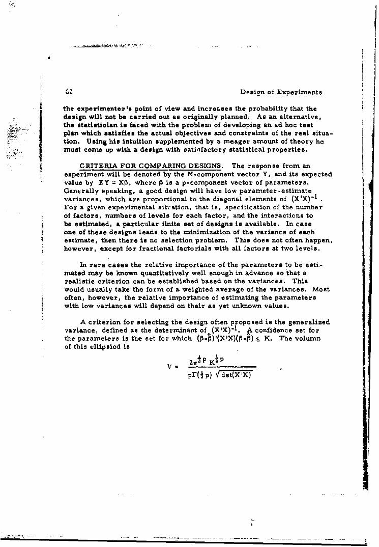
Design of Exveriments
the experimenter's point of view and increases the probability that thedesign will not be carried out am originally planned. As an alternative,the statistician is faced with the problem of developing an ad hoc test
* plan which satisfies the actual objectives and constraints of the real situa-tion. Using his intuition supplemented by a meager amount of theory hemust come up with a design with sati-ifactory statistical properties.
CRITERIA FOR COMPARING DESIGNS. The response from anexperiment will be denoted by the N-component vector Y, and its expectedvalue by EY = XP, where P is a p-component vector of parameters.Generally speaking, a good design will have low parameter-estimatevariances, which are proportional to the diagonal elements of (X'X)"IFor a given experimental sitvation, that is, specification of the numberof factors, numbers of levels for each factor, and the interactions tobe estimated, a particular finite set of designs is available. In caseone of these designs leads to the minimization of the variance of eachestimate, then there is no selection problem. This does not often happen,however, except for fractional factorials with all factors at two levels.
In rare cases the relative importance of the parameters to be esti:-mated may be known quantitatively well enough in advance so that arealistic criterion can be established based on the variances. Thiswould usually take the form of a weighted average of the variances. Mostoften, however, the relative importance of estimating the parameters
* with low variances will depend on their as yet unknown values.
* A criterion for selecting the design often proposed is the generalizedvariance, defined as the determinant of (X'X)"l. A confidence set forthe parameters is the set for which (p-•)'(XX)(Pop) . K. The volumnof this ellipsiod is
2v aP KiP
p1r(I p) v-det(Tx')

Design of Experiments 63
which is seen to be related to the design only through the determinant ofthe cross-product matrix. It is convenient to consider the determinantin the form of an index, called the estimation index, defined by $
1E det(X'X)/(NPII=wE
The weights w. are defined as follows. Let Z be the coefficient matrixassociated with the full factorial; that is, if Y14 were a vector ofI •' response for a full factorial then EY* = Z6. (The standard parameteri-
zation is such that Z'Z is a diagonal matrix. ) Let d. represent the i-thdiagonal entry of Z'Z and let M represent the total number of runs inthe full factorial. Then w, = di/M
r iOften the purpose of an experiment is to obtain overall informationabout the response. In these cases the appropriate criterion is basedon the average variance of a fitted response, where the average is takenover all M points of the full factorial. The average variance is propor-tionai to 7 w.V., where the V are the diagonal elements of (X'X)- 1 .A convenient representation is through the "fitting index"
I =p/(NzlWivi) W V)
More generally, an index could be based on the integrated variance of Ia fitted response. Such an index would in general involve off-diagonalelements of (X'X)" 1 , and would be difficult to define in a way which is
general enough for both quantitative and qualitative factors. Experiencehas showed I to be a very useful index.
F
Consider the class of models which is "complete" in the sense that F
if any interactions between a pair of factors appear in the model, thenall interactions between them appear. It has been proved [1] that formodels which are complete in this sense, the maximum value of bothI and I is unity. In [2] it is shown that the maximum is achievedE F'if certain combinations of levels appear with equal frequency. An
equivalent criterion is that the cross-produce matrix XIX is propor-tional to the cross-product matrix Z'Z for the full factorial. All
!A

64 Design of Experiments
regular fractional factorials have this property. If interaction parametersdo not appear in complete sets, either or both indices may be greater thanunity.
Thus far nothing has been said about the parameterization used toj, describe the response, that is, how P is defined in terms of the expectedj responses at the various treatment combinations, or equivalently, how
the elements of the X matrix are defined. Since the parameterization, •is to a large extent arbitrary, a particularly appealing property of the two
indices is that they are invariant under nonsingular reparameterizations.That is, suppose EY = XP = XAa, and similarly EY,: = ZP = XAa., where
r A is nonsingular. It can be demonstrated that IF and IE are identical
whether calculated under the parameterization 3 or a. Thus, theparameterization is immaterial as far as these criteria are concerned.
Without the use of electronic computers, the computation of theindices would be extremely tedious. A computer code has been writtenfor routine and convenient comparison of alternative incomplete factorialdesigns. A detailed description of this code and its use is available [31Any number of designs may be evaluated simultaneously by reading into the computer the treatment combinations in each. The evaluation willbe made for up to five models (specification of interaction terms to beincluded in the model). A number of options is available to the user,including changing the parameterization used for two-, three-, or four-level factors, or changing the weights used in computing the indices.A Fortran listing is included in reference [3]
ii ; •METHODS OF CONSTRUCTION,
1. Exhaustive Enumeration. For a few simple experimental situa-
tions it is feasible to enumerate all possible designs. The optimumdesign can then easily be chosen. As an example, consider as anexperimental situation a 23 in 5 runs with no interactions. There areexactly eleven nonsingular designs, which together with their propertiesare given in Table I. Clearly, the best designs are the eighth and ninth,for which each variance is minimized.
2. One Parameter at a Time. It is always possible to construct asaturated design (although they are very inefficient) by allocating onerun ts the estimation of each parameter. For example, a 32 x ZZ with
_ _ _ _ _ _ .... . ........... ..... ........ .... ..........

o .
65
TABLE I
t-0- 0 0~000J-'-I ,
EI0000 0 0
LM<
0000-Lr r% 0 0
000.--
~k4 0000-
o o 0000 0 0
UN 000.-0LC\0000-H~~ U ;;; 10 0,
I.-I

66 TABLE I (Continued)
U Q ~9 -'-000
UNQ 0 0 00'
000
0.00,-
00i8 8 q 8 0 tL
-t-
-0 0 00 -
I 00 0 0
4~ ~ 1 0 00'
8 o'do' WN otL

Design of Experiments 67
the linear-by-linear interaction between the two three-level factors isas follows
o 0 0 0 mean10001l:1 o o 0. 0. .0
~ 00 1 effect of first factora01 0 0]
0 2 0 0 J effects of second factor
2 2 0 0 interaction
0 0 1 0 effect of third factor
0 0 0 1 effect of fourth factor
where we have indicated the parameter estimated from each run. Thefitting and estimation indices are . 24 and . 025, respectively.
3. Correspondence. The theory for mixed factorial designs isless well developed than that for designs in which all factors appear atthe same number of levels. A useful technique is to construct a designwith all factors at the same number of levels, then replace some ofthe factors with ones of real interest using a fixed correspondencebetween sets of levels. The best.known examples of this techniqueare the proportional-frequency designs of Addelman [4] . To dernon.strate this approach consider a Latin Square of side 3.
0 000
01 11z
20h lattofcos a erpaedb w-ee fcosb sn
2102 .
The last two factors may be replaced by two-level factors by using i
tim correspondence
7

68 Design of Experiments
0 -. U
which results in the design
1 0 1 11 1 1 0
120 1Z 0 1 1
2 1 0 1
2 2 1 0
This design is quite efficient, having a fitting index of . 93 and an estima-tion index of . 79. A number of different types of correspondences isgiven by Addelman in [4]
4. Permutation-variant Designs. The salient property of
permutation-invariant designs, defined in L51 , is that estimatesinvolving factors which appear at the same number of levels have thesame variance properties. .More formally, the cross-product matrixX'X remains unaltered if factors appearing at the same number oflevels are permuted. An example of a 32 x 23 main effect design,for which I :80 and 1 .47, is:
FE° 0 0 1 0 0
S0 1 0 0 1!0 a 0 1 0
1 0 0 0 0
a 0 0 1 12. 1Z 1 1 022 101
Using a standard parameteriz.ation, the X and XIX matrices forthis design are-
S... :,...••. 0..0..0
10000......"1111

JDesign o0 Experiments
1-1 -1 1 1 1- 0 1 90 0 11
1-1 0 1 -2 -1 -11 0 6 0 0 0 2 2 2-- 0 0 6 0 0 2 2 2
1 0 -1 -2 1 -1 -1 -1 0 0 0 18 0-2-2-2X= 3 0 .2 -2 1 1 (XIX)= 0 00 0 18 -2 -2 -2
i 1 -2 1 1 1 1 1 2 2 -2 -2 9 1 11I -- 1 2 2 -2 -2 1 9 1
1 1 0 1 2 1 1 -1 1 2 2 -2-2 1 1 91 1 1 11 -11
Permutation of factors appearing at the same numbers of levels hasthe effect of permuting rows and columns of the submatrices in thepartitioned cross-product matrix. Since the submatrices are invariant,
the design is permutation-invariant.
This principle has been used* to construct a series of as yet unpub-lished saturated second-order designs for three-level factors. For fivefactors the design contains the treatment combination 0 0 0 0 0, thefive treatment combinations which are permutations of 1 1 I 1 0, thefive permutations of 2 2 2 2 0, and the ten permutations of 2 2 0 0 0.For this design the fitting index is . 66 and the estimation index is 2.35.Relative tothe full factorial but adjusting for the difference in the numberof runs, the efficiency of the estimate off the mean is 82%0, of the linear [!
main effects is 114%1, of the quadratic main effects if 25%, and of thelinear by linear interactions is 171%. The reason that the linear effectsand interactions are so efficient is that the points of the design tend tobe concentrated around the outside of the hypercube.
5. Balancing Levels. A very useful technique for constructingdesigns is to start with an ordinary factorial structure for the firstgroup of factors, and then insert the remaihg factors in such a way thatpairs of levels appear together with nearly equal frequencies. Forexample, the following two designs are obtained by adding another two-level factor to a basic 2x3 full factorial:
*This work was carried out by R. L. Rechtschaffner of Rocketdynes'sStatistical Test Design Unit.

70 Design of Experiments70 Design I Design 2
0 00 00 00 11 0 11
4a 1 1 0 11 10 1 112 00 20 1
There variance properties are given in Table II.
EXAMPLES. Three ad hoc designs which have been used successfullyat Rocketdyne will be mentioned briefly. The first involved determinationof char formation rate in ablative heat-shield material under simulated
I reentry conditions. The testing was done in a small stationary hydrogen-I oxygen rocket engine. The experimental variables were rocket engine
combustion chamber pressure, propellant mixture ratio, and the angle¶ of the sample in the rocket exhaust. The experimental design chosen
was one of the optimum 23 designs in 5 runs discussed earlier.
TargetChamber Target Inclination
Run Pressure Mixture AngleNumber (psia) Ratio (degreeE')
1 170 4 0
2 250 4 1Z2
3 170 16 121
4 250 16 0
5 250 16 12.
Another such design was used on a Signal Corps battery program. Theexperimental work involved screening 4 cathode materials, 3 solvents,and 4 salts. The design was constructed by balancing the levels of thesecond four-level factor within the framework of the 12-run 3 x 4factorial.
S..-. - .- - , - - - - - -- ~ - - - - - -. - - - . - . .... . .. . .

71
TABLE II
"I"D.o
m CY
r-~ IvN
00000 0 0
1:
04^
1P4rN

72 Design of Experiments
RunNumber Cathode Solvent Salt
1 0 0 0
3 0 2 34 10 1
6 1 z7 2 0 28 2 1 39 2 2 1
10 3 0 311 3 1 212 3 Z 0
Although there was no justification for assuming interactions did notexist, they could reasonably be expected to be less important thanmain effects. It was intended that this experiment be used to elimi-nate from contention some of the candidate materials with just a fewtests, so that later tests could concentrate on the better ones. Theactual decision made from these tests was that none of the four cathodematerials was satisfactory, and later testing should be directed atfinding additional materials. If all interactions had been considered, 48tests, using these four unsatisfactory materials, would be required.
The balancing technique was used effectively to construct a 34 x2 design in 27 runs for a program concerned with the valuation of fiber-reinforced plastic laminates. The variables are as follows:
Variable Code Levels
Bonding Pressure A 3Bonding Temperature B 3Resin Concentration C 3Post-Cure Temperature D 3Bonding Time E 2Post-Cure Time F 2Fiber Quality G 2

73
0 - 000".-. .--.- 0 -000 -00 --- ý 0 -
0 000 0-- -00 -- -- 0 - - - - - "
-0-0r.--- Or.--- .r0r---00rO0 -0000ON.- cv- -ONN -O-ONON.-v-ONON.-N.-o
0-N0.-N0-N0-N0.-N0.-N0.No.-N0-NA000 -.-.- NNN000.-.-.-NNN000.-"-,NNN~
0 000000
ON- N".-0-0N-OV-ON0N*-.0N0N.-N.-o
O.-NO-NO-No.-NO.NO.-NO.-No.-No-Noo000-.-.-N NN ------ N NNO00..-O-N
- -- - - - - NN4NN N NN
O-0.-.0-.-..--00-0-0-0--00"00.
N o.--O.-00.-0.--00 --.- 0-.-.-.Oo.-o
0.-NO-NO.-No.NO.-No.NO.-NO.-N0-N
S0 00 .- -- qN NN0 0- - -N N N0 0- - -N NN
p000000000".-q-.----.-- NNNNNNNNN
N~ ~ ~ -l' -t UN kDt C )0.Yt,,L - CD aN N~ N NC% LM%0N
0-0-0 -.-.- 000.-0-00-0--00"O.--.
O 0-NO.-NONO-NO.-NO-NO.-NO.-NO.-N
000 --- N(N000. -.-.- NNN00o-"-NNN
S000000000--. --.-.--.- NNNNNNNNN
- ~~ 0C-G~O 0- ~ f~(01-~O' 0-N CYNNNP~(0~

IN,
g- 3 4 t-o" N
0"t 0( K'l ONt- 4 0(N0
H L( f '% Cul,
M ~ ~ ~ ~ ~ ~ - r4% P4 04 4L% .
OOO COO; O 00000 C 0. 0.
MIR r4 LC% r
'4'
000O0OC000000000000 0 0
C CH F L o fI 10 WLMH R HH ,-4 p
N4K.ý.13k Tl 4N m 0 LA U, t- n -
0 0

IS
Design of Experiments 75
It was established that the linear interactions AB, AC, BC, BE,and DF are expected to be important. Since the factor D does notinteract with the other three three-level factors, the starting point wasa 1/3 replicate of a 34 using as defining contrast I = A2 B C2 D .
For the 2 part of the design three replications of the 2 plus three3 4
additional points were used. The 2 part was associated with the 3 parta number of ways, and the best design selected. The third and fourthdesigns were singular. The first, and best, design in presently beingimplemented.
REFERENCES
[1] WebbS. R. (1964). Otimality properties of orthogonal designs.Presented at the annual meeting of the American StatisticalAssociation, Chicago. .(Appendix C of ARL 65-116, Part I.)
[2] W ebb, S. R. (1964). Orthogonal incomplete factorial designs andtheir construction using linear programming. Research ReportRR 64-20, Rocketdyne, Canoga Park. (Appendix A of ARL 65-416,Part I. )
[3] Webb, S. R. and Galley, S. W. (1965). A computer routine forevaluating incomplete factorial designs. Technical DocumentaryReport ARL 65-116, Part IV, Aerospace Research Laboratories,Wright-Patterson Air Force Base.
[4] Addelman, S. (1962). Orthogonal ,nain-effect plans for asymmetricalfactorial experiments. Technometrics 4, 21-46.
[5] Webb, S. R. 41964). Characterization of non-orthogonal incompletefactorial designs. Research Report RR 64-18, Rocketdyne, CanogaPark. (Appendix B of ARL 65-116, Part I. I*1-i' I

b~i AT iST 1GAL ANALYSIS#' AU T1'~ OAT 1C AT .T .V
RECORDED PH-YSIOGRAPH DATA
J. C. AtkinsonDirectorate of Medical Research, CRDL,
Edgewood Arsenal, Maryland
The Directorate of Medical Research, CRDL, Edgewood Arsenal,
Maryland has the mission of investigating the physiological effects of
certain chemical substances on both human and animal subjects. Oneof the machines used to measure these effects is a physiograph. Thismachine which is commonly used in hospitals measures temperature,pulse, breathing rate and both systolic and diastolic blood pressure.
•• The common hospital versions displays the information only, how-ever, in our scientific work a permanent recording was desired so ananalog to digital converter and a punch paper tape output was installedon a unit by the manufacturer, Air Shields of Hatboro, Pennsylvania.Originally a flexowriter was used for the output device; later, aFrieden SP-2 tape punch was substituted to reduce noise.
This machine can be used on both human and animal subjects. Itwas first used by our Clinical Division with humans. It was shut downfor some months when difficulties were encountered with the sensorspicking up the signal from the subject. Later with better sensors itwas put to use again this time with dogs, The speed of recording canbe adjusted, So far we have run at a rate where a complete set of5 measurements are recordedevery 5 seconds. Lower rates are pos-sible and in many cases desirable particularly where changes occuronly gradually.
When the- paper tape is received by the computer section what isseen is a series of 4 digit numbers followed by a stop code where every5th number is of the same kind. The numbers are first checked by thecomputer for magnitude. For human's temperature is assumed to beat least 90, pulse 50, breathing 5, systolic blood pressure 5u, anddiastolic 20. If all readings are at least as large as those above, thereadings are reduced by the above for internal computations. Otherwise,an error stop occurs. It is felt that if the physiograph ever gets out ofsequence the above checks would bring it to a rapid halt since, forinstance, reading breathing rate for blood pressure would bring anerror halt.

rlI
/
78 Design of Experiments
After reading a predetermined number of enterims, or from a signal'Ell on the input tape, computations are begun. The mean, 950/ confidence
limits, standard error and coefficient of variations are computed forN. each of the S types of measurements together with all ten 2 factor correla-
tion coefficients.
It is hoped that the mean values and their standard errors willindicate longer term effects of the chemical. For instance, significantchanges might be shown to occur from I to 4 hours after administration,and apparent recovery thereafter, The correlations are hoped to showup more subtle changes. For instance a negative correlation betweenpulse and blood pressure is considered abnormal.
Unfortunately the change from a flexowriter to an SP-Z punch outputRM itook longer than anticipated and to date we have only data from early
human runs with inaccurate sensors but no drug runs. It is hoped thatdog drug runs will start this month. An output from a test run is shownas Figure 1 to illustrate format.
/ 4.
\,

79
0~N0
E- IAo IO $
000 00A0 0,coo103
0,0 g %00 a,
----- ~~L --%NII
Ln cr 0**M N
:44 alenQ4
ui ... ,

AN APPLICATION OF EXPERIMENTAL DESIGN IN ERGONOMICS:ijr'AD"I RATI. AS A r'TTNWrTTCN F WORK STRESS AND TIME
H. B. Tingey* and W. H. Kirby, Jr.Ballistic Research Laboratories
Aberdeen Proving Ground, Maryland
ABSTRACT: This presentation concerns the establishment of a
relationship between heart rate and imposed physical workloads for a given,
time period for a small group of young males. A hypothesis was developed,
experiments designed, data collected under controlled conditions, and theresults analyzed using classical statistical methods. The results dersion-
strate that the underlying functional relationship alters as the stimulus
changes. In this case the alterations may be defined over five segments
of time.
1. INTRODUCTION. Studies of changes in the human circulation
have been made from many points of view. Physiologists and others have
long been interested in the effects of physical work on the circulatory
system. Many of these studies have used heart rate behavior as an indica-
tion of the circulatory system's capacity to respond to physical workloads. I
Heavy, medium and light workloads have been considered under various
environmental conditions of temperature and humidity.
However, to the best of our knowledge, there has been no attempt to
study these clinical and physical relationships using more classical
statistical procedures in association with pre..experimental hypothesisformulation. The usual approach is to collect large amounts of data,
tabulate it and/or plot it on a graph. Then generalized clinical interpre-
tations are made. Occasionally, a statistician is asked to assist in doing
something with the data following its collection.
This study was done as an exploratory exercise not only to investigate
the possibility of an underlying relationship between heart rate and physical
load, but as a meana of bringing the engineer, physician, and statistician
together on a problem of common interest. We wanted to consider each
other's viewpoints In reference to a physical-medical problem. There
are also a common interest to employ more scientific method in. this area
of research,
*•Now Assistant Professor of Statistics and Computer Science,,4 .U U rilty:. -
of Delaware, Newark, Delaware.
----------------------------------.

82 Design of Experiments
We all knew that heart rate would increase with phy.iud vx.ttu,, aad
decrease following the cessation of it. However, we were interested inknowing the more precise nature of the rise and fall for different degreesof work intenoity. As simplifications we decided to hold the work periodand envitonntent constant. The phyo!-al workloads were chosen in thisfirst, study for conveuience and measurability.:
Our longer range objectives include the development of predictivefunctions relating more generalized stress situation& on the human systemusing this type of approach. Additional cardiovascular system phenomenawhich are also of potential interest to other researchers, clinicians, andthose concerned with the effects of various forrns of stress are beingconsidered. Such phenomena may include, among others, coagulation"factors, measure of hypoxia, and biochemical constituents,
2. METHODS.
,1 Scope and Procedure.
The purpose of this experiment was to assess the reaction of thehuman heart rate to -work stimulation, The conduct of the experimenttook the following line.
* A method of work was selected which may be described as a formof weight lifting, Preliminary trials were made to determine a set of
' I weights, number of repetitions and frequency which could be accomplishedby the five involved subjects, It was decided that available bar-bell weights,namely 21. 6 lbs. , 26. 6 lbs. , and 31. 6 lbs, would be used. Each bar-bellwas to be raised from the chest position to maximum vertical height andlowered with minimum restraint to the starting position, This cycle wasrepeated 30 times at a timed (metronome) rate of two seconds resultingin approximately one minute of intensive physical activity. The subjectsthemselves were a non-random sample of available personnel.
A brief physical description of the five subjects who were healthymales is as follows:
' .- •," ' ' .,' " q . . . . .. - . -... .. . .. . . . .- , - - . .. . . . . . . ...

Design of Experiments 83
No. Ane Weight Height
1. 35 175 5"-9"12. 30 230 6'-44"3. 44 180 51-9114. 24 135 514115. 25 155 5i-91,
successive weeks, Each repetition of the experiment started on Sunday
and terminated on Tuesday of the week. On each day the experiment wasstarted at the same time of day and the subjects performed in the samesequence. On the first day the 21. 6-lb. weight was used with the 26. 6-lb.and 31. 6-lb. weights used on the second and third days, respectively.The room was air conditioned and temperature and humidity were essen-tially constant throughout the investigation.
Five minutes prior to the initiation of the weight-lifting exerciseeach subject was seated in a chair adjacent to the apparatus. Small patchelectrodes had already been positioned on each side of the bare chest atthe mid-clavicular line just above the lower costal border for the contin-uous recordilkg of the electrocardiogram, The recording was accomplishedusing a telernetering apparatus and commenced immediately after thesubject was seated. This first phase which began at -300 secondsterminated at -60 seconds,
The subject then arose, stepped onto the force platform, moved intoa predetermined starding position with the forearms against the chest,elbows acutely ýlexed, and hands positioned to receive the bar-bell fromothers. At approximately -5 seconds he was handed the bar-bell and atzero second~sle began the exercise, ending with the termination of the30th. cycle at -:60 seconds. Others relieved him of the bar-bell immedi-ately folloing t.he cessation of exercise. The subject then stepped downfrom the platforni and sat in a chair resting for the remaining 540 seconds.Then he was removed from the experiment and the continuous monitoringof the electrocardiogram ceased.
This sequence of events led to five time zones to consider for curvefitting, namely, (1) a rest phase with essentially constant heart rate(time: -300 sec. to -60 sec.); (2) a preparation phase with linear increase
ilk,

84 Design of Experiments
in heart rate (time: -60 sec. to -40 sec.); (3) a short recovery phase withlinear decrease in heart rate (tirne: -45 sec. to -5 sec.);,* (4) the meadured
i - work phase with linear increase (time: actually 0 sec. to 60 sec. but heartrate changes occurred between -5 sec. to 55 sec. - the latter is used); and(5) the recovery phase with exponential decrease (time: 55 sec. to 600 sec,).As mentioned, heart rate was recorded continuously (via telemetered EC0s)and the distance of each lift recorded photographically. Apparatus andmeasurement equipment are discussed in Section 2. 5.
2. 2 Hypothesis.
The general hypothesis initially considered expressed heart rate tobe some function of workload and time. Symbolically, it was stated, H. R. Mf(L,T). One could make the expression more explicit by adding a. constantof proportionality and giving both L (measured load) and T (measured time)exponentials, Because of the sequence of events which took place, theinitial hypothesis was modified to consider the five time pe'.,iods duringwhich the individuals were measured. This led us to the following:
H : (a) The regression relationship between a workload and
heart rate is given over each of the five segments as a function of time.
S(1) H. R. =k k > 0•.300 -ct- -120.)
(2) H.R, k I + Pt ki, P >0 -60 c (t< -40,
(3) H. B. kz + P It k2 >0j P1 <0-35 <t .5,
(4) HR, R k3 +P 2 t k? 03 P2 >0)0 <t <5%"" 2
(5) H.R, k4 te 3 k4 > 0, c'>0), 3 > 0)60 <.t<600.
Note: The actual relationship might be specified by a singlerelationship but more careful planning in the light of thisthis experiment is required. One might state the overallrelationship as:
'*One might be led to considering this interval as two segments whereasour original hypothesis was that over a short interval our heart rate decreasecould be considered linear.
...... . ...-

Design of Experiments 85
H. R. Kta ePt
(b) The regression relationship between a time and heart K
rate is given as a function of load:
H. R. a(t) + P(t)L
Initially the data are subjected to the analysis of variance for athree-way layout and appropriate tests for the significance of main effects(and the particular intervals over whic they are significant) and to detectpossible interactions which may be present, The hypothesis tests havefollowed the stindard F-test procedure ahd are indicated in the ANOVA(Analysis of Variance) Table III,
2.3 Design.
The basic design employed for each replicate of the experiment isa two-way layout using time and theoretical load as controlled variableswith heart rate as the response variable. The general formulas aregiven in Table 1.
TABLE I
General Formulas for Two-Way Layout
Source SS df E(ms)
2 2 2Time SSt = JK (yi, y - I-I a +JKO
2 2 2Time X Load SS tf KE XYij. . yi, " Yj "y.. all( -) +Ka
i j
Error SS MZEZ •. N 2 IJ(K-l) 2• ij k ' j'
Total SSr = - 2 IJK-lZEE j k ''
r i j k

Ti npri-nents
It is, perhaps more desirable to analyze the data over the three trialsof the experiment by introducing another main effect for repetitions of theexperiment. Hence the analysis of variance takes on the pattern of a three-way layout with several (say n) observations per cell, The general formulastior this situation are presented in Table II.
The data from the experiment are used according to the formulas inTable II to calculate the results given in Table III. The error sum ofsquares should indicate the approximate value of the renidual error afterfitting the regression lines proposed in the original hy-•othesis. One may,as a matter of interest, test the significance of the rean squares for maineffects and interactions. This would then lead the ir.vestigatbr to an analysisto determine the regression which might exist over each of the five intervals.
Additionally, results from the mean squares fitting for the fixed time-load variable and the fixed load time variable are presented in TablesIV and V.
2.4 Instrumentation and Equipment.
The weignts used in this equipment were obtained from a commerciallyavailable bar-bell (dumb bell) set, the components of which were weighedto the nearest tenth of a pound. The components were assembled in threecomLlaations to give the test weights of 21, 6, 26. 6, and 31. 6 pounds,
The experiment was conducted on the surface of a force-platformof special design capable of making accurate measurements of forces inthe three orthogonal axes and of moments about these three axes. Whilethe platform impulses were measured, discussion concerning them arebeyond the scope of this presentation,
Heart rates were obtained from a TFLEMEDICS Radio-Electro-cardiograph known c-,mmercially as the RKG 100 System which is composedof a receiver Model MCM and transmitter Model 100 A. The associatedelectrodes, as mentioned previously, were positioned in order to minimizemuscular noise and prevent premature loosening of them. Very sharpQRS complexes were obtained, The e. c. tf. profiles were recorded simul-taneously with impulses from the platform on both , Sanborn 8-channelPaper Recording System, Model 858-5460 and a Sanborn-Ampex MagneticData Recording System, Model 2007.

87
4*
b b• N Kb t
r -4 .. :4
I
SN N N
E-44
.......
•,*1: . . *,
. II *

88 Design of Experiments
The metronome was a battery-powered electromechanical oscillatorwith amplifier and speaker calibrated to give the desired frequency (onlepulse per second).
....... ..•i•! ...16mm motion pictures were taken of each subject during each exercise.The camera was located in order to record the appropriate movementsof each subjdct in association with fiducial markers.
3. RESULTS.
3.1 Results and Interpretations.
The computations noted in Tables I and II were carried out and areshown in Table III.
due to different loads. This was, of course, a gratifying result inasmuch
as the increment between levels of load was rather small. The resultingF-ratio is more than adequate for the stated significance level. Thiseffect can be appreciated graphically by referring to Figure 1.
The next control variable, time, is again highly significant as was tobe expected. The significance here, as well as the previous effect, ie.load, may well stimulate the analyst to consider the functional fit to thedata proposed in the original hypothesis,
A difficulty encountered from the analytical point of view occurs whenone observes that both the Repetitions by Load interaction and Load byTime interaction are both significant. Considering the former, Repetitionsby Load, the explanation here must come more from clinical considerationsthan from statistical interpretations alone. While the entire experimentwas considered to be one that could be repeated, one can note that thesubjects under consideration, although healthy, were not in top physicalcondition. As the experimental series progressed, an improvement (ordegradation) in the physical condition probably occurred, Techniquesalso improved during the conduct of the experiment. In addition, therewere one or two minor changes in apparatus which might account for thiseffect. Additionally, the subjects were not isolated from normal dailyroutine before and during the. 3xperiment, Perhaps the effect of psycholog-ical factors operating through the autonomic nervious system may be mcreimportant than can be identified at this time.

89
TABLE III
Analysis~ of Variance
Source ___ SS Ms F-Ratio Significance
Replications 2026.58 1013.29 8.64 None
Load 2 7504,00. 3752.00 31.99
Time 43 317105.39 7374.54 62.87
RxL 4 5462.93 1365.73 11.674
RxT 86 4874.66 56.68 0.483 None
LxT 86 15868.31 184.52 1.573 88
RLxT 172 9693.96 56.36 0.480 None
Error 1584 185808.71 117.30 F
Total 1979 548344.54 M .
*Significant at 5% Level.
* *Significant at 1% Level.

91
a
____., - -- -- L 98o
. J,.
gq-•
- - ---- ' -
dew
AM ,
SI3 I_ .2 _ : ° .. . . ... .. . . .. . . . ... .. ... . . . . .. ... .. . .. . . . . .. ... ... ... ... .. .

Design of Experiments 93
The Load by Time interaction probably receives its largest contributionfrom the differences in heart rate acceleration@ and peak values which occurover the working phase. In comparisbn with the close similarity of thecurves of the other time segments of the experimental cycle, this interactioncould perhaps be avoided in subsequent experimentation by consideringmeasurements only over the working phase. However, this approach cannotbe taken until reasonable baselines are established for pre- and post-workpe riod an.
In view of the purpose of the experiment and the original hypothesispresented, an attempt in made to perform the regression analysis set
forth under the null hypothesis. Table IV indicates the linear regressionfunctions in reference to time. One may observe that the residual errorafter fitting closely resembles, on the average, the error mean squarefrom the analysis of variance. Table V indicates the regression function@in reference to load. In like manner, the residual error after fitting resem-bl es the error mean square from the analysis of variance.
Tests of significance have not been performed on the individual constantslisted in Tables IV and V in that the appearance of interaction effects doesnot allow the combining of all the data or the three replicates as was donefor these calculations. We have not formulated the precise nature of themultiple test procedure implied here. The basic intent again was to developan idea of the form to assist in future designs.
4. DISCUSSION.
4.1 Subtle Observations.
a. Heart rate prior to leaving the sitting rest position.
It is interesting to observe (Figure 1) the resting heart ratepatterns. Fluctuations for a given subject on a given experimental runwere essentially similar for the different loads and repetitions. Thusthere was an identifiable pattern for each of the participating subjects,One would judge that some of the fluctuation in general might be lessenedif subjects were isolated and testing singly in an environment in whichexternal stimuli were essentially nil. Statistically, of course, we havetreated the values in this phase am constants.
Ii

94| TABLE I V
Table of Linear Regression Functions:Heart Rate vs. Time
TimeS(Seconds) _ ERMS 0
.300, 79.244444 - .05333333 7.0593 1.6639 .25777
.-240. 78.655555 .06000000 6.3054 1.4862 .23024-180. 78.777777 .13333335 5.6110 1.3225 .20488-120. 78.222222 .28000001 7.0641 1.6650 .25795- 60. 86.499999 - .41999997 9.7390 2.295S .35562- 55. 90.899999 - .SS333331 13.227 3.1178 .48300- SO. 91.977777 - .35999996 11.914 2.8081 .43503- 45. 92.655555 .00666670 12.102 2.8524 .44190- 40. 94.411110 .23333336 13.937 3.2849 .50890S- 35. 92.622222 .26666670 12.917 3.0446 ,47166
- 30. 88.433333 .52666668 13.759 3.2431 .50242- 25. 86.388888 .15333334 11.775 2.7755 .42997- 20. 87.199999. .07999997 11.938 2.8139 .43592- 15. 87.333333 .10666670 10.728 2.5286 .39172- 10. 88.755555 .02666669 9.5600 2.2533 .34908- 5. 89.677777 .40666669 8.5388 2.0126 .31179
0. 95.911110 .12000002 7.8273 .1.8449 .28581S. 99.966666 .32666671 8.1022 1.9097 .29585
10. 99.899999 .72666669 8.7247 2.0564 .31858IS. 101.44444 .86666670 9.4751 2.2333 .3459820. 103.70000 .60666668 9.,6506 2.2747 .352392S. 105.47778 .91333333 11.449 2.6985 .4180530. 106.04444 1.0133333 11.570 2.7271 .4224835. 106.05555 1.4733333 11,876 2.7993 .4336640. 108.48889 1.5866667 12.465 2.9380 .4551545. 109.68889 1.5600000 13.738 3.2382 .50166.50, 110.62222 1.8000000 12.613 2.9729 .46056
55, 112.45555 1.9266667 13.713 3.2321 .5007260. 107.64444 2.0133334 13.540 3.1914 .4944165. 101.70000 1.3133334 10.333 2.4355 .3773170. 99.799999 A'6666669 10.289 2.4251 .3756975. 97.411110 .55333335 8.1311 1.9165 .2969180. 94.766666 .47333335 8.8753 2.0919 .3240885. 93.644444 .42666669 8.9016 2.0981 .3250490. 93.766666 .43333337 9.8854 2.3300 .36096
120. 90.755555 .10666665 8.9511 2.1098 .32685180. 83.622222 .25333335 8.1302 1.9163 .29687240. 81.633333 .11333336 8.2653 1.9482 .30181300. 80.422222 .49333335 8.5371 2.0122 .31173360. 81.888888 .25333336 8.5314 2.0109 .31152420. 81.866666 .05333333 6.9260 1.6325 .25290480. 81.011110 .07333336 5.7840 1.3633 .21120540. 81.033333 .07333334 6.5464 1.5430 .23904600. 82.266666 .10666665 5.9303 1.3978 .21655

95
TABLE V
Table of Regression Functions VHeart Rate vs. Load V
p: ~Time•
Segment 21.6 lbs. 25.6 lbs. 31.6 lbs.
I 79.7 79.7 79.7
"11 82.6 '.55M' 82.6 + .5"&t 82.6 + .5SAt*
11i2 92.5 - .614t* 92.5 - .614t* 98.5 - .61At*
IIIb 83.6 + .154t* 83.6 + .ISAt* 83.6 + .lSAt*IV 96.2 * .32t** 96.7 * .43t** 99.2 + .62t** tl
V e4.6bt. 0015o ea.087t** er4.74t.0014-. It** 04.820019 13t**
Start At at zero at the beginning of the respective segments andincrease by 5 for each interval,
Start t at zero at the beginning of the respective segments endincrease by I for each 5 seconds.
.... .. ...

96' Design of Experiments
Sb. Heart rate during immediate pre-work phase.
After the subjects left.their reiting chairs, they took several4i• paces and took a single step up to the work platform and assumed a
predetermined work position. The subject then remained in this positionto await the signal to receive the bar-bell and commence the excercise.
, :It was this phase that caused us some unexpected concern from ananalytical point of view in that we lost control of the individual in trans-ferring him from the resting phase to the working phase More carefulplanning should avoid this problem in the future, The same kinds ofvariations mentioned in (a) above likewise were found in this phase. TheseI • were also treated in linear fashion.
c, Heart rate during work.
While it was expected that the heart rate would rise rapidlywith the sudden onset and continuation of intensive physical exercise, amore precise statement on how it would rise was desired, rhis, hope..fully, would give some insight in reference to the posuibility of an under-lying functional relationship between workload and heart rate response.The data points for each of the three loads for the five subjects areshown graphically in Figures 2, 3, and 4. These data were fitted withlinear regression lines as shown also on the graphs. It is interestingto look now at the individual pattern for this phase of the experiment.Figures 5, 6, and ! show their chariacteristics. To us these were very
interesting observations for they provided additional insight on themanner that individuals respond to a physical stress in a physiologicalway using a set of quantitative measures as opposed to the more commonbut less rigorous clinical impressions, However, we are mindful ofthe exploratory natttre of this project as well as its being a orsall non-random sample.
d. Heart rate during recovery,
It is very interesting that heart rate falls so rapidly followingthe cessation of physicalwork. This well known exponential fall, thegreater part of which taken place within approximately the first 10 to 15seconds, was demonstrated iL association withthe raw data points forthe various loads shown in Figures 8, 9, and 10, According to theresults in this study heart rate began, to fall several seconds prior to

97
thft
wWXwIAo3 L&JiLJJ
p,) w NI.OW ___Cl
U- W
Y.. -X
oo
o U
Ix
04.Y
(3.LflNIV H3 d SIV31a) 3JXH .LMV3H

4t III
".. I� j-�I �-
�
I
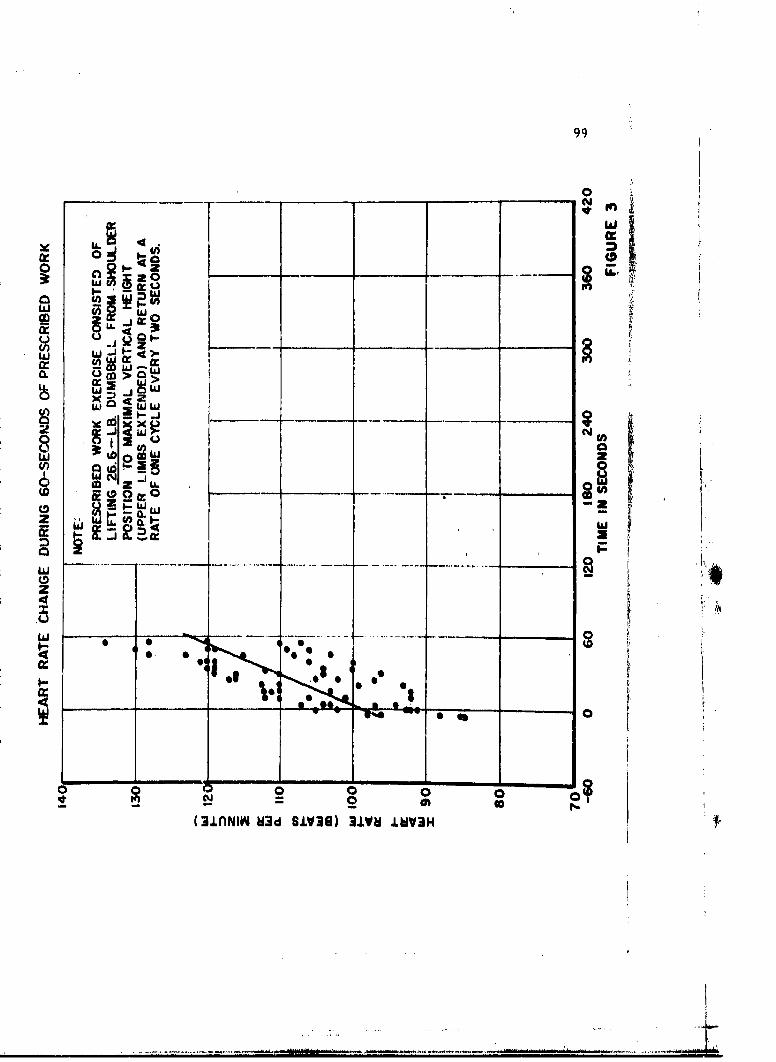
99
0.0
cr.j~
2 LU
w w R
x x_0cj U)
0W 'oC1
(3.ANW .39.VI)3V~.~3

ff
..:/ j
PRCDt
PAEBPN
iI

101
_ _ _ _ _ _ _ _ _ _ _0
q.l
ILWQ
at~
wa~
0. at m> I
0 Li :D ,
e C
w -w
Cc zC w 0 U
-~~~ý a .__
0
4C
4r
0
oi 1 31nANVI O3d S.LV31) 31VUd .LJV3H

e
I II
I II

103
HEART RATE CHANGE OF INDIVIDUAL SUBJECTSDURING 60-SECOND WORK PERIOD USING 21.6 LB
DUMBBELL (AVERAGE OF 3 TRIALS)
120
1000
90 - NO. AGE WEIGHT HEIGHT
2. 30 230 0-4"3. 44 ISO fg
T"M IN ucoWNs
FIGURE B

Iii
U� 1
U KII
I
PRECEDING
PAGE CLANK
�

105
HEART RATE CHANGE OF INDIVIDUAL SUBJECTSW.UYa 60-SEOW& wu R Ui61 •.•i i6, Li
DUMBBELU (MIERAGE OF 3 TRIALS) "
./! .
,,./-I -/- /. I
It, -s MIMI
o l -00
I t
M AU M IONT HEIGHT
L330 ag 6O-40
it 14 In W7
T M@ 0 80
ft ~ lums ~I NT

V41
iji
PAGE ULAVI.

107HEART RATE CHANGE OF INDIVIDUAL SUBJECTS1*IEING SO-SECONDo WORK PERIOD USING 31.6 LB/DUJMBBELL (AVERAGE OF 3 TRIALS)
15/0
// MEAN
100
1. //IT W
jD In / '-o
@o 0--4 a7, to s/o t
\jM li49o
100 * - ~Vv

I I
II
iv..
- K
I.

npa'g 1 109
the cessation of the work, Our explanation for this is that it may in partbe anticipation by the individual toward the end of the work cycle and, inpart, due to the method of discretizing the data. Since the participants inthis investigation were conaidered to be clinically healthy males in a some-what restricted age range, no inferences are made regarding variationsin the return of individual heart rates to the normal or resting baselines.
F ~ The fitted exponential regression curves shown in the figures mentionedL ~ above are treated statistically. Variations are attributed to circulatory
system characteristics and their nervobus system interactions. Presumablyexternal stimuli which may influence heart rates in the re.sting and thefinal stages of recovery would be less significant during intensive
i. physiological stress derived from physical work.
e. Heart rate over the experimental cycle.
A summary or heart rate profile over all phases of the experi-mental cycle averaged for each load in recalled as shown in Figure 1.It is interesting to observe the slopes of the surves showing heart rateincrease in that they are clearly different even for the small incrementsof work intensity. The same may be said in reference to the peak values.
4. 2 Direction of Subsequent Investigation.
In brief the following are being considered for subsequent investiga-tions:
a. Longer work periods in order to understand more about heartrate behavior at maximum range under prolonged work stress.
b. The utilization of an open system in order to accomplish a. above. I.,Weight lifting, unlike bicycling or tasks utilizing more of the muscles tendsto generate exhaustion prior to the onset of peak heart rate.
c. Certain biochemical parameters associated with circulatorysystem response to work stress may be useful particularly as it may, inturn, be related to such medical conditions as shock. Here then we becomeconcerned with multivariate models and analysis.
d. Planning of experiments for additional insight on roles of otherphysical and psychological factors,
e. An ultimate objective is to relate "stress" to cardiovuscularsystem changes associated with early signs of cardiovascular deteriorationand a particular condition known an hemorrhagic shock.

II
I
I?
* V
......................................

I llit
(Dos
wx Iww
42 I
-(NIVY Od SJ.V39) 31Vb 11 3H

In W
Ii cnLC 311h1Vi
a-z
CL Irl
of'
(NI ___ SI3) itli

030
z z
'0
1w ui.-___vi qL)
so- WOeeilg-S-S
w (.- 0CL SoO4 X---.
0 >
22
LL IAJCD ..--.-
(3n6l 83 SiV8 3**V * 1M l

STRATEGY FOR THE OPTIMAL USE OF WEAPONSBY AREA COVERAGE*
J. A. Nickel, J. D. Palmer, and F. J. KernUniversity of Oklahoma, Norman, Oklahoma
(Representing the U, S. Army Edgewood Arsenal)
ABSTRACT. The development of non-nuclear ground-based weaponssystems in a historical perspective is briefly reviewed. The implicationsof this development to target acquisition and logistics in terms of efficiencyof coverage are included.
By defining a new concept termed Efficiency of Target Destructionas the ratio of expected area destruction of a target complex to the maxi-
mum theoretical area destruction possible, the authors have demonstratedthat a delivery of a number of small effects patterns can be most efficient,
Through use of the SADI Mark IV, Statistical Additive Density Integrator,it was found that the delivery error (standard deviation of delivery) mustbe in the neighborhood of 50% of the target radius for maximum efficiency.It was further found that the efficiency is not appreciably reduced if theactual aim point is within 30% of the target's radius of the center.
These results clearly indicate that for certain classes of targets adecided advantage is attained in terms of efficiency of the weapons system,reduction of target locator accuracy requirements, and a lessening ofthe impact of logistics support.
INTRODUCTION. In the generations of ground based weapons systemssince World War II, three readily identifiable stages have existed in thedevelopment of non-nuclear weapons. In the first instance, the attemptwas to develop a warhead with the greatest possible damage or effectspattern which required larger and larger lethal radii for each particularsystem. During this initial phase, it was tacitly assumed that if one
could develop a larger effects pattern, this was most easily deliveredon target. A major effort during this period was toward warhead design
and development, with little effort toward determining the accuracyrequiremente, It was further assumed that once the warhead was avail-
able, delivery on target would be readily achieved.
':*This acticle appeared earlier as a University of Oklahoma Research
Institute Technical Report: Contract DA 18-035-AMC-116(A); InternalMemorand%,,- 1454-1-2, July 1965,

118 Design of Experiments
The second phase initiates with the realization that the warhead couldnot hf delivered on target with a high degree of reliability, that is with ahigh assurance level. This led into the second phase which was the develop-
ment of more accurate locators and target acquisition devices forsophisticated target acquisition--techniques such as infrared, radar,radiometers, acoustics, etc. In this phase the dependence of any systemon the inherent ability of a locator to not only locate the target, but alsolocate itself relative to the weapon was realized, This presented thethird problem with even more difficulties for designers and tacticians.The situation now becomes that of large lethal area weapons with a rela-tively low accuracy yielding the resultant of the net amount of lethalpattern placed on a target being less than that which could be achievedshould a highly accurate method of firing be developed. With the realiza-tion that these two viewpoints were mutally opposing, atte pts have been
made to develop closely coordinated systems involving locators andweapons. Considerable research has been performed in an attermpt to
* formulate a methodology which would serve to alleviate this inherent
difficulty.
In establishing minimum criteria for target location and firing patterns,the objectives have been aimed at generating more accurate locatingsystems and larger effects patterns. Target requirements have becomemore and more stringent. More potent effects patterns (non-nuclear)have been developed with the rather obvious end result of requiring greaterlocator accuracy to achieve a maximum effective firepower per unit.Most recent studies have been directed to ascertaining error sources andattempting to provide a maximum assurance level of target coverage: fora given system. This has usually resulted in going to larger and largertotal effects patturns as a consequence of the inability to supply moreaccurate target location methods. Tests to determine the mraximum allow-able error for multiple effects patterns have resulted in a promulgationof this same trend. Hence, a higher required assurance value of targetdestruction has resulted in specifications for more accuracy in location,
The problems which accrue from this trend are many. They includethe requirement for more accuracy and mobility in target location systems,logistic difficulties associated with increased firing rates, loss of targetduring "zero-in" fire due to target mobility, and high initial and mainte-nance costs associated with larger more complex weapons systems. Theresults have been the generation of requirements for more accurate radars,

Design of Experiments 119
infrared devices, and optical detectors with accompanying data processingequipment, weapons selectors as well as more accurate delivery systems.
A re-examination of simulation data originally run to determineminimum accuracy requirements to yield maximim area coverage hasresulted in a number of factors which point toward an entirely differentassessment of applicable criteria contradicting previous concepts, Inattempting to determine the "efficiency" of various weapons systemsagainst standard target sizes, it was found that maximum efficiency seemedto occur when use was made of smaller values of RD/lRT (lethal patterns)
and that a deliberate error of up to 1516 RT had only a minor elfect on
area coverage at the maximum efficiency levels and further that a sacrificein assurance level could. be made and yet have a better system than ispresently available against certain classes of targets under the previousoptimization requirements.
Through the use of the OURI-SADI Mark IV, a systematic study ofS ef.fects patterns and their effectiveness on area targets has been under
investigation, An analysis of the data has brought forward several observa-tions, Foremost among the observations is that the effectiveness in useof munitions can be increased by reducing the size of the effects patternof a given round and distributing a number of these with a delivery errorthat is bounded away from zero, i. e. , not perfectly accurate, as well as
having an upper bound on the weapons errors.
For flame technology, this is particularly important since by not
attempting to cover the entire target with ftiel, the insulation effect ofunburned fuels is minimized, The desirability of small portable flamedevices increases since on the criteria enumerated they are tacticallysound. Furthermore, multiple bursts with each component yielding asmall effects pattern, requires less delivery accuracy than a singlelarger burst having the same potential of destruction,
The SADI Mark IV, Statistical Additive Density Integrator, asdeveloped by the personnel of the Systems Research Center, Universityof Oklahoma Research Institute, permits the evaluation of lethality to atarget by simulation techniques. Through such studies, several factorsinfluencing the effectiveness of multiple firings on a target have come tolight. Area coverage affected by flame devices is particularly well-modeled by this simulation technique.

120 einc :;rniný
At this juncture of study, the basic configuration has been the randomj placement of six circular "cookie-cutter" effects regions. Each
component, with total destruction or lethality throughout the circle, isdistributed about a point on a circular target. Circular effects regionshave been employed since in a first approximation, this is approximatelythe shape experienced under actual firings, Circular targets have beenused since maximum efficiency coild be designed into the SADI Mark IVwith this coniiguration. It is known, however, that a topological equiv-alence exists between this configuration and any other for which the
I:i boundaries of the target and lethality region are simple closed curves.It should be further observed that the numerical discrepancy betweenusing circular patterns and rectangular patterns is negligible. (Ewing,George. Predicting the Effects of Multiple Firing on an Area Target
* and Related Questions, OCDD, USA AMS, Ft, Sill, 1955). Implicit inthe foregoing equivalence are questions of approxim~ated symmetry andother regulatory conditions which will not be considered,
APPROXIMATING CONVOLUTION OF THE MOMENT GENERATINGINTEGRAL. In trying to estimate a suitable approximation to theprobability density function f(x) of a population from which samples aredrawn, the following scheme approximating the density function from theempirical moments is proposed,
it is known in statistical theory, that if the Moment Generating Func-tion, M(x), is known for a sampling distribution, then the moments ofthat distribution are readily obtained from the derivatives,
For simplicity it is assumed that the probability density f(x) at acortinuous variable has -i rmnverient McLaurin t;xpansion on the unitiiiwrval (0, 1) and is zero elsewhere, ii.e. ,
f(x) = Z bxkX o <_. x <1kk=o
: 0 elsewhere.
This assumption permits the Moment Generating Function M(x) to beexpretsed as an integral over the unit interval, ie.,

b esign oi Ex perim ent s +00
+• 1
M(x) e f(t)dt e f(t)dt
- 0 0
This function can furthermore be expressed as a power series
SkM(x) = + E XVk
k=l kW
where v is the kth moment about the origin,
A second possible interpretation is available by considering M(x)as an Integral Transform instead of an expected value, As an IntegralTransform, the following needed properties can be established.
(]) M(ax + by) aM(x) + bM(y) e -
(2) M I [f I(x)] M ix x~)fO
(3) M(O) 0
S~kx( 4) M(l) E . '(~)
k=O
(5) M() M (k + M) (k + 2),k=O 0
16 (6) M(x2 L= (k + 11) (k + 2) + (k + 3) kk=O
and in generalnk n M [xn-l
(7) M(Xn) = k-- = [n lk=O L

ii2 Design of Experiments
)Uning Lhe assumed power series expansion for the probability density
[k= k
b bk M ]
kWhen the transforms of x are substituted into this last expression asecond power series expansion is obtained for the Moment Generating
Function, this time in terms of the McLaurin coefficients of f(x). Twopower series converging to the same function necessarily have identical
coefficients, From this, it follows that
® b= E] k 1, 2Vkl j=l k + j-2
where v = 1. These constitute an infinite system of equations in the0
variables b j =l, 2,i-l
b Letting B denote the column matrix of the McLaurin coefficientsSbi, N the column matrix of the moments vi~ calculated from the
sample, and A the !ilbert matrix
The foregoing system of equations can be written
AB = N.
The matrix A is singular and has no inverse. However, if the systemis truncated sj as to utilize only a specific number (n) of moments, theresulting (n 4 1) by (n + I) square matrix A does have an inverse An'
n n

Design of Experiments 12
The approximating polynomial coefficients can then readily be obtained as
B = A Nn
It should be observed that the matrix A , and hence, its inverse iFn
independent of the sampling distribution, hence, one A can be usedfor all samples at that degree of approximation.
From a casual observation of the data it is apparent that the densityfunction is not uniform, normal, or even symmetrical. It follows that anyadmissible polynomial approximation should be by a polynomial of degreegreater than two. To allow for the possibility of symmetry it is reasonableto consider an approximating polynomial of degree four (4). If a leastsquares analysis were to be employed in determining the coefficients forsuch a polynomial, it would be necessary to use eight (8) moments of therelative areas. Since the basis for accepting the polynomial of degreefour as a good approximation to the density function is not established,an abbreviated procedure over a least squares evaluation is desired.
A polynomial approximation to the probability density function wasdeveloped through the use of an approximating convolution of the MomentGenerating Integral. If the approximating density function is given by
2 3 4f(x) = b +bIx + b2x +b3x + b4x
where x is the relative area reduced to the unit interval. The aboveapproximating convolution gives the following formulas for the coefficients.
b = 25 - 300vI + 1050v2 - 1400v3 + 630v4
bI -300 + 4 800vI - 18900v 2 + 26880v 3 - 1Z600v4
b2 = 1050 - 18900v1 + 79380v2 - ll7600v3 + 56700v4
b3 = -1.400 + 26880v - 117600v2 +179Z00u3 - 88200v 4
b = 630 - 12600vI + 56700v - 88200v + 44100v4
4 2 3 4

124 Design of Experiments
where v1, v2, v3 , and v are the moments of the relative areas of
coverage about the origin reduced (or scaled) so that the maximum relativearea is one (1). This calculation only requires the use of four momentsof the distribution to give an approximating polynomial. The only segmentof the ensuing polynomial used is that part lying above the axis and corre-sponding to the range of values of the original sampling distribution.
For the purposes of the original problem, the cumulative probabilitydistribution is needed. This is readily approximated by the polynomial
P b x +/ (1 xŽ +(I/b, x3 +/(I/bx 4 +(l/5) 4 x
obtained from integrating the approximating density polynomial. Thisagain is used only over the domain corresponding to the observed areainput obtained from the simulator. As a statistical control, a kolmogorov-Smirnov Test was applied to the empirical distribution and the calculatedapproximating cumulative probability polynomial.
SYSTEMATICALLY INTRODUCED BIAS. It has long been recognizedthat a knowledge of the exact position of a target relative to the weapon isgenerally not initially known. This raises the question of bias effects inthe assumed target location relative to the actual target center. A studyhas been initiated to investigate the systematic introduction of bias in thelocation of ground zero. The actual procedure used is probably bestdescribed through the use of the flow chart of Figure 1.
Initially, in the. study of bias effects, the parameters consideredhave been a- = 0.5 and r = 0. vr 5 ,. For this particular case, it becameapparent in preliminary investigations that a bias less than or equal to0. 3 of the target radius produced minor decrease in the exp'cted areacoverage. The fall off to a first approximation is parabolic and the areacoverage can be approximated by multiplying the expected area coverageof a symmetrical distribution by the factor.
1 - ;0.925X 0 !X !S 0.4
In this factor, the bias X is the ratio of the distance between the targetcenter and aim point, and the target radius. For X = 0. 3, the fall off

125
FIGURE 1
Bins Effect Analysis on a Sampling Distribution of & K
Comiposite of N Effects Patterns
patterns on the targetcenter
SRecord area and rotate
p attern by 3600/k
4I
a sandar devition of d deliery
y elasv raiu afvfect.shpattern Shiftonent
s ~ ~ ~ be maoadume fshfst e? cobdee (1asefetsi te rgmsof 1/5taruerradii
k -toal umer f aystobee consideredi
Specify 4
Halt

127
FIGURE 8
w210 DRT:04
AD/TE20
IOFS UIT/R 00. 4R 5
VVW OFFSET

129
0
mo~p
ui4
uJ4
at4
cr ¶ot)
UCA.
O 0~10 W.0 Qi dV.
d d

I ~FIGURE 10
~-6-425% CONF.0-0-13 50% CONF.
60 0--0-0 75%
50S
'3,0
.040 1 2 3 4 5 6 7 8 9 10
OFFSET -UNITSI UNIT a 0.2 RT
AREA COVERAGE AS A FUNCTION OFDISPLACEMENT OF TARGET AIM POINT

Design of Experiments 133
is approximately 15%, and hence for smaller bias, the correction is quiteinsignificant. It must be again pointed out that the foregoing corrcctionis based upon the observations of one pair of parameters. A larger setof parameters must be considered before general conclusions can bedrawn with a high degree of certainty.
One conclusion inferred from the foregoing observation is that formultiple firings on an area target, the accompanying target acquisitionproblem is not of major significance, since minor inaccuracies in thetarget location will not significantly affect the expected amount of destruc-tion when all rounds are aimed at what is considered to be the targetcenter.
SYMMETRICAL PROBLEM. The first study to be consideredconsisted of six rounds being aimed at the center of a circular targetand distributed with a circular normal probability distribution about theaim point. Standard deviations equal to one-half and three-fourths of thetarget radius were used with a larger variety of effects circles. (Nickel,J. A. , Palmer, J. D. , Battlefield Simulation for First Round AccuracyRequirements of Simultaneous Multiple _Firin. Proceedings of WinterConvention on Military Electronics, IRE, 1963; Nickel, J. A. , Palmer,J. D., Gajjar, J. T. , Kern, F. J. , and Williams, D. R. BattlefieldSimulation for First Round Accuracy Requirements of SimultaneousMultiple Firings. Data Supplement No. 1. DA 34-031=AIV-679, 1107-5-6,January 8, 1963.)
In all cases considered, it was observed that the smaller standarddeviation consistently yielded a greater statistical area coverage. Inother words, for a given size of the component effects circle, thestandard deviation of one-half the target radius gave a greater areacoverage than did the larger standard deviation of three-fourths thetarget radius. A local minimum area coverage is to be had with astandard deviation of zero, in which case all effect@ components wouldlie on top of each other, giving a total effective area equivalent to thatproduced by a single component.
Consider the statistical area coverage as a function of the stan~darddeviation of delivery, cr , as well as the radius of the effects circlecomponent, r. Notationally, this will be written as A(ao,'r). From the"remarks of the preceding paragraph one observes that

134 Design of Experiments
SA(O, r) < A(0. 5, r) r < I
A(0. 75, r) < A(0. 5, r)
Since r can be varied continuously, it is reasonable to surmise thatthe area function also varies continuously. One now concludes from themean value theorem of differential calculus that the area function achievesan expected maximum value for some a in the neighborhood of a- = 0. 5
, .for each value of r. The associated values are yet to be approximatedby simulation studies. A fundamental conclusion to be drawn from theseobservations is that for a given size of effects components, there is acritical value for the standard deviation of delivery which will yielda maximum area coverage at a given statistical level, when the aimpoint is the target center. Figure 2 illustrates this fact by exhibitinga random delivery pattern, delivered with standard deviation of(a) w = 0. 5 and (b) w = 1. 0. In Figure (2a) there is considerable over-lapping of lethality components. In Figure (2b) two of the lethalitycomponents are so far removed from the target center that no damageto the target is experienced by them and are not recorded in the figure,
A second observation based upon this modeling is that for a givennumber of effects components, the total effects or area coverage as"measured on the simulator, increases with an increase in r, the radius
", of the component circles. However, an increase in r is accompaniedwith an increase in the areas shared by two or more components. Thiseffect is illustrated in Figures 3a and 3b. These figures are compositesshowing the effect of distributing six rounds (lethal components) about
s • • the center of the target with a. = 0. 5. The shaded set of circles cor-respond to an r = 0. 25 whereas the larger boundary about these shadedcircles correspond to r = 0.5.
From a tactical point of view, a weapon is most effective if it deploysto a given target only the minimum quantity of casualty producing material.Using this as a basis, it is proposed that an index of efficiency E, canbe determined by
,Expected Target Area CoverageTheoretical Area Coverage

135
tot
90
-~II
-SIN
1&44

13?
44 U
p~4J
4-
K0
41
/b
'44
':4

137
(ago
44 t
144'
CAn
"41
r-I2
.I0

Design of Experiments 139
The Theoretical Area Coverage in the formula is defined as the total areathat could be covered by the casualty producing material if it were dis-tributed uniformly. This value, the Theoretical Area Coverage, ukay
exceed the total area of the target. If A is the effects area producedby one component, then NAL is the Theoretical Area Coverage, N
S~being the number of effects areas used.
t•:: .......... iDefining efficiency as above, it is readily observable its efficiency
decreases with an increase in the size of the effects components for agiven number of components. The dependence on the standard deviationof the distribution again enters in with an apparent maximum again some-where near o- = 0. 5. This criteria of efficiency no longer demandsextreme accuracy. The classical phrase "don't shoot until you see thewhites of their eyes," is in general not applicable, excepting certain
!il i• limited tactical situations,
At all levels of significance and for all w" , the efficiency curvesappear to approach each other asymptotically for large component radii,r. Further, it should be observed that the limit value for the efficiencyS index on increasing r is 0. Figures 4 and 5 indicate the efficienciesfo r o- = 0. 5 and c" = 0.75 respectively. From these curves, the follow-ing qualitative information is evident. First, the efficiency increaseswith a decrease in the level of assurance demanded. For small r andlarge r there seems to be an achievable maximum of efficiency obtain-able. This may, however, be an apparent condition peculiar to the"particular sample set used. Further investigation is needed on this point.A flow chart describing the proposed investigation on the SADI Mark IVis found in Figure 6,
4",, A conjecture resulting from these observations is that the efficiency",,1 -•' can be increased by reducing the size of the effects circles to a critical
size dependent upon the target size and the standard deviation of deliverya- . This implies an entirely new concept for matched weapons systems.
F LOGISTICAL IMPLICATIONS. For tactical neutralization of* destruction of area targets, a number of tentative conclusions can be
formulated in light of the foregoing observations. If it is desirable tostrike the target without forewarning, several features need to beconsidered. A single round could be used, but in such situations theeffects of bias and delivery errors play a major role (Nickel, J. A.,
~~1.

141FIGURE 4
100 iP=CONFIDENCE LEVEL =0O.50
90 EFFICIENCY P=0.75
80 Pz0.50 AREACOVERAGE
70- P0.90
• 60zW.0 P=0.90o50 /!,
S40
30-
20ARgEA COVERAGE
10 MWITH SIX ROUNDS({ /R,.T m.. 50)
• I I . iL I I I m . I . t a
0 0.2 0.4 0.6 0.8 1.0RD/RT
Area Coverage and Efliciency with Six Round Salvo"cr7/RT "0.50)

143
FIGURE 5
100~ooPsCONFIDENC.E LEVEL
90 PO5
so8 AREACOVERAGE
701 P-0.75
w P*O.50o50 s.5P.9
~40
30
20
AREA COVERAGE
go WITH SIX ROUNDS
0 0.2 0.4 0.6 0.8 1.0RD/RT
Area Coverage and Efficiency with Six Round Salvo(a/RT -0.75)

145
FIGURE 6 IFlow Chart for Sampling the Optimum
Number of Rounds
Spe~cify 4/RT for
Deeni.area
coverage for 4easel
i) No templateii) Template A
iii) Template Biv) TemplateC
and Rec ord
Is k 25
Yem NoIsA>3%
YeLN

Design of Experiments '147
Palmer, J. D. Nomograph for the Determination oi the Cummui A•a ofIntersection of Two Distributed Circles, DA 34-031-AIV-679, 1107-5-9,March, 1964.in the relative effecLiveness of that round, that ia, targetlocation problems are of paramount importance.
As an alternate approach, multiple rounds, each with a smaller effect* i . pattern can be employed. In such a deployment of munitions, the effects
of bias (if not too great) are minimized. Furthermore, the efficiency ofeffective area coverage can be increased for a suitable matching of effectsradius and standard deviation of delivery to the target radius.
An immediate implication is that an effective weapons system to beemployed against area targets for which protective procedures can beaffected, such as mobile targets, personnel, etc. , are those which candeliver a number of rounds, each with a small effects radius. The
!}•!•i!;!i'effectiveness of the system is optimized and does not require excessive
accuracy. Such weapons presumably would include small caliber cannons,rocket launchers, and mortars, with a variety of warheads from HE toflame and other incendiary devices, Stated another way, minor inaccu-
racies in the location of a target under the fire of a volley will notsignificantly affect the expected amount of destruction.
Unloading a volley on a target before protective measures can beundertaken, may be tactically more efficient than attempting to zero inon a target by successive firings and corrections, Not only does thezeroing give forewarning, but increased accuracy in the knowledge oftarget location is not found, As an illustration consider the problem ofusing two rounds to bracket the target and the third for effect. First,in order to assure equivalent ballistic trajectories, missiles of the samesize and mass must be used, and hence two rounds are wasted. Tofurther assess the consequences of bracket firing, suppose the first
ý7 ,Zround is fire'd short (deliberately), by an amount S. Due to errorsinherent to the system, the round lands at P instead of P For
symmetrical bracketing, Figure 7, the second round is aimed at P
a point symmetrically located with respect to the target point T, IfP1 hid coordinates (0, -s), then P has coordinates (-x, -y-s) where x
and y are distributed by the appropriate error ellipse of the wcapon,The intended coordinates of P3 are (x, y + s), but in actuality the aim}3

149
P 1 (2x, 2y + )
(I +
Ox- x' a, 2y +Y' +a)
/71
2(..x, Y)
-x' -y'
p~ (0, -8)
p2 (-x. *y*- 9)
FIGURE 7
. -----

Design of Experiments 151
point is at P with coordinates (Zx, 2 y + s). The second round actually
aimed at P4 lands at a point P with coordinatcs (Zx + x', Zy + y' + s) ,1
when x' and y' are again distributed according to the error ellipse of theweapon. From the coordinates of P and P the observed burst points,
2 5'corrections are calculated for determining the target location T. Thecorrection is applied either to the coordinate P 2 or P 5 where in
actuality it should have been and actually is applied to the unknown
coordinates of point P1 and P 4 . If the correction is applied to P2V the
aim point, Z. has coordinates (x, y), whereas if the correction is
applied to P5, the aim point, Z1, has coordinates (x', y'), This isinterpreted to being equivalent that the weapon can now "know" the loca-
tion of the target to within the probability distribution of the weapon
under bracket fire techniques, and hence in firing for effect, the loca-tion of the third round be distributed about the target with a probabilitydistribution with twice the variance of the weapon.
It should be observed that successive rounds fired at the target
without further correction will be distributed about an aim point offsetfrom the target in some direction. This offset is an example of the
unknown bias in the delivery of munitions. This further emphasizesthe desirability of multiple small round firings in order to take advantage
of insensitivity to bias in delivery effectiveness.
Manpower requirements and other aspects of logistical support, R1
point to other desirable features of such systems, The importance ofsuch consideration has been noted many times and has been particularlywell-stated by Marshak and Mickey (Rand Corporation) when commentingon the optimal choice for weapons when they said,
"We want to choose a weapon system that, subjectto'a given cost constraint, will maximize the
4' mathematical expectation of a military utility(probability of victory), ".
The foregoing model is based on the correlation of probability of victoryto the target area coverage. Some further comments on the nature of .. .
cost constraints have been briefly considered by Nickel and Palmer
-----------------------------------------......"-.- .....

152 Design of Experiments
(Methodology Utilized in the Determination of Weapons System AccuracyRe uirements, Proceedings of the Winter Convention on Military Electronics,
APPENDIX A
Data for studying the bias effects (lack of knowledge concerning targetcenter) on a sampling distribution of a composit of N-effects patterns havebeen taken on the SADI Mark IV. A flow chart exhibiting the basic datataking procedure is presented in Figure 1. The data have been subsequentlyreduced to cumulative probability curves by means of the movementgenerator technique discussed in this paper. All parameters are normalizedwith respect to the radius of the target.
A preliminary analysis using six rounds distributed with a normalizedstandard deviation of 0. 5, and a destructive component radius of 0. 45 isshown in Figure 8. This curve exhibits the relstive change in the averagearea of destruction for each displacement from the center and for which itwas observed that small displacements had little effect on the area coverage.
'I In order to get a more detailed view of the results, another set ofpatterns was investigated. During this investigation the distribution errorwas specified in terms of cizcular probable error (CPE = 1.177o), butthe same circles of destruction (RD/RT T 0. 45) were employed as in the
preliminary investigation. Figure 9 exhibits the family of cumulativeprobability curves as functions of area coverage resulting from the setof more than 50 patterns. Each curve in the family specifies the displace-ment of intended aim point in terms of 0.2 of the target radius, i. e. , eachcurve represents a shift of aim point by 2016 of the target radius from thetarget center.
In considering these several curves, their similarity and orderingis as would be expected. It must be pointed out, however, that fordisplacements less than 30% of the target radius, the fall off in areacoverage is small. To further clarify this point, Figure 10 illustratesthe area coverage as a function of the aim point displacement forconfidence levels of 10, 25, 50, 75, and 90%.
.. -

Design of Experiments 153
.Iik-.-±NJDDC b
Data for determining the optimum number of rounds to be deployedj against a target was obtained on the SADI Mark IV according to theacheine exhibited in the flow chart Figure 6, At the time of writingthis report all of the desired data had not been generated and the analysis
dispe'rsion errors are under investigation with the hope of determining
optmumparameters.

THE VARIABILITY OF LETHAL AREA
i•a•a Bruce BarnettDar.& Frocesoiig Gy-LtAA-, .
Picatinny Arsenal, Dover, New Jersey
The purpose of this paper is to describe a statistical model thatestimates the variability of lethal area when fragment mass and initialfragment velocity are allowed to randomly vary between specifiedlimits. Prior to this development, the general lethal area equationwill be derived to illustrate the nature of the equations involved andto show the assumptions made in its derivation.
The lethal area concept is usually applied to anti-personnel muni-
' 'tions that are of a fragmenting nature such as bombs, mines, grenades
and shells. The lethal area is a number that yields a measure ofeffectiveness of the particular munition under investigation - the largerthe lethal area the more effective the weapon. The usual mathematicaldefinition is the following: "The lethal area of a weapon is that numberwhich when multiplied by a constant density of targets will yield theexpected number of incapacitations". Figure 1 illustrates a typicalsituation.
Shown here is a shell bursting over some area A containing Ntargets, uniformly distributed. Let h be the height of the shell atdetonation, w its angle of fall, and 8G, e the zone angles within
which fragments are ejected. These fragments are to incapacitate asmany targets as possible. Let the position of each target temporarily
A be known, the coordinates of the ith target being (Xi, Y1 ). The density
of targets lT is the ratio N/A. The lethal area, (AL), can be written
as
(A A A NL N - cJ
so that multiplying AL by pT yields E(Nc] according to the definition,
Here
Nc F random variable the number of casualties
and E[Nc is the expected value of Nc.
rn,

157
~A r

Design of Experiments 159
The Lethai area equation ib 11UL UncabluL,, ,kLUvVr , , AAA 6A. a$-1-
form of equation (1). To refine this equation let
Y, random variable = I if the ith target is in:apacitated
0 otherwise +
The number of casualties can, therefore, be expressed as
N(z) N - Y.
ii=
Defining P as the probability that Yi 1., it follows that'1' 1N A N(3) A A M E[Yi E" P=
(3) AL N -
Refining the lethal area equation further let
N random variable = number of fragments striking the ithtarget
P random variable probability that any one fragmentHK 0i striking the ith target incapacitates that target I
M random variable = 1 if the jth fragment to strike the ithtarget is the first fragment to incapacitate that target-
0 otherwise.I'• ' (ji) .
Expressing Y, in terms of the X( yields.1I
(4) Y " X.:)
j=l
Applying equation (5),
ha

160 Design of Experiments
(5E[Y) [EE[Y i PK.' Nil 3
it follows that•'i ....... • E L x(i)IP N,P NJ
: j=l
N.
E[ ' P.rob X W 1 K., N1)
NE[Xi (IP FK. 1 F) HK.
S..=;j~l 1
Summing the geometrical series in the latter equation produces
(,7) E[Y] = EF[ - (l-PHK) Ni]
-Using the Poisson distribution as an approximation to the binomial,
equation (7) becomes
(8) E(]-e -NiPHK
This equation i& further approximated as follows
(9) i[•iI -- -I e
This is equivalent to expanding l-ex about the point E[XN , X N PHKand using the first term.

Design of Experiments 161
Letting
(to) N. = P1 .A
where
IP = random variable = density of fragments at the ith targeti -AP = random variable = presented area of the ith target
p x
then
(11) E[N1J = 3ip1J E (As]I F
so that finally
A - N. A N =E( 1 ]EE[A ]E[PHK11 E
(12•) AL E E [Y] - E- • l-e•L N E[Yl1]I N" "e
This equation can be used when the targets are at predeterminedpositions and should yield a good estimate of the lethal area. This is .•so, because the kitown target locations enable reasonable estimates forE(pi] , E]AP and E[P to be assigned. Data for P , the
probability that a random fragment striking the ith target incapacitatesthat target, can be obtained experimentally depending in part on themass and striking velocity of the fragment.
hanIn a tactical situation, however, the target coordinates are rarelyknown and it is desirable to obtain an analogous lethal area equation tohandle this typical case. To accomplish this, let
E[Yi where now P is a function of (Xi, Yi), Xi, Y"" Ki
being random variables defining the coordinates of the ith target.
- .-.- . .- -~:::~.:-*-'-------------------..--

lf"EY1 --; --. 7,
iI 7162 Design of Experiments
!.+ IIn this case
EY I E (PK Xi, Y ' d
(12) E[mPx (xi# Yi
- PK(X,,Y fxl Xi) Y X dY,
Since a uniform density of targets is assumed
(13) f(x Yi+ A
so thatI+I(14) E[(Y] PK(Xi, Y1) dXidYi+I"i,• ,, A
Substituting this equation in the lethal area equation produces
A /.A N N(15) A Y Y PdXdY.
L N ~ i- N A j~ A~
Each of these N integrals are identical, so that
16) A- N PdXdY = YL• N A Y AKSAK
This is the usual lethal area equation. It can be evaluated by judiciouslyselecting various points in the groundplane, evaluating PK at thesepoints and numerically obtaining the value of the integral.
S. ..... ............... .... . ... ... ..... . .. ... ... ... ... . ... ... ...... .•+ + - ..... • .. ... -+ - i ii~ i + • +, +..

k.
Design of Experiments 163
This equation, howtrrr, does not allow lor any ot the parametersto be randomized; that is, it cannot be used directly to ascertain thevariability of lethal area. Before describing the statistical model, 1t
is worth-while to state several reasons for analyzing the variabilityof lethal are'. Some are:
1. A quantitative measure of the variability of lethal area due tospecific parameters is provided. A possible application of this is forestablishing tolerances. For example, there are controlled and un-con-
trolled variables associated with a shell. Fragment breakup and explosive - -
weight being somewhat controlled, burst height (for an air burst) andangle of iall being uncontrolled. Tendencies exist to maintain tight-tolerances on variables that can be controlled even at more expense.In lieu of the variability induced by parameters that cannot be controlled,these possibly tight tolerances may possibly be relaxed without signiifi-.cantly affecting the overall effectiveness. Conversely, variability can•point out those parameters that need be better controlled to assuremore uniform effectiveness.
2. Variability affects the design of optimum rounds. Briefly, 141rounds should not be designed to produce high effectiveness under ideal AUburst conditions, but decrease sharply in effectiveness when variations ,.from these ideal conditions are present.
3. Variability analysis permits probabilistic bounds to be placedon the number of casualties. For example, it may be advantageous insome situations to have a minimum assurance level for incapacitatingat least P%/ of the targets.
To study the variability of lethal area in the most general casewould first necessitate establishing the independent random variablesand those quantities in the lethal area equation that depend on them.For example, one may write
(17) AT, SSA(l-e'P(m(8 Vo),h,0e1 ,G 2' Ap (h)PHK(m' Vo,'Oc))dAL A
Here, it is assumed that the density p of fragments depends on themass breakup, which in turn depends on the intial fragment velocityVo and the angle measured off the nose of the shell. The burst height,
0PR
: . ;,-r.-,Lr•
.,,!-
S.. .. .. . . .. . . ... . . . .. . . - ..

4
164 Design of Experiments
spray angles and angle of fall also affect the density of fragments at a=c.1•-t-• *tr.rt Similarly, for A end Pule' As a first analysis,
however, several simplifying assumptions will be made. Some of theassumptions are somewhat unrealistic; for example, the drag coefficientaL is assumed independent of the fragment mass. It is for this reason
.V 6ý that the results from this analysis should not be strictly interpreted.R• However, what may be of importance is to see how well the statistical
model estimates the variability, for then in the favorable case, thepossibility exists of generalizing the model to include more realism.
• •The assumptions used in this analysis are listed below.
1. Only the fragment mass m and initial fragment velocity V willbe considered as random variables. This means that.the burst height,angle of fall, weight of fragmenting material, etc. , are precisely knownin advance.
2. A 900 fall angle is assumed.
3. The fragments are all of the same mass and initial velocity,although the particular mn and V are random variables.
0
4. m, V are independent random variables, both uniformlydistributed. o, the drag coefficient is independent of both m and V
0
5. Inverse square law for density is assumed,
6. A , the presented area of a target is a known function of h andSR ( is thi ground range to the target under consideration).
7, P is specified by an exact formula given as a function of mand V, the•Hiriking velocity.
8. The maximum effective range of a fragment depends on m andE[Vo.
As a result of these assumptions, one may write
m max -p(m). E[A] PHK(mD V)A18)A (I-ea )RdR
LJW 0

Design of Experiments 165
Thi ietv lethal skr~a mauation written in polarcoordinates, making useof the fact that w = 900 yields radial symmetry. The density p is
(19) p122
whr ~ :nr is the range frmthe burst point to the target under considera-
tio an =egto rgetn material. The relation
(20) Nf*
N~ being the number off ragments, was used in obtaining equation (19).
A (fh, R) a known quantityp
~~~1/3P J zf(M. V);'V Voe_1
A typical plot of P1 is shown in Figure 2.
0 A f (m. V)inrangnincreasing V
FIGURE Z
hkV
.~~~~~7 ... ... ...... . .

166 Design of Experiments
Note that a certain cut-off point A exists such that for £i(m,V) 5 A,
]PHK ; 0. PHK is non-differentiable at this point A.
To obtain the variability of lethal area, it is first convenient to reducethe integral form of the lethal area equation to one that is purely algebraic.This is accomplished by selecting a numerical scheme to evaluate theintegral. In this case the Trapesoidal rule was used. Thus
M(21) A 2•r A R E RP
L 1m iK
Here it is assumed that R 0 and m is so large that0
(22) PK PK RM)0
Clearly
M12z3) E (A L]Ui AR V R E(PK
i=1 1
and
2M(24) V[AL - 42r (AR)Z V[; R PK
The latter equation can be Put in the more convenient form by employingequation (25).
., .- -

Design of Experiments 167
M M M
V[ ; R P K j EL2E R P K E[Z R iP K]1i=1 1=1 iK izl
(.;S) M - P
- R R V[PJ +2 RR(E[P K 1KJ= iC j K
E[PK . E EPK] )
Since V[P~J K [[ IPK. E[P]K
equations (23) and (24) require only that expressions of the form
, E [P 3,and E (P toK L'Ke K KiJ
be evaluated to ascertain the end result. This is doscribed next.,
Following Reference I a logical method of proceeding would be toexpand PK in a Taylor series in the independent random variables 7 ,
m and V0
Thus
P =P +P +P (K K M
0m 44a
'KK -K2KnPKoV.• :i;
(27)+ • (PKIT('n1~)z + • PKniV (n.•) (yo-Vo)
(27) 0
i+ PKV V (v0'vo)0 0
In the right members of (Z7) PK, PKm "i 8PK/Om, ,. ., are each under-stood evaluated at the point (ff, VO).
. . .. .., ....+L, .

I168 Design of Experiments
j Here the subscript i has been omitted. Unfortunately a deficiency in theabove expansion exists in that P may take on negative values and thus
IU becomes meaningless. This is illustrated in Figure 3.
RANGE=R
~i
SERIES EXPANSION
0 mmrj - 0
FIGURE 3
In addition a. second deficiency results when using this expansion in thatfor any given initial velocity V0 there is a corresponding mass (atm)
where P is non-differentiable. This arises from the point of non-dif-ferentiabffhty in the P equation which is subsequently carried through
to the PK equation. (By assumption (8) E[V0 will be used instead of
the random variable V to determine in)00
Both difficualties are overcome, however, if one forms twoseparate expansion~s for P., namely;
for znk mn
nuo 0
for mnm
P Ka0

Desig%% of Experiments 169
where for algebraic uimplicitv mn is chos~n hv
(29) zn C E(m Imam (R)]
so that
since *Ir ()
(3)=[]ECY f X< X ]*Prob [cx
+ E(Y IX kXQ P roib(~
One may write for P
E(PK u(PK+P E [n-'M]
+i P E Noy jZ Ikma i Prob m t km 3
0 0
each term of which is easily avaluated.
The covariance terms are handled by expanding P P about a
~electsi point and formally taking the expectedvauoftepdc.
aFor example .v~~o 1epout

-AgI
170 Design of Experiments
P P (P (P + P rk-m+
1+ PK (m.M)(PK + Pm (Mm ~+.]
V so that
E [rn-W')K K K Kmn Km
q+..) Prob (m m}l
i For the uniformn distribution2
~fv*. -.-------
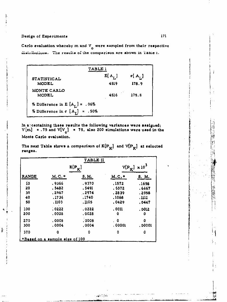
Design of Experiments 171
Carlo evaluation whereby m and V were sampled from their respective0
daiuZ&-uu~iunim. The resuiin o, ihe comparison are shown in !'able I.
TABLE 1
STATISTICAL L LMODEL 4519 178.9
MONTE CARLOMODEL 4516 179.8
o Difference in E (AL]= .06%
76 Difference in a [AL) .s50
In acertaining these results the following variances were Assiged;V (m] = .75 and VVo] 75, also 200 simulations were used in the
Monte Carlo evaluation.
The next Table shows a comparison of E[PK] and V(PK] at seloctedrange = i6'.,
E[PKJK v x 10] 3
RANGE M. C. S. M. M. C.* S. M.10 ..9366 .9370 .1572 .165820 .5482 .5491 .1372 .6667
30.z• •o .6o,72 .6,667~0 .2q67 .2974 .2839 .295840 .1736 .1740 .1068 .1112s0 .1103 .1105 .0429 .0447
100 '0222 .0222 .0011 .0012200 .0028 .0028 0 0
270 .0008 .0008 , 0 0300 .0004 .0004 .00001 .00001
370 0 0 0 0•*Based on a sample size of 100
-.- ILL,

172 Design of Experiments
A review of these results indicate that the statistical model doesprovide a good approximation to the variability of lethal area - a methodwhich may possibly be generalized to include more realism in the model.
It is of interest to note that the covariance terms contributed as highas 87%1o of the total variance of lethal area. The final table also includedfor interest, shows the effect of step size used in the numerical integra-tion scheme on the results.
TABLE fI
R 5 R =O R=20
LEAL] 4554. 4519. 4304.
,oIAL] 179.4 178.9 185.5
"In summary, therefore, it is not the numerical results of this paperthat should be emphasized, but rather the possible application of astraight-forward technique to a couriplex problem involving the variabilityof lethal area.
REFERENCE
1. Picatinny Arsenal Technical Report 2508, "Variability of Lethal
Area", by Sylvain Ehrenfeld, February 1959.

SI.
DECISION PROCEDURE FOR MINIMIZING COSTSI ~ ~~OF c ALIBaATINGJ LWULD ROC iEiTNG:,NES !" I .ALSidney H. Lishman and E. L. Bomtara°-
Engine Program Office, Marshall Space Flight Center
SUMMARY: Prior to acceptance of a liquid rocket engine for use inSaturn vehicles, the average thrust of two consecutive tests without anintervening calibration must satisfy specification requirements. Thecontractor may recalibrate after the first and subsequent tests if he bo
chooses, based upon decision limits, until the above requirement in met,
This paper provides a method for calc-4ating decision limits suchthat the total number of tests required for acceptance it minimnixed. Themodel for calculating the decision limit takes into account operational
reliability and life of the engine, ratio of cost of testing to cost o.f aI %.engine, and correlation between teuts as a function of engine-to-engineand run-to-run variance components.
INTRODUCTION. One of the requirements for NASA acceptance, .. ....- ,of a Saturn vehicle engine is that the thrust averaged from two successivetests without an intervening calbration fall within specification limits.In the past, most engines were accepted from the contractor aiter threetests, but when the specification was recently tightened itwas estimatedthat more than 50% of all engines would have tn be tested at least fourtimes prior to acceptance. Their increase in number of testa per engine .
represented an appriciable increase in costs,
This paper presents the results of a study made to determine whatcould be done to reduce acceptance testing costs when the specificationlimits are held constant. ,.
DISCUSSION. Engine testing is conducted in accordance with the :ifollowing ground rules until the engine meets acceptance requiremtnsor until it is scrapped:
1. If thrust in a test following a calibration is outside certaindecision limits, the engine is successively recalibrated andtested until thrust falls inside the decision limits.
.
* I~i
4 i'

174 Design of Experiments
2. If thrust in a test following a calibration is inside the decisionSI~t limits, no changes arc mane to the engin'e and 4•,AIBhT ty t i=
S ...... conducted in an attempt to satisfy acceptance requirements.
3. If the average thrust from two consecutive tests without inter-vening calibration falls outside of specification limits, theengine is recalibrated, and the test cycle is repeated.
It should be pointed out that the value in using a procedure such asdescribed below is greatest when specification limits are tight. Ifspecification limits are very wide, there is not much point in usingdecision limits at all, because the need for recalibration becomes remote.
ILLUSTRATIONS. For the purpose of applications herein, thefollowing assumptions were made:
1. The engine is always calibrated after the first test (due to high
variability of thrust prior to the first calibration),
Z.,. 2. 'There is no bias introduced in calibrating the engine.
3, After the initial calibration, ability to recalibrate does not'.improve between tests.
4. Cost of calibration is negligible compared to cost of a test.
5. The engine is scrapped after N tests that do not satisfy thecriterion for acceptance described above.
6, The engine-to-engine and run-to-run variance components,ad .. ,respectively, are known, the mean thrust
)4. .:." is also known.
S7. R is the same for all engines.S~RR
8. Engine-to-engine and run-to-run deviates are normally andindependently distributed.
The models described below can easily be altered to change assumptions1 through 5.
1, 7 -,
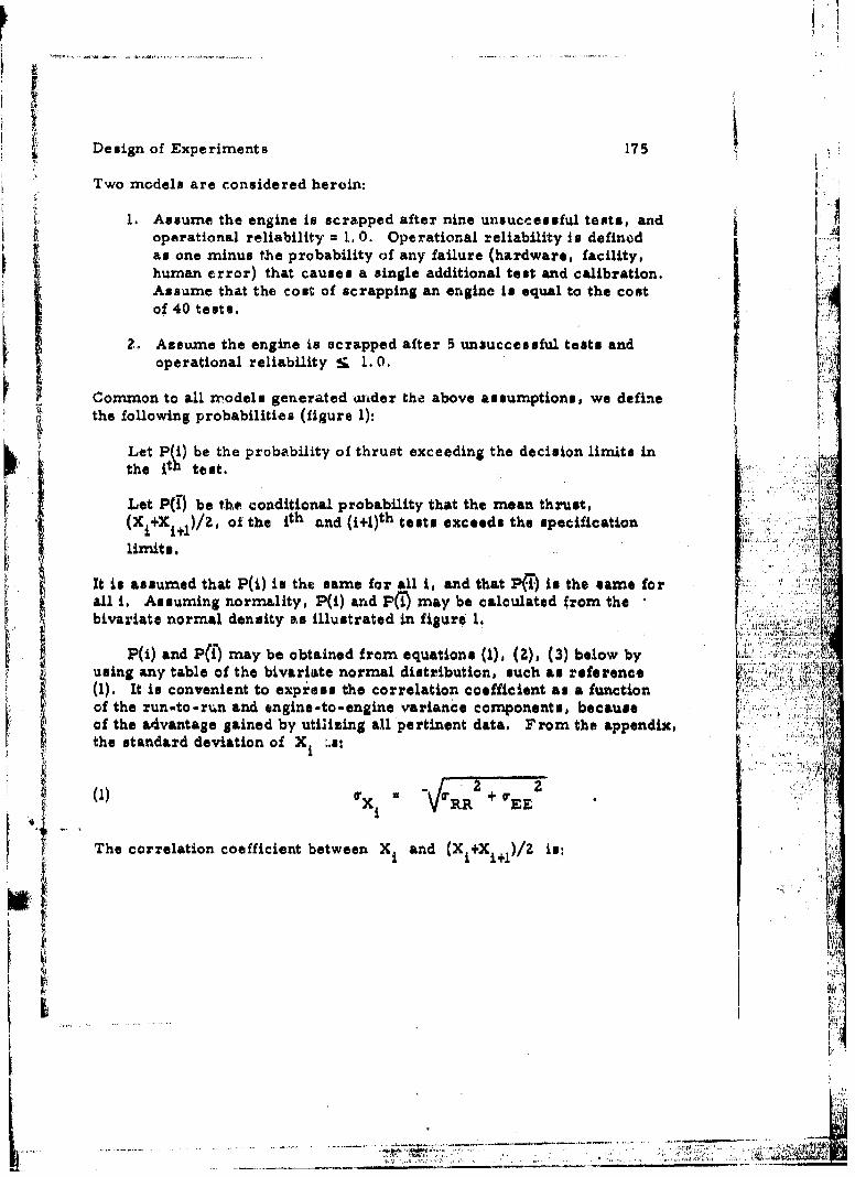
SDesign of Experiments 17S
Two models are considered heroin:
1. Assume the engine is scrapped after nine unsuccessful tents, andoperational reliability = 1. 0. Operational reliability is defined Ias one minus the probability of any failure (hardware, facility,human error) that causes a single additional test and calibration,Assume that the cost of scrapping an engine is equal to the costof 40 tests.
2ý Assume the engine is scrapped after 5 unsuccessful tests andoperational reliability S. 1.0.
Common to all ro.odels generated under the above assumptions, we definethe following probabilities (figure 1):
S Let Pt,) be the probability of thrust exceeding the decision limits int h e i t , t e s t ,.-• : • : • .
Let P(M) be the conditional probability that the mean thrust,(Xi+X )/Z. eof the ith and (i+l)th tests exceeds the specification
limits.
It is assumed that P(i) is the same for all i, and that P3() is the same for rall i. Assuming normality, P(i) and Pni may be calculated from thebivariate normal density as illustrated in figure 1. ".. E.
P(i) and P(i) may be obtained from equations (1), (Z), (3) below byusing any table of the bivariate normal distribution, such as reference(1). It is convenient to express the correlation coefficient as a functionof the run-to-run and engine-to-engine variance components, becauseof the advantage gained by utilizing all pertinent data. From the appendix,the standard deviation of X ',s:
(X) TX --- EE
The correlation coefficient between X and (X +X )/ is:n
- - .-

DIVAER7 NORML PROBMBLIZIS ~ 177/
Calibration~wgg~
~ lb~g.
Oaltbrration
CCalibratio
.SMIR
pI
Reesr

Design of Experiments 179
( 2) Px iS2
(r X
The standard deviation of (Xi+Xi+l)/2 is.
(3) (X i+X i+,)/z a 'X i PXi ,(X i Xi+l)/2 , ,
MODEL 1- Reliability : 1. 0; engine is scrapped after 9 unsuccessfultests.
Let the notation HZ 3" describe the event that thrust of the-secondtest was Within decision limits and that the average thrust of the secondand third test was within specification limits. Let the notation112 3 4 5 1" deac~ribe the following event:
c c
Calibration after second test (thrust outside of decision limits),
No calibration after third test (thrust within decision limits),
* Calibration after fourth test (mean thrust of third and, fo*.rth
test outside of specification limits).
, Thrust in fifth test within decision limits.
* Average thrust of fifth and+ sixth tests within specification limits.
Using this notationp.nd the notation of figure 1, probabilities for thevarious events are as follows:
............. . ....... . " "'

ISO
TABLE I
KWH?,PROBABILITY
24. 3~4
2 ~ 2
2 Sc 4o 7 E-P(1)P(T8JLP(7)pj) ID1 P(03)2 3o to -3
2 5* 4,5w 6~ D.%(I.-PJ1)'(I)J PM) D-'pct
[I.P(±).P(TJ])[P()) )2~PiI) 4E'Ci2
[ -P ,...........[t J3

181
TABLE I (Cont.'d)
IV'VwrR~ PROBABILITY
2 4 ' 6 8 P(* Li- (')l t P(73 D~ - 2.
2 4 6 678 LI - P~)- P~) P~±V( 1)1 [Ip~)
C C
2 IS 4 5 67 8 Vl-p E12() P(-)] P( 2[() E, p(]ý2
2 4 C. 5 6 C 8 T L .(i)F( IJ)]JEP(i 2q 2 [1 p(t12
2~ 3 Z 5 6 a7 a8 T [iI (±)( 2(7)) LP(d)J4 P(-,) [I - j]
2 3 We . 6 7 8 ; [1 -P(j) - P(-))L ?4 ()~ JcC 4 0 C c I-2 P
2 3 45 6 7 8 [1-V () ( P-) [ y
c aC a. a ..e i I *(1 .. I() -P ) I(7 -
CCP C C() F M
2 ~ ~ ~ ~ ~ ~ ~ ~ ~ ~ ~ ~ ~ L 3 S6781 1 ().P ~) c)[ y
[I pyl~ .
2 3.4. . . . .. &.[ I . . . . . . . . . . . . . . . ..p r

182 Design of E~xperiments
Assume that the cost of one engine is equivalent to the cost ofM a 40 tests. L~et i) Lot Uiiv =... prc-~1-itifl5 in table I associated
with tLose events requiring Jtests. Then the expected number of testsper accepted engine is:N
E~ JP 4 M(= - EP)
(4) E(N) J~=3 N 3J
J123'A. '
The quantity in parentheslsv in the probability that more than 9 testsare requir~ed; i.ea., the probability of scra~pping the engine. Holding thespecification limit constant, the decision limit (figure 1) is varied untilE(N) is minimised,
In illustration, this model was u~sed to support contract negotiationsin an enginie program where reliability of the engine is very high.:Practice is to scrap the engine after 9 unsuccessful tests. Data. showedthat the squar,ý root of the within-engines or ruan-to-run variancej compsonent of thrust was 600 lbs, , and the square root of the engine-to-engine variance component was between 1200 and 1500 lbs. Bothextreme* were analysed, au follows-
......J Case I a, 1200 lbs. Cr 600 lbs.Fm tEEI, RR 14 ls
From equaton (1,I -(600)'ý+(1200)' 34 ls
From tiquation (2) p1 (x1 x1 1 )2
From equation (3) r(X1 + X 1+)/Z 9 5(1340) z: 1270 lbs.
Suppose the~ specification limits for thrust are nominal + Z000 lbs.Then the number of standard deviations between nominal and thL specifi-cation limit (two-sided) is 000/1270 = .57. By trial and error, equa-tion (4) is minimnized when the decision limits are nominal + 1. 7(1340)nominal + 120.s hn ,N 318 o.oz) 998 3.2tesper accepted engine.

I L .. ~ : B -,B'~lB.P4~4
~ 4,'' ~'
Design of Experimentb 183
Case 2: a' 1500 lbs. WR 600 lbs.E4 R
rFrom equation (1), a.X V(600)' + (1500)' 1620 lbs.
xi 1'600' 2From equation MZ, p, ,.1 671H 0 .9,61
A 1 , (X i ,jJ1
From equation (3), 0p.( +. .965(1620) 1560 lbs..i Xi+1 )
The number of standard deviations between nominal and thes~pecification limit (two-sided) is 2000/11560 = 1. 28. Bly trial and error,[equation (4) is minimized when the decision '[`Ynits are nominal*1. 5(1620) nominal + 2430 lbs, when E(N) [3. 286 t 40(. 0122,)] .988
3. 8 tests per accepted engine. (Note that changing the ratio of
T R ck from 600/1340 in case 1 to 600/1620 In case 2 changes thecorrelat~on coefficient by only . 015, and merely changes the optimumdecision liisfo-.7t .5sadr eitos ,N hne
signficntl, fom . 3to 3. 8 tests per accepted engine,)
Other info rmation of interest corresponding to decision limits i sthe. followingi
VA. Prob. of acceptance after N tests EJ=3N
C. Percent engines requiring calibration after second test PWi
Of these, the four 'corners" of the bivariate distributionare necessary (see figure 1),
Prior to this analysis, the contractor had been using arbitrarydecision limits of nominal +1 (2000-2 a-RR Advantages gained by
minimizing expected number of tests are also obtained from A, B,
and C above, as follows-.

184 Design of Experiments
COMPARISON OF DECISION LIMITS
THE ENGINE IS SCRAPPED
0 EF !~203 lbs. aR 600 lbs.
ISpec. Nomiinal + 1. 6 Sigma)
(Assume 1 Engine Decisioni Limit Optimum Dec. Limitis 40 Tests) nominal +±0. 6 w *nominal +1. 7.Xi -. Xi
*Prob. of Acceptance .45 . 87after 3 Tests
0/ Engines requiring 55%0 10%calibration after (of these, 201c (of theae, 771oZnd test are necessary) are necessary)
-Aeaenumber of 4. 11(diie to recalibration) 3.18tests requi*red for 0. 61(due to scrapped engine) 0. 08acceptance 4.72 (Total) 3.26
A 15tests/egn
Expect.~d Number of 1. 5 0. 2
Scrapped Engi4iesPer 100 Tested
after NTests 69.9 N = 4 95.583.5 N a 99.090.0 N z6 99.695,0 N =7 99.7697.3 N =8 99.7998.5 N =9 99.80

Design of Experiments 185
COMPARISON OF DECISION LIMITS
ASSUMING THAT AFTER 9 UNSUCCESSFUL TESTS
THE ENGINE IS SCRAPPEDg,,a' EE 1500 lbs. T'RR = 600 lbs.
(Spec. Nominal + 1. 3 Sigma)
(Assume 1 Engine Decision Limit Optimum Dec. Limit40 Tests) = nominal + 0. 5 "r nominal + 1. 5 o-•' - - Xi
Prob. of Acceptance .38 .78after 3 Tests.
%Engines Requiring 627, 16%Calibration After (of these, 31%0 (of these, 84%2nd Test are necessary) are necessary)
Average Number of Tests 4.4 (due to recalibration) ., 3Required for Acceptance 1.4(due to scrapped engia, ) 0.5
5.8 (Total) 3.8
2. 0 Teats/Engina
Expected Number of 2Scrapped Engines 3.5 1,2per 100 Tested
% Engines Accepted 38.0 N = 3 78.0after N Tests 61.9 N = 4 90.6 N
76.4 N = 5 96.585.4 N = 6 98,0 I91.0 N = 7 98.594.4 N-- 8 98.796.5 N-r 9 98.8
;V

186 Design of Experiments
MODEL Z: Reliability 1. 0; Engine is scrapped after 5 unsuccessfultests. Assume that the engine is scrapped when the contractor fails tomeet'requiremrents for acceptance after 5 successive teats with calibration.Let I-RI be the probability of failure in the first test, where "failure" isany event that causes a single additional test as in table 2, and similarlyfor l-R in the seond test, etc. A curve of reliability vs. number of tests
S-nmay be obtained from past experience, as in figure Z.
Figure 2
OPERATIONAL RELIABILITY VS. NUMBER OF TESTS
r 7'
500
.70
A 0000
a60
.50
1 2 3 4 5
Numbet of Tests
./... ..

Design of Experiments 1871
Let the notation "I1 2 FZ3 c4 5describe the following event:
Calibration after first test,.AFailure during second test.jCalibration after third test.Thrust in fourth test within decision limits.Average thrust of fourth and fifth tests within specifica~tion liltilts.
As before, the engine ir, always calibrated after the first test'unless failure occurs. Using the notation P(i) and P(T) as in model 1,Vprobabilities for the various events are as follows:
TABLE 2
EVENT PROBABILITY
C1 2 3 .1 ",Ji)I1C2 3 4 R *R 2R3 P(i) P4) PI
1Fl 2 3 4 (1 R )R R R 11 PW )P(T~)
1 2 3 4 (1 R ) R R R [I P(i) pff)]C FZ
1 23 45 RRR R R ()J(11 P(i) -P(i-) I
1 234 R RR R R 5 F) 1C C 1 2 3 4 ~ LI 5~J
1 2345 (1 R) (1-fl) R R R (1- P(i) -P(i)JFl F2 c 1 2 3 4 5 .
1 2 3 4 5 (1 - R 1) (1 -R 3 ) P6"R5 l-)i I~(~Fl cF3 R 4R 1P'
1c 2 F2 3 34 5 (1- R2 )(l - R) R, R4 R5 (1 - P(i) -P(7T)J
c12 3 F3 3) ( R R 45
22

188 Design of Experiments
1 Assuming that the cost of one engine is equivalent to the cost of M•.•!t• i tests, and letting Pj be the sum of probabili•.ies in table 2 associated
Ii;•i with J tests, the expected number of tests per accepted engine is given by
• •',:=7--•- Ca3e 1: Reliability • 1.0,•,•,, -...... u 1200 Ibs. = 600 Ibs. , specification
i!• .=:•.. In illustration suppose SEE ' wRR
• ii-l.ii •imt. at. no=,inal _.* ZOO0 •b,., aria the cost of one engine is equ•vale=,• z!•": :.
StO the cost of 40 tests Then as in model 1 case 1, we have:b, • 0 p
. i)•:!•!!!!,•.;.i.. •Xi = 1340 Ibs.
•-.•.• .....:!!]•: •xi' ¢xi + Xj+l)la : .,•
:i: . . .., . ,..:.• o" (X" +X' l)/Z = I•-70 lbs.
S " - . ........ ........ i I J•"
.j" ,
SNumber of standard deviations between non•nal and specification limit!:• •,"-::.L - .'.'[ = I. •7.
:ii':;:":';!•;: • ,i •alculate P. from table 2 for j = 3, 4, 5, utilizing operational/?)'i!i'i','/:i;.•i..i ...... :";;J reliability value• of figure •, By trial and error, equation (4) isi !iiii :i !iiiiiiii-, ,,.:•.,.,s:•..:..: :,• ,,,..:.:;. mL•imi•ed when the decision limits are nornlnal .+ I. 8 standard
•i}' i';::i::;•j !. "= : : • -----.---Case •.: Reliability = 1, 0 (SamedeviationsCOrrelatiOnin coefficient•\ and standard
Sas case ,•;.:.::/!. ': It is of interest to observe the partial effect of reliability on the
S...... optimum decision limits and expected number 0£ tests, ]•(N). Let R1
i•i! through i•5 be I. 0, Then utilizing table •., (or table 1 for • = 3, 4, 5)Siii1
Scalculate Inj. The standard deviations of Xi a•d (Xi+Xi+l)/• and correla-
..•7• tics coefficient are the same as in ca•e 1, Equation (4) is minimizedSwhen the decision limits are nominal _.+ 1.5 standard deviations and E(N)
•..: = 3.6 tests per accepted engine, In cor•paring these values to those in•. case 1, note that the optimum decision limits become tighter, and the

Design of Experiments 189
number of tests per accepted engine decreases as reliability increases.
By comparison of results in Model 1, case I to those of Model 2,7~M ^.a ta tka ah ffai-t r~f af ."~~r 0h~ ut ,u,
S tests is obtained. The optimum decision limits are nominal + 1. 7standard deviations in the former, and E(N) = 3. 3 tests per acceptedengine; in the latter, the optimum decision limits are nominal + 1.5standard deviations, and E(N) = 3.6 tests.
APPLICATIONS: The minimum expected number of tests peraccepted engine, E(N), provides a convenient yardstick for trade-offstudies, For example, one might want to determine whether or notthe cost of overhauling test facilities in order to improve operationalreliability by, say, 576, is worthwhile, Or, one might want to deter-mine whether the cost of reducing engine-to-engine variability by -improving calibration techniques or equipment is offset by the reducednumber of tests required for acceptance, etc.
REFERENCES
(1) Tables of the Bivariate Normal Distribution Function and Related ' /Functions, National Bureau of Standards, U. S. Department ofCommerce.
(2) Tables of Normal Probability Functions, National Bureau of Standards, ,U. S. Department of Commerce.
,pn,
-.-I-.- • -
i °/I

190 Design of Experiments
APPENDIX
coy XA*, zi~
P i X +X
Substituting from equations (7) and (8), this is
IT IT~ + * IT)
/21 2 2r*X ~ aX1 + Zw~- RR
12 2 22v +. -Zw 2RB
/8, + o0xi aR
alssuming ITa- =~

Design of Experiments 191
2a2 2
2 RR~
(6A) Xji+Xj~ zizl 2.
2 22ax
I2
or, letting w =0 in equation (5), this result may be expressed
(63) P x~ x=/ p
2
L~et w, be the engine -to- engine variance component. Using the ~ ~
relttion 2 2 T tgther with equation~s (6A) and (8B),iX -EE 0 RR tg
the volume in the corners of figure 1 are computed from a bivariateno~rmal distribution table. Using this result plus a wnivariate normaltable, P(i) and P(I') as defined pge. 175 and. 177, trio.calculated.
cov (X1 0!X1 1
2
=E F(x + Xi+ 1 )] i 1+12 EtXiE(

19 Design of Exp~eriments, II ~f~E(X) + zEIx.~) x [E(X,)] E(X) E (
* w[r coy (Xi. x~~
Uf w * r this becomes
ITX
(7A) COy (X1, 2 f+p Px
(B) =1 Ir + 2 p2 x x rx~
ii.l
IfO w q
(8A) crX+ [7
Frorn.6B), this becomes

Design of Experimen~ts 193
(SB) X +X Xi 1+1 XX.+X
ItIfrom equation (9A), (8A) becomes
B 2
2 I2Sum of squares run-,to-run is
1N
SSRRAusuming ýL 11, and since MSSS N
MES z + E(X~ 1 z& E -2(Xw g~)Xj-f~]RR __l +I+ ¾~)N N N JJ
Takilng expectations, the run-to-run variance component is:
2 1 2+ 1a- 2 XW
X X+- ovX 1 ,X+)
I ~ it ~

194 Design of Experiments
and
+ r 2w
yRR(9A) PX x. 2 =
1 14 ' x+1
2 i~
II WX -r
1.01019+96.4 2
.98 .92.08 .R
.90 .6 .R6
V V
*- ~ ~ ~ W en r 0 when 0.-----**---*.- ,------ ... ..

TT 195
L11
Ii lit : 1P 1ýiA , ýi i
I''l
04.
4p 11 1

MIT'I
iI I il ld
Tit

.9- 199
2 T101
FE W ..... ... .. X iii
Imm4444

201-77[17100!1
ILIT.F. . --+J 17.
j tZ
It -.-' TfI V.I., 3
7T
.. fffl
orll, A
44AT
T,- 7ff It .:.II.TTL t±ffF-fTTT
JL
;, f4-L L :7 71
2-4:
-44

THE THEORETICAL STRENGTH OF TITANIUMCALCULATED FROM THE COHESIVE ENERGY
Perry R. Smoot
Research Phyeical MetallurgistU. S. Army Materials Research Agency
F Watertown, Massachusetts
ABSTRACT. The derivation of the equation for theoretical strength
max = was reviewed, and certain assumptions made werer
econsidered questionable, Therefore, the accuracy of the equation wasconsidered questionable, 'and a new method for calculating the theoretical L ..:iitstrength of crystals was derived, utilizing'the Morse potential'equationand the cohesive energy. The theoretical strength of titanium calculatedby this method was 3.28 x i06 pei.
I. ITRODUCTION. Tha U. S. Army Materials Research Agencyi s engaged in the development of strong, lightweight titaniurn aloywf'foruse in Army weaponsd In the course of this inve.stigation,, a questio'n •T
arose concerning the maximum, strength theoretically'obt'aihýable,..,;a4 a" '"kdhow it mightyeon. .It has been'rpoPosed for soiee jtm 1htj fetheoretical. strength of metals is considerably higher than that normally
observed. Polanyi1 presented a method of calculating theoretical. strength,in which the bonding force between atoms, as a function of internuclear,separation, was taken to be approximately ýa shown in Figlre ?... As a >.
brittle crack progressed through the crystal in the manner shown in m f
Figure 2, the interatomic bonds were extended and broken, and the workdone against each bond was equal to the area under the curve from rto r in Figure 1. As the brittle crack progressed, new surfaces Vwere created having a surface energy of 2S, and this energy was assumed
equal to the work done against the interatomic bonds. On this basis,an algebraic solution for °max, the maximum theoretical stress atfracture was obtained, as follows:
max
where E : the elastic modulus.S = the surface energyr = the equilibrium atomic spacing
i 1,+C!.

204 Design oi Experiments
The value of w was ordinarily expected to be of the order of E!max 16 2
which was about 1 to 10 x 10 psi for most common metals . Indeed, veryhigh strength values of this order of magnitude have been obtained inmetallic and ceramic whiskers.
In the deviation of this expression, the following energy balanceis assumed:
'iii Energy to fracture bonds surface energy of new surfacecreated by fracture .
No theoretical basis for this assumption is apparent, since the mechanismS' by which surface energy arises, and its relationship, if any, to the energy
j e.ýp required to fr&cture the interatomic bonds is not known. Consequently,lthis expresyon for the theoretical strength is considered to be of question-
•,• :,able accuracy.,
Another questionable aspect in the derivation of this method is theassumption that the interatomic force vs. displacement curve (Figure 1)is sinusoidal. I In addition, there is a practical difficulty in calculatingtheoretical strengths by this method, since surface energy values forJi,'• t ,: i solids are not available for most elements (including titanium).
Because of these questions as to the correctness of this method,and because of the lack of surface energy data, it was desired to discoveranother method for calculating theoretical strength in which more confi-dance could be felt, perhaps by some meansiinvolving computation of theactual forces between atoms.
3•n inquiry,-• Dr R
II. CALCULATIONS. As a result of an inquiry, Dr. RJ 3. Weiss•,•:!•suggested a method for calculating the4theoretical strength of metals by
means of the Morse potential equation
'V = D [eZa(rre) -a(r-r)]
where V(Ev) potential energyEv
D(aom cohesive energy (the heat ofvaporization, &H v per atom

De Dign U! Experiments ZUu
a( a constant I
r(A) = the internuclear separation
r.e = the equilib•pum separation
This equation related the bonding energy of two hydrogen atoms to theinternuclear separation, as shown in Figure 3.
The energy values given by this function agreed well with:
+a. experimental values of bonding energy v% separation for the HZmolucule (except under compression; see Table I) ,
b. theoretical valaen of bonding energy calculated in a few casesby quantum mechanics,
y c. experimental values for compressibility for sixteen metals
(see Figure 4)7.
It was therefore considered reasonable to assume that this relation- -ship applied between the atoms in a crystal, with a modification consisting•i of multiplying the cohesive energy by a factor to take into account the"':..
division of the cohesive energy between nearest neighbors in a crystal.Differentiation of this equation yielded an expression for interatomicforce, and it was suggested that this be used to calculate the maximum 'f6rce between atoms and the theoretical strength of metals. The accuracyof the calculations was expected to be within a factor of two at worst,
A and probably much better.
As mentioned above, it was necessary to multiply the cohesiveenergy by a factor to take into account its division between N nearestneighbors. The energy contributed by each atom to each interatomic
N bond was PD. Since this contribution was made by one atom at each
end of each bond, the total energy of one bond was RD, Therefore, thecohesive energy, D, was multiplied by A when the Morse potential aqua.
tion was applied to a crystal.
I-

The theoretical strength of a titanium crystal was calculated bymeans of the method suggested above by Dr. Weiss. The Morse potentialequation for a crystal was differentiated as follows:
V(Ev) = RD (Moere potential(1)2 [- 2 -a +are] equation for a
•..=.. . e crystal)-:,: : .,:V R •D e -2e
2 -Zar 2ar -ar ar2e 4D e•V -De e -- D e
This equation was similar to:
bx,y : k e where k and b are constants.
Since bk= k• thendx
SEZar -2ar ar -ar= F(interatomic force, += -a eZae e,: .,dr = -N' )2a = -DeR2D
A( !4 [ 2a(re-r) a(re-r)
SF = Da . -e+ ]and
20d7V dF K(interatomic spring constant, 6 =) z
dr A
Zar - Zar ar -ar(3) 4a e 22 e e 2
-De -De
4 ~ [ 2ea(re r) a(rer)]K - Da 2e -e.

Design of Experiments 207
It should be noted that when r =re
K ±Da'N
and when K 0
2ar -2ar ar -ar2 2 2 2
4ae N =Dae -DeN
ar -areZ e e = 1
1 1. '=2e
ar ar
arar • a
• ffi 2e rthe iteate a
26l
ar ne = =n2 +ar Ina
SIn2
and !, 'SlnW. .693 •
(s) r •'e a-''ne 0 ae+ • ..
In order to utilize theme equations to calculate the theoreticalstrength of a crystal, it was necessary to obtain numerical values for
S a, D, and r .Values for D and r were found in the literature asS. .follows: •e
•. atom
Sr =2. 95 A

208 Design of Experiments
The value "a" was determined from the elastic modulus of the crystal.[ •The structure of titanium is hexagonal close packed, and was considered. . .to be an assembly of unit tensile cells, as shown in Figure 5. As a
hypothetical stress was applied to the crystal in the [ 100 ] direction,an elastic strain occurred, as shown in Figure 6, so that bonds betweenatoms in the plane of atom A such as bond AS were extended, but bondssuch as AT and AS were not. Also, the bonds between atoms in theplane of atom A and the atoms above and below this plane were not
S extended. For example, bonds AG, AV and AO (Figure 7) were not
extended, Trigonometric calculation derronstrated that this was possiblewithout physical interference between atoms, As a result, the springconstant of the unit tensile cell was equal to the spring constant, K, of.the singl interatomic bond, AS. A numerical value for K was determinedfrom Young's modulus, E, as follows,
E 17.85 x10⁶ psi = 7.67 xlO' 0" /A
•t7-7 l0 6,2.9 = 16. Z2x10"1 =v' K1 6.247. 67 X10 X - L.Z 02. 95A
where 6. 24 transverse area of unit tensile cell, A0
.295 : length of unit tensile cell, A
From equation (4), above
- -Da 16.22 xlo10
and
a 1. 014 "6K AHaving numerical values for all the constants required, the Morse
potential energy and ixkteratomic force were calculated as a function ofinternuclear displacement, r, and the results are shown in Figure 8.It will be noted that an a stress was applied and the interatomic bond

Design of Experiments 209
extended, the maximum force was reached at the internuclear separationdF'
for which = 0. The internuclear separation at this point was cal-
culated from the equation:
"T sprir - r + .693 (equation 5, above) Ev
0 Ev •
S This separation was 3.63A, and the corresponding force was 0. 402 --
(0, 645 x 10-4 dynes). A
This data was then used to calculate the theoretical strength of a U4titanium crystal. A tensile force was considered to be applied in the[001) direction in the crystal, an equal part of which was transferredto each atom in the (001) plane (see Figure 9). These tensile forces oneach atom are represented by the vectors AB and AF. The tensilevector AB is the resultant of the vectors AC, AD, and AE, These vectorsarise from the extension of the interatomic bonds AC, AD and AE. Asthe applied tensile force increased, the bonds extended until they reachedthe fracture extension; and the force in each bond increased to equal thefracture force mentioned above. As the applied tensile increased stillfurthew, the bonds exceeded the fracture separation and the force in V'M
each one decreased in accordance with Figure 8. Thereafter, the sumof the bond forces was less than the applied force, so that the appliedforce was able to fracture the crystal on the (001) plane,
The theoretical maximum strength was attained immediatelyprior to fracture. The stress on the crystal at this time was determinedby calculating the magnitude of the vertor AB and dividing it by the areaper atom in the (001) plane. The value so calculated was 3. 28 x 106 psi.It should be noted that, in this theory of fracture,, it was assumed thatno slip occurred and no brittle crack propagated through the crystal ata stress lower than the theoretical maximum.
A calculation of the theoretical strength of a monatomic titaniumfilament was made by means of equations 1 and 2, letting N = 2, and theAtheoretical maximum strength of a monatomic filament was found to be8,200,000 (8.2 x 10⁶) psi, which was considerably higher than for thecrystal. This increased strength was due to greater cohesive energy

per bond, since there were fewer nearest neighbors, The strength of a £monatomic sheet would be above that of the crystal and below that of afilament, due to the same effect.
Using this method, the theoretical cleavage strength of iron in the[100] direction was calculated to be 12. 7 x 10⁶ psi. It is interesting tocompare this value with the observed yield strength of iron whiskers inthe (100] direction, which is . 664 x 106 psI 0 . The strength of the
V• whiskers is considerably higher than normally observed in iron and iron-base alloys, showing that the material is capable of much higher strengththan it normally exhibits. On the other hand, the whisker yield strengthis considerably less than the calculated cleavage strength, due to the onsetof plastic flow. If plastic flow could be prevented by some means, it ispossible that the high cleavage strength predicted by the calculationscould be attained.
III. DISCUSSION. The theoretical strength calculated for titanium,3.28 x 106 psi, is much larger than the normally observed strength ofabout 200, 000 psi. Greater confidence is felt in this method of calculatingtheoretical strength than in the method of Polanyi, because of the ques-tionable aspects of the Polanyi deriviation mentioned in the Introduction.
High theoretical strengths may be obtainable in real materials ifthe necessary conditions can be maintained, namely, that no slip occurand no brittle crack propagate at a stress below the theoretical maximum
strength. The method of obtaining these conditions is problematical, andseveral possible methods may be suggested. One method might be togrow whiskers of such perfection that no slip would occur and no brittlecrack would propagate until a stress level approaching the theoreticalwere reached. Another method might be to simply produce very fine fila-ments (not necessarily whiskers) by some method, such as drawing fromthe melt. Slip in these filaments might be inhibited by alloying elementsand brittle crack formation supressed by the small size. (There is someevidence that in filaments, the tendency for brittle cracks to nucleateand propagate is suppressed by decreasing the diameter.) Slip mightalso be inhibited by suitable control of crystal orientation, the productionof very fine grain sizes, or by amorphous (vitreous) structures. Thehigh strengths calculated for monatomic filaments and sheets may beapproached ii these or similar structures can be produced. There issome hope that these high strength levels may be attained in metals suchas titanium, since strength levels of 3 x 10⁶ psi have already beenachieved with graphite whiskers1 l.

Denign oi Experiments 211
IV. RECOMMENDATIONS FOR FURTHER WORK. Since this areaof study offers considerable promise for the development of ultra-highstrength materials, it is suggested that further work be undertaken tofurther develop the theory of the strength of solids, verify it experimentally,and find methods of applying it to the production of engineering materialshaving these high strengths. From a survey of the literature, it appearsthat further developments are necessary in the methods of quantummechanics so that more accurate calculations of the energy vs. internuclearseparation may be made. Experiments are required to verify the resultsobtained and to provide data for engineering application.
The materials offering the best combination of properties should beidentified, and developmental programs initiated to establish methods ofproviding high strength engineering materials at acceptable cost and inthe quantities required.
ACKNOWLEDGEMENT. The author ls indebted to Dr. R. J. Weissof the U. S. Army Ma'terial•s'Research Agency for providing the theoretical
physical basis and guidance on which these calculations were based.
II

Design of Experiments
TABLE 1I
BoningEner gy and Interatomic Spacing for 2
n-(Energy Unit: Rydberge)
V Vr Exact Calcula~ted*
0.2 7.1426 0.96540.4 2. 3984 0.58210.6 0.9903 0. 30930.8 0.3910 0.11841.0 0.0964 -0.0122z1.2 -0.0O579 -0,0989
1.4 -0.1399 -0.15361.6 '-0.1819 WO. 1854I1.8 -0. 2005 -0. 20102,0 -0.2053 -0. 20532.2Z -0.2017 -0.2020Z. 4 -0.1931 -0.1937z. 6 -0.1817 -0.18242. 8 -0.1687 -0.16933.0 .0.1551 .0.15563.2 -0.1415 -0,14173.4 -0.1282 -0.12823.6 -0.1154 -0.11533. e -0.1034 -0.10334. 0 -0. 0922 -0. 09225.0 -0.0489 -0.05026.0 -0. 0240 -0. 02647.0 -0.1002 .10?8.0 -0.0051 -0.00709.0 -0.0024 -0.0036
*Calculated by means of the Morse potential equation.
Credit: From Quantum Theory of Molecules and Solids,by J. C. Slater, Copyright (S 1963 by theMcGraw Hill Book Co. , Inc. Used by permissionof McGraw Hill Book Co.

Design of Experiments 213 LR.EFERENC ES
1. Polanyl, M., Z. Phys. 7, 323, (1921)
2. 3. W. Spretnank, A Summary of the Theory of Fracture in Metals,D. M. I.C. Report No. 157, 1961.
3. Dr. R. 3. Weiss, private comnmunication, U. S. Army MaterialsResearch Agency.
4. Dr. R.. J. Weiss, Solid State Physics for Metallurgists,Page 67, Pe'rmagon Press, Oxford, 1963.
5. Slater, 3. C. , Quantum Theory of Molecuales &k Solids, 1, P9ge 18.
6. Slater, 3.C. , Introduction to Chemical Physics, page 133, --
7. Girifalco, L. A., Application of Morse Potential F~unction to.CubicMetals, Technical Report R-5, NASA, 1959, page 6.
8. Ref. 5, page 55.
9. Metals H~andbook~, 8th Edition, 1, American Society for Metals, 19.61.
10. Doremus, R. H. , Growth and Perfection of Crystals, pages 163 and173. John Wiley anaxon,; inc.
11. Ibid. page 197.

2114
U. 3.AM AEIL EEMNAEC
1906115At6

CRIMIV.~~~~~~,~ 8,AR ATRIL ASEAN mE
... ~~~~~~~ ..... ..... ..

216
SEPARATION
.0 a
U.S.AM MAEI AL EERHAEC1906-16AC6

217
6111
IIAl V,

AA
Figure S. CRYSTAL STRUCTURE OF TITANIUMHEXAGONAL CLOSE PACKED
U. S. ARMY MATERIAL$ RESEARCH AGENCY1 ~ 19-066-191 ?/AI4C-6 9

219
(EXTENDED)
BOND As(EXTE DID)
Figure 6. TITANIUM CRYSTAL,ELASTICALLY $TRAINED
Us. So ARMY MATERIALS RESIARCII AGENCY
19-066-191l&/AMC-6M
.-.-------.-- - - ---

E y> '.
ATOM IN TNE PLANE OF ATOM A
/ N ATOM 1N THE PLANE AlOVE AND BELOW THE PUANE OF ATOM A
.~.-.Poo
<W00 -vWf
Figure I. TITANIUM CRYSTAL, ELASTICALLY 11TRAINED
U. 0. ARMY 4AiTER ALC 418EARIN AGENCY

221
~ saaIV
HUNE
8.~~~~~~~~~~~~~~~~~~ NOMPTN*1EEG NDITUOI OC EII NRNCERSPRTOV. 8.A1 AEIL IKRNAEC
r*. A

222
(all Direction
Atolled Tensile* Fares -Vester As
CK .4y
for - -6trA
SF
Flom .0. Preotur OFPlaneRIA (MoU l,
0-6110/m- --
.. ~ ~ ... ...

TEN SNAKE VENOMS: A STUDY OF THEIR EFFECTSON PHYSIOLOGICAL PARAMETERS AN) .TTT?.!T1rAL
James A. Vick, Henry P. Ciuchta, and James H. MantheiNeurology Branch, Experimental Medicine Department
Medical Research Laboratory, U.S. Army Chemical and Research Labs,Edgewood Arsenal, Maryland
The poisonous snakes and the venoms they produce have both fascinatedand confounded the scientific world for a number of centuries. In the pastinaccurate and incomplete descriptions of the physiologic changes observedifollowing envenomation have aided the advance of folklore concerning thevenomous snake, Even now there are numerous conflicting reports con-cerning the mechanism by which these venoms produce their lethality. Itis no small wonder, therefore, that because of these reports many mis-givings and misconceptions concerning the snake and its lethal and/orincapacitating capabilities have arisen,
With this background in mind a study was designed to determine theexact sequence of physiologic changes which follow the injection of a lethaldose of snake venom. Precise data concerning the minimum lethal dose ."
for each of ten venoms was also determiaed, as well as a comparison ofrelative potencies in the mouse and dog.
MATERIALS AND METHODS. The snake venoms used in themeexperiments were obtained commercially from the Miami Serpentarium, '0"Miami, Florida and from the Medical Research Laboratory at Ft. Knox,Kentucky. Each venom, which was collected by inducing the snake tostrike a rubber covered jar, was mucous free and devoid of cellular debris.Bacteria were removed by high-speed centrifugation and the supernatantliquid was lyophilized. Ten venoms., representing three fanilie.s of snakes,were studied. These were an follows:
Family - C~rotalidae
1. Crotalus Adamanteus ........ Eastern Diamondback Rattlesnake
2. Agkistrodon Piscivorus . . Cottonmouth Moccasin
3. Crotalus Atrox ........... Western Diamondback Rattlesnake
4. Agkistrodon ContortixContortix ............ Southern Copperhead

I
5. Agkistrodon ContorttxMoke son ..... ........... Northern Copperhead
Family - Elapidae
1. Bungarus Caeruleus ...... Indian Krait
2. Naja Naja ................. Indian Cobra
"3. Micrurus Fulvius ............. Coral Snake
.. a __. -4_ _ Vieridae
'I. Vipers Russelli . . ........... Russell's Viper
2bitis Ariea a..........Puff Adder
Initial toxicity of the ten venoms was determined using a total of 1864mice. Just prior to administration, the lyophilized venom was dissolvedin normal saline (1. 0 mg/ml) for intravenous injection into the dorsaltail vein of the mouse, Table 1 shows the number cif-mice used toestablish the LD and time to death for each venom.'1 99
Eighty adult mongrel dogs, anefithetized with 30 mg/kg pentobarbitalsodium, were employed in the second phase of this study. Arterial bloodpressiewas monitored using a polyethylene catheter inserted into thefemoral artery and connected to a statham pressure transducer and anE and M physiograph recorder. Portal venous pressure was recordedvia a catheter inserted into the splenic vein and advanced into the portalcirculation. Respiratory rate, electrocardiogram (EKG), and heartrate were continuously monitored ising a pair of needle-tip electrodesplaced in either side of the chest wall, and connected to the E and Mphysiograph through appropriate preamplifiers.
Cortical electrical activity (9EG) was monitored using four unipolarsilver electrodes placed directly on the dura of each hemisphere of thebrain and connected to hi-gain preamplifiers. Two of the electrodes wereplaced in the frontal area and two in the occipital region of the brain.Continuous recordings of EEG were made on a Model 5 grass polygraph.
S . .. . . . . .~~ ~~.. . . .. . . . .... . .. . . . . . .. . ,

Design of Experiments 225
The LD 9 9 ' as well as the approximate time to death, was determined
for each venom. All data were statistically evaluated using standardisedprocedures (1).
Evisceration was performed in 20 dogs to determine if the initialfadl in blood pressure observed following venom administration was dueto the pooling of blood in the hepato-mplanchnic bed. The surgicalevisceration procedure was carried out as follows: the celiac, superiorand inferior mesenteric arteries were ligated, and the stomach, spleenand intestines were removed after ligation of the esophagus and sigmoidcolon. The portal vein was also ligated and sectioned. Blood flow to theadrenal glands and kidneys was carefully preserved and not impaired bythe procedure.
Vagotomy was performed through an incision made at the level of, M1,
the larynx. Both vagi were cut following a careful dissection from thetissues surrounding the carotid arterly. A recovery period of 60 minutes ,'"!' .was allowed before venom was administered.
R.ESULTS. The intravenous mouse LD with 95per cent confidence.'.
limits for each of the ten venoms is shown in Table 1 [Figures and tableshave been placed at the end of this article. J. Comparative potencies foreach venom are also graphically displayed in Figure 1, It is to be noted .that the most lethal venom (Indian Krait) is approximately o`ei.luhdredtimes more potent than the venoms of either the Norther .or Sou'hern .....
Copperhead. Also shown in Table I is the average time to deah- for I ' Weach venom. There appears to be no clear relationship between potencyand survival in that the most potent venom (Krait)has the longest our- rvival tim e. .. . . .. ,.. .
The I. V. LD of each venom in the dog is shown in Table Z. Average99
time to death is also indicated for the ten venoms. Comparative potenciesfor all venoms are presented in Figure 2. In general, this data indicatesthat, on a mg/kg basis, the lethal dose of each venom in the dog issignificantly less than the corresponding lethal dose of venom in themouse (p <. 05). This is not entirely true, however, because the lethaldoses of Russell's Viper and Coral snake venoms are nearly identicalin both the dog and mouse (p>. 05). Relative potencieslof the venoms are ..
.. . .- --- --

226 Design of Experiments
2 quite similar in that the venom which is the most potent in the dog is also
tne one that is most potent in the mouse. Likewise, the venom which is theleast potent in the dog is also the one that is the least potent in the mouse.
The specific effects of lethal injections of each venom on EEG, EKG,heart rati, respiration and blood pressure in the dog are shown inFigures 3-12:
FiSure 3, Following a lethal injection of Eastern Diamondbackrattleshage venom, there occurred a precipitous fall in arterial bloodpressure and a marked narrowing of the pulse pr 'essure. This wasfollowed at from 8 to 10 minutes by partial recovery of blood pressureto near normal levels and an increase in pulse pressure. Finally, just
S. -prior to death arterial pressure once again decreased sharply, terminat-ing with cardiac arrest.
.espiration appearedunaffected during the first 2-5 minutes postinjection at which time an abrupt cessation in ventilation occurred.Changes in EKG observed after the injection of the venom were cansistantwith progressive cardiac anoxia. Fast tracing during the post injectionperiod showod depression of the ST segment, inversion of the spikesegment, and finally, overwhelming cardiac hypoxia.
This venom produced marked bradycardia immediately post injec-tion becoming progressively severe until just prior to death. At this timean anoxic tachycardia was observed leading to ventricular fibrillation.
' .... Within 3-5 minutes after injection a complete loss of all corticalelectrical activity occurred. This change was irreversible and appearedto occur prior to depression of respiratory movements.
Evisceration, for the most part, prevented the sharp fall in arterial"blood pressure and the decrease in heart rate observed in the intact dog.Instead, a very moderate decrease in blood pressure occurred with anassociated increase in heart rate.
Bilateral vagotomy did not prevent the drop in blood pressure butdid allow for an increasc in heart rate following a lethal injection ofEastern Diamondback rattlesnake venom.

Design of Experiments 227
Figure 4. The venom of the Cottonmouth moccasin also produced aorednitmin fA11 in, j.Yt,. 4
!a M'I^,, Z.-.. . . ,'I .,c r r I" p",,Sal
pressure rather than a decrease was noted. This was followed by partialrecovery at from 3-5 minutes and a subsequent decline in both arterial 1and pulse pressures. Just prior to death a second marked increase inboth arterial pressure and pulse pressure occurred. This appeared tobe due to depressed respiratory movements and generalized cardiovascularhypoxia. Respiration was temporarily interrupted after injection of venom.This was followed by partial recovery and a subsequent decrease in bothrate and volume over the following 10-20 minutes, leading to completeapnea. No significant changes in EKG were noted until severe respiratoryembarrassment became apparent at whicht ime changes consistent withgeneralized myocardial hypoxia appeared. Likewise, heart rate was Ionly slightly affected by this venom until time of apnea when terminaltachycardia was noted. This was followed by cardiac arrest.
No significant changes in cortical electrical activity were notedimmediately following the injection of venom. Only after prolongedhypotension were alterations in EEG noted. At time of apnea completeelectrical silence was observed.
Evisceration did not prevent the precipitous decrease in blood pres-sure or the bradycardia produced by this venom. In contrast, vagotomy ,allowed for an increase in heart rate as the blood pressure fell following 1the injection of the venom.
Figure 5. The venom of the Western Diamondback rattlesnakeproduced a less dramatic fall in arterial blood pressure. Pulse pressure
increased initially and returned to normal as blood pressure recovered.No anoxic rise in blood pressure was observed at any time prior to death.Rather, a slow progressive decline in both arterial and pulse pressures
occurred during the 10-15 minutes preceeding cardiac arrest. Respirationwas not significantly affected by the venom during the first 10 minutespost injection, however, an abrupt decrease in both respiratory rate andvolume was noted, at approximately 15-20 minutes which quickly lead to
complete cessation of respiration.
With this venom the EKG was relatively normal until the time atwhich both apnea and severe hypotension became prominent. When thisoccurred changes consistent with cardiac hypoxia were noted. The only

S228 Design of Experiments
alteration in heart rate noted following injection of venom was a terminalbradycardia which occurred at time of cardlovascuiar collapse.
A decrease in cortical electrical activity was observed followingWestern Diamondback rattlesnake venom and occurred prior to any signifi-cant alterations in normal physiologic function. This change in corticalactivity progressed to complete electrical silence just prior to death.
Zvtsce-ration partially prevented the decrease in arterial bloodpressure observed with this venom and allowed for an increase in heart
.. - rate.
Vagotomy also eliminated'the post venom bradycardia but did notprevent the sharp fall in blood pressure.
Figure 6. A lethal injection 6f Northern Copperhead venom producedan unusually sharp fall in. arterial blood pressure and a remarkableincrease in pulse pressure. Arterial pressure remained at a very lowlevel (30-40 mm Hg) until respiratory arrest occurred at which time ananoxic -induced hypertension and subsequent cardiovascular failureoccurred. This entire sequence of events required a total of from 8-12minutes. Complete respiratory arrest occurred approximately 2-1/2minutes after the injection of the venom. Changes in EKG and heartrate were observed only after prolonged apnea. This also is true forthe change in cortical electrical activity. Loss of EEG appeared dueprimarrily to prolonged cerebral hypoxia. Average time to death withthis venom was approximately 2 hours.
Evisceration did not significantly alter the changes in heart rateand blood pressure observed in the intact dog.
Vagotomy did allow, however, for an increase in heart rate asarterial pressure fell following injection of venom.
Figure 7. Southern Copperhead snake venom produced changes inthe dog similar to those observed with the venom of the Northern Copper-head. A precipitous fall in arterial blood pressure occurred with anassociated increase in pulse pressure. At 5-10 minutes post injectionpulse pressure narrowed as arterial pressure increased slightly. Nosignificant changes in respiration, EKG, heart rate or EEG were notedduring the initial post injection period. Progressive respiratory
- * -

Design of Experiments 229
depression was noted at from 30-60 minutes, terminating in apnea and asubsequent cardiovascular collapse. With this venom a slow progressivedecline in cortical electrical activity was observed which occurred priorto any significant change in respiration. Time to death was approximately1- 1-1/2 hours.
The efiect of evisceration and vagotomy was identical to that observedwith Northern Copperhead.
Figure 8. The venom of the Indian Krait produced a gradual decreasein arterial blood pressure with little or no change in pulse pressure.Arterial pressure returned to normal at from 5-15 minutes and remainedstable until the final anoxic rise and abrupt decline at death. Respirationremained affected by the venom until approximately 20-30 minutes postinjection at which time a decrease in amplitude but not rate of respirationwas observed. No significant change in heart rate or EKG were observedat any time prior to cessation of respiration. Cortical electrical activityalso remained essentially normal following Indian Kraft venom, decreas-ing abruptly only after prolonged apnea and following the onset ofcardiovascular difficulties. Average time to death for this group was2 hours.
Evisceration partially prevented the sharp fall in arterial pressure
but did not affect the profound bradycardia observed in the intact dog.
Following vagotomy no significant decrease in arterial blood pressurewas noted, The bradycardia previously noted in the intact and evisceratedanimals was eliminated by vagotomy, being replaced by an actual increasein heart rate.
Figure 9. A lethal .njection of Indian Cobra venom produced animmediate fall in arterial blood pressure and a narrowing of the pulsepressure. This was followed by a progressive increase in both arterialand pulse pressure to near normal levels reaching maximum recoveryat from 20-25 minutes. With the onset of respiratory paralysis a sharp34 rise in both pressures was noted which terminated in cardiovascularcollapse and death. The effect of cobra venom on the respiratorymechanism of the dog has previously been described in great detail.This study confirmed previous results in that there was a slow progres-sive decrease in respiratory rate and volume with complete arrest at
-... -.. ..-- - - -.. .

Design of Experiments
I ,approximately 20-30 minutes post injection. Heart rate and EKG were notmarkedly affected by the venom until respiratory arrest at which timeterminal anoxic changes were observed. A remarkable change in corticalelectrical activity was noted following administration of the cobra venom.W~thln 30-60 seconds there was a complete and irreversible loss of allcortical electrical activity resulting in an isoelectric EEG tracing.
The initial fall in arterial pressure and decrease in heart rate wascompletely prevented by surgical evisceration. Instead, a marked
¶ ~"increase in heart rate followed the administration of the venom andoccurred as blood pressure fell slowly over the entire observation periodof I to 2 hours.
Vagotomy had no significant effect upon the changes in heart rate andblood pressure previously noted in the intact dog.
Figure 10. The venom of the Coral snake produced an initial risein arterial blood pressure. This was followed in 30 to 60 seconds bysharp fall in arterial pressure and a decrease in pulse pressure. Bothpressures then gradually increased reaching normal or near normallevels in 15-30 minutes post injection. At time of severe respiratoryembarrassment arterial pressure fell off abruptly. The hypoxic rise insystemic pressure previously noted with other venoms at time of apneawas not seen. Immediately after venom administration a temporaryperiod of apnea was also observed which lasted from 3 to 5 minutes.Breathing gradually returned to normal and remained such until time ofrespiratory failure. Heart rate decreased abruptly during the time ofinitial hypotension. Heart rate returned to normal in approximately 10minutes and remained stable until terminal bradycardia was observed.SEKG was not affected by the venoin until time of respiratory arrest. Agradual decrease in cortical electrical activity was noted at from 3 to 5minutes post injection. This change was reversible and EEG returned tonormal or near normal 15 minutes post injection. A second loss ofcortical activity was noted at the terminal stage at a time when severerespiratory difficulties were apparent. Average time to death withcoral snake venom was 2. 5 hours.
With this venom an increase in heart rate andi a decrease in arterialblood pressure were noted in both the eviscerated and the vagotomizedanimals.

Design of Experiments 23!
Figure 11. A lethal injection of Russell's Viper venom produced at)immediate and irreversible decline in arterial blood pressure. Pulsepressure decreased as arterial pressure fell and remained narrow until . F:1(,ath, No terminal signs of hypoxia were exhibited with this venom.Re-piration was not affected during the initial post injection period.However, at approximately ten minutes there was an abrupt cessation ofrespiratory movements. Heart rate decreased as arterial blood pressurefell, showing some increase in rate just prior to death. Followingrespiratory r.rest, however, profound bradycardia was noted.
Progressive hypoxic changes in EKG were noted after administrationof the venom. At time of death electrical disassociation leading tocardiac arrest was seen. No alteration in electrical cortical activitywas noted immediately post injection. Following the prolonged hypo-tension a gradual decrease in activity was observed. At no time prior V
P to death, however, was a completely isoelectric tracing (EEG quiiescence)recorded such as was observed with certain other venoms. Eviscerationprevented the initial hypotension and bradycardia produced by Russell'sViper venom. A rather slow progressive decline in arterial blood pres-sure occurred over a 15-30 minute period of time. Death followedrespiratory paralysis. Vagotomy did not prevent the sharp fall in arterialblood pressure previously noted in the intact animal, however, bradycardiawas prevented and a significant increase in heart rate occurred.
Figure lZ, The venom of the Puff Adder produced a somewhattransient fall in arterial blood pressure. Following the brief fall bothblood pressure and heart rate decreased progressively over the 15-30minutes preceeding death. An abrupt cessation of breathing was alsonoted with this venom. Sporadic irregular movements were observed atapproximately 15 minutes post injection. This was followed by complete pcessation of respiratory movements. Profound bradycardia and EKGchanges were noted shortly after envenomation progressing rapidly tocardiac arrest. Cortical electrical activity decreased sharply atapproximately 3 to 5 minutes, remaining "quite" until death. Eviscera-tion did not prevent the initial fall in arterial blood pressure but dideliminate the sharp decrease in heart rate produced by the venom of :the Puff Adder. Eviscerated animals went on to expire, however, inmuch the same manner as the intact envonomated dogs. Vagotomyeliminated the bradycardia, allowing for an increase in heart rate butdid not prevenit the initial fall in blood pressure.
- ? .i.I - : *

232Design of ExperimentsI
~IS1CUS8ION, The results of this study indicated that the toxicity ofsak, venom is not a species specific phenomenon. Even though thelethal dome of venom for the mouse is in many instances 5 to 10 timesgreater than that for the dog, relative potencies are remarkably similar.That is: venorms which appear most toxic in the mouse are likewisemost potent In the dog -- the reverse of this is also true. As the potencyo( the venom decreasts, however, the difference between the lethal dose,on a mg/kg basis, for the mouse and dog increasesa. This is most probablydue to differences in the rate of the metabolism for each species whichm'ay be obscured in the extremely potent venoms. Our data would tend
* to substantiate this in that the mouse and dog LD Is are quite alike for99
two of the more potent venoms, 1. E. Russell's Viper and Coral snake.
The injection of a lethal dose of snake venom produced a precipitousfall in arterial blood pressure and a marked decrease in heart rate.
j This is not unlike those changes observed following administration of
certain other toxins where hypotension, bradycardia and decreasedvenkous return have been observed and are attributed to the hepatooeplanchnicpooling of blood (2, 34). In this study surgical removal of the viscera
* prior to envenomation was seen to prevent the initial fall in blood pressureand apparent pooling of blood in dogs administered either cobra orRussell's Viper venoms. These data. support the concept that thesevenoms produce a marked pooling of blood in the hepatoeplanchnic bedof the dog. Evisceration, however, did not prevent death of the animals.With Rattlesnake and Krait vmnoms evisceration modified but did not
A due to pooling of blood in the pulmonary tissues as well as in the hepato-
splanchnic bed (5, 6). Pulmonary vascular pooling per se is also thoughtto occur with the venomns of the puff adder, coral snake, copperhead andcottonmouth moccasin. In these ceses evisceration did not in any waymodify the initial drop in blood pressure previously observed in the intactdog. Studies are currently underway in these laboratories to moreclosely examine this phenomenon.
A cholinergic -like response has been described following the injec-tion of gram negative endotoxin in which a decrease in heart rate wasnoted and appeared to be due to an increase In parasympathetic tone (7).Lethal doses of venom also produced bradycardia in conjunction with theearly fall in blood pressure. Bilateral vagotomy prior to administratio~nof venom not only eliminated the slowing of the heart but actually allowed

Ii
SDesign of Exnerimernts -
for a significant increase in rate. Vagotomy in deference to evisceration
did not, however, prevent the initial fall intiood pressure nor did itin any way alter the ultimate lethal effects of envenomation. The only Lexception in this study of venoms was found with that of the Indian Krait,which, if administered following vagotomy, did not result in either a
decrease in heart rate or blood pressure. All animals treated in this
manner did eventually expire, however.
The effect of certain venoms on cortical electrical activity haspreviously been described (8,9). This study confirmed the earlier reportsin that a marked change in EEG was observed following the intravenousadministration of crude cobra venom. This observation has been extended
to include the venoms of the Eastern and Western Diamondback Rattle-snakes and the Puff Adder. No significant changes in EEG appeared tooccur with the remaining venoms. The mechanism by which the venomsproduced a quieting of cortical activity is as yet obscure.
The most nebulous aspect of this study was the apparent mode ofdeath by which the venoms produced their lethal effects. For the most
part the primary mechanism of death appeared to be'of a respiratorynature. It is important to note, however, that the respiratory failure
observed with certain venoms followed a prolonged period of hypotension.The apparent cause of respiratory failure may not in fact be due to the .direct action of venom on the respiratory system but to a medullary
hypoxia. None the less it has been proposed by some that cobra venomproduces respiratory paralysis by interference with nerve impulse trans-
mission at the myoneural junction of the diaphragm (10, 11). Others
postulate that this phenomenon may be the result of increased nervemembrane permeability (12). Although other venoms may act in much
the same manner as cobra venom preliminary o~bservations vmuldindicate that central respiratory involvement is indeed a possibility.Halmagyi et al have shown that rattlesnake venom decreases sensitivity
of medullary respiratory neurons rather than affect either thes'eripheralnerve or neuromuscular apparatus (13). These possibilities have notyet been explored.
SUMMARY. Lethal doses of venom representing three families
of poisonous snakes (Crotalidae, Elapidae and Viperidae) were adnmin- . Vistered intravenously to mice and dogs. The approximate lethal doseof ten venoms was established, as well as a characterization of tht patho-
- 1•

234 Design of Experiments
J ~physiological events proceeding death in the anesthetized dog. Resultsindicate:
I1. On a mg/kg basis the lethal doese of each venom for the dogis significantly 1..e than that for the mouse.
2. The venom which is most potent in the dog Is also the one thatis most potent in the mouse. Likewise, the venom which isthe least potent in the dog is also the one that is least potentin the mouse.
3.. All venoms produced a precipitous fall in arterial bloodpressure immediately post injection which appeared to be
-- due to pooling of blood in the viscera and/or the pulmonaryvasculatuze.
4. A significant decrease in heart rate occurred simultaneously* I with the drop in arterial blood pressure and can be completely
eliminated by prior vagotomy.
5. The venoms of the Indian Cobra, Rattlesnake and the PuffAdder all produced a marked decrease in cortical activityImmzediately following injection.
6. The apparent mode of death with these venoms appeared to berespiratory in nature although the role of prolonged cardio-vascular hypotension has not yet been fully evaluated.
REFERENCES
1. Snedecor, G. W. : Statistical Methods. Iowa State College Press,Arne&, Iowa, 1946,
Z. Vick, 3. A.: Etiology of Early Endotoxin -Induced Bradycardia andHypotension. Military Medicine, 129: 659, 1964.
3. Lillehei, R. C. and L. D. MacLean: The Intestinal Factor in* Irreversible Endotoxin Shock. Ann. Surg., 148: 513, 1958,

Design of Experiments 235
4. Gilbert, R. P. : Mechanism of the Hemodynamic Effects ofEndotoxin. Physiol. Rev., 40: 245, 1960.
5. Vick, I. A., R. 3. Blanchard and 3. F. Perry, Jr.: Effects ofEpsilon Amino Caproic Acid on Pulmonary Vascular ChangesProduced by Snake Venom. Proc. Soc. Exper. Biol. Med. , 113:841, 1963.
6. Feldberg, W, and C. H. Kellaway: Circulatory Effects of theVenom of the Indian Cobra. Ast, 3. Exp, Biol. Med. Sci, 15:81, 1937.
7. Trank, 3. W. and M. B. Visacher: Carotid Sinus BaroreceptorModifications Associated with Endotoxin Shock, Amer. J. Physiol.,20Z2: 971, 1962.
8. Vick, 3. A., H. P. Ciuchta and E. H. Polley: Effect of SnakeVenom and Endotoxin on Cortical Electrical Activity. Nature, 203:1387, 1964.
9. Bicher, H, I,, C. Klibansky, J. Shiloah, S. Gitter and A. de Vriies:Isolation of Three Different Neurotoxins from Indian Cobra Venomand the Relation of their Action to Phospholipase A. Biochern,Pharma., ,14: 1779, 1965.
10. Vick, J. A. , H, P. Ciuchta and E. H. Polley: The Effect of ICobra Venom on the Respiratory Mechanism of the Dog. Arch.Inter, Pharmacol. et de Therapie, 153: 424, 1965.
I11. Meldrum, B, S. : Depolarization of Skeletal Muscle by a Toxin
From Cobra Venom. J. Physiol., 168: 49, 1963 (London).
12. Narahashi, T, and J. M. Tobias: Properties of Axon Membranesas Affected by Cobra Venom, Digitonin and Proteases. Amer, 3.Physiol. , 207: 1441, 1964.
13. Halmagyi, D. F. 5., B. Starzecki and G. 3. Horner: Mechanismand Pharmacology of Shock Due to Rattlesnake Venom in Sheep.3. Applied Physiol., 20: 709, 1965.
S, ' Tv ; : '.. . .. . . .. . ... . ... . . . . ... . . . ..

236 ~I
K WI* 0x
Ca -% P4
IA~ ~~~ -V M 0 0% N* V
000 o C3 0 0y
04
'I
U CY
a. -e 2.id cm 0
CLC
su o q46 4a 0
.? II m m II C'm C4 E E "P4 c
cl*
. - ob 04- - - - - - - - -

237
0u S. ci u
0 .0 AUACL Liat.
o u, u * u u uPO a *l a. is ~ Cl c l C
" "' 04 0~ 1
04C Y
0m C P P- 0p P4>
"4W
m 0
0 U
'00
a a
".4
* .u UCA
U 0.0.0
1.
-w -w wCL 0 C
"4 +0 a4I
zi~~ V4a

239
ITT -11, "T7 "FIV7 9 OT .1 7

--- T7
4, co" :a
t) r
.2 E
_ "A 4'r
L - 14, *~~ a -. '4 ;4A*V~ i
~ ~att at
IT 0
t. A -j* are
-~ý' t 4 i
A
Ms*
,"Mll~~ 111* 1

tt
- I
310 0

91
�4-
I:
� -Ia0
'S.�, 4-i-- "��s,,t±�a&' '�I . . t&t��ga.pL�. � S
L.. -. ' � " ,# cNe-. '-$z.. '�k�W4..�t ... &�;
� �%- '-r*-'-I �*�JrLJ
-.- 4-cI .- �4.'
-��2
t4tt
0'-1 '-..�4;; -
K-r - 1- ad.-?�
-� .1K: *� p
Pt r�-� -CL. -'"4
%'t-� *
V it
it' I
½..
'It
-A'a _.4 Li
i--KVI - . .' .1Ž
I: . I 0 A."''
� ) I
* � b� ,y-.¶S¶ £� �
V�44�4N4�
�
� '�%r� Z4�;1" � 4
�Ji'
2>; �- -.

440
too
I,-,
I-,, -+ -(4
"I '1- 4
Sa" f
I I
a o LA N
ao a x

1 -�
0- C..
U,*1__ m
.iio- B
��bE '�
00
-0
20 io'S., 1
m0
5��
a-UF � 0C
- 0
0�t- - 4
o o
�uJ
4 0 -� _
4- �-( �o -� 0

Z 47
awa
as C6
x~04
N- j"mJ K L

249
10
pf a
Z7 -.-
- 02

2cS
1 2%
4C
=~ $6
1- -acýle ix= 0u
C19 CLcr0

4-1
400,
at "A at
iOf
0,' '
1"
l a
'.
ki
|0

r ---________
I,"
-- -.
-"-" 0" •• :•. '
Ti 2 2 •"•'

257
1-0-
at
I• I-
d • .0
- w Z
S! -
g l
- 0I

259
S1-
LU
rz C.4
090
-4 W
AJ~. 6.- -
ve 0 0. 0-c IN-ca
C) un hv
t -p -A *1 6.
%AU0 m

261
//
- /
-4 -4
C/ &
r 4-im
0 i "aD
-- •.., •. .•S__ -
C-A0 0 0 0•'
• -- C.. -:•

PIRICULARIA ORYZAE - RELATIONSHIP BETWEENLESION COUNTS AND SPORE COUNTS
Thomas H. Barksdale, William D, Brener,Walter D. Foster, and Marian W. Jones
U. S. Army Biological LaboratoriesFort Detrick, Frederick, Maryland
INTRODUCTION: On theoretical grounds, one spore of Piriculariaj oryza can cause one lesion on a rice leaf under suitable environmentalconditions. In nature, however, when a plant population (that has leavesoriented in all possible planes) is exposed to a population of spores the
Sratio of spores to lesions is necessarily much greater than 1: 1. This istrue for a variety of reasons, e. g. , (a) not all spores are viable,(b) not all spores land on leaves because most fall on soil or are carried
away from fields by air currents, and (c) not all leaves are equallysusceptible. It was desired to simulate natural conditions and to findthe relationship between spore and plant population. in terms of a sampleof a spore cloud and lesion counts, respectively. Of particular interestwas an estima:te of the range of spore counts below which lesions arenot likely to form, and above wl-ich lesions will usually appear.
MATERIALS AND METHODS: Weighed amounts of a dry sporepreparation (1) of Piricularia oryzae, Race 1, were discharged with aCO. pistol into a small closed chamber (30 x 18 inches x 26 inches high)placed flush against an ordinary chemical fume hood with a floor surface35 inches across and 28 inches deep (Figure 1.).
After one minute was allowed for the cloud to equalize, the frontand rear sides of the chambe-r we2e quickly removed, and the cloudwas drawn through the hood. Pots of one-month-old Gulfrose riceplants were arranged in the hood to the front-left, front-right, rear-left, and rear-right of hood center where a rotobar spore sampler waslocated at plant height. Spores collected on the rotobar were counted
'• after each run.
S~Four runs (designated Al. A2. BI, and B2) per day were made on
__ each of five successive days. The following amounts of inoculum wereused for runs designated "A": 2, 4, 8, 16, and 32 mg; for runs "B":1, 5, 10, 25, and 50 mg were used. Following inoculations on a givenday, plants were placed in dew chambers at 72 to 75oF for 16 hours,
•'_
,i....

264 Design of Experiments
after which they were ?laced on a greenhouse bench. Eight days later,
[ ,data for each pot were taken in terms of (a) number -)f lesions, and(b) number of leaves,
ANALYSIS: Variables for analysis were "lesions per leaf,' and"number of spores on rotobar". We had hoped to find transformations ofspore counts and/or lesion counts that would linearize the relationshipbetween the two variates, X-intercepts of tolerance limits for theregression line providing the desired range of spore counts, as shownin Figure 2.
Some of the mathematical models investigated are shown as follows:
Number Equation
I Log [Log(Lesions + a,) + a,] a + • (Log Spores)
a , Log [Log(Leslons + a,) + a2 ] a + • (Spores)
"3 Log [Log(Lesions - Background + al) + a,] = a + p (Log Spores)
4 Log (Lesions - Background + a) a + f (Spores)
S(Lesion). a + A (Spores)
Preliminary tests based on a more limited range of spore countsindicated that Equation 1, which is a special case of the Weibull function,linearized the data for each individual test; however, parameters variedamong tests. At that time the variation was attributed to non-standardexperimental variables. For the tests discussed in this paper, particularemphasis was placed on standardization of experimental variables such
[A •as method of firing the CO 2 pistol, time elapsed between steps in theprocedure, and plant age. Also, an extended range of spore counts wasused. Equation 1 did not linearize the data obtained from these tests.
S...Equation 2 differs from Equation I in that original spore countswere not transformed. This equation resulted in linearity, but varia-tion in the transformation of lesions increased with number of spores onrotobar, and a positive Y-intercept was obtained. When this equationwas fitted to the data, approximately 52%6 of the variation in "lesions perleaf" was explained.
- " ": -- - • ............ .

Design of Experiments 265
The positive Y-intercept of Equation 2 indicates Ihat some lesionswvould have been formed in the absence of spores. This is not possible.The data could have resulted from use of previously infscted plants, orif the chamber and/or hood were contaminated from previous runs. Itwas assumed that some background was present, and the average numberof lesions obtained with very low spore counts was used am an estimateof this background, shown in Equation 3. A linear relationship in thistransformation did not exist.
A plot of the data transformed as in Equation 4 gave results similar
to those obtained with Equation 2; i.e. , the function appeared to belinear, but with unequal variances in the transformation of lesions, andit appeared that a positive Y-intercept would still exist. Results fromEquations 2 and 4 did, however, seem to imply that spores shouldremain untransformed,
Equation 5 gave the desired properties of linearity and homogeneityof variances. When this equation was fitted to the data, results shownin Figure 3 were obtained. This equation explained about 65% of thevariation in "lesions per leaf". A positive Y-intercept is again evident.Untransformed data, together with the fitted equation and 80% tolerancelimits for individual values are shown in Figure 4.
DISCUSSIONS AND PROBLEMS: Our problem is, of course, thatwe did not obtain the expected positive X-intercept from which tolerancelimits for individual values would have~givdn an. estimate of the range
r of number of spores below which lesions would not form and above whichlesions would usually appear.
Some deficiencies of the experimental design have occurred to us,
First, we should have included runs in which no spores werereleased as a check on methods and a measure of any background thatmay have been present.
Second, consideration should have been given to the ratio of leafarea (this involves orientation of the leaves among other factors) tovolume of air sampled by the rotobar, An attempt should have beenmade to equalize the probability of obtaining one spore on the rotobarand the probability of one spore landing on any one leaf in the hood.
'S
.-------

266 Design of Experiments
Detection oi small numbers oi sporeYb pc....a. •--.Z... Since our interest is in a range of counts that is probably low, perhaps
S .. it might be more accurate to estimate lesion counts expected from lowspore counts by extrapolation of a function derived from a range of highercounts, in which we have more confidence.
We have been measuring number of spores collected at plantheight. Perhaps this is not the measurement wo need. Fallout would not
"4 be included in this measurement. Perhaps an additional measurement of1 .spores collected from the floor of the hood should be made. We may need
a measurement of the cloud before it reaches the plants, in which caseshould we go to a wind tunnel ?
Suggestions for the design and analysis of an experiment to find therelationship between spore counts and lesion counts, particularly therange of spore counts below which lesions will not be likely to form andabove which lesions will usually appear, will be appreciated.
REFERENC ES
1. Andersen, A. L. , B. W. Henry, and E. C. Tullis, 1947. Factorsaffecting infectivity, spread, and persistence of PiriculariaSoryza Cay, Phytopathology 37: 94-110,
'!- - " ' w " •..... . . .. .. . ... ..... -- '

267
_ _ _ _ ___ I- Xau to Ii a
MMIK loatiA Ofvuna W rc~daa spre sm~pr I th
ft zI A h lu hne ihr= 'l % liof Ul odiIikfu

IXl
~Lwam Uamr tad
'00//
Yzuzu tem of ftm 'oOmats
Point jIs then dea~lro Ulu& an the span axis belm WAo
Imotom. viLl mt bo Uke3y to toa m~ *sAt pl ta .t vab1
ibmv *idak Liniin wll urs12y appar4
FIgpllar 2

270
C2
00
\- °.to=
0
* 0
.L\
14 \
o T

271
SJ
aa
jua~ljad an~ma

SXTQ'•MF. VERTICES DESIGN OF MIXTURE EXPERIMENTS*
R. A. McLean, University of Tennessee [V. L. Anderson, Purdue University
ABSTRACT. The extreme vertices design is developed as a proce-dure for conducting experiments with mixtures when several factorshave constraints placed on them. The constraints so imposed reduce thesize of the factor space which would result had the factor levels beenrestricted to only 0 to 100 per cent. The selection of the verticesand the various centroids of the resulting hyper-polyhedron as the designis a method of determining a unique set of treatment combinations. Thissellection is motivated by the desire to explore the extremes as well asthe center of the factor space,
A non-linear programming procedure is used in determining the
optimum treatment combination.
INTRODUCTION. In experiments dealing with mixtures one studiesthe response surface of a given dependent variable, y, (e.g. , amountof illumination, in candles, for a given size flare) as a function of qfactors (q ? 3). The q factors (components) are all represented by aproportion, x,, of the total mixture. Thus
q
ZI} 2 x. I and 0 < a. < x. < b. < 1i=l
where i = 1, ,, q, and the a. and b. are constraints on the x11 1
imposed by the experimenter or by the physical situation invelved.
Scheff4 16) introduced the topic of mixture experiments for thecase a, = 0 and b, 1 for i = 1..... q. He defined the (q,m]
1 1
simplex lattice design as a design which uniformly covers the factorspace with each factor having m+l equally spaced values from 0 to Iq
such that E x. = 1. A complete (3, Z) lattice would consist of
"*This paper has been subrnitted to Technometrics for publication.

274 Design of Experiments
ob rations taken at the following points (1,0,0), (0,1,0), (0,0,1), 4
(0. 5, J. 5,0), (0.5, 0, 0. 5), and (0, 0. 5, 0. 5) which are seen to lie onthe plane x1 + x + x 3 = I in the first octant (Mason and Hazard (3] ).
This lattice is pictured in Figure I and redrawn in Figure 2 as a two-
dimensional simplex. Since the example which is presented latercontains four factors, a (4, 3) lattice is presented in Figure 3 as athree-dimensional simplex
xZ2
(0,1,0)
o . X./ "
Figure I ( I 2 3 3 plane /
(010 0 , ,)(100
( )0,1 )(o ; , 0,0)( ,o.o
x
Figux x •X+X+3 : 1} ln Figure 2 (- 3,2) latticej
(0,O,1, 0) - 0,0,0
Figure 3 - [4, 3) lattice
Design of Experiments 275
(tetrahedron). In general the q dimensional factor space will reduce
to a (q-1) dimensional polyhedron.
Scheffe discusses the use of a polynomial of degree n in estimatingthe response function defined on any (q,n} lattice design. A simple
procedure is derived for estimating the regression coefficients for these
polynomials in the case of ýq, 21 and tq, 3) lattice designs, Thismethod was extended by Gorman and Hinman [2] to the case of a (q,4)lattice design and the corresponding quartic polynomials, Both of these
papers give detailed information on testing the fit of the polynomial to
the response surface and for determining the variance of a predictedresponse.
Scheffe briefly discusses the problem where one factor has anupper bound less than one, thus the restriction x. < b. < I for some
i. The notion of a "pscudocomponent" (coding of the original variables)is introduced which permits the establishment of a regression equationin terms of the coded variables. It is pointed out that this procedure
can be extended to more than one factor. It is also noted that thedesign of the experiment for this method has a shortcoming of not corn-
pletely covering the factor space of interest.
It is the purpose of this paper to introduce a design which willallow each factor to be constrained as described in (I1 and cover the
extremes of the factor space. It is assumed throughout that the degen-erate situation of
q qZ a. :t. 1 or Z b, < I
i=l i--- 1-
does not occur. In the case of either equality only one treatmentcombination would be feasible, i.e., either (a,, . . a q) or (bi b q),respectively. In the case where a. b. for the ith factor, the
1 I
dimensionality of the factor space is reduced by one and the remaining
components must sum to (1-ai) which indicates that the design problem
is essentially the same. Hence we also assume that a. b. for anyi~l.... ,q.
1F

Z76 Design of Experiments
J EXTREME VERTICES DESIGN. The constraints piaced on nhe
j individual factors describe an irregular hyper-polyhedron (q-1 dimen-
sions). T[he vertices and centroidb of this figure dcscribc a unique setof points (the design of the experiment) which may be used to estimate
the response surface. Throughout the paper it will be assumed thatthere is a sufficient number and adequate placemen't of points in thedesign to permit estimation of all parameters in the polynomial that is
used to approximate the response surface. In the case of the quadratic, •, model
S~q
izj 1< i j < q ,j .j
which is used exclusively in this paper, a minimum of lq(q+l) pointsare required. Additional points would, of course, be necessary if an
estimate of error is needed or if the lack of fit is to be tested. In caseadditional points are desired in any given design they may be obtained,
tfor example, by using mid points of the edges of the hyper-polyherdonor repeating some of the existing points. A more elaborate descriptionof the variousi polynomials that may be used can be found in the Gorman
and Hinman paper.
Once the constraints for each factor are given all the points of thebasic design are uniquely determined. The vertices of the design nmustfall on the boundary formed by upper or lower constraints of (q-l) factors.Hence, the vertices of the design may be found by using the two followingrules:
(1) Write down all possible two level treatment combinatiqnsusing the a. and b. levels for all but one factor whic'h1 1
is left blank, e. g. (a 1, b 2 , a 3 , -, a 5 , b6 ) for a six factor
experiment. This procedure generates q. 2 ql possibletreatment combinations with one factor's level blank ineach.
(2) Go through all q. 2 q- possible treatment combinationsand fill in those blanks that are admissible, i.e. , that
level (necessarily failing within the constraints uf the

Design of Experiments 277
missing factor) which will make the total of the levels
for that treatment combination add to one. Each of theadmissible treatment combinations is a vertex; how-ever, some vertices may appear more than once.
The hyper-polyhedron so constructed contains a variety of centroids.There ic one located in each bounding 2-dimensional face, 3-dimen-sional face, .... , r-dimensional face (r < q - 2), and the centroid ofthe hyper-polyhedron. The latter point being the treatment combinationobtained by averaging all the factor levels of the existing vertices. Thecentroids of the 2-dimensional faces by isolating all sets of verticesfor which each of (q-3) factor levels remains constant within a givenset and by averaging the factor levels for each of the three remainingfactors. All remaining centroids are found in a similar fashion usingall vertices which have (q-r-l) factor levels constant within a setfor an r-dimensional face where 3 < r < q - 2. It should be notedthat under the assumptions given above the dimensionality of the hyper-polyhedron formed by the extreme vertices will always be q-1.
EXAMPLE. In manufacturing one particular type of flare the chern-ical constituents are magnesium (xl), sodium nitrate (x2 ), strontium
nitrate (x 3 ), and binder (x4 ). Engineering experience has indicated that
the following constraints on a proportion by weight basis should beutilized:
.40 < x < .60,
.10 < x2 < .50,
.10 < x .50,and .03 < x4 < .08
The problem is to find the treatment combination (x , x, x 3 , 4)
which gives maximum illumination as measured in candles.
The vertices of the polyhedron consisting of all the admissiblepoints of the factor space are found by applying rules (1) and (2) above.
The listing appears as
_ _ _ _ _ _ -

278 Design of Experiments
Treatment TreatmentCombination x1 x 2 x 3 x4 ..........
.40 .10 .10 (1) .40 .10 .47 03
.40 .10 50 (Z) .40 .10 .42 .08
.40 50 .10 .40 .50 . 03
.40 50 .50 .40 .50 .08
. 60 .10 .10 (3) 60 .10 .27 .03
.60 .10 .50 (4) 60 .10 .22 .08
.60 50 .10 60 50 .03
.60 50 .50 60 50 . 08
(5) .40 .47 .10 .03 .10 .10 .03
(6) .40 .4Z .10 .08 .10 .10 .08
.40 . 50 .03 .10 50 .03
.40 .50 .08 .10 50 .08
(7) .60 .Z7 .10 .03 50 .10 03
(8) .60 .22 .10 .08 50 .10 o08
.60 .50 .03 50 .50 .03
.60 .50 .08 .50 .50 .08
thus indicating eight admissible vertices and six faces. These eighttreatment combinations are shown in Figure 4.
In order to complete the design, one must determine the six centroidsfor each face and the centroid for the polyhedron. To do this we listthe treatment combinations that make up the six faces with the resultingccntroids as follows:

279
(0,1,0,0)
7 - i
i
I
'(5) 1)i
(6)
a(7)
(0(000,001)
(ooouc)
Figuz 4• - Extrem vertices tow tier. erptriz~en

iI
Z80 Design of Experiments
Treatment Treat__nt hinatin
Combination Centroid which form the face
(9) (.50, .1000, .3450, .o55.) (1) , (2, (3')I, (
(10) (.50, 3450, 0OO0, .o0s5 (s), (6), (7), (s)
(11) (.40, 2725, .2725, .055) (1), (z), (5), (6)
(12) (.60, 1725, .1725, .055) (3), (4), (7), (8)i(13) c, o, 2350, . 350. .o030) (1), (3), (5), (7)
(14) (.50, .2100, .2100, .080) .(z), (4), (6), (8)
and the final centroid of the polyhedron, of course, comes from the
average of all eight treatment combinations and is
(15) (.SO, .2225, .2225, .055).
Fifteen flares assembled at each of the above treatment combina-
tions produced, respectively, the following amounts of illumination
(measured in 1000 candles):
(1) 75 (6) 230 (11) 190
(2) 180 (7) 220 (12) 310
(3) 195 (8) 350 (13) 260
(4) 300 (9) 220 (14) 410
(5) 145 (10) 260 (15) 425
Standard least squares techniques were used on the above data to
obtain the complete quadratic model (equation (z2 above)
y -1,558xI - 2, 351x2 2,426x3 + 14, 372x4 + 8, 300Xx + 8,076xx1 -
6, 6ZSIxX4 + 3, 213x' x - 16, 998x x2 - 17,1Z7x3 x 4
14 '2 24 3
I1
mm m m lm m m m m • lmmm ( = mm m m= mm m mmmI

Design of Experiments 281
2Thp~ -nq P --itil ______t4^ IP I f-- - - 4-
is .9833, with only five degrees of freedom for residual, If onlyxI, x?, x 3 , Xxg, x 1 x3 , xx 4 , xx3 were used, the R 2 would be .9829,
with eight degrees of freedom. Since all four variables still appearedin the latter model, the authors decided to retain the full model. Thereader should recognize that, as in any model development problem, onemust have stopping rules for evolving models from data. The purpose
1 of this example, however, is merely to demonstrate the use of theregression model to determine the optimum treatment combination notto elaborate on model development, per se.
In an attempt to determine the optimum treatment combination,Lagrange multipliers were utilized to determine the maximum of theabove equation subject to the constraint
4il x. =1.E X.
The resulting equations to be solved are
8,300x 2 + 8,076x3 - 6, 625x + X= 1,5582 3 4
8,300x1 + 3, 213x 3 - 16 ,998x 4 +X = 2,3.51
8,076x1 + 3,213x2 - 17,127x4 + X = 2,426
-6, 625xI - 16, 998x2 - 17,127x3 + X = -14, 372
xI + 7. + x3 + x4 1x1 2 + 3 + 4 1
where X is the unknown Lagrange factor. The solution to these
equations indicates the optimum treatment combination is
(.5020, .2786, .2203, -. 0009)
"which is obviously incorrect since all factor levels must be positive.It should be noted that the above approach would only be valid if theresulting factor levels (for the maximum y) fell within their respec-
tive constraints.

282 Design of Experiments
In order to consider ali the necessary constraints, a more appro-priate tool was utilized in estimating the optimum trealment combin-ation. A non-linear programming routine (SHARE program No. 1399r.- a. " Proje-Ocion (G P 90)' by Ruth P M erriii, Sheii Development Co.Emeryville, California) was used to yield the treatment combination
(.5233, ,2299, .1668, .0800)
which is the dejired solution to the problem. The predicted value of y
for this optimum point is 397. 48. It should be noted that this procedureonly guarantees an optiri.um in the case where the response surface is aconcave function.
It is quite feasible that one would like to further verify the initialestimate of the optimum condition. This could be done by applyinganotherextreme vertices design to a localized region containing this
initial point.
An additional comment on this experiment is that the fifteenth obser-
vation seems to be too large for the equation used, Further experimenta-tion is necessary to investigate this feature thoroughly. It is hoped thatthis peculiarity does not detract from the purpose of the paper, namelyto show a unique design of experiment for mixture problems.
FEATURES OF THE DESIGN. The extreme vertices design for
mixture problems is uniquely determined once the investigator decideson the constraints for the chosen factors to be used in the experiment.In addition, the design allows investigation of the extreme points of thefactor 3pace as well as internal points in a manner similar to that used
quite successfully in evolutionary operations, As pointed out in theexample above, this design can be used sequentially to locate the opti-nium treatment combination.
As with all factorial type experiments the number of treatmentcombinations increases quite rapidly as the number of factors increases.As a guide to the number of treatment combinations which one nmght
expect, Table I displays the mininmumn number of vertices and numberof centroids in the 2-dimncnsional faces, 3-dimensional faces, etc ., ior
use in dcsigns containing up to 8 factors. Formulae for dcterImning

Design of Experiments 283
the3e figures as well as conservative upper bounds on the number ot treat-ment combinations are given in a pap,,r uy $3-iay '5] . AUdiOIud1 reaulxg"on the geometry of this type of configuration is given in references [1]and [4] . it is .een in Table 1 that the number of the various diin Mensiona!faces rapidly iacreases as the number of necessary treatnient combina-tions. One way of reducing the number of observations would be to deletecertain centroids, say, those belonging to the even dimensional faces.
Table I
Minirnunr, design structure compared to
number of parameters for a quadratic modelNumnbe r
Face dimension Miriirnum ofa Vertices 2 3 4 5 6 7 design size Parameters
3 3 1 4,:( 64 4 4 1 9) 1o5 5 10 5 1 21 156 6 20 15 6 1 48 217 7 35 35 21 7 1 106 288 8 56 70 56 28 8 1 227 36
'*Extreme vertices design would have to be augmented withadd .tional points if these cases occur.
Another method for reducing the size of the design would be tocompute a normalized distance between points of the design and randomlyomit points that are less than a certain minimum distance from otherdesign points. The minim-num distance and the method of normalization,which would be required if certain components are much more sensitivethan others, would have to be chosen by the experimenter. One possiblemeans of normalization would be to define the distance between twopoints (xil ..... xiq) and (x jl... xjq) as
q X. - x.d = ( 2dij b
rl r
4I

4284 Design of Experiments
This method of r.ormalization would assume that the sensitivity for eachfactor is inversely proportional to the length of its constraint interval.
In light of the above discussion it is easily seen that a computerprogram for determining the various extreme vertices, centroids, and
normalized distances between points would be highly desirable when qgets greater than 4 or 5. At the moment, no such program exists;however, writing such a program should not be too difficult.
ACKNOWLEDGEMENTS. The authors wish to thank Mr. Jerry L.Kemp of the R and D Department at the U. S. Naval AmmunitionsDepot, Crane, Indiana, for providing the example on flares, and Mrs.Shirley Wolfe and Mrs. Louise Lui for handling the computations of theexample.
REFERENCES
[1) Uass, Saul I. , 1958, "Linear Programming. Methods and Applica-tions", McGraw-Hill Book Co., Inc. , New York.
[2] Gorman, J.W. and J.E. Hinman, 1962, "Simplex Lattice Designsfor Multicomponent Systems", Technometrics, Vol. 4, p. 463-487
(3] Mason, T. E. and C. T. Hazard, 1947, "Brief Analytic Geometry",second edition, Ginn and Company, Boston.
[4] Murdock, D.C. , 1957, "Linear Algebra for Undergraduates", JohnWiley & Sons, New York
[51 Saaty, T. L. , 1955, "The Number of Vertices of a Polyhedron",American Mathematical Monthly Vol. 62, p. 326-331.
(61 Scheffeg. H. , 1958, "Experiments with Mixtures", Journal ofRoyal Statistical Society, Series B, Vol. 20, p. 344-360
[7] Scheffe', H , 1963, "The Simplex Centroid Design for Experimentswith r.,,xture", Journal cf Rcyal Statistical Society, Series B,Vol. 25, p. 235-263,

,'Tr,. T c"! .CN O F. A .I~f -.Lt. ,nT .T A -.F'_R P F A K l) 'W N -
IN-VACUUM EXPERIMENT*
M. M. Chrepta, J. Weinstein, G. W. Taylor, and M. H. Zinn
Electronic Components Laboratory
U. S. Army Electronics Command, Furt Monmouth, New Jersey
INTRODUCTION. Present-day requirements for extremely high-
power radar and communication systems, high-energy particle accelerators,
and ion-propulsion systems demand reliable operation of components at
voltages up to a million volts. The demand is greatest in components such
as vacuum tubes, vacuum capacitors, and ion-propulsion systems where
high voltage must be insulated by vacuum in small spaces. Therefore, a
reliable relation between the hold-off voltage and the factor or factors
that affect an electrical breakdown in vacuum is needed for the design of
these components.
The mechanism of voltage breakdown in a vacuum medium has beenthe object oi wide investigation for many years. In spite of the voluminous i
lite- ature on the subject, there are insufficient data available to permit a Istraight-forward approacn tothe design of high-voltage sections of high-
power electron tubes or other types of devices. In a study of the available
literature, one finds a wide divergence in both the data and the theories
that have been generated from the data. Fig. 1 shows the spr.ead of the
scattered data:
to -
1 t4
to'%
-I
10.- , ,-
GR[AKOOWN DISTANCE (CM)
Fig. 1. Breakdown Data - Voltage versus Distance
*Spontored by Advanced Research Projects Agency (ARPA Order No. 517),
PROJECT DEFENDER, under ECOM Contract DAZB-043 AMC-00394(L)
I
I~i

Lou Design of Experiments
These curves are a few of the most closely grouped brea•kdown curves ofthose reported. For each curve a new theory was probably presented.Our own experiments with high-voltage breakdown showed that there is morethan one breakdown mechanism; a break in the curve exists around 1. 5 mmspacing with a slope of 0. 75 below 1. 5 mm and a slope of 0. 5 above. Theseexperiments were carried out in the traditional manner, varying thedistance between electrodes and recording a breakdown voltage for thatspacing. It is obvious that, after each breakdown, measurement conditionsin the electrode system are changed; surfaces are pitted or melted, gasis liberated, and even the conductivity of the insulating vacuum envelopeis changed. For ideal experimentation, therefore, a method of avoidingbreakdown would be desirable.
FACTORS AFFECTING BREAKDOWN. In order to investigate themechanism of breakdown, the 16 factors shown in Table I were consideredas probably contributors to the breakdown process:
TABLE I
FACTORS AFFECTING BREAKDOWN
1. Cathode Material 9. Envelope Diameter
2. Anode Material 10. Electrode Shield Size
3. Cathode Finish 11. Electrode Shield Placement
4. Anode Finish 12, Residual Gas Pressure
5. Cathode Geometry 13. Energy of Supply
6. Anode Geometry 14. Contaminant
7. Vehicle Bakeout 15. Magnetic Field
8. Envelope Material 16. Electrode Spacing
Traditional experimentation varying a few of these factors for eachexperiment leads to the neglecting of joint effects of more than one factor
and probably is responsible for some of the spread in data seen in Fig. 1.A full factorial experiment, on the other hand, would require a prohibitiveamount of experiments and time even though tests were performed at only
two levels of each factor. The initiation of such a massive experimentwould only contribute to the already existing chaos in this field. I

IDesign of Experiments 287
So as to bring order to this problem, a program of investigation ofthe breakdown process was initiated. The program is based on a statisticaldesign plan that will consider all pertinent factors, without bias, so thatthe significance of the main effects and interaction effects can be analyzed.
It was recognized* that the list of 16 factors could be separated intotwo groups, as shown in Table II: -
TABLE II
INFLEXIBLE AND FLEXIBLE FACTORS
Inflexible Factors Flexible Factors
I. Cathode Material 12. Residual Gas Pressure
2. Anode Material 13. Energy of Supply
3. Cathode Finish 14. Contaminant
4. Anode Finish 15. Magnetic Field
5. Cathode Geometry 16. Electrode Spacing
6. Anode Geometry
7. Vehicle Bakeout
8. Envelope Material
9. Envelope Diameter
10. Electrode Shield Size
11. Electrode Shield Placement
The inflexible factors are those that are constructional. With the ex-ception of factor 7 - Ve".icle Bakeout - they can.not be varied without open-ing the vacuum test chamber. The flexible factors are all susceptible tobeing varied continuously without disturbing the test setup. It was alsorecognized that the last four of the inflexible factors were factors concernedwith a particular application device design and they could be dropped atthis time to reduce the complexity of the experiment and to accelerate theinvestigation. They will be introduced into future experiments.
",,In discussions with C. Daniel.

Z88 Design o! Expcriuitzi~
The remaining factors will be investigatcd at the two levels shown inTable III, recognizing that we are assuming a linear model. Futureexperiments will allow us to build a prediction model from the resultsand to test at other levels in each factor space.
EXPERIMENTAL SETUP. The experiments will be run in the t#-stvehicle shown in Fig. 2 at voltages up to 320 kilovolts. The chamber is1i equipped with access ports for electrode changes, optical viewing, X-riydetectors, and a mass spectrometer for monitoring the gap activity. For
cleanliness, the whole chamber can be baked out by an oven assembly sur-rounding the chamber as well as the titanium sputter pump appended tothe side, which controls the degree of vacuum. The power supply is a
*. Van de Graaff generator that, for the high-energy level, charges up a bank
* of capacitors to 7000 joules. For the low level, the energy bank is notconnected. The stored energy in this case is less than 1000 jouleo.. 7hemagnetic field is generated by two large field coils pivoted at the sides ofthe chamber so that they can generate perpendicular, parallel, and oblA.quefields. The chamber is constructed so that the factors that were droppedfor the initial experiment can be included in future experiments by placingglass and ceramic envelopes at two levels (large and small) of di;'metersand electric shields could be placed around the electrodes at levels ofinterest. The length of the gap can be varied by a drive mechanism at thetop of the chamber.
F EXPERIMENTAL PROCEDURE. The first experiments will be con-ducted using a limited series of trials consisting of 32 runs as shown inTable IV. The table constitutes a quarter replicate of a seven-factorexperiment taken at two levels of each factor. The seven factors used
for this test plan will be the seven inflexible factors previously discusseid.
In each test run the flexible factors will be tested on a factorial basis attwo or more levels for each treatment. Table IV was derived by usingthe live letters, A, B, D, E, and G, with defining relations, C + ABE,
F + ABDO in Table M of Davies' "Design and Analysis of Industrial
Experiments. " Ill
The design shows the levels of each factor for each of the 32 runs.The minus sign in each run means that the factor is either at the low level
or absent from the treatment; the plus sign means that the factor is at thehigh level or present in the treatment. The set is orthogonal; i. e. , each
level of any factor is tested equally against each of the other factor levelcombinations.

289
15 1 1...II 0
Ia-Vf ,/ I
I:.
h|i

IZ91
I!
':~N i -• .. M A GN E T IC F IE L DtL .-- • / COIL HI)e
A 16 ACCESS PORT
500 LIT/SEC._ 6* PORT
ION PUMP REAR H1 + Ha
BAKEABLEFEED -THRU
.BUSHING
FEEl- THIU PROTECTIVEBUoSHING RETOR
GENERATOR
7,000 JOULE
TBANK PRESSUREVESSEL
Fig. 2 Test Vehicle

293
TAML ZY - 27-1 PLAN
TRCATMENT ABC DE FO
- -lf + + - + -+
bet - + + - + -
df " " 4+ + -ecd + + + - - -
.bc It + + + . .. •
' ,to- + - - -Goti + 4 " - + - '" -
bet + + . 4
boef "4.+ + -+ +
ode + + +4. '- ,•
_______. _ _-4 b.ie -+ - + + - ,- p•U +e I - I +. . +bd - " - ±- -± ' +
" +edl$o + - + - + '! "
beti4. 4. 4. + - + +edo +
oedel + ' " + + + +bef +o + + + +464 +,o + - + - +to l-il -i + + -- ;" +
414t 1 + ÷ ÷ +beg -4.- + +4+4'Oleofs + + + + +
SI I
oitde$ + + + - +
&dof ++
b.

Design of Experiments -95
The following letter assignments were carefully chosen so that in thetreatment and analysis of the results the effect of any two-factor inter-action involving the Bakeout factor, D, would bt clear of any other maineffect or two-factor interaction of interest:
TABLE V jLETTER ASSIGNMENT
A - Anode Material
B - Cathode Shape
C - Cathode Material
D - Bakeout
E - Anode Shape
F - Anode Finish
G - Cathode Finish
The isolation of the bakeout main effect and all two-factor interactionsinvolving bakeout was designed into the experiment with the objective ofeliminating bakeout in future experiments. Since bakeout of the largemass of the test vehicle is a long time process of heating and cooling, itwould be dr-sirable to eliminate it if results indicate negligible main andtwo-factor effects. The absence of bakeout in the test run involves theuse of inert gases during the time that the test vehicle is being modifiedand the testing of the electrodes, themselves., using built-in heaters.There is, therefore, a possibility that the lack oi a bakeout of the entirestructure will, not inflience the test results.
A, B, and C were assigned to factors whose interactions with eachother could be assumed to be negligible.
The tabulation of minus and plus signs shown in Table IV not onlygives the levels of the factors but indicates how the data collected fromall of the test runs, or treatments, should be handled in order to deter-mine each effect; i.e., to determine the A effect, the test results fortests 1 to 32 are added where a plus sign is present under column A andsubtracted for the minus signs. For two-factor interactions, the twocolumns are first multiplied one by the other and then the data are treated

296 Design of Experiments
in accordance with the resulting column. The re~u!L,•,--i l ur,'u,,si" t .c
a more systematic manner by using the Yates Algorithm, which consistsof repeatedly adding and subtracting adjaccnt tcst results [2] until theresults for mean, main effects, and two-factor interactions are obtained
.as shown in Table VI. All the two-factor interactions are measurableexcept AB, CE, AC, BE, AE, and BC. As can be seen, we can get seven
main effects and six two-factor interactions with D (the bakeout) plus themean, which allows eighteen degrees of freedom for estimating error.We expect that this analysis will tell us the significance of each main"factor and two-factor interaction involving D and thus allow us to betterdesign an experiment that includes only the important factors in a fullfactorial for a complete significant factor space investigation.
An investigation is now under way searching for a repeatable, non-
destructive, performance criterion that can be obtained without takingthe electrodes to breakdown. This criterion is necessary to make meas-
urements for the values of voltage to be used for the analysis, The areasbeing investigated to find a breakdown criterion are: gap current;X-radiation; gas evolution and gas analysis; and the spectral responseof visible radiation as a function of voltage. All of these characteristicswill be continuously monitored vith the hope that one or all will permitthe onset of breakdown to be predicted. To prevent severe damage to
the electrodes and the system in the event that breakdown does occur, anelectronic energy diverter will be incorporated in the test setup. Thediverter can be triggered by a chosen level of current, X-ray output, orthe output of a photomultiplier, and can respond in a micro-second orless after a fault is sensed to remove the voltage from the gap.
Two or three runs per week will be carried out according to thedictate of the inflexible factors that require change. Changes of theinflexible factors will be made in an ultraclean, dry nitrogen, pressurizedwhite-bench atmosphere. This atmosphere is monitored for dust particles
and water vapor content. The materials for the electrodes will be certifiedfrom a single heat and will be chemically analyzed for recorL purposes.The electrode finishes will be obtained by precise polishing techniques,with prescribed abrasives down to 0. 05 micron size particle finish forthe "fine" level. The electrode3 are being constructed with Bruce pro-files so that the E field is maximum in the gap. The vacuum pumping
system is an ultraclean, oil-free cryogenic and titanium ion sputter system.

297-4
TDAX& VI -DWININ RKMATfl
I -- ABDFG,-CDEFG, ABCEYIELDS OF YATES ALGORITHM I
I mean 12 ABE + 23 BDG- AF
2 13 FDEl 24 ABDO-®
3 @ 14 ADE 25 EG
4 AB + CE 1I BDE 26 AEG
5 FM 16 ABDE CO" 27 BEG6 FA ,, ®7 20 A BEG CO
8 ABD-FG 19 Be 30 ADEG
9 20 AB-D7F 31 ODES
10 AE + BC 21 DG 32 ABDEG-EF <I,II BE ÷ AC 22 ADS- BF I
I I
Ig;i,p,
r. .. ......:. . ..• i }-.-__ . .. ." . ..- - •_ = :"_:: •:..

298 Design of Experiments
CONCLUSIONS. It is expected that sufficient information will be
collected during these pilot experiments to permit elimination ot factorshaving minor effects and to permit a more comprehensive design for thefinal experiment. The initial 32 runs are specifically aimed at the bakeout
,.A iafactor, D; hopefully to eliminate this time-consuming process in subsequentexperiments. The final experiment will be a full factorial using only thosefactors that are determined to be significant in this pilot experiment.
51; Results from the pilot experiment are now being collected.
The techniques developed for this program are applicable to otherstudies in the physical sciences where large numbers of variables of botha qualitative and nonqualitative nature are involved,
REFERENCES
1. Owen L. Davies, Design and Analysis of Industrial Experiments (HafnerPublishing Company, New York, N. Y.) 1963.
2. For an exact description of the process see Davies, Ibid. , pp 262-264.

SOME INFERENTIAL STATISTICS WHICH ARE RELATIVELYt"'tID A~r'Tl:)T • WT'r'T-T AN•T TT•T~T1T''TITT & T f"tDr•' ¶g.'TTC'A Iiw'rilrZTr'il-' t r €-•r
Samuel H. Revusky
U. S. Army Medical Research Laboratory, Fort Knox, Kentucky
ABSTRACT. A number of new statistica) techniques are describedwhich are very sensitive to effects of an independent variable when a t
relatively small number of subjects are used and the effects of theSindependent variable are irreversible. The same notions are generalized
to the case when the effects of the independent variable are reversible.
INTRODUCTION. Operant conditioning techniques are most usefulwhen a number of experimental conditions are tested on a single animal.
It is an empirical fact that within-subject comparisons are far moresensitive to small effects than between-subject comparisons. Further-more, when within-subject experimental manipulations are not made,each S can only contribute one data item (strictly speaking) toward avalid statistical analysis because of the requirement, central to inferen-tial statistics, of random sampling. The net result is that splitting anumber of subjects into groups will yield evidence only of very pronounced
effects unless a very large number of Ss are used. The establishmentof a complex operant performance is usually too time consuming anddifficult to permit use of a large number of Ss, so that statistical proce-dures in which each S supplies only one data item are usually notpractical. Similar considerations are applicable to many subject mattersin addition to operant conditioning. For these reasons, as well as someothers, single organism methodologies with.within-subject control# havebeen among the most prominent scientific techniques.
But the use of a number of scores from a single S as separate inputsinto statistical tests does not rigorously adhere to the assumptionsinvolved in inferential statistics when the independent variable (IV) hasirreversible effects. 1 Examples of such IWs are x-irradiation and
1By irreversible effect we mean, in the present context, the case in whichbaseline data cannot readily be recovered after the IV is administered.
*' It is possible to compare performance after the IV with baseline perform-ance, but, for each S, only one statistically independent data item, suchas a difference score, can be used rigorously as input into statisticaltestsof the type in general use. This is because the data obtained after intro-duction of the IV always follows the baseline data so that the sampling can-not be random. Of course, one may decide (legitimately, I think) that suchviolation of random sampling will be of little practical importance in someparticular instance.
I .
-' murgery; in certain contexts, drive operations and novel stimuli may alsobe considered irreversible. Thus, it would seem, at first glance, thatthe use of difficult individual organism techniques is usually impracticalwhen irreversible IVs are studVd and assessment of the results is bymeans of inferential statistics. But due to a recent development instatistical methodology (Cronholm and Revusky, 1965), such assessmentis not as impractical as it used to be. The reason is that statisticallyrigorous inference about irreversible IVs may be made with a smallernumber of So then har, hitherto been feasible. First, I will describethe basic idea underlying the Cronholm - fevusky paper in concrete andintuitive form, and then I will extend some of its notions to more complexexperimental designs.
THE R METHOD. Suppose 6 Sm are trained to final performance
on a complex schedule of reinforcement and we wish to assess the effectsof a novel stimulus on this performance. Since exposure to a novel
S .stimulus has irreversible effects, (in the weak sense that after the firstexposure the stimulus no longer is novel), conventional experimental"design requires that we randomly divide the 6 Ss into groups of 3 each,subject one group to the novel stimulus and the other group to a controlprocedure. For analytic purposes, we shall always refer to rank tests
[. !.and in the present example, the rank test to be used would be the Mann-
Whitney U Test (Siegel, 1956). With this test, the total number ofpossible and equiprobable) outcomes is 6.' /(3! 3.)= 20 and theprobability of the most extreme outcome is 3! 3!/6! = 1/20 = .05. Thus,the maximum significance level obtainable with 6 S. and a conventionalexperimental design is . 05 (one-tailed). Only with extremely pronouncedeffects would it seem intuitively reasonable to study any hypothesis withless than 10 So, and for many operant conditioning procedures, this isan impracticably large number of Ss.
With the same 6 Ss a result significant beyond the one-tailed.. 002level is possible, if the following technique described by Cronholm andRevusky is used. First, administer the novel stimulus to one randomly
.•+ selected S and the control procedure to the remaining 5 So. Rank the
performance of the experimental S with respect to the 5 controls. Thus,the statistical outcome of this procedure (which may be called a sub-
2No claimis made here that all results must be assessed by means of
* inferential statistics.

Design of Experiments 301
experiment) is a rank from I to 6. We now have 5 Se which have notbeen exposed to novelty. Randormily select one for exposure to thenovel stimulus and rank it, as before with respect to the 4 controls.This rank will be between I and 5. Now continue this process until oneS remains; this last S will receive a rank of I regardless of what itdoes. Table 1 is a precis of the procedure.
TABLE 1
Precis of the experimental design used with R . Each linen
contains the possible outcomes of one sub-experiment.
The sub-experiments are numbered in chronological order.
Sub-experiment Possible, equiprobable, ranks1 1, Z, 3, 4, 5, 6 ,2 1, 2, 3, 4, 5
3 1, 2, 3, 4.. .
4 1,Z, 3
53, 4
Since the total number of outcomes in each sub-experiment isequal to the number of possible ranks, the total number of outcomesover all 6 sub-experiments shown in Table 1 is equal to the productof the number of equiprobable outcomes for each sub-experiment; thatis, 6x5x4x3x2xl = 6! = 720. It is this large number of outcomes,cornpared to the 20 possible outcomes of the Mann - Whitney U with6 Ss, which is the secret of the remarkable sensitivity of the procedurewe are describing.
Now we will determine the chance distribution of the results oathe sub-experiments so that results obtained by this procedure canbe subjected to inferential statistical analysis. Chance is defined tomean that the random selection of the experimental S in each sub-experiment alone determines the probability of any rank outcome; in
i. ...... .. ....... . - -::•: 7:. .,. ' , . . : .. • .. ,• • z.,: i- _ _ _. • .

302 Design of Experiments
other words, the novel stimulus is assumed to hnvt ,ul.tzly ... cffcc. . on what is measured. Given this definition of chance, in each sub-
experiment each of the pousible outcomrcs is equally probahie. Thus,in sub-experiment 1, each rank from Ito 6 has a probability of 1/6. In
sub-experiment 2, each possible rank has a probability of 1/5. And soon. A physical model of the chance distribution may make it clearer,
j- Sub-experiment 1 is similar to the toss of a true die and the rank out-
come is ecluivalent to the number of pipe which appear. Sub-experimentY-•-2 is the toss of a five-sided die. with a different number of pips (from
1 to 5) on each side. And so on.
Under this assumption, each sub-experiment may be said to have aprobability generating function of its own, which is of no intrinsicinterest, but is necessary for the understanding of the probabilitygenerating function of R., as well as the other statistics to be described
in this paper. When k is the number of possible ranks, this function is
k
Es
i~im. k
The coefficient of the ith power of s in this function is equal to theprobability that the rank obtained in the sub-experiment will be equalto i ; s has no numerical meaning and its only function is to supply aplace for the exponent i, which indicates the outcome for which thecoefficient of s is the probability. For instance if k = 5, the function
i
E s1- 11+ 12 + 13+ 1,4 +151
This function means that each rank from 1 to 5 has a probability of 1/5.
The statistic to be used to evaluate the probability of the entireseries of sub-experiments is simply the sum of the ranks obtained ineach sub-experiment (called Rn). To find the generating function of
n

Design of Exp( ,'iments 303
"R , we multiply together the generating functions for each sub-experiment.n
For instance, when n = 6, we have6 1 6Zs a s • s; Z 818) 1 6 E
6J\5 4 3 _2_1_6
I will clarify the meaning of this generating function by multiplying itout and then explaining it; the more formally inclined reader may con-sult Cronholm and Revusky (1965), where an intuitively less understandablebut easier to use version of this generating function is explained.
6 s Ls 8 29s9 49s0 71
720 720 720 720 720 720
I I,+ 012 +LI13 0114 9015 116720 720 720 720 720
17 Z~18 s19 520 21t •e+ =2s + + -- --4+ - -- + + .-.sr
720 720 720 720
In the above expansion, the coefficient of any power of a is equal to thechance probability that the value of R equal to that power will occur.
More specifically, the coefficient is afraction, the numerator of whichis equal to the number of outcomes which result in the correspondingvalue of R and the denominator of which is equal to the total numbernof possible outcomes. The probabilities shown are not cumulative. Toobtain the cumulative probability the probabilities of all more extremeevents must be added to the probability of the event itself. For instance,the probability that R = 8 is 14/720, the probability that R < 8 is
n -
1/720 + 5/720 + 14/720 = 20/720. It is apparent that the smallestpossible value of R, 6, has a probability of 1/720, as against a small- jest possible probability of 1/20 for a U test utilizing the sarne number
of Sa. I
I21

304 Design of Experiments
Gronnoim and Revu•ky (193'S' Lav= ,,. =d a dctailed deatitirsn
of the propertie3 of R n a rigorous discussion of its sensitivity to small
S _ .effects as compared with the Wilcoxon T (which is functionally identical
to the U test), and a table suitable for practical use of the statistic withSup to 1Z So. They also discuss when the R procedure should and should
not be used, as well as its use as a quasi-sequential test. One matter ofparticular importance to operant conditioners, is that one can use suchmeasures as percentage change in each sub-experiment without affectingthe chance distribution; this permits a correction for the base line ofeach S. This will be true of all the tests to be mentioned in this paper,as well as most common statistical tests.
PURPOSE OF EXT r; NSION OF THE R METHOD. The basic idea
[1 • underlying Rn, the use of a number of sub-experiments each containing
one experimental S an.d a number of controls, can generate a largenumber of statistical techniques more compatible with a single-organism
mthodology than conventional statistics. Unfortunately, in practice, theexperimenter will have to supply his own probability generating functionif he must depart from a straightforward use of R , because the num-nber of possible variations on the basic procedure is huge. The tedium
of computing generating functions is partially compensated for by theease with which the statistics can be computed. The remainder of thispaper will consist of examples of statistics tailored for particular
* experiments in the hope that they will be a guide for anybody who hasspecial needs to be filled. The rationale for this unusual procedure isthat it increases the flexibility of the experimenter's attack on the
subject matter.
A VARIETY OF LEVELS OF THE IV; ONE LEVEL STUDIED INEACH SUB-EXPERIMENT. Suppose we are studying the affects of apoison on stabilized performance and wish to use 3 dose levels. Weare willing to assume that the direction of the effects does not changeas a function of dose level; for example, if one dose level eitherimproves or interferes with performance, any of the other dose levelsto be used either will do the same or will have no effect. If it isreasonable to suppose that one dose level improves performance and"a second dose level interferes with it, the present type of analysis"makes no sense, although modifications, to be mentioned later, maybe made for such situations.
"" •-• "-,-• -- • ... .... ...

Design of Experiments 305
W e begin w ith 10 So undpr. • i,•,, .a ...... ° -f t erc ---r .
described by Table 2. The change in our procedure is that for each i "sub-experiment one of the 3 dose levels is used for the experiment S.
TABLE 2 K
The experimental procedure by which the R statistic is used
to study the effects of 3 levels of an IV.
Chronological order is from top to bottom.III
Sub-experiment Dose Level Possible, equiprobable, ranks
1A 1, 2, 3, 4, 5, 6, 7, 8, 9, 10
2 B 1, 2, 3, 4, 5, 6, 7, 8, 9
3 C 1, 2, 3, 4, 5, 6, 7, 8
4 A 1, 2, 3, 4, 5, 6, 7
Ct5 B 1, 2, 3 , 4, 5, 66 c 1, 2, 3,4, 5
8 B 1, 2, 3
9 A 1,2
Thus, we select 3 sub-experiments to test each of the 3 dose levels;we do not use the last sub-experiment for purposes of statistical infer-ence becausl its outcome is predetermined, To assess the probabilityof the overall affect, we simply use R n ignoring the individual doselevels. To obtain a seaaestatistic--for each dose level, weadd the• 'iranks obtained in the sub-experiments in which that dose level was
-used. Thus for dose levels A, B and C, we have r A# rB and rC.
The generating functions for each of these 3 statistics are straight-forward. Consider rA and remember our physical analogy. Table 2
AA
j'
... ..

306 Design of Experiments
analogy for each of these sub-experiments, respectively is a ten-sideddie, a seven-sided die, and a two-sided die. Thus, the probability
- generating function of rA may be constructed much like the probability
�-.• I g�generating function forn
10 7 2
10 • 7 .2
where, as before, the coefficient of any power of s corresponds to theprobability that a sum of ranks equal to that power may be obtained.For similar reasons, the generating function for rB is
9 i 6 3iE E is E a
il i--6 i=l-9 6 ; 3
and the generating of r• is
8 5 4
Inspection of the denominators of these 3 generating functions, shows140 possible outcomes for dose level A, 162 outcomes for B and 160
* outcomes for C. I contrived the sequence of administration of the doselevels, so that the number of outcomes for each dose level would be asnearly 3qual as I could make it in the hope that the statistical power ateach dose level would then be similar. Of course, this may not bedesirable in some cases.
- The net result is that in the above example, the significance ofan overall effect can be determined, Given a significant overall effect,
S ' .. • ... . • _ . .... -._.. , ..:• .. ...... .... . . :

Design of Experiments 307
the significance of the effect at each dose level can be determined.Uniortunateiy, however, Lhere • ,•e ,ou,,iuy A,, tiCiOU.,itCL F:assess differences between the effects of the different dose levels. Thebest that can be done is to use the Kruqkall-Wallis one-way analysisof variance (Siegel, 1956) to compare the magnitude of the effects atdifferent dose levels; the input into this test is all the experimentalscores! and none of the control scores; the assumption is made that theeffects do not change over sub-experiments.
Still more statistical sensitivity may be obtained with the aboveprocedure if some results may be discounted before the data arecollected. An analcgy from conventional statistics is the one-tailedtest in which the experimenter is so certain that the results willoccur in only one direction, that he is willing to state that any resultin the opposite direction, no matter how extreme, is a sampling error.
Similarly, in the prese.it case, we may be entirely certain that if anyeffect exists, dose level A (the lowest level) will have the smallesteffect and dose level C (the highest level) will have the largest effect.If we are willing to assert that any other result is due to chance, wemay divide our obtained probability levels by 1/6 because there are3! = 6 possible permutations of the results obtained for the 3 doselevels, and we are assuming only one of these 6 possible outcomes 1.can be non-chance. Alternatively, we may also accept a significantresult if A has the largest effect and C has the smallest effect, in whichcase the probability level may be divided by 3 since 2 of the 6 possiblepermutations are acceptable as not due to chance. Of course, if thedata seem to clearly contradict oneIs preconceptions; one is in theunenviable position of discarding data not because of anything in naturebut because of the foolishness of his a priori notions. On the otherhand, if one does accept the unexpected result as not due to chance, thetrue probability of rejection of the null hypothesis at the chance . 05 levelwill be . 30 if only one permutation had been expected and . 15 if one of ttwo permutations had been expected. I think the best solution in event rof an unexpected outcome is to repeat the experiment unless theunexpected result is entirely convincing without any formal statisticalevidence in its favor.
A NUMBER OF LEVELS OF THE IV; ONE S IN EACH LEVELTESTED IN EACH SUB-EXPERIMENT. The preceding applicationincluded 9 sub-experiments. A variant on this procedure, also utilizing
. . ....... " -- - ,.. - - -,- -

308 Design of Experiments
10 So, permits a reduction to 3 sub-experiments as follows: (a) Sub-experiment 1. Beginning with 10 Se, randomly assign 1 5Sto each doselevel and utilize 7 controls. (b) S-ub-experiment 2, Of the 7 controls ofsub-experiment 1, randomly assign 1 S to each of the dose levels and usethe 4 remaining Ss as controls. (c) Sub-experiment 3. Repeat the proce-
; .... dure with 3 experimental Ss and I control. In this design, the probabilitygenerating function for ea'ch dose level is straightforward, but theassessment of whether an overall effect occurred is difficult. Therefore,"we will begin backward with an assessment of the effects at the separatedo!e levels and then we will consider the overall effect.
Consider dose level A. A rank is obtained for each sub-experimentby ranking the subject receiving dose level with respect to the controlsand ignoring the results obtained with levels B and C. These ranks are
.I. then summed over the 3 sub-experiments. The following probability
generating function is applicable.
i8 i5 i2 i
ii=i
8 , 5 . 2
A similar statistic is obtained for levels B and C; of course, theirprobability generating functions are the same as for level A. It shouldbe noted that the denominator of the generating function shows 80possible outcomes; when only one experimental S was run at a timein the otherwise similar design of the preceding section, the smallest
number of outcomes was. 140. Thus it is evident that this method reducesthe number of sub-experiments needed in the preceding section at theprice of some power. Whether this price is worth paying is up to the
experimenter.
We ar'e now faced with 3 statistics and the problem of deciding ifthe overall pattern is due to chance; obviously the probability that atleast one of these statistics will be significant at the . 05 level has ahigher chance level than . 05, which will be taken, in this discusskon,to be the rejection level for the chance hypothesis. There are 3 waysof doing this and the experimeter must select the most reasonable wayfor his particular experiment. before he has seen the data. The first2 of these ways are also applicable to the method of the preceding
---

Design of Experiments 309
section in cases where one dose level may improve performance and asecond level may interfere with it. Following are the 3 ways:-Li
a. If the result is significant at the .05 level at the highest dose Jýlevel, assume any other apparently significant results are real. If itis not, assume any other significant results are spurious.
b. If each of 3 statistical probabilities were independent, one ormore of the 3 results would be significant at the .017 level with aprobability of . 05. Since the results are not entirely independentbecause they all depend on the same control scores, a conservativeguess at the chance level is . 02. If one of the 3 results has a chanceprobability below .02, regard any other results significant at the . 05level as non-chance.
c. Combine all 3 dose levels for each sub-experiment and regardit as the comparison of an experiment with a control group. Then, foreach sub-experiment, obtain a probability level by some conventional
to t; heMann-Whitney IL test (Siegel, 1956) would be very consistentwith our other tests because it is a rank test. Then combine the 3obtained probabilities by means of the z-transformation (Mosteller andS Bush, 1954). If, and only if, the combined probability level is below :!
.05, there is a significant overall effect. If this method is to bej sensitive, it must be reasonable to suppose that all dose levels actin the same direction on the performance. 3 Because U is a discretedistribution, the combined probability will be conservative.
THE CASE WHERE THE EFFECTS OF THE IV ARE REVERSIBLE.So far, we have dealt with cases in which the Ss are irreversibly
L affected by the IV, because this in the situation in which the newstatistical method makes a unique contribution. Nevertheless, anextension in which a subject is used for control data after it has beensubjected to the IV may be of interest to some experimenters, par-ticularly psychopharmacologists.
Suppose there are n subjects. On each of k occasions, one S israndomly selected for the experimental treatment and the remaining
3 It is cautioned that combination of the probabilities obtained for eachSt dose level is not valid, strictly speaking, because the same controlscores are used for each dose level. L
So'
. ....

310 Design of Experiments
S• are used an controls. For the foregoing material to be rigorous, itTi necessary that the selection be entirely aL random, even if it resultsin the same S being administered the experimental treatment on each ofthe k occasions, The probability generating functions for the sum of theranks obtained by the experimental So is
k
IIkn
Irreversible effects will not affect the statistical validity of any rejection] of the null hypothesis, although the sensitivity of the test will be reduced,
so that it is only necessary that the effects of the IV be reversibleenough so that a significant result is conceivable and will make scientificsense.
Now consider a concrete example, There are 4 Ss, each trained toa high performance criterion. On each of the 8 occasions, one of theseSo is randomly selected for drug administration and the remaining 3 S.act as controls. The probability generating function looks like this!
1 2~ s3 48(S + s + S +
48
The denominator of the above function, 48 = 65,536, is the number ofpossible outcomes. I hope the reader shares my intuition that this hugenumber is indicative of remarkable sensitivity to small effects.
jBecause of this large number of outcomes, the probability generat-ing function diocussed in the preceding twvc paragraphs cannot usuallybe computed except by an electronic computer. Fottunately, botheditions of Feller's (1950, 1957) textbook on probability theory includeequations for the chance probability of any sum of ranks under thisprocedure. For the 1950 edition: examples 11 and 12 on page 236 withnecessary background on pages 40-41. For the 1957 edition: examples18 and 19 on page 266 with necessary background on pp-ges 48-49.
' • :'•'•' .. ... •'• ...... ...... ... ....... .. -...,- .•I

I
Deo!i., ^C •- . . ." ÷ 311
As already mentioned, if the use of the statistic is to be mathematiý..
cally rigorous, the experiment S to be used in each sub-experiment mustbe sa.lected entirely at'random so that some Ss may receive the experi- Imental treatment more often than others. From an experimental view- Ipoint, however, it usually seems more desirable to administer theexperimental treatment in a restricted random sequence in which no Sreceives the treatment a second time until all So have received it once.My preference is for use of restricted randomization and I expect, withoutsolid proof, that its effects are to reduce the probability of a significantresult dve to chance. If the experimenter prefers statistical rigor and Istill wishes to use restricted randomization, he may use the R. procedure.
nOf course, in this case, discarded Ss will simply be ignored for statia-tical purposes and may remain in trainlng. After all So have receivedthe experimental treatment, the group can be reinstate;d and another R
procedure be administered. Cronholm and Revusky (1965) describehow a joint generating function can be obtained for a number of R
experiments.
There are other usable statistical methods for reversible effects andI am not sure the present method is better. It has been mentioned withreference to the effects of drugs on behavior because it permits a greatdeal of sensitivity with a low frequency of drug injection. Furthermore,
computation of the statistic is almost instantaneous. If it happens to beuseful, it can be elaborated much as procedures for irreversible effectshave been elaborated in this paper. For instance, in the case we usedas an example, 4 sub-expe.-iments can be administered at one dose leveland 4 sub.experiments at a second level. ,
I.fP l
A14:i

tI
312 Design of Experiments
Cronholm, J. N. and Revusky, S. H. A sensitive rank test for comparing• the eff~ta of two treatments on a single group. Peychornetrika,
1965, 30.
Feller, William. An Introduction to Probability Theory and its Applica-tions, Vol. 1, Now York, John Wiley. First edition, 1950; Second
edition, 1957.
Mosteller, F. and Bush, R. R. Selected quantitative techniques in 0.Kindzey (Ed.), Handbook of Social Psychology. Reading, Mass.Addison-Wesley, 1954.
Siegel, S. Nonpararetric Statistics for the Behavioral Sciences,
New York- McGraw-Hill, 1956.
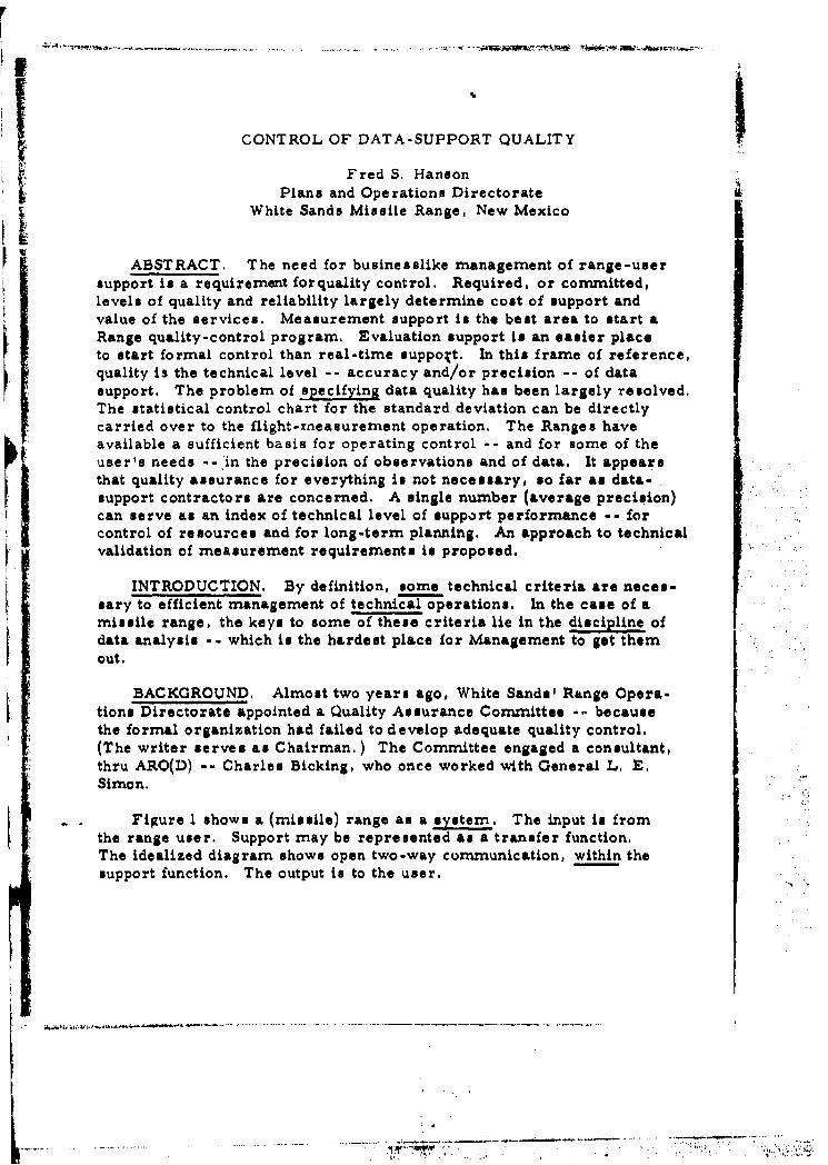
CONTROL OF DATA-SUPPORT QUALITY
Fred S. HansonPlans and Operations Directorate
White Sands Missile Range, New Mexico
ABSTRACT. The need for businesslike management of range-usersupport is a requirement forquality control. Required, or committed,levels of quality and reliability largely determine cost of support andvalue of the services. Measurement support is the best area to start aRange quality-control program. Evaluation support is an easier placeto start formal control than real-time suppott. In this frame of reference,quality is the technical level -- accuracy and/or precision -- of datasupport. The problem of specifying data quality has been largely resolved.The statistical control chart for the standard deviation can be directlycarried over to the flight-measurement operation. The Ranges haveavailable a sufficient basis for operating control -- and for some of theuser's needs -- in the precision of observations and of data. It appearsthat quality assurance for everything is not necessary, so far as data-support contractors are concerned, A single number (average precision)can serve as an index of technical level of support performance -- forcontrol of resources and for long-term planning. An approach to technicalvalidation of measurement requirements is proposed.
INTRODUCTION. By definition, some technical criteria are neces-sary to efficient management of technical operations, In the case of amissile range, the keys to some of these criteria lie in the discipline ofdata analysis -- which is the hardest place for Management to get themout.
BACKGROUND. Almost two years ago, White Sands' Range Opera-tions Directorate appointed a Quality Assurance Committee -- becausethe formal organization had failed to develop adequate quality control.(The writer serves as Chairman.) The Committee engaged a consultant,thru ARO(D) -- Charles Bicking, who once worked with General L., E.Simon.
Figure I shows a (missile) range as a system, The input is fromthe range user. Support may be represented as a transfer function,The idealized diagram shows open two-way communication, within thesupport function. The output is to the user.

314 Design of Experirrents
A need of this system is businesslike management ot user SupJort --
co make the output match the input -- and to minimize the cost of the$ ,.nufa. ftin,-tir-p, %ath41 4- 1,i,.hi.ripe rnna,~g~rvvnt 1tnhiR n anndl v qhart- of
the overhead), This paper shows the extent to which this need is a require-ment for quality control.
DEFINITIONS. Quality is how well and how good, Broadly, quality
i- is any desirable characteristic of process or product other than sheer
quantity or rate.
- The viewpoint that a missile range need be concerned only with pro-" f duction; that exactly what it turns out is less important; and that how good
-l- -is i. is scarcely worth mentioning is, of course, not rational, However,.. pressures to meet deadlines - and limitations of resources of all kinds -
tend to reduce a Range to this viewpoint.
Reliability is how often -- either within a test or among tests. It ib
Support reliability in - strictly speaking - a production characteristic.
However, hardware reliability is sustained quality - of the hardware, So,as a discipline, reliability is found with quality. This paper considersreliability control common to production control and quality control, formissile ranges,
Required, or committed, levels of quality and reliability largely deter.mine cost of support and value of the services. So, can a Range have aneconomical, consistently-valid support operation without (some form of)
I -. quality control ?
This paper considers the distinction between quality assurance andquality control to be a matter of degree. Assurance is broader -- more
1 'stafflike.
This paper defines statistical quality control - industrial quality con-trol - as: closed-loop control of operations. It's emphasis is on formula-tive and evaluative control actions, A. a separate discipline, or function,quality control is taken (in Figure 2) to comprise: specification, score-keeping, feedback, and followup. Let's explore quality control, itself,and each of these phases (in relation to a range),

Design of Experiments 315
QUALITY CONTROL. The (missile) Ranges tend to overemphaB:ze
&--- %A VA.".. at -th -ex ens - - - -rh r - - .--- -- -
(emphasis) is partly due to the cost. But, it's mostly that data supportto a focus of confusion (and difficulty). Measurement is the best place to-;tart a support) quality-control program. Because it offers a big pay-off(thr" inore economic control of resources and of planning-) because it isa key to the technical level of the missile effort; and because it lendsitself dir•telv to conventional (statistical) quality control -- as will beSb,,•vn.
Evaluation support is an easier place than real-time support to startformal quality control. Because the data holds still - and sits around -
during postflight reduction. And there's less sound and fury connectedwith it.
An overland missile range is ideal for (pioneering) statistical qualitycontrol of flight data -- because it has an unlimited number of possiblelocations for instruments.
In this frame of reference, quality is the technical level of a range's - I
(daily-operating) data support -- evaluated against the correspondingrequirement. Quality (level) is the percent to which a particular (quality)requirement is met.
A range may need other things as much - or more - than it needsquality control. For instance: standard operating procedures forinstrumentation; reliability control; an integral production-controlsystem. The National Ranges have to work on all of these, V.
SPECIFICATION. As this paper sees it, specification is the corner-stone of quality control, A spec, is a practically foolproof (and knave-proof) description of an item or service. It is the standard that tellswhat counts as a goal - in the particular game. It has to be definite, and 'Iq u a n titativ e . ,....
In specifying measurement quality, one should ask the question:"What do we mean, 'accuracy'?"
Suppose a user has furnished the characteristics of his vehicle -
and its proposed trajectories, Assume that a missile-performancevariable (to be measured) has been identified; and the desired units,
~~~~~~~~~~~~W 011".- .- - - - .. - - - - -. - - - - -

316 Design of Experiments
and coordinate system, have been specified. It takes about nine morequestions to -pin down" Lh;i uo '•.. ........ r .....
Figure 3 shows the e!ementu - dnmonstrably - required to specifythe "accuracy" of flight measurements:
1. What part of the trajectory? (trajectory phase)
2. At what intervals (do you want data)? (reporting interval)
3. Is this accuracy or precision? (quality characteristic)The user could be stating the allowable discrete error (of the data) withrespect to his (preferred) coordinate system. Or, he could be statingthe allowable inconsistency of the data with itself.
4, Does this number apply to the vector or to a component?(mode or representation)(If he says "component", there is a second question: Is the requirementthe same for each component ?)
5. What % (of the data) must be within this tolerance ? (probabilitylevel - 9 compliance)
6. Precision (or accuracy) or exactly what? (data phase)i. e. , What stage of the measurement-computation-analysis process ic
S . being characterized?
7, What is the "operational" basis of the quality characteristic?(quality criterion)In other words, what sort of procedure is (to be) employed to obtain"this precision (or accuracy) figure ?
8. Over what interval do you want the precision (or accuracy)to average out to the requirement? (lot size)Question 5 was; What Is (of the time) do you want the data (to be) withinthe stated tolerance ? If the user said "1685c of the time", the presentquestion is: 685a of what time -- what is the minimum lot size to whichthe spec. applies? (W-hat constitutes an acceptance lot?)
, 9, How much variation is acceptable within a lot ? (variability
w/in lot)Of course, this is already reflected in the lot-average tolerance.

Design of Experiments 317
10. Finally, what support-reliability (level) will you accept?
neither the users nor the Ranges are ieady for quantitative specification
of data-support reliability.
People go around saying "accuracy". Figure 3 shows the kinds ofuncertainty implicit in that word - when applied to flight measurement.
It turns out - if one says accuracy without further qualification - the
uncertainty as to what is mei~nt can be as large as 15 or 16 times the
requirement. This was shown in the writer's paper-(Ref.-1) at the 196. 3 F-Army Operations Research Symposium. People should be more scientific
than being away from what they are dealing with by a factor of 15 or 16 -as aimatter of pride. Also, the taxpayer can't afford to have the Rangesspend his dollars so vaguely.
These elements of a spec, apply to all performance variables. Actually,
they cover any quantity -- no matter how obtained. Asking these questions,
of the user was an oxpository device. They could, just as well, be askedof a range - regarding its capability. In practice, White Sands has built a
sufficient basis, and a standard basis, for a measurement-quality spec.into its user-document formats -- with the door left open for (the user to
state) a different basis.
WSMR's standard basis is:
Quality characteristic -- precision
Mode of representation -- component
Probability level -- 68%5
Data phase -- a single value of the missile variable - at a given point
in time - in component form
Quality criterion -- propagation of error (from the previous data
* phase)
Lot size -- the series of firings covered by the requirement (the Vaverage precision for that)WSMR wants to be judged on the average quality of "the whole trainload LI
of apples". First, it was necessary to state what constitutes an "apple"(data phase) in this case.
_____ ____ _____ ____II
-..- . ............... ... - - -..- ,-- -.

318 Design of Experiments
Reliability -- in the White Sands edition of the National Range Documen-
... • tation, categorizing a requirement as "Mandatory", "KequireQ", or
"Desired" yields a qualitative judgment of the user's need for reliability•,i of (obtaining this) support.
Because WSMR's standard'basis is (rath r) concisely stated, it'snot foolproof - unless one (also) refers to the procedure for its calcula-
tion (stated) in Final Data Reports. It would improve communication if"that were expressed in "English" - as well as matrix algebra. Forinstance, WSMR calculates the precision of a single value of a positioncomponent from the precision of observations of (physical) determinants
of that position. In three dimensions, and matrix algebra, the squareroot of the sample size is replaced by the square root of: a11 over &.
It would be desirable to spell out vwhat that means in ordinary algebra -
and ordinary English.
It is more in accord with a search for ultimate purity, and more con-venient, to say that accuracy and precision should be left in the qualita-
tive realm. But, the Ranges are in business, So, they have to go aheadaas best they are able. The writer has collected many publicgtions onmeasurement semantics, This paper's semantic criteria are:
First -- usefulness (for the particular purpose)
Second simplicity, clarity, ordinary logic
Third -- tradition, rigor, abstract symbolism
In the unsheltered world, communication between disciplines is moreuseful than purit of discipline, If it's authoritarian, it's not science -
anyhow.
The writer's paper at the Tenth Conference (Ref.' 2) may lead WSMRto (separately) specify the quality of measurement of the time dimensionof missile -performance variables.
The economic goal is to give the range user exactl what he asksfor -- and not one iota more. If the user finds he needs more, he has
only to ask.

Design of Experiments 319
SCOREKEEPING. Standard statistical quality control can be directlyA.,, t^- Ant-ain. r ^ -npratinnv - an m nn
A manufacturer of "widgets" will inspect a sample of (several) widgetstaken from production. The average caliper of the sample will becomea dot on a control chart showing the level at which his operation is run-ning. The average variation (standard deviation), from-widget-to-widget i
within the sample, nmay become a dot on a control chart showing the(current) variabilit of his process. Control of the level of a missile-performance variable is a (range-) user function, The Ranges candirectly carry over the control chart for vibility - of their measuringoperation. The dot on a Range's chart can be a statistical average of thevariability for an entire (phase of a) trajectory; because feedback controlcan only be from-firing-to-firing - of a given type. Variability of themeasuring operation is, of course, precision of measurement. We aretalking, here, about using a standard measure of final-data quality as anoverall-performance index for a data-support operation -- besides using t
it as a consistent basis for user-range communication of (data-support) Rt
requirements.
Physical accuracy is important. But, the least we can be is con-sistent. The Ranges have available a sufficient basis for operating control
-- and for some of the user's needs -- in the (internal) precision of theirinsufficiently-calibrated data-support systems. (Insufficiently-calibratedas systems.) White Sands' standard precision of position measuresconsistency between (observing) stations -- which contains a portion ofphysical truth.
A few samples of WSMR scorekeeping:
1. Our consultant, Mr. Bicking, developed a control chart forinstrument and system support reliability, The number of unusablerecords, of a system, is plotted directly from Data Reduction's FieldRecord Quality Report - without (the necessity of) calculating (the) frac-tion defective. The horizontal scale is total number of instrumentoperations (in a week). This avoids fluctuating limits. So, the chartcan be preparedin advance -- with (2-sigma) limits which increasesmoothly with number operated.
2, Figure 4 is another control chart on an intermediate"product". This is from Data Reduction's monthly Data Quality Report
..... ...... ....i...l...

320 Design of Experiments
(Ref. 3). It shows the (rms-) average precision of azimuth-angle obser-vations by each (Askania-) cinetheodolitc station - identified by rumbber.(Ordinate scale is minutes of arc.) The precisions for August are theplain bars. The shaded bars are cumulative-average preciiions. TheUCL is a 3-sigma control limit -- basee on the fluctuations of cher cumulativw-ave rage precisions (cumulative from I January) about theircentral value, during the March-April period. (It should be realizedthis is 3-sigma of sigma,
3. Let's look at (an example of) overal data-support quality.Figure 5 is from Data Reduction's Data. Quality Report for May (Ref. 4).It slows the (rms-) average precision of (cinetheodolite) position measure-ment, in feet, for (the) Little Jo) (component of NASA's Apollo). Thesolid curve shows the average (data-point component) precision for each
I round. The dotted curve is tht; cumalLtlve-average precision, For thisProject, the requirement and the range commitment happen to be thesame, In the beginning, Data Reduction didn't use statistical controllimits; because WSMR's greatest need was to see where, it :,rood -- andwhat sort of creature it was. There were better - and worE.- - chartsthan Figure 5. The main point is: the quality of WSMR data supportcan vary widely from-test-to-test. (Also, from-month-to-month - andfrom-project-to-project.)
The average precision of final data is a hneasure of support perfor-mance. When the user's requirement is valid, average precision is(a-lso)a measure of Range effectiveness.
Two of WSMR's operating chiefs were displeaced by the test-to-test precision charts. The bad data waL too evident. Since the MayReport, prec'sions for each test have been shown only in tables. Start-ing with the current Data Quality Report (Ref. 5), monthly andcumulative-average precisions for each project - along with therequirement and commitment - are shown on bar gr".phs.
One of WSMR's operating supervisors suggested (seriously) final-data charts could he improved by editiug the input to the averagepreciaions - at (about) 75% confidence. That's editing at 1.15 timesigma (the variable being plotted), It would do a great deal for thechart,, but it would nullify their usefulness.

Design of Experiments 321
A comment on (the problern o0) monitorih.•. ,a,1 -u.pm.t c-n-rc t"'' S I!iMIL-Q-9858, etc. furnish guidelines for quality assurance - almost "from-womb-to-tomb". These are procurement-oriented regulations. When [q 71
procurement requirements "cannot" be niumnerically specified: compliance""cannot' be demonstrated by test; or initial failure to meet "cannot" betolerated; it is necessary to inspect a contractor for "everything". Thispaper has shown a basis for dcfinite, numerical specification of flightmeasurement - and demonstration of compliance. The tact that, in thepast, the Ranges have not had systems for reporting whether requirementswere met (in a technical sense) is evidence that initial failure to meetcan be tolerated. So, it appears that quality assurance for "everything"S is not necessary - so far as data-support contractors are concerned,. A t
single number - average precision of measurement - can serve as anindex of variability of (a given data-support) procesp and pioduct; and asan index of technical level of support performance (add effectiveness) --
for control of resources and for (long-term) planning.
FEEDBACK, Open-loop control gives good results only for verysimple, basily-controlled procn.sses. Flight measurement is not simpleor easily -controlled.
In the past year, WSMR has increased faedback on field-recordassessments; and on which stations are thrown out in data reduction.WSMR ha- also initiated feedback on average angular errors of each(optical) station (Fig. 4); and feedback on final-data quality (Fig7-, TPurposes of these feedbf.cks include: input to an "calibration" ofstation-selection (computer) programs (Pef. 6); and input to (the actual)instrumentation plans. Which feedbacks have the greatest "profit
potential" • and what the optimum and achievable time frames are -
remains to be determined.
.Some range personnel, who are not quality-minded, make a counter-issue of "timeliness" (of data delivery). So, the (Plans & OperationsDirectorate's) Quality Assurance Committee has adopted that word. TheCommittee is stressing timeliness of feedback -- timeliness of qualityreporting, as well as of data reporting.
It should be realized that final-data quality reports are (also) a* formal system for knowing Range capabilities -- the beginning of such
• ii :1
- --- ;-' -* --

S 322 Design of Experiments
a. System. Conies of final-data qualitv reports now go to White Sands'(long-Term) planners. These reports also serve as feedup to top r, anage-
...- .- ment, They put numbers on some of WSMR's technical, operating, and
management problems.
FOLLOWUP. Assurance of followup, in a procedural sense, is aQuality Control rcsponsibility. Actual followup is an operating respor,-
sibility.
When Data Reduction QC gets a very bad average precision of final.data, they check to be sure the analyst is not including the poorest partof that trajectory in the formal report.
When ar optical station has the same (major) deficiency in its fieldrecord for two consecutive tests, Data Reduction assessment personnelreport this, by telephone, to Optical Division technical personnel. Whenthis proves insufficient, Data Reduction will send a (written) memo toData Collection requesting a reply stating what corrective action hasbeen taken, and what further action is planned,
The writer suggestedData Reduction look at average relative biasof each (cinetheodolite) station -- by taking algebraic means of arguiaarresiduals (from least-square3 solutions). A good deal of what WSMRtreats as random error is persistent bias. It turns out this step willnot be practical until WSMR ham quality control per segment of trajectory
i- o average relative bias (of a station) will be with respect to a singlegroup of stations. The fact the reference changes with each station
\' added (or subtracted) shows the extent of the station-bias problem,
Of course, White Sands is setting its sights on controlling (both)the level and the test-to-test consistency of average precision (of data).To do this, it needs to learn how to break down the firing-to-firingvariability (for a given project) into that due to: project; weather;collectiorn; reduction; other, Major factors are: number of stations;whe-re s+h. missile flies; reliaoility of stations; "visibility"; relativelocations oi stations; quality of stations.
V. WSMR won't have real control until it moves its feedback out ofa management tiie frame into an operating time frame, It is alsonecessary to increase aupervisory awareness of the quality feedback(and feedup) now available,

Desipn of Experiments 323
White Sands is slowly moving toward: reliability and precision standardsfor each type of instrument and systenm; clearly defined responsibilities (of
Collection and Reduction) in relation to final-data quality; functional manage- rment of this shared responsibility.
Mr. Bicking essayed an analysis of variance of undesiined, operationalprecision data, He was able to test whether: stations, film-readingmachines, (human) readers, etc. had significant effects on data precision.He was not able to determine the amount by which each affected precision.Further investigation (of this approach) is certain to be fruitful.
Range support is a hard place to carry out classical design of experi-
ment. The missile Project does the test design. The Range has, occa-sionally, put two (similar) instruments at the same site. WSMR runs arange-calibration "test" (Ref. 7), at infrequent intervals. Instrumentation(support) planning is a statistical-design problem. However, current ""0station-selection computer programs (Ref. 6) are a long stop away fromrepresenting analyses of variance. P&O's Quality Assurance Committeeaims to develop the Range 'i quality-control situation to the point whereit will use Evolutionary Operation (EVOP) (Ref. 8). Presently, the Rangeneeds to carry out (more)correlations - and analyses of variance - onundesigned, operational data. WSMR urgently needs a statistical-calculat-ing service,. It also needs better coordination of its applied-statisticsefforts. . A
REAL TIME. Quality control applies - in its entirety - to real-timedata support. Specification is e t the same; but WSM4R hasn't builtthis into its edition of the National Range Documentation (to the sameextent) - yet. Realtime scorekeeping and feedback can be carried outon a firing-to-firing basis. To some degree, they can be included inthe real-time computer program. Followup is the same (problem) as for
STATUS OF QUALITY CONTROL, The suggestion to use (a
standardized) average precision as an index of overall data-supportperformance was made five years ago, by this writer (Ref. 9). It tookfour years, one Committee, and John Carrillo (of Data Reduction) to
implement this.
In applying statistical quality control to data support, White Sandsis running counter to Thurnian Arnold's corollary (to Parkinson's law):
N.-.-

324 Design of Experiments
No new government activity can possibly be effectively carried out by any
Only a little over a year ago, the most important product of P&O's QualityAssurance Conimittee was hop hope that data support could be put ona more objective basis.
The focus of Quality Control has caused White Sands to correct afew errors in its data-reduction methods.
P&O's Quality Assurance Committee is still selling quality controlto operators -- as a tool for th, ir use -- not as a club held by Manage-ment, Data Collection (people) ,eecently asked that Data Reduction's FieldRecord Quality Report be discontinued -- on the ground that Data Reduction'sassessments were not valid. Data Collection personnel have since beentold to exchange assessment sheets with Data Reduction - both ways - toimprove understanding. A Quality Assurance Subcommittee is developinga single set of standards, and a single SOP, for assessment of opticalrecords. Data Reduction Groups on the Ranges are predominantlymathematicians. To this writer, they seem inclined toward monodisci-plinary and laboratory viewpoints - and to favor a priori approaches,Resistance by data-reduction personnel to quality control may have beenduo to QC's management, and factory, and a posteriori connections. But,quality control is not the factory in science, It's science in the factory,(This is now recognized by White Sands data-reduction personnel.)
Data Collection Quality Control has been mainly concerned withsolving the problems of station reliability.
There is still a need to sell quality control (of range support) tovarious echelons of Range Mangement -- as a tool for their use -- not asa constraint, The key to selling Management probably lies in the factthat - for data support - quality control is resource control. The prospectof better bridging the (communication) gulf between Management and data-analysis (personnel) may cause some discomfort on both sides, Ofcource, at some date, White Sands will have to bring cost into itsQuality Control picture. Specifically: precision/manhour, precision/dollar, and value of precision (as distinquished from cost).
PSYCHOLOGICAL IMPACT OF QUALITY CONTROL. It is thiswriter's observation that truth for the sake of the mission i. psychologically
- . .• .---- -- - ..- --- - w----- Y ----- -- - - - - ----

|
Design of Experiments 325
closer to truth for its own sake than it is to truth as an instrument ofpower. raiiiNegative reactions to quality control appear to be due to resistance
to change - and to dislike of the "criticism" inherent in scorekeeping(feeling threatened by any demand to be objective). Quality control is
partly an educational - and re-educational - problem. AMETA gave acomposite of its basic and advanced Statistical Quality Control coursesat White Sands, This writer is working on an executive primer offlight-measurment quality (and specification). WSMbR may bring in aquality-control speaker. The Chief of Data Collection Quality Controlhas written a memo to the individual (field) operators, and their super-visors, asking them to identify - verbally or in writing - existing orpotential causes of error; and to grade these as critical, major, orminor. (This will also be an input to the work of the optical-assessmentSubcommittee,)
On the positive side, keeping score adds meaning and significanceto any game. Keeping score makes how-to-play (Ilow-to.operate) moreimportant - not less, It improves the motivation and morale offunctionally -oriented people,
PHYSICAL ACCURACY. This paper defines accuracy as: thenumerical difference between any value and the "true" value. It isfurther necessary to say that the "true" value must be a referencephysically independent of the value characterized. Physically independentmeans: the errors of measurement (of the two) are uncorrelated. (Ofcourse, accuracy is the inverse of the "absolute" error defined here asits measure.)
The development of the potential of its star-reference BC-4 camerasystem is White Sands' only real hope for an absolute-accuracy referencefor flight data.
WSMR could derive accuracy (am well as precision) estimates fortwo kinds of data in its current operation. Besides star-referencedballistic-camera data, it could do this for (launch and terminal) fixed-
camera data - in which the reference-target poles are photographed inthe same frame as the missile.

32b Design of Experiments
.1 Of course, measurements cannot be consistently accurate unlessI• they are also precise. Differences in the accuracies of stations affect
v system precision.
, 2 This writer holds that being more definite and quantitative about
precision will increase (range and user) understanding of accuracyand awareness of specific needs for it.
VALIDATION OF REQUIREMENTS, Range-support personnel areoften asked "Why don't you tell them they don't need all this data?"
Of course, user requirements should be based on missile technologyand missile-test design. Support personnel have no particular qualifica-tions in those fields.
This writer has suggested an approach to deriving measurementrequirements in which the Range can assist the user (Ref, 10).
The simplest way to derive estimates of required data quality is to
wconvert missile-performance tolerances to measurement "tolerances"-- directly, when they are the same variable -- or by (complete)propagation of error (formulas) thru an equation relating the performancevariable and the measured variable. As Figure 6 shows, the resulting"tolerance" must then be tgened -- on the basis that the actual
r, uncertainty whether missile performance meets its specified toleranceis the sum of the uncertainty of the measured performance and the
I~ allowable uncertainty of the specified performance. The requiredmeasurement tolerance depends on the level of risk at which the missile.using agency is, practically, willing to operate. While a Rangesuperiority of 10 times (in standard deviation - sacrificing elegancefor clarity) would be ideal -- 2-2times is the necessary level; 5times is certainly the sufficient level.
1p

Design of Experiments 327
REFERENCES
1. Hanson. F. S. "An Operational Specification for Flight Measurement", '
Proceedings of the United States Army Operations ResearchSymposium - Part 1, 1963, pp. 307-314. I
2. Hanson, F. S. "System Configuration Problems and Error Separa-tion Problems", Proceedings of the Tenth Conference on the Design Iof Experiments in Army Research, Development, and Testing, 1964,pp. 119-143.
3. "Data Quality", 24 July - 31 August 1965, Data Analysis Directorate,White Sands Missile Range, New Mexico, p. 8.
4. Carrillo, J, V. "Cinetheodolite Statistical Data,,, 1 - 31 May 1965,Data Analysis Direcrorate, White Sands Missile Range, New Mexico,p. 12. V
p. .a.
5. Carrillo, J. V. "Data Quality", I - 30 September 1965, Data AnalysisDirectorate, White Sands Missile Range, New Mexico, pp. 3-5.
6. Hall, C'. A. "Deleting Observations from a Least Squares Solution",Paper presented at the Eleventh Conference on the Design of Experi-ments In Army Research, Develupment, and Testing, 1965,
7. Williams, B. L. "Precision and Bias Estimate@ for Data fromCinetheodolites and FPS-16 Radars", Paper presented at the EleventhConference on the Design of Experiments in Army Research,Development, and Testing, 1965.
8. Hunter, J. S. "Experimental Methods of Determining OptimumConditions", Proceedings of the First Conference on the Desi~gn of
Experiments in Army Research, Development, and Testing, 19,55,
9. Hanson, F. S. "Quality Control", Memo to Deputy for TechnicalOperations, Integrated Range Misvion, White Sands Missile Range,Now Miexico, 21 November 1960. :i:•
10. Hanson, F. S. "Exploring the Need for Quality Control", WSMRPresentations at Inter-Range Conference on Performance Evaluation
and Quality Assurance, May 1965, Section 4D.
g -l.. ... ...... .. . ...... ... . . . . . . ... . .. . .... .. . .. . ...

FsrSupr System
input requiement
Ounput: sreqireens
Figure I

1 ~3291
I ~Quality ControlA
SpecificeationScore keeping
FeedbackI ~Fol lowup t
Figure 2

J 330
I Trajectory Phase
I Reporting Frequency
Quality Characteristic
Mode of Representation
Probability Level
.!Data Phase
Quality Criterion
* Lot Size
Reliability
Figure 3

33
0-
44
>~\\\\\\\\P_ _ _ _~~
ýj 0)
z
inni00
CD
0.~ a? .CR N 0 1I o 0(s3iLfNIIA)
N011LVIA30 OUVQNV.S A0 S3.LVWAI.S3 03100d

3331LITTLE JOE
(feet)
14REQUIREMENT .. *131
S COMMITMENT - -
PC12
IcROUND OF TEST SERIES R~
6
4
3
0
a nd v vs CWHRONOLOGICAL DATA SET
FIGURE 5

335EVALUATION __ MEASURED SPECIFIED
yARIAMCIF - VARIANCE ± VA.RIANCE F
FACTOR OF fs ERO INSUPERIORITY emEVALUATIO N H
1.7 x 36 %
2x 25 %
2.5 X 1%
3.3 X 9 %
5x 4V%lox 1%
REQUIRED = SPECIFIED aXII:VARIANCE VARIANCE ( CHOSEN FACTOR)
FIGURE 6
;Ir

DESIGNS AND ANALYSES FOR INVERSERESPONSE PROBLEMS IN SENSITIVITY TESTING*
M. J. Alexander and D. RothmanRocketdyne, A Division of North American Aviation, Inc.g ~Canoga Park, California :
INTRODUCTION. Sensitivity testing is that area of experimentationin which each test is characterized by a quantal response. To somesample specimen or realization of a system one or more stimuli areapplied and the result is either a "response" or a "nonresponse", depend- YNZing on whether some critical physical threshold was or was not exceeded ,-for that particular sample. The most commonly encountered type ofsensitivity problem is that of finding at what level of the stimulus vari-able a given percent response will occur. For example, in biologicalassay it is often necessary to determine the dose (called LD 50 or ED 50)which is effective half the time, and in testing explosives, it is often ofinterest to find the stroes that results in a detonation, say, 9596 of thetime. In each of these situations we are concerned with inverting therelationship which gives the probability of a reaponse as a function of thestimulas; thus the terminology (probably due to J. W. Tukey) of the"Inverse Response Problem,
The general problem can be stated more precisely as follows:Suppose we have a stress variable x, and suppose that a test at thisstress can result in a response which is either "1" or "O". This is thewell known quantal response experiment. Let M(x) denote the mean oraverage response fraction at x. In this situation M(x) is called theresponse function. If M(x) is monotone nondecreasing, it may be thoughtof as representing a cumulative distribution function, as, for example,the cumulative normal diatribut..on
X ~ C-(Y-11)/12w dy,
In most cases, however, the explicit form of M(x) is not known. " fI i" .IThis work wag supported by the George C. Marshall Space Flight
Center, NASA, Huntsville, Alabama. under Contract No. NAS 8-11061. I ,
S--. . .... . ",.-.,. .

"338 Design of Experiments
For the inverse response problem the experimental objective is theestimation of that x x (generally unique, but not neccaDily Di) "U
which M(x) = a , for a given value of a . We shall be concerned here' both with experimental designs for the inverse response problem andj methods for analyzing the test results.
"V The first approach to this problem was based on the use of the probitdesign [1] which was originally formulated for biological applications.This design requires a fixed number of tests at each of a given set ofstimulus levels, and thus a large number of tests is necessary. Theanalysis generally used with the probit design to based on assumptionsconcerning the response function M(x) and the objective of the analysisis the determination o. response function parameters. Once these havebeen estimated, the soluticn of the inverse response problem can beobtained for any a
. •When cost of availability of materials is an important consideration,the probit design, because of the larger number of tests involved,becomes impractical. To obtain estimates of xa, particularly for
a = 0. 5, in fewer tests, a sequential design was introduced in 1943 atthe Explosives Research Laboratory at Bruceton, Pa. (2] . The rulesfor the Bruceton or up-and-down design require increasing the stimulusby a fixed step-size after a nonresponse and decreasing the stimulusone step after a response. The up-and-down design is still the mostwidely known and most extensively used test procedure, particularly forexplosive testing and other engineering applications. For a = 0.5 it isused in conjunction with the Dixon-Mood (3] or more recently Dixon [4]analysis, both of which assume that the response function M(x) iscumulative normal.
Other methods generally used with distributional assumptions are
the Langlie (10] and rundown designs. When these procedures are usedto estimate x for values of a near , 5, inappropriate distributional
assumptions do not have a critical effect on the efficiency'of the design.However, for more extreme values of a the situation is more cr-ticalnot only because the tails of the response distribution are more sensi-tive to inappropriate assumptions, but also the estimates of x in
these cases are generally less robust.

Design of Experiments 339
•" th• xhoiit.• ,f distributional assumptions on M(x) the inverseresponse problem was first attacked directly by Robbins and Monro [5]who employed a stochastic approximation design. In this procedure the Istep-size is no longer fixed, and the rules for determining successive
test levels depend only on the last test (as in the up-and-down design).The levels converge to the desired critical level, x , not only in
a.probability but with probability one. This design and its variations,Kesten [6) , Odeli (7] , and delayed [8] , particularly the latter, areslightly more efficient than the Bruceton or probit designs for ac = 0. 5.However, for more extreme values of a (e.g. , c. = 0.05, 0.95), simula-tions (9] indicate that the design seems to be much less efficient thanexpected.
For many years the major attention in the inverse response problemwas focused on the case a. = 0. 5. For this problem both the up-and-downand Robbins-Monro types of designs give reasonable answers in about6-12 tests. However, reliability and safety problems require estimatesof x CL for a < ..05 or a > .95. For such extreme values of a ,when
prior knowledge of the response function M(x) is limited, it wasnecessary to consider new design and analysis procedures. In theRobbins-Monro design, successive test levels are determined from onlythe previous test results. One would expect that improved estimatesof x could be obtained if all data were analyzed before the next test levelwas selected,
The two designs described in this paper were formulated from thispoint of view; they give good results with limited sample sizes fora , 05 (. 95) and are still useful in many applications for a ,- . 02 (. 98).One design is appropriate when it is desired to continue testing on a setof discrete test levels until a specified precision in the estimate of x
is attained. The other is appropriate when the sample size is fixed inadvance and there are no restrictions on test levels. Both designs havebeen evaluated by simulation and it is shown that they compare favorablywith existing procedures and with a conjectured asymptotic criterion fordistribution-free inverse response problems.

340 Design of Experiments
ALEXANDER DES ON
GENERAL DESCRIPTION. In sequ--ntial oesigns new levels for
testing are determined fromr, previlis tcbt results, and this may beaccomplishes in many difterent ways. In tie AMeNander design the step"mze is uonstant but (unlike the brac-eton anu Rorobins-1Monro rroccoircs)
inew test levels depend on all previous test resuits. It is assunwCa only:.hat the response function M(x) is monotone nondecreasing, so that theciesign in otherwise c.istribution-trce. '/1, kses alternatsyincreasing ander,.rctsinlg dCcuelnces to oounet the sought-tor stirnuius ievel ,.. cc-
ing ends when x is, wv-h i speciiied prooability, located within an
iL, ,',i of len1 tin rot n.cor" tharn ZA , where A is L-I ttcp si,,. F'ronm.,*•- : d (I Citiiatc of this interVVa1l, in osti,. ('101: 0.l ( 1'011,L1J iJ [l'-i'-'s
line,, r inte ruolatlon.
I•(: . Th, initio.ion. Luni tcri&isatiou raiic s Co r tL.c S C •,n:. ; lBi. ( Ciil
in tc.x oý nonoionc estimates of the response probabuiitici at the Lct
S. ;. jievels. In one version of the design, which should be used for a nearIi7 " 0. 5, maximum-likelihood estimates are used. However, for extreme
values of a, it is more efficient to use both maximum-likelihood osti-.1 mates and certain estimates based on confidence bounds which will be
described subsequently,
Simulations of both 0. 5 and 0. 05 designs have been carried out.IM The design is generally quite efficient relative to other available distri-
bution-free designs, and is roughly as efficient as the best parametric* stochastic approximation when distributional assumptions on M(x) can
be made,
.'rh general rules for the design may be described as followb:
1. Thd first test is at L 1 , the a prior- best guess of x.
Z. By the method of reversals (Appendix I) monotone estimatesare evaluated at all test levels after each test.
3. Testing will be performed by alternately increasing andi !decreasing sequences of test levels.
4. The first test of an increasing (decreasing) sequence is at[6
- - .7: ... .... . ........ .. . .. .. . . . .. , . . .

Design of Experiments 341
either the highest (lowest) level, strictly above (below) the lasttest level, at which the estimate is less (greater) than or equalto a or, if there is no such level, at the level above (below) thelast test level.
5. An increasing (decreasing) sequence will be terminated at thefirst level at which the estimate after a test at that level isstrictly greater (less) than a .
6. The rules for ending the design depend on the value of a. and Lare given explicitly below.
THE DESIGN FOR a = 0.5. For a = 0. 5 the estimates uted infollowing the design rules are the maximum-likelihood estimates givenby the method of reversals. When the testing is finished we wish tohave an intervi.l I such that Prob(x tl) > P, where P is some pre-
scribed probability. The length of I depends on the particular experi-ment; it is never more than twice A, the step size, but in most casesit is A. The occurrence of an interval of length 24 correRponds tothe situation when is at the center of I. 'resting will be stopped twhen either of the following conditions is satisfied: (a) there are threeadjacent test levels L0 < L < L2 such that the response estimate at
is . 5 and the respense estimates o and P at levels L and L
respectively, lead to the confidence staternentx
Prob {p, > .5 < (I-P)/2
Prob(p. .5) < (l-P)/2
or (b) there are two adjacent levels L < L for which the aboveconfidence statements can be made. 0
When P is. 5 then the conditions for L1 and L2 are given by "the following table:
V

MUM-.
342 Design of Experiments
A B
• 9 0 Zr 1 3
2 43 64 75 86 97 10
9 1310 14
In this table, A denotes the number of responses at L and Bdenotes the minimum number of nonresponses which mutst beobservedat the level for the condition in (a) to be satisfied. Similarly, if A isthe number of nonresponses at L2 then at least B responses at L
S are required for termination,
THE DESIGN FOR EXTREME VALUES OF a. In a desirabledistribittion-free design for the inverse response problem, most of thetest levels are concentrated in a region around x• . Therefore, when
. 05 we would expect on the average 19 nonresponies for everyresponse. Thus in this case a good design forces some testing in thestimulus region below tho lowest level at which a response has beenobserved. Since the maximum-likelihood estimates of the response
. probabilities are all zero in such a region, a new kind of "estimate"will be introduced to insure a sufficient number of zero responses. This"estimate" is actually used only to determine when to terminate adecreasing sequence. The method is most easily introduced in termsof an example.
Suppose that after some testing the following responzet haveoccurred
S • 0
Is0 0 0 1L L L L (LI < 2 < L3 < L4);1 2 3 4 1 2 3 4
Fi

Design of Experiments 343
Smt 4. nim. ^ ipnm-afnnnse. at each of the levels L. and L-, two nonresponses .1at L 3and one response at L 4 ' At L, L 2and L 3we would like to obtain Iestimates which satisfy the monotonicity assumption on M(x) and whichindicate that it is likely that the actual response fractions at these levelsare greater than zero. We will accomplish this by introducing an appro-priate confidence bound. In the example being considered two nonresponses Liwere observed at L and either from binominal tables or the equation
(1) ( 1'P0 = 1-P (N = 2) r
one can obtain an estimate, p3' for a given probability P (specified in"advance) such that IProb (p 3 < p3) P .
If the same criterion is used at L a larger e stimate than that atL
should result. To insura monotonicity an interval estimate will be used.This will be accomplished by introducing a "zero region" for each level -
defined as that level and all consecutive higher levels at which no responaes • .have occurred. Thus the zero region Z 2 for L2 is the interval (L., L3)
and similarly Z (L"l L ). The estimate for can then be found from
(1) with N = 3 (the number of zeros in Z2 ).
The objective in using the new type of "estimate" is to be reasonably.Isure that decreasing sequences end below x From the rules of the
design, a decreasing sequence will terminate at level L where P < a.
Because of the way p is defined the following confidence statement can . -
be made: -.
Prob (p < a j observed reoponses } > P ;
i. e., on the basis of the observed responses the probability that L 0 is
below x is greater than P. For each decreasing sequence, the same
_. t2
.~***,-

344 Design of Experiments
total number of nonresponses in the appropriate zero region will berequired for termination. Thus, it Is not necessary to determine estimatesat each level. Instead, from
(2) ( 1-)n -P , N= [n] + 1
one can determine the appropriate N for a givcin P and then it in onlynecessary to count zeros in the zero region.
A uniform set of rules for the design can now be given:
1. The first test of an increasing sequence is at the level below thelowest level at which a response has been observed. If the resultof this test is a response the sequence ends; otherwise, one moretest (at the next higher level) is performed.
2. The first test of a decreasing sequence is at the level below thelowest level at which a response has been observed. The sequenceends at level L whose zero region contains at least N non-
responses. Values for N can be found from (2). The followingtable gives values of N for P = 5
a N.1 7.09 8.08 9.07 10
o06 12.05 14".04 17.03 23.02 35.01 69
3. Testing ends when there are three adjacent levels Loy Ll, ad
L sith that at least one response has been observed at L2 (and2
none at a lower level), and a total of at least N nonresponseshas been observed at L and L The value of N is given in thepreceding table. 0

Design of Experiments 345
A4. An estimate x C:an be found by linear interpolation between
th ~* #;-#-4 T -.. A T- -. .l . . . .. . . . .. . . . 2.. .Z
The Alexander desIgns have the virtue, that once the rules are under-stood, the actual procedure is fairly straightforward and the calculations
required between tests are extremely simple. Of course, as with anydistribution-free design, distribution assumptions can always be adoptedafter testing is complete. If,for example, it is desired to find x 01 under
the assumption of an underlying cumulative normal distribution, theestimates determined from the data generated by this design are some-what better than those based on the data obtained from an up-and-down
design, and are in fact almost as good asymptotically au the optimum forthe 1% cumulative normal inverse response problem, Furthermore, anydeparture from normality will probably affect the estimates obtainedfrom these data much less than the (extrapolated) estimates gotten fromup-and-down data. One of the advantages of these designs is the smallnumber of tests required. An estimate of the expected upper bound N
is given by
N =ZN(l + +. + .1FN/2
N , N an integer
N=
LOJ +1, otherwise
When P 0 5 this gives an expected upper bound of 76 tests for a . 05.
The design has been simulated for a = . 5 and . 05. It appears that
this design, particularly for extreme values of a., is more efficientthan other nonparametric designs which are not based on analysis of allprevious results at each stage. In our simulations, the median number :.of tests was about 64 for a : 05; for a : . 5 the median number of testswas about 16.
EXAMPLES:
I. In the following sirmulated example, the Alexander design is usedfor a .5, A= :5, with a cumulative normal response function,• 0, o':

346 Design of Experiments
Test Number Stress Response
1 1.3 1
3 .3 04 .8 15 .3.
- I: 6 -. 2 17 -.7 08 -. 2 09 .3 1
10 -. 2 111 -. 7 0
12 -. 2 1
Since the response traction at -. 2 is 3/4, while at . 3 it is 2/3,CA- mIethod oi reversals must be used, giving 5/7 at -. 2 and at3. Linear interpolation between 5/7 at -. 2 and 0/2 at -. 7 gives
as final estimate x" .. 35..5
2. The following data were simulated using a normal responsefunction with = 0, w = 1, so that for a .05, x = -1. 645.
The first test was at -3q and the step size chosen was .25a,
(The X 's and O's indicate responses and nonresponses,
respectively.)
Stimulus Level Test Results
-3.00 0,2.75 0-2.50 0 0 0-2.25 0 0 0 0-2.00 0 0 0 0 0 0-1.75 0 0 0 0 0 0 0 0-1.50 0 0 0 X 0 0-1.25 0 0 0 0-1.00 0 0 0 0 0 0-. 75 0 X 0 0- . 50 X
ID DI D I3 D3 :4 D4 I5 D
1.... . 1 2... .. 2.. .. 3.. .. 3 4. . .. ..4 . . .. .. . ...5

SDesign of Experiments 347
In the above table, the columns indicate sequences (I for increasing, D for
decreasing). The final estimate is obtained by linear interpolation whichyields •_ = -1. 675. Note that a total of 44 tests wa8 required. a
ROTHMAN DESIGNI
BACKGROUND. The second new design for the inverse responseproblem is built on a design by Marks [11] for locating the step in a step I r-.
response function. Thus we shall begin with a brief review of that designin the case of infinite sample size (the same design is very nearly optimumeven for small samples). I
Let the siep response function M(x) be such that.• IM0 , x < x
M(x) : M x = x and 0 < < 1.
Suppose we have some previous estimate of the step location x which .
we denote by x" and which we assume is normally distributed with unknown
mean, x, and known standard deviation, w. Let the successive test f I -
levels be Li (i = 1, 2...) and the response at Li be Ri, The first test
is at that stress, L which is the best prior guess of x Then
L I - 1.17w if R = I.
1 + 1.17w if R = 0
Since the design is symmetric about L 1 , we shall give the next two test
"'- *levels only for R1 0 0; these are
. 55w R = 0, R = I
L+199w RI 0, R20

8 Design of Experiments
and
[L, + .273w R, 0, R, 1, R, I
- i] L1 + .847w R, 0,R I, R2 1,
•.: LI +1" I. 537w Rl0, R 2 =O, R 3 I
L + 2. 657w R =0, R 0 , R -
In order to simplify the computations, the following approximation, which
only slightly affects the efficiency of the Marks design, will be used:
1. If RP = R . Ft., then L L. + 1. 167w/Vr, i 1, 2,.1 1i+1 1-
2. For all other cases the successive test levels are determined by"splitting the difference" between the lowest I and the highest 0.
For the fourth test, for example, this approxmation gives (for the sameresult situation as above)
"� .875wL4 1 1 580w
2. 666w
The effect of these small changes from the Marks values on the efficiencyof the design is negligible. In fact Marks has shown [11] that even largerchanges do not have a significant effect.
It is interesting to note that the factor 1/fi can be thought of as acompromise between the term I/i in the original Robbins-Monro processand the constant step used to start the delayed R-M process.
RULES FOR ROTHMAN DESIGN, If it is known that w is verylarge compared to the distance of the interval in which the response func-tion essentially goes from 0 to 1, then it is obvious that the Marks designcould very profitably be used for the first few tests. Thus we propose thefollowing de sign:

Design of Experiaments 349
L= Yo + 1. 167w(a-. 5)
"where y du.civue. :----i--*- CL . ta •' f The secondtest is at
L = L + 1.167w2 1
if the first result is a 0, and at
L 2= L 1.167w
if it is a 1. The general rules for planning the (r+l)St test are:th
1. After the r test, all of the data are analyzed by the method ofrever~sals (Appendix 1).
2. Compute
= (1/i) , v + fn(r+. 5) + 1/2<r+. 5)
*where y is Euler's constant V r 7Z This quantity is asymptoticV.to the expected number of plateaus given by the method of reversals.Thus nY is roughly the average number of points which have gone
into each response estimate.
3. Compute =64 ala i
4. If there are any stress levels at which the estimated response isgreater than or equal to min(a + A, 1), let S denote the lowest of
these, If there are any stress levels at which the estimated response
Kis less than or equal to max(CL A 0), let S 2 denote the highest of these.
I:,i4
L ;

;i350 De sign of Experiments
5. If neither S, nor S2 exists, let
r+l 1 L
- I If S exists, but not S2 , let
L (S +L )/2 - l.167w/{rr+1 1 r
If S exists, but not S1, let2
L 1 =(L + S )/2 + 1,167w/V'r
If both S1 and S exist, as is generally the case lor large
sample sizes, let
Lr+l -(SI+SZ)/Z + 1,167w(-r-a)
where Q is the fraction of responses in the first r tests,r
ra = E R/rr 11 r
i=l
For large sample sizes, the second term should be replaced by(L ... r)/dr, where dr is an estimate of M'(x ) based on the
sample, For example, dr Z /ASI-S2) could be used, but
only if there is some data in the interval (S 2 ,S 1 ). (Note that
this interval is also an approximate 50% confidence interval ona.
SIMULATED EXAMPLE OF DESIGN, Let a = . 05, w = 5, and thetrue response function be cumulative ý"mal with ýk 0, o* = 1. Thenx = -1,645. Suppose y 2-.. Then
S7--.- - - - - I

Design of Experiments 351
L -. 2 + (1,167)(5)(. 05-. 5) =-2 - 2. 626 z -2. 826.
Now suppose A z U k denotes the respusu uc t th ...... \ A*1 r
thi apoint Y =1, A .67455 IV 0x,95- .15 , .
Since the estimated response at -2. 826 is 0, and since this is thehighest level at which the estimate is less than or eqmal to max(. 05-. 15, 0)
0, we have S = 0. Since there are no test levels at which the estimatedresponse exceeds min(. 05+. 15, 1) = 0>, SI does not exist, Then r-:
L= (Ll+S2 )/2 + (1. 167)5/;f1 K.:.=Z,826 + 5.835
=3. 009 ,
Suppose now R. 1. Now we have S - 3. 009, S = -2.826,2 1 '2
L,3 (.S83)/2 + 1.167(5) .05.. 50)
u.2. 534
Suppose now R =0. Then S 3.,009, S -2. 534,32
"L (. 575)/Z + 1.167(5) 05-. 3333)4
u -1.366
Suppose now R 0. Then S 3.009, S -1. 366,
" ik
- .,-. - LJI

352 Design of Experiments
L5 = (1,643)/Z + 1.167(5) (.05-. 25)
• • • = -. 345
If R 5 1, then 81 345, S2 .1. 366,
L6 (1. 711)/2 + 1.167(5) 05.. 4)
s -2.898
The design might continue as follows:
r L, R r L R r L Rr r r r r r
6 -2.898 0 16 -1. 342 0 Z6 -1. 505 08..2, -37 -Z 509 0 17 -1.281 0 27 -1.478 0
,°; 8 -2, 231 0 is -1.208 0 28 -1.454 0
9 -2.03 0 19 -1.133 0 29 -1.430 0'.. j10 -1.860 0 20 -1.061 1 30 -1.409 0
11 -1.731 0 21 -1.681 0 31 -1.389 012 -1.625 0 2Z -1,639 0. 32 .1.370 013 -1.536 0 23 -1.601 0 33 -1.352 114 -1.461 0 24 -1.566 0
15 -1.398 0 25 '.1. 535 0
At this point the analysis of results by means of the method of reveraalsbecomes nontrivial, The estimate is I/5 = . 2 at -1. 352. It turns out
V- that S -1.35Z, S2 .1.366,
:;L 3 4 - "1. 359 + 1. 167(5)(, 05-4/33)
= -1. 774
We continue:V-
/

Design of Experiments 353
r L Rr r
34 -1.774 0IC I 75A f
36 -1.734 037 -1.716 0
t 38 -1.698 1
Let us present the entire analysis at this step, for this is the firstS time it is possible to get a decent estimate of M'(x') [
Strtig Responses/Trials E stimates
3.009 i/1..345 1/1 1.00
.1.061 1/ 1 1.00-1. 133 0-1 .20-1: .1 208 0/1 .20 •
. .28 0/1 1/5 .20
-1.342 0/1 .20-1. 352 1 .20.1.366 01 .056-1 .370 0/1 .056
-. 389 0/1 .056-1 . 398 0/1 056-1.409 0/1 .056.1.430 0/1 .056-1.454 0/1 .056-1.461 0/1 .056-1.478 0/1 1/18 .056-1.55 0/1 .056.1. 535 0/1 . 056
.1.536 0/1 .056-1.566 0/1 .056-1.601 0/1 .056
-162 *0/1 .056-1.639 0/1 .056.1.681 0/1 .056.1.698 .056-1.716 0/i .0-1.731 0/1 .0
h ..

I'PA354 Design of Experiments
Stress Re&Ponses/Trials Estimates (continued)
-1.734 0/1 .0
-. 774 0/1 .0-1.860 0/1 .0-2. 023 0/1 .0
-2.231 0/1 .0-2.509 0/1 .0-2.509 0/1 .0-2.826 0/1 .0
:• .!;: : 2.89@ 0/1 .0
Nowwe have r= 38, Y .5772 + 1n(38.5) 4.228,r
.6745 (. 5) (.95) (4. 2Z8)/38
.049
Since rnr(• + 4 , 1) .099, we have S -1. 352. Since max(. - A, 0) =
.001, we have SVI -1. 716. Furthermore, (S,, S~ is not empty, so weI may replace 1.167w= 5.835 by our estimate of l/M'(x), which isL•,L
S "• .364- = - = 3,71
SZA .098
(The true value is actually 1/M'(x )C 9.7, so we have accidentally
adjusted the coefficient in the wrong direction.) Then L
v1 L3 9 = (.1, 352-1. 716)/2 + 3.7 (. 05-5/38)
= -1. 837
The analysis again becomes routine until the next 1 occurs.
JI
L I m m

II
Design of Experiments 355
SIMULATION RESULTS FOR ALEXANDER AND ROTHMAN DESIGNS.The new designs for the inverse response problem have been simulatedon a diaital comouter for a wide variety of response functions and (in eachcase) for two different values of w, the standard deviation of the densityof the prior estimate of x%. The response functions used were
1. Cumulative normal: L m 0, w. = 1
2. Cumulative uniform: x, 0 < x <
3. The five functions given by Odell (7]
(a) x 2 5 0< x < I
2-4x0 < x< .25•:(b) 2
() -4(:-x) /3, .25 x < 1
2x ,0 < X<.5 x<
4x/3 < x <.75(d) (4x/3. o ,
1 .4'( , - x).75 < x < I
4S(e) x4,0 x <I
4, Two functions with pathologies atx. 5 U0
(a) .5+x 5 , -. 87056 < x < .87056
Here M'(x 5 )0
2+ ' 1
(b) X a O
Sa~•1:..5 + x> 0
I 2+x
I'-
,'f .p..

356 Design of ExperimentsS~ ~~Here MI(x5)=,•
n� -.., -, .1 .u.i..1otinn do not differ very much, we sh~li
report here only the results for the cumulative normal response function..•:• .i=•.These rt.sudlt are tabulated below:
.Dsn w Sample Asymptotic Minimum Variance (if
Desist% Size Varitfce for c . 5 Estimator in
SRoariance for~:.5(N)(n@'/2N100 Slmnu~ationa.
Alexander 1~ul 4 8 17'' .9.. .042. K .40 .14
Rtmn 316 32 64 .ZO .098 .049 .02.5 .36 .15 '10 u)
Alexander (A 21) 10 4 8 14".: .39 .20 , 456 1.98 .39
Rothman 110 8 16 12 64 .20 .098 .09 .045 1.10 ,36 .12 .061
Asymptotic Minimum Variance of
Rothman 1 l 32 64 28 .14 .00 .60 Z4 092
Alexander (A 25 ) i10 16 32 65",' .28 .14 .069 17,5 5,88 ,2.3
"Rothman 110 16 32. 64 .2 8 .14 .070 1.04 .31 .14
Asymptotic' Minimum Variance ofi Variance fora a ,01 E•stimator in
a .0113.91caz/N) 2 Simulationsma4 .u 0 0 ' ' . ..e".
"Rothrnan 10 64 IZ 256 Z . 1.. ,.1 ,054 .33 .11 .07a.
Median sample size required to complete design:,O Without altering design to incorporate estimates of the derivative
' Unsatisfactory because 1. 167w was much smaller than I/M'(x 01)
01.

Design of Experiments 357
From this table we may draw certain conclusions:
1. The Alexander designs are excellent if completed or if carried-1 ..:; 6- - - - - - -- 2. AA' t,,at fnr r. - O"}
2. The Rothman designs are excellent for smaller sample sizes.However, if large samples are intended, the experimentershould utilize the more complicated verslon of the design (notyet simulated) in which M'(x ) is eventually estimated from
aLthe sample and then used to modify the spacing of the subsequenttest levels. Otherwise, as in the anomalous result for a = . 01,w = 1, we may find that the initial spacing (based on 1. 167w ratherthan on an estimate of I/M'(x )) is completely inappropriate.
A comparison of all simulations reported in [15] indicates that theRothman method is slightly better for poor prior information, and theAlexander design is slightly better for small w, for most responsefunctions included in our simulations.
Simulations of other 500/ designs have appeared in the literature.Wetherill [9] has shown that for the 5076 logit problem, the Robbins-Monro process gives an estimator with variance very close to theasymptotic minimum. However, his initial test level is very close tothe level sought, which corresponds to a small value of w (i.e., agreat deal of prior information). But the R-M process would be verypoor for small samples if w is very large. Our designs are intendedto cover bath cases, and it follows that their efficiencies at smallvalues of w are therefore somewhat impaited.
Wetherill claims that small sample inefficiency is clue to lack of jlinearity in the neighborhood of xa.. However, there is a "growth of
information" (growth of efficiency per test) aspect of small sampleiwork for any response problem (cf [15] , pp. •l-220) even for thehomoscedastic problem on a straight line (non-quantal response).
Wetherill apparently found unsatisfactory the performance of allknown designs for the inverse response problem when a is not near50•/. This seems to have been due to the bias of the estimators in thesmall-sample situation, which we believe is due in turn to increased
A_
,,~ ,-
'I- L

358 Design of Experiments
nonlinearity of conventionally uped types of response functions a6 orie
leaves the neighborhood of a. = .5. For example, IM"(x) I for thecumulative normal response function in maximized at 4 t o- . For valueseven further out, it might be imagined that heteroscedasticity would havean effect.
- i• :Our designs for a = .05 show the same small-sample inefficiency,but we do not conclude that this necessarily implies that the designs areunsatisfactory. More work is needed on the effect of (1) M"(x ),
(2) heteroscedasticity, and (3) prior information on the minimum vari-ance which can be reached for a particular sample size.
REFERENCES
[1) Finney, D. J. (1952). Probit Analysis. Cambridge University Press,Cambridge, second edition.
[(2 (1944). Statistical analysis for a new procedure insensitivity experiments. Statistical Research Group, Princeton,No. 40 (Applied Mathematics Panel Report No. 101.1R) 58 pp.
[3) Dixon, W. J. and F. -1. Massey. (1957). Introduction to Statistical
Analysis. McGraw-Hill, New York, second edition, 318-327,
([41 Dixon, W. J. (1965). The up-and-down method for small samples,To be published in the J. Amer. Statist. Assoc.
a
(5] Robbins, H. and S. Monro. (1951). A stochastic approximationmethod. Ann. Math. Statist. , 2Z, 400-407.
[6] Kesten, H. (1958). Accelerated 8tochastic approximation. Ann.Math, Statist. , 29, 41-59.
[7] Odell, P. L. (1962' Stochastic approximation and nonparametricinterval estimation in sensitivity testing which involves quanti lrespon3e data. Oklahoma State University, Ph.D. Thesis.

Design of Experiments 359
[8] Cochran, W. G. and Miles Davis. (1964). Stochastic approximationto the median effective dose in bioassay. Stochastic Models in
Medicine and Biology. University of Wisconsin Press, Madison.
(9) Wetherill, G. B. (1963). Sequential estimation of quantal responsecurves. J. Roy. Statist. Soc. Ser. B, 25, 1-48.
* [10: Langlie, H. J. (1962). A reliability test method for "one-shot"
items. Aeronutronic Publication No. U-1792.
(11] Marks, B. L. (1962). Some optimal sequential schemes for estimat-ing the mean of a cumulative normal quantal response curve. J. Roy.Statist. Soc. Ser. B (Method.), 24, 393-400.
(121 Ayer, M., H. D. Brunk, G. M. Ewing, W. T. Reid, and E. Silver-man. (1955). An empirical distribution function for sampling with
incomplete information. Ann, Math. Statist. , 26, 641-647.
(13] Van Eeden, C. (1958). Testing and estimating ordered parametersof probability distributions. Studentendrukkerij Pootpers N. V.
a I :
[14] Chernoff, H. (1962). Optimal design of experiments. TechnicalReport No. 82, Applied Mathematics and Statistics Laboratories,Stanford University.
[15] Rothman, D., M. J. Alexander, and J. M. Zimmerman. (1965).The design and analysis of sensitivity experiments, Rocketdyne
Repcrt R-6152, 438 pp. (two volumes).
St l !
IA.

360 Design of Experiments
APPENDIX I
METHOD OF REVERSALS
The method of reversals was first proposed by Brunk, Ayers, VanEeden and others (12, 13] . The method is based only on the assumptionthat the response function is nondecreasing with increasing stimuluslevel. This method is best dernoiistrated by an example (see [151 forexamples and uses of this method):
Stress Responses/Trial's First Attempt Second Attempt ResponseI |Probability
__ __ _ Estimate s
5.02/3 2/3 Z/3 Z/33.7 0/1 5/12
3..2 2/4 2/5 5/12 5/12
1.9 3/7 3/7 5/12
The sample response fractions are first arranged in order of increas-ing stress. Since the response function is assumed to be nondecreasingwith increasing stress, the sample response fractions may be used asestimates unless they violate this rule. Whenever such a violation occurson consecutive stress levels, an attempt is made to correct the situationby merging the two response fractions. In the example, the fractions 0/iand 2/4 violate this rule, and are therefore merged to give Z/5. Theother response fractions remain the same, At this point 3/7 and Z/5 area violation, and are merged to get 5/12. The result is now satisfactory.No matter what order the violations are corrected, it can be shown thatthe final estimates are the unique maximum likelihood estimates.
Since we need it in the test, let us define a "plateau" as an ordinateon the partially estimated response function. In the above example thereare two plateaus.

*I
Design of Experiiicnts 361
APPENDIX II
GENERAL CRITERIA FOR EVALUATING DESIGNS FORTHE INVERSE RESPONSE PROBLEM f
D. Rothman e_ !
The estimation of the abscissa x at which a nondecreasing mean
response function M(x) takes on a specified ordinate a may be calledthe distribution-free inverse response problem. A judiciously chosenexperimental design for this problem would very likely enjoy certaincommon properties independent of considerations due to the intendedsample size, the domain of allowable test levels, the desired responsefraction, the technique of analyzing the data, and the extent to whichblocking is required. One would also expect that designs which lackedsome of these characteristics, but were otherwise excellent, could beeasily modified to conform, and would thereby be slightly improved.The properties are:
1. The design is as sequential as possible, in that as much aspossible of the past data is utilized at each step to plan.the next testlevel, or block of test levels,
2. The stress levels in a test block average the same or less (more)than the stress levels in the previous block if the average response inthat previous block was greater (less) than the desired response fraction,
3. The test levels converge as rapidly as possible to x or tosome minimal set in the test level domain spanning x ,
4. The sample response fraction converges to a, and
5. The spacing of the early test levels takes into consideration theprior density on x
Let us discuss these characteristics in detail.
1, The design should be as sequential as possible. A purely sequen-tial design would be one in which each test level is not chosen until allprevious data have been carefully analyzed. The reason for this is that

J62 I) ýi n oi lxpcrinicnt-
the design must be able to correct itself if it has I,, i, lostir',g in tht %ronin:rcgion due to a poorly thosen initial test level. im r ,\,ruple, a RHobbins-
5 ~Monro process which starts out with too small a mtp size and a bad firstm guess is very poor for small samples, and there is no nmechanism for
altering the design after a few results have been ohsq.rxed.
A maximum likelihood technique for such data anitlysis in the distri-"•-.::iI bution-frec case which can be used with any sequLntidal de siun is the
'method of reversals" discussed in Appendix 1.
In practice such ananalysi, may not be feasible, since the results
of .ill previous tests may not bc available when the new test is planned.or there may not be time for the calculations. Nevertheless, as muchdata as are available should be analyzed, and it would 1e hard to beat thenmthod of reversals for simplicity. We know of no d,.jign presently usedwhich obeys this precept, and we feel that this is really I serious defect.
Both of our new designs were conceived to meet this need.
2. The stress levels in a test block should average the same or ,ess
(.more) than the stress levels in the previous block if the average response.'
in that previous block was greater (less) than the desired responset raction, a,
For purely sequential designs this condition inmplies that the testlevel after a "Ill will bL at an equal or lower level, and the test levelafter a "0" will be at an equal or higher level. The up-and-down designand the stochastic approximations all follow this rule, whoreas theDerman design does not,
For extremely small values of a one would not bc too fussy indemanding that the test after a "0" be at a higher level. In practice thetest efficiency is relatively insensitive to the location o! the test follow-
Sin1 a "0". This is why it is possible to violate this rule in the Alexanderdesign for a 5=%. A similar observation could be made for high values
0o' q,
i. The test levels should converge as rapidly as possible to x orto nie minimal set in the test level domain spanning \
.I the allowable test levels are discrete, then the design shouldon\erge to the two levels bounding x. If the allowable test levels are
,;2 (4

Design of Experiments 363
dense in a neighborhood of x , the design should actually converge to
x . Such a design is called a stochastic approximation (of x )' and an
example is given by the Robbins-Monro process,
L L + cn(a-R)n+l n n n
th thwhere L denotes the n test level, R denotes the n test result,
n nand c is generally of the form c/(n+n ). It has been conjectured that
the minimum asymptotic variance for such designs, and for the generalnonparametric inverse response problem for quantal data, is given by
2V in(X ) ' a(l-o)/N[M'(x)]nin a C
where M'(x) denotes the derivative of the response function, and Ndenotes sample size. M'(x) should be continuous at x , and
0 < M'(x ) < c. For example, if a = .5 and M(x) is cumulative nor-
mal, then IVmin(", 5) (i/2)r /N
Based on this conjecture, a relative asymptotic efficiency may be defined Ias follows-
To our knowledge this conjecture at present lacks proof, but maybe justified as follows:
a. The R-M process can match this asymptotic variance for theright choice of c , namely, c = Il/nM'(x ).
b. When the response function is known to be cumulative normaland when the optimal design still turns out to be a stochasticapproximation of x (as in Chernoff (14]), the variance is
aL

364 Design of Experiments
v U equal to the expression above, thus making it plausible to- .- conclude that we can generally do no better.
f..It is intended that the new designs satisfy this rule. The up-and-down, Langlie, and Derman designs do not. It should be pointed outhowever that the first two of these were intended only for the cumulative
• ,normal inverse response problem.
4. The sample respons" fraction a should converge to a.
If the design is a stochastic approximation, and if M(x) is continu-ous at x , then this property will hold. Of the allowable test levels are
ai' , discrete, then this rule gives the asymptotic percentage at each of the
.H two levels that the design converges to.
taeOne might deduce from this a principle of "compensation': If a > a,"take the next test at a level under the latest estimate, to compensate rforthe lack of 0's. A similar statement could be made for a < a. TheRothman design does this explicitly.
5. The spacing of the early test levels should take into considera-tion the prior density on x
Let w denote the known standard deviation of the (normal) priordensity on x , L. denote the ith test level, R, denote the itn response,
and let g = wM'(x )/"\r . Then the situation g > > I corresponds to
the Marks problem of locating a step; the situation g < < I would permitus to imagine that we are merely continuing a design which had alreadygone quite far.
Then the above property has the following ramifications:
a. The quantity I L2-LII should be close to 1.17w (as in the Marksdesign) for g > > 1, and close to g2 a.RI /M'(x ) for g < < I
(c.f. L 2 - L = (a-Rl)/M'(Xa) for the Robbins-Monro process).
b. If R R, then2 1

If g > > I, the lower bound is more useful, as in the Marks design.If g < < 1, the upper bound is more appropriate,as in the delayedR..M process. The conventional R-M process,
Ln+I =L + (a-Rn)c/n
violates this precept.
c. If R2 /R 1 , then IL 3 -L 2 / LZ-LLI should be close to 1/2 (as
in the Marks design) for g > > 1, and close to Ia-R 2 1 /I ac-Rlfor g<<l.
The big question here is the quantity w. If the prior density is uniformwith range D, then the Marks design would change. Nevertheless, theabove rules with
w D/11-12
should still be useful guidelines.,I
Often one is testing a population similar to populations previouslytested h. the past, differing perhaps only because of small changes inchemical formulation or test equipment. In this case the distribution ofpast estimates of x is just the "prior density" we are using.
If w itself is extremely uncertain, the experimenter should use ahigh value as a precautionary measure.
ACKNOWLEDGEMENTS
The authors would like to acknowledge the encouragement and supportof Dr. J. M. Zimmerman, formerly of Rocketdyne, and Dr. J. B. Gayle,formerly of NASA, Marshall Space Flight Center, Huntsville, in develop-ing the techniques described above.
U

1•)tCNThE" ARLO t TiTrl'Il. A T'rt(•N' ,' T'IJ !' DDiPt PT r TTV
DISTRIBUTIONS OF DIXON'S CRITERIA FOR TESTING
OUTLYING OBSERVATIONS
Wal' , L Mowchan
Surveillance BrL.. Ballistic Research Laboratories,Aberdeen Proving Ground, Maryland
ABSTRACT. An empirical or Monte Carlo method for determiningthe distribution of Dixon-type sample statistics for testing outlyingobservations is presented. Results are presented for samples generatedfrom a normal distribution and for samples generated from a uniformdistribution. The method employed was to select random samples ofsizes n = 5, 10, 15, and 20 from each of the aforementioned distributions.After ordering the sample values such that X, < X < Xn, the six
different statistics (defined later) for each sample size were computedfor each distribution. A sampling distribution was therefore obtainedempirically for each sample size for each distribution after 500 suchsample trials. The cumulative frequency functions were then plottedfor both the normal and the uniform distributions. With respect to thenormal distribution, these results can be compared with theoreticalvalues which are published in tabular form by W. J. Dixon [I Withrespect to the uniform distribution, two contributions are made to the
statistical literature:
I. A procedure for detecting outlying observations in samplesfrom a uniform distribution is presented.
2. A comparison of the cumulative frequency functions indicatesthat all extreme values, except for sample size n = 5,rejected under the assumption of normality would also berejected if the actual data were in fact selected from auniform distribution, since the upper percentage points forthe normal distribution are higher than for the uniformdistribution.
Finally, a comparison of the two cumulative distribution functions
indicates which statistics of the six presented are best suitable forchecking an extreme value given a certain sample size.
t

368 Design of Experiments1. INTRODUCTION.
1.1 Definitions of Statistics to be Investigated
Six statistics proposed by Dixon (9) for testing the significance ofoutliers are presented. The author has attempted to obtain theprobability distributions of these statistics by the Monte Carlo methodof sampling on an electronic computer. Let us consider n observationsof a sample from Normal and Uniform distributions such thatX, < X2 < . . , < X , where X, is the suspect outlier. Since both1+ - 2- - n1
th-% normal and the uniform distribution are symmetric, we could alsohave considered the largest observation, X , to be a suspected outlier.Of course, it is easy to observe that for any of the six statistics thesampling distribution of the smallest value, X1 would be equivalent
to the sampling distribution of the largest value, Xn, except for3 location or mnean.
For definition purposes, let us consider the following six statistics
which will be investigated in detail:
1. For a single outlier, X
10 X -X
n 12. For a single outlier X avoiding X
1 n
r xz - x
Srn-I 1
3. For a single outlier X avoidiig Xn, X
•+•i Z " 1:" r12 = X -x (

Design of Experiments 369
4. For outlier X avoiding X2
X -X
3 1r20 -X X
n 1
5. For outlier X avoiding X2 and Xn
3 1
6. Foroutlier X avoiding X and X X1 n' n-i
r 22 : 3 1~
n-Z I
12. Brief Historical Background
The testing of extreme values is a very old problem in appliedstatistics. The data obtained in experimentation must be carefullyexamined so that one can be reasonably certain that the results of L
sampling are representative of the process. It is quite obvious thatrejection (or acceptance) of outliers could lead to a much differentcourse of action than otherwise taken. It shoulo be noted that in somecases the problem of outliers may depend on common sense and hencemay be a practical problem as well as a statistical problem. A reviewof the literature indicates that the problem of outliers received muchattention prior to ).940. In fact explanations concerning outliers werepresented as early as 1850 by W. Chauvenet [z]. His hypothesisbasically stated that some samples contained a very small portionof observations from a population with a different mean value.P. R. Rider (3], for example, proposed a solution based on theassumption that the population standard deviation, a , be accuratelyknown. In a similar manner, J. 0. Irwin [4] published in 1925criteria based on the difference of the first and second (ranked)observations and on the difference of the second and third (ranked)
ii

370 Design of Experiments
observations in a random sample from a normal population. Anothervery practical approach was presented in 1935 by McKay [5 ]who
published a paper on the difference between an extreme observation"and the sample mean. "In conjunction with his work, K. R. Nair [6] in1948 tabulated the distribution of the difference between an extreme
observation and the sample mean for small sample sizes. W. R.
Thompson (7] in 1935 working on the assumption that the standard devia-tion was not known presented a paper, "On a Criterion for the Rejection
of Observations and the Distribution of the Ratio of the Deviation to theSample Standard Deviation. " One interesting fact concerning Thompson's
Swork is that he presented an exact test for the hypothesis that all sampleobservations were from the same normal population. Another significantcontribution is presented by Grubbs [8] whose criteria are based on thesample sum of squared deviations from the mean for all observationsas compared to the sum of the squared deviations omitting the "outlier"., W. J. Dixon (9] in 1950 presented a paper based on sample ranges andsubranges. His paper assumes that the random samples are drawnfrom a normal population. In connection with this, Dixon and Massey(10] proposed a method for estimating the mean and standard deviation
k_. when the effect of outliers (light, medium or heavy) is known. Thispaper is concerned primarily with the statistics presented by Dixon [9)•! - in 1950 since for practical purposes they are very easy to compute.
In addition, one would like to know how much non-normality wouldaffect the tests and this is also studied. As an example, this paperattempts to develop empirically how sample criteria for non-normaldistribution (the uniform) compares to that for the normal distributionwhen various tests for suspected outliers are performed, As alreadymentioned, one of the primary reasons for selecting Dixon's criteria is
that the statistics presented are very easy to compute.
"1. 3 Monte Carlo Method
With the aid of high speed electronic computers such as BRLESC(Ballistic Research Laboratories Electronic Scientific Computer) atAberdeen Proving Ground, Maryland, a program was available to obtainrandom numbers with frequencies equal to those of the uniform or normal
distribution, In order to generate random numbers for both the uniformAM,:•i and the normal distributions, it was necessary therefore only to enter
a subroutine already on tape. Basically, the subroutine works as follows
"K for the uniform distribution. An initial value, X , 54781Z619135913)

~i
is selected and multiplied by a "K" factor which is always 25 X-60The last fourteen digits are then preceeded by a decimal point so thatthe number X lies between 0 and 1. The X is then used to generate X
in an identical manner and the process is continued until the n randomnumbers desired are generated.
In order to generate numbers which follow the normal distribution,i.e., N(0, 1) a very similar procedure is employed. The computerfirst selects 64 random numbers from the uriform distribution and -
computes the mean, XI. One-half is then subtracted from the mean X
and the whole quantity is multiplied by 1613. Therefore the first randomnormal observation X would be 16,13(X - .5). For the second random
normal number, the computer again selects 64 random uniform numbersand follows exactly the same process until n observations are generated.Since the ", (i = 1, 2, 3, . . . n) are obtained from a uniform distribu-
tion, it can easily be shown by use of the well known central limit"theorum (11) that X is approximately N (1/2, V/768). Therefore, it isobvious that (R - .5)/ 1/161'3 is approximately normally distributedwith mean 0 and variance 1. These routines have been checked byX 2
for Normality and Uniformity and the results are contained in BRL .Report No. 855 dated May 1953 [12] . Incidentally, the periodicity ofthe subroutine is one in every four million computing years.j
In order to obtain a sampling distribution for each of the previouslymentioned six statistics for each distribution, it was de 'ided that 500trials might be acceptable. For example, for sample size n = 5 from r
the uniform distribution, r1 0 - (X-2 X1)/(X 5 - X1 ) was computed from
500 trikls and the observed cumulative distribution was plotted. Like-wise, this same general procedure was used to obtain ri for the
normal distribution. Since Dixon [1] has already published tabularresults based on an analytical function of the distribution for r1 0 for the
normal universe, it is of primary interest to compare his analyticalfunction with both the uniform and normal distributions which werederived in this work empirically by Monte Carlo techniques. Theseresults (see Appendices I and II) are tabulated and plotted for each ofthe six statistics for each of the sample sizes n 5, 10, 15 and 20.

S 37 Design of Experiments
2. MONTE CARLO NORMAL VERSUS THEORETICAL NORMAL.The general contribution of Dixon [1] was to obtain analytical results
-:-• -based on small sample sizes for the distributions of the six previouslymentioned statistics. Percentage points were then obtained by numericalintegration for various sample sizes from n = 5 to n = 30.
As an example let us consider r1 0 (Xn - Xnl)/(Xn -X l) where the
subscripts on the X's indicate ordered values such that XI <X < < X
Dixon (I •indicates the density function for X,, X n., X to be
() n. •xndl f(t)dt) n.3 3~
(a) (n-3 'l) d t f(xn! 1 ) dxn.1 f(x,) dx
... If we let v X n - X1, rv -x. Xn-, x n and integrate x and vover
their range of definition we get the density of (v, r, x) to be
~x-rvn-(b) [ f(t)dt] f(x-v) f(x-rv) f(x) v dv dx
7n- T3).1 0 .x-v
r where -, < x <s and 0 < v <a. Also let f(t) = (l/ 1 2rr) e a
Let us now consider a specific case where n = 3. Formula (b) nowappears as
2 2 2x-rv 3-3 +(~v
.. •!.• [_____ (xrv)2 z
(c) f-.- 35 e v dv dx0 X -= 02n)
and collecting terms we get the density function to be
vd) (2r)3/ Se 3xv"I l+r))(d) 6 3 e v e dx dv,
.21T)/ 0

Design of Experiments 373
Upon completing the square we get
(e) (l+r 1/3 (1+r+r Z(l/3)
l /341+r) 2
1/ 3 dx dv
which can easily be integrated to obtain
(f) f(r) - 3 3
21(1-r+r )
Integration of the density function results in the cumulative densityfunction (cdf) which is expressed as
3 2F(R) arc tan [.(R 1 0 - 1/2)] + I/Z
and upon setting (g) equal to 1 - a, we can easily obtain
V3(h) R1 0 tan if/3 (1/2 - a) + 1/2 where R1 0 is the upper a
a Qprobability level or percentage point.
In comparison, the Monte Carlo distribution (based on a sampleof 500 trials) for r1 0 for sample size n = 5 agrees very well with tie
analytical functionderived by Dixon for n a 5. In general, the sixstatistics for sample sizes n = 5, 10, 15, and 20 agree quite well withDixon's results - particularly for the upper percentage points. A
2 goodness of fit test indicated that the percentage points for the
Monte Carlo method of sampling did not differ significantly (.05 level
•"... .. ....."-- • i .... "+• "•:"!=+" •+: "+-" "+ -..... --.tLV " +" .. .. -".. . ... . "-- '

374 Design of Experiments
7':.•of significance) from those derived theoretically by Dixon; however, it
is strongly recommended that in future work more than 500 trials beutilised in order that more accuracy may be obtained by Monte Carlo
we methods.
Let us derive the density function, the cdf and the upper a probabilitylevel for the uniform distribution for the statistic, ri 0 . As indicated in
(a) and (b) earlier, we can write the density of (v, r, x) to be
n!r pxrv ),(i) - 3)! (3v f(t)dt)n 3 f(x-v) f(x-rv) f(x) v dv dx
: •""i/•: (i) (n- 3): -
and let f(t) = I/b-a where a < x < b which readily gives us
,.(J) n- v d77731 ,,a S (l) (b-a)3
Upon performing the integration in (J) we get the density function
(k) f(r) = (n-2)(l-r) where 10n > 3
Integration of the density function results in the cdf which is expressed
(1) F(R) 1 - (1.- R 1 0 )n 2 and upon setting (1) equal to I- a we• i obtain
() R 1 - /nZ where R1 0 is the upper a probability level
"L or percentage point. These theoretical results are compared with theMonte Carlo results and are contained in Appendix No. I.
Another point of interest is that the Monte Carlo results for theuniform distribution were significantly different from the (theoretical)
A.- 4_ _

* :-"' .'.4.• . ••,.:÷ . • .... . .
SDesign of ExperiuntlM 2fnormal when the X goodness of fit test was applied at the 05 level ofsignificance as might have been suspected. This would indicate that
Dixon's criteria are rather sensitive to departures from a normal universe.
3. COMPARISON OF NORMAL AND UNIFORM DISTRIBUTION.
3.1 Sampling from a Normal Distribution.
As previously mentioned, the Monte Carlo method based on a sample rof 500 trails did not differ significantly from the analytical methoddeveloped by Dixon for Normal distributions. If one assumed that hewere sampling from a normal distribution, it can be seen that all extremevalues rejected under the assumption of normality (with the exception ofn = 5) would also be rejected if in fact the actual distribution sampled Vwere uniform. (See Appendix No. I)
3.2 Sampling from a Uniform Distribution.
If one assumed that he were sampling from a uniform distribution,then many extreme values rejected values under the assumption o!sampling a uniform distribution would be wrongly rejected if in factthe actual distribution sampled were normal. (See Appendix No. I)Hence, the error involved in 3.1 would probably be less serious than kthe error involved in 3.2. wl
4. AN EXAMPLE.
This section will seive to illustrate the use of Dixon's criteriafor determining whether a doubtful observation is to be retained orrejected. One of the classic examples consists of a sample of fifteenobservations of the vertical semi-diameters of Venus made by aLieutenant Herndon in 1846 and presented by Chauvenet (2). In theanalysis of the data which followed the following fifteen residuals wereobtained and have been arranged in ascending order of magnitude
-1.40" -0.24 -0,05 0.18 0.48
-0.44 -0.22 0.06 0, 20 0.63
-0.30 -0.13 0,10 0.39 1.01 .
-7
_____ ___
...-..-.------. ~ -'

376 Design of Experiments
The residuals -1,40 (X) and 1. 01 (X 5 ) appear to be questionable.
Here the suspect outliers lie at each end of the sample. Since nooptirnun procedure for testing outliers at both ends of the sample iscurrently available unless the population variance, o,2, is known, weshall now illustrate the simplicity or ease at which Dixon's statisticsmrtay be computed. Let us first test the observation -1.40 since it is mostdistant from the mean of the sample. Also, we shall select a CS 0 whichmeans tha-t Pr (r2 > R) =.05. For sample size n =15, we get:
_3_" XI - 30 + 1.40 1.10.48+1.40 ~= -- .585rzZ X 13 - 1 .48 + 1.40 1.88
Since the calculated value of . 585 is greater than the critical value3 of ,525, we reject the observatiun -1.40 by Dixon's test and now proceedj to check the observation 1. 01 for sample size n = 14.
r ' 14 12 1.01 - .48 .53 .425SX - X.01 + .24 1.25
14 3
Since the calculated value of . 4Z5 is less than the critical valueof . 546, we accept the observation 1. 01 by Dixon's test and no othervalues would be tested in this sample.
5. CONCLUSIONS.
5.1 Extension of Tables Based on the Normal Distribution
Since the Monte Carlo Normal Distribution can be used to representthe analytical solution presented by W. J. Dixon, it is therefore possibleto extend these tables (See Appendix I) to sample sizes for larger valuesof n, which in many cases would be of considerable interest in appliedstatistic s.
5. 2 Development of Criteria Based on the Uniform Distribution
The Monte Carlo uniform distribution can be employed to developa criteria for the rejection of extreme values based on the assumption
" I . ,

TDPRion of Exoerirnents 377
of sampling a uniform distribution. Thus, the tables and figures pre-sented in Appendices I and 11 may be of significant in'purtance in manypractical situations where the actual distribution is in fact uniform.
5.3 Choice of Statistics
The cumulative distribution functions plotted in Appendix II providevery helpful information regarding which statistic should or should notbe used given a certain distribution and a certain sample size. For
example, if given the normal distribution, the statistic ri 0 appears to
perform very well for small sample sizes such as n z 5 while it isobvious that the statistics r12 and r."would not provide a good test for
these small samples because of the slope of the curves.
5.4 Additional Comments
In this paper, I have attempted to show that Dixon's (1] criteriafor testing of extreme values based on the assumption of normality
can be established empirically. Also, I have attempted to show whatwould happen if the distribution sampled were in fact uniformly distri-buted.
Since analytical or theoretical functions for testing outlyingobservations generally become quite involved, further work involvingthe effect of skewed distributions such as some of the Pearson Type
curves [11] could be accomplished by Monte Carlo methods on a highspeed computer.
It would also be of interest to develop a two sided test for examiningextreme values from a sample. In this connection it is suggestedthat the sample observations be arranged such that XI <.X < . . . <X.
A proposal for the two sided test would be to first let X be the
suspected outlier (Dixon's approach) and then to compute the desired
statistic. Next, from the same sample, let X be the suspected outlierand again compute the statistic. The higher ofthe two values obtainedwould then be chosen. If this procedure were repeated at least 500times, then a two sided test could be developed empirically for testingextreme values and this might have rather wide application. Again, itis once more repeated that at least 500 trials should be used.
ZA,
1.K ~ -

378 Design of Experiments
Finally, Appendices III and IV contain machine programming datawhich could easily be ustd for obtaining Monte Carlo distributions of IDixon's statistics []] based on the assumption of uniformity or normality,
4. vvvif sample sizes of greater than 20 are desired.
BIBLIOGRAPHY
(•I Dixon, W. J., Ratios Involving Extreme Values, Annals of Math.4; .Stat, , Vol. 22 (1951), pp 68-78.
"[21 Chauvenet, William, Sperical and Practical Astronomy, J. B.Lippincott Co., Philadelphia, 1863.
(3] Rider, P, R.., Criteria for Rejection of Observations, WashingtonUniversity Studies - New Series, Science and Technology - No. 8,St. Louis (1933).
[4] Irwin, J. 0. , On a Criterion for the Rejection of Outlying Observa-tions, Biometrika, Vol, 17 (1925), pp 238.250,
[5] McKay, A. T., The Distribution of the Difference Between theExtreme and the Sample Mean in Samples of n from a NormalUniverse, Biometrika, Vol. 27 (1935), pp 466-471.
[6] Nair, K. R. , The Distribution of the Extreme Deviate from theSample Mean and its Studentized Form, Biornetrika, Vol. 35 (1948),pp. 118-144.
[7] Thompson, W, R. , On a Criterion for the Rejection of Observationsand the Distribution of the Ratio of the Deviation to the SampleStandard Deviation, Annals of Math, Stat. , Vol. 6 (1935), pp 214-219.
[8] Grubbs, F. E. , Sample Criteria for Testing Outlying Observations,Annals of Math. Stat., Vol. ZI (1950), pp Z7-58.
[9) Dixon, W. 3., Analysis of Extreme Values, Annals of Math. Stat.Vol. 21(1950), pp 488-506.
"(10) Dixon, W. J. , and Massey, 1'. J. Jr. Introduction to StatisticalAnalysis, McGraw Hill Book Co. Inc., New York, 1957.
- .-- .[

Design of Experiments 379
(11] Mood, A. M. , Introduction to the Theory of Statistics, McGrawHill Book Co. , Inc. , New York, 1950.
[iz] Juncosa, M. L., Random Number Generation of the BRL High-speed Computing Machines, BRL, Report No, 855, Aberdeen ProvingGround, Maryland, May 1953.
* K
I IK.
"-- i . i -• ~ ~I- . ... ..÷

APPENDIX I
Ta~bles Of Upper Percentage Points forthe Unifornm and the Normanl Distribution
I'.
I -
Vo.
A t
1' ••i

382
Table of the Upper Percentage Points for the Uniform Distribution
Pr(rl> R) =Cwhere j u 0,1,2
Bample o= .005 1 - .01 - = .02 1 - .05Sir* 'Statiutil "AL U-•' a -w UF " T- I U- "" U
r-o 0 .9 .533 .785 .7T5 .J29 .716 .626
.&4 r 11 .928 .918 .900 .886 .859 .831 .716 .736
12 .995 .996 .990 .990 .980 .980 .950 .946
no r .531. ,5314 .482 .1484 .4,28 .427 .3•, .349
r12 .586 .588 ,536 .541 79 1.476 .393 .393
r0 ,335 .298 .300 .260 .262 .726 .209
n-15 r .357 .356 .319 .323 .278 .279 .221 .223
12 .382 .381 .342 .345 .299 .298 .238 .235
10 0 .226 .221 195 .193 .153 .14
nw20 r .268 .2614 .23T .231 .206 .197 .162 .153
12 .282 .281 .250 .253 .235 .230 .lT1 .166
*U¶Jpper percentage points based On Dixon's Uniform (theoretical).**pper percentage points based un Monte Carlo Uniform.
t7

383
I% :•
iII iTable of Upper Percentage Points for the Normal Distribution
Pr (ri, >R) = o where i 1 i, 2 and J * 0, 1, 2
Sample __ __ e 005 CI .01 Of 02 10Size Statistic T*' N** T* N** T* N** T* N** ý
.6r .82. .82 9780 .5790 .5729 7.T543 .4 .9720
n-5 r .93. ..639 .91 6 .162 6 62r6 .882 807 .812r .2 ,996 .996 .992 993 984 .985 .965 .963r2 o .950 .952 .929 .927 .967 .961 .845 .604
r .5 ,9982 .998 .995 .996 .990 .996 .9T68 .909
r2 .56 .5642 .525 .526 .483 .488 .416 .M5ir20 .655 .626 .522 .579 .581 .599 .4TT .49"
r2 1 .607 . 60 5 .57 .575 .61o .65 3T 5, o .- . .
r20 .664 .663 .632 .62.3 .59 .-599 .525 .539
r T6o .756 .726 .-TO .692 .6T1 .618 .6,o
n22 .260 .815 .759 .802 .749 .742 .582 .59.
r .494 .470 .438 .452 .30 .424 .572 .375
r122 .506 .529 .526 .527 .482 .4•7 .419 .432
r2,2 .562 .556 .525 .510 .502 508 .43o .438
r~~~~~~ .67.0 54 55-3 54.43.9
Upper percentage points based on Dixon'. Normal (theoret9e52 ). .52
* *Upper percentage points based on Monte Carlo Normal..
r . . . .. . . .... .4 2 2
10 ~~~~~-39 -39rt 5 31 36'1
r ~~~~~ ~ ~ ~ ~ .,4.5 4o .3 32 .8 34 M
nw" 12 .43 .8 48 43 .1 41 38 .5

t�i
VAPPENDIX II I;
F igi.�ea of C urriulative Di utributior�.
LI'
L
V
F 'LX
"-A

386
.... ... ...
'liL
J!, I s. I'
t 1lt I ' i I' ;1i . :t I m ~ l :1 '
iii id 11,IF
1 .k i If I-l II III .. l. ..
41''i till1 till l 11
I -i 1 " l lt M i ;! :.: I: r.I : i0

381
T7ý4z Iw m
I I .. ...-
.1. r .: .... .
F:. I j I~ 1111 i il
*W I Hii ' 1 . 1 1 1: ý-iJ~ . H .
-i 1: 1, : 1;
1 1 o

~ - ~- ----------.-.-- -- -. . ------- ----
d I,
t!A 1'i'' ii!' ! i i''
8AI i :i R I il iiilW il 1::17
.:: !:i, VI I;
I' Pi ; !
-iji.~ i i I 11H : ii ,! I!i ýi !
Aii~- -1----II 10
1 !1. i j~ I t_ _ _ _ _ __TNi l_ _ _ _ _ _ _ _ _ _ _ _ __I.,_ X_ _ _ _ .

389
. ~ ._ . .. .
. .. .. 1 .. .. .
Km m
j.:: N ;:ij~ i
I i ii ..H. ,J j ii~ :i.! . ...
iz, I I' I:I i. '' ; I ; I Pi. ~ lii I
4L.'
111 i i:;wiAl
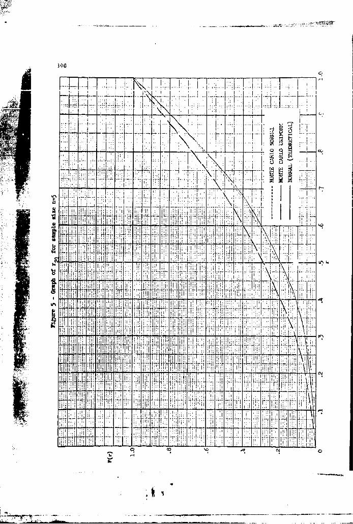
71 0
-~-V-Li- J.- 2 i Im .. f .
T.1
Ile)
2D.,
11.H !W
I ~ ~2 IitrP ~i ~TI~ K4 ,;..
iIII iII

FFEIII ±]IZ]Z7
wm- 2Lm
.. ..... .. ..... ..
! : . . . .. . . . .. . . ...II t !
pI j: -i; 'I 1.tI i~i i; ;:
I!\.. 111111 11111dA On
11 : t !I I
H1 Hi I Ii
AlI ILL i .1 .1.

392 71 I.... ... ...lb
.... .....
T~
i'IT
'114
1!I -I ij:E:.
L 1: 17;1 1 : , 1 I l ! I it1; 1 : 1 1i l
'-J

393 L
m!)
ti~~ ..... ....I : . k- I
:1 m
m ... .....
FI F Mil t!,
iif i I.?t._, I
HI 7 ;I!,.:
MIT

3q4 IiT77~~ Iii~i.......
k 10H Ly qv
;ý~~~1. lipi U O A;i Iý:i i1
I~~Hn n~{It i Lj !~~F :1 F!
at d W ilk-, o A 1:d 11 AA PQ4 bud! 4
o ~ I L~I~rihi,,1 jirflji i ~ I
ii -is *i W tIDE A i:I. ** ' .
1 t1 !1 , 1
T- WO " i!l; 1!P ;ld i] '

fra
395 A
T.... ... ... ...
.F1 iL 1:,
K1
I.:p
I ;ri I7.1 1-.II I I i j
*-T 111
'r-v-7 _:_ 17

I i.. .. .1 1. :1 *1 I...........-
I L -I
III Iii T 1
... .... ....
"I7 .1 0
Tit'*" *'l''. 7 :-;;
'iPiiT
N1:T1T11:1:
"II

...4.....jj~Jiu .i..z { ... ....A mI F1 rrFrT1 1- r T.I
ii ~ ~ .. . .Il~! ~ ...
77,'
I ai
-i 1 ; !L I. . ....

398
I k
i l;j ;!: Wi..... .... ... ...... i~I
r i
I.m:

... .. ;E Ti
7KF TF77I77Kf Tm F9
I.!
:'I':' 'T'
j i 1;
I' Ii' I.
0j T.:j
.. .. ... m s2 i ; ! p 1

400
i: I:;: m
I; m
k.' 1:::: k 1
1* 5! Awi
-I0 0

401
II
1 11
-H il
to I
41-
h ;I. . : I.
T-, 7.7 1 W

402
; r.: Is I: I Ij i
om I -
m~lI
!,IIu l !jjj IT im
r 11,11W
I'.~~. .'!I
Ims.
I~j 11111 I,
I -r

403
H. ..... .i44-
IF w I I I
r~ mti m . . ... .. , m
]j~mi.. ,, 1F I*-*4--'Tims
... ..I J j .' .i ...
-I m I Iij
I
P ; II..I.. . .
-i I-
o 0o

404
L J
II I
+ I I7I 7tEdCID
21~
4'..Rr
C.g.

~i~ii~i222222VI K405
V 1, IlL ?
I A CID'I ~ ~ : .I
12 j, II I d
1E.I W !:1 . 1:.!11: 1. 1: . . I ... I iiLI
i:;! A; I H
.1.: ............................... *I ilic
L:~~1ww&IL W ]t'I-. q . lIý . 1t Pk
*: iiiE U I!! 111HIýl I..A.i

406 ' ''
2 -~'1-2. 2W1Z 7
IIN :
I ,i 1; I
Pu " j ]
T i !I l .. ... ..
:;I 7' ' 7I I l:ý"
mI 1. .. I 1I
*~,~*~*I II' I'I .~~I .I i. m

a
co
. ....II I I...
I~. ...Ht t ~.. ..
~1~T'
7, -r -7
I i I I
T1mI.. ..I..
r ..I.T....I --
j- ±4 .~~
L LI
______
Imi.
I Ii:

j 408
H-ý
i ... .... .... .... .. L.. .... ...
rI m
.W i1 l 1 ~ IT Ivi 4 1; VI
I~~~~ 'jmj Ii~:j
11111111 IN II~ti l 1 HIF:i: :
I r
p+ IIt 1
H.
IS- - - ~ - -- - - q - -

APPENDIX III
Machine Programmi1ng of Distributions
U..

410 PR0BW-Ob9 DISTR~t5UrION SKEET W. MCvdHAN 10 MAY 6129 PAW,!
SLOC(NI-1430)UL-U30)BLOC lOIS 1-DISSi) 0-01440)SAL0CITI-TAO)SI-S30) SUML-SUMb)i
F2 FORM19-10)9-L0)4-10)4-10)4-5,5-1-5)START Y~v.02492A4$5% LO=-.00021346561%
CLEAR 11440)NOS.AT(DI)2S8T(S8u)NNSOO)t FSSuSZ OESw0t SET(MAX-O)t
3.0 SET(IB0)t3.1 Slau1:x
COUNT4301INI !200T043.1)%1.0 SET(ImOIX ENTIF6IZEROCC)%
SE TI M 0) PQaOlIF(0ESu0)GOTOII.2)t
1.1 ENTEiR(URNOS2)URN)2 GOTO(1.3Vt1.2 ENTEI4(URNOSI)URN)%1.3 U1ItIURN% Tl#I.14.5eUKN-4.51
cou~wf(ss)lN( I)GOTOf1.1)%4.0 SETUNmO:
IF(DES.O)G0T014.1)t GOTO(4.2)%4.1 ENT.k(NRN05ISWS1 l)fNI#I)% L)ES&IS GOTO(4.3)24.2 ENTERINRN0SZSM, I) 1N1,U4.3 COUNT(SS)IN(I)GOT014.2)t900 SE-T(C Ter-It
I - SETIMsN1)2X10.0 INT(IIM411% INT(KnM)% SETlX.0)Zn0)%
T1,@K% pKaott ,LaTll12.0 COUNT(SS-1)IN(X)GOTO(13.012 GOTO(14.01213. INCII.I'+I)% G0TO(11.01%
¶14.0 COUNTISS-IIIN(Z)G0T0(L5.03z GOTO(16.0)%15.0 INT(K.M.*Zlt INT(I-K+11% INTIXuZlt
GOTOI 11.0)g16.0 INCICTeCT4I)I
GOTOC 17.0)216.1 SETIM.UI)2 GOTOI10.0)217.0 SETICTa1)t SETIMuNI)% ENTER(ZE5K0CC)%0171 INTIIaM+SS-1)218.0 T1.,(MIt1)-tMX T2a9(M421-,M%
18.1 DIS~oTI/T3% DIS2aTl/T4% 0[S3uTl/TS%L)!S4aT2/T3% D1S~..T2IT4* 01S6uT2/T5%
Tlu,1-plL-1)2 T2., I-,II-2)% T4-ol-t(M+1)% T50u!-#t4+2)tDlS7-TI/T39 DZSSaT1/T49 DZS9=T1/T~S'DIS1CiuT2/T3Z UIS1I.T2/T4% DlSI2uT2/TSZ
24.0 IFl0IS2>DlS8)G0T0C25.l)% DIý14ADIS8%24.1 IF(UItý3>O1S9)GOTU( 25.2)% DlS15.Lfl59*4
24.3 IF(UIS5>DIS1 1)GOTO(25.4)% OlSl7m01S1Ll24.4 IF(OIS6>IS12)GOTO(25.5)% DtSI8aD1S12%24.5 GOTO ( ALLY I)25.0 DjISI3.L)1S14 GOTO(24.0)%2b. 1 DIS14vDIS2,4 COTO(24.11Z25.2 OISL5mD013 CG0TC(24.2)%25*3 0 1S lei aL S4% GOTO3(24.3)%25.4 L)IS17uDIS5% GUTO(24.4)4
2b.ý DISttJ-OiS64 GQTJC24.511ýTALLYI SET(CG0)% STlQa0k)ý1

ii t T~u)IS .G; IT(M=u~Q) ~10 MAY 6:)t t'Ai-i
IH T~x>.52LGOrt.(LL2 )%I ~IF (Tls>.25)G;OTO( LL3)*T2-0". T3a.025Y. GOTO(O;EN)4
LL2 IFlT!->.75)G0TO(LL5)%INT;ML-M342C)' T2-.5Z T3-.525% GOTO(OPEN)%
LL3 INT(MluM3.+10)X T2-.25% r3-.275% GOTO(OPEN)%
LL5 IFtTlu>.875)GOTO( LL6)tlNT(mlmMl+30)% T2=n.754 T3a.775% GOTO(OPEN)l
LL6 IN(l~l3) T2-.075% T3m.9tOPEN 1FCI2-<Tl<T3)G0T0(TALLY2)%
T2zT2t.025%1 T3=T3+.02b5t IF(T2u1)W!THIN( .001)G0T0CTALLYZ)'%
TALLY2 1N1(otM1l,MI1+fl
ZtIP INT (PQ- zi+4'ý GOTO (LL I) 4
IF-INT(C~u2)GOTC(19.2)2GOTO(20.0)t
19.2 SET(M*UL14 GO0TO17.1)%20.0 couNrIN)IN(MAX)G0T0(I.0)*26.0 ENTtER(ZEROCC)% SEiT(ZaO)26.1 TI*OZ T2-.025% SET(Lu0)Z INT(SUMuO)226.2 INTlSUMvSUM*Dl*Zl%
PRINT-F~kMA4TIF2)-(Tl) (T2)D1,Z)SUM )SS)iTlaTl+.O259 T2-T24.025% INCIIaZ+1)%C0UiNT(40) INCI)GOT0(26.2)%IF-INT(Z-1440)GOTO( 21 .0)% GOTOC 26. 1)X
21.0 1NC(SSmSS+5)4 FSS-FSS45CLEAR( 1440)N0S*AT(01A%SET(MAXu0)%
2290 IF-INT(SS>3O)GOTO(N*PROB)%GOTOC 2.0)*LIST
END G0TO(STAR~T)%
Y7,V.

I
APPENDIX IV
Machine Programming for Cumulative Frequency Distribution
i tii

j 414 I'KCt 6-089 ~1STi41fUT 10. SKEET FOi4 W.MUWCHA!14 LC ;.;AY uj 'Ak,r
Fl, FORM(4-5)M-!i 8-S1F2 FOaMt9-10)3-70)IF3 F0Rm(9-10)cj-1c,)4-1O)4-10)'.-5)8ý-2,7)-5ISTAR~T *READ-FOR~. '( F I I-(S S)R)J))
REALU-FO1IMAT(F2)-(5OO)NOS.AT( Al)CLEAR(4CF)N05*AT(Cl )`CLEAK(40)NC3.S.AT( TALl)'.
L.0 ETLno~l TUC2. STLO;
T~aT,.0~s ~wtcri2)..2oO lIF(Ts''ta',' ~ i3(,ý
~OU:~ (~:.J I ( ii.025. .
.UIC(sl.i ) GO-TU
710 TlIOt T~em.O~Z$ aLT(IsCR%Boo ~PR!NIT-FOitU4ATIU3)-(TI)T2)Cils)rA4LII)SS)R)C)c)
COUlTr40oNhl)oT0(8*0o; GOTO(START)%
END GOTO(STAKTI%

V
A SIMPLIFIED TECHNIQUE FOR ESTIM:VFTING DEGREES OF FREEDOM
FOR A TWO POPULATION T TEST WHEN THE STANDARD
DEVIATIONS ARE UNKNOWN AND NOT NECESSARILY EQUAL
Eugene Dutoit and Robert Webster
Quality Assurance DirectordL, Aminunition Rcliability DiviRi n 4Mathematics and Statistics Branch,
Picatinny Arsenal, Dover, New Jersey•~
The purpose of this paper is to develop a practical aid for the descrip-tive statistician performing tests of statistical significance who must domost of his computing at a desk using an ordinary "desk-top' calculator.
The t statistic is used to test for significant differences between two
s;ample means when samples are randomly selected from two normallydistributed populations. If samples are drawn from two normal popula-tions and the standard deviationb oi these populations are unknown andtheir computed estimates indicate they are not necessarily equal, thenthe t test statistic is computed by-,
x -X1 2(1) (2 +t 2//) 1/2•i ~ ~(Sl/l + S2/na,.
J'•~~ 2 ~ i .
where this random variable follows a t-distribution with degrees of
freedom (d. f. ) equal to-
S + S 2
1 2
(a) d. f. -2 2
n ~ +1 ,
Z 2 22where S and S 2are estimates of T and a respectively and n1 andn are the sample sizes. Since equation (2) is a cumbersome expression
to work with, an alternate form of this expression would be desirable foranalysis performed on a desk calculator or a slide rule.
I
;,' • 5 i 'r , .'• "; • " " ' • .. ... .. .. ..... . . .. ." • 1. 4."

Mi
416 Design of Experiments
In order to determine whether or not tne standard deviations areequal the F ratio test is used:
22(3)F S /S 1
2 2 2where S is denoted suchthat S > S This guarantees that F > 1.
22 2 tIfthe coptdF ratio is larger than the tabulated critical values of F
ratios, the two standard deviations are unequal. Equation (Z4 can bemanipulated so that the d.f. can be expressed as a function of the ratiosII-. : " •'of thc• variances and the values n1 and n. Since the ratio of the
variances has already been computed as the F test statistic, equation
(2) can be generalized as:
(4) d.f. f(F S S n 2 )
If n 1 n 2 thIn equation (2) can be rewritten as:
(5)(n 1 ; 1) (n2 "1) (n2 +n (n2 -1) + F n (nt 1 )
or alternatively:
.2(n + nlF)(6) d.f. 2 I .n2 2-2
n- nI
Equation (6) is more efficient because twelve operations are needed tocalculatt. the d. f. whereas equation (5) requires 17 separate operations,Equation (5) howcver, has eliminated the "coinplex iunction" appearancea-•,d might be more palatable to the 9tatist'cal employee who would have
to co:. pute the value.

I L
Design of Experiments 1! 7
If n, n= n, then equationrs() and (6) reduce to:
2(7) d.f. :_(1 + F) ( - 1)( + F 2
The derivation of equations (5), (6) and (7) will be presented in AppendixA. These equations lend to cornouter applications for selected values ofn,, n_ and F. The number of degrees of freedom can then be calculatedand presented as tzbles or graphs. The output format used for the initialcomputer run was of the type:
Figure 1
n2 10 Is . . . . . . . 180
10 d.f. d.f. . . d.f. . d.f.'11 12 lj 1
= Fk 15 d.f. 21 d.f. 2 2 . d.f. 2j d. f.2m .
* I
I t
d. f. d.f. i2 d. f.. ... d m,
180 d.f. d. f. d.f. d. f.rnl m2 mi Manlf
Twenty values of F were chosen so that twenty tables (see Figure 1)were generated, These tables were then used to generate sets of curvesas per Figure 2 below:
'I
ii

I 418 Design of Experiments
Figure 2
d.f. nI Some fixed value
140
20 aFb
10 C
10 20 . . . . . 180 2
A fixed value for n and F produces a set of smooth curves for various
values of n . The first attempt at plotting curves proved to be a bit
impracticJ for larger valuees of nl, n2 because the curves become highly
confounded. A more realistic plot can be made (for Ordnance purposes)by using values of n1 , n2 < 50.
Example: Suppose we should like to compare the test scores of twohigh school science classes. We wish to detect a significant differencein the dispersion of scores within each class and, in addition, we shouldlike to detect whether or not the average score of one class is significantlygreater than the other.
We consider the following data:

Design of Experiments 419
Class a. Class b.
95 81 b9 80
83 67 74 77
46 81 91 92
71 85 90 86
76 52 82 78
64 86 71 82
82 79 72
84 80 80
84 88 91
56 64 98
n 20 n 16
x = 75.2 X 81.3a b
2 2= 170.06 *b * 60.10a b. . ...
ea 13.04 sb 7.75
Using the F-ratio test for equality of variances (dispersions),
2
F = 2 = Z.83 > Z.77 = Fa/ 2 n--1, nblI0 a/ a b ..
b
when a = 0. 05. We conclude that a significant difference between thevariability (or dispersion) of test scores is detected.
Since we only have estimates of the true variance of the data andhave shown these estimates to be unequal, we should employ the twopopulation t-test for data with unknown and unequal variances to deter-mine whether the average score of Class b significantly exceed that ofClass a. We must, therefore, compute
S., .., ,: . .

0 .... '1.420 Desi- n of Exoeriments
_ -
:-~~li
's:-•: i
2
12 2
andd. f. b
"Then, t 81.3 - 75.2
-0 + -I 0,01
6.-\4i,ý'2 2 6,
, 1.73
2170.06 60o10
,20and d ;16
and ~f 170.062 60.10)
20 16
i -= (12. 26) 2
3.81 + 0. 94
... , .. ,; ,..: ,.Ii.• . .. ""-

Design of Experiments 421
-_150. 31i ~4.75
: 31. 6 11 3 2 -• -
As might be expected, these calculations are lengthy, time-comsumii. gand error prone. An alternate method to determine d. f, would be toconsult the graphs which have been prepared to yield values of d. f. whenthe sample sizes and F-ratio are known. r IThe graphs plot d. f. vo N for a specified value of N and for certain
values of F .In this case N 20=Z and N, 16 since the variance of
n > variance of n The simple steps to determine d, f. are as follows:
1. Find the graph corresponding to N = 16
2. On this graph find N 20.
3. On the vertical line corresponding to NZ = 20 find the points of
intersection corresponding to F-ratiots of 2. 00 and 3.00 (only values ofF = 1.50, 2.00, 3.00, 4.00, 5.00, 8.00 and 14.00 are plotted).
4. From these points read d. f. (F=2. 00) and d. f. (F = 3.00) off theo rdinate
ordiated. f. (F=2. 00) = 33. 5d.f. (F=3. 00) = 31.3
5. Interpolate'to determine d.f. (F = 2.83)
33.5-31.3 = 2.2(.83) (2.2) 1.83% 33.5 - 1. 8 =31. 7 d. f. (F 2. 83) ! i
Thus d. f. = 31.7 • 32 - which is compatible with the calculated valueof 31.6 • 32.
SL ,;.

d 422 Design of Experiments
U REFERENCES
(1] Li, J: Introduction to Statistical Inference, Distributed by EdwardsBros. Inc., Ann Arbor, Michigan, 1957.
(2] E. L. Bombara: Probability That Stress is Less Than Strengthat Prescribed Confidence Levels, For Normally Distributed Data,Proceedings of the Ninth Conference on the Design of Experimentsin Army Research Development and Testing, October 1963.
ACKNOWLEDGEMENT. A special acknowledgement is extended toMr. Stuart Ritter who dcevloped the -oniputer program for this work.
1h.
.. . .. . .. ------ ~.

L m n-., -L, • . ...... . ; - .•..
423
Design oi Experiments
Derivative of equation (6);
d f. f a 2 / n 2a /nI- *1 n- -
r a tio -. - F > • L. . ,
td+ + 2
S (1/n1 )2 (F/n 2 )2
nI - I+n -
multiplying by (nI 1 2 (n1 n 2 )2 •ivcs equation (5):
(n 2 + n1 F)£
d~ f. = 2 2 F2 . • ,
n nF
n 2 n I. ..1, -
nI -1 * 2 - 1.. .
(n1 -k) (nF-l) nmquation (5) follows by rrultiplyini by (n(-l) (n 2 .():
I0*~~

424 Design of Experiments
d. 1n-I) (n ) (nz + nIF)-d., f., n 2 (n -) + n 2 (n 2
when n1 n 2 = n
d.f ( + F)2 (n -I)
I + F 2
which is a linear function for d. f. with 'n" intercept n 1 and slope2
LI +F)
-+F 2
" . .... ..........

4Z5
APPENDIX B
logic diagram of oomputer program'
START READ Nj F[
iwC+
II jS
IINO

I 426The FrtirtDea satienan for the abovre logic aiagrea Is presmented
below tie F7gre 4.
DEGREES OF FREEI)IM FOR UNEQUAL VARIANCE T-TEST
DI4F.NSION SIZE.'I20btS1ZEL(20) ,F(20),OFI2t2,t20OI99 READ INPUT TAPL 2t100,N1t1NZN3
1%; FORMAT(312)REAn INPUT TAPE 2t1O19(S[LESIU)oI-iNL)RViAD I-NPUf TAPE 2,lrhl,(SIZELIJhJ-loN2)NRtAD INPUT TAPt. ,101gIF(K)9KziN3)I .I~ FIRMA7(12F6.0)00i 1000 KnuhN3DO 1000 J@IN2
UPPEReISILEL IJ *SI ZESt 1) 'Ft V.i 2
DblSZE LLJI-hI ZLJl/SZSI-l)IIISlE(1*2
S 1U0~ DF(K.,JoI)*UPfiHEI/DEN9M4 ~00 400 VKu1,N3I WRITE OUTPUT TAPE 3,3a)1,P(K)oISILESIIbtI91?N1)* Q1 F0RMA7B1H1,?X998HDEGREES OF FREEDOM FOR TWO POPULATION T-TEST WITH
N ~I UNEdUAL VARIANCES WHERE VAI&(NZI EXCEEDS VAR(N1)9s//I.OX#3HF 8#F6.22,/ION X X#iOH X NI. Xt/8H A X#/OH X#X.I180t4.092X))WRITE OUTPUT TAPE 3,3011
3011 FORMATIGH N2 X Xt/6X,2liXX,/1KU15(1HXI,/?X,1HXI00 400 Jvl,N2wRITE OUTPUT TAPE 3,3D2,SlZEL(J),(OFIKJIbtlu1,Nfl
)C02 FORMATI2X,P4.O.I.K,1MX,18(IXPS,llIWiAITE OUTPUT TAPE 3,3022
3022 FOI'MATI?X#IHX)4ý;O CONTINUE
000 TO 99j ~ENU(I,OCt,0O,OCe10C irP*G).O,0,0,00)
The computed output follows the format as given In Figure 5

.wlw] I' t t. -. t+..• :a, F =5.+•) ii.r4 nu, Itnq ]+, 7 . . ..2
Inarviarnts of 2
I' -L, ' F INO . 'M Al 101 1|-rtLS; % l 3I IIIO f.,UA[ VA' lA! S(.L 1 1 111I VA.41£ ,) I jr I IDS VAf i I1 .
A I,
% 1 12. 14.. 16. 1". 11o. ?2. 2.. 26. 28. 30. 32. 34. J6. )a. 40. 42.
iA:P 4$1 t I -.• AX XA K &XXX A.•I ~ l t X AI A X• All A JA XXAA X AAAl lJXAAXXXAXAAAX AAA XX KXXX AAAL X Aggll 4 XXX A X lX XXX XXAX I• +X A [ XXXXXX IX XXXXA
I). A II.A Ii.) L2.1 12.1 11.9 1. 6 31.4 31.2 ll.• 10.9 10.5 t0 .? 10.6 1 .%. 10.4 L(A.- 10
A I 1. , l..q 16.1 15 . I . 14. . t , I. ' . 2. 14.3 1 11H 1. .61 31.4 13.) 3 3.2 l3.0 12.9 312.
A',. .1 14,,4 1'1 ,li.3 1I ,I Ij, , 11.d 11.4 11.I 1,.8 16.6 16.1 16.2 16.j IS.8 IS,1 15.A
A4 1 ,-b Z•.. t.'3 2.9 e2.1 1,? I2It.2 2 .Q 201.4 10.0 19,f 19.4 . 1.L I 5,) 1.1 I .5 Is.A
I, A It,. 4.6 2,.1 2(.. 24.8 24.2 , , •." 2I . 3 21. 21 .6 22. J 22.0 It. 1 21.11 ,21A4 1 1 1-. $0.A 1, lj.1 P .1, 2 H . N d I'. 211 11.31 26.b, Z6.13I' 2.1 21.95 2 .2 24.91 24.6 24.
VA 21.2 12,.!, 13.1 1J.5 13.2 , 2. 32.1 11.6 1.).4 3ý .3 29.0 29.3 25.9 08. 21.1 21.1 it.
A+4 ZI+).r 1 1.4l Vj+l , 6.6 36.7 16. 1 14.6+ )).z ".5+. 5.9 M l 1 2.4 32. 31 3 1).5 31.4 11.0 30.
I&. A 10.0 Ili .0 ,i. 11,4 31)9 . '.,1 S9 ),9.4 )86,5 31.2 J1 6 31,0 16.4 1S.8 3 .1 34.1. 14.4 14.1A
i13i. A 3',J . 31.'1 .J'.I 't1. .9 4,10 43.3 42.9 42.5 4 1.9 41.1 40.6 40.0 J9.4 38.9 15.3 3r.4. 11.0
J3. A 21.1 It. A 4 1 , 4.,,0 4'5., 46. .Q 46.3 46.0 4S,% 44.13 44.J 41.1 43. L 42,5 41,9 41.3 40.1
AA. J 2 .b.1 1. .'j 45,? 47,3) ,9. 1 49.5 49.4 4.3.1 441.6 48.0 41.4 46. 1 46.1 45, 44.9 44.1A
4 A 1 2.11 1 .34. 2 '. 1.. .71 4*.0 . 9 1. I '2.% o , "1 , i2 .l.2 5 . t .•9 1 50.4 41. A 4Y.2 41.6 41.k
A -'.6. ' .tI. 1',2 .')','3.t ',,.7 '14.0 V,) 1 $5.3.4 6'i.9 ','1. 1 5,.' 3 4.1 'A, 3J. S '4Z .. 12.2 93 I.1
4+I ilI ' '.+ ,• ' t.l S1l.1 Sh.0 1) 1. I SI). 1 54.1 59 . 1 58.8 ? .1 1 t 8 A 1. 2 %60+ 55.9 55..
' ... . S I .. f ,U 0. . It b.. b.. . ..1 . .9 1 4 6 . 10.2 5 .6 9.
mII
i.i1-1

428 Design of Experiments
U APPENDIX C
1. Charts for n1 , nz, F
n, n, = 10, 12, 14 ........... 44
cilarC ior iin ii~,2 F
76I
ii

I w : 11
Il
J-1'
1I. FI :J IiI
j IR-i~ I
Th~t~tE{ itil
* ~ t..L4444'1
5 V, tR N
~~~f MR It
:4' -fl i41 f_[.
-4.T
'Al :".j11-1 M11 111

I '0 L i.. ......
CLLid
in IL). vft
I II
?7L-
1J14
2LC~'i~f 41 41!i fi L 11
tt ti t .j . 1 Kr ' . I ... IM I %I jR
--- - ..1 . l

1:. .77
7 -F.
:j I Li
. . . . .... ... .....
II I :iz~lizI
II . .II. .... ..... .. ~
TývL.l 4I--.. ~ 1 41 hl d Wil.
TillP ILI
".:11 ..
!111 II-.- M Ti
l~i -P4 11 uL. *I ~ I iU~h~..It
fftm -1

-7I
f lu * it ;,* .
iorl d'~il ®Ii T u l it ~. ~ .
.W1i' -111 bill
II H ±44:
!- 1:1.1-11V
T TA~ !'TI<N: ii
if141J4~ ~ ~j4 Ij:f'VpfI~
..a.. ..
'.tf It
j I . . . . .

Ii~~~ - j33
'UXI
::is . *'- 1:*- !
*~~~~~ ANT .2j 1 j70
1,14

j434
*.ij
:I AI t JBf
Jj3Tht j77. 1F- IL
;.L ....... i
T I.
_~~ 4 '
-4 4
i4j. Li~i~jili'i' . It..A.,~- 4i-i~hIW
0T 0' -;I;

V c~q
1_1 .... ..... ..
... ... ... M.~ . ~ t II-.I~.I.iI.I
1, M
2421~- IttT '
t
!ýW
I P tt' W ~I~ u~2i
0C
NIQ
MT:tM

X. es
L~~ X 'fihi~'~n n i j
tt
+. 1.;~~tri~:~4
ýItf:j I t 'F~f~j ~ -12
AlLv
t'f7P !T7PYtr
-r~~ t, ril T, 'VNt'~lv... .'....i t:wj~
Pu l E, 1; ill. 4i ii
rI L......'..... .I'riI~ "j44 j Nj i rj jr.i ~ .~f~tl
.... ......
0 ~0'9. C(17 s

;:I
I. . . ........ . ,
~ ..... .....
.ttI
Alf Xfftmy.tdku I~
L~~~iJI4~~1 411""1i2T :gr"1~Ixr.j RI -i 1fT r1 .. ...I .- ..
I~ ~ K :14 I ~ 1 H
C a a
-o'It
trt

- 00 0 o [... ..
j :II
Ii...i. .. pj L:I b?;..... .. .... ; iij~ ij~ h t .t 1
'I~Io' ~ I IPN ____ fi:qjjOIMANV '-IM t fl'.
1. t4:j-r~ t- I w r .4 ; r'''
j7"n

4 All
- -Z 1' ,I I*' I :.
-Ij- 441 _ ii' 4 H i dENT 0't
I4L..jbtU I flf t UMillI'"ft .~4.fl1 lf;;;tIt~lj~tvU~i~ LU I.'t'*' n D
'14 f 1 ~ ;:" j:;p A
*~~ I _ _ _
Ivin
~414~ IT
4 4 (r

ýIj IFl 'i ¶3r. ImK~~4
\ I till1k1; fy±Lt' ::i .
1'71.h i << tQ;t4;4t
1,4 ill~ji... .. ... .... L4 ~
t IX
LIT t' 4 7'2-
-A L _N -
12I. IBI Noi
71:77 I LU]

V I . * 4 4 1
Oo 0 00,
. . . . ....
j 1 ,,t~~~li I24~j I iINmil IT
-IN
12"1 L- I ~t 4 I
11l 4 ,IF1F- !IT
1. '. ~ .. 4 4. ..V . .. ,.
pip.
coI
4a

442 .-
-~.1 $1\.. 'i-.i~
I'
t IRRI[IMI t .!IIIFAi
-- V r j~iN
.i .... .. tEEa
f±L7&6EjJ 410
co
iu
=N Mtt
fflAMt

j iiý i iJTI4.:
K I
J~ L.-:
~~1-C w~iis~tqi .7 4Ž;iPt72 j I
I, v
t-LM
4- 4 ... .
..... .. .... ........
.... ......

A I 4 i I . ii
17 T~ i U
[.r. ~~~~ ~ i t2. !,i I~~~j ~iI
4 4;1 41 flA '1 0 1 t1i H
.L I. 'I. Tf
t 1 .a R,~r I.
-'it

h II
~SLII-- i ,~~ ~~ ~ N, *IIJIJJl*~~l.
j ...k
____ __ ri ' J1::i 1jt~j'tj ~ I F*. 1t' 'T"U'~.IT'~~~i' I~fJ _ ll 1Tj L__Irr ~ .4 ~ y .~ n ¾ . .uT]' I Tj\ h1 I' .I
L~ ~~ ~~~~~~. N. thj13!l 4 id<¶LjINII L
.71kkig: 1\1 'V
- 4L~s'....4-
I 5 I. NI L- Tr
r-,Ia , ;t V.~1 .I - I tt
-- "-r~L { w-yyA 1-ri~.LtII ~ 2, j~ A4~
1
4 4ii~717 '
A7. .
f-A .4~O du4SnL.~a*.

- ~ -. N.~
11~ H11~
¶ I I It I
___~~f 4f IzSjJi
fl47~~ 'Sa 1±4 4 -I
tb'itipf ' i.i~n -j~ --iuftgAII! ...w- . ,iuJnt~~14
LW tý4 Fit- C ihggi~ ~~ ~~I~ 1
r.LI r.Yrjzf~~n~i~7zI¶3 '1v~ j .. lý
's II1P ff*"irA±~~ 1ý,J, it ff * -
[h- x2: ccttV- _3
.IZI. S4 .44t0... 5s± gtql4'4 1- N~ ~rCMT!.I.L±t[I+t. flii 44 rjV-N~zI'TI
K~i;2K£f- 1 Y~ '_I j J4j 4,41,t4t-Ali.........
32I A4 'I'
r~~ ~ ~ .. I::.;1'"lfjI
Vj: _____ ________
71 i 71 -
to ~ a,7. - J:' t-I

CA I
447
4. '
itiltW1 I "l L [
r44 - H-
5 101
so1 ~ ~~~~~ ~~~ /ýl TL'r-'1.. i tt ! 2 ~ .~I3d
IT, il
q0 : o. @ L to 19 0 90to o JO to );,a a 30 No01 11l

DELETING OBSERVATIONS FROM A LEAST SQUARES SOLUTION
Charles A. HallTechnical Services Division, Data Analysis Directorate,
White Sands Missile Range, New Mexico
ABSTRACT. In this paper we give a matrix treatment of the classicalleast squares theory and determine each observation~s contribution to theleast squares solution. If each observation's (or observer's) contributionis known, then it may be possible to delete certain observations (or ob-servers), (1) to improve the least squares solution or (Z) to minimize thenumber of observations (or observers) entering the least squares solution.It should be emphasized that redundancy is necessary to obtain a statis-tically sound least squares solution, however it may be advantageouslylimited without significantly changing the solution,
Although we present a general least squares theory for uncorrelatedobservations, special emphasis is given to the least squares missileposition problem generated by a set of observed azimuths, elevations and
slant ranges from a system of missile tracking systems such as Radar.The above treatment is used to develope a geometric ordering of availabletracking stations, which is then combined with station ability and reliabilityto determine pre-flight minimal station participation. That is, given anapproximate trajectory and n available tracking stations we predict theminimum station combination for an adequate coverage of a flight alongthis trajectory.
1.0 INTRODUCTION. In this paper we give a matrix treatment ofthe classical least squares theory and determine each observation's con-tribution to the ieast squares solution. If each observa~ionas (or observer's)contribution is known, then it may be possible to delete certain observa-tions (or observers), (1) to improve the least squares solution or (2) tominimize the number of observations (or observers) entering a leastsquares solution. It should be emphasized that redundancy is necessaryto obtain a statistically sound least squares solution, however it may beadvantageously limited.
The following procedure has been applied successfully in [4, 5, 6]to the following problem:-
GIVEN: An approximate missile trajectory and the co-ordinatesof n tracking stations (Cinetheodolite, Radars or Dovap receivers) alongwith various other pre-flight data-

450 Design of Experrnents jDETERMINE: The best minimal station combination (how many? and
which ones?) for an adequate coverage of a flight along this trajectory.
We will use the n-station radar position solution presented in [51 asan example of the general theory which follows.
2. 0 LEAST SQUARES THE.)RY. A brief outline of a least squaresmethod following the notation of D. Brown [1] will now be given. Themodel under consideration is assumed to be non-linear. There are obvioussimplifications if the model is linear,
Let (Xil be a set of random variates (i 1, 2, ...... q)
Xkbe a set if uncorrelated observations of the set ýX
f0 0 0~For example: A, F.' Ri , the set of azimuth, elevation and range
readirgs from a system of n radar stations to a missile (i = 2, .. ),
F Let ýY3) be a'set of variates (parameters) dependent on the Xi,
: Y -= Y (Xl, x 2 .. . Xq) (j = 1, 2 ... p)
We note- that the explicit form the for Y. as functions of the X may
not cxist, in which case only an implicit form for this dependence isavailable.
For example: (x, y, z), the missile co-ordinates are dependent onAV, Ei, PRi.
If the set (Xi is such that not all the Xi are necessary to deter-
mine the entire set of iX. or what is of more importance here and
in (I1 , to determine the derived set , then the set X is said
to be over-determined. A least squares solution is in order. We needto find ( g a set of approximations to {Y,3 such that the sum of the•i } ~is a minimum.,)
squares of the residuals of the observed set ýXi
For example: In the n-station radar case (b] , each radar determines amissile position (x(j), y(j), z(j)), (j = ,. 2. n). *These points willcoincide with probability zero. We use the least squares method below todetermine the "true"l missile position.

Design of Experiments 451
We have X X + i 1,2,,.. q) I]y. Y + 6, (j=1, 2,. , p) L-
.1 J .1 1-where (Y0 j ise a first approximation to ( , j and (Y. are
least squares approximations and the y, and 6 are undetermined
residuals.
Suppose the minimum number of [X. required to determine
the entire set of {X)y is qo, then the nu~mber of independent condi-
tional equations relating the jX 11 and ý J is mn = (q -qo) + p. Let
these m equations be given by
(2,. 1) if (X , .. q, Y1 ' ... Y ) = 0 (1 1, 2 . .... n).
For example: In the radar case if 3 observations are known (azimuth,
elevation and ri'nge readings from one station) then the others can be
determined, thus mn = (3m - 3) + 3 = 3m. In this example.
f A " Tan"1 y Yi 031-2 ~ 1 [L X...]
f3-1 E= .Tan- L 0
f = R. -R (xx 1i)2 + (y-yi) + (z-z 1 0
( 1, tr2 ... n). Note that here (xi, yi, z.) are the co-ordinates of
h-
o....h i radar. ..ation.

452 Design of Experiments
Assume that the fi can be expanded in a Taylor series about thej0 0 0 0 th0b hpoint t= (X , X 2 # ..... X, Y 1 ... , Y ). Approximate the f by the
pconstant and linear terms of these Taylor expansions and replaceX by x, + y". Equation (2, 1) becomes (in matrix notation)
(2.2) AV + BD + E 0 where
A is the m by q matrix (A 1 ) with Ai= 8 8fi/OX] (t),
B is the m by p matrix (Bik) with BEk ([fi/aYk) (t),
E is the m by 1 matrix Ei with E. = fi(t)
t tV=(v 1 , V, . .. , Vq)t and D ( 6(1, 6, ... 6
For example: Note that A I in the Radar and Cinetheodolite cases,and A is a scalar matrix in the Dovap case.
Assuming uncorrelated observations, the least squares solution isthat which results in minimizing the weighted sum of the squares of the
S• residuals
(2,3) S Vt(o.), V where
(a-) is the relative variance matrix of the observations .X , The1~ th
element ()i = Wi is the weight of the ith observation.
For example: In the radar case the weight ( = W. can be determinedan follows. Compute
E x(i)
j n-I
j n-i, •; Z~i)
z j n 1 1, 2, n).
- -,_ n -I_ ___... .7<

Design of Experiments F -3
Compute the back azimuth-:A Tan-1~ -~
the back elevation: E Tan' (/x " ( ]j[IJ -Xj) + (Vj -yj)>- /
the back rangeR R-x~ + (yJY.) +. -(.zj)
Le t: W = " ( .AO)Z
3j- (j Rjw3jl -I
W = l/(R- I )ý , (j 1, 2, ... , n).
In the terminology of inatrix algebra the problem of least squares asconsidered by Brown (1, 2] and.Hall (4, 5, 6] consists of determining ofall possible vectors V and D satisfying (2. 2), those which minimize (Z. 3).
We solve the constrained minima problem with the aid of Lagrangemultipliers. Let X (XI, fX, .. X)t, from (2. 2) and (2. 3) we have
(2.4) S= Vt(r) l V-2At (AV+ BD +E),
To determine the minimum value of S, equate to zero the partial
Differentiation of S with 'respect to the residuals y, yields
(2,5) (O)- V At X 0 or V =(o-)AtX.
S~. .i

454 Design of Experiments
Differentiation of S with respect to the residuals 6. yields
t(2.6) B A = 0.
Substitution of (2. 5) into (2. 2) yields
(2.7) (A(a) At)A + BD + E a 0
If (A (a) At) is nonsingular then the least squares solution resultsfrom(1.) Solve (2.7) for X - (A(r)A) (BD + E)
(2.) Substitute X into (Z. 6) and derive the Reduced Normal Equation
(2.8) ND+C =0 where
N =Bt (A (a) At)" B and C = Bt (A (a) At) E.
(3.) Solve (2. 8) for D.(4.) Solve (Z. 5) for V.
In most cases the matrix A (a) At is nonsingular and (2. 8) is valid.
In the few cases where this is not true, it is possible to remove thedifficulty by manipulating the conditional equations, (2] .
We have computed a least squares approximation to the parameters
i using an initial approximation. We now repeat this procedure using
Sinstead of fYi as an approximation and compute a new
residual matrix D. The iteration continues until I D is sufficiently
small.
Since we want to delete observations (or observers), we need somebasis fo2 determining which observations are the most likely candidates
for deletion. We use the partial derivativesT9XV eXvautda X a
evaluated at t to aid in this determination.

Design of Experiments 455
3,U .. C, IZR V A T I C ,ol ri C, .D-,.-4,..A r.,i,,t in thý introiduction there 4are two distinct motives for deleting observations. In general if we are
trying
(a.) TO IMPROVE THE SOLUTION
WAN 8 / 8Xo small, so that errors in Xwill have littl
effect on 6,w
0 0DELETE-: 6 / 8X large, since a small error in X will
result in a large error in the 68
(b.) To MINIMIZE PARTICIPATION
WANT: 863 / aXo large, since this observation (X') has a
great effect on the solution. K.
86/8 0 X0) aDELETE: 6 /ax small, mince this observation (X haA
little effect on the solution,
Let U (X1 , ... , X ) and define thep by q matrix
Sq •6 "86.- , [61 + , , 6z 1 . . 1xx .,
ox p ex xU .... .
D =[8/8U])D
66 .. I6I Ii•
,P-
wher -a 0 D = =- (t) '
ax 0 axa
j 3
0a<o axx.?+
q - i .. :,--.-- ------

456 Design of Experiments
One of the objectives of this paper is the derivation of D Note thatU.
() is the rate of change of 6 (the correction in the dependentU~jij
variable Y ) with respect to the observation Xi
For example: In the radar case (Du)ij is the rate of change of the
correction in one of the missile position co-ordinates with respect to achange in azimuth, elevation or range at the JM station.
From (2. 8) we have
-l t tl 1 t ID -N" C -[Bt(A(c) At)1 B] [B (A ()A)] E.
Since observational errors have no significant effect on the matricesA. B and (ws), they may be regarded as constants in the propagation oferror under consideration. The vector E however is affected by theobservational errors. Thus the error in D arises primarily from errorsin E, which in turn are caused by errors in the observational vector U.Therefore
-l t t 1.rmDU =-N REU whereR=B(A(u)A) andEU a[ I E]
But EU =A and thus(3.1) D U : A.
Note the simplification if A I, as is the case in (4, 51
4.0 VARIANCE - COVARIANCE MATRIX. A well known, [2. 7]d -generalized law of covariance (in matrix notation) states that if
D = (6 ... 6 ) is a vector of functions of the elements of the vector
.iacU (X, X0.. , X) which has the variance matrix "r (o), then the
variance -covariance matrix of the vector D is given by
zD ( t
- -- - ------- - - -- - -- - T ~

~~2
(4.1) D 0 N
Note that ir 2is the population variance and (a-) in a relative varia'tce matrixIk of the cbservations.
ZY2 2i 2 Y wIn the radar case 0-.2 1=1 (v1 wl + 2 w12 + U~ w
o 3n -3
5. 0 VARIABILITY ESTIMATE. For each correction 6, of the derived
quantities Yip a "variability estimate,, will now be associated with each
observation. *
In the radar case, for each co-ordinate residual a variability estimate isassociated with each tracking station.
Consider the matrix H cr D Wo Note that
N H__ (i1 2, .. ,P; j =1, 2, .. ,q)
and
NH
It follows that the variance in the derived quantity Y.
q q 2 r62j 2 [
Y 11 0
2 th
2~ thihioboe~~~~ rv.-n (11 , pj ,2 )

j 458 Design of Experiments
• Il In the radar case there are three observations per station (azimuth,U elevation and range) and thus the variability estimate "for the jth station"
is defined as the sum of the variability estimates (as defined above) for 1the azimuth, elevation and range readings at the jth station. We are
interested in eliminating stations and thus observations three at a time.
2 2 2 H2.ij i3J-Z + i,3j-1 + i,3j
this the variability estimate for the j station, where
SX3J = A , X3j-1 Ej and X3j =R R (j =l,2... 3n).
1 6,0 MOTIVES FOR DELETING OBSERVATIONS. We will nowdiscuss motives or reasons why one might want to delete observationsbefore computing a least squares solution.
6.1 TO IMPROVE LEAST SQUARES SOLUTION. In this case weare interested in deleting observations which are "extremely" poor,
I that is, observations which contribute greatly to the variances. Certainlyif all of the H2 (j = 1, 2, , q) are relatively close to being equal then
no observation is predominately worse than the others and no observatiun
should be deleted as a result of investigating the variability estimates. Oneshould remember that usually the variances increase with a decrease in"observations. However, if one (or more) observation's variabilityestimate is quite large in comparison to the others, then this observationwould be considered a predominate contributor to the variances (r2 (or
least squares solution) and would definitely be a candidate for deletion,One must consider an observation's contribution to each variance
W (i = 1. 2, . , p) when deciding if an observation should be deleted.•Yi'"
There are various ways one might want to combine these contributionsto the variances a2 so as to be able to order the observations (or
SYi 2 Zobservers). In the radar case we have three variances, a' , 7 y a'(p=3) to consider and define station constants X Y

IDesign of Experiments 459
D. 2 +C2 +c 2 (j 1, 2,.. n)" VCj 2j 3j
The stations are then ordered according to the magnitude of their stationconstants. (D1 a Di k . D
11 1 2 n
To improve a least squares solution the station corresponding tothe largest station constant is designe.ted the most likely to be deleted.
This case of improving solution, not being our main motive for the
study, has not yet been thoroughly investigated.
6.2 TO MINIMIZE THE NUMBER. OF OBSERVATIONS. In thiscase we are not primarily interested in an improved solution, butrather deleting observations Which contribute "very little" to the solution,so as to minimize the data that we must consider for a solution. Theobservations (or observers) that contribute least to the variances of thosewith the smallest variability estimates are the most likely• candidate's fordeletion. Our motive here might be completely logistical.
In the radar case, it should be pointed out that the matrices neededto obtain the ordering of stations given above (Di i D • ... Z Di )
can be determined (or at least approximated) before flight. To find thevariability estimates we need to know,
(1)B=(bx, Y, Z). This matrix is readily computed(I)B (ij) = -(AjEjRj)'
given station co-ordinates and an approximate missile position.
(2) (o-) d dg (a-ll, p2 .. , 32) -- variance-covariance matrix
of the observation variables. If the standard deviations orAj Ej 'Rj ,
(j =1, 2,,. n) are known from past histories then set:
• ' :.

.- +
460 Design of Experiments
2 2
-.,1 (0.)3j-z,3j-2 = / con2 Ej /a%
()3j -1, 3 j 1 = 0E
()q = 2o (j 2, .... .n)3j 3j" 0.RJ /J o
E 2 + 2 2S --(0.j + aE' +_ r / R)2 j=1 Apij 0 Ej Rj /where =0 3n
In the Cinetheodolite Study, DR.- has estimates of ra' and a, and
plans are being made to keep records for the Radar and Dovap systems.
If the standard deviations are not available, then the present weightingscheme at WSMR may be used setting
(e.) Sj Co. 1R 2 2
33-2,3j.2
3J1 l/R~:+'•3j -1, 3j -1
-0 (j =1 2, , .. n).
2In this latter case an approximation of (r is used instead of the above
0
calculated values, (If neither of these weighting schemes are acceptable,then one can simply set (r ) = I. )
, (3. ) DU 1-[B' (a-)-IB] B1 (B r (')'I since A = I.
(3) 1/2(4.) H a'DU (o-)/, and thus the variability estimates and station
constants are available before flight,
- -:. "-" - --- -- "- ---.

Design of Experiments 461
"observational" errors, with the standard deviations a, T and arAj' 1Ej IRj'in a simulated least squares solution. A
It should be pointed out here that this ordering determines the bestk station combination (k 5n) as the stations (i, iz , i Otherwise1 ... . kt ' i
one would have to consider C possible combinations of k
station solutions to arrive at this stage.
In the final stage the Minimal Station Participation problem (4,5,,6)takes the form:
GIVEN: (1) A geometric ordering of n stations (D. Ž . >. _ Di )2.1 1n(2) A reliability factor P for each station - the probability I-
of successful operation if scheduled,
(3) Data precision factors for each variable (AE,R) perstation q W E•,w:. °Aj # Ej °'Rj
(4) Necessary data to determine tracking capabilities suchas tracking rates (focal lengths and object size in the case of Cinetheodolite),etc.
FIND: A subsystem of k stations (k e n), k a minimum, such thatfor th as particular point and missile we have:
(1.) Each station in the subsystem is able to track,
(2.) The probability of two or more (three or more in
Cinetheodolite case) of the k stations will operate successfully is greaterthan P,
(3.) The geometric ordering given above is such that the
stations deleted are insignificant contributors to the solution.
Thus we consider station ability, reliabilit, and eImet• y in deter-
mining the Minimal Station Participation Before Flight (MSPARB) System.
.t.
•,I-

i1
a Ubg l U~ AJ -ELt.;IIIVI11Lb
The RADAR and DOVAP programs are in the procese ot being written.Consider the following SLIDE of the MSPARB Cinetheodolite program (4] , asof 13 August 1965.
• . •. The input includes
(1) Jy, zj) ------- (j 1 2, .... , n), WSCS co-ordinates
. . of the jth station,
(2) (x, y, 7.) ----------- n approximate missile position,
(3) (x, y*, z) --------- approximate velocity components,
(4) (X, y, --------- -approximate acceleration comnpoiaez-ts,
A (5) .-------------- (j = 1, 2, n), the standard deviationA in azimuth readings at the PI station,
(b) -r -.............- (j = 1, 2, " n), the standard deviationE in elevation readings at the ith station,
(7) k -. -------------- (j = 1, 2, ,. , n), the angular velocity
limit in azimuth for the jth station,
(8) k-j -------------- (j = 1, 2, ... n), the angular accelera-* I tion limit in azimuth for the jth station,
(9) k --------------- (j = 1, 2,., , n), the angular velocityIj limit in elevation for the jth station,
(10) k . .. 4j (j -1 2, ... n), the angular accelera-tion limit in elevation for the ith station,
(11) F. -------------- (j = 1, 2, . . , n), eifective focal lengthof the jth camera,
(12) 0 --------------- object size
(13) P ---------------- (j 1 1, 2, .. . , n), the probabiUty that
station j will operate successfully ifscheduled.

F..,
Design of Experiments 463
Notice that the criterion for deletion of stations contains three mainconsiderations:
I. STATION ABILITY. All stationi considered will first be testedas to inability to track for a certain interval for one or all of the following
(I) Image size too small,
(2) Tracking rates too large,
(3) Elevation angle too small.
II. STATION RELIABILITY. The minimum number of stations ischosen so that the probability of three or more stations operating .Isuccessfully at any one time is greater than a pre-determined number.
station geometry. Stations are deleted if their geometric contributions " f ':;/•)•:,
"are "insignificant".
Program output includes:
(1) Print out of all or part of input to program, .* ..
(2) Computed azimuth and elevation angles from each station to
the point under consideration,
(3) Cornputd• approximations to expected standard deviations inmissile co-ordinates and angular standard deviation,
(4) Geometric ordering of stations to include station numbers
(5) The probability that three or more of the stations in MSPARBwill operate successfully if scheduled.
Modifications of the above MSPARB Cinetheodolite program since 13 Aug 65include (1) a print out of error estimates for the system of the worst threestations in MSPARB as vwell as error estimates for MSPARB, (2) a printout of cumulative error estimates over the entire trajectory. (3) a print out
!I :!

Y'
A I.IDesign of Experiments
of how many timcs a station was used over the entire ti-ajectory. (I haveavailable here sample print oults for a few trajectories if anyone ia interested,)
Areas where MSPARB can be used include:
(1) Schedule determination.
(2) Minimizing the current scheduling efforts,
(3) Determination of beat launch point (balloons).
(4) Determination of best positioning of mobile units.
* (5) Determination of beat positioning of future station sites,
(6) tatement of expected system (.MSPARB) errors -(confidence
inerva~l) ýpro'-flight.
(7) Determination of which system (Cinetheodolites, Radar, orDova~p) or cornbination of systems will yield the best trajectory coverage-
(8) Pure error studies concerning geometry versus data precision.
L-Ft us close by stating again that redundancy is necessary to obtain astatistically sotnd least squares solution, however, through the methodsoutlined here it can very definitely be advantageously limited.
41'

465
IN IjjAj STATI~j ISTATION ABILITIY 4 30
>05TL-ST TLST 11/W DLLLTL
SIZE ANGLL JMTIS
DELE~h 1 GO OD Tn(
STATION
STATION GEOMTRY n-
CONPTUTE COMPUT~E CQUDTEIOPUTL2 COMPUTFE
(N)-lZ±NfIOA (B)
COMPT _ iP . COMPUTE 1-PLTSTATION RE~LIABILITYti
k~n INCRES TEST COMEU~ ORDER
STATION .4MER
CINl LOLLK)hGOO FLAfl 13AAG (2)

"Design of Experiments 467
BIBLIOGRAPHY
1. BROWN, D. C. , A- Treatment of Analytical Photogramrnmetry, RCA DataReduction Tech. Report No. 39, 1957.
2. BROWN, D. C. , A Matrix Treatment of the General Problem of LeastSquares Considering Correlated Observations, BRL ReportNo, 937, 1955.
3. COMSTOCK, WRIGHT, TIPTON, Handbook of Data Reduction Methods,Data Analysis Directorate (DR-T) Tech. Report, WSMR, 1964.
4. HALL, C, A. , Minimal Station Participation Before Flight (MSPARB):"Cinetheodolite Case, Data Analysis Directorate (DR-T) Tech.Report, WSMR, 1965.
"5, HALL, C. A. , Minimal Station Participation: Radar Case, DR-TTech, Report, WSMR, 1965.
6. HALL, C. A. , Minimal Station Participation: Dovap Case, DR-TTech. Report, WSMR, 1965.
4" 7, WORTHING and GEFFNER, Treatment of Experimental Data, New York,John Wiley and Son, 1948.
i,

IzI
PRECISION AND BIAS ESTIMATES FOR DATA FROMCINETHEODOLITE AND AN/FPS-16 RADAR
TRAJECTORY MEASURING SYSTEMS
Oliver L. Kingsley and Burton L. WilliamsRange Instrumentation Systems Office
White Sands Missile Range, New Mexico
INTRODUCTION. A series of flight tests have been conducted atWhite Sands Missile Range in an effort to obtain a comparison of trajectorydata derived from the measurements produced by different instrumentationsystems. The instrumentation systems that have been used in some ofthese tests are Ballistic Camera, DOVAP, Cinetheodolite, and FPS-16Radars. Interim reports were prepared, based on the data from the threeearlier flights conducted on March 29, 1960, September 19, 1960, andJanuary 29, 1962. Mr. Kingsley and Mr. Free presented a summary ofthe analysis and results of these earlier flights at the sixth, seventh andninth annual meetings of this conference.
Purpose of Report
The fourth flight test was conducted on October 1, 1962 using a modifiedNike Hercules Missile, The purpose of this report is to present an analysisof the bias and random error associated with some of the major rangeinstrumentation systems used for this flight and to compare this data withthe data from the earlier flight tests.
Comparability of Results and Earlier Flight Tests
The precision estimates are directly comparable but the bias estimatesare not, because the comparison with trajectory data from the BallisticCamera System was not available,
The earlier three flight tests were conducted at night so the Ballistic
Camera System could be utilized to obtain trajectory data to be used asa standard for position bias error estimation. The Ballistic Camera, usedon earlier tests, photographed a flashing light beacon on-board the missileagainst a star trail background, The light beacon flashes were controlledfrom the ground by a trasponder aboard the missile,
. - )
- -..-.- i..--i -----. - • ... • ..

470 Design of Experiments
Fourth Flight Test
The fourth flight test was conducted during the daylight hours utilizingtwo cinetheodolite systems and seven AN/FPS-16 radar systems, thoughonly two of the radar systems are analyzed here. The Askania Cinetheo-dolite System was used as the reference standard for system position biaserror estimation for the Contraves cinetheodolite and FPS-16 radar systems.No DOVAP or Ballistic Camera systems were used for this fourth flighttest. The AN/FPS-16 radar systems were operated successfully in thebeacon tracking mode for the first time during this fourth test of the series.Attempts were made to use the FPS-16 radar systems in the beacon track-ing mode for the three earlier flight tests, but the, on-board beacon did notoperate properly.
Position, Velocity and Acceleration, Precision and Bias
In addition to the estimates of bias and precision for the position data.as given in the earlier reports, estimates of the bias and precision givenfor the derived velocity, acceleration and smoothed trajectory positiondata are presented. These fourth flight test estimates of bias for position,velocity and acceleration are based on data taken from the Askania cinetheo-
F. dolite system,
PRECISION ESTIMATES FOR TRAJECTORY DATA.
Standard Deviation Estirnate
• I Precision estimates were derived from trajectory data obtained from
two cinetheodolite systems and two AN/FPS-16 radar systems in termsK .of standard deviations for the Cartesian component trajectory data. The
* standard deviation estimates were derived by the multi-instrumentcomponents of variance technique as given by Simon and Grubbs. 1,23
". . Instrument Reduction for Position
The cinetheodolite trajectory position data were derived from a leastsquares reduction of angular measurements 13) The Askania cinetheo-
dolite system warn a five instrument system making ten angular observations' for each trajectory space point-, the Contraves cinetheodolite system wasa three instrument system for trajectory section one and a two instrument
[ T
' ' "t • L• ." "....... - . " . . " , ',•:••...,. T = •.. . • -, -•. .. •...... .,

T)Pigir nf Experiments 471
system for trajectory section two, making six and four angular observa-tions respectively for each trajectory space point. The radar traje-ctoryposition data were derived from the range, azimuth, and elevation obser-vations that were reduced to the Cartesian coordinate system.
Mathematical Model
A mathematical model for the trajectory position data from the jth instru-ment system at the ith time may be written: Xij = Xi (true) + e ., where
13 ,
eij represents a composite random error for the jth instrument system
at the ith time, Standard deviation estimates were determined for theseposition data, and also for sets of smoothed position, velocity, andaccelerati6n data that were derived by fitting a set of component positiondata to an eleven point second degree polynomial in time, and evaluatingat the midpoint for successive trajectory space points (50 per trajectorysection). The polynomial equation for the smoothed X-component data forthe ith time would be of the form:
(1) Xi (smoothed) aoj + a1 jti + a "..
for the jth instrumentation, system, An error would generally be associatedwith each of the coefficients for the Jth instrumentation system. Acompositerandom error for the jth system can be expressed in themathematical model:
(4) Xij (smoothed) Xi (true) + ij
where e is the composite random error for the jth system at the ith time,
The velocity equation is written:
S(3) xtj alj + 2a 2jti ;
The composite random error for the velocity data can be expressed bythe velocity equation:-
(4) Xij X Xi (true) + i)
•A Z '

I 472 Design of Experiments
where the composite random error in velocity (c..) arises in the two ofij
the terms of the velocity equation. A similar pair of equations could bewritten for the derived acceleration data.
Discussion of Precision Estimates
The position standard deviation estimates presented in Table I representessentially random erroT in position data from the particular system. The
.i . standard deviation estimates range from two to twenty-two feet with theexception of trajectory section two for the Contraves system where the"system geometry is very poor. Generally, this would not be considered
"- satisfactory coverage; it is included for the sake of continuity.
The position, velocity, and acceleration standard deviation estimatespresented in Tables II, III, IV, and V represent the residual random errorin the derived (or smoothed) position, derived velocity, and derivedacceleration data respectively. The velocity standard deviations for thecinetheodolite data ranged from two feet per second to eleven feet persecond except for the second trajectory section for the Contraves cinetheo-
dQlite, The velocity standard deviations for the radar data ranged fromthree feet per second to sixteen feet per second. Velocity data derivedfrom the radar observations is as good as the velocity data derived fromthe cinetheodolites with respect to variability. The cinetheodolite systemsand the radar systems are essentially equivalent in variability with respect
to the acceleration data-, the only exceptional values are the two largeacceleration standiard deviations due to the poor system geometry for theContraves system.
BIAS ESTIMATES FOR TRAJECTORY DATA.
Standards Used In Computation.
All of the bias estimates for Flight Test Nr. 4 of the Operation
Precise Program are based on trajectory data from the Askania c inetheo-LI : dolite system with a mode of ten angular measurements. Earlier flight
tests have used trajectory data from the Ballistic Camera System whichwas based on star trail background for calibration, The Askania systemdoes very well in the determination of the horizontal trajectory positionpoints but has some bias in the vertical determination as indicated byearlier flight tests [9. 11, '21
. ...........
IIL _/:

Design of Experiments 473
Definition of Bias Errors and Discussion
The average bias estimates tor position, velocity and acceieraL••nare presented in Tables VI, VII, and VIII for the respective Contraves.Radar 112 and Radar 122 systems. A positive average bias means that theparticular system trajectory data was on the average greater than that
corresponding data from the Askania system.
KThe average absolute component position bias estimates ranged froma lowof six feet to a high eighty-two feet. The velocity and accelerationaverage bias estimates were low. The largest velocity component biaswas four feet per second; the largest acceleration component bias was
only seven feet per second squared. The explanation for the large average
position bias error and the much smaller average velocity and accelerationbias error is that the trajectories as determined by the instrumentationsystems are parallel but differ by a constant amount in position. Thismeans that the least squares fitting differ by essentially the constant termof the second degree polynomial in time,
A comparison of the unsrnoothed position data from the Contraves andradar systems with the corresponding data from the Askanla system revealsthat the average bias does not differ from the corresponding bias estimatesshown in Tables VI, VII, and VIII by more than one foot. This indicatesthat the smoothing process either moves the average bias estimate the sameamount for all systems or that smoothing does not change the bias, Afurther study of the smoothed and unimoothed trajectory data from theAskania system reveals that the smoothing process leaves the Askaniatrajectory data essentially unchanged.
SOME COMPARISONS OF~ PRECISION ESTIMATES WITH EARLIERFLIGHT TESTS. Comparison of earlier flight tests were possible for theAska:.ia System and the two FPS-16 Radar Systems. The Contraves Systemnxwas not operated on the earlier tests, Table IX shows the mode numberoi instruments that make up the Askania System for each flight test, Datafrom the first trajectory section were selected from the third flight testso as to approximate more closely the other tests. The standard devia-tion estimates for the Askania system are smaller for the X and Ycomponent data for the later two flight tests.
Precision estimates for data from the earlier flight tests for radarsystems 112 and 122 are shown in Table X. These standard deviation

474 Design oi Experiment:L,
estimates indicate that the best performance ior the radar systenms wasduring the fourth flight test. The FPS-16 radars were operated in the beacoltracking mode with a radar beacon aboard the tracked missile.
SUMMARY AND CONCLUSIONS. The Ptandard deviation estimates forthe position data ranged from two to nineteen feet for the cinctheodolitcsystems and ranged from five to twenty-two feet for the Fd-tS-16 radarsystems. This indicates that the radar system position data precision areas good as the cinetheodoiite system position data p~recision for themic- fligittest data. The velocity standard deviation estimates ranged from two toeleven feet per second for the cinotheodolite systems (exception Contravessection 2 data) and ranged from three to sixteen feet per second for the
+ FPS-16 radar systems. Again, a precision equivalence for velocity diAtUfrom these systems can be stated. The acceleration standard deviationestimates for all four tracking systems ranged from eight to forty feet persecond squared (with the exception of Contraves section 2 data). Again anequivalence can be stated for precision of the acceleration data from thesesystems.
The position component average bias were based on the trajectory datafrom the Askania cinetheodolite system. The average bias for positiondata from the Contraves cinetheodolite ranged in absolute (component)value from six to seventeen feet (except for section 2 data). The averagebias for position data from radar 122 ranged in absolute (component) valuefrom eight to thirty-eight feet and from radar 112, the average bias range
+' ' in absolute value from a low of 23 to 73 feet. Based on the Askaniacinetheodolite position data, the radar systems did not do as well as theContraves systems, with respect to bias error estimates. The average
component bias for the derived velocity data ranged in absolute value fromzero to four feet per second for the Contraves system and ranged inabsolute value from zero to three feet per second for the FPS-16 radarsystems, Essentially the average velocity bias errors are equal.
Sto The acceleration component bias ranged in absolute value from zero
to six feet per second squared for Contraves system and from zero toseven feet per second squared for the FPS-16 radar systems. Thesederived acceleration data for eleven point (two second) smoothed data are
a,, essentially equal in average component bias error.
3r/A

475 1
I
TABLE I£
PRECISION ESTIMATES FOR TRAJECTORY POSITION DATA
FROM FLIGHT TEST NUMBER FOUR
Component Standa rd DeviationInstrumentation Trajectory Estimate in Feet
System System North (X) East (Y) Up (Z)
Askania 1 5 8 10Askania "..2 7 3 17
Contrave. 1 10 2 19Contraves 2 45* 2 67*
Radar 112 1 1z 8 16 1'Radar 112 2 1z 5 7 . .
Radar 122 1 9 5 2Z .Radar 122 2 9 8 22
4 *Very poor geomtetry for a two instrtiment (theodolite) systern.
P.
p
Iii
t

476
TABLE II i
STANDARD DEVIATION ESTIMATES
FOR DERIVED (SMOOTHED) TRAJECTORY DATA
FROM ASKANIA CINETHEODOLITE SYSTEM
FOR FLIGHT TEST NUMBER FOUR
Derived Component Estimates of'rajectc ry Trajectory Staiida rd Deviation
* "Section Element* Dimendiuns North (X) East (Y) Up (Z)
I position feet 5 a 6" poiition feet 5 13
I velocity ft/sec. 5 4 5a" " • 2 velocity ft/dec. 6 3 11
I acceleraticn ft/sec. I 8 252 acceleration ft/bec 2 15 8 40
*All data were derived frum mid-point evaluation of a secoand degree leastsquare polynomial fitted over a two second interval (11 points) with timeas the independent variable.
•:.

477
TABLE III
STANDARD DEVIATION ESTIMATES
FOR DERIVED (SMOOTHED) TRAJECTORY DATA
FROM CONTRAVES CINETHEODOLITE SYSTEM
FOR FLIGHT TEST NUMBER FOUR
Derived Component Estimates ofTrajectory Trajectory Standard Deviation
Section Element* Dimensions North (X) East (Y) Up (Z)
1position feat 5 2 102*' position feet 19 1 34
1 velocity ft/sec. 5 2 42** velocity ft/sec. 25 4 43
1 acceleration ft/sec. 2 16 3 382*4 acceleration it/sec. 87 12 148
*All data were derived from mid-point evaluation of a second degree leastsquares polynomial fitted over a two second interval (11 points) with time
as the independent variable.**Poor geometry for a two cinetheodolite instrumentation system. . . li
AI-.
-1 ,•

478
,• TABLE IVi F STANDARD DEVIATION ESTIMATES
FOR DERIVED (SMOOTHED) TRAJECTORY DATA
FROM RADAR (112) SYSTEM
FOR FLIGHT TEST NUMBER FOUR
Derived Component Estirnatep ofTrajectory Trajectory Standard Deviation
Section Element* Dimensions North (X) East (Y) Up (Z)
I position feet 10 7 13wii i,-:'"; 2 position , feet 12 4 7
1 velocity it/sec. 10 10 10S. . ./2 veloc ity it/sec. 6 "4 6
322 acceleration ft/sec. 30 20!i' "•.il .. ; ;•a ce e ato ft/sec. 30t.0 .
*All data were derived from mid-point evaluation of a second de.ree leastsquare polynomial fitted over two second interval (11 points) with tim&e anthe independent variable. The standard deviation estimates are based ona sample of fifty (50) trajectory points for each trajectory section.

479
TABLE V
STANDARD DEVIATION ESTIMATES
FOR DER.IVED (SMOOTHED) TRAJECTORY DATA
FROM RADAR (122) SYSTEM
FOR FLIGHT TEST NUMBER FOUR
Derived Component Estimates ofTrajectory Trajectory Standard Deviation
Section Eloer nt* Dimensions North (X) East ly) Up (Z)
1 position feet 7 4 10 ..2 position, feet 6 2 9
1 velocity it/sec. 6 4 162 velocity it/sec. 4 3 9
"1 acceleration it/sec.2 10. 16 442 acceleration it/sec. to0 12 30
*All data were derived from mid-point evaluation of- a second degree leastsqueres polynomial fitted over a two second interval (I I points) with timeas the independent variable.
5 1
,,r
_ _ _ j

480
TABLE VI
SIAS ESTIMATES FOR DERIVED (ELEVEN POINT SMOOTHING) DATA
FROM CONTRAVES SYSTEM FOR FLIGHT TEST NUMBER FOUR
Derived Component Estimaten ofTrajectory Trajectory Bias Average Bias**
Section Element* Dimensions North (X) East (Y) Up (Z)
1 position feet - 6 9 -172 poiltion feet; -28 13 -82
I velocity ft/sec. - 2 1 - 42 velocity ft/sec. 0 0 2
21acceleration ft/0ec, 2 0 1 I "1 . .
* acceleration ft/sec. - 4 0 - 6
* See note in Table 11.
**The trajectory data at simultaneous times fronm the Askania System (chosenstandard) were subtracted from corresponding data from the Contravos Systemto form an error set of data which were averaged for each trajeLtory section.
•,,,,.+.• ........ •........ ..

F
481
TABLE VII
BIAS ES TIMATES FOR DERIVED (ELEVEN POINT SMOOTHING) DATA
FROM RADAR 112 SYSTEM FOR FLIGHT TEST NUMBER FOUR
Derived Component Estimates ofTrajectory Trajectory Bias Average Bias**
S ection Element* Dimensions North (X) East (Y) Up (Z)
1 position feet -55 -23 -5z2 position feet -73 -27 -41
I I velocity it/sec. -z 1 12 2 velocity it/sec. 2 - 1 0
r
1 acceleration ft/ ec. 2 -1 0 22 acceleration ft/sec. 3- -1 3
*See note in Table I.
**The trajectory data at simultaneous times from the Askania System (chosenstandard) were subtracted from corresponding data from Radar 112 Systemto form an error set of data which were averaged for each trajectory section.
•I.
Ii
-s - -

i+' I •.482
TABLE VM
t
BIAJS UTDIATSI FOR DERIVED (ELEVEN POINT SMOOTHINO) DATA
FROM RADAR 122 BYBTEM NOR FUOHT TEST NUMBEZR FOUR
Derived Component Estimates ofTra Jectory Trajectory Bias Aversge Bias**
section Eloment$ Dimensions North (X) Zest (T) Up (Z)
1 posliton foet .38 -11 31. position feet .21 -6 26
v elocity it/see, a 1 02velocity it/see., 3 0 3
1 acceleration it/see. 1 1 7acceleration it/ec. 0 0
,, Olo %*$ in Table U.
, ',•'•++ ... •, *The trajectory data at shaultalsous times from teh Askania sysetm (Ghooon
sta.ndard wove subtract1ed from sorrIpOlding datai tram Ridl 121 Systemtoform on error seot of data which were ,v~eald foreaoch trajectory, section,
A•! • I I ni
SiL+ ,

483
TABLE IX
COMPARISON OF ASKANIA CINETHEODOLITE SYSTEM
BY FLIGHT TEST PERFORMANCE
Flight Mode Component Standard DeviationTest Numer of Estimate in Feet
Num-ber Cinetheodolite North (X) East (Y) Up(Z)
1 6 11 11 82 7 10 15 123* 7 7 4 104** 5 6 6 14 1_ _.__.._'_ _
*Trajectory section-one and mode number of instruments corresponding Imore closely to earlier tests. Average set for the three trajectorysections is 8, 8 and 12 respectively for Flight Test tiree.
**The first three flight tests were night tests with a point source oflight for optical system tracking; whereas, the fourth flight test wasconducted during daylight hours.
~ ~ - -. .
- - - - - - - - - -- - - - - . - ~ * L *----"- -

AN --o
TABLE~ X
COMPARISON OF RADAR SYSTEMS
BY FLIGHT TEST PERFORMANCE
Fliglit Component Standard DeviationTest Radar Estimaticrn in Feet
*Number Designation North (X) East (Y) Up (Z)
Ii- R-112 I 18 46 342 R-112 I 25 68 923 R- 112* 19 39 164 R- i 2** 12 7 12
R R.12 29 29 212 R- 124 21 is 203 R- 122 26 34 31
4 R122* 22
*V~riate difference estimates for trajectory section I; data sampled at2 per occond.
- **These radars were operated in the beacon tracking mode-,whe roa, priortests have utilized the skin tracking mode.

i
Design of Experiments 485
(1] . Sirrinon, L. E, , "On the Relation of Instrumentation of QualityControl, "Instruments, Vol. 19, November 1946.
[Z] Grubbs, F. E. , "On Estimating Precision of Measuring Instruments Iand Product Variability", American Statistical Assn, Vol. 43,
pp 243-264.
[3] Davis, R. C. , "Techniques for the Statistical Analysis of.......Cinetheodolite Data, "NAVORAD Report 1299, China Lake, Calif.(March 22, 1951).
(4] Pearson, K. E., "Evaluation of the AN/FPS-16(System No. 1) at
White Sands Missile Range," WSMR Technical Memorandum No. 606,February 1959, t
[5] Dibble, H. L. , Carroll, C. L, Jr. , "A Best Estimate of Trajectoryusing Reduced Data from Various Instruments at a Single Point inTime," AFMTC-TR-60-12, May 1960, Patrick Air Force Base,
Florida,
(6] Wine, L. R. , "Statistics for Scientists and Engineers," Prentice-Hall Inc., Englewood Cliffs, N. 3. , 1964.
(7] Duncan, David B. , "On the Optimum Estimation of a MissileTrajectory from Several Tracking Systems", AMFTC-TR-60-16,
24 August 1960, Patrick Air Force Missile Test Center, Florida.
(8] Kendall, M. G. , "The Advanced Theory of Statistics,", Vol. II,
3rd Ed, C. Griffin and Co. Ltd. London, 1951.
[9] Kingsley, 0. L. , "Analysis of Some Trajectory Measuring Instru-
mentation Systems," Paper presented at the Sixth Conference onthe Design of Experiments in Army Research, Development andTesting, October 1960, Aberdeen Proving Ground, Aberdeen, Maryland.
(10] Weiss, J. E. , Kingsley, 0. L. , "Study of Accuracy and Precisionof Trajectory Measuring Systems," 30 June 1961 (U) ORDBS-IRMTask 5-4-2. WSMR, New Mexico,
.Vll

486 Design of Experiments
[111 Kingsley, 0. L. ,"A tkurther Andlyals wl Ra1-~nge TracrkingSystems." Paper presented at the Seventh Conference on the Designof Experiments in Army Research, Development, and Testing,October 1961, Fort Monmouth, N. J.
(12] Kingsley, 0. L. , Free, B. R., "Additional Analysis of MissileTrajectory Measuring Systems. " Paper presented at the Ninth Con-ference on the Design of Experiments in Army Research, Developmentand Testing, October 1963, Redstone Arsenal, Alabama.
[13) "Final Data Report No. 14775. AN/FPS-16 Radar R-112 for NikeHercules RT-- in Support of Accuracy and Precision of TrajoctoryMeasuring System Launched I October 196?. " (U) IRM-DRD WSMR,N. Mex, (16 November 1962) Classified Confidential.
[14) "Final Data Report No. 14777, AN/FPS-16A Radur Xh12Z for Nikel Hercules RT.2 In Support of Accuracy and Precision of Trajectory
Measuring System Launched 1 October 1962" (U) IRM-DRD, WSMR,N. Max, (16 November 1962) Classified Confidential.
(151 "Final Data Report No, 14847. Contraves Trajectory Data for NikeHercules RT-Z In Support of Accuracy and Precision of TrajectoryMeasuring Systems. Launched 1 October 1962. "(U) IRM.DRD, WSMR,N. Mex. (3 December 1962) Classified Confidential,
(16) "Final Data Report No. 14829. Askania Trajectory Data for NikeHercules RT-2 In Support of Accuracy and Precision of TrajectoryMeasuring Systems. " (U) IRM.DRD, WSMR, N, Mex, (28 November1962) Classified Confidential,
L-n

'rHEIAMAL CYCLES IN WELDING
Mark M. D'Andrea, Jr.U. S. Army Materials Research Agency
Watertown, Massachusettu
INTRODUCTION: The mechanical property integrity of weld heat-affucted zones is an inherent and vital consideration in arc welding applica- .
tions, A weld heat-affected zone, hereinafter termed "weld-HAZ", indefined as that volume of base material in a weldment that has been heated,as a result of wolding, to a range of peak temperatures between the pre-heat temperature and the materials melting point.
P-revious work conducted at the U. S. Army Materials ResearchAgency, concerning the welding of fully heat-treated high-strength ý:teclsfor service in the as-welded condition, demonstrated that weld-HAZ ,rva.'characterized by peak temperatures at or about the lower critical temper- 0'tture, suffered a marked loss of strength, thus roducing weld-jointetficiuncies considerably. Other studies with high-strongth and maragingstcls N!avc rovealed delhteriCnzO mec'hLnit.ti ')ronc!'ty effcwts ,resulting
from thermal cycles charactrerivd by pclak tcinpu iatutres above the uppercritical temnperature. In hlflition, it is well known that an ernbrittling
,,',•ot in alloy stecls is generally associated with weld-HAZ structurescharacterized by peak temperatures between the lower and upper criticaltemperatures.
Recent work conducted at AMRA, established the general parametersnecessary to define and rnprodi;xc thc transformational behavior of weld-HAZ microstruc~ures. '[h'eso paramcters included (but are not necesshrily
limited to) the following; (i) The timer-temperature shape of a weld-HAZthermal cycle, (2) the peak temperature of a thermal cycle, (3) the *microstructure of the base material (defined by heat treatment, chemistry,working, etc.), prior to the imposition of a thermal cycle, and (4) factors
affecting restraining stresses and strains produced in the base materialas a result of the overall welding operation,
The gamut of microstructures prociuccd in ;. weld-TIAZ is the endresult of the complex and varied transformations caused by welding thermalcycles. An important consideration which has been a pertinent referencepoirit in the present investigation, was the fact that in any arc weld in agiven material there will always be thermal cycles that have the same peak

488 Dcsign of I L'pc r lHli t-.s
temperature; these thermal rycles wii aoilier oniy in that Llne zii• a,
position of associated heating and cooling curves will be displaced some-
what in time "nzd temperature. It is a wcll cstablished metallurgical fartthat the mechanical properties of a material depend primarily uponmicrostructure. In order to predict and perhaps control weld-HAZ7 micro-structures resulting from welding thermal cycles, it is necessary firstto investigate the effects of basic rarameters of such structures.
OBJECT AND SCOPE:
, Welding Metallurg,
The overall objective is to investigate and to establish basic metal-lurgical concepts to account for the phenomena of the attendant transfornir -
tion behavior of weld-HAZ microstructures produced in 4340, H-Il, and 318 1/2%6 Ni (300) maraging steels, The work is limited to a study of theefftcts of fundamental material and welding time-temperature parameterspertaining to single pass, arc welding situations, Realizing the potentiallystaggering number of general and sub-parameters that may significantlyaffect resultant microstructure, it was deemed advisable to initiate theinvestigation by studying only the effects of some of the general parameters,
?W.i viz; the prior base material microstructure, the peak temperature of athermal cycle, and the time-temperature shape of thermal cycles imposedby welding. The number and kind of stress-strain conditions that areapplicable to welding were initially considered to be overwhelming;consequently the utilization of this general parameter in this initial investi-gation was abandoned in the sense that such conditions were kept constant.
Statistical Inference
The overall objective of the utilization of statistical ileference
techniques is to assist the metallurgical investigation by determiningthe significant factors (i.e. , the more critical variables), affecting thisphenomena. and to detect the specific significant differences that mayexist among each set of significant factors. The transformational behaviorand the resultant heat-affected zone microstructures produced will beevaluated metallurgically in terms of such specific significant differnces•i• obtained.
tHE EXPERIMENT, A high-speed time-temperature controller
is being used in this investigation to produce weld-HAZ synthetically.

I- Si
Design of Experiments 489
The "PqqPnti11iV iP A Rim1,latino device which permits the duplica.tion of welding thermal cycles experienced in weld-heat-affected zones, Eachspecimen is heated by its resistance to the passage of an A C e]ectric current
*: furnished irom a transformer, and is cooled by the removal of heat from I -
the specimen by conduction through water-cooled copper clamps. A -•
thermocouple percussion welded to the surface of the specimen, providesa signal which is balanced against a reference control signal designed toreproduce the desired thermal cycle. The resultant error signal isamplified and utilized by the controller to maintain temperature controlduring the cycle to within + 51F.
The basic experirrment involves two of the general parameters asvariables, viz. , the prior base material microstructure (defined byvarious heat treated conditions of a given single heat of steel) and thetime-temperature shape of various welding thermal cycles. The thermalcycle peak temperature parameter is a constant in each basic experiment,i. e. , each basic experiment is conducted utilizing thermal cycles having jthe same peak temperature.
In each basic experiment, it is desired to determine the effects ofprior base material microstructure (denoted factor code "H"), and thetime-temperature shape of thermal cycles (denoted factor code "C"), or,the notch toughness (quantitative response variable, measured inin. -lb/in. 2, indicative of microstructural change) of the resultant weld-HAZ microstructures.
In a given heat of steel, the interest lies in the effects of five partic-ular prior base material microstructures and seven particular chermal - -
cycles, i.e., factor "H" is a fixed factor at five fixed levels and factor"C" is a fixed factor at seven fixed levels.
There are three steels (one heat of each) involved in the investiga-
tion along with seven different peak temperatures per heat; therefore,there are three times seven or twenty-one basic experiments to be :
evaluated independently. Metallurgical considerations preclude statis-tical correlations between steel types and between peak temperaturesper heat of steel.
THE DESIGN AND ANALYSIS: The number of observations (notch : - ,ftoughnes values) to be taken is initially unknown; however it is desired
* r-j

o dDesign of Experiments
to design the statistical analysis to allow for the 2eneral situation of deal-ing wIth an unweven number of replications per cell, since some experimentalobservations are lost occasionally. A basic model appears to be a fixed,two-way analysis of variance- the suggested mathematical model for thesum of squares is:
Tot&_l H C
2 T. 2 TTz T. kI T.
14ij k npq j nq npq np p
Inte raction Residual
2 2 T..T.F ~LT..k +2 T2.ki ..- - T. A + T. EE 2 3
nq np npq ijk n
Once the individual ANOVA's are run for each basic. experiment, one ofthe following techniques could be used to detect specific significantdifferences that may exist among each set of significant factors obtained.
(1) Use Duncan's Test of the means if, and only if, the cells havethe same number of replications. The means used here are those ofthe columns, or rows as the case may be, of the cells pertaining to thesignificant factor; if both factors are significant, two such tests aremade regardless of irteraction effects. Perhaps this is not a propertechnique, in that only the individual cell averages should be tested byDuncan's method.
(2) Use the following relationship to test the means of each cell ifthere are minor variations in the number of observations per cell.
Sx(entry from studentized range)
N no. observations/cell

II
Design of Experiments 491
(3) Use the following rilatinnt pn , t,_t the . . Ithere are major variations in the number of observations per cell.
- + - x(k-1) ý (k-l,
The foregoing is the author's suggested method of analysis. It isimportant to note that the author is merely a novice at this business ofstatistical analysis.
It has been suggested since the presentation of this paper that theuse of regression analysis techniques may be a better approach to solvingthis statistical p.7oblem. Unfortunately, circumstances to date have notyet permitted a further investigation into the most efficient statisticalprocedures to be used in this problem.
-.
-q~.'ri I

IISTATISTICAL ANALYSIS OF TENSILE STRENGTH-HARDNESS
f RELATIONSIUPS IN THERMOMECHANICALLY
Albert A. AnctilU. S. Army Materials Research Agency
Watertown, Massachusetts 02172
INTRODUCTION. Generally speaking, statistical analysis finds limitedapplications in metallurgical problems. This is true because the samplesize is usually quite small and in most cases, the variables are known andcan be controlled. The clinical (statistical) problem described here is asegment of an investigation entitled, "Tensile Strength-Hardness Relation-ships in Thermornechanically Treated Steels. " [1] The objective of thestudy was to determine metallurgically and statistically how well therrno-
mechanically treated steels followed established tensile strength-hardnesscorrelations.
The generally accepted tensile strength-hardness correlations arepublished Jy the American Society for Testing and Materials (ASTM) (2]and-the Society of Automotive Engineers (SAE) (3] . These correlationsspecifically excluded cold worked, stainless steels and other thermo-mechanically treat.ed steels. The ASTM and SAE correlations have beenobtained from a particular steel quenched and tempered to various strengthlevels. Tensile specimens which contain hardness coupons were machinedfrom each strength level condition. These specimens were distributedrandomly to several laboratories participating in a standardized testingprogram. The assembled data were treated statistically to obtain atensile strength-hardness correlation.
Thermomechanical treatments which are under consideration here,
involve the introduction of cold work into the heat treatment cycle ofsteel to obtain higher strengths. There are three types of thermomechan-ical treatments based upon when in the heat treatment cycle the working
*• cycle is performed, [4]
Type I - Deformation of austenite followed by transformationType II - Deformation of austenite during transformationType III - Deformation after transformation of austenite
"*Comments on this paper by one of the panelists can be found at the endof this article.
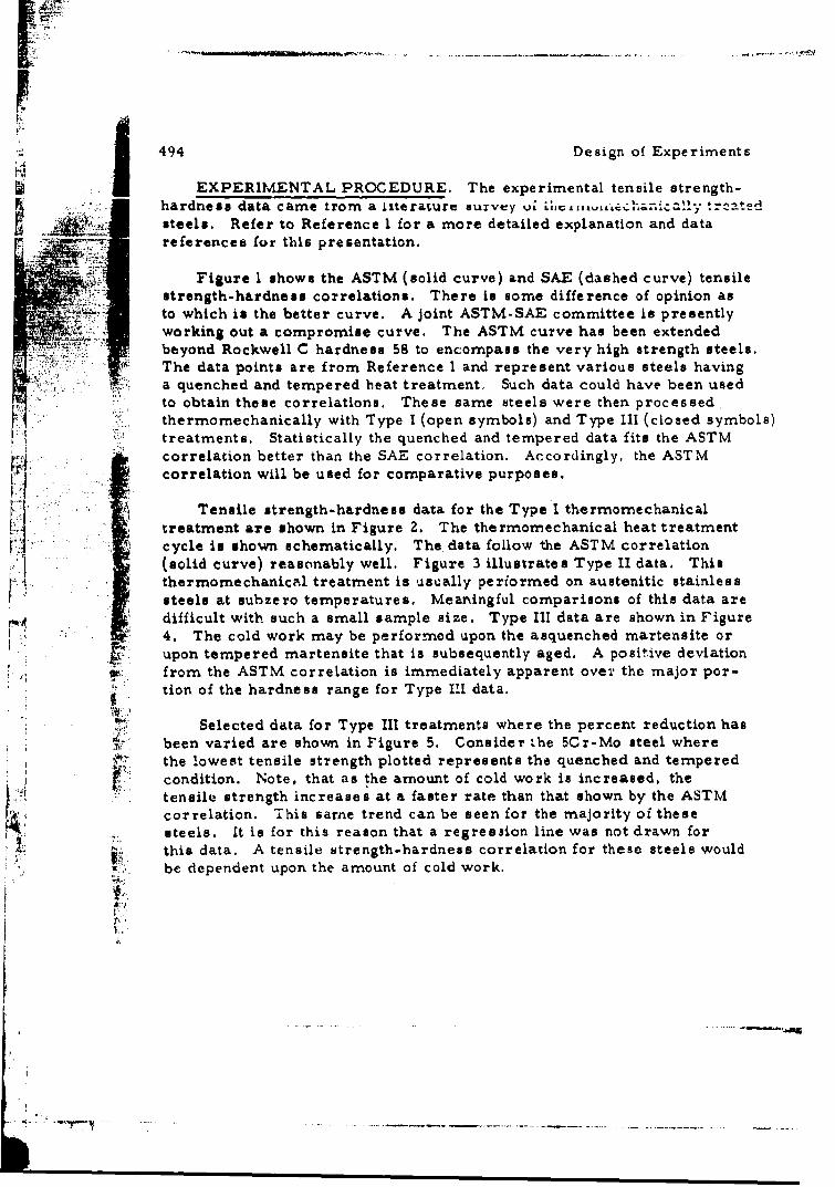
OT
3 494 Design of Experiments
S* EXPERIMENTAL PROCEDURE. The experimental tensile strength-hardness data came trom a Literature survey u iii . iCa.-: . ,2Lt^d
steels. Refer to Reference I for a more detailed explanation and dataS~references for this presentation.
Figure n shows the ASTM (solid curve) and SAE (dashed curve) tensile
strength-hardness correlations. There is some difference of opinion asto which is the better curve. A joint ASTM-SAE committee is presentlyworking out a compromise curve. The ASTM curve has been extendedbeyond Rockwell C hardness 58 to encompass the very high strength steels.The data points are from Reference 1 and represent various steels havinga quenched and tempered heat treatment, Such data could have been usedto obtain these correlations. These same steels were then processed.thermrnomechanically with Type I (open symbols) and Type III (closed symbols)treatments. Statistically the quenched and tempered data fits the ASTM
correlation better than the SAE correlation. Accordingly, the ASTMcorrelation will be used for comparative purposes.
Tensile strength-hardness data for the Type I thermomechanicaltreatment are shown in Figure 2. The thermomechanical heat treatment
N .cycle is shown schematically. The data follow the ASTM correlation
(solid curve) reasonably well. Figure 3 illustrates Type II data. Thisthermomechanical treatment is usually periormed on austenitic stainlesssteels at subzero temperatures. Meaningful comparisons of this data aredifficult with such a small sample size. Type III data are shown in Figure4. The cold work may be performed upon the asquenched martensite orupon tempered martensite that is subsequently aged. A positive deviationfrom the ASTM correlation is immediately apparent over the major por-tion of the hardness range for Type III data.
"Selected data for Type III treatments where the percent reduction hasS:' been varied are shown in Figure 5. Consider the 5Cr-Mo steel whereS•7 the lowest tensile strength plotted represents the quenched and tempered
condition. Note, that as the amount of cold work is increased, thetensile strength increases at a faster rate than that shown by the ASTM
IA correlation. This sarne trend can be seen for the majority of thesesteels. It is for this reason that a regression line was not drawn forthis data. A tensile strength-hardness correlation for these steels wouldbe dependent upon the amount of cold work.
|..... v- •..

Design of Experiments 495
DISCUSSION. Metallurgically the behavior was explained usingTabor's analysis [5] which relates hardness and tensile strength throughan additional parameter, tme strain hardening cpui.t z.. Thc ... 1.•is summarized in Figure 6. Quenched and tempered steels have strainhardening exponentb in the range from 0. 04 to 0.12, In this range thetensile strength-hardnes3 ratio is nearly constant. It is for this reasonthat a unique tensile strength-hardness correlation exists. For Type Itreatments the strain hardening exponents fall in the same range, there-
fore, the data fit the ASTM correlation. With Type III treatments theratio starts at the minimum and increases as the exponent decreases tonearly zero with increasing amounts of cold work. This results in posi-tive deviations from the ASTM correlation. Type II treatments areusually performed on austenitic stainless steels at subzero temperatures.
These steels have verl high exponents (0. 3) in the annealed condition whichdecrease to nearly zero with increasing amounts of deformation. Onewould expect positive deviations from the high and low exponents and
adherence to the correlation as the ratio passes through its minimum value.Cold-worked steel (Type III) and stainless steels (Type II) have beenexcluded from the ASTM correlation because of these drastic changesin strain hardening characteristics. [.
Statistical analysis of the data is summarized in Table I. Thedeviation d refers to the experimental tensile strength a" , minus thecorresponding tensile strength rASTM' from the ASTM correlation at a
particular hardness. This deviation was determined for every data pcint.The arithmetic mean of the deviations T-" was taken as the surn of
the deviations divided by the sample size. It serves as an indication ofhow well the data for thermomechanically treated steels fit the ASTMcorrelation. This value would be zero for a regression line of the data. tThe absolute deviation IT-r and the standard error of estimate Sy*•
were calculated as measures of the dispersion of the data about the ASTMcurve. These differ from the usually defined mean absolute deviationand standard error of estimate which measure the dispersion around aregression line,
__Statistical results are shown in Table II. The mean of the deviationsL(r , shows a better fit of the quenched and tempered data about the
ASTM rather than the SAE correlation. Further, the data for the Type Itreatment fit the ASTM correlation better than the Type III treatments.
IL

496 Design of Experiments
Also, the predominantly positive deviation of the Type III data from the
±k• . curve yield approximately the same results. They b not, however, reflect• •-'--• •the poaitive deviation of data for the Type Ill treatments.
The problem before the panel is that of offering more descriptive
statistical alternatives for comparing several populations of data (tensilestrength-hardneas values for thermomechanically treated steels) to agiven regression line (the standard ASTM tensile strength-hardnesscorrelation). Consider further that it may not be possible or meaningfulto draw a regression line through each population of data.
REFERENCES
1. E. B. Kula and A. A. Anctil, Tensile Strength-Hardness Relationships...in Thermomechanically Treated Steels, Proceedings, Am. Soc. Testing
Mat'ls, Vol, 64, 1964, p. 719
2. Methods and Definitions for Mechanical Testing of Steel Products,1965 Book of ASTM Standards, Part 1 (currently available as aseparate reprint)
3. Hardness Tests and Hardness Number Conversions - SAE J417, SAEHandbook, 1964, p, 94
4. S. V. Radcliffe and E. B, Kula, Deformation, Transformation and
Strength, Fundamentals of Deformation Processing, Syracuse=.5ý University Press, Syracuse, N. Y. , 1964, p. 321; also, E. B. Kula
-and S. V. Radcliffe, Thermomechanical Treatment of Steel, Journalof Metals, Vol. 16, 1963, p. 755,
5. D. Tabor, The Hardness of Metals, Oxford University Press,ILondon, 1951

, A
4()7
\0.
0 ~ 0
0 0i
0 09
II
Iin
in to IN uj.ao'4n
19M~ 41UJSatuioom

08 0 I0 w
0,0D 5c0 0I-
0 3a-A
0~ 0fcf
0
0 0~
IE:.
~j0 00
0 0 0 0 0 0 0 0
0 0f 0 0f 0 in oto P) N N--
1 4 4 8UGJIS ilasuaisol jwlim

00
00
0
00 ~o 1*-*00
o 0 00* -
0 0 Fn
60 0
o 00
0 00
0L) 0 U')00r -~ -C K

503
000 0
0Q~
00n
00~J
0
0 2C
0
K0 0
(5--
0 In Lai
0 fu
00 fn
----. 0 0 6 6
006
oo It 0 0 0
o~0 wn 0 L) I
to to -
q4uJcr_ sa ouJ~f

505
uiLOO
LI M ty• C.
40 in 000 h O 0 00 0 0 0 0U
00 0 on
A
'a __
In__ _ _ _ _ _
LM
=IiU)L tlI fl6 00 In 0
!s4t 446•{u aj•S s su s-L 9ol ti• N
i m i ii i m i- i i i--
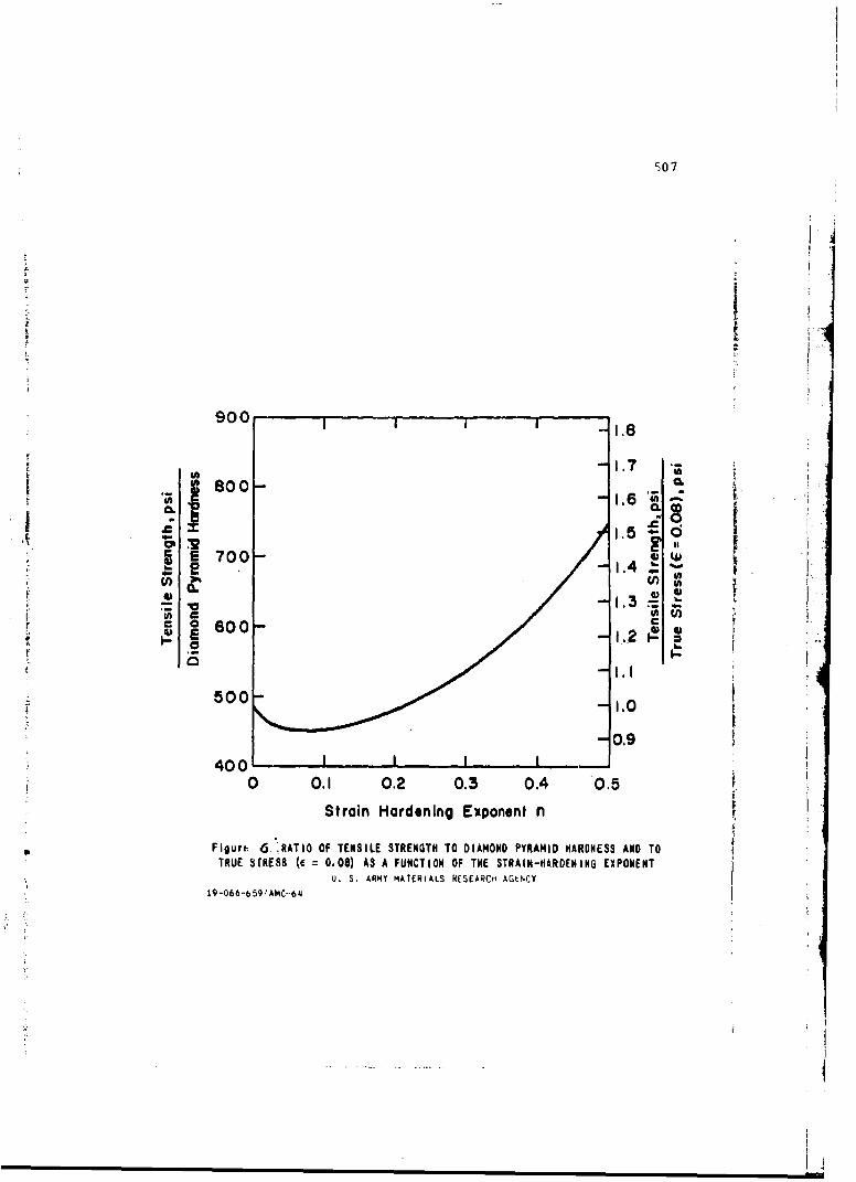
507
CL
-i
A r
900_
o1.3
•.• 600- - cz• =
500 -
-0.9400 1
0 0.1 0.2 0.3 0.4 0.5 0
Strain Hardening Exponent In
Figure 6 RATIO OF TENSILE STRENGTH TO DIAMOND PYRAMID HARDNESS AND TOTRUE sr0E0. (4 0.08) AS A FUNCTION OF THE STRAIN-HARDENING EXPONENT
pU, S. ARMY MATERIALS N(SEARCH AGENCY
t 9-066-6Q59!AHC-.6
.* I.2-0 .
500 .0

�O8
I 'T'�LL.. V �TA't1�T1CAI AhJAIVQIQ
I d =
&. L� d
n
(4)�I= .L�I�Isyc.
Table II. STATISTICAL RESULTS FOR QUENCHED ANDTEMPERED AND THERMONECHAN I CALLY TREATED STEELS
Type III' 11.00 17.2 20.8 176
a-

COMý%.IM NTS 0N PRESEN±TAT[II Bf ilbERiT A. ANCIiLL
Joan Raup RosenblattStatistical Engineering Laboratory
National Bureau of Standards, Gaithersburg, Maryland
The evaluation of empirical relations of the kind you discussed is adifficult problem. The various functions of deviations from the ASTMcurve that are presented in your Table II are extremely difficult to •}
interpret: By themselves, they are nearly meaningless. Taken togetherwith the data, as exhibited in your figures, they add very little and maybe misleading.
For example, looking at Figure 1, I notice that the steels used inType I and Type III thermomechanical treatments respectively seem tobe grouped preponderantly in different hardness ranges. Is it possible -that the ASTM curve fits better for Type I and the SAE curve for TypeIII? If this were so, an explanation would have to be sought in the 3metallurgical facts about the data used, and in the history of the twostandard curves.
Table II gives overall measures of goodness-of-fit. Since these arewell-defined functions of the data, they cannot be "wrong" in themselves.But if the deviations from the standard curves occur for different reasonsif different types of steels and in different hardness ranges, the overallmeasures cannot be relied upon to describe the uncertainty of tensilestrength estimates derived (using the curves) from hardness measure-ments. Furthermore, if the overall measures are used to select the"best-fitted" curve, there is great danger that the resulting curve willhave systematic errors arising from the particular choice of data.
Of course, for many purposes a standard curve is entirely adequate.But your data seem to make it clear that one possible long-run goal wouldbe the development of a collection of curves each applicable to specificcircumstances. This development would probably require the perform-ance of mnany new experiments. It could lead to the evolution of yourqualitative explanation of the behavior of thermomechanically treatedsteels into a quantitative explanation.
The statistical measures quite properly play a very small role inyour valuable summary of the published evidence on tensile-strength/
I.

hardness relationships. I am sure that in future studies you will continueto be guided by the totality of scientific information available to you, and
I hope you will often find that statistical techniques are helpful in data[ ~anal ys is.
Ai
i i
IiI
Ka

SOME PROBLEMS IN STA'i ISTICAL INFERENCE FOR(~t'Nlr 0 A IT 17rM %AITT r %Tr'%1 k TAT A r% T T A `T'TnN.T4
Bernard HarrisMathematics Research Center, U. S. Army
University of Wisconsin, Madison, Wisconsin
INTRODUCTION. Assume that a random sample of size N has beendrawn from a "multinomial population" with an unknown and possiblycountabie infinite number of classes. That is, if X. is the ith observa-tion and M. the jth class, then .
P{X. M.}= pj > 0, j 1, 2, ... ; i -,2..., N
co
and Z pi 1. The classes are not assumed to have a natural ordering.
Let nr be the number of classes occurring exactly r times in the sample.
Then, we clearly have
- rn rN.
Vv e will be concerned with estimating the following two quantities
which are generally of interest to experimenters.
(1) The sample coverage, defined by
(1) C = pi
where the sum runs over all classes which have occurred at least once
in the sample. 4.
(2) The population entropy, defined by
(H - - P logp ii=l
~i.

512 Design of Fxperiments
It will be convenient in our definition of entropy to violate the usual conven-tions and use natural logarithms rather than logarithms to base 2. This isequivalent to a scale change in units of measurement and will have noessential effect on any uses for which the entropy might be employed. Ofcourse, we will assume throughout, that the series (2) converges, sincotherwise the discussion will not be relevant.
of the pits are too small, small sample infercnce appears to be virtually
S hopeless, hence, all results described herein will be asymptotic results,i.e. for large N.
Estimation of H and C. For the moment, we will restrict to the case:. •oi an ordinary multinomi~al population, that is, one with a finite number,
k, of classes. Then the 'natural estimator" of entropy H is defined by
N in. n. klog\ log4(3) 11 E -f log p = i Pi
i=l N NIi- l
where j. is the maximum likelihood estimator of p
Its properties has been discussed by G. P. Basharin (1] and we notethem briefly. Basharin showed that
(4) r ) -k-I 2(4 + O(N"
and
(1 2k 2 2 -[Pi log Pi" H + 0(N')I
and F-N(- H) is asymptotically normally distributed. If we attemptto apply Basharin's results to the more general case described earlier,it is easily seen that the naive replacement of pi by Pi in (2) may not
Ibe successful. Essentially, Basharin's technique depends on the followingsort of asymptotic behaviour,

Design of Expcrinients
as N -- , Np. i z 1, . k
Consequently, if we have zero as a limit point of the pi's, or even, if
we have the limiting behaviour associ:t'4-, 'Vith the Poisson approximation,
).s N - p, p. -0, Npi - X. 0 < <
for a sufficiently large number of classes, then Basharin's estimator,H, may be quite poor. The following illustration will exhibit this. Let
P i = 1,Z,....N Then H = 2 log N. However, since the maxi-i 1,12
mun of II occurs for pi = - , when there are k classes, we have thatk
H < log N. Hence, it is quite clear, that if there are "too many classeswhose probabilities are too small", H will not be a satisfactory estimator.One of the causes of the difficulty is that H gives no weight to unobserved
Acells, so that if the total probability in unobserved cells is large, H willnot perform too well.
We can gain some insight in dealing with this, if we examine thesecond question we advanced, the estimation of the sample coverage.This problem is discussed in greater detail in B, Harris [3] , but it isconvenient at this Lime to make some intuitive observations concerning theestimation of C, so that we can resolve the difficulties noted above in theestimation of H.
First, note that if we were to proceed as Basharin did and set
A AC p i
then we have that C = I for all samples, which is clearly inappropriate.We can guide our intuition by first examining some extreme cases.
(1) If nI N, then we readily reach the conclusion that C must besmall, We can see this as follows. If we now take another observation,inasmuch as every past observatiorn resulted in a new class being observed,it is apparent that with probability quite close to unity, the N+lth observa-tion will also result in a new class. In fact, the probability that theN+lth observation will not result in a new class is C, which of courseshould be near 0, as noted.

514 Design of Experiments
(2) If, on the other hand, there is an integer t, substantiallh largerthan one, such that n 1 = n2 n . tl x 0, nt > 0. Then, similar
reasoning would lead us to conclude that most of the probability isconcentrated in classes with high probability, and therefore C shouldbe near unity.
()1 - " he •>Ne -
(3) Let pi i 1,2,...,N. 1Then E(nl) and E(n 0 ,)Ne
Thus, we should have C-1 - e
In short, as is shown in B. Harris [3] , it is the low order occupancynumbers, such as nV, n 2 , and n 3, which contain the principal information
concerning the probability content of unobserved classes. A cursoryexamination of the three examples cited above suggest that an appropriateestimator for C is given by
ni(6) I
In Harris [3] , it is shown that C is in iact an suitable estimator, inthat it has good asymptotic properties.
In E. B. Cobb and B. Harris [2) , a method for estimating entropy,when "all the sample information is contained in the low order occupancynumbers" was exhibited. In order to do this, we will show that we canrepresent entropy asymptotically by
(7) H E(n) e log dF,:(x)
where
(8) F"':(x) ; Npje'Np/ 2 NpjeNpNp.<x i / j =I
It is easily verified that F'l'(x) is a cumulative distribution function.Since

I ÷_
Design of Experiments 41
(9) E(nE) j e
j1 l
substitution of (8) and (9) into (7) produces
1w Np. 1 Np,. e log (-)Np.e "N L p log p HN=l N j=l
which verifies (7),
Under the assumptions stated above Cobb and Harris [3] suggestedthat the entropy be estimated by
n1 (N-mr1 ) (Nm- m 2 )/AN-m,) N(N-•m)%110) H 2 e- log[,Nm ~mz(0) H N (N-ml) 2 + (m-ml2) e
where mi = 2n./nI and m2 a max (m1 , 6n 3 /n 1 ).
I At this point it is worthwhile to present a numerical example, which
will illustrate the behavior of H,
Example p 1 2,., N Then n' n T- e - and
e N N-a.d m I andn"T eThus, mn •, m2• an
F *X o x < I
•: Then
The Ne"I (N-i)e (N-I)/(N-1) log N(N-l)H! -•,N (N-1) zN1
and H -log N, which is as it should be.
and H log , N (N-I) N-I log

f 516 Design of Experiments
Clearly, it is principally the classes with small probabilities that
contribute to non 1 ,n 2 , and n3 . For those classes with large probabilities,
we can estimate p, by P.
Then, the natural way of proceeding is to estimate the contributionto entropy from large classes by means of Basharin's method and the
contribution of small classes by H, and we denote the final estimator by
H*. Recall that in order to use H, we have taken n1 ,n?, and n3 to deter-
mine H.
There is one last detail which must be taken into account, Part ofthe contribution to moderate order occupancy numbers, such as n4 , n5 ,
and some of the succeeding occupancy numbers, will be due to classeswith small probabilities and the effect of sample fluctuations. There-fore, we need to examine the following. 'What proportion of eachn j o = 4 5, ... is, some sufficiently large integer, is due to a large
deviation from a class with small probability? We can adopt a Theoremdue to A. Wald (41 obtaining the following inequalities.
7k- )k-l6(3k n
'(11) if m2 > in, E(n>+k)3 k-2.• kl -(k+l)1 n 2
2 k n k
(12) if m 2 m1 , E(n - 2 k 3,4,..k..- n, (k+l)!
The right hand side of each inequality gives the expected values of" n k+], if "the sample information is contained in nI, n 2, and n 3 ". Thus
the difference between the left and right hand sides of (11) and (12) givesan estimate of the contribution to nk+l which is due to classes with larger
probabilities. We apply Basharin's estimator (3) to these, upon replacingthe expected values in the left hand sides of (11) and (12) by the observedvalues.

I .' 5' ~ I. ILj~,(,t. ~517
Ti'hu. we finajil% write
-where 0 <X <1I is the proportion of the observations in n ,n, 411: n,
and the parts of n , n ,.,, A dcetinined by (11) and (1.2). For thc4 S
parts of the sariple allocated týD sinall clatsses as notedi above we use V,and use H- on the part allocated to Jargc ciasscs.
T he- nmatheinatic al cketail-, will bc, (liven in a later ouolica.t~io-..
REFERENCES
i]Basharin, G. P. (19 59) On a statistical estimate for the entropy ofa sequence of indcpený.ent ranc~or variables. Te~orija Vcrojatnostei
i ce Prirneniija, 3~33-336.
(2 CobE.B n.HriB naypoi oe on o h
trop W ofd A. is9)remte pofulatiostribthoap funcation to heestcinmatiby
tr ansactions ?of thei Annrianso Matheiatical Socniety, 4, W8,36
absolute vioo~unis and inequalities aatisfleO by absclute imome'nts. 0
Trnatoso h mrcnMteaia oSt,4,2036

APPLICATION OF NUMERICAL, TECHNIQUESI
EXPERIMENTALLY ViODEL AN AERODYNAMIC FUNCTION':' *
Andrew H. Jenkins•-, ~Physical Sciences Laboratory, Directorate of Research and Developnment i.x
U. S. Army Missile Command, Redstone Arsenal, Alabama
ABSTRACT, This report describes the use of an aeroballistic rangein the design and execution of an aerodynamic experiment, the analysisof the experimental data by numerical techniques to develop a model of aphysical function, and the statistical testing of the data and the model.The report discusses the approach, the experimental design, and the
. testing of the data using several frequency distributions, It presents anddescribes a multivariate nonlinear regression analysis performed on thedata, the physical model developed by the regression analysis, and the
9 testing of the model. It also lists and presents the tests of hypothesesmade and discusses the results of the tests.
SYMBOLS
a Acoustic velocity in air
A Pure constant of regression equation
b First coefficient of regression equation
C Counts per inch of photoreader = 3502
c Second coefficicnt of regression equation
c Coefficient of specific heat at constant pressurecp
C Coefficient c,,- specific heat at constant volumev
d. f. Statistical degrees ot freedomi
F Frequency distribution
* F Magnification factor of shadowgraph = 1. 009sh
F Magnification factor of Schlieren = 0. 855
K Ratio of shock density ps to free stream density p'
SIn Natural logarithm (base e)
))tThis article was initially issued as U. S, Army Missile Command Report
No. RR-TR-65-11.
t,
i i i i m i m

I
520 Design of Experiments
SYMBOLS (continued)
M Mach number = V/a
NIL Mach factor level = 1,1 to 1. 5
NI Mach factor level = 2. 5 to 2. 9
M Mach factor level = 3.9 to 4. 33
M. Mach factor effect in statistical equation1
M Mach factor linear effect
Mq Mach factor quadratic effect
MR.. Main faitor interaction effect
N Total observation
P Statistical probability
2 Regression correlation coefficient
R Universal gas constant. = 1715 sq. ft/sq. sec./°R.
R RadiusR Model nose/base radius ratio = 1. 0
t R Model nose/base radius ratio 1 ;, 7
R Model nose/base radius ratio = 0, 43
HR Model base radius = 0,11Z inch
R , Radius factor effect in statistical equationJ
" Rrn Nose radius of model
RI Rr Model nuse to base radius ratio
Radius factor linear effect
I" Rq Radius factor quadratic effect
S Surface roughness of model
" S2 'Exr)criniemtal sanmple variance
S 1:;: :J)crimVtIII baIIap)le standaIrd d eviation

6.4
Design of Experiments 521
7 :SYM13OLS (continued)
SS Sum of squares
J1. t Value of students frequency distribution &.0
T Absolute temperature (*Rankine) .
V Flight model velocity } I...X Mean
Xaw Mean of Ambrosio-Wortrnan model
X Mean of experimental responses
X. ith response
Xr Mean of regression model responses
X?, 3 Dependent variable of regression equation (computer language)
Y Independent variable of regression equation (computerlanguage)
Z Normal frequency distribution
Q •Type I error risk level
Type Il error risk level
4; 7Ratio of specific heats = Cp/C.'p hv
6 Shock detachment distance from Shadowgraph optical systemsh
5 Shock detachment distance from Schlieren optical systemnsc
A Shock detachment distance in photoreader counts (corrected)
,'k(ij) Experimental error
Ze Variance of experimental responsesZ• Variance of regression modelr
7 ¢wVariance of Arnbrosio-Wortman model
Universal means
• •Frequency distribution•.P Density
friq~i::•:•".:i;*

522 Design of Experiments
1. INTRODUCTION. A number of new aerodynamic problems havecome into prominence in recent years. The source of the problems hasbeen the very high flight velocities achieved by use of rockets. Thecharacteristics of the problems of the very high flight velocities, referredto as supersonic or hypersonic flight, are those of a hydrodynamic nature.The Mach numbers are high and problems of a physical and chemicalnature also exist because the energy of the flow is large. The gases arerarefied so that the mean free path is not negligibly small compared withan appropriate macroscopic scale of the flow field. Under such condi-tions, kinetic thoery is included with the hydrodynamics.
The new features of a hydrodynamic nature allow the use of certainsimplifying assumptions in developing theories for hypersonic flow. Onthe other hand, certain important featuras which appear introduce addi-tional complications over those rnet within gas dynamics at more mod-erate speeds. The techniques of linearization of the flow equations andthe use of mean-surface approximation for boundary conditions have adiminishing range of applicability. Also, entropy gradients produced bycurved shock waves make the classical isentropic irrotational approachinapplicable.
The additional problems of a physical and/or chemical nature areassociated with the high temperatures of the flow as the gases traversethe strong bow shock wave, The sudden shock heating of the gasesexcites the vibrational degrees of freedom of the molecules resulting indissociation of the species into atoms, electrons, and ions which do notrequire treatment at lower velocities. Therefore, it must be recognizedthat physical phenomena rather than hydrodynamic phenomena may notonly influence the flow but in many cases control it. In view of thecomplexities of the flow at high Mach numbers and the number of technicaldisciplines involved, many have resorted to experimental or empiricaldevelopment of functional relationships.
The flow field originates at the bow shock. The shock wave charac-teristics are very important to the stagnation region characteristics.The volume of the stagnation region is dependent on the shock deta'.hmentdistance. Therefore, much of the knowledge of the flow characteristicsis dependent on the knowledge of the shock location. Experiments havebeen performed on wind tunnels to study the shock location. However,few experiments have been made to study this problem under free flight

Design of Experiments 523
conditions. Also, the studies which have been made and the derivedk' relationships are lacking as tests have not been attempted to determine
their reliability. -
V; It is apparent that the community recognizes the need for improvedhypersonic design theory. One of the important areas is the predictionof shock detachment distance. It is important to the computation of notonly heat transfer but also pressure distributions and drag on the fore-
part of the vehicle, This has been pointed out by Serbin (1] , Ambrosioand Wortman [2] , DiDonato and Zondek [31 , Heberle, Wood, andGooderum [4] , and Love [5]
The lack of purely theoretical models for the prediction of shock
detachment distance at transonic and supersonic velocities has led to thenatural consequence of an experimental approach. This is to be expectedand in addition the theoretical hypothesis is inevitable subject to exper-
imental verification. For this reason, one can also expect to contributeto scientific progress by the inverted approach of formulating models ofthe mathematical relationships between physical variables by experimen-
t, tation. However, the relationships derived are subject to experimentalcontrol, measurement accuracy, human error, and many other sourresof unexplained or unaccounted for deviations from the true universalrelationships.
In the direct approach (i. e. , the a priori derivation of a mathernati-
cal model ) quite often ideal physical conditions are assumed and simplify-ing mathematical assumptions are made which depart from the real case,Therefore, one cannot be sure of the theory nor can one be certain of the
experimental data, Yet, in scientific endeavor, exacting conclu.•ions are I
often drawn by the comparison of an idealized hypothesis and real case
data. That is, both quantities are coupled to each other and not to an•. ~independent estimate of the deviation present, •,
Empirical models of the shock detachment distance for blunt bodies
of revolution have been made by Serbin I]1 , Ambrosio and Wortman [2"1and Heberle, Wood, and Gooderum [4] . The data were obtained by thu, c
authors using moving streams oi air surrounding stationary spheres(i. e. , radius nosed bodies) in such experimental devices as wind tunnelsand jet nozzles. Both of these devices have two common disadvantages.
* The gaseous medium is in a state of expansion just prior to the shock
J

524 Design of E.Iperirnnt
compression. Also, holding devices are present in the flow around thebody which cause perturbations in the flow. The flow is often not uniformin cross section. The measurements, therefore, include these perturba-tions and do not represent the real case of a vehicle in free flight,
Serbin [I] derived the following relationship for a sphere:
(1) R 2/3 (K-1)
Ambrosio and Wortman derived the following relationship:
(2) 0 , 14 3e34/M
4{ and Heberle, Wood, and Gooderum derived this relationship:
(3) = 4/3 (M - 1)"/3
Each author stated that agreement between the model and the datawas very satisfactory. However, the standard by which this was deter-mine was not stated or explained. This type of unexplained, seemingly
arbitrary, acceptance of a model and data appeared to be typical,
A machine literature search was made, In this search, over190, UO documents were screened and matched by computer on the basisof key words and terms in aerodynamics and statistics. This was doneto determine if, in the past, any use of statistics in testing aerodynamicexperimental data had been done. Not one document was found duringthe search. However, this is not to imply that statistics have not beenused. Apparently, it is either not a prevalent or accepted practice orpossibly has not been reported.
Ambrosio and Wortrnan [6] did attempt the use of some simpiestatistical methods. This was done to the extent o' computing the mean,the absolute nican, and the standard deviation. However, it was not forthe purpose of testing the reliability of their data and model but to objec-tively establish the relative worth of their model as compared to Serbin[l]

Design of Experiments 525
This work has two objectives as follows:
I) To develop an empirical model of shock oetachnrient distance asa lunction of Mach number and vehicle nose radius with experimentaldata obtained under free flight conditions
2) I'o subject this model and data to analysis by statistical eucthodsto objectively define the level of confidence of such a model.
II. EXPERIMENTAL PROCEDURES.
1. Design csa
The shock detachment distance can be described aerodynamicallyfor radius nosed bodies of revolution as: 1'
SI.(4) (M)
Explicit models of several investigators were mentioned in the introduc-
tion.
Statistically, the model can be expressed as:
(5) 4 M, +R -MR,, +Ei.).1 + k(ij)1
The model contains two independent factors, Mach number (Ma) and body 1r '1"
radius (Rj). It also contains a second order effect, the MRij interaction.
The design of the experiment required consideration of both the aero-dvnaniic and the 3tatistical aspects. Past experience indicated that theshock detachment distance was a nonlinear function of Mach number (M)and a linear function of radius (R) The objectives of the experiment areto determine if the linear and quadratic effects of Mach number and ra-dius contribute significantly to the shock detachment distance. Also,it was desired to determine if a second order or interaction effect be-tween radius and Mach number contributes significantly to the shock
location. The analysis of variance is a useful tool for this. In addition,it was also desired to develop an empirical model of the functional re-lationships between the independent and cependent variables. A regres-sion analysis was planned for this,
I,:
F.. . . .. .w . . . . . .

5Z6 Design of Experiments
The analysis of data by regression calculation can be simplified bythe equal spacing of the independent variables which permits the use oforthogonal polynomials. This helps also in the subsequent adjustmentarising from the discarding of insignificant variables or the addition ofnew terms. One objective of the experiment is to estimate the slope ofthe regression, The slope of a -egression is estimated more preciselyif the values of the independent variables are selected with equal spacingat the extremes of the quantified ranges of the variable. This is becauseinterpolation is more reliable than extrapolation and the computationsare simplified.
The effects of the main factors in this experiment could not beconsidered theoretically independent. Therefore, it is necessary to rep-licate the experiment within cells of all factor levels in order to testfor interactions between factors and to estimate the experimental error.Since one objective is to statistically test for interaction, the analysisof variance will enable the test of interaction and estimates of errorvariance. The two best tests for statistical analysis of the aerodynamicexperiment are the analysis of variance and the multivariate regreosion
analysis. The experimental design most efficient for these methods isthe factorial experiment with replication.
The factorial experiment enables one to test the effects of Machnumber (M) and radius (R) on the shock location (a) over the ranges ofinterest of M and R at each factor level. It also promotes testing forthe existence of interaction between M and R and the effect of interac-tion on A. One is also able to differentiate interaction effects frommain effects. In addition, it allows the determination of confidencelimits for the estimates of main and interaction effects based on theestimate of experimental error derived from replication.
•-- 32Therefore, the experiment was designed as a fixed model 3 fac-
torial. Both the radius and Mach number factors are equispaced threeSlevel, fixed and quantitative. The Mach number range of interest was
1.0 to 4. 5. The levels selected were M. = 1.1 to 1. 5, M 2 = Z, 5 to 2. 9,and M = 3. 9 to 4.3. The radii selecteJ were nose to ba~se radius ratiosof R = 1. 0, R = 0.7, and R z 0.4. The experiment was replicatedthree times in each factor cell; therefore, a total of 27 observations
was recorded (N 3 x 3 x 3 27).

All 27 responses could not be obtainec. in I 6av. Therefore. tocompensate for day-to-day variations in personnel, voltages, Qevelo.-
ing solutions, film batches. ana printing, the firing sequence wasrandomized. All combinations of Eactors and replicates were listed an.-:
the experimental sequence was ranomizec, by use of a ranoom number
generator (71 which was entered in a ranc~om manner. The results of the4randomization are shown in Table I. The numbers shown without par-entheses are the sequence of firing while the numbers in parenthesesare the corresponding round identification numbers, Table I also showsthe factor levels selected for the experiment.
Table I. Randomized Experimental Sequence
Mach Number Levels
Nose/Base M-Radius NlMM3 i .],,
Ratio Replicate 1.1 to 1. 5 2. 5 to 2.9 3.9 to 4.3
1 26 (75) 7 (56) 11 (60)
1:1'.O 2 22 (71) 8 (57) 6 (5',.)
3 2 (49) 14 (63) 10 (59)
1 12 (61) 13 (62) 9 (58)
R? 0. 7 Z Z3 (72) 27 (76) 25 (14)
3 24 (73) 18 (67) 15 (6,.)
1 16 (65) 3 (50) 19 (68)
R:0,4 2 1 (48) 17 (66) 5 (53)3
3 4 (52) 20 (69) 21 (70)
Note s: I1. Numbers without parentheses are randomly determined
prograr._ firing sequence.
2. Numbers with parentheses are for experiment identification.
I4

528 Design of Experiments
The radii of the models are discrete levels, The Mach numberlevels are discrete intervals as it is almost impossible to duplicateexact velocities by this method of experiment. This is due to variationsin propellants, model material homogeneity, and model-launch tubeinterference. The Mach number levels chosen were fixed in selectedranges between Mach 1. 0 and 4. 5 which is the velocity regime of interestin this aerodynamic study. As a two factor fixed model experiment, itis assumed that ýL is a fixed constant and the Ek(ij)'s are normallyand independently distributed with a zero mean.
2. Procedure
The experimental data were obtained on the Physical SciencesLaboratory's free flight aeroballistic range. Figure 1 shows the ex-perimental apparatus. It consists of a light gas gun for launching themodels, and altitude simulation chamber, a shadowgraph and a Schlierensystem for photographing the model and the flow around the model.Also, submicrosecond electronic counters to determine the model'stime of flight are included,
The aerodynamic data required from this experiment are the radiusof the model, the Mach number of the model, and the detachment dis-tance of the shock. The radius of each model was known as the modelswere formed in accurately machined dies, Their geometries are shownin Figure 2. The models were made of copper coated lead. The Machnumber. is determined by taking the ratio of the model velocity to theacoustic velocity when the photographs are made. The acoustic velocityis computed as shown in Appendix A. It is seen that the acoustic velo-city varies as the square root of the temperature and specific heatratio. The temperature was recorded at the time of launching eachmodel. The specific heat ratio was taken as 1. 4. The model velocitywas computed by taking the ratio of the distance between the shadow-graph and Schlieren stations to the time recorded on the counter. Thedistance between the shadowgraph and Schlieren stations is a constantof 5 feet. It was assumed that the deceleration of the model over 5 feetwas linear; therefore, the velocity computed wao the velocity of themodel midpoint between the two stations.
Photographs of the model showing the shock detachment distance'were taken by both the shadowgraph and Schlieren systems The mea-sure of the shock detachment distance from either one of these photos

529
ii~ F
iii
III :• n
.' . K
11 I. ,
I -O-h Lii "'
, -i
EU I.
. I .
K,,

530
Ito$
*edius~w out0
01470
tjR1 ' 0.4
K Figure 2. Sketch of Experim~ental Flight Miodels

Design of Experiments 531
as•umption of lincarity, the shuck detachment distance was corrected
to the velocity computation. The correction of the detachment distancerequired the consideration of the magnification factors for the photo-graphs. The magnification factor for the shadowgraph camera was1. 009 and the Schlieren camera was 0. 855. The photo reader uponwhich the negatives were read was calibrated at 3502 electronic countsper inch in the plane of the negative on the photo reader, The shockdetachment distance was read in counts from both the shadowgraph andSchlieren negatives. The detachment distance and radius of each typemodel was corrected to counts as follows:
(6) F= h F + 6 Fsh sc sc sh
and
(7) R ZxCxR b xF h xF scxR r
The values of A and R computed for each round are shown in Table If. 6A sketch of a typical shock detachment distance as taken by the shadow-graph and Schlieren is shown in Figure 3.
The experimental data obtained from the experimental programare compiled in Table 11. The data are tabulated and identified by theround number assigned on the aeroballistic range. Computations ofcertain data presented in Table II are shown in Appendix.A. The datafrom round number 75 were used to show a typical example of thecomputational procedures.
II

532
1 I,
/0 09ooL IN FLIGOT
SUPERSIONIC
I VliTy Vl[ITOR
F r3SU3cSOMIc h T SklON? ' •-- IONIC L.INESl
Figure 3. Sketch of• Typical Shock D,,%tachrnent

533
O~N4 ~N~ c;- 6 N o 0 . 4 0 - O C
2 t t 9 9 t -9O -NNNNA
_ _ 0' rb It I lo _9 _
Io z
d-.o add -14- o~ o i
~ 2 N 4 9
4 3 NN .*3 92

534 Design of Experiments
11. ANALYSES. The cata obtainec Irom Lhe iepvrei,• •I MAsented in Table II. The observations taken as the dimensionless ratioof the standoff distance divided by the model radius are presented in thefactorial design layout in Table ill along with some computations inpreparation for performing an analysis of variance. The statisticalcomputations are presented in Appendix B.
The gathering of the data, the analysis, and derivation of the model.of the functional relationships from the experimental observations areoased on certain aerodynamic and statistical assumptions. Theseassumptions are:
1) Small angles of attack of the models (i.e. less than V°) do notsignificantly effect the detachment distance.
2) The models were free from ablation products in the stagnationregion.
3) The effects of gas constituent dissociation on the dynamics offlow was insignificant.
4) The effects of spin stabilization on the dynamics of flow wasinsignificant.
5) The effect of the conical section of two of the models on thedynamics of the flow was insignificant (i.e. , all projectiles were hem-ispheres of various radii).
AI• 6) The experimental error is normally and independently distrib-K! uted.
7) The experimental precision is essentially the same for allt: factor combinations,
8) The factors were fixed at discrete levels so, therefore, arenot independent of each other.
Assumptions I through 5 are made concerning the aerodynamics ofthe experiment. These represent sources of variation which are con-sidered regligible. They cannot be separated explicitly from the main
†††††††††††††††††††††††††††††††††††††††††††††††††††††††††††††††

i
535
Table. II Data Layout for Shock Detachment Experiment
Mach Number Region
M M M Ex
1.049 0. 146 0.223
R, 1.0 1.492 0. 146 0.139 4.810 0.5344
1.286 0. 189 0.140
3.827 0.481 0.502
1.461 0.268 0.182
R.a 0.? 5.478 0. 188 0.179 10, 135 .1.126
1.921 0. 253 0.205 K8.860 0.709 o.566 I.
1.034 0.225 0.203
R3- 0.4 2.243 0.280 0.210 6.469 0.719• .
1.736 0.321 0.217
5.013 0.826 0.630
E 1 17.700 2.016 1.698 EX.. , 21.414
1.967 0.244 0.189 0. • 0.793
ME!. • 50.7464
- -- ... - . .. . ...- -

536 Design of Experiments
. •and interaction effects. It is important to note that, even though con-
6idered negligible, these variations are present and are rtatisticallyS......accounted for by summation into experimental error. The statistical
assumptions 6 through 8 allude to these conditions.
1. Analysis of Variance
The experiment was described in Section II by the statisticalmodel
(8) A= 1 . +M + R + MR + k(ij)
The theoretical model underlying the analysis of variance assumes that
each experimental response of the shock detachment distance (a) is thealgebraic sum of,
sao 1) An overall mean of the detachment distance, it (i.e. true
,standoff distance)
2) A Mach number effect on the standoff distance, M
3) A radius effect on the standoff distance,R
"4) An interaction effect on the standoff distance, MR.i
. 5) A random residual error (experimental), o
Since the model is a fixed model, none of the effects can be meatsuredabsolutely. They can be measured only as differential deviations, i.e..,the Mi as deviations from F., the Rj as deviations from sL, and the MRijas deviations from Mi + Rj.
4 The results of the analysis of variance are shown in Table IV. TheI,.computations are presented in Appendix B.
From Table IV, it can be seen that the main effects of radius haveapparently no significant effect on the shock detachment distance at the95 percent level of confidence. The linear and quadratic effects arealso insignificant. The quadratic effects of radius seem to have themost effect on the standoff distance. They would be significant at the80 percent level of confidence though still not significant at the 95 per-cent level.

537
.A * 0r17�i .. -
- .� A,
.1
A,[ v�: �
� £ S S
V 4w V.1km ,.W,,� V V
A, - - - -if'----U� V 1' A, 1� 1' *� V 1* 1' �
4.4. .�1
� i �'1 - - - N - -.1
3- -g - �
'4' .� - 3-ow- $ 4.j N p.I- -
0 5. 0
� - _________ -
- � p
41 j... d .4 ii 'ii d 14
S .40
114 p1 Al
t - - - - - - - -
N N 4 0 4
- N
'a.
I
JJ �K-.r� N(j �r� 5 f
a...�.K 4n.4
-' -. -, -. '.- - -" ,W fl.I *Js�.,c .

538 Cby1 I1AAjThe Mach number in significant at the 95 percent level of confidence.
The computed value in the F test is greater than the F distributiontable value by a factor of about 5. The linear and quadratic effects arealso significant. The linear effect of the Mach number fact•,r wasfound to be more significant than the quadratic effect.
. ,The analysis of variance also shows that there io apparently no
significant effect of the MRij interaction on the standoff distance. It isinteresting to note, however, that of all the combinations of linear andquadratic interactions between Mach numbers and radi s, the quadraticradius and linear Mach number were nmost nearly significant at the 95percent lev-1 of confidence. This is congruent with the fact that the
V test of the quadratic effects of radiius and the linear effects of Machnumber 'was highest in the main effects tests, Under the interactioneffects tests, the computed value of 3. '59 for the RqM1 combinationwould be significant at the 92 percent level as comparec to 4.41 for theF value at the 95 percent level.-
It is also noted in Table IV that the mean square for radius andS~~radius-Mvach number interactiuns were only slightly higher than the
mean square for error. On the basis of the assumption that the exper-imental error is normally distributed between all factors and all levels,then radius and interaction effects do not significantly contribute toshock detachment distance within the limits of this experiment.
The results of the analysis of variance, as shown in Table IV, iafurther analyzed as shown in Figure 4. Figure 4 ii the graphic displayof the results of the Duncar. range tests as computed in Appiendix 5.Figure4(a), for the Mach number range signi.h-ance test, shows thatthe Ml level (1.1 to 1.5) is significantly different irom the M1 and M 3levels of 2. 5 to 2.9 and 3.9 to 4. 3, respectively'. The M 2 and M 3levels were not found to be significantly different from each other. Theradius factor range test as shown in Figure 4(b) shows the ridius factorlevels not significantly different from each other. The fact that the M2and M 3 levels are not significantly differerL. from each other will bediscussed later in this section.
2. Regression Analysis
The analysis of variance can be performed whether the iactorsare quantitative or qualitative. Khen the factctrs are quantitative, then
- .* **.... . ---. r*.. .... .--

II
MACH NO. LEVELI
0.109 0,224 .6
(a) MACH NUMBER RANGE SIGNIFICANCE TEST
RADIUS TREATMENT
0.534 0,719 ilia$i
(b) RADIUS RANGE SIGNIFICANCE TEST
(COMMONLY UNDERLINtO MEANS ARE NOT SIGNIFICANTLY DIFFERENTAND COULD HIAVE COME FROM A COMMON POPULATION)
Figure 4. Graphic Display of Duncan Rang. Tests

540 Design oi ExperiiTnents
i zn~v i1alyai #-q )r% n 1rfnrneci rn the data. Trhis analysis is
espeialy uefu inthe determination of the general functional relation-Lhips of the factors ~at other than the experimentally assigned, levels.The analysis of variance has led to knowledge of the important factorconsidered in this experiment which contributes to the shock detach-
-~ ~ ment dtstance. This was found to he the linear and. quadratic effects ofMa'-h number. This led to a bivariate regression analysiks. The regre6-slon anclysis used was the SNAP Multiple Regression Artakysis for the. BIM 7090 computer. !t was the Army Missile Gomir~ian' SIARE 183programA
An pointed out, it is realized that the ishock detachment distanceisa n.-t singularly a function of Mach number. There are other factorswhich were roct included in this experiment. For the factors consideredby the analysis of variance, some knowledge of the main significantfactor (Mach number) is now available.
Before progressing with the regression analysis, the physicalaspect~s of the shork detachment distance must be considered. Thefa.nction4LI relationship must b~e consistent with the aerodynamic concepts
4'of the det~achment distance. The detachment distance is inversely propor-¾ tional to Mat-h nuinber. Thk~t is-
.:f~
The limits of the functional relationships are then
lirnf(.~~)u lixvn 4 .3 Urn~
a-o
Urn f~a 1i f(irnm& 0
Ur f(7 %lirn -V-0o M-o

Design of Experiments 541
limrf ) f lirn • limrA 00(10)
V - -O M - o
lm f ( )V li rm lir A constant.V - .a M - 1Il
The functional relationship as determined by the regression analysisshould be compatible with these bounds and pass the limit tests.
The computer program is a linear multiple regression analsis.However, the analysis of variance indicated that the linear and quadratic
effects of Mach number are significant. Therefore, a transformation
was required to make the computer program applicable to the hypothe-
sized relationship, The relationship is hypothesized as
b cS( I) = A M M .
A physical limitation of the functional aspect of A is that I '
A + R n
(12) R - > 1
nH
because as the free stream Mach number goes to infinity, the shock isno longer detached but attached and the standoff distance is zero.
Therefore, the desired functional form of the equation is
(13) A A bcM c
n
which presents the detachment distance as a dimensionless ratio, which Iis a more usable form for design engineering purposes.
This is not to indicate the dependence of detachmnent distance on
body nose radius but to account for differences in body geometry. That
is, the equations of detachment distance for bodies with radius noses
cannot be used for sharp pointed bodies such as cones or p-arely bluntbodies such as right circular cylinders. Therefore, this functionalrelationship is for a geometric class of bodies, i.e. , radius nosed bodies.
j - <1

-•54Z Design of Experiments
Equation (11) was programmed for the regression analysis by usingthe natural logarithm transformation. The equation programmed was
(14) In n= A + b lnM + clnM.
In computer language, the equation was
1-nYn(, , A + b In X + c In X
3 The values of A/R and M were taken from Table II and programmed
K into the computer, where
Y A
j . (16) X M
The computer transformed the experimental data to the natural loga-'rithrm form.
The results of the computer regression analysis are shown inTable V. The computer made two runs. After the first run, the resultsare automatically tested for significance ( a = 0.05) and the insignificantvariables are dropped. It can be seen that the X2 term was dropped bythe computer. The data for run 2 were taken as the final regressionanalysis values, The pure constant (A), t&e first coefficient (b), andthe regression coefficient (r) were tested and found significant as shownin Table V and Table VI, The regression equation is therefore:
(17) nY = nA + b InXI
In Y In 0. 751Z -1.911 inX
Taking the antilog the equation becomes

I.IC.Design of Experiments 543
Y 2.1 ZX 1 -1.911
(18)
y _ 2.12x1.911 .
or
(19) A_ 2.12S (M).9
with a standard error of estimate of 0. 3933.
3. Testing the Model
Through the use of the analysis of variance, the effect of Machnumber on the detachment distance was determined to be significantboth linearly and quadratically, Based on this, a regression analysis
was used to derive a general mathematical relationship between detach-ment distance and Mach number. Certain physical limits were pre-scribed for the form of the equation. These physical limits are tested
as follows:
"if M 0) 21-= (o i 911 [.. .
0 " "
Test of Significance of Regression Coefficients A, b hypothesis A * 0b 0
t(• 0.O025, df 25) + 2.06
~ 0.751177-0t 1 - 10, 002 > 2.06 Test significant, reject
0. 39033/, 27 hypothesis1. 910723-0 :
t 90. 23 = 13.25 > 2.06 Test significant, rejecthypotha.iis,..
II
~L

544 Design of Experiments
Table V. Compilation of Regression Analysis Data
JModel: InY = InA + blnX1 + clnX 2
Type of Data Run I Run 2
V7 ' Pure Constant "JA) 0.748900 0.751177
-- First Coefficient 4(b) -27. 610352 -1. 910723
Second Coefficient (c) 1Z.842773 (dropped)
Standard Deviation Y from Mean 1, 084638 1. 084638
Coefficient of Determination (r 2 ) 0.878570 0.875469
Multiple Correlation Coefficient (r) -0.937321 -0.935665
Variance 1.22 0.154759 0.152363
Standard Error of Estimate ' 1.2 0. 393394 0. 390337
Standard Deviation of FirstCoefficient b 31.500086 0.144127
. :Standard Deviation of SecondCoefficient c 15. 740889 (dropped)
* T Value for Coefficient Check afterFirst Run (C a 0.05) 2,60
Test of Significance of Simple Correlation Coefficient rhypothesis r , 0
' 0.935665-0""0.95266 • 6.14 > 2.06 Test significant, reject0.152363 hypothesis
2.12if M 1~ (1 1. 911'121) ~(1)l:•
.2.12

Design of Experiments 545fM a Z.12
R 1 911(22) -. 1 I
Z .12
0.I
Therefore, the regression equation has the correct form for the physi-cal limitations, Since Mach number is dimensionless, the inclusion ofR gives dimension to A. R is not tested for limits of 0 and •, asR = 0 implies a pointed body and R = ao a flat plate.
Table VI. Compilation of Test Hypotheses
Hypo - Frequency Type Hypo-thesis df Distribution a Test Significant thesis
R 0 a, 18 F 0.05 1lTail No Accept
M 0 2, 18 F 0.05 i Tail Yes Reject t. •
MR = 0 4, 18 F 0.05 i Tail No Accept "
= X 26 t 0.05 2 Tall No Accepte r L26 x2 0.05 2 Tail Yes Reject
r
Zr = aw Z 0.05 2 Tail No Accept
2 22T = aw 26 X 0.05 2 Tail No Accept
A = 0 25 t 0,05 2 Tall Yes Reject
b 0 25 t 0,05 2 Tail Yes Reject
r = 0 25 t 0. 05 2 Tail Yes Reject
i ..

546 Design of Experiments
Next, the regression model was statistically tested against theexperimental data and the Ambrosio-Wortman model mentioned in Sec-tion II. These computations are shown in Appendix B. The means andvariances for the experimental data, the regression model, and theAmbrosio-Wortman model were computed based on responses computed
i ~for the experimental Mach numbers. Table VI shows a compilation ofthe hypotheses for testing the regression model means and variances.Table VII shows the computed 95 percent confidence limits of the means
for the experiment, the regression model, and the Ambrosio-Wortmanmodel. The hypothesis that there is no difference between the variance"as experimentally determined and as determined by the regressionmodel is the only hypotheses rejected. The hypothesis that there is nosignificant difference between the experimental mean and the regressionmodel mean or between the regression model mean and the Ambrosio-Wortman model mean are accepted. The test of no significant difference
between the regression model variance and the Ambrosio-Wortrnan rnodelvariance is also accepted.
Table VII. Compilation of 95 Percent ConfidenceLimits on Means
Type Mean Mean A /R Increment Limits
Experiment 0.793 + 0.451 1. 244 to 0, 342
J Regression Model 0,726 + 0,249 0.. 975 to 0. 477
Ambrosio-Wortman 0. 687 0. Z93 0. 981 to 0. 395
The computation for the 95 percent confidence limits for the experi-mental responses, the regreasion model, and the Ambrosio-Wortmanmodel are shown in Table VII, The regression model has the narrowestrange of values for this level of confidence, However, the 'XZ test ofthe difference between the variances (the second statistical inoment) isnot significant nor is the difference in their means (the first statisticalmoment), Therefore, evert though the limits of the regression model arenarrower than the Ambrosio-Wortman model, they are not significantlydifferent.

Design of Experiments 547
of the regression moodel and the experimental responses is indicative ofthe insight into the functional relationship between detachment diRtanceand Mach number obtained by the analysis of variance performed priorto the regression analysis. The fit of the equation by the method ofleast squares is approaching the true mean as evidenced by the high and ".significant correlation coefficient (r) of 0.94 (Table V). e
In order to determine the power of the tests between the means ofthe two models (regression model and Ambrosio-Wortnman model), anoperating characteristics curve was computed. The calculations arein Appendix B and the plotted values are shown in Figure 5. From thisplot, the probabilities of an acceptance of the hypothesis when it isactually false (type II error) can be determined for selected differencesin the means of the two models. For example, the probability of accept-ance when the difference between Xr and Xaw is +0. 30 is about 65 per- icent, and the probability of rejecting the hypothesits is 35 percent,
Plots of the values of A/R computed for Mach numbers from I to 8K for the regression model and the Ambrosio-Wortman model are. hown .
in Figure 6, The locus of the points for the regression model and theAmbrosio-Wortman model are shown for comparison. There is aregion of high curvature or nonlinearity between Mach 1. 5 and about ' .Mach 2. 5 with the curvesa becoming aisymptotic beyond 2. 5. TheAmbroslo-Wortman model becomes asymptotic to a A/R value of 0.143,whereas the regression model has a zero asymptote, the ultimate physi.cal limit. As mentioned earlier in this section, the Duncan range testindicated that the MI level was significantly different from the Mp andM 3 level. Figure 6 shows the curve becoming essentially asymptoticat about Mach 2. 5 or at about the beginning of the MZ factor level.
SI-
i '
:I,
**.% t

549
NO123fal dO Alill6Vowsod 0-1
o a _ _ _ _ _ _ _ _ _ _ For_
Ise* 6d
00 >
to X
-) 0
onI I - _ _ _ _
00
a . 6 Id g3Mv.Ldlov 410 AIfLISIYOVd 0

w 0m
ai
FA'U0
3%.l
00dlE
~4j~ w

552 Design of Experiments
IV. SUMMARY. This experimental and analytical exercise has ledJ .to the development of a mathematical model of shock detachment distance.
•,I-T This nmv~l has been statistically tested for significance on the basis of
comparison with several universal frequency distributions. The hypo-theses made and tested are compiled in Table VI.
The hypothesis that the radius has no effect on the detachment dis-tance was accepted. This does not mean that radius has no effect on theshock detachment distance but that, within the limits of the tests, asignificant effect cannot be detected. That 's, one cannot reject thehypothesis.
The hypothesis that the Mach number has no effect on the detachmentdistance was rejected. Mach number is apparently a significant contrib-utor to shock location. This means that within the limits of the test asignificant variance. - 4sociated with Mach number is detectable and can-not be-attributed to experimental error.
The hypothesis that the MR .tnteraction has no effect on detachmentdistance was also accepted. This hypothesis is accepted £n- similarreasons as the hypothesis on radius effects. From Table IV, theANOVA table, it can be seen that the radius effect accounts for only1. b5 percent of the total expected mean square of the experiment. Machnumber accounts for 59.25 percent, MR interaction accounts for 3. 30percent, and error accounts for 35. 80 percent. It is pointed out that thevariance attributable to variables not included in the experiment couldbe summed in the Mach number factor, which ii separated would reducethe detectable effects of Mach number. For example, body surfaceroughness, free stream density, and humidity, possible sources notincluded in the experiment, may significantly effecL shock location.
The hypothesis on the derived regression constants, coefficient,correlation coefficient were all rejected. This implies that these valueswere significantly different from the values one would derive from datawhere tlere was no correlation between the variables included in theanalysis. The standard error of estimate of 0. 390337 shows that thefit for the universe line of regr 7%ision is good but not perfect. For aperfect fit, the standard error of estima:e would be 'zero and the. cor-relation coefficient 1. 0 instead of 0. 935665. rhi emphasizes the factthat all variables which affect the shock location are not included and all

Design of Experiments 5531
variances present have not been accounted for. However, the model does
that is "explained" by the independent variable (M).
The mean of the experimental data was not found to be significantlydifferent from the mean ol the regression mcdel, whereas the variances
were significantly different. However, since the variance test is a
more sensitive test (i.e. ,the second statistical moments as compared~to the first statistical moment), it in believed that this also attributes
to the reliability of the model. The mean of the regression model was
not found to be significantly different from the mean of the Ambrosio-Wortman model. This was also true for the variances of the two
models. This indicates that within the limits of this investigation there
is nc significant difference between the model derived from wind tunnel i
data and free flight data. That is, the hypothesis that the perturbations
of holding devices and expanding flow in wind tunnel tests increase the
variance of main effects or experimental effects cannot be detected.. [This is not to say that they do not. It is indicated in Table VII that the
regression model is to some degree more accurate than the Ambrosio-Wortman model as the 95 percent confidence limits on the means are "
more narrow but not significantly so.
Therefore, within the limits of the aerodynamic and statistical
assumptions of this investigation, the following general observations
are made:
1) The model derived is reliable model ior the prediction of
shock detachment distance as a function of Mach number,
2) The model derived with free flight data is apparently not signif- .
icantly better than models derived by data from wind tunnels.
3) The use of the statistical methods for the analysis of data can .
lead to increased knowledge of the functional relationships of physical
variables. '
4) The inferences that can be made through the analysis of data
by statistical methods are more objective inferences than could other-
wise be made.

554 Design of Experinments
5) The use of statistics in an extremely useful tool for the analysisof data which are functions of physicai relutionships and in manv caseslead to increased confidence in the results of the analysis over merevisual inspection of experimental responses.
V. SUGGESTED FUTURE STUDIES. The results of this studyindicate that the shock detachment distance for radius nosed bodies isstrongly a function of Mach number between 1. 0 and about Z. 5. After2. 5, the detachment distance is practically independent of Mach number,This was established by the Duncan range test which shows that there isapparently no significant difference between the responses obtained at theM2 (2, 5 to 2. 9) and the M 3 level (3. 9 to 4. 3). Therefore, it ;eernsappropriate to perform future studies in the Mach range of 1. 0 to 2. 5to obtain a better understanding of the function where the variation ismost sensitive. This will provide a better estimate of the universeregressior. line of the shock detachment distance in this velocity range.
Another important point to consider for future experimental studiesJi "is to confound the daily variation with a selected interaction, since this
study shows that there is apparently no significant effect of interactionon the. shock detachment distance. In this study, the dey effect wasconfounded with the experimental error and main effects through rtn-domization of all factor levels and combinations with days, Anotherapproach would be through design, to confound a priori the day effectswith the interaction. This would separate the variance due to dayeffects fromn• the experimental error and main effects and may resultin a more sensitive test for main effects. However, this does not nec-essarily follow because the degrees of freedom for error would bereduced for the same number of responses. If the day effects are notlarge, the separation of the day effects may not be sufficient to offsetthe reduction in error degrees of freedom. This would require Judg-ment in future designs. In this study, it is believed that it was advan-"tageous to randomly distribute the day effects rather than confoundingthem with the main or secondary effects since one objective was to testfor significance of interaction.
The very high significance of the Mach number factor indicatedthat further test should be initiated to include other factors as freestream density and some discrete levels of body surface roughness(deneity and body surface roughness effects were summed as experi-mental error in this stui..y),

Design of Experiments 555
A suggested experiment of academic interest would be a 43 factor-i .l ... . "". ........ i, ,.,;e: tha LigahpAr nrder interaction. The
three factor, four level experimnent is suggested in order to test forone degree higher order (cubic) effects. Models of constant radius, butwith four levels of surface roughness, at four levele of free stream
density and four levels of velocity would be flown in free flight. I,
This experiment would enable, throagh the analysis of variance the Adetermination of cubic, surface roughness (S) and density (p) effects inaddition to velocity eifects. Since the fPrst order interaction in this3tudy (MR)i was not significant, the day effects could be confoundedwith the seconid order interaction (MSP)ijk.
LITERATURE CITED
i. H. Serbin, SUPERSONIC FLOW AROUND BLUNT BODIES, Journalof the Aeronautical Scicnces, Vol 25, No. 1, January 1958.
2. A. Ana brosio, and A. Wortman, STAGNATION POINT SHOCK "DETACHMENT DISTANCE FOR FLOW AROUND SPHERES ANDCYLINDERS, ARS Journal, Vol 32, No. 2, February 1962.
3. DiDonato, and B. Zondek,' CALCULATION OF THE TRANSONICFLOW ABOUT A BLUNT-NOSED BODY. WIT11 A REAR SKIRT,U. S. Naval Weapons Laboratory Unclausified Report (undated).
4. National Advisory Comminttee of. Aeronautics, DATA ON SHAPEAND TLOCATION OF DETACHED SHOCK WAVES ON CONESAND SPHFERES bv J. W. Heberle, 0. P. Wood, and P. B.Goodermrn, January 1950, -TN 2000. -
5, Natlonal Advisory Committee on Aeronautics, A RE-EXAMINATIONOF THE USE OF SIMPLE CONCEPTS FOR PREDICTING THE •SHAPE AND LOCATION OF DE;TACHED) SHOCK WAVES by E. S. I
Love, December 19.57, TN 4110.
6. A, Anabrosio, and A. Wortman, STAGNATION-POINT SHOCK-DETACHMENT DiSTANCE FOR FLOW AROUND SPHERES ANDCYLINDERS IN AIR, Journal of the Aerospace Sciences, Vol 29,No. 7, July196Z. -
7. A. J. Duncan, QUALITY CONTROL AND INDUSTRIAL STATISTICS,Hornewood, Illinois, Richard D, Irwin, Inc, 1959.
S~~~~~~~~~~~~~~~~~~~.....:.............. .•.-:.. ", ............................ .. ,., ..

556 Design of Experiments
Appendix Aj. i EXPERIMENTAL COMPUTATIONS C
Sonic velocity was computed for each round from the followingequation:
(A-1) a ='vR T.0
Model velocity was computed for each round from the followingequation-
5 feet•i •(A.2) V -t
Mach number was computed for each round from the followingequation:
V(A-3) . a
The magnification factors for the shadowgraph (Fah) and Schlieren( (Fmc) systems were computed for all rounds from the following equation:-
.8E Film Model Diameter/NN=1-
(A-4) F h and F =,uh•m ZE Model Diameter/N
N=l
The computed values are:
I 0. 2Z6
SFsh .. 224 1. 009
(A- 5)
F 0.1915 0.855.sh 0.224
Shock detachment distance and model radius correcting for mag-nification and location was computed as follows:
I

Design of Experiments 557
a --sc -nsh "f,
(A-6) - " V i
but 3
(Rs(counts) a CxRbxFehxRrRsc(counta) =C x Rb XF sh X
b shi
therefore 6 86 6sc+ sc
bCxe IF x R C XRbxF~hxR.(counts) 2____________
(A-B) a
bc s c sh rc
Therefore,
(A-9) A(counts corrected) a 6 F 6 usc
and
(A-9) R(counts corrected) 2(C x Rb X FlcX Fsh x R d.
Example computations for round 75 as shown in Table H. 4.: a /1'4 x 1715 x (460 + 71)
a 1131
V5ft a 14160. 003531 sec*
*This value for round 75 and all other rounds obtained from subnmicro-
second electronic counters as recorded in aeroballistic data log.
•- - • 1 -- I , . . . ..

I (A-10) M~ I4- 1. 39(.52 u70.
A 373(0 8S.) 390l. 00)71046(counts)
R 2 (3502 x 0. 114 x 1. 009 x 0.R 85 1. 0)
.. 676. 74(counts)
A 710.46 104R 676.74

Design ot Experiments 559
Appendix BSTATISTICAL COMPUTATIONS
L. Analysis ol Variance
The computations for the analysis of variance was made fronI
the data shown in Table'lII.
Sums of squares are listed below.
Total sum of squares a .""abr (EX
Xz (EX.St = b x
ijk ta
(13-1) (21. 414)2= 50, 746
=33.7628.
Sum of squares due to radius
b,2 x ,
s = - X,R jru rab
(B-Z)= (4 810) + (10._135)2 + (6,469)2 (2414)9 27
S18. 6335 - 16. 9836
1. 6499.
Sum of squares due to Mach number. I
tM.

50 Design of Experiments
2X XI. 2
m irb rtab
1 22 2I .. (17. 700) + (0. 481)? + (0. 502) (21,.414)(B -3) 9 27
:-i .- . 35. 5819 -16. 9836
18. 5983.
Sum of squares due to MR interaction
a b 2• •EE X2. 71,X.. ;X ...
(B-4) SSM• -= Ir ._ rabMIIi r 7 i r' " ra ta
(3.87)z + (0.481) + (0. 502) +
(8.860) + (0. 799) + (.0, 566)2 +
I (5.i0 3)2 + (0. 826)2 + (9 630) 2- 1.6499 -18.5989 -16.9836
3
=2.9885.
Sum uf squares due to error
S•SS =SSt - SS - SSM SSM4 t R M MR
i(B-5 = 33. 7628 - 1.6499 - 18. 5983 - 2.9885
.= 10 5261.
Sum of square, due to linear and quadratic effects within main andinteraction effects. (Coefficients of orthogonal polynomials)1
C. R. Hicks, Fundamental Concepts in the Design of Expeeirnents,New York, New York, Holt, Rinehart and Winston, 1964

Design of ExperimentsC.1(4.910) + 0(10.135) + 1(6.4t.9)1
3.3.2
S [1.101 -21.0. 135) + 1(6. 469)] 1 4Rq 3. 3. 6S•SSq = =_ 14 31467 ,
L.1(17. 7U) +_ O(Z. 016) + 1(1. 698)1' 14r34
SSSMq - [1(17.70) + -2(."o6) + 1(1.698)] 4.2837
8- 6) __ _ _ _ _ _ __ _ _ _ _>
-([1(3. 827) 4- -1(0. 502) + -1(5. 013) + 1(o. 630 L 0. 5-S W - = 0,08551
Rf Mj 3.
[-1(3.627) + l 01+28.8 , 60) + . Z(0, 566) + -1(5. 013) + 1(0. 630o1
SSR/M
RqMj 3. 1Z
SSRM * -1( 3.8 27) 4 2(0, 481) + -1(0. 502) + 1(S, 013) + -20,8) + 1(0, 630)]
= 0.0108
(+1( 3.8$27) + -2(0. 481) + 1(0. 502) + .2(8. 860) + 4(0. 709)-Z(o, 566) + + 1(S. 013)+ .(0. 826 + 1(0.630)1]
IStqM q 3. " ,36 .
* 0.6910.
2. Multiple Range Toots
Multiple range tests are listed below.
a. Mach Number Effects
1. ,967 0. 22 0. 188( S7) treatment. 1 2 3
I.•.... .

4
562 Design of Experiments
Error mean square = 0. 5847 with 18 d. f.
. .Standard error of mean is
I: (B/8) Error M = 0. 5847:••+:•:+(B-8) S-- 0, 9S- Xi. V No. of Obs. V9
... From Table (a 0.052 18) the significant ranges arep,. .. 3
•,:': ... ,•(B -9) p(8-9) ranges 2. 9? 3.12.
Multiplying p values by S--., the least significant ranges are
•. . (B-jo) p = - -
p2 3LSR m 0,756 0.796
Largest versus smallest:
(B-li) 1. 967 - 0, 224 = 1. 743 > 0. 796"1'(signiflcant)
Largest versus second smallest:
(B-12) 1. 967 - 0.189 1. 778 > 0, 7561:1 (significant)
Second largest versus smallest:
(B-13) 0.224 - 0,189 0 0,035 < 0.756
(See Figure 4 for display of results).
b. Radius Effects
(B-14) X , treatments 1.126 0.719 0,534
Standard error of mean is
'1IHicks, loc, cit.
.+ + ,. . ... . . ,.... .... ... ... .r,....... . ......... .. .. ....... ......... . -.-. +.. .... i

Design of Experiments 563
Eikrror MS _ 0. 847 0 2545(a-15) No. of Obs. 9 9 '
From Table E, (a 0. 05 n, 18) the significant runges art!
(B-16) p= _" ---
ranges = 2.97 3.12
Multiplying p values by S).., the least significant ranges areJ
(Bp - 3LSE = 0.756 0.796
Largest versus smallest:
1,126 - 0,5344 0. 5916 < 0.796.
Largest versus second smallest:
1,126 - 0.719 = 0.407 < 0.756
Second largest versus smallest: I
0.719 - 0.534 = 0.184 < 0,756,
(See Figure 4 for display of results).
3, Computations for Testing the Model
a, Computation o' Experiment Mean and Variance
H o
• " " ": ;;:< .. .. . .
, . : . . • . .. . . .. .

564 Design of Experiments
x 2 - z(xi e) x ( -e
1.049 0. 793 0.0655 0.188 0. 36601.492 0, 4886 0.253 0,29161.286 0.2430 0.182 0. 37320.146 0.4186 0.179 0. 37690.146 0.4186 0.205 0. 34570.189 0. 3648 1,034 0.05800.223 0. 3249 2.243 2.10250.139 0. 4277 1,736 0. 88920.140 0.4264 0. 226 0. 32-61.461 0, .'462 0. 280 0, 26315. 478 21. 9492 0. 321 0. 22271.921 1. 2723 0. 203 0. 34810.268 0. 2756 0.210 0. 3398
0. 217 0. 3317E 21. 414
j X 21.414/27 z 0,793e
2S = 33.752/27-1 = 1.298e
S T298 1.139
b. Computation of Regression Model Mean and Variance
XXr (Xi X r)2 X-i r (X i r)2
1. 382 0.726 0,4303 0. 314 0.16971,618 0.7956 0. 282 0,19711. 535 0. 6544 0. 154 0. 32710. 303 0.1789 0. 151 0. 33060. 336 0. 1521 0. 152 0. 32940. 288 0.1918 1. 271 0. 29700.149 0. 3329 1. 668 0.88730. 154 0. 3271 1. 568 0. 70890. 152 0. 3294 0. 276 0. 20251, 557 0. 6905 0. 283 0.1962i 035 1.7134 0. 232 0.24401. 74 0.9761 0. 137 0. 34690. 299 0.1323 0.167 0. 3124
0. 142 0. 3410E 19. 597 E 11, 84,19
-- -.--.-. -----.-..- --.-

Design of Experiments 565
"X 19. 597/27 0. 726r
2 io" 11.8449/27 = 0.4387r
VO -438iTh 0. 662 31rKc. Computation of Mean and Variance of Ambroptio and
Wortman's Model (Z) for the Experimental Conditionsof this Study
S~3. 24/MzModel - 0. 143e
X. X (X. X 2 ("1 aw I aw 1 aw x aw I
1.133 0. 6875 0.1984 0.176 0,2616 I1.642 0.9110 0.176 0.26161.444 0. 5722 1.493 0. 65680.218 0.2199 3.180 6. 2125 T,0. 2Z9 0.2097 1.910 1.49450.214 0,2237 0.218 0.2204 ' .0.175 0,2626 0.222 0, 2166 tp.
X X ( X (Saw 1 r I. aw ____r
0.212 0,2261 0.209 0.22890.176 0.2616 0.212 0.22610.175 0.2626 0.197 0.24110.176 0.2616 0.172 0.26570.951 0,0694 0.179 0.26361.783 1,2096 0.173 0.26471.519 0.6914 E 18.564 Z16. 3939 .
X = 18, 564/27 = 0.6875
aw 2i
a. = vO.6-072 0. 7792-.aw

a j36 Design of Experiments
95 percent confidence limits on experiment mean
L .' (B-19) e 9 0. 793 + -7-- (2. 06) - 0. 793 + 0. 451 - L. Z4 to 0. 342
S 1: 95 percent confidence limits on regression mean
0.. 662
.(B-0) Rr(0 95) 0. 726 + (1. 96) = 1726 + 0.249 = 0.975 to 0.477
95 percent confidence limits on Ambrosio-Wortman Model mean
(B-2 1)0. 7792• ii! " Xaw(0.95)= 0. 685+O.79
,I 95) 0 _(1. 96) = 0.6875 + 0.293 0.981 to 0. 395.
d. Tests of Means and Variances
; Hypothesis: X X
t =0. 02,5 d. f, +26) =_+ 06
(B-Z2)X - X'I 0.793 - 0. 726 0.1067S e 7ti 1.139/T/27 1. 139/5.196
Computed value less than table value, Test not significant. Accepthypothesis.
* ~2 2Hypothesis: S qe r
2 a(B-23) • (I = 0.025 d.f. = 26) + 13.8 to 41.9
s2
X2 1e - 1.298 ,= n--•j =Y(087) - 79.885.
0r
r"

r
Design of Experimente 567
"Computed value exceeds table value. Test is significantly higher.Reject hypothesis.
Hypothesis: X r Xaw
(B-24) Z(a = 0.025) = + 1.960
S0. 4387 0.6072 0. 01624 + 0.0.248 :/0.03872 = 0.1968r-aw 27 27
Z .Z -0.7 = +0.1981.0. 726 - 0. 687
0.1968
Computed value less than table value. Test not significant. Accepthypothesis.
Hypothesis: o, o-r aw...
xlS = 0.02 5•d.f. = 26) = 13.8 to 41.9
Nr 2
2 rN 0. 4387 ,04387 = 19. 510.
aw
Computed value between table values. Test not significant. Accepthypothesis.
e. Comuutations for OQeratina Characteristics Curve forTwo-Tail Test of Differences Between the Mean of the"Regression Model (Xr) and the Mean of the Ambrosio-Wortman Model (Xaw)
Assumption - the variances are known for both models,
i)

568 Design of Experiments
2N _w r_ +_N r a__w 27(0.4387) + Z7(0. 607o)€*:N + N "27 +27
aw r
(B-26) - 0.7299
Thesf- data are plotted in Figure 5.
Probability Probability
d'. d' Z 0.95 - dO/cr.aw Acqe.tance Rejection
t•i• .r ,R'aw) (d'/*) w • 1.9b-'Ir. 5 -V. W __ __ __ _ _ _ _ _ _ _ .. ..___ _ _ __ __ _
0 0 0' 1.96" MIS9 0,1.050.04912 0.0680 0.25 1.71 0.93 0:07
0.0984 0.1360 0, S . 1.46 0.90 0.05
0.1476 0. 2040 0.75 1.21 0.86 0.14
0.1965 0.3720 1.00 0,96 0.61 0.19.0.2460 .0.3400 1..35 0:7-1 0.74 0.6 a,10. 2952 O 4080 1,150 .0.46 0.65 0.35
i. 0.3936 0.5440 Z. 00 .0.04 0.50 0. so
O,492,0 o .6so1 2.:5 :0,.4 0. 32 0.68I0.s904 0.,8160 3.06 .1.04 0.17 0.53
i 0.688B 0.5520 3.50 -1.54 0.09 0.91
0.876a 1.0860 4.00 .Z.04 0.05 0.95-J
(.
i- '-----,------ ----.- .. ~

PRESENTATION OF THE FIRSTSAMUEL S. WILKS MEMORIAL MEDAL*:,
ACCEPTANCE OF THE FIRST WILKS MEMORIAL AWARD
John W. Tukey i i
It is indeed a pleasure to have Mrs. Samuel S. Wilke with us thisevening for the presentation of the first Samuel S. Wilke MemorialMedal Award.
The Samuel S. Wilke Memorial Award for statisticians was estab-lished and announced a year ago at the Tenth Conference on Design ofExperiments in Army Research, Development and Testing. An accountof the announcement of the Wilke Award is given in the American Statisti-cian for December, 1964. The idea for the Award was due to MajorGeneral Leslie E. Simon (Ret.), who gave the opening paper at the TenthDesign of Experiments Conference entitled "The Stimulus of S. S. Wilketo Army Statistics". The Wilks Memorial Award is sponsored by theAmerican Statistical Association through the generosity of Mr. PhilipG. Rust, retired industrialist of the Winnstead Plantation, Thomasville,Georgia. The American Statistical Association accepted the obligationof administering the Award and funds in accordance with guidance andcriteria which are consonant with law and with the wishes of the Armyrepresentatives, Mr. Rust, and the American Statistical Association.The name of the recipient of the Wilks Award is announced each year
Development and Testing,during the annual Conference on Design of Experiments in Army Research, ,
With the approval of the President of the American Statistical Asso-ciation the Wilks Award Committee for 1965 consisted of:
Dr. Francis G. Dressel, Duke University and the Army ResearchOffice -Durham
Dr. Churchill Eisenhart, National Bureau of Standards
*'After the dinner meeting at the Eleventh Cdnference on Design of Experi.ments in Army Research, Development and Testing, the chairman of the
F conference, Dr. Frank E. Grubbs, gave the above address. ProfessorJohn W, Tukey was presented the first Wilks Memorial Award, Follow-ing his acceptance of this honor he spoke to the group about his friendSam Wilks.I, ~

570 Design of Experiments
Professor Oscar Kempthorne, Iowa State University
Dr. Alexander M. Mood, U. S. Office of EducationMajor General Leslie z.. Simon ( lxr..j...er P_•r 1r FloridaDr. Frank E. Grubbs, Ballistic Research Laboratories, Aberdeen
' -- ' Proving Ground, Maryland - Chairman
The Wilks Award Committee met during the annual meeting of theAmerican Statistical Association in Philadelphia on 8-10 September 1965.Many candidates for the 1965 Wilke Award were considered based on
T-Z,: nominations from individuals and also statisticians thought worthy ofconsideration by the committee.
The Wilke Award is not limited to contributbrp to design of experi-ments activities in connection with Army research, development and test-ing, but rather all statisticians who have made significant contributions tothe general field of Army statistical endeavors, whether theoretical orapplied, are eligible, Moreover, persons eligible for the award includenot only government statisticians but also those fronm universities andindustry. The annual programs of the Conference on Design of Experi-ments in Army Research, Development and 'Testing indicate rather broadlythe nature of statistical endeavors of interest to th-ý Army, but the achieve-rnents of those being considered for the award need not, be restricted tothese areas. Rather, as indicated earlier, the awardee is selected forthe advancement of scientific or technical knowlodge in statistical effortswhich co-incidentally will have benefited the Army and goveramrrent in oneI t way or another.
As a result of the committee meeting, it is a great pleasure toannounce that.Professor John W. Tukey of Princeton University has beenselected to receive the first Samuel S. Wilke Memorial Medal Award.
Professor Tukey has long been an authority on the statistical analysisat data and has received wide recognition for his many contributions tomathematical statistics and applied statistic, in many different fields,
, Professor Tukey has contributed to the Army Design of Experiments* Conferetnces from the beginning and gave freely of his time to promulgat-
ting the uses of statistics in Army applications, DOD applications,Government and industrial applications. The citation for the first Wilkemedalist reads as follows:

Design of Experiments 571
To John W. Tukey for his contributions to the theorln(f tatistical inference, his development of procedures jfor analyzing data, and his influence on applications ofstatistics in many fields,
Upon receiving the Wilke Medal, Professor Tukey responded as
follows-We are met to honor Sam Wilks' memory. All of us would have so
much preferred to have had him here instead. Many of us knew him for [ten or twenty years, some for thirty. No matter whether we knew himinitimately as a close colleague and friend or only as someone met oncea year at such a recurring event as this, we all respected him and allhe stood for. In this we are but a small sample.
The memorial minute of the Princeton University faculty beginsthus: "Samuel Stanley Wilke died in his sleep on March 7, 1964 at thepeak of a distinguished career in teaching, research, and public service,His sudden death, without any warning leaves many friends and associatesstunned by a sudden loss of a man upon whom they depended for advice onproblems large and small, for a wise appraisal of proposals under con-sideration, ior getting many. jobs done --- a man instinctively so friendlyand fair that everyone responded to him with great affection. His deathterminates a quiet, penetrating, and influential leadership in the workof many organizations---especially in mathematics, statistics, andsocial science---to which he brought wisdom, commitment, persist-ence, and a remarkable sense of the importance of new developments.His passing leaves an emptiness in so many plans, that one wonders howone man was so versatile and did so much".
The memorial notice of tho American Philosophical Society approachesits end thus (1] : "In his service to our Society, Sam showed all the won-derful characteristics we have noticed elsewhere: quiet, modestdiligence, deep wisdom, a technical skill that was always adequate toany demand; the ability to comprehend, and bring others to comprehend,the broader issues. " The notice then ends: "Mosteller's memoir,written for statisticians, was fittingly entitled: "Samuel S. Wilks:Statesman of Statistics". As members of Benjamin Franklin's ownsociety it is only right that we salute ourdeparted colleague and friend as"Sam: A Quiet Contributor to Mankind".
II

NF
i7ý Design of Experiments
On the afternoon of his death Sam told my wife- "Now that so many
j I u .'.~iti t ini that J ohn and .I worked out something new to do. I-i.-% NA W ~.111 a~m~g~iin: what we art,' working oilt in P~rinreton today is rnot
'.vf.iL it wouldd have been micit~r hiis leaderbhip. hut we can, and will, doJ~',l IWNI if) make the nom iDepa~rtment of Statistics something of whichSam would have been proud.
For thirty years he kept Fine Hall statistics in balaniccr! contact withmathematics on the one hand and with a wick variety of applicatiolih on
hlic othcer, showing clearly by his example how it was best to combine both.!I. I i stcogflitiofl of the dangers of tight Gaussiax assumptions led him topion'vr with non-parametric methods. His recognition of the growing-olport.imcc! of computing came very early; the first punched card equip-
A miil on the~ Princeton campus occupied the room next to his office.
pwii As a unified Princeton statistics comes into being and grows, wew l1 do all we can to continue his tradition. We will emphasize the neediar combining contact with mathematics and contact with applications.We will do all -we can to bring statistics, computer science, and the use
KI of compine. ficilitics,.evci' f.loser together. We will try to be ever morervalislic in understanding the problems of the real world and in formulat-ing thos~e pale ropies of real. problems, whose solutions serve to guide
'III ;t.9 %*tV fa' cle reality. We can do no less if we are to follow his noble1 11,11 i [Itill
RE1 E RI;N..E
11 1 San-itie Stanliey Wilke (1906-1964). 1964 Yearbook of the American
IPhilosophical Society, 147-154.

TAI'GET COVERAGE PROBLEMS
William C. Guenther
University ot Wyomin~g, Laramie, Wyoming
Much of the material contained in this paper is a review of
literature which has appeared in many different publications.The definition of a single shot coverage problem which was
given in a paper by Guenther and Terragno [1] is extended to
a multiple shot case. T.he results which were reviewed in
reference 1 appear here in abstracted form since they are use-
ful for the new extension, Some models for the multiple shot .
case are considered in detail. The latter include some for
which results have not been previously pu'blished, It is hoped ,
that this paper will be a coordinating force for future research.
In recent years a large number of publications have appeared onrproba-r
bility problems arising from ballistic applications, Many of these papers U
and reports are concerned with topics which are often referred to as
coverage problems. A definition of a coverage problem, which yields
many interesting models as special cases, appears in a paper by Guonther
and Terragno (1] and will be reproduced here. That definition was forthe single shot case but only minor modifications are required to extend .
it to a multiple 3hot situation. Further modifications may be necessary
ifi sdesired that the definition yield certain other problems, which havealready been investigated or may be formulated in the future, as specialcases,
Although most work in this field has been rostricted to the two-
dimensional case, some applications are meaningful in three dimensions.
It is doubtful that the coverage problem has any useful interpretation inmore than three dimensions. We will use n-dimensional notation not only
because it includes the cases n = 2 and n = 3 but also because results Hone derives can occasionally be used in unexpected places where n dimen-
sions are meaningful.
For brevity we will use the notation X= (xt, xt, ... , xi)and
dF(Xi) will represent an n-fold integral. . I
"I:i

574 Design of ExperimentsDEFINITION FOR THE SINGLE SHOT CASE, Before attempting to
define a coverage problem, let us consider a special case which will help
ti nt-Ar-oa-,' <mo. rf the• essential ideas and lannlualge. Suppose that apoint target is located at the origin of a two-dimensional coordinate system.
A weapon with killing radius R is aimed at the origin with the intentfn ofdestroying the point target. When the weapon arrives at the target, the
. latter is located at X, = (x 2 1 x2 2 ), a randomly selected position within
or on a circle of radius D centered at the origin (see Figure 1). That
Fig.1. X is point target and weapon has killing radius R.
.. "is, the probability density function of X. is
12 2 2g(x= 0 x2 1 + x <D.•! . 2x1, x22) .2D1 22
i!r
Assume that aiming errors are circularly normally distributed withunit variance so that the center of the lethal circle X ) tl,)2 hasp.d.f.
.. ,• 11 2 2.ill ) 12 V 2Xll + '1)1
C, .

Design of Experiments 575
Now a given point X2 will be destroyed if the impact point of the weapon
is within R units of X2 . The probability that this happens is
h(x2 , x) dx1 dx
22 2where C is the region (X 1 - x +z R . The probability & U11 +1 (' 12-x,,)of destroying the target (that is, the probability that the impact point iswithin R units of the target given that the target is as likely to be at onepoint as at any other within the circle of radius D) is
P(R,D) = ' h(x 1 , x22) g(,. x2)d1 dx
22 2 < 2
where C in the region x 1 + x < D. The evaluation of P(RD) for
any number of dimensions is discussed in Section 2 of reference l-and ismentioned in the abstract of that paper which appears in the next section.
Now let us formulate the definition of a coverage problem for thesingle shot case. Let X be the impact point of the weapon, X be the
position of the target at the time of impact, P XIX)=probability of jdestroying the target for given values of X1 and Xc (sometimes calledthe damage iunction), F(X ) the distribution on of the impactpoint, G(X 2 ) the distribution function of X . Then
P 2 (x 2 ) - j P1 (Xl' X 2 ) dF(X l )
= probability a given X 2 is destroyed
and I
') = $ P(X 2 ) dG(X,)
probability of destroying a point target whoseposition is governed by G(X 2).
-------- *,

576 Design of Experiments
1 We will define a single shot coverage problem an the computation of aJ probability of the type P(.), that is, the evaluation of
J,•::; (1) P(.) = P1 (Xl, X2 ) dF(Xl) dG(X 2 )
SAll three functions P(X 1 , X 2 ) F(X 1), and G(Xz) (and consequently
P(.) ) will in general depend upon parameters.
Although the order of integration in (1) has proven to be the mostefficient in the majority of problems which have been studied, there isno reason why that order cannot be reversed if it is profitable to do so.This change gives
(2) P(.) $ P1(xl, X.) dG(X 2 ) dF(Xl)
Several special cases are worthy of consideration. If
(a) P (XI X2 ) = 1, X 1 Eregion C1 (usually a sphere)
(3) -0 otherwise
(b) g(X2 ) = 1, X- B =(hb,
0, otherwise,
then (1) reduces to
(4) P() = dF (X1)
which is the probability content of region C1 under distribution F(XI)
If (a) of (3) is satisfied (sometimes called a zero-one damage function)

Design of Experiments 577
but G(X,) does not concentrate all the probability at one point, then (I)
reduces to
(•15) P( $dF(Xl) dG(X2 )
C1
where in general C1 is defined in terms of both X and X
If X is uniformly distributed over a region C?, that is
0, otherwise
where V(C 2 ) is the volume of C21 and the damage function is zero-one,
then P(.) can be interpreted as the expected fraction of overlap of theregion of total destruction and a target area C 2 , To see this integrate
in reverse order, Given a value of X1 (see Figure 2)
RIR
2: 2
Fig, 2. Circular area of total destruction and target area C 2 .
h2v9-i
S---- *-*- *-*~~**- *- ~ ~ §

t
S578 Design of Experiments
X is captured if it'lies in the region common to C1 and C The proba-
bility that happens is
$ V(Cz dX~= v(X)
where V(X 1) is the volume common to C and C for given X1. Then
integrating over X we get
_____ 1[)(vx 1
which, is, by definition, the expected fraction overlap. Multiplying thelatter result by Y(C gives E [V(XI)] or the expected overlap.
When the damage function is not of the zero-one type and X has thedensity (6), then P(' can again be interpreted as the fraction of thetarget area destroyed. This i beat seen by writing P() as
()P(. xX
P2(X22
and observing that since P (X2) can be interpreted as the fraction of
the point X destroyed, ,[P (X2)) is the fraction of the target area
C which is destroyed. Morganthaler [2] has used this interpretation.2
SOME SPECIFIC RESULTS FOR SINGLE SHOT CASE--GUENTHER-TERRAGNO PAPER. A comprehensive review of results for the singleshot case has been published by Guenther and Terragno [1]. This paperlists 58 references of which about 30 deal directly with target coverage.A thorough knowledge of results for the single shot case is extremelyhelpful in the multiple shot situation. This section will be an abstractof that paper.

Design of Experiments 579
For most models discussed in the review it is assumed that X hasdensity
f(X 1 ) - f('1 ... ' X) Kin(7) n- 5
-= ~ 2) n -l exp " n. i /l i)Z].
Section I is devoted to probability content problems, special casesS of (4) with the region CI being ; (xli-bi)z <. R. Thus the point B '
is destroyed if the point of impact is within R units of the fixed point.
If all =r ai ( then P(.) is the integral of a non-central chi-square
density function with n degrees of freedom and non-centrality parameter In 2 2
E b2 . Very extensive tables exist for n=2, adequate tables fori=1 i
in = 3(1)30(2)50(5)100. Results are less abundant if the variances are notequal. However, for B = o, n = 2, 3 and B / 0, n = 2, existing tablesseem to be quite adequate.
Section 2 describes some special cases of (5). The most interest-ji ing results are obtained by using (7) with equal variances for the density.
oTus f XzI isa within R units
of X1 and E (x l-x zi)a for C. is withi i
2of2 X 2 is destroyed. For these cases the probability can be
expressed as the integral
2 2 2 2(8) -(.) (--;n, -- C dGX)= H-Tn dQ(-)
R rwhere H( n, -) is the non-central chi-square distribution function
I V
7I:
Ii

580 DCeeln_ C'~v¶inf
with n uoagre es of freedom and non-centrality parameter XZE = r /a-iJ=
Q(r,/w) is the distribution function of r/a (which is, of course, determinedby G(X2 ) ). The evaluation of the integral (8) i discussed for the cases:
I. The distribution of X. gives equal weight to each point on2 2x = DI, no weight elsewhere. That is, X is uniformly
:1 21. 2
distributed over the surface of a sphere of radius D centered at theorigin.
II. X2 is uniformly distributed within or on a sphere of radius D
centered at the origin. Thus,
?(. vD ' x <i
0 , elsewhere
* where V(D) is the volume of the sphere.
III. X has a density g(X2 ) taking on the form (in spherical coordinates)z 2)
p(r,cy, IM. On-1) =(2Dfn)f 0 <_r D
0 ng- n-i -2 -l
= 0, elsewhere
so that the spherical coordinates are each independently and uni-eformly distributed.
IV. r/r has a gamma distribution.
2 2V. T /'r ', has a gamma distribution.
VI. r/r, has a beta distribution.

Finally, a ease not falling under (8) in which X and X both have density
(7) (but v'ith different variances) is discussed. Perhaps II is the mostinteresting since it generalizes a well known result by Gerrnond (3] . For -this case 1 '4
R D R 2 D 2 H.L D D2 2(9) P(.=P( H(. D
and evaluation is accomplished by using tables of the non-central chi-square distribution [4]
In Section 3 a few models with damage functionn 2x .2i~/
P 1 (Xl ,X2 ) Aexp[- (X
are discussed. Again X, is assumed to have density (7), Then P(,)is evaluated for
I. Same as Case I of Section 2.
II. Same as Case II of Section 2 except that unequal variances are
permitted in (7).
III. Same as Case III of Section 2.
IV. Same as Case V of Section 2. r
V. Both X and X2 have density (7) but with different variances. .
EXTENDING THE DEFINITION TO THE MULTIPLE SHOT CASE.Again, having a special problem in mind will help in constructing thedefinition. Let us consider the following case discussed by Jarnagin
I

582 Design of Experiments
and Di Donato (5] . A big bomb is aimed at a point target located at theorigin of a two-dimensional coordinate system. When the weapon arrivesat the target, the latter is located at X2 , a randomly selected position
within or on a circle of radius D. Assume that aiming errors for the bigbomb are circularly normally distributed with unit variance. That is, whenthe big bomb detonates its position X3 is governed by the density
f3 (x 3 1 ' '32) 2T exp 2- (X 3 1 + x3z2 ]
At detonation the big bomb scatters N bomblets, each with lethal radius R,with impact points uniformly and independently distributed over a circleof radius A. Thus, the density of X1 , the impact point of a bomblet,is for given X 3
1 22 2f1 3 (XI X 3) 2 (x 11 .x 3 1) +(x1 2.X32)- AwA,
- 0 , *otherwise.
Now, given that the target is at X2 and the big bomb detonates at XX is captured by-a bomblet.if X is within a diatance R• of X• (see Figure
3). The pr.obability that this happens is
F S -- dX,C iA
where C is the region (xI_-X2 1) 2+(Xl2-,z2) 2 R2. The target will be
captored if it is coviged by at least one bomblet. This happens withprobability 1-(I-Ps) because of the independence condition. The prob-
ability that the target will be captured regardless of where the big bombdetonates is
I.' Nh(X 2 ) [1 - f3 (X 3) dX3
I

Design of Experiments 583
/ 4
I
F IG. 3. Big bomb detonates at X, bomblet at XI ... •
Target is at X . ...!.-,
Finally, the probability that the target will be captured no matter where . ':=
it is located is:i.
Sh(X 2) 9(X?.) dX2 .
Z 2
where C2 is the region X2 + X2 ea and ".
2 HI 2
12 2 Z
g(X 2) i r"D 20 X 2f + X ZZ D .
This problem will be discussed further d a matte whereon
To generalize the above result let X3 = the impact point of the biga
bomb, Fr(X the distribution function of X X impact point of3 3 30 otherwise
This prbe-ile u
To gneraizethe bov reslt et X the mpat pont f th.bi
bob,......h.dsriuio untono X.X~=imat onto

584 Design of Experiments
a bomblet. F1 3 (X I X 3) conditional distribution of X, given X 3 , the
same for each of the N bomblets with all N impact points being independ-: ently distributed, X 2 = position of target when the bomblets impact,
G(X2 ) = distribution function of the point target, P (X 1, X2 ) probability
of destroying the target for given values of X and X., P probability
S.of capturing the target for any one bomblet given X and X2.f ThenI3P - PI(x 1,X2 ) F 1 3(X1 X 3 )
:,-,.. * aand
(0)p() NI - dF dG(X2)
is the probability of destroying the target. Expanding the binomial under
the integral in (10) leads to the alternate form
i .N to 0:• .... , (.lk+l N) p" k d (!I~ ~~~~ (-I d (I)d( - "1: 8dX(
We wili define an n-d(mensNonal coverage problem as the evaluation of aprobability of the type given by (10) or (11).
If X has density3 fX
(12) f (X3 , X -B (a fixed point)
- 0, otherwise
then (10) reduces to
d•I

Design of Experiments 585
(13) P(.) [ - ( 1-P) dG(X )-0
where X B in P Formula (13) yields P(.) for N shots aimed inde-3 S'pendently at B ( at the origin if B 0). Fprther if N = 1, (13) becomes
P XiX') dF(X) dG(X)-•, -- mr
the single shot formula (where F(XI, = FI 3 (XII B) ).
SOME SPECIAL CASES OF FORMULA (13),
Big Bomb Hits Origin with Probability 1, Zero-One Damage Function I
Assume that aiming errors of the big bomb are governed by the p. d. f.of (12) with B = 0 and that X is uniformly distributed over a sphere ofradius D centered at the origin, that is, has p.d.f.
(14) .g(X 2V)] 2< (region Cn)= , 21 am_ 2rgo~ )
= 0 , otherwise
where V(D) is the volume of sphere of radius D. We will also assumethat the density of X1 given X 3 is
1 1 gie eX[ 3 'a(15) f 3(X zX3 )(15) f X T) ra exp[- E (X -i Xi /a-1
with "r or, i=l,2,... ,n and where x 0, i,Z .. 2 n because the
big bomb hits the origin with probability 1. Then
. .. q .. , .

586 Design of Experiments
P dF1 3 (X1 10)Cl
where C is the region 1)2 R2. It is well known that this
integral has the value
h 2 2( 16) PS H(--;n -- )
whore r2 E X Hence
iml 2 ) C (1(.-
SC2 rO"(D 2
N R 2 2 I-R nr
I2
• , D
q()k+l N4 [ H(-..R nth~)]k -n r
k=l iCa r T D
The multiple integral converts to a single integral by virtue of the resulton page 248 of [1] . We know from Formula (9) that the single integral in(17) can be expressed in terms of H functioni for k z 1. A correspondingresult fnr k > 2 may be possible but it is unknown at the present time.
For the case n=2, Jarnagin [6] has prepared tables of (17) for R/w.005(. 005). 05(. 01).10(. 02). 20(. 05)1(.1)2(. z)4(.5)10, D/O" = . 05, 1.(.1)
4(. 5)12, N ='1(1)20. Also included is an inverse table giving the numberof bomblets N required to make P(.) = . 05(. 05). 95 for the range ofD/o" given above and with R/w ranging over values reqluired to make Ngo from 1 to 999.
"K.

Design of Experiments 587 1
Big Bomb Hits at Point B with Probability 1, Exponential Damage Function
Assume that the damage function is(18) P1(X1 X2 ) =exp[- E (xzi-xli),/ I]
and that the p. d. f. of X1 given X 3 B is given by (15) with = bi,
1i-l, 2, ... n. Then an easy integration yields K;Exa!in T Xn+Z 1p 2 (:•i.=bi)2/(w•±+A2)]
P -r exp[(- E ( - b Aa + .X- 1 1( +r 1- +,A) IjA
Expanding the binomial in (13) we can write p e h r
E (-l) [) l, zi ( 2 2 1 ( gion 2 )k(. l - T( +Xz) +"'• X °(
1=1
=:First assume that X2 is unifformly distributed over an ellipsoid
•, whose aecenter Thnis at the origin and whose axes are parallel to the coordinate
Sg(X)= [VC2) L, (. /a , I (the region Ca
= 0 otherwise
S where V(C 2 ) is the volume of C2 . Then if we let' k a(x b/(-+ +A
* yi the probability (19) becomes aI
ir
I.r::
,I
•p-... 11:
,...

588 Design of Experiments
(20) N (~1)k+. (N) Xnk ?)*7.- (20) Nk~ ( k na1½
2kk
;•?:i• kul V(C) k w''n +12 '(-) S
fo(Y) is the standard normal density in n dimensions, and Ck is the
whreginZ ( 0+
b.Y ter snd ] onat and in ( dmnow(, and R os e sthl
andRod.n(10. If b1 . l0 o tha t .e elis .cet .da h-E R
2. 2.. .2
. Tables from which Jk can be obtained when n=-2 have been prepared': .'i •"Iby Germand (7] , DiDonato and 3arna$1n (8] , Lowe (91 , and Rosenthal
.. • and Rodden [10) . If b! = b2 = 0 so that the ellipse is. centered at the
40 origin, then Jk can be evaluated from the tables published by Esperti (11],
Harter [12] , DiDonato and Jarnagin (1 3] , and Marsaglia (14] . All thtabove tables are described by Guenther and Terragno [1] . Groves (15]derived (20) for the case n r 2 and includes a 16 page table of 3 for thiscase (with/bI x b 2 = 0) in his report.
If all a U o, anda 1 = D, then
22 23 k n, r~ 2X
where
2 k n 2r = 2 2 Z b
0a + i=x

Design of Experiments 589
Further if B = 0, then Jk reduces to a central chi-square probability.
For both the latter two cases many tables are available and a descriptionf of these tables is found in Section 1 of [1)
If in (19) we take B =0, w a, and assume that G(X2.) give. equaln k!
S2 2weight to each point on the sphere E K2 1 D , then (19) reduces to
kN I nkI
(21) PH) E (-l) k) xflf exp 2k=l (
since everything comes out in front of the multiple integral except dG(X,)
which when integrated over the whole space yields 1. Fov a (X,) so
chosen, X. picks its position at random on the surface of the sphere. The
answer is the same, of course, no matter how G(X) assigns probabilityion the surface of the sphere but uniform assignment is the most reaistic,
model.
As one further model let us assume that B =0 and X2 has p. d. i.
(22) g( C (2?r) in n .1i a x[-~ E(x/2]
Then (19) readily reduce@ to
N ~ N nk
P()= . k n [ 2+x2 (k.1) ( 2 + 2 + 2)k=l ( X(k-+r+
SOME SPECIAL CASES OF FORMULA (10).
The Jarr~agin-DiDonato Mcdel
Let us return to the example which we used to introduce multipleshot coverage problems but generalize the discussion to n-dimensions.

4590 Tc.-!;! t-f r-roiriments
Then X, given X3 is uniformly distributed over a sphere of radius A
centered at X so that
f13(X1 [3 V(A)] .1 A -~i (regionC)
- 0, otherwise,
X2is uniformly distributed over a sphere of radius D centered at the
origin so, that ithas the p. d. f. given by (14), arid
(3) (Xx3 /a.w) ~ -1 (
Here V(A) in the volume of -a sphe re of radius A, We will assumne thatT3i r , !1i2'... ,n and for convenience (as. IiDonato and Jarnagin havedone) we will take a- = 1 which means all distances are expressed in
1 :. ... standard units. The damage. function in
2 2P1XzX) 1, E (x 1 X21 :S R .(region C,)
Then
"'1 2P I -.-. dX.-X~-A
Cl
2 2where t E (x 21 -x 3 1) and V(t )is the volume common to C and
C.,Hance, since all functions appearing in (10) are known, the Zn-fold
integral could be written down with the integrand expressed in terms ofX 2and X

Design of Experiments 591
2 2Some simplification in possible. We seek E[u(t )Jwhere u(t iL
=1-(l-PS) N. If the density of t 2were known, then P(.) could be expressed2 z
as a single integral with integrand in t . We know from working wi~single shot coverage problems that the density of t2 given rw 2 =E
is non-central chi-square- with non-centrality parameter r .This isC1 1 t (n.2)/2t 2odr (n-2)/Z. The
where~~~ I (xstemdfe Bs ucino othrwder(-/ZTh
C ~2 2 2 2 2
2 z 2 22 2
(25)g(.)S ut)~ r )q0 rd <t
a dobl 2 t2ral
since (4isthejont dsymmeutrion oft and r 2 Ths, itn ~(25) ta nderto
of~~~~~~ r 2 yed2(Z , 2 otaz( ) It 2 22 2 2
(26) P(.) )h~ H(;n,t)q~ dt
0 .
a~~~~ dobl ntgrl
Fo te -imenZIion. -casea frthr smplfictio isposiblic (2)i hn ymti i zadr2 hs n 2)t .inerto

592 Design of Experiments
j The Jarnagin and DiDonato report includes over 100 pages of graphs"which yield the P(.) of (26). Two cases are considered. For Case I,
R < A and 20 % N S 500 for various values of D, A, and rR , For CaseII, R >.A and I < N S 20 for selected values of R, D, A. The Case Igraphs gWve irD2 P(.) while the set for Case II give P(. ) directly.Various:approximations to P(.) are discussed.
From a practical point of view the most interesting case is R < A.For this situation it is immediately apparent that bounds on the P(.) of(26) are
RZ (A-2R) 2i...[1 (1 R R-ZN" I( ' - H(D?; , t 2 dt 2 < P(-)
SA J D
17)A (. HD 2 2t t2
A 2.A 0D
Both integrals appearing in (27) can be expressed in terms of H functionsby using (9). The H functions in.turn can be evaluated by usigg thetables of Hayman, Govindarajulu, and Leone [4] . Of course, the smallerthe R the closer the bounds will be.
ANDEXPONENTIAL DAMAGE FUNCTION, DETONATION POINTS OF BIGAND LITTLE BOMBS NORMALLY DISTRIBUTED, Assume that thedamage function is given by (18) the density of given X by 115)
and the density of X3 by (23). Then a straight forward evaluation yields
PS = P1(Xl, X2) f13(X1 X3) dX1
4 n ne(• (r+ X ) i=)
i;1
7 - ""-7" ''"-" . . . .

Design of Experiments 593
The same itnd of evaluation next gives
Ankn X x[2 / 2 2 2 2
8 Pk fp(X[)dXi =21/ M31 I(28)S 33 3 n 2 2 (k-) 2 27t I (O'li +A (kT R +q li+X )
i=l
To write down P(.) as given by (10) we need finally to integrate (28) overthe range of X 2 .
For several distributions of X P(. is obtained very quickly. Wewill consider(
LCase I: a3 , = w3. °'l =o. and G(X ) gives equal weight to each point
on th"per. X D Then with the same reasoning'used.. •:'::::i!'ion the sphere• 1 ~ :!.. :.
to obtain (21) we get D.Tnwht.araoi..kn kl . 2 "z. 2
N X exp[-kD /2,(ke +r +XA).(29) k' 2 (k.1)
k=l [ +X (k)3 +r2 1
* Case II: The density of X2 is given by (14). Letting .
yi ~ r1xi ,.,Yi = • " "... z +W z...k 3i+ i , ,
and recalling that V(D) n/2 _ •, + ,:i:.'-,:::=( D D r / rI 2 n."::ii!,-!:
we get ("'DA )7 7I.

594 Design of Experiments
13 kn 11+2 2n/itN k+1 N T ()2
(30) P. = c Dk/ z)ki1
/2 e E Yi yI y
whr C2th 2 ,2 2 221hr i h region (ka ~~ 3 +a1 +A y /k <. D. The
evaluation of standardi norwial integrals over ellipsoida~l andspherical regions is discussed in Sec~tion 1. 3 of [1)
Case III.. The density of X2 Is given by (22). A routine integration yields
N k+1 N X___________(31) k() n(1 2 2 (IZ (k-1) ( 2 +k 2 +a 2 i
kvl ff 'Ii' ijx+ki 2k 31+
CONCLU.DING. RE MARKS. Although the definition of a coverageproblem which we have given can be further generalized, many of theinteresting models which have received attention are special cases ofthe definition. as we have given it. Certainly there are models whichmay be of interest ether than those covered in the Guenther -Terragno
r review and in this paper.
In this review we have considered only the zero-one damage functionand the exponential damage functio~n given by (18). Many others have beenproposed. For example, another possibility that has some merit is
n 2 2APA 1(X 2 ) = 1, (xli-x 2 i) R
(32)
KIexp - . ( 1E R(x1 -x21 )2 - R2 >R

Design of Experiments 595
T'he damage function (32) is found in Ll] but the topic is not pursued. Otherdamage functions are mentioned in [16] and [17]
I The first step for a potential researcher in the field of coverageproblems is to select a useful and realistic model. Having made thatchoice, the remainder of the task confronting an investigator i mainlynumerical. It is possible that most or all ,f the computation requiredis already available in the literature if one. knows where to look. Even ifno such results are in existence, chances are excellent that probabilitiesof interest can be evaluated if one is clever enough in handling specialfunctions and computers.
Work on target coverage problems has suffered from a mass duplica-tion of effort. This is in part due to (a) some company publications beingdifficult if not impossible to obtain, (b) results having been published notonly in obscure publications but also in many different journals so that" ~it in difficult to keep current in the field, and (c) some piprer bein
difficult to read unless one has background in both probability and targetcoverage,
REFERENCES
1, William C. Guenther and Paul J. Terragno, "A Review of the Litera-ture on a Class of Coverage Problems," The Annals of MathematicalStatistics 35, 232-260 (1964).
2. George W. Morganthaler, "Some Target Coverage Problems,"Biometrika 48, 313-324 (1961).
3. G. E. Haynam, Z, Govindarajulu, and F. C. Leone, "Tables of the'Cumulative Non-Central Chi-Square Distxibution, " AD 426 500 Officeof Technical Service, U. S. Department of Commerce, Washington,D . C T 20230 (196 a) M li e W h a " WL e o N . 1 3
... 5. M. P. Jarnagin, Jr. and A. R. DiDonato, "Expected Damage to aCircular Target by a Multiple Warhead, ', NWL Report No. 1936, | ."
U. S. Naval Weapons Laboratory, Dahlgren, Virginia (1964).
6. M. P. Jarnagin, Jr. , "Expected Coverage of a Circular Target byBombs all Aimed at the Center, " NWL Report No. 1941, U. S.Naval Weapons Laboratory, Dahlgren, Virginia (1965).
h•.
• • -: :. , .: : -. , . : , ,, , t • , '. ... • =. -',• ' '
, ~ ~~~~~.....--,,," "• -- !:'' , .-- - - - - -- - - --- •. .•• _..,,•.L , '- . . . . • -- - ""-

596 Design of Experiments
-4Offset Ellipse," Rand Report No. 1P-94, The Rand Corporation, SantaMonica, California (1949).
8. A. R. DiDonato and M. P. Jarnagin, Jr. ,"Integration of the GeneralBivariate Gaussian Distribution over an Offs5et Ellipse," NWL ReportNo. 1710, U. S. Naval Weapons Laboratory, Dahigren, Virjinia (1960).
9. J. R.. Lowe, "A Table of the Integral of the Bivarlate Normal Distribu-tion over an Offset Circle, "1Journal of the Royal Statistical Soie,
Series B 22, 177-187 (1960).
10. 0. W. Rosenthal and I. J. Rodden, "Tables of the Integral of the.3 Elliptical Bivariate Normal Distribution over Offset Circles,Lockheed Report No. IMSD-800619, Sunnyvale, California (1961).
11. P.. V. Esperti, "Tables of the Elliptical Normal Probability Function,Defense Systems Division, General Motors Corporation, Detroit,Michigan (1960).
12. 1H. Leon-H~arter, "Circular Error Probabilities, "Journal of the Amer-ican Statistical Association 55, 72::.7:1 (19 60). foCopig
Dahlgren, Virginia (196'2),..avaoary
14.GeogeMaragiaIýTbls o te DstrbuionofQuadratic Formsof ank Tw an Thee,11Boeng cietifc RseachLaboratories
Reor FNcto. "Nl-8eport-1.eattl,U Wahngtonla overage
1.Arthur D. Groves, "A Method for Hand-Computing the Expected Frac-tional Kill of an Area Targec with a Salvo of Area Kill Weapons,"Ballistic Research Laboratories Memorandum Report No. 1544,Aberdeen Proving Ground, Maryland (1964).
16. Operations Evaluation Group, " Probability -of -Damage Problems ofFre~quent Occurrence," Q1EG Study 626, Office of the Chief of NavalOperations, Washington, D. C. (1959).
17. Frank McNolty, "Kill Probability When Lethal Effect is Variable,Operations Be search 13, 478-482 (1965).

MAXIMUM LIKELIHOOD ESTIMATION FOR
UNBALANCED FACTORIAL DATA*
H - 0. Hartley
institute oi SLtbLiictp
Texas A&M University II. 'INTRODUCTION. The statistical literature is abundant with results
concerning the design and analysis of factorial experiments. Most of theseresults relate to design experiments whose intricate balance usuallyprovides orthogonal contrasts for the estimation of parameter functions
for which inferences are desired. The consequences of such designs arestatistical efficiency of estimation with exactness of estimation theoryand simplicity of computational procedures thrown in as'fringe benefits'.
Unfortunately, however, in basic and operation research there aremany situations where the scientist is forced to draw inferences fromdata which have not arisen from carefully balanced factorial experimentsmainly because part of the origin of his data is beyond his control. Thuswe may be concerned. with an analysis of ope rational data in a chemicalplant attempting to relate the quality and yield of the output to varioustypes and sources of input materials, ; to,different types of catalysts, tovarious modes of operating the plant such as temperaturre-and pressurelevels and running times. Even if it is possible to control the change inthe various input factors tt will often not be possible to conduct balancedexperiments. Again in genetical research concerned with heritabilitystudies we may study certain traits of the progeny resulting from themating of a number of sires each to a different set of dames, We maytry to arrange for the 'breeding pens' of the progeny trail to have anequal number of dames in each but the progeny resulting from each mat-ing is beyond the conrtrol. of the experimenter, resulting in an 'unequalnumber nested classification' of data. Again, in medical research we.may wish to compare the follow-up of patients who have recoived differenttreatments. Such follow-up data are often classified with regard tonumerous concomitant characteristics concerning the medical history,environmen.tal and genetical background of patients resulting in data , ,
arranged in completely unbalanced factorial patterns. There is clearlyno possibility of a designed experiment here.
",This paper gives only a summary of some of the results derived inmore detail by Hartley, H. 0. and Rao, J. N. K. "Maximum LikelihoodEstimation for the Mixed Analysis of Variance Model" submitted forpublication in Blometrika.
. ...... .. . ..
~~~~~~~....... .............. m m +• • •.• . . , .. •,
A1*

W- --
598 Design of Experiments
We do not need to add further examples of this kind; indeed it Isgenerally recognized that they will outnumbcr, by far, the situations ofdata from balanced experiments.
In the case of balanced designs the estimation problem for the con-stants and variances involved in the linear model theory of the experimentaldata has been extensively treated: Confining ourselves to just one referenceon varlance;.estimation, optimality properties of the classical analysis ofvariance procedures have already been demonstrated for various balanceddesigns (see e.g., Graybill (1961)). However, results for unbalancedfactorial and nested data are much more restricted: Henderson (4953)has suggested a method of unbiased estimation of variance componentsfor the unbalanced two-way classification but his method is computationally"cumbersome for a mixed model and when the numbers of classes is large.Searle and Henderson (1961) have suggested a simpler method also for theunbalanced two way classification with one fixed factor containing amoderate number of levels and a random factor permitted to have quitea large number of levels. Bush and Anderson (1963) have investigatedfor the two-way classification random model the relative efficiency of"Henderson's (1953) method and two other methods, A and B, based on therespective methods of fitting constants and weighted squares of means
,described by Yates (1934) for experiments based on a fixed effects modelwhich also provide unbiassed estimates of variance components. Possi-bilities of generalizations are indicated. In all the above methods theestimates of any constants in the model are computed from the 'Aitken
I Type' weighted least squares estimators based on the exact variance-Scovariance matrix of the experimental responses which involves the
unknown variance ratios. The estimation of the latter is then based onvarious unbiassed procedures so that little is known about any optimalityproperties of any of the resulting estimators. However, all these methodsreduce to the well known procedures based on minimal sufficient statisticsin the special cases of balanced designs.
The method of maximum likelihood estimation here developed differs"from the above in that maximum likelihood equations are used and solvedfor both the estimates of constants and variances. This method hasapparently not been used by the above authors (and is indeed rejected'by Bush and Anderson, 1963) because the computational effort is not (intheir view) warranted by the known properties of maximum likelihoodestimation. This point is well taken. However, we have neverthelessundertaken to develop this theory on the following grounds:

Design of Experiments 599
(a) Withini reason and with the help ot suLtabie numeric4i L ,LuL.iothe argument of computational labor looses its stigma with theprogress in computer technology.
(b) Our technique of maximum likelihood estimation provides a anumerical analysis for the completely general mixed modeland does not require the development of new devices whenevera more involved situation of unbalanced factorial data arises.Moreover, it provides the basis for a coinprftely general'analysis of variance test' procedure in the form of 'likelihood--ratio testt'.
I,
(c) We have established large sample optimality properties andit is already apparent that for small experiments the amount ofcomputational labor is quite comparable with that involved inalternatives. Here our technique will permit Monte Carlo :evaluations of small sample variances (on the lines made byBush and Anderson) for the maximum likelihood estimators.For really large experiments (such as arise with certain:genetical problems) the large sample optimality properties ofmaximum likelihood estimators should provide a clear justi-fication of additional comxputer time (if any).
(d) Recent researches in identifying minimal sufficient statisticsfor the estimation of the parameters (see .e. g. . Hultquist andGraybill, (1965) Furukawa (1960)) is at this time confined to i'several special designs. Since a universal method of identifyingsuch statistics when they exist is not available it is a consider-able (small sample) advantage of maximum likelihood estimatorsthat they will automatically be functions of such statistics when-eve~r they exist.
(e) Our estimates of variance components are always > 0 (see section4) and whiles the alternative estimators could be modified to I"also be > 0 they would thereby loose the property of unbiassednesswhich is the main justification of their use.
2. SPECIFICATION OF THE GENERAL MIXED MODEL. The speci-fication of the general mixed model will be sufficiently general to covermost of the situations of unbalanced factorial data arising in practice.
/ KiA
-. .-.--.------ - r~.~-.------.---.------. .- *-,. .. .

600 Design of Experiments
On the other hand, it utilizes certain speciiic •`af " ,.,vh distinguishanalysis of variance models from a completely general linear modelinvolving both 'constants' as well as random variables.
The linear model here treated is given by
(0) yX +Ub + .. +Ub +
where
X is an n x k matrix of known fixed numbers
U1 is an n x mi matrix of known fixed numbers
7i.. C is a k x I vector of unknown constants
b is an mi x I vector of independent variables fromN(O, cr)
a is an n x I vector of independent variables from N(O, a.
The random vectors b, b2 , ... , b , and e are mutually independent
* and y is given by (1),
We -assume that the design matrices X and U are all of full rank
iii.e. , the rank of X is k and the rank of U is mi. In terms of analysis
of variance terminology the vector of constants a comprises in itselements all levels of all fixed factors, i. e., the levels of all fixedmain effects and interactions appropriately re-parameterised so thatthe design matrix X has full rank. For the c random factors we arekeeping the components separate since all elements of b have the same
z iunknown variance a-ri Usually (with "analysis of variance models)
each y is associated with precisely one level of the it random factorso that the design matrix Ui will have in each row precisely one I and
the remaining mi-l elements zero. We therefore assume that the U1
have this property which imples that all mi x mi matrices U,'Ui arediagonal.

I.
Design of Experiments 601
One additional important assumption must be made about the designmatrices which may be described as a condiiiusi L, -;'•tma÷.bity -f th
"a and crz: Denote by m
(-) ma= m
the total number of levels in all random components. Then the adjoined
n x (k+m) mnatrixt
(3) M- (X I Ut u)
is assumed to have as a base an n x r matrix W of the form
(4) W (XJ U*)
where the n x (r-k) matrix U must contain at least one column fromeach Ui so that •.:;;
() k + c <r < k + m.
3. THE LIKELIHOOD EQUATIONS. From.(1) it is obvious that yfollows a multivariate normal distribution with variance-"cova; .rianc"e.(6) H'Z c H+-0V {n+iUlU+.. + cC C
where
(7) 7, = I W
Hence the likelihood of y is given by
iIn -L it 01 . f l y ,.{,,,,: ,,..-y X o.....~ X c=,.-a-2

602 uesign oi -xper.iuciLc
The differentiation of the log likelihood
(9) m a Log L
with regard to a, o" and V, yields the equations
8A -2 -1 -(10)= {X' H'y - (X' H X)}= 0
DI n 1 1l(,y -- In)) H- nyXM
+-3
and
•;•'I 8.- .. , . j~tr (H'U0 (- (y
By, ' -1r -
tr -if H u+ W• (y U U.).
Whitist it has long been recognised that 4Lquatioz.s8 (10) and (11) readilyyield the maximum likelihood estimates a and op as functions of the Vi
involved in H, the solution of equations (12) i., . 0 has not beenaviattempted in the past. We give in the next section a numerical proce-dure of solving the simultaneous equation (10), (11), and 0 givenby (12). W•
4. SOLUTION OF THE MAXIMUM LIKELIHOOD EQUATIONS BY"STEEPEST ASCENT. As mentioned in 3. the equations (10) and (11)are readily solved for a and o- in terms of the - We obtain thefamiliar answers for 'weighted least squares'
(13) =(X .H X) (X H- y)
and
(14) nw =y'1 y - (X'H' y)( X IX) I(XI • y).
!,T7

Design of Experiments 603
Equations (13) and (14) yield a and a 2 in terms of the y and 'i" We
13require symbols for this functional relationship and write in place of .
(13) and (14)(15) a = 4 i, : "
and
Substitution of (15) and (16) in (12) and equating to zero would yield
c simultaneous equations for the c values of V.. The solutions of these
equations are now obtained as the asymptotic limits of asystem of. c
simultaneous differential equations, namely the equations of steepest
ascent given by
(17)-dt - V , (Y i)' dy",d..
where the k + I + c argument function (aIVFi) is given by the right871
hand side of (12) and (15) and (16) are substituted for'a and r .
The variable of integration, t, in (17) is auxiliary and the numerical
integration of (17) commences at initial trial values 0oV (usually chosen
as consiitant estimators) so that
(18) Vi oi at t 0. A
It can now be shown that asa t
(19) lirn i(t) = V (say)
t
and
(20) lm( ia e) it-, Oy
," .- 4,744 -S. ........... .............." • -' = • • ., • • ... .• .. ... .... • , " ,• : .: :': : ; : i ; , : - IZl • [ l

604 Design of Experiments
Therefore, ytogether wii. "'- i) repret-nt- anlution of the maximumlikelihood equations (10),(11), and - 0 gien by (12). It should be notedthat although the limit along a specific path of integration is unique as
t -. 0 it does not follow that there is only one solution of the maximumlikelihood equations since a change in the starting point oyi may giverise to a different path of integration.
Finally we should comment on a modification of our steepest ascentintegration which ensures that Vi = 0 along the path: First observe that
the log likelihood is a differentiable function of -r = is
symmetrical at =r 0. It follows that if T is used as a parameter in
place of y we have
Therefore, the steepest ascent differential equations (17) can be replacedby
(2)d adr ---- =(•(• ), ;(i), i)* I
"The integration would commence at positive values Y but should the
path of integration reach a point where one or several of the r, = 0, a
new integration would be started at that point and the one or several -r,
would be held at -r = 0 for the rest of the integration path. The limit as
t - w will again be a solution of the likelihood equations8A A A2
(23) BA = A 0.2 , L =0S•r - = o-
This procedure ignores and avoids any posslble solutions of the likelihoodj ' i equations with y, < 0.
.6

Design of ExperimentsCo
Itwould carry us to far afield if we were to discuss in this paper[K
computational details ot solving the system of c ordinary first orderdifferential equations (17) or (Uk). It suffices to state that a large step
to be quite serviceable. For large ri (i. e. , n > 50) numerical inversionof the n x n matrix H involved in (12), (13), ana"(14) can be completelyavoideC. by reducing this task to operations involving only matrix inver-sions of order m x m where rm = E m1 on lines similar to Hendersonet al (1959). The relevant equation is
(24) H =I z(z'z +I) z . {~:where
(.5) Z is the adjoined n x m matrix-.,.,-
With the help of (24) the computational work is quite manageable on hgh---speed computers and a program is in preparation covering data fr which
n 50,c< k<150, m < 150. The computer time on the. IBM 7094is stmaedtorange bten5minutes and 2 hours largely depending
on the magnitudes of m and k.
REFERENCES
*Bush, N, and Anderson, R. L. (1963). "A Comparl~on of Three DifferentProcedures for Estimating Variance Components."1 Technornetrics,5, 421-40.
Furukawa, N. (1960). "The Point Estimation of the Parameters in the
Mixed Model." Kumamoto 3. Sci, A, 5. 1-43.
Graybill, F. A. (1961). An Introduction to Linear Statistical Models,Vol. 1. McGraw-Hill Book Company, Inc. -
Graybill, F. A., Martin, F. and Godfrey, G. (1956). "Confidence Intervalsfor Variance Ratios Specifying Genetic Heritability. "Biometrics,
1__ 99-09

A6A4 Design of Experiments
Henderson, C. R. (1953). "Estimation of Variance and CovarianceComponents. BSiomet:ics, 9. 226-52.
Henderson, C. K., Kempthorne, 0., Searle, S. R. and Von Krosigk,C. M. (1959). "The Estimation of Environmental and Genetic Trendsi ron- Records Subject to Culling. 1 Biometrics, 15, 192-218.
Henrici, P. (1962). Discrete Variable Methgds in Ordinary Differential
Equations. John Wiley k Sons, inc.
Hultquist, R. A. and Graybill, F. A. (19§S).. "Minirmal 5ufficientStatistics for the Two-Way Classification Mixed Model Design."J. Amenr. Stat. Assoc. 60, 182-9Z.
'Searle, S. R. and Henderson, C. R. (19(1). "Computing Procedures forEstimating Qomponents of Variance in the Two-Way ClassificationMixed Model." Biometrics, 17, 607-16.
Yates; F. (.1934). "The.Analysis of Multiple Classifications with UnequalNumbers in the Different Classes. J". Amer. Stat. Assoc. 29,51-66.
•..- -.- -
- -

I r
LIST Or ATTENDEESKAlley, Bernard US Army Missile CommandAnctil, Albert A. Army Materials Research AgencyAndcrson, Virgil L. Purdue UniversityAtkinson, John C. Edgewood Arsenal iBailey, Milton US Naval Supply Res & Dev Facility
Barksdale, Thomae H. .Fort Detrick fBarnett, Bruce D. Picatinny ArsenalBechhofer, Robert Cornell UniversityBell, Raymond BRL, Aberdeen Proving Ground, Md.Biser, Erwin Fort Monmouth
Bohidar, Neeti R. Fort Detrick rBoldridge, A. TECOMBoxnbara, E. L. Marshall Space Flight CenterBrown, George A. Thiokol Chemical Corp. ,Denville, NJBrown, William A. Dugway Proving GroundBruce, C. .RAC
Brujno, 0. P. BRL, Aberdeen Proving Ground, Md.'Bulfinch, Alonso Picatinny ArsenalCameron, Joseph M. National Bureau of Standard4sCarrillo, 3. V. White Sands Missile Range, NwMKCQ ICarter, F. L. Fort DetrickkCharnack, Gilbert Thiokol Chemical Corp., ]Denville. NJChrepta, M. M. Fort MonmiouthCiuchta, Hen~'y P. Edgewood ArsenalCohen, A. C. .University of GeorgiaCouington, George F. Picatinny ArsenalCousin, Thomas BRL, Aberdeen Proving Ground, Md.Cox, Paul C. White Sands Missile Range, New MexicoCurtis, William E. Picatinny Arsenal
D'Andrea, Mark M. US Army Material Research AgencyDeCicco, Henry US Army Munitions Conunand
Dick, John S. US ArmyDressel, F. G. Army Research Of~lce-Durha~mI
~...Duff, James B. Fort BelvoirDutoit, Eugene Picatinny ArsenalDziobko, John Picatinny ArsenalEhrenfeld, Sylvain New York UniversityEisenhart, Churchill National Bureau of StandardsFetters, William B. Naval Propellant Plant, Indian Head, Md.Fontana, W. US Army Electronics LaboratoryFoohey, Sean P. Research Analysis Corporation

608 LIST OF ATTENDEES (cont'd)
Foster, Walter D. Fort Detrickr utzerer, j~rnoLc I. zogewooo Ar senaiGalbraith, A. S. Army Research Office-Durha~mGeshner, John A. Picatinny ArsenalGroenewoud, Cornelius Cornell Aeronautical Lab., Buffalo, N. Y,Grubbs, Frank E. ERL, Aberdeen Proving GroundGuenther, William C. University of WyomingGupta, Shanti S. Purdue UniversityHall, Charles A. White Sands Missile RangeHanson, Fred S. White Sands Missile RangeHarris, Bernard University of Wisconsin
SHarshbarger, Boyd Virginia Polytechnic InstituteHartley, H. 0. Texas UniversityHassell, Louis D. Picatinny ArsenalHeacock, Frederick E. LOH Field Office, St. Louis, Missouri
4Hecht, Edward C. Picatinny Arsenal
Helvii, To' N. Honeywell, Inc.Howard B.A., US Army Weapons CommandHunter, 3,' Stuart Princeton UniversityJacobus-,. favid P. WRAIR
ýA James i,:Petet G. .. Bureau of Medicine, FDAJenkins; Andrew H. Redstone ArsenalJessup, Gordon L. Fort DetrickJohn, Frank J. Watervliet ArsenalKirby, William BRL, Aberdeen Proving GroundKocornik, Richard W. Picatinny ArsenalKolodnySme Harry Diamond Labs.Krueger, Albert C. !Picatinny ArsenalLanderman, J. ONRLavin, George I. BRL, Aberdeen Proving GroundLawrence, Myron C. USAF, Oprs. Analysis Ofc. , Wash. ,D. C.1~ehnigk.* Siegfried H. Redstone ArsenalLevy, Hugh B. Picatiriny ArsenalLittle, Robert E.. University of MichiganLucas, H. L. North Carolina State UniversityLum, Harry S. Fort DetrickLum, Mary D. Wright-Patterson Air Force BaseMacy, Donald M. US Army Aviation Materiel CommandMandelson, Joseph Edgewood Arsenal
4 . Mann, H. B. University of Wisconsin,Math Res CenterMannello, Edmund L. Picatinny ArsenalManthei, James H. Edgewood Arsenal
----------- 7 ri7T.%'t7.7

I
LIST OF ATTENDEES (conit'd) 609
Margolin, Barry H. Fort Monmnouthi•viasaiti., Geuiova~s Baiiiudic •,euearch LabcruLwrice :,
Mazzio, Vincent J. US Army Natick LaboratoriesMcBroom, C. W. 0. Walter Reed HospitalMcKeague, Robert L. USA Amnrunition Procurement& Supply Agcy.McLaughlen, G. NRB IMcMains, Forest Picatinny Arsenal
McMullen, W. C. Naval Supply, R&D V.Miller Picatinny Arsenal
Miller, Morton Scherring RCMioduski, Robert BRL, Aberdeen Proving Ground
"p Moore, James R. BRL, Aberdeen Proving GroundMowchan, Walter BRL, Aberdeen Proving GroundNagorny, George W. Naval Base, Philadelphia, Pa.Nelson, Harold Hercules Power Co.Nickel, J. A. University of OklahomaOlivieri, Peter G. Nuc Rel Div, QAD, Dover, N. 1.Orleans, B. S. BU ShipsOniecki, Charles H. Picatinny Arsenal j .Palme r, J. D. University of OklahomaParks, Albert Harry Diamond LaboratoriesParrish, Gene B. Army Research Office-DurhamPoll, William H. National Science Foundation'IPliml, James R. LOH Field Office, St. Louis, MissouriProvost, Robert G. U. S. Army Missile CommandRevusky, Samuel H. Fort Knox, KentuckyRigga, Charles W. Fort DetrickiRinkel, Richard C. Research Analysis Corporation.'Rose, Carol D. (Mr.) US Army Tank-Automotive CenterRosenthal, Arnold S. Cclanese Corporation of AmericaRosenblatt, Joan R.. National Bureau of StandardsRothman, David Rocketdyne, A Division of JMAARotkin, I, Harry Diamond LaboratoriesSabo*, John C. International Resist. Co.Sarakwash, Michael Thiokol Chemical CorporationSchlenker, George J• U. S. Army Weapons CommandSchmidt, Th. W. Army Research Office-DurhamScholten, Roger W. The Boeing CompanySelig, Seymour M. Office of Naval ResearchSelman, Jerry H. U. S. Army Munitions Command
"".- -,I.

610 LIST OF ATTENDEES (cont'd)
Sloane, Harry S. Dugway Proving Ground
Slutter, Carl G. Picatinny Arsenal
Smoot, Perry R. AMRA, Watertown, Mas..
Solomon, Herbert Stanford University
Sornody, Edward V. Aberdeen Proving Ground
Starr, Selig Army Research Office-Washilngton
Strauch, R. Vitro Laboratory
Tang, Douglas B. Walter Reed. Army Institute of Research
Tilden, Donald A. Picatinny Arsenal
Tingey, H. B. Univeriity of Delax/axe
Uherka, David J. U. S. Army Natick Labora~rries
Vick, James k. Edgewood Arsenal
Walner, Arthur W. US Naval Applied Science Laboratory
Webb, S. R. Rocketdyne, A Division of NAA
Webster, Robert D. Picachnny Arsenal
Weinstein, Joseph Fort Monmouth
\ eintraub, Gertrude Picatinny Aveanal
Wiesenfeld, Louis Plcatirnny Arsenal
Williams, Burton L. White Sands Miiisile .Range
Willoughby, Weldon BRL,' Abrdeen Proving Ground
Youden, W. J. George Washington University
,•.•-"•. -... ....... .. <.,. . . -.-.