International Journal of Inventory Control and Management ISSN- 0975-3729 © AACS. (www.aacsjournals.com) All right reserved.

A two warehouse inventory model for deteriorating items with time dependent partial backlogging and variable demand dependent on marketing strategy and time

Volume 1 | Number 2 | July-Dec: 2011 pp. 95-110

ARTICLE INFO

Article History Received : 29.7.11 Accepted : 1.12.11

A. K. Bhunia1* and Ali Akbar Shaikh2 1Department of Mathematics, The University of Burdwan, Burdwan – 713104, W. B., India Ph: +919933059881. 2Department of Mathematics, Krishnagar Govt. College, Krisnagar, Nadia-741101, W. B., India Ph : +919474792822 * Corresponding author

Abstract

This paper deals with a deterministic inventory model for single deteriorating items with two separate storage facilities (own and rented warehouses) due to limited capacity of the existing storage i.e., own warehouse. The demand rate of this item is dependent on continuous time, selling price of the item and the frequency of advertisement in the popular electronic and print media and also through the sales representatives. The replenishment rate is infinite. The stock is transferred from the rented warehouse to own warehouse in continuous release pattern and the associated transportation cost is taken into account. Shortages, if any, are allowed and partially backlogged with a rate dependent on the duration of waiting time up to the arrival of next lot. The corresponding problem has been formulated as a constrained non-linear mixed integer problem. Finally, the model has been illustrated with a numerical example and to study the effect of changes of different system parameters on initial stock level, maximum shortage level, cycle length, frequency of advertisement along with the maximum profit of the system, sensitivity analyses have been carried out by changing one parameter at a time and keeping the other parameters at their original values. Keywords: Inventory; deterioration; partially backlogging; time dependent demand; two warehouse model.

A two warehouse inventory model for deteriorating items with time dependent partial....... 96

1. Introduction

In the present competitive market situation, for promoting a product into the market, the management first attempts to advertise the same in the modern mass/ electronic/ point media. The propaganda and canvassing of a product by time-to-time glamorous advertisements in the well known media such as T.V., Radio, Newspaper, Magazine, etc. and also through the sales representatives have a motivational effect on the public to buy more. As a result, we can conclude that the demand of a product is dependent on the frequency of advertisement of the same. On the other hand, the selling price of an item plays a crucial role for selecting the same for use. Again, the demand of some items, specially seasonal products, increases with time. Hence, it can be concluded that the demand rate of an item is dependent on the frequency of advertisements, selling price and time simultaneously.

According to the existing literature of inventory control theory, most of the inventory models have been developed for single warehouse facility under the basic assumption that the management owns a warehouse with limited capacity. However, in reality, a warehouse is always of limited capacity. On the other hand, when the attractive price discount for bulk purchase is available or the cost procuring goods is higher than the inventory related cost or the demand of items is very high, the management then decides to purchase (or to produce) a large quantity of items at a time. These items can not be stored in the existing warehouse (viz. OW) with limited capacity. Then for storing the excess items, one (sometimes more than one) more warehouse, located away from or nearer to OW, is hired on rental basis. The demand of the customer is met from OW only. Usually, the holding cost in the rented warehouse (viz. RW) will be greater than that in OW. Hence, in order to reduce the holding cost, the items are stored first in OW and only the excess stock is stored in RW. Again, the stocks of RW are emptied first by transferring the stocks from RW to OW in either continuous or bulk release pattern. This system is known as two-warehouse inventory system.

During the last two decades, a number of research papers on two-warehouse inventory system has been published by several researchers. Hartely (1976) first proposed this problem in his book “Operations Research – A Managerial Emphasis”. In the formulation, the transportation cost for transferring the items from RW to OW was not considered. After Hartely (1976), Sarma (1983) extended the model under the assumption that the stocks of RW are transferred from RW to OW in a bulk release fashion with fixed transportation cost per unit. Dave (1988) discussed the two-warehouse inventory models for finite and infinite rate of replenishment rectifying the errors of the model developed by Sarma (1983) and gave analytical solution of each model. Further, Goswami and Chaudhuri (1992) developed the

97 A. K. Bhunia and Ali Akbar Shaikh

models with and without shortages for linearly time dependent demand. In their formulation, stocks of RW are transferred to OW in equal time interval. Correcting and modifying the assumptions of Goswami and Chaudhuri (1992), Bhunia and Maiti (1994) investigated the same model and graphically presented the sensitivity analysis on the optimal average cost and the cycle length for the variations on the location and shape parameters of demand. The same type of model was developed by Kar et al.(2001), Zhou and Yang(2003) and Mondal et al.(2007) for different types of demand.

In reality, there are so many physical goods which deteriorate during the stock-in period due to different factors, like, dryness, damage, spoilage, vaporization, etc. This deterioration effect depends on the preserving facilities of the warehouses. Hence, this effect can not be ignored in the studies of inventory problems. Considering this effect in both warehouses with different preserving facilities, Sarma (1987) first developed a two-warehouse inventory model with infinite replenishment and completely backlogged shortages. Pakkala and Achary (1992) then extended Sarma’s (1987) model for finite replenishment rate. These models were developed for prescribed scheduling period (cycle length), uniform demand and stocks of RW transferred to OW in continuous release fashion ignoring the transportation cost for this purpose. Benkherouf (1997) presented a two-warehouse model for deteriorating items with the general form of time dependent demand under continuous release fashion. Bhunia and Maiti (1997) discussed the same type of problem considering linearly (increasing) time dependent demand with completely backlogged shortages. This model was developed for infinite time horizon with the repetition of entire cycle with the changed value of the location parameter of the time dependent demand. Recently, several researchers developed this type of model considering finite time horizon. All these models mentioned earlier were discussed only for non-deteriorating items. Lee and Ma (2000) developed a no-shortage inventory model for perishable items with free form of time dependent demand and fixed planning horizon. In their models, some of the cycles are of single warehouse system and the remaining cycles are of two-warehouse system. Kar et al. (2001) discussed two storage inventory problems for non-perishable items with linear trend in demand over a fixed planning horizon considering lot-size dependent replenishment cost (ordering cost). On the other hand, considering two-storage facilities, Yang (2004) developed two inventory models for deteriorating items with uniform demand rate and completely backlogged shortages under inflation. Recently, Yang (2006) extended the models introduced in Yang (2004) by incorporating the partially backlogged shortages. In the year 2007, Chung and Huang (2007) proposed two-warehouse inventory model for

A two warehouse inventory model for deteriorating items with time dependent partial....... 98

deteriorating items. However, all these models were developed based on an impractical assumption that the rented warehouse has unlimited capacity.

In this paper, we have developed an inventory model for single deteriorating items with two warehouses (one is OW and other is RW) having limited capacities by removing the impractical assumption regarding the storage capacity of rented warehouse. Due to different preserving facilities and storage environments, separate inventory holding costs and deterioration rates are considered in the different warehouses. The demand rate is assumed to be variable and it is dependent on continuous time, selling price and the frequency of the advertisement. The stocks of RW are transferred to OW in continuous release pattern. Shortages, if any, are allowed and partially backlogged with a rate dependent on the duration of waiting time up to the arrival of next lot. The corresponding problem is formulated as a constrained non-linear mixed integer programming problem with three decision variables having one as integer and other two as non-integer (floating point) variables. Now, to illustrate the results of the system, a numerical example has been solved. Finally, to study the effect of under and over estimations of different parameters, like demand, deterioration and backlogging rate, on initial and reorder point stock levels, cycle length and frequency of advertisement along with the maximum profit of the system, sensitivity analyses have been performed.

2. Assumptions and Notations The following assumptions and notations have been used in developing the model.

(i) Replenishment rate is infinite and lead-time is constant.

(ii) The entire lot size is delivered in one batch.

(iii) The inventory planning horizon is infinite and the inventory system involves only one item.

(iv) Deterioration is considered only after the inventory stored in the warehouse. There is neither repair nor replacement of the deteriorated units during the inventory cycle.

(v) T be the cycle length of the system

(vi) Shortages, if any, are allowed and partially backlogged. During the stock-out period, the backlogging rate is dependent on the length of the waiting time up to the arrival of fresh lot. Considering this situation, this rate is defined as

1

1 T t , where 0, T be the cycle length of the inventory system

and ,t the instantaneous time during stock-out period.

99 A. K. Bhunia and Ali Akbar Shaikh

(vii) q(t) be the inventory level at any time t.

(viii) S be the highest stock level at the beginning of the cycle.

(ix) W1, W2 be the storage capacities of OW and RW.

(x) , be the deterioration rates in OW and RW respectively and 0 < , <<

1.

(xi) R be the shortage level at reorder point.

(xii) C4 be the transportation cost per unit for transferring the items from RW to OW.

(xiii) A1 be the replenishment cost(ordering cost) for replenishing the item in OW.

(xiv) A2 be the additional cost for replenishing the excess items in RW.

(xv) m(> 1) be the mark-up rate.

(xvi) C3 be the purchase cost per unit quantity of item.

(xvii) p be the selling price per unit of item which is of the form p = mC3.

(xviii) A be the frequency of advertisement.

(xix) The demand rate D(A, p, t) is dependent on continuous time (t), selling price(p) of an item and the frequency of advertisement(A). We assume it as follows:

, ,D A p t A a bp ct where , , , 0a b c and A is an integer.

(xx) C5 be the advertisement cost per advertisement.

(xxi) 1 1,C C 1 1

C C be the holding costs per unit per unit time at OW and RW

respectively.

(xxii) C2 be the shortage cost per unit per unit time.

(xxiii) The capacity of a transport vehicle is k units.

(xxiv) L be the distance between the show-room / shop and the source of the items / commodities from where items / commodities to be transported.

(xxv) Ct be the transportation cost for full load of the transport vehicle and CtF be the transportation cost per unit item.

(xxvi) U be the upper break point. Some quantities less than k but above ,U the

transportation cost for the whole quantity is t

C .

A two warehouse inventory model for deteriorating items with time dependent partial....... 100

Hence /t tF

U C C k where /t tF

C C represents the greatest integer

value which is less than or equal to /t tF

C C .

3. The Mathematical Model Initially, an enterprise purchases (S + R) units of the item. Then after fulfilling the backorder quantities, the on-hand inventory level is S units of which W1 units are stored in OW and the remaining amount (S-W1 ) units in RW. During the time

interval1

0 t t , the inventory (S – W1 ) units in RW decreases due to meet up the

customers’ demand and deterioration effect of the item and it varnishes at 1

t t . In

OW, the inventory level W1 decreases during 1

0 t t due to deterioration only

and during 1 2t t t due to both the demand and deterioration. At time

2t t , the

inventory level in OW reaches to zero. There after the shortages are allowed to occur

during the time interval 2

t t T with a rate 1

1 ,( 0).T t At time

,t T the maximum shortage level is R. This entire cycle then repeats itself after the cycle length T with the changed demand as it is time dependent. Our objective is to

determine the optimal values of 1 2

, , A t t and T such that the average profit of the

system is maximized and also to obtain the corresponding values of S and R.

The stock depletion at RW during 1

0 t t is mainly due to demand and partly due

to deterioration of the items which are disposed continuously as they come to the

selling point. Hence the inventory level rQ t at RW satisfies the following

differential equation:

1, 0

r rQ t Q t A a bp ct t t ...(1)

subject to the condition that

10 at

rQ t t t . ...(2)

Again, 1 at 0

rQ t S W t . ...(3)

With the help of (2), the solution of (1) is given by

1 1 2exp

/ ,r

A a bp ct A c t tQ t

A a bp ct A c

10 t t ...(4)

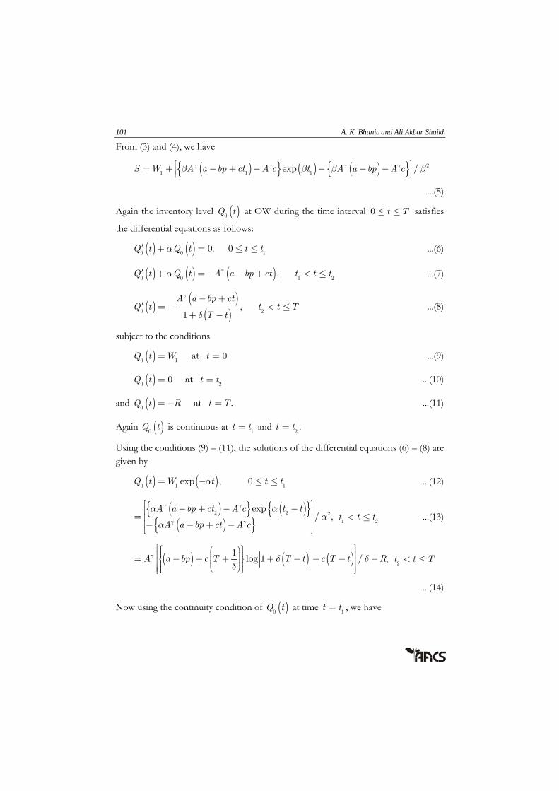
101 A. K. Bhunia and Ali Akbar Shaikh

From (3) and (4), we have

21 1 1

exp /S W A a bp ct A c t A a bp A c

...(5)

Again the inventory level 0Q t at OW during the time interval 0 t T satisfies

the differential equations as follows:

0 0 10, 0Q t Q t t t ...(6)

0 0 1 2,Q t Q t A a bp ct t t t ...(7)

0 2

,1

A a bp ctQ t t t T

T t

...(8)

subject to the conditions

0 1 at 0Q t W t ...(9)

0 20 at Q t t t ...(10)

and 0 at .Q t R t T ...(11)

Again 0Q t is continuous at

1t t and

2t t .

Using the conditions (9) – (11), the solutions of the differential equations (6) – (8) are given by

0 1 1exp , 0Q t W t t t ...(12)

2 2 2exp

/ ,A a bp ct A c t t

A a bp ct A c

1 2t t t ...(13)

1log 1 / ,A a bp c T T t c T t R

2t t T

...(14)

Now using the continuity condition of 0Q t at time

1t t , we have

A two warehouse inventory model for deteriorating items with time dependent partial....... 102

1 1

2 2 1 2

1

exp

exp/

W t

A a bp ct A c t t

A a bp ct A c

i.e.,

2 2

21 1 1

exp

exp 0

A a bp ct A c t

A a bp ct A c t W

...(15)

Again, from the continuity of 0Q t at

2t t , we have

2 2

1log 1 /R A a bp c T T t c T t

...(16)

Now the total deteriorated units in RW and OW over the stock-in period are given by

1 2

1 2 0

0 0

and t t

rD Q t dt D Q t dt respectively.

Hence we can write

1 2

1 0 2

0 0

/ and /t t

rQ t dt D Q t dt D ...(17)

Again, 1

1 1

0

t

D S W A a bp ct dt ...(18)

and 2

1

2 1

t

t

D W A a bp ct dt ...(19)

Hence the total holding cost hold

C over the entire cycle is given by

1 2

1 1 0

0 0

t t

hold rC C Q t dt C Q t dt

1 2

1

1 1 1 1

0

/ /t t

t

C S W A a bp ct dt C W A a bp ct dt

...(20)

Again, the total shortage cost sho

C over the entire cycle is given by

103 A. K. Bhunia and Ali Akbar Shaikh

2

2 0 2 2

11

T

sho

t

C C Q t dt C A a bp c T T t

2

2 2 2 2log 1 / / 2T t T t c T t R T t

...(21)

The transportation cost 1tran

C for transferring the items from RW to OW is given by

1

21 4 4 1 1

02

t

tran

cC C A a bp ct dt C A a bp t t

...(22)

Again, the transportation cost 2tran

C for replenishment of items is given by

2 when

tran t tFC nC S R nk C nk S R nk U

1 when 1t

n C nk U S R n k

Hence the total transportation cost tran

C is given by

1 2tran tran tran

C C C

During the entire inventory cycle, the total cost TC of the system is given by

TC = <ordering cost> + <advertisement cost> + <purchase cost> + <holding cost> + <shortage cost> + <transportation cost>

i.e. 1 2 5 3 hold short tranTC A A C A C S R C C C ...(23)

Therefore the net profit (X) of the system is the difference between the sales revenue and the total cost of the system, i.e.

22 2 3 1 22

cX p A a bp t t R C S R A A

5 hold short tran

C A C C C ...(24)

Hence, the profit function Z (average profit per unit time) for the entire cycle of the system is given by

1 2, , , , ,

XZ m n A t t T

T

A two warehouse inventory model for deteriorating items with time dependent partial....... 104

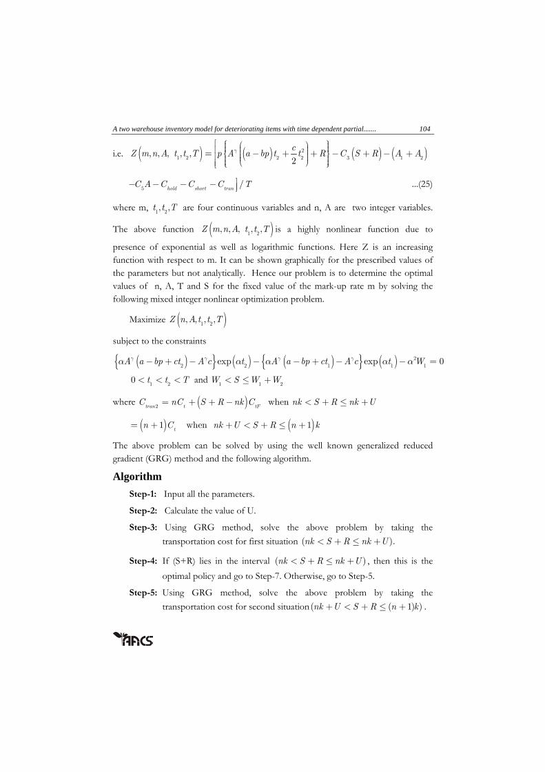
i.e. 21 2 2 2 3 1 2

, , , , ,2

cZ m n A t t T p A a bp t t R C S R A A

5

/hold short tran

C A C C C T ...(25)

where m, 1 2, ,t t T are four continuous variables and n, A are two integer variables.

The above function 1 2, , , , ,Z m n A t t T is a highly nonlinear function due to

presence of exponential as well as logarithmic functions. Here Z is an increasing function with respect to m. It can be shown graphically for the prescribed values of the parameters but not analytically. Hence our problem is to determine the optimal values of n, A, T and S for the fixed value of the mark-up rate m by solving the following mixed integer nonlinear optimization problem.

Maximize 1 2, , , ,Z n A t t T

subject to the constraints

22 2 1 1 1

exp exp 0A a bp ct A c t A a bp ct A c t W

1 2

0 t t T and 1 1 2

W S W W

where 2 when

tran t tFC nC S R nk C nk S R nk U

1 when 1t

n C nk U S R n k

The above problem can be solved by using the well known generalized reduced gradient (GRG) method and the following algorithm.

Algorithm Step-1: Input all the parameters.

Step-2: Calculate the value of U.

Step-3: Using GRG method, solve the above problem by taking the transportation cost for first situation ( ).nk S R nk U

Step-4: If (S+R) lies in the interval ( )nk S R nk U , then this is the optimal policy and go to Step-7. Otherwise, go to Step-5.

Step-5: Using GRG method, solve the above problem by taking the transportation cost for second situation( ( 1) )nk U S R n k .

105 A. K. Bhunia and Ali Akbar Shaikh

Step-6: If (S+R) lies in the interval ( ( 1) )nk U S R n k , then this is the optimal policy.

Step-7: Stop.

4. Numerical Illustrations To illustrate the developed model, a numerical example with the following values of different parameters has been considered.

Let C1 = $1.00 per unit per unit time, 1

$0.50C per unit per unit time, A1 = $150.00

per order, A2 = $50.00 per order, C2 = $15.00 per unit per unit time, C3 = $25.00 per

unit, C4 = $0.50 per unit, tF

C = $1.25 per unit, C5 = $50.00 per advertisement, t

C =

$100.00 per load, S0 = 50, S1 = 250, a = 250, b = 5, c = 5, 0.1 , = 0.1, δ = 1.5,

W1 = 150, 2

W =100, k = 100 unit, =0.07, = 0.1, L=50 km.

The parameter values considered here are realistic, though these values are not taken from any case study of an existing inventory system.

To show the profit function as an increasing function with respect to the mark-up rate m, first of all, we have computed the profit function for different values of m and drawn the graph (see Fig.-1). From Fig.-1, it is evident that the profit Z is an increasing function of m.

According to the proposed algorithm, the optimal solution has been obtained with the help of GRG method for different values of m. The optimum values of n, A, t1, t2,T, S and R along with maximum average profit are displayed in Table 1.

Table 1: Optimal solution for different values of mark-up rate m

m A S R 1t

2t T Z

1.25 1 153.6615 26.3385 0.03896 1.46354 1.77925 119.4907 1.27 1 154.4600 25.5400 0.04872 1.50495 1.81765 156.9375 1.30 2 161.7843 25.8259 0.12466 1.5284 1.83341 211.8844 1.32 2 160.8528 24.93338 0.118225 1.55853 1.85977 246.311 1.35 2 159.3756 23.69333 0.106906 1.60585 1.90258 293.4273

A two warehouse inventory model for deteriorating items with time dependent partial....... 106

Fig.-1 : Mark-up rate (m) vs. Average profit (Z)

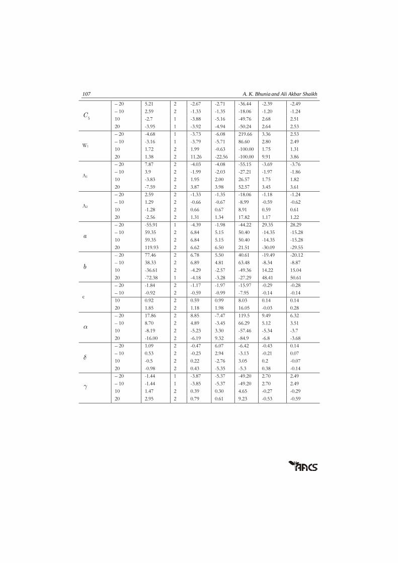
5. Sensitivity Analysis The earlier numerical example is used to study the effect of under or over estimation of system parameters on the optimal values of the initial stock level, maximum shortage level, cycle length, frequency of advertisement along with the maximum profit of the system. The percentage changes in the above mentioned optimal values are taken as measures of sensitivity. The analysis is carried out by changing (increasing and decreasing ) the parameters by -20% to +20%. The results are obtained by changing one parameter at a time and keeping the other parameters at their original values. The results of these analysis are given in Tables 2 which are self- explainatory.

Table 2 : Sensitivity analysis with respect to different parameters

Parameter % changes of parameters

% changes in Z*

*A

% changes in

*S *R

*1t *

2t *T

1C

– 20 0.04 2 0.75 0.06 10.27 0.67 0.56 – 10 0.02 2 0.36 0.03 4.90 0.32 0.27 10 -0.02 2 -0.33 -0.03 -4.41 -0.29 -0.25 20 -0.03 2 -0.63 -0.05 -8.51 -0.56 -0.47

1C

– 20 3.16 2 2.05 -1.26 27.85 1.83 1.24 – 10 29.89 2 1.03 -0.63 14.13 0.92 0.63 10 -1.55 2 -1.05 0.62 -14.29 -0.94 -0.32 20 -3.09 2 -2.11 1.23 -28.89 -1.9 -1.3

2C

– 20 3.26 2 -1.35 14.71 -18.35 -1.21 2.00 – 10 1.52 2 -0.63 6.85 -8.59 -0.56 0.91 10 -1.34 2 0.56 -6.02 7.62 0.50 -0.77 20 -2.52 2 1.05 -11.36 14.37 0.89 -1.43

3C

– 20 3.94 1 7.88 -1.40 62.28 -13.40 -15.08 – 10 6.88 2 7.2 2.86 67.09 -8.10 -8.99 10 -16.1 2 -4.6 -0.67 -54.57 13.9 15.26 20 -42.51 2 -5.21 3.16 -54.49 38.77 42.89

107 A. K. Bhunia and Ali Akbar Shaikh

5C

– 20 5.21 2 -2.67 -2.71 -36.44 -2.39 -2.49 – 10 2.59 2 -1.33 -1.35 -18.06 -1.20 -1.24 10 -2.7 1 -3.88 -5.16 -49.76 2.68 2.51 20 -3.95 1 -3.92 -4.94 -50.24 2.64 2.53

W1

– 20 -4.68 1 -3.73 -6.08 219.66 3.36 2.53 – 10 -3.16 1 -3.79 -5.71 86.60 2.80 2.49 10 1.72 2 1.99 -0.63 -100.00 1.75 1.31 20 1.38 2 11.26 -22.56 -100.00 9.91 3.86

A1

– 20 7.87 2 -4.03 -4.08 -55.15 -3.69 -3.76 – 10 3.9 2 -1.99 -2.03 -27.21 -1.97 -1.86 10 -3.83 2 1.95 2.00 26.57 1.75 1.82 20 -7.59 2 3.87 3.98 52.57 3.45 3.61

A2

– 20 2.59 2 -1.33 -1.35 -18.06 -1.18 -1.24 – 10 1.29 2 -0.66 -0.67 -8.99 -0.59 -0.62 10 -1.28 2 0.66 0.67 8.91 0.59 0.61 20 -2.56 2 1.31 1.34 17.82 1.17 1.22

a

– 20 -55.91 1 -4.39 -1.98 -44.22 29.35 28.29 – 10 59.35 2 6.84 5.15 50.40 -14.35 -15.28 10 59.35 2 6.84 5.15 50.40 -14.35 -15.28 20 119.93 2 6.62 6.50 21.51 -30.09 -29.55

b

– 20 77.46 2 6.78 5.50 40.61 -19.49 -20.12 – 10 38.33 2 6.89 4.81 63.48 -8.34 -8.87 10 -36.61 2 -4.29 -2.57 -49.36 14.22 15.04 20 -72.38 1 -4.18 -3.28 -27.29 48.41 50.61

c

– 20 -1.84 2 -1.17 -1.97 -15.97 -0.29 -0.28 – 10 -0.92 2 -0.59 -0.99 -7.95 -0.14 -0.14 10 0.92 2 0.59 0.99 8.03 0.14 0.14 20 1.85 2 1.18 1.98 16.05 -0.03 0.28

– 20 17.86 2 8.85 -7.47 119.5 9.49 6.32 – 10 8.70 2 4.89 -3.45 66.29 5.12 3.51 10 -8.19 2 -5.23 3.30 -57.46 -5.34 -3.7 20 -16.00 2 -6.19 9.32 -84.9 -6.8 -3.68

– 20 1.09 2 -0.47 6.07 -6.42 -0.43 0.14 – 10 0.53 2 -0.23 2.94 -3.13 -0.21 0.07 10 -0.5 2 0.22 -2.76 3.05 0.2 -0.07 20 -0.98 2 0.43 -5.35 -5.3 0.38 -0.14

– 20 -1.44 1 -3.87 -5.37 -49.20 2.70 2.49 – 10 -1.44 1 -3.85 -5.37 -49.20 2.70 2.49 10 1.47 2 0.39 0.30 4.65 -0.27 -0.29 20 2.95 2 0.79 0.61 9.23 -0.53 -0.59

A two warehouse inventory model for deteriorating items with time dependent partial....... 108

6. Concluding Remarks In this paper, an attempt has been made to incorporate the different preservation facilities in own and rented warehouses for deteriorating items with variable demand dependent on marketing variables like, selling price of the item and frequency of advertisement in popular media and continuous time. It is also assumed that the preservation facility in RW is better than in OW.

As the rate of demand is assumed to be time dependent for the fixed values of selling price of the item and number of advertisement, so the entire cycle over the first period can not repeat after the cycle length T. It can subsequently be repeated with the changed value of the constant ‘a’ computed from a + cT where T is associated value of the previous cycle.

In this paper, the demand rate is taken as , ,D A p t A a bp ct . It is well

known that , ,D A p t a bp ct for fixed A. But, why should we take

, ,D A p t A for fixed values of p and t ? Generally, the demand varies due to the

advertisement in the well known media such as Radio, T.V., Newspaper, Magazine, Cinema, etc. The demand of items increases with the increase of frequency of advertisement and is directly proportional to the number of advertisement. Hence, we

can take , ,D A p t A for fixed p and t.

The present model is also applicable to the problems where the selling prices of the items as well as the advertisement of items affect the demand. It is applicable for seasonal and fashionable goods.

The two-warehouse model can be applied to many practical situations, due to introduction of open market policy and also to occupy the maximum possible market for highly business competition. For this reason, in order to attract more customers, a departmental store is forced to provide a better purchasing – environment to the customers such as well decorated show-room with modern light and electronic arrangements and enough free space for choosing items, etc. Again, due to the expanding market situation, there is a crisis of space in the market places specially in the super market, corporation market, etc. As a result, the management of the departmental store is bounded to hire a separate warehouse on rental basis at a distance place for storing of excess items. Hence, from the economical point of view, sometimes two-storage system is more profitable than the single storage system.

109 A. K. Bhunia and Ali Akbar Shaikh

References [1] Benkherouf, L A. (1997), A deterministic order level inventory model for

deteriorating items with two storage facilities, International Journal of Production Economics, 48, 167-175.

[2] Bhunia, A. K. and Maiti M. (1994), A two-warehouse inventory model for a linear trend in demand, Opsearch, 31, 318-329.

[3] Bhunia, A. K. and Maiti, M. (1997), A two warehouses inventory model for deteriorating items with linear trend in demand and shortages, Journal of Operational Research Society, 49, 287-292.

[4] Chung, K.J. and Huang, T.S(2007), The optimal retailer’s ordering policies for deteriorating items with limited storage capacity under trade credit financing, International Journal of Production Economics, 106, 127-145.

[5] Dave, U. (1988), On the EOQ models with two levels of storage, Opsearch, 25.

[6] Goswami, A. and Chaudhuri, K. S. (1992), An economic order quantity model for items with two levels of storage for a linear trend in demand, Journal of Operational Research Society, .43, 157-167.

[7] Hartely, R. V. (1976), Operations Research-a managerial emphasis, Goodyear Publishing Company, 315-317.

[8] Kar, S., Bhunia , A. K. and Maiti, M. (2001), Deterministic inventory model with two levels of storage, a linear trend in demand and a fixed time horizon, Computers and Operations Research, 28, 1315-1331.

[9] Lee, C. C. and Ma, C. Y. (2000), Optimal inventory policy for deteriorating items with two warehouse and time dependent demands, Production Planning and Control, 7, 689-696.

[10] Mondal, B., Bhunia, A.K. and Maiti, M. (2007), A model on two storage inventory system under stock dependent selling rate incorporating marketing decisions and transportation cost with optimal release rule, Tamsui Oxford Journal of Mathematical Sciences,23(3), 243-267.

[11] Pakkala, T.P.M. and Achary, K.K. (1992), A deterministic inventory model for deteriorating items with two warehouse and finite replenishment rate, European Journal of Operational Research, 57, 71-76.

[12] Sarma, K. V. S.(1983), A deterministic inventory model with two levels of storage and an optimum release rule, Opsearch, 29, 175-180.

A two warehouse inventory model for deteriorating items with time dependent partial....... 110

[13] Sarma, K. V. S.(1987), A deterministic order-level inventory model for deteriorating items with two storage facilities, European Journal of Operational Research , 29, 70-72.

[14] Yang, H.L(2004), Two-warehouse inventory models for deteriorating items with shortages under inflation, European Journal of Operational Research, 157, 344-356.

[15] Yang, H.L(2006), Two-warehouse partial backlogging inventory models for deteriorating items under inflation, International Journal of Production Economics, 103, 362-370.

[16] Zhou, Y.W. and Yang, S.L. (2003), A two-warehouse inventory model for items with stock-level-dependent demand rate, International Journal of Production Economics, 95, 215-228.

Biographical Note Ali Akbar Shaikh is a faculty member of Krishnagar Government College. He obtained M.Sc in Applied Mathematics in the year 2007 from Kalyani University, West Bengal, India and M.Phil in Mathematics in 2009 from Burdwan University, West Bengal, India. His research interests include inventory control theory, interval optimization and Particle Swarm Optimization.

A. K. Bhunia is an Associate Professor in the Department of Mathematics, Burdwan University, India. Several students obtained their Ph.D. degree under his supervision. His research interests include Computational Optimization, Soft computing, Interval mathematics, Interval ranking, etc. He has published several research papers in various international SCI journals published by Elsevier Science, Springer, Taylor & Francis, Oxford, Macmillan, etc. He has also written two research monographs and a book entitled “Advanced Operations Research”. He is also an Associate Editor of the Springer journal ‘OPSEARCH’.