EPQ Model of Deteriorating Inventory with Exponential Demand Rate under Limited Storage

AFRICA DEVELOPMENT AND RESOURCES RESEARCH INSTITUTE (ADRRI) JOURNAL (www.adrri.org)

ISSN: 2343-6662 VOL. I,No.1, pp 23-31,October, 2013

AFRICA DEVELOPMENT AND RESOURCES RESEARCH INSTITUTE (ADRRI) JOURNAL

ADRRI JOURNAL (www.adrri.org)


EPQ Model of Deteriorating Inventory with Exponential Demand Rate under Limited Storage

1Sanjay Sharma and 2S.R.Singh

1Department of Mathematics, Graphic Era University, Dehradun, City: Dehradun India

Email:[email protected]

2Department of Mathematics, D.N. (P.G.) College, Meerut, India, City: Meerut (UP)

Email:[email protected]

Abstract

With today’s high competitive market, to afford the cost of warehouses is a very difficult task for the management in most of the countries. So it is

economical to order the inventory according to available storage space. This problem is developed with the concept of space restriction in which

demand is exponential, and deterioration is time dependent. Production is taken as a function of demand.

Keywords: Deteriorating Inventory, Limited Storage, Space Restriction

Introduction

The problem discussed in this paper is of major concern in today’s high competitive market. Normally upon the receipt of the stock, the extra

stock is stored in a warehouse, which could be subject to deteriorate. Either option will result in extra cost. Most of the researches confronted this

Problem of land acquisition. Storage space is one of the scarcest resources that affect the efficiency of inventory control policy. Consequently,

management’s concern is to ensure that there is inventory control policy. Consequently, management’s concern is to ensure that there is enough

space to accommodate the product upon its receipt. inventory control policy. Consequently, management’s concern is to ensure that there is enough

space to accommodate the product upon its receipt.

Therefore the ordering quantity of the product is limited by the free space in the storage facility at the time of delivery. Under this type of review

policy, an order of size Q is placed when the inventory level drops to the reorder point R. The ordering quantity is delivered after a period of time,

called lead time. Therefore the recorder point quantity should be enough to satisfy the random demand during lead time, otherwise a stock out

situation will be observed. Very few papers have been published in this field. Hariga and Jackson (1995) provide their review of this literature. Beyer

et al (2001) obtain the optimal ordering policy for the stochastic multi-product problem with finite and infinite horizon as well as stationary and non-

stationary discounted costs. Jeddi et al (2004) study a multi-item continuous review system with random demand subject to a budget constraint when

the payment is due upon order arrival. Haksever a Moussourakis (2005) developed deterministic multiproduct, multi-constraint inventory systems

with stationary ordering policies. Minner and Silver (2005) study the space constrained multi-product continuous review problem with zero lead

times and non-allowed backorders. Recently Xu and Leung (2009) propose an analytical model in two party under managed system where the

retailer restricts the maximum space allocated to the vendor.

An important assumption in inventory models found in the existing literature is that the lifetime of an item is infinite while it is in storage. But

the effect of deterioration plays an important role in the storage of some commonly used decaying items like radioactive substances, breakable items,

fruits and many perishable products. A certain fraction of these goods are either damaged or decayed and are not in a perfect condition to satisfy the



future demand. Deterioration in such items is continuous and time dependent or stock dependent. A number of research papers have been published

on such types of problems by Datta and Pal (1990), Goswami and Choudhary (1991) Kar et. al (2001)

In this paper we developed a deterministic inventory model of deteriorating items with space restriction and exponential demand rate with the help

Hariga (2010).

II. ASSUMPTIONS

Inventory position is continuously monitored for the retailer and an

Units are demanded in small quantities; overshooting of the reorder point is not appreciable.

Deterioration rate is taken as time dependent.

Demand rate is taken as exponential function.

Production is taken as demand rate dependent.

An area with limited space W is reserved for the storage of the product for the retailer.

The over ordered quantity that cannot be accommodated in the available space at the delivery time is returned to the supplier.

The ordering quantity is smaller than the storage space capacity.

The time the system is out of stock during a cycle is small compared to the cycle length.

The supplier charges of the purchasing cost for each unit of the product returned because of over-ordering.

III.NOTATIONS

P = Production Rate

T = Cycle Time

1T = The time for which production occurs

2T = The non-production time for +ve inventory.

0p = Production cost per unit

= Selling price per unit for the supplier

2p = Selling price per unit for the retailer

dsc = Deterioration cost per unit for the supplier

dc = Deterioration cost per unit for the retailer

1h = Inventory holding cost per unit for the supplier

2h = Inventory holding cost per unit for the retailer

= Set up cost for the supplier

R = Reorder point for the retailer

x = Lead time demand for the retailer

W = Storage capacity for the retailer

Q = Order quantity for the retailer

= Rate of backlogging

O R = Ordering cost for the retailer

v = the time for –ve inventory in the case of shortage

1p



IV. Model Formulation

A. Supplier’s Model

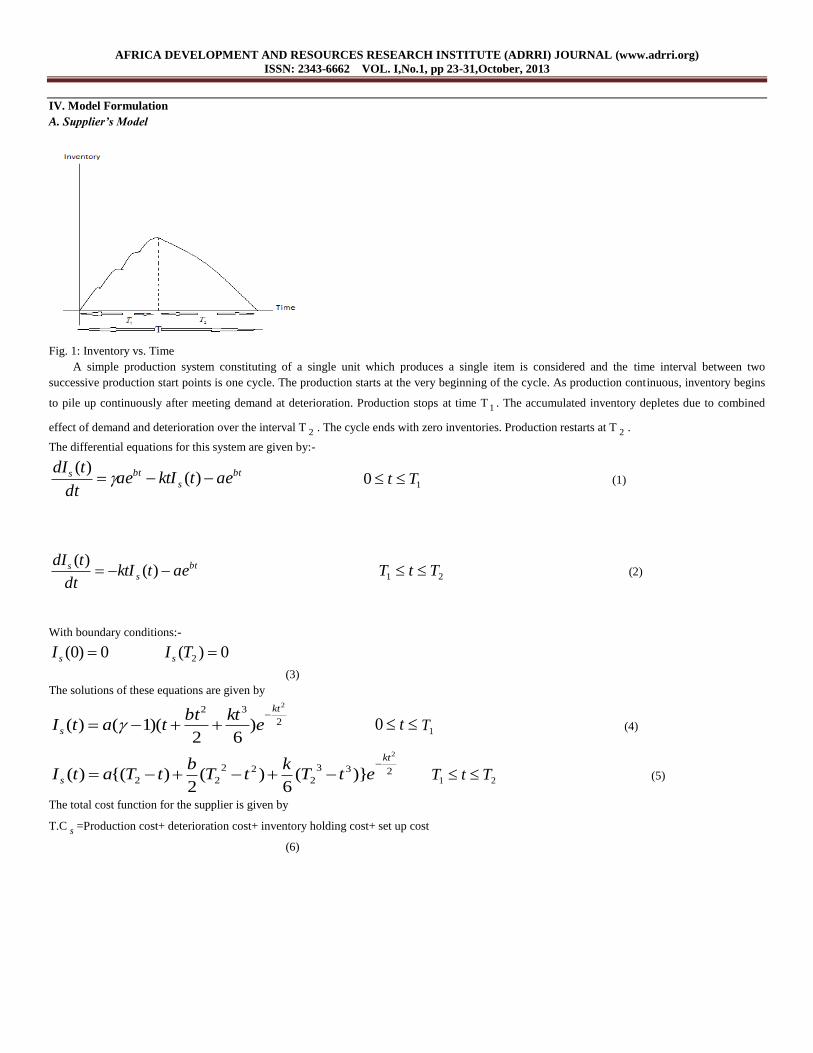
Fig. 1: Inventory vs. Time

A simple production system constituting of a single unit which produces a single item is considered and the time interval between two

successive production start points is one cycle. The production starts at the very beginning of the cycle. As production continuous, inventory begins

to pile up continuously after meeting demand at deterioration. Production stops at time T 1 . The accumulated inventory depletes due to combined

effect of demand and deterioration over the interval T 2 . The cycle ends with zero inventories. Production restarts at T 2 .

The differential equations for this system are given by:-

bt

s

bts aetktIaedt

tdI )(

)( 10 Tt (1)

21 TtT (2)

With boundary conditions:-

0)0( sI 0)( 2 TI s

(3)

The solutions of these equations are given by

2

322

)62

)(1()(kt

s ektbt

tatI

t01T (4)

233

2

22

22

2

)}(6

)(2

){()(kt

s etTk

tTb

tTatI

21 TtT (5)

The total cost function for the supplier is given by

T.C s =Production cost+ deterioration cost+ inventory holding cost+ set up cost

(6)

bt

ss aetktIdt

tdI )(

)(



Production cost= dtaep

T

bt

1

0

0

= p )1( 1

0 bTeb

a

(7)

Total deteriorated units =Total production – Total demand

Deterioration cost = c )}1()1({ 21 bTbT

ds eb

ae

b

a

(8)

Holding cost= h dttIdttI

T

T

s

T

s ))())((2

1

1

0

1

2 23 4 3 41 2

1 1 1 2 2

2 3 4 3 42 31 1 1 1 1

2 1 2 1 2 1 2

{ ( 1)( ) {2 6 12 2 3 12

( ) ( ) ( ) ( )}}2 2 3 6 4 2 3 4

T Tb k b kh a T T a T T

T T T T Tb k kT T T T T T T

(9)

Set up cost = (10)

Put all these values in equation (6)

T.C s = )}1()1({)1( 211 bTbT

ds

bT

o eb

ae

b

ace

b

ap

)}}43

(2

)4

(6

)3

(2

)2

(

1232{)

1262)(1({

4

12

3

1

4

11

3

2

3

11

2

2

2

112

4

2

3

2

2

24

1

3

1

2

11

TT

TkTTT

kTTT

bTTT

Tk

TbT

aTk

TbT

ah

(11)

T.A.C s = T

1 T.C s

= )(

1

21 TT T.C s (12)

B. Buyer’s Model

Buyer’s model is developed with the concept of space restriction. When an order quantity of size Q is placed, the actual quantity unloaded into

the storage facility depends on the inventory level immediately after the receipt of the order. In fact three different cases have to be distinguished

depending on the values of lead time, the reorder point, and the inventory level just after the receipt of an order and the storage capacity W.

Case 1:

If x is the demand during the lead time:

R-x 0 and R-x+QW

This condition status that the quantity demanded during the lead time is smaller than the reader point (Fig. 1 Hariga, 2010).

The differential equation governing the transition of the system for the relation is given by

bt

rr aetKtIdt

tdI )(

)( t0 T



(13)

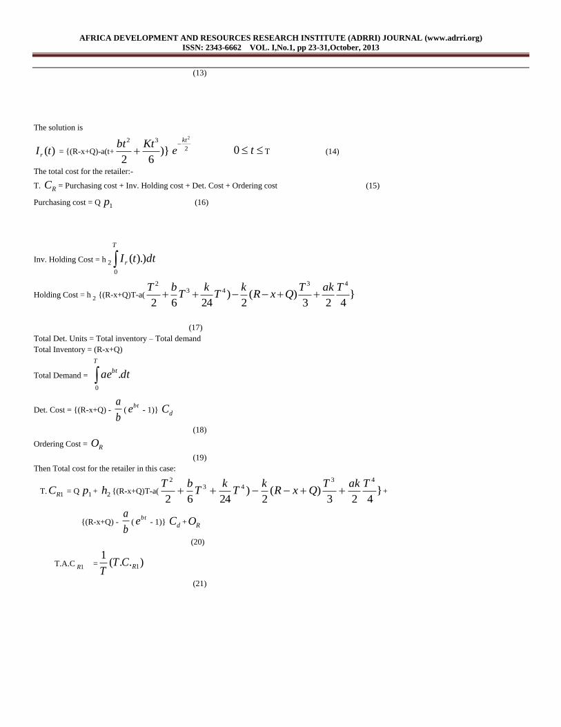
The solution is

)(tI r = {(R-x+Q)-a(t+ )}62

32 Ktbt 2

2kt

e

t0 T (14)

The total cost for the retailer:-

T. RC = Purchasing cost + Inv. Holding cost + Det. Cost + Ordering cost (15)

Purchasing cost = Q 1p (16)

Inv. Holding Cost = h dttI

T

r )).(0

2

Holding Cost = h2

{(R-x+Q)T-a( }423

)(2

)2462

4343

2 TakTQxR

kT

kT

bT

(17)

Total Det. Units = Total inventory – Total demand

Total Inventory = (R-x+Q)

Total Demand = T

bt dtae0

.

Det. Cost = {(R-x+Q) - b

a(

bte - 1)} dC

(18)

Ordering Cost = RO

(19)

Then Total cost for the retailer in this case:

T. 1RC = Q 1p + 2h {(R-x+Q)T-a( }423

)(2

)2462

4343

2 TakTQxR

kT

kT

bT +

{(R-x+Q) - b

a(

bte - 1)} dC + RO

(20)

T.A.C 1R = )..(1

1RCTT

(21)



Case-2:

When R-x+Q>W

In this case (R-x) is nonnegative and after the receipt of an order, inventory level exceeds the storage capacity (Fig. 2

Hariga, 2010).

In this case, the quantity required that can be accommodated within the available space is (W-(R-x)) and the maximum

inventory level over the cycle is now W. The retailer has to pay the material return cost for extra inventory as a penalty cost.

The differential equation governing the transition of the system is given by

bt

rr aetktIdt

tdI )(

)( Tt 0

(22)

With boundary condition

I )()0( xRWr

The solution of this equation is given by:-

I 232

2

)}62

())({()(t

k

r etk

tb

taxRWt

Tt 0

(23)

The total cost for the retailer in this case:-

T.C 2R = Purchasing cost+ inventory holding cost+ deterioration cost+ material return cost+ ordering cost

(24)

Purchasing cost = (W-(R-x))p1 (25)

Holding cost = T

r dttIh0

2 )(

}83

))((2

)2462

())({(43432

2

akTTxRW

KKTbTTaTxRWhHR (26)

Deteriorated units = Total inventory – Total demand

= ))(( xRW - dtaeT

bt

0

Deteriorated Cost = { ))(( xRW - (b

ae d

bt c)}1 (27)

Ordering Cost = RO (28)

Material Returned = (R-x+Q-W)

Material Returned Cost = 1p (R-x+Q-W) (29)

T.C 2R = )

2462())({(+ x))p-(R-(W

432

21

KTbTTaTxRWh

}83

))((2

43 akTTxRW

K + 1p (R-x+Q-W)

+{(W-(R-x))- (b

ae d

bt c)}1 + RO (30)

T.A. C 2R = T

1 (T.C 2R ) (31)

Case 3:

When R-x <0

This case corresponds to the shortage situation, since the demand during late time is greater than the reorder point. So

the minimum inventory in this case is zero and after the arrival of stock maximum inventory level is Q-(x-R).

It is assumed that the inventory level starts with shortage. At t = 0 inventory level is zero and it results in shortage. At t=v,

after the arrival of stock and satisfying backlogging demand, the inventory level becomes Q-(x-R) (Fig. 3 Hariga, 2010).

The diff. eqn governing the transition of the system are given by

btr aedt

tdI

)( vt 0 (32)



bt

rr aetktIdt

tdI )(

)( Ttv (33)

With boundary conditions:-

0)0( rI )()( RxQvI r

(34)

The solutions of these equations are given by:-

)1()( bt

r eb

atI vt 0

(35)

223322

22

}))(()}(6

)(2

{{)(t

kv

k

r eeRxQtvk

tvb

tvatI

Ttv

(36)

Total cost for the retailer in this case is given by:-

T.C 3R = Purchasing cost + Inv. Holding cost + Ordering cost + Det. Cost + Shortage Cost (37)

Purchasing cost = Qp 1 (38)

Inv. Holding Cost = h T

v

2 dttI r )(

2 3 42 3 2

2

3 4 2 33 4

2 4 3

{ ( ) ( ) ( )} ( ( ))(1 )2 2 3 6 4 2

Holding Cost = ( ) ( ( )) {( )} ( ))2 3 4 6 2 3 8

(1 ) ( ( ))}2 24 6

T b T k T kh a vT v T v T Q x R v T

ak vT T k v bv kT Q x R a v Q x R

k ak kv v v v Q x R

(39)

Ordering Cost = RO (40)

Deteriorated units = Total inventory – Total demand

Deteriorated Cost = { ))(( xRQ - (b

ae d

bvbt ce )} (41)

Shortage Cost = c s v

0

dttI r )(

= c s ))1(

(b

ev

b

a bv (42)

TC 3R =

R

342

432

343

24

33

22

2

O ))}((624

)2

1(

))()}832

{())((6

)43

(2

)2

1))((()}4

(6

)3

(2

)2

({+ [Qp

RxQvk

vak

vvk

RxQvkbvv

aRxQTkTvTak

Tvk

RxQT

TvkT

TvbT

vTah { ))(( xRQ - (b

ae d

bvbt ce )} + c s

))1(

(b

ev

b

a bv ] (43)

T.A.C 3R = R3 TC1

T (44)

Total Average Cost for whole the supply chain is given

T.A.C. (Supply) = ) TC (TC1

RsT

(45)

The Objective Function is given by

Mini T.A.C.(T 1 , T 2 )



S.t. T 1 0

T 2 0 (46)

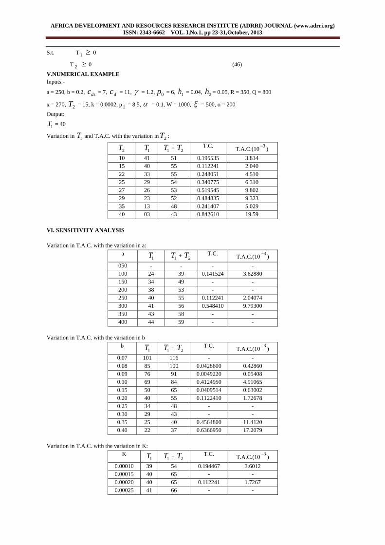
V.NUMERICAL EXAMPLE

Inputs:-

a = 250, b = 0.2, dsc = 7, dc = 11, = 1.2, 0p = 6, 1h = 0.04, 2h = 0.05, R = 350, Q = 800

x = 270, 2T = 15, k = 0.0002, p 1 = 8.5, = 0.1, W = 1000, = 500, o = 200

Output:

1T = 40

Variation in 1T and T.A.C. with the variation in 2T :

2T 1T 1T + 2T T.C. T.A.C.(10

3)

10 41 51 0.195535 3.834

15 40 55 0.112241 2.040

22 33 55 0.248051 4.510

25 29 54 0.340775 6.310

27 26 53 0.519545 9.802

29 23 52 0.484835 9.323

35 13 48 0.241407 5.029

40 03 43 0.842610 19.59

VI. SENSITIVITY ANALYSIS

Variation in T.A.C. with the variation in a:

a 1T 1T + 2T T.C.

T.A.C.(103

)

050 - - - -

100 24 39 0.141524 3.62880

150 34 49 - -

200 38 53 - -

250 40 55 0.112241 2.04074

300 41 56 0.548410 9.79300

350 43 58 - -

400 44 59 - -

Variation in T.A.C. with the variation in b

b 1T 1T + 2T T.C.

T.A.C.(103

)

0.07 101 116 - -

0.08 85 100 0.0428600 0.42860

0.09 76 91 0.0049220 0.05408

0.10 69 84 0.4124950 4.91065

0.15 50 65 0.0409514 0.63002

0.20 40 55 0.1122410 1.72678

0.25 34 48 - -

0.30 29 43 - -

0.35 25 40 0.4564800 11.4120

0.40 22 37 0.6366950 17.2079

Variation in T.A.C. with the variation in K:

K 1T 1T + 2T T.C.

T.A.C.(103

)

0.00010 39 54 0.194467 3.6012

0.00015 40 65 - -

0.00020 40 65 0.112241 1.7267

0.00025 41 66 - -



0.00030 41 66 0.101263 1.5342

0.00035 42 67 - -

0.00040 42 67 0.158999 2.3731

0.00045 43 68 - -

0.00050 44 69 - -

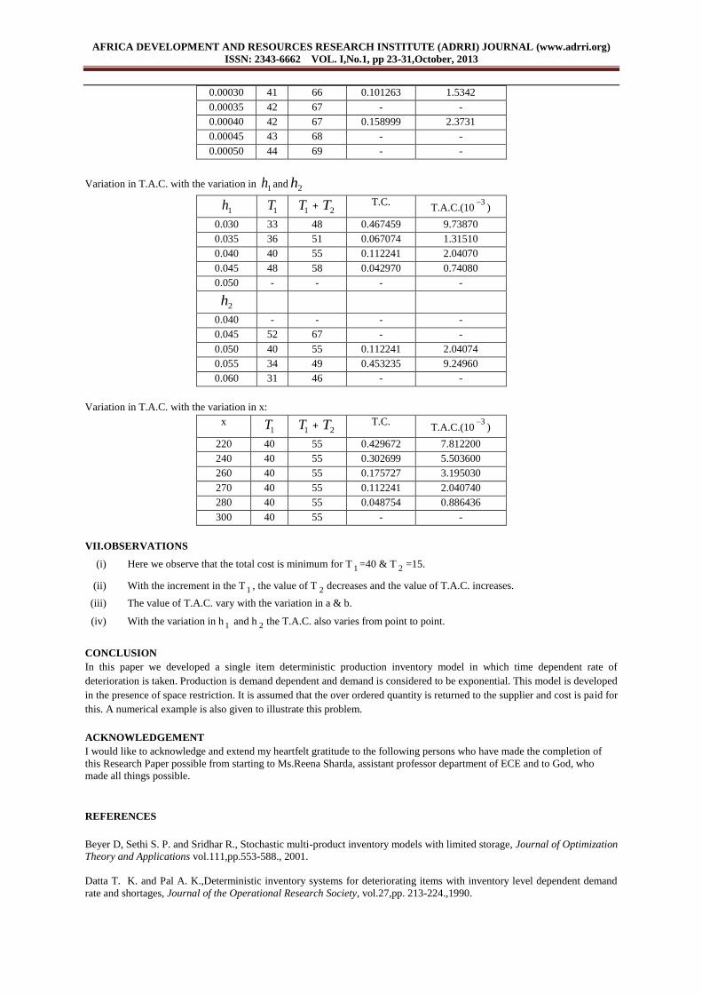
Variation in T.A.C. with the variation in 1h and 2h

1h 1T 1T + 2T T.C. T.A.C.(10

3)

0.030 33 48 0.467459 9.73870

0.035 36 51 0.067074 1.31510

0.040 40 55 0.112241 2.04070

0.045 48 58 0.042970 0.74080

0.050 - - - -

2h

0.040 - - - -

0.045 52 67 - -

0.050 40 55 0.112241 2.04074

0.055 34 49 0.453235 9.24960

0.060 31 46 - -

Variation in T.A.C. with the variation in x:

x 1T 1T + 2T T.C.

T.A.C.(103

)

220 40 55 0.429672 7.812200

240 40 55 0.302699 5.503600

260 40 55 0.175727 3.195030

270 40 55 0.112241 2.040740

280 40 55 0.048754 0.886436

300 40 55 - -

VII.OBSERVATIONS

(i) Here we observe that the total cost is minimum for T 1 =40 & T 2 =15.

(ii) With the increment in the T 1 , the value of T 2 decreases and the value of T.A.C. increases.

(iii) The value of T.A.C. vary with the variation in a & b.

(iv) With the variation in h 1 and h 2 the T.A.C. also varies from point to point.

CONCLUSION

In this paper we developed a single item deterministic production inventory model in which time dependent rate of

deterioration is taken. Production is demand dependent and demand is considered to be exponential. This model is developed

in the presence of space restriction. It is assumed that the over ordered quantity is returned to the supplier and cost is paid for

this. A numerical example is also given to illustrate this problem.

ACKNOWLEDGEMENT

I would like to acknowledge and extend my heartfelt gratitude to the following persons who have made the completion of

this Research Paper possible from starting to Ms.Reena Sharda, assistant professor department of ECE and to God, who

made all things possible.

REFERENCES

Beyer D, Sethi S. P. and Sridhar R., Stochastic multi-product inventory models with limited storage, Journal of Optimization

Theory and Applications vol.111,pp.553-588., 2001.

Datta T. K. and Pal A. K.,Deterministic inventory systems for deteriorating items with inventory level dependent demand

rate and shortages, Journal of the Operational Research Society, vol.27,pp. 213-224.,1990.



Goswami A. and Chowdhury K. S., A EOQ model for deteriorating items with shortages and linear trend in demand, Journal

of Operational Research Society, vol.42(12),pp.1105-1110.,1991

Haksever C. and Moussourakis J.,A model for optimizing multi-product inventory systems with multiple constraints,

International Journal of Production Economics vol.97, pp.18-30.,2005

Hariga M. A.,A single-item continuous review inventory problem with space restriction, International Journal of Production

Economics vol.128(1),pp.153-158.,2010

Hariga M. and Jackson P. L.,Time-variant lot sizing models for the warehouse scheduling problem, IIE Transactions

vol.26,pp162-170. ,1995

Jeddi B.G., Shultes B.C., Haji R.,A multi-product continuous review inventory system with stochastic demand, backorder,

and a budget constraint, European Journal of Operational Research vol.158,pp.456-469.,2004

Kar S., Bhunia A. K. and Maiti M. ,Inventory of multi-deteriorating items sold from two shops under single management

with constraints on space and investment, Computers and Operations Research, vol.28.pp1203-1221.,2001

Minner S. and Silver E. A.,Multi-product batch replenishment strategies under stochastic demand and a joint capacity

constraint, IIE Transactions vol.37,pp.469-479.,2005

Xu K. and Leung M. T.,Stocking policy in a two-party vendor managed channel with space restrictions, International

Journal of Production Economics vol.117(2),pp.271-285.,2009.

This academic research paper was published by the Africa Development and Resources

Research Institute’s Journal (ADRRI JOURNAL). ADRRI JOURNAL is a double blinded,

open access international journal that aims to inspire Africa development through quality

applied research.

For more information about ADRRI JOURNAL homepage, follow: www.adrri.org/journal.

CALL FOR PAPERS

ADRRI JOURNAL calls on all prospective authors to submit their research papers for

publication. Research papers are accepted all yearly round. You can download the submission

guide on the following page: www.adrri.org/journal

ADRRI JOURNAL reviewers are working round the clock to get your research paper

publishes on time and therefore, you are guaranteed of prompt response. All published papers

are available online to all readers world over without any financial or any form of barriers

and readers are advice to acknowledge ADRRI JOURNAL. All authors can apply for one

printed version of the volume on which their manuscript(s) appeared.

http://www.adrri.org/journal

http://www.adrri.org/journal

EPQ Model of Deteriorating Inventory with Exponential Demand Rate under Limited Storage

Documents

Transcript of EPQ Model of Deteriorating Inventory with Exponential Demand Rate under Limited Storage