Minimizing the total completion timein a two-machine flowshop withsequence-independent setup timesT Ladhari

1,2, MK Msakni3� and A Allahverdi

4

1Ecole Superieure des Sciences Economiques et Commercials de Tunis, University of Tunis, Tunisia;

2King

Saud University, Riyadh, Saudi Arabia;3Ecole Polytechnique de Tunis, University of Carthage, Tunisia;

and4Kuwait University, Safat, Kuwait

We consider the problem of minimizing the sum of completion times in a two-machine permutationflowshop subject to setup times. We propose a new priority rule, several constructive heuristics, localsearch procedures, as well as an effective multiple crossover genetic algorithm. Computationalexperiments carried out on a large set of randomly generated instances provide evidence that aconstructive heuristic based on newly derived priority rule dominates all the proposed constructiveheuristics. More specifically, we show that one of our proposed constructive heuristics outperforms thebest constructive heuristic in the literature in terms of both error and computational time. Furthermore,we show that one of our proposed local search-based heuristics outperforms the best local searchheuristic in the literature in terms of again both error and computational time. We also show that, interms of quality-to-CPU time ratio, the multiple crossover genetic algorithm performs consistently well.

Journal of the Operational Research Society (2012) 63, 445–459. doi:10.1057/jors.2011.37

Published online 11 May 2011

Keywords: scheduling; flowshop; total completion time; independent setup times; heuristics; genetic localsearch algorithm

Introduction

The two-machine flowshop scheduling problem has been

addressed by many researchers ever since Johnson (1954)

introduced the problem. Flowshop environments are still

common in current production environments since, in gene-

ral, flowshop production has higher production efficiency

than other types of production such as job shop or open-

shop. The main performance measure considered in the lite-

rature has been makespan. Minimizing makespan is

important in environments where a simultaneously received

batch of jobs is required to be completed as soon as possible.

Minimizing makespan also increases the utilization of resou-

rces. There are other environments where each completed job

is needed as soon as it is processed. In such environments, the

main concern is not to minimize completion time of the last

job but rather to minimize the mean completion time of all

jobs. The objective of minimizing mean completion time is

particularly important in real-life situations where reducing

inventory or holding cost is of primary concern. The signi-

ficance of minimizing the cost of inventory has been dis-

cussed by many researchers, for example, Singh and Chand

(2009), Warburton (2009) and Sharma (2009). This obejtive

is also important in supply chains, for example, Bahroun et

al (2010), Lehoux et al (2010) and Dath et al (2010).

In the majority of the work on flowshop scheduling,

setup times are ignored or assumed to be included in the

processing times. While this assumption is valid for some

scheduling environments, it may not be valid for some other

scheduling environments, for example, Allahverdi et al

(2008). In other words, many applications of setup times

can be found in many real life and practical situations. The

importance of setup times has been addressed by Allahverdi

and Soroush (2008) and Allahverdi et al (2008).

In this paper, the two-machine flowshop scheduling

problem to minimize mean, equivalentley total completion

time, is addressed where setup times are explicitly consi-

dered and assumed to be sequence independent. This

problem can be represented as F 2|STsi|P

Cj by following

the notation of Allahverdi et al (2008).

The F2|STsi|P

Cj scheduling problem was first pro-

posed by Bagga and Khurana (1986). They proposed two

lower bounds and a dominance rule, which are incor-

porated in a branch-and-bound algorithm. Their proposed

exact algorithm can solve small size instances. The problem

was also considered by Allahverdi (2000). He proposed

three constructive heuristics. Moreover, he developed a

Journal of the Operational Research Society (2012) 63, 445–459 © 2012 Operational Research Society Ltd. All rights reserved. 0160-5682/12

www.palgrave-journals.com/jors/

�Correspondence: MKMsakni, ROI—Combinatorial Optimization Research

Group, Ecole Polytechnique de Tunisie, BP 743, La Marsa 2078, Tunisia.

E-mail: msakni_kais@yahoo.fr

branch-and-bound algorithm and provided optimal solutions

for two special cases. The main feature of his algorithm is

using two new dominance relations for the problem in

addition to the one proposed by Bagga and Khurana (1986).

Allahverdi’s algorithm can solve up 35 job problems.

Al-Anzi and Allahverdi (2001) showed that the three-tiered

client-server database internet connectivity problem can be

modelled as F2|STsi|P

Cj scheduling problem. They also

proposed additional heuristics based on local search proce-

dures. Recently, Gharbi et al (2010) porposed five new

polynomial lower bounds. Their computational result carried

on randomly generated data reveals that the proposed lower

bounds outperform those of Bagga and Khurana (1986).

There are some other related problems that have been

addressed in the literature. Allahverdi and Al-Anzi (2006)

extended the problem to three-machine flowshop environ-

ment. They proposed a lower bound, a dominance relation

and some conditions under which an optimal solution can

be obtained. Moreover, they presented a branch-and-

bound algorithm. In addition, they presented a three-phase

heuristic. This hybrid algorithm consists first in obtaining

an initial solution by simulated annealing algorithm,

second improving the initial solution by an insertion

technique and finally improving the solution further by a

local search optimization technique. The problem has also

been addressed for no-wait flowshop environments, for

example, (Ruiz and Allahverdi, 2007).

In a preliminary version of this work (Msakni et al, 2009),

we proposed a constructive heuristic (denoted hereafter by

H3) that is based on a new priority rule (denoted hereafter

by PRTCT_SIST), and a genetic algorithm for the F2|STsi|PCj. The present paper revisits those heuristics in a more

thorough fashion, both from the theoretical and computa-

tional perspectives, and introduces newly devised ones.

First, we mathematically prove that, under some particular

settings, PRTCT_SIST constitutes a sufficient condition

for local optimality. Moreover, we show that implementing

this priority rule in a dynamic procedure represents the

key effectiveness factor of H3. Indeed, H3 relies on two

major features: an NEH-based framework and a dynamic

implementation of the proposed priority rule at each step

of the sequence building. In this paper, the performance of

H3 is compared to that of three newly proposed con-

structive heuristics. The first two ones purely rely on the

NEH-based framework, while the third one partially uses

the dynamic priority rule. Our experimental results show

that, although the three latter heuristics are highly

competitive with the best ones of the literature, they are

still surpassed by H3. Moreover, our proposed local search

procedures have been compared to nine procedures that are

known to be the most efficient and effective local search

algorithms for the F2|STsi|P

Cj in the literature (Al-Anzi

and Allahverdi, 2001). Our experimental study reveals that

all of these methods are dominated by our local search

technique both in terms of error and computational time.

The best parameters combination for our genetic algo-

rithm has been determined through a careful statistical study

that is based on factorial experimental design. The obtained

variant has been therefore reinforced by the local search

procedure, together with additional crossover operators that

have been cautiously selected from a panel of several

deemed operators. Finally, the performance of the proposed

heuristics is more accurately estimated by using some of the

recently proposed lower bounds of Gharbi et al (2010).

Description

The problem can be defined as follows. Each of n jobs from

the job set J¼ {1, 2,..., n} has to be processed non-

preemptively on two machines M1 and M2 in that order.

The processing time of job j on machine Mi (i¼ 1, 2) is pij.

Job j requires s1j unit of time on the first machine as a setup

time, and then during s2j time units on the second machine.

Each machine is available at time zero and can process

at most one job at a time. The objective is to minimize

the sum of job completion times. This problem can be

denoted by F 2|STsi|P

Cj by using the notation of

Allahverdi et al (2008).

The problem F2|STsi|P

Cj is NP-hard in the strong

sense. This is an immediate consequence of the NP-

hardness result of the F 2||P

Cj (Garey and Johnson, 1979).

Consequently, the existence of a polynomial algorithm to

solve the F 2|STsi|P

Cj is unlikely.

The problem can be formulated as follows. Let:

pij the processing time of job j(j¼ 1, 2, . . . , n) on

machine Mi (i¼ 1, 2).

sij the setup time of the job j on machine Mi.

Cij the completion time of the job j on machine Mi.

TCT sum of completion times.

Also let [ j ] denote the job in position j. Therefore, pi [ j ]denotes the processing time of the job in position j on

machine Mi. si [ j ] and Ci [ j ] are defined similarly.

Let STi [ j ] denote the sum of the setup times and pro-

cessing times of jobs in positions 1, 2, . . . , j on machine Mi,

that is, STi [ j ]¼P

h¼ 1j (si [h ]þ pi [h ]), j¼ 1, 2, . . . ,n and i¼ 1, 2.

Let d[ j ]¼ST1[ j ]�(ST2,[j�1]þ s2[ j ]), j¼ 1, 2, . . . , n, where

ST2[0]¼ 0.

Let IT2[ j ] denote total idle time on the second machine

until the job in position j on the machine M2 is completed.

It is known that (Allahverdi, 2000) IT2[j ]¼max{0,d[1],d[2], . . . , d[j ]}.Therefore, C2[ j ]¼ST2[ j ]þ IT2[ j ].

Once the completion times of jobs on the second machine

are known, then total completion time (TCT) can be

computed as follows.

TCT¼Xn

j¼1C2½j �:

446 Journal of the Operational Research Society Vol. 63, No. 4

A priority rule for sequence-independent setup times

In this section, we provide a new priority rule for the total

completion time with sequence independent setup times

(PRTCT_SIST ).

Denote by i and j, two jobs that have to be scheduled on

two machines M1 and M2. M1 and M2 are available after

times v1 and v2, respectively.

Assuming that SCTij (v1, v2)(i¼ 1, . . . , n; j¼ 1, . . . , n

and iaj) is the sum of total completion time of jobs i

and j obtained by scheduling i before j. Let Cki and Ckj

denote the completion time of the job i and j on machine

Mk (k¼ 1, 2) if i precedes j and C 0ki, and C 0kj denote the

completion time of jobs i and j on machineMk (k¼ 1, 2) if j

precedes i.

The priority rule for total completion time sequence

independent setup times of a job i under v1 and v2 is defined

as follows:

PRTCT SISTði; v1; v2Þ ¼ 2max ðv2þs2i;C1iÞþp2i:

The following theorem provides a sufficient condition to

obtain

SCTijpSCTji:

Theorem 1 Consider two jobs i and j such that

PRTCT_SIST(i, v1, v2)pPRTCT_SIST( j, v1, v2), s2iXs2jand C2iXC1j. Then, SCTijpSCTji.

Proof. If we schedule i before j then:

K The completion time of the job i on M2 is

C2i ¼ maxðv2 þ s2i; v1 þ s1i þ p1iÞ þ p2i

¼ maxðv2 þ s2i; C1iÞ þ p2i

K The completion time of the job j on M2 is

C2j ¼ maxðC2i þ s2j; v1 þ s1i þ p1i þ s1j þ p1jÞ þ p2j

¼ maxðC2i þ s2j; C1i þ s1j þ p1jÞ þ p2j

¼ maxðC2i þ s2j; C1jÞ þ p2j

K The sum of completion time of jobs i and j obtained by

scheduling i before j is

SCTi j ¼ C2i þ C2j

¼ maxðv2 þ s2i; C1iÞ þ p2i

þmaxðC2i þ s2j; C1jÞ þ p2j

¼ maxðv2 þ s2i; C1iÞ þmaxðmaxðv2 þ s2i; C1iÞþ p2i þ s2j ; C1jÞ þ p2i þ p2j

¼ maxð2maxðv2 þ s2i; C1iÞ þ p2i þ s2j; C1j

þmaxðv2 þ s2i;C1iÞÞ þ p2i þ p2j

¼ maxðPRTCT_SISTði; v1; v2Þ þ s2j ;C1j

þmaxðv2 þ s2i; C1iÞÞ þ p2i þ p2j

K Since C2i¼max(v2þ s2i,C1i)þ p2iXC1j, then

2maxðv2 þ s2i; C1iÞ þ p2iXC1j þmaxðv2 þ s2i; C1iÞ:That is;SCTij¼PRTCT SISTði; v1; v2Þ þ s2j þ p2i þ p2j :

If we schedule j before i then:

K The completion time of the job j on M2 is

C0

2j ¼ maxðv2 þ s2j; v1 þ s1j þ p1jÞ þ p2j

¼ maxðv2 þ s2j; C0

1jÞ þ p2j

K The completion time of the job i on M2 is

C0

2i ¼ maxðC 0

2j þ s2i; v1 þ s1j þ p1j þ s1i þ p1iÞ þ p2i

C0

2i ¼ maxðC 0

2j þ s2i; C0

1j þ s1i þ p1iÞ þ p2i

¼ maxðC 0

2j þ s2i; C0

1iÞ þ p2i

K The sum of completion time of jobs j and i obtained by

scheduling j before i is

SCTji ¼ C0

2j þ C0

2i

¼ maxðv2 þ s2j ; C0

1jÞ þ p2j þmaxðC 0

2j þ s2i; C0

1iÞ þ p2i

¼ maxðv2 þ s2j ; C0

1jÞ þ p2j þmaxðmaxðv2 þ s2 j ; C0

1jÞþ p2j þ s2i; C

0

1iÞ þ p2i

¼ maxð2maxðv2 þ s2j ; C0

1jÞ þ p2j þ s2i; C0

1i

þmaxðv2 þ s2j ; C0

1jÞÞ þ p2j þ p2i

¼ maxðPRTCT_SISTðj; v1; v2Þ þ s2i; C0

1i

þmaxðv2 þ s2j ; C0

1jÞÞ þ p2j þ p2i

Since PRTCT_SIST(i, v1, v2)pPRTCT_SIST ( j, v1, v2), and

s2jps2i then PRTCT_SIST (i, v1, v2)þ s2jpmax(PRTCT_

SIST ( j, v1, v2)þ s2i, C 01iþmax(v2þ s2j,C01i)). Therefore,

SCTijpSCTji.

Therefore, we can consider PRTCT_SIST function as a

heuristic dynamic priority measure: the higher priority is

given to the job with smallest value of the PRTCT_SIST.

Constructive heuristics

In this section, we present four constructive heuristics for

the problem under consideration. The proposed heuristics

are based on the adaptation of the well-known NEH

procedure (Nawaz et al, 1983) for the completion time

objective function and on the PRTCT_SIST presented in

T Ladhari et al—Minimizing TCT in a two-machine flowshop 447

the previous section. Following is the description of the

NEH procedure originally proposed for the permutation

flowshop scheduling problem.

NEH heuristic

Step 1: Index the jobs by decreasing total processing time.

Step 2: Schedule the first job in the first position.

Step 3: For j¼ 2 to n do: insert job j at the position that

minimizes makespan among the j available

positions.

The first two constuctive heuristics, H1 and H2, are obtained

by ordering jobs based on a quantity Kj calculated for each

job in the first step of NEH heuristic. More specifically,

H1 Rank the jobs in non-decreasing order of Kj¼ s1jþp1jþ s2jþ p2j.

H2 Sort the jobs in non-decreasing order of Kj¼ 2max

(s1jþ p1j, s2j)þ p2j.

The proposed next two heuristics, H3 and H4, are based

on the assumption that a job with low PRTCT_SIST

should be given higher priority than a job with high

PRTCT_SIST. The basic idea for this set of heuristics

consists in building the solution in an iterative way, adding

at each iteration the job with higher priority and finding

the best partial solution. We denote by:

s a partial sequence of the scheduled jobs�J the set of unscheduled jobs

Csi the completion time of s on the machine i (i¼ 1, 2).

H3 s¼+; �J ¼ J.

Step 1: Rank the jobs in J in non-decreasing order of

Kj¼ 2max(s1jþ p1j, s2 j )þ p2 j.

Step 2: Schedule the first job j1 provided by Step 1 and set�J ¼ �J \ { j1}.

Step 3: Update Kj¼ 2max(Cs1þ s1jþ p1j,Cs

2þ s2j )þ p2 jfor each job jA�J and set K¼minjA�JKj.

Step 4: Construct a subset S¼ {jA�J |Kj¼K}.

Step 5: If |S|¼ 1,S¼ { j �} then select j � otherwise select

from S, the j� having the minimum TPTj¼s1jþ p1jþ s2 jþ p2J.

Step 6: Insert the job j � into the partial schedule s in

position, which minimizes the completion time

and remove it from �J.Step 7: If �J ¼+; then stop otherwise goto Step 3.

H4 s¼+; �J ¼ J.

Step 1: Let Kj¼ 2max(s1jþ p1j, s2 j)þ p2j and K¼minjA�JKj.

Step 2: Construct a subset S¼ {jA �J |Kj¼K}.

Step 3: If |S|¼ 1, S¼ {j �} then s¼sj�and �J ¼ �J \{j �}otherwise generate from S a new sequence S 0

using the NEH heuristic and set s¼ sS0.Step 4: If �J ¼+ then stop otherwise update 8jA�J,

Kj¼ 2max(Cs1 þ s1jþ p1j,Cs

2 þ s2 j)þ p2 j, find K¼minjA�JKj, and goto Step 2.

Heuristics based local search

We propose to incorporate a basic local search procedure

in one of the developed constructive heuristics in order to

improve solution further. This choice is justified since local

search algorithms try to improve a schedule by removing a

job and inserting it into a better position. Generally, this

improvement corresponds to a non-investigated search

space by constructive heuristics.

We add a local search procedure to the best deve-

loped constructive heuristic, H3, which will be indicated

in the computational results section. This procedure, called

Exchange local Search Procedure, consists on interchan-

ging two jobs from two randomly selected positions of

a given schedule. The description of this procedure is as

follows.

Exchange_Local_Search_Procedure(r: schedule)

For i¼ 1 to n¼ |s|

Step 1: Choose randomly two positions i and j on s.Step 2: Construct a schedule s 0, a copy of s and

interchange the jobs at positions i and j.

Step 3: IfP

Cj (s 0)oP

Cj (s) then replace s by s0.

End For

The Exchange Local Search Procedure is integrated

to H3 with two ways according to the following

description.

H3LS I

Step 1–6: Similar as Step 1 to 6 in H3.

Step 7: Call Exchange_Local_Search_Procedure (s).Step 8: If �J ¼+ then stop otherwise goto Step 3.

H3LS II

Step 1–5: Similar as step 1 to 5 in H3.

Step 6: Insert the job j� into the partial schedule s in

all possible positions.

Step 7: For each partial schedule s obtained at Step 6,

call the procedure Exchange_Local_Search_

Procedure (s). Denote s� the partial schedule

with minimum completion time.

Step 8: Replace s by s� and remove J� from �J.Step 9: If �J ¼+ then stop otherwise goto Step 3.

448 Journal of the Operational Research Society Vol. 63, No. 4

Design of a genetic local search algorithm

Genetic algorithms have been used for solving scheduling

problems for long time. These metaheuristics are general

search techniques based on the mechanism of natural

selection and genetic operators. In this section, we propose

a standard genetic algorithm (SGA), a multiple crossover

genetic algorithm (MCGA) and a multiple crossover

genetic local search algorithm (MCGLS) for the problem

under consideration. The design of the proposed genetic

algorithms is given next.

A standard scheme of genetic algorithm

The natural choice of encoding scheme is the job sequences

themselves as chromosomes, which is represented by a

string of integers. This representation is widely used for the

combinatorial optimization problems having the permuta-

tion property, for example, the regular flowshop scheduling

problem. For our problem, the relative order of the jobs in

the string indicates the processing order of the jobs by the

machines in the shop.

In the most cases, Genetic Algorithms (GAs) assume

that the initial solution is completely generated randomly.

However, the efficiency of GAs can be greatly improved by

selecting a good initial population. In our genetic algo-

rithms, we propose including a ‘good chromosome’, which

is the solution provided by our priority-based-constructive

heuristic H3, in the initial population and we generate ran-

domly all the remaining individuals.

The fitness evaluation function Fitness_Function(chromo-

some) assigns to each chromosome (permutation) in the

population a value reflecting their relative superiority (or

inferiority). The fitness value assigned to each chromosome is

the total completion time of the corresponding permutation.

In our algorithms, the parent selection is a binary

tournament selection scheme based on individual fitness.

Each execution of this selection scheme provides one

individual to play the role of parent.

A crossover operator is simply a matter of replacing

some of the genes in one parent by the corresponding genes

of the other in order to produce a new chromosome (child).

However, doing so for our coding scheme could result in

infeasible strings: some jobs may be repeated while some

other may be missed in the schedule. Hence, a modification

has to be carried out in the crossover operators to

guarantee the creation of correct offspring. Regarding the

permutation-based representation, the following crossovers

are considered in the implementation of the different

proposed versions of GA with a probability Pc.

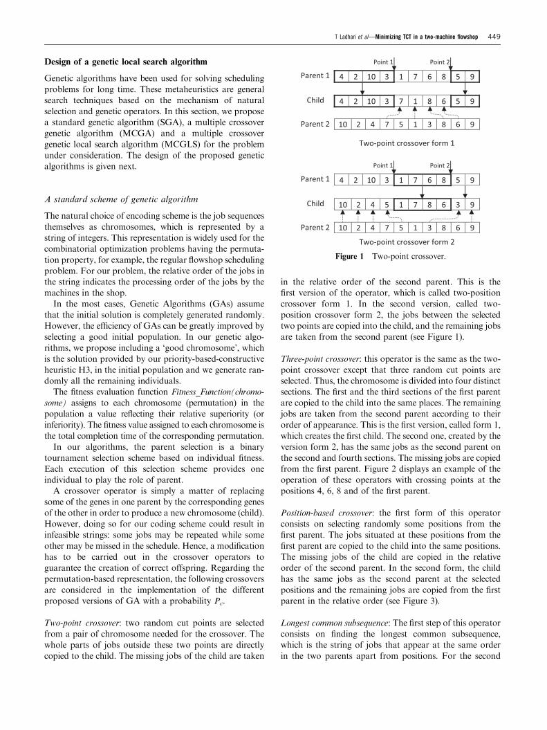
Two-point crossover: two random cut points are selected

from a pair of chromosome needed for the crossover. The

whole parts of jobs outside these two points are directly

copied to the child. The missing jobs of the child are taken

in the relative order of the second parent. This is the

first version of the operator, which is called two-position

crossover form 1. In the second version, called two-

position crossover form 2, the jobs between the selected

two points are copied into the child, and the remaining jobs

are taken from the second parent (see Figure 1).

Three-point crossover: this operator is the same as the two-

point crossover except that three random cut points are

selected. Thus, the chromosome is divided into four distinct

sections. The first and the third sections of the first parent

are copied to the child into the same places. The remaining

jobs are taken from the second parent according to their

order of appearance. This is the first version, called form 1,

which creates the first child. The second one, created by the

version form 2, has the same jobs as the second parent on

the second and fourth sections. The missing jobs are copied

from the first parent. Figure 2 displays an example of the

operation of these operators with crossing points at the

positions 4, 6, 8 and of the first parent.

Position-based crossover: the first form of this operator

consists on selecting randomly some positions from the

first parent. The jobs situated at these positions from the

first parent are copied to the child into the same positions.

The missing jobs of the child are copied in the relative

order of the second parent. In the second form, the child

has the same jobs as the second parent at the selected

positions and the remaining jobs are copied from the first

parent in the relative order (see Figure 3).

Longest common subsequence: The first step of this operator

consists on finding the longest common subsequence,

which is the string of jobs that appear at the same order

in the two parents apart from positions. For the second

Figure 1 Two-point crossover.

T Ladhari et al—Minimizing TCT in a two-machine flowshop 449

step, the jobs belonging to the longest common subse-

quence are directly copied to the child at the same positions

as they are in the first parent. The remaining jobs are taken

from the second parent according to their relative order

(see Figure 4).

Similar job order: The jobs that are similar for the two

parents are copied to the child at the same positions. Then,

a randomly cut point is selected to divide the chromosomes

into two parts. The remaining jobs of the first part of the

child are copied from the first parent and the missing jobs

of the child are copied from the second parent according to

their relative order (see Figure 5).

In the proposed GAs, a mutation operator is incorpora-

ted to avoid convergence to local optimum and to reintro-

duce variability in the population. It can be seen as a way

of enlarging the search space. Mutation is done by selecting

randomly two different positions on the chromosome and

interchanging the jobs at these positions (Figure 6). This

operation is applied with high probabilityMu to every child

obtained from crossover.

After crossover and mutation, new offsprings are born,

which they are candidates for the members of the popula-

tion. The improved offspring that is better than any current

individual in the population is inserted into the population

and the worst one is deleted.

Statistical tests

The relevant choice of parameters and operators greatly

affects the solution quality of GA. To obtain the best cali-

bration, we have done a factorial exeprimental desgin

where all possible combinations for the different values of

the following parameters are tested:

K population size (M): 20, 30, 50, 100, 200;

K crossover probability (Pc): 0.5, 0.6, 0.7, 0.8, 0.9, 1.0;

K crossover operator: two point crossover (form 1 and

form 2), three point crossover (form 1 and form 2),

position-based crossover (form 1 and form 2), longest

common sequence and similar job order;

K mutation probability (PM): 0.1, 0.2, 0.3, 0.5, 0.7, 0.9;

K mutation operator: exchange mutation and insertion

mutation.

Figure 3 Position-based crossover.

Figure 4 Longest common subsequence.

Figure 5 Similar job order.

Figure 2 Three-point crossover.

Figure 6 Exchange mutation.

450 Journal of the Operational Research Society Vol. 63, No. 4

So in our exeprimental design, we have 5�6�8�6�2¼ 2880

different versions of GA, the combination of all different

values of prestented parameters. To remove the bias

possible because of the initial GA sequences and with the

aim of making the comparison between all the versions

more effective, we provide the same initial starting solu-

tions for any GA according to its population size. Note

that the stop criterion is when a maximum number of

generations (1000) or a consectuive non-improving gene-

rations (100) is reached.

To test all these versions, we consider different problem

dimensions that include small, meduim and moderately

large problems. The problem dimensions we consider are

20, 30, 40, 50, 70, 100 and 200 jobs. We use the uniform

distribution to simulate the processing times that are drawn

from [1, 100]. For the setup times, they are taken from

[1, 100K], where K is the expected ratio of setup to pro-

cessing (sij/pij). The K values are equal to 0.25, 0.5, 0.75

or 1.0 yielding to four diffrenet subsets. Here, also the

uniform distributions are used. For each subset, we gene-

rate 10 instances. Therefore, in all we have 280 instances to

solve by each version of GA.

In order to choose the best combination of parameters,

we use a statistical tests. We wish to test the hypothesisH0:

‘m1Xm2’ against the alternative H1: ‘m1om2’, where m1

and m2 are the average total completion time obtained by

two versions GAi and GAj of the genetic algorithm,

respectively. If the hypothesis H0 is accepted, then we

consider that GAj is better than GAi (iaj).

Let a1¼ 1, 2, . . . , 280, the difference ofP

Cj of the

version GAi minus that for the version GAj on the same

instance l.

To obtain the best version among all 2880 implemented

versions, we apply the following algorithm:

Step 1: BestVersion’GA1

Step 2: For i¼ 2 to the number of implmented versions of

GA do

If the version GAi is better than the BestVersion

according to the statistical test

then BestVersion’GAi

The test statistic is given by:

t ¼ a

s=ffiffiffinp

where %a is the average observed al values and s their sample

standard deviations. Let a denote the level of signi-

ficance of the test and the ta denote the values for which

area to the right of student’s t-distribution with n�1¼ 240

(X120 so we can take n¼ 120) of freedom equals a. If wetake a¼ 0.005 (1% of error), which is indicative of a highly

significance result, we reject H0 when to�tn�1, 2a with

tn�1, 2a¼ t120, 0.01¼ 2.617.

The result of experimental design concludes that the

following parameters contribute to have better results:

K population size M¼ 200;

K crossover probability (Pc¼ 0.95);

K mutation probability (PMu¼ 0.7);

K crossover operator : two-point crossover form 2;

K mutation operator: exchange mutation.

By fixing these parameters, we have the first version of

genetic algorithm called SGA.

Designing a multiple crossover genetic algorithm

Unlike traditional SGAs, we applied five crossovers at the

same time on the two parents. We obtained, respectively,

five new sequences (or chromosomes) S1, S2, S3, S4 and S5.

After, we applied the mutation operator to S1, S2, S3, S4and S5 to have new chromosomes S01, S

02, S

03, S

04 and S05

with probability PM. Now, the generated sequences (S01,S02, S

03, S

04 and S05) are evaluated and the best one which

has the smallest fitness called S�is selected to replace the

worst chromosome in the population. This version is

baptized MCGA.

In order to choose the crossover operators of MCGA,

we used the statistical test described above by keeping

all the values of best parameters as constant except the

crossover operator. We find that the best five crossovers

are two-point crossover form 2, three-point crossover

form 1, three-point crossover form 2, Position-based

crossover form 1 and Position-based crossover form 2.

Multiple crossover genetic local search algorithm

To improve the quality of individual solutions in the

population, we propose a hybridization of the MCGA

with a local search procedure, thus yielding an MCGLS.

The main objective of the local search is to enhance the

intensification process in the genetic search. As an example,

Murata et al (1996) show that a genetic local search

algorithm outperforms a traditional genetic algorithm for

minimizing the makespan in a flowshop. Reeves and

Yamada (1998) propose a genetic local search algorithm,

which is competitive with the tabu search algorithm dev-

eloped by Nowicki and Smutnicki (1996) for the permuta-

tion flowshop scheduling problem.

In our implementation of local search methods, the

definition of the neighbourhood is by far the most important

ingredient. Thus far, we have used the two following

neighbourhood procedures:

Exchanging (p, i, j ): given a permutation p, a neighbour p0

is obtained by interchanging the jobs in positions i and j.

The positions i and j are selected randomly.

T Ladhari et al—Minimizing TCT in a two-machine flowshop 451

Swapping (p, i, j): given a permutation p, a neighbour p0 isobtained by interchanging the jobs in positions i and j. The

positions i and j are enumerated in some systematic ways

such as adjacent pair wise interchange.

These neighbourhoods present the advantage of being

polynomial sizes and easy to enumerate. To integrate the

local search phase in the GA, several alternatives are

possible. Murata et al (1996) propose an improvement step

by applying a local search procedure before selection and

crossover in a GA. Tseng and Lin (2009) developed a

hybrid genetic local search algorithm for the permutation

flowshop scheduling problem that applies two local search

methods before mutation in a GA. In our implementation,

we embed a local search phase to the MCGA after using

the mutation operators and this for each individual in the

population. The use of local search scheme is based on two

different improvement procedures and generates k neigh-

bours for each chromosome in the population. The

proposed local search scheme is described as follows.

Local_Search_Procedure(k)

Step 1: Generate a probability PLS

Step 2: If (PLSox)-(x¼ 0.05) then

Call Improvement_Procedure1(k, permutation)

else

Call Improvement_Procedure2(k, permutation)

Improvement_Procedure1(k,p)

Step 1: Generate k(k¼ 30) neighbours of a given

solution p.k/2 of the neighbours are generated by Ex-

changing(p, i, j ).k/2 of the neighbours are generated by Swap-

ping(p, i, ,j ).Step 2: Insert the best neighbour in the population.

Improvement_Procedure2(k,p)

Step 1: p0 ¼Exchange(p, i, j ).Step 2: Call Fitness_Function(p0).Step 3: If Fitness_Function(p0)o Fitness_Function(p) then

replace p by p0.Step 4: If the termination condition is not reached then

goto Step 1.

Step 5: Insert p in the population.

An outline of MCGLS is as follows.

MCGLS_Algorithm

Step 1: Initialize control parameters

Step 2: Generation of the initial population

(a) Call the Initialization_Population_Procedure

in order to generate the initial population.

(b) Call the Fitness_Function (compute the total

completion time of each solution).

Step 3: Improvement of the population

(a) Select two parents using Binary_Tournament_

Strategy.

(b) Apply crossover operators on the two parent

permutations according to the probabilityPc.

(c) Apply Mutation operator on the generated

offsprings with probability PMu.

Step 4: Evaluation and selection

(a) Evaluate the generated offspring. Replace the

worst chromosome in the population by the

new generated offspring if the fitness of this

later is better.

(b) Call the Local_Search_Procedure(k) in order

to perform a local search for each chromo-

some of the population.

Step 5: Termination condition

(a) If termination condition is satisfied then STOP

else goto Step 2.

Computational results

In this section, we present an empirical analysis of the

performance of the proposed heuristics. All the algorithms

have been coded in C and compiled with the Microsoft

Visual C++ (version 6.0). The computational experiments

were carried out on a Pentium IV 2.8GHz PC with 1GB

RAM.

In order to assess the quality of the different proposed

algorithms, we carried out a series of experiments on test

problems that were randomly generated in the following

way. The considered number of jobs n are 20, 20, 30,

40, 50, 70, 100, 200, 300 and 500. The processing times

are drawn from the discrete uniform distribution on the

range [1, 100]. The setup times are drawn from the

discrete uniform distribution on the range [1, 100K],

where four different values K are considered as

0.25, 0.5, 0.75 or 1. We combined these problem char-

acteristics to obtain 36 problem classes. For each class,

50 instances were generated.

In order to assess the quality of the different proposed

heuristics, we based our analysis on the following

measures:

1. The average relative gap(100 � ((UBi�LB)/LB)), whereUBi (i¼ 1, 2, 3 and 4) denotes the solution value of any

heuristic to be evaluated and LB is the best obtained

lower bound on the optimal solution among the five

polynomial lower bounds developed by (Gharbi et al,

2010).

2. The average relative percentage deviation (ARPD) from

the best-known solution, which is defined to be

ARPD¼ (100 � ((UBi�LB�)/LB�)), where UB� is the

452 Journal of the Operational Research Society Vol. 63, No. 4

best obtained value from the heuristics compared to

each other in the same table:

K UB� ¼min(H1, H2, H3, H4) for Table 1,

K UB� ¼min(H1, H2, H3, H4, HA1, HA2, HA3) for

Table 2

K UB� ¼min(H3, H3LSI, H3LSII) for Table 3

K UB� ¼min(H3LSI, H3LSII, PAj)j¼ 1, . . . , 9 for

Table 4

K UB� ¼min(SGA, MCGA, MCGLS, H3LSII) for

Table 6

Comparison of the proposed constructive heuristics H1–H4

In this subsection, we compare the four proposed con-

structive heuristics, H1–H4, with each other in order to find

the best constructive heuristic among the four. Then, we

compare our proposed constructive heuristics with those of

the best ones in the literature (Allahverdi, 2000).

The results of the computational study of the proposed

constructive heuristics are summarized in Table 1. The

headings have the following meanings: n is the number of

jobs, GAP is the average relative gap, ARPD is the average

Table 1 Computational results of constructive heuristics

n k H1 H2 H3 H4

GAP ARPD Time GAP ARPD Time GAP ARPD Time GAP ARPD Time

20 0.25 10.563 3.426 0.000 8.545 1.546 0.000 6.936 0.065 0.000 8.989 1.983 0.0000.50 10.111 3.653 0.000 7.400 1.097 0.000 6.272 0.048 0.000 8.623 2.247 0.0000.75 8.788 3.232 0.000 6.799 1.366 0.000 5.466 0.106 0.000 8.849 3.297 0.0001.0 11.469 4.123 0.000 8.550 1.413 0.000 7.098 0.063 0.000 11.548 4.201 0.000

30 0.25 12.173 4.209 0.000 9.709 1.922 0.000 7.679 0.064 0.000 10.052 2.260 0.0000.50 11.415 4.521 0.001 8.358 1.673 0.000 6.574 0.015 0.000 9.448 2.700 0.0000.75 11.361 4.700 0.000 8.178 1.716 0.000 6.339 0.001 0.000 9.837 3.284 0.0001.0 11.805 4.522 0.000 8.824 1.738 0.000 6.962 0.009 0.000 11.254 4.006 0.000

40 0.25 13.598 4.862 0.000 11.081 2.557 0.000 8.290 0.000 0.000 10.864 2.368 0.0000.50 11.511 4.514 0.000 9.019 2.183 0.000 6.684 0.000 0.000 9.466 2.593 0.0000.75 12.807 5.228 0.000 9.576 2.232 0.000 7.179 0.000 0.001 10.763 3.326 0.0001.0 12.064 4.776 0.000 9.097 1.998 0.000 6.956 0.000 0.000 11.525 4.266 0.000

50 0.25 14.954 5.759 0.000 12.105 3.149 0.000 8.673 0.000 0.000 11.264 2.382 0.0000.50 12.865 5.343 0.000 9.975 2.648 0.000 7.125 0.000 0.000 9.764 2.465 0.0000.75 11.952 4.735 0.000 9.237 2.201 0.001 6.884 0.008 0.001 10.241 3.142 0.0001.0 13.078 5.077 0.000 10.268 2.464 0.001 7.609 0.000 0.001 12.185 4.246 0.000

70 0.25 15.322 6.203 0.000 12.178 3.306 0.001 8.567 0.000 0.002 11.154 2.381 0.0020.50 13.521 5.501 0.001 10.801 2.984 0.001 7.570 0.000 0.001 10.777 2.974 0.0010.75 13.157 5.127 0.001 10.633 2.781 0.001 7.627 0.000 0.002 11.041 3.164 0.0011.0 12.738 5.286 0.001 9.758 2.502 0.001 7.062 0.000 0.001 11.170 3.819 0.002

100 0.25 15.468 6.033 0.002 12.640 3.442 0.002 8.880 0.000 0.003 11.474 2.380 0.0010.50 14.213 5.938 0.002 11.317 3.253 0.001 7.798 0.000 0.002 10.614 2.615 0.0010.75 13.949 5.670 0.002 11.437 3.335 0.001 7.831 0.000 0.002 11.505 3.404 0.0011.0 13.183 5.141 0.002 10.578 2.721 0.002 7.640 0.000 0.002 11.656 3.725 0.001

200 0.25 16.856 6.824 0.012 14.108 4.309 0.013 9.386 0.000 0.015 12.201 2.573 0.0080.50 14.763 6.064 0.013 12.460 3.936 0.012 8.198 0.000 0.015 11.153 2.732 0.0080.75 13.897 5.370 0.013 11.588 3.230 0.013 8.094 0.000 0.013 11.318 2.982 0.0081.0 14.018 5.187 0.013 11.891 3.223 0.013 8.395 0.000 0.015 12.264 3.568 0.008

300 0.25 18.193 7.454 0.041 15.343 4.864 0.039 9.988 0.000 0.048 13.305 3.014 0.0250.50 15.232 6.103 0.042 13.099 4.137 0.039 8.601 0.000 0.045 11.342 2.523 0.0290.75 14.144 5.447 0.043 12.120 3.576 0.039 8.245 0.000 0.046 11.288 2.808 0.0291.0 14.319 5.072 0.043 12.181 3.108 0.039 8.798 0.000 0.044 12.518 3.418 0.028

500 0.25 17.639 7.209 0.206 15.085 4.881 0.187 9.727 0.000 0.208 13.550 3.484 0.1450.50 15.948 6.276 0.206 13.606 4.130 0.189 9.098 0.000 0.207 12.104 2.754 0.1500.75 14.836 5.538 0.206 12.836 3.700 0.187 8.808 0.000 0.202 11.886 2.830 0.1491.0 14.149 4.821 0.207 12.413 3.228 0.188 8.897 0.000 0.203 12.288 3.113 0.149

Average 13.502 5.248 0.029 10.911 2.849 0.027 7.832 0.010 0.030 11.091 3.029 0.021

T Ladhari et al—Minimizing TCT in a two-machine flowshop 453

Table

2ComparisonbetweenH1–H4andAllahverdi’s,(2000)heuristics

nk

H1

H2

H3

H4

HA1

HA2

HA3

GAP

ARPD

Tim

eGAP

ARPD

Tim

eGAP

ARPD

Tim

eGAP

ARPD

Tim

eGAP

ARPD

Tim

eGAP

ARPD

Tim

eGAP

ARPD

Tim

e

20

0.25

10.563

3.568

0.000

8.545

1.685

0.000

6.936

0.202

0.000

8.989

2.121

0.000

14.879

7.615

0.000

9.052

2.183

0.000

8.015

1.209

0.000

0.50

10.111

3.770

0.000

7.400

1.212

0.000

6.272

0.163

0.000

8.623

2.364

0.000

13.303

6.760

0.000

8.004

1.790

0.000

7.174

1.015

0.000

0.75

8.788

3.404

0.000

6.799

1.533

0.000

5.466

0.271

0.000

8.849

3.467

0.000

12.587

7.011

0.000

7.457

2.172

0.000

6.149

0.925

0.000

1.0

11.469

4.479

0.000

8.550

1.755

0.000

7.098

0.401

0.000

11.548

4.554

0.000

14.729

7.508

0.000

8.562

1.770

0.000

7.391

0.681

0.000

30

0.25

12.173

4.300

0.000

9.709

2.012

0.000

7.679

0.152

0.000

10.052

2.349

0.000

16.463

8.277

0.000

10.134

2.426

0.001

8.880

1.264

0.016

0.50

11.415

4.609

0.001

8.358

1.757

0.000

6.574

0.098

0.000

9.448

2.785

0.000

14.154

7.192

0.000

8.910

2.296

0.001

7.461

0.933

0.015

0.75

11.361

4.871

0.000

8.178

1.879

0.000

6.339

0.161

0.000

9.837

3.449

0.000

14.129

7.483

0.000

8.420

2.120

0.002

6.942

0.737

0.014

1.0

11.805

4.759

0.000

8.824

1.968

0.000

6.962

0.235

0.000

11.254

4.239

0.000

13.986

6.783

0.000

8.675

1.843

0.001

7.336

0.588

0.014

40

0.25

13.598

4.927

0.000

11.081

2.620

0.000

8.290

0.062

0.000

10.864

2.431

0.000

17.069

8.145

0.000

10.853

2.425

0.002

9.363

1.053

0.065

0.50

11.511

4.579

0.000

9.019

2.246

0.000

6.684

0.061

0.000

9.466

2.656

0.000

14.277

7.154

0.000

9.178

2.400

0.002

7.775

1.083

0.065

0.75

12.807

5.363

0.000

9.576

2.364

0.000

7.179

0.129

0.001

10.763

3.459

0.000

14.745

7.170

0.000

9.037

1.862

0.002

7.653

0.575

0.062

1.0

12.064

5.040

0.000

9.097

2.256

0.000

6.956

0.253

0.000

11.525

4.528

0.000

14.778

7.582

0.000

8.491

1.701

0.002

7.184

0.472

0.063

50

0.25

14.954

5.804

0.000

12.105

3.192

0.000

8.673

0.042

0.000

11.264

2.425

0.000

17.562

8.206

0.000

10.888

2.081

0.005

9.668

0.962

0.126

0.50

12.865

5.371

0.000

9.975

2.674

0.000

7.125

0.026

0.000

9.764

2.491

0.000

15.021

7.387

0.001

9.379

2.134

0.004

7.890

0.744

0.126

0.75

11.952

4.854

0.000

9.237

2.317

0.001

6.884

0.121

0.001

10.241

3.260

0.000

14.320

7.076

0.001

8.587

1.720

0.005

7.224

0.444

0.126

1.0

13.078

5.325

0.000

10.268

2.707

0.001

7.609

0.236

0.001

12.185

4.493

0.000

15.170

7.265

0.001

9.008

1.535

0.004

7.586

0.216

0.127

70

0.25

15.322

6.223

0.000

12.178

3.325

0.001

8.567

0.019

0.002

11.154

2.401

0.002

17.957

8.649

0.001

11.172

2.414

0.013

9.615

0.986

0.598

0.50

13.521

5.519

0.001

10.801

3.001

0.001

7.570

0.017

0.001

10.777

2.991

0.001

15.867

7.707

0.001

10.124

2.390

0.013

8.485

0.867

0.599

0.75

13.157

5.226

0.001

10.633

2.879

0.001

7.627

0.094

0.002

11.041

3.262

0.001

15.232

7.154

0.001

9.453

1.792

0.013

7.964

0.411

0.601

1.0

12.738

5.460

0.001

9.758

2.671

0.001

7.062

0.165

0.001

11.170

3.992

0.002

14.386

7.001

0.001

8.466

1.481

0.013

7.196

0.295

0.604

100

0.25

15.468

6.036

0.002

12.640

3.445

0.002

8.880

0.004

0.003

11.474

2.383

0.001

17.770

8.162

0.002

11.434

2.351

0.041

9.763

0.818

11.293

0.50

14.213

5.960

0.002

11.317

3.274

0.001

7.798

0.021

0.002

10.614

2.636

0.001

16.154

7.770

0.002

9.920

1.991

0.042

8.417

0.597

10.856

0.75

13.949

5.783

0.002

11.437

3.444

0.001

7.831

0.106

0.002

11.505

3.514

0.001

15.273

7.006

0.002

9.275

1.447

0.043

8.008

0.272

11.129

1.0

13.183

5.395

0.002

10.578

2.968

0.002

7.640

0.241

0.002

11.656

3.976

0.001

15.091

7.177

0.002

8.904

1.424

0.041

7.552

0.165

11.488

200

0.25

16.856

6.824

0.012

14.108

4.309

0.013

9.386

0.000

0.015

12.201

2.573

0.008

18.132

7.995

0.010

12.825

3.142

0.356

10.222

0.766

209.809

0.50

14.763

6.072

0.013

12.460

3.944

0.012

8.198

0.007

0.015

11.153

2.739

0.008

15.874

7.103

0.010

12.886

4.342

0.356

8.765

0.533

216.534

0.75

13.897

5.494

0.013

11.588

3.351

0.013

8.094

0.117

0.013

11.318

3.103

0.008

15.136

6.636

0.010

13.765

5.370

0.355

8.123

0.145

222.899

1.0

14.018

5.570

0.013

11.891

3.599

0.013

8.395

0.364

0.015

12.264

3.945

0.008

15.599

7.030

0.010

15.055

6.530

0.354

8.024

0.022

228.547

300

0.25

18.193

7.454

0.041

15.343

4.864

0.039

9.988

0.000

0.048

13.305

3.014

0.025

18.632

7.857

0.023

12.208

2.019

1.531

10.785

0.725

1144.410

0.50

15.232

6.139

0.042

13.099

4.172

0.039

8.601

0.033

0.045

11.342

2.557

0.029

15.936

6.785

0.024

10.091

1.406

1.538

8.937

0.305

1149.159

0.75

14.144

5.601

0.043

12.120

3.727

0.039

8.245

0.146

0.046

11.288

2.958

0.029

15.208

6.586

0.024

9.306

1.129

1.548

8.183

0.129

1195.492

1.0

14.319

5.595

0.043

12.181

3.621

0.039

8.798

0.497

0.044

12.518

3.932

0.028

15.520

6.704

0.023

9.241

0.907

1.553

8.267

0.000

1248.540

500

0.25

17.639

7.209

0.206

15.085

4.881

0.187

9.727

0.000

0.208

13.550

3.484

0.145

17.656

7.224

0.018

11.695

1.794

17.365

*0.50

15.948

6.276

0.206

13.606

4.130

0.189

9.098

0.000

0.207

12.104

2.754

0.150

16.159

6.473

0.016

10.429

1.220

17.599

*0.75

14.836

5.539

0.206

12.836

3.700

0.187

8.808

0.001

0.202

11.886

2.831

0.149

15.478

6.130

0.016

9.496

0.633

17.852

*1.0

14.149

4.881

0.207

12.413

3.286

0.188

8.897

0.056

0.203

12.288

3.171

0.149

15.406

6.034

0.017

9.046

0.193

18.155

*

Averagew

13.234

5.293

0.007

10.589

2.837

0.007

7.669

0.139

0.008

10.920

3.158

0.005

15.467

7.373

0.005

9.961

2.268

0.245

8.187

0.623

176.981

� Outofmem

ory

w Theaveragevalues

donotincluden=500

jobsmeasures

454 Journal of the Operational Research Society Vol. 63, No. 4

relative percentage deviation from the best-known solution

and Time is the mean CPU time (in sec). As can be seen

from Tale 1, the constructive heuristics can solve large scale

instances within a few seconds. For instance, on the four

subsets (K¼ 0.25K¼ 0.5,K¼ 0.75 and K¼ 1) and for all

problem sizes, the mean CPU time required byHi (i¼ 1, 2, 3

and 4) is less than 0.21 s. In addition, the results of Table 1

provides strong evidence that H3 is very effective and

outperforms all the proposed heuristics. Indeed, H3

presents lower values of average relative gap and average

relative percentage deviation from the best-known solution

compared with the other heuristics for almost all instances.

Moreover, the effectiveness of H3 increases as the number

of the jobs increases (ARPD¼ 0 from n¼ 70).

In order to evaluate the effectivenss of our proposed

constructive heuristics, we compare them with the best

known constructive heuristics in the literature. These

heuristics were proposed by Allahverdi (2000) and denoted

Table 3 Computational results of heuristics-based local search

n k H3 H3LS I H3LS II

GAP ARPD Time GAP ARPD Time GAP ARPD Time

20 0.25 6.936 1.157 0.000 6.199 0.463 0.000 5.715 0.004 0.0070.50 6.272 1.035 0.000 5.688 0.483 0.000 5.187 0.014 0.0080.75 5.466 1.000 0.000 4.841 0.405 0.000 4.424 0.011 0.0081.0 7.098 1.353 0.000 6.193 0.501 0.000 5.666 0.007 0.008

30 0.25 7.679 1.174 0.000 6.865 0.411 0.001 6.427 0.002 0.0120.50 6.574 1.027 0.000 5.962 0.451 0.001 5.484 0.002 0.0120.75 6.339 0.961 0.000 5.778 0.432 0.001 5.330 0.008 0.0131.0 6.962 1.164 0.000 6.199 0.444 0.001 5.727 0.002 0.013

40 0.25 8.290 1.079 0.000 7.583 0.419 0.001 7.136 0.003 0.0590.50 6.684 0.909 0.000 6.046 0.309 0.001 5.719 0.001 0.0550.75 7.179 1.114 0.000 6.438 0.420 0.002 5.992 0.000 0.0551.0 6.956 1.173 0.000 6.266 0.523 0.002 5.709 0.000 0.059

50 0.25 8.673 1.005 0.000 8.008 0.388 0.004 7.589 0.000 0.1460.50 7.125 0.916 0.000 6.535 0.362 0.006 6.149 0.000 0.1480.75 6.884 0.994 0.001 6.274 0.421 0.005 5.829 0.000 0.1481.0 7.609 1.169 0.001 6.851 0.459 0.005 6.362 0.000 0.148

70 0.25 8.567 0.769 0.002 8.046 0.287 0.018 7.737 0.000 0.7430.50 7.570 0.752 0.001 7.110 0.321 0.019 6.766 0.000 0.7470.75 7.627 0.978 0.002 6.961 0.354 0.018 6.583 0.000 0.7411.0 7.062 1.004 0.001 6.453 0.433 0.017 5.991 0.000 0.752

100 0.25 8.880 0.708 0.003 8.378 0.243 0.071 8.116 0.000 4.2740.50 7.798 0.705 0.002 7.271 0.212 0.067 7.043 0.000 4.1980.75 7.831 0.874 0.002 7.267 0.348 0.067 6.894 0.000 4.1631.0 7.640 1.064 0.002 6.951 0.419 0.068 6.502 0.000 4.214

200 0.25 9.386 0.494 0.015 9.017 0.156 0.957 8.847 0.000 122.9070.50 8.198 0.529 0.015 7.832 0.190 0.913 7.628 0.000 118.7010.75 8.094 0.813 0.013 7.571 0.326 0.883 7.221 0.000 119.6071.0 8.395 1.085 0.015 7.718 0.454 0.881 7.229 0.000 122.946

300 0.25 9.988 0.356 0.048 9.730 0.121 4.362 9.598 0.000 903.9730.50 8.601 0.529 0.045 8.235 0.190 4.272 8.029 0.000 901.6960.75 8.245 0.774 0.046 7.781 0.342 4.195 7.413 0.000 896.7901.0 8.798 1.110 0.044 8.141 0.500 4.150 7.602 0.000 895.599

500 0.25 9.727 0.287 0.208 9.524 0.101 31.436 9.413 0.000 11134.9420.50 9.098 0.473 0.207 8.773 0.174 30.282 8.584 0.000 10631.4660.75 8.808 0.829 0.202 8.282 0.341 29.892 7.914 0.000 9903.6191.0 8.897 1.211 0.203 8.151 0.518 29.827 7.593 0.000 12046.456

Average 7.832 0.905 0.030 7.248 0.359 3.956 6.865 0.002 1328.318

T Ladhari et al—Minimizing TCT in a two-machine flowshop 455

Table

4ComparisonbetweenheuristicsbasedlocalsearchandAl-Anzi

andAllahverdi’s(2001)heuristics

nk

H3LSI

H3LSII

PA1

PA2

PA3

PA4

PA5

PA6

PA7

PA8

PA9

GAP

ARPD

Tim

eGAP

ARPD

Tim

eGAP

ARPD

Tim

eGAP

ARPD

Tim

eGAP

ARPD

Tim

eGAP

ARPD

Tim

eGAP

ARPD

Tim

eGAP

ARPD

Tim

eGAP

ARPD

Tim

eGAP

ARPD

Tim

eGAP

ARPD

Tim

e

20

0.25

6.199

0.461

0.000

5.715

0.003

0.007

10.528

4.553

0.000

7.366

1.564

0.000

7.309

1.507

0.003

7.341

1.522

0.000

6.563

0.798

0.000

6.621

0.857

0.003

8.043

2.189

0.001

7.261

1.457

0.001

7.429

1.619

0.004

0.50

5.688

0.484

0.000

5.187

0.015

0.008

9.613

4.212

0.000

6.738

1.483

0.001

6.464

1.226

0.005

6.632

1.371

0.000

6.047

0.823

0.000

5.918

0.704

0.004

7.015

1.738

0.001

6.577

1.330

0.001

6.742

1.484

0.003

0.75

4.841

0.412

0.000

4.424

0.018

0.008

9.043

4.431

0.000

6.048

1.568

0.000

5.429

0.976

0.003

5.998

1.510

0.000

5.199

0.753

0.000

4.962

0.530

0.003

6.341

1.840

0.001

5.737

1.263

0.001

5.400

0.946

0.004

1.0

6.193

0.502

0.000

5.666

0.007

0.008

10.421

4.480

0.000

7.171

1.428

0.000

7.001

1.267

0.003

7.765

1.985

0.000

6.659

0.938

0.000

6.353

0.654

0.003

8.118

2.314

0.000

7.169

1.421

0.001

7.087

1.344

0.004

30

0.25

6.865

0.409

0.001

6.427

0.001

0.012

12.526

5.722

0.000

8.550

1.988

0.001

8.041

1.511

0.015

7.993

1.464

0.000

7.420

0.929

0.001

7.358

0.869

0.016

8.851

2.270

0.002

8.174

1.644

0.003

8.131

1.595

0.016

0.50

5.962

0.451

0.001

5.484

0.002

0.012

10.871

5.090

0.000

7.348

1.767

0.001

6.836

1.277

0.015

6.927

1.360

0.000

6.482

0.945

0.001

6.217

0.693

0.014

7.549

1.949

0.002

7.069

1.504

0.003

7.006

1.440

0.017

0.75

5.778

0.431

0.001

5.330

0.007

0.013

10.620

5.023

0.000

7.043

1.631

0.001

6.564

1.174

0.015

6.873

1.464

0.000

6.234

0.859

0.001

5.835

0.485

0.015

7.279

1.850

0.002

6.780

1.377

0.003

6.583

1.195

0.017

1.0

6.199

0.444

0.001

5.727

0.003

0.013

10.419

4.424

0.000

7.307

1.498

0.001

6.872

1.083

0.014

7.334

1.513

0.000

6.631

0.853

0.001

6.389

0.626

0.015

7.584

1.753

0.002

7.071

1.270

0.002

7.084

1.285

0.017

40

0.25

7.583

0.419

0.001

7.136

0.003

0.059

13.820

6.242

0.000

9.302

2.026

0.002

8.572

1.343

0.065

9.124

1.850

0.001

8.274

1.062

0.003

8.038

0.840

0.068

9.883

2.561

0.003

8.897

1.645

0.006

8.658

1.419

0.067

0.50

6.046

0.309

0.001

5.719

0.001

0.055

11.402

5.357

0.000

7.669

1.844

0.003

6.949

1.161

0.064

7.517

1.692

0.000

6.790

1.009

0.003

6.435

0.676

0.066

8.126

2.270

0.003

7.310

1.502

0.005

7.094

1.300

0.068

0.75

6.438

0.420

0.002

5.992

0.000

0.055

11.642

5.317

0.000

7.647

1.556

0.002

7.116

1.059

0.063

7.977

1.860

0.000

7.133

1.071

0.003

6.675

0.640

0.065

8.393

2.257

0.003

7.497

1.414

0.005

7.340

1.267

0.068

1.0

6.266

0.526

0.002

5.709

0.004

0.059

11.751

5.716

0.000

7.367

1.572

0.003

6.728

0.965

0.062

7.852

2.028

0.001

6.652

0.896

0.003

6.249

0.514

0.066

8.246

2.401

0.003

7.106

1.324

0.004

6.827

1.058

0.066

50

0.25

8.008

0.388

0.004

7.589

0.000

0.146

14.241

6.163

0.000

9.475

1.752

0.004

8.859

1.179

0.127

9.361

1.642

0.001

8.565

0.907

0.004

8.397

0.753

0.125

9.947

2.188

0.007

9.160

1.462

0.012

8.909

1.226

0.132

0.50

6.535

0.362

0.006

6.149

0.000

0.148

12.106

5.606

0.001

8.128

1.868

0.003

7.267

1.054

0.127

7.787

1.539

0.001

7.172

0.964

0.004

6.833

0.643

0.125

8.324

2.048

0.008

7.595

1.366

0.012

7.433

1.210

0.135

0.75

6.274

0.421

0.005

5.829

0.000

0.148

11.434

5.293

0.001

7.418

1.503

0.003

6.776

0.894

0.127

7.523

1.591

0.001

6.657

0.781

0.004

6.369

0.510

0.127

7.928

1.978

0.007

7.038

1.141

0.012

6.859

0.973

0.142

1.0

6.851

0.459

0.005

6.362

0.000

0.148

12.317

5.588

0.000

7.901

1.445

0.003

7.261

0.844

0.128

8.231

1.753

0.001

7.283

0.864

0.004

6.848

0.457

0.128

8.751

2.241

0.008

7.743

1.296

0.012

7.323

0.903

0.138

70

0.25

8.046

0.287

0.018

7.737

0.000

0.743

15.039

6.771

0.001

9.864

1.973

0.008

8.869

1.053

0.602

9.826

1.929

0.002

8.773

0.960

0.012

8.448

0.658

0.641

10.420

2.483

0.022

9.184

1.342

0.032

8.925

1.100

0.660

0.50

7.110

0.321

0.019

6.766

0.000

0.747

13.232

6.047

0.002

8.805

1.909

0.010

7.838

1.003

0.602

8.841

1.934

0.003

7.826

0.990

0.012

7.424

0.615

0.646

9.438

2.495

0.020

8.191

1.332

0.032

7.951

1.109

0.644

0.75

6.961

0.354

0.018

6.583

0.000

0.741

12.746

5.772

0.002

8.271

1.584

0.009

7.443

0.807

0.605

8.833

2.105

0.003

7.586

0.937

0.012

7.094

0.479

0.583

9.334

2.576

0.022

7.980

1.308

0.031

7.527

0.884

0.624

1.0

6.453

0.434

0.017

5.991

0.001

0.752

11.965

5.627

0.000

7.432

1.359

0.010

6.786

0.749

0.607

8.398

2.260

0.002

6.881

0.836

0.012

6.429

0.413

0.578

8.851

2.690

0.022

7.234

1.170

0.032

6.844

0.805

0.616

100

0.25

8.378

0.243

0.071

8.116

0.000

4.274

15.664

6.981

0.002

10.339

2.060

0.043

9.118

0.931

11.291

9.961

1.703

0.005

9.110

0.920

0.046

8.713

0.552

11.413

10.506

2.215

0.039

9.450

1.236

0.078

9.087

0.901

10.687

0.50

8.235

0.190

4.272

8.029

0.000

901.696

14.309

5.810

0.038

9.517

1.377

1.279

8.937

0.841

1149.418

9.954

1.780

0.115

8.717

0.635

1.232

8.372

0.316

1157.958

10.052

1.871

0.909

8.812

0.723

2.138

8.496

0.432

1183.071

0.75

7.781

0.342

4.195

7.413

0.000

896.790

13.523

5.686

0.040

8.736

1.233

1.246

8.183

0.717

1195.793

9.603

2.037

0.114

8.117

0.654

1.272

7.715

0.281

1203.961

9.650

2.081

0.848

8.216

0.746

2.085

7.846

0.404

1227.551

1.0

8.141

0.500

4.150

7.602

0.000

895.599

13.696

5.662

0.040

8.716

1.035

1.324

8.267

0.618

1248.770

10.077

2.298

0.115

8.287

0.636

1.364

7.885

0.262

1251.770

10.035

2.260

0.861

8.394

0.736

2.256

7.985

0.355

1277.176

200

0.25

9.017

0.156

0.957

8.847

0.000

122.907

16.097

6.661

0.013

10.819

1.812

0.266

10.222

1.264

209.900

10.842

1.831

0.035

9.759

0.837

0.281

9.318

0.433

214.221

11.128

2.096

0.267

9.959

1.022

0.521

9.487

0.588

215.181

0.50

7.832

0.190

0.913

7.628

0.000

118.701

13.863

5.794

0.013

9.301

1.556

0.266

8.765

1.057

216.624

9.657

1.884

0.036

8.419

0.736

0.282

8.008

0.353

220.538

9.839

2.054

0.265

8.627

0.929

0.529

8.208

0.539

221.162

0.75

7.571

0.326

0.883

7.221

0.000

119.607

13.250

5.620

0.014

8.590

1.277

0.265

8.123

0.842

222.989

9.301

1.938

0.036

7.909

0.642

0.285

7.559

0.315

222.583

9.381

2.014

0.269

8.062

0.785

0.522

7.738

0.483

226.686

1.0

7.718

0.454

0.881

7.229

0.000

122.946

13.621

5.955

0.013

8.505

1.190

0.267

8.024

0.741

228.635

9.381

2.004

0.036

7.878

0.605

0.292

7.560

0.308

233.927

9.406

2.028

0.269

8.048

0.763

0.535

7.724

0.461

233.520

300

0.25

9.730

0.121

4.362

9.598

0.000

903.973

16.734

6.508

0.040

11.514

1.749

1.269

10.785

1.083

1144.672

11.489

1.725

0.114

10.454

0.780

1.347

10.098

0.456

1144.855

11.704

1.921

0.853

10.599

0.913

2.069

10.217

0.564

1152.141

0.50

8.235

0.190

4.272

8.029

0.000

901.696

14.309

5.810

0.038

9.517

1.377

1.279

8.937

0.841

1149.418

9.954

1.780

0.115

8.717

0.635

1.232

8.372

0.316

1157.958

10.052

1.871

0.909

8.812

0.723

2.138

8.496

0.432

1183.071

0.75

7.781

0.342

4.195

7.413

0.000

896.790

13.523

5.686

0.040

8.736

1.233

1.246

8.183

0.717

1195.793

9.603

2.037

0.114

8.117

0.654

1.272

7.715

0.281

1203.961

9.650

2.081

0.848

8.216

0.746

2.085

7.846

0.404

1227.551

1.0

8.141

0.500

4.150

7.602

0.000

895.599

13.696

5.662

0.040

8.716

1.035

1.324

8.267

0.618

1248.770

10.077

2.298

0.115

8.287

0.636

1.364

7.885

0.262

1251.770

10.035

2.260

0.861

8.394

0.736

2.256

7.985

0.355

1277.176

500

0.25

9.524

0.101

31.436

9.413

0.000

11134.942

16.171

6.177

0.170

11.181

1.617

17.760

*11.458

1.868

0.522

10.012

0.547

17.814

*11.342

1.762

3.935

10.076

0.606

22.084

*

0.50

8.773

0.174

30.282

8.584

0.000

10631.466

14.703

5.635

0.175

9.977

1.283

18.086

*10.597

1.853

0.518

9.071

0.448

18.013

*10.460

1.727

3.940

9.153

0.523

22.253

*

0.75

8.282

0.341

29.892

7.914

0.000

9903.619

13.874

5.522

0.174

9.056

1.059

18.287

*10.031

1.961

0.524

8.351

0.405

18.366

*9.836

1.780

3.914

8.435

0.483

22.434

*

1.0

8.151

0.518

29.827

7.593

0.000

12046.456

13.745

5.714

0.176

8.633

0.966

18.661

*9.868

2.113

0.531

8.015

0.391

18.827

*9.634

1.896

3.927

8.097

0.467

22.751

*

Averagew

7.068

0.369

0.656

6.676

0.002

128.217

12.685

5.621

0.007

8.378

1.596

0.200

7.751

1.009

177.026

8.587

1.785

0.020

7.575

0.842

0.207

7.248

0.537

178.087

8.979

2.155

0.151

7.958

1.202

0.349

7.712

0.973

180.758

*Outofmem

ory

w Theaveragevalues

donotincluden=500jobsmeasures

456 Journal of the Operational Research Society Vol. 63, No. 4

by HA1, HA2 and HA3. We coded these heuristics and

we compared them with H1, H2, H3 and H4 on the same

PC (Pentium IV 2.8 GHz PC with 1GB RAM). Table 2

presents the results of an analysis of the performance of

our constructive heuristics compared with those of

Allahverdi’s (2000) heuristics.

From Table 2, we observe that for all generated insta-

nces, except the 500 job classes, our constructive heuristic

H3 provides better average relative gap, better average

relative percentage deviation and better CPU time than all

heuristics of Allahverdi (2000). For instance, the overall

average gap are 7.669 and 8.187 for H3 and HA3 (the best

heuristic of Allahverdi, 2000), respectively. More precisely,

the average ARPD ratio (Average ARPD(HAi)/Average

ARPD(H3); i¼ 1, 2, 3) computed with up n¼ 300 for HA1,

HA2 and HA3 with respect to H3 are 53.043, 16.317 and

4.482, respectively.

Moreover, all our proposed constructive heuristics

dominate HA1. In addition, on average the performance

of H2 is close. However, HA2 dominates H1 and H4. Also,

it should be noted that HA3 is very time consuming. For

instance, it takes about 1184 s to solve an instance with 300

jobs, while H3 takes only about 0.046 s. Furthermore, HA3

cannot solve large size problems (n¼ 500) on the tested

machine because of the large memory it needs.

Performance of the heuristics based local search

Table 3 compares the performance of H3, H3LSI and

H3LSII in terms of average relative gap, average relative

percentage deviation and CPU time. It is obvious that

H3LSII dominates H3LSI in terms of solution quality. In

fact, H3LSII presents lower values of the two first criteria

compared with H3LSI for all problem sizes. Table 3 reveals

that ARPD of H3LSII decreases as the number of jobs

increases. More precisely, when nX50 the ARPD is equal

to 0. However, H3LSI performs better than H3LSII when

CPU time is concerned. Indeed, the mean CPU time

needed by H3LSI and H3LSII to solve the all tested

instances are 3.956 s and 1328.318 s, respectively. The CPU

time of H3LSII quickly increases when nX200. Table 3

shows that H3LSI solves all the instances with 500 jobs

within a mean CPU time nearly equal to 0.5 mn.

Moreover, the instances with np200 were solved within a

mean CPU time less than 1 s. The results indicate that for

all generated instances H3LSI and H3LSII improve

significantly the performance of the constructive heuristic

H3. Indeed, the average gap ratios are (GAP_H3/

GAP_H3LSII)¼ 1.080 and (GAP_H3/GAP_H3LSII)¼1.140.

In the previous subsection, we indicated that the

proposed H3 outperforms the best constructive heuristic

in the literature (Allahverdi, 2000). In this subsection, we

will show that our local search based algorithms perform

better than the best known local search heuristics presented

by Al-Anzi and Allahverdi (2001). In the latter work,

the authors presented nine different local search based

heuristics and showed that their heuristics outperform the

earlier existing one.

In order to specify the efficiency of the proposed local

search procedures, we compare them with those proposed

by Al-Anzi and Allahverdi (2001). These heuristics are

denoted by PA1, PA2, PA3, PA4, PA5, PA6, PA7, PA8

and PA9. All these nine algorithms were coded and

compared with H3LSI and H3LSII on the same PC

(Pentium IV 2.8 GHz PC with 1GB RAM). It is worth-

noting that PA3, PA6 and PA9 cannot solve instances with

n¼ 500, because these heuristics starts with the HA3

solution and as mentionned in the previous section, HA3 is

not able to solve this problem size because of the large

memory it needs.

The results in Table 4 provide strong evidence that our

proposed H3LSII yields very good solutions and dom-

inates all the improvement heuristics of Al-Anzi and

Allahverdi (2001). In fact H3LSII presents lower values of

average gap and average percentage deviation from the

best-known solution. On the other hand, on average PA6

shows slightly worse performance, similar to that of

H3LSI. The computational results reveals that the CPU

time needed by H3LSI or H3LSII is less than that needed

by the PA3, PA6 and PA9. As regards the CPU times, the

results depicted in Table 5 confirm and explain the time

complexities of the proposed heuristics, as well as those

presented by Al-Anzi and Allahverdi (2001) (see Table 5).

Performance of the genetic algorithms

Table 6 shows that MCGA performs better than SGA in

terms of solution quality (as measured in terms of GAP

and ARPD). Nevertheless, MCGA requires more CPU

time than SGA. We observe from Table 6 that our

MCGLS algorithm is able to solve very large instances

with up to 500 jobs within a relatively moderate CPU time.

For instance, we found that all the 200 to 500 job instances

were solved within a mean CPU time less than 5.5 mn.

Moreover, a relatively large number of instances (1400 out

Table 5 The complexity of heuristic algorithms

Heuristic Complexity Heuristic Complexity

H1 O(n2) PA1 O(n2)H2 O(n2) PA2 O(n3)H3 O(n2) PA3 O(n4)

H4 O(n2) PA4 O(n2logn)H3LSI O(n2) PA5 O(n3)H3LSII O(n3) PA6 O(n4)

HA1 O(n2) PA7 O(n2logn)HA2 O(n3) PA8 O(n3)HA3 O(n4) PA9 O(n4)

T Ladhari et al—Minimizing TCT in a two-machine flowshop 457

of 1800) were solved within a mean CPU time less than

1 mn. According to the GAP values, which is an absolute

measue, presented from Tables 2, 4 and 6, the MCGLS

consistently outperforms all the constructive heuristics

(H1, H2, H3 and H4), H3LSI, SGA and MCGA. How-

ever, it requires more CPU times. Indeed, for small and

meduim-size problems (np70), MCGLS provides the best

average relative gap and average relative percentage

deviation from the best-known solution. For large size

problems (nX100) and except for n¼ 100 and k¼ 1.0,

H3LSII dominates the MCGLS algorithm but requires

much more CPU time.

Conclusion

This paper investigates the scheduling problem of two-

machine permutation flowshop with the objective of

Table 6 Computational results of genetic algorithms

n k SGA MCGA MCGLS H3LSII

GAP ARPD Time GAP ARPD Time GAP ARPD Time GAP ARPD Time

20 0.25 5.754 0.100 0.066 5.660 0.012 0.260 5.647 0.000 0.678 5.715 0.062 0.0070.50 5.292 0.178 0.072 5.143 0.037 0.269 5.105 0.002 0.690 5.187 0.080 0.0080.75 4.437 0.103 0.065 4.351 0.022 0.255 4.329 0.001 0.702 4.424 0.091 0.0081.0 5.717 0.165 0.063 5.600 0.055 0.272 5.545 0.003 0.741 5.666 0.117 0.008

30 0.25 6.646 0.275 0.167 6.417 0.060 0.662 6.357 0.003 1.601 6.427 0.069 0.0120.50 5.727 0.326 0.175 5.450 0.065 0.651 5.383 0.002 1.423 5.484 0.097 0.0120.75 5.597 0.364 0.161 5.332 0.113 0.632 5.216 0.004 1.392 5.330 0.111 0.0131.0 6.052 0.410 0.157 5.704 0.085 0.678 5.614 0.001 1.393 5.727 0.107 0.013

40 0.25 7.479 0.403 0.281 7.168 0.113 1.606 7.051 0.004 2.032 7.136 0.082 0.0590.50 6.019 0.364 0.277 5.761 0.121 1.554 5.643 0.009 2.000 5.719 0.081 0.0550.75 6.365 0.426 0.271 6.090 0.167 1.638 5.915 0.003 1.987 5.992 0.076 0.0551.0 6.054 0.486 0.273 5.687 0.140 1.603 5.541 0.002 2.100 5.709 0.160 0.059

50 0.25 8.025 0.476 0.455 7.621 0.101 2.621 7.516 0.004 4.125 7.589 0.071 0.1460.50 6.510 0.411 0.518 6.212 0.132 2.613 6.072 0.000 3.869 6.149 0.072 0.1480.75 6.186 0.425 0.433 5.872 0.128 2.743 5.737 0.001 4.411 5.829 0.087 0.1481.0 6.714 0.452 0.467 6.396 0.152 2.518 6.234 0.000 4.421 6.362 0.120 0.148

70 0.25 8.000 0.299 0.980 7.827 0.139 6.950 7.682 0.005 7.600 7.737 0.055 0.7430.50 7.091 0.344 0.913 6.877 0.145 7.709 6.733 0.010 7.595 6.766 0.041 0.7470.75 6.976 0.430 0.975 6.694 0.165 7.569 6.518 0.001 8.206 6.583 0.062 0.7411.0 6.410 0.461 0.969 6.128 0.197 7.462 5.926 0.006 8.309 5.991 0.067 0.752

100 0.25 8.398 0.271 2.771 8.246 0.130 17.707 8.152 0.043 14.225 8.116 0.010 4.2740.50 7.343 0.284 2.526 7.180 0.133 17.616 7.073 0.033 14.985 7.043 0.005 4.1980.75 7.276 0.378 2.673 7.065 0.181 17.536 6.895 0.023 14.800 6.894 0.022 4.1631.0 6.944 0.437 2.864 6.681 0.192 17.812 6.497 0.020 14.585 6.502 0.025 4.214

200 0.25 9.070 0.205 16.578 9.048 0.185 63.785 9.023 0.161 50.011 8.847 0.000 122.9070.50 7.875 0.229 16.415 7.852 0.208 63.712 7.795 0.155 52.057 7.628 0.000 118.7010.75 7.625 0.377 16.990 7.559 0.315 63.913 7.385 0.153 62.651 7.221 0.000 119.6071.0 7.797 0.528 16.960 7.668 0.408 63.749 7.376 0.137 66.558 7.229 0.000 122.946

300 0.25 9.807 0.190 35.947 9.814 0.197 138.632 9.840 0.221 75.983 9.598 0.000 903.9730.50 8.328 0.276 35.958 8.326 0.274 136.605 8.264 0.217 125.387 8.029 0.000 901.6960.75 7.900 0.453 35.892 7.855 0.411 135.898 7.657 0.227 149.280 7.413 0.000 896.7901.0 8.318 0.664 35.936 8.177 0.534 139.220 7.844 0.225 151.787 7.602 0.000 895.599

500 0.25 9.627 0.195 96.036 9.636 0.204 373.869 9.661 0.227 152.710 9.413 0.000 11134.9420.50 8.911 0.301 96.065 8.915 0.305 376.561 8.876 0.269 353.021 8.584 0.000 10631.4660.75 8.525 0.566 96.156 8.494 0.537 369.991 8.252 0.314 434.437 7.914 0.000 9903.6191.0 8.513 0.854 96.367 8.367 0.718 371.896 7.941 0.323 410.087 7.593 0.000 12046.456

Average 7.203 0.364 17.052 7.024 0.197 67.188 6.897 0.078 61.329 6.865 0.049 1328.318

458 Journal of the Operational Research Society Vol. 63, No. 4

minimizing the total completion time with sequence-

independent setup times. We proposed a new priority rule,

constructive heuristics, local search procedures and a

genetic local search algorithm. Our computational experi-

ments that were carried out on a large set of randomly

instances provide strong evidence that a constructive

heuristic based on the proposed priority rule, the local

search procedures and the MCGLS algorithm consistently

yield near-optimal solutions. More specifically, we have

shown that our proposed constructive heuristic H3 out-

performs the best constructive heuristic in the literature in

terms of both error and computational time. Furthermore,

we have shown that our proposed local search based

heuristic of H3LSII outperforms the best local search

heuristic in the literature in terms of again both error and

computational time.

There are many possible extension of the problem

considered in this paper. One possible extension is to

consider the problem with more than two machines.

Another extension is to consider the problem with

sequence-dependent setup times, since for some scheduling

problems it may not be valid to consider setup times as

sequence-independent. Yet, another possible extension is to

consider the problem with other criteria.

Acknowledgements—The first author would like to thank FatimahAlnijris’s Research Chair for Advanced Manufacturing Technologyfor the financial support provided for this research. Also, the authorswould like to thank Anis Gharbi for his suggestions regarding theimprovement of this paper.

References

Al-Anzi F and Allahverdi A (2001). The relationship between threetiered client-server internet database connectivity and two-machine flowshop. Int J Dist Sys Net 4: 94–101.

Allahverdi A (2000). Minimizing mean flowtime in a two-machineflowshop with sequence-independent setup times. Comput OpnsRes 27: 111–127.

Allahverdi A and Al-Anzi F (2006). A branch-and-bound algorithmfor three-machine flowshop scheduling problem to minimizetotal completion time with separate setup times. Eur J Opl Res169: 767–780.

Allahverdi A and Soroush HM (2008). The significance of reducingsetup times/setup costs. Eur J Opl Res 187: 978–984.

Allahverdi A, Ng CT, Cheng TCE and Kovalyov Mikhail Y (2008).A survey of scheduling problems with setup times or costs. Eur JOpl Res 187: 985–1032.

Bagga PC and Khurana K (1986). Two-machine flowshop withseparated sequence-independent setup times: Mean completioncriterion. Indian J Manage Syst 2: 47–57.

Bahroun Z, Moalla M, Baazaoui G and Campagne JP (2010).Multi-agent modelling for replenishment policies simulation insupply chains. Eur J Ind Eng 4: 450–470.

Dath TNS, Rajendran C and Narashiman K (2010). An empiricalstudy on supply chain management in India: The perspective oforiginal equipment manufacturers and suppliers. Eur J Ind Eng4: 2–39.

Garey MR and Johnson DS (1979). Computers and Intractability:A Guide to the Theory of NP-Completeness. Freeman W-H: SanFrancisco, CA.

Gharbi A, Ladhari T, Msakni MK and Serairi M (2010).Polynomial lower bounds for the two-machine flowshopproblem with sequence-independent setup times. Electo NotesDiscret Math 36: 1089–1096.

Johnson SM (1954). Optimal two- and three-stage productionschedules with setup times included.Nav Res Log Quart 1: 69–81.

Lehoux N, D’Amours S and Langevin A (2010). A win-wincollaboration approach for a two-echelon supply chain: Acase study in the pulp and paper industry. Eur J Ind Eng 4:493–514.

Msakni MK, Ladhari T and Allahverdi A (2009). Heuristicalgorithms for minimizing total completion time in a two-machine flowshop with sequence-independent setup times.Comput Ind Eng: 90–95.

Murata T, Ishibuchi H and Tanaka H (1996). Genetic algorithms forflowshop scheduling problems. Comput Ind Eng 30: 1061–1071.

Nawaz M, Enscore EE and Ham I (1983). A heuristic algorithm forthe m-machine, n-job flow-shop sequencing problem. OMEGA11: 91–95.

Nowicki E and Smutnicki C (1996). A fast tabu search algorithmfor the permutation flow-shop problem. Eur J Opl Res 91:160–175.

Reeves C and Yamada T (1998). Genetic algorithms, path relinking,and the flowshop sequencing problem. Evol Computation 6: 45–60.

Ruiz R and Allahverdi A (2007). Some effective heuristics for no-wait flowshops with setup times to minimize total completiontime. Ann Opns Res 156: 143–171.

Sharma S (2009). On price increases and temporary price reductionswith partial backordering. Eur J Ind Eng 3: 70–89.

Singh OP and Chand S (2009). Supply chain design in theelectronics industry incorporating JIT purchasing. Eur J IndEng 3: 21–44.

Tseng LY and Lin YT (2009). Hybrid genetic algorithm forpermutation flowshop scheduling problems with total flowtimeminimization. Eur J Opl Res 196: 869–876.

Warburton RDH (2009). EOQ extensions exploiting the LambertW function. Eur J Ind Eng 3: 45–69.

T Ladhari et al—Minimizing TCT in a two-machine flowshop 459