This article appeared in a journal published by Elsevier. The attachedcopy is furnished to the author for internal non-commercial researchand education use, including for instruction at the authors institution

and sharing with colleagues.

Other uses, including reproduction and distribution, or selling orlicensing copies, or posting to personal, institutional or third party

websites are prohibited.

In most cases authors are permitted to post their version of thearticle (e.g. in Word or Tex form) to their personal website orinstitutional repository. Authors requiring further information

regarding Elsevier’s archiving and manuscript policies areencouraged to visit:

http://www.elsevier.com/copyright

Author's personal copy

Single CNC machine scheduling with controllable processing timesto minimize total weighted tardiness

M. Selim Akturk �, Taylan Ilhan

Department of Industrial Engineering, Bilkent University, Ankara, Turkey

a r t i c l e i n f o

Available online 22 September 2010

Keywords:

Single machine scheduling

Weighted tardiness

Tool management

Controllable processing time

a b s t r a c t

Advanced manufacturing technologies, such as CNC machines, require significant investments, but also

offer new capabilities to the manufacturers. One of the important capabilities of a CNC machine is the

controllable processing times. By using this capability, the due date requirements of customers can be

satisfied much more effectively. Processing times of the jobs on a CNC machine can be easily controlled

via machining conditions such that they can be increased or decreased at the expense of tooling cost.

Since scheduling decisions are very sensitive to the processing times, we solve the process planning and

scheduling problems simultaneously. In this study, we consider the problem of scheduling a set of jobs

on a single CNC machine to minimize the sum of total weighted tardiness, tooling and machining costs.

We formulated the joint problem, which is NP-hard since the total weighted tardiness problem (with

fixed processing times) is strongly NP-hard alone, as a nonlinear mixed integer program. We proposed a

DP-based heuristic to solve the problem for a given sequence and designed a local search algorithm that

uses it as a base heuristic.

& 2010 Elsevier Ltd. All rights reserved.

1. Introduction

Buyer–manufacturer relationship plays an important role inbusiness. Buyers desire reliable delivery times for meeting theirown schedules. From the perspective of the manufacturers, eachbuyer has a different priority. All of these require manufacturersto consider weighted tardiness problem in their schedulingdecisions. If manufacturers have a flexible manufacturing system,in addition to its other capabilities, they also gain a capability tobe more competitive in meeting customer due dates. Thiscapability is to be able to control processing times, which is areadily available feature on modern computer numerical con-trolled (CNC) machines.

This study deals with scheduling a set of jobs on a single CNCmachine to minimize the total weighted tardiness, 1J

PwiTi.

When we analyze the single machine total weighted tardinessproblem, there are two important parameters, namely theprocessing time vector, p, and due date vector, d. In the literature,the p vector is treated as a hard constraint, i.e., we are not allowedto change it. On the other hand, the d vector is considered as a softconstraint that means we are allowed to deviate from the desireddue dates but a certain cost penalty is incurred for thesedeviations. In this study, one of the most important objectives isto show that the processing times can be treated as decision

variables as well and their cost impact can be measured in termsof the corresponding machining and tooling costs.

Processing times on a CNC machine are controlled bymachining conditions. We can increase or decrease the processingtime of a job by changing the machining conditions. However,there is an additional tooling cost which is incurred when weincrease the cutting speed and/or feed rate. In the currentliterature, process planning and scheduling problems are solvedsequentially. After calculating locally optimal process parametersthat minimize the manufacturing cost, processing times are thenpassed to the scheduling level. In reality, however, the time ittakes to process each part can be controlled (albeit at higher cost).Since it is well known that scheduling problems are very sensitiveto processing times, a controllable processing time bringsadditional solution flexibility in finding solutions to the schedul-ing problem.

Processing time control and its impact on sequencing decisionsand operational performance have been receiving an increasingattention in the scheduling literature. Most of the studies onscheduling with controllable processing times assume that theprocessing time is a linear function of the amount of resourceallocated to the processing of the job as summarized in the recentsurvey of Shabtay and Steiner [11]. Since the analysis of linearcost functions is tractable, most of the current literature oncontrollable processing time problems focus on such functions(e.g. Vickson [14], Cheng et al. [3], Tseng et al. [13]). However,using linear cost functions does not reflect the law of diminishingreturns. There are some papers, similar to our study, that relax the

Contents lists available at ScienceDirect

journal homepage: www.elsevier.com/locate/caor

Computers & Operations Research

0305-0548/$ - see front matter & 2010 Elsevier Ltd. All rights reserved.

doi:10.1016/j.cor.2010.09.004

� Corresponding author.

E-mail address: akturk@bilkent.edu.tr (M.S. Akturk).

Computers & Operations Research 38 (2011) 771–781

Author's personal copy

linearity assumption by using either a specific or a general type ofconvex decreasing resource consumption function. Al-Ahmari [1]minimize the sum of completion times in conjunction withdetermining the optimal machining conditions that specify theprocessing time of each job. Shabtay and Kaspi [9] and Gurel andAkturk [4] study the problem of minimizing the total weightedflow time on a single machine with controllable processing timesusing different nonlinear compression cost functions. Yedidsionet al. [17] minimize maximum lateness on a single machine,whereas Xu and Feng [16] develop a local search algorithm tostudy a single machine scheduling problem with fixed deliverydates.

The value of the controllable processing times becomes evenmore critical during the current economical crisis, since it allowscompanies to adjust their production resources more effectivelyto meet the due date requirements. As far as our problem isconcerned, controllable processing times may constitute a flex-ibility in capacity since the available production time is no longerfixed and can be increased by compressing the processing times ofjobs with, of course, an additional amount of cost. Thus, it bringsup the trade-off between the revenue gained by satisfying duedates on time and the amount of compression cost.

This study considers the problem of scheduling a set of jobs ona single CNC machine to minimize the sum of total weightedtardiness, tooling and machining costs. This is the first study thatuses the total weighted tardiness as a scheduling objective inaddition to minimizing the manufacturing cost. The joint problemis NP-hard since the total weighted tardiness problem (with fixedprocessing times) is strongly NP-hard alone as showed by Lawler[7]. Therefore, no algorithm is likely to be proposed to solve theproblem optimally in polynomial time. Hence, it is justifiable totry heuristic approaches to solve our problem.

In this study, we develop an efficient dynamic programming(DP) based algorithm that considers interactions among the jobsin a given sequence. The proposed algorithm minimizes the sumof total weighted tardiness, tooling and machining costs for agiven sequence. We employ a problem space genetic algorithm(PSGA) that uses the proposed algorithm as a base heuristic todetermine the processing and starting times of each jobsimultaneously to minimize the stated objective function. Ateach stage of the base DP algorithm, we generate a set ofprocessing time alternatives for each job (i.e., states of the DP) in arecursive equation. After finding the processing time for the firstjob in the sequence, it generates the processing times for the restof the jobs by using the recursive equations and alternative statesof each job in a forward DP algorithm.

In the next section, we define the scope of this study and givethe mathematical formulation of the problem. In Sections 3 and 4,we introduce our proposed local search and DP-based algorithms,respectively. Computational results are given in Section 5. Finally,we give concluding remarks in Section 6.

2. Problem definition

We are given N jobs, and each job may have a different duedate, tardiness penalty and cutting tool type. The problem isscheduling these jobs on a single CNC machine in order tominimize the sum of total weighted tardiness, machining andtooling costs. CNC machine that is continuously available canprocess one job at a time. Preemption is not allowed and all jobsare ready at time 0. Furthermore, we assume that the CNCmachine is equipped with an off-board tool magazine, and toolscan be replaced while the machine is working without interrupt-ing the actual cutting operation. Cutting speed, vi, and feed rate, fi,of the CNC machine constitute the machining conditions for each

job i and they can easily be adjusted to new settings. The pair of(vi, fi) determines the processing time of each job.

The notation used for the mathematical formulation is givenbelow:

Parameters

C0 operating cost of the CNC machine ($/min)pu

i , pli upper and lower bounds for the processing time of job i

wi weight of job i

di due date of job i

Decision variables

pi processing time of job i

si starting time of job i

Ti tardiness of job i

If we ignore the scheduling problem, the remaining problem isreduced to determine the optimum machining conditions, i.e. vn

i

and f ni , for each job that minimizes the sum of machining andtooling costs. This problem can be solved independently for eachjob since there is no coupling constraints among the jobs asdiscussed in Kayan and Akturk [5]. There is a one to onerelationship between the machining conditions and processingtime. We can calculate the processing time of each job aspu

i ¼ ðpDiLiÞ=ð12v�i f �i Þ, where Di and Li are the diameter and lengthof the generated surface for the job i, respectively. The processingtime in the optimal solution of this reduced problem gives anupper bound of the processing time, pu

i , for our problem since ifwe increase the processing time above that value, the sum ofmachining and tooling costs also increase. Furthermore, theweighted tardiness is a regular scheduling measure so that theweighted tardiness cost does not decrease beyond this value aswell. Moreover, the available horsepower of the CNC machine andthe cutting tool life place upper bounds on the cutting speed,whereas the required surface finish of each job limits the feedrate. Consequently, these parameters specify another bound onthe processing time such that there is a lower bound for theprocessing time of each job, pl

i, due to technological limitations ofthe CNC machine along with the job related attributes. In sum, thelower and upper bounds for the processing times in our problemare found by determining optimal machining conditions for eachjob (i.e., by considering machining and tooling costs only, subjectto the tool life, machine power and surface finish constraints).

As we stated before, our overall objective is minimizing thesum of total weighted tardiness, machining, and tooling costssimultaneously. A tardiness penalty is incurred for each time unit,if job i is completed after its due date, di, such thatTi ¼maxf0,siþpi�dig. As discussed in Kayan and Akturk [5], themachining cost for each job, Machi(pi), is a strictly increasinglinear function of the processing time and defined as Machi(pi) ¼C0pi. The tooling cost of job i is a strictly decreasing nonlinear func-tion of the processing time and defined as TooliðpiÞ ¼ cai

=ððpiÞcbi Þ

such that cai40 and cbi

40. The parameters caiand cbi

depend onthe diameter, length, CNC machine power and cutting tool type foreach job i. We have to make two decisions: an optimal processingtime for each job and the sequence of the jobs. By using lower andupper bounds of the processing times defined above, thenonlinear mixed integer programming formulation of the originalproblem is given below:

MinimizeXN

i ¼ 1

ðwiTiþMachiðpiÞþTooliðpiÞÞ

subject to plirpirpu

i , i¼ 1, . . . ,N ð1Þ

siþpirsj3sjþpjrsi, i,j¼ 1, . . . ,N4ia j ð2Þ

M.S. Akturk, T. Ilhan / Computers & Operations Research 38 (2011) 771–781772

Author's personal copy

pi40, siZ0, i¼ 1, . . . ,N ð3Þ

The first term in the objective function is the weightedtardiness cost. The second term is machining cost and the lastone is tooling cost. The first constraint set is the lower and upperbounds for the processing times. The next set of constraints arethe set of disjunctive noninterference constraints such that theCNC machine can process one job at a time.

In the following sections, we will present the local searchalgorithm for the original problem and the DP-based heuristic forthe subproblem.

3. The proposed simultaneous algorithm

In current literature, determination of processing times andscheduling these jobs on a production resource are generallyconsidered as separate problems. These two problems are solvedsequentially at different levels of factory management. Processingtimes are determined at the process planning level, while thescheduling problem is solved afterwards at the operational level. Themost significant drawback of any sequential approach is the fact thatthe interaction between two levels is ignored. By using theflexibilities provided by a CNC machine, the due date requirementcan be satisfied better or operation cost due to machining andtooling costs can be decreased. Therefore, we propose a problemspace genetic algorithm (PSGA) to exploit the interaction betweentwo levels. Consequently, the machining conditions and theweighted tardiness problems can be solved simultaneously togenerate better solutions for the overall problem.

Problem space genetic algorithms (PSGAs) have been shown inprevious research to be quite effective for a variety of schedulingproblems [12]. PSGAs are basically local search algorithms. Todevelop a PSGA, it is necessary to define an initial feasiblesolution, a base heuristic and a neighborhood structure. In orderto generate an initial solution, we will employ the apparenttardiness cost (ATC) sequencing rule, which is shown to besuperior to other sequencing rules for the 1J

PwiTi problem.

Under the ATC rule, jobs are scheduled one at a time; i.e., everytime the machine becomes free, a ranking index is computed foreach remaining job i. The job with the highest ranking index isthen selected to be processed next. The ranking index is a functionof the time t at which the machine became free, as well as the pi,wi and di of the remaining jobs and a look-ahead parameter K asdiscussed in Pinedo [8].

As outlined in Algorithm 1, we first form a job sequence byutilizing the ATC rule. Afterwards, for a given sequence, wedetermine the optimum processing times for the overall objectivefunction in Step 2.6. The neighborhood is constructed throughperturbation of the ATC priorities and the search is performed in thespace of these perturbations. We then employ the basic principles ofa genetic algorithm in Steps 3–5 to generate new sequences.

Algorithm 1. Simultaneous algorithm, PSGA.

Require pil, pi

u, wi and di for each job i, and N.Step 1. Create an initial population of perturbation vectors,

d, at random from a range of ð�y,yÞ.Step 2. Sequence generation: For each perturbation vector l

(chromosome) of the population do;Step 2.1. Set the current time t ¼ 0 and number of

scheduled jobs to k¼0, and calculate average of averages of

processing times as follows: pavg ¼PN

i ¼ 1ððpui þpl

iÞ=2Þ=N.

Step 2.2. For each unscheduled job i at time t, calculate theATC priorities as follows:

aiðtÞ ¼wi

pavgi

expð�maxð0,di�t�pavgiÞ=Kpavg Þ

Step 2.3. ATC priorities are normalized into interval [0,1]yielding ZiðtÞ as follows, let amin(t) ¼ mini ai(t) and amax(t) ¼

maxi ai(t):

ZiðtÞ ¼aiðtÞ�aminðtÞ

amaxðtÞ�aminðtÞ

Step 2.4. Perturb the priorities of the jobs with this

member by adding the perturbation value dli to the normalized

ATC priorities as follows:

ZiðtÞ ¼ ZiðtÞþdli

Step 2.5. Select the job with the highest perturbed priority andschedule it next in the sequence. Set t¼ tþpavgi

and k ¼ k + 1. If

there are any unscheduled jobs, koN, then go to Step 2.2.Step 2.6. Solve the following nonlinear mathematical model

to determine the optimum processing times for the newly gene-rated sequence, and calculate the objective function value forthe given perturbation vector, denoted by V(l).

MinimizeXN

i ¼ 1

ðwiTiþMachiðpiÞþTooliðpiÞÞ

subject to siþpirsiþ1 i¼ 1, . . . ,ðN�1Þ ð4Þ

plirpirpu

i i¼ 1, . . . ,N ð5Þ

pi40 and siZ0 ð6Þ

Step 3. After finishing all members in the population, savethe best and worst solutions. If the number of generationsreaches the limit, then stop and report the best solution.

Step 4. Compute the fitness value, f(l), of each perturbationvector as follows, let Vmax be the maximum objective value in

the population and the parameter f is the selectivity constantof the algorithm such that:

fl ¼ðVmax�VlÞ

fPlðVmax�VlÞ

f

As the selectivity constant, f, increases, better solutions will

have a greater chance of being selected. If f is too large, thepopulation will converge quickly, which is not desirable, sincewe are trying to find a diversified set of solutions.

Step 5. Apply crossover and mutation to get the nextgeneration using the fitness distribution and updateperturbation vectors, then go to Step 2.

When we reformulate the problem for a given sequence inStep 2.6, the complexity of the problem decreases. We still needto calculate the optimum processing times that minimize thenonlinear objective function (the most time consuming part of theproposed algorithm), but we are free from sequencing problemand consequent binary variables. In the original problem,constraint set (2) includes all permutations of jobs, on the otherhand the set (4) includes just one sequence. Therefore, wegenerate different sequences in PSGA to find the best solution.To increase the computational efficiency of the PSGA, we proposea DP-based heuristic instead of solving the mathematical model inStep 2.6 as discussed below.

4. The proposed DP-based heuristic

The motivation behind this algorithm is that if we canminimize the cost contribution of each job to the total cost, we

M.S. Akturk, T. Ilhan / Computers & Operations Research 38 (2011) 771–781 773

Author's personal copy

can minimize the total cost. Thus, we define a contributed costfunction for each job as the sum of its tooling and machining costs(which are calculated independently for each job as a function ofits own processing time), and the deviation in the weightedtardiness costs of itself and all the succeeding jobs for the givensequence depending on the selected processing time calculated asPN

j ¼ i wjDTardjðpiÞ. In this summation, we measure the impact ofpi on the weighted tardiness cost of each succeeding job includingthe job i itself as follows:

ContCostiðpiÞ ¼ TooliðpiÞþMachðpiÞþXN

j ¼ i

wjDTardjðpiÞ ð7Þ

In constructing this function, we initially assumed that pk ¼ pkl for

k ¼ 1,y,i�1, in order to define the contributed cost only on theprocessing time of job i. In our DP-based heuristic, finding thiscontributed cost is named as Graph Generation, which correspondsto Steps 2 and 3 below, since we generate a graph that shows howthe contributed cost of job i changes.

For each job, we can easily construct the function given inEq. (7). However, we cannot directly calculate the processing timethat minimizes this function. Although we initially set theprocessing times of the previous jobs to their lower bounds aswe constructed the contributed cost function, their optimumprocessing times may differ from the lower bounds. To deal withthis issue, we first define Di, which is the total deviation in thesum of processing times of jobs before job i:

Di ¼Xi�1

k ¼ 1

pk�plk ð8Þ

Machining and tooling costs of a job are independent fromDi. However, DTardi is dependent on it. Therefore, our aim isto find the corresponding processing times of each job forall possible values of Di. This corresponds to the State Generation

step in our algorithm, in which we generate the state space,in other words ranges, of Di and processing times for these states.

The proposed algorithm is similar to a backward DP. Its step bystep definition is given in Algorithm 2. Beginning from the last jobprocessed in the given sequence, generating graphs and states

iteratively, it defines a function for each job that gives how theprocessing times of the jobs processed after that job depend on thedeviation of processing time of that job. After finding the processingtime of the first job, the algorithm finds the processing time of thesecond job, third job and so on. It is an approximation algorithmsince the defined contributed cost considers the interaction betweenjobs on the basis of just tardiness costs. There is also an interactionthrough the tooling cost. However, due to the nonlinearity of toolingcost, developing a practical solution procedure could be very timeconsuming.

Algorithm 2. DP-based heuristic.

Step 1. Set i¼N.Step 2. Graph Generation: For j¼ i to j¼N do;

Step 2.1. Set pk ¼ pkl for k¼1,y,i�1 and construct the

function Pj(pi) that shows how the processing time of job j

depends on the processing time of job i.Step 3. Graph generation: Construct the contributed cost for jobi, which is defined in Eq. (7).

Step 4. If i41 goto Step 5, else goto Step 7.Step 5. State Generation: Generate the function PiðDiÞ, where Di

is the total deviation of processing times of jobs 1 to i�1 fromtheir corresponding lower bounds as defined in Eq. (8).Step 6. Generate the function Pi(pi�1) from PiðDiÞ by replacingDi with pi�1�pi�1

l , then set i ¼ i�1 and goto Step 2.

Step 7. Find the minimum of the following total cost functionfor job 1:

ContCost1ðp1Þ ¼PN

i ¼ 1

wjDTardiðp1ÞþTool1ðp1ÞþMach1ðp1Þ

Step 8. Calculate Piðp%

1Þ for i ¼ 2,y, N, which give the

processing times of all jobs in the sequence.

In the following two subsections, we give further explanationabout the Steps 2 and 3 and the Step 5 of the proposed algorithmthat are named as graph generation and state generation,respectively. These are the critical steps of the algorithm sincemost of the computational effort in the algorithm is spent in thesesteps.

4.1. Explanation of graph generation

In Steps 2 and 3, our aim is to find the contributed cost of job i.For that purpose, we first find how processing times of jobsprocessed after job i depend on the processing time of job i. Then,we find how the tardiness costs of job i to job N deviate dependingon the increase in the processing time of job i. By using thisinformation, we construct the contributed cost. As we statedbefore, the machining and tooling costs of a job are only afunction of its own processing time. However, the deviations intardiness’ of the other jobs are dependent on both starting timeand their processing times. The problem in constructing thecontributed cost of job i arises from calculating how we find thedeviations of the tardiness costs of job j for j¼ i, y, N consideringthe changes in the processing times of job l for l ¼ i, y, j.

Since minimizing the total weighted tardiness is a regularscheduling measure, there is no need to insert idle times in thefinal schedule. Therefore, even a slight change in the processingtime of job i changes the starting times of the succeeding jobssuch that we need to determine the processing and starting timesof each job simultaneously to minimize the joint objectivefunction. To find the DTardj for j¼ i, y, N, we have to firstconstruct the function Pj(pi) that shows how the processing timeof job j depends on processing time of job i while pk¼pl

k fork¼1,y,i�1. This is a piecewise linear function which can bediscontinuous. For kth state of pi, which is defined asrk

j,irpiorkþ1j,i , it returns a value by a function in the form of

ckj,i�xk

j,ipi. In this function, ckj,i symbolizes a parameter whose

superscript k indicates which state it corresponds, and subscript{j,i} indicates which P function it corresponds. xk

j,i is a 0 or 1 binaryparameter, which indicates pj either decreases in the samemagnitude as pi increases or it remains the same in the kth state.

rkj,i and rk + 1

j,i are also parameters that show the boundaries ofstates. The general form of Pj(pi) is given in Eq. (9). In sum, for agiven sequence, each job corresponds to a different stage in a DPformat and the maximum number of states at each stage isdenoted by Yj,i.

PjðpiÞ ¼ fckj,i�xk

j,ipi for rkj,irpiorkþ1

j,i ; k¼ 1, . . . ,Yj,ig ð9Þ

For i¼N, it is obvious that PN(pN) ¼ pN where puN ZpN Zpl

N . ForioN, when we come to this step we have already known Pj(pi + 1)for j¼(i+2), y, N. This function is generated by setting pk¼pl

k fork¼1, y, i and making pi + 1 variable. In other words,Diþ1 ¼ piþ1�pl

iþ1. Thus, we can write down Pj depending onDiþ1, e.g. PjðDiþ1Þ.

From the previous iteration, we know Pi+ 1(pi). Now, in Eq. (8),we put the Pi + 1(pi) in place of pi + 1, make pi a variable and set pk ¼

plk for k ¼ 1, y, i�1 to obtain the Diþ1 as follows:

Diþ1 ¼ Piþ1ðpiÞ�pliþ1þpi�pl

i ð10Þ

M.S. Akturk, T. Ilhan / Computers & Operations Research 38 (2011) 771–781774

Author's personal copy

When we put the Diþ1 in its place in function PjðDiþ1Þ, we findPj(pi), j ¼ (i+2), y, N.

After finding Pj(pi) for j ¼ i, y, N (given that pk ¼ pkl for k ¼ 1,

y, i�1), we can constructPN

j ¼ i wjDTardjðpiÞ as described inAlgorithm 3.

Algorithm 3. Graph generation.

Step 1. From functions Pj(pi) for j ¼ i, y, N collect all rkj,i for

k¼ 1, . . . ,oj,iþ1, where oj,i is the number of states of function

Pj(pi). Call the set of them as Oi. Then eliminate duplicateentries in Oi and name remaining ones as r[k]

i for k¼ 1, y, Wi

such that r½1�i or½2�i o . . .or½Wi �

i .

Step 2. Set pj0¼ Pj(pl

i), where pj0 is the processing time of job j

when there is no deviation in pi from pil. We can define it as

follows: p0j ¼ c½0�j,i �x½0�j,i pi for r½0�i rpirr½1�i .

Step 3. For k ¼ 1 to Wi�1 do;Step 3.1. Find the pj for j ¼ i+1, y, N by using Pj(pi) over

r½k�i rpirr½kþ1�i , it is defined as follows:

pj ¼ c½k�j,i�x½k�j,i pi for r½k�i rpirr½kþ1�i :

Step 3.2. Set si�1 ¼Pi�2

t ¼ 1 plt and for j ¼ i to N do;

Step 3.2.1. Calculate starting time of job j as sj ¼

sj�1+pj�1.Step 3.2.2. Calculate the deviation in the tardiness cost of

job j as

DTardjðpiÞ ¼maxf0,sjþðpj�pljÞ�djg for r½k�i rpirr½kþ1�

i :

Step 3.3. Sum up all wjDTardjðpiÞ and find total weighted

deviation in tardiness’

TotalTardiðpiÞ ¼XN

j ¼ i

wjDTardjðpiÞ ¼mki piþnk

i for r½k�i rpirr½kþ1�i

mki and nk

i are just constants that come from the weighted

summation of the constants in the DTardj functions. If we

define P as the set of jobs whose Tardj40 for j¼ i, y, N, then

mki ¼

XjAP

wjðx½k�j,i�x½0�j,i Þ and nk

i ¼XjAP

ðsjþðc½k�j,i�c½0�j,i Þ�djÞ:

At the end of this algorithm, we reach the function thatshows the total deviation in tardiness costs of job i to job N

depending on pi. It is a piecewise linear function in the followingform as in Fig. 1 and the maximum number of break points isdenoted by W:

TotalTardiðpiÞ ¼ fmki piþnk

i for r½k�i rpior½kþ1�i ; k¼ 1, . . . ,Wg ð11Þ

For example, if all of the consecutive lines form a convex shape,i.e. there is no concavity, then the maximum number of breakpoints is less than or equal to the number of jobs, N. Each suchpoint represents when a job becomes tardy.

When we sum up this function with Tooli(pi) and Machi(pi), theGraph Generation steps finish with the contributed cost function athand. The algorithm continues with the State Generation step untilthe processing time of the first job is found.

4.2. Explanation of state generation

Our main aim in this step is, by using the contributed costfunction given in Eq. (7), to construct the function that gives theprocessing time of job i over the different states, or ranges, of Di. InSteps 2 and 3 of the main algorithm, while constructing thecontributed cost function of job i, we set pk¼pl

k for k¼1, y, i�1

(although optimum processing times could be higher than theirlower bounds). We give the sum of the variations in the processingtimes in Eq. (10) for job i. We have to include these variations in ourtotal cost function so that we can search over Di. We only need tomodify the tardiness cost function as given below. The other costcomponents, tooling and machining costs, remain constant withrespect to Di since they are independent from the deviations in theprocessing times of the previous jobs in the sequence:

TotalTardu

iðpi,DiÞ ¼ fmki ðpiþDiÞþnk

i for r½k�i rpiþDior½kþ1�i ; k¼ 1, . . . ,Wg

Each piece in the function above is called as a ‘line’. This lineand the corresponding contributed cost are defined as follows:

Lki ðpi,DiÞ ¼mk

i ðpiþDiÞþnki for r½k�i rpiþDior½kþ1�

i ; and 1,o:w:

CLki ðDi,piÞ ¼ Lk

i ðpi,DiÞþToolðpiÞþMachðpiÞ

To find the PiðDiÞ, we have to solve the following minimizationproblem:

PiðDiÞ ¼ fpiAargminfTotalTardu

iðpi,DiÞþTooliðpiÞþMachiðpiÞ

: plirpirpu

i gg

For Di ¼ 0, TotalTardu

iðpi,DiÞ is equivalent to TotalTardiðpiÞ

function (given in Eq. (11)) and its example shape is also givenin Fig. 1.

For each Di value, there is only one minimum value of the totalcost function. Moreover there is a range of xrDiry such thatminimum point still remains as the minimum. Our purpose is to findthe minimum values and corresponding ‘‘D�ranges’’ defined in thefunction PiðDiÞ so that we can solve the minimization problem above.To find the minimum of the total cost, we present Algorithm 4. In thisalgorithm, we take two adjacent pieces and analyze the contributedcost function that corresponds to these two pieces. In Step 2.2, if thesetwo lines form a convex shape (as in Fig. 2), to find RiðDÞ we useUseConvex subroutine, else we use UseConcave subroutine. Forreadability, in the next two subsections, we will drop the subscript i

from all parameters, functions and variables except for pi and Di.

Algorithm 4. Cost function.

Step 1. Set PiðDiÞ ¼ 0 for 0rDirDmaxi where

Dmaxi ¼

Pi�1k ¼ 1ðp

uk�pl

kÞ.

Step 2. For k ¼ 1 to Wi�1 do;Step 2.1. Generate the function RiðDiÞ for kth and (k+1)th

pieces in the TotalTardu

jðpi,DiÞ as follows:

RiðDiÞ ¼ fpiAargminfminfCLki ðDi,piÞ,CLkþ1

i ðDi,piÞg : plirpirpu

i gg:

Tooling CostCost

Machining Cost

pi

Tardiness Cost

Fig. 1. Cost components for each job.

M.S. Akturk, T. Ilhan / Computers & Operations Research 38 (2011) 771–781 775

Author's personal copy

Step 2.2. Find Pu

iðDiÞ by combining RiðDiÞ and PiðDiÞ as follows:

Pu

iðDiÞ ¼ fpiAargminfminfContCostiðRiðDiÞÞ,ContCostiðPiðDiÞÞggg

Step 2.3. Set PiðDiÞ ¼ Pu

iðDiÞ.

4.2.1. UseConvex subroutine

Two adjacent tardiness cost lines may form a convex shape asin Fig. 2. The reason for this is obvious, when a job becomes tardyat a point without affecting the other jobs, the slope of thefunction after that point increases. RðDiÞ has a direct formulationin this case which we call the UseConvex subroutine. For given Lk

and Lk +1, RðDiÞ is formulated as follows:

RðDiÞ ¼

r½k��Di for 0rDior½k��mink

mink for r½k��minkrDior½kþ1��mink

r½kþ1��Di for r½kþ1��minkrDior½kþ1��minkþ1

minkþ1 for r½kþ1��minkþ1rDior½kþ2��minkþ1

r½kþ2��Di for r½kþ2��minkþ1rDirDmaxi

8>>>>>>>><>>>>>>>>:

where

mink¼ arg minfCLk

ð0,piÞ : plirpirpu

i g

and

minkþ1¼ arg minfCLkþ1

ð0,piÞ : plirpirpu

i g

In this formulation r[k] is greater than mink. In other cases, forexample r½k�rmink, r½kþ1�rminkþ1 and so on, the formulation ismodified by deleting ranges in which both sides of Di are non-positive and by changing left side of the Di, whose left side isnegative but whose right side is positive, to zero.

The construction of this formula is based on graphicalobservations. First of all, if we take the partial derivatives of CLk

and CLk +1 over their defined regions for Di, we see thatminkþ1rmink since:

@

@piCLkðDi,piÞ ¼mk�

cacb

pcbþ1i

þC0 ¼ 0¼)pi ¼cacb

mkC0

� �1=ðcbþ1Þ

¼mink

rk+2rk+1rk

Cost

Tooling Cost

pi

Tardiness Cost

minkmink+1

Lk+1

Lk

rk+2rk+1

Lk+1

Cost

Tooling Cost

pi

Tardiness Cost

rkmink+1 mink

Lk

mink+1 mink rk+2rk+1rk

Cost

Tooling Cost

pi

Tardiness Cost

Lk

Lk+1

Fig. 2. Illustration of possible locations of breakpoints of tardiness lines and minimum cost points that corresponds to those lines.

M.S. Akturk, T. Ilhan / Computers & Operations Research 38 (2011) 771–781776

Author's personal copy

@

@piCLkþ1

ðDi,piÞ ¼mkþ1�cacb

ðpiÞcbþ1þC0 ¼ 0¼)pi

¼cacb

mkþ1C0

� �1=ðcbþ1Þ

¼minkþ1

mkomkþ1¼)minkþ1rmink

Initially, let r½kþ2�Zr½kþ1�

Zr½k�ZminkZminkþ1 as in Fig. 2a.

In this case, RðDiÞ ¼ r½k��Di, and this case is valid for 0rDior½k��mink.

When r½k��minkrDior½kþ1��mink, the tardiness cost functionbecomes as in Fig. 2b. In this case, the minimum for L 1 is theminimum of total cost function (considering only L 1 and L 2).

When rkþ1�minkrDior½kþ1��minkþ1, the tardiness costfunction becomes as in Fig. 2c. In this case, the breakpoint betweentwo lines, r½kþ1��Di, is the minimum of total cost function. The restof the function RðDiÞ can be derived in a similar way.

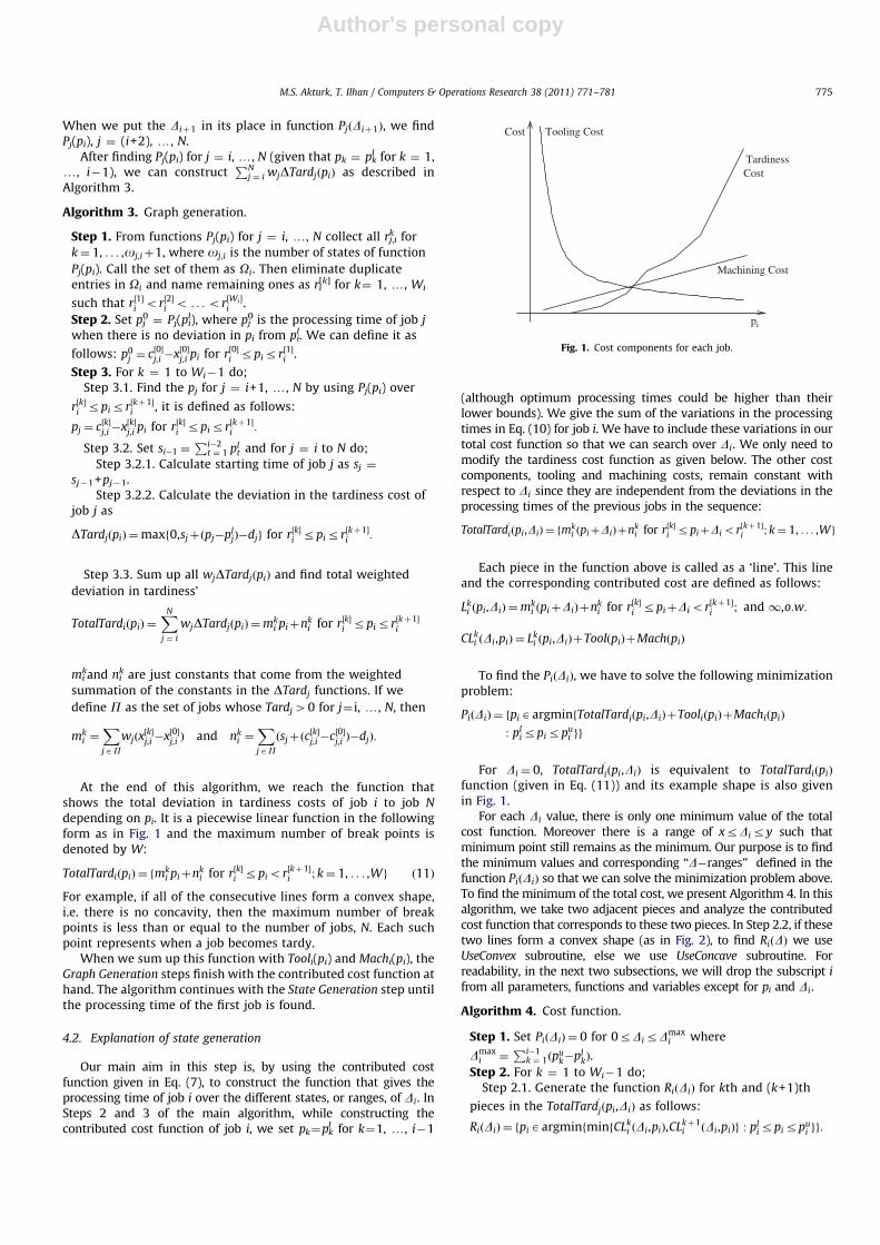
4.2.2. UseConcave subroutine

Sometimes, two consecutive tardiness cost lines form aconcave shape as in Fig. 3. To explain the reason behind this, letus consider three jobs, namely i, j, and k, whose processing orderis job i, job j, and job k. Furthermore, let job k be tardy and have aconstant processing time. While pj is constant and as pi increases,tardiness of job k increases. However, if at a point, say t, pj maystart to decrease as pi increases, at that point, the tardiness of jobk equals to a constant value and remains at that value as long as pj

decreases. This causes concavity because the slope of the totaltardiness cost function falls down after point t. In such a case,RðDiÞ requires a more detailed analysis. The same subroutine canalso be used for non-consecutive lines, which might occur at Step2.3 of the State Generation algorithm.

Now consider the following simplified versions of Lk and Ls

with r½s�Zr½kþ1�:

LkðpiÞ ¼mk � piþðn

kÞu, b1rpiob2

1 o:w:

(LsðpiÞ ¼

ms � piþðnsÞu, b3rpiob4

1 o:w:

(

where

b1 ¼ r½k��Di, b2 ¼ r½kþ1��Di, b3 ¼ r½s��Di

b4 ¼ r½sþ1��Di, ðnkÞ

u¼ nkþmkDi, ðn

sÞu¼ nsþmkDi:

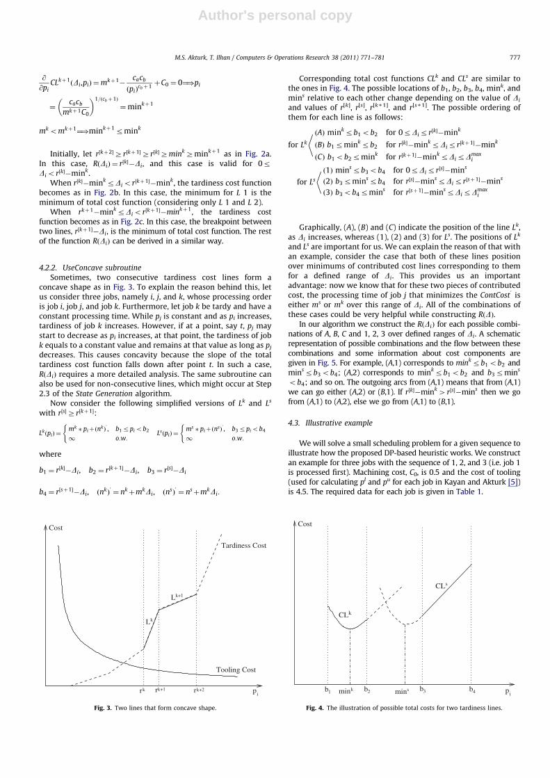
Corresponding total cost functions CLk and CLs are similar tothe ones in Fig. 4. The possible locations of b1, b2, b3, b4, mink, andmins relative to each other change depending on the value of Di

and values of r[k], r[s], r[k + 1], and r[s +1]. The possible ordering ofthem for each line is as follows:

for Lk

ðAÞ minkrb1ob2 for 0rDirr½k��mink

ðBÞ b1rminkrb2 for r½k��minkrDirr½kþ1��mink

ðCÞ b1ob2rmink for r½kþ1��minkrDirDmaxi

*

for Ls

ð1Þ minsrb3ob4 for 0rDirr½s��mins

ð2Þ b3rminsrb4 for r½s��minsrDirr½sþ1��mins

ð3Þ b3ob4rmins for r½sþ1��minsrDirDmaxi

*

Graphically, (A), (B) and (C) indicate the position of the line Lk,as Di increases, whereas (1), (2) and (3) for Ls. The positions of Lk

and Ls are important for us. We can explain the reason of that withan example, consider the case that both of these lines positionover minimums of contributed cost lines corresponding to themfor a defined range of Di. This provides us an importantadvantage: now we know that for these two pieces of contributedcost, the processing time of job j that minimizes the ContCostu iseither ms or mk over this range of Di. All of the combinations ofthese cases could be very helpful while constructing RðDÞ.

In our algorithm we construct the RðDiÞ for each possible combi-nations of A, B, C and 1, 2, 3 over defined ranges of Di. A schematicrepresentation of possible combinations and the flow between thesecombinations and some information about cost components aregiven in Fig. 5. For example, (A,1) corresponds to minkrb1ob2 andminsrb3ob4; (A,2) corresponds to minkrb1ob2 and b3rmins

ob4; and so on. The outgoing arcs from (A,1) means that from (A,1)we can go either (A,2) or (B,1). If r½k��mink4r½s��mins then we gofrom (A,1) to (A,2), else we go from (A,1) to (B,1).

4.3. Illustrative example

We will solve a small scheduling problem for a given sequence toillustrate how the proposed DP-based heuristic works. We constructan example for three jobs with the sequence of 1, 2, and 3 (i.e. job 1is processed first). Machining cost, C0, is 0.5 and the cost of tooling(used for calculating pl and pu for each job in Kayan and Akturk [5])is 4.5. The required data for each job is given in Table 1.

kr k+1r k+2r

Cost

Lk+1

Tardiness Cost

Tooling Cost

pi

Lk

Fig. 3. Two lines that form concave shape.

b1 b4b3b2

CLk

CLs

Cost

pi

kmin mins

Fig. 4. The illustration of possible total costs for two tardiness lines.

M.S. Akturk, T. Ilhan / Computers & Operations Research 38 (2011) 771–781 777

Author's personal copy

Job 3 : We start with generating total tardiness function of thelast job in the given sequence, job 3, because its TotalTardu

function includes only its own tardiness cost:

s3 ¼ pl1þpl

2 ¼ 0:70þ1:23¼ 1:93

Dmax3 ¼ ð2:42�0:70Þþð3:04�1:23Þ ¼ 3:53

P3ðp3Þ ¼ p3

TotalTard3ðp3Þ ¼0 for 0:56rp3o1:07

2ðp3�1:07Þ for 1:07rp3r2:08

(

TotalTardu

3ðp3,D3Þ ¼0 for 0:56rp3þD3o1:07

2ðp3þD3�1:07Þ for 1:07rp3þD3r2:08þ3:53¼ 5:61

(

This function gives how tardiness cost value changes accordingto the changes in the processing times of jobs 1, 2 and 3. Now, wehave to generate P3ðD3Þ. The total contributed cost lines thatcorrespond to each tardiness cost range is as follows:

CL1ðD3,p3Þ ¼

0:5p3þ2:92=ðp3Þ1:24 for 0:56rp3þD3o1:07

1 o:w:

(

CL2ðD3,p3Þ ¼

2:5p3�2:14þ2D3þ2:92=ðp3Þ1:24 for 1:07rp3þD3r5:61

1 o:w:

(

The minimums of lines CL1 and CL2 are min1¼2.08

and min2¼1.05, respectively. We can construct the RðD3Þ by

using the UseConvex subroutine. Since there is no more lineP3ðD3Þ ¼ RðD3Þ:

P3ðD3Þ ¼ RðD3Þ ¼1:07�D3 for 0:00rD3o0:02

1:05 for 0:02rD3r5:61

(

Afterwards, we can reduce P3ðD3Þ to P3(p2) by settingD3 ¼ p2�1:23:

P3ðp2Þ ¼2:30�p2 for 1:23rD3o1:25

1:05 for 1:25rD3r3:04

(

Job 2 : We have to generate TotalTard function of job 2. Theonly job after job 2 is job 3 and we already know how itsprocessing time changes with respect to the processing time ofjob 3 from P3(p2). We calculate the tardiness cost for each job andsum them up:

s3 ¼ pl1þp2 ¼ 0:70þp2

Tard3ðp2Þ ¼maxf0,p2þP3ðp2Þ�2:30g ¼0 for 1:23rp2o1:25

p2�1:25 for 1:25rp2r3:04

(

Let s2 ¼ pl1 ¼ 0:70, such that Dmax

2 ¼ 2:42�0:70¼ 1:72: Consequently,

Tard2ðp2Þ ¼maxf0,p2�1:28g ¼0 for 1:23rp2o1:28

p2�1:28 for 1:28rp2r3:04

(

TotalTardðp2Þ ¼w2Tard2ðp2Þþw3Tard3ðp2Þ ¼

0 for 1:23rp2o1:25

2ðp2�1:25Þ for 1:25rp2o1:28

5ðp2�1:28Þ for 1:28rp2r3:04

8><>:

TotalTardu

2ðD2,p2Þ ¼

0 for 1:23rp2þD2o1:25

2ðp2þD2�1:25Þ for 1:25rp2þD2o1:28

5ðp2þD2�1:28Þ for 1:28rp2þD2r4:76

8><>:

Now, we have to calculate P2ðD2Þ. There are three distinctpiecewise lines in total cost function of job 2 as follows:

CL1ðD2,p2Þ ¼

0:5p2þ5:18=ðp1:412 Þ for 1:23rp2þD2o1:25

1 o:w:

(

CL2ðD2,p2Þ ¼

2:5p2�2:50þ2D2þ5:18=ðp1:412 Þ for 1:25rp2þD2o1:28

1 o:w:

(

CL3ðD2,p2Þ ¼

5:5p2�6:40þ5D2þ5:18=ðp1:412 Þ for 1:28rp2þD2r4:76

1 o:w:

(

The processing times that minimize CL1, CL2 and CL3 are min1

¼ 3.04, min2¼1.56, and min3

¼1.23, respectively. As it is seen, allconsecutive lines form a convex shape. A graphical representationis given in Fig. 6. Thus, we can use the UseConvex subroutine andfind the corresponding P2ðD2Þ easily:

P2ðD2Þ ¼1:28�D2 for 0:00rD2o0:05

1:23 for 0:05rD2r1:72

(

Job 1 : The TotalTard function for job 1 can be found in a similarway as follows:

TotalTardðp1Þ ¼

2ðp1�0:73Þ for 0:73rp1o0:77

5ðp1�0:77Þ for 0:77rp1o1:00

6ðp1�0:80Þ for 1:00rp1r2:42

8><>:

Since we reach to the first job in the given sequence, weskip the state generation step and directly find the point thatminimize the contributed cost function. Its minimum is 0.83, andhence p1 ¼ 0.83. We can now calculate the processing times ofthe jobs 2 and 3 in a backward manner. Since p1¼0.83, then D2,

A,1

A,2

B,3 3,C3,A

C,2

C,1

B,2

B,1

for Ls is fixed

tardiness costfor Lk is fixed

Tooling costfor Lk is fixed

tardiness cost Tooling costfor Ls is fixed

Fig. 5. Possible combinations of locations of ranges for two tardiness lines and

information about cost components corresponding to each line.

Table 1Job data for the illustrative example.

Job # D L w d pl pu ca cb

1 7.2 6 1 1 0.70 2.42 2.06 1.35

2 7.1 8 3 2 1.23 3.04 5.18 1.41

3 7.1 5 2 3 0.56 2.08 2.92 1.24

M.S. Akturk, T. Ilhan / Computers & Operations Research 38 (2011) 771–781778

Author's personal copy

2.42�0.83 ¼ 1.59, correspond to the second state of P2ðD2Þ. Thus,p2 ¼ 1.23. Now, we know both p1 and p2 and can calculateD3 ¼ 2:42�0:83þ1:23�1:23¼ 1:59. For this value of D3, p3¼1.05.In this particular instance, the mathematical formulation alsogives the same solution, and hence it is an optimal solution.

When we compare different processing time alternatives inTable 2 for a given sequence of {1�2�3}, we can easily observethat the processing time upper bounds, pu, give the minimumtooling cost, but the maximum machining and weighted tardinesscosts. On the other hand, the processing time lower bounds, pl,give the minimum machining and weighted tardiness costs, butthe maximum tooling cost. Therefore, the controllable processingtimes, denoted by p*, provide an important tradeoff. It isimportant to note that the pu values (that minimize the sum ofmachining and tooling costs) are the processing time values usedin the scheduling literature. By utilizing the inherent flexibility ofthe CNC machines, we could reduce the overall cost by 58%. Thecost of implementing the controllable processing time idea isvirtually negligible; it only requires few changes in the CNC partprogram.

5. Experimental results

In this section, the experimental factors of the problem arespecified and the performance of both the proposed DP-basedheuristic and local search algorithm are compared with theircorresponding bench-mark algorithms. Both local search and DP-based heuristics are coded in C language and compiled with GNUcompiler. The nonlinear model of the original problem for a givensequence is formulated in GAMS 2.25 and solved by MINOS 5.3.All problems are solved on a sparc station (Sun Enterprize 4000)under SunOS 5.7.

We developed a four-factorial experimental design to test bothproposed DP-based heuristic and PSGA. The first factor was the

number of jobs, N, and we generated a variety of problems with40 and 80 jobs. The difficulty of the problem increases exponen-tially when we increase the N. Furthermore, as the number of jobincreases, the decision on the processing times of the jobsbecomes more critical since an increase in the processing timeof a job has greater effect on the total tardiness cost value. In ourcomputational setting, the operating cost of the CNC machine wasa fixed parameter, and C0¼0.5. On the other hand, the cost oftooling, Ct, for each job was the second experimental factor, andwere selected randomly from the interval UN[0.5,1.5] andUN[3.5,4.5] for the low and high levels, respectively, where UNstands for an uniform distribution. As tooling cost increases, thetradeoff between tooling cost and the sum of tardiness andmachining costs increases. This increases the difficulty of theproblem as well. Due dates, di, were randomly generated from theinterval UN½ð1�TF�RDD=2Þ,ð1�TFþRDD=2Þ� �Spi, where TF isthe tardiness factor, RDD is the range of due dates, pi is theaverage processing time of job i and Spi is the sum of averageprocessing times of all jobs. Both TF and RDD were set to 0.2, 0.5and 0.8. In sum, the number of jobs and tooling cost can takevalues in two levels, whereas tardiness factor and range of duedate can take values in three levels. Thus, the experimental designis a 2*2*3*3 full factorial design.

5.1. Computational results for a given sequence

By using the full factorial design, we first tested our DP-basedheuristic. For the benchmark, we solved the mathematicalformulation given in Step 2.6 of the Algorithm 1 (we have anonlinear objective function with a linear set of constraints). Foreach factor combination, we took 25 replications resulting in 900randomly generated runs. The summary of the results is listed inTable 3 showing the minimum, maximum and average results foreach algorithm.

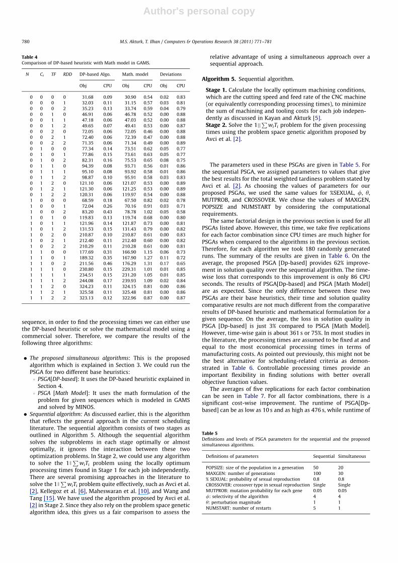
The averages of 25 replications for each factor combination aregiven in Table 4. Under the ‘Deviations’ column, we report thedeviation from the optimal solution under ‘Obj’ and what percentthe CPU time (in seconds) of our heuristic is less than the one ofthe mathematical formulation under ‘CPU’. The results show thatour proposed heuristic deviates from the optimal solution only 2%on the average. However, we gain about 82% improvement in theCPU time on the average. The most difficult case is the factorcombination of (1 1 0 2), where the number of jobs, tooling costand the range of due date are at their highest level and thetardiness factor is at its lowest level. Even in the worst case, ouralgorithm deviates 17% on the average. Both of these approachescan be used as a basic heuristic in Step 2.6 of the proposed PSGA.Even if the average CPU times for the mathematical model inTable 4 may seem small, since this step is called hundreds oftimes, its effect in the main algorithm becomes very significant.

5.2. Local search parameters and results

We now compare the proposed simultaneous algorithm with atwo-stage sequential algorithm. We first generate differentsequences using a PSGA based local search algorithm. For a given

tardyjob 3 becomes

tardyjob 2 becomes

3.04min1min2

1.56

Cost

p2

Tooling Cost

1.281.25

tardiness+machining cost

1.23min3

Fig. 6. Processing time variation of Job 2.

Table 2Processing time alternatives for the illustrative example.

Processing time Machining

cost

Tooling

cost

Weighted

tardiness

Total

pu¼(2.42, 3.04, 2.08) 3.77 2.831 20.88 27.481

pl¼(0.7, 1.23, 0.56) 1.245 12.89 0.0 14.135

p*¼(0.83, 1.23, 1.05) 1.555 9.516 0.4 11.471

Table 3Summary results for the problem with given sequence.

Algorithms Objective Runtimes

Min Average Max Min Average Max

DP-based heuristic 25.54 134.41 410.16 0.03 0.14 0.82

Math. model in GAMS 25.12 131.40 410.05 0.40 0.73 1.48

M.S. Akturk, T. Ilhan / Computers & Operations Research 38 (2011) 771–781 779

Author's personal copy

sequence, in order to find the processing times we can either usethe DP-based heuristic or solve the mathematical model using acommercial solver. Therefore, we compare the results of thefollowing three algorithms:

� The proposed simultaneous algorithms: This is the proposedalgorithm which is explained in Section 3. We could run thePSGA for two different base heuristics:3 PSGA[DP-based]: It uses the DP-based heuristic explained in

Section 4.3 PSGA [Math Model]: It uses the math formulation of the

problem for given sequences which is modeled in GAMSand solved by MINOS.

� Sequential algorithm: As discussed earlier, this is the algorithmthat reflects the general approach in the current schedulingliterature. The sequential algorithm consists of two stages asoutlined in Algorithm 5. Although the sequential algorithmsolves the subproblems in each stage optimally or almostoptimally, it ignores the interaction between these twooptimization problems. In Stage 2, we could use any algorithmto solve the 1J

PwiTi problem using the locally optimum

processing times found in Stage 1 for each job independently.There are several promising approaches in the literature tosolve the 1J

PwiTi problem quite effectively, such as Avci et al.

[2], Kellegoz et al. [6], Maheswaran et al. [10], and Wang andTang [15]. We have used the algorithm proposed by Avci et al.[2] in Stage 2. Since they also rely on the problem space geneticalgorithm idea, this gives us a fair comparison to assess the

relative advantage of using a simultaneous approach over asequential approach.

Algorithm 5. Sequential algorithm.

Stage 1. Calculate the locally optimum machining conditions,which are the cutting speed and feed rate of the CNC machine(or equivalently corresponding processing times), to minimizethe sum of machining and tooling costs for each job indepen-dently as discussed in Kayan and Akturk [5].Stage 2. Solve the 1jj

PwiTi problem for the given processing

times using the problem space genetic algorithm proposed byAvci et al. [2].

The parameters used in these PSGAs are given in Table 5. Forthe sequential PSGA, we assigned parameters to values that givethe best results for the total weighted tardiness problem stated byAvci et al. [2]. As choosing the values of parameters for ourproposed PSGAs, we used the same values for %SEXUAL, f, y,MUTPROB, and CROSSOVER. We chose the values of MAXGEN,POPSIZE and NUMSTART by considering the computationalrequirements.

The same factorial design in the previous section is used for allPSGAs listed above. However, this time, we take five replicationsfor each factor combination since CPU times are much higher forPSGAs when compared to the algorithms in the previous section.Therefore, for each algorithm we took 180 randomly generatedruns. The summary of the results are given in Table 6. On theaverage, the proposed PSGA [Dp-based] provides 62% improve-ment in solution quality over the sequential algorithm. The time-wise loss that corresponds to this improvement is only 86 CPUseconds. The results of PSGA[Dp-based] and PSGA [Math Model]are as expected. Since the only difference between these twoPSGAs are their base heuristics, their time and solution qualitycomparative results are not much different from the comparativeresults of DP-based heuristic and mathematical formulation for agiven sequence. On the average, the loss in solution quality inPSGA [Dp-based] is just 3% compared to PSGA [Math Model].However, time-wise gain is about 361 s or 75%. In most studies inthe literature, the processing times are assumed to be fixed at andequal to the most economical processing times in terms ofmanufacturing costs. As pointed out previously, this might not bethe best alternative for scheduling-related criteria as demon-strated in Table 6. Controllable processing times provide animportant flexibility in finding solutions with better overallobjective function values.

The averages of five replications for each factor combinationcan be seen in Table 7. For all factor combinations, there is asignificant cost-wise improvement. The runtime of PSGA[Dp-based] can be as low as 10 s and as high as 476 s, while runtime of

Table 4Comparison of DP-based heuristic with Math model in GAMS.

N Ct TF RDD DP-based Algo. Math. model Deviations

Obj CPU Obj CPU Obj CPU

0 0 0 0 31.68 0.09 30.90 0.54 0.02 0.83

0 0 0 1 32.03 0.11 31.15 0.57 0.03 0.81

0 0 0 2 35.23 0.13 33.74 0.59 0.04 0.79

0 0 1 0 46.91 0.06 46.78 0.52 0.00 0.88

0 0 1 1 47.18 0.06 47.03 0.52 0.00 0.88

0 0 1 2 49.65 0.07 49.41 0.53 0.00 0.87

0 0 2 0 72.05 0.06 72.05 0.46 0.00 0.88

0 0 2 1 72.40 0.06 72.39 0.47 0.00 0.88

0 0 2 2 71.35 0.06 71.34 0.49 0.00 0.89

0 1 0 0 77.34 0.14 73.51 0.62 0.05 0.77

0 1 0 1 77.86 0.15 73.61 0.63 0.05 0.77

0 1 0 2 82.31 0.16 75.53 0.65 0.08 0.75

0 1 1 0 94.39 0.08 93.71 0.56 0.01 0.86

0 1 1 1 95.10 0.08 93.92 0.58 0.01 0.86

0 1 1 2 98.87 0.10 95.91 0.58 0.03 0.83

0 1 2 0 121.10 0.06 121.07 0.53 0.00 0.89

0 1 2 1 121.30 0.06 121.25 0.53 0.00 0.89

0 1 2 2 120.31 0.06 119.97 0.54 0.00 0.88

1 0 0 0 68.59 0.18 67.50 0.82 0.02 0.78

1 0 0 1 72.04 0.26 70.16 0.91 0.03 0.71

1 0 0 2 83.20 0.43 78.78 1.02 0.05 0.58

1 0 1 0 119.83 0.13 119.74 0.68 0.00 0.80

1 0 1 1 121.96 0.14 121.87 0.73 0.00 0.81

1 0 1 2 131.53 0.15 131.43 0.79 0.00 0.82

1 0 2 0 210.87 0.10 210.87 0.61 0.00 0.83

1 0 2 1 212.40 0.11 212.40 0.60 0.00 0.82

1 0 2 2 210.29 0.11 210.28 0.61 0.00 0.81

1 1 0 0 177.69 0.31 166.90 1.15 0.06 0.73

1 1 0 1 189.32 0.35 167.90 1.27 0.11 0.72

1 1 0 2 211.56 0.46 176.29 1.31 0.17 0.65

1 1 1 0 230.80 0.15 229.31 1.01 0.01 0.85

1 1 1 1 234.51 0.15 231.20 1.05 0.01 0.85

1 1 1 2 244.08 0.17 239.93 1.09 0.02 0.84

1 1 2 0 324.23 0.11 324.15 0.81 0.00 0.86

1 1 2 1 325.58 0.11 325.48 0.81 0.00 0.86

1 1 2 2 323.13 0.12 322.96 0.87 0.00 0.87

Table 5Definitions and levels of PSGA parameters for the sequential and the proposed

simultaneous algorithms.

Definitions of parameters Sequential Simultaneous

POPSIZE: size of the population in a generation 50 20

MAXGEN: number of generations 100 30

% SEXUAL: probability of sexual reproduction 0.8 0.8

CROSSOVER: crossover type in sexual reproduction Single Single

MUTPROB: mutation probability for each gene 0.05 0.05

f: selectivity of the algorithm 4 4

y: perturbation magnitude 1 1

NUMSTART: number of restarts 5 1

M.S. Akturk, T. Ilhan / Computers & Operations Research 38 (2011) 771–781780

Author's personal copy

PSGA[Math Model] is between 300 and 859 s and seem morestable. According to our computational results, both the sequen-tial algorithm and PSGA[Math Model] do not exploit the problemstructure to improve the solution quality, or to reduce the runtime. However, the DP-based heuristic exploits the problemcharacteristics, such as position of a job in a given sequence, toimprove the solution quality and computational requirements.

6. Conclusion

The integration of scheduling and process planning issuescreates more realistic problems. In this paper, we proposed a jointalgorithm to determine the processing time of each job and toschedule these jobs on a single CNC machine considering the totalweighted tardiness and manufacturing cost. To the best of our

knowledge, the single CNC machine scheduling problem thatconsiders job-dependent tardiness penalties and controllableprocessing times simultaneously is not studied in the literature.We first compared the proposed DP-based heuristic with an exactalgorithm for a given sequence and show that the deviation fromthe optimal solution is very small compared to the gain from thecomputational time. Afterwards, we compared the proposed PSGAwith a two-stage sequential algorithm. The experimental resultsindicate that there is a significant interaction between machiningconditions and weighted tardiness problems and solving thesetwo problems together increases the cost effectiveness of thesystem greatly. Our results clearly indicate that the proposedPSGA that uses proposed DP-based heuristic gives the best resultsin terms of time-cost ratio. As a future research, for the CNCmachines with an on-board tool magazine (that means machinehas to be stopped in order to replace a cutting tool due to toolwear or part change due to limited tool magazine size), toolreplacement decisions should be integrated to the joint problemin addition to the process planning and part sequencing problemssince they also affect the part completion times.

Acknowledgments

The authors thank anonymous referees for their constructivecomments.

References

[1] Al-Ahmari AMA. Computer aided optimization of scheduling and machiningparameters in job shop manufacturing systems. Production Planning andControl 2002;13:401–6.

[2] Avci S, Akturk MS, Storer RH. A problem space genetic algorithm for singlemachine weighted tardiness problems. IIE Transactions 2003;35(5):479–86.

[3] Cheng TCE, Chen ZL, Chung-Lun L. Parallel machine scheduling withcontrollable processing times. IIE Transactions 1996;28(2):177–80.

[4] Gurel S, Akturk MS. Considering manufacturing cost and schedulingperformance on a CNC turning machine. European Journal OperationalResearch 2007;177(1):325–43.

[5] Kayan RK, Akturk MS. A new bounding mechanism for the CNC machinescheduling problems with controllable processing times. European JournalOperational Research 2005;167(3):624–43.

[6] Kellegoz T, Toklu B, Wilson J. Comparing efficiencies of genetic crossoveroperators for one machine total weighted tardiness problem. AppliedMathematics and Computation 2008;199:590–8.

[7] Lawler EL. A ‘pseudopolynomial’ algorithm for sequencing jobs to minimizetotal tardiness. Annals of Discrete Mathematics 1977;1:331–42.

[8] Pinedo M. Scheduling: theory, algorithms and systems. 2nd ed. New Jersey:Prentice-Hall; 2002.

[9] Shabtay D, Kaspi M. Minimizing the total weighted flowtime in a singlemachine with controllable processing times. Computers & OperationsResearch 2004;31:2279–89.

[10] Maheswaran R, Ponnambalam SG, Jawahar N. Hybrid heuristic algorithms forsingle machine total weighted tardiness scheduling problems. InternationalJournal of Intelligent Systems Technologies and Applications 2008;4:34–56.

[11] Shabtay D, Steiner G. A survey of scheduling with controllable processingtimes. Discrete Applied Mathematics 2007;155(13):1643–66.

[12] Storer RH, Wu SD, Vaccari R. New search spaces for sequencing problemswith application to job shop scheduling. Management Science 1992;38(10):1495–509.

[13] Tseng CT, Liao CJ, Huang KL. Minimizing total tardiness on a single machinewith controllable processing times. Computers & Operations Research2009;36:1852–8.

[14] Vickson RG. Choosing the job sequence and processing times to minimizeprocessing plus flow cost on a single machine. Operations Research 1980;28:1155–67.

[15] Wang X, Tang L. A population-based variable neighborhood search for thesingle machine total weighted tardiness problem. Computers & OperationsResearch 2009;36:2105–10.

[16] Xu K, Feng Z, Jun K. A tabu-search algorithm for scheduling jobs withcontrollable processing times on a single machine to meet due-dates.Computers & Operations Research 2010;37(11):1924–38.

[17] Yedidsion L, Shabtay D, Kaspi M. A bicriteria approach to minimize maximallateness and resource consumption for scheduling a single machine. Journalof Scheduling 2007;10:341–52.

Table 6Summary results of PSGA’s for the problem.

Algorithms Objective Runtimes

Min Average Max Min Average Max

Two-stage PSGA 26.39 246.40 984.15 8.48 33.71 79.83

PSGA[DP-based] 20.75 93.36 282.33 10.15 119.29 476.29

PSGA[GAMS] 20.75 90.42 282.87 300.55 480.23 859.81

Table 7Comparison of the sequential and the proposed simultaneous algorithms.

N Ct TF RDD Sequential PSGA[DP-based] PSGA[GAMS]

Obj CPU Obj CPU Obj CPU

0 0 0 0 49.15 10.89 24.96 83.31 24.92 296.97

0 0 0 1 64.50 10.70 23.73 71.88 23.35 304.92

0 0 0 2 70.37 9.11 22.48 77.61 22.19 308.27

0 0 1 0 72.86 10.55 32.21 41.96 31.93 275.96

0 0 1 1 81.74 10.62 30.49 46.12 29.80 285.26

0 0 1 2 95.46 9.52 29.87 46.12 28.71 274.66

0 0 2 0 106.97 10.37 47.00 28.56 46.80 251.13

0 0 2 1 106.18 10.14 45.56 28.74 45.58 250.20

0 0 2 2 118.00 9.52 46.37 29.47 45.03 249.41

0 1 0 0 138.71 10.95 58.90 88.38 57.96 322.38

0 1 0 1 148.32 10.83 59.02 71.08 56.47 325.26

0 1 0 2 166.80 9.88 55.63 72.49 54.40 327.03

0 1 1 0 170.78 11.07 70.66 52.35 70.38 306.79

0 1 1 1 172.67 10.96 70.44 57.65 68.14 307.30

0 1 1 2 198.70 9.82 69.88 48.69 67.48 303.50

0 1 2 0 210.21 9.92 89.54 29.20 89.26 282.63

0 1 2 1 202.72 9.38 89.23 31.43 87.68 279.76

0 1 2 2 223.46 9.02 89.03 32.85 87.14 276.51

1 0 0 0 114.11 54.61 52.90 197.85 51.41 475.91

1 0 0 1 134.36 40.38 50.55 229.91 47.64 540.17

1 0 0 2 142.78 45.14 51.24 313.44 45.70 584.54

1 0 1 0 185.31 51.63 75.16 80.60 73.34 410.46

1 0 1 1 201.67 37.00 70.33 86.83 69.07 405.22

1 0 1 2 226.78 47.83 73.00 99.29 71.68 397.48

1 0 2 0 294.62 47.70 128.13 56.08 127.46 326.97

1 0 2 1 299.13 39.32 135.96 56.19 132.90 330.88

1 0 2 2 341.28 40.46 140.09 56.58 138.90 339.80

1 1 0 0 374.20 47.29 137.15 226.80 125.96 653.18

1 1 0 1 377.78 41.37 133.31 232.28 121.27 658.71

1 1 0 2 427.82 47.03 135.17 268.00 119.05 661.15

1 1 1 0 476.72 46.88 166.16 99.82 161.54 568.34

1 1 1 1 469.41 41.83 169.34 94.78 160.84 570.60

1 1 1 2 541.59 45.45 177.17 85.90 169.00 498.64

1 1 2 0 606.89 47.12 233.04 57.85 229.17 457.64

1 1 2 1 586.60 36.38 237.79 58.30 234.60 446.81

1 1 2 2 671.74 39.67 239.37 61.71 238.47 461.38

M.S. Akturk, T. Ilhan / Computers & Operations Research 38 (2011) 771–781 781