adfa, p. 1, 2013.

© Springer-Verlag Berlin Heidelberg 2013

A Rank-based Hybrid Algorithm for Scheduling Data-

and Computation-intensive Jobs in Grid Environments

Mohsen Abdoli, Reza Entezari-Maleki, and Ali Movaghar

Department of Computer Engineering, Sharif University of Technology, Tehran, Iran

Email: {abdoli,entezari}@ce.sharif.edu, movaghar@sharif.edu

Abstract. Scheduling is one of the most important challenges in grid computing

environments. Most existing scheduling algorithms in grids only focus on one

type of grid jobs which can be data-intensive or computation-intensive. Howev-

er, merely considering one type of jobs in scheduling does not result in proper

scheduling in the viewpoint of all system, and sometimes causes wasting of re-

sources on the other side. To address the problem of simultaneously considering

both types of jobs, a rank-based hybrid scheduling (RBHS) algorithm is pro-

posed in this paper. At one hand, RBHS algorithm takes both data server and

computational resource availability of the network into account, and on the oth-

er hand, considering the corresponding requirements of each job, it assigns a

factor called Z to the job. Using the Z factor, the importance of two dimensions

(being data or computation intensive) for each job is determined, and then the

job is scheduled to the available resources. Results obtained from simulating

different scenarios in hypothetical grid environments show that the proposed

algorithm outperforms other existing algorithms.

Keywords: Scheduling algorithm, grid computing, data-intensive jobs, compu-

tation-intensive jobs.

1 Introduction

Nowadays, most applications especially in scientific and engineering fields tend to be

data-intensive and/or computation-intensive. Due to the fact that it is ineffective to

manage these applications in a central server, grid technology has been developed as a

proper infrastructure to replace it. Grid gathers resources from multiple administrative

domains to reach a common goal, solving a single huge problem [1]. One of the most

important challenges in grids is task scheduling problem. Indeed, finding the optimal

schedule for a grid environment which can distribute the submitted jobs to the grid

resources to optimize a given measure is a well-known NP-complete problem [2]. To

overcome this difficulty, many heuristic methods have been proposed to appropriately

schedule jobs among resources [3], [4] and [5]. None of these types of scheduling

algorithms can be clearly claimed to find optimal solution. They just make a search on

possible solution space of the problem and find the most suitable solution which can

satisfy the optimization measure.

In addition to the type of algorithms, the nature of applications can also affect the

result of the scheduling and should be considered during scheduling phase. Generally

speaking, the applications can be divided into two basic classes, data-intensive and

computation-intensive applications. Data-intensive applications dedicate most of their

operation time to access data [6] however computation-intensive applications devote

most of their operation time to compute and process on data [7]. In fact, almost no

application belongs to one of these two classes specifically; nevertheless it needs

data/computational resources proportionally to be executed. In other words, each

application is both data-intensive and computation-intensive. However the ratio be-

tween being data and computation intensive differs among applications.

Most existing grid scheduling algorithms merely focus on either data-intensive or

computation-intensive aspects [6], [7]. However, focusing on only one of these di-

mensions causes serious problems, since the other one is not negligible. At one hand,

considering only data-intensive dimension leads to a waste of computational power;

on the other hand, considering only computation-intensive dimension causes a waste

of network resources such as bandwidth. We propose a Rank-based Hybrid Schedul-

ing (RBHS) algorithm that addresses these problems. The proposed algorithm is a

way to simultaneously consider data-intensive and computation-intensive characteris-

tics of the job, while taking into account the same characteristics of the available grid

environment. In other words, the scheduler needs to schedule any submitted job adap-

tively based on the current status of the network as well as the job.

The rest of the paper is organized as follows. In Section 2, the basic concepts of

grid environment are described. The proposed algorithm and results obtained from

simulating the algorithm and another famous benchmark are presented in Section 3

and Section 4, respectively. Finally, Section 5 concludes the paper.

2 Model and Problem Definition

In this section, the grid environment under study is briefly described and some basic

characteristics of grids are introduced. A grid environment is considered to include a

set of M nodes, each of which representing a cluster. A cluster within the grid envi-

ronment can be made of individual computational resources and data servers. Some

characteristics of a grid environment considered in this paper are mentioned below.

Multiple replicas of a dataset which is needed for an application to be processed

may coexist in data servers over grid environment, and computational resources

need to obtain them from the nearest data server(s).

Each job is finally submitted to a single cluster to use computational resources;

nevertheless, datasets can be supplied by any other cluster over the grid environ-

ment.

Grid environment can be considered to consists of a set of M clusters,

𝐶 = {𝐶1 , 𝐶2, … , 𝐶𝑀}. A cluster is denoted by 𝐶𝑖 = 𝐷𝑆𝑖 , 𝐶𝑃𝑖 , 1 ≤ 𝑖 ≤ 𝑀, that

provides specific data servers and computational resources. Data servers within the

clusters are in the form of data-hosts which consist of datasets and are denoted by

𝐷𝑆i = {𝑑𝑠1, 𝑑𝑠2, … , 𝑑𝑠𝑕} and the provided computational power is denoted by

CPi.

The requirement of each job 𝐽𝑘 is denoted by 𝐽𝑘= (𝐷𝑆𝑘 , 𝐶𝑃𝑘 ), where CPk is compu-

tational power required by 𝐽𝑘 and 𝐷𝑆𝑘= {𝑑𝑠1,𝑑𝑠2 , … , 𝑑𝑠𝑙} is a set of l datasets rep-

licated in data-hosts over the grid environment.

The computational capacity provided by resources and the computational power

required by jobs to be processed are measured in terms of Million Instructions per

Second (MIPS) and Million Instructions (MI), respectively. Although we are aware

of the fact that a single number such as MIPS cannot reveal the complexity and the

factual capacity of a set of CPUs, due to its simplicity in computing, MIPS (MI) is

a proper criterion to show the performance of a computer (computational complex-

ity of a job), especially in fields of scientific calculations.

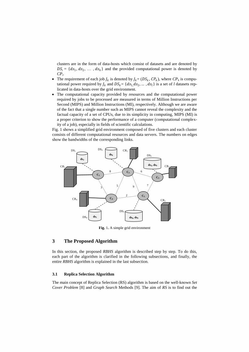
Fig. 1 shows a simplified grid environment composed of five clusters and each cluster

consists of different computational resources and data servers. The numbers on edges

show the bandwidths of the corresponding links.

Fig. 1. A simple grid environment

3 The Proposed Algorithm

In this section, the proposed RBHS algorithm is described step by step. To do this,

each part of the algorithm is clarified in the following subsections, and finally, the

entire RBHS algorithm is explained in the last subsection.

3.1 Replica Selection Algorithm

The main concept of Replica Selection (RS) algorithm is based on the well-known Set

Cover Problem [8] and Graph Search Methods [9]. The aim of RS is to find out the

ds2

ds2, ds9

C2

C4

C1 C3

C5

ds6

ds5 ds6, ds9

8 6

7 9

2

5 3

DS1 DS2

DS3

DS5

DS4

CR1

CR2

CR3

CR4 CR5

minimum cost of collecting a set of datasets needed for processing a job. These data-

sets might be located inside the cluster which executes the job or other existing clus-

ters in the grid environment. In the proposed model, bandwidths of links between

clusters are the criterion for how near a cluster is.

Suppose that cluster Ci is selected to process the submitted job Jk which needs da-

taset ds to be executed. As mentioned earlier, a dataset can be provided either from

the cluster Ci itself or a remote cluster Cj. In case that the dataset ds needs to be trans-

ferred from a remote cluster Cj, which is directly connected to the base cluster Ci,

transfer cost is given by the Eq. (1)

𝑇𝑖𝑚𝑒 𝑑𝑠, 𝐶𝑖 , 𝐶𝑗 = 𝑠𝑖𝑧𝑒 𝑑𝑠

𝐵 𝐿𝑖 ,𝑗 , (1)

where 𝐵(𝐿𝑖 ,𝑗 ) is the bandwidth of the link between the clusters Ci and Cj.

Sometimes the dataset ds does not exist in any of the adjacent clusters, so the algo-

rithm has to find it by exploring in the network. In this situation, transfer procedure

uses more than one link to obtain the dataset. Therefore, the algorithm needs to find a

path from the cluster providing ds to the cluster demanding it to compute the transfer

cost. After that, the total time to provide the dataset ds for cluster Ci is computed by

iteratively use of Eq. (1).

In order to find the path, it is better to consider the grid environment as a graph.

Therefore, RS algorithm can explore into nodes of the resulted graph to find the near-

est datasets. To achieve this, RS algorithm uses uniform cost search which is a search

algorithm used to traverse and find the shortest path in weighted graphs [10]. The

problem that uniform cost search tackles is very similar to ours. In our problem, edges

between nodes denote the communication links between clusters and the assigned

weights to each of the edges are the inversed value of links' bandwidths.

RS algorithm takes two parameters: a job characterized by 𝐽𝑘 = (𝐷𝑆𝑘 , 𝐶𝑃𝑘) and a

cluster Ci that needs to collect datasets existing in DSk. First of all, the algorithm in-

itializes a variable called Total Transfer Time (TTT) to zero. TTT will increase while

gathering datasets from remote clusters. It should be noted that at each stage of ex-

ploring the graph, it is essential to keep track of the path, because the cost of transfer-

ring a dataset is directly calculated from the path between Ci as well as the cluster

containing the datasets.

At the first step, the algorithm removes datasets from DSk, which are currently resi-

dent inside Ci. No transfer cost is considered at this step. Remaining datasets in DSk

have to be transferred from the nearest possible remote cluster. At this point, the clus-

ter Ci should expand as a graph node to form all the clusters connected to Ci via direct

link. Then, the following three steps must be iterated until DSk is empty.

Step one: Find the cluster Ct with the minimum distance from Ci (distance of a clus-

ter Ci from cluster Ct is sum of the edge weights existing in path from Ci to Ct).

Step two: Search the remaining datasets in Ct. The cost of data transferring should

be calculated using Eq. (2) for all datasets found in this step. The path from Ci to Ct is

characterized by: 𝑝𝑎𝑡𝑕(𝐶i , 𝐶𝑡) = {𝐶𝑖 , 𝐶′1 , 𝐶′2 … 𝐶′𝑝 , 𝐶𝑡}.

𝑇𝑟𝑎𝑛𝑠𝑓𝑒𝑟𝑇𝑖𝑚𝑒 𝑑𝑠 , 𝐶𝑖 , 𝐶𝑡

= 𝑇𝑖𝑚𝑒 𝑑𝑠, 𝐶𝑖 , 𝐶′1 + 𝑇𝑖𝑚𝑒 𝑑𝑠, 𝐶 ′

𝑗 , 𝐶 ′𝑗 +1

𝑗 =𝑝−1

𝑗 =1

+ 𝑇𝑖𝑚𝑒 𝑑𝑠, 𝐶 ′𝑝 , 𝐶𝑡 . (2)

For each dataset dsf which is found in this step, the algorithm first removes it from

DSk, and then adds 𝑇𝑟𝑎𝑛𝑠𝑓𝑒𝑟𝑇𝑖𝑚𝑒 𝑑𝑠𝑓 , 𝐶𝑖 , 𝐶𝑡 to TTT.

Step three: Expand Ct to generate its children in the graph and compute the distance

of the children from Ci.

Finally, the output of calling RS algorithm with the input of job Jk and the cluster Ci

is Total Transfer Time (TTT) which is used as RSScore(Jk,Ci), a measure for fitness of

cluster Ci for job Jk. Table 1 shows pseudo-code of the RS algorithm. Algorithm

shown in Table 1 is executed for a given job and all clusters existing in the environ-

ment. Therefore, if a new job is submitted to the environment, this algorithm should

be applied to all combinations of the new job with all available clusters.

Table 1. The RS algorithm

1 Set TTT to zero

2 Remove from DSk locally available data sets in Ci

3 Compute the distances (dist) of all adjacent clusters from Ci using Eq.(1)

Set the value of non-adjacent clusters to Inf

4 Sort the clusters in ascending order of distance in dist

5 While 𝑫𝑺𝐤 is not empty do

6 select first cluster as 𝑪𝐭 from dist

7 find the intersection of DSk and 𝑫𝑺𝐭

8 compute the transfer-time using Eq.(2)

9 add transfer-time to TTT

10 expand Ct and append the distance of its children to dist

11 set dist(l) to Inf and sort it again and remove found datasets

12 End While

13 return TTT

3.2 Computational Resource Allocation (CRA) Algorithm

computational resource allocation algorithm uses the number of time units it takes to

complete a specific job assuming that all required datasets are locally available (i.e.

transfer time needed to collect datasets is zero). For a given job, this score should be

calculated for all of the available computational resources.

As described earlier in section 3, the processing power provided by resources (re-

quired for jobs) is presented in the form of MIPS (MI). Therefore, the total time

needed for the job Ji to be completed in the computational resource Cj can be calcu-

lated by Eq. (3).

𝐶𝑅𝐴𝑆𝑐𝑜𝑟𝑒 = 𝐶𝑃𝑖

𝐶𝑃𝑗

, (3)

where CPj is the computational power provided by the computational resource Cj and

CPi is the computational power required by the job Ji. The CRAScore is used as a

score for fitness of the resource Cj for the job Ji.

The RS algorithm treated the submitted job as if it only has a data-intensive dimen-

sion. CRA algorithm in a comparable way focuses only on computation-intensive

dimension. As mentioned before, the available information about each job submitted

to the environment is presented in two areas. The first one contains information about

required datasets, so we can compute the total size of datasets, and the second one

gives information about the total computational power required by the job in terms of

MI. The aim at this step is to estimate the proportion of being data-intensive to being

computation-intensive, while considering the availability of resources in each area.

Hence, the algorithm needs to jointly consider both required and provided resources,

and then obtain a value for scheduler to show how much the submitted job is general-

ly data/computation intensive in the context of available grid environment. To achieve

this, the algorithm first estimates the expected value of the provided computational

power using Eq. (4).

𝐸 𝐶𝑜𝑚𝑝𝑢𝑡𝑎𝑡𝑖𝑜𝑛𝑃𝑜𝑤𝑒𝑟 = 𝐶𝑖

𝑀𝑖=1

𝑀. (4)

To obtain the corresponding value for data-intensive dimension of the submitted

job, the algorithm needs to apply an equivalent mean operation on network links. Eq.

(5) calculates this value by averaging on time needed to collect a specific set of data-

sets DS for each cluster. Mean path length for each cluster C is calculated using Eq.

(6), where M is the number of clusters and count(DS) is the number of datasets in DS.

Moreover, TransferLength(C,ds) denotes the distance between C and the closest clus-

ter providing ds.

𝐸 𝑇𝑟𝑎𝑛𝑠𝑓𝑒𝑟𝑇𝑖𝑚𝑒 = 𝑇𝑜𝑡𝑎𝑙𝑇𝑟𝑎𝑛𝑠𝑓𝑒𝑟𝐿𝑒𝑛𝑔𝑡𝑕(𝐷𝑆, 𝐶𝑖)

𝑀𝑖=1

𝑀. (5)

𝑇𝑜𝑡𝑎𝑙𝑇𝑟𝑎𝑛𝑠𝑓𝑒𝑟𝐿𝑒𝑛𝑔𝑡𝑕 𝐷𝑆, 𝐶 = 𝑇𝑟𝑎𝑛𝑠𝑓𝑒𝑟𝐿𝑒𝑛𝑔𝑡𝑕 𝐶, 𝑑𝑠 . 𝑠𝑖𝑧𝑒 𝑑𝑠 .

𝑑𝑠∈𝐷𝑆

(6)

The algorithm assesses the expected values of run time by Eq. (7). Finally, the fac-

tor Z is calculated by using Eq. (8) for a given job.

𝐸 𝑅𝑢𝑛𝑇𝑖𝑚𝑒 =𝐶𝑃𝑖

𝐸[𝐶𝑜𝑚𝑝𝑢𝑡𝑎𝑡𝑖𝑜𝑛𝑃𝑜𝑤𝑒𝑟] , (7)

𝑍 =𝐸 𝑅𝑢𝑛𝑇𝑖𝑚𝑒

𝐸 𝑇𝑟𝑎𝑛𝑠𝑓𝑒𝑟𝑇𝑖𝑚𝑒 + 𝐸 𝑅𝑢𝑛𝑇𝑖𝑚𝑒 . 8

3.3 Rank-based Hybrid Scheduling Algorithm

After describing the roles of different components of the proposed algorithm, RS and

CRA, it is the time to explain the main algorithm. Actually, the algorithm combines

the results of RS and CRA algorithms considering the weight of the factor Z. The

Rank-based Hybrid Scheduling (RBHS) algorithm is described in the pseudo-code

form in Table 2.

Table 2. The Rank-based Hybrid Scheduling algorithm

1 For each job j do

2 compute the factor Z for j

3 For each cluster Ci do

4 call RS and compute RSScore (j, Ci)

5 call CRA and compute CRAScore (j, Ci)

6 compute FinalScore (j, Ci) using

𝐅𝐢𝐧𝐚𝐥𝐒𝐜𝐨𝐫𝐞 𝐣, 𝐂𝐢 = (𝟏 − 𝐙) ∗ 𝐑𝐒𝐒𝐜𝐨𝐫𝐞(𝐣,𝐂𝐢) + 𝐙 ∗ 𝐂𝐑𝐀𝐒𝐜𝐨𝐫𝐞(𝐣, 𝐂𝐢)

7 End For

8 select cluster 𝑪𝐨𝐩𝐭 with minimum FinalScore and assign j to it

9 End For

As can be seen in Table 2, when the RBHS algorithm is executed for a submitted

job, both RSScore and CRAScore are generated by calling RS and CRA for each clus-

ter. Combining these two scores by affecting the factor Z generates the FinalScore for

all clusters. The task of scheduling the submitted job is then completed by selecting

the cluster with minimum FinalScore and assigning the job to it.

4 Performance Evaluation

In this section, the scheduling problem of 1000 jobs on 100 clusters within a hypo-

thetical grid environment is considered. The results obtained from simulating our

proposed algorithm are compared to the results of an algorithm proposed by Buyya et

al. [8], which is called SCP Tree Search. In SCP Tree Search algorithm, the problem

of finding the subset of data servers providing required datasets is reduced to a Set

Cover Problem. In SCP Tree Search algorithm, for each job submitted, it first finds a

subset of data servers with minimum number of data servers which provides required

datasets. Afterward, for those selected data servers, the algorithm finds the best com-

putational resource for executing the job. The best computational resource is the one

which can gather the required datasets from the selected data servers and complete the

job in minimum possible time.

4.1 Network Topology and Randomly Generated Grid Environment

The topology of the network is generated by Erdős–Rényi model which sets an edge

between each pair of nodes with equal probability, independent of the other edges

[11].

The size of the datasets as well as the computational power required by the jobs

can be approximated by Power Law distribution [12] in which the more the size of a

dataset increases, the less it is probable to occur [13]. However, the distribution of the

computational power provided by the clusters and the bandwidth of the links are de-

cided to follow Gaussian distribution. Datasets are spread over grid environment

uniformly.

4.2 Numerical Results

In order to compare the performance of the proposed algorithm with SCP Tree

Search, two metrics named total makespan and transfer time are selected. The ma-

kespan of a resource is the time slot between the start and completion of a sequence of

tasks assigned to the resource, and the total makespan of a grid environment is de-

fined as the largest makespan of the grid resources [4]. Moreover, transfer time is

defined as the total time that the submitted job spends on collecting datasets regard-

less of the time required for executing the job. These two metrics are calculated when

each job arrives at the scheduler during the batch mode simulation of jobs in grid

environment.

Simulations are done in three different scenarios: the first and second scenarios

show grid environments with more computation-intensive and data-intensive jobs,

respectively, and the third one simulates an environment with an equal amount of

both classes of jobs. The results of comparison when most of submitted jobs are com-

putation-intensive are shown in Fig. 2 and Fig. 3. According to the Fig. 2 and Fig. 3,

the performance of the proposed algorithm is reasonably better than SCP Tree Search

algorithm in terms of both makespan and transfer time.

The results of the second scenario are shown in Fig. 4 and Fig. 5. Furthermore, the

results of the combination situation, the third scenario, are demonstrated in Fig. 6 and

Fig. 7. As can be seen in Fig.4 and Fig.5, the proposed algorithm still outperforms

SCP Tree Search algorithm; however the performance is not as dominant as perfor-

mance of the previous scenarios. This is mainly due to the fact that in scheduling by

SCP Tree Search algorithm, the data-intensive dimension of the jobs is first consi-

dered, so the computation-intensive dimension is in lower priority. In point of fact, if

the submitted jobs get more data-intensive, the performance of SCP Tree Search algo-

rithm comes close to the performance of RBHS algorithm, and vice versa.

5 Conclusion

Considering different requirements of jobs during scheduling phase within grid envi-

ronments is the main concern of this paper. To achieve a more suitable scheduling in

grids, an algorithm named RBHS is presented in this paper to address the problem of

simultaneously considering data-intensive and computation-intensive dimensions of

the jobs. The proposed algorithm brings into account the ratio of being data-intensive

to being computation-intensive for each submitted job, and then scales the effect of

two sub-algorithms that each one considers one of the dimensions mentioned above.

Fig. 2. Makespan of RBHS and SCP Tree

Search in first scenario.

Fig. 3. Mean transfer time of RBHS and

SCP Tree Search in first scenario.

Fig. 4. Makespan of RBHS and SCP Tree

Search in second scenario.

Fig. 1. Mean transfer time of RBHS and

SCP Tree Search in second scenario.

Fig. 6. Makespan of RBHS and SCP Tree

Search in third scenario.

Fig. 7. Mean transfer time of RBHS and

SCP Tree Search in third scenario.

adfa, p. 10, 2013.

© Springer-Verlag Berlin Heidelberg 2013

REFRENCES

1. Foster, I., Kesselman, C.: The Grid 2: Blueprint for a New Computing Infrastructure.

Second edition, Elsevier and Morgan Kaufmann, San Francisco (2004)

2. Fernandez-Baca D.: Allocating Modules to Processors in a Distributed System. IEEE

Transactions on Software Engineering. 15, 1427–1436 (1989)

3. Kardani-Moghadam, S., Khodadadi, F., Entezari-Maleki, R., Movaghar, A.: A Hybrid Ge-

netic Algorithm and Variable Neighborhood Search for Task Scheduling Problem in Grid

Environment. Procedia Engineering. 29, 3808–3814 (2012)

4. Entezari-Maleki, R., Movaghar, A.: A Genetic-based Scheduling Algorithm to Minimize

the Makespan of the Grid Applications. In: Kim, T., Yau, S., Gervasi, O., Kang, B., Stoica,

A., lzak, D., (eds.): Grid and Distributed Computing, Control and Automation. CCIS, vol.

121, pp. 22–31, Springer, Heidelberg (2010)

5. Mousavinasab, Z., Entezari-Maleki, R., Movaghar, A.: A Bee Colony Task Scheduling

Algorithm in Computational Grids. In: Snasel, V., Platos, J., El-Qawasmeh, E. (eds.): In-

ternational Conference on Digital Information Processing and Communications (ICDIPC).

CCIS, vol. 188, pp. 200–211, Springer, Heidelberg (2011)

6. Wong H.M., Bharadwaj V., Dantong Y., Robertazzi, T.G.: Data Intensive Grid Schedul-

ing: Multiple Sources with Capacity Constraints. In: Proceedings of the 15th International

Conference on Parallel and Distributed Computing Systems (PDCS), pp. 163–170. IEEE

Press, Cambridge, MA, USA (2004)

7. Xhafa, F., Abraham, A.: Computational Models and Heuristic Methods for Grid Schedul-

ing Problems. Future Generation Computer Systems. 26, 608–621 (2010)

8. Venugopal, S., Buyya, R.: An SCP-based Heuristic Approach for Scheduling Distributed

Data-intensive Applications on Global Grids. Journal of Parallel and Distributed Compu-

ting. 68, 471–487 (2008)

9. Karp R.M.: Reducibility among Combinatorial Problems. In: Jünger, M. et al. (eds.) 50

Years of Integer Programming 1958–2008. pp. 219–241, Springer, Heidelberg (2010)

10. Galinier, P., Hertz, A.: A Survey of Local Search Methods for Graph Coloring. Journal of

Computers & Operations Research. 33, 2547–2562 (2006)

11. Erdős, P., Rényi, A.: The Evolution of Random Graphs. Publication of the Mathematical

Institute of the Hungarian Academy of Sciences, pp. 17–61 (1960)

12. Park, K., Kim, G., Crovella, M.: On the Relationship between File Sizes. In: Proceedings

of the 1996 International Conference on Network Protocols (ICNP). pp. 171–180. IEEE

Press, Atlanta, GA, USA, (1996)

13. Newman, M.E.J.: Power Laws, Pareto Distributions and Zipf's Law. Contemporary Phys-

ics. 46, 323–351 (2005)