Documents de Travail duCentre d’Economie de la Sorbonne

Maison des Sciences Économiques, 106-112 boulevard de L'Hôpital, 75647 Paris Cedex 13http://ces.univ-paris1.fr/cesdp/CES-docs.htm

ISSN : 1955-611X

Regional Debt in Monetary Unions : Is it Inflationary ?

Russell COOPER, Hubert KEMPF, Dan PELED

2008.70

hals

hs-0

0344

475,

ver

sion

1 -

4 D

ec 2

008

Regional Debt in Monetary Unions: Is it Inflationary?∗

Russell Cooper†, Hubert Kempf‡and Dan Peled§

Abstract

This paper studies the inflationary implications of interest bearing regional debt in a monetary union.

Is this debt simply backed by future taxation with no inflationary consequences? Or will the circulation

of region debt induce monetization by a central bank?

We argue here that both outcomes can arise in equilibrium. In the model economy, there are multiple

equilibria which reflect the perceptions of agents regarding the manner in which the debt obligations

will be met. In one equilibrium, termed Ricardian, the future obligations are met with taxation by a

regional government while in the other, termed Monetization, the central bank is induced to print money

to finance the region’s obligations. The multiplicity of equilibria reflects a commitment problem of the

central bank. A key indicator of the selected equilibrium is the distribution of the holdings of the regional

debt. We show that regional governments, anticipating central bank financing of their debt obligations,

have an incentive to create excessively large deficits. We use the model to assess the impact of policy

measures within a monetary union.

Keywords: Monetary Union, Inflation tax, Seigniorage, public debt.

JEL classifications: E31, E42, E58, E62.

∗We are grateful to the CNRS and the NSF for financial support. Cooper thanks the Research Department at the Federal

Reserve Bank of Minneapolis for its support. Helpful comments and questions from Maria Alzua, Marco Bassetto, Micha

Ben-Gad, Eddie Dekel, Etienne Farvaque, Patrick Kehoe, Todd Keister, Robert E. Lucas, Henri Pagès, John Shea, and Yoram

Weiss, as well as seminar participants at the European Central Bank, the Banque de France, the Federal Reserve Bank of

Dallas, the Bank of Israel, the University of Maryland, Tel Aviv University, the University of Haifa, the Anglo-French seminar

in macroeconomics, the European University Institute, the University of Pavia and the University of Bologna are very much

appreciated.†Department of Economics, University of Texas, Austin, TX. 78712, cooper@eco.utexas.edu‡Banque de France, Universite Paris-1 Pantheon-Sorbonne, 106 Boulevard de l’Hopital, F-75013 Paris, France, and Paris

School of Economics, hubert.kempf@banque-france1.fr§Department of Economics, University of Haifa, Haifa 31905, Israel, dpeled@econ.haifa.ac.il

1

hals

hs-0

0344

475,

ver

sion

1 -

4 D

ec 2

008

Résumé

Nous étudions dans cet article les implications inflationnistes des dettes publiques émises par les pays

membres d’une union monétaire. La dette d’un pays membre est-elle simplement remboursée à terme par

des taxes décidées par ce pays, ou sera-t-elle monétisée par la banque centrale de l’union??

Nous montrons que les deux options sont possibles à l’équilibre. Nous proposons un modèle simple d’une

union monétaire. Le modèle engendre des équilibres multiples qui dépendent des anticipations des agents

sur la façon dont les obligations financières des Etats seront remplies. Dans un équilibre que nous appelons

l’équilibre "ricardien", les obligations sont remboursées à ternme par des impôts prélevés dans le pays émet-

teur; dans l’autre, que nous appellons l’équilibre "de monétisation", la banque centrale de l’union est amenée

à émettre de la monnaie pour financer les titres de dette parvenus à échéance. La multiplicité d’équilibres

reflète un problème d’engagement de la banque centrale. Un facteur essentiel pour la détermination de

l’équilibre est la répartition de la détention des titres de dette publique. Nous montrons que les Etats mem-

bres, anticipant la possibilité de ce financement monétaire de leur dette ont une incitation à pratiquer les

déficits de manière excessive. Nous utilisons ces résultats pour discuter de diverses mesures susceptibles de

traiter ce problème dans une union monétaire.

Mots-clés : Union monétaire, taxe inflationniste, seigneuriage, dette publique.

JEL classifications: E31, E42, E58, E62.

2

hals

hs-0

0344

475,

ver

sion

1 -

4 D

ec 2

008

1 Introduction

This paper studies the inflationary implications of regional debt in a monetary union. A priori there should

be no effects of regional debt on inflation, as this debt is an obligation of the region and not the whole union.

Yet, both in theory and in practice it appears that determining who bears the regional tax obligation is more

subtle: central banks may monetize regional debt thus substituting the inflation tax for regional taxation.

The point of this paper is to develop a framework to determine the conditions under which regional debt is

monetized by the central bank. Using this model, we discuss how existing institutions confront these issues

in practice.

Recent experiences within the European Monetary Union and Argentina highlight the complex interac-

tions between regional fiscal authorities and the central bank within a monetary union. Within the EMU,

measures to constrain fiscal policy at the national level were discussed early on. As the EU’s fiscal policy is

only marginal, the European Central Bank (ECB) is the sole “supra-national" authority in the EMU facing

the national governments of the EMU and their fiscal policies. The issue then is how the ECB will respond,

if at all, to these national deficits.

The institutional framework of the EMU addressed this concern in two stages. The initial step was Article

104c of the Maastricht treaty which prohibits excessive deficits by Member States of the European Union.

The looseness of the excessive deficits procedure triggered an intense debate within the EMU. An initiative

of the German government to reinforce this procedure lead to the adoption of a “Stability and Growth Pact"

(hereafter, the SGP). The SGP has been incorporated in various provision of the Amsterdam treaty, adopted

by the EU’s countries in 1997. It had three main features. First, a detailed definition of excessive deficits

was adopted. Second, the European Commission was given the role of a watchdog on national fiscal policies.

Third, detailed penalties were designed in case of excessive deficits with the objective that the deviating

country be induced to quickly adopt corrective fiscal measures.

But the provisions of the SGP have proven to be difficult, if not impossible, to enforce. France and

Germany, the two biggest economies of the EMU, breached the deficit ceilings in 2002 and 2003, making

them liable to the provisions of the SGP. But, on November 25, 2003, a majority of European Union’s

ministers of finance voted against the imposition of sanctions on these two countries.1 This failure has lead

in March 2005 the European council (the EU’s supreme governing authority) to revise the implementation

of the SGP.2

1Financial Times, “EU sanctions deal leaves euro pact in tatters", November 25 2003.2On 20 March 2005 the Council adopted a report entitled “Improving the implementation of the Stability and Growth

Pact". On 27 June 2005 the Pact was complemented by two additional Regulations, 1055/2005 and 1056/2005, amending

3

hals

hs-0

0344

475,

ver

sion

1 -

4 D

ec 2

008

The turmoil surrounding the SGP highlights two points. First, it indicates the concern over the conse-

quences of regional fiscal affairs on monetary policy. Second, it makes clear that designing and implementing

enforceable regulations of regional deficits and debts is not an easy matter.

This issue is not restricted to monetary unions formed by a coalition of sovereign countries like the EMU.

It also applies to monetary unions formed of regions (states) in which monetary policy is centralized and

various fiscal authorities coexist, at different levels of governments. Countries, such as Argentina and the

U.S., fit this description.

The experience in Argentina starting in the 1990s represents an extreme but vivid example of the infla-

tionary effects of regional fiscal deficits. Here, during a few years, regional bonds were not just monetized into

pesos, the Argentine currency, they circulated as currencies within the Argentine federation. The province

of Buenos Aires circulated about 1.8 billion pesos of interest bearing provincial bonds starting in July 2001,

at the end of the currency board regime in Argentina. The notes comprising this debt, called Patacones,

were of small denomination and had almost the same size and a design quite similar to the Argentine peso

notes. The initial issue of Patacones were paid-off with interest in July 2002. At that time, about 2.65 billion

pesos of new regional debt was issued with a maturity of November 13, 2006. Interestingly, the province an-

nounced that taxes could be paid with this debt, evidently at face value. In addition, the federal government

issued 3.3 billion pesos of small denomination bonds called Lecops. Other provinces have also issued small

denomination bonds.3 These “quasi-monies" have been redeemed by the Argentine federal Government after

the accession to power of President Kirchner.4

These experiences in Europe and Argentina reflect the interplay between the fiscal authorities and the

central bank within a monetary union, and the possibility that the central bank be pressured to monetize

the deficits. Thus, we are interested in addressing the following questions:

the Regulations 1466/97 and 1467/97. According to these texts, national deficits should be analyzed with a medium-term

perspective; the assessment of excessive deficits should take into consideration the level of debts and “structural reforms",

including the reform of the pension system; finally, the corrective phase in case of excessive deficits may be extended in case

of negative external circumstances. These various provisions correspond to a much watered-down pact. Eventually, France’s

deficit remained above the 3 percent limit up to 2005. Germany’s deficit is expected to come under this limit in 2007. The

various texts dealing with the SGP can be found at http://ec.europa.eu/economy-finance/about/activities/sgp/sgp.en.htm. .

Beetsma and Debrun (2007) provide a recent analysis of the flexibility in the revised Pact.3To create some perspective, nominal GDP in Argentina in the fourth quarter of 2002 was 342 billion pesos and the money

supply (M1) was 42 billion pesos in January 2003. We are extremely grateful to Maria Alzua for supplying us with these data

about the regional debt and to George McCandless and Carlos Zarazaga for discussions on this experience. The money supply

and nominal GDP figures are from http://www.mecon.gov.ar/progeco/dsbb.htm.4See “Report on Province indebtness", April 2006, 6, http://www.ec.gba.gov.ar/financiamiento/Archivos/Deuda/

informe14/ROPI14.pdf.

4

hals

hs-0

0344

475,

ver

sion

1 -

4 D

ec 2

008

• Does the circulation of debt by a regional government lead to the creation of money by the central

bank and thus inflation?

• Or, does the issuance of such debt lead to future taxation without any money creation and thus without

any inflation?

• What types of government interventions, such as limitations on regional debt, are required?

From a positive perspective, addressing the first two questions provides insight into the inflationary

implications of regional debt, and answers the question posed in the title. The analysis also allows us to

evaluate various forms of intervention which have been proposed to limit the temptation to run excessive

deficits. Our theory is therefore helpful in assessing the ongoing debate over the excessive deficits in countries

belonging to the EMU.5

We address these questions in an abstract model of a monetary union where one regional government

issues bonds to finance transfers to its citizens. We show the existence of two types of equilibria: one in

which regional debt is backed by regional taxation and another in which regional debt is financed by an

inflation tax.6 This multiplicity reflects a commitment problem of the central bank. We thus argue that the

inflationary effects of regional debt must be determined by the interactions of the market participants and

cannot be ascertained a priori. From this perspective, policy interventions may be useful to coordinate on

a socially preferred outcome.

2 A Monetary Economy with Regional Debt

We construct an overlapping generations model of a monetary union to study the interactions of agents and

their governments across regions. The section describes the basic environment, with particular attention

to the interactions of the governments. We also discuss the optimization problems of the agents and the

constraints of the governments.

2.1 Environment

The economy is composed of two regions, indexed i=1,2. There are Ni agents in region i and total population

is given by N =∑

Ni. As the equilibria will depend on the fraction of agents in region 1, we define ∆ ≡ N1

N.

5Beetsma and Uhlig (1999) provided a theoretical justification of the SGP based on myopic behavior by national governments.

Here we develop a perspective based on perfect rational behavior by the various policymakers.6These results are the monetary analogues of those reported in Cooper, Kempf and Peled (2005) in the discussion of

“consumption smoothing".

5

hals

hs-0

0344

475,

ver

sion

1 -

4 D

ec 2

008

Agents live for two periods, consuming the single consumption good in each period. Lifetime utility

is given by u(cy) + v(co). Both u(·) and v(·) are strictly increasing and strictly concave. All agents are

endowed with ωy units of the consumption good in youth and ωo in old age. Agents have access to a storage

technology that yields x > 1 units of the consumption good in period t + 1 for each unit stored in period

t. In addition, agents may save by holding debt issued by the region 1 government. Finally, there is a legal

restriction that requires money to be held in proportion to the level of real storage, as in Smith (1994). One

interpretation is that access to the storage technology requires an intermediary which must hold money as

a reserve requirement.7

Each agent is born in one of the two regions and mobility between regions is ruled out. A fraction of the

agents live in region 1, which is fiscally active and issues regional debt. Our focus is on the question of who

pays this regional obligation. There is a second group of agents living in region 2, whose government does

not issue debt.8 Nonetheless region 2 agents are important as their welfare is reflected in the decisions of

the central bank, denoted CB.

In any period, two levels of government are active: the government of region 1, denoted RG, and the

CB. There is a sequence of regional governments maximizing the lifetime utility of each generation.9 The

RG representing generation t makes a real transfer to region 1 agents in period t, sells its debt and can levy

a lump-sum tax on region 1 agents in period t+ 1. The CB can print money to bailout the debt obligation

of the region 1 government. These governments have different objectives: the region 1 government is only

concerned with the welfare of its citizens while the CB considers the welfare of all agents living in the union.

Formally, we consider a extensive form game, played each period, with the following sequence of choices:

• the region 1 government representing the current old either;

— raises taxes to fully pay its obligation (pay) or

— chooses not to raise taxes (no pay) and passes the debt obligation to the CB ;

• if the region 1 government chooses (no pay), the CB either pays the obligation, financed by printing

money, or denies it;

7We are grateful to Todd Keister for discussions on this point. Alternatively, we could assume there is a reserve requirement

on all savings, including the holding of government debt. If we assume that the regional bond has a small nominal value, as is

the cases with patacones, there is no need for it to be intermediated and thus no basis for a reserve requirement.8 In the context of Argentina, region 1 is intended to represent the province of Buenos Aires and region 2 representing the

citizens outside of this region. This simplification clearly misses the fact that other regions have also issued small denomination

debt. But the province of Buenos Aires accounts for about 60 % of the regional debt outstanding.9 In fact, this choice of objectives is without loss of generality since a regional government in period t has no influence over

any state variables that matter for future generations.

6

hals

hs-0

0344

475,

ver

sion

1 -

4 D

ec 2

008

• if the CB denies the obligation, then the region defaults and its citizens suffer a fixed default cost of κ.

This game is played in period t + 1 by the regional government representing region 1, generation t old

agents. Importantly, the taxation decisions associated with generation t agents are made in period t + 1,

after savings decisions have been made by that generation.

We focus on steady state equilibria of this economy. Each young agent of generation t born in region 1

receives a real transfer of g, given exogenously, from the region government 1 and that government sells debt

of B per capita.10

We construct two types of steady states for this economy. In one equilibrium, which we term Ricardian,

agents in a region who receive a transfer from their regional government save in anticipation of future taxes.

As the regional debt is held largely by agents of that region in this equilibrium, the central bank will not

bailout the region but instead allow it to default. Anticipating this, the regional government will prefer to

tax its own citizens to repay the debt. So the circulation of these regional bonds does not lead to any money

creation.

In a second equilibrium, which we term Monetization, all agents union-wide anticipate a bail-out by the

central bank. Thus they all hold money and the debt issued by a region and, given this distribution of debt

holdings, the central bank will choose to monetize the debt. Anticipating this, the regional government will

not raise taxes to pay its debt but will choose to turn the obligation over to the central bank.11 Here the

circulation of regional bonds is analogous to money creation by the central bank. This monetization of its

debt will lead a region to run excessive deficits since the burden of the debt is shared by all regions.

The co-existence of these equilibria reflects the commitment problem faced by the CB. In the extensive

form game, the objective of the CB is the sum of the weighted utilities of all old agents. Accordingly, it is

ultimately interested in equalizing the real consumptions of these agents. Whether or not it allows default

on the debt depends on the holdings of this debt across agents. In the monetization equilibrium, the debt is

widely held and allowing default is undesirable due to the default cost. But, if the debt is held by region 1

agents, then allowing default by the CB leads to more equitable consumption. This supports a decision to

tax by the regional government and thus a Ricardian equilibrium.

10So here B is total region 1 debt divided by total population, normalized at 1, while g is total region 1 transfers divided by

region 1 population.11This theme of a region inducing monetization is present in related papers, including Aizenman (1992), Chari and Kehoe

(1998), Cooper and Kempf (2001) and Cooper and Kempf (2004). Here that argument is made in a setting with bonds and

money. Further, those papers do not characterize the multiplicity of equilibria that may occur. Inman (2003) describes the

reputational game between the central authority and sub-national units, highlighting the analogy of that game to the “Chain

Store Paradox".

7

hals

hs-0

0344

475,

ver

sion

1 -

4 D

ec 2

008

A key distinguishing feature across the two equilibria is whether the debt is widely held in the economy

or concentrated with agents in the bond-issuing region. In the former case, there is a bail-out as the central

bank will pay-off the regional debt. Knowing this, the regional government does not meet its obligation. In

the latter case, the effects of the default are isolated as the agents in the bond-issuing region are, in effect,

defaulting on themselves. Consequently, the central bank will allow default rather than pay the obligation

of the region. Anticipating this, the regional government will prefer to tax its citizens and a Ricardian

equilibrium arises. In all cases individuals are indifferent with regards to the composition of their portfolios:

it is the aggregate distribution of holdings which is key to the equilibrium outcome. Despite this indifference

at the level of the individual, the outcomes in the two equilibria may be quite different.

2.2 Individual Optimization

We begin with the generic optimization problem of a representative young agent in region i = 1, 2. The

problem is later refined depending on the type of equilibrium and the region of the agent.

The representative agent solves

maxki,bi,miu(ωy + gi − ki − bi −mi) + v(ωo + kix+ biR+miπ − τ i) (1)

where gi is the real transfer to each region i young agent and τ i is the tax paid in old age. Since only region

1 is fiscally active: g1 = g and g2 = τ2 = 0. The magnitude of τ1 will be determined in equilibrium.

There are three types of savings: ki is real storage with return x, bi is the holding of real debt with a real

return of R and mi is the holding of real money. We impose a legal restriction that a fraction (λ) of capital

must be held as money, so that required real money balances are: mi ≥ λki. This restriction generates a

demand for money. The real return on the holding of money, π, is the inverse of (one plus) the inflation rate.

Along the equilibrium path, the inflation rate is anticipated by young agents.

Since the return on holding of money will, in equilibrium, be less than the return on storage, the reserve

requirement binds: mi = λki. Thus the return on storage, given the reserve requirement, is x+λπ1+λ

per unit

placed in storage.12 In equilibrium, this must be the same as the return on regional debt, R.

With this in mind, (1) simplifies to

maxsu(ωy + gi − si) + v(ωo + siR− τ i) (2)

where si ≡ ki(1+λ)+bi represents total saving and R = x+λπ1+λ

. The optimal savings decision, which depends

on R, is denoted by si∗(R), and satisfies

u′(ωy + gi − si∗) = Rv′(ωo + si∗R− τ i) (3)

12Put differently, it costs 1 + λ units of consumption today to get x+ λπ units of consumption tomorrow.

8

hals

hs-0

0344

475,

ver

sion

1 -

4 D

ec 2

008

for i = 1, 2.

We assume throughout that wy is sufficiently large relative to wo implying si is strictly positive. Further,

in the equilibria we construct, the constraint that ki ≥ 0 does not bind.

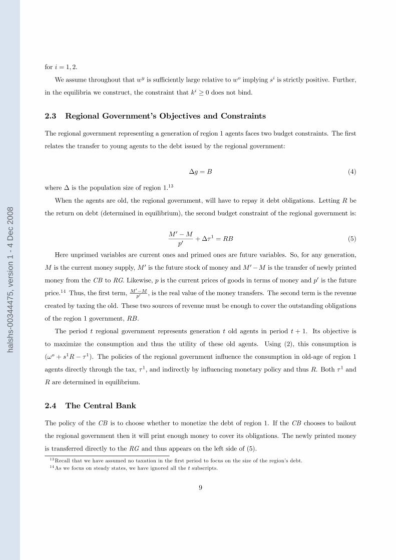
2.3 Regional Government’s Objectives and Constraints

The regional government representing a generation of region 1 agents faces two budget constraints. The first

relates the transfer to young agents to the debt issued by the regional government:

∆g = B (4)

where ∆ is the population size of region 1.13

When the agents are old, the regional government, will have to repay it debt obligations. Letting R be

the return on debt (determined in equilibrium), the second budget constraint of the regional government is:

M ′ −M

p′+∆τ1 = RB (5)

Here unprimed variables are current ones and primed ones are future variables. So, for any generation,

M is the current money supply, M ′ is the future stock of money and M ′−M is the transfer of newly printed

money from the CB to RG. Likewise, p is the current prices of goods in terms of money and p′ is the future

price.14 Thus, the first term, M′−Mp′

, is the real value of the money transfers. The second term is the revenue

created by taxing the old. These two sources of revenue must be enough to cover the outstanding obligations

of the region 1 government, RB.

The period t regional government represents generation t old agents in period t + 1. Its objective is

to maximize the consumption and thus the utility of these old agents. Using (2), this consumption is

(ωo + s1R − τ1). The policies of the regional government influence the consumption in old-age of region 1

agents directly through the tax, τ1, and indirectly by influencing monetary policy and thus R. Both τ1 and

R are determined in equilibrium.

2.4 The Central Bank

The policy of the CB is to choose whether to monetize the debt of region 1. If the CB chooses to bailout

the regional government then it will print enough money to cover its obligations. The newly printed money

is transferred directly to the RG and thus appears on the left side of (5).

13Recall that we have assumed no taxation in the first period to focus on the size of the region’s debt.14As we focus on steady states, we have ignored all the t subscripts.

9

hals

hs-0

0344

475,

ver

sion

1 -

4 D

ec 2

008

The CB maximizes the utility of old agents in both regions.15 Its objective is assumed to be:

∆v(ωo + s1R− τ1) + (1−∆)v(ωo + s2R). (6)

Through its decision to bailout the regional government, the CB influences the tax paid by old agents, τ1,

as well as the return on savingR. In equilibrium, the CB will also affect the saving decision of forward-looking

agents in both regions.16

3 Equilibria

This section constructs two types of equilibria. In one, the CB prints money and transfers it to the regional

1 government. In the other, there are no transfers and the regional government levies taxes on old agents to

pay its debt.

3.1 Equilibrium with Monetization

Here we construct a stationary equilibrium in which the CB monetizes the regional obligation rather than

allowing default. The agents anticipate this and adjust their saving accordingly. The region chooses no pay,

sets its tax rate to zero and sends the obligation to the CB. In equilibrium, the CB prefers monetization

over default: regional debt is inflationary.

This equilibrium is comprised of a vector of choices by agents in each region and a rate of return on

money: (k1∗, s1∗, k2∗, s2∗, π∗). Along the equilibrium path, given the constant level of government debt B∗,

there will be constant growth of the money supply, constant inflation and thus a constant real return on

money, π∗. This gets factored into the return on savings so that R∗ = x+λπ∗

1+λis the return on savings along

the equilibrium path and determines si∗. As storage and regional debt have the same return, we can freely

construct agents’ portfolios as part of the equilibrium. We focus on steady state equilibria where all young

agents of region 1 hold a fraction θ of the outstanding debt: b1∗ = θB∗

∆.

The rate of inflation is determined from market clearing and the activity of the central bank. Using (5),

monetization of the debt B by the central bank implies

M ′ −M

p′= RB. (7)

15We argue below that the power of the CB is limited to affecting only consumptions levels in old age of the present generation.16Though, as explained below, the CB decides upon its policy given (s1, s2).

10

hals

hs-0

0344

475,

ver

sion

1 -

4 D

ec 2

008

A monetary equilibrium requires that the supply of real money balances (by both old agents and the CB)

equals the demand by the young who have to meet their reserve requirement. So market clearing implies

M

p= λk∗(R) (8)

where

k∗(R) ≡ ∆k∗1(R) + (1−∆)k∗2(R) (9)

represents total storage. Using (8) in (7) yields

M ′

p′−

M

p

p

p′= λk∗(R)(1− π) = RB∗ (10)

where π = pp′.

In characterizing the individual decisions and market clearing, we have assumed an equilibrium with CB

monetization. So we write (3) with τ1 = 0 and all financing is through money creation, as in (7). We need

to check that this is an equilibrium by evaluating the incentives of the regional government and the central

bank. The following intuition underlies the proof of Proposition 1.

First, consider the incentives of the CB. Its choice about monetizing the regional debt influences the

current nominal money supply and thus may redistribute purchasing power across old agents. But this

choice has no effect on future generations since the inherited stock of fiat money is completely neutral.17 So

the CB looks only at the welfare of the current old. If it chooses a bail-out, then social welfare, W b, is given

by

W b = ∆v(ωo +R∗s1∗) + (1−∆)v(ωo +R∗s2∗) (11)

in the steady state. If the CB allows default, then the welfare of the current old is given by

W d = ∆v(ωo + k1∗(x+ λ)) + (1−∆)v(ωo + k2∗(x+ λ)) (12)

since, under default, there is no return on the holding of government debt and no inflation for this generation

of old agents. Importantly, we are considering a one-time deviation from a candidate equilibrium. The default

cost is assumed to be negligible and is not included in W d.

To compare W d against W b we have to compare the ex post consumption levels. As argued in the proof

of Proposition 1, for particular distributions of debt holdings, the consumption allocation under bail-out will

be closer to the social optimum of equal consumption and hence W b > W d. Finally, we need to be sure

that the region will not tax and pass the obligation to the CB given that it recognizes the CB will choose

to monetize, i.e. W b > W d. Again this is intuitive: why pay a tax which can in part be passed to other

agents? This is formalized in the proof of Proposition 1.

17So while the stock of fiat money is changing over time, it has no influence on the set of feasible consumption allocations.

11

hals

hs-0

0344

475,

ver

sion

1 -

4 D

ec 2

008

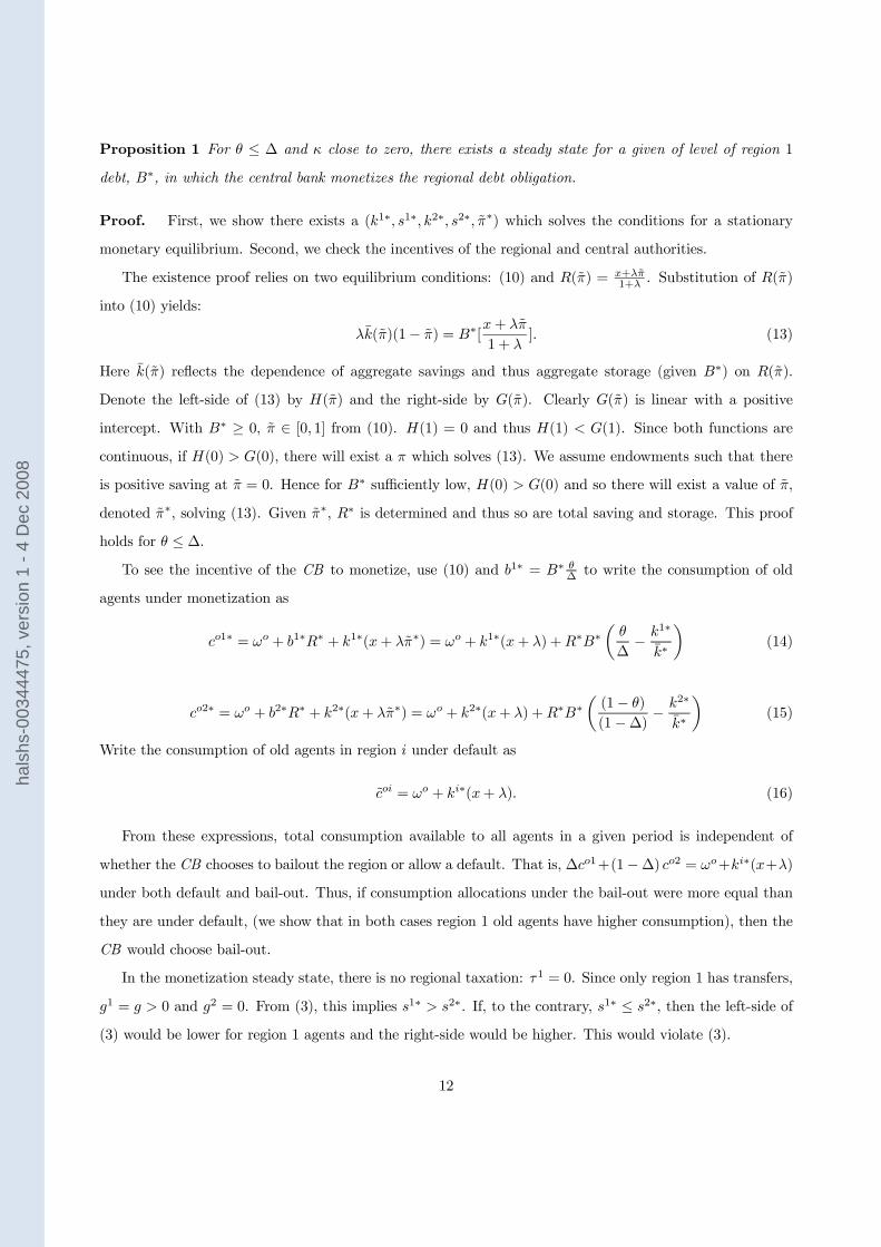
Proposition 1 For θ ≤ ∆ and κ close to zero, there exists a steady state for a given of level of region 1

debt, B∗, in which the central bank monetizes the regional debt obligation.

Proof. First, we show there exists a (k1∗, s1∗, k2∗, s2∗, π∗) which solves the conditions for a stationary

monetary equilibrium. Second, we check the incentives of the regional and central authorities.

The existence proof relies on two equilibrium conditions: (10) and R(π) = x+λπ1+λ

. Substitution of R(π)

into (10) yields:

λk(π)(1− π) = B∗[x+ λπ

1 + λ]. (13)

Here k(π) reflects the dependence of aggregate savings and thus aggregate storage (given B∗) on R(π).

Denote the left-side of (13) by H(π) and the right-side by G(π). Clearly G(π) is linear with a positive

intercept. With B∗ ≥ 0, π ∈ [0, 1] from (10). H(1) = 0 and thus H(1) < G(1). Since both functions are

continuous, if H(0) > G(0), there will exist a π which solves (13). We assume endowments such that there

is positive saving at π = 0. Hence for B∗ sufficiently low, H(0) > G(0) and so there will exist a value of π,

denoted π∗, solving (13). Given π∗, R∗ is determined and thus so are total saving and storage. This proof

holds for θ ≤ ∆.

To see the incentive of the CB to monetize, use (10) and b1∗ = B∗ θ∆

to write the consumption of old

agents under monetization as

co1∗ = ωo + b1∗R∗ + k1∗(x+ λπ∗) = ωo + k1∗(x+ λ) +R∗B∗

(θ

∆−

k1∗

k∗

)(14)

co2∗ = ωo + b2∗R∗ + k2∗(x+ λπ∗) = ωo + k2∗(x+ λ) +R∗B∗

((1− θ)

(1−∆)−

k2∗

k∗

)(15)

Write the consumption of old agents in region i under default as

coi = ωo + ki∗(x+ λ). (16)

From these expressions, total consumption available to all agents in a given period is independent of

whether the CB chooses to bailout the region or allow a default. That is, ∆co1+(1−∆) co2 = ωo+ki∗(x+λ)

under both default and bail-out. Thus, if consumption allocations under the bail-out were more equal than

they are under default, (we show that in both cases region 1 old agents have higher consumption), then the

CB would choose bail-out.

In the monetization steady state, there is no regional taxation: τ1 = 0. Since only region 1 has transfers,

g1 = g > 0 and g2 = 0. From (3), this implies s1∗ > s2∗. If, to the contrary, s1∗ ≤ s2∗, then the left-side of

(3) would be lower for region 1 agents and the right-side would be higher. This would violate (3).

12

hals

hs-0

0344

475,

ver

sion

1 -

4 D

ec 2

008

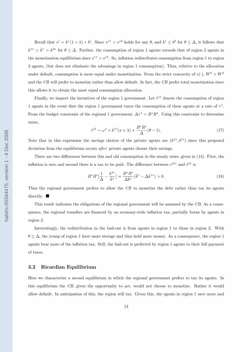
Recall that si = ki (1 + λ) + bi. Since s∗1 > s∗2 holds for any θ, and b1 ≤ b2 for θ ≤ ∆, it follows that

k1∗ > k∗ > k2∗ for θ ≤ ∆. Further, the consumption of region 1 agents exceeds that of region 2 agents in

the monetization equilibrium since s∗1 > s∗2. So, inflation redistributes consumption from region 1 to region

2 agents, (but does not eliminate the advantage in region 1 consumption). Thus, relative to the allocation

under default, consumption is more equal under monetization. From the strict concavity of v(·), W b > W d

and the CB will prefer to monetize rather than allow default. In fact, the CB prefer total monetization since

this allows it to obtain the most equal consumption allocation.

Finally, we inspect the incentives of the region 1 government. Let co1 denote the consumption of region

1 agents in the event that the region 1 government taxes the consumption of these agents at a rate of τ1.

From the budget constraint of the regional 1 government, ∆τ1 = B∗R∗. Using this constraint to determine

taxes,

co1 = ωo + k1∗(x+ λ) +B∗R∗

∆(θ − 1). (17)

Note that in this expression the savings choices of the private agents are (k1∗, b1∗) since this proposed

deviation from the equilibrium occurs after private agents choose their savings.

There are two differences between this and old consumption in the steady state, given in (14). First, the

inflation is zero and second there is a tax to be paid. The difference between co1∗ and co1 is

B∗R∗[1

∆−

k1∗

k∗] =

B∗R∗

∆k∗(k∗ −∆k1∗) > 0. (18)

Thus the regional government prefers to allow the CB to monetize the debt rather than tax its agents

directly.

This result indicates the obligations of the regional government will be assumed by the CB. As a conse-

quence, the regional transfers are financed by an economy-wide inflation tax, partially borne by agents in

region 2.

Interestingly, the redistribution in the bail-out is from agents in region 1 to those in region 2. With

θ ≤ ∆, the young of region 1 have more storage and thus hold more money. As a consequence, the region 1

agents bear more of the inflation tax. Still, the bail-out is preferred by region 1 agents to their full payment

of taxes.

3.2 Ricardian Equilibrium

Here we characterize a second equilibrium in which the regional government prefers to tax its agents. In

this equilibrium the CB, given the opportunity to act, would not choose to monetize. Rather it would

allow default. In anticipation of this, the region will tax. Given this, the agents in region 1 save more and

13

hals

hs-0

0344

475,

ver

sion

1 -

4 D

ec 2

008

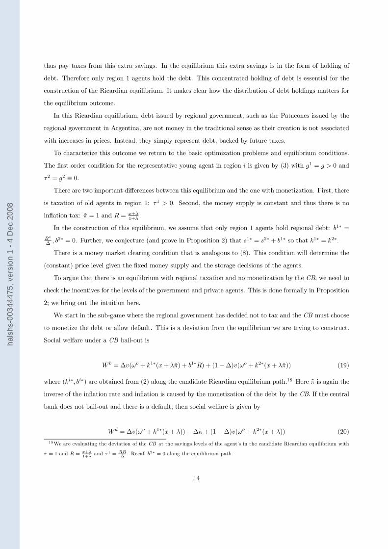
thus pay taxes from this extra savings. In the equilibrium this extra savings is in the form of holding of

debt. Therefore only region 1 agents hold the debt. This concentrated holding of debt is essential for the

construction of the Ricardian equilibrium. It makes clear how the distribution of debt holdings matters for

the equilibrium outcome.

In this Ricardian equilibrium, debt issued by regional government, such as the Patacones issued by the

regional government in Argentina, are not money in the traditional sense as their creation is not associated

with increases in prices. Instead, they simply represent debt, backed by future taxes.

To characterize this outcome we return to the basic optimization problems and equilibrium conditions.

The first order condition for the representative young agent in region i is given by (3) with g1 = g > 0 and

τ2 = g2 ≡ 0.

There are two important differences between this equilibrium and the one with monetization. First, there

is taxation of old agents in region 1: τ1 > 0. Second, the money supply is constant and thus there is no

inflation tax: π = 1 and R = x+λ1+λ

.

In the construction of this equilibrium, we assume that only region 1 agents hold regional debt: b1∗ =

B∗

∆, b2∗ = 0. Further, we conjecture (and prove in Proposition 2) that s1∗ = s2∗ + b1∗ so that k1∗ = k2∗.

There is a money market clearing condition that is analogous to (8). This condition will determine the

(constant) price level given the fixed money supply and the storage decisions of the agents.

To argue that there is an equilibrium with regional taxation and no monetization by the CB, we need to

check the incentives for the levels of the government and private agents. This is done formally in Proposition

2; we bring out the intuition here.

We start in the sub-game where the regional government has decided not to tax and the CB must choose

to monetize the debt or allow default. This is a deviation from the equilibrium we are trying to construct.

Social welfare under a CB bail-out is

W b = ∆v(ωo + k1∗(x+ λπ) + b1∗R) + (1−∆)v(ωo + k2∗(x+ λπ)) (19)

where (ki∗, bi∗) are obtained from (2) along the candidate Ricardian equilibrium path.18 Here π is again the

inverse of the inflation rate and inflation is caused by the monetization of the debt by the CB. If the central

bank does not bail-out and there is a default, then social welfare is given by

Wd = ∆v(ωo + k1∗(x+ λ))−∆κ+ (1−∆)v(ωo + k2∗(x+ λ)) (20)

18We are evaluating the deviation of the CB at the savings levels of the agent’s in the candidate Ricardian equilibrium with

π = 1 and R = x+λ

1+λand τ1 = RB

∆. Recall b2∗ = 0 along the equilibrium path.

14

hals

hs-0

0344

475,

ver

sion

1 -

4 D

ec 2

008

so agents avoid the inflation tax but only get a return on their storage and money holdings.

Proposition 2 For any κ > 0, there exists a steady state equilibrium given B∗ in which the regional debt is

held only by region 1 agents and the region 1 government chooses to raise taxes to pay its obligations.

Proof. First, we show there exists a (k1∗, s1∗, k2∗, s2∗, π∗) which satisfies the conditions for a stationary

monetary equilibrium. Second, we check the incentives of the regional and central authorities.

In the steady state, the level of region 1 transfers to each young agent is g∗, the per capita debt in the

whole economy is B∗, with all of it held by region 1 agents in the equilibrium characterized in Proposition

2. By the budget constraint of region 1, B∗ = ∆g∗ and taxes in old age are given by ∆τ1 = R∗B∗ so that

τ1 = R∗g∗. The debt held by each agent in region 1 is b1∗ where ∆b1∗ = B∗ and region 2 agents do not hold

any debt.

In equilibrium, the saving decisions of the agents, in regions i = 1, 2, are given by

u′(ωy + gi − ki∗(1 + λ)− bi∗) = R∗v′(ωo + ki∗(x+ λ) +R∗bi∗ − τ i) (21)

where R∗ = x+λ1+λ

. With τ1 = R∗g∗, τ2 = 0, the choices k1∗ = k2∗, b1∗ = B∗/∆ and b2∗ = 0 satisfy the first

order conditions. Thus the equilibrium level of per capita storage k∗ satisfies

u′(ωy − k∗(1 + λ)) = R∗v′(ωo + k∗(x+ λ)). (22)

Given the strict concavity of u(·) and v(·), and ωy sufficiently larger than ωo, there exists a unique k∗ ≥ 0

which solves this condition.

We now turn to the incentives of the central bank. We argue that if the region does not set taxes to

pay its debt obligation, then the central bank will not monetize. To see why, from (20) and k1∗ = k2∗, the

consumption levels of agents are equal if the CB allows a default. However, the allocation under monetization

provides greater consumption for region 1 agents since they bear only a fraction of the inflation tax and receive

full repayment of their debt.

Yet, the aggregate consumption of the old is the same, regardless of default or monetization. Under

default, aggregate consumption of the old agents is

ωo + k∗(x+ λ). (23)

Under monetization, total consumption is

ωo + k∗(x+ λ) + λ(π − 1)k∗ +B∗R∗. (24)

15

hals

hs-0

0344

475,

ver

sion

1 -

4 D

ec 2

008

where the rate of inflation is determined from the money creation needed to finance the bail-out as in (10).

Thus if the monetary authority deviates and bails-out the region, the resulting inflation cancels out the last

two terms in (24). Hence aggregate consumption is the same regardless of default or bail-out.19 Since a

bail-out leads to a less equitable consumption distribution, the CB will prefer default to monetization.

Given that the CB will not monetize the debt, the region 1 government will tax rather than default. This

allows it to avoid the default penalty, κ. Under both regional taxation and default, the consumption of the

region 1 old is given by ωo + k∗(x+ λ).

The proof of Proposition 2 shows that W d > W b. This reflects two factors which were present in the

proof of Proposition 1 as well. First, the actual resources available to distribute to the old agents is the same

regardless of the action of the central bank. Second, the central bank wishes to obtain the most equitable

distribution of consumption across the old agents since v(·) is strictly concave. This is achieved under default

given that k1∗ = k2∗.

Anticipating this, the region 1 government prefers to raise taxes rather than default. Interestingly, in

both cases, the consumption of region 1 old agents is the same. Intuitively, the taxes they pay to their

regional government are used to pay-off the debt which they hold. But, by taxing, the region 1 government

can avoid the default cost.

3.3 Multiple Active Regions

We informally consider the situation where each of the two regions makes a favorable transfer to its agents,

hoping to shift the debt burden to the central bank. It might appear that the ex-post incentive for consump-

tion equality by the central bank will no longer motivate a bail-out once both regions issue debt. If so, then

such symmetric regional behavior could, by itself, eliminate the free riding problem. However, the central

bank’s choice of a bail-out or allowing default is considered region by region, depending on the move made

by that region, holding the other region’s decision fixed. Consequently, profligate behavior of both regions

will not necessarily eliminate the free riding problem.20

Suppose, for instance that both regions made a transfer in period 1. Consider the case where region 1

debt is held by agents in both regions while region 2 debt is held only by region 2 agents. Using the results

above, it is easy to construct an equilibrium in which the CB is induced to bailout the debt of region 1 while

the debt obligations of region 2 are met by regional taxation. In this case, the outcome combines aspects of

19This result could have been anticipated in a stationary monetary equilibrium, where the real money balances of young

agents, which finance the returns on old agents money holdings, are invariant to default or bail-out on debt held by the previous

generation.20We are grateful to Eddie Dekel for prompting discussion of this point.

16

hals

hs-0

0344

475,

ver

sion

1 -

4 D

ec 2

008

both the monetization and the Ricardian equilibria.

3.4 Choice of B∗

The equilibria described in the previous section take the steady state level of region 1 transfers, g, and thus

the debt needed to finance it, B∗, as given. We now explore the determination of this level of debt.21 From

the region 1 government’s budget constraint, g = B∗

∆, so that the choice of B∗ implies an endogenous level

of transfers.

In this discussion it is also useful to recall the benchmark planner’s solution. The ex ante optimal

allocation entails equal consumption across regions in all periods of agent’s lives. This reflects the symmetry

of the economy, the strict concavity of u(·) and v(·) and the use of population weights in the planner’s

objective function. The planner’s solution can be decentralized either by the selection of the Ricardian

equilibrium or when B∗ = 0.

Let V (B) be the welfare of a region 1 agent if the stock of debt is B. In the Ricardian equilibrium,

the choice of B is, by construction, irrelevant for the welfare of region 1 agents. But in the monetization

equilibrium, this is not the case. If one takes the perspective that the equilibrium will be determined

by a sunspot process, then V (B) places some weight on the monetization equilibrium and the remaining

probability on the Ricardian equilibrium.22 Since welfare of region 1 agents is independent of B in the

Ricardian equilibrium, the only effect of B occurs when the monetization equilibrium is selected. Thus we

focus our discussion of the choice of B assuming the selection of the monetization equilibrium.

So consider

V (B) = u(ωy +B

∆− s) + v(ωo + sR(B)). (25)

This is the level of lifetime expected utility for a representative region 1 agent in an equilibrium with

monetization. Here B is the level of debt per capita so that B∆

is the level of debt, and thus the transfer,

per young region 1 agent. The function R(B) is the return on savings if the stock of debt is B from the

equilibrium with monetization, as in (10). Our main result is that the region 1 government will prefer a

positive level of transfers given the positive probability that the central bank will monetize this obligation.

Proposition 3 The solution to (25) entails B∗ > 0.

21Having established an incentive for bailout, this part of the analysis parallels the literature on the incentive implications of

common pool problems in fiscal federations, such as Persson and Tabellini (2000), particularly Chapter 7, and Velasco (2000).22Consider the following timing. The regional government chooses B and then a sunspot occurs which selects from the set

of equilibria insofar as young agents condition their portfolio choice on the sunspot. This timing may occur each period or just

at the start of time.

17

hals

hs-0

0344

475,

ver

sion

1 -

4 D

ec 2

008

Proof. Using the envelope condition and region 1 agents’ optimal choice of s given B and R(B), the

optimal choice of B by the region 1 government satisfies

V ′(B) = v′(co)[R(B)

∆− sR′(B)] = 0. (26)

To show V ′(0) > 0, we view both R and π as functions of B, using R = x+λπ1+λ

and (10) rewritten as

λk(R)(1− π) = RB. (27)

Taking derivatives to calculate R′(B), and evaluating that derivative at B = 0, where π = 1, yields

R′(0) = −R(0)

(1 + λ)k(R(0)). (28)

Substituting this into (26), recalling that with no debt issued s1 = (1 + λ)k1, yields

V ′(0) = v′(co1)R(0)[1

∆−

k1

k]. (29)

Since k1 = k in a symmetric steady state with B = 0, V ′(0) is positive when ∆ < 1. Thus the optimal policy

of the region 1 government will entail a positive level of B.

4 Policy Implications

The two steady state equilibria characterized above have very different welfare implications for agents in the

two regions. Agents in region 1 strictly prefer the monetization equilibrium while those in region 2 prefer

the equilibrium with regional taxation. Thus, as indicated by Proposition 3, the RG will increase the level

of B above zero and will try to support the equilibrium with monetization. In contrast, agents in region 2

would act to limit region 1 and eliminate the monetization equilibrium. We consider policy measures, either

proposed or effectively implemented, from the perspective of these two groups of agents. These policies can

also be viewed as devices for supporting the planner’s solution.

A commitment by the central bank not to bailout any regional government would of course eliminate the

monetization equilibrium. The Ricardian equilibrium would be the sole equilibrium and the social optimum.

In this equilibrium, the level of government debt would be irrelevant.

This form of commitment for the central bank is precisely the provision included in the Maastricht

Treaty governing the EMU. But of course, this begs the question: what is the basis of this commitment

power, particularly if the CB is not independent from political pressures? Within the EMU, restrictions

on deficits and debt levels supplement the Maastricht provisions. In Argentina, dollarization was widely

18

hals

hs-0

0344

475,

ver

sion

1 -

4 D

ec 2

008

discussed as a remedy for a weak CB. Motivated by these experiences, we discuss restrictions on debt and

dollarization as a substitute for CB commitment not to monetize debt.

4.1 Restrictions on debt

We consider two types of restrictions. The first restriction is a debt limit. If B∗ is forced to be zero, then

there is no monetization. Clearly a restriction of this form would be favored by region 2 agents.

Within Argentina, there have been numerous attempts to place limits on regional debt. But, not sur-

prisingly, not all regions are in favor of these limits. Interestingly, recent negotiations with the International

Monetary Fund have included a discussion of the regional fiscal situation.23 As far as the Stability and

Growth Pact is concerned, many critics claim that the focus on actual deficits was ill-conceived and suggest

that limits be imposed on national public debts. Clearly though these limits are not costless since efficiency

often dictates that government’s run deficits for tax smoothing reasons.24

The second restriction is on the holding of debt. Suppose there is a capital control which makes it

prohibitively expensive for a private agent in region 2 or a financial intermediary intervening on his behalf

to hold region 1 debt. This intervention implies that monetization is no longer a steady state and makes

the Ricardian equilibrium the only steady state equilibrium. It is in the interest of region 2 agents. Such

restrictions on the holding of debt emulate a commitment device ruling out monetization.

In Argentina, the small-denomination debt of the Buenos Aires region, the so-called Patacones, issued in

July 2002 allowed for the repayment of public obligations using these notes. But no other regions appeared

willing to accept these notes for payment of taxes. While this is not a policy that prohibits Patacones to be

held outside of the Buenos Aires region, this policy clearly reduces their attractiveness for residents of other

regions.

4.2 Dollarization

There is a more drastic measure to avoid the monetization of regional debt which has been widely discussed

both by policymakers and economists: dollarization. This entails the complete surrender of monetary sov-

ereignty, say by Argentina to the U.S., and not just restrictions on the supply of money. Clearly dollarization

eliminates the possibility of monetization by the Argentine central bank. Put differently, the delegation of

monetary authority under a dollarization regime provides a type of commitment to a weak CB in a multi-

23Details are available on the recent agreement between the IMF and Argentina, http://www.mecon.gov.ar.24The tradeoff between tax smoothing and bailout incentives arising from fiscal restrictions in a fiscal federation is the focus

of Cooper, Kempf and Peled (2005).

19

hals

hs-0

0344

475,

ver

sion

1 -

4 D

ec 2

008

region economy. But there are two important caveats.

First, there is still the possibility that the Argentine central government will bail-out by means of central

taxes. This corresponds to the analysis of a fiscal federation in Cooper, Kempf and Peled (2005) which

shows multiple equilibria, indexed by the distribution of debt holding across regions in an economy with

fiscal rather than monetary interactions. Hence dollarization per se does not eliminate the multiplicity of

equilibria, nor does it eliminate the ability of a regional government to exert (ex post) pressure on the central

government.

Second, under dollarization, a version of the multi-region monetary economy studied above reappears

at the world level. Suppose that it is Argentina that dollarizes and adopts the currency issued by the U.S.

central bank. Assume that prior to dollarization, the U.S. had succeeded in eliminating pressures by the

states on the federal government.25 With dollarization, the U.S. is like region 1 in the model of section

?? and Argentina now behaves as the region 2 passive government and does not issue debt. There is one

important difference though: the U.S. central bank does not include the welfare of Argentina in its objective.

Clearly there is now a gain for U.S. citizens to monetization of the debt by the U.S. central bank since

part of this tax will be paid by citizens of Argentina. Does this imply that the U.S. central bank will monetize

in order to help U.S. citizens through an inflation tax partly paid by Argentina? More generally, what are

the consequences of dollarization for the existence of multiple equilibria in this multi-country economy?

To study these issues we consider a world economy formed of two countries, the U.S. and Argentina. If

the dollar is used in both countries, the world economy is described by the model we used before. Under

dollarization, the inflation rate is common to both countries and is set by the U.S. central bank, the FED.

Crucially the objective of the Fed is the utility of the representative U.S. household: here the use of common

currency does not imply a political union. This is in marked contrast to what was assumed as the objective

of the monetary union’s central bank in the previous section.26

With this model, we find that the Ricardian equilibrium disappears leaving only a monetization equilib-

rium. Formally,

Proposition 4 Under dollarization, for a given value of B∗, there exists a monetization equilibrium for θ

sufficiently close to 1. There is no Ricardian equilibrium.

Proof. To characterize the monetarization equilibrium, we check the incentives of the U.S. Treasury

and the FED. The FED takes into consideration the utility of region 1 (American) old agents only. Hence

25Exactly how this is done within the U.S. is an open question, but for now we assume that the central U.S. government has

adequate commitment relative to its states.26 In other words, the Fed’s objective is given by (6) with ∆ = 1.

20

hals

hs-0

0344

475,

ver

sion

1 -

4 D

ec 2

008

the FED’s choice of default or bail-out depends only on the consumption of region 1 agents in these two

outcomes. As in (14), the consumption level of U.S. citizens under a monetized bail-out is

co1∗ = ωo + b1∗R∗ + k1∗(x+ λπ∗) = ωo + k1∗(x+ λ) +R∗B∗

(θ

∆−

k1∗

k∗

), (30)

and by (16) for i = 1 under default:

co1 = ωo + k1∗(x+ λ). (31)

The FED will choose to monetize rather than default iff co1∗ > co1. From the above expressions:

co1∗ > co1 ⇔

(θ

∆−

k1∗

k∗

)> 0. (32)

Since k∗ ≡ ∆k1∗ + (1−∆)k2∗, this inequality holds strictly for θ = 1. By continuity, the inequality in (32)

holds for θ near 1.

Therefore when θ, the fraction of debt held by U.S. residents, is sufficiently large, the FED will monetize

the U.S. debt. This is preferred by the Treasury since the difference in consumption level under bail-out

exceeds that under taxation of U.S. citizens, as in (18). Thus for θ near 1, there is a monetization equilibrium.

In a Ricardian equilibrium, agents in region 1 anticipate future taxes and thus s1 = s2 + B∗

∆. As both

the U.S. Treasury and the FED have the same objective of maximizing the consumption of old U.S. agents,

the outcome of the game played each period will provide to U.S. agents the maximal consumption level.

In a Ricardian equilibrium, the U.S. Treasury levies a tax on U.S. citizens so that the consumption of a

region 1 old agent is:

co1 = ωo + k1∗(x+ λ) +R∗B∗

∆(θ − 1). (33)

Suppose instead that the U.S. Treasury does not levy the tax. The consumption levels under a bail-

out (viewed as a defection for a candidate Ricardian equilibrium) and a default are given in (30) and (31),

respectively, where the values of ki∗ in these expressions are evaluated in the candidate Ricardian equilibrium.

Comparing (33) and (30), bail-out dominates regional taxation for region 1, co1 ≥ co1, since k1

k≤

1∆. The

inequality is strict if k2∗ > 0. If k2∗ = 0, then the consumption under default, given in (31), is higher than

that under bail-out: co1 ≥ co1 and thus default dominates the consumption under taxation. Thus there is

no equilibrium in which the U.S. Treasury taxes U.S. citizens since it will always prefer the outcome under

either a bail-out or a default.

The disappearance of the Ricardian equilibrium reflects the difference in objective function between the

FED in the dollarized economy and the CB in the monetary union studied previously. For a sufficiently high

θ the FED will always prefer to monetize in order to tax the money holdings of Argentine citizens and avoid

21

hals

hs-0

0344

475,

ver

sion

1 -

4 D

ec 2

008

default: if θ is high enough, default would represent a high cost for region 1’s old agents which are the sole

concern of the FED. On the contrary, if θ is low, representing a significant holding by region 2 of region 1’s

debt, a regional default may NOT be bailed out at all.

We find also that dollarization indeed will induce a monetization equilibrium if a sufficiently large fraction

of the debt is held in the U.S. In this case, the FED may be induced to bail-out the U.S. government, and

in doing so tax Argentine citizens who hold dollars. In other words, dollarization does not eliminate the

incentives for monetization.

Again, the issue of debt distribution is crucial for the existence of such an equilibrium in this economy.

The relative gain of a bail-out over default from the FED’s perspective depends on the relative inflation tax

burden on U.S. residents. The more Argentine residents hold dollars, the more they bear of the inflation tax.

The demand for money is proportional to the amount of capital held by Argentine residents. Therefore the

higher is θ, the smaller is the share of capital held by U.S. citizens and the larger is the inflation tax borne

by Argentina.

Clearly this is a cost of dollarization for Argentine citizens, since they bear not only any Argentine taxes

to finance their own public goods, but also the inflation tax for the benefit of U.S. citizens. Cooper and

Kempf (2001) discuss the implications of a treaty between the U.S. and Argentina as an incentive device on

the U.S. central bank to limit the inflation tax.

Note that we obtained the opposite result than that of the previous section. There, the monetary

authority, caring about equalizing consumption among regions, chooses the best way to redistribute from

region 1 to region 2. In the case of dollarization, as the FED cares only about the U.S. welfare, it chooses

the best way to redistribute from region 2 (identified to Argentina) to region 1 (identified with the U.S.).

This result stands in contrast to that in Proposition 2 in which there was an isolated Ricardian equilibrium

in which region 1 agents held all of that debt. In that equilibrium, the central bank prefers default to a

bail-out since the allocation under a default was equal across old agents in the two regions. But, under

dollarization, the objective of the FED coincides with the U.S. Treasury and so the payment of taxes by U.S.

citizens is dominated by either a bail-out or a default.

In effect, dollarization solves the multiplicity of monetary equilibria but by eliminating the virtuous one!

5 Conclusion

The goal of this paper was to determine the impact of issuing debt by a regional government in a monetary

union. Recent events in Argentina, (the issue and circulation of small denomination bonds by some provinces,

22

hals

hs-0

0344

475,

ver

sion

1 -

4 D

ec 2

008

such as the Patacones), and in Europe, (the de facto demise of the Stability and Growth Pact at the end

of 2003), prove the necessity of a better understanding of how “soft" is regional debt in monetary unions.

Two leading views are relevant: (i) the debt is just a claim on future tax revenues and (ii) the debt is “like"

money; issuing it is tantamount to the printing of fiat money and is inflationary.

Our analysis indicates that both interpretations are consistent with an equilibrium of our monetary model.

The multiplicity reflects a commitment problem on the part of the central bank. Without commitment, the

central bank will ex post always redistribute consumption to achieve greater equality in consumption across

different regions. Depending on the distribution of the holding of the regional government debt, this desire

for redistribution may lead the central bank to bailout a region or it may lead the central bank to allow

default. In equilibrium, the distribution of the holdings of regional governments’ debt has powerful effects

on the incentives for the central bank. The more even is this distribution, the more likely it is that the

central bank will prefer a bail-out to a costly default. Debt holding is arbitrary since in equilibrium savers

are indifferent between holding bonds or storage.

The creation of a secondary market would amount to a change in the distribution of bonds but not to the

suppression of the multiplicity of equilibria, since it does not break the savers’ indifference and introduce a

wedge between storage and bonds. In other words, the introduction of a secondary market would not change

our results as in equilibrium there is no default. Hence there is no scope for discounting debt and no trade

opportunity.27

The commitment problem of the central bank has some important incentive effects on the regions. A bail-

out creates a free-rider problem in that regional governments will have an incentive to run inefficiently large

deficits in anticipation of the central bank’s monetization of its debt.28 Not surprisingly, other agents in the

economy will have an incentive to erect impediments to this free-rider problem including: debt restrictions,

limits on the holding of debt by other regions and even dollarization.

The analysis did not require that the regional debt be small denomination. Nonetheless the paper does

27Broner, Martina and Ventura (2007), studying the related subject of sovereign risk, have shown that the introduction of

secondary markets allows to obtain a unique equilibrium with debt.. However their model differs much from ours. In particular,

there is no lender of last resort. In addition, there is a multiplicity of bond issuers: the issuers of bonds are private agents,

living in the "debtor" country and not its government. They individually have an incentive to buy back bonds from the savers

living in the sovereign "creditor" contry. This leads to a prisoner’s dilemma, which ends up with an equilibrium where all the

debts issued by "debtor" agents and sold to "creditor" agents are bought back by "debtor" agents on the secondary market.

Such a non-cooperative behaviour between debtors is impossible in our model where there is a unique issuer of bonds.

28This point is brought out in the context of monetary unions in Chari and Kehoe (1998), Chari and Kehoe (2002) and

Cooper and Kempf (2004).

23

hals

hs-0

0344

475,

ver

sion

1 -

4 D

ec 2

008

provide an explanation for the choice of denomination. As argued above, monetization of the regional debt is

more likely if that debt is widely held. From that perspective, small denomination debt may be more likely

to circulate outside a narrow set of individuals and banks within a region. Thus a regional government may

perceive a gain to issuing small denomination debt.

An open issue which deserves further attention is the effect of monetary policy rules on the fiscal actions

of regional governments. At one extreme, a central bank which operates according to a fixed money growth

rule is not likely to be influenced by the level of regional debt. This type of monetary rule may support

the Ricardian equilibrium. At the other extreme, a monetary rule pursuing an interest rate target may be

susceptible to manipulation by a regional government. If the marketing of regional debt induces a reaction

by the monetary authority, then a link arises between regional debt and monetary policy. Thus, alternative

monetary rules can provide links between regional debt and inflation.

24

hals

hs-0

0344

475,

ver

sion

1 -

4 D

ec 2

008

References

[1] Aizenman, J. (1992): “Competitive Externality and Optimal Seigniorage," Journal of Money, Credit

and Banking, 24, 61-71.

[2] Beetsma, R., and X. Debrun (2007): “The new stability and Growth Pact: a First Assessment,"

European Economic Review, 51, 453-77.

[3] Beetsma, R., and H. Uhlig (1999): “An Analysis of the Stability and Growth Pact," Economic Journal,

109, 546-571.

[4] Broner, F., A. Martina and J. Ventura (2007): “Sovereign Risk and Secondary Markets”, CEPR Dis-

cussion Paper #6055, january 2007.

[5] Chari, V. V., and P. Kehoe (1998): “On the Need for Fiscal Constraints in a Monetary Union," Federal

Reserve Bank of Minneapolis, Working Paper #589.

[6] Chari, V. V., and P. Kehoe (2002): “Time Inconsistency and Free-Riding in a Monetary Union," Federal

Reserve Bank of Minneapolis, Staff Report # 308.

[7] Cooper, R., and H. Kempf (2001): “Dollarization and the Conquest of Hyperinflation in Divided Soci-

eties," Federal Reserve Bank of Minneapolis Quarterly Review, 25(3).

[8] Cooper, R., and H. Kempf (2004): “Overturning Mundell: Fiscal Policy in a Monetary Union," Review

of Economic Studies, 71(2), 371-396.

[9] Cooper, R., H. Kempf, and D. Peled (2005): “Is it is or is it Ain’t my Obligation? Regional Debt in a

Fiscal Federation," NBER Working Paper #11655.

[10] Inman, R. (2003): “Transfers and Bailouts: Enforcing Local Fiscal Discipline with Lessons from U.S.

Federalism," in Fiscal Decentralization and the Challenge of Hard Budget Constraint, ed. by G. S. E. J.

Rodden, and J. Litvack. MIT Press.

[11] Persson, T., and G. Tabellini (2000): Political Economics: Explaining Economic Policy. MIT Press.

[12] Smith, B. (1994): “Efficiency and Determinacy of Equilibrium under Inflation Targeting," Economic

Theory, 4(3), 327-344.

[13] Velasco, A. (2000): “Debts and Deficits with Fragmented Policymaking," Journal of Public Economics,

76, 105-125.

25

hals

hs-0

0344

475,

ver

sion

1 -

4 D

ec 2

008

[14] Zarazaga, C. (1995): “Hyperinflations and Moral Hazard in the Appropriation of Seignorage," Federal

Reserve Bank of Dallas, Working Paper 95-17.

26

hals

hs-0

0344

475,

ver

sion

1 -

4 D

ec 2

008