A two-warehouse inventory model for items with three-parameter Weibull distribution deterioration,...

A two-warehouse inventory model for items withthree-parameter Weibull distribution deterioration, shortages

and linear trend in demand

Snigdha Banerjee and Swati Agrawal

School of Statistics, Devi Ahilya University, Vigyan Bhawan, Khandwa Road, Indore, India 452017

E-mail: [email protected]

Received 2 June 2007; received in revised form 9 April 2008; accepted 11 April 2008

Abstract

Depending on the type of goods and storage facilities available, perishable goods decay in different mannersin terms of the initial point and rate of deterioration. The three-parameter Weibull distribution is anexcellent generalization of exponential decay, with the flexibility of modeling various types ofdeteriorations. Since inventory management of perishable goods involves expensive storage facilities, theretailer with small storage may have to rent a warehouse. In this paper, we discuss a two-warehouseinventory model where deteriorations in the two warehouses follow independent three-parameter Weibulldistributions. Transfer of units is from the rented warehouse to the own warehouse, and incurs a positivecost per unit. Demand is a non-decreasing linear function of time, shortages are backlogged andreplenishment is instantaneous. A solution procedure for obtaining optimal values of initial inventory leveland cycle time is presented. Sensitivity analysis is carried out. The effect of using other related deteriorationdistributions is illustrated.

Keywords: inventory; three-parameter Weibull deterioration; warehouse; linear trend in demand; shortage

1. Introduction

A wide variety of food, pharmaceutical and chemical products, blood in blood banks, plants in anursery, etc., are degraded by exposure to improper temperature, humidity and other conditions.Exposure of such ‘‘perishable’’ or ‘‘deteriorating’’ goods to adverse conditions increases thepotential for them to diminish in value. However, different categories of perishable goods candegrade at different rates. For example, the value of food products can decrease incrementally,while the death rate of plants in a nursery decreases with age. In such situations, investment inequipment and labor is considerable, both while storing the units as well as during transit. This

Intl. Trans. in Op. Res. 15 (2008) 755–775

INTERNATIONAL TRANSACTIONS

IN OPERATIONALRESEARCH

r 2008 The Authors.Journal compilation r 2008 International Federation of Operational Research SocietiesPublished by Blackwell Publishing, 9600 Garsington Road, Oxford, OX4 2DQ, UK and 350 Main St, Malden, MA 02148, USA.

may include refrigerated trucks, containers, warehousing, packaging and specially trainedpersonnel. Despite all such precautions, with increasing time in storage, items are bound todeteriorate. Thus, deterioration is one of the important features that must be taken into accountwhile analyzing such inventory systems. Ghare and Schrader (1963) first considered an inventorymodel for deteriorating items with exponential decay. Goyal and Giri (2001) presented a review ofinventory literature since the early 1990s for deteriorating items. Wu et al. (2006) consider aninventory model with stock-dependent demand, non-instantaneous deterioration rate andpartially backlogged shortages.Most of the existing inventory models for deteriorating items deal with items stored in a single

warehouse. However, owing to exorbitant costs of building a specially equipped storage fordeteriorating items, the retailer may have a small warehouse providing the requisite conditions,which we call own warehouse (OW). This may require another storage facility called the rentedwarehouse (RW), such that all the units ordered by the retailer in excess of the capacity of the OWare to be kept at the rented warehouse.Even if the holding cost at the RW is higher than that at the OW, keeping provision for a

second warehouse may be profitable in the situations, where attractive price discounts are offeredon bulk purchase or demand is high, or growing with time. In practice, the retailer may tend to sellthe goods stored at the RW first, even if the outlet is at the OW, by transporting goods from RWto OW till the RW is empty. This is the situation when one or more of the following conditions aresatisfied:

(a) Storage facility in OW is better than that in the RW.(b) The RW is available for a limited duration.(c) The cost of storing items at the RW is much higher than that at the OW.

Two warehouse models are quite useful in practice. Recent work on two warehouse models fornon-deteriorating items includes papers by Kar et al. (2001) and Zhou and Yang (2005).In the past two decades, several authors have considered inventory models for deteriorating

items stored in two warehouses. Sarma (1987) presented a model with shortages andinstantaneous replenishment. Pakkala and Achary (1992a, b) considered models with finitereplenishment rate and shortages, taking time as discrete and continuous variables, respectively.Yang (2004, 2006) studied models with inflation in which shortages are considered to be totallyand partially backlogged, respectively. Dye et al. (2007) have dealt with time-proportionalbacklogging. All these papers assume a constant demand rate. Benkherouf (1997) reconsidered themodel given by Sarma (1987) for a general time-dependent function to represent demand, andrelaxed the assumption of fixed cycle length and known quantity to be stored in OW. Bhunia andMaiti (1998) developed a model with linear trend in demand, taking into consideration the cost oftransporting units from RW to OW.However, in all these models, it was assumed that the rate of deterioration is constant. This

assumption is not true for many types of deteriorating items. The rate of deterioration of someitems depends not only on the on-hand inventory, but also, in general, depends on the time theseitems have spent in storage. Incorporating this practical aspect of deteriorating items, time-dependent deterioration rates have been considered by several authors for single warehouseinventory systems. Covert and Philip (1973) used a two-parameter Weibull distribution torepresent time of deterioration. They pointed out that the two-parameter Weibull distribution is

S. Banerjee and S. Agrawal / Intl. Trans. in Op. Res. 15 (2008) 755–775756

r 2008 The Authors.Journal compilation r 2008 International Federation of Operational Research Societies

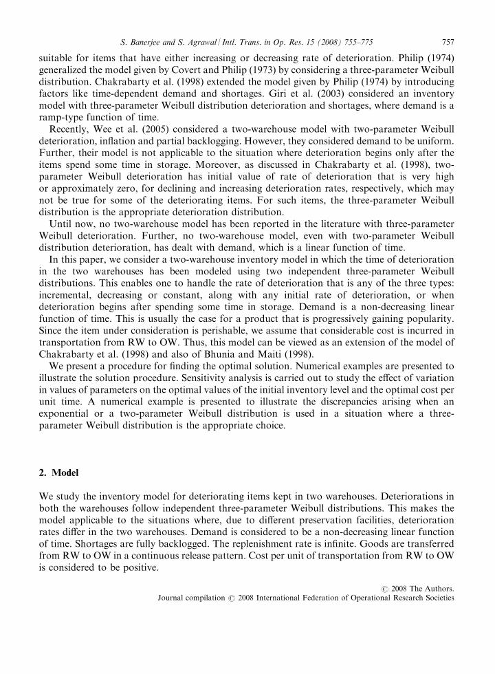
suitable for items that have either increasing or decreasing rate of deterioration. Philip (1974)generalized the model given by Covert and Philip (1973) by considering a three-parameter Weibulldistribution. Chakrabarty et al. (1998) extended the model given by Philip (1974) by introducingfactors like time-dependent demand and shortages. Giri et al. (2003) considered an inventorymodel with three-parameter Weibull distribution deterioration and shortages, where demand is aramp-type function of time.Recently, Wee et al. (2005) considered a two-warehouse model with two-parameter Weibull

deterioration, inflation and partial backlogging. However, they considered demand to be uniform.Further, their model is not applicable to the situation where deterioration begins only after theitems spend some time in storage. Moreover, as discussed in Chakrabarty et al. (1998), two-parameter Weibull deterioration has initial value of rate of deterioration that is very highor approximately zero, for declining and increasing deterioration rates, respectively, which maynot be true for some of the deteriorating items. For such items, the three-parameter Weibulldistribution is the appropriate deterioration distribution.Until now, no two-warehouse model has been reported in the literature with three-parameter

Weibull deterioration. Further, no two-warehouse model, even with two-parameter Weibulldistribution deterioration, has dealt with demand, which is a linear function of time.In this paper, we consider a two-warehouse inventory model in which the time of deterioration

in the two warehouses has been modeled using two independent three-parameter Weibulldistributions. This enables one to handle the rate of deterioration that is any of the three types:incremental, decreasing or constant, along with any initial rate of deterioration, or whendeterioration begins after spending some time in storage. Demand is a non-decreasing linearfunction of time. This is usually the case for a product that is progressively gaining popularity.Since the item under consideration is perishable, we assume that considerable cost is incurred intransportation from RW to OW. Thus, this model can be viewed as an extension of the model ofChakrabarty et al. (1998) and also of Bhunia and Maiti (1998).We present a procedure for finding the optimal solution. Numerical examples are presented to

illustrate the solution procedure. Sensitivity analysis is carried out to study the effect of variationin values of parameters on the optimal values of the initial inventory level and the optimal cost perunit time. A numerical example is presented to illustrate the discrepancies arising when anexponential or a two-parameter Weibull distribution is used in a situation where a three-parameter Weibull distribution is the appropriate choice.

2. Model

We study the inventory model for deteriorating items kept in two warehouses. Deteriorations inboth the warehouses follow independent three-parameter Weibull distributions. This makes themodel applicable to the situations where, due to different preservation facilities, deteriorationrates differ in the two warehouses. Demand is considered to be a non-decreasing linear functionof time. Shortages are fully backlogged. The replenishment rate is infinite. Goods are transferredfrom RW to OW in a continuous release pattern. Cost per unit of transportation from RW to OWis considered to be positive.

S. Banerjee and S. Agrawal / Intl. Trans. in Op. Res. 15 (2008) 755–775 757


2.1. Assumptions and notations

Demand rate f (t) is given byf(t)5 a1bt, where a and b are known constants, (a40, bX0).L1, the inventory system with a single warehouse.L2, the inventory system with two warehouses.

The known parameters areW, storage capacity of OWH, holding cost per unit item per unit time in OWF, holding cost per unit item per unit time in RWC1, shortage cost per unit short per unit timeC2, deterioration cost per unit itemC3, cost of transporting a unit from RW to OWA, ordering cost per order

A ¼ A1 for L1 system;A1 þ A2 for L2 system;

�

A2, the additional ordering cost incurred for the items stored in RW.Zo(t)5 ao bo(t� go) bo� 1, ao40, bo40, tXgo, deterioration rate at epoch t in OWZr(t)5 ar br (t� gr) br� 1, ar40, br40, tXgr, deterioration rate at epoch t in RWwhere ao and ar are scale parameters, bo and br are shape parameters, go and gr are locationparameters of Weibull distributions for OW and RW respectively.The decision variables aret1, the time epoch when the inventory level of RW becomes zeroT1, the time epoch when the inventory level of OW becomes zeroT, scheduling periodS1, initial inventory level at time t5 0, for the L1 systemS, initial inventory level at time t5 0, for the L2 system

The model is developed under the following assumptions:

(1) Replenishment is instantaneous(2) Shortages are fully backlogged(3) Lead-time is zero(4) Goods kept in OW are consumed only when the inventory level in RW becomes zero(5) Time of transportation from RW to OW is ignored(6) RW has infinite capacity(7) Deteriorated items cannot be replaced or repaired(8) Holding cost is incurred for good items only(9) Define g0o and g0r as

g0o ¼go if go*00 if go <0

; g0r ¼gr if gr*00 if gr <0

��



where g0o and g0r are the time points when deterioration starts in OW and RW, respectively.(10) Deterioration in both the warehouses, in both the L1 system and the L2 system, starts before

the inventory level in the respective warehouses becomes zero, i.e.

g0r < t1 and g0o < T1:

(11) In the L1 system, let tw be the time epoch at which the inventory level of OW becomes zerowhen the initial inventory level is W. In this case, T1 5 tw.

We assume that g0ootw. This ensures the existence of some value of T1 for which assumption (10)holds.

3. Analysis

We now present the analysis for the L2 system of our model.

3.1. Two warehouse (L2 system)

At time t5 0, the amount of inventory ordered enters the system, a part of which is used to fulfillthe shortages of the previous period. S units of inventory remain in the system, out of which, Wunits are kept in OW and the remaining (S–W) units are kept in RW.In RW, there is no deterioration during time interval (0, g0r) and inventory is depleted only due

to demand. Hence, the instantaneous change in inventory level IgrðtÞ in RW at any time t, where04t4g0r is given by the following differential equation

d

dtIgrðtÞ ¼ �f ðtÞ; 0)t)g0r; ð1Þ

which gives

IgrðtÞ ¼ Igrð0Þ � at� bt2

2; 0)t)g0r:

Since Igrð0Þ is the inventory level in RW at t5 0

Igrð0Þ ¼ S �W :

Hence, the solution of (1) is given by

IgrðtÞ ¼ S �W � at� bt2

2; 0)t)g0r: ð2Þ

During the time interval (g0r, t1), the inventory in RW is depleted due to both deterioration anddemand. Hence, the inventory level I1(t) in RW at any time t, where g0r4t4t1, satisfies thedifferential equation

d

dtI1ðtÞ ¼ �I1ðtÞZrðtÞ � f ðtÞ; g0r)t)t1; ð3Þ



along with the boundary condition

I1ðt1Þ ¼ 0: ð4ÞThe solution of differential equation (3), using the boundary condition (4) is given by

I1ðtÞ ¼ e�arðt�grÞbrZ t1

t

f ðuÞearðu�grÞbrdu; g0r)t)t1 ð5Þ

Also, using the boundary condition

Igrðg0rÞ ¼ I1ðg0rÞ;

we obtain

S ¼W þ ag0r þ bg02r2þ e�arðg

0r�grÞ

brZ t1

g0r

f ðuÞearðu�grÞbr

du: ð6Þ

In OW, depending on the relative values of g0o and t1, we consider the following two cases:

Case (i): g0oot1.This is the case when deterioration in OW starts before the inventory level of RW becomes zero.

Figure 1 depicts the change in inventory level with respect to time, during the entire cycle forcase (i).In this case, there is no change in inventory level during interval (0, g0o), because during this

period there is neither deterioration nor supply of items from OW. Thus, at any time t, where04t4g0o, inventory level I(t) is

IðtÞ ¼W ; 0)t)g0o: ð7ÞFrom time epoch g0o till time epoch t1, inventory depletes only due to deterioration. After time

t1, demand is met from OW, and hence the inventory level decreases due to both demand as wellas deterioration during the interval (t1,T1). Thus, differential equations governing the inventory

TimeT1t1

W

S-W

Ren

ted

War

ehou

seO

wn

War

ehou

se

Inve

rtor

y L

evel

T0 �′

r�′

0

Fig. 1. Inventory levels at own warehouse and rented warehouse.



position in OW during time (g0o,T1) are

d

dtI 02ðtÞ ¼ �I 02ðtÞZoðtÞ; g0o)t)t1 ð8Þ

and

d

dtI2ðtÞ ¼ �I2ðtÞZoðtÞ � f ðtÞ; t1)t)T1 ð9Þ

with boundary conditions

I 02ðg0oÞ ¼W ; I2ðT1Þ ¼ 0 ð10Þand

I2ðt1Þ ¼ I 02ðt1Þ: ð11ÞThe solutions of differential equations (8) and (9) using the conditions in (10) are given by

I 02ðtÞ ¼Weaoðg0o�goÞ

boe�aoðt�goÞ

bo; g0o)t)t1 ð12Þ

and

I2ðtÞ ¼ e�aoðt�goÞboZ T1

t

f ðuÞeaoðu�goÞbodu; t1)t)T1: ð13Þ

Further, using condition (11), we obtain

W ¼ e�aoðg0o�goÞ

boZ T1

t1

f ðuÞeaoðu�goÞbo

du: ð14Þ

It is very difficult to solve equation (14) so as to obtain T1 in terms of t1. In practice, becauseao is very small, we truncate the exponential series at the second term to obtain the followingrelation:

baobo þ 2

� �ððT1 � goÞboþ2 � ðt1 � goÞboþ2Þ þ

aoðaþ bgoÞbo þ 1

ððT1 � goÞboþ1 � ðt1 � goÞboþ1Þ

þ b

2ðT2

1 � t21Þ þ aðT1 � t1Þ �Weaoðg0o�goÞ

bo ¼ 0

: ð15Þ

Case (ii): t14g0ooT1.This is the case when deterioration in OW starts after the inventory level of RW becomes zero.

Thus, in this case, there is no change in the inventory level of OW in the interval (0, t1). Hence,

IðtÞ ¼W ; 0)t)t1 ð16ÞSince the inventory level of RW becomes zero at time t1, demand is met from OW and the

inventory level of OW decreases only due to demand in the interval (t1, g0o) and due to bothdemand and deterioration in the interval (g0o,T1). Thus, the differential equations governing theinventory situation in OW during interval (t1, T1) are

d

dtI 02ðtÞ ¼ �f ðtÞ; t1)t)g0o ð17Þ



and

d

dtI2ðtÞ ¼ �I2ðtÞZoðtÞ � f ðtÞ; g0o)t)T1; ð18Þ

with the boundary conditions

I 02ðt1Þ ¼W ; I2ðT1Þ ¼ 0 ð19Þand

I2ðg0oÞ ¼ I 02ðg0oÞ: ð20ÞUsing the conditions given in (19), the solutions of differential equations (17) and (18) are,

respectively,

I 02ðtÞ ¼W � aðt� t1Þ �b

2ðt2 � t21Þ; t1)t)g0o ð21Þ

and

I2ðtÞ ¼ e�aoðt�goÞboZ T1

t


du; g0o)t)T1 ð22Þ

and using (20), we obtain

W ¼ aðg0o � t1Þ þb

2ðg02o � t21Þ þ e�aoðg

0o�goÞ

bo

Z T

g0o

f ðuÞeaoðu�goÞbodu:

As with equation (14), it is very difficult to solve this equation too, so as to obtain T1 in terms oft1. Hence, as with case (i), we truncate the exponential series at the second term to obtain thefollowing relation:

baoðbo þ 2Þ

� �ððT1 � goÞboþ2 � ðg0o � goÞboþ2Þ þ

aoðaþ bgoÞðbo þ 1Þ ððT1 � goÞboþ1 � ðg0o � goÞboþ1Þ

�

þ b

2ðT2

1 � g02o Þ þ aðT1 � g0oÞ�e�aoðg

0o�goÞ

bo

þ b

2ðg02o � t21Þ þ aðg0o � t1Þ �W ¼ 0:

ð23ÞFor both case (i) as well as case (ii), the following holds:The total amount of shortage in the interval (T1, T) isZ T

T1

ðT � uÞf ðuÞdu: ð24Þ

The total amount of inventory deteriorated in RW is

ðS �WÞ �Z t1

0

f ðtÞdt:

The total amount of inventory deteriorated in OW is

W �Z T1

t1

f ðtÞdt:



Thus, the total amount of deterioration during the entire cycle (0, T) is

S �Z T1

0

f ðtÞdt: ð25Þ

The total holding cost is given by

HC ¼ F

Z g0r

0

IgrðtÞdtþZ t1

g0r

I1ðtÞdt( )

þH Wg0o þZ maxðg0o;t1Þ

minðg0o;t1ÞI 02ðtÞdtþ

Z T1

maxðg0o;t1ÞI2ðtÞdt

( )" #:

Many authors, such as Covert and Philip (1973), Chakrabarty et al. (1998), Giri et al. (2003),etc., have taken linear approximation to time–inventory graph. In order to simplify the expressionon the right-hand side of HC, and avoid complications in the derivations, we follow theirapproach, and hence, approximate the total holding cost as follows:

HC ffi FðS �WÞt12

þHWðT1 þminðt1; g0oÞÞ2

� �:

Thus, we obtain the total cost of the system during the entire cycle approximately as

C ¼ Aþ FðS �WÞt12

þHWðT1 þminðt1; g0oÞÞ2

þ C1

Z T

T1

ðT � uÞf ðuÞduþ C2

�S �

Z T1

0

f ðuÞdu�þ C3ðS �WÞ: ð26Þ

Hence, the total cost per unit time is given by

cðt1;TÞ ¼C

T: ð27Þ

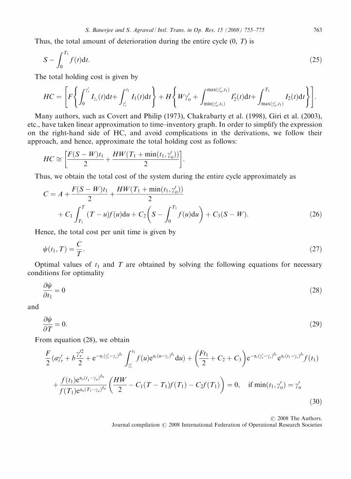
Optimal values of t1 and T are obtained by solving the following equations for necessaryconditions for optimality

@c@t1¼ 0 ð28Þ

and

@c@T¼ 0: ð29Þ

From equation (28), we obtain

F

2ðag0r þ b

g02r2þ e�arðg

0r�grÞ

br

Z t1

g0r

f ðuÞearðu�grÞbrduÞ þ Ft1

2þ C2 þ C3

� �e�arðg

0r�grÞ

brearðt1�grÞ

brf ðt1Þ

þ f ðt1Þeaoðt1�goÞbo

f ðT1ÞeaoðT1�goÞboHW

2� C1ðT � T1Þf ðT1Þ � C2f ðT1Þ

� �¼ 0; if minðt1; g0oÞ ¼ g0o

ð30Þ



or

F

2ðag0r þ b

g02r2þ e�arðg

0r�grÞ

br

Z t1

g0r

f ðuÞearðu�grÞbrduÞ þ Ft1

2þ C2 þ C3

� �e�arðg

0r�grÞ

brearðt1�grÞ

brf ðt1Þ

þ f ðt1Þeaoðg0o�goÞ

bo

f ðT1ÞeaoðT1�goÞboHW

2� C1ðT � T1Þf ðT1Þ � C2f ðT1Þ

� �þHW

2¼ 0; if min ðt1; g0oÞ ¼ t1:

ð31ÞFrom equation (29), we obtain

1

T

�Aþ�Ft1

2þ C2 þ C3

��ag0r þ b

g02r2þ e�arðg

0r�grÞ

br

Z t1

g0r

f ðuÞearðu�grÞbrdu

�þHW

2ðT1 þminðt1; g0oÞÞ

þ C1

Z T

T1

ðT � uÞf ðuÞduþC2 W �Z T1

0

f ðuÞdu�� C1

Z T

T1

f ðuÞdu ¼ 0:

�ð32Þ

These values of t1 and T must also satisfy the sufficient conditions

@2c@t21

> 0; ð33Þ

@2c@T2

> 0 ð34Þ

and

@2c@t21

@2c@T2� @2c

@t1@T

� �2

> 0; ð35Þ

along with the feasibility conditions

g0r < t1; g0o < T1; ð36Þ

S �W > 0 ð37Þand the constraint

T > T1 > t1: ð38ÞIf any condition in (36) is violated, the case becomes a model without deterioration, and can be

solved by considering the corresponding ax 5 0, x5o, r. We shall not discuss this case explicitly inour paper.For the L2 system, the expressions for necessary conditions are complicated to obtain an

analytical closed-form solution for the decision variables. As expressions (33)–(35) arecomplicated, and involve a large number of parameters, it is also not possible to prove convexityof the cost per unit time with respect to the decision variables, for general parameter sets. Hence,we cannot guarantee the existence of a solution or optimality of a solution. However, if a solutionexists, its optimality can be checked numerically.



3.2. Single warehouse (L1 system)

The cost equation for the L1 system can be obtained by considering the OW to have infinitecapacity. At time t5 0, the amount ordered enters the system, a part of which is used to fulfill theshortage of the previous period and S1 units of inventory remain. This inventory depletes only dueto demand during (0, g0o). Thereafter, deterioration begins and hence, the inventory level decreasesdue to both demand and deterioration until time T1. At T1, the inventory level becomes zero andshortages accumulate until time T.Taking the linear approximation to time inventory graph while computing the holding cost, as

in the L2 system, the total cost per unit time for the L1 system is given by

c1ðT1; TÞ ¼1

TA1 þ

HS1T1

2þ C1

Z T

T1

ðT � uÞf ðuÞduþ C2

�S1 �

Z T1

0

f ðuÞdu��

; ð39Þ

where

S1 ¼ ag0o þbg02o2þ e�aoðg

0o�goÞ

bo

Z T1

g0o

f ðuÞeaoðu�goÞbodu: ð40Þ

We observe that S1 is a non-decreasing function of T1 in the feasible range g0o4T1oT. We referto S1 as S1(T1) when required.The necessary conditions for c1(T1, T) to be minimum with respect to the decision variables T1

and T are @c1/@T1 5 0 and @c1/@T5 0. This gives

@c1

@T1¼ 1

T

HS1

2þ HT1

2þ C2

� �e�aoðg

0o�goÞ

bof ðT1ÞeaoðT1�goÞbo � C2f ðT1Þ � C1ðT � T1Þf ðT1Þ

� �

¼ 0

ð41Þand

@c1

@T¼ �1

T2A1 þ

HS1T1

2þ C2 S1 �

Z T1

0

f ðuÞdu� �

� C1a

2ðT2 � T2

1 Þ þb

3ðT3 � T3

1 Þ� ��

¼ 0: ð42ÞThe values of T1 and T obtained on solving (41) and (42) must also satisfy the feasibility

condition g0ooT1, along with the constraint T4T1. After applying some simple algebraicmanipulations to (41) and (42), we obtain, respectively,

T ¼ T1

þHS1

2þ H

2T1e

�aoðg0o�goÞbof ðT1ÞeaoðT1�goÞbo þ C2f ðT1ÞðeaoðT1�goÞbo e�aoðg

0o�goÞ

bo � 1Þh i

C1f ðT1Þð43Þ

and

C1a

2ðT2 � T2

1 Þ þb

3ðT3 � T3

1 Þ� �

� A1 þHS1T1

2þ C2ðS1 �

Z T1

0

f ðuÞduÞ� ��

¼ 0: ð44Þ



Let

X ¼ HS1

2þH

2T1e

�aoðg0o�goÞbof ðT1ÞeaoðT1�goÞbo þ C2f ðT1ÞðeaoðT1�goÞbo e�aoðg

0o�goÞ

bo � 1Þ� �

=C1f ðT1Þ:

It can be easily verified that X40. Using this notation in (43), we obtain

T ¼ T1 þ X ð45ÞFrom (44) and (45), we obtain

C1a

2ððT1 þ XÞ2 � T2

1 Þ þb

3ððT1 þ XÞ3 � T3

1 Þ� �

� A1 �HS1T1

2� C2 S1 �

Z T1

0

f ðuÞdu� �

¼ 0:

ð46Þ

Thus, the problem of finding the optimal values of T1 and T is now reduced to that of findingthe value of T1 satisfying (46). The corresponding value of T can be obtained from equation (45).The left-hand side of (46) is a function of T1 only, which we denote by G(T1). Let G(g0o) and G(tw)be the values of G(T1) at T1 5 g0o and T1 5 tw, respectively.We now present the following results.

Lemma. G(T1) is an increasing function of T1.

Proof: Please see Appendix A.&

Theorem 1. (a) If G(g0o)40 and G(tw)X 0, then the function c1(T1, T) reaches its minimum at thepoint ðT�1 ; T�Þ where ðT�1 ; T�Þ is the value of (T1, T) that satisfies equations (41) and (42),simultaneously.(b) If G(g0o)40, then the function c1(T1, T) has a minimum at the point ðT�1 ; T�Þ, where T�1 ¼ g0o

and T� is given by (45).

Proof: Please see Appendix B. &

Theorem 2. If G(tw)o0, then the optimal initial inventory level S�1 for the L1-system will be greaterthan W.

Proof: Please see Appendix C. &

Theorem 1 and Theorem 2 together imply that when G(tw)X0, the decision maker shouldchoose the L1 system and order S�1 units of inventory. On the other hand, if G(tw)o0, the decisionmaker needs to consider the optimal ordering policy for the L2 system.



3.3. Boundary cost for the L1 system

Boundary cost for the L1 system can be obtained by substituting S1 5W in (40). Here, we obtainT1 5 tw (fixed), so that the total cost per unit time is

c1ðTÞ ¼1

TA1 þ

HWtw

2þ C1

Z T

tw

ðT � uÞf ðuÞduþ C2 W �Z tw

0

f ðuÞdu� ��

; ð47Þ

which is a function of T alone. Thus, the conditions for c1(T) to be minimum are

dc1ðTÞdT

¼ 0

and

d2c1ðTÞdT2

> 0:

Substituting the value of T satisfying these conditions into (47), we obtain the optimalboundary cost for the L1 system.

4. Solution procedure

We now present a solution procedure for obtaining numerically the optimal values t�1; T�1 ; T

�; S�1and S� of t1, T1, T, S1 and S, respectively.Step 1: Input all the parameter values.Step 2: Solve the model for the L1 system as follows:Calculate G (g0o) and consider the following cases:Case I. G(g0o)40. In this case, T�1 ¼ g0o.Case II. G(g0o)40. Calculate tw by substituting S1 5W into equation (40). Find the value ofG(tw), and consider the following cases:II(a). G(tw)X0. In this case, find the value of T1 iteratively till G(T1)50. This value of T1 is T

�1 .

In both case I and II(a), S�1)W . Thus, in these cases, the L1 system is optimal. Find thecorresponding value of T� from (45). Calculate the value of cðT�1 ; T�Þ and S�1 from (39) and(40), respectively. Stop the procedure.II(b). G(tw)o0. In this case, calculate the boundary cost c1ðT�Þ for the L1 system as

explained in Section 3.3 and go to Step 3.Step 3: Solution procedure for the L2 system:

(i) Start with a guess value of t1 such that the feasibility conditions (36), (37) are satisfied.(ii) Find the values of T1, T and t1 iteratively, using equations (15), (30), (32) if min (t1, g0o)5 g0o

or, using equations (23), (31), (32) if min (t1, g0o)5 t1, such that these values satisfy conditions(36), (37) and (38). Continue the iterations until the necessary conditions are satisfied.

(iii) These values t�1; T�1 and T� must satisfy the optimality conditions (33), (34), (35). Calculate

the corresponding values of S� andc� ¼ cðt�1; T�Þ by using equations (6) and (27),respectively. Go to Step 4.



Step 4: Compare the value of cðt�1; T�Þ with c1ðT�Þ obtained in Step 2(II(b)). Ifcðt�1; T�Þ < c1ðT�Þ, choose the L2 system; otherwise, choose the L1 system with S1 5W. Stopthe procedure.Note: Since demand is assumed to be a non-decreasing linear function of time, the cycle repeats

itself with a changed value of the constant ‘‘a’’, which will eventually be replaced for the ith cycleby ‘‘a1bUi� 1’’, where Ui� 1 is the total time elapsed till the beginning of the ith cycle, i5 1,2 . . .with Uo 5 0.

5. Special cases

We now present some special cases of our model, which have been studied earlier in the literature.(a) The model discussed by Chakrabarty et al. (1998) can be obtained from our model by

considering the OW to be of zero capacity and treating RW as OW with unlimited capacity. Thiscondition can be obtained by substitutingW5 0, C3 5 0, replacing F by H, A by A1, gr by go, g0r byg0o, ar by ao, br by bo and putting the original H5 0, ao 5 0, bo 5 0, go 5 0, g0o 5 0, in theL2 system of our model. With these parameters, the expression for the total cost per unit timereduces to

c ¼ 1

TA1 þ

HST1

2þ C1

Z T

T1

ðT � uÞf ðuÞduþ C2ðS �Z T1

0

f ðuÞduÞ� �

; ð48Þ

where

S ¼ ag0o þbg02o2þ e�aoðg

0o�goÞ

boZ T1

g0o


du: ð49Þ

Expressions (48) and (49) are the same as expressions (15) and (11), respectively, ofChakrabarty et al. (1998), after simplification.(b) Substituting go 5 0, gr 5 0, bo 5 1 and br 5 1, into the L2 system of our model, we obtain the

model of Bhunia and Maiti (1998). The total cost per unit time is obtained as

c ¼ 1

TAþ FðS �WÞt1

2þHWT1

2þ C1

Z T

T1

ðT � uÞf ðuÞduþ C2 S �Z T1

0

f ðuÞdu� �

þ C3ðS �WÞ� �

:

ð50ÞThis expression is the same as expression (17) obtained by Bhunia and Maiti (1998), except for

the second and the third terms on the right-hand side of (50). This difference is due to the linearapproximation that we have considered while obtaining the holding cost in our cost equation, toavoid complications in the derivations. If we had taken the exact expression for HC in place of thelinear approximation, the expressions would have matched exactly.The special cases of the deterioration distribution for the model in warehouse x, x5o, r, are

stated as follows:

(a) Two-parameter Weibull, when gx 5 0,(b) Lagged Exponential, when gx6¼0, bx 5 1,(c) Exponential, when gx 5 0, bx 5 1



(d) Degenerate at 0 (Case with no deterioration), when ax 5 0.

A single-warehouse model with deterioration as in any case (a) to (d) mentioned above holdswhen the capacity of OW is infinity.

6. Numerical examples

Example 1. We illustrate the solution procedure through this example.Consider the inventory model with the following parameter values:

W ¼ 100; H ¼ 0:8; F ¼ 1:5;C1 ¼ 6; C2 ¼ 3;C3 ¼ 0:2;A1 ¼ 160;A2 ¼ 40;A ¼ 200;

a ¼ 300; b ¼ 5; ao ¼ 0:1; ar ¼ 0:07; bo ¼ 1:5; br ¼ 2:5; go ¼ 0:3 ¼ g0o; gr ¼ 0:5 ¼ g0r:

For these values of parameters, G(g0o)5 � 147.695 and G(tw)5 � 144.7, where tw 5 0.332405.Thus, S�1 > W . Hence, optimal solution for L1 system is not feasible. The optimal boundary costfor the L1 system is c1ðT�Þ ¼ 393:096 with T� ¼ 0:549199.For the L2 system, values of the decision variables as calculated using the solution procedure

described above are:

t�1 ¼ 0:5041735; T�1 ¼ 0:826553;T� ¼ 1:02697; S� ¼ 251:888;c� ¼ 366:323:

Because c1ðT�Þ > c�, the L2 system with values of variables as given above gives the optimalsolution.Example 2. In order to study the effect of linear approximation used in our model, we now

consider the numerical example of Bhunia and Maiti (1998) with the parameter values as used bythem:

W ¼ 100; H ¼ 0:5; F ¼ 1; C1 ¼ 4; C2 ¼ 2; C3 ¼ 0:2; A1 ¼ 150; A2 ¼ 50; A ¼ 200;

a ¼ 300; b ¼ 5; ao ¼ 0:1; ar ¼ 0:07; bo ¼ 1; br ¼ 1; go ¼ 0 ¼ g0o; gr ¼ 0 ¼ g0r:

Optimal values of the variables calculated by our model are as follows:

t�1 ¼ 0:58195; T�1 ¼ 0:888689; T� ¼ 1:1542; S� ¼ 279:06; c� ¼ 324:09;

while optimal values of the variables calculated by the model given by Bhunia and Maiti (1998)are

t�1 ¼ 0:562295; T�1 ¼ 0:869507; T� ¼ 1:1437; S� ¼ 272:83; c� ¼ 334:62:

Thus, linear approximation has resulted in slightly overestimated values of the decisionvariables T�; S� and slightly underestimated value of the optimal cost per unit time c�.Example 3. In this example, we consider different special cases of the three-parameter Weibull

deterioration where the following parameter values are common for all the cases:

W ¼ 50; H ¼ 0:001; F ¼ 0:05; C1 ¼ 4; C2 ¼ 2; C3 ¼ 0:2; A1 ¼ 150; A2 ¼ 50; A ¼ 200;

a ¼ 5; b ¼ 2; ao ¼ 0:1; ar ¼ 0:07:



From Table 1, we observe that the value of T�1 and hence, of S� depends on the values of boththe parameters gr and br, and can be smaller for either the two-parameter or the three-parameterWeibull distribution deterioration. For bro1, the three-parameter Weibull distribution resulted inthe smallest value of T�1 , while for br41, the two-parameter Weibull distribution resulted in thesmallest value of T�1 .

7. Sensitivity analysis

Table 2 shows the results of sensitivity analysis carried out for studying the effect of change invalues of parameters of Example 1 on the optimal values S� and c� of initial inventory level S andcost per unit time c. Optimal values of variables S and c for the changed parameter values aredenoted by S0 and c0, respectively. Percent changes in the values of S� and c�, respectively,are taken as measures of sensitivity. The analysis is carried out by changing the value(s) ofparameter(s) used in the Example 1 by 5%, 10% and 15%, while fixing others at their originalvalues. Only ‘‘�’’ in a cell indicates that for the L2 system there does not exist any solution toequations (28) and (29) satisfying the feasibility conditions for the changed value of theparameter(s).From Table 2, the following inferences can be drawn:

(1) Both optimal inventory level and optimal cost per unit time are sensitive to changes in thevalues of parameters a, H and A.

(2) On increasing the values of parameters a and A, both optimal inventory level and optimal costper unit time increase, but on increasing the value of H, optimal inventory level decreaseswhile optimal cost per unit time increases.

(3) Change in the values of all cost parameters affects the value of optimal cost per unit timesignificantly, while the effect of such a change on the optimal value of the initial inventorylevel is not significant.

(4) Change in the values of all demand parameters results in a significant change in both optimalcost per unit time as well as the optimal inventory level.

Table 1

Effect of using two-parameter Weibull, exponential and lagged exponential distribution in place of three-parameter

Weibull distribution

Deterioration distribution go gr bo br t�1 T�1 T� S� c�

Three-parameter Weibull deterioration 1 2 1.5 0.5 2.85 5.28 5.94 72.74 43.29

1 2 1.5 1.5 2.94 5.31 5.98 73.59 43.12

Two-parameter 0.0 0.0 1.5 0.5 3.91 5.91 6.26 88.53 45.54

Weibull deterioration 0.0 0.0 1.5 1.5 1.34 4.37 5.22 58.91 49.48

Exponential 0.0 0.0 1.0 1.0 4.89 6.77 7.29 109.29 39.50

Lagged exponential 1.0 2.0 1.0 1.0 5.72 7.47 7.91 118.73 35.67



Table2

Sensitivityanalysis

Percentagechangein

thevalues

ofparameter

Changingparameter

�15

�10

�5

510

15

aððS0 �

S� Þ=S� Þ�100%

�7.14048

�4.83469

�2.31452

��

�

ððC0 �

C� Þ=C� Þ�100%

�9.05396

�5.98269

�2.9659

��

�

bððS0 �

S� Þ=S� Þ�100%

0.130614

0.086546

0.04367

�0.04486

�0.08655

�0.13458

ððC0 �

C� Þ=C� Þ�100%

0.009554

0.006279

0.003549

�0.003

�0.00601

�0.00928

g oððS0 �

S� Þ=S� Þ�100%

��0.36286

�0.17706

0.183018

0.375167

0.571286

ððC0 �

C� Þ=C� Þ�100%

��0.01256

�0.0202

0.023204

0.048045

0.075344

g rððS0 �

S� Þ=S� Þ�100%

�0.03017

�0.01509

�0.003176

��

�

ððC0 �

C� Þ=C� Þ�100%

0.001092

0.000546

0.000273

��

�

a oððS0 �

S� Þ=S� Þ�100%

0.927793

0.616544

0.303309

�0.30569

��

ððC0 �

C� Þ=C� Þ�100%

�0.3527

�0.23395

�0.11629

0.115472

��

a rððS0 �

S� Þ=S� Þ�100%

0.003176

0.003176

0.003176

0.003176

0.003176

0.003176

ððC0 �

C� Þ=C� Þ�100%

0.000273

0.000273

0.000273

0.000273

0.000273

0.000273

C1

ððS0 �

S� Þ=S� Þ�100%

��

�0.43551

0.402957

0.771772

1.112399

ððC0 �

C� Þ=C� Þ�100%

��

�0.5083

0.467348

0.898117

1.296127

C2

ððS0 �

S� Þ=S� Þ�100%

0.711824

0.474814

0.23701

�0.23701

�0.47124

�

ððC0 �

C� Þ=C� Þ�100%

�0.26807

�0.17799

�0.08872

0.08872

0.176621

�

C3

ððS0 �

S� Þ=S� Þ�100%

1.144159

0.759862

0.387474

�0.38112

��

ððC0 �

C� Þ=C� Þ�100%

�1.22051

�0.81185

�0.40484

0.403743

��

HððS0 �

S� Þ=S� Þ�100%

7.062663

4.514308

2.165248

��

�

ððC0 �

C� Þ=C� Þ�100%

�2.50818

�1.62289

�0.78838

��

�

FððS0 �

S� Þ=S� Þ�100%

�0.1326

�0.08694

�0.04486

0.042479

0.085752

0.129026

ððC0 �

C� Þ=C� Þ�100%

�1.79951

�1.19867

�0.59893

0.598927

1.196761

1.793504

AððS0 �

S� Þ=S� Þ�100%

��

�2.215667

4.385679

6.509639

ððC0 �

C� Þ=C� Þ�100%

��

�2.62474

5.192699

7.7077

WððS0 �

S� Þ=S� Þ�100%

�1.31805

�0.90755

�0.46965

��

�

ððC0 �

C� Þ=C� Þ�100%

1.975038

1.292852

0.63496

��

�

Allcost

parameters

ððS0 �

S� Þ=S� Þ�100%

0.003176

0.003176

0.003176

0.003176

0.003176

0.003176

ððC0 �

C� Þ=C� Þ�100%

�14.9996

�9.99967

�4.99997

5.000519

10.00049

15.00046

Alldem

and

parameters

ððS0 �

S� Þ=S� Þ�100%

�7.10236

�4.67073

�2.3046

��

�

ððC0 �

C� Þ=C� Þ�100%

�9.14578

�6.04113

�2.99381

��

�



8. Concluding remarks

An inventory model is developed for deteriorating items stored in two warehouses when demandis a non-decreasing linear function of time. Two independent three-parameter Weibulldistributions are used to represent deterioration patterns in the two warehouses.As can be seen from Table 1, the values of S� and T� depend on the deterioration distribution.

From Table 2, we find that the percentage change in cost per unit time is approximately 9%, 2%,7% and 15% when initial demand level, holding cost in OW, setup cost and all cost parameters,respectively, are changed by � 15%. These changes in the cost per unit time are significantlylarger than those due to changes in the values of other parameters.It would be interesting to check generalizations, in keeping with practical situations, by

considering partial backloggingFpossibly, time-dependent or stochastic, inflation, finite replen-ishment rate and demand dependent on the inventory level.

Acknowledgements

The authors are grateful to the Chief Editor and the referees for their constructive comments andsuggestions, resulting in considerable improvement in the paper. Thanks are due to Prof. S.Papachristos, University of Ioannina, Greece, for providing some of the relevant literature.

Appendix A

Proof of Lemma: The first derivative of G(T1) with respect to T1 is

dGðT1ÞdT1

¼ C1ðT1 þ XÞ aþ bðT1 þ XÞf g dXdT1þ bX

� �;

where

dX

dT1¼ H

C1þ ðHT1 þ 2C2Þ

2C1aoboðT1 � goÞbo�1

� �e�aoðg

0o�goÞ

boeaoðT1�goÞbo

�Hbðag0o þ

bg02o2þ e�aoðg

0o�goÞ

bo R T1

g0of ðuÞeaoðu�goÞbo duÞ

2C1ðaþ bT1Þ2:

ðA1Þ

Using the fact that if U4LX0 and f (x)40, then, for any non-decreasing function f(x) ofxA(L,U),

efðUÞZ U

L

f ðxÞdx >

Z U

L

f ðxÞefðxÞdx;



we obtain

dX

dT1>

Hða2 þ 3ðaþ bT1Þ2Þ4C1ðaþ bT1Þ2

þ ðHT1 þ 2C2Þ2C1

aoboðT1 � goÞbo�1 þHbðag0o þ

bg02o2 Þ

2C1ðaþ bT1Þ2

!e�aoðg

0o�goÞ

boeaoðT1�goÞbo

�Hbðag0o þ

bg02o2Þ

2C1ðaþ bT1Þ2> 0: ðA2Þ

Since X40 and dXdT1

> 0, we conclude that

dGðT1ÞdT1

> 0:

Hence, G(T1) is a strictly increasing function of T1. &

Appendix B

Proof of Theorem 1: Part (a): If G(g0o)40 and G(tw)X0, then it follows from the Lemma that there

exists a unique point T�1 such that GðT1Þ T1¼T�1

�� ¼ 0. Let T� be the value of T obtained

from equation (45) when T1 ¼ T�1 . The value ðT�1 ; T�Þ is such that conditions (41) and (42) are

satisfied simultaneously.The sufficient conditions for ðT�1 ; T�Þ to be the minimal point of c1(T1, T) are

@2c1

@T�21> 0;

@2c1

@T�2> 0 and

@2c1

@T�2@2c1

@T�21� @2c1

@T�@T�1

� �2

> 0:

The second-order derivatives of c1 with respect to T1 and T are given by

@2c1

@T2¼ � 2

T

@c1

@Tþ C1f ðTÞ

T: ðB1Þ

@2c1

@T21

¼ 1

THe�aoðg

0o�goÞ

boeaoðT1�goÞbo f ðT1Þ þ

HT1

2þ C2

� �e�aoðg

0o�goÞ

boeaoðT1�goÞbo

�

� ðbþ f ðT1ÞaoboðT1 � goÞbo�1Þ � C2bþ C1ðaþ 2bT1 � bTÞi ðB2Þ

and

@2c1

@T@T1¼ � 1

T

@c1

@T1� C1f ðT1Þ

T: ðB3Þ

For the value ðT�1 ;T�Þ satisfying the necessary conditions (41) and (42), we have from (B1)–(B3), respectively,

@2c1

@T�2¼ 1

T�C1f ðT�Þ; ðB4Þ



@2c1

@T�21¼ 1

T�He�aoðg

0o�goÞ

boeaoðT

�1�goÞbo f ðT�1 Þ þ

HT�12þ C2

� �e�aoðg

0o�goÞ

boeaoðT

�1�goÞbo

�

� ðbþ f ðT�1 ÞaoboðT�1 � goÞbo�1Þ�C2bþ C1ðaþ 2bT�1 � bT�Þi ðB5Þ

and

@2c1

@T�@T�1¼ �C1f ðT�1 Þ

T�: ðB6Þ

From (B4), it is clear that

@2c1

@T�2> 0:

Using (43) and (A1), (B5) can be written as

@2c1

@T�21¼ C1f ðT�1 Þ

T�dX

dT�1þ 1

� �: ðB7Þ

Hence, from (B4), (B6) and (B7), we have

@2c1

@T�2@2c1

@T�21� @2c1

@T�@T�1

� �2

¼ 1

T�2C2

1f ðT�Þf ðT�1 ÞdX

dT�1þ 1

� �� ðC1f ðT�1 ÞÞ

2

� �

¼C21f ðT�1 ÞT�2

f ðT�Þ dXdT�1þ bðT� � T�1 Þ

� �: ðB8Þ

Using (A2) in (B7) and (B8), we conclude that

@2c1

@T�21> 0 and

@2c1

@T�2@2c1

@T�21� @2c1

@T�@T�1

� �2

> 0:

Hence proved.Part (b):When G(g0o)40, it follows from Lemma that G(T1)40 for all T1Xg0o. Thus, there exists

no (T1, T) such that equations (41) and (42) are satisfied simultaneously, along with the feasibilitycondition. However, in this case,

@c1

@T¼ GðT1Þ

T2> 0 forT1*g0o:

Hence, c1ðT1; TÞ will be an increasing function of T. Thus minimum c1 will be obtained whenT is minimum. From equation (43), the minimum value of T corresponds to T1 5 g0o. &

Appendix C

Proof of Theorem 2: It is clear from equation (46) that the optimal value T�1 of T1 must satisfyGðT1Þ T1¼T�

1

�� ¼ 0. G(T1) is an increasing function of T1. Hence, T�1 will satisfy T�1 > tw ifG(tw)o0.



The value of S1 corresponding to optimal value T�1 will be the optimal initial inventory level forthe L1 system. Since S1(T1) is also an increasing function of T1, it follows that for the L1 system,

S�1 ¼ S1ðT�1 Þ > S1ðtwÞ ¼W :

That is S�1 > W . Hence proved. &

References

Benkherouf, L., 1997. A deterministic order level inventory model for deteriorating items with two storage facilities.

International Journal of Production Economics 48, 167–175.

Bhunia, A.K., Maiti, M., 1998. A two warehouse inventory model for deteriorating items with a linear trend in demand

and shortages. Journal of the Operational Research Society 49, 287–292.

Chakrabarty, T., Giri, B.C., Chaudhuri, K.S., 1998. An EOQ model for items with Weibull distribution deterioration,

shortages and trended demand: an extension of Philip’s model. Computers and Operations Research 25, 649–657.

Covert, R.P., Philip, G.C., 1973. An EOQ model for items with Weibull distribution deterioration. American Institute of

Industrial Engineers Transactions 5, 323–326.

Dye, C.Y., Ouyang, L.Y., Hsieh, T.P., 2007. Deterministic inventory model for deteriorating items with capacity

constraint and time proportional backlogging rate. European Journal of Operational Research 178, 3, 789–807.

Ghare, P.M., Schrader, G.F., 1963. A model for an exponentially decaying inventory. Journal of Industrial Engineering

14, 5, 238–243.

Giri, B.C., Jalan, A.K., Chaudhuri, K.S., 2003. Economic order quantity model with Weibull deterioration

distribution, shortage and ramp-type demand. International Journal of Systems Science 34, 4, 237–243.

Goyal, S.K., Giri, B.C., 2001. Recent trends in modeling of deteriorating inventory. European Journal of Operational

Research 134, 1–16.

Kar, S., Bhunia, A.K., Maiti, M., 2001. Deterministic inventory model with two levels of storage, a linear trend in

demand and a fixed time horizon. Computers and Operations Research 28, 1315–1331.

Pakkala, T.P.M., Achary, K.K., 1992a. Discrete time inventory model for deteriorating items with two warehouses.

Opsearch 29, 90–103.

Pakkala, T.P.M., Achary, K.K., 1992b. A deterministic inventory model for deteriorating items with two warehouses

and finite replenishment rate. European Journal of Operational Research 57, 71–76.

Philip, G.C., 1974. A generalized EOQ model for items with Weibull distribution deterioration. American Institute of

Industrial Engineers Transactions 6, 159–162.

Sarma, K.V.S., 1987. A deterministic order level inventory model for deteriorating items with two storage facilities.

European Journal of Operational Research 29, 70–72.

Wee, H.M., Yu, J.C.P., Law, S.T., 2005. Two warehouse inventory model with partial backordering and Weibull

distribution deterioration under inflation. Journal of Chinese Institute of Industrial Engineers 22, 451–462.

Wu, K.S., Ouyang, L.Y., Yang, C.T., 2006. An optimal replenishment policy for non-instantaneous deteriorating items

with stock-dependent demand and partial backlogging. International Journal of Production Economics 101, 369–

384.

Yang, H.L., 2004. Two warehouse inventory models for deteriorating items with shortages under inflation. European

Journal of Operational Research 157, 344–356.

Yang, H.L., 2006. Two warehouse partial backlogging inventory models for deteriorating items under inflation.


Zhou, Y.W., Yang, S.L., 2005. A two-warehouse inventory model for items with stock-level-dependent demand rate.




A two-warehouse inventory model for items with three-parameter Weibull distribution deterioration,...

Documents

Transcript of A two-warehouse inventory model for items with three-parameter Weibull distribution deterioration,...