
Stochastic Modeling of Deterioration in Nuclear Power Plant Components
191
Stochastic Modeling of Deterioration in Nuclear Power Plant Components by Xianxun Yuan A thesis presented to the University of Waterloo in fulfilment of the thesis requirement for the degree of Doctor of Philosophy in Civil Engineering Waterloo, Ontario, Canada, 2007 c Xianxun Yuan 2007
Transcript of Stochastic Modeling of Deterioration in Nuclear Power Plant Components

Stochastic Modeling of Deterioration in
Nuclear Power Plant Components
by
Xianxun Yuan
A thesispresented to the University of Waterloo
in fulfilment of thethesis requirement for the degree of
Doctor of Philosophyin
Civil Engineering
Waterloo, Ontario, Canada, 2007c© Xianxun Yuan 2007

I hereby declare that I am the sole author of this thesis. This is a true copy of thethesis, including any required final revisions, as accepted by my examiners.
I understand that my thesis may be made electronically available to the public.
ii

Abstract
The risk-based life-cycle management of engineering systems in a nuclear power plantis intended to ensure safe and economically efficient operation of energy generation in-frastructure over its entire service life. An important element of life-cycle management isto understand, model and forecast the effect of various degradation mechanisms affectingthe performance of engineering systems, structures and components.
The modeling of degradation in nuclear plant components is confounded by largesampling and temporal uncertainties. The reason is that nuclear systems are not readilyaccessible for inspections due to high level of radiation and large costs associated withremote data collection methods. The models of degradation used by industry are largelyderived from ordinary linear regression methods.
The main objective of this thesis is to develop more advanced techniques based onstochastic process theory to model deterioration in engineering components with thepurpose of providing more scientific basis to life-cycle management of aging nuclear powerplants. This thesis proposes a stochastic gamma process (GP) model for deteriorationand develops a suite of statistical techniques for calibrating the model parameters. Thegamma process is a versatile and mathematically tractable stochastic model for a widevariety of degradation phenomena, and another desirable property is its nonnegative,monotonically increasing sample paths. In the thesis, the GP model is extended byincluding additional covariates and also modeling for random effects. The optimizationof age-based replacement and condition-based maintenance strategies is also presented.
The thesis also investigates improved regression techniques for modeling deterioration.A linear mixed-effects (LME) regression model is presented to resolve an inconsistencyof the traditional regression models. The proposed LME model assumes that the ran-domness in deterioration is decomposed into two parts: the unobserved heterogeneity ofindividual units and additive measurement errors.
Another common way to model deterioration in civil engineering is to treat the rateof deterioration as a random variable. In the context of condition-based maintenance,the thesis shows that the random variable rate (RV) model is inadequate to incorporatetemporal variability, because the deterioration along a specific sample path becomes de-terministic. This distinction between the RV and GP models has profound implicationsto the optimization of maintenance strategies.
The thesis presents detailed practical applications of the proposed models to feederpipe systems and fuel channels in CANDU nuclear reactors.
In summary, a careful consideration of the nature of uncertainties associated withdeterioration is important for credible life-cycle management of engineering systems. Ifthe deterioration process is affected by temporal uncertainty, it is important to model itas a stochastic process.
iii

Acknowledgments
I would like to express my greatest gratitude to my supervisor, Professor Mahesh D.Pandey, for his enlightening discussions, refreshing encouragement and financial supportsthroughout the doctorate program. Without his help the thesis could not have completed.
My sincere thanks go to Professor S. T. Ariaratnam for sharing his life-long experienceof teaching and research, for his parent-like love, and for his financial support to my wifeand myself so that I can concentrate on the study at ease.
I would also like to thank two professors from the Delft University of Technology, theNetherland: Professor J. A. M. van der Weide taught me random measure and conditionalexpectation and Professor Jan M. van Noortwijk gave me the first concepts of gammaprocess and many first-hand research materials. From Professor van Weide I learned“less is more”, meaning that we shall aim to simple probabilistic models, rather thancomplicated ones.
In several critical points of the study Professor J. F. Lawless helped me out fromstatistical side. Without him I would still have been struggling in some basic statisticalnotions such as likelihoods and score statistics.
The data used in the case studies of the thesis were provided by Dr Grant A. Bickel,Chalk River, Atomic Energy Canada Limited, to whom I am very grateful.
I am tremendously indebted to my first academic mentor, Professor Wei-Jian Yi, fromHunan University, China. For over ten years he has been encouraging me to explore abroader area of research in civil engineering.
The leisure time in Waterloo would be too boring if I had not known these fellows:Ying An, Wensheng Bu, Xiaoguang Chen, Suresh V. Datla, Qinghua Huang, HongtaoLiu, Yuxin Liu, Anup Sahoo, Jinyu Zhu, and lately, Tianjin Chen, Guru Prakash andRizwan Younis. I thank them for sharing their wits and laughs during the coffee time.
My final and special thanks are due to my wife, parents, brothers and sisters, for theirlove, understanding, patience, support and sacrifice.
iv

To My Parents
v

Contents
Contents vi
List of Figures x
List of Tables xiv
1 Introduction 1
1.1 Background . . . . . . . . . . . . . . . . . . . . . . . . . . . . . . . . . . . 1
1.2 Objectives . . . . . . . . . . . . . . . . . . . . . . . . . . . . . . . . . . . . 5
1.3 Model, Modeling and Proposed Methodology . . . . . . . . . . . . . . . . 6
1.3.1 Models and Modeling . . . . . . . . . . . . . . . . . . . . . . . . . 6
1.3.2 Uncertainty Modeling and Model Uncertainties . . . . . . . . . . . 9
1.3.3 Proposed Deterioration Modeling Strategy . . . . . . . . . . . . . . 11
1.4 Organization . . . . . . . . . . . . . . . . . . . . . . . . . . . . . . . . . . 12
2 Literature Review 14
2.1 Advances in Engineering Reliability Theory . . . . . . . . . . . . . . . . . 14
2.2 Stochastic Modeling of Deterioration . . . . . . . . . . . . . . . . . . . . . 18
2.2.1 Random Variable Model . . . . . . . . . . . . . . . . . . . . . . . . 19
2.2.2 Marginal Distribution Model . . . . . . . . . . . . . . . . . . . . . 21
2.2.3 Second-Order Process Model . . . . . . . . . . . . . . . . . . . . . 22
2.2.4 Cumulative Damage/Shock Model . . . . . . . . . . . . . . . . . . 23
2.2.5 Pure Jump Process Model . . . . . . . . . . . . . . . . . . . . . . . 26
vi

2.2.6 Stochastic Differential Equation Model . . . . . . . . . . . . . . . . 29
2.3 Statistical Models and Methods for Deterioration Data . . . . . . . . . . . 30
2.3.1 Nature of Deterioration Data . . . . . . . . . . . . . . . . . . . . . 30
2.3.2 Mixed-Effects Regression Models . . . . . . . . . . . . . . . . . . . 32
2.3.3 Statistical Inference for Stochastic Process Models . . . . . . . . . 34
2.4 Concluding Remarks . . . . . . . . . . . . . . . . . . . . . . . . . . . . . . 36
3 Linear Mixed-Effects Model for Deterioration 38
3.1 Introduction . . . . . . . . . . . . . . . . . . . . . . . . . . . . . . . . . . . 38
3.2 Linear Regression Models . . . . . . . . . . . . . . . . . . . . . . . . . . . 39
3.2.1 Ordinary Least Squares Method . . . . . . . . . . . . . . . . . . . 39
3.2.2 Weighted Least Squares Method . . . . . . . . . . . . . . . . . . . 41
3.2.3 Limitation of Linear Regression Models in Lifetime Prediction . . 43
3.3 Linear Mixed-Effects Models . . . . . . . . . . . . . . . . . . . . . . . . . 45
3.3.1 Parameter Estimation . . . . . . . . . . . . . . . . . . . . . . . . . 47
3.4 Case Study — Creep Deformation of Pressure Tubes in Nuclear Reactors 49
3.4.1 Background . . . . . . . . . . . . . . . . . . . . . . . . . . . . . . . 49
3.4.2 Exploratory Data Analysis . . . . . . . . . . . . . . . . . . . . . . 49
3.4.3 Linear Regression Models . . . . . . . . . . . . . . . . . . . . . . . 51
3.4.4 Linear Mixed-Effect Model . . . . . . . . . . . . . . . . . . . . . . 52
3.5 Concluding Remarks . . . . . . . . . . . . . . . . . . . . . . . . . . . . . . 56
4 Gamma and Related Processes 60
4.1 Stationary Gamma Processes . . . . . . . . . . . . . . . . . . . . . . . . . 60
4.1.1 Distribution and Sample Path Properties . . . . . . . . . . . . . . 61
4.1.2 Distribution of Lifetime . . . . . . . . . . . . . . . . . . . . . . . . 67
4.1.3 Distribution of Remaining Lifetime . . . . . . . . . . . . . . . . . . 69
4.1.4 Simulation . . . . . . . . . . . . . . . . . . . . . . . . . . . . . . . 70
4.2 Nonstationary Gamma Processes . . . . . . . . . . . . . . . . . . . . . . . 72
4.3 Local Gamma Processes . . . . . . . . . . . . . . . . . . . . . . . . . . . . 73
vii

4.4 Mixed-Scale Gamma Processes . . . . . . . . . . . . . . . . . . . . . . . . 74
4.5 Hougaard Processes . . . . . . . . . . . . . . . . . . . . . . . . . . . . . . 77
4.5.1 Hougaard Distributions . . . . . . . . . . . . . . . . . . . . . . . . 77
4.5.2 Hougaard Processes . . . . . . . . . . . . . . . . . . . . . . . . . . 79
4.6 Summary . . . . . . . . . . . . . . . . . . . . . . . . . . . . . . . . . . . . 80
5 Statistical Inference for Gamma Process Models 81
5.1 Introduction . . . . . . . . . . . . . . . . . . . . . . . . . . . . . . . . . . . 81
5.2 Estimating Parameters of Gamma Process Models . . . . . . . . . . . . . 82
5.2.1 Methods of Moments . . . . . . . . . . . . . . . . . . . . . . . . . . 82
5.2.2 Maximum Likelihood Method . . . . . . . . . . . . . . . . . . . . . 85
5.2.3 Effects of Sample Size . . . . . . . . . . . . . . . . . . . . . . . . . 86
5.2.4 Comparison of Maximum Likelihood Method and Methods of Mo-ments . . . . . . . . . . . . . . . . . . . . . . . . . . . . . . . . . . 89
5.3 Modeling Fixed-Effects of Covariates in Deterioration . . . . . . . . . . . 91
5.3.1 Likelihood Ratio Test . . . . . . . . . . . . . . . . . . . . . . . . . 92
5.4 Effects of Measurement Errors . . . . . . . . . . . . . . . . . . . . . . . . 93
5.5 Modeling Random Effects in Deterioration . . . . . . . . . . . . . . . . . . 95
5.5.1 Test of Random Effects . . . . . . . . . . . . . . . . . . . . . . . . 98
5.6 Case Study — Creep Deformation . . . . . . . . . . . . . . . . . . . . . . 102
5.7 Summary . . . . . . . . . . . . . . . . . . . . . . . . . . . . . . . . . . . . 104
6 Case Study — Flow Accelerated Corrosion in Feeder Pipes in CANDUPlants 106
6.1 Background . . . . . . . . . . . . . . . . . . . . . . . . . . . . . . . . . . . 106
6.2 Wall Thickness Data and Exploratory Analysis . . . . . . . . . . . . . . . 110
6.3 Gamma Process Model and Statistical Inference . . . . . . . . . . . . . . . 115
6.3.1 Model Structures . . . . . . . . . . . . . . . . . . . . . . . . . . . . 115
6.3.2 Parameter Estimation . . . . . . . . . . . . . . . . . . . . . . . . . 116
6.3.3 Model Checks . . . . . . . . . . . . . . . . . . . . . . . . . . . . . . 117
6.4 Prediction of the Lifetime and Remaining Lifetime . . . . . . . . . . . . . 122
6.5 Probability Distribution of the Number of Substandard Feeders . . . . . . 129
6.6 Summary . . . . . . . . . . . . . . . . . . . . . . . . . . . . . . . . . . . . 133
viii

7 Effects of Temporal Uncertainty in Planning Maintenance 135
7.1 Introduction . . . . . . . . . . . . . . . . . . . . . . . . . . . . . . . . . . . 135
7.2 Random Variable Model . . . . . . . . . . . . . . . . . . . . . . . . . . . . 136
7.3 Age-Based Replacement . . . . . . . . . . . . . . . . . . . . . . . . . . . . 137
7.3.1 Example: Age-Based Replacement of Pressure Tubes for Creep De-formation . . . . . . . . . . . . . . . . . . . . . . . . . . . . . . . . 138
7.4 Condition-Based Maintenance . . . . . . . . . . . . . . . . . . . . . . . . . 139
7.4.1 The Strategies . . . . . . . . . . . . . . . . . . . . . . . . . . . . . 140
7.4.2 Formulation for Random Variable Model . . . . . . . . . . . . . . . 140
7.4.3 Formulation for Gamma Process Model . . . . . . . . . . . . . . . 143
7.4.4 Example: Condition-Based Maintenance of Pressure Tubes for CreepDeformation . . . . . . . . . . . . . . . . . . . . . . . . . . . . . . 147
7.5 Sensitivity Analysis . . . . . . . . . . . . . . . . . . . . . . . . . . . . . . . 149
7.5.1 Calibration of the Models . . . . . . . . . . . . . . . . . . . . . . . 150
7.5.2 Age-Based Replacement . . . . . . . . . . . . . . . . . . . . . . . . 151
7.5.3 Condition-Based Maintenance . . . . . . . . . . . . . . . . . . . . . 153
7.5.4 Comparison of Age-Based and Condition-Based Policies . . . . . . 153
7.6 Summary . . . . . . . . . . . . . . . . . . . . . . . . . . . . . . . . . . . . 157
8 Conclusions and Recommendations 159
8.1 Conclusions . . . . . . . . . . . . . . . . . . . . . . . . . . . . . . . . . . . 159
8.2 Recommendations for Future Research . . . . . . . . . . . . . . . . . . . . 162
A Abbreviations And Notations 163
References 165
ix

List of Figures
1.1 Layout of a CANDU nuclear power plant . . . . . . . . . . . . . . . . . . 3
1.2 CANDU 6 reactor assembly (from http://canteach.candu.org) . . . . . . . 4
1.3 Procedure of modeling uncertainties in deterioration . . . . . . . . . . . . 8
2.1 Typical cumulative damage models . . . . . . . . . . . . . . . . . . . . . . 24
2.2 Components of randomness in deterioration data: random effects, temporaluncertainty and measurement errors . . . . . . . . . . . . . . . . . . . . . 32
3.1 Typical sample paths of diametral strain with average fluence . . . . . . . 50
3.2 Standardized residuals from WLS . . . . . . . . . . . . . . . . . . . . . . . 51
3.3 Standardized residuals from IWLS . . . . . . . . . . . . . . . . . . . . . . 52
3.4 Predicted versus observed diametral strains from IWLS. The circled crossesrepresent data from Tube C2 . . . . . . . . . . . . . . . . . . . . . . . . . 53
3.5 Normal quantile plot for within-unit residuals εij . . . . . . . . . . . . . . 56
3.6 Normal quantile plot for the random slope Θ . . . . . . . . . . . . . . . . 57
3.7 Populational (dashed line) and individual (solid line) mean deteriorationpath of Tube C2. The circled crosses represent diametral strain measuredfrom Tube C2 . . . . . . . . . . . . . . . . . . . . . . . . . . . . . . . . . . 58
3.8 Probability density function of the lifetime of a typical pressure tube withflux 2.4× 10¹⁷ n/(m2·s) . . . . . . . . . . . . . . . . . . . . . . . . . . . . 59
4.1 Probability density functions of gamma random variables with unit scaleparameter and different shape parameters . . . . . . . . . . . . . . . . . . 61
4.2 Time-scale effect of sample paths of a gamma process . . . . . . . . . . . 63
4.3 A compound Poisson process goes to a gamma process when c goes to zero 66
x

4.4 Distribution of first passage time of a gamma process and its Poisson ap-proximation . . . . . . . . . . . . . . . . . . . . . . . . . . . . . . . . . . . 68
4.5 Distributions of the remaining lifetime of a gamma process based on dif-ferent information . . . . . . . . . . . . . . . . . . . . . . . . . . . . . . . 70
4.6 Comparison of a mixed-scale gamma distribution with its equivalent gammadistribution . . . . . . . . . . . . . . . . . . . . . . . . . . . . . . . . . . . 76
5.1 Coefficient of variation of the estimated (a) shape and (b) scale parame-ters from different numbers of measurements. Dotted lines represent theanalytical results, and solid lines the simulation results . . . . . . . . . . . 88
5.2 Histograms of maximum likelihood estimates for stationary gamma pro-cess with or without consideration of measurement errors. Parameters areestimated based on 1000 sample paths of one record. True values of theparameters are α = 5, β = 2, σε = 0.5 . . . . . . . . . . . . . . . . . . . . 96
5.3 Histograms of maximum likelihood estimates for stationary gamma processwith or without consideration of measurement errors. Parameters are esti-mated based on 50 sample paths of 5 record. True values of the parametersare α = 5, β = 2, σε = 0.5 . . . . . . . . . . . . . . . . . . . . . . . . . . . 97
5.4 Histogram of the score statistic for 20 sample paths of 30 equally sampledrecords . . . . . . . . . . . . . . . . . . . . . . . . . . . . . . . . . . . . . . 101
5.5 Histogram of the score statistic for 500 sample paths of 30 equally sampledrecords . . . . . . . . . . . . . . . . . . . . . . . . . . . . . . . . . . . . . . 101
5.6 Predicted versus observed diametral strain increments from the stationarygamma process model . . . . . . . . . . . . . . . . . . . . . . . . . . . . . 103
5.7 Comparison of probability density functions for the lifetime of a typicalpressure tube with average flux 2.4× 10¹⁷ n/(m2·s) . . . . . . . . . . . . . 104
6.1 Subsequent processes of flow-accelerated corrosion (Burrill and Cheluget1998) . . . . . . . . . . . . . . . . . . . . . . . . . . . . . . . . . . . . . . . 107
6.2 Illustration of end-fitting and outlet feeder pipe (Burrill and Cheluget 1999)108
6.3 Ovality of the feeder cross section and initial wall thinning during fabrica-tion (Kumar 2004) . . . . . . . . . . . . . . . . . . . . . . . . . . . . . . . 109
6.4 Typical wall thinning paths. Left: 2” feeders; right: 2.5” feeders . . . . . 113
6.5 Dependence of wall thinning rate on flow velocity. Left: 2” feeders; right:2.5” feeders . . . . . . . . . . . . . . . . . . . . . . . . . . . . . . . . . . . 114
6.6 Measured versus fitted values with 95% bounds: Group II . . . . . . . . . 118
xi

6.7 Measured versus fitted values with 95% bounds: Group III . . . . . . . . 118
6.8 Measured versus fitted values with 95% bounds: Group IV . . . . . . . . . 119
6.9 Measured versus fitted values with 95% bounds: Group V . . . . . . . . . 119
6.10 Measured versus fitted values with 95% bounds: Group VI . . . . . . . . . 120
6.11 Measured versus fitted values with 95% bounds: Group VII . . . . . . . . 120
6.12 Probability density functions of feeder lifetime due to FAC . . . . . . . . . 124
6.13 Mean lifetime of feeders against flow velocity . . . . . . . . . . . . . . . . 125
6.14 The latest measured wall thickness. Left: 2” feeders; right: 2.5” feeders . 126
6.15 Comparision of original (solid lines) and updated (dotted lines) lifetimedistributions of the feeders with the least remaining thickness . . . . . . . 127
6.16 Comparison of original (solid line) and updated (crosses) mean lifetimes offeeders . . . . . . . . . . . . . . . . . . . . . . . . . . . . . . . . . . . . . . 128
6.17 Histograms of probability of feeders reaching substandard state based onoriginal (left panels) and on updated (right panels) lifetime distributions . 131
6.18 Probability distribution of the number of substandard feeders based onoriginal (left panels) and on updated (right panels) lifetime distributions . 132
6.19 Survival functions of the time to the first appearance of a substandard feeder133
7.1 Optimal age-based replacement policies for a pressure tube due to diame-tral expansion . . . . . . . . . . . . . . . . . . . . . . . . . . . . . . . . . . 139
7.2 CBM decision tree for the RV model . . . . . . . . . . . . . . . . . . . . . 141
7.3 CBM decision tree for the GP model . . . . . . . . . . . . . . . . . . . . . 144
7.4 Comparison of condition-based maintenance policy based on different de-terioration models for a pressure tube due to diametral expansion . . . . . 147
7.5 Decomposition of mean cost rate for the RV model . . . . . . . . . . . . . 148
7.6 Decomposition of mean cost rate for the GP model . . . . . . . . . . . . . 148
7.7 Probability of the pressure tube being substandard over time under theoptimal CBM policy based on the GP model . . . . . . . . . . . . . . . . 149
7.8 Comparison of lifetime distributions of the equivalent RV and GP modelsfor νT = 0.3: (a) probability density function, and (b) survival function . 152
7.9 Comparison of age-based replacement policies in equivalent RV and GPmdoels: (a) optimal replacement age, and (b) minimal mean cost rate . . 153
xii
7.10 Comparison of CBM results for equivalent RV and GP models: (a) optimalinspection interval, and (b) minimal mean cost rate . . . . . . . . . . . . . 154
7.11 Comparison of the CBM policies with the ABR in the GP model . . . . . 155
7.12 A two-dimensional CBM optimization for the GP model (νT = 0.3) . . . . 156
7.13 Comparison of two-dimensional CBM policies with ABR policies . . . . . 157
7.14 Maximum allowable inspection cost with COV of lifetime and PM to CMcost ratio . . . . . . . . . . . . . . . . . . . . . . . . . . . . . . . . . . . . 158
xiii

List of Tables
3.1 Number of repeated measurements of creep diametral strains in pressuretubes . . . . . . . . . . . . . . . . . . . . . . . . . . . . . . . . . . . . . . . 50
5.1 Mean and standard errors of estimated parameters from different methods 90
6.1 Ratio of repeated measurements of Feeder wall thickness data . . . . . . . 111
6.2 Geometry parameters of the 1st bends of outlet feeders in a CANDU 6 Plant112
6.3 Maximum likelihood estimates and the score statistics for different groups 117
6.4 Likelihood ratio tests for the corrosion incubation period t0 . . . . . . . . 121
6.5 Likelihood ratio test of effects of bend direction . . . . . . . . . . . . . . . 122
6.6 Maximum and minimum mean lifetimes and associated standard deviationsfor different groups . . . . . . . . . . . . . . . . . . . . . . . . . . . . . . . 124
7.1 Parameters used in the model calibration . . . . . . . . . . . . . . . . . . 151
7.2 Example parameters in the RV and GP models . . . . . . . . . . . . . . . 151
xiv

Chapter 1
Introduction
1.1 Background
The success and progress of human society depend on reliable physical infrastructure
— roads, bridges, hospitals, fire stations, dams, sewage, gas pipelines, nuclear power
plants, transmission lines, etc. — for distributing resources and essential services to
the public. A common problem of the infrastructure is that, as service time progresses,
the infrastructure ages, its performance deteriorates and its reliability declines. The
deteriorating infrastructure can have an adverse impact on a utility’s profit and sometimes
even on a whole nation’s economy (Choate and Walter 1983). Consider an example of the
nuclear power generation industry. According to the International Atomic Energy Agency
(IAEA), as of January 12, 2007, there were 114 out of 435, or 26% of operational nuclear
reactors around the world that had been working over 30 years (International Atomic
Energy Agency 2007). For a nuclear reactor with design life of 30-40 years, this implies
that large investments are needed to maintain the generation infrastructure to meet the
increasing energy needs in the next 10 to 20 years. In Canada particularly, nuclear utilities
are planning several big refurbishment programs to replace or upgrade the aging systems,
structures and components of the nuclear power plants. These programs involve billions
1

of dollars (Atomic Energy of Canada Limited 2007).
To ensure safety and reliability throughout the service life, including any extended
life, aging in the infrastructure must be effectively managed. In nuclear generation in-
dustry, aging management programs that integrate equipment qualification, in-service
inspection, deterioration modeling and preventive maintenance have been implemented
(Pachner 2002). Aging management deals with problems such as when and where an
inspection should be undertaken, what specific maintenance actions and when these ac-
tions should be taken. A characteristic feature of the aging management is that decisions
often must be made under uncertainty. One of the most important uncertainties is the
uncertainty in the deterioration rate and the time to failure, or the lifetime. Traditionally,
the uncertainty in aging and deterioration is characterized by a lifetime distribution, in
which aging is described by its failure rate function. But the lifetime distribution model
is suitable only to time-based maintenance (e.g., age-based replacement) as it only quan-
tifies whether a component is functioning or not. It cannot be used for condition-based
maintenance optimization, which is at the core of an aging management program. The
need for an advanced stochastic model of deterioration to support condition assessment,
life prediction and efficient life-cycle management program of the aging infrastructure is
compelling.
A nuclear power plant (NPP) is a complex technical system consisting of a vast number
and variety of engineered subsystems, structures and components (SSCs) that experience
uncertain aging and degradation. As sketched in Figure 1.1, a CANDUTM1 nuclear power
plant consists of a reactor core, heat transport system (e.g. feeder pipes and steam gen-
erators), secondary side (e.g. turbine and generator), and safety systems. Among the
many SSCs, fuel channels inside the reactor core, steam generators, and feeders con-
necting them are the three key, potentially life-limiting systems (Figure 1.2). Working in
high-temperature and high-pressure environment, the zirconium alloy pressure tubes may1CANDU, abbreviated for CANadian Duterium Uranium, is a trademark for Atomic Energy of Canada
Limited.
2

Figure 1.1: Layout of a CANDU nuclear power plant
experience different kinds of degradation phenomena such as delayed hydride cracking,
sag, elongation, diametral expansion, and even a break before leak, due to irradiation
enhanced deformation and embrittlement (IAEA 1998). Similarly, the heat exchanger
tubes in the steam generators are susceptible to different types of degradation such as
pitting, denting, fretting, stress corrosion cracking, high-cycle fatigue, and wastage (IAEA
1997). For the other CANDU reactor assemblies (e.g., calandria vessels, end shields, feed-
ers), the following potential degradation mechanisms have been identified (IAEA 2001) :
neutron irradiation embrittlement, stress corrosion cracking, corrosion (pitting, denting,
flow-accelerated), erosion, fatigue, stress relaxation, creep, and mechanical wear.
In general, the deterioration data from field inspections during previous outages ex-
hibits considerable variability. The data suffers from both sampling uncertainty and
temporal uncertainty. The sampling uncertainty arises from the fact that the inspected
components are generally a small portion of the overall population over a limited time
horizon. Due to the small sample size, the determination of a representative distribution
type becomes difficult, resulting in modeling error. Another consequence of the small
sample size is that it hinders an accurate estimation of the distribution parameters. In-
ference of the population parameters from the finite samples therefore suffers from afore-
mentioned uncertainties. The uncertainty inherent in the progression of deterioration
3

1
2
3
4
5
6
7
1 CALANDRIA
2 CALANDRIA END SHIELD
3 SHUT-OFF AND CONTROL RODS
4 POISON INJECTION
5 FUEL CHANNEL ASSEMBLIES
6 FEEDER PIPES
7 VAULT
Figure 1.2: CANDU 6 reactor assembly (from http://canteach.candu.org)
4

over time is referred to as temporal uncertainty.
Traditional regression-based models assume a deterministic functional relationship
between the response and the independent variables. The choice of the functional form
is usually guided by certain empirical relationship from existing scientific investigations.
The randomness of the response is characterized by adding an extra “error” term. The
parameters of the model are usually estimated by the ordinary or generalized least square
technique, depending on the assumption of the error structure (Rao 1973; Weisberg 2005).
Although the regression models are probably one of the most sophisticated statisti-
cal techniques known to engineers, its limitation in reliability prediction was reported
recently (Pandey, Yuan, and van Noortwijk 2006). In addition to some common mod-
eling difficulties such as error diagnostics and normality check, an important limitation
is that the repeated measurements, although from the same component and therefore
dependent, are treated as independent observations in the linear or nonlinear regression
models. Mixed-effects models (Crowder and Hand 1990) can be used to model the co-
variance structure for the repeated measurements, but the random-variable nature of the
regression models prevent a proper consideration of the effects of temporal uncertainties
in prediction of the remaining lifetime. This motivates the exploration of stochastic pro-
cess based models to take into account the temporal uncertainty in aging management of
nuclear power plant systems.
1.2 Objectives
The thesis aims to develop a stochastic process model for generic deterioration phenomena
in nuclear power plant components. In particular, the thesis attempts to answer the
following questions:
• What is the need for a stochastic process based model of deterioration? A common
practice in deterioration modeling is to use random variable models via regression
5

techniques. The stochastic process model differs from the random variable model
in that the former takes into account time-varying uncertainty inherent in the de-
terioration. To answer this question, we examine the significance of the temporal
uncertainty on preventive maintenance decision-making by comparing the results
from the random variable model with those from the stochastic process model.
• Which stochastic process model shall be used? There are a large inventory of
stochastic process models, for example, discrete-state Markov chain models, Wiener
processes, compound Poisson processes, renewal processes, etc. In the thesis, a
gamma process model is investigated. We examine the mathematical characteris-
tics of the gamma process and their implications in modeling physical degradation
mechanisms.
• How does one estimate model parameters from available deterioration data? As
the main body of the modeling procedure, the question includes model verification
(i.e., parameter estimation) and model validation.
• Applications. An important objective of the thesis is to show that stochastic models
are useful in practical life-cycle management of NPPs. For illustration purposes,
two case studies are presented, one for the creep deformation of pressure tubes in
the CANDU reactor core and the other at more details for the wall thinning of
feeder pipes due to flow-accelerated corrosion.
1.3 Model, Modeling and Proposed Methodology
1.3.1 Models and Modeling
What do we mean by a model and a stochastic model in particular of a system or a
phenomenon? Simply speaking, a model is a physical, mathematical, or computational
6

representation of a system that can be used to predict the system’s behavior. A small-
scaled beam in a structural laboratory can be treated as a physical model of some highway
bridge. An artificial neural network is an example of computer models for some complex
system of which the input and output have complex nonlinear relationship. Here we
focus on stochastic model of deterioration that are used to predict the deterioration in
the future and the time at which the deterioration reaches a critical level.
A mathematical model consists of a set of structural assumptions and embedded
parameters and it can be expressed conceptually as M = (S, θ), in which S denotes
the model structure and θ the model parameters (Draper 1995). Depending on the
model structure S, mathematical models can be categorized as deterministic models and
stochastic models. A stochastic model includes certain random or chance elements in
its structural assumptions whereas a deterministic model assumes the system behavior is
predictable with certainty. Deterioration usually evolves randomly with time. Failing to
include inherent uncertainties in the deterioration model would make the understanding
of the systems unrealistic. Therefore, a stochastic deterioration model is necessary.
By modeling we mean an iteratively refining process of identifying important pa-
rameters, making reasonable assumptions, specifying model structure, estimating model
parameters, assessing model performance, and modifying assumptions and model struc-
ture. In the case of deterioration modeling, the deterioration process X (t), or X for
brevity, is the important parameter that we want to know its value in the future time
for the purpose of maintenance decision. Sometimes other variables may also be helpful
for the prediction of X. They are called explanatory variables or covariates and labeled
as Y in general although they may be random processes as well. For modeling deterio-
ration that exhibits obvious variability, assumptions are made as the first step about the
mean deterioration curve (e.g., linear or quadratic with time) and about the dependence
structure of the deterioration process (e.g., Markov assumptions, or more strongly, in-
dependent increments). Then the model parameters are estimated from observations of
both X and Y that are possibly contaminated by measurement errors. So far the induc-
7

System Model Decision
YX , ! ,,|, YZSM "#
Data $%# XZY,
X~
Subject matter knowledge ),~
( XU
Aleatory uncertainty
Inherent randomness
Epistemic uncertainty
Measurement error
Lack of knowledge
Structural uncertainty
Parameter uncertaintyConflict information
?~
$&'XX Yes
No
Information
Figure 1.3: Procedure of modeling uncertainties in deterioration
tion stage of the modeling is completed. Next, we compare the deduction results X from
the constructed models with (usually new) observations. According to certain prescribed
acceptance criterion, say∥∥∥X − X
∥∥∥ ≤ ε, the model is either accepted or rejected for its
inadequacy. If accepted, it can then be used for supporting our decision-making (e.g.
risk-informed in-service inspection), which may be based on some utility criteria U that
is a function of X. If the model is rejected, we shall then modify the model assumptions,
re-estimate the parameters, and so on, until it is accepted. The whole modeling procedure
is shown in Figure 1.3.
Since no model is correct in the sense that there is no model that can consistently rep-
resent all aspects of the system under study, we should be alert to distinguish important
errors in the model. Keeping this in mind can help build a model that is no more refined
than necessary for the application. That said, however, it does not mean that we do not
need to consider the uncertainty the model has brought to the information, represented
by X, upon which the decision making is based. As a matter of fact, how to deal with
the model uncertainty has become an important topic in modeling (Ferson et al. 2004;
Oberkampf et al. 2004), and in particular, in stochastic deterioration modeling (Ang
and De Leon 2005) in which the situation is compounded by the inherent uncertainty of
8

deterioration. We elaborate this matter in detail in the next.
1.3.2 Uncertainty Modeling and Model Uncertainties
Uncertainties are generally categorized as aleatory uncertainty and epistemic uncertainty
(Bedford and Cooke 2001; Aven 2003). Also known as irreducible uncertainty, the
aleatory uncertainty refers to the inherent indeterminacy or unpredictability of a sys-
tem or a phenomenon. The epistemic uncertainty relates to the phenomenon that the
decision maker does not have the information which is quantitatively and qualitatively
appropriate to describe or predict the system’s behavior. While aleatory uncertainty is a
property of the system, the epistemic uncertainty is a situational property of the inter-
actions among the system, the modeler and the decision maker (Zimmermann 2000). As
shown in Figure 1.3, causes of epistemic uncertainty in deterioration include measurement
error of data, lack of knowledge of the deterioration mechanism, inappropriateness of the
model structure, parameter uncertainty due to scarce data, and conflict information of
the system from different models.
Aleatory uncertainties in deterioration can be further classified into unit-varying un-
certainty and time-varying uncertainty. Although both uncertainties can be characterized
by probability, the specific probabilistic models for these two uncertainties are different.
For the unit-varying uncertainty, or random effect across units, a random variable model
may be adequate. But for the time-varying uncertainty, or temporal uncertainty, a model
considering the stochastic time dependence is essential.
Many researchers have studied the epistemic uncertainty in different applications (e.g.,
statistical inference (Box 1976; Draper 1995; Laskey 1996), probabilistic risk analysis
(Hora 1996; Parry 1996; Bedford and Cooke 2001; Aven 2003), expert systems (Zimmer-
mann 2000), system identification (Moon and Aktan 2006), etc.). According to the cause
of the epistemic uncertainty and the form of data (e.g., numerical, interval or linguis-
tic), different theories may be applied, for example, probability theory, possibility theory,
9

fuzzy logic, evidence theory, expert judgement, interval arithmetic, and convex modeling.
For details of those theories, refer to Zimmermann (2000) and the references therein.
Most of existing research, however, focused on parameter uncertainty in the Bayesian
framework. Draper (1995) attempted to attack the uncertainty in the model structure
using the so-called standard Bayesian solution. The entire model M = (S, θ) was treated
as a nuisance parameter and the conditional predictive distributions p (x |y, z ) is expressed
as
p (x |y, z ) =∫
Mp (x |y, z, M ) p (M |y, z ) dM
=∫ ∫
p (x |y, z, θ, S ) p (θ |y, z, S ) p (S |y, z ) dθdS, (1.1)
in which p (M |y, z ) is written as p (θ, S |y, z ) = p (θ |y, z, S ) p (S |y, z ) and denotes the
posterior distribution of the model M , and x, y, z denotes the deterioration, covariates,
and noise-contaminated measurements, respectively, as in Figure 1.3. When p (S |y, z ) is
concentrated on S∗, a specifically chosen model, (1.1) is reduced to
p (x |y, z ) =∫
p (x |y, z, θ ) p (θ |y, z ) dθ, (1.2)
which assesses the parameter uncertainty only, as done in Ang and De Leon (2005).
Working backwards from p (θ, S |y, z ) to the prior distribution upon which the posterior
model probabilities are based gives
p (θ, S |y, z ) = cp (S) p (θ |S ) p (y, z |θ, S ) , (1.3)
where c denotes a normalization constant, p (S) the prior distribution of the model struc-
ture, p (θ|S) the prior conditional distribution of the model parameter given a model
structure, and p (y, z |θ, S ) the likelihood function. The standard Bayesian solution hopes
an automatic updating process from p (S) to p (S |y, z ) via Bayesian formula. But the
10

difficult part of the Bayesian updating is the specification of p (S), because, as Draper
argued, the space of all possible models is either “too big to support a diffuse p (S)” or
“too small to be well calibrated”. This difficulty makes the standard Bayesian solution
inapplicable in practice.
A less-ambitious but very pragmatic solution is the model expansion approach. This
approach starts with a single structural choice S∗ and then it is expanded in directions
suggested by context, by model calibrations, or by other considerations. One special
case of this approach is the conventional sensitivity analysis in which the assumptions
in S∗ are challenged by qualitatively exploring how much the conclusions would change
if an alternative set of plausible assumptions were made. This thesis adopts the model
expansion approach for modeling updating. This is detailed in the next subsection.
1.3.3 Proposed Deterioration Modeling Strategy
It would be extremely satisfying if a theory could be formulated in such a way that all
of the physical and chemical processes can be dealt with on a microscopic scale and the
observed characteristics of the deterioration process can be portrayed. Such theory, also
known as mechanistic model — truly rooted in the physics of the deterioration — does
not seem to be available at present. While existing physical theories (e.g., thermodynam-
ics, statistical physics) are helpful in providing important insights into and qualitative
explanation for the deterioration process, they cannot yet give a basis for the micro-
macro modeling of the deterioration and for obtaining results of interest in engineering.
In light of these difficulties, it is rational and important to construct a phenomenological
or empirical model in order to provide a reasonable basis for prediction of deterioration.
Thus, the thesis adopts an empirical, data-driven methodology for deterioration mod-
eling. A model that has a simple structure and captures important uncertainties and
other sample path characteristics of the deterioration is preferable. If the model is meant
to be applicable in practice, its parameters should also be easily estimated, especially
11

when data is relatively scarce. This thesis proposes a gamma process model. We will
show that this model is mathematically simple but it is also easy to expand to more
advanced models if necessary.
As far as validating the model assumptions is concerned, we use the above mentioned
model expansion approach. We start with a simple gamma process model, its stationarity
and relationship with covariates depending on context and subject matter knowledge of
deterioration. The model parameters are estimated by using maximum likelihood method.
After that, we expand the gamma process model into a mixed-scale gamma process of
which the scale parameter is a random variable. This new model considers the random
effects across the units. Likelihood-based procedures are used to test whether the gamma
process is a good model.
1.4 Organization
The thesis is divided into eight chapters, including this first introductory chapter. Chap-
ter 2 provides a literature review of the deterioration modeling from both probabilistic
and statistical points of view. Chapter 3 starts with traditional linear regression models,
followed by a linear mixed-effects model that is proposed to solve a logical inconsistency
of the traditional regression model in lifetime prediction. Chapter 4 focuses on theoretical
aspects of gamma processes and other related processes. In particular, the definition, dis-
tribution and sample path properties, first passage time, simulation, and generalizations
of gamma processes are discussed in details. Chapter 5 deals with statistical aspects
of gamma processes. Methods of parameter estimation in cases of single sample path
records, covariates, measurement errors and random effects, are developed in this chap-
ter. Likelihood ratio test and score test are also discussed for model validation. Creep
deformation of pressure tubes in fuel channels of CANDU reactor is modeled by both a
linear mixed-effects model and a stationary gamma process model. This case study is
reported in Chapter 3 and 5, respectively. Another case study of feeder piping system in
12

which the wall thickness gets thinning due to flow-accelerated corrosion is performed in
Chapter 6. This particular degradation is modeled by a gamma process model. Chap-
ter 7 examines the significance of temporal uncertainty on deterioration modeling and
preventive maintenance decision-making. Finally Chapter 8 describes conclusions of the
thesis and highlights other interesting topics for the future research.
Commonly used abbreviations and notations are listed in Appendix A and References
are documented at the end of the thesis.
13

Chapter 2
Literature Review
2.1 Advances in Engineering Reliability Theory
Reliability, to simply put, is the ability of a physical object (e.g., an electronic device,
a bridge, a product line, etc.) to perform its required function under stated conditions
for a specified period of time. Opposite to reliability is failure, referring to the event of
failing to perform the required function or failing to conform to performance standards.
Probabilistic reliability theory define reliability as the probability that the object per-
forms its required function throughout its service life under specified conditions. Clearly,
reliability and probability of failure sum up to 1.
Since any physical object deteriorates over time and the environment in which the
object works always changes, reliability is also a time-related concept. The time at
which the object fails to perform the required function is called the failure time, or
lifetime. The probability distribution of lifetime characterizes the object’s reliability over
time and can be expressed by probability density function (pdf), cumulative distribution
function (CDF), survival function (SF), or failure rate function (also known as hazard
rate function). The relationship among these functions can be found in many textbooks
of reliability theory, for example, in Gertsbakh (2000). The SF denotes the reliability at
14

any given time and is thus also called reliability function.
Reliability theory evolved apart from the mainstream of probability and statistics. It
was originally a tool to help nineteenth-century maritime insurance and life insurance
companies compute profitable rates to charge their customers. The reliability theory did
not join engineering until the end of the second world war. But once engineers found out
the utility of reliability theory, they advanced the theory in two different approaches at an
almost isolated manner. Safety being their major concern in design, civil and structural
engineers defined the reliability as the probability of the structural strength being greater
than the stress applied from loads on the structure (Freudenthal 1947). They expressed
the reliability as the following mathematical form:
pr =∫
R≥Lf (r, l) drdl, (2.1)
in which pr denotes the reliability, R and L denotes the random strength and stress,
respectively; f (r, l) denotes their joint probability distribution. The lower case of R and
L represents a realization of the corresponding random variable. To calculate the relia-
bility, one first establishes probabilistic models for the strength and the stress separately.
Depending on the nature of randomness, the strength and the stress may be modeled by
either a random variable or a stochastic process. For time-variant variables such as wind
load and deteriorating strength, extreme value analysis is usually employed to find the
statistical distributions of their maximum or minimum values during the nominal design
life, assuming that the stochastic processes are stationary. The strength and stress may
be further modeled if necessary as functions of some basic random variables. The reliabil-
ity is then calculated using first-order or second-order reliability methods, or simulation
techniques. This is called the Stress-Strength Interference (SSI) approach. Details on the
methods for reliability analysis based on the SSI approach can be found in, e.g., Ang
and Tang (1975), Thoft-Christensen and Baker (1982), Madsen, Krenk, and Lind (1986),
Ditlevsen and Madsen (1996), and Melchers (1999). A recent thorough investigation of
15

this approach in a statistical inference fashion can be found in Kotz, Lumelskii, and Pen-
sky (2003). Although the SSI approach is traditionally used in structural engineering,
strength and stress should be better understood as the capacity and demands accordingly.
Knowing this one would not be puzzled that nowadays many other engineering disciplines
and even social sciences such as psychology also employ the SSI approach to reliability
analysis.
Engineers in other disciplines such as electrical and electronic engineering and plant
engineering concerns mainly the system availability and maintainability. To ensure system
availability, the component lifetimes are essential information. Life testing and statistical
inference from the lifetime data are their approach. This is called the Lifetime approach.
How to deal with incomplete information such as censored or missed failure time data
is one of the main themes in the research of lifetime data analysis. For more details on
these topics, refer to, for example, Barlow and Proschan (1981), Gertsbakh (1989), Nelson
(1990), Crowder et al. (1991), Meeker and Escobar (1998), Kalbfleisch and Prentice
(2002), and Lawless (2003).
Although both approaches give a probabilistic measure of reliability, they have their
own advantages and disadvantages. One of the advantages of the SSI approach is that
it provides the sensitivity information during the reliability analysis. This is important
because from the sensitivity information engineers would know the direction of optimizing
their designs in order to achieve the reliability and cost target. Its drawback is that it
usually gives only the reliability at one point of time and fails to provide an explicit
interpretation of the reliability profile along time. Although many research efforts have
been made in the last two decades to accommodate the stochastic process into the SSI
approach via outcrossing theory, the present time-dependent reliability analysis still needs
many unrealistic assumptions and simplifications.
The advantage of the Lifetime approach is that one can easily see from the failure rate
function the deterioration of the system performance as the time elapses, which enables
16

one to specify the maintenance policies as early as the design stage. But this approach
does not directly consider the physical mechanism of failures. As a result, condition-based
maintenance decisions can hardly be made from this approach.
The last two decades have witnessed the trend of merging the two isolatedly developed
approaches into a stochastic process approach. As systems become more and more reli-
able, collecting enough data for confident statistical inferences is more and more difficult
because of prohibitive cost and tight time constraint in the competitive market environ-
ment. Even if enough data can be collected from accelerated life tests, the validation of
underlying failure mechanisms is difficult. Furthermore, a lifetime distribution is argued
to be static in the sense that it is not suitable for describing the lifetime of items that
operate in dynamic environments and hence not applicable for condition-based mainte-
nance decision making. From the viewpoint of modern civil engineers, on the other hand,
their major concern has been shifted from designing and building new structures and fa-
cilities to maintaining the existing but aging ones with safety and satisfying performance.
The traditional time-dependent reliability theory using the SSI approach is clearly not
adequate as the Poisson assumption underlying in the outcrossing technique implies a
no-action-until-failure paradigm (Mori and Ellingwood 1993, 1994a, 1994b). One way to
overcome the above difficulties is by examining the underlying failure mechanisms using
appropriate stochastic processes and thus updating the lifetime distribution in a dynamic
fashion with the aids of inspection data (Singpurwalla 1995). It is in this context that
van Noortwijk and his co-workers advocate the use of stochastic process based models
in bridge maintenance decision making (van Noortwijk and Frangopol 2004; Frangopol,
Kallen, and van Noortwijk 2004; van Noortwijk and Klatter 2004). It is believed that
the merge in the framework of the stochastic process approach be the new direction of
reliability theory.
17

2.2 Stochastic Modeling of Deterioration
Deterioration modeling is closely related to failure modeling in the context of risk and
reliability analysis. Deterioration-related failures can be classified into shock failures and
first passage failures. A shock failure, also called a traumatic or ‘hard’ failure in literature,
occurs when a traumatic event (e.g., severe earthquakes, tornadoes, tsunami, lightning,
etc.) happens , no matter how healthy the system was before the event happens. In
contrast, a first passage failure relates directly to the continuous deterioration process and
is thus also classified as a ‘soft’ failure. It occurs when the deterioration process reaches to
some threshold over which that the system no longer works. This literature review places
emphasis on the first passage type of failures except explicitly mentioned otherwise. For
a review of general stochastic failure models, see, for example, Singpurwalla (1995).
There are many different degradation mechanisms, brittle fracture, creep, fatigue,
wear and corrosion, just to name a few. We are not going to discuss physical modeling of
a specific deterioration phenomenon; rather we treat deterioration as a stochastic process
and review the inherent probabilistic structures in different models. For a general overview
of the physical and mechanical mechanisms of various deterioration phenomena, readers
may refer to the special tutorial series in IEEE Transactions on Reliability starting with
Dasgupta and Pecht (1991).
The literature review of stochastic deterioration models in the next is to be proceeded
in the order of model complexity. Starting from the simplest random variable models,
the discussion is followed by marginal distribution models, second-order process models,
and finally full distribution models. The full distribution models are further divided into
cumulative damage models, pure jump process models, and stochastic differential models.
18

2.2.1 Random Variable Model
A random variable model describes the randomness of the deterioration process by a
finite-dimension random vector Θ as
X (t) = g (t; Θ) (2.2)
where g is a deterministic function with g (0, Θ) ≡ 0. Once the probability distribution of
Θ is determined, the distribution of X (t) is also known using, for example, transformation
techniques for functions of random variables (Soong 2004). The distribution of the first
passage time, defined as
Pr {T ≤ t} = Pr {X (t) ≥ ζ, X (s) < ζ, for 0 ≤ s < t} , (2.3)
where ζ is the predetermined failure threshold, can be computed in a straightforward
manner as well.
Usually the functional form of g in (2.2) is suggested from empirical studies. For
example, the well-known Paris-Erdogan law expresses the fatigue crack size at time t,
A (t), by the following nonlinear function (Sobczyk and Spencer 1992):
A (t) =A0[
1− CβAβ0 t
]1/β, (2.4)
in which A0 denotes the initial crack size at t = 0; C and β are empirical material
constants that are functions of stress intensity factor. A simple stochastic Paris-Erdogan
law replaces the parameters (A0, C, β) with random variables in order to capture the
scatter in stress intensity, material properties and environmental factors.
Two special forms of random variable models were extensively used in time-dependent
structural reliability analysis. The first one relates to the deterioration modeling of struc-
tural resistance R (t) that assumes a random initial resistance R0 and a deterministic
19

and possibly nonlinear deterioration curve g (t) (Kameda and Koike 1975; Oswald and
Schueller 1984; Ellingwood and Mori 1993; Mori and Ellingwood 1993a; Mori and Elling-
wood 1993b; Lewis and Chen 1994; Enright and Frangopol 1998; Melchers 1999; Huang
and Askin 2004), i.e.,
R (t) = R0 [1− g (t)] . (2.5)
The other special random variable model is the so-called random rate model, in which
the deterioration is assumed a linear function of time with a random deterioration rate,
i.e.,
X (t) = Bt, (2.6)
in which B denotes the deterioration rate. If there is another constant A added in the
linear model above and both the intercept A and the rate B are normally distributed,
then the distribution of the first passage time is called Bernstein’s distribution, a three-
parameter normal distribution with variance a function of time as (Gertsbakh and Kor-
donskiy 1969)
FT (t) = Pr {A + Bt ≥ ζ} = 1− Φ
ζ − µA − µBt√
σ2A + σ2
Bt2
= 1− Φ
[t− α0√
α1 + α2t2
](2.7)
where Φ (·) denotes the cumulative distribution function of standard normal distribu-
tion, µA, µB, σ2A andσ2
B are mean and variance of A and B, respectively, and α0 =
(ζ − µA) /µB, α1 = σ2A/µ2
B and α2 = σ2B/µ2
B.
Motivations of using random variable models are two-fold. First, the random variable
models are simple. Second, they are directly related to statistical analysis of deterioration
data. Given a set of deterioration data, an analyst’s first response may be using regression
techniques — fit the data with some kind of curves! That idea is exactly what appears
in (2.2) if some or all of the model parameters are randomized to model the random
effects across samples. In this context, the random variable models are also called general
degradation path models. Typical example of such is Lu and Meeker (1993). More detailed
20

discussions on statistical methods and models for deterioration data are to be made in
Section 2.2.7.
2.2.2 Marginal Distribution Model
Instead of randomizing the parameters of general deterioration curves, a marginal dis-
tribution model specifies directly a probability distribution for the deterioration at any
time t as
X (t) ∼ D [θ1 (t) , · · · , θn (t)] , (2.8)
in which D denotes symbolically the distribution, and θ1, · · · , θn are the associated pa-
rameters of D, which are usually assumed to be functions of time to reflect the change
with time of moments of deterioration. The parameters can be estimated by moment
methods or by the least squares technique as proposed by Zuo, Jiang, and Yam (1999)
for Weibull distribution.
Extreme cautions should be exercised, however, when the distribution of first-passage
time is to be derived when using the marginal distribution models. Since the marginal
distribution model does not specify the correlation between values of deterioration at two
different times, the sample path behavior of X (t) is not specified. Therefore, Simply
applying the following equation
Pr {T ≤ t} = Pr {X (t) ≥ ζ} = 1− FX (ζ; θ1 (t) , · · · , θn (t)) , (2.9)
in which FX is the CDF of X (t), to find the first passage time distribution is not correct.
But this type of calculations has been observed not rarely in the literature (Li 1995;
Yang and Xue 1996; Xue and Yang 1997; Zuo, Jiang, and Yam 1999). In order to solve
the problem, additional assumptions are necessary for the dependence structure of the
deterioration path. One of the simplest assumptions for this is through auto-covariance
functions, which leads to second-order process models as discussed next.
21

2.2.3 Second-Order Process Model
A second-order process model, as indicated by the name, specifies the first two moments
of deterioration, i.e., the mean and auto-covariance function. Since the deterioration must
be non-negative and nonstationary, direct specification of its auto-variance functions is
inconvenient. To bypass this difficulty, an auxiliary non-negative stationary process Y (t)
is multiplied, for example, with the mean deterioration curve g (t) as
X (t) = Y (t) g (t) . (2.10)
To further reflect the non-Gaussian property of X (t), Y (t) is assumed a translation
process that is generated from a stationary zero-mean Gaussian process G (t) with spe-
cific correlation structure by the memoryless transformation (Grigoriu 1984; Zheng and
Ellingwood 1998):
Y (t) = F−1 [Φ {G (t)}] , (2.11)
where F is the cumulative distribution function of Y (t).
An example of this kind is the log-normal process proposed by Yang and Manning
(1996) for fatigue crack growth as the following. Instead of a random variable model
such as (2.4), the authors introduced a stationary log-normal process to capture the
fluctuations in fatigue crack growth as
dA
dt= X (t) g (t, Θ) , (2.12)
in which X(t) is the log-normal process with a unit median and a covariance function as
follows
cov [X (t1) , X (t2)] = σ2Xe−|t2−t1|/τ , (2.13)
in which τ is the so-called correlation length. In order to get a simple closed-form ex-
pression for the crack exceedance probability and thus the distribution of service time to
22

reach any crack size, they further proposed a second-order approximation for the quantity∫ t0 X (s) ds. With the correlation being considered, the analysis method was proved to
be flexible enough to cover a wide range of dispersion characteristics in predicting the
stochastic crack growth (McAllister and Ellingwood 2001; Wu and Ni 2003).
Note, however, it is not easy in the real world to collect sufficient data for an accurate
estimation of the correlation or covariance functions. Therefore, strong assumptions (e.g.,
a constant coefficient of correlation along time) may have to be made (Li and Melchers
2005a, b) , which jeopardizes the applications of the model in more general deterioration
modeling practices.
2.2.4 Cumulative Damage/Shock Model
In a cumulative damage (CD) model, deterioration is deemed to be caused by shocks and
accumulates additively. CD models are also called shock models in the literature. Let us
denote by Di the damage size caused by the ith shock and by N (t) the number of shocks
up to time t. Then the deterioration, X (t), is expressed by
X(t) =N(t)∑
i=1
Di. (2.14)
Suppose the times between two successive shocks are modeled by W1, W2, . . .. We have
N (t) = min
{n = 0, 1, 2, · · ·
∣∣∣∣∣n+1∑
i=1
Wi > t
}. (2.15)
That is, N (t) is a counting process that counts the number of shocks up to time t.
Therefore, the CD model specifies two probability laws: one for the counting process
N(t), or equivalently for the inter-occurrence time Wi, and the other for the damage
size Di each shock causes. The simplest example of the CD model is the compound
Poisson process in which N (t) follows a Poisson process, or Wi follows an exponential
23

W i D i
Deter- ministic
DTMC
Renewal
Poisson Process
CTMC
Compound Poisson Process
Renewal
Semi- Markov
Pure Jump Processes
Det
erio
ratio
n
Time
W i
D i
Failure Threshold (Deterministic or Random Variable)
Failure Threshold (Stochastic Process)
General Exponential Dirac
Gen
eral
D
iscr
ete
Dira
c
Figure 2.1: Typical cumulative damage models
distribution, whereas Di is a non-negative random variable. When the damage size Di is
fixed or follows a Dirac distribution, the compound Poisson process reduces to a simple
Poisson process scaled by the value of Di.
Figure 2.1 shows several typical cumulative damage models according to different
assumptions on Wi and Di. If Wi is fixed, say Wi = 1, and Di is discretely distributed,
X (t) is a discrete-time Markov chain model, as the discrete distribution of Di stipulates
a transition probability as
Pr {Xt+1 = j |Xt = i} = Pr {Di = j − i} . (2.16)
If Wi is not fixed but follows an exponential distribution, then the deterioration becomes
a continuous-time Markov chain model. Yet if Wi follows a general distribution, a semi-
Markov chain characterizes the deterioration. These correspond to the three models
in the middle row of the table in Figure 2.1. If both Wi and Di follow some general
24

distributions, the deterioration is said, in the terminology of Morey (1966), to follow a
compound renewal model.
The survival function, S(t), or probability that a component will survive t units of
time in a CD model has the following general mathematical form:
S(t) =∞∑
k=0
Pr {M > k}Pr {N (t) = k} , (2.17)
in which M denotes the random number of shocks survived. For the first passage type
of failures, Pr {M > k} equals the kth convolution of distribution function of Di, i.e.,
Pr {M > k} = F1 (ζ) ∗ F2 (ζ) ∗ · · · ∗ Fk (ζ), in which Fi (·) is the CDF of Di and ζ is the
failure threshold. For a shock-type failure, i.e., shocks either make the component fail
if Di ≥ ζ or have no influence otherwise, Pr {M > k} =∏k
i=1 [1− Fi(ζ)]. This model is
also called an extreme shock model (Gut and Husler 1999).
Fatigue of metals and composite materials has provided the first stimulus from en-
gineering for the development of mathematical models of cumulative damage. The first
deterministic CD model was proposed, according to Saunders (1982), by Palmgren in
1924, who sought to calculate the lifetime of ball bearings due to high-cycle fatigue. This
result, now known as Palmgren-Miner rule (Miner 1945), was reinterpreted by Birnbaum
and Saunders (1958) in a renewal process framework. Later they proposed a new lifetime
distribution for fatigue, now bearing their names, based also on renewal theory (Birnbaum
and Saunders 1969). More recently, the Markov chain models were successfully applied to
model fatigue crack growth (Bogdanoff and Kozin 1985; Ganesan 2000a; Ganesan 2000b).
Largely owing to its nice “no after-effect” property and the ease of statistical infer-
ence, the Markov chain models have also been widely used for bridge deck deterioration
(Madanat and Ibrahim 1995a; Madanat and Ibrahim 1995b; DeStefano and Grivas 1998),
storm water pipe deterioration (Micevski, Kuczero, and Coombes 2002) and many other
deterioration phenomena.
25

Compound Poisson processes were first proposed by Mercer and Smith (1959) for
modeling the wear of a conveyor belt. Later Morey (1966) generalized it to a compound
renewal process model. Gertsbakh and Kordonskiy (1969) used the Poisson process model
to explain when an exponential distribution or a gamma distribution is appropriate for
the lifetime.
Since semi-Markov process was presented by Levy and Smith independently in 1954,
the semi-Markov chain model has been applied to various fields. Its applications be-
fore 1984 can be found in Janssen (1984). More recent applications on reliability are
summarized by Limnios and Oprisan (2001). The applications of SMC on deterioration
modeling for maintenance optimization can be found in, for example, Feldman (1976),
Gottlieb (1982), Posner and Zuckerman (1986),Osaki (1985), and Abdel-Hameed (1995).
Esary, Marshall, and Proschan (1973) first proposed the shock models in the general
form of (2.17) and assumed shocks are governed by a homogeneous Poisson process. These
shock models were later extended into the cases of nonhomogeneous Poisson processes
and pure birth processes by Abdel-Hameed and Proschan (1973, 1975).
There are three common assumptions underlying in the CD models: (1) W1, W2, · · ·are independent and identically distributed (i.i.d.); (2) D1, D2, · · · are also i.i.d.; and (3)
Wi’s and Di’s are independent of each other. Relaxation of these assumptions leads to a
pure jump process model in general, which is to be discussed in the next subsection.
2.2.5 Pure Jump Process Model
A stochastic process X(t) is said to be an increasing pure jump process if X (0) = 0 and
for each t ≥ 0 we have (Abdel-Hameed 1984a; Drosen 1986)
X(t) =∫
(0,t]×(0,∞)c(X(s−), z)N(ds, dz), (2.18)
26

in which X(s−) is the left limit of X(t) at time s; and N(ds, dz) is called random measure
or jump measure that is an integer-valued random variable characterizing the number
of shocks occurring in the time interval [s, s + ds) with magnitudes in [z, z + dz). A
simple example of the random measure is a Poisson random measure that is independent
and Poisson distributed for any disjoint subsets (sk, tk] × (uk, vk], (k = 1, 2, . . .). The
non-negative, deterministic function c(x, z) represents the damage caused by a shock of
magnitude z when the deterioration state is x. We often assume c(x, z) a non-decreasing
function of z in order to reflect the fact that greater shocks usually induce bigger damages.
This construction has several advantages. First of all, it describes explicitly the de-
pendence of damage size on both the shock magnitude and the present deterioration level
through function c (x, z). Moreover, unlike in the compound Poisson process, the occur-
rence intensity of shocks in the pure jump process can be related to the magnitude of
shock, z, as well. Furthermore, the pure jump process X(t) can have an infinite number
of shocks or jumps in a finite time interval. For example, suppose N(ds, dz) = dsdz/z2,
then N([s, t] × (0, ε)) =∫ ts ds
∫ ε0 dz/z2 = +∞ for any ε > 0 and 0 ≤ s < t. The infinite-
ness of the number of jumps/shocks, when some conditions for boundedness of X (t) are
satisfied, allows one to model, in a unified way, different shocks that may be very big but
rare, or very small but frequent. For details on this discussion, see Drosen (1986).
Examples of pure jump processes include compound Poisson processes, pure-birth
processes, gamma processes, and Levy processes, just name a few. When N (ds, dz)
is a Poisson random measure and c (x, z) is a function only of z, the pure jump process
becomes a Levy process, of which the gamma process is a special case. When the function
c(x, z) is an arbitrary Borel function, X (t) is called a marked point process. More details
about random measure, Levy processes and marked point processes can be found in Daley
and Vere-Jones (1988), Sato (1999), Sato (2001), and Cont and Tankov (2005).
Abdel-Hameed (1984a) gave a concise non-measure introduction of pure jump Markov
processes. He may be the first person who used the pure jump process to model the dete-
27

rioration Abdel-Hammed (1984b, 1984c). Drosen (1986) also investigated the pure jump
shock models in reliability. Shaked and Shanthikumar (1988) gave a weaker condition
than that in Drosen (1986) on the parameters of the pure jump process under which the
first passage time has certain lifetime distribution properties such as increasing failure
rate. Abdel-Hameed (1987) studied the inspection and maintenance policies of devices
subject to pure jump shock damage.
As a special pure jump process, a gamma processes is a continuous-time stochastic
process with stationary and independent increments that are gamma distributed with
common scale parameter. Due to its mathematical tractability, gamma processes have
been used during the last three decades to model a vast variety of degradation phe-
nomena such as concrete creep (Cinlar, Bazant, and Osman 1977), rock transport in
berm breakwaters (van Noortwijk and van Gelder 1996), rock rubble displacement (van
Noortwijk, Cooke, and Kok 1995), current-induced scour erosion in block mats of the
Eastern-Scheldt barrier in the Netherlands (van Noortwijk and Klatter 1999), sand ero-
sion in Dutch coastline (van Noortwijk and Peerbolte 2000), fatigue crack growth (Lawless
and Crowder 2004), steel corrosion of pressure vessel (Kallen and van Noortwijk 2005),
feeder wall thinning due to flow accelerated corrosion (Yuan, Pandey, and Bickel 2006),
and diametral expansion of fuel channels in nuclear power plants under neutron irradia-
tion and thermal stresses.
Relevant to the pure jump process models are Markov additive processes (MAP). The
MAP model, introduced by Cinlar (1972), provides a more flexible tool to model the
additive deterioration under a dynamic environment that is further modeled by a Markov
model. An important result of interest is that when the additive process is a gamma
process with its shape parameter varying as a function of a Brownian motion, the first
passage lifetime distribution is Weibull (Cinlar 1977). The optimal replacement policy
for systems governed by a MAP has been discussed by Feldman (1977).
28
2.2.6 Stochastic Differential Equation Model
Both the CD models and the pure jump process models take a macroscopic approach
to modeling deterioration. Emphases have been placed on the probabilistic mechanisms
of deterioration growth with no explicit consideration of the effects of the external and
internal driving forces on the growth of deterioration. A stochastic differential model,
however, provides a microscopic description of the deterioration development.
Suppose a differential equation of the following form has been derived from empirical
investigationsdX(t)
dt= m(X(t), t), (2.19)
in which m(·) is a deterministic function and represents the mean curve in the differential
relationship. To describe the variability over the mean trend, it is reasonable to add a
noise term in the right hand side as
dX(t)dt
= m(X(t), t) + σ(X(t), t)ε(t), (2.20)
in which ε(t) denotes the noise term and σ(·) is another deterministic function to repre-
sent the interaction between the noise and the present deterioration state. The noise ε (t)
is usually assumed to be a Gaussian white noise, namely, for any two different times the
noises are independent and identically distributed normal variables. Under this assump-
tion, (2.20) can be rewritten as
dX(t) = m(X(t), t)dt + σ(X(t), t)dB(t) (2.21)
in the Ito’s sense, where B(t) represents the standard Wiener process.
The process X(t) satisfying (2.21) is known as a diffusion process. Its conditional
probability density function, p(x, t|x0, t0), at any time t given X (t0) = x0 satisfies the
29

Fokker-Planck (FP) equation as
∂
∂tp(x, t|x0, t0) +
∂
∂x[m(x, t)p(x, t|x0, t0)]− 1
2∂2
∂x2
[σ2(x, t)p(x, t|x0, t0)
]= 0, (2.22)
with certain initial and boundary conditions (Karlin and Taylor 1981). Theoretically,
the first passage time distribution can be found by solving the FP equation. However,
very few exact solutions exist in practice, and approximations and numerical methods
are usually used. For more details, see, for example, Lin and Cai (1995), and Soong and
Grigoriu (1993).
Stochastic differential models have been applied to random fatigue crack growth
(Sobczyk and Spencer 1992). Lemoine and Wenocur (1985) and Wenocur (1988) discussed
the stochastic differential models with extra Poisson killing due to traumatic failures and
they expressed the survival probability as a Feymann-Kac functional.
The assumption of Gaussian white noises may be too strong in some cases. Some
efforts have been made to relax this assumption into, say non-Gaussian white noise.
Grigoriu (2002) discussed in details stochastic calculus with Levy and Poisson white
noises using advanced analysis tools such as martingale theory. Ciampoli (1998) presented
a reliability assessment methodology for deteriorating structural systems using stochastic
differential equations driven by Poisson noises. A case study of deteriorating shear walls
in a nuclear power plant due to expansive alkine-aggregate reactions of concrete was
reported by Ciampoli (1999).
2.3 Statistical Models and Methods for Deterioration Data
2.3.1 Nature of Deterioration Data
Deterioration data often show some sort of randomness. The randomness underlying in
the deterioration data can be decomposed into three parts: random effects, temporal un-
30

certainty or serial correlation, and measurement errors (Verbeke and Molenberghs 2000).
Figure 2.2 illustrates the three stochastic components in deterioration data. Suppose the
units of the population under consideration work in the same environment; that is, the
fixed effects due to known covariates are assumed to have been considered. The thick
solid line represents the population average path. The two thick dot-dash lines represent
the individual average paths for unit i and j. The difference between the population and
individual average path is referred to as random effects, effects due to unit heterogeneity
that is not explained by observed covariates. The thin solid sinuous lines represent the
actual deterioration path of the units. The haphazard curves demonstrate the temporal
uncertainty meaning that knowing the present deterioration state does not necessarily
ensure a certain prediction in the future. Since the deterioration usually does not change
too abruptly, there exists some correlation between two neighboring time points. There-
fore the temporal uncertainty is sometimes referred to as serial correlation. The dotted
lines in the figure represent the actual observations of the deterioration of the units. The
difference between the solid and dotted lines is due to the measurement error. An ade-
quate statistical model for deterioration data should be able to consider all these three
parts of randomness.
Deterioration data are often highly unbalanced in the sense that not an equal number
of measurements is available for all units and/or that measurements are not taken at fixed
instants of time. Due to their unbalanced nature, many deterioration data sets cannot be
analyzed by using multivariate regression techniques Therefore, new statistical models
and methods are needed.
31

Population average path
Unit i
Unit j
Time
Deterioration
Figure 2.2: Components of randomness in deterioration data: random effects, temporaluncertainty and measurement errors
2.3.2 Mixed-Effects Regression Models
A general nonlinear mixed-effects (NLME) regression model for the ith unit with ni
measurements is expressed as (Pinheiro and Bates 2000)
yij = η (β, Θi, xij , zij) + εij , i = 1, . . . , n, j = 1, . . . , mi
Θi ∼ N (0, D) , εi = (εi1, . . . , εimi)T ∼ N
(0, σ2Λi
)
(2.23)
where η(·) is a nonlinear function denoting the average deterioration path, β is a p-
dimensional vector of fixed effects; Θi is a q-dimensional random effects vector associated
with the ith unit and it is assumed Gaussian distributed with mean zero and covariance
matrix D; xij and zij are covariate vectors associated with fixed-effects parameters β
and random-effects vector Θi, respectively; and εij is a normally distributed within-unit
error term. For deterioration models, the time, tij , at which the jth measurement of
the ith unit is taken, is usually a natural covariate. In order to describe the temporal
dependence structure of deterioration within one unit, the error terms εij are assumed
32

to be correlated with covariance matrix σ2Λi. The random-effects variable Θi are often
assumed independent of each other and also independent of εi’s. To correspond to the
randomness decomposition as shown in Figure 2.2, the error terms can be factorized into
two parts, one representing the stationary and independent measure error and the other
representing the inherent serial correlation and/or heteroscedasticity (i.e., the changing
variance). Accordingly, the covariance matrix Λi is expressed as
Λi = In + Λi, (2.24)
where In is a unit matrix and Λi = Λi − In. When η(·) is a linear function of β and Θi,
yij = xijβ + zijΘi + εij , (2.25)
the NLME model becomes a linear mixed-effects (LME) regression model. When Θi’s are
identically zero, i.e., D = 0, the LME and NLME model degerate into the conventional
linear and nonlinear models, respectively.
Parameter estimation for both LME and NLME models can be performed by the
method of maximum likelihood in general. For LME models, the estimation is relatively
simple due to the Gaussian and linearity assumptions. Computational efforts are mild
and can be further reduced if the least squares (LS) technique, or the generalized LS
technique when serial correlation or changing variance is considered, is incorporated with
the profile likelihood maximization. In order to obtain unbiased estimate for σ2, the
restricted maximum likelihood method is usually used. In contrast, NLME models have
no closed-form likelihood function for most cases, as the likelihood functions include a
complicated high-dimensional integration. Numerical integration techniques are usually
used but the numerical integration introduces numerical stability problems during the
maximization procedure. More discussions on computing likelihood functions for NLME
models can be found in Pinheiro and Bates (2000).
33

A computationally simple and intuitively appealing alternative to the maximum like-
lihood method is the so-called two-stage method (Lu and Meeker 1993). The two-stage
method is carried out as the following: First of all, the deterioration model is fitted to
each sample path separately and the Stage 1 estimates of the model parameters, say β, θi
and σ2, are obtained. Then, in the second stage, the Stage 1 estimates of the random-
effects variables θi are treated as realizations of random variable Θ so that its mean and
variance can be estimated accordingly. The Stage 1 estimates of fixed-effects parameter
β and error term parameter σ2 are usually pooled to obtain the population means. This
method has also been adopted by some other researchers, for example, Caregy and Koenig
(1991), and Crk (2000).
Statistical inferences for the mixed-effects models are traditionally made using large-
sample theory (Lehmann 1999; Pinheiro and Bates 2000). Lu and Meeker (1993) proposed
a parametric bootstrap simulation to find the confidence intervals for the estimated quan-
tities. Liski and Nummi (1996) suggested an interative Expectation-Maximization (EM)
algorithm for predicting future measurements for a unit with repeated measurements. In
a Bayesian framework, Robinson and Crowder (2000) presented a Markov chain Monte
Carlo (MCMC) simulation technique for estimating model parameters and constructing
confidence bands of associated lifetime distributions. A similar MCMC technique was
used by Hamada (2005) for a set of laser degradation data.
Applications of the mixed-effects models to designs of accelerated degradation tests or
reliability improvement programs can be found at Meeker and Escobar (1998) and Chiao
and Hamada (2001).
2.3.3 Statistical Inference for Stochastic Process Models
Two basic stochastic processes have been used extensively to model deterioration for life-
time and reliability prediction. They are Wiener process (or Brownian motion) models
and gamma process models. Since the two processes have the common property of inde-
34

pendent increments, likelihood functions can be easily constructed and thus the maximum
likelihood method is frequently used for parameter estimation and inferences. Recently
a geometric Brownian motion was proposed for deterioration modeling in order to reflect
the fact that deterioration is usually positive (Park and Padgett 2006). But estimating
its parameters would not be more difficult than for the Wiener process, as a logarithm
transform makes the former back to a Wiener process.
It has long been recognized that the first passage time of a Wiener process is an inverse
Gaussian distribution. But the applications of Wiener processes on modeling degradation
for lifetime in engineering may be traced back to Doksum and Hoyland (1992). Whitmore
(1995) discussed the effect of measurement errors in degradation data when using a Wiener
process model. Whitmore and Schenkelberg (1997) proposed a time-scale transformation
of Wiener processes for accelerated degradation data. More acceleration models were
considered by Padgett and Tomlinson (2004).
A breakthrough of using Wiener process models is Whitmore, Crowder, and Lawless
(1998), in which they proposed a bivariate Wiener process model, one for the latent, un-
observable deterioration process and the other for the observable marker that is somehow
correlated with the deterioration. The term marker here is another name for a covariate
that is usually time-varying and it is used widely in biomedical applications. An example
of such a marker is the measurement of the deterioration contaminated by measure errors.
Extensions of their work include Lee, DeGruttola, and Schoenfeld (2000) in which they
considered static covariates and uncertain baseline information, and Hashemi, Jacqmin-
Gadda, and Commenges (2003) in which they further considered random effects in the
model.
Although the Wiener process has independent and Gaussian distributed increments,
the likelihood function for a set of sample path records of a failed or surviving unit is not
straightforward because of the diffusion property. Lu (1995) realized this fact and chose
to use the terminology of truncated Wiener process to indicate the version of Wiener
35

process restricted by the predefined failure threshold ζ. Using four different methods, he
derived the joint probability density function of X (t) and the event A = {X (s) < ζ for
0 ≤ s ≤ t} as the following
f (x,A) =
{1√
2πνtexp
(−(x− δt)2
2νt
)}[1− exp
(2ζ (x− ζ)
νt
)](2.26)
where δ and ν are the drift and diffusion coefficient, respectively. Note the term in the
brace bracket is the density function for a conventional Wiener process. This expression
can then be used for establishing the likelihood function (Lu 1995).
In contrast to Wiener processes, a gamma process has monotone increasing sample
paths. This property makes the likelihood construction simple and straightforward. We
are going to discuss the parameter estimation of gamma processes in detail in Chapter 5.
2.4 Concluding Remarks
Early studies on deterioration modeling adopted simple probabilistic models such as ran-
dom variable models or marginal distribution models that focused more on the statistics
of cross-sectional deterioration data. These methods provide ad hoc analyses and they do
not consider an important issue of temporal dependence in a clear cut manner. Later on,
more sophisticated stochastic models such as Markov pure jump models and stochastic
differential models emerged. However, the focus of these studies was to derive probabilis-
tic characteristics of lifetime and conditions for maintenance optimization. Statistical
model fitting and validation through practical data were rarely investigated in the early
literature. Some stochastic models are so complicated that the parameter estimation
becomes unpractical.
In recent years, stochastic models with a rich probabilistic structure and simple meth-
ods for statistical inference (e.g. gamma process models) are emerging due to modern
developments in computational technology and theory of stochastic processes. It is be-
36

lieved that use of such advanced models will become more common in the analysis of
deterioration data.
37

Chapter 3
Linear Mixed-Effects Model for
Deterioration
3.1 Introduction
Before discussing gamma process models, we would like to examine regression models at
first. The regression model has a simple mathematical structure and has been extensively
used for deterioration modeling in the engineering community. In this chapter we would
like to discuss the underlying assumptions about the randomness of deterioration in this
model and its limitation in predicting lifetime. To overcome the limitation, we propose
a mixed-effects model in which the heterogeneity of individual units is described by a
Gaussian random variable. A case study of creep deformation of pressure tubes in a
CANDU reactor is performed, in which both regression and mixed-effects models are
used.
38
3.2 Linear Regression Models
3.2.1 Ordinary Least Squares Method
Consider n units that have been inspected for deterioration. Suppose for now that each
unit was inspected only once in a time interval [0, t]. Given the deterioration data
(yi, ti) , i = 1, . . . , n, where yi is the measured deterioration for the ith unit at time
ti, a linear regression (LR) model is expressed for each unit as
yi = β0 + β1ti + εi (3.1)
where εi is random noise, which is added to account for the deviation of the observed
deterioration from the expected linear relationship. Depending on the context, the ran-
dom noise can be interpreted as the measurement error or any other effect that cannot
be explained by the explanatory variables (here, the time only). The noises ε1, . . . , εn are
usually assumed to be independent and identically distributed (i.i.d.) Gaussian random
variables with mean zero and constant variance σ2. In matrix form, we have
y = Xβ + ε, ε ∼ N(0, σ2I
), (3.2)
in which
y =
y1
...
yn
, X =
1 t1...
...
1 tn
, β =
β0
β1
, ε =
ε1
...
εn
. (3.3)
and In denotes the n-dimensional unit diagonal matrix. Without loss of generality, we
assume that the time is the only explanatory variable of deterioration. But this assump-
tion can be easily relaxed by augmenting the matrix X. Clearly, E [y (t)] = β0 + β1t and
Var [y (t)] = Var (ε) = σ2.
The ordinary least squares (OLS) solution of the LR model minimizes the residual
39

sum of squares (RSS) defined by
RSS = (y −Xβ)T (y −Xβ) (3.4)
where the superscript T denotes the tranpose of a vector or a matrix. Simple algebraic
operations lead to the OLS estimates
β =(XTX
)−1XTy (3.5)
and the unbiased estimate for the variance σ2
σ2 =
(y −Xβ
)T (y −Xβ
)
n− 2, (3.6)
where the denominator n− 2 is the degree of freedom of the LR model which in general
case equals the number of observations minus the dimension of β.
It is well known that under the Gauss-Markov assumptions (i.e., E (ε) = 0, and
Var (ε) = σ2I) the OLS estimator β is the best linear unbiased estimator (BLUE) for β,
i.e., among all estimates that are linear combinations of the y’s and unbiased, the OLS
estimator has the smallest variance (Rao 1973; Rawlings, Pantula, and Dickey 2001).
Under the extra assumption of Gaussian distribution for ε, the estimator β follows a
multivariate Gaussian distribution and σ2 chi-square distribution. In particular, we have
β ∼ N(β, σ2V
)(3.7)
where V =(XTX
)−1, and(n− 2) σ2
σ2∼ χ2
(n−2). (3.8)
It has been proved that the estimators β and σ2 are independent of each other (Rao 1973).
So if the estimated value is used for σ2 in (3.7), β becomes a multivariate Student’s t
40

distribution. Based on this fact, we can construct confidence intervals (or region) for β.
Note that equations (3.7) and (3.8) represent the probability measures for the sampling
uncertainty of the estimates. When the number of data points n approaches infinity, the
variance matrix V will go to zero and χ2/ (n− 2) will concentrate on 1, and therefore the
distribution of the estimators will degenerate to the true values, β and σ2, respectively.
The unbiased estimate for the mean deterioration µy = E [y] at a specified value of
time, say τ , is
µy (τ) = x (τ) β = β0 + β1τ, (3.9)
where x (τ) = (1 τ). As a linear combination of β, the estimator of the mean deteriora-
tion, y (τ), is also normally distributed with mean x (τ) β and variance x (τ)VxT (τ) σ2.
Henceµy (τ)− µy (τ)
σ√
x (τ)VxT (τ)∼ t(n−2) (3.10)
the Student’s t distribution with n − 2 degrees of freedom. (3.9) is also an unbiased
estimate for the future random observation of deterioration at time τ , y (τ). But the
variance of the estimator includes an additional term for variance of the random noise ε,
i.e. Var [y (τ)] = Var(x (τ) β
)+ Var (ε) =
(x (τ)VxT (τ) + 1
)σ2. Similarly, we have
y (τ)− y (τ)
σ√
1 + x (τ)VxT (τ)∼ t(n−2). (3.11)
(3.10) and (3.11) can be used for constructing the confidence intervals for the mean
deterioration and for the future observations of deterioration. The confidence interval
about the future observation is also called a prediction interval.
3.2.2 Weighted Least Squares Method
The basic assumption for OLS to validate is that the random noises εi’s are independent
and have the same variance. When this assumption does not hold true, the model (3.2)
41
should be modified and the weighted least squares (WLS) method may be used to estimate
the model parameters. This situation happens when the deterioration in one unit is
measured several times in the inspection history or the variance of deterioration varying
with time t.
When the units were inspected several times and we have mi (> 1) repeated mea-
surements of deterioration for the ith unit, the measured deterioration yi1, yi2, . . . , yimi
should be reasonably assumed dependent, i.e., εi=(εi1, . . . , εimi)T ∼ N
(0, σ2Σ
)where
Σ is a positive definite matrix. When Σ is given, the estimates for β and σ2, using the
weighted least squares, are
β =(X′Σ−1X
)−1 X′Σ−1y (3.12)
and
σ2 =
(y −Xβ
)TΣ−1
(y −Xβ
)
n− 2. (3.13)
But when Σ is not known, parametric models for the correlation may be helpful although
validation of the correlation structure is difficult (Verbeke and Molenberghs 2000). An
ad hoc way is to ignore the dependence and to assume Σ is a diagonal matrix with mi
on the diagonal so that each unit has the same contribution to the RSS.
Quite often the variance of deterioration may not be constant, but be a function of
the mean value of deterioration, i.e., for the ith unit,
σ2i = f (µyi) , (3.14)
in which µyi = β0 + β1ti. The function f is called variance function. In this case, the
traditional approach to fitting is to use an iteratively weighted least squares (IWLS)
technique (Sen 1990; Weisberg 2005). For each iteration, we use the WLS to estimate
β, and then evaluate the residuals from which the variance function is estimated. This
iteration procedure continues until convergence.
42

The modern approach to fitting the variance function is to use a generalized linear
model (GLM) in which the distribution of the response (i.e., deterioration in our case)
belongs to the exponential dispersion family with the form (Dobson 2002; Lindsey 1997;
McCullagh and Nelder 1983)
f (y; θ, φ) = exp {(yθ − b (θ)) /a (φ) + c (y; φ)} ,
for some specific functions a (φ) , b (θ) and c (y; φ). Since µ = E [Y ] = b′ (θ) and
V ar [Y ] = b′′ (θ) a (φ) = V (µ) a (φ), the GLM has greater flexibility than the tradi-
tional LR model in modeling the relationship between the mean and variance. But the
dependence of deterioration is more difficult to model in GLM than in the traditional LR
model, because dependence in Gaussian distributions amounts to correlation whereas in
other distributions this relationship breaks down. Since the dependence structure is vital
in lifetime prediction, the limitation of LR in lifetime prediction to be discussed next may
also apply to the GLM. Therefore we are not going to discuss the GLM any further.
3.2.3 Limitation of Linear Regression Models in Lifetime Prediction
In the linear regression model in which the random noises are assumed i.i.d. Gaussian
random variables, the deterioration level y (τ) at a future time τ can be predicted from
the Student’s t distribution with n− 2 degrees of freedom, as shown in (3.11). One may
want to use this result to predict the lifetime of a unit, which is defined as the first time
that the deterioration y (τ) exceeds a prescribed failure threshold, ζ. This immediately
leads to
FT (τ) = Pr {y(τ) ≥ ζ} = 1− tcdf
ζ − x (τ) β
σ√
1 + x (τ)VxT (τ); n− 2
, (3.15)
where tcdf (u; ν) denotes the cumulative distribution function of a Student’s t distribution
with ν degrees of freedom evaluated at u. However, this estimation of lifetime distribution
43
is not correct. Recall that the lifetime is defined as the first time when the deterioration
path exceeds a threshold ζ, or symbolically,
T ≡ inf {y(t) ≥ ζ} = {t | y(t) ≥ ζ, Y (s) < ζ for 0 ≤ s < t} . (3.16)
Equation (3.15) used the fact of Y (t) ≥ ζ but missed the condition “Y (s) < ζ for
0 ≤ s < t”. In order for the condition to be included, the sample path behavior of the LR
model has to be considered carefully. But the assumption that random noises are i.i.d.
Gaussian in the LR models implies that the deterioration should be a Gaussian white
noise adding to the deterministic, mean curve µy (t) = β0 +β1t. Since the Gaussian white
noise is so erratic, no meaning can be attached to its first-passage time. Therefore, the
probability estimated by (3.15) should not be understood as the lifetime distribution in
the first passage sense.
When the random noises are assumed correlated Gaussian for repeated measurements,
the deterioration becomes a Gaussian process with linear mean function and some speci-
fied covariance function. In this case, the distribution of predicted deterioration in (3.11)
is only an approximation because β and σ2 are no longer independent in this case. Even
worse, an exact expression for the distribution of the first passage time of second-order
Gaussian processes is still lacking to the author’s knowledge. Intensive research efforts
have been made to find the distribution of the first passage time in the last four to five
decades, but most of the results were based either on upcrossing theory with Poisson
assumptions for differentiable processes or on the Fokker-Planck equation for diffusion
processes (Lin and Cai 1995).
One way to solve the problem could be by interpreting the error term εi as an mea-
surement error. This interpretation implies a deterministic deterioration model because
the actual deterioration becomes a linear function, i.e., y(τ) = β0 +β1τ . The randomness
in the observed deterioration comes from the measurement error. Since it is the actual
44

but not the observed deterioration that defines the failure time, the lifetime is
T =ζ − β0
β1, (3.17)
in which no inherent randomness exists unless a Bayesian view is taken for β’s. When
the sampling uncertainty of β0 and β1 is considered, the probability distribution of the
lifetime can be derived. Recall that the joint distribution of β0 and β1 is a multivariate
t distribution, as indicated by (3.7), the lifetime distribution is similar to the Bernstein’s
distribution (Gertsbakh and Kordonskiy 1969) except that in the latter both the intercept
and slope are independent and normally distributed, c.f. (2.7). But keep in mind that the
lifetime distribution here is a measure of sampling uncertainty propagated to the lifetime.
Since the interpretation of the error term as measurement errors does not always make
sense, especially when a varying variance as (3.14) is seen from the regression. A linear
mixed-effects model discussed in the next may provide a logically consistent way to deal
with varying variance, correlation in deterioration and lifetime prediction.
3.3 Linear Mixed-Effects Models
It would be more adequate to interpret the random noise ε as a term that includes both
random effects and measurement errors. This is equivalent to assuming the regression
coefficients as random variables instead of fixed, though unknown, parameters. This
assumption leads to a linear mixed-effects (LME) model. Symbolically, we have, for unit
i (i = 1, . . . , n),
yi = Θ0i + Θ1iti + εi = xΘi + εi (3.18)
45

where x = (1 ti); Θi = (Θ0i Θ1i)T are assumed to be a bivariate Gaussian distribution
with mean vector β and covariance matrix D as
D =
d11 d12
d21 d22
. (3.19)
Assume Θ1, . . . ,Θn are i.i.d. Also assumed is that ε1, . . . , εn are i.i.d. Gaussian N(0, σ2
).
Then the deterioration yi is a linear function of three Gaussian random variables Θ0i, Θ1i
and εi. Hence, yi follows also a Gaussian distribution with mean E (Θ0i + Θ1iti + εi) =
β0 + β1ti and variance xDxT + Var (ε) = d11 + (d12 + d21) ti + d22t2i + σ2. Hence, by
introducing random effects into the linear model, the varying variance is explained and
the awkward iteratively weighted least squares procedure discussed earlier is avoided.
The LME model also fits well the cases of repeated measurements. Indeed, for unit i
that has mi repeated measurements, the LME model has the following general form:
yi = Xiβ + ZiΘi + εi, Θi ∼ N (0,D) , εi ∼ N(0, σ2Imi
), (3.20)
where
yi =
yi1
...
yimi
, Xi =
xi1
...
ximi
=
1 ti1...
...
1 timi
, β =
β0
β1
, εi =
εi1
...
εimi
(3.21)
and Θi is a q-dimensional random vector and Zi is a covariate associated with Θi. The
dimension q can be 1 or 2, depending on whether the randomness of the intercept and
slope is significant or not. Although the measurement errors εi1, . . . , εi,mi are still assumed
independent of each other, the observed values of deterioration at different times are no
longer independent, as the covariance of yij and yik equals zijDzTik > 0 for j 6= k. Hence,
the correlation between the repeated measurements of the same unit is considered while
different sample paths are kept independent of each other.
46

In the LME model, the estimation of lifetime distribution is much straightforward.
Since εi’s are measurement errors, the lifetime distribution can be easily derived based
on the actual deterioration y (τ) = x (τ) β + z (τ)Θ in which Θ is a bivariate Gaussian
vector. Unlike in (3.17) where the uncertainty of lifetime comes only from the sampling
uncertainty, this estimation includes the inherent randomness of the deterioration through
the random coefficient Θ.
3.3.1 Parameter Estimation
Several methods of parameter estimation have been developed for linear mixed models.
Among them, maximum likelihood (ML) and restricted maximum likelihood (REML) are
the two most frequently used methods. For the model of (3.20), the likelihood function
of the parameters in β,D and σ2 is ready from the marginal distribution of yi, the
deterioration for unit i. It is clear that the marginal distribution of yi is N (Xiβ,Vi),
where
Vi = ZiDZTi + σ2Imi . (3.22)
Hence the log likelihood for unit i is
li = −12
(yi −Xiβ)T V−1i (yi −Xiβ)− 1
2log |Vi| (3.23)
where |Vi| denotes the determinant of Vi. In fact, given the variance D and σ2, the
regression coefficients β can be found from the generalized least squares as
β =
(n∑
i=1
(XT
i V−1i Xi
))−1 (
n∑
i=1
(XT
i V−1i yi
))
. (3.24)
Substituting this estimate into the log likelihood function gives the profile log likelihood
function of variance components D and σ2. The variance components can then be ob-
tained by maximizing the profile log likelihood. Since ML estimates tend to underestimate
47

the variance components, the REML method is usually adopted. But when the number
of parameters is not very big, the estimates from both methods shall not differ too much.
More technical details about ML and REML can be found in several contemporary text-
books about linear mixed models, for example, Pinheiro and Bates (2000).
Many numerical optimization routines can be used for the maximization purpose.
Quite a few of them (e.g. MATLAB optimization toolbox) implement optimizations
without the need of feeding explicitly gradient information. One further advantage of
these routines is that they also provide useful outputs such as the maximized log likelihood
and the Hessian matrix. The latter is used to derive the observed information matrix
and standard errors of the maximum likelihood estimates (m.l.e.).
Estimation of the random coefficient Θ for a specific unit is required when one wants
to predict the future deterioration of the unit. Using the fact that (yi |Θ = θi) ∼N
(Xiβ + Ziθi, σ
2I)
and Θi ∼ N (0,D), the estimate for θi is
θi = DZTi
(ZiDZT
i + σ2Imi
)−1(yi −Xiβ) . (3.25)
This estimator is an empirical Bayes estimator as it can be regarded as the posterior
mean of Θi given observation yi. By ‘empirical Bayes’ we mean the fact that the (hy-
per)parameters in the prior distribution β and D are estimated from data but not from a
prior assumption (Carlin and Louis 2000). More discussion on the relationship of mixed
models and Bayesian analysis can be found in Demidenko (2004).
48
3.4 Case Study — Creep Deformation of Pressure Tubes
in Nuclear Reactors
3.4.1 Background
Creep deformation of pressure tubes in fuel channels of a nuclear reactor due to irradiation
damage induced by fast neutrons is an important degradation phenomenon, which must be
considered for management of an aging reactor. The creep-induced diametral expansion
of the pressure tubes causes flow by-pass of primary heat transport coolant around the
fuel bundles and this may result in lower critical heat flux values. Safety margins to
prevent fuel from overheating during operation must be maintained. The current design
limit for pressure tube diametral strain, defined by the relative increase in the inner tube
diameter at a chosen operating time from its original value, varies from station to station
but the safety margins up to 5.1% have been validated. A challenging problem for plant
engineers is to predict the end-of-life, the time when the pressure tubes exceeds the 5.1%
diametral strain, based on the diametral expansion data collected from the inspection
and surveillance program.
The objective of the case study is to estimate the creep strain rate and the lifetime of
a pressure tube, with lifetime defined as the time when the diametral creep strain reaches
the substandard threshold 5.1%. We also hope that the ideas introduced in the previous
sections can be illustrated in the case study.
3.4.2 Exploratory Data Analysis
In this study, diametral expansion data from 61 out of the total 380 pressure tubes in a
CANDU 6 reactor are analyzed. The 61 tubes were inspected at five different points in
time, giving in total 76 measurements of the creep strain. The associated average flux
and cumulative irradiation fluence are also recorded for every tube in the reactor. The
measurements are highly unbalanced in the sense that most of the tubes were measured
49
Table 3.1: Number of repeated measurements of creep diametral strains in pressure tubesNumber of repeated measurements 1 2 3 4 5 TotalNumber of tubes 51 7 2 0 1 61
0 2 4 6 8 10 12 140
1
2
3
4
Fluence (x1025 n/m2)
Dia
met
ral s
trai
n (%
)
C1
C2
C3
Figure 3.1: Typical sample paths of diametral strain with average fluence
only once and one tube five times (Table 3.1). To get some idea of the growth trend of
the creep deformation, we plot in Figure 3.1 the sample paths of three tubes that were
measured 3 or more times. They all show a fairly linear trend, which implies that a linear
model can be used.
Note in this study we use as the time index the average fluence which is the product
of average flux with operating time (measured by effective full power year or EFPY).
Since different tubes have different average flux, the average fluences are different for the
tubes even though they might be inspected at the same time.
50

0.5 1 1.5 2 2.5 3−3
−2
−1
0
1
2
3
Predicted diametral strain (%)
Stan
dard
ized
res
idua
ls
Figure 3.2: Standardized residuals from WLS
3.4.3 Linear Regression Models
Denote by y the creep strain in percentage and by Ψ the tube’s average fluence at time
t. As mentioned above, Ψ = φt, where φ is the average flux in unit of n/(m2 · s). As a
simple attempt, we first assume a linear regression model
yi = a0 + a1Ψ + εi, (3.26)
for i = 1, 2, . . . , 76, in which εi’s are assumed to be independent of each other and
εi ∼ N(0,miσ
2)
where mi is the number of repeated measurements. Using the WLS
technique, the estimates are a0 = 0.1234 and a1 = 0.2010. But the residuals plot in
Figure (3.2) shows that the residuals increases with the predicted diametral strain µy,
indicating a varying variance of y. This is against the underlying assumptions of the WLS
that σ2 is a constant.
A quadratic variance function, σ2i = cµ2
yi where µyi = a0 +a1Ψi, is chosen to stabilize
the variance. The corresponding IWLS estimates are a0 = 0.0564, a1 = 0.2083 and
51
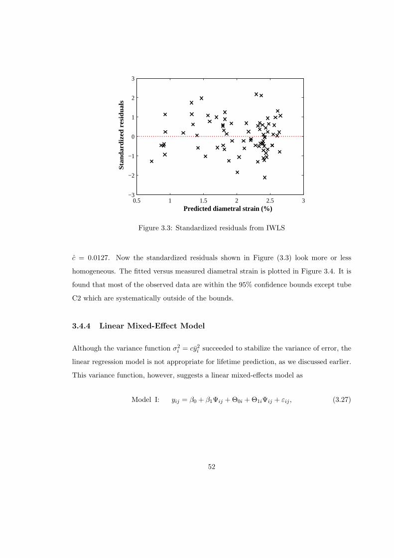
0.5 1 1.5 2 2.5 3−3
−2
−1
0
1
2
3
Predicted diametral strain (%)
Sta
nd
ard
ized
res
idu
als
Figure 3.3: Standardized residuals from IWLS
c = 0.0127. Now the standardized residuals shown in Figure (3.3) look more or less
homogeneous. The fitted versus measured diametral strain is plotted in Figure 3.4. It is
found that most of the observed data are within the 95% confidence bounds except tube
C2 which are systematically outside of the bounds.
3.4.4 Linear Mixed-Effect Model
Although the variance function σ2i = cy2
i succeeded to stabilize the variance of error, the
linear regression model is not appropriate for lifetime prediction, as we discussed earlier.
This variance function, however, suggests a linear mixed-effects model as
Model I: yij = β0 + β1Ψij + Θ0i + Θ1iΨij + εij , (3.27)
52

3 4 5 6 7 8 9 10 11 12 130.5
1
1.5
2
2.5
3
3.5
4
Fluence (x 1025 n/m2)
Dia
met
ral s
trai
n (%
)
Measured
Mean
95% bound
Figure 3.4: Predicted versus observed diametral strains from IWLS. The circled crossesrepresent data from Tube C2
53

for i = 1, . . . , n = 61 and j = 1, . . . , mi where most of mi equals 1 as shown in Table 3.1.
In the form of (3.20), we have Xi = Zi and
Xi =
xi1
...
xi,mi
=
1 Ψi1
......
1 Ψi,mi
(3.28)
There are 6 parameters in total to be estimated: β0, β1, d11, d12 = d21, d22 and σ2.
Since the covariance matrix of b, D, should be nonnegative definite, this gives an implicit
constraint for the parameter space of all the d’s. To avoid the nuisance, we reparameterize
D by using the Cholesky factorization, i.e.,
D = UTU (3.29)
where U is an upper triangle matrix including entities u11, u12 and u22 which can be any
real number in theory. If the noise variance is also reparameterized as σ2 = exp (s), then
the log likelihood function can be maximized with respect to θ = (β0, β1, u11, u12, u12, s)T
in an unconstrained fashion.
The maximum likelihood estimates for the parameters are β0 = 0.0503, β1 = 0.2090,
σε = 0.0831, σΘ0 = 0.0353, σΘ1 = 0.0197 and ρ(Θ0, Θ1) = 0.9999 where ρ(Θ0, Θ1) repre-
sents the coefficient of correlation of the intercept Θ0 and slope Θ1. The corresponding
maximized log likelihood is −82.53.
Since the coefficient of correlation of Θ0 and Θ1 (both have been assumed to be random
variables) is very close to 1, we can thus assume only Θ1 is random and Θ0 = αΘ1 where
α is a constant. Therefore we have Zi = (α + Ψi1, . . . , α + Ψimi)T , or
Model II: yij = β0 + β1Ψij + (α + Ψij)Θ1i + εij . (3.30)
Under this new assumption, we have β0 = 0.0503, β1 = 0.2090, σε = 0.0831, σΘ1 = 0.0197
54

which are the same as before and α = 1.7916 which equals σΘ0/σΘ1 = 0.0353/0.0197.
Alternatively, we choose the slope, denoted as Θ for brevity, as the only random
coefficient and let the intercept fixed for all units. This amounts to assuming Zi =
(Ψi1, . . . ,Ψi,mi)T or
Model III: yij = β0 + β1Ψij + ΨijΘi + εij (3.31)
Under this assumption, we obtain β0 = 0.0637, β1 = 0.2077, σε = 0.0864, σΘ = 0.0232
with maximized log likelihood of −83.08. It is clear from the likelihood ratio test that it
is plausible to assume a fixed intercept. We adopt Model III for the next discussion.
In order to validate the assumptions of (1) normal within-unit measurement errors
and (2) normal random slope in the model, the normal quantile plots for the within-unit
residuals εij (i = 1, . . . , n = 61; j = 1, . . . , mi) and for the random slope Θ are shown in
Figure 3.5 and 3.6, respectively. Both plots are close to a straight line and symmetrical
about zero except one data point from Tube C1 in Figure 3.5 which may be considered
as an outlier. Hence no obvious evidence is shown against the assumptions.
Figure 3.7 plots the fitted versus observed diametral strain in both populational and
individual levels. Comparing to Figure 3.4, the populational mean path is very close to
that from IWLS. Recall that in the LR model, measurements of Tube C2 are out of the
predictive bound. In the LME model, however, we can estimate the random slope Θ
for the tube. For Tube C2, we have Xi = (1 Ψi1; . . . ; 1 Ψi5), Zi = (Ψi1, . . . ,Ψi5)T and
D = σ2Θ. So from (3.25) we get θi = 0.0594. That is, the total deterioration rate for
Tube C2 equals β1+ θi = 0.2671. The individual mean path for Tube C2 is shown as
a thick solid line in Figure 3.7 A conservative (without considering the uncertainty in
β’s) prediction bound for the diametral strain of Tube C2 is plotted as well. In the LME
model, the five measurements all lie within the 95% bound.
55

-0.15 -0.10 -0.05 0.00 0.05 0.10 0.15
Within-unit standardized residuals
-2-1
01
2
Qua
ntile
s of
sta
ndar
d no
rmal
C1
C1
Figure 3.5: Normal quantile plot for within-unit residuals εij
The lifetime distribution can then be calculated from the following expression:
FT (τ) = Pr (β0 + β1τ + Θτ ≥ ζ) = Pr(
Θ ≥ ζ − β0
τ− β1
)= 1− Φ
(ζ − β0
τσΘ− β1
σΘ
).
(3.32)
Figure 3.8 shows the lifetime distribution of a typical pressure tube with failure threshold
ζ = 5.1%. For an illustration, the lifetime density function for a typical tube with average
flux 2.4× 10¹⁷ n/(m2·s) is plotted in Figure 3.8.
3.5 Concluding Remarks
Traditional regression models consist of a parameterized mean function and an error
term that quantifies the deviation of the observations from the mean function. The
errors are usually assumed independent of each other. While the data analysis becomes
56

-0.06 -0.04 -0.02 0.00 0.02 0.04 0.06
Random slope
-2-1
01
2
Qua
ntile
s of
sta
ndar
d no
rmal
Figure 3.6: Normal quantile plot for the random slope Θ
straightforward under this assumption, it compromises the lifetime prediction. Although
the independence assumption can be relaxed and replaced with some correlation structure,
exact solutions for the lifetime under such assumptions are not yet available, unless further
unrealistic approximations or assumptions are introduced.
This chapter presents a linear mixed-effects model to solve the problem. The feature
of an LME model is that the inherent randomness of deterioration is decomposed into
unobserved heterogeneity of individual units, or random effects, and additive measure-
ment errors. By introducing the random effects into the model, the varying variance of
deterioration and correlation in deterioration are characterized, which leads to a logical
method for lifetime estimation.
The case study of creep deformation of pressure tubes starts with a simple linear re-
gression model with variance of error weighted by the number of repeated measurements.
The LR model is improved by an iteratively weighted least squares technique to stabilize
57

3 4 5 6 7 8 9 10 11 12 130.5
1
1.5
2
2.5
3
3.5
4
Fluence (x 1025 n/m2)
diam
etra
l str
ain
(%)
Measured
Individual Mean
95% bound
Figure 3.7: Populational (dashed line) and individual (solid line) mean deterioration pathof Tube C2. The circled crosses represent diametral strain measured from Tube C2
58

10 15 20 25 30 35 40 45 50 55 600
0.02
0.04
0.06
0.08
0.1
0.12
Lifetime (EFPY)
Pro
babi
lity
dens
ity
func
tion
µT = 32.45 EFPY
σT = 3.82 EFPY
Figure 3.8: Probability density function of the lifetime of a typical pressure tube withflux 2.4× 10¹⁷ n/(m2·s)
the variance of residuals. The LME model is a better alternative with a random slope.
As a result the tubes with high deterioration rate, which were classified as outliers in the
LR model, are now fitted quite well in the LME model.
Despite a success in fitting the data in pressure tube example, the LME model is
essentially a random variable model. For this reason, LME or LR models are inadequate
to quantify the temporal variability and not well suited for condition-based maintenance
optimization, as discussed in Chapter 7.
59

Chapter 4
Gamma and Related Processes
This chapter discusses basic concepts and properties of gamma and other related pro-
cesses. We start with a stationary gamma process. Its characteristics are discussed from
distribution, sample paths, lifetime and simulation perspectives. The discussion is then
extended to nonstationary gamma processes, local gamma processes, mixed-scale gamma
processes and finally Hougaard processes. The relationship among these stochastic pro-
cesses is investigated.
4.1 Stationary Gamma Processes
A gamma distributed random variable X with shape parameter a > 0 and scale parameter
b > 0 has probability density function
fZ(z) =(z/b)a−1
bΓ (a)exp (−z/b) (4.1)
for z ≥ 0, where Γ(u) =∫∞0 su−1e−sds is the gamma function. We write Z ∼ Ga (a, b)
to mean a random variable Z follows gamma distribution with shape a and scale b.
Depending on the value of shape parameter a, the probability density function of Z can
60

0 2 4 6 8 100
0.5
1
1.5
z
f(z)
a = 0.2
a = 1
a = 2
a = 5
Figure 4.1: Probability density functions of gamma random variables with unit scaleparameter and different shape parameters
be monotonically decreasing or nearly of a bell shape (Figure 4.1). The mean and variance
of Z are ab and ab2, respectively.
A continuous-time stochastic process {X(t), t ≥ 0} is called a stationary gamma pro-
cess with shape parameter α > 0 and scale parameter β > 0 if it has the following
properties (Singpurwalla 1997):
(i) X (0) = 0 with probability one;
(ii) ∆X(t) = X (t + ∆t)−X(t) ∼ Ga (α∆t, β) for any t ≥ 0 and ∆t > 0; and
(iii) For any choices of n ≥ 1 and 0 ≤ t0 < t1 < · · · < tn < ∞, the random variables
X(t0), X(t1)−X(t0), . . . , X(tn)−X(tn−1) are independent.
In short, a stationary gamma processes is a continuous-time stochastic processes with
stationary, independent and gamma distributed increments.
4.1.1 Distribution and Sample Path Properties
The gamma distribution is infinitely divisible in the sense that if Z is a gamma r.v.,
then for every positive integer n there exist n i.i.d. r.v. Z1, Z2, . . . , Zn that sum to
61

Z (Sato 1999). In the other direction we have that the sum of n independent gamma
random variables, each having shape ai (i = 1, . . . , n) and the same scale b, is still gamma
distributed with shape∑
ai and scale b. Therefore, at any time t > 0, X (t) is a gamma
random variable, i.e., X (t) ∼ Ga (αt, β). As t gets large, the probability density function
of X (t) changes from a monotonically decreasing function to a bell shape as shown in
Figure 4.1.
Another important characteristic of gamma distribution is the so-called “gamma-
bridge” property. That is, for two independent gamma r.v. U ∼ Ga(α1, β) and V ∼Ga(α2, β) the ratio U/(U +V ) is beta distributed and independent of U (Johnson, Kotz,
and Balakrishnan 1994). This implies that the ratio of X (u) to X (t) for 0 < u < t < ∞follows a beta distribution with parameter αu and α (t− u). This property can be used
for simulating gamma processes. We will discuss this in detail later on.
As far as the sample path properties of gamma process are concerned, we first note
that gamma process is Markovian because of its independent increments and that its
sample path is non-negative and monotonically increasing. Note also that the mean and
variance of X(t) are
E [X(t)] = αβt and Var [X (t)] = αβ2t, (4.2)
both linear functions of time. The coefficient of variation (COV), defined by the ratio of
the standard deviation to the mean, is thus
COV [X(t)] = 1/√
αt. (4.3)
The decreasing COV suggests that the sample paths get closer and closer to the mean
path over time in the relative sense. Figure 4.2 plots two sample paths of the same gamma
process with α = 3 and β = 2 at two different time scale. The solid line represents the
path at a small scale with time t1 ranging from 0 to 2 and the dashed line corresponds
to time frame t2 from 0 to 20. The dashed line looks very close to a straight line — the
62
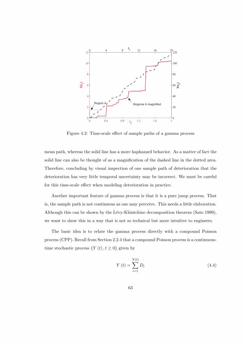
0 0.4 0.8 1.2 1.6 20
2
4
6
8
10
12
t1
X(t
1)
0 4 8 12 16 20
0
20
40
60
80
100
120
t2
X(t
2)
Region A Regiona A maginified
Figure 4.2: Time-scale effect of sample paths of a gamma process
mean path, whereas the solid line has a more haphazard behavior. As a matter of fact the
solid line can also be thought of as a magnification of the dashed line in the dotted area.
Therefore, concluding by visual inspection of one sample path of deterioration that the
deterioration has very little temporal uncertainty may be incorrect. We must be careful
for this time-scale effect when modeling deterioration in practice.
Another important feature of gamma process is that it is a pure jump process. That
is, the sample path is not continuous as one may perceive. This needs a little elaboration.
Although this can be shown by the Levy-Khintchine decomposition theorem (Sato 1999),
we want to show this in a way that is not so technical but more intuitive to engineers.
The basic idea is to relate the gamma process directly with a compound Poisson
process (CPP). Recall from Section 2.2.4 that a compound Poisson process is a continuous-
time stochastic process {Y (t) , t ≥ 0} given by
Y (t) =N(t)∑
i=1
Di (4.4)
63

where {N (t) , t ≥ 0} is a homogeneous Poisson process with rate λ, and Di (i = 1, 2, . . .)
are i.i.d. random variables with CDF G, which are also independent of {N (t) , t ≥ 0}.Suppose Di are positive random variables, i.e., G (0) = 0. Suppose also the CDF G is
differentiable and has pdf g. Then the Laplace transform of Y (t) is
E[e−sY (t)
]= exp
{λt
∫ ∞
0
(e−su − 1
)G (du)
}= exp
{t
∫ ∞
0
(e−su − 1
)νP (du)
}, (4.5)
in which
νP (du) = λG (du) = λg(u)du (4.6)
is called the Levy measure of Y (t).
Consider now a gamma process {X (t) , t ≥ 0} with shape α and scale β. The Laplace
transform of X (t) is
E{
e−sX(t)}
=(
11 + βs
)αt
= exp {−αt log (1 + βs)} = exp{
t
∫ ∞
0
(e−su − 1
)νΓ (du)
},
(4.7)
in which
νΓ (du) = (α/u) e−u/βdu. (4.8)
Comparing (4.7) to (4.5) we can find that the gamma process is closely related to a
CPP if λ and G in the CPP is appropriately chosen the limit of a compound Poisson
process. Indeed, according to Dufresne, Gerber, and Shiu (1991), we may assume the
Poisson rate λ = αβcΓ (c) and G as a gamma distribution, i.e., Di ∼ Ga (c, β). Then
νP (du) = λg(u)du = αβcΓ (c)uc−1
βcΓ (c)e−u/βdu =
α
u1−ce−u/βdu. (4.9)
As c tends to zero from above, the Poisson rate λ goes to infinity, the random jumps Di
gets more and more concentrated at zero (Figure 4.1), and the Levy measure νP of the
CPP tends to νΓ of the gamma process.
64

The Levy measure ν (y) ≡ ν ([y,∞)) represents the mean number of jumps of sizes
greater than y in a unit interval of time. In particular, ν (0) is the mean number of all
jumps. For a CPP, νP (0) = λ∫∞0 G (du) = λ is finite. For a gamma process, however,
νΓ(0) = α∫∞0 u−1e−u/βdu = ∞. But it is easily checked that the mean number of jumps
of sizes larger than any positive number ε is finite, or νΓ(ε) = α∫∞ε u−1e−u/βdu < ∞
for any ε > 0. Therefore, within any finite time interval there are infinitely many small
jumps of size less than ε for any ε > 0 but only a finite number of big jumps. However,
the cumulative sum of all these jumps in a finite time interval [t, t + ∆t) is always finite,
no matter how infinitely many jumps there are. That is
E [X (t, t + ∆t)] =N(t,t+∆t)∑
i=1
Di =∫ t+∆t
t
∫ ∞
0u νΓ (du) ds = αβ∆t. (4.10)
Adding these facts altogether explains why the gamma process is a pure jump process
while its sample path looks continuous.
The sample paths and associated jump sizes of two CPPs and one gamma process
are plotted in Figure 4.3. The gamma process has a shape parameter α = 1 and scale
parameter β = 1/√
2. Its sample path is shown in Figure 4.3(e). The two CPPs have
a intensity rate λ = αβcΓ (c) and a gamma distribution Ga (c, β) for the jumps. Figure
4.3(a) shows a sample path of the CPP with c = 2. Only 8 jumps occur. The jump sizes
and associated occurrence times are shown in Figure 4.3(b). In contrast, Figure 4.3(c)
shows a sample path of the CPP with c = 0.01, which is very similar to the sample path
of the gamma process, the limiting case when c = 0. The jumps shown in Figure 4.3(d)
have a skewer distribution, for most of them are small jumps. Figure 4.3(f) shows the
magnified plot of (d) for the jumps with size less than 0.03. It is not difficult to imagine
that, when c is sufficiently close to zero, a similar plot to (f) can be obtained even a
smaller truncation than 0.03 is chosen.
To summarize, the sample path of a gamma process embraces both minute invisible
jumps and big traumatic jumps. This feature makes the gamma process a very good
65

0 5 10 150
5
10
X(t
)
0 5 10 150
0.5
1
1.5
Jum
p si
ze, D
i
0 5 10 150
5
10
X(t
)
0 5 10 150
0.5
1
1.5Ju
mp
size
, Di
0 5 10 150
0.01
0.02
0.03
time, t
Smal
l Jum
ps
(Di <
0.0
3)
0 5 10 150
5
10
time, t
X(t
)
(a) CPP, c = 2
(c) CPP, c =0.01
(e) GP, α = 1, β =0.7
(b) CPP, c = 2
(d) CPP, c = 0.01
(f) CPP, c = 0.01
Figure 4.3: A compound Poisson process goes to a gamma process when c goes to zero
66

candidate for deterioration models, as the deterioration may develop in a very slow,
invisible fashion due to daily usage and in some points of time it may grow very quickly
when some traumatic events (e.g., earthquakes, forced outages) happen. The gamma
process fits both types of damage modes.
4.1.2 Distribution of Lifetime
Many physical failures and performance failures (that is the system performance no longer
conforms to a standard) are of first passage type. That is, once the deterioration process
X (t) of an item reaches a certain critical level ζ, the item fails. The failure time T is
then defined as the first time when the sample path of X (t) exceeds ζ. Symbolically, we
have
T ≡ inf {X(t) ≥ ζ} = {t |X(t) ≥ ζ, X (s) < ζ for 0 ≤ s < t} . (4.11)
When X (t) is a stationary gamma process, the distribution of the first passage time is,
according to the monotonicity of its sample paths,
FT (t) = Pr(T ≤ t) = Pr(X(t) ≥ ζ) =Γ(ζ/β, αt)
Γ(αt)(4.12)
where Γ(w, z) denotes the incomplete gamma function, defined as
Γ(w, z) =∫ ∞
wuz−1e−udu. (4.13)
The first two moments of the lifetime are expressed as
E [T ] =∫ ∞
0(1− FT (t)) dt, and (4.14a)
E[T 2
]= 2
∫ ∞
0t (1− FT (t)) dt, (4.14b)
which should be evaluated numerically.
A discrete-time approximation of (4.12) can be made by choosing tn = n/α, n =
67

0 5 10 15 20 250
0.02
0.04
0.06
0.08
0.1
0.12
0.14
First passage time
Pro
abili
ty d
ensi
ty/m
ass
func
tion α = β = 1
ζ = 10
Figure 4.4: Distribution of first passage time of a gamma process and its Poisson approx-imation
0, 1, . . .. Let qn = Pr {tn < Tξ ≤ tn+1}. Then one has
qn =Γ(ζ/β, n + 1)
Γ(n + 1)− Γ(ζ/β, n)
Γ(n)=
(ζ/β)n
n!e−ζ/β , (4.15)
which is a Poisson distribution. That is, the probability of first passage time being the
time interval (n/α, (n + 1) /α] follows a Poisson distribution with parameter ζ/β. This
result was first observed by van Noortwijk et al. (1995). From the property of Poisson
distribution, the mean and variance of the lifetime equals ζ/ (βα) and ζ/(βα2
), which is
remarkable as if they were derived directly from (4.2).
Figure 4.4 shows an example for the pdf of the first passage time and its Poisson
approximation for the gamma process with unit shape and scale and failure threshold of
10. The exact values of the mean and variance are 10.495 and 10.022, respectively while
the Poisson approximation gives both of 10.
68

4.1.3 Distribution of Remaining Lifetime
The distribution of remaining lifetime, the remaining time to the first passage level ζ,
of the stationary gamma process, given its value at time s, X (s) = xs < ζ, is readily
established using the independent increments property as
FT (t | s) = Pr(T ≤ t |X (s) = xs)
= Pr(X(t)−X (s) ≥ ζ − xs)
=Γ [(ζ − xs) /β, α (t− s)]
Γ [α (t− s)](4.16)
for t ≥ s, which is the same as (4.12) with ζ and t replaced by ζ−xs and t−s, respectively.
If more recent values of the gamma process is known, the remaining lifetime distribution
can be updated in the same way.
This update scheme of remaining lifetime is different from the way based on known
surviving time. In the traditional lifetime approach to reliability modeling, the remaining
lifetime distribution, given the item has survived up to the present time s, is given as
FT (t | s) = Pr (T ≤ t |T > s) =FT (t)− FT (s)
1− FT (s)(4.17)
for t > s.
Figure 4.5 shows three different distributions of the remaining lifetime after the item
has survived 8 units of time for the gamma process in Figure 4.4. The distribution of
the time-based remaining lifetime (with the only information of s = 8) is the truncated
version of the original distribution at s = 8. But the real remaining lifetime can differ a
lot from this truncated lifetime, depending on the actual level of state x (s) at time s = 8.
69
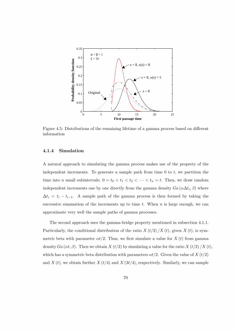
0 5 10 15 20 250
0.05
0.1
0.15
0.2
0.25
0.3
0.35
First passage time
Pro
babi
lity
dens
ity
func
tion
s = 8, x(s) = 8
s = 8, x(s) = 5
s = 8Original
α = β = 1ζ = 10
Figure 4.5: Distributions of the remaining lifetime of a gamma process based on differentinformation
4.1.4 Simulation
A natural approach to simulating the gamma process makes use of the property of the
independent increments. To generate a sample path from time 0 to t, we partition the
time into n small subintervals: 0 = t0 < t1 < t2 < · · · < tn = t. Then, we draw random
independent increments one by one directly from the gamma density Ga (α∆ti, β) where
∆ti = ti − ti−1. A sample path of the gamma process is then formed by taking the
successive summation of the increments up to time t. When n is large enough, we can
approximate very well the sample paths of gamma processes.
The second approach uses the gamma-bridge property mentioned in subsection 4.1.1.
Particularly, the conditional distribution of the ratio X (t/2) /X (t), given X (t), is sym-
metric beta with parameter αt/2. Thus, we first simulate a value for X (t) from gamma
density Ga (αt, β). Then we obtain X (t/2) by simulating a value for the ratio X (t/2) /X (t),
which has a symmetric beta distribution with parameters αt/2. Given the value of X (t/2)
and X (t), we obtain further X (t/4) and X (3t/4), respectively. Similarly, we can sample
70

X (t/8), X (3t/8), X (5t/8), X (7t/8), and so on (Dufresne, Gerber, and Shiu 1991).
The approach to simulation applies the functional representation theory of stochastic
processes. Sometimes it is possible to represent a stochastic process as a countable sum
of some deterministic functions with random variable coefficients. If so, then we can
generate a finite number of random coefficients and approximate the sample path by
the finite summation. The well-known Karhunen-Loeve expansion is an example of this
application to stationary second-order Gaussian processes (Ghanem and Spanos 2003).
Another example is the Wiener process, for which we have
W (t) = Y0t +√
2∞∑
m=1
Ymsin (mt)
m, (4.18)
where W (t) denotes the Wiener process and Y0, Y1, . . . are independent normal random
variables with zero means and unit variance. We wish a similar representation for gamma
processes.
Indeed, it has been found (Ferguson and Klass 1972) that an independent increment
process without Gaussian components can be represented as a countable sum of step
functions each with a random point of discontinuity at a random height. For a stationary
gamma process {X (t) , 0 ≤ t ≤ 1} with shape α and scale β in specific, it can be expanded
as a compound Poisson process with the ordered random heights J1 ≥ J2 ≥ · · ·having
the following distributions:
Pr (J1 ≤ x1) = exp {−νΓ (x1,∞)} = exp{−α
∫ ∞
x1
y−1e−y/βdy
}(4.19)
and
Pr (Jj ≤ xj | Jj−1 = xj−1, . . . , J1 = x1) = exp {−νΓ (xj , xj−1)} . (4.20)
71

Under this representation, the gamma process is expressed as
X (t) =∞∑
j=1
JjI[0,t] (Uj) , (4.21)
where U1, U2, . . . are independent and identically uniformly distributed on [0, 1] and inde-
pendent of J1, J2, . . .; and I[0,t] (·) is indicator function. One advantage of this simulation
is that the fineness of the sample path can be controlled by the number of jumps, n.
The disadvantage is also obvious: more computational efforts are needed to generate the
sequence of random jump heights.
4.2 Nonstationary Gamma Processes
A nonstationary gamma process {X (t) , t ≥ 0} is a continuous-time stochastic process
with increments ∆X (t) that are independent and have gamma distribution Ga (∆α (t) , β),
in which α (t) ≥ 0, is a nondecreasing continuous function with α (0) = 0 and ∆α (t) =
α (t + ∆t) − α (t). α (t) is called the shape function and β > 0 is again the scale pa-
rameter. Clearly, when the shape function is linear of time, i.e., α (t) = αt, the process
becomes a stationary gamma process with shape parameter α and scale parameter β.
Since the nonstationary gamma process can be obtained by a deterministic nonlinear
time transformation from the stationary gamma process, many results for stationary
gamma processes are readily extended to the nonstationary case. For example, for any
fixed t, X (t) is still gamma distributed; its mean and variance are E [X(t)] = α (t) β and
Var [X (t)] = α (t)β2; and X (t) is also a pure jump process. We are not going to give
further details for the nonstationary gamma process.
72

4.3 Local Gamma Processes
A local gamma process is a continuous-time stochastic process X (t) with shape function
α(t) and scale function β(t), satisfying the following properties (Cinlar 1980):
(i) Almost surely, the sample path is right-continuous and increasing and starts from
0.
(ii) The shape function α(t) is increasing and right-continuous, and scale function β(t)
is strictly positive and finite.
(iii) For every 0 < t < ∞,∫ t0 dα(u)/β(u) < ∞.
(iv) For every t ≥ 0, ∆t > 0 and s ≥ 0, the Laplace transform of the increments,
∆X (t) = X (t + ∆t)−X (t), is
E{
e−s∆X(t)}
= exp{∫ t+∆t
tdα (u)
∫ ∞
0x−1
(e−sx − 1
)e−x/β(u)dx
}
= exp{−
∫ t+∆t
tlog(1 + sβ(u))dα(u)
}. (4.22)
In essence, the local gamma process has the property that increments within infinites-
imal time interval are gamma distributed, i.e.,
∆X(t) = X(t + ∆t)−X(t)∼Ga(α(t + ∆t)− a(t), β(t∗)), for ∆t → 0 (4.23)
where ∼ denotes “approximately distributed as” and t∗ is anytime between t and t + ∆t.
Note that for any fixed t, X(t) does not necessarily follow a gamma distribution unless
the scale function β (t) is constant.
73
A simple example of the local gamma process is the case where β(t) = bt and α(t) = at,
both linear function of time t. Then
− log E{
e−sXt)}
=∫ t
0a log(1 + sbu)du
= a [(1/sb + t) log(1 + sbt)− t] , (4.24)
Or
E{
e−sXt)}
= eat(1 + sbt)−a(1+sbt)
sb . (4.25)
However, no simple analytical form exists for the distribution of which the characteristic
function is as such. Saddlepoint approximation (Daniels 1954; Goutis and Casella 1999)
may be helpful for evaluating the probability density function.
Cinlar (1980) has shown that any local gamma process can be transformed into sta-
tionary gamma process by a change of scale using β (t) and a change of time using α, or
formally we write
X (t) =∫ α(t)
0
1β (s)
dY (s) , (4.26)
where the integration is with respect to the sample paths of Y (t), a stationary gamma
process with unit shape and scale parameter. With this construction, the local gamma
process is also known as extended gamma process (Dykstra and Laud 1981), or weighted
gamma process (Ishwaran and James 2004).
4.4 Mixed-Scale Gamma Processes
A mixed-scale gamma process X (t) is a nonstationary gamma process with a shape
function α (t) ≥ 0 and a random scale parameter B that follows an inverse gamma
distribution, i.e. W = B−1 ∼ Ga(δ, γ−1
). It is first proposed by Lawless and Crowder
(2004) to model the random effects in degradation growth data. The scaled X (t) follows
74

an F distribution. In particular,
δX (t)γα (t)
∼ F (2α (t) , 2δ) , (4.27)
which follows from
fX(t)(x) =∫ ∞
0ga
(x; α (t) , w−1
)ga
(w; δ, γ−1
)dw
=∫ ∞
0
wα(t)xα(t)−1
Γ (α (t))e−xw γηwδ−1
Γ (δ)e−γwdw
=Γ (δ + α (t))Γ (α (t)) Γ (δ)
γδxα(t)−1
(γ + x)δ+α(t). (4.28)
Figure 4.6 shows the probability density function of a mixed-scale gamma random variable
with α (t) = 2, γ = 10 and δ = 10 in comparison with an equivalent gamma density
function with shape parameter 2 and scale parameter 1. It is found that the mixed-scale
gamma density has a heavier tail.
It is clear that the increments are only conditionally independent. The joint probabil-
ity density function of ∆Xi = X (ti)−X (ti−1) for i = 1, . . . , n and 0 = t0 < t1 < · · · < tn
is
f(∆x1, · · · , ∆xn) =∫ ∞
0ga
(w; δ, γ−1
) n∏
i=1
ga(∆xi;∆αi, w
−1)dw
=Γ (δ + αn)
Γ (δ)n∏
i=1Γ (∆αi)
γδn∏
i=1(∆xi)
∆αi−1
(γ + xn)δ+αn, (4.29)
where xn = x(tn), αn = α (tn), ∆αi = α (ti)−α (ti−1) and ∆ti = ti−ti−1. The coefficient
of correlation between two increments at two disjoint time intervals is
ρ (∆Xi, ∆Xj) =
√∆αi∆αj
(∆αi + δ − 1) (∆αj + δ − 1)(4.30)
75

0 1 2 3 4 5 6 7 8 9 100
0.05
0.1
0.15
0.2
0.25
0.3
0.35
0.4
x
Pro
babi
lity
dens
ity
func
tion
GammaMixed−Gamma
Figure 4.6: Comparison of a mixed-scale gamma distribution with its equivalent gammadistribution
for δ > 1. From (4.29) we can also derive the conditional distribution of ∆X (t) =
X (t + s)−X (s) conditional on X (s) = xs as
f (∆x |xs) =Γ (δ + αt+s)
Γ (αs) Γ (δ + ∆α)(γ + xs)
δ+αs ∆x∆α−1
(γ + xs + ∆x)δ+αs+t, (4.31)
orδ + αs
γ + xs
∆X (t)∆α
∼ F (2∆α, 2δ + 2αs) (4.32)
where ∆α = α (t + s)− α (s) and αs = α (s).
Similar to (4.12), the first passage time of the mixed-scale gamma process has a
distribution function as
Pr(Tζ ≤ t) = Pr(X(t) ≥ ζ) = 1− F
(δζ
γα (t); 2α (t) , 2δ
). (4.33)
76

The remaining lifetime distribution given X (s) = xs is, following from (4.32),
Pr(Tζ ≤ t |X (s) = xs) = 1− F
(δ + αs
γ + xs
(ζ − xs)∆α
; 2∆α, 2δ + 2αs
). (4.34)
4.5 Hougaard Processes
Hougaard processes include compound Poisson processes, gamma processes, inverse Gaus-
sian processes, positive stable processes, and deterministic paths as special cases, and
hence are very flexible for deterioration modeling. This section discusses basic proper-
ties of Hougaard processes. But before doing so, let us first introduce a three-parameter
family of distribution, named Hougaard distribution.
4.5.1 Hougaard Distributions
A non-negative random variable X is said to follow a Hougaard distribution if its Laplace
transform, ϕ (s) = E[e−sX
], has the following differential form:
d log ϕ (s)ds
= −δ (θ + s)α−1 , (4.35)
with log ϕ(0) = 0, where α ≤ 1, δ > 0, θ ≥ 0. For α 6= 0,
ϕ (s) = exp {− (δ/α) [(θ + s)α − θα]} . (4.36)
For α = 0, ϕ (s) = [θ/(θ + s)]−δ is the Laplace transform of gamma distribution with
shape parameter δ and scale parameter 1/θ. We denote the Hougaard distribution by
X ∼ H (α, δ, θ) where α, δ, θ are called index, shape and scale parameter, respectively.
Clearly, the family of Hougaard distributions includes gamma distribution as a special
case. Some other special cases are
• Dirac distribution. For α = 1, X is concentrated on δ.
77

• Inverse Gaussian distribution when α = 1/2.
• Positive stable distribution. For θ = 0 and 0 < α < 1, ϕ (s) = exp {− (δ/α) sα},which is the Laplace transform of positive stable distribution with characteristic
exponent α.
• Poisson-Gamma distribution. For α < 0, ϕ (s) = exp {− (δ/α) [(θ + s)α − θα]},which is the Laplace transform of Y = X1 + · · · + XN where N is a Poisson dis-
tribution with mean −δθα/α and Xi (i = 1, 2, . . .) are independent gamma random
variable with as shape −α and scale parameter 1/θ, respectively.
Although Hougaard distribution has a very simple expression for its Laplace trans-
form, it does not have explicit expression for its density function. It is known that the
Hougaard density function, denoted by h(x; α, δ, θ), has an infinite series representation
based on positive stable distribution. For 0 < α < 1, δ > 0, θ ≥ 0 is
h(x;α, δ, θ) = exp (δθα/α− θx) g(x;α, δ), (4.37)
where
g(x; α, δ) = − 1πx
∞∑
k=1
Γ (kα + 1)k!
(−δx−α/α)k sin (αkπ) (4.38)
is the probability density of positive stable distribution with index α and parameter
δ. This series may converge very slowly especially near the origin in which the terms
x−αk become unmanageable for large k and α. For that reason, Hougaard (1986) gave a
saddlepoint approximation for the Hougaard density function
f∗(x) =
√q (δ/x)q
2πxexp
[δθα/α− θx− x (δ/x)q
q − 1
], (4.39)
where q = 1/ (1− α). The approximation is exact only for α = 1/2, which corresponds
to the inverse Gaussian distribution. It can be shown that the mode of the pdf is located
at x = δ1/α[
2(1−α)2−α
](1−α)/α.
78

Hougaard (1986) is the first person who introduced the new three-parameter family of
distributions and applied it as a frailty distribution in survival models for heterogeneous
populations. He derived the new distribution by using a technique called “exponential
tilting” from the positive stable distribution. Later, he named it power variance function
(PVF) distribution to reflect the fact that the variance of the distribution is a power
function of its mean (Hougaard 2000). Fook Chong (1992) documented basic properties
and methods of parameter estimation of Hougaard distributions and Hougaard processes.
4.5.2 Hougaard Processes
A Hougaard process {H (t) ,≥ 0} is a continuous-time stochastic process that has sta-
tionary independent increments and its Laplace transform, ϕ (s) = E[e−sH(t)
], has the
following differential form
d log ϕ (s)ds
= −δt (θ + s)α−1 , (4.40)
with log ϕ(0) = 0, where α ≤ 1, δ > 0, θ ≥ 0. The Levy measure of the Hougaard process
is
νH (du) =δ
Γ (1− α) uα+1e−θudu. (4.41)
When α = 0, νH (du) = νΓ (du) as shown in (4.8). When α < 0, νH (du) is the Levy
measure for a compound Poisson process, as shown in (4.9). Therefore, the Hougaard pro-
cesses include as special cases gamma processes (α = 0, δ > 0, θ > 0), inverse Gaussian
processes (α = 1/2, δ > 0, θ > 0), positive stable processes (0 < α < 1, δ > 0, θ = 0),
compound Poisson processes with gamma increments(α < 0, δ > 0, θ > 0) and determin-
istic paths (α = 1).
79

4.6 Summary
This chapter discusses basic properties of gamma processes and several other closely
related processes. A stationary gamma process has stationary, independent and gamma
distributed increments. It has linear mean and variance functions. It is Markovian and
its sample paths are non-negative and monotonically increasing. The relation of the
gamma process with a compound Poisson process is illustrated. It has been shown that
the gamma process can be easily adapted to both minute damages and traumatic ones,
which is an important property for deterioration modeling.
Nonstationary gamma process, local gamma process, mixed-scaled gamma process and
Hougaard process are also discussed in this chapter. A common feature among them is
that they all have positive and independent (or conditionally independent) increments and
are pure jump processes. Nonstationary gamma process can be regarded as a deterministic
time transform of the stationary process. The mixed-scale gamma process has a random
scale parameter but for a given sample path, it is a deterministic constant. In contrast,
the local gamma process has a time-varying scale parameter. Hougaard process includes
many known stochastic processes as its special cases. However, it does not have an explicit
expression for the probability density function, which makes it less amenable to practical
applications.
80

Chapter 5
Statistical Inference for Gamma
Process Models
5.1 Introduction
Consider the general case in which n units are inspected for deterioration. Suppose
each unit is inspected at different instants of time and for the ith unit we have mi (≥ 1)
measurements of the deterioration at different points of time. Suppose also each unit is
associated with a vector of covariate variables zi. Then the observed data of each unit
have the following form: (xij , tij , zi) in which xij denotes the deterioration at time tij
where i = 1, . . . , n and j = 1, . . . , mi. The numbers of repeated measurements mi’s are
not necessarily the same for different units.
This chapter discusses techniques for parameter estimation and hypothesis tests of
gamma process models of deterioration. Section 5.2 discusses the simplest cases in which
there exists no covariate in the deterioration data and the n units are modeled by a
stationary gamma process with the same shape and scale parameters. Two schemes
of method of moments and the maximum likelihood method are developed. The three
81

methods are then compared in a simulation study. To study the effects of sample size on
estimation accuracy, asymptotic variances of the maximum likelihood estimates are also
derived. Section 5.3 presents likelihood-based techniques for modeling the fixed-effects of
covariates. Section 5.4 discusses parameter estimation when the deterioration data are
contaminated with measurement errors. The effects of measurement errors are studied
through Monte Carlo simulations. Statistical inferences for mixed-effects gamma process
models are discussed in Section 5.5, with emphasis on a score test for random effects.
Section 5.6 revisits the diametral expansion data in Section 3.4 using a gamma process
model. Section 5.7 concludes the chapter.
5.2 Estimating Parameters of Gamma Process Models
Recall a gamma process has stationary and independent increments. When no covariate
presents in the deterioration data, the increments from the n records of sample paths of
the gamma process (xij , tij) can be pooled without change of information together as if
they are from one sample path with total time length Σni=1ti,mi . For ease of presentation,
we assume for this section that the data has the form of (xi, ti), i = 0, 1, . . . , n with
x0 = t0 = 0. We want to estimate the shape parameter α and the scale parameter β from
the given data. Method of moments and maximum likelihood method can be used.
Since nonstationary gamma process can be thought of as a time transformation from
a stationary gamma process, the techniques discussed in this section can also be used for
the nonstationary cases once the shape function is well parameterized.
5.2.1 Methods of Moments
The basic idea behind the method of moments is to match the moments of a certain
random variable with its corresponding statistics. For example, given n independent
observations u1, . . . , un of a Gaussian random variable U with mean µ and variance σ2,
82

the sample mean and sample variance are
U =1n
n∑
i=1
ui and S2U =
1n− 1
n∑
i=1
(ui − U
)2 (5.1)
Since E[U
]= µ and E
[S2
U
]= σ2, the estimates for µ and σ2 are U and S2
U , respectively.
As far as the gamma process is concerned, let ∆xi = xi − xi−1, ∆ti = ti − ti−1.
The deterioration rate Ri, defined by ∆Xi/∆ti, are independent and gamma distributed.
Therefore, similar to the Gaussian case in the above, we can calculate the sample mean
and sample variance of the rate as
R =1n
n∑
i=1
∆xi
∆tiand S2
R =1
n− 1
n∑
i=1
(∆xi
∆ti− R
)2
. (5.2)
It is clear that E[R
]= αβ and Var
[R
]= 1
n2 αβ2∑n
i=1 (1/∆ti). Hence
E[S2
R
]=
1n− 1
n∑
i=1
E(
∆Xi
∆ti− R
)2
=1
n− 1
n∑
i=1
E[(
∆Xi
∆ti− αβ
)− (
R− αβ)]2
=1
n− 1
n∑
i=1
{Var
[∆Xi
∆ti
]− 2
nVar
[∆Xi
∆ti
]+ Var
[R
]}
=1n
αβ2n∑
i=1
(1
∆ti
). (5.3)
Relating the sample moments to the expected values, we have
αβ = R, (5.4a)
αβ2 =nS2
R∑ni=1 (1/∆ti)
. (5.4b)
Solving them gives the estimates for the parameters.
Cinlar et al. (1977) proposed another scheme of method of moments. Instead of find-
83

ing the moments of the deterioration rate, they calculated the moments of the increments
as
Y =∑n
i=1 ∆xi∑ni=1 ∆ti
=xn
tn, (5.5a)
S2Y =
n∑
i=1
(∆xi − Y ∆ti
)2. (5.5b)
Since
E[Y
]= E
[∑ni=1 ∆xi∑ni=1 ∆ti
]=
E [X (tn)]tn
= αβ (5.6)
and
E
[n∑
i=1
(∆Xi − Y ∆ti
)2
]= E
[n∑
i=1
{(∆Xi − αβ∆ti)−
(Y − αβ
)∆ti
}2
]
=n∑
i=1
Var (∆Xi) +n∑
i=1
∆tiVar(Y
)
= αβ2tn
[1−
n∑
i=1
(∆titn
)2]
, (5.7)
we match the expected values with the estimations and get
αβ = Y =xn
tn, (5.8a)
αβ2 =S2
Y
tn
[1−∑n
i=1 (∆ti/tn)2] , (5.8b)
from which the estimates for parameters α and β are obtained as
α =x2
n
[1−∑n
i=1 (∆ti/tn)2]
tnS2Y
, (5.9a)
β =S2
Y
xn
[1−∑n
i=1 (∆ti/tn)2] . (5.9b)
84

We can think of the bracketed terms as a correction factor in the same way as (n− 1) for
S2U in (5.1) so that the estimates are unbiased. It is clear that when ∆ti (i = 1, . . . , n)
are equal, the estimates from both schemes are the same.
5.2.2 Maximum Likelihood Method
Given the increments (∆xi, ∆ti) , i = 1, . . . , n, of a gamma process {X (t) , t ≥ 0} with
shape α and scale β, the likelihood function for α and β can be easily established. Recall
from the definition of the gamma process,
∆Xi ∼ Ga(α∆ti, β) =(∆xi/β)α∆ti−1
βΓ (α∆ti)e−∆xi/β. (5.10)
The log likelihood function is
l (α, β) =n∑
i=1
(α∆ti − 1) log ∆xi − αtn log β −n∑
i=1
log Γ (α∆ti)− xn
β. (5.11)
Differentiating l (α, β) with respect to α and β, respectively, we have the following max-
imum likelihood equations:
∂l
∂α=
n∑
i=1
∆ti (log xi − ψ (α∆ti)− ln β) = 0, (5.12a)
∂l
∂β=
xn
β2− αtn
β= 0, (5.12b)
in which ψ (u) denotes the digamma function, the derivative of log gamma function
log Γ(u). Solutions of the two simultaneous equations are the maximum likelihood esti-
mates for the parameters. In particular, from the last equation we have
β =xn
αtn, (5.13)
85

which is a natural result from the fact that E [X (tn)] = αβtn. Substituting it back into
the first maximum likelihood equation leads to
n∑
i=1
∆ti log ∆xi − tn logxn
αtn−
n∑
i=1
∆tiψ (α∆ti) = 0. (5.14)
This is a transcendental equation and hence numerical techniques are usually called for.
5.2.3 Effects of Sample Size
Next we discuss the effects of sample size on statistical errors of parameters of gamma
processes in terms of asymptotic variances of the maximum likelihood estimates. The
asymptotic variances are derived from the observed Fisher’s information matrix, I, which
is defined as the negative Hessian matrix of log likelihood or the second derivatives of
l (α, β). From (5.11), we have
I =
∑ni=1 ∆t2i ψ
′ (α∆ti) tn/β
tn/β αtn/β2
(5.15)
where ψ′ (u) = dψ (u) /du. The entity I22 follows from the fact that ∂2l/∂β2 = αtn/β2 −2xn/β3 and xn = αβtn. Taking the inverse of I we obtain the asymptotic covariance
matrix for α and β.
Suppose ∆ti = ∆t = tn/n for i = 1, 2, . . . , n. Then
I =tnβ
β∆tψ′ (α∆t) 1
1 α/β
. (5.16)
Hence, the asymptotic covariance matrix is
I−1 =β
tn [α∆tψ′ (α∆t)− 1]
α/β −1
−1 β∆tψ′ (α∆t)
. (5.17)
86

From Bleistein and Handelsman (1975) we have
ψ′ (u) ∼ 1u
+1
2u2+
16u3
− · · · , (5.18)
and thus
uψ′ (u)− 1 ∼ 12u
+1
6u2− · · · . (5.19)
Using the first term of the asymptotic expansion, we have
Var(α) =α
tn [α∆tψ′ (α∆t)− 1]∼ 2α2∆t
tn=
2α2
n, (5.20a)
Var(α, β
)= − β
tn [α∆tψ′ (α∆t)− 1]∼ −2αβ
n, and (5.20b)
Var(β)
=β2/α
tn (1− 1/ [α∆tψ′ (α∆t)])∼ β2
(2n
+1
αtn
). (5.20c)
The asymptotic variance of α and covariance of α and β are dependent on the size of
sample, n: the greater is the sample size, the smaller the standard error will be. However,
the asymptotic variance of β, the scale parameter, depends not only the sample size but
also on the total time length of the sample path. As the maximum likelihood estimates
are asymptotically unbiased, the coefficient of variation (COV) of the estimate for the
shape parameter is√
2/n and the COV for the scale parameter is√
2/n + 1/(αtn).
To verify the above observations, a Monte Carlo simulation is performed. With fixed
shape parameter α and scale parameter β, a sample path of the gamma process is gener-
ated with a number n of measurements from the time interval [0, tn]. Using the simulated
data, the parameters are estimated and the associated standard errors are computed as
well. Figure 5.1 demonstrates the trend of the COV of the estimated shape and scale
parameter with increasing n at three different length of sample path tn. Both plots agree
well to the analytical results.
87

0 50 100 150 200 250 300 350 400 450 5000
0.2
0.4
0.6
0.8
1
Number of measurements
CO
V o
f sh
ape
0 50 100 150 200 250 300 350 400 450 5000
0.2
0.4
0.6
0.8
1
Number of measurements
CO
V o
f sc
ale
tn = 500 s
tn = 10 s
tn = 50 s
(a)
(b)
Figure 5.1: Coefficient of variation of the estimated (a) shape and (b) scale parametersfrom different numbers of measurements. Dotted lines represent the analytical results,and solid lines the simulation results
88

5.2.4 Comparison of Maximum Likelihood Method and Methods of Mo-
ments
A simulation study is undertaken to compare the effectiveness and efficiency of the three
methods of parameter estimation. For brevity, we use MLE for maximum likelihood
estimates, MoMR for estimates from (5.4) based on the method of moments of rate, and
MoMX for estimates from (5.8) based on the method of moments of increments. Table
5.1 lists the mean and standard error of estimated shape and scale parameters for the
gamma process with the true shape and scale of 3 and 2, respectively. When the sample
size N is greater than 50, three methods all provide reasonable results. But the standard
errors of the MLEs are slightly smaller than those from the two methods of moments.
The maximum likelihood method needs a little more computational efforts than the
methods of moments does. But the former provides an asymptotic variance of the es-
timates without much more efforts as discussed above. To get the confidence intervals
of the estimates of the methods of moments, however, bootstrap simulation (Efron and
Tibshirant 1993), a very computationally intensive tool, is usually called for. Another
reason of preferring maximum likelihood method is that this method is adapted to models
with more complicated structures, as discussed next.
89

Tab
le5.
1:M
ean
and
stan
dard
erro
rsof
esti
mat
edpa
ram
eter
sfr
omdi
ffere
ntm
etho
dsM
LE
MoM
RM
oMX
Nα
βα
βα
β
104.
2476
(2.5
799)
1.80
62(0
.867
0)4.
0514
(2.5
383)
1.94
55(1
.053
8)3.
9934
(2.5
093)
1.97
93(1
.057
6)20
3.49
36(1
.225
3)1.
9018
(0.6
157)
3.46
00(1
.323
0)1.
9735
(0.7
651)
3.40
63(1
.281
9)1.
9899
(0.7
194)
503.
1803
(0.6
499)
1.96
19(0
.401
0)3.
1824
(0.7
556)
1.99
47(0
.512
7)3.
1531
(0.7
237)
2.00
07(0
.464
7)10
03.
0863
(0.4
325)
1.98
02(0
.280
6)3.
0877
(0.5
112)
1.99
74(0
.352
3)3.
0765
(0.4
854)
1.99
70(0
.319
9)50
03.
0148
(0.1
882)
1.99
73(0
.128
2)3.
0174
(0.2
317)
1.99
99(0
.161
6)3.
0140
(0.2
132)
2.00
00(0
.145
2)10
003.
0093
(0.1
317)
1.99
79(0
.091
1)3.
0087
(0.1
633)
2.00
07(0
.114
4)3.
0075
(0.1
498)
2.00
02(0
.102
8)
90

5.3 Modeling Fixed-Effects of Covariates in Deterioration
We now consider to estimate the parameters of a gamma process X (t) of which, for
general purpose, both the shape and scale parameters are functions of some covariates.
Denote the covariates by a vector zi for unit i, i = 1, . . . , n. Suppose the shape and scale
parameters are linked with the covariates by the following parametric forms
αi = α (zi; δ) and βi = β (zi; γ) (5.21)
where both δ and γ are parameter vectors to be estimated. Suppose we observed one
sample path of length mi for ith unit . Given deterioration data as (xij , tij , zi), j =
0, 1, . . . , mi, we cannot pool the data as one sample path as we did in the last section,
because each unit here has different shape and scale parameters.
When the sample path record of each unit is long enough, we can use the methods
proposed in the last section to estimate the shape and scale parameters separately for each
unit at first. The parameters δ and γ can then be estimated using regression techniques
based on the parametric relationship of (5.21). This is equivalent to the two-stage method
used for growth curve models (Meeker and Escobar 1998). Clearly, the effectiveness and
efficiency of this method depends on both large n and large mi. For practical deterioration
data of which mi is usually very small, this method is not applicable.
Maximum likelihood method is suitable for this case. As a matter of fact, only a
small modification of the likelihood function in (5.11) is needed for the method to fit
the situation. Instead of pooling all the data into one sample path, we write the log
likelihood function of each unit as (5.11) with α and β replaced by αi and βi from (5.21).
The sum of all the individual log likelihoods gives the log likelihood function for δ and γ.
The parameters can then be estimated by maximizing the total log likelihood function.
The standard error of the estimates can also be computed from the observed information
matrix. Numerical procedures for the maximization have been discussed in Section 3.3.1.
91

5.3.1 Likelihood Ratio Test
When modeling the effects of covariates, we often want to know the significance of certain
covariates. This can be done by a hypothesis test. For example, to check the significance
of a covariate, we can check whether the parameter associated with this covariate is zero.
Likelihood ratio test is an effective procedure for this purpose.
Denote by θ the parameter vector including both δ and γ. Suppose we want to
test the null hypothesis H0 : θ = θ0 against its alternate H1 : θ 6= θ0 for a known θ0.
The likelihood ratio test statistic is defined to be twice the difference between the two
maximum log-likelihoods (Lawless 2003),
Λ(θ0) = 2l(θ)− 2l (θ0) (5.22)
where l(θ)
is the maximized log likelihood and l (θ0) is the log likelihood associated
with θ0. If θ is k dimensional, then Λ(θ0) is asymptotically chi-square distributed with
k degrees of freedom, i.e., Λ(θ0) ∼ χ2(k). When the observed value of the likelihood ratio
statistic is large enough, we have significant evidence against the null hypothesis. As to
how large the observed value is enough, it depends on the degrees of freedom and the
significance level.
Quite often, we want to test only part of the parameters. This corresponds to a
composite hypothetical test. Suppose the parameters are partitioned as θ =(θT1 , θT
2
)T
and H0 : θ1 = θ10, the likelihood ratio statistic is
Λ(θ01) = 2l(θ)− 2l
(θ)
(5.23)
where l(θ)
is the profile log likelihood with θ1 = θ10. In this case, Λ(θ01) ∼ χ2(p), where
p is the dimension of θ10.
92

5.4 Effects of Measurement Errors
When the measurement error is significant, it cannot be ignored in the data analysis.
In this case, inspection data are noise-contaminated sample paths of gamma process.
Denote the measured deterioration at time tij by yij = xij + εij where xij is the actual
deterioration and εij ’s are assumed to be normally and independently distributed random
variables with mean zero and variance σ2ε . Note ∆yij = ∆xij + εij − εi,j−1. So although
∆xij are independent by definition, the observed increments ∆yij are not independent.
This complicates the construction of likelihood function. In a matrix form,
∆yi1
∆yi2
...
∆yimi
=
∆xi1
∆xi2
...
∆ximi
+
1
−1 1. . . . . .
−1 1
εi1
εi2
...
εimi
(5.24)
or ∆yi = ∆xi + Cεi = ∆xi + ηi, where ηi ∼ N(0, σ2Σ
)and
Σ = CC′ =
1 −1
−1 2 −1. . . . . . . . .
−1 2 −1
−1 2
. (5.25)
93
Although εi1, . . . , εimi are independent each other, ηi1, . . . , ηimi are clearly not. The
marginal distribution of ∆yi is
f (∆yi1, . . . ,∆yimi)
=∫· · ·
∫
{ηij≤∆yij}
mi∏
j=1
f∆Xij (∆yij − ηij)
f (ηi1, · · · , ηimi) dηi1 · · ·dηimi
=∫· · ·
∫
{ηij≤∆yij}
mi∏
i=1
[(∆yij − ηij)
αi∆ti−1
βαi∆tij−1i Γ (αi∆tij)
e−(∆yij−ηij)/βi
]f (ηi) dηi (5.26)
where f (ηi) = f (ηi1, · · · , ηimi) denotes the multivariate normal density function with
mean zero and covariance σ2Σ. When the number of repeated measurements mi is greater
than 3, Monte Carlo simulation may be helpful for evaluating the above integration.
The marginal distribution of ∆yi in (5.26) can serve as the likelihood function of the
parameters (α (δ) , β (γ) and σ2ε) for unit i. Usually, the noise variance σ2
ε is known from
the characteristic curve of the inspection device. If it is not known, we can also estimate
the variance and use likelihood ratio test to check whether the effects of measurement
error is statistically significant.
In order to see the significance of measurement error on the parameter estimation, a
simulation study is conducted for a stationary gamma process with shape parameter α = 5
and scale parameter β = 2. Two cases are considered. For the first case, 1000 sample
paths are generated and each sample path has only one record at time t = 0.25. The
second case considers 50 sample paths, each having 5 records at time interval ∆t = 0.25.
For both cases, each observation of the sample path is contaminated by a measurement
error with standard deviation σε = 0.5. For both cases, the estimations with and without
consideration of the measurement errors are carried out. When the measurement errors
are ignored, the parameters are estimated using the method introduced in Section 5.1.2
and the estimates are denoted by α0 and β0. The estimates when measurement errors
are considered are denoted by αe, βe and σe for α, β and σε, respectively. To get the
94

statistics of the estimates, 200 simulations are run for each case.
The histograms of the maximum likelihood estimates with or without consideration
of measurement errors are plotted in Figure 5.2 and 5.3. It is clear from the first case
that ignoring the measurement errors would lead to biased estimation with misreported
standard errors (se) from observed information matrices. For the second case where more
repeated measurements are used, however, the differences of results with and without
consideration of measurement errors are not so obvious. The reason may be that the
measurement error is getting relatively smaller when the deterioration gets larger. Note
that less total amount of data are used,in the second case than in the first one. This
observation implies that repeated measurement along the time is preferable in the context
of compensating the effects of measurement errors.
5.5 Modeling Random Effects in Deterioration
We have discussed how to estimate the parameters of a gamma process model when
there are covariates associated the deterioration. But there still are situations where the
covariates do not explain all of the differences across the units. The effect due to the
unobserved heterogeneity is called a random effect. The random effect in deterioration
can be modeled by the mixed-scale gamma process introduced in Section 4.4.
Recall that a mixed-scale gamma process X (t) is a nonstationary gamma process
with scale parameter B being an inverted gamma random variable. That is, W = B−1 ∼Ga
(δ, γ−1
)and given B = 1/w, X (t) is a nonstationary gamma process with shape
function α (t) and scale parameter 1/w. When there are covariates attached to the units,
the fixed-effects due to the covariates can be incorporated as we did in the Section 5.3.
For ease of presentation, we assume the covaiates are integrated in the scale parameter
so that the scale parameter B is replaced by Bξ (z), where z denotes the covariates and
ξ (z) represents the effect of covariates. Under these assumptions, the joint distribution
95

4 4.5 5 5.5 6 6.50
0.1
0.2
0.3
1.5 2 2.50
0.1
0.2
0.3
4 4.5 5 5.5 6 6.50
0.1
0.2
0.3
1.5 2 2.50
0.1
0.2
0.3
0.3 0.4 0.5 0.6 0.70
0.1
0.2
0.3
0.24 0.09 0.31 0.13 0.04
0.492.005.031.905.60
σe
βe
αe
β0
α0
se
mean
α0
β0
αe
βe
σe
Figure 5.2: Histograms of maximum likelihood estimates for stationary gamma processwith or without consideration of measurement errors. Parameters are estimated based on1000 sample paths of one record. True values of the parameters are α = 5, β = 2, σε = 0.5
96

4 4.5 5 5.5 6 6.50
0.1
0.2
1.5 2 2.50
0.1
0.2
4 4.5 5 5.5 6 6.50
0.1
0.2
1.5 2 2.50
0.1
0.2
0.2 0.4 0.6 0.80
0.1
0.2
0.31 0.13 0.26 0.11 0.08
0.481.995.112.015.14
α0
β0
αe
βe
σe
mean
se
α0
β0
αe
βe
σe
Figure 5.3: Histograms of maximum likelihood estimates for stationary gamma processwith or without consideration of measurement errors. Parameters are estimated basedon 50 sample paths of 5 record. True values of the parameters are α = 5, β = 2, σε = 0.5
97

of disjoint increments ∆X1, . . . ,∆Xn, according to (4.29), is expressed as
f (∆x1, . . . , ∆xn) =Γ (δ + αn)
Γ (δ)n∏
i=1
Γ (∆αi)
(γξz)δ
n∏
i=1
(∆xi)∆αi−1
(γξz + xn)δ+αn, (5.27)
where xn = Σni=1∆xi, αn = Σn
i=1∆αi and ξz = ξ (z) for brevity. Using this joint den-
sity as the likelihood function, we can use the maximum likelihood method to estimate
parameters δ, γ, and those in α (t) and ξz.
5.5.1 Test of Random Effects
We are certainly interested in testing the significance of the random effects. When γ →∞and δ = γν with ν fixed and finite, the inverted gamma random variable B will concen-
trate around 1/ν and the mixed-scale gamma process will tend to the simple gamma
process with shape function α (t) and the common scale parameter ξz/ν. Therefor, to
test the random effects, we test whether γ is small enough. In this case, the null hypoth-
esis is expressed as H0 : γ = ∞.
Lawless and Crowder (2004) proposed a score statistic but made a small mistake on
the variance of the statistic. Following them, we want to rederive the score statistic in
detail. First note that under the null hypothesis, we have
E0 [Xt − αt ξz/ν] = 0 (5.28a)
E0
[(Xt − αt ξz/ν)2
]= αt ξ2
z/ν2 (5.28b)
E0
[(Xt − αt ξz/ν)4
]= 3 (1 + 2/αt) α2
t ξ4z/ν4 (5.28c)
The subscript “0” is put to emphasize the expectations under the null assumption.
98

From (5.27), the log likelihood function for a single unit is
l = log Γ (δ + αn)− log Γ (δ)−n∑
i=1
log Γ (∆αi)
+ δ log (γξz) +n∑
i=1
(∆αi − 1) log (∆xi)− (δ + αn) log (γξz + xn) . (5.29)
Let δ = γν. Then
∂l
∂γ= ν {1 + log (γξz) + ψ (γν + αn)− ψ (γν)− log (γξz + xn)}
− ξz (γν + αn) (γξz + xn)−1 (5.30)
where ψ (·) denotes the first derivative of logarithm gamma function. As γ →∞, ∂l/∂γ →0, so a more detailed calculation is called for. From Bleistein and Handelsman (1975) we
have
ψ (u) = log u− 12u
− 112u2
+ O(u−3
). (5.31)
Thus,
∂l
∂γ= ν
{log
(1− xn
γξz + xn
)+ log
(1 +
αn
γν
)+
αn
2γν (γν + αn)+
αnξz/ν − xn
γξz + xn+ O
(γ−3
)}
(5.32)
Note that for small u, log (1 + u) can be approximated as u−u2/2+u3/3−· · · . Applying
this approximation to the above expression and simplifying those terms, we have ∂l/∂γ =
Aγ−2 + O(γ−3
)where
A = −12νξ−2
z
{(xn − αnξz/ν)2 − αnξ2
z/ν2}
. (5.33)
A is the statistic for testing the random effects. Although it is not the raw score statistic
as defined by the first derivative of the log likelihood, it is nevertheless the leading term
of the derivative. Therefore, it is also called a score statistic.
99

Note from (5.28) that the quantity inside the bracket of (5.33) represents the difference
of sample variance of X (tn) from its population variance. Therefore, from (5.28) we have
E0 [A] = −12νξ−2
z
{E0
[(Xn − αnξz/ν)2
]− αnξ2
z/ν2}
= 0 (5.34)
and
Var0 [A] = E0
[A2
]=
14ν2ξ−4
z
{E0
[(Xn − αnξz/ν)4 − α2
nξ4z/ν4
]}=
αn (αn + 3)2ν2
. (5.35)
According to the large-sample theory (Lehmann 1999), the score statistic defined as
U =A√
Var0 (A)(5.36)
follows the standard normal distribution. Therefore, given a dataset, one can estimate
the parameters of a gamma process and use the estimates to calculate the score statistic
U . If |U | is greater than a normal quantile zα/2 where α is the significance level, we have
significant evidence against the null hypothesis. If so, we may want to further model the
data with a mixed-scale gamma process.
A Monte Carlo simulation study is performed to verify the proposed score statistic.
Figure 5.4 and 5.5 show the histograms of the score statistic U for a stationary gamma
process with shape parameter α = 3 and scale parameter β = 2. For a relatively small
dataset, the distribution of the score statistic is biased and skewed as shown in Figure
5.4. In case of a large dataset with 500 units, each having 30 records, the simulated
distribution is very close to the standard normal distribution (Figure 5.5). These verify
our derivation of the score statistic.
100

−5 −4 −3 −2 −1 0 1 2 30
0.02
0.04
0.06
0.08
0.1
0.12
0.14
Score statistic U
Fre
quen
cy
Mean = 0.1567Standard error = 0.9457Skewness = −0.6003Kurtosis = 3.5704
Figure 5.4: Histogram of the score statistic for 20 sample paths of 30 equally sampledrecords
−4 −3 −2 −1 0 1 2 3 40
0.02
0.04
0.06
0.08
0.1
0.12
0.14
0.16
0.18
Score statistic U
Fre
quen
cy
Mean = 0.0017Standard error = 0.9775Skewness = −0.0793Kurtosis = 2.9949
Figure 5.5: Histogram of the score statistic for 500 sample paths of 30 equally sampledrecords
101

5.6 Case Study — Creep Deformation
We now re-investigate the dataset of creep deformation of pressure tubes in Chapter 3
where the diametral expansion data was fitted to a linear mixed-effects model. Here we
want to explore the possibility of a gamma process model.
Define also the time as the average fluence as did in Chapter 3. Assume the strain
increase follows a homogeneous, stationary gamma process with shape parameter α and
scale parameter β. The maximum likelihood estimates are
α = 7.3462 (1.1420) , β = 0.0291 (0.0045) (5.37)
with maximized log likelihood l(α, β
)= 9.572. For the score test for random effects,
we get A = −2.78, se(A
)= 12.41. Hence A/se
(A
)= −0.2243, which indicates no
significant evidence of random effects in the data. Considering the measurement errors,
the estimates are α = 8.3636 (1.5230), β = 0.0256 (0.0047) and σε = 0.0575 (0.0271)
with maximized log likelihood l(α, β, σε
)= 10.373. The Likelihood ratio test shows
no significant measurement error. Therefore, the random effects and measurement errors
are not considered in the subsequent analyses. Figure 5.6 shows the measured versus the
fitted creep strain increments with 95% confidence bound.
For an illustration, the lifetime distribution of a typical pressure tube with average flux
2.4× 10¹⁷ n/(m2· s) is shown in Figure 5.7. Comparing to the lifetime from LME model,
the lifetime from the GP model has similar mean but smaller standard deviation. The
smaller standard deviation seems counter-intuitive as, after all, the GP model includes the
temporal uncertainty of the diametral expansion whereas the LME model, as a random
variable model in essence, does not. But recall that in the LME model the diametral
strain has a quadratic variance function of time, as mentioned in Chapter 3, whereas the
GP model implies only a linear variance function. The more scattered deterioration leads
to a larger standard deviation of lifetime, of course.
102

0 2 4 6 8 10 12 140
0.5
1
1.5
2
2.5
3
3.5
Fluence (x 1025 n/m2)
Dia
met
ral s
trai
n (%
)
Measured
Mean
95% bound
Figure 5.6: Predicted versus observed diametral strain increments from the stationarygamma process model
103

0 10 20 30 40 50 600
0.02
0.04
0.06
0.08
0.1
0.12
0.14
0.16
0.18
Lifetime (EFPY)
Pro
babi
lity
dens
ity
func
tion
GP: µT = 31.61
σT = 2.45
LME: µT = 32.45
σT = 3.81
GPLME
Figure 5.7: Comparison of probability density functions for the lifetime of a typicalpressure tube with average flux 2.4× 10¹⁷ n/(m2·s)
5.7 Summary
A suite of statistical techniques are developed in this chapter for estimating parameters of
gamma process models. In particular, both the method of moments and maximum likeli-
hood method are developed for estimating parameters of gamma process models without
covariates. An asymptotic covariance matrix of the maximum likelihood estimates for
the stationary gamma process is derived and validated by numerical simulation. The
maximum likelihood method is further extended for cases with covariates, measurement
errors and random effects.
The influence of measurement error on the parameter estimation is studied via a
simulation study. The results show that when there are few repeated measurements and
the measurement error relative to the deterioration is not small, the inclusion of the
measurement error in parameter estimation is important.
104
In order to test the significance of random effects in a mixed-effects model, a new
score statistic is rederived based on the original work of Lawless and Crowder (2004).
Monte Carlo simulation results are used to validate the derivation.
The diametral expansion data of pressure tubes discussed in Chapter 3 is re-investigated
using a stationary gamma process model. Hypothesis tests show no significant evidence of
measurement errors and cross-unit heterogeneity. Although the estimated lifetime from
the gamma process has similar mean value to that from the linear mixed-effects model,
the former is less dispersed, because the gamma process model assumes the deteriora-
tion a linear variance function of time whereas the linear mixed-effects model implies a
quadratic function.
105

Chapter 6
Case Study — Flow Accelerated
Corrosion in Feeder Pipes in
CANDU Plants
6.1 Background
Feeder pipes are important parts of the primary heat transport system of a CANDU
reactor (Figure 1.2). Considerable wall thinning of feeder pipes was observed for the
first time at the Point Lepreau reactor in 1995. The degradation mechanism is identi-
fied as flow-accelerated corrosion (FAC). Excessive thinning occurs on the inside of the
feeder pipes, especially on the outlet elbows close to the exit of the pressure tubes. This
prompted generating stations to implement an inspection program to assess the extent
of the problem. It is important for a CANDU life extension program to predict the wall
thickness and lifetime of feeders based on inspection data.
Flow accelerated corrosion is a process whereby the normally protective oxide layer
on carbon steel dissolves into a stream of flowing water or wet steam (Dooley and Chexal
106

����Carbon Steel
Oxide Layer
Boundary Fluid Layer
Bulk Fluid
1a ) Oxidation m '/2
1c ) Dissolution k d
2) Mass Transfer k m
C 0 C C eq
Flow
1b ) Diffusion m '/2
Figure 6.1: Subsequent processes of flow-accelerated corrosion (Burrill and Cheluget 1998)
2000). Although several different physical-chemical mechanisms of the FAC process have
been proposed (Berge, Ducreux, and Saint-Paul 1980; Burrill 1995; Burrill and Cheluget
1999; Lang 2000), it is generally agreed that the FAC is an electrochemical corrosion
enhanced by mass transfer in flowing water and it can be generally divided into two
subsequent processes (Figure 6.1). The first stage is the production of soluble ferrous
ions at the oxide-water interface, which involves three simultaneous actions: a) metal
oxidation, b) diffusion of ferrous species from the iron surface to the boundary fluid layer
through the porous oxide layer, and c) dissolution of magnetite oxide layer. The second
stage involves the transfer of the ferrous ions into the bulk water across the diffusion
boundary layer.
Feeder pipes connect fuel channels and headers. High-temperature (about 310-312 ◦C)
heavy water flows out of individual fuel channels via the feeder pipes into outlet headers
and then goes together to steam generators. After heat exchange in the steam generators,
107

Extrados
First Bend
Intrados Feeder Pipe
Weld
Outboard End
Closure Plug Seal Disc
Grayloc Hub
Liner Tube
Flow
From Core
Liner Holes
End Fitting
73.1 o
Figure 6.2: Illustration of end-fitting and outlet feeder pipe (Burrill and Cheluget 1999)
the lower-temperature (typically 266◦C) heavy water flows back to inlet header and is then
distributed to fuel channels through inlet feeders (Burrill and Cheluget 1999). Made of
SA 106 Grade B carbon steel, the outlet feeder pipes have typical nominal outer diameter
of either 2.0 or 2.5 inches at the reactor face. The flow leaves the end-fitting annulus via a
right-angle turn and enters a Grayloc hub (SA 105 carbon steel), resulting in a turbulent
flow at the entrance to the outlet feeder pipe, which triggers the flow-accelerated corrosion
at the downstream of the hub especially at the first bend (Figure 6.2). The operating
flow velocity in individual pipes varies with channel power from 8 to 18 m/s (Burrill and
Cheluget 1999). The water is mildly alkaline (10.2 < pHa < 10.8) and contains dissolved
deuterium.
The bending process during pipe fabrication causes initial thinning at the extrados
and thickening at the intrados (Figure 6.3). Depending upon the bending process and
radius of the bend (bending angles), the difference in thickness between intrados and
extrados can be up to 25% (Kumar 2004). Therefore, it is presumed that the extrados is
108

Cross section at center of the elbow
73.1 o
Intrados
Extrados
2"/2.5"
Figure 6.3: Ovality of the feeder cross section and initial wall thinning during fabrication(Kumar 2004)
most vulnerable to FAC because of the lower wall thinning allowance.
Factors affecting the rate of FAC include the fluid flow velocity, pipe geometry (e.g.
bend configuration and bend angle), water temperature, water chemistry (e.g. pH value)
and metallurgical variables such as chromium content in the steel ((Slade and Gendron
2005)). As far as the FAC in feeder pipes is concerned, however, the effective factors
reduce to the flow velocity and geometry configuration of bends, as the other variables
are simply constant across the feeders of the reactor. Since there are only a few different
geometries used in the pipes, we will discuss in detail the effects of geometry configuration
in the data analysis.
For the influence of flow velocity on the FAC rate, Berge, Ducreux, and Saint-Paul
(1980) expressed the FAC rate or mass loss of metal per unit time, R, as
R =1
12kd
+ 1km
(Ceq − C0) (6.1)
where kd is the magnetite dissolution coefficient, km the mass transfer coefficient, Ceq
and C0 the concentration of ferrous ions in the metal surface and bulk water, respec-
tively. When mass transfer controls the FAC, which is common for CANDU systems, the
109

following linear relationship was proposed by Ducreaux (1983):
R ≈ km (Ceq − C0) . (6.2)
Since the mass transfer coefficient km is usually expressed as a power function of the flow
velocity (Berger and Hau 1977), the FAC rate is a power function of the flow velocity,
i.e., R ∝ V δ where V stands for the flow velocity and δ > 0.
However, a sophisticated mechanistic FAC model for predicting the wall thinning and
end of life has not yet been available, largely because of the complexity of the problem
and of the varying working environment. The observed FAC rate varies considerably
both across the feeders and over the service life. A probabilistic model that models both
the across-feeder uncertainty and the within-feeder uncertainty in the FAC process is
essential, as an effective and efficient life-cycle management of the feeders requires an
adequate consideration of these uncertainties.
This case study aims to develop a stochastic process model for the feeder thinning
and attempts to answer the following questions:
(i) What is the mean lifetime of a feeder, with lifetime defined as the time when the
remaining wall thickness falls below a specific substandard threshold wth?
(ii) Given the observed data, what is the remaining lifetime of an inspected feeder?
(iii) How many substandard feeders will there be before the next outage period? and
(iv) When will the first substandard feeder appear?
6.2 Wall Thickness Data and Exploratory Analysis
In this case study a set of wall thickness data from feeder pipes in a CANDU 6 NPP is
analyzed. The data consists of 637 measurements of minimum wall thickness near the
110

Table 6.1: Ratio of repeated measurements of Feeder wall thickness dataNumber ofRepeatedMeasure-ments
Numberof Pipes
Percentage(%)
1 232 61.12 94 24.73 24 6.34 16 4.25 6 1.66 5 1.37 3 0.8Total 380 100.0
bend extrados of the first outlet bend taken from all of the 380 feeders at 8 inspection
outages. As shown in Table 6.1, about 61% of the inspected bends were measured only
once, and only about 15% were measured three or more times. For each feeder, the flow
velocity and bend geometry configuration, characterized by its bend type (BT), nomi-
nal outer diameter (OD) and bend angle (BA), were recorded. Upon thermohydraulic
considerations, two sizes of OD were used in the feeders; 320 feeders (BT1 to BT6) are
2.5” and the other 60 feeders (BT7 to BT12) are 2”. Table 6.2 presents the geometry
parameters of the first bend of outlet feeders in detail. The flow velocity at the first bend
of the outlet feeder was obtained from thermohydraulic analysis and the time-averaged
flow velocity from both one- and two-phase flow is used. Different for each feeder, the
flow velocity of 2” feeders ranges from 7.72 to 12.63 m/s while that of 2.5” feeders from
6.49 to 14.54 m/s.
The initial wall thickness of the feeders is not known. However, measurements of the
wall thickness from two groups of spare bends ( 16 of 2.5” and 12 of 2”) that had not been
installed provide the baseline information. The coefficients of variation of the initial wall
thickness of the two groups are 1.4% and 1.9%, respectively, both very small. Therefore
the mean values, 6.223 mm for 2.5” bends and 4.913 mm for 2” bends, are used as the
initial thickness in the subsequent analysis.
111
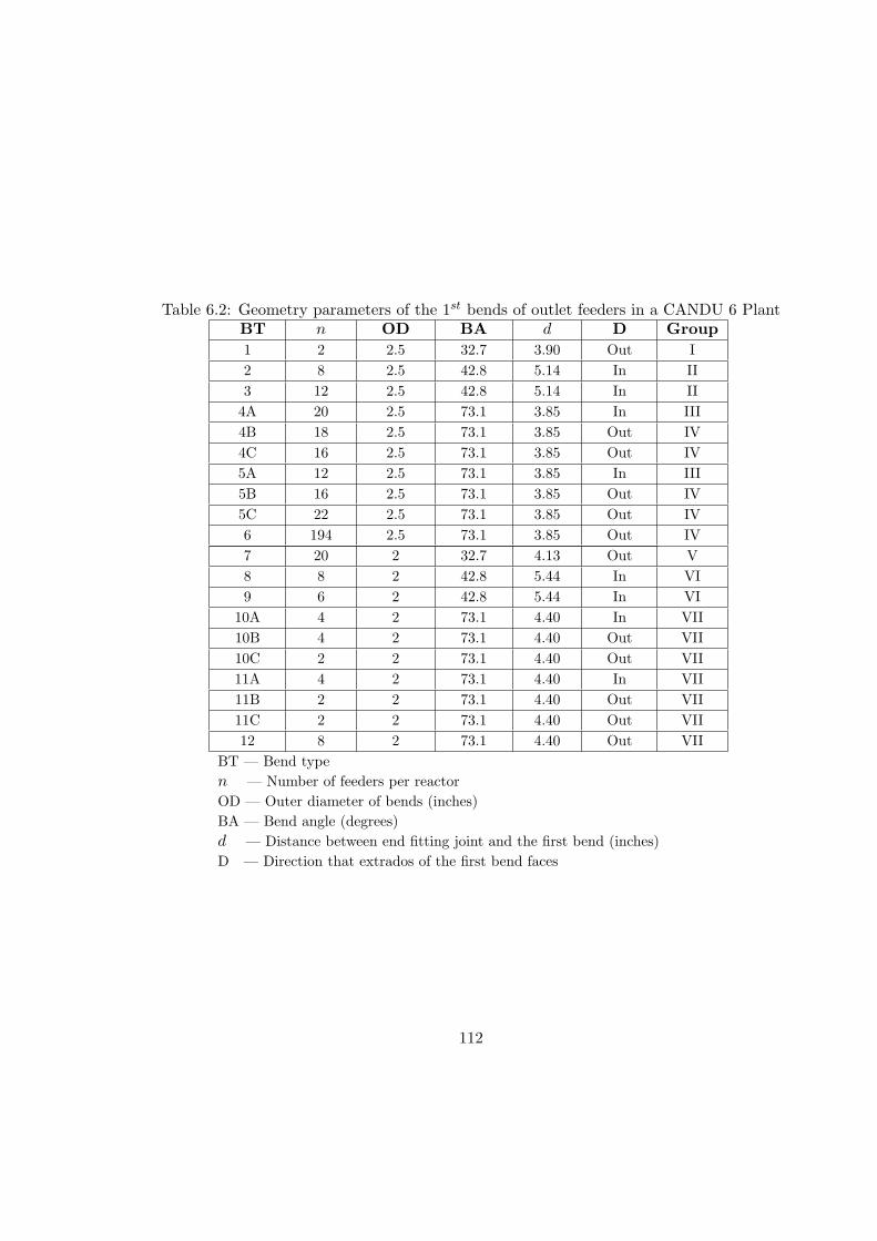
Table 6.2: Geometry parameters of the 1st bends of outlet feeders in a CANDU 6 PlantBT n OD BA d D Group1 2 2.5 32.7 3.90 Out I2 8 2.5 42.8 5.14 In II3 12 2.5 42.8 5.14 In II
4A 20 2.5 73.1 3.85 In III4B 18 2.5 73.1 3.85 Out IV4C 16 2.5 73.1 3.85 Out IV5A 12 2.5 73.1 3.85 In III5B 16 2.5 73.1 3.85 Out IV5C 22 2.5 73.1 3.85 Out IV6 194 2.5 73.1 3.85 Out IV7 20 2 32.7 4.13 Out V8 8 2 42.8 5.44 In VI9 6 2 42.8 5.44 In VI
10A 4 2 73.1 4.40 In VII10B 4 2 73.1 4.40 Out VII10C 2 2 73.1 4.40 Out VII11A 4 2 73.1 4.40 In VII11B 2 2 73.1 4.40 Out VII11C 2 2 73.1 4.40 Out VII12 8 2 73.1 4.40 Out VII
BT — Bend typen — Number of feeders per reactorOD — Outer diameter of bends (inches)BA — Bend angle (degrees)d — Distance between end fitting joint and the first bend (inches)D — Direction that extrados of the first bend faces
112
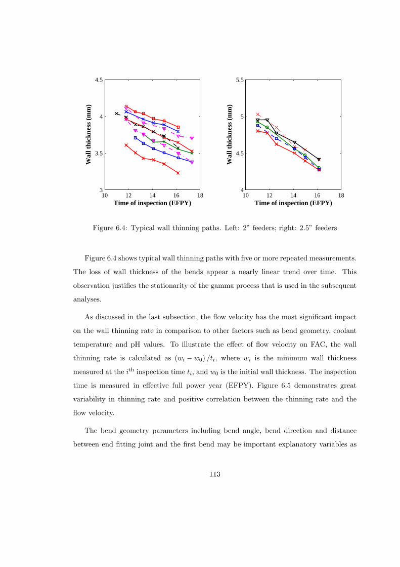
10 12 14 16 183
3.5
4
4.5
Time of inspection (EFPY)
Wal
l thi
ckne
ss (
mm
)
10 12 14 16 184
4.5
5
5.5
Time of inspection (EFPY)
Wal
l thi
ckne
ss (
mm
)Figure 6.4: Typical wall thinning paths. Left: 2” feeders; right: 2.5” feeders
Figure 6.4 shows typical wall thinning paths with five or more repeated measurements.
The loss of wall thickness of the bends appear a nearly linear trend over time. This
observation justifies the stationarity of the gamma process that is used in the subsequent
analyses.
As discussed in the last subsection, the flow velocity has the most significant impact
on the wall thinning rate in comparison to other factors such as bend geometry, coolant
temperature and pH values. To illustrate the effect of flow velocity on FAC, the wall
thinning rate is calculated as (wi − w0) /ti, where wi is the minimum wall thickness
measured at the ith inspection time ti, and w0 is the initial wall thickness. The inspection
time is measured in effective full power year (EFPY). Figure 6.5 demonstrates great
variability in thinning rate and positive correlation between the thinning rate and the
flow velocity.
The bend geometry parameters including bend angle, bend direction and distance
between end fitting joint and the first bend may be important explanatory variables as
113

6 8 10 12 140
20
40
60
80
100
120
140
Flow velocity (m/s)
Wal
l thi
nnin
g ra
te (µ
m)
R = 0.885V1.818
6 8 10 12 140
20
40
60
80
100
120
140
Flow velocity (m/s)
Wal
l thi
nnin
g ra
te (µ
m)
R = 0.696V1.888
Figure 6.5: Dependence of wall thinning rate on flow velocity. Left: 2” feeders; right:2.5” feeders
they affect the turbulence structure of the flow at the neighboring area of the bends and
thus change the wall thinning rate. According to Table 6.2, we can divide the 2.5” feeders
into four groups:
Group I including 2 Type 1 feeders,
Group II including 20 Type 2 and 3 feeders,
Group III including 32 Type 4A and 5A feeders, and
Group IV including 266 Type 4B, 4C, 5B, 5C and 6 feeders.
Similarly, the 2” feeders can be divided into three groups:
Group V including 20 Type 7 feeders,
Group VI including 14 Type 8 and 9 feeders, and
Group VII including 26 Type 10 (A, B, C), 11 (A, B, C) and 12 feeders.
114

Each group has the same geometry characteristics, except that in Group VII Type
10A and 11A bend into the reactor face whereas the other in the group bend outward.
Preliminary study indicated that the bend direction has no significant effect for the 2”
feeders, although it does for the 2.5” feeders.
Other FAC factors such as coolant temperature, pH value, metallurgical characteris-
tics are not considered because they are deemed to be the same for all feeders.
6.3 Gamma Process Model and Statistical Inference
6.3.1 Model Structures
The loss of feeder wall thickness due to FAC is a slow, incremental process of mass loss by
electrochemical and diffusion reactions, which can be modeled by a gamma process. Since
the mean thinning paths appear linear as shown in Figure 6.4, we propose a stationary
gamma process with shape parameter α and scale parameter β. To account for the
dependence of FAC rate on the flow velocity, the scale parameter is further modeled as a
power function as suggested from empirical studies mentioned in Section 6.1:
β = ηV δ. (6.3)
Furthermore, both corrosion theory and field experiences of plant engineers indicate
that there is an incubation period before any wall thinning can be observed. In other
words, the wall thinning due to FAC starts a few years after the system was put in service.
Thus it is reasonable to assume that the wall thickness keeps the initial value until some
time t0, the corrosion incubation period. Denote the wall thickness at time t by W (t), the
thickness loss by X (t), and its initial value by w0. Then the wall thickness is expressed
as
W (t) =
w0, 0 ≤ t ≤ t0
w0 −X (t; α, β) , t > t,(6.4)
115

in which X (t) is assumed as a stationary gamma process. In summary, the model consists
of four parameters: α (shape), η, δ (related to scale) and t0 (incubation time).
6.3.2 Parameter Estimation
Recall that increments of a stationary gamma process are independent and the gamma
distributed with probability density function as
g(∆x; α, β) =xα∆t−1
βα∆tΓ (α∆t)e−x/β. (6.5)
Given the inspection data we can estimate the process parameters by using the method
of maximum likelihood. Suppose we inspect a number n of components, each being
inspected at mi different points of time. Then we have the deterioration data in the form
of (wij , tij , Vi) (i = 1, . . . , n, j = 1, . . . , mi), in which wij stands for the wall thickness
at time tij and Vi for the flow velocity associated with the ith pipe. From (6.5) and the
independent-increments assumption of gamma process, the likelihood function for the ith
feeder with flow velocity Vi is expressed as
Li(α, η, δ, t0) =ni∏
j=1
(∆wij)α∆tij−1
βα∆tiji Γ (α∆tij)
e−∆wij/βi , (6.6)
in which ∆wj = wi(ti,j−1) − wi(tij), ∆tij = tij − ti,j−1, βi = ηV δi , wi(ti0) = w0 and
ti0 = t0. Then the complete log likelihood for is expressed as the following:
l(α, η, δ, t0) =n∑
i=1
mi∑
j=1
[(α∆tij − 1) ln∆wij − ln Γ(α∆tij)
− α∆tij(ln η + δ ln Vi)−∆wijV−δi /η. (6.7)
The parameters are estimated by maximizing the log likelihood function in (6.7). The
results from the maximum likelihood estimation are summarized in Table 6.3, in which the
116

Table 6.3: Maximum likelihood estimates and the score statistics for different groupsGroup η δ α t0 l U
II 0.0177 (0.0052) 1.6295 (0.3052) 4.7589 (1.4952) 6.0525 (1.0361) 18.75 0.05III 0.0158 (0.0038) 1.8334 (0.2224) 4.5921 (1.3484) 3.6872 (1.7469) 22.43 0.47IV 0.0106 (0.007) 1.5227 (0.0460) 6.6894 (0.4555) 1.3425 (0.2512) 365.17 1.70V 0.0125 (0.0033) 2.8550 (0.8817) 4.2826 (1.1297) 4.2974 (0.7840) 35.03 0.64VI 0.0152 (0.0043) 2.1462 (0.2397) 2.9809 (0.8321) 0.0000 (0.0031) 27.31 -0.52VII 0.0132 (0.0019) 1.6909 (0.1810) 4.9092 (0.6794) 0.5885 (0.5767) 159.82 0.94
Note: Since Group I has only 2 feeders, no meaningful statistical analysis can be done separately.It is pooled into Group V as they have the most similar geometry except OD.
m.l.e., standard errors, and the corresponding maximized log likelihoods are presented.
It is interesting to note that the estimated exponent of the flow velocity is about 1.75
whereas previous FAC studies on secondary side pipes suggested an exponent less than 1
(Burrill and Cheluget, 1999)
6.3.3 Model Checks
To check the fitness of the proposed gamma process model for the wall thickness data,
the scatter plots with predicted values and 95% confidence bounds are shown in Figure
6.6 to 6.11 for different groups. The gamma process model appears to fit the data fairly
well for all the groups.
Besides the qualitative model check, there are three hypotheses to be tested. First, as
we mentioned in Chapter 5, the heterogeneity in each group should be checked. Second,
we want to test whether a corrosion dormant period does exist, i.e., t0 = 0. Third,
we have modeled the effects for each group separately, that is, we used different sets of
parameters (α, β, η, t0) for different groups of feeders. In order to check the effects of
the size of OD and of the geometry configuration, we want to test whether two different
groups have the same.set of parameters. If they do, it means no significant effects on the
wall thinning. For the first hypothesis we use the score test whereas likelihood ratio tests
are used for the last two hypotheses.
117

10 11 12 13 14 15 16 17 1810
20
30
40
50
60
70
Time (EFPY)
Scal
ed m
easu
red
decr
emen
ts (
mm
)
measures
mean
95% bound
Figure 6.6: Measured versus fitted values with 95% bounds: Group II
10 11 12 13 14 15 16 17 1820
30
40
50
60
70
80
Time (EFPY)
Scal
ed m
easu
red
decr
emen
ts (
mm
)
measures
mean
95% bound
Figure 6.7: Measured versus fitted values with 95% bounds: Group III
118

10 11 12 13 14 15 16 17 1840
50
60
70
80
90
100
110
120
130
Time (EFPY)
Scal
ed m
easu
red
decr
emen
ts (
mm
)
measures
mean
95% bound
Figure 6.8: Measured versus fitted values with 95% bounds: Group IV
10 11 12 13 14 15 16 17 1810
20
30
40
50
60
70
Time (EFPY)
Scal
ed m
easu
red
decr
emen
ts (
mm
)
measures
mean
95% bound
Figure 6.9: Measured versus fitted values with 95% bounds: Group V
119

10 11 12 13 14 15 16 17 1820
25
30
35
40
45
50
55
60
65
Time (EFPY)
Scal
ed m
easu
red
decr
emen
ts (
mm
)
measures
mean
95% bound
Figure 6.10: Measured versus fitted values with 95% bounds: Group VI
10 11 12 13 14 15 16 17 1830
40
50
60
70
80
90
100
110
Time (EFPY)
Scal
ed m
easu
red
decr
emen
ts (
mm
)
measures
mean
95% bound
Figure 6.11: Measured versus fitted values with 95% bounds: Group VII
120

Table 6.4: Likelihood ratio tests for the corrosion incubation period t0Group t0 l η0 δ0 α0 l0 Λ p
II 6.0525 18.75 0.0269 1.6844 1.8256 13.52 10.5 0.0012III 3.6872 22.43 0.0169 1.8609 3.1305 21.20 2.46 0.1168IV 1.3425 365.2 0.0109 1.5345 5.8854 353.1 24.2 0V 4.2974 35.03 0.0181 2.6262 2.0547 28.32 13.4 0.0003VI 0.0000 27.31 0.0152 2.1462 2.9809 27.31 0 1VII 0.5885 159.8 0.0130 1.7035 4.8000 159.3 1.0 0.3173
Let us first look at the test of heterogeneity. For each group, we calculate the score
statistics U and they are listed in the last column of Table 6.3. It is clear no group
shows strong evidence against the null hypothesis which assumes homogeneity across the
feeders in the same group, except for Group IV for which U = 1.7, only a mild suggestion
of possible heterogeneity. Hence we keep the gamma process model and do not fit a
mixed-scale gamma process.
Table 6.4 lists the new maximum likelihood estimates for each group with t0 = 0.
The likelihood ratios Λ = 2 (l − l0) and the corresponding p-values are shown also in
the last two columns. Group II, IV and V have shown significant evidence against the
null hypothesis while the other three groups have not. Note that no significant evidence
against the null hypothesis is not equivalent to accepting the null hypothesis. We may
or may not accept the null hypothesis. We choose not to accept the null hypothesis here
just for model consistency purpose.
To check the effects of OD and of the geometry configuration, we notice that Group
III (Type 4A and 5A) and IV (Type 4B, 4C, 5B, 5C and 6) differ only by the direction
that extrados of the first bend faces (see Table 6.2). Both groups have 2.5” OD, the same
bend angle of 73.1o and the same distance between the end fitting joint and the first bend.
But Group III feeders bend into the reactor face and Group IV feeders bend outward.
If we treat the two groups as one and fit them with a gamma process model, we get
results shown in Table 6.5 with maximized log likelihood l = 360.3. The corresponding
likelihood ratio statistic Λ = 2× (22.43 + 365.17− 360.3) = 54.6. The degree of freedom
121

Table 6.5: Likelihood ratio test of effects of bend directionGroup η δ α t0 l Λ p
III 0.0158 1.8334 4.5921 3.6872 22.43IV 0.0106 1.5227 6.6894 1.3425 365.17
III+IV 0.0121 1.6347 5.7211 1.5006 360.3 54.6 ≈ 0VII-1 0.0129 1.7601 4.8551 0.1098 54.11VII-2 0.0132 1.6726 4.9612 0.7998 105.89VII 0.0132 1.6909 4.9092 0.5885 159.8 0.4 0.98
is (4 + 4)− 4 = 4. Therefore the p-value is 4× 10⁻¹¹ ≈ 0, a very significance level.
Similarly, Group VII includes Type 10A and 11A feeders that bend inward, and
other feeders that bend outward. We label Type 10A and 11A as Group VII-1 and the
other feeders in the group as Group VII-2. In this case, no significant improvement of
maximized log likelihood has been found. Hence we can treat them altogether.
Similar exercise can be done for Group II and Group VI, as the two groups differs
only by their outer diameters. The results are not shown here to save the space, but
the conclusion is that the OD has significant effects on the thinning behavior, at least in
terms of parameter estimation.
In summary, the model checks do not show obvious conflict against the assumptions
we made in Section 6.3.1 and therefore we use the results in Table 6.3 in the subsequent
analyses.
6.4 Prediction of the Lifetime and Remaining Lifetime
When the wall thickness of a feeder reduces to a certain threshold, the feeder is no longer
conformed to the standard requirements and becomes a substandard pipe even though
it may not break immediately. The time when the feeder reaches the threshold is then
called the lifetime of the feeder. Current industrial practice for thinning feeders defines
the substandard criteria based on the thinning region and extent and the remaining
122

wall thickness (Gerber et al. 1992; Deardorff et al. 1999; Hasegawa et al. 2004). For
illustration purpose, we consider only the remaining wall thickness as the criterion and
the substandard threshold, wth, is chosen as 60% of the nominal thickness, w0.
Due to the monotone nature of the sample path of the gamma process, the lifetime
of the feeder has a cumulative distribution function as
FT (t) = Pr {W (t) < wth} = Pr {X(t) > w0 − wth}
=
0, t ≤ t0
1−GA(0.4w0; η(t− t0), δ), t > t0(6.8)
in which wth = 0.6w0, δ = αV β, and α, β, η, t0 are the m.l.e. of the parameters, as
shown in Table 6.3.
Different feeders have different lifetime distributions, as their flow velocity and geom-
etry configuration differ. The probability density functions of lifetime of the feeders are
plotted in Figure 6.12. Each subpanel of the figures shows two density functions associ-
ated with maximum and minimum flow velocities of the group. For other feeders in the
group, depending on their flow velocity, the lifetime distribution should locate somewhere
between the two densities. Table 6.6 lists the maximum and minimum mean lifetimes of
each group and their corresponding standard deviations. Figure 6.13 demonstrates the
trend of the mean lifetime along the flow velocity. At the same flow velocity, feeders
in Group VII (or Type 10, 11 and 12) deteriorate faster than those in the other groups
and feeders in Group VI (Type 8 and 9) appear to deteriorate slowliest. At the same
flow velocity, the 2.5” feeders (Group II, III and IV) have very close values of lifetime.
In contrast, the lifetime of 2” feeders at the same flow velocity has large range across
different configurations of bend geometry.
The remaining lifetime, given that the remaining wall thickness of the feeder is known,
123

0 50 1000
0.05
0.1
0.15
0.2
0.25Pr
obab
ility
den
sity
fun
ctio
n
0 50 1000
0.05
0.1
0.15
0.2
0.25
0 50 1000
0.05
0.1
0.15
0.2
0.25
0 50 1000
0.05
0.1
0.15
0.2
0.25
Lifetime (EFPY)
Prob
abili
ty d
ensi
ty f
unct
ion
0 50 1000
0.05
0.1
0.15
0.2
0.25
Lifetime (EFPY)0 50 100
0
0.05
0.1
0.15
0.2
0.25
Lifetime (EFPY)
Group II Group III Group IV
Group V Group VI Group VII
Figure 6.12: Probability density functions of feeder lifetime due to FAC
Table 6.6: Maximum and minimum mean lifetimes and associated standard deviationsfor different groups
Group Minimum mean (st. dev.) Maximum mean (st. dev.)II 24.64 (2.40) 46.80 (3.55)III 25.80 (2.65) 52.91 (3.95)IV 21.23 (2.23) 69.20 (4.11)V 29.76 (2.91) 40.96 (3.49)VI 26.41 (3.38) 75.68 (5.74)VII 21.14 (2.50) 40.65 (3.49)
124
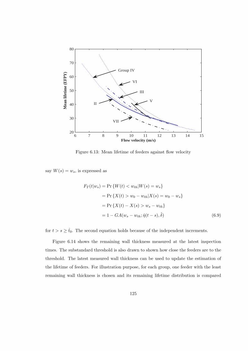
6 7 8 9 10 11 12 13 14 1520
30
40
50
60
70
80
Flow velocity (m/s)
Mea
n lif
etim
e (E
FPY
)
VI
V
III
VII
II
Group IV
Figure 6.13: Mean lifetime of feeders against flow velocity
say W (s) = ws, is expressed as
FT (t|ws) = Pr {W (t) < wth|W (s) = ws}
= Pr {X(t) > w0 − wth|X(s) = w0 − ws}
= Pr {X(t)−X(s) > ws − wth}
= 1−GA(ws − wth; η(t− s), δ) (6.9)
for t > s ≥ t0. The second equation holds because of the independent increments.
Figure 6.14 shows the remaining wall thickness measured at the latest inspection
times. The substandard threshold is also drawn to shown how close the feeders are to the
threshold. The latest measured wall thickness can be used to update the estimation of
the lifetime of feeders. For illustration purpose, for each group, one feeder with the least
remaining wall thickness is chosen and its remaining lifetime distribution is compared
125

10 12 14 16 18 202.5
3
3.5
4
4.5
5
5.5
Latest inspection time (EFPY)
Lat
est m
easu
red
wal
l thi
ckne
ss (
mm
)
10 12 14 16 18 203.5
4
4.5
5
5.5
6
6.5
Latest inspection time (EFPY)
Lat
est m
easu
red
wal
l thi
ckne
ss (
mm
)
w0
wth
w0
wth
Figure 6.14: The latest measured wall thickness. Left: 2” feeders; right: 2.5” feeders
with the original lifetime distribution, as shown in Figure 6.15 The updated lifetime
distributions have less standard deviation than the original ones. This is also true for
other feeders that are not displayed here, because the remaining thickness introduces new
useful information for the lifetime prediction. But the mean lifetime from the updated
distributions should not always be less than the original mean lifetime as shown in the
figure, because shown here are only those feeders with the least remaining thickness. For
the comparison of the mean lifetime of other feeders, see Figure 6.16. The updated values
are evenly scattered around the mean values predicted from the original distribution, as
witnessed by the variation of the latest measurements in Figure 6.14. The difference of
the predicted mean lifetimes based on the original and updated distribution can be as
large as 3 EFPYs.
126

10 20 30 400
0.1
0.2
0.3
Prob
abili
ty d
ensi
ty f
unct
ion
10 20 30 400
0.1
0.2
0.3
10 20 30 400
0.2
0.4
0.6
20 400
0.1
0.2
0.3
Lifetime (EFPY)
Prob
abili
ty d
ensi
ty f
unct
ion
20 400
0.1
0.2
0.3
Lifetime (EFPY)
10 20 300
0.2
0.4
0.6
Lifetime (EFPY)
Group II Group III Group IV
Group VIGroup V Group VII
Figure 6.15: Comparision of original (solid lines) and updated (dotted lines) lifetimedistributions of the feeders with the least remaining thickness
127

8 10 12 1420
30
40
50
Mea
n lif
etim
e (E
FPY
)
8 10 12 1420
30
40
50
60
5 10 15
20
30
40
50
60
70
9 10 11 1225
30
35
40
45
Flow velocity (m/s)
Mea
n lif
etim
e (E
FPY
)
6 8 10 12 1420
40
60
80
Flow velocity (m/s)8 10 12 14
15
20
25
30
35
40
45
Flow velocity (m/s)
Figure 6.16: Comparison of original (solid line) and updated (crosses) mean lifetimes offeeders
128
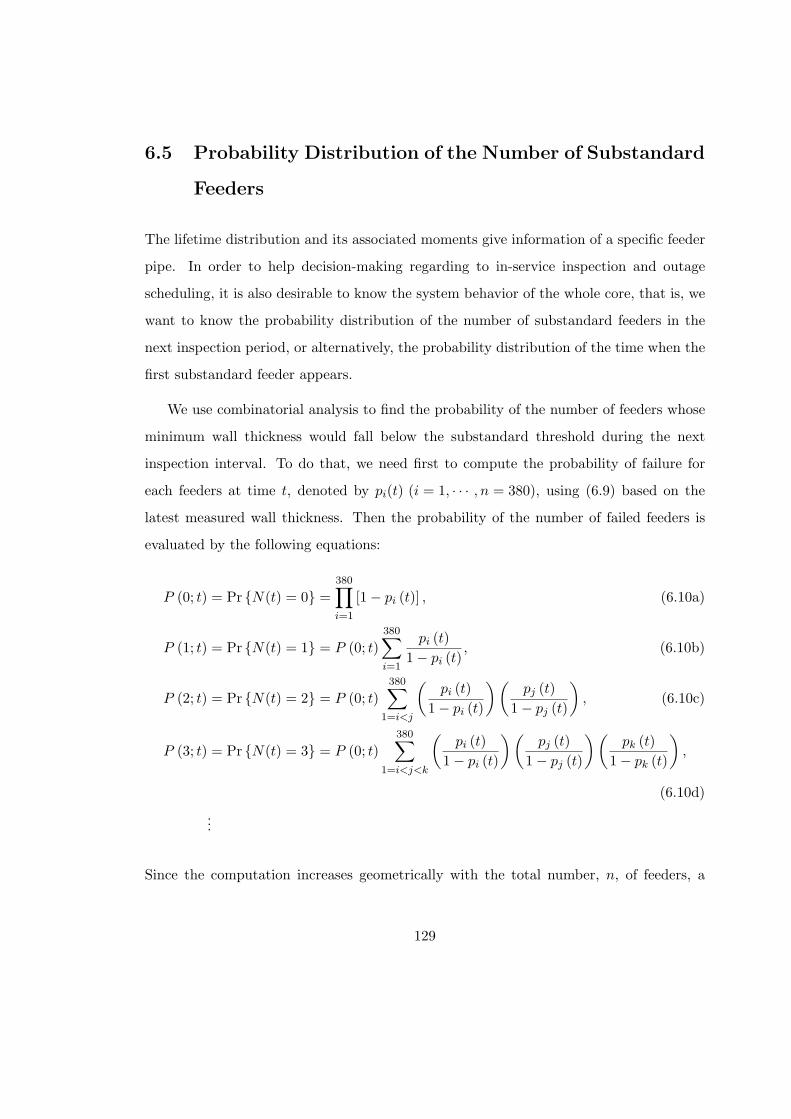
6.5 Probability Distribution of the Number of Substandard
Feeders
The lifetime distribution and its associated moments give information of a specific feeder
pipe. In order to help decision-making regarding to in-service inspection and outage
scheduling, it is also desirable to know the system behavior of the whole core, that is, we
want to know the probability distribution of the number of substandard feeders in the
next inspection period, or alternatively, the probability distribution of the time when the
first substandard feeder appears.
We use combinatorial analysis to find the probability of the number of feeders whose
minimum wall thickness would fall below the substandard threshold during the next
inspection interval. To do that, we need first to compute the probability of failure for
each feeders at time t, denoted by pi(t) (i = 1, · · · , n = 380), using (6.9) based on the
latest measured wall thickness. Then the probability of the number of failed feeders is
evaluated by the following equations:
P (0; t) = Pr {N(t) = 0} =380∏
i=1
[1− pi (t)] , (6.10a)
P (1; t) = Pr {N(t) = 1} = P (0; t)380∑
i=1
pi (t)1− pi (t)
, (6.10b)
P (2; t) = Pr {N(t) = 2} = P (0; t)380∑
1=i<j
(pi (t)
1− pi (t)
)(pj (t)
1− pj (t)
), (6.10c)
P (3; t) = Pr {N(t) = 3} = P (0; t)380∑
1=i<j<k
(pi (t)
1− pi (t)
)(pj (t)
1− pj (t)
)(pk (t)
1− pk (t)
),
(6.10d)
...
Since the computation increases geometrically with the total number, n, of feeders, a
129

Monte Carlo simulation algorithm is developed to carry out the combinatorial analysis.
For each time t, we first compute pi (t) for each feeder. Then generate n 0-1 random
variates, U1, U2, . . . , Un, where the Ui follows the following distribution: Pr (Ui = 0) =
pi (t) = 1−Pr (Ui = 1). The number of substandard feeders is just the number of zeros in
the generated variates. To get the probability distribution of N (t) = j, (j = 1, . . . , n), we
count the number of times when the number of substandard feeders equals j and divide
this number by the total number of simulations.
Instead of displaying individual probabilities, we plot histograms of the individual
failure probability at three different times in Figure 6.17 for sake of conciseness and clar-
ity. Figure 6.17 also compares the histograms from the original lifetime distributions and
from the updated distributions using the latest inspection information. At the time of 18
and 19 EFPY, the updated lifetime distributions predict no feeders of which the substan-
dard probability is greater than 0.02 while the original distributions predict several such
feeders. At 20 EFPY, however, the updated distributions can tell two feeders of which
the substandard probability has already reach over 0.5 whereas the original distributions
predict none of such feeders.
This trend is reflected in the plots of probability of the number of substandard feeders
in the whole reactor core, as shown in Figure 6.18: The original lifetime distributions
predict the probability of no substandard feeder at 18 EFPY is about 0.4 and drops below
0.1 one EFPY later. But the updated lifetime distributions predict the probability of no
substandard feeder is above 0.9 at 18 EFPY and just around 0.4 at 19 EFPY. As a result
of this difference, the system behavior differs significantly, as demonstrated in Figure
6.19. The original lifetime distributions predict the mean time to the first appearance
of a substandard feeder being 17.75 EFPY with standard deviation 0.61 EFPY and the
updated distributions predict the mean time of 18.85 EFPY and associated standard
deviation of 0.43 EFPY, again smaller than the previous standard deviation.
130

0 0.02 0.04 0.060
100
200
300
400
Freq
uenc
y
0 0.02 0.04 0.060
100
200
300
400
0 0.05 0.1 0.150
100
200
300
Freq
uenc
y
0 0.1 0.2 0.3 0.4 0.50
100
200
300
400
0 0.1 0.2 0.3 0.40
100
200
300
Probability of being substandard
Freq
uenc
y
0 0.2 0.4 0.6 0.8 10
100
200
300
400
Probability of being substandard
t = 18
t = 19
t = 20t = 20
t = 19
t = 18
Figure 6.17: Histograms of probability of feeders reaching substandard state based onoriginal (left panels) and on updated (right panels) lifetime distributions
131
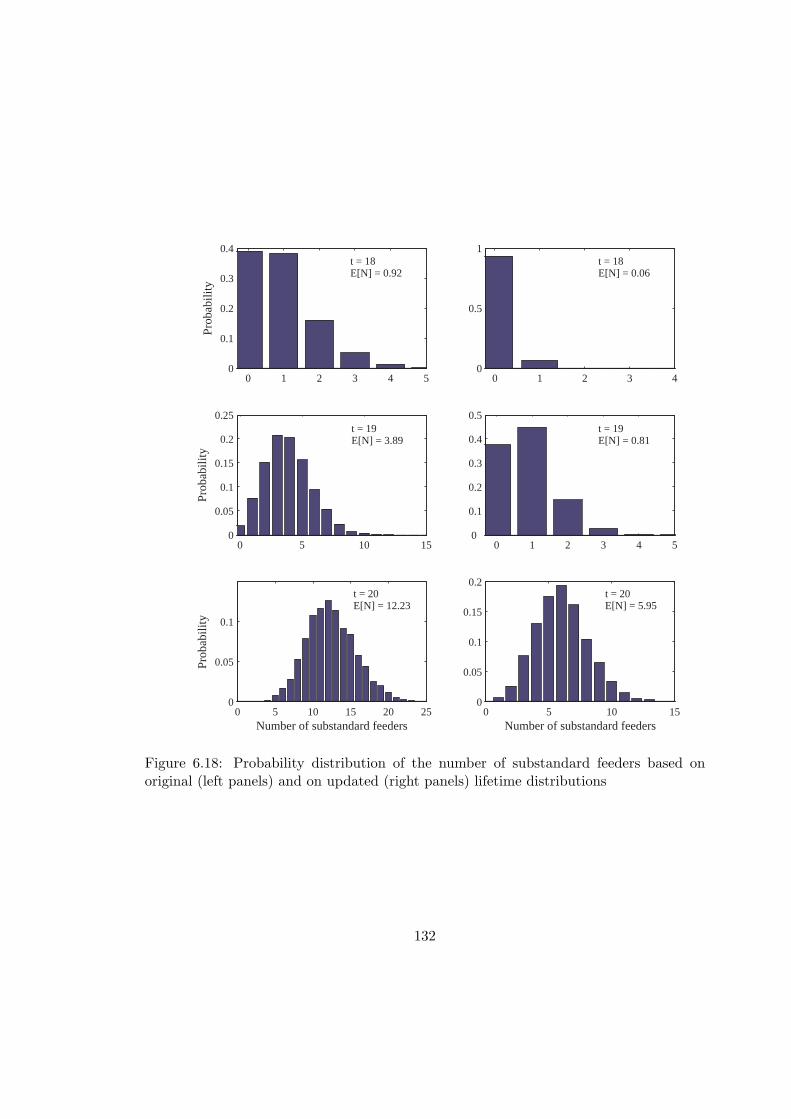
0 1 2 3 4 50
0.1
0.2
0.3
0.4
Prob
abili
ty
0 5 10 150
0.05
0.1
0.15
0.2
0.25
Prob
abili
ty
0 5 10 15 20 250
0.05
0.1
Number of substandard feeders
Prob
abili
ty
0 1 2 3 40
0.5
1
0 1 2 3 4 50
0.1
0.2
0.3
0.4
0.5
0 5 10 150
0.05
0.1
0.15
0.2
Number of substandard feeders
t = 18E[N] = 0.92
t = 18E[N] = 0.06
t = 19E[N] = 3.89
t = 19E[N] = 0.81
t = 20E[N] = 12.23
t = 20E[N] = 5.95
Figure 6.18: Probability distribution of the number of substandard feeders based onoriginal (left panels) and on updated (right panels) lifetime distributions
132

14 15 16 17 18 19 20 21 220
0.1
0.2
0.3
0.4
0.5
0.6
0.7
0.8
0.9
1
Time to first feeder reaching substandard threshold
Surv
ival
fun
ctio
n
OriginalUpdated
Figure 6.19: Survival functions of the time to the first appearance of a substandard feeder
6.6 Summary
Wall thinning due to the flow accelerated corrosion is a pervasive degradation in the
outlet feeder pipes of the CANDU nuclear power plants. This chapter undertakes a
comprehensive analysis of the wall thickness data from the outage inspections and fits
them with the gamma process model proposed in Chapter 4 and 5. Taking into account
the empirical knowledge of FAC, the model integrates both temporal variation and fixed
effects of flow velocity and of geometry configuration of the bends. The parameters are
estimated by using the maximum likelihood method and the model is carefully checked
using both qualitative and quantitative techniques.
Based on the stochastic thinning process, the lifetime of every feeder pipe is estimated.
The reliability of the feeder piping system is then computed by a combinatorial analysis,
which can be easily implemented by a simple Monte Carlo simulation. An advantage of
the gamma process model is that when new inspection data is available, the remaining
133

lifetime can be updated in a simple way. The value of inspection is seen from the change
of mean number of substandard feeders and the system survival curve.
134

Chapter 7
Effects of Temporal Uncertainty
in Planning Maintenance
7.1 Introduction
Maintenance decisions regarding the time and frequency of inspection, repair and re-
placement are complicated by temporal uncertainty associated with the deterioration of
systems. Although many stochastic models of deterioration with applications have been
reported (see Chapter 2), the impact of temporal uncertainty on maintenance optimiza-
tion problem has been lacking in the engineering literature. To address this issue, this
chapter chooses a random variable (RV) model as the benchmark and evaluates the ef-
fects of temporal uncertainty in planning maintenance through comparisons of optimized
maintenance strategies of a gamma process (GP) model and the RV model.
The chapter is organized as follows. First of all, the RV model is reviewed and basic
results about it are given for easy reference. Then the maintenance optimization problems
including both age-based replacement (ABR) and condition-based maintenance (CBM)
are formulated. For each policy, we use as a case study the diametral expansion data
135

of pressure tubes discussed in the earlier chapters to compare the two models. To get a
better insight into the effects of temporal uncertainty, a sensitivity analysis is carried out,
in which the deteriorate rate is assumed as a gamma random variable for the RV model
and the two models are calibrated in terms of the first two moments of lifetime. The two
versions of the deterioration models are then compared in terms of the life-cycle cost of
both ABR and CBM policies. The last section concludes the chapter with summaries.
7.2 Random Variable Model
The random variable model characterizes the randomness of deterioration by a finite-
dimension vector of random variables Θ as X (t; Θ). Consider here a simple random
deterioration rate model as
X (t) = At (7.1)
where A is the random deterioration rate that reflects the uncertain nature of deterioration
in a population of similar components. Given the probability distribution of the random
rate, FA(a), the probability distribution of the amount of the deterioration, X(t), is
derived as FX(t)(x) = FA(x/t). The mean, variance and coefficient of variation (COV) of
X(t) are expressed, respectively, as
µX(t) = µAt, σ2X(t) = σ2
At2 and νX(t) =σX(t)
µX(t)= νA. (7.2)
The lifetime, defined as the first passage time over a threshold ζ and denoted by T ,
has the probability distribution function as
FT (t) = Pr (T ≤ t) = Pr (At ≥ ζ) = 1− FA (ζ/t) . (7.3)
Depending on the distribution of A, the lifetime distribution can be derived analytically
or computed numerically.
136

7.3 Age-Based Replacement
Age-based replacement (ABR) is the simplest policy for the renewal of deteriorating fleets
of components. Under this policy, a component is replaced when it reaches a specific age
regardless of its condition. The specific age is called replacement age and denoted by ta.
The component is of course also replaced if failure occurs before the replacement age.
Denote by CF the total cost associated with all the consequences of a failure, and by
CP the cost of a preventive replacement. According to the renewal theory, the average
cost per unit time in long term, also known as the mean cost rate Ka, can be computed
as the ratio of mean cycle cost to mean cycle length. A renewal cycle refers to the period
from the instant when the unit is put in service to the instant when the unit is replaced
upon failure or upon the replacement age. Therefore the renewal cycle length, denoted
by L, has the probability distribution as
FL (s) = Pr {L ≤ s} =
FT (s) , for s < ta, or a premature failure
1, for s ≥ ta, or a preventive replacement,(7.4)
Since for a positive random variable with survival function G, its mean value equals∫∞0 G (s) ds, the mean cycle length is evaluated by E [L (ta)] =
∫ ta0 [1− FT (s)] ds. The
cycle cost is the cost incurs during a renewal cycle. This includes a possible failure cost CF
with FT (ta) as the probability of failure before ta and a possible preventive maintenance
cost CP with 1− FT (ta) as the probability of no failure by ta. Therefore the mean cycle
cost is E [C (ta)] = FT (ta) CF + [1− FT (ta)]CP . Hence the mean cost rate is expressed
as (Barlow and Proschan 1965):
Ka (ta) =FT (ta) CF + [1− FT (ta)]CP∫ ta
0 [1− FT (s)] ds. (7.5)
It is easy to check that Ka → CF /µT as ta → ∞, where µT is the mean lifetime. Using
(7.5), an optimal age of preventive replacement (ta) can be found that would minimize
137

the mean cost rate.
Since the calculation of the mean cost rate is sensitive to the lifetime distribution
FT (t), it would be of interest to examine the impact of RV and GP models on the
replacement policy. For an illustration, the ABR of pressure tubes due to irradiation
creep is discussed in the next.
7.3.1 Example: Age-Based Replacement of Pressure Tubes for Creep
Deformation
Section 3.4 and 5.6 fitted a linear mixed-effects (LME) model and a GP model, respec-
tively. In Section 3.4, the diametral strain due to creep expansion, is modeled by an LME
model: Y (t) = β0 + β1t + Θt + ε, where β0 = 0.0637 and β1 = 0.2077 are regression
constants and Θ is a normal random variable N(0, σ2
Θ
)with σΘ = 0.0232 to account for
the random effects. Note here t stands for the total fluence experienced on the pressure
tubes, which is the product of average flux and working time. Since ε represents measure-
ment error, the true deterioration X (t) is the remaining value of Y (t) without ε. That
is, X (t) = β0 +Bt where B ∼ N(β1, σ
2Θ
). β0 is a fixed number and can be absorbed into
the failure threshold ζ. So the LME model is in effect a RV model discussed in Section
7.2. The growth of the diametral strain is also modeled in Section 5.6 by a gamma process
with shape parameter 7.3462 and scale parameter 0.0291.
Let again the substandard threshold ζ = 5.1. The lifetime distributions in Figure 5.7
are used for finding the optimal ABR policy. Recall that these two lifetime distributions
correspond to a typical pressure tube with average flux 2.4×10¹⁷ n/(m2·s). The coefficient
of variation of the lifetime is around 0.1 in the RV model whereas it is 0.08 in the GP
model.
Suppose CP = 10 and CF = 50. The mean cost rates for the RV and GP model
are plotted against the replacement age in Figure 7.1. Interestingly, although the limited
mean cost rate in the GP model is less than that in the RV model, the minimal mean
138

10 15 20 25 30 35 40 45 500
0.2
0.4
0.6
0.8
1
1.2
1.4
1.6
1.8
2
RV: (25.3, 0.409)
GP: (26.0, 0.397)
Replacement age (EFPY)
Mea
n co
st r
ate
RVGP
Figure 7.1: Optimal age-based replacement policies for a pressure tube due to diametralexpansion
cost in the GP model is higher than the minimal value in the RV model. Nevertheless,
the difference of the ABR policies from the two models is slight.
7.4 Condition-Based Maintenance
The deterioration along a specific sample path is deterministic in the RV model, whereas
it varies probabilistically in the GP model. In the linear RV model, one inspection
determines the deterioration rate and it fixes the future deterioration path. An inspection
in GP model, however, reveals only the current state of deterioration from which we
can infer only the probability distribution of future deterioration. This distinction has
profound implications to the optimization of condition-based maintenance strategies.
139

7.4.1 The Strategies
The condition-based maintenance (CBM) strategy involves the periodic inspection of a
deteriorating component at a fixed time interval tI and cost CI . We assume that the
inspection is accurate such that the deterioration X(t) can be measured with negligible
error. The threshold for the preventive maintenance (PM), ζP = cζ (0 < c < 1) is a
fraction of the failure threshold. c is called PM ratio. The PM results in a complete
renewal (as good as new) of the component. If X(tI) < cζ, no action is taken until the
next inspection. A component is renewed with PM cost CP when cζ ≤ X (tI) < ζ. If
the structure fails between two successive inspections, i.e., X (t) ≥ ζ, failure is detected
immediately and a corrective maintenance (CM) would renew the structure immediately,
incurring a total failure cost, CF . Typically PM cost is much lower than the failure cost,
i.e., CP < CF .
The optimization of the condition-based maintenance means finding the inspection
interval (tI) and the PM ratio (c) that would minimize the long-run mean cost rate. This
in principle involves a two-dimensional optimization problem. When, however, the PM
threshold cζ is known from experience or prescribed by industry standards or regulations,
the inspection interval is the only optimization variable.
7.4.2 Formulation for Random Variable Model
For the RV model, the three possibilities that arise at the time of first inspection (tI) are:
do nothing, PM or CM followed by a failure, as shown in the decision tree in Figure 7.2.
When X (tI) < cζ, no action is taken, but the time of preventive maintenance in future
can be predicted as tPM = cζtI/X (tI), since one inspection is sufficient to determine the
linear sample path. The other two situations are straightforward. The PM is immediately
conducted when cζ < X (tI) < ζ, and it is correctively replaced when X (tI) > ζ.
The most important point is that under the assumption of the linear RV deterioration
140

Start Inspection
Failed & CM
Immediate PM
Delayed PM
TimetI
X(t)
tF
Failure threshold
PM level
tPM
(C = CI + CP, L = tI)
(C = CI + CP, L = tPM)
(C = CF, 0 < L < tI)X(tI) >
c
X(tI) > c
c < X(tI) <
Figure 7.2: CBM decision tree for the RV model
141

model, only one inspection is required for the implementation of CBM strategy. In
a general RV model with n random variables, only n inspections are required for the
implementation of CBM.
From the decision tree and associated costs shown in Figure 7.2, the mean value of
renewal cycle cost (C) is simply evaluated as
E [C (tI , c)] = (CI + CP ) Pr {X (tI) ≤ ζ}+ CF Pr {X (tI) > ζ}
= (CI + CP − CF ) FA (ζ/tI) + CF . (7.6)
Similarly, we have the mean cycle length is evaluated as
E [L (tI , c)] =∫ tI
0Pr {X (t) < ζ} dt +
∫ ∞
tI
Pr {X (t) < cζ} dt
=∫ tI
0FA (ζ/t) dt +
∫ ∞
tI
FA (cζ/t) dt. (7.7)
Equations (7.6) and (7.7) can be easily evaluated given the parameter of the distribu-
tion of the deterioration rate. According to renewal theory, the mean cost rate is given
as
Ki (tI , c) =E [C (tI , c)]E [L (tI , c)]
. (7.8)
As tI → 0, the mean cycle cost approach to CI + CP and the mean cycle length ap-
proaches the mean time to the PM threshold that equals to∫∞0 F (cζ/t) dt. As tI →∞,
the mean cycle cost approaches to CF and the CBM policy becomes equivalent to the cor-
rective replacement policy. When c = 1, the mean cycle length equals the mean lifetime
irrespective of the inspection interval.
The cumulative probability of failure up to time is simple to obtain as
Pf (t) = Pr {X (t) > ζ} =
1− FA (ζ; t) , 0 ≤ t < tI
0, t ≥ tI(7.9)
142

Note that Pf (t) becomes zero for t > tI , because one inspection reveals the actual sample
value of the deterioration rate and removes the uncertainty about the time of failure after
the first inspection.
7.4.3 Formulation for Gamma Process Model
The inspection and replacement scenarios in the GP model are more involved due to
temporal uncertainty. The three possible situations arise at every inspection, namely,
safe state and do nothing, PM, or failure and subsequent corrective maintenance, as
shown in Figure 7.3.
According to the decision tree, a PM renewal happens at L = ntI when Xn−1 < cζ
and cζ < Xn < ζ, where Xn = X (ntI) with PM cost nCI + CP . When Xn−1 < cζ but
Xn > ζ, a CM renewal is called for with cost (n− 1)CI + CF for n ≥ 2 and CF for
n = 1. In this case, the renewal is done at a point of time interval from (n− 1) tI to ntI .
Accordingly, the mean cost associated with a renewal cycle is derived as
E [C (tI , c)] =∞∑
n=1
[(nCI + CP ) Pm (n) + ((n− 1)CI + CF ) Pf (n)] (7.10)
where
Pm (n) = Pr {PM at ntI} = Pr {Xn−1 < cζ, cζ < Xn < ζ} (7.11)
and
Pf (n) = Pr {Failed in ((n− 1) tI , ntI ]} = Pr {Xn−1 < cζ, Xn > ζ} . (7.12)
From the property of independent increments of gamma process, we have, for n ≥ 2,
Pm (n) = Pr {Xn−1 < cζ, cζ −Xn−1 < Xn −Xn−1 < ζ −Xn−1}
=∫ cζ
0gan−1 (x) [GA1 (ζ − x)−GA1 (cζ − x)] dx, (7.13)
143

Start Inspection
Failed & CM
Immediate PM
Failed & CM
Immediate PM
Inspection Inspection
c
TimetI
X(t)
tF
Failure threshold
PM level
2tI
c < X(tI) <
X(tI) < c
X(tI) >
X(2tI) >
X(2tI) < c
c < X(2tI) <
(C = CF
0 < L < tI )
(C = CI + CF,
tI < L < 2tI )
(C = CF
L = tI )
(C = 2CI + CP,
L = 2tI )
Figure 7.3: CBM decision tree for the GP model
144

in which gan (·) and GAn (·) denotes the pdf and CDF of a gamma distribution Ga (nαtI , β),
respectively. It is clear that Pm (1) = GA1 (ζ)−GA1 (cζ). Similarly,
Pf (n) = Pr {Xn−1 < cζ, Xn −Xn−1 > ζ −Xn−1}
=∫ cζ
0gan−1 (x) [1−GA1 (ζ − x)] dx (7.14)
for n = 2, 3, . . ., and Pf (1) = 1 − GA1 (ζ). Substituting these probabilities into (7.10)
and simplifying them, we have
E [C (tI , c)] = CP + (CF − CI) [1 + S (cζ)]
− (CF − CI − CP )[GA1 (ζ) +
∫ cζ
0s (x) GA1 (ζ − x) dx
](7.15)
where S (x) =∑∞
n=1 GAn (x) and s (x) =∑∞
n=1 gan (x).
The mean cycle length can be obtained as
E [L (tI , c)] =∞∑
n=1
[ntIPm (n) + En (TF )] (7.16)
where En (TF ) represents the mean failure time between (n− 1) tI and ntI and is ex-
pressed as
En (TF ) =∫ cζ
0gan−1 (x)
∫ tI
0[(n− 1) tI + s] fT (s; ζ − x) dsdx, (7.17)
in which fT (s; ζ − x) is the pdf of the first passage time of the gamma process with a
threshold ζ − x. Using integration by parts and rearranging all the terms, we obtain
E [L (tI , c)] =∫ tI
0GA (ζ; αt, β) dt +
∫ cζ
0
∫ tI
0s (x) GA (ζ − x; αt, β) dtdx (7.18)
where GA (x; a, b) denotes the CDF of the gamma distribution with shape a and scale b.
Equations (7.15) and (7.18) are derived by Park (1988a, 1988b). An alternative
145

way to compute the mean cycle cost and the mean cycle length is by using the Poisson
approximation for the lifetime distribution of the gamma process, as suggested by van
Noortwijk et al. (1995). When the inspection interval is n times of the reciprocal of
the shape parameter α, the Poisson approximation gives an exact solution to the mean
cycle cost. But this approach gives only an approximation to the mean cycle length and
therefore it is not used in the subsequent computations.
There are two limiting cases of the CBM policy. As the inspection interval tI becomes
large, the mean cost rate tends to CF /µT where µT is the mean lifetime. As the PM
ratio c → 1, tI converges to the optimal replacement interval obtained from the age-based
replacement policy.
The probability of failure over time within any inspection interval is given by the
following expression:
Pf (t) = Pr {X (t) ≥ ζ, X ((n− 1) tI) < cζ} , for (n− 1) tI ≤ t < ntI . (7.19)
In particular, for n = 1, i.e., the first inspection interval,
Pf (t) = 1−GA (ζ; αt, β) (7.20)
and for n ≥ 2,
Pf (t) =∫ cζ
0gan−1 (x) {1−GA (ζ − x; α [t− (n− 1) tI ] , β)} dx. (7.21)
Note that the probability of failure at the time of inspection reduces to zero, since the
inspection is perfect in the sense that it reveals the actual situation without any uncer-
tainty.
For a GP model dealing with imperfect inspection, we refer to Kallen and van Noortwijk
(2005). More recently, Crowder and Lawless (2007) discussed a simplified CBM policy
for a mixed-scale gamma process model.
146

0 5 10 15 20 25 30 35 40 45 500.4
0.6
0.8
1
1.2
1.4
1.6
1.8
2
2.2
2.4
Inspection interval (EFPY)
Mea
n co
st r
ate
(1, 0.5557)
(5, 0.7585)
RV
GP
Figure 7.4: Comparison of condition-based maintenance policy based on different deteri-oration models for a pressure tube due to diametral expansion
7.4.4 Example: Condition-Based Maintenance of Pressure Tubes for
Creep Deformation
The diametral expansion data are used again for illustration purpose. Suppose CI = 1,
CP = 10 and CF = 50. Figure 7.4 shows the mean cost rate versus the inspection interval
for the RV and GP model. The minimal mean cost rate for the GP model is greater than
that for the RV model, as the GP model takes into consideration the temporal uncertainty
even though it predicts the same mean value and smaller variance of lifetime. Figure 7.5
and 7.6 show the cost decomposition for the RV and GP model, respectively.
At the optimal inspection interval of 5 EFPY, the probability of the pressure tube
reaching substandard performance (i.e. the diametral strain exceeding 5.1%) has been
controlled within 0.08, as illustrated in Figure 7.7. This shows the indirect benefit of the
inspection and preventive maintenance.
147

0 5 10 15 20 25 30 35 40 45 500
0.5
1
1.5
2
2.5
Inspection Interval
Mea
n C
ost
Rat
e
Insp
PM
Fail
Total
Figure 7.5: Decomposition of mean cost rate for the RV model
0 5 10 15 20 25 30 35 40 45 50−0.5
0
0.5
1
1.5
2
2.5
Inspection Interval
Mea
n C
ost
Rat
e
Insp
PM
Fail
Total
Figure 7.6: Decomposition of mean cost rate for the GP model
148

0 5 10 15 20 25 30 35 40 45 50
0.01
0.02
0.03
0.04
0.05
0.06
0.07
0.08
Age of the pressure tube (EFPY)
Pro
babi
lity
of s
ubst
anda
rd
Figure 7.7: Probability of the pressure tube being substandard over time under theoptimal CBM policy based on the GP model
7.5 Sensitivity Analysis
The case studies of pressure tubes in the previous examples give interesting but never-
theless very limited comparisons of the RV and GP models in maintenance optimization.
To get a better insight, we proceed next with a comprehensive sensitivity analysis for
the two deterioration models, considering different degree of variation of deterioration.
In this analysis, the variation of deterioration is described by the coefficient of variation
(COV) of the lifetime. By fixing the mean lifetime and varying the lifetime COV, we
compares the impacts of temporal uncertainty in both ABR and CBM policies.
In order to have a consistent comparison between the RV and GP models, a careful
scheme is required for the calibration of the model parameters. In this study, we assume
the mean and COV of the lifetime are given. Calibration of the models is based on the
two moments of the lifetime.
149

7.5.1 Calibration of the Models
Suppose the deterioration rate A in the RV model is a gamma distributed random variable
with shape parameter η and scale parameter δ, i.e., A ∼ Ga (η, δ). Then the deterioration
at any time t also follows a gamma distribution Ga (η, δt). The lifetime T , defined as
T = ζ/A, however follows an inverted gamma distribution. Its pdf is expressed
fT (t) =(δ/ζ)Γ (η)
(ζ
δt
)η+1
exp(− ζ
δt
)(7.22)
and the CDF as
FT (t) = 1−GA (ζ/t; η, δ) = 1−GA (ζ; η, δt) (7.23)
The moments of the lifetime distribution can be derived as
µT =ζ
δ (η − 1), σ2
T =ζ2
δ2 (η − 1)2 (η − 2)and νT =
1√η − 2
(7.24)
for η > 2. Therefore, given the values of µT and νT , the parameters of deterioration rate
A can be easily calculated by the following expressions:
η = 2 + 1/ν2T and δ =
ζν2T
µT
(1 + ν2
T
) . (7.25)
Recall that the CDF of the lifetime in a GP model with shape parameter α and scale
parameter β is expressed as the following:
FT (t) = 1−GA (ζ; αt, β) (7.26)
Although (7.26) differs from (7.23) only at whether the time t is associated with the shape
parameter or scale parameter in the gamma distribution, the lifetime in the GP model
has no explicit expression for its moments. Therefore in the case of GP model, given µT
and νT , the shape and scale parameters can be only obtained by numerically solving the
150

Table 7.1: Parameters used in the model calibrationMean lifetime µT COV of lifetime νT Failure threshold ζ
50 units of time (fixed) Varied from 0.1 to 0.9 100 units of deterioration (fixed)
Table 7.2: Example parameters in the RV and GP modelsParameters νT = 0.3 νT = 0.6 νT = 0.9RV model Shape (η) 13.1111 4.7778 3.2346
Scale (δ) 0.1651 0.5294 0.8950GP model Shape (α) 0.2099 0.0408 0.0078
Scale (β) 10.01 64.63 1453.6
following equations of the first and second moments (c.f. (4.14)):
µT =∫ ∞
0GA (ζ; αt, β) dt (7.27a)
µT 2 = µ2T
(1 + ν2
T
)= 2
∫ ∞
0tGA (ζ; αt, β) dt (7.27b)
The parameters of the two models are given in Tables 7.1 and 7.2. The two models
are equivalent in the sense that they have identical mean and variance of the lifetime.
7.5.2 Age-Based Replacement
Although the RV and GP models are calibrated so that they have the same mean and
variance of the lifetime, the lifetime distributions in the two models are nevertheless
different. As an example, Figure 7.8 compares the probability density functions and
survival functions for νT = 0.3. The survival function shows that the tails of the lifetime
distribution in the RV and GP models can be remarkably different and the RV model
overestimates the reliability of the component.
A comprehensive comparison of ABR results about the minimum cost rate and optimal
replacement age for different coefficients of variation of lifetime, νT , in the RV and GP
models are shown in Figure 7.9. CP = 10 and CF = 50 are assumed in the analysis.
The results of optimal replacement age obtained from the two models are qualitatively
151

0 50 100 150 2000
0.01
0.02
0.03
0.04
Lifetime
Pro
ba
bili
ty D
en
sity
0 50 100 150 20010
−12
10−8
10−4
100
Lifetime
Su
rviv
al F
un
ctio
nRV
RV
GP
GP
(a) (b)
Me
an
Life
time
Figure 7.8: Comparison of lifetime distributions of the equivalent RV and GP models forνT = 0.3: (a) probability density function, and (b) survival function
different. In the RV model, the optimal replacement age decreases continuously as the
lifetime COV νT increases. This observation is somewhat intuitive in the sense that when
faced with increased uncertainty about lifetime, it is prudent to reduce the replacement
age. The results of GP model exhibit two distinct trends. Initially, with increase in
lifetime COV the replacement age decreases. However, as νT increases beyond 0.5, the
trend reverses and the replacement age begins to increase. It suggests that in case of
highly uncertain lifetime, the life-cycle cost could not be optimized by manipulating
the replacement age. Note that a similar reasoning can be applied for an exponentially
distributed lifetime – having a constant failure rate and a COV of 1 – for which it is
optimal to never schedule a preventive replacement (Barlow and Proschan 1965).
Figure 7.9(b) shows that mean cost rate obtained from GP model is always higher
than that of the RV model as a result of additional temporal uncertainty associated with
it. The difference between the optimum cost rates increases with increase in lifetime
uncertainty. This explains the very small difference of the ABR in Figure 7.1 because
relatively small variation exhibits in the growth of diametral strain.
152

0 0.2 0.4 0.6 0.8 110
20
30
40
50
60
70
COV of lifetime
Opt
imal
rep
lace
men
t age
GP
RV
0 0.2 0.4 0.6 0.8 10.2
0.3
0.4
0.5
0.6
0.7
0.8
0.9
1
COV of lifetime
Min
imal
mea
n co
st r
ate
GP
RV(a) (b)
Figure 7.9: Comparison of age-based replacement policies in equivalent RV and GPmdoels: (a) optimal replacement age, and (b) minimal mean cost rate
7.5.3 Condition-Based Maintenance
Assume CI = 1, CP = 10 and CF = 50. The optimization results of CBM for RV and
GP models for different values of the lifetime COV are compared in Figure 7.10. It is
remarkable that in the RV model both the optimum cost rate and inspection interval
are insensitive to the variability of the lifetime distribution, which is due to the lack of
consideration of temporal uncertainty. In contrast, the minimum cost rate in the GP
model increases with lifetime uncertainty. The cost rate increases from 0.38 to 0.97 as
the COV of lifetime is increased from 0.1 to 0.8. In general, the GP cost rate is higher
than that for the RV model due to the effect of temporal uncertainty.
7.5.4 Comparison of Age-Based and Condition-Based Policies
Although the CBM policy is generally considered as a more advanced approach to the
life-cycle management, an age-based strategy is easier to implement than the condition-
based one after all. In light of this, we would like to compare the cost rates of ABR and
CBM policies. In this Section, the results are presented for the GP model only because
153

0 0.2 0.4 0.6 0.8 10
5
10
15
20
25
30
COV of lifetime
Opt
imal
insp
ectio
n in
terv
al
0 0.2 0.4 0.6 0.8 10.2
0.3
0.4
0.5
0.6
0.7
0.8
0.9
1
COV of lifetime
Opt
imal
mea
n co
st r
ate
GP
RV
GP
RV
(a) (b)
Figure 7.10: Comparison of CBM results for equivalent RV and GP models: (a) optimalinspection interval, and (b) minimal mean cost rate
we have concluded that the RV model is too unrealistic for a CBM policy.
The results for minimum mean cost rate shown in Figures 7.9(b) and 7.10(b) are
plotted together in Figure 7.11. It is remarkable that the cost rate of CBM is higher
than age-based replacement policy, especially when the lifetime COV is relatively small
(νT < 0.5).
Although the above comparison is dependent on the specific cost structure (CI = 1,
CP = 10 and CF = 50), it is clear that CBM is not universally superior to the age-based
policy. In fact, an optimum domain of application of CBM policy in terms of the lifetime
COV and costs can be explicitly derived to develop the life-cycle management strategies.
We next illustrate this point in details.
Two-Dimensional CBM Optimization
It has been argued that the one-dimensional optimization of inspection interval leads
to suboptimal results (Grall et al. 2002; Jia and Christer 2002; Dieulle et al. 2003).
The mean cost rate can be further optimized by allowing the PM ratio, c, be another
154

0 0.1 0.2 0.3 0.4 0.5 0.6 0.7 0.8 0.9 10.2
0.3
0.4
0.5
0.6
0.7
0.8
0.9
1
COV of lifetime
Opt
imal
mea
n co
st r
ate
GP−CBM
GP−ABR
Figure 7.11: Comparison of the CBM policies with the ABR in the GP model
optimization variable. This leads to a two-dimension (2D) CBM optimization.
Taking νT = 0.3 for an example, the surface of minimum cost rate for various combi-
nations of inspection interval (tI) and PM ratio is plotted in Figure 7.12. On this surface,
the optimal point corresponds to tI = 13, c = 0.54 and the associated minimum mean
cost rate is 0.44. This cost rate is much less than that obtained from either the corre-
sponding one-dimensional CBM optimization (0.54 at tI = 7 and c = 0.8) or the ABR
policy (0.45 at tI = 29 and c = 1).
Now, a more fair comparison of ABR and CBM can be taken. Figure 7.13 compares
the minimal mean cost rate from the 2D CBM optimization with that of the ABR policy.
It shows that an age-based policy is better than CBM when νT < 0.25. In other words,
the benefit of a condition-based policy gained from the value of deterioration information
through inspection outweighs the cost of inspection only when the uncertainty associated
with deterioration is large (νT > 0.25). Given a fixed νT , the CBM policy is preferable
only if the inspection cost is below a certain value. This motivates us to find out the
155

010
2030
40
00.2
0.40.6
0.810
0.5
1
1.5
Inspection IntervalPM Ratio
Mea
n C
ost R
ate
(13, 0.54, 0.44)
Figure 7.12: A two-dimensional CBM optimization for the GP model (νT = 0.3)
maximum allowable inspection cost to justify the CBM policy. This threshold value
of inspection cost provides an answer to a question such as, how much money can be
justifiably spent for inspections given the probabilistic characteristics of a deterioration
process. For example, Figure 7.13 shows that maximum allowable inspection cost is 1
(20% of the PM cost) when νT = 0.25 and CP /CF = 5/50 = 10%. Next we investigate
the maximum allowable inspection cost for more general cases.
Maximum Allowable Inspection Cost to Justify the CBM Policy
By definition, the maximum allowable inspection cost can be calculated from the following
equality:
Ka (ta,opt; νT , CP , CF ) = Ki (ta,opt, copt; νT , CI , CP , CF ) (7.28)
where Ka and Ki are the optimal cost rates for the ABR policy and two-dimensional
CBM polices that are calculated from (7.5) and from (7.15) and (7.18), respectively. The
156

0 0.1 0.2 0.3 0.4 0.5 0.6 0.7 0.8 0.9 10.2
0.3
0.4
0.5
0.6
0.7
0.8
0.9
1
COV of lifetime
Opt
imal
mea
n co
st r
ate
GP−CBM
GP−ABR
Figure 7.13: Comparison of two-dimensional CBM policies with ABR policies
maximum allowable inspection cost is obtained by solving (7.28) with fixed and while
ta,opt, tI,opt and copt are the optimization results depending on CI .
In Figure 7.14, the optimal inspection cost is expressed as a percentage of the PM
cost. The increasing trend shows that the higher inspection cost is justified with increase
in uncertainty associated with the lifetime distribution and the deterioration process.
On the other hand, inspection cost proportionately decreases with increasing PM cost,
though the cost still increases in an absolute sense. The optimal inspection cost curves
provide guidance about the optimal cost structure of a maintenance program.
7.6 Summary
The chapter emphasizes an important fact that the random variable rate (RV) model
cannot capture temporal variability associated with evolution of deterioration. As a con-
sequence, the deterioration along a specific sample path is deterministic in the RV model,
157

0 0.1 0.2 0.3 0.4 0.5 0.6 0.7 0.8 0.9 10
5
10
15
20
25
30
35
40
COV of lifetime
Cri
tical
insp
ectio
n co
st (
% o
f C
P)
CP/C
F = 10%
= 20%
= 40%
Figure 7.14: Maximum allowable inspection cost with COV of lifetime and PM to CMcost ratio
whereas it varies probabilistically in the GP model. This distinction has profound impli-
cations to the maintenance optimization of both age-based and condition-based strategies.
The results presented in the chapter show that the optimum cost and inspection
interval obtained from the GP model are qualitatively different than those obtained from
the RV model. The RV model tends to underestimate the life-cycle cost due to lack of
consideration of temporal uncertainty.
The age-based replacement policy is easier to implement than the condition-based
maintenance. The chapter determines a domain of inspection, preventive maintenance
and corrective costs in which the condition-based policy is always superior to the age-
based policy. A general observation is that condition-based maintenance strategy is justi-
fied when the uncertainty associated with deterioration is large. In other words, under a
given cost structure the tradeoff between the cost of inspection and value of information
gained is beneficial only when the uncertainty of deterioration exceeds a critical limit.
158

Chapter 8
Conclusions and
Recommendations
8.1 Conclusions
The thesis presents a versatile stochastic gamma process model for modeling deterioration
in engineering systems, structures and components. Questions relevant to stochastic
modeling of deterioration, such as why and which stochastic process model should be used
and how to calibrate and validate the model using practical data, have been addressed.
Detailed practical applications of the proposed models to feeder pipe systems and fuel
channels in CANDU reactors are presented. The thesis also formulated the maintenance
optimization problems for both age-based replacement and condition-based maintenance
strategies.
Traditional regression models consist of a parameterized mean function and an error
term that quantifies the deviation of the observations from the mean function. The errors
are usually assumed independent of each other. Under this assumption data analysis
and modeling of deterioration becomes a straightforward task, though it confounds the
159

estimation of the lifetime distribution. The thesis proposes a linear mixed-effects model
to resolve the inconsistency of interpretation associated with ordinary regression model.
By introducing the random effects into the model, the varying variance of deterioration
and correlation with time are characterized, which leads to a logical method for lifetime
estimation.
A gamma process is a continuous-time stochastic process with stationary and inde-
pendent, gamma-distributed increments. Comparing to other deterioration models, the
gamma process is a versatile stochastic process model for a wide variety of degradation
phenomena. As a pure jump process, it includes both tiny and big jumps, making the
model flexible for deterioration that develops either gradually or abruptly. The gamma
process has nonnegative, monotonically increasing sample paths, which is suitable to
model an irreversible degradation process.
The gamma process model is statistically tractable. Using its property of independent
and gamma-distributed increments, the likelihood function can be easily constructed for
parameter estimation purposes. Two algorithms based on the method of moments are
also developed in the thesis and they are as effective as maximum likelihood method when
a reasonable long record of deterioration is available. Asymptotic analysis of maximum
likelihood estimates showed that the asymptotic variance of the shape parameter is in-
versely proportional with the sample size, whereas the asymptotic variance of the scale
parameter depends not only on the sample size but also on the total time length of the
recorded sample paths.
The gamma process model is also flexible for modeling both fixed and random ef-
fects. Fixed effects of observed covariates can be modeled by the scale parameter with a
parametric form that depends on the mechanistic knowledge about degradation process.
The underlying heterogeneity that is not explained by the observed covariates is termed
random effect and it can be modeled by a random scale parameter in the gamma pro-
cess. Estimating the parameters in the mixed-scale gamma process model is similar to
160

the gamma process, but testing the existence of random effects is challenging. The thesis
proposed a score test for this purpose and verified its effectiveness by simulations.
Another common way to model deterioration in civil engineering is to treat the rate
of deterioration as a random variable. In the context of condition-based maintenance,
the thesis shows that the random variable rate model (RV) is inadequate to incorporate
temporal variability, because the deterioration along a specific sample path becomes de-
terministic. In the gamma process model however, the deterioration along a sample path
varies probabilistically. This distinction has profound implications to the maintenance
optimization of both age-based and condition-based strategies. The results presented in
the thesis show that the optimal cost and inspection interval obtained from the gamma
process model are qualitatively different than those obtained from the RV model. The RV
model tends to underestimate the life-cycle cost due to lack of consideration of temporal
uncertainty. Although the linear mixed-effects model is found to be effective in fitting
given data, it is essentially a random variable model in nature.
The age-based replacement policy is easier to implement than the condition-based
maintenance. The thesis determined a domain of inspection, preventive maintenance and
corrective costs in which the condition-based policy is always superior to the age-based
policy. A general observation is that condition-based maintenance is justified when the
uncertainty associated with deterioration is large. In other words, under a given cost
structure the tradeoff between the cost of inspection and value of information gained is
beneficial only when the uncertainty of deterioration exceeds a critical limit.
In summary, a careful consideration of the nature of uncertainties associated with
deterioration is important for a credible model of deterioration and its effective applica-
tion to the life-cycle management of engineering systems. If the deterioration process is
affected by temporal uncertainty, it is important to model it as a stochastic process.
161

8.2 Recommendations for Future Research
Likelihood ratio test and score test have been proposed to check the significance of fixed
effects and random effects. But the assumption of independent increments is still an
important assumption in the gamma process model left unchecked. More research work
should be done to address this issue.
Another promising work is about the Hougaard process mentioned in Chapter 4. As
pointed out there, when the index parameter goes to zero, the Hougaard process reduces
to a gamma process. Following the model expansion approach, estimation of the index
parameters can validate whether or not the choice of gamma process model is legitimate.
The parameter estimation is not easy, because the Hougaard process has no explicit
expression for the probability density function. This needs further studies.
This thesis focuses on deterioration modeling from the temporal uncertainty perspec-
tive. However, the spatial uncertainty can be an important aspect of the deterioration.
For example, the wall thickness data of feeders were actually the minimum thickness
found at the inspection time along a finite inspection area. The reported thickness of the
same feeder at different times may not come from the same position. A more sophisticated
stochastic field model of deterioration may be an area of future investigation.
162

Appendix A
Abbreviations And Notations
ABR Age-based replacement
CBM Condition-based maintenance
CD Cumulative damage model
CDF Cumulative distribution function
COV Coefficient of variation
CPP Compound Poisson process
EFPH Effective full-power hour
EFPY Effective full-power year
GLM Generalized linear model
GP Gamma process
i.i.d. Independent and identically distributed
IWLS Iteratively weighted least squares
LME Linear mixed-effects model
LR Linear regression
LS Least squares
MAP Markov additive process
MCMC Markov chain Monte Carlo simulation method
163

NLME Nonlinear mixed-effects model
NPP Nuclear power plants
OLS Ordinary least squares
pdf Probability density function for continuous random variable
pmf Probability mass function for discrete random variable
SF Survival function
SMC Semi-Markov chain
SSI Strength-Stress Interference
r.v. random variable(s)
RV Random variable model
WLS Weighted least squares
E(X) Expectation of a random variable
cov Covariance function
fX (x) pdf of a random variable X
FX (x) CDF of a random variable X
ga (x; a, b) pdf of a gamma random variable with shape parameter a and scale parameter b
Ga (a, b) Gamma distribution with shape parameter a and scale parameter b
GA (x; a, b) CDF of a gamma random variable with shape parameter a and scale parameter b
N(µ, σ2
)Normal (Gaussian) distribution with mean µ and variance σ2
Var(X) Variance of a random variable
Φ (z) CDF of standard normal distribution
Γ (z) Gamma function defined by Γ (z) =∫∞0 uz−1e−udu
Γ (w, z) Incomplete gamma function, defined by Γ (w, z) =∫∞w uz−1e−udu
ψ (z) digamma function, the derivative of log gamma function, i.e., d log Γ(z)/dz
ζ Threshold for a first passage failure
164

References
Abdel-Hameed, M. (1984a). “Deterioration processes.” Semi-Markov Models: Theoryand Applications, J. Janssen, ed., New York. Plenum Publishing Corporation, 231–252.
Abdel-Hameed, M. (1984b). “Life distribution properties of devices subject to a Levywear process.” Mathematics of Operations Research, 9, 606–614.
Abdel-Hameed, M. (1984c). “Life distribution properties of devices subject to a purejump damage process.” Journal of Applied Probability, 21, 816–825.
Abdel-Hameed, M. (1987). “Inspection and maintenance policies of devices subject todeterioration.” Advances in Applied Probability, 19, 107–114.
Abdel-Hameed, M. (1995). “Inspection, maintenance and replacement models.” Com-puters & Operations Research, 22, 435–441.
Abdel-Hameed, M. S. and Proschan, F. (1973). “Nonstationary shock models.” Stochas-tic Processes and their Applications, 1, 383–404.
Abdel-Hameed, M. S. and Proschan, F. (1975). “Shock models with underlying birthprocess.” Journal of Applied Probability, 12, 18–28.
Ang, A. H.-S. and Tang, W. H. (1975). Probability Concepts in Engineering Planningand Design, Vol. II, Decision, Risk and Reliability. John Wiley & Sons.
Ang, A.-S. and De Leon, D. (2005). “Modeling and analysis of uncertainties for risk-informed decisions in infrastructures engineering.” Structure and Infrastructure Engi-neering, 1(1), 19 – 31.
Atomic Energy of Canada Limited (2007). “20 years of active and plannedlife extension projects”. AECL web page: http://www.aecl.ca/Assets/Publications/Fact+Sheets/Current-Projects.pdf.
Aven, T. (2003). Foundations of Risk Analysis. John Wiley & Sons, New York.
Barlow, R. E. and Proschan, F. (1965). Mathematical Theory of Reliability. John Wiley& Sons, New Yorks.
165

Barlow, R. E. and Proschan, F. (1981). Statistical Theory of Reliability and Life Testing:Probablity Models. To Begin With, Silver Spring.
Bedford, T. and Cooke, R. M. (2001). Probabilistic Risk Analysis: Foundations andMethods. Cambirdge University Press, Cambridge.
Berge, P., Ducreux, J., and Saint-Paul, P. (1980). Effects of chemistry on corrosion-erosion of steels in water and wet steam, Vol. 1 of Proc. 2nd BNES Int. Conf. Wa-ter Chemistry of Nuclear Reactor Systems, 19–23. British Nuclear Energy Society,Bournemouth, U.K.
Berger, F. P. and Hau, K.-F. F.-L. (1977). “Mass transfer in turbulent pipe flow mea-sured by the electrochemical method.” International Journal of Heat and Mass Transfer,20, 1185–1194.
Birnbaum, Z. W. and Saunders, S. C. (1958). “A statistical model for life-length ofmaterials.” Journal of the American Statistical Association, 53(281), 151–160.
Birnbaum, Z. W. and Saunders, S. C. (1969). “A new family of life distributions.”Journal of Applied Probability, 6, 319–327.
Bleistein, N. and Handelsman, R. A. (1975). Asymptotic Expansions of Integrals. Holt,Rinehart and Winston, New York.
Bogdanoff, J. L. and Kozin, F. (1985). Probabilitistic Models of Cumulative Damage.John Wiley & Sons, New York.
Box, G. P. (1976). “Science and statistics.” Journal of the American Statistical Associ-ation, 71(356), 791–799.
Burrill, K. (1995). “Modeling flow-accelerated corrosion in candu.” Report No. AECL-11397, COG-95-384, Atomic Energy of Canada Limited, AECL, Reactor ChemistryBranch, Chalk River Laboratories, Chalk River, Ontario.
Burrill, K. and Cheluget, E. L. (1999). “Corrosion of candu outlet feeder pipes.” ReportNo. AECL-11965, COG-98-292-1, Atomic Energy of Canada Limited, AECL, ReactorChemistry Branch, Chalk River Laboratories, Chalk River, Ontario.
Caregy, M. B. and Koenig, R. H. (1991). “Reliability assessment based on accelerateddegradation: a case study.” IEEE Transactions on Reliability, 40(5), 499–506.
Carlin, B. P. and Louis, T. A. (2000). Bayes and Empirical Bayes Methods for DataAanlysis. Chapman & Hall, second edition.
Cinlar, E. (1972). “Markov additive processes. I & II.” Z. Wahrscheinlichkeitstheorieverw. Geb., 24, 85–121.
166

Cinlar, E. (1977). “Shock and wear models and Markov additive process.” The Theoryand Applicatio of Reliability, I. N. Shimi and C. P. Tsokos, eds., New York. Academic,193–214.
Cinlar, E. (1980). “On a generalization of Gamma processes.” Journal of Applied Prob-ability, 17, 467–480.
Cinlar, E., Bazant, Z. P., and Osman, E. (1977). “Stochastic process for extrapolatingconcrete creep.” Journal of the Enginnering Mechanics Division, ASCE, 103(EM6),1069–1088.
Chiao, C.-H. and Hamada, M. (2001). “Analyzing experiments with degradation datafor improving reliability and for achieving robust reliability.” Quality and ReliabilityEngineering International, 17, 333–344.
Choate, P. and Walter, S. (1983). America in Ruins: the Decaying Infrastructure. DukePress Paperbacks. Originally published by Coucil of State Planning Agencies in 1981.
Ciampoli, M. (1998). “Time dependent reliability of structural systems subject to dete-rioration.” Computers and Structures, 67(1-3), 29 – 35.
Ciampoli, M. (1999). “A probabilistic methodology to assess the reliability of deterio-rating structural elements.” Computer Methods in Applied Mechanics and Engineering,168, 207–220.
Cont, R. and Tankov, P. (2005). Financial Modelling with Jump Processes. Chapman& Hall/CRC.
Crk, V. (2000). “Reliability assessment from degradation data.” Proceedings AnnualReliability and Maintainability Symposium, IEEE.
Crowder, M. and Lawless, J. (2007). “On a scheme for predictive maintenance.” Euro-pean Journal of Operational Research, 176, 1713–1722.
Crowder, M. J. and Hand, D. J. (1990). Analysis of Repeated Measures. Chapman andHall, London.
Crowder, M. J., Kimber, A. C., Smith, R. L., and Sweeting, T. J. (1991). StatisticalAnalysis of Reliability Data. Chapman & Hall.
Daley, D. J. and Vere-Jones, D. (1988). An Introduction to the Theory of Point Processes.Springer-Verlag.
Daniels, H. E. (1954). “Saddlepoint approximations in statistics.” The Annals of Math-ematical Statistics, 25, 631–650.
167

Dasgupta, A. and Pecht, M. (1991). “Material failure mechanism and damage models.”IEEE Transactions on Reliability, 40, 531–536.
Deardorff, A., Goyette, L., Krishnaswamy, P., and Kupinski, M. (1999). “ASME sec-tion XI evaluation methods and acceptance criteria for analytical evaluation of wallthinning due to flow accelerated corrosion (FAC).” Service Experience in Fossil and Nu-clear Power Plants, J. Pan, ed., PVP-Vol. 392, 1999 ASME/JSME Pressure Vessels andPiping Conference, Boston, MA, USA. 187 – 206.
Demidenko, E. (2004). Mixed Models: Theory and Applications. John Wiley & Sons.
DeStefano, P. D. and Grivas, D. A. (1998). “Method for estimating transition probabilityin bridge deterioration models.” Journal of Infrastructure Systems, 4(2), 56–62.
Dieulle, L., Berenguer, C., Grall, A., and Roussignol, M. (2003). “Sequential condition-based maintenance scheduling for a deteriorating system.” European Journal of Opera-tional Research, 150, 451–461.
Ditlevsen, O. and Madsen, H. O. (1996). Structural Reliability Methods. John Wiley &Sons.
Dobson, A. J. (2002). An Introduction to Generalized Linear Models. Chapman & Hall.
Doksum, K. A. and Hoyland, A. (1992). “Models for variable-stress accelerated lifetesting experiments based on Wiener processes and the inverse Gaussian distribution.”Technometrics, 34(1), 74–82.
Dooley, R. B. and Chexal, V. K. (2000). “Flow-accelerated corrosion of pressure vesselsin fossil plants.” The International Journal of Pressure Vessels and Piping, 77(2-3),85–90.
Draper, D. (1995). “Assessment and propagation of model uncertainty, with discus-sions.” Jouranl of Royal Statistical Society, Series B, 57(1), 45–97.
Drosen, J. W. (1986). “Pure jump shock models in reliability.” Advances in AppliedProbability, 18, 423–440.
Ducreaux, J. (1983). “The influence of flow velocity on the erosion-corrosion of carbonsteel in pressurized water.” Water Chemistry of Nuclear Reactor Systems 3, Institutionof Chemical Engineers, Royal Society of Chemistry, 227–233.
Dufresne, F., Gerber, H. U., and Shiu, E. S. W. (1991). “Risk theory with the gammaprocess.” ASTIN Bulletin, 21(2), 177–192.
Dykstra, R. L. and Laud, P. (1981). “A Bayesian nonparametric approach to reliability.”The Annals of Statistics, 9, 356–367.
168

Efron, B. and Tibshirant, R. (1993). An Introduction to the Bootstrap. Chapman &Hall.
Ellingwood, B. R. and Mori, Y. (1993). “Probabilistic methods for condition assessmentand life prediction of concrete structures in nuclear power plants.” Nuclear Engineeringand Design, 142, 155–166.
Enright, M. P. and Frangopol, D. M. (1998). “Failure time prediction of deterioratingfail-safe structures.” Journal of Structural Engineering, 124(12), 1448–1457.
Esary, J. D., Marshall, A. W., and Proschan, F. (1973). “Shock models and wearprocesses.” The Annals of Probability, 1, 627–649.
Feldman, R. M. (1976). “Optimal replacement with semi-Markov shock processes.”Journal of Applied Probability, 13, 108–117.
Feldman, R. M. (1977). “Optimal replacement for systems governed by Markov additiveshock processes.” The Annals of Probability, 5(3), 413–429.
Ferguson, T. S. and Klass, M. J. (1972). “A representation of independent incrementprocesses without Gaussina component.” The Annals of Mathematical Statistics, 43(5),1634–1643.
Ferson, S., Joslyn, C. A., Helton, J. C., Oberkampf, W. L., and Sentz, K. (2004). “Sum-mary from the epistemic uncertainty workshop: Consensus amid diversity.” ReliabilityEngineering and System Safety, 85(1-3), 355 – 369.
Fook Chong, S. M. C. (1992). “A study of Hougaard distributions, Hougaard processesand their applications,” Master’s thesis, McGill University.
Frangopol, D. M., Kallen, M.-J., and van Noortwijk, J. M. (2004). “Probabilistic modelsfor life-cycle performance of deteriorating structures: review and future directions.”Progress in Structural Engineering and Materials, 6, 197–212.
Freudenthal, A. M. (1947). “The safety of strucutres.” Transactions, ASCE, 112, 125–180.
Ganesan, R. (2000a). “A data-driven stochastic approach to model and analyze testdata on figue response.” Computers and Structures, 76, 517–531.
Ganesan, R. (2000b). “A stochastic modelling and analysis methodology for quantifi-cation of fatigue damage.” Computer Methods in Applied Mechanics and Engineering,190, 1005–1019.
Gerber, T. L., Deardorff, A. F., Norris, D. M., and Lucas, W. F. (1992). “Acceptancecriteria for structural evaluation of erosion-corrosion thinning in carbon steel piping.”Nuclear Engineering and Design, 133(1), 31–36.
169

Gertsbakh, I. (2000). Reliaibility Theory with Application to Preventive Maintenance.Springer-Verlag, Berlin.
Gertsbakh, I. B. (1989). Statistical Reliability Theory. Marcel Dekker, New York.
Gertsbakh, I. B. and Kordonskiy, K. B. (1969). Models of Failures. Springer-Verlag.
Ghanem, R. G. and Spanos, P. D. (2003). Stochastic Finite Elements: A SpectralApproach. Dover Publications, revised edition edition.
Gottlieb, G. (1982). “Optimal replacement for shock models with general failure rate.”Operations Research, 30(1), 82–92.
Goutis, C. and Casella, G. (1999). “Explaining the saddlepoint approximation.” TheAmerican Statistician, 53(3), 216–224.
Grall, A., Dieulle, L., Berenguer, C., and Roussignol, M. (2002). “Continuous-timepredictive-maintenance scheduling for a deteriorating system.” IEEE Transactions onReliability, 51(2), 141–150.
Grigoriu, M. (1984). “Crossing of non-Gaussian translation processes.” Journal of En-gineering Mechanics, ASCE, 110(4), 610–620.
Grigoriu, M. (2002). Stochastic Calculus: Applications in Scientific and Engineering.Birkhauser, Botston.
Gut, A. and Husler, H. (1999). “Extreme shock models.” Extremes, 2(3), 295–307.
Hamada, M. (2005). “Using degradation data to assess reliability.” Quality Engineering,17, 615–620.
Hasegawa, K., Goyette, L. F., Wilkowski, G. M., and Scarth, D. A. (2004). “Developmentof analytical evaluation procedures and acceptance criteria for pipe wall thinning in asmecode section xi.” Fracture Methodologies and Manufacturing Processes, P. L. Lam, ed.,PVP-Vol. 474, 2004 ASME/JSME Pressure Vessels and Piping Conference, San Diego,CA, United States. 83 – 89.
Hashemi, R., Jacqmin-Gadda, H., and Commenges, D. (2003). “A latent process modelfor joint modeling of events and marker.” Lifetime Data Analysis, 9, 331–343.
Hora, S. C. (1996). “Aleatory and epistemic uncertainty in probability elicitation withan example from hazardous waste management.” Reliability Engineering and SystemSafety, 54(2-3), 217 – 223.
Hougaard, P. (1986). “Survival models for heterogeneous populations derived from stabledistributions.” Biometrika, 73(2), 387–396.
170

Hougaard, P. (2000). Analysis of Multivariate Survival Data. Springer.
Huang, W. and Askin, R. G. (2004). “A generalized SSI reliability model consideringstochastic loading and strength aging degradation.” IEEE Transactions on Reliability,53(1), 77–82.
International Atomic Energy Agency (1997). “Assessment and management of ageing ofmajor nuclear power plant components important to safety: Steam generators.” IAEA-TECDOC-981, Vienna, Austria.
International Atomic Energy Agency (1998). “Assessment and management of ageing ofmajor nuclear power plant components important to safety: CANDU pressure tubes.”IAEA-TECDOC-1037, Vienna, Austria.
International Atomic Energy Agency (2001). “Assessment and management of ageingof major nuclear power plant components important to safety: CANDU reactor assem-blies.” IAEA-TECDOC-1197, Vienna, Austria.
International Atomic Energy Agency (2007). “Nuclear power plants information: Oper-ational reactors by age”. Web page: http://www.iaea.org/programmes/a2/index.html.
Ishwaran, H. and James, L. F. (2004). “Computational methods for multiplicative inten-sity models using weighted gamma processes: proportaional hazards, marked point pro-cesses, and panel count data.” Journal of the American Statistical Association, 99(465),175–190.
J. Janssen, ed. (1984). Semi-Markov Models: Theory and Applications, New York.Plenum Press.
Jia, X. and Christer, A. H. (2002). “A prototype cost model of functional check decisionsin reliability-centred maintenance.” Journal of the Operational Research Society, 53,1380–1384.
Johnson, N. L., Kotz, S., and Balakrishnan, N. (1994). Continuous Univariate Distri-butions, Vol. 1. John Wiley & Sons, 2nd edition.
Kalbfleisch, J. D. and Prentice, R. L. (2002). The Statistical Analysis of Failure TimeData. John Wiley & Sons, second edition.
Kallen, M. J. and van Noortwijk, J. M. (2005). “Optimal maintenance decisions underimperfect inspection.” Reliability Engineering and System Safety, 90, 177–185.
Kameda, H. and Koike, T. (1975). “Reliability theory of deteriorating structures.”Journal of the Structural Division, ASCE, 101(1), 295 – 310.
Karlin, S. and Taylor, H. M. (1981). A Second Course in Stochastic Processes. AcademicPress, New York.
171
Kotz, S., Lumelskii, Y., and Pensky, M. (2003). The Stress-Strength Model and ItsGeneralizations: Theory and Applications. World Scientific, New Jersey.
Kumar, R. (2004). “Assessment of remaining life for class 1 piping components experi-encing wall thinning.” Aging Management and License Renewal, M. H. Sanwarwalla, ed.,PVP-Vol. 487, 2004 ASME/JSME Pressure Vessels and Piping Conference, San Diego,CA, United States. 15 – 21.
Lang, L. C. (2000). “Modelling the corrosion of carbon steel feeder pipes in candureactors,” Master thesis, University of New Brunswick.
Laskey, K. B. (1996). “Model uncertainty: theory and practical implications.” IEEETransactions on Systems, Man and Cybernetics—Part A: Systems and Humans, 26(3),340–348.
Lawless, J. F. (2003). Statistical Models and Methods for Lifetime Data. John Wiley &Sons, second edition.
Lawless, J. F. and Crowder, M. (2004). “Covariates and random effects in a gammaprocess model with application to degradation and failure.” Lifetime Data Analysis, 10,213–227.
Lee, M.-L. T., DeGruttola, V., and Schoenfeld, D. (2000). “A model for markers andlatent health status.” Journal of Royal Statistical Society, Series B, 62, 747–762.
Lehmann, E. L. (1999). Elements of Large-Sample Theory. Springer.
Lemoine, A. J. and Wenocur, M. L. (1985). “On failure modeling.” Naval ResearchLogistics Quarterly, 32, 497–508.
Lewis, E. and Chen, H.-C. (1994). “Load-capacity interference and the bathtub curve.”IEEE Transactions on Reliability, 43(3), 470 – 475.
Li, C. Q. (1995). “Computation of the failure probability of deteriorating structuralsystems.” Computers & Structures, 56(6), 1073–1079.
Li, C. Q. and Melchers, R. E. (2005a). “Time-dependent reliability analysis of corrosion-induced concrete cracking.” ACI Structural Journal, 102(4), 543–549.
Li, C. Q. and Melchers, R. E. (2005b). “Time-dependent risk assessment of structuraldeterioration caused by reinforcement corrosion.” ACI Structural Journal, 102(5), 754–762.
Limnios, N. and Oprisan, G. (2001). Semi-Markov Processes and Reliability. Birkhauser,Boston.
172

Lin, Y. K. and Cai, G. Q. (1995). Probabilistic Structural Dynamics: Advanced Theoryand Applications. McGraw-Hill, Inc., New York.
Lindsey, J. K. (1997). Applying Generalized Linear Models. Springer.
Liski, E. P. and Nummi, T. (1996). “Prediction in repeated-measures models withengineering applications.” Technometrics, 38(1), 25–36.
Lu, C. J. and Meeker, W. Q. (1993). “Using degradation measure to estimate a time-to-failure distribution.” Technometrics, 35(2), 161–174.
Lu, J. (1995). “Degradation processes and related reliability models,” Phd thesis, McGillUniversity, Faculty of Management.
Madanat, S. and Ibrahim, W. H. W. (1995a). “Estimation of infrastructure transitionprobabilities from condition rating data.” Journal of Infrastructural Systems, ASCE, 1,120–125.
Madanat, S. and Ibrahim, W. H. W. (1995b). “Poisson regression models of infrastruc-ture transition probabilities.” Journal of Transportation Engineering, 121(3), 267–272.
Madsen, H. O., Krenk, S., and Lind, N. C. (1986). Methods of Structural Safety. Prentice-Hall.
McAllister, T. and Ellingwood, B. (2001). “Reliability-based condition assessment ofwelded miter gate structures.” Journal of Infrastructure Systems, 7(3), 95 – 106.
McCullagh, P. and Nelder, J. A. (1983). Generalized Linear Models. Chapman & Hall.
Meeker, W. Q. and Escobar, L. A. (1998). Statistical Methods for Reliability Data. JohnWiley & Sons.
Melchers, R. E. (1999). Structural Reliability Analysis and Prediction. John Wiley &Sons, Chichester, second edition.
Mercer, A. and Smith, C. S. (1959). “A random walk in which the steps occur randomlyin time.” Biometrika, 46, 30–35.
Micevski, T., Kuczero, G., and Coombes, P. (2002). “Markov model for storm waterpipe deterioration.” Journal of Infrastructure Systems, 8(2), 49–56.
Miner, M. A. (1945). “Cumulative damage in fatigue.” Journal of Applied Mechanics,12, A159–A164.
Moon, F. and Aktan, A. (2006). “Impacts of epistemic (bias) uncertainty on structuralidentification of constructed (civil) systems.” Shock and Vibration Digest, 38(5), 399 –420.
173

Morey, R. C. (1966). “Some stochastic properties of a compound renewal damagemodel.” Operations Research, 14(5), 902–908.
Mori, Y. and Ellingwood, B. R. (1993a). “Reliability-based service-life assessment ofaging concrete structures.” Journal of Structural Engineering, 119(5), 1600 – 1621.
Mori, Y. and Ellingwood, B. R. (1993b). “Time-dependent system reliability analysisby adaptive importance sampling.” Structural Safety, 12(1), 59 – 73.
Mori, Y. and Ellingwood, B. R. (1994a). “Maintaining reliability of concrete structures.I: role for inspection/repair.” Journal of Structural Engineering, 120(3), 824 – 845.
Mori, Y. and Ellingwood, B. R. (1994b). “Maintaining reliability of concrete structures.II: optimum inspection/repair.” Journal of Structural Engineering, 120(3), 846 – 862.
Nelson, W. (1990). Accelerated Testing: statistical models, test plans, and data analyses.John Wiley & Sons.
Oberkampf, W. L., Helton, J. C., Joslyn, C. A., Wojtkiewicz, S. F., and Ferson, S.(2004). “Challenge problems: Uncertainty in system response given uncertain parame-ters.” Reliability Engineering and System Safety, 85(1-3), 11 – 19.
Osaki, S. (1985). Stochastic System Reliability Modeling. World Scientific, Singapore.
Oswald, G. F. and Schueller, G. I. (1984). “Reliability of deteriorating structures..”Engineering Fracture Mechanics, 20(3), 479 – 488.
Pachner, J. (2002). “Overview of IAEA project on safety aspects of NPP ageing.” IAEATechnical Meeting on Enhancing NPP Safety, Performance and Life Extension throughEffictive Ageing Management, Vienna.
Padgett, W. J. and Tomlinson, M. A. (2004). “Inference from accelerated degradationand failure data based on Gaussian process models.” Lifetime Data Analysis, 10(2),191–206.
Pandey, M. D., Yuan, X.-X., and van Noortwijk, J. M. (2006). “The influence of tempo-ral uncertainty of deterioration on life-cycle management of structures.” Structure andInfrastructure Engineering. in print.
Park, C. and Padgett, W. J. (2006). “Stochastic degradation models with several accel-erating variables.” IEEE Transactions on Reliability, 55(2), 379–390.
Park, K. S. (1988a). “Optimal continuous-wear limit replacement under periodic inspec-tions.” IEEE Transactions on Reliability, 37(1), 97–102.
Park, K. S. (1988b). “Optimal wear-limit replacement with wear-dependent failure.”IEEE Transactions on Reliability, 37(3), 293–294.
174

Parry, G. (1996). “The characterization of uncertainty in probabilistic risk assessmentsof complex systems.” Reliability Engineering and System Safety, 54(2-3), 119 – 26.
Pinheiro, J. C. and Bates, D. M. (2000). Mixed-Effects Models in S and S-PLUS.Springer.
Posner, M. J. M. and Zuckerman, D. (1986). “Semi-Markov shock models with additivedamage.” Advances in Applied Probability, 18, 882–890.
Rao, C. R. (1973). Linear Statistical Inference and Its Applications. John Wiley & Sons,second edition.
Rawlings, J. O., Pantula, S. G., and Dickey, D. A. (2001). Applied Regression Analysis.Springer, second edition.
Robinson, M. E. and Crowder, M. J. (2000). “Bayesian methods for a growth-curvedegradation model with repeated measures.” Lifetime Data Analysis, 6, 357–374.
Sato, K.-I. (1999). Levy Processes and Infinitely Divisible Distributions. CambridgeUniversity Press.
Sato, K.-I. (2001). “Basic results on Levy processes.” Levy Processes: Theory andApplications, O. E. Barndorff-Nielsen, T. Mikosch, and S. I. Resnick, eds., Boston.Birkhauser, 3–37.
Saunders, S. C. (1982). “Cumulative damage models.” Encyclopedia of Statistical Sci-ences, S. Kotz and N. L. Johnson, eds., Vol. 2. John Wiley & Sons, 230–233.
Sen, A. K. (1990). Regression Analysis: Theory, Method and Applications. Springer-Verlag.
Shaked, M. and Shanthikumar, J. G. (1988). “On the first-passage times of pure jumpprocesses.” Journal of Applied Probability, 25, 501–509.
Singpurwalla, N. (1997). “Gamma processes and their generalizations: an overview.”Engineering Probabilistic Design and Maintenance for Flood Protection, R. Cooke, M.Mendel, and H. Vrijling, eds. Kluwer Academic Publishers, 67–75.
Singpurwalla, N. D. (1995). “Survival in dynamic environment.” Statistical Science, 10,86–103.
Slade, J. P. and Gendron, T. S. (2005). “Flow accelerated corrosion and cracking ofcarbon steel piping in primary water — operating experience at the point lepreau gener-ating station.” Environmental Degradation of Materials in Nuclear Systems XII, T. D.Allen, P. J. King, and L. Nelson, eds., Proceedings from the 12th International Confer-ence on Environmental Degradation of Materials in Nuclear Systems-Water Reactors,Salt Lake City, UT. 773–782.
175

Sobczyk, K. and Spencer, B. F. J. (1992). Random Fatigue: From Data to Theory.Academic Press, Boston.
Soong, T. T. (2004). Fundamentals of Probability and Statistics for Engineers. JohnWiley & Sons.
Soong, T. T. and Grigoriu, M. (1993). Random Vibration of Mechanical and StructuralSystems. Prentice Hall, Englewood Cliffs, New Jersey.
Thoft-Christensen, P. and Baker, M. J. (1982). Structural Reliability and its Applica-tions. Springer-Verlag.
van Noortwijk, J. and Klatter, H. (1999). “Optimal inspection decisions for the blockmats of the Eastern-Scheldt barrier.” Quality and Reliability Engineering International,65, 203–211.
van Noortwijk, J. and Klatter, H. (2004). “The use of lifetime distributions in bridgemaintenance and replacement modelling.” Computers and Structures, 82(13-14), 1091 –1099.
van Noortwijk, J. M., Cooke, R. M., and Kok, M. (1995). “Bayesian failure model basedon isotropic deterioration.” European Journal of Operational Research, 82(2), 270 – 282.
van Noortwijk, J. M. and Frangopol, D. M. (2004). “Two probabilistic life-cycle mainte-nance models for deteriorating civil infrastructures.” Probabilistic Engineering Mechan-ics, 19(4), 345 – 359.
van Noortwijk, J. M. and Peerbolte, E. B. (2000). “Optimal sand nourishment decisions.”Journal of Waterway, Port, Coastal and Ocean Engineering, 126(1), 30 – 38.
van Noortwijk, J. M. and van Gelder, P. H. A. J. M. (1996). “Optimal maintenancedecisions for berm breakwaters.” Structural Safety, 18(4), 293 – 309.
Verbeke, G. and Molenberghs, G. (2000). Linear Mixed Models for Longitudinal Data.Springer.
Weisberg, S. (2005). Applied Linear Regression. John Wiley & Sons, third edition.
Wenocur, M. L. (1988). “Diffusion first passage times: approximations and relateddifferential equations.” Stochastic Processes and their Applications, 27, 159–177.
Whitmore, G. A. (1995). “Estimating degradation by a Wiener diffusion process subjectto measurement error.” Lifetime Data Analysis, 1, 307–319.
Whitmore, G. A., Crowder, M. J., and Lawless, J. F. (1998). “Failure inference from amarker process based on a bivariate Wiener model.” Lifetime Data Analysis, 4, 229–251.
176

Whitmore, G. A. and Schenkelberg, F. (1997). “Modelling accelerated degradation datausing Wiener diffusion with a time scale transformation.” Lifetime Data Analysis, 3,27–45.
Wu, W. F. and Ni, C. C. (2003). “A study of stochastic fatigue crack growth modelingthrough experimental data.” Probabilistic Engineering Mechanics, 18, 107–118.
Xue, J. and Yang, K. (1997). “Upper & lower bounds of stress-strength interferencereliability with random strength-degradation.” IEEE Transactions on Reliability, 46(1),142–145.
Yang, J. and Manning, S. (1996). “A simple second order approximation for stochasticcrack growth analysis.” Engineering Fracture Mechanics, 53(5), 677 – 86.
Yang, K. and Xue, J. (1996). “Continuous state reliability analysis.” Proceedings ofAnnual Reliability and Maintenance Symposium, IEEE. 251–257.
Yuan, X.-X., Pandey, M. D., and Bickel, G. A. (2006). “A probabilistic degradationmodel for the estimation of the remaining life distribution of feeders.” Nuclear Energy:A World of Service to Humanity, 27th Annual Conference of Canadian Nuclear Society,Toronto, Ontario, Canada, June 11-14.
Zheng, R. and Ellingwood, B. (1998). “Stochastic fatigue crack growth in steel structuressubject to random loading.” Structural Safety, 20(4), 303 – 323.
Zimmermann, H.-J. (2000). “An application-oriented view of modeling uncertainty.”European Journal of Operational Research, 122, 190–198.
Zuo, M. J., Jiang, R., and Yam, R. C. M. (1999). “Approaches for reliability modelingof continuous-state devices.” IEEE Transactions on Reliability, 48(1), 9–18.
177