IMPLICATIONS OF AERO-ENGINE DETERIORATION FOR A ...

CRANFIELD UNIVERSITY

SCHOOL OF MECHANICAL ENGINEERING

DEPARTMENT OF PROPULSION, POWER, ENERGY AND

AUTOMOTIVE ENGINEERING

Ph. D. THESIS

ACADEMIC YEAR 1998-99

MUHAMMAD NAEEM

IMPLICATIONS OF AERO-ENGINE DETERIORATION FOR A MILITARY AIRCRAFT'S PERFORMANCE

Supervisor: Professor Riti Singh

April, 1999

ABSTRACT

World developments have led the armed forces of many countries to become more aware of how their increasingly stringent financial budgets are spent. Major expenditure for military authorities is upon aero-engines. Some in-service deterioration in any mechanical device, such as an aircraft's gas-turbine engine, is inevitable. However, its extent and rate depend upon the qualities of design and manufacture, as well as on the maintenance/repair practices followed by the users. Each deterioration has an adverse effect on the performance and shortens the reliable operational life of the engine thereby resulting in higher life cycle costs. The adverse effect on the life-cycle cost can be reduced by determining the realistic fuel and life-usage and by having a better knowledge of the effects of each such deterioration on operational performance. Subsequently improvements can be made in the design and manufacture of adversely-affected components as well as with respect to maintenance / repair and operating practices.

For a military aircraft's mission-profiles (consisting of several flight-segments), using computer simulations, the consequences of engine deterioration upon the aircraft's operational-effectiveness as well as fuel and life usage are predicted. These will help in making wiser management decisions (such as whether to remove the aero-engines from the aircraft for maintenance or to continue using them with some changes in the aircraft's mission profile), with the various types and extents of engine deterioration. Hence improved engine utilization, lower overall life-cycle costs and the optimal mission operational effectiveness for a squadron of aircraft can be achieved.

iii

ACKNOWLEDGEMENTS

I would like to take this opportunity to thank my sponsor, Pakistan Air Force for

giving me the chance to study abroad at Cranfield University, UK.

Much appreciation and thanks to Professor Riti Singh for his supervision, guidance, help and support throughout the preparation of this thesis.

I wish to express thanks to Dr. John Fielding of the College of Aeronautics, Cranfield University, for his guidance concerning the development of the aircraft's mission-profile and the performance-simulation model, and to Dr. Pericles Pilidis of School of Mechanical Engineering, Cranfield University, for his instruction on the use of the engine-performance simulation computer program 'Turbomatch'. Many thanks to Dr. John Nicholas of the School of Industrial and Manufacturing Science and Professor R. A. Cookson of the School of Mechanical Engineering, both of Cranfield University for their guidance concerning the development of the computer model for predicting a HPT blade's life-usage.

Also many thanks are expressed to Professor D. Probert of the School of Mechanical Engineering, Cranfield University for his guidance in writing skills.

Finally, I am sincerely grateful to my parents, my wife Farida, daughter Fatima and sons Umer and Ali for their sacrifices, patience and prayers throughout my postgraduate studies.

Cranfield, England Muhammad Naeem

26'h April, 1999.

iv

TABLE OF CONTENTS

Section Title Page

Abstract ii Acknowledgements iii Table of Contents iv Abbreviations and Nomenclature x List of Figures xiv List of Tables xxxi Glossary and Jargon xxxiv

Chapter I Introduction

1.0 Background I 1.1 Role of Engineering Analysis 3 1.2 Analysis Strategy 3 1.3 Thesis Structure 3

Chapter 2 En2ine Deterioration

2.0 Introduction 5 2.1 Performance Deterioration of Gas-Turbines 5 2.2 Types of Deterioration 6

2.2.1 Recoverable Deterioration 6 2.2.2 Non-Recoverable Deterioration Despite

Cleaning and Washing 6 2.2.3 Permanent Performance Deterioration 6

2.3 Rate of Deterioration 7 2.4 Causes of Deterioration 7

2.4.1 Flight Loads 8 2.4.2 Thermal Distortion 8 2.4.3 Erosion 9 2.4.4 Fouling 10 2.4.5 In-Service Damage and Abuse 11 2.4.6 Type of Engine Operation or Duty Cycle 11 2.4.7 Maintenance Practices 12

2.5 Component Deterioration 12 2.5.1 Fan or Low Pressure Compressor Deterioration 13 2.5.2 High Pressure Compressor Deterioration 13 2.5.3 Combustor Deterioration 13 2.5.4 High Pressure Turbine Deterioration 14 2.5.5 Low Pressure Turbine Deterioration 14

2.6 Performance Deterioration Models for The JT9D Engine's Behaviour 15

V

TABLE OF CONTENTS (CONT)

. Section Title Page

2.7 Describing Component-Performance Deterioration 15 2.8 Operating Procedures to Reduce Engine Deterioration 16 2.9 Influence of Component-Performance Deterioration 17

Chapter 3 Life-Usag

3.0 Introduction 19 3.1 Need for Accurate Life-Assessment 20 3.2 Life-Limiting Failure Modes of Aircraft Gas-Turbine

Engines 21 3.2.1 Short-Life Failures 21 3.2.2 Non-Localized Damage 21 3.2.3 Localized Damage 22

6.2.3.1 Creep 22 6.2.3.2 Fatigue 22

3.2.4 External Failure-Mechanisms 25 3.3 Potential-Failure Modes 26 3.4 Mission-Cycle Analysis 26 3.5 The Remaining Operational Lifetime 27 3.6 Safety Versus Operating Cost 28

3.6.1 Safety in Civil Aviation 29 3.6.2 Safety in Military Aviation 29

Chapter 4 Computer Modelling and Simulation

4.0 Introduction 31 4.1 Engine and Aircraft Chosen 31

4.1.1 F404 Aero-Engine 31 4.1.2 F-18 Aircraft 32

4.2 Computer Modeling 33 4.2.1 Engine-Simulation Program 33 4.2.2 Aircraft's Flight-Path and Performance

Simulation Program 34 4.2.3 Aircraft and Engine Performance-Simulation

Program 34 4.2.4 HPT Blade's Life-Usage Prediction Program 35 4.2.5 Computer Programs' Listings 36 4.2.6 Validation 37

4.3 Aircraft's Mission-Profile 38 4.3.1 Mission-Profile Types 38 4.3.2 Variability of Mission-Profiles 39

vi


Section Title Page

4.3.3 Assumed Mission-Profile 40 4.3.3.1 Mission-Profile 'A' 40 4.3.3.2 Mission-Profile 'B' 41

4.4 HPT Blade's Material Data 41 4.5 Undertaking the Computer Simulation 42

Chapter 5 Im plications of Engine Deterioration upon Aircraft's Op erational Effectiveness

5.0 Introduction 45 5.1 Aircraft's Operational Effectiveness 45 5.2 Mission's Operational-Effectiveness Index 46 5.3 Discussions and Analysis of Results 47

5.3.1 Effect Upon Net and Specific Thrusts 47 5.3.2 Effect Upon the Take-off Phase Performance 48 5.3.3 Effect Upon the Time Taken to Climb 48 5.3.4 Effect Upon the Maximum Attainable Mach

Number While Cruising at Maximum Throttle Setting 48

5.3.5 Effect Upon the Time Taken to Reach a Pre-Set Target 49

5.3.6 Effect Upon the Range Covered Until a Pre-Set Mission Time 50

5.3.7 Effect Upon the Maximum Attainable Mach Number With Reheat-On 50

5.3.8 Effect Upon the Total Mission Time 50 5.3.9 Effect Upon the Aircraft's Overall Mission

Operational Effectiveness 51

Chapter 6 Implications of Engine Deterioration on Fuel-Usag

6.0 Introduction 52 6.1 Why Fuel-Usage Analysis 52 6.2 Discussions and Analysis of Results 52

6.2.1 Effect of Whole Engine's Deterioration 53 6.2.2 Effect of Engine Component's Deterioration 54 6.2.3 Effect of Aircraft's Cruising at Different Altitude 55 6.2.4 Effect of Aircraft's Cruising at Different Mach

Number 56 6.2.5 Effect of Reheat-On Duration 57 6.2.6 Effect of Standard-Day Temperature 58

Vil


Section Title Page

6.2.7 Effect of Fan's Deterioration 59 6.2.8 Effect upon Aircraft's Weapon Carrying Capability 60

Chapter 7 Implications of Engine Deterioration Upon Creel) Life

7.0 Introduction 62 7.1 Creep 62 7.2 Larson-Miller Parameter 63 7.3 Mission-Creep Life 64 7.4 Cumulation of Creep Damage 64 7.5 Stress Analysis 65 7.6 Temperature of the Metal Blades 66 7.7 Discussions and Analysis of Results 67


number 69 7.7.5 Effect of Reheat-On Duration 70 7.7.6 Effect of Standard-Day Temperature 71 7.7.7 Effect of Fan's Deterioration 72 7.7.8 Effect of Engine's Design-Point Stress and

Rotational Speed 73

Chapter 8 Implications of Emine Deterioration on Low-Cycle Fatigue Life

8.0 Introduction 74 8.1 Importance of Engine Durability 74 8.2 Low-Cycle Fatigue 75 8.3 Measuring Low-Cycle Fatigue 76 8.4 Causes of Low-Cycle Fatigue 77

8.4.1 Centrifugal Loads 77 8.4.2 Thermal Loads 77 8.4.3 Pressure Loads 78

8.5 Variability in an Engine's LCF Life Usage 78 8.5.1 Factors Affecting LCF Life Usage in Civil

Aviation 78 8.5.2 Factors Affecting LCF Life Usage in Military

Aviation 78 8.6 Aircraft's Gas-Turbine Engine Low-Cycle Fatigue-Life

Consumption 80 8.6.1 Cycle Counting Methods 81

viii


Section Title Page

8.6.1.1 Early Cycle-Counting Methods 82 8.6.1.2 Modem Cycle-Counting Methods 82

8.6.2 Fatigue-Damage Calculation 83 8.6.2.1 The Stress-Life Method 83 8.6.2.2 The Strain-Life Method 84

8.6.3 Cumulative-Damage Laws 86 8.7 Discussions and Analysis of Results 87


number 90 8.7.5 Effect of Reheat-On Duration 91 8.7.6 Effect of Standard-Day Temperature 91 8.7.7 Effect of Fan's Deterioration 92

Chapter 9 Implications of Enzine Deterioration on Thermal-Fatimue Life

9.0 Introduction 93 9.1 Thermal Fatigue 93 9.2 Equivalent Full Then-nal-Cycle 94 9.3 Discussions and Analysis of Results 95


number 99 9.3.5 Effect of Reheat-On Duration 100 8.3.6 Effect of Standard-Day Temperature 101 8.3.7 Effect of Fan's Deterioration 102

Chapter 10 Discussions and Summary of Predictions

10.0 Introduction 104 10.1 Thrust Setting Parameter 104 10.2 Temperature Limit Control 105 10.3 Multiple Component Deterioration 105 10.4 Comparing Deteriorated and Clean Engines 106 10.5 Some Considerations, Assumptions and Limitations 106 10.6 Statistical Data 108 10.7 Summary of Predictions 108

ix


Section Title Page

Chapter II Conclusions and Recommendations

1.1.1 Conclusions 112 11.2 Recommendations 114

References 116

Appendix A Atmospheric and Aerodynamic Characteristics 122

Appendix B Input Data for Engine Performance Simulation Program 139

Appendix C Input Data for Engine & Aircraft Performance Simulation Program 147

Appendix D Input Data for HPT Blade's Life Usage Prediction Program 150

Appendix E Output Data for Engine & Aircraft's Performance-Simulation Program 152

Appendix F Output Data for HPT Blade's Life Usage Prediction Program 162

Figures 163

Tables 270

x

ABBREVIATIONS AND NOMENCLATURE

Abbreviations

A/C Aircraft ACM Air-combat manoeuvre BFM Basic-flight manoeuvre CAF Canadian Air Force cc Contribution coefficient CEFF Cooling effectiveness CF Centrifugal force DFD Data-flow diagram DI Deterioration index EDI Engine deterioration-index EFTC Equivalent full thermal-cycle El Erosion-index ENG For whole engine EOT Engine's operating time EPR Engine's pressure-ratio ESDU Engineering Sciences Data Unit FF Fuel flow (kg sec-) F1 Fouling-index FOD Damage resulting from the presence of a foreign object in the engine GE General Electric HCF High-cycle fatigue HP High pressure HPC High-pressure compressor HPT High-pressure turbine IEPR Integrated engine pressure-ratio km h-' kilometres per hour kN kiloNewton Kt Knot (or Nautical mile per hour); I Kt 1.15 mph 1.85 kni/hr LCC Life-cycle cost LCF Low-cycle fatigue LEFM Linear elastic fracture mechanics LP Low pressure LPC Low-pressure compressor LPT Low-pressure turbine MOE Mission's operational-effectiveness mph Miles per hour NT Net thrust (kN)

xi

PLA Power lever angle PF Priority factor PMP Performance monitoring parameter PYTHIA A gas-path analysis computer program for general application RPM Revolutions per minute SEP Specific excess power SFC Specific fuel-consumption (kg N-1 sec-1) ST Specific thrust (N sec kg-1) TET Turbine's entry-temperature (K) TOT Time to reach the target (sec) VEN Variable exhaust nozzle

Nomenclature

b Fatigue-strength exponent C Fatigue-ductility exponent C Coefficient dependent on the material CP Specific heat of a gas at constant pressure (J kg-1 IC')

e Nominal strain E Elastic modulus (N M-2) K Cyclic strength coefficient K, Theoretical elastic-stress concentration factor

III slope of S-N curve plotted on log-log basis

M Mass-flow rate (kg sec- ) MOEIB A Mission's operation al-effectiveness index for an aircraft with engine's

condition V (expressed as a percentage of aircraft's mission operational effectiveness index with engine's condition W)

n Number of the considered performance-monitoring parameter n' Cyclic strain hardening coefficient N, LP spool speed N2 HP spool speed NE Number of cycles to failure for minor cycle (D L -4 (DH-> (D L Nf Number of cycles before failure ensues Nf,, N f2 Number of cycles to failure, for thermal cycles type I and 2 respectively Ni Number of cycles to failure at condition i Nref Number of cycles to failure for reference cycle

122 P Pressure (kg m- sec- Nm- 1= W) P Power (J sec- -

xii

P Larson-Miller Parameter

PCN (D (D design

Fin Turbine's entry total-pressure (kg m-1 seC-2 =- NM-2)

P.., Turbine's exit total-pressure (kg m-1 seC-2 =- NM-2)

r Mean radius of rotation of the blade (metres) R Number of flight segments in a mission S Stress imposed (Pa =- NM-2 )

Si M-2) Blade stress at blade speed (Di (Pa =_ N S

ref Blade stress at reference condition blade speed (Dref (Pa NM-2) SU Ultimate static tensile stress (Pa _=

NM-2 )

tf Period to failure, (hours)

tfi Period up to failure during the ith flight-segment, (hours)

thi Duration at ith flight-segment, (hours)

tR Mission creep life (i. e. operational period before failure ensues), (hours) T Temperature (K) To, TI, T2 Maximum temperatures of the metal blade for the reference thermal-cycle

and for thermal cycles I and 2 respectively, (K) Tblade Metal-blade's temperature TC001 Temperature of the cooling air prior to being influenced by the blades (i. e.

HPC's exit temperature) Tgas Relative gas-temperature

7 Ratio of specific heats r Flow capacity AMON Percentage change in mission's operational-effectiveness index APMP Percentage change in the performance-monitoring parameter ASE Blade stress range for cycle from blade speed (D L -4 OH-ý (D L ASref Blade stress range across the reference cycle (i. e. engine's start up to

maximum rpm to shut down) AC Strain range &e Elastic strain range ACP Plastic strain range Ao Local stress range E Strain CO Initial or time-independent strain on loading

Ef Fatigue ductility coefficient 77 Isentropic efficiency

xiii

CY Stress 0 design Stress at design point

0f Fatigue strength coefficient

00 Mean stress (D Spool-speed, (% rpm) (Dc Cumulative damage

(Di Spool-speed at condition i (1) design Spool-speed at design point, (RPM)

(DH Spool-speed (high)

(D L Spool-speed (low)

(DLp3 (DHp Mechanical LP and HP spool-speeds respectively, (RPM) 0) Angular velocity of the rotor

xiv

LIST OF FIGURES

Figure No Title Page

1.1 Typical engine power-setting variations for commercial transport, military transport and fighter aircraft [31]. 163

1.2 Number of "engine" papers presented for stated year at technical meetings of the ASAE [7]. 164

2.1 Typical performance deterioration for a gas turbine [7]. 164

2.2 JT9D fan-perfon-nance deterioration [8]. 165

2.3 JT9D LPC-perforinance deterioration [8]. 166

2.4 JT9D HPC-performance deterioration [8]. 167

2.5 JT9D HPT-performance deterioration [8]. 168

2.6 JT9D LPT-performance deterioration [8]. 169

2.7 Relationship between a gas-turbine engine's dependent and independent parameters [2]. 170

2.8 Effect of fouling on power [25]. 171

2.9 Effect of fouling on specific ftiel consumption [25]. 171

2.10 Preliminary model of JT9D performance deterioration: reductions in flow through the LPC and HPC [25]. 172

2.11 Preliminary model of JT9D performance deterioration: reductions in efficiency of the LPC and HPC [25]. 172

3.1 A typical S-N curve for an alloy used in a gas turbine [19]. 173

3.2 The fatigue-crack mechanism [19]. 174

3.3 Factors influencing a turbine-component's life [30]. 175

xv

LIST OF FIGURES (CONT)


3.4 Engine usage definition and typical duty cycle for military fighter

aircraft [31]. 176

4.1 DFD for the aircraft and engine's performance-simulation model. 177

4.2 DFD for the HPT blade's life-usage prediction model. 178

4.3 DFD for the HPT blade's creep-life usage model. 179

4.4 DFD for the HPT blade's LCF-life consumption prediction model. 180

4.5 Mission-profile 'A' adopted for this investigation by the aircraft with clean engines. 181

4.6 Mission-profile 'A' for the aircraft with engines suffering a 6% DI. 181

4.7 Mission profile 'B' adopted (for this investigation) by the A/C with clean engines. 182

5.1 Specific and net thrusts for the complete mission for the aircraft with clean engines. 183

5.2 As for figure 5.1, but with the engines suffering a 6% DI. 183

5.3 Percentage extra-time taken by the aircraft during the take-off phase(for the deterioration of the two engines or their specified components). 184

5.4 Percentage extra run-way distance covered by the aircraft (for the deterioration of the two engines or their specified components). 184

5.5 Percentage reduction (relative to that with the aircraft having clean engines) in the altitude achieved by the aircraft during the take-off phase (as a result of the deterioration of the two engines or their specified components). 185

5.6 Maximum net-thrust during the take-off phase (with both engines or their stipulated components suffering the specified DI). 185

xvii


Fizure No Title Page

home base) for the stipulated deterioration of the two engines or their specified components. 190

5.17 Percentage reduction in the range covered until a set time (=3300

seconds from take-off) with the deteriorations of the two engines or their specified components. 191

5.18 Maximum net-thrust during the 'reheat ON' phase (with both engines or their stipulated components suffering the specified deterioration. 191

5.19 Percentage reduction in the maximum Mach number attained once reheat is switched 'ON' for a specified period (=20 seconds) with various deteriorations of the two engines or their specified components. 192

5.20 Percentage extra time taken to accomplish the complete mission (for the deteriorations of the two engines or their specified components). 192

5.21 Mission's operational-effectiveness index (for the stipulated deteriorations of the two engines or their specified components). 193

6.1 Specific fuel consumption for the complete mission. 194

6.2 Fuel flow for the complete mission. 194

6.3 Total fuel used (expressed as a percentage of total fuel used with clean engines) for stipulated EDI. 195

6.4 Specific fuel consumption (at an altitude of 103 metres, Mach number of 0.95 and a TET of 1000 K) for stipulated EDI. 195

6.5 Fuel flow (at an altitude of 103 metres, Mach number of 0.95 and a TET of 1000 K) for stipulated EDI. 196

6.6 Net thrust available from engine (at an altitude of 103 metres, Mach number of 0.95 and a TET of 1000 K) for stipulated EDI. 196

xviii



6.7 Net thrust available from clean engine (at an altitude of 103 metres and a Mach number of 0.95) for stipulated TET. 197

6.8 Fuel flow with clean engine (at an altitude of 103 metres and a Mach

number of 0.95) for stipulated TET. 197

6.9 Specific fuel consumption with clean engine (at an altitude of 103

metres and a Mach number of 0.95) for stipulated TET. 198

6.10 Total fuel used (expressed as a percentage of total fuel used with clean engines) for stipulated LPC's Fl. 198

6.11 Total fuel used (expressed as a percentage of total fuel used with clean engines) for stipulated HPC's FI. 199

6.12 Total fuel used (expressed as a percentage of total fuel used with clean engines) for stipulated LPT's El. 199

6.13 Total fuel used (expressed as a percentage of total fuel used with clean clean engines) for stipulated HPT's El. 200

6.14 Change in total fuel used (expressed as a percentage of total fuel used with clean engines) for a 10% deterioration of stipulated components. 200

6.15 Specific fuel consumption (at an altitude of 103 metres, a Mach number of 0.95 and a TET of 1000 K) for stipulated LPC's FI. 201

6.16 Specific fuel consumption (at an altitude of 103 metres, a Mach number of 0.95 and a TET of 1000 K) for stipulated HPC's FI. 201

6.17 Specific fuel consumption (at an altitude of 103 metres, a Mach number of 0.95 and a TET of 1000 K) for stipulated LPT's EI. 202

6.18 Specific fuel consumption (at an altitude of 103 metres, a Mach number of 0.95 and a TET of 1000 K) for stipulated HPT's El. 202

6.19 Change in specific fuel consumption (expressed as a percentage of

xix



of specific fuel consumption with clean engine) for a 10% deterioration of stipulated components. 203

6.20 Fuel flow (at an altitude of 103 metres, a Mach number of 0.95 and a TET of 1000 K) for stipulated LPC's FI. 203

6.21 Fuel flow (at an altitude of 103 metres, a Mach number of 0.95 and a TET of 1000 K) for stipulated HPC's Fl. 204

6.22 Fuel flow (at an altitude of 103 metres, a Mach number of 0.95 and a TET of 1000 K) for stipulated LPT's El. 204

6.23 Fuel flow (at an altitude of 103 metres, a Mach number of 0.95 and a TET of 1000 K) for stipulated HPT's El. 205

6.24 Net thrust available from clean engine (at an altitude of 103 metres, a Mach number of 0.95 and a TET of 1000 K) for stipulated LPCs Fl. 205

6.25 Net thrust available from clean engine (at an altitude of 103 metres, a Mach number of 0.95 and a TET of 1000 K) for stipulated HPC's Fl. 206

6.26 Net thrust available from clean engine (at an altitude of 103 metres, a Mach number of 0.95 and a TET of 1000 K) for stipulated LPT's EI. 206

6.27 Net thrust available from clean engine (at an altitude of 103 metres, a Mach number of 0.95 and a TET of 1000 K) for stipulated HPT's EI. 207

6.28 Change in fuel flow (expressed as a percentage of fuel flow with clean engine) for a 10% deterioration of stipulated components. 207

6.29 Change in net thrust available (expressed as a percentage of net thrust available from clean engine) for a 10% deterioration of stipulated components. 208

xx


FiRure No Title Page

6.30 Total fuel used with a 6% engine deterioration for stipulated aircraft's cruising altitudes. 208

6.31 Specific fuel consumption with clean engines (at a Mach number of 0.95 and a TET of 1000 K) for stipulated aircraft's cruising altitudes. 209

6.32 Fuel flow with clean engine (at a Mach number of 0.95 and a TET of 1000 K) for stipulated aircraft's cruising altitudes. 209

6.33 Net thrust available from clean engine (at a Mach number of 0.95 and a TET of 1000 K) for stipulated aircraft's cruising altitudes. 210

6.34 Aircrafts drag coefficient at stipulated aircraft's cruising altitudes. 210

6.35 Time taken by the aircraft to reach a pre set target (at 2100 km from home base) while cruising at stipulated altitudes. 211

6.36 Total fuel used with a 6% engine deterioration while aircraft cruises at stipulated altitudes. 211

6.37 Total fuel used with a 6% engine deterioration while aircraft cruises at stipulated Mach numbers. 212

6.38 Specific fuel consumption with clean engines (at an altitude of 103 metres and a TET of 1000 K) at stipulated Mach numbers. 212

6.39 Fuel flow with clean engine (at an altitude of 103 metres and a TET of 1000 K) at stipulated Mach numbers. 213

6.40 Net thrust available from clean engines (at an altitude of 103 metres and a TET of 1000 K) at stipulated Mach numbers. 213

6.41 Aircraft's drag coefficient at stipulated aircraft's cruising Mach numbers. 214

6.42 Time taken by the aircraft to reach a pre set target (at 2100 km from home base) while cruising at stipulated Mach numbers. 214

xxi



6.43 Total fuel used with a 6% engine deterioration (expressed as a percentage of total fuel used with clean engines) while aircraft cruises at stipulated Mach numbers. 215

6.44 Total fuel used with a 6% engine deterioration (expressed as a percentage of total fuel used without reheat-on) for stipulated reheat-on periods. 215

6.45 Specific fuel consumption with a 6% engine deterioration at stipulated reheat-on period. 216

6.46 Fuel flow with a 6% engine deterioration at stipulated reheat-on periods. 216

6.47 Time taken by the aircraft (with a 6% engine deterioration) to reach a pre set target at 2100 km from home base, for stipulated reheat-on periods. 217

6.48 Total fuel used with a 6% engine deterioration (expressed as a percentage of total fuel used with clean engines) for stipulated reheat-on periods. 217

6.49 Total fuel used with a 6% engine deterioration (expressed as a percentage of total fuel used with zero deviation from standard- day temperature) for stipulated deviations from standard-day temperature. 218

6.50 Specific fuel consumption with clean engines at an altitude of 103 metres, a Mach number of 0.95 and a TET of 1000 K) for stipulated deviations from standard-day temperature. 218

6.51 Fuel flow with clean engine (at an altitude of 103 metres, a Mach number of 0.95 and a TET of 1000 K) for stipulated deviations from standard-day temperature. 219

6.52 Net thrust available from clean engine at an altitude of 103 metres, a Mach number of 0.95 and a TET of 1000 K) for stipulated

xxil



deviations from standard-day temperature. 219

6.53 Total fuel used with a 6% engine deterioration (expressed as a percentage of total fuel used with clean engines) for stipulated deviations from standard-day temperature. 220

6.54 Total fuel used with a 5% LPC's flow-capacity deterioration (expressed as a percentage of total fuel used with zero LPC's

efficiency deterioration) for the stipulated LPC's efficiency deterioration. 220

6.55 Specific fuel consumption with a 5% LPC's flow-capacity deterioration (at an altitude of 103 metres, a Mach number of 0.95 and a TET of 1000 K) for the stipulated LPC's efficiency deterioration. 221

6.56 Fuel flow with a 5% LPC's flow-capacity deterioration (at an altitude of 103 metres, a Mach number of 0.95 and a TET of 1000 K) for the stipulated LPC's efficiency deterioration. 221

6.57 Net thrust available from engine with a 5% LPC's flow-capacity deterioration (at an altitude of 103 metres, a Mach number of 0.95 and a TET of 1000 K) for the stipulated LPC's efficiency deterioration. 222

6.58 Total fuel used with a 5% LPC's efficiency deterioration (expressed as a percentage of total fuel used with zero LPC's efficiency deterioration) for the stipulated LPC's efficiency deterioration. 222

6.59 Specific fuel consumption with a 5% LPC's efficiency dweterioration (at an altitude of 103 metres, a Mach number of 0.95 and a TET of 1000 K) for the stipulated LPC's flow-capacity deterioration. 223

6.60 Fuel flow with a 5% LPC's efficiency deterioration (at an altitude of (103 metres, a Mach number of 0.95 and a TET of 1000 K) for the stipulated LPC's flow-capacity deterioration. 223

xxiii



6.61 Net thrust available from engine with a 5% LPC's efficiency deterioration (at an altitude of 103 metres, a Mach number of 0.95 and a TET of 1000 K) for the stipulated LPC's flow-

capacity deterioration. 224

7.1 The creep curve for a material [8]. 225

7.2 HPT's rotational speed for the complete mission profile for the aircraft with clean as well as 6% deteriorated engines. 226

7.3 TET for the complete mission profile for the aircraft with clean as well as 6% deteriorated engine. 226

7.4 Blade's predicted creep-life for the stipulated engine's- deterioration-index. 227

7.5 Blade's predicted creep-life for engines with: - a 6% F1 for the LPC and HPC separately; a 6% El for the LPT and HPT separately; and a 6% engine-deterioration index. 227

7.6 Blade's predicted creep-life for the stipulated LPC's Fl. 228

7.7 Blade's predicted creep-life for the stipulated HPC's Fl. 228

7.8 Blade's predicted creep-life for the stipulated LPT's EL 229

7.9 Blade's predicted creep-life for the stipulated HPT's EL 229

7.10 Blade's predicted changes in creep life for engines with a 10% F1 for the LPC and HPC, and a 10% EI for the LPT and HPT separately, compared with those for a clean engine. 230

7.11 Blade's predicted creep-life for the engines suffering a 6% deterioration (expressed as a percentage of its creep-life when the A/C cruises at 8000 metres altitude) when the A/C cruises at the stipulated altitude. 230

7.12 Blade's predicted creep-life for the engines suffering a 6%

xxiv



deterioration (expressed as a percentage of its creep-life for a clean engine) when the A/C cruises at the stipulated altitude. 231

7.13 Blade's predicted creep-life for the engines suffering a 6% deterioration (expressed as a percentage of its creep-life for a Mach number of unity) when the A/C cruises at the stipulated Mach number. 231

7.14 Blade's predicted creep-life for the engines suffering a 6% deterioration (expressed as a percentage of its creep-life for a clean engine) when the A/C cruises at the stipulated Mach number. 232

7.15 Blade's predicted creep-life for the engines suffering a 6% deterioration (expressed as a percentage of its creep-life without the reheat-on) for the stipulated reheat-on period. 232

7.16 Blade's predicted creep-life for the engines suffering a 6% deterioration (expressed as a percentage of its creep-life for a clean engine) for the stipulated reheat-on period. 233

7.17 Blade's predicted creep-life for the engines suffering a 6% deterioration (expressed as a percentage of its creep-life at zero deviation from standard day temperature) when the A/C's mission is accomplished at day temperature with the stipulated deviation. 233

7.18 Blade's predicted creep-life for the engines suffering a 6% deterioration (expressed as a percentage of its creep-life for a clean engine) when the A/C's mission is accomplished at day temperature with the stipulated deviation. 234

7.19 Blade's predicted creep-life for the engines suffering a 5% LPC flow-capacity deterioration (expressed as a percentage of its creep- life for the engines without any LPC's efficiency deterioration) for the stipulated LPCs efficiency deterioration. 234

7.20 Blade's predicted creep-life for the engines suffering a 5% LPC efficiency deterioration (expressed as a percentage of its creep-

xxv



life for the engines without any LPC's flow capacity deterioration) for the stipulated LPC's flow capacity deterioration. 235

7.21 Blade's predicted creep-life for the engines suffering a 6% deterioration (expressed as a percentage of its creep-life at design point stress) with the stipulated stress at the design-point. 235

7.22 Blade's predicted creep-life for the engines suffering a 6% deterioration (expressed as a percentage of its creep-life at design point speed) with the stipulated rotational speed at the design-point. 236

7.23 Blade's predicted creep-life for the engines suffering a 6% deterioration (expressed as a percentage of its creep-life for a clean engine) with the stipulated stress at the design-point. 236

7.24 Blade's predicted creep-life for the engines suffering a 6% deterioration (expressed as a percentage of its creep-life for a clean engine) with the stipulated rotational speed at the design- point, 237

8.1 A hypothetical civil -aircraft's mission [31]. 238

8.2 Red Arrows' engine RPM traces for the lead aircraft and one at the rear of the aerobatic fonnation [42]. 239

8.3 HP spool speed history with clean engines during mission profile 'A'. 240

8.4 Loading history for Range-Mean analysis [19]. 241

8.5 Simple loading history for Rainflow analysis [44]. 242

8.6 Rainflow analysis of loading history in Figure 8.5 [44]. 243

8.7 The stress-life technique (Typical flowchart for the calculation of LCF) [29]. 244

xxvi


Fiaure No Title Page

8.8 Modified Goodman diagram [19]. 245

8.9 Blade's predicted LCF life-consumption for the stipulated engine- deterioration index. 245

8.10 Blade's predicted LCF life-consumption for engines with a 6% F1 for the LPC and HPC separately, 6% EI for the LPT and HPT separately and 6% EDI. 246

8.11 Blade's predicted LCF life-consumption for the stipulated LPC's fouling-index. 246

8.12 Blade's predicted LCF life-consumption for the stipulated HPC's fouling-index. 247

8.13 Blade's predicted LCF life-consumption for the stipulated LPT's

erosion-index. 247

8.14 Blade's predicted LCF life-consumption for the stipulated HPT's erosion-index. 248

8.15 Blade's predicted LCF life-consumption for engines with a 10% fouling-index for the LPC and HPC, and a 10% erosion index for the LPT and HPT separately. 248

8.16 Available thrust from the engines (expressed as a percentage of the available thrust for clean engines) with increasing deterioration of whole engines or their stipulated components separately (at a constant TET of 1000 K, Mach number of 0.95 and at an altitude of 10000 metres). 249

8.17 HPT's rotational speed (expressed as a percentage of the HPT's rotational speed for clean engines) with increasing deterioration of the whole engines or their stipulated components separately (at a constant TET of 1000 K, Mach number of 0.95 and at an altitude of 10000 metres). 249

8.18 Thrust available from the engines and HPT's rotational speed

xxvii



(expressed as a percentage of their values at a TET of 1000 K)

with varying TET. 250

8.19 Blade's predicted LCF life-consumption for the engines suffering a 6% deterioration (expressed as a percentage of its LCF life-consumption when the aircraft is cruising at 8000 metres altitude) when the aircraft is cruising at the stipulated altitude. 250

8.20 Blade's predicted LCF life-consumption for the engines suffering a 6% deterioration (expressed as a percentage of its LCF life-consumption for a clean engine) when the aircraft is cruising at the stipulated altitude. 251

8.21 Blade's predicted LCF life-consumption for the engines suffering a 6% deterioration (expressed as a percentage of its LCF life-consumption for

a Mach number of unity) when the aircraft is cruising at the stipulated Mach number. 251

8.22 Blade's predicted LCF life-consumption for the engines suffering a 6% deterioration (expressed as a percentage of its LCF consumption for a clean engine) when the aircraft is cruising at the stipulated Mach number. 252

8.23 Blade's predicted LCF consumption for the engines suffering a 6% deterioration (expressed as a percentage of its LCF consumption without reheat on) for the stipulated reheat-on period. 252

8.24 Blade's predicted LCF life-consumption for the engines suffering a 6% deterioration (expressed as a percentage of its LCF consumption for a clean engine) for the stipulated reheat-on period. 253

8.25 Blade's predicted LCF consumption for the engines suffering a 6% deterioration (expressed as a percentage of its LCF consumption at zero deviation from standard-day temperature) when the aircraft's mission is accomplished at day temperature with the stipulated standard-day temperature deviation. 253

8.26 Blade's predicted LCF life-consumption for the engines suffering a 6% deterioration (expressed as a percentage of its LCF consumption for

xxvill


Fiaure No Title Page

a clean engine) when the aircraft's mission is accomplished at a day with stipulated deviation from standard day-temperature. 254

8.27 Blade's predicted LCF life-consumption for the engines suffering a 5% LPC flow-capacity deterioration (expressed as a percentage of its LCF life-consumption for the engines without any LPC's efficiency deterioration) for the stipulated LPC's efficiency deterioration. 254

8.28 Blade's predicted LCF life-consumption for the engines suffering a 5% LPC efficiency deterioration (expressed as a percentage of its LCF consumption for the engines without any LPC's flow capacity deterioration) for the stipulated LPC's flow capacity deterioration. 255

9.1 Blade's predicted relative severity of thermal-fatigue for stipulated engine-deterioration index. 256

9.2 Blade's predicted relative severity of thermal-fatigue for the stipulated LPC's Fl. 256

9.3 Blade's predicted relative severity of thennal-fatigue for the stipulated HPC's Fl. 257

9.4 Blade's predicted relative severity of thennal-fatigue for the stipulated LPT's El. 257

9.5 Blade's predicted relative severity of thermal-fatigue for the stipulated HPT's EI. 258

9.6 Blade's predicted change in the relative severity of thermal-fatigue for engines with a 10% F1 for the LPC and HPC, and a 10% El for the LPT and HPT separately_(expressed as a percentage of blade's relative severity of thermal-fatigue for a clean engine). 258

9.7 Blade's predicted relative severity of thermal-fatigue for engines with: - a 6% FI for the LPC and HPC separately; a 6% EI for the LPT and HPT separately; and a 6% engine-deterioration index (expressed as a percentage of the blade's relative severity of thermal fatigue for a clean engine). 259

xxix


. gl- Figure No Title Pa e

9.8 Blade's predicted relative severity of thermal-fatigue for the engines suffering a 6% deterioration (expressed as a percentage of its relative severity of thermal-fatigue when the A/C cruises at 8000 metres altitude) when the A/C cruises at the stipulated altitude. 259

9.9 Blade's predicted relative severity of thermal-fatigue for the engines suffering a 6% deterioration (expressed as a percentage of its relative severity of thermal-fatigue for a clean engine) when the A/C cruises at the stipulated altitude. 260

9.10 Blade's predicted relative severity of thermal-fatigue for the engines suffering a 6% deterioration (expressed as a percentage of its relative severity of thermal-fatigue for a Mach number of unity) when the A/C cruises at the stipulated Mach number. 260

9.11 Blade's predicted relative severity of theri-nal-fatigue for the engines suffering a 6% deterioration (expressed as a percentage of its relative severity of thermal-fatigue for a clean engine) when the A/C cruises at the stipulated Mach number. 261

9.12 Blade's predicted relative severity of thermal-fatigue for the engine suffering a 6% deterioration (expressed as a percentage of its relative severity of thermal-fatigue without the reheat on) for the stipulated reheat-on period. 261

9.13 Blade's predicted relative severity of thermal-fatigue for the engines suffering a 6% deterioration (expressed as a percentage of its relative severity of thermal-fatigue for a clean engine) for the stipulated reheat-on period. 262

9.14 Blade's predicted relative severity of thermal-fatigue for the clean engine (expressed as a percentage of its relative severity of thermal fatigue without any deviation from standard-day temperature) for the stipulated deviation from standard-day temperature. 262

9.15 Blade's predicted relative severity of thermal-fatigue with a 6% engine deterioration (expressed as a percentage of its relative severity of thermal-fatigue for a clean engine) for the stipulated

xxx


FiRure No Title Page

deviation from standard-day temperature. 263

9.16 Blade's predicted relative severity of thermal-fatigue for the engines suffering a 5% LPC's flow capacity deterioration (expressed as a percentage of its relative severity of thermal-fatigue for the engines without any LPC's efficiency deterioration) for the stipulated LPC's efficiency deterioration. 263

9.17 Blade's predicted relative severity of thermal-fatigue for the engines suffering a 5% LPC's efficiency deterioration (expressed as a percentage of its relative severity of thermal-fatigue for the engines without any LPC's flow capacity deterioration) for the stipulated LPC's flow capacity deterioration. 264

A-1 The standard day (ISA) atmosphere static pressure and temperature Relationship [74]. 265

A-2 Origin of aerodynamic forces [35]. 266

A-3 Drag terminology matrix [35]. 267

A-4 Take-off analysis [35]. 268

A-5 Landing analysis [35]. 269

xxxi

LIST OF TABLES

Table No Title Pag

2.1 Effects on the engine's thrust of reductions in flow capacity and efficiency for each of the stipulated components [8]. 270

4.1 Creep properties for the NIMONIC 115.270

4.2 Fatigue properties for the INCO 718.270

5.1 Values of the performance-monitoring parameters for the aircraft with a 6% EDI applying simultaneously for both

engines or both indicated components. 271

5.2 Percentage reductions in the aircraft's mission operational effectiveness index for the stipulated flight stage and performance monitoring parameter (with specified component alone or for the whole engines suffering a 6% EDI). 272

5.3 The maximum rotational speed of fan and HPT and maximum available thrust during take-off phase (for 6% deterioration of both engines or their both indicated components simultaneously). 273

5.4 Time taken, range covered and the aircraft's average horizontal speed during the specified flight-segment (with the engines suffering the stipulated deterioration). 273

5.5 Flight-segments/phases, in decreasing order of severity with respect to the mission's operational effectiveness of the aircraft. 274

5.6 Performance-monitoring parameters in decreasing order of severity with respect to the mission's operational effectiveness of the aircraft. 274

5.7 Engine components in decreasing order of severity with respect to the mission's operational effectiveness of the aircraft. 274

6.1 Breakdown of the extra fuel consumed during the complete mission with a 6% deterioration for (i) the major engine components as indicated or (ii) for the complete engines. 275

xxxii

LIST OF TABLES (CONT)

Table No Title Page

6.2 Difference in the values of the SFC, the FF and the NT available from engines suffering a 6% deterioration and that of clean engines at stipulated aircraft's cruising altitude. 275

6.3 Breakdown of extra and total fuel consumed for the same complete mission for three different scenarios (i. e. for different values of the two-engine aircraft's gross weight at take-off and landing). 275

7.1 Values of the maximum HPT speed and TET during the take- off phase, and reheat-on flight segment and percentage extra time taken during the take-off phase as a result of 10% stipulated deterioration as compared with that for the aircraft with clean engines. 276

8.1 Engine's perfonnance at stipulated engine's deterioration index. 276

8.2 Effects of the stipulated deteriorations on available thrust from engines and the HPT's rotational speed. 276

9.1 Reduction in the available thrust from each engine (expressed as a percentage of the available thrust for the engine when clean) with stipulated deteriorations. 277

9.2 Maximum TET during stipulated flight segments of the mission profile. 277

9.3 Difference in the values of the maximum TET (for the clean and the 6% deteriorated engines) during the stipulated flight segments of the mission profile). 278

9.4 Difference in the values of the maximum TETs and the HPT's rotational speeds (for the clean and the 6% deteriorated engine). 278

9.5 The maximum TET and HPT's rotational speed for an engine suffering a 6% deterioration (when the reheat is switched on for the stipulated period). 279

xxxiii

LIST OF TABLES (CONT)

Table No Title Pag

A-1 Ground rolling resistance [35]. 279

xxxiv

GLOSSARY

a An aircraft's configuration is the physical appearance and weight disposition of the aircraft: it includes a description of the gross weight at take-off, aerodynamic characteristics during the flight as well as suc

'h information as to whether the aircraft is

loaded with external weapons such as bombs, rockets and missiles for the purpose of air interception/ground attack.

0 Attrition replacement aircraft are the additional aircraft procured to preserve a desired number of aircraft in a squadron or a fleet of squadrons. A replacement aircraft is kept in storage and put into service only when an existing aircraft has been destroyed. Typically an attrition rate of 2% per year is considered reasonable for military aircraft.

0A clean engine is one that, at this time, is not suffering from any performance deterioration.

0 Compressor-washing or cleaning means washing or cleaning the blades of the compressor in order to remove deposits (e. g. dust, dirt, ash, soot and carbon particles) using techniques such as with jets of pressurized water (i. e. washing) 'or blasting (i. e. cleaning) with sand or walnut seeds.

0 The engine's design-Point describes the expected values of the influential

parameters or characteristics (such as the turbine's entry-temperature and net thrust) under specified conditions (such as when the aero-plane is stationary and at sea level).

0A flight-cycl is the total flight covered by the aircraft starting from rolling out the aircraft for take-off until its landing back, taxiing and finally switching-off the engines. A flight cycle consists of all the flight-segments.

0 The aircraft's flight envelop indicates the limiting boundaries (mainly in terms of Mach number and altitude) of the flight path followed during the mission.

0A flistht-Phase is the flight path covered by the aircraft for two or more consecutive flight-segments and/or phases partially or in full, besides the flight path covered between first and last two points on the mission profile. The path covered between first two points is the take-off phase, whereas between last two points is the landing phase. Climbing, to a pre-selected altitude (e. g. 6000 metres) while accelerating to a pre-selected Mach number (=0.7), followed by cruising at a Mach number of 0.7 for 30 seconds, is a flight-phase. Here both the consecutive flight-segments climbing and cruising are covered in full. Whereas, touch-and-go is another flight-phase: in this case the aircraft covers the landing and take-off phases partially. For the landing phase, the first two segments (i. e. approach and flare) are completed, whereas only a very small part of the third segment (i. e.

xxxv

taxi back) is covered. For the take-off phase, only the latter part of the ground-roll segment is covered, whereas the remaining two segments (i. e. transition and climb to clear obstacle height) are satisfied fully.

0A flight-segment is the flight path between two consecutive points on the mission profile, except for the first two and last two points on the mission profile. The first two specify the take-off phase, which itself consists of three flight segments (i. e. ground-roll, transition and climb to clear obstacle height). The last two points specify the landing

phase, which itself consists of three flight-segments (i. e. approach, flare and taxi-back flight-segments). During a flight-segment, the aircraft's flying attitude remains constant and is governed by the values of the characteristics of consecutive points. For example, climb to a pre-selected altitude (=6000 metres) while accelerating to a pre-selected Mach

number (=0.7) is the first flight-segment in the assumed mission profile. This flight-

segment is defined by the values of the characteristics for respective points of the mission profile (as specified by the user through the input file).

0 Fouling occurs when foreign matter, e. g. carbon, is deposited on a surface.

0 The ims-vath is the track through the engine via which air travels from the engine's entrance from the atmosphere into the engine until it emerges once again to the atmosphere. All the engine parts through which air flows, such as the intake, compressor, combustor and turbine are called gas-path components.

0 The handle is a set operating parameter, whose value is held constant, relative to which all other parameters are measured. The parameters are normally the measured dependent variables, which influence the engine's performance. They typically include pressure, temperature, and fuel flow.

0 Hard-time maintenance is a programme in which maintenance actions are performed at pre-stipulated dates irrespective of how well an engine or its components are functioning. In particular, an engine or an engine's part is periodically overhauled or removed from service in accordance with the schedule stated in the operator's manual.

0 On-condition maintenance is not undertaken at regular time intervals or after prescribed periods of operation, but on the basis of the actual condition of the engine, i. e. "as and when" required.

0 An outage is the breaking down of a component and thereby stopping the further

use of machine (i. e. an engine in this case) until an appropriate replacement or repair is undertaken.

0 The relative severitv of the thermal-fatipm means the ratio of any considered thermal-cycle (e. g. EFI'Q to a reference thermal-fatigue cycle. The reference then-nal-

xxxvi

cycle is typically taken as induced by a temperature cycle from engine start-up to idling rpm to engine shut-down.

a Reliabilitv-centred maintenance (RCM) plans and manages maintenance / servicing activities. RCM tries to match the characteristics and consequences of failure to a maintenance programme that will ensure that the considered component is maintained at the desired performance most economically and effectively. RCM is directed at either preventing or reacting to the failure, and so is dependent upon the consequences.

0 The soool is the shaft connecting a turbine with its compressor (i. e. HPT with HPC, or LPT with LPQ. Spool speed means the speed (normally expressed in revolutions per minute) at which the stipulated shaft rotates.

0 The compressor's surge margin is the tolerance between the compressor's equilibrium running line and the surge line. The surge margin becomes zero if the equilibrium running line intersects the surge line: then the engine will not be capable of being brought up to full speed without some remedial action being taken. Even when clear of the surge line, if the running line approaches it too closely, the compressor may surge when the engine is accelerated rapidly. Among other things to minimize the tendency of a compressor to surge, it can be "unloaded" during certain operating conditions by reducing the pressure ratio across it for any given airflow. One method of doing this is by bleeding air from the middle or towards the rear of the compressor.

The take-off phase consists of the following three flight-segments: (i) the ground- roll flight-segment, i. e. the distance travelled by the aircraft before the wheels leave the ground; (ii) the transition flight-segment, during which the aircraft accelerates from the take-off speed (I. I times the stall speed) to climb speed (1.2 times the stall speed); and (iii) the climb to clear surrounding obstacles. The required obstacle clearance is typically 15.24 metres for military and 10.67 metres for commercial aircraft.

0 Touch-and-go practic is the activity whereby the aircraft comes in for landing but, just after touch down, it accelerates and takes off again, instead of slowing down gradually and finally switching off.

I

CHAPTERI

INTRODUCTION

1.0 Background

High-performance aircraft, as used in modem aviation, especially for military purposes, are complex in design and required to operate under severe stresses and temperatures [1]. Thus users of these aircraft continually search for greater reliability and availability, improved performance and safety as well as low LCCs. In-service costs consist mainly of those associated with [2]:

the fuel consumed during the operation; and the replacement of the system's components.

Therefore, any extensions of life expectations or reductions in fuel-usage of an aircraft's gas-turbine engines directly lower the LCC and depend upon the types of operation or mission undertaken, operating conditions experienced and rate of in-service engine deterioration. Each type of the latter [3] has an adverse effect on the performance and reliable operational-life of the aircraft and therefore contributes to an increased LCC [2]. The factors involved are the:

aircraft's integrity and safety, which depend upon each engine's life; economy of operation, which is dictated by the SFC; and aircraft's performance and mission operational-effectiveness: a reduced

thrust, with all other factors remaining unchanged, would lead to a lower thrust-to- weight ratio; a higher SFC would lead to more fuel consumption, so resulting in either a reduced range or a lower weapon-carrying capability or some combination of these two.

Several publications describe engine-performance deterioration and engine diagnostics using gas-path-analysis techniques: a pertinent generic computer-program, called 'PYTHIA', has been developed [4]. For the JT9D engine, Sallee [5] and Sallee et al [6] devised mathematical models to predict the reductions in flow capacity and efficiencies of engine components, such as the LPC, HPC, LPT and HPT, arising due to faults such as increased tip-clearance or airfoil erosion. However, as a result of a comprehensive literature review concerning engine-performance deterioration and diagnostics, as well as the author's personal experience of using aero-engines in the Pakistan Air Force, it was realised that the in service deterioration of any mechanical device, such as an aircraft's engine, is inevitable. However, the extents to which such deteriorations adversely affect (i)

2

the fuel and life-usage as well as (ii) the aircraft's operational-effectiveness, all remain to some extent esoteric. Hence this investigation was undertaken.

There are several types of engine employed in present-day aircraft. Military engines are designed for exposure to much more severe extremes of steady state and cyclic usages than are experienced by engines in commercial aircraft, as illustrated by the power-setting variations during flight in Figure I. I. The manoeuvres, generally experienced by combat aircraft, impose during flight far larger stresses on the engines than encountered normally by either commercial or military transport planes. Consequently, the ability to predict realistically the resulting associated active-life shortening (i. e. life consumption) for these types of engines is desirable from a management viewpoint and it affects the life-cycle costing.

Gas-turbine engines may be subjected to severe operating conditions, which eventually lead to costly and catastrophic failures if a run-to-failure philosophy is adopted. Therefore, military gas-turbines are operated on a safe-life principle, whereby the engine is withdrawn from service for maintenance well before failure is likely to ensue. Early attempts to predict the safe operating life of an engine were primarily undertaken by assessments of engine failure, and upgraded as more engine-usage experience was gained. However, it soon became obvious, for engines experiencing a wide range of, and frequent, changes in operating conditions, that predictions of the residual life based solely on the engine operating time (EOT) were often highly inaccurate. Each resulting anticipated life was consistently underestimated because the prediction was based on a worst-case scenario, regardless of the actual engine usage. The end result was an excessive financial expenditure as a consequence of the associated unnecessarily high maintenance and employed spares costs.

There are many components in a gas-turbine engine, but its performance is highly sensitive to changes in only a few and so only these are considered in this life-usage analysis. The majority of these potentially critical parts are the rotating components: the failures of these are principally due to cyclic and steady-state stresses. Modem aero-gas- turbines are required to produce extremely high thrusts or shaft powers as well as to withstand the severe thermal conditions and high mechanical loads that arise during military operations. The high-pressure turbine (HPT) blades are the most critical components, because they are subjected to both the highest rotating speeds and gas temperatures, and so have been selected for investigation in this project.

The failure mechanisms, resulting from engine usage, may be considered singly or in combination. Within each mechanism, there is a multiplicity of influential variables. To include all of these that could affect the life prediction is beyond the scope of this investigation, whose aim is to highlight the most important variables and failure mechanisms resulting from the application of mechanical loads at high temperatures. The

3

processes to which high-temperature structural components are subjected are time- dependent (creep) and cyclic-dependent (fatigue) deformations.

1.1 RoIe of Engineering Analysis

The literature concerning aero-engines is expanding rapidly --- see e. g. Fig 1.2. Simultaneously, the complexity of aero-engines has also escalated due to the requirement for improved performance. Among the major achievements are lower rates of fuel consumption, decreased emissions, reduced engine size-and-weight, improved reliability and the development of electronic engine-controls [7]. Our current knowledge of engine phenomena consists of-

a vast experimentally-derived data base, largely empirical, which has evolved (and continues to develop at rapid rate), and an ever-broadening array of theoretical analysis-tools based on our steadily increasing fundamental understanding of engine phenomena and processes.

Many gas-turbine improvements (e. g. increased power outputs, higher efficiencies and reduced emissions) have occurred during the past three decades. There is always an "appropriate" engineering-analysis methodology, which aids a particular development and design process. This methodology has evolved because a sufficiently quantitative understanding of the phenomenon or process considered has been obtained. The resulting understanding'helps the practising engineer to further organize what would otherwise be an empirical data base, and thereby facilitate extracting and using the pertinent information that it contains much more effectively, especially when faced with a new challenge.

1.2 Analysis Strateg

A step-by-step approach via the following four phases (i) --ý (iv) has been adopted: -

generic computer modelling for simulating: (i) the engines' performance; and (ii) the aircraft's flight-path, and subsequently

computer modelling for: (iii) describing the worsening engines' performance; and (iv) to predict the implications of engine deterioration upon the aircraft's

mission operational-effectiveness as well as fuel and life usage.

1.3 Thesis Structure

As this thesis considered several topics, it has been divided in such a manner as to afford maximum understanding of all the elements involved. To achieve this goal,

4

following this introductory chapter, this thesis is structured into two main parts reflecting the two main tasks of the project.

The first part describes the important aspects / overview regarding the engine deterioration, life usage and aircraft's aerodynamic characteristics. These are covered in chapter 2,3 and appendix A respectively.

The second part describes the computer modelling/simulation, the implications of engine deterioration upon the aircraft's operational-effectiveness, aircraft's fuel usage, and a HPT blade's life usage (creep, low-cycle fatigue and thermal fatigue lives). Sample input and output data files for the computer programs (used in this investigation) are also included. These subjects have been covered in chapters 4,5,6,7,8, and 9 and appendices B-F respectively. Because of their large volumes, the complete listings of the computer programs have not been included in this thesis. Instead these are given as a separate ancillary volume entitled "The listings of computer programs as used for the prediction of the implications of engine deterioration for a military aircraft's performance".

Finally a discussion and summary of the predictions are presented in chapter 10 and the conclusions and recommendations in chapter 11.

5

CHAPTER. 2

ENGINE DETERIORATION

2.0 Introduction

In an ideal world, an engine would operate with the same perfon-nance from the time it enters service until it is removed. This of course does not happen as the engine will deteriorate. Additionally, if the engine is considered as a number of components, then the deterioration in any one will affect adversely the engine's overall performance. Therefore, it is desirable to try to understand the processes leading to each individual component's deterioration [8]. To estimate the levels of performance and deterioration, behaviour simulation programs are used [2].

2.1 Performance Deterioration of Gas Turbines

During its operating life, a gas turbine is subjected to various environmental and operating conditions resulting in erosion, corrosion, wear, buckling, etc. of its components in the gas path [2].

Performance deterioration varies from one engine type to another and even between engines of the same type [2,8,9]. There is very little reliable quantitative data, on the magnitudes of performance deterioration of engine components as their service lives are extended, except for that in the papers written by Grewal [10], Sallee [5], Kruckenberg et al. [6], and Saravanmutto et. al. [11,12]. Also evident was the anticipated general trend, that the levels of deterioration were least for industrial engines and significantly higher for aero-engines. Sallee's [51 paper pertains to studies conducted on the JT9 family of engines. In the absence of sufficient data available for F404 (used for the purpose of analysis), in this investigation JT9D was referred to for the purpose of illustration only. The F404 engine is significantly different from the JT9D. However, the trends established in these papers may be applied to most turbofan engines. For a fighter engine, one would expect even greater rates of performance deterioration than that experienced by the JT9s, as a fighter engine spends a major part of its life operating under severe transient condition [2]. Additionally, it is believed that deterioration would occur much earlier in the life of the engine, due to the higher number of transient alterations to which the engine is subjected [8].

Even under normal engine operating conditions, the engine's gas-flow path components will become fouled, eroded, corroded, covered with rust scale, damaged, etc.

6

[13-16]. The result will be deterioration in performance, which will become progressively worse with increasing operating time, unless appropriate maintenance occurs.

2.2 Types of Deterioration

Types of engine performance deterioration may be classified under the following main headings [17]:

Recoverable, with cleaning or washing. Non-recoverable, despite cleaning or washing. Permanent deterioration, which is not recoverable, even after an overhaul

and the refurbishment of all clearances, replacement of damaged parts, etc.

2.2.1 Recoverable deterioration

Normal operation of an engine results in the accumulation of dirt, dust, pollen, etc. on the compressor airfoils and gas path surfaces [11,18]. These particles, in addition to soot particles produced in the combustor, can also accumulate on the flow-path surfaces of the turbine. Oil leaks into the compressor inlet or the presence of oily hydrocarbons or other sticky chemicals in the atmosphere exacerbate the situation. The oil or "oily" substances in the incoming air tend to act as glue, so that dirt particles adhere to the compressor's airfoils and shroud surfaces. At the back end of the compressor, where the temperatures are high enough, these "oils" bake on to the surfaces to produce thick non- uniform coatings. Such "fouling" of the flow-path surfaces results in varying degrees of performance deterioration in the different components and hence in the overall engine performance. Compressor fouling results in a reduction of (i) the rate of inlet mass now and (ii) compressor efficiency. Hot-end fouling results mostly in a reduction in the turbine's overall efficiency and in a reduction in the engine's firing-temperature, but, this deterioration is recoverable to a great extent through cleaning or washing.

2.2.2 Non-recoverable deterioration despite cleaning and washing

Even with such regular maintenance, some surface deposits will persist and so detract from the performance of the affected component. Any flow-path damage, surface erosion or corrosion, tip and seal clearance increase, cylinder distortion, etc. will not be affected by cleaning or washing and the resulting performance deterioration will remain and probably get worse with time.

2.2.3 Permanent performance deterioration

7

During an engine overhaul, the flow-path components are usually thoroughly cleaned, damaged parts replaced or damaged areas repaired, tip and seal clearances restored to the "as new" condition, any obvious leakage paths sealed and eroded airfoils re- coated. These actions ensure that the engine is restored as closely as possible to the "as new and clean" condition. After completion of a major overhaul, the engine performance would be expected to be as per the initial performance-acceptance test. However, because of cylinder distortion (and hence changed eccentricities and wider leakage paths), increased surface roughness of flow-path components (due to erosion or rust-scale deposits on compressor discs and annulus surfaces), distortion of component's surfaces (causing loss of aerodynamic performance and increased leakage and airfoil untwist), the performance is not restored to "as new". Fortunately, under normal circumstances, the unrecoverable performance deteriorations are relatively small.

A typical performance curve - see Fig 2.1 [17] - shows the results of frequent

compressor cleaning and also the non-recoverable with cleaning, performance deterioration line; the latter applying equally to power or heat rate. This is because, once the effect of compressor fouling (which has a more significant influence on air flow and hence Power, than on compressor efficiency and heat rate) has been removed, then the deteriorations of power and heat rate will be approximately similar.

2.3 Rate of Deterioration

Prior to an engine entering service, the manufacturer or user will subject the engine to a break-in run and acceptance test. These runs allow the engine to slowly adjust its clearances without damaging components. However, once it enters service, it will be exposed to demands to which it would not have been subjected previously. The associated new loads will lead to component and engine performance deteriorations. The rate of engine deterioration is not constant, as the deterioration versus time curve is characterized by a steep slope initially, a much lower slope for a long middle period followed by a high rate of deterioration near the end of the life of a component [8].

2.4 Causes of Deterioration

These can be analysed under the following categories [2,8]:

Flight loads Thermal distortions Erosion of airfoils Engine fouling due to deposits within the engine In-service damage and abuse The type of engine operation or duty cycle implemented

8

0 The maintenance practices employed for the engine

Corrosion of the engine components is also a cause of engine deterioration: for the purpose of this report, engine corrosion will be considered in conjunction with erosion. There are several other factors, e. g. foreign-object ingestion and engine surge that can also lead to mechanical damage and performance deterioration of the engine. However, as the levels of damage from these phenomena can vary (experienced from zero to engine failure according to the particular situation), it is difficult to provide general, quantifiable guidance concerning their effects and so realistically simulate their impact on the engine's life [8]. So each case is analysed, in retrospect, on its merits.

2.4.1 Flight Loads

Designers of engines have tried to achieve improved performances by increasing the respective mass flows, pressure ratios, operating temperatures, efficiencies, as well as decreased clearances and weight [8,19]. The increased mass flows have frequently meant a corresponding increase in engine size. This, coupled with the reduction of clearances, has enhanced the engine's sensitivity to the imposed flight-manoeuvre load. These loads will influence each of the engine modules, with the greatest effects usually occurring in the rotating components, with high rates of wear being experienced between the blades and the engine seals [8].

When experiencing rapid changes in behaviour, i. e. transients, it is likely that the engine will exhibit its greatest distortions [19]. During an engine's acceleration, the rotating components will expand to their largest size, so resulting in maximum interaction and larger blade clearances than would be expected if the engine was allowed always to operate under a constant load [8]. An example of the large effects of clearance change, caused by flight loads, was described by Sallee [5], who identified that a 0.254 mm increase in clearance for the LPT results in a 0.5% decrease in adiabatic efficiency and a 0.83% decrease in flow capability.

There have been several attempts to reduce the effects of flight loads on the rate of engine deterioration. One recent advance for commercial engines involved the active control of the turbine's casing temperature by forced cooling using air bled from the compressor. Thus clearances are maintained small when the engine is in a stable flight- regime. However, when the flight loads are higher, such as during take-off and landing, the casing temperature is allowed to increase and so the casing expands. The resulting greater clearance leads to less wear of the seals, and hence to less deterioration of the turbine [8].

2.4.2 Thermal Distortion

9

The combustor, turbines and exhaust nozzles become distorted as a result of their prolonged operation in a high-temperature and high-stress fluctuating environment [2]. Thermal distortions are primarily seen as the twisting, bowing and welding together of the turbine's vanes [10]. Changes in the turbine's entry conditions (for the same power or thrust requirement) are caused by alterations in both the compressor's and combustor's performances. Variations in the combustor lead to differences in the radial temperature- distribution at the entry to the turbine. This can result in localized elevated temperatures, flow-area alterations, greater leakages, increased clearances and distortions. These will reduce the efficiency and remaining life of the turbine [8].

Thermal distortions, in the other hot sections of the engine, such as the combustor and the afterburner, often result in their premature failures and increased life-cycle costs [8].

2.4.3 Erosion

This, in the present context, is the abrasive removal of material from the flow-path components by hard particles (e. g. sand, volcanic ash, combustion-produced carbon fragments and salt particles) suspended in the gas stream. As a result, the gas-turbine's aerofoil blades become eroded, some of the leading edges blunted, the trailing edges thinned and the surface roughness increased. It also causes losses of the blades' camber and length, as well as of the seal material. These effects will be felt primarily at the tips of the rotor blades, so resulting in increased blade-tip leakages [20], aerodynamic changes in the behaviour of the blades, increases in pressure losses, permanent performance deterioration and even blade failure [8]. The erosion of each aerofoil's profile leads to changes in the aerofoil's inlet angle and throat opening. The consequent widenings of the tip and seal clearances result in increased air-leakage losses [2].

Erosion of the aerofoils will also occur as a result of the engine's ingestion of foreign particles, arising from ground debris or detritus, such as hail, volcanic ash, soot and pollution. The rate of foreign particle entry will be greatly influenced by the engine-intake design. This is particularly evident with A/C such as the General Dynamics F-16 whose intake acts as a large air scoop and is located below the belly of the A/C. This is in contrast to some Russian fighter A/C, such as the MIG 29, where precautions have. been taken to reduce the possibility of incurring FOD. When the MIG 29 is on the ground, the main intakes are blocked off and flow is directed to the engines through open doors located on top of the A/C [8]: these doors are shut after take-off.

Because of the ingestion of particles, the engine's performance can be reduced dramatically. This is often exhibited during formation flying, where the ingestion of hot exhaust-gases and pollutants from the preceding A/C has been known to result in an engine

10

stalling. A second effect is that the particles erode seals and blade material [8]. Grewal [10] describes the effects of erosion in both the compressors and turbines for various engines.

Sallee [5] concluded that a ten percent increase in the average overall aerofoil's surface-roughness correlates with a one percent drop in fan efficiency, and Grewal [10] suggests that the typical erosion encountered can result in up to a 5% loss of performance of the compressor or turbine. In addition, the erosion of the blades can have a noted adverse effect on the blade-cooling effectiveness due to changes to the cooling holes. This has the potential to lead to excessive blade-metal temperatures and premature failure [8]. The reduction in blade-cooling effectiveness has not been simulated in the present study.

Erosion of the aerofoils in addition to reducing the engine's performance will shorten its life. Each blade will be subjected to corrosion due to chemical attack and high- temperature oxidation. Corrosion will have qualitatively similar adverse impacts on performance. However, the effects of corrosion can be more severe: once corrosion is started, it cannot be stopped easily and will lead to premature failure [8].

2.4.4 Fouling

In the present context, this is the deterioration of flow capacity and efficiency caused by the adherence of material to the gas-turbine's aerofoils and annulus surfaces [2]. The impurities in the air, in addition to the engine-oil leakages, abradable coating wear and fuel impurities, can all stick to the surface of stators, guide vanes and blades [21]. This will influence the aerofoils' aerodynamic-behaviour and reduce the flow area. The result will be reduced power achieved, loss of efficiency and an increased rate of fuel consumption [17]. Fouling, which normally can be eliminated by cleaning, occurs both in the compressor and the turbine [2]. However, compressor fouling is recognized as one of the most common causes of engine deterioration [2,8]. Typically about 70 to 85 % of all gas- turbine-engine performance losses ensuing during operation are attributed to compressor fouling [2]. Acker et al. [22], using a compressor-stacking technique, observed that compressor fouling could result in turbine temperatures increasing by as much as 150 C: in addition, it can result in flow reductions of up to 8% and efficiency drops of 1% [11].

. Gas turbines are particularly susceptible to fouling because of the high flow rates

through them. Leaked oil can act as glue and worsen the fouling problem, particularly in the high-temperature regions near the rear of the compressors, where oils may become 'baked-on' and difficult to remove. Fouling deposits alter the aerofoils' profiles of the gas- turbine blades. Fouling may change the aerofoils' inlet angle and reduce their throat openings. The surface roughnesses of the flow path surfaces (i. e. of the aerofoils and casings) are increased due to the effects of fouling [2].

11

All compressors are susceptible to fouling. The degree and rate of fouling, and the effect on engine performance, depend on the following principal factors [2]:

compressor's design compressor's airfoil loading aerofoil's incidence

0 aerofoil's surface-smoothness and coating-material type and condition of airborne pollutant operational environment (e. g. a high humidity increases the rate of fouling)

The cleanliness of the compressor can have a significant effect on both the performance and the specific fuel-consumption. The increases in TET and spool-speed give rise to both creep and fatigue [8]. The compressor's surge margin is significantly reduced due to compressor fouling [23], thus increasing the likelihood of introducing surges and stalling. Grewal [10] emphasized that fouling is not only evident in the compressor, but is a major problem in the turbine. The pollutants that cause compressor fouling enter the compressor with the inlet air. Those that cause turbine fouling enter the turbine with the inlet air, ftiel, fuel additives and water [2]. The effect on the turbine is qualitatively similar to that on the compressor in that the fouling will decrease the flow area and the efficiency of the turbine [8].

The overall decreases in efficiency and mass flow area will result in reductions of the engine's perfon-nance. These in turn will lead to increases in the rotational speed and TET in order to maintain the required output. Together these two factors will result in a shorter engine life and increased operating cost [8].

2.4.5 In-Service Darnaae and Abuse

Gas-turbine components may be damaged by a variety of factors during the engine's operation. Foreign objects (e. g. birds, stones and tools) may be ingested through the engine's intake and damage its components. Carbon deposits which have built up on the combustor's fuel injectors, may subsequently break loose and damage downstream components, as would dislodged engine components. Wear and tear associated with normal engine operation will also result in perfon-nance deterioration. Engine abuse may occur when the engine is operated outside the specified operating limits: for example, the engine's TET or power output may be accidentally raised above the specified operating limits [2].

2.4.6 Type of Engine Operation or Duty Cycle

The manner in which an engine is operated will influence both the rate that it degrades and the lives of its components. If the engine was able to be operated in the

12

steady-state, then the components will pass over each other with very little rubbing, and once this initial rubbing occurred there would be no further deterioration. However, for most gas turbines and in particular military engines, rapid throttle movements are required. These rapid throttle movements will cause unequal growths of hot end parts and hence additional rubbing [8).

The engine's duty-cycle can have a significant effect on both the type of engine deterioration and the rate at which the performance reduction ensues. Engines, which experience many start cycles or which undergo transient operations, are more susceptible to perfon-nance deterioration. Severe temperature gradients are experienced during the engine start cycle. Oxidation and corrosion of hot end-components can be severe during the start cycle. Engine rotors may pass through critical speeds during the start-cycle acceleration and excite rotor vibrations: blade tip and seal wear are accelerated as a consequence. Under transient conditions, the differing thermal masses of the engine rotor and stationary assemblies (e. g. the engine casing) will lead to different expansion rates between components and cause blade tip and seal rubs. Subsequent increased tip and seal clearances will cause performance deterioration because of the increased leakages [2].

2.4.7 Maintenance Practices

The maintenance that an engine will receive will affect its performance and rate of deterioration. T manufacturers and repair facilities. These differences will have significant impacts upon the amounts of deterioration recovery achieved [8]. Poor engine-maintenance practices can result in reduced engine performance. For example, a faulty engine-control system may cause the engine to operate outside recommended limits. Incorrect operation of the bleed- air valves results in a lower performance. Poorly-maintained fuel nozzles can result in inappropriate fuel-spray patterns. The combustor temperature traverse pattern can be altered as a result and cause accelerated turbine-wear [2]. Sallee [5] identified that the differences in deteriorations of engines, based on various employed maintenance practices, could be as great as 13%, and that compressor cleaning and dressing of blades has the capability of improving the engine efficiency by over two percent. The turbine's durability and performance losses could be related to changes in combustor-repair practices. Sallee further observed that the practices used when repairing gas-turbine components also influence the rate of performance deterioration.

2.5 Component DeRradation

This is caused by the combined effect of (some or all of) the flight loads, thermal distortions, erosion of airfoils, engine fouling due to internal deposits, in-service damage and abuse, the type of engine operation or duty cycle implemented and the maintenance practices employed for the engine. The following sub-sections will outline the causes of

13

component degradation and provide a quantitative assessment of the amount of degradation that may be experienced. The representative degradation values were based on the JT9D turbofan-engine family as analysed by Sallee [5,24]. In the absence of sufficient data available for F404 (used for this analysis), those for JT9D have been referred to for the purpose of illustration. The aim is to develop a qualitative (not quantitative) assessment of how a typical turbofan-engine deteriorates with time. However, it is anticipated for a low by-pass two-spool engine, as used in fighter aircraft, that the degradations and the rates at which they occur will be greater than those suggested in the present illustration [8].

2.5.1 Fan or Low-Pressure Compressor Performance-Deterioration

Fan or LPC deteriorations are caused by increases in tip clearances, rising aerofoil's surface roughness and through the blunting of the fan-blade's leading edges. Fan blade's tip clearance increases with engine usage due to blade tip and casing wear. Most casings are equipped with wear strips to allow break in wear and prevent damage to the blades; however, additional blade growth occurs due to flight loads and transient operations producing gap larger than required for steady state operations. In addition, the wear strip experiences erosion and thereby further increase in the clea

, rances. Engine

testing [6] established that tip-clearance increases caused a reduction in both compressor flow capacity and in compressor efficiency. This reduces the compressor's surge margin. Surface roughness, caused by the impact of erosive particles, also adversely affects compressor perfon-nance. The study showed that a 10 percent increase in aerofoil roughness resulted a one percent loss in compressor efficiency. It was further established that the roughness builds up rapidly (within the first 1000 cycles) and then remains relatively constant. Particulate matter, entrained into the engine, also causes blunting of the leading edges of the compressor blades: the resulting change in aerofoil shape leads to a decrease in compressor efficiency [2,9].

In summary, for the JT91), compressor deterioration is dictated primarily by tip- clearance increases, surface roughening and aerofoil contour changes. The combination of these loss mechanisms results in both a decrease in compressor flow capacity and efficiency [9].

2.5.2 Hizh-Pressure Compressor Performance-Deterioration

This is qualitatively similar to those for the fan and LPC. Performance loss is associated with changes in tip clearances, rub-strip erosion, blade-length loss and aerofoil erosion. The combined effect of these four deteriorations exceeds that for the fan; total flow-capacity and efficiency losses being as high as 10 and 8 percent respectively [2,8].

2.5.3 Combustor Performance-Deterioration

14

This may involve (i) coking of the fuel nozzles thereby changing the fuel-spray pattern, and/or (ii) combustor-casing distortion, which may alter the critical dimensions of the combustor. From a performance perspective, the two parameters of interest are the resulting overall pressure-loss and the combustor efficiency [9]. However, Sallee [6] found that these two parameters remained relatively invariant despite engine usage. Therefore, combustor deterioration does not have a direct impact on overall performance-loss. Nevertheless, these same deteriorations do have indirect effects on turbine performance. If the fuel-nozzle spray pattern changes or the combustor casing is distorted due to flight loads, the temperature profile as seen by the turbine will change [2] - see the next section.

By contrast to the conclusion proposed by Sallee, Little [8] believes that the combustor will experience degradation due to the buckling and bum-through of the combustor liners. He based his opinion on assessments of engine combustors that had been subjected to military-fighter operations.

2.5.4 Hiph-Pressure Turbine Performance-Deterioration

The performance-loss mechanisms which cause the majority of HPT deterioration are (i) blade-tip clearance increases and (ii) vane twisting and bowing. The surface roughness of the blades also adversely affects turbine performance but compared with the other loss mechanisms, its effect is negligible. Increased clearances between the rotor blades and the casing are caused predominately by centrifugal and thermal loads imposed during engine transients and by distortions of the engine casing as a result of changing flight loads [8].

Vane distortion ensues as a result of both aerodynamic loads (arising from gas- pressure bending moments, as well as centrifugal untwist and loads) and from stresses due to thermal gradients. As the vanes distort, coolant air is allowed into the main gas-stream so resulting in a reduction in the turbine's efficiency [2]. The magnitude of the resulting leakage can be as great as 2% of the flow, leading consequently to an efficiency drop of up to 1.5% [8]. Bowing of the HPT's vanes causes the flow area to increase and hence an increase in the flow capacity [9].

The majority of performance loss due to tip clearance increase occurs in the first 500 flight-cycles. Subsequently, the clearances remain relatively invariant with the majority of flow and efficiency deteriorations occurring as a result of blade twist and bowing [2].

2.5.5 Low-Pressure Turbine Performance-Deterioration

15

This is caused by clearance changes, twisting and bowing of turbine vanes and the vane's inner diameter soldering. Vane soldering is caused by the misalignment of the vane's inner platform. This misalignment results in steps in the inner flow-path surface thereby causing aerodynamic losses, and hence a loss in turbine efficiency. The aerofoil's surface roughness increases with engine usage, but, its effects are minimal compared with the other loss mechanisms [2].

Twisting and tilting of the inner platform relative to the fastened-in-place outer platform will result in the leakage of coolant air into the main-stream gas. The result is a reduction in the LPT's efficiency [8,9]. As with the HPT, the LPT may suffer from vane bowing, which causes the gas-path flow area to change, so resulting in a decrease in flow capacity [9].

2.6 Performance Deterioration Models for the JT9D Enaine's Behaviour

Sallee [5] produced several of these mathematical models based on the information presented in the previous section - see Figures 2.2 to 2.6. These models show that the performance-loss mechanisms associated with: -

(a) the compressors cause reductions in both flow capacity and efficiency; and (b) the turbines result in a flow capacity increase and an efficiency fall.

The (a) and (b) situations worsen as the number of flight cycles increases.

2.7 Describing Component-Performance Deterioration

Physical faults change one or more of the basic parameters used to describe an individual component's performance. Typical basic-performance parameters include: -

Compressor flow capacity and isentropic efficiency. Combustion efficiency. Turbine's isentropic efficiency. Nozzle guide-vane area and exhaust nozzle area.

The set of basic performance parameters (also called as independent parameters) will vary according to the configuration of each engine. The engine-performance parameters, which change as a consequence of deteriorated values of independent parameters are 'dependent parameters'. The set of dependent parameters will also vary from engine to engine. Typical dependent parameters include [2]: -

a Fuel flow.

16

Shaft power. Engine temperatures and pressures. Spool speeds.

Dependent parameters are normally measured for gas turbines. The relationship between physical faults, independent engine parameters and dependent engine parameters is illustrated in Figure 2.7.

2.8 Operating Procedures To Reduce Engine Degradation

The two factors that govern the rate of degradation of an engine are the ways in which the engine is operated and maintained. Close adherence to specified repair schedules, frequent cleaning and repairs to components will reduce the rate at which degradation occurs. This increased maintenance activity and the reduction in availability due to the use of otherwise serviceable engines, that are brought into the maintenance shop needs to be assessed against the increased costs associated with operating degraded engines. The responsibility for the rate of degradation must also be borne by the user, as the manner in which he/she operates the engine will usually have the greatest effect on the rate at which the engine will deteriorate [8].

Sallee [24] made the following recommendations in order to reduce the rate at which a gas turbine will degrade-. -

After starting the engine, operate it at idle power for a minimum of five minutes before accelerating. 0 The initial acceleration from idling, for a repaired engine, should be achieved by a gradual incremental power increase. 0 Unnecessarily large accelerations should be avoided: -

(i) Whenever possible, only a low acceleration or deceleration should be employed, e. g. a minimum of 60 seconds should be allowed before requiring the achievement of full power. (ii) Following periods exceeding one minute at full power, the engine should be permitted to idle for seven minutes prior to slowly accelerating, or 15 minutes prior to a rapid acceleration. (iii) When snap decelerations are required, they should be accomplished as soon as possible after reaching high power-settings.

0 Each engine calibration should be undertaken for a decreasing power sequence, such that the engine will be relatively cool at the end for shut down. a Allow the engine to idle for five minutes prior to shutting down (in order to avoid abrupt large reductions in the temperatures of the engine components).

17

These operations may be appropriate for some industrial gas-turbine applications, and for some transport aircraft, but for an operational fighter aircraft, the majority of them are not feasible.

2.9 Influence of Component-Performance Deterioration

The power P developed by a turbine is given by [25]:

Pm Cp (TET) I-

pi"

------------------------------------------------ (2.1)

.1

P.

1

The pressure Pi,, at entry to HPT turbine is essentially the compressor's discharge- pressure minus the pressure drop in the combustion chamber. As the mass-flow rate and the compressor's delivery-pressure drop due to engine deterioration, the work output of the turbine declines. In order to maintain the power output, the fuel-control system would increase the fuel-flow rate and hence the turbine's inlet-temperature. Because the deterioration also causes the compressor's efficiency to drop, the turbine is made to work harder to maintain the same flow rate and the compressor's delivery-pressure increases. These factors shorten the lives of the hot-section components.

To illustrate the variations in the values of the engine parameters due to fouling, Lakshminarasimha et al [25] conducted a study by matching the simulated compressor characteristics with those measured for two turbines. The variations of power and specific fuel-consumption, as functions of compressor speed, are shown in Figures 2.8 and 2.9. The significant drop in power observed is primarily due to a reduction in the air-flow capacity of the compressor. It should be noted that a nominal one percent drop in compressor efficiency resulted in about a3 percent increase in SFC, due to changes in both the pressure ratio and the efficiency.

A newly-installed engine initially experiences an unrecoverable degradation in performance caused by thermal distortions and the rubbing of blade tips. This phase is followed by a gradual increase in viscous losses: these are partly recoverable. The magnitude and time variations of this recoverable loss are component dependent. Figures 2.10 and 2.11 indicate almost linear reductions of both flow and efficiency of the low- pressure compressor (LPQ with the number of engine cycles, but an almost exponential reduction in these parameters for the high-pressure compressor (HPQ due to in-service deterioration [25]. The non-zero intercepts in Figures 2.10 and 2.11 are indicative of the

18

initial unrecoverable losses mentioned earlier. The losses in flow and efficiency shown were obtained by measuring the component performance and then introducing this performance variation in a cycle analysis program to calculate the overall losses in flow and efficiency for the considered engines [251.

In the analysis, to try to elucidate the effects of engine degradation, it is wise to maintain invariant the values of certain engine parameters. These could be the rotational speed, the TET, the fuel flow or any of a several others. Little [81 made several engine runs to determine the impact on thrust and highlighted the performance trends due to engine degradation shown in Table 2.1.

These results are reasonable given the interaction between the behaviours of the engine components and the effects of changing the non-dimensional mass-flow and efficiency, while maintaining the power-setting constant. However, for such a setting, the result will be overly optimistic, as it would indicate that the operator was satisfied with the performance of his engine for any selected throttle angle. This is not realistic, because, in all probability, the engine operator will advance the throttle to get the required performance, up to the point where he will be exceeding the engines' permissible limits. As such, for those degradations that result in a decrease in performance, it was anticipated by Little [8] that the use of a constant power-setting will provide a lower limit with regard to the effects of engine degradation on life-usage (i. e. creep, low-cycle fatigue and thermal fatigue life). There is a large impact on performance due to degradation of the fan. Additionally, the impact of flow degradation of the compressor, which could be as great as 10%, will have a relatively large adverse impact on the performance. The LPT will experience the least amount of degradation over its lifetime and hence its knock-on effects are of minor consequence in practice [8].

19

CHAPTER 3

LIFE USAGE

3.0 Introduction

Reductions in commercial gas-turbine engine user profits, and military operating budgets have resulted in an increased requirement to reduce the life-cycle costs of engines. This has resulted in detailed examinations of the amount of time that each engine component can remain in service, and the rate at which the useful life of the component is being consumed. Its life expectancy is governed by low-cycle fatigue, thermal fatigue and creep damage. In an ideal world, an engine would have the same performance from the time it enters service until it is removed. This of course does not happen in practice. Deterioration of engine components, such as compressor(s) and turbine(s) alter their efficiencies and flow capacities. The changes in compressor's and turbine's efficiencies and flow capacities require the engine to run at higher TETs and/or HPT's rotational speeds in order to match the thrust requirement to achieve the same aircraft performance. Rises in the TETs and the HPT's rotational-speed result in greater creep and fatigue damage of the hot-end components occurring and thereby increased engine's life-cycle costs.

With the breakup of the Warsaw pact, there has been a rapid move towards reducing defence budgets of all the concerned countries. Politicians and the press have referred to this as a "peace dividend"; the governments reallocating funds from defence to social programmes. The resulting financial cut-backs require that managers of military forces are having to concentrate on reducing the life-cycle costs of their programmes to meet their new objectives. One way whereby this is being accomplished is through better engine-parts usage. This has involved re-ascertaining how the lives of components have been set and investigations into ways in which operating costs may be reduced, either through incurring less wear, decreased maintenance or raising the safe-life limits of components. All of these require accurate information concerning the condition of the engine and the stresses to which it is likely to be exposed.

The effects of the reductions in military spending are being felt throughout the aerospace industry, resulting in an increased competitiveness and a hesitancy to engage in high-risk engine developments. The resulting decreases in such initiatives have led contractors to achieve enhancements of in-service components (i. e. which are already in use), thereby achieving improved performance or safety. Regrettably, this tends to be expensive and may not be in the best interest of the individual user in terms of reducing total life-cycle cost. Consequently, the onus is on the user to demand developments with

20

high benefit-to-cost ratios. Much of this push has been devoted to enhancing gas-path techniques, material-property improvements, and engine-component usage analyses.

Simultaneous to the occurrences of the reductions in defence expenditures, there have been accompanying increases in the cost and complexity of the gas-turbine engine. Because the largest proportion of the cost of ownership is expended upon maintenance and logistic support, significant efforts have been expended in attempting to decrease these associated costs. This is evident by the more advanced engines being equipped with instrumentation to monitor the conditions and stresses to which the engine components are subjected.

3.1 Need For Accurate Life-Assessment

There has been a growing requirement by the users of gas-turbines to be able to predict the remaining life of each of their aging components. A properly-managed life- assessment and refurbishment programme can help extend the lives of these gas-turbines significantly, thus reducing the frequency of major capital expenditures. In most gas- turbines, the manufacturer's recommendations constitute the principal basis for the replacement of components. Often, these recommendations are based on the past empirical experience and are not machine specific. The methodologies and criteria by which they are arrived at are usually obscure and esoteric. Users would often prefer independent assessments of the conditions of their components. Their concerns have become increasingly serious as the expenditures on replacement parts has escalated. The total cost of the super-alloy components alone may constitute 20 percent of the cost of a gas-turbine. Operating practices also vary widely among users and can be at variance with the manufacturer's recommended practice. Both above and below design-operation are common. In such cases, users need a life-assessment predictive procedure to assess the penalties and benefits respectively associated with such operations [26].

Wise scheduling of inspections also requires accurately-predicting techniques for assessing the life expenditures on the considered components. Lengthening the intervals between inspections, based on judicious life assessments, can result in significant running- cost savings. The wise choice of schedules can also help avoid unforeseen outages.

Because of the escalating financial expenditures on replacement parts, the future trends in gas-turbine designs also highlight the need for improved life-assessment techniques. There is also a trend towards increasing the turbine's inlet-temperatures in order to increase its efficiency. Time-dependent damage, such as creep, is thus occurring more frequently. The subsequent eventual failure of the turbine's blades can lead to consequential damage of other components down stream, and to catastrophic failure of the gas turbine. So the implementation of accurate life-assessment techniques can help avoid such hazardous occurrences with respect to the safety of the engine, aircraft and pilot [26].

21

3.2 Life-Limiting Failure Modes of An Aircraft Gas-Turbine Engines

The durability of an aircraft's gas-turbine engine is a function of its in-service resistances to its component's failures, which mostly are dependent upon the operating environment of the engine [19]. In order to predict the likely serviceable life of an engine component, it is essential to first understand its actual in-service usage [27].

3.2.1 Short-Life Failures

These occur after a short period of operation and are usually associated with the incorrect application of the design rules, a failure to determine accurately the likely loads to be imposed on the component or failure to manufacture the component to specification. Typical examples of such failures are [19]: -

Excessive elastic deflections, causing components to jam or suffer excessive rubbing.

Elastic instability leading to buckling. Plastic instability leading to necking. Gross plastic deformation leading to yielding. Fast fracture by an unstable crack-propagation.

The first four of these mechanisms are well understood and, in advanced engineering designs, now rarely occur. In the case of the gas-turbine engine, the over- speeding inhibition set by the regulatory authorities, is usually implemented to ensure that they do not ensue. The fifth case is usually due to flaws caused by material processing or other manufacturing inadequacies.

3.2.2 Non-localized Damag

This can be corrosion, erosion, FOD and uniform creep. The first three are typically ftinctions of the external environment of the engine. Of these, only corrosion has an impact on LCF failure, as fatigue damage is typically exacerbated in a corrosive environment [28]. As these three failure modes are functions of external factors, then their exact prevalence can be difficult to predict. They are usually dealt with by periodic inspections and other maintenance actions, such as anti-corrosion washing.

Uniform creep occurs when the application of a steady load at high temperature leads to excessive distortion of a component, typically a turbine's rotor-blade. This then leads to failure by excessive rubbing. Although uniform creep can be considered a macroscopically non-localized damage-accumulation mechanism, it may be localized to microscopic grain-boundaries. However, there are usually sufficient grain boundaries,

22

suitably oriented to the stress direction, to ensure that, overall, non-localized behaviour ensues. Uniform creep is tackled typically by applying a hard-life preservation programme (i. e. through maintenance occurring after fixed pre specified periods of EOT), to components. Nevertheless, some life-usage monitoring systems do not have as yet a creep algorithm whereby creep usage can be predicted.

3.2.3 Localized Damag

There are two significant localized-damage mechanisms, namely creep and fatigue.

3.2.3.1 Creep

The application of steady loads at high temperatures can cause cracks to nucleate and grow. This form of creep is macroscopically localized, unlike uniform creep. The crack-growth process can be exacerbated by the application of fluctuating loads. Creep is particularly prevalent in the turbine's rotor and stator blades, although it can ensue in other components, e. g. turbine discs. However, the lower temperatures of the disc relative to those of the blades means that creep is less prevalent in the former. Creep life tf has been

described by the Larson-Miller equation:

log tf = 10, P-c

T (3.1)

where P is the Larson-Miller parameter, which is a function of the operating stress. As can be realized from this equation, a slight increase in the operating temperature T can lead to a large reduction in creep life.

3.2.3.2 Fatigue

This is caused by the imposition of varying loads upon a component of an aero- engine, so producing fluctuating stresses [19]. If these are high enough, they will lead to failure, even though the maximum stress is lower than the static strength of the material. A failure induced in this manner is called a fatigue failure [27]. Fatigue was first studied by Victorian engineers, who were puzzled as to why, after a period of prolonged use, a component could fail at a lower stress than its static tensile strength. The first significant worker in this field was Hem Wohler, who was the Chief Engineer for the German State Railway Company. He investigated the axle failures that were a frequent occurrence on railway rolling-stock. He carried out experiments subjecting specimens to many cycles of varying load. From these, he determined that a relationship could be drawn between the stress range applied and the number of load cycles before failure ensued. This can be

23

shown graphically by a S-N curve, S being the stress and N number of cycles to which the system has been subjected --see Figure 3.1 [191.

Fatigue is often divided into the following four phases [19,27,29] and is shown in Figure 3.2 [19]:

I. Crack initiation at the stress concentration point (on the surface or within the body).

Microstructure sensitive short-crack growth, involving the deepening of the initial crack along planes of high shear-stress.

3. Steady long crack-growth--involves the development of a well-defined crack in the direction normal to maximum tensile stress.

4. Rapid crack growth and failure--occurs when the crack has so weakened the material that the remaining cross section of the material cannot support the mechanical load.

In phase I, the initial period of load cycling causes a crack to nucleate within the material microstructure. In phase 11, this crack grows, but it is short compared with the microstructure unit dimensions, i. e. grain sizes, and thus the growth rates vary significantly depending upon the size and orientation of the grains. When there are sufficient grains around the crack front to average out these variations, phase III is reached. The crack is now termed "long" and linear elastic fracture mechanics (LEFM) methods can be used to predict the crack's growth. Finally, a rapid fracture phase IV occurs, as the stress intensity of the crack becomes equal to the fracture toughness of the material [19]. It is established that a fatigue crack initiation can ensue before 10% of the component's life has elapsed. Therefore, the resistance to crack propagation is an important parameter. Finally, the interaction of creep with fatigue can result in the acceleration of the crack-propagation and should be taken into account when considering high number of stress cycles, high- temperature applications [27].

To determine the response of a material to a cyclic loading is more difficult than usually portrayed. Some of the factors which influence the fatigue behaviour are: -

type and nature of loading; size of the component; surface finish and directional properties of the material; stress or strain concentrations; mean stress or strain; and environmental effects.

To aid in the understanding of fatigue, it is important to realize that metals are made up of small crystals which may be arranged haphazardly or oriented directionally,

24

and that slip will eventually occur at the crystal boundaries in the direction of the cyclic load. Therefore, if these crystal boundaries can be strengthened or eliminated through the use of single-crystal components or directional solidification, a stronger component will result. However, if and when slip does occur, a local stress riser (i. e. stress concentration point) is established, from which failure due to fatigue will result. As the majority of fatigue cracks are initiated on the material's surface, where the stresses are the greatest, the surface's condition and preparation are important. The strengthening of the surface, through treatment to extend the life and remove stress risers will aid in the delay of crack initiation [8].

(a). High-Cycle Fatigue (HCF)

This failure mode is associated with the application of a large number of low-stress loads. HCF occurs in the region on the right-hand side of the standard S-N curve (see Figure 3.1), with a duration to failure of the order of 107 cycles [19]. HCF failures are often caused by vibration [8], which leads to the occurrence of high-frequency, low-amplitude load cycles. Unlike LCF, HCF is characterised by spending the greatest proportion of time in the crack initiation (phase I) and short-crack growth (phase III). Therefore, it is essential to design against HCF, because cracks can progress rapidly from the detectable long-crack growth (phase M) to ultimate failure [27).

At the rotational speeds encountered in gas turbines, the HCF region is usually reached during the testing of the engine. It is often associated with vibration, which can affect all engine components, either directly or indirectly. The vibration frequencies of the engine are easily determined early in the development of the engine. However, the vibration amplitude is difficult to predict. Therefore, the goal of development testing is to ensure that HCF problems are avoided by minimising vibration amplitudes and ensuring that the vibration frequencies do not excite natural resonances within the engine [27].

The main causes of vibration are imbalance, misalignment, loose-fitting installation and whirl, each of which can be introduced to varying degrees during the design, manufacture, repair or in-service periods of the engine's life. The aim of vibration control is to minimise the vibration amplitudes, thereby avoiding forced-vibration induced LCF problems, and extending the HCF life of all engine components [27].

The material data used to characterise HCF failure are provided by the load-cycling S-N curve. The main strategy of the designer, when faced with HCF, is to tackle the problem at source by removing or at least reducing the vibratory load. It can be seen from Figure 3.1, that the S-N curve approaches asymptotically a constant value as N increases. Thus a stress level exists, the so called "endurance limit", below which the fatigue life can be considered infinite. The existence of the endurance limit has only been found to be strictly true for certain steels, but it is a common design assumption for other materials as

25

the slope of the S-N curve reduces as alternating stress levels decrease. This approach, of reducing the stresses below the endurance limit, is favoured for two reasons. The first is that the component suffering HCF spends little time in the long-crack growth fatigue phase (where cracks can be detected before failure by periodic inspection). The second is that it is difficult to predict and subsequently monitor the exact magnitudes and frequencies of vibratory loads. This rules out an approach of setting a HCF service-life limit and withdrawing the component before failure occurs [19].

Assuming that vibration-caused stresses are low enough and the vibration frequencies are known, it may be possible to predict the HCF life based on engine- operating time (EOT). Unfortunately, the authors know of no method for performing this calculation with high accuracy. Instead, components (e. g. bearings) known or suspected of experiencing HCF problems are assigned an EOT life; the value being based on previous experience. The relationship between HCF and vibration, while often acknowledged, is not sufficiently well understood to allow a HCF analysis to play a useful role in calculating the component lives for gas-turbine engines [27]. Therefore, a detailed consideration of HCF is regarded as being beyond the scope of this present investigation.

(b). Low-C-vcle Fatigue (LCF)

This failure mode is associated with relatively low numbers of high stress applications [27]. A fatigue is typically described as LCF when the number of cycles to failure is less than 50000. LCF and its related aspects have been discussed later in chapter 8.

(c). Thermal Fatigu

This is associated with rapid engine-throttle movements, which create temperature- gradients within components. The resulting thennal stresses superimposed upon the existing mechanical and gas-pressure stresses, result in localised high transient-strains. If repeated often enough, cracks may be initiated on the component's surface (because of the highest temperature occurring there) and subsequently propagate through the material. Thermal fatigue has been described later in chapter 9.

3.2.4 External Failure-Mechanisms

There are several externally-influenced life-limiting failure modes, which must also be considered in component life considerations. These inducers include: - corrosion; erosion; foreign-object damage (FOD); fretting; material defects; wear; and engine over- stressing. As these effects are encountered to varying degrees by different aircraft in the

26

fleet, it is extremely difficult to quantify their effect on an in-service engine. Moreover, combinations of these factors with fatigue, such as corrosion and LCF, accelerate the rate at which fatigue cracks are initiated and propagated [271.

3.3 Potential-Failure Modes

The major ones for turbine components are presented schematically in Figure 3.3 [30]. Stresses, high enough to produce premature fracture or buckling, can generally be avoided by a preliminary elastic stress analysis. The long-term failure mechanisms are those that dictate the life achieved. At temperatures below approximately 8000 C, mechanical fatigue is usually the dominant failure-mode. The engine environment usually exerts only a second-order influence in this temperature range. At higher temperatures, i. e. above about 10000 C, creep, oxidation and thermal fatigue (acting alone or together) usually cause failure. Environmental effects are dominant in this temperature range. In the intermediate temperature range, i. e. 800 to 10000 C, any of the several failure modes shown in the Figure 3.3 can be dominant, depending on the structure, the material, and the engine cycle employed. This temperature range is particularly critical for the occurrence of sulphidation, a failure mode of particular importance for marine gas-turbines [30].

A protective coating can lead to a different mode of failure being predominant and extend the life of the component until the coating itself is depleted by oxidation or becomes cracked by fatigue. Generally, mechanical fatigue and creep dictate the upper limit to the achievable life, for a given application. Although Figure 3.3 is merely a schematic representation of possible interactions of the major failure-modes, it does illustrate that several failure mechanisms interact and there is a region of available life, which is shown as the crosshatched area.

3.4 Mission-Cycle Analvsis

The type of mission to be undertaken is of prime importance in designing an engine's components, whose lives are limited by low-cycle fatigue and creep. Low-cycle fatigue lives are set by the number and severity of the cycles and sub-cycles imposed on the material. The creep life of a turbine blade depends on the duration it spends within the creep range of temperature of the material. Both of these are dependent on the mission flown [31].

History has demonstrated the importance of understanding, during the engine- design phase, the flight envelopes and mission requirements. Figure 3.4 [311 illustrates the flight envelope, mission requirements and duty cycle for a typical fighter A/C. The engine design should include features that permit unrestricted steady-state and transient operation

27

within the A/C's envelope. The mission requirements define the durations that the engine must operate for in various sectors of the flight map.

Engine manufacturers devote effort to life analysis and prediction as part of the detailed design phase. However more emphasis should be placed on possible duty-cycle changes during the preliminary design in order to evaluate their effects on life requirements and overall system performance.

The definition of realistic duty-cycle requirements early in the design phase is critical in order to achieve improved performances and durabilities for cost-effective advanced tactical A/C-engines. Such an early duty-cycle projection can be factored into a component-improvement programme, or used to improve service resource allocations and maintenance planning. An accurate, early definition of service usage is essential in achieving superior durabilities for advanced engines, as acknowledged by the engine manufacturers. This is important, both in the design process and in predicting life, after component durability characteristics have been established, to produce better engines at lower programme cost.

Engine usage is determined with respect to a given mission profile (or a family of profiles). In order for the life of a component to be predicted accurately, it is essential that the mission profile(s) be defined correctly with respect to the known (or anticipated) engine service. For a given A/C, an engine's duty-cycle will then dictate the frequency, ordering and magnitude of power level angle (PLA) or percentage spool-speed (PCN) changes as functions of time. This in turn involves their effects on the magnitudes and changes of such engine parameters as the turbine's inlet-pressure and temperature, which are needed in order to define the detailed boundary conditions for the use of each component.

The engine usage can also be determined from the in-flight recorded data and the calculated time-dependent stresses and time-dependent temperatures for each PLA level (or PCN) change. The incremental life damage occurring in each change (i. e. sub-cycle) is determined, then summed using an appropriate damage-accumulation rule. However, in order to define the damage associated with each sub-cycle, an appropriate counting method must be used.

3.5 The Remaining Operational Lifetime

The mechanical design requirements for each gas-turbine engine of an aircraft are, like those for any machine, heavily influenced by operating conditions. The gas turbine has to operate over wide ranges of temperature and pressure and may need to develop huge thrusts. As such the compression and expansion of the gas impose large variations of aerodynamic load on the engine's components. The rotating components experience large

28

inertial loads. Manoeuvre loads are imposed on the engine by the motion of the aircraft. In addition, the engine should be designed to withstand the loads caused by various emergency situations, such as the imbalance following a blade failure. The loads and operating conditions are among the most severe of those faced by any machine, and can only be successfully accommodated by careffil design [19,32] and choice of suitable materials. The continual improvements in the available materials have allowed the spectacular advances of the gas turbine since the inception of the design by Whittle and other pioneers [19].

During the last two decades, dramatic increases in the costs of advanced engines have been caused primarily by the use of more complex designs involving advanced materials and processing techniques. Simultaneously, the cyclic lives of these engines have tended to decrease, because of the additional performance requirements, such as higher thibst-to-weight ratios. Nevertheless, it is widely believed that the stipulated current life- limits may be overly conservative and that significant cost savings could be achieved through more accurate assessments of the real lifetimes of the components. Rapidly escalating maintenance costs for existing and likely next-generation engines, operating at even higher temperatures than those currently used, dictate that this option should be thoroughly assessed [311.

A critical factor in reducing the costs of engine ownership is the achievement, through optimization of the maximum safe lives of the major rotating-components. Ideally, for each of these, this requires the accurate prediction of the degree of deterioration and life remaining due to thermal fatigue, thermal shock, creep and low cycle fatigue. These factors do not have a direct correlation with the engine's operating time (EOT). This highlights the importance of achieving a good understanding of how an engine's life is consumed, and the essential, requirements of recording accurately and calculating the amounts of fatigue and creep that the engine is suffering [8].

In recent years, numerous theories and techniques have evolved that give some insight into the creep-and-fatigue failure mechanisms at elevated temperatures. This has led to the development of remaining-life prediction methods that have achieved some degree of success. The ability to predict accurately the lifetimes of engine components requires a basic understanding of the gas turbine's operating environment, and the ways in which the each component sustains and accumulates damage [31].

3.6 Safety Versus Operating CoSt

Deciding what should be chosen as an appropriate "working life" of a critical component of a gas-turbine for an aircraft involves achieving a balance between safety and profitable operation. The degree of safety achieved can be increased by using conservative criteria, which will translate into the components possessing short service-lives and

29

extremely low probabilities of failure. However, short service-lives will result in more frequent and hence more costly programmes of replacement of the critical components. This will also lead to more frequent maintenance caused by the need to remove the life- expired critical component and this is likely to lead to other parts of the engine being replaced prematurely. Another means of improving safety would be to design the turbine's blades and discs very conservatively, i. e. return to the early design methodology of blade and disc operating at low stress levels. This design route would enable long and hence economic lives to be achieved, even with very conservative rules governing. However, the weight penalty would reduce the payload of the aircraft, which they would carry and hence:

the revenue-generating capability of a civil aircraft, and the performance of a military aircraft.

3.6.1 Safety in Civil Aviation

The civil-aviation industry has achieved a creditable record of safety: flying is between 10 and 100 times safer for a passenger than with other modes of transport [19]. This safety record has improved consistently over the years and much of this can be ascribed to the far greater reliability and integrity of modem gas-turbine engines compared with the reciprocating engines of earlier aircraft. Despite this, air safety has remained a subject of close scrutiny and frequent public concern, exacerbated by, in the authors' opinion, a technologically-illiterate mass media. In recent years, safety concerns have led to the US airline ValuJet being ordered to suspend operations, and the UK charter airline Excalibur entering receivership because of adverse publicity about passengers refusing to fly its DCIO aircraft because of reliability problems. Thus safety must rightly be considered paramount in civil aviation operations.

3.6.2 Safety in Military Aviation

Emphasis is also placed on safety in military operations. Although these missions are often inherently more risky than those in civil aviation, e. g. operation at low altitude at night in adverse weather, the safety regulations for the design of military aircraft are generally similar to those for civil aircraft. In particular, the regulations, for attributing likely safe lives for critical components of military aircraft, issued by the UK Ministry of Defence are substantially identical to UK CAA regulations [19]. Military-aircraft operators place emphasis on safety, due to a desire to avoid the loss of expensively-trained aircrew and to avoid casualties or damage to civilian facilities in the vicinity. The procurement of military aircraft typically includes attrition-replacement aircraft purchased to preserve the desired force structure (i. e. the fixed number of aircraft in a squadron) over the operational lifetime of the aircraft. Accident loss rates for fast-jet type aircraft are typically 1.5 (± 0.5)

30

% of the fleet per year, and with an operational life exceeding 20 years, the number of aircraft purchased must be increased by 30 to 50% to cater for attrition. With the procurement cost of advanced military aircraft typically in excess of E20x 106 each, then it can be seen that safety has a major economic impact on military-aircraft operations.

31

CHAPTER4

COMPUTER MODELLING AND SIMULATION

4.0 Introduction

During recent years, the use of the computer-simulation techniques (for the purpose of design, research and analysis) has attained a status of an advanced engineering tool. This is mainly because of enormous benefits achieved by using computer simulations as compared with that of experimental/trial techniques. In aviation engineering, the use of computer simulation techniques has made the design, research and analysis tasks economical, safe and less time consuming. The advantages of using such computer models are that many various scenarios can be simulated without incurring the large financial costs of preparing and testing engines of known levels of deterioration. Hence the implications of component deterioration can be studied before they are encountered in service. This can be important where new engines or modified versions of existing engines are used or when the operational environment or flight route is changed. However, it should be stressed that more accurate and realistic is the simulation, i. e. based on actual measured data, the more meaningftil will be the predictions achieved. This chapter describes the computer modelling and simulation aspects used for the purpose of analysis in this thesis.

4.1 Enzine and Aircraft Chosen

For this investigation, the McDonnell Douglas F- 18 aircraft, powered by two F404- GE-400 aero-engines (referred to subsequently as F404s), has been considered because of the availability of sufficient relevant data. However, the computer models, developed for simulating the engine's performance as well as the aircraft's flight-path and performance, are capable of being employed for any type of engine and/or aircraft.

4.1.1 F404 Aero-engine

The F404 is a low-bypass turbofan engine, designed and manufactured by General Electric (GE) A/C Engines. The engine assessment is dependent upon data derived from nine stations (including the reheat chamber) within it. It has a maximum take-off thrust (i. e. with reheat) of 71.2 kN and unaugmented rated thrust (i. e. without reheat) of 48.0 kN. [2]. The reason for selecting the F404 was twofold. Firstly, the F404 engine is a typical new-technology engine, and, as such, the results of the investigation will be applicable to

32

other similar new-generation engines. Secondly, sufficient relevant data were available. These engines allow the F- 18 to reach speeds up to Mach 1.6 at 10700 metres altitude and pen-nit it to be used as a multi-role fighter and attack aircraft. The engine is of modular construction and is maintained using an "on-condition maintenance" philosophy, based on the modular-engine concept.

The F404 engine consists of the following major components [8,27,33]: -

three-stage fan, driven by a single-stage LPT fan and compressor incorporating variable-geometry inlet stators seven-stage axial-flow compressor, driven by a single-stage HPT through-flow annular combustor afterburner with a variable-exhaust nozzle (VEN)

The F404 engine has the following characteristics [8,27,33]: -

design mass flow of 64.4 kg sec-1 fan pressure-ratio of 4.1: 1 engine by-pass ratio of 0.34 HPC pressure ratio of 6.09: 1 approximately 25% of the air entering the combustor is mixed with the :

ombustion products to ensure a safe TET 0 seventh-stage compressor air is used to cool the HPT's blades and drive the accessories package 0 cooling air is bled from the fourth stage of the compressor to provide anti- ice and LPT's nozzle cooling.

4.1.2 F-18 Aircraft

The McDonnell Douglas F-18 aircraft is a dual-mission fighter and attack aircraft used by the armed forces of several countries including Canada, the USA, Australia and Spain. Its wing gross area is 37.16 M2 and wing's aspect ratio is 3.52. The empty aircraft's weight is 10,810 kg. The maximum fuel-carrying capacity is 4926 kg internally, but an additional 4246 kg can be carried in external tanks, which can be attached when required. The maximum take-off weight is 16,650 kg for a fighter mission and 23,541 kg for an attack mission. It can achieve a maximum level-speed exceeding Mach 1.8 at maximum power, whereas the maximum speed at intennediate power exceeds Mach one. The aircraft's combat ceiling is approximately 15,240 in. It can accelerate from 460 Kt (850 km/h; 530 mph) to 920 Kt (1,705 km/h; 1,060 mph) at 10,670 in (35,000 ft) altitude in under 2 minutes [331. The present analysis will consider the effect of the performances of both similar engines of the F- 18 aircraft simultaneously deteriorating identically.

33

4.2 Computer-Modellin

The author had no previous programming experience and was keen to explore this field. It was decided that the most appropriate way to develop a relatively complex computer program such as used for present analysis, was to use a modular approach. This was achieved by breaking the program into many sub-models and sub-sub-models. The sub-sub-models and sub-models were developed individually, and after debugging and testing, added to the main program.

Throughout the project, a constant balance had to be stuck between the potential to expand the capability of the program and the constraints of time and knowledge of the computer programming, the aircraft's performance and life-consumption processes. Considering the large range of engineering theories that had to be embedded in the computer programming within the time constraints of a Ph D task, the chosen approach was of accepting in some cases simple semi-empirical models, that can feature coherent behaviours within reasonable accuracy.

4.2.1 Enaine-Simulation Propra

Because, in practice, mission profiles for military applications experience many transient conditions, the simulation program should possess a transient-simulation capability. However, the complexity and computing power required for solving the associated equations usually preclude this approach. Thus in this analysis, a steady-state model is used for this first-approximation analysis for each stage of the mission profile.

The current version of the 'TURBOMATCH' model is used to simulate the engines powering the aircraft. The TURBOMATCH model was developed at School of Mechanical Engineering, Cranfield University, as a separate computer program for the purpose of gas-turbine performance-simulation [34]. It provides the 'aircraft flight-path and performance-simulation program' with the thrust and specific fuel-consumption needed to compute the flight parameters for each step of the flight. It facilitates design- point and off-design performance calculations for gas-turbine engines which are clean as well as those that have deteriorated. It is based on aero and thermodynamic balancing of the gas turbines, using the method of component matching in which the compatibilities of the flow between the various compressors and turbines are determined. Also evaluated are the temperature, pressure, velocity and the component operating characteristics at various locations within the engine. This general-purpose program is built up of standard routines corresponding to the various thermodynamic processes taking place within the engine. It employs a simultaneous iterative method for detennining the off-design performance. The engine model, defined through an input file, consists of a modular assembly of engine components, such as the intake, compressor, combustor, turbine and nozzle.

34

4.2.2 Aircraft's Flight-Path and Performance-Simulation Progra

This has been written in FORTRAN and integrates the simulation of each substage to give a complete mission-profile for the military aircraft. It calculates the fuel weight, time spent, range flown and various other parameters for different stages (such as climb, cruise and descent) of the flight. Its input consists of the mission requirements, aircrafts (empty) weight, fuel weight, weapon's weights as well as the aircraft's geometric and aerodynamic data. The flight is divided into several stages. In order to provide each stage with the thrust level required, 'TURBOMATCH' has inputs into it of the Mach number, altitude, power setting, time to complete the flight-path segment or range to be covered (as specified by the user through a separate file). In return, the engine-simulation module supplies the engine's net thrust and specific fuel-consumption, so enabling the pertinent flight parameters to be evaluated for the each flight-stage.

4.2.3 Aircraft & Engine's Performance-Simulation Prottram (NaeemPAKa)

For the purpose of this investigation, both the engine-simulation program as well as the aircraft's flight path and performance-simulation program were interfaced. Subsequently, this combination, called the "Aircraft & Engine Performance-Simulation Computer Program" (NaeemPAKa) was further enhanced (to obtain the required engine and aircraft performance parameters) and tailored to accomplish the present task. This consists of many sub-models, namely:

the atmospheric model, the aerodynamic model, the aircraft's flight path and performance-simulation model, the interface model and the engine performance-simulation model (TURBOMATCH).

A Simplified DFD for this program is shown in Figure 4.1

This model simulates the flight path of the military aircraft. It provides values for the atmospheric pressure, temperature and density at any altitude as well as the flight- influencing parameters, such as dynamic pressure, drag and lift coefficients, aircraft's drag and lift, aircraft's gross weight, weight of fuel used and the thrust requirement. It also determines the aero-engine's performance-characteristics, such as gross thrust, net thrust, specific fuel-consumption, specific thrust, fuel flow as well as the pressure and temperature along the engine's gas-path. The program also warns the user and directs him to change the mission profile in case the thrust requirement of the aircraft, any where along the mission profile (as specified by the user), exceeds the maximum thrust available from the engines.

The 'aircraft and engine performance model' requires data for:

35

the engines, the geometric and aerodynamic characteristics of the aircraft and the mission profile.

These inputs are defined by the user through separate files.

The latest version of the model is capable of simulating the aircraft's flight-path and providing the engines' and aircraft's performance parameters (as required for aircraft's mission effectiveness and engine's fuel and life-usage determinations) for the following sub-stages:

take-off (for the aircraft with a clean configuration as well as with configurations for combat or ground-attack) 0 climb, after take-off, at constant as well as at variable power, to achieve a specified Mach number within a specified time 0 acceleration or deceleration, to achieve a pre-selected Mach number within a specified time 0 cruise, at a user-defined power or Mach number, for a specified time or range 0 cruise to reach a set target or until a pre-set time 0 en-route climb, at a constant power and speed or with acceleration or deceleration, for a time specified by the pilot 0 acceleration, followed by (i) cruising once the reheat is switched on, (ii) deceleration and (iii) cruising once the reheat is switched off 0 descend at either constant power or Mach number, with acceleration or deceleration within a time specified by the pilot 0 descend to land, landing and switch off.

4.2.4 HPT Blade's Life-Usa2e Prediction ProRram (NaeemPAKb)

For the purpose of life evaluation, a computer program called " HPT blade's life- usage prediction model" (NaeemPAKb) was developed. This was written in FORTRAN language and consists of three sub-models, namely:

the HPT blade's creep life-usage prediction model, the HPT blade's low-cycle fatigue-life consumption prediction model and

0 the HPT blade's thermal life prediction model.

This model requires data for:

the engine's design and blade material (defined by the user through a separate file) and

36

the time, speed and temperature history obtained from the "aircraft and engine's performance-simulation model.

A simplified DFD for this model is shown in Figure 4.2

The Blade's creep-life usage prediction model" consists of several sub-models, namely:

the blade's stress model, the blade's temperature model, the Larson-Miller parameter model and the blade's creep-damage model.

A simplified DFD for this model is shown in Figure 4.3.1

The Blade's low-cycle fatigue-life consumption prediction model" consists of several sub-models, namely:

the nominal CF stress, the turning points model, the nominal delta stress model, the local delta stress model, the local stress model, the local delta strain model, the array shift model, the local strain model, the stress zero strip out model, the rain flow stress model, the reference strain life model, the mean stress model, the high and low speeds model, the reference cycles model, the local strain range model, the minor strain life model, the mission cycles model, the cycle damage model and the fractional life consumed model.

A simplified DFD for this model is shown in Figure 4.4

4.2.5 Computer programs' ListinRs

A complete listing of the computer programs used for the purpose of analysis in this thesis is given in a separate volume entitled "The listings of computer programs as

37

used for the prediction of the implications of engine deterioration for a military aircraft's performance". The computer code is also available on a computer disk and may be obtained from the department of Propulsion, Power, Energy and Automotive Engineering, School of Mechanical Engineering.

4.2.6 Validation

The engine-performance simulation program (Turbornatch) has been used widely at Cranfield University for many years. Performance predictions from the "aircraft and engine's performance-simulation program (NaeemPAKa)", using the present simulation of an F-18 aircraft's behaviour are reasonable compared with published values [33].. Validation of the HPT blade's life-usage prediction model (NaeemPAKb) was achieved by three complementary approaches:

Comparison of the outputs of individual sub and sub-sub models against hand calculations to check the accuracy of the mathematical logic. Testing of the model against published example / case study. Once the model had passed this (i. e. (i) and (ii) above) test, it would be used in a validation-of-concept manner. Comparison would be made of the model's results against the published theory for various input parameter's variations (e. g., the effect of component stress level on LCF life- consumption).

Despite wide literature review, the author could not find any suitable worked example / case study for creep and thermal fatigue lives. However, a comprehensive study was discovered on LCF life-consumption by Balderstone [19]. As the method adapted for the purpose of LCF life-consumption prediction model was also principally taken from the same study, therefore, it was decided to use this study for the validation purpose. This involved some additional programming, as the input data were in the form of throttle settings. Therefore, temporarily a test version of the program was developed to allow for this. Applying the same loading history to the author's program revealed some undiscovered flaws, underlining the merit of validation against a known example / case study. The final results achieved showed extremely close (99 -ý 100%) agreement with the case study. The program alterations carried out to achieve concurrence with the case-study conclusions [191 were then adapted to the author's program. Based on the comparison of results of the LCF life-consumption prediction model with the case study by Balderstone [19], and the cross checking of all program sub models against hand calculations, it is considered by the author that the model is sufficiently accurate in achieving a level of accuracy appropriate to the aims of the model, which were to be simple and generic, rather than definitive and special to type. The use of the model also confirmed the basic features affecting the HPT blade's life-usage as detailed in the literature and also covered later (in chapters 7 -4 9) in this thesis.

38

4.3 Aircraft's Mission-Prorile

The 4ircraft can be used for air intercept, air combat, air-to-ground weapons delivery, croýs-country or low-level surveillance missions [1]. The aircraft's performance and engines' fuel and life usage will be dependent upon flying altitude, Mach number and power s Therefore, as a first step, one must define the mission profile, including any information required for input into the engine-simulation program, such as inlet conditions, throttle setting, altitude and Mach number.

4.3.1 Mission-Prorile Types

These, which are typical of mission types flown by fighter aircraft world-wide, are as follows [1,2>

0 Clearhood wdssions: - These pilot-familiarity missions, performed (during the day or night) in a clear sky ( i. e. with no cloud cover ), are characterized by a low number of throttle movements and are generally the least severe of all missions.

0 Air-intercept n-dssions :- The associated profiles are characterized by periods of high-speed, predominantly high-altitude flight and the search for the target. More time is spent at full-power setting than for clearhood missions. This has adverse effects on fuel usage and useful life. However, these are somewhat compensated for by the low ambient temperatures and pressures at high altitudes, which tend to reduce metal-blade temperatures and the specific fuel-consumption.

0 Basic fighter and air-combat manoeuvres : -The associated BFM and ACM profiles are severe because the simulation of various combat scenarios results in many throttle movements. These flights are generally at high altitude and hence achieve the associated extensions in life usage and reductions in fuel consumption.

0 Air-to-ground weapons :- These profiles are performed at low altitude and involve a series of passes at a target using a variety of dive angles, and weapons- release altitudes. The highly cyclic throttle-setting variations required to perform these flight profiles, coupled with the low altitudes, make this type of mission severe in terms of life-usage.

The range of ambient-environment ground-temperatures for these mission types is very important. Countries with high ambient-temperatures such as the USA, Australia and Kuwait can expect to experience more severe life-usage but lower SFCs for the same mission profile. Colder climates, such as experienced during Canadian winters, would result in lower life-usage but higher SFCs. Some account of seasonal or even daily

39

variations in temperature would also need to be considered by any agency investigating the effect of engine deterioration upon fuel and life-usage for their particular application.

4.3.2 Variability of Mission Profiles

It is desirable to know how truly representative are the mission profiles used in this analysis. Each mission-type contains some essential defining operational components [1, 2], such as: -

0 Mission scenario .: - In peace-time, the considered missions represent simulated wartime situations. A wide variety of target locations, target types or potential threats will result in large differences in mission types.

0 Outbound and return-to-base phases :- The aircraft will be flown to the target, before carrying out the mission and returning home. The flying pattern is generally independent of the mission type. 0 Add-on Min :-A pilot may have sufficient fuel remaining after a mission to carry out other manoeuvres, such as touch-and-go practices.

0 Formation flyin :- Often a group of aircraft will travel in formation to and from the mission target. The difference in throttle movements for the leading aircraft relative to a following one can result in a large variability in engine-usage rates and fuel consumptions between aircraft flying the same mission. An extreme example is that non-lead aircraft in aerobatics teams can "consume" its useful life (e. g. due to low-cycle fatigue because of excessive throttle movements in order to try to continually maintain position with respect to the lead aircraft) at many times the rate of the lead aircraft. However, it may have a lower fuel-consumption because of benefiting from the lift provided by the trailing vortices of the lead aircraft.

0 Pursuer/pursued roles: - Some mission types (e. g. air intercept or combat) involve a pair of aircraft in simulated roles of the pursuer and the pursued.

0 Pilot-to-vilot variations: - The experience, habits and aggressiveness of individual pilots can contribute greatly to the variability of engine usage and rate of fuel consumption within each mission type.

Consequently, large variations in flight profile and engine usage for missions of nominally the same type occur for military aircraft. Therefore, the more accurate the description of the flight profile and its subsequent simulation, the greater the confidence that can be attached to the subsequent predictions.

40

4.3.3 Assumed mission-proriles for this investigation

In general, unlike those for civil aircraft, the mission profiles for military aircraft can be relatively complex. However, for the purpose of the present analysis, two relatively simple aircraft mission-profiles have been assumed (see Figures 4.5 - 4.7). The mission profile 'A' has been used for the purpose of predicting implications of engine deterioration upon the aircraft's mission operational-effectiveness. Whereas the mission-profile 'B' has been used for predicting implications of engine deterioration upon engine's fuel usage and a HPT blade's life-usage.

4.3.3.1 Mission-Profile 'A'

Short take-off at full power setting with the reheat on. Climbing, from sea level to 6000 m altitude, while accelerating to a Mach

number of 0.7 within the shortest possible time, followed by cruising at a Mach number of 0.7 for 30 seconds.

Accelerating from Mach number 0.7 to unity within the shortest possible time, followed by deceleration to a Mach number of 0.7 within 150 seconds. 0 Climbing, at a constant Mach number of 0.7, from 6000 to 8000 m altitude in 60 seconds followed by a climb to 10000 m altitude within the shortest possible time. 0 Cruising, towards the target for 400 km, at an altitude of 10000 m and maximum attainable Mach number, followed by deceleration to a Mach number of 0.90 within 150 seconds. a Cruising, at an altitude of 10000 m and a Mach number of 0.9, towards the target until a pre-set mission time of 3300 seconds (from take-off) followed by a climb from 10000 to 15000 m, while accelerating to a Mach number of 0.95 within 700 seconds. 0 Accelerating and cruising, at maximum attainable Mach number and an altitude of 15000 m for 500 seconds, followed by a deceleration to a Mach number of unity within 30 seconds. 0 Cruising, at an altitude of 15000 m and a Mach number of unity, to the first target some 1500 km from the home base, followed by a descent from 15000 to 8000 m altitude, while accelerating to a Mach number of 1.1 within 250 seconds. 0 Cruising, at an altitude of 8000 m and a Mach number of 1.1, for 30 seconds, followed by a descent from 8000 to 6000 m altitude while decelerating to a Mach number of 0.9 within 150 seconds. 0 Descending, at a constant Mach number of 0.9, from 6000 to 5000 m altitude within 100 seconds, followed by acceleration as a result of switching on the reheat for 20 seconds.

41

0 Decelerating, by switching off the reheat, to a Mach number of 0.8 within 200 seconds, followed by a descent from 5000 to 3500 m altitude, while decelerating to a Mach number of 0.6 within 100 seconds. 0 Cruising, at an altitude of 3500 m and a Mach number of 0.6, to the second target some 2300 km from base. 0 Descending to land within 200 seconds, followed by switch-off.

4.3.3.2 Mission-Profile IBI

0A short take-off at full power with the reheat on. 0 Climbing, from sea level to 5000 m altitude, while accelerating to a Mach number of 0.7 within 380 seconds, followed by acceleration to a Mach number of 0.95 within 60 seconds.

Cruising, at an altitude of 5000 m and a Mach number of 0.95 for 30 seconds, followed by climbing to 8000 rn altitude at a constant Mach number of 0.95 within 300 seconds. 0 Climbing, to an altitude of 10500 metres while accelerating to a Mach number of unity within 100 seconds, followed by cruising towards a pre-set target (which is 2100 km from home base). 0 Decelerating, from a Mach number of unity to 0.95 within 200 seconds, followed by descending to 8000 m altitude at a constant Mach number of 0.95 within 300 seconds. 0 Descending, to 5000 m altitude while decelerating to a Mach number of 0.90 within 400 seconds.

Accelerating, as a result of switching on the reheat for 30 seconds, followed by deceleration, by switching off the reheat, to a Mach number of 0.8 within 200 seconds. 0 Descending, from 5000 to 3500 rn altitude while decelerating to a Mach number of 0.6 within-150 seconds. 0 Cruising, at an altitude of 3500 m and a Mach number of 0.6, to another base some 2500 km from the home base. 0 Descending to land within 250 seconds, and landing followed by switch-off.

4.4 HPT Blade's Material Data

Despite a wide literature review the author was unable to determine the exact type and specification of the material used for HPT's blades of F404 engine. Therefore, it was decided to assume any of the typical materials (such as MAR M002, INCO 792, INCO 713, INCO 718, NIMONIC 75, NIMONIC 80A, NIMONIC 115 etc. ) used for manufacturing of turbine's blade, for the purpose of present investigation. During literature

42

review to determine the material properties required for predicting the creep and the LCF life (for the methods chosen), the author could not find the relevant data for both (i. e. creep and LCF properties) for the same material. Hence, different materials were assumed for the purpose of analysis (i. e. NIMONIC 115 for the blade's creep life prediction and INCO 718 for the LCF life-consumption prediction). The relevant creep and LCF properties for these two materials are shown in Tables 4.1 and 4.2 respectively.

4.5 Undertaking the Computer Simulation

The success of the present computer simulation depends on how accurately the engine performance and the aircraft's flight-path can be described, and how the resulting performance can be interpreted in terms aircraft's mission operational-effectiveness, fuel- usage and life-usage parameters. Nevertheless, even a reasonably-simple simulation can usually help in making "ballpark" estimates. In the considered instance, there are six elements that must be undertaken: -

0 developing/choosing an available engine-simulation computer-program and tailoring it to make it more appropriate

within the engine-simulation program, modelling of the effects of component deterioration

choosing/developing an aircraft's flight-path and performance-simulation computer-program and subsequently enhancing and tailoring it to meet the demands of the present task 0 Interfacing of "engine performance simulation program" and "aircraft's flight path and performance simulation program".

developing a HPT blade's life-usage prediction computer program selection of the mission profile(s)

Physical faults within the compofients of the aircraft's engines [2] lead to a poorer perfonnance by adversely affecting the: -

compressors' flow capacity and isentropic-efficiency combustion efficiency turbines' isentropic-efficiency nozzles' guide-vane area and exhaust's nozzle area

In practice, the set of basic performance parameters to be considered will depend upon each engine's configuration [2]. Sallee [5] and Sallee et al [6] have described how the two main engine-parameters; namely the flow capacity and efficiency are affected by the engine configuration and degradation. Lakshminarasimha [25] described these two parameters as the basic factors affecting performance deterioration. He suggested that various degrees and types of deterioration can be obtained by giving different

43

combinations of values to these two factors. As yet, precise performance-parameter changes due to typical faults in an engine's components and their inter-relationships are not known accurately [3]. Therefore, on the basis of performance simulations by Lakshminarasimha et al [25] and the performance deterioration models produced by Sallee [5], it is assumed (for present investigation) that compressor's fouling. and turbine's erosion cause 0.5% reduction and increase in the flow capacity respectively for every 1% reduction in the efficiency. So, for this assessment, empirical 'fouling' and 'erosion indices' were defined to describe the effects of changes in efficiency as well as flow capacities of the compressors and the turbines respectively. Another single-term empirical 'engine deterioration index' was defined to describe the effects of changes in these two parameters for the engines as a whole. These three single-term empirical parameters are defined as follows:

The fouling-index (FI) is a proposed parameter combining the adverse : ffects upon the engine's performance of reductions in (i) the flow capacity and (ii)

the efficiency of any gas-path component. It is presumed, for the purpose of this investigation, that aI% decrease in efficiency accompanied by a 0.5 % reduction in flow capacity results in a 1% FI. Linear relationships are assumed: so a2% FI represents the combined effect of 2 and 1% falls in efficiency and flow capacity respectively.

0 The erosion-index (EI) is a proposed parameter combining the adverse effects upon the engine's performance of (i) an increase in the flow capacity and (ii) a reduction in the efficiency of any gas-path component. It is presumed, for the purpose of this investigation, that aI% decrease in efficiency accompanied by a 0.5 % increase in flow capacity result in a I% El. Linear relationships are assumed: so a2% EDI represents the combined effect of a 2% fall in efficiency and a 1% rise in flow capacity respectively.

0 The engine deterioration-index (EDI) is a proposed parameter combining the adverse effects upon the engine's performance of (i) fouling and (ii) erosion of any gas-path component. It is presumed, for the purpose of this investigation, that a I% fouling of the compressor(s) accompanied by aI% erosion of the turbine(s) results in a 1% engine-deterioration index. Linear relationships are assumed: so a2 % EDI represents the combined effect of a 2% FI (see later) for the compressor(s) and a 2% El for the turbine(s).

For the purpose of present analysis, the effects of the following sets of component- and-whole-engine conditions have been assessed: -

clean engines, i. e. a EDI of zero for all components; a FI of 1,2,3 . .......... or 10% for each of either the LPC or HPC

separately;

44

0 an EI of 1,2,3 . .......... or 10% for each of either the LPT or HPT

separately; 0 an EDI of 1,2,3 . ...... or 6% for both engines (i. e. a FI of 1,2,3, or 6% for the LPC and HPC, and an El of 1,2,3 . ........ or 6% for the LPT and HPT together).

The basic methodology is to simulate flying the aircraft through a complete mission profile with both engines:

functioning properly and suffering identical prescribed degrees of deterioration.

The relevant fuel-usage and aircraft's performance monitoring parameters are predicted for each flight, so determining the impact of the deterioration on the fuel usage and aircraft's mission effectiveness as a function of aircraft's flight-path. Stress, temperature and time history is also predicted for each flight. This is required later for the purpose of HPT blade's life usage analysis. Subsequently the HPT blade's life usage prediction program is run using the results of the aircraft and engine's performance simulation program along with relevant material data as inputs. Thus the HPT blade's life usage is predicted for each flight, so determining the impacts of the engines' deterioration on the life usage of a HPT's blade, as a function of the aircraft's flight-path.

45

CHAPTER5

IMPLICATIONS OF ENGINE DETERIORATION UPON

AIRCRAFT'S OPERATIONAL EFFECTIVENESS

5.0 Introduction

Some in-service deterioration in any mechanical device, such as an aero-engine, is inevitable. As a result of experiencing deterioration, an engine will seek a different steady operating point relative to that for an engine with no deterioration. This results in changes in the available thrust from engine(s) at the same levels of TETs and rotational-speeds. Any reduction in the available thrust especially in maximum available thrust (i. e. at maximum throttle setting) will have a significant adverse effect upon the aircraft's performance. For a military aircraft, using a computer simulation, the consequences of engine deterioration upon the operational effectiveness are predicted and described in this chapter.

5.1 Aircraft's Operational-Effectiveness

The engines have major influences on the aircraft's safety, economy of operation and performance. The latter is of vital consequence for military aircraft, whereas economy of operation is a priority in civil aviation, but with safety being regarded as of even greater importance in both sectors [2]. Many criteria have to be satisfied to ensure the overall effectiveness and high utilization of military aircraft (e. g. for air-combat or ground-attack roles). Among these, the operational performance is the most important: it depends upon several factors, namely [35]: -

0 total fuel consumed and hence carried in order to complete the specified mission

total time to complete the specified mission run-way distance covered during the take-off phase time to take-off maximum altitude that can be achieved during the take-off phase time to climb after take-off to a specified height and/or achieve a required Lach

number time to reach the specified target time to cover a specified range, at a specified height and/or Mach number or

power setting

46

time to accelerate from a lower to a higher specified speed maximum attainable Mach number during a specified flight segment increase in Mach number once reheat is switched 'ON' for a specified

duration

5.2 Mission's Operational-Effectiveness Index

Mission's operational effectiveness index (MOEI) is a proposed terin defined for the purpose of this investigation. It is expressed as:

MOEIB= 100 + CC, x PF, x APMP, + CC2X PF2 XAPMP2 . .......... + CC,, x PF,

ý x APMP,, A 100

------------------------------------------------ (5.1)

The contribution coefficient (CC) for any PMP is dependent upon its APMP value. The contribution coefficient is unity for PMPs contributing positively, whereas it is minus unity for those which affect the mission's operational-effectiveness adversely. For example, CC will be unity for any reduction in take-off distance or take-off time, whereas it will be minus unity for any reduction in height that is gained during the take-off phase by the aircraft with engines suffering deterioration as compared with the aircraft with clean engines. It will also be minus unity for any extra time required to take-off or for any additional run-way distance required, whereas it will be taken as unity for any additional height that is gained during the take-off phase. The priority factor (PF) is introduced in order to indicate relative importance among the different PMPs. It ranges from zero to 100, such that sum of all the priority factors is always equal to 100. Changes in the performance-monitoring parameters are indicated as percentages relative to the value for clean engine(s) [or any other specified condition of the engine(s), which may be used as a benchmark].

The following performance-monitoring parameters have been used for the purpose of present investigation: -

PMPI = Time taken during the take-off phase PMP2 = Run-way distance that has to be covered before the wheels "leave"

the ground PMP3 = Altitude achieved during the take-off phase PMP4 = Time taken to climb to a pre-selected altitude (=6000 metres),

while accelerating to a pre-selected Mach number (=0.7) PMP5 = Time taken to reach a pre-set target (=1500 krn from the home

base) 0 PMP6 = Range covered by a pre-set time of 3300 seconds (from take-off)

47

0 PMP7 = Maximum Mach number attained during cruising to cover a specified range (=400 km)

0 PMP8 Maximum Mach number attained once reheat is switched 'ON' for 20 seconds

PMP9 Time taken to accomplish the complete mission PMPIO Time taken to cover a specified range (=400 km) while cruising at

10000 metres altitude

For the present investigation, the performance of an aircraft with deteriorated engines has been compared with the aircraft with clean engines (i. e. used as a benchmark). The resulting APMP values for all PMPs contribute adversely towards aircraft's operational effectiveness. Therefore, the contribution coefficient for all PMPs is taken as minus unity. It is also assumed that all PMPs are equally important, so setting the priority factors for all PMPs as 10.

5.3 Discussions and Analysis of Results

The aim of the present investigation is to quantify the dependence of the decreasing operational effectiveness of a military aircraft upon the engines' deterioration for different engine and flying conditions. Predicting this impact will facilitate users and managers taking appropriate corrective or remedial actions or making changes in the mission profile and/or configuration of the aircraft.

5.3.1 Effect Upon Net and Speciric Thrusts

Net and specific thrusts are the two prime engine-performance parameters, which dictate the aircraft's effectiveness. Both of these are influenced by the engines' deterioration (see Figs 5.1 & 5.2). Net and specific thrusts are dependent on many factors mainly TET, N, (LP spool speed) and N2 (HP Spool speed) as well as by any TET limiting and/or minimum N, limiting. For a simple understanding it is sufficient to mention here that net and specific thrusts are higher for clean engines as compared with engines suffering deterioration during flight stages where the maximum Ni is restricted due to TET limiting (such as during take-off phase and climb/cruise with maximum-power flight stages). In other words, net and specific thrusts are higher for clean engines as compared with "deteriorated" engines for the same TET values. Whereas net and specific thrusts are higher for such engines as compared with those for clean engines during those flight stages where minimum N, limiting is imposed (such as during the descent-to-land flight segment). This is at the cost of much higher TET values, which in turn adversely influence creep and thermal fatigue lives. In other words, net and specific thrusts are higher for worn engines as compared with those for clean engines for same LP spool speeds (Ni).

48

5.3.2 Effect Upon the Take-off Phase Performance

The most crucial phase, from both a safety and performance standpoint, is the take- off [3]. Therefore, maximum PMPs (i. e. time to take-off, run-way distance covered and height gained during the take-off phase) have been considered in this investigation. Time to take-off as well as run-way distance covered both increase, whereas the height gained during the take-off phase is significantly less, with increasing engine deterioration (see Figures 5.3-ý5.5). Approximately 177 and 340 % extra-time taken to take-off and extra run-way distance covered respectively, as well as a reduction of 71 % in the height gained during the take-off phase for the aircraft with engines suffering a6% deterioration are quite alarming from an operational point-of-view. The reason is the remarkable reductions in net and specific thrusts of the engines resulting from the engine deterioration (see Figures 5.6 & 5.7). The aircraft, with engines experiencing a 6% deterioration, takes approximately 47 extra seconds to complete the take-off phase, requires 1897 metres more run-way length and gains 222 metres less height during the take-off phase as compared with the aircraft with clean engines (see Table. 5.1). Also the mission's operational- effectiveness index is reduced by 59 % during the take-off phase (see Table. 5.2).

When the TET is limited to 100% of the design point TET value, the reductions of the maximum available take-off thrust are mainly due to restricted fan and HPT speeds. The effects on the maximum available take-off thrust (for 6% deteriorations of both engines or both their indicated components) are as shown in Table 5.3.

5.3.3 Effect Upon the Time Taken to Climb

The extra time taken to climb after take-off to a pre-selected altitude, while accelerating to a pre-selected Mach number, increases almost linearly initially, with increasing deterioration of the whole engines or its components separately, but at a faster rate later. To accomplish climb, an aircraft with engines suffering a 6% deterioration takes 238 seconds more (i. e. 74 % extra time) as compared with the aircraft with clean engines (see Figure 5.8 & Table. 5.1). The reason for the aircraft's performance deterioration during this flight segment is due to the notable reduction in net and specific thrusts (see Figures 5.9 & 5.10). The reduction of net thrust of the engines during the climb segment is shown in Figure 5.11. The simulation predicts the trend found in practice [25], i. e. a gradual decrease in thrust with increasing Mach number and altitude. It also predicts a relatively low thrust-variation at high altitude. The percentage reduction in the MOEI is larger during the take-off and immediate climb afterwards flight segment than for all other flight segments/phases considered (see Table. 5.2).

5.3.4 Effect Upon the Maximum Attainable Mach Number While Cruisim! a Maximum Throttle Settin

49

The maximum attainable Mach number during cruising for the specified range (=400 km) at maximum power-setting flight segment continuously drops with increasing deterioration of the engines as well as each of their major components separately, mainly due to lower thrusts then available (see Figure 5.12 & 5.13). This results in increased extra-time taken to cover the specified range (see Figure 5.14). To cover the specified range, the aircraft, with engines suffering a 6% deterioration, takes approximately 199 seconds (i. e. 23 %) more than the aircraft with clean engines (see Table. 5.1).

Stevenson et al [25] observed that the effect that the deterioration has on the accuracy of setting the cruise thrust using one of the indirect thrust-setting parameters (i. e. N1, EPR or IEPR) is of secondary importance. The matter of having sufficient cruise thrust is not solely one of safety, but of economics. They established, through the simulation of various cruise-flight conditions, that the effect of thrust deterioration is very minor when observed for constant N1, EPR or IEPR with a maximum error of about 2%. If fuel flow is controlled to dictate the thrust, the effect appears to be more pronounced, with all the deterioration resulting in a lowered thrust for the same FF. This is true when cruising at well below the maximum power (or in other words, when the TET limiting does not restrict the NI). Figure 5.15 indicates that the effect on thrust is significant. The reason is that, during the flight segment under consideration, the throttle setting is set to its maximum. Therefore, the effect of TET limiting becomes dominant and N, is restricted. With TET limiting, even in the case of clean engines, the N, will be restricted to a maximum of 95.3 %, whereas in the case of the engines suffering a 6% deterioration, it drops to 87.7 %. Because of continuing fuel-usage during the flight, the weight and hence the drag of the aircraft and therefore the net thrust required by the aircraft during this flight segment also drops continuously (see Figure 5.15). Cruising at maximum power to a cover specified range is the third most serious flight segment (among the performance monitoring flight segments/phases considered) in terms of the mission's operational- effectiveness (see Table. 5.2).

5.3.5 Effect Upon the Time Taken to Reach a Pre-Set Tame

The extra time taken to reach a set target increases more than linearly with deterioration of the engines or of each of their major components separately (see Figure 5.16). To reach a set target, 1600 krn from the home base, an aircraft with engines suffering a 6% deterioration takes 513 seconds (i. e. II %) more than the same aircraft but with clean engines (see Table. 5.1). This extra time is the result of less net thrust being available with the deteriorated engines. In the considered (theoretically simulated) operation, there are 4 performance-monitoring stages prior to reaching the target. These are:

(i) take-off,

50

climb to a pre-selected altitude while accelerating to a pre-selected Mach number, climb with maximum power-setting and

(iv) cruising at maximum power setting to cover the specified range.

All other stages, such as cruising for a set time-period, acceleration, deceleration, climb at constant Mach number, climbing while accelerating and cruising at constant power setting (not the maximum) have the same (for aircraft with clean engines as well as for with deteriorated engines) aircraft's performance characteristics (i. e. time duration, altitude and Mach number). So these stages do not affect the mission's operational- effectiveness. However, they will have an effect on the aircraft's life and fuel usage. The more time taken to reach a set target by the aircraft with engines suffering deterioration is due to the lower average horizontal speed during the mentioned performance-monitoring stages i. e. mainly climbing with maximum power setting and cruising at maximum-power setting, to cover the specified range (see Table. 5.4).

5.3.6 Effect Upon the Range Covered Until a Pre-Set Mission Time

The range covered until a pre-set mission time (i. e. 3300 seconds) continuously reduces with increasing deterioration of the engines or of each of their major components separately. The aircraft, with engines suffering 6% deterioration covered 145 km (i. e. 12 %) less compared with the aircraft with clean engines (see Figure 5.17 & Table. 5.1).

5.3.7 Effect Upon the Maximum Attainable Mach Number With Reheat-On

The maximum attainable Mach number, once the reheat is switched 'ON' for 20 seconds, reduces by 0.145 (i. e. from 1.260 to 1.115) for the aircraft with the engines suffering from a 6% deterioration as compared with the aircraft with clean engines (see Table. 5.1) because of the significant reduction in net thrust (see Figure 5.18). The maximum attainable Mach number reduces almost linearly with increasing deterioration of the engines or of each of their major components alone (see Figure 5.19). Reduction in the net thrust for engines suffering deterioration is mainly the result of lower maximum achievable value of N, because of limiting the TET. The maximum achievable value of NJ is about 97.9 % with clean engines, whereas it reduces to about 84.8 % if the engines suffered a 6% deterioration.

5.3.8 Effect Upon the Total Mission Time

The total time to accomplish the intended mission increases more than linearly with deterioration of the engines or of each of their major components alone (see Figure 5.20).

51

The aircraft with engines suffering a 6% deterioration takes about 535 seconds (i. e. 6.6 %) more time to accomplish the complete mission as compared with the same aircraft with clean engines (see Table. 5.1). The extra time taken by the aircraft with engines suffering deterioration is the result of the reduced net-thrust and thereby less average horizontal speed during the performance monitoring flight-segments prior to landing (see Table. 5.4).

5.3.9 Effect Upon the Aircraft's Overall Mission Operational Effectiveness

For the assumed conditions, the take-off is the most severe flight-phase (see Table 5.5), run-way distance covered during the take-off phase is the most important performance-monitoring parameter (see Table 5.6) and HPC is the most critical engine- component (see Table 5.7) with respect to their adverse effects upon the operational performance of the aircraft.

The mission's operational-effectiveness index decreases more than linearly with increasing deterioration of the engines or of each of their major components alone (see Figure 5.21). The mission's operational-effectiveness index is only 25 % for the aircraft with engines suffering a 6% deterioration as compared with 100 % for the aircraft with clean engines (see Table 5.1): this is significant from a military operation point-of-view.

52

CHAPTER6

IMPLICATIONS OF ENGINE DETERIORATION

UPON FUEL-USAGE

6.0 Introduction

Deterioration of an engine normally results in the engine seeking a different steady operating-point relative to that for an engine without any deterioration. The variation in engine's steady operating point leads to changes in the specific fuel consumption (SFC). Any rise in SFC and thereby the increased quantity of fuel required and to be carried by the aircraft is of prime importance in military aviation. For a military aircraft's mission profile (consisting of several flight-segments), using a computer simulation, the consequences of engine deterioration upon the fuel consumption and aircraft's weapon carrying capability have been predicted and described in this chapter.

6.1 Why Fuel-Usage Analysis?

In the operation of an aircraft, the engines have a major influence on its safety, economy of operation and performance. The latter is of major importance for military aircraft, whereas economy of operation is a priority in civil aviation, with safety being regarded as of even greater importance in both sectors. Consequently, the integrity and performance of the fitted engine(s) are vital [2]. Prior to 1973, the operators of military aircraft did not consider the inefficient operation of engines as a serious economic problem, mainly due to the availability of cheap fuels. However, the subsequent rising unit-fuel costs have caused the more efficient operation of gas turbines to become a matter of prime concern [23].

Many criteria have to be satisfied to ensure the overall effectiveness of an aircraft. Among these, the fuel usage is the most important. The weight of the fuel carried has a direct effect on the cargo pay-load and/or number of passengers that can be conveyed in the case of civil aviation and on the weapon-carrying capability, range and the time to reach the target for military operations [2]. A one-percent increase in SFC for a fleet of 45 single-engined aircraft could typically increase the expenditure by a million US dollars a year due to the additional fuel usage alone [25].

6.2 Discussions and Analvsis of Results

53

There are two main engine parameters, namely the specific fuel consumption and the effective fuel flow, which influence the fuel-usage during a specific mission profile. Higher values of these two parameters result in more fuel-usage. The SFC and effective FF for an engine suffering 6% deterioration are significantly higher than had the engine been clean throughout the mission profile --- see Figures 6.1 and 6.2. The SFC and FF both decrease slightly during the cruise stage. The reason is the reduction in the aircraft's gross weight because fuel is continuously consumed, so resulting in a lower rate of energy consumption to provide the required lift and thrust. The lower requirement results in the movement of the throttle to a lower power setting and thereby a lower rotational speed for the engine is required. The abrupt and relatively large reduction in fuel flow at the end of the acceleration stage and just before the cruise stage is because of the sudden reduction in net thrust due to the movement of throttle to a lower setting.

6.2.1 Effect of Whole Enizine's Deterioration

The weight of the total fuel used increases initially linearly but at a slightly lower rate subsequently with increasing engine deterioration (see Figure 6.3). The amount of extra fuel used because of engine's deterioration is significant. For example, the amount of total fuel used to accomplish the complete mission, with both engines suffering a 6% deterioration is 14% higher (i. e. 4915 kg of fuel instead of 4313 kg) as compared with that for the clean engines. The shape of curve in Figure 6.3 is dictated by the overall effect of mainly three factors. These are:

nearly linear rise in SFC (for same level of TET) with increasing engine deterioration (see Figure 6.4); nearly linear reduction in fuel flow (for same level of TET) with increasing engine deterioration (see Figure 6.5) and nearly linear reduction in net thrust available from engine (for same level of TET) with increasing engine deterioration (see Figure 6.6).

The first factor contributes adversely (i. e. higher fuel-usage) whereas second contributes favourablY (i. e. lower fuel usage). However, the favourable effect of second factor is exceeded by the resulting adverse effect due to third factor. For the mission profile considered for the present analysis, the reducing net thrust (available from engines) with increasing engine deterioration requires the engines to run at higher TET to meet the thrust requirements in order to maintain the same aircraft's performance (see Figure 6.6 & 6.7). The rise in TET results in higher values of FF (see Figure 6.8) and thereby increasing effective FF (for the assumed mission-profile) with increasing engine deterioration (see Figure 6.2). The rise in TET also increases the SFC (see Figure 6.9), resulting in further higher SFC (i. e. in addition to the rise in SFC due to engine's deterioration as mentioned earlier).

54

6.2.2 Effects of Engine Comonent's Deterioration

The impacts of the deterioration of individual components i. e. fouling of LPC and HPC and erosion of LPT and HPT, on fuel-usage, were also studied separately. The Figures 6.10 -ý 6.13 show the impacts of the compressors' fouling and turbines' erosion for LPC, HPT, LPT and HPT respectively. The trend for LPC's fouling (see Figure 6.10) is similar to that of the engines' deterioration (see Figure 6.3). However, the associated adverse effect on fuel-usage (at same percent levels of deterioration) is less than that of engines' deterioration. The total fuel used increases with increasing deterioration of all the four components (i. e. LPCs, HPCs' LPTs' and HPTs). However, the trend of variation and the amount of total fuel used for any percent level of deterioration is different for different components. For the assumed conditions, the LPC's deterioration is most serious followed by the LPT's, in terms of adverse effect upon fuel usage. The amount of total fuel used is 9% higher with a 10% LPC's F1 as compared with that for the clean engines (see Figure 6.14).

Like Figure 6.3, the shape of curves in Figures 6.10 -) 6.13 is also dictated by the overall effect of same three factors (i. e. rise in SFC and reductions in FF and NT available from engines with increasing deterioration). The SFC increases initially at a higher rate but subsequently at a lower rate, with increasing deterioration of LPC's, whereas it increases nearly linearly with increasing deterioration of HPC's (see Figures 6.15 and 6.16). The SFC also increases with increasing deterioration of both turbines (i. e LPTs and HPTs). The trend of variation of SFC is almost similar with both turbine (see Figures 6.17 and 6.18). However, SFC is higher for HPTs as compared with LPTs at same percent level of deterioration. For same level of deterioration, the highest increase in SFC is due to the LPC's deterioration (see Figure 6.19). At a fixed TET, the FF and the NT available from engines decrease nearly linearly with increasing deterioration of LPC's, HPC's LPT's and HPT's (see Figures 6.20 -4 6.27). The trend of variations in the FF and the NT with increasing deterioration is almost similar for respective components (see Figures 6.28 and 6.29). Unlike the SFC variation which is highest for deteriorated LPC's, the FF and the NT variations are highest for deteriorated HPC's, when considered at same percent levels of deterioration. For both compressors and turbines, the favourable effect of reduction in FF, on the fuel-usage, with increasing deterioration, is exceeded by the resulting adverse effect due to the decreasing NT with increasing deterioration. The reduced available NT requires the engines to run at higher TET to meet thrust requirements in order to maintain the aircraft's performance at same level. The overall effect of deterioration of both compressors and turbines is an increasing SFC and effective FF with increasing deterioration and thereby a higher total fuel used in accomplishing the considered mission profile.

The effects of component deterioration are not exactly additive --- see Table 6.1. The reason for this is the component matching (i. e. aero-thermal balancing within the gas-path components) which tends to occur during engine running.

55

6.2.3 Effect of Aircraft's Cruisina at Different Altitudes

As in almost all the flying missions, the aircraft spends most of its time cruising in straight and level flight [3]. For the mission profile considered, the cruising towards a pre- set target (at 2100 km from home base) flight segment takes 71% of the total mission time (i. e. 6355 seconds out of a total mission time of 8956 seconds) when the aircraft is with clean engines. Therefore, it was considered appropriate to analyse the effect of any change (i. e. in Mach number and/or altitude) in this flight segment on the total fuel used to accomplish the complete mission. For this purpose, several simulation runs were carried out at different Mach numbers and altitudes separately. For the range considered (at 8000 to 15000 metres altitude), it was seen that the total ftiel used decreases (initially at a larger rate but later at a lower rate) with increasing aircraft's cruising altitude (see Figure 6.30). The total fuel used with engines suffering a 6% deterioration reduces to 72% when aircraft cruises at an altitude of 15000 metres as compared with that of 100%, at an altitude of 8000 metres (both values expressed as a percentage of total fuel used at an altitude of 8000 metres). The evaluation of fuel-usage as a function of aircraft's cruising altitude is quite complex and is governed mainly by five factors. These are:

reduction in SFC (for same level of TET) (initially at a larger rate but later at a lower rate) with increasing aircraft's cruising altitude (see Figure 6.3 1); nearly linear reduction in FF (for same level of TET) with increasing aircraft's cruising altitude (see Figure 6.32); decreasing aircraft's drag (initially at a larger rate but later at a comparatively lower rate) and thereby thrust requirement with increasing aircraft's cruising altitude (see figure 6.33);

(iv) reduction in NT available from engines (for same level of TET) (initially at a lower rate but later at a larger rate) with increasing aircraft's cruising altitude (see Figure 6.34); and

(V) increasing time to reach a pre set target with increasing aircraft's cruising altitude until an altitude of 11000 metres. For aircraft's cruising altitudes above 11000 metres the time to reach a pre set target remains same (see Figure 6.35).

The first three factors have a favourable effect upon fuel-usage (i. e. fuel-usage decreases) whereas remaining two factors affect the fuel-usage adversely (i. e. fuel-usage increases). Less NT available from engines requires the engines to run at higher TET and thereby result in higher fuel-usage. As fuel used is the product of FF and the time, therefore any increase in time to reach pre set target also results in higher fuel-usage. For the conditions considered for present analysis, the overall effect of all five factors remains favourable (i. e. fuel-usage decreases) throughout. However, the extent of this favourable effect decreases with increasing aircraft's cruising altitude. This behaviour is because of increasing variations in NT available from engines, with increasing aircraft's cruising altitude.

56

The adverse impact of engine's deterioration upon fuel-usage slightly reduces (i. e. the weight of extra fuel used with deteriorated engines as compared with that for clean engines, decreases) with increasing aircraft's cruising altitude (see Figure 6.36). The total fuel used with engines suffering a 6% deterioration reduces to 115.2% when aircraft cruises at an altitude of 15000 metres as compared with that of 115.8%, at an altitude of 8000 metres (both values expressed as a percentage of total fuel used with clean engines). This behaviour is because of the decreasing difference in the values of the SFC, the FF and the NT available from engines suffering a 6% deterioration and that of clean engines (see Table 6.2). The difference in time taken to reach pre set target (with deteriorated and clean engines) remains same, with increasing aircraft's cruising altitude thereby having no effect upon the impact of engine's deterioration on fuel-usage. As aircraft's drag is not a function of engine's deterioration, therefore it also does not effect the impact of engine's deterioration on fuel-usage.

6.2.4 Effect of Aircraft's Cruisiniz at Different Mach Numbers

For the effect of aircraft's cruising at different Mach numbers, it was seen that for the considered range (i. e. Mach number of unity to 1.5), the total fuel used increases (initially at a larger rate but later at a lower rate) with increasing aircraft's cruising Mach number (see Figure 6.37). The total fuel used with engines suffering a 6% deterioration increases to 166% when aircraft cruises at a Mach number of 1.5 as compared with that of 100%, at a Mach number of unity (both values expressed as a percentage of total fuel used at a Mach number of unity ). The evaluation of fuel-usage as a function of aircraft's cruising Mach number, like aircraft's cruising altitude, is quite complex and is governed mainly by five factors. These are:

rise in SFC (for same level of TET) (initially at a lower rate but later at a larger rate) with increasing aircraft's cruising Mach number (see Figure6.38); nearly linear rise in FF (for same level of TET) with increasing aircraft's cruising Mach number (see Figure 6.39); nearly linear reduction in NT available from engines (for same level of TET) with increasing aircraft's cruising Mach number (see Figure 6.40);

(iv) variation in aircraft's drag and thereby aircraft's thrust requirement with increasing aircraft's cruising Mach number (see Figure 6.41); and

(V) reduction in time to reach a pre set target with increasing aircraft's cruising Mach number (see Figure 6.42).

The factors (i) to (iv) mentioned above have an unfavourable effect upon fuel-usage (i. e. fuel-usage increases) whereas remaining the last factor affects the fuel-usage favourably (i. e. fuel-usage decreases). For the conditions considered for present analysis, the overall effect of all five factors upon fuel-usage remains unfavourable (i. e. fuel-usage

57

increases) throughout. However, the extent of this unfavourable effect decreases with increasing aircraft's cruising Mach number.

The adverse impact of engine's deterioration upon fuel-usage reduces (i. e. the weight of extra fuel used with deteriorated engines as compared with that for clean engines, decreases) with increasing aircraft's cruising Mach number (see Figure 6.43). The total fuel used with engines suffering a 6% deterioration reduces to 108% when aircraft cruises at a Mach number of 1.5 as compared with that of 115%, while aircraft cruising at a Mach number of unity (both values expressed as a percentage of total fuel used with clean engines).

6.2.5 Effect of Reheat-On Duration

As the reheat-on flight segment influences the aircraft's mission effectiveness so significantly because of the then high net thrust available from engines, it was considered appropriate to see how the change in reheat-on time affects the fuel-usage. For this purpose, several simulation runs were carried out with different reheat-times. For the range considered (i. e. reheat-on time of zero to 30 seconds), it was seen that the total fuel used reduces (with continuously decreasing rate of reduction) with increasing reheat-on time until a reheat-on time of 15 seconds. For the reheat-on time above 15 seconds, the total fuel used starts increasing (with continuously increasing rate of increase) with increasing reheat-on time (see Figure 6.44). For example, the total fuel used with engines suffering a 6% deterioration, is 99.24,99.73, and 100.53 % for a reheat-on time of 15,25 and 30 seconds respectively as compared with that of 100%, without reheat-on (all values expressed as a percentage of total fuel used without reheat-on). There are mainly three factors responsible for this trend. These are:

an abrupt reduction in the SFC, once reheat is switched on and subsequently a nearly linear rise with increasing reheat-on time (see Figure 6.45); an abrupt rise in the FF, once reheat is switched on and subsequently a nearly linear rise with increasing reheat-on time (see Figure 6.46); a reducing total mission time (with continuously increasing rate) with increasing reheat-on time (see Figure 6.47).

Initial reduction in the total fuel used, once reheat is switched on, is because of less mission time and an abrupt reduction in the SFC. The favourable effect (upon fuel-usage) of these two exceeds the adverse effect of an abrupt rise in the FF. A reducing rate of reduction in total fuel used until a reheat-on time of 15 seconds, and later an increasing rate of rise, for a reheat-on time of above 15 seconds is because of a linear rise in the SFC and the FF, with increasing reheat-on time (see Figure 6.44).

The adverse impact of engine's deterioration upon fuel-usage reduces (i. e. the weight of extra fuel used with deteriorated engines as compared with that for clean

58

engines, decreases) slightly initially, but later at a much larger rate with increasing reheat- on time (see Figure 6.48). The total fuel used with engines suffering a 6% deterioration reduces to III% for a reheat-on time of 30 seconds as compared with that of 116 %, without reheat (both values expressed as a percentage of total fuel used with clean engines). There are two factors responsible for this behaviour. These are:

difference in increasing FF of clean and deteriorated engines with increasing reheat-on time; and difference in reducing mission time for clean and the deteriorated engines with increasing reheat-on time.

The difference in SFC remains almost same. The difference in mission times increases with increasing reheat-on time thereby resulting in larger adverse impact of engine's deterioration upon fuel-usage with increasing reheat-on time. However, this adverse effect is exceeded by the favourable effect of much lower difference in the values of FF thereby overall effect upon the impact of engine's deterioration on fuel-usage remains favorable with increasing reheat-on time.

6.2.6 Effect of Standard-Day Temperature

For a given deterioration level, the total fuel used increases nearly linearly with increasing standard-day temperature. For example with a 6% engine deterioration it increases to 101.7 %, when the standard-day temperature deviation is +100 C as compared with that of 100%, for the same mission flown on a day when standard-day temperature deviation is zero (see Figure 6.49). Mainly there are three factors responsible for this trend. These are:

a rise in the SFC (for same level of TET) (initially at a lower rate but subsequently at a larger rate) with increasing standard-day temperature ( see Figure 6.50); nearly linear reduction in the FF (for same level of TET) with increasing standard-day temperature (see Figure 6.5 1); nearly linear reduction in NT available from engines (for same level of TET) with increasing standard-day temperature ( see Figure 6.52).

Rise in SFC effects the fuel-usage adversely whereas reduction in FF effects favourably. Reduction in NT available from engines with increasing standard-day temperature requires the engines to run at higher TET to meet the thrust requirement in order to keep the aircraft's performance at same level thereby increasing ftiel-usage. The overall effect of all three factors upon fuel usage remains adverse throughout for the range considered (i. e. deviation of zero to + 100 C from standard-day temperature).

59

The adverse impact of engine's deterioration upon fuel-usage increases slightly with increasing standard-day temperature (see Figure 6.53). For example, the total fuel used with engines suffering a 6% deterioration increases to 114.8% at a deviation of + 100 C from standard-day temperature as compared with that of 114.1%, with zero deviation from standard-day temperature (both values expressed as a percentage of total fuel used with clean engines).

6.2.7 Effect of Fan Deterioration

LPC's (fan's) deterioration is the most serious in terms of its adverse effects upon the fuel-usage. In addition to the impacts of the LPC's fouling which combines the effects of deteriorating flow capacity and efficiency, the impacts of these two parameters upon fuel-usage were also analysed separately. For a 5% LPC's flow-capacity deterioration, the weight of the total fuel used increases linearly with increasing LPC's efficiency deterioration (see Figure 6.54). The amount of extra fuel used is significant. For example, the amount of total fuel used to accomplish the complete mission, with both engines suffering a 5% LPC's flow-capacity deterioration and a 10% LPC's efficiency deterioration is 6.33 % higher as compared with that for the engines suffering a 5% LPC's flow-capacity deterioration and are without any LPC's efficiency deterioration. The shape of curve in Figure 6.54 is dictated by the overall effect of mainly three factors. These are:

nearly linear rise in SFC (for same level of TET) with increasing LPC's efficiency deterioration (see Figure 6.55); nearly linear reduction in FF (for same level of TET) with increasing LPC's efficiency deterioration (see Figure 6.56); and nearly linear reduction in NT available from engine (for same level of TET) with increasing LPC's efficiency deterioration (see Figure 6.57).

Rise in SFC contributes adversely (i. e. higher fuel-usage) whereas reduction in FF favourably (i. e. lower fuel usage). However, the favourable effect of reduction in FF is exceeded by the resulting adverse effect due to reduction in NT. For the mission profile considered, the reducing NT available from engines, with increasing LPC's efficiency deterioration, requires the engines to run at higher TET to meet the thrust requirements in order to maintain the same aircraft's performance. The rise in TET results in higher values of FF (see Figure 6.8) and thereby increasing effective FF (for the assumed mission- profile) with increasing LPC's efficiency deterioration. The rise in TET also increases the SFC (see Figure 6.9), resulting in further higher SFC (i. e. in addition to the rise in SFC due to LPC's efficiency deterioration as mentioned earlier).

On the other hand, for a 5% LPC's efficiency deterioration, the total fuel used increases initially at a larger rate but subsequently at a lower rate for a LPC's flow- capacity deterioration ranging from zero to 2%. For a LPC's flow capacity deterioration of 2 to 10%, the total fuel used decreases nearly linearly with increasing LPC's flow-capacity

60

deterioration, but still remains higher than that of, as compared with the total fuel used with zero LPC's flow-capacity deterioration (see Figure 6.58). The shape of curve in Figure 6.58 is dictated by the overall effect of mainly three factors. These are:

rise in SFC initially at a much larger rate but subsequently at a lower rate (for same level of TET) with increasing LPC's flow-capacity deterioration (see Figure 6.59); nearly linear rise in FF (for same level of TET) with increasing LPC's flow- capacity deterioration (see Figure 6.60); and nearly linear reduction in NT available from engine (for same level of TET) with increasing LPC's flow-capacity deterioration (see Figure 6.61).

The reducing NT available from engines, with increasing LPC's flow-capacity deterioration, requires the engines to run at higher TET to meet the thrust requirements in order to maintain the aircraft's performance at same level. The rise in TET results in higher values of FF and SFC (see Figure 6.8 and 6.9) and thereby resulting in further higher FF and SFC (i. e. in addition to the rise in FF and SFC due to LPC's flow-capacity deterioration as mentioned earlier).

6.2.8 Effect upon Aircraft's WeapOn Carrvinji Capability

In order to assess the adverse effect of engine deterioration upon the aircraft's weapon carrying capability, the aircraft's flying was simulated for the following three different scenarios:

0 Scenario A: The aircraft has clean engines (i. e. a EDI of zero for all components). It carries the maximum fuel load (consisting of the fuel consumed during the intended mission, surplus fuel brought back at the end and the fuel to be consumed to carry this unnecessary fuel throughout the flight).

0 Scenario B: The aircraft's both engines have suffered a 6% deterioration. It carries the same fuel load as in scenario A. However, this time whole fuel is consumed during the mission.

0 Scenario C: The aircraft has clean engines as in scenario A. However, it carries just the fuel necessary, i. e. which will be consumed completely during the mission. The breakdown of weights of the aircraft and fuel is given in Table 6.3 for the three

scenarios:

Data for scenario B show that 651 kg of extra ftiel is burned if both the engines suffered a deterioration of 6%. However, this extra fuel (i. e. which is not consumed for completing the intended mission profile with clean engines but due to other effects such as

61

"deteriorated" engines or/and carrying surplus fuel) consumed reduces to 49 kg, if the engine has suffered no deterioration and the aircraft's gross take-off weight is kept same. In this case, 602 kg of fuel is brought back unused. In other words, there was no requirement to carry this 602 kg of fuel for the intended mission. As the engine did not suffer any deterioration, 49 kg of extra fuel was burned to carry the 602 kg of surplus fuel throughout the mission and to land with it.

These numbers prompted the author to run the program (i. e. simulate the aircraft flying) through the same mission profile but with a reduced gross weight for the aircraft at take-off which gives the aircraft's gross weight at landing equal to that for scenario B. This was achieved with a gross-weight at take-off (i. e. scenario Q of 15085 kg as compared with 15736 kg in scenario B. This reduction of 651 kg, which is almost 4.3 % of the gross weight in scenario 'C', or carrying extra weapons weighing 602 kg instead of surplus fuel in scenario W, is a considerable bonus with respect to the military-aircraft's mission operational effectiveness. Hence the importance and need for a thorough quantitative analysis of the impact of engine deterioration on fuel usage.

62

CHAPTER 7


UPON CREEP LIFE

7.0 Introduction

Deterioration of an engine generally results in a lower specific thrust and a higher specific fuel consumption for the same spool-speed and turbine's entry-temperatures (TET). In order to meet the thrust requirements for the same aircraft's performance, the engines are run at higher spool-speeds and turbine's entry-temperatures. Rises in spool- speeds and TETs result in a shorter life of hot-end components (due to the greater creep damage). Besides a brief description of basic creep-related aspects, for a military aircraft, using a computer simulation, the consequences of engine deterioration upon a HPT blade's creep life are predicted and described in this chapter.

7.1 Creep

This is the progressive deformation of a material that occurs under mechanical load and a constant temperature: it becomes a major concern when operating temperatures exceed 50% of the material's melting-point [36]. This deformation is the result of slip occurring in the crystal structure, together with flow of the grain boundary layer. The ramification of this is a change in the dimensions of the hot-section components, to the point where the load-bearing area of the component can no longer withstand the peak operating. stresses. If allowed to continue, this will eventually cause failure either through rupture or dimensional change [8].

In practice, the rate of creep is a function of the stress, the temperature and the duration spent at each combination thereof. The resistance of a material to creep reduces as the temperature increases. In other words, for a given loading, a material will have a higher creep rate at a higher temperature: the damage caused by creep, like then-fial fatigue, becomes exponentially more severe as the temperature is increased [31]. Therefore, creep presents the largest potential problem in applications involving high temperature and high stress. These are the conditions to which turbine blades and discs, and nozzle guide vanes are subjected.

As shown in Figure 7.1, creep can be considered as a three-stage process [8,311:

63

0 Primary creep represents a region in which the creep resistance of the material increases as a function of its own deformation. This is the predominant stage for most materials that are subjected to low stresses and temperature.

The secondary region is of nearly-constant creep rate, resulting from the : onflict between the processes of strain hardening and recovery of the material. The

average value of the creep rate during this stage is called the minimum creep-rate. Because the components that operate at high temperatures and stresses (e. g. the hot end of the gas turbine), spend most of their lives in secondary creep, the minimum creep-rate is of major significance in determining a component's creep-life. 0 Tertiary creep occurs when there is an effective reduction in the cross- sectional area caused by necking of the component, so leading to its rapid failure.

For an aero gas-turbine component, its temperature is the most influential variable in the creep process followed by the duration at that temperature. With the increase of the combustor-exit's temperatures in advanced engines, although less time is spent at high temperatures, the higher temperatures encountered can significantly reduce the creep life of each component. Determination of the life usage of the engines, at each operating point, requires the development of correlations between the measurable parameters, such as temperature and rotational speed or stress. The calculation of the cumulative creep is a function of the basic method of combining increments. An accurate method of assessing creep life employs a piecewise integration of creep damage [311.

7.2 Larson-Miller Parameter

Accurately predicting the effects of creep in a gas-turbine engine is a complicated process. The reasons for this are fourfold: firstly, most components are of complex geometry; secondly, the imposed loads produce multi-dimensional stress and strain distributions; thirdly, material degradation must be taken into consideration; and lastly, the true temperature-distribution in the engine is difficult to measure with a high degree-of- accuracy. However, to obtain a reasonably conservative estimate of creep life, the problem can be simplified by examining creep as a simple function of uniform axial stress, time and temperature [37].

The Larson-Miller parameter is useful in understanding and quantifying the time versus temperature trade-off for various materials [31]. Its use results in a very effective meth6d for rationalizing the time-temperature (and even rate-temperature) effects observed in stress-rupture and creep testing. Since its introduction in 1952, this parameter has been used extensively and is one of the most well known of all the parametric approaches in this field [31]. The Larson-Miller parameter is given as [8]:

P=f (a)= 10-3T (log tf + C) ------------------------------------------------------------- (7.1)

64

where P is the Larson-Miller parameter (which is a function of stress only), T is in K, tf is in hours; and C is a coefficient, whose value is dependent on the material chosen. In the Larson-Miller study, data for some 40 materials were evaluated: it was found that the constant C was very close to 20 for all materials. Hence, the Larson-miller parameter is nonnally expressed as [311:

P= 10-3T (log tf + 20) -------------------------------------------------------------------- (7.2)

or

log tf =103 P

-20- ----------------------------------------------------------------------- (7.3) T

and hence the time to failure

103 P-20

f =10 T

---------------------------------------------------------------------------------- (7.4)

So with a known material, stress level and temperature, the time to failure can be determýined. An increase in temperature, by'as little as 150 C, can result in reducing the life of the component by 50%. This time to failure need not be based upon the time to fracture but rather upon the percentage strain, as the component will frequently become unserviceable due to its deformed geometry prior to actual rupture [8].

7.3 Mission-Creep Life

In carrying out mission-creep estimation, it is necessary to go through several stages. Firstly, one determines the stress experienced by the component from knowledge of the engine's spool speed. Secondly, the metal temperature must be evaluated from what is known of the temperature distribution of the flowing-gas stream. Finally, the time spent at each of the separate operating conditions is tabulated. From these data, obtained from engine-duty cycles Or mission profiles, it is possible to compute the total stress-rupture damage for the component [31].

7.4 Cumulation of Creep Damage

Several cumulative-damage theories describe the relative importance of stress interactions and the amount of damage, i. e. plastic deformation, crack initiation and propagation, suffered by a component. If the same amount of damage is done to a component at any stress level as a result of a given fraction of the number of cycles

65

required to cause failure, then this may be described in more a general form (according to Minor's rule [31]) by

Ih ---------------------------------------------------------------------------------------- (7.5)

tf

or the cumulative damage is given as

(Dc thi

---------------------------------------------------------------------------- (7.6) tfi

When the Larson-Miller parameter, as expressed by equation (2), is applied to Aetermine the creep life, the above equation can be rewritten to indicate the time to failure of each segment in a mission as described by equation (4). Then, the mission creep life is calculated through use of Minor's rule for linear damage-accumulation, viz.,

tR : - thi

t fi

7.5 Stress Analysis 4-

(7.7)

To determine accurately the stresses, deflections, vibratory modes and thennal responses of both rotating and static engine components, the engine manufacturers have at their disposal a complete library of computerized analysis methods. The detailed structural- analysis techniques employed for the final design-evaluation are basýd on finite-element modelling. However, this type of analysis is beyond the scope of this investigation, and so will not be discussed here.

The stresses that actually shorten life cannot be obtained dirFAly-fýorn the performance data (i. e. engine performance data give onlythe value of thkfCN)and the stress is calculated using equations (8) and (9) below). To enable a reasonable assessment of the stress distribution for the rotating components in the engine, thý-method-adopted assumes that the stf6ss is proportional to the. square of the spool speed_ [31]. Therefore, given te at any time during the mission,,. t e instant stress can be assessed using the equation (8) based on the RPM and the stress of a chosen design point, which occurs at some intermediate-power delivered by the engine [31].

66

s=- Sdesign -------------------------------------------------------------------------- (7.8) ýý

deign

T

and therefore can be expressed as:

S= pCN2 Sdesign ------------------------------------------------------------------------------ (7.9)

7.6 Temperatures of the Metal Blades

The temperature at any location in the considered blade depends upon the temperatures of (i) the gas flow around the outside of the blade, and (ii) the coolant at the inlet to, and the outlet from, the blade [31]. In developing the computer program for the determination- of metal blade's temperature distribution, the following factors were ýonsidered [8]:

0 The HPT blades are cooled through multiple-pass convection cooling and leading-edge film cooling: this relatively cool air will have the effect of increasing the blades resistance to both creep and thermal fatigue.

Cooling air is injected into the blades near their leading and trailing edges, i. e. the regions of the blade exposed to the greatest thermal assaults. 0 Cooling air is bled from the last stage of the HPC.

The combined convection/film cooling effectiveness has been defined [8,31] as

CEFF = (Tg-

- T""') (Tg.

- T.., ) (7.10)

The cooling effectiveness for a rotor blade is dependent upon the gas and coolant temperatures. If it is assumed that the axial velocity does not change across the rotor, and the tangential velocity is zero, the rotor's relative gas temperature may be written as a function of the high-pressure spool speed [8].

(2; r r (D,, p

Tg,,, = TET + (tUry

= TET + 60

--------- ------------------------------- (7.11) 12

Cp _2

Cp

It is assumed that the temperature of the coolant gas will be the same as the exit temperature of the HPC. It is not unreasonable to assume that the overall cooling

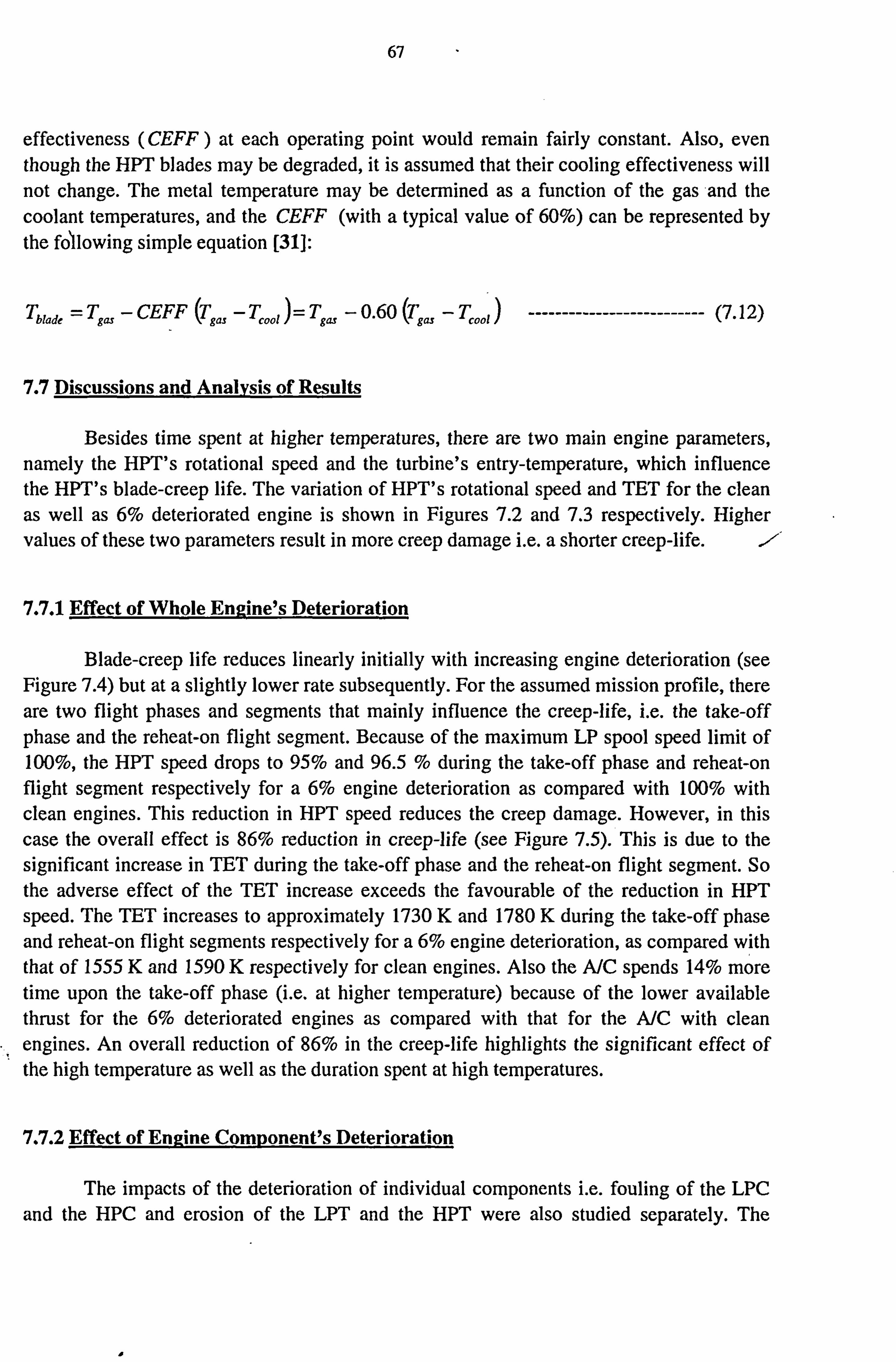
67

effectiveness (CEFF ) at each operating point would remain fairly constant. Also, even though the HPT blades may be degraded, it is assumed that their cooling effectiveness will not change. The metal temperature may be determined as a function of the gas and the coolant temperatures, and the CEFF (with a typical value of 60%) can be represented by the fobowing simple equation [31]:

Tblade '=Tgas -CEFF (Tg�,

-T, ý, ý, 1)=Tg�, -0.60 (Tg�,

-T��1) -------------------------- (7.12)


Besides time spent at higher temperatures, there are two main engine parameters, namely the HPT's rotational speed and the turbine's entry-temperature, which influence the HPT's blade-creep life. The variation of HPT's rotational speed and TET for the clean as well as 6% deteriorated engine is shown in Figures 7.2 and 7.3 respectively. Higher values of these two parameters result in more creep damage i. e. a shorter creep-life. 1/11'

7.7.1 Effect of Whole Engine's Deterioration

Blade-creep life reduces linearly initially with increasing engine deterioration (see Figure 7.4) but at a slightly lower rate subsequently. For the assumed mission profile, there are two flight phases and segments that mainly influence the creep-life, i. e. the take-off phase and the reheat-on flight segment. Because of the maximum LP spool speed limit of 100%, the HPT speed drops to 95% and 96.5 % during the take-off phase and reheat-on flight segment respectively for a 6% engine deterioration as compared with 100% with clean engines. This reduction in HPT speed reduces the creep damage. However, in this case the overall effect is 86% reduction in creep-life (see Figure 7.5). This is due to the significant increase in TET during the take-off phase and the reheat-on flight segment. So the adverse effect of the TET increase exceeds the favourable of the reduction in HPT speed. The TET increases to approximately 1730 K and 1780 K during the take-off phase and reheat-on flight segments respectively for a 6% engine deterioration, as compared with that of 1555 K and 1590 K respectively for clean engines. Also the A/C spends 14% more time upon the take-off phase (i. e. at higher temperature) because of the lower available thrust for the 6% deteriorated engines as compared with that for the A/C with clean engines. An overall reduction of 86% in the creep-life highlights the significant effect of the high temperature as well as the duration spent at high temperatures.

7.7.2 Effect of Enpine Component's Deterioration

The impacts of the deterioration of individual components i. e. fouling of the LPC and the HPC and erosion of the LPT and the HPT were also studied separately. The

68

Figures 7.6 -4 7.9 show the impacts of the compressors' fouling and turbines' erosion for

the LPC, HPT, LPT and HPT respectively. The trend for the LPC's fouling (see Figure 7.6) is qualitatively similar to that of the engines' deterioration (see Figure 7.4). However, the associated adverse effect on creep life is less than that of engines' deterioration, i. e. 70% reduction in creep life at 6% LPC F1 as compared with that of 86% reduction at the same percentage level of EDI (see Figure 7.5). The extent of the reduction in blade-creep life due to fouling of the HPC (see Figure 7.7) and LPT erosion (see Figure 7.8) is almost same at the same percentage levels of F1 and EI respectively. However the trend of the LPT's erosion on creep life is more linear with increasing El as compared with that of the HPC's fouling. The HPC fouling curve is initially linear whereas the slope slightly increases later. Contrary to the trends for the LPC, HPC and LPT, the creep life increases linearly with increasing erosion of the HPT (see Figure 7.9) and this rise reaches 102% at 10% HPT El as compared with that for clean engines (see Figure 7.10). The governing factors for changes in the creep life due to the fouling of the compressors and the erosion of turbines are again the same, i. e. HPT speed, TET and duration at higher temperature. The values of these three characteristics for the take-off phase and the reheat-on flight

segment are shown in Table 1. The increase in blade-creep life with increasing erosion of the HPT is because of the much greater reduction in HPT speed with not much difference in the TET as compared with that for the LPC, HPC and LPT (see Table 7.1). This favourable effect of the HPT's erosion on the blade's creep-life (i. e. a reduction in creep damage) seems illogical at first glance, because any deterioration of a component should have a negative effect. The reader should keep in mind that erosion of blades will make them weaker because of thinning, so resulting in lowering of the creep-life upper limit. The effect due to lowering of the creep-life limit may well exceed the effect of the reduction in

creep damage caused by the blade's erosion.

7.7.3 Effect of the Aircraft Cruisiniz at Different Altitudes

As the cruising towards a pre-set target (at 2100 km from home base) flight segment takes the longest time (i. e. 6355 seconds out of a total mission time of 8950 seconds), it was considered appropriate to analyse the effect of any change (i. e. in Mach number and/or altitude) in this flight segment on the blade's creep-life. For this purpose, several simulation runs were carried out at different Mach numbers and altitudes separately. For the range considered (at 8000 to 15000 metres altitude), it was seen that the blade's creep-life (with a 6% engine deterioration) initially increases at a low rate, reaches its peak at about 10500 metres altitude, and then it starts decreasing at a larger rate, reaching the lowest value, i. e. 41 % of the creep life as compared with that while cruising at 8000 metres altitude (see Figure 7.11). The reason for this is the decreasing TET and HPT's rotational speed (the two main factors influencing the creep-life) for the cruising altitude changing from 8000 to 10500 metres and then increasing of these two characteristics as the cruising altitude alters from of 10500 to 15000 metres. For the altitude range considered, these two characteristics have minimum values at 10500 metres

f

69

cruising altitude and thereby the blade's best creep-life is achieved while cruising at this altitude. The variation of the TET and the HPT's rotational speed between the altitudes of 8000 to 15000 metres is governed mainly by three factors. These are:

the reduction in the aircraft's drag and thereby thrust requirement with increasing aircraft's cruising altitude; the nearly linear reduction in available thrust from the engines (for the same TET levels) with increasing altitude; and the reduction in atmospheric temperature with increasing altitude (within the troposphere, i. e. sea level to 11000 metres altitude). The atmospheric temperature remains almost constant within the stratosphere, i. e. between 11000 and 20000 meters altitude.

The first factor has a favourable effect upon the blade's creep-life because it requires the engine to run at lower TETs and HPT's rotational speedg in order to match the decreased thrust requirement. This favourable impact exceeds the negative effect upon the blade's creep-life due to a second factor (i. e. reducing available thrust from engines requires the engines to run at higher TETs and HPT's rotational-speed). The over-all effect of these two factors upon the blade's creep-life remains favourable until an altitude of 10500 metres is achieved. From an altitude of 10500 to 11000 metres, the negative effect of the second factor exceeds the favourable effect of first factor and thereby the blade's creep-life is reduced. As the atmospheric temperature remains almost constant within the stratosphere (i. e. above 11000 metres altitude), therefore, the rate of reduction in the aircraft's thrust requirement also reduces. This results in the blade's creep-life decreasing continuously as the altitude increases from 11000 to 15000 metres.

The trends of TET and HPT's rotational-speed are almost identical for the clean as well as the deteriorated engine. Therefore, the least adverse impact of the engine's deterioration on the blade's creep-life occurs also at a cruising altitude of -10500 metres (see Figure 7.12). The blade's creep-life, with a 6% engine deterioration, reduces to 5% while cruising at 15000 metres altitude as compared with 14% when cruising at 8000 metres altitude (both expressed in a percentage of its creep life for a clean engine at the stipulated altitude).

7.7.4 Effect of the Aircraft- Cruising at Different Mach Numbers

As for the effect of cruising at different Mach numbers, it was seen that for the considered range (i. e. 1.0 to 1.5), for a given deterioration level, the blade's creep-life decreases almost linearly initially but at a greater rate later, and towards the end again at a much lower rate with increasing Mach number (see Figure 7.13). With a 6% engine deterioration, while cruising at a Mach number of 1.5, it reaches its lowest value, i. e. 2.3% of the creep life, as compared with the value while cruising at a Mach number of unity.

70

This reduction in blade's creep-life is due to increasing (i) TET and (ii) HPT's rotational speed, with increasing cruising Mach number. The maximum TET and HPT's rotational speed during cruising to a set target is 1693 K and 92% respectively while the cruising Mach number is 1.5 as compared with that of 1261 K and 77.5% respectively while the cruising Mach number is unity. The variation of the TET and the HPT's rotational speed, while cruising at different Mach numbers, is mainly because of two factors. These are:

increasing of the aircraft's drag and thereby thrust requirement with increasing aircraft's cruising Mach number, and decreasing available thrust (at the same TET level) from the engines upon increasing the cruising Mach number.

Less available thrust and a higher aircraft's thrust requirement require the engines to run at higher TETs and HPT's rotational speeds and thereby negatively influence the blade's creep-life.

The adverse impact of engine deterioration on the blade's creep-life initially decreases with increasing Mach number (i. e. for Mach numbers 1.0 to 1.15). However, it starts increasing as the Mach number 1.15 is exceeded (see Figure 7.14). This was determined by comparing the variations in the blade's creep-lives (for the clean as well as the deteriorated engine) due to variations in the cruising Mach number. The blade's creep- life with a 6% engine deterioration increases to 12% and decreases to 5% while cruising at Mach numbers of 1.15 and 1.5 respectively, as compared with that of 9% when cruising at a Mach number of unity (all expressed as percentages of its creep life for a clean engine at the stipulated Mach number). For a given cruising Mach number, the TET increases whereas the HPT's rotational speed decreases with increasing engine deterioration. However, the favourable impact upon the creep-life because of reduction in the HPT's rotational speed is exceeded by the negative impact due to increasing the TET. Therefore the overall effect is a reduction of the blade's creep-life. Also the TET and HPT's rotational speed both increase with increasing cruising Mach number for the clean as well as the engines suffering a deterioration. Another important factor that affects the creep life is the time taken during cruising to reach a pre-set target. This time decreases with increasing Mach number at which cruising ensues. There are four main factors (i. e. the HPT's rotational speed, TET, cruising time to reach a pre-set target, and the differences in the TET's and HPT's rotational speeds for clean and 6% deteriorated engines), which dictate the shape of the curve as shown in Figure 7.14. The overall adverse effect of these four factors seems to be 'least' at a cruising Mach number of 1.15 (see Figure 7.14).


As the TET is very high during the reheat-on flight segment, therefore, it was considered appropriate to see how the change in reheat-on time affects adversely the

71

blade's creep-life. For this purpose, several simulation runs were carried out with different reheat-times. The blade's creep-life decreases (i. e. the creep damage increases) slightly more than linearly with increasing reheat time (see Figure 7.15). This reduction in the blade's creep-life is because of the longer time spent at higher temperature as the take-off phase and reheat-on flight segment are the two flight segments/phases wherein the TET is the highest. The blade's creep-life, while the reheat is switched on for 30 seconds, reduces to 22% of that for when no reheat is used.

The adverse impact of the engine's deterioration on the blade's creep-life decreases continuously (initially at a low rate but later at a faster rate) with increasing reheat-on time (see Figure 7.16). There are two factors responsible for this behaviour. These are:

the difference in increasing TET's of the clean and deteriorated engines, and the difference in increasing HPT's rotational speeds for the clean and the deteriorated engines (both with increasing reheat-time).

The difference in TETs remains almost same, however, the difference in the HPT's rotational speeds decreases with increasing reheat-time thereby resulting in a longer creep- life (i. e. a lesser effect of the impact of engine deterioration upon the blade's creep-life). The blade's creep-life with a 6% engine deterioration increases to 14.5 % for a reheat-on time of 30 seconds as compared with that of 2% without reheat on (both expressed as percentages of its creep life for a clean engine).

It is important to mention here for all these three cases (i. e. changes in cruising Mach number and altitude as well as reheat times), that there was no other change in the mission profile and the A/C still covered the same range. However the A/C took a different time to accomplish the complete mission because of the aforementioned changes.


Change in the standard-day temperature has a significant effect on the blade's creep-life usage and so the performance in different parts of the world could vary. For a given deterioration level, the blade's creep-life decreases linearly with increasing standard- day temperature. For example, with a 6% engine deterioration, it reduces to 55% (when the standard-day temperature deviation is +100 C) as compared with that of 100%, for the same mission flown on a day when standard-day temperature deviation is zero (see Figure 7.17). This reduction in the blade's creep-life is mainly due to:

increasing the TET, increasing the HPT's rotational speed and

72

the lower thrust available (thereby resulting in more time being taken by the aircraft during take-off, which is a high-temperature phase for the HPT's blades) with increasing standard-day temperature.

The maximum thrust available, the TET, the HPT's rotational speed during the take-off phase and the time to take-off are 64945 kN, 1776 K, 96.8% and 29.4 seconds respectively at zero standard-day temperature deviation as compared with 63820 kN, 1780 K, 96.9% and 31.6 seconds respectively at +100 C standard-day temperature deviation.

The adverse impact of engine deterioration on a blade's creep-life increases linearly with increasing standard-day temperature (see Figure 7.18). This was determined by comparing the variations in the blade's creep-lives (for a clean as well as deteriorated engines) due to variations from the standard-day temperature. The blade's creep-life on a day with +100 C standard day temperature deviation reduces to 12.5% as compared with that of 14.5% on a day without any standard day temperature deviation (both expressed as percentages of creep-life for a clean engine under the stipulated standard-day temperature deviation). For a given standard-day temperature, the TET increases whereas the thrust available decreases (thereby increasing the time to take-off) with increasing engine deterioration. For example, at a zero standard-day temperature deviation during the take- off phase, the maximum available thrust, the TET and the time to take-off are 71188 kN, 1555 K and 25.7 seconds respectively for a clean engine as compared with 64945 kN, 1776 K and 29.4 seconds respectively for a 6% deteriorated engine. However, the HPT's rotational speed decreases with increasing engine deterioration, e. g. it is 96.8% for a 6% deteriorated engine as compared with 100% for a clean engine. This reduction in speed affects the creep-life favourably (i. e. the creep-life increases). However, this favourable effect is less than the combined adverse effect due to the increased TET and time to take- off. Therefore, overall, the effect is a reduction in the blade's creep-life.


As LPC deterioration is the most serious (among the major engine's components considered i. e. LPC, HPC, LPT and HPT) in terms of its adverse effects upon the blade's creep-life. Therefore, in addition to the impacts of the LPC's fouling which combines the deteriorating flow capacity and efficiency, the impacts of these two parameters upon blade's creep-life were also analysed separately. For a 5% LPC's flow-capacity deterioration, the blade's creep-life decreases sharply initially at a much faster rate but subsequently at a lower rate, with increasing LPC's efficiency deterioration (see Figure 7.19). For example at 10% efficiency deterioration the blade's creep-life is just 4.5% of the blade's creep-life without any efficiency deterioration. On the other hand, for a 5% LPC's efficiency deterioration, the blade's creep-life decreases slightly in the beginning but immediately starts increasing initially at a lower rate but later at a faster rate, with increasing LPC's flow-capacity deterioration (see Figure 7.20). For example the blade's

73

creep-life is 77,90,110 and 575% at 1,2,3 and 10% LPC's flow-capacity deterioration respectively, as compared with that of 100% without any LPC's flow-capacity deterioration.

7.7.8 Effect of Engine's Design-Point Stress and Rotational Speed

According to equation 8, values for Sd,, ig,, and (Dd,, ig,, (i. e. the blade's stress and HPT's rotational speed at the engine's design point) are required for creep-life analysis. Despite an extensive literature review, the exact values of these two characteristics for the engine (i. e. F404) chosen for the present investigation were not available. So typical values for this type of aero-engine were assumed for the purpose of this investigation. It was considered worth seeing how any errors in the assumed values influence the blade's creep- life for a specific condition of engine as well as the impact of the engine deterioration on the blade's creep-life. Therefore, a study was carried out. Blade's creep-life continuously decreases with increasing stress imposed on the blade as well as the HPT's rotational speed (while considered separately, i. e. one at a time) at the engine design-point provided the other engine conditions / characteristics are unchanged (see Figures 7.21 and 7.22). The reduction in the blade's creep-life is more significant upon increasing the HPT's speed at the engine's design-point as compared with that of increasing the blade's stress at the engine's design-point. As for the effects of increasing the blade's stress and HPT's speed at the engine's design-point, on the impact of the engine's deterioration upon the blade's creep-life, it is almost negligible in the case of increasing the blade's stress at the engine's design-point (see Figure 7.23). However, increasing the HPT's speed at the engine's design-point slightly reduces the impact of engine deterioration upon blade's creep-life (i. e. the blade's creep-life increases) in a linear manner (see Figure 7.24). The blade's creep-life increases by 3% (i. e. to 15% with a 5% increase in the HPT's speed at the engine's design-point, as compared with that of 12% with a 5% reduction in the HPT's speed at the engine's design-point). The 15 and 12 % blade's creep-lives are expressed as percentages of creep lives for a clean engine at the stipulated HPT's speeds at the engine's design-point.

74

CHAPTER 8


UPON LOW-CYCLE FATIGUE LIFE

8.0 Introduction

For an engine that experiences deteriorations in its efficiency and/or mass flow, the engine will seek a different-steady state operating point, thereby resulting in a variation of the HPT's rotational speed. As such, the stresses that the engine is subjected to will change (and thereby alter the blade's LCF life-consumption) relative to that for an engine with no deterioration. Rises in the HPT's rotational speed result in greater fatigue damage for the hot-end components and thereby increase engine life-cycle costs. Possessing a better knowledge of the impacts of engine deterioration upon the low-cycle fatigue life- consumption of engine's hot-end components, such as a HPT's blade, helps the users to take wiser management-decisions and hence achieve improved engine utilization. Besides a brief description of LCF related aspects, for a military aircraft, using a computer simulation, the consequences of engine deterioration upon a HPT's blade LCF life- consumption are predicted and described in this chapter.

8.1 Importance of Engine Durability

Even though safety is still the prime aim in civil aviation, the operating cost and hence profitability are now of prime importance to the operator. This is due to several trends including: the competitive pressures of the global economy; the privatisation of airlines, which are no longer seen in their traditional role as heavily subsidised agents of the state; a more deregulated airline market; and a belief that civil air-transport is now a mass market service rather than a premium facility for the few.

In the field of military aviation, economics have also become of increased significance during the last decade. The collapse of monolithic communist governments in the former eastern bloc and in parts of the third world has dramatically reduced the perceived risk of a large-scale global conflict. This has led to major reductions in defence budgets as the need to maintain large standing forces, at high levels of readiness, to fight a zero notice super-power conflict, has decreased. Simultaneously, the traditional long-term trend of defence cost inflation being several percent above that in the wider economy has led to severe pressures being placed upon defence budgets. These two factors have resulted

75

in a marked cultural change in the defence sphere, with a greatly increased emphasis being placed upon achieving cost effectiveness when providing defence capability.

One route to achieve reduced costs is to adapt a better maintenance strategy. Early gas-turbine engines for aircraft were serviced according to a regular overhaul schedule on the basis of engine operating time, i. e. the engine was overhauled after every "x" operating hours regardless of its actual condition. However, once the engine has been in service for a few months, there is only typically a slight correlation between time since the last overhaul and the probability of its failure. Therefore, the traditional "hard time" approach has largely been replaced by the use of Reliability-Centred Maintenance (RCM) methodologies, where engines are maintained according to "on-condition" requirements. These achieve greater reliability and reduced maintenance costs [19].

Although it is likely that a complete engine will now be maintained "on-condition" using RCM methodologies, certain components within the engine will still only be allowed to remain in service for pre specified periods, i. e. have fixed life-limits. This is because failure of these components, typically the engine's shafts, discs and turbine blades, would directly endanger the aircraft as they possess, while in operation, vast amounts of rotational energy. For this reason, such items are usually defined as "critical components". They are prone to life-related failure modes, especially low-cycle fatigue and thermal-fatigue. Many regulations and procedures have evolved to ensure that these critical components are given appropriate, i. e. safe service lives. However, in principle, these systems entail undertaking determinations of--

a safe life limit for each component in terms of a life limiting parameter, e. g. permitted number of operating cycles. the rate of life usage in actual service, e. g. the number of cycles consumed per operating hour [19].

8.2 Low-Cycle Fatigue (LCF)

This is the failure mode associated with relatively low numbers of high-stress applications [23]. Fatigue is typically defined as LCF, when the number of cycles to failure is less than 50000. Thus it occurs in the left-hand region of the S-N curve [19].

Due to the high stress levels implicit in LCF, it is normally accompanied by plastic deformation, and is often termed "high-strain fatigue", as plastic strain is the primary parameter governing life. Thus the material is subject to strain (or deformation) cycling rather than stress (or load) cycling. This means that it is appropriate to use material data produced by strain cycling to characterise the LCF life. Thus the S-N curve is replaced by a strain-life curve. In low-cycle fatigue, due to the higher stresses encountered, there is a greater accumulation of energy in the form of Plastic deformation per reversal than would

76

be the case if the cyclic stresses or strains were small as in high-cycle fatigue. As a result, the proportion of a component's life spent in the crack-initiation phase is often very short, i. e. -10%. Consequently the component spends -90% of its life, in the 3rd phase of the fatigue mechanism shown - see Figure 3.2, i. e. long-crack growth - phase H [19,311. This will enable the crack growth to be predicted based on crack propagation rates and thereby safe life limits can be set on parts.

For a military-fighter aircraft's engine, LCF is probably the most significant life- reducing failure mechanism and is the direct result of the many throttle changes experienced in this application [27]. This is in contrast to the transport aircraft engines, for which the LCF is of less concern because the number of throttle excursions is likely to be far less. In general, the engine components that are subject to LCF are also those that are unlikely to be contained (because of normally very high rotational speeds and thereby damage occurring to components down stream) in the event of a fatigue failure. It is these that are critical to flight safety and must be monitored [8].

8.3 Measuring Low-Cycle Fatiaue

In examining the weighting factors used in determining the LCF life, it is normal to use a full reference cycle from start-up to maximum RPM to shut-down. This is the greatest stress level change that the engine will experience during the flight, and the engine is likely to be subjected to this condition only once per flight. In examining other cyclic excursions, it should be noted that the mean stress and the cyclic stress of each cycle will also vary: the damage resulting from a high RPM throttle excursion will exceed that arising from lower RPM excursions due to the higher mean stresses involved. This difference leads to the requirement that one should take into account both the amplitude of the cyclic load change and the mean stress.

Also of concern is that the probability of failure is not a linear function of the number of cycles experienced. This has been demonstrated in one practical example, in which 3000 load cycles corresponds to a failure probability of 0.1%, while for 3300 load cycles, the failure probability increased to 0.28%, or almost a threefold rise [8]. This increase is one of the main drivers behind the application of safety factors to life limits, and emphasises the importance of an accurate method for measuring the number of cycles to which a component has been subjected.

LCF stresses will also occur due to fluctuating inertia, precession and pressure loads. The latter will normally be a life-limiting factor in non-rotating components, such as the combustor casing and engine mounts. For the pressure cycles, it is possible to monitor the static-pressure fluctuations and convert these to stresses, from which it is possible to determine the fatigue damage caused to the component. The inertial and precession loads will also be significant given that fighter aircraft can be exposed to loads as great as 12

77

times the force of gravity. However, these loads are small in comparison with the centrifugal and pressure loads on the engine, and are normally specified in the engine design but not considered in setting life limits [8].

8.4 Causes of Low Cycle FatiRue (LCF)

Fatigue is caused by a component being subjected to fluctuating stresses, which cause deformation cycling. The fluctuations can be due to changes in any of the loads to which the engine is subjected, e. g. centrifugal, then-nal and pressure loads [19]. [The variations in these loads are due to the changing operational conditions that the engine experiences. In particular, the alterations in the values of the engine's parameters, caused by the pilot operating the throttle, have the biggest effect on these loads, which can also vary due to the aircraft manoeuvring to a different operating point of the flight envelope, e. g. involving a change of altitude or airspeed. These two factors are most pronounced in military combat aircraft operation. Thus, it is for this type of engine that the LCF life is of most significance. ]

8.4.1 Centrifu2al (CF) Load

These are caused by the rotation of turbomachinery. The CF loads and hence the CF stresses induced are proportional to the square of the engine's rotational speed.

8.4.2 Thermal Loads

In the considered component, these (and the resulting strains) are induced by the thermal gradients, which arise due to rapid throttle movements as well as the non-uniform thermal storage capacity and non-uniform heat fluxes in the component. The thermal stresses change in a complex manner during a mission due to the transient differential heating and cooling. Thermal stresses can also be induced, even if no thermal gradient exists, when the free expansion of a component is constrained, or if materials, with different thermal-expansion rates, are rigidly attached. The damage caused by a thermal stress is a function of temperature, and so thermal stresses are of great concern with respect to turbine components which are subjected to high temperatures. However, in modem high-pressure-ratio engines, the operating temperatures at the rear stages of the high- pressure compressor are sufficient to lead to significant thermal stresses. The thermal stresses induced in the hot-section components can be comparable in magnitude with the CF stresses. However, they may, at times, be of benefit in reducing the LCF life consumption because the thermal transient stresses can be compressive in nature and will thus tend to reduce the effect of the CF stress field, which is always tensile. However, this

78

is a secondary effect compared with the large increase in fatigue damage if the thermal transient stress is tensile, which increases the magnitude of the overall stress field.

8.4.3 Pressure Loads

Modem gas-turbine engines operate at high pressures and, therefore, significant pressure-loads develop on casings and other structural members. Fatigue damage can be induced by the varying stresses caused by the fluctuating operating pressures during engine operations. Pressure loads are those normally affecting the LCF lives of non-rotating components, such as combustor casings. They have only a minor influence on the stressing of discs and blades due to the relatively smaller difference in pressures on either side of the component. The stresses induced by this type of load are typically small compared with those due to the CF and the thermal stresses present. Therefore the pressure-load induced LCF will not be considered further in this paper.

8.5 Variability In An Engine's LCF Life Usaae

The basic algorithms for calculating the fatigue damage caused by a given pattern of loading are considered later in this chapter. Although this process contains inherent assumptions, our understanding of it can be considered to be reasonably accurate as the predictions obtained via the algorithm have been validated experimentally [38]. The principal quest has been to monitor more accurately the in-service loading history that components, especially critical ones, actually experience.

8.5.1 Factors Affecting LCF Life Usage in Civil Aviation

These are likely to be predictable with reasonable accuracy because of both the mission profiles flown and the relatively low number of throttle movements during the flight. A typical mission profile is shown in Figure 8.1 [31]. The actual mission profiles are qualitatively similar: one of the principal variables is the duration of the cruise phase. The majority of throttle movements, and hence fatigue damage, occurs during the take-off, climb, descent, holding and landing phases. It is likely that these will be of similar magnitude and duration for each sortie, while the length of the cruise sector varies depending on type of mission e. g. short haul or long haul. Thus it can be anticipated that aircraft which are used on predominantly short sectors will accrue more fatigue damage of their engines per hour of operation, than the same aircraft/engine combination used on longer haul flights.

8.5.2 Factors Affecting LCF Life Usap-e in Military Aviation

79

There is a wider spectrum of usage for military aircraft gas-turbine engines because military aircraft fly a greater variety of mission profiles than civil airliners, and this is particularly true for modem multi-role fast jet-aircraft. It is rare for a modem military plane to be restricted to a single role. And this, together with the need to maintain crew proficiency in the various aspects of their roles, such as weapon delivery, instrument flying and air-to-air refueling, means that many different mission profiles are flown regularly. For example, the RAF defines 10 different standard mission-profiles for the Tomado Interdictor Strike Aircraft and another 10 for the Tomado Air Defence variant. These missions are, by necessity, somewhat "elastic" as speeds, altitudes and mission durations are frequently varied to meet the requirements of the particular training-scenario.

The large throttle movements necessary to exploit fully the performance of military aircraft also have a dramatic impact on the LCF life consumption. Modem fighter-aircraft designs are optimized to achieve high values of the SEP and this leads to pilots using large throttle transients to manoeuvre the aircraft. Studies [3941] have shown that as the aircraft's thrust-to-total-weight ratio increases, the number and magnitude of throttle transients increases, whilst the duration at high-power settings decreases. This latter effect is due to the lower throttle settings required to maintain the value of a specified performance parameter, e. g. cruise speed.

It should be remembered that the relationship between applied stress and remaining life is logarithmic, and that mechanical stress imposed upon the engine varies as the square of its rotational speed. Therefore, a modest increase in the range of throttle movement can have a drastic impact on the fatigue-life consumed. For example, a throttle transient from 90 to 100% spool speed and back to 90% may consume five times more of the remaining fatigue life than one from 90 to 95% and return, the exact relationship depending on the material properties and component stressing [19].

In addition to the wide range of missions flown by military aircraft, there can also be huge variations in the engine usage on what are nominally-identical missions. The most published example of this is for display aerobatics teams, such as the RAF Red Arrows. The throttle usages for the lead aircraft and one at the rear of the formation are shown in Figure 8.2 [42]. The LCF life usage between the engines of the two aircraft differs by an order of magnitude. It is for this reason that the Red Arrows Hawks were the first RAF aircraft to be fitted with individual LCF life-usage monitoring systems.

Fighter aircraft also fly in tactical formations, albeit with rather greater spacings than the Red Arrows. It is likely that the pilot of the lead aircraft will make fewer throttle- movements than those in the rest of the formation. In addition, there is evidence of large variations in throttle handling that may occur between different pilots flyixig the same mission even using the same aircraft type. May et al [43], after studying several USAF missions flown in F15, F5 and AlO aircraft, concluded that different pilots made significantly different usages of the throttle while flying the same mission. This led to a

80

variation by a factor of as much as 5 in the number of idle-maximum power-idle throttle- excursions per sortie.

There are other factors that can affect the LCF-life used on a given mission. These include:

Fighter aircraft are frequently required to simulate actual combat missions. Therefore, some aircraft will operate as attackers and some as the enemy (target) aircraft. To fulfil these different roles, the aircraft will effectively fly different missions. 0 Ambient environment conditions affect the engine operation, e. g. the spool speeds and gas temperatures and thus will influence the LCF-life consumed for given throttle movements. 0 Continuation training requirements: To maintain a high proficiency, pilots have to practise the various aspects of their craft, such as take-offs, approaches and landings. These are often used to round out a sortie, and their frequency varies in an essentially random manner.

Thus there is a wide variation in the amount of LCF life consumed during military- aircraft sorties. In addition to this, the performance requirements of military-aircraft have tended to push designers to optimise critical components to achieve least weight rather than maximum LCF life. These two factors translate into LCF lives in operating hours that may be an order of magnitude less than those for comparable components in a civil- aircraft's engine. Thus LCF has far more impact on the support of military aircraft operations. Consequently, efforts to develop LCF life-usage monitoring have primarily been focused on military operations in order to achieve economic lives in this highly- demanding environment without compromising safety.

8.6 Aircraft's Gas-Turbine Enizine Low-Cycle Fatigue-Life Consumption

It is necessary to carry out two steps to ensure that the useful life of critical components is not exceeded. The first is the setting of an accurate life expectancy, which can be accomplished by various methodologies. The second process is a means of determining and controlling the rate of life usage in actual service, to ensure that the life expectancy is not exceeded. This section outlines the theory describing this latter process.

The fatigue-damage calculation algorithm can be broken down into three discrete steps:

0 Determine the number of load cycles already completed from measured values of the pertinent engine parameters. 0 Calculate the fatigue damage incurred during each individual load-cycle.

81

0 Estimate the total life consumed by summing damage during each individual load cycle.

8.6.1 Cycle Counting Methods

LCF damage of an aircraft's gas-turbine engine results from the application of varying loads. In order to determine these loads, it is necessary to relate them to measurable engine parameters. For example, the CF stresses in a place can be determined [19] via:

si =S (8.1)

If the blade stress at the reference condition, i. e. typically 100% of the spool-speed, is known from design data, then it is possible to calculate the blade stress at any other spool-speed from equation (1). Thus if an engine's spool-speed history is available from a flight-data recorder, then a stress history can be calculated. HP spool-speed history for clean engines during mission profile 'A' is shown in Figure 8.3.

An essential step in the prediction of the fatigue life is the reduction of a service strain or stress history to a series of cycles and half-cycles. This process is known as cycle counting and can be the source of large, but usually unnecessary, errors in the subsequent fatigue-life prediction. The essence of cycle counting is to take an irregular load history, such as that shown in Figure 8.3, and break this waveform down into a number of individual cycles each consisting of maxima and minima of the waveform. This allows the complex loading history that exists in reality to be translated into a number of individual cycles. The fatigue damage for each individual cycle can then be calculated and summed by a cumulative-damage law.

Various methods have been developed to identify the individual cycles from a complex loading-history. The different methods of cycle extraction will analyze the loading waveform into different individual cycles and thus lead to different assessments of the fatigue damage caused. Different cycle-identification methods can give estimates of the damage, caused by a given load-history, that vary by a factor of more than two [44]. Unfortunately, most of them have flaws which severely limit their general application. Basically the methods can be divided into two groups. The first consists of methods which identify and count single events, which are not necessarily related to cyclic damage accumulation in any simple fashion. For example, peaks, peak distributions and level- crossing counting have been used. Their success has been limited to special classes of signals and hence they can be eliminated from serious consideration for more general use. The second group consists of methods which are based on the ranges of stress or strain

82

which occur. These techniques are to be preferred because fatigue damage is closely related to stress and strain ranges. They include range counting, range-mean analysis, range-pair counting and the rainflow cycle-counting method [19]. Two of these, namely the range-mean and rainflow methods, have the additional advantage that they also identify the mean levels of stress or strain in each range. The effect of mean stress on fatigue damage can be very important.

8.6.1.1 Early Cycle-Counting Methods

One of the early cycle-extraction methods was the Range-Mean method. This technique divides the waveform into a succession of half cycles, peak-to-trough or trough- to-peak, and values of stress amplitude and mean stress are then recorded for each half cycle. The principal disadvantage of this method can be seen by examining the loading history as in Figure 8.4 [19], which is essentially a sine wave with a perturbation about the mean load. The Range-Mean technique would assess this as a succession of low-amplitude cycles about a gradually changing mean. Thus, it would ignore the major cycle from the minimum point A, to the maximum B and returning back to the minimum C. This masking of the major cycle can be partially overcome by the use of gate levels, below which the cycles are ignored. However, care must be taken in setting the gate levels, because, if they are too large, then significant minor cycles could be missed. Conversely, if the gate level is too small, then a large-amplitude cycle could be broken down into a number of smaller load cycles, which could be below the material endurance limit and thus assessed as causing no fatigue damage. The solution to this dilemma is to analyse the waveform with several gate-levels and use the one which maximises the calculated damage, thus erring on the conservative side [44].

8.6.1.2 Modern Cycle-Counting Methods

In an attempt to overcome the problems inherent in the Range-Mean and similar counting methods, as discussed in more detail by Dowling [45], various alternative methods have been proposed, which share the following two characteristics: -

Each part of the overall history is counted only once. Smaller ranges are counted down to a pre-determined threshold.

Probably the most widely-used method is the Rainflow or Pagoda-roof method developed by Matsuishi and Endo [46] and subsequently by others [45,47-48]. The Rainflow method works by the rather bizarre analogy of rain flowing down a series of pagoda roofs. To understand the method, the load-time history is turned through 900 so that the time axis extends vertically downwards. A simple waveform is shown in Figure 8.5

83

[19]. The profile is assumed to be a series of "pagoda roofs" and the "rain" flows from the top and obeys the following rules: -

0 Rain starts at the beginning of the history and again at the inside of each peak. 0 Rain flows down a pagoda roof and over the edge until it reaches a level

opposite a maximum which is more positive (or a minimum more negative) than the maximum (minimum) from which it started.

Rain also stops where it is joined by rain from a pagoda roof above. The horizontal length of each rainflow is a half cycle at that stress range.

A graphical representation of the process for the simple wavefonn of Figure 8.5 is shown in Figure 8.6 [19]. For a more complete description of the Rainflow method, the reader is referred to Dowling [45] or Downing [47].

8.6.2 Fatipme-Damage Calculation

The chosen cycle-counting technique will transform the complex load history into a succession of stress ranges about a mean stress. The next stage in the algorithm process is to calculate the actual fatigue damage caused by each individual cycle.

8.6.2.1 The Stress-Life Method

This calculates the fatigue damage by taking the stress range generated by the cycle-counting method and applying it to the corresponding S-N curve. The stress-life technique can be illustrated by Figure 8.7 [38]. It is virtually certain that the minor cycle will alternate about a non-zero mean stress, whilst the stress-life curve will be based on loads ranging from zero to maximum stress. Therefore, a method must be found which will equate the damage caused by the cycle extracted (by the cycle-counting technique), to that caused by an equivalent cycle alternating about a zero mean stress or strain. This latter

cycle is then used to calculate the life of the component under minor cycle conditions. The

most common technique used is the modified Goodman diagram method, as shown in Figure 8.8 [19]: the load condition A of alternating stress amplitude AaN about mean stress cr. can be represented by load condition B of alternating stress ACTN/2 about a mean stress of A(TN/2. Alternatively this can be represented by [38]: -

22

ASE = ASref (D

HL

2S ref .2 (D

ref suls L

(8.2)

84

Thus the actual loading conditions are transformed by the modified Goodman diagram method to a loading condition that gives equal fatigue damage and is compatible with a zero to maximum stress, S-N curve. This can then be used to estimate the life at that loading condition by applying Miner's Hypothesis to the S-N curve as in: -

AS,,, f N,,, f m

---------------------------------------------------------------------------------- (8.3) ASE NE

So, for any single minor-cycle, the LCF damage occurred can be expressed in terms of reference cycles as in equation 4 [38]: -

ref =

[_ASE

2ýref (8.4)

It should be remembered that allowance has to be made for the effect of stress concentrations and this can be done by one of two methods. The first is to use the S-N data for the feature causing the stress concentration, e. g. a bolt hole or a fillet radius. The alternative is to calculate the actual notch root-stress at the feature from the concentration factors as described by ESDU [49].

8.6.2.2 The Strain-Life Method

While discussing LCF earlier, the concept of LCF as a high-strain fatigue was described and hence it is generally considered to be more appropriate to calculate LCF damage by means of a strain-life method. As with the stress-life technique, the first step is to calculate the nominal CF stress at each measured value of spool speed using equation 1. The next step is to determine the local notch-root stress at the part of the critical component under study. If the load is the first applied to the component, then the local stress can be calculated by combining Neuber's rule (equation 5) and the cyclic stress- strain curve (equation 6) to give equation 7 [49]:

KI 2=0 -9 -------------------------------------------------------------------------------------- (8.5) Se

n -------------------------------------------------------------------------

E +[

K --------- (8.6)

------------------------------------------------------------------- (8.7)

85

For subsequent load-applications, the local delta stress is calculated by combining equation 5 with the hysteris stress-strain rule of equation 8 to give equation 9 [49].

Aa FAcT I ----------------------------------------------- (8.8)

2 2E iK ---------------------------- L2 --71

1 AU n' AS

2E +'äor[2K ,]= 2E ---------------------------------------------------------- (8.9)

The term 2 appears in the denominators of each of the terms of this equation because a complete hysteris loop includes two full strain-reversals. Having calculated the local delta stress Acr, then the local notch-stress can be deduced by adding Aa to the value of a at the origin of the hysteris loop.

The local strain range Ae, from the origin of the hysteris loop, can be determined from equation 10:

Ae = (K, ASY

AoE (8.10)

The local strain P- can be now calculated with reference to the value of the local

strain at the origin of the hysteris loop

The local stress history can be passed through a rainflow or other cycle-counting algorithm; the output being cycle pairs of local stress with their associated local strain pairs. From these strain pairs, F-H and EL. the local strain range Ae for the cycle pair can be determined with equation 11:

A-6 ='ell - EL ----------------------------------------------------------------------------------

This value of local strain range is then inserted into the strain-life equation 12 to determine the cyclic life Nf:

Ae Av Ae 0 ýýf +p=f (2Nf ý +. ef (2Nf Y ---------------------------------------------- (8.12) 222E

Thus, the fatigue resistance of a metal can be described by four parameters namely; of q the fatigue strength coefficient; b, the fatigue strength exponent; cf I the fatigue ductility coefficient; and c, the fatigue ductility exponent. Details of the determination of these material properties are given by Raske and Morrow [50]. The

86

relation between elastic strain and cyclic life is provided by Basquin's equation [51] whilst the plastic strain-cyclic life term is from Coffin and Manson [52-53]. Equation 12 can be modified to account for the mean stress effects by including the mean stress co in the elastic strain term [54]. This leads to

AE =(Of

-0o) (2Nf ý+ Ef (2Nf Y ------------------------------------------------------- (8.13)

2E

Most of the stress-strain cycles to be evaluated have a tensile or compressive mean stress associated with them. It is generally recognized that tensile mean stresses reduce the fatigue life and compressive mean stresses increase it [55].

Thus the cyclic life has been calculated for each cycle pair in the load history. This strain-life technique used on CF stresses has formed the basis for the computer model developed for the purpose of LCF life consumption prediction in this investigation.

8.6.3 Cumulative-Damage Laws

The preceding section has shown how the life in cycles for the component under the minor-cycle (NL -) NH -4 NL ) condition is determined. The final step is to sum the damage arising during each individual cycle to determine the cumulative damage caused. Several researchers [56-61] have presented theories of cumulative damage. Many comparisons [62-65] have been made of the theories to determine which will give the most accurate predictions. The most common and well known for this is the Palmgren-Minor Cumulative Damage Law [57]. This rule was first postulated by Palmgren and then again independently by Minor [56). The essence of the Palmgren-Minor Law is both simple and logical. It states that the life fractions consumed by each different loading cycle can be simply added, and, when the sum has reached unity, the material can be deemed to have failed. This can be expressed as

nf =

n, + n2

+ _! ý3

. .............

n,, ni + ----------------------------------- (8.14) Nf N, N2 N3 N,, Ni

where n, n2 nn= number of cycles occurring at stress levels 1,2 n Nit N2***** Ný, = number of cycles to failure from S-N curve for the component

(under consideration) at stress levels 1,2 n

When the value IL, i. e. the proportion of the life used to the total life to failure, is Nf

unity, the component is considered to have failed.

87

In reality, component failure can occur at ratios of _ý_f between 0.61 and 1.49 [56]. Nf

Therefore as a conservative measure, some design methodologies specify that a specified

value of -ýýf- of less than unity is considered to be the failure point. As pointed out in the Nf

ESDU paper on fatigue-life estimation [49], although the Palmgren-Minor law may be considered inaccurate in some respects, it is simple, has been widely applied, and the reasons for its inadequacies are recognised and can be compensated for in the design process. Alternatively the Palmgren-Minor law can be expressed in the form of equation 15:

ni =NREF

nref N, ----------------------------------------------------------------------------------- (8.15)

the reference cycles consumed by the minor cycle ni is simply the ratio of the life at the reference condition NREF to that at the minor cycle condition NJ. Both of these can be found from the stress-life or strain-life expressions as appropriate to the method selected. The damage caused during each minor cycle can thus be calculated in terms of reference cycles. These are then added to get a cumulative value and the component is considered to have failed when this cumulative value is equal to the life (in terms of reference cycles) under the reference-cycle conditions.

8.7 Discussions and Analvsis of Results

The prime aim of this study was to evaluate the impacts of various engine deteriorations on a HPT blade's LCF life consumption. The prime factor responsible for any change in the HPT blade's LCF life-consumption is the variation in the HPT's rotational speed as a result of engine's deterioration. A higher HPT's rotational speed results in greater LCF life-consumption and thereby lowering the blade's LCF life. The variation of the HPT's rotational speed throughout the aircraft's mission profile (for the clean as well as 6% deteriorated engines) is shown in Figure 7.2. Large variations in blade-life usage occur during the flight with relatively small changes in the operating conditions. For example, in the assumed mission-profile, using reheat for only 5 seconds increases the blade's LCF life consumption (i. e. the blade's remaining life is shortened) to 113% as compared with the blade's LCF life consumption of 100% without any reheat use, the A/C covering the same mission-profile with both engines clean.

8.7.1 Effect of the Whole Engine's Deterioration

The blade's LCF life-consumption reduces (i. e. LCF life increases) nearly linearly with increasing engine deterioration (see Figure 8.9). For engines suffering a 6%

88

deterioration, the blade's LCF life-consumption reduces by 40% as compared with that for the clean engines (see Figure 8.10). This reduction in blade's LCF life-consumption is because of lower HPT's rotational speed for the deteriorated engine. At first glance, this reduction in blade's LCF life-consumption with increased engine's deterioration may appear odd. However, this behaviour becomes clear if the variations in major engine's parameters / characteristics such as TET, thrust available, LP and HP spool speeds (which are also inter-related because of gomplete component matching / aero-thermal balancing established within the engine) are analysed together. For same level of TET, engine deterioration results in lower thrust available from engines accompanied with lower LP and HP spool speeds. In order to keep the aircraft's performance invariant (i. e. constant thrust requirement), the engines suffering deterioration are required to run at higher TETs and/or HPT's rotational speeds. As in the present investigation, TET is used as a controlling handle, therefore, TET is increased until the thrust available from engines equals the thrust available from clean engines. Increase in TET is also accompanied by increase in LP and HP spool speeds (see Table 8.1). However, the increase in TET is significantly higher as compared with increase in LP and HP spool speeds. Therefore, the final HPT's rotational speed still remains lower than that of clean engines (for same level of thrust developed) and thereby resulting in lower HPT blade's LCF life-consumption.

8.7.2 Effect of an EnRine Component's Deterioration

The impacts of the deterioration of individual components i. e. fouling of the LPC and HPC and erosion of the LPT and HPT were also studied separately. The Figures 8.11

-4 8.14 show the impacts of the compresso rs' fouling for the LPC and the HPC and the turbines' erosion for the LPT and the HPT respectively. The change in blade's LCF-life- consumption for 10% deterioration of these four components is shown in Fig 8.15. The blade's LCF life-consumption increases as a result of the LPC's fouling, whereas for all other deterioration conditions, i. e. the engines' deterioration as a whole, HPC's fouling and erosion of both LPTs and HPTs, the blade's LCF life-consumption decreases. The reason for this behaviour is the variation of the HPT's rotational speed with any increasing deterioration. For all types of deterioration, i. e. the engines as a whole, compressors' fouling and turbines' erosion, the available thrust from the engines (for the same TET level) and HPT's rotational speed decrease with increasing deterioration (see Figures 8.16 and 8.17). However, the rates of reduction of the HPT's rotational speed and available thrust are different with different types of deterioration (see Table 8.2). Both of these engine parameters, i. e. the HPT's rotational speed and the available thrust increase with TET (see Figure 8.18). The reduction in the HPT's rotational speed influences the LCF life-consumption favourably (i. e. the LCF life increases). Whereas the reduction in the available thrust from the engines has a negative effect upon the LCF's life because it requires the HPTs to run at higher rotational speeds in order to match the thrust requirement to maintain the aircraft's performance.

89

The reason for increasing of the blade's LCF life-consumption with increasing LPC fouling is the much lesser reduction in the HPT's rotational speed and much larger reduction in the available thrust (thereby requiring the engines to run with much higher HPT's rotational speed) due to the LPC's fouling. So, in this case, the favourable effect upon the LCF life-consumption because of the reduction in the HPT's rotational speed with increasing LPC's fouling is exceeded by the negative effect of increasing HPT's rotational speed in order to match the thrust requirement for maintaining the aircraft's performance. However, for all other deteriorations, the favourable effect upon the LCF-life exceeds the negative effect upon the LCF-life. The negative effect upon the LCF-life is due to any increase in the HPT's rotational speed (as a result of the lower thrust available with increasing deterioration and thereby requiring the engines to run at higher HPT's rotational speed). The favourable effect upon the LCF-life is a result of a reduction in the HPT's rotational-speed with increasing deterioration.

8.7.3 Effect of the Aircraft Cruising at a Different Altitude

As traversing the cruising segment towards a pre-set target (at 2100 km from home base) takes 6355 seconds out of a total mission time of 8950 seconds, it was considered appropriate to analyse the effect of any change (i. e. in Mach number and/or altitude) in this flight segment, on the blade's LCF life-consumption. For this purpose, several simulation runs were carried out for different Mach numbers and altitudes separately. For the range considered (namely 8000 to 15000 metres altitude), it was seen that blade's LCF life consumption (with a 6% engine deterioration) decreases (i. e. the LCF life increases) slightly from 8000 to 11000 metres and above 11000 metres starts increasing with increasing cruising altitude (see Figure 8.19). Mainly three factors are responsible for this behaviour. These are:

decreasing aircraft's drag and thereby decreased thrust requirement with increasing altitude; decreasing thrust available from engines with increasing altitude; and decreasing atmospheric temperature within troposphere (Le from 8000 to 11000 metres), the temperature remains almost constant within stratosphere (i. e. from 11000 to 20000 metres).

The first factor requires the engines to run at lower TET / HPT's rotational speed in order to keep the aircraft's performance invariant, whereas the second factor requires the engine to run at higher TET / HPT's rotational speed. The favourable effect of first factor upon blade's LCF life-consumption exceeds the negative of second factor throughout the troposphere. As the atmospheric temperature remains almost constant within stratosphere, therefore blade's LCF life-consumption starts increasing above 11000 metres, because of increasing HPT's rotational speed.

90

8.7.4 Effect of the Aircraft Cruising at a Different Mach Number

As for the effect of cruising at different Mach numbers, for the considered range (i. e. Mach number of unity to 1.5), for a given deterioration level, the blade's LCF life- consumption increases (i. e. the LCF life decreases) at a faster rate initially, but at a much lower rate subsequently, with increasing Mach number (see Figure 8.21). With a 6% engine deterioration, while cruising at a Mach number of 1.5, the blade's LCF life- consumption reaches its highest value, i. e. 13 1% of the LCF life-consumption of that while cruising at a Mach number of unity. This increase in LCF life-consumption (i. e. a reduction in the blade's LCF-life) is due to increasing HPT's rotational-speed, with increasing aircraft's cruising Mach number. The maximum HPT's rotational-speed during cruising, to a set target, is 92% (of the design point speed) while the aircraft's cruising Mach number is 1.5 as compared with that of 77.5% while the aircraft's cruising Mach number is unity. The variation of the HPT's rotational speed, while cruising at different aircraft's cruising Mach numbers, is mainly because of two factors. These are:

increasing of the aircraft's drag and thereby thrust requirement as the Mach number rises from unity to 1.5 for the cruising phase, and decreasing of the available thrust (at the same TET) from the engines upon increasing the cruising Mach number.

Less available thrust and a higher aircraft's thrust requirement require the engines to run at higher TETs and HPT's rotational speeds and thereby negatively influence the blade's LCF-life.

The adverse impact of the engine deterioration on the blade's LCF life- consumption initially decreases with increasing Mach number (i. e. for Mach numbers 1.0 to 1.15). However, it starts increasing (i. e. the blade's LCF-life decreases as compared with its LCF life if the engine was clean) as the Mach number of 1.15 is exceeded (see Figure 8.22). This was deten-nined by comparing the variations in the blade's LCF life- consumption (for clean as well as for the engine suffering deterioration) due to variations in the cruising Mach number. The blade's LCF life-consumption with a 6% engine- deterioration is 53 and 62% while cruising at Mach numbers of 1.15 and 1.5 respectively as compared with that of 58%, at a Mach number of unity. All three values are expressed as percentage of LCF life-consumption for a clean engine at the stipulated Mach number. For a given cruising Mach number, the TET increases whereas the HPT's rotational speed decreases with increasing engine deterioration. The favourable impact upon the LCF-life, due to the reduction in the HPT's rotational speed, with increasing engine deterioration, is exceeded by the negative impact upon the LCF-life, due to an increase in the HPT's rotational speed, with increasing Mach number. Therefore the overall effect is a rise in the LCF life-consumption (i. e. a reduction of the blade's LCF-life). The governing factor influencing the impact of the engine deterioration upon the blade's LCF life-consumption is the difference in the HPT's rotational speeds (for clean and deteriorated engines) with

91

increasing aircraft's cruising Mach number. As this difference widens with increasing Mach number, the adverse influence of engine deterioration upon the blade's LCF-life also increases with increasing Mach number.


As the reheat-on flight segment influences the creep-life so significantly [7], because of the then higher temperature and HPT speed, it was considered appropriate to see how the change in the reheat-on time affects the blade's LCF-life. For this purpose, several simulation runs were carried out with different reheat-times. It was seen that the blade's LCF life-consumption increases (i. e. the LCF life decreases) initially at a faster rate, but subsequently at a relatively low rate with increasing reheat time (see Figure 8.23). This reduction in the blade's LCF-life is because of the increasing HPT's rotational speed with increasing Mach number (i. e. the speed of aircraft) due to the longer time spent with the reheat-on. The blade's LCF life-consumption while the reheat is switched on for 30 seconds, increases to 120% of that when no reheat is used.

The adverse impact of the engine's deterioration on the blade's LCF-life decreases continuously (initially at a fast rate, but later at a lower rate) with increasing reheat-on time (see Figure 8.24). The factor responsible for this behaviour is the difference in the HPT's rotational speeds for the clean and the deteriorated engine (with increasing reheat-on time). This difference decreases with increasing reheat-on time, thereby resulting in a longer LCF-life (i. e. the lesser effect of the impact of the engine deterioration upon the blade's LCF-life). The blade's LCF consumption with a 6% engine deterioration decreases to 60% for a reheat-on time of 30 seconds as compared with that of 70% without the reheat-on (both expressed as percentages of its LCF life consumption for a clean engine).


As the changes in the standard-day temperature have significant effects on the blade's creep-life usage [7], it was considered appropriate to see if there is any effect of change in the standard-day temperature on the blade's LCF-life. For this purpose, several simulation runs were carried out at different standard-day temperatures. There is a small effect of the standard-day temperature variation upon the blade's LCF life-consumption (see Figure 8.25). The reason is that, for same thrust requirement, unlike the TET (which mainly effects the creep-life), there is almost no change in the HPT's rotational speed (which affects the LCF life-consumption) due to any variation in the standard-day temperature.

The adverse impact of engine deterioration on a blade's LCF life consumption decreases linearly with increasing standard-day temperature (see Figure 8.26). This was

92

determined by comparing the variations in the blade's LCF life consumption (for clean as well as deteriorated engines) due to variations from the standard-day temperature. The blade's LCF life-consumption on a day with a +100 C standard-day temperature deviation

reduces to 57% as compared with that of 60% on a day without any standard-day temperature deviation (both expressed as percentages of the blade's LCF life consumption for a clean engine under the stipulated standard-day temperature deviation). For a given standard-day temperature, the HPT's rotational speed decreases with increasing engine deterioration e. g. it is 96.8% for a 6% deteriorated engine as compared with 100% for a clean engine. This reduction in speed affects the blade's LCF life-consumption favourably (i. e. the LCF-life increases).


LPC deterioration is the most serious in terms of its effects upon the blade's LCF life-consumption. Therefore, in addition to the impacts of the LPC's fouling which combines the deteriorating flow capacity and efficiency, the impacts of these two parameters upon blade's LCF life-consumption were also analysed separately. For a 5% LPC's flow-capacity deterioration, the blade's LCF life-consumption increases almost exponentially from zero to 2% efficiency deterioration. It increases almost linearly at a relatively low rate from 2 to 7% efficiency deterioration. From 7 to 10% efficiency deterioration it increases at a much faster rate initially, but subsequently at a relatively low

rate, with increasing efficiency deterioration (see Figure 8.27). On the other hand, for a 5% LPC's efficiency deterioration, the blade's LCF life-consumption decreases almost linearly with increasing LPC's flow capacity deterioration (see Figure 8.28).

93

CHAPTER9


UPON THERMAL-FATIGUE LIFE

9.0 Introduction

Deteriorations of engine components, such as compressor(s) and turbine(s) alter their efficiencies and flow capacities. The changes in compressor's and turbine's efficiencies and flow capacities require the engine to run at different TETs and/or rotational speeds relative to that for an engine with no deterioration, in order to meet the thrust requirement to achieve the same aircraft's performance. Rises in TETs and HPT's rotational speeds result in greater thermal fatigue damage of the hot-end components occurring and thereby increase engine's life-cycle costs. For a military aircraft, using a computer simulation, the consequences of engine deterioration upon a HPT Blade's thermal fatigue life are predicted and described in this chapter.

9.1 Thermal Fatigue

This is associated with rapid engine-throttle movements, which create temperature- gradients within components. The resulting thermal stresses superimposed upon the existing mechanical and gas-pressure stresses, result in localised high transient-strains. If repeated often enough, cracks may be initiated on the component's surface (because of the highest temperatures occurring there) and subsequently propagate through the material [25].

In gas-turbine engines, the components that come into direct contact with the high- temperature gases (i. e. the turbine blades or nozzle guide-vanes, which are completely immersed in the hot gas-stream, or turbine discs, which are partially immersed) are highly susceptible to thermal fatigue. The high thrust-to-weight ratio expected of military aircraft's engine results in high turbine-temperatures, which combined with rapid throttle movements, creates a very severe thermal-fatigue environment [27].

The damage caused by thermal fatigue, like creep, rises exponentially as the temperature is increased [27]. Therefore, a small reduction in engine deterioration may have a dramatic effect on prolonging the thermal-fatigue life. The stages involved in calculating the transient thermal-stresses are as follows [66]-. -

The computation of gas-stream temperatures, pressures and velocities from Lown engine characteristics.

94

0 The calculation of the appropriate hot gas to metal-components heat- transfer coefficients. 0 The determination of transient temperatures, throughout the considered component, during each flight using evaluated gas-stream temperatures and heat- trýnsfer coefficients. 0 The calculation of the resulting thermal stress-distribution profiles (for several stages during the flight).

In practice this procedure is extremely complex and requires major computing power. This means that for on-board real time processing of thermal transient stresses in a life-usage monitoring system, a simplified thermo-mechanical model has to be developed [19].

9.2 Equivalent Full Thermal-Cycle (EFTC)

EFTCs provide an indication of the degree of thermal fatigue (which is the life- limiting failure mechanism for the F404 engine chosen to be investigated) experienced by the HPT's blades. EFrCs are based on a prediction of the HPT metal-blade's leading-edge temperature.

Thermal fatigue is a condition whereby the strain cycles are predominantly caused by temperature cycling [27]. The total strain range is determined by

Ac =P(T- TO) --------------------------------------------------------------------------------

where A is the co-efficient of thermal expansion of the material of the blade, which is cycled between temperatures T and To. The reference temperature To depends principally on the engine's idling-rpm at standard sea-level conditions.

The strain range A-r is related to the number of cycles Nf completed before failure ensues [27] by

Aev _

Of (2 Nf ý +Ef (2 Nf 2E (9.2)

where E is the elastic modulus of the blade's material, and b and c for most materials equal -0.12 and -0.6 respectively.

In equation (2), the first terrn results from elastic strain HCF and the second term from inelastic LCF [27]. Generally, for aero-engines, the life for a HPT's blade is long, e. g. for the F404 HPT blade, the life is -30,000 cycles. Therefore, it is assumed that the elastic term will dominate and hence, equation 2 may be re-written as:

95

AE _

Of (2 Nf 2E

(9.3)

The strain range of any second thermal cycle, i. e. from To to T2 to To, may be

expressed [27] in terms of the first thermal cycle, i. e. from To to T, to To, as follows:

f -------------------------------------------------------------------- (9.4)

AS2 -

T2 -To =[VN

0.12

T-T AE, 10f

12

The ratio is the relative severity of the second thermal cycle compared with that of Nf2

the first thermal cycle. The thermal-fatigue relative severity (R/S) can be expressed [27] in terms of the temperature differences as follows:

RIS = Nf,

= T2

-TO 8.333

Nf2

[TI

-TO

I (9.5)

The EFTC is based on calculating the severity of thermal cycles relative to a reference thermal cycle and summing the total. Measurement of the thermal cycle begins as the PLA passes through the idling setting (i. e. 60 to 70% of design point LP spool-speed for typical engines) and terminates when the cycle passes back through that point. For the present investigation, it has been assumed that the PLA directly proportional to the LP spool speed. During this cycle (i. e. idling RPM to maximum RPM to idling RPM), the maximum value of the metal-blade's temperature is used in determining the thermal- fatigue relative-severity (RIS).


The prime aim of this study was to predict the impacts of different types of engine's deteriorations upon a HPT blade's thermal fatigue-life. For this purpose, over 150 engine and aircraft's performance-simulation runs were required: each run took approximately 30 to 35 minutes of computer time. There are two main engine parameters, namely the turbine's entry temperature (TET) and the HPT's rotational speed, which influence the HPT blade's relative temperature and thereby blade's thermal fatigue-life. Higher values of these two parameters significantly contribute towards greater thermal fatigue damage for the blades. The variations of HPT's rotational and TET (for the clean as well as 6% deteriorated engine) for the complete mission profile of the aircraft, are shown in Figures 7.2 and 7.3 respectively.

9.3.1 Effect of the Whole Engine's Deterioration

96

HPT blade's relative severity of thermal-fatigue increases (i. e. the blade's thermal fatigue-life decreases) more than linearly, initially at a lower rate, but at a faster rate later,

with increasing engine deterioration (see Figure 9.1). The extent of additional thermal fatigue damage due to increased engine deterioration is significant. For example, the blade's relative severity of thermal fatigue, with engines suffering 6% deterioration is 120 % higher as compared with that for the clean engines. There are mainly two factors that dictate the shape of the curve in Figure 9.1. These are:

the variation of HPT's rotational speed (for the same level of thrust developed) with increasing engine's deterioration; and the variation of TET (for the same level of thrust developed) with increasing engine's deterioration.

For the assumed mission profile, there are mainly two flight phases and segments i. e. the take-off phase and the reheat-on flight segment, that mainly influence the thermal fatigue life because of higher blade's relative temperature encountered. Because of the maximum LP spool speed limit (i. e. 100% of the design point LP spool speed) employed, the HPT's rotational speed (for the same level of thrust developed) drops by 5 and 4.5 % during the take-off phase and reheat-on flight segment respectively, for an engine suffering a 6% deterioration as compared with that for clean engine. This reduction in HPT's rotational speed contributes towards lower blade's relative temperature and thereby lower thermal fatigue damage. However, the corresponding increase in the TETs; is much higher (i. e. the TET increases by 11.25 and 11.95 % during the take-off phase and reheat-on flight segment respectively, for a 6% engine deterioration as compared with that for clean engine). So the adverse effect of the TET increase exceeds the favourable of the reduction of the HPT's rotational speed thereby resulting in an overall higher blade's relative severity of thermal fatigue with increasing engine's deterioration.

9.3.2 Effect of an Engine Component's Deterioration

The impacts of the deteriorations of the individual components, i. e. fouling of the LPC and HPC and erosion of the LPT and HPT were also studied separately. The Figures 9.2 -4 9.5 show the impacts of the compressors' fouling for the LPC and HPC and the turbines' erosion for the LPT and HPT respectively. The blade's relative-severity of then-nal-fatigue rises more than linearly with increasing fouling of the LPCs (see Figure 9.2) and nearly linearly with increasing fouling of the HPCs (see Figure 9.3). However, the extent of the rise in relative severity of thermal-fatigue is much less in the case of the HPC's fouling compared with that for LPC's fouling. For example, with a 10% fouling index, the blade's relative severity of therrnal-fatigue is 182 and 128 % for LPC and HPC fouling respectively (both values expressed as a percentage of the blade's relative severity of thermal-fatigue for the clean engine). The relative severity of thermal-fatigue also rises more than linearly with increasing erosion of both the LPT and HPT (see Figures 9.4 and

97

9.5). The trend of rise in relative severity of thermal-fatigue is almost identical with erosion indices for LPT and HPT, whereas the extent of rise is higher with LPT compared with that of HPT at same erosion indices. The available thrust from the engines (for the same TET) decreases with increasing deterioration of all types, i. e. for engines as a whole, compressors' fouling and turbines' erosion (see Figure 8.16). However, the extent and rate of reduction in available thrust is different for different types of deterioration (see Table 9.1). On the other hand, the available thrust increases upon increasing the TET (see Figure 8.18). The reduction in available thrust from the engines has a negative effect upon thermal-fatigue life, because it requires the engines to run at higher TETs in order to match the thrust requirement to maintain the aircraft's performance. The percentage reduction in available thrust (at the same TET) for 10% deteriorations of LPC and HPT as compared with that of clean engine is almost same i. e. 15% (see Table 1). However, for 10% deterioration (i. e. 10% FI and El for LPC's and HPT's respectively), the relative severity of thermal-fatigue (expressed as a percentage of the relative severity of thermal-fatigue for clean engine) is 182 and 113 % for the LPC and HPT respectively (see Figure 9.6). The much higher blade's relative severity of thennal-fatigue with LPCs suffering fouling as compared with the HPT's erosion (for the same percentage deterioration) is because of the much higher HPT's rotational-speed with the fouled LPC (for the same developed thrust and at same TET). For example, at a TET of 1000 K and with a 10% deterioration, the thrust developed is 4929 and 4935 kN with LPC's and HPT's fouling and erosion respectively. Whereas, the HPT's rotational speed is 75 and 69.5% of the design-point rotational speed with the LPC's fouling and the HPT's erosion respectively. Higher HPT's rotational-speeds result in higher relative temperatures at the blade's surface and thereby higher relative severity of thermal-fatigue. It was also observed that the effects of component deterioration are not exactly additive (see Figure 9.7).

9.3.3 Effect of the Aircraft Cruising at a Different Altitude

The cruising flight-segment (towards a pre-set target at 2100 km from home base) takes the longest time (i. e. 6355 seconds out of a total mission time of 8950 seconds) in the assumed mission profile. Therefore, it was considered appropriate to analyse the effect of any change (e. g. in Mach number and/or altitude) during this flight segment on the blade's thermal-fatigue life. For this purpose, several simulation runs were carried out at different Mach numbers and altitudes separately.

For the range considered (i. e. 8000 to 15000 metres altitude), it was seen that the blade's relative severity of thermal-fatigue (with the engines suffering a 6% deterioration) decreases (i. e. the thermal-fatigue life extends) slightly with increase of the cruising altitude from 8000 metres to 11000 metres. After that, it rises initially at slow rate, but later at comparatively faster rate from 11000 to 15000 metres (see Figure 9.8). The shape of the curve in Figure 9.8 is dictated by the overall effect of three main factors on the TET's

98

variation in order to match the thrust requirement for maintaining the aircraft's performance invariant. These factors are:

the reduction in the aircraft's drag and thereby thrust requirement with increasing altitude; the nearly linear reduction in available thrust from the engines (for the same TET) with increasing altitude; and the reduction in atmospheric temperature with increasing altitude (within the troposphere, i. e. sea level to 11000 metres altitude). The atmospheric temperature remains constant within the stratosphere, i. e. between 11000 and 20000 metres altitude.

The first factor has a favourable effect upon the thermal-fatigue life, because it requires the engines to run at a lower TET in order to satisfy the thrust requirement for maintaining the aircraft's performance constant. The second factor effects the thermal fatigue life adversely because it requires the engines to run at higher TET. The favourable effect upon thermal fatigue life exceeds the negative one till the end of troposphere. However, the negative effect exceeds the favourable within stratosphere (i. e. above 11000 metres) because of atmospheric temperature being almost constant and thereby no partial reduction of aircraft's thrust requirement as was within troposphere. Aircraft's thrust requirement still reduces because of decreasing atmospheric density with increasing altitude.

The three factors mentioned in the previous paragraph influence the TET's variation (with change of the cruising altitude) mainly during four flight segments of the assumed mission-profile. These segments are:

cruising at the stipulated altitude towards a pre-set target, climbing from 8000 metres to the stipulated cruising altitude while accelerating from a Mach number of 0.95 to unity, decelerating from a Mach number of unity to 0.95 at the stipulated cruising altitude, and

(iv) descending from a stipulated cruising altitude to 8000 metres at a constant Mach number.

The TET's variation (with cruising altitude) is shown in Table 9.2 (TET is not shown for flight segments (ii) and (iv), because at a cruising altitude of 8000 metres, these flight segments do not actually exit). Minimum values of the TET occur for flight- segments (i) and (iii) at cruising altitude of 11000 metres. This is because of the favourable effect of reduced local atmospheric temperature (from 8000 to 11000 metres), which is minimum at this altitude. Although atmospheric temperature remains same above 11000 metres altitude but reducing available thrust requires the engine to run at higher TET to keep the aircraft's performance invariant. Any reduction in the TET influences the

99

thermal-fatigue life favourably. The overall impact of the TET variation upon the then-nal- fatigue remains favourable from 8000 metres until 11000 metres altitude. From 11000 to 15000 metres altitude, its adverse effect starts increasing (i. e. relative severity of thermal- fatigue increases, thereby reducing the thermal-fatigue life of the HPT's blade) with altitude.

The adverse impact of the engine's deterioration upon the blade's thermal-fatigue life reduces slightly upon increasing the cruising altitude from 8000 metres to 11000 metres. For a cruising altitude exceeding 11000 metres, it initially increases at a lower rate but subsequently at a comparatively larger rate (see Figure 9.9). The factor responsible for this behaviour is the difference in the TET's values for the clean and the deteriorated engines at stipulated increasing cruising altitudes from 8000 to 15000 metres. A greater difference in the TETs for the clean and the deteriorated engines (with the TET value for the deteriorated engine greater than that for the clean engine) means a larger adverse impact of the engine's deterioration upon the blade's thermal-fatigue life. The shape of the curve in Figure 9.8 is dictated by the overall effect of the difference in the TETs (for the clean and the deteriorated engines) during the same four flight-segments as mentioned in previous paragraph --- see also Table 9.3.

9.3.4 Effect of the Aircraft Cruising at a Different Mach Number

As for the effect of cruising at different Mach numbers, it was seen that for the considered range (i. e. Mach number of unity to 1.5), for a given deterioration level, the blade's relative severity of the then-nal-fatigue increases (i. e. the thermal-fatigue life decreases) almost linearly for cruising Mach number of 1.0 to 1.2. For Mach number above 1.2, it increases initially at a faster rate but at a lower rate subsequently (see Figure 9.10). With a 6% engine deterioration, while cruising at a Mach number of 1.5, it reaches its highest value, i. e. 203 % as compared with the relative severity of thermal-fatigue while cruising at a Mach number of unity. This rise in the blade's relative severity of thermal- fatigue is due to the increased:

TET and HPT's rotational speed, with the increasing cruising Mach number.

The maximum TET and HPT's rotational speed during cruising to a set target are 1693 K and 92% respectively while the cruising Mach number is 1.5 as compared with that of 1261 K and 77.5% respectively while the cruising Mach number is unity. The variation of these characteristics is mainly because of.

increasing aircraft's drag and thereby thrust requirement with increasing Mach number; and decreasing available thrust (at the same TET level) from the engines upon increasing the cruising Mach number.

100

Less available thrust and a higher aircraft's drag require the engines to run at higher TETs and HPT's rotational speeds (to keep the aircraft's performance invariant) and thereby result in the greater severity of thermal-fatigue. The reducing rate of rise in the relative severity of thermal-fatigue from Mach number 1.2 to 1.5 is because of the gradual reduction in the aircraft's drag.

The adverse impact of an engine's deterioration on the blade's relative severity of thermal fatigue increases initially at a lower rate but later at a faster rate with increasing cruising Mach number from a Mach number of unity to 1.2. For a cruising Mach number exceeding 1.2, it increases initially at a faster rate but later at a lower rate reaching its highest value at cruising Mach number of 1.33. Subsequently it decreases nearly linearly with increasing cruising Mach number. However, its value at a Mach number of 1.5 (the maximum cruising Mach number considered for the present investigation) still remains higher than that at a Mach number of unity (see Figure 9.11). The shape of the curve in Figure 9.11 is dictated by the overall effect of two main factors. These are:

the difference in the TETs for the clean and the deteriorated engines, and the difference in the HPT's rotational speeds for the clean and the deteriorated engines, at the stipulated aircraft's cruising Mach number.

A greater difference in the TETs and the HPT's rotational speeds (with the TET and HPT's rotational speed for the deteriorated engine greater than that of clean engine) means a larger adverse impact of the engine deterioration upon the blade's thermal fatigue- life. In this case, the variation in TET affects adversely, whereas the variation in the HPT's rotational speed has a favourable impact upon the blade's then-nal fatigue-life (see Table 9.4). However, the overall effect of these two factors upon the blade's thermal fatigue-life remains adverse throughout the range considered (i. e. from a Mach number of unity to 1.5). The blade's relative severity of thermal fatigue, with a 6% engine deterioration, increases to 275 and 252 %, while the aircraft cruises at Mach numbers of 1.33 and 1.5 respectively, as compared with that of 219 % when cruising at a Mach number of unity (all expressed as percentages of the blade's relative severity of thermal fatigue when the aircraft has clean engines).


As the "reheat-on" flight segment influences the creep and LCF life [67,68] so significantly because of the then high temperature and HPT's rotational speed, it was considered appropriate to see how the change in 'reheat-on' time affects adversely the blade's thermal-fatigue life. For this purpose, several simulation runs were carried out with different reheat-times. The blade's thermal-fatigue life decreases abruptly on switching on the reheat, but subsequently it increases nearly linearly with increasing reheat-on time (see Figure 9.12). The abrupt rise in the relative severity of thermal-fatigue on switching on the reheat is because of the much higher TET and HPT's rotational speed as compared with that of without reheat-on. The subsequent rises in the TET and HPT's rotational speed are much less and nearly linear with increasing reheat-on time (see Table 9.5).

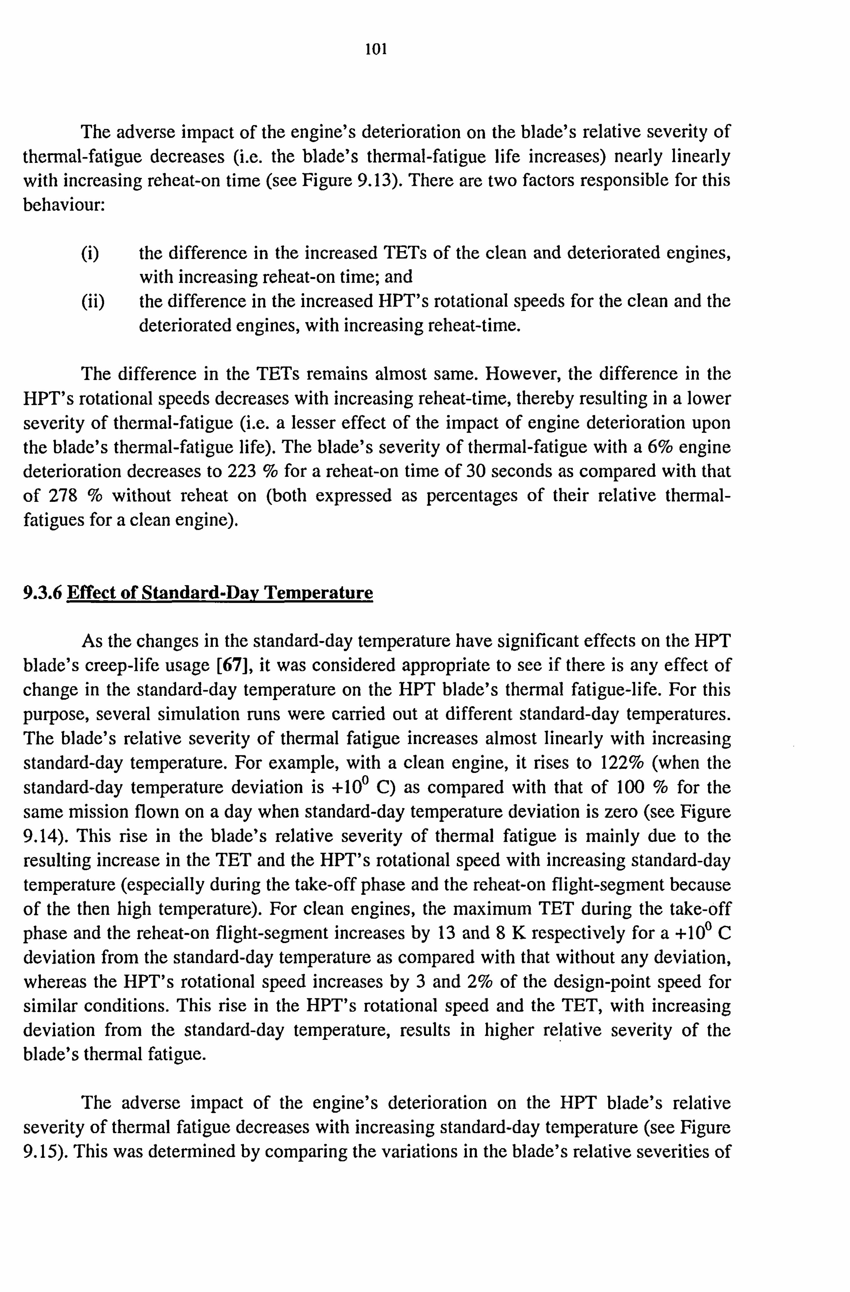
101

The adverse impact of the engine's deterioration on the blade's relative severity of thermal-fatigue decreases (i. e. the blade's thermal-fatigue life increases) nearly linearly with increasing reheat-on time (see Figure 9.13). There are two factors responsible for this behaviour:

the difference in the increased TETs of the clean and deteriorated engines, with increasing reheat-on time; and the difference in the increased HPT's rotational speeds for the clean and the deteriorated engines, with increasing reheat-time.

The difference in the TETs remains almost same. However, the difference in the HPT's rotational speeds decreases with increasing reheat-time, thereby resulting in a lower severity of thermal-fatigue (i. e. a lesser effect of the impact of engine deterioration upon the blade's thermal-fatigue life). The blade's severity of thermal-fatigue with a 6% engine deterioration decreases to 223 % for a reheat-on time of 30 seconds as compared with that of 279 % without reheat on (both expressed as percentages of their relative thermal- fatigues for a clean engine).


As the changes in the standard-day temperature have significant effects on the HPT blade's creep-life usage [67], it was considered appropriate to see if there is any effect of change in the standard-day temperature on the HPT blade's thermal fatigue-life. For this purpose, several simulation runs were carried out at different standard-day temperatures. The blade's relative severity of thermal fatigue increases almost linearly with increasing standard-day temperature. For example, with a clean engine, it rises to 122% (when the standard-day temperature deviation is +100 Q as compared with that of 100 % for the same mission flown on a day when standard-day temperature deviation is zero (see Figure 9.14). This rise in the blade's relative severity of thermal fatigue is mainly due to the resulting increase in the TET and the HPT's rotational speed with increasing standard-day temperature (especially during the take-off phase and the reheat-on flight-segment because of the then high temperature). For clean engines, the maximum TET during the take-off phase and the reheat-on flight-segment increases by 13 and 9K respectively for a +10() C deviation from the standard-day temperature as compared with that without any deviation, whereas the HPT's rotational speed increases by 3 and 2% of the design-point speed for similar conditions. This rise in the HPT's rotational speed and the TET, with increasing deviation from the standard-day temperature, results in higher relative severity of the blade's thermal fatigue.

The adverse impact of the engine's deterioration on the HPT blade's relative severity of thermal fatigue decreases with increasing standard-day temperature (see Figure 9.15). This was determined by comparing the variations in the blade's relative severities of

102

thermal fatigue (for the clean as well as the engine suffering deterioration) due to variations from the standard-day temperature. For a 6% deteriorated engine, the blade's

relative severity of thermal fatigue reduces to 232% on a day with a +100 C deviation from

standard-day temperature, as compared with that of 282% on a day without any deviation from the standard-day temperature. Both values are expressed as percentages of the blade's

relative severity of then-nal fatigue for a clean engine, under the stipulated standard-day temperature deviation. The main reason for this behaviour is the variation in the resulting difference in the HPT's rotational speeds and the TETs (for the deteriorated and clean engine) with increasing deviation from the standard-day temperature. Higher differences of these two characteristics (with HPT's rotational speed and TET for deteriorated engine greater than that for clean engine) mean a greater adverse impact of the engine's deterioration upon blade's relative severity of thermal fatigue. For the considered case, during the reheat-on flight-segment, the variation of the differences in the maximum TETs

and HPT's rotational speeds for the deteriorated and clean engine is quite small. The variation of the differences in the HPT's rotational speeds and TETs (with zero and +100 C deviation from the standard-day temperature) is only 1% and 3K respectively. However, during the take-off phase, these variations are significant. The difference in the HPT's

rotational speed for the deteriorated and clean engine is 3 and 13% (the HPT's rotational speed for the deteriorated engine being higher) at zero and +100 C deviation from standard- day temperature respectively. Whereas the difference in TETs for the deteriorated and clean engine is 217 and 163 K (TET for the deteriorated engine being higher) at zero and +100 C deviation from standard-day temperature respectively. Therefore, the nature and the extent of the variation in the differences of the HPT's rotational speed and TET with increasing deviation from standard-day temperature result in lower adverse impacts of the engine's deterioration upon the blade's relative severity of thermal fatigue.


LPC deterioration is the most serious factor in terms of its effects upon the blade's thermal-fatigue. Therefore, in addition to the impacts of the LPC's fouling, which combines the deteriorating flow capacity and efficiency, the impacts of these two parameters upon blade's relative severity of thermal-fatigue were also analysed separately. For a 5% LPC's flow-capacity deterioration, the blade's severity of thermal-fatigue increases (i. e. the blade's thermal-fatigue life decreases) with slightly increasing rate of rise, with increasing efficiency deterioration (see Figure 9.16). For example for a 10% efficiency deterioration, the blade's relative severity of thermal-fatigue rises to 294% as compared with that of 100% without any efficiency deterioration. On the other hand, for a 5% LPC's efficiency-deterioration, the blade's relative severity of thermal-fatigue increases in the beginning but immediately starts decreasing at a faster rate but subsequently at a comparatively lower rate with the increasing LPC's flow capacity deterioration (see Figure 9.17). For example the blade's severity of thermal-fatigue is 112,

103

105,88 and 60% at 1,2,4 and 10% LPC's flow-capacity deterioration respectively, as compared with that of 100% without any LPC's flow-capacity deterioration.

104

CHAPTER10

DISCUSSIONS AND SUMMARY OF PREDICTIONS

10.0 Introduction

Detailed discussions and analyses of the predictions regarding the implications of the engine's deterioration upon the aircraft's mission operation al-effectiveness, aircraft engine's fuel usage and its HPT blade's creep life, low-cycle fatigue-life-consumption and thermal fatigue-life have already been presented separately in chapter 5,6,7,8 and 9 respectively. This chapter describes only those considerations that are related to present investigation and which are also important from an overall point of view. A summary of predictions in chapter 5 -> 9 is also presented in this chapter. Efforts have been made to describe only the overall picture and inter relationships among different predictions and avoid any repetition of material from previous chapters.

10.1 Thrust-Setting Parameter

Although jet engines have been used commercially for 40 years, there is still no direct method of measuring the thrust generated during flight. So indirect methods, based on pressure measurements or rotational speeds, are used. The three most common indirect thrust-setting parameters are [3]:

Fan-rotor's speed, which is also called the LP spool speed, NJ Engine's pressure-ratio (EPR), (of the exhaust to the engine's inlet-

pressure). 0 Integrated engine pressure-ratio (IEPR).

Other parameters are used in combination with the three primary thrust-setting parameters to give an indication of the engine's operational condition. The most common secondary indicators are: core speed (NA fuel flow (FF) and the turbine's temperature. Significant variations from nominal (i. e. values at reference design conditions) N, versus N2, an abnormally high FF to maintain a desired cruise speed (or to generate sufficient take-off thrust) and an abnormally high temperature are usually indicative of engine deterioration, which may eventually lead to a breakdown [3].

While the thermodynamic basis for using either the EPR or the IEPR as the primary-thrust indicator is straightforward, such pressure ratios fail to provide an

105

instinctive "feel" for the thrust developed. However, rotational speeds, such as NJ, can be related readily to thrust: anyone who has driven a vehicle equipped with a tachometer can readily recognise the red-line limits and instinctively keep within them.

Stevenson and Saravanamuttoo [3] determined the effects of both engine-cycle choice and various forms of in-service deterioration on the performance and concluded that there is no major difference between the attributes of the three most popular thrust- indicators listed earlier. However, N, provides a better intuitive appreciation of thrust level and appears to be less sensitive to changes in engine cycles. Thus, for the present investigation, the fan speed N, has been adopted as the thrust-setting parameter.

10.2 Temperature-Limit Control

For the purpose of predicting implications of engine deteriorations upon the aircraft's operational effectiveness, initially, it was assumed that there is no temperature- limit control as is employed later, when investigating the implications of engine deterioration upon fuel and life usages. However, initial predictions from the simulations were rather unexpected, e. g. the LPC or HPC deterioration simulations yielded increased thrusts for the same flight conditions and fan-speed settings. Before discussing this further, it is important to consider the role of temperature limit control for an actual turbofan operation. At first glance, an increase in net thrust with a drop in the efficiency of a particular component may appear odd. However, such results can be explained by examining what happens to the temperatures inside the engine, especially the TET. In the case of the LPC or HPC, the efficiency drops, the exit temperatures increase: these lead to rises of the TET and hot-end temperature. An increased TET, in general, results in more thrust, but at the penalty of increased rate of fuel-bum and decreased engine-life [3]. If the 100% design point TET is used as the limiting TET value, the increased thrust perfon-nance due to increased TET will not be realised. In practice, the TET will be limited by adjusting the fuel flow, so resulting in a reduction in the fan's speed. It is also important to note that, while Ni appears to be independent of any efficiency drops of the engines' components, the EPR is directly affected because changes in component efficiencies cause changes in the LPT's exhaust-pressure. This is the main reason for the differences in net thrust when the TET limit is applied [3]. So the computer model was enhanced to cater for the temperature-] imit control. For the purpose of the present investigation, the 100% design point TET value has been assumed to be the TET limiting value throughout the mission profile W.

10.3 Multiple-Component Deterioration

The aims of this investigation were twofold. Firstly, to detennine the effects of single component deterioration on the aircraft's operational effectiveness as well as fuel

106

and life usage under different flying conditions. Secondly, to determine if the effects of single-component deterioration can be superimposed upon one another, thus providing an insight into the effects of multiple-component deterioration. This was undertaken due to the potential benefits that could be realized if this hypothesis was found to be valid, or if there was an easily-identifiable correlation. This would have allowed the determination of the impacts of multiple component deterioration based on knowledge of the conditions of each of the modules separately. Once this impact has been predicted, then it will be easy for users and managers to take corrective or remedial actions with greater confidence. The analysis carried out was similar to that used for the single component degradations, and involved a multitude of engine simulation runs with various multiple degradations implanted. To carry out the required analysis, over 150 engine-simulation runs were required: each run took approximately 30 to 35 minutes of computer time. Regrettably, the results obtained suggested that superimposition was not generally valid. Nevertheless, it is author's belief that some form of complex correlation does exist between multiple implanted deterioration and the fuel & life usage. Regrettably this investigation was unable to develop that correlation, but was able to conclude that the effect of multiple deterioration is not an additive process.

10.4 Comparing the Deteriorated and Clean En2ines

To analyze the implications upon aircraft's mission operational-effectiveness, aircraft engine's fuel usage and its HPT blade's life usage for a "deteriorated" engine, comparison was made on a percentage basis with that for an engine suffering no deterioration. This eliminated common factors, i. e. unchanged parameters, and isolated the effects of the changed parameter. It cancelled out any discrepancy in the procedure or deficiency in the available data and also made the results more representative for a generic two-spool turbofan engine. The fact that the engine being simulated is of a two-spool configuration is significant when examining the results, as the impact of a deterioration on different spools provided conflicting results. In the majority of situations due to the deterioration, the engine responded by increasing the TET with minimal changes in the RPM. It is unknown if the actual engine responds in a similar manner, and would require substantial engine data to verify this assertion.

10.5 Some Assumptions, Considerations and Limitations

A component does not have to fracture in order to fail in service: its performance can deteriorate to such an extent that it requires replacement. A failure due to component deterioration, is defined, by the performance or capability decline in relation to that which occurred when it was new. If the deterioration becomes such that the component needs to be replaced, then it is considered to have failed. For the purpose of this investigation, it was assumed that component is replaced at a deterioration level of 10 % for individual

107

components and at 6% for whole engine. Failures in components are mainly due to: design deficiencies, material defects, manufacturing deficiencies, assembly errors, unintended service operation, failure to follow maintenance procedures, improper operation, adverse environmental conditions and abuse [10).

Gas-turbine engine components are subjected to a complex system of both steady and cyclic, thermal fatigue, and inertial stresses. These in combination with the effects of creep will eventually cause components to fail. In an effort to determine the safe-life limits, an understanding of the effects of these combined stresses is required-see Arvantis et. al. [69) and Breitkopf et. al. [70]. Arvantis described a multi-axial life-prediction system using a ductility exhaustion method, that includes the evaluation of transient metal temperatures, corresponding elastic and inelastic strains, creep, and subsequently creep and fatigue lives. Breitkopf used a method of determining the transient temperatures at different locations throughout the turbine disk, deducing the thermal gradients from these temperatures and then superimposing the fatigue stresses at these locations. These two methods demonstrate that the analysis of complex stresses in gas-turbine engines is feasible but complicated, and requires access to data that are not readily available. As such, the majority of the literature tends to look at life limits based on more simplistic approaches. In this investigation, the combined effects of creep and fatigue are not considered. Rather each of the different failute mechanisms has been looked at separately.

It is assumed that the gas-bending load on each turbine-blade's aerofoil is negligible and therefore was not considered in the present analysis. Also no thermal gradient was taken into account. The only practical mechanical loading that was applied to the blades under operating conditions that was considered was the direct centrifugal load. This was assumed to be distributed uniformly. The effect of the environment also was not studied in this investigation. It is well known that the operating environment inside the hot- gas path of a gas turbine is extremely hostile. The compound most commonly found is Na2SO4. which is formed in the combustion chambers of the gas turbine by the reaction of Na-containing salts such as NaCl, which may be present in the air or fuel with S02 and S03 created by the combustion of, the sulphur-bearing fuel. In conventional operating environments, the conversion of NaCl to Na2S04 occurs according to the following reaction [71]:

2 Na Cl+S02 +1 (02)+ H20

--> Na2 S04 +2H Cl ------------------------ 2

The Na2SO4 deposit is molten at the elevated temperatures on the metal surfaces of the first-stage vanes and rotor blades. This modifies the oxidation conditions at the metal surfaces and so results in accelerated corrosion, because of the formation of sulphides at the interface between the metal and the oxide layer. Corrosion then penetrates along the grain boundaries into the metal, and also causes blistering of the protective oxide-layer. Under a creep load, the stress field will promote the corrosion attack on the grain

108

boundaries so leading to severe degradation [71]. This creep-corrosion interaction is a complex phenomenon, and therefore not considered in this investigation.

10.6 Statistical Data

In this investigation, the emphasis has been placed upon the need to have actual statistical data concerning engine operating conditions in order to develop a rational programme for calculating fuel and life usage. Statistical data will reveal the magnitude of the usage variation between engines having the same total number of hours of operation and will demonstrate, in advance, the gains likely to be achieved. Whether or not substantial benefits are likely will depend on the type and role of the A/C.

Statistical data are required concerning the significance of other phenomena on engine's fuel and life usage, and in the study of how due account may be taken of them in determining engine-overhaul programmes. Examples of such relative ignorance are the effects of variations in stress and temperature on the turbine disc (e. g. low-cycle fatigue), and the cracking of parts by thermal-shock effects. Statistical data on the number and magnitude of changes in RPM and temperature, and on the rates of change of temperature, are necessary when trying to evaluate such effects. It should not be overlooked, of course, that if statistical data recording is undertaken, it will normally be most desirable to take the opportunity simultaneously of obtaining data on a broader range of variables than the RPM and TET, with which we have been primarily concerned in this investigation. Study of the lives of some components will involve other considerations. The behaviour of compressor blades for example, may be expected to be influenced by the air-intake conditions, as well as by the engine's RPM, so that records of the A/Cs speed and altitude as well as the air temperature, will be required [72].

10.7 Summary of Predictions

An important factor, which needs to be realised when examining the results, is that the numerical values for the effects of deterioration are not definitive, but nevertheless are considered good "ball park" figures. In addition, the trends of the effects are important as they provide an insight into how the engine behaves. The points that do not fall on the smooth curve are the results of the engine's complexity and insufficient data being available. Moreover, as there have been in excess of 750 simulated engine-runs, the results provide a comprehensive analysis of the effects of engine deterioration in the majority of situations.

For a specified aircraft's mission profile, the deteriorated engine normally seeks a different steady operating point relative to that for an engine without any deterioration. The

109

variation in the engine's steady operating-point results in changes in the engine's parameters / characteristics such as:

thrust available from engines; specific fuel-consumption; turbine's entry temperature (TET); and

(iv) HPT's rotational speed.

Besides the engine's deterioration, any change in the operating / surrounding conditions such as the aircraft's cruising-altitude and Mach number, engine's reheat-on duration and standard-day temperature also result in changes in the above mentioned engine parameters. These changes are also affected by the engine's temperature-control (i. e. TET limiting value) and any lower and upper limit imposed for the LP and/or HP spoolspeed.

Any rise in the available thrust from the engines, especially the maximum thrust available, results in an improved aircraft's mission operational-effectiveness, whereas any rise in the specific fuel-consumPtion increases the fuel usage and thereby the fuel to be carried by the aircraft for a specified mission profile. A rise in the TET increases the HPT blade's metal temperature and therefore, results in more creep and thermal fatigue damage to the blades. A rise in the HPT's rotational speed results in a greater blade's LCF life- consumption. It also increases the HPT blade's relative temperature and therefore, contributes towards greater blade's creep and thermal fatigue damage.

For the conditions assumed in this investigation, for same the level of TET, the SFC rises whereas the available thrust from the engines reduces with increasing engine's deterioration. Reduction in the available thrust (especially the maximum available thrust) results in a reduced aircrafts mission operational-effectiveness. This also contributes towards higher blade's creep damage, because of the more time taken by the aircraft during the take-off phase (i. e. a high temperature zone of the mission's profile). A reduction in the available thrust is also accompanied by a reduction in the LP and HP spool speeds with increasing engine's deterioration. In order to keep the aircraft's perforinance invariant (i. e. during the mission profile 'B'), the deteriorated engines are run at a higher TET. An increase in the TET increases the blade's creep and the thermal fatigue damage. An increase in the TET is also accompanied by an increase in the LP and HP spool speeds. However, for the same level of thrust developed, the HP spool speed still remains lower for the 6% deteriorated engine as compared with that for the clean engine. A reduced HPT's rotational speed results in a lower blade's LCF life-consumption. It also reduces the creep and thermal fatigue damage by lowering the blade's relative temperature. However, this favourable effect upon the creep and thermal fatigue lives is exceeded by the negative one of a much larger increase in the TET. For the engine suffering a 6% deterioration, the aircraft's mission operational-effectiveness, the aircraft engine's HPT blade's creep life and the LCF life-consumption reduce by 75,86 and 40 % respectively, whereas aircraft

110

engine's fuel usage and its HPT blade's relative severity of thermal fatigue increase by 14 and 120 % respectively as compared with that for a clean engine.

For the same level of TET, the SFC and NT available from the engines both decrease with increasing aircraft's cruising altitude. The aircraft's drag and thereby thrust requirement also reduce upon increasing the aircraft's cruising altitude. In order to keep the aircraft's performance invariant, the reduction in NT requires the engines to run at a higher TET and HPT's rotational speed, whereas the reduction in the aircraft's thrust requirement requires the engine to run at lower TET and HPT's rotational speed. The overall effect of these two factors results in decreasing the TET and the HPT's rotational speed until the end of troposphere (i. e. 11000 metres altitude). Above I 1000 metres, the TET and the HPT's rotational speed start increasing because the atmospheric temperature remains almost constant within the stratosphere (thereby resulting in the lower rate of reduction of the aircraft's thrust requirement). The decreasing atmospheric temperature, within the troposphere, also results in the aircraft's true air speed being smaller. This contributes favourablY towards the creep life, because aircraft takes more time to cruise and thereby more time to spent with a comparatively lower TET as compared with high temperature zones of the flight path such as take-off phase and reheat-on flight segment. For engines suffering 6% deterioration, the engine's fuel usage, HPT blade's creep life, LCF life- consumption and relative severity of thermal fatigue are 80,118,99.6 and 97 % while aircraft cruises at approximately 10500 metres altitude and 72,41,115 and 128 % when aircraft cruises at 15000 metres respectively as compared with that of all four being 100% with aircraft cruising at 8000 metres altitude.

For the same levels of TET, the SFC increases, whereas the NT available from the engine decreases with increasing the aircraft's cruising Mach number. The aircraft's drag and thereby thrust requirement rise upon increasing the aircraft's cruising Mach number. For the same aircraft's performance, the overall effect of reducing the thrust available from the engines and the increasing aircraft's thrust requirement upon increasing the aircraft's cruising Mach number results in the engines running at higher TET and HPT's rotational speed. For engines suffering a 6% deterioration, the engine's fuel usage, HPT blade's creep life, LCF life-consumption and relative severity of thermal fatigue are 166,2.3,131 and 203 % while the aircraft cruises at a Mach number of 1.5 as compared with that of all four being 100% when the aircraft cruises. at Mach number of unity.

For the same level of TET, the SFC increases slightly whereas the NT available from engine decreases with increasing standard-day temperature. The aircraft's drag and thereby thrust requirement increase slightly with increasing standard-day temperature. The overall effect of the reduced thrust available from engines and at the same time increased aircraft's thrust requirement to keep the aircraft's performance invariant, results in engines running at higher TET with a little variation in HPT's rotational speed. For engines suffering a 6% deterioration, the engine's fuel usage, HPT blade's creep life, LCF life- consumption and relative severity of thermal fatigue are 101.7,55,99.88 and 122 % with +

III

100 C deviation from the standard-day temperature as compared with that of all four being 100% without any deviation from the standard-day temperature.

The SFC reduces abruptly on switching on the reheat and then it starts increasing almost linearly with increasing reheat-on time. Also the TET and the HPT's rotational speed increase with increasing reheat-on time. Increasing the reheat-on time also results in more time being spent with high values of the TET and HPT's rowional speed and thereby shortening the blade's creep life. For engines suffering a 6% deterioration, the engine's fuel usage, HPT blade's creep life, LCF life-consumption and relative severity of thermal fatigue are 100.5,22,121 and 320 % respectively with 30 minutes of reheat-on operation as compared with that for all four parameters being 100% without any reheat.

Large variations in blade-life usage occur during the simulated flight with relatively small changes in the operating conditions. Expressing this more dramatically, one could say that, with respect to blade's life usage, one minute at take-off power is equivalent to nearly seven hours operation at maximum continuous conditions [72]. Thus blade-life usage varies greatly during the different phases of a specific flight-profile, and consequently for different profiles involving different times at various operating conditions, there can be large differences in the total life-usage. Even for nominally similar flight-profiles, there will be differences because of minor variations in the engines' conditions from one flight to another. It is therefore evident that, in real circumstances, there will be wide variations in the actual life-usage from engine to engine during a given number of hours flying.

112

CHAPTER11

CONCLUSIONS AND RECOMMENDATIONS

11.1 Conclusions

This investigation has quantified the impacts of various deteriorations in the aircraft's engine or its components upon the: -

aircraft's mission operational-effectiveness; aircraft engine's fuel usage; HPT blade's creep-life;

(iv) HPT blade's LCF-life consumption; and (v) HPT blade's thermal-fatigue life.

For the conditions assumed, the take-off phase was the most stressful followed by the climb after take-off (to a pre-selected altitude, while accelerating to a pre-selected Mach number) flight-segment in terms of its adverse effect on the mission's operational- effectiveness. Among the major engine components (i. e. LPC, HPC, LPT and HPT) considered in this investigation, the deterioration of the HPC has the most adverse effect upon the aircraft's mission operational-effectiveness.

For the conditions assumed in this investigation, the LPC fouling was the most deleterious phenomenon encountered in terms of its adverse effects upon the aircraft engine's fuel usage and its HPT blade's creep-life, LCF-life consumption as well as thermal-fatigue life. A slight variation in mission profile, especially during the take-off phase and reheat-on flight segment greatly influences the HPT blade's creep and thermal fatigue lives. It is also concluded that the impacts of deterioration for different engine's components is not an additive process (i. e. the impacts of deterioration of individual engine's components cannot be superimposed linearly).

The effects of variations in the following, on the aircraft engine's fuel usage as well as its HPT blade's life-usage, were significant: -

aircraft's cruising Mach number aircraft's cruising altitude reheat-on time standard-day temperature

This investigation has highlighted the importance of having installed the appropriate instrumentation to monitor the compressor's deterioration (e. g. due to fouling),

113

turbine deterioration (as a result of erosion) and consequently reduction in the mission's operational effectiveness. It is only with such instrumentation to monitor these parameters that managers can make wise decisions in order to reduce the adverse effects of engine deterioration on aircraft's operation al-effectiveness as well as the engine's fuel and life usage. The absence of appropriate instrumentation and ignorance of compressor fouling or turbine erosion and thereby reduction in the mission's operational effectiveness can lead to many in-flight problems, which contribute towards operational inefficiency. Some of these problems are: -

(a) In the case of a mass air-raid upon a target, normally aircraft are required to take-off from several locations and meet at a specified TOT (time-on-target). The aircraft suffering engine deterioration will tend to lag behind because of the lower thrust available and hence it will take longer to reach the target.

(b) In the case of formation flying, the aircraft with engines suffering deterioration may not be able to accelerate to a specified flight-speed if it is very close to the maximum achievable flight speed with clean engines. This wi ,

11 result in a mission abort and therefore greatly reduce the mission's operational effectiveness.

(c) In the case of formation flying, when the specified flight speed is significantly lower than the maximum achievable flight-speed, although the aircraft with engines suffering deterioration will not lag behind and keep on flying with the rest of the formation, this will be achieved at the cost of running the engines hotter (as compared with the situation when the engines are clean) and therefore a higher fuel-flow will be incurred. This situation will ultimately lead to the aircraft with engines suffering deterioration seeking a priority landing because of its shortage of fuel on its return flight. This can be serious when the runway at the home base is closed or damaged and the aircraft has to be diverted for landing to another airfield.

Use of appropriate instrumentation and the results of such an investigation as the present for a variety of mission profiles under various operating conditions will provide a wide data base and can lead to managers taking wiser decisions concerning the following considerations: -

Planning compressor washings and necessary repairs. Grouping aircraft, with similartypes and degrees of engine deterioration,

when planning mission profiles. 0 Planning different fuel and weapon weights, so maintaining the same gross aircraft take-off weight.

Planning different take-off timings for aircraft with different types and degrees of engine deterioration. 0 Briefing the pilots of aircraft with engines suffering deterioration to fly hotter (i. e. at higher power settings) provided it is permitted by the specified "handle" (such as the TET and rotational speed) range.

114

Changing the aircraft's mission profile and/or configuration. Planning flights under different operating conditions (e. g. time of day

corresponding to the pertaining temperature conditions).

Hence the engine utilization and operational -effectiveness of the mission can be improved. However, greater benefits will be achieved if the present analysis is considered as a complete package (i. e. consisting of a more comprehensive analysis including aircraft's mission operation a]-effectiveness and aircraft engine's fuel and life-usage aspects).

The lack of complete engine-performance measurements has been a handicap in this investigation. It is desirable that efforts should be made to obtain such data in order to be able to predict the impacts of engine's deterioration more accurately.

11.2 Recommendations

This study took a new and unique approach to examine the implications of an aero- engine's deterioration for a military aircraft, through the use of computer simulation techniques. The computer program developed was able to resolve the objectives of this thesis. The author believes that the predictions and conclusions developed have significantly advanced this area of study. However, there remain other potential areas of study; and possible enhancement to the model, such as are enlisted below.

11.2.1 PotentiaI Areas of Stud

Besides the present study, there are other potential areas where the present model could be applied. These include:

predicting the implications of changing the aircraft's payload, drag, wing area, wing sweep angle, aspect ratio and maximum lift coefficient (separately or any combination of these) upon the aircraft's mission operation al-effectiveness, aircraft engine's fuel usage and its HPT blade's life usage. predicting the effects of different HPT blade's materials upon the blade's life usage and thereby obtaining a trade-off between the factors influencing the blade's design (i. e. weight, stressing, production cost and service life. selecting the best suitable engine to be fitted to an aircraft, thereby enabling it to achieve a specified level of performance.

(iv) comparing the effects of engine's deteriorations for different types of engines (e. g. between a single-spool and a two-spool engine).

115

11.2.2 Possible Enhancements

There are several pertinent further avenues that can be explored. Possible improvements to the existing model are:

enhancing the engine perform ance-simul ati on model to be able to model transient behaviour; enhancing the applicability of aircraft's flight path and performance- simulation model by incorporating more of the aircraft's design parameters in order to make it more comprehensive and generic; enhancing the HPT blade's life-usage prediction model by:

a. developing LCF life-consumption algorithms that account for both the mechanically-induced stresses and the thermal stresses that are present in the engine and apply this to the data made available from a transient program; and

b. developing the thermal fatigue-life model, as the present model only predicts the relative severity of thermal fatigue.

11.2.3 Furtber Investi2ations

There remain several areas that require further investigation. These include:

the prediction of true engine's deterioration levels (i. e. in terms of EDI, FI

and EI as used in this thesis) through the use of computer simulation techniques; and the prediction of a correlation between multiple engine's component deteriorations and the aircraft's mission operational-effectiveness, aircraft engine's performance, fuel usage and its HPT blade's life-usage.

It would be wise to refine the present computer model by conducting a similar study as the present, but with a proper participation of aircraft and engine's manufacturers as well as the agency using the aircraft. Their participation will ensure the availability of true and realistic data regarding the aircraft and engine's design and performance, HPT blade material's properties and the mission profile of the aircraft.

116

REFERENCES

1. Devereux B. and Singh R., "Use of computer simulation techniques to assess thrust rating as a means of reducing turbo-jet life cycle costs". International Gas-Turbine and Aero Engine Congress and Exposition, The Hague, Netherlands, June 13-16,1994.

2. Naeem M., "Fuel usage and its effects on operational performance for GE-F404/F-18", MSc Thesis, Cranfield University, UK, 1996.

3. Stevenson J. D. and Saravanamuttoo H. 1. H., "Effects of cycle choice and deterioration on thrust indicators for civil engines" ISABE 95-7077, Twelfth International Symposium on Air-Breathing Engines, Melbourne, Australia, Sep 10- 15,1995.

4. Escher P. C., "PYTHIA: an object oriented gas-path analysis computer-program for general applications", Ph. D. Thesis, Cranfield University UK, 1995.

,? "Sallee G. P., "Performance deterioration based on existing (historical) data, NASA-CR-

135448, May 1980.

6. Sallee G. P., Kruckenberg H. D. and Toomy E. H., "Analysis of turbofan-engine perfonnance deterioration and proposed follow-on test", NASA-CR-134769, Oct. 1986.

7. Heywood I B., "Future engine-technology: lessons from the 1980s for the 1990s", Journal of Engineering for Gas Turbines and Power, Vol. 113, pp. 319-330,199 1.

v-& Little P. D., "The effects of gas turbine engine degradation on life usage" M. Sc Thesis, Cranfield University, UK, 1994.

9. MacDonald S., "A dynamic simulation of the GE F404 engine for the purpose of engine health monitoring", M. Sc Thesis, Cranfield University, UK, 1993.

10. Grewal A S., "Gas-turbine engine performance deterioration modelling and analysis", Ph. D Thesis, Cranfield University, UK, 1988.

11. Saravanamuttoo H. 1. H. and Lakshminarasimha A. N., "A preliminary assessment of compressor fouling", ASME 85-GT-153, March, 1985.

12. Zhu P. and Saravanamuttoo H. 1. H., "Simulation of advanced twin-spool industrial gas turbine", ASME 91 -GT-34, June, 199 1.

13. Bammert K. and Stobe H., "Results of experiments for determining the influence of blade-profile changes and manufacturing tolerances on efficiency, the enthalpy drop and the mass flow of multi-stage axial turbines", ASME Paper No. 70-WA/GT-4,1970.

117

14. Bammert K. and Woelk G. U., "The influence of the blading-surfaces roughness on the aerodynamics behavior and characteristics of an axial compressor", ASME Journal of Engineering for Power, Vol. 102, No. 2,1980.

15. Degreef I L., Maes P. and Johnson K. W., "Operating experience on residual fuel oil with a W251 combustion turbine", ASME Paper No. 78-GT-104,1978.

16. Haub G. L. and Hauhe W. E., "Field evaluation of on-line compressor cleaning in heavy-duty industrial gas-turbines", ASME Paper No. 90-GT-107,1990.

17. Diakunchak 1. S., "Performance deterioration in industrial gas-turbines", Journal of Engineering for Gas Turbines and Power, Vol. 114, pp. 161-168,1992.

18. Thames J. M., Stegmaier I W. and Ford J. J., "On-line washing practices and benefits", ASME Paper No. 89-GT-91,1989.

19. BaIderstone A. W., "A generic computer model to predict an acro-engine's low-cycle fatigue", M. Sc Thesis, Cranfield University, UK, 1996.

20. Tabakoff W., "Compressor erosion and performance deterioration", Lecture presented at the Department of Aerospace Engineering and Engineering Mechanics, University of Cincinnati, Cincinnati, Ohio, May 1986.

2 1. Dunn M. G., . Padova C., Moller J. E. and Adams R. M., "Performance deteriorations of a turbofan and a turbojet engine upon exposure to a dust environment ASME 87-GT- I 11, Feb, 1987.

22. Acker G. F. and Saravanamuttoo H. 1. H., "Predicting a gas-turbine's performance- degradation due to compressor fouling using computer simulation techniques", ASME 88- GT-206, Aug, 1987.

23. Seddigh F. and Saravanamuttoo H. 1. H., "A proposed method for assessing the susceptibility of axial compressors to fouling", Journal of Engineering for Gas Turbines and Power, Vol. 113, pp. 595-601,199 1.

24. Sallee G. P., " Performance deterioration based on in-service engine data", JT9D jet- engine diagnostic program, NASA CR- 15925, July 1980.

25. Lakshminarasimha A. N., Boyce A P. and Meher-Homji C. B., "Modelling and analysis of gas-turbine perfonnance deterioration", Journal of Engineering for Gas Turbines and Power, Vol. 116, pp. 46-52,1994.

26. Viswanathan R. and Dolbec A. C., "Life-assessment technology for a combustion turbine-blades", Journal of Engineering for Gas Turbines and Power, Vol. 109, pp. 115- 123,1987.

119

27. Devereux B., "Improving life-usage of the F404 engine through thrust rating", M. Sc Thesis, Cranfield University, UK, 1992.

28. Cookson R. A., "Environmental influences on fatigue", School of Mechanical Engineering, Cranfield University, UK, Notes SME/PPA/RAC/2245,1996.

29. Cookson R A., "Properties of materials-fatigue", Lecture Notes SME/PPA/RAC/2198, Cranfield University UK, 1996.

3P. David A. Spera. and Salvatore J. Grisaffe., "Life predictions of turbine components: on-going studies at the NASA Lewis Research Center", NASA TM X-2664, Jan, 1973.

g. Wu F. E., "Aero-engine's life evaluated for combined creep and fatigue, and extended by trading-off excess thrust ... ... Ph. D. Thesis, Cranfield University, UK, 1994.

32. Cookson R. A., "Loads and operating conditions experienced by an aero gas turbine ", Cranfield University, School of Mechanical Engineering Notes, SME/PPA/RAC/2269, 1996.

33. Jackson P., Munson K. and Taylor J. W. R., "Jane's All the World's Aircraft", published by Jane's Information Group Ltd., Sentinel house, 163 Brighton Road, Coulsdon, Surrey, UK, 1995-96.

34. Palmer I R., "The TURBOMATCH scheme for gas-turbine performance calculations: user's guide", Cranfield University, UK, 1983.

35. Daniel P. Raymer., "Aircraft design: a conceptual approach (AIAA education series) published by American Institute of Aeronautics and Astronautics, Inc., Washington, DC, 1992.

36. Cookson R. A., "Mechanical design of turbornachinery - Creep", Notes SME/PPA/RAC/1998, School of Mechanical Engineering, Cranfield University, UK.

37. Penny R. K. and Weber M. A., "Integrity assessment of components in the creep range", ASME paper 90-GT- 125, Jan, 1990.

. W. Harrison G. F., Smith M. and Nurse J., "Algorithm for an aero-engine's component life-usage prediction: a UK perspective", DRA TR 93043, UK, July, 1993.

39. Hall C. L., Hathaway R. W. and Cote S. M., "Investigation of F/A-18A engine- throttle usage and parametric sensitivities", ASME Journal of Engineering for Power, Vol. 105, pp. 627-634, July, 1983.

119

40. Deitrick C. C. and Schuppan K. L., "Engine-usage prediction for advanced fighter

aircraff', American Institute of Aeronautics and Astronautics, Report No. AIAA-81-1367, July, 198 1.

41. Stabrylla R. G. and Troha W. A., "Effect of an aircraft's power-plant usage on a turbine engine's relative durability/life", American Institute of Aeronautics and Astronautics, Report No. AIAA-80-1115, July, 1980.

42. O'Connor C. M., "Military engine condition monitoring systems: the UK experience", Advisory Group for Aerospace Research and Development, 7 Rue Ancelle 92200 Neuilly Sur Seine France, Conference Proceedings, AGARD-CP-448,1988.

43. May Jnr R. J., Chaffee D. R., Sturnbo P. B. and Reitz M. D., "Tactical aircraft engine usage-a statistical study", American Institute of Aeronautics and Astronautics, Report No. AIAA-81-1652, August, 198 1.

44. Watson P. and Dabell B. J., "Cycle counting and fatigue damage", Journal of the Society of Environmental Engineers, Vol. 15-3 (issue 70), pp. 3-8, September, 1976.

45. Powling N. E., "Fatigue failure predictions for complicated stress-strain histories", Journal of Materials, ASTM, Vol. 7, No. 1, pp. 71-87, March, 1972.

46. Matsuishi M. and Endo T., "Fatigue of metals subjected to varying stress" Paper presented to Japan Society of Mechanical Engineers Conference, Fukuoka, Japan, March, 1969.

47. Downing S. D. and Socie D. F., "Simple rainflow counting algorithms", International Journal of Fatigue, Vol. 4, No. 1, pp. 31-40, January, 1982.

48. Rychfik I., "A new definition of the rainflow cycle counting method", International Journal of Fatigue, Vol. 9, No. 2, pp. 119-12 1, April, 1987.

49. ESDU "Fatigue-life estimation under variable-amplitude loading using cumulative damage calculations", Fatigue-Endurance Data Contents, Vol. 2, Guide card No. 95006, ESDU International p1c, 27 Corsham Street, London, September, 1995.

50. Raske D. T. and Morrow J., "Mechanics of materials in low cycle fatigue testing", ASTM STP 465, American Society for Testing and Materials, pp. 1-26,1969.

51. Basquin 0. H., "The exponential law of endurance tests", Proceedings of the American Society of Testing of Materials, Vol. 10, pp. 625-630,1910.

120

52. Manson S. S., " Behaviour of materials under conditions of thermal stress", NACA TN 2933,1953.

53. Coffin L. F., "A study of the effects of cyclic thermal stresses on a ductile metal", Transactions of the ASME (Series A), Vol. 76, pp. 931-950,1954.

54. James A. G., "Fatigue-design hand book: a guide for product design and development engineers", SAE, Advances in Engineering, Vol. 4,1968.

55. Wetzel R. M., "Fatigue under complex loading: analysis and experiments", prepared under the auspices of the cumulative fatigue damage division of the SAE fatigue design and evaluation committee, SAE, Advances in Engineering, Vol. 6, pp. 117-135,1977.

56. Miner M. A., "Cumulative damage in fatigue" ASME Joumal of Applied Mechanics", Vol. 12, pp. A 159 -A 164,1945.

57. Palmgren A., "Die lebensdauer von Kugellagern", ZVDI Vol. 68, pp. 339-341,1924.

58. Grover H. J., "An observation concerning the cycle ratio in cumulative damage", ASTM, STP No. 274, American Society for Testing and Materials, 1960.

59. Manson S. S., Nachfigall A. J. and Freche J. C., "A proposed new relation for cumulatiye fatigue damage in bending", Proceedings of ASTM, Vol. 61, pp. 679-703, 1961.

60. Corten H. T. and Dolan T. J., "Cumulative fatigue damage", IME and ASME, Proceedings of the International Conference on Fatigue of Metals, London: IME, pp. 235- 246,1956.

61. Richart F. E. and Newmark N. M., "An hypothesis for the determination of cumulative damage in fatigue", Proceedings of ASTM, Vol. 48, pp. 767-800,1948.

62. Kaechele L. E., "Review and analysis of cumulative fatigue damage theories", The Rand Corp., RM-3650-PR, 1963.

63. Spitzer R. and Corton H. T., "Effects of loading sequence on cumulative fatigue damage of 7075-T6 aluminum alloy", Proceedings of ASTM, Vol. 6 1, pp. 719-731,196 1.

64. Liu H. W. and Corton H. T., "Fatigue damage during complex stress histories", NASA TN-D-256, Washington, November 1959.

65. Liu H. W. and Corton H. T., "Fatigue damage under varying stress amplitudes", NASA TN-D-647, Washington, Novenber 1960.

121

66. Harrison G. F. and Shephard D. P., "Lifing philosophies for aero-engine fracture of critical parts", DR TR 93054, Aug 1993.

67. Naeem M., Singh R. and Probert D., "Implications of engine deterioration for creep- life", Applied Energy, Vol. 60, No. 4, pp 185-225,1998.

68. Naeem M., Singh R. and Probert D., "Implications of engine deterioration for a high-

pressure turbine blade's low-cycle fatigue-life consumption", awaiting publication.

69. Arvantis S. T., Syrnko Y. B. and Tadros R. N., "Multi-axial life-prediction system for turbine components", Journal of Engineering for Gas Turbines and Power, Vol. 109, pp. 107-114,1987.

70. Breitkopf G. E. and Speer T. M., "In-flight evaluation of LCF consumption of critical rotor-components subjected to high transient thermal-stress", AGARD CP-368, Engine's cyclic durability by analysis and testing, Sept, 1994.

71. Foo W. P. and Castillo R., "Fracture mechanics approach to creep growth in welded IN738LC gas-turbine blades", Journal of Engineering for Gas Turbines and Power, Vol. 114, pp. 275-283,1992.

72. Wood F. J. P., "The effects of operating conditions on AVON Mk. 26 turbine-blade's creep-life", Department of Supply, Australian Defence Scientific Service, Aeronautical Research Laboratories, Mechanical Engineering note: 309, Oct, 1969.

73. Eshelby., "Propulsion system performance and integration", lecture notes, M. Sc. Course, Department of Propulsion, power, Energy and Automotive Engineering, School of Mechanical Engineering, Cranfield University, UK, 1996.

74. Williams D. D., "Propulsion system performance and integration", lecture notes, M. Sc. Course, Department of Propulsion, power, Energy and Automotive Engineering, School of Mechanical Engineering, Cranfield University, UK, 1996.

75. Dilosquer M. L., "Implications of long range civil aircraft flight routes on atmospheric pollution", M. Sc Thesis, Cranfield University, UK, 1993.

122

APPENDIX A

ATMOSPHERIC AND AERODYNAMIC CHARACTERISTICS

1.0 Atmospheric Characteristics

The performances of an aircraft and air-breathing engines depend on the temperature, pressure and density of the surrounding air. The movement of air masses and seasonal changes produce large variations in the Earth's atmosphere. Therefore, there is a need for a reference atmosphere. The one most commonly used is based on conditions in the mid-latitudes of the Northern Hemisphere and is known as the "International Standard Atmosphere" or ISA [73]. The ISA forms the basis for computation presented in this thesis. The following parameters can be computed as a function of altitude and ISA deviation.

Atmospheric temperature T. I. Relative temperature 6 Atmospheric pressure P..

Relative pressure 6 Atmospheric density

10,11M Relative density

The atmosphere consists of air, which is assumed to be static with respect to the earth. The air is also assumed to be a perfect gas consisting of neutral particles in chemical equilibrium and to be free from water vapour, moisture and dust [73].

Thus the air will obey the equation of state: -

P= pRT ------------- where

P= pressure N

and sea-level reference value In 2

g p= density -L and sea-level reference value In 3

T= temperature K and sea-level reference value

R= gas cons tan t= 287.05307 m s2 OK

Po = 101.325 x 103 -i

jo = 1.225 0m3 To = 288.15" K

(A-i)

123

The main features of the ISA climate are shown in Figure A-1. The lower part of the figure covers the troposphere, up to 36,089 ft altitude, in which the temperature lapse rate is 1.98 OC per 1000 ft altitude change. The ambient temperature in the stratosphere, above 36,089 ft is constant at -56.6

OC [74].

The relationships between different atmospheric parameters are as follows 173 74]:

0 TsL = To + ISA deviation -------------------------------------- (A-2)

where TsL = Temperature at sea level, and To = reference temperature at sea level

TTR OP. END I-I(LT, -, -, )(ý-, )f1XTSL -------------------- (A-3)

Ir SL

where TTROP.

END :- temperature at the end of troposhere

6=1.0 if altitude = 0 OR altitude is > 36,089 but :! g 65,617 ft

0=1-( 1.981 XH if altitude is > 0.0 but :5 36,089 ft TSL 1000

H- 65617 0.3048 0=1+( X if altitude > 65,617 ft TTROP.

END 1000

---------------------------- ---------- (A-4)

Tam = TTROP.

END if altitude= 36,089 ft =6XTTROP. END if altitude> 36,089 ft

6 xTsL if altitude< 36,089 ft

---------------------------- ---------- (A-5)

6 5.256 if altitude< 36,089 ft H

1.265 xeI OOOx2O. 81 if altitude > 36,089 ft

----------------------------- --------- (A-6)

P. tm =6xpo ----------------------------- --------- (A-7)

j a= ----------------------------- --------- (A-8)

6

124

0 Pam =0 Xpo ------------------------------------- (A-9)

2.0 Aerodynamic Characteristics

The important aerodynamic characteristics/parameters which effect the flight path of an aircraft are:

Aerodynamic forces and coefficients Oswald span efficiency factor Drag-due-to-lift factor

2.1. Aerodynamic Forces / Coefficients

Figure A-2 shows the only two ways that the air mass and the aircraft can act upon each other. As the aircraft moves for ward, the air molecules are pushed aside. This causes the relative velocity of the air to vary about the aircraft. In some places, mostly toward the nose, the air is slowed down. In other places the air is speeded up relative to the free stream velocity. According to the Bernoulli's equation, the total pressure along a subsonic stream line remains constant. If the local air velocity increases, the dynamic pressure has increased so the static pressure must decrease. Similarly, a reduction in local air velocity leads to an increase in static pressure. Thus, the passage of the aircraft creates varying pressures around it, which push on the skin as shown in Fig A-2 [35].

If the aircraft is travelling near or above the speed of sound, additional pressure forces are produced by the shock waves around the aircraft. Shock waves result whenever supersonic flow is being slowed down [351.

All aerodynamic lift and drag forces result from the combination of shear and pressure forces. However, the dozens of classification schemes for aerodynamic forces can create considerable confusion because of overlapping terminology. For example, the drag on a wing includes forces variously called airfoil profile drag, skin-friction drag, separation drag, parasite drag, camber drag, drag-due-to-lift, wave drag, wave-drag-due-to-lift, interference drag ----- and so forth [35].

Lift and drag forces are usually treated as non-dimensional coefficients as defined in the following equations [35].

L= qSCL and D= qSCD ------------------------------------- (A-10)

where L= Lift

125

D= Drag S =Wing reference area which is the full trapzoidal area extending to the aircraft

centre line

CL = Lift Coefficient CD =Drag Coefficient, and q= Dynamic pressure of the free stream air, which is expressed as

I =_ )PM

2

where ý= Ratio of specific heats P= Static air pressure M= Free stream Mach number

1)

By definition, the lift force is perpendicular while the drag is parallel to the flight direction. Figure A-3 presents the various drag terminology using a matrix that defines the drag type based upon the origin of the drag force (shear or pressure) and whether or not the drag is strongly related to the lift force being developed [35].

Drag forces not strongly related to lift are usually known as "parasite drag" or "zero-lift drag". In subsonic cruising flight of a well-designed aircraft, the parasite drag consists mostly of skin-friction drag, which depends mostly upon the wetted area. Drag forces that are a strong function of lift are known as "induced drag" or "drag-due-to lift. " The induced drag is caused by the circulation about the airfoil that, for a three dimensional wing, produces vortices in the airflow behind the wing. The energy required to produce these vortices is extracted from the wing as a drag force, and is proportional to the square of the lift. The aircraft drag coefficient in terms of zero-lift drag coefficient and lift dependent or induced drag coefficient is given as follows [351:

CD ý CDO + CDj -------------------------------------

where CDO

= Zero lift drag coefficient CDj = Lift dependent or induced drag coefficient

The induced-drag coefficient at moderate angles of attack is proportional to the square of the lift coefficient with a proportionality factor called the "drag-due-to-lift factor, " or "K" and is expressed as follows [351:

CD, = KC L2 ------------------------------------- (A-13)

126

For a typical fighter aircraft zero-lift-drag coefficient is 0.012 for subsonic speeds and 0.022 for supersonic speeds [35]. It increases substantially during transonic region. In this thesis following values of zero-lift-drag coefficient have been used.

CDo =CD Subsordc= 0.012 for Mach 5 0.8 (A-14)

CDO "":

[CD

Subsonic + Mach - 0.8 ) (CD

Supersonic - CD

Subsonic) 0.4

for Mach > 0.8 and < 1.2

CDO =CD Supersoaic = 0.022 for Mach -: 2! 1.2

2.2. Oswald Span Efficiency Factor

---------- (A-15)

(A-16)

According to classical wing theory, the induced drag coefficient of a 3-D wing with an elliptical lift distribution equals the square of the lift coefficient divided by the product of aspect ratio and x. However, few wings actually have an elliptical lift distribution. Also, this does not take into account the wing separation drag [35].

The extra drag due to the non-elliptical lift distribution and the flow separation can be accounted for using "e" the "Oswald span efficiency factor. " This effectively reduces the aspect ratio [35].

The Oswald span efficiency factor is typically between 0.7 and 0.85. Numerous estimation methods for "e" have been developed over the years, such as those by Glauert and Weissinger. These tend to produce results higher than the "e" values of real aircraft. More realistic estimation equations based upon actual aircraft are represented below [35]:

for straight-wing aircraft ( i. e. ALs = 00) :

1.78(1- 0.045A 0.68) _ 0.64

and for swept-wing aircraft ( i. e. ALs r> 0') :

e=4.61(1- 0.045A 0.68 )(cosALE )0.15 -3.1

where e Oswald span efficiency factor A Wing aspect ratio A Ls = Wing leading edge sweep angle

(A-17)

(A-18)

127

2.3. Draa-Due-To-Lift Factor

The drag-due-to-lift factor "K" is estimated based upon "e", the Oswald span efficiency factor. At subsonic speeds, the "K" is expressed as [35]:

----------------------------------------------

At supersonic speeds, the drag-due-to-lift factor increases substantially. In terms of Oswald span efficiency factor "e" is reduced to approximately 0.3 --ý 0.5 at Mach 1.2. Following equation provides a quick estimate of "K" at supersonic speeds [35].

K A(M 2_ 1)

XcosALE ------------------- (A-20) 44M2-1-2

3.0. Take-Off

Figure A-4 illustrates the segments of the take-off analysis [35]. A number of different values are referred to as "take-off distance". The "ground-roll" is the actual distance traveled before the wheels leave the ground [2]. The ground roll includes two parts, the level ground-roll and the ground roll during rotation to the angle of attack for lift off. After rotation, the aircraft follows approximately circular arc ("transition") until it reaches the climb angle [35].

3.1. Level Ground-Roll

During the ground-roll the forces on the aircraft are the thrust, drag, and rolling friction of the wheels, this last being expressed as a rolling friction coefficient "li " times the weight on the wheels (Weight - Lift). The aircraft's rolling resistance "/J" is determined by the type of runway surface and by the type, number, inflation pressure, and arrangement of the tires. A thin, high-pressure tire operated over a soft dirt runway will have so much rolling resistance that the aircraft may be unable to move. A large, low- pressure tire can operate over a softer runway surface but will have more aerodynamic drag if not retracted, or will take up more room if retracted. A typical ", a " value for rolling resistance on a hard runway is 0.03. Values for various runway surfaces are presented in Table A-1 [35]. Also aerodynamic drag on the ground depends largely upon pilot technique. For example, if the pilot rotates (lifts the nose) too early, the extra drag may prevent the aircraft from accelerating to take-off speed. This was a frequent cause of accidents in early jets, which were under powered by today's standards [35].

128

The take-off velocity is related to the stall speed. It must be no less than 1.1 times the stall speed. The aircrafts stall speed is determined directly by wing loading and maximum lift coefficient. Stall speed is a major contributor to flying safety, with a substantial number of fatal accidents each year due to "failure to maintain flying speed. " Also, the approach speed, which is the most important factor in landing distance and also contributes to post-touchdown accidents, is defined by the stall speed [35]. The maximum lift coefficient is with the flaps in the take-off position. The maximum lift coefficient is very difficult to estimate. Values range from about 1.2 to 1.5 for a plain wing with no flaps to as much as 5.0 for a wing with large flaps immersed in the prop wash orjet wash [2].

The maximum lift coefficient for an aircraft designed for short take-off and landing applications will be typically about 3.0. For a regular transport aircraft with flaps and slats, the maximum lift coefficient is about 2.4. Other aircraft, with flaps on the inner part of the wing, will reach a lift coefficient of about 1.6 --> 2.0 [2 & 35]. The stall speed, take-off velocity, and take-off Mach numbers are expressed by the following equations [35].

f -2W VTO

(A-21) VS1.11

psc L.. ,

VTO = 1.1 O(Vs,,,,, ), and MTO = ý*-T ------------------

The resulting acceleration of the aircraft, as expressed by the following equation [35], can be expanded in terms of the aerodynamic coefficients. This requires evaluating the lift and drag of the aircraft with flaps in take-off position.

accG, = 1- [T -D-, u(W - L)] w

where aCCGR= aircraft acceleration during ground roll g= acceleration due to gravity T= thrust available D= aircraft drag

p= rolling resis tan ce on the runway L= aircraft lift, and W= aircraft weight

(A-22)

For take-off, the initial velocity is zero and the final velocity is VTO. Since the thrust actually varies somewhat during the ground-roll, an averaged thrust value must be used. The average thrust to use is the thrust at about 70% of V7.0. Also the lift and drag

values to be used in the above equation to calculate acceleration are the values with flaps in the take-off position and are expressed as follows [35]:

129

40 = CLTO

xL and DTO = CD2

xD CL CD

where L and D are the lift and drag without flaps down Lro and DTO are the lift and drag with flaps in take-off position CL andCD are the lift and drag coefficients without flaps down CLTO

and C DTO are the lift and drag coefficients with flaps in take-off position

(A-23)

The take-off lift coefficient is the actual lift coefficient at take-off, not the maximum lift coefficient at take-off conditions as used for stall calculation. The aircraft takes off at about 1.1 times the stall speed so the take-off lift coefficient is the maximum takeoff lift coefficient divided by 1.21 (1.1 squared). Lift and drag coefficients for take-off (i. e. with flaps in take-off position) are expressed as [35]:

c CL-

and CDTO =CD+ CDFI,

------------------- (A-24) 1.21

where CDr.,,

= Flap contribution to drag coefficient

Flaps affect both the parasite and induced drag. The induced effect is due to the change in the lift distribution, but is relatively small and can be ignored. The flap contribution to parasite drag is caused by the separated flow above the flap, and can be estimated using following expression for most types of flaps. Note that this is referenced to wing area. Typically the flap deflection is about 60-70 degree for landing and about 20-40 degree for take-off. Light aircraft usually take off with no flaps [35].

flapspan ACDOF,

P = 0.0023( . -" ------------------- (A-25) .

)5FI,, p

wing span where J Flap is in degree.

As the initial velocity is zero and final velocity during ground-roll is VTO Therefore, time for ground-roll is expressed as follows [35]:

tGR :-

VTO

---------------------------------------------- (A-26) aGR

3.2. Ground-Roll During Rotation to Liftoff Attitude

The time to rotate to liftoff attitude depends mostly upon the pilot. Maximum elevator deflection is rarely employed. A typical assumption for large aircraft is that

130

rotation takes three seconds. The acceleration is assumed to be negligible over that short time interval, so the rotation ground-roll distance SR is approximated by three times VTO . For small aircraft the rotational time is on the order of one second, and rotation ground-roll distanceSR _'ý VTO *

3.3. Transition

During the transition, the aircraft accelerates from take-off speed ( 1.1 Vs,,,,, ) to

climb speed (1.2 Vs,,,,, ). The average velocity during transition is therefore about 1.15 vs, "11.

The average lift coefficient during transition can be assumed to be about 90% of the maximum lift coefficient with take-off flaps. The average vertical acceleration in terms of load factor can then be found from the following equation [35]:

LI PsgqcL, ý.

)(I. 15vs"ll )2

w -2 1 psc LV2

-1.2 ------------------- (A-27)

2_ Stall

The vertical load factor must also equal 1.0 plus the centripetal acceleration required to cause the aircraft to follow the circular transition-arc. This is shown in following equation [35].

L=1.0+ VTR 2=1.2

--------------------------- (A-28) w Rg

The radius of the transition arc is expressed by the following equation [35].

V, 2=2

R TR - 0.205Vs,,,,, --------------------------- (A-29)

g(n-1) 0.2g

The climb angle 7 at the end of the transition is determined from the following equation, and is equal to the included angle of the transition-arc in Figure A-4 [35].

sin YCfimb : ": T-D

---------------------------- (A-30) w

The altitude gained during transition is determined from the geometry of Fig A-4 to be as indicated in following equation [351.

hTR= R(I-COS7CUmb) ---------------------------- (A-3 1)

131

The vertical velocity during transition and the time for transition is expressed by the following equations [35].

Vv =V and hTR

---------------------------- (A-32) m TR(sinrClimb)

tTR = VVI.

3.4. Climb to Clear Obstacle Hebzh

This is the last segment of the take-off phase. The required obstacle clearance is typically 50 ft (15.24 meters) for military and small civil aircraft and 35 ft (10.67 meters) for commercial aircraft. The "obstacle height" is different from "obstacle clearance distance". The "obstacle clearance distance" is the distance required from brake release until the aircraft has reached some specified altitude (obstacle height).

Normally the "obstacle height" is cleared before the end of the transition segment. In case the altitude gained during transition is less than the "obstacle height" then the time to climb to clear the "obstacle height" is expressed as follows [35]:

tobst -"2 hob� - hR

VV. where hobs, =-- 50 ft = 15.24 metres

(A-33)

The flap position is kept same during this segment, as it was in ground-roll and transition segments.

4.0. Initial and En-Route Climb

The optimum climb performance may require either minimum time or minimum fuel usage to a given altitude. Two climb conditions especially concern the aircraft designer: the "best rate of climb, " which provides the maximum vertical velocity (Vv), and the "best angle of climb, " which provides a slightly lower vertical velocity but at a reduced horizontal speed, so that the angle of climb is maximized. Therefore, the aircraft gains more altitude for a given horizontal distance; important for clearing mountains. However, operational and other limitations may well override these optimum conditions [73]. Following are the different approaches that may be followed in order to climb to a given altitude.

climb at a constant Mach number climb with increasing Mach number climb at constant EAS but increasing TAS and Mach number

132

0 climb at constant throttle setting climb at best angle of climb climb at best rate of climb climb at a constant angle of climb climb to a given altitude at constant Mach number within a specified time climb to a given altitude and Mach number within a specified time.

Each of the approaches mentioned above or any combination of these has a different analytical procedure for the purpose of analysis. For the purpose of this thesis the approaches of "climb to a given altitude within a specified time", at constant angle of climb and at constant/increasing/decreasing Mach number as well as at constant engine's throttle setting have been used. Normally the initial climb which starts from the end of the "climb to clear obstacle heighf' segment of take-off phase is made until an altitude of 4000/5000 meters and Mach number of 0.4/0.5. The en-route climb may be made at any stage during the mission.

Climb performance is computed by means of a step-by-step calculation procedure. For most conventional aircraft the angle of climb is limited to roughly 100-150. For such small climb angle the rate of climb over a flight step is given by [35,75]:

ROC = (T - D)Vs

---------------------------- (A-34) (jgýs I AV mg 1+

Ah

where

ROC = rate of climb = Ah

where t=timetoclimb t

in = aircraft mass g= acceleration due to gravity Vs =velocity at the start of c limb T thrust D drag AV = change in velocity = Vf - Vs where Vf =velocity at the end of c limb

Vs = velocity at the start of climb Ah = change in altitude = hf - hs where hs = altitude at the start of c limb

and hf =altitude at the end of c limb

To bring it in line with the approaches selected the above equation can be written in the following two forms:

133

ZT-: (hf -h, )(mg) l+

Mfj)-RTf -M., JA-T

+ DM�FA-T, 9 (hf - h, )

MsV7RT3 (, ätchmb)

(A-35)

(hf - h, )(mg) I+ Mf. VF*-Tf -MJýi-T-,

Atefimb 9.

-- (hf - h, )

------------ (A-36) Ms (T - DV*T,

where M, Mach number at the start of c limb

Mf Mach number at the end of climb T, atmospheric temperature at the start of climb Tf atmospheric temperature at the end of climb R gas cons tan t ý= ratio of specific heats, and Atclimb =time to climb

5.0 Cruise / Straight and Level Fligh

The cruise segment of a flight path is that segment in which the height and speed are essentially constant. Usually, but by no means always, the majority of the fuel carried in the aircraft is used during cruise and the horizontal distance flown, or time taken, for a given amount of fuel to be burned is of prime importance. In civil aircraft operation it will determine the range of the aircraft and has a strong influence on the economics of the operation of the aircraft. In military operation the cruise performance determines the Radius of Action or the Endurance of the aircraft; both of these are important parameters in the aircraft operational effectiveness [731.

In the analysis of cruise performance steady state flight with no acceleration / deceleration or manouvre is considered. Cruise is a condition of flight that can be treated as a condition of equilibrium in which the forces and moments acting on the aircraft are in balance [35,73]. The following set of equations is used for simulation of this flight segment.

Ah=O i. e. hl=h2 ---------------------------------------------------------------- (A-37)

MI =M2 ---------------------------------------------------------------- (A-38)

134

L=W=mg ---------------------------------------------------------------- (A-39) T=D ---------------------------------------------------------------- (A-40) ROC=O ---------------------------------------------------------------- (A-41) 7=0 ---------------------------------------------------------------- (A-42)

Following are the number of cruise approaches that may be followed:

cruise until a pre-specified mission time; cruise for a specified time duration; cruise until a pre-set target; cruise to cover a specified distance; and cruise at a constant engine's throttle setting for a set time period.

In case of cruise at a constant engine's throttle setting, the aircraft initially accelerates / decelerates to a Mach number such that the thrust available from engines is equal to the aircraft's drag. Aircraft then cruises for a specified time period. Type of cruise, specified cruising distance, cruising Mach number and the specified cruising time period all are user input whereas thrust is supplied by the engine performance-simulation program i. e. Turbomatch. Aircraft drag is computed through same procedure as described earlier in section 2.1. As the aircraft bums fuel during the cruise, its weight will decrease, affecting the drag and hence thrust required for cruise.

6.0 Reheat-On / Off Phase

The available thrust from engine(s) increases abruptly on switching on the reheat. This increases the aircraft's speed significantly until available thrust equals the aircraft's drag. The Mach number attained finally by the aircraft after switching on the reheat is highly dependent upon the reheat-on time and is given by the equation [35,75]:

t, eheal(D-TJ

-Vr *--T

,,, )(SFC)-m t,

-, heat(T,

where Mf = Mach number attained ji-nally with reheat on for specified duration

tr, hea, = time period reheat is switched on T.

v = thrust available from engine(s) with reheat on M5 = Mach number before reheat is switched on T= atmospheric temperature

(A-43)

135

,,, and SFC are supplied by the engine Reheat-on time is a user input whereas T

performance-simulation program Turbomatch.

The thrust available from engine(s) drops abruptly on switching off the reheat and therefore aircraft decelerates to a lower Mach number. This deceleration of the aircraft is governed by the equation [35,75]:

m(M,. 4*T, -M.

VýRT, ) +D

T,, q

'-": tdec

- I+ SFC(M2ý)RT2) (A-44)

where T,

eq thrust required from engine(s) M, Mach number before reheat is switched off (i. e. at the end of reheat on phase) M2= Mach number to be attained after switching off the reheat td, = time to decelerate from M, to M2

D= average aircraft's drag during deceleration step T, = atmospheric temperature before reheat is switched off T2 = atmospheric temperature at the end of deceleration step

M, is the Mach number finally attained with reheat-on, whereas M. and tdec are

user input through mission profile data input file. T,,, q and SFC are supplied by the

Turbornatch whereas the drag is computed through procedure as described earlier in section 2.1 of this appendix.

7.0 Acceleration / Deceleration

Acceleration / deceleration involves an imbalance of forces acting on the aircraft. An aircraft accelerates if the available thrust from engine(s) is greater than the aircraft's drag and it decelerates if the thrust is lower than the drag. The aircraft accelerates / decelerates until the available thrust from engine(s) equals the aircraft's drag. The aircraft's acceleration / deceleration is governed by the equation [35,75]:

m(M, V-)-, RT, -M, T) )

+D t,,

ccldec

1.

I+ SFC (M f

V7-RTf (A-45)

136

where taccIdec -,, ý time to accelerate or decelerate, and SFC = engine's specific fuel consumption Ms= Mach number at the start of acceleration /deceleration

Mf = Mach number at the end of acceleration I deceleration

T, atmospheric temperature at the start of acceleration/ deceleration Tf atmospheric temperature at the end of acceleration/ deceleration

D average aircraft drag during acceleration/ deceleration

Aircraft's drag is a function of aircraft weight, altitude and Mach number. it is computed as described earlier in section 2.1. The Mach numbers at the start and end of acceleration / deceleration flight segment and the time to accelerate / decelerate are user input through mission profile input data file, whereas the thrust and SFC are supplied by Turbomatch.

8.0 En-route Descend and Descend to land

An aircraft has an almost unlimited ability to descend. It can make variations in speed and thrust to give any descent path from very shallow to very steep. In practice, however, limitations may be necessary. For transport operations it would be undesirable to make a very steep, high speed descent since this would entail a steep nose down attitude, which would be uncomfortable if not dangerous, and could lead to requirements for restraint against forward movement of passengers and cargo. A shallow, low speed descent may produce a nose up attitude that will lead to a poor forward visibility from the flight deck [73]. Following are the some descent approaches that may be followed:

descent at constant Mach number; descent with acceleration; and descent with deceleration.

Following is the set of equations which is used for computation of flight parameters during descent [35,73,751:

T=D- mg(sin 7,, .. ---------------------------------------------------------------- (A-46) VTAS =M

4)RT

---------------------------------------------------------------- (A-47)

rd.. = arcsin EOD

---------------------------------------------------------------- (A-48) [

VTA SI

ROD = Ah

---------------------------------------------------------------- (A-49) Atdesc

137

where 7 desc = the angle of descent VTAS= true airspeed ROD = aircraft's rate of descent Atdesc= time to descend

", Pp V, =

For the purpose of descent to land the velocity at the end of descent step is equal to V.

PP and the height is equal to the obstacle clearance over a 50 feet object.

9.0 Landim and Switch-Off

Landing is much like taking off, only backwards! Figure A-5 illustrates the landing analysis, which contains virtually same elements as the take-off. Note that the aircraft weight for landing analysis is specified in the design requirements, and ranges from the take-off value to about 85% of take-off weight. For the purpose of aircraft's design, landing weight is not taken as the end-of-mission weight, because this would require dumping large amounts of fuel to land immediately after take-off in the event of an emergency. The approach begins with obstacle clearance over a 50 feet (i. e. 15.24 metres) object. For a military aircraft the approach speed V,,

PP is 1.2 V,,,,,, and the steepest approach

angle can be calculated from the equation, with idle thrust and drag with full flaps deflected [35]:

yý, pp = arcsin T-D-

(A-50) 1

mg

Touchdown speed V7Dfbr military aircraft is taken as I. lVs,,,,,. The aircraft decelerates from V,,

Pp to VTDduring the flare. The average velocity during the flare V,,,,, is

therefore 1.15 Vs,,,,,. The radius of the flare circular arc and flare height can be found by

equations [35]:

2

Rflare = _j7are and hflare= Rfl,,., (I - cos ý, Pp) 0.2 (g) (A-51)

After touchdown the aircraft rolls free for several seconds before the pilot applies the brakes. The distance is VTD times the assumed delay (I to 3 seconds). The initial

velocity is V7D and the final velocity is zero. The deceleration is given by the equation [351:

138

deCGR =

[-ý; (Tidle-

Dflop I

m - (, u)(mg -

Ol (A-52)

where deCGR ý aircraft's deceleration during landing ground roll Tidle = idle thrust Dflap= aircraft's drag with flaps deflected

p= rolling resis tan ce on the runway

If a jet aircraft is equipped with thrust reversers, the thrust will be a negative value approximately equal to 50% of maximum forward-thrust. Thrust reversers cannot be operated at very slow speeds because of re-ingestion of the exhaust gases. Thrust reverser "cut-off speed" is determined by the engine manufacturer, and is typically about 50 knots. The drag term may include the additional drag of spoilers, speed brakes or drogue chutes. Drogue chutes have a drag coefficient of about 1.4 times that of the inflated frontal area, divided by the wing reference area. The rolling resistance will be greatly increased by the application of the brakes. Typical p values for a hard runway surface are about 0.5 for civil and 0.3 for military aircraft.

139

APPENDIX B

INPUT DATA FOR ENGINE PERFORMANCE-SIMULATION PROGRAM

Input data files for the engine performance simulation program have been shown here for illustration only. It is not intended to describe the complete procedure for modelling the input file. This procedure is described in detail in reference [34]. Only those points are described which are considered important from the point-of-view of interface of the engine performance-simulation program and the aircraft's flight path and performance simulation program. The computer programs developed for the purpose of investigation in this thesis can be used for any type of engine as for as the points mentioned later are taken care of while modelling the input data file for engine perfon-nance simulation program. The input data consist of two files (first is for the performance simulation of normal engine, whereas the second is for engine with reheat-on).

1.0 ENGINPUT. DAT

The first column from left is not the part of actual input data file. It is included here only to indicate the serial numbers of lines for the purpose of explanation.

1. Line numbers 36-37 and 124-132 are written in order to determine the LPC speed (in % age of the design point speed). These lines should be included in any input data file.

2. Line numbers 39-40 and 133-141 are written in order to determine the HPT speed (in % age of the design point speed). These lines should be included in any input data file.

3. The lines number 38,4142 and 142-150 are written in order to determine HPT inlet temperature, HPT outlet temperature and LPC outlet temperature. Any input data file should have these lines. However, their position and BD/SV values may vary in accordance with the modelling procedure.

4. The line number 230 has been included to overcome the problem of program's crashing/ not converging for off-design engine performance-simulation. The TET (i. e. 1400 in this case) is not fixed. It may be any value below design point TET (to be chosen by hit and trial) at which the program runs and converges properly.

S. The last 10 lines (i. e. line number 303-312) have to be there at the end of any input data file. These lines are included for the purpose of updating the altitude, Mach

140

number and TET throughout the mission profile. The values of altitude, Mach number and TET used here are only dummy values. The actual values (along the flight path) are computed and used by the computer program automatically. However, these dummy values can not be missed otherwise program will not run.

Note: Very rarely it happens that the program does not run / converge at some point on the specified mission profile. In such cases, it is suggested to use the altitude, Mach number and TET (on line number 306,307 and 310 respectively) that is close to the actual values at that point on the flight path and then choose the TET for intermediate throttle setting at line number 230 (by hit and trial) such that the program runs / converges properly.

GE F404//// OD Sl KE VA FP

-1 -1 INTAKE S1 -2 DI-4 R180 ARITHY D300-306 ARITHY D308-314 ARITHY D500-506 ARITHY D508-514 COMPRE S2-3 D5-11 R181 V5 V6 PREMAS S3,4,14 D12-15 V12 ARITHY D316-322 ARITHY D324-330 ARITHY D516-522 ARITHY D524-530 COMPRE S4-5 D16-22 R182 V16 V17 PREMAS S5,6,17 D23-26 PREMAS S 17,18,19 D27-30 BURNER S6-7 D31-33 R183 ARITHY D400406 ARITHY D408-414 ARITHY D600-606 ARITHY D608-614 TURBIN S7-8 D34-41,182 V35 MIXEES S8,18,9 ARITHY D416-422 ARITHY D424-430 ARITHY D616-622 ARITHY D624-630 TURBIN S9-10 D4249,181 V43 MIXEES S10,19,11 DUCTER S 14-15 D50-53 R184 NOZDIV S 15,16,1 D54-55 R185 DUCTERSH-12 D56-59 R186 NOZCON S 12,13,1 D60 R187 ARITHY D210-216 R218 OUTPBD D218 OUTPSV D241-242

141

39 40 41 42 43 44 45 46 47 48 49 50 51 52 53 54 55 56 57 58 59 60 61 62 63 64 65 66 67 68 69 70 71 72 73 74 75 76 77 78 79 80 81 82 83 84 85 86 87 88 89 90

ARITHY OLJTPBD OUTPSV OUTPSV PERFOR S 1,0,0 CODEND DATA ITEMS////

10.00 INTAKE 20.00 30.00 4-1.0

5-1.0 LPC 6-1.0 74.1 80.88 90.00 104.0 110.0

120.75 ! PREMAS 130.0 141.0 150.00

16-1.0 HPC 17-1.0 186.09 190.88 200.00 214.0 220.00

230.92 ! PREMAS 240.03 251.0 260.0

270.75 ! PREMAS 280.0 291.0 300.0

310.05 ! BURNER 320.95 33-1.0

340.00 HPT 35-1.0 36-1.0 370.88

D219-225 R227 D227 D243-244 D245-246 D61-64,185,180,183,187,0,184,0,0,0

! Free Stream Altitude I. S. A. Deviation (K) Flight Mach Number Pressure Recovery

z PCN = Rotational speed N Pressure ratio Isentropic Efficiency Error selection Compressor Map Number

Lambda (W) Delta W Lambda (P) Delta P

z PCN = Rotational speed N Pressure Ratio Isentropic Efficiency Error Selection Compressor Map Number

Lambda (W) Delta W Lambda (P)

1 Delta P

Lambda (W) Delta W Lambda (P) Delta P

Pressure Loss Ratio Combustion Efficiency

Auxiliary work Relative Non-Dimensional inlet mass flow Relative Non-Dimensional Speed CN Isentropic Efficiency

142

38-1.0 392.0 ! Compressor Number 405.0 ! Turbine Map Number 41-1.0 ! Power Law Index

420.00 LPT ! Auxiliary work 43-1.0 ! Relative Non-Dimensional Inlet mass flow 44-1.0 1 Relative Non-Dimensional Speed CN 450.88 Isentropic Efficiency 46-1.0 471.0 Compressor Number 485.0 Turbine Map Number 49-1.0 Power Law index

500.0 ! DUCTOR Switch 510.02 Total Pressure Loss Ratio 520.0 Combustion Efficiency 530.0 Limiting value of fuel flow

541.0 NOZDIV Switch 55-1.0

561.0 ! DUCTOR Switch 570.02 Total Pressure Loss Ratio 580.95 1 Combustion Efficiency 59100000. Limiting Value of fuel flow

60-1.0 ! NOZCON Switch

61-1.0 PERFOR Power (-I=Turbcjet/f; an) 62-1.0 Propeller Efficiency (-I = Turbojet/fan) 630.0 Scaling index 640.0 Required Design point net Thrust

ARITHY: LPC SPEED IN %RPM 2103.0 211-1.0 212218.0 213-1.0 2146.0 215-1.0 216217.0 2171.0

ARITHY: HPT SPEED IN %RPM 2193.0 220-1.0 221227.0 222-1.0 22317.0 224-1.0 225226.0 2261.0

! STATION VECTORS: HPT INLET TEMP

143

2417.0 2426.0

2438.0 2446.0

2453.0 2466.0

-1 12 64A 761555.0 1262365.0

-1 3003.0 301-1.0 302820.0 303-1.0 304820.0 305-1.0 306307.0 3070.97

3163.0 317-1.0 318821.0 319-1.0 320821.0 321-1.0 322323.0 3230.97

4003.0 401-1.0 402850.0 403-1.0 404850.0 405-1.0 406407.0 4070.97

4163.0 417-1.0 418851.0 419-1.0 420851.0 421-1.0 422423.0 4230.97

! STATION VECTORS: HPT OUTLET TEMP

! STATION VECTORS: LPC OUTLET TEMP

Inlet Air Mass Flow TET

CIA5F 11-1 CoaWl-

c--T-f\I3P e9 compe

C--TA5p 4-1

ýJASýF 4- ý, TV? 8

5003.0 501-1.0

144

502830.0 503-1.0 504830.0 505-1.0 506507.0 5070.985

5163.0 517-1.0 518831.0 519-1.0 520831.0 521-1.0 522523.0 5230.985

6003.0 6 01-1.0 602840.0 603-1.0 604840.0 605-1.0 606607.0 6071.015

6163.0 617-1.0 618841.0 619-1.0 620841.0 621-1.0 622623.0 6231.015

-1 761400.0

-1 3084.0 309-1.0 310820.0 311-1.0 312820.0 313-1.0 314315.0 3150.97

3244.0 325-1.0 326821.0 327-1.0 328821.0 329-1.0

wf\5ý- : tý I CJOPP2-

Lu A bý 4 (D cotjpz

-Tpslp ! t- 1 -1 Ok &

-Tpsp :ýp -\UM

! TET INTERMEDIATE THROTTLE SETTING

C- -r h SP -L k fo? A pp-

e7f, ýU -ýa cro P? -

145

247 330331.0 248 3310.97 249 250 4084.0 251 409-1.0 252 410850.0 253 411-1.0 254 412850.0 255 413-1.0 256 414415.0 257 4150.97 258 259 4244.0 260 425-1.0 261 426851.0 262 427-1.0 263 428851.0 264 429-1.0 265 430431.0 266 4310.97 267 268 5084.0 269 509-1.0 270 510830.0 271 511-1.0 272 512830.0 273 513-1.0 274 514515.0 275 5150.985 276 277 5244.0 278 525-1.0 279 526831.0 280 527-1.0 X! co p 281 528831.0 282 529-1.0 283 530531.0 284 5310.985 285 286 6084.0 287 609-1.0 288 610840.0 289 611-1.0 -rpsp 290 612840.0 291 613-1.0 292 614615.0 293 6151.015 294 295 6244.0 296 625-1.0 297 626841.0 298 627-1.0

146

299 628841.0 300 629-1.0 301 630631.0 302 631 1.015 303 304 -1 305 -1 306 110000.0 307 30.95 308 210.00 309 -1 310 761000.0 311 -1 312 -3

! OFF DESIGN SIMULATION

NEW ALTITUDE NEW MACH NEW I. S. A. Deviation

! NEW TET

2.0 ENGINPUTRH. DAT

Engine input data file for engine(s) with reheat-on is exactly same as the input data file mentioned earlier except that the value of switch is set to 2.0 instead of 1.0 on line number 113. All the points as mentioned for previous file are also true for this file. The TET (on line number 230) for intermediate throttle-setting is either equal to design point TET or close to this value. It may be lower or higher than the design point TET. It is to be chosen (by hit and trial) such that the program runs and converges properly.

147

APPENDIX C

INPUT DATA FOR AIRCRAFT & ENGINE'S PERFORMANCE SIMULATION PROGRAM (NaeemPAKa)

A sample input data file (flightdata. input) for the aircraft and engine's performance-simulation program (NaeemPAKa) is given in this appendix. The first column from the left is not a part of the actual file. It is included her only to indicate the lines' serial number for the purpose of explanation. The format of any input file should be exactly same as shown. A brief description of the numerical values entered is as under.

1. On line number 2, the data for deviation from standard-day temperature, the ratio of specific heats and the number of sub stages into which each flight segment is to be divided is entered (i. e. in this case these three values are 0.0,1.4 and 3 respectively).

2. On line number 4, the aircraft's empty weight, the weight of the total fuel carried, and the weights of three types of weapons is entered (i. e. in this case these values are 10810 kgs, 4926 kgs and zero kgs for all three types of weapons).

3. On line number 6, the data for aircraft's wing area, aspect ratio, leading edge sweep angle, maximum life coefficient, subsonic (i. e. at Mach number of 0.8) and supersonic (i. e. at Mach number of 1.2 and 2.0) zero-life drag coefficients is entered. In this case these values are 37.16 square meters, 3.52,20 degrees, 3.0,0.015,0.024 and 0.020 respectively.

4. On line number 8, the number of engines fitted, the design point TET, idle speed for fan (in % age of maximum design point speed) and limiting value for TET are entered. In this case these are 2.0,1555 K, 0.65 and 2000 K respectively.

5. The lines 10-27 represent the aircraft's mission profile data. The total number of lines will vary with the length of the actual flight path. Each line represents one point on the flight path. The first and last three lines for the aircraft's mission profile data (i. e. line number 10,25-27) are fixed and will always be there.

6. The second column from the left represents the aircraft altitude in kilometres.

7. The third column represents the aircraft's Mach number except that if it is shown as 11.0,12.0,13.0 or 14.0. The 11.0 represents the end of take-off flight segment. The 12.0 represents the end of descent to land flight segment. The 13.0 represents the

148

aircraft touch down for landing. Whereas the 14.0 represents the end of reheat-on flight segment. Actual Mach numbers at these points are automatically computed by the program.

8. The fifth (i. e. the last) column represents the identification code for the mission profile's flight-segment. Whereas the fourth column represents one of the following: (i) the time (in seconds) to complete the subsequent flight segment; (ii) the total time (in seconds) to reach a pre-set target; (iii) the specified distance (in kms) to be covered while cruising; and (iv) the distance (in kms) of a pre set target from the home base. The 0.0 in the fourth column represents that the time for the subsequent flight-segment will be computed by the program itself, such as during the take off etc. the codes in the fifth column and the corresponding values in the fourth column are inter related, and briefly described as follows:

Flight-segment Code in the fifth column

Numerical value in the fourth column

Take-off 1 0.0 Climb with constant throttle setting 0.1->0.99

(throttle setting) 0.0

Cruise with constant throttle setting 0.1->0.99 (throttle setting)

Time (in seconds) for cruising

Climb with constant Mach number I Time (in seconds) to climb Climb after take-off 1 Time (in seconds) to climb

Climb while accelerating decelerating

I Time (in seconds) to climb

Descent with constant Mach number I Time (in seconds) to descent Descent to land I Time (in seconds) to descent

Landing 1 0.0 Descent while accelerating

decelerating I Time (in seconds) to descent

Reheat-on I Reheat-on duration (in seconds)

Reheat-off I Time (in seconds) to decelerate after switching off

the reheat Acceleration/deceleration I Time (in seconds) to

accelerate / decelerate Cruise until a pre set time on target 2 Total pre set time (in

seconds) to reach target Cruise for a set time duration 2.1-42.9 Time (in seconds) for cruising

Cruise towards a set target 3 Distance (in krns) of target from the home base

Cruise to cover a set distance 3.1 -43.9 Distance (in kms) to cover while cruising

Switch-off 1 0.0

149

flightdata. inpu

I GENERAL DATA 2 1.0 0.0 1.4 3 A/C VVTIGHT DATA 4 10810.0 4926.0 0.0 0.0 0.0 5 A/C DESIGN DATA 6 37.16 3.52 20 3.0 0.015 0.024 0.020 7 ENGINE DATA 8 2.0 1555.0 0.65 2000.0 9 MISSION PROFILE DATA 10 0.0 0.001 0.0 1 I1 0.0 11.0 380.0 1 12 5000 0.7 60.0 1 13 5000 0.95 30.0 2.2 14 5000 0.95 300.0 1 15 8000 0.95 100.0 1 16 10500 1.0 2100.0 3 17 10500 1.0 200.0 1 18 10500 0.95 300.0 1 19 8000 0.95 400.0 1 20 5000 0.9 30.0 1 21 5000 14.0 200.0 1 22 5000 0.8 150.0 1 23 3500 0.6 2500.0 3 24 3500 0.6 250.0 1 25 5.0 12.0 0.0 1 26 0.0 13.0 0.0 1 27 0.0 0.0 0.0 0

150

APPENDIX D

INPUT DATA FOR HPT BLADE'S LIFE-USAGE PREDICTION

PROGRAM (NaeemPAKb)

A sample of the input data file (lifedata. input) for HPT blade's life-usage prediction program (NaeemPAKb) is given in this appendix. The first column from the left is not a part of the actual file. It is included her only to indicate the lines' serial number for the purpose of explanation. The format of the input file should be exactly same as shown. A brief description of the numerical values entered is as under.

1. On line number 2-11, the larson miller parameter (LMP) data for the blade's material is entered. The stress value (in MPa) is entered in the second column (i. e. the column after line's serial number) whereas the corresponding LMP is entered in the third column. The total number of lines for this data may vary depending upon the number of stress versus LMP data. However the last line (i. e. 11 in this case) should have a zero value for both (i. e. stress and the LMP).

2. On line number 13, the HPT's rotational speed (in rpm) at engine's design point, the stress at blade's critical area (in MPa) at engine's design point, the coolant's cooling effectiveness and the HPT blade's mean radius (in metres) is entered. In this case these values are 30000 rpm, 400 MPa, 0.6 (i. e. 60%) and 0.2732484 metres respectively.

3. On line number 15, the data for the stress concentration factor at blade's critical area, the blade material's youngs modulus, cyclic strength coefficient, cyclic strain coefficient, fatigue strength coefficient, fatigue strength exponent, fatigue ductility coefficient, fatigue ductility exponent and endurance strain are entered. In this case these values are 1.75,158E+9,1433E+6,0.0945,131 IE+6, -0.0596,0.389, -0.631 and 0.001 respectively.

4. On line number 17, the blade's stress at reference cycle maximum condition (in MPa), blade's nominal stress range for the reference cycle (in MPa) and the blade's speed (in % age of the design point speed) at the peak of the reference cycle are entered. In this case these are 800.0 MPa, 800.0 MPa and 100 respectively.

5. On line number 19, the HPT blade's rotational speed (in rpm) at engine's design point, the coolant's cooling effectiveness, the TET value for engine's idle setting at sea level (in 0Q, TET for reference cycle (in OQ and the HPT blade's mean radius (in metres)

151

are entered. In this case these are 30000 rpm, 0.6,300 OC, 670 OC and 0.02732484 metres respectively.

6. On line number 21 the codes for the type of life-usage prediction data required are entered (i. e. for LCF, creep and thermal fatigue life-usage prediction). The '1' is entered if the data is required and '0' is entered in case the data for that type is not required.

Note: - The serial number of the lines as mentioned in points 2 -ý 6 above may vary depending upon the total number of lines covered by stress versus LMP data. However, the sequence and the format will remain same as mentioned in the sample input data file given below.

lifedata. iniDu

C C HPT BLADE'S LIFE-USAGE PREDICTION INPUT DATA FILE C I LMP DATA 2 80.0 28.7 3 90.0 28.4 4 100.0 28.0 5 150.0 27.0 6 200.0 26.4 7 250.0 25.7 9 300.0 25.15 9 400.0 24.2 10 500.0 23.4 11 0.0 0.0 12 CREEP LIFE PREDICTION DATA 13 30000 400 0.6 0.2732484 14 LCF PROPERTIES 15 1.75 158E+9 143313+6 0.0945 131113+6 -0.0596 0.389 -0.631 0.001 16 LCF LIFE PREDICTION DATA 17 800.0 800.0 100 18 THERMAL FATIGUE LIFE PREDICTION DATA 19 30000 0.6 300.0 670.0 0.2732484 20 LIFE USAGE PREDICTION 21 111 C

152

APPENDIX E

OUTPUT DATA FOR AIRCRAFT AND ENGINE'S PERFORMANCE-

SIMULATION PROGRAM (NaeemPAKa)

ATMOSPHERIC CHARACTERISTICS

Mission Atmospheric Atmospheric Atmospheric Time Temperature Pressure Density

(seconds) (K) (N/Sq metre) (kg/cub metre)

Take-Off 1.00 288.1 101325. 1.225 16.53 288.1 101325. 1.225 18.53 288.1 101325. 1.225 27.45 286.3 97972. 1.192

Climb after Take-off 29.45 286.3 97972. 1.192 156.92 276.1 80934. 1.021 282.28 265.9 66380. 0.870 408.19 255.7 54021. 0.736

Acceleration 410.19 255.7 54021. 0.736 430.19 255.7 54021. 0.736 450.19 255.7 54021. 0.736 470.19 255.7 54021. 0.736

Cruise For a Set Time Pe riod 480.19 255.7 54021. 0.736 490.19 255.7 54021. 0.736 500.19 255.7 54021. 0.736

Climb at Constant Mach Number 502.19 255.7 54021. 0.736 602.36 249.2 47182. 0.660 701.33 242.7 41062. 0.590 801.20 236.2 35601. 0.525

Climb & Acceleration 803.20 236.2 35601. 0.525 836.71 230.7 31514. 0.476 869.95 225.3 27815. 0.430 903.10 219.9 24476. 0.388

Cruise Towards a Set Target 3021.28 219.9 24476. 0.388 5139.47 219.9 24476. 0.388

153

7257.65 219.9 24476. 0.388 Deceleration

7259.65 219.9 24476. 0.388 7326.32 219.9 24476. 0.388 7392.99 219.9 24476. 0.388 7459.65 219.9 24476. 0.388

Descent at Constant Mach Number 7461.65 219.9 24476. 0.388 7561.65 225.3 27815. 0.430 7661.65 230.7 31514. 0.476 7761.65 236.2 35601. 0.525

Descent While Decelerating 7763.65 236.2 35601. 0.525 7896.99 242.7 41062. 0.590 8030.32 249.2 47182. 0.660 8163.65 255.7 54021. 0.736

Reheat ON Phase 8165.65 255.7 54021. 0.736 8170.65 255.7 54021. 0.736 8175.65 255.7 54021. 0.736 8180.65 255.7 54021. 0.736 8185.65 255.7 54021. 0.736 8190.65 255.7 54021. 0.736 8195.65 255.7 54021. 0.736

Reheat Switched Off 8197.65 255.7 54021. 0.736 8264.32 255.7 54021. 0.736 8330.99 255.7 54021. 0.736 8397.65 255.7 54021. 0.736

Descent While Decelera ting 8399.65 255.7 54021. 0.736 8449.65 258.9 57729. 0.777 8499.65 262.2 61641. 0.819 8549.65 265.4 65765. 0,863

Cruise Towards a Set Target 8596.69 265.4 65765. 0.863 8643.73 265.4 65765. 0.863 8690.76 265.4 65765. 0.863

Descent to Land 8692.76 265.4 65765. 0.863 8776.10 273.0 76212. 0.973 8859.43 280.5 87964. 1.092 8942.76 288.1 101142. 1.223

Landing Approach Flare

8946.26 288.1 101290. 1.225 Touch Down

8947.16 288.1 101325. 1.225 Free Ground Roll

8950.16 288.1 101325. 1.225 Ground Roll

8954.68 288.1 101325. 1.225

154

8962.23 288.1 101325.1.225 Switch Off

AERODYNAMIC CHARACTERISTICS

Mission Altitude Mach Drag Lift Time Number Coefficient Coefficient

(seconds) (metres)

Take-Off 1.00 0.0 0.000 0.0000 0.000 16.53 0.0 0.108 2.3892 2.479 18.53 0.0 0.154 0.5978 2.479 27.45 283.0 0.170 OA42 2.479

Climb after Take-off 29.45 283.0 0.170 0.4141 2.093 156.92 1855.3 0.347 0.0489 0.607 282.28 3427.7 0.523 0.0246 0.323 408.19 5000.0 0.700 0.0195 0.220

Acceleration 410.19 5000.0 0.700 0.0194 0.219 430.19 5000.0 0.783 0.0178 0.175 450.19 5000.0 0.867 0.0184 0.143 470.19 5000.0 0.950 0.0197 0.119

Cruise For a Set Time Period 480.19 5000.0 0.950 0.0197 0.119 490.19 5000.0 0.950 0.0197 0.119 500.19 5000.0 0.950 0.0197 0.119

Climb at Constant Mach Number 502.19 5000.0 0.950 0.0197 0.118 602.36 6000.0 0.950 0.0201 0.136 701.33 7000.0 0.950 0.0206 0.155 801.20 8000.0 0.950 0.0213 0.178

Climb & Acceleration 803.20 8000.0 0.950 0.0213 0.177 836.71 8833.3 0.967 0.0222 0.193 869.95 9666.7 0.983 0.0232 0.211 903.10 10500.0 1.000 0.0244 0.232

Cruise Towards a Set Target 3021.28 10500.0 1.000 0.0244 0.231 5139.47 10500.0 1.000 0.0238 0.216 7257.65 10500.0 1.000 0.0232 0.200

Deceleration 7259.65 10500.0 1.000 0.0227 0.185 7326.32 10500.0 0.983 0.0225 0.192 7392.99 10500.0 0.967 0.0224 0.198 7459.65 10500.0 0.950 0.0222 0.205

Descent at Constant Mach Number

155

7461.65 10500.0 0.950 0.0213 0.180 7561.65 9666.7 0.950 0.0213 0.180 7661.65 8833.3 0.950 0.0207 0.158 7761.65 8000.0 0.950 0.0202 0.140

Descent While Decelerating 7763.65 8000.0 0.950 0.0194 0.125 7896.99 7000.0 0.933 0.0194 0.125 8030.32 6000.0 0.917 0.0188 0.112 8163.65 5000.0 0.900 0.0182 0.101

Reheat ON Phase 8165.65 5000.0 0.900 0.01 82 0.100 8170.65 5000.0 0.996 0.0182 0.100 8175.65 5000.0 1.089 0.0200 0.082 8180.65 5000.0 1.177 0.0222 0.068 8185.65 5000.0 1.257 0.0241 0.058 8190.65 5000.0 1.335 0.0243 0.051 8195.65 5000.0 1.413 0.0238 0.045

Reheat Switched Off 8197.65 5000.0 1.413 0.0234 0.040 9264.32 5000.0 1.209 0.0246 0.055 8330.99 5000.0 1.004 0.0193 0.079 8397.65 5000.0 0.800 0.0164 0.124

Descent While Decelerating 8399.65 5000.0 0.800 0.0167 0.138 8449.65 4500.0 0.733 0.0167 0.138 8499.65 4000.0 0.667 0.0172 0.156 8549.65 3500.0 0.600 0.0180 0.180

Cruise Towards a Set Target 8596.69 3500.0 0.600 0.0180 0.179 8643.73 3500.0 0.600 0.0179 0.179 8690.76 3500.0 0.600 0.0179 0.178

Descent to Land 8692-76 3500.0 0.600 0.0179 0.178 8776.10 2338.4 0.447 0.0220 0.276 8859.43 1176.8 0.294 0.0428 0.550 8942.76 15.2 0.141 0.4061 2.062


8946.26 2.9 0.134 0.4017 2.050 Touch Down

8947.16 0.0 0.128 0.4017 2.050 Free Ground Roll

8950.16 0.0 0.128 0.4017 2.050 Ground Roll

8954.68 0.0 0.076 0.5799 2.478 8962.23 0.0 0.000 4.5897 7.052

Switch Off

ENGINE'S PERFORMANCE CHARACTERISTICS

156

Mission HPT TET Net Fuel Sp Fuel Specific Fan Time Speed Thrust Flow Consumption Thrust Speed

(seconds) (%RPM) (K) (N) (kg/sec) (kg/N sec) (N sec/kg) (%RPM)

Take-Off 1.00 0.976 1642. 64294. 1.072 16.68 1061. 0.999

16.53 0.976 1644. 62526. 1.081 17.28 1025. 1.000 18.53 0.976 1644. 62029. 1.085 17.49 1013. 0.999 27.45 0.976 1645. 61990. 1.088 17.55 1010. 1.000

Climb after Take-off 29.45 0.935 1559. 35259. 0.879 24.94 643. 0.931

156.92 0.828 1310. 17871. 0.470 26.29 496. 0.782 282.28 0.818 1283. 14613. 0.406 27.81 452. 0.770 408.19 0.771 1163. 9539. 0.280 29.32 356. 0.702

Acceleration 410.19 0.877 1426. 17507. 0.526 30.05 496. 0.852 430.19 0.873 1426. 17348. 0.540 31.12 479. 0.843 450.19 0.886 1463. 18800. 0.607 32.27 471. 0.858 470.19 0.809 1274. 12488. 0.407 32.59 365. 0.743

Cruise For a Se t Time Period 480.19 0.809 1274. 12488. 0.407 32.59 365. 0.743 490.19 0.809 1274. 12488. 0.407 32.59 365. 0.743 500.19 0.809 1274. 12488. 0.407 32.59 365. 0.743

Climb at Constant Mach Number 502.19 0.836 1346. 14642. 0.482 32.93 401. 0.781 602.36 0.833 1334. 13311. 0.433 32.49 405. 0.782 701.33 0.832 1322. 12118. 0.387 31.97 411. 0.784 801.20 0.794 1221. 8914. 0.278 31.23 367. 0.734

Climb & Acceleration 803.20 0.901 1469. 15562. 0.500 32.13 472. 0.887 836.71 0.912 1490. 15146. 0.488 32.20 476. 0.908 869.95 0.927 1522. 14704. 0.476 32.38 485. 0.930 903.10 0.808 1244. 7793. 0.241 30.92 396. 0.764

Cruise Towards a Set Target 3021.28 0.907 1243. 7776. 0.240 30.91 395. 0.763 5139.47 0.803 1232. 7585. 0.234 30.84 390. 0.757 7257.65 0.799 1221. 7396. 0.228 30.78 384. 0.751

Deceleration 7259.65 0.779 1172. 6571. 0.201 30.54 359. 0.722 7326.32 0.780 1173. 6575. 0.199 30.34 363. 0.724 7392.99 0.761 1128. 5861. 0.176 30.07 341. 0.700 7459.65 0.775 1160. 6410. 0.191 29.74 361. 0.721

Descent at Constant Mach Number 7461.65 0.761 1125. 5825. 0.173 29.76 344. 0.700 7561.65 0.765 1140. 6455. 0.195 30.19 343. 0.703 7661.65 0.769 1150. 7049. 0.216 30.59 339. 0.702 7761.65 0.770 1160. 7653. 0.238 31.06 335. 0.702

Descent While Decelerating 7763.65 0.770 1160. 7653. 0.238 31.06 335. 0.702

157

7896.99 0.772 1170. 8393. 8030.32 0.774 1180. 9169. 8163.65 0.776 1190. 10009.

Reheat ON Phase 8165.65 0.978 1657. 45700. 8170.65 0.978 1657. 45700. 8175.65 0.982 1672. 48192. 8180.65 0.985 1686. 50690. 8185.65 0.989 1701. 52964. 8190.65 0.992 1713. 55431. 8195.65 0.996 1728. 58037.

Reheat Switched Off 8197.65 0.905 1570. 23342. 8264.32 0.910 1558. 23007. 8330.99 0.824 1312. 13684. 8397.65 0.773 1177. 9766.

Descent While Decelerating 8399.65 0.773 1177. 9766. 8449.65 0.772 1172. 10003. 8499.65 0.772 1172. 10392. 9549.65 0.771 1167. 10666.

Cruise Towards a Set Target 8596.69 0.771 1167. 10666. 8643.73 0.771 1167. 10666. 8690.76 0.771 1167. 10666.

Descent to Land 8692.76 0.771 1167. 10666. 8776.10 0.771 1167. 11830. 8859.43 0.770 1167. 13383. 8942.76 0.773 1177. 15798.


8946.26 0.773 1177. 15903. Touch Down

8947.16 0.774 1178. 15956. Free Ground Rol l

8950.16 0.774 1178. 15956. Ground Roll

8954.68 0.772 1173. 16225. 8962.23 0.772 1173. 17135.

Switch Off

0.263 31.29 334. 0.702 0.291 31.72 331. 0.701 0.320 32.00 329. 0.702

0.927 20.28 870. 0.999 0.927 20.28 870. 0.999 1.001 20.77 851. 0.999 1.076 21.22 836. 1.000 1.149 21.69 809. 1.000 1.227 22.13 796. 0.999 1.314 22.64 779. 0.999

0.952 40.78 391. 0.848 0.854 37.11 428. 0.874 0.456 33.34 374. 0.759 0.299 30.63 343. 0.703

0.299 30.63 343. 0.703 0.300 29.98 349. 0.702 0.306 29.44 356. 0.702 0.307 28.80 362. 0.701

0.307 28.80 362. 0.701 0.307 28.80 362. 0.701 0.307 28.80 362. 0.701

0.307 28.80 362. 0.701 0.323 27.29 383. 0.702 0.341 25.48 409. 0.701 0.373 23.64 445. 0.702

0.373 23.49 448. 0.702

0.375 23.48 449. 0.703

0.375 23.48 449. 0.703

0.368 22.71 461. 0.700 0.368 21.47 488. 0.701

SPEED, TIME AND TEMPERATURE HISTORY

HPT Mission Gas Gas Coolent Coolent Speed Time Temp I Temp 2 Temp I Temp 2 0.9757 1. 1642. 0. 469. 0. 0.9763 17. 1642. 1644. 469. 470. 0.9760 19. 1644. 1644. 470. 471.

158

0.9764 27. 1644. 1645. 471. 471. 0.9348 29. 1645. 1559. 471. 452. 0.8281 157. 1559. 1310. 452. 441. 0.8184 282. 1310. 1283. 441. 436. 0.7705 408. 1283. 1163. 436. 423. 0.8767 410. 1163. 1426. 423. 448. 0.8728 430. 1426. 1426. 448. 456. 0.8859 450. 1426. 1463. 456. 465. 0.8090 470. 1463. 1274. 465. 457. 0.8090 480. 1274. 1274. 457. 457. 0.8090 490. 1274. 1274. 457. 457. 0.8090 500. 1274. 1274. 457. 457. 0.8360 502. 1274. 1346. 457. 466. 0.8334 602. 1346. 1334. 466. 457. 0.8315 701. 1334. 1322. 457. 448. 0.7938 801. 1322. 1221. 448. 429. 0.9012 803. 1221. 1469. 429. 442. 0.9120 837. 1469. 1490. 442. 436. 0.9274 870. 1490. 1522. 436. 431. 0.8076 903. 1522. 1244. 431. 417. 0.8072 3021. 1244. 1243. 417. 417. 0.8029 5139. 1243. 1232. 417. 416. 0.7986 7258. 1232. 1221. 416. 414. 0.7789 7260. 1221. 1172. 414. 408. 0.7796 7326. 1172. 1173. 408. 407. 0.7615 7393. 1173. 1128. 407. 401. 0.7751 7460. 1128. 1160. 401. 401. 0.7607 7462. 1160. 1125. 401. 399. 0.7652 7562. 1125. 1140. 399. 407. 0.7679 7662. 1140. 1150. 407. 414. 0.7698 7762. 1150. 1160. 414. 421. 0.7698 7764. 1160. 1160. 421. 421. 0.7717 7897. 1160. 1170. 421. 428. 0.7736 8030. 1170. 1180. 428. 436. 0.7759 8164. 1180. 1190. 436. 442. 0.9778 8166. 1190. 1657. 442. 481. 0.9778 8171. 1657. 1657. 481. 481. 0.9819 8176. 1657. 1672. 481. 493. 0.9854 8181. 1672. 1686. 493. 506. 0.9894 8186. 1686. 1701. 506. 516. 0.9918 8191. 1701. 1713. 516. 529. 0.9956 8196. 1713. 1728. 529. 542. 0.9054 8198. 1728. 1570. 542. 546. 0.9099 8264. 1570. 1558. 546. 510. 0.8236 8331. 1558. 1312. 510. 467. 0.7734 8398. 1312. 1177. 467. 432. 0.7734 8400. 1177. 1177. 432. 432. 0.7720 8450. 1177. 1172. 432. 429. 0.7723 8500. 1172. 1172. 429. 428. 0.7706 8550. 1172. 1167. 428. 427. 0.7706 8597. 1167. 1167. 427. 427. 0.7706 8644. 1167. 1167. 427. 427.

Bg

0.7706 8691. 1167. 1167. 427. 427. 0.7706 8693. 1167. 1167. 427. 427. 0.7709 8776. 1167. 1167. 427. 426. 0.7705 8859. 1167. 1167. 426. 427. 0.7731 8943. 1167. 1177. 427. 431. 0.7731 8946. 1177. 1177. 431. 431. 0.7736 8947. 1177. 1178. 431. 431. 0.7736 8950. 1178. 1178. 431. 431. 0.7715 8955. 1178. 1173. 431. 430. 0.7716 8962. 1173. 1173. 430. 430. 0.0000 9964. 0. 0. 0. 0.

AIRCRAFF'S PERFORMANCE CHARACTERISTICS

Mission Aircraft Cum Fuel Flying Segment Cum Time G Weight Consumed Angle Range Range

(seconds) (kgs) (kgs) (deg) (lans) (lans)

Take-Off 1.00 15736.0 0.0 0.000 0.00 0.000 16.53 15700.3 35.7 0.000 0.61 0.605 18.53 15695.9 40.1 0.000 0.10 0.710 27.45 15676.5 59.5 0.000 0.51 1.225

Climb after Take-off 29.45 15673.0 63.0 0.000 0.12 1.340 156.92 15553.3 182.7 0.105 14.64 15.983 282.28 15451.6 284.4 0.072 21.39 37.373 408.19 15402.2 333.8 0.055 28.21 65.580

Acceleration 410.19 15400.1 335.9 0.000 0.45 66.028 430.19 15378.5 357.5 0.000 5.02 71.049 450.19 15354.2 381.8 0.000 5.56 76.605 470.19 15338.0 398.0 0.000 6.09 82.694

Cruise For a Set Time Period 480.19 15329.8 406.2 0.000 3.04 85.739 490.19 15321.7 414.3 0.000 3.04 88.784 500.19 15313.6 422.4 0.000 3.04 91.829

Climb at Constant Mach Number 502.19 15311.7 424.3 0.000 0.61 92.438 602.36 15225.0 511.0 0.033 30.09 122.528 701.33 15148.4 587.6 0.034 29.34 151.869 801.20 15092.9 643.1 0.034 29.21 181.079

Climb & Acceleration 803.20 15090.9 645.1 0.000 0.59 181.664 836.71 15058.2 677.8 0.084 9.83 191.493 869.95 15026.6 709.4 0.084 9.80 201.292 903.10 15010.7 725.3 0.084 9.82 211.113

Cruise Towards a Set Target

160

3021.28 13992.5 1743.5 0.000 629.63 840.742 5139.47 13001.5 2734.5 0.000 629.63 1470.371 7257.65 12037.1 3698.9 0.000 629.63 2100.000

Deceleration 7259.65 12036.3 3699.7 0.000 0.59 2100.595 7326.32 12009.7 3726.3 0.000 19.49 2120.081 7392.99 11984.5 3751.5 0.000 19.16 2139.237 7459.65 11959.2 3776.8 0.000 18.83 2158.063

Descent at Constant Mach Number 7461.65 11958.6 3777.4 0.030 0.57 2158.634 7561.65 11927.0 3809.0 0.030 28.57 2187.206 7661.65 11890.6 3845.4 0.029 28.91 2216.120 7761.65 11848.7 3887.3 0.029 29.25 2245.371

Descent While Decele rating 7763.65 11847.7 3888.3 0.026 0.59 2245.964 7896.99 11777.7 3958.3 0.026 38.84 2284.809 8030.32 11700.2 4035.8 0.026 38.66 2323.467 8163.65 11614.8 4121.2 0.026 38.45 2361.914

Reheat ON Phase 8165.65 11611.0 4125.0 0.000 0.58 2362.491 8170.65 11601.8 4134.2 0.000 1.60 2364.087 8175.65 11591.8 4144.2 0.000 1.74 2365.832 8180.65 11581.0 4155.0 0.000 1.89 2367.717 8185.65 11569.5 4166.5 0.000 2.01 2369.732 8190.65 11557.3 4178.7 0.000 2.14 2371.872 8195.65 11544.1 4191.9 0.000 2.26 2374.137

Reheat Switched Off 8197.65 11540.3 4195.7 0.000 0.91 2375.043 8264.32 11426.6 4309.4 0.000 25.83 2400.870 8330.99 11365.8 4370.2 0.000 21.46 2422.331 8397.65 11345.7 4390.3 0.000 17.09 2439.424

Descent While Decelerating 8399.65 11344.5 4391.5 0.039 0.52 2439.940 8449.65 11314.6 4421.4 0.039 11.82 2451.757 8499.65 11284.0 4452.0 0.042 10.81 2462.565 8549.65 11253.2 4482.8 0.046 9.79 2472.352

Cruise Towards a Set Target 8596.69 11224.3 4511.7 0.000 9.22 2481.568 8643.73 11195.4 4540.6 0.000 9.22 2490.784 8690.76 11166.5 4569.5 0.000 9.22 2500.000

Descent to Land 8692.76 11165.3 4570.7 0.178 0.39 2500.385 8776.10 11111.5 4624.5 0.071 12.31 2512.694 8859A3 11054.7 4681.3 0.094 8.20 2520.889 8942.76 10992.4 4743.6 0.142 3.97 2524.858


8946.26 10989.8 4746.2 0.074 0.16 2525.017 Touch Down

8947.16 10989.1 4746.9 0.000 0.04 2525.056 Free Ground Roll

8950.16 10986.9 4749.1 0.000 0.13 2525.187

161

Ground Roll 8954.68 10983.5 4752.5 0.000 0.12 2525.304 8962.23 10978.0 4758.0 0.000 0.00 2525.304

Switch Off [End of file]

162

APPENDIX F

OUTPUT DATA FOR HPT BLADE'S LIFE-USAGE PREDICTION

PROGRAM (NaeemPAKb)

HPT BLADE'S LIFE-USAGE PREDICTION DATA

LOW CYCLE FATIGUE LIFE: The stress at the reference speed was: 800.0000 MPa The stress concentration factor Kt was: 1.750000 The stress range at the reference cycle was: 800.0000 MPa The reference speed was: 100.0000 % RPM There were a total 66 points in the input. Of these 38 were not turning points There were 14 cycle pairs output by the rain flow Of these 4 inflicted fatigue damage The strain range at reference condition was: 9.2070736E-03 The life at reference condition was: 1914.617 reference cycles. The simulated mission consumed 1.187552 reference cycles. Thisis 6.2025548E-04 of the life of the component.

Creep Life: 4973.370 Flight Cycles = 12380.93 Hours

THERMAL FATIGUE RELATIVE SEVERITY: 45.61882

163

tL-

ILJ ct LLJ

Li

C: ) CO LLJ

vi LU

x < x:

Li

X <

CY- ý_i

2:

[)NIIAS 83MOd

t-- r

L7-

FE

I

cr ILL LL

2:

cl E tý 0

Of < E LLJ 0 C. )

o l C: )

c i

1-- < 0

M CZ t. r- P

LL- CZ) cz = >

C)

4ý U- 0 cl

'n t

0 a4

Lij

0

<

C: ) Co LLJ LLI

04

>. b

x Li Of L-)

X

9NIIAS 83MOd

x C; R < Uj X

MLL13S HIMOd

164

2600

D z 2200 z

all z w 1800 (n w a: CL cn m Ul 1400 CL

U. 0 cc uj 1000

D z 6004-

1960

YEAR

Figure 1.2: Number of "engine" papers presented for stated year at technical meetings of the ASAE, [7].

No -T __ F*ýFOULED 10 -

COMPRESSOR

JEFFECT OF

-CLEANING < AND WASHING

Li LLJ C31

LLJ

, -ý NON -RECOVERABLE EVEN < AFTER CLEANING AND 1: M WASHING C) cx:

SERVICE HOURS (linear scale)

AFTER: - )OVERHAUL MAJOR OVERHAUL

Figure 2.1: Typical performance deterioration for a gas turbine (7].

1965 1970 1975 1980 1985 1990 1995

165

(I) I-

-J U-

U-

ix LU c2

10

422

Z- K

iz vi e-

tm

u- C: )

c2: LLI Co

Z

(143N N3HM ), II]VdV)-IAOIA Sil ýO 39VIN3383d V SV 03SS3? JdX3)

, LL13VdV)-MOIA S, NVJ NI NOLLM038

(M3N N3HIA MMIJA Sil ýO 39VIN3383d V SV (13SS38dX3)

AIN3131443 S, NVA NI NOU311038

166

10

Ln

Z Z) 2z

C>

=

LL-

LL- C)

cr LLJ co

I- 00 c: 0

ll. (

(M3N NNIA k)N3111IJ3 Sil ýO 39VIN3)83d V SV (13SS38dX3)

AMDHA3 S, Idl NI N01IM038

(M3N N3HM AIDVdVJ MUIA Sil ýO 39VIN3383d V SV 03SS3ZIdX3)

, kll)VdV)-MOIA S. Idl NI Nommd

167

9, 52,

LO M LL- U- Cp

Q: uj co

9,

U- LL- C)

ix LLJ

Ici

42 9. ID

F-

ýL4

(M3N N3HM Ail3VdV] -tAOIA Sil JO 39VIN3)83d V SV (13SS38dX3)

, kll)VdV)-MOIA S. )dH Nl NOU36038

(M3N N3HM MMIJA Sil JO 39VIND83d V SV 03SS38dX3)

AJN3DIJA3 S, 3dH -NI

N0113n(138

168

(143N N3HM AJN3DIJA3 Sil JO 39VIN3)83d V SV (13SS38dX3)

, 001314B S, IdH NI NOIDA038

U)

-i LL LL. Cý

cx LLJ M

c12

00 r_ 0

Cli 1-. 0

40

4.4

(IA3H N3HM kl[)VdV]-PMA Sil : 10 39VIN3)83d V SV (13SS38dX3) A113VdV]-MOlA S. IdH NI 3SV383NI

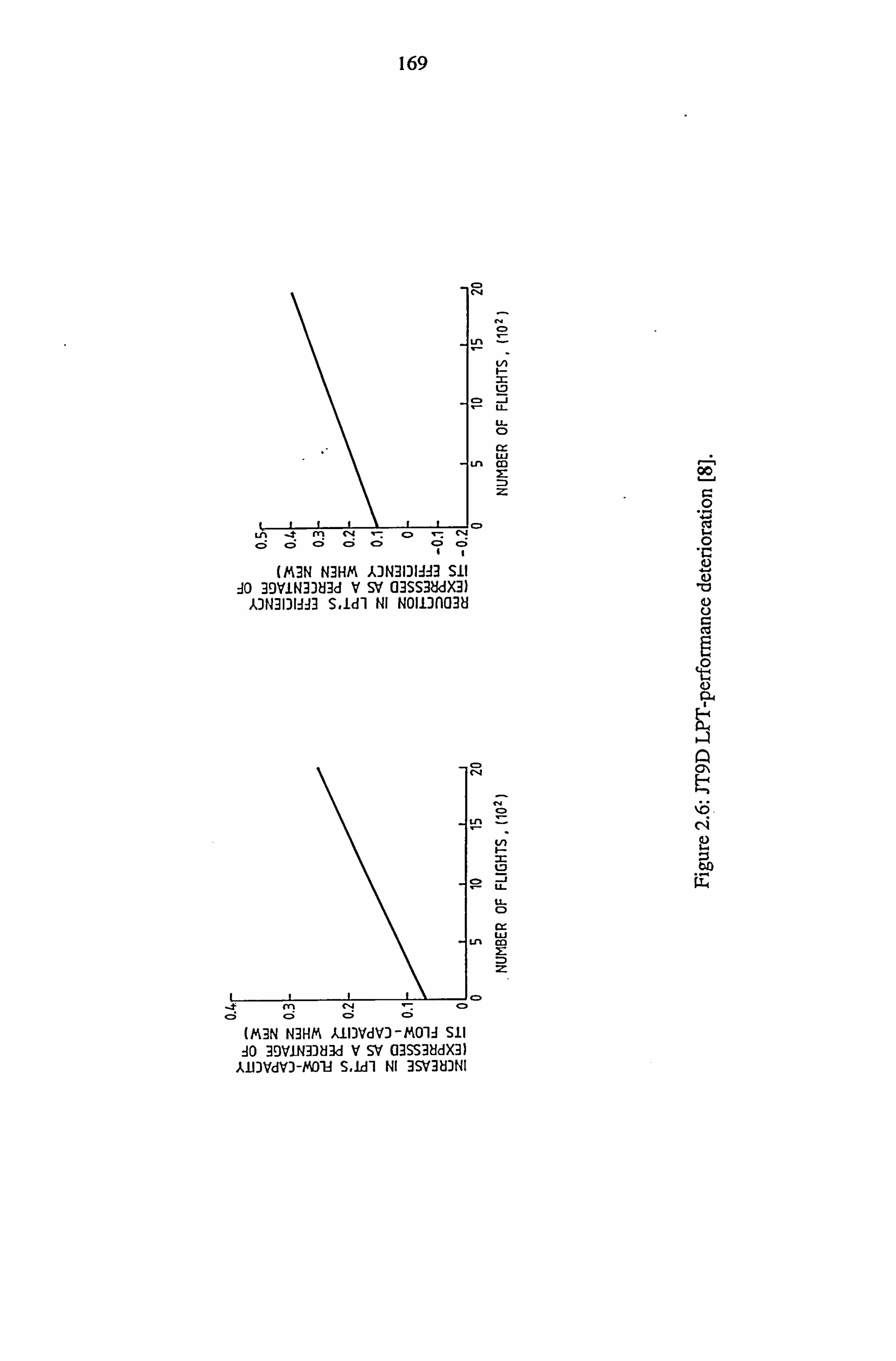
169

U) I

LL

U- C)

cr- LLJ CO

C-4

C.

tn

_j LL- U- Q cr LLJ U. 1 co

r-: Oo r.

9)

Z to

ý1-(

II (M3N N3HM kIN3131AA3 Sil

ýO 39VIN3383d V SV (13SS38dX3) AIN3131AA3 S, Idl NI NOE6038

(M3N N3HM klDVdV)-MOlA Sil JO BVIN3383d V SV (13SS3HdX3)

AIDVdV)-tAOIA S. Idl NI 3SV38INI

170

PHYSICAL FAULTS

FOD WEAR CLEARANCE CHANGES

INFLUENCE

INDEPENDENT PARAMETERS

" FLOW CAPACITY

" ADIABATIC EFFICIENCY

" NOZZLE'S FLOW-AREA

INFWENCE

DEPENDENT PARAMETERS

" TEMPERATURE

" PRESSURE " FUEL FLOW

" ROTOR SPEED

" TORQUE

Figure 2.7: Relationship between a gas-turbine engine's dependent and independent parameters [2].

171

120

(L 100

9

uj 3: 0

CL 80 Z 0 UJ

LU in 3: U. 60 00 0. LU

z w 40 C. ) cc ui IL

CLEAN

20 111 86 88 90 92 94 96 98 100

ROTATIONAL SPEED, (PERCENTAGE OF DESIGN SPEED)

Figure 2.8: Effect of fouling on power [25].

1.4

2ý ff 1.3 ow I IL Z z0

0 w a LL 0 1.2 w

0Z M Lu Z3 (. ) UJ CC

uj 1.1 a e: ý

1.0 iIIII --a 86 88 90 92 94 96 98 100

ROTATIONAL SPEED, (PERCENTAGE OF DESIGN RPM)

Figure 2.9: Effect of fouling on specific fuel consumption [25].

--A- -FOULED (level of fouling not mentioned

172

20

F 0 1 15 LL z 00 i U. (1) LU go

z U- 10 00 r- w 00

LU Z it

cc 5 LU pt.

0

Figure 2.10: Preliminary model of JT91D performance deterioration: reductions in flow through the LPC and HPC [25].

10

z > Z U- Lu

z 0 U. r4 LU LU z0 z LL 0 ý- uj

0 UJ Z cc LU

CL

0

Figure 2.11: Preliminary model of JT91D performance deterioration: reductions in efficiency of the LPC and HPC [25].

0 1000 2000 3000 4000 5000 6000

NUMBER OF FLIGHT CYCLES

0 1000 2000 3000 4000 5000 6000

NUMBER OF FLIGHT CYCLES

173

LU

Li

LLI

LLJ

Z: r_

LU 0- x LU

Lf)

LU 0

CD

2: C: )

9.

0 L. i 4 2 LU

m Z

Z Li cý :C

3-1 Ul LU -i

>lb

< L-i : Li

Li- CD Z

2Z

C>

(31VDS HVNII) S' SS38iS WL

174

LU

LLI vi Li ý% c:, <

K. 12 = 92: (2: t-i (3 < U-

m : ý- LL21 C) -If

I-- - zl; y : 3: < U3 =< CD a: týj C: ) cr CX 0- --1 Li LO

LU -_CI:

LU -i

92: -,

'n f= l

! F C: ) :Z CD w=Oýim v) tn t-, (3

tu ul < LLJ

LL) LL

-j

.4 r_

Q

4C. Z

E- 6i clei

to

ý4

HIgN31 )OV83

175

- CREEP IkArri IA &iir AI f-A'rlrl Ir

LU LL-

-i

LL- C)

C) r,

METAL TEMPERATURE, 'C

Figure 3.3: Factors influencing a turbine-component's life [30].

700 800 900 1000 1100

176

LLI

-j

(A

LIJ

LLJ

CD

(31V3S HV3NII) DNILDS 831AOd SJNIDN3

LLJ LLJ

LLJ Lf)

< U) :z 11 LLJ <

LLI 2:

Ln LLJ a- I

I zu C) LU

L-o> clý 21- -J; z WU-LU

LU S9

LLJ Lij L-j ý

cc: L. j LLJ

M C, <

cli

cl

DO

CAI

40.

>1 0

7ý

.2

cl r- 0 4: ý

Cd 0 =1

z to 1.1.4

MV3S HV3NII) ioniov

�-7

177

Aircmft's Mission Gcomcbric Profik Atrody"arnic Dtfa Deta (inVA)

)

(kPA)

Aircraft & Engine, Performance A E

Initial R Engine 0 Data Aircraft's Hi& Path & PerformanceSi mutation model

D Onput) y

N A M

Take-off I

I C

Climb After Take-off M 0 D

Turboma(ch Input-Updating Modd aimb at Constent Mach Number E L

Climb With Acceleration or Deceleration 0 F

T U

Climb With Constant Power Setting A I

RI R B 0 Acceleration or Deockration

C R

Turboinatch A Program M

A Cruise at Constant Mach Number or Power F T

T Is C H Cruise Lo Cover Specified Range P

E I R N Cruise so Reach a Set Target F T 0 E R R Cruise until it Set Time

Turbomatch F M A

output A N C Rehed'ON/OFF* Mo&

C E E

Dcsocnd it Constwt M&ch Nnber

Airc. rtft Descend with Acodawim or Dood"ation A T D ý Engine Da-u I

s

' C (OUVA) Descend To LAM 0

s I p

LaWing I H E

I R Swith'Gfr ,

C

M

0 D Out put Model E

Figure 4.1: DFD for the aircraft and engine's performance-simulation model.

178

Engine's Design and

HPT Blade's Material Data

input

Time, Speed and

Temperature History input

HPT Wad S Life-Usage Prýiction

I

Model

I

HPT Blade's LCF Life-Consumption

Prediction

I

Model

I HPT Blade's HPT Blade's Thermal Creep-Life Fatigue Relative Prediction Severity Prediction

Model

II

Model

HPT Blade's Life-Usage

Prediction Data output

Figure 4.2: DFD for the HPT blade's life-usage prediction model.

179

Engine's Design and

Material Data input

Blade's Creep-Ufc Usage

I

m(Acl

I

Blade's Stress Model

Time, Speed and

Temperature History

input

Blade's Temperature

Model

Model

Creep-Life Creep Damage Model Data

r

output

Figure 4.3: DFD for the HPT blade's creep-life usage model.

180

Engine's Design vW Material-Dau iryuc

Tinx-and-Speed History input

i Blade's Low-Cycle Fatigue-Lific Consumption Model I

Nominal CF Stress [A---l Turning Points

Nominal Delta Stress ip Local Delta Stress

LOW SU= ýR--j Lzcal Dclu Strain

ArrayShift pq Local Strain

Stress Zero Strip Out RainflowStress (t+-

Reference Strain Life Mean Stress

Spoeds

Refercncc Cycles L=W S"in Pmgc

Minor Strain Life:

Mission Cycles ip Cycle Damage

Fractional Ufc Consumed

Blade's Low-Cycle Fatigui: -IAfc Consumption

Data Output

Figure 4.4: DFD for the HPT blade's LCF-life consumption prediction model.

181

16- -ALTITUDE

T 1.5

MACH NUMBER 0

UJ -1.2 m

I- 1ý_ 12- i/I it I IZ U) Lu W

z

0 9 0

EZ

w .

1 L X LLJ

0 C6 Ul 8- 1. 1 U. Z 04 z

oZ t 0.6 LmLl x Lu

uJ z 0 Z 4- x

0.3

0 0 0 1500 3000 4500 6000 7500 9000

MISSION TIME, (SECONDS)

Figure 4.5: Mission profile 'A' adapted for this investigation by the aircraft with clean engines.

16

ýgo L0L1 12

w

Ul La.

«c 0 ý- Li. 0 0 LLJ Et w0

ZW W w

0

T ALTITUDE

0 MACH NUMBER

z

0 1.2 0

Gi

0.9

a LL Z 0 rr 0.6 UJ IL m LL M :) Zw = UJ

0.3 Z a

2z ul

Figure 4.6: Mission profile 'A' for the aircraft with engines suffering a 6% EDI.

II10 1500 3000 4500 6000 7500 9000


182

12

10

a uj F8 ui 2

6 w

54 -C

2

0 0

1.5

1.2

w 0.9 uj

z

0.6

0.3

Figure 4.7: Mission-profile '13' adopted by the aircraft with clean engines.

IIIai0 246 10

MISSION TIME, (103 SECONDS)

183

200, T 1-2

-NETTHRUST I 2 T,

z < 0 160

------ SPECIFIC THRUST its LL. Z

0.8 cm rh ui 0 120-

z 0 Lu 0

U) 0 u. F- - Z

CC < X Lu

cn (6 M LIJ _j

80 Z

w 11

1 .

0.4 w

- 0

9 v . 1 . ............ I

LL 0

0 40 ., ul 1. - 02

CL

0 0 1500 3000 4500 6000 7500 9000


Figure. 5.1: Specific and net thrusts for the complete mission for the aircraft with clean engines.

200

-NETTHRUST

0 160 ------ SPECIFIC THRUST 1 m

0. -0 Ir 40 LL Z c! ) Z? F,

ZZ ;i

120

-M 0 Lu

U.

U)

U) Ir- r UJ LU x

LU

z z Lu

.j 9 40

0

i 0 1500 3000 4500 6000


T

U) 0) LLI z Z

zz uj 0

T 0.8

0 cc 0

0 uj 10.6 LL L cm

CO) a

0.4

........... z

LL LL

0.2 U)

i0 7500 9wo

Figure. 5.2: As for Figure 5.1, but with the engines suffering a 6% EDI.

184

200

0

-C 160 ENG

9 cc UJO ...... HPC 19 FK

V 120 HPT ul 00

U. 0 LPT Z Uj ul I- 80

--- LPC

UJ Z U . 0 40

X Uj (A

Uj 0 cc 0 123456

DETERIORATION-INDEX APPLYING SIMULTANEOUSLY FOR BOTH ENGINES OR BOTH INDICATED COMPONENTS, (%)

Figure. 5.3: Percentage extra-time taken by the aircraft during the take off phase (for the deterioration of the two engines or their specified components).

400 LU le

0

0 300 ENG Uj

...... HPC

Uj HPT cc - Uj 0 () - 200 LPT z U: U. 0 --- LPC

100

X 0 0 123456


Figure. 5.4: Percentage extra run-way distance covered by the aircraft (for the deterioration of the two engines or their specified components).

185

LL 75- 0>W M Cb ENG

:)w-...... HPC ,j3, LL

0 c? HPT 2w

LPT

EC w 0 LPC

Z w ir 25- Z

Z 0w

Da0* ýý Irý lý -- wZ

01356


Figure. 5.5: Percentage reduction (relative to that with the aircraft having clean engines) in the altitude achieved by the aircraft during the take-off phase (for deterioration of the two engines or their specified components).

150

125 0 IM U- LC 0 LL 100 ý- 9 (A w D cr 75

UJ LU z 50 2z

25 5 (A 2 ui .j g0

z 0 uj I. -

Figure. 5.6: Maximum net-thrust during the take-off phase (with both engines or their stipulated components suffering a specified DI).

Clean LPC 6%Fl LPT 6%El HPT 6%EI HPC 6%Fl Engines 6% Engines EDI

EACH COMPONENT ALONE (SIMULTANEOUSLY IN BOTH ENGINES) OR SIMULTANEOUSLY BOTH ENGINES SUFFERING THE SPECIFIED

DETERIORATION

186

1.12

0-. m 0 1.09 I.. Co CO) z n : 1ý

LL. U.

1.06 U.

Z 1.03

SR LU z z

o UJ I. -

Figure. 5.7: As for Figure 5.6, but for the maximum specific thrust.

-Z -:, Lu 0

o iz; = to uj m ir

LU Lu i to

ui

0z Z

W aZ

am 44 ý- I. - vol

Z r- (a C) - W'IZW ! h- 0 dx ý_ In 00

ul Lu W CC

-j I-- W LLI C. ) 0 cn wZ Lh Jm W Ir

Ic w ix I. - Lb cc n. 12.

100

75

50

25

-----------

0- ý awl

012456

DETERIORATION-INDEX APPLYING SIMULTANEOUSLY FOR BOTH ENGINES OR BOTH THEIR INDICATED COMPONENTS, (%)

Figure. 5.8: Percentage extra-time taken by the aircraft for climbing to a pre-selected altitude (=6000 m) while accelerating to a pre- defined Mach number (=0.7) for various deteriorations of the two engines or their specified components.

Clean LPC 6%FI LPT 6%EI HPT 6%EI HPC 6%Fl Engines 6% Engines EDI


DETERIORATION

187

Ul X CL UJ

100

U. w ooU, -1

F 80 I.. P2W. X

(n M8 12. co --' w r- X: 3 ZM * -0 CL ?l 60

Lu LU <CC LLI Xa 'm Lu 0

z F- mW ý- a 40

zrZZ 20 0D M iD -- - 2 cc < ui I. - z

CC LU

20

LU cn -3 j ui w 0

. 9RU -3 w 0 (n ý- w


DETERIORATION

Figure. 5.9: Maximum net-thrust during climbing to a pre-selected altitude (=6000 m) while accelerating to a pre-defined Mach number (=0.7) with both engines or their stipulated components suffering a specified deterioration.

Z 800 Lu 10 cc F P: 700

C) ul 4 in cc w CC

I. - w LU LL C) w _5 m 0 600

P U) M 1ý- to :) th z 500

-J (j (. ) 400 Z< ý- U, U, -tt m je

X - (3 a1 0 rL cn cl 300 (5 Z ul Z0Z w-0- 200

a. ir ul a UJ Lu 100 wa cn I.. Z. w LU 05 M Z 0

X LU LU a -J z Lu w (A 0

I. -


DETERIORATION

Figure. 5.10: Maximum specific-thrust during climbing to a pre-selected altitude (=6000 m)while accelerating to a pre-defined Mach number (=0.7) with b6th engines or their stipulated components suffering a specified deterioration.

Clean LPC 6%Fl LPT 6%El HPT 6%El HPC 6%Fl Engines Engines 6% EDI

Clean LPC 6%Fl LPT 6%El HPT 6%El HPC 6%Fl Engines Engines 6% EDI

188

100 UJ Z U) UJ

b2 -cc WMO 80 ui id Uj F- 71 U) z cc

ui a) ui I cc m

IL 2 60 4 U) D t: 0m -i

z LU x

Z) - 42 40 cc -J 0 ý_ a X UIZW i- ul UJ ý- UJ U) W za0Z -1 20

zm0 ul ý- 0 co,

Lu 0


Figure. 5.1 1: Total net thrust of the clean engines during climbing to a pre-selected altitude(=6000 m) while accelerating to a pre

defined Mach number (=0.7).

a 00 - xK-E o Ir X

2 -C :)a8 0 : -. a Itt z 13 - 11 LU I. - - LL --p -JW OM= (5 I-- R CO) z 3 lu D< M cc

w 93 MMw jr t?, - if, - 0= 00

w

cn I. - IL < (n Z0X at Ul

0 Fr jý I. - uj wz cc m Ul LLI 0 Im Z0

25

20

15

10

5

Figure. 5.12: Percentage reduction in maximum Mach number attained by the aircraft during cruising to cover the specified range (=400km) flight-segment (for deterioration of the two engines or their both specified components.

iII 0 so 100 150 200 250 300 350 400

0-I-IIII 0123456


189

w 50

0 m LU Z 40 U. 0> ;ý 0z0 -4z 1ý- ra UE CD -oX n Rc P8 30 cc x0 air P (5 LU 11

z Ir w ý- o 20 z CC uj z

IL IS 80 10 30 UJ 0 if M

mz L) w LU

M CL 0 o

Figure. 5.13: Maximum net-thrust during cruising to cover the specified range (=400 km) with both engines or their stipulated components suffering a specified deterioration.

25

3 - ENG IOU

------ HPC

0, HPT W. - W

C, tL U. 15- LPT

D 0 Ui LPC

ZW 10- W

W XW le W 0 U ,

2 !! ý 8 ZU 0

5- 0

0, Uj

0- 11 0123456

DETERIORATIO144NDEX APPLYING SIMULTANEOUSLY FOR BOTH ENGINES OR BOTH THEIR INDICATED COMPONENTS, (%)

Figure . 5.14: Percentage extra time taken by the aircraft during cruising to cover the specified range (for the deterioration of the two engines or their specified components).

Clean LPC 6%Fl LPT 6%El HPT 6%El HPC 6%Fl Engines 6% Engines EDI

EACH INDICATED COMPONENT (SIMULTANEOUSLY IN BOTH ENGINES) OR SIMULTANEOUSLY BOTH ENGINES SUFFERING THE SPECIFIED

DETERIORATION

190

38

U) LLI 0w

UJ Z X- CC I. - Z

0 1. - X 37.8 z ul Ir - Ul a UJ -Z X ý* E ý- 400 _2 D0 0808 m U. 0 :S LU

37.6

uj ý- 000 (A Z Z CC m-04 Inc CC 37.4

Z M gui

UJ 0a U- Z0D L) E != uj

cc ý - 37.2

J D- U)

374- 1500

Figure. 5.15: Net-thrust for the aircraft with clean engines during cruising to cover the specified range (=400 km).

25

26 cc ;i - ENG

0

20- ...... HPC cr 9

=, lz ---- HPT

ir .a 15- LPT

ý lu ý r u --- LPC

z 0 U, 10-

0

5- ul

80 x 0- 111

12345


Figure. 5.16: Percentage extra-time taken to reach a set target (=l 500 krn from home base) for deterioration of the two engines or their specified components.

1700 1900 2100 2300 2500


191

14- r_ Z - ENG Z0

ci 93 12 W UJ

w cn ý- --- HPC

tr 80t m -

10- HPT a >Z ?Z0 %0 Z:

w 8- LPT

W (3 30

--- LPC 0 4Z 6- :) rr ir 0 Co W Lu

« - ý 0 r- ý- U)

W< .-.

-. ....:. -..

... -. --, --- tz Lü w CC Ir 0.

123456


Figure. 5.17: Percentage reduction in the range covered until a set time (= 3300 seconds from take-off) with the deteriorations of the two engines or their specified components.

w 125 0 U.

0Z mo 100 CE 0 U.

0t 2' 75 Z 3:: e CC cn - = Co 0

50 W0 ZW C) =W UJ Cß

3 gr 0 25 w c4

Z 0

w0 0Z Z

w


DETERIORATION

Figure. 5.18: Maximum net-thrust during the 'reheat ON' phase (with the both engines or their stipulated components suffering specified deterioration).

Clean LPC6%Fl LPT6%El HPT6%El HPC6%Fl Engines6% Engines EDI

192

0 25- ui x-

0 1-- e 8 it 4 -f - ENG

52 UJ cn Xa 20- ...... HPC Z2wz ý: m Ic o om5 HPT

w

M2.0 15- ---- LPT 00 04 ui LL, ir. cr Z0

z --- LPC

U. 0 z 10-

z CC 2 UJ UJ I= MX UJ C. ) 5-

00 0 LU ,, s%.. -. 3-: : Jý -- '.. = -=. Z .

cc 0

0123456


Figure. 5.19: Percentage reduction in the maximum Mach number attained once reheat is switched 'ON' for a specified period (=20 seconds with various deteriorationsof the two engines or their specified components.

7

ul 6- U. 0 W Ilp

M 5- CO Z w0

< 4- 0

0z ý- 0w 3- z ul

uj uj ul

cr 0 ý- 0 x ; cjffý.

Figure. 5.20: Percentage extra time taken to accomplish the complete mission (for the deteriorations of the two engines or their specified components).

123456


193

x LLI a z

100

80

%r. 5r

LLI z w

;=F ul

U. LL. Lu

cc 40 z 0 I. - 40 CC 1. ui IL. 0

9) z 0 U) co 2

60

40

20


Figure. 5.21: Mission's operational-effectiveness index (for the stipulated deteriorations of the two engines or their specified components).

012345

194

45

40 ID

35-

E e 30- 0

25

0 Z 20- 0

w 15-

LU 5

0]

0 0

Figure 6.1: Specific fuel consumption for the complete mission.

1.6

1.4

1.2

0 1.0

0.8 0 I U.

-i LU 0.6 D It

0.4

0.2

0.0 4- 0

Figure 6.2: Fuel flow for the complete mission.

1000 2000 3000 4000 5000 6000 7000 8000 9000


1000 2000 3000 4000 5000 6000 7000 8000 9000


195

115

0 3: <0 im w 112 W u) (0 _j Lii w& Ir :)w x, Iliz- log

Z w 0

ui ý- Z U) IL <

106 ww

Z La 103 00 cc

ui KL

1004 0

Figure 6.3: Total fuel used (expressed as a percentage of total fuel used with clean engines) for stipulated engine-deterioration-index.

35 LU W

z U) 33

LL 0 ZM 0 UJ 31

z E Z

Z 0 29 0

C6 LL W Ul 0 M CC LL 27

LU CL U. 0) 0

25+ 0

0

Figure 6A Specific fuel consumption (at an altitude of 103 metres, Mach number of 0.95 and a TET of 1000 K) for stipulated EDI.

23456

ENGINES'S DETERIORATION-INDEX, (%)

23456

ENGINE'S DETERIORATION-INDEX,

196

tm 0.20 ca :ý UJ

0.16 U. 0

U- I. - 0W ui ý- cc 0.12

Z ul C! 0 z U. 0.08 40

ui

02 -i D 0.04 IL. Z -J UJ U.

0.00+ 0

Figure 6.5: Fuel flow (at an altitude of 103 metres, Mach number of 0.95 and a TET of 1000 K) for stipulated EDL

10 z LL

0 cc w

ui m z2 mZ 0z Zýý z LU

0 20 6 LL U. ww _j

LU

LU

LL 0 In w C;

ul z

0 0

Figure 6.6: Net thrust available from engine (at an altitude of 103 metres, Mach number of 0.95 and a TET of 1000 K) for stipulated EDI.

23456

ENGINE'S DETERIORATION-INDEX, (%)

23456


197

w 20

z LU z <a 16 UJ Z -1 4- 0 U) Z M UJ . 5f

o Ir Ls 12 LU C; w LL .10

LL C) LU to 8 LU

Z

cc 4 Z

LU Z 04- 1000

Figure 6.7: Net thrust available from clean engine (at an altitude of 103 metres and a Mach number of 0.95) for stipulated TET.

0.50 LL 0

z cc uj

0.40 ca Z UJ m

z UJ 0.30 z 9<6 10 _j

U) CA 0 UJ ; 0 C r

LU 0.20

0 LL i U. 0 _j LU Lu

0.10 U. ý-

0.004- 1000

Figure 6.8: Fuel flow with clean engine (at an altitude of 103 metres and a Mach number of 0.95) for stipulated TET.

1100 1200 1300 1400 1500

TURBINE'S ENTRY TEMPERATURE, (K)

1100 1200 1300 1400 1500


198

a 35

zz U) w cc VA 33 ui -k 2

tm Z 'b E 0 ý- U0 Ics'; ' 31 0. uj C;

U. o z 0

-j ul 29 z m LU Z

LL z 3"- 27 1E cn L) U) LU

ul CL. cn z

ui 254- 1000

Figure 6.9: Specific fuel consumption with clean engine (at an altitude of 103 metres and a Mach number of 0.95) for stipulated TET.

115-

Z UJ wZ "j 0 112- CE Z LU LU a. <Z 0ý

ui Z 109 -

Cß 1. - Co e.

ui U)

106 -

0Z

103- U.

U. 0 0

1004 0

Figure 6.10: Total fuel used (expressed as a percentage of total fuel used with clean engines) for stipulated LPC's Fl.

1100 1200 1300 1400 1500


23456789 10

LPC's FOULING-INDEX, (%)

199

z 104 -

t 102-

uj ca U) LU LLI IL -i

Zloo 40 x uj e :) -Z LL. 0) w 0 -J Z LU m0z 98 - _j LU LU LL :)0 U. ul

96- oZ LU 0 cc ul CL

94 -- 0

Figure 6.11: Total fuel used (expressed as a percentage of total fuel used with clean engines) for stipulated HPC's Fl.

115

CO) 40 C3 UJ 112 LU 0 w uj cr Z) IL U- CA log X _j

LU

0z I. - w Ll- Z 106 0<

wW UJ

LL -i z 103 w 00

tu 0. 100 46

0

Figure 6.12: Total fuel used (expressed as a percentage of total fuel used with clean engines) for stipulated LPT's El.

456789 10

HPC's FOPULING4NDEX, (%)

456789 10

LPT's EROSION-INDEX, (%)

200

115-

w

t: 112-

LU 0w cn w cr

ri. tiog - XW le :> -Z LL U)

w

w 0) F- 0

0 z106 - F- w W U. 0

W

103 0Z F- w Q

at w 0.1 1004

0

Figure 6.13: Total fuel used (expressed as a percentage of total fuel used with clean engines) for stipulated HPT's El.

a 15

cn W ca CA ul m X

_j 12 ui m U.

d (0) wýw ca o9

-j LL Z LU 0

UJ z a W< ;5 -j Z0 LU x 0 z ir ui 9L 3

Z4 c ca x4 0

0

Figure 6.14: Change in total fuel used (expressed as a percentage of total fuel used with clean engines) for a 10% deterioration of stipulated components.

456789 10

HPT's EROSION-INDEX, (%)

LPCs HPCs LPTS HPTS

COMPONENTS SUFFERING A 10% DETERIORATION

201

35 LL 0 U. ,j0 a t'; t n 33

z 44 Z

0.0

zo 31 0 Cc Z

ME

ZX 29 00c,

UJ :3 U. Ul cc 0 27 rL ui 5m Ul " 0.0 0ý

0123456789 10

LPC'S FOULING-INDEX, (%)

Figure 6.15: Specific fuel consumption (at an altitude of 103 metres, Mach number of 0.95 and a TET of 1000 K) for stipulated LPC's Fl.

35 LL 0

Z Ir X- LU to 33 zz 0 P r=

31

zw 0 cc I- LL LU 0

Lu 29 LL 0 LL 0 rL 0Z Z5 LU < ui a U. ) 27

P J

4

25+ 0

Figure 6.16: Specific fuel consumption (at an altitude of 103 metres, Mach number of 0.95 and a TET of 1000 K) for stipulated HPC's Fl.

23456789 10

HPC'S FOULING4NDEX, (%)

202

35 UJ UJ

z 4

< Lo 33 z (ý

0 IL o

Z cr oW

Im E z.

U) X Id

0 29 z8

CJ 0 -J ce U. wwo M LL Uw 27 rL

w0 CL LL U) 0 254

0

Figure 6.17: Specific fuel consumption (at an altitude of 103 metres, Mach number of 0.95 and a TET of 1000 K) for stipulated LPT's El.

35 U. 0

lu m 33 zz 2

31 w (n § z ui 0 cc

r- LL w w0 29

UJ U. 0 LL 0 rL 0z E5 LU < w Lo 27

t: ci

25+ 0

Figure 6.18: Specific fuel consumption (at an altitude of 103 metres, Mach number of 0.95 and a TET of 1000 K) for stipulated HPT's El.

456789 10

LPT'S EROSION-INDEX, (%)

456789 10

HPT'S EROSION-INDEX, (%)

203

10

x 2E t: 7.5 03'. P (L) CL LL 2w M LL (A 0- Z UJ

5 00 04

-Z -i w ui zz Dw U. 0 2.5 C) wZ

Uj LU Z

w lu U) <0 cl LU ui U) am

zW IL -2.5 X W.

.5

Figure 6.19: Change in specific fuel consumption (expressed as a percentage of specific fuel consumption with clean engine) for a 10% deterioration of stipulated components.

0.2

ui CD,

L Lu il >, U. 10 eb 0

F- LL W

0 ý- w0 0.12

LD 'U, -! C)

Zö0.08

0 _j

0.04

LU m2 LL

Figure 6.20: Fuel flow (at an altitude of 103 metres, Mach number of 0.95 and a TET of 1000 K) for stipulated LPC's Fl.

456789 10


204

(6 LL, IZ ui

0.20

cc 8 Lu 0.16 160

F.. U. w 0 az0.12

U, 0x

4 U. z00.08

w m

o _j Z LL 0.04 ul :32 LL

0.004 0

Figure 6.21: Fuel flow (at an altitude of 103 metres, Mach number of 0.95 and a TET of 1000 K) for stipulated HPC's Fl.

cof ul

0.20

ý8 ui 0 2 LL 0.16

LL Ul 0 uj az0.12

LL 32 zo-0.08

Ir w

0D _j

Z 0.04 U. -i LU p U.

0.00+ 0

Figure 6.22: Fuel flow (at an altitude of 103 metres, Mach number of 0.95 and a TET of 1000 K) for stipulated LPT's El.

23456789 10

HPC'S FOULING4NDEX. (%)

456789 10


205

0.20

a IZ ul w8 tj a 0.16 LL lb 0

0 LL

w C5 az0.12

;=-! U) j0

< LL z00.08

cc LU m

0 _j Z U. x 0.04 -1 0 w4 :)2 LL.

0.00+ 0

Figure 6.23: Fuel flow (at an altitude of 103 metres, Mach number of 0.95 and a TET of 1000 K) for stipulated H PT's E 1.

10 z

LU

LU Z) Z Z Z! ý, 8

z ui 8 2a 0ý6 ir u U. (60 LU LU I... CC LU

LU 4

z U. 0 U') LU

cr LL 2 0

LU z 0 4-

Figure 6.24: Net thrust available from clean engine (at an altitude of 103 metres, a Mach number of 0.95 and a TET of 1000 K) for stipulated LPC's Fl.

456789 10

HPT'S EROSION-INDEX, (%)

46 10

LPC'S FOULING-INDEX,

206

10 z

LL 0

w Z

z z w

0 20 M<- LL U. w Cl) 0 _j LU t- CD CC UJ

z LL 0 w

ul z

0 0

Figure 6.25: Net thrust available from clean engine (at an altitude of 103 metres, a Mach number of 0.95 and a TET of 1000 K) for stipulated HPC's Fl.

10 z

uj ox 2- LU :)Z

z 4ý 8 x IZ Z0

UJ .48 2 0 cc LL 6 U. ui o LU LU p- _j CC Lu

LU 4

z U. 0

cn C! Ma0 cc LL 2

:30 E

LU z 0

0

Figure 6.26: Net thrust available from clean engine (at an altitude of 103 metres, a Mach number of 0.95 and a TET of 1000 K) for stipulated LPT's El. 203

468 10

HPC'S FOULING4NDEX, (1/6)

46 10

LPT'S EROSION-INDEX,

207

10 Z U.

0 cc LU

uj m z2 DZ

Z z ul

8 0 U. ir

LL w C6 o J U) ý- M Cc LU I- I. - Lu

z U. 0 LU

0

Figure 6.27: Net thrust available from clean engine (at an altitude of 103 metres, a Mach number of 0.95 and a TET of 1000 K) for stipulated HPT's El.

10

<Z 0 «C 5 W

-i W

U) - LU

x0 LL

Z -" LL, -5 0 LIJ Z

.i :)- U. LL (3 -i LL Z W0W :)w

0 -10

j-, >- Z Z cr

w -15

-20

Figure 6.28: Change in fuel flow (expressed as a percentage of fuel flow with clean engine) for a 10% deterioration of stipulated components.

046 10

HPT'S EROSION-INDEX,

208

10

Z la z

tu z <0 Uji

10 .2 0

LL ui

< -10

-15

-20

Figure 6.29: Change in net thrust available from engine (expressed as a percentage of net thrust available from clean engine) for 10% deterioration of stipulated components.

100 z0

ui w Z cc

< UJ LU 2 90

uj 00o ,e UJ -1 0

- c, -J co w LU

cr D

12. U. a 80 X U) Cl -i UJ ui

0 5p w0 U) r- LL 70 0 LU cc ui D00 Ir U- RE ý<- 0

Wz Ir I. - wR 60 0 Ul I-- Ir :r LU IL

50+ 8

Figure 6.30: Total fuel used with a 6% engine deterioration for stipulated aircraft's cruising altitude.

10 11 12 13 14 15

ALTITUDE, (lCP METRES)

209

35

,c Z 33

Z LL 0 00 0

r- 1r -k 31 CL. UJ MM m MM E U) Z 0 29

W 0

U. 27 0W WZ CL U) Z

w 25+

5 9 11 13 15

ALTITUDE, (I CP METRES)

Figure 6.31: Specific fuel consumption with clean engines at a Mach number of 0.95 and a TET of 1000 K) at stipulated aircraft's cruising altitudes.

x '? 0 Co

8 LU 0 Z Z5 LL z0 LU F- z LU ox P- uj

< : r,

z

Lo

C! 0 U. 00 -J x LL uj -J In UJ

LL z

0.25

0.20

0.15

0.10

0.05

0.004 5

Figure 6.32: Fuel flow with clean engine at a Mach number of 0.95 and a TET of 1000 K) at stipulated aircraft's cruising aititudes.

9 11 13 15


210

12

10

cr

cc 0 cc 4

2

0 8

Figure 6.33: Aircraft's drag at stipulated aircraft's cruising altitudes.

z uj U.

z0 <I-- LLI Ul

0Z M 4c LL. U) LU

co LL

!50 aM LLJ >m

(n z Dx cc

uj z

10

8

6

4

2

0 5

Figure 6.34: Net thrust available from clean engine at a Mach number of 0.95 and a TET of 1000 K) at stipulated aircraft's cruising aititudes.

10 11 12 13 14 15

CRUISING ALTITUDE, (10 METRES)

79 11 13 15

ALTITUDE, (ICP METRES)

211

8000

00 Ir z o 7600 0 UJ

LU A (A . UJ UJ cc CL 7200

Oo 4 UJ M cc m 6800 00 ý- R: z wE

6400 cli

6000

Figure 6.35: Time taken by the aircraft to reach a pre set target (at 2100 krn from home base) while cruising at stipulated altitude.

120

w Z

500 116 z4 ul LU Do LU M U) U) -i Lu UJ :ý lz U- 112 X -J Z

z wzP Lu 00 D; -- U0 Zx 10 8 -1 4 W ui uj

0a _j U. 40

cc P LU Z LU 104 UJ ui IL

100+ 8

Figure 6.36: Total fuel used with a 6% engine deterioration (expressed as a percentage of total fuel used with clean engines).

10 11 12 13 14 15

CRUISING ALTITUDE, (I CP METRES)

10 11 12 13 14 15


212

200 z

LL

'o LL, x cc Z 3.

. UJ

Z5 cn m Z4Q2 LU am 175 LU z

w _j UJ UJ cr U. X _j uj -Z ": r 150

UJ Z0- U) 0 ý- U) Z 3pU. UJ D

-i <o LU Cc w m00 cc LL -4C. )

-i CC

LU ýZ- t 125 UJ 4 () 0 Jr. cr

100

Figure 6.37: Total fuel used with a 6% engine deterioration (expressed as a percentage of total fuel used when aircraft cruises at a Mach number of unity).

50 Z WW

40

Z LL 0) 00E r- w ; lu

Z -. i 0< LL 0Z0 20 _j < k-

w

LL

UJ ZZ 10

WZ KL LU CA

0iI11

0.5 0.6 0.7 0.8 0.9 1.0 1.1

MACH NUMBER

Figure 6.38: Specific fuel consumption with clean engines at an altitude of 103 metres and a TET of 1000 K) at stipulated Mach numbers.

1.2 1.3 1.4 1.5

MACH NUMBER

1.2 1.3 1.4 1.5

213

0- U, ti , < ze Z

LLI Z LL

z5 0 Z k- W LLI

w Z

k: w cc w

0 _j

U. 0

LL

0.20

0.16

0.12

0.08

0.04

0.00 iII 0.5 0.6 0.7 0.8 0

.91 .01.1

MACH NUMBER

Figure 6.39: Fuel flow with clean engine (at an altitude of 103 metres and a TET of 1000 K) at stipulated Mach numbers.

10 W LL

0

zW W ý- 8 z WZ .J< 00 ý U, 0 cc U. W UJ M

-b IL 0

> UJ

CO)

cr I- z F- 4 w z

04- 0.5

Figure 6.40: Net thrust available from clean engine (at an altitude of 103 metres and a TET of 1000 K) at stipulated Mach numbers.

1.2 1.3 1.4 1.5

0.7 0.9 1.1 1.3 1.5

MACH NUMBER

214

20

16

12

8

4

04 1

Figure 6.41: Aircraft's drag at stipulated cruising altitudes.

8000

cr Z 7000 0 0 w

uj U) w UT CC

m 6000 w o

cc 00 ý- M z U. 5000

E

40004- 1.0

Figure 6.42: Time taken by the aircraft to reach a pre set target (at 2100 km from home base) while cruising at stipulated Mach number.

1.2 1.3 1.4 1.5

MACH NUMBER

1.2 1.3 1.4 1.5

MACH NUMBER

215

120 Z

w r3 en F- 116 Z< 3-. ui 0.

W 42 U) ui

000

112 IL W xD 3: W LL W

U) 0 k- (3 Z) r- 0Z 108 j9 ý- ul

CE ti- 00 U. LU

w 104 r2 Z F- w 0

Ir 1. a CL

1004 1

Figure 6.43: Total fuel used with a 6% engine deterioration (expressed as a percentage of total fuel used with clean engines).

104

Z F3 z wa 102 , ui LU e V) CA to 0M

w -i Cc LU E IL z 3: 0 a ý- 100 lu < Ch 00 ul -i ý IA. Ul ui Ir 0 Ir m0 ul 1.2 a

-J UJ 98 z ui

IL 96+

0 5 10 15 20 25 30

REHEAT-ON PERIOD, (SECONDS)

Figure 6.44: Total fuel used with a 6% engine deterioration (expressed as a percentage of total fuel used without reheat-on).

1.2 1.3 1.4 1.5

MACH NUMBER

216

35

9 "-1'- 30 ox 0 CD m co

cm 25 0E I- 2f

_0 20

z 02 is 0 CC -i LU its :)W U. a 10 0 LU rL Z 00 UJ Z UJ 5

0 0

Figure 6.45: Specific fuel consumption with a 6% engine's deterioration at stipulated reheat-on time.

2.0

1.6

1.2 0-, w0 , ýe

3: 0.4

0.0+ 0

Figure 6.46: Fuel flow with a 6% engine's deterioration at stipulated reheat- on time.

5 10 15 20 25 30

REHEAT-ON TIME, (SECONDS)

5 10 15 20 25 30


217

21 0 cr Z 00 CE 0

W

w 0 L, j

Z 0 gr

Z W

W Kr

Z occ

r-

9000

8900

8800

8700

8600+ 0

Figure 6.47: Time taken by the aircraft (with 6% deteriorated engines) to reach a pre set target at 2100 from home base.

120

ui Z<

oen ui 116 Z w0 (0 0 0)

(0 -1 ý9 w: > -Z ot Li- ' 112 CL w x

zýO Z 0

:> r- Lo, Z« 10 8 -i < w rzow-UJ, :20

WZ ). - W 104 UJ fj 0 92 CL.

100 + 0

0

Figure 6.48: Total fuel used with a 6% engine deterioration expressed as a percentage of total fuel used with clean engines.

5 10 15 20 25 30


5 10 15 20 25 30


218

110.0

w Z W ir 108.0

w Co A :i 40

Co (n -i

Z wW

=xu. 0U xJ

106.0 1. - 0. W<0 :2

0 >- -0 UJ Z >.. ir

cn 0 LL Zw 2 r- 00 104.0 .j<P w KE uj < Lu

> (3 - 1-- -2 2> Z '0 102.0

00 Ct Ir LU 9WN

100.04 0 10

Figure 6.49: Total fuel used with a 6% engine deterfloration expressed as a percentage of total fuel used with zero deviation from standard- day temperature.

35.0 z ý (6 ui

z 33.0

z U. 00 PW LL E 31.0 IL 00

LU z 0 0 Z U

29.0 Z . 40

M U. () (a it I..

UJ 27 0 z . E3 5 UJ Z 0. W CA

25.0+ 0

Figure 6.50: Specific fuel consumption with clean engines at an altitude of 10 3 metres, Mach number of 0.95 and a TET of 1000 K) for stipulated deviation from standard-day temperature.

2468 10

DEVIATION FROM STANDARD-DAY TEMPERATURE (1.0 1 dC), CC)

2468

DEVIATION FROM STANDARD-DAY TEMPERATURE (Le. I dC), CC)

219

0.2 w

z ui ý- M 4) <Z C* 0.16 w z zMC, w z ww LL 0

E 0.08

ii. z 00 4 -J W U. -J no 0.04 LU P U. 0

0 0

Figure 6.51: Fuel flow with clean engine at an altitude of 103 metres, Mach number of 0.95 and a TET of 1000 K) for stipulated deviation from standard-day temperature.

w 10 9- 0mz Za :ý ul 4 IZ z8

_j U) 0 UJ LL cc 0 2 ý- 0 U)

U. 6

LLJ UL 0Z LL, -C

LO 4 > cp

LL 0 U) n cr Z U) 2

z z0

Figure 6.52: Net thrust available from clean engine clean engines at an altitude of 103 metres, Mach number of 0.95 and a TET of 1000 K) for stipulated deviation from standard-day temperature.

2468 10

DEVIATION FROM ATANDARD-DAY TEMPERATURE (i. e. I 6C), (OC)

2468 10

DEVIATION FROM STANDARD-DAY TEMPERATURE (i. e. 1 dC), CC)

220

120.0

w

=9 w 116.0 LU 0 to LU Z

w Ir U. CL w 112.0 x -j Z

0 -oz wZ >- ui Co 0 U. Z :, r- 09 108.0 W cr UJ w 25 0 U. rr -J LIJ Fw cj 104.0 0 c2 tr w

IL

100.0

Figure 6.53: Total fuel used with a 6% engine detedioration (expressed as a percentage of total fuel used with clean engines) for stipulated deviation from standard-day temperature.

115 cl

0 ui UJ -j CA (A U. U) :) UJ

_j LU L) 12 mu :

-F e ,,, - _j C5-. - Ln 2E rL 40 U- z 109

I. - UJ U. 0

0 LU W LU 40& 106 (1) 1. - F.. M UJ D Lu 7- UJ -i a ul uj LU

w 103 -J 4 0. ý< a. 0

100 46 0

Figure 6.54: Total fuel used with a 5% LPC's flow-capacity deterioration (expressed as percentage of total fuel used with zero LPC's efficiency deterioration) for the stipulated LPC's efficiency deterioration.

2468 10

DEVIATION FROM STANDARD-DAY TEMPERATURE (Le. ift), eC)

3456789 10

LPC's EFFICIENCY DETERIORATION, (%)

221

Z 35 « JE - k- w Lo m

33 cm E

Z IK - 0 20 3 -Z

w 0 29

W CL

Z 0 «x 27 Ln

w0 IL m LA. U) 0 CL 0 j

-25 0

Figure 6.55: Specific fuel consumption with a 5% LPCs flow-capacity dete-

rioration (at an altitude of 103 metres, a Mach number of 0.95 and a TET of 1000 K) for the stipulated LPC's efficiency deterioration.

cc 0.20 w ra 7 ý- zm C)

0 -R Z) al i ý- zm u .4 Ale 0.16 Z

L, U) 0.12 0w LL < rr mo Ul I- I- UJ UJ ui 0 08 .

0 i-U. z U. a0 -La J Jýc U, 0.04

U.

0 0.00+

0

Figure 6.56: Fuel flow with a 5% LPC's flow-capacity deterioration at an altitude of 103 metres, a Mach number of 0.95 and a TET of 1000 K) for the stipulated LPC's efficiency deterioration.

3456789 10


23456789 10


222

1= z ý: 2 ui z 004 z

LU LU 0 ir 0 1. - 1-- cc UA Ul U. 2 1- w Cb

LL Z ri UJ

0 0 k- LL -i W LL.

5 Z) Cc xz

CL i

9z Z Ln

10

8

6

4

2

0 4-

Figure 6.57: Net thrust available from engine with a 5% LPC's flow-capacity dete rio ration (at an altitude of 103 metres, a Mach number of 0.95 and a TET of 1000 K) for the stipulated LPC's efficiency deterioration.

115 00

ui w 0. cc -J .J0. UJ 0 112 xz W z 0 -0z I. - I. - w0 log

3: 4 LL pP a 004 WO ILM U, 0 0 cc

-i Cc LU LU Z LU

Ul N 0 min w

z LU ul CL 103 004

LL IL ui 100 *

0

Figure 6.58: Total fuel used with a 5% LPC's efficiency deterioration (expressed as percentage of total fuel used with zero LPC's efficiency deterioration) for the stipulated LPC's flow-capacity deterioration.

3456789 10

LPC'S EFFICIENCY DETERIORATION, (0/6)

23456789 10

LPC's FLOW CAPACITY DETERIORATION, (%)

223

35 ,0Z . er CC - Ln UJ -

m

33 3: 0Z r- Zm

«c (> E F- 0 CL be cr <

)w- c6 0 LL1 Ul Z 12 tr LL. 0: 0 C) ul ZZ ý- 29 w w F-

0 Z Lou «zc 27

25+ 0

Figure 6.59: Specific fuel consumption with a 5% LPC's efficiency deterioration (at an altitude of 103 metres, a Mach number of 0.95 and a TET of 1000 K) for the stipulated LPC's flow-capacity deterioration.

0.2

Z LL Z oR W LO 0.16

LL :)0-0 LU I. - U.

.P50 0 0. < cc ol ul ;? 5, 0 12 -J zm .r

. , e4m

In ý- :) z =-

C) U. 0.08

20 ul er 00

i CA 0 04 LL Fc w . -i UJ CC W ý- 1ý- UJ W 02

0 0

Figure 6.60: Fuel flow with a 5% LPC's efficiency deterioration at an altitude of 103 metres, a Mach number of 0.95 and a TET of 1000 K) for the stipulated LPC's flow-capacity deterioration.

23456789 10


23456789 10


224

Z 10

w in 2 21 z0 Z0ZX8 a r- =! if z .c0 ui cc <§

E02 0 cc -

ou 6

In >- z QW04

>0< M ý- LL 0 -, ca ww;

U. 2 o

Z0

LPC's FLOW CAPACITY DETERIORATION, (0/6)

Figure 6.61: Net thrust available from engine with a 5% LPC's efficiency dete rio ration (at an altitude of 10 3 metres, a Mach number of 0.95 and a TET of 1000 K) for the stipulated LPCs flow-capacity deterioration.

10

225

LLJ cl: :D t-

LL-

x

cx < Cl- j= LLJ CX LLJ LU = t- Lj

CL LU LU cr

cx

LLI

'L

/: ),

I

< Cl. LLI LU

re rY (i. Li

LLJ

a- LLJ LLI clý

WK- 13-0

11

F- Z:

LU 0- LLI C: )

X< i=q CY- = C: ) C: )

-Jz:

t7; 0

w -i

LLJ I

LLJ

LLJ

r-: 00

c; i

cu

E ce 1-.

zi C)

E-

(31V3S HV3NII) '3 NIV81S

226

100 wQ k- w W cc

W 1 CL

0. cn 0 2 -« -1 80 0 c2 -« t) UJ ZZ

(n i= CL. 0 UJ :t LL CC 1-. Z t2 CL 0 uj x w LL, cr u) u LU a. - Co W

uj ;-0 12- Co = üi LL. U. Z 40 0 0 tt 00

r- a. wZ <Zw

cc U) Z 20 (0 W

LU

04-

Figure 7.2: HPT's rotational speed for the complete mission profile for the aircraft with clean as well as 6% deteriorated engines.

2000

0

1600 ur

W U. 0 IL 1200 z

w0 0. U) mco w 800 I. - W

Z UJ Y) 0 w 400 z

M

0

Figure 7.3: TET for the complete mission profile for the aircraft with clean as well as 6% deteriorated engines.

1500 3000 4500 6000 7500 9000


0 1500 3000 4500 6000 7500 9000


227

100

0 U. uj W U. 75

(a :] UJ CL CC CL Lu x ui Z gk CC Z5

0Z Lim w 50 t= z

U. 0 ui

z 25 uj W DO !5w

LU W CL

0 0

Figure 7A Blade's predicted creep-life for the stipulated engine's deterioration index.

100 CL w w cc 75 ui () a: 0

50 ui Lu 0z cc ju C3 Y)

F zw 25 Ul zz U, 4 all 0 -1 0

Ul cc 0 -25

z0U. c Lu UJ a U. 0w -50 z U) cc (n =w 0 cc -75 M x 9 -100

Figure 7.5: Blade's predicted creep-life for engines with: - a 6% F1 for the LPC and HPC separately; a 6% El for the LPT and HPT separately; and a 6% eng ine-deterio ration index.

234


WHOLE ENGINE OR SPECIFIED COMPONENTS SUFFERING A 6% DETERIORATION

228

100 z 4 UA

Uj 75 CA U. U) Lu W m IL g CL w Er Lj

LU Z cc 5 50 () Z i to uj IL I. -

LU - U) LL

0 w

F)a 25 wg az 45 w co o

cc LLI a.

Figure 7.6: Blade's predicted creep-life for the stipulated LPC's Fl.

100

z cc LU -j co 0

<4 0 CC U) o 75 0 U. w uj Ul CC U. 0. .j 0

CL - LU ui

Lj UJ Z

cr 5 50 0Z U) Lu

UJ U. Ir 0 () ul co 0 iu 14 25

z LU m C. ) cc all IL

0 0

Figure 7.7: Blade's predicted creep-life for the stipulated HPC's Fl.

0iIIIIII 0123456789 10

LPC'S FOULING4NDEX, (%)

468 10

HPC's FOULING-INDEX,

229

100 z

UJ o U) 75 W LL W ul

U.

X CL - !! ý ww La

LU Z

Ir Z5 50 0Z ý CA w a. I- w- W U-

0 Lu

w 25

z

w a. 0

LPT's EROSION4NDEX, (%)

Figure 7.8: Blade's predicted creep-life for the stipulated LPT's El.

225

Z «x W i 200

0 wW 175 X LL 0. -1 x d. - ! ew ui a UJ Z

ik z5 150 Z -e u) ui

W LL

125

w Z (') loo w CL

75+ 0

Figure 7.9: Blade's predicted creep-life for the stipulated HPT's El.

10

46 10

HPT's EROSION-INDEX,

230

150

. uj loo U. ul 0Z

0. UJ 5 LU wz ir U, 50 0ZZ 9) w< ul (> UJ

cc ui n. <0 CO <Z

ui 'A - Ul

zW '71 -50 w U) IL M ui Ul LU Z cc w 0. u X L) w -100

-150

Figure 7.10: Blade's predicted changes in creep-life for engines with a 10% Fl for the LPC and HPC, and a 10% El for the LPT and HIPT separately, compared with those for a clean engine.

150 w z co < Z a ui

cn LU cr Z UJ 4X

a 31. Ly 125 Lu uj m

10 w U. 0 0 :]0 ui 0 CL CO ul I- w 100 x LU 4a LU Ir CO D uj 0 ul F- z (D U) I- 0 1. - 5 -j p Z:

w 75 Lu 0 CC CC o Ul 0 ir- a

LU LU F- Z LU UJ cr 50

C. ) -R ui a.

25+ 7

ALTITUDE, (ICP METRES)

Figure 7.11: Blade's predicted creep-life for the engines suffering a 6% deterioration (expressed as a percentage of its creep-life when the aircraft cruises at 8000 metres altitude) when the aircraft cruises at the stipulated altitude.

13 15 17

231

20

w4 z CC Z5 0 Z LU UJ 16

ul w0 CL - ul ww cc ui z

a. cc a 12 Xz ww - (n lu 2Eý: Z 0 LL <

LU 0 Ul 8 -j w wo M fr (5 00

ul lu Ul 01--o 4 5a cr m ul

0 4-

Figure 7.12: Blade's predicted creep-life for the engines suffering a 6% deterioration (expressed as a percentage of its creep-life for a clean engine) when the aircraft cruises at the stipulated altitude.

LLI

Z

Z w0

w LL

Z LU -i

ý:

ir CL Z l= a. LJ Z 3: xW IL

w ecc 0

lu

-e 00W CL m wýZ: m w JE 0

:) Z 0w

Co E0 1 ui ý< Lu Z

312 Lu 0

w CL

100

75

50

25

04- 1.0

Figure 7.13: Blade's predicted creep-life for the engines suffering a 6% deterioration (expressed as a percentage of its creep-life for a Mach number of unity) when the aircraft cruises at the stipulated Mach number.

9 11 13 15 17

ALTITUDE, (le METRES)

1.2 1.3 1.4 1.5

MACH NUMBER

232

20 z dX cc a0 Z U. Ul uj 16 1 op ru LL

W ui CC wZ 5 12 Z LU -0 W

Ll" 2F 1-: Z ý0U. 4

a. -0 UJ UJ ý- -A UJ ox LLI C. ) CC CIC 0 (. ) _0 ;! Y) Im Z UJ Ul UJ 4

ul m 0- 04-

0.9

Figure 7.14: Blade's predicted creep-life for the engines suffering a 6% deterioration (expressed as apercentage of its creep-life for a clean engine) when the aircraft cruises at the stipulated Mach number.

100 wý z0 (3 4X z I., <- 9031. U, w 75

U) U. UJ Ir UJ IL Ui x CC 9

ui eu 50 U- :f co ui

0 1= m w F= U- cc w U, 0 Ir CC Ul

25 so w UJ I. - Z a LU UJ

cc w n

0 4- 0


Figure 7.15: Blade's predicted creep-life for the engines suffering a 6% deterioration (expressed as apercentage of its creep-life without the reheat-on) for the stipulated reheat-on period.

1.2 1.3 1.4 1.5 1.6

MACH NUMBER

5 10 15 20 25 30

233

20 LU z a0 Z LL ww 16 e

U) U) ul Cc tu Z t it cc a 12 ý: X0 7- WSOM !!:: i t: z J 0 LL

ýo8 LU ui -j W Ir Ir CJ 0 4c RI. - so uj z

uj b uj 4 aV

Cl CC Lu m CL 0-

0


Figure 7.16: Blade's predicted creep-life for the engines suffering a 6% deterioration (expressed as a percentage of its creep-life for a clean engine) for the stipulated reheat-on period.

w0 M >. U,

100

Z. 4 6 w w 0 w LU -c !! ý a 75 CA . Coq za

Lu n- w . U, M ui CA M 3: xM Lu I- wW0x U. ý U) P

7- Ul 50

C) IL CL - U. 2

1-- 0w Ng D- ý- Ul w ec oZ 0 0 25 FE 9* wzý a ui 5: 0 ul cr LU 0. 0

Figure 7.17: Blade's predicted creep-life for the engines suffering a 6% deterioration (expressed as a percentage of its creep-life at zero deviation from standard-day temperature) when the aircraft's mission is accopfished at day temperature with the stipulated deviation.

5 10 15 20 25 30

2468 10

POSITIVE DEVIATION FROM (i. e. INCREASE ABOVE) THE STANDARD-DAY TEMPERATURE (= leC), CC)

234

w< 20- 0 Z. g U. LU M: 16-

fn -0 U) IL - 4N

Ul UJ wZ 12- CC a 0Z

UJ -0 UJ

2f Z 0 8-

UJ .., .4 UJ

0 im Z ui Ui LU aý0

M 5 Cl ul 0--

2468 10

POSITIVE DEVIATION FROM (i. e. INCREASE ABOVE) THE STANDARD-DAY TEMPERATURE (= I eC), CC)

Figure 7.18: Blade's predicted creep-life for the engines suffering a 6% deterioration (expressed as a percentage of its creep-life for a clean engine) when the aircrafts mission is accoplished at day temperature with the stipulated deviation.

CO) CO) >.

bz! = () 100

CL jL Z

-J J= 0W

at -C tu Ln Ir 0 U- 80 .C04U. ý- - x rr Z >. z

lu Z ty- 0

60 w LU M cc U. CL - o

0. U) W LU - ui 3: ui C3 40

cr LU 0 ui to - Y) U) q Lu 3r. Uj CL 20 a0 Cc Lu J CL uj U. X a:

0 0

LPC's EFFICIENCY-DETERIORATION,

Figure 7.19: Blade's predicted creep-life for the engines suffering a 5% LPC's flow capacity deterioration (expressed as a percentage of its creep life for the engines without any LPCs efficiency deterioration) for the stipulated LPC's efficiency deterioration.

1 10

235

ZIP, U) Z 0- 0 ul -i

z p (5 U. 0

ý- 4 -C >. p it I. - z< ý: 0 Z< cr Lu 0 LU IIC () I-- - LL. UJ r ,CD

CC :3 ý- Lu 0 ul ii. UJ a. 2: ui 0 F- W w >- 4-a cc 0 U) 3:

Z< ul Lu o M: 0 Es w -5 -c W jL- Cp CL CL

a CO) UJ 4 LL LU

W LU CC CC IL a x

e

700-

600-

500-

400-

300-

200-

100

0 0

Figure 7.20: Blade's predicted creep-life for the engines suffering a 5% LPC's efficiency deterioration (expressed as a percentage of its creep life for the engines without any LPCs flow-capacity deterioration) for the stipulated LPC's flow capacity deterioration.

150

LU z 3 'C4O) ZW IWO 125 Z

W LU U. :3z 100

mw &0 CC uj a.

uj z cr .3 uj 0- 75 U. U. cn w 0 a- P: U, LU LU z m

50 0 ZZ Ew LU tu %. J, M IAJ

LU UJ OUJ 25 CL X

w

Figure 7.21: Blade's predicted creep-life for the engines suffering a 6% deterioration (expressed as a percentage of its creep-life at design-point stress) with the stipulated stress at the design-point.

23456789 10

LPC'S FLOW-CAPACITY DETERIORATION, (*A, )

-6 -4 -2 024

BLADE'S STRESS-DEVIATION FROM THAT AT THE DESIGN-POINT, (EXPRESSED AS A PERCENTAGE OF THE STRESS AT THE DESIGN-POINT)

236

w LU z- = 200 < I. - am z La < 175

W U. - m :3 50 LU ul x LU a. I. - cc ui (A 5 a. cc 31: x LU w -u 0

100 U.

ZP IL 0 U. 75 Po w I'l cc Ir CD 0 50

It LU

Y) rx -0 uj Z U) I... UJ 25 ui (. )

ul 0 IL

HPT'S ROTATIONAL SPEED-DEVIATION FROM THAT AT THE DESIGN-POINT, (EXPRESSED AS A PERCENTAGE OF ITS ROTATIONAL SPEED AT THE DESIGN-

POINT)

Figure 7.22: Blade's predicted creep-life for the engines suffering a 6% deterioration (expressed as a percentage of its creep-life at design-point speed) with the stipulated rotational speed at the design-point.

20 uj z Ir 0 Co 0 Z U. uj W 16 0 ul

UJ UJ LU CC uj Z

t: 0. jr .5 12

3: x C. ) Z ui to ul LL j= Z q0 LL 4 0. r0 ui 8 uj 't ui LU m0 cc C. ) _0 g Y) MZ UJ LU ui 4

uj LU cc CL.

0

BLADE'S STRESS-DEVIATION FROM THAT AT THE DESIGN-POINT, (EXPRESSED AS A PERCENTAGE OF THE STRESS AT THE DESIGN-POINT)

Figure 7.23: Blade's predicted creep-life for the engines suffering a 6% deterioration (expressed as a percentage of its creep-life for a clean engine) with the stipulated stress at the design-point.

-6 -4 -2 0246

-6 -4 -2 0246

237

LU

z LU

'R ul 16 40 0 -J < (a IL - Uj LU LU

m ui Z a- cc a 14 X0z

ul (A ul ZZ 0 U. <Q

IL r0W LU w at w cc cc

0

0- - 0 CC Z4 Fa UJ lij 0 1- 5 LLI ui

In a. 0

HPT'S ROTATIONAL SPEED-DEVIATION FROM THAT AT THE DESIGN-POINT (EXPRESSED AS A PERCENTAGE OF ITS ROTATIONAL SPEED AT

THE DESIGN-POINT)

Figure 7.24: Blade's predicted creep-life for the engines suffering a 6% deterioration (expressed as a percentage of its creep-life for a clean engine) with the stipulated rotational speed at the design-point.

-6 -4 -2 0246

LLJ V)

Li

1-- Z: LLI 9-1 tn LU C: )

LID : 7-

Co

238

Li

C: ) CY- Ci- 0-

z C)

LLJ

C3

C) cx CL

-j

LL- LL C) LL. j

r--;

0 rA

06

239

AIRCRAFT 1

AIRCRAFT 8

44 4,

<32 L. j V)

6 <

4h

9 4'

7

CL

TIME, (LINEAR SCALE)

32

64

8

TIME, (LINEAR SCALE)

Figure 8.2: Red Arrows' engine RPM traces for the lead aircraft and one at the, rear of the acrobatic formation [42].

240

C) C) C) CT)

C: ) CD

CD C: )

(1) M t2 lu Z 0

w CD U) r_ C: ) LO LLi le :E ci

r- .2

C: ) C) C: ) JA m m

lö

cn

CD C: ) tr)

0

U. NlOd NOISM JLv agadS -IOOdS dH : 10 aE)V. LN33U3d V SV (13SS3UdX3)'. V. 3-11AOUd

NOISSIVI DNluna S3NION3 NV3-10 HOA (133dS -100dS dH

CD C: ) CD CD OD (0 . C\i T-

241

I-

5-P tA

ty- 0 < 4-f LLJ

C4

LLJ

10 cl

06 2 9b ril

MV3S 8V3NII) 'SS3? JiS

242

STRESS, (LINEAR SCALE)

r- m

Figure 8.5: Simple loading history for Rainflow analysis [44].

243

RAIN - FLOW CYCLE COUNTING STRAIN

"***ýSTRAIN

PA

RAINFLOW

TIME

Figure 8.6: Rainflow analysis of loading history in Figure 8.5 [44].

244

CALCULATE STRESS HISTORY FROM ENGINE'S

FLIGHT-DATA

I

IDENTIFY STRESS CYCLES

ALLOW FOR MEAN STRESS EFFECT

CALCULATE FATIGUE DAMAGE PER CYCLE

I

SUM FATIGUE DAMAGE FOR WHOLE FLIGHT

TIME

TIME

TIME

AA

tA tA ui

iq cc F-

No. OF STRESS CYCLES TO FAILURE

FATIGUE DAMAGE No. OF CYCLES

TO FAILURE

Figure 8.7: The stress-life technique (Typical flowchart for the calculation of LCF) [29].

245

ACFN

-T-

Figure 8.8: Modified Googman diagram [19].

100 2F UJ

-j 0 C) -Z p >- 0 CL Z UJ

0z zw 75 0 Cl) C. ) I- w U- U. 0 a: -J w0 th a U. D4 ý -K z

Z0 Lu P 50 (. ) a. a: LU w

Z 0 w

0 LL 25 UJ cn w w

p x< m ýSu-

0


Figure 8.9: Blade's predicted LCF-life consumption for the stipulated engine- deterioration index.

-111 (1-8 =f (T)

0123456

246

Lä w

WZ

<W (3 U. 0 LL. Z ui Uw LLS

-J gn U. Z 0 uj Q «c > tr -J Lu 9 KL to -i >x C) LLI

-J Z0 CC

u) 0 LLJ 0

r- 0 LIL-

IL <Z ). - 0 Z r-

U) Ul KL Z CJ 0 Ir

ui o ul Co UJ

CL Z U. 0

50

25

0

-25

-50 WHOLE ENGINES OR SPECIFIED COMPONENTS SUFFERING

A 6% DETERIORATION

Figure 8.10: Blade's predicted LCF-life consumption for engines with a 6% FI for the LPC and HPC separately, 6% El for the LPT and HIPT separately and 6% EDI.

W- 150 ZW 0Z pa a. z w

C) z _j 4 z LU 0w -j

125 011-0 ui U- < ýL- 0 cc Jw0

u- z p loo z or-

U. cc 2 w ui m -J 0. W

z U)

w 75 0w LL 10q

ca U) w LJ ui

x 1 50

LPC's FOULING4NDEX,

Figure 8.11: Blade's predicted LCF-life consumption for the stipulated LPC's Fl.

10

247

100 00

r-

ih UJ Z 75 0- 0w wZ

Z w UJ W

-i Co ZZ 0 (n 0« 50 > Lu rW

x 0w 0

> L, wo 25

311-0 m

Z 0

HPC's FOULING-INDEX, (%)

Figure 8.12: Blade's predicted LCF-life consumption for the stipulated HPC's Fl.

100 zw- ul Z IL 9z W

0Z Z _j 75

t IL U. 0 LU 0 Lh a U.

Z o z Lu 50 LL W UA M -J IL J) Z 0 9 U) 0 3.. qw 02 j LU

wwm cc x

0

LPT's EROSION-INDEX, (%)

0

Figure 8.13: Blade's predicted LCF-life consumption for the stipulated LPT's El.

10

10

248

w2 100 00 41--

w LL

.7 W LU 0 75 Z 11 0w c3 <wZ >-- CO LL Z5 1< f] Z w Lü

0 Co - >0 '« 50 ww

0w .. i 93 >0 ui 9 U. Q r_ 25

20 Co (4 Z C) Lj. 00

0

HPT's EROSION-INDEX,

Figure 8.14: Blade's predicted LCF-life consumption for the stipulated HPT's El.

50

z 0 P

25 UJ Z

i cn o 0, U) oz LU IL z x -. 1 LU t! ý z z<, 0 0 UJ V -- M -i

U. 0 Cc w0

Z

UJ o 0 0 uj -25 z Z U. ul < :1(. ) cr L) w 0.

-50 1 11 1

Figure 8.15: Blade's predicted LCF-life consumption for engines with a 10% Fl for the LPC and HPC separately, and a 10% El for the LPT and HPT separately.

10

249

im .4 UJ 100

w -i U) CD

LLI R

pw z 80 Z lu x LL, z w ý; x R .j LU 70 tn Z LL _j 00a 5ý- uj 4 60 40 CC cc 40

0 U. cr LU 50 Ul P cc . rr a LU CL 40

Figure 8.16: Available thrust from the engines (expressed as a percentage of the available thrust for clean engines) with increasing deterioration of whole engines or their stipulated components separately (at a TET of 1000 K, a Mach number of 0.95 and at an altitude of 10000 metres.

ui z x< 100 I. - uj IL -J

z0

o Lu cc 5 0

Ui IL m0za - Ul UJ cc 0 Lu 990 UJ CC CL Z UJ U) Z LU CL 00 -JZ a4 UJ to 1 85

<0 0 CC Lu rl

CL U) 0 80 LU w to M X !! ý x 75

Figure 8.17: HPT's rotational speed (expressed as a percentage of the HPT's rotational speed for clean engines) with increasing deterioration of whole engines or their stipulated components separately ( at a TET of 1000 K, a Mach number of 0.95 and at an altitude of 10000 metres.

123456789 10

DETERIORATION INDEX FOR WHOLE ENGINES OR THEIR STIPULATED COMPONENTS

123456789 10

DETERIORATION INDEX FOR WHOLE ENGINES OR THEIR STIPULATED COMPONENTS

250

(n U. LU

z0z 0 (J) IM cc

F- LU 45 CC Z w U.

1-01--o M Lu ui CL (1) (a W dl

ui > ui in w U) > uj 5 Ix CL

uj >- 99L Cc

CO) I-. I-

in WZ

U) w ix LU

Ul Ir

300

260

220

180

140

10 0 tv-, 1000

TURBINE's ENTRY TEMPERATURE, (K)

Figure 8.18: Thrust available from the engines and HPT's rotational (expre-

ssed as a percentage of their values at a TET of 1000 K) with with varying TET.

- U) w 0 120-

w < KL UJ 032 3 «c :)0 115-

Z trog 00 c2 Z U. W0

Ul CO tu 110-

U, W

ZX c2 0 uj 9 -, cc 0Z

105- UJ Co cj >- U. Z0 b- i CC 1. - -

U. «t LL- cc 0 100 0w Fr l r 0 to c u j 2 ci W ic 0

w uj ,- ! EZ 93 Z L'Li 'Z

c( 95- a 92 U, w Z LU W

0. LL 90-- 8 9 10 ll 12 13 14 15

CRUISING ALTITUDE, (ld3 METRES)

Figure 8.19: Blade's predicted LCF-life consumption for the engines suff ur- ing a 6% deterioration (expressed as a percentage of its LCF- life consumption when the aircraft cruises at 8000 metres altitude) when the aircraft is cruising at the stipulated altitude.

1100 1200 1300 1400 1500

251

100 LU w U. wz Z to Wa . (3 ý LL Z

LU zo :3w UJ Ul . 75

LL Z 0 -Cc LU -J ui M CL wx

-j I- x t) 0w 50 9 >. ýýUj o zo0 U- 3: 0P4z oP <I--o CL jr Z M0W - :)-QX. 25 LLI (a cc cc az Lu ui

0ý0. zu)

In 0 U

o 8

Figure 8.20: Blade's predicted LCF-life consumption for the engines suffer- ring a 6% deterioration (expressed as a percentage of its LCF- life consumption for a clean engine) when the aircraft is cruising at the stipulated altitude.

150 U.

LU UJ 0 LL z (n . ir wi a<T

IMLI

in :3 z V- W LU LL M U) VZ 125

(n ul -j x U. < it 0Q w Q. t .3 ýU, I&L

0 100 - Zwz 9zoo<:, 3: 0FZ oF4o .Ja. CC Z

0 ui -0 CL 55 cc =m

75 Cl zw ul m

oýA. cn z M000

504- 1.0

Figure 8.21: Blade's predicted LCF-life consumption for the engines suffering a 6% deterioration (expressed as a percentage of its LCF- life consumption for a Mach number of unity) when the aircraft is cruising at the stipulated Mach number.

10 11 12 13 14 15

CRUISING ALTITUDE, (lCP METRES)

1.2 1.3 1.4 1.5

MACH NUMBER

252

100

ww Wz z (a w U. Z uj zC :3 uj :) LU LU . 75

(3 cn U. Z p*M0< <w UJ -J w U. CC CO -J w CL I-.

I-. x LL LU 0 cc 50 ýý uj 0 9zoa- ý: 0 r- <z o r- ox 0 IL mz M0W W (1) CC 25 0Z LU LU

0 1-- a. czn w 00 0 04-

1.0

Figure 8.22: Blade's predicted LCF-life consumption for the engines suffering a 6% deterioration (expressed as a percentage of its LCF- life consumption for a clean engine) when the aircraft is cruising at the stipulated Mach number.

- z 125

ui W LL z0-4 <ILU U. 100 LU z0 LU jw Lu Ul

_ Cl) pew <W Lu

U. 4 Ir 90 75 LU p- -i X0

9zo ý- z -o 0- 3: P U. p 50 0<0 CL j Ir uj z 0 a lu z z 1ý- z0

0WW (J 25

ui LL w 1 a. - 0

0


Figure 8.23: Blade's predicted LCF-life consumption for the engines suffering a 6% deterioration (expressed as a percentage of its LCF- life consumption without reheat-on) for the stipulated reheat-on period.

1.2 1.3 1.4 1.5

MACH NUMBER

5 10 15 20 25 30

253

100

lu U. z ui

ul LU 75 w -j Lu w -i co 0 Iw

Lu a. X00 w U. 50 zz 0-0 LL - o t- o IL

-j M UJ 2 ýo DaM UJ 00 oz z 25

0Z0 W I: c UJ ul U. 0. :3

0


Figure 8.24: Blade's predicted LCF-life consumption for the engines suffering a 6% deterioration (expressed as a percentage of its LCF- period.

0 125 LU U. 4w in .j U) U ze dj < >. 0 100 z0C? LL < (3 Ul 0-6

(a ?,: zz- p0 < cn 0 U. U. Ul -J Mw CL C) 75 uj 12- P ui Iii Jx-T ir p lu LL m >. -0 z z LU 0 50 00x 0P

(3 C. ) Cc ui 4x Ul U. -i n.

Z, U- z LU 0 U,

25 z 0w5:

ul

0

Figure 8.25: Blade's predicted LCF-life consumption for the engines suffering a 6% deterioration (expressed as a percentage of its LCF- life consumption at zero deviation from standard-day temperature) when the aircraft's mission is accomplished at day temperature with the stipulated deviation.

05 10 15 20 25 30

2468 10

DEVIATION (IN OC) FROM THE STANDARD-DAY TEMPERATURE OF 1 dC

254

8- 100 W

uj Z 80

25 0w« w --, w to 0 -. ' �> (> w CE 60 W a. X00 WA LL > -U) Z 1-. Z 0 LL 0 40

0 r- 0 KL

w04 90 12 Z k- Z

0Z0 20 W0

w w LL CL. -J 0

Figure 8.26: Blade's predicted LCF-life consumption for the engines suffering a 6% deterioration (expressed as a percentage of its LCF- life consumption for a clean engine) when the aircrafts mission is accomplished at day temperature with the stipulated deviation.

.0 *,. W 200

LLJ 0 iL. 0 U) i .Jw -i >

tr .Z w Co 0

175 -J

Kg ZE0 c e c ) LL 0 LL x- Ln tr !ý0w

w cc >0Z - 0 150

9 - e rr ý- 1, > ZwZ 0- <J 00 1-- W2Z

i wo

). - 12 a: Zw 0 (0 0 125 a. ý: LU üu 3 a. Z E: 0Z z5 <0u. 3 (n <00w rn Z C. < 0 CC 0 c) 100

LPC's EFFICIENCY-DETERIORATION, (%)

Figure 8.27: Blade's predicted LCF-life consumption for the engines suffering a 5% LPC's flow capacity deterioration (expressed as a percentage of its LCF-life consumption for the engines without any LPC's efficiency deterioration) for the stipulated LPCs efficiency deterioration.

2468 10

DEVIATION (IN CC) FROM THE STANDARD-DAY TEMPERATURE OF I IC

10

255

>- 100

ul a U. Z (1) 0 .i it -j - Lb - LL. z

ic ul q >- 0 U. LL. Z J= 75 w0<< e ui _j CC

LL cc 00 . Ln LLI 4 IL t: 0 Fr X LL. W -i C. ) ix

9oP >, zw

50 9 3: oz Z;, .zp0 004 ip ir Z I-

Y) CL 0 LU -00. w2 cr

25 CC 5X 0D UJ LU U) 0

U) ti 0. z z 0 w0 0

LPC's FLOW-CAPACITY DETERIORATION,

Figure 8.28: Blade's predicted LCF-life consumption for the engines suffering a 5% LPC's efficiency deterioration (expressed as a percentage of its LCF-life consumption for the engines without any LPC's flow capacity deterioration) for the stipulated LPC's flow capacity deterioration.

10

256

LL ar 250 - 0z UJ 4ý5 x (a -z M LU

LU LL > 0 LU UJ 220-

Ul w LU CE jr . 2: UJ I- A. cr >w xo 190-

Lu 0- Ul LL. w cc w > UJ

160- uj < LL < cc U. 0 U.

Ul J _j - in 4% 0< Wm cg 2

m I. - m 130 WZW X UJ x M j- 0

l

w LU UJ x IP loo 0

Figure 9.1: Blade's predicted relative severity of thermal-fatigue for stipulated engine-dete rio ration index.

250 LL 0 Lu

uj a x4 cc P LU ui = 220

Z LU W X Z LL L Uý -I U 0 a. IL Z

40 14 LU 190 co CC 4- -i LU 0

> CC III w ul cc U) co > CO) LU 0 LU Lu to LL 160 >w LU UJ I-- IL > x

U, = ui 0 LU 130

100

Figure 9.2: Blade's predicted relative severity of thermal-fatigue for the stipulated LPC's Fl.

234


3456789 10


257

U. G 250 0z

Ul 4ra X0-Z I. - r CC Ul LL

w 0>z

0 UJ LLI 220

U) co) ui ui UJ >x re 1.1 0 190

ui 0WU. w UT cc w

ul :5 ;= ý- F: U 160

< . 4

Lu -J j uj 130

LU z UJ LU X ir ui wm IL 1004

0

Figure 9.3: Blade's predicted relative severity of thermal-fatigue for the stipulated HPC's Fl.

250 -i LL 4c 0 20 -1 CC UJ -CC Lu 2

UA uj 220 ZXz LU I. -

W ,Z LL Uj 1= LU 0 CL U. Z 190 4 09 (A FE < ý: 'd LU - >0 Ir

UJ UJ Ul U) > U) ui 0 160 uj Lu 0 LL 2: cc UJ LU ý- 0. > :3

5 ux, LU --ý- CC LU UJ cn cr 130 iu uj

LL 1004

Figure 9A Blade's predicted relative severity of thermal-fatigue for the stipulated LPT's El.

3456789 10

HPC'S FOULING4NDEX, (%)

3456789 10


258

LL a 250- 0z

LU 4ýa cn -Z CC LU w LL >Z 0 LU UJ < 220- U) 0 Ul ý0 -j Ul . LU

>X UJ 0 190-

Uj 0- Lu LL W Law W > Lu

p < LL <

160- uj U. 0 LL

_j LU -J

jr 1. - 130- uj Z ui Ul X

M LU LU x M 1004 0

Figure 9.5: Blade's predicted relative severity of thermal-fatigue for the stipulated HPT's El.

ý: z 250 Ui << x CD m ui I-- <W _j > U. 0 Lij o LLJ US 220

CO) Ul ir cn >o UJ - U. Ir cr I-- ul w >D Ui6wag 190 ca - CC V- z W La Ui :; ý 5 >4Z

-j W 160 0 ui ui

0 -1 C3 w ,C4X F.. 130

z uj

U. 0.0 100

Figure 9.6: Blade's predicted change in the relative severity of thermal- fatigue for engines with a 10% Fl for the LPC and HPC, and a 10% El for the LPT and HPT separately (expressed as a percentage of blade's relative severity of thermal-fatigue for

a clean engine).

3456789 10

HPT's EROSION-INDEX, (*/*)

LPC HPC LPT HPT

COMPONENTS SUFFERING A 10% DETERIORATION

259

W< w 250 LL 0> r-

Co W -J Z 220

cr JE -9& - w 30 W Z r > wXxww w 1-- 190 U) =Z LL b.. 9 w UFO WW Z UJ = -J 160 w0 ar Co) ý LL 0 130

cr WW W> 100

WHOLE ENGINES OR SPECIFIED COMPONENTS SUFFERING A 6% DETERIORATION

Figure 9.7: Blade's predicted relative severity of thermal-fatigue for engines with: - a 6% Fl for the LPC and HPC separately; a 6% El for the LPT and HPT separately; and a 6% engine-deterioration index (expressed as a percentage of the blade's relative severity of thermal-fatigue for a clean engine).

P. - UJ .< 140

w= -i U) uj z P- UJ 12 F 120 U- -Z -0

Lo, CC :)

0(31- WMUI Z4 UJ x L) cc

ui it 0 0< UJ IZ ui 100

LM cc ZxC uw > LU 13C ww () U. L) 0W Ir 0 IX 80 UJ w > R. '0

w PP 'D O: c Fc x ui 60 440 LU 0

LU LL. (3 <> LL, D

ZaW _j I-

Ix <-0-n M UJ 40 uj (a UJ EU M U. U) >

0 UJ U. LU F: UJ Z 20

X UJ 0

CRUISING ALTITUDE, (1 CP METRES)

Figure 9.8: Blade's predicted relative severity of thermal-fatigue for the engines suffering a 6% deterioration (expressed as a percentage of its relative severity of thermal-fatigue when the A/C cruises at 8000 metres altitude) when the A/C cruises at the stipulated altitude.

10 12 13 14 15

260

UJ wx 300

x -1--< I. - wz Zo 0 LL 00P WE- w

250 z< xa w it aPz

Fcxogww =z ui 0cz 200 i >W ui < ui I-- C. ) LL w U) LLI LLI Ir 0 -j U, M UJ

a CL 150 > pPW4E I= 4<0 Lu 0

U- a<> U- 100 LU za

LU Lu UJ

(A M U) U, a

ui mU Iw2: p T In UJ LL UJ ý- < X0 ir -1 U. 50

x Y;. cc 0 8

Figure 9.9: Blade's predicted relative severity of thermal-fatigue for the engines suffering a 6% deterioration (expressed as a percentage of its relative severity of thermal-fatigue for a clean engine) when the A/C cruises at the stipulated altitude.

w ui x -. 5 co) U, z ý- -C LU z0 LL

LL. -; = o 00 ox LU ui cc

tug r. a ý=-- C-) - 0-9 ui t: :) MZ=<U. LU tu F- w0

all 1- 5 U. 0 co LU

ul cc o Ir Ir

UJ LU ui

> a. m 10 <-w2 P IX x :)

w ul ý- z a<>Lu= w Ir in U) .w

Y) ww> 3'. 2 w Cc LL. (A

LU LL. wS U) x :3 rr

U) IL co xw0

cc

250-

220-

190-

160-

130-

100

ý

1.0

Figure 9.10: Blade's predicted relative severity of thermal-fatigue for the engines suffering a 6% deterioration (expressed as a percentage of its relative severity of thermal-fatigue for a Mach number of unity) when the A/C cruises at the stipulated Mach number.

10 11 12 13 14 15

CRUISING ALTITUDE, (ICP METRES)

1.2 1.3 1.4 1.5

MACH NUMBER

261

UJ 300

ul z I- zo U- 2 ar U. --0 ir 0 (3 ]ý- z

4 ul w z r Lu Ir (3 Pz 0 UJ LU

250 Ir

zz UJ UJ > tu 0 LL W w U) LU ui it 0 -1 Ow w 200 > I. - pW< cc cc dC( 4 U) Uj 0

U. LI <>U. ui

-ý za Uj Lu

M dCC r W0 : ýj r 02

LU (n LU X V) ?:

150 W U. LU IL U) I-- <

LL

Xw !S IT 100

MACHNUMBER

Figure 9.11: Blade's predicted relative severity of thermal-fatigue for the engines suffering a 6% deterioration (expressed as a percentage of its relative severity of thermal-fatigue for a clean engine) when the A/C cruises at the stipulated Mach number.

400 W

LL, Z L 7- 0 L0 350

o5p ui 9 z 4t L" = 1ý- uj cc P4 =o L'i Lu Ir ,- rr z 300 w-

> 3.. LU W UJ or w ul C) U. U) us m0 LU uj > IL 0

= 250 pP ID 4 cc P

ui > W JZ LLI

Ir <-0W 200 Y) 2 UJ (a ul im U. M

UJ U. Ul

(a 150 xw e cc

100


Figure 9.12: Blade's predicted relative severity of thermal-fatigue for the engine suffering a 6% deterioration (expressed as a percentage of its relative severity of thermal-fatigue without the reheat on) for the stipulated reheat-on period.

1.0 1.1 1.2 1.3 1.4 1.5

05 10 15 20 25 30

263

Ot Ir LU ui 0

> U. I- LLI LL Z

0 LU ul LU r ý, co Ir - 2 40 U) 4 < uj U) U.

ui .w > CC w -J Z

IL 04- Wxm (3 ca ul -1 Ir Z Ul UJ -M

UJ LU :)Z LL. MZ (5 004

Lu Lu LU X -J

ir 0 1. - LL

wW pi 0ý P jr uj LU UJ CC Lu

w U)

300

250

200

150

100

Figure 9.15: Blade's predicted relative severity of thermal-fatigue with a 6% engine deterioration (expressed as a percentage of its relative severity of thermal-fatigue for a clean engine) for the stipulated deviation from standard-day temperature.

LU 300 ui ?. x Xo, "

_j &; IL. M z

LL U. U 0w U) . 0w0Ww- m (3 0.

o --, 250

ýUz ý-rL 0. o< ui U- W E-j -I--X LUX I-- Z 1ý- UJ < >< ul I-, >- LL LU XM0 LL Z0 0o cc 0<

200 U) U. -WZ ui cc n. o uj Lu > P<0 w Lu X

o>E 150 ui < r Uw) -Z g OR

u - .- UJ (j) -j (-) (A uj LU

>I iu 4 U) A Lu U) cc 4 cc

loo UA 0 0. xx M F- w cc

50+ 0

Figure 9.16: Blade's predicted relative severity of thermal-fatigue for the engines suffering a 5% LPC's flow capacity deterioration (expressed as a percentage of its relative severity of thermal fatigue for the engines without any LPC's efficiency deterioration) for the stipulated LPC's efficiency deterioration.

0123456789 10

DEVIATION (IN CC) FROM THE STANDARD-DAY TEMPERATURE OF 1!? C

23456789 10


264

w U. LL ý0g0W0 125

U. b U. uj z 0 00.00 Az U- 4o

100

CC M o

w0 44 0 U. cc cc im

U, 0 Ul ul

> 75

to ul cc LU 5a -j )aw > u

l u p4w<>Pý: t, - 50 -i La r- U. w w ui jr

5 .ý co CL z w Ui to . cc a: ui ui cc

ui zs Ir. 9 25 i M. IL ý: -E U. 0

im w -j LL 0

LPC'S FLOW-CAPACITY DETERIORATION, (%)

Figure 9.17: Blade's predicted relative severity of thermal-fatigue for the engines suffering a 5% LPCs efficiency deterioration (expressed as a percentage of its relative severity of thermal-fatigue for the engines without any LPCs flow capacity deterioration) for the stipulated LPCs flow capacity deterioration.

10

265

r- M

j Lu

0 N

tij

zN -72 C) LLJ W LJ (1) to < sl < (-D M0

C) SV7 z cr- z <I I, - U)

Z If 3(InILL-N tz C) z CL! -0 C) C)

CL 0

ýa Llj c- C; U) co

(-) C14 (n 0 C) <0

0 C) 00

0 tjj 0 mco (D

CL

r- ui llý co IN r- In I (n - C, 4 11) (D 0-

C, 4 Cý CD 6

w LLJ 0-

a C'4 Cý CD

CD

CL 0-

in co tij 00

U-1

Ld w a:

'all a -r a

CL I CL

CL V) 01

CL CD 0 co 15 L

V)

rA

H P4 U

4ý Cli

rA U r--;, S. 0

0 E rA

41 r-

4: 1 0

Ici

*0 r_ tu Gn

C)

E-

I JJ 04) : 3an. LLI-IY 0

w *00

r C)

ro

; 264

266

S.

c)

p

0

cn m

ix ý 'ý L4 H2 Z

13, ;D MM2

"U.

>b

4-t

to

0

2 9b t4

267

z 0

5 cz

rn w

z z fil 0

Cl s t

0

rn z <

8% w ; ). A. 0 g XWw 4a0.4 0 cil

z

0

u % Z 0 z

;26 Z

z Ix

1 0 rj) 91 k ilk

P W

w u

ZQ=

-J

.

0 0

ý4

268

�

S-

co 11-19 0-4

\4 43

1-9

0

4fl Cl)

w

j rw-T E-4

in

ro

269

zU

9 A.,

-10p CA

Z

P 9z ;;.

P6.

A-6;

Pl-

H

12

0

r--; in en

co

270

Engine's component 1% Decrease in % Change in thrust Fan 71 -1.2

17 -1.5 HPC +0.2

-1.2 Combustor -0.35

Combustor's pressure-loss +0.2 HPT 11 -0.4

+0.4 LPr -0.2

+1.0

indicates rise; - indicates fall

Table 2.1: Effects on the engine's thrust of reductions in flow capacity and efficiency for each of the stipulated components [8].

Stress (MPa) Larson miller parameter 80 28.70 90 28.40 100 28.00 150 27.00 200 26.40 250 25.70 300 25.15 400 24.20 500 23.40

Table 4.1: Creep properties for NIMONIC, 115.

Fatigue property Numerical value for the property Youngs modulus 158xlO9 Cyclic strength coefficient 1433 X 106

Cyclic strain coefficient 0.0945 Fatigue strength coefficient 131 IX106

Fatigue strength exponent -0.0596 Fatigue ductility coefficient 0.389 Fatigue ductility exponent -0.631 Endurance strain 0.001

Table 4.2: Fatigue properties for the INCO 718.

271

Value of the PMP for the aircraft Flight- Performance with 6% DI applying simultaneously

segment/ monitoring parameter for both engines or both indicated phase/cycle (PMP) components

LPT LPC HPC HPT ENG Extra time (in see) 2.20 1.77 3.59 3.06 47.26

required for take-off Extra run-way distance 124 102 192 167 1897

Take-off (in metres) required Less altitude (in metres) 68.5 58.3 93.2 84.8 222.4 achieved during take-off

phase Climb after Extra time (in see) taken 57 28 68 71 238

take-off to climb Cruise to Extra time (in see) taken 69.0 40.2 93.9 89.4 199.3

cover to cover specified range Specified _ Reduction in maximum 0.104 0.070 0.138 0.132 0.293

range Mach number attained (=400 km) Cruise to Extra time (in see) taken 145 50 231 211 513

reach a pre- to reach a set target settarget

Cruise Reduction in range (in 39.6 23.6 63.9 57.4 144.9 until a pre-set krn) covered until a pre-

time set time Reheat'ON' Reduction in maximum 0.034 0.030 0.053 0.049 0.145

for 20 seconds Mach number attained

I

Flight cycle Extra time (in see) taken 149 59 237 217 535 to accomplish mission

Aircraft's mission operational- 90.6 9 .2 86.6 97.7 25 effectiveness index (%)

I I

Table. 5.1: Values of the performance-monitoring parameters for the aircraft with a 6% EDI applying simultaneously for both engines or both indicated components.

272

Performance Percentage reduction in mission's Flight- monitoring parameter operational-effectiveness index

segment (PMP) LPT LPC HPC HPT ENG Extra time (in sec) required 0.83 0.66 1.35 1.15 17.74

for take-off Extra run-way distance (in 2.23 1.83 3.45 3.00 34.06

Take-off metres) required Less altitude (in metres) 2.19 1.86 2.98 2.71 7.12 achieved during take-off

phase Total % AMOEI during take-off flight- 5.25 4.35 7.78 6.86 58.92

segment Climb after Extra time (in sec) taken 1.56 0.87 1.87 1.95 7.44

take-off to climb Cruise to Extra time (in sec) taken 0.76 0.47 1.03 0.98 2.32

cover Specified to cover specified range range Reduction in maximum 0.71 0.45 0.94 0.90 1.88

(=400 kni) Mach number attained Total % AMO EI during cruise to cover 1.47 0.92 1.97 1.88 4.20

specified range (=400 km) flight-segment Cruise to reach Extra time (in sec) taken 0.30 0.10 0.47 0.43 1.08 a pre-set target to reach a set target

Cruise Reduction in range 0.35 0.20 0.56 0.50 1.24 until a (in km) covered until

pre-set time a pre-set time Reheat 'ON' for Reduction in maximum 0.27 0.24 0.42 0.38 1.15

20 seconds Mach number attained Flight cycle Extra time (in sec) taken 0.18 0.07 0.29 0.26 0.66

to accomplish mission Grand. Total % AMOEI 9.4 6.8 13.4 12.3 74.7

Table. 5.2: Percentage reductions in the aircrafts mission operational effectiveness index for the specified flight stage and performance monitoring parameter (with specified component alone or for the whole engines suffering a 6% EDI).

273

For deterioration of

Maximum rotational speed of stipulated component (% of

rotational speed with clean engines)

Maximum available take-off thrust

(% of take-off thrust LPC (fan) HI"T with clean engines)

Engines 85.7 87.1 67.9 LPCs 96.3 98.9 93.5 HPCs 95.3 95.5 89.5 LPTs 96.1 96.3 92.5 HPTs 95.9 94.5 90.5

Table. 5.3: The maximum rotational speed of fan and HPT and maximum available thrust during take-off phase (for 6% deterioration of both engines or their both indicated components simultaneously).

Time (see) Range (km) Average taken by covered by horizontal

Flight aircraft with aircraft with speed (m see") segment/phase engines engines of aircraft with

suffering suffering engines suffering 0% 6% 0% 6% 0% 6% EDI EDI EDI EDI EDI EDI

Take-off 26.64 73.90 1.207 2.837 45.31 38.39 Climb to 362.93 555.31 60.89 93.31 167.76 168.04

pre-selected altitude while accelerating to a

pre-selected Mach number

Climb with 832.66 922.52 362.55 345.90 435.41 374.95 maximum power-setting

Cruise with 907.5 1059.4 400.00 400.00 440.77 377.59 maximum power

to cover specified range Reheat 'ON' 20 20 7.238 6.664 361.9 333.2

for 20 seconds

Table. 5.4: Time taken, range covered and the aircraft's average horizontal speed during the specified flight-segment (with the engines suffering the stipulated deterioration).

274

Order of severity Flight segment/phase I Take-off 2 Climb to a pre-selected altitude, while accelerating to a pre-

selected Mach number 3 Cruising at maximum power-setting to cover the specified range 4 Cruise until a pre-set time 5 Reheat 'ON' for specified time period 6 Cruise to a set target

Table. 5.5: Flight-segments/phases, in decreasing order of severity with respect to the mission's operational effectiveness of the aircraft.

Order of severity Performance-monitoring parameter _ I Run-way distance covered during the take-off phase

2 Time to take-off 3 Time to climb to a pre-selected altitude, while accelerating to a

pre-selected Mach number 4 Altitude achieved during the take-off phase 5 Time to cover specified range, while cruising at maximum power-

setting 6 Maximum attainable Mach number, while cruising at maximum

power-setting 7 Range covered until a pre-set time 8 Maximum attainable Mach number with reheat 'ON' for specified

time period 9 Time to reach a set target 10 Total time to accomplish the complete mission

_J

Table. 5.6: Performance-monitoring parameters in decreasing order of severity with respect to the mission's operational effectiveness of the aircraft.

Order of severity Engine's component I High pressure compressor 2 High pressure turbine 3 Low pressure turbine 4 Low pressure compressor

Table. 5.7: Engine components in decreasing order of severity with respect to the mission's operational effectiveness of the aircraft

275

Component ýuffeong dete rioration

Only LPC

Only' HPC'

Ha- UPC,

Extra fuel weight (kg) 302 10 383 ponent Icom

MIQ&W- ration I Only, LPT Only HPT

Extra fuel weight (kg) 50 28 103 t

ke oration, LPc& -,

IIPC oth.

L"&-ITPTI: f Extra fuel weight (kg) 383 103 602

ir Wc T dy LPC IIPC LIPT

Extra fuel weight (kg) 302 10 50 28 602

Table 6.1: Breakdown of the extra fuel consumed during the complete mission with 6% deterioration for (i) the major engine components as indicated or (ii) for the complete engines.

Aircraft's Difference in the values of Cruising Altitude

(metres) SFC

(mg N"' see") FF

(kg sec") NT (kN)

Time to reach pre set target(sec)

8000 6.646 0.0433 2.494 7.8 9000 5.735 0.0402 2.262 7.8 10000 5.117 0.0371 2.068 7.9 11000 4.006 0.0333 1.748 7.8 12000 5.031 0.0301 1.735 7.8 13000 4.933 0.0256 1.465 7.8 14000 4.832 0.0218 1.237 7.8 15000 4.721 0.0185 1.043 7.8

Table 6.2: Difference in the values of the SFC, the FF and the NT available from engines suffering a 6% deterioration and that of clean engines at stipulated aircraft's cruising altitude.

Extra Total A/C's Gross A/C's Gross Surplus Scenario EDI Fuel Fuel Weight at Weight at Fuel

M Used Used Take-Off Landing Carried

I (kg) (kg) (kg) (kg) (kg)

A 0 49 4313 15736 11422 602 B 6 651 4915 15736 10820 0 C 0 0 4264 15085 10820 0

Table 6.3. Breakdown of extra and total fuel consumed for the same complete mission for three different scenarios (i. e. for different values of the two-engine aircrafts gross weight at take-off and landing).

276

Take-off phase Reheat-on flight segment Deterioration

index Maximum HPT speed

M

Maximum TET (K)

Extra time M

Maximum HPT speed

M

Maximum TET (K)

LPC Fl 102.1 1619 3.1 104 1704 HPC Fl 97.4 1636 7.4 99.2 1719 LPT El 97.9 1619 3.9 99.9 1709

I H17 El 1 94.5 1 1631 1 7.0

-1 97.2 1698 :: ]

Table 7.1: Values of the maximum HPT speed and TET during the take-off phase, and reheat-on flight segment and percentage extra time taken during the take-off phase as a result a 10% stipulated deterioration as compared with that for the aircraft with clean engines.

Engine's Turbine's Thrust LP spool speed IHP spool speed deterioration entry available (% age of LP spool (% age of HP spool

index temperature from engine speed at engine's speed at engine's M (K) (N) design point) design point)

0 1555 15200 98.78 98.71 6 1555 12839 89.14 88.49 6 1717 15200 95.70 92.98

Table 8.1: Engine's performance (at an altitude of 10000 metres, a Mach number of 1.0 and a deviation of +100C from standard day temperature) at the stipulated engine's deterioration index.

System Considered

% Deterioration

Reductions in Thrust and HPT's Rotational Speed (as a Percentage of their values for a clean engine)

and Type Available Thrust HPT's Rotational Speed Whole

Engines 6% EDI 36 11

LPCs 10% F1 15 0.6 HPCs 10% Fl 17 4.7 LPTs 10% EI 9.5 5.2 HPTs 10% EI 15 7.8

Table 8.2: Effects of the stipulated deteriorations on available thrust from engines and the HPT's rotational speed.

277

Deteriorated Component

Deterioration Level and

Type

Reduction in Available Thrust (expressed as a percentage of the available thrust for a clean

engine) Whole Engine

6% EDI 35.7

LPC 10% FI 14.9 HPC 10% F1 17.0 LPT 10% EI 9.5 HPT 10% EI 14.8

Table 9.1: Reduction in the available thrust from each engine (expressed as a percentage of the available thrust for the engine when clean) with stipulated deteriorations.

Maximum TET (K)

Cruising Altitude (metres)

Cruise to a Pre- Set Target

(at 2100 km from Home

Base)

Climbing From 8000 metres to the Stipulated

Cruising Altitude

Decelerating at the

Stipulated Cruising Altitude

Descending From the Stipulated

Cruising Altitude to 8000

metres 0% EDI

6% EDI

0% EDI

6% EDI

0% EDI

6% EDI

0% EDI

6% EDI

8000 1134 1294 ------- ------- 1120 1272 ------- ------- 9000 1119 1277 1409 1532 1073 1216 1057 1221 10000 1108 1265 1448 1553 1059 1200 1056 1220 11000 1103 1258 1490 1588 1046 1184 1054 1218 12000 1138 1292 1550 1654 1065 1211 1054 1218 13000 1193 1351 1597 1736 1104 1251 1054 1219 14000 1254 1415 1625 1822 1162 1313 1055 1220

1 15000

1 1328

j 1498 1633 , 1851 , 1235 , 1389 1055 1

Table 9.2: Maximum TET during stipulated flight segments of the mission profile.

278

Aircraft's Difference in the values of the maximum TET (for the clean and the

6% deteriorated engines) cruising altitude (metres)

Cruising to a pre-set target (at 2100 km from home

base)

Climbing from 8000 metres

to the stipulated cruising altitude

Decelerating at the

stipulated cruising altitude

Descending from the stipulated

cruising altitude to 8000 metres

8000 160 -------- 152 -------- 9000 158 123 148 164 10000 157 105 141 163 11000 155 90 138 164 12000 156 104 146 165 13000 158 139 147 165 14000 161 197 151 163 15000 165 218 154 163

Table 9.3: difference in the values of the maximum TET (for the clean and the 6% deteriorated engines) during the stipulated flight segments of the mission profile).

Difference in Parameter Value Aircraft's cruising Mach

number

TET for the clean engine minusthe

TET for the deteriorated engine

(K)

HPTIs rotational speed for the clean engine minus the HPT's rotational speed for the

deteriorated engine (expressed as a percentage its value at the engine design

point) 1.0 -158 3.6 1.1 -147 5.3 1.2 -127 6.6 1.3 -124 7.0 1.4 -136 7.0 1.5 -136 7.2

Table 9.4: Difference in the values of the maximum TETs and the HPT's rotational speeds (for the clean and the 6% deteriorated engine).

279

Reheat-on Time (sec)

TET (K)

HPIT's Rotational Speed (expressed as a percentage of HPT's rotational speed at design point)

0 1253 76.2 5 1748 95.9 10 1761 96.2 15 1774 96.5 20 1792 96.9 25 1803 97.3 30 1816 97.6

Table 9.5: - The maximum TET and HPT's rotational speed for an engine suffering a 6% deterioration (when the reheat is switched on for the stipulated period).

Type of surface g-Typical values Rolling (brakes off) Brakeson

Dry concrete/asphalt 0.03-0.05 0.3-0.5 Wet concretelasphalt 0.05 0.15-0.3 Icy concrete/asphalt 0.02 0.06-0.10 Hard turf 0.05 0.4 Firm dirt 0.04 0.3 Soft turf 0.07 0.2 Wet grass 0.08 0.2

Table A-1: Ground rolling resistance [35].

IMPLICATIONS OF AERO-ENGINE DETERIORATION FOR A ...

Documents

Transcript of IMPLICATIONS OF AERO-ENGINE DETERIORATION FOR A ...