Load Path Visualization in Aero-engineStructures Using U* Index MethodMaster’s thesis in Applied Mechanics

RAJESH RAMESH

DEPARTMENT OF INDUSTRIAL AND MATERIALS SCIENCE - IMSX30

CHALMERS UNIVERSITY OF TECHNOLOGYGothenburg, Sweden 2021www.chalmers.se

Master’s thesis 2021

Load Path Visualization inAero-engine Structures Using U* Index Method

RAJESH RAMESH

Department of Industrial and Materials ScienceDivision of Material and Computational Mechanics

Chalmers University of TechnologyGothenburg, Sweden 2021

Load Path Visualization in Aero-engine Structures Using U* Index MethodRAJESH RAMESH

© RAJESH RAMESH, 2021.

Academic supervisor: Ragnar Larsson, Professor, Head of Division Material andComputational Mechanics, Department of Industrial and Materials Science, ChalmersUniversity of Technology

Industrial supervisor: Visakha Raja, Solid Mechanics Engineer, Department of Sys-tem Analysis and Intellectual properties, GKN Aerospace Sweden AB.

Examiner: Ragnar Larsson, Professor, Head of Division Material and ComputationalMechanics, Department of Industrial and Materials Science, Chalmers University ofTechnology

Master’s Thesis 2021Department of Industrial and Materials ScienceDivision of Material and Computational MechanicsChalmers University of TechnologySE-412 96 GothenburgTelephone +46 31 772 1000

Cover: Load Path Visualization of a 3D complex structure from the developedroutine.

Typeset in LATEX, template by Magnus GustaverPrinted by Chalmers ReproserviceGothenburg, Sweden 2021

iv

Load Path Visualization in Aero-engine Structures Using U* Index MethodRAJESH RAMESHDepartment of Industrial and Materials ScienceChalmers University of Technology

AbstractIn the aerospace industry, there exists an extensive demand for improving the perfor-mance of mechanical structures in the aircraft components. Such performance canbe improved by various measures such as reducing the weight and improving thestiffness of the existing structures. To achieve this, it is important to study how themechanical load is distributed in the structure which can be done by analyzing so-called load paths. The load paths are the trajectories that represent the flow of loadwithin the structure. Existing stress-based concepts generally suffer from stress con-centrations due to geometrical features, such as joints and curved sections. Hence,stress concentrations can provide misleading information when applied to study loadpaths. The load transfer index U∗ is a relatively modern concept, proposed by pre-vious researchers to study the load distribution in the structures. It expresses theinternal stiffness between loading and arbitrary points within the structure. Unlikemany other approaches, U∗ index is unaffected by the presence of geometrical fea-tures. The load paths based on U∗ can provide useful insights that would help instiffness modification and design evaluation. Thus, this method has the potentialto play a key role in structural mechanics. However, the U∗ index concept-basedanalysis is not widely used in engineering problems since the calculation and visual-ization routines are not widely incorporated in finite element software. The purposeof this thesis is to visualize load paths based on U∗ and enhance design on existingaero-engine structures.

This thesis focuses on developing computational methods to calculate the U∗ indexand routines to visualize load paths for structural engineering problems. Differentsoftware were used to develop the methodology in this thesis. The necessary finiteelement method calculations were performed by using ANSYS APDL and the resultsare post-processed in ParaView to visualize the load paths. The load paths arevisualized for 2D and 3D structural problems. The influence of boundary conditions,types of loading, mesh elements and mesh sensitivity analysis were studied. Thisthesis sets the platform for wider application of the load path visualization concept instructural engineering problems which is of particular importance at GKN AerospaceSweden AB, Trollhättan where the thesis work was carried out.

Keywords: Computational Mechanics, Design Optimisation, Finite Element Method,Load Path, Load Transfer, Structural Analysis, Structural Design, U* index .

v

AcknowledgementsThis master thesis was performed at GKN Aerospace Sweden AB in Trollhättan,Sweden. Hence, I would like to show my sincere gratitude and respect to the peopleat the company for offering me the opportunity to work on this thesis project despitethe pandemic. It has been a great time working at the company that provided mewith a trove of knowledge.

First of all, I would like to thank my industrial supervisor Visakha Raja for support-ing me throughout the project through his guidance, encouragement and valuableinputs which are crucial for this thesis.

Further, I would like to thank my academic supervisor Ragnar Larsson for his valu-able and timely feedback on different issues during this thesis.

At last, I would like to thank my parents for their constant support and motivationto complete this thesis.

Rajesh Ramesh, Gothenburg, 6 2021

vii

Contents

List of Figures xi

List of Tables xiii

1 Introduction 11.1 Company Background . . . . . . . . . . . . . . . . . . . . . . . . . . 11.2 Project Background . . . . . . . . . . . . . . . . . . . . . . . . . . . . 11.3 Project Description . . . . . . . . . . . . . . . . . . . . . . . . . . . . 21.4 Aim and Objectives of the Project . . . . . . . . . . . . . . . . . . . . 31.5 Limitations . . . . . . . . . . . . . . . . . . . . . . . . . . . . . . . . 3

2 Theory 52.1 Introduction to Finite Element Method . . . . . . . . . . . . . . . . . 52.2 Load Transfer Analysis . . . . . . . . . . . . . . . . . . . . . . . . . . 62.3 The U∗ index . . . . . . . . . . . . . . . . . . . . . . . . . . . . . . . 6

2.3.1 Method . . . . . . . . . . . . . . . . . . . . . . . . . . . . . . 72.3.2 Visualization . . . . . . . . . . . . . . . . . . . . . . . . . . . 82.3.3 Design Criteria . . . . . . . . . . . . . . . . . . . . . . . . . . 92.3.4 Drawbacks . . . . . . . . . . . . . . . . . . . . . . . . . . . . . 10

2.4 Streamlines . . . . . . . . . . . . . . . . . . . . . . . . . . . . . . . . 112.5 Ansys Parametric Design Language . . . . . . . . . . . . . . . . . . . 122.6 Visualization of Streamlines in ParaView . . . . . . . . . . . . . . . . 12

2.6.1 Filters . . . . . . . . . . . . . . . . . . . . . . . . . . . . . . . 122.6.1.1 Gradient Of Unstructured datagrid . . . . . . . . . . 132.6.1.2 Streamtracer . . . . . . . . . . . . . . . . . . . . . . 13

2.7 The Visualization Tool Kit (VTK) . . . . . . . . . . . . . . . . . . . 13

3 Methodology 153.1 Problem Approach . . . . . . . . . . . . . . . . . . . . . . . . . . . . 153.2 Load Path Visualization - Routine development for 2D problems in

Matlab . . . . . . . . . . . . . . . . . . . . . . . . . . . . . . . . . . 163.3 Load Path Visualization - Routine Development through software . . 18

3.3.1 Preprocessing . . . . . . . . . . . . . . . . . . . . . . . . . . . 183.3.2 Solution . . . . . . . . . . . . . . . . . . . . . . . . . . . . . . 193.3.3 Post Processing . . . . . . . . . . . . . . . . . . . . . . . . . . 20

3.3.3.1 Data Processing . . . . . . . . . . . . . . . . . . . . 203.3.3.2 Visualization . . . . . . . . . . . . . . . . . . . . . . 22

ix

Contents

3.4 Design evaluation based on the principle load path . . . . . . . . . . 223.5 Visualization Enhancement . . . . . . . . . . . . . . . . . . . . . . . . 23

4 Results and Discussion 254.1 Verification of results for 2D problem . . . . . . . . . . . . . . . . . . 254.2 Routine test - 3D Cantilever problem . . . . . . . . . . . . . . . . . . 26

4.2.1 Type of loading . . . . . . . . . . . . . . . . . . . . . . . . . . 264.2.2 Mesh Size . . . . . . . . . . . . . . . . . . . . . . . . . . . . . 324.2.3 Computational Time . . . . . . . . . . . . . . . . . . . . . . . 344.2.4 Conclusions . . . . . . . . . . . . . . . . . . . . . . . . . . . . 35

4.3 Routine test - 3D Complex Structure . . . . . . . . . . . . . . . . . . 36

5 Conclusion and Future work 395.1 Concluding Remarks . . . . . . . . . . . . . . . . . . . . . . . . . . . 395.2 Future Work . . . . . . . . . . . . . . . . . . . . . . . . . . . . . . . . 39

Bibliography 41

A Appendix IA.1 APDL program for U∗ calculation . . . . . . . . . . . . . . . . . . . . IA.2 Matlab program for data transfer . . . . . . . . . . . . . . . . . . . . VIII

x

List of Figures

1.1 Flowchart of design optimisation based on load paths using U∗ . . . 21.2 Missing links for load path visualization at GKN Aerospace . . . . . 3

2.1 Stages of Finite Element Analysis . . . . . . . . . . . . . . . . . . . . 62.2 Spring model of the problem for U∗ analysis . . . . . . . . . . . . . . 72.3 Load path using U∗ index . . . . . . . . . . . . . . . . . . . . . . . . 92.4 Illustration of design criteria based on U∗ . . . . . . . . . . . . . . . . 102.5 Components of the scalar. Picture taken from [6] . . . . . . . . . . . 112.6 General structure of VTK file . . . . . . . . . . . . . . . . . . . . . . 14

3.1 Systematic approach to the problem . . . . . . . . . . . . . . . . . . . 153.2 The algorithm to visualize load paths using U∗ index method . . . . . 173.3 Load Path visualization routine in Software . . . . . . . . . . . . . . 183.4 Model tree from Ansys Workbench with named selections used for

Support and Loading nodes . . . . . . . . . . . . . . . . . . . . . . . 193.5 Transferring Preprocessed model to Ansys Mechanical APDL . . . . . 193.6 General Structure of the VTK structure for the ParaView input . . . 213.7 ParaView pipeline browser . . . . . . . . . . . . . . . . . . . . . . . . 223.8 Routine for Load Path evaluation . . . . . . . . . . . . . . . . . . . . 233.9 Generation of additional nodes in ParaView . . . . . . . . . . . . . . 23

4.1 Load Path visualization on 2D cantilever beam . . . . . . . . . . . . . 254.2 Cantilever beam point load [Hexahedral mesh] . . . . . . . . . . . . . 264.3 Discontinuity of Load paths . . . . . . . . . . . . . . . . . . . . . . . 274.4 Load paths visualization for cantilever beam point loaded [hexahedral

mesh element] . . . . . . . . . . . . . . . . . . . . . . . . . . . . . . 274.5 Cantilever point loaded [Tetrahedral mesh] . . . . . . . . . . . . . . . 284.6 Load path visualization for cantilever beam point loaded [Tetrahedral

mesh element] . . . . . . . . . . . . . . . . . . . . . . . . . . . . . . . 284.7 Cantilever beam with distributed load along the edge. . . . . . . . . . 294.8 Load path visualization for cantilever beam with distributed load on

the edge. . . . . . . . . . . . . . . . . . . . . . . . . . . . . . . . . . . 304.9 Representation of load paths passing through the contour planes for

the cantilever beam with edge distributed load. . . . . . . . . . . . . 304.10 Cantilever beam with distributed load along the surface. . . . . . . . 314.11 Load path visualization for the surface loaded cantilever beam . . . . 31

xi

List of Figures

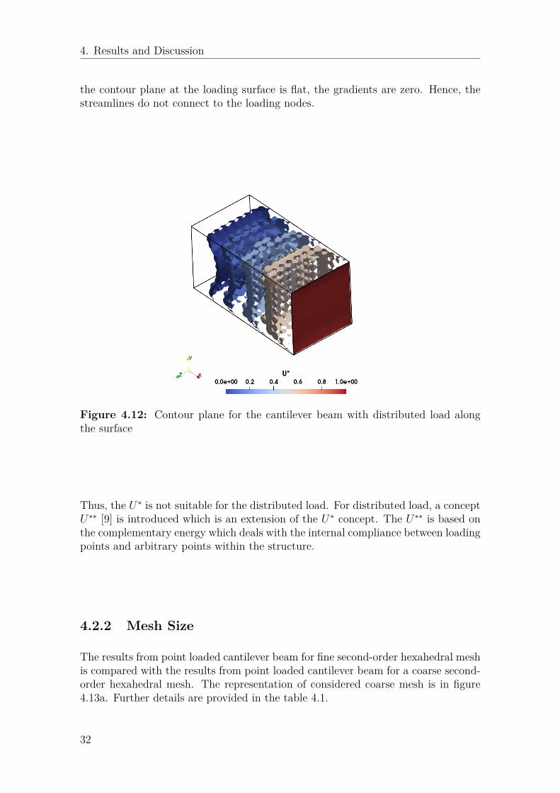
4.12 Contour plane for the cantilever beam with distributed load along thesurface . . . . . . . . . . . . . . . . . . . . . . . . . . . . . . . . . . . 32

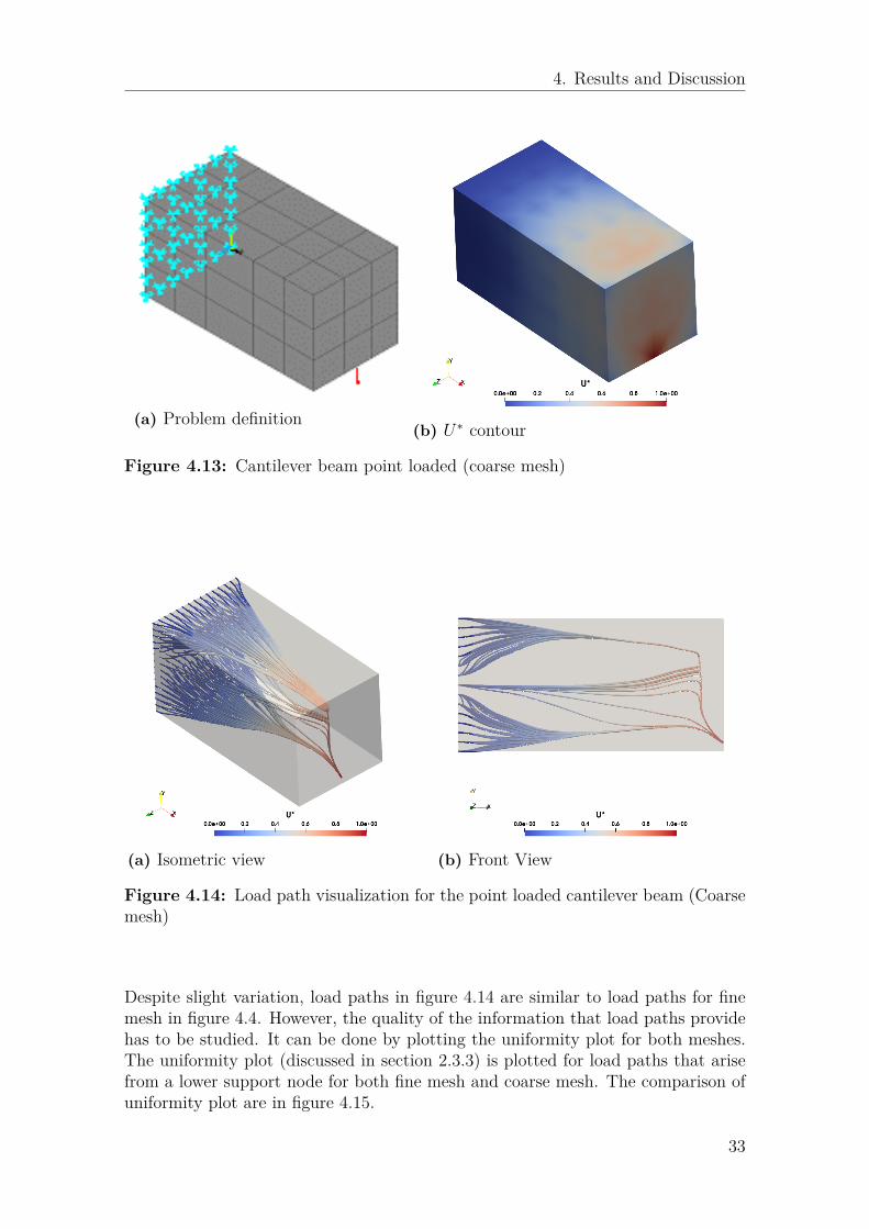
4.13 Cantilever beam point loaded (coarse mesh) . . . . . . . . . . . . . . 334.14 Load path visualization for the point loaded cantilever beam (Coarse

mesh) . . . . . . . . . . . . . . . . . . . . . . . . . . . . . . . . . . . 334.15 Uniformity plot for load paths for Fine and Coarse mesh . . . . . . . 344.16 Computational time vs Total number of nodes. . . . . . . . . . . . . . 354.17 Problem definition for the complex structure . . . . . . . . . . . . . . 364.18 Comparison of U∗ and Stress contours for the complex structure . . . 364.19 Load path visualization for the complex structure . . . . . . . . . . . 374.20 Load path taking surface for the load transfer . . . . . . . . . . . . . 38

xii

List of Tables

3.1 Description of terms in VTK file structure in figure 3.6 . . . . . . . . 203.2 Supported mesh element for data transfer . . . . . . . . . . . . . . . 21

4.1 Comparison between fine mesh and coarse mesh . . . . . . . . . . . . 34

xiii

List of Tables

xiv

Nomenclature

List of Acronyms

2D Two Dimension3D Three DimensionAPDL Ansys Parametric Design LanguageDOF Degrees of FreedomFEA Finite Element AnalysisFEM Finite Element MethodVTK Visualization Toolkit

List of Notations

nload Load nodesnboundary Boundary nodesnfree Free nodesdload Displacement at load nodesK Global Stiffness MatrixP Load Vectord Displacement VectorU Total Strain Energy of the original load caseU ′ Total Strain Energy of the modified load caseU∗ Index expressing the internal stiffnessU∗∗ Index expressing the internal compliance

xv

List of Tables

xvi

1Introduction

This chapter gives an overview of the company’s background, projectbackground, project description, aim and limitations of the project.

1.1 Company BackgroundGKN Aerospace Sweden AB is a subsidiary of the company group GKN AerospaceEngine Systems within GKN Aerospace who are pioneers in manufacturing aero-engines, wing structures and other components of the aircraft. The company wasformed in 2012 when Volvo Aero was integrated into the GKN group of companies.The headquarters is located at Trollhätan, Sweden. At Trollhättan, the companydevelops and manufactures structure components for commercial aero-engines foraircraft and space rockets and carries out engine maintenance. GKN AerospaceEngine Systems collaborates with major aircraft engine manufacturers such as Rolls-Royce, Pratt & Whitney, Snecma, and General Electric on large civil aircraft engines.Currently, GKN Aerospace engine components are used in about 90 per cent of allnewly designed aircraft worldwide [1].

1.2 Project BackgroundOne of the problems in the modern engineering industry is how to improve thestructural design of the structures taking account of the product’s performance andmanufacturing cost during the initial stages of the product development. An im-proved structural design should have high strength to weight ratio or high stiffnessto weight ratio. Although lightweight materials can be used for this purpose, an im-proved structural design will make the product structurally stronger and efficient.While designing the structure, it is important to study how the imposed load passesthrough the structure to the supporting points. It can be done by analyzing so-called load paths. The load paths are the trajectories that represent the flow of loadwithin the structure. Hence, the load path visualization is considered in this thesis.Conventional stress-based concepts already exist in the structural mechanics for thismotive. However, these concepts are vulnerable to factors like stress concentrationdue to the geometry features of the design such as bends, curves and holes. Hence,there exists a need for an analysis based on alternative methods that are unaffectedto such stress concentration.

1

1. Introduction

The index U∗, which defines the internal stiffness of the structure, expresses thedegree of connection between an arbitrary point and loading point within the struc-ture [13]. This index is independent to stress concentrations. The load paths basedon the U∗ field provides information about the load distribution, regions of highstresses. By knowing the load distribution, the material at locations that do notcontribute to the load distribution can be removed and material can be added wherethe stiffness modification is required. Thus, the stiffness can be improved to achievea high strength-weight ratio or a high stiffness-weight ratio. Hence, by taking ac-count of this information, the structural design can be modified according to itspurpose.

Previous research conducted at GKN Aerospace around the architecture and com-plexity of aero-engine components [2] examined the possibility of developing loadpath analysis for aero-engine structures. This included development of analysisscripts as well as looking into existing software.

A software developed by FRONE Corporation [4] exists to perform the necessarypre&post processing to visualize U∗. Due to the problems of integration with ex-isting software practices at GKN Aerospace, the software was not used. Thus, theconsequence led to the origin of this thesis.

1.3 Project DescriptionThe purpose of the project to use load path visualization in existing aero-enginestructures and thereby enable design improvements. Figure 1.1 illustrates how theload path visualization can be used in the design optimisation of the structure.

Figure 1.1: Flowchart of design optimisation based on load paths using U∗

The method takes advantage of the Finite Element Method technique to calculatethe U∗. The contours and load paths are plotted based on U∗ data field. The designcan be evaluated based on the criteria from the load paths explained in section 2.3.3and modified until the design satisfies the criteria. Thus, the structurally improveddesign can be obtained.

2

1. Introduction

Figure 1.2: Missing links for load path visualization at GKN Aerospace

Although the procedure to visualize load paths and design evaluation are known, themethods to calculate U∗ from the finite element model, visualizing the load pathsand evaluating design based on the load path are not widely available in commercialFE software. Hence, this thesis focuses on the implementation of these methodswith existing commercial software and for the wider use of load path visualizationin GKN Aerospace to analyse and enable design improvement in the aero-enginestructures.

1.4 Aim and Objectives of the ProjectThe thesis aims to carry out methods to do the necessary calculations and to plotload paths by the U∗ index method in the aero-engine structures in 3D space. Toachieve this, the following objectives are needed to be completed.

1. Implementation of the U∗ calculation routine in commercial FEA softwareused at GKN Aerospace.

2. Produce contour plot of U∗ for the physical problem.3. Produce methods to visualize the Load paths within the structure.4. Establish methods to evaluate load paths.

1.5 LimitationsDue to the limits on time for completion of this thesis, the scope had to be reducedand few limitations exist in this thesis. They are the following,

1. The thesis is limited to purely static mechanical loaded problems.2. Only linear isotropic elastic material model is considered.3. Only the routine for the direct method calculation of U∗ is developed, the time

reduction methods [11] are kept as future work.

3

1. Introduction

4

2Theory

This chapter illustrates the basic theory to understand the Finite ele-ment method and how it is used to visualize load path. This chapter alsocovers the theory of the U∗ index method. The supporting literature isalso presented to discuss relevant studies carried out in a similar fieldof work.

2.1 Introduction to Finite Element MethodThe Finite Element Method (FEM) is a numerical procedure for solving partialdifferential equations. It is generally used to obtain solutions to boundary valueproblems in mathematical physics and engineering analysis. This method employsdiscretizing a continuous domain into several smaller, simpler subdomains calledfinite elements interconnected at points (nodes) common to two or more elements,each of which represents the unknown function with simple interpolation functionswith unknown coefficients. This method formulates the equations for each finiteelement and combines them to obtain the solution of the whole body [5]. Thus, Thesolution of the whole body is approximated by a finite number of unknown coeffi-cients. FEM is applied when the geometry is complex, where the analytical solutioncan not be implied. The study of a phenomenon with FEM referred to as FiniteElement Analysis (FEA). It is widely used in several areas of engineering analysisand research.

The general procedure for finite element analysis (FEA) can be categorised in threesteps as follows

1. Pre-processing2. Solution3. Post-processing

The Pre-Processing involves Geometry definition, Material property definition, Meshgeneration (discretization of the domain), Selection of element types and physicalconstraints definition (Boundary conditions and loading conditions). The solutionsolves the system of equations in the form of matrices using numerical techniquesto get unknown variables such as displacements, stresses, reaction forces and heatflow. Post-Processing is the analysis and evaluation of the results in the form ofplots and graphs to make decisions. Usually, Post-Processing is done using computerprograms/software.

5

2. Theory

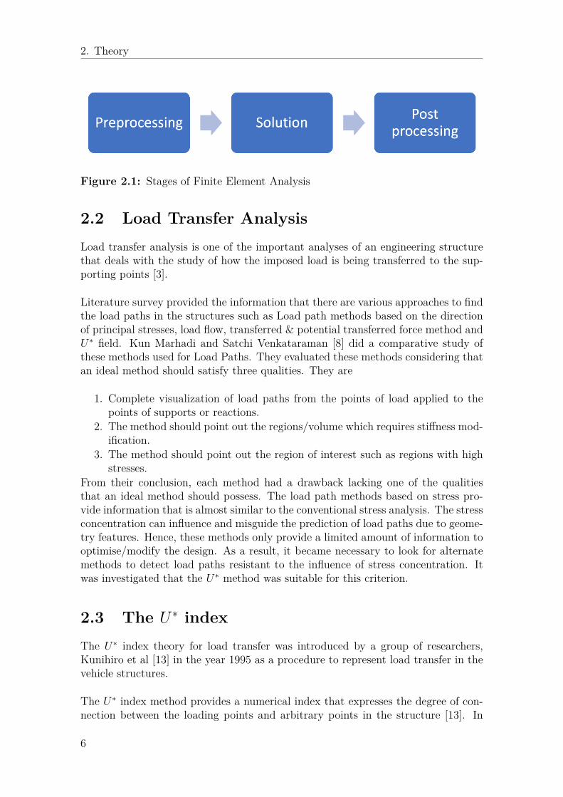
Figure 2.1: Stages of Finite Element Analysis

2.2 Load Transfer AnalysisLoad transfer analysis is one of the important analyses of an engineering structurethat deals with the study of how the imposed load is being transferred to the sup-porting points [3].

Literature survey provided the information that there are various approaches to findthe load paths in the structures such as Load path methods based on the directionof principal stresses, load flow, transferred & potential transferred force method andU∗ field. Kun Marhadi and Satchi Venkataraman [8] did a comparative study ofthese methods used for Load Paths. They evaluated these methods considering thatan ideal method should satisfy three qualities. They are

1. Complete visualization of load paths from the points of load applied to thepoints of supports or reactions.

2. The method should point out the regions/volume which requires stiffness mod-ification.

3. The method should point out the region of interest such as regions with highstresses.

From their conclusion, each method had a drawback lacking one of the qualitiesthat an ideal method should possess. The load path methods based on stress pro-vide information that is almost similar to the conventional stress analysis. The stressconcentration can influence and misguide the prediction of load paths due to geome-try features. Hence, these methods only provide a limited amount of information tooptimise/modify the design. As a result, it became necessary to look for alternatemethods to detect load paths resistant to the influence of stress concentration. Itwas investigated that the U∗ method was suitable for this criterion.

2.3 The U ∗ indexThe U∗ index theory for load transfer was introduced by a group of researchers,Kunihiro et al [13] in the year 1995 as a procedure to represent load transfer in thevehicle structures.

The U∗ index method provides a numerical index that expresses the degree of con-nection between the loading points and arbitrary points in the structure [13]. In

6

2. Theory

other words, it provides information about the participation of the arbitrary pointin the structure towards the load distribution. This method is based on the totalstrain energy of the structure under different boundary conditions.

2.3.1 MethodLet us consider a simple elastic body structure as shown in the figure 2.2 which hasthree points A, B and C. A is the point of loading, B is the point of support and Cis an arbitrary point in the structure.

(a) Original loading case (b) Modified loading case

Figure 2.2: Spring model of the problem for U∗ analysis

Since the body is elastic, the connection between these points can be representedby linear springs. The force-displacement relation of the system can be written as

P = K d

Where P and d are the load/force vector and displacement vector respectively. Kis the stiffness matrix that points out the force-displacement relationship of eachpoint due to external load and the mutual relationship between two arbitrary pointswithin the structure [14]. The expression of the force-displacement relation for theproblem in figure 2.2a can be written as PA

PB

PC

=

KAA KAB KAC

KBA KBB KBC

KCA KCB KCC

dA

dB

dC

The suffices in the vectors and matrix refers to the corresponding points in thestructure.

If PA is the load applied at point A, dA is the displacement due to the loading atpoint A, then the total strain energy of the system is defined by

7

2. Theory

U = 12 PA dA

Since the point B is fixed (dB=0),

U = 12 (KAAdA +KACdC) dA

The loading case/physical constraint is modified by replacing the force by enforcingthe displacement dA and constraining the arbitrary point C as shown in figure 2.2b.The total strain energy of the modified system can be written as

U ′ = 12 P

′A dA

where P ′A is the load required to enforce displacement dA. Since the point B and Care fixed,

U ′ = 12 (KAAdA) dA

According to the U∗ theory, the U∗ index is defined as

U∗ = 1 − U

U ′(2.1)

U∗ = 1 − (KAAdA +KACdC)(KAAdA) (2.2)

From equation 2.2, it is evident that U∗ index of an arbitrary point depends on thestiffness between the loading point A and arbitrary point C. It points out the degreeof connection between these points. Following the same procedure of constrainingarbitrary points, the U∗ distribution within the structure can be obtained by calcu-lating U∗ at other arbitrary points within the structure.

2.3.2 VisualizationAccording to the U∗ theory, the path tracing through the regions with the highestinternal stiffness within the structure is called the Load path. In other words, theload path connects the loading points to the supporting points through the highestU∗ index values (points having the highest degree of connection).

If a vector is introduced such that

λ = −grad U∗

then, the line traced along the lowest λ value is the load path [9].

It is the path that passes through the highest points of the contour lines obtainedfrom the U∗ field within the structure. Figure 2.3 illustrates the load path (Blue

8

2. Theory

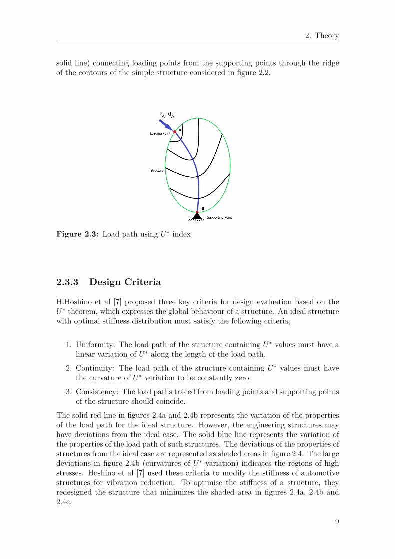
solid line) connecting loading points from the supporting points through the ridgeof the contours of the simple structure considered in figure 2.2.

Figure 2.3: Load path using U∗ index

2.3.3 Design Criteria

H.Hoshino et al [7] proposed three key criteria for design evaluation based on theU∗ theorem, which expresses the global behaviour of a structure. An ideal structurewith optimal stiffness distribution must satisfy the following criteria,

1. Uniformity: The load path of the structure containing U∗ values must have alinear variation of U∗ along the length of the load path.

2. Continuity: The load path of the structure containing U∗ values must havethe curvature of U∗ variation to be constantly zero.

3. Consistency: The load paths traced from loading points and supporting pointsof the structure should coincide.

The solid red line in figures 2.4a and 2.4b represents the variation of the propertiesof the load path for the ideal structure. However, the engineering structures mayhave deviations from the ideal case. The solid blue line represents the variation ofthe properties of the load path of such structures. The deviations of the properties ofstructures from the ideal case are represented as shaded areas in figure 2.4. The largedeviations in figure 2.4b (curvatures of U∗ variation) indicates the regions of highstresses. Hoshino et al [7] used these criteria to modify the stiffness of automotivestructures for vibration reduction. To optimise the stiffness of a structure, theyredesigned the structure that minimizes the shaded area in figures 2.4a, 2.4b and2.4c.

9

2. Theory

(a) Uniformity (b) Continuity

(c) Consistency

Figure 2.4: Illustration of design criteria based on U∗

These design criteria helps the designers in evaluating the design to find out thecritical regions in the structure or to modify the physical constraints that wouldmake the structure stiffer.

2.3.4 DrawbacksAlthough this U∗ index method has great significance over the conventional stressconcepts, it has some drawbacks which are needed to be addressed.

1. Since the calculation of U∗ index within a structure involves solving the prob-lem for multiple physical constraints, the computational time becomes heavywhen the problem has more nodes. In other words, for fine mesh, the compu-tational time becomes enormously heavy which is a serious problem in usingthis U∗ index method. However, alternative methods of calculating the U∗was proposed by Sakurai T et al [11] which was proven to drastically reducethe computational time.

10

2. Theory

2. Initially, the concept of load path using U∗ was proposed for the concentrat-ed/point load. When this concept was applied to the distributed load, itproduced unreliable results. As the contour near the loading has the highestgradient at the middle of the loading, the load paths connect to the middleof the loading. Thus, it does not provide reliable information about the stressnear the points of loading. Sakurai T et al. [12] continued the calculation ofU∗ for multiple loading conditions. Wang et al. [18] introduced a new conceptU∗∗, complementary to U∗ for distributed loading conditions provided reliableresults.

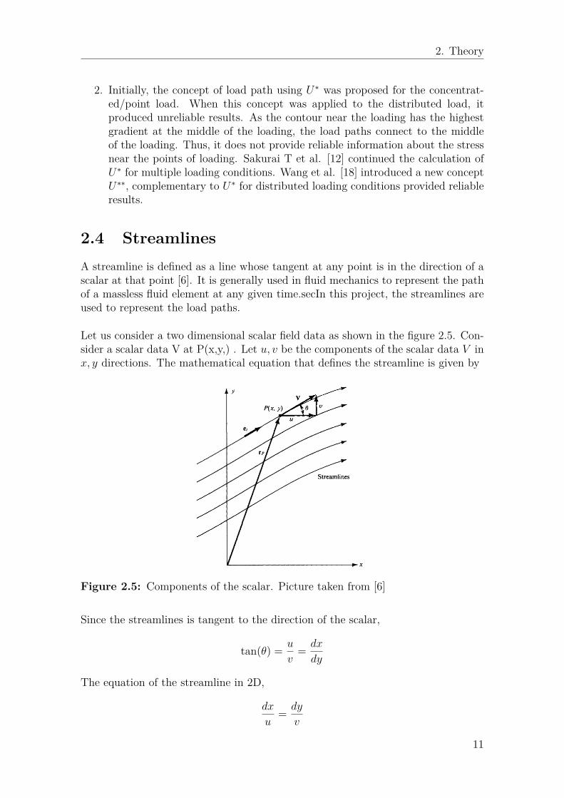
2.4 StreamlinesA streamline is defined as a line whose tangent at any point is in the direction of ascalar at that point [6]. It is generally used in fluid mechanics to represent the pathof a massless fluid element at any given time.secIn this project, the streamlines areused to represent the load paths.

Let us consider a two dimensional scalar field data as shown in the figure 2.5. Con-sider a scalar data V at P(x,y,) . Let u, v be the components of the scalar data V inx, y directions. The mathematical equation that defines the streamline is given by

Figure 2.5: Components of the scalar. Picture taken from [6]

Since the streamlines is tangent to the direction of the scalar,

tan(θ) = u

v= dx

dy

The equation of the streamline in 2D,

dx

u= dy

v

11

2. Theory

similarly the equation of the streamline in three dimensions can be written asdx

u= dy

v= dz

w(2.3)

where w is the component of the scalar variable in z direction.

The equation 2.3 is solved to plot streamlines tangent to the vector of the scalarvariable. In this thesis, the streamlines are used to represent the load paths basedon the U∗ contour.

2.5 Ansys Parametric Design LanguageThe Ansys Parametric Design Language (APDL) is a finite element solver used forvarious finite element simulations such as Thermal, Structural, Acoustic, Piezoelec-tric, Electrostatic and Circuit Coupled Electromagnets. It provides the user withmany boundless features such as parameterization, macros, branching and loop-ing, and complex math operations. The commands in the APDL enables the userto define user-defined routines and calculations which are not standard in APDL.Using these advantages, the U∗ calculation routine is created by using the APDLcommands.

2.6 Visualization of Streamlines in ParaViewParaView is an open-source, multi-platform scientific data analysis and interactivevisualization tool that enables analysis and visualization of extremely large datasets[19]. it is both a general-purpose, end-user application with a collection of tools andlibraries for various applications including scripting (using Python), web visualiza-tion (through ParaViewWeb), or in-situ analysis (with Catalyst). It also supportsscripting and batch processing using Python.

ParaView uses the Visualization Toolkit (VTK), to provide the cornerstone for vi-sualization and data processing. ParaView has file readers that support variousfile formats typically used in computational software. VTK contributes a valuabledata model that ParaView uses to efficiently interpret data from diverse fields withvarying features. File readers in ParaView build a data type that is suitable forexpressing the data in the files. ParaView permits to create and add filters to trans-form data based on the data type. In computational science, it is commonly usedfor post-processing the results obtained from the simulations.

2.6.1 FiltersThe filters are the algorithms that read in the data, transform the data, exportthem to interpret results through data visualization or further processing. Thereare various filters in-built in ParaView which can be used to create pipelines toperform different operations, processing types and desired task by connecting thesefilters in a pipeline.

12

2. Theory

2.6.1.1 Gradient Of Unstructured datagrid

It is an in-built feature in ParaView which is used to calculate the gradients of thescalar field of cell data or point data. The filter functions by iterating over all thecells and calculating the local gradients based on parametric coordinates inside thecells. The gradients are obtained as vectors. The gradients obtained is used by thefilter are used by the Streamtracer filter to plot the streamlines to visualize the loadpaths.

2.6.1.2 Streamtracer

Stream Tracer filter is an in-built feature in ParaView which generates streamlinesfor vector fields from the collection of seed points. The algorithm functions byreading an array of points, known as seed points, in the dataset and then integratingthe streamlines starting at these seed points. This filter has options that lets theuser tune the streamlines using the type of integrator, the direction of integrator,length of the streamline. This filter can be accessed from the Filters menu. Thisfilter is used in this project to visualize the load-paths from the U∗ index vectorfield.

2.7 The Visualization Tool Kit (VTK)

The Visualization Tool Kit (VTK) is one of the commonly used scientific data fileformats. It is an open-source system for scientific visualization, 3D computer graph-ics and image processing and volume rendering [20]. It is produced by the companyKitware. VTK file formats are used to import the sets of data to ParaView .

VTK file format has two different styles. One is Simple Legacy format and the otheris XML format. In this project, the Simple legacy format is used to communicatethe data (Geometry, nodes, element topology, nodal results) from ANSYS APDL toParaView. The Simple Legacy file format has five parts. The first parts correspondto file version and identifier. The second section refers to the header, and it describesthe data and any other relevant information. The third part is where the type offile format is described between ASCII and BINARY. The fourth part refers to thedataset structure. This is where the geometry, nodes, element topology are defined.The last part describes the dataset attributes which is nothing but the scalar data,vector data at elements and nodes from the results are defined. The figure 2.6illustrates all these parts.

13

2. Theory

Figure 2.6: General structure of VTK file

Generally, the VTK file format supports has five types of dataset formats such as

1. Structured Points: defines a dataset of points having equal spacing in everythree directions (X, Y, Z).

2. Structured Grid: defines a dataset of a grid of points having equal spacing inevery three directions (X, Y, Z).

3. Unstructured Grid: defines a dataset of points having unequal spacing withany possible cell type.

4. Polygonal Data: defines a dataset of points associated with regular topology,polygonal geometry.

5. Rectilinear Grid: defines a dataset of the grid of points associated with regulartopology, and semi-regular geometry aligned along the x-y-z coordinate axes.

6. Field: defines a dataset of points or cells without topological and geometricstructure and a particular dimensionality.

14

3Methodology

In this chapter, the method of approach to visualize the load paths for3D structures is described. Further, the methods to evaluate the designbased on the load paths are also described.

3.1 Problem ApproachThe aim, scope of the thesis were studied and the milestones are set considering thetime frame. A Gantt Chart is created and appropriate days are fixed as a deadlinefor each milestone. A systematic approach for the thesis to achieve the milestoneswas framed as shown in figure 3.1.

Figure 3.1: Systematic approach to the problem

The approach begins with the literature study. The literature study included thestudy of Load transfer analysis and its application, programming using APDL com-mands and creating VTK format files. The books, journals, research papers relatedto load transfer analyses gave exposure to a breadth of concepts in U∗ theory, FEMcalculations and provided plenty of insights to proceed with the thesis. Then, certainresults from the literature are benchmarked and a Matlab program is developed todo the calculations and to visualize the load paths. Initially, a simple 2D structure

15

3. Methodology

(cantilever problem) is considered for the ease of developing routines. The resultsobtained from Matlab are verified with the literature results.

After, the thesis is concentrated on developing routines through software. AnsysWorkbench, Ansys Mechanical APDL, ParaView and Matlab are used for this pur-pose. A detailed description of how these software used in this thesis is in section3.3. Once the routines are developed, the load paths are visualized and verified withthe literature results. After verifying the results, the method to evaluate the designbased on the load paths is developed. Finally, the complete routine is tested on 2Dproblems and 3D problems including complex shapes for different boundary condi-tions, different mesh elements and different mesh size. The results and discussionsare provided in the chapter 4.

3.2 Load Path Visualization - Routine develop-ment for 2D problems in Matlab

With the knowledge gained from the literature study, a routine to visualize the loadpaths for simple 2D structures is created by scripting in Matlab and to replicateliterature results. This is done to have a deep perception of all relevant aspectsto plot load paths using U∗ theory. The streamline function in Matlab plotted theridgeline through the contours within the structure. The theory to streamlines isexplained in the section 2.4.

Figure 3.2 illustrates the routine to visualize the load paths for a structural prob-lem. The routine can be generally categorised into Pre-processing, Solution andPost-processing. The blocks in yellow colour correspond to the Pre-Processing ofthe load path visualization.

The blocks in green colour correspond to the U∗ calculation algorithm (Solution).The blocks in red colour correspond to the Post-processing of the load path visual-ization. The algorithm in figure 3.2 is explained in the following.

1. The routine starts with the general pre-processing of a physical problem.2. The solver does the calculation routine for U∗ field in a structure.3. First, the original load case is solved. The total strain energy of the structureU and the displacements at the loading nodes are calculated.

4. A loop is created that runs for all freenodes. Freenodes are an array of nodesthat are a complement to the nodes that contribute to the loading and bound-ary nodes from total nodes.

5. In each loop, the load case is modified such that the DOFs of a Freenode isconstrained in addition to the supporting nodes.

6. The force applied to the system is replaced by the enforced displacementswhich are calculated from the results of the original loading case.

7. The modified load case is solved and the strain energy of the modified systemU’ is calculated.

16

3. Methodology

Figure 3.2: The algorithm to visualize load paths using U∗ index method

8. The constrained DOFs of freenode is removed and the loop continues with thenext freenodes.

9. Once the loop gets done, the U∗ index values to the loading points and sup-porting points are assigned as 1 and 0.

10. The load paths are visualized by post-processing the results. To visualize theload paths, the streamlines can be plotted. The streamline plots line over theridge of the contour lines. The streamlines require components of the scalarquantity (U∗ index) in three dimensions. The components of the U∗ index canbe derived by taking the gradients of the U∗ index in directions concerningtheir nodal coordinates.

17

3. Methodology

3.3 Load Path Visualization - Routine Develop-ment through software

Figure 3.3: Load Path visualization routine in Software

Unlike traditional stress-strain analysis, the U∗ star calculation requires a loopingof solution routine under different modified physical constraints. To calculate theU∗ field, a routine has to be defined in FEM software. The methods to implementthe calculation of U∗ field in the structure was investigated in various software. TheAnsys Mechanical APDL was chosen to be a solver since it has great features thatpermit the user to define a user-defined calculation routine. Although the U∗ canbe calculated by using the Ansys Mechanical APDL, post-processing the result tovisualize the contour and load paths are difficult using APDL. Hence, ParaView ischosen as a postprocessor is to visualize the contour of U∗ and load paths.

Figure 3.3 illustrates the workflow carried in this thesis to visualize the load pathsof a structure.

3.3.1 PreprocessingThe general preprocessing of a physical problem is carried out using commercialsoftware Ansys Workbench where the geometry, material, mesh, element type aredefined. Instead of applying the boundary and loading conditions, their correspond-ing nodes are selected as components using specific names as shown in the figure 3.4.

The “loadnodes” and “fixnodes” in the model tree in figure 3.4 corresponds to thenodes that are associated with loading and boundary conditions respectively. Theload magnitude and orientation are applied using the Ansys Mechanical APDL.The preprocessed model is exported to Ansys Mechanical APDL for the SOLUTION(U∗ calculation) as shown in the figure 3.5.

18

3. Methodology

Figure 3.4: Model tree from Ansys Workbench with named selections used forSupport and Loading nodes

Figure 3.5: Transferring Preprocessed model to Ansys Mechanical APDL

3.3.2 SolutionAPDL commands are used to define a user-defined to calculate the U∗ field withinthe structure. A program with APDL commands is created in the “.inp” file formatthrough which the commands can be imported to the Mechanical APDL solver. Theprogram reads the load-nodes nload, boundary-nodes nboundary data from the set ofcomponents created during pre-processing. The commands are programmed suchthat it follows the calculation of U∗ routine.

Initially, the original loading case is solved. The strain energy U and load node dis-placements dload are calculated. Then, for each free node nfree, a load step is writtenwith a modified loading case (removing force and enforcing load node displacementdload). So, the total number of load steps equals the total number of free nodes nfree.The programmed APDL commands solve all the load steps and the strain energyU ′ for all the load steps are calculated. From the set of strain energies for modifiedloading cases U ′ , the index U∗ is calculated by using the equation 2.1 for all nodes.

Further, the program is developed to export some information such as mesh elementtype, element nodal connectivity and U∗ data along with nodal coordinates in “.txt”file formats as “element_type.txt”, “element_table.txt” and “nodal_results.txt” re-spectively. These “.txt” file formats are exported for post-processing the results ob-tained from the Ansys Mechanical APDL solver.

19

3. Methodology

In figure 3.3, “U_star.inp” contains the APDL commands, which is inputted to theSolver Ansys Mechanical APDL. The “U_star.inp” is appended to this report inAppendix A.1.

3.3.3 Post ProcessingThe solution is followed by post-processing of the results to visualize the load paths.Usually, the Ansys Mechanical APDL results are exported in the “.rst” file format.But, the ParaView has no reader to read the results directly from the “.rst” fileformat. However, the results obtained from the Ansys Mechanical APDL can be fedinto the ParaView through “.vtk” file format. Thus, the result data from the AnsysMechanical APDL are exported as “.txt” file formats.

3.3.3.1 Data Processing

A programming script is developed in Matlab to construct a “.vtk” format file. TheMatlab program reads the results from “element_type.txt”, “element_table.txt”and “nodal_results.txt” files and generates a “.vtk” format file to transform resultsfrom the solver Ansys Mechanical APDL to post-processor ParaView.

The “.vtk” file format has a structure through which the data can be inputted to theParaView. The general structure of the VTK file format is described in the section2.7 in figure 2.6. However, the detailed structure of the VTK file format that is usedin this thesis is described in the figure 3.6. ASCII type of dataset is chosen. Fromthe five types of dataset formats described in section 2.7, the unstructured grid hasbeen chosen since it supports the non-equidistant nodes.

A sample structure of the “.vtk” file generated by the Matlab used in this thesis ispresented in the figure 3.6.

Table 3.1: Description of terms in VTK file structure in figure 3.6

SI Variables Description1 nnodes Total number of nodes2 nelem Total number of elements3 U∗n U∗ of nth node4 typen Type of mesh element of nth element5 Pnx x-coordinate of nth node6 Pny y-coordinate of nth node7 Pnz z-coordinate of nth node

In figure 3.6, the keywords are colour-coded to differentiate the keywords and vari-ables for the explanation. The keyword “POINTS” is used to define the locations ofthe nodes requires two parameters (Total number of nodes and type of data). Thekeyword “CELLS” defines the element-nodal connectivity, requires two parameters

20

3. Methodology

Figure 3.6: General Structure of the VTK structure for the ParaView input

(Total number of elements and total number of integer values required to representthe list). The keyword “CELL_TYPES” defines the type of element, requires oneparameter (Total number of elements). The legacy type of VTK file format has aseparate list of cell types. Hence, the APDL element type number and the matchingcell type number must be studied and chosen accordingly. The keyword "SCALARS"is used to define the U∗ values, requires two parameters (name of the scalar and typeof the data).

The Matlab program was developed with some limitations as it supports only cer-tain mesh elements from Ansys Mechanical APDL. The supported mesh elementsare listed in table 3.2.

Table 3.2: Supported mesh element for data transfer

SI No Mesh Element Description1 SHELL181 4-Node Structural Shell2 PLANE182 2-D 4-Node Structural Solid3 PLANE183 2-D 8-Node or 6-Node Structural Solid4 SOLID185 3-D 8-Node Structural Solid5 SOLID186 3-D 20-Node Structural Solid6 SOLID187 3-D 10-Node Tetrahedral Structural Solid

The Matlab code for transferring the result from Ansys Mechanical APDL to Par-aView is appended to this report in Appendix A.2.

21

3. Methodology

3.3.3.2 Visualization

The “.vtk” format file generated from the Matlab is inputted to the ParaView. Byreading the “.vtk” file, the ParaView plots the contour of U∗ data set. The gradientsare calculated by using the filter “GradientOfUnstructuredDataSet”. From the gra-dients, the streamlines are plotted using the filter “StreamTracer”. While plottingthe streamlines, the locations of seed points for the streamlines should be chosen atthe location of supporting nodes.

Figure 3.7: ParaView pipeline browser

Figure 3.7 shows the pipeline browser illustrating how the filters are used to visu-alize the load paths. The plot may show many streamlines. Thus, the streamlinesflow from the nodes of support to the nodes of loading. But, not all the streamlinesconnect the supporting nodes to loading nodes. The streamlines that connect sup-porting nodes and loading nodes should be concentrated.

At the end of the flowchart on figure 3.3, the first three objectives mentioned in thesection 1.4 are achieved.

3.4 Design evaluation based on the principle loadpath

According to the U∗ theory, the structural design of a structure should be optimisedbased on the insights obtained from the evaluation of load paths. The load paths areto be evaluated using the design criteria as explained in section 2.3.3 which requirescontinuity plot and uniformity plot. Hence, this section explains how the Uniformityand continuity plots are developed for load paths.

22

3. Methodology

Figure 3.8: Routine for Load Path evaluation

To plot the continuity plot and uniformity plot, Matlab is used in this thesis. Thedata of the principal load path containing the U∗ values are extracted from Par-aView and exported in the “.csv” file format. The “.csv” file is imported into Matlaband programmed to plot continuity and uniformity plots.

3.5 Visualization EnhancementIn this study, an approach is developed to enhance the visualization of the loadpaths and avoid the discontinuities of the load paths. The approach includes theconstruction of more nodes with interpolation of the nodal values from the solutionof U∗. Hence, the streamlines take advantage of more nodal locations and producea smooth visualization of load paths. This can be achieved can using the in-builtfilter “ResampleToImage” in ParaView.

(a) Actual nodes (b) Additional nodes

Figure 3.9: Generation of additional nodes in ParaView

23

3. Methodology

24

4Results and Discussion

In this chapter, the results obtained from developed routine is presented.The results includes contour of U∗, visualization of load paths. Theinfluence of mesh element, mesh size, boundary condition, loading con-ditions are explained.

4.1 Verification of results for 2D problem

As mentioned in the section 3.1, simple 2D problems are considered to developroutines to visualize load paths and to verify with the results from the literature.Figure 4.1a shows the comparison between the result of a 2D cantilever problem fromthe literature [8] and the result for the same problem obtained from the developedroutine explained in section 3.3.

(a) Result from Literature [8](b) Result from developed methodol-ogy

Figure 4.1: Load Path visualization on 2D cantilever beam

Plane stress condition with thickness and quadrilateral mesh element were consid-ered in the FEM calculation for figure 4.1b. It is obvious that load paths in figure4.1b are in correspondence with load paths in figure 4.1a. Thus, it can be concludedthat the developed routine delivers the desired results for the 2D structural problem.

25

4. Results and Discussion

4.2 Routine test - 3D Cantilever problem

Once the results obtained from the developed routine are verified for 2D problems,the routines are tested for 3D problems. For simplicity, a 3D cantilever problem isstudied to understand the behaviour of load paths under different mesh elements,different element size and different types of loading cases. Further, the routines aretested for 3D complex shape.

load paths in the 3D cantilever beam are investigated under different loading con-ditions such as point load, distributed load on the edge and distributed load on theface to study the influence of types of loading on load paths. Also, the influence ofthe type and size of the mesh elements and computational time are studied.

4.2.1 Type of loading

Point Load

A 3D cantilever beam is point-loaded as shown in the figure. A study on the influ-ence of the type of mesh element is carried out for the point load loading condition.Two mesh elements were investigated for the point loaded cantilever problem. First,the results for second-order hexahedral mesh is studied. A fine mesh of second-orderhexahedral mesh element is used to visualize load paths. The developed routine isused to calculate the U∗ and visualize load paths.

The U∗ contour and load paths obtained from the developed routine for the pointloaded cantilever beam with second-order hexahedral mesh are presented in thefigures 4.2 and 4.4.

(a) Problem definition(b) U∗ contour

Figure 4.2: Cantilever beam point load [Hexahedral mesh]

26

4. Results and Discussion

(a) Isometric view (b) Front view

Figure 4.3: Discontinuity of Load paths

It is observed from the figure 4.3, that there exists a discontinuity in load pathsarising from the boundary nodes near the loading node. This discontinuity of loadpaths may be due to the size of the mesh is inefficiently larger to take gradient as theU∗ values take a sharp increase near the loading node. However, this discontinuitycan be fixed using plotting streamlines seeding from near the point of discontinu-ity. The complete visualizations of load paths for point loaded cantilever beam arepresented in figure 4.4.

(a) Isometric view (b) Front view

Figure 4.4: Load paths visualization for cantilever beam point loaded [hexahedralmesh element]

Further, the same problem is studied with the second-order tetrahedral mesh ele-ment. The U∗ contour and load paths obtained from the developed routine for thepoint loaded cantilever beam with second-order tetrahedral mesh are presented inthe figures 4.5b and 4.6.

27

4. Results and Discussion

(a) Problem definition(b) U∗ contour

Figure 4.5: Cantilever point loaded [Tetrahedral mesh]

(a) Isometric view (b) Front view

Figure 4.6: Load path visualization for cantilever beam point loaded [Tetrahedralmesh element]

Although the U∗ contour for both mesh elements are similar, some dissimilaritiesare observed for load paths. load paths in the figure 4.6 are irregular and unsmooth.In addition to that, some of the load paths that originate from supporting nodesare not connected to the loading node. Instead, they get diverted back to thesupporting nodes. Whereas, for the hexahedral mesh (see figure 4.4), all load pathsthat originate from the support point connects to the loading point which providedcomparatively reliable results. Thus, the second-order tetrahedral mesh producespoor results whereas the second-order hexahedral mesh provides regular and smoothresults. Hence, it can be concluded that the second-order hexahedral mesh is thesuitable mesh element for the visualization of load paths.

28

4. Results and Discussion

Distributed Load

The developed routine is tested on a 3D cantilever beam for the distributed load.This is done to study the behaviour of the load path for distributed loading in3D space. For distributed loading, two loading cases were considered. First, thedistributed load is applied vertically to the bottom edge of the free end of thecantilever beam as shown in figure 4.7a. Then, the distributed load is appliedvertically on the face of the free end of the cantilever beam.

Edge load

The figure 4.7b shows the contour of U∗ distribution for the first distributed loadingcase.

(a) Problem definition (b) U∗ contour

Figure 4.7: Cantilever beam with distributed load along the edge.

Figure 4.8 represents two different views of visualization of load paths obtained fromthe developed routine. load paths in figure 4.8a provide a controversial argument forthe distributed loading as follows. Figure 4.8a represents load paths that originatefrom the support nodes that get converged to a single loading node. This convergenceof load paths is not acceptable for the distributed load, as it portrays the inactiveparticipation of the rest of the loading nodes. The results obtained are similar tothe case of point load. The reason is as follows.

29

4. Results and Discussion

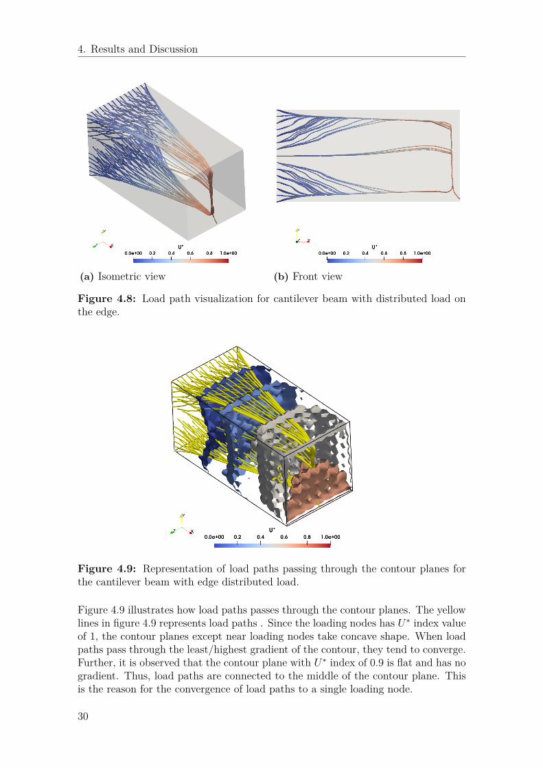
(a) Isometric view (b) Front view

Figure 4.8: Load path visualization for cantilever beam with distributed load onthe edge.

Figure 4.9: Representation of load paths passing through the contour planes forthe cantilever beam with edge distributed load.

Figure 4.9 illustrates how load paths passes through the contour planes. The yellowlines in figure 4.9 represents load paths . Since the loading nodes has U∗ index valueof 1, the contour planes except near loading nodes take concave shape. When loadpaths pass through the least/highest gradient of the contour, they tend to converge.Further, it is observed that the contour plane with U∗ index of 0.9 is flat and has nogradient. Thus, load paths are connected to the middle of the contour plane. Thisis the reason for the convergence of load paths to a single loading node.

30

4. Results and Discussion

Surface load

The figure 4.10b shows the contour of U∗ distribution for the the second distributedloading case.

(a) Problem definition(b) U∗ contour

Figure 4.10: Cantilever beam with distributed load along the surface.

(a) Isometric View (b) Front View

Figure 4.11: Load path visualization for the surface loaded cantilever beam

Figure 4.11 visualizes load paths for the surface loaded cantilever beam in two dif-ferent views. It can be observed that load paths do not connect to the loadingnodes. Thus, it is observed from both loading cases, load paths are experiencingproblem near the loading nodes due to the contour plane shapes of the U∗. Thecontour planes for the surface loaded cantilever problem is in the figure 4.12. Since

31

4. Results and Discussion

the contour plane at the loading surface is flat, the gradients are zero. Hence, thestreamlines do not connect to the loading nodes.

Figure 4.12: Contour plane for the cantilever beam with distributed load alongthe surface

Thus, the U∗ is not suitable for the distributed load. For distributed load, a conceptU∗∗ [9] is introduced which is an extension of the U∗ concept. The U∗∗ is based onthe complementary energy which deals with the internal compliance between loadingpoints and arbitrary points within the structure.

4.2.2 Mesh Size

The results from point loaded cantilever beam for fine second-order hexahedral meshis compared with the results from point loaded cantilever beam for a coarse second-order hexahedral mesh. The representation of considered coarse mesh is in figure4.13a. Further details are provided in the table 4.1.

32

4. Results and Discussion

(a) Problem definition(b) U∗ contour

Figure 4.13: Cantilever beam point loaded (coarse mesh)

(a) Isometric view (b) Front View

Figure 4.14: Load path visualization for the point loaded cantilever beam (Coarsemesh)

Despite slight variation, load paths in figure 4.14 are similar to load paths for finemesh in figure 4.4. However, the quality of the information that load paths providehas to be studied. It can be done by plotting the uniformity plot for both meshes.The uniformity plot (discussed in section 2.3.3) is plotted for load paths that arisefrom a lower support node for both fine mesh and coarse mesh. The comparison ofuniformity plot are in figure 4.15.

33

4. Results and Discussion

Figure 4.15: Uniformity plot for load paths for Fine and Coarse mesh

It is observed from the figure 4.15, there exists a significant difference in U∗ variationbetween fine mesh and coarse mesh. Since the cantilever beam is point loaded, highstresses exist close to the loading node. This information can be figured out fromthe uniformity plot, as the U∗ takes a sharp increase at the end. On the otherend, for coarse mesh, the U∗ exhibits comparatively linear variation which is notacceptable/reasonable for the point load. Thus, it can be concluded that coarse meshprovides the visualization of load paths with slight inaccuracy. But, it provides anunreliable result for the stiffness distribution.

Table 4.1: Comparison between fine mesh and coarse mesh

Properties Fine Mesh Coarse MeshTotal Number of nodes 5121 320Fixed nodes 225 40Load nodes 1 1Free nodes 4895 279CPU time [s] 3805 25.3

Although the fine mesh provides desired results, from table 4.1, it is observed thatthe CPU time is enormous for the fine mesh when compared to the coarse mesh.

4.2.3 Computational TimeSince the routine to calculate U∗ includes looping of the solution under differentmodified conditions, the computational cost for the visualization of load paths hasto be considered seriously. For the point loaded cantilever beam, the computationaltime to solve for U∗ is recorded for various mesh sizes. The computational time isplotted against the total number of nodes in figure 4.16.

34

4. Results and Discussion

Figure 4.16: Computational time vs Total number of nodes.

From figure 4.16, it can be inferred that, the computational time required to get areliable result increases exponentially with the total number of nodes in the geome-try. From the conclusion of section 4.2.2, it is advisable to have a fine mesh to getclear detailed insights to improve the design. Thus, it is observed for a simple can-tilever problem, the solution becomes computationally heavy to obtain reasonableresults. This exponential increase in computational time is a serious problem whencomes to the application in aero-engine structures. As the finite element model ofaero-engine structures may have a large set of nodes that may require months tovisualize load paths. Although it is desired to have a fine mesh for good results, theeffect of computational time creates a contradiction for the use of fine mesh.

4.2.4 Conclusions

From the study on cantilever beam to visualise load paths under different cases,certain cases are filtered out that are most applicable for the U∗ conce. They arethe following,

1. Type of Loading: Point load2. Type of mesh: Fine and Moderate3. Type of mesh element: Hexahedral mesh element

35

4. Results and Discussion

4.3 Routine test - 3D Complex StructureThe robustness of the developed load path visualization routine has to be tested be-fore its application in aero-engine structures. For this purpose, a complex structurefrom the previous research [3] at GKN Aerospace is considered. The geometry andthe loading case of the structure are provided in the figure 4.17. The loading casesare assumed such that load paths would take diversions in three directions. Fromthe study on the cantilever beam, a point load is applied, a moderate mesh is usedand a second-order hexahedral mesh element is considered.

Figure 4.17: Problem definition for the complex structure

(a) U∗ contour (b) Von mises stress contour

Figure 4.18: Comparison of U∗ and Stress contours for the complex structure

Figure 4.18 shows the comparison between the U∗ contour and stress contour forthe complex structure. Stress concentrations can be observed in figure 4.18b at theregion D due to the influence of bends in the structure.

36

4. Results and Discussion

The developed routine visualizes load paths for the complex structure for the as-sumed loading case. The visualization of load paths from different perspectives forthe complex structure is provided in the figure 4.19.

(a) Isometric View (b) Side View

(c) Top View (d) Front View

Figure 4.19: Load path visualization for the complex structure

Design Improvement suggestionsFigure 4.19 clearly illustrates how the load is being transferred from the supportareas to the loading point. Also, it indicates what regions of the structure activelycontributes to the load distribution and inactive regions. This structure can bestructurally improved by considering the design criteria as explained in the section2.3.3. It would result in improvement of the stiffness of the structure.

Based on the load path visualization, the volume of the regions G and F in the figure4.19a can be reduced, since it does not contribute to the assumed loading case. The

37

4. Results and Discussion

Figure 4.20: Load path taking surface for the load transfer

region D in the figure 4.19a requires attention because it provides a channel for loadpaths originating from both support ends to connect to the loading node. Loadpaths flowing through region C in the figure 4.19c has sharp curvatures which maycause improper stiffness distribution. Load paths should have smooth curvaturesfor better load transfer. Thus, the design can be improved by creating fillets on theadjacent sides of region C which enhance smoother curvatures for load paths.

It is observed from figures 4.19 and 4.18b wherever the regions that load pathspasses close to the boundaries of the geometry except for the support regions, theregions experience high stresses. It may be due to load paths that tend to moveout of the geometry space, get diverted by the surface constraint and passes alongthe surface. As a consequence, load paths takes the surface of the geometry as amedium for the load transfer which is evident in figure 4.20. This would subject thestructure to higher risk. For instance, if a crack was initiated on the surface wherethe load path pass, it would increase by successive loading. Thus, load paths takeanother direction which may affect the stiffness distribution and result in failure ofthe structure. Hence, the design must be modified such that alternate load pathsshould exist in case of failure of one of the load paths.

38

5Conclusion and Future work

This chapter includes the concluding remarks and some suggestionswhich can be considered for further development of the routines.

5.1 Concluding RemarksDeveloping routines to calculate the U∗ and to visualize load paths in structural com-ponents that could be used by GKN Aerospace for further use was the main interestin this thesis. It was achieved by using different software. The FEM calculations tocalculate U∗ were performed by developing a program script in Ansys MechanicalAPDL. The visualization process is carried by both Matlab and ParaView. Thedeveloped routine was verified with literature results. For 3D structures, a study iscarried out under different cases using the developed routine. From the study, it wassuggested, a geometry with a fine mesh of second-order hexahedral mesh elementwith point load is more suitable for the visualization of load paths using the U∗concept. The mesh size and the computational time plays a significant factor inderiving insights in this thesis. Fine mesh provides desirable result but the compu-tational cost becomes a major drawback for the U∗ approach. Due to the effect ofcomputational time, the routine was not performed on the aero-engine structuresin this thesis as it may take a long duration or may require special computers tovisualize load paths within the time frame of this thesis. The developed routine wastested on a complex structure and design improvement suggestions were provided.

5.2 Future WorkThis thesis had few limitations and the scope of the thesis was reduced to fit thethesis within the time frame. Hence, the future work which has to be carried out atGKN Aerospace after this thesis should focus on those limitations and other workas follows.

• The Matlab script developed to transfer the results from Ansys MechanicalAPDL to ParaView supports certain mesh elements as mentioned in table 3.2.The Matlab program script can be updated that supports more mesh elements.

• The routine to visualize the load paths based on the reaction forces for theConsistency plot (explained in the section 2.3.3) can be developed.

39

5. Conclusion and Future work

• The discontinuity in load paths visualization using ParaView makes hard toconstruct uniformity and continuity plots. Hence, future work should focus onmethods to solve the discontinuity in load paths.

• Since the direct method of calculation U∗ is computationally heavy, the futurework should focus on alternative U∗ calculation methods such as InspectionLoading method and Inverse Stiffness method [11].

• The existing routine can be extended that supports the concept U∗∗ [9] tovisualize load paths for distributed loading conditions.

• The existing routine can be extended to support non-linear material models[15].

40

Bibliography

[1] Facts about GKN Aerospace Sweden AB http://aerospace.se/wp-content/uploads/2013/12/FAKTABLAD_GKN-Aerospace-Sweden_131209.pdf

[2] Raja, Visakha, On the Design of Functionally Integrated Aero-engine Struc-tures: Modeling and Evaluation Methods for Architecture and Complexity,Chalmers University of Technology, Doctoral thesis, 2019.

[3] Raja, V., Kokkolaras, M. & Isaksson, O. A simulation-assisted complexitymetric for design optimization of integrated architecture aero-engine struc-tures. Struct Multidisc Optim 60, 287–300 (2019). https://doi.org/10.1007/s00158-019-02308-5

[4] Frone corporation, The CAE solution provider https://frone.jp/[5] Daryl L. Logan (2011). A first course in the finite element method. Cengage

Learning. ISBN 978-0495668251.[6] Granger, Robert A.. (1995). Fluid Mechanics - 8.2 Equation of a Streamline.

(pp. 422-424). Dover Publications. Retrieved from https://app.knovel.com/hotlink/pdf/id:kt00B0E7C8/fluid-mechanics/equation-streamline

[7] H. Hoshino, T. Sakurai, K. Takahashi, Vibration reduction in the cabin ofheavy-duty trucks using the theory of load transfer paths, JSAE Review, 24165-171 (2003).

[8] Marhadi K, Venkataraman S. Comparison of quantitative and qualitative in-formation provided by different structural load path definitions. InternationalJournal for Simulation and Multidisciplinary Design Optimization. 2009 Jul1;3(3):384-400.

[9] Wang, E.Y., Nohara, T., Ishii, H., Hoshino, H., Takahashi, K., 2010. LoadTransfer Analysis Using Indexes U* and U** for Truck Cab Structures in InitialPhase of Frontal Collision. AMR 156–157, 1129–1140. https://doi.org/10.4028/www.scientific.net/amr.156-157.1129

[10] Naito T, Kobayashi H, Urushiyama Y. Application of load path index U* forevaluation of sheet steel joint with spot welds. SAE Technical Paper; 2012 Apr16.

[11] Sakurai T, Takahashi K, Kawakami H, Abe M. Reduction of calculation time forload path U* analysis of structures. Journal of Solid Mechanics and MaterialsEngineering. 2007;1(11):1322-30.

[12] Sakurai T, Tada M, Ishii H, Nohara T, Hoshino H, Takahashi K. Load path U*analysis of structures under multiple loading conditions. Nippon Kikai GakkaiRonbunshu A Hen(Transactions of the Japan Society of Mechanical EngineersPart A)(Japan). 2007 Feb;19(2):195-200.

41

Bibliography

[13] Shinobu M, Okamoto D, Ito S, Kawakami H, Takahashi K. Transferred loadand its course in passenger car bodies. JSAE review. 1995 Apr 1;16(2):145-50.

[14] Naito T, Kobayashi H, Urushiyama Y, Takahashi K. Introduction of new con-cept U* sum for evaluation of weight-efficient structure. SAE International Jour-nal of Passenger Cars-Electronic and Electrical Systems. 2011 Apr 12;4(2011-01-0061):30-41.

[15] Wang, Q., Pejhan, K., Telichev, I. et al. Extensions of the U* theoryfor applications on orthotropic composites and nonlinear elastic materials.Int J Mech Mater Des 13, 469–480 (2017). https://doi.org/10.1007/s10999-016-9348-z

[16] Pejhan, K., Wu, C.Q. and Telichev, I. (2015) ‘Comparison of load transfer index(U*) with conventional stress analysis in vehicle structure design evaluation’,Int. J. Vehicle Design, Vol. 68, No. 4, pp.285–303.

[17] Pejhan, K., Wang, Q., Wu, C.Q. and Telichev, I. (2017) ‘Experimental valida-tion of the U* index theory for load transfer analysis’, Int. J. Heavy VehicleSystems, Vol. 24, No. 3, pp.288–304.

[18] E. Wang, X. Zhang and K. Takahashi, "Load Path U* analysis of a square pipeunder collision," in Society of Automotive Engineers of Japan Annual Congress,Yokohama, 2007.

[19] ParaView users’s guide [Online]. Available : https://docs.paraview.org/en/latest/index.html

[20] The VTK user’s guide [Online]. Available : https://www.kitware.com/products/books/VTKUsersGuide.pdf

42

AAppendix

This chapter contains the programmed script used in Matlab and Ansysto construct the routine as discussed in section 3.3 to visualize loadpaths.

A.1 APDL program for U ∗ calculationThe FEM calculations to calculate the U∗ is done by developing a program in AnsysAPDL. The programmed script with APDL commands is the following.

1

2 /CLE3 ∗DEL,ALL4 ! Analyses input s t a r t s here5 /NOPR ! Suppress p r i n t i n g o f UNDO proce s s6 FINISH ! Make sure we are at BEGIN l e v e l7 /PREP7 ! Enter the p r ep ro c e s s o r8

9

10 f i le_name = ’−−−−−’ ! Enter the f i l ename11 NODES_PER_ELEMENT = 20 ! Enter Number o f nodes per element12 DOF_PER_NODE = 3 ! 2 − 2D problem ; 3 − 3D problem13

14 CDREAD,DB, cant i lever_3d_coarse , cdb15 EPLOT16

17 !−−−−−−−−− GET FREENODES & TOTALNODES −−−−−−−−−−−−−−−−−−−−−18

19 nse l , a l l20 nse l , u , , , f i xnode s21 nse l , u , , , loadnodes22 CM, f reenodes , node23

24 nse l , a l l25 cm, tota lnodes , node26

27 !−−−−−−−−− COUNT THE NODES −−−−−−−−−−−−−−−−−−−−−28 NSEL, S , , , f i xnode s

I

A. Appendix

29 ∗GET, f ixnodes_count ,NODE, 0 ,COUNT30 NSEL, S , , , loadnodes31 ∗GET, loadnodes_count ,NODE,0 ,COUNT32 NSEL, S , , , f r e enode s33 ∗GET, freenodes_count ,NODE, 0 ,COUNT34 NSEL, S , , , t o ta lnode s35 ∗GET, totalnodes_count ,NODE, 0 ,COUNT36

37

38

39 !−−−−−−−−− GET THE NODE NUMBERS −−−−−−−−−−−−−−−−−−−−−40

41 NSEL, S , , , loadnodes ! S e l e c t i n g load s i d e nodes42 ∗VGET, loadnodes_no , NODE, 0 , n l i s t43 NSEL, S , , , f i xnode s ! S e l e c t i n g load s i d e nodes44 ∗VGET, fixnodes_no , NODE, 0 , n l i s t45 NSEL, S , , , f r e enode s46 ∗VGET, freenodes_no , NODE, 0 , n l i s t47

48 ALLSEL49 NSEL, S , , , f r e enode s ! s e l e c t nodes s e t d i f f ( al l_nodes , [

load_nodes , boundary_nodes ] )50 ∗GET,min_node_no ,NODE, 0 ,NUM,MIN ! Get and a s s i gn the

l e a s t node number o f f r e enode s in the varab le "min_node_no "

51

52 ∗DIM, loaded_nodes_lc ,ARRAY,2 , freenodes_count53

54 !−−−−−−−−− Apply o r i g i n a l boundary cond i t i on s−−−−−−−−−−−−−−−−

55

56 /PREP7 ! Enter the p r ep ro c e s s o r57 ALLSEL58 D, f ixnodes ,ALL,ALL ! Al l do f s o f the f i x nodes to zero59 F, loadnodes , Fy,−10 ! Apply f o r c e60

61 !−−−−−−−−−−−−−−−−−−−−−− Solve the problem−−−−−−−−−−−−−−−−−−−−−−

62 /SOLU ! Enter the s o l u t i o n63 SOLVE64

65 !−−−−−−−−− Calcu la te the s t r a i n Energy−−−−−−−−−−−−−−−−−−−−−−

66 /POST167 SET,68 /POST26

II

A. Appendix

69 ENERSOL, 2 ,SENE, ,STRAINENERGY70

71 FILE, ’% fi le_name% ’ , ’ r s t ’ , ’ . ’72 /UI ,COLL,173 NUMVAR,20074 SOLU,191 ,NCMIT75 STORE,MERGE76 FILLDATA,191 , , , , 1 , 177 REALVAR,191 ,19178

79 ∗GET,U_VALUE,VARI, 2 , REAL,1 ! Store the St ra in energy value80

81 !−−−−−−−−− Calcu la te the load node disp lacement−−−−−−−−−−−−−−−−−−−−−−

82

83 ∗DIM, LOADNODE_DISP,ARRAY,DOF_PER_NODE, loadnodes_count84

85 ∗IF ,DOF_PER_NODE,EQ, 2 ,THEN86 ∗DO, I , 1 , loadnodes_count87 ∗GET,LOADNODE_DISP(1 , I ) ,NODE, loadnodes_no ( I )

,U,X88 ∗GET,LOADNODE_DISP(2 , I ) ,NODE, loadnodes_no ( I )

,U,Y89 !∗GET,LOADNODE_DISP(3 , I ) ,NODE, loadnodes_no ( I

) ,U, Z90 ∗ENDDO91 ∗ELSEIF ,DOF_PER_NODE,EQ, 3 ,THEN92 ∗DO, I , 1 , loadnodes_count93 ∗GET,LOADNODE_DISP(1 , I ) ,NODE, loadnodes_no ( I )

,U,X94 ∗GET,LOADNODE_DISP(2 , I ) ,NODE, loadnodes_no ( I )

,U,Y95 ∗GET,LOADNODE_DISP(3 , I ) ,NODE, loadnodes_no ( I )

,U, Z96 ∗ENDDO97 ∗ENDIF98

99

100 !−−−−−−−−− Do the loop ing −−−−−−−−−−−−−−−−−−−−−−101

102 /PREP7 ! Enter the p r o c e s s o r e r103

104 ∗DO, I , 1 , f reenodes_count105 DDELE,ALL106 FDELE,ALL107 ALLSEL

III

A. Appendix

108 ! Apply Normal boundary Condit ion109 D, f ixnodes ,ALL,ALL ! Al l do f s o f the f i x nodes to

zero110 ! Assign en fo rced disp lacement111 ∗IF ,DOF_PER_NODE,EQ, 2 ,THEN112 ∗DO, J , 1 , loadnodes_count113 D, loadnodes_no ( J ) ,UX,

LOADNODE_DISP(1 , J )114 D, loadnodes_no ( J ) ,UY,

LOADNODE_DISP(2 , J )115 ∗ENDDO116 ∗ELSEIF ,DOF_PER_NODE,EQ, 3 ,THEN117 ∗DO, J , 1 , loadnodes_count118 D, loadnodes_no ( J ) ,UX,

LOADNODE_DISP(1 , J )119 D, loadnodes_no ( J ) ,UY,

LOADNODE_DISP(2 , J )120 D, loadnodes_no ( J ) ,UZ,

LOADNODE_DISP(3 , J )

121 ∗ENDDO122 ∗ENDIF123 NSEL, S , , , f r e enode s124 loaded_nodes_lc (1 , I )=min_node_no125 min_node_no=NDNEXT(min_node_no)126 D, loaded_nodes_lc (1 , I ) ,ALL,ALL127 ALLSEL128 LSWRITE, I ! Write l oads t ep129 DDELE,ALL ! d e l e t e a l l c ons t ra ined do f s130 ∗ENDDO131 DDELE,ALL132

133

134

135 !−−−−−−−−− SOLVE ALL THE SETS −−−−−−−−−−−−−−−−−−−−−−−−−136 ∗GET,TBEFORE,ACTIVE, ,TIME,CPU137 /SOLU138 ALLSEL139 LSSOLVE, 1 , f reenodes_count140 ∗GET,TAFTER,ACTIVE, ,TIME,CPU141 SOLUTION_TIME = (TAFTER−TBEFORE) ! record the computat ional

CPU time142

143

144 !−−−−−−−−− CALCULATE STRAIN ENERGY FOR ALL SET−−−−−−−−−−−−−−−−−−−−−−−

IV

A. Appendix

145

146 /POST26147 /OUTPUT,U_prime , txt148 ENERSOL, 3 ,SENE, ,U_PRIME149 /OUTPUT ! send the output back again to usua l f i l e150

151 !−−−−−−−−− ASSIGN U∗ VALUES TO THE NODES−−−−−−−−−−−−−−−−−−−−−−

152

153 FILE, ’% fi le_name% ’ , ’ r s t ’ , ’ . ’154 /UI ,COLL,1155 NUMVAR,200156 SOLU,191 ,NCMIT157 STORE,MERGE158 FILLDATA,191 , , , , 1 , 1159 REALVAR,191 ,191160

161 ∗DO, J , 1 , f reenodes_count ! RECORDING U’ PRIME VALUES FOR THEFREENODE

162 ∗GET, loaded_nodes_lc (2 , J ) ,VARI, 3 , REAL, J163 ∗ENDDO164

165 ∗DIM,U_STAR,ARRAY,1 , f reenodes_count166

167

168 ∗DO,K, 1 , f reenodes_count169 U_STAR(1 ,K)= 1 − (U_VALUE/ loaded_nodes_lc (2 ,K) ) !

ORIGINAL RATIO170 !U_STAR(1 ,K)= 1 − ( loaded_nodes_lc (2 ,K) /U_VALUE) !

REVERSE RATIO171 ∗ENDDO172

173 !−−−−−−−−− PLOTTING −−−−−−−−−174

175 /POST1176 SET,LAST177 /GRAPHICS,FULL178

179 ∗DO, I , 1 , f reenodes_count180 DNSOL, freenodes_no ( I ) ,U,X,U_STAR(1 , I )181 ∗ENDDO182

183 ∗DO, I , 1 , loadnodes_count184 DNSOL, loadnodes_no ( I ) ,U,X, 1185 ∗ENDDO186

V

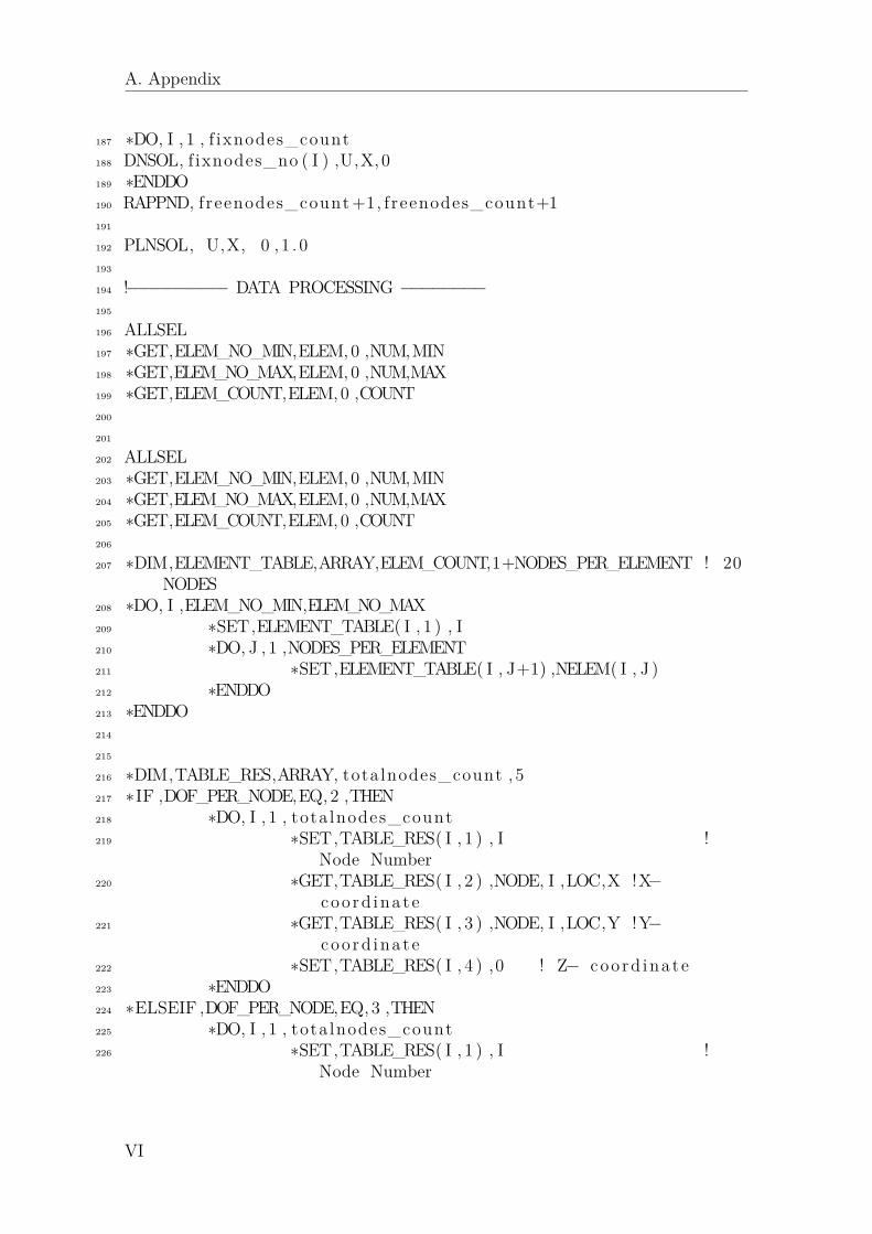
A. Appendix

187 ∗DO, I , 1 , f ixnodes_count188 DNSOL, f ixnodes_no ( I ) ,U,X, 0189 ∗ENDDO190 RAPPND, freenodes_count+1, freenodes_count+1191

192 PLNSOL, U,X, 0 , 1 . 0193

194 !−−−−−−−−− DATA PROCESSING −−−−−−−−195

196 ALLSEL197 ∗GET,ELEM_NO_MIN,ELEM,0 ,NUM,MIN198 ∗GET,ELEM_NO_MAX,ELEM,0 ,NUM,MAX199 ∗GET,ELEM_COUNT,ELEM,0 ,COUNT200

201

202 ALLSEL203 ∗GET,ELEM_NO_MIN,ELEM,0 ,NUM,MIN204 ∗GET,ELEM_NO_MAX,ELEM,0 ,NUM,MAX205 ∗GET,ELEM_COUNT,ELEM,0 ,COUNT206

207 ∗DIM,ELEMENT_TABLE,ARRAY,ELEM_COUNT,1+NODES_PER_ELEMENT ! 20NODES

208 ∗DO, I ,ELEM_NO_MIN,ELEM_NO_MAX209 ∗SET,ELEMENT_TABLE( I , 1 ) , I210 ∗DO, J , 1 ,NODES_PER_ELEMENT211 ∗SET,ELEMENT_TABLE( I , J+1) ,NELEM( I , J )212 ∗ENDDO213 ∗ENDDO214

215

216 ∗DIM,TABLE_RES,ARRAY, totalnodes_count , 5217 ∗IF ,DOF_PER_NODE,EQ, 2 ,THEN218 ∗DO, I , 1 , tota lnodes_count219 ∗SET,TABLE_RES( I , 1 ) , I !

Node Number220 ∗GET,TABLE_RES( I , 2 ) ,NODE, I ,LOC,X !X−

coo rd inate221 ∗GET,TABLE_RES( I , 3 ) ,NODE, I ,LOC,Y !Y−

coo rd inate222 ∗SET,TABLE_RES( I , 4 ) ,0 ! Z− coo rd inate223 ∗ENDDO224 ∗ELSEIF ,DOF_PER_NODE,EQ, 3 ,THEN225 ∗DO, I , 1 , tota lnodes_count226 ∗SET,TABLE_RES( I , 1 ) , I !

Node Number

VI

A. Appendix

227 ∗GET,TABLE_RES( I , 2 ) ,NODE, I ,LOC,X ! X−coo rd inate

228 ∗GET,TABLE_RES( I , 3 ) ,NODE, I ,LOC,Y ! Y−coo rd inate

229 ∗GET,TABLE_RES( I , 4 ) ,NODE, I ,LOC,Z ! Z−coo rd inate

230 ∗ENDDO231 ∗ENDIF232

233

234 ∗DO, J , 1 , f reenodes_count235 ∗SET,TABLE_RES( freenodes_no ( J ) ,5 ) ,U_STAR(1 , J

)236 ∗ENDDO237

238 ∗DO, J , 1 , loadnodes_count239 ∗SET,TABLE_RES( loadnodes_no ( J ) ,5 ) ,1240 ∗ENDDO241

242 ∗DO, J , 1 , f ixnodes_count243 ∗SET,TABLE_RES( f ixnodes_no ( J ) ,5 ) ,0244 ∗ENDDO245

246

247 !−−−−−−−−− EXPORTING DATA −−−−−−−−−−−−−−−−−−−−−248 ∗ cfopen , element_type . txt249 ! l i s t element types250 ∗GET, net ,ETYP, 1 ,NUM,COUNT251 ∗DO, i , 1 , net252 ∗GET,ETname ,ETYP, i ,ATTR,ENAM253 ∗VWRITE, ’ET ’ , i , ’ ’ ,ETname254 (A3 , F4 . 0 , A1 , F4 . 0 )255 ∗ENDDO256 ∗ c f c l o s e257

258 ∗MWRITE,ELEMENT_TABLE, element_table , txt259 (F10 . 0 , F10 . 0 , F10 . 0 , F10 . 0 , F10 . 0 , F10 . 0 , F10 . 0 , F10 . 0 , F10 . 0 , F10

. 0 , F10 . 0 , F10 . 0 , F10 . 0 , F10 . 0 , F10 . 0 , F10 . 0 , F10 . 0 , F10 . 0 , F10 . 0 ,F10 . 0 , F10 . 0 )

260

261 ∗MWRITE,TABLE_RES, r e su l t_tab l e , txt262 (F10 . 0 , F10 . 6 , F10 . 6 , F10 . 6 , F10 . 6 )263 ! 6 d i g i t p r e c i s i o n . i f you want more p r e c i s i on , i n c r ea s e ’ x ’

in F10 . x

VII

A. Appendix

A.2 Matlab program for data transferThis sections contains the Matlab script to transfer the data from Ansys MechanicalAPDL to ParaView.

1 c l e a r2 c l o s e a l l3 c l c4

5 f i l e I d 1 = fopen ( ’ canti lever_beam_3d_pointload . vtk ’ , ’w ’ ) ; %open f i l e f o r wr i t i ng ; d i s ca rd e x i s t i n g contents

6 f p r i n t f ( f i l e I d 1 , ’# vtk DataFi le Vers ion 2 .0 \n ’ ) ;7 f p r i n t f ( f i l e I d 1 , ’ Unstructured Grid −

canitlever_beam_3d_pointload \n ’ ) ;8

9 %read data10 e t ab l e = dlmread ( ’ e lement_table . txt ’ ) ;% get the element−

nodes c onne c t i v i t y11 r e su l t_tab l e= dlmread ( ’ r e su l t_tab l e . txt ’ ) ;12 element_type = f g e t s ( fopen ( ’ element_type . txt ’ ) ) ;13 element_type = str2num ( element_type ( 9 : end ) ) ;14

15 %convert i t to array16 U_star = re su l t_tab l e ( : , 5 ) ;17 nodal_coord inates = r e su l t_tab l e ( : , [ 2 3 4 ] ) ;18 e t ab l e = int64 ( ( e t ab l e ) ) ;19

20 e t ab l e ( : , a l l ( e t ab l e == 0) ) = [ ] ; % remove a l l the zero columns21 e t ab l e=etab le −1; % because the index ing in paraview s t a r t s

from 0 not from 122 etable_vtk = e tab l e ;23 nodes_per_element = length ( e t ab l e ( 1 , : ) )−1 ;24 etable_vtk ( : , 1 ) = nodes_per_element ; % i n s e r t the number o f

nodes f o r element in the f i r s t column25

26 i f element_type == 18127 ce l l_type = 9 ;28 e l s e i f element_type == 18229 ce l l_type = 9 ;30 e l s e i f element_type == 18531 ce l l_type = 12 ;32 e l s e i f element_type == 18633 ce l l_type = 25 ;34 e l s e i f element_type == 18735 ce l l_type = 24 ;36 end37 %%

VIII

A. Appendix

38 f p r i n t f ( f i l e I d 1 , ’ASCII \n ’ ) ;39 f p r i n t f ( f i l e I d 1 , ’DATASET UNSTRUCTURED_GRID \n ’ ) ;40 % Def ine po in t s − nodal coo rd ina t e s41 f p r i n t f ( f i l e I d 1 , ’ \nPOINTS %d f l o a t \n ’ , l ength (

nodal_coord inates ( : , 1 ) ) ) ;42 f o r i =1 : l ength ( nodal_coord inates ( : , 1 ) )43 f p r i n t f ( f i l e I d 1 , ’%d ’ , nodal_coord inates ( i , : ) ) ;44 f p r i n t f ( f i l e I d 1 , ’ \n ’ ) ;45 end46 % de f i n e c e l l s − e lements47 f p r i n t f ( f i l e I d 1 , ’ \nCELLS %d %d \n ’ , l ength ( e t ab l e ( : , 1 ) ) ,

s i z e ( e tab le , 1 ) ∗ s i z e ( e tab le , 2 ) ) ;48

49 f o r i =1 : l ength ( etable_vtk ( : , 1 ) )50 f p r i n t f ( f i l e I d 1 , ’%d ’ , etable_vtk ( i , : ) ) ; % order i s

changed because o f the format51 f p r i n t f ( f i l e I d 1 , ’ \n ’ ) ;52 end53 %%54 % de f i n e c e l l data − element type55 f p r i n t f ( f i l e I d 1 , ’ \nCELL_TYPES %d \n ’ , l ength ( e t ab l e ( : , 1 ) ) ) ;56 f o r i =1 : l ength ( e t ab l e ( : , 1 ) )57 f p r i n t f ( f i l e I d 1 , ’%d \n ’ , c e l l_type ) ;58 end59 % de f i n e s c a l a r data − U∗ data60 f p r i n t f ( f i l e I d 1 , ’POINT_DATA %d \n ’ , l ength (U_star ( : , 1 ) ) ) ;61 f p r i n t f ( f i l e I d 1 , ’SCALARS U_star f l o a t 1 \n ’ ) ;62 f p r i n t f ( f i l e I d 1 , ’LOOKUP_TABLE de f au l t \n ’ ) ;63 f o r i= 1 : l ength (U_star ( : , 1 ) )64 f p r i n t f ( f i l e I d 1 , ’%d \n ’ , U_star ( i ) ) ;65 end66

67 f i g u r e68 p lo t3 ( nodal_coordinates ( : , 1 ) , nodal_coordinates ( : , 2 ) ,

nodal_coord inates ( : , 3 ) , ’ ∗ ’ )69 hold on70 % text ( n l i s t ( : , 2 ) , n l i s t ( : , 3 ) , n l i s t ( : , 4 ) , s t r i n g ( n l i s t ( : , 1 ) ) )71 ax i s equal

IX

DEPARTMENT OF MECHANICS AND MARITIME SCIENCESCHALMERS UNIVERSITY OF TECHNOLOGYGothenburg, Swedenwww.chalmers.se