Supply chain models for deteriorating products with ramp type demand rate under permissible delay in...

This article appeared in a journal published by Elsevier. The attachedcopy is furnished to the author for internal non-commercial researchand education use, including for instruction at the authors institution

and sharing with colleagues.

Other uses, including reproduction and distribution, or selling orlicensing copies, or posting to personal, institutional or third party

websites are prohibited.

In most cases authors are permitted to post their version of thearticle (e.g. in Word or Tex form) to their personal website orinstitutional repository. Authors requiring further information

regarding Elsevier’s archiving and manuscript policies areencouraged to visit:

http://www.elsevier.com/copyright

http://www.elsevier.com/copyright

Author's personal copy

Supply chain models for deteriorating products with ramp type demand rateunder permissible delay in payments

K. Skouri a, I. Konstantaras a,b,⇑, S. Papachristos c, J.-T. Teng d

a Department of Mathematics, University of Ioannina, 45110 Ioannina, Greeceb Department of Business Administration, Business Excellence Laboratory, University of Macedonia, 156 Egnatia Street, 54006 Thessaloniki, Greecec Department of Business Administration of Food and Agricultural Products, University of Ioannina, 30100 Agrinio, Greeced Department of Marketing and Management Sciences, The William Paterson University of New Jersey, Wayne, NJ 07470-2103, United States

a r t i c l e i n f o

Keywords:Ramp type demand rateDeteriorationPartial backloggingDelay in payments

a b s t r a c t

In this paper an order level inventory model for deteriorating items with general ramp type demand rateunder conditions of permissible delay in payments is proposed. In this model shortages are allowed andpartially backlogged. The backlogging rate is variable and dependent on the waiting time for the nextreplenishment. Its study requires exploring the feasible ordering relations between the time parametersappeared, which leads to three models. For each model the optimal replenishment policy is determined.The sufficient conditions of the existence and uniqueness of the optimal solutions are also provided. Suit-ably selected numerical examples highlight the obtained results. Sensitivity analysis of the optimal solu-tion with respect to major parameters of the system has been carried out and the implications arediscussed.

� 2011 Elsevier Ltd. All rights reserved.

1. Introduction

In today’s competitive business transactions, it is common forthe supplier to offer a certain fixed credit period to the retailerfor stimulating his/her demand. During this credit period the retai-ler can accumulate the revenue and earn interest on that revenue.However, beyond this period the supplier charges interest on theunpaid balance. Hence, a permissible delay indirectly reduces thecost of holding stock. On the other hand, trade credit offered bythe supplier encourages the retailer to buy more. Thus it is also apowerful promotional tool that attracts new customers, who con-sider it as an alternative incentive policy to quantity discounts.Hence, trade credit can play a major role in inventory control forboth the supplier as well as the retailer (see Jaggi, Goyal, & Goel,2008). Owing to this fact, during the past few years, many articlesdealing with various inventory models under a variety of tradecredits have appeared in the literature. The Table 1 summarizesthe key assumptions of the models appeared in the relativeliterature.

In the literature referring to models with permissible delay inpayments, the demand is mostly treated either as constant or ascontinuous differentiable function of time. However, it is observedthat the demand rate of new brand of consumer goods comes to themarket, increases at the beginning of the season up to a certain

moment (say, l) and then remains to be constant for the rest ofthe time. For example, the demand rate is increasing during thegrowth stage and then the market grows into a stable stage suchthat the demand becomes a constant until the end of the inventorycycle. The term ‘‘ramp type’’ is used to represent such a demandpattern. Therefore, a ramp type demand rate function has two dif-ferent time segments. In its first segment, the demand is anyincreasing function of time. But the demand remains constant inits second time segment. It is obvious that any ramp type demandfunction has at least one break point l between two time segmentsat which is not differentiable. This non-differentiable break point lmakes the analysis of the problem more complicated. This hasurged researchers to study inventory models with ramp typedemand patterns. Hill (1995) proposed an inventory model withvariable branch being any power function of time. Research on thisfield continues with Mandal and Pal (1998), Wu and Ouyang (2000)and Wu (2001). In the above-cited papers, the optimal replenish-ment policy requires to determine the decision time (say, t1) atwhich the inventory level falls to zero. Consequently the followingtwo cases should be explored: (1) the inventory level fall to zero be-fore the demand reaches constant (i.e., t1 < l), and (2) the inventorylevel falls to zero after the demand reaches constant (i.e., t1 > l). Al-most all of the researchers examined only the first case. Deng, Lin,and Chu (2007) first reconsidered the inventory models proposedby Mandal and Pal (1998) and Wu and Ouyang (2000), and dis-cussed both cases. Panda, Saha, and Basu (2007) built an inventorymodel for deteriorating items (with three-parameters Weibull dis-tributed deterioration rate) with generalized exponential ramp

0957-4174/$ - see front matter � 2011 Elsevier Ltd. All rights reserved.doi:10.1016/j.eswa.2011.05.061

⇑ Corresponding author. Address: Department of Mathematics, University ofIoannina, 45110 Ioannina, Greece. Tel.: +30 2651008230.

E-mail address: [email protected] (I. Konstantaras).

Expert Systems with Applications 38 (2011) 14861–14869

Contents lists available at ScienceDirect

Expert Systems with Applications

journal homepage: www.elsevier .com/locate /eswa

https://www.researchgate.net/publication/245280509_Inventory_Models_for_Increasing_Demand_Followed_by_Level_Demand?el=1_x_8&enrichId=rgreq-6fdf2409-9ef2-4632-aa4d-b9a14ad91b43&enrichSource=Y292ZXJQYWdlOzIxNTY0NTM2NDtBUzoyMTI1MjU5MDkwNTc1MzZAMTQyNzY4MTUzMzkwMg==


type demand rate and complete backlogging. Skouri, Konstantaras,Papachristos, and Ganas (2009) extend the work of Deng et al.(2007) by introducing a general ramp type demand rate and Wei-bull deterioration rate.

In this paper we propose an inventory model with generalramp type demand rate, constant deterioration rate, partial back-logging of unsatisfied demand and conditions of permissible de-lay in payments. Its study requires exploring the feasibleordering relations between the time parameters appeared, whichleads to three models. For each model the optimal replenishmentpolicy is determined. The necessary and sufficient conditions ofthe existence and uniqueness of the optimal solutions are alsoprovided. An easy-to-use algorithm is proposed to find the opti-mal replenishment policy and the optimal order quantity.Numerical examples are presented to demonstrate the developedmodel and the solution procedure. Sensitivity analysis of theoptimal solution with respect to major parameters of the systemis carried out and their results are discussed. Consequently, thispaper is an extension of the model by Deng et al. (2007) to allowfor permissible delay in payments or as an extension of previousmodels with delay in payments to a more general demand rate.The paper is organized as follows: The notation and assumptionsused are given in Section 2. In Section 3 the quantities and func-tions common and used to each of the three possible models arederived. Sections 4–6 are devoted to the mathematical formula-tion of the models and their derivation of the optimal policy.Numerical examples highlighting the results obtained are givenin Section 7. The paper closes with concluding remarks inSection 8.

2. Notation and assumptions

The following notation and assumptions are used in the paper.

2.1. Notation

T the constant (since the demand is ramp type) schedulingperiod (cycle)

t1 the time at which the inventory level falls to zero (adecision variable)

S the maximum inventory level at each scheduling period(cycle)

Cp the unit purchase costc1 the inventory holding cost per unit per unit time

(excluding interest charges)c2 the shortage cost per unit per unit timec3 the cost incurred from the deterioration of one unitc4 the per unit opportunity cost due to the lost salesp the unit selling priceIe the interest rate earned per unit per unit of timeIc the interest rate charged per unit per unit of timeM the offered credit periodl the parameter of the ramp type demand function (break

point)I(t) the inventory level at time t 2 [0,T]

2.2. Assumptions

The inventory model is developed under the followingassumptions:

1. The ordering quantity brings the inventory level up to the orderlevel S. Replenishment rate is infinite.

2. Shortages are backlogged at a rate b(x) which is a non-increas-ing function of x with 0 < b(x) 6 1, b(0) = 1and x is the waitingtime up to the next replenishment. To make it mathematicaltractable, we assume that b(x) satisfies the relation b(x) +Tb0(x) P 0, where b0(x) is the derivate of b(x). The cases withb(x) = 1 correspond to complete backlogging model.

3. The retailer can use the sale revenue to earn the interest withannual rate Ie during the period [0, t1]. Beyond the fixed creditperiod, the product still in stock is assumed to be financed withan annual rate Ic (for this credit scheme see Jamal, Sarker, &Wang (1997) and Chang & Dye (2001)).

4. The on hand inventory deteriorates at a constant rate h(0 < h < 1) per time unit. The deteriorated items are withdrawnimmediately from the warehouse and there is no provision forrepair or replacement.

5. The demand rate D(t) is a ramp type function of time given by:

Table 1Key assumptions of inventory models with permissible delay in payments.

Demand rate Allowing fordeterioration

Allowing forshortages

Trade credit period

Goyal (1985) Constant No No FixedDave (1985) Constant No No FixedAggarwal and Jaggi (1995) Constant Constant rate No FixedJamal et al. (1997) Constant Constant rate Complete

backloggingFixed

Chang and Dye (2001) Constant Constant rate Time dependent FixedTeng (2002) Constant No No FixedChang et al. (2003) Time dependent Time dependent rate No Depending on the ordering quantityShah (2006) Constant Constant rate Complete

backloggingFixed

Huang (2007) Constant No No Fixed, but partially delay in paymentsJaber and Osman (2006) Constant No Yes Decision variableJaber (2007) Increasing No No FixedJaggi et al. (2008) Function of the credit-

periodNo No Fixed

Ouyang et al. (2009) Constant Constant No Partially permissible delay in payments linked to orderquantity

Teng and Chang (2009) Constant No No Two levels of trade credit policyKreng and Tan (2010) Constant No No Two levels of trade credit policyGeetha and Uthayakumar

(2010)Constant Constant rate Partial backlogging Fixed

14862 K. Skouri et al. / Expert Systems with Applications 38 (2011) 14861–14869

https://www.researchgate.net/publication/222974056_A_note_on_the_inventory_models_for_deteriorating_items_with_ramp_type_demand_rate?el=1_x_8&enrichId=rgreq-6fdf2409-9ef2-4632-aa4d-b9a14ad91b43&enrichSource=Y292ZXJQYWdlOzIxNTY0NTM2NDtBUzoyMTI1MjU5MDkwNTc1MzZAMTQyNzY4MTUzMzkwMg==

https://www.researchgate.net/publication/254321331_An_inventory_model_for_deteriorating_items_with_partial_backlogging_and_permissible_delay_in_payments?el=1_x_8&enrichId=rgreq-6fdf2409-9ef2-4632-aa4d-b9a14ad91b43&enrichSource=Y292ZXJQYWdlOzIxNTY0NTM2NDtBUzoyMTI1MjU5MDkwNTc1MzZAMTQyNzY4MTUzMzkwMg==


DðtÞ ¼f ðtÞ; t < lf ðlÞ; t P l

�

where f(t) is a positive, increasing and differentiable function oft 2 (0,T].

3. Deriving the common quantities for the inventory models

The inventory level, I(t), 0 6 t 6 T satisfies the following differ-ential equations:

dIðtÞdtþ hIðtÞ ¼ �DðtÞ; 0 6 t 6 t1; ð1Þ

with boundary condition I(t1) = 0 and

dIðtÞdt¼ �DðtÞbðT � tÞ; t1 6 t 6 T; ð2Þ

with boundary condition I(t1) = 0.There are two possible relations between parameters t1 and l:

(i) t1 6 l and (ii) t1 > l. Each case implies different holding cost,deterioration cost, shortage cost and cost of lost sales. Let us dis-cuss them separately below:

Case I (t1 6 l)In this case, Eq. (1) becomes:

dIðtÞdtþ hIðtÞ ¼ �f ðtÞ; 0 6 t 6 t1; ð3Þ

with boundary condition I(t1) = 0. Eq. (2) leads to the followingtwo:

dIðtÞdt¼ �f ðtÞbðT � tÞ; t1 6 t 6 l; ð4Þ

with boundary condition I(t1) = 0 and

dIðtÞdt¼ �f ðlÞbðT � tÞ; l 6 t 6 T; ð5Þ

with boundary condition I(l�) = I(l+).The solutions of Eqs. (3)–(5) are:

IðtÞ ¼ e�htZ t1

tf ðxÞehxdx; 0 6 t 6 t1; ð6Þ

IðtÞ ¼ �Z t

t1

f ðxÞbðT � xÞdx; t1 6 t 6 l ð7Þ

and

IðtÞ ¼ �f ðlÞZ t

lbðT � xÞdx�

Z l

t1

f ðxÞbðT � xÞdx;

l 6 t 6 T: ð8Þ

The total amount of deteriorated items during [0, t1] is

D1 ¼Z t1

0f ðtÞehtdt �

Z t1

0f ðtÞdt: ð9Þ

The time-weighted inventory level during the interval [0, t1] isfound from Eq. (6) and is

I1;1 ¼Z t1

0IðtÞdt ¼

Z t1

0e�ht

Z t1

tf ðxÞehxdx

� �dt: ð10Þ

Due to Eqs. (7) and (8), the time-weighted amount of backordersdue to shortages during the interval [t1,T] is:

I2;1 ¼Z T

t1

½�IðtÞ�dt ¼Z l

t1

½�IðtÞ�dt þZ T

l½�IðtÞ�dt

¼Z l

t1

ðl� tÞf ðtÞbðT � tÞdt þ f ðlÞ

�Z T

l

Z t

lbðT � xÞdx

" #dt

þZ T

l

Z l

t1

f ðxÞbðT � xÞdx� �

dt: ð11Þ

The amount of lost sales during [t1,T] is

L1 ¼Z l

t1

ð1� bðT � tÞÞf ðtÞdt þ f ðlÞZ T

lð1� bðT � tÞÞdt:

ð12Þ

Case II (t1 > l)

In this case, Eq. (1) reduces to the following two:

dIðtÞdtþ hIðtÞ ¼ �f ðtÞ; 0 6 t 6 l; ð13Þ

with boundary condition I(l�) = I(l+) and

dIðtÞdtþ hIðtÞ ¼ �f ðlÞ; l 6 t 6 t1; ð14Þ

with boundary condition I(t1) = 0. Eq. (2) becomes:

dIðtÞdt¼ �f ðlÞbðT � tÞ; t1 6 t 6 T; ð15Þ

with boundary condition I(t1) = 0.Their solutions are:

IðtÞ ¼ e�htZ l

tf ðxÞehxdxþ f ðlÞ

Z t1

lehxdx

" #; 0 6 t 6 l; ð16Þ

IðtÞ ¼ e�htf ðlÞZ t1

tehxdx; l 6 t 6 t1; ð17Þ

IðtÞ ¼ �f ðlÞZ t

t1

bðT � xÞdx; t1 6 t 6 T: ð18Þ

The total amount of deteriorated items during [0, t1] is

D2 ¼ Ið0Þ �Z t1

0DðtÞdt

¼Z l

0f ðtÞehtdt þ f ðlÞ

Z t1

lehtdt �

Z l

0f ðtÞdt � f ðlÞðt1 � lÞ: ð19Þ

The time-weighted inventory level during the interval [0, t1] isfound from (16) and (17) as:

I1;2¼Z t1

0IðtÞdt

¼Z l

0IðtÞdtþ

Z t1

lIðtÞdt¼

Z l

0e�ht

Z l


Z t1

lehxdx

" #dt

þ f ðlÞZ t1

le�ht

Z t1

tehxdx

� �dt: ð20Þ

The time-weighted amount of backorders due to shortages duringthe interval [t1,T] is:

I2;2 ¼Z T

t1

½�IðtÞ�dt ¼ f ðlÞZ T

t1

Z t

t1

bðT � xÞdx� �

dt

¼ f ðlÞZ T

t1

ðT � xÞbðT � xÞdx: ð21Þ

K. Skouri et al. / Expert Systems with Applications 38 (2011) 14861–14869 14863


The number of lost sales in the interval [t1,T] is:

L2 ¼ f ðlÞZ T

t1

½1� bðT � tÞ�dt: ð22Þ

For simplicity, we assume here that T >l. Otherwise, demandrate is increasing but not ramp-typed through the entire planninghorizon T, which is not the subjective of this research. Conse-quently, from the value of M, we have three possible models: (i)M 6 l (ii) l 6M 6 T (iii) T 6M. These three distinct models leadto three different mathematical formulations. Let us discuss themaccordingly.

4. Model I – The inventory model for the case M < l

It is obvious that the results of Section 3 are not enough to de-rive the total cost function for this case, as the revenues earnedduring to credit period or costs charged thereafter have not be ta-ken into account. So, the determination of the total cost functionrequires the further examination of the ordering relations betweenthe time parameters,M, t1, l, T. It is noticed that for the calculationof interest earned during the period, where the stock level is posi-tive, and interest charged for the inventory still keeps in stock,after the due date M, the approach of Jamal et al. (1997) will beused.

4.1. The derivation of the cost function for model I, (M 6 l)

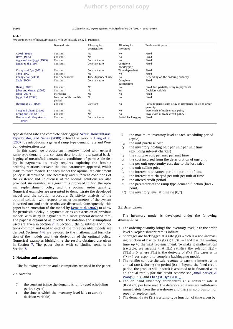
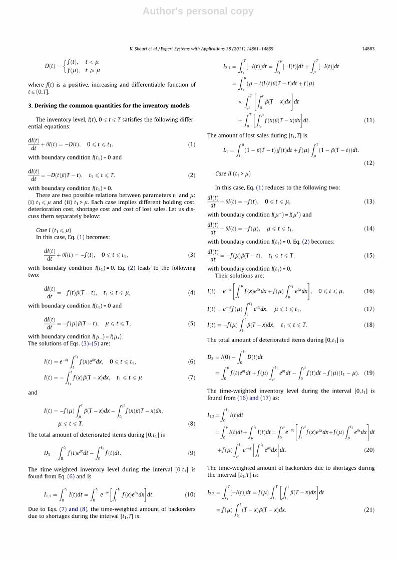
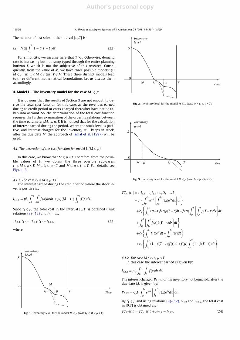
In this case, we know that M 6 l < T. Therefore, from the possi-ble values of t1, we obtain the three possible sub-cases,t1 6M 6 l < T, M 6 t1 6 l < T and M 6 l 6 t1 6 T. For details, seeFigs. 1–3.

4.1.1. The case t1 6M 6 l < TThe interest earned during the credit period where the stock le-

vel is positive is:

IT;1;1 ¼ pIe

Z t1

0

Z t

0f ðxÞdxdt þ pIeðM � t1Þ

Z t1

0f ðxÞdx:

Since t1 6 l, the total cost in the interval [0,T] is obtained usingrelations (9)–(12) and IT,1,1 as:

TC1;1ðt1Þ ¼ TCp;1ðt1Þ � IT;1;1; ð23Þ

where

TCp;1ðt1Þ¼ c1I1;1þc2I2;1þc3D1þc4L1

¼ c1

Z t1

0e�ht

Z t1

tf ðxÞehxdx

� �dt

� �

þc2

Z l

t1

ðl� tÞf ðtÞbðT� tÞdtþ f ðlÞZ T

l

Z t

lbðT�xÞdx

" #dt

(

þZ T

l

Z l

t1

f ðxÞbðT�xÞdx� �

dt

)

þc3

Z t1

0f ðtÞehtdt�

Z t1

0f ðtÞdt

� �

þc4

Z l

t1

ð1�bðT� tÞÞf ðtÞdtþ f ðlÞZ T

lð1�bðT� tÞÞdt

( ):

4.1.2. The case M < t1 6 l < TIn this case the interest earned is given by:

IT;1;2 ¼ pIe

Z t1

0

Z t

0f ðxÞdxdt:

The interest charged, PT,1,2, for the inventory not being sold after thedue date M, is given by:

PT;1;2 ¼ CpIc

Z t1

Me�ht

Z t1

tf ðxÞehxdx

� �dt:

By t1 6 l and using relations (9)–(12), IT,1,2 and PT,1,2, the total costin [0,T] is obtained as:

TC1;2ðt1Þ ¼ TCp;1ðt1Þ þ PT;1;2 � IT;1;2: ð24Þ

T µ

S

Inventory level

Time 1t0

M

Fig. 1. Inventory level for the model M 6 l (case t1 6M 6 l < T).

Inventory level

T µ

S

Time 1t0

M

Fig. 2. Inventory level for the model M 6 l (case M < t1 6 l < T).

T 1t0

µ Μ

S

Inventory level

Time

Fig. 3. Inventory level for the model M 6 l (case M < l 6 t1 < T).


https://www.researchgate.net/publication/245279077_An_Ordering_Policy_for_Deteriorating_Items_with_Allowable_Shortage_and_Permissible_Delay_in_Payment?el=1_x_8&enrichId=rgreq-6fdf2409-9ef2-4632-aa4d-b9a14ad91b43&enrichSource=Y292ZXJQYWdlOzIxNTY0NTM2NDtBUzoyMTI1MjU5MDkwNTc1MzZAMTQyNzY4MTUzMzkwMg==


4.1.3. The case M 6 l 6 t1 6 TThe interest earned, IT,1,3, is given by:

IT;1;3 ¼ pIe

Z l

0

Z t

0f ðxÞdxdt þ

Z t1

l

Z l

0f ðxÞdxdt þ

Z t1

l

Z t

lf ðlÞdxdt

!:

The interest charged PT for the inventory not being sold after thedue date M, is given by:

PT;1;3 ¼ CpIc

Z l

Me�ht

Z l

tehxf ðxÞdxdt þ f ðlÞ

Z l

Me�ht

Z t1

lehxdxdt

þ f ðlÞZ t1

le�ht

Z t1

tehxdxdt

!:

Since l 6 t1, the total cost in the interval [0,T] is now derived usingthe relations (19)–(22) IT,1,3 and PT,1,3, and it is given as:

TC1;3ðt1Þ ¼ TCp;2ðt1Þ þ PT;1;3 � IT;1;3; ð25Þ

where

TCp;2ðt1Þ ¼ c1I1;2 þ c2I2;2 þ c3D2 þ c4L2

¼ c1

Z l

0e�ht

Z l


Z t1

lehxdx

" #dt

(

þ f ðlÞZ t1

le�ht

Z t1

tehxdx

� �dt

)

þ c2 f ðlÞZ T

t1

ðT � xÞbðT � xÞdx� �

þ c3

Z l


Z t1

lehtdt

(

�Z l

0f ðtÞdt � f ðlÞðt1 � lÞ

)

þ c4 f ðlÞZ T

t1

1� bðT � tÞð Þdt� �

:

Now we have all quantities needed to formulate the total inventorycost and proceed with optimization.

4.2. The optimal replenishment policy for model I(M 6 l)

The results in previous sub-sections lead to the following totalcost function:

TC1ðt1Þ ¼TC1;1ðt1Þ; t1 6 M;

TC1;2ðt1Þ; M < t1 6 l;TC1;3ðt1Þ; l 6 t1

8><>:

and the problem is

mint1

TC1ðt1Þ:

Its solution requires, separately, studying each of three branchesand then combining the results to obtain the optimal policy. It iseasy to check that TC1(t1) is continuous at the points M and l.The first order condition for a minimum of TC1,1(t1) is:

dTC1;1ðt1Þdt1

¼ aðt1Þf ðt1Þ ¼ 0; ð26Þ

with

aðt1Þ ¼c1 þ c3h

hðeht1 � 1Þ � c2ðT � t1ÞbðT � t1Þ � c4ð1� bðT � t1ÞÞ

� pIeðM � t1Þ:

It is easily verified that a(0) < 0, a(T) > 0 and further daðt1Þdt1

>0. So thederivative dTC1;1ðt1Þ

dt1vanishes at t1,1, with 0 < t1,1 < T, which is the un-

ique root of:

aðt1Þ ¼ 0: ð27Þ

For this t1,1 we have

dTC21;1ðt1Þdt2

1

��t1¼t1;1

¼ ðc1þc3hÞeht1;1þc2bðT�t1;1Þþc2ðT�t1;1Þb0ðT�t1;1Þ��c4b

0ðT�t1;1ÞþpIeÞf ðt1;1Þ>0:

Consequently t1,1 is the unique unconstrained global minimum ofTC1,1(t1). Moreover if t1,1 is feasible, i.e. t1,1 6M, the optimal valueof the order level, S = I(0),is:

S� ¼Z t1;1

0f ðtÞehtdt ð28Þ

and subsequently the optimal order quantity Q⁄ is

Q� ¼ S� þZ l

t1;1

bðT � tÞf ðtÞdt þ f ðlÞZ T

lbðT � tÞdt: ð29Þ

The first order condition for a minimum of TC1,2(t1) is:

dTC1;2ðt1Þdt1

¼ c1 þ c3hh

ðeht1 � 1Þf ðt1Þ � c2ðT � t1ÞbðT � t1Þf ðt1Þ

� c4ð1� bðT � t1ÞÞf ðt1Þ � pIe

Z t1

0f ðxÞdxþ CpIc

h

�ðehðt1�MÞ � 1Þf ðt1Þ ¼ 0: ð30Þ

Let us set h(x) = c2xb(x) + c4(1 � b(x)) � pIex. If t1,2 is the root of (30)(this may or may not exist) and if h0(x) > 0 then

d2TC1;2ðt1Þdt2

1

��t1¼t1;2

¼ pIef 0ðt1;2ÞZ t1;2

0f ðxÞdxþ ððc1 þ c3hÞeht1;2

þ c2½bðT � t1;2Þ þ ðT � t1;2Þb0ðT � t1;2Þ�� c4b

0ðT � t1;2Þ � pIe þ CpIcehðt1;2�MÞÞf ðt1;2Þ > 0

and this t1,2 corresponds to minimum.If t1,2 is feasible, i.e. M < t1,2 6 l, the optimal value of the order

level, S = I(0), is:

S� ¼Z t1;2


and subsequently the optimal order quantity, Q⁄, is

Q� ¼ S� þZ l

t1;2




dTC1;3ðt1Þdt1

¼ c1 þ c3hh

ðeht1 � 1Þf ðlÞ � c2ðT � t1ÞbðT � t1Þf ðlÞ

� c4ð1� bðT � t1ÞÞf ðlÞ þCpIc

hðehðt1�MÞ � 1Þf ðlÞ

� pIe

Z l

0f ðxÞdx� pIeðt1 � lÞf ðlÞ ¼ 0: ð33Þ

The second order condition for a minimum of TC1,3(t1) is:

d2TC1;3ðt1Þdt2

1

¼ ððc1 þ c3hÞeht1 þ c2½bðT � t1Þ þ ðT � t1Þb0ðT � t1Þ�

� c4b0ðT � t1Þ � pIe þ CpIcehðt1�MÞÞf ðlÞ > 0;

which is valid if h0(x) > 0.



If t1,3 is the root of (33) (this may or may not exist) and isfeasible, i.e. l < t1,3 6 T, the optimal value of the order level,S = I(0), is:

S� ¼Z l


Z t1;3

lehtdt ð34Þ


Q � ¼ S� þ f ðlÞZ T

t1;3

bðT � tÞdt: ð35Þ

Remark 1. Due to (26) and (30) the function TC(t1) is notdifferentiable at the point M.

Then a procedure is proposed to determine the optimalreplenishment policy:

Step 1. Find the global minimum of TC1,1(t1), say t�1;1, as follows:Step 1.1 Compute t1,1 from (26), if t1,1 < M then set t�1;1 ¼ t1;1 and

compute TC1;1ðt�1;1Þ else go to step 1.2.Step 1.2 Find the min{TC1,1(0),TC1,1(M)} and accordingly set t�1;1.Step 2. Find the global minimum of TC1,2(t1), say t�1;2, as follows:

Step 2.1 Compute t1,2 from (30), if M < t1,2 < l then set t�1;2 ¼ t1;2

compute TC2ðt�1;2Þ else go to step 2.2.Step 2.2 Find the min{TC1,2(M),TC1,2(l)} and accordingly set t�1;2.Step 3. Find the global minimum of TC1,3(t1), say t�1;3, as follows

Step 3.1 Compute t1,3 from (33), if M < t1,3 < l then set t�1;3 ¼ t1;3

and compute TC1;3ðt�1;3Þ else go to step 3.2.Step 3.2 Find the min{TC1,3(M),TC1,3(l)} and accordingly set t�1;3.

Step 4. Find the min TC1;1ðt�1;1Þ; TC1;2 t�1;2�

; TC1;3 t�1;3� n o

and

accordingly select the optimal value for t1.

5. Model II – The inventory model for the case l < M < T

We shall, again, follow the steps of Section 4.

5.1. The derivation of the cost function for model II, (l < M < T)

In this case, the offered credit period M is longer than the de-mand stabilizing point l and shorter than the planning horizonT. To obtain the total cost function the three cases t1 6 l < M < T,l < t1 6M < T and l < M < t1 6 T must be considered.

5.1.1. The case t1 6 l < M < TThe interest earned during the period of positive inventory level

is:

IT;2;1 ¼ pIe

Z t1

0

Z t

0f ðxÞdxdt þ pIeðM � t1Þ

Z t1

0f ðxÞdx:

Since t1 6 l the total cost in the time interval [0,T] is calculatedusing the relations (9)–(12) and IT and is:

TC2;1ðt1Þ ¼ TCp;1ðt1Þ � IT;2;1: ð36Þ

5.1.2. The case l < t1 6M < TThe interest earned is given by:

IT;2;2 ¼ pIe

Z l

0

Z t

0f ðxÞdxdt þ

Z M

l

Z l

0f ðxÞdxdt

þZ t1

l

Z t

lf ðlÞdxdt þ

Z M

t1

Z t1

lf ðlÞdxdt

!:

Since l < t1, the total cost over [0,T] is calculated using the relations(19)–(22) and IT,2,2 and is:

TC2;2ðt1Þ ¼ TCp;2ðt1Þ þ IT;2;2: ð37Þ

5.1.3. The case l < M < t1 6 TThe interest earned, IT, is given by:

IT;2;3¼pIe

Z l

0

Z t

0f ðxÞdxdtþ

Z t1

l

Z l

0f ðxÞdxdtþ

Z t1

l

Z t

lf ðlÞdxdt

!:

The interest payable for the inventory not being sold after the duedate M is

PT;2;3 ¼ CpIc

Z t1

Me�ht

Z t1

tehxf ðlÞdxdt:

Since l < t1, the total cost over [0,T] is again calculated from(19)–(22), PT,2,3, IT,2,3 and is:

TC2;3ðt1Þ ¼ TCp;2ðt1Þ þ PT;2;3 � IT;2;3: ð38Þ

5.2. The optimal replenishment policy for model II (l < M 6 T)

The total cost function is now given by:

TC2ðt1Þ ¼TC2;1ðt1Þ; t1 6 l;TC2;2ðt1Þ;l < t1 6 M;

TC2;3ðt1Þ;M 6 t1

8><>:

and the problem is

mint1

TC2ðt1Þ:

It is easy to check that this function is continuous at l and M. Thesolution approach is the same as in Section 4.2.


dTC2;1ðt1Þdt1

¼ f ðt1Þaðt1Þ ¼ 0: ð39Þ

So using similar arguments as in Section 4.2 TC2,1(t1) has a uniqueminimum.

If t1,1 is feasible, i.e. t1,1 6 l, the optimal value of the order level,S = I(0), is

S� ¼Z t1;1



Q � ¼ S� þZ l

t1;1



The first and second order derivatives of TC2(t1) are:

dTC2;2ðt1Þdt1

¼ f ðlÞaðt1Þ; ð42Þ

d2TC2;2ðt1Þdt2

1

¼ f ðlÞdaðt1Þdt1

> 0: ð43Þ

The inequality in (43) ensures the strict convexity of TC2,2(t1) and sothe unconstrained global minimum of TC2,2(t1) is given by (27).

If t1,2 is feasible, i.e. l < t1,2 6M the optimal value of the orderlevel, S = I(0), is:

S� ¼Z l


Z t1;2

lehtdt ð44Þ





t1;2


The first condition for a minimum of TC3(t1) is:

dTC2;3ðt1Þdt1

¼

c1þc3hhðeht1 �1ÞþCpIc

hðehðt1�MÞ �1Þ�c2ðT� t1ÞbðT� t1Þ

�c4ð1�bðT� t1ÞÞ�pIeðt1�lÞ!

f ðlÞ�pIe

Z l

0f ðxÞdx:

ð46Þ

If (c1 + c3h + CpIc) P pIe then the second order condition for a mini-mum is satisfied (this is a sufficient but not necessary condition):

dTC22;3ðt1Þdt2

1

¼ ðc1þc3hþCpIcÞeht1 þc2bðT� t1Þþc2ðT� t1Þb0ðT� t1Þ��c4b

0ðT� t1Þ�pIeÞf ðlÞ>0:

If t1,3 is feasible, i.e. M < t1,3 6 T, the optimal value of the order level,S = I(0), is:

S� ¼Z l


Z t1;3

lehtdt ð47Þ



t1;3


Remark 2. The function TC2(t1) is not differentiable at the point M.

The following procedure is proposed to determine the optimalreplenishment policy:

Step 1. Find the global minimum of TC2,1(t1), say t�1;1, as follows:Step 1.1 Compute t1,1 from (27), if t1,1 < l then set t�1;1 ¼ t1;1 and

compute TC2;1ðt�1;1Þ else go to step 1.2.Step 1.2 Find the min{TC2,1(0),TC2,1(l)} and accordingly set t�1;1Step 2. Find the global minimum of TC2,2(t1), say t�1;2, as follows:

Step 2.1 If l < t1,2 = t1,1 < M (t1,2 is computed from (27)) then sett�1;2 ¼ t1;1 and compute TC2;2ðt�1;2Þ else go to step 2.2.

Step 2.2 Find the min{TC2,2(l),TC2,2(M)} and accordingly set t�1;2.Step 3. Find the global minimum of TC2,3(t1), say t�1;3, as follows

Step 3.1 Compute t1,3 from (46), if M < t1,3 < T then set t�1;3 ¼ t1;3

and compute TC2;3ðt�1;3Þ else go to step 3.2.Step 3.2 Find the min{TC2,3(M),TC2,3(T)} and accordingly set t�1;3.

Step 4. Find the min TC2;1 t�1;1�

; TC2;2 t�1;2�

; TC2;3 t�1;3� n o

and

accordingly select the optimal value for t1.

6. Model III – The inventory model for the case T < M

Again, we shall follow the steps of Section 4.

6.1. The derivation of the cost function for model III (T < M)

In this case the offered credit period M is longer than the plan-ning horizon T and the following sub cases, t1 < l and l < t1 mustbe considered.

6.1.1. The case t1 6 lThe interest earned during the period with positive inventory

level is:

IT;3;1 ¼ pIe

Z t1

0

Z t

0f ðxÞdxdt þ

Z M

t1

Z t1

0f ðxÞdxdt

þZ M

T

Z l

t1

bðT � xÞf ðxÞdxdt þZ M

T

Z T

lbðT � xÞf ðlÞdxdt

!:

Since t1 6 l, the total cost over [0,T] is calculated using the relations(9)–(12) and IT,3,1 and is:


6.1.2. The case l < t1

The interest earned is now given by:

IT;3;2 ¼ pIe

Z l

0

Z t

0f ðxÞdxdt þ

Z t1

l

Z l

0f ðxÞdxdt þ

Z t1

l

Z t

lf ðlÞdxdt

þZ M

t1

Z l

0f ðxÞdxdt þ

Z M

t1

Z t1

lf ðlÞdxdt

þZ M

T

Z T

t1

bðT � xÞf ðlÞdxdt�:

Since l < t1, the total cost over [0,T] is calculated using the relations(19)–(22) and IT,3,2 and is:


6.2. The optimal replenishment policy for Model III (T < M)

The total cost is given by:

TC3ðt1Þ ¼TC3;1ðt1Þ; t1 6 l;TC3;2ðt1Þ; l < t1

�

and is continuous at l.The first and second order derivatives of TC3,1(t1) are

respectively:

dTC3;1ðt1Þdt1

¼ f ðt1Þgðt1Þ; ð51Þ

d2TC3;1ðt1Þdt2

1

¼ df ðt1Þdt1

gðt1Þ þ f ðt1Þdgðt1Þ

dt1;

where

gðt1Þ ¼c1 þ c3h

hðeht1 � 1Þ

�� c2ðT � t1ÞbðT � t1Þ

� c4ð1� bðT � t1ÞÞ � pIeðM � t1Þ þ pIeðM � TÞbðT � t1Þ:ð52Þ

It is easily verified that g(0) < 0, g(T) > 0 and further dgðt1Þdt1

> 0, so thist1,1 corresponds to the unconstrained global minimum of TC3,1(t1).

If t1,1 is feasible, i.e. t1,1 6 l, the optimal value of the order level,S = I(0), is:

S� ¼Z t1;1



Q� ¼ S� þZ l

t1;1



Now we come to the second branch TC3(t1). Its first and second or-der derivatives are:

dTC3;2ðt1Þdt1

¼ f ðlÞgðt1Þ; ð55Þ

d2TC2ðt1Þdt2

1

¼ f ðlÞdgðt1Þdt1

> 0; ð56Þ



where the function g(t1) is given by (52). Consequently based onproperties of gðt1Þ dTC3;2ðt1Þ

dt1is vanished at the point t1,2 = (t1,1) with

0 < t1,2 < T, which is the unique solution of g(t1) = 0. This t1,2 corre-sponds to the unconstrained global minimum of TC3,2(t1).

If t1,2 is feasible, i.e. l 6 t1,2 the optimal value of the order level,S = I(0), is:

S� ¼Z l


Z t1;2

lehtdt ð57Þ



t1;2


Remark 3. As easily follows from (51) and (55) the function TC(t1)is differentiable.

A procedure for the determination of the optimal policy is thefollowing:

Step 1. Compute t�1 ¼ t1;1 ¼ t1;2 from (52).Step 2. Compare t�1 to l.

2.1. If t�1 6 l then the optimal order quantity and the totalcost function are given from (54) and (49), respectively.

2.2 If t�1 > l then the optimal order quantity and the total costfunction are given from (58) and (50), respectively.

7. Numerical examples and sensitivity analysis

In this section, we provide some numerical examples to illus-trate the theoretical results obtained in previous sections. In addi-tion, we also carry out a sensitivity analysis of the values of mostimportant parameters on the optimal order quantity and total cost.

Example 1 (M < l). The input parameters are: c1 = $ 3 per unit permonth, c2 = $ 15 per unit per month, c3 = $ 5 per unit, c4 = $ 20 perunit, l = 3 months, h = 0.001, T = 5 months, f(t) = 3e4.5t and b(x) =e�0.2x, M = 1 month, p = 12 per unit, Cp = 10, Ie = 0.09 and Ic = 0.1.

Using (26) the unconstrained optimal value t1 for TC1,1 (t1) ist1,1 = 4.036, which is not feasible because t1,1 = 4.036 > M = 1. Sincethere is no inner point between 0 and M satisfied the first ordercondition for a minimum of TC1,1(t1), we know that the optimalsolution must be on the boundary points. From TC1,1(0) =7.97394x107 and TC1,1(M) = 7.9737x107, we get t�1;1 ¼ M. Similarly,using (30) the unconstrained optimal value t1 for TC1,2(t1) ist1,2 = 4.063, which again is not feasible. By TC1,2(M) = TC1,1(M) =7.9737x107 and TC1,2(l) = 7.07102x107, we have t�1;2 ¼ l. Using(33) the unconstrained optimal value t1 for TC1,3(t1) is t1,3 ist1,3 = 4.13 which is feasible since l < t1,3 < T. The related cost is TC1,3

(t1,3) = 4.97987 � 107(from (25)) and therefore t�1;3 ¼ t1;3. In con-

clusion TC�1 t�1;3�

¼ min TC1;1ðMÞ; TC1;2ðlÞ; TC1;3 t�1;3� n o

and so

t�1:3 ¼ 4:13 is the optimal value for t1 while the optimal orderingquantity is Q⁄ = 4.71758 � 106 (from (34)).

Using the data of example 1 presented earlier, a sensitivityanalysis is performed to explore the effect of change on some, ofthe basic, model’s parameters (l,M,T, Ie and Ic) to the optimalpolicy (i.e. optimal ordering quantity and optimal total cost). Theresults are presented in Table 2 and some interesting findings aresummarized as follows:

(1) The changes of parameters M, Ie and Ic have no impact on theoptimal order quantity, while the effects of other parameters(l and T) on the optimal order quantity are very significant.

(2) The changes in the total optimal cost indicate that the modelis highly sensitive to the changes on l and T, moderatelysensitive to the changes on Ic, while it is low sensitive tothe error on the parameters’ estimation of M and Ie.

Table 2Sensitivity analysis: the effect of changing the parameter (i) keeping all otherparameters unchanged.

Parameter(i)

Percentage of changes(%)

t�1 D.I.Q⁄ (%)a D.I.C (%)b

l �50 4.23 �99.8005 �99.8458�25 4.19 �95.3728 �99.5818+25 4.08 1791.4720 1800.3510+50 4.06 26635.5300 17828.7800

M �50 4.10 �0.2317 2.9523�25 4.11 �0.1147 1.4842+25 4.15 0.1126 �0.4964+50 4.16 0.1592 �3.0168

T �25 3.09 �56.7658 �69.1978+25 5.16 56.3198 85.8354+50 6.16 2021.00300 188.0617

Ie �50 4.09 �0.3300 2.1691�25 4.11 �0.1653 1.1012+25 4.16 0.1660 �1.1366+50 4.18 0.3322 �2.3097

Ic �50 4.23 0.6862 �7.5954�25 4.18 0.3493 �3.7144+25 4.09 �0.3608 3.5527+50 4.04 �0.7326 6.9486

Base example 1: c1 = 3, c2 = 15, c3 = 5, c4 = 20, l = 3, M=1, h = 0.001, T = 5, p = 12,Cp = 10, Ie = 0.09, Ic = 0.1, f(t) = 3e4.5t, b(x) = e�0.2x.

a D.I.Q⁄ (%) = [(Q0⁄ � Q⁄)/Q⁄] � 100%, where Q⁄ is the optimal order quantity for the

base example.b D:I:C: ð%Þ ¼ TC0�i � TC�i

� �=TC�i

�� 100%; i ¼ 1;2 where TC�i is the optimal total

cost for the base example.

Table 3Sensitivity analysis: The effect of changing the parameter (i) keeping all otherparameters unchanged.

Parameter (i) Percentage of changes (%) t�1 D.I.Q⁄ (%)a D.I.C (%)b

l �50 4.34 �98.5374 �98.8639�25 4.31 �87.7878 �89.1277+25 4.25 698.0441 780.1397+50 4.22 6040.1790 7210.8980

M �50 4.21 �0.32694 11.0359�25 4.25 �0.15894 5.1068+25 4.32 0.15028 �3.6613+50 4.35 0.29202 �5.8720

T �50 2.16 �77.6331 �88.2134�25 3.24 �38.6846 �51.3215+25 5.73 53.6991 97.0557+50 6.33 76.5162 147.5309

Ie �50 4.21 �0.3432 6.5172�25 4.25 �0.1694 3.3082+25 4.32 0.16450 �11.4967+50 4.36 0.32357 �6.9277

Ic �50 4.34 0.2177 �3.2203�25 4.31 0.1095 �1.5870+25 4.26 �0.1107 1.5424+50 4.23 �0.2226 3.0417

Base example 2: c1 = 3, c2 = 15, c3 = 5, c4 = 20, ct = 1.5, l = 2, M = 2.5, h = 0.001, T = 5,p=12, Cp = 10, Ie = 0.09, Ic = 0.1, f(t) = 3e4.5t, b (x) = e�0.2x.

a D.I.Q⁄ (%) = [(Q0⁄ � Q⁄)/Q⁄] � 100%, where Q⁄ is the optimal order quantity for the

base example.b D:I:C: ð%Þ ¼ TC0�i � TC�i

� �=TC�i

�� 100%; i ¼ 1;2 where TC�i is the optimal total

cost for the base example.



Example 2 (l < M). This example is identical to Example 1, exceptthat l = 2 months and M = 2.5 months. Following the proceduredescribed in pages (18) and (19) the optimal values for t1, Q andTC(t1) are as follow: t1,3 = 4.28 (from 46), Q⁄ = 77323.8 (from (48))and TC2(t1,3) = 618363.2 (from (37)). Again a sensitivity analysisis performed to explore the effect of change on some, of the basic,model’s parameters (l,M,T, Ie and Ic) to the optimal policy. Theresults are presented in Table 3 and the findings are the same asthe previous example.

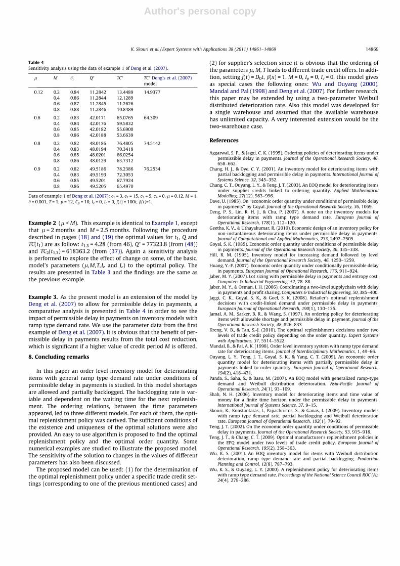
Example 3. As the present model is an extension of the model byDeng et al. (2007) to allow for permissible delay in payments, acomparative analysis is presented in Table 4 in order to see theimpact of permissible delay in payments on inventory models withramp type demand rate. We use the parameter data from the firstexample of Deng et al. (2007). It is obvious that the benefit of per-missible delay in payments results from the total cost reduction,which is significant if a higher value of credit period M is offered.

8. Concluding remarks

In this paper an order level inventory model for deterioratingitems with general ramp type demand rate under conditions ofpermissible delay in payments is studied. In this model shortagesare allowed and partially backlogged. The backlogging rate is var-iable and dependent on the waiting time for the next replenish-ment. The ordering relations, between the time parametersappeared, led to three different models. For each of them, the opti-mal replenishment policy was derived. The sufficient conditions ofthe existence and uniqueness of the optimal solutions were alsoprovided. An easy to use algorithm is proposed to find the optimalreplenishment policy and the optimal order quantity. Somenumerical examples are studied to illustrate the proposed model.The sensitivity of the solution to changes in the values of differentparameters has also been discussed.

The proposed model can be used: (1) for the determination ofthe optimal replenishment policy under a specific trade credit set-tings (corresponding to one of the previous mentioned cases) and

(2) for supplier’s selection since it is obvious that the ordering ofthe parameters l, M, T leads to different trade credit offers. In addi-tion, setting f(t) = D0t, b(x) = 1, M = 0, Ip = 0, Ic = 0, this model givesas special cases the following ones: Wu and Ouyang (2000),Mandal and Pal (1998) and Deng et al. (2007). For further research,this paper may be extended by using a two-parameter Weibulldistributed deterioration rate. Also this model was developed fora single warehouse and assumed that the available warehousehas unlimited capacity. A very interested extension would be thetwo-warehouse case.

References

Aggarwal, S. P., & Jaggi, C. K. (1995). Ordering policies of deteriorating items underpermissible delay in payments. Journal of the Operational Research Society, 46,658–662.

Chang, H. J., & Dye, C. Y. (2001). An inventory model for deteriorating items withpartial backlogging and permissible delay in payments. International Journal ofSystems Science, 32, 345–352.

Chang, C. T., Ouyang, L. Y., & Teng, J. T. (2003). An EOQ model for deteriorating itemsunder supplier credits linked to ordering quantity. Applied MathematicalModelling, 27(12), 983–996.

Dave, U. (1985). On ‘‘economic order quantity under conditions of permissible delayin payments’’ by Goyal. Journal of the Operational Research Society, 36, 1069.

Deng, P. S., Lin, R. H. J., & Chu, P. (2007). A note on the inventory models fordeteriorating items with ramp type demand rate. European Journal ofOperational Research, 178(1), 112–120.

Geetha, K. V., & Uthayakumar, R. (2010). Economic design of an inventory policy fornon-instantaneous deteriorating items under permissible delay in payments.Journal of Computational and Applied Mathematics, 233, 2492–2505.

Goyal, S. K. (1985). Economic order quantity under conditions of permissible delayin payments. Journal of the Operational Research Society, 36, 335–338.

Hill, R. M. (1995). Inventory model for increasing demand followed by leveldemand. Journal of the Operational Research Society, 46, 1250–1259.

Huang, Y.-F. (2007). Economic order quantity under conditionally permissible delayin payments. European Journal of Operational Research, 176, 911–924.

Jaber, M. Y. (2007). Lot sizing with permissible delay in payments and entropy cost.Computers & Industrial Engineering, 52, 78–88.

Jaber, M. Y., & Osman, I. H. (2006). Coordinating a two-level supplychain with delayin payments and profit sharing. Computers & Industrial Engineering, 50, 385–400.

Jaggi, C. K., Goyal, S. K., & Goel, S. K. (2008). Retailer’s optimal replenishmentdecisions with credit-linked demand under permissible delay in payments.European Journal of Operational Research, 190(1), 130–135.

Jamal, A. M., Sarker, B. R., & Wang, S. (1997). An ordering policy for deterioratingitems with allowable shortage and permissible delay in payment. Journal of theOperational Research Society, 48, 826–833.

Kreng, V. B., & Tan, S.-J. (2010). The optimal replenishment decisions under twolevels of trade credit policy depending on the order quantity. Expert Systemswith Applications, 37, 5514–5522.

Mandal, B., & Pal, A. K. (1998). Order level inventory system with ramp type demandrate for deteriorating items. Journal of Interdisciplinary Mathematics, 1, 49–66.

Ouyang, L. Y., Teng, J. T., Goyal, S. K., & Yang, C. T. (2009). An economic orderquantity model for deteriorating items with partially permissible delay inpayments linked to order quantity. European Journal of Operational Research,194(2), 418–431.

Panda, S., Saha, S., & Basu, M. (2007). An EOQ model with generalized ramp-typedemand and Weibull distribution deterioration. Asia-Pacific Journal ofOperational Research, 24(1), 93–109.

Shah, N. H. (2006). Inventory model for deteriorating items and time value ofmoney for a finite time horizon under the permissible delay in payments.International Journal of Systems Science, 37, 9–15.

Skouri, K., Konstantaras, I., Papachristos, S., & Ganas, I. (2009). Inventory modelswith ramp type demand rate, partial backlogging and Weibull deteriorationrate. European Journal of Operational Research, 192(1), 79–92.

Teng, J. T. (2002). On the economic order quantity under conditions of permissibledelay in payments. Journal of the Operational Research Society, 53, 915–918.

Teng, J. T., & Chang, C. T. (2009). Optimal manufacturer’s replenishment policies inthe EPQ model under two levels of trade credit policy. European Journal ofOperational Research, 195(2), 358–363.

Wu, K. S. (2001). An EOQ inventory model for items with Weibull distributiondeterioration, ramp type demand rate and partial backlogging. ProductionPlanning and Control, 12(8), 787–793.

Wu, K. S., & Ouyang, L. Y. (2000). A replenishment policy for deteriorating itemswith ramp type demand rate. Proceedings of the National Science Council ROC (A),24(4), 279–286.

Table 4Sensitivity analysis using the data of example 1 of Deng et al. (2007).

l M t�1 Q⁄ TC⁄ TC⁄ Deng’s et al. (2007)model

0.12 0.2 0.84 11.2842 13.4489 14.93770.4 0.86 11.2844 12.12890.6 0.87 11.2845 11.26260.8 0.88 11.2846 10.8489

0.6 0.2 0.83 42.0171 65.0765 64.3090.4 0.84 42.0176 59.58320.6 0.85 42.0182 55.69000.8 0.86 42.0188 53.6639

0.8 0.2 0.82 48.0186 76.4805 74.51420.4 0.83 48.0194 70.34180.6 0.85 48.0201 66.02540.8 0.86 48.0129 63.7312

0.9 0.2 0.82 49.5186 78.2386 76.25340.4 0.83 49.5193 72.30530.6 0.85 49.5201 67.79240.8 0.86 49.5205 65.4970

Data of example 1 of Deng et al. (2007): c1 = 3, c2 = 15, c3 = 5, c4 = 0, l = 0.12, M = 1,h = 0.001, T = 1, p = 12, Cp = 10, Ie = 0, Ic = 0, f(t) = 100t, b(t)=1.


Supply chain models for deteriorating products with ramp type demand rate under permissible delay in...

Documents

Transcript of Supply chain models for deteriorating products with ramp type demand rate under permissible delay in...