Integrated Approach to Variable Speed Limits & Ramp Metering
126
Integrated Approach to Variable Speed Limits & Ramp Metering extension of COSCAL v2 algorithm with ramp metering and ramp queue constraints Niharika Mahajan
-
Upload
khangminh22 -
Category
Documents
-
view
2 -
download
0
Transcript of Integrated Approach to Variable Speed Limits & Ramp Metering
Integrated Approach toVariable Speed Limits &Ramp Meteringextension of COSCAL v2 algorithm withramp metering and ramp queue constraints
Niharika Mahajan

Integrated Approach to Variable
Speed Limits & Ramp Meteringextension of COSCAL v2 algorithm with ramp metering and
ramp queue constraints
MASTER OF SCIENCE THESIS
For the degree of Master of Science in Transport & Planning at Delft
University of Technology
Niharika Mahajan
December ,
Graduation committee: Prof.dr.ir. Serge P. Hoogendoorn
Dr.ir. Andreas Hegyi
Ir. Goof van de Weg
Dr.ir. Meng Wang
Dr.ir. Lidwien Visser-Goossens
Ir. Paul Wiggenraad
Faculty of Civil Engineering and Geosciences(CiTG) · Delft University of Technology

Copyright c© Transport & Planning
All rights reserved.

Executive Summary
Traffic congestion continues to remain a serious problem in most countries, with significant economic
and environmental losses. ‘Intelligent Transport Systems (ITS)’ that utilize advanced information and
communication technology for managing road infrastructure, including vehicles and users, have shown
great potential in dealing with this problem. However, most current traffic management measures, like
route guidance, ramp metering and variable speed limits are designed and implemented independently.
Potentially counter-productive when deployed simultaneously, integration of these measures can benefit
from synergic effects.
The aim of this work is to integrate a near-future variable speed control strategy with ramp metering, to
operate efficiently at a freeway merging section. From a policy perspective, this is a challenge because
freeways and urban network are managed by different authorities. Currently, a spillback of ramp queue to
the urban network results in a deactivation of ramp metering, and an abrupt release of on-ramp vehicles
onto the freeway. This is undesirable for the freeway control measure. Therefore, the development of the
integrated strategy considers both, an improvement in freeway efficiency, and at the same time queue reg-
ulation at the on-ramp.
The research arch is initiated by conducting a literature survey, wherein the theoretical and control as-
pects of available speed control approaches are studied first. Subsequently, different queue management
approaches used in current ramp metering strategies are reviewed to identify the desirable features for a
queue controller. Finally, integration approaches for combining ramp metering with variable speed limits
are looked at.
It is seen that optimization-based integration strategies may offer huge potential to improve freeway effi-
ciency but these strategies are computationally complex for systems available in practice. Therefore, a so-
phisticated reactive variable speed limits strategy - COoperative Speed Control ALgorithm (COSCAL v2)
is chosen for integration with ramp metering. COSCAL v2 is a counteractive control strategy that resolves
moving jams to recover loss in efficiency from capacity drop. It uses shockwave theory concepts to speed
limit the exact the number of vehicles required to first resolve a jam, and next, to stabilize the traffic while
recovering traffic throughput.
The theory development is conducted in two stages from a simplistic to a more advanced approach that
relaxes some of the initial assumptions. The basic strategy is developed to guarantee jam resolution under
the condition of a constant ramp metering flow during the activation of COSCAL v2. Additionally, ramp
queue constraints are not included, which implies that in order to prevent a spillback, a sufficiently high
metering flow must be chosen. The theoretical formulation to determine when and how many vehicles must
be speed-limited, as in COoperative Speed Control ALgorithm (COSCAL) v2, is preserved here.
Master of Science Thesis Niharika Mahajan

ii
The core principle involves instantaneously speed-limiting the vehicles entering the moving jam. In this
way, the inflow into the jam is reduced as compared to the flow exiting the jam, resulting in jam resolution.
In the integrated strategy, the theory to determine the most upstream speed-limited vehicle that resolves
the jam, given a constant ramp metering flow, is formulated. Similarly, the theory for determining the
last vehicle speed-limited for stabilization is extended for the additional ramp flow. For this, COSCAL v2
checks for a maximum (average) density in the speed-limited area to ensure traffic stability. The value
of the target density determines the freeway flow arriving at the on-ramp. Then, the integrated approach
determines reduced target densities required to accommodate the ramp flow. It is also described how these
densities can be implemented in practice, and how errors its realization can be compensated within the
feedback structure of the scheme.
However, this approach is not feasible for time-dependent ramp metering flows. This is essentially because
accommodating a varying ramp flow will require implementing different densities in space-time, which
is both difficult to determine and implement in the COSCAL v2 algorithm. Therefore, in the advanced
strategy the theory of COSCAL v2 is extended for compatibility to a more sophisticated ramp metering
approach. In the new approach, rather than regulating density the flow arriving at the on-ramp is directly
controlled by determining when and where vehicles should enter and exit speed-limits. This addition-
ally improves the effectiveness of COSCAL v2. Further, a new ramp metering strategy using cumulative
curves is developed to include: queue-length constraints; policy restrictions on ramp metering flows; and
limitations on the minimum freeway flow that can be achieved with speed limits given the traffic state mea-
surements. One of the main advantages of the advanced strategy is its responsiveness to changing ramp
flows, and the utilization of freeway speed-limitation to prevent a queue spillback on the ramp.
Following the development of the two integration strategies, the advanced approach is translated to an al-
gorithm. This step ensures that a controller can be designed to realize traffic behaviour according to the
developed theory. Here, the complete strategy is divided into five modules that together determine the
spatial extent of speed limits at any given time. Similarly to the algorithmic formulation of COSCAL v2,
unique driving modes for the different detection and actuation tasks of the algorithm are used to communi-
cate the control scheme for implementation.
The control strategy thus developed is tested by means of simulation. Of the five modules, three modules
related to the speed control strategy are implemented in this work. Simulation runs under different de-
mand conditions are performed to verify the behavioural performance of the approach. Jam waves - that
otherwise occur when ramp metering and COSCAL v2 are implemented independently - are prevented in
the integrated approach. The results offer an initial indication of potential improvement from the strat-
egy. However, a more comprehensive quantitative evaluation is recommended. Furthermore, some critical
developments to the approach following the simulation study are identified.
In conclusion, this work demonstrates two ways in which COSCAL v2 can be integrated with ramp me-
tering (RM); how cumulative curves can be used for integration of control measures; and how efficiency
gains on the freeway and urban network can be balanced. The simulations offer a proof of concept for the
working of the advanced integrated strategy. However, the basic strategy should be both implemented and
tested further.
Niharika Mahajan Master of Science Thesis

Table of Contents
Acknowledgements vii
1 Introduction 1
1-1 Research Motivation . . . . . . . . . . . . . . . . . . . . . . . . . . . . . . . . . . . 1
1-2 Research Scope . . . . . . . . . . . . . . . . . . . . . . . . . . . . . . . . . . . . . 3
1-2-1 Focus Areas . . . . . . . . . . . . . . . . . . . . . . . . . . . . . . . . . . . 4
1-2-2 Relevance . . . . . . . . . . . . . . . . . . . . . . . . . . . . . . . . . . . . . 5
1-3 Research Objective . . . . . . . . . . . . . . . . . . . . . . . . . . . . . . . . . . . 5
1-4 Research Approach . . . . . . . . . . . . . . . . . . . . . . . . . . . . . . . . . . . 5
1-5 Overview of the Report . . . . . . . . . . . . . . . . . . . . . . . . . . . . . . . . . 7
2 Literature Survey 9
2-1 Introduction and Overview . . . . . . . . . . . . . . . . . . . . . . . . . . . . . . . . 9
2-2 Theoretical Aspects of Freeway Speed Control . . . . . . . . . . . . . . . . . . . . 10
2-2-1 Speed Homogenization Approach . . . . . . . . . . . . . . . . . . . . . . . 10
2-2-2 Flow Reduction Approach . . . . . . . . . . . . . . . . . . . . . . . . . . . . 11
2-2-3 Fundamental Diagram and Effects of variable speed limits (VSL) . . . . . . 14
2-3 VSL Control Approaches . . . . . . . . . . . . . . . . . . . . . . . . . . . . . . . . 14
2-3-1 Heuristic Strategies . . . . . . . . . . . . . . . . . . . . . . . . . . . . . . . 15
2-3-2 Regulatory Strategies . . . . . . . . . . . . . . . . . . . . . . . . . . . . . . 15
2-4 Ramp Metering (RM) - Queue Management . . . . . . . . . . . . . . . . . . . . . . 17
2-4-1 Rule-based Queue Management . . . . . . . . . . . . . . . . . . . . . . . . 18
2-4-2 ALINEA/Q and PI-ALINEA/Q . . . . . . . . . . . . . . . . . . . . . . . . . . 18
2-4-3 Queue Management Aspects in Comprehensive Controls . . . . . . . . . . 19
2-5 Integration of VSL and RM . . . . . . . . . . . . . . . . . . . . . . . . . . . . . . . 20
2-5-1 Advantages of an Integrated Control Strategy . . . . . . . . . . . . . . . . . 21
2-5-2 Recommendations for the Design of an Integrated Strategy . . . . . . . . . 21
2-6 Summary and Discussion . . . . . . . . . . . . . . . . . . . . . . . . . . . . . . . . 21
Master of Science Thesis Niharika Mahajan

iv Table of Contents
3 Basic Approach for Ramp Metering with COSCAL v2 25
3-1 Introduction . . . . . . . . . . . . . . . . . . . . . . . . . . . . . . . . . . . . . . . . 25
3-1-1 Overview of the roadside-cooperative algorithm . . . . . . . . . . . . . . . . 26
3-1-2 Overview of the chapter . . . . . . . . . . . . . . . . . . . . . . . . . . . . . 26
3-2 Assumptions and design parameters . . . . . . . . . . . . . . . . . . . . . . . . . . 27
3-2-1 Notation . . . . . . . . . . . . . . . . . . . . . . . . . . . . . . . . . . . . . . 27
3-2-2 Assumptions related to the jam characteristics . . . . . . . . . . . . . . . . 27
3-3 TASK 1: Jam detection . . . . . . . . . . . . . . . . . . . . . . . . . . . . . . . . . . 28
3-4 TASK 2: Initial speed limitation and jam resolution . . . . . . . . . . . . . . . . . . 28
3-4-1 Initial speed limitation for jam resolution - variable speed limits only . . . . . 28
3-4-2 Initial speed limitation for jam resolution - variable speed limits and rampmetering . . . . . . . . . . . . . . . . . . . . . . . . . . . . . . . . . . . . . 31
3-5 TASK 3: Speed limitation for stabilization . . . . . . . . . . . . . . . . . . . . . . . . 39
3-5-1 Speed limitation for stabilization - variable speed limits only . . . . . . . . . 39
3-5-2 Speed limitation for stabilization - variable speed limits with ramp metering 42
3-5-3 Correction for density errors in downstream stabilization states . . . . . . . 47
3-6 TASK 4: Speed limit release . . . . . . . . . . . . . . . . . . . . . . . . . . . . . . . 48
3-7 Resolvability of jam . . . . . . . . . . . . . . . . . . . . . . . . . . . . . . . . . . . . 48
3-8 Limiting the algorithm to a single jam . . . . . . . . . . . . . . . . . . . . . . . . . . 49
3-9 Summary and Discussion . . . . . . . . . . . . . . . . . . . . . . . . . . . . . . . . 50
4 Advanced Approach for Ramp Metering with COSCAL v2 53
4-1 Introduction . . . . . . . . . . . . . . . . . . . . . . . . . . . . . . . . . . . . . . . . 53
4-2 Assumptions and design parameters . . . . . . . . . . . . . . . . . . . . . . . . . . 53
4-2-1 Notations and notions . . . . . . . . . . . . . . . . . . . . . . . . . . . . . . 53
4-2-2 Assumptions related to on-ramp flows . . . . . . . . . . . . . . . . . . . . . 54
4-3 RM integration with TASK 3 of COSCAL v2 -speed limitation for stabilization . . . . . . . . . . . . . . . . . . . . . . . . . . . . . 54
4-3-1 Scenarios of stabilization scheme at the merged freeway section . . . . . . 55
4-3-2 Calculation of the time S-head and S-tail cross the on-ramp section . . . . 56
4-3-3 Constraints and design choices for the ramp metering strategy . . . . . . . 58
4-3-4 Determining the feasible solution space for ramp metering . . . . . . . . . . 61
4-3-5 Selecting a feasible ramp flow trajectory . . . . . . . . . . . . . . . . . . . . 70
4-3-6 Implementation of variable speed limits in the stabilization area . . . . . . . 70
4-4 Summary and Discussion . . . . . . . . . . . . . . . . . . . . . . . . . . . . . . . . 74
5 Algorithm Development 77
5-1 Introduction . . . . . . . . . . . . . . . . . . . . . . . . . . . . . . . . . . . . . . . . 77
5-2 Modes and Mode Transitions in COSCAL v2 . . . . . . . . . . . . . . . . . . . . . 78
5-2-1 Detection segment modes . . . . . . . . . . . . . . . . . . . . . . . . . . . . 78
5-2-2 Actuation segment modes . . . . . . . . . . . . . . . . . . . . . . . . . . . . 79
5-2-3 Mode Transitions . . . . . . . . . . . . . . . . . . . . . . . . . . . . . . . . . 79
5-3 Algorithmic formulation for the developed theory . . . . . . . . . . . . . . . . . . . 80
5-4 Pseudo-Algorithm for the Modules . . . . . . . . . . . . . . . . . . . . . . . . . . . 83
Niharika Mahajan Master of Science Thesis

Table of Contents v
6 Simulation Design and Evaluation 87
6-1 Introduction . . . . . . . . . . . . . . . . . . . . . . . . . . . . . . . . . . . . . . . . 87
6-2 Simulation Set-up . . . . . . . . . . . . . . . . . . . . . . . . . . . . . . . . . . . . 87
6-2-1 Network Characteristics . . . . . . . . . . . . . . . . . . . . . . . . . . . . . 88
6-2-2 Traffic Characteristics . . . . . . . . . . . . . . . . . . . . . . . . . . . . . . 88
6-2-3 Tuning Control Parameters . . . . . . . . . . . . . . . . . . . . . . . . . . . 89
6-3 Simulation Results . . . . . . . . . . . . . . . . . . . . . . . . . . . . . . . . . . . . 90
6-3-1 Base Case . . . . . . . . . . . . . . . . . . . . . . . . . . . . . . . . . . . . 90
6-3-2 COSCAL v2 without RM . . . . . . . . . . . . . . . . . . . . . . . . . . . . . 90
6-3-3 COSCAL v2 with stand-alone RM . . . . . . . . . . . . . . . . . . . . . . . 91
6-3-4 Advanced strategy for integrated RM with COSCAL v2 . . . . . . . . . . . . 93
6-3-5 Quantitative evaluation . . . . . . . . . . . . . . . . . . . . . . . . . . . . . . 97
6-4 Summary . . . . . . . . . . . . . . . . . . . . . . . . . . . . . . . . . . . . . . . . . 98
7 Conclusion 101
7-1 Motivation and contributions . . . . . . . . . . . . . . . . . . . . . . . . . . . . . . . 101
7-2 Findings and recommendations . . . . . . . . . . . . . . . . . . . . . . . . . . . . . 102
7-2-1 Research Objective 1: Learnings from literature survey . . . . . . . . . . . 102
7-2-2 Research Objective 2: Development of COSCAL v2 for integration withramp metering . . . . . . . . . . . . . . . . . . . . . . . . . . . . . . . . . . 103
7-2-3 Research Objective 3: Verification of the algorithm . . . . . . . . . . . . . . 104
7-3 Future work and practical implications . . . . . . . . . . . . . . . . . . . . . . . . . 105
7-3-1 Recommendations for further theoretical development . . . . . . . . . . . . 105
7-3-2 Considerations for field implementation . . . . . . . . . . . . . . . . . . . . 106
7-3-3 Policy implications . . . . . . . . . . . . . . . . . . . . . . . . . . . . . . . . 106
Glossary 113
List of Acronyms . . . . . . . . . . . . . . . . . . . . . . . . . . . . . . . . . . . . . 113
List of Symbols . . . . . . . . . . . . . . . . . . . . . . . . . . . . . . . . . . . . . . 113
Master of Science Thesis Niharika Mahajan

vi Table of Contents
Niharika Mahajan Master of Science Thesis

Acknowledgements
This report marks the end of quite a few months of vigorous effort - in part exciting, in part challenging and
overall a fulfilling journey. More importantly, it marks the completion of my curious pursuit of a Masters
at TU Delft two years ago. It has been with the support of many people that I got here, and I would like to
mention them all.
First of all, I would like to thank Serge Hoogendoorn for his heartening encouragement, and for the many
opportunities that he opened me to in the two years. I sincerely appreciate your role at the crucial time,
right before the start of this research thesis.
I can’t appreciate enough the careful supervision that I have received from Andreas Hegyi. He has been
vital in guiding through the theoretical developments in this work. Extremely approachable, he always
received all my queries very encouragingly. It was simply amazing the kind of confidence he showed in
me. It is appropriate to mention Goof van de Weg here - he mentored closely and almost always was the
first one to provide useful comments on my work. His pragmatic viewpoint really helped me set bounds to
the work time and again. Truly, I have taken real pleasure in working with both of them. It goes without
saying, the outcome in this research has immensely benefited from the extensive discussions I have had
with them.
Furthermore, I would like to thank Lidwien Goossens and Meng Wang for their timely inputs to this work.
Their comments have been useful in improving the work from alternative viewpoints. I would also like to
mention their cooperation in accommodating to my working schedule.
Finally, I would like to thank my family for their unfailing encouragement in every endeavour that I have
taken on so far. They always have been and will be my favourite people. Last but not the least, I would like
to thank Srivatsav for the rock-support that he has been in this process.
Master of Science Thesis Niharika Mahajan

viii Acknowledgements
Niharika Mahajan Master of Science Thesis

Chapter 1
Introduction
The functional characteristic of freeway infrastructure is to transport high volumes of people and goods at
high speeds. However, there is a trade-off between maximizing supply and maintaining highest efficiency.
With growing mobility and traffic demand, providing sufficient infrastructural capacity has become a lim-
itation. This makes a traffic breakdown increasingly likely when traffic intensity peaks spatio-temporally.
As a result, freeway congestion continues to remain a serious problem in most countries, with many adverse
effects - from lost vehicle hours, energy consumption to emissions.
This research aims to develop an ‘intelligent’ traffic management system that addresses the problem of
freeway congestion. In this chapter, the main goal is to identify the research objectives, the approach that
will be adopted, focus areas and the scope of the research.
1-1 Research Motivation
In order to arrive at the relevant research questions, three intriguing questions are answered in this section:
How does traffic congestion deteriorate freeway efficiency?
The most undesirable consequence of congestion is the result of the difference in driver behaviour while
entering and leaving a congestion. It is observed that drivers maintain a larger headway when exiting a
congestion than before breakdown; in other words, for the same distance headways, drivers prefer a lower
speed and take longer during acceleration than that during deceleration (Hoogendoorn & Knoop, 2012).
This difference in the microscopic behaviour, characteristic of a state transition, i.e. from congestion to free
flow or free flow to congestion is referred to as traffic hysteresis. It is this non-equilibrium transition process
that results in a capacity drop - a flow reduction of about 10-30 % - characteristic of a traffic breakdown
(Kerner & Rehborn, 1996). Such a capacity drop is often observed at freeway merging sections, upon
activation of on-ramp bottlenecks. The drop in capacity from a congestion also implies a lower queue
discharge flow, which further worsens the resolution of the congested state. Therefore, the mechanism of
traffic breakdown, capacity drop, and resulting slower resolution of congestion, results in a substantial loss
of freeway efficiency.
The potential of advanced application of information and communication technologies (ICT) in the field of
road transport, including infrastructure, vehicles and users, and in traffic management, has been recognized
in meeting the growing challenge of road congestion. Such ‘Intelligent Transport Systems (ITS)’ have
Master of Science Thesis Niharika Mahajan
2 Introduction
enabled better information provision, safer, more coordinated and smarter use of transport networks (Di-
rective 2010/40/EU). Most advanced traffic management systems, such as, ramp metering (RM), dynamic
route guidance, dynamic lane use etcetera have been designed to eliminate the causes leading to conges-
tion. This thesis focuses on variable speed limits as a dynamic traffic management approach for freeways,
which is motivated next.
Why would we want to regulate freeway traffic with variable speed limits (VSL)?
In practice, congestion is a common occurrence during high traffic load conditions, in spite of control
systems that aim to manage road use. However, these strategies tend to regulate traffic on the sub-network
in order to ensure an increased throughput on the freeways. In the early 80’s, researchers envisioned VSL
as an innovative approach that could regulate the mainstream traffic. The full potential of VSL remains in
its immediate response to the actual traffic situation on the freeway, to weather and daylight setting, and
any other real-time circumstance. The three main advantages of speed control systems are:
(1) VSL allow immediate intervention that can influence dynamics of the traffic nearest to the problem
location
(2) traffic can be managed while avoiding diverting or restricting access for unrelated streams of traffic
(3) benefits from VSL can be realized at both microscopic and macroscopic levels - the harmonization
effects on traffic speeds have shown to dampen disturbances from individual driver behaviour, and
controlled application of speed limits is being explored to prevent and resolve congestion.
Even so, the only common application of VSL has been seen in incident management and near temporary
road-works, and static speed limits remain the most widespread means of informing how fast users can
drive on the road. Clearly, the potential of VSL to improve freeway efficiency is yet to be realized in prac-
tice.
What are the policy and practice related challenges in the adoption of VSL control measures?
The challenges in the widespread adoption of VSL systems are both technical and policy related. First ma-
jor technical hurdle is the lack of generalized VSL strategies that are independent of specific infrastructure
configuration and traffic scenarios. For instance, a recent approach is designed exclusively for stationary
jams at infrastructural bottlenecks (Carlson et al., 2011). The transferability of such approaches to practice
is then limited by the occurrence of the specific conditions, and the efficiency gains thereof.
Another important deterrent is the lack of complementarity of VSL approaches to the existing control
systems. This means that different control measures are designed independently, which can deteriorate
overall performance when these measures are deployed simultaneously.
RM is the most popular control measure used to regulate the traffic entering a freeway. On-ramp infras-
tructure offers access to traffic from the sub-network to enter the freeway at specific locations. RM control
allows to restrict this additional flow from on-ramps to prevent traffic deterioration on the freeway. At the
same time, on-ramp merging sections are potential bottlenecks; merging disruptions at ramp section can
induce queueing in the shoulder lane as on-ramp demand increases (Cassidy & Rudjanakanoknad, 2005).
These disturbances can propagate forward to result in a congestion downstream of the on-ramp. Therefore,
on-ramps with RM are critical locations for potential activation of VSL systems as well.
Therefore, to facilitate the adoption of VSL approaches in the near future, their integration with other more
commonly implemented control measures, and the validation of benefits from their synergic effects are
crucial. Some recent works have demonstrated that integration of RM and VSL strategies can enhance the
overall performance of the freeway (Carlson et al., 2010, Kotsialos & Papageorgiou, 2004, Van de Weg
et al., 2014). However, no such integrated systems have been tested in the field yet. This is also due to their
Niharika Mahajan Master of Science Thesis
1-2 Research Scope 3
computational complexity, given the capacity of the available systems.
Finally, a crucial policy-specific difficulty in using current integrated control systems is about achieving a
compromise between regional benefits (dis-benefits) and large network-level gains. The consequence of
RM measure is a faster growth rate of the on-ramp queue. Under peak traffic loads, this situation results in
spillback of ramp queues onto the surface roads. While freeways are most commonly maintained centrally,
the performance of surface roads and the adjacent lower network is managed by local (municipal) agencies.
This explains that a spillback of on-ramp queues is highly undesirable for the local traffic managers. Since
sub-networks commonly lack sophisticated traffic management systems, congestion aggravates faster, lead-
ing to a deteriorated performance and in a worse case, a network gridlock. For this reason, current traffic
management policies in the Netherlands allow deactivation of RM under such conditions.
However, this policy can have adverse effects on an integrated control strategy involving RM. This is
because a sudden deactivation of RM results in an abrupt flux of vehicles which may disrupt the control
strategy active on the freeway. Therefore, the work attempts to investigate an integrated VSL and RM
approach that can also prevent spillback of on-ramp queues to the surface roads. Such an approach will
ensure improved efficiency on the freeway and the sub-network.
1-2 Research Scope
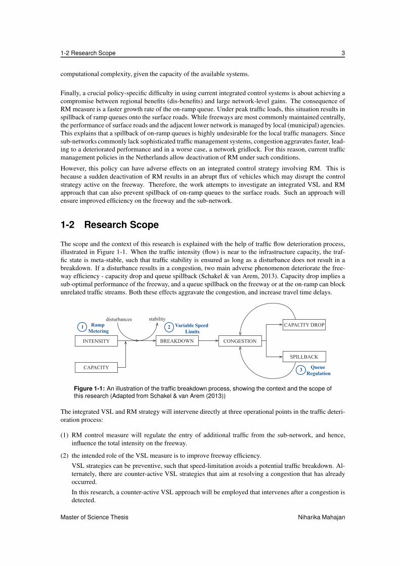
The scope and the context of this research is explained with the help of traffic flow deterioration process,
illustrated in Figure 1-1. When the traffic intensity (flow) is near to the infrastructure capacity, the traf-
fic state is meta-stable, such that traffic stability is ensured as long as a disturbance does not result in a
breakdown. If a disturbance results in a congestion, two main adverse phenomenon deteriorate the free-
way efficiency - capacity drop and queue spillback (Schakel & van Arem, 2013). Capacity drop implies a
sub-optimal performance of the freeway, and a queue spillback on the freeway or at the on-ramp can block
unrelated traffic streams. Both these effects aggravate the congestion, and increase travel time delays.
CAPACITY
SPILLBACK
INTENSITY CONGESTION
CAPACITY DROP
BREAKDOWN
disturbances stability
1 2
3
Ramp
MeteringVariable Speed
Limits
Queue
Regulation
Figure 1-1: An illustration of the traffic breakdown process, showing the context and the scope of
this research (Adapted from Schakel & van Arem (2013))
The integrated VSL and RM strategy will intervene directly at three operational points in the traffic deteri-
oration process:
(1) RM control measure will regulate the entry of additional traffic from the sub-network, and hence,
influence the total intensity on the freeway.
(2) the intended role of the VSL measure is to improve freeway efficiency.
VSL strategies can be preventive, such that speed-limitation avoids a potential traffic breakdown. Al-
ternately, there are counter-active VSL strategies that aim at resolving a congestion that has already
occurred.
In this research, a counter-active VSL approach will be employed that intervenes after a congestion is
detected.
Master of Science Thesis Niharika Mahajan

4 Introduction
(3) from a policy viewpoint, controlling the spillback of on-ramp queues to the surface roads was identified
as important for practical suitability of VSL systems. Therefore, queue constraints will be additionally
incorporated in the integrated strategy that will intervene to prevent spillback.
1-2-1 Focus Areas
With an understanding of the problem situation and the intended intervention with an integrated control
strategy, the focus areas are described in further detail. This will help define the research boundaries within
each of the research areas: VSL, RM and queue management, which are themselves extensive areas of
research.
1-2-1-1 Macroscopic VSL measures
Speed control systems can be macroscopic or microscopic. Most current microscopic systems, like adaptive
cruise control (ACC) and cooperative adaptive cruise control (CACC), aim to improve car-following tasks
and safety. In such systems, each individual vehicle employs radar sensing, and additionally vehicle-to-
vehicle communication in CACC, to locate the leader and adjust speed and acceleration accordingly. On
the contrary, macroscopic systems use the aggregate traffic flow characteristics, like average flow, density
and speed, to generate control advice. The control advice is typically displayed via variable message
signs (VMS) mounted over roadside gantries in this case.
The scope of this work is restricted to macroscopic speed control measures. One major reason is the diffi-
culty to implement microscopic traffic control strategies in practice. The limitations include the practical
problem of insufficient penetration of in-car technologies, and the theoretical complexity of incorporating
lane-changing behaviour in the design of traffic management systems.
1-2-1-2 Near-future implementation
The suitability of the designed approach for near-future field testing is an important consideration in this
work. Therefore, the focus will be on developing systems that are computationally and technologically
comparable to the existing traffic systems.
1-2-1-3 Local RM with queue regulation
Sophisticated approaches for RM consider coordination of multiple on-ramps to utilize the additional ca-
pacity and distribute delays effectively. However, the scope here is limited to local RM approaches at a
single on-ramp merging section. Integration of coordinated RM strategies with VSL could be potential
future extensions to this work.
The integration of RM control with VSL will focus on on-ramp queue regulation. This is because of the
hierarchical management of freeway and urban networks that entails deactivation of RM control when the
on-ramp queue spills back to the surface road. The subsequent release of the on-ramp queues substantially
deteriorates the performance of the VSL system and therefore, the freeway.
1-2-1-4 Efficiency improvement for freeway and the sub-network
The objective of a control strategy can vary from improving safety, travel time, travel time reliability, or
environmental impact. The goal of the integration strategy here is to improve the freeway efficiency while
preventing performance degradation of the secondary network. The focus on on-ramp queue regulation is
in line with this. The indicators used for measuring efficiency will be discussed in Section 1-4.
Niharika Mahajan Master of Science Thesis
1-3 Research Objective 5
1-2-1-5 Simple test network
The test network will consider a simple merging section with a single lane on-ramp and a two-lane freeway
section. This simple network is only a representation of more complex networks in reality. The focus of
the evaluation will be to validate the expected behaviour of the control design which can be sufficiently ex-
amined with the proposed network. However, evaluating network effects of the integrated control measure
requires a larger and more realistic network. Network effects will therefore not be considered.
1-2-2 Relevance
Most traffic control measures are typically designed and implemented stand-alone. However, managing
traffic disruptions at a local level is not always the most efficient at a higher network-level. At the same
time, various control strategies deployed locally can be mutually counter-productive. This gap is recognised
in the concept of network-wide traffic regulation. The concept aims to benefit from utilization of storage
capacity at locations other than the point of disruption, distribution of delays over a larger network, and
the synergic effects from more coordinated control measures. This drives the network towards a system
optimum. However, the first step towards realizing such a concept is the integration of the different traffic
management measures currently being used or being designed for near-future implementation. The work
in this thesis thus demonstrates how a widely-used traffic management measure, RM, can be integrated
with a VSL strategy.
1-3 Research Objective
The potential of VSL to improve freeway efficiency, and the current barriers in the practical implementation
of these systems motivate this research. We recognized that freeway on-ramp locations are bottlenecks
where VSL can be beneficial in improving traffic efficiency. At the same time, RM is a more commonly
deployed control measure at on-ramps. Therefore, integration of VSL strategy with RM is an opportunity
to improve the practical suitability of VSL systems.
In this work, an integrated VSL and RM strategy will be developed and implemented in a traffic simulator.
The aim is to test the functional performance of critical design aspects, and to inform design improvements
from practical considerations. To that end, the main research question that guides the final outcome is:
Can COoperative Speed Control ALgorithm (COSCAL v2) be integrated with ramp metering, in a way
suitable for roadside and near-future implementation, to improve freeway efficiency and regulate on-
ramp queues?
In order to answer this research question, the following objectives have been formulated for this research:
(1) Explore the different theoretical and control approaches for variable speed limits systems, and for
on-ramp queue control.
(2) Develop an integrated VSL and RM strategy that improves freeway efficiency and prevents spillback
of on-ramp queues.
(3) Verify the functional correctness of the developed strategy by means of simulation.
1-4 Research Approach
The research approach involves three parts - a literature survey, theoretical development and simulation-
based testing:
Master of Science Thesis Niharika Mahajan

6 Introduction
• The literature survey is conducted for two main purposes. First, to understand the theoretical un-
derpinnings of VSL from the available control approaches and second, to identify the desirable
characteristics for the design of an integrated VSL and RM strategy. The focus areas identified
in Section 1-2-1 guide the boundaries of the literature survey, which further informs of the design
process.
• In the theory development part, COoperative Speed Control ALgorithm (COSCAL) v2 algorithm
for VSL will be adapted and extended to be integrated with a suitable RM approach. Compatibility
of the theoretical approach to COSCAL v2 will therefore be important throughout the design process.
COSCAL v2 algorithm for VSL
COSCAL v2 is a macroscopic speed control approach based on shockwave theory, to resolve moving
jams and hence, improve freeway efficiency. It is suitable for roadside deployment, and designed for
multi-lane, heterogeneous traffic conditions. Additionally, COSCAL v2 and its microscopic coun-
terpart COSCAL v1 are designed with transition to cooperative systems in mind. Both versions of
the algorithm are compatible for roadside and in-car detection as well. This offers the advantage of
leveraging faster and more accurate sensing via in-car technology, regardless of the penetration rates.
The theory will be built from a simplistic approach to a more sophisticated approach that relaxes
some of its design assumptions. Two different approaches for integrating RM with VSL are pro-
posed in the process:
Basic approach for RM with COSCAL v2
The theoretical formulation of the approach is macroscopic, with the simplifying design choice of
constant RM flow during the activation of the VSL scheme. In this case, the approach does not
explicitly consider any constraints for queue-length on the on-ramp. Thus, the RM rate must be the
highest outflow required to prevent a queue spillback at any time.
In a situation that the VSL scheme crosses the on-ramp section, the adapted approach must ensure
that the freeway flows arriving at the on-ramp section are reduced to accommodate the additional
ramp flow. In other words, the higher the desired RM flow, the more stringent the VSL scheme must
be to sufficiently reduce mainstream flow arriving at the ramp section. In effect, such a conservative
integrated strategy reduces the efficiency of the VSL scheme. This is a major drawback of the basic
approach, that is addressed in the advanced approach.
Advanced approach for RM with COSCAL v2
In the advanced approach, the goal is to design and integrate a more sophisticated RM approach with
the VSL strategy. The RM strategy should dynamically respond to changing on-ramp demand, while
ensuring a maximum queue-length limit to prevent spillback. The advantage here is that the on-ramp
storage is better utilized, requiring less conservative RM rate.
For the integration of the VSL scheme with time-dependent RM flows, a predictive approach is
considered desirable. In this case, RM flows are available over a prediction horizon and anticipatory
decisions can be determined to (1) adapt VSL, and (2) ensure all necessary constraints are met in the
future .
• In the final part of this research, specific design aspects of the developed approaches are evaluated
in VISSIM micro-simulation package. This mainly entails a qualitative analysis of the control be-
haviour observed as compared to that expected based theoretically.
Niharika Mahajan Master of Science Thesis

1-5 Overview of the Report 7
1-5 Overview of the Report
Table 1-1 summaries how chapters are organized in this report; the third column provides the essence of
the content in each chapter.
Table 1-1: Overview of the report
Description Chapter Content/relevance
Literature Survey Chapter 2 theoretical insights from literature useful for the-
ory development in Chapter 3 and Chapter 4
Theory Development-I Chapter 3 adaptation of COSCAL v2 for constant RM flows
without ramp queue constraints
Theory Development-II Chapter 4 integration of COSCAL v2 with sophisticated RM
strategy with ramp queue constraints
Algorithm Development Chapter 5 translation of theory to an algorithm for the con-
troller
Simulation Testing Chapter 6 verification of the algorithm and validation of the
theoretical model
Conclusions Chapter 7 results and recommendations
Master of Science Thesis Niharika Mahajan

8 Introduction
Niharika Mahajan Master of Science Thesis

Chapter 2
Literature Survey
Research studies in traffic management systems have shown novel ways to intervene at different operational
levels with advanced controls, such as, route information systems, ramp metering (RM), variable speed
limits (VSL), and individual lane guidance. These systems allow to manage road usage and improve the
capacity of the network. In practice, they are often implemented stand-alone with the common goal to ease
local traffic deterioration. However, the potential of integrated traffic control measures for improved traffic
efficiency has been discussed in theory and practice (Papageorgiou et al., 2003). This chapter discusses the
literature on freeway traffic control with three main objectives:
1. to survey the principle design and control approaches for dynamic speed control. The insights from
this part are used to understand and apply traffic flow theory to the VSL strategy.
2. to review RM strategies with a focus on queue-management; the goal is to understand desirable
features for an on-ramp queue regulator that can be integrated with COoperative Speed Control
ALgorithm (COSCAL) v2.
3. to identify the most important considerations for integration of RM with VSL strategies, and specif-
ically COSCAL v2
2-1 Introduction and Overview
VSL offer a responsive and flexible way to influence traffic dynamics, almost instantaneously. This is
an important reason why speed control for improving freeway efficiency has received growing attention
in the recent years. The additional advantage of speed control systems is the growing availability of
variable message signs (VMS) on freeways, which offer ready infrastructure for deployment. Moreover,
technological advances towards in-car systems offer the potential of even more precise implementation,
and a richer data source which has been pointed out in some recent studies (Grumert & Tapani, 2012,
Van de Weg et al., 2014). However, the full potential of speed limits has not been utilized in practice yet.
On the other hand, RM is considered as the most direct and efficient control measure to upgrade freeway
performance (Papageorgiou et al., 2003). However, in keeping flow from entering the freeway, the queue on
the on-ramp grows faster, i.e. RM and queue management are essentially counteracting. The propagation of
the resulting ramp congestion to its sub-networks is usually prevented by deactivation of RM and discharge
of the entire queue. The subsequent uncoordinated release of on-ramp flows can disrupt any mainstream
Master of Science Thesis Niharika Mahajan

10 Literature Survey
speed control. This stands as an obstacle in the implementation of other control strategies, as well as their
integration with RM.
The Literature Survey is used to understand the challenges and the opportunities in the two control ap-
proaches, which then helps to identify the desirable characteristics for the integrated strategy. While
conducting the Literature Survey, the following main considerations are central: resolving congestion,
improving freeway efficiency, preventing a spillback of on-ramp queues to surface streets, compatibility of
the RM and VSL approach, and suitability for implementation in practice.
This Chapter is structured as follows; first, VSL approaches are reviewed from two different standpoints -
traffic flow theory related in Section 2-2 and systems control related in Section 2-3. While the theoretical
aspects helps understand the design choices and their realised impacts, the control strategy is crucial for
realizing expected performance in the field. Next, in Section 2-4, different queue management approaches
are discussed. Further, different schemes for the integration of RM with VSL are presented in Section 2-5
and finally, the main conclusions important for the theoretical design of the control approach are presented
in Section 2-6.
2-2 Theoretical Aspects of Freeway Speed Control
The direct impact of speed control on the freeway is reduced speeds. However, there are additional macro-
scopic effects like cumulative flow and density changes, speed and flow differences between lanes, and
microscopic effects like speed differences between consecutive vehicles. These effects are the conse-
quence of not only the magnitude of speed decrease, but also the dynamics of the control procedure. When
developing a speed based traffic regulator, two dynamic choices have to be made: (1) the spatial extent
over which the control is applied and changed over time, and (2) the value of applied speed limits. As an
example, variable speed limit values could be applied over a fixed length of freeway in one case or a fixed
speed limit over varying segments in another. The impacts of these choices are non-trivial for the achieved
efficiency and are the focus in this section.
In the earliest works on traffic control using VSL, Smulders (1990) explains two possibilities to avoid
congestion, either by removing the sources of disturbances (increasing homogeneity) or by reducing shorter
headway (increasing stability). Hegyi et al. (2008) later embodied these principles into two analytically
different approaches towards speed limitation: one utilizing the homogenization effects from decreased
speeds, and the other using flow reduction for preventing traffic breakdown or resolving a prevailing jam.
The approaches are detailed in the following sections.
2-2-1 Speed Homogenization Approach
If the speed limits used are above the critical speed, i.e. the speed at the critical density with maximum
flow, speed limitation is understood to have a homogenization effect (Smulders, 1990). The fundamental
principle involves slowing down the faster driving vehicles without limiting the speed of the slower traffic.
This reduces speed differences, and the need for acceleration and braking manoeuvres. Hence, by keeping
the speed above the critical speed, lower than the free flow speed and only slightly lesser than the average
speed, speeds are better homogenized (Hegyi et al., 2008).
Smulders (1990) used this approach, founded on contemporary work by van Toorenburg (1983), in a macro-
scopic traffic flow model based optimization that maximized time to congestion and traffic throughput to
determine the switching time for control. The work attributes the reduction of small time headways (<1s) in
the faster lane as most important to the homogenizing effect. Alessandri et al. (1999) used the same speed
regulator, maximizing a flow cost function based on an alternate traffic model and optimization technique
to demonstrate a slight improvement in efficiency. The improvement was theoretically attributed to the
increased critical density at lower average speed.
Niharika Mahajan Master of Science Thesis

2-2 Theoretical Aspects of Freeway Speed Control 11
2-2-2 Flow Reduction Approach
The flow reduction approach is central to improving freeway efficiency. This follows from the under-
standing of how a jam is resolved; when the inflow into the jam reduces below its outflow the jam state
diminishes over time. Similarly, if the flow into a bottleneck is reduced sufficiently, a capacity drop can
be prevented at the bottleneck. Therefore, by using speed limitation to achieve lower flows a maximum
capacity flow can be maintained on the freeway.
Flow reduction from speed limitation can be achieved in different ways, depending on the value of the
applied speed limits. For speeds lower than the critical speed, reduction effects additionally depend on the
traffic demand. These mechanisms will be summarised after a discussion on the fundamental impacts of
how speed limits are imposed:
space
time
inflow
indirect flow reductionduring state transition
flowconservation
(a) Stationary speed limits. Holds for over-
critical VSL in all inflow conditions, and for
under-critical VSL in low inflow conditions
space
time
inflow
flowreduction
density
conservation
(b) Instantaneous speed limits. Direct flow
reduction in all inflow conditions
space
time
flowconservation
flowconservation
density
conservation
density
conservation
reducedoutflow
recoveredoutflow
increasedoutflow
(c) Time-varying outflow from VSL over a freeway
length and time interval. Holds in low inflow condi-
tions. Gating effects result in different flow reduction
mechanism in high inflow conditions.
Figure 2-1: Effects of VSL application dynamics, value of speed limits and inflow condition
Master of Science Thesis Niharika Mahajan

12 Literature Survey
2-2-2-1 Dynamics of Imposing Speed Limits
The dynamics used in the SPEed Controlling ALgorIthm using Shockwave Theory (SPECIALIST) algo-
rithm emphasize on how the application of the speed limits - regardless of the value of the speed limit itself
- influences the traffic flow dynamics (Hegyi et al., 2008). This difference is exploited in this algorithm to
serve two main objectives with speed control. The first is employed for jam resolution, while the second
is used to create an additional buffer space on the freeway that can store the speed limiting vehicles at a
higher density than achievable without control. Essentially, the differences translate to unique flow and
density consequences for the outflow from the speed-limited area.
The different possibilities for application of VSL can be categorised between the two extreme cases, namely
instantaneous and stationary application of speed limits. Moving fronts, wherein the head and the tail of
the speed limited area are continuously changed over time, at a chosen speed, comprise all intermediate
possibilities. Their impact on the traffic state can be more easily understood by visualizing one vehicle
following the other at the same speed, maintaining a fixed headway. With this hypothetical scenario as
the basis of the explanation, the three possibilities: instantaneous application, stationary speed limits and
moving fronts for the control area are detailed.
• Instantaneous application of speed limits
In the case that the two vehicles are subjected to speed limitation at the same time, both would
simultaneously adjust to this lower speed, from their original free flow speed, without changing the
spacing between them. The implication is that there’s no impact on the density from application of
speed limits itself. However, since the speed is reduced, these vehicles would take longer to cross
an arbitrary downstream location as compared to the case without speed limitation. The result is a
reduced flow, as illustrated in Figure 2-1b. On the fundamental diagram, this can be understood with
a vertical line, corresponding to a given density. Now, this density line crosses the speed limit line (a
line from the origin at a slope equal to the applied speed limit) at a lower flow value compared to the
free flow branch, indicating a reduction of flow Figure 2-1b.
• Stationary speed limits
Stationary speed limits refers to point implementation of speed control, e.g. at a single gantry, for
a given time interval. In keeping the location fixed over time, a time difference between when the
vehicles enter speed limits is effectuated. This is because a following vehicle would cross a fixed
location at a later time than the leader. This time difference in the application of speed limits on
consecutive vehicles, results in a change (increase) in density downstream of the controlled area. The
important consequence of stationary speed limits is that flow is conserved at the boundary. However,
Papageorgiou et al. (2008) hypothesizes a VSL triggered temporary reduction in flow, during the
period of transition to the new, higher density state. This can be understood from Figure 2-1a and is
the theoretical reasoning utilized in modelling the control approach (Carlson et al., 2011) under low
arrival demand conditions.
The author understands that when VSL below the critical speed are applied, the resultant free flow
branch crosses the congested arm of the fundamental diagram. In this case, the flow reduction is not
indirect always, and is conditional on the demand flow. For higher inflows, above the flow at the
cross-over point, the reduction effect is direct. The flow in this case is reduced to the flow value at
the congested state for the applied speed limits. For lower inflows, the flow reduction is indirect.
• Moving fronts for application or release of speed limits
Time varying location of the head and tail of the speed control area are referred to as moving fronts.
By changing the speed of these fronts over time, the speed limited section can be leveraged to regulate
traffic flow and density. When the tail of the control section propagates upstream, the speed limits
apply to the following vehicle at a later time compared to its leader. In doing so, the following
vehicle drives at a higher speed while the leader is already speed limited. This diminishes the spacing
between the two vehicles to achieve a higher density in the process of speed control. The time lag in
Niharika Mahajan Master of Science Thesis
2-2 Theoretical Aspects of Freeway Speed Control 13
speed limit application to the vehicles determines the realized density; the higher the lag, the greater
the resultant density. Just as time difference in speed limitation can be exploited to achieve different
densities inside the controlled area, a similar logic can be translated to the vehicles leaving this area.
The head of the controlled section can be allowed to propagate upstream at varying speeds; the faster
the propagation speed (more negative), the higher is the resultant flow downstream, i.e. flow leaving
the section.
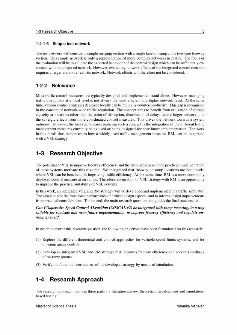
2-2-2-2 Implication of VSL Dynamics for Flow Reduction Approaches
The mechanism of flow reduction differs based on the dynamics of imposed speed limits, and was differ-
entiated as direct and indirect flow reduction. Direct flow reduction results when the density is conserved
in the new traffic state on application of VSL; a reduced speed then results in a lower flow. Indirect flow
reduction occurs from a flow inefficiency, typically attributed to the transition period, wherein traffic state
changes to a higher density state at the same flow value when speed-limits are applied; the phenomenon
becomes clear in Figure 2-1a.
Further, it is understood that flow reduction can be achieved directly with instantaneous application of speed
limits, for all speed limit values above and below critical speed. Alternately, stationary speed limits result
in an indirect reduction in flow in most cases. This is true when when speed limits are applied (1) at over-
critical speeds, and (2) at under-critical speed-limits in low demand condition (lower than the congestion
flows at that speed).While moving fronts for application and release of speed-limits can result in both an
increase or decrease in traffic flow based on the speed of head, tail and the state of traffic under speed-
limitation; this flow variation is essentially direct due to changes in traffic density. Stationary speed limits
can also result in a direct flow reduction, only when applied with sufficiently low speed limit values. These
are VSL values that induce a capacity flow lower than the average freeway demand. When this holds, the
speed limited area holds up the excess, to allow only the capacity flow to exit downstream. Hegyi (2014)
refers this approach as ‘gating’ and Carlson et al. (2011) uses this aspect to create a controlled congestion
upstream of a fixed bottleneck. Additionally, the author recognises that in case of speed limits, as low as 40
km/h to 20 km/h, any gain in critical density (and hence, capacity) is likely to be exceeded by the reduction
in flow from a lower speed. Therefore, the resulting outflow is lower than without speed control for such
cases.
Density
(veh/km)
Flow
(veh/h)
inflow 1
(low)
inflow 2
(high)
critical
density
jam
density
congestion
branch
instantaneous speed
limits
stationary speed
limits
gating with stationary
speed limits
veffvff
Figure 2-2: Effects of VSL dynamics on the fundamental diagram.
Master of Science Thesis Niharika Mahajan

14 Literature Survey
2-2-3 Fundamental Diagram and Effects of VSL
A well-founded understanding of the effects of VSL control on the fundamental diagram (FD) is important
for selection of appropriate speed limits, and for heuristic approaches that are otherwise based on arbitrary
desired values of traffic state variables. It also helps to develop more effective control strategies whose
impacts can be anticipated qualitative without simulation-based-analysis.
The impact of VSL on aggregate traffic flow, and most importantly the critical values in the macroscopic
FD: critical density and capacity flow, are not well evidenced in empirical data. This is because of: (1) the
difficulty to ensure comparable conditions for with (after) and without VSL(before)data used in ex-post
analysis, (2) the difficulty to obtain sufficient speed-flow data across all occupancies under VSL and (3) dif-
ficulty to validate that the observed impacts are from speed control, independent of local infrastructure and
driving characteristics.
Papageorgiou et al. (2008) in their important work to empirically validate the effects of VSL, presented
some evidence for an increase in critical occupancy for under-critical speed limits. However, they con-
firmed no conclusive impact on the flow-capacity (this aspect is used in Alessandri et al. (1999) to motivate
an increased efficiency from homogenization approach). The work also surveys some of the more influ-
encing notions of aggregate traffic behaviour under speed control.
A general hypothesis based on the literature surveyed and the author’s understanding is summarised below
and will be considered while formulating the control strategy in this research:
• When speed limits are applied on free flowing traffic, the free flow branch shifts to a slope equivalent
to the effective (average) speed from speed control.
The effective speed can be lower or higher than the applied speed limits depending on whether the
speed limits are mandatory or advisory, respectively, and on the level of enforcement. Jonkers et al.
(2011) report a difference in applied and realized average speed from a VSL field-test results. In
addition, this phenomenon is being studied in simulation as varying levels of compliance (Hellinga
& Mandelzys, 2011).
• Papageorgiou et al. (2008) hypothesizes a positive shift in the critical density from speed limitation.
The work proposes that FD under speed limitation crosses that without control, close to or at a
slightly higher density than the critical density of the original flow-density curve. This was validated
with some empirical evidence.
• Reduction in flow is indirect-during state transition to a higher density-when stationary speed limits
are imposed at over-critical speeds (Figure 2-1a). The flow drop is proportional to the magnitude of
speed reduction; the higher the reduction in speed, the greater is the flow reduction and the longer it
takes for the state transition.
• When stationary speed limits below the critical speed are applied, the resultant free flow branch
crosses the congested arm of the original curve. The flow reduction is therefore, not indirect in all
cases and is conditional on the demand flow. For inflows above the flow at the cross-over point, the
flow reduction is direct due to gating effects. For lower inflows, the reduction is indirect.
• Flow reduction from instantaneous application are achieved from the time of application to the time
that the last speed limited vehicle leaves a given downstream location, illustrated in Figure 2-1b. The
reduction is proportional to the decrease in speeds but is observed for any speed-limit values.
2-3 VSL Control Approaches
The objective of this section is to identify the desirable properties of a speed control system for this re-
search. The surveyed literature on available VSL approaches can be classified into three main categories:
Niharika Mahajan Master of Science Thesis

2-3 VSL Control Approaches 15
heuristic, regulatory, and optimization based controls. The categorization highlights the trade-off between
effectiveness (optimality) and the computation and data requirements of different approaches. It also high-
lights the lack of effective and easily implementable non-heuristic speed control approaches in practice.
2-3-1 Heuristic Strategies
Heuristic strategies use occupancy, speed, flow values or a combination, as threshold for activation and
deactivation of control. More advanced heuristic approaches employ decision-tree based thresholds, and
are understood as effective for field implementation (Allaby et al., 2007, Waller et al., 2009, Li et al.,
2014a).
Such approaches can be offline or online. Offline approaches use historical time and day data (Waller et al.,
2009). This consists of demand profile and aggregated speed and flow data, collected over considerable
time for the control area. The data serves as a proxy for the actual traffic situation on which control
decisions are based. Such an approach is an option for fixed infrastructural bottlenecks and daily peak-
hour condition but is seldom used in practice. This is because of the obvious drawback that such a system
cannot respond to real-time occurrences and factors like weather, incidents and driver-induced disturbances.
Hence, they cannot be designed to respond to non-recurrent congestion.
Control decisions in online strategies are based on real-time data, collected from traffic sensors like loop
detectors, video based recordings, and more recently, from in-car devices. Waller et al. (2009) evaluated
an online and offline algorithm in a simulation-based study. The results showed an improvement in safety
but non-significant increase in throughput from speed control.
In their work, Papageorgiou et al. (2008) critique the ad-hoc nature of speed and occupancy thresholds
used in heuristic control approaches. Not just do these approaches necessitate location based tuning, but
also, frequent online tuning for both seasonal and long-term changes in traffic patterns. However, the ease
of implementation, makes heuristic strategies most common in practice. VSL strategies applied on the
E4 motorway in Stockholm (Nissan & Koutsopoulosb, 2011), M25 motorway in the UK (dep, 2006) and
German Autobahns (Weikl et al., 2013) are all heuristic. Field-results of these approaches concur on safety
improvements from VSL strategies. However, no significant improvement in flow-capacity is evidenced.
In fact, Weikl et al. (2013) report a higher capacity drop with VSL than without, and conclude that there
is a trade-off between capacity gains and speed homogenization effects. In summary, heuristic approaches
are easily implementable but efficiency improvements from these strategies are not sufficiently known.
2-3-2 Regulatory Strategies
Regulatory strategies are designed to achieve a predetermined traffic state, by using desired values for flow,
occupancy or speed as design parameters. The variation of the measured traffic data from these design
values or set-points, is used to determine the speed control decisions. These set-points are chosen to drive
the system to an optimal performance. However, to ensure maximum efficiency they usually require fine-
tuning post-implementation.
These strategies can be feed-forward, in which case the freeway state measurements are used to generate
a one-time control scheme that does not consider the response of the system to the control (Hegyi et al.,
2008). Alternately, in more sophisticated feedback approaches, the control scheme is calculated repeatedly
based on the divergence of the online measurements from the target state. MTFC-VSL (Carlson et al., 2011)
and COSCAL v2 (Hegyi, 2013) are two such recent approaches that have been designed to improve freeway
efficiency. Additionally, these approaches are computationally suitable for practical implementation with
significantly positive results in simulation (Weg & Hegyi, 2014, Carlson et al., 2014).
For the direct relevance of these approaches to the research objective, the Mainstream Traffic Flow Control
(MTFC)-VSL and COSCAL-v2 are studied in detail:
Master of Science Thesis Niharika Mahajan

16 Literature Survey
2-3-2-1 Mainstream Traffic Flow Control (MTFC)-VSL
Mainstream Traffic Flow Control via Variable Speed Limits (MTFC-VSL) has been an influential control
approach in the recent years. First designed as a sophisticated optimal controller (Carlson et al., 2010), it
was later reformulated to a simpler feedback approach because of the practical limitations of implement-
ing it the field. MTFC works on the principle of regulating mainstream flow upstream of a bottleneck,
by creating a ’controlled congestion’ that can achieve an outflow equal to the flow capacity of the bottle-
neck. The design principle uses the controlled congestion to prevent an uncontrolled congestion that would
have otherwise resulted in a capacity drop at the bottleneck. Therefore, the approach derives throughput
improvement from three main aspects: (1) preventing a capacity drop, (2) limiting the spatial-temporal ex-
tent of uncontrolled congestion, and (3) speed improvement within the controlled congestion; with speeds
above jam speeds.
Principally, MTFC-VSL uses a cascade control approach, with two controller loops arranged such that
the primary (outer) loop controls the set-point of the secondary (inner) loop. Here, the secondary loop
regulates the outflow from the controlled congestion area towards a desired flow value provided by the
primary loop. An integral controller achieves this by determining suitably low speed limits, using the error
in the achieved outflow as a feedback input. Further, the primary loop uses a proportional-integral (PI)
controller, in which the fluctuation of the bottleneck density from a predetermined critical value provides
a feedback input. In short, the primary loop monitors the density fluctuations at the bottleneck to provide
the desired outflow value from the controlled congestion area. The secondary loop then determines the
appropriate VSL value based on the divergence of the actual outflow from this desired value. From control
engineering fundamentals, a proportional control is a linear feedback that responds proportionally to an
error, while an integral controller reacts proportionally to the integral of the error term (add wiki ref).
Note, the critical density or occupancy is reflective of the bottleneck capacity. Densities near capacity drop
are empirically known to show little variation as compared to flow (Chung et al., 2007). Hence, the author
concludes that the primary loop should have a stabilizing effect on the secondary.
2-3-2-2 COoperative Speed Control ALgorithm (COSCAL) v2
Hegyi et al. (2008) in their work used shockwave theory to design a theoretical approach to resolve jam
waves (1-2 km long travelling congestion that propagate upstream). The approach uses moving fronts for
application and release of speed limits, and applies a fixed speed limit value over a dynamically changing
length of freeway. In spite of conclusive results of its effectiveness in a field-experiment in the Netherlands
(Hegyi & Hoogendoorn, 2010), the algorithm had an inherent drawback from a feed-forward structure.
With the growing potential of cooperative systems (based on in-car detection and actuation), the conceptual
framework of SPECIALIST was developed to a feedback, fully cooperative system - with assumptions
of 100% penetration, single lane with no overtaking behaviour and single vehicle class - at TU Delft
in cooperation with UC Berkeley (Hegyi et al., 2013). Most recently, a more realistic version of this
algorithm, COSCAL v2, which considers low penetration rates of in-car devices, combined roadside and
in-car deployment, multiple lanes and user class has been formulated (Hegyi, 2013).
The design objective of COSCAL v2 is to resolve a moving jam by reducing the flow entering it below the
outflow from it. Once the jam is resolved, the head and tail fronts of the speed-limited area are manipulated
in a way that a desired flow is recovered after. These moving fronts enable a compaction mechanism, such
that the freeway itself is utilized as a buffer space to hold vehicles at a high but stable density. Essentially,
this allows to lower the flow entering the jam without creating another jam upstream of it.
2-3-2-3 Discussion on MTFC-VSL and COSCAL v2
In this part, the author contrasts the two strategies and highlights the takeaways relevant for this research.
Both, MTFC-VSL and COSCAL v2, are non-heuristic approaches suitable for practical implementation
Niharika Mahajan Master of Science Thesis
2-4 Ramp Metering (RM) - Queue Management 17
that stress on the effectiveness of VSL to improve freeway efficiency. The functional similarity is that both
approaches use a flow reduction aspect of VSL.
However, MTFC-VSL uses flow reduction to prevent a capacity drop from congestion, and COSCAL v2
is a counter-active measure deployed when a jam is detected. The author would like to add here that
COSCAL v2 could be adapted to prevent breakdown at an infrastructural bottleneck. This would require
an alternate actuation mechanism (than jam detection) and suitable tuning of the controller parameters.
Moreover, a primary control loop similar to MTFC-VSL could be employed to regulate this desired flow
in real-time.
The flow reduction approach used in these strategies also differs. MTFC-VSL primarily uses a gating tech-
nique, as discussed under stationary speed control measures in Section 2-2-2-1. In addition, fundamentals
of temporary flow reduction are used for low demand conditions. On the other hand, COSCAL v2 uses
instantaneous application of speed limits to reduce the flow entering a jam. The downside of the former
approach is the state of the speed-limited area, referred to as a ’controlled congestion’; gating approach
creates a congested state within this area, even though it is limited in extent. In contrast, the dynamics of
speed-limitation are leveraged in COSCAL v2 to ensure a free flow condition before and after the jam is
resolved. The author recommends that this aspect is favourable from the point of view of efficiency, and
safety as well.
Overall, the limitation of either approaches is their specific use case - while one prevents capacity drop at
an infrastructural bottleneck, the other resolves moving jams in particular. A generalised solution for using
VSL to prevent or resolve congestion on the freeway remains a challenge for such simpler strategies that
do not use elaborate traffic models.
2-4 Ramp Metering (RM) - Queue Management
RM is used as access control for the freeway, the underlying objective being to improve freeway efficiency
by limiting the entry of vehicles from the secondary access points. The impetus to integrate RM with VSL
strategies is to avoid degenerative effects from uncoordinated implementation of the control measures. One
of the main reasons is the result of limited storage capacity of ramp infrastructure. The spillover of on-
ramp queues to the surface streets necessitates queue control measures that adversely affect VSL strategies.
Therefore, this section focuses particularly on the current state of queue management approaches used in
RM strategies, in practice and in research. Before that, the different RM strategies themselves are discussed
briefly in the next paragraphs.
Papageorgiou & Kotsialos (2000) and Zhang et al. (2001) offer a complete overview and categorization
of the available RM strategies. The former distinguishes the approaches from a control and effectiveness
perspective as, fixed-time, reactive and optimal ramp-metering. While, the latter categorizes them from an
implementation standpoint as, isolated and coordinated strategies.
Papageorgiou & Kotsialos (2000) identifies the use of historical data for demand estimation as the main
drawback of fixed-time strategies. In doing so, the demand is assumed constant, when in reality it varies
within the time of a day, and between days. Hence, they cannot predict non-recurrent disturbances and
long term changes in demand.
Reactive strategies are described as a tactical control measure based on real-time traffic measurements.
Their aim is to keep the freeway traffic state at prescribed target values. Two such principal approaches
- demand-capacity and Asservissement linéaire d’entrée autoroutière (ALINEA) - are discussed in detail
in (Smaragdis & Papageorgiou, 2003). However, both of these are local strategies, using only the traffic
measurements closely downstream of the on-ramp as control input. This is addressed in METALINE RM
approach by using all available freeway measurements, to calculate RM rates for all adjacent controllable
ramps. The control formulation is based on ALINEA local RM approach and hence, can be understood as
its generalization (Papageorgiou & Kotsialos, 2000).
Master of Science Thesis Niharika Mahajan

18 Literature Survey
The most sophisticated control strategies are proactive and use forecasting models to predict freeway
traffic conditions and disturbance propagation. The advantage of these type of controls is that they allow
optimal coordination and strategic allocation of infrastructure, with the knowledge of traffic evolution over
a sufficiently long time horizon. In spite of the explicit advantage of these strategies to dramatically improve
freeway efficiency, they cannot yet be implemented in practice because of real-time computational demand.
Also, practical effectiveness in such controls is contingent on performance deterioration from prediction
errors, and more fundamental model-versus-reality mismatches (Papamichail & Papageorgiou, 2008).
2-4-1 Rule-based Queue Management
When the freeway condition aggravates due to increasing traffic demand, fixed-time RM strategies fail and
reactive RM strategies tend to lower the metering rates. At the same time, it is realistic that when the
traffic on freeway is at a peak, the demand at the on-ramp is high as well. Then, the intensified RM makes
the on-ramp queues grow faster, making queue management necessary. Such growing queues are mostly
detected by a queue detector placed at the entrance of the on-ramp.
In a rudimentary queue management strategy, the occupancy measurement from the queue detector is used
as a measure of the queue length on the on-ramp. The strategy entails deactivation of the local RM in
order to disperse the on-ramp queue when a pre-set occupancy threshold is reached (Gordon, 1996). This
approach is also referred to as the ‘queue-flush’ strategy and is commonly employed in practice.
In a nutshell, a higher freeway flow orders a lower ramp outflow, which in turn fastens the queue growth
leading to a breach of the control threshold, and a subsequent activation of the queue-flush policy. Since the
freeway state is likely to be near critical when this happens, a traffic breakdown is probable. Therefore, the
author would like to argue that the outcome of this policy is conflicting with the primary objective of RM
itself. Moreover, it appears that RM and queue management are intrinsically competitive which can lead
to oscillatory switching between the two measures. Besides, the fundamental downside in this approach
is that on-ramp demand or occupancy give only a rough approximation of queue dynamics. Additionally,
counting errors from loop detectors would make such strategies sub-optimal.
In another rule-based approach, Jiang et al. (2012) uses a queue-length threshold that activates and deac-
tivates to the same threshold value. Upon activation, the strategy proposes incrementing the metering-rate
proportional to the amount by which the queue overshoots its target length. Moreover, it uses a minimum
speed threshold of 45 km/h for the freeway; when the average speed is measured below this value, the
freeway performance is given priority by switching off the queue regulator. The work demonstrates that
any queue-management strategy, sophisticated or simply heuristic, would not deactivate by itself in dense
traffic conditions. Therefore, a deactivation strategy for queue-management strategies is required, all the
more when RM is integrated with another mainstream control. A complementary control approach that can
improve the buffer space on the freeway can also be effective in increasing the duration of queue control,
without deteriorating freeway performance.
2-4-2 ALINEA/Q and PI-ALINEA/Q
One of the variants of a local RM strategy ALINEA, called ALINEA/Q, incorporates queue management
(Smaragdis & Papageorgiou, 2003). The controller uses the vehicle conservation equation describing queue
dynamics in order to determine the ramp outflow required to achieve a desired queue-length in the next time
step (in control theory called a dead-beat controller that drives the system to steady state in smallest number
of time steps). The queue regulator overrides the RM control only if the ramp flow it requests is higher
than that estimated by the RM control. This queue-override policy allows optimal utilization of the freeway
under free flow - low demand conditions. To elaborate, when the freeway demand is low, RM orders a large
RM rate while the queue regulator order a low ramp flow, in order to achieve the desired queue length. Since
the greater of the two flows apply, RM decision supersedes to maximize freeway performance.
In order to define the queue dynamics in a subsequent time step, the on-ramp inflow in that time step must
be known. ALINEA/Q overcomes this issue by using the inflow in the previous step as an approximation
Niharika Mahajan Master of Science Thesis
2-4 Ramp Metering (RM) - Queue Management 19
for the following. Alternately, Spiliopoulou et al. (2010) uses the same queue-management approach with
PI-ALINEA and employs a one-step demand forecast using linear exponential smoothing. PI-ALINEA
is an extension of ALINEA designed for distant bottlenecks (Wang et al., 2010). Essentially, the useful-
ness of this queue-management methodology is its compatibility to most local RM approaches and easy
implementability in practice.
2-4-3 Queue Management Aspects in Comprehensive Controls
Rule-based coordination strategy HEuristic Ramp-metering coOrdination (HERO) coordinates multiple on-
ramps that use ALINEA algorithm for local RM. In this algorithm, the higher level coordination between
ramps, when necessary, is achieved by considering a minimum queue condition for on-ramps (called slave
ramps) upstream of the critical merge area (Papamichail & Papageorgiou, 2008). The coordination decision
itself is based on a relative queue ratio (actual queue length divided by the maximum desired length)
for the master (critical) on-ramp, and the freeway density measurements at a downstream segment. The
coordination is activated when the relative queue exceeds a threshold and the freeway density is close to
critical. Therefore, by maintaining a minimum queue at multiple on-ramps, more space is made available
on the freeway. Then, this allows more vehicles to enter from the master ramp. Additionally, to ensure
equity, comparable queue lengths are kept on the slave ramps. This is achieved by updating the minimum
desired queue length for every ramp in each control cycle.
Based on Papamichail & Papageorgiou (2008), two core insights relevant for this research have been iden-
tified below:
• Maximum efficiency benefits can be achieved by enlarging the storage space nearest to the critical
location where freeway deterioration initiates. In this work, the storage space on multiple slave ramps
is used to allow a longer metering time for the master ramp closest to the bottleneck.
• Typical queue-management strategies can lead to under-utilization of the ramp infrastructure. This
unused storage could otherwise be distributed for better network efficiency.
Another network-wide RM approach, Advanced Motorway Optimal Control (AMOC), provides an ideal
open-loop solution using a macroscopic model-based optimization. The approach is formulated under the
assumption of known ramp demand and off-ramp exit profiles. The application of the control approach on
the Amsterdam ring network, in simulation, demonstrated high levels of efficiency improvements (Kotsia-
los & Papageorgiou, 2004). The results highlight the potential of optimal predictive control, attributable to
the timely prognosis of congestion and anticipatory activation of control in these approaches. The optimiza-
tion uses a minimization criteria for total time spent (TTS), including the waiting times on the on-ramp.
Additionally, a penalty (quadratic term) for the fluctuations in the control output and another for the queue
length itself (to maintain a minimum queue when desired) are used.
This approach meets the favourable aspects of the HERO algorithm and above that, distributes delays over
on-ramps and the freeway equitably. The results also suggest a significant improvement in TTS from
increasing the on-ramp storage (nearly 10 percent decrease in travel time from increasing ramp storage
from 40 to 80 vehicles).
The desirable characteristics of AMOC can be pointed out as:
• The assumption of a known demand and turning-ratios for the ramps can be useful for developing an
anticipatory control approach. Such an approach can predict a traffic disruption well in advance, and
initiate control suitably.
• Efficiency of AMOC was found to be sensitive to the on-ramp storage capacity. The author under-
stands this as an important infrastructural aspect that is often limited by spatial design specific to
different locations. Hence, sensitivity of the designed strategy to the ramp storage is an important
evaluation criterion for implementing an approach in practice.
Master of Science Thesis Niharika Mahajan

20 Literature Survey
2-5 Integration of VSL and RM
This section focuses on the coordination of a VSL strategy with RM and a queue regulator. First, three
different strategies are discussed here and the most relevant aspects are identified for each. The insights are
later used to identify the desirable design characteristics for such systems.
Carlson et al. (2012) integrate MTFC-VSL with PI-ALINEA ramp metering control using a split range
controller. In this approach, the controller output of combined flow, from the speed limited area and the
on-ramp, is used to determine the input for both the control measures. The design policy prioritizes RM
as the preceding control, such that the VSL system is activated either upon the activation of ramp queue-
management or when RM orders a flow value below its lower limit. The latter situation occurs when the
freeway condition is so dense that the metering rate requested is lower than the minimum required.
The design choices of RM as the first control measure and the actuation criteria for VSL have some impli-
cations. First, if the freeway demand increases after the start of the queue-management strategy (and hence
after VSL), then the speed limit value would continue to decrease to keep the queue regulated. Essentially,
this could necessitate extremely low (near-zero) VSL values. Second, there is likely to be a cumulative
demand (freeway plus on-ramp) for which the integrated control is not sufficient to prevent a capacity drop
at the bottleneck or a queue spillback. With the knowledge of these extreme conditions, over-ruling acti-
vation and deactivation decisions can be specified. Both these considerations can improve the design of an
integrated control strategy.
In an alternate coordination approach, Lu et al. (2011) combines a similar VSL logic with a Coordinated
Ramp Metering (CRM) strategy. The VSL approach creates a regulated speed limited area upstream of the
discharge section of an infrastructural bottleneck. The discharge section allows for the necessary acceler-
ation required for the vehicles to be able to achieve a desired speed before they arrive at the bottleneck.
Further, the design policy is to estimate the VSL control before evaluating the on-ramp flows. In each
time step, first the VSL value in the control area is chosen such that the discharge section flow matches
the downstream bottleneck capacity. The VSL value is based on the freeway flow, the on-ramp demand
and storage space, and the variations in speed allowable for safety considerations. Subsequently, a Model
Predictive Control (MPC) is used to compute ramp flows that minimize the difference of total travel time
and total travel distance; this objective function improves the throughput until the margin cost of adding
more vehicles does not exceed the additional travel time gain from them.
The advantage of employing an MPC is that it can optimize the system by coordinating the ramps, given the
VSL scheme. Additionally, it can consider the state over a larger freeway state and hence, compatible for a
network level control. However, the approach does not explicitly include queue constraints for the on-ramp.
Similarly to the previous two methods, Li et al. (2014b) proposes an approach to prevent capacity drop at
a downstream bottleneck section. The approach uses reactive strategies for both, VSL and RM. RM flows
are first determined with X-ALINEA/Q, after which, a logic tree type VSL algorithm, based on real-time
bottleneck flow and occupancy measurements, determines the speed limits. Meanwhile, queue length is
checked at each time step, which if exceeds its prescribed value, the queue regulator is switched on. In the
case that the queue regulator orders a flow higher than the ramp controller, the queue control overrides and
the VSL scheme is recalculated for this increased ramp outflow.
The rule-based formulation of the VSL strategy makes it possible to recalculate the scheme when neces-
sitated by the queue regulator. This brings forth an important consideration for the integration of VSL
and RM with queue management. Integrated strategies in which the VSL scheme is generated before the
RM, the queue management decisions require the VSL scheme to be adapted in the case of a queue-length
violation. However, this may not very feasible for more sophisticated approaches.
Niharika Mahajan Master of Science Thesis
2-6 Summary and Discussion 21
2-5-1 Advantages of an Integrated Control Strategy
From the discussion in this chapter so far, the following core advantages of integrating RM and VSL have
been understood:
• Integration of RM and VSL is expected to improve the performance of speed control against disrup-
tion from ramp flows.
• Integration of control measures increases useful storage capacity of the network that can be allocated
more effectively.
• VSL control on the freeway can improve RM performance - by regulating freeway traffic with VSL,
higher flows can be allowed from the on-ramp. Then, higher ramp flows can prevent a spillback for
a higher range of total on-ramp and freeway demand. In the case of COSCAL v2, jam waves are
resolved to restore a capacity drop, that allows for higher RM flows.
• Additional consideration of ramp queue constraints can prevent employment of a ‘queue-flush’ strat-
egy in practice while VSL control is still active.
2-5-2 Recommendations for the Design of an Integrated Strategy
Given the advantage of integrating RM with VSL control, some recommendations for the design of an in-
tegrated strategy are assimilated. The desirable characteristics are identified for coordination of the control
strategy with a queue regulator:
• On-ramp queue control ensures that the queue does not exceed a desired maximum value. At the
same time, it should not result in an under-utilization of ramp storage space. Therefore, a minimum
queue criteria should be included in the design of the queue regulator.
• Using two control measures to regulate the freeway state offers an additional degree of freedom.
This requires making design choices such as: (1) the conditions under which the control measures
are activated, (2) the restrictions that result in their deactivated, and (3) condition for reactivation
when one of the controls is deactivated temporarily.
• A queue regulator should include deactivation criteria that depends on the freeway condition. In
the situation that preventing a spillback on the urban network deteriorates the performance of the
freeway traffic, the trade-off should be considered.
• In typical feedback controllers, when the input variable overshoots its desired set-value by a large
magnitude, a significant error accumulates in a given direction. The control output continues to be
driven in that direction, for a significant amount of time, until the error is compensated (unwound) in
the opposite direction. The resulting lag in response, due to the slow unwinding process, is referred
to as ’wind-up effect’. This should be avoided by bounding the control variables within a maximum
and minimum value.
2-6 Summary and Discussion
In this literature survey, two freeway control measures, namely variable speed limits (VSL) and ramp
metering (RM) were studied. The research objective was to integrate RM with COSCAL v2 to improve
freeway efficiency, for which "resolving congestion, improving freeway efficiency; preventing a spillback
of on-ramp queues to surface streets, compatibility of the RM and VSL approach, and suitability for imple-
mentation in practice" were the key criteria. Three main objectives were identified for the literature review,
Master of Science Thesis Niharika Mahajan

22 Literature Survey
which are briefly answered here.
The first objective was to survey the principle design and control approach for VSL. Speed homogenization
and flow reduction were identified as the two main theoretical approaches to designing VSL strategies.
Flow reduction approaches were found to be more suitable for improving freeway efficiency. Further, two
main dynamic choices - the spatial extent and the value of applied speed limits, and their implication on the
realized traffic state were discussed elaborately in Section 2-2-2-1. This offers a framework to anticipate
the effect of the design of the VSL strategy on the traffic state.
From a control perspective, reactive controllers have the advantage of straightforward implementation,
computational affordability in view of present day control systems, and near-optimal effectiveness if de-
signed properly. Since these controllers are largely regulatory, i.e the control is determined to drive the
system towards a pre-determined desirable state; the choice of the pre-set parameters is found important to
achieve desired performance. In comparison, the advantage of model-based optimization methods is not
just solution optimality, but also, the possibility of superior coordination at the network level. Currently
deployed reactive systems are therefore limited because of their stand-alone design. In order to improve
reactive control strategies, integration of different control systems in a way that advantages from their
synergic effects is required.
Further, COSCAL v2 was compared to a contemporary reactive VSL strategy – MTFC-VSL, in Sec-
tion 2-3-2. While COSCAL v2 employs speed limits to resolve a jam and recover capacity drop, MTFC-
VSL uses it to prevent capacity drop at infrastructural bottlenecks. Even though both approaches improve
freeway efficiency, the theoretical principle used differs. A downside of the MTFC-VSL approach is that
in order to sufficiently reduce outflow, it creates a congested traffic state in the speed-limited area. Alter-
nately, the unique attribute of COSCAL v2 to resolve moving jams, and to maintain free-flow condition
before and after jam resolution is considered more desirable.
The second objective required to identify the desirable characteristics of an on-ramp queue controller for
COSCAL v2. For this, RM approaches and some comprehensive strategies were reviewed. ALINEA/Q
strategy is a reactive approach with ramp queue regulation that is suitable for near-future implementation.
From a control systems perspective, ALINEA/Q was found to be compatible with COSCAL v2. However,
theoretically adapting COSCAL v2 for real-time responsiveness to changing on-ramp flows is a challenge.
The HERO coordinated RM approach focused on the under-utilization of ramp storage, when RM flows
are so high to even keep a minimum queue length. In such a situation, freeway efficiency is needlessly
decreased due to the high ramp flows. Therefore, a minimum queue length criteria is desirable for the
queue controller. Additionally, when the ramp queue can no longer be managed without deteriorating the
performance of the freeway, the trade-off between the efficiency of the urban network and the freeway must
be considered. Hence, the control design should result in deactivation of the ramp queue management if
the trade-off is not balanced. Over and above, minimal tuning parameters and a generic formulation are
attractive characteristics.
The third objective related to the integration of VSL and RM strategies. The integration of RM and VSL
is recognized as beneficial for both the systems, and can improve their combined operating efficiency. On
the one hand, integration with RM improves the effectiveness of VSL when speed limits are active at the
on-ramp section, and on the other, the possibility to regulate freeway flows with VSL can allow higher RM
flows. Over and above, an integrated strategy can ensure that the freeway traffic is effectively regulated even
when ramp queue restriction is reached. On surveying various integrated strategies, three main approaches
to integration were highlighted. These can be generalized as: (1) inputs of one control measure are used to
determine the output of the other, (2) output of one is used to determine output of the other, and (3) inputs
to both measures together determine outputs (in model based approaches). Furthermore, the conditions
for activation and deactivation of RM and VSL are understood to offer a degree of freedom, since two
flow stream are regulated to control the freeway traffic state. Hence, these must be carefully specified in
the design of the integrated strategy. Finally, it was observed that based on the integration approach, on-
Niharika Mahajan Master of Science Thesis

2-6 Summary and Discussion 23
ramp queue regulation may require re-estimation of the control scheme. This is not so desirable for more
complex and computationally demanding strategies.
In this process, some core insights into VSL strategies, their integration with RM approaches and ramp
queue management have been gained. These insights will be used in the theory development phase.
Master of Science Thesis Niharika Mahajan

24 Literature Survey
Niharika Mahajan Master of Science Thesis

Chapter 3
Basic Approach for Ramp Metering
with COSCAL v2
The literature survey identified some desirable characteristics for an integrated ramp metering (RM) and
variable speed limits (VSL) strategy with ramp queue regulation. In this chapter, the theory for extension
of a macroscopic speed control algorithm, COoperative Speed Control ALgorithm (COSCAL) v2 in Hegyi
(2013) is developed. The extension is made for a basic RM strategy that considers a constant RM rate,
without any constraints on the ramp queue; this is a simplification of practice. However, it is the first
step to understanding the functional workings of an integrated strategy. The theory is further developed in
Chapter 4, for an advanced RM strategy with time-varying ramp flows and ramp queue constraints.
The work in this Chapter is influenced by a recent work that adapts the microscopic counterpart of COSCAL v2
for a constant RM rate (Van de Weg et al., 2014). To remain consistent with the original work and for ease
of understanding, parts of the original algorithm in Hegyi (2013) are reproduced before presenting its
extension. The new theoretical contributions in this chapter include:
• Section 3-4-2: extension of jam resolution task in COSCAL v2 for RM flows
• Section 3-5-2-3: adaptation of stabilization task in COSCAL v2 for RM flows
• Section 3-5-3: correction for difference in actual density and the target (design) density in the area
speed-limited for stabilization
3-1 Introduction
Cooperative speed control algorithms – COSCAL v1 and COSCAL v2 – are more sophisticated feedback
strategies based on the conceptual framework of SPEed Controlling ALgorIthm using Shockwave Theory
(SPECIALIST) (Hegyi et al., 2008). These algorithms are based in shockwave theory and aim to improve
freeway efficiency by resolving jam waves. The basics of SPECIALIST useful to this research will be
discussed in Section 3-1-1. The fundamental principle in all these algorithms is to speed limit the minimum
number of vehicles required for two main purposes: (1) to resolve a moving jam, and (2) for stabilizing
traffic further upstream such that a increased outflow is achieved after the jam is resolved.
The development of COSCAL v2 was preceded by a microscopic algorithm, COSCAL v1 that used sensing
and actuation capability of vehicles for both detection and actuation processes. However, due to low
Master of Science Thesis Niharika Mahajan
26 Basic Approach for Ramp Metering with COSCAL v2
penetration rate of cooperative vehicles, detector loops and roadside speed limit gantries need to be used in
combination with in-car capabilities. Additionally, from the Dynamax in-car project (Netten et al., 2013)
it became clear that the main advantage of cooperative systems over a purely roadside system came from
the improved jam detection accuracy and the faster jam detection. Consequently, COSCAL v2 does not
exploit the possibility to actuate in-car. For higher penetration rates, roughly 10–20%, a combination of
the two algorithms remains an interesting opportunity.
The other important considerations made in COSCAL v2 compared to COSCAL v1 include:
• Multi-lane and heterogeneous traffic – In a multi-lane setting, the vehicle type distributions may
be different over the lanes which may lead to different macroscopic traffic dynamics. This difference
will not lead to difficulties as long as the assumptions of the theory hold, i.e. as long as the jam head
is (roughly) at the same location on all lanes and the jam is created or resolved roughly at the same
location on all lanes. It is expected that the microscopic traffic dynamics ensures that this assumption
holds. This is because it is expected that vehicles will change lanes when one lane is jammed and a
neighbouring lane is in free flow. Hence, it is assumed that there is no significant difference between
the jam locations on different lanes.
• Lane changing and overtaking – On a multi-lane freeway vehicles can change lanes and can over-
take. While this complicates the algorithm formulation on vehicle level, COSCAL v2 is less sensitive
(or insensitive) to these behaviours. The theory of COSCAL v2 holds on road section level; the num-
ber of vehicles to be speed-limited is determined based on actuation segments (i.e. gantry locations)
which typically contain tens of vehicles. The rounding error made in the process is much larger than
the number of vehicles that may overtake during one time period. Furthermore, the feedback mech-
anism compensates for errors caused by overtaking in the determination of the necessary length of
the speed-limited stretch.
3-1-1 Overview of the roadside-cooperative algorithm
The development of the cooperative speed control algorithm qualitatively follows the same steps as taken in
the SPECIALIST and COSCAL v1 algorithms. However, due to the different methods for the measurement
and actuation, the mathematical formulation differs. The qualitative steps can be summarized as four main
tasks:
1. TASK 1: Moving jam detection. The jam should be detected.
2. TASK 2: Speed-limitation for jam resolution. As soon as the jam is detected and the jam is
assessed to be resolvable or not. If resolvable, the vehicles directly upstream of the jam are slowed
down to the lowest admissible speed. The length of the speed-limited stretch (and hence, the number
of slowed down vehicles) should be just enough to resolve the jam.
3. TASK 3: Speed-limitation for traffic flow stabilization. The traffic joining the speed-limited vehi-
cles at the tail, are also slowed down, in order to stabilize the traffic flow. These vehicles do not only
maintain the speed, but also realize a given target density (on the average). This continues as long as
there are speed-limited vehicles on the freeway.
4. TASK 4: Release of speed limits. After the jam has been resolved, the speed limits can be released,
starting at the head of the speed-limited stretch (which consists by then only of the stabilized area),
until the head of the speed-limited area meets its tail.
3-1-2 Overview of the chapter
For the development of the theory for integrated RM with COSCAL v2, the basic assumptions and starting
points are first given in Section 3-2. Following this, each of the Sections 3-3, 3-4, 3-5 and 3-6 detail the
Niharika Mahajan Master of Science Thesis

3-2 Assumptions and design parameters 27
core tasks in COSCAL v2. The jam detection and the release of speed limits (task 1 & task 4 respectively)
remain the same as in the original work, and are given in Section 3-3 and Section 3-6. The remaining
two tasks are detailed in Sections 3-4-2 and 3-5-2-3; here the original formulation of the tasks is discussed
before the integration approach.
Further, Section 3-7 describes how the algorithm determines a jam as resolvable, which is based essentially
on the physical limitation of infrastructure over which speed limits can be applied. Another important
implementation issue is regarding the detection of multiple jams while speed limits are active. How the
algorithm is restricted to resolve a single jam in one complete scheme is discussed in Section 3-8. Finally,
the conclusions from the theory development in this chapter will be given in Section 3-9.
3-2 Assumptions and design parameters
3-2-1 Notation
We assume that the freeway stretch is partitioned into detection segments, and also partitioned into actu-
ation segments, where the segment boundaries physically correspond to the loop detector and speed limit
gantry locations respectively. The detection and actuation segment boundaries do not need to be aligned.
We denote the segment index of the detection segments with idet, idet ∈ {1, 2, . . . , Idet} and the gantry
index with iact, iact ∈ {1, . . . , Iact}, where idet(iact) is the detection segment index of the segment in
which gantry iact is positioned. The typical segment length is 100m (determined by the available detectors:
induction loops, floating car, video based monitoring), while the typical distance between gantries is about
500–600m (determined by the available speed limit gantries). We also assume that the speed limit gantry
of actuation segment iact is at the upstream end of the segment, and the loop detector of segment idet is at
the downstream end of detection segment idet. The segment indices increase in the flow direction.
We refer to the the upstream and downstream end of the actuation segment iact by xu,actiact and xd,act
iact respec-
tively, and likewise for detection segment idet by xu,detidet and xd,det
idet .
In the description below, we will use vehicle index iveh to refer to individual vehicles, where the more
downstream vehicle has a lower index. We also will use the discrete time index k, referring to the time
period t ∈ [kT , (k +1)T ), where T (h) is the discrete time step size of the roadside detection and actuation
system. Time step T will be typically in the range around 5-30s.
3-2-2 Assumptions related to the jam characteristics
• The jam head has a known, constant propagation speed vjam-h (km/h) (for jam waves, this is about
-18 km/h, for jams at on-ramps this is zero).
• The flow q[1] (veh/h) and the density ρ[1] (veh/km/lane) downstream of the jam after the traffic has
reached its free-flow speed, are also known and constant. (The superscript [1] also refers to the
corresponding traffic state in SPECIALIST.) For moving jams this flow equals the queue discharge
rate, and is around 70% of the normal free-flow capacity, for jams at on-ramps this is usually around
90-95% of the freeway capacity.
• The average speed v[2] and density ρ[2] inside the jam are assumed to be known from historical data.
Typically, the jam speed should be close to zero and the jam density near about 100 veh/km/lane.
These assumptions are not very limiting, since there are many empirical observations that support them.
The last two assumptions entail the first.
Master of Science Thesis Niharika Mahajan

28 Basic Approach for Ramp Metering with COSCAL v2
3-3 TASK 1: Jam detection
While in the case of 100% penetration rate in COSCAL v1 the jam is detected by measurements from
individual vehicles, for low penetration rates the jam has to be detected by fusing the individual vehicle
data with other data sources, such as inductive loop data or VBM. The result of the data fusion is a state
estimate (speed and density) for each detection segment idet.
The structure of the jam detection algorithm is similar to the individual vehicle based formulation: a jam
is detected if the speed videt (k) of segment idet drops below a certain threshold vth by a sufficient amount
and for a sufficient time (i.e., for very low speeds a shorter detection time is sufficient). Similarly, the
detected jam state is restored to free flow if the speed is above the threshold for a sufficiently long time. In
order to determine what is sufficiently long, the time integral zidet(k) is taken of videt (k) − vth as long as
the speed vi(k) remains continuously above or continuously below vth, and the integral is compared with
thresholds zff (free flow) and zjam (jam), with zjam < 0 < zff according to
z̃idet(k) =
zidet(k − 1) + T (videt (k) − vth)
if (zidet (k − 1) ≥ 0 ∧ videt (k) > vth) ∨ (zidet (k − 1) ≤ 0 ∧ videt (k) < vth)
T (videt (k) − vth) otherwise
,
(3-1)
zidet(k) = min(
2zff, max(
2zjam, z̃idet(k)))
, (3-2)
jidet (k) =
1 if zidet(k) ≤ zjam
0 if zidet(k) ≥ zff
jidet (k − 1) otherwise
, (3-3)
where z̃idet(k) is truncated in (3-2) to prevent that zidet(k) grows to plus or minus infinity (to prevent
numerical problems), and jidet (k) indicates the jam state of vehicle i, where 1 means jam and 0 means free
flow. The integration and thresholding prevents the chattering of the jams state, for the case when the speed
closely fluctuates around vth.
If the measurement videt (k) is not available (e.g. due to no vehicles in the segment), then it is assumed that
zidet(k) = zidet(k − 1) and jidet (k) = jidet (k − 1). It is also assumed that in the first time step videt (0) is
available for all segments.
If one or more segments detect a jam, then the location of the jam head location xjam-h is determined by
the location xd,detijam-h of the downstream end of detection segment ijam-h, where ijam-h refers to the most
downstream segment in jam state.
3-4 TASK 2: Initial speed limitation and jam resolution
The second task involves the start the of the speed limit scheme following the jam detection. Jam resolution
task uses instantaneous speed-limitation for flow reduction in order to resolve a moving jam. The principle
is to reduce the inflow into the jam below the discharge flow at the jam-head. Hence, when extra vehicles
from the on-ramp enter, the spatio-temporal extent of speed-limitation for this task is under-estimated in
the original algorithm. Therefore, there is a need to adapt the original algorithm.
3-4-1 Initial speed limitation for jam resolution - variable speed limits only
After the jam has been detected in one or more detection segments, the vehicles in and upstream of the
detection segment containing the jam head should reduce their speed according to the effective speed limit
veff . The effective value of the speed limit is defined as the speed that vehicles will drive at when the speed
limits are on (displaying a speed vdisp (km/h)), including possible non-compliance.
Niharika Mahajan Master of Science Thesis

3-4 TASK 2: Initial speed limitation and jam resolution 29
In this step, it is determined which actuation segment is the last segment that needs to be slowed down in
order to resolve the jam. To determine the last segment the following reasoning is used.
Let us consider a vehicle that is slowed down and that will join the queue at some point before the jam is
resolved. An example of a trajectory of such a vehicle is shown by the blue dashed line in Figure 3-1.
Based on these assumptions the flow that crosses the head of the jam can be calculated, using the same
reasoning as Lighthill and Whitham citeLighthill used for the derivation of front speeds. A moving observer
who moves parallel with the head of the jam will see not only a flow q[1] (or q[2], depending on on which
side of the front he is looking), but also the vehicles that he is passing due to his own speed. The total flow
qjam-h he sees is given by
qjam-h = q[1] − vjam-hρ[1] , (3-4)
or equivalently by,
qjam-h = q[2] − vjam-hρ[2] . (3-5)
This means that for vehicle iveh upstream of the jam head, the time texitiveh when it will exit the queue, can
be calculated, using the number of vehicles Niveh(k) (veh) between the first (most downstream) vehicle in
the queue and vehicle iveh. The exit time is given by:
texitiveh (k) =
Ni(k)
qjam-h. (3-6)
This time implicitly includes a partial free-flow travel (up to the tail of the queue) and a queuing part, as
indicated by the dashed blue line in Figure 3-1. This equation holds as long as vehicle iveh can join the
queue before it exits the queue.
Note that (3-6) implies that the exact trajectory of the vehicle is irrelevant as long as the vehicle will join
the queue at least for a moment. (After the jam has been resolved, the outflow calculation doesn’t hold
anymore.) This simplifies the calculations compared to the original SPECIALIST, since states 2, and 6 do
not have to be determined explicitly.
Now, if vehicle iveh slows down earlier (by speed limitation), and slows down sufficiently, such that it does
not have to join queue, this is equivalent to saying that the queue has resolved downstream of vehicle i. Not
joining the queue means that the vehicle crosses the imaginary head of the queue later than it would do so
based on (3-6) (like the green dashed line crosses the black dotted line in Figure 3-1).
If we now assume that vehicle iveh will travel at speed veff after it has been slowed down, then the time
tsliveh (k) when its trajectory will cross the (imaginary) trajectory of the queue front is given by:
tsliveh (k) =
xjam-h(k) − xiveh (k)
−vjam-h + veff, (3-7)
where xjam-h(k) is the location of the jam head at time step k. The corresponding trajectory for the blue
vehicle is indicated by the blue dotted line.
For vehicles that will join the queue, it holds that
texitiveh(k) > tsl
iveh (k) , (3-8)
Master of Science Thesis Niharika Mahajan
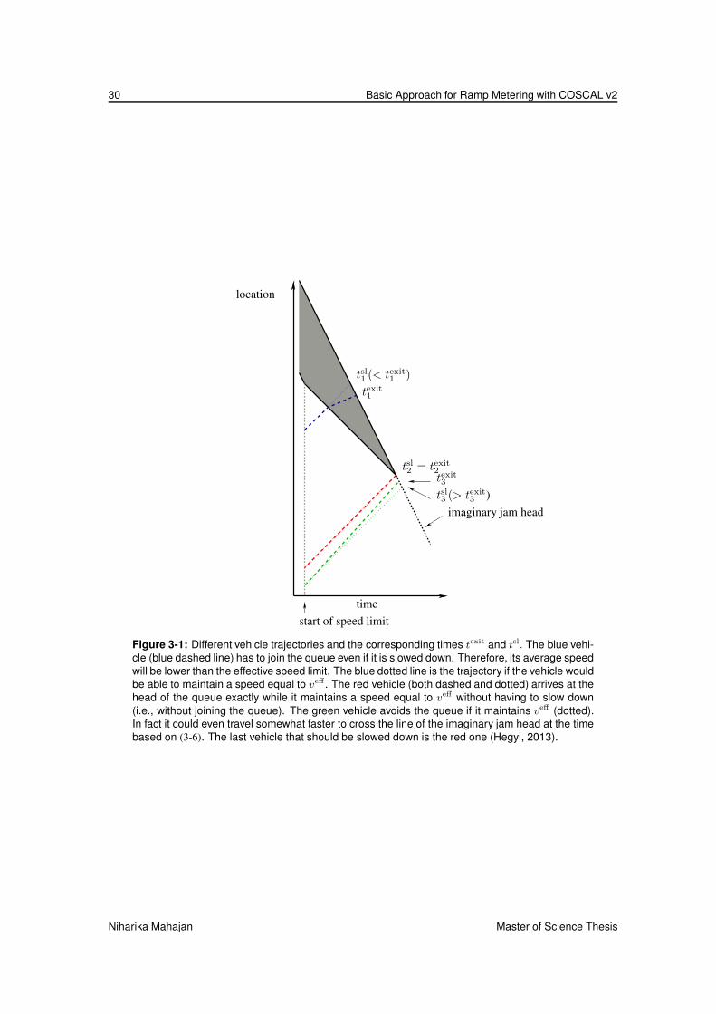
30 Basic Approach for Ramp Metering with COSCAL v2
tsl1 (< texit
1 )
texit1
time
tsl2 = texit
2
tsl3 (> texit
3 )
texit3
location
imaginary jam head
start of speed limit
Figure 3-1: Different vehicle trajectories and the corresponding times texit and tsl. The blue vehi-
cle (blue dashed line) has to join the queue even if it is slowed down. Therefore, its average speed
will be lower than the effective speed limit. The blue dotted line is the trajectory if the vehicle would
be able to maintain a speed equal to veff . The red vehicle (both dashed and dotted) arrives at the
head of the queue exactly while it maintains a speed equal to veff without having to slow down
(i.e., without joining the queue). The green vehicle avoids the queue if it maintains veff (dotted).
In fact it could even travel somewhat faster to cross the line of the imaginary jam head at the time
based on (3-6). The last vehicle that should be slowed down is the red one (Hegyi, 2013).
Niharika Mahajan Master of Science Thesis

3-4 TASK 2: Initial speed limitation and jam resolution 31
such as the blue vehicle in Figure 3-1. For the vehicle that joins the queue at the moment that the queue is
being resolved (red vehicle in Figure 3-1), it holds that
texitiveh(k) = tsl
iveh (k) , (3-9)
and for the vehicles that will not join the queue anymore (green vehicle), it holds that
texitiveh (k) < tsl
iveh(k) (3-10)
Using this, the last vehicle that should be slowed down in order to resolve the jam, is the first (counting
from i = 1, 2, . . . ) for which holds that
texitiveh (k) ≤ tsl
iveh(k) (3-11)
In this case, this is the red vehicle.
Now, since detection segments are the fundamental units of the measurements, (3-11) is evaluated for each
detection segment, using the upstream end xu,det of the segment as the location of the most upstream
vehicle in that segment. If inequality 3-11 holds for the upstream end of a certain detector segment, then
the gantry that is at the same location or just upstream of it, is the most upstream one that is needed for jam
resolution.
So, for the evaluation of the time tsliveh (k) in (3-7), the vehicle location xiveh (k) is replaced by the location
of the upstream end xu,detidet of the detector segment idet. For the evaluation of the time texit
iveh(k) in (3-6) the
number of vehicles between the jam head and the upstream end of the detection segment under considera-
tion is determined based on the densities of the segments between the jam head and the current detection
segment:
Nidet (k) =
ijam-h∑
j=idet
Ljλjρj(k) (3-12)
where ijam-h is the detector index of the detector segment containing the jam head, and Lj , ρj(k), λj are
respectively the link length, the density, and the number of lanes of segment j. If ijam-h is the detector
segment index of the jam head and if idet is the first detector index for which (3-11) holds (the first when
going from downstream into the upstream direction), then the speed limits will be activated on the actuation
segments that include detection segments idet, . . . , ijam-h. The range of actuation segments goes from
iact, . . . , jact, where xd,actiact > xu,det
idet ≥ xu,actiact and xd,act
jact ≥ xd,detijam-h > xu,act
jact . Important to note is that the
data from a given time step, k is used for activation in the following time step, k + 1.
Equation (3-11) can then be rewritten as:
texitidet (k) ≤ tsl
idet (k) (3-13)
where,
texitidet (k) =
Nidet (k)
qjam-h, (3-14)
tslidet (k) =
xjam-h(k) − xu,detidet
−vjam-h + veff(3-15)
3-4-2 Initial speed limitation for jam resolution - variable speed limits andramp metering
If the last vehicle that must be slowed down to resolve the jam crosses an on-ramp location xramp, equa-
tion (3-13) must be adapted for ramp flows. For roadside control, this corresponds to a case when the most
Master of Science Thesis Niharika Mahajan

32 Basic Approach for Ramp Metering with COSCAL v2
clock-start
start of speed-limits
and ramp metering current time step
0 kstartT kT
0tdelay(kstart)
trampjam−t(k
start)
trampjam−h(kstart)
0
trampidet (k)
trampjam−t(k)
trampjam−h(k)
Figure 3-2: Schematization of the time variables for a possible case, where the jam is resolved
upstream of the on-ramp and the on-ramp delay elapses before the jam-tail crossing (such that
the R-tail line would pass the on-ramp after the jam-head). The times in black are associated to
the jam, in blue to the on-ramp and the one in green to an individual vehicle.
upstream segment used for resolving the jam is upstream of the on-ramp segment, including the detection
segment iramp that contains the on-ramp and satisfies xu,detidet < xramp ≤ xd,det
idet . In the absence of such
modification, the vehicles from the on-ramp entering the jam before the last vehicle on the detector segment
that satisfies equation (3-13) are not included. This leads to an underestimation of texitidet (k), and hence the
vehicles speed-limited would not be sufficient to resolve the jam.
Therefore, theory is developed to determine the additional ramp vehicles that enter the jam before its
resolution. An iterative approach has been adopted for this. At each time step, iterations are performed in
space - moving upstream from the first detection segment where a jam is detected. For ease of execution
and understanding, the spatial iterations are identified within three broad cases, as illustrated in Figure 3-4.
These cases differ in how merging flows influence jam resolution. For better clarity, the variables used for
the important time intervals, estimated either relative to the start of the control scheme or the current time
step, are plotted in Figure 3-2.
3-4-2-1 Assumptions for merging flow during jam resolution
• The on-ramp flows merging onto the freeaway can take known constant values - qramp, qmetered or
qcongested. Here, qramp equals the on-ramp demand and occurs when RM is switched off; qmetered is
the metered flow when RM is active; qcongested is the ramp flow realized when vehicles merge into a
congested state on the freeway.
• The RM starts simultaneously with the VSL scheme at time kstartT , when a jam is detected down-
stream of the on-ramp.
• There is a considerable delay between the time when the RM is turned on and the time when the
metered flow enters the freeway merging area. This delay is because of the vehicles on the merging
lane (between the stop line of the ramp signal and the entry point on the freeway) when RM starts.
These vehicles must clear before the RM flow can enter the freeway.
The length of the merging segment is taken as xr and the average speed on the merging segment as
v̄r. The total delay from the start of the scheme is given by the extreme situation of a vehicle crossing
the stop line just before the RM is switched on. The time it takes this vehicle to enter the freeway
gives an estimate of the total delay tdelay(kstart):
Niharika Mahajan Master of Science Thesis

3-4 TASK 2: Initial speed limitation and jam resolution 33
tdelay(kstart) =xr
v̄r(3-16)
Therefore, demand flow qramp merges into the freeway from the start of the scheme for a time interval
of tdelay(kstart). The delay remainder at a time instant kT , later than the start of the control scheme
at kstartT , is given by:
tdelay(k) = max(tdelay(kstart) − (k − kstart)T , 0) (3-17)
• After the elapse of tdelay(k), until the tail of the jam crosses the on-ramp, qmetered flow enters the
freeway. The time beyond the current time that it takes the tail of the jam to cross the ramp is denoted
as trampjam−t(k). The calculation of this time is detailed in (3-36).
• If the tail of the jam crosses the on-ramp before tdelay(k) expires, qramp flow merges until the
trampjam−t(k) and metered flow qmetered is not observed. This is because the crossing jam results in a
merging flow qcongested after the jam tail crosses.
• Finally, during the time the freeway is in congested state, i.e between the time the tail and the head of
the jam pass the on-ramp, the flow equals qcongested. In reality, this can cause queueing on the ramp
resulting in a reduced merging even if RM is active. It is thus assumed that qcongested ≤ qmetered.The time, tramp
jam−h(k), it takes from the current time instant for the jam head to pass the ramp location
can be calculated using the jam head velocity:
trampjam−h(k) =
xd,detijam-h (k) − xramp
−vjam(3-18)
• After the head of the jam crosses the on-ramp, the on-ramp flow merges into the free-flowing freeway
traffic downstream of the jam head (state [5A]). The merging mechanism here does not influence jam
resolution and hence,RM flows need not be accounted for.
3-4-2-2 Calculation of merging flow from on-ramp
We have discussed so far that the on-ramp flow is time dependent and may change during the jam resolution
task. At any given time, the effective accumulation between the jam head and the most upstream jam
resolving segment, given by N effidet (k), is equal to or greater than the actual accumulation Nidet (k) over
these segments. This is considered by calculating the additional merging vehicles that would cross the
head of the jam, Nmergeidet (k), between the current time step till the time the jam is resolved.
N effidet(k) = Nidet(k) + Nmerge
idet (k) (3-19)
where,
Nidet(k) =
ijam-h(k)∑
j=idet(k)
Ljλjρj(k) (3-20)
The estimate of Nmergeidet (k) depends on one, the on-ramp flow profile, second, the time that the jam arrives
at the on-ramp and thirdly, the time it takes for the most upstream speed-limited vehicle used in jam
Master of Science Thesis Niharika Mahajan
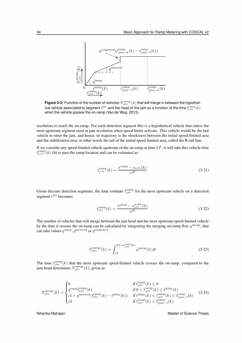
34 Basic Approach for Ramp Metering with COSCAL v2
0
Nm
erg
eid
et
(k)
tdelay(k)trampidet (k)
trampjam−t(k) tramp
jam−h(k)
qmetered
qramp
qcongested(trampjam−h(k) − tramp
jam−t(k))
Figure 3-3: Function of the number of vehicles Nmerge
idet (k) that will merge in between the hypothet-
ical vehicle associated to segment idet and the head of the jam as a function of the time tramp
idet (k)when the vehicle passes the on-ramp (Van de Weg, 2013).
resolution to reach the on-ramp. For each detection segment this is a hypothetical vehicle that enters the
most upstream segment used in jam resolution when speed limits activate. This vehicle would be the last
vehicle to enter the jam, and hence, its trajectory is the shockwave between the initial speed-limited area
and the stabilization area, in other words the tail of the initial speed-limited area, called the R-tail line.
If we consider any speed-limited vehicle upstream of the on-ramp at time kT , it will take this vehicle time
trampiveh (k) (h) to pass the ramp location and can be estimated as:
trampiveh (k) =
xramp − xiveh (k)
veff(3-21)
Given discrete detection segments, the time estimate trampidet for the most upstream vehicle on a detection
segment idet becomes:
trampidet (k) =
xramp − xu,detidet (k)
veff(3-22)
The number of vehicles that will merge between the jam head and the most upstream speed-limited vehicle
by the time it crosses the on-ramp can be calculated by integrating the merging on-ramp flow qmerge, that
can take values qramp, qmetered or qcongested.
Nmergeidet (k) =
∫ kT +tramp
idet(k)
kT
qmerge(t) dt (3-23)
The time trampidet (k) that the most upstream speed-limited vehicle crosses the on-ramp, compared to the
jam-head determines Nmergeidet (k), given as:
Nmergeidet (k) =
0 if trampidet (k) ≤ 0
qramptrampidet (k) if 0 < tramp
idet (k) ≤ tdelay(k)
c1 + qmetered(trampidet (k) − tdelay(k)) if tdelay(k) < tramp
idet (k) ≤ trampjam−t(k)
c2 if trampidet (k) > tramp
jam−t(k)
(3-24)
Niharika Mahajan Master of Science Thesis

3-4 TASK 2: Initial speed limitation and jam resolution 35
where,
c1 = qramptdelay(k) (3-25)
c2 = c1 + qmetered max(
trampjam−t(k) − tdelay(k), 0
)
+ qcongested(trampjam−h(k) − tramp
jam−t(k)) (3-26)
The constant value for Nmergeidet after the jam tail crosses the on-ramp is a simplification. Once the tail of
the jam has crossed the on-ramp, the jam can only be resolved upstream of the ramp. In other words, no
vehicle that crosses the on-ramp in congestion can resolve it. Since, the vehicles merging after the head
of the jam crosses the ramp do not affect jam propagation, the constant accounts for the total number of
vehicles merging until trampjam−h(k).
Now, the predicted number for the vehicles merging between the jam head and the most upstream jam
resolving vehicle, Nmergeidet (k) can be substituted in equation (3-19) to adapt equation (3-13), which now
becomes:
texitidet (k) ≤ tsl
idet (k) (3-27)
where,
texitidet (k) =
N effidet (k)
qjam-h, (3-28)
tslidet (k) =
xjam-h(k) − xu,detidet
−vjam-h + veff(3-29)
3-4-2-3 Guiding cases and the iterative control approach
The different jam resolving scenarios that may occur when a jam is detected downstream of the ramp can
be identified within three broad cases, as illustrated in Figure 3-4. These cases should guide the control
scheme - the determination of Nmerge, and the choice of qmetered for more efficient integration of RM with
VSL. Two critical cases are used to identify the applicable situation. In essence, the classification is based
on whether the jam can be resolved downstream of the on-ramp or not, and if the last jam resolving vehicle
is downstream or otherwise.
An understanding of the cases also explains the iterative approach; iterations are performed over detection
segments (in space) at every time step. The iterations are continued in time till the last jam resolving
segment is found.
At any given time kT , Nmergeidet (k) is determined for a detector segment idet, upstream of the segment
containing the jam head, i.e ijam-h. The time trampidet (k) it takes a hypothetical vehicle that enters idet when
speed limits are activated decides Nmergeidet (k) (refer Figure 3-3). Nmerge reflects in N eff and the condition
in equation (3-27) that must be satisfied by the most upstream jam resolving segment. This iterations start
at detector segment ijam-h − 1; if the condition is not met here, the next upstream segment is checked
similarly till the condition holds for some detection segment. If no detector segment (within the length of
actuation infrastructure) satisfies the condition, the jam is considered as unresolvable. This is discussed in
more detail in Section 3-7. The guiding cases are detailed next:
• Case a: When a jam is detected downstream of the on-ramp, the iterations begin by assuming Case
a. This scenario occurs when the detected jam can be resolved by a detection segment downstream
of the on-ramp (more specifically, the vehicle that enters this detection segment just when the speed
limits are activated). The ramp flows do not impact the jam resolution area in this case and hence,
Master of Science Thesis Niharika Mahajan
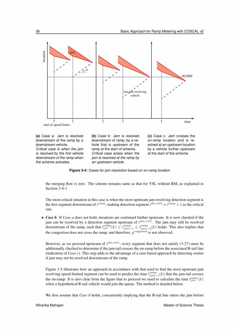
36 Basic Approach for Ramp Metering with COSCAL v2
time
loca
tio
n jam
on-ramp
veff
last jam resolving
vehicle
start of speed limits
(a) Case a: Jam is resolved
downstream of the ramp by a
downstream vehicle.
Critical case is when the jam
is resolved by the first vehicle
downstream of the ramp when
the scheme activates.
(b) Case b: Jam is resolved
downstream of ramp, by a ve-
hicle that is upstream of the
ramp at the start of scheme.
Critical case arises when the
jam is resolved at the ramp by
an upstream vehicle.
(c) Case c: Jam crosses the
on-ramp location and is re-
solved at an upstream location
by a vehicle further upstream
at the start of the scheme.
Figure 3-4: Cases for jam resolution based on on-ramp location
the merging flow is zero. The scheme remains same as that for VSL without RM, as explained in
Section 3-4-1
The most critical situation in this case is when the most upstream jam resolving detection segment is
the first segment downstream of iramp, making detection segment idet,crit1 = iramp + 1 as the critical
one.
• Case b: If Case a does not hold, iterations are continued further upstream. It is now checked if the
jam can be resolved by a detection segment upstream of idet,crit1. The jam may still be resolved
downstream of the ramp, such that trampidet (k) ≤ tramp
jam−t ≤ trampjam−h(k) holds. This also implies that
the congestion does not cross the ramp, and therefore, qcongested is not observed.
However, as we proceed upstream of idet,crit1, every segment that does not satisfy (3-27) must be
additionally checked to determine if the jam-tail crosses the on-ramp before the associated R-tail line
(indication of Case c). This step adds to the advantage of a case-based approach by detecting sooner
if jam may not be resolved downstream of the ramp.
Figure 3-5 illustrates how an approach in accordance with that used to find the most upstream jam
resolving speed-limited segment can be used to predict the time trampjam−t(k) that the jam-tail crosses
the on-ramp. It is also clear from the figure that to proceed we need to calculate the time tenteridet (k)
when a hypothetical R-tail vehicle would join the queue. The method is detailed below.
We first assume that Case b holds, concurrently implying that the R-tail line enters the jam before
Niharika Mahajan Master of Science Thesis

3-4 TASK 2: Initial speed limitation and jam resolution 37
location
time
start of speed-limits(k)
on-ramp
idet
idet+2
idet+4
iramp
ijam-h
veff
vjam
Nmerge(k)
tramp1
(< tenter1 )
tramp2
(= tenter2 )
tramp3
(> tenter3 )
texit1
texit2
texit3
(over-estimated)
tenter1
tenter2
tenter3
(under-estimated)
Figure 3-5: Illustration of the approach used for jam-tail detection. The thin dotted horizontal
lines represent the detector locations. The jam evolution appears in red and the trajectories of the
vehicles entering the detection segment just when the speed-limits are activated in green.
the jam tail reaches the on-ramp. The N effidet estimate under this assumption is used to first calculate
a make-do estimate of texitidet . To estimate tenter
idet (k) we use the average velocity of vehicles in the jam
vjam. This velocity can be calculated off-line from historical data, avoiding the estimation of flow
and density inside and downstream of the jam.
For any speed-limited vehicle that joins the queue its trajectory comprises of two parts; it travels
under free flow with veff till it enters the queue, and under queue condition with a speed vjam after,
until it exits the queue. Thus, the intersection of the R-tail line and a line at vjam slope gives the time
that the associated vehicle enters the jam.
Master of Science Thesis Niharika Mahajan

38 Basic Approach for Ramp Metering with COSCAL v2
The two parts of the trajectory then give:
xenteridet (k) = xexit
idet(k) + vjam(tenteridet (k) − texit
idet (k)) (3-30)
where xexitidet(k) is known from the evolution of the jam head,
xexitidet(k) = xd,det
ijam-h (k) + vjam-htexitidet (k) (3-31)
and
xenteridet (k) = xu,det
idet (k) + vefftenteridet (k) (3-32)
Eliminating xenteridet results in:
tenteridet (k) =
xd,detijam-h (k) − xu,det
idet (k)
veff − vjam+
vjam-h − veff
veff − vjamtexitidet (k) (3-33)
Finally, substituting equation (3-14) gives:
tenteridet (k) =
veff − vjam-h
veff − vjamtslidet(k) +
vjam-h − veff
veff − vjamtexitidet (k) (3-34)
With the prescribed approach, trampjam−t can be calculated from the first detector segment for which the
following condition holds:
trampidet (k) ≥ tenter
idet (k) (3-35)
This implies that the vehicle has crossed the on-ramp in congestion and the time the tail crosses the
on-ramp can then be given as:
trampjam−t(k) = min
idet
{
trampidet (k)|tramp
idet (k) ≥ tenteridet (k)
}
(3-36)
In performing the two checks iteratively, we will either detect a jam resolving segment or find the
time the tail of the jam crosses the on-ramp. The latter is an indication that Case c holds.
The critical situation occurs when the jam is resolved exactly at the on-ramp location xramp. The
corresponding detector segment idet,crit2 that resolves the jam would be further upstream. idet,crit2
is determined by tracking the trajectory of the speed-limited vehicle that crosses the on-ramp at the
same time as the jam head. Then, the time it takes for the jam head in the current time step to reach
the on-ramp will be equal to the time it takes this vehicle to reach the on-ramp. The location of the
last speed limited vehicle xiveh , at the current time step can be found:
xramp − xiveh
veff=
xd,detijam-h (k) − xramp
−vjam-h, (3-37)
and thus
xiveh = xramp + veff xd,detijam-h (k) − xramp
vjam-h. (3-38)
The critical detector segment idet,crit2 then will satisfy xu,detidet,crit2 (k) ≥ xiveh < xd,det
idet,crit2 (k).
Niharika Mahajan Master of Science Thesis
3-5 TASK 3: Speed limitation for stabilization 39
• Case c: In this case, the jam crosses the on-ramp and is therefore resolved upstream of the on-ramp
by a detection segment upstream of idet,crit2. Here, for the most upstream jam resolving vehicle
trampidet (k) > tramp
jam−h(k) holds and all three flows qramp, qmetered and qcongested may be observed.
From the iterative approach used, if Case c holds, the time trampjam−t will already be known. However,
in this case the starting assumption that the most upstream jam-resolving vehicle crosses the on-ramp
before the jam tail does not hold, and so we have wrongly calculated Nmergeidet using qmetered instead
of qcongested. Since qcongested < qmetered, Nmergeidet and hence, texit
idet are over-estimated. In doing so,
tenteridet is under-estimated as can be understood from Figure 3-5. Because for a vehicle crossing the
on-ramp in jam tenteridet ≤ tramp
idet should hold, the under-estimation would still satisfy the condition in
equation (3-36). Therefore, when trampjam−t is known, the assumption is relaxed to recalculate Nmerge
idet
as the constant c2 in equation (3-26).
With the correct estimate of Nmergeidet and hence, N eff
idet , the iterations are continued upstream to check
equation (3-27) in order to find the most upstream jam resolving segment.
3-5 TASK 3: Speed limitation for stabilization
The goal of this task is to achieve a desired efficiency (that ensures traffic flow stability) of the flow leaving
the stabilization area after the jam is resolved. For this, vehicles upstream of those used for resolving the
jam are also speed-limited. These vehicles are controlled towards a target density ρ̄ in addition to their
target speed veff . This target density should be higher than the free flow density but low enough to ensure
stable traffic flow at veff speed. A high density in this stabilisation area accumulates vehicles, and allows
recovery to a traffic state with flow higher than the queue discharge flow. It is from this mechanism that an
improvement in efficiency is achieved.
Since the aim is to maximize efficiency, the target density is chosen to ensure maximum stable flow in
the stabilization area. This implies that when extra ramp flows enter, the traffic flow becomes metastable,
and is prone to a traffic breakdown at the on-ramp section. Therefore, both the task must be adapted for
integration with RM. First, the VSL only strategy will be presented in Section 3-5-1. This is extended to
include ramp flows in the subsequent Section 3-5-2
3-5-1 Speed limitation for stabilization - variable speed limits only
In the SPECIALIST algorithm, the target density was on the average achieved by determining the fixed
slope (in the time-space plane) of the front between the upstream free-flow area and the stabilizing region
under the speed limits. The slope was determined by shock wave theory, based on a single measurement of
the traffic state upstream of the jam and on the pre-defined state (speed and density) of the stabilization area
under the speed limits. Using a single measurement was sufficient for the feed-forward algorithm, however,
COSCAL v2 has a feedback structure, and therefore the slope is not fixed anymore, and is adjusted based
on the updated measurements every time step.
In the COSCAL v1 algorithm, S-tail lines were used to determine the target trajectory for each individual
vehicle. Each vehicle was slowed down at the right moment based on its S-tail line and its speed and
deceleration characteristics. Since for COSCAL v2 a basic assumption is that the penetration rate is low,
there are many vehicles of which the deceleration will be controlled by roadside speed limit gantries instead
of the S-tail lines. Therefore, their location and start time of the deceleration cannot be controlled at such
a detail.
The approach is based on the location of the region where vehicles will accumulate if the speed at a speed
limit gantry is reduced. The basic idea is to extend the speed-limited area in the upstream direction until
the target density is reached in the accumulation region. However, in some cases the upstream traffic may
Master of Science Thesis Niharika Mahajan
40 Basic Approach for Ramp Metering with COSCAL v2
have such a low flow that the tail of the speed-limited stretch can (and thus should) be shortened, without
exceeding the target density. This approach has a homogenizing effect on the density in the stabilization
area.
The stabilisation area is demarcated by the R-tail or S-head shockwave on the downstream end depending if
the jam has been resolved, and the S-tail line on the upstream side. The downstream end of the stabilization
area is at the upstream end of the jam resolving area, called the R-tail line, if the jam has not been resolved
yet, or at the S-head line (defined in Section 3-6) once the jam is resolved. The R-tail line represents the
most upstream vehicle that was ever used to resolve the jam. Due to the feedback structure, this vehicle may
change over time. Therefore, it is the line that goes through the point of time step k and location xu,actiact (k),
where segment iact is the most upstream actuation segment used for jam resolution in the current time
step. The index of the detector segment that the R-tail line crosses in the next time step can be given as
iR-t(k + 1). The slope of the R-tail line equals the speed veff of the speed-limited vehicles. The R-tail
line is retained until the jam is resolved, unless at some moment a new R-tail line follows from the most
upstream resolving actuation segment, that is more upstream than the current R-tail line. In that case, the
new R-tail line is used in the subsequent steps.
So, let us denote the detection segment index that contains the R-tail or S-head line, by id,det, such that
xu,detid,det < xS-line,ds(k + 1) ≤ xd,det
id,det , where xS-line,ds(k + 1) denotes the location of the R-tail or S-head
line in the current time step (whichever will be active then).
The estimation of the most upstream segment in the stabilization area, idet will be explained using Fig-
ure 3-6. If a vehicle passes the speed limit gantry exactly when the speed limit becomes activated, it should
create the density ρ̄ (veh/km/lane) required for stabilization when it has reached its target speed veff . In
the figure the black dash-dotted line represents the vehicle trajectory and the blue dashed line its target
trajectory. If the speed limit gantry is actuated later, then the vehicle will slow down later, and it will create
a higher density. If the gantry is activated earlier, then the target density may not be reached.
Let us denote the number of vehicles between the R-tail line (or S-head, if that is active) and an upstream
stabilisation segment by N and the distance between the target trajectory line and xS-line,ds(k) by ∆x, and
let denote the time and distance that the vehicle needs to decelerate by tdec (h) and xdec respectively (where
tdec = (veff − videt )/adec, and xdec = tdec(veff + videt )/2 and adec (km/h2) is the nominal deceleration
rate). Now for every detection segment idet = id,det, id,det − 1, . . . the following expression is evaluated:
N
∆x≤ ρ̄ , (3-39)
where
N =
id,det∑
i=idet
ρi(k)λiLi , (3-40)
∆x =
id,det∑
i=idet
Li − (xdec − tdecveff) (3-41)
If expression (3-39) does not hold, then the density is too high and the next upstream detector segment
has to be evaluated. If the expression holds then the first detection segment for which it holds is the most
upstream detection segment that needs speed limits (first in the direction from downstream to upstream),
and this part of the procedure can stop.
In an idealized situation the above procedure would lead to a homogeneous density in the stabilization area,
but in practice the area may become inhomogeneous over time, due to differences in the individual vehicle
speeds. If this inhomogeneity means that at the tail of the stabilization area the density is close to or above
the critical value, then the upstream speed limits should be extended at a faster rate to prevent too high
densities there, even if the average density in the complete stabilization area is below ρ̄. For this reason, the
above procedure is repeated starting at all detector segment locations in the current stabilization area plus
a (negative) offset dstab (km) in the upstream direction. This offset helps to prevent too high densities just
Niharika Mahajan Master of Science Thesis

3-5 TASK 3: Speed limitation for stabilization 41
target trajectory
vehicle trajectory
R−tail line
veff
k+1
time
tdec
xdec
location
gantry i+3
gantry i+1
gantry i
gantry i+4
gantry i+5
detector segments
dx
gantry i+2
k
N
Figure 3-6: Illustration of the stabilization approach. The thick solid horizontal lines represent the
gantry locations, the thin dotted lines the detector locations. In the red areas the speed limits are
active for jam resolution, in the yellow areas for stabilization (Hegyi, 2013).
Master of Science Thesis Niharika Mahajan

42 Basic Approach for Ramp Metering with COSCAL v2
S-head line (ds)
R-tail line
Location
Time
Flow
Density
Jam(J)
Speed limitation
to resolve jam (R)
Speed limitation
for stabilization (S)
[4A]
[4B]
[4C]
[5A]
[5B]
[5C]
[1DS]
[1US]
free flowbranch
[5A]=[5B]
[5C]
[1DS]
[1US][4A]
[4B]
[4C]
veff
ρmin ρ̄[4A] ρmax
Figure 3-7: The left figure shows the different states that are achieved when speed limiting ve-
hicles for stability. The right figure shows the corresponding states in the fundamental diagrams.
Traffic in areas 1US and 1DS is traveling in free flow respectively upstream and downstream of
the on-ramp. Vehicles in areas 4A, 4B, and 4C are speed limited for stabilization. The target
densities are different in these areas and depend on the flows that have to be realised in areas
5A and 5B, and are controlled with the slope of the S-head lines. The dashed lines in the fun-
damental diagram represent the shockwaves between the different states (adapted from Van de
Weg (2013)).
upstream of the speed-limited area. For all starting locations the detection segment is determined that needs
speed limits. The overall detection segment that needs speed limits will be the most upstream one among
these. The speed limits that will be activated for stabilization, will correspond to the actuation segments
that include the detection segments from the most upstream one that needs speed limits to id,det.
3-5-2 Speed limitation for stabilization - variable speed limits with rampmetering
The approach that has just been presented to realize stable traffic has to be extended when the moving jam
is propagating near an on-ramp. The difference with the approach presented in the previous section is that
a different density must be achieved at different locations depending on the location of the on-ramp. This
section will calculate these different densities and in what situation they must be applied.
Figure 3-7 shows the different situations that a vehicle which is speed-limited for stabilization can en-
counter. These states are labelled as 4A, 4B, and 4C. The density in area 4A, downstream of the on-ramp
is equal to the design density for the stabilisation area, ρ̄ (veh/km/lane). ρ̄ is the maximum possible density
that ensures stability at velocity veff . Vehicles driving in area 4B and 4C, however, must maintain different
densities. First, it is explained what these densities must be, in Sections 3-5-2-1 and 3-5-2-2. This theory
is reproduced from the extension of COSCAL v1 with RM, by Van de Weg (2013). Following which it is
explained how these densities are imposed in the macroscopic formulation of COSCAL v2.
Niharika Mahajan Master of Science Thesis

3-5 TASK 3: Speed limitation for stabilization 43
3-5-2-1 Target density of vehicles in area 4B
Vehicles driving in area 4B are upstream of the on-ramp and should create extra space for traffic from the
on-ramp. These vehicles will be passing the on-ramp while they are speed-limited thus they should have
lower density to accommodate the on-ramp flow, such that downstream of the on-ramp the density is ρ̄ on
an average.
Note that the flow q[4A] (veh/h) downstream of the on-ramp in the stabilization area can be derived from
the density ρ̄[4A], assuming stationary traffic conditions:
q[4A] = ρ̄[4A]veff . (3-42)
The flow q[4B] (veh/h) upstream of the on-ramp in stabilization area 4B is then given by:
q[4B] = q[4A] − qmetered . (3-43)
The target density ρ̄[4B] (veh/km/lane) upstream of the on-ramp in the stabilization area 4B is given by:
ρ̄[4B] =q[4A] − qmetered
veff(3-44)
= ρ̄[4A] −qmetered
veff(3-45)
3-5-2-2 Target density of vehicles in area 4C
Now that the density in area 4B has been determined, the target density ρ̄[4C] (km) in area 4C can be
determined. The goal of realizing this headway distance in area 4C is to stabilize traffic. Note that the
the flow q[5C] (veh/h) in area 5C is realized by releasing vehicles from the speed limits from area 4C.
Therefore, the flow in area 5C is higher or equal to the flow in area 4C:
q[5C] ≥ q[4C] . (3-46)
Furthermore, the flow q[5B] (veh/h) in area 5B is equal to the flow in area 5C plus the on-ramp flow:
q[5C] + qmetered = q[5B] , (3-47)
thus, it holds that:
q[5B] ≥ q[5C] ≥ q[4C] . (3-48)
This implies that realizing a stable flow in area 5B means that the flow in area 5C and 4C will be stable as
well. Choosing the flow q[5B] equal to the flow q[5A] in area 5A will result in stable traffic in area 5B as
well. The reason for this is that the S-head line has been tuned to realize a stable flow in area 5A. Note that
this only holds when the speed in area 5A equals the speed in area 5B, which is a reasonable assumption
since the flows are equal. The flow q[5A] is computed using shock wave theory with the speed v[4A-5A]
(km/h) of the S-head line downstream of the on-ramp, between areas 5A and 5B, the free-flow speed vff
(km/h) of vehicles in area 5A. The speed of the S-head line is given by:
v[4A-5A] =q[5A] − q[4A]
ρ[5A] − ρ̄[4A], (3-49)
v[4A-5A] =q[5A] − ρ̄[4A]veff
q[5A]
vff− ρ̄[4A]
, (3-50)
Master of Science Thesis Niharika Mahajan

44 Basic Approach for Ramp Metering with COSCAL v2
this can be rewritten to give the flow q[5A]:
q[5A] = ρ̄[4A]vff v[4A-5A] − veff
v[4A-5A] − vff. (3-51)
Now choosing the flow q[5B] in area 5B equal to the flow q[5A] in area 5A will result in stable traffic.
From the flow q[5B] in area 5B the flow q[5C] in area 5C can be determined:
q[5C] = q[5B] − qmetered . (3-52)
The flow q[5C] is realized by traffic that has driven from area 1US through area 4C to area 5C. By tuning
the density in area 4C and the speed v[4C-5C] (km/h) of the S-head line between areas 4C and 5C the flow
q[5C] is realized. Using shock wave theory, the speed v[4C-5C] of the S-head line upstream of the on-ramp
can be given as:
v[4C-5C] =q[5C] − ρ̄[4C]veff
q[5C]/v[5C] − ρ̄[4C](3-53)
Thus, the speed v[4C-5C] can be expressed as a function of the density ρ̄[4C].
How is the density ρ̄[4C] chosen? Consider the fundamental diagram on the right of Figure 3-7. This figure
shows, among other things, the states of areas 1US, 5C, and 4C. The slope of the line connecting states
5C and 4C in this figure has speed v[4C-5C] (km/h). The slope of the line connecting states 1US and 4Chas speed v[4C-1US] (km/h) which is given by:
v[4C-1US] =ρ̄[4C]veff − q[1US]
ρ̄[4C] − ρ[1US]. (3-54)
Hence, by tuning the density ρ̄[4C], the slopes of these two lines can be changed. Note that in Figure 3-7 a
minimum density ρmin and a maximum density ρmax have been indicated. The density in area 4C should
not be chosen lower than the minimum density which is given by:
ρmin = ρ[5C] . (3-55)
Additionally, the density ρ̄[4C] should not exceed the maximum density given by:
ρmax =q[5C]
veff(3-56)
These extreme densities ensure that the stabilisation area 4C is bound and not increasing in size over time.
So, when exceeding the maximum density, the S-head line will propagate downstream making the area in
the state grow larger in time; this is undesirable from the point of view of implementation. However, this
maximum density ρmax does not guarantee stable traffic. The density ρ̄[4A] in area 4A has been tuned to
realize stable traffic and exceeding this density can result in unstable traffic. Therefore, the density ρ̄[4C]
should be chosen in the following interval:
ρmin ≤ ρ̄[4C] ≤ max(
ρ̄[4A], ρmax)
(3-57)
Now that the bounds in which the density ρ̄[4C] can be chosen have been defined, the value of the den-
sity should be chosen. Note that the speed with which the stabilization area 4C is propagating upstream
Niharika Mahajan Master of Science Thesis
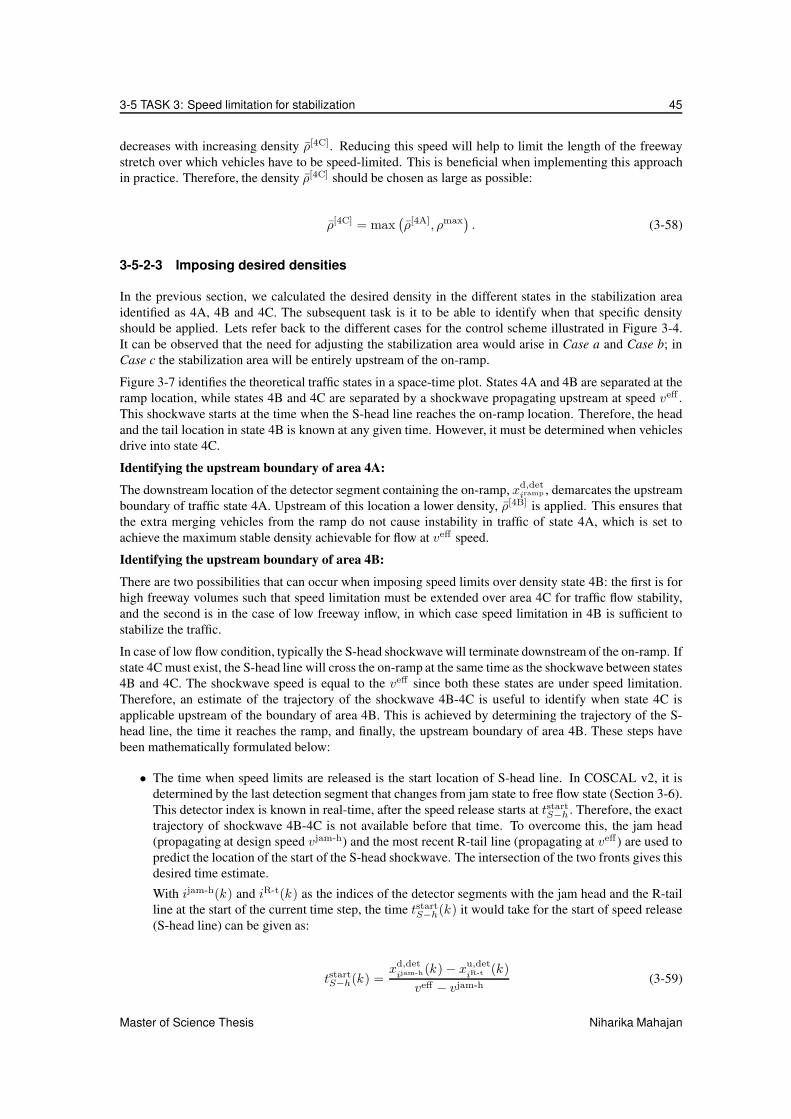
3-5 TASK 3: Speed limitation for stabilization 45
decreases with increasing density ρ̄[4C]. Reducing this speed will help to limit the length of the freeway
stretch over which vehicles have to be speed-limited. This is beneficial when implementing this approach
in practice. Therefore, the density ρ̄[4C] should be chosen as large as possible:
ρ̄[4C] = max(
ρ̄[4A], ρmax)
. (3-58)
3-5-2-3 Imposing desired densities
In the previous section, we calculated the desired density in the different states in the stabilization area
identified as 4A, 4B and 4C. The subsequent task is it to be able to identify when that specific density
should be applied. Lets refer back to the different cases for the control scheme illustrated in Figure 3-4.
It can be observed that the need for adjusting the stabilization area would arise in Case a and Case b; in
Case c the stabilization area will be entirely upstream of the on-ramp.
Figure 3-7 identifies the theoretical traffic states in a space-time plot. States 4A and 4B are separated at the
ramp location, while states 4B and 4C are separated by a shockwave propagating upstream at speed veff .This shockwave starts at the time when the S-head line reaches the on-ramp location. Therefore, the head
and the tail location in state 4B is known at any given time. However, it must be determined when vehicles
drive into state 4C.
Identifying the upstream boundary of area 4A:
The downstream location of the detector segment containing the on-ramp, xd,detiramp , demarcates the upstream
boundary of traffic state 4A. Upstream of this location a lower density, ρ̄[4B] is applied. This ensures that
the extra merging vehicles from the ramp do not cause instability in traffic of state 4A, which is set to
achieve the maximum stable density achievable for flow at veff speed.
Identifying the upstream boundary of area 4B:
There are two possibilities that can occur when imposing speed limits over density state 4B: the first is for
high freeway volumes such that speed limitation must be extended over area 4C for traffic flow stability,
and the second is in the case of low freeway inflow, in which case speed limitation in 4B is sufficient to
stabilize the traffic.
In case of low flow condition, typically the S-head shockwave will terminate downstream of the on-ramp. If
state 4C must exist, the S-head line will cross the on-ramp at the same time as the shockwave between states
4B and 4C. The shockwave speed is equal to the veff since both these states are under speed limitation.
Therefore, an estimate of the trajectory of the shockwave 4B-4C is useful to identify when state 4C is
applicable upstream of the boundary of area 4B. This is achieved by determining the trajectory of the S-
head line, the time it reaches the ramp, and finally, the upstream boundary of area 4B. These steps have
been mathematically formulated below:
• The time when speed limits are released is the start location of S-head line. In COSCAL v2, it is
determined by the last detection segment that changes from jam state to free flow state (Section 3-6).
This detector index is known in real-time, after the speed release starts at tstartS−h . Therefore, the exact
trajectory of shockwave 4B-4C is not available before that time. To overcome this, the jam head
(propagating at design speed vjam-h) and the most recent R-tail line (propagating at veff) are used to
predict the location of the start of the S-head shockwave. The intersection of the two fronts gives this
desired time estimate.
With ijam-h(k) and iR-t(k) as the indices of the detector segments with the jam head and the R-tail
line at the start of the current time step, the time tstartS−h(k) it would take for the start of speed release
(S-head line) can be given as:
tstartS−h(k) =
xd,detijam-h (k) − xu,det
iR-t (k)
veff − vjam-h(3-59)
Master of Science Thesis Niharika Mahajan

46 Basic Approach for Ramp Metering with COSCAL v2
The location of the start of speed release then becomes:
xstartS−h(k) = xu,det
iR-t (k) + vefftstartS−h(k) (3-60)
This gives an interim estimate of the associated detector segment iS-h,start, where xu,det(iS-h,start) <xstart
S−h(k) ≤ xd,det(iS-h,start) holds. The estimate is replaced once the actual detector segment where
the jam is resolved is located.
• Under the assumption that the S-head line is not terminated before it crosses the on-ramp, the hypo-
thetical time trampS−h (k) is calculated to check if density 4C applies. The location of the start of S-head
line and its slope gives:
trampS−h (k) = tstart
S−h(k) +xstart
S−h(k) − xramp
−v[4A-5A]. (3-61)
• With the time when the S-head line reaches the on-ramp known, the equation of the shockwave 4B-
4C can be determined. In the event that state 4C occurs, it will necessarily be upstream of shockwave
4B-4C. Therefore, the location of the most upstream detector segment idet, that achieves an average
density ρ̄[4B] between iramp and idet, is of interest. If idet lies upstream of the estimated location of
the shockwave, x[4B-4C](k) at a given time, state 4C exists. Then, x[4B-4C](k) defines the boundary
of area 4B. To include the time it takes the first vehicle that arrives at idet when speed-limitation
starts to decelerate to veff speed, an additional deceleration time tdec and distance xdec are added.
The shockwave 4B-4C trajectory can be given as:
x[4B-4C](kT + tdec) = xramp − veff(
trampS−h (k) − tdec
)
(3-62)
Then, the condition to check for state 4C becomes xu,detidet + xdec < x[4B-4C](kT + tdec); if it holds
the x[4B-4C](kT ) defines the upstream boundary of state 4B, and target density in state 4C, ρ̄[4C]
must be applied upstream of it.
The assumption of S-head crossing the on-ramp does not affect the outcome if it terminates down-
stream of the ramp. In this case the above condition will not hold and ρ̄[4B] will be correctly applied.
The core principle used in estimating the most upstream detection segment idet of the stabilisation area
remains the same, given in equation (3-39). However, with three different densities in the stabilization
area, the scheme first checks for the most upstream stabilization state. Then the target density is applied
accordingly. To ensure that the appropriate density is applied idet is checked for the cases below:
ρ̄(k) =
ρ̄[4A] if xd,detiramp ≤ xu,det
idet (k) + xdec
ρ̄[4B] if x[4B-4C](kT + tdec) ≤ xu,detidet (k) + xdec < xd,det
iramp
ρ̄[4C] otherwise
(3-63)
This check ensures that density ρ̄[4A] is applied downstream of the ramp, ρ̄[4B] is applied between the on-
ramp and the extreme 4B-4C boundary, and ρ̄[4C] upstream of this boundary.
Finally, in addition to the choice of desired density based on the idet location, the downstream segment
id,det of the stabilization state in consideration also changes. Here, iS-line is the index of the detection seg-
ment containing the R-tail or S-head line depending on whether the jam has been resolved or not, respec-
tively. Further, i[4B-4C] is the detection segment containing the shockwave 4B-4C. The most downstream
segment of the most upstream stabilisation state is therefore given as:
Niharika Mahajan Master of Science Thesis

3-5 TASK 3: Speed limitation for stabilization 47
id,det =
iS-line if xd,detiramp ≤ xu,det
idet (k) + xdec
iramp if x[4B-4C](k + tdec) ≤ xu,detidet (k) + xdec < xd,det
iramp
i[4B-4C] otherwise
(3-64)
It is important to note that once a new upstream state is identified (state 4B or 4C), the density in the
downstream stabilisation states is no longer checked, and id,det is updated as per the above equation. N is
then accumulation in the most upstream stabilization state. It equals the total number of vehicles between
id,det and an upstream detection segment idet. The effective distance ∆x used to check for the appropriate
density therefore is the length of the freeway between id,det and idet. The conditionN
∆x≤ ρ̄ to find
the most upstream segment idet, given in equation (3-39), is adapted such that ρ̄(k) and id,det are now
determined using equations (3-63) and (3-64).
3-5-3 Correction for density errors in downstream stabilization states
When making a transition from state 4A to 4B or 4B to 4C, the actual density achieved in the downstream
state may not be equal the desired density. Therefore, when locating the most upstream segment of the most
upstream stabilization state, the actual density error in the downstream stabilization states is accounted for.
While a positive density error, where the actual density is higher than the desired density, is accommodated
by suitably increasing the stabilization area, a negative error would then mean reducing the freeway length
over which speed limits are applied. The latter can, however, cause a local spike in density leading to
a breakdown even if the average density in the complete stabilization area is below the desired value.
Therefore, only a negative density error will result in a correction.
We now discuss the procedure to adjust the upstream stabilisation area according to the achieved density in
downstream stabilisation areas, denoted by ρ[state,ds] compared to their desired values, ρ̄[state,ds]. Firstly, at
any given time instant, the spatial extent of the different stabilization states in the following time step must
be calculated. The effective length in each of the stabilization states at any given time, cumulated over all
lanes, is estimated based on the location of idet relative to the extreme location of the shockwaves 4A-4B
and 4B-4C. The lengths can be given as:
L[4A](k) =
iS-line∑
i=max(idet,iramp+1)
Liλi
L[4B](k) =
iramp∑
i=min(iramp+1,max(idet,i[4B-4C]+1))
Liλi
L[4C](k) =
i[4B-4C]∑
i=min(i[4B-4C]+1,idet)
Liλi
(3-65)
The compensation scheme is designed to provide as much surplus gaps in the most upstream state as
required for the number of surplus vehicles downstream. The extra number of vehicles are the difference
of the actual accumulation and that desirable to achieve the densities calculated in Section 3-5-2, over their
lengths of actuation calculated in the preceding equation (3-65). The surplus accumulation Nsur(k) can
then be given as below, where D is the set of all downstream stabilisation states:
Nsur(k) =∑
d∈D
max(ρ[state,ds] − ρ̄[state,ds], 0)L[state,ds](k) (3-66)
Master of Science Thesis Niharika Mahajan

48 Basic Approach for Ramp Metering with COSCAL v2
To ensure space for the surplus vehicles, the actual accumulation on a given freeway segment plus the
additionalNsur(k) vehicles, should meet the desired density. The governing condition to locate the most
upstream speed limited detector segmentN
∆x≤ ρ̄ then becomes:
N + Nsur
∆x≤ ρ̄[state,us] (3-67)
where
N =
id,det∑
idet
Liλi,
∆x =
id,det∑
idet
Li
3-6 TASK 4: Speed limit release
Since the speed in the stabilization area is constant and the density is more or less homogeneous, the speed
limits can be released along a straight line in the time-space plane, from downstream to upstream, similarly
to SPECIALIST and COSCAL v1. Let us call this line the S-head line. After releasing the speed limit along
the S-head line, the vehicles will accelerate to a free-flow state with a lower density than in the stabilization
area. The S-head line should begin at the point when and where the last vehicle in the jam leaves the jam
(corresponding to point D in the SPECIALIST scheme). In case of COSCAL v2 this is defined as the
head of the last detection segment that has changed from jam state to free flow state. The same S-head
line should apply for all vehicles in the stabilization area. The slope of the S-head line v[4A-5A] is a tuning
variable, and the more steep it is (more negative) the higher the resulting flow will be.
3-7 Resolvability of jam
Some jams cannot be resolved, and for these jams intervening with speed control measures is not mean-
ingful. For the COSCAL v2 algorithm a jam cannot be resolved when the most upstream vehicle that has
to be slowed down is physically outside (upstream) of the stretch that can be controlled by speed limits. In
such a case it makes no sense to reduce the speed of the other vehicles, because the jam will not be resolved
and the associated capacity drop will not be removed. Since the algorithm has a feedback structure, the
vehicle in question may vary, and consequently the resolvability of the jam may fluctuate when in one case
the resolving vehicle is within the speed-limited stretch, and in the other case it is not. This would mean
that the algorithm decides in one time step to set the speed limits, and in the next time step to remove
them. This is undesired, and therefore the initial tail location of the resolving actuation segments should be
such that it remains withing the physically available stretch, including the fluctuations. For this reason the
algorithm may only be activated if the initial tail location xu,actiact of the most upstream actuation segment
iact (including the lead-in) is downstream of the pre-defined location xact,min:
xu,actiact ≥ xact,min , (3-68)
where xact,min should be sufficiently downstream of the upstream end of the stretch equipped with dynamic
speed limits to make sure that all fluctuations remain within the controllable area.
Once the algorithm activated the speed limits, the threshold xact,min is ignored, in order to allow fluctua-
tions that are within the physically available space (but are possibly upstream of xact,min).
Niharika Mahajan Master of Science Thesis

3-8 Limiting the algorithm to a single jam 49
In addition, there is another case when the complete speed limit scheme will not fit on the physically
available stretch, namely when the stabilization area grows out (upstream) of the available area. In this
case the jam can be resolved, but the stability of the upstream traffic cannot be guaranteed. Since in this
case the jam can be resolved, and at least a temporal flow improvement can be achieved, one may decide to
accept the risk that a new jam will occur. However, if this type of breakdown has to be prevented xact,min
can be chosen even more downstream.
3-8 Limiting the algorithm to a single jam
In the development of the algorithm it is implicitly assumed that there is only one jam on the freeway.
However, in a real situation there may be more than one jam at the same time, and it could lead to unpre-
dictable behavior when the speed limits are active for one jam, but another jam requires speed limits at an
overlapping stretch. For this reason the algorithm is limited to activate for a single jam and will not try to
solve another jam until all speed limits are deactivated.
To achieve this, after a jam has been detected and the speed limits are activated to resolve it (i.e., the jam is
considered to be resolvable) the jam head is tracked until it has been resolved. The tracking of the jam head
ensures that the speed limits will be activated only due to this specific jam, and not to others that possibly
appear during operation. Furthermore, new jams are ignored until all speed limits have been released,
including the speed limits for traffic flow stabilization. This is necessary, because after the jam has been
resolved, there will be remaining active speed limits in the stabilization region. These speed limits should
not be disturbed by speed limits due to a new jam. Therefore, new jams are ignored until all speed limits
have been resolved.
The jam is tracked by tracking its head propagation over time. Since the jam head speed vjam-h is limited,
the jam head location from time step k to k + 1 may be between the two locations what can be expected
based on the minimum and maximum jam head propagation speed. This speed is assumed to be vjam-h,but due to measurement errors and the discretization of time and space, the measured jam head may prop-
agate somewhat slower or faster then vjam-h and therefore the fastest propagation speed is assumed to be
vjam-h,max (km/h), such that vjam-h,max < vjam-h (more negative), and the slowest jam head propagation
speed is assumed to be zero. If the jam head location in time step k was xjam-h(k), then for time step k +1the jam head is required to be at a segment between xjam-h(k) and xjam-h(k) + T vjam-h,max. The most
downstream segment that is in jam state and satisfies this condition, is taken as the new jam head.
Since the detection of a new jam should be postponed not only for the duration of an already existing jam,
but also for the duration of the release of the stabilizing speed limits after the jam has been resolved, the
following steps are taken:
• If there is a jam detected, but there was no jam in the previous time step and the speed limits were
not activated in the previous time step then the detected jam is a new jam and the speed limits may
be activated.
• If there is a jam detected, but there was no jam in the previous time step and the speed limits were
active in previous time step (for stabilization), then no jam location is passed to the rest of the
algorithm.
• If there is a jam detected, and there was a jam in the previous time step, the jam is tracked according
to the constraints above. If the same jam still exists in the current measurement then only this jam is
passed to the rest of the algorithm as jam location. Otherwise, the jam under consideration has been
resolved, and the currently measured jam is a new one, that should be ignored until all speed limits
are resolved.
• If no jam is detected, then the algorithm should either continue with the already active speed limits
(for stabilization) or do nothing, depending on the stabilization part of the algorithm.
Master of Science Thesis Niharika Mahajan

50 Basic Approach for Ramp Metering with COSCAL v2
3-9 Summary and Discussion
In this chapter, the COoperative Speed Control ALgorithm (COSCAL) v2 in Hegyi (2013) was extended
for integration with ramp metering (RM). The macroscopic algorithm uses VSL in four main tasks to
resolve a moving jam, and subsequently stabilize the traffic flow while it recovers from the capacity drop.
For the integration of RM and VSL strategy, two of these tasks, namely, (1) jam detection, and (2) speed-
limitation for stabilization were modified. The traffic theoretic principles used in the original algorithm
were utilized for this.
Jam detection task in COSCAL v2 uses instantaneous speed-limitation for flow reduction in order to resolve
a moving jam, whereby the inflow into the jam is reduced below the outflow at the jam-head. Hence, when
extra vehicles from the on-ramp enter onto the freeway, the spatio-temporal extent of speed-limitation
required for this task is under-estimated. In the modified algorithm, the excess vehicles from RM were
estimated to determine the freeway length necessary to be speed-limited for jam resolution.
In the stabilization task, vehicles upstream of the ones used for resolving the jam are speed-limited to
achieve a maximum flow efficiency (that ensures traffic flow stability) after the jam is resolved. Likewise,
ramp flows can disrupt the stabilization area where the traffic state is likely to become metastable. There-
fore, in order to prevent a traffic breakdown from the RM flow, the algorithm was adapted to determine
lower target densities for the speed-limited area upstream of the on-ramp. These densities are chosen and
implemented in a way that the flow arriving at the ramp section is appropriately reduced to accommodate
the additional ramp flow.
Most parameters used in the COSCAL v2 algorithm can be interpreted as a traffic flow variable or a physical
attribute of the infrastructure. For the extension of the VSL algorithm, a few additional parameters were
considered:
Ramp infrastructure related
• the location xramp of the on-ramp
• the merging length xr, and the average speed v̄r on the merging segment
RM strategy related
• the RM flow qmetered
• the ramp flow qcongested merging into freeway flow in congestion
Freeway traffic related
• the average speed vjam in moving jam state
• the average free-flow speed vff of vehicles in state [5A]
All of the above parameters, except RM flow qmetered can be tuned using off-line or on-line traffic data.
Based on the desirable characteristics for a ramp controller, the RM flow qmetered must be chosen to prevent
both, a queue spillback and underutilization of the on-ramp storage capacity. Additionally, a low RM rate
should theoretically improve the effectiveness of the VSL approach.
The above discussion highlights the caveat in the developed strategy. Even though the simple RM strategy
is suitable for field-implementation, it is not as sophisticated as reactive RM strategies. Moreover, it lacks
responsiveness to how queue on the on-ramp grows. If queue length constraint is indirectly considered by
selecting a high enough RM flow that ensures that the queue-length does not exceed a maximum value, it
will be the most restricting value. Hence, at the cost of the effectiveness of the VSL scheme.
Niharika Mahajan Master of Science Thesis

3-9 Summary and Discussion 51
In order to incorporate a more advanced RM strategy, which responds to the traffic state on the freeway
and queue length on the ramp, a more advanced adaptation for the VSL strategy is required. As opposed to
the macroscopic adaptation in this chapter, where density criteria for the speed-limited area is used to limit
the freeway flows arriving at the on-ramp section, an advanced strategy will require microscopic traffic
flow concepts to control freeway flows directly according to time-dependent RM flows. Accordingly, an
advanced RM and VSL strategy is developed in the next chapter.
Master of Science Thesis Niharika Mahajan

52 Basic Approach for Ramp Metering with COSCAL v2
Niharika Mahajan Master of Science Thesis

Chapter 4
Advanced Approach for Ramp
Metering with COSCAL v2
4-1 Introduction
In the previous sections, we first discussed the basic formulation of stand-alone speed control for road-side
implementation. Subsequently, this control approach was adapted for additional flow from an on-ramp
infrastructure, which may disrupt implementation of speed limits. The assumption of a constant outflow
from ramp metering (RM) was made for this extension. Lastly, a corrective feedback for realised densities
in the stabilization areas that are higher than their design values was incorporated.
In this section, an advanced RM strategy integrable with the speed control approach is presented. The
most important considerations for the RM strategy have been: responsiveness to limitation of storage space
on the on-ramp, and at the same time limitation on reducing main stream flow with the variable speed
limits (VSL) approach.
In a very rudimentary understanding , n fewer vehicles from the main traffic stream would allow n more to
merge from the on-ramp. This explains the trade-off between any measurable performance criteria - total
time spent (TTS) or waiting times between the two streams. On one hand, a lower metering rate means
higher waiting times for the on-ramp traffic, on the other hand, it improves the supply on the freeway and
its corresponding travel times. Hence, the design goal is to formulate and integrate a RM strategy that
maximizes the performance of the VSL strategy, while ensuring that at no time during the control scheme
the on-ramp queue spills over to the surface streets.
4-2 Assumptions and design parameters
4-2-1 Notations and notions
The notations for detection and actuation segments are in line with those used for the basic ramp meter-
ing strategy, detailed in Section 3-2-1. To simplify the theoretical explanation, three traffic streams are
identified as: (1) freeway main stream flow: qfw (2) on-ramp flow qrm and, (3) combined flow qcomb at the
on-ramp section. All traffic characteristics related to each of these traffic streams are denoted by a subscript
‘fw’, ‘rm or ‘r’ depending if the ramp flow is metered or not, and ‘comb’, respectively. Cumulative ve-
hicle curves - derived from plotting the number of vehicles that have crossed a specific location at a given
Master of Science Thesis Niharika Mahajan

54 Advanced Approach for Ramp Metering with COSCAL v2
time instant - are used extensively and follow the same labelling convention. Additionally, a ‘max’, ‘min’,
‘max,adm’ or ‘min,adm’ superscript specifies when the curve forms an admissible or limiting boundary
condition (detailed later in the chapter). In general, cumulative curves are calculated at the merged freeway
section, just downstream of the on-ramp.
4-2-2 Assumptions related to on-ramp flows
• A single lane on-ramp infrastructure is assumed for the ease of control formulation. The choice does
not have an impact on the formulation of the integrated strategy.
• The on-ramp demand qinr (k) (veh/h) is known over the time duration of speed control, and the control
itself does not affect this demand from re-routing.
The assumption allows to develop an anticipatory control that can adapt RM and VSL strategies
based on the knowledge of future ramp demand.
• The storage capacity on the on-ramp is limited to a maximum of smaxr (veh/lane). However, the
queue controller is designed to not exceed a desired queue length sdesr (veh/lane) ≤ smax
r at any time.
sdesr has practical relevance; it is a tuning parameter that can compensate for inaccuracies in counts
from loop detectors, demand prediction, and queue length estimation.
• A minimum on-ramp queue sminr (veh/lane) is assumed. In the integrated control approach, smin
r is
strategically used to keep a minimum queue at the on-ramp at all times.
Additionally, sminr gives a generic formulation which allows changing the minimum utilization of
the ramp storage, if so required by a higher-level network control.
• A ruling threshold [qminrm ,qmax
rm ] (veh/s/lane) is assumed for RM. This follows from the minimum and
maximum cycle time constraints for the traffic signal at the ramp exit.
• The effects of merging efficiency and lane distribution on the freeway are not included theoretically
in the integration of the scheme.
In the following sections, the details of the RM strategy and its integration with COoperative Speed Control
ALgorithm (COSCAL) v2 are presented. There are two possibilities for disruption of speed control scheme
from ramp flows: (1) when the ramp flow merges into the jam-resolving area, i.e. TASK 2, and (2) when the
ramp flows joins the traffic speed-limited for stabilization, i.e. TASK 3. In this chapter, the focus remains
on TASK 3 which requires developing a more advanced approach for the VSL strategy. Adaptation of
TASK 2 follows similarly as in Chapter 3, and is therefore not included.
4-3 RM integration with TASK 3 of COSCAL v2 -
speed limitation for stabilization
Principally, the TASK 3 of COSCAL v2 is designed to recover a desired free flow state after resolving a
moving jam. The area speed-limited for stabilization is bound between shockwaves R-tail and S-tail until
the jam is resolved and between S-head and S-tail after that, as shown in Figure 3-7. The speed of the
S-head shockwave is a design parameter that can be varied to adjust the flow exiting the speed limited area.
Additionally, the propagation speed of the S-tail front, i.e. the speed at which speed-limits are extended
upstream, can control the main stream flow entering speed-limitation.
As discussed earlier in Section 4-2, qfw and qrm traffic streams combine to enter the merged freeway
section resulting in qcomb. To achieve a particular qcomb at this section, either qfw or qrm may be regulated.
This requires some design choices to be made in the integrated control strategy. To that end, the different
situations that may occur at the on-ramp section, depending on a VSL activation downstream of it, offers a
starting point to understand what is desirable for the system. These are discussed before elaborating on the
design principle for the RM strategy.
Niharika Mahajan Master of Science Thesis

4-3 RM integration with TASK 3 of COSCAL v2 -
speed limitation for stabilization 55
4-3-1 Scenarios of stabilization scheme at the merged freeway section
The location where the jam is detected compared to the on-ramp location, and the freeway demand profile
determine the development of the speed-limitation scheme at the on-ramp section. The different scenarios
that may occur are essentially based on the time the S-tail and S-head fronts of the stabilization area cross
this location. Figure 4-1 illustrates three possible scenarios; each scenario shows the base case that assumes
zero ramp flow and the influence of an additional constant RM flow. Assuming a constant RM flow allows
a clear understanding of the core mechanisms that can then guide the design choices for the advanced RM
strategy. The traffic states notation used in the basic RM formulation is used here.
In contrast to a base case with zero RM flow, any additional inflow increases the propagation speed of the S-
tail shockwave. This is because, in order to realize the target density for a higher inflow requires extension
of speed-limits further upstream than in the base case. Microscopically, the faster the tail propagates
upstream, the lesser is the time difference between the application of speed limits on any consecutive
vehicles. This results in a lower compaction, as desired for the higher flow.
The relevance of identifying these scenarios relates to the flow capacity at the on-ramp section. The capac-
ity at the on-ramp section varies depending on whether the merged traffic stream qcomb is in free flow or
under speed-limitation. In this work, we assume that the free flow capacity of the on-ramp section is higher
than the flow in the stabilization state, i.e. q[4A] = ρ̄[4A]veffλ. Now, the scenarios will be briefly discussed.
time
loca
tio
n jam
on-ramp
task 2
task 3
with ramp flows
without ramp flows
vff
veff
trajectory 1
trajectory 2
trajectory 3
trajectory 4
S-headS-tail
S-tail1
S-tail2
S-tail3
S-head1
S-head2
ff ffffffff slsl
start of speed limits
(a) Scenario 1: Task 3
ends downstream of the
on-ramp in both the base
case and with RM.
(b) Scenario 2: Task 3
ends downstream of the on-
ramp in the base case but
crosses the on-ramp with
RM.
(c) Scenario 3: Task 3 ends
upstream of the on-ramp in
both the base case and with
RM.
Figure 4-1: Three possible scenarios of the stabilization scheme at the on-ramp. For each case,
the base case without any on-ramp flows is contrasted with the expected progression of speed-
limitation with constant ramp metering. The capacity at the on-ramp section is qcap,ff
comb when the
freeway traffic is in free flow condition, and qcap,sl
comb when the flow is speed-limited. This is indicated
over time intervals with ‘ff’ and ‘sl’ symbols, respectively.
In the first scenario speed limitation finishes downstream of the on-ramp, both in the base case as well as
with additional qrm flow. However, one can notice in Figure 4-1a that due to the faster propagation of S-tail
Master of Science Thesis Niharika Mahajan

56 Advanced Approach for Ramp Metering with COSCAL v2
shockwave with RM, the scheme ends at a later time than in the base case. Clearly, the capacity of the
on-ramp section in this scenario corresponds to its free flow capacity at all times.
In the second scenario, the S-tail does not pass the on-ramp in the base case but does with additional
ramp flows. Once the S-tail passes the on-ramp, the on-ramp section is under speed limitation until the
S-head passes at a later time. For the on-ramp vehicles to merge under speed-limitation, the freeway flow
qfw arriving from the upstream side must keep a lower density than before. This results in an even faster
propagation of the S-tail upstream of the on-ramp, referred as S-tail2 in Figure 4-1b. The S-tail2 trajectory
continues until the last main stream vehicle that enters the on-ramp section under speed-limitation regime
is speed limited. An important remark here is that in order to provide an acceptable headway for qrm flow
at the on-ramp section, the density within the entire upstream state 4B must be decreased. This creates an
inefficient region in this area. After the S-head passes the on-ramp location, free flow state is resumed at
the on-ramp section.
In the third scenario, the S-tail crosses the ramp location with and without qrm flows. The speed-limitation
regime at the on-ramp section follows similarly to the previous scenario. The regime at the on-ramp section
has been specified accordingly in Figure 4-1c. Similarly to the S-tail above, the S-head (labelled S-head2)
front propagates faster to achieve a lower flow in state 5B. This is necessary so that the flow in state 5A
and the ramp flow together can achieve the desired flow in downstream state 5A. Furthermore, based on
the chosen density in traffic state 4C, the scheme resolves at a later time than in the base case.
From the above discussion, the importance of the time after the start of the control scheme that the S-tail
and the S-head fronts cross the on-ramp section becomes evident. Since the speed of the S-head is a design
variable, its corresponding crossing time trampS−h is easily computable. However, the time tramp
S−t when the
S-tail crosses, is influenced by the freeway state and the RM strategy adopted. The next section details the
methodology to estimate these time instants.
4-3-2 Calculation of the time S-head and S-tail cross the on-ramp section
The time when the S-head and S-tail shockwaves cross the ramp location determine the flow capacity
profile at the on-ramp section. Therefore, a prediction of these times is necessary for determining the RM
strategy.
The notation tramp denotes the time when a vehicle or shockwave crosses the on-ramp section. In line with
it, trampS−h and tramp
S−t are respectively the times that the S-head and S-tail are predicted to reach the on-ramp.
Using the predicted location of the start of S-head shockwave, the location of the on-ramp and the propaga-
tion speed of S-head, trampS−h can be determined easily, as derived in equation (3-61). Further, COSCAL v2
determines the extent of speed-limitation by checking for a target density within the controlled area. Ensu-
ing, at time trampS−t , the density downstream of this section should be the target density in state 4A: ρ̄[4A].
The accumulation over the freeway sections between the S-tail (i.e. the most upstream segment under
speed limits) and the on-ramp section is available from the most recent sensor data; lets denote it as N(k)(veh). Let iS-t(k) and iramp denote the detector segment indices containing the S-tail line and the on-ramp,
respectively. Then, N(k) can be calculated directly from the available density measurements; here Ldenotes the length of the detector segment, λ the corresponding number of lanes, and ρ the average density
on it. The estimate can be be given as:
N(k) =
iS-t(k)∑
j=iramp
Ljλjρj(k) (4-1)
The accumulation N(k̃) (veh) at any future prediction time is the result of two fluxes: (1) the inflows qrm
and qfw arriving at the on-ramp section, and (2) the outflow at its head during the same interval. These
Niharika Mahajan Master of Science Thesis

4-3 RM integration with TASK 3 of COSCAL v2 -
speed limitation for stabilization 57
time
loca
tio
n
on-ramp
N(k) N(k̃)
N in(k̃)
Nout(k̃)
task 2
start of speed limits
Figure 4-2: An illustration of the methodology used to calculate the time the S-tail crosses the
on-ramp location.
fluxes have been indicated in Figure 4-2. Note, k̃ is the index of a future time step for which the prediction
is made based on real-time data available at the current time step k.
Now, for the S-tail to cross the on-ramp section, the average density over the total length L (refer to
Figure 4-2) should be ρ̄[4A]. Then, the difference of the measured accumulation N(k) from the target
accumulation required to achieve this density must be compensated by the two fluxes. The deficit in the
desired number of vehicles over length L, Ndef(k), can be given as below:
Ndef(k) = ρ̄[4A]
iS-t∑
j=iramp
Ljλj
− N(k) (4-2)
The inflow flux is the combined freeway and RM flow that arrives at the on-ramp section, between time
kT and k̃T . However, this should not exceed the free flow capacity qcap,ffcomb (veh/h) at the on-ramp section.
Therefore, the cumulative influx can be given as the minimum of the two demands: the sum of qinr from
the on-ramp and qin,rampfw arriving in free flow, and the free flow capacity at the on-ramp section:
N in(k̃|k) = min
k̃∑
j=k
(
qinr (j) + qin,ramp
fw (j))
, qcap,ffcomb
(4-3)
The cumulative outflow flux follows from the flow in the speed-limited state 4A, q[4A], and can be given
as:
Nout(k̃|k) = q[4A] × (k̃ − k)T (4-4)
= veff ρ̄[4A]λ × (k̃ − k)T (4-5)
Master of Science Thesis Niharika Mahajan
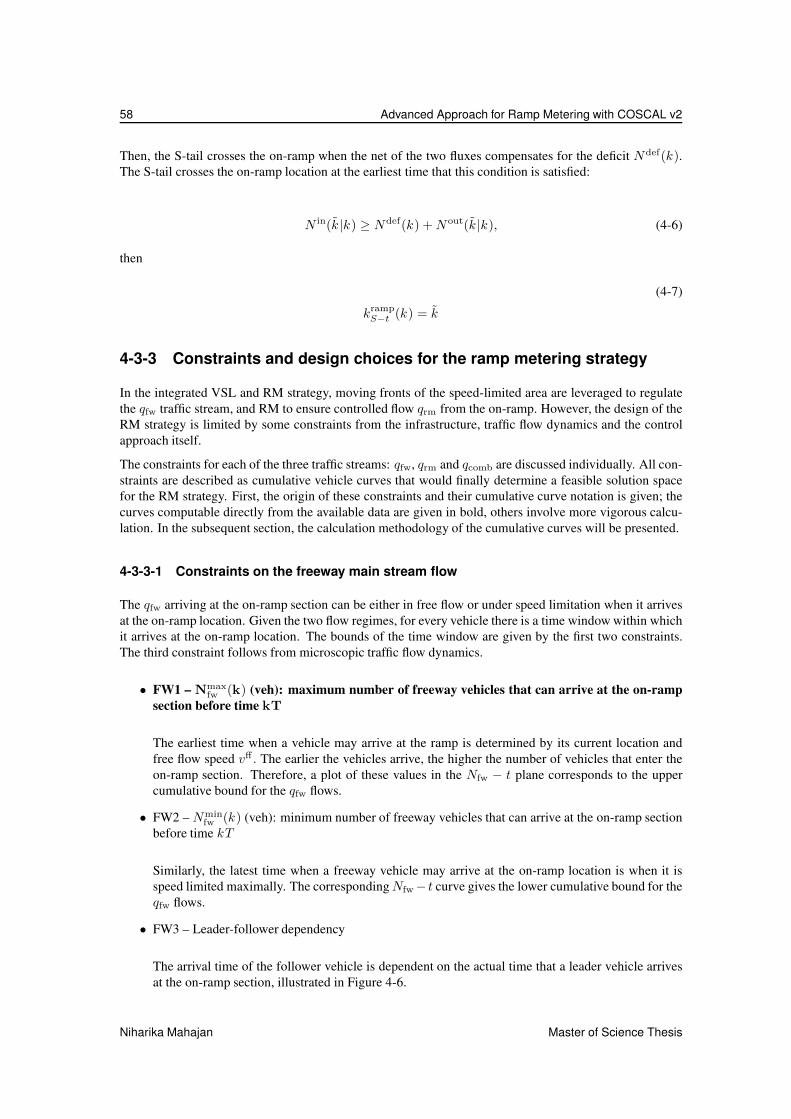
58 Advanced Approach for Ramp Metering with COSCAL v2
Then, the S-tail crosses the on-ramp when the net of the two fluxes compensates for the deficit Ndef(k).
The S-tail crosses the on-ramp location at the earliest time that this condition is satisfied:
N in(k̃ |k) ≥ Ndef(k) + Nout(k̃ |k), (4-6)
then
(4-7)
krampS−t (k) = k̃
4-3-3 Constraints and design choices for the ramp metering strategy
In the integrated VSL and RM strategy, moving fronts of the speed-limited area are leveraged to regulate
the qfw traffic stream, and RM to ensure controlled flow qrm from the on-ramp. However, the design of the
RM strategy is limited by some constraints from the infrastructure, traffic flow dynamics and the control
approach itself.
The constraints for each of the three traffic streams: qfw, qrm and qcomb are discussed individually. All con-
straints are described as cumulative vehicle curves that would finally determine a feasible solution space
for the RM strategy. First, the origin of these constraints and their cumulative curve notation is given; the
curves computable directly from the available data are given in bold, others involve more vigorous calcu-
lation. In the subsequent section, the calculation methodology of the cumulative curves will be presented.
4-3-3-1 Constraints on the freeway main stream flow
The qfw arriving at the on-ramp section can be either in free flow or under speed limitation when it arrives
at the on-ramp location. Given the two flow regimes, for every vehicle there is a time window within which
it arrives at the on-ramp location. The bounds of the time window are given by the first two constraints.
The third constraint follows from microscopic traffic flow dynamics.
• FW1 – Nmaxfw (k) (veh): maximum number of freeway vehicles that can arrive at the on-ramp
section before time kT
The earliest time when a vehicle may arrive at the ramp is determined by its current location and
free flow speed vff . The earlier the vehicles arrive, the higher the number of vehicles that enter the
on-ramp section. Therefore, a plot of these values in the Nfw − t plane corresponds to the upper
cumulative bound for the qfw flows.
• FW2 – Nminfw (k) (veh): minimum number of freeway vehicles that can arrive at the on-ramp section
before time kT
Similarly, the latest time when a freeway vehicle may arrive at the on-ramp location is when it is
speed limited maximally. The corresponding Nfw − t curve gives the lower cumulative bound for the
qfw flows.
• FW3 – Leader-follower dependency
The arrival time of the follower vehicle is dependent on the actual time that a leader vehicle arrives
at the on-ramp section, illustrated in Figure 4-6.
Niharika Mahajan Master of Science Thesis

4-3 RM integration with TASK 3 of COSCAL v2 -
speed limitation for stabilization 59
CUMULATIVE CURVES
ON FREEWAY PLANE
CUMULATIVE CURVES
ON RAMP PLANE
QUEUE CONSTRAINTS POLICY CONSTRAINTS
FW1: Maximum
freeway flows
RM2: Minimum
ramp flows
FW2: Minimum
freeway flows
RM3: Maximum
ramp flowsRM4: Minimum
ramp flows
RM1: Maximum
ramp flows
FW3: Leader -
follower dependency
C1: Minimum admissable
ramp flows
C2: Maximum admissable
ramp flows
ramp section capacity in free-flow
ramp section capacity under speed limits
ramp section capacity in free-flow
(Nfw − t) (Nrm − t)
Figure 4-3: Relation of the different constraints as cumulative curves (determined at the on-ramp
section) on the freeway plane - Nfw − t and the ramp plane - Nrm − t. The arrows in blue indicate
the translation of cumulative curves on Nfw −t plane to Nrm −t. The activation of the VSL scheme
influences the capacity flow at the on-ramp section, and thereby the translation.
4-3-3-2 Constraints on the on-ramp flow
The primary constraints on the on-ramp flows follow from the queue restrictions on the on-ramp and over-
arching policy restrictions on the RM rates.
• RM1 – Nmaxrm (k) (veh): maximum number of vehicles that can enter the on-ramp section from
the on-ramp before time kT
This cumulative curve in the Nrm − t plane follows from the on-ramp demand. The outflow from the
on-ramp can be no more than its inflow. Therefore, Nmaxrm (k) follows directly from the cumulative
qinr (k) profile and minimum queue-length condition.
It should be mentioned here that it costs an incoming vehicle some travel time over the length of the
on-ramp, before it merges onto the freeway. This translates to an equivalent delay between the inflow
and the outflow curve for the on-ramp traffic. However, we have ignored this delay when considering
the inflow profile as the maximum outflow curve.
• RM2 – Nminrm (k) (veh): minimum number of vehicles that must enter the on-ramp section from
the on-ramp, before time kT
The lower bound for the RM outflow is governed by the maximum queue-length assumption. The
minimum cumulative ramp outflow curve must ensure that the queue on the on-ramp never exceeds
its maximum design value. This curve can be determined directly from the cumulative qinr (k) profile
and the smaxr value.
• RM3 – Nmax,prm (k)(veh): policy constraint on the maximum RM rate
Master of Science Thesis Niharika Mahajan

60 Advanced Approach for Ramp Metering with COSCAL v2
These constraints follow from the maximum cycle time for the ramp signal. It is often regulated by
the traffic network managers due to policy considerations.
• RM4 – Nmax,prm (k)(veh): policy constraint on the minimum RM rate
Similarly to RM3, it follows from the minimum cycle time for the ramp signal.
4-3-3-3 Constraints on the combined flow at the on-ramp section
The constraints on the qcomb traffic stream follow from the variations in flow capacity based on the evolu-
tion of the stabilization scheme itself. The time intervals where qcap,ffcomb and qcap,sl
comb apply are illustrated in
Figure 4-1. Essentially, qcap,slcomb applies when the freeway flow arriving at the on-ramp and the combined
flow downstream of it are speed-limited. At all other times, when the freeway flow arriving at the on-ramp
flow is in free flow regime, the free flow capacity qcap,ffcomb holds. Then, the prevailing capacity qcap
comb(k̃ |k)at any time in the prediction horizon can be given as:
qcapcomb(k̃|k) =
{
qcap,ffcomb if kT < tramp
S−t (k) ∨ kT ≥ trampS−h (k)
qcap,slcomb = q[4A] = ρ̄[4A]λveff if tramp
S−t (k) ≤ kT < trampS−h (k)
(4-8)
Given this total flow capacity of the combined flows qrm plus qfw, all constraints on the freeway flow qfw
translate to additional constraints for ramp flow qrm, and vica versa. These additional constraints are given
as admissible cumulative curves and are defined below.
• C1 – Nmin,admrm (k): (veh) minimum number of vehicles admissible from the on-ramp before
time kT, to achieve the capacity flow at the on-ramp section, when traffic stream qfw arrives
in free flow (maximal main flow)
It is the minimum admissible flow required to achieve capacity flow for the combined stream, when
the main stream flow is at its maximum, corresponding to Nmaxfw . Then, the cumulative curve is
obtained directly as the difference of the prevailing capacity at the on-ramp section and the Nmaxfw (k)
curve:
Nmin,admrm (k) = T
∑
k
qcap(k) − Nmaxfw (k) (4-9)
• C2 – Nmax,admrm (k): (veh) maximum number of vehicles admissible from the on-ramp before
time kT, to achieve the capacity flow at the on-ramp section, when the traffic stream qfw is
speed-limited (minimal main flow)
The cumulative curve is obtained directly as the difference of the prevailing capacity at the on-ramp
section and the Nminfw (k) curve:
Nmax,admrm (k) = T
∑
k
qcap(k) − Nminfw (k) (4-10)
• C3 – Nmax,admfw (k): (veh) maximum number of vehicles admissible from the main stream when
the ramp metering flow is minimal
The cumulative curve is obtained directly as the difference of the capacity of the on-ramp section
and the Nminrm (k) curve.
Niharika Mahajan Master of Science Thesis

4-3 RM integration with TASK 3 of COSCAL v2 -
speed limitation for stabilization 61
• C4 – Nmin,admfw (k): (veh) minimum number of vehicles admissible from the main stream when
the ramp metering flow is maximal
The cumulative curve is obtained directly as the difference of the capacity of the on-ramp section
and the Nmaxrm (k) curve.
4-3-4 Determining the feasible solution space for ramp metering
When all the constraints presented in the previous section are superimposed on the Nrm-t plane, we obtain
a set of possible cumulative ramp flow values at each time step. A choice of cumulative outflow at each
control time step, from within this range, then determines the RM rate at any given time.
To that end, in this section we discuss how each constraint translates to a corresponding condition in the
Nrm-t plane. The feasible solution space is defined as a region in the Nrm-t plane such that, from any given
point at least one feasible RM trajectory exists until the end of the prediction horizon. The end goal is to
determine the upper: U(k̃|k) and the lower: L(k̃|k) bounds of this feasible region; here k̃ is the index of a
future time step for which the prediction is made based on real-time data available at the current time step
k . The calculations are presented procedurally, depending on which inputs are known and which become
available in successive steps.
4-3-4-1 Unregulated freeway flow upstream of the on-ramp
The freeway flow qfw is in free flow when the traffic stream is unregulated. Since vehicles can drive fastest
in free flow, they arrive at the on-ramp section earliest in this regime. Recall that the Nmaxfw
(idet, k̃|k)curve (constraint FW1) is the cumulative vehicle count at the on-ramp section when flow qfw arrives in free
flow regime. A point (Nfw, k̃) on this curve implies that a total of Nfw mainstream vehicles can cross the
on-ramp section at the earliest by time k̃T .
In order to determine the cumulative curve, it is assumed that the traffic stream is travelling at an average
free flow speed vff , which is known. In practice, it could be determined as a moving average of speeds on
detector segments further upstream of the VSL scheme.
The earliest time tramp,min(idet) when the most upstream vehicle in each detector segment idet (according
to the density measurements at time kT ) segment passes the on-ramp section can then be given as:
tramp,min(idet) =xramp − xu,det
idet
vff(4-11)
The cumulative number of vehicles that will cross before time tramp,min(idet) is calculated below. Here,
ρj is as available from the traffic data at time step k .
Nfw(idet, k̃|k) =
iramp∑
j=idet
Ljλjρj(k), (4-12)
Ensuing, a plot of(
Nfw(idet, k̃|k), tramp,min(idet))
in the Nfw-t plane gives the cumulative curve Nmaxfw (k̃ |k).
The capacity at the on-ramp section is time-dependent and was expressed in equation (4-8). A capacity flow
constraint necessitates that when the total unregulated demand at the on-ramp section exceeds the capacity
flow qcapcomb(k̃ |k) at that time, either qrm or qfw flow should be reduced. Further, notice in Figure 4-1 that
the flow qfw is unregulated until the S-tail crosses, and must be speed-limited to be reduced.
Master of Science Thesis Niharika Mahajan

62 Advanced Approach for Ramp Metering with COSCAL v2
Therefore, a design choice is made here, that the controller prefers to limit qrm over qfw until the S-tail
shockwave has crossed the on-ramp. The rationale is that an increase in RM flow requires a proportional
reduction of the freeway flow arriving at the on-ramp section. In order to achieve a lower freeway flow
in the future requires speed-limiting vehicles upstream of the on-ramp before they arrive at the on-ramp.
Hence, the stabilization area upstream of the on-ramp becomes less efficient in order to accommodate ramp
flows. The higher the RM flows, the lower is the efficiency of the upstream speed-limited states (state 4B
and 4C in the basic strategy).
Thus, the choice entails that the freeway traffic stream qfw is unregulated, i.e. follows the Nmaxfw (k̃ |k)
curve, for as long as possible (at this point, this is the time trampS−t (k) that the S-tail is predicted to cross
the on-ramp). Consequently, the RM strategy must not allow flows more than the difference of the arriving
unregulated flow from the capacity at the on-ramp section.
The appropriate RM flows in this duration are determined by translating the Nmaxfw (k̃|k) curve to the the
Nrm-t plane. This gives the minimum admissible cumulative RM flow, Nmin,admrm (k̃|k) (constraint C2),
and represents the ramp flow required to fully utilize the on-ramp section capacity. Since higher on-ramp
flows can be allowed when the freeway traffic is speed-limited, the label minimum admissible signifies that
the RM flows are more restrictive in this case. The translation is given below:
Nmin,admrm (k̃ |k) = qcap
comb(k̃ |k)T − Nmaxfw (k̃) (4-13)
4-3-4-2 Formulation of the primary RM constraints in the Nrm-t plane
Next, the primary constraints for RM given in Section 4-3-3-2 are expressed as cumulative curves on the
Nrm-t plane.
When the RM rate is maximum, the queue on the on-ramp will be minimum. Then, Nmaxrm (k̃) curve
(constraint RM1) can be calculated with the on-ramp demand, on-ramp queue sr(k) at the current time
step, and the minimum desired queue length as:
Nmaxrm (k̃ |k) = max
sr(k) + T
k̃∑
j=k
qinr (j) − smin
r , 0
(4-14)
Similarly, offsetting the cumulative qinr profile by the maximum desired queue length sdes
r gives the lower
bound Nminrm (k̃) (constraint RM2) for RM flows:
Nminrm (k̃|k) = max
sr(k) + T
k̃∑
j=k
qinr (j) − sdes
r , 0
(4-15)
In addition to the queue regulation, the minimum and maximum allowed ramp outflow [qminrm , qmax
rm ] ap-
ply due to policy considerations (constraints RM3 and RM4). The corresponding cumulative curves
Nmax,prm (k̃|k) and N
min,prm (k̃|k) assume qmax
rm and qminrm , respectively at all future times. The two curves
can be given as:
Nmax,prm (k̃|k) = qmax
rm
(
k̃ − k)
T , (4-16)
Niharika Mahajan Master of Science Thesis

4-3 RM integration with TASK 3 of COSCAL v2 -
speed limitation for stabilization 63
and
(4-17)
Nmin,prm (k̃|k) = qmin
rm
(
k̃ − k)
T
Together, constraints RM1, RM2, RM3 and RM4 provide an ad-hoc upper and lower bound of the feasible
area: [Urm(k̃ |k), Lrm(k̃|k)].
Urm(k̃ |k) = min(
Nmaxrm (k̃|k), Nmax,p
rm (k̃ |k))
, (4-18)
and
Lrm(k̃|k) = max(
Nminrm (k̃|k), Nmin,p
rm (k̃|k))
200
400
600
100
200
500
600
0.25 0.75 1.25
RM3
RM4
RM1
RM2
Time
(h)
Ramp inflow
(veh/ h)
cumulative
inflow
200 veh/h
600 veh/h
(veh)Nrm
Figure 4-4: Plot of cumulative curves from primary ramp metering constraints for a simple ramp
demand profile. An initial queue length of 50 veh; a policy maximum and minimum RM rate of
600 veh/h and 200 veh/h is assumed in this illustration. The red shaded area in Nrm − t plane
then gives the feasible RM solution due to policy restrictions, and the grey shaded area gives the
feasible RM solution from queue length constraints. The overlap of the two areas (hatched) is the
resultant feasible solution space.
Master of Science Thesis Niharika Mahajan

64 Advanced Approach for Ramp Metering with COSCAL v2
4-3-4-3 Adapting S-tail when total demand exceeds the capacity flow at the on-ramp
At this point, we have three curves in the Nrm-t plane - the upper and lower bounds [Urm(k̃|k), Lrm(k̃|k)]
from the primary RM constraints, and the Nmin,admrm (k̃|k) cumulative curve. While the lower bound
Lrm(k̃ |k) corresponds to the minimum ramp flows required by the RM strategy, Nmin,admrm (k̃|k) gives
the maximum ramp flow allowable when the freeway flows are unregulated. Now, if the required RM flows
are larger than the allowable, the freeway and the ramp flows together will exceed the capacity at the ramp
section.
Therefore, if the the lower bound Lrm(k̃|k) exceeds Nmin,admrm (k̃|k) at some time k̃T , it implies that
even the minimum possible RM flow determined by the ramp controller is too high to satisfy the capacity
constraint, if the freeway flow is not speed-limited. Consequently, the main stream flow qfw must be
regulated, for which speed limits should have crossed the on-ramp before such a situation arises.
In other words, the S-tail must have crossed the on-ramp before the time that the Lrm(k̃|k) curve exceeds
the curve Nmin,admrm (k̃|k); we denote this cross-over time as kramp,ext
S−t (k)T (s). If this is not true and
kramp,extS−t (k) < kramp
S−t (k), calculated in equation (4-6), then the propagation of the S-tail shockwave must
be adapted to cross the on-ramp sooner. Lets denote the smaller of the two time steps as kramp,minS−t (k) =
min(
krampS−t (k), kramp,ext
S−t (k))
.
If kramp,minS−t (k) = kramp,ext
S−t (k), then regardless of the S-tail position determined by the procedure de-
scribed later in Section 4-3-6-2, the freeway flow must be controlled after time kramp,minS−t (k)T . This is
achieved by enforcing VSL up to the on-ramp segment. Now, between time kramp,minS−t (k)|k̃ and the time
that the S-head crosses the ramp location, the freeway flow qfw arriving at the on-ramp is speed-limited.
4-3-4-4 Regulated freeway flow upstream of the on-ramp
When the freeway flow upstream of the on-ramp is speed-limited, it implies that the vehicles can arrive at
the on-ramp section later than in free flow regime. The cumulative curves related to the freeway mainstream
flows under speed limits are of interest now.
We consider the most extreme case of speed-limitation. Here, the freeway segments upstream of the on-
ramp are speed-limited simultaneously at the time kramp,minS−t (k)T , i.e. the time when the S-tail is deter-
mined to cross the on-ramp as per the prediction of the control scheme at time kT (or at the current time
kT if the S-tail has already crossed the on-ramp). This situation gives the latest time (equivalently, the low-
est possible flows) that the mainstream vehicles can arrive at the on-ramp section. The cumulative curve
Nminfw (k̃|k) (constraint FW2) captures this restriction, and its formulation is described next.
The number of vehicles on a typical detection segment of a few hundred metres length, is of the order of
magnitude 1-2. Due to the lack of traffic information about individual vehicles on a detection segment, a
theoretical simplification is made here. We consider homogeneous traffic condition within a single detec-
tion segment. Further, the upstream end of each detection segment is assumed to be the rear bumper of the
most upstream vehicle on it. Then, all vehicles on a segment, ahead of this vehicle, will arrive at the ramp
section earlier than the vehicle itself.
From the density measurements over the detection segments at time kT , the location of the last vehicle on
a detector segment idet, at the time that it is speed-limited can be given as:
xidet = xu,detidet + vff max
(
kramp,minS−t (k) − k, 0
)
T (4-19)
The time that this vehicle then arrives at the on-ramp section can be calculated using location xidet and the
effective speed under speed limits as:
Niharika Mahajan Master of Science Thesis
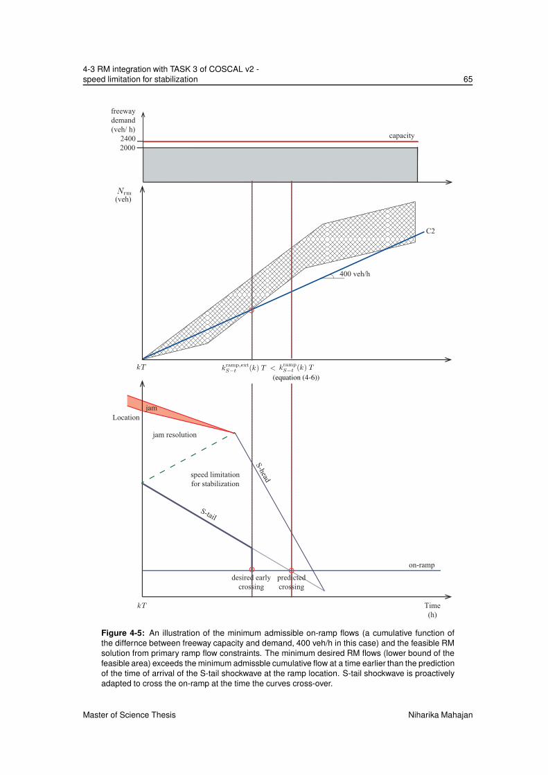
4-3 RM integration with TASK 3 of COSCAL v2 -
speed limitation for stabilization 65
Time
(h)
2000
freeway
demand
(veh/ h)
2400 capacity
C2
400 veh/h
on-ramp
S-head
S-tail
jam resolution
speed limitation
for stabilization
Location
desired early
crossing
jam
predicted
crossing
(veh)Nrm
kT
kT kramp,extS−t (k) T < kramp
S−t (k) T
(equation (4-6))
Figure 4-5: An illustration of the minimum admissible on-ramp flows (a cumulative function of
the differnce between freeway capacity and demand, 400 veh/h in this case) and the feasible RM
solution from primary ramp flow constraints. The minimum desired RM flows (lower bound of the
feasible area) exceeds the minimum admissble cumulative flow at a time earlier than the prediction
of the time of arrival of the S-tail shockwave at the ramp location. S-tail shockwave is proactively
adapted to cross the on-ramp at the time the curves cross-over.
Master of Science Thesis Niharika Mahajan

66 Advanced Approach for Ramp Metering with COSCAL v2
tramp,max(idet) =xd,det
iramp − xidet
veff(4-20)
The cumulative number of vehicles Nfw(idet) that would cross before time tramp,max(idet) is calculated
in equation (4-12). Then upon interpolation, the Nfw-t curve:(
Nfw(idet), tramp,max(idet))
gives the
Nminfw (k̃|k) cumulative curve.
Hence, at any time after kramp,minS−t (k)T , the feasible region in the Nfw-t plane lies between two extreme
cumulative curves: Nmaxfw (k̃|k) and the revised Nmin
fw (k̃|k) (constraints FW1 and FW2). The former cor-
responding to qfw is in free flow regime, and the latter to qfw in speed-limited regime.
4-3-4-5 Formulation of the Leader-Follower constraint
We determined that the cumulative curves Nmaxfw (k̃|k) and Nmin
fw (k̃|k) in the Nfw-t plane enclose the fea-
sible freeway flow curves. However, not all curves (flows) in this area can be realized. The reason is that
some curves may correspond to very high or low flows that cannot be produced given the current vehicle
spacing on the freeway, and for vehicle speeds between veff and vff . This has been illustrated in Figure 4-6.
Here, given a headway of ∆x between two consecutive vehicles i and i + 1, the following vehicle i + 1can not arrive, at the given location, sooner than its arrival time in free-flow. At the same time, it can not
arrive later than its arrival time under speed-limitation.
time
loca
tio
n
∆x
leaderveh i
followerveh i + 1
vff veff
tt +
∆x
vff
(earliest arrival)
t +∆x
veff
(latest arrival)
Figure 4-6: Arrival time dependency between a leader and follower due to car-following (micro-
scopic) behaviour
Therefore, to incorporate the leader-follower dependency (constraint FW3), some additional conditions
must be checked. In essence, this constraint entails a dependency of the arrival time of a following vehicle,
at a pre-specified location (on-ramp section in this case), on its leader’s arrival time.
However, this arrival time dependency does not include any restrictions on the value of ∆x, and the re-
sulting density achieved inside the speed-limited (stabilization) area. In order to ensure that the density
upstream of the on-ramp is not arbitrarily too high, we must also check if the resulting density is higher
Niharika Mahajan Master of Science Thesis

4-3 RM integration with TASK 3 of COSCAL v2 -
speed limitation for stabilization 67
than the desired density ρ̄[4A]. The corresponding maximal flow for this density is qmax = veff ρ̄[4A], and
then the minimum acceptable headway becomes1
qmax. Hence, ∆x should not be smaller than
1
qmaxat any
time.
Then, the arrival time dependency for the leader-follower pair with an additional criteria for density can be
given as:
ti + max
(
∆x
vff,
1
qmax
)
≤ ti+1 ≤ ti + max
(
∆x
veff,
1
qmax
)
(4-21)
The condition may be re-written as:
ti+1 − max
(
∆x
veff,
1
qmax
)
≤ ti ≤ ti+1 − max
(
∆x
vff,
1
qmax
)
(4-22)
The above equation expresses the time ti a leader must arrive at a given section for a follower to arrive there
at a desired time ti+1. The formulation of the condition in the latter form is desirable because, the integrated
strategy is predictive such that anticipatory decisions ensure a desired traffic state in the future. Then, a
leader (arriving earlier) constitutes the flow at an earlier time than its follower. Hence, the microscopic
formulation in equation (4-22) allows for anticipatory control of traffic.
Next, these microscopic car-following constraints need to be converted to mesoscopic conditions suitable
for the discrete formulation of COSCAL v2. For this, the condition in equation (4-22) is applied to each
detection segment. For any detection segment idet, the most upstream vehicle on segment idet + 1 is taken
as a leader, and the most upstream vehicle on segment idet as its mesoscopic follower.
Then, accumulation Nfw(idet + 1) according to equation (4-12), gives the cumulative vehicle count of
the representative leader for segment idet. Likewise, accumulation Nfw(idet) gives the cumulative vehicle
count of its mesoscopic follower. ∆x, the hypothetical headway between these mesoscopic leader-follower
pair is approximated as the length of detection segment idet.
4-3-4-6 Adapting freeway cumulative curves for the Leader-Follower constraint
As per the original cumulative curve Nmaxfw , a follower Nfw(idet) could at the earliest arrive at tramp,min(idet),
and likewise its leader Nfw(idet + 1) at tramp,min(idet + 1), as determined in equations (4-11) and (4-12).
These variables have been identified in Figure 4-7.
Further, the arrival time of the leader as per the leader-follower condition in equation (4-22) is deter-
mined in the equation below. The desired arrival time based on the leader-follower criteria is denoted as
tramp,minl−f (idet).
tramp,minl−f (idet + 1) ≥ tramp,min(idet) − max
(
Lidet
veff,ρidet λidet Lidet
qmax
)
(4-23)
The additional constraint requires the leader Nfw(idet +1) to arrive no later than time tramp,minl−f (idet +1).
Therefore, the more restrictive of the two times, i.e. max(
tramp,min(idet + 1), tramp,minLF (idet + 1)
)
gives
the earliest time for Nfw(idet + 1) vehicles to have crossed the on-ramp section. The adapted Nmaxfw curve
gives the revised upper bound in the Nfw-t plane.
Lets denote it as Ufw :(
Nfw(idet), max(
tramp,min(idet), tramp,minLF (idet)
) )
.
Master of Science Thesis Niharika Mahajan

68 Advanced Approach for Ramp Metering with COSCAL v2
2000 veh/h
desired early
crossing of
S-tail
predicted
crossing of
S-head
Time
(h)
2000
1500
freeway
demand
(veh/ h)
2400 capacity
(veh)
FW2
FW1
Nfw
ρλvffρλveff
Nfw(idet − 1)
Nfw(idet)
Nfw(idet + 1)
tramp,minl−f (idet) tramp,max
l−f (idet)
Figure 4-7: Mesoscopic translation of the arrival time depedency between a leader and follower
due to car-following behaviour. The red dashed lines in the on the Nfw-t plane represent the
function for this constraint, and the red shaded area the reduction of the feasible freeway flows
thereof.
Additionally, the flow capacity of the on-ramp section is qcap,slcomb when the freeway flow upstream of the
on-ramp is regulated. Hence, the cumulative curve Nmin,admfw (k) as calculated in equation (4-13) is revised
beyond time kramp,minS−t (k)T . With the flow capacity qcap,sl
comb under speed limits, the cumulative curve can
be revised as:
Nmin,admrm (k̃|k) = qcap,sl
comb
(
k̃T − kramp,minS−t T
)
− Ufw(k̃), ∀k̃ k̃ ≥ kramp,minS−t (k) (4-24)
Similarly to the leader-follower constraints for the upper boundary in Nfw-t plane, the Nminfw curve is also
adapted. The latest time for Nfw(idet+1) vehicles to cross at the on-ramp section due to the leader-follower
constraint can be given as:
tramp,maxl−f (idet + 1) ≤ tramp,min(idet) − max
(
Lidet
vff,
ρidetλidet Lidet
qmax
)
(4-25)
Niharika Mahajan Master of Science Thesis

4-3 RM integration with TASK 3 of COSCAL v2 -
speed limitation for stabilization 69
Then, min(
tramp,max(idet + 1), tramp,maxl−f (idet + 1)
)
is more restrictive and gives the latest time for
Nfw(idet) vehicles to have crossed the on-ramp section. Now the revised lower bound in the Nfw-t plane
can be given as Lfw :(
Nfw(idet), min(
tramp,max(idet), tramp,maxLF (idet)
))
.
4-3-4-7 Translating freeway curves to the Nrm-t plane and the feasible ramp flows
The upper Ufw and lower bound Lfw for the freeway flows, determined in the previous section, can be
translated to the Nrm-t plane similarly to equation (4-24). Then, the new curve Nmax,admrm (k̃|k) gives the
maximum admissible RM flow that ensures that the prevailing capacity at the on-ramp section qcap,slcomb not
exceeded. The formulation of constraint C1 then becomes:
Nmax,admrm (k̃|k) = qcap,sl
comb
(
k̃T − kramp,minS−t T
)
− Lfw(k̃), ∀k̃ k̃ ≥ kramp,minS−t (k) (4-26)
At this point, we have a feasible area in the Nrm-t plane from the primary RM constraints. This region com-
prises of all discrete Nrm values between the curves Urm and Lrm. Additionally, we have similar curves
Ufw and Lfw on the Nfw-t. These were translated to the Nrm-t plane as Nmax,admrm and Nmin,adm
rm , respec-
tively. Therefore, the resulting feasible set is given by the superimposition of [Urm,Lrm] and [Nmax,admrm ,
Nmin,admrm ] on the Nrm-t plane:
U(k̃|k) = min(
Urm(k̃ |k), Nmax,admrm (k̃ |k)
)
(4-27)
and
L(k̃|k) = max(
Lrm(k̃ |k), Nmin,admrm (k̃|k)
)
Lastly, one final check must be performed to ensure that a feasible solution space has been found in accor-
dance with its starting definition, i.e. at any given time at least one feasible RM path is possible till the final
prediction time. This entails a backcasting approach to check for the cumulative ramp outflow value at time
(k̃ − 1)T which can realize the desired outflow U(k̃) at the minimum RM rate qminrm . This backcasted Nrm
is denoted as U′(k̃ − 1) and is mathematically given as:
U ′(k̃ − 1|k) = U(k̃|k) − qminrm T (4-28)
Then the effective upper bound at time step k̃ is min(
U(k̃ − 1|k), U ′(k̃ − 1|k))
.
Likewise, for the lower bound L(k̃|k) the backcasting approach checks for the minimum L′(k̃ −1) that can
realise L(k̃) in the subsequent time step at a maximum RM rate qmaxrm . L′(k̃ − 1) can be given as:
L′(k̃ − 1|k) = L(k̃|k) − qmaxrm T (4-29)
Then, the effective lower bound at time step k̃ is max(
L(k̃ − 1|k), L′(k̃ − 1|k))
. Together, the effective
upper and lower bound curves for all k̃ > k, gives the feasible RM flow values.
Master of Science Thesis Niharika Mahajan

70 Advanced Approach for Ramp Metering with COSCAL v2
4-3-5 Selecting a feasible ramp flow trajectory
The previous section detailed the method to predict a set of feasible ramp outflow values at every future time
step in the prediction horizon. Ideally, the possibility to pick any one value from this set for a subsequent
time step is most desirable. However, in the current formulation of COSCAL v2 the profile of the RM
flow in the future affects VSL implementation at earlier times. In other words, to accommodate a high RM
outflow in a future time step may require extending speed limits further upstream in the most current time
step.
Hence, selecting a complete RM trajectory, once COSCAL v2 scheme is initiated, is necessary. At each
time step, the RM controller selects a trajectory that is closest to the previously chosen trajectory, and at
the same time, feasible based on the current measurements and prediction.
Essentially, two criteria are used to determine the desired RM trajectory. First is the desired queue length at
time trampS−h when the S-head crosses the on-ramp location; this is when qfw flow recovers to free flow con-
dition, i.e. the capacity of the on-ramp section is qcap,ffcomb once again. Here, we may chose to keep the queue
at a fixed percentage of its maximum capacity smaxr , say Ksmax
r where 0 < K ≤ 1. While selecting the
value of the parameter K, the consequence of a high or low parameter value must be understood. A higher
K value improves VSL performance (reduces area under speed limits), however, offers lesser flexibility to
adapt RM flows in the future if required for queue management. Additionally, a moderate on-ramp queue
at time trampS−h when the S-head crosses the on-ramp, increases the likelihood that the stabilization area after
that time reduces in space-time regardless of a drastic spike in on-ramp demand.
The second criteria relates to the efficiency of the speed-limited area upstream of the on-ramp (state 4B).
Consider, the RM flow is first high and then lowered to arrive at some end cumulative outflow value.
Alternately, the same cumulative outflow could be achieved by keeping the RM flow low initially and
increasing it later. In spite of the same cumulative outflow finally, the former strategy would result in a less
efficient state 4B than the latter. For this reason, the RM flow trajectory is kept as low as possible, for as
long as possible, and subsequently increased to achieve the set ramp storage capacity at time trampS−h .
However, the above criteria do not determine the RM trajectory beyond time trampS−h . The integrated strategy
after trampS−h poses a design choice; the on-ramp queue may either be released while theVSL scheme is
still active or after the stabilization area is resolved. It is chosen to release the on-ramp queue while the
freeway flow is speed-limited. The argument here is that the VSL scheme offers more flexibility to achieve
the higher ramp flows desirable for releasing the entire ramp queue. At the same time, it does imply that
the freeway vehicles further upstream of the problem area may be speed-limited for this. However, it is
understood as more reliable to achieve the end goal.
Lets denote the selected RM flow trajectory as N selrm(k̃ |k), such that the desired RM rate at a future time
k̃T becomesN sel
rm(k̃ + 1) − N selrm(k̃)
T.
4-3-6 Implementation of variable speed limits in the stabilization area
In general, any vehicle that is speed-limited, even for the shortest interval of time, enters speed-limitation
at the S-tail shockwave and exits at the S-head. Further, the freeway flow qfw arrives at the on-ramp section
in different regimes - the flow is in free flow before time trampS−t , under speed-limitation between time tramp
S−t
and trampS−h , and again in free flow after time tramp
S−h . Note that the location of the S-tail and the S-head
shockwaves is uniquely determined in each case.
The freeway vehicles entering the merging location before time trampS−t , enter and exit speed-limitation
downstream of the on-ramp, i.e shockwaves S-tail and S-head are both downstream of the on-ramp. For
the freeway vehicles merging between time trampS−t and tramp
S−h , the S-tail is located upstream of the on-ramp
and the S-head downstream of it. And for vehicles entering the on-ramp section after trampS−h , both S-tail and
S-head are upstream of the on-ramp location. This is illustrated with three unique vehicle trajectories in
Figure 4-1c.
Niharika Mahajan Master of Science Thesis

4-3 RM integration with TASK 3 of COSCAL v2 -
speed limitation for stabilization 71
Now, when the S-head and S-tail shockwaves lie upstream of the on-ramp section, their propagation can
be dynamically regulated in order to accommodate the on-ramp flow. The chosen RM trajectory N selrm(k̃ |k)
provides the number of vehicles that must be allowed to merge from the on-ramp in a given time step. Then,
speed-limitation must ensure an appropriate density of the freeway traffic arriving at the on-ramp section
in that time step. An appropriate density is low enough to offer sufficient gaps for the ramp vehicles and to
achieve the desired density downstream of the on-ramp section. Therefore, by dynamically managing the
propagation of the S-head and S-tail shockwaves, RM and VSL strategies are integrated.
The methodology to determine the desired location of the S-head and S-tail in the integrated control ap-
proach is detailed in the next two sections.
4-3-6-1 Calculating the S-head position
The location of the S-head downstream of the on-ramp section (labelled S-head1 in Figure 4-1c) depends
on its design speed vS-h. Thus, it can be calculated from an estimate of time and location of the start of
S-head shockwave, as determined in equations (3-59) and (3-60), respectively.
The S-head shockwave upstream of the on-ramp section is labelled as S-head2 in Figure 4-1c. Observe
the vehicle trajectory 3 in the same figure. The location of the S-head determines when the vehicle exits
speed-limitation and hence, the time that it arrives at the on-ramp section; all vehicle that exit S-head2
arrive after the S-head1 crosses the on-ramp at trampS−h . Therefore, these arrival times and hence, the speed
of S-head shockwave determine the flow in state 5C at any given time.
The flow in state 5C, q[5C] together with the RM flow qrm gives the design free flow in state 5B. Therefore,
in order to maintain the desired flow q[5B] while the RM flow varies in each time step, the flow in state 5C
must change as below:
q[5C](k̃) = q[5B] − qrm(k̃) (4-30)
Further, the target value of density in state 4C is the same as that established for basic RM strategy in
Section 3-5-2-2. Then, using shockwave theory the desired speed of S-head shockwave between states 4C
and 5C can be determined from the flow and density in these states as:
v[4C-5C](k̃) =q[5C](k̃) − q[4C]
ρ[5C](k̃) − ρ̄[4C]λ(4-31)
=q[5C](k̃) − veff ρ̄[4C]λ
q[5C](k̃)
vff− ρ̄[4C]λ
Notice in Figure ?? the hypothetical vehicle nk that arrives at the on-ramp at time (k̃ + 1)T , travels in
free flow velocity after it exits the S-head. Therefore, a ray at vff slope from X-t point(
xramp, (k̃ + 1)T)
will intersect the S-head ray, at slope v[4C-5C](k̃), in a point where vehicle nk exits speed limits. Similar
iterations for all time steps after time trampS−h gives the desired trajectory of the S-head shockwave upstream
of the on-ramp. Lets denote the S-head trajectory as (xhead(k̃), thead(k̃)). Then, the equations of the two
rays can be given as:
xhead(k̃) = xramp − vff ×(
(k̃ + 1)T − thead(k̃))
(4-32)
and
xhead(k̃) = xhead(k̃ − 1) + v[4C-5C] ×(
thead(k̃) − thead(k̃ − 1))
(4-33)
Master of Science Thesis Niharika Mahajan

72 Advanced Approach for Ramp Metering with COSCAL v2
Subtracting equation (4-33) from equation (4-32) gives the time coordinate thead(k̃) of the S-head trajec-
tory:
thead(k̃) =xhead(k̃ − 1) − xramp
vff − v[4C-5C]+
vff × (k̃ + 1)T − v[4C-5C](k̃) × thead(k̃ − 1)
vff − v[4C-5C](4-34)
then the corresponding location becomes,
xhead(k̃) =xhead(k̃ − 1) + xramp
2−
v[4C-5C](k̃) × thead(k̃ − 1) + vff × (k̃ + 1)T
2(4-35)
+vff + v[4C-5C](k̃)
2× thead(k̃)
In a nutshell, the freeway flow desired at the on-ramp section in a time step determines the desired S-head
speed v[4C-5C](k̃), given in equation (4-31). Subsequently, it is determined when a vehicle that exits at the
on-ramp, at the free flow speed, at the end of the next prediction time step should leave the S-head.
4-3-6-2 Calculating the S-tail position
The propagation of the S-tail shockwave is identified as three distinct parts in Figure 4-1b. S-tail1 deter-
mines when the merged flow qcomb enters speed-limitation downstream of the on-ramp. S-tail2 determines
when the freeway flow qfw enters speed-limitation, to merge with the ramp flow between the time Stail1 and
S-head1 cross the on-ramp. Finally, S-tail3 determines when the freeway flow qfw enters speed-limitation,
to exit at S-head2 and arrive at the on-ramp after the S-head1 has crossed it.
The goal of speed-limitation is to create a homogeneous flow at a desired density within the control area.
This homogeneous state then ensures a desired outflow at a downstream shockwave. To that end, the core
principle to determine the location of the S-tail parts entails matching the number of vehicles that enter
speed-limitation to the desired outflow at a downstream shockwave.
Determining S-tail1
Vehicles entering at the S-tail1 shockwave, exit at the S-head1 shockwave downstream of the on-ramp.
Hence, the exact prediction of the S-tail1 trajectory does not influence the determination of a feasible ramp
flow trajectory and its integration with the VSL scheme. In fact, the methodology used to determine the
most upstream segment in the stabilization area (refer to Section Section 3-5-1), in the original formulation
of COSCAL v2, will adjust the S-tail1 according to the on-ramp flows.
The most upstream speed-limited segment determined here applies until the time tramp,minS−t (k) that the
S-tail is predicted to cross the on-ramp. Beyond this time, the trajectory of S-tail2 is adjusted to accommo-
date flows at the on-ramp. The prediction of the S-tail2 is vital for the integration of VSL with RM, and is
discussed next.
Determining S-tail2
The part of the S-tail trajectory after the S-tail1 shockwave crosses the on-ramp is called S-tail2. The
vehicles that enter speed-limitation at the S-tail2 shockwave, merge with the on-ramp vehicles at the on-
ramp location. The total outflow downstream of the on-ramp, from the design of the integrated strategy, is
q[4A].
To achieve this desired flow, given the selected RM trajectory N selrm(k̃|k), the number of freeway vehicles
that should arrive in a future time step k̃ can be given as below:
Niharika Mahajan Master of Science Thesis

4-3 RM integration with TASK 3 of COSCAL v2 -
speed limitation for stabilization 73
Noutramp(k̃|k) = q[4A]T −
(
N selrm(k̃ + 1|k) − N sel
rm(k̃|k))
(4-36)
= ρ̄[4A]λveffT −(
N selrm(k̃ + 1|k) − N sel
rm(k̃|k))
Now, the location of the S-tail2 should be such that the above cumulative outflow is matched by speed-
limiting the exact number of vehicles at an appropriate time.
Lets denote the last detector segment for which the S-tail position has been determined as itail,us(k) and
any detector segment upstream of it as idet. Then the cumulative inflow N intail(i
det) of vehicles towards the
S-tail, from all detection segments between itail,us(k) and idet, can be calculated as below:
N intail(i
det) =itail,us
−1∑
j=idet
Ljλjρj(k) (4-37)
When N intail(i
det) just suffices the desired outflow Noutramp(k̃|k), i.e. N in
tail(idet) > Nout
ramp(k̃ |k), the most
upstream detector segment to be speed-limited in order to realise the outflow at the on-ramp is found. For
a more conservative design, detector segment idet + 1 is speed-limited to realise the outflow in time k̃T .
Lets assume vehicle ni is the last vehicle on detection segment idet +1. Now, the part of its trajectory under
speed limits will intersect with the part in free flow at the time that it should be speed-limited, i.e. location
of the S-tail2 shockwave. This implies that a ray at slope vff from the upstream end of detector idet + 1will intersect a ray at slope veff from X-t point
(
xramp, (k̃ + 1)T)
in the location of the S-tail shockwave.
Equating the location at the point of intersection gives:
xu,detidet+1
+ vff(
ttail(idet + 1) − (k + 1)T
)
= xramp − veff(
(k̃ + 1)T − ttail(idet + 1)
)
(4-38)
On rearranging, we get the desired time that the last vehicle ni on segment idet + 1 is speed-limited:
ttail(idet + 1) =
xramp − xu,detidet+1
vff − veff+
vff × (k + 1)T − veff × (k̃ + 1)T
vff − veff(4-39)
and the corresponding location of the S-tail is:
xtail(idet + 1) = xramp − veff
(
(k̃ + 1)T − ttail(idet + 1)
)
(4-40)
S-tail2 applies until the last vehicle that exits at the on-ramp at time trampS−h (k) is speed-limited. Vehicles
further upstream are speed-limited to exit into free flow at the S-head2. How this part of the S-tail is calcu-
lated is detailed next.
Determining S-tail3
Lets denote the last detector segment for which the S-tail location is determined as itail,us(k). For the first
prediction for S-tail3, this will be given by the last detection segment that is speed-limited as per S-tail2, and
exits speed-limitation at the on-ramp location. The freeway vehicles upstream of this detection segment,
enter speed-limitation at the S-tail3 shockwave and leave the stabilization area at the S-head2 shockwave.
Master of Science Thesis Niharika Mahajan

74 Advanced Approach for Ramp Metering with COSCAL v2
In Section Section 4-3-6-1, the desired flow in state 5C that should arrive at the on-ramp in a given time step
was determined by equation (4-30). Now, the number of freeway vehicles that cross the on-ramp, say in
time step k̃T equals the number of vehicles that leave the S-head between the points(
xhead(k̃), thead(k̃))
and(
xhead(k̃ + 1), thead(k̃ + 1))
on its trajectory. This cumulative outflow Nouthead(k̃|k) at the S-head is
given below; the independent variable k̃ in its notation represents that these vehicles cross the S-head2 to
arrive at the on-ramp in time step k̃T .
Nouthead(k̃|k) = q[5C](k̃)T (4-41)
The cumulative inflow N intail(i
det) of vehicles towards the S-tail3, from detection segments between itail,us(k)and an upstream detector idet can be calculated as below:
N intail(i
det) =
itail,us−1
∑
j=idet
Ljλjρj(k) (4-42)
When N intail(i
det) just suffices the desired outflow Nouthead(k̃|k), i.e. N in
tail(idet) > Nout
head(k̃|k), the most
upstream detector segment to be speed-limited in order to realise the outflow at S-head3 is found. Similarly
to the calculations for S-tail2, for a conservative design, S-tail3 is located for the accumulation upto the
detector segment just downstream of idet.
This implies that a ray at slope vff from the upper edge of segment idet + 1 at time kT will intersect a
ray at slope veff from S-head2 point(
xhead(k̃ + 1), thead(k̃ + 1))
. Corresponding to equations (4-39) and
(4-40), the coordinates of the S-tail3 for freeway vehicles arriving at the on-ramp at time k̃T are:
ttail(idet + 1) =
xhead(k̃ + 1) − xu,detidet+1
vff − veff+
vff × (k + 1)T − veff × thead(k̃ + 1)
vff − veff(4-43)
and
xtail(idet + 1) = xhead(k̃ + 1) − veff
(
(k̃ + 1)T − ttail(idet + 1)
)
(4-44)
4-4 Summary and Discussion
COSCAL v2 was extended with an advanced RM and VSL approach, to overcome some of the limitations
of the basic integrated approach in Chapter 3. A predictive approach with feedback is used for both the
control measures. In the case of RM, the queue-length on the ramp and the most recent freeway traffic
measurements are used to predict a set of feasible ramp flows in the future. The feasible solution space
ensures that (1) the ramp queue is always between a maximum and minimum queue-length (2) the RM rate
is always between the maximum and minimum policy dictated RM rates, and (3) the freeway flow can be
regulated to accommodate the desired RM flow.
In the advanced VSL strategy, if the scheme crosses a ramp location, an approach different from the original
algorithm is required to appropriately (as per the RM flow at any time) reduce the freeway flows arriving at
the ramp section. In the new approach, the propagation of the S-head and S-tail shockwave is controlled.
The underlying microscopic concept was to determine the trajectory of each vehicle, and the time when
it enters and exits speed limits, to ensure a desired flow profile at the ramp section. This concept was
converted to a macroscopic formulation in terms of the accumulation measured over detection segments.
Niharika Mahajan Master of Science Thesis
4-4 Summary and Discussion 75
It must be mentioned here that the original COSCAL v2 and COSCAL v1 algorithms were designed with
a transition towards cooperative systems in mind, and have the capacity for in-car detection and actuation.
Given the microscopic conceptualization of the new VSL approach, this capacity can be further utilized.
Since equipped vehicles can be regulated more accurately, they can be used to create gaps for the additional
vehicles to merge from the on-ramp. A similar RM strategy using in-car communication technologies was
proposed in a recent work (Scarinci et al., 2013), which could be a very useful extension to the proposed
theory. Besides, in-car actuation capability can in itself help in realising the shockwave trajectories more
accurately.
In developing these advanced approaches for RM and VSL, some additional parameters were considered
other than the tuning parameters in COSCAL v2:
Ramp infrastructure related
• the location xramp of the on-ramp
RM strategy related
• on-ramp demand flow qinr (k)
• the maximum smaxr and minimum smin
r on-ramp queue length
• the maximum qmaxrm and minimum qmin
rm RM flow
• parameter K for the desired queue-length Ksmaxr on the on-ramp at time tramp
S−h when the S-head
shockwave crosses the on-ramp
Freeway traffic related
• the average speed vjam in moving jam state
• the average free-flow speed vff of vehicles
In comparison to the RM strategy used in the basic approach, the advanced RM requires a prediction for
the demand on the on-ramp. Since the present demand prediction algorithms are not very accurate, the
parameters related to the RM strategy should be tuned to compensate for it in practice. However, the
performance sensitivity of the integrated strategy to the accuracy of the demand prediction should be tested
in simulation before field-testing.
At the same time, the VSL strategy uses the freeway traffic measurements at any time to predict the evo-
lution of the VSL scheme. The prediction horizon in the approach extends till the time the most upstream
vehicle that enters speed-limitation has crossed the on-ramp location. Therefore, the duration of the pre-
diction horizon depends on the detection location of the jam, and the traffic condition on the freeway. The
longer the prediction horizon gets, traffic data from detection segments even further upstream is required
for the prediction of the VSL scheme. For instance, for a prediction horizon of 15 min and an average
free-flow speed of 100 km/h, freeway measurements 25 km upstream of the on-ramp should be available.
This is practically not feasible. Hence, alternative approaches to prediction of the VSL scheme should be
explored. One possibility is to assume constant traffic variables upstream of the most upstream detector
measurements available.
Lastly, the entire approach was detailed for the case that the area speed-limited for stabilization crosses
the on-ramp. However, as was discussed in Section 3-4-2, the on-ramp flows can also merge into the
jam resolving area. This scenario should be treated similarly to the basic approach, by accounting for the
additional vehicles from the on-ramp while determining the total number of vehicles to be speed-limited
for resolving the jam. The exact formulation of the scenario is excluded here for lack of time.
Master of Science Thesis Niharika Mahajan

76 Advanced Approach for Ramp Metering with COSCAL v2
Niharika Mahajan Master of Science Thesis

Chapter 5
Algorithm Development
Two different theoretical strategies for integration of COoperative Speed Control ALgorithm (COSCAL) v2
with ramp metering (RM) strategy were developed in Chapters 3 and 4. In this chapter, the objective is to
formulate an algorithm that enables the controller to achieve the traffic behaviour in accordance with the
theoretical scheme.
The algorithmic formulation of COSCAL v2 (Hegyi, 2013) is used as the basis of extension for the new
theory. Relevant parts of the algorithm will therefore be briefly reproduced.
5-1 Introduction
The algorithmic development is focused on the advanced integrated strategy in Chapter 4. The choice is
made due to time limitation; for the same reason, only the advanced strategy is evaluated in a simulation
based study.
For the ease of implementation, the entire strategy is identified in five unique modules. A modular approach
allows for a more methodical evaluation procedure, and a clearer schematization of the control scheme. A
description of the identified modules can be found in Table 5-1.
Table 5-1: Different modules in the advanced integrated VSL and RM strategy
Module label Module description Reference to theory
VSL
related
Module 1 adaptation of the trajectory of S-head shock-
wave for RM flows
Section 4-3-6-1
Module 2 prediction of the time that S-tail shockwave
crosses the on-ramp location
Section 4-3-2
Module 3 adaptation of the trajectory of S-tail shock-
wave according to the RM flows
Section 4-3-6-2
RM
related
Module 4 prediction of feasible RM rates, for the dura-
tion of the VSL scheme, such that there is no
queue spillback
Section 4-3-4
Module 5 selection of a RM rate at each time step from
the feasible flows determined in Module 4
Section 4-3-5
Master of Science Thesis Niharika Mahajan

78 Algorithm Development
Figure 5-1: The position of the vehicle modes (in red) in the control scheme. Note that the
detection segment modes may overlap with the actuation segment modes.
In the following sections, first the algorithmic formulation of COSCAL v2 is revisited. Then, the inter-
vention of the new theory is understood within the original algorithm. Finally, flow diagrams are used to
describe the algorithm development for the new modules.
5-2 Modes and Mode Transitions in COSCAL v2
In the original COSCAL v2, different driving modes are identified for detection and actuation segments
that have different roles, and use different speed limits. Specifically, modes for the detection segments
relate to traffic state estimation, including jam detection. Modes for the actuation segments are used for the
actuation of speed limits, to keep track of their roles, and hence to determine future roles and modes.
The different modes in the control scheme are identified in Figure 5-1. A resemblance to the functional
traffic states in COSCAL v2 is evident here.
5-2-1 Detection segment modes
The detection segments can be in two modes only, a jam mode (mode DJ) and a free-flow mode (mode DF)
depending on whether or not there is a jam in the segment.
The detection segment modes serve to keep track of the jam location, and can be in mode DJ (jam) or mode
DF (free flow, no jam). The first letter (D) of the jam mode refers to the fact that these modes are related to
detection segments.
• Mode DF: free driving
By default, the detection segments are in mode DF, which means that the vehicles are not in a jam.
• Mode DJ: the vehicle in the jam
If for a detection segment it is determined that there is a jam on it, then the segment is in mode
DJ. The role of the segments in mode DJ is to keep track of the jam head location, i.e. the most
downstream detection segment in mode DJ.
Niharika Mahajan Master of Science Thesis
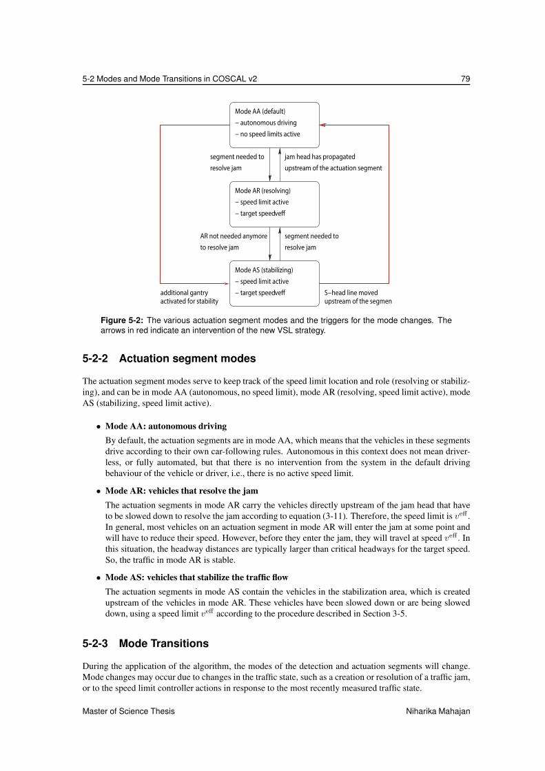
5-2 Modes and Mode Transitions in COSCAL v2 79
segment needed to
resolve jam
− autonomous driving
− no speed limits active
jam head has propagated
AR not needed anymore segment needed to
resolve jam
Mode AA (default)
Mode AR (resolving)
Mode AS (stabilizing)
− speed limit active
− target speed
− speed limit active
− target speed
upstream of the actuation segment
S−head line movedupstream of the segmen
ve�
ve�additional gantryactivated for stability
to resolve jam
Figure 5-2: The various actuation segment modes and the triggers for the mode changes. The
arrows in red indicate an intervention of the new VSL strategy.
5-2-2 Actuation segment modes
The actuation segment modes serve to keep track of the speed limit location and role (resolving or stabiliz-
ing), and can be in mode AA (autonomous, no speed limit), mode AR (resolving, speed limit active), mode
AS (stabilizing, speed limit active).
• Mode AA: autonomous driving
By default, the actuation segments are in mode AA, which means that the vehicles in these segments
drive according to their own car-following rules. Autonomous in this context does not mean driver-
less, or fully automated, but that there is no intervention from the system in the default driving
behaviour of the vehicle or driver, i.e., there is no active speed limit.
• Mode AR: vehicles that resolve the jam
The actuation segments in mode AR carry the vehicles directly upstream of the jam head that have
to be slowed down to resolve the jam according to equation (3-11). Therefore, the speed limit is veff .
In general, most vehicles on an actuation segment in mode AR will enter the jam at some point and
will have to reduce their speed. However, before they enter the jam, they will travel at speed veff . In
this situation, the headway distances are typically larger than critical headways for the target speed.
So, the traffic in mode AR is stable.
• Mode AS: vehicles that stabilize the traffic flow
The actuation segments in mode AS contain the vehicles in the stabilization area, which is created
upstream of the vehicles in mode AR. These vehicles have been slowed down or are being slowed
down, using a speed limit veff according to the procedure described in Section 3-5.
5-2-3 Mode Transitions
During the application of the algorithm, the modes of the detection and actuation segments will change.
Mode changes may occur due to changes in the traffic state, such as a creation or resolution of a traffic jam,
or to the speed limit controller actions in response to the most recently measured traffic state.
Master of Science Thesis Niharika Mahajan
80 Algorithm Development
The mode transitions for the detection segments are straight-forward and depend on the creation and the
resolution of moving jams. The mode changes for the actuation segments have different triggers, which are
summarized in Figure 5-2.
5-3 Algorithmic formulation for the developed theory
In the integrated strategy, the additional RM flows influence the desired trajectory of the S-head and S-tail
shockwaves. In adjusting their location, the freeway flows arriving at the on-ramp are sufficiently lowered.
Therefore, the integrated strategy intervenes in the original algorithm at the mode transitions between
Mode AS and Mode AA. In Figure 5-2, these transitions make-up the outermost loop.
In the original algorithm, the trigger for initiating a Mode AA to Mode AS is determined by the requirement
for an additional segment to achieve the desired stabilization density. Correspondingly, a Mode AS to
Mode AA transition is triggered if the segment lies downstream of the S-head location in that time step.
Recall that the COSCAL v2 algorithm makes a one time step prediction for the next time step k + 1 based
on the traffic measurement data and modes information in time step k . In contrast, the new strategy predicts
the entire (remaining) scheme at each time step, to adapt control decisions in the next time step. Therefore,
prediction of S-head and S-tail shockwaves, and the appropriate RM flow trajectory constitute additional
algorithmic steps that influence the earlier mentioned mode changes.
Figure 5-3 and Figure 5-4 illustrate the flow diagrams with the algorithmic steps involved in the deter-
mination of the most upstream and most downstream segments in speed-limitation, in the new strategy.
Hence, the mode transitions from Mode AA to Mode AS, and vice versa, are triggered under the following
conditions:
• Mode AA → Mode AS: If the threshold density has not been reached in the stabilization area,
according to the theory in Section 3-4-1, an additional speed limit gantry will be activated to stabilize
the traffic. If the most upstream gantry is upstream of the on-ramp location, the predicted trajectory
of the S-tail shockwave in the new strategy determines the most upstream actuation segment in Mode
AS. In other words, the actuation segments downstream of the S-tail shockwave, and upstream of the
R-tail or S-head shockwave change mode from AA to AS.
• Mode AS → Mode AA: If the S-head shockwave in the next time step, as determined by the original
algorithm, is downstream of the on-ramp, current segments in mode AS that lie downstream of it
change mode to AA. However, if the shockwave is predicted to cross the downstream end of the on-
ramp segment, then the trajectory of the S-head shockwave determined by the new strategy applies.
Correspondingly, segments downstream of the new S-head location change mode to AA.
Niharika Mahajan Master of Science Thesis

5-3 Algorithmic formulation for the developed theory 81
Predict the time S-head
shockwave starts
Predict the time S-head
arrives at the on-ramp
Most d/s segment in Mode
AS in time step k+1
S-head shockwave
has crossed
on-ramp
Release of speed
limits has started
(S-head exists)
MODULE 1: Determine
S-head trajectory u/s of
on-ramp
time step k
Yes Yes
No No
end
krampS−h
Figure 5-3: Algorithm for determining the most downstream actuation segment in speed-limitation
(Mode AS) with the new VSL strategy.
Master of Science Thesis Niharika Mahajan

82 Algorithm Development
Determine the earliest time that
S-tail must cross the on-ramp
due to capacity overshoot
MODULE 2: Prediction of
time when S-tail crosses the
on-ramp
MODULE 4: Recalculate all
feasible RM flows
MODULE 5: Select a RM
flow trajectory
MODULE 4: Determine all
feasible RM flows
prediction
time step k
S-tail has crossed
on-ramp
Most u/s segment in Mode
AS in time step k+1
No
No
Yes
Yes<
krampS−t
krampS−tkramp
S−t
kramp,extS−t
kramp,extS−t
Figure 5-4: Algorithm for determining the most upstream actuation segment in speed-limitation
(Mode AS) with the new VSL strategy.
Niharika Mahajan Master of Science Thesis

5-4 Pseudo-Algorithm for the Modules 83
5-4 Pseudo-Algorithm for the Modules
The psuedo-algorithm for the five modules in the integrated strategy will ensure implementation of the
controller in simulation. The algorithm for each Module defines its inputs, output and the procedural steps
involved in its implementation.
Input:
1. desired RM flows from Module 5
2. flow capacity profile at the ramp section
3. time trampS−h (k) when the S-head shockwave is predicted to or already has crossed the on-ramp location
4. freeway density estimates from loop detector measurements at time kT
Output: Desired location of the S-head shockwave (most downstream segments in Mode AS) upstream of
the on-ramp
if jam is detected according to equation (3-3) then
get RM flows after time trampS−h (k) ;
get freeway capacity at the ramp section using equation (4-8);
calculate the freeway flows desired at the ramp section using equation (4-30);
calculate the adapted S-head trajectory (xhead, thead) with equations (4-35) and (4-34);
get the position of the adapted S-head shockwave in the next time step;
if most downstream segment in Mode AS has crossed the on-ramp then
set mode of actuation segments downstream of adapted S-head position to Mode AA ;
elseset mode of actuation segments downstream of the original S-head position (as determined by
COSCAL v2) to Mode AA ;
end
end
Algorithm 1: Procedure in Module 1
Input:
1. desired RM flows from Module 5
2. freeway density estimates from loop detector data at time kT
3. actuation modes in the previous time step
Output: A prediction of time trampS−t (k) when the S-tail shockwave will cross the on-ramp location
if any actuation segments in Mode AR or Mode AS are found in the previous time step then
get the most upstream segment in Mode AR or Mode AS ;
determine total cumulative freeway plus on-ramp flows arriving at the ramp section using
equation (4-3);
calculate the additional number of vehicles, over the detection segments between the most upstream
speed-limited segment and the on-ramp, required to achieve the target density in the speed-limited
area, with equations (4-4) and (4-2);
if condition in equation (4-6) holds then
update trampS−t (k − 1) prediction from the previous time step ;
else
keep trampS−t (k − 1) ;
end
end
Algorithm 2: Procedure in Module 2
Master of Science Thesis Niharika Mahajan

84 Algorithm Development
Input:
1. desired RM flows from Module 5
2. flow capacity profile at the ramp section
3. time trampS−t (k) when the S-tail shockwave is predicted to cross the on-ramp location
4. adapted S-head trajectory from Module 1
5. freeway density estimates from loop detector measurements at time kT
Output: Desired location of the S-tail shockwave (most upstream segments in Mode AS) upstream of the
on-ramp
if jam is detected according to equation (3-3) then
get RM flows ;
get freeway capacity profile at the ramp section using equation (4-8);
if most upstream Mode AS segment is downstream of the on-ramp then
the first detection segment idet used in S-tail calculation is determined by back-calculating the
detection segment where the vehicle that will cross the ramp at trampS−t (k) is located in the current
time step;
else
the first detection segment idet used in S-tail calculation is the most upstream segment in Mode AS
end
while speed-limited vehicles are predicted to cross the on-ramp before trampS−h (k) do
check detection segments upstream of idet to calculate the adapted S-tail trajectory (xtail, ttail)
using equations (4-40) and (4-39) ;
end
while xtail(k̃) is upstream of xhead(k̃) docalculate the adapted S-tail trajectory (xtail, ttail) using equations (4-44) and (4-43)
end
get the position of the adapted S-head shockwave in the next time step;
if most upstream segment and downstream segments in Mode AS have crossed the on-ramp then
set mode of actuation segments between adapted S-tail and adapted S-head position to Mode AS ;
set most of actuation segments upstream of adapted S-tail position to Mode AA ;
else if most upstream segment in Mode AS has crossed the on-ramp and the most downstream segment
in Mode AS has not thenset mode of actuation segments between the original S-head or R-tail line in COSCAL v2 and the
adapted S-tail position to Mode AS ;
set most of actuation segments upstream of adapted S-tail position to Mode AA ;
elseset mode of actuation segments upstream of original S-head or R-tail line in COSCAL v2 to
Mode AS, as per equation (3-39) ;
set mode of actuation segments of the needed stabilization area to Mode AA ;
end
Algorithm 3: Procedure in Module 3
Niharika Mahajan Master of Science Thesis
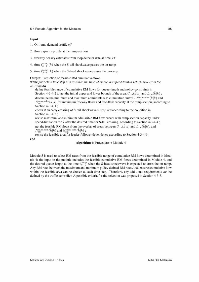
5-4 Pseudo-Algorithm for the Modules 85
Input:
1. On-ramp demand profile qinr
2. flow capacity profile at the ramp section
3. freeway density estimates from loop detector data at time kT
4. time trampS−t (k) when the S-tail shockwave passes the on-ramp
5. time trampS−h (k) when the S-head shockwave passes the on-ramp
Output: Prediction of feasible RM cumulative flows
while prediction time step k̃ is less than the time when the last speed-limited vehicle will cross the
on-ramp dodefine feasible range of cumulative RM flows for queue-length and policy constraints in
Section 4-3-4-2 to get the initial upper and lower bounds of the area, Urm(k̃|k) and Lrm(k̃|k) ;
determine the minimum and maximum admissible RM cumulative curves - Nmin,admrm (k̃ |k) and
Nmax,admrm (k̃ |k) for maximum freeway flows and free-flow capacity at the ramp section, according to
Section 4-3-4-1 ;
check if an early crossing of S-tail shockwave is required according to the condition in
Section 4-3-4-3 ;
revise maximum and minimum admissible RM flow curves with ramp section capacity under
speed-limitation for k̃ after the desired time for S-tail crossing, according to Section 4-3-4-4 ;
get the feasible RM flows from the overlap of areas between Urm(k̃|k) and Lrm(k̃ |k), and
Nmin,admrm (k̃|k) and Nmax,adm
rm (k̃ |k) ;
revise the feasible area for leader-follower dependency according to Section 4-3-4-6;
end
Algorithm 4: Procedure in Module 4
Module 5 is used to select RM rates from the feasible range of cumulative RM flows determined in Mod-
ule 4; the input to the module includes the feasible cumulative RM flows determined in Module 4, and
the desired queue-length at the time trampS−h when the S-head shockwave is expected to cross the on-ramp.
Any RM rate, between the maximum and minimum policy defined RM rates, that ensures cumulative flow
within the feasible area can be chosen at each time step. Therefore, any additional requirements can be
defined by the traffic controller. A possible criteria for the selection was proposed in Section 4-3-5.
Master of Science Thesis Niharika Mahajan

86 Algorithm Development
Niharika Mahajan Master of Science Thesis

Chapter 6
Simulation Design and Evaluation
In the previous chapter, the theory for the advanced approach for integration of ramp metering (RM) with
variable speed limits (VSL) was translated to an algorithmic formulation. The next step involves verifi-
cation of this algorithm, i.e to test if the different modules accurately implement the theoretically desired
control behaviour. In other words, the simulations should demonstrate that the controller does what it has
been built to do. Hence, the simulations are performed in a microscopic simulation environment, and the
results thereof are presented here.
6-1 Introduction
The objective of a simulation based evaluation is to offer a proof of concept for the developed theory. Of
the two integration approaches for combing RM with VSL, the advanced strategy was translated to five
algorithmic modules in Chapter 5. First three of the five modules are implemented in the simulation en-
vironment. Contour plots for spatio-temporal variations of flow, speed, density, actuation segment modes,
detection segment modes and speed limit value are used to analyse the performance of the algorithm.
To that end, aspects relating to the simulation set-up prior to the implementation of the control algorithm are
discussed in Section 6-2. These include the network layout and the traffic characteristics to achieve the test
traffic behaviour, parametric tuning of the original COoperative Speed Control ALgorithm (COSCAL) v2
algorithm, and quantitative criteria for analysing the results. Section 6-3 discusses the simulation results
for different scenarios - from the no control situation to complete implementation of the VSL related
modules in the advanced strategy. Finally, a summary of the key finding from the simulations is presented
in Section 6-4.
6-2 Simulation Set-up
The integrated control strategy is evaluated in version 5.40 of VISSIM - a traffic microsimulation software,
and MATLAB software. VISSIM simulates traffic behaviour, while the controller itself is designed in
MATLAB. The two software communicate via the COM interface; VISSIM communicates relevant traffic
state measurements to the controller in MATLAB, which based on this data communicates back the ap-
propriate control action to be implemented in the subsequent time step. A systematic simulation set-up is
crucial for the accuracy of the simulation results. Hence, in the following sections, the simulation set-up is
discussed:
Master of Science Thesis Niharika Mahajan

88 Simulation Design and Evaluation
6-2-1 Network Characteristics
A freeway merging section of a total length of 20.3 km, comprising of a 10 km long freeway section
upstream of the on-ramp, a 0.3 km long freeway section with an additional merging lane, and a 10 km long
freeway section downstream of the on-ramp is chosen. The length of the network is suitable for visualizing
the spatial extent of a COSCAL v2 scheme in which the stabilization area crosses the ramp location. The
freeway has 2 lanes, while the on-ramp section has a single lane - each lane is 3.5 m wide. Loop detectors
are placed every 100 m and VSL gantries every 500 m, such that the gantry locations coincide with a loop
detector location. Although in practice these infrastructures are typically less dense, this configuration
allows for more accurate implementation and evaluation of the control system. Furthermore, the on-ramp
is metered with a traffic signal located 100 m upstream of the upstream end of the merging area.
6-2-2 Traffic Characteristics
The simulations are performed for homogeneous traffic condition, with a mandatory speed limit of 120
km/h when the VSL scheme is not active. The speed distributions curve for cars defined in VISSIM realizes
an average free-flow speed of 100 km/h in free-flow regime. When VSL scheme is activated, speed limits
of 60 km/h are displayed at the appropriate gantries and an effective speed of nearly 68 km/h is achieved.
Further, VISSIM uses the Wiedamann 99 car following model that consists of ten calibration parameters
to control the driving behaviour of individual vehicles in the simulation model. These parameters relate
to car-following behaviour, lane changing distances, and lane changing behaviour. The tuning of these
parameters is hugely important to simulate realistic traffic situations; in our case, these are (1) efficient
merging condition at the on-ramp, and (2) a capacity drop from a moving jam. The used values of the
Wiedemann 99 parameters are summarized in Table 6-1. These settings result in a freeway capacity of
about 2060 veh/h/lane in simulation.
Table 6-1: Wiedemann 99 car-following model settings in VISSIM
Vissim Code Parameter Default Value Used Value
CC0 Standstill distance 1.5 m 2 m
CC1 Headway time 0.90 s 0.70 s
CC2 Following Variation 4 m 6 m
CC3 Threshold for entering ”Following’ state -8 s -8 s
CC4 Negative ’Following’ Threshold -0.35 -0.1
CC5 Positive ’Following’ Threshold 0.35 0.1
CC6 Speed dependency of oscillation 11.44 6
CC7 Oscillation acceleration 0.25 m/s2 0.25 m/s2
CC8 Standstill acceleration 3.5 m/s2 0.5 m/s2
CC9 Acceleration at 80 km/h 1.5 m/s2 1.5 m/s2
The two main parameters important to generate desirable traffic situation are the standstill distance (CC0)
and standstill acceleration (CC8). Standstill distance is the desirable spacing between vehicles when they
are at rest. The inverse of this distance gives the density in jam state; the higher the standstill distance, the
lower the jam density. As a result, it also determines the slope of the congestion branch in the fundamental
diagram. A higher value than its default setting of 1.5 m ensures the typical propagation velocity of moving
jams in real traffic. Similarly, the setting of the standstill acceleration parameter is crucial to create a
capacity drop from a jam. With a low value of the parameter is chosen, vehicles take longer to accelerate
to free-flow speed after leaving a jam. Hence, a low queue-discharge flow is realized in simulation.
Niharika Mahajan Master of Science Thesis

6-2 Simulation Set-up 89
6-2-3 Tuning Control Parameters
COSCAL v2 uses several control parameters that must be tuned to appropriate values for the algorithm
to perform desirably, i.e to resolve moving jams and improve freeway efficiency. Values of some of these
parameters are chosen based on off-line traffic data, while others must be fine tuned to real-traffic mea-
surements. Details about the tuning process and appropriate values of all the parameters can be found in
(Hegyi, 2013). The used settings of the tuning parameters in COSCAL v2 are tabulated in Table 6-2.
Table 6-2: Values for tuning parameters in COSCAL v2
Related COSCAL
task
Parameter Description Used Value
Jam detection
vth speed threshold for jam detection 30 km/h
zff hysteresis parameter for transition
from free-flow to jam state
100 km/h*s
zjam hysteresis parameter for transition
from jam to free-flow state
-40 km/h*s
Jam resolution
veff effective speed limit 70 km/h
vjam-h jam head propagation speed -5.5 km/h
qjam-h flow that crosses the jam head 3350 veh/h
Stabilization
ρ̄ target density in stabilization area 29 veh/km/lane
dstab offset to check for too high densities 2 km
adec nominal deceleration of vehicles -3 m/s2
Speed limits release v[4A-5A] speed of the S-head shockwave -21 km/h
Resolvability xact,min offset for most upstream point ini-
tial speed limit location
2 km
Jam head tracking vjam-h,max maximum upstream propagation
speed of jam
-72 km/h
Two parameters related to the stabilization scheme have been changed from the original setting, namely,
the propagation speed of the S-head (under zero RM flow condition) and target density in the speed-limited
stabilization area. The S-head speed is changed from its original value of -18 km/h to -21 km/h, and the
stabilization density from 18 veh/km/h to 29 veh/km/lane. The values have been chosen such that the
outflow from the stabilization area is closest to the free-flow capacity, and at the same time, the speed-
limited flow is stable at the set target density. In the current setting, theoretically an outflow of 2181
veh/h/lane (4362 veh/h for 2 lanes) should be realized. Additionally, choosing a faster (more negative)
propagation speed for the S-head offers a higher range of (negative) speeds for the S-head upstream of
the on-ramp. This range determines the admissible range of RM flows for which the S-head shockwave
does not propagate downstream (with a positive slope); the larger the range of negative S-head speeds, the
higher the admissible RM flows can be.
Master of Science Thesis Niharika Mahajan

90 Simulation Design and Evaluation
6-3 Simulation Results
Multiple simulations for different boundary conditions were performed to verify the functioning of the
developed algorithm. Select results from these runs are presented to discuss the control performance and
potential improvements to the algorithm.
6-3-1 Base Case
The base case defines the ’no control’ situation against which an improvement in traffic performance under
different control scenarios can be evaluated. In this study, the no control situation is a moving jam that
results in a capacity drop on the freeway. To that end, a slow moving bottleneck is created by slowing
down vehicle to a speed of 10 km/h in space-time area of 1.1 km and 110 s. This results in a moving
jam as shown in Figure 6-1. The queue discharge flow is about 1802 veh/h/lane (3604 veh/h for two-lane
freeway), resulting in a capacity drop of nearly 12.5 %.
Figure 6-1: Contour plots of the base case showing a moving jam with a queue discharge rate of
approximately 1810 veh/h/lane.
6-3-2 COSCAL v2 without RM
If no additional RM flows disrupt the VSL scheme, the algorithm performs as per the chosen tuning pa-
rameters in Section 6-2-3. As can be observed in Figure 6-2, the moving jam is resolved with speed-limits,
after which the stabilization area (further upstream) ensures an improvement in efficiency. However, it
must be noted that the traffic simulator realizes an average density of 27.5 veh/km/lane for a target density
of 29 veh/km/lane. This results in flow of 4022 veh/h after the jam is resolved. Although this flow is higher
than the queue-discharge flow of 3604 veh/h, it is 7.8% lower than its theoretically expected value of 4362
veh/h (given the target stabilization density and speed of S-head shockwave).
Niharika Mahajan Master of Science Thesis

6-3 Simulation Results 91
Figure 6-2: Contour plots of COSCAL v2 scheme for freeway demand of 1860 veh/h/lane.
6-3-3 COSCAL v2 with stand-alone RM
An important postulate in this work was that when RM and VSL strategies are implemented stand-alone,
the effectiveness of COSCAL v2, as well as overall freeway efficiency are reduced. For this reason, the
performance of COSCAL v2 algorithm with different RM flows was tested.
In order to achieve maximum efficiency improvement, the target density inside the stabilization is set to its
critical value. Its value can be critical due to two possible reasons - either it is the maximum stable density
achievable under speed-limits or it results in a capacity flow downstream of the stabilization area (state
[5A]). Depending on which criteria holds and the value of RM flows, a congestion can be triggered at the
ramp section inside the stabilization area and/or after the S-head shockwave crosses the on-ramp location.
In Figure 6-3, it can be seen that the merging flow initiates a congestion inside the stabilization area just
downstream of the on-ramp. Such a situation is unfavourable since the implementation of COSCAL v2
is limited to a single jam. As a result, the algorithm does not adapt to a jam that occur while the scheme
is active. Furthermore, the unresolved congestion blocks the RM flows, and reduces the flow exiting the
stabilization area. This results in gain of total time spent (TTS). Furthermore, as the freeway demand in-
creases, even a low value of RM flow can result in the onset of congestion. This is illustrated in Figure ??,
wherein a RM flow of 50 veh/h triggers jam waves inside as well as downstream of the stabilization area.
The performance of the algorithm is found to be sensitive to the tuning of the jam resolving parameters.
TTS gains were noted, especially when the tuning parameters underestimate the number of vehicles re-
quired for jam resolution. The outcome is similar to the situation when RM is active and the jam resolving
Master of Science Thesis Niharika Mahajan

92 Simulation Design and Evaluation
area crosses the on-ramp. In such a case, the jam resolving task does not account for the additional merging
vehicles. This leads to intermediate increase in the length of freeway speed-limited for jam resolution, and
hence a lowered effectiveness of the algorithm. For this reason, for all cases with RM flow higher than 100
veh/h, the flow is set to 50 veh/h in the first 1000s to ensure that the jam resolution area does not cross the
on-ramp.
Figure 6-3: Congestion onset in COSCAL v2 scheme with 200 veh/h RM flow & 1860 veh/h/lane
freeway demand.
Niharika Mahajan Master of Science Thesis

6-3 Simulation Results 93
Figure 6-4: Congestion onset in COSCAL v2 scheme with 50 veh/h RM flow & 1880 veh/h/lane
freeway demand.
6-3-4 Advanced strategy for integrated RM with COSCAL v2
Module 1, 2 and 3 of the advanced strategy were implemented in simulation. These modules relate to the
adaptation of the S-head and S-tail shockwaves upstream of the on-ramp, and prediction of the time when
the S-tail will cross the on-ramp. The shockwave trajectories are estimated based on the RM flow which
should merge onto the freeway at any time.
Theoretically, it is expected that as the RM flow increases, the S-head shockwave should become less steep
(less negative slope) and the S-tail shockwave should propagate faster upstream (more negative slope).
The adaptation of S-head reduces the freeway flow arriving after the stabilization area has crossed the
ramp section, and of the S-tail reduces the flow arriving while speed-limitation is active at the location.
The difference in the slope of the S-head shockwave becomes clear on comparing the contour plots in
Figures 6-5 and 6-7. In the latter case, the RM flow is lower and hence the slope of the S-head is more
steep.
The propagation of the S-tail shockwave in Figure 6-5 is determined as per Module 3 of the advanced strat-
egy. The flow and density profile at the on-ramp section for this case are plotted to analyse its performance.
The graphs reflect an increase in density and a decrease in flow between the time the S-tail and the S-head
shockwaves cross the ramp section, i.e during the time speed limits are active at the on-ramp. Additionally,
a few important aspects in the implementation of the module were discovered from the tests related to the
S-tail propagation. These are discussed next:
Master of Science Thesis Niharika Mahajan

94 Simulation Design and Evaluation
Figure 6-5: Contour plots of the integrated approach for 100 veh/h RM flow & 1860 veh/h/lane
freeway demand.
0 500 1000 1500 2000 2500 30000
500
1000
1500
2000
2500
3000
3500
4000
4500
5000
Time (s)
Flo
w (
veh/
h)
(a) Flow profile at the ramp section
0 500 1000 1500 2000 2500 30000
10
20
30
40
50
60
70
80
Time (s)
Den
sity
(ve
h/km
)
(b) Density profile at the ramp section
Figure 6-6: Flow and density profiles at the ramp section for integrated approach with RM flow of
100 veh/h and freeway demand of 1860 veh/h/lane. The vertical lines in either plots indicates the
time instants when the S-tail and S-head shockwaves crossed the ramp location.
Niharika Mahajan Master of Science Thesis

6-3 Simulation Results 95
• Multiple crossing of the S-tail shockwave over ramp location: during theoretical development,
the presumption is that if the S-tail shockwave crosses the ramp location it propagates upstream until
the VSL scheme is resolved upstream of the on-ramp. However, this may not always hold. When the
S-tail shockwave crosses the on-ramp but the freeway demand and the RM flow are not sufficiently
high, S-tail tends to oscillate about the ramp section. This is problematic for two reasons - (1) the
freeway capacity at the section varies in free-flow and under speed limits; so the freeway flow that is
allowed to arrive at the ramp section does not account for these fluctuations in capacity, and (2) the
oscillations can result in vehicles driving in and out of speed-limited area multiple times in a short
interval of time (undesirable from a driving comfort and safety perspective).Such a situation can be
seen in Figure 6-7, where the S-tail tends to oscillate about the on-ramp and as a result propagates
disturbances which lead to a downstream congestion.
Figure 6-7: Contour plots showing oscillations of S-tail shockwave at the ramp section in the
integrated approach; boundary condition include RM flow of 200 veh/h and freeway demand of
1865 veh/h/lane.
• Fast downstream propagation of S-tail shockwave: the theory specifically does not include a
criteria for the maximum positive propagation speed of the S-tail shockwave. However, it is found in
simulation that when the speed-limits are released sharply, i.e. the forward propagating speed of the
shockwave is too high it leads to sudden increase in traffic density that may trigger jam waves. Hence,
speed-limits should not be deactivated too fast. Further testing should be performed to determine
the maximum release speed based on local traffic characteristics. Simulation results in Figure 6-8
exemplify such a situation.
Master of Science Thesis Niharika Mahajan

96 Simulation Design and Evaluation
Figure 6-8: Contour plots showing jam waves from steep downstream propagating S-tail shock-
wave in the integrated approach; boundary condition include 100 veh/h RM flow & 1870 veh/h/lane
freeway demand.
• Downstream propagating S-head shockwave: to lower the mainstream flow according to the ad-
ditional RM flows, the speed of the S-head shockwave upstream of the on-ramp is adjusted. Theo-
retically, it was understood that the higher the RM flows, the higher (less negative) is the required
propagation speed of the S-head.
However, the situation of a downstream propagating S-head shockwave was not anticipated. In
simulation, this was found to be a common occurrence for high RM flows - flows higher than about
350 veh/h/lane (refer to Figure 6-9). A downstream propagating S-head has consequence for the
design of the strategy. In current strategy, the flow capacity at the on-ramp section after the S-head
crosses the on-ramp is taken as the free-flow capacity of the freeway section. However, this capacity
does not hold if the shockwave propagates downstream with a positive slope.
In order to avoid this situation, the original COSCAL v2 parameters were re-tuned, and RM flows
were chosen from within a correspondingly suitable range of values. However, from an implemen-
tation perspective this is restrictive for the RM strategy and can deteriorate the performance of the
queue controller. Therefore, the theory must be adapted to predict such a situation, and to consider
the capacity flow accordingly.
Niharika Mahajan Master of Science Thesis

6-3 Simulation Results 97
Figure 6-9: Scenario showing forward propagating S-head shockwave; boundary condition in-
clude 800 veh/h RM flow & 1860 veh/h/lane freeway demand.
6-3-5 Quantitative evaluation
Total time spent (TTS) is the total time spent by all the vehicle in a network in a given control time interval.
A TTS decrease is indicative of efficiency improvement for similar network inflow profiles in the compared
scenarios. This can be used as the quantitative criteria for measuring improvement in freeway efficiency.
The TTS in the network over a time horizon K , can be theoretically determined as in the equation below.
Here, N(k) are the total number of vehicles in the network in time step k.
TTS = T
K∑
k=0
N(k) (6-1)
A desirable control strategy should then minimize the TTS. The minimization of the TTS is mathematically
equivalent to maximization of the time-weighted freeway outflows in that time horizon. The proof for their
equivalence can be found in Papageorgiou et al. (2003). Lets denote the time-weighted flow as TWF, which
can be formulated as:
TWF = T 2K−1∑
k=0
(K − k)qout(k) (6-2)
Master of Science Thesis Niharika Mahajan

98 Simulation Design and Evaluation
here, qout(k) is the flow exiting at the downstream end of the network at time step k.
Furthermore, TTS can alternately be determined from an estimate of TWF. In its formulation below, N(k)is the the total number of vehicles on the network and qin(k) the freeway demand at time step k:
TTS = T
K∑
k=0
(
N(0) +
k−1∑
κ=0
qin(κ)
)
− TWF (6-3)
= T KN(0) + T 2K−1∑
k=0
(K − k)qin(k) − TWF
The advantage of formulating TTS in terms of TWF is that it does not require individual vehicle data or
density measurements over the freeway length which are typically less accurate. Therefore, the above
macroscopic formulation of TTS is suitable for the formulation of COSCAL v2 and its extensions.
The criteria is used to get a rough estimate of the impact of the developed strategy on freeway efficiency.
However, initial results with the above criteria were not very conclusive. A TTS of 575.7 veh*h is reported
for the base case in Figure 6-1. Only a 2.3% improvement in TTS was found when COSCAL v2 is
implemented without RM (Figure 6-2). This is unrealistic since the jam is resolved and capacity drop of
about 12.5% is recovered. Likewise, for the advanced strategy with 100 veh/h RM flows the TTS is 569.9
veh*h - not reflective to the improvement observable from its contour plot in Figure 6-5. It is therefore
recommended that the implementation of the criteria and other possible reasons for conflicting results
should be further investigated.
6-4 Summary
Simulation results in this chapter offer some evidence for the feasibility of the developed integration strat-
egy in Chapter 4. Contour plots for select traffic and control variables for the no-control case, COSCAL v2
without RM, COSCAL v2 with RM, and COSCAL v2 integrated with RM were compared to demonstrate
the potential improvements from the developed approach; these include -
• In COSCAL v2, congestion aggravates as RM flow increases. The integrated strategy can regulate
the freeway flows arriving at the ramp to prevent such breakdown.
• Jam resolution parameters of COSCAL v2 require fine-tuning such that the number of speed-limited
vehicles required for jam resolution are not under-estimated. An identical undesirable effect oc-
curs when RM is not integrated with VSL. This is because the additional merging vehicles are not
included in the prediction of the jam resolution area, and the feedback structure of COSCAL v2
responds by abruptly extending speed-limits at some future time instants. Such under-estimation of
the jam resolution area can have a huge effect on the overall VSL performance.
• The integrated strategy is currently suitable for a range of RM flows based on the chosen stabilization
parameters of COSCAL v2. The restriction follows from downstream propagation of the S-head
shockwave for higher ramp flows.
Learnings from the simulations that should guide some additional considerations for the integrated strategy
include -
• The capacity function at the ramp section is crucial to the prediction of the VSL scheme in the
integrated strategy. This function should be responsive to the actual propagation of the S-head and
S-tail shockwaves, in a way it not currently implemented. However, the feedback structure of the
algorithm is suitable for necessary development.
Niharika Mahajan Master of Science Thesis

6-4 Summary 99
• A slow moving vehicle due to the merging mechanism at the ramp section can result in disturbances
in the stabilization area. These were typically observed as widening downstream propagating gaps
in simulation tests. A possible reasoning could be that the high density stabilization area is prone
to moving bottlenecks, easily triggered for even slightly lower speeds than the effective speed limits
value. Alternately, it could possibly be due to unrealistic driving behaviour in Vissim.
• Multiple crossings of the S-tail shockwave can be dealt with a responsive capacity function. How-
ever, an alternative could be to prevent such an occurrence by suitable selection of RM rate in Mod-
ule 5 of the advanced strategy. An increased RM rate would necessitate a lower freeway flow at the
ramp section, and hence extension of speed-limits further upstream.
Master of Science Thesis Niharika Mahajan

100 Simulation Design and Evaluation
Niharika Mahajan Master of Science Thesis
Chapter 7
Conclusion
Variable speed limits (VSL) strategies have been found to be effective as a preventive and counter-active
traffic control measures. A macroscopic speed control algorithm, COoperative Speed Control ALgo-
rithm v2 (Hegyi, 2013), was specifically studied in this work. The research objective was to adapt and
extend the algorithm for integration with ramp metering (RM) control measure. To that end, the key focus
remained on theoretical advancement and its functional verification in simulation.
In this chapter, first, the motivations and main contributions are broadly presented in Section 7-1. Next,
Section 7-2 describes how the three main research objectives were met. Subsequently, practical and policy
recommendations for further development, and field implementation of the control system are made in
Section 7-3.
7-1 Motivation and contributions
This research was motivated by a practical difficulty in implementing COSCAL v2. On-ramp sections are
potential bottlenecks for activation of the variable speed limits (VSL) strategy. However, ramp flows are
not included in the design of the algorithm. This deteriorates the effectiveness of the algorithm at these
merging sections. Simulation results in Chapter 6 demonstrated how additional flows at a freeway merging
section can result in jam waves while the VSL scheme is still active. This is an undesirable situation that
can result in increased total time spent (TTS) on the freeway, reduced merging flows and hence, faster
growing queues at the on-ramp.
Furthermore, RM measure on the one hand can improve: the efficiency on the freeway, and the effectiveness
of COSCAL v2, on the other, it can result in deteriorated performance of the sub-network. This is because
RM and ramp queue control are inherently competitive - the lower the RM flows, the faster the queue on
the on-ramp grows. However, the situation gets problematic for the VSL strategy if the ramp queue spills
over to the sub-network. When this happens, RM control is switched off to release the on-ramp queue and
restore traffic deterioration of the lower network. The abrupt influx from the on-ramp can disrupt the VSL
scheme deteriorating freeway performance. This trade-off between efficiency improvement for the freeway
and the urban network - in implementing two traffic control measures - offers a research opportunity.
Therefore, two possible theoretical extensions to the COoperative Speed Control ALgorithm (COSCAL) v2
algorithm for integration with RM were developed in this work:
• A basic integration approach that can resolve moving jams to improve freeway efficiency, given a
constant RM flow. The extension fits with the reactive formulation of the original algorithm, and
Master of Science Thesis Niharika Mahajan
102 Conclusion
uses a similar feedback structure to generate the VSL scheme at each time step based on traffic
measurements in the previous. This approach can prevent a spillback of on-ramp queue as long as
a suitably high RM flow is chosen that the VSL strategy can be adapted for (given its controller
parameters).
• An advanced integrated strategy that balances efficiency improvement on the freeway with deterio-
ration of urban network from ramp queue spillback. The advantage in this strategy is derived from
its integration approach that uses cumulative curves to combine RM, VSL and queue control. Cu-
mulative curves are applied to determine a range of feasible RM flows that consider: queue-length
constraints, policy restrictions on maximum and minimum RM rates, the VSL approach and the
freeway state. Further, COSCAL v2 is extended to guarantee jam resolution while RM flows are
chosen from within this feasible range. Both RM and VSL approaches are anticipatory, and predict
the scheme in the future to determine optimal control decisions in the current time step. Therefore,
queue spillback on-ramp and freeway breakdown - while speed-limits are active - are pro-actively
prevented in this approach.
The exploration of two different extensions to COSCAL v2 has highlighted the advantage of anticipatory
traffic control for higher responsiveness. In the predictive formulation of the advanced RM strategy, proac-
tive decisions can be made for a deteriorating traffic condition on the freeway or on the on-ramp at a later
time.
The advanced strategy was therefore developed to an algorithmic version that can implemented to a con-
troller. Due to time constraints, only a few algorithmic modules of the advanced strategy could be evaluated
in simulation. The insights from the simulation study are used to recommend further improvements to the
developed theory.
7-2 Findings and recommendations
The main findings and the recommendations thereof are presented in this section, by addressing the research
objectives that were designed to answer the main research question, restated below -
"Can a macroscopic variable speed control strategy integrated with ramp metering improve freeway effi-
ciency, while managing queues at a merging section?"
7-2-1 Research Objective 1: Learnings from literature survey
The literature survey was conducted with three main objectives: (1) to identify different traffic flow the-
oretic and different control approaches to dynamic speed limits, (2) to understand the desirable features
for an on-ramp queue controller, and (3) to find the most important considerations for integration of
COSCAL v2 with RM.
To that end, first VSL approaches were differentiated as those resulting in traffic homogenization, and
those resulting in flow reduction. The importance of the implementation dynamics for flow reduction
based approaches was presented. Here, the flow reduction approaches were further classified on the basis
of implementation mechanics as: instantaneous speed limits applied over a length of freeway at the same
time; stationary speed limits applied at a fixed freeway section for a considerable time interval; and speed
limits with moving fronts which include all intermediate scenarios between instantaneous and stationary
implementation of VSL. Regulating the fronts (shockwaves) of the speed-limited area allow to create traffic
states with desired flow and density conditions. Further, VSL were understood from a control perspective.
Here, regulatory strategies were found to be a middle ground between the low responsiveness of heuristic
approaches and high computational demand of model-based optimization approaches.
Next, various queue management approaches were surveyed to identify some design guidelines for a queue
controller. The most important requisite was found to be that the queue controller should not result in
Niharika Mahajan Master of Science Thesis

7-2 Findings and recommendations 103
underutilization of the on-ramp storage capacity. Therefore, a minimum ramp queue length requirement
was recommended. Also, the triggers for override of control decisions from the queue controller should be
well-defined. It was identified that the performance of the queue management approach can be sensitive to
the length (storage capacity) of the on-ramp. This is an important consideration for field implementation
and should be tested for. Lastly, it was suggested that the criteria for deactivation of queue management -
when the freeway is in a congested traffic state - should be identified in the design of the controller.
Lastly, a key advantage of integrating control measures is that the traffic can be continued to be managed,
even when restrictions for one of the measures are reached. For the integration of RM with VSL con-
trol measure, ramp queue violation was understood as important. The response of the integrated strategy
to queue restrictions being reached on the on-ramp can be limited by its complexity and computational
demand.
7-2-2 Research Objective 2: Development of COSCAL v2 for integrationwith ramp metering
The second research objective entailed development of an integrated VSL and RM strategy that improves
freeway efficiency and prevents spillback of on-ramp queues.
To achieve this goal, COSCAL v2 algorithm was used as the testbed for an integrated control strategy.
Some theoretical assumptions and simplifications were made while developing the new theory. In order to
ensure the functional correctness of the algorithm, these assumptions must be recognised.
The validity of these assumptions determines how realistically the traffic behaviour is represented, and how
well the desired behaviour can be achieved from application of the control strategy in practice. While some
of these assumptions can relaxed by tuning the controller parameters, others should be relaxed for desired
performance. The main assumptions are summarised below:
7-2-2-1 Theoretical assumptions
(1) A constant average free flow speed. Traffic information in free flow regime is assumed to propagate
forward, in the direction of the traffic, at this speed; free flow speed of 100 km/h was used in the
simulation study.
(2) A constant effective speed under speed limits. This assumes requisite compliance to the displayed
speed limit value; an effective speed of 70 km/h for displayed speed limits of 60 km/h was used in the
simulation study.
(3) Homogeneous traffic flow conditions within the length of each detection segment; a regular detection
segment length of 100 m was used in simulation.
(4) A known on-ramp demand profile for the duration of the VSL scheme.
(5) Constant capacity of the freeway on-ramp section in free-flow condition and under speed limits.
7-2-2-2 Basic and advanced integrated VSL and RM strategies
Two alternative integrated strategies were developed, as mentioned earlier. The main characteristics, advan-
tages and shortcomings of the two strategies are concluded here. The theoretical development was initiated
with a basic extension of COSCAL v2 that is compatible with its current formulation. The core principle
employed in this strategy is to lower the density in the area upstream of the on-ramp that is speed-limited
for stabilization. The reduced density is chosen to sufficiently decrease the flow arriving at the on-ramp.
This is theoretically possible, since the speed within the controlled freeway stretch is the effective speed
under speed-limitation. Then, lowering the density achieves a lower flow. This is understood from the
Master of Science Thesis Niharika Mahajan

104 Conclusion
fundamental relationship between traffic flow variables - flow q(k), density ρ(k) and space-mean speed
v(k):
q(k) = ρ(k) × v(k) (7-1)
However, there are some limitations to the basic RM strategy which were addressed in the advanced RM
strategy. In the basic strategy, a desired density criterion determines the most upstream speed-limited seg-
ment, i.e. the tail of the stabilization area. This is less desirable because in order to reduce the flow at the
ramp section, the target density in the entire stabilization area upstream of the on-ramp must be lowered.
A lower target density also implies an increase in the spatio-temporal area that should be speed-limited
and hence, an increase in TTS. This is also why the strategy holds only for a constant RM flow rate. A
varying RM flow requires a varying desired freeway flow at the on-ramp section. In turn, to achieve this,
a variable target density is needed over the freeway segments at any given time. The density distribution
thus required is one, hard to estimate, and second, hard to implement given how target density is realized
in COSCAL v2. The requirement of a constant RM rate leads to another limitation from this strategy. If
the integrated strategy is to prevent a queue spillback at the on-ramp, the ramp controller must enforce the
least restrictive (highest) RM rate, which is not optimal for freeway efficiency.
In an alternate methodology, the VSL approach in the advanced strategy was extended to be compatible
with time-varying RM flows. The approach used for this regulates the propagation of the upstream and
downstream fronts of the speed-limited area. In doing so, a desired freeway flow - based on the RM flows
and the capacity at the ramp section - can be achieved at any given time. This extension required translation
of microscopic traffic flow concepts to a macroscopic formulation compatible with COSCAL v2.
Additionally, a cumulative curves based approach was used for the design of a new RM strategy, and for its
integration with the extended VSL approach. The approach can determine a range of feasible RM flows,
given a known on-ramp demand profile. A unique advantage of the approach is that it includes queue-
length restrictions on the on-ramp, and the most restrictive implementation of speed-limits, to determine
the achievable ramp flows. Furthermore, both RM and VSL use a predictive approach wherein the control
scheme is determined over a prediction horizon at each time step. Therefore, both control measures pro-
actively determine control based on traffic predictions in the future, making it more suitable for on-ramp
queue management. In other words, the integrated strategy pro-actively prevents a queue-spillback at the
on-ramp. The advantages of the advanced strategy were interesting for testing in simulation. The main
insights from the simulation study are presented next.
7-2-3 Research Objective 3: Verification of the algorithm
The third research objective is to check for the functional correctness of the developed strategy by means
of simulation.
To achieve this objective, the advanced integrated strategy was translated to an algorithm that enables the
controller to achieve the desired control behaviour. The algorithmic formulation of COSCAL v2 was used
as a basis for this - using unique driving modes to identify the different detection and actuation states in its
implementation. Furthermore, the developed integration strategy was identified into five unique modules,
three relating to the VSL measure and two to RM. Pseudo-algorithms for all of these modules were de-
tailed. However, only modules related to the VSL approach were implemented in Vissim micro-simulation
environment. The simulations performed for different traffic scenarios suggest a potential improvement in
freeway efficiency from the approach. Jam waves that otherwise occur from independent implementation
of VSL and RM were prevented by the adaptation of the S-head and S-tail shockwaves in the advanced
strategy.
Some critical design limitations were highlighted in the evaluation process. Firstly, the capacity profile at
the on-ramp section is based on the prediction of the first time that the S-head and the S-tail shockwaves
Niharika Mahajan Master of Science Thesis

7-3 Future work and practical implications 105
cross the on-ramp (while propagating upstream). It is assumed that the arriving flows at this section are
speed-limited between these time instants. However, depending on the freeway demand, fluctuations in
RM flow can cause the shockwaves to cross the on-ramp multiple times. A higher flow arrives at free
flow speed each time the S-tail propagates downstream over the on-ramp, triggering disturbances at the
location. Therefore, if the capacity function is responsive to the actual propagation of these shockwaves,
these disturbances can be avoided. The capacity profile is determining in the estimation of these shockwave
trajectories, and hence, this very relevant for implementation of the strategy in practice.
Secondly, when the ramp controller orders high RM flow (after the S-head crosses the on-ramp), the desired
S-head trajectory propagates downstream of the on-ramp. This situation was not anticipated during theo-
retical development. Simulation tests were therefore restricted to suitable range of RM values. However,
this restriction could be relaxed with some modifications to Module 3 of the algorithm.
Finally, the VSL strategy uses the freeway traffic measurements at any time to predict the evolution of
the VSL scheme. The prediction horizon in the approach extends till the time the most upstream vehicle
that enters speed-limitation has crossed the on-ramp location. Therefore, the duration of the prediction
horizon depends on the detection location of the jam, and the traffic condition on the freeway. The longer
the prediction horizon gets, traffic data from detection segments even further upstream is required for the
prediction of the VSL scheme. In simulation, traffic data further upstream of the network boundary was
required. This was resolved by assuming constant values of the traffic flow variables upstream of the first
detection segment. Since detector measurements over extremely long freeway lengths is a practical limita-
tion as well, the inaccuracy of the assumption should be validated with real traffic data.
This work has in part demonstrated the conceptual validity of the tested integrated strategy. Therefore, there
is substantial potential and need for further evaluation - in terms of correctness and performance - of the
developed theory. Subsequent research steps should be performed for a complete evaluation. These include:
(1) implementation of the RM related modules, (2) testing the complete strategy with more dynamic RM
flow profile, and (3) exhaustive quantitative analysis of efficiency improvement from the approach for the
advanced integrated strategy. The basic strategy must be translated to an algorithmic formulation first, and
then verified and evaluated for performance.
7-3 Future work and practical implications
In this section, a discussion on the future research and practical implications of the performed research
is presented. Suggestions for theoretical modules that directly complement the developed theory are
made first. Then, the most important considerations for testing the strategy in a field-test, and support-
ing decision-making are discussed.
7-3-1 Recommendations for further theoretical development
This research initiated theory development towards addressing a practical problem that faces the imple-
mentation of COSCAL v2 at freeway merging sections. In the process, some theoretical bottlenecks, and
some useful extension possibilities have come forth. Theoretical directions, in addition to the ones that
followed from the simulation-based evaluation, are recommended here.
(1) Adjusting the speed of the S-head shockwave downstream of the on-ramp: the integration strategy was
based on controlling the propagation of the S-head and S-tail shockwaves upstream of the on-ramp
location. In doing so, the mainstream flows arriving at the on-ramp could be regulated desirably. The
same theoretical principle can be useful to dynamically control the outflow from the S-head shockwave
downstream of the on-ramp.
In an interesting application, the S-head speed could be adapted to counteract inefficiencies, created
as a result of the control strategy or measured otherwise. As an example, consider the situation when
Master of Science Thesis Niharika Mahajan

106 Conclusion
the combined freeway and RM flows exceed the capacity at the on-ramp section. If this occurs before
speed-limits cross the on-ramp, the designed response is to instantaneously apply speed-limits till the
on-ramp location, at the earliest time of capacity overshoot (Section 4-3-4-3). However, doing so
creates a downstream propagating low flow gap, of the size of the time difference between the time
that the capacity overshoots and the time that the speed-limits would have otherwise crossed the on-
ramp. The gap is the case of an inefficiency that is a result of the control strategy itself. Such an
inefficiency can be eliminated by appropriate and timely adjustment of the S-head shockwave.
(2) Relaxing the assumption of known on-ramp demand: in the developed strategy, especially the queue
controller, depends crucially on the prediction of on-ramp demand flow profile for the duration of the
VSL scheme. This function is assumed as a known in the current formulation. However, present-
day systems do not allow for sufficiently accurate demand forecasts. Relaxation of this assumption
therefore is an important theoretical development for testing the algorithm in practice.
Aside from the readiness of better prediction models in the future, a potential solution could be to use
more restrictive thresholds for the control parameters. For instance, the desired maximum queue length
in the queue controller could be set to an appropriate fraction of its maximum possible value such that
inaccuracies in the demand forecast are compensated. Alternately, it could be explored how to adapt
the strategy to be independent of the on-ramp demand profile.
7-3-2 Considerations for field implementation
(1) Detection-actuation and communication delays: In the developed control strategy, measurements at
each time step are used to predict the control scheme for the remaining duration of the scheme. This
informs the control action in the subsequent time step. However, depending on the size of the control
time step, a variation in the delays between (1) when traffic measurements are available, (2) the compu-
tation time of the control algorithm, and (3) the time it takes for the generated scheme to be displayed
on the speed limit gantries, is likely. Depending on the magnitude of these delays, the performance of
the algorithm may be affected.
Hence, from an implementation point of view, it is important to estimate these delays and to compen-
sate for them in the control algorithm.
(2) Estimation of vff speed: The prediction methodology in the advanced integrated strategy uses an es-
timate of the average free-flow speed. This value however is dependent on multiple factors - road
design, flow rates, traffic composition (e.g. higher truck percentage would result in a lower vff ), and
external time-dependent factors (e.g. day-light, weather condition etcetera). Therefore, accuracy of the
prediction model may require time to time on-line tuning of the free-flow speed.
(3) Length of the detection segments: Even though the developed theory is suitable for varying detection
segment lengths, it has not been tested for the same. This is considered important because, the predic-
tion of the control scheme in each time step assumes homogeneous traffic condition in each segment.
If the length of the segment gets too long, the assumption may not be valid.
Overall, the control scheme prediction translates measurements from the detection segments to cumu-
lative curves at the on-ramp location. This implies that the density/ scarcity of loop detectors on the
freeway can influence the accuracy of the predictions.
7-3-3 Policy implications
One of the hurdles in the implementation of new traffic control measures is their compatibility with more
widely used control measures. Lack of coordination between multiple measures deployed simultaneously
can compromise benefits from either strategies. By developing approaches to integrate a sophisticated VSL
approach with RM measure, an advance has been made in this regard. The contributions in this work will
enable a more smooth implementation of the VSL strategy in practice.
Niharika Mahajan Master of Science Thesis

7-3 Future work and practical implications 107
Specifically, the integration of a control measure with RM raises a policy concern. The current policy
is designed to balance losses from congestion on freeways (managed centrally), and queuing on ramps
and subsequent performance deterioration on the urban network (managed regionally). The directive is
to deactivate RM if the ramp queue spills-back onto a lower network. Consideration for a sudden surge
in merging RM flow must be made when integrating RM with another measure. Adding queue-length
constraints to a RM strategy prevents queue-spillback, and hence the occurrence of such a situation. In the
design of the advanced integrated strategy, queue-length constraints were additionally incorporated for this
reason.
Additionally, simulation tests revealed some safety concerns in implementing the advanced strategy. A
high variation in the RM flows can result in a significant fluctuation in the estimated propagation of the
S-tail shockwave. Multiple simultaneous fluctuations would imply that vehicles drive in and out of speed-
limits more than once in a fairly short interval of time, which is undesirable from driving safety perspec-
tive. Therefore, policy directive should guide development of a smoothing module that dampens over-
fluctuations to ensure vehicles drive into speed-limits once in a VSL scheme. Furthermore, large values of
positive slopes (fast downstream propagation) of the S-tail shockwave can destabilize traffic to trigger jam
waves. Therefore, a suitable maximum value of the S-tail shockwave must be determined. This also leads
to an understanding that VSL scheme should not be deactivated abruptly from another conflicting policy.
The potential of vehicle-to-vehicle and vehicle-to-infrastructure communication is increasingly being ex-
plored for traffic management. In that regard, the VSL approach is forward-looking; while COSCAL v2
algorithm uses vehicle-to-infrastructure communication in the detection tasks, COSCAL v1 is compatible
for both, in-car detection and actuation. The benefits of vehicular intelligence for COSCAL v2 include
faster jam detection, better jam tracking and more accurate traffic state estimation. The advanced integra-
tion approach can additionally benefit from in-car technology - (1) infrastructure-to-vehicle communication
can improve compliance to speed limits, (2) speed-limits can be communicated more timely resulting in
a more accurate realization of the desired trajectories of the stabilization fronts, and (3) vehicle-to-vehicle
communication can facilitate assisted merging; thereby, more homogeneous flow can be achieved at the
ramp section.
Master of Science Thesis Niharika Mahajan

108 Conclusion
Niharika Mahajan Master of Science Thesis

Bibliography
(2006). Controlled motorways m25. Technical report.
Alessandri, A., Di Febbraro, A., Ferrara, A., & Punta, E. (1999). Nonlinear optimization for freeway
control using variable-speed signaling. Vehicular Technology, IEEE Transactions on, 48(6), 2042–2052.
Allaby, P., Hellinga, B., & Bullock, M. (2007). Variable speed limits: Safety and operational impacts of a
candidate control strategy for freeway applications. Intelligent Transportation Systems, IEEE Transac-
tions on, 8(4), 671–680.
Carlson, R. C., Manolis, D., Papamichail, I., & Papageorgiou, M. (2012). Integrated ramp metering and
mainstream traffic flow control on freeways using variable speed limits. Procedia-Social and Behavioral
Sciences, 48, 1578–1588.
Carlson, R. C., Papamichail, I., & Papageorgiou, M. (2011). Local feedback-based mainstream traffic flow
control on motorways using variable speed limits. Intelligent Transportation Systems, IEEE Transactions
on, 12(4), 1261–1276.
Carlson, R. C., Papamichail, I., & Papageorgiou, M. (2014). Integrated feedback ramp metering and
mainstream traffic flow control on motorways using variable speed limits. Transportation Research Part
C: Emerging Technologies, 46, 209–221.
Carlson, R. C., Papamichail, I., Papageorgiou, M., & Messmer, A. (2010). Optimal motorway traffic flow
control involving variable speed limits and ramp metering. Transportation Science, 44(2), 238–253.
Cassidy, M. J. & Rudjanakanoknad, J. (2005). Increasing the capacity of an isolated merge by metering its
on-ramp. Transportation Research Part B: Methodological, 39(10), 896–913.
Chung, K., Rudjanakanoknad, J., & Cassidy, M. J. (2007). Relation between traffic density and capacity
drop at three freeway bottlenecks. Transportation Research Part B: Methodological, 41(1), 82–95.
Directive 2010/40/EU (2010). Directive 2010/40/EU. (207), 1–4.
Gordon, R. L. (1996). Algorithm for controlling spillback from ramp meters. Transportation Research
Record: Journal of the Transportation Research Board, 1554(1), 162–171.
Grumert, E. & Tapani, A. (2012). Impacts of a cooperative variable speed limit system. Procedia-Social
and Behavioral Sciences, 43, 595–606.
Hegyi, A. (2013). A roadside-cooperative speed control algorithm to resolve moving jams (COSCAL v2).
Technical report, TU Delft. Sponsoring organization: Rijkswaterstaat – Water, Verkeer en Leefomgev-
ing.
Master of Science Thesis Niharika Mahajan

110 BIBLIOGRAPHY
Hegyi, A. (2014). An overview of speed control approaches to improve freeway traffic flow. In Control
Conference (ECC), 2014 European, (pp. 2264–2267). IEEE.
Hegyi, A. & Hoogendoorn, S. (2010). Dynamic speed limit control to resolve shock waves on freeways-
field test results of the specialist algorithm. In Intelligent Transportation Systems (ITSC), 2010 13th
International IEEE Conference on, (pp. 519–524). IEEE.
Hegyi, A., Hoogendoorn, S., Schreuder, M., Stoelhorst, H., & Viti, F. (2008). Specialist: A dynamic speed
limit control algorithm based on shock wave theory. In Intelligent Transportation Systems, 2008. ITSC
2008. 11th International IEEE Conference on, (pp. 827–832). IEEE.
Hegyi, A., Shladover, S., Lu, X.-Y., & Chen, D. (2013). A cooperative speed control algorithm to resolve
jams. Technical report, TU Delft. v1.2.
Hellinga, B. & Mandelzys, M. (2011). Impact of driver compliance on the safety and operational impacts
of freeway variable speed limit systems. Journal of Transportation Engineering, 137(4), 260–268.
Hoogendoorn, S. & Knoop, V. (2012). Traffic flow theory and modelling. In v. B. Wee, A. J. Annema,
& D. Banister (Eds.), The Transport System and Transport Policy: An Introduction chapter 7. Edward
Elgar Publishing Limited.
Jiang, R., Chung, E., & Lee, J. B. (2012). Local on-ramp queue management strategy with mainline speed
recovery. Procedia-Social and Behavioral Sciences, 43, 201–209.
Jonkers, E., Wilmink, I., Stoelhorst, H., Schreuder, M., & Polderdijk, S. (2011). Results of field trials
with dynamic speed limits in the netherlands: improving throughput and safety on the a12 freeway. In
Intelligent Transportation Systems (ITSC), 2011 14th International IEEE Conference on, (pp. 2168–
2173). IEEE.
Kerner, B. S. & Rehborn, H. (1996). Experimental features and characteristics of traffic jams. Physical
Review E, 53(2), R1297.
Kotsialos, A. & Papageorgiou, M. (2004). Efficiency and equity properties of freeway network-wide ramp
metering with amoc. Transportation Research Part C: Emerging Technologies, 12(6), 401–420.
Li, D., Ranjitkar, P., & Ceder, A. (2014a). A Logic Tree Based Algorithm for Variable Speed Limit
Controllers To Manage Recurrently Congested Bottlenecks. In Transportation Research Board 93rd
Annual Meeting.
Li, D., Ranjitkar, P., & Ceder, A. (2014b). Integrated Approach Combining Ramp Metering and Vari-
able Speed Limits to Improve Motorway Performance. In Transportation Research Board 93rd Annual
Meeting.
Lu, X.-Y., Varaiya, P., Horowitz, R., Su, D., & Shladover, S. E. (2011). Novel freeway traffic control with
variable speed limit and coordinated ramp metering. Transportation Research Record: Journal of the
Transportation Research Board, 2229(1), 55–65.
Netten, B., Hegyi, A., Wang, M., Schakel, W., Yuan, Y., Schreiter, T., van Arem, B., van Leeuwen, C., &
Alkim, T. (2013). Improving moving jam detection performance with v2i communication. In Proceed-
ings 20th World Congress on Intelligent Transport Systems, number EPFL-ARTICLE-188480.
Nissan, A. & Koutsopoulosb, H. N. (2011). Evaluation of the impact of advisory variable speed limits on
motorway capacity and level of service. Procedia-Social and Behavioral Sciences, 16, 100–109.
Papageorgiou, M., Diakaki, C., Dinopoulou, V., Kotsialos, A., & Wang, Y. (2003). Review of road traffic
control strategies. Proceedings of the IEEE, 91(12), 2043–2067.
Papageorgiou, M., Kosmatopoulos, E., & Papamichail, I. (2008). Effects of variable speed limits on mo-
torway traffic flow. Transportation Research Record: Journal of the Transportation Research Board,
2047(1), 37–48.
Niharika Mahajan Master of Science Thesis

BIBLIOGRAPHY 111
Papageorgiou, M. & Kotsialos, A. (2000). Freeway ramp metering: An overview. In Intelligent Trans-
portation Systems, 2000. Proceedings. 2000 IEEE, (pp. 228–239). IEEE.
Papamichail, I. & Papageorgiou, M. (2008). Traffic-responsive linked ramp-metering control. Intelligent
Transportation Systems, IEEE Transactions on, 9(1), 111–121.
Scarinci, R., Heydecker, B., & Hegyi, A. (2013). Analysis of traffic performance of a ramp metering
strategy using cooperative vehicles. In 16th International IEEE Conference on Intelligent Transportation
Systems (ITSC 2013), number EPFL-ARTICLE-188478, (pp. 324–329). IEEE.
Schakel, W. J. & van Arem, B. (2013). Improving traffic flow efficiency by in-car advice on lane, speed,
and headway.
Smaragdis, E. & Papageorgiou, M. (2003). Series of new local ramp metering strategies: Emmanouil
smaragdis and markos papageorgiou. Transportation Research Record: Journal of the Transportation
Research Board, 1856(1), 74–86.
Smulders, S. (1990). Control of freeway traffic flow by variable speed signs. Transportation Research Part
B: Methodological, 24(2), 111–132.
Spiliopoulou, A. D., Manolis, D., Papamichail, I., & Papageorgiou, M. (2010). Queue management tech-
niques for metered freeway on-ramps. Transportation Research Record: Journal of the Transportation
Research Board, 2178(1), 40–48.
Van de Weg, G. (2013). Cooperative systems based control for integrating ramp metering and variable
speed limits. Masters thesis, TU Delft.
Van de Weg, G., Hegyi, A., Hellendoorn, H., & Shladover, S. E. (2014). Cooperative Systems Based
Control for Integrating Ramp Metering and Variable Speed Limits. In Transportation Research Board
93rd Annual Meeting.
van Toorenburg, J. (1983). Homogeniseren. effekt van aangepaste adviessnelheid op de verkeersafwikkel-
ing. Traffic Engineering Division, Dutch Ministry of Transport, The Hague.
Waller, S. T., Ng, M., Ferguson, E., Nezamuddin, N., & Sun, D. (2009). Speed harmonization and peak-
period shoulder use to manage urban freeway congestion. Technical Report FHWA/TX-10/0-5913-1,
University of Texas at Austin,Texas A & M University-Kingsville.
Wang, Y., Papageorgiou, M., Gaffney, J., Papamichail, I., & Guo, J. (2010). Local ramp metering in the
presence of random-location bottlenecks downstream of a metered on-ramp. In Intelligent Transporta-
tion Systems (ITSC), 2010 13th International IEEE Conference on, (pp. 1462–1467). IEEE.
Weg, V. d. G. & Hegyi, A. (2014). Resolvability analysis of moving jams on the a13. Technical report,
Delft University of Technology.
Weikl, S., Bogenberger, K., & Bertini, R. L. (2013). Traffic management effects of variable speed limit
system on a german autobahn. Transportation Research Record: Journal of the Transportation Research
Board, 2380(1), 48–60.
Zhang, M., Kim, T., Nie, X., Jin, W., Chu, L., & Recker, W. (2001). Evaluation of on-ramp control
algorithms. California Partners for Advanced Transit and Highways (PATH) working paper ; UCB-ITS-
PWP-2001-14.
Master of Science Thesis Niharika Mahajan

112 BIBLIOGRAPHY
Niharika Mahajan Master of Science Thesis

Glossary
List of Acronyms
VSL variable speed limits
VMS variable message signs
RM ramp metering
SPECIALIST SPEed Controlling ALgorIthm using Shockwave Theory
COSCAL COoperative Speed Control ALgorithm
TTS total time spent
TWF time weighted flow
FD fundamental diagram
ALINEA Asservissement linéaire d’entrée autoroutière
MTFC Mainstream Traffic Flow Control
HERO HEuristic Ramp-metering coOrdination
AMOC Advanced Motorway Optimal Control
CRM Coordinated Ramp Metering
AMOC Advanced Motorway Optimal Control
MPC Model Predictive Control
Master of Science Thesis Niharika Mahajan

114 Glossary
Niharika Mahajan Master of Science Thesis