* Corresponding author. Tel.: TelFax: +91 11 27666672 E-mail: ckjaggi@or.du.ac.in, ckjaggi@yahoo.com (C. K. Jaggi) © 2010 Growing Science Ltd. All rights reserved. doi: 10.5267/j.ijiec.2010.07.003

  

International Journal of Industrial Engineering Computations 2 (2010) **–**

Contents lists available at GrowingScience

International Journal of Industrial Engineering Computations

homepage: www.GrowingScience.com/ijiec   

 

Economic order quantity model for deteriorating items with imperfect quality and permissible delay on payment

 

Chandra K. Jaggia*, Satish K. Goela and Mandeep Mittalb

aDepartment of Operational Research, Faculty of Mathematical Sciences, New Academic Block, University of Delhi, Delhi-110007, India bAmity School of Engineering and Technology, 580-Delhi Palam, Vihar Road, Bijwasan, New Delhi-110061, India

A R T I C L E I N F O A B S T R A C T

Article history: Received 10 July 2010 Received in revised form 12 October 2010 Accepted 14 October 2010 Available online 14 October 2010

  In the classical inventory models, most of the time the issue of quality has not been considered. However, in realistic environment, it can be observed that there may be some defective items in an ordered lot, because of these defective items retailer incurs additional cost due to rejection, repair and refund etc. Thus, inspection/screening of lot becomes indispensible in most of the organizations. Moreover, it plays a very essential role when items are of deteriorating in nature. Further, it is generally assumed that payment will be made to the supplier for the goods immediately after receiving the consignment. Whereas, in practice, supplier does offers a certain fixed period to the retailer for settling the account. During this period, supplier charges no interest, but beyond this period interest is being charged as has been agreed upon. On the other hand, retailer can earn interest on the revenue generated during this period. Keeping this scenario in mind, an attempt has been made to formulate an inventory model for deteriorating items with imperfect quality under permissible delay in payments. Results have been validated with the help of a numerical example using Matlab7.0.1. Comprehensive sensitivity analysis has also been presented.

© 2010 Growing Science Ltd.  All rights reserved.

Keywords: Inventory Imperfect items Deterioration Inspection Permissible delay

 

 

1. Introduction

A very common assumption of the economic order quantity is that all the units produced or purchased are of good quality. But practically it is difficult to produce or purchase items with 100% good quality. Thus, the inspection of lot becomes indispensable in most of the organizations. By considering this very fact, researchers developed various EPQ/EOQ models with defective items. Porteus (1986) incorporated the effect of defective items into the basic economic order quantity model. He assumed that there is a probability q that the process would go out of control while producing one unit of the product. Rosenblatt and Lee (1986) assumed that the time between the beginning of the production run; i.e., the in-control state; until the process goes out of control is exponential and that defective items can be reworked instantaneously at a cost and they concluded

that the presence of defective products motivates smaller lot sizes. In a subsequent paper, Lee and Rosenblatt (1987) considered using process inspection during the production run so that the shift to out-of-control state can be detected and restoration is made earlier. Salamesh and Jaber (2000) extended the work done for imperfect quality items under random yield and developed economic order quantity which contradicts with the findings of Rosenblatt and Lee (1986) that the economic lot size quantity tends to decrease as the average percentage of imperfect quality items increases. Cardenas-Barron (2000) corrected the optimal order quantity expression and Goyal and Cardenas-Barron (2002) suggested a practical approach on economic order quantity for imperfect items. Papachristos and Konstantaras (2006) looked at the issue of non-shortages in model with proportional imperfect quality, when the proportion of the imperfects is a random variable. They point out that the sufficient conditions given in the Salamesh and Jaber (2000) paper to ensure that shortages will not occur may not really prevent their occurrence. Maddah and Jaber (2008) rectify a flaw in an economic order quantity model with unreliable supply, characterized by a random fraction of imperfect quality items and a screening process. Recently, Maddah et al. (2010) proposed an improved practical approach for preventing shortages during screening period and they suggested that the order is placed when the inventory level is just enough to cover the demand during the screening period. Then, the demand during the screening period of an order is met from the inventory of the “previous” order.

Further, when the items are deteriorating in nature, the role of inspection becomes more prominent. However, none of the aforementioned papers considered deterioration in their models. But deterioration is a well established fact in the literature, due to which utility of an item does not remain the same with the passage of the time. Ghare and Schrader (1963) were first who presented an economic order quantity model for exponentially decaying inventory. Thereafter, several interesting papers for controlling the deteriorating items appeared in different journals and they were summarized by Raafat et al. (1991).

Furthermore, it is generally assumed that payment will be made to the supplier for the goods immediately after receiving the consignment. However, in day-to-day dealing, it is found that the supplier allows a certain fixed period to settle the account. During this period, no interest is charged by the supplier, but beyond this period interest is charged under certain terms and conditions agreed upon, since inventories are usually financed through debt or equity. In case of debt financing, it is often a short-term financing. Thus, interest paid here is nothing but the cost of capital or opportunity cost is significant. Also, short-term loans can be thought of as having been taken from the supplier on the expiry of the credit period. However, before the account has to be settled, the customer can sell the goods and continues to accumulate revenue and earn interest instead of paying the overdraft that is necessary if the supplier requires settlement of the account after replenishment. Interest earned can be thought of as a return on investment, since the money generated through revenue can be ploughed back into the business. Therefore, it makes economic sense for the customer to delay the settlement of the replenishment account up to the last day of the credit period allowed by the supplier. Kingsman (1983) explored the effects of payment rules on ordering and stocking in purchasing. Goyal (1985), Davis and Gaither (1985) developed economic order quantity under conditions of permissible delay in payments. Mandal and Phaujdar (1989) studied the buyer’s interest earned in the credit term. Aggarwal and Jaggi (1995) extended Goyal (1985) model by considering the point that if the credit period is less than the cycle length, the customer continues to accumulate revenue and earn interest on it for the rest of the period in the cycle, from the stock remaining beyond the credit period. Further, Chu et al. (1998) proved the piecewise convexity of the total cost function of Aggarwal and Jaggi (1995). Since then, many research papers have appeared in different journals, which have been summarized by Soni et al. (2010). Chung and Huang (2006) developed EOQ model with imperfect quality and a permissible period for non-deteriorating items.

In this paper, an inventory model for deteriorating items with imperfect quality under permissible delay in payments is developed. The screening rate is assumed to be more than the demand rate. This

C. K. Jaggi et al. / International Journal of Industrial Engineering Computations 2 (2010)  

assumption helps one meet his demand parallel to the screening process, out of the items which are of perfect quality. The proposed model optimizes retailer’s order quantity by maximizing his total profit. A comprehensive sensitivity analysis is also performed to study the effects of deterioration, expected number of imperfect quality items and permissible delay in payments.

2. Assumptions and Notations

The following assumptions are used in developing the model:

1. The demand rate is known, constant, and continuous.

2. Shortages are not allowed.

3. The lead-time is negligible.

4. The replenishment is instantaneous.

5. A constant fraction )10( ≤≤θθ of the on-hand inventory deteriorates per unit time.

6. The supplier provides a fixed credit period M to settle the accounts to the retailer.

7. The screening and demand proceeds simultaneously, but the screening rate ( λ ) is greater than demand rate (D), D>λ .

8. The defective items are independent of deterioration.

9. The defective items exist in lot size (Q) and the percentage defective (α) is a random variable

having uniform p.d.f. as )(αf with expected value 10 ,)()( <<<= ∫ badfEb

aαααα .

10. The screening rate (λ) is sufficiently large such that screening time (t1) is always less than the permissible delay period (M), i.e. Mt ≤1 and TQt ≤= )/(1 λ . In general, this assumption should be acceptable since the automatic screening machine usually takes only little time to inspect all items produced or purchased.

The following notation is also used:

Q : Order quantity

A : Ordering cost

D : Demand rate (units per unit time)

h : Holding cost per unit per unit time

c : Purchasing cost per unit

p : Selling price per unit

sp : Salvage value per defective unit, cps <

β : Screening cost per unit

M : Permissible delay in settling the accounts

T : Inventory cycle length

eI : Interest earned per unit per unit time

pI : Interest paid per unit per unit time, ep II ≥

t1 : Screening time

)(1 TTπ : Total profit for case 1, when TMt ≤≤1

)(2 TTπ : Total profit for case 2, when TMt ≥≤1

3. Mathematical Model

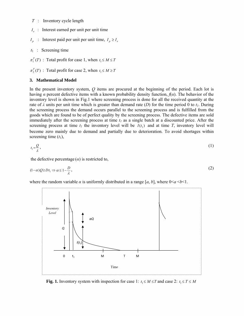
In the present inventory system, Q items are procured at the beginning of the period. Each lot is having α percent defective items with a known probability density function, f(α). The behavior of the inventory level is shown in Fig.1 where screening process is done for all the received quantity at the rate of λ units per unit time which is greater than demand rate (D) for the time period 0 to t1. During the screening process the demand occurs parallel to the screening process and is fulfilled from the goods which are found to be of perfect quality by the screening process. The defective items are sold immediately after the screening process at time t1 as a single batch at a discounted price. After the screening process at time t1 the inventory level will be )( 1tI and at time T, inventory level will become zero mainly due to demand and partially due to deterioration. To avoid shortages within screening time (t1),

λQt =1 , (1)

the defective percentage (α) is restricted to,

⇒≥− 1)1( tDQαλ

α D−≤ 1 , (2)

where the random variable α is uniformly distributed in a range [a, b], where 0<a <b<1.

Fig. 1. Inventory system with inspection for case 1: TMt ≤≤1 and case 2: MTt ≤≤1

Q 

αQ 

t1  T

Inventory Level

Time

0

I(t1) 

M  M

C. K. Jaggi et al. / International Journal of Industrial Engineering Computations 2 (2010)  

Let I(t) be the inventory level at any time t, (0 ≤ t ≤ T) . The differential equation that describes the instantaneous states of I(t) over the period (0, T) is given by

TtDtIdt

tdI≤≤−=+ 0,)()( θ

(3)

The solution of the above differential equations along with the boundary condition, QtIt == )(,0 is

10.]1[)( tteDeQtI tt ≤≤−+= −− θθ

θ (4)

Inventory level at time t1, including the defective items is

.]1[)( 111 −+= −− tt eDeQtI θθ

θ

After the screening process, the number of defective items at time, t1 is .Qα

Hence, the effective inventory level during Ttt ≤≤1 is given by

TttQeDeQtI tt ≤≤−−+= −−1,]1[)( α

θθθ (5)

At Tt= , 0)( =TI , Eq. (5) gives order quantity which follows as

)1()1(

T

T

eeDQ θ

θ

αθ −−

= . (6)

The retailer’s total profit during a cycle, 2,1),( =jTjπ is consisted of the following

)(Tjπ = Sales revenue + Interest earned – Ordering cost – Purchasing cost – Screening cost – Holding cost – Interest paid, (7)

Individual costs are now evaluated before they are grouped together as the total profit,

1. Total sales revenue is the sum of revenue generated by the demand meet during the time period (0, T) and sale of imperfect quality items is

QpDTp sα+= (8)

2. Ordering cost A= (9)

3. Purchase cost = c Q (10)

4. Screening cost = Qβ (11)

5. Holding cost during the time period 0 to t1 and t1 to T,

⎥⎥⎦

⎤

⎢⎢⎣

⎡+= ∫∫

T

t

t

dttIdttIh1

1

0)()(

{ } ⎥

⎦

⎤⎢⎣

⎡+−−

⎭⎬⎫

⎩⎨⎧ +−−−+−−= −−−− )()()()(11)1( 112

111

θα

θθθ

θθθθθθ DQtTDQeeetDe

Qh tTtt

(12)

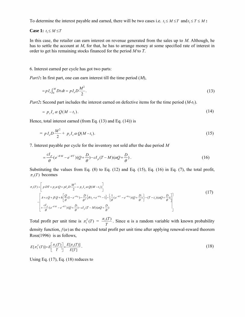
To determine the interest payable and earned, there will be two cases i.e. TMt ≤≤1 and MTt ≤≤1 :

Case 1: TMt ≤≤1

In this case, the retailer can earn interest on revenue generated from the sales up to M. Although, he has to settle the account at M, for that, he has to arrange money at some specified rate of interest in order to get his remaining stocks financed for the period M to T.

6. Interest earned per cycle has got two parts:

Part1: In first part, one can earn interest till the time period (M),

.

2

2

0MDIpdttDIp e

Me == ∫ (13)

Part2: Second part includes the interest earned on defective items for the time period (M-t1).

.)( 1tMQIp es −= α (14)

Hence, total interest earned (from Eq. (13) and Eq. (14)) is

=2

2MDIp e + .)( 1tMQIp es −α (15)

7. Interest payable per cycle for the inventory not sold after the due period M

.)()()()(θ

αθθ

θθ DQMTcIDQeecI

pTMp +−−+−= −− (16)

Substituting the values from Eq. (8) to Eq. (12) and Eq. (15), Eq. (16) in Eq. (7), the total profit, )(1 Tπ becomes

{ }

⎥⎥⎥⎥

⎦

⎤

⎢⎢⎢⎢

⎣

⎡

+−−+−+

⎥⎦

⎤⎢⎣

⎡+−−

⎭⎬⎫

⎩⎨⎧ +−−−+−−+++

−

⎥⎦

⎤⎢⎣

⎡−+++=

−−

−−−−

)()()()(

)()()()(11)1(

)(2

)(

111

121

1

2

1

θα

θθ

θα

θθθ

θθβ

ααπ

θθ

θθθθ

DQMTcIDQeecI

DQtTDQeeetDeQhQQcA

tMQIpMDpIQpDTpT

pTMp

tTtt

eses

(17)

Total profit per unit time is )(1 TTπ = TT )(1π . Since α is a random variable with known probability

density function, )(αf as the expected total profit per unit time after applying renewal-reward theorem Ross(1996) is as follows,

][)]([)()]([ 11

1 TETE

TTETE T πππ =⎥⎦

⎤⎢⎣⎡= . (18)

Using Eq. (17), Eq. (18) reduces to

C. K. Jaggi et al. / International Journal of Industrial Engineering Computations 2 (2010)  

{ }

⎥⎥⎥⎥⎥⎥⎥⎥

⎦

⎤

⎢⎢⎢⎢⎢⎢⎢⎢

⎣

⎡

⎥⎥⎥⎥

⎦

⎤

⎢⎢⎢⎢

⎣

⎡

+−−+−+

⎥⎦

⎤⎢⎣

⎡+−−

⎭⎬⎫

⎩⎨⎧ +−−−+−−+++

−

⎥⎦

⎤⎢⎣

⎡−+++

=

−−

−−−−

)()()()(

)()()()(11)1(

)(2

][1)]([

111

121

1

2

1

θα

θθ

θα

θθθ

θθβ

αα

π

θθ

θθθθ

DQMTcIDQeecI

DQtTDQeeetDeQhQQcA

tMQIpMDIpQpDTp

ETE

TE

pTMp

tTtt

eses

T

(19)

where λQt =1 and

)1()1(

T

T

eeDQ θ

θ

αθ −−

=

The optimal value of T=T1 (say), which maximizes )]([ 1 TE Tπ can be obtained by solving the equation,

0)]([ 1 =dT

TdE Tπ which gives

{ }[ ] { }

( )

{ } ,0)())1(

2)(/2/1

1)/()1(

22

2

222

2

2222

=+′+⎥⎦

⎤⎢⎣

⎡+

+−′+

−−′

+⎥⎦

⎤⎢⎣

⎡−−−−−

⎥⎦

⎤⎢⎣

⎡+

−−++−−−+

−′

−

−

−−

ααθθ

θ

ααλλθ

θθ

θθθαθβα

θ

θ

θθ

pp

T

esMp

e

pT

Mpes

cIhQcIh

TQQe

hIpT

QTQQMeDcI

hDADMpIT

DcIhDT

TeMecIcMIpT

QQT

(20)

provided

{ }[ ]

{ } { }( )

[ ]

0)(

))1(()))(1(())1((

)(2)2(22)2()(

)(/2/2))1(2(

)/()1(22

)]([

2

4

2222

222

3223

22

4

23

21

2

≤+′′+

⎥⎦

⎤⎢⎣

⎡+

+−′−−+−′++′−′′+

−−′−−′+′′+′

+

⎥⎦

⎤⎢⎣

⎡−−−−+⎥

⎦

⎤⎢⎣

⎡+

+++

+−−−++′−′′

=

−−−

−−

−

ααθθ

θθθθ

ααλ

λλλλλλ

θθ

θθθ

θθ

αθβα

π

θθθ

θθ

θ

p

pTTT

es

Mpe

pT

Mpes

T

cIhQ

cIhT

QQeeQQQQeT

hIpT

TQTQQQQQTQQQT

MeDcI

hDADMpIT

DcIhDT

TTe

MecIcMIpT

TQQTQTdT

TEd

where)1(

)1(T

T

eeDQ θ

θ

αθ −−

= ,λQt =1 ,

2)1()1(

T

T

eeDQ

dTdQ

θ

θ

αα

−−

=′= , and 32

2

)1()1)(1(

T

TT

eeeDQ

dTQd

θ

θθ

αθαα

+−++−

=′′= .

Case 2: MTt ≤≤1

Here, the retailer can earn interest on revenue generated from the sales up to permissible delay period M and pays no interest for the items kept in stock.

8. Interest earned per cycle has three parts:

Part1: In first part, one can earn interest till the time period (T),

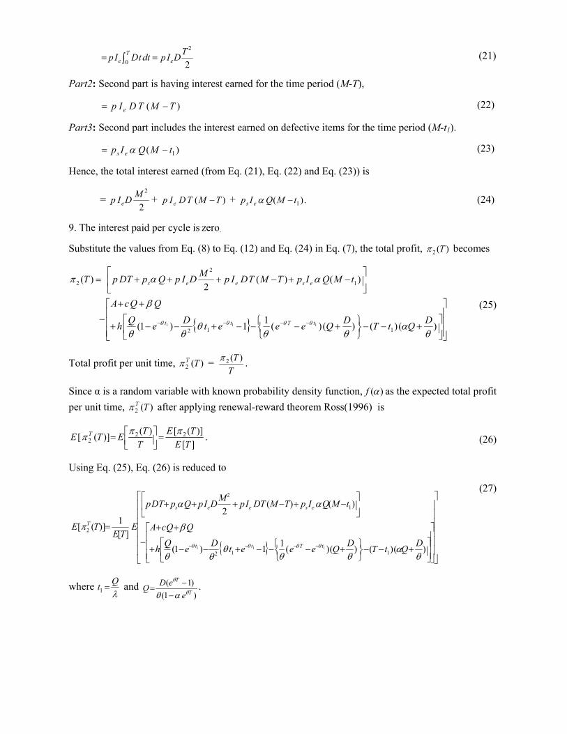
2

2

0TDIpdttDIp e

Te == ∫ (21)

Part2: Second part is having interest earned for the time period (M-T),

)( TMTDIp e −= (22)

Part3: Second part includes the interest earned on defective items for the time period (M-t1).

)( 1tMQIp es −= α (23)

Hence, the total interest earned (from Eq. (21), Eq. (22) and Eq. (23)) is

=2

2MDIp e + )( TMTDIp e − + .)( 1tMQIp es −α (24)

9. The interest paid per cycle is zero.

Substitute the values from Eq. (8) to Eq. (12) and Eq. (24) in Eq. (7), the total profit, )(2 Tπ becomes

{ }⎥⎥⎥

⎦

⎤

⎢⎢⎢

⎣

⎡

⎥⎦

⎤⎢⎣

⎡+−−

⎭⎬⎫

⎩⎨⎧ +−−−+−−+

++

−

⎥⎦

⎤⎢⎣

⎡−+−+++=

−−−− )()()()(11)1(

)()(2

)(

112

1

2

2

111

θα

θθθ

θθ

β

ααπ

θθθθ DQtTDQeeetDeQh

QQcA

tMQIpTMTDIpMDIpQpDTpT

tTtt

esees

(25)

Total profit per unit time, )(2 TTπ = T

T )(2π .

Since α is a random variable with known probability density function, )(αf as the expected total profit per unit time, )(2 TTπ after applying renewal-reward theorem Ross(1996) is

][)]([)()]([ 22

2 TETE

TTETE T πππ =⎥⎦

⎤⎢⎣⎡= . (26)

Using Eq. (25), Eq. (26) is reduced to

{ } ⎥⎥⎥⎥⎥⎥

⎦

⎤

⎢⎢⎢⎢⎢⎢

⎣

⎡

⎥⎥⎥

⎦

⎤

⎢⎢⎢

⎣

⎡

⎥⎦

⎤⎢⎣

⎡+−−

⎭⎬⎫

⎩⎨⎧ +−−−+−−+

++

−

⎥⎦

⎤⎢⎣

⎡−+−+++

=

−−−− )()()()(11)1(

)()(2

][1)]([

112

1

2

2

111

θα

θθθ

θθ

β

αα

π

θθθθ DQtTDQeeetDeQh

QQcA

tMQIpTMTDIpMDIpQpDTp

ETE

TE

tTtt

esees

T

(27)

whereλQt =1 and

)1()1(

T

T

eeDQ θ

θ

αθ −−

= .

C. K. Jaggi et al. / International Journal of Industrial Engineering Computations 2 (2010)  

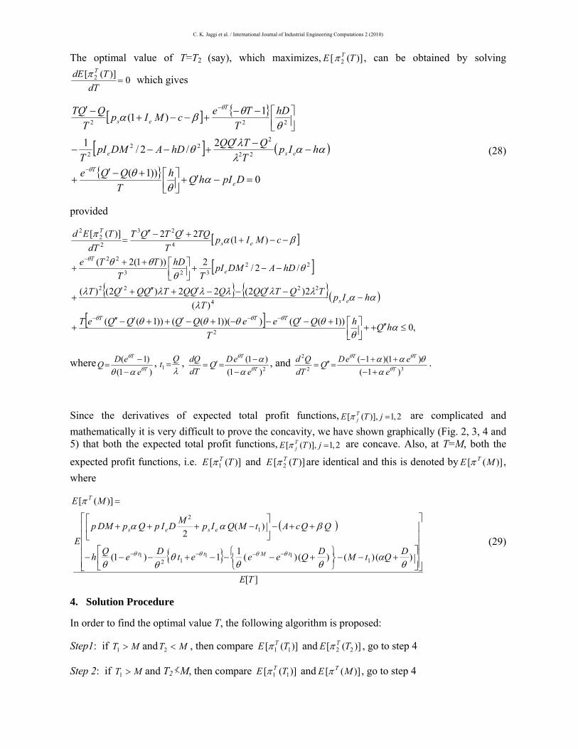
The optimal value of T=T2 (say), which maximizes, )]([ 2 TE Tπ , can be obtained by solving

0)]([ 2 =dT

TdE Tπ which gives

[ ] { }

[ ] ( )

{ } 0))1(

2/2/1

1)1(

22

222

2

222

=−′+⎥⎦⎤

⎢⎣⎡+−′

+

−−′

+−−−

⎥⎦⎤

⎢⎣⎡−−

+−−+−′

−

−

DpIhQhTQQe

hIpT

QTQQhDADMpIT

hDT

TecMIpT

QQT

e

T

ese

T

es

αθ

θ

ααλλθ

θθβα

θ

θ

(28)

provided

[ ]

[ ]{ } { }( )

[ ] ,0))1(()))(1(())1((

)(2)2(22)2()(

/2/2))1(2(

)1(22)]([

2

4

2222

22323

22

4

23

22

2

≤′′++⎥⎦⎤

⎢⎣⎡+−′−−+−′++′−′′

+

−−′−−′+′′+′

+

−−+⎥⎦⎤

⎢⎣⎡++

+

−−++′−′′

=

−−−

−

αθ

θθθθ

ααλ

λλλλλλ

θθ

θθ

βαπ

θθθ

θ

hQhT

QQeeQQQQeT

hIpT

TQTQQQQQTQQQT

hDADMpIT

hDT

TTe

cMIpT

TQQTQTdT

TEd

TTT

es

e

T

es

T

where)1(

)1(T

T

eeDQ θ

θ

αθ −−

= ,λQt =1 ,

2)1()1(

T

T

eeDQ

dTdQ

θ

θ

αα

−−

=′= , and 32

2

)1()1)(1(

T

TT

eeeDQ

dTQd

θ

θθ

αθαα

+−++−

=′′= .

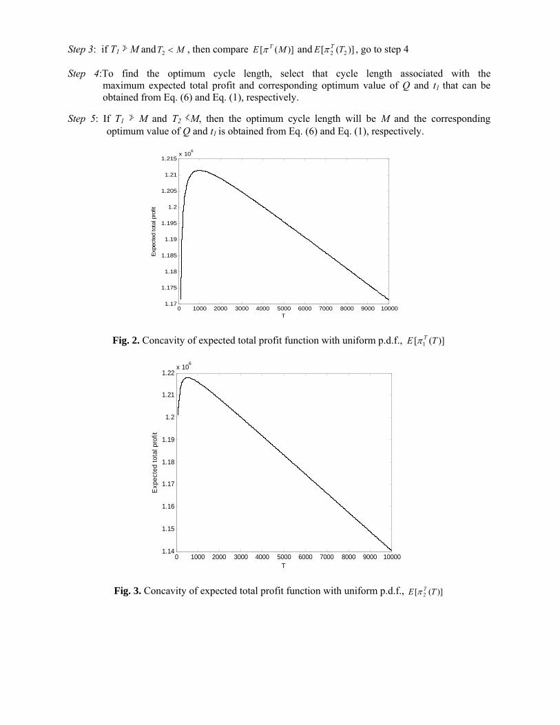
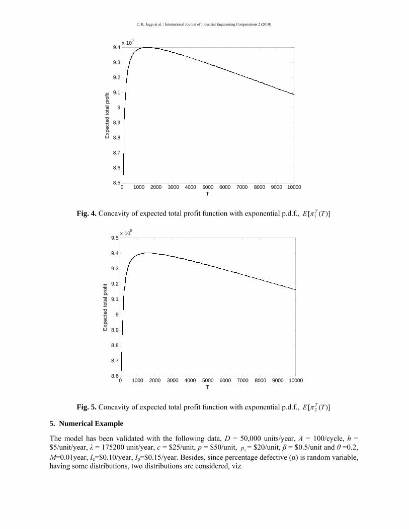
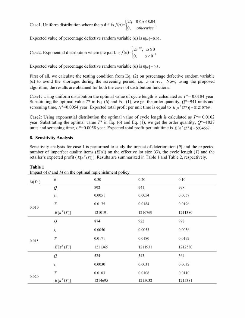
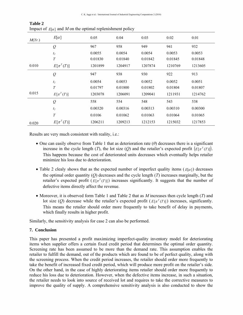
Since the derivatives of expected total profit functions, 2,1)],([ =jTE Tjπ are complicated and

mathematically it is very difficult to prove the concavity, we have shown graphically (Fig. 2, 3, 4 and 5) that both the expected total profit functions, 2,1)],([ =jTE T

jπ are concave. Also, at T=M, both the

expected profit functions, i.e. )]([ 1 TE Tπ and )]([ 2 TE Tπ are identical and this is denoted by )]([ ME Tπ , where

( )

{ }][

)()()()(11)1(

)(2

)]([

111

121

1

2

TE

DQtMDQeeetDeQh

QQcAtMQIpMDIpQpDMpE

ME

tMtt

eses

T

⎥⎥⎥⎥⎥

⎦

⎤

⎢⎢⎢⎢⎢

⎣

⎡

⎥⎦

⎤⎢⎣

⎡+−−

⎭⎬⎫

⎩⎨⎧ +−−−+−−−

++−⎥⎦

⎤⎢⎣

⎡−+++

=

−−−−

θα

θθθ

θθ

βαα

π

θθθθ

(29)

4. Solution Procedure

In order to find the optimal value T, the following algorithm is proposed:

Step1: if MT >1 and MT <2 , then compare )]([ 11 TE Tπ and )]([ 22 TE Tπ , go to step 4

Step 2: if MT >1 and T2 ≮M, then compare )]([ 11 TE Tπ and )]([ ME Tπ , go to step 4

Step 3: if T1 ≯ M and MT <2 , then compare )]([ ME Tπ and )]([ 22 TE Tπ , go to step 4

Step 4:To find the optimum cycle length, select that cycle length associated with the maximum expected total profit and corresponding optimum value of Q and t1 that can be obtained from Eq. (6) and Eq. (1), respectively.

Step 5: If T1 ≯ M and T2 ≮M, then the optimum cycle length will be M and the corresponding optimum value of Q and t1 is obtained from Eq. (6) and Eq. (1), respectively.

Fig. 2. Concavity of expected total profit function with uniform p.d.f., )]([ 1 TE Tπ

Fig. 3. Concavity of expected total profit function with uniform p.d.f., )]([ 2 TE Tπ

0 1000 2000 3000 4000 5000 6000 7000 8000 9000 100001.17

1.175

1.18

1.185

1.19

1.195

1.2

1.205

1.21

1.215x 106

T

Exp

ecte

d to

tal p

rofit

0 1000 2000 3000 4000 5000 6000 7000 8000 9000 100001.14

1.15

1.16

1.17

1.18

1.19

1.2

1.21

1.22x 106

T

Exp

ecte

d to

tal p

rofit

C. K. Jaggi et al. / International Journal of Industrial Engineering Computations 2 (2010)  

Fig. 4. Concavity of expected total profit function with exponential p.d.f., )]([ 1 TE Tπ

Fig. 5. Concavity of expected total profit function with exponential p.d.f., )]([ 2 TE Tπ

5. Numerical Example

The model has been validated with the following data, D = 50,000 units/year, A = 100/cycle, h = $5/unit/year, λ = 175200 unit/year, c = $25/unit, p = $50/unit, sp = $20/unit, β = $0.5/unit and θ =0.2, M=0.01year, Ie=$0.10/year, Ip=$0.15/year. Besides, since percentage defective (α) is random variable, having some distributions, two distributions are considered, viz.

0 1000 2000 3000 4000 5000 6000 7000 8000 9000 100008.5

8.6

8.7

8.8

8.9

9

9.1

9.2

9.3

9.4x 105

T

Exp

ecte

d to

tal p

rofit

0 1000 2000 3000 4000 5000 6000 7000 8000 9000 100008.6

8.7

8.8

8.9

9

9.1

9.2

9.3

9.4

9.5x 105

T

Exp

ecte

d to

tal p

rofit

Case1. Uniform distribution where the p.d.f. is⎩⎨⎧ ≤≤

=otherwise

f,0

04.00,25)(

αα ,

Expected value of percentage defective random variable (α) is 02.0][ =αE .

Case2. Exponential distribution where the p.d.f. is⎩⎨⎧

<≥

=−

0,00,2)(

2

ααα

αef ,

Expected value of percentage defective random variable (α) is 5.0][ =αE .

First of all, we calculate the testing condition from Eq. (2) on percentage defective random variable (α) to avoid the shortages during the screening period, i.e. 715.0≤α . Now, using the proposed algorithm, the results are obtained for both the cases of distribution functions:

Case1: Using uniform distribution the optimal value of cycle length is calculated as T*= 0.0184 year. Substituting the optimal value T* in Eq. (6) and Eq. (1), we get the order quantity, Q*=941 units and screening time, t1*=0.0054 year. Expected total profit per unit time is equal to $1210769*)]([ =TE Tπ .

Case2: Using exponential distribution the optimal value of cycle length is calculated as T*= 0.0102 year. Substituting the optimal value T* in Eq. (6) and Eq. (1), we get the order quantity, Q*=1027 units and screening time, t1*=0.0058 year. Expected total profit per unit time is $934667.*)]([ =TE Tπ

6. Sensitivity Analysis

Sensitivity analysis for case 1 is performed to study the impact of deterioration (θ) and the expected number of imperfect quality items (E[α]) on the effective lot size (Q), the cycle length (T) and the retailer’s expected profit ( )]([ TE Tπ ). Results are summarized in Table 1 and Table 2, respectively.

Table 1 Impact of θ and M on the optimal replenishment policy M(Yr.) θ 0.30 0.20 0.10

0.010

Q 892 941 998

t1 0.0051 0.0054 0.0057

T 0.0175 0.0184 0.0196

)]([ TE Tπ 1210191 1210769 1211380

0.015

Q 874 922 978

t1 0.0050 0.0053 0.0056

T 0.0171 0.0180 0.0192

)]([ TE Tπ 1211365 1211931 1212530

0.020

Q 524 543 564

t1 0.0030 0.0031 0.0032

T 0.0103 0.0106 0.0110

)]([ TE Tπ 1214695 1215032 1215381

C. K. Jaggi et al. / International Journal of Industrial Engineering Computations 2 (2010)  

Table 2 Impact of ][αE and M on the optimal replenishment policy M(Yr.) ][αE 0.05 0.04 0.03 0.02 0.01

0.010

Q 967 958 949 941 932

t1 0.0055 0.0054 0.0054 0.0053 0.0053 T 0.01830 0.01840 0.01842 0.01845 0.01848

)]([ TE Tπ 1201899 1204917 1207874 1210769 1213605

0.015

Q 947 938 930 922 913

t1 0.0054 0.0053 0.0052 0.0052 0.0051 T 0.01797 0.01800 0.01802 0.01804 0.01807

)]([ TE Tπ 1203078 1206091 1209041 1211931 1214762 0.020

Q 558 554 548 543 538

t1 0.00320 0.00316 0.00313 0.00310 0.00300

T 0.0106 0.01062 0.01063 0.01064 0.01065

)]([ TE Tπ 1206211 1209213 1212153 1215032 1217853

Results are very much consistent with reality, i.e.:

• One can easily observe from Table 1 that as deterioration rate (θ) decreases there is a significant increase in the cycle length (T), the lot size (Q) and the retailer’s expected profit ( ))]([ TE Tπ . This happens because the cost of deteriorated units decreases which eventually helps retailer minimize his loss due to deterioration.

• Table 2 clealy shows that as the expected number of imperfect quality items ( ][αE ) decreases the optimal order quantity (Q) decreases and the cycle length (T) increases marginally, but the retailer’s expected profit ( )]([ TE Tπ ) increases significantly. It suggests that the number of defective items directly affect the revenue.

• Moreover, it is observed form Table 1 and Table 2 that as M increases then cycle length (T) and lot size (Q) decrease while the retailer’s expected profit ( )]([ TE Tπ ) increases, significantly. This means the retailer should order more frequently to take benefit of delay in payments, which finally results in higher profit.

Similarly, the sensitivity analysis for case 2 can also be performed.

7. Conclusion

This paper has presented a profit maximizing imperfect-quality inventory model for deteriorating items when supplier offers a certain fixed credit period that determines the optimal order quantity. Screening rate has been assumed to be more than the demand rate. This assumption enables the retailer to fulfill the demand, out of the products which are found to be of perfect quality, along with the screening process. When the credit period increases, the retailer should order more frequently to take the benefit of increased fixed credit period, which will produce more profit on the retailer’s side. On the other hand, in the case of highly deteriorating items retailer should order more frequently to reduce his loss due to deterioration. However, when the defective items increase, in such a situation, the retailer needs to look into source of received lot and requires to take the corrective measures to improve the quality of supply. A comprehensive sensitivity analysis is also conducted to show the

effects of the key parameters on the optimal order quantity, screening time, cycle length and retailer’s expected total profit. For future study, it is desirable to extend the proposed model for linearly increasing and stock dependent demand where shortages may be allowed.

Acknowledgement

The first author would like to acknowledge the financial support provided by University Grant Commission (Grant No. Dean (R/ R&D/2009/487).

References

Aggarwal, S. P. & Jaggi, C. K., (1995). Ordering policies of deteriorating items under permissible delay in payments. Journal of the Operational Research Society, 46, 658–662.

Ca´ rdenas-Barro´ n, L. E. (2000). Observation on: Economic production quantity model for items with imperfect quality. International Journal of Production Economics, 67 (2), 201.

Chung, K. J. & Huang, Y. F. (2006). Retailer’s optimal cycle times in the EOQ model with imperfect quality and permissible credit period. Journal of Quality and Quantity, 40, 59-77.

Chu, P., Chung, K.J. & Lan, S.P. (1998). Economic order quantity of deteriorating items under permissible delay in payments. Computers and Operational Research, 25, 817-824.

Davis , R. A. & Gaither , N. (1985). Optimal ordering policies under conditions of extended payment privileges, Management Sciences. 31, 499-509.

Ghare, P. M. & Schrader, G. F. (1963). A model for exponential decaying inventory. Journal of Industrial Engineering, 14(3), 238-243.

Goyal, S. K. & Ca´ rdenas-Barro´ n, L. E. (2002). Note on: Economic production quantity model for items with imperfect quality—a practical approach. International Journal of Production Economics, 77(1), 85–87.

Goyal, S. K. (1985). Economic order quantity under conditions of permissible delay in payment. Journal of the Operational Research Society, 36, 335–338.

Kingsman, B. G. (1983). The effect of payment rules on ordering and stocking in purchasing. Journal of the Operational Research Society, 34, 1085–1098.

Lee, H. L. & Rosenblatt, M. J. (1987). Simultaneous determination of production cycles and inspection schedules in a production system. Management Science, 33, 1125-1137.

Maddah, B. & Jaber, M. (2008). Economic order quantity for items with imperfect quality: revisited. International Journal of Production Economics, 112(2), 808–815.

Maddah, B., Jaber, M. & Haidar, M., L. (2010). Order overlapping: A practical approach for preventing shortages during screening. Computers and Industrial Engineering, 58, 691–695.

Mandal, B. N. & Phaujdar, S. (1989). Some EOQ models under permissible delay in payments. International Journal of Managements Science, 5 (2), 99–108.

Papachristos, S. & Konstantaras, I. (2006). Economic ordering quantity models for items with imperfect quality. International Journal of Production Economics, 100(1), 148–154.

Porteus, E. L. (1986). Optimal lot sizing, process quality improvement and setup cost reduction. Operations Research, 34(1), 137-144.

Raafat, F., Wolfe, P. M., & Eddin, H. K. (1991). An inventory model for deteriorating items. Computers and Industrial Engineering, 20(1), 89-94.

Rosenblatt, M. & Lee, H., (1986). Economic production cycles with imperfect production processes. IIE Transactions, 18(1), 48–55.

Ross, S. M. (1996). Stochastic Processes, second ed. Wiley, New York, NY. Salameh, M. & Jaber, M. (2000). Economic production quantity model for items with imperfect

quality. International Journal of Production Economics, 64 (3), 59–64. Soni, H. Shah, N. H. & Jaggi, C.K. (2010). Inventory models and trade credit. Journal of Control and

Cybernetics, 39. (To appear) Yano, C. A. & Lee, H. L. (1995). Lot sizing with random yields: A review. Operations Research, 43

(2), 311–334.