Two Maximum Entropy Based Algorithms for Running Quantile Estimation in Non-Stationary Data Streams

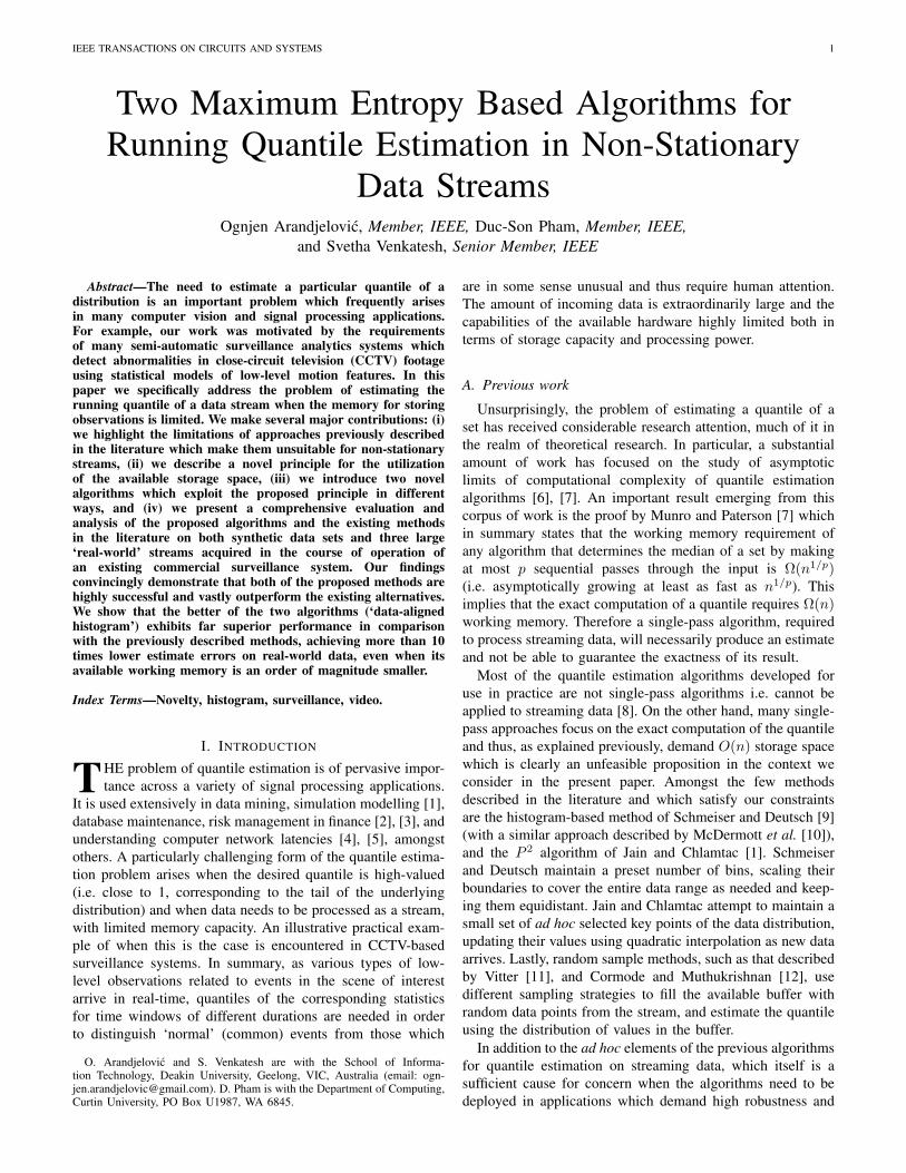
IEEE TRANSACTIONS ON CIRCUITS AND SYSTEMS 1

Two Maximum Entropy Based Algorithms forRunning Quantile Estimation in Non-Stationary

Data StreamsOgnjen Arandjelovic, Member, IEEE, Duc-Son Pham, Member, IEEE,

and Svetha Venkatesh, Senior Member, IEEE

Abstract—The need to estimate a particular quantile of adistribution is an important problem which frequently arisesin many computer vision and signal processing applications.For example, our work was motivated by the requirementsof many semi-automatic surveillance analytics systems whichdetect abnormalities in close-circuit television (CCTV) footageusing statistical models of low-level motion features. In thispaper we specifically address the problem of estimating therunning quantile of a data stream when the memory for storingobservations is limited. We make several major contributions: (i)we highlight the limitations of approaches previously describedin the literature which make them unsuitable for non-stationarystreams, (ii) we describe a novel principle for the utilizationof the available storage space, (iii) we introduce two novelalgorithms which exploit the proposed principle in differentways, and (iv) we present a comprehensive evaluation andanalysis of the proposed algorithms and the existing methodsin the literature on both synthetic data sets and three large‘real-world’ streams acquired in the course of operation ofan existing commercial surveillance system. Our findingsconvincingly demonstrate that both of the proposed methods arehighly successful and vastly outperform the existing alternatives.We show that the better of the two algorithms (‘data-alignedhistogram’) exhibits far superior performance in comparisonwith the previously described methods, achieving more than 10times lower estimate errors on real-world data, even when itsavailable working memory is an order of magnitude smaller.

Index Terms—Novelty, histogram, surveillance, video.

I. INTRODUCTION

THE problem of quantile estimation is of pervasive impor-tance across a variety of signal processing applications.

It is used extensively in data mining, simulation modelling [1],database maintenance, risk management in finance [2], [3], andunderstanding computer network latencies [4], [5], amongstothers. A particularly challenging form of the quantile estima-tion problem arises when the desired quantile is high-valued(i.e. close to 1, corresponding to the tail of the underlyingdistribution) and when data needs to be processed as a stream,with limited memory capacity. An illustrative practical exam-ple of when this is the case is encountered in CCTV-basedsurveillance systems. In summary, as various types of low-level observations related to events in the scene of interestarrive in real-time, quantiles of the corresponding statisticsfor time windows of different durations are needed in orderto distinguish ‘normal’ (common) events from those which

O. Arandjelovic and S. Venkatesh are with the School of Informa-tion Technology, Deakin University, Geelong, VIC, Australia (email: [email protected]). D. Pham is with the Department of Computing,Curtin University, PO Box U1987, WA 6845.

are in some sense unusual and thus require human attention.The amount of incoming data is extraordinarily large and thecapabilities of the available hardware highly limited both interms of storage capacity and processing power.

A. Previous work

Unsurprisingly, the problem of estimating a quantile of aset has received considerable research attention, much of it inthe realm of theoretical research. In particular, a substantialamount of work has focused on the study of asymptoticlimits of computational complexity of quantile estimationalgorithms [6], [7]. An important result emerging from thiscorpus of work is the proof by Munro and Paterson [7] whichin summary states that the working memory requirement ofany algorithm that determines the median of a set by makingat most p sequential passes through the input is Ω(n1/p)(i.e. asymptotically growing at least as fast as n1/p). Thisimplies that the exact computation of a quantile requires Ω(n)working memory. Therefore a single-pass algorithm, requiredto process streaming data, will necessarily produce an estimateand not be able to guarantee the exactness of its result.

Most of the quantile estimation algorithms developed foruse in practice are not single-pass algorithms i.e. cannot beapplied to streaming data [8]. On the other hand, many single-pass approaches focus on the exact computation of the quantileand thus, as explained previously, demand O(n) storage spacewhich is clearly an unfeasible proposition in the context weconsider in the present paper. Amongst the few methodsdescribed in the literature and which satisfy our constraintsare the histogram-based method of Schmeiser and Deutsch [9](with a similar approach described by McDermott et al. [10]),and the P 2 algorithm of Jain and Chlamtac [1]. Schmeiserand Deutsch maintain a preset number of bins, scaling theirboundaries to cover the entire data range as needed and keep-ing them equidistant. Jain and Chlamtac attempt to maintain asmall set of ad hoc selected key points of the data distribution,updating their values using quadratic interpolation as new dataarrives. Lastly, random sample methods, such as that describedby Vitter [11], and Cormode and Muthukrishnan [12], usedifferent sampling strategies to fill the available buffer withrandom data points from the stream, and estimate the quantileusing the distribution of values in the buffer.

In addition to the ad hoc elements of the previous algorithmsfor quantile estimation on streaming data, which itself is asufficient cause for concern when the algorithms need to bedeployed in applications which demand high robustness and


well understood failure modes, it is also important to recognizethat an implicit assumption underlying these approaches isthat the data is governed by a stationary stochastic process.The assumption is often invalidated in real-world applications.As we will demonstrate in Section III, a consequence of thisdiscrepancy between the model underlying existing algorithmsand the nature of data in practice is a major deterioration inthe quality of quantile estimates. Our principal aim is thusto formulate a method which can cope with non-stationarystreaming data in a more robust manner.

II. PROPOSED ALGORITHMS

We start this section by formalizing the notion of a quantile.This is then followed by the introduction of the key premiseof our contribution and finally a description of two algorithmswhich exploit the underlying idea in different ways [13]. Thealgorithms are evaluated on real-world data in the next section.

A. Quantiles

Let p be the probability density function of a real-valuedrandom variable X . Then the q-quantile vq of p is defined as:∫ vq

−∞p(x) dx = q. (1)

Similarly, the q-quantile of a finite set D can be defined as:

|x : x ∈ D and x ≤ vq| ≤ q × |D|. (2)

In other words, the q-quantile is the smallest value belowwhich q fraction of the total values in a set lie [14]. Theconcept of a quantile is thus intimately related to the tailbehaviour of a distribution.

B. Methodology: maximum entropy histograms

A consequence of the non-stationarity of data streams thatwe are dealing with is that at no point in time can it be assumedthat the historical distribution of data values is representativeof its future distribution. This is true regardless of how muchhistorical data has been seen. Thus, the value of a particularquantile can change greatly and rapidly, in either direction(i.e. increase or decrease). This is illustrated on an example,extracted from a real-world data set used for surveillancevideo analysis (the full data corpus is used for comprehensiveevaluation of different methods in Section III), in Figure 1.In particular, the top plot in this figure shows the variationof the ground-truth 0.95-quantile which corresponds to thedata stream shown in the bottom plot. Notice that the quantileexhibits little variation over the course of approximately thefirst 75% of the duration of the time window (the first 190,000data points). This corresponds to a period of little activity inthe video from which the data is extracted (see Section III for adetailed explanation). Then, the value of the quantile increasesrapidly for over an order of magnitude – this is caused bya sudden burst of activity in the surveillance video and thecorresponding change in the statistical behaviour of the data.

To be able to adapt to such unpredictable variability in inputit is therefore not possible to focus on only a part of the

1 1.5 2 2.5

x 105

0

1

2

3

4

5

6x 10

11

Datum index

Qua

ntile

est

imat

e

1 1.5 2 2.5

x 105

0

5

10

15x 10

11

Datum index

Dat

um v

alue

Fig. 1. An example of a rapid change in the value of a quantile (specificallythe 0.95-quantile in this case) on a real-world data stream.

historical data distribution but rather it is necessary to storea ‘snapshot’ of the entire distribution. We achieve this usinga histogram of a fixed length, determined by the availableworking memory. In contrast to the previous work which eitherdistributes the bin boundaries equidistantly or uses ad hocadjustments, our idea is to maintain bins in a manner whichmaximizes the entropy of the corresponding estimate of thehistorical data distribution.

Recall that the entropy of a discrete random variable is:

Hr = −∑x∈X

p(x) log2 p(x) (3)

where p(x) is the probability of the random variable taking onthe value x, and X the set of all possible values of x [15] (ofcourse

∑x∈X p(x) = 1). Therefore, the entropy of a histogram

with n bins and the corresponding bin counts c1, c2, . . . , cn is:

Hh = −n∑

i=1

ciC

log2

( ciC

)(4)

where C =∑n

i=1 ci is the normalization factor which makesci/C the probability of a randomly selected datum belongingto the i-th bin [16]. Our goal is to dynamically allocateand adjust bin boundaries in a manner which maximizes theassociated entropy for a fixed number of bins n (which isan input parameter whose value is determined by practicalconstraints). Much like the problem of computing a specificquantile which, as we discussed with reference to Munro andPaterson’s work [7] in Section I-A, is not solvable exactlyusing a single-pass algorithm, the construction of the maximalentropy histogram as defined above is not possible to guaranteein the setting adopted in this paper whereby only a limitedand fixed amount of storage is available, and historical data isinaccessible.

C. Method 1: interpolated bins

The first method based around the idea of maximum entropybins we introduce in this paper readjusts the boundaries of afixed number of bins after the arrival of each new data point


di+1. Without loss of generality let us assume that each datumis positive i.e. that di > 0. Furthermore, let the upper binboundaries before the arrival of di be bi1, b

i2, . . . , b

in, where n

is the number of available bins. Thus, the j-th bin’s catchmentrange is (bij−1, b

ij ] where we will take that bi0 = 0 for all i.

We wish to maintain the condition that the piece-wise uniformprobability density function approximation of the historicaldata distribution described by this histogram has the maximumentropy of all those possible with the histogram of the samelength. This is achieved by having equiprobable bins. Thus,before the arrival of di+1, the number of historical data pointsin each bin is the same and equal to i/n. The correspondingcumulative density is given by:

f i(d) =1

n×

[j +

d− bij−1bij − bij−1

](5)

and

bij−1 < d ≤ bij . (6)

After the arrival of di, but before the readjustment of binboundaries, the cumulative density becomes:

f i(d) =

i

i+1 ×1n ×

[j +

d−bij−1

bij−bij−1

]for d < di

ii+1 ×

1n ×

[j +

d−bij−1

bij−bij−1

]+ 1

i+1 for d ≥ di(7)

Lastly, to maintain the invariant of equiprobable bins, thebin boundaries are readjusted by linear interpolation of thecorresponding inverse distribution function.

1) Initialization: The initialization of the proposed algo-rithm is simple. Specifically, until the buffer is filled, i.e. untilthe number of unique stream data points processed exceedsn, the maximal entropy histogram is constructed by allocatingeach unique data value its own bin. This is readily achievedby making each unique data value the top boundary of a bin.

D. Method 2: data-aligned bins

The algorithm described in the preceding section appearsoptimal in that it always attempts to realign bins so as tomaintain maximum entropy of the corresponding approxima-tion for the given size of the histogram. However, a potentialsource of errors can emerge cumulatively as a consequence ofrepeated interpolation, done after every new datum. Indeed, wewill show this to be the case empirically in Section III. Wenow introduce an alternative approach which aims to strike abalance between some unavoidable loss of information, inher-ently a consequence of the need to readjust an approximationof the distribution of a continually growing data set, and thedesire to maximize the entropy of this approximation.

Much like in the previous section, bin boundaries arepotentially altered each time a new datum arrives. There aretwo main differences in how this is performed. Firstly, unlikein the previous case, bin boundaries are not allowed to assumearbitrary values; rather, their values are constrained to thevalues of the seen data points. Secondly, only at most a singleboundary is adjusted for each new datum. We now explain thisprocess in detail.

As before, let the upper bin boundaries before the arrivalof a new data point be bi1, b

i2, . . . , b

in. Since unlike in the

case of the previous algorithm in general the bins will notbe equiprobable we also have to maintain a corresponding listci1, c

i2, . . . , c

in which specifies the corresponding data counts.

Each time a new data point arrives, an (n+1)-st bin is createdtemporarily. If the value of the new datum is greater than bin(and thus greater than any of the historical data), a new binis created after the current n-th bin, with the upper boundaryset at d(i). The corresponding datum count c of the bin is setto 1. Alternatively, if the value of the new data point is lowerthan bin then there exists j such that:

bij−1 < d ≤ bij , (8)

and the new bin is inserted between the (j − 1)-st and j-thbin. Its datum count is estimated using linear interpolation inthe following manner:

c = cij ×d− bij−1bij − bij−1

+ 1. (9)

Thus, regardless of the value of the new data point, temporarilythe number of bins is increased by 1. The original numberof bins is then restored by merging exactly a single pair ofneighbouring bins. For example, if the k-th and (k+ 1)-st binare merged, the new bin has the upper boundary value set tothe upper boundary value of the former (k + 1)-st bin, i.e.bik+1, and its datum count becomes the sum of counts for thek-th and (k + 1)-st bins, i.e. cik + cik+1. The choice of whichneighbouring pair to merge, out of n possible options, is madeaccording to the principle stated in Section II-B, i.e. the mergeactually performed should maximize the entropy of the newn-bin histogram. This is illustrated conceptually in Figure 2.

New data point

Bin 4Bin 3Bin 2Bin 1Bin 3Bin 2Bin 1

Fig. 2. Conceptual illustration of the key update step of the second algorithmfirst described in the present paper. The algorithm attempts to maximize theentropy of the histogram approximating the distribution of historical data whileusing bins with data-aligned boundaries. The figure shows the initial histogrambefore the arrival of the new datum whose value is indicated by the arrow(left-most illustration). A temporary new bin is created with the boundarycoinciding with the value of the new datum (shown in the centre of thediagram). Lastly, to maintain a fixed number of bins, a single merging of twoneighbouring bins is performed; the three small illustrations on the right-handside show the possible options. The merge which results in highest entropyis chosen and actually performed.

1) Initialization: The initialization of the histogram in theproposed method can be achieved in the same manner asin the interpolated bins algorithm introduced previously. Torepeat, until the buffer is filled, i.e. until the number of uniquestream data points processed exceeds n, the maximal entropyhistogram is constructed by making each unique data value


the top boundary of a bin, thereby allocating each unique datavalue its own bin.

III. EVALUATION AND RESULTS

We now turn our attention to the evaluation of the proposedalgorithms. In particular, to assess their effectiveness andcompare them with the algorithms described in the literature(see Section I-A), in this section we report their performanceon two synthetic data sets and three large ‘real-world’ datastreams. Our aim is first to use simple synthetic data tostudy the algorithms in a well understood and controlledsetting, before applying them on corpora collected by systemsdeployed in practice. Specifically, the ‘real-world’ streamscorrespond to motion statistics used by an existing CCTVsurveillance system for the detection of abnormalities in videofootage. It is important to emphasize that the data we usedwas not acquired for the purpose of the present work norwere the cameras installed with the same intention. Rather,we used data which was acquired using existing, operationalsurveillance systems. In particular, our data comes from threeCCTV cameras, two of which are located in Mexico and onein Australia. The scenes they overlook are illustrated using asingle representative frame per camera in Figure 3. Table Iprovides a summary of some of the key statistics of the threedata sets. We explain the source of these streams and thenature of the phenomena they represent in further detail inSection III-A2.

TABLE IKEY STATISTICS OF THE THREE REAL-WORLD DATA SETS USED IN OUREVALUATION. THESE WERE ACQUIRED USING THREE EXISTING CCTV

CAMERAS IN OPERATION IN AUSTRALIA AND MEXICO.

Data set Data points Mean value Standard deviation

Stream 1 555, 022 7.81× 1010 1.65× 1011

Stream 2 10, 424, 756 2.25 15.92

Stream 3 1, 489, 618 1.51× 105 2.66× 106

A. Evaluation data

1) Synthetic data: The first synthetic data set that weused for the evaluation in this paper is a simple streamx1, x2, . . . , xn1

generated by drawing each datum xi indepen-dently from a normal distribution represented by the randomvariable X:

X ∼ N (5, 1) (10)

Therefore, this sequence has a stationary distribution. We usedn1 = 1, 000, 000 data points.

The second synthetic data set is somewhat more complex.Specifically, each datum yi in the stream y1, y2, . . . , yn1

isgenerated as follows:

yi = ci × y(1)i + (1− ci)× y(2)i (11)

where ci is drawn from a discrete uniform distribution overthe set 0, 1, and y

(1)i and y

(2)i from normal distributions

represented by the random variables Y1 and Y2 respectively:

Y1 ∼ N (5, 1) (12)Y2 ∼ N (10, 4). (13)

In intuitive terms, a datum is generated by flipping a fair coinand then depending on the outcome drawing the value eitherfrom Y1 or Y2. Notice that this data set therefore does nothave the property of stationarity. As in the first experiment weused n2 = 1, 000, 000 data points.

2) Real-world surveillance data: Computer-assisted videosurveillance data analysis is of major commercial and law en-forcement interest. On a broad scale, systems currently avail-able on the market can be grouped into two categories in termsof their approach. The first group focuses on a relatively small,predefined and well understood subset of events or behavioursof interest such as the detection of unattended baggage, violentbehaviour, etc [17], [18]. The narrow focus of these systemsprohibits their applicability in less constrained environmentsin which a more general capability is required. In addition,these approaches tend to be computationally expensive anderror prone, often requiring fine tuning by skilled technicians.This is not practical in many circumstances, for example whenhundreds of cameras need to be deployed as often the casewith CCTV systems operated by municipal authorities. Thesecond group of systems approaches the problem of detectingsuspicious events at a semantically lower level [19], [20], [21],[22], [23]. Their central paradigm is that an unusual behaviourat a high semantic level will be associated with statisticallyunusual patterns (also ‘behaviour’ in a sense) at a low semanticlevel – the level of elementary image/video features. Thusmethods of this group detect events of interest by learning thescope of normal variability of low-level patterns and alertingto anything that does not conform to this model of what isexpected in a scene, without ‘understanding’ or interpretingthe nature of the event itself. These methods uniformly startwith the same procedure for feature extraction. As video datais acquired, firstly a dense optical flow field is computed.Then, to reduce the amount of data that needs to be processed,stored, or transmitted, a thresholding operation is performed.This results in a sparse optical flow field whereby only thoseflow vectors whose magnitude exceeds a certain value areretained; non-maximum suppression is applied here as well.Normal variability within a scene and subsequent noveltydetection are achieved using various statistics computed overthis data. The three data streams, shown partially in Figure 4,correspond to the values of these statistics (their exact meaningis proprietary and has not been made known fully to theauthors of the present paper either; nonetheless we haveobtained permission to make the data public as we shall dofollowing the acceptance of the paper). Observe the non-stationary nature of the data streams which is evident bothon the long and short time scales (magnifications are shownfor additional clarity and insight).

B. ResultsWe now compare the performance of our algorithms with

the three alternatives from the literature described in Sec-tion I-A: (i) the P 2 algorithm of Jain and Chlamtac [1], (ii)


(a) (b) (c)

Fig. 3. Screenshots of the three scenes used to acquire the data used in our experiments. Note that these are real, operational CCTV cameras, which werenot specifically installed for the purpose of data acquisition for the present work. Also see Figure 4.

0 1 2 3 4 5 6

x 105

0

0.5

1

1.5

2

2.5

3x 10

12

Datum index

Dat

um v

alue

(a) Data stream 1

0 2 4 6 8 10 12

x 106

0

50

100

150

200

250

300

Datum index

Dat

um v

alue

0 100 200 300 400 500 600 700 800 900 10000

50

100

150

200

250

(b) Data stream 2

0 5 10 15

x 105

0

0.5

1

1.5

2

2.5

3x 10

8

Datum index

Dat

um v

alue

0 100 200 300 400 500 600 700 800 900 10003500

4000

4500

5000

5500

6000

6500

(c) Data stream 3

Fig. 4. The three large data streams used to evaluate the performance ofthe proposed algorithms and compare them with the approaches previouslydescribed in the literature. Also see Figure 3.

the random sample based algorithm of Vitter [11], and (iii) theuniform adjustable histogram of Schmeiser and Deutsch [9].

1) Synthetic data: We start by examining the results ofdifferent algorithms on the first and simplest synthetic stream,with stationary characteristics and data drawn from a normaldistribution. Different estimates for the quantile values of 0.95,0.99, and 0.995 are shown in the stem plots of Figure 5.Several trends are immediately obvious. Firstly, Jain andChlamtac’s algorithm consistently performed worse, signifi-cantly so, than all other methods in all three experiments. Thisis unsurprising, given that the algorithm uses the least amountof memory. The best performance across all experiments was

exhibited by the data-aligned algorithm introduced in thispaper, while the relative performances of the sample-basedalgorithm of Vitter and the uniform histogram method arenot immediately clear, one performing better than the otherin some cases and vice versa in others.

Figure 5 also shows that in all cases except that of thesample-based algorithm of Vitter in the estimation of 0.995-quantile, a particular method performed better when its avail-able storage space was increased. This observation too is inline with theoretical expectations. However, this is only apartial picture because it offers only a snapshot of the estimatesafter all data has been processed. The plot in Figure 6 plotsthe running estimates of all algorithms as more and moredata is seen, and reveals further insight. The data-alignedbins algorithm proposed herein (black lines) can again beseen to perform the best, showing little fluctuation during theprocessing of the stream, its performance with 100 being noworse than with 500 bins. The plot also confirms the inferiorityof Jain and Chlamtac’s method. A more interesting resultpertains to the comparison of the sample-based algorithmof Vitter and the uniform adjustable histogram of Schmeiserand Deutsch. Specifically, despite its good accuracy at mosttimes, the latter can be seen to suffer intermittently from largeerrors, as witnessed by the pronounced high-frequency straysin the plot (green lines). These can be readily explained byconsidering the operation of the algorithm and in particularits behaviour when a new extreme datum, outside of the rangeof the current uniform histogram, arrives. In such instances,the bin boundaries need to be readjusted and are consequentlygreatly altered, producing a number of poorly-sampled bins.This results in inaccurate estimates (most markedly of highquantiles), which are transient in nature as the samplingbecomes more accurate with the arrival of further data.

Lastly, considering that this data set has stationary charac-teristics, we examined what we termed ‘time until accuracy’.Specifically, we define time until accuracy t(α) as the numberof data points until the relative error of the estimate of analgorithm on a stream s1, s2, . . . , sns permanently drops to atmost α:

t(α) = arg maxi=1,...,ns

|vq(i)− vq(i)|vq(i)

> α, (14)

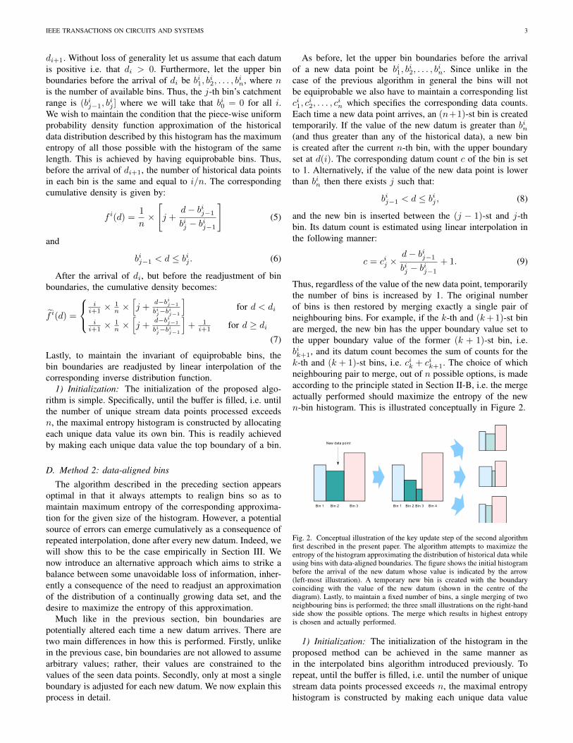
where vq(i) is the true value of a quantile after the first i datapoints have been seen, and vq(i) an estimate of the quantile.The plots in Figure 7 summarize the results obtained with


Jain SampleQ(100) SampleQ(500) UniformQ(100) UniformQ(500) ProposedQ(100)ProposedQ(500)6.4

6.6

6.8

7

7.2

7.4

7.6

7.8

8

Method

Qua

ntile

Qest

imat

e

(a) 0.95 quantile

Jain SampleQ(100) SampleQ(500) UniformQ(100) UniformQ(500) ProposedQ(100)ProposedQ(500)7

7.2

7.4

7.6

7.8

8

8.2

8.4

Method

Qua

ntile

Qest

imat

e

(b) 0.99 quantile


7.4

7.6

7.8

8

8.2

8.4

8.6

8.8

Method

Qua

ntile

Qest

imat

e

(c) 0.995 quantile

Fig. 5. A comparison of different methods on the first synthetic data set used in this paper. This stream has stationary statistical characteristics and wasgenerated by drawing each datum (of 1,000,000 in total) independently from the normal distribution N (5, 1). The label ‘Jain’ refers to the P 2 algorithmof Jain and Chlamtac [1], ‘Sample’ to the random sample based algorithm of Vitter [11], ‘Uniform’ to the uniform adjustable histogram of Schmeiser andDeutsch [9], and ‘Proposed’ to the data-aligned bins described in Section II-D. The number in brackets after a method name signifies the size of its bufferi.e. available working memory. The dotted red line shows the true quantile values.

0 2 4 6 8 10

xf105

0

1

2

3

4

5

6

7

8

9

10

Datumfindex

Qua

ntile

fest

imat

e

Jain

Samplef(100)

Samplef(500)

Uniformf(100)

Uniformf(500)

Proposedf(100)

Proposedf(500)

4100 4200 4300 4400 4500 4600 4700 4800 4900 5000

6.55

6.6

6.65

6.7

6.75

6.8

6.85

Fig. 6. Running estimate of the 0.95-quantile produced by different methodson our first synthetic data set. The label ‘Jain’ refers to the P 2 algorithm ofJain and Chlamtac [1], ‘Sample’ to the random sample based algorithm ofVitter [11], ‘Uniform’ to the uniform adjustable histogram of Schmeiser andDeutsch [9], and ‘Proposed’ to the data-aligned bins described in Section II-D.The number in brackets after a method name signifies the size of its bufferi.e. available working memory. Both of the proposed algorithms rapidlyachieve high accuracy which is maintained throughout. Since the two runningestimates are indistinguishable by the naked eye at the scale of the originalplot, for the benefit of the reader a small portion of the plot under themagnification of approximately 200 times is shown too; at this scale a smalldifference between the proposed methods can be observed.

different methods for accuracies of 0.01 (or 1%), 0.05 (or5%), and 0.1 (or 10%). The same trends observed thus far areapparent in these results as well.

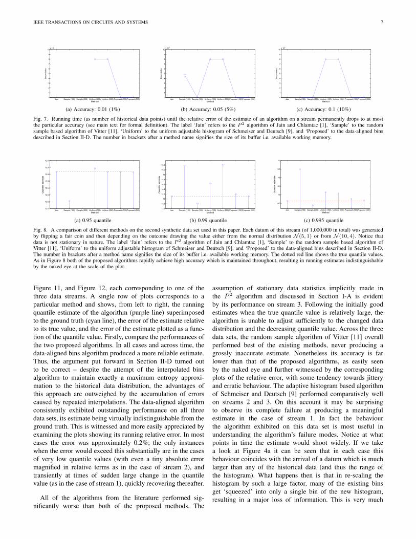
We now turn our attention to the second synthetic dataset which, unlike the first one, does not exhibit stationarystatistical properties. As before, we first summarized theestimates of three quantile values for different algorithms afterall available data has been processed, as well as the runningestimates. The results are summarized in respectively Figure 8

and Figure 9. Most of the conclusions which can be drawnfrom these mirror those already made on the first syntheticset. The proposed data-aligned bins algorithm consistentlyperformed best and without any deterioration when the buffersize was reduced from 500 to 100. The uniform adjustablehistogram of Schmeiser and Deutsch outperformed the sample-based algorithm of Vitter on average but again exhibited short-lived but large transient errors. The only major difference incomparison with the results obtained on the first data set is thatin this case the simple method of Jain and Chlamtac performedextremely well (the corresponding running quantile estimate inFigure 9 is indistinguishable from that of the proposed methodon the scale shown).

0 2 4 6 8 10

x 105

0

2

4

6

8

10

12

14

16

18

20

Datum index

Qua

ntile

est

imat

e

Jain

Sample (100)

Sample (500)

Uniform (100)

Uniform (500)

Proposed (100)

Proposed (500)

Fig. 9. Running estimate of the 0.95-quantile produced by different methodson our second (non-stationary) synthetic data set. The label ‘Jain’ refers to theP 2 algorithm of Jain and Chlamtac [1], ‘Sample’ to the random sample basedalgorithm of Vitter [11], ‘Uniform’ to the uniform adjustable histogram ofSchmeiser and Deutsch [9], and ‘Proposed’ to the data-aligned bins describedin Section II-D. The number in brackets after a method name signifies thesize of its buffer i.e. available working memory.

2) Real-world surveillance data: Having gained some un-derstanding of the behaviour of different algorithms in a settingin which input data was well understood and controlled, weapplied them to data acquired by a real-world surveillance sys-tem. Representative results, obtained using the same numberof bins n = 500, for 0.95-quantile are shown in Figure 10,


Jain Samplet(100) Samplet(500) Uniformt(100) Uniformt(500) Proposedt(100)Proposedt(500)0

1

2

3

4

5

6

7

8

9

10xt10

5

Method

Dat

umtin

dex

(a) Accuracy: 0.01 (1%)


1

2

3

4

5

6

7

8

9

10xt10

5

Method

Dat

umtin

dex

(b) Accuracy: 0.05 (5%)


1

2

3

4

5

6

7

8

9

10xt10

5

Method

Dat

umtin

dex

(c) Accuracy: 0.1 (10%)

Fig. 7. Running time (as number of historical data points) until the relative error of the estimate of an algorithm on a stream permanently drops to at mostthe particular accuracy (see main text for formal definition). The label ‘Jain’ refers to the P 2 algorithm of Jain and Chlamtac [1], ‘Sample’ to the randomsample based algorithm of Vitter [11], ‘Uniform’ to the uniform adjustable histogram of Schmeiser and Deutsch [9], and ‘Proposed’ to the data-aligned binsdescribed in Section II-D. The number in brackets after a method name signifies the size of its buffer i.e. available working memory.

Jain Sampleh(100) Sampleh(500) Uniformh(100) Uniformh(500) Proposedh(100)Proposedh(500)12.51

12.52

12.53

12.54

12.55

12.56

12.57

12.58

Method

Qua

ntile

hest

imat

e

(a) 0.95 quantile


13.8

14

14.2

14.4

14.6

14.8

15

15.2

15.4

Method

Qua

ntile

Qest

imat

e

(b) 0.99 quantile

Jain Sample (100) Sample (500) Uniform (100) Uniform (500) Proposed (100)Proposed (500)

14.5

15

15.5

16

16.5

17

Method

Qua

ntile

est

imat

e

(c) 0.995 quantile

Fig. 8. A comparison of different methods on the second synthetic data set used in this paper. Each datum of this stream (of 1,000,000 in total) was generatedby flipping a fair coin and then depending on the outcome drawing the value either from the normal distribution N (5, 1) or from N (10, 4). Notice thatdata is not stationary in nature. The label ‘Jain’ refers to the P 2 algorithm of Jain and Chlamtac [1], ‘Sample’ to the random sample based algorithm ofVitter [11], ‘Uniform’ to the uniform adjustable histogram of Schmeiser and Deutsch [9], and ‘Proposed’ to the data-aligned bins described in Section II-D.The number in brackets after a method name signifies the size of its buffer i.e. available working memory. The dotted red line shows the true quantile values.As in Figure 8 both of the proposed algorithms rapidly achieve high accuracy which is maintained throughout, resulting in running estimates indistinguishableby the naked eye at the scale of the plot.

Figure 11, and Figure 12, each corresponding to one of thethree data streams. A single row of plots corresponds to aparticular method and shows, from left to right, the runningquantile estimate of the algorithm (purple line) superimposedto the ground truth (cyan line), the error of the estimate relativeto its true value, and the error of the estimate plotted as a func-tion of the quantile value. Firstly, compare the performances ofthe two proposed algorithms. In all cases and across time, thedata-aligned bins algorithm produced a more reliable estimate.Thus, the argument put forward in Section II-D turned outto be correct – despite the attempt of the interpolated binsalgorithm to maintain exactly a maximum entropy approxi-mation to the historical data distribution, the advantages ofthis approach are outweighed by the accumulation of errorscaused by repeated interpolations. The data-aligned algorithmconsistently exhibited outstanding performance on all threedata sets, its estimate being virtually indistinguishable from theground truth. This is witnessed and more easily appreciated byexamining the plots showing its running relative error. In mostcases the error was approximately 0.2%; the only instanceswhen the error would exceed this substantially are in the casesof very low quantile values (with even a tiny absolute errormagnified in relative terms as in the case of stream 2), andtransiently at times of sudden large change in the quantilevalue (as in the case of stream 1), quickly recovering thereafter.

All of the algorithms from the literature performed sig-nificantly worse than both of the proposed methods. The

assumption of stationary data statistics implicitly made inthe P 2 algorithm and discussed in Section I-A is evidentby its performance on stream 3. Following the initially goodestimates when the true quantile value is relatively large, thealgorithm is unable to adjust sufficiently to the changed datadistribution and the decreasing quantile value. Across the threedata sets, the random sample algorithm of Vitter [11] overallperformed best of the existing methods, never producing agrossly inaccurate estimate. Nonetheless its accuracy is farlower than that of the proposed algorithms, as easily seenby the naked eye and further witnessed by the correspondingplots of the relative error, with some tendency towards jitteryand erratic behaviour. The adaptive histogram based algorithmof Schmeiser and Deutsch [9] performed comparatively wellon streams 2 and 3. On this account it may be surprisingto observe its complete failure at producing a meaningfulestimate in the case of stream 1. In fact the behaviourthe algorithm exhibited on this data set is most useful inunderstanding the algorithm’s failure modes. Notice at whatpoints in time the estimate would shoot widely. If we takea look at Figure 4a it can be seen that in each case thisbehaviour coincides with the arrival of a datum which is muchlarger than any of the historical data (and thus the range ofthe histogram). What happens then is that in re-scaling thehistogram by such a large factor, many of the existing binsget ‘squeezed’ into only a single bin of the new histogram,resulting in a major loss of information. This is very much


like what we observed previously on simple synthetic datain experiments in Section III-B1. When this behaviour iscontrasted with the performance of the algorithms we proposedin this paper, the importance of the maximum entropy principleas the foundational idea is easily appreciated; although ouralgorithms too readjust their bins upon the arrival of eachnew datum, the design of our histograms ensures that nomajor loss of information occurs regardless of the value ofnew data. Figure 13 illustrates the evolution of bin boundariesand the corresponding bin counts in a run of our data-alignedhistogram-based algorithm.

Considering the outstanding performance of our algorithms,and in particular the data-aligned histogram-based approach,we next sought to examine how this performance is affected bya gradual reduction of the working memory size. To make thetask more challenging we sought to estimate the 0.99-quantileon the largest of our three data sets (stream 2). Our resultsare summarized in Table II. This table shows the variation inthe mean relative error as well as the largest absolute error ofthe quantile estimate for the proposed data-aligned histogram-based algorithm as the number of available bins is graduallydecreased from 500 to 12. For all other methods, the reportedresult is for n = 500 bins. It is remarkable to observe that themean relative error of our algorithm does not decrease at all.The largest absolute error does increase, only a small amountas the number of bins is reduced from 500 to 50, and moresubstantially thereafter. This shows that our algorithm overallstill produces excellent estimates with occasional and transientdifficulties when there is a rapid change in the quantile value.Plots in Figure 14 corroborate this observation.

020

4060

80100

5001000

15002000

0.8

0.9

1

1.1

1.2

1.3

1.4

x 1010

Bin indexData stream index

Upp

er b

in b

ound

ary

020

4060

80100

0

1000

2000

30000

10

20

30

40

Bin indexData stream index

Dat

um c

ount

Fig. 13. An illustration of a typical evolution of the histogram used in theproposed data-aligned bins algorithm. Shown on the left is the adaptationin the upper bin boundary values; on the right are the corresponding datumcounts per bin. For this figure we used n = 100 bins.

IV. SUMMARY AND CONCLUSIONS

In this paper we addressed the problem of estimating adesired quantile of a data set. Our goal was specificallyto perform quantile estimation on a data stream when theavailable working memory is limited (constant), prohibitingthe storage of all historical data. This problem is ubiquitous incomputer vision and signal processing, and has been addressedby a number of researchers in the past. We show that amajor shortcoming of the existing methods lies in their usuallyimplicit assumption that the data is being generated by astationary process. This assumption is invalidated in mostpractical applications, as we illustrate using real-world dataextracted from surveillance videos.

TABLE IIA SUMMARY OF THE EXPERIMENTAL RESULTS OBTAINED ON THE

REAL-WORLD SURVEILLANCE DATA SET FOR THE 0.99-QUANTILE. ALSOSEE FIGURE 14.

Method Mean relative error Absolute L∞ error

Prop

osed

data

-alig

ned

bins

w/

bin

no. 500 0.5% 2.43

100 0.5% 2.45

50 0.5% 3.01

25 0.4% 14.48

12 0.5% 28.83

P 2 algorithm [1] 45.6% 112.61

Random sample [11] 17.5% 64.00

Equispaced bins [9] 0.9% 76.88

Therefore we introduced two novel algorithms which dealwith the described challenges effectively. Motivated by theobservation that a consequence of non-stationarity is that thehistorical data distribution need not be representative of thefuture distribution and thus that a quantile value can changerapidly, we adopt a histogram-based representation to allowan adaptation to such unpredictable variability to take place.In contrast to the previous work which either distributes thebin boundaries equidistantly or uses ad hoc adjustments, ouridea was to maintain bins in a manner which maximizes theentropy of the corresponding estimate of the historical datadistribution. The first method we described and which utilizesthe stated principle readjusts by interpolation the locations ofbin boundaries with every new incoming datum, attempting tomaintain equiprobable bins. In contrast, our second algorithmconstrains bin boundaries to the values of seen data. When anew datum arrives, a novel bin is created and the originalnumber of bins restored by selecting the optimal (in themaximum entropy sense) merge of a pair of neighbouring bins.

The proposed algorithms were evaluated and comparedagainst the existing alternatives described in the literatureusing three large data streams. This data was extracted fromCCTV footage, not collected specifically for the purposes ofthis work, and represents specific motion characteristics overtime which are used by semi-automatic surveillance analyticssystems to alert to abnormalities in a scene. Our evaluationconclusively demonstrated a vastly superior performance ofour algorithms, most notably the data-aligned bins algorithm.The highly non-stationary nature of our data was shownto cause major problems to the existing algorithms, oftenleading to grossly inaccurate quantile estimates; in contrast,our methods were virtually unaffected by it. What is more,our experiments demonstrate that the superior performance ofour algorithms can be maintained effectively while drasticallyreducing the working memory size in comparison with themethods from the literature.


0 1 2 3 4 5 6

x 105

0

1

2

3

4

5

6x 10

11

Datum index

Qua

ntile

est

imat

e

0 1 2 3 4 5 6

x 105

0

0.01

0.02

0.03

0.04

0.05

0.06

0.07

0.08

0.09

0.1

Datum index

Qua

ntile

est

imat

e re

lativ

e er

ror

1010

1011

1012

10−3

10−2

10−1

100

Quantile estimate relative error

Gro

und

trut

h qu

antil

e es

timat

e

(a) Proposed: interpolated bins

0 1 2 3 4 5 6

x 105

0

1

2

3

4

5

6x 10

11

Datum index

Qua

ntile

est

imat

e

0 1 2 3 4 5 6

x 105

0

0.002

0.004

0.006

0.008

0.01

0.012

0.014

0.016

0.018

0.02

Datum index

Qua

ntile

est

imat

e re

lativ

e er

ror

1010

1011

1012

10−5

10−4

10−3

10−2

10−1

100


Gro

und

trut

h qu

antil

e es

timat

e

(b) Proposed: data-aligned bins

0 1 2 3 4 5 6

x 105

0

1

2

3

4

5

6

7x 10

11

Datum index

Qua

ntile

est

imat

e

0 1 2 3 4 5 6

x 105

0

0.002

0.004

0.006

0.008

0.01

0.012

0.014

0.016

0.018

0.02

Datum index

Qua

ntile

est

imat

e re

lativ

e er

ror

1010

1011

1012

10−3

10−2

10−1

100

101


Gro

und

trut

h qu

antil

e es

timat

e

(c) P 2 algorithm [1]

0 1 2 3 4 5 6

x 105

0

1

2

3

4

5

6x 10

11

Datum index

Qua

ntile

est

imat

e

0 1 2 3 4 5 6

x 105

0

0.01

0.02

0.03

0.04

0.05

0.06

0.07

0.08

0.09

0.1

Datum index

Qua

ntile

est

imat

e re

lativ

e er

ror

1010

1011

1012

10−4

10−3

10−2

10−1

100


Gro

und

trut

h qu

antil

e es

timat

e

(d) Random sample [11]

0 1 2 3 4 5 6

x 105

0

2

4

6

8

10

12

14

16x 10

11

Datum index

Qua

ntile

est

imat

e

0 1 2 3 4 5 6

x 105

0

0.002

0.004

0.006

0.008

0.01

0.012

0.014

0.016

0.018

0.02

Datum index

Qua

ntile

est

imat

e re

lativ

e er

ror

1010

1011

1012

10−3

10−2

10−1

100

101

102


Gro

und

trut

h qu

antil

e es

timat

e

(e) Uniform histogram [9]

Fig. 10. Running estimate of the 0.95-quantile on data stream 1. A single row of plots corresponds to a particular method and shows, from left to right, therunning quantile estimate of the algorithm (purple line) superimposed to the ground truth (cyan line), the error of the estimate relative to its true value, andthe error of the estimate plotted as a function of the quantile value.


0 2 4 6 8 10

x 106

0

20

40

60

80

100

120

140

160

180

Datum index

Qua

ntile

est

imat

e

0 2 4 6 8 10

x 106

0

0.01

0.02

0.03

0.04

0.05

0.06

0.07

0.08

0.09

0.1

Datum index

Qua

ntile

est

imat

e re

lativ

e er

ror

100

101

102

103

10−5

10−4

10−3

10−2

10−1

100

101


Gro

und

trut

h qu

antil

e es

timat

e


0 2 4 6 8 10

x 106

0

20

40

60

80

100

120

140

160

180

Datum index

Qua

ntile

est

imat

e

0 2 4 6 8 10

x 106

0

0.002

0.004

0.006

0.008

0.01

0.012

0.014

0.016

0.018

0.02

Datum index

Qua

ntile

est

imat

e re

lativ

e er

ror

100

101

102

103

10−4

10−3

10−2

10−1

100


Gro

und

trut

h qu

antil

e es

timat

e


0 2 4 6 8 10

x 106

0

20

40

60

80

100

120

140

160

180

200

Datum index

Qua

ntile

est

imat

e

0 2 4 6 8 10

x 106

0

0.002

0.004

0.006

0.008

0.01

0.012

0.014

0.016

0.018

0.02

Datum index

Qua

ntile

est

imat

e re

lativ

e er

ror

100

101

102

103

10−1

100

101

102


Gro

und

trut

h qu

antil

e es

timat

e


0 2 4 6 8 10

x 106

0

20

40

60

80

100

120

140

160

180

Datum index

Qua

ntile

est

imat

e

0 2 4 6 8 10

x 106

0

0.05

0.1

0.15

0.2

0.25

0.3

0.35

0.4

0.45

0.5

Datum index

Qua

ntile

est

imat

e re

lativ

e er

ror

100

101

102

103

10−3

10−2

10−1

100


Gro

und

trut

h qu

antil

e es

timat

e


0 2 4 6 8 10

x 106

0

50

100

150

200

250

Datum index

Qua

ntile

est

imat

e

0 2 4 6 8 10

x 106

0

0.01

0.02

0.03

0.04

0.05

0.06

0.07

0.08

0.09

0.1

Datum index

Qua

ntile

est

imat

e re

lativ

e er

ror

100

101

102

103

10−5

10−4

10−3

10−2

10−1

100


Gro

und

trut

h qu

antil

e es

timat

e




0 5 10 15

x 105

0

2

4

6

8

10

12

14x 10

5

Datum index

Qua

ntile

est

imat

e

0 5 10 15

x 105

0

0.002

0.004

0.006

0.008

0.01

0.012

0.014

0.016

0.018

0.02

Datum index

Qua

ntile

est

imat

e re

lativ

e er

ror

103

104

105

106

107

10−4

10−3

10−2

10−1

100

101


Gro

und

trut

h qu

antil

e es

timat

e


0 5 10 15

x 105

0

2

4

6

8

10

12

14x 10

5

Datum index

Qua

ntile

est

imat

e

0 5 10 15

x 105

0

0.002

0.004

0.006

0.008

0.01

0.012

0.014

0.016

0.018

0.02

Datum index

Qua

ntile

est

imat

e re

lativ

e er

ror

103

104

105

106

107

10−7

10−6

10−5

10−4

10−3

10−2

10−1

100


Gro

und

trut

h qu

antil

e es

timat

e


0 5 10 15

x 105

0

0.5

1

1.5

2

2.5x 10

6

Datum index

Qua

ntile

est

imat

e

0 5 10 15

x 105

0

0.002

0.004

0.006

0.008

0.01

0.012

0.014

0.016

0.018

0.02

Datum index

Qua

ntile

est

imat

e re

lativ

e er

ror

103

104

105

106

107

10−3

10−2

10−1

100

101


Gro

und

trut

h qu

antil

e es

timat

e


0 5 10 15

x 105

0

2

4

6

8

10

12

14

16

18x 10

5

Datum index

Qua

ntile

est

imat

e

0 5 10 15

x 105

0

0.002

0.004

0.006

0.008

0.01

0.012

0.014

0.016

0.018

0.02

Datum index

Qua

ntile

est

imat

e re

lativ

e er

ror

103

104

105

106

107

10−5

10−4

10−3

10−2

10−1

100


Gro

und

trut

h qu

antil

e es

timat

e


0 5 10 15

x 105

0

0.5

1

1.5

2

2.5

3

3.5

4

4.5x 10

7

Datum index

Qua

ntile

est

imat

e

0 5 10 15

x 105

0

0.1

0.2

0.3

0.4

0.5

0.6

0.7

0.8

0.9

1

Datum index

Qua

ntile

est

imat

e re

lativ

e er

ror

103

104

105

106

107

10−2

10−1

100

101

102

103


Gro

und

trut

h qu

antil

e es

timat

e




0 2 4 6 8 10

x 106

40

60

80

100

120

140

160

180

200

220

240

Datum index

Qua

ntile

est

imat

e

0 2 4 6 8 10

x 106

0

0.002

0.004

0.006

0.008

0.01

0.012

0.014

0.016

0.018

0.02

Datum index

Qua

ntile

est

imat

e re

lativ

e er

ror

101

102

103

10−6

10−5

10−4

10−3

10−2

10−1

100


Gro

und

trut

h qu

antil

e es

timat

e

(a) Data stream 2, 0.99-quantile, 12 bins

0 2 4 6 8 10

x 106

40

60

80

100

120

140

160

180

200

220

Datum index

Qua

ntile

est

imat

e

0 2 4 6 8 10

x 106

0

0.002

0.004

0.006

0.008

0.01

0.012

0.014

0.016

0.018

0.02

Datum index

Qua

ntile

est

imat

e re

lativ

e er

ror

101

102

103

10−7

10−6

10−5

10−4

10−3

10−2

10−1


Gro

und

trut

h qu

antil

e es

timat

e

(b) Data stream 2, 0.99-quantile, 25 bins

0 2 4 6 8 10

x 106

50

100

150

200

Datum index

Qua

ntile

est

imat

e

0 2 4 6 8 10

x 106

0

0.002

0.004

0.006

0.008

0.01

0.012

0.014

0.016

0.018

0.02

Datum index

Qua

ntile

est

imat

e re

lativ

e er

ror

101

102

103

10−6

10−5

10−4

10−3

10−2

10−1


Gro

und

trut

h qu

antil

e es

timat

e

(c) Data stream 2, 0.99-quantile, 50 bins

0 2 4 6 8 10

x 106

50

100

150

200

Datum index

Qua

ntile

est

imat

e

0 2 4 6 8 10

x 106

0

0.002

0.004

0.006

0.008

0.01

0.012

0.014

0.016

0.018

0.02

Datum index

Qua

ntile

est

imat

e re

lativ

e er

ror

101

102

103

10−6

10−5

10−4

10−3

10−2

10−1


Gro

und

trut

h qu

antil

e es

timat

e

(d) Data stream 2, 0.99-quantile, 100 bins

0 1 2 3 4 5 6

x 106

50

100

150

200

Datum index

Qua

ntile

est

imat

e

0 1 2 3 4 5 6

x 106

0

0.002

0.004

0.006

0.008

0.01

0.012

0.014

0.016

0.018

0.02

Datum index

Qua

ntile

est

imat

e re

lativ

e er

ror

101

102

103

10−5

10−4

10−3

10−2

10−1


Gro

und

trut

h qu

antil

e es

timat

e

(e) Data stream 2, 0.99-quantile, 500 bins

Fig. 14. Running estimate of the 0.99-quantile on data stream 2 produced using our data-aligned adaptive histogram algorithm and different numbers ofbins. A single row of plots corresponds to a particular method and shows, from left to right, the running quantile estimate of the algorithm (purple line)superimposed to the ground truth (cyan line), the error of the estimate relative to its true value, and the error of the estimate plotted as a function of thequantile value. Also see Table II.


REFERENCES

[1] R. Jain and I. Chlamtac, “The P 2 algorithm for dynamic calculation ofquantiles and histograms without storing observations.” Communicationsof the ACM, vol. 28, no. 10, pp. 1076–1085, 1985.

[2] R. Adler, R. Feldman, and M. Taqqu, Eds., A Practical Guide to HeavyTails., ser. Statistical Techniques and Applications. Birkhauser, 1998.

[3] N. Sgouropoulos, Q. Yao, and C. Yastremiz, “Matching quantiles esti-mation.” London School of Economics, Tech. Rep., 2013.

[4] C. Buragohain and S. Suri, Encyclopedia of Database Systems, 2009,ch. Quantiles on Streams., pp. 2235–2240.

[5] G. Cormode, T. Johnson, F. Korn, S. Muthukrishnany, O. Spatscheck,and D. Srivastava, “Holistic UDAFs at streaming speeds.” In Proc. ACMSIGMOD International Conference on Management of Data, pp. 35–46,2004.

[6] S. Guha and A. McGregor, “Stream order and order statistics: Quantileestimation in random-order streams.” SIAM Journal on Computing,,vol. 38, no. 5, pp. 2044–2059, 2009.

[7] J. I. Munro and M. Paterson, “Selection and sorting with limitedstorage.” Theoretical Computer Science, vol. 12, pp. 315–323, 1980.

[8] A. P. Gurajada and J. Srivastava, “Equidepth partitioning of a data setbased on finding its medians.” Computer Science Department, Universityof Minnesota, Technical Report TR 90-24, 1990.

[9] B. W. Schmeiser and S. J. Deutsch, “Quantile estimation from groupeddata: The cell midpoint.” Communications in Statistics: Simulation andComputation, vol. B6, no. 3, pp. 221–234, 1977.

[10] J. P. McDermott, G. J. Babu, J. C. Liechty, and D. K. J. Lin, “Dataskeletons: simultaneous estimation of multiple quantiles for massivestreaming datasets with applications to density estimation.” BayesianAnalysis, vol. 17, pp. 311–321, 2007.

[11] J. S. Vitter, “Random sampling with a reservoir.” ACM Transactions onMathematical Software, vol. 11, no. 1, pp. 37–57, 1985.

[12] G. Cormode and S. Muthukrishnany, “An improved data stream sum-mary: the count-min sketch and its applications.” Journal of Algorithms,vol. 55, no. 1, pp. 58–75, 2005.

[13] O. Arandjelovic, D. Pham, and S. Venkatesh, “Stream quantiles viamaximal entropy histograms.” In Proc. International Conference onNeural Information Processing (ICONIP), vol. II, pp. 327–334, 2014.

[14] R. R. Wilcox, Introduction to Robust Estimation and Hypothesis Testing,iii ed. Academic Press, 2012.

[15] C. Shannon, “A mathematical theory of communication.” The BellSystems Technical Journal, no. 27, pp. 379–423, 623–656, 1948.

[16] C. Wang and Z. Ye, “Brightness preserving histogram equalization withmaximum entropy: a variational perspective.” IEEE Transactions onConsumer Electronics, vol. 51, no. 4, pp. 1326–1334, 2005.

[17] Philips Electronics N.V., “A surveillance system with suspicious be-haviour detection.” Patent EP1459272A1, 2004.

[18] G. Lavee, L. Khan, and B. Thuraisingham, “A framework for a videoanalysis tool for suspicious event detection.” Multimedia Tools andApplications, vol. 35, no. 1, pp. 109–123, 2007.

[19] iCetana, “iMotionFocus.” http://www.icetana.com/ , Last accessed May2014.

[20] O. Arandjelovic, “Contextually learnt detection of unusual motion-basedbehaviour in crowded public spaces.” In Proc. International Symposiumon Computer and Information Sciences (ISCIS), pp. 403–410, 2011.

[21] intellvisions, “iQ-Prisons,” http://www.intellvisions.com/ , Last accessedMay 2014.

[22] R. Martin and O. Arandjelovic, “Multiple-object tracking in clutteredand crowded public spaces.” In Proc. International Symposium on VisualComputing (ISVC), vol. 3, pp. 89–98, 2010.

[23] D. Pham, O. Arandjelovic, and S. Venkatesh, “Detection of dynamicbackground due to swaying movements from motion features.” IEEETransactions on Image Processing (TIP), 2014.

Two Maximum Entropy Based Algorithms for Running Quantile Estimation in Non-Stationary Data Streams

Documents

Transcript of Two Maximum Entropy Based Algorithms for Running Quantile Estimation in Non-Stationary Data Streams