Trends in brother correlations in class and incomes in Finland:

A comparison of cohorts born in 1932-62

Jani Erola Turku School of Economics, jani.erola@tse.fi

Juho Härkönen Yale University, juho.harkonen@yale.edu

Markus Jäntti Åbo Akademi, markus.jantti@iki.fi

Prepared for the ISA Research Committee 28 Spring Meeting in Florence, 15-18 May 2008

[First draft; please do not quote without permission]

Abstract

Recent assessments of cross-national and cross-cohort comparisons of intergenerational mobility

have found intriguing differences in income and class mobility. For example, the United States

seems to be an open society when it comes to class mobility but a rigid one in terms of income

mobility. Furthermore, recent analyses have shown differences in trends in income and class

mobility in Britain. In this paper, we compare trends in brother resemblance in class and incomes

in Finland across cohorts born in 1932-62. We use population register data from the Finnish

Census Panel to calculate brother correlations for class and incomes. We also compare brothers

using loglinear models. We find diverging trends in brother resemblance in class and incomes,

suggesting that intergenerational mobility in and family background effects on incomes and class

may be governed by different processes.

Introduction

The analysis of the effects of family background on socioeconomic success is a central field of

research in sociology and economics alike. The most common approach in this tradition is a

comparison of the incomes or class positions of parents and their children (e.g., Blau and Duncan

1967; Erikson and Goldthorpe 1992; Solon 1992; Björklund and Jäntti 1997; 2000; forthcoming;

Breen 2004; Corak 2004). This research has found surprising robustness, but also international and

cross-temporal variation in socioeconomic mobility between parents and children.

While measures of the association between parents’ and their children’s socioeconomic positions

appeal to our common-sense understandings of socioeconomic mobility and the role of family

background, they provide a limited picture of the role of family background, as parents'

socioeconomic background is only one measure of the multiple family background factors that

affect adulthood outcomes. To better account for these factors, several studies have used

correlations between siblings’ socioeconomic statuses to estimate the ―total‖ effect of family

background and other factors that are shared by siblings (such as neighborhood conditions and

schools) (e.g., Hauser and Mossel 1985; Ganzeboom et al 1992; Sieben and DeGraaf 2001; Sieben

et al. 2001; Björklund et al. 2002). Not surprisingly, these correlations are generally higher than

those between parents and their children (on the relationship between intergenerational

correlations and sibling correlations, see Solon (1999)).

While questions of intergenerational mobility and family background have been of interest to both

sociologists and economists, there has been surprisingly little overlap between the two disciplines

(for a recent exception, Morgan et al. 2006). However, a comparison of the estimates of

intergenerational mobility from economics and sociology can produce a very different picture of

the extent of mobility in societies. For instance, the United States appears as a highly mobile

society when class mobility is concerned, but more rigid when one looks at intergeneration

mobility in incomes (Björklund and Jäntti 2000) (although according to other studies the US does

not seem exceptional even in class mobility, e.g. Erikson & Goldthorpe 1992; Beller and Hout

2006). Measures of class and income mobility can also produce a very different picture of trends

in intergenerational mobility within countries. A recent example concerns mobility trends in

England (Blanden et al. 2004; Goldthorpe and Jackson 2007; Erikson and Goldthorpe 2008).

According to measures of income mobility, intergenerational inheritance seems to have

strengthened considerably between two cohorts born just 12 years apart (Blanden et al. 2004). At

the same time, Goldthorpe and Jackson (2007) found notable stability in class mobility using the

same data. Erikson and Goldthorpe (2008) also found that associations between fathers' and

childrens' class were generally stronger than those between family incomes and childrens' earnings

in adulthood. This is the only explicit test that has systematically compared the measures that we

are aware of.

These differences in the perceptions of intergenerational inheritance and openness are intriguing.

One would certainly wish and expect consensus between different measures on this important

social issue. However, one can think of reasons for as to why the results differ.

First, social class and income are complementary, although related, measures of social position.

Therefore, it may simply be that mobility in one is stronger than in the other, and countries differ

with respect to their relative strength. We can, for example, think of a society in which parents are

more interested in ensuring their children's social class or status than in maximizing their incomes,

and the other way around. Parental class and income can also capture a different range of factors

that affect socioeconomic outcomes. For example, class can be more strongly correlated with

cultural capital than income. Furthermore, cultural and social capital may be a more important

determinant of socioeconomic success in one society, whereas parental wealth and incomes open

doors in another society, due to for instance differences in education systems (cf. Checchi et al.

1999). Björklund and Jäntti (2000, 24-6) offered a more formalised version of a related argument,

according to which countries' (and periods') relative ranking of intergenerational inheritance may

vary across mobility measures depending on the relationship between class-independent factors

that affect the incomes of both parents and children.

The differences in estimates of the degree of mobility can, second, result from methodological

differences across the disciplines or different methodological and data problems facing researchers

on income and class mobility. Sociologists have often analysed intergenerational mobility with

loglinear models in the case of social classes and correlations and regression analysis in the case of

socioeconomic indeces, while economists establish intergenerational correlations and elasticities

(by regressing childrens' log incomes on parents' or families' log incomes). These intergenerational

measures based on correlations and elasticities on the one hand, and parameters from log-linear

models on the other are obviously not directly comparable, in part because most former measures

do not take account of possible nonlinearities (there are exceptions, however, e.g. Bratsberg et al.

2007). Thus, the comparability of the association measures poses an obvious challenge to

comparisons of income and class mobility. Income measures are also more prone to measurement

error than questions about respondents' occupation, which form the basis for measures of social

class and socioeconomic status. Typical analyses of income mobility also focus on earnings,

which often excludes incomes from self-employment and farming (e.g. Björklund and Jäntti

2000). Recent results have also shown that the picture of income mobility is sensitive to the

number of years over which (parental) incomes are averaged in order to create a proxy for

permanent incomes (e.g., Solon 1992; Mazumder 2005). The estimates are also sensitive to the

stage of the life-course in which permanent (both of parents and children) incomes are measured

(Böhlmark and Lindquist 2006; Haider and Solon 2006). All these issues increase the demands for

suitable data for studying income mobility. Class mobility, on the other hand, can be more readily

analysed with a wider range of data. As mentioned, respondents' answers on their (and their

parents) occupations are generally more reliable. Classes and occupations also arguably show

more year-to-year stability, which is why the above issues have not received similar focus in

standard analyses (Ganzeboom ym. 1991), and the early examples of the application of multiple

class observations on the analysis of class mobility of Bielby et al (1977) and Hauser et al (1983)

have not inspired much replication. However, the downside of using class as the measure of status

is that it is not always clear what distinguishes the classes and how to determine class

membership. Due to this class membership is likely to include more measurent error than for

example individual's earnings, which are more straightforward to define (assuming no recall or

other measurent error as in the case of register data).

In this paper, we estimate brother correlations in class and earnings across five birth cohorts

(1932-38, 1939-44, 1945-51, 1952-56, and 1957-62) in Finland using register data for a total of

33,767 men from 20,715 families from the Finnish Census Panel. We have two main questions,

one substantive and one methodological. Regarding the former, we ask whether the brother

correlations--and thus, whether the effect of factors shared by brothers--have changed across the

three decades. The five cohorts grew up in very different socioeconomic circumstances. While

poverty was widespread during the earlier periods and the older cohorts grew up during the

hardship of the second world war and its direct aftermath, younger cohorts experienced more

favorable conditions as education and the welfare state expanded and living conditions improved.

We would thus expect that family background mattered more for the older cohorts than the

younger ones. Our methodological question concerns the (dis)similarity in the results gained from

different measures of social position, namely, class and incomes. We focus on brothers due to

lower stability in class and earnings patterns of women (e.g., Böhlmark and Lindquist 2006),

which may affect our estimates and also compromise comparability of income and class measures.

This descriptive paper makes three contributions. First, our paper is, to our knowledge, the first to

compare brother resemblance in income and class (as a categorical variable) using the same data.

In fact, our paper is to our knowledge also the first to provide estimates of sibling resemblance in

class (instead of socioeconomic or prestige indeces). Second, we use multilevel modeling to

provide comparable estimates of brother resemblance in earnings and class. We use identical

cohorts, class and income measures across the same stages in the life-course, and similar models.

These improve the comparability of the estimates across income and class. We also use high-

quality register data, which help avoid common problems of measurement error and attrition in

income measurement in particular. To further facilitate comparability, we also use multiple

measurements both for income and for class for the same phase in the life-course. Third, we

provide evidence of changes and stability in brother resemblance across five Finnish birth cohorts,

who came to age under very different socioeconomic conditions. Our results suggest that the

picture of the total family effect on socioeconomic attainment and its trends may indeed depend on

whether one looks at class attainment or at incomes. Furthermore, our results for both brother

resemblance in class and in incomes are somewhat sensitive to the choice of method (variance

decomposition using multilevel models versus loglinear models).

The structure of the paper is following. First we provide a brief overview of previous related

research in Finland and elsewhere. After that we describe the data and methods. The empirical

section begins with the description of the changes in class structure in Finland for the analysed

cohorts. We then analyse sibling resemblance with multilevel ordered probit (class) and multilevel

linear regression (income) models. Then we compare the difference of the background effect

applying the ―traditional‖ loglinear models for the father-brother mobility in class for the studied

cohorts. The last section concludes.

Previous research

Occupational class mobility has been studied fairly little in Finland, if compared to many other

European countries. The studies conducted in the 1970s and 1980s showed that a large share of the

white collar and manual labourer classes had their origins among the self-employed farmers and

farm workers. This was explained with the rapid pace of industrialization that took place during

two decades after the Second World War. The studies suggested that social mobility in Finland

was very similar to that in Sweden and Norway, two other Nordic welfare states with high level of

equality of opportunity. (Pöntinen, Alestalo & Uusitalo, 1982; Pöntinen, 1983; Erikson &

Pöntinen, 1985).

After the eighties, there was a long gap in mobility studies. In 2002, Erola and Moisio analysed

occupational class mobility of the 31-35 years old in 1990 and 1995, also using the Census Data.

Although the analysed period was very short and only two cohorts were used, the study suggested

that Finland was still a very equal society in terms of social mobility. (Erola & Moisio 2002,

2005.) Moisio (2006) analysed the change in social mobility by comparing mobility differences

between different cohorts, using a single cross-sectional survey data set collected in 2005. The

result indicated that social mobility in Finland had increased since the World War II. This was also

suggested by a study of social mobility between three consequent generations by Erola and Moisio

(2007). When social fluidity between two consequent generations were studied, it signalled the

weakening of the social inheritance of status. It also showed that the effect of grandparents’ class

on the class status of the grandchildren was practically non-existing in Finland, when the

association between two consequent generations were controlled for.1

Income mobility in Finland has been quite frequently studied in the past few years. Jäntti and

Östebacka (1995) report father-son correlation of 0.22 in incomes according to five year average

incomes. Österbacka (2001) reports correlations in earnings between fathers and children that are

as low as 0.12-0.16.Bratsberg et al (2007) report intergenerational elasticities of about 0.20 for

the cohort born 1956-60, but find strong non-linearities across the distribution. The association is

very weak in the lowest income decile, and much stonger in the highest. Generally, the association

is approximately at the same level as in other Nordic countries, but much weaker than in US or

UK.

Importantly for the current study, there are also sibling association models for income available

for Finland. Österbacka (2001) reports a correlation of 0.26 for brothers and 0.11 for sisters.

Björklund et al (2002) report borther income correlation of 0.25 for Finnish 25-42 years old

brothers. However, when controlling for autocorrelated errors between years of observations

(1985, 1990, 1995), Finnish estimate increases to 0.52, which is on par with the results from US

rather than with other Nordic countries.

Although not studied in Finland, sibling associations of index-based measures of occupational

class have been previously elsewhere. One of the early examples by Hauser and Mossel (1985)

estimated that family background explained about one third of the sibiling resemblance in SEI

index between brothers in US. Sieben and De Graaf (2001) compared brother resemblance

according to ISEI in England, Hungary, the Netherlands, Scotland, Spain, and the USA, and found

that shared family background contributed about 36.4 percent of the variance in occupation.

Conley and Glauber (2004, 2007) found the sibling correlation in SEI of 0.418. This was clearly

lower than in education (0.576) but fairly comparable to income (0.458). As mentioned above, to

our knowledge there are no similar tests applying class classifications, such as EGP.

Due to obvious data restrictions, there are few studies looking at trends in sibling correlations

(however, Kuo and Hauser 1995; Mazumder and Levine 2003; Björklund et al. 2007). In an

analysis of males born between 1932-1968 in Sweden, Björklund et al (2007) report a dramatic

decline in the brother correlation in income from 0.34 to 0.23 between cohorts born in 1932-38

and 1944-50, respectively, after which the association remained rather stable. The authors of this

study associated this decline to the effects of family background on education between these

cohorts.For the United States, Mazumder and Levine (2003) found increasing brother correlations

in earnings across time despite stable brother correlation in education.

Models and estimation

Sibling correlations in income and class

Our modeling strategy begins with a simple description of socioeconomic attainment, where we

assume that we have a measure of long-run socioeconomic attainment of sibling j in family i

(1),

where is the population mean and is an individual specific component with variance .

This component shows the individual’s relative long-term socioeconomic attainment. This can be

decomposed into a family specific component of permanent attainment ( ) that is common to all

siblings in a family and an individual specific component of permanent attainment :

(2).

The former captures the family-specific deviations from the population mean whereas the latter

denotes individual deviations from the family component average. These components are also

independent by construction. The variance, , of the individual specific component in the

population model is similarly a sum of the variances of the common family component and the

individual deviations from the family mean

(3).

We can calculate the share of the variance in long-term socioeconomic attainment that stems from

family background with

(4),

which equals the correlation between two randomly drawn pairs of brothers. The bigger the rho,

the stronger the influence of shared effects shared by the brothers (including family background,

neighborhoods, schools, and genetic traits).

To estimate this brother correlation, we need to estimate the variance of the family component and

the variance of the individual component, respectively.

In the case of (logged) income, we have multiple observations of annual income so that

(5),

where is logged annual income for sibling j in family i in year t, is the population mean of

logged incomes in year t, is a family specific component of permanent income, is an

individual specific component of permanent income, and denotes possible measurement error

and annual transitory income shocks. We estimated this two-level model the nlme package in R (R

Development Core Team 2008).

Models for estimating the variance components for social class face additional difficulties due to

the categorical nature of commonly used class variables, including the one (eight class Erikson-

Goldthorpe class variable) used here. The optimal way of estimating the variance components for

classes is through multilevel multinomial logit or probit models. To estimate the variances for the

(long-term) individual and family components, one needs to specify both separate random effects

at each level for each outcome (excluding the reference category) and, at each level, a full set of

covariances between these random effects. This exercise proved computationally very burdensome

and has to wait for future versions of the paper.

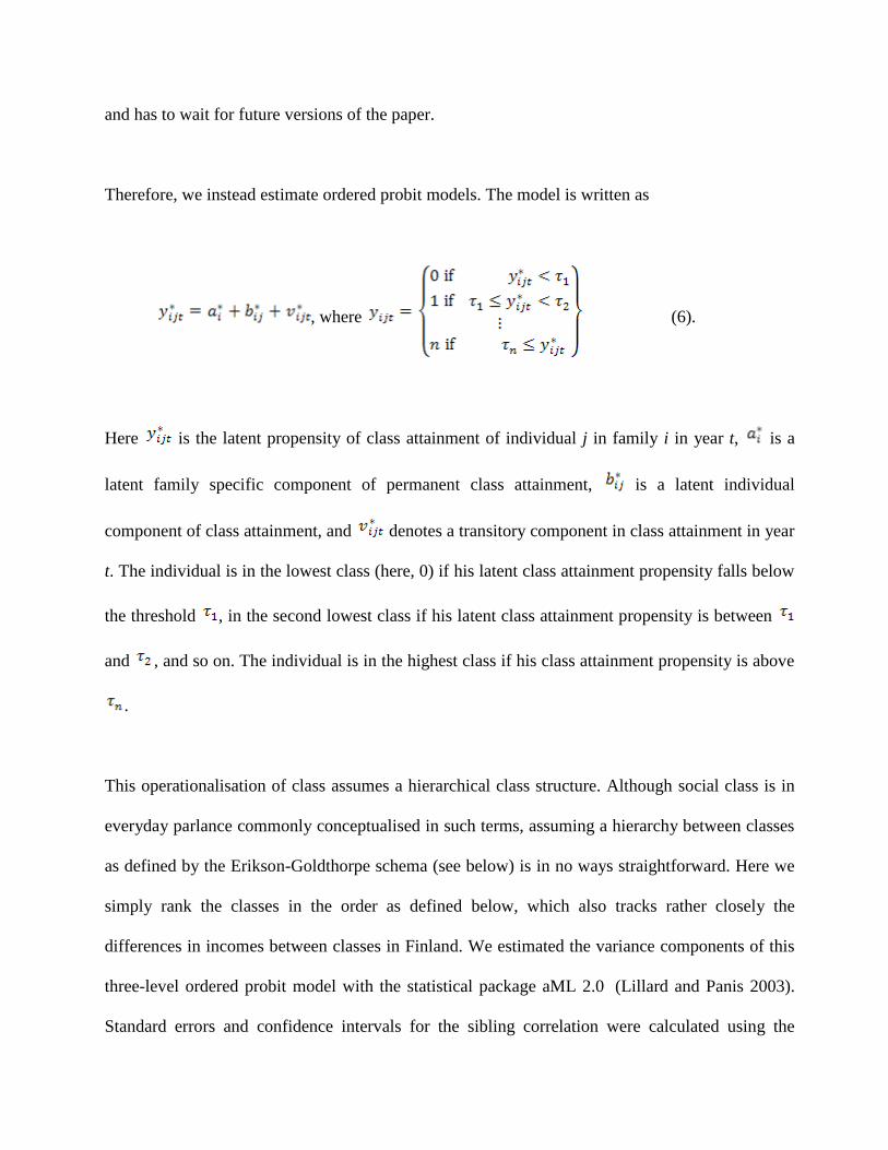
Therefore, we instead estimate ordered probit models. The model is written as

, where (6).

Here is the latent propensity of class attainment of individual j in family i in year t, is a

latent family specific component of permanent class attainment, is a latent individual

component of class attainment, and denotes a transitory component in class attainment in year

t. The individual is in the lowest class (here, 0) if his latent class attainment propensity falls below

the threshold , in the second lowest class if his latent class attainment propensity is between

and , and so on. The individual is in the highest class if his class attainment propensity is above

.

This operationalisation of class assumes a hierarchical class structure. Although social class is in

everyday parlance commonly conceptualised in such terms, assuming a hierarchy between classes

as defined by the Erikson-Goldthorpe schema (see below) is in no ways straightforward. Here we

simply rank the classes in the order as defined below, which also tracks rather closely the

differences in incomes between classes in Finland. We estimated the variance components of this

three-level ordered probit model with the statistical package aML 2.0 (Lillard and Panis 2003).

Standard errors and confidence intervals for the sibling correlation were calculated using the

Maximum Likelihood method as described in Donner and Wells (1986, 405).

Log-linear analyses of sibling resemblance

As secondary means to examine trends in sibling resemblance in income and class, we use

loglinear models, which are commonly used in sociological analyses of intergenerational mobility.

Typically, the class position of a parent and a child form the dimensions of the mobility table; in

sibling models the statuses of two siblings are used instead. We construct mobility tables for

brothers according to EGP classes and income octiles. In addition, we match the brothers to their

fathers, so that we can apply the usual parent-child setting to the data as well. We apply four rather

commonplace mobility models: the independence model of no association between variables; the

model assuming changing marginals but no association between class or income variables; the

constant social mobility (fluidity) model, allowing interaction between positions of two brothers or

fathers and sons in addition to changing marginals; and finally, the unidifference (or log-

multiplicative layer effect) model for the sibling or father-son association according to cohort,

testing the significance of the change in the strength of status association (Erikson & Golthorpe

1992; Xie 1992). As in studies applying the mobility tables approach, the models are fitted to one

observation only, in this case to the first observation of class or incomes of brothers. Loglinear

models were estimated using gnm-package in R (Turner & Firth 2006, R Development Core Team

2008).

Data

We use data on 33,767 Finnish men born in 1932-1962 from the Finnish Census Panel (FCP). The

FCP is a register-based panel database compiled and provided by Statistics Finland. Since the data

are collected from administrative registers, it suffers less from missing data, measurement error,

and attrition problems than common survey data. Therefore, it promises a good source for

comparing results for family background effects using income and class. We classified our sample

into five mutually exclusive birth cohorts, born in 1932-38, 1939-44, 1945-51, 1952-56, and 1957-

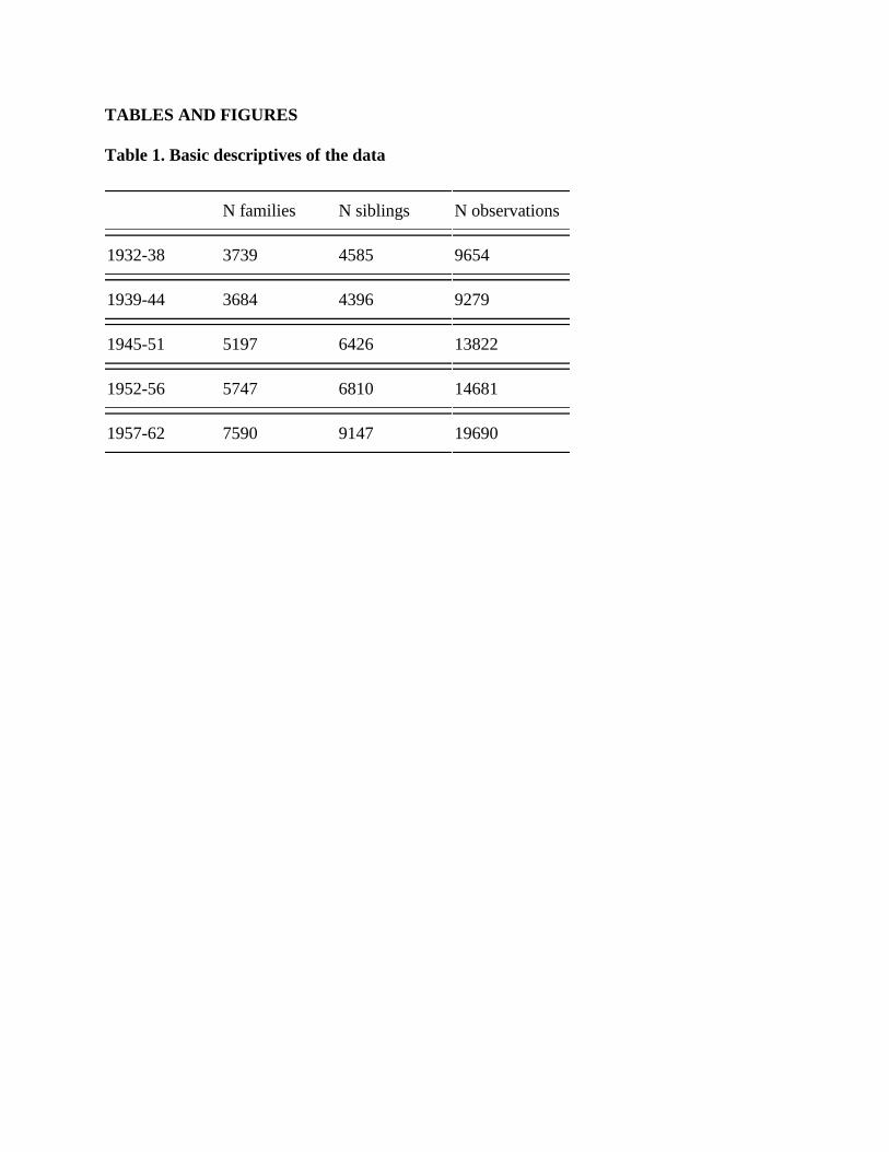
62. Table 1 shows the number of individuals (males), families, and observations in each cohort.

Table 1

The dataset includes 20 waves: 1950, 1970, 1975, 1980, 1985, and annual observations from 1987

to 2001. From this information we matched brothers and compiled follow-up data for our five

cohorts. We matched brothers by, first, defining males as children if they were age 18 or less, and

second, if they resided in the same family during our observations. Less than 10 percent of the

individuals lived in independent households at age 18 in each cohort. Brothers were defined as

belonging to the same cohort if they were born during the same range of years: brothers belonging

to different cohorts were excluded from the cohort-specific analyses. Therefore, we calculate

correlations for brothers from the same family who belong precisely to the same birth cohort.

Research on intergenerational income mobility and sibling correlations in income have paid much

attention to attenuation bias that arises from the use of (parental) income observations from a

single or a limited number of years (Solon 1992; Zimmerman 1992; Björklund and Jäntti 2000;

Mazumder 2005; Björklund et al. 2007). This arises because of fluctuations in annual earnings,

which produce measurement error to measures of permanent earnings, and thus bias

intergenerational correlations downwards.

Another source of bias concerns lifecycle bias. Haider and Solon (2006) and Böhlmark and

Lindquist (2006) examined this issue in the United States and Sweden, respectively, by analysing

the correspondence between short-term and longer-term earnings across different stages of the

life-course. They concluded that for men, the correspondence is the highest during the early/mid-

30s to early 40s. Since life-cycle bias can lead to biased estimates of the intergenerational or

sibling correlations, incomes should be measured during this phase where the correspondence

between short- and long-term incomes is the highest (see appendix in Björklund et al. 2007 for

discussion of life-cycle bias in analyses of sibling correlations in income).

Building on these results, we restrict our observations from age 33 to age 43, both for incomes and

class. Issues of biases stemming from poor proxies of permanent status or life-cycle bias have not

received much attention in sociological studies (the latter may be why, for example, Hauser et al.

(1999) and Conley and Glauber (2007) find strengthening sibling correlations across the life

course, a result in line with Haider and Solon’s (2006) findings of a weakening link between short-

term and permanent incomes at later ages). However, although we are here not able to examine

these issues further, we believe that they are of possible concern also to sociologists.

To reduce bias in estimating long-term incomes (and class), we would optimally include

observations for each year during this age range (cf. Mazumder 2005). However, our data enable

annual observations in this age range only for cohorts born 1954 or later, and for the eldest

cohorts, we only have observations for every fifth year. Therefore, to maximize comparability, we

observe incomes and class every five years for all birth cohorts. This leads to a three-level data

structure, with observations at the lowest level, males at the middle, and families at the highest

level.

Table 2

Table 2 describes our observation window. We have observations from eight years: first, from

1950 and then from 1970 to 2000 for every fifth year (x-axis). Each row shows the age of each

annual birth cohort during these years. The ages shaded in grey represent the ages during which

the males were defined as children (0-18 years): males residing in the same family during

childhood were further defined as brothers. The ages shaded in black represent the ages during

which we collected information on their incomes and class (33-43 years). For example, we

observe the oldest males (born in 1932) first in 1950, when they were 18 years old, and thus were

defined as children and eligible to be included in our analyses. They were next observed in 1970,

when they were 38 years old, and then in 1975, when they were 43 years old. For this cohort, we

have income/class data for these two years, and for some cohorts, we have data for three years.

Variables

Our class variable is based on a eight-class version of the Erikson-Goldthorpe class schema. The

classification coding was based on the coding key by Ganzeboom and Treiman (2001). Our class

schema and its distributions are described in Table 3. Our income variable is deflated and includes

all personal taxable gross incomes during a year. These include earnings, social benefits, capital

incomes, and other incomes. In the multilevel analysis, we used a logged transformation of

incomes, while controlling for age and the year of income observation. For loglinear models, we

instead use income octiles in order to enhance comparability with the class schema.

Table 3

Changes in class structure, absolute career mobility and income distribution

Table 2 shows the class structure of the analysed cohorts at the age of 33-37 using EGP class

schema (see above). It can be seen that contrary to the expectations of some, the growth of service

classes with the expense of the size of the manual labour classes has been very modest, almost

non-existing since the second cohort.

Table 4

Although the class structure remains largely the same over time, there is quite much variation in

the class positions of individuals between observations not only between the first and second, but

also the second and third observation; whereas one fourth of the cases change occupations

between two first observations, around one fifth of the cases do so also between second and third

observation. This applies also to vertical career mobility between observations (this refers to the

mobility across three hierarchy levels of the classes, as proposed by Erikson and Goldthorpe

(1992), according to which the classes I, II and IVa+b are most advantageous and the classes VIIa

and VIIb least advantageous, the other classes remaining between them.) The amount of mobility

is about one third lower than according to absolute career mobility, but nonetheless far from being

non-existent. There is little variation between the cohorts. The tables are reported in Appendix

Table 1 and 2).

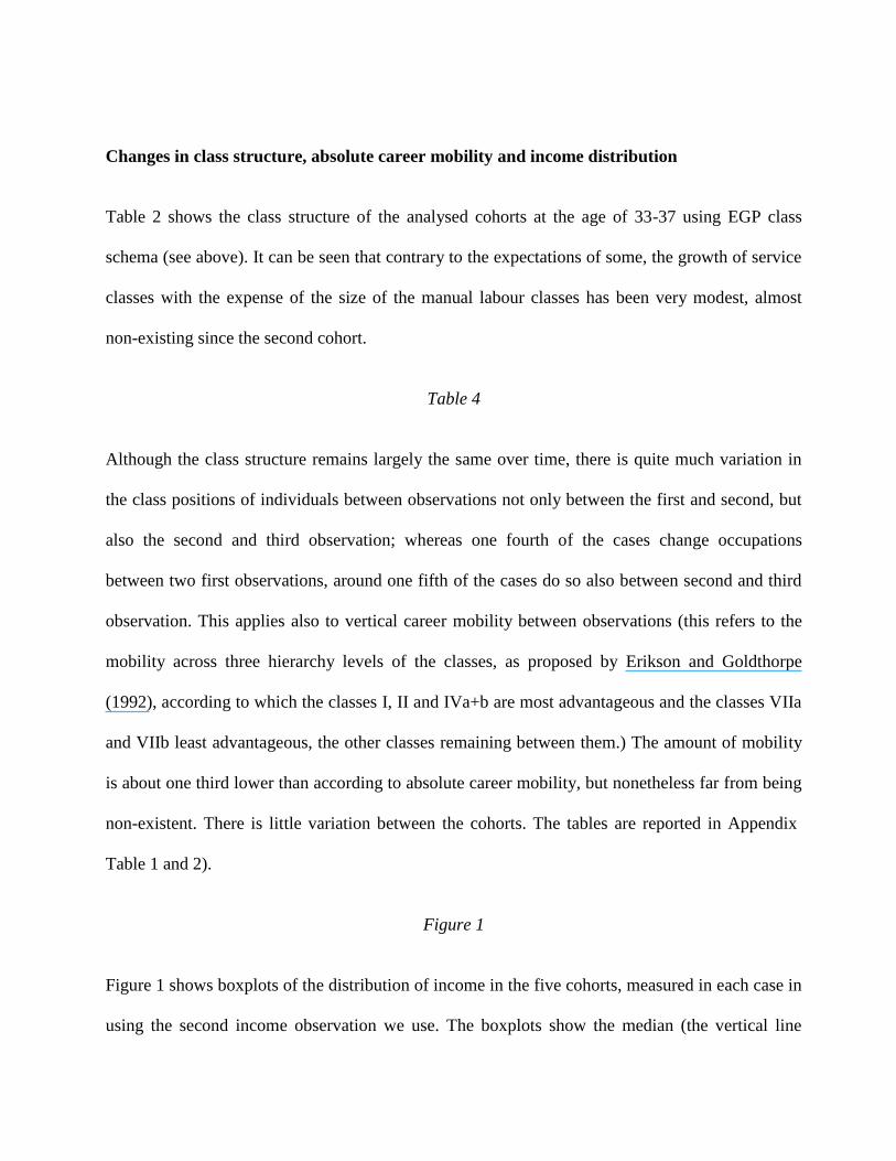
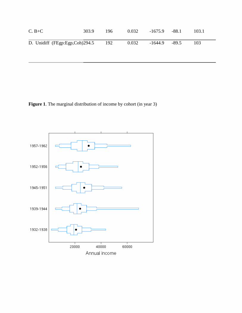
Figure 1

Figure 1 shows boxplots of the distribution of income in the five cohorts, measured in each case in

using the second income observation we use. The boxplots show the median (the vertical line

where the box is tallest), the mean (the black dot) and the percentiles 5, 12.5, 25, 37.5, 62.5, 75,

87.5 and 95, indicated by changes in the height of each box. The graphs suggest that average

incomes have grown quite substantially across these cohorts. The average among those born

between 1932 and 1938 was about 19000 euro, while for the last cohort born between 1957 and

1962 it was about 30000 euro. The next to last cohort, born between 1952-1956, is shown here

with incomes in 1995, just after the deep 1990s recession and they are the only cohort to have a

decline in mean income relative to their preceding cohort. The dispersion of income appears also

to have increased, as suggested by the increased difference between the mean and the median. If

we redraw the same picture using log income to reveal relative income differences (not shown

here), the increase in relative dispersion turns out to be more modest.

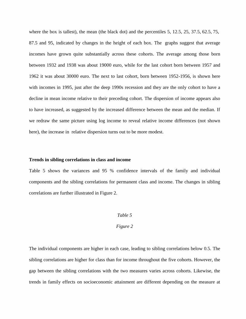
Trends in sibling correlations in class and income

Table 5 shows the variances and 95 % confidence intervals of the family and individual

components and the sibling correlations for permanent class and income. The changes in sibling

correlations are further illustrated in Figure 2.

Table 5

Figure 2

The individual components are higher in each case, leading to sibling correlations below 0.5. The

sibling correlations are higher for class than for income throughout the five cohorts. However, the

gap between the sibling correlations with the two measures varies across cohorts. Likewise, the

trends in family effects on socioeconomic attainment are different depending on the measure at

hand.

The total estimated effect of family background on income decreased somewhat between the first

and second birth cohorts (born in 1932-38 and 1939-44, respectively), after which it increased,

decreased again between the third (1945-50) and fourth (1952-1956) cohort, and then increasing

somewhat again for the youngest cohort (1957-62). The trend seems to be towards increasing

family background effect. Overall, the estimates are in line with those reported by Österbacka

(2001) and Björklund et al (2002). On the other hand, the effect of family background on social

class increased clearly between the first two birth cohorts, then declined rather linearly from the

second birth cohort to the fourth, after which it again increased slightly for the youngest cohort.

We checked the results against ordered logit measures, and found a similar pattern, although the

estimated brother correlations were generally somewhat stronger (except in the oldest cohort) and

more stable across cohorts.2 Therefore, we cannot yet find a definite answer to the surprising

increase in the family effect between the first two birth cohorts. However, all cohorts the family

background effect on class appears stronger clearly stronger than for incomes, although the gap

seems to be closing after the second cohort.

Especially to the question of whether we find diverging trends in the total family background

effect on class and income, we next turn to results from loglinear models on the association

between brothers’ class position and their income octiles.

Loglinear models for brother resemblance and father-son mobility

As a further investigation for our results, in this section we model brother resemblance in class and

income (octiles) using loglinear models. We also compare these results to models of father-son

mobility tables. As discussed above, an important difference between these and the multilevel

models shown above—apart from the obvious difference of different models—is that here we

resort to single observations (namely, the first) per individual.

In Table 6 we provide the loglinear models for brother association using eight-class EGP and

income octiles when observed at the age of 33-37 years. In the lowest part of the panel we show

the similar models for father-son occupational class mobility. Models A are independence models

(baseline models). Models B that only marginals change and there is no association between either

the positions of bothers or positions of fathers and sons. Here the dissimilarity index is very

similar in the case of class-relate models, about one third lower according to income. This

suggests that marginal changes play a bigger role altogether in the case of income than in the case

of class. Models C test the constant association either between classes or incomes. Now the model

fit statistics change so that in the case of brother associations the fit is in practice equal in the case

of class and income. This means that for the overall model fit the association between incomes

play a smaller role than between classes. Thus like in the case of multilevel models we observe a

stronger background effect for class than for incomes. Further, model fit is much better in the case

of father-son class associations; the dissimilarity index is about the half of the brother association

models. This reflects the general motivation for sibling models; inequalities according to socio-

economic background are stronger when it comes to sibling associations than when measured

directly between parents and children.

Table 6

Thus far the results are in line with the multilevel models; when modeling the change they depart.

In all cases, assuming change between cohorts in the strength of association (unidifference

models; Models D) does not improve the model fit. In the case of class measures we could

linearize the effect, and get a statistically significant model fit improvement according to

conventional levels of significance; the magnitude of improvement according to dissimilarity

index would not, however, change. Linearization would not make a difference in the case of

income.

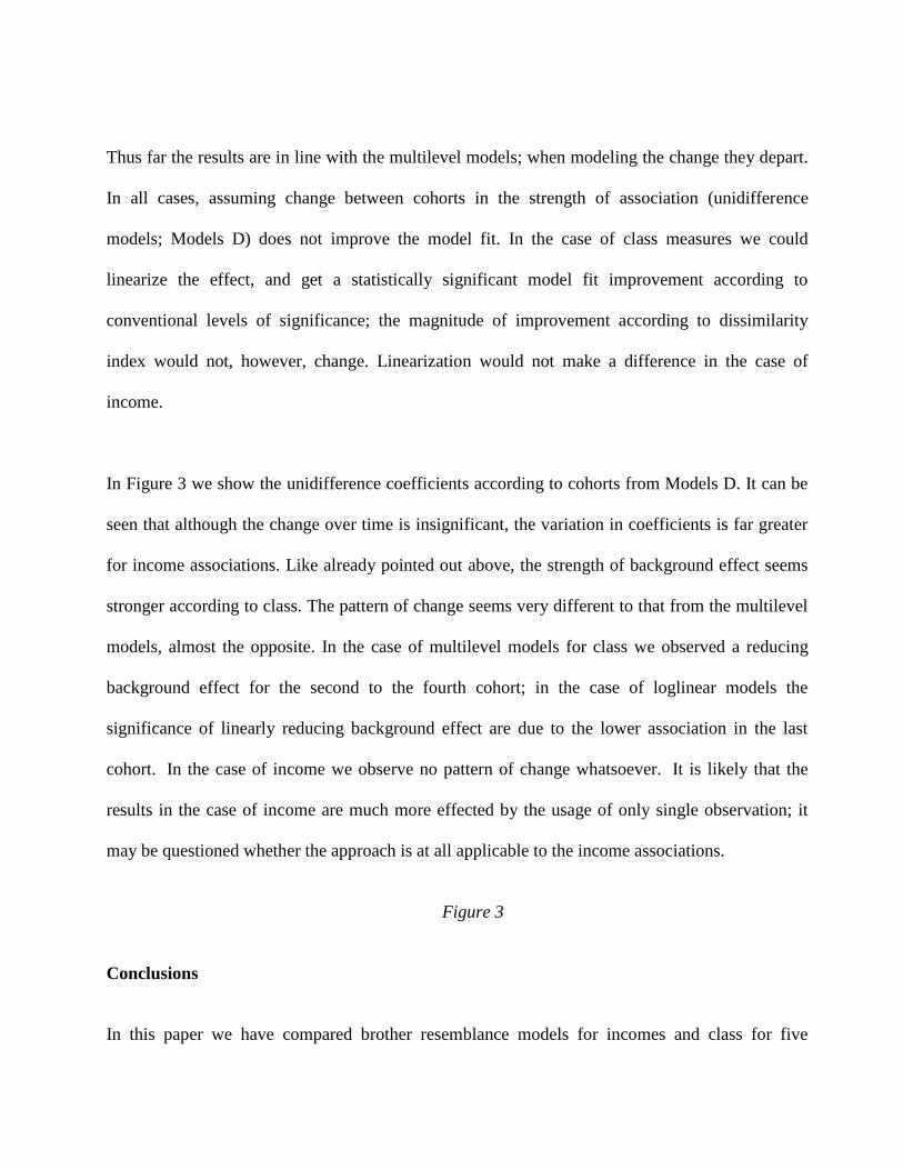
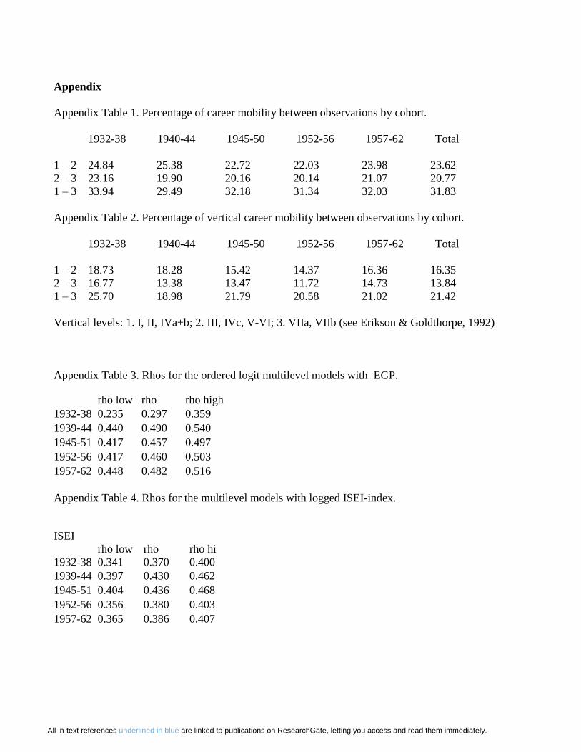
In Figure 3 we show the unidifference coefficients according to cohorts from Models D. It can be

seen that although the change over time is insignificant, the variation in coefficients is far greater

for income associations. Like already pointed out above, the strength of background effect seems

stronger according to class. The pattern of change seems very different to that from the multilevel

models, almost the opposite. In the case of multilevel models for class we observed a reducing

background effect for the second to the fourth cohort; in the case of loglinear models the

significance of linearly reducing background effect are due to the lower association in the last

cohort. In the case of income we observe no pattern of change whatsoever. It is likely that the

results in the case of income are much more effected by the usage of only single observation; it

may be questioned whether the approach is at all applicable to the income associations.

Figure 3

Conclusions

In this paper we have compared brother resemblance models for incomes and class for five

different cohorts in Finland, using Finnish Census Panel data. The cohorts analysed were born in

1932-38, 1939-44, 1945-51, 1952-56, and 1957-62. The main question in our analyses was

whether similar conclusions of brother resemblance in socioeconomic attainment could be reached

when analysing class and income. This question relates to the recently increasing interest in cross-

fertilization in research on intergenerational mobility between sociology and economics.

We used multilevel models (ordered probit for class and OLS for (logged) income) with up to

three observations on class and income for each member of the data; at the ages of 32-37; 37-42

and 43. We compared these results with loglinear models for class and income octiles each pair of

brothers using the first observation. Further, we also matched the brothers with their fathers and

applied loglinear modelling also for these more conventionally used intergenerational assocations.

According to our findings, the brother correlation is approximately 0.4 and above for class and

around 0.3 for income. The class effect is approximately at the same level as reported elsewhere

accoding to socio-economic status indeces. The income effect was approximately at the same level

as reported previously elsewhere. The finding of a stronger effect according to class than income

was also confirmed by the loglinear models, and is in line with the previous finding elsewhere.

Overall, these results suggest that the picture of the effects of family background on

socioeconomic attainment can vary rather considerably depending on whether one analyses class

or incomes. In this sense, the diverging results on intergenerational class and income mobility

reported by Goldthorpe and Jackson (2007) and Blanden and associates (2004), respectively, can

possibly be real, that is, not methodological artefacts.

According to the brother correlations estimated from the variance decomposition using multilevel

models, the family background effect on income decreased somewhat between the first and second

birth cohorts, then increased a bit between the second and third cohort, decreased between the

third and fourth cohort, and then increased somewhat again for the youngest cohort. In the case of

income, the influence of the total family effect seems to be growing. The results for the changing

family background effect according to class were more mixed, however. On the other hand, the

effect of family background on social class increased clearly between the first two birth cohorts,

then declined rather linearly from the second birth cohort to the fourth, after which it again

increased slightly for the youngest cohort. The results indicate that the gap between the two

socioeconomic measures may be closing. In the case of loglinear models for class, we observed

rather clear stability with some decrease in brother resemblance in the youngest cohort. For

income the results from loglinear models were clearly more mixed.

However, one should treat our results with caution given that in this version of the paper, we had

to resort to ordered models of class attainment instead of more appropriate multinomial methods.

The issue thus clearly warrants further investigation, and we seek to address it in the future.

Neither—due to the essentially descriptive nature of this paper—do we here seek to explain the

differences in the strength of the family background effect on class and income.

In addition to the methodological improvements, one of the important extensions of the multilevel

analyses conduced here is to model class and income together. We also modeled each cohort

separately. Albeit providing less accurate parameter estimates, the dissimilarity index from the

loglinear model for class suggest that the changes in background effects may have played --

although statistically significant if linearized -- a very small overall role. The real magnitude of the

changes over time could be more accurately estimated if the cohorts were modeled together.

Our analysis is--to our knowledge--the first one to examine sibling correlations in class (as a

categorical variable). Despite the rather considerable challenges in estimation (which could not be

fully resolved for this version of the paper), we argue that using categorical class measures in

addition to socioeconomic indeces promises to link sibling analyses better to the tradition in

sociological research on intergenerational mobility, which has dominated the scene especially in

Europe.

Notes

1 According to our knowledge, all studies on class mobility in Finland have applied categorical

status measures and loglinear models of mobility tables. However, Björklund and Jäntti (2000)

report ISEI correlation between fathers and sons of 0.346 in the case of Finland, and Erola and

Moisio (2007) ISEI elasticity of 0.28 between fathers and sons and 0.22 between mothers and

daughters.

2 The rhos for the ordered logit analysis are reported in Appendix Table 3. If the equivalent

analysis is done applying logged ISEI-index, the RHOs more or less overlap with the values from

the probit-analysis (see Appendix Table 4).

References

Beller, E., & Hout, M. (2006). Intergenerational Social Mobility: The United States in

Comparative Perspective. The Future of Children, 16(2), 19-36.

Blanden, J., Goodman, A., Gregg, P. and Machin, S. (2004). Changes in intergenerational mobility

in Britain, in (M. Corak, ed.), Generational Income Mobility in North America and Europe, pp.

122–46, Cambridge: Cambridge University Press.

Bielby, W. T., Hauser, R. M., & Featherman, D. L. (1977). Response Errors of Black and

Nonblack Males in Models of the Intergenerational Transmission of Socioeconomic Status. The

American Journal of Sociology, 82(6), 1242-1288.

Björklund, A., Eriksson, T., Jäntti, M., Raaum, O., & Österbacka, E. (2002). Brother correlations

in earnings in Denmark, Finland, Norway and Sweden compared to the United States. Journal of

Population Economics, 15(4), 757-772.

Björklund, A. and Jäntti, M. (2000) Intergenerational Mobility of Socio-Economic Status in

Comparative Perspective. Nordic Journal of Political Economy 26: 3-32.

Björklund, A., Jäntti, M. and Lindquist, M.J. (2007) Family Background and Income during the

Rise of the Welfare State: Brother Correlations in Income for Swedish Men Born 1932-1968. IZA

Discussion Paper No. 3000. IZA, Bonn.

Blau, P. M., & Duncan, O. D. (1967). The American Occupational Structure. New York: John

Wiley and Sons, Inc.

Bratsberg, B., Røed, K., Raaum, O., Naylor, R., Jäntti, M., Erikson, T., and Österbacka, E. (2007)

Nonlinearities in Intergenerational Earnings Mobility: Consequences for Cross-Country

Comparisons. The Economic Journal 117(March): C72-C92.

Breen, R. (2004). Social Mobility in Europe. Oxford University Press.

Böhlmark, A. and Lindquist, M.J. (2006) Life-Cycle Variation in the Association Between Current

and Lifetime Income: Replication and Extension for Sweden. Journal of Labor Economics 24(4):

879-896.

Conley, D. S., & Glauber, R. (2005). Sibling Similarity and Difference in Socioeconomic Status:

Life Course and Family Resource Effects. , NBER Working Papers. National Bureau of Economic

Research, Inc. Retrieved February 25, 2008, from http://ideas.repec.org/p/nbr/nberwo/11320.html.

Conley, D., & Glauber, R. (2007). Family Background, Race, and Labor Market Inequality. The

ANNALS of the American Academy of Political and Social Science, 609(1), 134-152.

Donner, A. and Wells, G. (1986) A Comparison of Confidence Interval Methods for the Intraclass

Correlation Coefficient. Biometrics 42(2): 401-412.

Erikson, R., & Goldthorpe, J. H. (1992). The Constant Flux: Study of Class Mobility in Industrial

Societies. Oxford: Clarendon Press.

Erikson, R., & Goldthorpe, J. H. (2008). Income and class mobility between generations in Great

Britain: the problem of divergent findings from the data-sets of birth cohort studies. Unpublished

manuscript.

Erikson, R., & Pöntinen, S. (1985). Social Mobility in Finland and Sweden: A Comparison of Men

and Women. In R. Alapuro, M. Alestalo, E. Haavio-Mannila, & R. Väyrynen (Eds.), Small States

in Comparative Perspective. Essays for Erik Allardt (pp. 138-162). Oslo: Norwegian University

Press.

Erola, J., & Moisio, P. (2002). Jähmettyikö Suomi? Sosiaalinen liikkuvuus ja

pitkäaikaistyöttömyys Suomessa 1970–1995.(Did Finland Stagnate? Social Mobility and Long-

Term Unemployment in Finland). Sosiologia, 39, 185–199.

Erola, J., & Moisio, P. (2005). The impact of the 1990s economic crisis on social mobility in

Finland. In T. . Wilska & L. Haanpää (Eds.), Lifestyles and social change – Essays in Economic

Sociology, Keskustelua ja raportteja. (pp. 11-28). Turku: Turku School of Economics.

Erola, J., & Moisio, P. (2007). Social mobility over three generations in Finland 19502000.

European Sociological Review, 23(2), 169-183.

Checchi, D., Ichino, A. and Rustichini, A. (1999) More Equal But Less Mobile? Education

Financing and Intergenerational Mobility in Italy and the US. Journal of Public Economics 74(3):

351-393.

Ganzeboom, H. B. G., & Treiman, D. J. (2001). International Stratification and Mobility File:

Conversion Tools. Retrieved from http://www.fsw.vu.nl/ h.ganzeboom/ismf.

Ganzeboom, H. B. G., Treiman, D. J., & Ultee, W. C. (1991). Comparative Intergenerational

Stratification Research: Three Generations and Beyond. Annual Reviews in Sociology, 17(1), 277-

302.

Goldthorpe, J. H., & Jackson, M. (2007). Intergenerational Class Mobility in Contemporary

Britain: Political Concerns and Empirical Findings. British Journal of Sociology, 58(4), 525-546.

Haider, S. and Solon, G. (2006) Life-Cycle Variation in the Association Between Current and

Lifetime Earnings. American Economic Review 96(4): 1308-1320.

Hauser, R. M., & Mossel, P. A. (1985). Fraternal Resemblance in Educational Attainment and

Occupational Status. American Journal of Sociology, 91(3), 650-673.

Hauser, R. M., Sheridan, J. T., & Warren, J. R. (1999). Socioeconomic Achievements of Siblings

in the Life Course: New Findings from the Wisconsin Longitudinal Study. Research on Aging,

21(2), 338-378.

Hauser, R. M., & Wong, R. S. (1989). Sibling Resemblance and Intersibling Effects in

Educational Attainment. Sociology of Education, 62(3), 149-171.

Kuo, H.D. and Hauser, R.M. (1995) Trends in Family Effects on the Education of Black and

White Brothers. Sociology of Education 68: 136-60.

Mazumder, B. and Levine, D.I. (2003) The Growing Importance of Family and Community: An

Analysis of Changes in the Sibling Correlation in Earnings. Working Paper 2003-24. Federal

Reserve Bank of Chicago, Chicago.

Lillard, L.A. and Panis, C.W.A. (2003) aML Multilevel Multiprocess Statistical Software. Version

2.0. EconWare, Los Angeles, California.

Mazumder, B. (2005), Fortunate Sons: New Estimates of Intergenerational Mobility in the United

States Using Social Security Earnings Data. Review of Economics and Statistics 87(2): 235-255.

Moisio, P. (2006). Sosiaalinen liikkuvuus ja mahdollisuuksien tasa-arvo 2000-luvun Suomessa. In

M. Kautto (Ed.) Suomalaisten hyvinvointi 2006 (pp. 264-284). Gummerus.

Morgan, S. L. Past Themes and Future Prospects for Research on Social and Economic Mobility.

In S. L. Morgan, D. B. Grusky, & G. S. Fields (Eds.) Mobility and Inequality: Frontiers of

Research in Sociology and Economics (pp. 3-20). Stanford: Stanford Unversity Press.

Pöntinen, S. (1983). Social Mobility and Social Structure. A Comparison of Scandinavian

Countries. Commentationes Scientiarum Socialium 20 1983. Helsinki: Societas Scientiarum

Fennica.

R Development Core Team. (2008). R: A Language and Environment for Statistical Computing.

Vienna, Austria. Retrieved from http://www.R-project.org.

Pöntinen, S., Alestalo, M., & Uusitalo, H. (1982). The Finnish Mobility Survey 1980: Data and

First Results. Suomen Gallup Oy report. Helsinki: Suomen Gallup.

Sieben, I., & Graaf, P. M. (2001). Testing the modernization hypothesis and the socialist ideology

hypothesis: a comparative sibling analysis of educational attainment and occupational status. The

British Journal of Sociology, 52(3), 441-467.

Sieben, I., Huinink, J., & de Graaf, P. M. (2001). Family Background and Sibling Resemblance in

Educational Attainment. Trends in the Former FRG, the Former GDR, and the Netherlands.

European Sociological Review, 17(4), 401-430.

Solon, G. (1992), ―Intergenerational Income Mobility in the United States‖, American Economic

Review 82/3: 393-408.

Solon, G. (1999), ―Intergenerational Mobility in the Labor Market,‖ in O. Ashenfelter and D. Card

(eds.) Handbook of labor economics vol. 3A. Elsevier, Amsterdam, North Holland.

Turner, H., & Firth, D. (2006). Generalized nonlinear models in R: An overview of the gnm

package. Retrieved from http://go.warwick.ac.uk/heatherturner/gnm/gnmoverview.pdf.

Vallet, L. (2004). Change in Intergenerational Class Mobility in France from the 1970s to the

1990s and its Explanation: An Analysis Following the CASMIN Approach. In R. Breen (Ed.),

Social Mobility in Europe (pp. 115-149). Oxford: Oxford University Press.

Xie, Y. (1992). The Log-Multiplicative Layer Effect Model for Comparing Mobility Tables.

American Sociological Review, 57(3), 380-395.

Zimmerman, D.J. (1992) Regression Toward Mediocrity in Economic Stature. American

Economic Review 82(3): 409-429.

Österbacka, E. (2001). Family Background and Economic Status in Finland. Scandinavian Journal

of Economics, 103(3), 467-484.

TABLES AND FIGURES

Table 1. Basic descriptives of the data

N families N siblings N observations

1932-38 3739 4585 9654

1939-44 3684 4396 9279

1945-51 5197 6426 13822

1952-56 5747 6810 14681

1957-62 7590 9147 19690

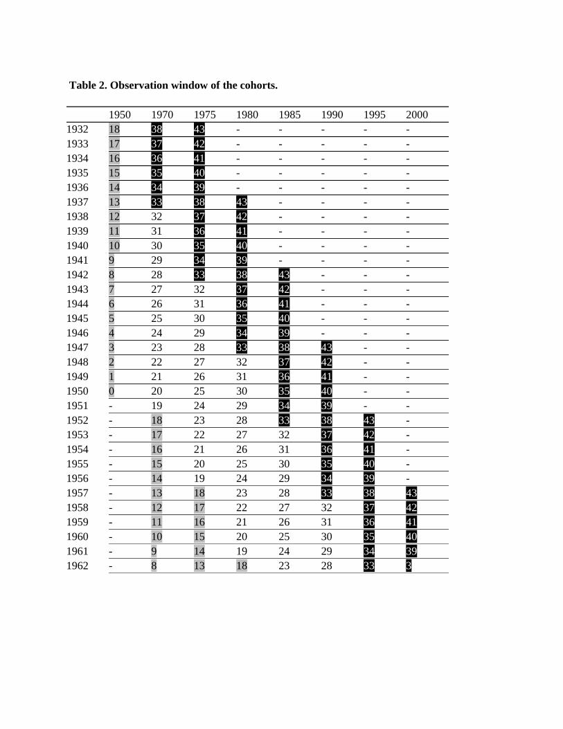
Table 2. Observation window of the cohorts.

1950 1970 1975 1980 1985 1990 1995 2000

1932 18 38 43 - - - - -

1933 17 37 42 - - - - -

1934 16 36 41 - - - - -

1935 15 35 40 - - - - -

1936 14 34 39 - - - - -

1937 13 33 38 43 - - - -

1938 12 32 37 42 - - - -

1939 11 31 36 41 - - - -

1940 10 30 35 40 - - - -

1941 9 29 34 39 - - - -

1942 8 28 33 38 43 - - -

1943 7 27 32 37 42 - - -

1944 6 26 31 36 41 - - -

1945 5 25 30 35 40 - - -

1946 4 24 29 34 39 - - -

1947 3 23 28 33 38 43 - -

1948 2 22 27 32 37 42 - -

1949 1 21 26 31 36 41 - -

1950 0 20 25 30 35 40 - -

1951 - 19 24 29 34 39 - -

1952 - 18 23 28 33 38 43 -

1953 - 17 22 27 32 37 42 -

1954 - 16 21 26 31 36 41 -

1955 - 15 20 25 30 35 40 -

1956 - 14 19 24 29 34 39 -

1957 - 13 18 23 28 33 38 43

1958 - 12 17 22 27 32 37 42

1959 - 11 16 21 26 31 36 41

1960 - 10 15 20 25 30 35 40

1961 - 9 14 19 24 29 34 39

1962 - 8 13 18 23 28 33 3

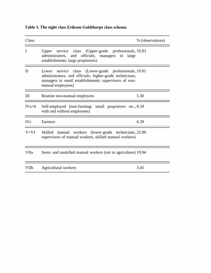
Table 3. The eight class Erikson-Goldthorpe class schema

Class % (observations)

I

Upper service class (Upper-grade professionals,

administrators, and officials; managers in large

establishments; large proprietors)

10.93

II

Lower service class (Lower-grade professionals,

administrators, and officials; higher-grade technicians;

managers in small establishments; supervisors of non-

manual employees)

19.91

III Routine non-manual employees 5.30

IVa+b

Self-employed (non-farming: small proprietors etc.,

with and without employees)

8.18

IVc Farmers 6.39

V+VI

Skilled manual workers (lower-grade technicians,

supervisors of manual workers, skilled manual workers)

25.90

VIIa

Semi- and unskilled manual workers (not in agriculture)

19.94

VIIb Agricultural workers 3.45

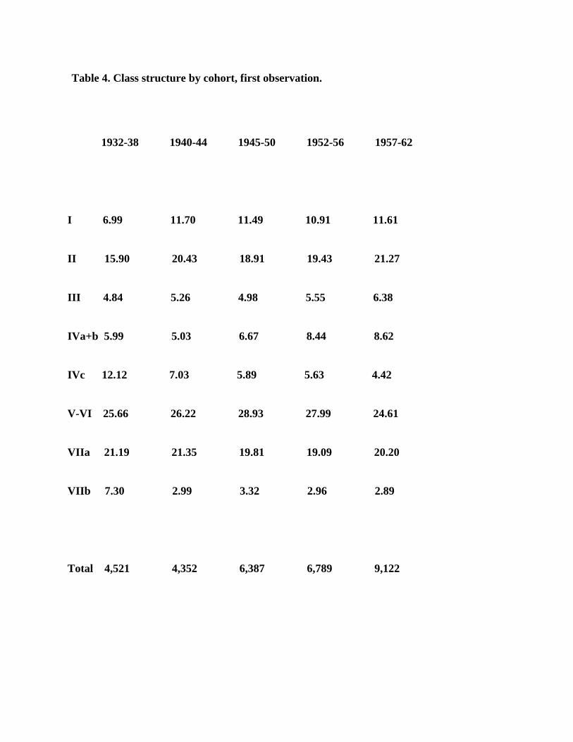
Table 4. Class structure by cohort, first observation.

1932-38 1940-44 1945-50 1952-56 1957-62

I 6.99 11.70 11.49 10.91 11.61

II 15.90 20.43 18.91 19.43 21.27

III 4.84 5.26 4.98 5.55 6.38

IVa+b 5.99 5.03 6.67 8.44 8.62

IVc 12.12 7.03 5.89 5.63 4.42

V-VI 25.66 26.22 28.93 27.99 24.61

VIIa 21.19 21.35 19.81 19.09 20.20

VIIb 7.30 2.99 3.32 2.96 2.89

Total 4,521 4,352 6,387 6,789 9,122

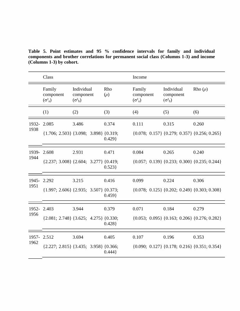
Table 5. Point estimates and 95 % confidence intervals for family and individual

components and brother correlations for permanent social class (Columns 1-3) and income

(Columns 1-3) by cohort.

Class Income

Family

component

(σ²a)

Individual

component

(σ²b)

Rho

(ρ)

Family

component

(σ²a)

Individual

component

(σ²b)

Rho (ρ)

(1) (2) (3) (4) (5) (6)

1932-

1938

2.085

{1.706; 2.503}

3.486

{3.098; 3.898}

0.374

{0.319;

0.429}

0.111

{0.078; 0.157}

0.315

{0.279; 0.357}

0.260

{0.256; 0.265}

1939-

1944

2.608

{2.237; 3.008}

2.931

{2.604; 3.277}

0.471

{0.419;

0.523}

0.084

{0.057; 0.139}

0.265

{0.233; 0.300}

0.240

{0.235; 0.244}

1945-

1951

2.292

{1.997; 2.606}

3.215

{2.935; 3.507}

0.416

{0.373;

0.459}

0.099

{0.078; 0.125}

0.224

{0.202; 0.249}

0.306

{0.303; 0.308}

1952-

1956

2.403

{2.081; 2.748}

3.944

{3.625; 4.275}

0.379

{0.330;

0.428}

0.071

{0.053; 0.095}

0.184

{0.163; 0.206}

0.279

{0.276; 0.282}

1957-

1962

2.512

{2.227; 2.815}

3.694

{3.435; 3.958}

0.405

{0.366;

0.444}

0.107

{0.090; 0.127}

0.196

{0.178; 0.216}

0.353

{0.351; 0.354}

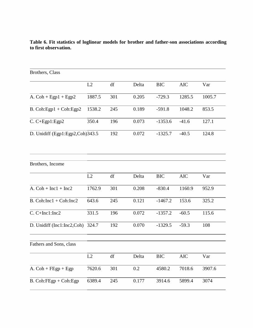
Table 6. Fit statistics of loglinear models for brother and father-son associations according

to first observation.

Brothers, Class

L2 df Delta BIC AIC Var

A. Coh + Egp1 + Egp2 1887.5 301 0.205 -729.3 1285.5 1005.7

B. Coh:Egp1 + Coh:Egp2 1538.2 245 0.189 -591.8 1048.2 853.5

C. C+Egp1:Egp2 350.4 196 0.073 -1353.6 -41.6 127.1

D. Unidiff (Egp1:Egp2,Coh)

343.5

192

0.072

-1325.7

-40.5

124.8

Brothers, Income

L2 df Delta BIC AIC Var

A. Coh + Inc1 + Inc2 1762.9 301 0.208 -830.4 1160.9 952.9

B. Coh:Inc1 + Coh:Inc2 643.6 245 0.121 -1467.2 153.6 325.2

C. C+Inc1:Inc2 331.5 196 0.072 -1357.2 -60.5 115.6

D. Unidiff (Inc1:Inc2,Coh) 324.7 192 0.070 -1329.5 -59.3 108

Fathers and Sons, class

L2 df Delta BIC AIC Var

A. Coh + FEgp + Egp 7620.6 301 0.2 4580.2 7018.6 3907.6

B. Coh:FEgp + Coh:Egp 6389.4 245 0.177 3914.6 5899.4 3074

C. B+C 303.9 196 0.032 -1675.9 -88.1 103.1

D. Unidiff (FEgp:Egp,Coh)

294.5

192

0.032

-1644.9

-89.5

103

Figure 1. The marginal distribution of income by cohort (in year 3)

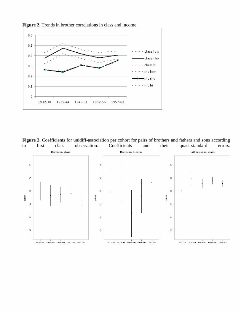
Figure 2. Trends in brother correlations in class and income

Figure 3. Coefficients for unidiff-association per cohort for pairs of brothers and fathers and sons according

to first class observation. Coefficients and their quasi-standard errors.

Appendix

Appendix Table 1. Percentage of career mobility between observations by cohort.

1932-38 1940-44 1945-50 1952-56 1957-62 Total

1 – 2 24.84 25.38 22.72 22.03 23.98 23.62

2 – 3 23.16 19.90 20.16 20.14 21.07 20.77

1 – 3 33.94 29.49 32.18 31.34 32.03 31.83

Appendix Table 2. Percentage of vertical career mobility between observations by cohort.

1932-38 1940-44 1945-50 1952-56 1957-62 Total

1 – 2 18.73 18.28 15.42 14.37 16.36 16.35

2 – 3 16.77 13.38 13.47 11.72 14.73 13.84

1 – 3 25.70 18.98 21.79 20.58 21.02 21.42

Vertical levels: 1. I, II, IVa+b; 2. III, IVc, V-VI; 3. VIIa, VIIb (see Erikson & Goldthorpe, 1992)

Appendix Table 3. Rhos for the ordered logit multilevel models with EGP.

rho low rho rho high

1932-38 0.235 0.297 0.359

1939-44 0.440 0.490 0.540

1945-51 0.417 0.457 0.497

1952-56 0.417 0.460 0.503

1957-62 0.448 0.482 0.516

Appendix Table 4. Rhos for the multilevel models with logged ISEI-index.

ISEI

rho low rho rho hi

1932-38 0.341 0.370 0.400

1939-44 0.397 0.430 0.462

1945-51 0.404 0.436 0.468

1952-56 0.356 0.380 0.403

1957-62 0.365 0.386 0.407

All in-text references underlined in blue are linked to publications on ResearchGate, letting you access and read them immediately.