Changes in the Distribution of Long Run Earnings and Retirement Incomes—Have Recent Cohorts Fallen

Behind?

Peter Gottschalk Boston College

and Minh Huynh

Social Security Administration

Prepared for the Fifth Annual Conference of the Retirement Research Consortium “Securing Retirement Income for Tomorrow’s Retirees”

May 15-16, 2003 Washington, D.C.

The research herein was performed pursuant to a grant from the U.S. Social Security Administration (SSA) to the Center for Retirement Research at Boston College (CRR). The opinions and conclusions are solely those of the authors and should not be construed as representing the opinions or policy of the Social Security Administration or any agency of the Federal Government or the CRR.

1

"Changes in the Distribution of Long Run Earnings andRetirement Incomes—Have Recent Cohorts Fallen Behind?"

June 2003Peter Gottschalk and Minh Huynh

Introduction

This study is motivated by the well documented increase in wage inequality during the

1980’s and the continued high levels of inequality during the 1990’s . Specifically, we examine

changes in the distribution of long run earnings and changes in economic mobility for recent

cohorts. These cohorts who either entered retirement in the 1990’s or are nearing retirement

experienced very different labor market conditions during their working lives than did earlier

cohorts. Economic growth led to higher mean earnings for recent cohorts but the distribution of

yearly earnings became less equal. As a result of these changes, the average worker nearing

retirement had higher long run earnings than members of previous cohorts. This, however, need

not have translated into higher long run earnings across the board. Those at the bottom of the

distribution of long run earnings might actually have had lower accumulated earnings than

previous cohorts if the gains from growth were more than offset by the increase in inequality of

earnings during the1980’s. If the accumulated earnings of those at the bottom of the distribution

fell then this could have had an impact both on decisions about whether to continue to work after

the period of normal retirement and on Social Security benefits.

We are specifically interested in those at the bottom of the earnings distribution who are

likely to have suffered disproportionately as a result of the rise in inequality of yearly earnings.

We, however, recognize that yearly earnings may be a poor measure of permanent earnings,

especially if there is substantial mobility. By using administrative earnings records that span a

half century we are able to classify workers on the basis of their long run earnings. This allows

us to examine changes in the distribution of long run earnings and to see how persons at the

bottom of this distribution have fared during their working lives and as they entered their 60’s.

This paper is purely descriptive. It attempts to document the stylized facts that a behavioral

model would have to explain. While making no pretense at identifying causal mechanisms, it

does address some important questions that often surface in policy debates about the extent and

importance of the increase in economic inequality. Critics rightly argue that there is substantial

earnings mobility so yearly earnings inequality overstates the extent of inequality of permanent

earnings. If individuals either have savings or can borrow then low earnings in one year can be

2

counter balanced by higher earnings in another year. This argues for a longer period over which

to aggregate earnings. Our ability to aggregate over a 24 year period certainly meets this goal.

The second, and related, policy question is whether mobility has increased. If mobility has

increased then this may partially offset the impact of the increase in earnings inequality.

Outcomes may be less equal but there is less chance of being stuck with a bad outcome. Our

ability to measure earnings mobility for five cohorts spanning a twenty five year period allows us

to address this important question.

Our paper can be viewed as a complement to Bosworth, Burtless and Sahm (2001), BBS.

The two papers ask similar questions but use different methodologies and data to address these

questions. Each approach has its relative strength and weaknesses. The fundamental empirical

problem both papers face is that no data set includes earnings histories covering the full working

lives of cohorts who precede the rise in inequality and cohorts who were affected by these

changes in labor markets. BBS deal with this problem by using the MINT microsimulation

model to extrapolate the earnings of persons who had not yet reached retirement age by 1998, the

last year of administrative data available to them. The approach they use is to splice the earnings

history of an older worker, whose history was observed, to that of a younger worker with similar

characteristics1. This allows them to construct earnings histories over full careers from age 22 to

612. As they acknowledge, the advantage of having earnings over the full career path comes at

the cost of having to assume that (a) the premium paid to higher education, experience and other

characteristics that they control for will be the same in the future as it was in the mid-1990’s and

that (b) inequality among workers with the same characteristics will also not change3.

We take a different approach which does not have to make assumptions about future changes

in the distribution of earnings. This advantage, however, comes at the cost of having shorter work

histories. As we will explain in the following section, this imposes a tradeoff between the cohorts

covered and the period over which we can observe their earnings using administrative records.

Given our desire to include cohorts whose working lives predate the rise in earnings inequality

1 They match workers on the basis of age, sex, race, educational attainment, disability status, average career earnings

prior to the matching period. They only use the most recent histories of older workers by splicing successive fiveyear earnings segments.

2 The earliest age is limited by the fact that the SER covers earnings starting in 19513 Bosworth et al (2001, p17). The latest five years of data used to hot deck comes from SER records covering earnings

in 1994-98. Therefore, the explicit assumption is that returns to characteristics and within group inequality will bethe same in the future as it was between 1994 and 1998. This does not imply that inequality will not change in thefuture but any changes would have to come from changes in the distribution of the characteristics they measure..

3

our measure of long run earnings is based on earnings between the ages of 36 and 60 rather than

22 to 61 as in BBS..

The data we use to measure long run earnings also differs in one important way with the data

available to BBS. Both studies use administrative records. However, BBS only had access to

earnings records with earnings up to the FICA taxable maximum. As they acknowledge this

limitation of the data can have important consequences for measures of inequality if the changes

in the distribution occurred above this ceiling. We have access to more recent data that provide

uncensored earnings starting in 1991. While our classification of persons on the basis of long run

income must still deal with the issue of top-coding prior to 1991, the availability of this data does

allow us to examine the earnings of persons during their late 60’s with uncensored data.

While both studies examine the impact of the rise in earnings inequality on the distribution of

permanent earnings and outcomes later in the focus of the two studies are somewhat different.

BBS present evidence on the overall distribution of permanent earnings and the distribution of

Social Security benefits. We focus more narrowly on the outcomes of persons in the bottom of

the distribution of long run earnings. This focus on the bottom of the distribution reflects not

only our substantive interests but also limitations of the data as described in the following section.

Data

The major problem with using any nationally representative longitudinal data set to measure

long run earnings is that workers are observed only over a relatively short period. Even the PSID,

the longest available national longitudinal data set, has only 23 years of complete data on

earnings and retirement outcomes4 While such data sets provide rich demographic information

there are at least two interrelated problems with these limited longitudinal data sets. First, since

these data sets cover at best a small part of the working lives of respondents, the resulting

histories may misclassify persons as low earners even if they had high earnings prior to the period

covered in the PSID. Second, comparing individuals in different cohorts over the same period of

their working lives greatly reduces sample size or limits the length of the period over which their

experiences can be compared5.

4 The income data for 1968 and 1969 are in bracketed form. 1993 is the latest year of final release data.5 The starting age for the common period of observation must be set high enough so that the oldest cohort is

observable at that age while the maximum age must be set low enough so the most recent cohort is observed atthat age

4

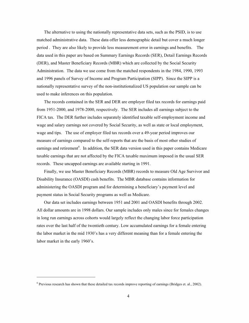
The alternative to using the nationally representative data sets, such as the PSID, is to use

matched administrative data. These data offer less demographic detail but cover a much longer

period . They are also likely to provide less measurement error in earnings and benefits. The

data used in this paper are based on Summary Earnings Records (SER), Detail Earnings Records

(DER), and Master Beneficiary Records (MBR) which are collected by the Social Security

Administration. The data we use come from the matched respondents in the 1984, 1990, 1993

and 1996 panels of Survey of Income and Program Participation (SIPP). Since the SIPP is a

nationally representative survey of the non-institutionalized US population our sample can be

used to make inferences on this population.

The records contained in the SER and DER are employer filed tax records for earnings paid

from 1951-2000, and 1978-2000, respectively. The SER includes all earnings subject to the

FICA tax. The DER further includes separately identified taxable self-employment income and

wage and salary earnings not covered by Social Security, as well as state or local employment,

wage and tips. The use of employer filed tax records over a 49-year period improves our

measure of earnings compared to the self-reports that are the basis of most other studies of

earnings and retirement6. In addition, the SER data version used in this paper contains Medicare

taxable earnings that are not affected by the FICA taxable maximum imposed in the usual SER

records. These uncapped earnings are available starting in 1991.

Finally, we use Master Beneficiary Records (MBR) records to measure Old Age Survivor and

Disability Insurance (OASDI) cash benefits. The MBR database contains information for

administering the OASDI program and for determining a beneficiary’s payment level and

payment status in Social Security programs as well as Medicare.

Our data set includes earnings between 1951 and 2001 and OASDI benefits through 2002.

All dollar amounts are in 1998 dollars. Our sample includes only males since for females changes

in long run earnings across cohorts would largely reflect the changing labor force participation

rates over the last half of the twentieth century. Low accumulated earnings for a female entering

the labor market in the mid 1930’s has a very different meaning than for a female entering the

labor market in the early 1960’s.

6 Previous research has shown that these detailed tax records improve reporting of earnings (Bridges et. al., 2002).

5

Methodology

Cohorts

We group all sample members into five year cohorts starting with those born between 1915

and 1919 and ending with persons born between 1935 and 1939. Table 1 shows the ages of each

cohort in the first year for which we have earnings data (1951) and the last year for which we

have earnings and OASDI data (2000 and 2002 respectively). We also show their ages in 1980,

the year when earnings inequality started to rise most dramatically, and in 1991, the first year for

which we have uncapped earnings..

Table 1-- Age of Cohorts in Selected Years

Age in

Cohort Year of birth 1951 1980 1991 2000 2002

1 Start 1915 36 65 76 85 87

End 1919 32 61 72 81 83

2 Start 1920 31 60 71 80 82

End 1924 27 56 67 76 78

3 Start 1925 26 55 66 75 77

End 1929 22 51 62 71 73

4 Start 1930 21 50 61 70 72

End 1934 7 46 57 66 68

5 Start 1935 16 45 56 65 67

End 1939 12 41 52 61 63

Pre-retirement earnings of members of the earliest cohort, born between 1915 and 1919, were

largely unaffected by the rise in inequality during the 1980’s since members of this cohort were

61 to 65 in 1980. At the other extreme, the cohort born between 1935 and 1939 were 41 to 45 in

1980. They were, therefore, in their prime earnings years during the 1980s. Our five cohorts can,

therefore, be characterized in the following way.

• Cohort 1—Members of this cohort were in their 60’s when earnings inequality

started rising. They serve as a benchmark against which to contrast later cohorts.

• Cohort 2-4—Members of these cohorts are observed working during the period

of rising inequality and are observed in years of normal retirement.

6

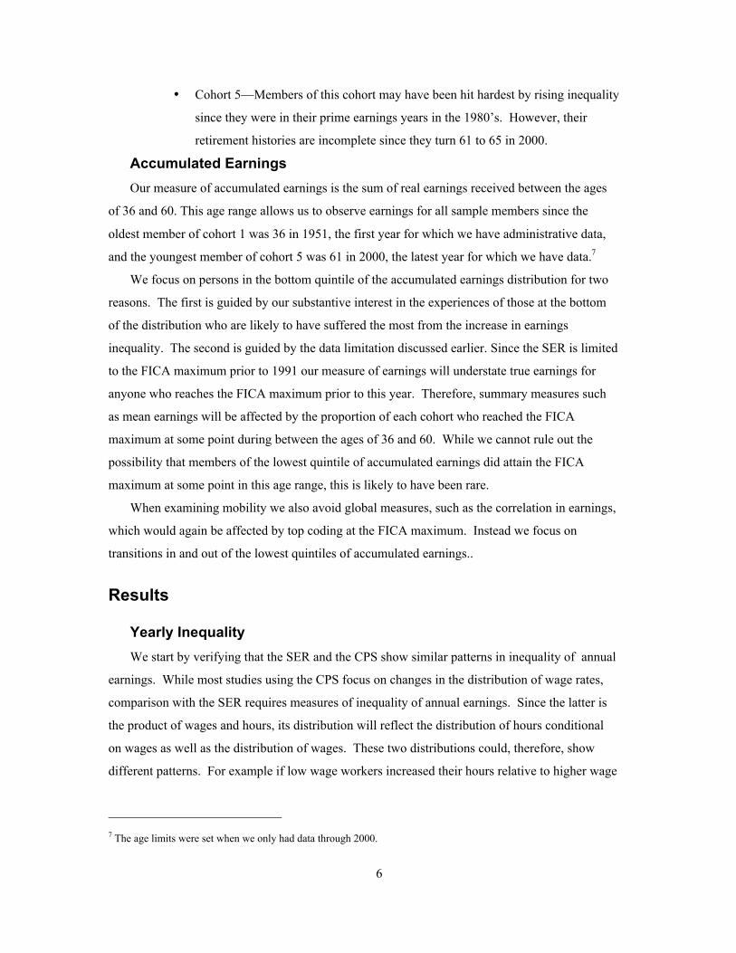
• Cohort 5—Members of this cohort may have been hit hardest by rising inequality

since they were in their prime earnings years in the 1980’s. However, their

retirement histories are incomplete since they turn 61 to 65 in 2000.

Accumulated Earnings

Our measure of accumulated earnings is the sum of real earnings received between the ages

of 36 and 60. This age range allows us to observe earnings for all sample members since the

oldest member of cohort 1 was 36 in 1951, the first year for which we have administrative data,

and the youngest member of cohort 5 was 61 in 2000, the latest year for which we have data.7

We focus on persons in the bottom quintile of the accumulated earnings distribution for two

reasons. The first is guided by our substantive interest in the experiences of those at the bottom

of the distribution who are likely to have suffered the most from the increase in earnings

inequality. The second is guided by the data limitation discussed earlier. Since the SER is limited

to the FICA maximum prior to 1991 our measure of earnings will understate true earnings for

anyone who reaches the FICA maximum prior to this year. Therefore, summary measures such

as mean earnings will be affected by the proportion of each cohort who reached the FICA

maximum at some point during between the ages of 36 and 60. While we cannot rule out the

possibility that members of the lowest quintile of accumulated earnings did attain the FICA

maximum at some point in this age range, this is likely to have been rare.

When examining mobility we also avoid global measures, such as the correlation in earnings,

which would again be affected by top coding at the FICA maximum. Instead we focus on

transitions in and out of the lowest quintiles of accumulated earnings..

Results

Yearly Inequality

We start by verifying that the SER and the CPS show similar patterns in inequality of annual

earnings. While most studies using the CPS focus on changes in the distribution of wage rates,

comparison with the SER requires measures of inequality of annual earnings. Since the latter is

the product of wages and hours, its distribution will reflect the distribution of hours conditional

on wages as well as the distribution of wages. These two distributions could, therefore, show

different patterns. For example if low wage workers increased their hours relative to higher wage

7 The age limits were set when we only had data through 2000.

7

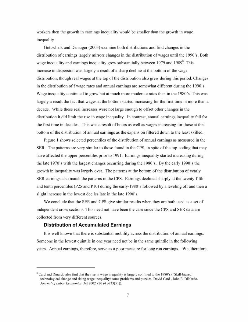
workers then the growth in earnings inequality would be smaller than the growth in wage

inequality.

Gottschalk and Danziger (2003) examine both distributions and find changes in the

distribution of earnings largely mirrors changes in the distribution of wages until the 1990’s. Both

wage inequality and earnings inequality grew substantially between 1979 and 19898. This

increase in dispersion was largely a result of a sharp decline at the bottom of the wage

distribution, though real wages at the top of the distribution also grew during this period. Changes

in the distribution of f wage rates and annual earnings are somewhat different during the 1990’s.

Wage inequality continued to grow but at much more moderate rates than in the 1980’s. This was

largely a result the fact that wages at the bottom started increasing for the first time in more than a

decade. While these real increases were not large enough to offset other changes in the

distribution it did limit the rise in wage inequality. In contrast, annual earnings inequality fell for

the first time in decades. This was a result of hours as well as wages increasing for those at the

bottom of the distribution of annual earnings as the expansion filtered down to the least skilled.

Figure 1 shows selected percentiles of the distribution of annual earnings as measured in the

SER. The patterns are very similar to those found in the CPS, in spite of the top-coding that may

have affected the upper percentiles prior to 1991. Earnings inequality started increasing during

the late 1970’s with the largest changes occurring during the 1980’s. By the early 1990’s the

growth in inequality was largely over. The patterns at the bottom of the distribution of yearly

SER earnings also match the patterns in the CPS. Earnings declined sharply at the twenty-fifth

and tenth percentiles (P25 and P10) during the early-1980’s followed by a leveling off and then a

slight increase in the lowest deciles late in the late 1990’s.

We conclude that the SER and CPS give similar results when they are both used as a set of

independent cross sections. This need not have been the case since the CPS and SER data are

collected from very different sources.

Distribution of Accumulated Earnings

It is well known that there is substantial mobility across the distribution of annual earnings.

Someone in the lowest quintile in one year need not be in the same quintile in the following

years. Annual earnings, therefore, serve as a poor measure for long run earnings. We, therefore,

8 Card and Dinardo also find that the rise in wage inequality is largely confined to the 1980’s (“Skill-biased

technological change and rising wage inequality: some problems and puzzles. David Card , John E. DiNardo.Journal of Labor Economics Oct 2002 v20 i4 p733(51)).

8

follow the procedures described earlier to construct the distribution of accumulated earnings,

which measures the total earnings an individual received between the ages of 36 and 60.

Figure 2 shows the median of accumulated earnings for each of our five cohorts measured in

1998 dollars9. As expected there was a sharp increase in the median accumulated earnings for the

first four cohorts since they gained from the wage increases of the 1950’s, 1960’s and early

1970’s. Wages then stopped growing which is reflected in the leveling off of median earnings.

As a result of these changes, the three cohorts born after 1929 all had median earnings roughly 25

percent higher than the cohort born between 1915 and 1919.

Figure 3 shows selected percentiles of the distribution of accumulated earnings for our five

cohorts10. Each percentile is measured relative to the corresponding percentile for the cohort born

between 1915 and 1919. If there had been growth but no increase in inequality of accumulated

earnings across cohorts, then all the percentiles would have grown at the rate and the lines would

have the same slope.

The rise and then stabilization of the median shown in Figure 1 is reflected in the leveling off

of the P50 at 1.25. While the P10 grew somewhat faster than the P50 between the first two

cohorts, it then dropped for successive cohorts. As a result, the accumulated earnings for a

person at the tenth percentile was only marginally higher for a person born between 1935 and

1939 as for a person born twenty years earlier.

Since median earnings had grown by 25 percent this means that the bottom of the

accumulated earnings distribution had fallen relative to the median. Earnings of those at the P10

reached a peak with the 1920-25 cohort. Successive cohorts all had earnings that were not only

low relative to their own median but also lower in real terms than the accumulated earnings at the

P10 of the 1920-25 cohort. Since accumulated earnings is measured over a 24 year period, this

measure of inequality is dominated by permanent differences across individuals rather than

transitory fluctuations. Furthermore, since accumulated earnings is calculated over the same age

span for each cohort, this measure does not reflect age related differences in inequality. We,

therefore, conclude the earnings inequality among the three most recent cohorts reflects an

increase in inequality of permanent earnings.

9 Medians rather than medians are shown in order to reduce the impact of top-coding.10 We show the p75 and p90 for completeness but we do not discuss these percentiles since they may have been

affected by changes in the FICA max prior to 1991.

9

Mobility

It is sometimes argued that focusing on inequality ignores the fact that that there is substantial

mobility within the income or earnings distribution11. Persons who are in the bottom of the

distribution in one period may not be the same as those who were at the bottom in the previous

period. Therefore, it is inappropriate to think of a drop in the income at the p10 as a drop in the

income of the same individual.

We have already partially addressed this issue by classifying persons on the basis of their

long run incomes. By using a sufficiently long accounting period we have allowed transitory

decreases in earnings to be averaged out. Thus, we have taken account of the effects of mobility

in reducing inequality of long term earnings.

However, there is another reason to be concerned about mobility. Mobility may be valued as

an end in itself. The easiest way to think of this is to consider two societies12. In society A there

is no mobility so a person’s position late in life is preordained by his position early in life. In

society B earnings are less evenly distributed both early in life and late in life. However, there is

sufficient mobility to offset this additional inequality. As a result the distribution of accumulated

earnings is the same in the two societies. While the two societies would be classified as similar in

terms of the distribution of accumulated earnings, society B would be considered more open than

society A.

The same concepts apply to the changes in the distribution of accumulated earnings across

cohorts that we documented in Figure 3. The increase in inequality of accumulated earnings for

cohorts 3, 4 and 5 can reflect the fact that these cohorts have greater inequality of earnings early

in life than earlier cohorts, that they have greater inequality of earnings late in life than earlier

cohorts, or that they have less mobility so that those who had low earnings early in life are more

likely to be the same people who have low earnings late in life.

Figures 4 and 5 explore the changes in mobility across the five cohorts. We calculate the

accumulated earnings over two twelve year age ranges for each cohort-- between the ages of 36

and 48 and between 49 and 60. We then classify individuals by quintile of accumulated earnings

in each age range. This is done separately for each cohort.

11 Note that this argument is sometimes inappropriately used to argue that mobility has offset the rise in inequality.

Mobility can offset the increase in inequality only if mobility is higher in the period of higher inequality.12 See Gottschalk and Spolaore (2002), “On the Evaluation of Economic Mobility” Review of Economic Studies Vol.

69, p. 191-208, for a discussion of this point.

10

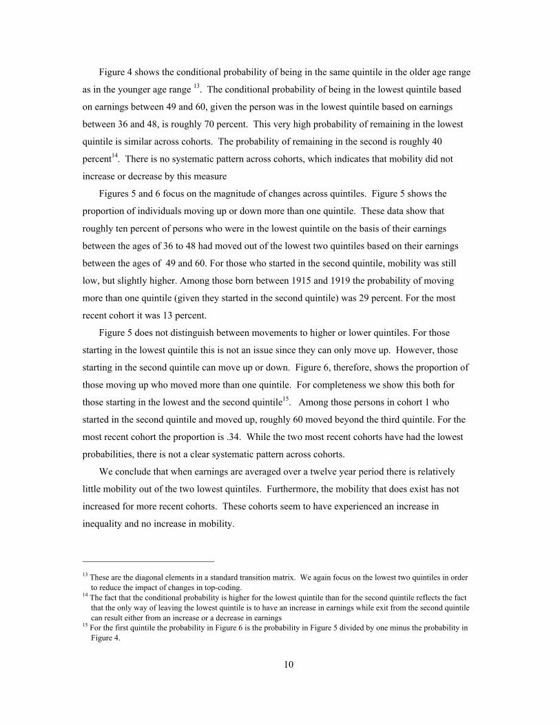
Figure 4 shows the conditional probability of being in the same quintile in the older age range

as in the younger age range 13. The conditional probability of being in the lowest quintile based

on earnings between 49 and 60, given the person was in the lowest quintile based on earnings

between 36 and 48, is roughly 70 percent. This very high probability of remaining in the lowest

quintile is similar across cohorts. The probability of remaining in the second is roughly 40

percent14. There is no systematic pattern across cohorts, which indicates that mobility did not

increase or decrease by this measure

Figures 5 and 6 focus on the magnitude of changes across quintiles. Figure 5 shows the

proportion of individuals moving up or down more than one quintile. These data show that

roughly ten percent of persons who were in the lowest quintile on the basis of their earnings

between the ages of 36 to 48 had moved out of the lowest two quintiles based on their earnings

between the ages of 49 and 60. For those who started in the second quintile, mobility was still

low, but slightly higher. Among those born between 1915 and 1919 the probability of moving

more than one quintile (given they started in the second quintile) was 29 percent. For the most

recent cohort it was 13 percent.

Figure 5 does not distinguish between movements to higher or lower quintiles. For those

starting in the lowest quintile this is not an issue since they can only move up. However, those

starting in the second quintile can move up or down. Figure 6, therefore, shows the proportion of

those moving up who moved more than one quintile. For completeness we show this both for

those starting in the lowest and the second quintile15. Among those persons in cohort 1 who

started in the second quintile and moved up, roughly 60 moved beyond the third quintile. For the

most recent cohort the proportion is .34. While the two most recent cohorts have had the lowest

probabilities, there is not a clear systematic pattern across cohorts.

We conclude that when earnings are averaged over a twelve year period there is relatively

little mobility out of the two lowest quintiles. Furthermore, the mobility that does exist has not

increased for more recent cohorts. These cohorts seem to have experienced an increase in

inequality and no increase in mobility.

13 These are the diagonal elements in a standard transition matrix. We again focus on the lowest two quintiles in order

to reduce the impact of changes in top-coding.14 The fact that the conditional probability is higher for the lowest quintile than for the second quintile reflects the fact

that the only way of leaving the lowest quintile is to have an increase in earnings while exit from the second quintilecan result either from an increase or a decrease in earnings

15 For the first quintile the probability in Figure 6 is the probability in Figure 5 divided by one minus the probability inFigure 4.

11

Employment and OASDI Income after 65

The preceding sections have shown that the increase in inequality of yearly earnings during

the 1980’s translated into a decline in the P10 of accumulated earnings for more recent cohorts.

We now turn to the outcomes of these cohorts as they entered retirement or semi- retirement. We

examine both the labor market outcomes and Social Security income between the ages of 65 and

70.

Labor Market Outcomes

The labor market outcomes after 65 for recent cohorts at the bottom of the accumulated

earnings distribution reflect two offsetting forces. With lower lifetime earnings, these individuals

may have had greater need to continue to work during their late 60’s. Countering this outward

shift in labor supply is the shift in demand for older persons with low skills. Whether earnings

increased or decreased depends both on elasticities of supply and demand and on the relative size

of these two shifts,

In this section we examine both the employment and earnings of persons classified by cohort

and age. In order to avoid the problems caused by top-coding of earnings we rely on the SER

data starting in 1991. This data allows us to measure labor market outcomes at each age between

65 and 70. However, since this data is only available for an eleven year period (1991 to 2001) we

cannot follow each cohort over the full age range. Members of the cohort born between 1915

and 1919 were 72 to 76 in 1991. They were, therefore, too old to be included in this part of the

analysis. The following cohort was born between 1920 and 1924 so we observe their non-top

coded earnings starting at age 67. The next two cohorts are observed over the full age range but

the most recent cohort, born between 1935 and 1939 can only be observed at age 65.

Probability of Working

Figure 7 plots the proportion of each cohort working at different ages16. As expected there is

a steep decline in the proportion working between the ages of 65 and 70 for each cohort. The

most recent cohort born between 1935 and 1939 is only observed at age 65 so we cannot trace its

full history. It, however, started with a higher proportion working (.589) than the previous cohort

(.558). This indicates that as a whole this cohort continued to work in greater numbers than

previous cohorts in spite of the fact that they had similar median accumulated earnings (see

Figure 2).

16 Work is defined as having positive earnings.

12

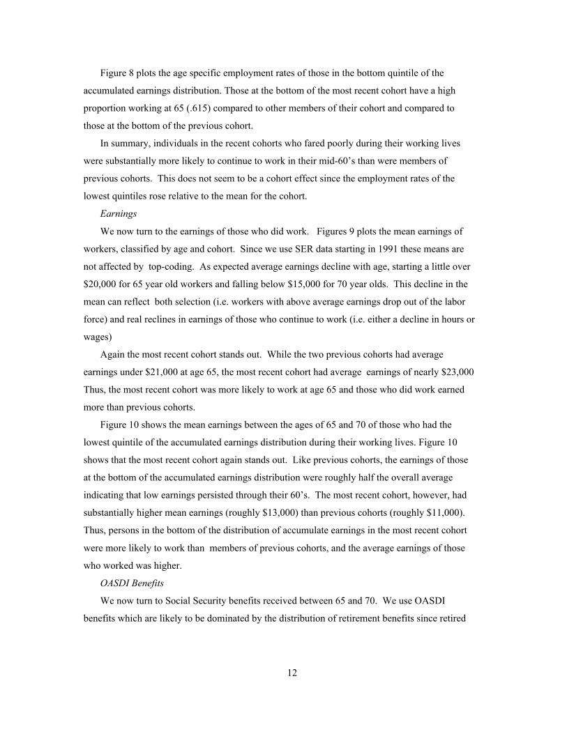
Figure 8 plots the age specific employment rates of those in the bottom quintile of the

accumulated earnings distribution. Those at the bottom of the most recent cohort have a high

proportion working at 65 (.615) compared to other members of their cohort and compared to

those at the bottom of the previous cohort.

In summary, individuals in the recent cohorts who fared poorly during their working lives

were substantially more likely to continue to work in their mid-60’s than were members of

previous cohorts. This does not seem to be a cohort effect since the employment rates of the

lowest quintiles rose relative to the mean for the cohort.

Earnings

We now turn to the earnings of those who did work. Figures 9 plots the mean earnings of

workers, classified by age and cohort. Since we use SER data starting in 1991 these means are

not affected by top-coding. As expected average earnings decline with age, starting a little over

$20,000 for 65 year old workers and falling below $15,000 for 70 year olds. This decline in the

mean can reflect both selection (i.e. workers with above average earnings drop out of the labor

force) and real reclines in earnings of those who continue to work (i.e. either a decline in hours or

wages)

Again the most recent cohort stands out. While the two previous cohorts had average

earnings under $21,000 at age 65, the most recent cohort had average earnings of nearly $23,000

Thus, the most recent cohort was more likely to work at age 65 and those who did work earned

more than previous cohorts.

Figure 10 shows the mean earnings between the ages of 65 and 70 of those who had the

lowest quintile of the accumulated earnings distribution during their working lives. Figure 10

shows that the most recent cohort again stands out. Like previous cohorts, the earnings of those

at the bottom of the accumulated earnings distribution were roughly half the overall average

indicating that low earnings persisted through their 60’s. The most recent cohort, however, had

substantially higher mean earnings (roughly $13,000) than previous cohorts (roughly $11,000).

Thus, persons in the bottom of the distribution of accumulate earnings in the most recent cohort

were more likely to work than members of previous cohorts, and the average earnings of those

who worked was higher.

OASDI Benefits

We now turn to Social Security benefits received between 65 and 70. We use OASDI

benefits which are likely to be dominated by the distribution of retirement benefits since retired

13

workers and their children and spouses comprise 70 percent of OASDI beneficiaries17 Since the

benefit formulae under this program is progressive it is possible that the decline in accumulated

earnings at the bottom of the distribution would be cushioned by OASDI benefits.

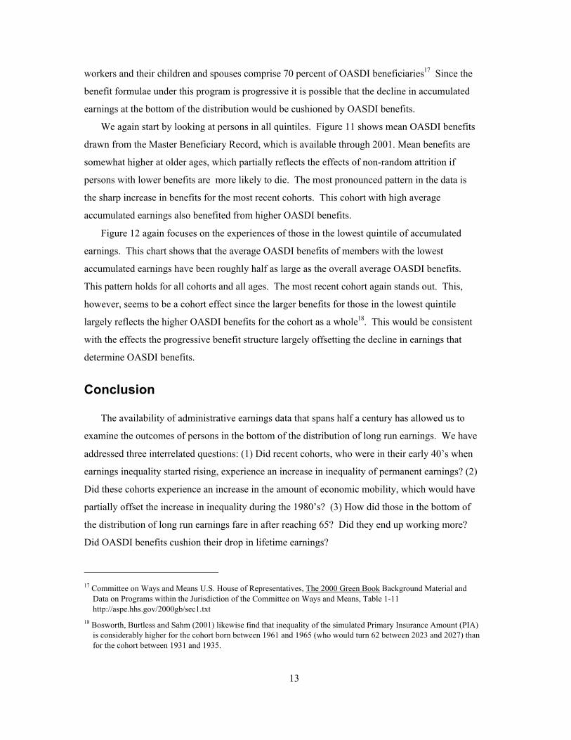
We again start by looking at persons in all quintiles. Figure 11 shows mean OASDI benefits

drawn from the Master Beneficiary Record, which is available through 2001. Mean benefits are

somewhat higher at older ages, which partially reflects the effects of non-random attrition if

persons with lower benefits are more likely to die. The most pronounced pattern in the data is

the sharp increase in benefits for the most recent cohorts. This cohort with high average

accumulated earnings also benefited from higher OASDI benefits.

Figure 12 again focuses on the experiences of those in the lowest quintile of accumulated

earnings. This chart shows that the average OASDI benefits of members with the lowest

accumulated earnings have been roughly half as large as the overall average OASDI benefits.

This pattern holds for all cohorts and all ages. The most recent cohort again stands out. This,

however, seems to be a cohort effect since the larger benefits for those in the lowest quintile

largely reflects the higher OASDI benefits for the cohort as a whole18. This would be consistent

with the effects the progressive benefit structure largely offsetting the decline in earnings that

determine OASDI benefits.

Conclusion

The availability of administrative earnings data that spans half a century has allowed us to

examine the outcomes of persons in the bottom of the distribution of long run earnings. We have

addressed three interrelated questions: (1) Did recent cohorts, who were in their early 40’s when

earnings inequality started rising, experience an increase in inequality of permanent earnings? (2)

Did these cohorts experience an increase in the amount of economic mobility, which would have

partially offset the increase in inequality during the 1980’s? (3) How did those in the bottom of

the distribution of long run earnings fare in after reaching 65? Did they end up working more?

Did OASDI benefits cushion their drop in lifetime earnings?

17 Committee on Ways and Means U.S. House of Representatives, The 2000 Green Book Background Material and

Data on Programs within the Jurisdiction of the Committee on Ways and Means, Table 1-11http://aspe.hhs.gov/2000gb/sec1.txt

18 Bosworth, Burtless and Sahm (2001) likewise find that inequality of the simulated Primary Insurance Amount (PIA)is considerably higher for the cohort born between 1961 and 1965 (who would turn 62 between 2023 and 2027) thanfor the cohort between 1931 and 1935.

14

The answer to the first question is clear. While the median permanent earnings of recent

cohorts is at an all time high, those at the bottom of the distribution lost ground. Cohorts who

were in their prime earning years during the 1980’s when earnings inequality started rising

dramatically, experienced a real decline in the permanent earnings at the bottom of the

distribution relative to cohorts born 20 years earlier.

The second claim, that mobility has been rising, is clearly not supported by the data. The

probability of leaving the lowest quintile of the distribution of long run earnings (measured over

a twelve year span) was roughly 30 percent for each cohort we follow. Not only are these escape

rates low but most of the transitions that do occur are only to the second quintile. As a result, less

than ten percent of those started in the lowest quintile moved more than one quintile.

Finally, we find that members of the most recent cohort at the bottom of the distribution of

long run earnings did differ in some ways from the corresponding members of previous cohorts.

They were substantially more likely to work at age 65, which could indicate that they continued

to work to compensate for their lower long run earnings. Furthermore, those who did work had

higher earnings. OASDI benefits were higher than for similar persons in earlier cohorts but this

seems to be a cohort effect..

We conclude that the persons reaching their mid 60’s in 2000 had done very well in terms of

earnings over their working lives. Furthermore,seemed to be doing well as the retired or reached

retirement. Both their average earnings and their average OASDI benefits were higher than

previous cohorts. But, as is often the case, the average experience should not be generalized to all

members of this cohort. For persons at the bottom of the distribution of long run earnings the

picture was considerably bleaker. Their long run earnings had not grown with the median and

were, in fact, not much higher than for persons born 20 years earlier. This indicates that effects

of the rise in inequality of yearly income does not dissipate over the lifecyle.

It is still too early to know what will happen to this cohort in retirement. However, their labor

market outcomes at 65 indicates that they are continuing to work in record numbers, even when

compare to other memebers of their own cohorts. This may indicate a need to compensate for

their lower earnings during their earlier working lives.

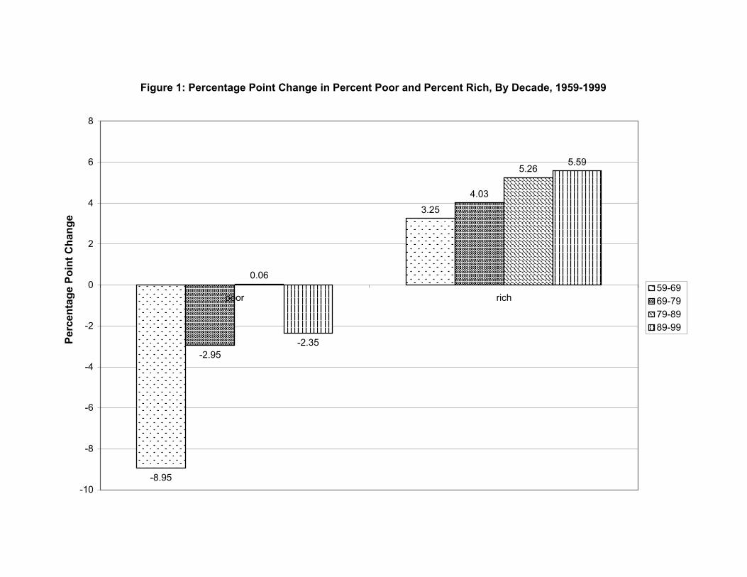
Figure 1: Percentage Point Change in Percent Poor and Percent Rich, By Decade, 1959-1999

-8.95

3.25

-2.95

4.03

0.06

5.26

-2.35

5.59

-10

-8

-6

-4

-2

0

2

4

6

8

poor rich

Per

cen

tag

e P

oin

t C

han

ge

59-69 69-7979-8989-99

Figure 2: Percentage Change in Mean Family Income and Mean Male Earnings, By Decade, 1959-1999

.373

.215

.146

.189

.309

.079

.049

.093

0

0.05

0.1

0.15

0.2

0.25

0.3

0.35

0.4

59-69 69-79 79-89 89-99

Per

cen

tag

e C

han

ge

Mean Fam IncMean Earnings

Figure 3: Percentage Change in Family Income Inequality, By Decade, 1959-1999

-.035

.001

.082 .081

-.113

.208

.102

.026

-0.15

-0.1

-0.05

0

0.05

0.1

0.15

0.2

0.25

59-69 69-79 79-89 89-99

Per

cen

tag

e C

han

ge

Gini P90/P10

Figure 4 : Mean Real Hourly Wage Rate, Males and Females, 1975-2001

9

10

11

12

13

14

15

16

17

18

75 77 79 81 83 85 87 89 91 93 95 97 99 01Year

Ho

url

y W

age

(199

9 $)

Male Female

Figure 5a: Percentage Change in Real Hourly Wages by Percentile, 1975-2001

-0.1

0.0

0.1

0.2

0.3

0.4

0.5

0.6

0.7

5 10 15 20 25 30 35 40 45 50 55 60 65 70 75 80 85 90 95

Percentile

Per

cen

tag

e C

han

ge

Male Female

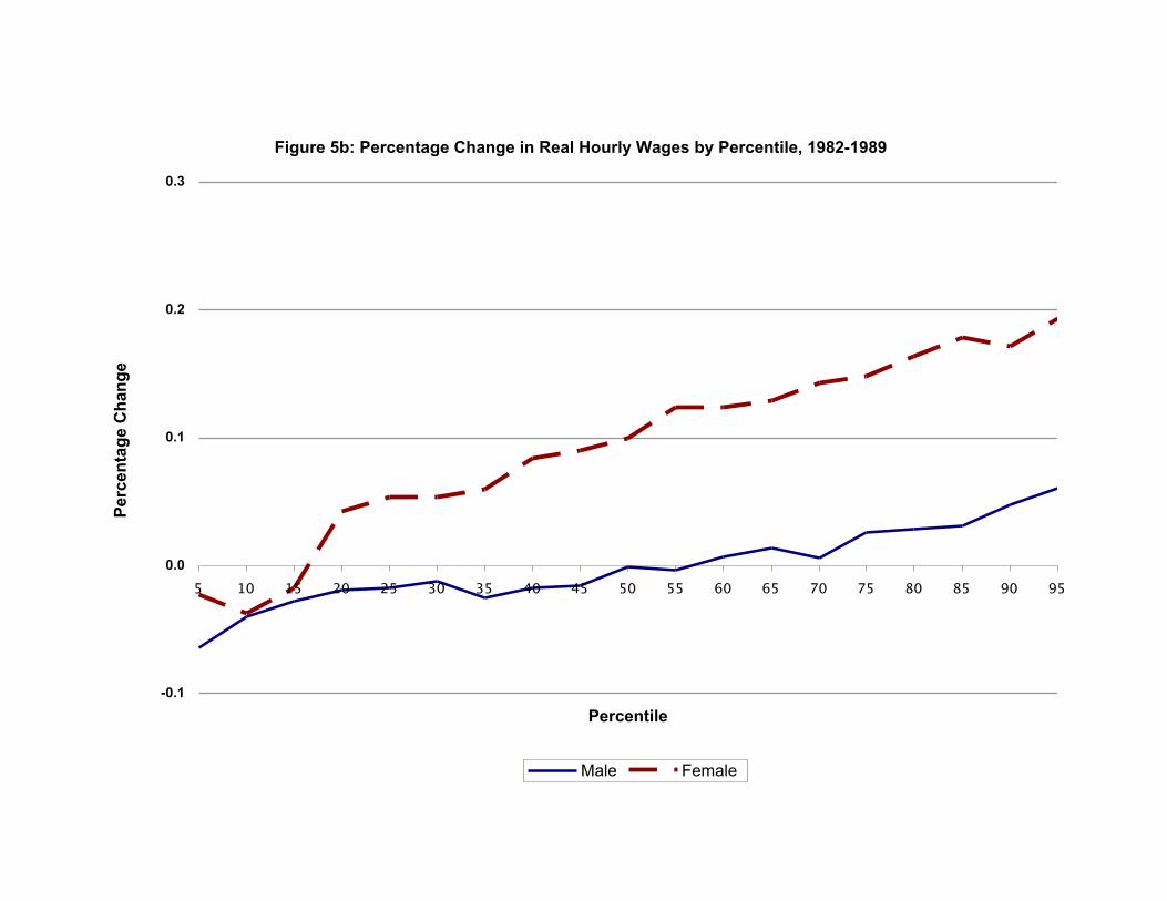
Figure 5b: Percentage Change in Real Hourly Wages by Percentile, 1982-1989

-0.1

0.0

0.1

0.2

0.3

5 10 15 20 25 30 35 40 45 50 55 60 65 70 75 80 85 90 95

Percentile

Per

cen

tag

e C

han

ge

Male Female

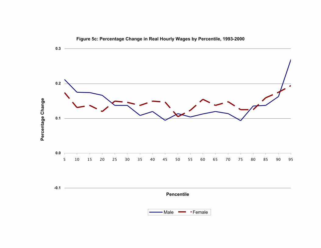
Figure 5c: Percentage Change in Real Hourly Wages by Percentile, 1993-2000

-0.1

0.0

0.1

0.2

0.3

5 10 15 20 25 30 35 40 45 50 55 60 65 70 75 80 85 90 95

Pencentile

Per

cen

tag

e C

han

ge

Male Female

Figure 6a: Ratio of Hourly Wage Rate at 90th Percentile to Wage at 10th Percentile, 1975-2001

3.5

4.0

4.5

5.0

5.5

6.0

75 77 79 81 83 85 87 89 91 93 95 97 99 01Year

P90

/P10

Male Female

Figure 6b: Standard Deviation of Log Hourly wage, 1975-2001

0.52

0.54

0.56

0.58

0.60

0.62

75 77 79 81 83 85 87 89 91 93 95 97 99 01Year

Sta

nd

ard

Dev

iati

on

sd(lnwage)-Card Dinardo Sd(lnwage)---Final Sample

Figure 7: Employment Rate and Coefficient of Variation of Hourly Wage Rate -- Males , 1975-2001

0.40

0.45

0.50

0.55

0.60

0.65

0.70

0.71 0.72 0.73 0.74 0.75 0.76 0.77Employment Rate

Co

effi

cien

t o

f V

aria

tio

n

1979

1975

1981

1993

2001

1983

19891992

2000

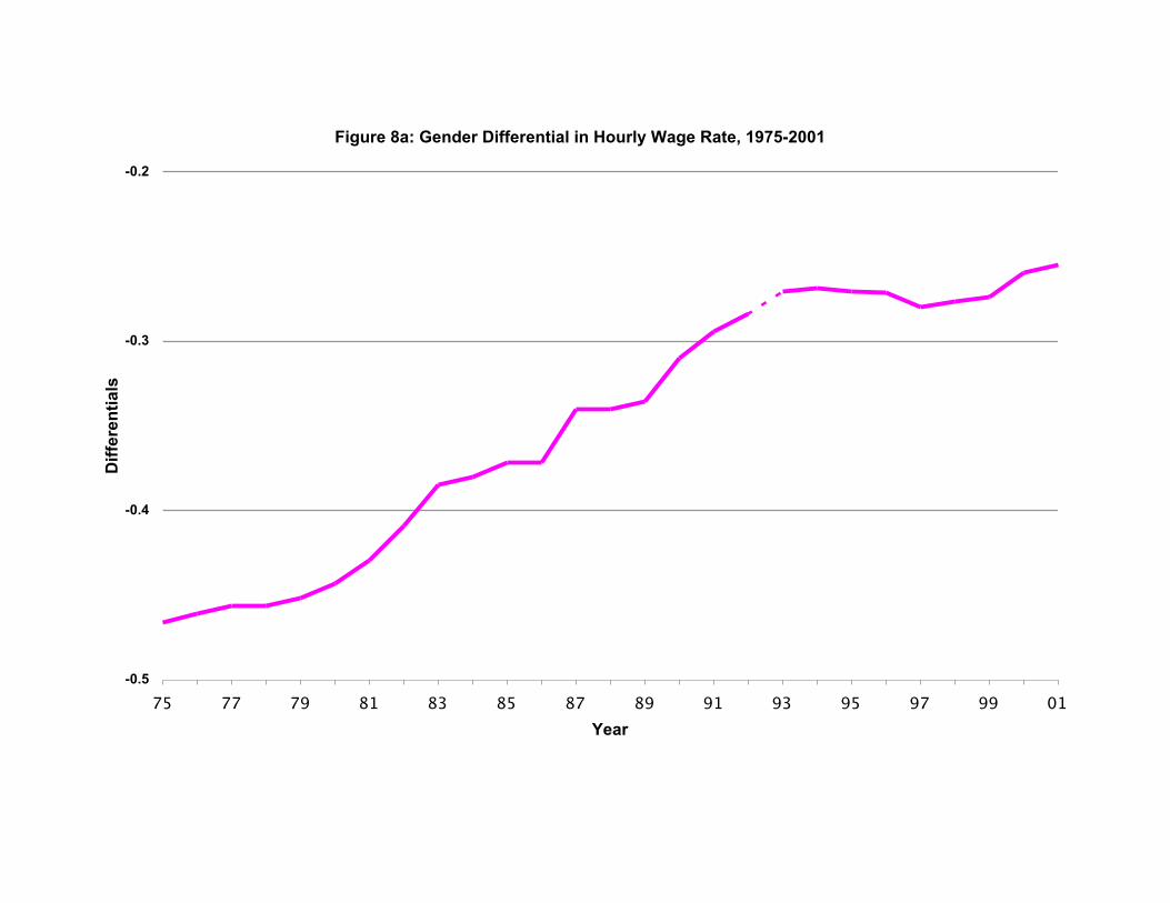
Figure 8a: Gender Differential in Hourly Wage Rate, 1975-2001

-0.5

-0.4

-0.3

-0.2

75 77 79 81 83 85 87 89 91 93 95 97 99 01Year

Dif

fere

nti

als

Figure 8b: Black-White Differential in Hourly Wage Rate, 1975-2001

-0.25

-0.20

-0.15

-0.10

-0.05

0.00

0.05

75 77 79 81 83 85 87 89 91 93 95 97 99 01Year

Dif

fere

nti

als

Female Male

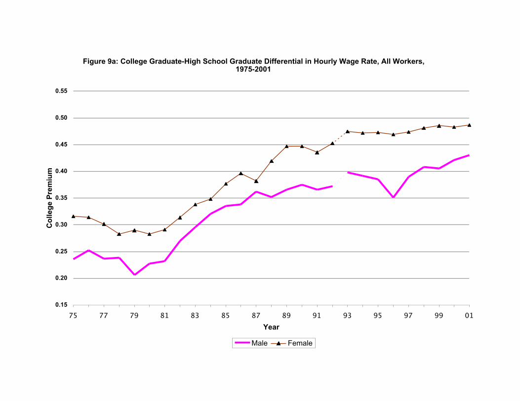
Figure 9a: College Graduate-High School Graduate Differential in Hourly Wage Rate, All Workers, 1975-2001

0.15

0.20

0.25

0.30

0.35

0.40

0.45

0.50

0.55

75 77 79 81 83 85 87 89 91 93 95 97 99 01Year

Co

lleg

e P

rem

ium

Male Female

Figure 9b: College-High School Wage Differential for New Labor Force Entrants, Males and Females, 1975-2001

0.15

0.20

0.25

0.30

0.35

0.40

0.45

0.50

0.55

0.60

0.65

75 77 79 81 83 85 87 89 91 93 95 97 99 01Year

Co

lleg

e P

rem

ium

Male Female

Figure 10: Returns to Experience by Gender and Education(Evaluated at Ten Years Experience)

0.0

1.0

2.0

3.0

4.0

75 77 79 81 83 85 87 89 91 93 95 97 99 01Year

Per

cen

t

Male_College Female_College Male_No_College Female_No_College

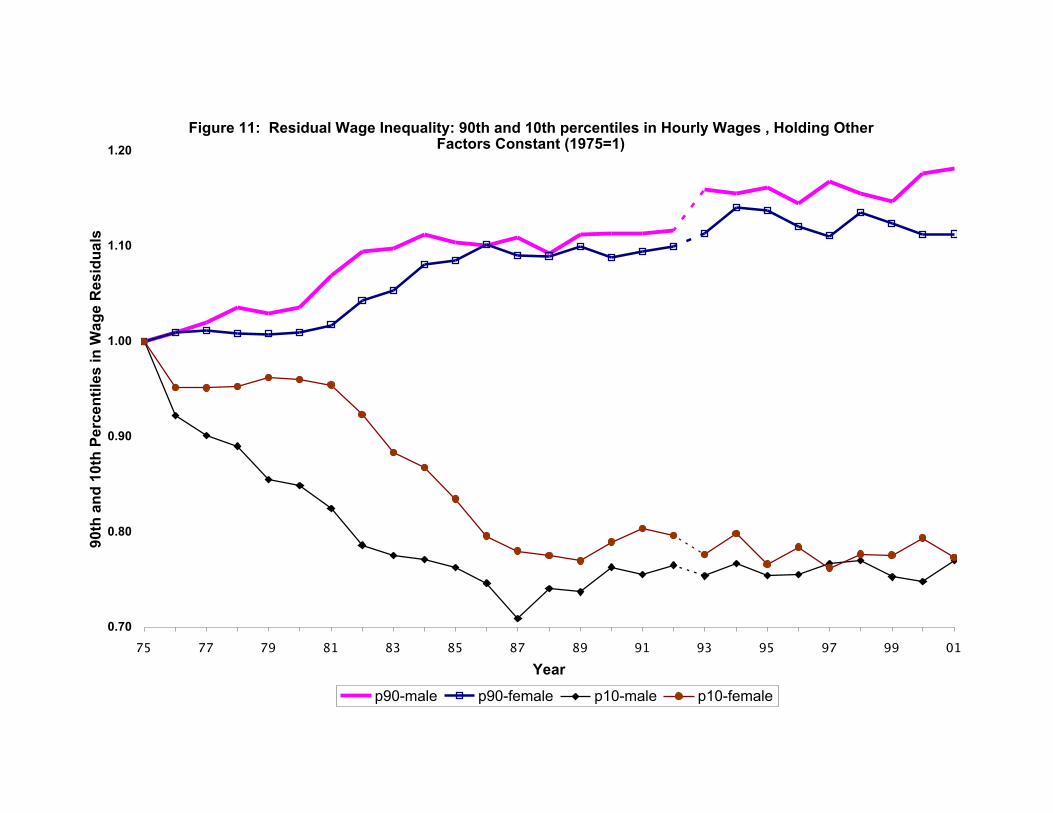
Figure 11: Residual Wage Inequality: 90th and 10th percentiles in Hourly Wages , Holding Other Factors Constant (1975=1)

0.70

0.80

0.90

1.00

1.10

1.20

75 77 79 81 83 85 87 89 91 93 95 97 99 01Year

90th

an

d 1

0th

Per

cen

tile

s in

Wag

e R

esid

ual

s

p90-male p90-female p10-male p10-female

Figure 12a: Change in Hours by Wage Quintile--Males

-50

0

50

100

150

200

Q1 Q2 Q3 Q4 Q5

Wage Quintile in Base year

Ch

ang

e in

Ho

urs

75-0182-8993-00

Figure 12b: Change in Hours by Wage Quintile--Females

0

50

100

150

200

250

300

350

400

Q1 Q2 Q3 Q4 Q5

Wage Quintile in Base year

Ch

ang

e in

Ho

urs

75-0182-8993-00

Figure 13a: Coefficient of Variation of Annual Earnings & Hourly Wage for Male(1975=1)

0.9

1.0

1.1

1.2

1.3

75 77 79 81 83 85 87 89 91 93 95 97 99 01Year

Co

effi

cien

t o

f V

aria

tio

n

cv(earn) cv(wage)

Figure 13b: Coefficient of Variation of Annual Earnings & Hourly Wage for Female(1975=1)

0.9

1.0

1.1

1.2

1.3

75 77 79 81 83 85 87 89 91 93 95 97 99 01Year

Co

effi

cien

t o

f V

aria

tio

n

cv(earn) cv(wage)

Figure 14: Employment Rate and Coefficient of Variation of Annual Earnings--Males, 1975-2001

0.40

0.45

0.50

0.55

0.60

0.65

0.70

0.71 0.72 0.73 0.74 0.75 0.76 0.77Employment Rate

Co

effi

cien

t o

f V

aria

tio

n

1979

1975

1992 2000

19841982

1989

1993 2001

Figure 15: Coefficient of Variation of Adjusted Family Income, 1969-2001

0.5

0.6

0.7

0.8

69 71 73 75 77 79 81 83 85 87 89 91 93 95 97 99 01Year

Co

effi

cien

t o

f V

aria

tio

n

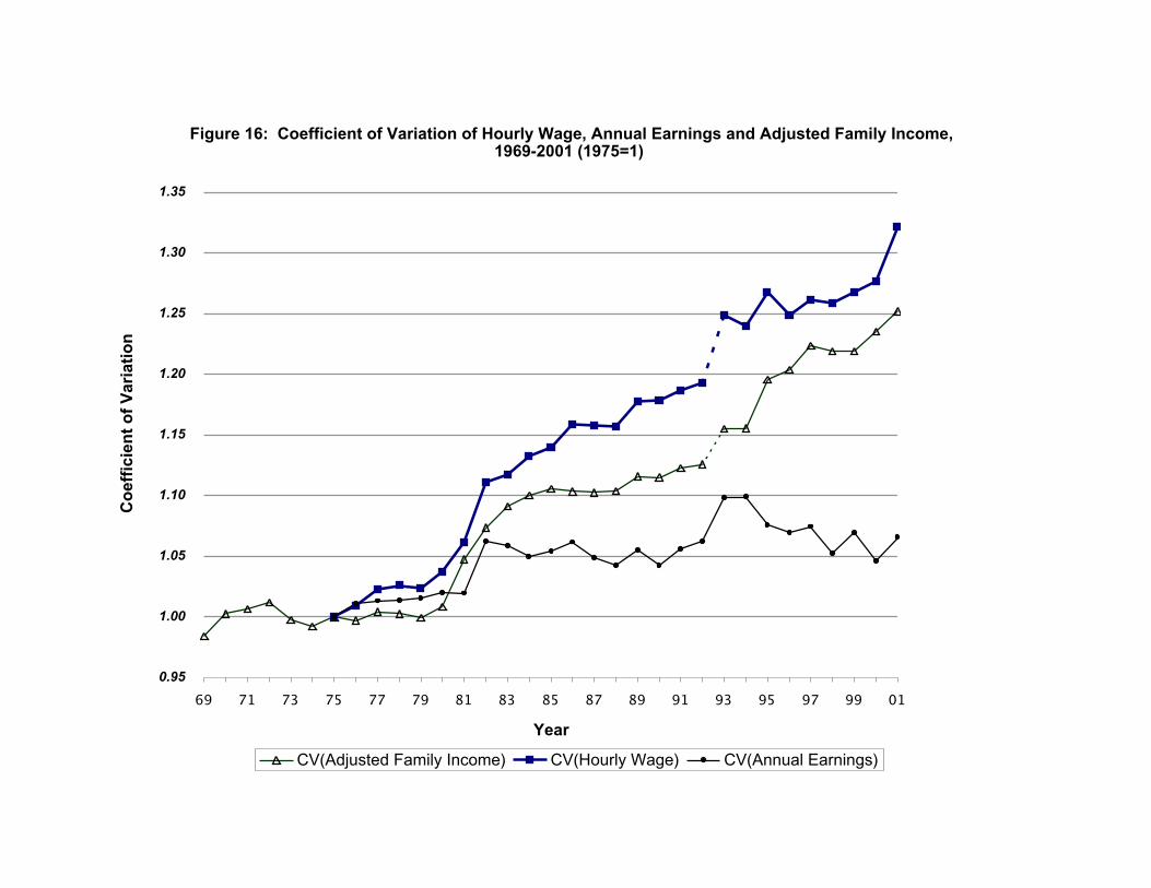
Figure 16: Coefficient of Variation of Hourly Wage, Annual Earnings and Adjusted Family Income, 1969-2001 (1975=1)

0.95

1.00

1.05

1.10

1.15

1.20

1.25

1.30

1.35

69 71 73 75 77 79 81 83 85 87 89 91 93 95 97 99 01Year

Co

effi

cien

t o

f V

aria

tio

n

CV(Adjusted Family Income) CV(Hourly Wage) CV(Annual Earnings)

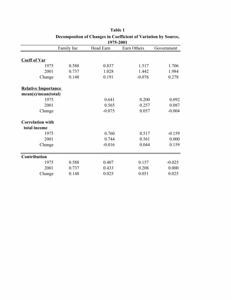
Family Inc Head Earn Earn Others Government

Coeff of Var1975 0.588 0.837 1.517 1.7062001 0.737 1.028 1.442 1.984

Change 0.148 0.191 -0.076 0.278

Relative Importance mean(s)/mean(total)

1975 0.641 0.200 0.0922001 0.565 0.257 0.087

Change -0.075 0.057 -0.004

Correlation with total income

1975 0.760 0.517 -0.1592001 0.744 0.561 0.000

Change -0.016 0.044 0.159

Contribution1975 0.588 0.407 0.157 -0.0252001 0.737 0.433 0.208 0.000

Change 0.148 0.025 0.051 0.025

Table 1

Decompositon of Changes in Coefficient of Variation by Source, 1975-2001

Other Income

2.9012.9890.088

0.0680.0900.022

0.2490.3580.108

0.0490.0960.047

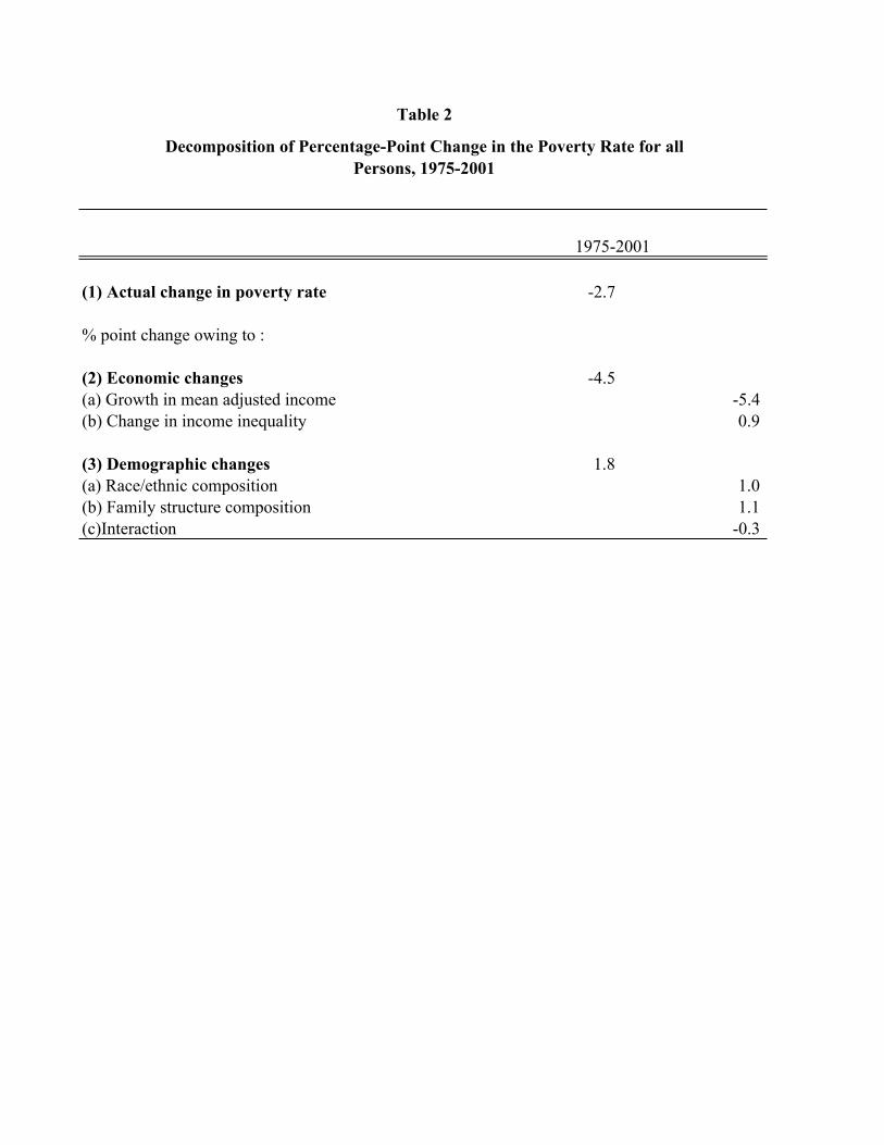
(1) Actual change in poverty rate -2.7

% point change owing to :

(2) Economic changes -4.5(a) Growth in mean adjusted income -5.4(b) Change in income inequality 0.9

(3) Demographic changes 1.8(a) Race/ethnic composition 1.0(b) Family structure composition 1.1(c)Interaction -0.3

Decomposition of Percentage-Point Change in the Poverty Rate for all Persons, 1975-2001

Table 2

1975-2001