I’ve Fallen and I Can’t Get Up: Can High Ability Students RecoverFrom Early Mistakes in CAT?

Kelly L. Rulison and Eric LokenThe Pennsylvania State University

AbstractA difficult result to interpret in Computerized Adaptive Tests (CATs) occurs when an ability estimateinitially drops and then ascends continuously until the test ends, suggesting that the true ability maybe higher than implied by the final estimate. We explain why this asymmetry occurs and show thatearly mistakes by high ability students can lead to considerable underestimation, even in tests with45 items. The opposite response pattern, where low ability students start with lucky guesses, leadsto much less bias. We show that using Barton and Lord’s (1981) four-parameter model and a lessinformative prior can lower bias and RMSE for high ability students with a poor start, as the CATalgorithm ascends more quickly after initial underperformance. We also show that the 4PM slightlyoutperforms a CAT in which less discriminating items are initially used. The practical implicationsand relevance for psychological measurement more generally are discussed.

KeywordsComputerized Adaptive Testing; Bayesian; Item response theory; Achievement testing; High stakesassessment

Computerized adaptive tests (CATs) combine item response theory (IRT) models with realtime estimation algorithms to provide tailored assessments that can improve measurementefficiency and reduce examinee burden (Chang, 2004; Meijer & Nering, 1999; Wainer et al.,2000; Weiss, 1982). Compared to non-adaptive “paper and pencil” measures, CATs are moreefficient because they update the latent trait estimate, θ ̂, after each response and then adaptivelyselect the most appropriate item to deliver next. Obtaining unbiased and efficient estimates ofθ in a CAT requires: 1) an underlying IRT model that closely corresponds to respondentbehavior (van Krimpen-Stoop & Meijer, 2000; Wainer et al., 2000); and 2) an effective itemselection algorithm (Chang & Ying, 1996; 1999; Passos, Berger, & Tan, 2007).

We focus on the first requirement as it relates to a specific estimation problem in CATs. Ideally,θ ̂ should reach the neighborhood of the true θ before the CAT concludes. In a typical test,ability estimates for a high ability student might initially ascend quickly and then oscillate alittle above and below the final θ ̂ as the student encounters questions that are closely matchedto his or her ability. In some cases, however, θ ̂ may drop at the beginning of the test, and thenascend continuously until the final estimate, suggesting that the student’s true θ is perhapssignificantly higher than the final θ̂.

In our first simulation study, we will demonstrate that a pattern of continuously ascendingability estimates can arise when a high ability student misses early items in a CAT. Under the

Corresponding Author: Kelly Rulison, The Pennsylvania State University, 113 S. Henderson Building, University Park, PA 16802,klr250@psu.edu.

NIH Public AccessAuthor ManuscriptAppl Psychol Meas. Author manuscript; available in PMC 2010 October 14.

Published in final edited form as:Appl Psychol Meas. 2009 March 1; 33(2): 83–101.

NIH

-PA Author Manuscript

NIH

-PA Author Manuscript

NIH

-PA Author Manuscript

widely used three-parameter model (3PM), the lower asymptote is a non-zero value thataccounts for the possibility of guessing the correct answer on multiple choice tests. However,the upper asymptote for the item response function is 1, suggesting that a high ability studentshould answer an easy question with probability approaching 1. It is conceivable, however,that P(θ) ≈ 1 may not always hold, even if the item appears too easy for the respondent. Highability students who are anxious, distracted by poor testing conditions, unfamiliar withcomputers, careless, or who misread the question, may on occasion miss items that theyotherwise should have answered correctly. If this happens early in the test, it may lead to theproblematic outcome in which the estimates are increasing even at the end of the test.

The potential for underestimation of high ability students in CAT is rarely discussed in theliterature. Most research on obtaining unbiased estimates of θ focuses on identifying aberrantresponse patterns through person misfit indices (van Krimpen-Stoop & Meijer, 2000) or onadapting item selection algorithms to reflect the uncertainty that exists as the test begins (Chang& Ying, 1996; 1999; 2002; Passos et al., 2007). Chang and Ying (2002) and Chang (2004),for example, argue that item selection algorithms based solely on Fisher’s information criterionselect items with high a parameters first, yielding step sizes for θ ̂ that are inappropriately largeat the onset of a CAT. They suggest using an item selection strategy that stratifies the item pooland uses less discriminating items early in the test. This stratification ensures that enough highdiscriminating items are left in the item pool to allow θ ̂ to ascend quickly at the end of the test(Chang & Ying, 1999; 2002).

Below, we consider another approach. We hypothesize that making minor adjustments to thecommonly used 3PM may protect against underestimation when a student starts the test poorly.Specifically, we revisit a 4-parameter model (4PM) proposed by Barton and Lord (1981) andargue that it might have some utility in CAT.

The Three-Parameter Model (3PM)In IRT, the probability of a correct response is modeled as a function of a latent trait, θ, anditem parameters. The 3PM is frequently used in academic testing and is given by

(1)

where aj is the item discrimination or “slope” parameter, bj is the item threshold or “difficulty”parameter, and cj is the lower asymptote or “pseudo-guessing” parameter. The non-zero lowerasymptote allows that low ability students may occasionally guess the correct answer todifficult items. In contrast, the upper asymptote of 1 reflects the stiff assumption that if an itemis easy enough relative to a student’s ability, then the probability of a correct response iseffectively 1.

Assuming the item parameters are known, the likelihood function for a response vector x,indicating correct and incorrect responses, is given by:

(2)

Choosing θ̂ to maximize (2) yields the maximum likelihood estimator (MLE).

Rulison and Loken Page 2

Appl Psychol Meas. Author manuscript; available in PMC 2010 October 14.

NIH

-PA Author Manuscript

NIH

-PA Author Manuscript

NIH

-PA Author Manuscript

Alternatively, in Bayesian estimation, multiplying the likelihood function by a priordistribution yields the posterior distribution

(3)

Bayesian estimation in IRT is widely used (Baker & Kim, 2004; Bock & Mislevy, 1982), mostoften with p(θ) ~ N(0,1) and taking either the posterior mean (EAP) or posterior mode (MAP)to estimate θ̂. The benefits of the Bayesian approach include guaranteed proper estimates andsmaller standard errors, at the cost of some bias in the tails of the ability distribution due topull from the prior (Baker & Kim, 2004).

Difficulties in Estimating AbilitySome response patterns, such as getting all items correct or incorrect, yield improper estimatesfor the MLE. In CATs, ad hoc measures are required to implement a floor or ceiling for θ̂ inthe early stages of the test. But even if the student has made both correct and incorrect responses,some response patterns can still yield improper estimates. It is worth exploring these patternsbecause they are related to the underestimation problem when high ability students miss easyquestions early in a CAT.

Consider responses to a three item test, two correct and one incorrect. The likelihood is:

(4)

If all items have aj = 1.1 and cj = 0.2, the likelihood is bounded for low θ at c2 – c3, or 0.032,and goes to 0 for high θ. What happens in between depends on the relative difficulty of theitems.

Figure 1 shows the likelihood when b1 = −1, b2 = 0, and b3 = 1. If the student answers the easyand moderate items correctly and misses the hardest item (solid line), the MLE is θ ̂ = 0.46. If,however, the easiest item is missed and the moderate and hard items are answered correctly(i.e., if x = (0,1,1)), the MLE is improper, tailing off to negative infinity (dashed line). Thelikelihood decreases monotonically because the term (1- P1(θ)) begins to drop to 0 faster thanP2(θ) P3(θ) increases from the lower asymptote. As long as the incorrect item is significantlyeasier than the other two items, the rise to P1(θ) =1 (and thus the decrease of 1- P1(θ) to 0)dominates the likelihood function.

The result is also explained by Bradlow’s (1996) demonstration that in the 3PM the observedinformation for an item response can actually be negative. Although the expectedinformation for an item is always positive, the observed information provided by a correctresponse can be negative under certain conditions. Bradlow showed that negative informationwill occur when an item is answered correctly and

(5)

The likelihood shown by the dashed line is not bounded for low θ because the informationprovided by the correct answers to questions 2 and 3 is negative. Therefore, for low θ, theobserved responses do not give adequate information for a proper ability estimate.

With a proper prior, the EAP for the three-item example is finite, regardless of the pattern ofresponses. If p(θ) ~ N(0,1) and the same response pattern that yielded the improper likelihood

Rulison and Loken Page 3

Appl Psychol Meas. Author manuscript; available in PMC 2010 October 14.

NIH

-PA Author Manuscript

NIH

-PA Author Manuscript

NIH

-PA Author Manuscript

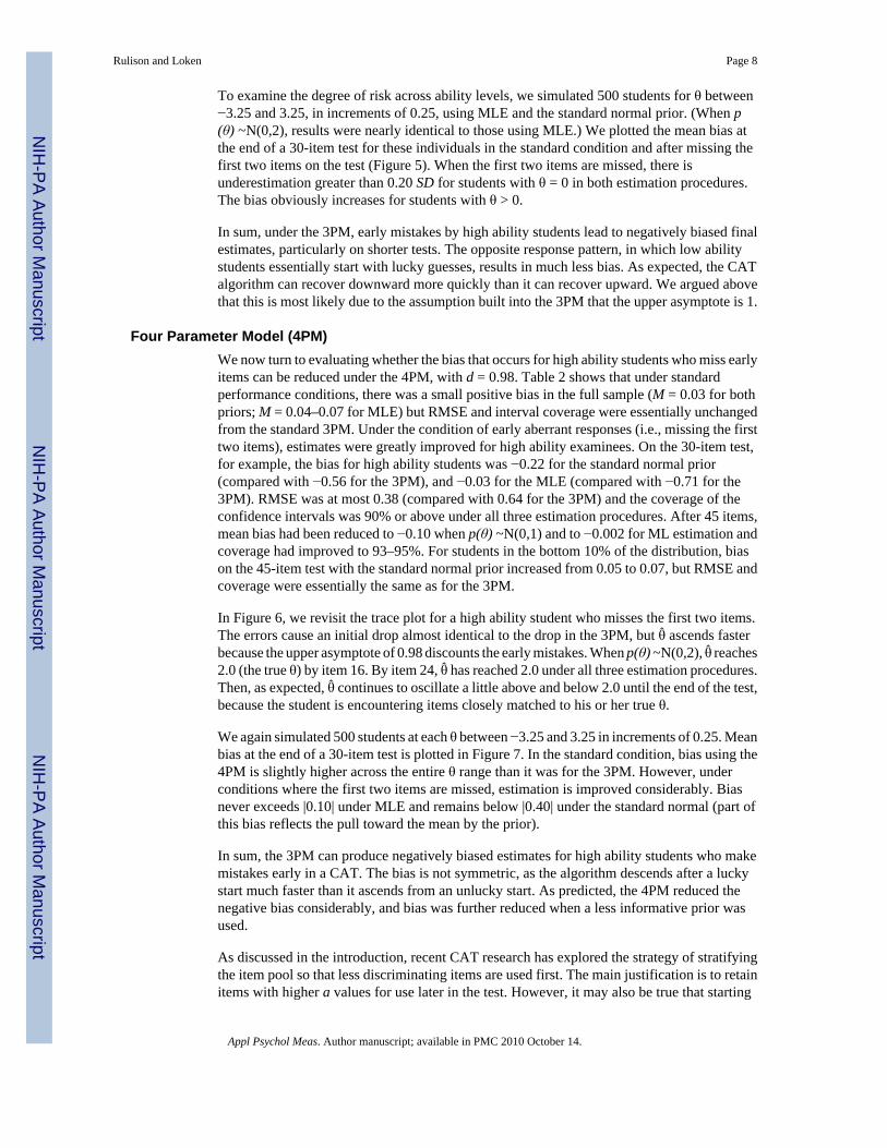
in Figure 1 (dashed line) is observed, θ ̂ = −0.4, SD = 0.94 (Figure 2, solid line). But even thoughthe Bayesian estimates are proper, abnormal response patterns can still yield surprising results.For example, if the difficulty of the correctly answered items were raised to b2 = b3 = 2.5 (withthe incorrect item still at b1 = −1), it might be expected that θ̂ would increase. Instead, theposterior mean shifts lower to θ̂ = −0.91 and the standard deviation shrinks to 0.91 (Figure 2,dashed line).

That θ̂ shifts lower, with greater certainty, is at first counterintuitive, as correctly answeringvery difficult questions would seem to indicate high ability. However, because 1- P1(θ) goesto 0 much faster than P2(θ) and P3(θ) rise from c, the information gathered from the moredifficult items is discounted; informally one might say that the correct answers to highlydifficult items “confirm” that they were “just guesses”. In terms of Bradlow’s (1996)discussion, the observed information becomes even more negative if the correct items are moredifficult relative to ability, and thus the increase in the posterior variance.

The problematic combination of incorrect answers to easy items with correct answers to harderitems has received some attention in the traditional non-adaptive testing literature. Mislevyand Bock (1982) explored the use of ability estimators that were robust to guessing by lowability students and “carelessness” by high ability students. They proposed down-weightingresponses to items that appeared to be too easy or difficult for the student, given the final θ̂,and completely trimming items that were far from the student’s final θ̂ . The weightingprocedure resulted in less biased estimates in the face of both guessing and “careless”responses.

Barton and Lord (1981) were also concerned that the 3PM may excessively punish errors byhigh ability students. They explored whether changing the upper asymptote improved scoringon standardized tests. They added a fourth parameter, d, to drop the upper asymptote below 1:

(6)

Barton and Lord then re-estimated test scores for thousands of students who had taken theScholastic Aptitude Test (SAT), Graduate Record Examination (GRE), and AdvancedPlacement (AP) exams to determine the effect of fixing d at 0.99 and 0.98. They concludedthat changes in ability estimates were too small to be of practical significance, especially giventhe difficulty (at that time) of implementing the new model.

Both of these examples assume that final estimates are derived after the student has completeda static test in which all students receive predetermined items from throughout the entire abilityrange. In CATs, however, estimation is dynamic and items are selected based on accumulatinginformation regarding student performance. Thus, unlike traditional test scoring, early aberrantresponses cannot be discounted with a retrospective evaluation of the entire response vector,as the early answers provide the only information with which to continue the CAT and selectfuture items. Although updating θ̂ after each response makes CATs very efficient, it may beproblematic for high ability students who miss initial questions. In such cases, the (almost-all)correct responses to easy items that are far from the respondent’s true θ contribute little (orperhaps negative) information, resulting in a very slow climb. Modifying the 3PM mayfacilitate faster recovery of the algorithm if the student makes early mistakes.

We argue that it is worth reconsidering Barton and Lord’s (1981) 4PM for use in CATs. Theupper asymptote < 1 allows a small probability of error even by very high ability students,

Rulison and Loken Page 4

Appl Psychol Meas. Author manuscript; available in PMC 2010 October 14.

NIH

-PA Author Manuscript

NIH

-PA Author Manuscript

NIH

-PA Author Manuscript

reducing the asymmetry of the 3PM. This might have a more obvious impact on test scoringin the early stages of a CAT, when relatively few items have been answered.

Reducing the Impact of Early Mistakes in CATsWe revisit the three-item example and consider model adjustments that might reduce the impactof early mistakes by high ability students. In Figure 3a, the posterior distribution is shown forthe response pattern x = (0, 1, 1), where b2 = b3 = 2.5. The left panel shows the 3PM and theright panel shows Barton and Lord’s (1981) 4PM with d = 0.98. The posterior distribution forthe 4PM is similar to that of the 3PM, but the density above θ = 1 is slightly greater, and theposterior mean is higher, θ ̂ = −0.73 (compared to θ ̂ = −0.91). When two more items with b4 =b5 = 2.5 are added, the 3PM barely moves (Figure 3b, left), but a second mode is evident inthe 4PM (right). The posterior distribution for the 4PM now allows the possibility that the firstresponse was aberrant, and that the four correct responses to difficult items reflect the true θ.The two modes in the posterior distributions represent opposing hypotheses: either the studentis truly of low ability and has just been lucky on the difficult items, or the student is of highability and was unlucky on the easy item. Even after adding two more difficult items, b6 =b7 = 2.5, the 3PM posterior distribution still barely acknowledges the second hypothesis, butit becomes the dominant mode for the 4PM posterior distribution. Clearly, the 4PM seemsbetter able to accommodate the possibility that a high ability student carelessly missed an easyitem.

Another modification that might make the model more flexible to aberrant responses is toimpose a less informative prior distribution. Ordinarily the prior is set to p(θ) ~ N(0,1) becauseθ is assumed to follow the standard normal distribution in the population (Bock & Mislevy,1982; Mislevy, 1984; Owen, 1975; Wang & Vispoel, 1998). Nevertheless, in a CAT whereestimation is continuous and begins after the first item, it is possible that using a less informativeprior, such as p(θ) ~ N(0,2), would allow θ̂ to ascend more quickly and further improveestimation.

When the example in Figure 3 was reconsidered with a 4PM and p(θ) ~ N(0,2), a similar contrastbetween the 3PM and 4PM was found. With the less informative prior, however, the 4PMadapted more quickly than it did with the standard normal prior. The second mode appearedafter only two items with b = 2.5 and became the dominant mode after only four items withb = 2.5. In the context of early aberrant responses, the less informative prior allows the highability student to fall more quickly after early misses, but it also allows θ̂ to rise faster.

Present StudyThe following analyses explore the extent to which early aberrant answers by high abilitystudents can lead to underestimation in CAT, and whether the impact of early mistakes can bereduced. We hypothesize that 1) a typical CAT 3PM algorithm will ascend slowly after startingwith incorrect early answers, regardless of estimation method; 2) the bias will be less seriouswhen a low ability student gets lucky and answers the first two items correctly, but finishesthe test by answering the remaining items according to true θ; 3) the 4PM proposed by Bartonand Lord (1981) will have utility in CAT by greatly reducing the risk for biased estimates; 4)the effectiveness of the 4PM will be further strengthened by using a less informative prior thanthe standard normal; and 5) the 4PM will outperform an alternative approach in which lessdiscriminating items are selected early in a CAT to reduce initial step size.

Rulison and Loken Page 5

Appl Psychol Meas. Author manuscript; available in PMC 2010 October 14.

NIH

-PA Author Manuscript

NIH

-PA Author Manuscript

NIH

-PA Author Manuscript

Data and MethodsSimulation

One hundred samples of 5,000 students were simulated, with θ ~ N(0,1). Within each sample,students were rank ordered, and the top and bottom 10% (N = 1,000 total) were selected. Anidealized item pool of 1,000 items was created, with ai ~ N(1.1, 0.1), bi ~ U(−3, 3), and ci ~ N(0.2, 0.04). Ignoring security issues or content balancing, this item pool should represent ahighly efficient testing environment.

In the simulated CAT, the initial ability estimate, θ ̂0, was set to 0 for each student. Items wereselected using a simple maximum information criterion. Specifically, an information grid wasconstructed with items rank ordered for their Fisher’s information value at discrete incrementsof 0.05 between −4 and 4. Fisher’s information for the 3PM is given by:

(7)

and Fisher’s information function for the 4PM is given by:

(8)

The item with the most information at θ̂k−1 that had not yet been answered was selected andadministered, where k was the current item number. Under standard conditions, the simulatedresponse xk was correct with Pj(θ) determined by the item’s parameters.

Tests with 15, 30 and 45 items were simulated under three conditions. In the first condition(“standard”), the full sample of students answered according to their true θ for all items. In thesecond condition, students in the top and bottom 10% of the distribution answered the first twoitems correctly, regardless of their true θ, and then answered the remaining items according totheir true ability. In the third condition, students in the top and bottom 10% of the distributionanswered the first two items incorrectly, and then answered the remaining items according totheir true θ. Student ability, θ̂k, was estimated in one of three ways: (1) as the MLE, (2) as theEAP estimate, with p(θ) ~ N(0,1), and (3) as the EAP estimate, with p(θ) ~ N(0,2). Resultswere obtained first for the 3PM and then repeated for the 4PM, in which d was fixed at 0.98

EvaluationWithin each replication, average bias and Root Mean Square Error (RMSE) were computedseparately for the top and bottom 10% samples:

(9)

Rulison and Loken Page 6

Appl Psychol Meas. Author manuscript; available in PMC 2010 October 14.

NIH

-PA Author Manuscript

NIH

-PA Author Manuscript

NIH

-PA Author Manuscript

(10)

Bias and RMSE were then averaged across the 100 replications. In addition, coverage wascomputed as the percentage of cases in which the true θ fell within the 95% confidence intervals,and these percentages were averaged across the 500 replications. The confidence intervals weregenerated by calculating the total test information at the conclusion of the test and constructingan interval +/− two standard errors from the final θ̂ . This method assumes a quadraticapproximation at the posterior mean, which would not be appropriate early in the test, butshould be less problematic for the final estimate after several items.

ResultsThree-Parameter Model (3PM)

Under standard performance, θ in the full sample was well estimated with our simulated CAT.When students performed according to true θ throughout the test, there was minimal bias (M= 0.00 – 0.05) under MLE and no bias under Bayesian estimation (Table 1). Coverage of theconfidence intervals was at or just under 95% with all three estimation procedures. RMSEranged from .32 for the 15-item test to .18 for the 45-item test when p(θ) ~N(0,1), and wasslightly higher (0.19 to 0.42) under MLE.

When students missed the first two items and then performed according to their true θ for theremainder of the test (second condition), estimates for the top 10% of students were stronglynegatively biased. On the 30-item test, mean bias ranged from 0.71 SD below the true θ underMLE to 0.56 SD below the true θ when p(θ) ~N(0,1). Even after 45 items, θ ̂ was still about 1/3SD too low across all three estimation methods. Not only was θ̂ biased, but interval coveragewas poor, with almost no coverage on the 15-item test (M ≤ 0.02), and only 70%-77% coveragefor the 45-item test. Predictably, for the bottom 10% of students there was considerably lessbias and RMSE was smaller, especially on longer tests. On the 30-item test, for example, therewas a small negative bias for the MLE (M = −0.08) and for the EAP with the less informativeprior (M = −0.04). There was a small positive bias (M = 0.07) under the standard normal priorbecause the prior tends to pull extreme values of θ ̂ toward the mean. Coverage was over 90%regardless of test length or estimation method.

In the third condition, when students started the test with two correct answers, bias was muchless pronounced. For high ability students, there was a small positive bias for the MLE and asmall negative bias for EAP, but RMSE and coverage were similar to the standard condition,especially on longer tests. Low ability students, who would be the ones to benefit from a goodstart to the test, had positive bias on shorter tests (M = 0.24 for the MLE to M = 0.53 for EAPon the 15-item test), but on longer tests, they were estimated almost as accurately as in thestandard condition (M = 0.0.06 to 0.17 on the 30-item test and M = 0.03 to 0.10 on the 45-itemtest).

To illustrate the negative bias when a student misses the first two items, the trajectory ofestimates for a single high ability student (true θ = 2) across a 30-item test is plotted in Figure4. Missing the first two items results in a considerable initial drop that is largest under MLE(θ ̂ = −4.0) and smallest under the standard normal prior (θ ̂ = −1.15). The initial drop is followedby a very slow ascent in θ̂, such that by item 30, the true θ is still not reached by any of theestimation procedures, even though 27 of the first 30 items are answered correctly in each case.

Rulison and Loken Page 7

Appl Psychol Meas. Author manuscript; available in PMC 2010 October 14.

NIH

-PA Author Manuscript

NIH

-PA Author Manuscript

NIH

-PA Author Manuscript

To examine the degree of risk across ability levels, we simulated 500 students for θ between−3.25 and 3.25, in increments of 0.25, using MLE and the standard normal prior. (When p(θ) ~N(0,2), results were nearly identical to those using MLE.) We plotted the mean bias atthe end of a 30-item test for these individuals in the standard condition and after missing thefirst two items on the test (Figure 5). When the first two items are missed, there isunderestimation greater than 0.20 SD for students with θ = 0 in both estimation procedures.The bias obviously increases for students with θ > 0.

In sum, under the 3PM, early mistakes by high ability students lead to negatively biased finalestimates, particularly on shorter tests. The opposite response pattern, in which low abilitystudents essentially start with lucky guesses, results in much less bias. As expected, the CATalgorithm can recover downward more quickly than it can recover upward. We argued abovethat this is most likely due to the assumption built into the 3PM that the upper asymptote is 1.

Four Parameter Model (4PM)We now turn to evaluating whether the bias that occurs for high ability students who miss earlyitems can be reduced under the 4PM, with d = 0.98. Table 2 shows that under standardperformance conditions, there was a small positive bias in the full sample (M = 0.03 for bothpriors; M = 0.04–0.07 for MLE) but RMSE and interval coverage were essentially unchangedfrom the standard 3PM. Under the condition of early aberrant responses (i.e., missing the firsttwo items), estimates were greatly improved for high ability examinees. On the 30-item test,for example, the bias for high ability students was −0.22 for the standard normal prior(compared with −0.56 for the 3PM), and −0.03 for the MLE (compared with −0.71 for the3PM). RMSE was at most 0.38 (compared with 0.64 for the 3PM) and the coverage of theconfidence intervals was 90% or above under all three estimation procedures. After 45 items,mean bias had been reduced to −0.10 when p(θ) ~N(0,1) and to −0.002 for ML estimation andcoverage had improved to 93–95%. For students in the bottom 10% of the distribution, biason the 45-item test with the standard normal prior increased from 0.05 to 0.07, but RMSE andcoverage were essentially the same as for the 3PM.

In Figure 6, we revisit the trace plot for a high ability student who misses the first two items.The errors cause an initial drop almost identical to the drop in the 3PM, but θ̂ ascends fasterbecause the upper asymptote of 0.98 discounts the early mistakes. When p(θ) ~N(0,2), θ ̂ reaches2.0 (the true θ) by item 16. By item 24, θ ̂ has reached 2.0 under all three estimation procedures.Then, as expected, θ ̂ continues to oscillate a little above and below 2.0 until the end of the test,because the student is encountering items closely matched to his or her true θ.

We again simulated 500 students at each θ between −3.25 and 3.25 in increments of 0.25. Meanbias at the end of a 30-item test is plotted in Figure 7. In the standard condition, bias using the4PM is slightly higher across the entire θ range than it was for the 3PM. However, underconditions where the first two items are missed, estimation is improved considerably. Biasnever exceeds |0.10| under MLE and remains below |0.40| under the standard normal (part ofthis bias reflects the pull toward the mean by the prior).

In sum, the 3PM can produce negatively biased estimates for high ability students who makemistakes early in a CAT. The bias is not symmetric, as the algorithm descends after a luckystart much faster than it ascends from an unlucky start. As predicted, the 4PM reduced thenegative bias considerably, and bias was further reduced when a less informative prior wasused.

As discussed in the introduction, recent CAT research has explored the strategy of stratifyingthe item pool so that less discriminating items are used first. The main justification is to retainitems with higher a values for use later in the test. However, it may also be true that starting

Rulison and Loken Page 8

Appl Psychol Meas. Author manuscript; available in PMC 2010 October 14.

NIH

-PA Author Manuscript

NIH

-PA Author Manuscript

NIH

-PA Author Manuscript

the test with less discriminating items could reduce the bias due to early errors by high abilitystudents; the lower a ensures a wider ability range across which there is at least a modest chanceof getting the item wrong. We therefore conducted a second simulation to evaluate the impactof using items with lower a parameters early in the test and to explore how this approachcompared to estimation under the 4PM.

CAT Simulation IIData and Methods

Simulation—The second simulation followed the same procedure described above, using thesame 100 samples of students generated in Simulation I. Performance on 15-, 30-, and 45-itemCATs using three estimation methods was assessed first for the 3PM and then for the 4PM.Across all conditions, the item selection algorithm chose the item with the largest expectedinformation at θk-1. The only modification was that the discrimination parameter for the firsttwo items was fixed to a = 0.9, such that the discrimination of these two items was setconsiderably lower than for the rest of the items in the test. We refer to this condition as thefixed-a condition, and we refer to the Simulation I results as the original 3PM and original4PM results.

ResultsThree-Parameter Model—Under standard performance, results for the fixed- a conditionwere identical to the original 3PM for the full sample (Table 3). When students in the top 10%of the distribution missed the first two items, however, performance was better in the fixed-acondition than the original 3PM but worse than the original 4PM. For example, on a 30-itemtest with MLE, bias was −0.39 for the fixed- a condition, compared to −0.71 for the original3PM and −0.03 for the original 4PM. Similarly, RMSE was 0.52 for the fixed- a condition,compared to 0.8 for the original 3PM and 0.38 for the original 4PM. Although coverageexceeded 90% for the original 4PM with tests of 30 items or more, coverage was still only 84–89% after 45 items in the fixed-a condition. The coverage, however, was better than for theoriginal 3PM (70–77%).

For students in the bottom 10% of the distribution, bias was generally similar or slightly smallerfor the fixed-a condition than for the original 3PM and 4PM with the standard normal prior,but for MLE and the less informative prior it was between the original 3PM and 4PM. RMSEand interval coverage were nearly identical across all three models and all three estimationprocedures.

Four-Parameter Model—Finally, when the fixed- a condition was used with the 4PM, biasand coverage for students in the top 10% of the distribution improved for the 15-item test butwere essentially identical to the original 4PM on the longer tests. RMSE was smallest with thecombined fixed-a and 4PM approach under all test lengths, particularly on the 15-item test.

DiscussionThere is a popular perception that the initial items on a CAT are especially influential indetermining a student’s final score. Some commercial test preparation services evenrecommend spending extra time on the first few items to ensure the best possible score (Kaplan,2004; Lurie, Pecsenye, Robinson, & Ragsdale, 2005). Although this advice reflects a generalmisconception about how a CAT functions, our results show that the advice does contain agrain of truth. Under the 3PM, the final θ̂ was strongly biased for high ability students whounderperformed early in the CAT. After missing the first two items, high ability students wereunable to ascend to their true θ, even after 45 items. However, spending extra time on the initial

Rulison and Loken Page 9

Appl Psychol Meas. Author manuscript; available in PMC 2010 October 14.

NIH

-PA Author Manuscript

NIH

-PA Author Manuscript

NIH

-PA Author Manuscript

items is unlikely to help average or low ability students obtain higher scores, especially whentrade-offs regarding allocation of time are taken into account. We showed that an unexpectedlygood start was mostly erased as the CAT algorithm descended more quickly to a final θ ̂ morereflective of true ability.

The problem that θ̂ sometimes has a large initial drop and then ascends continuously until theend of a CAT is recognized by some testing professionals, but has received very little attentionin the literature (Chang, 2004). Regarding biased estimates more generally, Chang and Ying(2002) and Chang (2004), argued that smaller step sizes later in a CAT (after the best itemshave been used) prevent students who over- or underperform on the initial items from reachingtheir true θ. Altering an item selection algorithm so that it does not use items with the highesta values first can limit overexposure and improve θ estimation (Chang & Ying, 1999).

Our results, however, show that underestimation bias is not only a consequence of shrinkingstep sizes. Although fixing the value of a to 0.9 for the first two items reduced the impact ofearly aberrant responses, we showed that due to the 3PM’s assumptions, there was a lingeringeffect of early aberrant responses not corrected by increasing step size alone. In addition, ourthree-item example showed that administering more difficult items to a student who misses aneasy item can actually lead to a lower θ ̂ . Chang (2004) further speculates that the step-sizeargument also implies the potential for overestimation after a lucky start. However, we haveshown that θ̂ falls much faster than it rises, and argued that the asymmetry occurred becausethe lower asymptote of cj, can accommodate lucky guesses by low ability students, whereasthe upper asymptote of 1 cannot accommodate unlucky mistakes by high ability students. Theproblem of bias due to aberrant early responses is much more serious when high ability studentsdo poorly early in the test.

We suggested two model adjustments that can allow the algorithm to ascend more quickly afterearly mistakes by high ability students. We revisited Barton and Lord’s (1981) 4PM, arguingthat in the context of dynamic θ estimation the 4PM may be better than the 3PM. We showedthat setting the upper asymptote slightly below 1 and using a less informative prior considerablyreduced bias for high ability students who missed the first two items. The model adjustmentsdid not compromise estimation quality under standard performance conditions.

Practical ImplicationsWe have only considered, so far, a statistical solution to a potential estimation problem. Butwhat is the “real world” significance? How often do high ability students miss early items? Isit appropriate to adjust the model to accommodate such mistakes? Although the model predictsthat a high ability student should very rarely miss the first two items on a test that starts withaverage items, there are plausible reasons for early poor performance. Nervousness,unfamiliarity with the testing situation, distractions, unexpected content, and carelessness areall possible reasons for early unexpected errors. We do not know the prevalence of suchbehaviors, but in 2000, ETS allowed 0.5% of examinees to re-test in the context of estimationproblems in the GRE CAT (Carlson, 2000). Although the reason for allowing 1/200 people tore-take the test is unknown, Chang (2004) argued that many of these students likely hadproblematic response patterns that suggested their final scores were underestimated.

If high ability students underperform on the first few items of a CAT, is it appropriate to adjustthe model to anticipate such mistakes, or should their responses be “punished” with a lowerscore? CATs are supposed to be flexible and dynamic so as to quickly arrive at accurateestimates. If high ability students return to their true level of performance for the rest of thetest, there should not be a built in model feature that prevents full recovery. If it is possible toaccommodate early aberrant responses without substantially altering the measurement

Rulison and Loken Page 10

Appl Psychol Meas. Author manuscript; available in PMC 2010 October 14.

NIH

-PA Author Manuscript

NIH

-PA Author Manuscript

NIH

-PA Author Manuscript

properties of the test under normal performance, then such model adjustments deserveconsideration.

Exactly how often high ability students begin a test with unexpectedly poor performance is anempirical question. In a high stakes setting, students are motivated to maximize theirperformance, so the actual frequency may be low. However, we showed that a large percentageof test takers are vulnerable to underestimation should they get off to an uncharacteristicallybad start. In fact, our analyses indicated that most students above θ = 0 are at risk. Modeladjustments could therefore act as an insurance protecting the interests of test takers and testadministrators.

Our findings are also relevant to uses of IRT in domains other than academic testing. Forexample, in fields such as psychopathology and personality assessment, IRT is becomingincreasingly popular. In such applications, respondents at the low and high end of the traitdistribution may provide aberrant responses for reasons such as social desirability, lying, multi-dimensionality, or simply because not all symptoms are universally present (or universallyabsent) at the poles of the distribution (Reise & Waller, 2003; Waller & Reise, in press). Modelsmust accommodate the true response pattern in the tails of the distribution or risk providingbiased estimates of θ. In addition, item calibration is complicated when questionableassumptions are made in the tails of the distribution (see Rouse, Finger & Butcher, 1999, foran example with a psychoticism scale). More generally, the measurement model must bealigned with actual response patterns, whether the model is used for dynamic assessment inCATs, or in the fixed-length instruments widely employed in psychological research andpractice.

LimitationsAlthough we identified several potential model adjustments that can improve a known problemwith θ estimation, we note some limitations to our work. First, our simulated CAT is not anexact replica of any operational CAT. Actual testing algorithms may incorporate ad hocprocedures early in the test to mitigate the effects described here. Second, our simulations weredone under ideal conditions with a rich database of questions and no constraints about testsecurity, item exposure, or content balancing. The measurement properties of the CAT couldbe different in the presence of these real world constraints (Chen, Ankenmann, & Chang,2000; Chang & Ying, 1999). We also did not consider alternative approaches to Fisher’sinformation for item selection. It could be that the early aberrant performance is less influentialunder an item-selection algorithm that considers expected information across the likelihood(Chang & Ying, 1996; Cheng & Liou, 2000; van der Linden, 1998).

Finally, we acknowledge that much validation research would need to be carried out beforewidely implementing the 4PM for CAT. The purpose of this paper was to document anestimation problem in CATs and give a promising solution. Many theoretical and empiricalissues must be investigated before making wholesale changes to standard CAT procedures.

By a similar token, our fixed-a simulation was not a full treatment of the stratified-a approach.Typically, the stratification is done across the test, and not just for the first two items. Webelieve that here, too, there is much research to be done in terms of evaluating overall testproperties and interactions with other aberrant response patterns. For example, would thedetrimental effects of guessing at the end of the test be exacerbated when the stratification hassaved some of the most discriminating items until the end?

Rulison and Loken Page 11

Appl Psychol Meas. Author manuscript; available in PMC 2010 October 14.

NIH

-PA Author Manuscript

NIH

-PA Author Manuscript

NIH

-PA Author Manuscript

ConclusionWe have shown that underestimation can occur in a CAT due to early underperformance byotherwise high ability students and we have shown why the 3PM is quicker to descend than itis to ascend. We have also shown that using Barton and Lord’s (1981) 4PM and using a lessinformative prior both reduce the bias at the end of a CAT after initial mistakes. Further researchshould be undertaken to investigate the consequences of implementing model adjustments inreal testing situations to avoid underestimation.

AcknowledgmentsSupport for this research was provided by NSF award SES-0352191 (PI Loken) and the National Institute on DrugAbuse (DA 017629; DA 024497-01).

ReferencesBaker, FB.; Kim, S. Item Response Theory: Parameter Estimation Techniques. 2nd Edition. New York:

Marcel Dekker, Inc; 2004.Barton, MA.; Lord, FM. Technical Report RR-81-20. Princeton, N.J.: Educational Testing Service; 1981.

An upper asymptote for the three-parameter logistic item-response model.Bock R, Mislevy RJ. Adaptive EAP estimation of ability in a microcomputer environment. Applied

Psychological Measurement 1982;6:431–444.Bradlow ET. Negative information and the Three-Parameter Logistic Model. Journal of Educational and

Behavioral Statistics 1996;21(2):179–185.Carlson S. ETS finds flaws in the way online GRE rates some students. Chronicle of Higher Education

2000;47:a47.Chang, HH. Understanding computerized adaptive testing: From Robbins-Munro to Lord and beyond.

In: Kaplan, D., editor. The Sage handbook of quantitative methodology for the social sciences. NewYork: Sage; 2004. p. 117-133.

Chang HH, Ying Z. A global information approach to computerized adaptive testing. AppliedPsychological Measurement 1996;20:213–229.

Chang HH, Ying Z. a-stratified multistage computerized adaptive testing. Applied PsychologicalMeasurement 1999;23:211–222.

Chang, HH.; Ying, Z. To weight or not to weight – Balancing influence of initial and later items in adaptivetesting; Paper presented at he annual meeting of the National Council on Measurement in Education;New Orleans, L.A.: 2002.

Chen SY, Ankenmann RD, Chang HH. A comparison of item selection rules at the early stages ofcomputerized adaptive testing. Applied Psychological Measurement 2000;24(3):241–255.

Cheng PE, Liou M. Estimation of trait level in computerized adaptive testing. Applied PsychologicalMeasurement 2000;24:257–265.

Kaplan. GRE Exam, 2005 Edition. New York, New York: Kaplan Publishing; 2004.Lurie, K.; Pecsenye, M.; Robinson, A.; Ragsdale, D. Cracking the GRE. New York, New York: Princeton

Review Publishing; 2005.Meijer RR, Nering ML. Computerized adaptive testing: Overview and introduction. Applied

Psychological Measurement 1999;23:187–194.Mislevy RJ. Estimating latent distributions. Psychometrika 1984;49:359–381.Mislevy RJ, Bock R. Biweight estimates of latent ability. Educational and Psychological Measurement

1982;42:725–737.Owen RJ. A Bayesian sequential procedure for quantal response in the context of adaptive mental testing.

Journal of the American Statistical Association 1975;70:351–356.Passos VL, Berger MPF, Tan FE. Test design optimization in CAT early stage with the nominal response

model. Applied Psychological Measurement 2007;31:213–232.Reise SP, Waller NG. How many IRT parameters does it take to model psychopathology items?

Psychological Methods 2003;8:164–184. [PubMed: 12924813]

Rulison and Loken Page 12

Appl Psychol Meas. Author manuscript; available in PMC 2010 October 14.

NIH

-PA Author Manuscript

NIH

-PA Author Manuscript

NIH

-PA Author Manuscript

Rouse SV, Finger MS, Butcher JN. Advances in clinical personality measurement: An item responsetheory analysis of the MMPI-2 PSY-5 scales. Journal of Personality Assessment 1999;72:282–307.

van der Linden WJ. Bayesian item selection criteria for adaptive testing. Psychometrika 1998;63(2):201–216.

van Krimpen-Stoop, EMLA.; Meijer, RR. Detecting person-misfit in adaptive testing using statisticalprocess control techniques. In: van der Linden, WJ.; Glas, CAW., editors. Computerized AdaptiveTesting: Theory and Practice. Boston: 2000. p. 201-219.

Wang T, Vispoel WP. Properties of ability estimation methods in computerized adaptive testing. Journalof Educational Measurement 1998;35:109–135.

Wainer, H.; Dorans, NJ.; Eignor, D.; Flaugher, R.; Green, BF.; Mislevy, RJ.; Steinberg, L.; Thissen, D.Computerized Aadaptive Testing: A primer. Hillsdale, NJ: Lawrence Earlbaum; 2000.

Waller, NG.; Reise, SP. Measuring psychopathology with non-standard IRT models: Fitting the fourparameter model to the MMPI. In: Embretson, S.; Roberts, JS., editors. New Directions inPsychological Measurement with Model-Based Approaches. (in press)

Weiss DJ. Improving measurement quality and efficiency with adaptive testing. Applied PsychologicalMeasurement 1982;6:473–492.

Rulison and Loken Page 13

Appl Psychol Meas. Author manuscript; available in PMC 2010 October 14.

NIH

-PA Author Manuscript

NIH

-PA Author Manuscript

NIH

-PA Author Manuscript

Figure 1.Likelihood for a three-item test, in which each item has aj = 1.1, cj = 0.2, and bj = −1, 0, and+1. The solid line shows the likelihood when only the easiest item is answered incorrectly. Thedashed line shows the likelihood when only the hardest item is answered incorrectly.

Rulison and Loken Page 14

Appl Psychol Meas. Author manuscript; available in PMC 2010 October 14.

NIH

-PA Author Manuscript

NIH

-PA Author Manuscript

NIH

-PA Author Manuscript

Figure 2.For the solid line, question difficulties are given by bj = [−1, 0, 1] (same as improper likelihoodin Figure 1). For the dashed line, bj = [−1, 2.5, 2.5]. The posterior mean is lower and the posteriorvariance is smaller when these two harder items are answered correctly.

Rulison and Loken Page 15

Appl Psychol Meas. Author manuscript; available in PMC 2010 October 14.

NIH

-PA Author Manuscript

NIH

-PA Author Manuscript

NIH

-PA Author Manuscript

Figure 3.(a) Left: The posterior distribution for the three-item test in Figure 2 (dashed curve; bj = [−1,2.5, 2.5]) under the 3PM. Right: The posterior distribution for the same response pattern underthe 4PM. Panels (b) and (c) represent the posterior distribution after two additional items withbj = 2.5 are answered correctly. The final panel represents x = [0, 1, 1, 1, 1, 1, 1] for items bj= [−1, 2.5, 2.5, 2.5, 2.5, 2.5, 2.5].

Rulison and Loken Page 16

Appl Psychol Meas. Author manuscript; available in PMC 2010 October 14.

NIH

-PA Author Manuscript

NIH

-PA Author Manuscript

NIH

-PA Author Manuscript

Figure 4.Ability estimates updated after each item in a 3PM CAT. The lines represent the estimationpattern after two incorrect answers followed by true performance. After 30 items, θ̂ does notreach the true θ of 2.0.

Rulison and Loken Page 17

Appl Psychol Meas. Author manuscript; available in PMC 2010 October 14.

NIH

-PA Author Manuscript

NIH

-PA Author Manuscript

NIH

-PA Author Manuscript

Figure 5.Mean bias in the final θ ̂ after 30 items under two conditions: student always answers accordingto true θ (standard performance) and student misses the first two items, regardless of true θ.

Rulison and Loken Page 18

Appl Psychol Meas. Author manuscript; available in PMC 2010 October 14.

NIH

-PA Author Manuscript

NIH

-PA Author Manuscript

NIH

-PA Author Manuscript

Figure 6.Ability estimates updated after each item in a 4PM CAT. By item 24, θ̂ reaches the true θ of2.0 for all three estimation procedures.

Rulison and Loken Page 19

Appl Psychol Meas. Author manuscript; available in PMC 2010 October 14.

NIH

-PA Author Manuscript

NIH

-PA Author Manuscript

NIH

-PA Author Manuscript

Figure 7.Mean bias in the final θ ̂ after 30 items under two conditions: student always answers accordingto true θ (standard performance) and student misses the first two items, regardless of true θ.

Rulison and Loken Page 20

Appl Psychol Meas. Author manuscript; available in PMC 2010 October 14.

NIH

-PA Author Manuscript

NIH

-PA Author Manuscript

NIH

-PA Author Manuscript

NIH

-PA Author Manuscript

NIH

-PA Author Manuscript

NIH

-PA Author Manuscript

Rulison and Loken Page 21

Tabl

e 1

Bia

s, R

MSE

, and

% C

over

age

at th

e C

ompl

etio

n of

a C

AT:

Thr

ee-P

aram

eter

Mod

el (3

PM)

Bia

sR

MSE

Perc

ent C

over

age

of 9

5% C

Is

ML

N(0

,1)

N(0

,2)

ML

N(0

,1)

N(0

,2)

ML

N(0

,1)

N(0

,2)

Stan

dard

Per

form

ance

Fu

ll Sa

mpl

e

15 It

ems

0.05

0.00

0.00

0.42

0.32

0.34

0.92

0.95

0.95

30 It

ems

0.01

0.00

0.00

0.25

0.22

0.23

0.94

0.95

0.95

45 It

ems

0.00

60.

000.

000.

190.

180.

190.

940.

950.

95

Mis

s Fir

st T

wo

Item

s

To

p 10

%

15 It

ems

−2.1

7−1

.29

−1.8

32.

211.

351.

880.

000.

020.

00

30 It

ems

−0.7

1−0

.56

−0.6

70.

800.

640.

750.

470.

510.

50

45 It

ems

−0.2

8−0

.31

−0.3

20.

380.

390.

400.

770.

700.

75

B

otto

m 1

0%

15 It

ems

−0.1

90.

13−0

.08

0.37

0.32

0.30

0.91

0.94

0.96

30 It

ems

−0.0

80.

07−0

.04

0.24

0.23

0.22

0.93

0.94

0.96

45 It

ems

−0.0

60.

05−0

.03

0.20

0.19

0.18

0.94

0.94

0.95

Get

Fir

st T

wo

Item

s Cor

rect

To

p 10

%

15 It

ems

0.08

−0.1

7−0

.02

0.40

0.35

0.32

0.91

0.93

0.96

30 It

ems

0.03

−0.0

8−0

.01

0.25

0.24

0.22

0.93

0.94

0.96

45 It

ems

0.02

−0.0

6−0

.008

0.20

0.19

0.19

0.94

0.95

0.95

B

otto

m 1

0%

15 It

ems

0.53

0.49

0.24

1.30

0.72

0.67

0.70

0.76

0.89

30 It

ems

0.08

0.17

0.06

0.43

0.33

0.30

0.90

0.89

0.94

45 It

ems

0.03

0.10

0.04

0.24

0.24

0.22

0.93

0.92

0.94

Appl Psychol Meas. Author manuscript; available in PMC 2010 October 14.

NIH

-PA Author Manuscript

NIH

-PA Author Manuscript

NIH

-PA Author Manuscript

Rulison and Loken Page 22

Tabl

e 2

Bia

s, R

MSE

, and

% C

over

age

at th

e C

ompl

etio

n of

a C

AT:

Fou

r-Pa

ram

eter

Mod

el (4

PM)

Bia

sR

MSE

Perc

ent C

over

age

of 9

5% C

Is

ML

N(0

,1)

N(0

,2)

ML

N(0

,1)

N(0

,2)

ML

N(0

,1)

N(0

,2)

Stan

dard

Per

form

ance

Fu

ll sa

mpl

e

15 It

ems

0.07

0.03

0.03

0.42

0.32

0.34

0.93

0.96

0.96

30 It

ems

0.04

0.03

0.03

0.25

0.23

0.23

0.94

0.95

0.95

45 It

ems

0.04

0.03

0.03

0.20

0.19

0.19

0.95

0.95

0.95

Mis

s Fir

st T

wo

Item

s

To

p 10

%

15 It

ems

−1.2

6−0

.92

−0.4

81.

331.

120.

770.

470.

600.

88

30 It

ems

−0.0

3−0

.22

−0.0

80.

380.

370.

330.

920.

900.

95

45 It

ems

−0.0

02−0

.10

−0.0

30.

250.

240.

230.

940.

930.

95

B

otto

m 1

0%

15 It

ems

−0.1

10.

15−0

.04

0.37

0.33

0.30

0.93

0.94

0.97

30 It

ems

−0.0

30.

10−0

.006

0.24

0.24

0.22

0.95

0.94

0.96

45 It

ems

−0.0

10.

070.

004

0.19

0.20

0.18

0.95

0.94

0.96

Appl Psychol Meas. Author manuscript; available in PMC 2010 October 14.

NIH

-PA Author Manuscript

NIH

-PA Author Manuscript

NIH

-PA Author Manuscript

Rulison and Loken Page 23

Tabl

e 3

Bia

s, R

MSE

, and

% C

over

age

at th

e C

ompl

etio

n of

a C

AT:

Low

er a

-par

amet

er o

n Fi

rst T

wo

Item

s

Bia

sR

MSE

Perc

ent C

over

age

of 9

5% C

Is

ML

N(0

,1)

N(0

,2)

ML

N(0

,1)

N(0

,2)

ML

N(0

,1)

N(0

,2)

Stan

dard

Per

form

ance

: 3PM

Fu

ll Sa

mpl

e

15 It

ems

0.05

0.00

0.00

0.41

0.32

0.34

0.92

0.95

0.96

30 It

ems

0.01

0.00

0.00

0.25

0.22

0.23

0.94

0.95

0.95

45 It

ems

0.00

80.

000.

000.

190.

180.

190.

940.

950.

95

Mis

s Fir

st T

wo

Item

s: 3

PM

To

p 10

%

15 It

ems

−1.7

8−0

.89

−1.0

41.

830.

981.

120.

000.

410.

47

30 It

ems

−0.3

9−0

.34

−0.3

00.

520.

440.

410.

760.

750.

83

45 It

ems

−0.1

7−0

.20

−0.1

60.

290.

290.

270.

880.

840.

89

B

otto

m 1

0%

15 It

ems

−0.1

40.

12−0

.04

0.36

0.33

0.31

0.93

0.94

0.96

30 It

ems

−0.0

70.

07−0

.02

0.24

0.23

0.23

0.94

0.94

0.95

45 It

ems

−0.0

40.

05−0

.01

0.19

0.19

0.19

0.94

0.95

0.95

Mis

s Fir

st T

wo

Item

s: 4

PM

To

p 10

%

15 It

ems

−1.0

1−0

.71

−0.4

61.

100.

810.

690.

720.

660.

88

30 It

ems

−0.0

5−0

.21

−0.1

00.

340.

340.

310.

940.

890.

94

45 It

ems

−0.0

1−0

.11

−0.0

40.

230.

230.

220.

950.

930.

95

B

otto

m 1

0%

15 It

ems

−0.0

90.

160.

010.

350.

350.

310.

940.

930.

97

30 It

ems

−0.0

20.

100.

020.

240.

240.

230.

950.

940.

96

45 It

ems

−0.0

10.

080.

020.

190.

200.

190.

950.

940.

96

Not

e. a

-par

amet

er fi

xed

at 0

.9 fo

r firs

t tw

o ite

ms

Appl Psychol Meas. Author manuscript; available in PMC 2010 October 14.