Convergence in the Agricultural Incomes: A Comparison between the US and EU

Convergence in the Agricultural Incomes: a Comparison between the US and EU

Cristina Brasili, Roberto Fanfani and Luciano Gutierrez [email protected]

Paper prepared for presentation at the I Mediterranean Conference of Agro-Food Social Scientists. 103rd EAAE Seminar ‘Adding Value to the Agro-Food Supply Chain in the Future Euromediterranean Space’. Barcelona, Spain, April 23rd - 25th, 2007 Copyright 2007 by [Cristina Brasili, Roberto Fanfani and Luciano Gutierrez]. All rights reserved. Readers may make verbatim copies of this document for non-commercial purposes by any means, provided that this copyright notice appears on all such copies.

Convergence in the Agricultural Incomes:

A Comparison between the US and EU

Cristina Brasili*, Roberto Fanfani* and Luciano Gutierrez**

Abstract

In this paper we compare the changes in farm incomes in EU regions and US States between1989 and 2002. The aim of this comparative analysis is highlight the patterns of convergence or divergence and how they differ over time. We use two recent analytical instruments: non-stationary panel analysis and dynamic distribution analysis. Both tools overcome the problems involved in using standard cross-section analysis. The results of the non-stationary panel analysis show that the EU regions are converging, and that family farm income is converging faster than net added value. In the US states the analysis shows that substantial differences in farm income persist, and there are no evident signs of convergence. While, the regions are heterogeneous, we modified the analysis to allow for the concept of conditional convergence. The results show that the regions converge towards different levels of productivity but regions that are further from their steady-state level will grow faster.

Department of Statistics, University of Bologna, Via Belle Arti, 41, 40126 Bologna (*) Brasili C., Ph. +39 051 2098260, Fax +39 051 232153, E-mail: [email protected]

(*) Fanfani R., Ph. +39 051 2098212, Fax +39 051 232153, E-mail: [email protected]

Department of Agricultural Economics, University of Sassari, Via De Nicola 1, 07100 Sassari (**)Gutierrez L., Ph. +39 079 229 256, Fax +39 079 229356, Email: [email protected]

1. Introduction

In this paper we examine the changes in farm revenue at regional EU level and US State level

for the period 1989 to 2002 in order to perform a comparative analysis of the pattern of

convergence or persistence of differences and how these patterns change during the period.

Convergence analysis is important because it leads to the question of whether the return level to

which agricultural markets converge is sufficient to keep agriculture viable. The aim of the paper is

to introduce new evidence on this topic.

During recent years the empirical literature on income convergence has evolved. The early

studies were mainly based on cross-country analysis, which regresses the average per-capita income

growth rates on the initial income level. Negative correlation between income growth and initial

income is interpreted as evidence of the convergence hypothesis. The appropriateness of the cross-

country regression method has been questioned by Quah (1993a), who shows that an inverse

relationship between income growth and initial income is consistent with a stable variance in cross-

country variance. In addition Bernard and Durlauf (1996) highlighted that cross-section tests tend to

spuriously reject the null of convergence when countries have different long-run steady states, or in

other words, transition matters in determining income dynamics.

Two different methodologies have been employed to solve the previous problems. The first

procedure was proposed and applied in a number of papers by Quah (1993b, 1996) and Brasili

(2005), who studied the entire distribution to assess cross-country convergence of per-capita

incomes. These studies usually show that “twin peaks” or convergence clubs are formed, i.e. the

income distribution polarises into “peaks” or “clubs” of rich and poor countries. The second

methodology uses panel unit root tests to evaluate per-capita income convergence. These are more

suitable for taking into account income heterogeneity across countries or regions and over time.

Because financial support to agriculture heavily influences the level of farm income and its

dynamics, in the following section we will start the analysis by presenting the recent changes in the

2

agricultural policies of the EU and USA. The main emphasis will be on the differences and

similarities in these changes. In section 2 we introduce the dataset and in section 3 and section 4 we

analyse the convergence process using panel time series analysis in section 3 and the stochastic

kernel in section 4. Section 5 is the conclusions.

2. Recent trends in the agricultural policies of the US and EU.

The chronic surplus situation of agriculture in USA (from the 1970’s) and in EU (from the

1980’s) was combined with a high level of support to farmers. Price and revenue support to farmers

were the main types of public financial intervention in agriculture, but their relative importance has

changed over the years because of reforms in agricultural policy.

US reform of agricultural policy started earlier, in 1973, with the reduction in the old price support

mechanism. The price support scheme was substituted with deficiency payments to farmers,

requirement of uncompensated set-aside and a safety net to allow for the market prices dropping

below the loan rate. The EU started to discuss reform of agricultural policy later, at the beginning of

the eighties, as the result of severe budget crises. The EU reform process was not linear. At first

they tried to impose quantitative limits on production (quotas for milk in 1984, maximum

guaranteed quantities for cereals and oilseeds in 1988) and only in 1992 did the EU change the old

price support system.

The changes and reform in UE and USA farm policies was particularly relevant during the

1990’s. The changes were the result of both internal and international pressure (budgetary pressure

and Uruguay round negotiations). The McSharry reform of the Common Agricultural Policy in

1992 and the FAIR Act reform of US policy in 1995 were the greatest changes made in the 1990’s.

The FAIR Act of 1996 further emphasised the move towards market-oriented strategies in US farm

policy. The de-coupling of payments from production was more widely used in US agriculture. The

deficient payment system was eliminated as were target prices and the limits on set-aside programs.

The farmers where compensated for the latter with payments based on acreages and past crop yields

3

(production flexibility contract). The FAIR Act of 1996 established a specific Fund for Rural

America as part of US agricultural policy. As a consequence of the FAIR Act, the total amount of

financial support to agriculture increased. The EU reform of agricultural policy in 1992 sharply

reduced the support price for cereals and oil seeds. To compensate the farmers for the losses, a

payment was introduced based on number of hectares and past yields, calculated differently for

each crop. This reform was not de-coupled because the payments were calculated for each crop,

using the historical yields at regional and sub-regional level. The reform was applied gradually

during a three year period, and the total financial support to agriculture increased slowly.

The almost complete de-coupling scheme of payments was only fully introduced in the EU

with the Mid Term Review of Common Agricultural policies in 2003 (Haniotis 2002). In the same

period, in 2002, a new Farm Bill was introduced in the USA. This reversed many of the FAIR Acts

policies, reintroducing, for example, the target price system and a new “counter–cyclical payment”,

which provided “emergency payments” in cases where the market price fell (Wescott, Yong and

Prices, 2002, USDA 2003). These important changes in the EU and US agricultural policies were

accompanied by more emphasis on the environment and on support for rural development.

Environmental support was introduced by the McSharry reforms of 1992, and new specific regional

rural development plans were supported by the reform of the structural Funds in 1998. In Agenda

2000 the EU policy reforms stressed the role of multi-functionality in rural development. These new

policies are of increasing relevance to the structure of EU agriculture, where there are still a great

number of farms (more than 6.7 million in 2002 in the EU-15) and farm workers (about 6.7 million)

and great regional disparities in agricultural revenue. In the US agriculture is characterised by large

farms and fewer farm workers (about 2.1 million farms and 3.4 million farm workers).

The OECD data base (OECD 2005) on the agricultural national Production Support Estimate

(PSE) shows the changes in the UE and US farm policies and their financial support from 1985 to

2003. The dynamics of US total PSE changed between 1985 and 2003. There was a steady

4

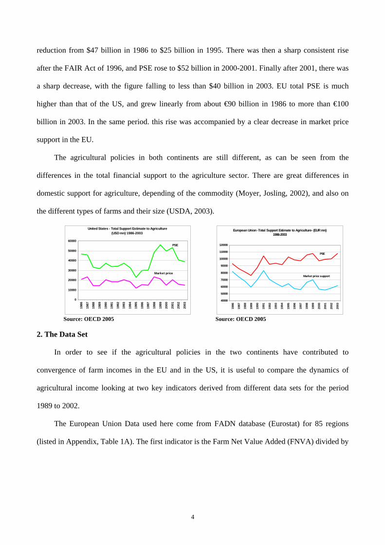
reduction from $47 billion in 1986 to $25 billion in 1995. There was then a sharp consistent rise

after the FAIR Act of 1996, and PSE rose to $52 billion in 2000-2001. Finally after 2001, there was

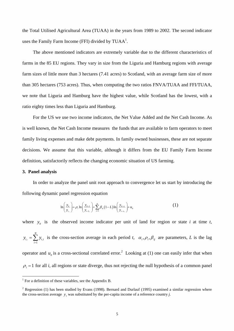
a sharp decrease, with the figure falling to less than $40 billion in 2003. EU total PSE is much

higher than that of the US, and grew linearly from about €90 billion in 1986 to more than €100

billion in 2003. In the same period. this rise was accompanied by a clear decrease in market price

support in the EU.

The agricultural policies in both continents are still different, as can be seen from the

differences in the total financial support to the agriculture sector. There are great differences in

domestic support for agriculture, depending of the commodity (Moyer, Josling, 2002), and also on

the different types of farms and their size (USDA, 2003).

United States - Total Support Estimate to Agriculture (USD mn) 1986-2003

0

10000

20000

30000

40000

50000

60000

198

6

198

7

198

8

198

9

199

0

199

1

199

2

199

3

199

4

199

5

199

6

199

7

1998

1999

2000

2001

2002

2003

PSE

Market price

Source: OECD 2005

European Union -Total Support Estimate to Agriculture- (EUR mn)

1986-2003

40000

50000

60000

70000

80000

90000

100000

110000

120000

198

6

198

7

198

8

198

9

199

0

199

1

199

2

199

3

199

4

199

5

199

6

199

7

1998

1999

2000

2001

2002

2003

PSE

Market price support

Source: OECD 2005

2. The Data Set

In order to see if the agricultural policies in the two continents have contributed to

convergence of farm incomes in the EU and in the US, it is useful to compare the dynamics of

agricultural income looking at two key indicators derived from different data sets for the period

1989 to 2002.

The European Union Data used here come from FADN database (Eurostat) for 85 regions

(listed in Appendix, Table 1A). The first indicator is the Farm Net Value Added (FNVA) divided by

5

the Total Utilised Agricultural Area (TUAA) in the years from 1989 to 2002. The second indicator

uses the Family Farm Income (FFI) divided by TUAA1.

The above mentioned indicators are extremely variable due to the different characteristics of

farms in the 85 EU regions. They vary in size from the Liguria and Hamburg regions with average

farm sizes of little more than 3 hectares (7.41 acres) to Scotland, with an average farm size of more

than 305 hectares (753 acres). Thus, when computing the two ratios FNVA/TUAA and FFI/TUAA,

we note that Liguria and Hamburg have the highest value, while Scotland has the lowest, with a

ratio eighty times less than Liguria and Hamburg.

For the US we use two income indicators, the Net Value Added and the Net Cash Income. As

is well known, the Net Cash Income measures the funds that are available to farm operators to meet

family living expenses and make debt payments. In family owned businesses, these are not separate

decisions. We assume that this variable, although it differs from the EU Family Farm Income

definition, satisfactorily reflects the changing economic situation of US farming.

3. Panel analysis

In order to analyze the panel unit root approach to convergence let us start by introducing the

following dynamic panel regression equation

( )1

1,. 1, ,.

ln ln 1 lnip

it it it si is it

st t t s

y y yL uy y y

ρ β− −

=− ⋅ −

⎛ ⎞ ⎛ ⎞ ⎛ ⎞= + − +⎜ ⎟ ⎜ ⎟ ⎜ ⎟⎜ ⎟ ⎜ ⎟ ⎜ ⎟

⎝ ⎠ ⎝ ⎠ ⎝ ⎠∑ (1)

where ity is the observed income indicator per unit of land for region or state i at time t,

, ,1

N

t t ii

y y⋅=

= ∑ is the cross-section average in each period t, , ,i i ijα ρ β are parameters, L is the lag

operator and itu is a cross-sectional correlated error.2 Looking at (1) one can easily infer that when

1iρ = for all i, all regions or state diverge, thus not rejecting the null hypothesis of a common panel

1 For a definition of these variables, see the Appendix B. 2 Regression (1) has been studied by Evans (1998). Bernard and Durlauf (1995) examined a similar regression where the cross-section average ty⋅ was substituted by the per-capita income of a reference country j.

6

unit root is the same as accepting the hypothesis that during the period of analysis all regions do

not convergence to the cross section average. The alternative hypothesis is usually stated as

1 : 1iH ρ < , at least for one region.

Looking at (1) it is simple to see that we are implicitly testing the hypothesis of convergence

toward a common trend. The literature has called this hypothesis absolute convergence hypothesis

(see Gutierrez, 2000). Absolute convergence is more likely to occur where regions have roughly

similar preferences, technology levels and institutional and legal systems. If this is the case, regions

converge to the same common trend. If regions are heterogeneous, the analysis must be modified to

allow for the concept of conditional convergence. The central idea is that regions converge towards

different levels of productivity but regions that are further from their steady-state level will grow

faster. The hypothesis of conditional convergence can be easily inferred as

( )1

1,. ,. ,.

ln ln 1 lnip

it it it si is it

si i i

y y yL uy y y

ρ β− −

=

⎛ ⎞ ⎛ ⎞ ⎛ ⎞= + − +⎜ ⎟ ⎜ ⎟ ⎜ ⎟⎜ ⎟ ⎜ ⎟ ⎜ ⎟

⎝ ⎠ ⎝ ⎠ ⎝ ⎠∑ (2)

where now the convergence process is analyzed looking at the differences between the income

indicator in each region and the regional temporal average , ,1

T

i t it

y y⋅=

= ∑ .

Before introducing results it is useful to answer the following questions. Why do we focalize the

attention on panel regression and not on time series regression and why do we introduce a degree of

cross-sectional dependence in (1)?

Over the last few years, a great deal of attention has been paid to the non-stationary property

of panels. Starting from the seminal works of Quah (1990, 1994), Breitung and Meyer (1991) Levin

and Lin (1992, 1993), and Im et al. (1997), many tests have been proposed which attempt to

introduce unit root tests in panel data. These show that, by combining the time series information

with that of the cross-section, the inference that unit roots exist can be more straightforward and

precise, especially when the time series dimension of the data is relatively short, and similar data

7

may be obtained across a cross-section of units such as countries or commodities. In synthesis,

panel unit root tests have higher power than time series unit root tests.

However all the panel unit root tests suffer from serious limitations when the cross-sectional

units are correlated (see O’Connell, 1998). Some papers have been presented in recent years that

address this issue. For example, Bai and Ng (2003), Moon and Perron (2003) and Phillips and Sul

(2003a) and Choi (2002) use common factor components. In brief, all the above mentioned works

propose a factor model in which cross-sectional dependence is generated by one or more factors3

which are common to all the individual units (but which may exert different effects on the

individual unit) and by uncorrelated idiosyncratic shocks across all the individual units.

The cross-sectional dependence is modelled as

'it i t itu f eλ= + (2)

where tf are K vectors of unobservable factors, 'iλ factor loading coefficient vectors and ite are

idiosyncratic shocks. Note that the panel unit root tests proposed by Levin and Lee (1992, 1993)

and Im and al. (1997) fail to take account of cross-sectional dependence, causing on one hand huge

size distortion of the tests and, on the other, introducing restrictive economic specification when, as

seems to be the case especially for EU and US, incomes per unit of land show strong cross-

sectional correlation.

The first task, when computing multifactor analysis as in (1), is to specify the number of

factors r correctly. We follow Bai and Ng (2002) and we use what they label 3BIC . These criteria

defines the correct number of factors, taking into account the mean squared sum of residuals, plus a

penalty function for over-fitting. Bai and Ng (2002) show that these criteria perform well for our

size of data sample. We compute the number of factors using a maximum of 5. The 3BIC criteria

suggest that there are from two to three common factors.

3 This is not true for the Phillips and Sul (2003) tests where only one factor is permitted.

8

Before using panel unit root tests it is useful to analyze their size and power for our sample of

data. We perform a Monte Carlo analysis, as in Gutierrez (2006), for a panel of 14 observations

and 85 units. The results of the simulation, not reported for brevity, highlight that Moon and

Perron’s (2004) t_b statistic has correct size and high power. Choi (2002) tests are strongly

oversized while Bai and Ng (2004) and Phillips and Sul (2003) tests are downsized with low power.

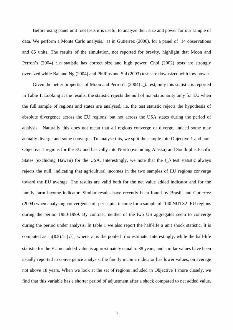
Given the better properties of Moon and Perron’s (2004) t_b test, only this statistic is reported

in Table 1. Looking at the results, the statistic rejects the null of non-stationarity only for EU when

the full sample of regions and states are analysed, i.e. the test statistic rejects the hypothesis of

absolute divergence across the EU regions, but not across the USA states during the period of

analysis. Naturally this does not mean that all regions converge or diverge, indeed some may

actually diverge and some converge. To analyse this, we split the sample into Objective 1 and non-

Objective 1 regions for the EU and basically into North (excluding Alaska) and South plus Pacific

States (excluding Hawaii) for the USA. Interestingly, we note that the t_b test statistic always

rejects the null, indicating that agricultural incomes in the two samples of EU regions converge

toward the EU average. The results are valid both for the net value added indicator and for the

family farm income indicator. Similar results have recently been found by Brasili and Gutierrez

(2004) when analysing convergence of per capita income for a sample of 140 NUTS2 EU regions

during the period 1980-1999. By contrast, neither of the two US aggregates seem to converge

during the period under analysis. In table 1 we also report the half-life a unit shock statistic. It is

computed as ( ) ( )ˆln 0.5 / ln ρ , where ρ̂ is the pooled rho estimate. Interestingly, while the half-life

statistic for the EU net added value is approximately equal to 38 years, and similar values have been

usually reported in convergence analysis, the family income indicator has lower values, on average

not above 18 years. When we look at the set of regions included in Objective 1 more closely, we

find that this variable has a shorter period of adjustment after a shock compared to net added value.

9

The picture for the US states is clearly different. Because we do not reject the null hypothesis of

unit root we conclude that during the period of analysis US states do not show convergence.

Table 1 - Panel Unit Root Tests EU and US Indicators (1989-2002) : absolute convergence

Group : EU regions Moon and Perron (2004)

t_b test (*)

Rho coeff.

Half-life shock

(n° years)

Net Value Added per Unit of Land -1.825(0.034) 0.970 31.8

Family Farm Income per Unit of Land -3.979(0.000) 0.947 17.7

Objective 1 Regions



Non Objective 1 Regions



Group : US States Moon and Perron (2004)

t_b test (*)

Rho coeff.

Half-life shock

(n° years)


Net Cash Income for Unit of Land -1.204(0.114) 0.989 87.3 Northeast, Lake States, Corn Belt, Northern Plains, Appalachian

Net Value Added per Unit of Land 0.376 (0.647) 1.003 Neg. Family Farm Income per Unit of Land -0.813 (0.208) 0.992 123.9

Southeast, Delta States, Southern Plains, Mountains States, Pacific States

Net Value Added per Unit of Land -1.477(0.070) 0.981 51.53 Family Farm Income per Unit of Land -0.964(0.164) 0.991 105.7

(*) In parentheses p-values

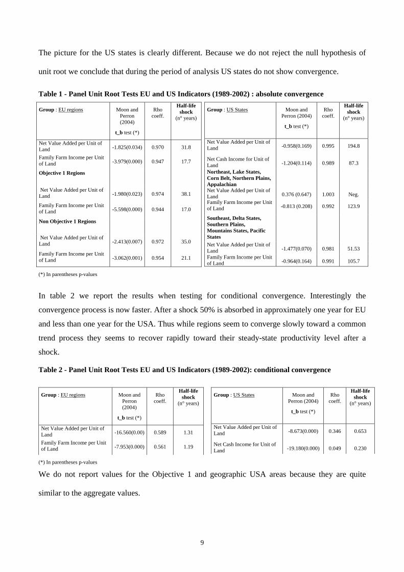
In table 2 we report the results when testing for conditional convergence. Interestingly the

convergence process is now faster. After a shock 50% is absorbed in approximately one year for EU

and less than one year for the USA. Thus while regions seem to converge slowly toward a common

trend process they seems to recover rapidly toward their steady-state productivity level after a

shock.

Table 2 - Panel Unit Root Tests EU and US Indicators (1989-2002): conditional convergence

Group : EU regions Moon and

Perron (2004)

t_b test (*)

Rho coeff.

Half-life shock

(n° years)



Group : US States Moon and Perron (2004)

t_b test (*)

Rho coeff.

Half-life shock

(n° years)


Net Cash Income for Unit of Land -19.180(0.000) 0.049 0.230

(*) In parentheses p-values

We do not report values for the Objective 1 and geographic USA areas because they are quite

similar to the aggregate values.

10

4. Distribution Dynamics

We used the stochastic kernel method to analyse how the dynamics of distribution of the farm

income indicators have changed between 1989 and 2002. This method of analysis makes it possible

to highlight the differential dynamic patterns of the groups of EU regions and the set of US states.

The stochastic kernel method has been presented in a great number of papers (see for example

Quah, 1993a, 1993b, 1996, 1997; Brasili 2005). Here will give only a brief outline, leaving the

interested reader to refer to the above cited works for a deeper analysis.

Assuming that the agricultural income ty can take values inside a certain finite set E, the

distribution of that variable at time t (labeled tF ), is time-invariant. tφ defines the associated

probability measures of tF . The dynamics of tφ can be modeled as a first order autoregressive

process: '1, 1t tM tφ φ −= ≥ (3)

When ty is discrete, the matrix M is usually defined as the transition probability of a Markov

process, i.e. each element in M describes the probability of transition from a given state to another

state in one step . However if ty can take infinite values, i.e E is an uncountable set, we need a

continuous counterpart of M. Let A be a subset of E and define a new function ( ),y AΡ , called the

stochastic transition function or stochastic kernel. This function describes the conditioned

probability that in the next period the agricultural income will have a value in set A, given that in

the previous period it is in the state y , i.e ( ) ( )1, Pr t ty A y A y y−Ρ = ∈ = .

Thus the income distributions in the two periods will be linked by the following relationship

( ) 1P ,t tF y A F dy−= ∫ (4)

In this section of the paper we will present an estimate of ( ),y AΡ for the variables Farm Net Value

Added (FNVA) divided by Total Utilised Agricultural Area (TUAA) for the European regions and

the variables Net Value Added per unit of land and Net Cash Income per unit of land for the US

11

states. We analyse how the distribution of the farm income indicators has changed over time. The

method allows us to establish whether the distributions around the EU and the US states average are

now more concentrated or not than they were a decade ago. The analysis also allows to be better

understood the results obtained in section 3.

As we have seen in the introduction, in the 1990’s there were great changes in agricultural policy in

both the EU (with the McSharry reform in 1992) and the US (with the 1990 Farm Bill and the 1996

FAIR Act). The EU 1992 reform substantially maintains the coupling of compensatory payments

and production, while the 1990-96 US reforms decoupled more extensively. Our work allows, at

least indirectly, to make inference on the impact of the two different policies on farm income

distribution.

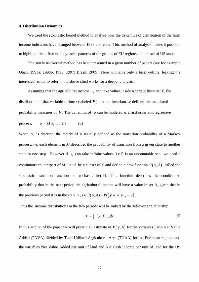
The stochastic kernel applied to the ratio of FNVA per TUAA4 relative to the average

(located on the 0) of the EU 85 regions shows that there are two main groups of regions (figure 1).

The literature on distribution dynamics has called this “twin-peaks” distribution. It was first

described by Quah (1996) when he was analysing the convergence of per capita GDP for EU

countries.

We found that, for FNVA per TUAA, a very large group of EU regions are located in a range

which is approximately from 0.25 to 3 times of the average value. The curve has the shape of a

“saddle”. The first mass point of the distribution is mainly located on the diagonal. This group has a

very gentle rotation, and so there is a convergence towards the average value. Another smaller set of

regions are around the second peak and located well above the average, more then eight times the

average value of the variable. The second main mass of the distribution is also concentrated on the

diagonal. Thus we have more persistence for the group of regions with higher values of FNVA per

TUAA. There is another small group of regions in the final part of distribution with very low

revenues (around 10% of the average revenue). This group rotates anti-clockwise and converges

12

towards the average value. The picture of distribution of the peaks can be better appreciated by

looking at the contour plot (figure 1a)5.

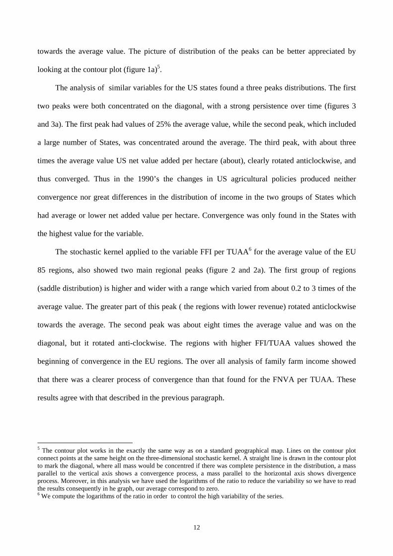
The analysis of similar variables for the US states found a three peaks distributions. The first

two peaks were both concentrated on the diagonal, with a strong persistence over time (figures 3

and 3a). The first peak had values of 25% the average value, while the second peak, which included

a large number of States, was concentrated around the average. The third peak, with about three

times the average value US net value added per hectare (about), clearly rotated anticlockwise, and

thus converged. Thus in the 1990’s the changes in US agricultural policies produced neither

convergence nor great differences in the distribution of income in the two groups of States which

had average or lower net added value per hectare. Convergence was only found in the States with

the highest value for the variable.

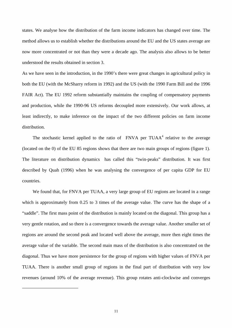
The stochastic kernel applied to the variable FFI per TUAA6 for the average value of the EU

85 regions, also showed two main regional peaks (figure 2 and 2a). The first group of regions

(saddle distribution) is higher and wider with a range which varied from about 0.2 to 3 times of the

average value. The greater part of this peak ( the regions with lower revenue) rotated anticlockwise

towards the average. The second peak was about eight times the average value and was on the

diagonal, but it rotated anti-clockwise. The regions with higher FFI/TUAA values showed the

beginning of convergence in the EU regions. The over all analysis of family farm income showed

that there was a clearer process of convergence than that found for the FNVA per TUAA. These

results agree with that described in the previous paragraph.

5 The contour plot works in the exactly the same way as on a standard geographical map. Lines on the contour plot connect points at the same height on the three-dimensional stochastic kernel. A straight line is drawn in the contour plot to mark the diagonal, where all mass would be concentred if there was complete persistence in the distribution, a mass parallel to the vertical axis shows a convergence process, a mass parallel to the horizontal axis shows divergence process. Moreover, in this analysis we have used the logarithms of the ratio to reduce the variability so we have to read the results consequently in he graph, our average correspond to zero. 6 We compute the logarithms of the ratio in order to control the high variability of the series.

13

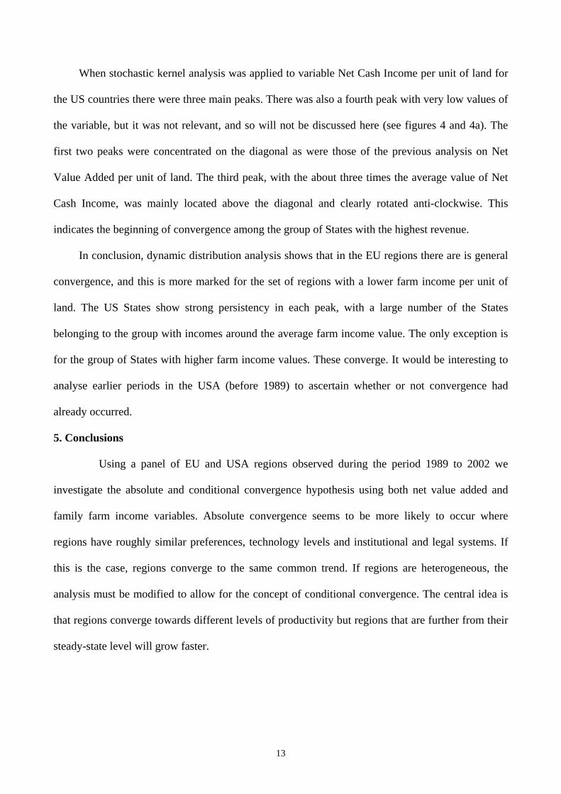
When stochastic kernel analysis was applied to variable Net Cash Income per unit of land for

the US countries there were three main peaks. There was also a fourth peak with very low values of

the variable, but it was not relevant, and so will not be discussed here (see figures 4 and 4a). The

first two peaks were concentrated on the diagonal as were those of the previous analysis on Net

Value Added per unit of land. The third peak, with the about three times the average value of Net

Cash Income, was mainly located above the diagonal and clearly rotated anti-clockwise. This

indicates the beginning of convergence among the group of States with the highest revenue.

In conclusion, dynamic distribution analysis shows that in the EU regions there are is general

convergence, and this is more marked for the set of regions with a lower farm income per unit of

land. The US States show strong persistency in each peak, with a large number of the States

belonging to the group with incomes around the average farm income value. The only exception is

for the group of States with higher farm income values. These converge. It would be interesting to

analyse earlier periods in the USA (before 1989) to ascertain whether or not convergence had

already occurred.

5. Conclusions

Using a panel of EU and USA regions observed during the period 1989 to 2002 we

investigate the absolute and conditional convergence hypothesis using both net value added and

family farm income variables. Absolute convergence seems to be more likely to occur where

regions have roughly similar preferences, technology levels and institutional and legal systems. If

this is the case, regions converge to the same common trend. If regions are heterogeneous, the

analysis must be modified to allow for the concept of conditional convergence. The central idea is

that regions converge towards different levels of productivity but regions that are further from their

steady-state level will grow faster.

14

The results show that the EU regions show absolute convergence, and the convergence

process seems to be greater for the family farm income variable than for the net value added per

hectare variable. By contrast US states show a substantial persistence of the differences in farm

income, with no evident signs of absolute convergence. In the EU regions the convergence of farm

income per hectare is greater for the less developed regions (objective 1 regions ), whereas in the

US there are no substantial differences between Northern and Southern states. Interestingly these

results are partially reverted when analysis the conditional convergence. In this case both EU and

the USA show a strong convergence process toward their productivity steady-state level.

Income distribution analysis shows that there is a “multi peak” distribution of farm incomes in

both EU and US, but with great differences. In the EU regions there is a large group of regions with

very low farm incomes and, on the other hand, another group of regions with very high income per

hectare, at more than eight times the EU average. Between these two peaks there are numerous

regions along the diagonal. This creates a sort of “saddle” distribution which is characteristic of the

EU regions. The first group of regions is larger and shows convergence, particularly when Family

Farm Income rather than Net Added Value is measured, and this could explain the convergence

found by the panel analysis.

In the USA we found a “three peak” distribution characterized by the presence of a great

number of states with farm incomes around the US average, and the other two groups of states far

from the average value (i.e. much higher or lower). Thus in the USA convergence is not evident,

and differences between states persist over time. Convergence towards the average value for farm

income probably occurred in the previous decades, and the time horizon of our analysis (1989-

2002) is not long enough capture these changes.

The distribution of farm income per hectare during the period 1989 to 1992 in the EU and US

shows, in general, more persistence over time. There were also important changes in the domestic

support given to agriculture. The already high level of domestic support in EU agriculture increased

15

during the 1990’s, with a price support scheme being replaced by a direct farmers’ income support

scheme. This essentially coupled payments to farm production. In the US support for agriculture first

declined sharply until 1995 and then increased until 2001, with a marked increase in de-coupling of

payment and production. Only with the FARM Bill of 2002 was the tendency towards a de-coupling

policy reversed. If we assume that the above-mentioned policies are able to influence farm income

distribution, it seems that only the EU policies influenced this distribution, with some convergence

occurring during the period 1989-2002. In the US income distribution appears unaffected and

determined manly by long term structural differences. Moreover, some preliminary analysis of US farm

incomes over a longer period, i.e. 1950-2002 seems to confirm the persistence in the revenue

distribution and it does not show great changes. We were unable to compare EU data for the same

period because of lack of data. Further research is needed to estimate the relative importance of the

agricultural policies in the EU and the USA on the distribution of farm income over time.

Figure 1.a Stochastic Kernel EU Net Value Added per ha Figure 1.b Countour plot EU Net Value Added per ha

Figure 2.a Stochastic Kernel EU Family Farm Income per ha Figure 2.b Contour plot EU Family Farm Income per ha

15

17

Figure 3.a Stochastic Kernel US Net Value Added per ha Figure 3.b Contour plot US Net Value Added per ha

Figure 4.a Stochastic Kernel US Net Cash Income per ha Figure 4.b Contour plot US Net Cash Income per ha

18

References

Bai, J., Ng, S. (2002). Determining the Number of Factors in Approximate Factor Models. Econometrica, 70:1, 191-221. Bai, J., Ng, S. (2003). A PANIC Attack on Unit Roots and Cointegration, mimeo, Boston College. Bernard, A.B., Durlauf, S.N. (1996). Interpreting test of convergence hypothesis. Journal of Econometrics, 71, 161-174. Brasili C. (2005) Non parametric approach in Cambiamenti strutturali e convergenza economica nelle regioni dell’Unione europea (Structural Changes and Economic Convergence in the UE regions) edited by C. Brasili, Bologna Clueb, 2005 Breitung, J., Meyer, W. (1991). Testing for Unit Roots in Panel Data: are Wages on Different Bargaining Levels Cointegrated? Institute für Wirtschaftsforschung Working Paper, June. Cheung, Y., Pascual A.G. (2004), Testing output convergence: a re-examination. Oxford Economic Papers, 56, 45-63. Choi, I. (2002). Combination Unit Root Tests for Cross-Sectionally Correlated Panels, mimeo, Hong Kong University of Science and Technology. Evans P. (1998) Using panel data to evaluate growth theories. International Economic Review, 39, 295-306. Gutierrez L. (2000). Convergence in US and EU agriculture, European Review of Agricultural Economics, 27:2, 187-206. Gutierrez L. (2006). Panel unit root tests for cross-sectionally correlated panels: A Monte Carlo comparison, Oxford Bulletin of Economics and Statistics, 68:4, 519:540. Im, K.S., Pesaran, M.H. and Shin, Y. (1997). Testing for Unit Roots in Heterogeneous Panels. Department of Applied Economics, University of Cambridge. Levin, A. and Lin, C.F. (1993). Unit Root Tests in Panel Data: New Results. Discussion Paper Series 93-56, Department of Economics, University of San Diego. Haniotis T. “The midterm review and the new challenge for the EU agriculture”, EuroChoise, n.3, Winter 2002. Moon, H. R., Perron, P. (2003). Testing for Unit Root in Panels with Dynamic Factors. Research Papers Series, University of Southern California Center for Law, Economics & Organization, n. C01-26. Moyer W., Josling T. (2002) Agricultural Policy Reform, politics and process in the EU and UA in the 1990s, Ashgate ed. OECD (2005), Producers and Consumer Support Estimates OECD data base 1986-2004, Paris 2005. Petit M., “ The new US Farm Bill: Lessons from a Complete Ideological Turnround”, EuroChoise, n.3, Winter 2002. Phillips, P.C.B., Sul, D. (2003). Dynamic Panel Estimation and Homogeneity Testing under Cross-Section Dependence, Econometrics Journal, 6, 217-259 Quah, D. (1993a). Galton’s fallacy and tests of convergence hypothesis. The Scandinavian Journal of Econometrics, 95, 9-19. Quah, D. (1993b). Empirical cross section dynamics in economic growth. European Economic Review, 37, 426-434. Quah, D. (1994). Exploiting Cross-Section Variations for the Unit Root Inference in Dynamic Data. Economics Letters, 44: 9-19. Quah, D. (1996). Twin peaks: Growth and convergence in models of distribution dynamics. Economic Journals, 106,1045-1055. Quah, D. (1997). Empirics for growth and distribution: stratification, polarization, and convergence clubs, Journal of Economic Growth, 2, 27-59.

19

Silverman, B.W. (1986). Density estimation for statistics and data analysis. Chapman & Hall, London. Thompson R. L. (2005), The US Farm Bill and the data Negotiation: on Parallel Traks or a collusion Course? International Policy Council, Issue Brief September 2005 USDA (2003), Farm and Commodity policy: government payments and the farm sector. Wescott, P.C., C.E. Young, J. Prices (2002), The 2002 Farm Act: Previsions and Impliation for commodity Market, USDA Information Bullettin n.778, Nov. 2002.

Web Site: http://www.ers.usda.gov/Briefing/FarmIncome http://europa.eu.int/comm/agriculture/rica/index_en.cfm Appendix A Table 1A. The 85 EU regions included in the sample ( 10) Schleswig-Holstein (182) Aquitaine (302) Campania (520) Navarra ( 20) Hamburg (183) Midi-Pyrénées (303) Calabria (525) La Rioja ( 30) Niedersachsen (184) Limousin (311) Puglia (530) Aragón ( 50) Nordrhein-Westfalen (192) Rhônes-Alpes (312) Basilicata (535) Catalana ( 60) Hessen (193) Auvergne (320) Sicilia (545) Castilla-León ( 70) Rheinland-Pfalz (201)Languedoc-Roussillon (330) Sardegna (550) Madrid ( 80) Baden-Württemberg (203) Provence-Alpes-Côte (340) Belgi(qu)e (555) Castilla-La Mancha ( 90) Bayern (204) Corse (360) Nederland (560) Comunidad Valenciana (100) Saarland (221) Valle d'Aoste (370) Danmark (565) Murcia (121) Île de France (222) Piemonte (411) England-North (570) Extremadura (131) Champagne-Ardenne (230) Lombardia (412) England-East (575) Andalucia (132) Picardie (241) Trentino (413) England-West (610)Entre Douro Minho/Beira litoral(133) Haute-Normandie (242) Alto-Adige (421) Wales (620) Tras-os-Montes/Beira interior (134) Centre (243) Veneto (431) Scotland (630) Ribatejo e Oeste (135) Basse-Normandie (244) Friuli-Venezia (441) Northern Ireland (640) Alentejo e do Algarve (136) Bourgogne (250) Liguria (450) Makedonia-Thraki (650) Açores (141) Nord-Pas-de-Calais (260) Emilia-Romagna (460) Ipiros-Peloponissos-Nissi Ioniou (151) Lorraine (270) Toscana (470) Thessalia (152) Alsace (281) Marche (480) Sterea Ellas-Nissi Egaeou-Kriti (153) Franche-Comté (282) Umbria (500) Galicia (162) Pays de la Loire (291) Lazio (505) Asturias (163) Bretagne (292) Abruzzo (510) Cantabria (164) Poitou-Charentes (301) Molise (515) Pais Vasco Source: FADN dataset Appendix B EU Variable Definitions Farm Net Value Added corresponds to the payment for fixed factors of production (work, land and capital), whether they be external or family factors. As a result, holdings can be compared irrespective of the family/non-family nature of the factors of production employed. This indicator is sensitive, however, to the production methods employed: the ratio (intermediate consumption + depreciation)/fixed factors may vary and therefore influence the FNVA level. For example, in the livestock sector, if production is mostly without the use of land (purchased feed) or extensive (purchase and renting of forage land).

Family Farm Income corresponds to the payment for family fixed factors of production (work, land and capital) and the payment for the entrepreneur’s risks (loss/profit) in the accounting year. The standard FADN results do not therefore use estimations of the payment for family factors (costs imputed for work, land and family capital).

Total Utilised Agricultural Area corresponds to the total utilised agricultural area of holding. Does not include areas used for mushrooms, land rented for less than one year on an occasional basis, woodland and other farm areas (roads, ponds, non-farmed areas, etc). It consists of land in owner occupation, rented land, land in share-cropping. It includes

20

agricultural land temporally not under cultivation for agricultural reasons or being withdrawn from production as part of agricultural policy measures.

Convergence in the Agricultural Incomes: A Comparison between the US and EU

Documents

Transcript of Convergence in the Agricultural Incomes: A Comparison between the US and EU