Trajectory Following Control of AUV: A Robust Approach

ORIGINAL CONTRIBUTION

Trajectory Following Control of AUV: A Robust Approach

S. Roy • S. N. Shome • S. Nandy •

R. Ray • V. Kumar

Received: 25 January 2013 / Accepted: 16 May 2013 / Published online: 26 September 2013

� The Institution of Engineers (India) 2013

Abstract A robust control technique based on the second

method of Lyapunov is proposed in this paper for accurate

trajectory tracking of autonomous underwater vehicles

(AUVs). The difficulty in control of AUVs not only resides

in the highly non-linear and coupled dynamics but is

enhanced by modeling errors, parametric uncertainty and

payload variations depending on application requirements.

Environmental hazards such as ocean currents sometimes

dominate and render the control of underwater systems

more challenging. The proposed control technique addres-

ses the design of a robust controller for AUVs incorporating

the effects of the aforementioned uncertain paradigms with

known bounds. The controller performance is verified using

the real-life parameters of an operational AUV considering

a few uncertainties.

Keywords AUV � Robust control � Trajectory �Lyapunov second method � AUV-150 �Bounded uncertainty

Introduction

Autonomous Underwater Vehicles are unmanned robotic

system having on-board power sources and intelligence

suitable for complicated applications. With scientific and

technological advancement, AUVs have attracted attention

of scientific communities over the last two decades in

regard to a host of issues related to design, control, com-

munication, autonomy, etc.

AUV controller design is in itself a very challenging

task as a number of factors such as the inherent highly non-

linear and time-varying coupled dynamics of AUV,

uncertain hydrodynamic parameters, variation of center of

mass (COM) for addition of payloads for different appli-

cations, uncertain operating condition and external distur-

bances such as ocean current, etc. are involved. These

complexities restrict the satisfactory performance of AUVs

when they employ controllers based on well-developed

linear control theory. Even implementation of feedback

linearization based control law presents considerable dif-

ficulty, as an exact knowledge of the hardware parameters

of the system such as mass, inertia, centre of mass, center

of buoyancy, etc. and the accurate sensory feedback it

requires becomes involved. Real life physical systems like

AUVs always possess bounded uncertainty in parameters

to some extent, causing inexact cancellation of nonlinear-

ities. Further, noisy sensory information and other distur-

bances indeed make necessary the development of new

control paradigms for underwater systems.

Adaptive control and robust control are the two common

control strategies that are employed to tackle controlling

difficulties of AUVs. Cristi and Healey [1] proposed a

model-based adaptive controller employing recursive least

square method for parameter estimation and pole place-

ment technique for controller development, assuming that

S. Roy (&) � S. N. Shome � S. Nandy � R. Ray � V. Kumar

CSIR-Central Mechanical Engineering Research Institute,

Durgapur 713209, West Bengal, India

e-mail: [email protected]

S. N. Shome


S. Nandy


R. Ray


V. Kumar


123

J. Inst. Eng. India Ser. C (July–September 2013) 94(3):253–265

DOI 10.1007/s40032-013-0069-x

the vehicle was almost linear within the operating region.

Fossen and Sagatun [2] used adaptive control with online

estimation of uncertain parameters. Yuh [3] and Choi and

Yuh [4] developed and implemented a multi-input multi-

output (MIMO) adaptive controller with bounded estima-

tion. Antonelli et al. [5] proposed an adaptive control law

considering the effect of hydrodynamic parameters on the

tracking performance. Adaptive control scores over robust

control techniques in that it can work efficiently with little

or no prior knowledge of the bounds of uncertainty. Pres-

ence of unbounded parametric uncertainty in AUV

dynamics and online calculation of the unknown parame-

ters using adaptive control is computationally very

intensive.

Taking into consideration the above scenario there is a

need to apply appropriate robust control techniques with

the knowledge of the bound in uncertainties. One of the

most powerful robust control techniques that many

researchers have adopted is the sliding mode control.

Yoerger and Slotine [6] designed a sliding mode control

neglecting the cross coupling terms to provide robustness

against the uncertainties caused by hydrodynamic coeffi-

cients. Healey and Lienard [7] proposed a sliding mode

control where the sliding surfaces have been designed

using state variable errors rather than the output errors.

They separated the whole system into non-interacting or

lightly interacting subsystems while designing separate

autopilots for separate subsystems. Cristi et al. [8] and

Papoulias et al. [9] proposed adaptive sliding mode control

based on the linearized dynamics of AUV around the

operating condition on the assumption that a linear model

is a good approximation of non-linear dynamics at constant

speed. Lee et al. [10] proposed a discrete time quasi sliding

mode control where the sampling time is large and claimed

improvement in performance when sampling time increa-

ses. One disadvantage of sliding mode approach is the

increase of chattering effect due to increase of controller

gain, which is varied to make reaching phase finite. Naik

and Sing [11] designed a dive plane controller for AUV

based on state dependent Riccati equation. A backstepping

method associated with Lyapunov based techniques to

design a dive plane controller of AUV was developed by

Lapierre [12].

In this paper, a robust control methodology, that con-

siders the parameter uncertainties through payload varia-

tion (sensor system for various applications) and variation

in hardware parameters (inertia, center of mass, etc.) within

a predefined bound, has been proposed. The bound on the

perturbation of the mass matrix has been derived within the

limit of which the controller design is feasible. The per-

formance of the developed controller has been verified for

various trajectories through rigorous simulation utilizing

the parameters of a developed AUV for 150 m depth.

The organization of the paper is as follows: Section II

presents brief design and dynamics of the AUV-150 and

subsequent conversions of dynamics for the proposed

controller. The robust control algorithm in the perspective

of AUV has been described in detail in Section III. Sim-

ulation results and analyses have been illustrated in Section

IV. At the end mentioned are the concluding remarks.

Brief Design Aspects and Dynamics of AUV-150

The mechanical system design of the AUV-150 had the

following as its main objectives:

• L/D (length to diameter) ratio should be less than 10

and the vehicle should have a positive buoyancy of

4–5 kg for safe recovery in case of any failure

• Adequate internal space to facilitate housing of all

internal components/devices

• Centre of mass should lie below the centre of buoyancy

• The vehicle should be capable of surviving in marine

environment

• Vehicle shape should facilitate modular design with

provision for future expansions

• The vehicle should provide a dry pressure hull for

accommodating onboard electronics and energy system

• Static and dynamic equilibrium to accomplish a variety

of tasks should be ensured

• Centers of drag should be aligned with the centers of

thrust i.e. external forces

• Symmetry for ease of design, modeling and manufacturing

The modular design of AUV-150 breaks down the

overall system into a number of modules such that the basic

configuration of the vehicle need not be altered for addition

or removal of payloads or energy system. Accordingly, the

designed AUV was divided into six modules as shown in

Fig. 1. Control was exercised for five degrees of freedom

(surge, sway, heave, pitch and yaw). The error in roll was

accounted for by ensuring the positive stability of the

vehicle. Multiple thrusters (four through-body tunnel

thrusters and one tail-side main thruster) were used with

independent control to propel and maneuver the AUV. For

real life applications the control inputs are converted to

corresponding voltage to feed the thrusters. The size of the

pressure hulls was finalized on the basis of the payload and

navigational sensors, energy system, mission time and

other multidisciplinary requirements. The torpedo shaped

AUV-150, measured 4.85 m in length and 0.5 m external

diameter, and had a weight of 485 kg in air. Design aspects

of AUV-150 are reported by Shome et al. [13].

The dynamics of AUV-150 was formulated based on the

above configuration. Underwater vehicles are subjected to

Inertia forces which consist of rigid body inertia and inertia

254 J. Inst. Eng. India Ser. C (July–September 2013) 94(3):253–265

123

due to added mass component, Coriolis and Centripetal

forces for rigid body and added mass component, linear

and quadratic damping forces due to low speed assump-

tions as well as restoring forces in the form of Buoyancy

and Gravity. The nearly accurate center of gravity and

center of buoyancy are determined based on the very

accurate 3D modeling of the AUV-150 using advanced

computer aided design (CAD) tools.

The equations of motion of the AUV-150 are generated

applying Kirchhoff’s equations [14] considering the rigid-

body and added mass kinetic energy components for linear

and angular motions. Thereafter, the rigid-body and added

mass components of inertia matrices, Coriolis and Cen-

tripetal matrices are evaluated. Equations of motion for

AUV-150 in the body-fixed coordinate frame are expressed

compactly in matrix–vector form as:

M _mþ CðmÞmþ DðmÞmþ gðgÞ ¼ s; ð1Þ

where,

M 2 R6�6 ¼MRB þMA;

CðmÞ 2 R6�6 ¼ CRBðmÞ þ CAðmÞ;

DðmÞ 2 R6�6 ¼ DLðmÞ þ DQðmÞ;

g 2 R6�1 ¼ ½x y z u h w�T ;

m 2 R6�1 ¼ ½u t w p q r�T :

MRB and MA represent the rigid body and added mass

matrices respectively. CRB and CA represent the rigid body

and added Coriolis and Centripetal matrices respectively,

while DL and DQ represent the linear and quadratic drag

matrices. The gravity and buoyancy force vector is denoted

by gðgÞ and vector s stands for the input forces and

moments. The linear positions and Euler angles expressed

in inertial reference frame are denoted by the vector g,

while m represents the linear and angular velocity vector

expressed in body coordinate frame. The overall mass

matrix, Coriolis and Centripetal matrix, damping matrix

and the gravity vector for AUV-150 as derived through

dynamic formulation are presented below:

M ¼

539 0 0 0 5:88 0

0 1326 0 �5:88 0 0

0 0 1326 0 0 0

0 �5:88 0 17:1 0 0

5:88 0 0 0 1836 0

0 0 0 0 0 1834

2666666664

3777777775;

CðmÞ ¼

0 0 0

0 0 0

0 0 0

0 �1326w 1326t� 5:88p

1326w 0 �539u� 5:88q

�1326tþ 5:88p 539uþ 5:88q 0

2666666664

0 �1326w 1326v� 5:88p

1326w 0 �539u� 5:88q

�1326tþ 5:88p 539uþ 5:88q 0

0 �1834r 1836qþ 5:88u

1834r 0 �17:1pþ 5:88t

�1836q� 5:88u 17:1p� 5:88t 0

3777777775;

DðmÞ ¼

120 uj j 0 0 0 0 0

0 1224 tj j 0 0 0 0

0 0 1224 wj j 0 0 0

0 0 0 0 pj j 0 0

0 0 0 0 2731 qj j 0

0 0 0 0 0 2731 rj j

2666666664

3777777775;

gðgÞ ¼ 0 0 0 296:1 cos h sin u 291:1 sin h 0½ �T :

Equations of motion derived in body-fixed frame are

converted to inertial frame representation, which is very

much pertinent to controller development. The vehicle

kinematics plays a dominant role in converting the body-

fixed representation to the inertial frame paradigm. Linear

and angular velocities expressed through both the frames

(inertial frame and body-fixed) are correlated by the

kinematic transformation of the form:

_g ¼ JðgÞm; ð2Þ

where, JðgÞ ¼ diagfJ1ðgÞ; J2ðgÞg is the Jacobian matrix.

Differentiation of Eq. (2) gives,

€g ¼ J _mþ _Jm;

) _m ¼ J�1ð€g� _JmÞ:ð3Þ

The dynamic equation given by Eq. (1) is expressed in

the inertial frame utilizing Eqs. (2) and (3) as follows:

�MðgÞ€gþ �Cðm; gÞ _gþ �Dðm; gÞ _gþ �gðgÞ ¼ �s; ð4Þ

where,

Fig. 1 Modular AUV-150 with Coordinate frames

J. Inst. Eng. India Ser. C (July–September 2013) 94(3):253–265 255

123

�M ¼ J�T MJ�1; �C ¼ J�T ½C�MJ�1 _J�J�1;

�D ¼ J�T DJ�1; �g ¼ J�T g; �s ¼ J�Ts:

Eq. (4) can be compactly written in the following form:

�MðgÞ€gþHðm; gÞ ¼ �s; ð5Þ

where,

Hðm; gÞ ¼ �Cðm; gÞ _gþ �Dðm; gÞ _gþ �gðgÞ:

Hðm; gÞ represents the nonlinear function associated

with the nonlinearities due to Coriolis, Centripetal and

damping forces. The modified form of Eq. (5) is written as

follows:

€g ¼ �fðm; gÞ þ bðgÞ�s; ð6Þ

where,

bðgÞ ¼ �M�1ðgÞ; ð6aÞ

and fðm; gÞ ¼ bðgÞHðm; gÞ: ð6bÞ

Robust Controller Design

Considering the transformed dynamics of the AUV given

in Eq. (6), a robust control method based on the Second

Method of Lyapunov [15] is adopted. The control law is

designed choosing the form of the input torque vector �s as

follows:

�s ¼ b�1ðgÞðuþ fðg; mÞÞ; ð7Þ

here, b; f represent the nominal values of the matrices b; f

respectively and u is the vector of auxiliary control input. The

uncertainties due to modeling error, external disturbances as

well as parameter variations due to inclusion of various

payloads to the AUV-150 are assumed to be bounded and

reflected through:

D �M :¼ MðgÞ � �MðgÞ; ð8Þ

DH :¼ Hðm; gÞ �Hðm; gÞ: ð9Þ

The bounds are chosen from the known bound of the

parameters and model uncertainty. Considering the nonlinear

control law given by Eq. (7), the system described by Eq. (6) is

transformed into the following form:

€g ¼ bb�1ðuþ fÞ � f: ð10Þ

Substituting fðm; gÞ ¼ bðgÞHðm; gÞ into Eq. (10) with

some manipulation Eq. (11) is obtained:

€g ¼ uþ ðbb�1 � IÞuþ bb�1

bH� bH

¼ uþ ðbb�1 � IÞuþ bðH�HÞ¼ uþ ðbb�1 � IÞuþ bDH

) €g ¼ uþ n;

ð11Þ

where, n ¼ Cuþ bDH with C ¼ ðbb�1 � IÞ:The uncertainty vector nðg; _g; uÞ depends on bounds on

the mass matrix, Coriolis and Centripetal matrix and

damping matrix as well as evolution of the states and the

input to the system. It also helps to estimate the additional

input required to compensate for the bounded uncertainties

and the disturbances present in the system to achieve the

robust performance.

Now, defining gdðtÞ as the reference trajectory to be

tracked, the corresponding positional and velocity error

vectors are given by:

e1ðtÞ ¼ gðtÞ � gdðtÞ; ð12Þ

e2ðtÞ ¼ _gðtÞ � _gdðtÞ; ð13Þ

respectively. Considering e ¼ e1 e2½ �T as state vector

Eqs. (12) and (13) are compactly written in the following

state-space form

_e ¼ Aeþ Bfuþ n� €gdg; ð14Þ

where,

A ¼ 0 I0 0

� �;B ¼ 0

I

� �; _e ¼ _e1

_e2

� �: ð15Þ

To ensure stability and to obtain robust performance it is

essential to feed additional control input into the system.

The following structure of the control law is selected to

track the desired trajectories gdðtÞ :

u ¼ uþ Du; ð16Þ

where, u represents the stabilizing control law for the time

varying nonlinear nominal model (assuming no uncertainty).

The extra corrective term Du is chosen to overcome the

effects of uncertainty caused by the parameter variations. The

structure of the control law u is similar for the nominal

dynamics and chosen as,

uðtÞ ¼ €gd �K1e1 �K2e2 ¼ €gd �Ke; ð17Þ

where,K1 ¼ diagfx21;x

22; . . .;x2

6g; and K2 ¼ diagf2x1; 2

x2; . . .; 2x6g:The gain matrix K ¼ ½K1;K2� determines the expo-

nential error convergence. The natural frequencies xi’s for

i ¼ 1; . . .; 6 determines the rate at which the tracking error

decreases. Substituting the control law given by Eq. (16),

combining with Eq. (17), into Eq. (14) the error dynamics

takes the following form:

_e ¼ Aeþ BfDuþ ng; ð18Þ

where, n ¼ CðDuþ €gd �KeÞ þ bDH,�A ¼ A� BK and �A is Hurwitz.

Thus the objective of tracking the desired time varying

trajectory gdðtÞ involves the problem of stabilizing the


123

nonlinear and time varying dynamic system of AUV. The

main idea of this control formulation is to compensate the

effect of the uncertain and unknown parameter n from the

knowledge of the ‘worst case’ bounds on parameter vari-

ations with the help of the term Du from the available

information. Following assumptions are made to estimate

the worst case bounds on the function nðg; _g; uÞ.

Assumption-1 As time propagates the desired trajectory

gdðtÞ and its derivatives remain bounded and smooth

having the properties:

supt� 0

gd�� \K\1; ð19Þ

where, K is a known value over the time t.

Assumption-2 It is assumed that the variation in the

inertia matrix �M is mainly due to the variation in payload

which causes variation of the gravity/buoyancy centre and

system inertia. For the bounded parameter variation in the

inertia matrix provided in the Appendix, the norm of C is

also bounded and lies according to:

Ck k ¼ bb�1 � I�� b\1; for all g 2 R

6: ð20Þ

Assumption-3 Exploring the structure of the individual

terms that constitute H and using the above assumptions, a

function of the state variables and other known values is

found such that:

DHk k� cðtÞ; ð21Þ

where, c is bounded in t.

From Assumption-2 a range of perturbation on the mass

matrix is evaluated given the nominal values of system

hardware parameters based on the following derivation.

Let us take, b ¼ bþ Db where, Db is the perturbation

in b. So,

bb�1 � I ¼ ðbþ DbÞb�1 � I ¼ Iþ Dbb�1 � I ¼ Dbb�1:

From Assumption-2, it can be written

b ¼ Dbb�1�� Dbk k b

�1��

��\1

) Dbk k\ 1

b�1

��:

ð22Þ

Theorem-1 If the maximum and minimum eigen values

of M and D �M are denoted by kminM

kmaxM

� �and kmin kmax½ �

respectively then maximum and minimum eigen values of�M are given by kmin

Mþkmin kmax

Mþ kmax

� �.

Proof The matrices �M and M are symmetric and real, i.e.,

Hermitian. It has been shown below that D �M of Eq. (8) is

also Hermitian validating the Theorem-1. For any non zero

vector y from Rayleigh quotient (Appendix-C) following

is obtained:

RðM; yÞ :¼ yT My

yT y; ð23Þ

with; kminM�RðM; yÞ� kmax

M; ð23aÞ

and RðD �M; yÞ :¼ yTD �My

yT y; ð24Þ

with; kmin�RðD �M; yÞ� kmax: ð24aÞ

Similarly Rayleigh quotient for �M yields,

Rð �M; yÞ :¼ yT �My

yT y:¼ yTðMþ D �MÞy

yT y:¼ yT My

yT yþ yTD �My

yT y

:¼ RðM; yÞ þ RðD �M; yÞ:

Thus, combining Eqs. 23a and 24a results in

kminMþkmin�Rð �M; yÞ� kmax

Mþ kmax:

Theorem-2 Given the maximum and minimum eigen

values of M the criterion for the allowable range of the

perturbation DM from the nominal value can be evaluated

and written as follows:

kmaxM

kminM

kminM� kmax

M

\kminMþ kmin:

Proof From b ¼ bþ Db we get,

Dbk k ¼ b� b�� bk k þ b

�� M�1

��þ M

�1��

��

The following Lemma’s are satisfied for a symmetric

matrix X 2 Rn�n:

Lemma 1

Xk k ¼ maxf k1j j; . . .; knj jg:

Lemma 2 If X�1 exists then X�1�� ¼ 1

kj j, where kj j is the

smallest eigen value of X:

So,

Dbk k� kmax�M�1 þ kmax

M�1 �

1

kmin�M

þ 1

kminM

;

and

b�1

�� ¼ M

�� ¼ kmaxM:

From Eq. (22) the following criterion is obtained:

1

kmin�M

þ 1

kminM

\1

kmaxM

)kmax

Mkmin

M

kminM� kmax

M

\kmin�M : ð25Þ

Theorem-1 and Eq. (25) yields


123

kmaxM

kminM

kminM� kmax

M

\kminMþ kmin:

Considering these assumptions, supplemented by the

theorems described above a corrective term Du is chosen to

tackle the uncertainties as provided below.

Theorem-3 The system given by Eq. (6) is globally

asymptotically stable (proof provided in Appendix-A)

using the control law represented by Eq. (16) if the nominal

control term u is given by Eq. (17) and the additional term

Du is chosen in the following manner:

Du ¼�dðe; tÞ ðB

T PeÞðBT PeÞk k if BT Pe

�� 6¼ 0

0 if BT Pe�� ¼ 0

(ð26Þ

where, P is the unique positive-definite symmetric matrix

which is the solution of the Lyapunov equation:

�ATPþ PA ¼ �Q;

with Q is a symmetric positive-definite matrix.

It is assumed that, a time bounded continuous function

dðe; tÞ satisfies the following two inequalities,

Duk k\dðe; tÞ; ð27Þnk k\dðe; tÞ: ð28Þ

Using the laid down assumptions and the above inequalities

the value of dðe; tÞ is constructed according to the following

basis:

nk k� CðDuþ €gd �KeÞ þ bDH�� bdðe; tÞ þ bKþ Kk k � ek k þ bk kc:¼ dðe; tÞ:

With, 0\b\1 the value of d is evaluated as:

dðe; tÞ ¼ 1

1� bfbKþ Kk k � ek k þ bk kcðtÞg: ð29Þ

However, the control law introduced in (26) causes

chattering which is a common phenomenon in discontinuous

control law and can excite high frequency unmodelled

dynamics. Introducing a control bandwidth l the control law

is converted into a continuous domain and as a result the

chattering effect is eliminated. The formulation of the

modified control law is described below.

Theorem-4 The system given by equation Eq. (6) is

uniformly ultimately bounded (u.u.b.) (proof provided in

Appendix-B) using the control law represented by Eq. (16)

if the nominal control term u is given by Eq. (17) and the

additional control input Du is chosen in the following

manner:

Du ¼�dðe; tÞ ðB

T PeÞðBT PeÞk k if BT Pe

�� l

� dðe;tÞl BT Pe if BT Pe

�� \l

8<: ð30Þ

The control laws are verified utilizing the parameters of

AUV-150 developed at CSIR-CMERI, Durgapur. The

results are presented in the subsequent section.

Simulation Results and Discussions

The performance of the proposed control laws are verified

while AUV-150 follows various path/trajectory. Keeping

in mind that the basic application of AUV-150 is surveying

a region at sea, attempt has been made to follow various

special types of trajectory i.e., circular, figure of eight

shape and lawn-mower. For practical implementation, the

control inputs provided through the directional thrusters to

follow the desired path are kept in the form of voltage.

Voltage requirement for each propeller node is calculated

by transforming the required controller force/torque to the

corresponding thruster voltages using a polynomial. The

thrust (force/torque) versus voltage characteristics poly-

nomial for each thruster node is determined through

experiments. AUV-150 is having four similar tunnel

thrusters and each thruster posses the same characteristics.

The voltage ðVÞand force/torque ð�sÞ relationship for each

tunnel thruster is governed by,

V ¼ 0:0005�s3 � 0:0468�s2 þ 2�s� 1:354: ð31Þ

Similarly, for main thruster the relation is governed by

the following equation,

V ¼ �0:003�s2 � 0:1048�s� 0:1962: ð32Þ

The initial pose g0 of the AUV-150 is selected judiciously

based on the trajectory definitions. The controller parameters

are chosen as K1 ¼ diagf4; 4; 4; 0; 4; 4g; K2 ¼ diagf4; 4;4; 0; 4; 4g; b ¼ 0:605; l ¼ 0:1: The reason behind choosing

the controller gains as above is to achieve a critically damped

performance for the nominal system. The fourth term of the

gain matrices is kept as zero as there is no active control for

roll compensation of AUV-150.

A whole spectrum of payload and inertia and gravity/

buoyancy center variations within bounds is considered

during simulation. The parametric deviations are given in

Table-3 (Appendix-D) while Table-2 (Appendix-D)

reflects the corresponding nominal values. Based on these

parameter variations/uncertainties, the AUV-150 is direc-

ted to move through various path and the respective sim-

ulated performances are presented.

For a circular path, the reference trajectory definitions

(commands) are given as follows:


123

xdðtÞ ¼ 10 sinð0:1Þt; ydðtÞ ¼ 10 cosð0:1tÞ; zdðtÞ ¼ 5;

udðtÞ ¼ 0; hdðtÞ ¼ 0; wdðtÞ ¼ 0:1t:

In this case the variations in parameters are chosen to

be sinusoidal (absolute value) e.g., the overall system

mass vary over time from the nominal mass to the varying

augmented mass (nominal mass with sinusoidal varying

payload). The reason behind the choice of sinusoidal

variation is to verify the performance of the controller

over time-varying uncertainties which lie within any

value between the maximum and minimum limit of the

parametric variation.

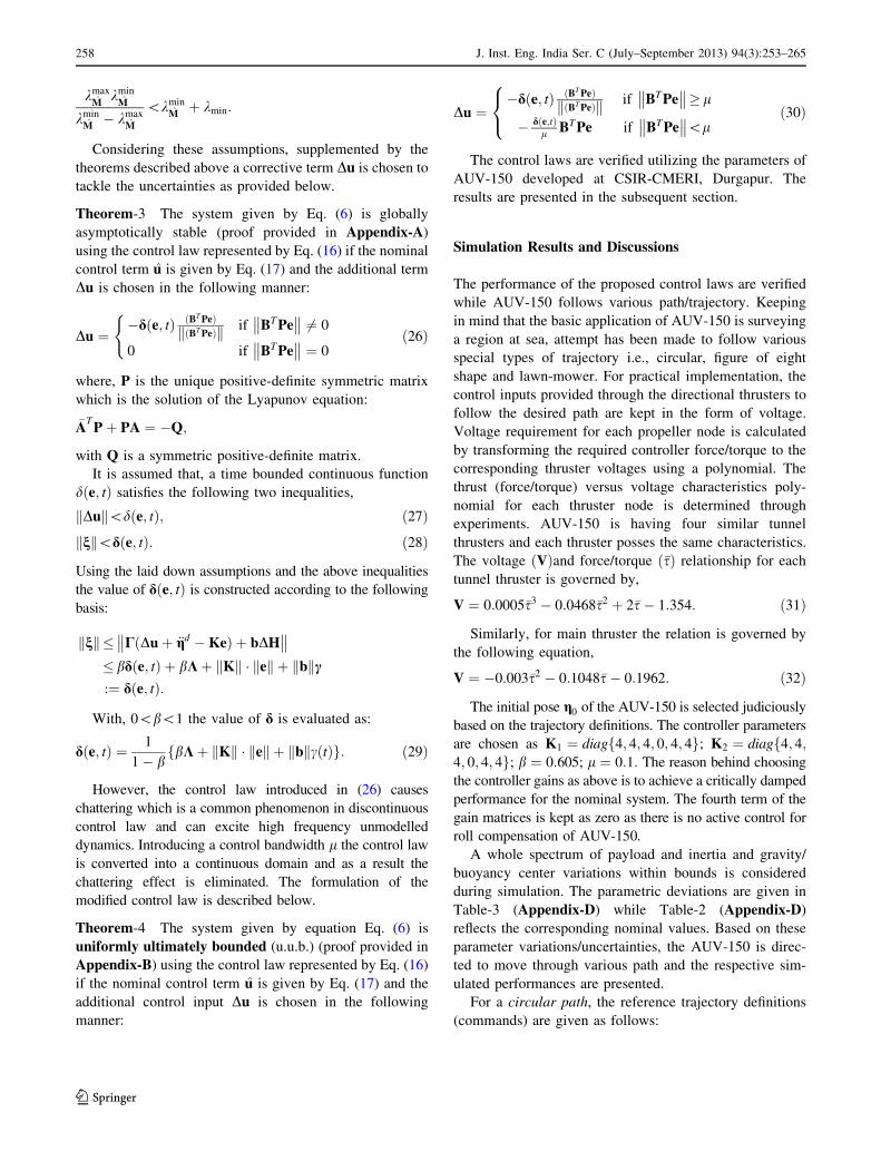
The minimum value of the variation in Fig. 2a signifies

nominal system mass and maximum value shows maxi-

mum augmented mass. Fig. 2b shows the corresponding

trajectory following performance applying compensation.

Figure 2c–e illustrate the effect of the additional term Du

over x-y-z tracking response respectively when the system

is subjected to varying uncertainties.

It is evident that x-y-z positional errors are oscillating in

nature when the trajectory is tried to achieve without

considering the corrective term for compensation of

uncertainties. Oscillatory behavior of the errors is absent

when control is improvised with an additional term Du and

errors attained a negligible steady value within a few

seconds.

The attitude ðu; h; wÞ errors are represented through

Fig. 2f–h, which illustrate the effect of the additional term

Du over roll-pitch-yaw tracking performance respectively.

It is observed that the errors, if uncompensated, are oscil-

latory in nature with multiple peaks of various amplitudes.

The error response with compensation shows a steady

behavior with negligible magnitude when the corrective

term is considered.

A time-invariant parametric variation is selected to

simulate the controller for figure of eight shape trajectory.

In this case, all the parametric variations are assumed to be

fixed but they assume the maximum value for which the

controller has been designed. The details are provided in

Table-2.

The trajectory definition for a figure of eight shape path

is as selected as:

xdðtÞ ¼ 15 sinð0:1tÞ; ydðtÞ ¼ 15 cosð0:05tÞ; zdðtÞ ¼ 5;

udðtÞ ¼ 0; hdðtÞ ¼ 0;

wdðtÞ ¼ 8

p

X1n¼1;3;5...

ð�1Þðn�1Þ=2

n2sinð0:1ntÞ:

Figure 3a demonstrates the performance of the controller

while following figure of eight shape path with compen-

sation and the differences between the desired and the actual

trajectory at any instant is negligible. The errors in position

and attitude for a figure of eight shape are shown in

Fig. 3b–g. The natures of the curves are similar to that of

circular trajectory with minor differences in the

magnitude.

Such practical situations may often arise, especially in

adverse sea condition or critical battery situation, when the

AUV needs to come up quickly on the surface by reducing

its weight suddenly or in a phased manner. This condition

has been accomplished with the lawn-mower trajectory

where the values of the hardware parameters (system mass,

inertia, gravity center etc.) remain constant for a given time

interval but fall down to another value sharply, thus gen-

erating a parametric variation like a staircase as depicted in

Fig. 4a.

The desired trajectory (commands) for lawn-mower

mission are envisaged through the following definitions:

xdðtÞ ¼ 0:25t þ 2:5 sinð0:1tÞ; ydðtÞ ¼ 15 cosð0:05tÞ; zdðtÞ¼ 5; udðtÞ ¼ 0; hdðtÞ ¼ 0; :

wdðtÞ ¼ 8

p

X1n¼1;2;...

sinðnp4Þ þ sinð3np

4Þ

n2sinð0:05ntÞ:

Figure 4b exhibits the tracking performance of the AUV

while following the lawn-mower motion; here the differ-

ence between the desired and the actual trajectory (when

additional corrective term in the control is considered) at

any instant is found to be negligible. Track errors are

represented in Fig. 4c–h and are found to be depicting

similar behavior as before with different amplitudes in the

oscillating curves.

It is clearly visible from Figs. 2f, 3e and 4f that the roll

track errors are not fully compensated due to absence of

active control for rolling compensation with AUV-150.

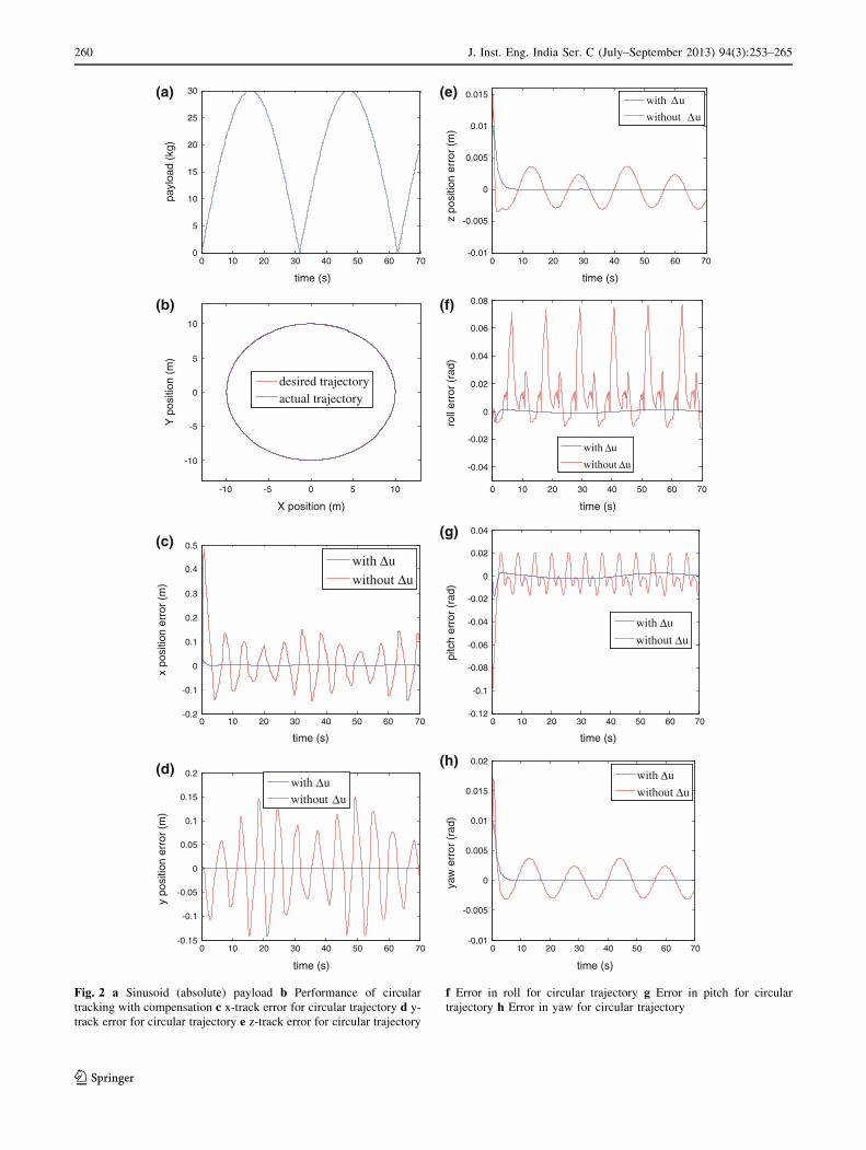
Figure 5 represents the variation of heading angle i.e.

yaw for different trajectory profiles. For circular tracking,

nature of yaw versus time curve is a straight line varying

from 0 to 2p rad for one complete revolution. The nature

of variations of heading angle for figure of eight shape

and lawn-mower trajectory are triangular and trapezoidal

respectively as shown in Fig. 5. From the simulation

results it is clear that the controller performance is very

promising under bounded parametric deviations. The

advantage of this controller is that it can work efficiently

for any perturbations within the maximum allowable

parametric deviations. This claim has been substantiated

by taking two special types of payload variations

(Figs. 2a and 4a).

The linear position errors (Figs. 2c–e, 3b–d, and 4c–e)

and attitude errors (Figs. 2f–h, 3e–g, and 4f–h) plots depict

how the error correcting term Du improves the perfor-

mance of the controller imparting robustness to the system.

Without the additional corrective control action sustained


123

0 10 20 30 40 50 60 700

5

10

15

20

25

30

time (s)

payl

oad

(kg)

-10 -5 0 5 10

-10

-5

0

5

10

X position (m)

Y p

ositi

on (

m)

desired trajectoryactual trajectory

0 10 20 30 40 50 60 70-0.2

-0.1

0

0.1

0.2

0.3

0.4

0.5

time (s)

x po

sitio

n er

ror

(m)

with Δuwithout Δu

0 10 20 30 40 50 60 70-0.15

-0.1

-0.05

0

0.05

0.1

0.15

0.2

time (s)

y po

sitio

n er

ror

(m)

with Δuwithout Δu

0 10 20 30 40 50 60 70-0.01

-0.005

0

0.005

0.01

0.015

time (s)

z po

sitio

n er

ror

(m)

with Δu

without Δu

0 10 20 30 40 50 60 70

-0.04

-0.02

0

0.02

0.04

0.06

0.08

time (s)

roll

erro

r (r

ad)

with Δu

without Δu

0 10 20 30 40 50 60 70-0.12

-0.1

-0.08

-0.06

-0.04

-0.02

0

0.02

0.04

time (s)

pitc

h er

ror

(rad

)

with Δu

without Δu

0 10 20 30 40 50 60 70-0.01

-0.005

0

0.005

0.01

0.015

0.02

time (s)

yaw

err

or (

rad)

with Δu

without Δu

(a)

(b)

(c)

(d)

(e)

(f)

(g)

(h)

Fig. 2 a Sinusoid (absolute) payload b Performance of circular

tracking with compensation c x-track error for circular trajectory d y-

track error for circular trajectory e z-track error for circular trajectory

f Error in roll for circular trajectory g Error in pitch for circular

trajectory h Error in yaw for circular trajectory


123

-15 -10 -5 0 5 10 15

-15

-10

-5

0

5

10

15

x position (m)

y po

sitio

n (m

)

desired trajectoryactual trajectory

0 10 20 30 40 50 60 70-0.4

-0.2

0

0.2

0.4

0.6

0.8

1

1.2

1.4

1.6

time (s)

x po

sitio

n er

ror

(m)

with Δuwithout Δu

0 10 20 30 40 50 60 70-1

-0.8

-0.6

-0.4

-0.2

0

0.2

0.4

0.6

0.8

1

time (s)

y po

sitio

n er

ror

(m)

with Δuwithout Δu

0 10 20 30 40 50 60 70-0.3

-0.25

-0.2

-0.15

-0.1

-0.05

0

0.05

0.1

0.15

0.2

time (s)

z po

sitio

n er

ror

(m)

with Δuwithout Δu

0 10 20 30 40 50 60 70-0.05

-0.04

-0.03

-0.02

-0.01

0

0.01

0.02

0.03

0.04

0.05

time (s)

roll

erro

r (r

ad)

with Δu

without Δu

0 10 20 30 40 50 60 70-0.08

-0.06

-0.04

-0.02

0

0.02

0.04

0.06

0.08

time (s)

pitc

h er

ror

(rad

)

with Δu

without Δu

0 10 20 30 40 50 60 70-0.015

-0.01

-0.005

0

0.005

0.01

time (s)

yaw

err

or (

rad)

with Δuwithout Δu

(a)

(b)

(c)

(e)

(f)

(g)

(d)

Fig. 3 a Figure of eight shape tracking response with compensation

b x-track error for figure of eight shape trajectory c y-track error for

figure of eight shape trajectory d z-track error for figure of eight shape

trajectory e Error in roll for figure of eight shape trajectory f Error in

pitch for figure of eight shape trajectory g Error in yaw for figure of

eight shape trajectory


123

0 10 20 30 40 50 60 700

5

10

15

20

25

30

35

40

time (s)

payl

oad

(kg)

0 10 20 30 40 50 60-20

-15

-10

-5

0

5

10

15

20

25

30

35

x position (m)

y po

sitio

n (m

)

desired trajectory trajectory with Δu trajectory without Δu

0 10 20 30 40 50 60 70-1.5

-1

-0.5

0

0.5

1

1.5

time (s)

x po

sitio

n er

ror

(m)

with Δuwithout Δu

0 10 20 30 40 50 60 70-1

-0.5

0

0.5

1

1.5

2

2.5

3

3.5

time (s)

y po

sitio

n er

ror

(m)

with Δuwithout Δu

0 10 20 30 40 50 60 70-0.2

-0.1

0

0.1

0.2

0.3

0.4

0.5

time (s)

z po

sitio

n er

ror

(m)

with Δu

without Δu

0 10 20 30 40 50 60 70-0.05

-0.04

-0.03

-0.02

-0.01

0

0.01

0.02

0.03

0.04

0.05

time (s)

roll

erro

r (r

ad)

with Δuwithout Δu

0 10 20 30 40 50 60 70-0.01

-0.005

0

0.005

0.01

0.015

0.02

time (s)

pitc

h er

ror

(rad

) with Δuwithout Δu

0 10 20 30 40 50 60 70-0.8

-0.6

-0.4

-0.2

0

0.2

0.4

0.6

time (s)

yaw

err

or (

rad)

with Δu

without Δu

(a)(e)

(f)

(g)

(h)

(b)

(c)

(d)

Fig. 4 a Time varying payload (stair-case profile) b Lawn-mower

tracking performance c x-track error for lawn mower trajectory d y-

track error for lawn mower trajectory e z-track error for lawn mower

trajectory f Error in roll for lawn mower trajectory g Error in pitch for

lawn mower trajectory h Error in yaw for lawn mower trajectory


123

oscillating behaviors have been observed as visible from

the error plots.

To generate a smooth motion, oscillatory behavior of the

trajectory is not acceptable and a tolerance limit is set as

the circle of acceptance depending on the length of the

AUV and the accuracy requirement for the specific appli-

cation. Normally, it is defined to be equal to the length of

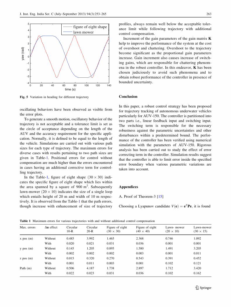
the vehicle. Simulations are carried out with various path

sizes for each type of trajectory. The maximum errors for

diverse cases with results pertaining to two path sizes are

given in Table-1. Positional errors for control without

compensation are much higher than the errors encountered

in cases having an additional corrective term for control-

ling trajectory.

In the Table-1, figure of eight shape ð30� 30Þ indi-

cates the specific figure of eight shape which lies within

the area spanned by a square of 900 m2. Subsequently

lawn-mower ð20� 10Þ indicates the size of a single loop

which entails height of 20 m and width of 10 m respec-

tively. It is observed from the Table-1 that the path errors,

though increase with enhancement of size of trajectory

profiles, always remain well below the acceptable toler-

ance limit while following trajectory with additional

control compensation.

Increment of the gain parameters of the gain matrix K

help to improve the performance of the system at the cost

of overshoot and chattering. Overshoot to the trajectory

become significant as the proportional gain parameters

increase. Gain increment also causes increase of switch-

ing gains, which are responsible for chattering phenom-

ena in the robust controller. In this endeavor, K has been

chosen judiciously to avoid such phenomena and to

obtain robust performance of the controller in presence of

bounded uncertainty.

Conclusion

In this paper, a robust control strategy has been proposed

for trajectory tracking of autonomous underwater vehicles

particularly for AUV-150. The controller is partitioned into

two parts i.e., linear feedback input and switching input.

The switching term is responsible for the necessary

robustness against the parametric uncertainties and other

disturbances within a predetermined bound. The perfor-

mance of the controller has been verified using numerical

simulation with the parameters of AUV-150. Rigorous

analysis has been carried out to study the effect of error

correcting term in the controller. Simulation results suggest

that the controller is able to limit error inside the specified

error boundary when various parametric variations are

taken into account.

Appendices

A. Proof of Theorem-3 [15]

Choosing a Lyapunov candidate VðeÞ ¼ eT Pe; it is found

Table 1 Maximum errors for various trajectories with and without additional control compensation

Max. errors Du effect Circular

10-R

Circular

20-R

Figure of eight

(30 9 30)

Figure of eight

(40 9 40)

Lawn- mower

(20 9 10)

Lawn-mower

(30 9 15)

x pos (m) Without 0.485 3.992 1.465 2.368 0.746 1.092

With 0.020 0.021 0.031 0.036 0.001 0.001

y pos (m) Without 0.145 1.205 0.895 1.580 1.491 3.205

With 0.002 0.002 0.002 0.003 0.001 0.011

z pos (m) Without 0.015 0.320 0.270 0.543 0.391 0.452

With 0.001 0.011 0.003 0.001 0.102 0.121

Path (m) Without 0.506 4.187 1.738 2.897 1.712 3.420

With 0.022 0.023 0.031 0.036 0.102 0.162

0 20 40 60 80 100 120 140-4

-3

-2

-1

0

1

2

3

4

5

time (s)

yaw

(ra

d)

figure of eight shapelawn mower

Fig. 5 Variation in heading for different trajectory


123

_VðeÞ ¼ _eT Peþ eT P_e

¼ eTð �ATPþ PAÞeþ 2eT PBðDuþ nÞ

¼ �eT Qeþ 2wTðDuþ nÞ;ð33Þ

where, w ¼ BT Pe is taken for simplicity.

If w ¼ 0 then Eq. (33) yields

_VðeÞ ¼ �eT Qe\0: ð34Þ

For w 6¼ 0 the second part of Eq. (33) becomes

wTð�dw

wk k þ nÞ ¼ �dwT w

wk k þ wTn

� � d wk k þ wk k � nk k¼ wk kð�dþ nk kÞ� 0

ð35Þ

Since, nk k\d so _VðeÞ\0

B. Proof of Theorem-4 [15]

Using a Lyapunov candidate VðeÞ ¼ eT Pe and considering

w ¼ BT Pe it is obtained from Eq. (33)

_VðeÞ ¼ �eT Qeþ 2wTðDuþ nÞ: ð36Þ

When BT Pe�� ¼ wk k� l from Eq. (35) one obtains

_VðeÞ\0:

When BT Pe�� ¼ wk k\l from Eq. (36)

_VðeÞ ¼ �eT Qeþ 2wTDuþ 2wTn

� � eT Qeþ 2wTDuþ 2 wk k � nk k� � eT Qeþ 2wTDuþ 2 wk kd

� � eT Qe� 2wTdw

lþ 2d

wT w

wk k

� � eT Qeþ 2wT �dw

lþ d

w

wk k

� �:

ð37Þ

Eq. (37) takes the maximum value lðd=2Þ when wk k ¼ðl=2Þ. Therefore,

_VðeÞ� � eT Qeþ ld2\0; ð38Þ

provided eT Qe [ lðd=2Þ:With the relationship

kminðQÞ ek k2� eT Qe� kmaxðQÞ ek k2;

where, kminðQÞ and kmaxðQÞ are the minimum and

maximum eigen values of Q respectively it can be

written that _VðeÞ\0 if

kminðQÞ ek k2 [ ld2

ð39Þ

) ek k�ffiffiffiffiffiffiffiffiffiffiffiffiffiffiffiffiffiffi

ld2kminðQÞ

s:¼ X: ð40Þ

Let S denote the smallest level surface of V containing the

ball BX with radius X centered at e ¼ 0. If eðt0Þ 2 S then

the solution remains in S. If eðt0Þ 62 S then V is decreasing

as long as eðtÞ 62 S.

C. Rayleigh quotient

For a complex Hermitian matrix D and nonzero vector q

Rayleigh quotient RðD; qÞ is defined as

RðD; qÞ :¼ q�Dq

q�q; ð41Þ

where, q� is the conjugate transpose of q. For real matrices

the Hermitian matrix is symmetric matrix and conjugate

transpose becomes normal vector transpose qT . RðD; qÞreaches to its minimum value vminðDÞ (minimum eigen

value of D) when q reaches amin (the corresponding eigen

vector). Similarly RðD; qÞ has its maximum value vmaxðDÞ(maximum eigen value of D) when q is at amax (the

corresponding eigen vector). So, vminðDÞ�RðD; qÞ� vmaxðDÞ.

D. Parameter values

The nomenclatures are according to [14].

See Tables 2 and 3.

Table 2 Nominal values of parameters

m

kg

xG

m

yG

m

zG

m

Ix

kg-m2Iy

kg-m2Iz

kg-m2�X _u

kg

�Y _v

kg

490 0 0 0.012 17.1 632 630 49 836


123

References

1. R. Cristi, A.J. Healey, Adaptive identification and control of an

autonomous underwater vehicle, in Proceedings of the 6th

International Symposium On Unmanned Untethered Submersible

Technology, pp. 563–572 (1989)

2. T.I. Fossen, S.I. Sagatun, Adaptive control of nonlinear under-

water robotic systems, in Proceedings of the IEEE International

Conference on Robotics and Automation Sacramento, California,

pp. 1687–1695, (April 1991)

3. J. Yuh, An adaptive and learning control system for underwater

robots, In 13th World Congress International Federation of

Automatic Control, San Francisco, CA, pp. 145–150 (1996)

4. S.K. Choi, J. Yuh, Experimental study on a learning control

system with bound estimation for underwater vehicles. Int.

J. Auton. Robots 3(2/3), 187–194 (1996)

5. G. Antonelli, F. Caccavale, S. Chiaverini, G. Fusco, A novel

adaptive control law for underwater vehicles. IEEE trans. Control

Sys. Technol. 11(2), 221–232 (2003)

6. D.R. Yoerger, J.-J.E. Slotine, Robust trajectory control of

underwater vehicle. IEEE J. Oceanic Eng. OE-10, 462–470

(1985)

7. A.J. Healey, D. Lienard, Multivariable sliding mode control for

autonomous diving and steering of unmanned underwater vehi-

cles. IEEE J. Oceanic Eng. 18(3), 327–339 (1993)

8. R. Cristi, F.A. Papoulias, A.J. Healey, Adaptive sliding mode

control of autonomous underwater vehicles in diving plane. IEEE

J. Oceanic Eng. 15, 152–160 (1990)

9. F.A. Papoulias, R. Cristi, D. Marco, A.J. Healey, Modelling,

sliding mode control design, and visual simulation of AUV dive

plane dynamic response, in Proceedings of the 6th International

Symposium on Unmanned Untethered Submersible Technology,

pp. 536–547 (1989)

10. P.M. Lee, S.W. Hong, Y.K. Lim, C.M. Lee, B.H. Jeon, J.W. Park,

Discrete time sliding mode control of an autonomous underwater

vehicle. IEEE J. Oceanic Eng. 24(3), 327–339 (1999)

11. M.S. Naik, S.N. Singh, State-dependent riccati equation-based

robust dive plane control of AUV with control constraints. Ocean

Eng. 34, 1711–1723 (2007)

12. L. Lapierre, Robust diving control of an AUV. Ocean Eng. 36,

92–104 (2008)

13. S.N. Shome, S. Nandy, S.K. Das, D.K. Biswas, D. Pal, AUV for

Shallow Water Applications—some Design Aspects, International

Offshore (Ocean) and Polar Engineering Conference, ISOPE-

2008, Vancouver, BC, Canada, (July 2008)

14. T.I. Fossen, Guidence and control of ocean vehicles (Wiley,

London, 1994)

15. M.W. Spong, M. Vidyasagar, Robot dynamics and control

(Wiley, London, 1989)

Table 3 Variation of parameters for different Trajectory

Circular Figure of

eight shaped

Lawn mower

Dm 30abs(sin0.1t) 30 30, 0 B t B 25

20, 25 \ t B 50

10, t [ 50

DxG 0.05abs(sin0.1t) 0.05 0.05, 0 B t B 25

0.03, 25 \ t B 50

0.02, t [ 50

DyG 0.02abs(sin0.1t) 0.02 0.02, 0 B t B 25

0.01, 25 \ t B 50

0.005, t [ 50

DzG 0.02abs(sin0.1t) 0.02 0.02, 0 B t B 25

0.018, 25 \ t B 50

0.015, t [ 50

DIx 2abs(sin0.1t) 2 2, 0 B t B 25

1.5, 25 \ t B 50

1, t [ 50

DIy 5abs(sin0.1t) 5 5, 0 B t B 25

3.5, 25 \ t B 50

2.5, t [ 50

DIz 10abs(sin0.1t) 10 10, 0 B t B 25

7, 25 \ t B 50

5, t [ 50

�DX _u 3abs(sin0.1t) 3 3, 0 B t B 25

2, 25 \ t B 50

1.5, t [ 50

�DY _v 50abs(sin0.1t) 50 50, 0 B t B 25

35, 25 \ t B 50

25, t [ 50


123

Trajectory Following Control of AUV: A Robust Approach

Documents

Transcript of Trajectory Following Control of AUV: A Robust Approach