Minimum cost trajectory planning for industrial robots

ints inunds onic splinequentialhown to

avere hardlyspecifieder,ease themetricaltask to bediciously

trol. The8;

redm which. In manyt a largethe robot

European Journal of Mechanics A/Solids 23 (2004) 703–715

Minimum cost trajectory planning for industrial robots

T. Chettibia,∗, H.E. Lehtiheta, M. Haddada, S. Hanchib

a Mechanical Laboratory of Structures, E.M.P., B.E.B., BP 17, 16111, Algiers, Algeriab Mechanical Laboratory of Fluids, E.M.P., B.E.B., BP 17, 16111, Algiers, Algeria

Received 18 August 2003; accepted 24 February 2004

Available online 27 March 2004

Abstract

We discuss the problem of minimum cost trajectory planning for robotic manipulators. It consists of linking two pothe operational space while minimizing a cost function, taking into account dynamic equations of motion as well as bojoint positions, velocities, jerks and torques. This generic optimal control problem is transformed, via a clamped cubmodel of joint temporal evolutions, into a non-linear constrained optimization problem which is treated then by the SeQuadratic Programming (SQP) method. Applications involving grasping mobile object or obstacle avoidance are sillustrate the efficiency of the proposed planner. 2004 Elsevier SAS. All rights reserved.

Keywords: Robotic manipulators; Motion planning; Obstacles avoidance; Grasping mobile objects; Non-linear optimization

1. Introduction

Due to their great ability ofspeed and precision and their cost-effectiveness in repetitive tasks, industrial robots hbeen used for decade in place of human workers in automatic production lines. But these powerful machines aautonomous in the sense that they require preliminary actions, such as calibration or motion planning, to achievetasks. In general, robotic manipulators areused at their limit capacities for obvious reasons of productivity. This leads, howevto quite significant joint torque and velocity magnitudes which can be harmful to the system state. In order to incrmanipulator performances, it is highly desirable to control the system dynamic taking into account technological, geoand environmental constraints as well as any other constraints inherent both to the robot design and to the nature of theexecuted. Since many different ways are possible to perform the same task, this freedom of choice can be exploited juto optimize a given performance criterion.

During the past decades, a great deal of attention has been given to the problem of motion planning and concomplexity of the problem made researchers divide the robot control structure into two levels (Fig. 1) (Dombre and Khalil, 198Bessonnet, 1992; Angeles, 1997; Chettibi, 2001): the upper level, calledpath or trajectory planning, and the lower level, calledpath tracking or path control. Path control is the process that makes the robotactual position and velocity match some desivalues provided to the controller by the trajectory planner. The trajectory planner receives a description of the path froit computes a time history of desired positions and velocities. Then, the path tracker compensates for any deviationpublications dealing with motion planning of robotic manipulators, authors state a variety of problems and suggesdiversity of solution schemes. Several regrouping can be done according to execution modes, adopted models forbehaviour and proposed numerical methods of treatment.

* Corresponding author.E-mail address: [email protected] (T. Chettibi).

0997-7538/$ – see front matter 2004 Elsevier SAS. All rights reserved.doi:10.1016/j.euromechsol.2004.02.006

704 T. Chettibi et al. / European Journal of Mechanics A/Solids 23 (2004) 703–715

d motionexample,,hand, inen two

secondr, 1977;in such

timizationtrajectoryverated for a;nge of which

ich wasmple, thet torques989). Itmotions

iven

jointt per joint)

in theer, 1987;iteng-bang)periods.dynamic

at can benstraints.

Fig. 1. Synoptic diagram of optimal motion planner for robotic manipulators.

Among the tasks which robot manipulators are devoted to, a first distinction can be made in regards to the desirenature. Depending on the robot task, it might be necessary to specify the end effector trajectory in the work space. Forif the effector’s tool acts withoutinterruption according to a predefined path (gluing, arc welding, laser cutting operationsetc.), the planner (or optimization process) defines optimal tracking modalities of the imposed path. On the otherpoint to point motions (pick-and-place operations, point to point welding), the end effector is free to move betweextremal positions. In this case, the planner tries to define the optimal trajectory and the corresponding controls. Adistinction can be made according to the type of model used. Earlier works (Kahn and Roth, 1971; Luh and WalkeLuh and Lin, 1981) use kinematic models where the imposed trajectory is geometrically defined in the work spacea way that the manipulator avoids existing obstacles. The main preoccupation being obstacle avoidance, the opproblem is synthesized using the inter-penetration distance between elements in collision. Of course, this type ofplanning can produce very high execution velocities, particularly when transfer time is minimized. It induces also excessitorque amplitudes which can be harmful for the system state. For these reasons, dynamic models were later incorpomore realistic control of the robot dynamic behavior (Bobrow et al., 1985; Pfeifferand Rainer, 1987; Eltimsahy and Yang, 1988Yamamoto and Ozaki, 1988; Jaques et al., 1989; Bessonnet, 1992;Chettibi, 2000). However, the problem of motion plannibecomes quite complex and requires specific schemes for its treatment. Fig. 2 shows examples of such schemes, somare widely used. Two main familiescan be distinguished: direct and indirect methods(Hull, 1997; Betts, 1998).

Indirect methods are based, in particular, on Pontryagin Maximum Principle (PMP) (Pontryagin et al., 1965) whfirst used to define the optimal control. The corresponding states may be obtained by another method. For exaphase plane method is among early techniques taking into account the robot dynamic model and bounds on join(Bobrow et al., 1985; Kang and McKay, 1986; Shin and Mckay, 1986; Pfeiffer and Rainer, 1987; Jaques et al., 1was first used to solve minimum time motion problems along specified paths. Then, it was extended to handle freeas well (Shiller and Dubowsky, 1986). In this minimum time trajectory planner, it is assumed that the desired path is gin a parameterized form (e.g., using curvilinear abscissa) which is substituted into the manipulator dynamic equations togive a set of second order differential equations in terms of the path parameter. Consequently, bounds on individualtorques are converted into bounds on parametric accelerations. The allowable sets of second derivatives (one seare intersected to give a single allowable set. Using the fact that the minimum time solution will be bang–bangacceleration, it is possible to construct phase plane plots (Bobrow et al., 1985; Shin and Mckay, 1986; Pfeiffer and RainChettibi and Yousnadj, 2001) which give the optimal trajectory in terms of the trajectory parameter and its derivatives. Despthe fact that this technique is elegant and solves the optimal time motion planning problem, the discontinuous nature (baof joint torques thus obtained creates many practical problems. In fact, the controller must work in saturation for longHence, the optimal control leaves no control authority to compensate for tracking errors caused by either unmodelledor delays introduced by the on-line feedback controller. In addition, this method only takes into account constraints thformulated in terms of the trajectory parameter and its time derivatives. Therefore, it spans a small field of possible co

T. Chettibi et al. / European Journal of Mechanics A/Solids 23 (2004) 703–715 705

ssonnet,ial

shootingations, itd that it is

f dynamicl., 1993;

7;fmeters to(Tan andg

cheme is

r time

icolve the

ower, etc.,

to handle

Fig. 2. Methods used for solving optimal free motions planning problem.

PMP is used also to treat directly the optimal dynamic motion planning problem (Bessonnet, 1992; Gaudin and Be1995; Lazrak, 1996; Danes, 1998). The optimality conditions for transfer modalities areexpressed as a set of differentequations (Pontryagin et al., 1965). This boundary values problem is solved by specific numerical techniques such asor relaxation methods (Hull, 1997; Betts, 1998). Although this approach has been used successfully in many applictends to be abandoned in recent years. The primary reasons are that the convergence domain is relatively small andifficult to incorporate inequality terms in path constraints.

Direct methods were introduced to reduce somewhat the problem complexity. They are based on a discretisation ovariables (states, controls) leading to a parameter optimization problem. Then, non-linear optimization (Richard et aMartin and Bobrow, 1997, 1999; Chettibi,2000, 2002; Bobrow et al., 2001), evolutionary (Nearchou and Aspragathos, 199Mao and Hsia, 1997) or classical stochastic (Chettibi and Lehtihet, 2002) techniques are applied to obtain optimal values othe parameters. A common characteristic of these methods is to try to solve directly the problem by adjusting paraminimize some cost function while taking into account imposed constraints. Other ways of discretisation can be foundPotts, 1988; Richard et al., 1993; Chettibi, 2000). However, these techniques suffer from numerical explosion when treatinhigh dimension problems.

In the present paper, a different direct method is used for optimal free motion planning problems. The proposed sshown in highlighted arrows in Fig. 2. The basic idea is to parameterize directly the joint evolution vectorq(t). The optimalcontrol problem becomes a parametric constrained optimization problem which is to be solved for the unknown transfeT

and the unknown parameters of the chosen model forq(t).Several choices are made here that can be summarized as follows. First, we use forq(t) a convenient clamped cub

spline model with free nodes uniformly distributed along the time scale. Second, we use the SQP method to soptimization problem with the unknowns being now theposition of spline nodes as well as the transfer timeT . Also, the costfunctionF , which can take many forms, is chosen as a weighted balance of transfer time, mean average of actuators, pFurthermore, in order to make the resulting motion physically feasible,F is minimised under position,velocity, accelerationjerk and torque constraints. The problem is formulated in such a way that the same approach can be easily extended


complex situations. Three examples are treated here: the first one concerns a pick-and-place operation with a six d.o.f robot; theto account

uations

r a

en by the

ssuchnextended

edssion is

second one deals with a grasping operation of a moving object by a planar redundant robot. The last example takes inthe presence of obstacles in the workspace.

2. Problem statement

Let us consider an d.o.f serial manipulator robot. Motion equations for this system can be derived using Lagrange’s eqor Newton–Euler formalism (Dombre and Khalil,1988; Angeles, 1997). They are simply given by:

M(q)q̈ + Q(q, q̇) + G(q) = τ, (1a)

whereM is the inertia matrix,Q is the vector of centrifugal andCoriolis forces in which joints velocities appear undequadratic form,G is the vector of gravitational forces andτ ∈ �n is the vector of actuators efforts.

In the presence of external forcesFext applied on the end effector, relation (1a) becomes:

M(q)q̈ + Q(q, q̇) + G(q) + JT(q)Fext = τ, (1b)

whereJT is the transpose of the robot Jacobian matrix.The robot is required to move freely (without following a specified path) from an initial to a final state,P0 and Pf ,

respectively. The problem is to find, in addition to actuators efforts vectorτ(t) and final timeT , the joint time evolutionvectorq(t) that matches initial and final states, satisfies given constraints and minimizes a given cost functionF .

2.1. Constraints

Constraints represent physical limitations imposed on the robot kinematic and dynamic performances. They are givfollowing inequalities:

Joint torques:∣∣τi (t)∣∣ � τmax

i , i = 1, . . . , n, (2a)

Joint jerks:∣∣...q i(t)

∣∣ �...q max

i , i = 1, . . . , n, (2b)

Joint accelerations:∣∣q̈i (t)

∣∣ � q̈maxi , i = 1, . . . , n, (2c)

Joint velocities:∣∣q̇i (t)

∣∣ � q̇maxi , i = 1, . . . , n, (2d)

Joint positions:∣∣qi (t)

∣∣ � qmaxi , i = 1, . . . , n. (2e)

Of course, non-symmetrical bounds on the above physical quantities can behandled without any difficulties. Relation(2a–e) traduce the fact that not all motions are tolerable, that power resources are limited and must be used rationally ina way that the robot dynamic behavior is correctly controlled. Jerk constraints are introduced due to the fact that joint positiotracking errors increase when jerk increases, and also to limit excessive wear on the robot so that the robot life-span is(Piazzi and Visioli, 1998; Macfarlane and Croft, 2001).

2.2. Objective function

The motion quality will depend strongly on theexpression adopted for the objective functionF . In fact,F represents thetransfer cost between initial and final postures. Hence, it would be judicious to includesignificant physical parameters relatdirectly to the global behavior of the robot and to the productivity of the industrial process. The following general exprea balance between transfer timeT and quadratic average of both actuator effortsA and corresponding powerB:

F = µT + (1− µ)

2

[αA + (1− α)B

], (3a)

where

A =T∫

0

n∑i=1

(τi

τmaxi

)2dt, (3b)

B =T∫

0

n∑i=1

(q̇i τi

q̇maxi τmax

i

)2dt, (3c)

A andB have the dimension of a time.


µ andα are weighting coefficients (0� µ � 1, 0� α � 1). The caseµ = 1 corresponds to the optimal time motion problem.others. In).

metricrs arejectoriesis choicend theires. By

es.

lved.of earliere ofm. These

the Kuhn–y et al.,

attemptby

ethods aregramming

a, accuracyblem.mizationtheir costlentrs such

wise, the) or to aer.

There are many situations where it is desirable and appropriate to give more importance to some links relatively to thethat case, we could just define additional normalized weighting coefficientswi (i = 1, . . . , n) inside expressions (3b) and (3c

3. Optimal control via direct parameter optimization of joint positions

The planning of optimal dynamic motion is a generic optimal control problem. It is transformed here into a paraoptimization problem as follows: joint variables are expressed as a function of a set of parameters. These parametevaried inside a non-linear optimization program until an optimum satisfying constraints has been reached. Joint traare represented here by clamped cubic spline functions with nodes uniformly distributed along time scale (Fig. 3). Thcan be justified by the well-known characteristics of cubic spline functions; continuity of second order is guarantied alower order greatly limits oscillations and enables us to compute easily extremum values between two consecutive nodparameterizing the joint trajectories, variables of the problem become the transfer time and the position of cubic spline nodConstraints that must be handled are those defined by relations (2a–e).

In constrained optimization, the general aim is to transformthe problem into an easier sub-problem that can be then soIt is used as the basis of an iterative process (Powell, 1984; Fletcher, 1987). A common characteristic of a large classmethods is the translation (using a penalty function) of the constrained problem to a basic unconstrained one. A sequencparameterized unconstrained optimizations is performed which may converge to the solution of the constrained problemethods are now considered relatively inefficient and have been overwhelmed by methods based on the resolution ofTucker (KT) equations which are the necessary conditions of optimality for a constrained optimization problem (Barcla1997).

The solution of the KT equations forms the basis to many non-linear programming algorithms. These methodsto compute directly the Lagrange multipliers. Constrained quasi-Newton methods guarantee superlinear convergenceaccumulating second order information regarding the KT equations using a quasi-Newton updating schedule. These mcommonly referred to as Sequential Quadratic Programming (SQP) and represent the state-of-the-art in non-linear promethods (Powell, 1984; Schittowski, 1985; Fletcher, 1987). For example, (Schittowski, 1985), has implemented and testedversion that outperforms, over a large number of benchmark problems, every other tested method in terms of efficiencyand frequency of successful convergences. This method is applied here to solve our new parametric optimization pro

(Martin and Bobrow, 1997, 1999; Bobrow et al., 2001) have already made use of SQP to solve a parametric optiproblem. But, instead of clamped cubic splines these authors have used B-splines to model joint variables. Also,function corresponds to the special case (µ = 0, α = 1), that is a minimum-effort problem. However, no bounds equivato inequalities (2a–e) are given. In addition, in contrast to (3a) their cost function does not include normalizing factoas τmax

i , i = 1, . . . , n. In many practical cases, these factors as well as bounds (2a–e) are in fact necessary. Otheroptimization process may lead either to a solution that is not physically feasible (violation of a technological constraintbiased solution in the case of a problem involving a large difference in torque magnitudes from one actuator to the oth

Fig. 3. Cubic spline approximation of joint position temporal evolution.


4. Results: pick and place operations

ial armarry outneout for

profilesn.

and,ons. Inxedtion acts

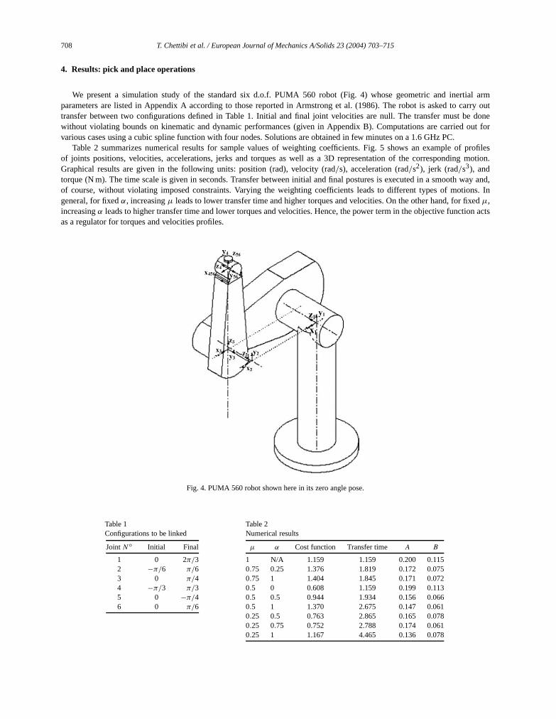
We present a simulation study of the standard six d.o.f. PUMA 560 robot (Fig. 4) whose geometric and inertparameters are listed in Appendix A according to those reported in Armstrong et al. (1986). The robot is asked to ctransfer between two configurations defined in Table 1. Initial and final joint velocities are null. The transfer must be dowithout violating bounds on kinematic and dynamic performances (given in Appendix B). Computations are carriedvarious cases using a cubic spline function with four nodes. Solutions are obtained in few minutes on a 1.6 GHz PC.

Table 2 summarizes numerical results for sample values of weighting coefficients. Fig. 5 shows an example ofof joints positions, velocities, accelerations, jerks and torques as well as a 3D representation of the corresponding motioGraphical results are given in the following units: position (rad), velocity (rad/s), acceleration (rad/s2), jerk (rad/s3), andtorque (N m). The time scale is given in seconds. Transfer between initial and final postures is executed in a smooth wayof course, without violating imposed constraints. Varying the weighting coefficients leads to different types of motigeneral, for fixedα, increasingµ leads to lower transfer time and higher torques and velocities. On the other hand, for fiµ,increasingα leads to higher transfer time and lower torques and velocities. Hence, the power term in the objective funcas a regulator for torques and velocities profiles.

Fig. 4. PUMA 560 robot shown here in its zero angle pose.

Table 1Configurations to be linked

JointN◦ Initial Final

1 0 2π/32 −π/6 π/63 0 π/44 −π/3 π/35 0 −π/46 0 π/6

Table 2Numerical results

µ α Cost function Transfer time A B

1 N/A 1.159 1.159 0.200 0.1150.75 0.25 1.376 1.819 0.172 0.0750.75 1 1.404 1.845 0.171 0.0720.5 0 0.608 1.159 0.199 0.1130.5 0.5 0.944 1.934 0.156 0.0660.5 1 1.370 2.675 0.147 0.0610.25 0.5 0.763 2.865 0.165 0.0780.25 0.75 0.752 2.788 0.174 0.0610.25 1 1.167 4.465 0.136 0.078


Fig. 5. Optimal motion obtained for (µ = 0.5, α = 1).


example,perfectly

enitsration by

als

t.object. Theet object.

ing

ionduring

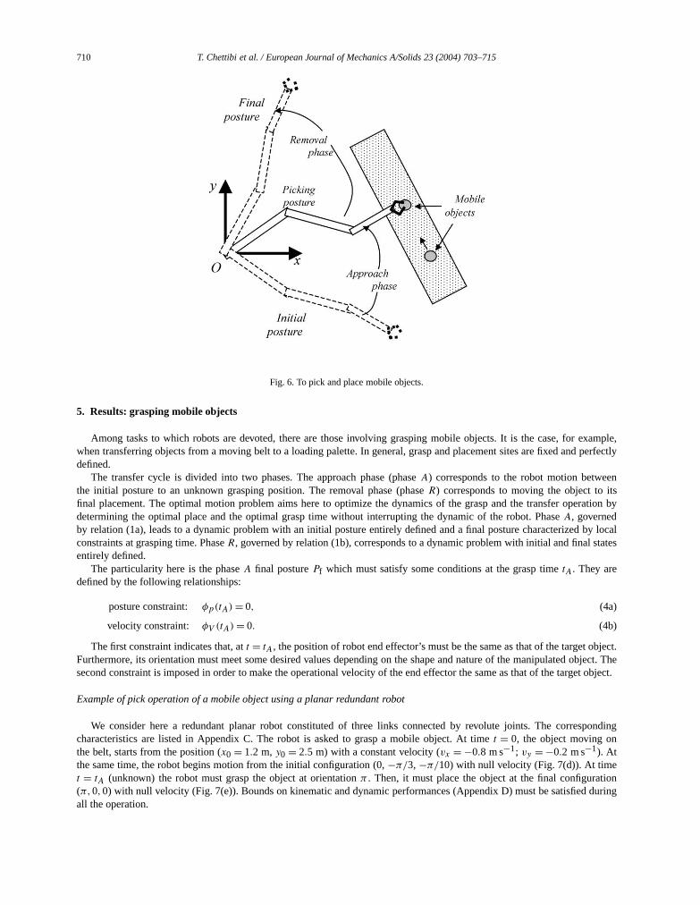
Fig. 6. To pick and place mobile objects.

5. Results: grasping mobile objects

Among tasks to which robots are devoted, there are those involving grasping mobile objects. It is the case, forwhen transferring objects from a moving belt to a loading palette. In general, grasp and placement sites are fixed anddefined.

The transfer cycle is divided into two phases. The approach phase (phaseA) corresponds to the robot motion betwethe initial posture to an unknown grasping position. The removal phase (phaseR) corresponds to moving the object tofinal placement. The optimal motion problem aims here to optimize the dynamics of the grasp and the transfer opedetermining the optimal place and the optimal grasp time without interrupting the dynamic of the robot. PhaseA, governedby relation (1a), leads to a dynamic problem with an initial posture entirely defined and a finalposture characterized by locconstraints at grasping time. PhaseR, governed by relation (1b), corresponds to adynamic problem with initial and final stateentirely defined.

The particularity here is the phaseA final posturePf which must satisfy some conditions at the grasp timetA. They aredefined by the following relationships:

posture constraint: φp(tA) = 0, (4a)

velocity constraint: φV (tA) = 0. (4b)

The first constraint indicates that, att = tA, the position of robot end effector’s must be the same as that of the target objecFurthermore, its orientation must meet some desired values depending on the shape and nature of the manipulatedsecond constraint is imposed in order to make the operational velocity of the end effector the same as that of the targ

Example of pick operation of a mobile object using a planar redundant robot

We consider here a redundant planar robot constituted of three links connected by revolute joints. The correspondcharacteristics are listed in Appendix C. The robot is asked to grasp a mobile object. At timet = 0, the object moving onthe belt, starts from the position (x0 = 1.2 m, y0 = 2.5 m) with a constant velocity (vx = −0.8 m s−1; vy = −0.2 m s−1). Atthe same time, the robot begins motion from the initial configuration (0,−π/3, −π/10) with null velocity (Fig. 7(d)). At timet = tA (unknown) the robot must grasp the object at orientationπ . Then, it must place the object at the final configurat(π,0,0) with null velocity (Fig. 7(e)). Bounds on kinematic and dynamic performances (Appendix D) must be satisfiedall the operation.


Fig. 7. Optimal pick and place motion.

Fig. 8. Example of ball modelling of robot and obstacles.


thees 3.131 s.,

eenance. Differente withoutsia, 1997;

ork space.is

folds up

Fig. 9. Optimal robot motion among static obstacles.

Numerical results are obtained withµ = 0.3, α = 0.5 and using a cubic spline function with four nodes. Fig. 7 showsevolution of the system during the approach and removal phases. The first is achieved in 2.633 s while the second takThe bounds imposed on kinematics and dynamics performances are respected. Fig. 7(a)–(c) show the continuity of positionsvelocities and torques during the transition from one phase to the other. Hence, the whole operation is done smoothly.

6. Results: motion planning in the presence of obstacles

When obstacles are present in the robot work space, motion must be planned in such a way collision is avoided betwrobot links and obstacles. In consequence, we need to model appropriately obstacles and links, then measure the distbetween obstacles and links. For example, here we use a finite number of spheres to cover obstacles and linksradii are used to cover different shapes of links and objects (Fig. 8), so that more accurate coverage is possiblincreasing complexity. Similar methods are proposed in references (Nearchou and Aspragathos, 1997; Mao and HGlass et al., 1995). Such a geometric simplification allows stating explicitly constraints due to the presence of obstacles.

We use here the same robot as in Section 5. It is asked to move among three static obstacles disposed in it’s wThe robot begins at (0,−π/3, −π/10) and stops at (π/2,0,0). Boundary velocities are null. The obtained optimal motionpresented in Fig. 9. Numerical results are obtained withµ = 0.2, α = 1 and using a four node cubic spline function.

The task is achieved in about 3.695 s and no violation of limit values of robot characteristics is recorded. The robotfirst the third arm then joins the final posture. This is a natural action otherwise the transfer will be impossible.


7. Conclusion

roboticatics and

modeloptimallem bye scale.g a costed power.ansferumerical

problemo approach. That is,ns).thishee problembstaclesstive studycomplex

We have presented a trajectory planner to deal with the problem of optimal dynamic free motion planning forarms. It computes minimum cost trajectories taking into account the main constraints imposed on the robot kinemdynamics performances. The problem is highly non-linear. This is due, firstly, to the complexity of the robot dynamicthat must be verified during the transfer and secondly to the non-linearity of the cost function and constraints. Themotion planning problem is originally an optimal control one. It has been converted into a non-linear optimization probparameterezing joint temporal variations via clamped cubic spline functions with nodes uniformly distributed along timThe proposed planner uses the powerful SQP optimization method. The optimal motions were obtained by minimizinfunction containing significant motion parameters such as transfer time, quadratic average of joint torques and consumThe cost function was written in a convenient weighted form which allows giving a relative importance for minimizing trtime, joint efforts or power. Smooth motions were obtained by choosing adequate weighting factors. Through the nexamples we have shown the great ability of the proposed method to handle various kinds ofproblems involving redundantrobots, obstacles avoidance or grasping mobile objects.

However, as any non-linear optimization method, SQP can be attracted by local minima. One way to overcome thisis to start the process from various initial guesses or to use a stochastic technique to scan the solution space and tthe global minimum. Also, SQP involves computing the gradient and the Hessian of objective function and constraintscontinuity of second order must be ensured. However, physicalmodels sometimes include discontinuous terms (e.g., frictioIn that case only stochastic techniques can be used. In consequence to these observations, we have studied, in parallel tomethod, the possibility to use a stochastictechnique to overcome previous drawbacks. In this case and according to Fig. 2, tmain difference in the new scheme is the numerical technique. Of course, several arrangements have to be done in thformulation in order to make it propitious to be solved by a stochastic technique while taking into account frictions and o(Chettibi and Lehtihet, 2002). Encouraging results have been already obtained in thetreatment of discontinuous physical model(Rebai, 2002) and handling obstacles (Hentout, 2004). In a future paper, we intend to present a complete comparabetween these two methods and we will show how it is possible to combine them to get better results and to treat moreproblems.

Appendix A. Geometric and inertial parameters of PUMA 560 (Armstrong et al., 1986)

Joint N◦ 1 2 3 4 5 6

α (rad) π/2 0 −π/2 π/2 −π/2 0di (m) 0 0.4318 0.0203 0 0 0ri (m) 0 0 0.15005 0.4318 0 0M (kg) – 17.4 4.8 0.82 0.34 0.09px (m) 0 −0.3638 −0.0203 0 0 0py (m) 0 0.006 −0.0141 0.19 0 0pz (m) 0 0.2275 0.0700 0 0 0.032Ixx (kg m2) 0 0.13 0.066 1.8e−3 0.3e−3 0.15e−3Iyy (kg m2) 0.35 0.524 0.086 1.3e−3 0.4e−3 0.15e−3Izz (kg m2) 0 0.539 0.0125 1.8e−3 0.3e−3 0.04e−3Ixy (kg m2) 0 0 0 0 0 0Iyz (kg m2) 0 0 0 0 0 0Ixz (kg m2) 0 0 0 0 0 0

Appendix B. limit performances used for PUMA 560

Joint N◦ 1 2 3 4 5 6

qmax (rad) π 3π/4 3π/4 π 3π/4 3π/4q̇max (rad/s) 8 10 10 5 5 5q̈max (rad/s2) 10 12 12 8 8 8...q max (rad/s3) 30 40 40 20 20 20τmax (N m) 97.6 186.4 89.4 24.2 20.1 21.3


Appendix C. Geometric and inertial parameters of the planar three degrees of freedom robot

t of

iers,

(3),

12),

nie

ial

ctic,

t

H2555-

(3),

11,

6),

Joint N◦ 1 2 3

di (m) 0.7 0.5 0.5M (kg) 7 5 5px (m) 0.35 0.5 0.5Izz (kg m2) 0.8 0.5 0.5

Appendix D. Limit performances of the planar three degrees of freedom robot

Joint N◦ 1 2 3

qmax (rad) π 3π/4 3π/4q̇max (rad/s) 3 3 3q̈max (rad/s2) 8 8 8...q max (rad/s3) 10 15 20τmax (N m) 30 25 25

References

Angeles, J., 1997. Fundamentals of Robotic Mechanical Systems. Theory, Methods, and Algorithms. Springer.Armstrong, B., Khatib, O., Burdick, J., 1986. The explicit dynamic model and inertial parameters of PUMA 560 arm. In: IEEE Int. Conf. on

Rob. & Aut., San Francisco, pp. 510–518.Barclay, A., Gill, P.E., Rosen, J.B., 1997. SQP Methods and their application to numerical optimal control. Report NA97-3, Departmen

Mathematics, University of California, San Diego.Bessonnet, G., 1992. Optimisation dynamique des mouvements point à pointde robots manipulateurs. Thèse d’état, Université de Poit

France.Betts, J.T., 1998. Survey of numerical methods for trajectory optimization. J. Guidance Cont. Dyn. 21 (2), 193–207.Bobrow, J.E., Dubowsky, S., Gibson, J.S., 1985. Time optimal control of robotic manipulators along specified paths. Int. J. Rob. Res. 4

3–15.Bobrow, J.E., Martin, B.J., Sohl, G., Wang, E.C., Park, F.C., Kim, J., 2001. Optimal robot motions for physical criteria. J. Rob. Syst. 18 (

785–795.Chettibi, T., 2000. Contribution à l’exploitation optimale des bras manipulateurs. Mémoire de Magister, EMP, Algiers, Algeria.Chettibi, T., 2001. Optimal motion planning of robotic manipulators. Maghrebine Conference of Electric Engineering, Constantine, Algeria.Chettibi, T., 2002. Research of optimal free motions of manipulators robots by non-linear optimisation. In: Séminaire international de gé

mécanique, Oran, Algeria, pp. 317–325.Chettibi, T., Lehtihet, H.E., 2002. A new approach for point to point optimal motion planning problems of robotic manipulators. In: 6th Bienn

Conf. on Engineering Syst. Design and Analysis (ASME), Turkey. APM10.Chettibi, T., Yousnadj, A., 2001. Optimal motion planning of robotic manipulators along specified geometric path. Int. Conf. on Produ

Algiers, Algeria.Danes, F., 1998. Critères et contraintes pour lasynthèse optimale des mouvements de robots manipulateurs. Application à l’évitemen

d’obstacles. Thèse d’état, Université de Poitiers.Dombre, E., Khalil, W., 1988. Modélisation et commande des robots, First ed. Hermes.Eltimsahy, A.H., Yang, W.S., 1988. Near minimum time control of robotic manipulator with obstacles in the workspace. C

1/88/000/IEEE, pp.358–363.Fletcher, R., 1987. Practical methodsof Optimization, Second ed. Wiley.Gaudin, H., Bessonnet, G., 1995. From identification to motion optimisation of a planar manipulator. Robotica 13, 123–132.Glass, K., Colbaugh, R., Lim, D., Seradji, H., 1995. Real time collision avoidance for redundant manipulators. IEEE Trans. Rob. Aut. 11

448–457.Hentout, A., 2004. Planification de trajectoires sans collision pour les robots manipulateurs. Mémoire de Magister, EMP, Algiers, Algeria.Hull, D.G., 1997. Conversion of optimal control problems into parameter optimization problems. J. Guidance Cont. Dyn. 20 (1), 57–62.Jaques, J., Soltine, E., Yang, H.S., 1989. Improving the efficiency oftime-optimal path following algorithms. IEEE Trans. Rob. Aut. 5 (1).Kahn, M.E., Roth, B., 1971. The near minimum time control of open looparticulated kinematic chains. ASME J. Dyn. Syst. Meas. Contr.

164–172.Kang, G.S., McKay, D.N., 1986. Selection of near minimum time geometricpaths for robotic manipulators. IEEE Trans. Aut. Contr. AC-31 (

501–512.


Lazrak, M., 1996. Nouvelle approche de commande optimale en temps final libre et construction d’algorithmes de commande de systèmesarticulés. Thèse d’état, Université de Poitiers, France.

.ns,

.

.

.

(4),

,

ach.

00.

C-

ob.

Luh, J.Y.S., Lin, C.S., 1981. Optimum path planning for mechanical manipulators. Trans. ASME J. Dyn. Syst. Meas. Contr. 102, 142–151Luh, J.Y.S., Walker, M.W., 1977. Minimum time along the path for mechanical manipulators. In: IEEE Conf. Decision & Cont., New Orlea

LA, pp. 755–759.Macfarlane, S., Croft, E.A., 2001. Design of jerk bounded trajectories for on-line industrial robot applications. In: Proc. IEEE Int. Conf. Rob

& Aut., pp. 979–984.Mao, Z., Hsia, T.C., 1997. Obstacle avoidance inverse kinematics solution of redundant robots by neural networks. Robotica 15, 3–10.Martin, B.J., Bobrow, J.E., 1997. Minimum effort motions for open chainmanipulators with task dependent end-effector constraints. In: Proc

IEEE Int. Conf. Rob. & Aut., Albuquerque, NM, pp. 2044–2049.Martin, B.J., Bobrow, J.E., 1999. Minimum effort motions for open chainmanipulators with task dependent end-effector constraints. Int. J

Rob. Res. 18 (2), 213–224.Nearchou, A.C., Aspragathos, N.A., 1997. A genetic path planning for redundant articulated robots. Robotica 15, 213–224.Pfeiffer, F., Rainer, J., 1987. A concept for manipulator trajectory planning. IEEE J. Rob. Aut. Ra-3 (3), 115–123.Piazzi, A., Visioli, A., 1998. Global minimum time trajectory planning of mechanical manipulators using internal analysis. Int. J. Cont. 71

631–652.Pontryagin, L., Boltianski, V., Gamkrelidze, R., Michtchenko, E., 1965. Théorie mathématiquedes processus optimaux. Mir.Powell, M.J., 1984. Algorithm for non-linear constraints that use Lagrangian functions. Math. Programming 14, 224–248.Rebai, S., 2002. Contribution à la planification optimale des mouvementslibres des robots manipulateurs. Mémoire de Magister, EMP, Algiers

Algeria.Richard, M.J., Dufourn, F., Tarasiewicz, S., 1993. Commande des robots manipulateurs par la programmation dynamique. Mech. M

Theory 28 (3), 301–316.Schittowski, K., 1985. NLQPL: a FORTRAN-subroutine solving constrained nonlinear programming problems. Ann. Oper. Res. 5, 485–5Shiller, Z., Dubowsky, S., 1986. Robot path planning with obstacles, actuators, gripper and payload constraints. Int. J. Rob. Res. 8 (6), 3–18.Shin, G.H., Mckay, D.N., 1986. A dynamic programming approach to trajectory planning of robotic manipulators. IEEE Trans. Aut. Contr. A

31 (6), 450–491.Tan, H.H., Potts, R.B., 1988. Minimum time trajectory planner for the discrete dynamic robot model with dynamic constraints. IEEE J. R

Aut. 4 (2), 174–185.Yamamoto, M., Ozaki, H., 1988. Planning of manipulator joint trajectories by an iterative method. Robotica 6, 101–105.

Minimum cost trajectory planning for industrial robots

Documents

Transcript of Minimum cost trajectory planning for industrial robots