Traffic Signal Control with Connected Vehicles

Noah Goodall, Brian L. Smith, Byungkyu (Brian) Park

University of Virginia

Published in Transportation Research Record: Journal of the Transportation Research Board,

No. 2381, 2013, pp. 65-72, https://doi.org/10.3141/2381-08.

ABSTRACT

The operation of traffic signals is currently limited by the data available from traditional point

sensors. Point detectors, often in-ground inductive loop sensors, can provide only limited vehicle

information at a fixed location. The most advanced adaptive control strategies are often not

implemented in the field due to their operational complexity and high-resolution detection

requirements. However, a new initiative known as connected vehicles would allow for the

wireless transmission of vehicles’ positions, headings, and speeds to be used by the traffic

controller. A new traffic control algorithm, the predictive microscopic simulation algorithm

(PMSA), was developed in this research to utilize these new, more robust data. The

decentralized, fully adaptive traffic control algorithm uses a rolling horizon strategy, where the

phasing is chosen to optimize an objective function over a 15-second period in the future. The

objective function uses either delay-only, or a combination of delay, stops, and decelerations. To

measure the objective function, the algorithm uses a microscopic simulation driven by present

vehicle positions, headings, and speeds. Unlike most adaptive control strategies, the algorithm is

relatively simple, does not require point detectors or signal-to-signal communication, and is

completely responsive to immediate vehicle demands. To ensure drivers’ privacy, the algorithm

stores no memory of individual or aggregate vehicle locations. Results from simulation show that

the algorithm maintains or improves performance compared to a state-of-practice coordinated-

actuated timing plan optimized by Synchro at low- and mid-level volumes, but performance

worsens during saturated and oversaturated conditions. Testing also showed improved

performance during periods of unexpected high demand and the ability to automatically respond

to year-to-year growth without retiming.

2

INTRODUCTION

Traffic signals, when operated efficiently, can enable safe and efficient movement of vehicles

through an intersection and minimize delays in a corridor. However, most signal timing plans in

use must ignore or make assumptions about many aspects of traffic conditions. Fixed time

control, where a signal system uses a static and repeating sequence of phases and durations

designed to serve a certain time period, has no way to detect vehicles and therefore relies on the

expected approach volumes from manual traffic counts. Actuated timing plans use point

detectors to modify a fixed timing plan, by occasionally skipping a phase if no vehicle is present,

or shortening a phase when vehicles are not being served. Some adaptive timing plans attempt to

adjust to slow or systematic changes in volumes. Split Cycle Offset Optimisation Technique

(SCOOT) (1) and Sydney Coordinated Adaptive Traffic System (SCATS) (2) are two prominent

examples. However, both are restricted in that they only alter a cyclic timing plan.

Other timing plans do allow acyclic operation, but differ in their approach. The most

common technique is to use the concept of rolling horizon, where a traffic control algorithm

attempts to optimize an objective function such as delay over a short period into the future,

generally one or two cycle lengths. The objective function is optimized by estimating the

positions of vehicles during the horizon over several possible phasings. Some examples of point

detector-based rolling horizon strategies are ALLONS-D (3), UTOPIA (4), PRODYN (5), OPAC

(6), and RHODES (7). However, because these strategies are point detector-based, they are

forced to make several estimations, including a vehicle’s precise positions after passing a

detector, queue length, and vehicle speeds. Additionally, these adaptive control strategies are not

widely implemented in the United States, due primarily to their operational complexity

(engineers typically require 4-6 months to understand the systems) and maintenance demands

(8).

Connected Vehicle Wireless Detection Systems

A new initiative to allow wireless communication between vehicles and the transportation

infrastructure, referred to here as “connected vehicles,” may have broad implications for how

traffic signal control will operate in the future. Instead of relying on point detectors (such as

inductive loops or video detection systems) that sense only presence at fixed locations, signal

systems would be able to use data from in-vehicle sensors transmitted wirelessly from equipped

vehicles to the signal controller. Traffic signal control logic would have access to many measures

that were previously estimated or unknown such as vehicle speeds, positions, arrival rates, rates

of acceleration and deceleration, queue lengths, and stopped time.

A clear definition of the types of data and communications used by connected vehicles is

found in the Society of Automotive Engineers (SAE) J2735 Dedicated Short Range

Communications (DSRC) Message Set Dictionary (9). This standard defines vehicle-to-vehicle

and vehicle-to-infrastructure communications using DSRC, the medium-range communications

channels dedicated for vehicle use by the Federal Communications Commission (FCC) in 1999.

For safety applications, each vehicle transmits a Basic Safety Message (BSM) that transmits its

temporary ID, location, speed, heading, lateral and longitudinal acceleration, brake system status,

and vehicle size to surrounding vehicles and the infrastructure. By “listening” to these messages,

a signal controller could gain a more comprehensive understanding of the movements of nearby

vehicles than with loop and video detection.

3

Traffic Signal Control Using Individual Vehicle Locations

Several traffic signal timing plans have been proposed which utilize some form of wireless

communication between vehicles and the signal controller. Premier and Friedrich (10) proposed

a rolling horizon algorithm using vehicle-to-infrastructure communications based on the IEEE

802.11 standard. The algorithm sought to minimize queue lengths by optimizing phases in five-

second intervals over a 20-second horizon using the techniques of dynamic programming and

complete enumeration on an acyclic, decentralized system.

Datesh et al. (11) proposed an algorithm which uses vehicle clustering to apply a

sophisticated form of actuated control. The acyclic timing plan assigns the next phase to the first

group of queued vehicles to surpass a predetermined cumulative waiting time threshold. The

phase is extended to allow the next platoon to pass, which are identified using k-means clustering

based vehicles’ speeds and locations.

Lee (12) proposed the Cumulative Travel Time Responsive (CTR) Real-Time

Intersection Control Algorithm. This algorithm uses connected vehicles to determine the amount

of time that a vehicle has spent traveling to the intersection from within 300 meters or the nearest

intersection, whichever is closer. The travel time includes the time that the vehicle is in motion,

as well as its stopped time at the intersection, if any. The algorithm then sums the travel times for

each combination of movements (i.e. NEMA phases 2 & 6, or 4 & 8). The phasing with the

highest combined travel time is selected as the next phase, with a minimum green time of five

seconds. To supplement the travel time figures obtained at less than 100% market penetration, a

Kalman filtering technique was used to estimate actual cumulative travel times based on a

prediction of future travel times and the measurement of sampled vehicles.

He et al. (13) proposed the platoon-based arterial multi-modal signal control with online

data (PAMSCOD) algorithm, which used mixed integer linear programming to determine

phasing and timings every 30 seconds for four cycles in the future, based on predicted vehicle

platoon sizes and locations. PAMSCOD was able to improve vehicle and bus delay at saturation

rates greater than 0.8, but often experienced higher delays at saturation rates less than 0.6. The

saturation rate was calculated using Synchro’s intersection capacity utilization metric (14).

To date, no research has investigated utilizing microscopic simulation as a tool to

estimate future conditions in a rolling horizon algorithm in a connected vehicle environment

without re-identifying vehicles. Unlike previous connected vehicle signal control algorithms that

required at least short-term tracking of vehicle locations (e.g. to measure platoon movements or

waiting time), this research proposed the first signal control algorithm to use wireless vehicle

locations without re-identification or short-term tracking of vehicles. Furthermore, no other

research has investigated multi-objective optimization over the short-term horizon and its affect

on delay in the long-term in a connected vehicle environment.

PROPOSED TRAFFIC SIGNAL CONTROL ALGORITHM DESCRIPTION

The traffic signal control algorithm proposed in this paper, called the predictive microscopic

simulation algorithm or PMSA, has the following three objectives:

1) to match or significantly improve the performance of a state-of-practice actuated-

coordinated system;

2) to respond to real-time demands only, thereby eliminating the need for manual timing

plan updates to adjust for traffic growth or fluctuations; and

3) to never re-identify, track, or store any records of individual or aggregate vehicle

movements for any length of time, thereby protecting driver privacy.

4

To accomplish these objectives, the PMSA uses a rolling horizon approach, where the

traffic signal controller attempts to minimize an objective function over a short time period in the

future. Although many detector-based traffic signal control strategies use rolling horizon, they

require complicated algorithms to estimate vehicle arrivals (15) and delay (3). They also require

reliable and highly accurate detection, generally in the form of loop detectors both at the

intersection and upstream of each approach. The failure of one or more detectors could be

catastrophic for the rolling horizon approach.

The PMSA, uses microscopic traffic simulation to simulate vehicles over the horizon

period, and calculates the objective function delay directly from the vehicle’s simulated

behavior. For the purposes of this description, an intersection’s movement is defined as a single

controlled vehicle path, e.g. westbound left, whereas a phase is defined as two non-contradictory

movements, e.g. westbound left and eastbound left. When the algorithm recalculates the signal’s

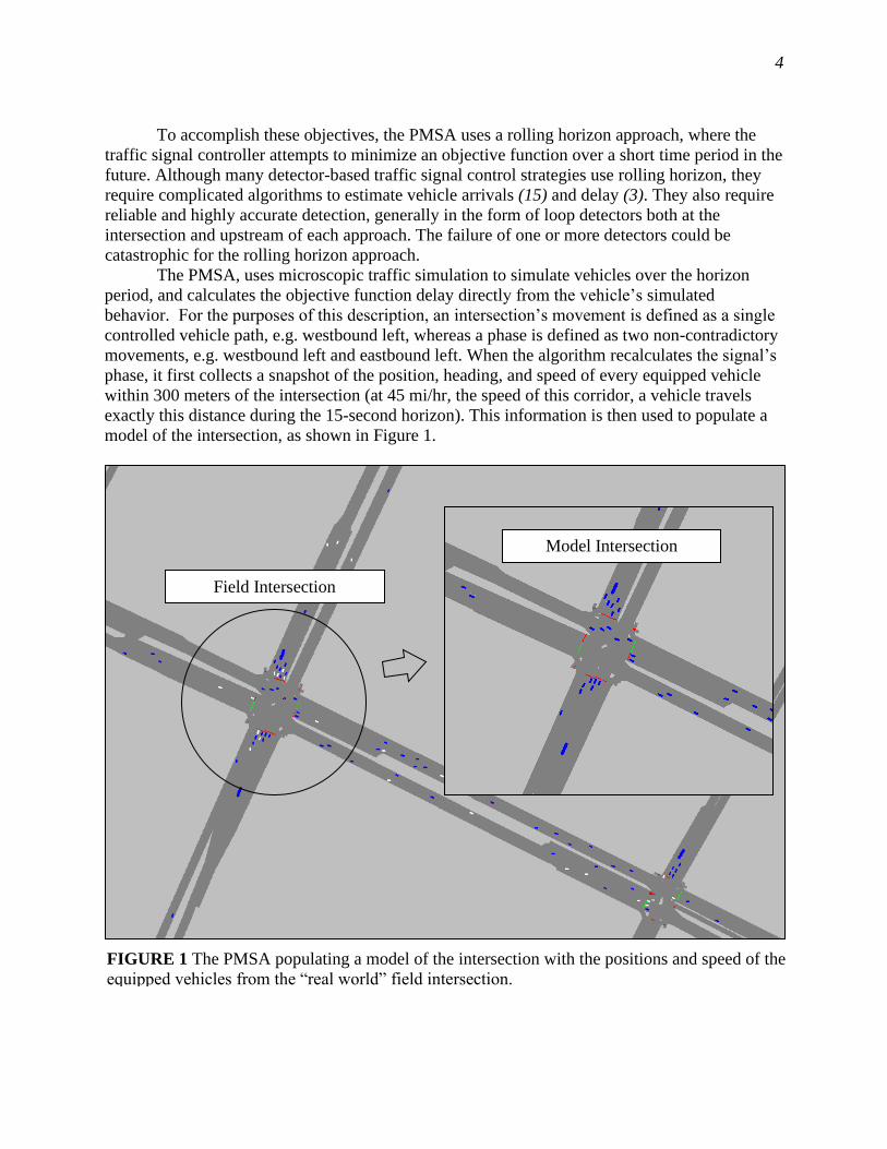
phase, it first collects a snapshot of the position, heading, and speed of every equipped vehicle

within 300 meters of the intersection (at 45 mi/hr, the speed of this corridor, a vehicle travels

exactly this distance during the 15-second horizon). This information is then used to populate a

model of the intersection, as shown in Figure 1.

Model Intersection

Field Intersection

FIGURE 1 The PMSA populating a model of the intersection with the positions and speed of the

equipped vehicles from the “real world” field intersection.

5

Once the model has been populated with the new vehicles, the vehicles are simulated

fifteen seconds into the future. Because the turn lanes in the test network were between 75 and

300 meters in length, the turning movement of many vehicles can be assumed based on their

current lane. For vehicle's upstream of the turning lane, it was assumed that 50% of those in the

lane nearest a turning lane would use the turning lane. This is repeated once for each possible

new phase configuration, as well as for the possibility of maintaining the current phasing. Four-

second amber phases and two-second red phases are simulated as well. The phase with the

optimal objective function over the fifteen second horizon is selected as the next phase.

The new phase’s green time is determined from the horizon simulation as the time

required to clear all simulated vehicles from a single movement. This time is bound with a

minimum of 5 seconds, and a maximum time before recalculation of 15 seconds.

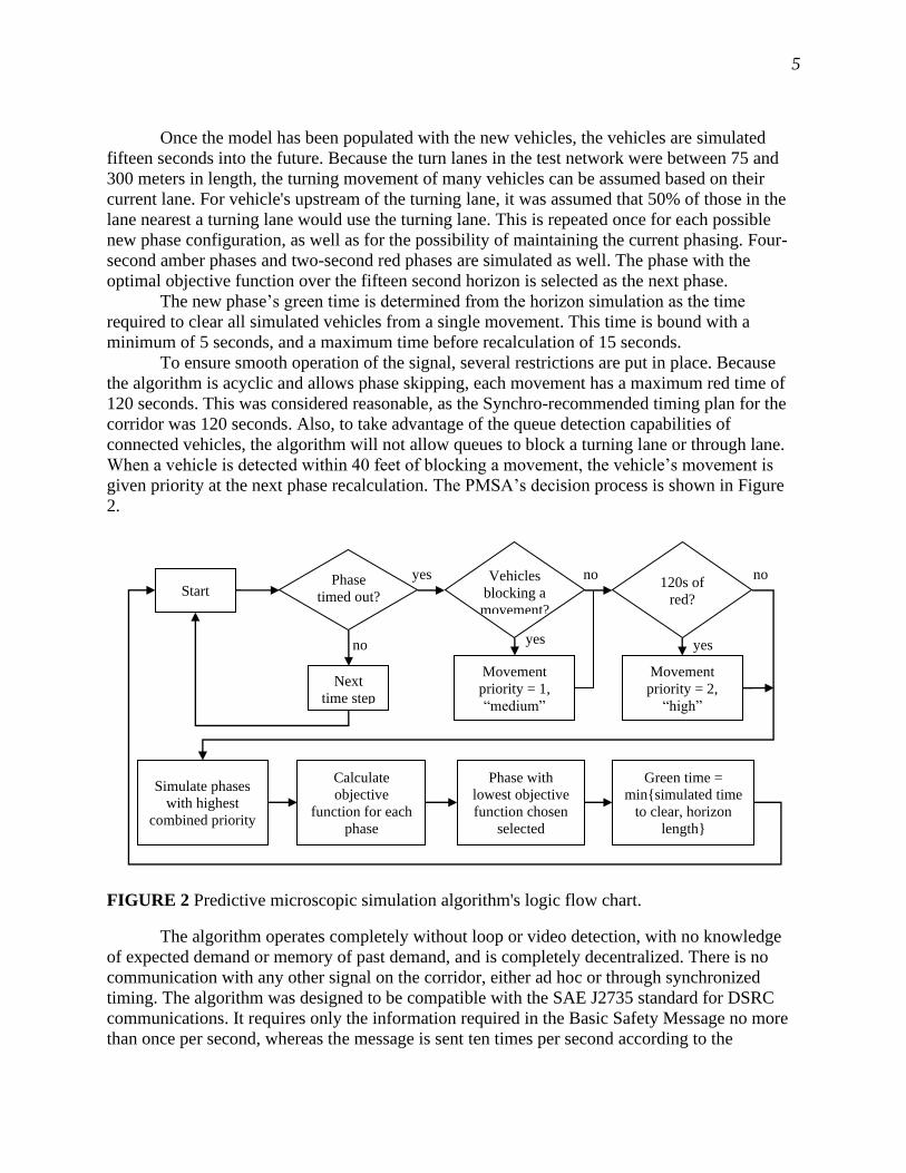
To ensure smooth operation of the signal, several restrictions are put in place. Because

the algorithm is acyclic and allows phase skipping, each movement has a maximum red time of

120 seconds. This was considered reasonable, as the Synchro-recommended timing plan for the

corridor was 120 seconds. Also, to take advantage of the queue detection capabilities of

connected vehicles, the algorithm will not allow queues to block a turning lane or through lane.

When a vehicle is detected within 40 feet of blocking a movement, the vehicle’s movement is

given priority at the next phase recalculation. The PMSA’s decision process is shown in Figure

2.

The algorithm operates completely without loop or video detection, with no knowledge

of expected demand or memory of past demand, and is completely decentralized. There is no

communication with any other signal on the corridor, either ad hoc or through synchronized

timing. The algorithm was designed to be compatible with the SAE J2735 standard for DSRC

communications. It requires only the information required in the Basic Safety Message no more

than once per second, whereas the message is sent ten times per second according to the

Start Phase

timed out? 120s of

red?

Next

time step

Movement

priority = 1,

“medium”

Movement

priority = 2,

“high”

Simulate phases

with highest

combined priority

Calculate

objective

function for each

phase

Phase with

lowest objective

function chosen

selected

Green time =

min{simulated time

to clear, horizon

length}

Vehicles

blocking a

movement?

no

no no yes

yes yes

FIGURE 2 Predictive microscopic simulation algorithm's logic flow chart.

6

standard. Further, the algorithm is able protect driver privacy by clearing any vehicle data

seconds after it is recorded. Specifically, the algorithm does not store any vehicle location data,

neither aggregated volumes nor individual vehicle trajectories, once the next phase has been

determined.

SIMULATION TESTING AND RESULTS

To simulate the connected vehicle environment, the microscopic simulation software package

VISSIM was used, as it allows users to easily access individual vehicle information via a COM

interface, and allows a second “future” simulation to run parallel to the primary simulation. For

this study, a program was written in the C# programming language using VISSIM’s COM

interface to extract individual vehicle characteristics such as speed and position no more than

once per second.

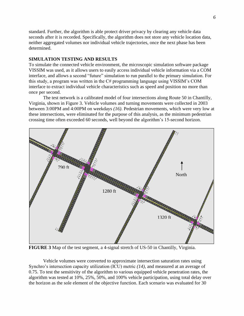
The test network is a calibrated model of four intersections along Route 50 in Chantilly,

Virginia, shown in Figure 3. Vehicle volumes and turning movements were collected in 2003

between 3:00PM and 4:00PM on weekdays (16). Pedestrian movements, which were very low at

these intersections, were eliminated for the purpose of this analysis, as the minimum pedestrian

crossing time often exceeded 60 seconds, well beyond the algorithm’s 15-second horizon.

FIGURE 3 Map of the test segment, a 4-signal stretch of US-50 in Chantilly, Virginia.

Vehicle volumes were converted to approximate intersection saturation rates using

Synchro’s intersection capacity utilization (ICU) metric (14), and measured at an average of

0.75. To test the sensitivity of the algorithm to various equipped vehicle penetration rates, the

algorithm was tested at 10%, 25%, 50%, and 100% vehicle participation, using total delay over

the horizon as the sole element of the objective function. Each scenario was evaluated for 30

790 ft

1280 ft

1320 ft

North

7

minutes after 400 seconds of simulation initialization (17). Each scenario was tested ten times at

different random seeds, and all produced statistically similar results with a 95% confidence level

(18).

Off-line signal system optimization tools such as Synchro (19) and TRANSYT-7F (20)

are often used in practice to develop timing plans. In this research, Synchro was used to develop

an optimized coordinated-actuated timing plan with a 120 cycle length as a base case for

comparison with the PMSA. Synchro’s recommended timing plans were programmed into and

tested in the VISSIM network.

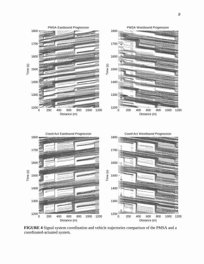
Single Variable Objective Function

The algorithm attempts to optimize some objective function over a 15 second interval. Initial

testing focused on a single variable, the cumulative vehicle delay. Although decentralized, the

algorithm produced coordinated flow, as evidenced by the signal timing and vehicle trajectories

shown in Figure 4.

8

FIGURE 4 Signal system coordination and vehicle trajectories comparison of the PMSA and a

coordinated-actuated system.

0 200 400 600 800 1000 12001200

1300

1400

1500

1600

1700

1800PMSA Eastbound Progression

Distance (m)

Tim

e (

s)

0 200 400 600 800 1000 12001200

1300

1400

1500

1600

1700

1800PMSA Westbound Progression

Distance (m)

Tim

e (

s)

0 200 400 600 800 1000 12001200

1300

1400

1500

1600

1700

1800Coord-Act Eastbound Progression

Distance (m)

Tim

e (

s)

0 200 400 600 800 1000 12001200

1300

1400

1500

1600

1700

1800Coord-Act Westbound Progression

Distance (m)

Tim

e (

s)

9

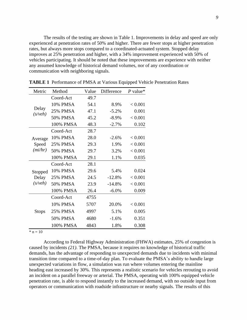
The results of the testing are shown in Table 1. Improvements in delay and speed are only

experienced at penetration rates of 50% and higher. There are fewer stops at higher penetration

rates, but always more stops compared to a coordinated-actuated system. Stopped delay

improves at 25% penetration and higher, with a 34% improvement experienced with 50% of

vehicles participating. It should be noted that these improvements are experience with neither

any assumed knowledge of historical demand volumes, nor of any coordination or

communication with neighboring signals.

TABLE 1 Performance of PMSA at Various Equipped Vehicle Penetration Rates

Metric Method Value Difference P value*

Delay

(s/veh)

Coord-Act 49.7

10% PMSA 54.1 8.9% < 0.001

25% PMSA 47.1 -5.2% 0.001

50% PMSA 45.2 -8.9% < 0.001

100% PMSA 48.3 -2.7% 0.102

Average

Speed

(mi/hr)

Coord-Act 28.7

10% PMSA 28.0 -2.6% < 0.001

25% PMSA 29.3 1.9% < 0.001

50% PMSA 29.7 3.2% < 0.001

100% PMSA 29.1 1.1% 0.035

Stopped

Delay

(s/veh)

Coord-Act 28.1

10% PMSA 29.6 5.4% 0.024

25% PMSA 24.5 -12.8% < 0.001

50% PMSA 23.9 -14.8% < 0.001

100% PMSA 26.4 -6.0% 0.009

Stops

Coord-Act 4755

10% PMSA 5707 20.0% < 0.001

25% PMSA 4997 5.1% 0.005

50% PMSA 4680 -1.6% 0.351

100% PMSA 4843 1.8% 0.308

* n = 10

According to Federal Highway Administration (FHWA) estimates, 25% of congestion is

caused by incidents (21). The PMSA, because it requires no knowledge of historical traffic

demands, has the advantage of responding to unexpected demands due to incidents with minimal

transition time compared to a time-of-day plan. To evaluate the PMSA’s ability to handle large

unexpected variations in flow, a simulation was run where volumes entering the mainline

heading east increased by 30%. This represents a realistic scenario for vehicles rerouting to avoid

an incident on a parallel freeway or arterial. The PMSA, operating with 100% equipped vehicle

penetration rate, is able to respond instantly to the increased demand, with no outside input from

operators or communication with roadside infrastructure or nearby signals. The results of this

10

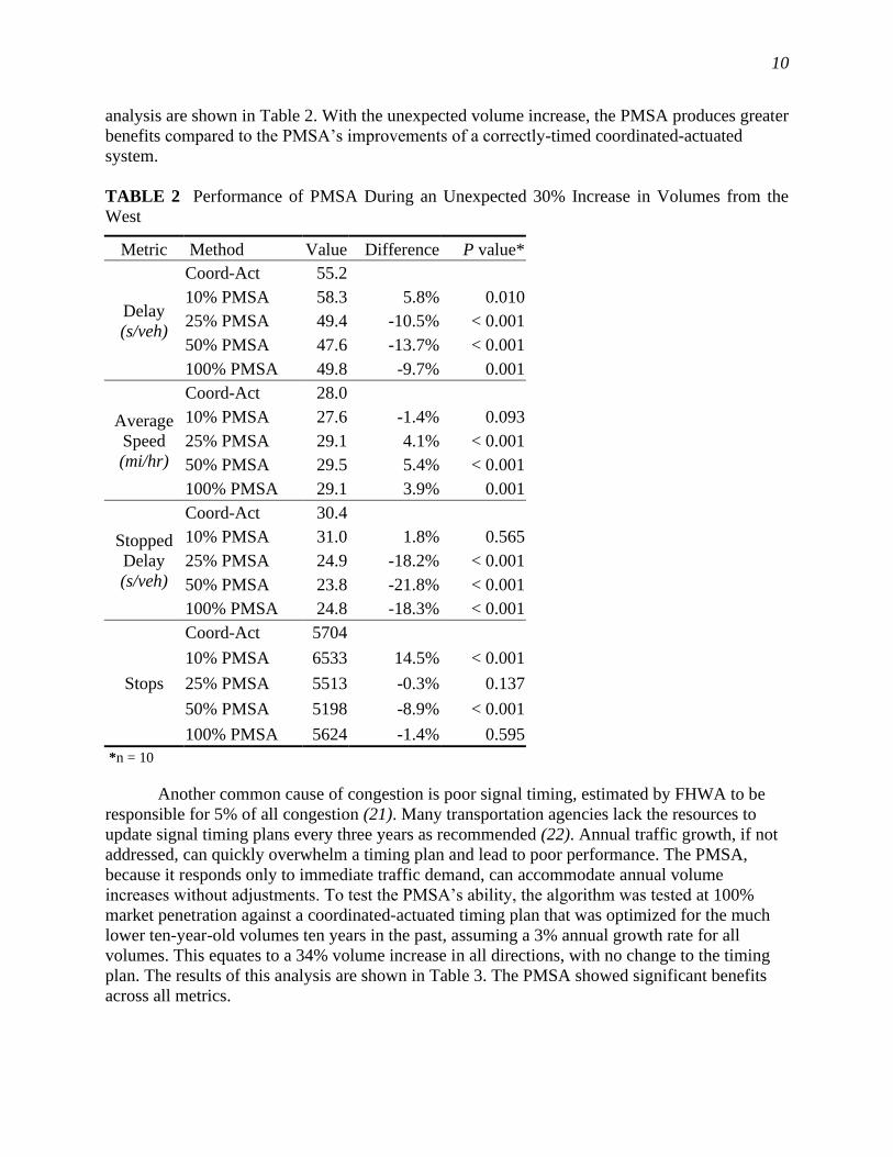
analysis are shown in Table 2. With the unexpected volume increase, the PMSA produces greater

benefits compared to the PMSA’s improvements of a correctly-timed coordinated-actuated

system.

TABLE 2 Performance of PMSA During an Unexpected 30% Increase in Volumes from the

West

Metric Method Value Difference P value*

Delay

(s/veh)

Coord-Act 55.2

10% PMSA 58.3 5.8% 0.010

25% PMSA 49.4 -10.5% < 0.001

50% PMSA 47.6 -13.7% < 0.001

100% PMSA 49.8 -9.7% 0.001

Average

Speed

(mi/hr)

Coord-Act 28.0

10% PMSA 27.6 -1.4% 0.093

25% PMSA 29.1 4.1% < 0.001

50% PMSA 29.5 5.4% < 0.001

100% PMSA 29.1 3.9% 0.001

Stopped

Delay

(s/veh)

Coord-Act 30.4

10% PMSA 31.0 1.8% 0.565

25% PMSA 24.9 -18.2% < 0.001

50% PMSA 23.8 -21.8% < 0.001

100% PMSA 24.8 -18.3% < 0.001

Stops

Coord-Act 5704

10% PMSA 6533 14.5% < 0.001

25% PMSA 5513 -0.3% 0.137

50% PMSA 5198 -8.9% < 0.001

100% PMSA 5624 -1.4% 0.595

*n = 10

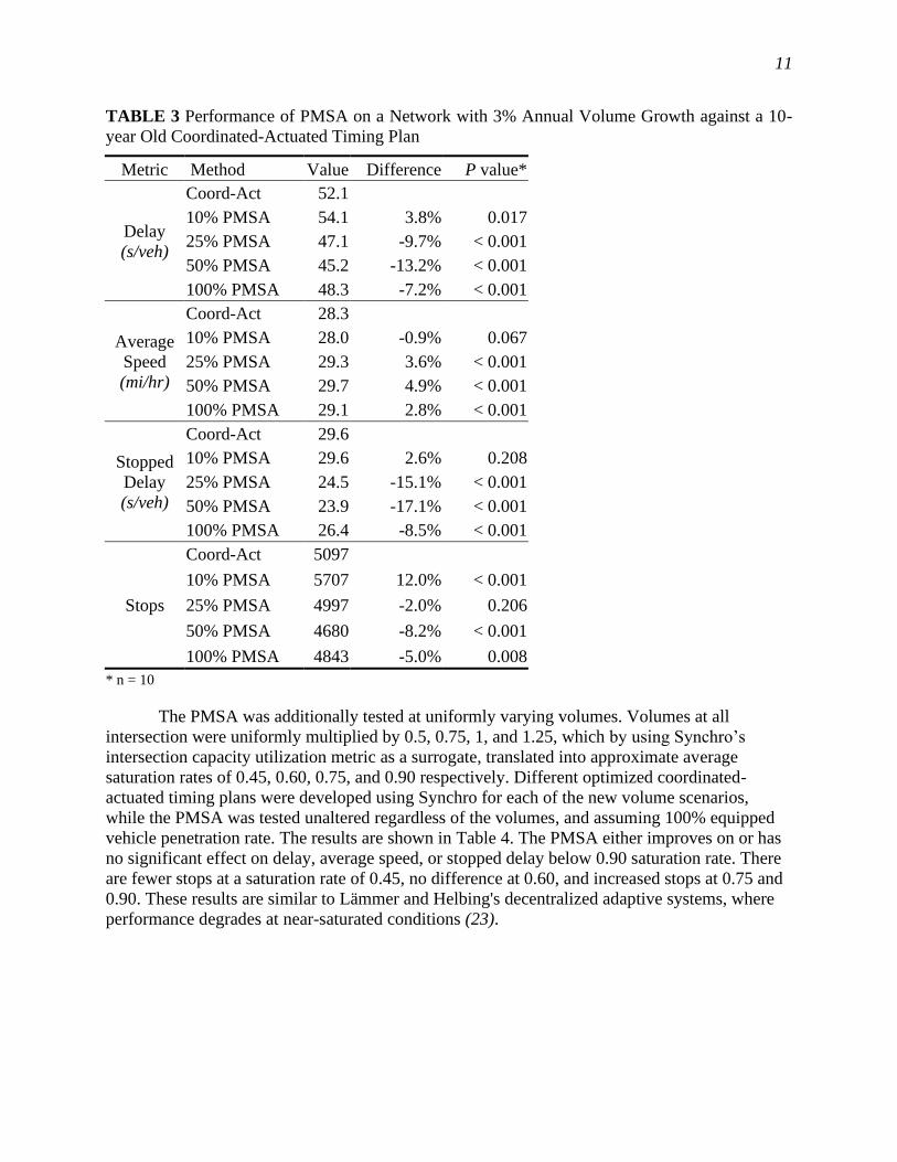
Another common cause of congestion is poor signal timing, estimated by FHWA to be

responsible for 5% of all congestion (21). Many transportation agencies lack the resources to

update signal timing plans every three years as recommended (22). Annual traffic growth, if not

addressed, can quickly overwhelm a timing plan and lead to poor performance. The PMSA,

because it responds only to immediate traffic demand, can accommodate annual volume

increases without adjustments. To test the PMSA’s ability, the algorithm was tested at 100%

market penetration against a coordinated-actuated timing plan that was optimized for the much

lower ten-year-old volumes ten years in the past, assuming a 3% annual growth rate for all

volumes. This equates to a 34% volume increase in all directions, with no change to the timing

plan. The results of this analysis are shown in Table 3. The PMSA showed significant benefits

across all metrics.

11

TABLE 3 Performance of PMSA on a Network with 3% Annual Volume Growth against a 10-

year Old Coordinated-Actuated Timing Plan

Metric Method Value Difference P value*

Delay

(s/veh)

Coord-Act 52.1

10% PMSA 54.1 3.8% 0.017

25% PMSA 47.1 -9.7% < 0.001

50% PMSA 45.2 -13.2% < 0.001

100% PMSA 48.3 -7.2% < 0.001

Average

Speed

(mi/hr)

Coord-Act 28.3

10% PMSA 28.0 -0.9% 0.067

25% PMSA 29.3 3.6% < 0.001

50% PMSA 29.7 4.9% < 0.001

100% PMSA 29.1 2.8% < 0.001

Stopped

Delay

(s/veh)

Coord-Act 29.6

10% PMSA 29.6 2.6% 0.208

25% PMSA 24.5 -15.1% < 0.001

50% PMSA 23.9 -17.1% < 0.001

100% PMSA 26.4 -8.5% < 0.001

Stops

Coord-Act 5097

10% PMSA 5707 12.0% < 0.001

25% PMSA 4997 -2.0% 0.206

50% PMSA 4680 -8.2% < 0.001

100% PMSA 4843 -5.0% 0.008

* n = 10

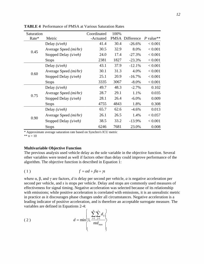
The PMSA was additionally tested at uniformly varying volumes. Volumes at all

intersection were uniformly multiplied by 0.5, 0.75, 1, and 1.25, which by using Synchro’s

intersection capacity utilization metric as a surrogate, translated into approximate average

saturation rates of 0.45, 0.60, 0.75, and 0.90 respectively. Different optimized coordinated-

actuated timing plans were developed using Synchro for each of the new volume scenarios,

while the PMSA was tested unaltered regardless of the volumes, and assuming 100% equipped

vehicle penetration rate. The results are shown in Table 4. The PMSA either improves on or has

no significant effect on delay, average speed, or stopped delay below 0.90 saturation rate. There

are fewer stops at a saturation rate of 0.45, no difference at 0.60, and increased stops at 0.75 and

0.90. These results are similar to Lämmer and Helbing's decentralized adaptive systems, where

performance degrades at near-saturated conditions (23).

12

TABLE 4 Performance of PMSA at Various Saturation Rates

Saturation

Rate* Metric

Coordinated

-Actuated

100%

PMSA Difference P value**

0.45

Delay (s/veh) 41.4 30.4 -26.6% < 0.001

Average Speed (mi/hr) 30.5 32.9 8.0% < 0.001

Stopped Delay (s/veh) 24.0 17.4 -27.3% < 0.001

Stops 2381 1827 -23.3% < 0.001

0.60

Delay (s/veh) 43.1 37.9 -12.1% < 0.001

Average Speed (mi/hr) 30.1 31.3 4.0% < 0.001

Stopped Delay (s/veh) 25.1 20.9 -16.7% < 0.001

Stops 3335 3067 -8.0% < 0.001

0.75

Delay (s/veh) 49.7 48.3 -2.7% 0.102

Average Speed (mi/hr) 28.7 29.1 1.1% 0.035

Stopped Delay (s/veh) 28.1 26.4 -6.0% 0.009

Stops 4755 4843 1.8% 0.308

0.90

Delay (s/veh) 65.7 62.6 -4.6% 0.013

Average Speed (mi/hr) 26.1 26.5 1.4% < 0.057

Stopped Delay (s/veh) 38.5 33.2 -13.9% < 0.001

Stops 6246 7681 23.0% 0.008

* Approximate average saturation rate based on Synchro's ICU metric

** n = 10

Multivariable Objective Function

The previous analysis used vehicle delay as the sole variable in the objective function. Several

other variables were tested as well if factors other than delay could improve performance of the

algorithm. The objective function is described in Equation 1:

( 1 ) sadf ++=

where α, β, and γ are factors, d is delay per second per vehicle, a is negative acceleration per

second per vehicle, and s is stops per vehicle. Delay and stops are commonly used measures of

effectiveness for signal timing. Negative acceleration was selected because of its relationship

with emissions; while positive acceleration is correlated with emissions, it is an unrealistic metric

in practice as it discourages phase changes under all circumstances. Negative acceleration is a

leading indicator of positive acceleration, and is therefore an acceptable surrogate measure. The

variables are defined in Equations 2-4:

( 2 )

=

= =

max

1 1,1min

ntd

d

d

n

i

t

j

ij

13

( 3 )

−

=

= =

max

1 1

0,max

,1minnta

a

a

n

i

t

j

ij

( 4 )

=

= =

max

1 1,1min

ns

s

s

n

i

t

j

ij

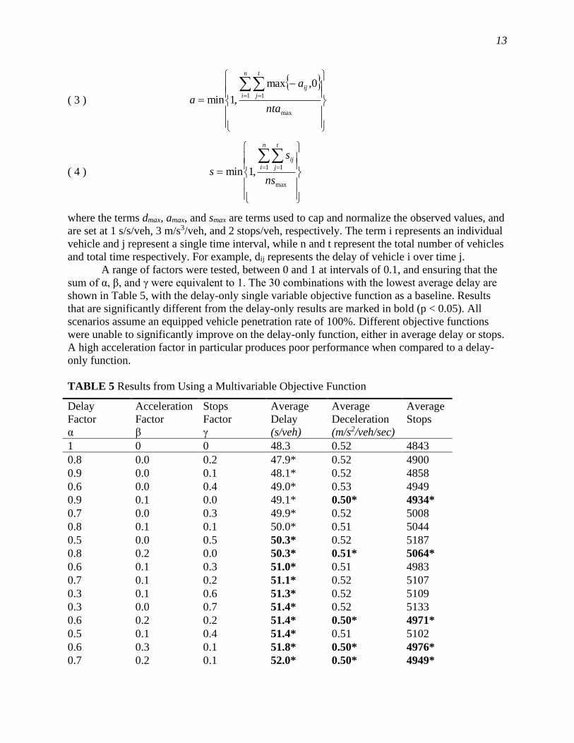
where the terms dmax, amax, and smax are terms used to cap and normalize the observed values, and

are set at 1 s/s/veh, 3 m/s3/veh, and 2 stops/veh, respectively. The term i represents an individual

vehicle and j represent a single time interval, while n and t represent the total number of vehicles

and total time respectively. For example, dij represents the delay of vehicle i over time j.

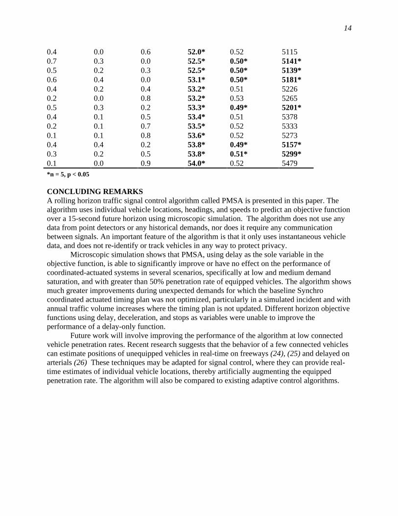
A range of factors were tested, between 0 and 1 at intervals of 0.1, and ensuring that the

sum of α, β, and γ were equivalent to 1. The 30 combinations with the lowest average delay are

shown in Table 5, with the delay-only single variable objective function as a baseline. Results

that are significantly different from the delay-only results are marked in bold (p < 0.05). All

scenarios assume an equipped vehicle penetration rate of 100%. Different objective functions

were unable to significantly improve on the delay-only function, either in average delay or stops.

A high acceleration factor in particular produces poor performance when compared to a delay-

only function.

TABLE 5 Results from Using a Multivariable Objective Function

Delay

Factor

α

Acceleration

Factor

β

Stops

Factor

γ

Average

Delay

(s/veh)

Average

Deceleration

(m/s2/veh/sec)

Average

Stops

1 0 0 48.3 0.52 4843

0.8 0.0 0.2 47.9* 0.52 4900

0.9 0.0 0.1 48.1* 0.52 4858

0.6 0.0 0.4 49.0* 0.53 4949

0.9 0.1 0.0 49.1* 0.50* 4934*

0.7 0.0 0.3 49.9* 0.52 5008

0.8 0.1 0.1 50.0* 0.51 5044

0.5 0.0 0.5 50.3* 0.52 5187

0.8 0.2 0.0 50.3* 0.51* 5064*

0.6 0.1 0.3 51.0* 0.51 4983

0.7 0.1 0.2 51.1* 0.52 5107

0.3 0.1 0.6 51.3* 0.52 5109

0.3 0.0 0.7 51.4* 0.52 5133

0.6 0.2 0.2 51.4* 0.50* 4971*

0.5 0.1 0.4 51.4* 0.51 5102

0.6 0.3 0.1 51.8* 0.50* 4976*

0.7 0.2 0.1 52.0* 0.50* 4949*

14

0.4 0.0 0.6 52.0* 0.52 5115

0.7 0.3 0.0 52.5* 0.50* 5141*

0.5 0.2 0.3 52.5* 0.50* 5139*

0.6 0.4 0.0 53.1* 0.50* 5181*

0.4 0.2 0.4 53.2* 0.51 5226

0.2 0.0 0.8 53.2* 0.53 5265

0.5 0.3 0.2 53.3* 0.49* 5201*

0.4 0.1 0.5 53.4* 0.51 5378

0.2 0.1 0.7 53.5* 0.52 5333

0.1 0.1 0.8 53.6* 0.52 5273

0.4 0.4 0.2 53.8* 0.49* 5157*

0.3 0.2 0.5 53.8* 0.51* 5299*

0.1 0.0 0.9 54.0* 0.52 5479

*n = 5, p < 0.05

CONCLUDING REMARKS

A rolling horizon traffic signal control algorithm called PMSA is presented in this paper. The

algorithm uses individual vehicle locations, headings, and speeds to predict an objective function

over a 15-second future horizon using microscopic simulation. The algorithm does not use any

data from point detectors or any historical demands, nor does it require any communication

between signals. An important feature of the algorithm is that it only uses instantaneous vehicle

data, and does not re-identify or track vehicles in any way to protect privacy.

Microscopic simulation shows that PMSA, using delay as the sole variable in the

objective function, is able to significantly improve or have no effect on the performance of

coordinated-actuated systems in several scenarios, specifically at low and medium demand

saturation, and with greater than 50% penetration rate of equipped vehicles. The algorithm shows

much greater improvements during unexpected demands for which the baseline Synchro

coordinated actuated timing plan was not optimized, particularly in a simulated incident and with

annual traffic volume increases where the timing plan is not updated. Different horizon objective

functions using delay, deceleration, and stops as variables were unable to improve the

performance of a delay-only function.

Future work will involve improving the performance of the algorithm at low connected

vehicle penetration rates. Recent research suggests that the behavior of a few connected vehicles

can estimate positions of unequipped vehicles in real-time on freeways (24), (25) and delayed on

arterials (26) These techniques may be adapted for signal control, where they can provide real-

time estimates of individual vehicle locations, thereby artificially augmenting the equipped

penetration rate. The algorithm will also be compared to existing adaptive control algorithms.

15

REFERENCES

1. Hunt, P. B., R. D. Bretherton, D. I. Robertson, and M. C. Royal. SCOOT Online Traffic

Signal Optimsation Technique. Traffic Engineering and Control, Vol. 23, 1982. pp. 190–192.

2. Sims, A. and K. W. Dobinson. The Sydney Coordinated Adaptive Traffic (SCAT) System

Philosophy and Benefits. IEEE Transportation Vehicle Technology, Vol. 29, No. 2, May

1980, pp. 130–137.

3. Porche, I. and S. Lafortune. Adaptive Look-ahead Optimization of Traffic Signals. Journal of

Intelligent Transportation Systems, Vol. 4, No. 3, 1999, pp. 209–254.

4. Mauro, V. and C. Di Taranto. UTOPIA. Presented at the the Sixth IFAC/IFIP/IFORS

Symposium on Control and Communications in Transportation, Paris, France, 1990.

5. Henry, J.J., J. L. Farges, and J. Tufal. The PRODYN Real Time Traffic Algorithm. Presented

at the 4th IFAC/IFIP/IFORS International Conference on Control in Transportation Systems,

Baden, 1983, pp. 307–311.

6. Gartner, N. H. OPAC: A Demand-Responsive Strategy for Traffic Signal Control. In

Transportation Research Record: Journal of the Transportation Research Board, No. 906,

Transportation Research Board of the National Academies, Washington, D.C., 1983, pp. 75–

81.

7. Mirchandani, P. A. Real-time Traffic Signal Control System: Architecture, Algorithms, and

Analysis. Transportation Research Part C: Emerging Technologies, Vol. 9, No. 6, December

2001, pp. 415–432.

8. Stevanovic, A. Adaptive Traffic Control Systems: Domestic and Foreign State of Practice.

NCHRP Synthesis 403. National Research Council, Transportation Research Board, National

Cooperative Highway Research Program, American Association of State Highway and

Transportation Officials, and Federal Highway Administration, 2010.

9. Society of Automotive Engineers. Dedicated Short Range Communications (DSRC) Message

Set Dictionary. Standard SAE J2735, Nov. 2009.

10. Priemer, C. and B. Friedrich. A Decentralized Adaptive Traffic Signal Control Using V2I

Communication Data. Presented at 12th International IEEE Conference on Intelligent

Transportation Systems, St. Louis, MO, 2009, pp. 1–6.

11. Datesh, J., W. T. Scherer, and B. L. Smith. Using K-Means Clustering to Improve Traffic

Signal Efficacy in an IntelliDrive Environment. Presented at 2011 IEEE Forum on Integrated

and Sustainable Transportation Systems, Vienna, Austria, June 2011.

12. Lee, J. Assessing the Potential Benefits of IntelliDrive-based Intersection Control

Algorithms. Dissertation, University of Virginia, Charlottesville, VA, 2010.

13. He, Q., K. L. Head, and J. Ding. PAMSCOD: Platoon-based Arterial Multi-modal Signal

Control with Online Data. Transportation Research Part C: Emerging Technologies, Vol.

20, February 2012, pp. 164–184.

14. Husch, D. and J. Albeck. Intersection Capacity Utilization. Trafficware, 2003.

15. www.trafficware.com/assets/pdfs/ICU2003.pdf. Accessed July 2, 2012.

16. Head, K. L. Event-Based Short-Term Traffic Flow Prediction Model. In Transportation

Research Record: Journal of the Transportation Research Board, No. 1510, Transportation

Research Board of the National Academies, Washington, D.C., 1995, pp. 45-52.

17. Park, B., and J. D. Schneeberger. Microscopic Simulation Model Calibration and Validation:

Case Study of VISSIM Simulation Model for a Coordinated Actuated Signal System. In

Transportation Research Record: Journal of the Transportation Research Board, No. 1856,

16

Transportation Research Board of the National Academies, Washington, D.C., 2003, pp.

185–192.

18. Dowling, R., A. Skabardonis, and V. Alexiadis. Traffic Analysis Toolbox Volume III:

Guidelines for Applying Traffic Microsimulation Software. Publication FHWA-HRT-04-040.

FHWA, U.S. Department of Transportation, June 2004.

19. Law, A. Simulation Modeling and Analysis, 4th Edition. McGraw-Hill, Dubuque , Iowa,

2007.

20. Synchro Studio 8.0 User’s Guide. Trafficware, June 2011.

21. TRANSYT-7F User’s Guide. TRANSYT-7F Version 11.3, McTrans, University of Florida,

Gainesville, Florida, 2011.

22. Focus on Congestion Relief | Describing the Congestion Problem. FHWA, 2004.

23. www.fhwa.dot.gov/congestion/describing_problem.htm. Accessed July 20, 2012.

24. National Transportation Operations Coalition. National Traffic Signal Report Card. Institute

of Transportation Engineers, 2012.

25. Lämmer, S. and D. Helbing. Self-control of Traffic Lights and Vehicle Flows in Urban Road

Networks. Journal of Statistical Mechanics: Theory and Experiment, Vol. 4, April 2008.

26. Herrera, J. C., and A. M. Bayen. Incorporation of Lagrangian Measurements in Freeway

Traffic State Estimation. Transportation Research Part B: Methodological, Vol. 44, No. 4,

May 2010, pp. 460–481.

27. Goodall, N. J., B. L. Smith, and B. Park. Microscopic Estimation of Freeway Vehicle

Positions Using Mobile Sensors. Presented at 90th Annual Meeting of the Transportation

Research Board, Washington D.C., 2012.

28. Sun Z., and X. Ban. Vehicle Trajectory Reconstruction for Signalized Intersections Using

Variational Formulation of Kinematic Waves. Presented at 89th Annual Meeting of the

Transportation Research Board, Washington D.C., 2011.