IN DEGREE PROJECT MATHEMATICS,SECOND CYCLE, 30 CREDITS

, STOCKHOLM SWEDEN 2021

Traffic Prediction From Temporal Graphs Using Representation Learning

ANDREAS MOVIN

KTH ROYAL INSTITUTE OF TECHNOLOGYSCHOOL OF ENGINEERING SCIENCES

Abstract

With the arrival of 5G networks, telecommunication systems are becoming more intelligent, in-tegrated, and broadly used. This thesis focuses on predicting the upcoming traffic to efficientlypromote resource allocation, guarantee stability and reliability of the network. Since networksmodeled as graphs potentially capture more information than tabular data, the construction of thegraph and choice of the model are key to achieve a good prediction. In this thesis traffic predictionis based on a time-evolving graph, whose node and edges encode the structure and activity ofthe system. Edges are created by dynamic time-warping (DTW), geographical distance, and k-nearest neighbors. The node features contain different temporal information together with spatialinformation computed by methods from topological data analysis (TDA). To capture the temporaland spatial dependency of the graph several dynamic graph methods are compared. Throughoutexperiments, we could observe that the most successful model GConvGRU performs best for edgescreated by DTW and node features that include temporal information across multiple time steps.

Keywords: Dynamic time warping (DTW), embedding, graph convolutional networks (GCN),graph neural networks (GNN), persistent homology, spectral graph theory, temporal graphs, topo-logical data analysis (TDA).

i

Sammanfattning

Svensk titel: Trafikforutsagelse fran dynamiska grafer genom representationsinlarning

Med ankomsten av 5G natverk blir telekommunikationssystemen alltmer intelligenta, integrerade,och bredare anvanda. Denna uppsats fokuserar pa att forutse den kommande nattrafiken, foratt effektivt hantera resursallokering, garantera stabilitet och palitlighet av natverken. Eftersomnatverk som modelleras som grafer har potential att innehalla mer information an tabular data, arskapandet av grafen och valet av metod viktigt for att uppna en bra forutsagelse. I denna uppsats artrafikforutsagelsen baserad pa grafer som andras over tid, vars noder och lankar fangar strukturenoch aktiviteten av systemet. Lankarna skapas genom dynamisk time warping (DTW), geografiskdistans, och k-narmaste grannarna. Egenskaperna for noderna bestar av dynamisk och rumsliginformation som beraknats av metoder fran topologisk dataanalys (TDA). For att inkludera savaldet dynamiska som det rumsliga beroendet av grafen, jamfors flera dynamiska grafmetoder. Genomexperiment, kunde vi observera att den mest framgangsrika modellen GConvGRU presterade bastfor lankar skapade genom DTW och noder som innehaller dynamisk information over flera tidssteg.

Nyckelord: Dynamisk time warping (DTW), inbaddning, convolutional grafnatverk (GCN),neurala grafnatverk (GNN), persistent homologi, spektral graf teori, dynamisk graf, topologiskdataanalys (TDA).

ii

Acknowledgment

Ericsson has provided a great, interesting, and stimulating thesis project, right at the heart ofcutting-edge methods. Ericsson has provided excellent supervision in the forms of Marios Daoutisand Yifei Jin. Our weekly discussions to explore new possibilities have made working on this thesisall the more interesting. The possibility to always have a quick call to discuss some matter oranother has been truly appreciated.

The support along the way has been extraordinary from the supervisors at KTH. Their drive,interest to explore new areas and include the field of TDA in the thesis have made this thesis evenmore fascinating to work on. I could not have wished for better supervision and guidance fromKTH than the one given by Martina Scolamiero and Andrea Guidolin.

iii

Contents

1 Introduction 11.1 Research questions . . . . . . . . . . . . . . . . . . . . . . . . . . . . . . . . . . . . 11.2 Outline . . . . . . . . . . . . . . . . . . . . . . . . . . . . . . . . . . . . . . . . . . 2

2 Mathematical background 32.1 Graph theory . . . . . . . . . . . . . . . . . . . . . . . . . . . . . . . . . . . . . . . 3

Definitions of graph theory . . . . . . . . . . . . . . . . . . . . . . . . . . . . . . . 3Spectral graph theory . . . . . . . . . . . . . . . . . . . . . . . . . . . . . . . . . . 5Static and temporal graph representations . . . . . . . . . . . . . . . . . . . . . . . 6

2.2 Topological data analysis (TDA) . . . . . . . . . . . . . . . . . . . . . . . . . . . . 6Definitions and background of TDA . . . . . . . . . . . . . . . . . . . . . . . . . . 7

3 Machine learning 133.1 Machine learning background . . . . . . . . . . . . . . . . . . . . . . . . . . . . . . 13

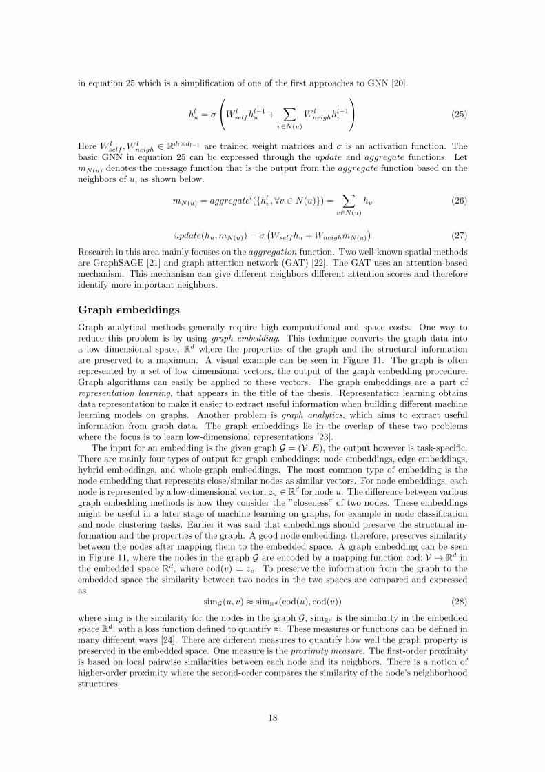
Machine learning on graphs . . . . . . . . . . . . . . . . . . . . . . . . . . . . . . . 14Spectral methods . . . . . . . . . . . . . . . . . . . . . . . . . . . . . . . . . . . . . 16Spatial methods . . . . . . . . . . . . . . . . . . . . . . . . . . . . . . . . . . . . . 17Graph embeddings . . . . . . . . . . . . . . . . . . . . . . . . . . . . . . . . . . . . 18

3.2 Graph convolutional neural networks and TDA . . . . . . . . . . . . . . . . . . . . 193.3 Recent methods . . . . . . . . . . . . . . . . . . . . . . . . . . . . . . . . . . . . . . 20

4 Data set 224.1 Data processing . . . . . . . . . . . . . . . . . . . . . . . . . . . . . . . . . . . . . . 22

5 Modeling 245.1 Graph model . . . . . . . . . . . . . . . . . . . . . . . . . . . . . . . . . . . . . . . 24

Three ways to create edges . . . . . . . . . . . . . . . . . . . . . . . . . . . . . . . 24Node features . . . . . . . . . . . . . . . . . . . . . . . . . . . . . . . . . . . . . . . 26Persistence image . . . . . . . . . . . . . . . . . . . . . . . . . . . . . . . . . . . . . 26

5.2 Machine learning model . . . . . . . . . . . . . . . . . . . . . . . . . . . . . . . . . 27

6 Experiments 28

7 Results 307.1 Edge constructions . . . . . . . . . . . . . . . . . . . . . . . . . . . . . . . . . . . . 317.2 Weekly predictions . . . . . . . . . . . . . . . . . . . . . . . . . . . . . . . . . . . . 347.3 Node features . . . . . . . . . . . . . . . . . . . . . . . . . . . . . . . . . . . . . . . 357.4 Persistence diagrams . . . . . . . . . . . . . . . . . . . . . . . . . . . . . . . . . . . 36

8 Discussion 378.1 Performance of edge constructions . . . . . . . . . . . . . . . . . . . . . . . . . . . 378.2 Performance of weekly prediction . . . . . . . . . . . . . . . . . . . . . . . . . . . . 378.3 Performance of node features . . . . . . . . . . . . . . . . . . . . . . . . . . . . . . 388.4 Persistence diagrams . . . . . . . . . . . . . . . . . . . . . . . . . . . . . . . . . . . 388.5 Research questions . . . . . . . . . . . . . . . . . . . . . . . . . . . . . . . . . . . . 388.6 Future work . . . . . . . . . . . . . . . . . . . . . . . . . . . . . . . . . . . . . . . . 39

9 Conclusion 39

References 40

iv

List of Figures

1 Example graph . . . . . . . . . . . . . . . . . . . . . . . . . . . . . . . . . . . . . . 32 Demonstration of different kinds of edges . . . . . . . . . . . . . . . . . . . . . . . 43 A temporal graph with timestamps on the edges . . . . . . . . . . . . . . . . . . . 64 A sequence of graph snapshots . . . . . . . . . . . . . . . . . . . . . . . . . . . . . 75 The pipeline for persistent homology . . . . . . . . . . . . . . . . . . . . . . . . . . 76 Example of first four p-simplices . . . . . . . . . . . . . . . . . . . . . . . . . . . . 87 Point clouds for increasing values of ε with their corresponding VRε complexes . . 98 An example of barcodes for Hp, with p ∈ {0, 1, 2} . . . . . . . . . . . . . . . . . . . 129 The Architecture of a neural network . . . . . . . . . . . . . . . . . . . . . . . . . . 1410 Example of different machine learning tasks on graphs . . . . . . . . . . . . . . . . 1511 A graph embedding from G to Rd . . . . . . . . . . . . . . . . . . . . . . . . . . . . 1912 Overview of the geographical areas included in the data set . . . . . . . . . . . . . 2213 A collection of patterns and distribution for the data set . . . . . . . . . . . . . . . 2314 The number of isolated vertices for ε-close and k-neighbors . . . . . . . . . . . . . 2415 Normalized and unnormalized hourly connections plotted for the DTW example . 2616 Illustration of node features . . . . . . . . . . . . . . . . . . . . . . . . . . . . . . . 2717 Example of performance . . . . . . . . . . . . . . . . . . . . . . . . . . . . . . . . . 3018 MAPE, RSME and MAE for different methods for different ways to construct edges 3119 Comparison between the 3 different approaches to construct edges for GConvGRU 3220 The performance for edges created by a combination of approaches . . . . . . . . . 3321 The performance for different weekdays . . . . . . . . . . . . . . . . . . . . . . . . 3422 The performance for different setup of node features . . . . . . . . . . . . . . . . . 3523 The persistence diagram for H0 and H1 for two different distances . . . . . . . . . 36

List of Tables

1 Common choices for activation functions . . . . . . . . . . . . . . . . . . . . . . . . 132 Performance of the ARIMA model . . . . . . . . . . . . . . . . . . . . . . . . . . . 33

v

1 Introduction

Many aspects of today’s society can be modeled, investigated, and understood thanks to graphs.In a general setting, a graph is a collection of objects (nodes/vertices), together with a set ofinteractions (edges/links) between the objects. Graphs are widely used across different areas.An example is social networks, where the nodes represent users and the edges represent someinteraction between the users. Another example comes from chemistry: chemical compounds areoften modeled as a graph where the nodes represent atoms and the edges represent chemical bonds.Graphs are also used in the fields of social sciences, linguistics, biology, physics, and technology.Technology networks, and in particular telecommunication networks, will be the focus of this thesis.

The use of the internet is a part of many aspects of our lives, ranging from work to entertain-ment. We are more connected than ever before. With the arrival of 5G networks, the telecommu-nication systems are becoming more intelligent, integrated, and more broadly used. To efficientlypromote resource allocation, guarantee stability and reliability of a network the upcoming traffichas to be accurately predicted. A correctly predicted network traffic can provide information toturn off part of the network to save energy or to improve and optimize signal coverage. Addition-ally, it is likely that the increasing interest in autonomous vehicles and remote IoT control will bea large part of future traffic demand. These applications require high bandwidth and low latency,and to meet these requirements an accurate traffic prediction can be very useful.

Network traffic prediction has been studied for a long time. It is however not an easy problem.The complex dependency between spatial and temporal aspects is especially hard to model, andmost of the proposed methods do not provide conclusive and fully satisfactory solutions. Recently,a new impulse to traffic prediction has been given by graph-based machine learning methods.

Machine learning on graphs or similar non-Euclidean spaces that can be modeled as a graphhas become an increasing area of research in recent years. Unlike the methods for Euclidean spacessuch as convolutional neural networks, widely used for image recognition, the methods for non-Euclidean spaces are not as well developed. Even if there are several well-established graph-basedmachine learning methods, they mainly cover the case of static graphs. Including the temporaldependencies, which is a key aspect of tasks such as traffic forecasting, is a challenging problem.

The external project provider for this thesis is Ericsson. Predicting the upcoming traffic can bevery useful for Ericsson, as it can contribute to guarantee stability and reliability of the network,improve resource allocation, and optimize signal coverage. In this thesis, we use an open data setof telecommunication traffic that we chose due to the similarity with Ericsson’s private data.

This thesis focuses on several aspects of traffic forecasting. First, a graph is generated from thedata: the nodes represent the base stations of the telecommunication network, while the edges canbe modeled to encode different features of the traffic on the network. Second, traffic prediction isdone by several machine learning methods that are applied to the previously defined graph. Third,with the aim of improving the performance of the machine learning methods, the use of techniquesfrom topological data analysis is explored.

1.1 Research questions

The aim of this thesis is to address the following research questions.

• How to formalize a graph to achieve the best possible traffic prediction?

• What method gives the most accurate traffic prediction?

The first research question can be subdivided into two tasks. The first one consists of decidinghow to construct edges between the graph nodes and how to assign them weights. The second taskis investigating which aspects of the spatial and temporal dependencies can be encoded as nodefeatures that enhance traffic prediction.

To address the second research question, several classes of models are considered, includinggraph neural networks, temporal graph neural networks, and time-series methods.

1

1.2 Outline

The outline of this thesis is the following. In Section 2 the mathematical background that isrequired to understand the upcoming models are presented, it consists of two main sections oneon graph theory and one on topological data analysis. With the mathematical background inhand, in Section 3 different machine learning methods are presented together with some recentmethods used for machine learning on graphs. Section 4 includes all information that is neededabout the data set. In Section 5 the modeling of the graph and the used networks are presented.The experimental setup is explained in Section 6, the experiments give the results presented inSection 7. The results are discussed and analyzed in Section 8. Lastly, the work is summarizedand concluded in Section 9.

2

2 Mathematical background

This section gives a background for a better understanding of the upcoming models and methodsused in this thesis. The two subsections include theory on graphs and the field of topological dataanalysis. These subsections will provide the necessary foundation to understand machine learningon graphs and how topological data analysis can be used in that area.

2.1 Graph theory

Many different real-world systems can be understood by formulating them as a graph. Thesegraphs can be used to model applications ranging from social media interactions to molecules. Tobe better understand the framework and the background some formal descriptions of graphs willnow be given.

v1

v2

v3

v4

v5

v6

Figure 1: An example of a graph with undirected and unweighted edges.

Definitions of graph theory

We start with the formal definition of a graph.

Definition 2.1 A graph G = (V, E) is a collection of two sets, a set of vertices V and a set ofedges E. An edge between u ∈ V and v ∈ V is denoted as (u, v) ∈ E and represents pairwiserelations between entities.

The set of edges E is referred to as the edge-set and the set of vertices V is referred to as the vertex-set. Some other common names for vertices and edges are respectively nodes and links, these willboth be used interchangeably throughout this thesis. Vertices and edges can represent differentobjects depending on what is modeled. For a social media platform the nodes might correspondto users and/or posts and the edges appear if one is a friend with another user or likes a certainpost. Or they can represent completely different things such as protein-protein interactions. Anexample of a graph can be seen in Figure 1, the vertices are there denoted by vi.

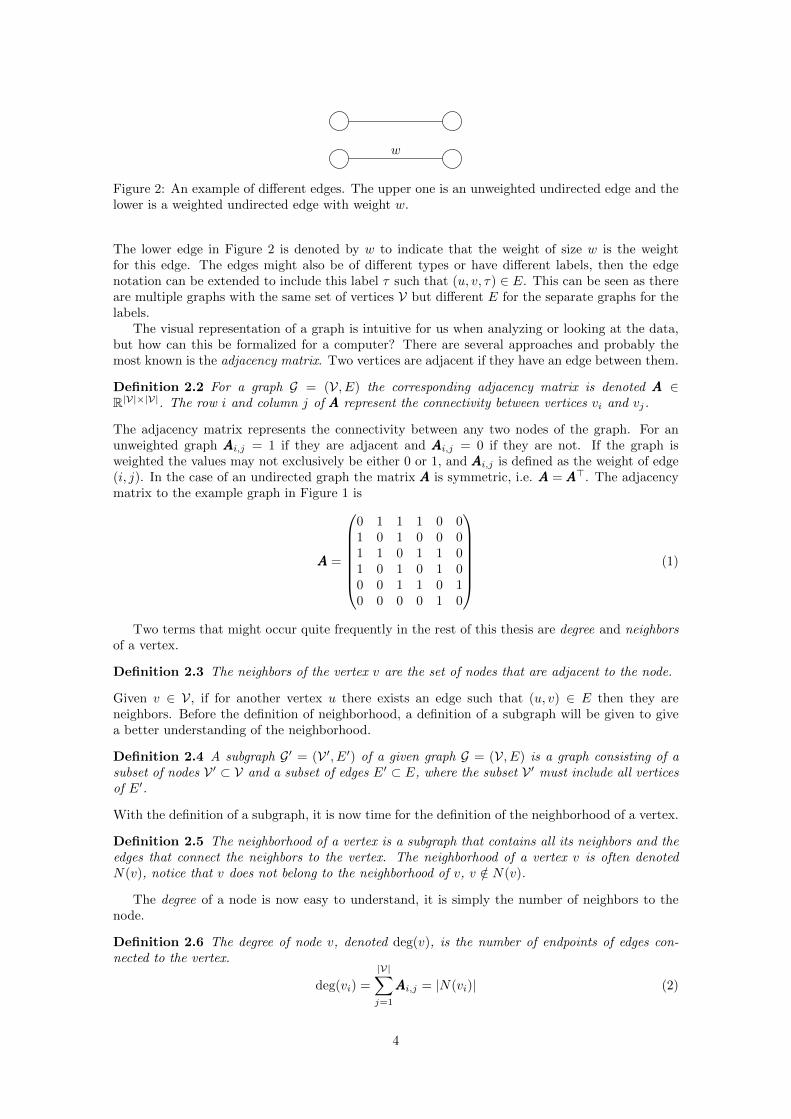
The edges of a graph may come in different forms. As mentioned in the above description ofa graph the edges are between a set of two vertices u ∈ V and v ∈ V and nothing is mentionedabout the order. This is called an undirected graph, meaning that it is a connection between thetwo vertices without going or ending up at any of the nodes, this is the upper edge in Figure 2.Another form of an edge is a weighted edge. Here the edge is a triple (u, v, w) ∈ E, where u ∈ Vand v ∈ V are vertices and w ∈ R is the weight for the edge. This weight might represent a cost orlength such as in the classical traveling salesman problem where weights are the path’s distance.

3

w

Figure 2: An example of different edges. The upper one is an unweighted undirected edge and thelower is a weighted undirected edge with weight w.

The lower edge in Figure 2 is denoted by w to indicate that the weight of size w is the weightfor this edge. The edges might also be of different types or have different labels, then the edgenotation can be extended to include this label τ such that (u, v, τ) ∈ E. This can be seen as thereare multiple graphs with the same set of vertices V but different E for the separate graphs for thelabels.

The visual representation of a graph is intuitive for us when analyzing or looking at the data,but how can this be formalized for a computer? There are several approaches and probably themost known is the adjacency matrix. Two vertices are adjacent if they have an edge between them.

Definition 2.2 For a graph G = (V, E) the corresponding adjacency matrix is denoted AAA ∈R|V|×|V|. The row i and column j of AAA represent the connectivity between vertices vi and vj.

The adjacency matrix represents the connectivity between any two nodes of the graph. For anunweighted graph AAAi,j = 1 if they are adjacent and AAAi,j = 0 if they are not. If the graph isweighted the values may not exclusively be either 0 or 1, and AAAi,j is defined as the weight of edge(i, j). In the case of an undirected graph the matrix AAA is symmetric, i.e. AAA = AAA>. The adjacencymatrix to the example graph in Figure 1 is

AAA =

0 1 1 1 0 01 0 1 0 0 01 1 0 1 1 01 0 1 0 1 00 0 1 1 0 10 0 0 0 1 0

(1)

Two terms that might occur quite frequently in the rest of this thesis are degree and neighborsof a vertex.

Definition 2.3 The neighbors of the vertex v are the set of nodes that are adjacent to the node.

Given v ∈ V, if for another vertex u there exists an edge such that (u, v) ∈ E then they areneighbors. Before the definition of neighborhood, a definition of a subgraph will be given to givea better understanding of the neighborhood.

Definition 2.4 A subgraph G′ = (V ′, E′) of a given graph G = (V, E) is a graph consisting of asubset of nodes V ′ ⊂ V and a subset of edges E′ ⊂ E, where the subset V ′ must include all verticesof E′.

With the definition of a subgraph, it is now time for the definition of the neighborhood of a vertex.

Definition 2.5 The neighborhood of a vertex is a subgraph that contains all its neighbors and theedges that connect the neighbors to the vertex. The neighborhood of a vertex v is often denotedN(v), notice that v does not belong to the neighborhood of v, v /∈ N(v).

The degree of a node is now easy to understand, it is simply the number of neighbors to thenode.

Definition 2.6 The degree of node v, denoted deg(v), is the number of endpoints of edges con-nected to the vertex.

deg(vi) =

|V|∑j=1

AAAi,j = |N(vi)| (2)

4

The node degree in an undirected graph is equal to the number of edges connected to the vertex.For an undirected graph where the degree of each node is deg(v) = |V| − 1, each node is uniquelyconnected to every other node in the graph, which is called a complete graph.

In a graph, G, it might be possible to go from one vertex to any other vertex in the graphthrough the edges. This is not generally the case. A graph can consist of several so-calledconnected components.

Definition 2.7 A subgraph G′ = (V ′, E′) of a given graph G = (V, E) is said to be a connectedcomponent if there exists at least one path between any pair of nodes in the graph G′ and the verticesin V ′ are not adjacent to any vertices in V \ V ′

The use of connected components will hopefully become more clear after the introduction totopological data analysis.

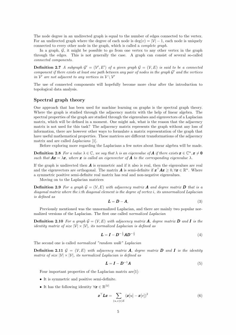
Spectral graph theory

One approach that has been used for machine learning on graphs is the spectral graph theory.Where the graph is studied through the adjacency matrix with the help of linear algebra. Thespectral properties of the graph are studied through the eigenvalues and eigenvectors of a Laplacianmatrix, which will be defined in a moment. One might ask, what is the reason that the adjacencymatrix is not used for this task? The adjacency matrix represents the graph without any loss ofinformation, there are however other ways to formulate a matrix representation of the graph thathave useful mathematical properties. These matrices are different transformations of the adjacencymatrix and are called Laplacians [1].

Before exploring more regarding the Laplacians a few notes about linear algebra will be made.

Definition 2.8 For a value λ ∈ C, we say that λ is an eigenvalue of AAA if there exists xxx ∈ Cn,xxx 6= 000such that AxAxAx = λxxx, where xxx is called an eigenvector of AAA to the corresponding eigenvalue λ.

If the graph is undirected then AAA is symmetric and if it also is real, then the eigenvalues are realand the eigenvectors are orthogonal. The matrix AAA is semi-definite if xxx>AxAxAx ≥ 0,∀xxx ∈ Rn. Wherea symmetric positive semi-definite real matrix has real and non-negative eigenvalues.

Moving on to the Laplacian matrices

Definition 2.9 For a graph G = (V, E) with adjacency matrix AAA and degree matrix DDD that is adiagonal matrix where the i:th diagonal element is the degree of vertex i, its unnormalized Laplacianis defined as

LLL = DDD −AAA, (3)

Previously mentioned was the unnormalized Laplacian, and there are mainly two popular nor-malized versions of the Laplacian. The first one called normalized Laplacian

Definition 2.10 For a graph G = (V, E) with adjacency matrix AAA, degree matrix DDD and III is theidentity matrix of size |V| × |V|, its normalized Laplacian is defined as

LLL = III −DDD− 12ADADAD−

12 (4)

The second one is called normalized ”random walk” Laplacian

Definition 2.11 G = (V, E) with adjacency matrix AAA, degree matrix DDD and III is the identitymatrix of size |V| × |V|, its normalized Laplacian is defined as

LLL = III −DDD−1AAA (5)

Four important properties of the Laplacian matrix are[1]:

• It is symmetric and positive semi-definite.

• It has the following identity ∀xxx ∈ R|V|

xxx>LxLxLx =∑

(u,v)∈E

(xxx[u]− xxx[v])2

(6)

5

• It has |V| non-negative eigenvalues (It can further be showed that the largest possible eigen-value is 2).

• Theorem: The geometric multiplicity of the 0:th eigenvalue of the Laplacian LLL corresponds tothe number of connected components in the graph (Proof can be found in [1]). The normalized

Laplacian has to be scaled by DDD12 .

The Laplacians can further be used for different applications. For example, spectral clusteringis done by examining the k smallest eigenvectors if k clusters are considered. The eigenvectors,often the second smallest eigenvector xxx2 also known as the Fielder vector, can be seen as a 1Dembedding. The three mentioned Laplacians are useful in different graphs, for example, if all thevertices have roughly the same degree all Laplacians are about the same. If there however is askewed degree distribution the normalized Laplacians often perform better [2].

v1

v2

v3

v4

v5

v6

t=

0

9.2

12.8

10.1 15.6

5.7

25.9

19.4

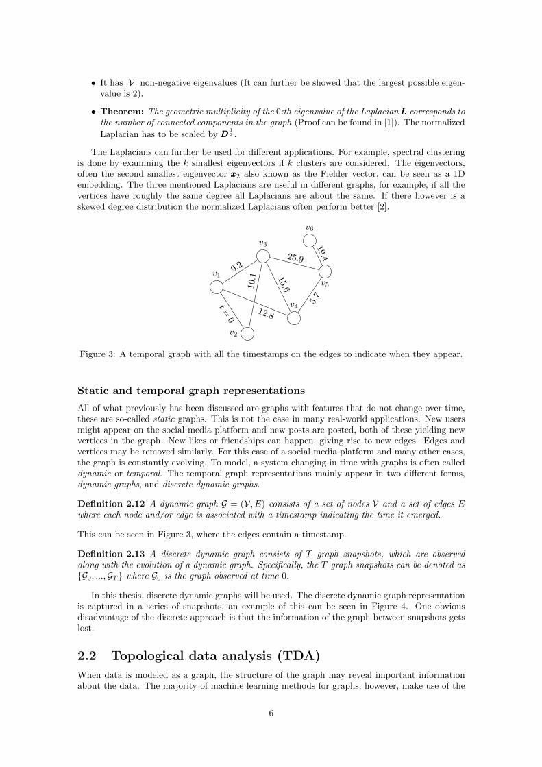
Figure 3: A temporal graph with all the timestamps on the edges to indicate when they appear.

Static and temporal graph representations

All of what previously has been discussed are graphs with features that do not change over time,these are so-called static graphs. This is not the case in many real-world applications. New usersmight appear on the social media platform and new posts are posted, both of these yielding newvertices in the graph. New likes or friendships can happen, giving rise to new edges. Edges andvertices may be removed similarly. For this case of a social media platform and many other cases,the graph is constantly evolving. To model, a system changing in time with graphs is often calleddynamic or temporal. The temporal graph representations mainly appear in two different forms,dynamic graphs, and discrete dynamic graphs.

Definition 2.12 A dynamic graph G = (V, E) consists of a set of nodes V and a set of edges Ewhere each node and/or edge is associated with a timestamp indicating the time it emerged.

This can be seen in Figure 3, where the edges contain a timestamp.

Definition 2.13 A discrete dynamic graph consists of T graph snapshots, which are observedalong with the evolution of a dynamic graph. Specifically, the T graph snapshots can be denoted as{G0, ...,GT } where G0 is the graph observed at time 0.

In this thesis, discrete dynamic graphs will be used. The discrete dynamic graph representationis captured in a series of snapshots, an example of this can be seen in Figure 4. One obviousdisadvantage of the discrete approach is that the information of the graph between snapshots getslost.

2.2 Topological data analysis (TDA)

When data is modeled as a graph, the structure of the graph may reveal important informationabout the data. The majority of machine learning methods for graphs, however, make use of the

6

tk tk+1 tk+n

Figure 4: A sequence of snapshots of the evolving graph. One snapshot corresponds to the graphat a specific timestamp.

structural information only to a limited extent. For example, some methods take into accountthe degree of the nodes, which is a quite simple and local measure of the structure of the graph.To extract and quantify more complex structural information of the graphs, we will resort to themethods of topological data analysis (TDA). The focus of TDA is applying data analysis techniquesfrom topology, the branch of mathematics that studies shape, proximity, and connection.

The aim of TDA can be summarized by the motto “Data has shape and shape matters”[3]. Themethods of TDA allow to quantify and visualize complicated structural information in complex orhigh dimensional data and have found application in a large variety of domains, including biology,economics, computer science, physics, and medicine.

Various methods of TDA can be applied to graphs. In some cases, the graph is endowed withhigher dimensional information and regarded as a simplicial complex, whose global structure canbe summarized for example in terms of its structural holes. In what follows, we will use TDAmethods to extract information on the global structure of graphs.

It is worth mentioning that, in the context of graph neural networks, TDA techniques havebeen mostly applied to spatial convolution methods. Spectral convolution methods also make use,differently and indirectly, of advanced structural information, since they involve convolutions inthe spectral or Fourier space. It may be argued, however, that the disadvantage of these methodsis that the convolution is much less flexible to different local structures [4].

This subsection will include the necessary background to understand the use and theory behindthe TDA that will be used in this thesis. The main method to study the structural features inthe graph will be persistent homology (PH). Some related works that use TDA on graphs will bepresented in the next section related to machine learning on graphs.

Definitions and background of TDA

The pipeline of the computation of persistent homology, from the graph to the interpretation canbe seen in Figure 5. This section will include the necessary background to understand the pipelineand will discuss each step in detail.

The method of persistent homology relies on homology, a theory in algebraic topology that

GraphFilteredComplex

Barcodes/Persistencediagrams

Interpretation

Figure 5: The pipeline for persistent homology.

7

Figure 6: Example of the first four p-simplices. A 0-simplex represented as a vertex, a 1-simplexrepresented as an edge, a 2-simplex represented as a triangle, and a 3-vertex represented as atetrahedron.

allows determining, for example, the number of connected components, ”holes” and ”voids” of atopological space. Homology (over a fixed field) associates a vector space Hi(X) to a topologicalspace X for a natural number i ∈ {0, 1, 2, ...}. Intuitively, the dimension of H0(X) counts thenumber of connected components in X, H1(X) counts the number of holes/loops, and H2(X)counts the number of voids.

Even if homology can be challenging to compute for many topological spaces, for the subclassof simplicial complexes, which can be described in a combinatorial way, efficient algorithms exist.In many applications, a discrete set of data points is given, from which a simplicial complex canbe constructed.

The definition [5] of the simplicial complex:

Definition 2.14 An (abstract) simplicial complex is a collection K of non-empty subsets of a setK0 such that τ ⊂ σ and σ ∈ K imply that τ ∈ K, and {v} ∈ K,∀v ∈ K0. The elements of K0 arecalled vertices, and the elements of K are called simplices.

Definition 2.15 A simplex has dimension p or is a p-simplex if it has a cardinality of p + 1.We use Kp to denote the collection of p-simplices. The k-skeleton of K is the union of the setsKp,∀p ∈ {0, 1, ..., k}. The dimension of K is defined as the maximum of the dimensions of itssimplices. A map of simplicial complexes, f : K → L, is a map f : K0 → L0 such that f(σ) ∈L,∀σ ∈ K.

Both these definitions might seem a bit technical, but they are fundamental for what follows. Toget some intuition on how to visualize p-simplices, the first four p-simplices are presented in Figure6. A 0-simplex corresponds to a vertex, a 1-simplex to an edge, a 2-simplex to a triangle, and a3-simplex to a tetrahedron. Notice that every (undirected) graph can be regarded as a simplicialcomplex of dimension 1 and that the 1-skeleton of a simplicial complex can be regarded as a graph.

Let us now introduce a way to associate a simplicial complex with a given graph.

Definition 2.16 The clique complex Cl(G) of an undirected graph G = (V, E) is the simplicialcomplex whose set of vertices is V and whose (p−1)-simplices are the p-cliques of G (i.e., completesubgraphs of G having p vertices).

Before moving on to the definition of homology for simplicial complexes some concrete methodsto associate a simplicial complex with the data will be presented.

We will consider at first the case in which the data consists of a finite set of points in a Euclideanspace. The definitions can be easily generalized to the case of point clouds in any metric space.Below, we will see how to further generalize these methods to (weighted) graphs.

Definition 2.17 Given a collection of points {xα} in Euclidean space En, the Cech complex, Cε,is the abstract simplicial complex whose k-simplices are determined by unordered (k + 1)-tuples ofpoints {xα}k0 whose closed ε/2-ball neighborhoods have non-empty intersection [6].

Definition 2.18 Given a collection of points {xα} in Euclidean space En, the Vietoris-Rips com-plex, VRε, is the abstract simplicial complex whose k-simplices correspond to unordered (k + 1)-tuples of points {xα}k0 which are pairwise within distance ε.

8

Figure 7: The point clouds with increasing value of ε and their corresponding Vietoris-Rips, VRεcomplexes. Image from R. Ghrist: Barcodes: The persistent topology of data [6].

Between these two complexes, the Cech complex is more expensive to compute, even though thereare in general more simplices in the Vietoris-Rips complex. Therefore the Vietoris-Rips complexis often the one that is used. One question that now might be asked is, when going from the pointcloud to any of these complexes what is a good parameter for ε? If ε is chosen too small then, thecomplex will just consist of points and if it is chosen too large the complex will be a single highdimensional simplex. The VRε complexes for different values of ε can be seen in Figure 7, whereone can see the problems with choosing too small or too large values of ε. As soon will be seen thestudy of one value of epsilon is not enough, to get information of the structure of the points onewill look at which features persist over a sequence of increasing values of ε. This is exactly whatpersistent homology does.

The next step is to define the homology for the simplicial complexes. Homology is a mathe-matical formalism for describing quantitatively and unambiguously how space is connected. Somebackground is necessary before this definition. For simplicity, we restrict to the case of the field F2.Let F2 be the field with two elements. If K is a simplicial complex, let Cp(K) denote the F2-vectorspace with basis given by the p-simplicies of K. For each p ∈ {1, 2, ...} define a linear map dp by

dp : Cp(K)→ Cp−1(K) : σ 7→∑

τ⊂σ,τ∈Kp−1

τ. (7)

where d0 is defined to be the zero map. Homology is defined as:

Definition 2.19 For any p ∈ {0, 1, 2, ...}, the pth homology of a simplicial complex K is thequotient vector space

Hp(K) := kernel(dp)/image(dp+1). (8)

Its dimensionβp(K) := dimHp(K) = dim kernel(dp)− dim image(dp+1) (9)

is called the p:th Betti number of K. Elements in the image of dp+1 are called p-boundaries, andelements in the kernel of dp are called p-cycles [5].

9

An important property of simplicial homology is functoriality. Any map f : K → K ′ ofsimplicial complexes induces the following F2-linear map:

fp : Cp(K)→ Cp(K′) :

∑σ∈Kp

cσσ 7→∑

σ∈Kp:f(σ)∈K′p

cσf(σ), for any p ∈ {0, 1, 2, ...} (10)

where cσ ∈ F2. The fact that fp ◦ dp+1 = d′p+1 ◦ fp+1 guarantees that fp induces the followinglinear map between homology vector spaces:

fp : Hp(K)→ Hp(K′), [c] 7→ [fp(c)] (11)

As a consequence, to any map f : K → K ′ of simplicial complexes a map fp : Hp(K)→ Hp(K′)

for any p ∈ {0, 1, 2, ...} can be associated. The following properties are satisfied, which we willrefer to as functoriality of homology: (g ◦ f)p = gp ◦ fp, for all simplicial maps f : K → K ′ andg : K ′ → K ′′, and (IdK)p = IdHp(K), for all simplicial complexes K.

To introduce persistent homology, we have to consider families of nested simplicial complexes.A filtration of simplicial complexes is a family {Kt}t∈R of simplicial complexes such that Kt ⊆ Kt′

whenever t ≤ t′. Since simplicial complexes associated with data are always finite, there exists afinite number of values {t1, . . . , tn} such that Kti−δ ( Kti , for all δ > 0. As a consequence, uponre-indexing one can always consider a finite filtration of simplicial complexes of the form

K1 ⊆ K2 ⊆ ... ⊆ Kn.

Filtrations of simplicial complexes can be constructed in many ways. The Vietoris-Rips filtra-tion was introduced in Definition 2.18 in the context of point cloud data to get some understandingof simplicial complexes. This approach can be applied to a similar setting for a weighted graph.The setup for this approach is very similar to what will be used in this thesis and is therefore of par-ticular interest. Let G = (V, E) be an undirected weighted graph with weight function W : E → R.For any ε ∈ R, the 1-skeleton Gε = (V, Eε) ⊂ G is the subgraph of G where Eε ⊆ E only includesthe edges that have a weight less than or equal to ε. Then the Vietoris-Rips filtration of a weightedgraph [7] is defined by

{Cl(Gε)}ε≥0, (12)

where Cl(G) is the clique complex introduced in Definition 2.16. This definition is easy to interpret.The filtration starts with all vertices V, then the weights of the edges are sorted in order such thatthe minimum weight comes first and the maximum weight comes last. Over this sorted set of edges,the value of ε is increased until it reaches the maximum weight. At each step, the correspondingedges are added to the graph.

Another useful filtration is the sublevel set filtration. Let h : K → R be a monotonic non-decreasing function, that is a function such that for any simplices σ, τ ∈ K if τ ⊆ σ then h(τ) ≤h(σ). Then the α-sublevel set of K is defined as Kα = {x ∈ K : h(x) ≤ α}, where the value of αgoing from −∞ to +∞ gives an increased sequence of sublevel sets to K, this is a filtration that isinduced by h. There are endless functions that could be used as h. The monotonicity of h impliesthat the sublevel set Kα = h−1(−∞, α] is a subcomplex of K, for every α ∈ R, and that {Kα}α∈Ris a filtration.

Homology can be applied to each of these subcomplexes, Ki. For any degree p of the homology,the inclusion maps Ki → Kj induce F2-linear maps fij : Hp(Ki) → Hp(Kj),∀i, j ∈ {1, 2, ..., n}where i ≤ j. From the previously explained functoriality, it follows that fk,j ◦fi,k = fi,j ,∀i ≤ k ≤ j[5], from which we arrive at the definition of persistent homology.

Definition 2.20 Let K1 ⊂ K2 ⊂ ... ⊂ Kn = K be a filtered simplicial complex. The pth persistenthomology of K is the pair (

{Hp(Ki)}1≤i≤n , {fi,j}1≤i≤j≤n)

(13)

where for all i, j ∈ {1, ..., n} with i ≤ j, the linear maps fi,j : Hp(Ki) → Hp(Kj) are the mapsinduced by inclusion maps Ki → Kj[5].

10

Given a sequence of filtered simplicial complexes, we are interested in studying the evolutionof homology across the filtration. This is expressed by the corresponding sequence of homologygroups in equation 14. For a fixed p, the inclusion simplicial maps gi : Ki → Ki+1 for the filtrationin definition 2.20 fit together into a sequence of vectors spaces

Hp(K0)g0−→ Hp(K1)

g1−→ ...gn−2−−−→ Hp(Kn−1)

gn−1−−−→ Hp(Kn) (14)

When going from Ki−1 to Ki there are new homology classes created and destroyed when theybecome trivial or merge.

The inclusion simplicial maps gi can be composed in sequence gi ◦ gi+1 ◦ ...◦ gj−1 to obtain fi,j .These maps fi,j contain important information that makes it possible to connect the p:th homologygroup of all the subcomplexes, K1,K2, ...,Kn = K in the filtered simplicial complex. The objectseen in equation 14 is called the persistence module. In equation 14 the sequence of vector spaceshas to be studied to get the information. In persistent homology, two common terms for a featureare birth and death. Their intuitive meaning can be understood by considering a function fi,j . Ahomology class u ∈ Hp(Ki) is born at filtration index i if u does not lie in the image of fi−1,i.Similarly, u is said to die at filtration index j ≥ i whenever j is the smallest number such thatfi,j(u) is non-zero in Hp(Kj); if no such j exists the death index is set to +∞. The persistencekeeps track of the filtration indices where topological features (connected components, loops, etc.)appear and disappear in this sequence. The name of persistence comes from that the topologicalfeature persists over the interval from its birth to its death [i, j]. The collection of these intervalscontain the structural information of the graph and this collection can be presented in differentways. Two ways that will be presented here are in the way of a persistence diagram and a barcode.They are visualized in two different ways but the information is the same for the two.

The barcode is a plot of the set of birth and death intervals from the collection described above.A barcode is a graphical representation of these intervals as a set of horizontal line segments,where the horizontal axis correspond to the filtration, for example, an increased value of α forKα = h−1(−∞, α] or an increased value of ε for the VRε complex. An illustration of a barcodecan be seen in Figure 8. In this figure, one can see how the different components of Hp are affectedby the increase in ε, where the VRε images for six values of ε are included. For H0, which is thenumber of components, each point has birth at ε = 0 and one dies when it is connected to anothercomponent. For large values of ε, there is only one component which also can be seen in the imagesat the top of the figure. The bars for H1 corresponds to loops, for the second image one can seethat two loops were just born and both of them exist over the next image. The length of these barstells which loops that persist over a broader range of values of ε, while those that are just shortsnippets might not say much about the structure of the points. The rank of Hp(VRε) is equal tothe number of bars/intervals the dashed line with the value of ε intersects in the barcode for Hp.

The second way to visualize the collection of these intervals is by a persistence diagram. Thatinstead of using horizontal bars to plot as in the barcode, it uses points in the R2 plane to plot thedifferent features. One axis, often the x-axis is the birth-time and the y-axis is the time of death.Since a birth must take place before its death, all points lie above y = x. This diagonal is oftenincluded in the diagram where an infinite amount of points are added on the diagonal. These pointsare added to facilitate the upcoming distance definitions between the two diagrams. The persistencediagram is often divided up into different dimensions where a p-dimensional persistence diagramDgp(K,h) consists of the diagonal and the birth and death points of the filtration for dimensionp, where K is a simplicial complex and h is the filtration.

One of many challenges with data is to cope with noise in the data. It can be a hard taskto distinguish between what is noise and what is a feature. This is where persistence homologyenters the picture. Previously defined homology gives structural information about a simplicialcomplex, but there is more information in the sequence of simplicial complexes. Which is exactlywhat persistence homology studies. By looking at how the features/noise are evolving for thesequence of simplicial complexes, persistence homology can provide which features persist over thesequence. These are often not that influenced by noise since the features have to be maintainedover sequences to be considered features. Persistence is a measure-theoretic concept that is built ontop of algebraic structures, one of the most important properties is its stability under permutationsof the data. In previous subsections it was mentioned the importance of permutation invariant,it comes back here. The stability of the persistence means that a small change in the data or

11

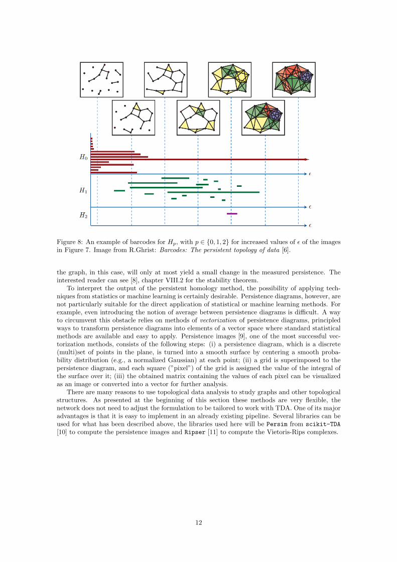
Figure 8: An example of barcodes for Hp, with p ∈ {0, 1, 2} for increased values of ε of the imagesin Figure 7. Image from R.Ghrist: Barcodes: The persistent topology of data [6].

the graph, in this case, will only at most yield a small change in the measured persistence. Theinterested reader can see [8], chapter VIII.2 for the stability theorem.

To interpret the output of the persistent homology method, the possibility of applying tech-niques from statistics or machine learning is certainly desirable. Persistence diagrams, however, arenot particularly suitable for the direct application of statistical or machine learning methods. Forexample, even introducing the notion of average between persistence diagrams is difficult. A wayto circumvent this obstacle relies on methods of vectorization of persistence diagrams, principledways to transform persistence diagrams into elements of a vector space where standard statisticalmethods are available and easy to apply. Persistence images [9], one of the most successful vec-torization methods, consists of the following steps: (i) a persistence diagram, which is a discrete(multi)set of points in the plane, is turned into a smooth surface by centering a smooth proba-bility distribution (e.g., a normalized Gaussian) at each point; (ii) a grid is superimposed to thepersistence diagram, and each square (”pixel”) of the grid is assigned the value of the integral ofthe surface over it; (iii) the obtained matrix containing the values of each pixel can be visualizedas an image or converted into a vector for further analysis.

There are many reasons to use topological data analysis to study graphs and other topologicalstructures. As presented at the beginning of this section these methods are very flexible, thenetwork does not need to adjust the formulation to be tailored to work with TDA. One of its majoradvantages is that it is easy to implement in an already existing pipeline. Several libraries can beused for what has been described above, the libraries used here will be Persim from scikit-TDA

[10] to compute the persistence images and Ripser [11] to compute the Vietoris-Rips complexes.

12

3 Machine learning

Today, examples of machine learning are all around us. Examples for two completely differentpurposes are a machine learning model that assists the doctor to spot tumors or a website thatrecommends new products based on your previous purchases. All machine learning methods relyon data, from which the models learn, without being told exactly what to do. The algorithms aretrained to find patterns to make as good predictions as possible.

3.1 Machine learning background

Machine learning models are often divided into mainly two categories, supervised and unsupervisedmachine learning. In supervised machine learning the data has labels to be trained on. For thetumor images, the training images have a label stating whether or not there is a tumor in the image.The models learn from the labels, evaluating their performance by comparing their output to thelabel. The other category is unsupervised machine learning, where there are no labels associatedwith the data. The methods of unsupervised machine learning try to gain insight into the data tosort, label, or classify different features. Usually, the supervised models are trained and patternsare learned on a labeled training set of the data. To assess the performance of these algorithms oneoften has an unlabeled test set to evaluate how well the predictions did in comparison to the truelabeled value. This is called the test error. There is a balance between how well the performanceis on the two sets. If one method learns the training data too well it will also adjust the modelto the noise. The model will then fit the training points very well but not work as well on asimilar data set that it has not been trained on. This model is said not to generalize well, sinceit generally does not give not a good prediction on the test set. The described phenomenon iscalled overfitting. There are several ways to deal with these problems and they are a major partof machine learning. This is for example dealt with by including a validation set, to compare withthe training set during the training to see when it starts to overfit and then stop the training.

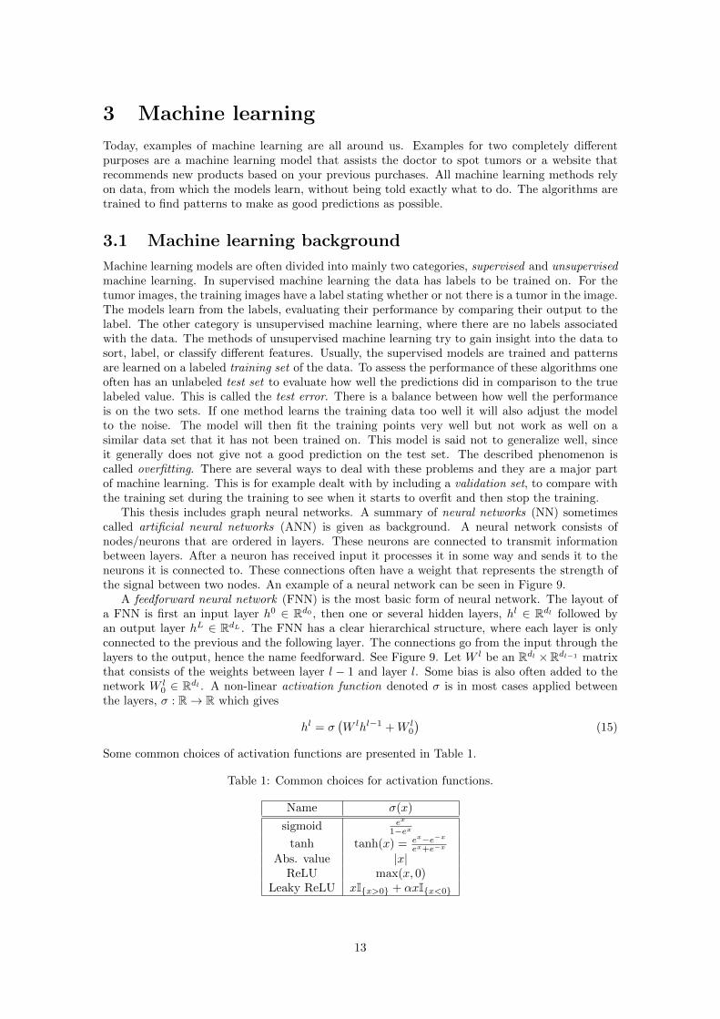
This thesis includes graph neural networks. A summary of neural networks (NN) sometimescalled artificial neural networks (ANN) is given as background. A neural network consists ofnodes/neurons that are ordered in layers. These neurons are connected to transmit informationbetween layers. After a neuron has received input it processes it in some way and sends it to theneurons it is connected to. These connections often have a weight that represents the strength ofthe signal between two nodes. An example of a neural network can be seen in Figure 9.

A feedforward neural network (FNN) is the most basic form of neural network. The layout ofa FNN is first an input layer h0 ∈ Rd0 , then one or several hidden layers, hl ∈ Rdl followed byan output layer hL ∈ RdL . The FNN has a clear hierarchical structure, where each layer is onlyconnected to the previous and the following layer. The connections go from the input through thelayers to the output, hence the name feedforward. See Figure 9. Let W l be an Rdl ×Rdl−1 matrixthat consists of the weights between layer l − 1 and layer l. Some bias is also often added to thenetwork W l

0 ∈ Rdl . A non-linear activation function denoted σ is in most cases applied betweenthe layers, σ : R→ R which gives

hl = σ(W lhl−1 +W l

0

)(15)

Some common choices of activation functions are presented in Table 1.

Table 1: Common choices for activation functions.

Name σ(x)

sigmoid ex

1−ex

tanh tanh(x) = ex−e−xex+e−x

Abs. value |x|ReLU max(x, 0)

Leaky ReLU xI{x>0} + αxI{x<0}

13

h01

h02

h03

h0m

Input layer h11

h12

h13

h14

h1n

Hidden layers

h21

h22

h23

h24

h2k

h31

Output layer

W 1n,m

W 2k,n

W 31,k

Figure 9: The architecture of a neural network with one input layer of dimension m, two hiddenlayers with dimensions n respective k, and one output layer with dimension 1. It is a fully connectednetwork, where each node is connected to all other nodes in the neighboring layers. The W arematrices with weights between neurons that are learned during training.

Convolutional neural networks (CNN) are special versions of FNN. While feedforward networksoften are fully connected (connections are present between all nodes for two neighboring layers),CNN preserves local connectivity. The CNN architecture usually contains convolutional layers,pooling layers, and fully connected layers [12]. CNNs are often used for computer vision tasks andhave proven to be successful in many other research fields.

In comparison with standard feedforward neural networks, the neurons in a recurrent neuralnetwork (RNN) do not only receive signal input from other neurons but also their own historicalinformation. RNN can use its internal state (memory) to effectively process series of data. Thereare however some challenges with long-term dependencies for RNN. Two networks that solve thisproblem by including a gate mechanism are gated recurrent unit (GRU)[13] and long short-termmemory (LSTM) [14]. Of these two methods, the LSTM has a longer training time due to itscomplex structure while the GRU model has a simpler structure, fewer parameters, and generallyfaster training time. Two fields where RNNs are widely used are in speech and natural languageprocessing [15]. Many recent methods on temporal graph learning use a form of RNN, often GRU,to capture the temporal dependencies.

Machine learning on graphs

Machine learning on graphs is not different from what has been discussed above. There is howevernot a clear distinction between supervised and unsupervised learning, as will be seen shortly.Machine learning on graphs is mainly done with four different tasks.

The first task is node classification. This is perhaps the most common machine learning task ongraphs. The goal is to predict the label of a node, where only the true labels on the training set ofthe graph are given. A simple example is presented in Figure 10a. There are some challenges withthis approach [1]. The models in standard supervised machine learning methods assume that thedata points are independent. For a graph, there are connections between the data points. It was

14

v1

v2

v3

?

v4

v5

v6

(a) Node classification.

v1

v2

v3

v4

v5

v6

?

?

(b) Edge prediction.

v1

v2

v3

v4v5

v6

v7

v8

v9

v10

(c) Community detection. (d) Graph classification.

Figure 10: Example of different machine learning tasks on graphs.

previously mentioned that machine learning can be divided into mainly two categories, supervisedand unsupervised. The node classification task is often called semi-supervised because duringtraining the whole graph, including node features, is often available and the only thing missingis the label for the testing nodes. This is somewhat between supervised and unsupervised, hencesemi-supervised. One example of node prediction is in a graph of transactions (edges) betweendifferent accounts (nodes) where the task is to find accounts that potentially are used for moneylaundering.

The second task is edge prediction. While node classification uses information from other nodesbased on their relationships’. For edge prediction, all vertices of the graph are included but someedges are excluded. The goal is to use this incomplete graph information, with the complete setof vertices and the incomplete set of edges, to infer the missing edges. Figure 10b shows a visualexample of edge prediction. This task is often both supervised and unsupervised as the nodeclassification. There are many applications of edge prediction, a recommendation system thatsuggests a user on a social media platform where the edges can indicate to ”follow” or ”befriend”someone. This is also an example of a graph that continues to evolve, the graph is temporal.Twitter [16] uses the graph up to a time point t, from which they predict the edges that mightoccur in the upcoming time steps.

The third task is community detection. The two previous tasks focused on the graph analogs ofsupervised learning. This is the unsupervised analog. The task is to divide the graph into differentcommunities or clusters, as shown in Figure 10c. The graph is divided in such a way that thereare many edges between nodes in the same community and few edges between nodes in differentcommunities.

The fourth task is applied to several graphs, it is graph classification. It captures a biggerpicture than the node classification, where instead of assigning labels to different nodes the taskis to assign labels to different graphs, see Figure 10d. An application to chemistry consists oflabeling properties of chemical molecules, regarded as graphs summarizing their structure. Theprocess is fairly straightforward where one trains on labeled graphs and predicts unseen ones. Thechallenge is to incorporate the complexity of the graph into the model. The unsupervised approach

15

with graph clustering can be conducted in a similar manner where the task is to find similaritiesbetween graphs.

Spectral methods

The graph convolutional operation can be carried out in two different ways, unlike normal convo-lutional operation which only has one. The first one is called spectral methods and is based onthe spectral graph theory by finding the corresponding Fourier basis for the graph Laplacian. Thesecond one is called spatial methods, which generalizes spatial neighborhoods by two functionsoften called update and aggregate to apply the regular convolutional operation.

Background for both of these approaches will follow, starting with spectral methods. In manygraphs, there are features or attributes associated with the nodes. This graph-structured data isin spectral methods treated as graph signals, that capture both the structural information and theattributes of data in the nodes. Like in classical signal processing a signal can be represented intwo domains, the time domain, and the frequency domain. One way to go between these domainsis by the Fourier transform. The Fourier transform of f(x) is

F(f(x)) = f(ξ) =

∫Rdf(x)e−2πx

>ξidx (16)

and the inverse defined as

F−1(f(ξ)) =

∫Rdf(ξ)e2πx

>ξidξ (17)

The two expressions above are for the continuous case. The general continuous convolution operator? between two functions f and h is defined as

(f ? h)(x) =

∫Rdf(y)h(x− y)dy (18)

which can be written in terms of an element-wise product of the Fourier transforms of the twofunctions as

(f ? h)(x) = F−1(F(f(x)) ◦ F(h(x))) (19)

The Fourier transform can be applied to a discrete case in a very similar way, for t ∈ {0, ..., N − 1}

ξk =1√N

N−1∑t=0

f(xt)e− i2πN kt (20)

An interpretation of the Fourier transform is a representation of the input signal as a weightedsum of (complex) sinusoidal waves [1]. The Fourier transform can now be applied to graphs. Thespectral convolution on graphs is defined as the multiplication of signal x ∈ Rd (a scalar for everynode) with the filter gξ = diag(ξ) parametrized by ξ ∈ Rd in the Fourier domain as

gξ ? x = UgξU>x, (21)

where the eigenvectors of LLL are the columns of U , i.e. LLL = UΛU>, with Λ being a diagonal matrixwith eigenvalues on the diagonal and U>x the graph Fourier transform of x [17]. The function gξis sometimes denoted as gξ(Λ).

Equation 21 is computationally expensive since it requires multiplication with U , which is ofcomplexity O(d2). It can be even more costly to compute the eigendecomposition of LLL to get U .This computation can be avoided or at least simplified [18], by approximating gξ(Λ) by a truncatedexpansion of Chebyshev polynomials Tk(x) up to the Kth order. The approximation is

gξ′(Λ) ≈K∑k=0

ξ′kTk(Λ) (22)

where Λ = 2λmax

Λ − III is a rescaled version of Λ, λmax is the largest eigenvalue of LLL and ξ′ is avector of Chebyshev coefficients. The Chebychev polynomials are defined recursively by Tk(x) =

16

2xTk−1(x)− Tk−2(x), with T0(x) = 1 and T1(x) = x. The convolution in equation 21 can now beapproximated by

gξ′ ? x ≈K∑k=0

ξ′Tk(LLL)x (23)

where LLL = 2λmax

LLL − III. The complexity to compute this approximation is O(|E|), linear in thenumber of edges.

The approximation of the Fourier transform applied to graphs is commonly used in recentworks on graph-based machine learning. This approach was suggested by Hammond et. al. [18]in 2009, and since then this approach has been widely used in the construction of new methods.Two recent spectral networks that are built on this are Graph Convolutional Network (GCN) [17]and Chebnet also known as GCNN [19], both published in 2017. The two methods have had animportant impact on recent networks, as they are either included as part of a network or used asa foundation for improvement.

Several of the mentioned networks use convolution in some way, similar to CNN. The expressionconvolution comes from the mathematical convolution operation that is applied in the network.CNNs are specialized to process data that has a grid-like structure, for example, an image is a2-dimensional grid of pixels. Generally, matrix multiplication is involved between the layers infor example a multi-layer perceptron (MLP). For a convolutional network, the convolution is usedinstead of matrix multiplication in at least one of the layers [12]. The CNN is essentially suitablefor data that belong to Euclidean space, with a constant number of neighbors to each node (pixel),an assumption that is not verified in general graphs. Because of these limitations of CNNs formore complex topological structures, there is much effort to develop new models inspired by CNNbut applicable for graphs.

Spatial methods

The methods presented so far have all been spectral methods that are built on spectral graphtheory. While these models have achieved great results [17, 18] there is one major drawback withthese methods, their lack of flexibility. Spectral methods are one of the two main approaches tomachine learning on graphs. The other one is called the spatial approach. The spectral approachis trained on a specific structure of the graph, therefore it can not be directly applied to a graphwith a different structure. Spatial approaches can however be used in this way since they define theconvolutions directly on the graph in the spatial domain and operates on some defined neighbor-hood. This approach has some challenges, including how to apply the operation to neighborhoodsof different sizes and how to make sure that the order of the neighbors in the convolution doesnot change the outcome. The latter is called permutational invariant. For CNNs the number ofneighbors are constant for each pixel, while for graphs the degree is in general not the same forall nodes. The collection of information from the neighbors N(v) of a node v needs to be permu-tational invariant. The order in which the information is collected should not matter, since it cannot be guaranteed to always collect information in the same order and it is very hard to definean ordering of subgraphs or set of neighbors. It is therefore important when designing a spatialgraph neural network that it is permutational invariant. Let PPP be a permutation matrix and AAA theadjacency matrix, then any function f that satisfies the equation below is permutational invariant

f(PAPPAPPAP>) = f(AAA) (24)

Examples of functions that are permutational invariant are the average and median. One suggestionto get more advanced information can be to compute the different possible outcomes for a functionthat is not permutational invariant and summarize this information in some way. This is notreasonable since it will be of high computational cost.

Graph neural networks (GNN) is a framework for deep neural networks on data in the form of agraph. The networks generate node representations that depend on the structure of the graph andthe feature information for each node. The spatial approach for graph convolution often consists oftwo functions, update, and aggregate. Different methods often have different update and aggregatefunctions. To better understand their relation to a GNN, the most basic version of GNN is given

17

in equation 25 which is a simplification of one of the first approaches to GNN [20].

hlu = σ

W lselfh

l−1u +

∑v∈N(u)

W lneighh

l−1v

(25)

Here W lself ,W

lneigh ∈ Rdl×dl−1 are trained weight matrices and σ is an activation function. The

basic GNN in equation 25 can be expressed through the update and aggregate functions. LetmN(u) denotes the message function that is the output from the aggregate function based on theneighbors of u, as shown below.

mN(u) = aggregatel({hlv,∀v ∈ N(u)}) =∑

v∈N(u)

hv (26)

update(hu,mN(u)) = σ(Wselfhu +WneighmN(u)

)(27)

Research in this area mainly focuses on the aggregation function. Two well-known spatial methodsare GraphSAGE [21] and graph attention network (GAT) [22]. The GAT uses an attention-basedmechanism. This mechanism can give different neighbors different attention scores and thereforeidentify more important neighbors.

Graph embeddings

Graph analytical methods generally require high computational and space costs. One way toreduce this problem is by using graph embedding. This technique converts the graph data intoa low dimensional space, Rd where the properties of the graph and the structural informationare preserved to a maximum. A visual example can be seen in Figure 11. The graph is oftenrepresented by a set of low dimensional vectors, the output of the graph embedding procedure.Graph algorithms can easily be applied to these vectors. The graph embeddings are a part ofrepresentation learning, that appears in the title of the thesis. Representation learning obtainsdata representation to make it easier to extract useful information when building different machinelearning models on graphs. Another problem is graph analytics, which aims to extract usefulinformation from graph data. The graph embeddings lie in the overlap of these two problemswhere the focus is to learn low-dimensional representations [23].

The input for an embedding is the given graph G = (V, E), the output however is task-specific.There are mainly four types of output for graph embeddings: node embeddings, edge embeddings,hybrid embeddings, and whole-graph embeddings. The most common type of embedding is thenode embedding that represents close/similar nodes as similar vectors. For node embeddings, eachnode is represented by a low-dimensional vector, zu ∈ Rd for node u. The difference between variousgraph embedding methods is how they consider the ”closeness” of two nodes. These embeddingsmight be useful in a later stage of machine learning on graphs, for example in node classificationand node clustering tasks. Earlier it was said that embeddings should preserve the structural in-formation and the properties of the graph. A good node embedding, therefore, preserves similaritybetween the nodes after mapping them to the embedded space. A graph embedding can be seenin Figure 11, where the nodes in the graph G are encoded by a mapping function cod: V → Rd inthe embedded space Rd, where cod(v) = zv. To preserve the information from the graph to theembedded space the similarity between two nodes in the two spaces are compared and expressedas

simG(u, v) ≈ simRd(cod(u), cod(v)) (28)

where simG is the similarity for the nodes in the graph G, simRd is the similarity in the embeddedspace Rd, with a loss function defined to quantify ≈. These measures or functions can be defined inmany different ways [24]. There are different measures to quantify how well the graph property ispreserved in the embedded space. One measure is the proximity measure. The first-order proximityis based on local pairwise similarities between each node and its neighbors. There is a notion ofhigher-order proximity where the second-order compares the similarity of the node’s neighborhoodstructures.

18

v1

v2

v3

v4

v5

v6

zv6

zv5

cod(v6 )

cod(v5)

Embedded space RdInput graph G

Figure 11: A graph embedding from the input graph G to an embedded space Rd.

Two graph embedding techniques worth mentioning are matrix factorization and deep learning.The methods differ in the way they define the graph property to be preserved. To learn more aboutthese along with some other methods see [23], which gives a rich background of embeddings anddifferent approaches for them.

To conclude the section of machine learning background, let us mention that machine learningon graphs is a quite new area of research, one of the first models in the area was the graph neuralnetwork (GNN) model [20] in 2009 which is built on networks that previously have not been usedfor graphs. The network can be thought of as an information diffusion mechanism, where eachnode exchanges and updates its information with its neighbors until an equilibrium is reached. Thetarget of the GNN is to gather information from the neighbors of each node to create embeddingsfor every node.

As discussed, the difference between the spatial and spectral approaches is that the spectralapproach relies more on the structure of the graph and is built on spectral graph theory. Theperformance of different methods is also very dependent on the structure of the graph. To this dayno method suits all problem formulations. The area of machine learning on graphs is still underdevelopment. The methods or architecture for a specific task should be chosen depending on thegraph structure.

3.2 Graph convolutional neural networks and TDA

In the paper Persistence Enhanced Graph Neural Network by Q.Zhao et al. [4] it is shown how theperformance of graph convolutional networks can be improved by incorporating local structuralinformation of the graph, extracted via TDA methods such as persistence homology. Most otherrecent methods only use rather easy topological information, for example, the number of neighbors.In the cited paper, the aim is to show that the inclusion of more complex structural informationcan provide better node classification. Previously it has been mentioned that a spatial approachuses messages to aggregate the information between nodes. The approach here is to re-weight thesemessages by using the local structural information of the graph to calculate these new weights. Thenetwork in the cited paper is a spatial GNN called Persistence Enhanced Graph Network (PEGN),where the convolution is a message-passing framework to update their feature representation. Toincorporate the structural information from the persistence homology into the architecture thereis a separate network, called Persistence Image Network (PIN) that takes the information from thepersistence homology into the vectors to re-weight the messages.

Consider a graph neural network with N nodes and each node has its feature representationhln ∈ Rdl , where l is the layer in the network and dl is the dimension of the features for that layer.The representation of node u is computed based on its neighbors and itself from the representation

19

in the previous layer by

hlu = σ

∑v∈N(u)∪u

W lhl−1v

(29)

where the transformation matrix W l is learned during training and σ is the activation function.This setup looks very similar to a standard neural network in Eq. (15) and a graph neural networkin Eq.(25). The inclusion of persistence homology is not part of Eq. (29). The additional re-weighting vectors need to be added, denoted τ lv→u. They are different for different edges anddepend on the structural information of that edge. The updated version of Eq. (29) looks like

hlu = σ

∑v∈N(u)∪u

diag(τ lv→u)W lhl−1v

(30)

To compute τ lv→u, one uses the persistence diagrams to create so-called persistence images, formore details see the paper [4] and Section 2.2. The persistence images are put through a multi-layer perceptron (MLP) that outputs the re-weighting vectors. This part can be thought of as the”Interpretation” step in the pipeline presented in Figure 5.

This paper demonstrates how structural information from graphs can be extracted with toolsfrom TDA and easily applied to an already existing pipeline. This area is very new and there ismuch more to explore on how to use TDA to get even better results, both for already existingarchitectures and new ones.

3.3 Recent methods

Many related methods have already been mentioned and discussed. Both spectral and spatialmethods such as GCN[17], Chebnet[18], GraphSAGE[21] have been mentioned briefly. The goal ofthis section is to include methods that are even more related to the task at hand. Methods morefocused on the temporal aspect will be presented together with some applications that are closelyrelated to traffic prediction. One aspect that several papers seemed to have agreed upon is thatCNN in its original form cannot be applied to graphs and classical RNNs usually are too slow totrain[25, 26]. There are several interesting approaches to address these two problems.

Related to our traffic mobility prediction for radio base stations, a well-studied task is thetraffic prediction task on roads [4, 25, 27, 28, 29]. This problem includes non-linear dynamics inthe road networks that perhaps make it even more challenging. These different networks have todeal with both the spatial and temporal aspects of the data. Different approaches can be found inthe literature. Several networks use GCN from [17] or in some cases even a standard CNN on theinput data to capture the relations from the graph structure and then apply a RNN on the timeaxis. One such method is the temporal graph convolutional network (TGCN)[4]. Developed fortraffic forecasting, with an unweighted graph. For the RNN a GRU is used to capture the dynamicvariation of traffic information. One similar architecture that is applied to a completely differentfield is the VStreamDRLS, with the aim to optimally coordinate live video distribution [30]. Thetask is to predict available network capacity between viewers(nodes), which is closely related toour task. Their network is applied to a weighted and dynamic graph.

While these approaches might seem the most obvious ones there are many more. Two separatenetworks that use the same spatial and temporal methods do not have to be identical, the architec-ture can vary. A network that uses GRU and GCN in the same aspects as the previous networksbut with a different architecture is the Spatial-Temporal Graph Neural Network (STGNN) model[29]. In the paper of STGNN, the task is traffic prediction, in the model they use a position-wiseattention mechanism to improve the aggregation from adjacent roads. Previously it was shortlymentioned of an attention mechanism for GAT [22]. To capture both the local and the global tem-poral dependencies a transformer layer is applied in combination with the GRU. The architectureof STGNN shows the importance that a different setup can perform better with the same two mainmethods.

Another way to gather the spatial information is implemented in a network called DiffusionConvolutional Recurrent Neural Network (DCRNN) [28]. For DCRNN the traffic flow is modeled

20

as a diffusion process, which uses a random walk on the graph to gather spatial information. Thena GRU is used to capture the temporal behavior. Their approach is costly during training butperforms well.

The selection of GRU is not the only choice for RNNs, the Gated Linear Unit (GLU) has beenused to predict traffic at radio base stations [26].

The methods presented so far all use some kind of RNN for the temporal aspects, which isa common choice but not the only choice. The method Spatio-Temporal Graph ConvolutionalNetwork (STGCN) [27] uses 1-D convolution on the time axis to capture the time dependencies.This method is significantly faster to train but treats the two aspects, spatial and temporal,completely separately which might result in missing information between spatial and temporaldynamics.

One of the research questions of this thesis is on the modeling of a graph for achieving goodtraffic prediction. A graph can be modeled differently and this can give very different results. De-pending on the modeling of the graph the dependencies might be different, there are even modelsthat construct the graph as part of learning [25]. Their construction of the graph is therefore com-pletely data-driven, by capturing more information can lead to better construction of the graph.Another approach to this problem is to use a Spatio-Temporal Hybrid Graph Convolutional Net-work (STHGCN) [31], that uses GRU to capture temporal dependency but the spatial dependencyis captured by three different GCN in a hybrid format. The GCN model relies heavily on the struc-ture of the graph. From the data, they saw the need for three different types of spatial correlations.The first one is spatial proximity: two base stations that are closely located are correlated due tosimilar movement. The second one is functional similarity, based on the observation that locationsthat share the same functionality have similar patterns. For example shopping malls with highdemand on weekends and residential areas with high demand in the mornings and evenings. Thethird is spatial dependency, a notion of correlation depending also on time, designed to capturesimilarities between base stations with similar trends. The paper that presents STHGCN is ofparticular interest since it is applied to data from telecommunications networks with the task topredict traffic. Their way of modeling the graph is based on regarding radio base stations as nodesand edges as interactions between the radio base stations, which is also the case for other networkswith a similar task[26]. The data their network has been applied to seems to be very similar toour data that will be explained in more detail in Section 4. Their data is from the telecommuni-cation network of a region in China where the traffic is recorded every 15 min, similar to our datawhere the traffic is recorded every hour. There are other observed patterns within their data thatthey have taken into account when designing the model, which is described in the paper and canbe useful for this thesis. From their data, one can easily see daily patterns, some stations evendistinguishable patterns between weekday and weekend while not for others. This is in contrastto another traffic prediction at radio base stations [26] that observed no significant variations be-tween different days but saw that the patterns are daily cyclical. For the STHGCN it is not onlythe spatial aspect that is treated differently but also the temporal aspect has some interestinginsights. The temporal patterns are explored in three different components, recent, daily-periodic,and weekly-periodic. Each of these components consists of a time series of segments. The mo-tivation behind this modeling is that the RNNs have a problem with long-term dependencies asdiscussed earlier, however, they also include GRU. To incorporate this into a network, the networkcan be given features like the day of the week, the hour of the day, etc[26].

The features of the spatial and temporal domain are in all cases above modeled separately butwith some influence between each other. In 3D Temporal Graph Convolutional Networks (3D-TGCN) [25] these features are learned together. Another applicable thing with this method is thatthe paper in which it was presented was modeled with weighted edges that represent the proximityof the nodes for traffic mobility prediction, which is highly related to this thesis.

There are many more interesting networks and papers to consider. Even if the most commonapplication is traffic prediction for vehicles, this application is very similar and flexible to work forother tasks too. There are several but not as many networks made specifically for traffic predictionfor radio base stations. The networks discussed above are often based on GCN and GRU, but thereare other networks. For both modeling of the graph and the upcoming structure of the network,there is much to have in mind, to combine the important aspects of these neighbors and define agraph structure that accounts for them.

21

4 Data set

Data is continuously collected from our daily life, in a lifestyle where we are constantly connectedto the internet and many of the objects we use every day are connected to the internet. Telecom-munication data allows us to study the structure and evolution of our connections. There arehowever not many publicly available data sets for position tracking of cellular phones. This type ofdata is usually owned by private companies, fortunately, Z. Du et al. recently published a publicdata set in this area [32].

The data set is collected from 3 million anonymous cellphone users in 167 separate locations,that cover 4 geographically adjacent areas (Changchun City, Dehui City, Yushu City, and Nong’anCounty) in northeastern China, as shown in Figure 12. The total population of this area wasalmost 8 million in 2017 [32]. The different locations in the data set are each a collection of basestations, on average each location includes 72 base stations. For each of the 167 locations, the GPSinformation with its latitude and longitude is included in a separate file. This data is collectedwith one-hour intervals for one week, starting on August 7, 2017, resulting in 168 snapshots intime.

Figure 12: Overview of the geographical areas included in the data set. Image from Z.Du etal: Inter-urban mobility via cellular position tracking in the southeast Songliao Basin, NortheastChina[32].

For each timestamp, the directed mobility between different locations is included. From thisinformation, both directions of mobility can be seen between any two locations. The authors ofthe data set define that a user has moved only when she/he stays in a new location for at least 30minutes. If the user spends less than 30 minutes in a location, it is not recorded as a visit. Therecorded location in each snapshot is the last known location for the user.

There are some shortcomings or possible shortcomings of the data worth pointing out. Tomerge such many base stations can yield a loss of local information. This data only includes oneweek during the summer, while a longer period would have been preferred. Lastly, to capturetraffic variations at a finer scale, a higher sampling rate could give more insight.

4.1 Data processing

For the data to be useful in the desired way it often requires data processing. It is done to getthe data in a form tailored towards the upcoming application. The process can look very differentdepending on the data and the application. A few processing steps for the data will be includedhere alongside plots about the data.

In the first step of processing the locations without any traffic at any time are removed, whichgives us the previously mentioned 167 stations.

The directed mobility in the data naturally yields a directed weighted graph between thelocations where the mobility is encoded as a weight on the edges. The initial approach to model

22

the number of connections at each base station was as

at base station = staying + arriving− leaving (31)

where staying is the mobility with the same origin and destination, arriving is the sum of allthe incoming mobility, and leaving is the sum of all the outgoing mobility. Unfortunately, thisapproach did not represent the data well due to the modeling of the data set[32].

To represent the number of connections for each location, the data with mobility to and from thesame locations are used, labeled staying in the expression above. The mobility between the samelocation contains the highest weights of mobility across all locations and timestamps in the dataset. This representation excludes the mobility information from the data. However, it provides theinformation needed for the upcoming modeling.

This data has a clear periodic pattern, both in total for all locations and individual locations.The periodic pattern shows that the number of staying are cyclical in the same way mobility is.This is the important feature of this data set. The total hourly connections periodicity of stayingfor all location can be seen in Figure 13a, and the periodicity of hourly connections for a specificlocation is shown in Figure 13b

(a) The total number of cellphones that stay inthe same location for each snapshot in time.

(b) The number of hourly connections to one spe-cific location for each snapshot in time.

(c) The distribution of closeness between the radiobase stations given in degrees. (d) Location of the base stations in northeastern

China.

Figure 13: A collection of patterns and distribution for the data set.

The location of each base station is the other important feature of this data. It consists of thelatitude and longitude of each location, as displayed in Figure 13d. The Euclidean distance, seeEq. 32, between any two locations, measuring the geographical distance between base stations, arecomputed and stored for further use in the graph modeling. The distribution of all the distancescan be seen in Figure 13c.

d(p, q) =√

(p1 − q1)2 + (p2 − q2)2 (32)

23

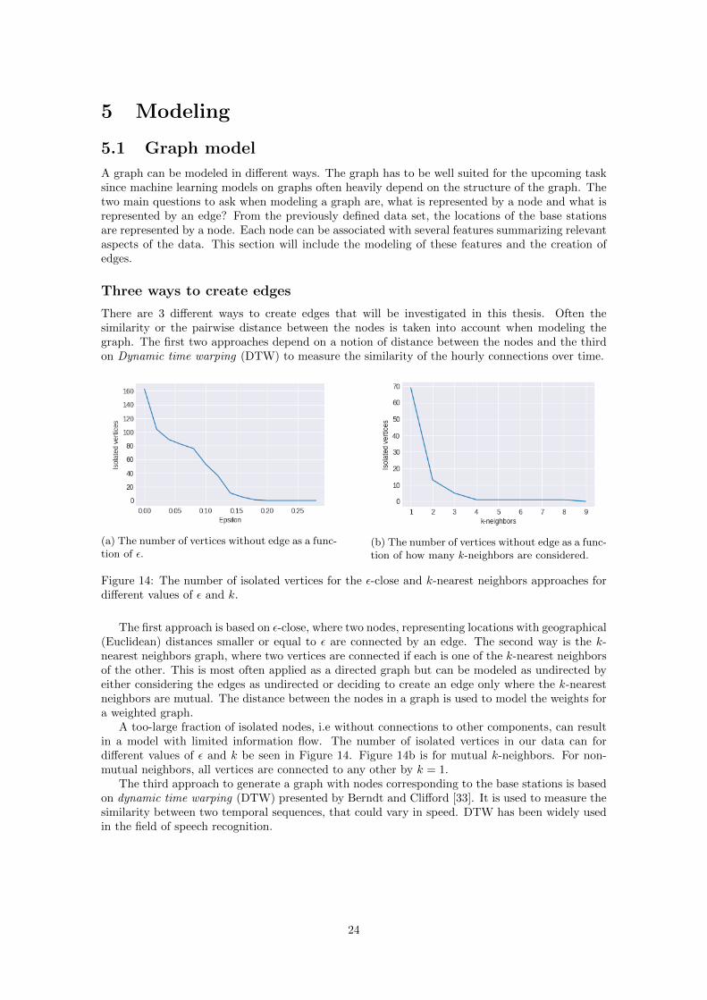
5 Modeling

5.1 Graph model

A graph can be modeled in different ways. The graph has to be well suited for the upcoming tasksince machine learning models on graphs often heavily depend on the structure of the graph. Thetwo main questions to ask when modeling a graph are, what is represented by a node and what isrepresented by an edge? From the previously defined data set, the locations of the base stationsare represented by a node. Each node can be associated with several features summarizing relevantaspects of the data. This section will include the modeling of these features and the creation ofedges.

Three ways to create edges

There are 3 different ways to create edges that will be investigated in this thesis. Often thesimilarity or the pairwise distance between the nodes is taken into account when modeling thegraph. The first two approaches depend on a notion of distance between the nodes and the thirdon Dynamic time warping (DTW) to measure the similarity of the hourly connections over time.

(a) The number of vertices without edge as a func-tion of ε.

(b) The number of vertices without edge as a func-tion of how many k-neighbors are considered.

Figure 14: The number of isolated vertices for the ε-close and k-nearest neighbors approaches fordifferent values of ε and k.

The first approach is based on ε-close, where two nodes, representing locations with geographical(Euclidean) distances smaller or equal to ε are connected by an edge. The second way is the k-nearest neighbors graph, where two vertices are connected if each is one of the k-nearest neighborsof the other. This is most often applied as a directed graph but can be modeled as undirected byeither considering the edges as undirected or deciding to create an edge only where the k-nearestneighbors are mutual. The distance between the nodes in a graph is used to model the weights fora weighted graph.

A too-large fraction of isolated nodes, i.e without connections to other components, can resultin a model with limited information flow. The number of isolated vertices in our data can fordifferent values of ε and k be seen in Figure 14. Figure 14b is for mutual k-neighbors. For non-mutual neighbors, all vertices are connected to any other by k = 1.

The third approach to generate a graph with nodes corresponding to the base stations is basedon dynamic time warping (DTW) presented by Berndt and Clifford [33]. It is used to measure thesimilarity between two temporal sequences, that could vary in speed. DTW has been widely usedin the field of speech recognition.

24

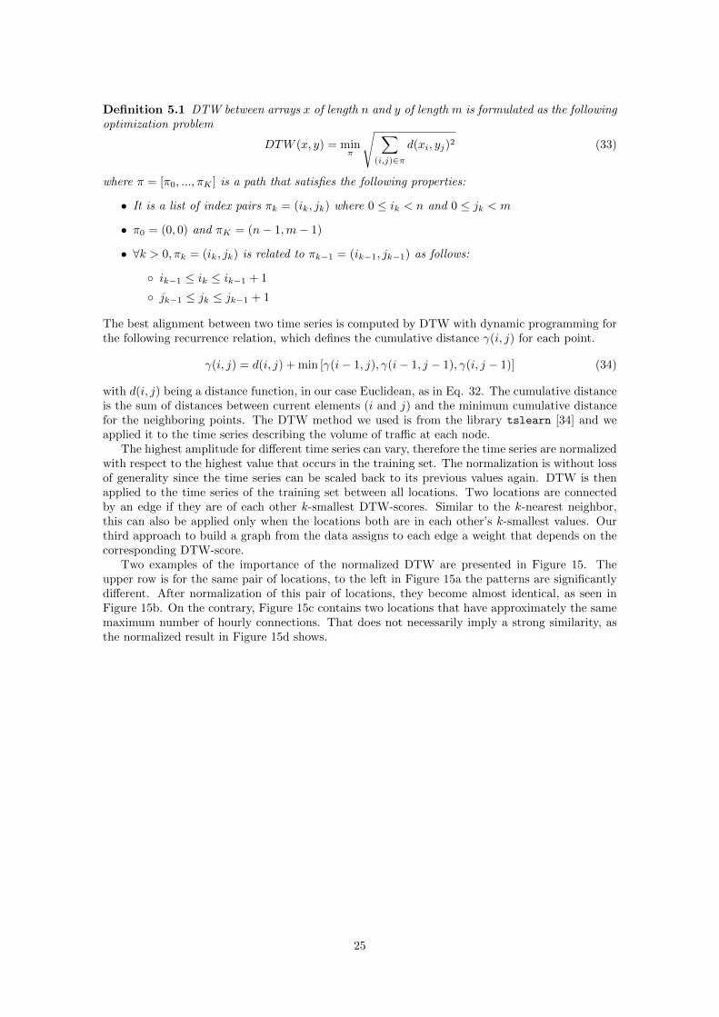
Definition 5.1 DTW between arrays x of length n and y of length m is formulated as the followingoptimization problem

DTW (x, y) = minπ

√ ∑(i,j)∈π

d(xi, yj)2 (33)

where π = [π0, ..., πK ] is a path that satisfies the following properties:

• It is a list of index pairs πk = (ik, jk) where 0 ≤ ik < n and 0 ≤ jk < m

• π0 = (0, 0) and πK = (n− 1,m− 1)

• ∀k > 0, πk = (ik, jk) is related to πk−1 = (ik−1, jk−1) as follows:

◦ ik−1 ≤ ik ≤ ik−1 + 1

◦ jk−1 ≤ jk ≤ jk−1 + 1

The best alignment between two time series is computed by DTW with dynamic programming forthe following recurrence relation, which defines the cumulative distance γ(i, j) for each point.

γ(i, j) = d(i, j) + min [γ(i− 1, j), γ(i− 1, j − 1), γ(i, j − 1)] (34)

with d(i, j) being a distance function, in our case Euclidean, as in Eq. 32. The cumulative distanceis the sum of distances between current elements (i and j) and the minimum cumulative distancefor the neighboring points. The DTW method we used is from the library tslearn [34] and weapplied it to the time series describing the volume of traffic at each node.

The highest amplitude for different time series can vary, therefore the time series are normalizedwith respect to the highest value that occurs in the training set. The normalization is without lossof generality since the time series can be scaled back to its previous values again. DTW is thenapplied to the time series of the training set between all locations. Two locations are connectedby an edge if they are of each other k-smallest DTW-scores. Similar to the k-nearest neighbor,this can also be applied only when the locations both are in each other’s k-smallest values. Ourthird approach to build a graph from the data assigns to each edge a weight that depends on thecorresponding DTW-score.

Two examples of the importance of the normalized DTW are presented in Figure 15. Theupper row is for the same pair of locations, to the left in Figure 15a the patterns are significantlydifferent. After normalization of this pair of locations, they become almost identical, as seen inFigure 15b. On the contrary, Figure 15c contains two locations that have approximately the samemaximum number of hourly connections. That does not necessarily imply a strong similarity, asthe normalized result in Figure 15d shows.

25

(a) Unnormalized hourly connections for two lo-cations.

(b) Normalized hourly connections for the sametwo locations as in (a).

(c) Unnormalized hourly connections for two lo-cations.

(d) Normalized hourly connections for the sametwo locations as in (c).

Figure 15: Hourly connections plotted for two pairs of locations. The same pair of locations appearsin the upper row (a) and (b) and are not similar in (a), after normalization they are very similar in(b). Another pair of locations appear in the lower row (c) and (d). They both have approximatelythe same maximum hourly connections but are not that similar.

Node features

Each node is associated with a vector that contains information, often referred to as node features.Traffic forecasting is made based on these features. Examples of information this vector can includeare location, altitude, node degree, and the number of connections at a previous time.

The feature vector will be tested for different components, three of which are recent activity,previous day activity, and an hour vector to indicate the hour of the day. The number of recentactivities for each location, Tr, is adjustable. The recent activity component contains the numberof cellphone connections for that specific location at the previous time steps. The previous daycomponent consists of the number of cellphone connections to the fixed location at the same timethe previous day, including plus-minus a specified number of hours around this time, Td. See Figure16. Lastly, the hour vector of length 24 indicates which hour of the day it is.

Two node features that capture local spatial information on the structure of the graph are thedegree of every node and the persistence image. The persistence image is a method from the fieldof topological data analysis to capture complex spatial relations between the nodes in the graph.The persistence image is computed from the persistence diagram that is created from a filtrationof the graph, as we described in Section 2.2.

Persistence image

In order to capture the local structure of the graph, the persistence image of size 5× 5 is added asa feature for each node. The persistence image of H1 is computed by PersImage from scikit-TDA

[10], in the following way. The graph for one value of the hyper-parameter of DTW is created. Foreach node in this graph, the following steps are applied. The DTW-score is computed for all thenodes that have DTW-score with the chosen node below a specified threshold and can be reached

26

?

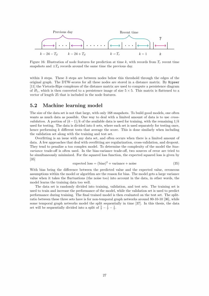
kk − 1k − Trk − 24 + Tdk − 24− Td

Previous day Recent time

Figure 16: Illustration of node features for prediction at time k, with records from Tr recent timesnapshots and ±Td records around the same time the previous day.

within 3 steps. These 3 steps are between nodes below this threshold through the edges of theoriginal graph. The DTW-scores for all these nodes are stored in a distance matrix. By Ripser

[11] the Vietoris-Rips complexes of the distance matrix are used to compute a persistence diagramof H1, which is then converted to a persistence image of size 5 × 5. This matrix is flattened to avector of length 25 that is included in the node features.

5.2 Machine learning model

The size of the data set is not that large, with only 168 snapshots. To build good models, one oftenwants as much data as possible. One way to deal with a limited amount of data is to use cross-validation. A portion of (k−1)/k of the available data is used for training, with the remaining 1/kused for testing. The data is divided into k sets, where each set is used separately for testing once,hence performing k different tests that average the score. This is done similarly when includingthe validation set along with the training and test set.

Overfitting is an issue with any data set, and often occurs when there is a limited amount ofdata. A few approaches that deal with overfitting are regularization, cross-validation, and dropout.They tend to penalize a too complex model. To determine the complexity of the model the bias-variance trade-off is often used. In the bias-variance trade-off, two sources of error are tried tobe simultaneously minimized. For the squared loss function, the expected squared loss is given by[35]

expected loss = (bias)2 + variance + noise (35)

With bias being the difference between the predicted value and the expected value, erroneousassumptions within the model or algorithm are the reason for bias. The model gets a large variancevalue when it takes the fluctuations (the noise too) into account in the data, in other words, themodel learns the training data too well.

The data set is randomly divided into training, validation, and test sets. The training set isused to train and increase the performance of the model, while the validation set is used to predictperformance during training. The final trained model is then evaluated on the test set. The split-ratio between these three sets have is for non-temporal graph networks around 80-10-10 [36], whilesome temporal graph networks model the split sequentially in time [37]. In this thesis, the dataset will be sequentially divided into a split of 5

7 −17 −

17 .

27

6 Experiments

The prediction performance is evaluated with three metrics, Root Mean Square Error (RMSE),Mean Absolute Error (MAE), and Mean Absolute Percentage Error (MAPE), defined as follows

RMSE =

√√√√ 1

NTN

NT∑t=1

N∑i=1

(yt(i)− yt(i))2 (36)

MAE =1

NTN

NT∑t=1

N∑i=1

|yt(i)− yt(i)| (37)

MAPE =1

NTN

NT∑t=1

N∑i=1

∣∣∣∣ yt(i)− yt(i)yt(i)

∣∣∣∣ (38)

where yt(i) and yt(i) are the predicted and the real value for snapshot t and location i. N is thetotal number of locations and NT is the number of snapshots.

Several models are compared for this application. The models are implemented by PyTorch

Geometric Temporal [38], PyTorch Geometric [39], and statsmodels [40].

• GConvGRU [41]: An architecture that combines the convolutional neural networks on agraph to identify the spatial patterns and a RNN in this case GRU to find dynamic patterns.Originally applied to moving MNIST data and modeling natural language. The defaultLaplacian used here is the symmetric one.

• DCRNN [28]: Model the traffic flow as a diffusion process, that incorporates both spatialand temporal dependencies in the traffic flow. The spatial dependency is captured by abidirectional random walk on the graph, and the temporal dependency using an encoder-decoder architecture. Originally applied to a directed graph.

• TGCN [4]: This temporal graph convolutional network model is a combination of a graphconvolutional network (GCN) and a gated recurrent unit (GRU). The GCN is used to learnthe spatial dependencies and the GRU is used to learn the dynamic changes of traffic datain their case.

• GCN [17]: A graph convolutional network. This model does not take the temporal depen-dencies of the graph into account.

• ARIMA: Short for Auto-Regressive Integrated Moving Average and is generally used ontime series data. Is often used for forecasting in time series. This model, like GRU, does nottake spatial dependencies into account.

The last two methods GCN and ARIMA are included to observe the importance of temporal andspatial dependencies. The GCN does not take temporal dependencies into account and the ARIMAdoes not look at the spatial dependencies. Note that GCN still uses the node features, that containinformation about recent and the day before connection activity, while ARIMA uses the whole timeseries of the number of connections up until the current time.

The methods presented above will be compared and evaluated based on the metrics defined inEquations (36), (37), and (38).

The experiments that will be conducted are

• Edge constructions: There are three ways to construct the edges of a graph that willbe considered here. They are DTW, geographical distance with threshold ε (ε-close), and k-neighbors. These methods each have one hyper-parameter that is tested for 5 different values.For DTW and k-neighbors these values are {1, 2, 3, 4, 5} and for ε it is {0.05, 0.1, 0.15, 0.2, 0.25}.The performance with respect to MAPE, RMSE, and MAE are compared for the methodsTGCN, DCRNN, GConvGRU, and GCN. Finally, the best performances of the ε-close andDTW creation of edges are combined to form a graph with a combination of the two. In this

28

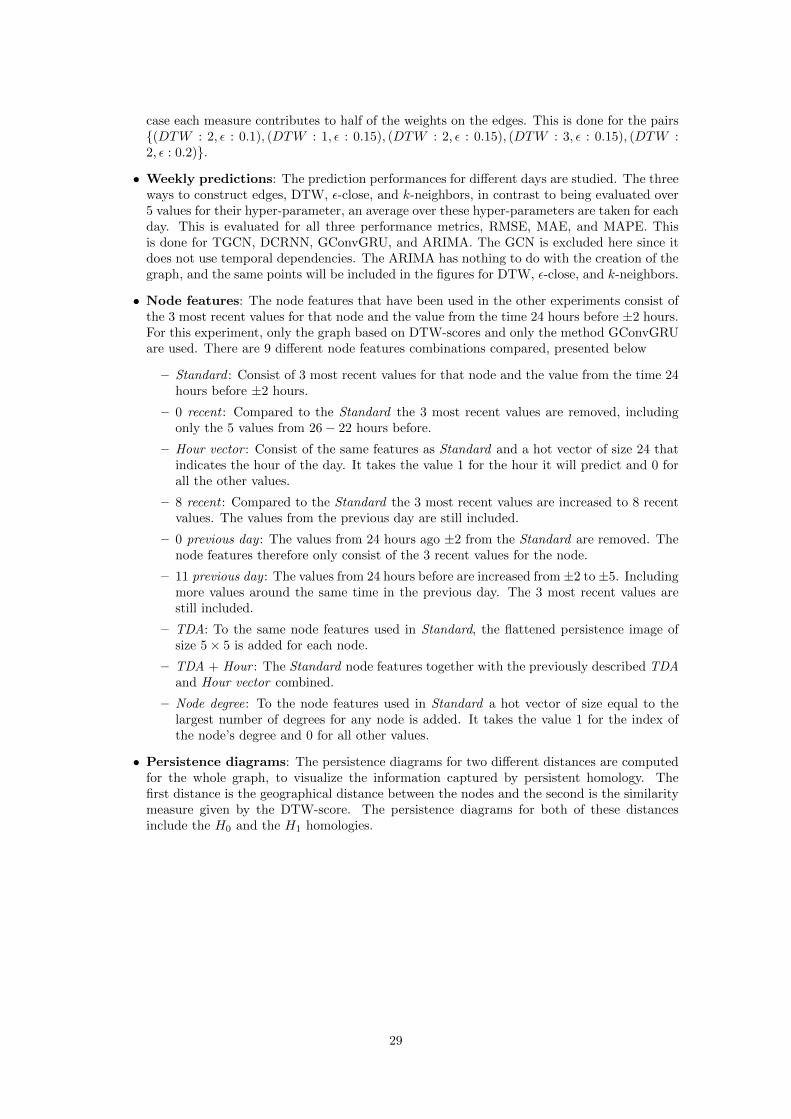
case each measure contributes to half of the weights on the edges. This is done for the pairs{(DTW : 2, ε : 0.1), (DTW : 1, ε : 0.15), (DTW : 2, ε : 0.15), (DTW : 3, ε : 0.15), (DTW :2, ε : 0.2)}.

• Weekly predictions: The prediction performances for different days are studied. The threeways to construct edges, DTW, ε-close, and k-neighbors, in contrast to being evaluated over5 values for their hyper-parameter, an average over these hyper-parameters are taken for eachday. This is evaluated for all three performance metrics, RMSE, MAE, and MAPE. Thisis done for TGCN, DCRNN, GConvGRU, and ARIMA. The GCN is excluded here since itdoes not use temporal dependencies. The ARIMA has nothing to do with the creation of thegraph, and the same points will be included in the figures for DTW, ε-close, and k-neighbors.

• Node features: The node features that have been used in the other experiments consist ofthe 3 most recent values for that node and the value from the time 24 hours before ±2 hours.For this experiment, only the graph based on DTW-scores and only the method GConvGRUare used. There are 9 different node features combinations compared, presented below

– Standard : Consist of 3 most recent values for that node and the value from the time 24hours before ±2 hours.

– 0 recent : Compared to the Standard the 3 most recent values are removed, includingonly the 5 values from 26− 22 hours before.

– Hour vector : Consist of the same features as Standard and a hot vector of size 24 thatindicates the hour of the day. It takes the value 1 for the hour it will predict and 0 forall the other values.

– 8 recent : Compared to the Standard the 3 most recent values are increased to 8 recentvalues. The values from the previous day are still included.

– 0 previous day : The values from 24 hours ago ±2 from the Standard are removed. Thenode features therefore only consist of the 3 recent values for the node.

– 11 previous day : The values from 24 hours before are increased from±2 to±5. Includingmore values around the same time in the previous day. The 3 most recent values arestill included.

– TDA: To the same node features used in Standard, the flattened persistence image ofsize 5× 5 is added for each node.

– TDA + Hour : The Standard node features together with the previously described TDAand Hour vector combined.

– Node degree: To the node features used in Standard a hot vector of size equal to thelargest number of degrees for any node is added. It takes the value 1 for the index ofthe node’s degree and 0 for all other values.

• Persistence diagrams: The persistence diagrams for two different distances are computedfor the whole graph, to visualize the information captured by persistent homology. Thefirst distance is the geographical distance between the nodes and the second is the similaritymeasure given by the DTW-score. The persistence diagrams for both of these distancesinclude the H0 and the H1 homologies.

29

7 Results

The results from the previously explained experiments are presented below. The GConvGRU,DCRNN, TGCN, GCN, and ARIMA are used for different sets of edges and node features. Theoutcome is presented in plots representing the performance on the test set for the different meth-ods. The performance of the different configurations is compared for the three metrics, RMSE,MAE, and MAPE. The performance in prediction for different days is also compared. Lastly,the persistence diagrams representing distance spaces based on the geographical distance betweenradio base stations and dynamic time warping are presented.

We start by illustrating the behavior of one of our models, the DCRNN. In particular, we showan example of RMSE error for training and validation set over the number of epochs, an exampleof a good prediction, and an example of a poor prediction.

(a) Example of error for training and validationset.

(b) Example of a good prediction.

(c) Example of a poor prediction.

Figure 17: The DCRNN used to show the outcome of different predictions and errors over epochsbehavior.

30

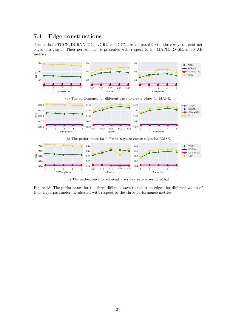
7.1 Edge constructions

The methods TGCN, DCRNN, GConvGRU, and GCN are compared for the three ways to constructedges of a graph. Their performance is presented with respect to the MAPE, RMSE, and MAEmetrics.

(a) The performance for different ways to create edges for MAPE.

(b) The performance for different ways to create edges for RMSE.

(c) The performance for different ways to create edges for MAE.

Figure 18: The performance for the three different ways to construct edges, for different values oftheir hyperparameter. Evaluated with respect to the three performance metrics.

31

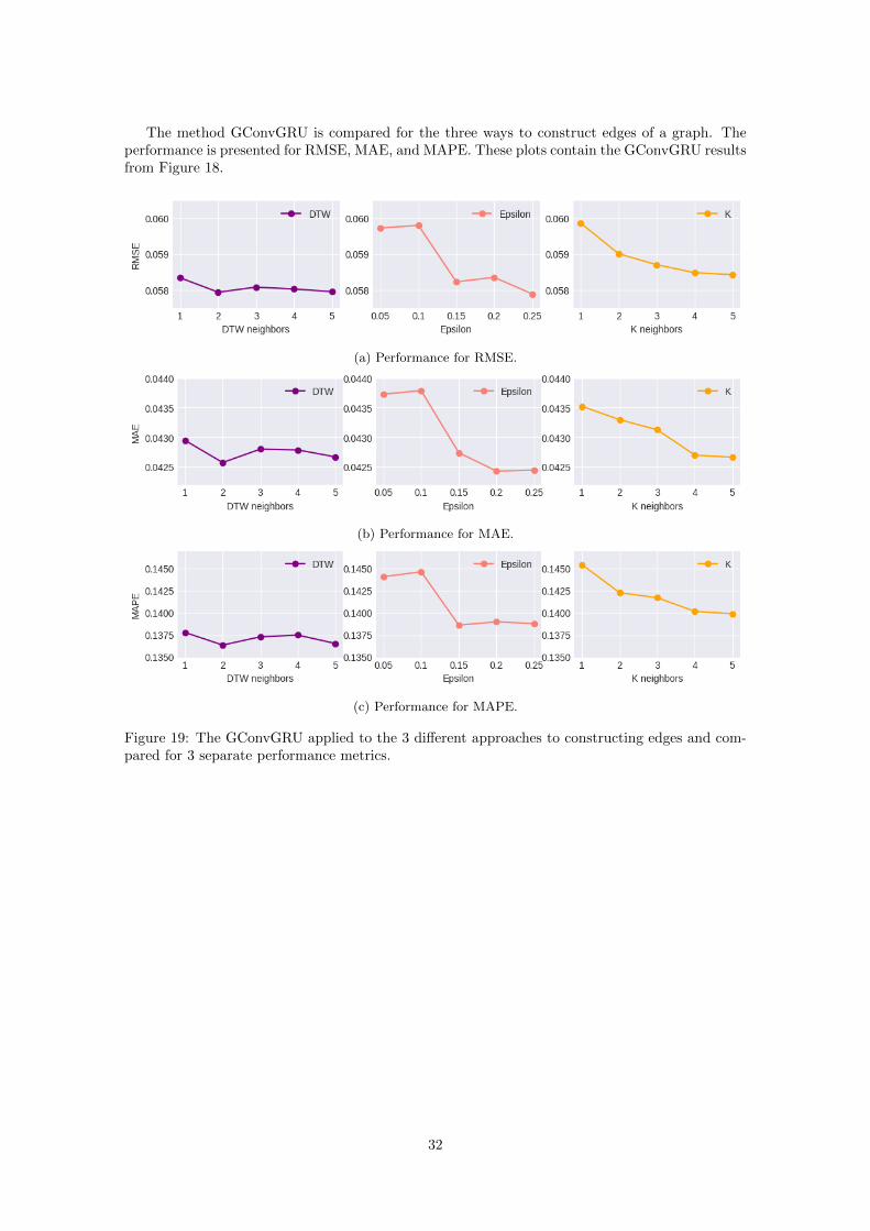
The method GConvGRU is compared for the three ways to construct edges of a graph. Theperformance is presented for RMSE, MAE, and MAPE. These plots contain the GConvGRU resultsfrom Figure 18.

(a) Performance for RMSE.

(b) Performance for MAE.

(c) Performance for MAPE.

Figure 19: The GConvGRU applied to the 3 different approaches to constructing edges and com-pared for 3 separate performance metrics.

32

The performance of the GConvGRU method for a combination of ε-close and DTW creatededges are presented for MAPE, RMSE and MAE in Figure 20.

(a) Performance of combination of edges byMAPE.

(b) Performance of combination of edges byRMSE.

(c) Performance of combination of edges by MAE.

Figure 20: The performance for edges created by a combination of ε-close and DTW approachcompared to models with only ε-close and DTW.

The performance of the ARIMA model for the three metrics for different days and on averageare presented in Table 2.

Table 2: Performance of the ARIMA model.

MAPE MAE RMSESunday 0.675 0.0675 0.256

Wednesday 0.743 0.0761 0.273Thursday 0.744 0.0760 0.272

Friday 0.757 0.0743 0.269Saturday 0.752 0.0732 0.267

Total avg. 0.734 0.0734 0.267

33

7.2 Weekly predictions

We now evaluate the performance of the methods TGCN, DCRNN, GConvGRU, and ARIMA overdifferent days. Where the edges are created in all three ways and the performance is evaluated byMAPE, RMSE, and MAE. Note that ARIMA is not affected by the graph and therefore has thesame value for all the three ways to create edges.

(a) The performance for different weekdays for MAPE.

(b) The performance for different weekdays for RMSE.

(c) The performance for different weekdays for MAE.

Figure 21: The performance for different weekdays with respect to MAPE, RMSE, and MAE fordifferent methods, for three different ways to construct edges.

34

7.3 Node features

The performance for different setup of node features is presented in Figure 22, where the edges ofthe graph are created by DTW similarity and the method is GConvGRU. The standard is the onethat previously has been used, with 3 recent values, 5 values from the day before, the current time±2 snapshots, and no hour vector. The first 5 setups for node features in the box change one ofthese parameters. The last 3 include TDA, a combination of TDA and the hour vector, and lastlythe node degree of every node.

(a) The performance for different node features for MAPE.

(b) The performance for different node features for RMSE.

(c) The performance for different node features for MAE.

Figure 22: The performance for different setups of node features for MAPE, RMSE, and MAE.

35

7.4 Persistence diagrams

The persistence diagrams for both H0 and H1, for the geographical distance and distance measuredby DTW-similarity.

(a) Persistence diagram for the geographical dis-tance.

(b) Persistence diagram for the DTW-score.hejMustafa Mustafa Mustafa

(c) Persistence diagram for the DTW-score, onlyfor H1.

Figure 23: The persistence diagram for H0 and H1 for two different distances, the first one in (a)for geographical distance and the second one in (b) for the similarity measure from the DTW-score.The third figure (c) contains only the H1 for the second one.

36

8 Discussion

To predict the number of connections for each location of a telecommunication network is not aneasy task, it is however of great importance for the telecommunication system. Good predictionsefficiently promote resource allocation, guarantee stability and reliability of the network.

The data set used for this thesis is limited in the number of samples and the time in whichthe data is collected. This may be one reason why the error rate (RMSE) for both validationand training are very similar, see Figure 17a. The limited size of the data set can imply that thetraining set and the validation set are very similar. Learning the noise of the training data cantherefore imply that the model learns the noise for the validation too.

The performance in prediction varies between different locations. An example of a good pre-diction can be seen in Figure 17b, while a poor prediction can be seen in Figure 17c. The challengefor the prediction in Figure 17c is mainly the amplitude of the second peak together with that thetrue value of the predicted peak is lower than all other peaks.

With these examples of predictions in mind, the upcoming subsection will discuss the resultsobtained in this thesis and presented in Section 7.

8.1 Performance of edge constructions

Across all performance metrics and almost every value of the hyper-parameters for all three meth-ods, DTW, ε-close, and k-neighbors, the performance of the methods are in the same order. SeeFigure 18. The GCN that does not take the temporal dependencies into account performs theworst. It does however have the node features of the recent number of connections and 5 valuesfrom around the same time last day. The difference in performance between GCN and TGCN,which is the second worst, is much larger for edges created by DTW than for the two other meth-ods. The creation of the edges for DTW is based on the temporal changes, which can be moreuseful for a method that uses the temporal dependencies in its method. See the leftmost figures inFigures 18a, 18b, and 18c.

For the graphs with edges created by k-neighbors and ε-close, the performance of TGCN andGCN is not that different. The TGCN performs worse than expected across all different setups.Recall that TGCN includes a GCN together with a GRU. There is a significantly better performancefor TGCN over GCN, indicating that the temporal dependency is of importance.

The TGCN performs worse than expected compared to the other two methods using a RNN,namely DCRNN and GConvGRU. Both these methods perform very similar across all evaluationmetrics and for all different creation of edges. With GConvGRU generally performs better thanDCRNN. All three of TGCN, DCRNN, and GConvGRU use a recurrent network, what differen-tiates them is how they capture the spatial dependency and the architecture of the network. Themajor difference in performance between TGCN and the other two methods shows the importanceof the architecture and network.

The method that has performed the best is the GConvGRU. The performance for this methodis compared for the three evaluation metrics for the three ways to construct edges in Figure 19.The two best constructions of edges are the DTW or the ε-close approach, depending on theperformance metric.

Edges created by a combination of the DTW and ε-close approach are seen in Figure 20. Thecombination does not in general perform better than any of the two separate edge creations for allperformance metrics. However, it lowers the RMSE which is the loss function that the models aretrained on, and just slightly the MAE. The lack of increased performance for any other combinationthan DTW:2 and ε : 0.2, maybe that the two methods capture similar dependencies in the graphand the same information in their edges. Another reason for the lack of increase in performancecan be the weighting between the two methods, which could have been done more efficiently.

8.2 Performance of weekly prediction

The five different values of the hyper-parameter for each way to create edges are averaged for thedifferent days used for the test. This approach is to see if there are days that are harder to predict

37

than others. The results can be seen in Figure 21 together with Table 2.The day that is hardest for prediction is one most cases Thursday. The ARIMA model has the

easiest for prediction on Sundays, with the other days being around the same performance. Theother methods, TGCN, DCRNN, and GConvGRU, perform better for Friday-Sunday for MAPE.For RMSE it performs quite similarly for the different days. For MAE, the TGCN performs bestfor Wednesday, Friday, and Saturday, while the DCRNN and the GConvGRU perform best forFriday and Saturday.

What generalizes through the different methods is that Thursday is the hardest day to predict.

8.3 Performance of node features

The methods so far have been conducted with the three recent values and the previous day ±2time steps as node features. The node features are of great importance as seen in Figure 22.

The recent values are of great importance. Removal of the most recent values has a negativeimpact on the results. In all plots, in Figure 22 one can see that going from 3 recent values inStandard to 0 in 0 recent gives a significantly higher error. The inclusion of more recent valueshas no major impact on any of the performance metrics.

The values from the previous day that also are included in Standard have to be chosen correctly.To exclude them completely as in 0 previous day or include too many as in 11 previous day affectsthe performance negatively.

The inclusion of the Hour vector showed great importance, by improving the results across allmetrics. The reason this was not used earlier was the increased training time for the model.

Both TDA and Node degree tries to capture the spatial information of the graph into the nodefeatures. These features do not change in time. By adding the TDA information to the nodesthe performance is perhaps increased slightly at least for MAE and RMSE. The values are stillvery close to the Standard that does not use TDA, making it hard to say with absolute certaintyfor such a small data set. Similar results can be seen when the TDA+Hour is used, the inclusionof TDA might increase the performance very little. Adding the degree of each node to the nodefeatures used in Standard does not change the outcome much for any metric. It may impair theresults to a very small extent.

From the different combinations of node features, there are a few conclusions that one candraw. The temporal features of the nodes are of more importance than the spatial features. Theconnection patterns as shown in Figures 17b and 17c vary much over time, it is nothing that thespatial node features can account for in the prediction. The importance of both recent values,values from the same time 24 hours before, and an indication of the hour are the node features ofthe highest importance. All of these features are related to the temporal aspects.

8.4 Persistence diagrams

The persistence diagrams are a way to visualize the difference in the structure of the two graphs.Figure 23 we can see that there are structural differences in the two graphs. Note that the per-sistence diagrams in Figure 23 are different from those applied in the node features. For thesediagrams, we look at the structure of the global graph, where for the node features we look at thestructure of the local neighborhoods. The two persistence diagrams for the two different distances,show quite different behavior for H1, as seen in Figure 23. Where H1 is the main interest here sinceit gives structure information in the form of cycles. The H0 gives the connected components. InFigure 23b uses DTW-distance there are 2 connected components, while for the geographical dis-tance in Figure 23a there is only one. The structure revealed by these two distances on the graphlooks different, as can be seen in the persistence diagrams. Implying that considering differentways to create edges makes the structure of the weighted graph different.

8.5 Research questions

The research questions are defined at the beginning of this thesis.

38

• How to formalize a graph to achieve the best possible traffic prediction?

Three different ways to create edges are considered, two based on geographical distance/closenessand one on similarity in connection patterns. Out of these three, the ε-close and DTW approachesare the best ones. The DTW approach connecting the two most similar patterns for every nodeperforms about the same as for ε = 0.25 for RMSE and MAE, but for MAPE the DTW outper-forms the ε-close approach. A combination of ε-close and DTW performs well and could also beconsidered.

The most important node features to include are those based on temporal dependencies. Thespatial features can not completely capture the periodic pattern and only gives a limited changein performance. For example, the small increase in performance the inclusion of TDA provides.The most important features to include are recent values, values from around the same time theday before, and an indication of the hour of the day.

• What method gives the most accurate traffic prediction?

Both the time-series in form of ARIMA and the graph network GCN fail to predict the upcomingtraffic as successfully as the temporal graph networks. Out of TGCN, DCRNN, and GConvGRU,the first one performs the worst. The other two perform similarly well with GConvGRU being alittle bit better.

8.6 Future work

This thesis opens up several doors to other and deeper research. One of the main challenges withthis thesis has been the data set. With only one week of data, it is hard to capture the longerdependencies. The original title for this thesis was ”Mining of events from temporal graphs usingrepresentation learning”, where events were to be detected from several weeks of data. This becameimpossible with only one week of data. A new data set is then needed or future work can create alarger data set that spans over several weeks from the one that is used.

More experiments could be conducted for the methods used in the thesis. By trying regulariza-tion techniques, like drop-out. To explore if the training and validation error could be separatedmore than in Figure 17a. If a larger data set was used, the error for training and validation mightbe less similar.

Aside from the data set, some more methods and networks would have been interesting to ex-plore. Both TGCN and GConvGRU use a graph convolution network and a GRU, the performanceis tested for a GCN that ignores the temporal dependency, but not for a GRU that ignores thespatial dependency. The performance of the GRU would possibly tell much about the importanceof the graph structure. Apart from the GRU, other methods capture the spatial or temporal de-pendencies differently. For example STGCN, STHGCN, and 3D-TGCN among others that wouldhave been interesting to explore.

The inclusion of TDA can improve performance as seen in Figure 22. The only filtration studiedin this thesis is the Vietoris-Rips filtration. There are more possible filtrations that would havegiven deeper insights. The original idea for this thesis was to build a new network architecturethat could include the TDA similar to Q.Zhao et al. [4]. The inclusion of TDA in a temporalgraph architecture has not been done to the best of my knowledge. This could give the network alarger understanding of the spatial dependencies.

9 Conclusion

In this thesis, we have conducted experiments to explore the important features of a graph thatis used for traffic prediction. To create a graph that captures spatial dependency the DTW showsgreat results. Important node features mainly captures temporal information such as recent con-nections and hour of the day, while spatial information from TDA can contribute to small improve-ments. The best performing method is the GConvGRU.

39

References

[1] W. L. Hamilton, “Graph representation learning,” Synthesis Lectures on Artificial Intelligenceand Machine Learning, vol. 14, no. 3, pp. 1–159, 2020.

[2] U. von Luxburg, “A tutorial on spectral clustering,” 2007.

[3] G. Carlsson, “Why topological data analysis,” Jan 2015.

[4] L. Zhao, Y. Song, C. Zhang, Y. Liu, P. Wang, T. Lin, M. Deng, and H. Li, “T-gcn: Atemporal graph convolutional network for traffic prediction,” IEEE Transactions on IntelligentTransportation Systems, vol. 21, p. 3848–3858, Sep 2020.

[5] N. Otter, M. A. Porter, U. Tillmann, P. Grindrod, and H. A. Harrington, “A roadmap for thecomputation of persistent homology,” EPJ Data Science, vol. 6, Aug 2017.

[6] R. Ghrist, “Barcodes: The persistent topology of data,” Bulletin of the American Mathemat-ical Society, vol. 45, pp. 61–75, 2008.

[7] M. E. Aktas, E. Akbas, and A. E. Fatmaoui, “Persistence homology of networks: Methodsand applications,” Applied Network Science, vol. 4, p. 61, 2019.

[8] H. Edelsbrunner and J. Harer, Computational Topology - an Introduction. American Mathe-matical Society, 2010.

[9] H. Adams, T. Emerson, M. Kirby, R. Neville, C. Peterson, P. Shipman, S. Chepushtanova,E. Hanson, F. Motta, and L. Ziegelmeier, “Persistence images: A stable vector representationof persistent homology,” Journal of Machine Learning Research, vol. 18, 2017.

[10] C. T. Nathaniel Saul, “Scikit-tda: Topological data analysis for python,” 2019.

[11] C. Tralie, N. Saul, and R. Bar-On, “Ripser.py: A lean persistent homology library for python,”The Journal of Open Source Software, vol. 3, p. 925, Sep 2018.

[12] I. Goodfellow, Y. Bengio, and A. Courville, Deep Learning. MIT Press, 2016. http://www.

deeplearningbook.org.

[13] K. Cho, B. van Merrienboer, C. Gulcehre, D. Bahdanau, F. Bougares, H. Schwenk, andY. Bengio, “Learning phrase representations using RNN encoder–decoder for statistical ma-chine translation,” in Proceedings of the 2014 Conference on Empirical Methods in NaturalLanguage Processing (EMNLP), (Doha, Qatar), pp. 1724–1734, Association for ComputationalLinguistics, Oct. 2014.

[14] S. Hochreiter and J. Schmidhuber, “Long short-term memory,” Neural Computation, vol. 9,no. 8, pp. 1735–1780, 1997.

[15] Z. Liu and J. Zhou, Introduction to Graph Neural Networks. Morgan & Claypool, 2020.

[16] E. Rossi, B. Chamberlain, F. Frasca, D. Eynard, F. Monti, and M. Bronstein, “Temporalgraph networks for deep learning on dynamic graphs,” 2020.

[17] T. N. Kipf and M. Welling, “Semi-supervised classification with graph convolutional net-works,” 2017.

[18] D. K. Hammond, P. Vandergheynst, and R. Gribonval, “Wavelets on graphs via spectral graphtheory,” 2009.

[19] M. Defferrard, X. Bresson, and P. Vandergheynst, “Convolutional neural networks on graphswith fast localized spectral filtering,” 2017.

[20] F. Scarselli, M. Gori, A. C. Tsoi, M. Hagenbuchner, and G. Monfardini, “The graph neuralnetwork model,” IEEE Transactions on Neural Networks, vol. 20, no. 1, pp. 61–80, 2009.

40

[21] W. L. Hamilton, R. Ying, and J. Leskovec, “Inductive representation learning on large graphs,”2018.

[22] P. Velickovic, G. Cucurull, A. Casanova, A. Romero, P. Lio, and Y. Bengio, “Graph attentionnetworks,” in International Conference on Learning Representations, 2018.

[23] H. Cai, V. W. Zheng, and K. C.-C. Chang, “A comprehensive survey of graph embedding:Problems, techniques and applications,” 2018.

[24] A. Gionis, “Lecture notes in dd2434 machine learning, advances course. module 4: learningwith graphs,” November 2020.

[25] B. Yu, M. Li, J. Zhang, and Z. Zhu, “3d graph convolutional networks with temporal graphs:A spatial information free framework for traffic forecasting,” 2019.

[26] S. Zhao, X. Jiang, G. Jacobson, R. Jana, W.-L. Hsu, R. Rustamov, M. Talasila, S. Aftab,Y. Chen, and C. Borcea, “Cellular network traffic prediction incorporating handover: A graphconvolutional approach,” in 2020 17th Annual IEEE International Conference on Sensing,Communication, and Networking (SECON), pp. 1–9, 06 2020.

[27] B. Yu, H. Yin, and Z. Zhu, “Spatio-temporal graph convolutional networks: A deep learn-ing framework for traffic forecasting,” Proceedings of the Twenty-Seventh International JointConference on Artificial Intelligence, Jul 2018.

[28] Y. Li, R. Yu, C. Shahabi, and Y. Liu, “Diffusion convolutional recurrent neural network:Data-driven traffic forecasting,” 2018.

[29] X. Wang, Y. Ma, Y. Wang, W. Jin, X. Wang, J. Tang, C. Jia, and J. Yu, “Traffic flowprediction via spatial temporal graph neural network,” in Proceedings of The Web Conference2020, WWW ’20, (New York, NY, USA), p. 1082–1092, Association for Computing Machinery,2020.

[30] S. Antaris and D. Rafailidis, “Vstreamdrls: Dynamic graph representation learning with self-attention for enterprise distributed video streaming solutions,” 2020.

[31] M. Kalander, M. Zhou, C. Zhang, H. Yi, and L. Pan, “Spatio-temporal hybrid graph convo-lutional network for traffic forecasting in telecommunication networks,” 2020.

[32] Z. Du, Y. Yang, Z. Ertem, C. Gao, L. Huang, Q. Huang, and Y. Bai, “Inter-urban mobilityvia cellular position tracking in the southest songliao basin, northeast china,” Scientific Data,vol. 6, 2019.

[33] D. J. Berndt and J. Clifford, “Using dynamic time warping to find patterns in time series,”in Proceedings of the 3rd International Conference on Knowledge Discovery and Data Mining,AAAIWS’94, p. 359–370, AAAI Press, 1994.

[34] R. Tavenard, J. Faouzi, G. Vandewiele, F. Divo, G. Androz, C. Holtz, M. Payne, R. Yurchak,M. Rußwurm, K. Kolar, and E. Woods, “Tslearn, a machine learning toolkit for time seriesdata,” Journal of Machine Learning Research, vol. 21, no. 118, pp. 1–6, 2020.

[35] C. M. Bishop, Pattern Recognition and Machine Learning (Information Science and Statis-tics). Berlin, Heidelberg: Springer-Verlag, 2006.

[36] V. P. Dwivedi, C. K. Joshi, T. Laurent, Y. Bengio, and X. Bresson, “Benchmarking graphneural networks,” 2020.

[37] W. Hu, M. Fey, M. Zitnik, Y. Dong, H. Ren, B. Liu, M. Catasta, and J. Leskovec, “Opengraph benchmark: Datasets for machine learning on graphs,” 2021.

[38] B. Rozemberczki, P. Scherer, Y. He, G. Panagopoulos, M. Astefanoaei, O. Kiss, F. Beres,N. Collignon, and R. Sarkar, “PyTorch Geometric Temporal: Spatiotemporal Signal Process-ing with Neural Machine Learning Models,” 2021.

41

[39] M. Fey and J. E. Lenssen, “Fast graph representation learning with PyTorch Geometric,” inICLR Workshop on Representation Learning on Graphs and Manifolds, 2019.

[40] S. Seabold and J. Perktold, “statsmodels: Econometric and statistical modeling with python,”in 9th Python in Science Conference, 2010.

[41] Y. Seo, M. Defferrard, P. Vandergheynst, and X. Bresson, “Structured sequence modelingwith graph convolutional recurrent networks,” 2016.

42

www.kth.se

TRITA-SCI-GRU 2021:194