Time and frequency users manual

A 11 10 3 07512T

o

JNBS SPECIAL PUBLICATION 559

U.S. DEPARTMENT OF COMMERCE / National Bureau of Standards

Time and Frequency Users' Manual

NATIONAL BUREAU OF STANDARDS

The National Bureau of Standards' was established by an act of Congress on March 3, 1901.

The Bureau's overall goal is to strengthen and advance the Nation's science and technology

and facilitate their effective application for public benefit. To this end, the Bureau conducts

research and provides: (1) a basis for the Nation's physical measurement system, (2) scientific

and technological services for industry and government, (3) a technical basis for equity in

trade, and (4) technical services to promote public safety. The Bureau's technical work is per-

formed by the National Measurement Laboratory, the National Engineering Laboratory, and

the Institute for Computer Sciences and Technology

THE NATIONAL MEASUREMENT LABORATORY provides the national system of

physical and chemical and materials measurement; coordinates the system with measurement

systems of other nations and furnishes essential services leading to accurate and uniform

physical and chemical measurement throughout the Nation's scientific community, industry,

and commerce; conducts materials research leading to improved methods of measurement,

standards, and data on the properties of materials needed by industry, commerce, educational

institutions, and Government; provides advisory and research services to other Government

agencies; develops, produces, and distributes Standard Reference Materials; and provides

calibration services. The Laboratory consists of the following centers:

Absolute Physical Quantities 2 — Radiation Research — Thermodynamics and

Molecular Science — Analytical Chemistry — Materials Science.

THE NATIONAL ENGINEERING LABORATORY provides technology and technical ser-

vices to the public and private sectors to address national needs and to solve national

problems; conducts research in engineering and applied science in support of these efforts;

builds and maintains competence in the necessary disciplines required to carry out this

research and technical service; develops engineering data and measurement capabilities;

provides engineering measurement traceability services; develops test methods and proposes

engineering standards and code changes; develops and proposes new engineering practices;

and develops and improves mechanisms to transfer results of its research to the ultimate user.

The Laboratory consists of the following centers:

Applied Mathematics — Electronics and Electrical Engineering 2 — Mechanical

Engineering and Process Technology 2 — Building Technology — Fire Research —Consumer Product Technology — Field Methods.

THE INSTITUTE FOR COMPUTER SCIENCES AND TECHNOLOGY conducts

research and provides scientific and technical services to aid Federal agencies in the selection,

acquisition, application, and use of computer technology to improve effectiveness and

economy in Government operations in accordance with Public Law 89-306 (40 U.S.C. 759),

relevant Executive Orders, and other directives; carries out this mission by managing the

Federal Information Processing Standards Program, developing Federal ADP standards

guidelines, and managing Federal participation in ADP voluntary standardization activities;

provides scientific and technological advisory services and assistance to Federal agencies; and

provides the technical foundation for computer-related policies of the Federal Government.

The Institute consists of the following centers:

Programming Science and Technology — Computer Systems Engineering.

'Headquarters and Laboratories at Gaithersburg, MD, unless otherwise noted;

mailing address Washington, DC 20234.:Some divisions within the center are located at Boulder, CO 80303.

Banroai mravm v. —JAN 1 8 1980

r\crt ftcc -£Lt/

Time and Frequency Users' Manual5^

Edited by:

r\0-

George KamasSandra L. Howe

Time and Frequency Division

National Measurement Laboratory

National Bureau of Standards

Boulder, Colorado 80303

U.S. DEPARTMENT OF COMMERCELuther H. Hodges, Jr., Under Secretary

Jordan J. Baruch, Assistant Secretary for Science and Technology

NATIONAL BUREAU OF STANDARDS, Ernest Ambler, Director

Issued November 1979

Library of Congress Catalog Card Number: 79-600169

National Bureau of Standards Special Publication 559Nat. Bur. Stand. (U.S.), Spec. Pubi. 559, 256 pages (Nov. 1979)

CODEN. XNBSAV

(Supersedes NBS Technical Note 695, May 1977)

U.S. GOVERNMENT PRINTING OFFICE

WASHINGTON: 1979

For sale by the Superintendent of Documents, U.S. Government Printing Office.

Washington, D.C. 20402

Stock No. 003-003-02137-1 - Price $6.

(Add 2u percent additional for other than U.S. mailing).

CONTENTS

PAGE

CHAPTER 1. INTRODUCTION: WHAT THIS BOOK IS ABOUT

1.1 WHO NEEDS TIME & FREQUENCY? 1

1.2 WHAT ARE TIME AND FREQUENCY ? 4

1.3 WHAT IS A STANDARD ? . . 5

1.3.1 CAN TIME REALLY BE A STANDARD? 6

1.3.2 THE NBS STANDARDS OF TIME AND FREQUENCY 6

1.4 HOW TIME AND FREQUENCY STANDARDS ARE DISTRIBUTED 7

1.5 THE NBS ROLE IN INSURING ACCURATE TIME AND FREQUENCY 7

1.6 WHEN DOES A MEASUREMENT BECOME A CALIBRATION ? •

. .81.7 TERMS USED . . 8

1.7.1 MEGA, MILLI, PARTS PER... AND PERCENTS ...... 8

1.7.2 FREQUENCY 10

1.8 DISTRIBUTING TIME AND FREQUENCY SIGNALS VIA CABLES AND TELEPHONE LINES . .111.9 TIME CODES 13

CHAPTER 2. THE EVOLUTION OF TIMEKEEPING

2.1 TIME SCALES 17

2.1.1 SOLAR TIME 17

2.1.2 ATOMIC TIME 18

A. Coordinated Universal Time ......... 19

B. The New UTC System 19

2.1.3 TIME ZONES 20

2.2 USES OF TIME SCALES 21

2.2.1 SYSTEMS SYNCHRONIZATION 21

2.2.2 NAVIGATION AND ASTRONOMY 22

2.3 INTERNATIONAL COORDINATION OF TIME AND FREQUENCY ACTIVITIES 23

2.3.1 THE ROLE OF THE INTERNATIONAL TIME BUREAU (BIH) 23

2.3.2 THE ROLE OF THE NATIONAL BUREAU OF STANDARDS (NBS) 23

2.3.3 THE ROLE OF THE U.S. NAVAL OBSERVATORY (USNO) AND THE DOD PTTI PROGRAM . 24

CHAPTER 3. THE ALGEBRA AND CONVENTIONS FOR TIME AND FREQUENCY MEASUREMENTS

3.1 EXPRESSING FREQUENCY DIFFERENCE (IN HERTZ, kHz, MHz , ETC.) 28

3.2 RELATIVE (FRACTIONAL) FREQUENCY, F (DIMENSIONLESS) 28

3.3 RELATIVE (FRACTIONAL) FREQUENCY DIFFERENCE, S (DIMENSIONLESS) . . . .283.4 EXAMPLE OF ALGEBRA AND SIGN CONVENTIONS IN TIME AND FREQUENCY MEASUREMENTS . . 29

3.4.1 Television Frequency Transfer Measurements (covered in Chapter 7) .293.4.2 Television Line-10 Time Transfer Measurements (covered in Chapter 8) . 29

iii

5 USING TIME TO GET FREQUENCY 30

3.6 A MATHEMATICAL DERIVATION 31

3.7 DEFINITIONS 32

CHAPTER 4. USING TIME AND FREQUENCY IN THE LABORATORY

4.1 ELECTRONIC COUNTERS . . . .33

4.1.1 SOURCES OF COUNTER ERROR 34

4.1.2 FREQUENCY MEASUREMENTS 34

A. Direct Measurement . . . . . . . . . . .35B. Prescaling 35

C. Heterodyne Converters .......... 35D. Transfer Oscillators .......... 37

4.1.3 PERIOD MEASUREMENTS 39

4.1.4 TIME INTERVAL MEASUREMENTS 404.1.5 PHASE MEASUREMENTS 42

4.1.6 PULSE-WIDTH DETERMINATION MEASUREMENTS 43

4.1.7 COUNTER ACCURACY 43

A. Time Base Error ... . . . . . . . .43B. Gate Error . 44

C. Trigger Errors . . . . . . . , .45

4.1.8 PRINTOUT AND RECORDING 48

4.2 OSCILLOSCOPE METHODS 48

4.2.1 CALIBRATING THE OSCILLOSCOPE TIME BASE ....... 494.2.2 DIRECT MEASUREMENT OF FREQUENCY 50

4.2.3 FREQUENCY COMPARISONS 50

A. Lissajous Patterns 50

B. Sweep Frequency Calibration: An Alternative Method . . . .55

4.2.4 TIME INTERVAL MEASUREMENTS 56

4.3 WAVEMETERS 56

4.4 HETERODYNE FREQUENCY METERS 57

4.5 DIRECT-READING ANALOG FREQUENCY METERS 58

4.5.1 ELECTRONIC AUDIO FREQUENCY METER 58

4.5.2 RADIO FREQUENCY METER 59

4.6 FREQUENCY COMPARATORS 60

4.7 AUXILIARY EQUIPMENT 60

4.7.1 FREQUENCY SYNTHESIZERS 604.7.2 PHASE ERROR MULTIPLIERS 61

4.7.3 PHASE DETECTORS 62

4.7.4 FREQUENCY DIVIDERS 63

A. Analog or Regenerative Dividers ........ 63

B. Digital Dividers ........... 63

4.7.5 ADJUSTABLE RATE DIVIDERS 64

4.7.6 SIGNAL AVERAGERS 65

iv

8 PHASE LOCK TECHNIQUES 66

4.9 SUMMARY '.67

CHAPTER 5. THE USE OF HIGH-FREQUENCY RADIO BROADCASTS FOR TIME AND FREQUENCY

CALIBRATIONS

5.1 BROADCAST FORMATS 69

5.1.1 WWV/WWVH 69

5.1.2 CHU 70

5.1.3 ATA 71

5.1.4 IAM 72

5.1.5 IBF 72

5.1.6 JJY 72

5.1.7 OMA . . .745.1.8 VNG 74

A. Time Signals 74

B. Time Code 74

C. Announcements ............ 74

D. DUT1 Code 75

E. Accuracy............. 75

F. Frequency and Time Generating Equipment ...... 75

5.1.9 ZUO 75

A. Carrier Frequencies and Times of Transmission . . . . .76B. Standard Time Intervals and Time Signals ...... 76

C. Standard Audio Frequencies ......... 76

D. Accuracy 76

E. DUT1 Code 76

5.2 RECEIVER SELECTION 81

5.3 CHOICE OF ANTENNAS AND SIGNAL CHARACTERISTICS 82

5.4 USE OF HF BROADCASTS FOR TIME CALIBRATIONS 86

5.4.1 TIME-OF-DAY ANNOUNCEMENTS 865.4.2 USING THE SECONDS TICKS 86

A. Receiver Time Delay Measurements ....... 86

B. Time Delay Over the Radio Path 87

C. Using an Adjustable Clock to Trigger the Oscilloscope . . .88D. Delayed Triggering: An Alternate Method that Doesn't Change the

Clock Output 90

E. Using Oscilloscope Photography for Greater Measurement Accuracy . 92

5.4.3 USING THE WWV/WWVH TIME CODE 92

A. Code Format . . 93

B. Recovering the Code . .94

5.5 USE OF HF BROADCASTS FOR FREQUENCY CALIBRATIONS 96

5.5.1 BEAT FREQUENCY METHOD 97

5.5.2 OSCILLOSCOPE LISSAJOUS PATTERN METHOD 98

5.5.3 OSCILLOSCOPE PATTERN DRIFT METHOD 100

5.5.4 FREQUENCY CALIBRATIONS BY TIME COMPARISON OF CLOCKS 100

v

6 FINDING THE PROPAGATION PATH DELAY 101

5.6.1 GREAT CIRCLE DISTANCE CALCULATIONS 101

5.6.2 PROPAGATION DELAYS '

. . . 102

5.7 THE NBS TELEPHONE TIME-OF-DAY SERVICE 105

5.8 SUMMARY. 105

CHAPTER 6. CALIBRATIONS USING LF AND VLF RADIO TRANSMISSIONS

6.1 ANTENNAS FOR USE AT VLF-LF 107

6.2 SIGNAL FORMATS 107

6.3 PROPAGATION CHARACTERISTICS AND OTHER PHASE CHANGES 108

6.4 FIELD STRENGTHS OF VLF-LF STATIONS Ill

6.5 INTERFERENCE .113

6.6 USING WWVB FOR FREQUENCY CALIBRATIONS 113

6.6.1 PHASE-SHIFT IDENTIFICATION 1146.6.2 METHODS OF FREQUENCY COMPARISON 115

6.7 USING OTHER LF AND VLF STATIONS FOR TIME AND FREQUENCY CALIBRATIONS . . .115

6.7.1 THE OMEGA NAVIGATION SYSTEM 115

A. Operating Characteristics of Omega ....... 115

B. Synchronization Control .......... 117C. Propagation Characteristics ......... 117

D. Omega Notices and Navigational Warnings ...... 118

6.7.2 DCF 77, WEST GERMANY (77.5 kHz) 118

A. Time Signals . 119B. Time Code 119

6.7.3 HBG, SWITZERLAND (75 kHz) 120

A. Signal Format 12,0

B. Time Code . ... . ' 120

6.7.4 JG2AS/JJF-2, JAPAN (40 kHz) . . . . - 1206.7.5 MSF, ENGLAND (60 kHz) 121

A. Fast Code 121

B. Slow Code 121

6.7.6 U.S. NAVY COMMUNICATION STATIONS 121

6.7.7 OMA, CZECHOSLOVAKIA (50 kHz) 123

A. Time Code 123

6.7.8 RBU (66-2/3 kHz) AND RTZ (50 kHz), USSR 124

6.7.9 VGC3 AND VTR3, USSR . . 124

6.8 MONITORING DATA AVAILABILITY 127

vi

9 USING THE WWVB TIME CODE 127

6.9.1 TIME CODE FORMAT 127

6.9.2 TIME TRANSFER USING THE TRANSMITTED ENVELOPE 128

6.10 SUMMARY 130

CHAPTER 7. FREQUENCY CALIBRATIONS USING TELEVISION SIGNALS

7.1 HOW THIS FITS INTO OTHER NBS SERVICES 131

7.2 BASIC PRINCIPLES OF THE TV FREQUENCY CALIBRATION SERVICE 131

7.2.1 PHASE INSTABILITIES OF THE TV SIGNALS 133

7.2.2 TYPICAL VALUES FOR THE U.S. NETWORKS 134

7.3 HOW RELATIVE FREQUENCY IS MEASURED 135

7.3.1 COLOR BAR COMPARATOR 136

7.3.2 THE NBS SYSTEM 358 FREQUENCY MEASUREMENT COMPUTER 138

A. Block Diagram Overview .......... 138

B. Use of FMC with Unstable Crystal Oscillators 141

7.4 GETTING GOOD TV CALIBRATIONS 141

7.5 THE DIGITAL FRAME SYNCHRONIZER 142

7.6 USNO TV FREQUENCY CALIBRATION SERVICE 142

CHAPTER 8. FREQUENCY AND TIME CALIBRATIONS USING TV LINE-10

8.1 HOW THE SERVICE WORKS 145

8.1.1 USING LINE-10 ON A LOCAL BASIS 145

8.1.2 USING LINE-10 FOR NBS TRACEABILITY 146

8.2 EQUIPMENT NEEDED 147

8.3 TV LINE-10 DATA, WHAT DO THE NUMBERS MEAN ? 148

8.4 WHAT DO YOU DO WITH THE DATA ? 149

8.5 RESOLUTION OF THE SYSTEM 149

8.6 GETTING TIME OF DAY FROM LINE-10 151

8.7 THE DIGITAL FRAME SYNCHRONIZER 151

8.8 MEASUREMENTS COMPARED TO THE USNO 151

8.9 LINE-10 EQUIPMENT AVAILABILITY 151

CHAPTER 9. LORAN-C TIME AND FREQUENCY METHODS

9.1 BASIC PRINCIPLES OF THE LORAN-C NAVIGATION SYSTEM 153

9.2 BASIC LORAN-C FORMAT 160

9.2.1 CARRIER FREQUENCY 161

9.2.2 TRANSMITTED PULSE SHAPE 161

9.2.3 TRANSMITTED PULSE 161

vii

2.4 GRAPHICAL REPRESENTATION 163

A. Envelope-to Cycle Difference . 163

B. ECD Determination 164

C. Pulse Group . 164

D. Existing Format 164

E. GRI 165

F. Blink Codes .165G. Spectrum 166

H. Fine Spectra 166

I. Harmonics 166

9.3 WHAT IS THE EXTENT OF LORAN-C COVERAGE? ... 166

9.3.1 GROUNDWAVE SIGNAL RANGE 166

9.3.2 SKYWAVE SIGNAL RANGE 167

9.4 WHAT DO WE GET FROM LORAN-C ? 167

9.4.1 SIGNAL CHARACTERISTICS 167

9.4.2 TIME SETTING 1689.4.3 FREQUENCY CALIBRATIONS USING LORAN-C 170

9.5 HOW GOOD IS LORAN-C ? 171

9.5.1 GROUNDWAVE ACCURACY 172

9.5.2 SKYWAVE ACCURACY . 172

9.6 ARE THE DATA VALID ? 172

9.7 SUMMARY 17>3

CHAPTER 10. SATELLITE METHODS OF TINE AND FREQUENCY DISSEMINATION

10.1 THE GOES SATELLITE TIME CODE 175

10.1.1 BACKGROUND 17510.1.2 COVERAGE 17610.1.3 SIGNAL CHARACTERISTICS 17710.1.4 TIME CODE FORMAT 177

10.1.5 ANTENNA POINTING 180

10.1.6 PERFORMANCE 180

A. Uncorrected ............. 180B. Corrected for Mean Path Delay 180C. Fully Corrected 180

10.1.7 EQUIPMENT NEEDED 180

A. Antennas 180

B. Receivers ............ 181

10.1.8 SATELLITE-CONTROLLED CLOCK 181

A. Delay Corrections . 182

B. Programs for Computing Free-Space Path Delay 182

10.1.9 SMART CLOCK..... 18210.1.10 CLOCK CALIBRATION 18310.1.11 RESULTS 184

viii

1.12 Precautions . . . 186

A. Interference ............ 186B. Outages 186C. Continuity 187

10.2 THE TRANSIT NAVIGATION SYSTEM 187

10.2.1 GENERAL 18710.2.2 EQUIPMENT NEEDED . 189

CHAPTER 11. AN INTRODUCTION TO FREQUENCY SOURCES

11.1 FREQUENCY SOURCES AND CLOCKS 191

11.2 THE PERFORMANCE OF FREQUENCY SOURCES . 193

11.3 USING RELATIVE FREQUENCY STABILITY DATA 194

11.4 RESONATORS . 196

11.5 PRIMARY AND SECONDARY STANDARDS 197

11.6 QUARTZ CRYSTAL OSCILLATORS 199

11.6.1 TEMPERATURE AND AGING OF CRYSTALS 20111.6.2 QUARTZ CRYSTAL OSCILLATOR PERFORMANCE 201

11.7 ATOMIC RESONANCE DEVICES '

. . . . 202

11.7.1 STATE SELECTION 20311.7.2 HOW TO DETECT RESONANCE 20411.7.3 ATOMIC OSCILLATORS 20511.7.4 ATOMIC RESONATOR FREQUENCY STABILITY AND ACCURACY 206

11.8 AVAILABLE ATOMIC FREQUENCY DEVICES 207

11.8.1 CESIUM BEAM FREQUENCY OSCILLATORS 207

11.8.2 RUBIDIUM GAS CELL FREQUENCY OSCILLATORS 20811.8.3 ATOMIC HYDROGEN MASERS 209

11.9 TRENDS 210

CHAPTER 12. SUMMARY OF AVAILABLE SERVICES 213

BIBLIOGRAPHY 217

GLOSSARY 219

INDEX 225

ix

TABLES

Table 1 1 PREFIX CONVERSION CHART 9

Table 1 2 CONVERSIONS FROM PARTS PER . . . TO PERCENTS 9

Table 1 3 CONVERSIONS TO HERTZ 10

Table 1 4 RADIO FREQUENCY BANDS 10

Table 4 1 READINGS OBTAINED WITH VARIOUS SETTINGS

OF TIME BASE AND PERIOD MULTIPLIER CONTROLS .... 40

Table 5. 1 STANDARD FREQUENCY AND TIME SIGNAL BROADCASTS

IN THE HIGH FREQUENCY BAND 77

Table 5 2 IMAGE FREQUENCIES FOR WWV/WWVH 82

Table 6 1 CHARACTERISTICS OF THE OMEGA NAVIGATION SYSTEM STATIONS . 116

Table 6 2 STANDARD FREQUENCY AND TIME SIGNAL

BROADCASTS IN THE LOW FREQUENCY BAND . 125

Table 9 1 LORAN-C CHAINS . 154

Table 9 2 ECD TABLE: HALF CYCLE PEAK AMPLITUDE vs ECD (LORAN-C) . . 163

Table 9. 3 GROUP REPETITION INTERVALS (LORAN-C) . 164

Table 10 1 SPECIFICATIONS FOR THE GOES SATELLITES . 175

Table 11. 1 COMPARISON OF FREQUENCY SOURCES . 211

Table 12 1 CHARACTERISTICS OF THE MAJOR T&F

DISSEMINATION SYSTEMS . . . 213

Table 12. 2 HOW FREQUENCY IS CALIBRATED . 214

Table 12. 3 HOW TIME IS CALIBRATED . . 214

FIGURES

Figure 1. 1 ORGANIZATION OF THE NBS FREQUENCY AND TIME STANDARD 6

Figure 1. 2 IRIG TIME CODE, FORMAT H 13

Figure 1. 3 IRIG TIME CODE FORMATS 14

Figure 2. 1 UNIVERSAL TIME FAMILY RELATIONSHIPS 18

Figure 2. 2 FIRST ATOMIC CLOCK 18

Figure 2. 3 CLASSES OF TIME SCALES & ACCURACIES 19

Figure 2. 4 DATING OF EVENTS IN THE VICINITY OF A LEAP SECOND .... 19

Figure 2. 5 STANDARD TIME ZONES OF THE WORLD REFERENCED TO UTC ... 20

Figure 2. 6 NBS, USNO, AND BIH INTERACTIONS 23

Figure 4. 1 ELECTRONIC COUNTERS 33

Figure 4 2 SIMPLIFIED BLOCK DIAGRAM OF AN ELECTRONIC COUNTER .... 34

Figure 4. 3 DIAGRAM OF A COUNTER IN THE FREQUENCY MEASUREMENT MODE . 35

Figure 4 4 PRESCALER-COUNTER COMBINATION . . . 36

Figure 4. 5 TYPICAL MANUALLY-TUNED HETERODYNE CONVERTER 36

Figure 4 6 TYPICAL MANUALLY-TUNED TRANSFER OSCILLATOR 37

Figure 4 7 AUTOMATIC TRANSFER OSCILLATORS 38

Figure 4 8 DIAGRAM OF COUNTER IN THE PERIOD-MEASUREMENT MODE .... 39

Figure 4 9 DIAGRAM OF COUNTER IN THE MULTIPLE-PERIOD MODE .... 39

X

Figure 4. 10 EFFECT OF NOISE ON TRIGGER POINT IN PERIOD MEASUREMENTS 41

Figure 4. 11 DIAGRAM OF COUNTER IN THE TIME INTERVAL MODE 41

Figure 4. 12 OPTIMUM TRIGGER POINTS FOR START-STOP PULSES 42

Figure 4. 13 USE OF TIME-INTERVAL UNIT FOR PHASE MEASUREMENTS .... 42

Figure 4. 14 TIME- INTERVAL COUNTER WITH START-STOP CHANNELS CONNECTED

TO COMMON SOURCE FOR PULSE-WIDTH OR PERIOD MEASUREMENTS 43

Figure 4. 15 TYPICAL TIME BASE STABILITY CURVE 44

Figure 4. 16 CONSTANT GATING INTERVAL WITH AMBIGUITY OF ± 1 COUNT 45

Figure 4. 17 ACCURACY CHART FOR PERIOD AND FREQUENCY MEASUREMENTS 45

Figure 4. 18 UNDIFFERENTIATED SCHMITT-TRIGGER WAVEFORMS 46

Figure 4. 19 TIME ERROR PRODUCED BY IMPROPER CALIBRATION OF

TRIGGER LEVEL CONTROL 47

Figure 4. 20 SINE WAVE METHOD OF CHECKING TRIGGER LEVEL CALIBRATION . . 47

Figure 4. 21 DIGITAL-TO-ANALOG ARRANGEMENT FOR CHART RECORDING .... .48Figure 4. 22 SIMPLIFIED BLOCK DIAGRAM OF A CATHODE-RAY OSCILLOSCOPE . 48

Figure 4. 23 WAVEFORM OF HORIZONTAL DEFLECTION VOLTAGE FROM

TIME-BASE GENERATOR . 49

Figure 4. 24 TIME BASE CALIBRATION HOOKUP USING AN EXTERNAL

FREQUENCY SOURCE .49Figure 4. 25 SINE WAVE DISPLAY AS VIEWED ON OSCILLOSCOPE 50

Figure 4. 26 EQUIPMENT HOOKUP FOR A 1:1 LISSAJOUS PATTERN 50

Figure 4. 27 ELLIPTICAL LISSAJOUS PATTERNS FOR TWO

IDENTICAL FREQUENCIES OF DIFFERENT PHASE 51

Figure 4. 28 DEVELOPMENT OF A 3:1 LISSAJOUS PATTERN 51

Figure 4. 29 LISSAJOUS PATTERNS 52

Figure 4. 30 ARRANGEMENT FOR MEASURING SMALL FREQUENCY DIFFERENCES

WITH OSCILLOSCOPE AND FREQUENCY MULTIPLIERS .... 53

Figure 4. 31 DOUBLE-BALANCED MIXER 54

Figure 4. 32 ARRANGEMENT FOR FREQUENCY COMPARISON USING OSCILLOSCOPE

AND PHASE-ERROR MULTIPLIER 54

Figure 4. 33 ARRANGEMENT FOR CALIBRATING A SIGNAL GENERATOR .... 54

Figure 4. 34 VIEWING FREQUENCY DRIFT 55

Figure 4. 35 WAVEMETER RESONANCE INDICATORS 56

Figure 4. 36 BLOCK DIAGRAM OF HETERODYNE FREQUENCY METER 57

Figure 4. 37 ARRANGEMENT FOR CHECKING TRANSMITTING FREQUENCY

WITH HETERODYNE FREQUENCY METER AND RECEIVER .... 58

Figure 4. 38 ELECTRONIC AUDIO FREQUENCY METER 59

Figure 4 39 DIRECT-READING RADIO FREQUENCY METER 59

Figure 4 40 BASIC FREQUENCY COMPARATOR 60

Figure 4 41 PHASE ERROR MULTIPLIER 61

Figure 4 42 LINEAR PHASE DETECTOR 62

Figure 4 43 SCHEMATIC DIAGRAM OF NONLINEAR PHASE DETECTOR .... 63

Figure 4 44 ANALOG OR REGENERATIVE TYPE OF DECADE FREQUENCY DIVIDER 63

Figure 4 45 BLOCK DIAGRAM OF A FOUR-STAGE FLIP-FLOP DIVIDER .... .

Figure 4 46 FOUR-STAGE FLIP-FLOP DIVIDER WAVEFORMS 64

Figure 4 47 SIMPLIFIED DIAGRAM OF A SIGNAL AVERAGER 65

Figure 4 48 SIMPLE PHASE-TRACKING RECEIVER 66

Figure 5 1 FORMAT OF WWV AND WWVH SECONDS PULSES 69

Figure 5 2 CHU BROADCAST FORMAT . . 70

Figure 5 3 TRANSMISSION SCHEDULE OF ATA OVER A DAY, HOUR, AND MINUTE 71

Figure 5 4 TIME FORMAT OF ATA SIGNAL . 71

Figure 5 5 TRANSMISSION SCHEDULE OF IAM 72

Figure 5 6 JJY EMISSION SCHEDULE . 73

Figure 5 7 METHOD OF INDICATING DUT1 ON JJY . 73

Figure 5 8 VNG TIME CODE . 75

Figure 5 9 DUT1 CODE ON ZUO . 76

Figure 5 10 BLOCK DIAGRAM OF A TYPICAL HIGH-PERFORMANCE HF RECEIVER . 81

Figure 5. 11 QUARTER-WAVELENGTH VERTICAL ANTENNA AND HORIZONTAL

HALF-WAVELENGTH ANTENNA 84

Fi gure 5. 12 MODIFIED HALF-WAVELENGTH VERTICAL ANTENNA FOR USE

AT 15, 20, AND 25 MHz . 85

Figure 5. 13 EQUIPMENT SETUP FOR RECEIVER TIME DELAY MEASUREMENTS . 87

Figure 5. 14 OSCILLOGRAM OF DELAYED AND UNDELAYED 1 kHz SIGNAL .... . 87

Figure 5. 15 BLOCK DIAGRAM OF EQUIPMENT CONNECTION FOR DIRECT

TRIGGER METHOD OF TIME SYNCHRONIZATION . 88

Figure 5. 16 WWV TICK AT A SWEEP RATE OF 0.2 SECOND/DIVISION .... 89

Figure 5. 17 CHU TIME TICK AT A SWEEP RATE OF 0.2 SECOND/DIVISION . 89

Figure 5. 18 WWV TICK AT A SWEEP RATE OF 0.1 SECOND/DIVISION .... . 89

Figure 5. 19 SECOND ZERO CROSSOVERS OF SECONDS PULSE AT A SWEEP RATE

OF 1 MILLISECOND/DIVISION (WWV & WWVH) 89

Figure 5. 20 EQUIPMENT SETUP FOR DELAYED TRIGGER METHOD OF

TIME SYNCHRONIZATION 91

Figure c 21 SECOND ZERO CROSSOVER OF WWV TICK AT A SWEEP RATE

OF 1 MILLISECOND/DIVISION 91

Figure 5. 22 SECOND ZERO CROSSOVER OF WWV TICK AT A SWEEP RATE

OF 100 MICROSECONDS/DIVISION (4 SWEEPS) . 91

Figure 5. 23 WWV TICK AT A SWEEP RATE OF 1 MILLISECOND/DIVISION

(5 OVERLAPPING EXPOSURES) . 92

Figure 5. 24 WWV TICK AT A SWEEP RATE OF 100 MICROSECONDS/DIVISION

(OVERLAPPING EXPOSURES) 92

F igure 5. 25 THE WWV SPECTRUM AT 10 MHz . 93

Figure 5. 26 WWV/WWVH TIME CODE FORMAT . . . .' . . 95

Figure 5 27 EQUIPMENT SETUP FOR BEAT FREQUENCY METHOD OF CALIBRATION 96

Fi gure 5. 28 DIODE CLIPPING CIRCUIT TO PRODUCE HARMONICS FROM

A PURE SINE WAVE SIGNAL . 97

Figure 5 29 OSCILLOSCOPE DISPLAY SHOWING LISSAJOUS PATTERN .... 99

Figure 5 30 OSCILLOSCOPE DISPLAY USING PATTERN DRIFT METHOD . 100

Figure 5 31 DIAGRAM FOR GREAT CIRCLE DISTANCE CALCULATIONS . 101

Figure 5 32 REFLECTION OF RADIO WAVES AT DIFFERENT IONIZED LAYERS . . . . . 103

Figure 5 33 SINGLE-HOP REFLECTIONS FROM F£

LAYER AT DIFFERENT WAVE ANGLES . 103

Figure 6 1 PHASE OF WWVB AS RECEIVED IN MARYLAND . 108

Figure 6 2 NBS DATA PUBLISHED IN NBS TIME AND FREQUENCY BULLETIN . . 109

Figure 6 3 USNO PHASE DATA, PUBLISHED WEEKLY . 110

Figure 6 4 MEASURED FIELD INTENSITY CONTOURS: WWVB @ 13 kW ERP . Ill

Figure 6 5 MEASURED FIELD INTENSITY, NANTUCKET, MASSACHUSETTS

RADIAL, WWVB 60 kHz . . . 112

Figure 6. 6 MEASURED FIELD INTENSITY, BROWNSVILLE, TEXAS RADIAL, WWVB 60 kHz . . 112

Figure 6. 7 WWVB RECORDING USING A HIGH-QUALITY OSCILLATOR . 113

Figure 6. 8 TYPICAL WWVB PHASE RECORDING . 113

Figure 6. 9 WWVB PHASE PLOT SHOWING PHASE-SHIFT IDENTIFICATION . . 114

Figure 6. 10 OMEGA SIGNAL TRANSMISSION FORMAT . . 117

Figure 6. 11 DCF 77 TIME CODE FORMAT . 119

Figure 6. 12 JG2AS EMISSION SCHEDULE . 120

Figure 6. 13 MSF 60 kHz FAST CODE FORMAT . 122

Figure 6. 14 MSF 60 kHz SLOW CODE FORMAT . 122

Figure 6. 15 TIME CODE FORMAT OF OMA-50 kHz . 123

Figure 6. 16 WWVB TIME CODE FORMAT . 128

Figure 6. 17 WWVB ENVELOPES AS TRANSMITTED . . 129

Figure 7. 1 EQUIPMENT SETUP FOR COMPARING A 5 MHz OSCILLATOR

WITH NETWORK 5 MHz OSCILLATOR . 132

Figure 7. 2 ILLUSTRATION OF PHASE INSTABILITIES INTRODUCED BY NETWORK PATH . . 133

Figure 7. 3 BLOCK DIAGRAM OF COLOR BAR COMPARATOR . 136

Figure 7. 4 SCHEMATIC, COLOR BAR COMPARATOR . 137

Figure 7. 5 THE NBS PROTOTYPE, SYSTEM 358 FREQUENCY MEASUREMENT COMPUTER . 139

Figure 7. 6 BLOCK DIAGRAM, SYSTEM 358 FREQUENCY MEASUREMENT COMPUTER . 139

Figure 7. 7 SAMPLE WORKSHEETS FOR USING TELEVISION SUBCARRIER FOR

FREQUENCY TRANSFER . 143

Figure 8. 1 DIFFERENTIAL TIME DELAY, Tg - T^ . 146

Figure 8. 2 TYPICAL ROUTING OF TV SIGNALS FROM NEW YORK CITY ORIGINATING

STUDIOS TO DISTANT RECEIVERS . 146

Figure 8. 3 NBS LINE-10 DATA FROM NBS TIME & FREQUENCY BULLETIN . . 147

Figure 8 4 EQUIPMENT NEEDED FOR TV LINE-10 METHOD OF CLOCK SYNCHRONIZATION . . 148

Figure 8 5 PRINTOUT OF NBC LINE-10 DATA . 148

Figure 8 6 TELEVISION NETWORK FREQUENCIES RELATIVE TO THE NBS FREQUENCY

STANDARD AS PUBLISHED IN THE NBS TIME & FREQUENCY BULLETIN . 149

Figure 8 7 COMPUTATION OF OSCILLATOR FREQUENCY USING TV LINE-10 DATA . . 150

Figure 8 8 SCHEMATIC OF TV LINE-10 EQUIPMENT DEVELOPED BY NBS . . 152

Figure 9 1 LORAN-C PULSE GROUP AND PHASE-CODE FORMAT . 153

Figure 9 2 LORAN-C SIGNAL FORMAT (CHAIN OF SIX STATIONS AT GRI CODE 9930) . 160

I

Figure 9 3 STANDARD LORAN-C PULSE (ECD = 0, POSITIVELY PHASE-CODED) . 162

Figure 9 4 LORAN-C PULSE WITH ECD = +3.0 MICROSECONDS . 162

Figure 9 5 LORAN-C PHASE CODES . 165

Figure 9 6 LORAN-C BLINK CODE . 165

Figure 9 7 THE 100 kHz LORAN-C PULSE . 167

Fgiure 9 8 INSTRUMENTATION FOR UTILIZING PULSES WITHIN THE LORAN-C

PULSE GROUPS ... . 168

Figure 9 9 TIMING OF LORAN-C SIGNALS . 168

Figure 9 10 STEPS IN LOCKING ONTO A LORAN-C SIGNAL . 169

Figure 9 11 SAMPLE RECORD OF RECEIVED LORAN-C SIGNAL . 171

Figure 9 12 PLOT OF THE RECEIVED LORAN-C SIGNAL . 172

Figure 10 1 COVERAGE OF THE GOES SATELLITES • 176

Figure 10 2 INTERROGATION CHANNEL FORMAT . 177

Figure 10 3 TIME CODE FORMAT . 177

Figure 10 4 WESTERN SATELLITE POINTING ANGLES . 178

Figure 10 5 EASTERN SATELLITE POINTING ANGLES . 178

Figure 10 6 WESTERN SATELLITE MEAN DELAYS . 179

Figure 10 7 EASTERN SATELLITE MEAN DELAYS . 179

Figure 10 8 TYPICAL DELAY VARIATIONS FOR THE EASTERN SATELLITE . 180

Figure 10 9 RIGHT-HAND CIRCULARLY POLARIZED HELIX ANTENNA USED

TO RECEIVE GOES SIGNALS . 181

Figure 10 10 MICROSTRIP ANTENNA USED TO RECEIVE GOES TIME CODE .... , 18a'

Figure 10 11 GOES TIME CODE RECEIVER . 181

Figure 10. 12 SMART CLOCK . 182

Figure 10. 13 SMART CLOCK BLOCK DIAGRAM . 183

Figure 10. 14 MEASUREMENT OF GOES SIGNALS . 185

Figure 10. 15 SATELLITE SIGNALS CORRECTED AND UNCORRECTED . 185

Figure 10. 16 TYPICAL RESULTS . 186

Figure 10. 17 FREQUENCY USE . 186

Figure 10. 18 SOLAR ECLIPSE TIME . 187

Figure 10. 19 TRANSIT SATELLITE CLOCK CONTROL SYSTEM . 188

Figure 10. 20 TRANSIT TIMING RECEIVER BLOCK DIAGRAM . 189

Figure 11. 1 EXAMPLE OF A CLOCK SYSTEM . 191

Figure 11. 2 DEFINITION OF TIME AND FREQUENCY . 192

Figure 11. 3 FREQUENCY SOURCE AND CLOCK . 193

Figure 11. 4 RELATIONSHIPS BETWEEN CLOCK ACCURACY, FREQUENCY

STABILITY, AND FREQUENCY OFFSET . 195

Figure 11. 5 EXAMPLES OF RESONATORS . 196

Figure 11. 6 DECAY TIME, LINEWIDTH , AND Q- VALUE OF A RESONATOR .... . 196

Figure 11. 7 THE U.S. PRIMARY FREQUENCY STANDARD, NBS-6 . 198

Figure 11. 8 HIERARCHY OF FREQUENCY STANDARDS . 198

Figure 11. 9 THE PIEZOELECTRIC EFFECT . 199

Figure 11 10 PRINCIPAL VIBRATIONAL MODES OF QUARTZ CRYSTALS .... . 200

/

Figure 11 11T\/r\T O A 1 AIIAHT7 Pn\/fTA 1 MAI HITTYPICAL QUARTZ CRYSTAL MOUNT ........ AAA

^UU

Figure 11 12 QUARTZ CRYSTAL OSCILLATOR ........ AAA200

Figure 11 13 FUNDAMENTAL AND OVERTONE RESONANCE FREQUENCIES .... 2UU

Figure 11 14rnrni irnp\/ a~ ~r a n t i tt\/ r\ r~ Till- nrTTrn ni ia nT7 /^n\/rT A l at ati i a ~rA n (~

FREQUENCY STABILITY OF THE BETTER QUARTZ CRYSTAL OSCILLATORS AAA202

Figure 11 15/-> r\ n ~r t a i

/—r a t r" rn rat t ahSPATIAL STATE SELECTION ......... AA *>

203

Figure 11 16 OPTICAL STATE SELECTION ......... 203

Figure 11 17A » i n TTTATT AilATOM DETECTION ........... 204

Figure 11 18 OPTICAL DETECTION .......... 205

Figure 11 19UT Afirtl 1 A I IT~ nTTTATT AllMICROWAVE DETECTION . . . - .

AAA206

Figure 11 20 ATOMIC FREQUENCY OSCILLATOR ........ 206

Figure 11 21Arr ti iki n r a kt rnrAi irki^v/ aaat i i a Trv nCESIUM BEAM FREQUENCY OSCILLATOR ....... 208

Fi gure 11 A

A

22 rnrAi itmau atadti t t\/ a r aAMimr nAT ai att tiiu n r amFREQUENCY STABILITY OF COMMERCIAL CESIUM BEAM

mrAi irn a\/ aa ati i atapitFREQUENCY OSCILLATORS ......... 208

Figure 11 23ni in t at i iiji a a r r* r i i rnrAi irkiA\/ a r a t i i ataaRUBIDIUM GAS CELL FREQUENCY OSCILLATOR ...... . 208

Figure 11. 24 rnrAi irkiA\/ t a n t i t t\/ Ar AAkuirnAT a i ni in t n ti imFREQUENCY STABILITY OF COMMERCIAL RUBIDIUM<-> a /- f> r— i i r— n ra i ii— ha\/ /"> /- i~> -r i i a t/"\ /~

GAS CELL FREQUENCY OSCILLATORS ....... . 209

Fi gure 11. 25i lUnnAArki k* a a rn a r a t i i ataaHYDROGEN MASER OSCILLATOR ........ . 209

Figure 11 26 FREQUENCY STABILITY OF A HYDROGEN MASER OSCILLATOR . 210

Figure 12. 1 WWV/WWVH HOURLY BROADCAST FORMAT . 215

XV

ABSTRACT

This manual has been written for theperson who needs information on making timeand frequency measurements. It has beenwritten at a level that will satisfy thosewith a casual interest as well as laboratoryengineers and technicians who use time andfrequency every day. It gives a brief his-tory of time and frequency, discusses theroles of the National Bureau of Standards,the U. S. Naval Observatory, and the Inter-national Time Bureau, and explains how timeand frequency are internationally coordinated.It also explains what time and frequency ser-

vices are available and how to use them. It

discusses the accuracies that can be achievedusing the different services as well as thepros and cons of using various calibrationmethods.

Key Words: Frequency calibration; high fre-quency; Loran-C; low frequency; radio broad-casts; satellite broadcasts; standard fre-quencies; television color subcarrier; timeand frequency calibration methods; time cali-bration; time signals.

PREFACE

This manual was written to assist usersof time and frequency calibration servicesthat are available in the U.S. and throughoutthe world. An attempt has been made to avoidcomplex derivations or mathematical analysis.Instead, simpler explanations have been givenin the hope that more people will find thematerial useful.

Much of the information contained in

this book has been made available in NBSTechnical Notes. These were published in the

last few years but have been edited and re-

vised for this book. Many people and organi-zations have contributed material for thisbook, including other government agencies,international standards laboratories, andequipment manufacturers.

Since each topic could not be covered in

great depth, readers are encouraged to requestadditional information from NBS or the respon-sible agency that operates the system or ser-vice of interest.

xvi

CHAPTER 1. INTRODUCTION: WHAT THIS BOOK IS ABOUT

Time and frequency are all around us. Wehear the time announced on radio and televi-sion, and we see it on the time and tempera-ture sign at the local bank. The frequencymarkings on our car radio dials help us findour favorite stations. Time and frequency are

so commonly available that we often take themfor granted; we seldom stop to think aboutwhere they come from or how they are measured.

Yet among the many thousands of thingsthat man has been able to measure, time andtime interval are unique. Of all the stan-dards—especially the basic standards oflength, mass, time, and temperature—time (ormore properly time interval) can be measuredwith a greater resolution and accuracy thanany other. Even in the practical world awayfrom the scientific laboratory, routine timeand frequency measurements are made to resolu-tions of parts in a thousand billion. This is

in sharp contrast to length measurements, forinstance, where an accuracy of one part in tenthousand represents a tremendous achievement.

1.1 WHO NEEDS TIME & FREQUENCY ?

Without accurate time, our daily livescould not function in an orderly manner. If

you don't know what time it is, how can youmeet a friend for lunch? Or get to school orwork on time? It's all right to get to churchearly, but it's embarrassing to walk in duringthe sermon. And you would probably be morethan a little disappointed if you missed yourairplane after months of planning a Hawaiianvacation.

In these instances, knowing the correcttime to within a few minutes is usually suffi-cient. But even a few minutes can sometimesbe quite important. For instance, every day

hundreds of people drop nickels, dimes, andquarters into parking meters, coin-operatedwashers and dryers, and "fun" machines thatgive children a ride on a galloping horse or a

miniature rocket. Housewives trust theircakes and roasts, their clothing and finechina to timers on ovens, washing machines,and dishwashers. Businesses pay thousands ofdollars for the use of a computer's time. We

all pay telephone bills based on the number of

minutes and parts of minutes we spend talk-

ing to relatives or friends halfway across the

nation.

All of these activities require accurate

time. Fifteen minutes on a parking meter

should really be 15 minutes and not 14. An

error in the meter's timer could mean a park-

ing ticket. And if we only talk on the phone

for 7 minutes, we don't want to be billed for

9 or 10.

Frequency is just as important as time.

Accurate frequency control at TV stations

means programs are transmitted on the exact

frequencies assigned by the Federal Communi-

cations Commission. Controlling electric

power flow in homes and offices at 60 hertz

keeps electric clocks from running too fast or

too slow. It means that a hi-fi will play a

record at 33-1/3 rpm (revolutions per minute)

instead of 32 or 34 rpm, thus reproducing the

recorded music accurately.

Our voices range in frequency from about

87- hertz (bass) to 1175 hertz (soprano), and

our ears can detect sounds ranging from about

16 to 16,000 hertz. For example, you hear a

telephone dial tone at about 400 hertz, a

smoke alarm at 600 hertz, and a dentist'sultrasonic drill at 10,000 hertz. A piano

1

- BARITONE

-

. BASS—I—

-z. a. ooO CSL

£ X ^CC LU

=n O o-

1 CDEFGABI I I

i i i

i i i

CYCLES PER SECONDBASED ON CURRENT MUSICAL PITCH A=440; PHYSICAL PITCH A=426.667; INTERNATIONAL PITCH A=435

LIMITS ON HUMAN EAR SENSITIVITY

ranges in frequency from 27.5 hertz (A4 ) to 4186 hertz (E4 ).

"A" above middle "C" in the musical scale is 440 hertz--thefrequency reference most often used to tune musical instru-ments.

There are many industries and professions that needaccurate time and frequency, and there are many services thatprovide this information. Many of these will be discussed in

this book.

But, you ask, who needs time and frequency to the accu-racy provided by these NBS stations? The truth is, for manyapplications, just knowing the exact minute is often notenough. Sometimes, it is essential to know the exact secondor even millionth of a second (microsecond). Let's take a

look at some of the more sophisticated users of time andfrequency:

CELESTIAL NAVIGATORS need time to determine their exactlocation. An error of 2 seconds could cause a ship to

miss its destination by about 1 kilometer. OtherSHIPPERS and BOATERS need time even more accurately.When using sophisticated electronic navigation systems,an error of only 3 microseconds could cause the same 1

ki lometer error.

POWER COMPANIES use frequency to control electric power flowat 60 hertz. If they didn't, clocks could not maintainthe correct time. They need time to monitor the powergrid to help alleviate "brownouts" and massive powerfailures. They use it to help locate power outages and

trouble on the lines. To minimize down time, they needto know the exact second when outages occur. Time is

also important for keeping track of power flow among the

various companies in the interconnected network for

bi 1 1 ing purposes.

RADIO & TV STATIONS need accurate frequency to send signalsat exactly their assigned frequencies. They need accu-

rate time to set station clocks so they can join the

network at the right instant.

The MEDICAL PROFESSION uses time and frequency for medical

test equipment calibration, for date and time printoutsin coronary care units, and for timing therapy and

observational procedures for daily health care.

2

The OIL INDUSTRY needs accurate time to help automate oilwell drilling, especially offshore.

JEWELERS & CLOCK/WATCH MANUFACTURERS need to set digitalwatches and clocks to the correct time before they leavethe factory.

RAILROADS use time to set watches and clock systems. E.g.,AMTRAK gets accurate time three times a day to setclocks in the AMTRAK system. This insures that trainsarrive and depart on schedule.

The COMPUTER INDUSTRY needs accurate time for billing pur-poses, for timing the beginning and end of events fordata processing, and for synchronizing communicationbetween systems many miles apart.

POLICEMEN need time to check stopwatches used to clockspeeders and they use frequency to calibrate radar"speed guns" used for traffic control.

SURVEYORS need time to measure distance and location. Asalready stated, 3 microseconds translates into 1 kilo-meter in distance when modern electronic instrumentationis used.

The COMMUNICATIONS INDUSTRY depends on accurate frequencycontrol for its ability to deliver messages to itsusers. Time is needed for labeling the time of occur-rence of important messages. For example, radio stationWWV is used at the communications center at YellowstoneNational Park.

The MUSIC INDUSTRY uses frequency (the 440-hertz tone fromWWV, for example) to calibrate tuning forks which areused to tune pianos, organs, and other musical instru-ments.

MANUFACTURERS need time and frequency to calibrate counters,frequency meters, test equipment, and turn-on/turn-offtimers in electric appliances.

The TRANSPORTATION INDUSTRY needs accurate time to synchro-nize clocks used in bus and other public transportationsystems, and for vehicle location, dispatching, andcontrol

.

SPORTSMEN use time. Sports car rallies are timed to 1 /l 00th

of a second. Even carrier pigeon racers need accuratetime.

The TELEPHONE INDUSTRY needs accurate time for billingpurposes and telephone time-of-day services. Accuratefrequency controls long-distance phone calls so that

messages don't become garbled during transmission.

NATURALISTS studying wildlife habits want accurate time and

frequency to help monitor animals they have fitted with

radio transmitters.

The TELECOMMUNICATIONS INDUSTRY needs time accurate to one

microsecond to synchronize satellite & other communica-tions terminals spread over wide geographical areas.

ASTRONOMERS use time for observing astronomical events, such

as lunar occultations and eclipses.

3

GEOPHYSICISTS/SEISMOLOGISTS studying lightning, earthquakes,weather, and other geophysical disturbances need time toenable them to obtain data synchronously and automati-cally over wide geographical areas. They use it forlabeling geophysical events. Other SCIENTISTS use timefor controlling the duration of physical and chemicalprocesses.

Accurate time is required in MASTER CLOCK SYSTEMS in largeinstitutions, such as airports, hospitals, large fac-tories, and office buildings so that all clocks in thesystem read the same time.

The AVIATION/AEROSPACE INDUSTRY needs accurate time for air-craft traffic control systems and for synchronization atsatellite and missile tracking stations. The FAA rec-ords accurate time on its audio tapes along with theair-to-ground communications from airplanes. Having anaccurate record of when particular events happened can

-T~ be an important factor in determining the cause of a

IZ_ plane crash or equipment malfunction.

MILITARY organizations use accurate time to synchronizeclocks on aircraft, ships, submarines, and land vehi-cles. It is used to synchronize secure communicationsbetween command posts and outposts. Stable frequencywill be necessary for navigation using a future satel-1 ite system.

1.2 WHAT ARE TIME AND FREQUENCY ?

We should pause a moment to consider whatis meant by the word "time" as we commonly useit. Time of day or date is the most oftenused meaning, and even that is usually pre-sented in a brief form of hours, minutes, andseconds, whereas a complete statement of thetime of day would also include the day of theweek, month, and year. It could also extendto units of time smaller than the secondgoing down through milliseconds, microseconds,nanoseconds, and picoseconds.

TIME OF DAY:

9:00 A.M.

5 MINUTES

TIME INTERVAL

We also use the word time when we meanthe length of time between two events, calledtime intervals. The word time almost alwaysneeds additional terms to clarify its meaning;for instance, time of day or time interval .

Today time is based on the definition ofa second. A second is a time interval and it

is defined in terms of the cesium atom. Thisis explained in some detail in the chapter onatomic frequency sources (chapter 11). Let us

say here that a second consists of counting9,192,631,770 periods of the radiation associ-ated with the cesium- 133 atom.

The definition of frequency is also basedon this definition. The term used to describefrequency is the hertz which is defined as onecycle per second.

What does all this mean to users of time

and frequency? Where does the laboratory sci-

entist, industrial engineer, or for thatmatter, the man on the street go when he needsinformation about frequency and time measure-ments or about performing those measurementshimself? That's what this book is about. It

has been written for the person with a casual

interest who wants to set his watch and for

those with a specific need for frequency and

time services to adjust oscillators or performrelated scientific measurements.

This book has been deliberately writtenat a level which will satisfy all of these

4

VOLUME !

users. It will explain what is available in

our world today in the form of services thatprovide time and frequency for many classes ofusers. In addition to providing informationregarding these services, detailed explana-tions are given on how to use each service.Many countries throughout the world providetime and frequency services.

You can get time of day by listening to

high frequency radio broadcasts, or you cancall the time-of-day telephone services. Youcan decode time codes broadcast on varioushigh, low, and very low frequency radio sta-tions. You can measure frequency by accessingcertain signals on radio and television broad-casts. You can obtain literature explainingthe various services. And if your needs arecritical, you can carry a portable clock toNBS or the USNO for comparison. This bookdescribes many of these services and explainshow to use them for time and frequency cali-brations.

1.3 WHAT IS A STANDARD?

Of course, before you can have a standardfrequency and time service

,you have to have a

standard , but what is it? The definition of a

legal standard is, according to Webster,"something set up and established by authori-

ty, custom, or general consent as a model or

example." A standard is the ultimate unit used

for comparison. In the United States, the

National Bureau of Standards (NBS) is legally

responsible for maintaining and disseminating

all of the standards of physical measurement.

There are four independent standards or

base units of measurement. These are length,

mass, time, and temperature. By calling them

independent, we mean that all other measure-ments can be derived from them. It can be

shown mathematically that voltage and pressuremeasurements can be obtained from measurementsof these four base units. It is also true

5

that frequency or its inverse, time interval,can be controlled and measured with the smal-lest percentage error of any physical quan-tity. Since a clock is simply a machine thatcounts frequency or time intervals, then timeis kept with equal accuracy.

1.3.1 CAN TIME REALLY BE A STANDARD?

Time is not a "standard" in the samesense as the meter stick or a standard set ofweights. The real quantity involved here is

that of time interval (the length of timebetween two events). You can make a timeinterval calibration by using the ticks ortones on WWV, for example, to obtain second,minute, or hour information, but you usuallyneed one more piece of information to makethat effort worthwhile. The information youneed is the time of day. All national labora-tories, the National Bureau of Standards amongthem, do keep the time of day; and even thoughit is not a "standard" in the usual sense,extreme care is exercised in the maintenanceof the Bureau's clocks so that they willalways agree to within a few microseconds withthe clocks in other national laboratories andthose of the U. S. Naval Observatory. Also,many manufacturing companies, universities,and independent laboratories find it conveni-ent to keep accurate time at their facilities.

1.3.2 THE NBS STANDARDS OF TIME AND FREQUENCY

As explained later in this chapter andelsewhere in this book, the United Statesstandards of frequency and time are part of acoordinated worldwide system. Almost theentire world uses the second as a standardunit of time, and any variation in time of dayfrom country to country is extremely small.

But unlike the other standards, time is

always changing; so can you really have a timestandard? We often hear the term standardtime used in conjunction with time zones. Butis there a standard time kept by the NationalBureau of Standards? Yes there is, but be-cause of its changing nature, it doesn't havethe same properties as the other physicalstandards, such as length and mass. AlthoughNBS does operate a source of time, it is

adjusted periodically to agree with clocks in

other countries. In the next chapter we willattempt to explain the basis for making suchchanges and how they are managed and organizedthroughout the world.

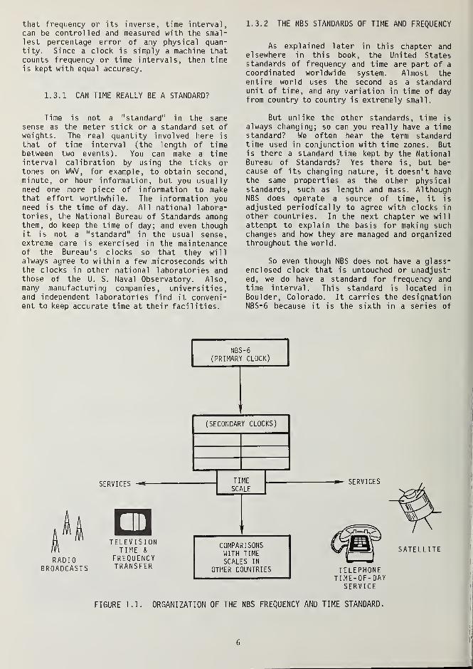
So even though NBS does not have a glass-enclosed clock that is untouched or unadjust-ed, we do have a standard for frequency andtime interval. This standard is located in

Boulder, Colorado. It carries the designationNBS-6 because it is the sixth in a series of

NBS-6(PRIMARY CLOCK)

(SECONDARY CLOCKS)

RADIOBROADCASTS

SERVICES

TELEVISIONTIME &

FREQUENCYTRANSFER

TIMESCALE

SERVICES

COMPARISONSWITH TIMESCALES IN

OTHER COUNTRIES TELEPHONETIME-OF-DAY

SERVICE

SATELLITE

FIGURE 1.1. ORGANIZATION OF THE NBS FREQUENCY AND TIME STANDARD.

6

atomic oscillators built and maintained by NBS

to provide the official reference for frequen-

cy and time interval in the United States.

NBS-6 is referred to as the "master" or "pri-

mary" clock. It is used to calibrate otheroscillators ("secondary" clocks) which are

used to operate the time scale. (A time scale

is a system of counting pendulum swings.) Theorganization of the NBS frequency and time

standard is illustrated in figure 1.1. Shown

is the primary atomic standard NBS-6, which is

used to calibrate an ensemble of other atomicoscillators which operate the time scale,

which is in turn compared and adjusted to

similar time scales in other countries. Peri-odic adjustments are made to keep them all in

agreement.

The useful output of the NBS standard andits associated time scale are the servicesprovided to users. These services can takemany forms and use several methods to get theactual needed calibration information to theuser.

Notice that figure 1.1 looks a lot likeany timepiece. We have a source of frequency,a means of counting that frequency and keepingtime of day in a time scale, and as mentioned,a way of getting a useful output. This is

exactly what is contained in almost everyclock or watch in use today. The frequencysource can be a 60 Hz power line, a balancewheel, tuning fork, or quartz crytal. Thecounter for totaling the cycles of frequencyinto seconds, minutes, and hours can be gearsor electronics. The readout can be a faceclock or digits.

In early times, the sun was the onlytimekeeping device available. It had certaindisadvantages--cloudy days, for one. Andalso, you could not measure the sun's anglevery accurately. People started developingclocks so they could have time indoors and atnight. Surely, though, the sun was their"standard" instead of a clock. Outdoors, thesundial was their counter and readout. It is

reasonable to suppose that if you had a largehour glass, you could hold it next to thesundial and write the hour on it, turn it

over, and then transport it indoors to keepthe time fairly accurately for the next hour.

A similar situation exists today in thatsecondary clocks are brought to the master orprimary clock for accurate setting and thenused to keep time.

1.4 HOW TIME AND FREQUENCY STANDARDS

ARE DISTRIBUTED

In addition to generating and distribut-ing standard frequency and time interval, theNational Bureau of Standards also broadcasts

time of day via its radio stations WWV, WWVH,

and WWVB. Each of the fifty United States has

a state standards laboratory which deals in

many kinds of standards, including those of

frequency and time interval. Few of thesestate labs get involved with time ofday,

which is usually left to the individual user,

but many of them can calibrate frequencysources that are used to check timers such as

those used in washing machines in laundromats,car washes, and parking meters.

STDS STDS STDSLAB LAB LAB

In private industry and other governmentagencies where standards labs are maintained,a considerable amount of time and frequencywork is performed, depending on the end pro-

duct of the company. As you might guess,electronics manufacturers who deal withcounters, oscillators, and signal generatorsare very interested in having an availablesource of accurate frequency. This will veryoften take the form of an atomic oscillatorkept in the company's standards lab and

calibrated against NBS.

Although company practices differ, a

typical arrangement might be for the companystandards lab to distribute a stable frequencysignal to the areas where engineers can use

the signal for calibration. Alternatively,test equipment can periodically be routed to

the standards lab for checking and adjustment.

As mentioned elsewhere in this book, the

level of accuracy that can be achieved by a

standards lab when making a frequency cali-

bration ranges from a few parts per thousand

to one part in a thousand billion, or 1 part

in 10 12. Precise calibrations do involve more

careful attention to details, but are not in

fact that difficult to achieve.

1.5 THE NBS ROLE IN INSURING ACCURATE

TIME AND FREQUENCY

The National Bureau of Standards is

responsible for generating, maintaining, and

7

NBSTO STDS STDS

LAB VIA WWV. LABWATCH

distributing the standards of time and fre-

quency. It is not a regulatory agency so it

does not enforce any legislation. That is,

you cannot get a citation from NBS for havingthe incorrect time or frequency.

Other government agencies, however, do

issue citations. Most notable among these is

the Federal Communications Commission. Thisagency regulates all radio and televisionbroadcasts, and has the authority to issuecitations and/or fines to those stations thatdo not stay within their allocated frequen-cies. The FCC uses NBS time and frequencyservices to calibrate their instruments which,in turn, are used to check broadcast trans-mitters.

trace the signal backward toward its source,

you will find that it perhaps goes through a

distribution amplifier system to a frequencysource on the manufacturing plant grounds.

Let's say this source is an oscillator. Some

means will have been provided to calibrate its

output by using one of several methods--let'

s

say NBS radio signals. With suitable records,taken and maintained at regular intervals, theoscillator (frequency source) can claim an

accuracy of a certain level compared to NBS.

This accuracy is transferred to your labora-tory at perhaps a slightly reduced accuracy.Taking all these factors into account, thesignal in your laboratory (and therefore yourwatch) is traceable to NBS at a certain level

of accuracy.

The Bureau's role is simply to provideaccess to the standards of frequency and timeinterval to users and enforcement agenciesalike. When radio and television stationsmake calibrations referenced to NBS, they canbe confident that they are on frequency andare not in violation of the broadcasting regu-lations.

1.6 WHEN DOES A MEASUREMENT BECOME

A CALIBRATION ?

Using an ordinary watch as an example,you can either move the hands to set the timeof day, or you can change the rate or adjustthe frequency at which it runs. Is thismeasurement a calibration? It depends on whatreference you use to set the watch.

If the source you use for comparison is

traceable at a suitable level of accuracy backto the National Bureau of Standards, (or theU.S. Naval Observatory in the case of DODusers), then you can say you have performed a

calibration. It is very important to keep in

mind that every calibration carries with it a

measure of the accuracy with which the cali-bration was performed.

The idea of traceability is sometimesdifficult to explain, but here is an example.Suppose you set your watch from a time signalin your laboratory that comes to you via a

company-operated distribution system. If you

What kind of accuracy is obtainable? As

we said before, frequency and time can both be

measured to very high accuracies with verygreat measurement resolution. As this bookexplains, there are many techniques availableto perform calibrations. Your accuracy de-

pends on which technique you choose and whaterrors you make in your measurements. Typi-

cally, frequency calibration accuracies range

from parts per million by high frequency radioI

signals to parts per hundred billion for

television or Loran-C methods. A great deal

depends on how much effort you are willing to

expend to get a good, accurate measurement.

1.7 TERMS USED

1.7.1 MEGA, MILLI, PARTS PER... AND PERCENTS

Throughout this book, we refer to such

things as kilohertz and Megahertz, millisec-

onds and microseconds. We further talk about ".

accuracies of parts in 10 9 or 0.5%. What do

all of these terms mean? The following tables

explain the meanings and should serve as a

convenient reference for the reader.

Table 1.2 gives the meaning of 1 x 10- 6

but what is 3 x 10- 6? You can convert in the

same way. Three parts per million or 3 x 10- 6

is .0003%. Manufacturers often quote percen-

tage accuracies in their literature rather ;

than "parts per. ..."

8

TABLE 1.1 PREFIX CONVERSION CHART

PREFIX DEFINITION EXAMPLE

LESS THAN 1

MILLI ONE THOUSANDTH MILLISECOND (ms) = ONE THOUSANDTH OF A SECOND

MICRO ONE MILLIONTH MICROSECOND (ys) = ONE MILLIONTH OF A SECOND

NANO ONE BILLIONTH NANOSECOND (ns) = ONE BILLIONTH OF A SECOND

PICO ONE TRI LLIONTH PICOSECOND (ps) = ONE TRI LLIONTH OF A SECOND

MORE THAN 1

Kl LO ONE THOUSAND KILOHERTZ (kHz) = ONE THOUSAND HERTZ (CYCLES PER SECOND)

MEGA ONE MILLION MEGAHERTZ (MHz) = ONE MILLION HERTZ

GIGA ONE BILLION GIGAHERTZ (GHz) = ONE BILLION HERTZ

TERA ONE TRILLION TERAHERTZ (THz) = ONE TRILLION HERTZ

TABLE 1.2 CONVERSIONS FROM PARTS PER... TO PERCENTS

PARTS PER PERCENT

1 PART PER HUNDRED 1 x 10"2 = 1

1001.0*

1 PART PER THOUSAND I x 10"3 1

1 ,0000. 1*

1 PART PER 10 THOUSAND 1 x 104 1

10,0000.01?

1 PART PER 100 THOUSAND 1 x 10~ 5 1

100,0000.001*

1 PART PER MILLION 1 x 10~ 6 1

1 ,000,0000.0001*

1 PART PER 10 MILLION 1 x 10" 7 1

10,000,0000.00001*

1 PART PER 100 MILLION 1 x 10" 8 1

100,000,0000.000001*

1 PART PER BILLION1 x 10" 9 1

1 ,000,000,0000.0000001*

1 PART PER 10 BILLION1 x l(f

10 1

10,000,000,0000.00000001*

1 PART PER 100 BILLION - 1 x 10" 11 1

100,000,000,0000. 000000001%

1 PART PER 1 ,000 BILLION(1 PART PER TRILLION)

= 1 x 10" 12 1

1 ,000,000,000,0000.0000000001%

1 PART PER 10,000 BILLION 1 x 10" 13 1

10,000,000,000,0000.00000000001*

9

1.7.2 FREQUENCY

The term used almost universally for

frequency is the hertz, which means one cycleper second. With the advent of new integratedcircuits, it is possible to generate that"cycle" in many different shapes. It can be a

sine wave or a square, triangular, or sawtoothwave. So the reader is cautioned as he pro-

ceeds through this book to keep in mind thatthe waveforms being considered may not in factbe sinusoids (sine waves). In this book wewill not concern ourselves greatly with thepossibility that the frequency of interest can

contain zero frequency or DC components.Instead we will assume that the waveformoperates, on the average, near zero voltage.

Throughout this book, consideration is

given to frequencies of all magnitudes--f romthe one hertz tick of the clock to many bil-lions of hertz in the microwave region. Table1.3 gives the prefixes used for frequencies in

different ranges and also the means of con-verting from one kind of unit to another.Thus it is possible to refer to one thousandon the AM radio band as either 1000 kHz or 1

MHz.

Table 1.4 lists the frequencies by bands.Most frequencies of interest are included in

this table--the radio frequency band containsthe often heard references to high frequency,very high frequency, low frequency, etc.

The reader is cautioned that the diffi-culty in measuring frequency accurately is notdirectly related to the frequency range.Precise frequency measurements at audio fre-quencies are equally as difficult as those in

the high frequency radio bands.

Scattered throughout this book are ref-erences to the wavelength rather than thefrequency being used. Wavelength is especi-ally convenient when calculating antenna

TABLE 1.3 CONVERSIONS TO HERTZ

FREQUENCY EXAMPLES

1 Hz = 10° =1 CYCLE PER SECOND2000 Hz = 2 kHz = 0.002 MHz

- 1 kHz = 103 =1 ,000 Hz

25 MHz = 25,000 kHz = 25 MILLION Hz1 MHz = 10

6 =1 ,000,000 Hz

1 GHz = 109

= 1,000,000,000 Hz

10 GHz = 10,000 MHz = 10 MILLION kHz

1 THz = 1012

= i 000 BILLION Hz

TABLE \.k RADIO FREQUENCY BANDS

RF BAND FREQUENCY RANGE WAVELENGTH (A)

h VLF (VERY LOW FREQUENCY) 3 - 30 kHz 105

- 10^ METERS

5 LF (LOW FREQUENCY) 30 - 300 kHz 10 - 105 "

6 MF (MEDIUM FREQUENCY) 300 kHz - 3 MHz3 2

lcr - 10

7 HF (HIGH FREQUENCY) 3 - 30 MHz 102

- 10 "

8 VHF (VERY HIGH FREQUENCY) 30 - 300 MHz 10-1 "

9 UHF (ULTRA HIGH FREQUENCY) 300 MHz - 3 GHz 1 - 0.1 "

10

lengths. In fact, a glance at an antique

radio dial shows that the band was actuallymarked in wavelengths. For example, radio

amateurs still refer to their frequency allo-

cations in terms of the 20, 10, or 2 meterbands.

The conversion of wavelengths to fre-

quency can be made for most purposes by using

the simple equation

. _ 300,000,000

where A. is the wavelength in meters,

300,000,000 meters per second is the speed of

light, and f is the frequency in hertz. So we

can see that the ten meter band is approxi-mately 30 MHz and 1000 on the broadcast bandis 300 meters.

This equation can be converted to feet

and inches for ease in cutting antennas to

exact length. Precise calculations of wave-length would have to take into account the

medium and allow for the reduced velocitybelow that of light, for instance, insidecoaxial cables.

Many users of frequency generating de-

vices tend to take frequency for granted,especially in the case of crystals. A popularfeeling is that if the frequency of interesthas been generated from a quartz crystal, it

cannot be in error by any significant amount.

This is simply not true. Age affects the

frequency of all quartz oscillators. Althoughfrequency can be measured more precisely thanmost phenomena, it is still the responsibilityof the calibration laboratory technician or

general user to keep in mind the tolerancesneeded; for example, musical notes are usuallymeasured to a tenth of a hertz or better.

Power line frequency is controlled to a milli-hertz. If you dial the NBS time-of-day tele-phone service, you will hear audio frequencytones that, although generated to an accuracyof parts per one thousand billion, can be sent

over the telephone lines only to a few partsin one thousand. So the responsibility is theusers to decide what he needs and whether, in

fact, the measurement scheme he chooses will

satisfy those needs.

Throughout this book, mention is made ofthe ease with which frequency standards can be

calibrated to high precision. Let us assumethat you have, in fact, just calibrated yourhigh quality crystal oscillator and set the

! associated clock right on time. What happens

j

next? Probably nothing happens. The oscil-lators manufactured today are of excellentquality and, assuming that a suitable batterysupply is available to prevent power outages,the clock could keep very accurate time for

many weeks. The kicker in this statement is,

of course, the word "accurate." If you wantto maintain time with an error as small or

smaller than a microsecond, your clock couldvery easily have that amount of error in -a fewminutes. If you are less concerned withmicroseconds and are worried about only milli-seconds or greater, a month could elapsebefore such an error would reveal itself.

The point to be made here is that nothingcan be taken for granted. If you come into

your laboratory on Monday morning hoping thateverything stayed put over the weekend, youmight be unpleasantly surprised. Digitaldividers used to drive electronic clocks do

jump occasionally, especially if the powersupplies are not designed to avoid some of the

glitches that can occur. It makes sense,

therefore, to check both time and frequencyperiodically to insure that the frequency rate

is right and the clock is on time.

Many users who depend heavily on theirfrequency source for cal ibrations--for exam-

ple, manufacturing plants--find it convenientto maintain a continuous record of the fre-

quency of their oscillators. This usuallytakes the form of a chart recording that shows

the frequency variations in the oscillatorversus a received signal from either an NBS

station or one of the many other transmissions

which have been stabilized. Among these are

the Omega and Loran-C navigation signals.

If you refer to Chapter 11 of this book,

which deals with the characteristics of oscil-

lators, you will notice that crystal oscilla-

tors and even rubidium oscillators will drift

in frequency so, depending on your applica-

tion, periodic adjustments are required.

1.8 DISTRIBUTING TIME AND FREQUENCY SIGNALS

VIA CABLES AND TELEPHONE LINES

Users of time and frequency signals some-

times want to distribute either a standard

frequency waveform or a time signal using

cables. This is often the case in a labora-

tory or manufacturing plant where the stan-

dards laboratory provides signals for users

throughout the plant area. Of course, the

solution to any given problem depends on good

engineering practices and consideration for

the kind of result desired. That is to say,

if you start with a cesium oscillator and want

to maintain its accuracy throughout a large

area, you must use the very best of equipment

and cables; and even then, the signal accuracy

will be somewhat deteriorated. On the other

hand, if all that is needed is a time-of-day

signal on the company telephone switchboard,

the specifications can be relaxed.

11

Without knowing the particular conditionsunder which signals are to be distributed, itwould be hard to specify the maximum accuracyobtainable. A number of articles have beenpublished for distribution systems using bothcoaxial cables and telephone lines. Theresults that the individual writers reportedvaried from parts per million to almost onepart in 10 billion. In each case the resultswere in direct ratio to the amount of effortexpended. Since the articles were written anumber of years ago, it is expected that bet-ter results could be achieved today. Otherthan the good engineering practices mentionedabove, there is no simple formula for success-ful transmission of standard frequency andtime signals.

Often the main problem is noise pickup inthe cables that causes the signal at the endof the line to be less useful than desired.Another problem often reported is the diffi-culty in certifying the received accuracy orto establish NBS traceability over such a

distribution system. A suggestion would bethat careful system management be observed andthat periodic evaluation of the system beattempted. One method of evaluating a distri-bution system would be to route the signal ona continuous loop and look at the signal goingin and the signal coming out for a particularcable routing.

For commercial telephone lines (which areusually balanced systems), the highest prac-tical frequency that can be distributed is1000 Hz. Coaxial cables have been used suc-cessfully for frequencies up to 100,000 Hz.

Any attempt to send pulses over a voice-gradetelephone line would be unsuccessful due tothe limited bandwidth.

At the NBS Boulder Laboratories, 5 MHzsignals are transmitted within the building.Commercial distribution amplifiers with fail-safe provisions are used to drive the cablesat a nominal 50 ohms impedance. Careful cablemanagement assures good results. Even so,

very often noise will appear on the cables anddegrade the signals. The noise on some cablesdue to their routing was so bad they wereabandoned.

The NBS telephone time-of-day signal is

received at Boulder via a leased commercialtelephone line that is about 100 miles in

length. The measured delay for this line is

approximately 3 to 5 milliseconds. This seemsto be the usual order of magnitude of delayreported for commercial telephone circuits.

If you plan to use such circuits for distri-bution of signals, keep in mind that a varietyof leased lines of varying quality are avail-

able from telephone companies.

For signals that are being transmittedover long distances on telephone lines, the

error in the received frequency is usuallyseveral hertz or more. This is a consequenceof the method used by the telephone companies

to combine several signals on a transmissionline using frequency division multiplexingtechniques. This would be the case, for

example, if you dialed the NBS time-of-dayservice on 303-499-7111. The tone as receivedcould be in error by several parts in 103 .

12

For those users wanting to distributeeither very accurate frequency or precise

time, it is almost fair to say that local

cable and wire systems are not economicallypractical. If your requirements are critical,

it is usually cheaper in the long run to

simply reestablish time and/or frequency at

the destination point. The burden of instal-

ling and maintaining a distribution system can

be very great for high accuracy systems.

1.9 TIME CODES

Whenever time is available from a digital

clock at one location and needed at another,it is often transferred over wires or radio by

means of a time code. A time code is a seriesof pulses which can easily be a simple tele-typewriter code, but is usually a more effi-

cient binary code where a set of pulses repre-

sents one digit. Let's say a 4 is sent, mean-ing 4 hours, 4 minutes, or 4 seconds. Thelocation of a particular binary digit in the

code tells you its meaning; that is, whetherit is an hour, minute, or second. Dependingon the application, the code can be sent as

a direct current level shift or as modulatedpulses on a carrier or perhaps as tones whereone frequency of tone represents a binary "1"

and an alternate tone represents a binary 0.

What has been described above is a serial

code where one digit is sent, then another,then another. Interspersed among the timebits are position locators which help theelectronic equipment to recognize what thefollowing bit is going to mean. It is alsopossible to send time codes in parallel on

many conductor cables. Each wire would thencarry its respective bit.

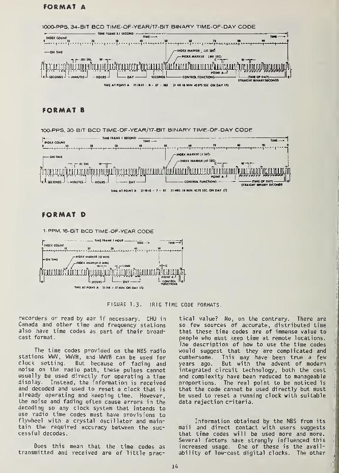
Time codes have evolved through the yearsand have been strongly influenced by therecommendations of the Inter Range Instrumen-tation Group, known as I RIG . Figure 1.2 showsa typical I RIG time code format which differsonly slightly from the WWV time code shownelsewhere in this book. Figure 1.3 shows themajor characteristics of a number of I RIG

codes. For those readers who want more infor-mation on time codes, many manufacturers ofdigital timekeeping equipment provide bookletslisting all of the popular codes being used

and detailed explanations of the individualformats.

If you look in a book listing the avail-able time codes, you will notice that theyvary in frame length and rate. The NBS timecodes were chosen as a compromise on speed andlength that matched the other radio stationcharacteristics. The codes on the NBS sta-

tions are transmitted very slowly--so slowlythat they can be recorded directly on chart

TIME FRAME I MINUTE20 30

nrP0

-REFERENCE TIME

— REFERENCE MARKER

_| I I 1 I|

I I I I|

I I I I|

I I I I|

I I I I|

l I I I

)I I I I |

'illINDEX COUNT 1 SEC.

DAYS

IU JU1 11.JLU

« 0.8 SEC.

1 2 4 8 10 20 40 2 4 8 10 20

JTUimUJljlJLJT^Dl Di DO Da O c j

— 0.2 SEC.8INARY '0 1

(TYPICAL) — 0.5 SEC.BINARY T(TYPICAL)

10 20 40 80 100 200

JITP4

- 1 SEC.(TYPICAL)

0.8 SEC.POSITIONIDENTIFIER(TYPICAL)

Time at this point equals 173 doys, 21 hours, 24 minutes, 57 seconds

TYPICAL MODULATED CARRIERRecommended Frequency 100 Hz of 1000 H*

IRIG STANDARD TIME CODEFORMAT H'

(1PPS Code)

Reference IRIG Document 104-70

FIGURE 1.2. IRIG TIME CODE, FORMAT H.

13

FORMAT A

1000-PPS, 34-BIT BCD TIME-OF-YEAR/17-BIT BINARY TIME-OF-DAY CODETIME FRAME 0.1 SECOND

INDEX COUNT»

L

t-*-' '1

I

'

TIME

401

I' ' ' '

I

'

—|

[— 001 SEC W—1|—

I T II"""""I I

I I"

mS\

f

""I

L«JLsECON0S J LM|NutesJ LhoURS-I ' DAY 1 SECOND!

TIME -

W'

I' ' '

1

I

'

-INDEX MARKER. 1.01 SEcl

-INDEX MARKER (.001 SEC)

POINT A-l

-CONTROl FUNCTIONS

Tl

-(TIME OF DAY)-STRAKvHT BINARY SECONDS

TIME AT POINT A 21 18 42 8 - 07 005 21 MR. IB MIN 42 875 SEC ON DAY 173

FORMAT B

100-PPS, 30-BIT BCD TIME-OF-YEAR/17-BIT BINARY TIME-OF-DAY CODE

STRAIGHT BINARY SECONDS

FORMAT D

1-PPM. 16-BIT BCD TIME-OF-YEAR CODE

TIME AT POINT A Jl HR. • S7 MIN ON DAY 173

FIGURE 1-3. IRIG TIME CODE FORMATS.

recorders or read by ear if necessary. CHU inCanada and other time and frequency stationsalso have time codes as part of their broad-cast format.

The time codes provided on the NBS radiostations WWV, WWVH, and WWVB can be used forclock setting. But because of fading andnoise on the radio path, these pulses cannotusually be used directly for operating a timedisplay. Instead, the information is receivedand decoded and used to reset a clock that isalready operating and keeping time. However,the noise and fading often cause errors in thedecoding so any clock system that intends touse radio time codes must have provisions toflywheel with a crystal oscillator and main-tain the required accuracy between the suc-cessful decodes.

Does this mean that the time codes astransmitted and received are of little prac-

tical value? No, on the contrary. There areso few sources of accurate, distributed timethat these time codes are of immense value topeople who must keep time at remote locations.The description of how to use the time codeswould suggest that they are complicated andcumbersome. This may have been true a fewyears ago. But with the advent of modernintegrated circuit technology, both the costand complexity have been reduced to manageableproportions. The real point to be noticed is

that the code cannot be used directly but mustbe used to reset a running clock with suitabledata rejection criteria.

Information obtained by the NBS from its

mail and direct contact with users suggeststhat time codes will be used more and more.

Several factors have strongly influenced thisincreased usage. One of these is the avail-ability of low-cost digital clocks. The other

14

factor, as previously mentioned, seems to be

the cost reductions in integrated circuits.

These circuits are so inexpensive and depend-

able that they have made possible new appli-

cations for time codes that were impractical

with vacuum tubes.

The accuracy of time codes as received

depends on a number of factors. First of all,

you have to account for the propagation path

delay. A user who is 1000 miles from the

transmitter experiences a delay of about 5

microseconds per mile. This works out to be 5

milliseconds time error. To this we must add

the delay through the receiver. The signal

does not instantly go from the receivingantenna to the loudspeaker or the lighted

digit. A typical receiver delay might be

one-half millisecond. So a user can experi-

ence a total delay as large as 8 to 10 milli-seconds, depending on his location. This

amount of delay is insignificant for mostusers. But for those who do require accuratesynchronization or time of day, there is a

method for removing the path delay. Manufac-turers of time code receivers very often

include a simple switching arrangement to dial

out the path delay. When operating time code

generators, the usual recommendations for

battery backup should be followed to avoiderrors in the generated code.

THE UTILITY OF TIME CODES . In additionto using codes for setting remote clocks from,

say, a master clock, time codes are used on

magnetic tape systems to search for informa-tion. The time code is recorded on a separatetape track. Later, the operator can locateand identify information by the time codereading associated with that particular spot

on the tape. Many manufacturers provide timecode generation equipment expressly for thepurpose of tape search.

Another application of time codes is for

dating events. The GOES satellite time code

(chapter 10) is used to add time and a date to

environmental data collected by the satellite.

There are many other uses. The electricpower industry automatically receives the time

code from WWVB, decodes the time of day, anduses this information to steer the electricpower network. Many of the telephone compa-nies use a decoded signal to drive theirmachines which actually answer the phone whenyou dial the time of day. Even bank signs

that give time and temperature are often

driven from the received time code. Why is

this? The main reason a time code is used is

to avoid errors. It also reduces the amountof work that must be done to keep the parti-

cular clock accurate.

15

CHAPTER 2. THE EVOLUTION OF TIMEKEEPING

2.1 TIME SCALES

A time scale is simply a system of as-signing dates to events or counting pendulumswings. The apparent motion of the sun in thesky is one type of time scale, called astro-nomical time. Today, we also have atomictime, where an atomic oscillator is the "pen-dulum". To see how the various time scalescame about, let's take a brief look at theevolution of time.

discrepancy was eventually identified as beingcaused by a wobble in the earth's axis. Theamount of wobble is about 15 meters. By care-ful measurements made at various observatoriesthroughout the world, this wobble was correct-ed for and a new time designation called UT1was born. In our search for uniformity, wehave now taken care of the non-circular orbit(UTO) and the axis wobble of the earth (UT1).

As science and technology improved pen-dulum and quartz crytal clocks, it was dis-

2.1.1 SOLAR TIME

To review what has happenedto timekeeping and the name giv-en to the resulting time of day,consider a time system that usesthe sun and the sundial. The sunis the flywheel and has a periodof 24 hours. The sundial canindicate the fractions of cycles(time of day). As complete dayselapse, calendars can be used tocount the days and divide theminto weeks and years. But ournewly formed clock is not uni-form in its timekeeping becausethe earth's orbit around the sunis not circular. It slows downand speeds up depending on itsdistance from the sun. The ear-ly astronomers and mathemati-cians understood these laws ofmotion and were able to correctthe "apparent solar time" to ob-tain a more uniform time called"mean solar time". This correc-tion is called the Equation ofTime and is often found engravedon sundials. Universal Time(UTO) is equal to mean solar timeif you make the correction at theGreenwich meridian in England.We now have UTO, the first inof designations for time that has evolvedthrough the past years.

series

If you use a star that is farther awaythan our own sun, the fact that the earth isnot in perfect circular orbit becomes unim-portant. This is called "sidereal time" andis similar to mean solar time since both arebased on the earth's spinning on its axis.The rate is different by one day per yearsince the earth circles the sun in a year.

As better clocks were developed, astron-omers began to notice a discrepancy in Univer-sal Time measured at different locations. The

covered that UT1 had periodic fluctuations

whose origin was unknown. Due to the availa-

bility of excellent clocks, these fluctuations

could be and were removed, resulting in an

even more uniform UT2.

To review, UT1 is the true navigator's

scale related to the earth's angular position.

UT2 is a smooth time and does not reveal the

real variations in the earth's position. When

the world's timekeepers went to UT2, they

bypassed the navigators' real needs. A little

later we shall describe the present-day system

which in effect remedies the dilemma.

17

Up until now we have been talking aboutthe Universal Time family, and figure 2.1

shows the relationship between the differentuniversal times. Let us now examine the othermembers of the time family. The first ofthese is "ephemeris time". An ephemeris is

simply a table that predicts the positions ofthe sun, moon, and planets. It was soonnoticed that these predicted positions on thetable did not agree with the observed posi-tions. An analysis of the difficulty showedthat in fact the rotational rate of the earthwas not a constant, and this was later con-firmed with crystal and atomic clocks. In

response to this problem, the astronomerscreated what is called "ephemeris time". It

is determined by the orbit of the earth aboutthe sun, not by the rotation of the earth on

its axi s.

UNIVERSAL TIME FAMILY

APPARENT SOLAR TIME

CORRECTED BY

EQUATION OF TIME MEAN SOLAR TIMEw[UTO]

CORRECTED FOR

MIGRATION OF POLES

Ai 0 05sec m UT1

CORRECTED FOR

KNOWN PERIODICITY

Al 0 OSsec ^ UT2

FIGURE 2.1. UNIVERSAL TIME FAMILYRELATIONSHIPS.

2.1.2 ATOMIC TIME

FIGURE 2.2. FIRST ATOMIC CLOCK.

Another kind of time that can be gener-ated and used is atomic time. Whereas theUniversal Time scale is obtained by countingcycles of the earth's rotation from someagreed-upon starting point, an atomic timescale can be obtained by counting cycles of a

signal locked to some atomic resonance.

In the late 1940' s, the National Bureauof Standards announced the first atomic clock.Shortly thereafter several national laborator-ies, including the International Time Bureau(BIH), started atomic time scales.

In 1971 the General Conference of Weightsand Measures officially recognized the AtomicTime Scale and endorsed the BIH time scale asthe International Atomic Time Scale, TAI. Therole of the BIH in international coordinationis discussed later in this chapter. Since thefirst of January 1972, the Atomic Time Scalehas been distributed by most countries in theworld.

Today, the time of day can be gotten to a

very high order of accuracy because, unlike a

coarse sundial, an atomic clock measures small

fractions of a second. Furthermore, it givesus essentially constant units of time--it is a

uniform timekeeper. Uniformity is important in

technology, synchronization of power gener-ators, and in the general problem of trying to

make two things happen or start at the same

time.

Let's review for a moment the several

time scales we have discussed. First, the

universal time family is dependent on the

earth's spin on its axis. Second, ephemeristime depends on the orbital motion of the

earth about the sun. And finally, atomic

time, which is very uniform and precise,

depends on a fundamental property of atoms.

Figure 2.3 illustrates the differences in

these several kinds of time. Because of the

slow orbital motion of the earth, about one

18

(!to

ER

uti

L

It?] ^ MEASURED T0 3ms IN 1 DAY

EPHEMERIS TIME A(ET) V MEASURED TO 50ms IN 9 YEARS

ATOMIC TIME ^ MEASURED TO 0.1 Ms IN 1 nun

FIGURE 2.3. CLASSES OF TIME SCALESAND ACCURACIES.

B. The New UTC System

The new UTC system came about as a solu-tion to the problem of changing the frequencyrate each year or so. It was adopted in

Geneva in 1971 and became effective in 1972.

Under the new system, the frequency drivingall clocks was left at the atomic rate withzero offset. But by using a zero offset, theclocks would gradually get out of step withthe day. The resulting situation was notunique because the year has never been an

exact multiple of the day, and so we have leapyears. Leap years keep our calendar in stepwith the seasons.

cycle per year, measurement uncertaintieslimit the accuracy of Ephemeris Time to about0.05 second in a 9-year period. UniversalTime can be determined to a few thousandths ofa second or several milliseconds in one day.

Atomic Time is accurate to a few billionths ofa second in a minute or less. From thesenumbers and the figure, it is easy to see whyscientists have been leaning toward a timescale derived from an atomic clock.

Coordinated Universal Time

Prior to 1972, most standard frequencyradio broadcasts were based on a time scalecalled Coordinated Universal Time (UTC). Therate of a UTC clock was controlled by atomicoscillators so it would be as uniform as

possible. These atomic oscillators operatedat the same frequency for a whole year, butwere changed in rate at the beginning of a newyear in an attempt to match the forthcomingearth rotational rate, UT2. This annualchange was set by the BIH. For instance,between 1965 and 1966, the relative frequency,F, of standard frequency radio broadcasts wasset equal to -150 x 10- 10

. This meant thatall of the WWV frequencies, for example, werelower than their nominal values. (See Chapter3 for a full explanation of nominal values.)

However, the earth's rotational ratecould not be accurately predicted, and so UTCwould slowly get out of step with earth time.This was a problem for navigators who neededsolar time--they had to apply a correction toUTC, but it was difficult to determine theamount of correction.

Experience rapidly showed that it wouldbe an advantage to simplify the UTC system to

I

avoid changing the rate each year. A decision1 was made to broadcast the nominal values ofthe frequency standards and to do away withannual changes in rate. Thus, a way wasdeveloped to keep UTC in closer agreement withsolar time.

The same scheme was adopted to keepclocks in step with the sun, and the "leapsecond" was born. To make adjustments in theclock, a particular minute would containeither 61 or 59 seconds instead of the conven-tional 60 seconds. You could, therefore,either have a positive or a negative leapsecond. It was expected and proved true thatthis would normally occur once a year.

The new UTC plan works like this. By

international agreement, UTC is maintainedwithin 9/10 of a second of the navigator'stime scale UT1 . The introduction of leap

seconds will permit a good clock to keep

approximate step with the sun. Since the

rotation of the earth is not uniform we can-

not exactly predict when leap seconds will be

added or deleted, but they usually occur on

June 30 or December 31. Positive leap seconds

were added on June 30, 1972, and December 31,

1972 through 1978.

NORMAL MINUTE(NO LEAP SECOND ADDED)

57 59

EVENT —I

30 June, 23" 59"

Doling ol Event Shown

30 June, 23 h 59 m 59 5 s UTC

I July, 0 h 0"

MINUTE WITH LEAP SECOND ADDED

Doling ol Event Shown.

30 June, 23" 59 m 60 5' UTC

EVENT —>

30 June, 23" 59 m 1 I July, 0 h 0"

FIGURE 2.4. DATING OF EVENTS IN THEVICINITY OF A LEAP SECOND.

What does this mean to the user of a time

and frequency broadcast? It simply means that

the time he gets will never differ from UT1 by

more than 9/10 of a second. Most users, such

as radio and television stations and telephone

19

FIGURE 2.5. STANDARD TIME ZONES OF THE WORLD REFERENCED TO UTC.

time-of-day services, use UTC so they don'tcare how much it differs from UT1. Even mostboaters/navigators don't need to know UT1 to

better than 9/10 of a second, so the new UTCalso meets their needs.

However, there are a small number of

users who do need UT1 time to better than 9/10of a second. To satisfy this need, moststandard time and frequency radio stationsinclude a correction in their broadcasts whichcan be applied to UTC to obtain UT1

.

On WWV, for instance, the corrections, in

units of 0.1 second, are encoded into thebroadcasts by using double ticks or pulsesafter the start of each minute. The amount ofcorrection is determined by counting thenumber of successive double ticks heard eachminute, and the sign of the correction is

given by the location of the double ticks

within the minute.

We should keep in mind that the advantage

we gain by using the new UTC system prevents

us from simply subtracting the dates of two

events to get the time difference between

them. We must, in fact, take into account any

leap seconds that were added or deleted. You

should be especially cautious if the time

interval of interest extends backward into a

period where the world time system was not

operating on the new UTC time scale (prior to

1972).

2.1.3 TIME ZONES

All standard time and frequency stations

broadcast Coordinated Universal Time, which is

on

referenced to the Greenwich meridian. How-

ever, many users want to display local time.

If the time is being decoded from a time code(as opposed to a voice time-of-day announce-ment), the problem can be solved by usingintegrated circuit logic. In fact, specialchips have been manufactured that allow the

clock to display time from any of the worldtime zones, even though it is receiving anddecoding DTC. Figure 2.5 shows a map of thetime zones currently in use.

Contrary to popular opinion, the NationalBureau of Standards is not involved withdetermining time zones in the United States.

This responsibility has been given to theDepartment of Transportation because the needfor designating time zones came about from theuse of railroads for interstate commerce. In-

formation about the time zones in the U. S.

can be obtained from the Department of Trans-portation, Washington, DC 20590.

To review then, we have the unfortunatesituation where the scientist wants a uniformtime scale (UTC) and the navigators require a

clock tied to the earth's position (UT1) whichis non-uniform. Therefore, corrections must be

made to convert UTC to UT1

.

With this discussion, the reader can moreeasily understand why the new UTC system wasdeveloped. It is a compromise between a pure-ly uniform time scale for scientific applica-tion and the non-uniform measurement of theearth's position for navigation and astronomy.As mentioned before, we keep the calendar in

step with the seasons by using the leap yearsand our clocks in step with the sun (day andnight) by using leap seconds.

2.2 USES OF TIME SCALES

2.2.1 SYSTEMS SYNCHRONIZATION

There are many applications for timingwhere it does not matter if the clock in useis on time or not, nor does it matter if theseconds are uniform. A child's race is a goodexample. If someone shouts "Go", the startingtime is synchronized and it doesn't matter if

it occurred on the second. In other words, it

is not essential that clocks be on the righttime-- it is only important that they all readthe same time--that is, they have to be synch-ronized.

It is only a matter of convenience andconvention to encourage the use of the correcttime. The convenience arises because of theease with which lost time can be recovered.If a locomotive engineer can get the time to

reset his watch by simply calling his local

telephone company or asking another trainman,he is able to maintain his schedule with ease.

In summary, there is an advantage andbenefit to keeping everyone synchronized and

on the correct time. In a way it is much like

the argument in favor of standards themselves.If you stop to help a motorist by the side of

the road, your confidence that your tools will

fit his car is reassuring. In the same way,

by using the same time of day, annoyancescaused by errors are reduced.

Before we leave the subject of synchro-

nization, we should mention that there are

applications in astronomy, communications, and

navigation where synchronizations to an

21

accuracy of a millionth of a second or betterare required. Although the average person is

not terribly concerned if he arrives at

school, church, or a picnic on time to withina few minutes or so, an airliner navigatingwith a clock in error by one millionth of a

second (microsecond) would have a positionerror of a quarter of a mile.

This is also true internationally withrespect to high-speed digital communicationswhere several million characters can be sentand received each second. Here the "time"being used may be a few microseconds, so thesending and receiving equipment must besynchronized to this accuracy. If thissynchronization can be obtained from a local

navigation or time and frequency station, it

enables rapid, error-free data transmission.

2.2.2 NAVIGATION AND ASTRONOMY

Although most users like the uniformityof atomic time, there is one application thatneeds the non-uniformity of solar time. Thisis in the area of celestial navigation wherethe motion of the earth is a way of findingout where you are on the earth.

Navigators who find their positions fromthe stars are among the greatest users ofstandard time broadcasts. Since the earthmakes one revolution in 24 hours, a person canfind his position (in longitude) if he knows

THE HARRISON

his local time and the time difference betweenthe Greenwich meridian and himself.

As an example, a person trying to findhis position uses an instrument like a sextantto measure the local solar time wherever hemight be on the earth. His problem then is

trying to find out what the time is at theGreenwich meridian. This is the same problemthat generated all the interest severalhundred years ago in developing a good chrono-meter. Thise clocks were used for many yearsuntil radio came on the scene. Even today,most vessels do not leave home without a goodchronometer.

Because of this vital need for time ofday on the high seas, many countries operatehigh frequency radio stations to serve navi-gators. The United States operates WWV in

Fort Collins, Colorado, and WWVH in Hawaii.Similar stations are operated by the Canadiansand the Japanese and many countries in Europeand Asia. The U. S. Navy also broadcasts timesignals from a number of radio stations.

Most large countries also maintain obser-vatories to measure and record astronomicaltime. This is done by using telescopes, andthe official United States Observatory is

operated by the Navy in Washington, D. C.

Astronomical time is somewhat difficult to

measure accurately. Errors of a few milli-seconds are realized only after a whole eve-

ning's sightings have been taken and averaged.

CHRONOMETER.

22

B I

H

(TAI £ UTC)

1 1UT INFO £ / \ ACCURATELATITUDE \ FREQUENCY

CLOCK DATASTfl6L

'

£ STABLE CLOCK DATA

FREQUENCY FREQUENCY i

1Z_ \

USNONBS

(TIME SERVICES DIV.

)

OPERATIONS, RESEARCH u. s. TIME £ FREQUENCY

£ PTTI MANAGEMENT COORDINATION D 1 V 1 S 1 ON

FOR DEPT. OF DEFENSE OPERATIONS £ RESEARCH

UTI

CORRECT I

T£F CONTROL OFNAVY BROADCASTS£ LORAN-C (DEPT.

OF TRANSPORTATION)

T£F CONTROL OFNBS BROADCASTS,(UWV, UWVH, WWV8

)

FIGURE 2.6. NBS, USNO, AND BIH INTERACTIONS.

2.3 INTERNATIONAL COORDINATION OF

TIME AND FREQUENCY ACTIVITIES

2.3.1 THE ROLE OF THE INTERNATIONAL

TIME BUREAU (BIH)

Unlike standards such as length or mass,time of day can be received from many sources.Both Canada and the U. S. have primary fre-quency standards that act as flywheels foraccurate timekeeping. In addition, the U. S.

Naval Observatory makes astronomical observa-tions for determining UTI and keeps accurateclocks running for use by the Department ofDefense.

Other laboratories throughout the worldalso maintain primary frequency standards fortheir countries: The PTB in Germany, theNational Physical Laboratory in England, theRadio Research Labs in Japan, and the NationalElectrotechnical Institute in Italy, just co

name a few.

Time and frequency information from allof these laboratories is collected by theInternational Time Bureau (BIH) in Paris,France, which is the agency responsible forinternational coordination. There, the infor-mation is evaluated and the actual time cor-rections for each contributing clock aredetermined.. By international agreement, allUTC time scales must agree with the UTC timescale operated by the BIH to within ± 1 milli-second. The result is a uniform world timesystem that differs from country to country byonly a few millionths of a second. So,whether you get your time from CHU in Canadaor the PTB in Germany, it will differ fromU. S. time by no more than a few microseconds.

2.3.2 THE ROLE OF THE NATIONAL

BUREAU OF STANDARDS (NBS)

The National Bureau of Standards is in

the Department of Commerce of the UnitedStates and has been authorized by Congress toundertake the following functions: "Thecustody, maintenance, and development of thenational standards of measurements and theprovisions of means and methods for makingmeasurements consistent with those standards,including the comparison of standards used in

scientific investigations, engineering, manu-facturing, commerce, and educational insti-tutions, with the standards adopted or recog-nized by the Government."

The Time and Frequency Division, locatedin Boulder, Colorado, is that part of the

National Bureau of Standards that carries outthe above functions related to time and fre-

quency. There are several groups within the

Division, each having different responsibili-ties. The Frequency and Time Standards Groupoperates the NBS standard of frequency and

time interval, as well as several time scales

based upon this standard. In addition to

maintaining the standard, research efforts are

carried out to improve it. This group also

offers a direct service for calibration of

osci 1 lators and clocks.

The Time and Frequency Services Group is

responsible for distributing the standards and

for finding new and improved methods of dis-

semination. At this writing, the dissemina-

tion services consist of high frequency radio

stations WWV and WVA/H, low frequency radio

station WWVB, a telephone time-of-day service,

time and frequency calibration services using

network television, and a satellite time code.

This Group also provides services in the form

23

of literature and courses on how to use theseservices and provides calibration and moni-toring data on a regular basis to users of NBSand other time and frequency services.

Research and development into new methodsof dissemination are being done in the Timeand Frequency Coordination Group. This Groupis also involved in national and internationaltime and frequency coordination activities.

A fourth group concerns itself withfrequency synthesis techniques and laserstabilization methods.

In addition, services are available in

the form of consultations, either by letter,telephone, or visits to the Boulder Labora-tories. Users of the time and frequencyservices are encouraged to call upon us foradvice or assistance.

To summarize, the Bureau of Standardsmaintains services based upon the primaryfrequency standards. These services areconstantly being improved and are designed tomeet the needs of users at all levels ofaccuracy for frequency and time calibration.They range from the telephone time-of-dayservice to the ultra-stable low frequencyradio service of WWVB which is used for pre-cise frequency calibration.

2.3.3 THE ROLE OF THE U.S. NAVAL OBSERVATORY

(USNO) AND THE DOD PTTI PROGRAM

The U. S. Naval Observatory (USNO) is in

the Department of Defense (DOD). It's missionwith reference to time is:

"Make such observations of celestialbodies, natural and artificial, derive andpublish such data as will afford to UnitedStates Naval vessels and aircraft as well as

to all availing themselves thereof, means forsafe navigation, including the provision ofaccurate time." The practical application of

this mission is for the USNO to serve as theoperational reference for the official UnitedStates time of day (as opposed to responsi-bilities for the unit of time and frequency in

NBS).

The Time Service Division of the USNOpursues several activities: It operatesPhotographic Zenith Tubes (telescopes) to

determine Universal Time. It operates a largebank of atomic clocks (more than 20) as thebasis of an extremely reliable and uniformatomic time scale. It transports portableatomic clocks worldwide for time synchroni-zation to "assure worldwide continuity of

precision". It promptly publishes and dis-

tributes Time Service Announcements regardingmeasurements of, and information on, manyelectronic systems useful for time dissemi-nation. It operates under contract withNational Science Foundation (NSF), a connectedradio interferometer at the Green BankNational Radio Astronomical Observatory for

the determination of UT with radio techniques.

The USNO contributes measurements, alongwith about 60 other observatories and stan-

dards laboratories throughout the world, to

the Bureau International de l'Heure (BIH) in

Paris, France, which combines the results into

final BIH values of UT1. The USNO is the onlyorganization in the United States that deter-

mines UT1 operationally. It distributes BIH

Circular D for the BIH in the United States.

24

Within the DOD, the USNO has been givenmanagement responsibilities to "accomplishoverall PTTI objectives at minimum cost, DOD

Directive 5160.51 of 31 August 1971.

The DOD provides frequency and timesignals throughout the world. These includemany different radio frequencies, satellitesignals, and portable clocks. These can pro-vide very high resolution time synchroniza-tion, one-tenth microsecond or better at thepresent time (1979) with 10 nanoseconds pos-sible in the near future. Specific examplesinclude the Transit system with worldwideautomatic timing capability to 50 us (singlepass, 1 sigma; averaging over a number ofpasses can give about 5 us, 1 sigma).

The Global Positioning System is cur-rently under development and will provide a

worldwide timing capability of about 10 ns.

Loran-jC is operated by the U. S. Coast Guard.It acts in a secondary mission for the dis-semination of time for the USNO. It providestime within ground wave coverage to about 1 uswith a precision of about 0.1 us. Loran-C is

the present operational system for the compu-tation and dissemination of the internation-ally coordinated clock time references TAI andUK.

The USNO accomplishes its global respon-sibilities with a system of cooperating"Precise Time Reference Stations (PTRS)". Anyof these PTRS clocks can be used to gainaccess to the USNO Master clock by correctinga reading against the PTRS clock with the pub-lished difference USN0MC-PTRS. The currently

designated PTRS's and the respective valuesare given in Time Service Announcement" Series16. Time Service Announcement Series 4 pub-lishes Loran-C, Omega, VLF TV phase (time)values and Time Service Announcement Series 7

has time scale information (atomic and astro-nomical, including polar coordinates). Thesebulletins are available on request from:

SuperintendentU. S. Naval ObservatoryAttention: Time Service Division34th & Massachusetts Avenue, NWWashington, D. C. 20390(Telephone: 202 254-4546, AV 294-4546)(TWX 710-822-1970)

The three military services of the DODhave established focal points for matters ofPrecise Time and Time Interval (frequency).These focal points coordinate PTTI efforts andprovide pertinent information to their organi-zations and contractors. They also arrangeportable clock synchronizations for theirorganizations. The focal points are:

1. Aerospace Guidance and MetrologyCenter, Newark Air Force Station, Ohio (for

the U. S. Air Force).

2. Navy Electronic Systems Command,

Code 510, Washington, DC 20360 (for the

Navy).

3. U. S. Army Material Development &Readiness Command, DRCQA-PC, Alexandria, VA

20315 (for the Army).

25

CHAPTER 3. THE ALGEBRA AND CONVENTIONS FOR TIME AND FREQUENCY MEASUREMENTS

Users of time and frequency signals,

equipment, and publications need to have a

language for keeping records, reporting per-

formance, and reading the published litera-

ture. It should be easily and correctlyunderstood. Thus, a convention is needed for

the algebra dealing with frequency sources

and clocks so that the meaning of data are

understandable and not confusing.

You might ask, "Hasn't this problem come

up before?" or "How has it been resolved?"Yes, it has come up before and it has been

resolved. The CCIR (International RadioConsultative Committee) has defined the prob-

lem and published a recommended, standardnotation. In this section, we will explain

the notation with examples. Notice that this

convention regarding the algebra and especial-ly the algebraic signs has been followedthroughput this book.

In many cases of time and frequencymeasurement, the user knows that his clock is

fast or that his frequency source is low withrespect to NBS, the USNO, or another oscilla-tor. Intuition is a good guide and the care-

ful worker will be able to confirm his sus-

picions by reference to his data and thepublished information he needs. But in some

cases, intuition is not enough and the adop-

tion of a standard notation will eliminatedifficulties. Annotation of data sheets or

charts should follow the CCIR recommendationsso that a person looking up something that

happened several months or years ago will not

be confused.

An example using the above equation would be:

A, - B,lpps Ipps

This time difference expression is ideallysuited to the kind of readings obtained withtime interval counters. This counter is

explained in Chapter 4 and produces a readoutby having one pulse open the counter gate or

START the count and another close the gate,

STOPPING the count. In the above equation,

clock A is the start pulse and clock B is the

stop pulse.

Can we ever get a negative algebraic sign

on the right-hand side of the CCIR equation?Based directly on the counter measurements, we

cannot because, if the pulse from clock B

occurs 50 microseconds before the pulse from

clock A, the counter will simply wait for the

next pulse and read 999,950 microseconds. It

does not display negative numbers at all!

Remember, these clocks are ticking once

per second and our counter looks only at this

seconds tick--it cannot see the minutes or

hours. We say then that our clocks have out-

puts that are ambiguous to one second. This

means that the counter reading of 999,950

microseconds is equivalent to -50. It means

the same thing. The problem of ambiguity is

i llustrated below.

The CCIR convention and notation is T [ CK

listed here and can also be found in the pub-

lications of that group. The following mater-CL0CK

ial was excerpted from Recommendation No. 459, tick

1970. The material has been rearranged for

clarity.

1. Algebraic quantities should be givento avoid confusion in the sign of a

difference in the time betweenclocks or the frequency of sources.

2. It is a good idea to give the date

and place of a clock reading or

frequency measurement.

3. The difference of the readings (a

and b) of clocks A and B is, by

convention:

A - B = a - b.

Another example, showing the correct

notation that should be used, follows. This

could be the result obtained by carrying an

NBS portable clock to the U. S. Naval Obser-

vatory and measuring it against the USNO

clock. The results of this comparison are

properly written:

NBS PORTABLE CLOCK - UTC(USNO) =

+12.3 MICROSECONDS

(7 JULY 68, 14h 35m UTC).

27

There can be no confusion about the meaning of

this measurement providing the whole expres-

sion is recorded. Do not simply make a claim

that the NBS portable clock leads, lags, is

fast or slow, or ahead or behind of the USNO

clock. The algebraic expression should be

used!

It is also important to follow the

notation for frequency differences. Termslike high, low, and offset should be avoided.

Since the algebra speaks for itself, it shouldbe used with a minimum of additional terms.

"fractional." We have reflected this through-out the text.

The relative frequency departure of

frequency source "c," for instance, from its

nominal value f is defined as:nc

F

- 1 (which is dimensionless)

,

3. 1 EXPRESSING FREQUENCY DIFFERENCE

(IN HERTZ, kHz, MHz, ETC.)

The actual frequency of a source is indi-cated by the lowercase letter, f. (Refer to

the glossary at the end of this book for a

further explanation and definition.) A sub-script can be used to identify the particularfrequency source; e.g., f for an oscillator

designated "c." Multiple letter subscriptsare sometimes used as in the case of NBS,USNO, ABC, NBC, and CBS. With this notation,we can write:

a b

where Af is the frequency difference in hertz,kHz, Mhz, etc.

The significance of this seemingly simpleexpression must be stressed. This is theactual frequency coming out of the source(e.g., oscillator) and not the nominal fre-quency, f , that is written on the manufac-

turer's nameplate or in the specifications.However, it is useful to note the nominalfrequency, f , of the source when writing down

this measurement result.

3.2 RELATIVE (FRACTIONAL) FREQUENCY, F

(DIMENSIONLESS)

The term "fractional," though in commonuse throughout the English-speaking world, is

being discouraged by the CCIR because ofdifficulties in translating that term intocertain other languages. The CCIR prefers theuse of "relative" or "normalized" rather than

where F is the designation for relative fre-

quency. This expression can be rearranged:

Fc

= — — (dimensionless)

^nc

It now has the form Af/f which is often usedin frequency measurements and computations.Be very careful to note the exact order of the

terms in the numerator!

3.3 RELATIVE (FRACTIONAL) FREQUENCY

DIFFERENCE, S (DIMENSIONLESS)

We can apply the formula in the aboveequation to two separate frequency sources and

then take a difference in that quantity. It

will be the relative frequency differencebetween two sources. For example, considersources NBS and USNO.

S FNBS

" FUSN0'

where S is the relative frequency difference.

Let's assume that an NBS oscillator was

measured against a USNO oscillator. The

results could be written as:

FNBS

" FUSN0

= +5 X 10 (? Ju1 y 1968>

14 h 35 m to 20 h 30 m UK; USNO).

This, then, is a complete, unambiguous

statement about the frequencies of two

28

sources. There is a general temptation to use

the resulting algebraic signs from such cali-

brations and make statements about such andsuch a frequency source being low or high

relative to another. The examples using this

notation shown below illustrate the difficultyin making such statements.

3.4 EXAMPLE OF ALGEBRA AND SIGN CONVENTIONS

IN TIME AND FREQUENCY MEASUREMENTS

3.4.1 TELEVISION FREQUENCY TRANSFER

MEASUREMENTS (covered in Chapter 7)

The NBS TIME AND FREQUENCY BULLETINreports the measured values of the three majorU. S. networks. On page 149 of this book, a

portion of that bulletin shows typical dataobtained from the TV measurements. Let's lookmore closely at this data.

The heading for the data is labeled"RELATIVE FREQUENCY (in parts in 10 11 )."

Following the CCIR convention, then, thesedata represent F. Rr ,

FNRr , and F rRC; .

Expressing the first NBC reading in

equation form, using the Af/f arrangement:

=fNBC

" fNBC(nominal) = -11

NBCfNBC(nominal)

fMRr = (5 x 105

- 0.15097) Hz.

The solution to the above equation yields:

4,999,999.84903 Hz

as the frequency of the NBC oscillator.

This computation reveals that the NBCfrequency source is lower in frequency thanits nominal value of 5 MHz.

Let's apply the above equation to the NBSfrequency standard itself. By definition,since NBS has the standard of frequency, therecan be no average difference between its

nominal value and its actual value. So:

FNBS

=°-

If we were to compute the relative differencein frequency between NBS and NBC, the solutionwould indicate:

SNBS-NBC

= FNBS

" FNBC

=^ "("3019.4 x 10~ ),

S = + 3019.4 x 10-11

.

What does this tell us? If we assume we aredealing with a frequency source at 5 MHz, wecan substitute that number for the nominalfrequency and solve for the actual frequencyof the signal being received from NBC via theTV color subcarrier:

F =fNBC ~ f

NBC( nominal) =-

5 x 106

Using the equality on the right:

fNBC

- (5 x 106

) = -3019.4 x 10" 11 x 5 x 106

,

fNRr- (5 x 10

6) = -15097 x 10" 5

,

3.4.2 TELEVISION LINE-10 TIME TRANSFER

MEASUREMENTS (covered in Chapter 8)

Let's take an example using data obtainedfrom time measurements. Here, the CCIR con-

vention, while clear enough, needs to be

applied with more care than usual. This is

because people use intuition more readily whendealing with time measurements. They feel at

home with fast, slow, early, and late, and are

prone to make mistakes.

Using the example on page 150 of this

book for the TV Line-10 measurements, the user

is expected to find the relative frequency for

his own oscillator. Notice that this probleminvolves the use of time measurements to

compute frequency! Figure 8.7, column one,

gives time difference data of:

29

UTC(NBS) - LINE-IO(NBC)

= 02216.54 microseconds,

which follows the CCIR convention and indi-cates that a counter was started with thepulse from the NBS clock and stopped with thenext Line-10 pulse. The data in column tworepresent the same measurement made at a

user's location, giving:

User Clock - Line-IO(NBC)

= 05339.9 microseconds.

From the above, column three is obtained, bysubtraction, giving:

UTC(NBS) - User Clock

= -3123.4 microseconds.

Since the user wants to know where his clockis with respect to NBS, by convention the NBSclock is listed first in the equation. Theminus sign (-) indicates that the user's clockpulse occurred before the NBS clock pulse.This can be illustrated graphically (as it

would appear on an oscilloscope, for example):

NBS CLOCK LINE-10

PULSE PULSE

3123.4 us I 2216.54 ps

5339.9 us

USER'S LINE-10

CLOCK PULSE PULSE

It also illustrates how Line-10 (or any commontime pulse) transfers information from NBS to

the user. To get the exact time error betweenthe two clocks, path and equipment delays mustbe taken into account. The final result couldeasily change the sign from (-) to ( + ) sincepath delays could contribute many thousands ofmicroseconds.

To use our derived relationship betweenfrequency and time measurements, we need thechange in time over the interval being con-sidered. As shown in figure 8.7, the clockbeing measured moved -42.5 microseconds in fourdays, or an average of -10.6 microseconds perday. (This information will give us theneeded At/T. ) Now,

Af _ At

f T

^ = -(- 1°^ = 1.23 x 10" 10.

f 86,400 x 10

What does this mean? According to theCCIR convention this is

user' s osci 1 lator

or, stated correctly, the oscillator being mea-sured using Line-10 TV measurements has a

fractional or relative frequency of +1.23 x10- 10

. The plus sign (+) on F indicates thatthe oscillator output frequency is higher thanits nominal value.

The actual frequency of the oscillatorcan be calculated from the CCIR definitionusi ng:

and if we assume that the oscillator has a

nominal frequency of 1 MHz, its actual fre-

quency can be computed. In this case, it is

1,000,000.000123 Hz. If the nominal frequencyof the oscillator being tested were 2.5 MHz,

its actual frequency would be

2,500,000.0003075 Hz.

The next page gives the derivation of ourequations and an example.

3.5 USING TIME TO GET FREQUENCY

But what about the frequency of theoscillator used to drive the user's clock? Is

it high or low in frequency with respect to

NBS?

In our search for a method of relatingtime measurements to frequency measurements,we would want to know how far a particularclock has drifted in a day. Notice that this

30

is a result that can be written, as micro-seconds per day. It tells us the form of theanswer we are seeking. We want to know thechange in time (microseconds) during a spec-ified period (day). If the above were ex-

pressed mathematically, it would be in theform,

At

T

To this we want to relate our frequency mea-surements. Although we could, we typically donot measure the frequency error of our oscil-lator in hertz. It is usually a percentage ora ratio. This method of rating oscillators is

very common and results in having the numberscome out as numerics, that is, without thedimension of hertz. Algebraically, the fre-quency measurements have the form:

Af

f

Our task is to relate our Af/f frequency mea-surements to our At/T time measurements.

This can be done with calculus and is

shown below. If the reader is not familiarwith calculus, he may want to skip to theresult, that states:

Af _ _ At

f T

'

Before we get to the derivation of thisequation by using calculus, let's look at a

simple example that is not too rigorous, butmight offer encouragement that the math works.We have an oscillator with a nominal frequencyof 1 MHz, but it is actually running at

999,999 hertz. Let's find

*I and ^f T

and see if they agree with the above equation.Clearly, Af is -1 Hz, both by inspection andby the CCIR definition of Af = f - f . Sincef = 1 MHz, then

n

f 1 x 10b

If we look at this 1 MHz oscillator in-

stalled in a clock, we note that it will not"tick" once per second, but at a slightly dif-ferent rate. Let's apply the CCIR formula forclocks to this one and let's further assume it

is being compared to the NBS clock. If westart the clocks together, their differencewill be zero, but a second later:

NBS CLOCK - 1 MHz CLOCK = 1 MICROSECOND.

Ten seconds later, we will have a result thatis 10 microseconds and so on. We now computeAt/T. It is one microsecond per second or10- 6 /l. This agrees with the CCIR notation,and the formula for relating Af/f to At/Tworks. This is hardly an exact proof nor is

the calculus that follows strictly rigorous,but it will serve for our purposes.

3.6 A MATHEMATICAL DERIVATION

In order to use time measurements to getfrequency information, we need to know therelationships between time and frequency. A

mathematical definition of frequency is:

where t is the period of the signal in secondsand f is the frequency in hertz. This canalso be written as:

f = t\

If we differentiate the frequency expressionwith respect to time and substitute we get:

df = - t' 2

dt = - d| = - f

\r t

and

df _ _ dt

f t

which can be written, for small changes, as:

Af _ _ At

f t

31

Both sides of this equation are dimensionless.Af/f is, in the CCIR notation, F. At is thechange in time read over a measurement time,

T.

3.7 DEFINITIONS

f = actual frequency of source in hertz.

Af = frequency difference in hertz,

f = nominal frequency in hertz.

F = relative frequency (dimensionless).

S = relative frequency difference(dimensionless)

32

CHAPTER 4. USING TIME AND FREQUENCY IN THE LABORATORY

Although simple devices for the measure-ment of electrical frequency were inventedduring the 1800's, modern instruments haveonly been around since the middle of thetwentieth century. Since World War II, how-ever, time and frequency measurement has ad-vanced at a rapid rate. Measurement of timeintervals as small as one ten-billionth(10- 10

) of a second and frequencies as high as

one-hundred trillion (10 14) hertz (cycles per

second) are now possible.

Such improvements, of course, are in

keeping with the need for higher precision andaccuracy in today's technology. Not long ago,the highest precision required for timingmeasurements was on the order of a millisec-ond. Today, however, the need for precisionsof a microsecond is commonplace. For a vari-ety of laboratory measurements, timing accu-racies to the nearest nanosecond are required.

Time interval and its reciprocal, frequen-cy, can be measured with greater precisionthan any other known physical quantity. Byallowing two oscillators to run for a suf-ficiently long time, we can compare theiraverage frequencies to a high degree of pre-cision. Conversely, we can measure time in-

tervals with the same precision by countingindividual cycles in the output waveform of anoscillator, provided its frequency remainsconstant. But a problem arises in attemptingto measure time intervals accurately.

Unlike two standard meter bars which canbe left side by side indefinitely while theirlengths are compared, time doesn't stand stillfor measurement. No two time intervals can beplaced alongside each other and held station-ary, so we must rely on the stability of anoscillator, a clock, a counter, or a similarmeasuring device to measure or compare timeintervals.

In following the practices set forth in

this chapter, one should keep in mind that theend result of a measurement can be no betterthan the performance of the equipment withwhich the measurement is made. Frequent andcareful calibration of the measuring instru-ments against reliable standards is absolutelynecessary if maximum accuracy is to beachieved.

In this chapter, we discuss the equipmentneeded to make time and frequency measurementsin the lab, what the equipment is used for,how it is used, and what the results of usingit will be. We do not discuss the referencesources of time and frequency signals beingmeasured since they are fully discussed in

later chapters.

4.1 ELECTRONIC COUNTERS

If you want to measure frequency or timeinterval, the modern electronic counter is a

good investment. It is easy to use, does a

large variety of measurements, and is rapidlygoing down in cost. The availability of newintegrated circuits and displays has drivencounter prices down while pushing their spe-cifications upward. A 50 MHz counter is onlya few hundred dollars or less at this writing.There is another advantage in using counters.This is the written material available ontheir construction and use. Articles in Hamradio publications, electronic hobby maga-zines, and manufacturers' application notesand other literature are plentiful, easy tofind, and easy to read. In this chapter, onlypart of the available information is presentedin a tutorial way. The reader is urged toobtain and study other material.

FIGURE 4.1. ELECTRONIC COUNTERS.

Modern general-purpose counters have a

variety of measurement features. Some haveprovisions for the insertion of plug-in mod-ules which adapt the counter to an even great-er range of applications. Although countersdiffer widely in specification and designdetails, all have several major functionalsections in common. The basic parts of a

typical counter are the time base, the maingate, and the decade counting assembly (DCA).

The time base provides uniformly spacedpulses for counting and control of the cir-cuitry within the counter. The time interval

between pulses must be accurately known be-

cause errors in the time base will appeardirectly in frequency and time measurements.Most counters incorporate an internal quartzcrystal oscillator for a time base; some usethe powerline frequency.

33

jJJJJJJ^_

INPUT SIGNAL

1 L

J L

GATECONTROL

DC A AND READOUT

DISPLAYCONTROL

FIGURE h.2. SIMPLIFIED BLOCK DIAGRAM OF AN ELECTRONIC COUNTER.

The oscillator may be followed by decadedividers to allow the user a choice of severaldifferent time signals. By adding more divid-ers to the chain, it is possible to obtainlonger time intervals. By increasing thecrystal oscillator frequency, one may obtainshort time increments.

The main gate controls the time at whichthe count begins and ends. The gate may beactuated automatically by pulses from the timebase or manually by means of a switch on thecontrol panel. Pulses which pass through thegate are routed to the decade counting assem-bly where they are displayed on the visualnumerical readout. After a pre-set displayperiod, the instrument resets itself andstarts another count.

Other counter sections include amplifi-ers, pulse shapers, power supplies, and con-trol circuits for the various logic circuits.The input channels are usually provided withlevel controls and attenuators to set theexact amplitude limits at which the counterresponds to input signals. Proper setting ofthe level controls allows accurate measurementof complex waveforms and also helps rejectnoise or other unwanted signals.

4.1.1 SOURCES OF COUNTER ERROR

The errors associated with using countersvary with the type of measurement. The mostimportant source of error is the counter timebase. This is the internal oscillator thatcontrols the counting time or is itself count-ed and displayed. For accurate measurements,a good time base is essential. Often, thedifference in cost of one counter over anotherdepends on the quality of this internal oscil-lator. You get what you pay for, so study thetime base specifications carefully when buyinga counter. Errors are discussed more fullylater in this chapter.

The second large source of error in coun-ters is the ± 1 count ambiguity. Notice in

figure 4.2 that the counter gate opens andcloses to let the pulses through. Since thetime base that drives the gate is not relatedin any way to the incoming pulses, sooner orlater it is going to try to close or open thegate at a time when the pulse to be counted is

already present. So the lack of synchronismbetween the signal counted and the gate willresult in an extra count sometimes and oneless count at other times. The effect on thecounter display is the ± 1 count ambiguity.If the correct answer is 100.8, you will seethe counter display either 100 or 101 some ofthe time. There are techniques for gettingaround this problem. Such techniques arediscussed in counter manuals and also in manu-facturers' application notes. Although oneextra count out of ten million is often notsignificant, that same one count with a dis-play of 100 could be very important.

The third main source of error using a

digital counter stems from noise on the sig-nals or from setting the controls. It is easyto be lulled into a sense of false security by

the fact that the counter is displaying brightdigits. But they may be wrong unless care is

exercised in setting the controls so you knowwhat signal is going into the counter. Accu-rate and precise measurements demand care andattention. Read the instruction manual care-fully and know what it is you are measuring.Manufacturers often recommend the use of an

oscilloscope in parallel with a counter. Thatway, you can see what is going on. Errors in

counter measurement are discussed more fullylater in this chapter.

4.1.2 FREQUENCY MEASUREMENTS

Modern counters can measure frequenciesup to several hundred megahertz directly. Withspecial methods of measurement, the frequency

34

wINPUTSIGNAL

DCA ANDREADOUT

AMPLIFIER ANDPULSE SHAPER

J—

L

iTIME I

GATE DISPLAYBASE CONTROL CONTROL

FIGURE 4.3. DIAGRAM OF A COUNTER IN THE FREQUENCY MEASUREMENT MODE.

range of the counter may be extended into themicrowave region. The maximum counting rateof the basic instrument is limited by theinability of its switching circuits to followextremely fast input signals.

A. Direct Measurement

For direct frequency measurements, theinput signal is first amplified and convertedinto a series of uniform pulses. The pulsesare then applied to the main gate, which is

opened for a known time interval by the timebase (see fig. 4. 3)

.

The gate time may be 1 microsecond, 1

millisecond, 1 second, 10 seconds, etc., as

determined by the setting of the time baseselector switch. During the gating interval,the signal pulses pass through the main gateand on to the DCA, where the pulses areactually counted. The count obtained in a

given gate time measures the average inputfrequency for that interval. The frequency is

displayed on the readout and held there untila new count comes along. The decimal point in

the display is automatically positioned to

give the correct readout.

B. Prescal ing

The high frequency limit of the countercan be extended by a technique known as pre-scaling. This means dividing the frequency ofthe input signal by some known factor beforethe signal is gated into the counter. Pre-scalers are available commercially.

If the signal frequency is prescaled by a

factor of D, the counter displays 1/D timesthe actual frequency of the signal. By simplemultiplication, the counter reading may beconverted to the true value of the inputfrequency.

As an example, let us suppose we wish tomeasure a frequency in the range between 200and 300 MHz with a counter capable of measur-ing to only 50 MHz directly. By means of a

scale-of-8 divider, we reduce the unknownfrequency to a value within the capability ofthe counter. If the counter indicates a

frequency of 35.180 MHz, the actual value of

the frequency being measured is 8 x 35.180MHz = 281.44 MHz. In principle, any numbermay be chosen for the divider D, but presca-lers are usually designed to divide the inputfrequency by an integral power of two. Thisis because high speed counting circuits arebinary; i.e., they divide by two. Integratedcircuits are becoming available which will

accept signals in the 100 MHz range and divideby ten.

To avoid the necessity of multiplying by

the factor D, some prescal ers incorporate a

provision for lengthening the counter's gate

time by the same factor. If the gating inter-

val is increased D times while the input fre-

quency is divided by D, the scale factor be-

comes self-cancelling and the counter displaysthe correct input frequency. Figure 4.4 de-

picts a counter equipped with a prescalerwhich divides the signal frequency and the

time-base frequency by the same amount.

Prescal ing offers a convenient way of

covering wide frequency ranges without elabor-ate equipment and/or tedious operating proced-ures. Accuracy of the prescaler-counter com-

bination is the same as that of the basiccounter alone; but since the technique re-

quires an increase in measurement time by

virtue of the scale factor D, it is slowerthan the direct method.

C. Heteordyne Converters

Another way of extending the upper fre-

quency limit of a counter is to use a hetero-dyne converter. The converter translates the

35

FREQUENCY -~

SIGNAL T

FREQUENCY

PREAMPLIFIER& TRIGGER

PRESCALER

AMPLIFIER& SHAPER

J LPULSE

RATE R/D

PULSERATE R

—J \ DCA

GATEcontrol!

DISPLAYCONTROL

FIGURE h.k. PRESCALER-COUNTER COMBINATION.

unknown signal frequency downward by beatingit against a known signal of different fre-

quency. The principle is the same as thatemployed in the familiar super-heterodyneradio receiver to produce an intermediatefrequency. Heterodyne converters are avail-able either as plug-in modules or as externalaccessories for many commercial counters. Theblock diagram of a typical, manual ly- tunedconverter is shown in figure 4.5. The beat,or difference frequency, is applied to thecounter and measured. The counter reading is

added to the known signal frequency, and thesum is the unknown signal frequency.

Looking at figure 4.5, a 10 MHz frequencyfrom the counter's internal time base is

multiplied to 50 MHz and drives a harmonicgenerator. The harmonic generator produces a

large number of frequencies, each 50 MHzapart. By means of a tunable cavity, thedesired Nth harmonic can be selected fromamong the many available. In practice, it is

best to pick the harmonic that is nearest to

but lower than the signal frequency. The

mixer is then within the passband of the video

amplifier as indicated by a movement of the

tuning meter. The mixer output [f - (N x 50

MHz)] goes to the counter input and is mea-

sured. The dial marking on the cavity tuningcontrol is added to the counter reading.

For example: Consider an input signal at

873 MHz. As the harmonic selector is tuned

upward, higher harmonics of 50 MHz are inject-

ed into the mixer. When the tuning dial

reaches 850 MHz (the 17th harmonic of 50 MHz),

the tuning meter will rise sharply and the

counter will display a reading of 23 MHz.

Thus, the signal frequency is the sum of the

dial setting (850) and the counter reading

(23) or 873 MHz.

If the dial setting and the counter

reading are to be added, the tuning point must

always be approached from the lower side and

stopped at the first peak. If the tuning

control is turned too far, so that a harmonic

IF = f N X 50MHzSIGNALFREQUENCY

MIXER

HARMONICSELECTOR

N x 50MHz

(TUNABLE CAVITY)

VIDEO(WIDEBAND)AMPLIFIER

0 TUNINGMETER

IFTO

-*- COUNTERINPUT

llllllllllllSPECTRUM HARMONIC

GENERATOR50MHz

FREQMULTX5

1 0MHzFROMTIMEBASE

FIGURE 4.5. TYPICAL MANUALLY-TUNED HETERODYNE CONVERTER.

36

SIGNALFREQUENCY

f

MIXER

Ill

SPECTRUM

N x f

N x fAMPLIFIER

NULL(ZERO-BEAT)DETECTOR

n

HARMONICGENERATOR VFO

TOCOUNTER

FIGURE 4.6. TYPICAL MANUALLY-TUNED TRANSFER OSCILLATOR.

higher than the input is selected, the counterreading must be treated as a negative number.

Equipment operating manuals recommend thateach measurement be repeated to be sure the

answer is right.

The heterodyne technique offers nominallythe same accuracy as direct counting. Of all

known frequency-extension methods, the hetero-dyne technique allows the operator to makeaccurate microwave measurements in the leasttime. Also, this method can stand largeamounts of frequency modulation on the mea-sured signal without changing the accuracy ofthe measurement.

D. Transfer Oscillators

Transfer oscillators can be used to

extend the frequency measuring range of

counters beyond the limit of prescalers andheterodyne converters. Transfer oscillatorsare usable at frequencies up to 40 GHz andhigher. Their wide bandwidth allows a singleplug-in unit to cover a great range of fre-quencies. Also, most versions allow accuratefrequency measurement of complex waveforms,such as frequency-modulated signals and pulsedrf.

A typical transfer oscillator consists ofa stable variable frequency oscillator (VFO),a harmonic generator, a mixer, and a null

detector. Like the heterodyne converter, thetransfer oscillator mixes the unknown signalfrequency with a selected harmonic of someinternal reference frequency. But the refer-ence frequency is derived from the VFO, andthe counter is used (sometimes in conjunctionwith a prescaler or converter) to measure theVFO fundamental

.

In operation, the VFO is carefully tuneduntil one of its harmonics matches the fre-quency of the signal being measured. Thefrequency match is indicated by a zero beat onthe null detector. At this point the counter

reading f 1 is recorded. The VFO is thenslowly tuned upward or downward until the nextadjacent harmonic produces a null. A newcounter reading f 2 is noted. The harmonic-number applicable to f t can be calculated fromthe formula

The bars mean a negative sign is ignored;i.e., the difference between fj and f 2 is

always a positive number.

Having found both H 1 and f x , the signalfrequency, f = H 1 f 1 . To illustrate this, let

us assume that the first null occurs when f 1=

88.0 MHz. As the VFO is tuned slowly upward,the next null is found at f 2 = 90.0 MHz. Theapplicable harmonic number is

N = 90^0 = 90_0 = 451

I 88.0 - 90.0 I 2.0

and the unknown frequency is

f = 45 x 88.0 MHz = 3960 MHz.

The same result would be obtained if theroles of fj and f 2 were interchanged; i.e., if

the VFO were tuneci downward from 88.0 MHz to

80.0 MHz in arriving at the second null.

For any given f ,many null points may be

noted as the VFO is tuned through its entirerange. Using 3960 MHz as an example, anadjacent null pair may be found at VFO set-tings of fj = 84. 25531 914. . . MHz and f 2 = 82.5MHz. Because the fractional part of f

x doesnot end, however, the counter cannot displaythat number accurately. N

x= 47 can be com-

puted from the formula (rounded off to the

37

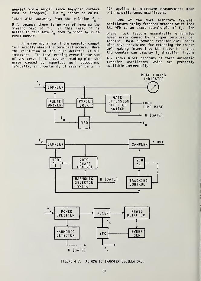
nearest whole number since harmonic numbersmust be integers). But f cannot be calcu-

lated with accuracy from the relation f =

N 1 f 1 because there is no way of knowing themissing part of f x . In this case, it is

better to calculate f from f2 since f2 is anexact number.

An error may arise if the operator cannottell exactly where the zero beat occurs. Herethe resolution of the null detector is all

important. The total reading error is the sumof the error in the counter reading plus theerror caused by imperfect null detection.Typically, an uncertainty of several parts in

10 7 applies to microwave measurements madewith manually-tuned oscillators.

Some of the more elaborate transferoscillators employ feedback methods which lockthe VFO to an exact submultiple of f . The

phase lock feature essentially eliminateshuman error caused by improper zero-beat de-tection. Most automatic transfer oscillatorsalso have provisions for extending the count-er's gating interval by the factor N so thatthe counter can display f directly. Figure

4.7 shows block diagrams of three automatictransfer oscillators which are presentlyavailable commercially.

SAMPLER

PULSEDRIVER

PHASELOCK

VFO

GATEEXTENSIONSELECTORSWITCH

PEAK TUNINGINDICATOR

0FROMTIME BASE

N (GATE)

SAMPLER

VCOf,

AUTOPHASE

CONTROL

HARMONICSELECTORSWITCH

SAMPLERf OUT

VCOfo

N (GATE) TRACKINGCONTROL

POWERSPLITTER

HARMONICDETECTOR

MIXER

VFO

PHASEDETECTOR

SWEEPGEN

N (GATE)

FIGURE 4.7. AUTOMATIC TRANSFER OSCILLATORS.

38

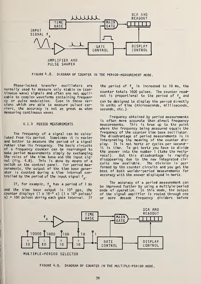
TIMEBASE

INPUTSIGNAL f

DCA ANDREADOUT

IMA IN

GATE.

GATECONTROL

DISPLAYCONTROL

AMPLIFIER ANDPULSE SHAPER

FIGURE h .8. DIAGRAM OF COUNTER IN THE PERIOD-MEASUREMENT MODE.

Phase-locked transfer oscillators arenormally used to measure only stable cw (con-tinuous wave) signals and often are not appli-cable to complex waveforms containing frequen-cy or pulse modulation. Even in those ver-sions which are able to measure pulsed car-riers, the accuracy is not as great as whenmeasuring continuous waves.

4.1.3 PERIOD MEASUREMENTS

The frequency of a signal can be calcu-lated from its period. Sometimes it is easierand better to measure the period of a signalrather than its frequency. The basic circuitsof a frequency counter can be rearranged tomake period measurements simply by exchangingthe roles of the time base and the input sig-nal (fig. 4.8). This is done by means of a

switch on the control panel. For period mea-surements, the output of the time base gener-ator is counted during a time interval con-trolled by the period of the input signal f .

If, for example, f has a period of 1 ms

and the time base output is 10 s pps, thecounter displays (1 x 10- 3 s) (1 x 10^ pulses/s) = 100 pulses during each gate interval. If

the period of f is increased to 10 ms, the

counter totals 1000 pulses. The counter read-out is proportional to the period of f and

can be designed to display the period directlyin units of time (microseconds, milliseconds,seconds, etc. ).

Frequency obtained by period measurementsis often more accurate than direct frequencymeasurements. This is true up to the pointwhere the frequency being measured equals thefrequency of the counter time base oscillator.The disadvantage of period measurements is in

interpreting the meaning of the counter dis-

play. It is not hertz or cycles per second--it is time. To get hertz you have to dividethe answer into the number 1 (take the recip-rocal). But this disadvantage is rapidlydisappearing due to the new integrated cir-cuits now available. The division is per-formed by the counter circuits and you get the

best of both worlds—period measurements foraccuracy with the answer displayed in hertz.

The accuracy of a period measurement canbe improved further by using a multiple-periodmode of operation. In this mode, the outputof the signal amplifier is routed through one

or more decade frequency dividers before

H>| loo oo y 1 o oo fioo } 10

MULTIPLE-PERIOD SELECTOR

10 10GATE

CONTROLDISPLAYCONTROL10 10

DCA ANDREADOUT

FIGURE J».9. DIAGRAM OF COUNTER IN THE MULTIPLE-PERIOD MODE.

39

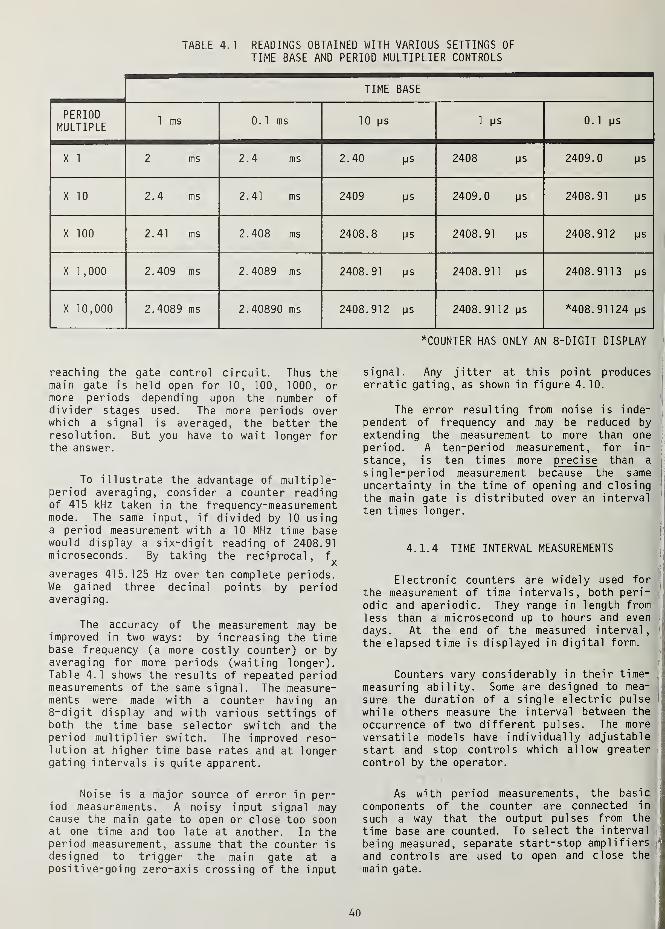
TABLE 4.1 READINGS OBTAINED WITH VARIOUS SETTINGS OF

TIME BASE AND PERIOD MULTIPLIER CONTROLS

TIME BASE

PERIODMULTIPLE

1 ms 0.1 ms 10 ps 1 us 0. 1 ps

X 1 2 ms 2.4 ms 2.40 us 2408 ps 2409.0 ps

X 10 2.4 ms 2.41 ms 2409 ps 2409.0 ps 2408.91 ps

X 100 2.41 ms 2.408 ms 2408.8 |js 2408.91 ps 2408.912 ps

X 1 ,000 2.409 ms 2.4089 ms 2408.91 us 2408.911 ps 2408.9113 ps

X 10,000 2.4089 ms 2.40890 ms 2408.912 ps 2408.9112 ps *408.91124 ps

^COUNTER HAS ONLY AN 8-DIGIT DISPLAY

reaching the gate control circuit. Thus themain gate is held open for 10, 100, 1000, ormore periods depending upon the number ofdivider stages used. The more periods overwhich a signal is averaged, the better theresolution. But you have to wait longer forthe answer.

To illustrate the advantage of multiple-period averaging, consider a counter readingof 415 kHz taken in the frequency-measurementmode. The same input, if divided by 10 usinga period measurement with a 10 MHz time basewould display a six-digit reading of 2408.91microseconds. By taking the reciprocal, f

averages 415.125 Hz over ten complete periods.We gained three decimal points by periodaveragi ng.

The accuracy of the measurement may beimproved in two ways: by increasing the timebase frequency (a more costly counter) or byaveraging for more periods (waiting longer).Table 4.1 shows the results of repeated periodmeasurements of the same signal. The measure-ments were made with a counter having an8-digit display and with various settings ofboth the time base selector switch and theperiod multiplier switch. The improved reso-lution at higher time base rates and at longergating intervals is quite apparent.

Noise is a major source of error in per-iod measurements. A noisy input signal maycause the main gate to open or close too soonat one time and too late at another. In theperiod measurement, assume that the counter is

designed to trigger the main gate at a

positive-going zero-axis crossing of the input

signal. Any jitter at this point producesj

erratic gating, as shown in figure 4.10.

The error resulting from noise is inde-pendent of frequency and may be reduced by

extending the measurement to more than one

period. A ten-period measurement, for in-

stance, is ten times more precise than a

single-period measurement because the samei

uncertainty in the time of opening and closing 1

the main gate is distributed over an interval

ten times longer.

4.1.4 TIME INTERVAL MEASUREMENTS

Electronic counters are widely used for

the measurement of time intervals, both peri-

odic and aperiodic. They range in length from

less than a microsecond up to hours and even

days. At the end of the measured interval,

the elapsed time is displayed in digital form.

f

Counters vary considerably in their time-

measuring ability. Some are designed to mea-

sure the duration of a single electric pulse

while others measure the interval between the

occurrence of two different pulses. The more

versatile models have individually adjustable

start and stop controls which allow greater

control by the operator.

As with period measurements, the basic

components of the counter are connected in

such a way that the output pulses from the

time base are counted. To select the interval

being measured, separate start-stop amplifiers j'

and controls are used to open and close the

main gate.

40

TRIGGER POINT-

TRIGGER POINT-

TRIGGERJPOINT

GATING INTERVALTOO SHORT

GATING INTERVALCORRECT

-TRIGGER POINT

GATING INTERVALTOO LONG

TRIGGERPOINT

FIGURE 4.10. EFFECT OF NOISE ON TRIGGER POINT IN PERIOD MEASUREMENTS.

JJJJJJO-

START SIGNAL

_FLSTOP SIGNAL

MAINGATE

J L

AMPLIFIERS ANDSIGNAL SHAPERS

DCA ANDREADOUT

FIGURE DIAGRAM OF COUNTER IN THE TIME INTERVAL MODE,

41

(A)

FIGURE 4.12. OPTIMUM TRIGGER POINTS FOR START-STOP PULSES.

During the time between the start andstop signals, the main gate is held open andcounts are accumulated according to the lengthof the gate interval. At the end of the gateinterval, the readout assembly can be made todisplay the elapsed time directly in micro-seconds, seconds, minutes, or other appropri-ate units.

The start-stop input circuits are de-signed to produce sharp, uniform triggerpulses from a variety of signals. Best re-sults are obtained if clean pulses are used.If the instrument has a trigger level control,it is possible to select the exact input am-plitude at which a trigger pulse from thatchannel is generated. If a slope control is

provided, it is possible to set the triggerpoint on either the positive-going or thenegative-going side of the input signal atwill.

Careful setting of the trigger level andslope controls is necessary to avoid measure-ment errors caused by noise, jitter, harmon-ics, and other forms of distortion on the

input signal. Figure 4.12 shows the besttriggering points for six different inputwaveshapes. In each case, the desired triggerpoint (as indicated by an x) is at the centerof the steepest, cleanest portion of thesignal. Note that for noise-free sinusoidal(sine wave) signals as in waveform (B), theoptimum trigger points occur at the zerocrossings.

4.1.5 PHASE MEASUREMENTS

The time interval counter can be used tomeasure phase relationships between two inputsignals of the same frequency. To do this,one of the signals goes to the start channelwhile the second signal goes to the stopchannel. The level and slope controls areadjusted to trigger at the same point on bothinput waveforms. For sinusoidal waves, thebest triggering point is the zero-crossover.The time interval between corresponding pointson the two input waveforms is then readdirectly from the counter. Time interval canbe converted to a phase angle by the formula

START

STOP 0^1

DCA ANDREADOUT

GATECONTROL

DISPLAYCONTROL

FIGURE 4.13. USE OF T I ME- I NTERVAL UNIT FOR PHASE MEASUREMENTS.

42

JJJJO.L DCA ANDREADOUT

J~~LCOMMONINPUT

SIGNAL

STOP

J L

GATECONTROL

DISPLAYCONTROL

FIGURE k.lk. TIME-INTERVAL COUNTER WITH START-STOP CHANNELS CONNECTEDTO COMMON SOURCE FOR PULSE-WIDTH OR PERIOD MEASUREMENTS.

a. snuncc AM/-I c \ - 360 x Time Interval .

<|> (PHASE ANGLE )= degrees

Zn x Time Intervalradians

,

where T is the known period of the two signalsexpressed in the same units as the timeinterval

.

necessary to connect both input channels tothe same source (figure 4.14).

The smallest measurable time interval is

limited by the resolution of the counter. In

general, the resolution of time interval andperiod measurements are affected by the samefactors. The presence of noise can seriouslyimpair the precision of pulse-width determi-nations.

4.1.7 COUNTER ACCURACY

4.1.6 PULSE-WIDTH DETERMINATION MEASUREMENTS

Trigger controls are seldom calibratedwith sufficient accuracy to measure the risetime or decay time of a single pulse. It is

almost always necessary to use an oscilloscopeto measure rise time. An oscilloscope usedwith a counter is very useful. By selectingone polarity of slope for the start triggerand the opposite polarity for the stop trig-ger, you can measure the total duration of a

pulse. The duration of pulse (A) in figure4.12, for example, could be determined byselecting point x on the positive slope forthe start trigger and point x on the negativeslope for the stop trigger. Some time inter-val counters bring the gate start-stop pulseout on connectors for oscilloscope viewing.

Carrying the idea one step further, theperiod of waveform (B) in figure 4.12 could bemeasured by choosing the positive zero-cros-sing as the trigger point for both the startand stop pulses. When measuring pulse widthor period with a time interval counter, it is

Depending upon the characteristics of thecounter and its method of use, the accuracy ofmeasurements may range from 1 part in 10 2 to a

few parts in 10 10 or better. Although thepossible causes for inaccurate measurement aremany, the main sources of error are (1) time-base instability, (2) uncertain gating, and

(3) faulty triggering. The total measurementerror is the algebraic sum of all individualerrors.

A. Time Base Error

The time base oscillator will changefrequency slightly during the course of a

measurement. This is due to temperaturechanges, line voltage changes, internal noise,

and crystal aging. Temperature effects can beminimized by allowing the instrument to warmup before use and by keeping the counter in a

constant- temperature location. If the linevoltage fluctuations are severe, it may be

necessary to operate the counter from a regu-lated power source. Check the operatingmanual for the manufacturer's recommendations.

43

(X10

6

10)

HOURS

FIGURE 4.15. TYPICAL TIME BASE STABILITY CURVE.

Any noise generated internally by thetime base oscillator produces a jitter in itsoutput frequency. This may cause erroneouscounts, especially when a measurement is per-formed during a brief time interval. As themeasurement time is made longer, the jittertends to average out. For this reason, thejitter is often called "short-term" instabili-ty. A typical time base stability graph is

shown in figure 4.15. Note that the verticalaxis is labeled Af/f, which is equal to F, therelative frequency of the time base. A com-plete explanation of this notation is given in

Chapter 3.

In modern counters, the amount of oscil-lator noise is generally so small that short-term stability is specified only for the mostprecise instruments. When reading specifica-tions, it should be realized that the averag-ing time has an important bearing on theactual meaning of stability figures. Forexample, an oscillator having a stabilityspecification of 5 x 10- 10 (per minute) mightbe noisier than one with a specification of 5

x 10- 9 (per second). To be absolutely mean-ingful, short-term stability figures should becompared for the same averaging period, pre-ferably of only a few seconds.

Long-term instability, on the other hand,refers to a slow, often predictable drift in

the average frequency of an oscillator due togradual changes in the crystal. Quartz cry-stals exhibit drift rates typically of 10- 10

to 10- 6 per day as a result of crystal aging.After a brief warmup period when the oscil-lator is first turned on, a high-qualitycrystal has a linear frequency drift, theslope of which reveals the crystal aging rate.

Because aging produces larger and largererror as time goes on, it is necessary to

recalibrate the oscillator if the time base is

to be accurate. For utmost accuracy it may be

wise to check the oscillator calibrationimmediately before and after a critical mea-surement. However, on inexpensive counters,this may be impractical.

For measurements which require a bettertime base accuracy than that of the counter'sinternal oscillator, you can use an externalfrequency source to drive the time base gen-erator. Most counters have a built-in con-

J

nector and switch for using an external oscil-lator. The internal oscillator is automatic-ally disconnected when the time base is

switched to an external source.

B. Gate Error

As previously mentioned, an uncertaintyof ± 1 count is inherent with all conventionalelectronic counters because the time base

j

pulses are usually not synchronized with the !

signal being measured. Because of this, it is

possible for the reading to be in error by one

count even if there are no other sources of

error! As an example, figure 4.16 shows how

the same signal might produce a count of

either 8 or 9, depending upon when the gatinginterval started.

It is obvious that the percentage error

becomes smaller as more pulses are counted. A

one count matters less for 1,000,000 than for

1,000. This explains why long gating inter-

vals permit greater accuracy of measurement.

44

GATING INTERVAL8 COUNTS

SIGNALPULSES

JJJ_LJ_L_L_LJ^L-L9 COUNTS

GATING INTERVAL

FIGURE ^. 16. CONSTANT GATING INTERVAL WITH AMBIGUITY OF + 1 COUNT.

If we count a 1 MHz frequency for 1

second, the ± 1 count error is one part per

million. If either the measured frequency is

increased to 10 MHz or the gating interval is

lengthened to 10 seconds, the error goes down

to 1 part per ten million. In measurements of

high frequencies, made directly or with the

aid of heterodyne converters, the uncertainty

of ± 1 count may be less important than the

counter's time base error. The same is true

of prescalers which incorporate gate extension

features.

Previously, we noted that low frequencies

can be measured more accurately by period

measurements than by direct frequency measure-

ments. For very high frequencies, however,

the reverse is true. At some point, the

effect of gate error must be identical for

either mode of operation. The chart in figure

4.17 depicts the crossover point as well as

the accuracy which can be expected both from

multiple-period measurements and direct fre-

quency measurements up to 100 MHz.

C. Trigger Errors

Trigger errors usually arise from the

presence of noise or other modulation on the

gate-control signal. This source of error has

been mentioned previously in conjunction with

period and time interval measurements. For

frequency measurements, the trigger error is

almost always negligible because the gate-

control signal, obtained directly from the

time base, can be virtually noise-free.

For period and time interval measure-

ments, the trigger error (etr

) is expressed

mathematically as the ratio of the gate time

deviation (At) to the total duration (T) of

the gating interval. Trigger error is also

proportional to the fraction of peak noise

voltage (E ) over peak signal voltage

FIGURE 4.17. ACCURACY CHART FOR PERIOD AND FREQUENCY MEASUREMENTS.

45

where k is a proportionality constant deter-mined by the nature of the modulation.

Although noise can sometimes be removedfrom the input signal by external devices;e.g., limiters, filters, etc., its effects canbe reduced more conveniently by multiple-period averaging. As more periods are aver-aged, the effects of both the ± 1 count ambi-guity and the trigger error diminish propor-tionately.

Most counters incorporate a Schmitt trig-ger or similar circuit to generate the triggerpulses. Because of a slight hysteresis or lagin switching action which characterizes suchcircuits, the rise and decay of the triggerpulses are not started at exactly the samevoltage. Instead, the width of the triggerpulse is determined by two voltage levels— onethat establishes the point at which the pulse

CONTINUOUS SINE WAVE INPUT

(FOUR PULSES produced)

HEAVY AMPLITUDE MODULATION(THREE PULSES PRODUCED)

FIGURED. 18. UNDIFFERENTIATED

begins to rise and the other that dictates thepoint where the pulse starts to fall. A com-plete pulse is produced, therefore, only whenthe input signal crosses both critical levels.

Figure 4.18 shows how counts may be lostor gained as a result of signal modulation.The shaded area in each example is the hyster-esis zone of the trigger circuit. Incorrectcounts are likely to result whenever the inputwaveform reverses direction within the shadedzone.

To measure the time interval between theoccurrence of a sharp pulse and the nextpositive-going zero crossing of a continuoussine wave, it would be logical to start thecounter with the pulse and adjust the stop-channel control (s) to trigger at zero volts onthe positive slope. If the trigger levelcontrol for the stop channel is improperly

LOW-FREQUENCY RIPPLE SUPERIMPOSED

(THREE PULSES PRODUCED)

II

1i kd

1

I

J 1i

i

i

i

U|i

I

I !!

fi

i

iI1

HIGH-FREQUENCY INTERFERENCE

(FIVE PULSES PRODUCED)

SCHM I TT-TR I GGER WAVEFORMS

.

46

-CALIBRATION LOW— (TRIGGER LEVEL TOO HIGH)

U— TIME INTERVAL TOO LONG H

CALIBRATION CORRECT

- CALIBRATION HIGH- (TRIGGER LEVEL TOO LOW)

U— TIME INTERVAL TOO SHORT-*]

I

1

FIGURE it. 19- TIME ERROR PRODUCED BY IMPROPER CALIBRATIONOF TRIGGER LEVEL CONTROL.

calibrated, however, the stop pulse may be

produced at a point that is actually positiveor negative when the control is set at zero.

This means that the measured time interval

will be too long or too short as shown byfigure 4. 19.

Of course, an opposite error will resultif the trigger level control for the startchannel reads too low or too high. If thecontrols for both channels are misadjusted in

opposite directions, the combined error will

be cumulative. Furthermore, the effect of

trigger calibration error is made worse if

instead of a steep wavefront the input signal

>T/2

T/2

<T/2

has a gradual slope at the selected triggering

point.

A low-frequency sine wave is convenient

for checking the calibration of trigger con-

trols. With the counter in the time interval

mode, the gating interval switch in the XI po-

sition, and both input channels adjusted to

trigger at zero volts on the same slope, the

counter should display exactly one period of

the test signal. Next the slope selector for

the stop channel is turned to its opposite po-

sition without adjusting any other controls.

If the counter reading changes by exactly one-

half period when the opposite slope is

(a) LEVEL TOO HIGH

(b) LEVEL CORRECT

(c) LEVEL TOO LOW

FIGURE A. 20. SINE WAVE METHOD OF CHECKING TRIGGER LEVEL CALIBRATION.

47

DIGITALCOUNTER

D TO A

CONVERTER ANALOG CHARTSTRIP RECORDER

FIGURE k. 21. DIGITAL-TO-ANALOG ARRANGEMENT FOR CHART RECORDING.

selected, the trigger level setting is cor-

rect. If the reading changes by more thanone-half period, as in (a) of figure 4.20, the

stop channel's trigger level is too high. If

the change is less than one-half period, as in

(c), the trigger level is too low. The starttrigger can be checked in a similar fashion byholding all other controls fixed and switchingthe slope selector for the start channel only.

4.1.8 PRINTOUT AND RECORDING

Some counters have provisions for con-necting a printer to get a permanent record ofthe readings. Using a digital-to-analog con-verter, the counter can also be used to drivea chart recorder. The printer must be compat-ible with the counter if a valid printout is

to be obtained.

used wires, mirrors, and light beams insteadof electronic circuits, but it could displaywaveforms of low-frequency alternatingcurrent.

The modern cathode-ray tube was developedin the early 1920' s. Since then, the elec-

tronic oscilloscope has evolved into an in-

strument that can display high-frequency wave-forms and store images for days. Measurementsor comparisons of frequencies and time inter-

vals are among the major uses of the oscillo-scope.

There are four main parts: (1) the

cathode-ray tube and its power supply, (2) the

vertical deflection amplifier, (3) the hori-

zontal deflection amplifier, and (4) the time-base generator. A block diagram is shown in

figure 4.22.

4.2 OSCILLOSCOPE METHODS

The cathode-ray oscilloscope is probablyone of the most useful laboratory tools avail-able to the electronics technician, engineer,or scientist. Whole volumes have been devotedto its many uses.

The basic physical principles of the

oscilloscope have been known for years. An

early oscillograph (as it was then called) wasin operation during the 1890' s. This device

The role of the time-base generator is

fairly involved. In order to display faith-

fully a signal that is a function of time, the

spot of light must traverse the cathode-raytube screen at a uniform rate from one side to

the other and then return to the original side

as quickly as possible. The voltage that

causes this horizontal sweep is generated by

the time-base generator. The waveform is a

ramp or "sawtooth" as shown in figure 4.23.

The frequency of the ramp voltage is

variable so that waveforms of any frequency

VERTICALINPUT

VERTICALAMPLIFIER

HORIZONTAL INPUT

TRIGGER INPUT

CRTPOWERSUPPLY

HORIZONTALAMPLIFIER

c

) TIME-BASEGENERATOR

c

FIGURE It. 22. SIMPLIFIED BLOCK DIAGRAM OF A CATHODE-RAY OSCILLOSCOPE.

48

FIGURE it. 23. WAVEFORM OF HORIZONTAL DEFLECTION VOLTAGE FROM TIME-BASE GENERATOR.

within the limits of the oscilloscope can be

displayed. The time-base generator has a

control to change the frequency of the ramp.

How fast the spot moves across the screen is

of interest to the operator; therefore, the

frequency control is usually labeled in sec-

onds (or fractions of seconds) per centimeter.

When the frequency of the traverse is

high enough, the persistence of the phosphor-ous and the retention capability of the humaneye combine to make the moving spot appear as

a solid line across the screen. If a periodicwave is applied to the input of the verticalamplifier and the time-base generator is

properly adjusted, the waveform will be dis-

played as a stationary pattern on the cathode-ray tube screen.

4.2.1 CALIBRATING THE OSCILLOSCOPE TIME BASE

If there is much doubt as to the accuracyof the time-base generator, it should be cali-brated. Use a signal that is more accurate

than the time-base signal being measured. The

calibration is done in much the same way as

the frequency measurement, but in reverse. If

you have a crystal oscillator that operates in

the same frequency range as the sweep time

base being measured, proceed as follows:

Display the calibration source signal on

the screen, and adjust the time-base switch to

the setting that should give one cycle per

centimeter. If the source is 100 kHz, for

example, the time-base step switch should be

set to 10 microseconds/centimeter. If the

time-base generator is off frequency, there

will be more or less than one cycle per centi-

meter displayed on the screen. Adjust the

variable frequency control of the time-basegenerator until the display is correct.

The adjustment may or may not hold for

other positions of the step switch, so it is

best to recalibrate each position. Many

laboratory oscilloscopes have built-in cali-

bration oscillators which can be used in the

same way as an external frequency source.

Refer to the oscilloscope manual for details.

EXTERNALFREQUENCYSOURCE

CRTPOWERSUPPLY

CRT

VERTICALAMPLIFIER

TIME-BASEGENERATOR

FIGURE 4.24. TIME BASE CALIBRATION HOOKUP USING AN EXTERNAL FREQUENCY SOURCE.

49

1 CM

FIGURE 4.25. SINE WAVE DISPLAY AS VIEWED ON OSCILLOSCOPE.

4.2.2 DIRECT MEASUREMENT OF FREQUENCY A. Lissajous Patterns

Suppose that we want to measure the fre-quency of a sine wave when it appears as shownin figure 4.25. By counting the number ofcycles and the number of scale divisions(centimeters), we see that five cycles occurin 15.5 centimeters. Now we observe the time-base generator dial, first making sure it is

in the calibrated mode. If the dial reads 0.1millisecond per centimeter, for instance, thefrequency computation would be:

5 cycles 1 cm 1000 ms3230 Hz.

15.5 cm 0.1 ms 1 s

Alternatively, we may divide the display (incycles per centimeter) by the time-base rate(in seconds per centimeter):

cycles ^ s_ _ cycles cmcm cm cm

Hz.

Direct frequency measurements with theoscilloscope have an accuracy limit of about 5

parts per thousand. Accuracy of the measure-ment is limited by the ability of the operatorto read the screen and by the accuracy of thetime base. In general, one should expect todo no better than about 0.5%. Still, if youwant to know whether you are looking at 60 Hzor 120 Hz, or if you are checking a radiocarrier frequency for harmonics, the accuracyis good enough.

4.2.3 FREQUENCY COMPARISONS

Unlike direct frequency measurements,

frequency comparisons with the oscilloscopecan easily be made with a precision of onepart per million. A precision of one part per100 million or even one part per billion canbe achieved by using extra equipment described1 ater.

The optical-mechanical oscillograph wasdeveloped in 1891, but the idea of a Lissajouspattern is even older, having been demonstra-ted by a French professor of that name in

1855.

If we apply a sine wave simultaneouslyto the horizontal and vertical inputs of anoscilloscope, the spot will move in some pat-tern that is a function of the voltages oneach input. The simplest Lissajous patternoccurs if we connect the same sine wave toboth inputs. The equipment hookup is shownin figure 4.26. The resulting pattern is a

straight line. Furthermore, if both signalsare of the same amplitude, the line will be

inclined at 45° to the horizontal.

FIGURE 4.26. EQUIPMENT HOOKUPFOR A 1:1 LISSAJOUSPATTERN.

If the input signals are equal in ampli-

tude and 90° out of phase, a circular pattern

results. Other phase relationships produce an

elliptical pattern. The phase difference in

degrees between the horizontal sine wave and

the vertical sine wave can be determined as

shown in figure 4.27.

The phase relationship between signals

that generate linear, circular, or elliptical

patterns is given by:

• L Asin 6 = „ ,

50

-0.866

9 = 150° 210° 9-180°

FIGURE k.27. ELLIPTICAL LISSAJOUS PATTERNS FOR TWO INDENT I CAL FREQUENCIES

OF DIFFERENT PHASE.

RESULTANT IMAGE

12 0-36

HORIZONTAL 271-

DEFLECTIONVOLTAGE

33FIGURE 4.28. DEVELOPMENT OF A 3:1

LISSAJOUS PATTERN.

51

where 8 is the angle between the two sine

waves, and A and B are relative distances

measured along the vertical axis of the trace.

The actual determination of frequency

ratio is done in a straightforward manner.

The number of loops touching, or tangent to, a

horizontal line across the top of the pattern

is counted. Likewise the number of loops

tangent to either the right or left side is

counted. The frequency ratio is then computedfrom the formula

where: f = the frequency of the verticalv

deflection voltage,

f. = the frequency of the hori-zontal deflection voltage,

T, = the number of loops tangentto the horizontal line, and

T = the number of loops tangentto the vertical line.

Figure 4.28 shows the graphical construc-tion of a 3:1 pattern. Note that the ratio of

T./T is 3:1.h v

Lissajous patterns become quite compli-cated when the two frequencies are widelyseparated. Some oscillograms for higherratios are shown in figure 4.29. Two versionsof each pattern are shown. Version (A) is the

typical closed-lobe pattern, and version (B)

is the double image that results if phaserelations cause the pattern to be folded andexactly superimposed upon itself.

The usefulness of Lissajous patterns

depends upon a number of things. Consider a

1:1 pattern. If we are trying to synchronize

two power generators at 60 Hz and our pattern

is changing through one complete cycle every

second, we have achieved synchronization to 1

Hz or about 1.7%--not very good. If our

frequency was 100 kHz, the same change of one

revolution per second in our pattern would

give a resolution of 1 x 10- 5. This shows

that the higher the frequencies we are workingwith, the better synchronization becomes.

In comparing or synchronizing precisionoscillators, a frequency multiplier may be

useful. Every time our signals are multipliedin frequency by a factor of ten, the precisionof measurement improves by a factor of ten.

When the two signals are multiplied and then

fed to a phase detector, they produce a low-

frequency signal equal to the difference in

hertz between our two multiplied signals.

This difference signal, Af. may then be com-

pared via Lissajous pattern against the sine

wave from a precision low-frequency oscil-

1 ator.

If we again use two 100-kHz signals as an

example but multiply their frequencies to 100

MHz before comparing them, we achieve a mea-

surement precision of 1 x 10- 8. This arrange-

ment is shown in figure 4.30.

The phase detector may be a double-

balanced mixer of the type shown in figure

4.31. These mixers are available com-

mercial ly.

Another system for comparing two oscil-

lators is indicated in figure 4.32. A phase-

error multiplier increases the phase or fre-

quency difference between the oscillators by

some factor, say 1000, without frequency

100kHz FREQUENCYMULTIPLIER

OSCILLATOR (X1000)

1 00MHz

100kHz FREQUENCYMULTIPLIER

OSCILLATOR (X1000) 1 00MHz

CALIBRATEDLOW FREQUENCYOSCILLATOR

1000 AF

FIGURE 4.30. ARRANGEMENT FOR MEASURING SMALL FREQUENCY DIFFERENCESWITH OSCILLOSCOPE AND FREQUENCY MULTIPLIERS.

53

INPUT INPUT B

DC OUTPUT

FIGURE 4.31. DOUBLE-BALANCED MIXER.

OSCILLATOR100 kHz

OSCILLATOR100 kHz

100 kHz

PHASE ERRORMULTIPLIER(X1000)

FIGURE 4.32. ARRANGEMENT FOR FREQUENCY COMPARISON USING

OSCILLOSCOPE AND PHASE-ERROR MULTIPLIER.

multiplication. The output from the phase-error multiplier can be connected directly to

the oscilloscope. The resulting Lissajouspattern will allow oscillator synchronizationwith the same precision as provided by thefrequency multiplier technique. If care is

taken, calibrations with errors as small as

1 x 10- 9 or 1 x IO- 10 can be accomplished.

A principal use of the 1:1 Lissajouspattern is for synchronization of oscillatorfrequencies. If the pattern is drifting, no

matter how slowly, it means that a frequencydifference exists between the oscillators.Neither the oscilloscope nor the operator cantell which oscillator is at the higher fre-quency. The Lissajous pattern is the sameregardless of which frequency is higher. Whatcan be done, though, is to slightly change thefrequency of one of the oscillators. If therate of pattern drift increases when the fre-

quency of oscillator #1 is raised, then oscil-lator #1 is at a higher frequency than oscil-lator #2. The opposite happens if the patterndrift slows down when the frequency of oscil-

lator #1 is increased.

Calibration of variable oscillators such

as rf signal generators and audio oscillatorsis easily done using Lissajous patterns of

higher than 1:1 ratio. Figure 4.33 shows a

method of calibrating an rf signal generator

using a fixed 100-Hz frequency source.

Starting with a 1:1 Lissajous pattern

between the standard oscillator and the signal

generator, mark the calibration points on the

generator dial each time the pattern becomes

stationary as the dial is turned. Each

stationary pattern represents a definite

frequency ratio which can be evaluated by one

of the methods explained previously. Patterns

of ratios up to 20:1 can be recognized if the

signal generator is stable enough.

100kHz CRYSTALOSCILLATOR

FREQUENCYMULTIPLIER

HO-

RF SIGNALGENERATOR

FIGURE 4.33. ARRANGEMENT FOR CALIBRATINGA SIGNAL GENERATOR.

54

If the oscillator has a base frequency of

1 MHz with internal dividers to 100 kHz, cali-

bration points can be found on the signal

generator dial every 100 kHz from 0.1 MHz to 2

MHz and every 1000 kHz from 2 MHz to 20 MHz.

This range is adequate for many rf signal

generators. Multipliers can be used to extendthe markers into the VHF range if necessary,but the calibration points will be fartherapart.

Not much can be learned from a driftingpattern of high ratio, and even the stationarypattern may be confusing. A complete rotationof the pattern in one second means a 1-Hzdeviation by the higher frequency no matterwhat the ratio. But for ratios other than1:1, the change in the lower frequency is not

as great.

With a 10:1 pattern, for instance, a

drift of one revolution per second could meanthat the higher frequency is off by 1 Hz, orit could mean that the lower frequency is offby 0.1 Hz. Unless one of the two frequenciesis assumed to be accurate, there is no way oftelling from the Lissajous pattern whichfrequency is in error. Only their relativedifference can be measured by this method (seeChapter 3).

B. Sweep Frequency Calibration:

An Alternative Method

Most frequency comparisons made in a

standards laboratory are between oscillatorsthat have very small frequency differences. A

1:1 Lissajous pattern between oscillatorshaving a relative frequency difference of 1 x10- 11 would take over a day if the comparisonwere made at 1 MHz! There are faster ways tomeasure the rate of change on the oscillo-scope. These methods allow the differencefrequency to be determined in much shortertimes than is possible with a slow movingLissajous pattern.

The output wave of an oscillator to bemeasured is displayed on the oscilloscope.Next, the oscilloscope sweep frequency oscil-lator is calibrated. Now, if the oscilloscopeis triggered by a reference oscillator, thepattern or waveform will appear to stand stillif the frequencies of the two oscillators arenearly equal. Actually, the pattern willslowly drift. The rate of drift in microsec-onds per day depends on the frequency differ-ence between the oscillators. The directionof drift tells us which oscillator is high orlow in frequency with respect to the other.

When a sine wave of an oscillator fre-quency is displayed and the oscilloscope is

triggered by a reference oscillator, themovement of the pattern can be used for cali-

bration. This pattern will move to the left

or right if the unknown frequency is -high

or low with respect to the reference oscil-lator. The question is, how fast is the

pattern moving? How many microseconds is it

moving in how many hours or days? Remember,

the sweep is calibrated in microseconds or

milliseconds per centimeter.

One could make a measurement of the

pattern position at, say, 10:05 am, then comeback at 2:30 pm for another look. Suppose in

the meantime, it moves exactly three centi-meters and the sweep speed is set at one

microsecond per centimeter. What does this

tell us?

ELAPSED TIME = 2:30 pm - 10:05 am

= 4 hours 25 minutes = 0.184 day.

PHASE DRIFT RATE = 3-00 cm x 1 . 00 us/cm

0.184 day

= 16.3 us/day.

This result tells us how much our oscil-lator moved in time (16.3 microseconds) duringan interval of one day. The result is in theform At/T (see Chapter 3 for a further expla-nation). Expressed as a numeric, At/T = 1.89

x 10- 10 since there are 86,400 x 106 micro-seconds in a day.

We can relate this to a frequency nota-

tion because Chapter 3 tells us that

_ At _ Af

T f

For this oscillator, the relative frequency,F = Af/f = -1.89 x 10- 10

. The negative sign

tells us that the measured frequency was lower

than its nominal value. In this case, it is

assumed that the reference frequency is equal

to its nominal value. Notice also that the

oscilloscope has performed a measurement much

like the time interval counter mentionedearlier in this chapter.

©T FREQUENCY

REFERENCEOSCILLATORTO BE

CALIBRATED-o o

FIGURE 4.34. VIEWING FREQUENCY DRIFT.

55

4.2.4 TIME INTERVAL MEASUREMENTS

Time- interval measurements are quite easyto perform with the oscilloscope. Usually,one time pulse is displayed on the screenwhile a different time pulse is used to trig-ger the oscilloscope. Another method is todisplay both time pulses on a dual-tracescope. Triggering can be achieved from eitherof the two displayed pulses or from a thirdtime pulse. An adjustable rate divider is

handy for this purpose.

A point worth remembering is that theaccuracy of the timeinterval measurement is

inversely proportional to the length of theinterval. If the time pulses are 10 milli-seconds apart, for instance, the measurementcan be performed to probably no better than± 50 microseconds. But if the pulses are only100 microseconds apart, the measurement can beperformed with an accuracy of ±0.5 microsec-ond. In both cases, however, the relativeuncertainty is the same (± 5 parts in 103 ).

For time pulses spaced close together,the pulse width may occupy an appreciablepercent of the time interval; therefore, largeerrors can be introduced by having the wrongtrigger slope or improper trigger amplitude.Unless care is taken by the operator, sucherrors can nullify the accuracy that is other-

RF VOLTMETER

wise attainable in the measurement of brieftime intervals.

The main advantage in using an oscillo-scope for time interval measurements is thatone can see the pulse waveform. For thisreason, time intervals between odd-shaped or

noisy pulses are better measured with the

oscilloscope than with other types of instru-ments. Time intervals in the submicrosecondrange can be measured easily and economicallywith high-frequency oscilloscopes, but long

intervals are more accurately measured with an

electronic counter, as described earlier.

Always refer to your oscilloscope manual; it

contains additional useful information.

4.3 WAVEMETERS

A wavemeter is an adjustable circuit thatcan be made to resonate over a range of fre-

quencies as indicated on a calibrated dial.

The dial may be marked in units of frequencyor wavelength. A typical wavemeter covers a

frequency range on the order of one octave.

Resonance is detected by observing the re-

sponse of a meter or other device incorporatedinto the measuring instrument or by noting a

disturbance in the system under test.

INCANDESCENT LAMP

THERMOCOUPLEMILLIAMMETER

SECONDARY WINDING SECONDARY WINDINGWITH LAMP WITH METER

FIGURE 4.35. WAVEMETER RESONANCE INDICATORS.

56

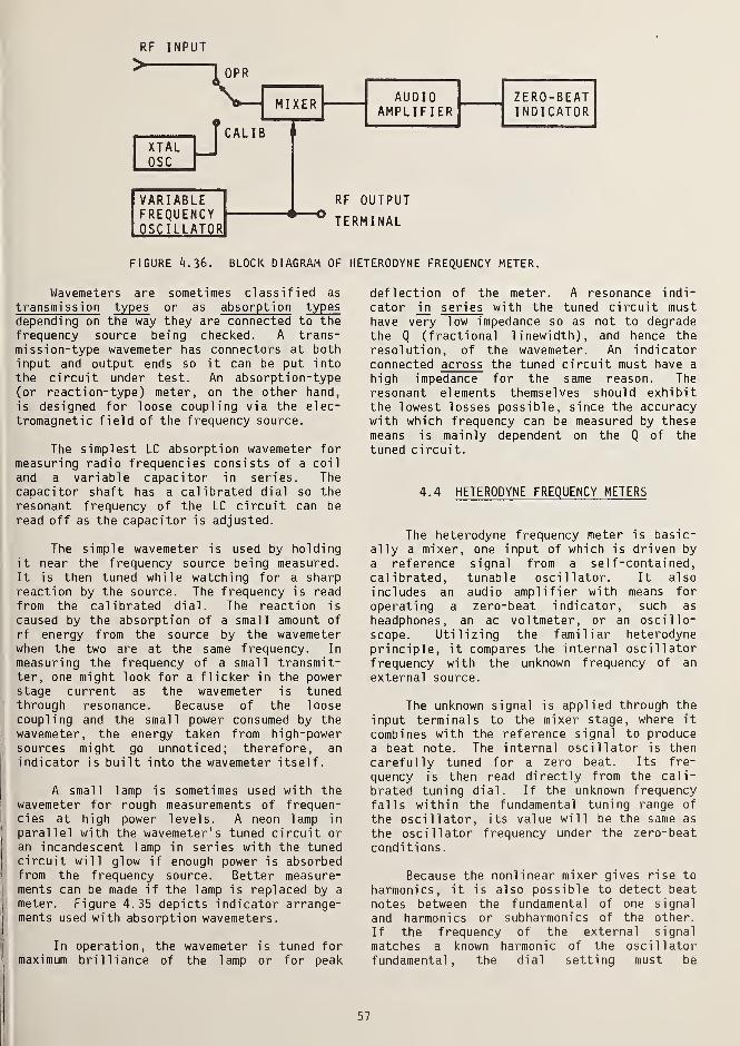
RF INPUT

>1 OPR

XTALOSCJ

MIXER

CALIB

VARIABLEFREQUENCYOSCILLATOR

AUDIOAMPLIFIER

RF OUTPUT

TERMINAL

ZERO-BEATINDICATOR

FIGURE 4.36. BLOCK DIAGRAM OF HETERODYNE FREQUENCY METER.

Wavemeters are sometimes classified as

transmi ssion types or as absorption typesdepending on the way they are connected to the

frequency source being checked. A trans-mission-type wavemeter has connectors at bothinput and output ends so it can be put into

the circuit under test. An absorption- type(or reaction-type) meter, on the other hand,

is designed for loose coupling via the elec-tromagnetic field of the frequency source.

The simplest LC absorption wavemeter for

measuring radio frequencies consists of a coil

and a variable capacitor in series. Thecapacitor shaft has a calibrated dial so theresonant frequency of the LC circuit can be

read off as the capacitor is adjusted.

The simple wavemeter is used by holdingit near the frequency source being measured.It is then tuned while watching for a sharpreaction by the source. The frequency is readfrom the calibrated dial. The reaction is

caused by the absorption of a small amount ofrf energy from the source by the wavemeterwhen the two are at the same frequency. In

measuring the frequency of a small transmit-ter, one might look for a flicker in the powerstage current as the wavemeter is tunedthrough resonance. Because of the loosecoupling and the small power consumed by thewavemeter, the energy taken from high-powersources might go unnoticed; therefore, anindicator is built into the wavemeter itself.

A small lamp is sometimes used with thewavemeter for rough measurements of frequen-cies at high power levels. A neon lamp in

parallel with the wavemeter 1

s tuned circuit oran incandescent lamp in series with the tunedcircuit will glow if enough power is absorbedfrom the frequency source. Better measure-ments can be made if the lamp is replaced by a

meter. Figure 4.35 depicts indicator arrange-ments used with absorption wavemeters.

In operation, the wavemeter is tuned formaximum brilliance of the lamp or for peak

deflection of the meter. A resonance indi-

cator J_n series with the tuned circuit musthave very low impedance so as not to degradethe Q (fractional linewidth), and hence the

resolution, of the wavemeter. An indicatorconnected across the tuned circuit must have a

high impedance for the same reason. Theresonant elements themselves should exhibitthe lowest losses possible, since the accuracywith which frequency can be measured by thesemeans is mainly dependent on the Q of thetuned circuit.

4.4 HETERODYNE FREQUENCY METERS

The heterodyne frequency meter is basic-ally a mixer, one input of which is driven by

a reference signal from a self-contained,calibrated, tunable oscillator. It also

includes an audio amplifier with means for

operating a zero-beat indicator, such as

headphones, an ac voltmeter, or an oscillo-

scope. Utilizing the familiar heterodyneprinciple, it compares the internal oscillatorfrequency with the unknown frequency of an

external source.

The unknown signal is applied through the

input terminals to the mixer stage, where it

combines with the reference signal to producea beat note. The internal oscillator is then

carefully tuned for a zero beat. Its fre-

quency is then read directly from the cali-

brated tuning dial. If the unknown frequencyfalls within the fundamental tuning range of

the oscillator, its value will be the same as

the oscillator frequency under the zero-beatconditions.

Because the nonlinear mixer gives rise to

harmonics, it is also possible to detect beat

notes between the fundamental of one signal

and harmonics or subharmonics of the other.

If the frequency of the external signal

matches a known harmonic of the oscillatorfundamental, the dial setting must be

57

RADIOTRANSMITTER

HETERODYNEFRE^UE

ITERTV

WHIPANTENNA

RADIORECEIVER

LOUDSPEAKER

FIGURE 4.37. ARRANGEMENT FOR CHECKING TRANSMITTING FREQUENCYWITH HETERODYNE FREQUENCY METER AND RECEIVER.

multiplied by the appropriate harmonic numberN. On the other hand, if the unknown frequencyequals a subharmonic, the dial reading must be

divided by N. Thus, from a knowledge of har-

monic relations, heterodyne measurements canbe made of frequencies far above or below thefundamental tuning range of the frequencymeter.

Figure 4.36 shows the block diagram of a

basic heterodyne frequency meter. The inter-nal variable-frequency oscillator must havegood stability. This calls for close tempera-ture regulation, complete shielding, and rug-

ged construction. The oscillator should alsobe thoroughly buffered to reduce frequency-pulling tendencies when strong signals areapplied from the external source, or whenother factors would cause the oscillator load

to change.

Some heterodyne meters are equipped witha whip antenna so the internal oscillatorsignal can be radiated over short distances.For checking the frequencies of transmittersor other high-power sources, a safe method is

to tune in the transmitter with a radioreceiver and then adjust the frequency meteruntil a zero beat is heard through thereceiver's loudspeaker. The unknown frequencycan be measured just as though it were coupleddirectly to the frequency meter.

The overall accuracy of measurementdepends on the calibration accuracy of thetunable oscillator and the resolution attain-able through the zero-beat process. At highfrequencies, the error introduced by imperfectzero-beat detection can be ignored. Providedthe temperature is kept nearly constant, the

variable-frequency oscillator may retain its

accuracy within 0.1% over long periods of timewithout recal ibration.

Most heterodyne meters contain a stablequartz crystal oscillator for use in gener-ating markers at fixed check points on the

tuning dial. By checking the dial calibrationat the point nearest the frequency to be

measured, it is possible to achieve an accu-racy approaching one part per million afterthe instrument has reached a stable operatingtemperature.

Heterodyne frequency meters combine widefrequency coverage with good accuracy in a

portable instrument. They can be obtained for

operating over fundamental frequency rangesfrom approximately 100 kHz to 200 MHz. Accu-

racy varies from about 0.01% at low frequen-cies to 0.00025% or better at very high fre-

quencies. Harmonics up to 3 GHz may be gen-

erated with a precision of 1 x 10- 6.

Because they are tunable devices, the

heterodyne frequency meters offer better noise

immunity and signal sensitivity than widebandinstruments such as oscilloscopes and count-

ers. The heterodyne meter is one of the most

useful of all frequency-measuring instruments

for checking transmitter frequencies, for

calibrating rf signal generators, and for

other applications which do not require a high

degree of signal purity.

4.5 DIRECT-READING ANALOG FREQUENCY METERS

Analog frequency meters operate by trans-

forming the unknown frequency into a different

physical quantity-such as voltage or current

ampl itude--which can be measured directly by

conventional instruments. Thus, the output

indicator might be an ordinary mi Hi ammeter

whose deflection is somehow made proportional

to the input frequency.

4.5.1 ELECTRONIC AUDIO FREQUENCY METER

A meter- type instrument that reads dir-

ectly in audio frequency units and requires no

manipulations of any kind is shown in figure

58

/\A,INPUT

OVERDRIVENAMPLIFIER(LIMITER)

-OIL

M I LL I AMMETE R

FIGURE ^.38. ELECTRONIC AUDIO FREQUENCY METER,

4.38. The input signal is shaped into a rec-

tangular waveform, differentiated, rectified,

and then applied to a mil 1 i ammeter. The

current spikes have the same frequency as the

input signal; but since their peak amplitude

is constant, the meter deflection is propor-

tional only to the number of spikes that occur

per unit of time. Deflection, therefore, is

determined by the frequency of the input

signal so the meter scale can be calibrateddirectly in hertz.

Operation of the instrument is no more

complicated than the operation of an elec-

tronic voltmeter. Besides its simplicity of

operation, the instrument has an additionaladvantage in that frequency indications are

independent of both waveform and amplitude of

the input signal over very wide limits. Its

overall accuracy is comparable to that of the

meter movement, typically 1 to 5 percent.

4.5.2 RADIO FREQUENCY METER

The operating range of the audio frequen-

cy meter may be extended to the VHF region or

higher by adding a series of decade frequencyscalers ahead of the instrument. Figure 4.39

shows a diagram of such a device which is

capable of measuring radio frequencies up to

50 MHz directly.

The audio frequency meter is preceded by

four mixer stages, each excited by a signal

derived from a standard 1 MHz crystal oscil-

lator. The injection frequency for the first

mixer consists of the 25th to the 49th har-

monic of 1 MHz as determined by the tuning of

harmonic selector A.

The difference between the input frequen-

cy and the selected harmonic is then applied

to a second mixer, where i L is heterodynedagainst a subharmonic of 1 MHz as determinedby the tuning of harmonic selector B. The

process continues until the input frequency is

eventually reduced to a value that falls

within range of the direct-reading audio

meter.

The instrument is operated by manuallytuning each harmonic selector and mixer in

succession for peak deflection on the associ-

ated tuning meter. Each harmonic selector

dial is calibrated so that the input frequency

can be read directly from the dial settings in

conjunction with the reading of the audio

meter. For example, if optimum tuning occurs

when dial A is set at 32, dial B is at 7, dial

C is at 5, dial D is at 9, and the audio meter

INPUT >-

TUNING METER TUNING METER TUNING METER TUNING METER

0TUNABLEMIXER

25-49

/HARMONICSELECTOR

1 MHz

1 MHzXTALOSC

0TUNABLEMIXER

0TUNABLEMIXER

0-1 MHz

J.HARMONICSELECTOR

0TUNABLEMIXER

0-100 kHz

HARMONICSELECTOR

0.1 MHz

• 1 0

AUDIOFREQUENCY —{/)

METER

0-10 kHz

HARMONICSELECTOR

10 kHz

no

1 kHz

no

FIGURE 4.39. DIRECT-READING RADIO FREQUENCY METER.

59

is reading 170, then the input frequency is

32.759170 MHz. Typical accuracy of the

instrument with an analog audio meter is

5 x 10- 7 at VHF. If the audio meter is re-

placed by an electronic digital counter, the

accuracy may be improved to 2 x 10- 8 or

better.

4. 6 FREQUENCY COMPARATORS

Frequency comparators are versatiledevices for making frequency measurements andcomparisons. These instruments combine phaseerror multipliers, phase detectors, integratedcircuits and frequency multipliers into useful

and accurate laboratory aids. The blockdiagram of this instrument is shown in figure4.40. The heart of the frequency comparatoris a variable-multiplication phase errormultiplier of special design.

The phase error multiplier, like all

electronic devices, is subject to noise.Through each stage of error multiplication,the noise at the input is amplified. Even-tually the noise out of the phase error multi-plier would be stronger than the signal, so to

maintain a useful signal-to-noise ratio themultiplication is usually limited to 10,000.

Probably the most important part of thisinstrument is the frequency discriminatorwhich is based on a tuned-circuit. The outputis a dc voltage proportional to the differencebetween the frequency of the discriminatorinput signal and the resonant frequency of thetuned circuit. The Q of the tuned circuitdetermines the sensitivity of the discrimi-nator.

As an example of the Q required, considera discriminator operating at 1 MHz with an

error multiplication of 10,000. If the com-parator is to respond to a frequency differ-ence of 1 part in 10 12

, the discriminator willhave to detect a frequency difference of Af =

10- 12 x 10 4 x 10 6 Hz = 0.01 Hz. If 0.01 Hz

corresponds to 1% of full-scale meter deflec-tion, the bandwidth of the discriminator mustbe 100 x 0.01 Hz = 1 Hz. This requires a Q of

106 . One commercial comparator solves thisproblem by using a quartz crystal as the tunedcircuit for the discriminator.

The comparator usually contains phasedetectors that also are connected to the out-

put of the phase error multiplier chain. The

phase detectors have various integratingtimes, or bandwidths, that allow one to opti-mize the accuracy of the particular measure-ment being made. As shown in figure 4.40, the

comparator can be used with an external chartrecorder, an electronic digital counter, or an

osci 1 loscope.

4.7 AUXILIARY EQUIPMENT

Some specialized types of equipment,though not complete systems for the measure-ment of frequency or time, are neverthelessvery useful as auxiliary devices to increasethe versatility, accuracy, and range of othermeasuring instruments. These auxiliary de-

vices include frequency synthesizers, phaseerror multipliers, phase detectors, frequencymultipliers, frequency dividers, signal aver-agers, and phase-locking receivers.

4.7.1 FREQUENCY SYNTHESIZERS

Not all frequency comparisons and mea-

surements are performed at even frequencieslike 100 kHz, 1 MHz, 5 MHz, etc. Many elec-

tronic applications involve odd frequencies.

An example is the television color subcarrierfrequency of 63/88 x 5 MHz. VHF and UHF

communications channel frequencies are another

example.

There are two general types of synthe-

sizers, each with points in its favor. The

direct synthesizer uses internal frequency

multipliers, adders, subtracters, and dividers

in combination to produce an output frequency.

The indirect method of synthesis uses a phase-

lock oscillator to provide the actual output

signal. The spectral purity of the latter

R

INPUT

FX

INPUT

PHASE ERRORMULTIPLIER

XI 01

TO XI

0

4

FR+10"AF

FREQUENCYDISCRIMINATOR

PHASEDETECTOR

0NAF

TO CHART"RECORDER

DC VOLTMETERCALIBRATED IN

'PARTS IN 10 N "

TO COUNTEROR

OSCILLOSCOPE

FIGURE k.kO. BASIC FREQUENCY COMPARATOR.

60

1

method is more a function of the phase-lockloop than of the spectrum of the locking

signal. Both types of synthesizers are widelyused in modern electronic equipment for the

generation of frequencies.

The synthesizer has two specificationswhich determine its usefulness in any appli-cation. One is range and the other is reso -

1 ution . If the instrument has a range of 10

MHz and a resolution of 0.1 Hz, any frequencyup to 10 MHz may be generated in steps of 0.1

Hz. The dials or buttons on the front of theinstrument display the output frequency.These controls interconnect the variousmultipliers, mixers, etc. that are necessaryto produce the output frequency.

As mentioned previously, the measurementand comparison of odd frequencies is simpli-fied by the use of a frequency synthesizer.As an example, assume that one wishes todetermine the frequency of a crystal oscil-lator. The output frequency may be measuredwith an electronic counter if one is avail-able. Barring the availability of a counter,a Lissajous pattern may be displayed on anoscilloscope with some reference frequency;but the pattern on the oscilloscope might b(

too complex for an accurate interpretation.

On the other hand, if a frequency syn-thesizer is available, a low-ratio Lissajouspattern may be obtained. Once the pattern is

stabilized, the oscillator frequency may beread off the synthesizer dials. If the pat-tern is other than 1:1, the oscillator fre-quency may be computed by using the dial valueand the pattern ratio. Similarly, phase orfrequency stability of odd-frequency oscil-lators may be determined using a synthesizerin conjunction with phase detectors, oscil-loscopes and chart recorders.

4.7.2 PHASE ERROR MULTIPLIERS

Oscilloscopes, phase detectors, chartrecorders, and similar devices used to makefrequency comparisons may be limited by theirfrequency response. This can be a serioushandicap when frequency multiplication is usedto speed up calibrations. A phase errormultiplier, however, multiplies the frequencydi f ference between two signals without chang-ing the frequencies themselves.

A phase error multiplier is shown in

figure 4.41. It consists of one or moredecade frequency multipliers in conjunctionwith one or more mixers whose outputs are thedifference frequency between their inputsignal s.

The reference frequency f is multiplied

by nine to produce 9f . The unknown frequency

f is multiplied by ten to produce lOf . But

f may be redefined as f = f ± Af, where Afx J x r

is the difference frequency. Then 1 Ofx

= 1 Ofp

± lOAf, and the mixer output will be 1 Ofr

±

lOAf - 9f = f ± lOAf.r r

The difference frequency is now 10 timeswhat it was initially. This process can berepeated, as shown in figure 4.41, until thenoise gets too big. Four such decades seem tobe about the limit. This is equivalent to

multiplying two 1-MHz signals to 10 GHz. Theoutput of the phase error multiplier is nowtreated the same way as the input would have

been, but the greatly amplified frequencydifference simplifies and quickens the mea-

surement process. An application of the phaseerror multiplier is discussed in the sectionson Lissajous patterns (4.2.3A) and frequencycomparators (4.6).

UNKNOWNIN

REFERENCE rR

IN *

MULT.X10

MULT,X9

r— MIXER-

<8>-

9F,

MULTX10

MULT.XI 0

FR+1 OAF

OUTPUTo „

AF = |FR-F

X |,Fx

= FR±

AF

FIGURE kM. PHASE ERROR MULTIPLIER.

61

4.7.3 PHASE DETECTORS

Why use a phase detector? If two

oscillators differed by 1 Hz and we com-

pared their frequencies, we'd see a 1 Hz inputsignal. But what if they only differed a

by 0.001 Hz? A chart record of theirdifference frequency or "beat note"would take 1000 seconds to trace a cycle.

We soon find ourselves dealing with frac-tions of a cycle. A cycle has 360 elec- input

trical degrees. If we measure the phase b

of the two signals, then we can calibrateour chart or oscilloscope in terms of

phase. This is simply a way of lookingat fractional hertz--parts of a cycle.

SHAPER "A"

FLIP-FLOP

SHAPER "B"

INTEGRATORDC

1

a. Block Diagram.

n

For example: Consider two 1 MHzoscillators that differ in frequency by1 part in 108 . This means that it willtake 100 seconds for a cycle of theirbeat note to occur. On a chart, wewould see 1 cycle (equals 1 microsecondat 1 MHz) in 100 seconds. In 10 seconds,only one-tenth of a microsecond changewill have occurred. These small changesof phase can be used to calibrate fre-quency differences. Of course, if thesignals we are comparing differ by largeamounts, the phase changes very rapidly.

There are two main types of phasedetectors--the linear type and the non-linear type. They are discussed sepa-rately in the following paragraphs. Thelinear phase detector gives a linear out-put as the relative phase of the inputsignals change. They are often used withphase error multipliers and strip chartrecorders. In a previous section, it wasnoted that linear phase detectors oftencannot accept very high frequencies.This is a good reason for combining a

phase detector with a phase errormultiplier.

A block diagram of a typical linear phasedetector is shown in figure 4.42a. Examina-tion shows that the heart of this type ofphase detector is a flip-flop. The action, or

duty cycle, of the flip-flop determines theoutput voltage of the detector. An upperfrequency limit for the detector occurs be-

cause of the flip-flop. If the shaped signalsfrom the two inputs are less than 0.1 micro-second apart, for instance, the flip-flopmight not react at all. So the dc voltage tothe chart recorder will not be a true timerecord of the phase difference. In fact, whathappens is that the sawtooth output shown in

figure 4.42b begins to shrink. The waveformshifts up from zero and down from full-scale.This shrunken response could be calibrated,but it is much more convenient to use thephase detector at a frequency which it can

Jl Jl JlSHAPER "A" OUTPUT

JTi i

SHAPER "B" OUTPUT FLIP FLOP

i INTEGRATORq--ra-..a-l-finFLIP-FLOP AND INTEGRATOR OUTPUT

SLOPE PROPORTIONAL TO FREQUENCY DIFFERENCE

TIME TYPICAL PHASE DETECTOR OUTPUT

b. Waveforms.

FIGURE h.kl. LINEAR PHASE DETECTOR.

handle. This is where a phase error multi-

plier proves helpful. With the phase error

multiplier, one is able to have very sensitive

full-scale values of phase shift, say 0.01

microsecond, with inputs in the 100- kHz range.

A nonlinear phase detector is essentially

a phase discriminator like that used in FM

receivers. The circuit diagram of a typical

nonlinear detector is presented in figure

4.43. These detectors are available with

cable connectors or in a printed circuit board

package. They are very small.

Because the response characteristic is

nonlinear, this phase detector is not used

extensively with chart recorders. It has,

however, one important characteristic—its

output voltage can reverse polarity. In other

62

FIGURE 4.43. SCHEMATIC DIAGRAM OF NONLINEARPHASE DETECTOR,

words, the output is a dc voltage proportionalto the sine of the phase difference betweenthe input signals, and the polarity of theoutput voltage depends on the lead or lag con-dition of the reference signal with respect tothe unknown signal phase.

If the input signals are different in

frequency, the output voltage is periodic likea sine wave and there is no dc component.This ac output can be measured with a frequen-cy counter, or it can be applied to an oscil-loscope to form a Lissajous pattern.

There are commercial meters available tomake phase measurements. Several of these cancompare signals at very high frequencies dir-ectly without the need to use phase errormultipliers, etc. By using sampling tech-niques, comparisons up to 1000 MHz can bemade. Read the equipment manuals carefully tonote the linearity and accuracy of any instru-ment so that the results can be correctlyunderstood.

Analog dividers lend themselves to rf appli-cations in conjunction with receivers andtransmitters. Digital types are found in

electronic counters, computers and slewabledividers.

A. Analog or Regenerative Dividers

Figure 4.44 shows the block diagram of ananalog or regenerative divider. Frequency f

is supplied to the input of the divider. Afteramplification, this signal becomes one of twoinputs to a mixer stage. The mixer output atf/10 is multiplied to 9f/10 and then fed backto the other input of the mixer.

The gain of the various stages is verycritical. The regenerative divider is actu-ally an oscillatory circuit though not self-oscillating. If the loop gain around thefeedback circuit is too high, the unit willcontinue to divide even with no input. Theoutput frequency in this condition is deter-mined by tuning of the various circuits. If

the circuit gain is too low, the unit will notfunction at all. The proper condition, as onewould suppose, is where the unit divides underconditions of input signal but ceases opera-tion when that input signal is removed.

Some commercial units have their gain setso that the dividers are not self-starting.This feature is designed to eliminate theproblems of division with no input signal.Also, since the unit isn't self-starting, theoutput phase should not shift due to momentaryloss of input or dc power. Once the dividerstops, it remains stopped until a start buttonis pressed.

4.7.4 FREQUENCY DIVIDERS

Frequency dividers are special forms offrequency synthesizers. They may be groupedinto two general types: analog dividers thatuse regenerative feedback, and digital divid-ers that use binary arithmetic together withlogic functions provided by bistable circuits.

INPUT ©F

B. Digital Dividers

Simple bistable circuits such as flip-flops may be combined to perform digitaldivision. Any flip-flop, whether assembledfrom discrete components or integrated cir-

cuits, performs the same basic function. Theoutput assumes two possible states, first one

FREQUENCYMULTIPLIER

X9

FIGURE h.kk. ANALOG OR REGENERATIVE TYPE OF DECADE FREQUENCY DIVIDER.

63

INPUTPULSES

FIRSTSTAGE

RESETLINE

SECONDSTAGE

THIRDSTAGE

FOURTHSTAGE

OUTPUTANDRESETPULSE

DECODING(COINCIDENCE)

GATE

FIGURE k.kS. BLOCK DIAGRAM OF A FOUR-STAGE FLIP-FLOP DIVIDER.

and then the other, when the circuit is trig-gered by two successive input pulses. Thus,we have division by two.

If the output of one flip-flop is con-nected to the input of another, the output ofthe second flip-flop will be a division byfour. A third flip-flop would allow divisionby eight, and so on. Each succeeding flip-flop provides an additional division by two.

The divisors are 2, 4, 8, 16, 32, etc.

A decade (-H0) divider is formed by usingextra circuitry. One such divider uses in-ternal feedback to supply six extra pulsesto a four-stage flip-flop chain, therebyforcing the circuit into supplying an outputpulse after only ten input pulses rather thanthe normal sixteen.

New digital logic circuits are beingproduced so rapidly and at such low cost thatwe cannot list all the possibilities here.

Every manufacturer has literature availablethat gives applications for their circuits.You can assemble dividers, synthesizers, andeven digital crystal oscillators to give youjust about any frequency and waveform youdesire. There are circuit "chips" that willgenerate triangular waves and pulse bursts.Complete phaselock loops are available in

small packages. There are low-power circuitsand high voltage dividers and drivers for a

variety of indicators and displays.

4.7.5 ADJUSTABLE RATE DIVIDERS

When using an oscilloscope to observeperiodic waveforms, such as pulses or short

bursts of sine waves extracted from radio

receivers, it is often advantageous to triggerthe oscilloscope from a separate source. The

problem arises as to how to position the

pattern for best viewing or measurement. An

2 3 5

INPUT PULSES

njnjnjnjn<jnj~LruFIRST STAGE OUTPUT

( + )

SECOND STAGE OUTPUT

(.+)

THIRD STAGE OUTPUT

(-)

FOURTH STAGE OUTPUT

FIGURE k.h(>. FOUR-STAGE FLIP-FLOP DIVIDER WAVEFORMS.

64

adjustable digital divider can solve this

problem.

Assume that we have a digital dividerwhich accepts a 1-MHz input signal, counts 106

cycles of this input, and then delivers a

narrow output pulse. If this process is

repeated continuously, the output pulses willoccur once every second. If we use the 1-ppsoutput to trigger an oscilloscope, we may needto shift this pulse around in time to see a

desired waveform.

If during the counting cycle, we were toadd an extra pulse to the input pulse train,the dividers would count this additional pulsealong with the normal pulses. The dividerchain would count along as usual until thenumber 1,000,000 is reached. At that instant,the unit would send out its normal secondspulse. But since we added one extra pulse tothe input train, the output pulse would occur1 microsecond earlier than it would haveotherwise. If we add a pulse to the inputtrain every second, the output pulse wouldadvance in time by 1 microsecond per second.If we subtract one pulse from the input traineach second, the output pulse would be retard-ed 1 microsecond per second. By adding orsubtracting pulses at different rates, we canmake the output pulses move rapidly or slowlyforward or backward. This is how the adjust-able divider works. It can be built up easilywith modern digital circuitry.

4.7.6 SIGNAL AVERAGERS

If the same point on the seconds pulse is

examined each time the pulse occurs, an aver-age voltage for that point will emerge. Thisis because the signal amplitude at the pointis constant, and ultimately the random noisevoltage at that point will average out tozero. The length of time required for the

average signal value to appear will depend on

the amount and nature of the noise.

The signal averager examines many pointson a pulse. The instantaneous value of volt-age at each point is stored in a memory cir-cuit comprised of a bank of high-qualitycapacitors. Each time the pulse occurs, thesame points are examined and stored in thesame memory elements. After a sufficientlength of time, each capacitor will havestored the average value of voltage from its

respective point on the pulse.

Each of the memory capacitors is in

series with an electronic switch. Theswitches are closed and opened by a controlcircuit, which operates each switch in succes-sion so that only one is closed at any giventime. Resistors between the input and outputamplifiers allow the time constant of thememory elements to be optimized with respectto the length of the pulse.

As each switch is closed, its associatedcapacitor charges to the instantaneous voltagepresent at the point on the waveform beingexamined. That voltage is simultaneouslydisplayed on an oscilloscope. The waveform of

the displayed pulse is composed then of manydiscrete voltage levels read from many storagecapacitors.

As one can imagine, the entire processmust be carefully synchronized. The switchcontroller is triggered simultaneously withthe oscilloscope trigger, and the switchingrate is adjusted nominally to allow a displayof all capacitor voltages during one sweep of

the oscilloscope beam.

The signal averaging technique allows one

to see weak signals in noise without loss of

signal bandwidth. Commercial instruments are

available using the analog method describedabove and also digital techniques. After thesignal has been recovered from the noise,

INPUT

R C

TIME CONSTANTRES I 5T0RS

.11111 —

I

SWITCHCONTROLLER —-FH

OUTPUT

OSCILLOSCOPE

ONE SWITCH CLOSEDAT A TIME

FIGURE k.kl. SIMPLIFIED DIAGRAM OF A SIGNAL AVERAGER

65

measurements can be made to determine the timeof arrival, etc. A local clock "tick" can be

used to trigger the start of the averagingprocess.

4.8 PHASE LOCK TECHNIQUES

There are many books and articles on thissubject. As mentioned, even integrated cir-cuits are available to phase lock signals.Here, we only want to acquaint the reader withthe concept of the phase-locked loop and whatit will do for our time and frequency measure-ment problems. If further information is

desired, the reader should seek out texts andapplication notes on the subject.

The phase-locked loop is made by con-necting a phase comparator, integrator, andvoltage-controlled oscillator (VCO). Any oneof these blocks can be implemented in manyways. Functionally, a crystal oscillator thatreacts to an input voltage by changing its

frequency is the same as a dc motor thatspeeds up or slows down as its input voltagei s changed.

The net effect of a phase-lock loop canbe one of several things. It can change theinput frequency. For example, if the input is

1 MHz, we could put a 100 kHz oscillator in

for a VCO and a multiplier in the circuit andhave a divider. Or, we could use a 10 MHz VCOand a divider in the circuit and have a multi-plier. We could also change the power level.That is, a very small input signal could be

made to control a powerful output stage. Thiswould give us a power amplifier.

Typical applications for a phase-lockedloop involve the idea of filtering the inputsignal. Usually a low-pass filter does thisfor us. The VCO is connected after the fil-ter. This prevents high frequency signals(where the noise usually is) from affectingthe VCO. So, if the input is a 1 MHz signalwith noise, we can remove the noise and keep

the 1 MHz signal. It's not really that easyor simple, but just an example of what is

happeni ng.

Since very narrow bandwidths can be

achieved, we could separate one signal fromanother even though they are very closetogether. If you read articles written in thefield of time and frequency technology, men-tion is often made of using phase-locked loops

to remove noise from signals after they havearrived over telephone lines, etc.

An important application of phase-locktechniques is in the VLF tracking receiver.The application of the loop is to measure thephase of a local oscillator with respect to a

received signal at VLF frequencies. Here thephase-locked loop filters provide an analogphase output and even synthesizes the neces-sary frequencies so the receiver can be tunedthroughout the VLF band.

The block diagram of a simple phase-tracking receiver is shown in figure 4.48.

Basically, this receiver adjusts the phase ofa local frequency standard to agree with thatof a received radio signal. The phase adjust-ment is performed by a phase snifter, whichalso accepts the output signal of the local

standard. This shifted signal becomes theinput signal for an internal frequency synthe-sizer whose frequency is set equal to thereceived frequency. Comparison between thesetwo signals is then made by a phase detectorwhich in turn controls the action of the phaseshifter in such a way as to maintain the phasedifference, e, at a nearly zero value.

A time constant in the servo loop limitsand controls the rate of phase change that can

be accomplished by the shifter. This time

constant permits the receiver to have a verynarrow bandwidth. Commercial receivers fea-

ture adjustable time constants which allow the

effective bandwidth to be reduced to as low as

RF

VLF OR LFFRF PHASE

FRF FREQUENCY

Fs

ELECTRONICOR

MECHANICALPHASE

SHIFTER

LOCALFREQUENCYSTANDARD

RECEIVER>

*RF

COMPARATOR <SYNTHESIZER

E =<t> RF

-<e

PHASE SHIFTER CONTROL

Ir

FIGURE k.k8. SIMPLE PHASE-TRACKING RECEIVER.

66

0.001 Hz. With bandwidths this narrow, the

receiver can follow a signal that is much

weaker than the neighboring noise levels.

Another way to view the action of a

phase-tracking receiver is to consider it a

signal-averaging process. The long time

constants (100 seconds or more) characteristicof these receivers may be thought of as aver-

aging times. The phaselocked output frequencyof the receiver is a faithful representationof the received frequency and phase. Only the

noise has been removed.

4.9 SUMMARY

There are many types of equipment avail-able for use in making time and frequencycalibrations. Perhaps the most important are

the electronic counter and the oscilloscope.There are also many techniques that can be

used, depending on the application. We again

encourage users to discuss their needs withmanufacturers of time and frequency equipment

and to read the available application notes

and other literature.

Now that we have discussed the use of

time and frequency in the lab, we will turn

our attention to some of the services that

provide accurate signals for calibration.

These services range from high and low fre-

quency radio broadcasts to newer services that

use network television as a transfer standardto satel 1 ites.

Obviously, you will not want to use all

of the services. The magnitude of your mea-

surement problems, your accuracy requirements,the manpower available, and your budget are

all contributing factors in choosing a servicethat best meets your needs. Hopefully, the

following chapters will provide enough infor-

mation to allow you to make a wise decision.

67

CHAPTER 5. THE USE OF HIGH-FREQUENCY RADIO BROADCASTS

FOR TIME AND FREQUENCY CALIBRATIONS

High frequency (HF) shortwave radiobroadcasts are one of the most popular sourcesof time and frequency information. HF signalsfrom stations such as WWV (Ft. Collins, Colo-rado), WWVH (Kauai, Hawaii), and CHU (Ottawa,Canada) are readily available and provideessentially worldwide coverage. In addition,the signals can be picked up with relativelyinexpensive receiving equipment.

5.1 BROADCAST FORMATS

As previously mentioned, there are manyHF radio stations worldwide that can be usedfor time and frequency measurements. Some ofthem are described in this chapter.

5.1.1 WWV/WWVH

Although HF broadcasts are extremelypopular, there are drawbacks to using them.

To date, no practical method has been found toautomate the use of HF signals. Also, theequipment requires human operators.

HF signals rely primarily on reflectionfrom the sky (ionosphere) to arrive at a

distant point. Changes in the density andheight of the ionosphere (or reflectingregion) change the distance a time signal musttravel. This produces a characteristic ofhigh frequency or "short" waves called fading.The signals that leave the transmitter take a

number of paths to reach the receiver. Asthese signals arrive at a distant point, theyhave shifted in phase by different amounts.Sometimes they recombine to produce a strongersignal, but at other times, they almost canceleach other and no signal is available.

It is this recombining-canceling patternthat produces the characteristic fading at HF.

This also changes the apparent time of a

received pulse or "tick." The arrival time ofa timing pulse may vary from day to day, evenfor measurements made at the same time of day.

Accuracies approaching 1 millisecond cantypically be achieved by taking measurementseach day and averaging over several days.This means that a user must have a clock andthe necessary equipment to keep good time andmeasure small time differences. It also meanshe must be dedicated and willing to expend theeffort to do the job.

Good signal reception is essential foraccurate frequency or time measurement usingHF broadcasts. Signal strength and geographi-cal location will determine the necessaryreceiver and antenna requirements. For exam-ple, a directional antenna may be necessary sothat it can be oriented to favor the trans-mission mode which consistently provides thestrongest received signal. Accuracy of mea-surements using HF signals is typically 10

milliseconds for time and 1 x 10- 6 forfrequency.

Standard time and frequency stations WWVand WWVH broadcast on carrier frequencies of

2.5, 5, 10, and 15 MHz. WWV also broadcastson 20 MHz. The stations get all of their sig-nals from a cesium beam frequency source.They each use three "atomic clocks" to providethe time of day, audio tones, and carrier fre-quencies. The rates or frequencies of thecesium oscillators at the stations are con-trolled to be within one part in 10 12 (1000billion) of the NBS frequency standard locatedin Boulder, Colorado. Time at the stations is

held to within a few microseconds of the NBSatomic time scale, UTC(NBS).

These cesium standards drive time codegenerators through various dividers, multi-pliers, and distribution amplifiers. The timecode generators generate audio tones and timeticks. Frequency multipliers provide the

radio carrier frequencies which are thenamplitude modulated.

The seconds pulses or "ticks" transmittedby WWV and WWVH are obtained from the samefrequency source that controls the carrierfrequencies. They are produced by a doublesideband, 100 percent modulated, signal on

each RF carrier. The first pulse of everyhour is an 800-mi 1 1 i second pulse of 1500 Hz.

The first pulse of every minute is an

800-mi llisecond pulse of 1000 Hz at WWV and

1200 Hz at WWVH. The remaining seconds pulsesare brief audio bursts (5-mi 1 1 isecond pulsesof 1000 Hz at WWV and 1200 Hz at WWVH) that

TONE0.010SEC

0.005SEC

0.025SEC

* -TONE

1000 Hz

1200 Hf WWVH

FIGURE 5.1. FORMAT OF WWV AND WWVHSECONDS PULSES.

6Q

sound like the ticking of a clock. All pulsesoccur at the beginning of each second. The29th and 59th seconds pulses are omitted.

Each tick is preceded by 10 millisecondsof silence and followed by 25 milliseconds ofsilence to avoid interference from other tonesand to make it easier to hear the tick. Thetotal 40-mi 1 1 i second protected zone aroundeach seconds pulse is illustrated in figure5.1. This means that the voice announcementsare also interrupted for 40 milliseconds eachsecond. This causes only a small audio dis-tortion. The ticks have priority and must bereceived clearly.

Transmitting equipment at each stationconsists of high-power linear amplifiers whichare connected to separate antennas. The sever-al WWVH antennas are directional arrays exceptfor the 2.5 MHz antenna. All the antennas atWWV are omnidirectional. The directionalproperty of the WWVH antennas is intended tominimize "interference" between the two sta-tions and to improve coverage in the WesternPaci f ic.

The complete broadcast format for WWV andWWVH, showing exactly what is broadcast duringeach minute of the hour, is shown on page 215of Chapter 12. See Table 5.1 for otherdetai Is.

5.1.2 CHU

Canada has many frequency and time ser-

vices that are quite similar to those of the

U. S. The Canadian HF broadcast station nearOttawa has the call letters CHU. Its signalscan be heard over much of the U. S. and are a

valuable alternative to the WWV signals. It

has the same propagation characteristics and

the same receiving techniques are used.

The CHU signals differ from those of the

U.S. stations in two ways. They are not in

the standard frequency bands (see below) andthey use a different format. The format is

principally voice and ticks. At CHU, dualcesium frequency sources are used to generatethe carriers and the seconds pulses. Twosystems are used to complement each other in

cases of maintenance or failure. The outputfrom the cesium oscillator is fed to a solidstate frequency synthesizer which produces the3330, 7335, and 14670 kHz carrier signals forthe transmitters.

The three excitation frequencies are fedinto a transmitter room and terminated in a

panel where each frequency is coupled into twotransmitters (main and standby) operating onthat frequency. A 100 kHz signal is fed intoone of two digital clocks where it is dividedinto seconds pulses of 1000 Hz tone. Theclock gates out the 51st to 59th second pulsesof each minute to permit the voice announce-ments to be inserted, and also gates out the29th pulse to identify the half-minute point.

The same 100 kHz signal is fed into a

"talking clock" where it is divided down to 50

Hz and amplified to a power level that willoperate a synchronous motor. The motor drivesa magnetic drum on which the voice announce-ments are recorded. Two talking clocks areused. One announces the station identifica-tion and time in English, and repeats the timein French. The other announces the stationidentification and time in French, and repeatsthe time in English. The format is shown in

figure 5. 2.

In 1975, CHU converted its operation to

single sideband. It now broadcasts upper side-

band with full carrier. This is called the

3A3H mode. Users can still get the carrier as

a frequency standard and an ordinary AM radio

will allow reception of the audio signals.

A time code is now being tested on CHU.

It appears in the 31st to the 39th secondspulses of each minute. The modulation is the

CHU DATA TRANSMISSION SEQUENCE

58th MIN.

2$ 27 21 21 30 31

—\ /

—

so 1

TT-4+K VOICE RECORDING'HOURS MINS."

48 43 50

I I I

1i

!

>W~4tK VOICE RECORDING"HOURS— EXACTLY'

n i i i I s I i I i ii ii i: ii

t 1st to 10th PULSES (INCL.)I OMITTED1OO0 CYCLES (1 SEC.)OF 1000 Hz.

NOTE: VOICE RECORDINGS ALTERNATE IN FRENCH AND ENGLISH:

"CHU CANADA, EASTERN STANDARD TIME HOURS MINUTES HEURES MINUTES" (EVEN MINUTES)

"CHU CANADA, HEURE NORMALS DE L'EST HEURES MINUTES HOURS MINUTES" (ODD MINUTES)

"CHU CANADA, EASTERN STANDARD TIME HOURS EXACTLY" HEURES PRECISES" (ON THE HOURI

FIGURE 5.2. CHU BROADCAST FORMAT.

70

TONE OFKHz

VOICE

ANNOUNCEMENT20 SEC) MONDAY TO SATURDAY

111 HOURS PER DAY]

0

30

SECOND PULSESONLY

100 MILLISECONDS

50

45

PULSE5 MILLISECONDS)

GEOALERTMESSAGE

SECOND SATURDAYAND SUNDAY

(4 HOURS PER DAY)

HOURLY SCHEDULE DAILY SCHEDULE (TIME IN 1ST) MINUTES SCHEDULE

FIGURE 5.3. TRANSMISSION SCHEDULE OF ATA OVER A DAY, HOUR, AND MINUTE.

commercial 300 baud FSK (frequency shiftkeying) at frequencies of 2025 and 2225 Hz.

The code is a modified ASCII in which each11 -bit character contains two BCD digits, withone start bit and two stop bits. The firstdigit is the number 6 for identification,which should be verified in the receivingclock, and the remaining 9 digits give theday, hour, minute and second of UTC. Theentire message is then repeated in order thatthe receiving clock can check for identicalmessages before updating. The code ends, andupdate occurs at 0.500s. This 0.500s must be

added in, along with the time zone hour, to

give the correct time. The same code is alsoavailable by telephone. Details can be ob-tained by writing to the Time and Frequency

Section, National Research Council, Ottawa,

Ontario, Canada. Other details of CHU'sservice are shown in Table 5.1, page 77.

If you are outside the United States or

Canada, the following HF stations are avail-

able for time and frequency measurements.

5.1.3 ATA

ATA, which broadcasts on 5, 10, and 15

MHz, is located in Greater Kail ash, Delhi,

India. It is operated by the National Physi-

cal Laboratory in New Delhi. The transmission

schedule is shown in figure 5.3.

58th SEC 59th SEC 60th SEC 1st SEC 2nd SEC

5 995

|

995 I 5—//-

995-//—

1001-452-1

5 ®4 5

JONE|lKH_z)_VVWVAVvV10

A/WW5 10

AAMAAAM/Vjo_n eii khz >_

TONE(lKH_z)_\A/vVW\/WV

10

A/VVCWVV100 10

AAAAAAAA/Wi°mm ;

TIME IN MILLISECONDS

FIGURE 5.4. TIME FORMAT OF ATA SIGNAL.

71

ATA gives time ticks for every second,minute, and quarter-hour (i.e., Oth, 15th,30th, and 45th minute of every hour). Thesecond pulses consist of a group of 5 cyclesof 1 kHz of 5 milliseconds duration. Theminute pulses, started at the Oth second, area 1 kHz signal of 100 milliseconds duration.At the beginning of every quarter-hour, a 1

kHz tone starts; it lasts for four minutes(i.e., from the Oth to 4th, 15th to 19th, 30thto 34th, and 45th to 49th minute).

The second and minute pulses are main-tained during the tone period by interruptingthe tone for 25 and 120 milliseconds respec-tively and introducing second and minutepulses. The second and minute pulses arepreceded and succeeded by 10 millisecondintervals as shown in figure 5.4.

5.1.5 IBF

IBF is operated by the Istitute Elettro-tecnico Nazionale Galileo Ferraris in Torino,Italy. It transmits on 5 MHz.

Seconds pulses consist of 5 cycles of 1

kHz modulation. Seven pulses mark the minute.Voice announcements (given in Italian, French,and English) are given at the beginning andend of each emission. Time announcements aregiven by Morse Code every 10 minutes beginningat 0 hours 0 minutes.

The UT1 correction is given by doublepulses. Additional details are shown on Table5.1.

A voice announcement, comprising thestation call sign and Indian Standard Time is

made about 20 seconds prior to the beginningof each quarter-hour. Other details of ATAare shown i n Table 5.1.

5.1.4 IAM

The Istituto Superiore delle Poste e

delle Telecomunicazioni (ISPT) in Rome, Italy,operates HF radio station IAM on 5 MHz. IAMbroadcasts time signals and standard frequen-cies.

The transmission is effected for 6 days a

week (week-days only) in accordance with thediagram in figure 5.5.

The second pulse is made up of 5 cyclesof a 1000 Hz standard frequency. Minutepulses consist of 20 cycles.

The UT1 correction is given by doublepulses. Additional details are shown on

Table 5.1.

5.1.6 JJY

The Radio Research Laboratories in Tokyo,Japan, operate radio station JJY. Like WWVand WWVH, JJY broadcasts Coordinated UniversalTime on 2.5, 5, 10, and 15 MHz. The types ofinformation broadcast are also similar toWWV/WWVH.

JJY transmissions are continuous exceptfor interruptions between minutes 25 and 34.

The call letters are announced six times anhour at 9, 19, 29, 39, 49, and 59 minutesafter each hour. The 1 Hz modulation pulsesare of 5 milliseconds duration (8 cycles of1600 Hz). The first pulse in each minute is

preceded by a 600-Hz tone 655 millisecondslong. The format is modulated by 1000 Hz for

intervals of 0 to 5, 10 to 15, 20 to 25, 30 to

35, 40 to 45, and 50 to 55 minutes, excludingthe periods of 40 milliseconds before and

after each second pulse. The hourly modula-tion schedule, waveform of second pulses, andidentification of minute signal by precedingmarker are shown in figure 5.6.

TS I TS

0730 07351030 1035

I A3 ANNOUNCEMENT

0745 07501045 1050

I TS I TS

08001100

08051105

08151115

08201120

08301130

TIME SIGNAL IN A3

TIME IS GIVEN IN SLOW-SPEED TELEGRAPHY AT 0735, 0750, 0805, 0820, 1035, 1050, 1105,

AND 1120 HRS UTC.

DURING SUMMER TIME, THE EMISSIONS ARE ADVANCED BY 1 HOUR.

FIGURE 5.5. TRANSMISSION SCHEDULE OF IAM.

72

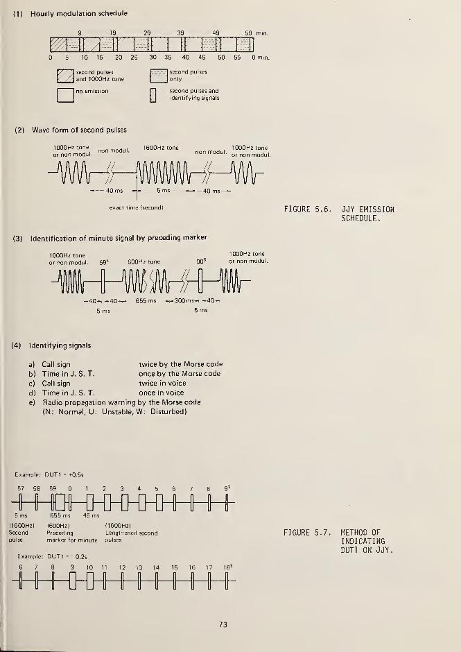
(1) Hourly modulation schedule

19 29 39 49 59 mm.

10 15 20 25 30 35 40 45 50 55 0 mm.

second pulses

and 1000Hz tone

no emission

D

ij] second pulses

only

second pulses and

identifying signals

(2) Wave form of second pulses

1000Hz tone

or non modul.non modul. 1600Hz tone

,1000Hz tone

non modul. . .

or non modul.

.- 40 ms - 5 ms 40 ms—exact time (second) FIGURE 5.6. JJY EMISSION

SCHEDULE.

(3) Identification of minute signal by preceding marker

1000Hz tone

or non modul. 59 s 600Hz tone 00 s

1000Hz tone

or non modul.

5 ms

/

^40-,^40-r- 655 ms—_300ms-H ,-40-

5 ms

(4) Identifying signals

a) Call sign twice by the Morse code

b) Time in J. S. T. once by the Morse code

c) Call sign twice in voice

d) Time in J. S. T. once in voice

e) Radio propagation warning by the Morse code

(N: Normal, U: Unstable, W: Disturbed)

Example: DUT1 = +0.5s

57 58 59 0 1 2 3 4

5 ms 655 ms 45 ms

(1600Hz) (600Hz) (1600Hz)

Second Preceding Lengthened second FIGURE 5.7. METHOD OFpulse marker for minute pulses INDICATING

DUT1 ON JJY

.

Example: DUT1 = -0.2s

6 7 8 9 10 11 12 13 14 15 16 17 18 s

73

DUT1 is given once each minute to the

nearest 0.1 second. The magnitude and signare indicated by the number and position of

the lengthened second pulses of 45 ms durationof 1600 Hz. Identifying signals and the

method of indicating DUT1 are shown in figures5.7. For additional details, see Table 5.1.

5.1.7 OMA

Station OMA in Li bl i ce,

Czechoslovakia,operates on 2.5 MHz. The station transmitsseconds, minutes, and five-minutes marksformed by interrupting the 1-kHz subcarrierfor 5 milliseconds, 100 milliseconds, and 500milliseconds, respectively. The modulationschedule, as follows, is repeated each hour:

Minute 00-01, 15-16, 30-31, 45-46:

10 times OMA in Morse Code, 800 Hz

tone.

Minute 01-05, 16-20, 31-35, 46-50:

1 kHz standard frequency transmittedfrom 6 hours to 18 hours UT only;replaced by seconds pulses the restof the day.

Minute 05-15, 25-30, 35-40, 50-60:

Seconds pulses 5 milliseconds long,

each 60th pulse is 100 milliseconds,each 300th pulse is 500 millisec-onds. From 18 hours to 6 hours UT,

the 5 millisecond pulses replace the1 kHz tone.

Minute 20-25:

Carrier frequency transmission with-out modulation.

Minute 40-45:

Transmission is interrupted.

At the end of the 15th, 30th, 45th, and60th minute of the hour, a short time signal

is transmitted consisting of six second pulses100 milliseconds long. See Table 5.1 for

further detai Is.

5.1.8 VNG

The Australian Telecommunications Commis-sion provides HF standard frequency and timesignals broadcasts from radio station VNG at

Lyndhurst, Victoria. This service transmitsprecise time signals and radio frequencies on

a schedule designed to provide an Australia-wide coverage. The transmitting scheduleis shown below.

SCHEDULE OF FREQUENCIES

TIMES OF EMISSION FREQUENCY

UTC AEST AEDT MHz

0945- 2130 1945- 0730 2045-•0830 4 5

2245- 2230 0845- 0830 0945-•0930 7 5

2145- 0930 0745- 1930 0845-•2030 12 0

UTC: Universal Coordinated Time

AEST: Australian Eastern Standard Time

AEDT: Australian Eastern Daylight Time

A. Time Signals

Seconds markers are transmitted by double-sideband amplitude modulation of the carrierand consist of various length bursts of 1000Hz tone. The start of a tone burst, whichcommences at a zero-crossing of the sine wave(increasing carrier power), marks the start of

a seconds i nterval

.

B. Time Code

Seconds markers are normally 50 millisec-onds of 1000 Hz. Seconds markers 55 to 58 are

5 milliseconds of 1000 Hz. Seconds marker 59

is omitted.

Minute marker (seconds marker 60) is 500

milliseconds of 1000 Hz. During the 5th,

10th, 15th, etc. minutes, seconds markers 50

to 58 are 5 milliseconds of 1000 Hz.

During the 15th, 30th, 45th, and 60th

minutes, a station identification announcementis given without interruption to the time

signals. During the first 15 seconds of each

minute, a group of emphasized seconds markers

(emphasized by 50 milliseconds of 900 Hz tone

immediately following the normal seconds mar-

kers) gives the UT1 correction. The time code

format is shown in figure 5.8.

C. Announcements

The announcement gives station identifi-

cation (call sign and frequencies) in English

74

SECONDS MARKERS ARE NORMALLY 50 MILLISECONDS LONG.

SECONDS MARKER 59 IS OMITTED. MINUTE MARKER (SEC-ONDS MARKER 60) IS 500 MILLISECONDS LONG.

STATION IDENTIFICATION ANNOUNCEMENT (INENGLISH) IS GIVEN DURING THE 15TH.30TH, 45THAND 60TH MINUTES OF THE HOUR WITHOUT INTER-RUPTION TO THE TIME SIGNALS.

DURING THE 5TH , 10TH, 1 5TH , ETC., MINUTES,SECONDS MARKERS 50 TO 58 ARE 5 MILLISECONDSLONG.

DURING NORMAL MINUTES, SECONDS MARKERS55 TO 58 ARE 5 MILLISECONDS LONG.

FIGURE 5.8. VNG TIME CODE.

and is approximately 30 seconds long, finish-ing approximately 10 seconds before each quar-ter hour. The speech is "notched" to allowthe seconds markers to continue and has spec-tral components around 1000 Hz reduced toavoid erroneous operation of tuned-relay timesignal receivers.

D. DUT1 Code

The difference between UTC and UT1 (DUT1)is given by the number of consecutive empha-sized seconds markers, each one representing0.1 second. DUT1 is positive when the firstemphasized marker of a group is seconds marker1 (i.e., the marker following the minute mar-ker). DUT1 is negative when the first empha-sized marker of a group is seconds marker 9.

DUT1 is zero if no seconds markers areemphasi zed.

E. Accuracy

Carrier frequencies and 1000 Hz tone asemitted by VNG are maintained within 1 partin 10 10 of Telecom Australia's standard offrequency (24 hour average value). As re-ceived, the accuracy may be degraded to theorder of 1 part in 10 7 due to the ionosphere.

Time interval as emitted (i.e., elapsedtime between any two seconds markers) has thesame accuracy as the carrier frequenciesexcept for intervals which include stepadjustments.

Time of day as emitted is maintainedwithin 100 microseconds of Telecom Australia'sstandard of Coordinated Universal Time,

UTC(ATC). As received, the signals mayexhibit jitter of the order of 1 millisecondrms due to the ionosphere.

The Telecom Australia standard referredto above is based on cesium beam frequency andtime standards at the Research Laboratories in

Melbourne. This standard is maintained suchthat its value of frequency and time intervalis within a few parts in 10 12 of the inter-national definition of time interval. Time-of-day signals generated by the TelecomAustralia standard are maintained within about100 microseconds of the international standardof UTC as determined by the BIH.

F. Frequency and Time Generating Equipment

The generating equipment is at Lyndhurstand includes precision quartz oscillators,frequency synthesizers, time code generators,announcing machines, and supervisory alarms.

A very low frequency signal, sent via

landline from the Telecom Australia standardin Melbourne, controls the frequency of theoperative quartz oscillator within 1 part in

10 11 . Regular visits with a portable clockensure that the VNG signals typically remainwithin 20 microseconds of UTC(ATC). Generalinformation is shown in Table 5.1.

5.1.9 ZU0

Radio station ZU0 is operated by the

Precise Physical Measurements Division of the

National Physical Research Laboratory (NPRL)

in Pretoria, South Africa. The signals are

generated at NPRL and broadcast by the PostOffice transmitting station at Olifantsfon-tei n.

75

EXAMPLES

I. DUTI = + 0.3 second

lengthened

FLLJLJLi0 I 2 3 4 5 6 7 8 9 10 II 12 13 14 15seconds

2. DUTI = -0,4 second l engthened

8 9 10 II |2 13 14 15

FIGURE 5.9. DUTI CODE ON ZUO.

A. Carrier Frequencies and

Times of Transmission

ZUO transmits on 2.5 and 5 MHz. There is

also a 100 MHz transmission which will not bediscussed here. Carrier frequencies arenormally derived from a cesium beam frequencystandard at NPRL.

B. Standard Time Intervals and Time Signals

The transmitters are amplitude modulatedby the time signals, the time difference(DUTI) code, and the Morse Code announcements.The signals consist of one pulse per second,each pulse consisting of 5 cycles of 1000 Hz.

The first pulse in every minute is lengthenedto 500 mi 1 1 i seconds.

Morse Code announcements are made duringthe minute preceding every fifth minute. Theyconsist of the call sign ZUO (repeated threetimes) and the Universal Time at the nextminute. The correct time is indicated by thebeginning of a time pulse. Double-sidebandmodulation is employed. Modulation of thefirst half cycle of each pulse is positive.

C. Standard Audio Frequencies

No continuous frequencies are broadcast,but in many cases the interrupted 1000 Hz

tone, which constitutes the time signalpulses, may be used as a standard frequency.The frequency of the Morse Code pulses is 600Hz.

D. Accuracy

Time intervals and standard frequenciescorrespond to the adopted cesium beam frequen-cy of 9 192 631 770 Hz. The frequency fromwhich all other ZUO frequencies are derivedcan be relied on to be within 1 part in 10 11

of the mean atomic frequency, as determined by

the BIH. Standard time intervals have thesame accuracy; i.e, 1 x 10- 11

, with an

additional uncertainty of ± 1 microsecond.

Time signals are Coordinated UniversalTime (UTC) and are kept within 1 millisecondof the signals of other coordinated time sta-

tions. To keep UTC in approximate agreementwith UT1

,leap seconds are inserted when di-

rected by the BIH. Inserted seconds are known

as positive leap seconds, and omitted seconds

as negative leap seconds.

E. DUTI Code

The approximate value of the differenceUT1 - UTC, to the nearest 10th of a second, is

denoted DUTI; i.e., DUTI = UT1 - UTC. DUTI is

indicated during the f i fteen- second periodfollowing each minute mark. This is done by a

group of lengthened second markers, the number

in the group being the value of DUTI in tenths

of a second. If the group begins with the

first second marker after the announced min-

ute, DUTI is positive. If the group begins

with the ninth second marker, DUTI is nega-

tive. If there are no lengthened second mark-

ers, DUTI is zero. Examples are shown in

figure 5.9.

76

ce CDLU LU LO LU

L0 CC 1— LJ • r— LU CDLO E LU CTl I—i LU LO LO u_ —

1 • z1 ^ CM LU O SI 1 CD • CD < <_) z o

LO CC LO > 1—

I

Z O LU LO D- O —

1

ro <E 4 Eoa: 1— CM =E O LD CD (_> i—i o

. |

—

u_ z. z o lu • r- C_> LO Z LU o I— cei— LU o o i—i s: lo u_ .— LU LU Z O 1— 1— lo <; a_

• CD z o ce lu o • Q LO 1—1 —

1

I—LO LO lo i—i ro id -z lO ZE o LU ZD LOLU o LU S Q Z '—1

1

—

Z QC 21 O CD LUI

—

2: i—

i

LO U_ i— IC Z Z i—l LO LO O LOo o u_ —i o c_> uj O Lu DZ O z LU iflZ Jz id s: t— C£ LU LO LU ID

1— CJ o_ z lu z az a lu 1— c_> LL. LO —

1

LO isl Q_ ECJ LU O LO O 1— Z C_)

LU Q_ q i—i — i-i cn < z lu a. ^-i LO O ZD a- ID LU oLO CO Z 1— ZZ> 1— LO ZD LO LO LO LU . Q_ Cu t— oo <c q- <: lu o LO LD 1— z t— ZD LOLU C£ c_> ce a a z LU Crl 3—i z ZD <_> zLU O LU ZD LO ZD Z O Z LU O LU ZD O i—i Q oLO Lu lo o •—i a <s c_> <c LO LU z a. h- s •X lo o e: 1—

Z oO 1 i 1—

i— CD 1— LO i— —

1

LU h— O E CXI LU i—i LO _j LU • • LU |

—

CD EID o Otfll-4 i^) CD Z i—i CD —1

—

1

CO LO cn lu lo cd zQ CJ LU i—i ZD Z —1 Z i—I o O O CL ZD ZD —1 1—1 CD —1 Z oce S CD ZD UJ z o o C_) C_> LO Q_ O ID CJ O ID LU z oi—• S LL. i—

1

a i lu I— i

—

o a. CJ CJ Q 1 LUQ LU O LO<Em>- o O CM —C_J >--ZL CJ

7"1 1 1

LU <c o o O oID C£cr ZDLU CJ X X X XQ£ CJU_ =r lO CM

n:

_x z ce 1—LU o z <c a.

>- zd ZL LUh- <c a lo LO LO

LO CD Z ' ro oZZL Q£ CXI o^J lO 1 ZrZ CM o

s: ZD o o o CMLO 1— Z O '

—

1 ro crl LO O LOoo z <c o z i— i— o u_ o ZD 1— O IDI

—

<t >- LO O ZD ZD o - o o 1— Ooo LO lO CTl ZD ID<c 1

—

o i <: Z CM LO O Z 1— Z\ Q LU O O 1—1 1 1 1 Q_ ac i—i

LO >- \ O ro ro s o o o 1

—

LU <c ^—<c ZD C£- <r LO CM LO O z LD LD LO LD s: zo zc a cn CT1 LO Z i

—

o O O o oa_: z 3: H- r—

1

LU - -O c_> CM rH CJL^CM

i— s <3- LO 3 .— s: 1 1 i

LO 1— I I o lo ins LO ZH«=t LU LU O O C£. LO LO o LO o

co i— <sr u_ i— ro ce ro ceCD i— CM Lu CM Lu

1

—

UO

LU^ LO zUJ o

1— o OCJ 1

—

o oQ z <C N o oLU 1 ZC

<c ZD ZDO"> lu cn Oo or lu

ZZL U_ LOUJ id__r> QO" Cd a; LO O LO LO LO

h—

!

oo o lo ooor CD M o o o o o o o ro ro is ro oo ld ro LD LOZ IC ro ro LD c£) CTl CM LD

<; a; j-: LO O LO lO O LO LO CMQ <c ro sr 00 LD 00 LD CMa: LO CJ<t

z:<ci— _loO <c <tz 1 Q LU |_ CJ LU

!_4 |

LU H |— CD O i—I LU Z I—1 LU < 1— o|

—

q; z l o_ Z C£L O Z C£. Z cn q_Z O O O i—

•

2; i-i m y m n LU 1—

(

lO DZ r^J Lu CD o a I

—

O O i—

'

> aLE

oo<ch-

Q£LU

oo LO o LO CM ro O ro O LO LO O LO LO LOo |— r—

CCLU i—i Z LU Z LU ex z 3 Z LU z LUZ LU CD TL LUO O ID 1 - - <T - - 0£ <"< - - ~ LU -

1—1 ID 1— LU ro 00 31 CM LD =C 3 CD CD LO Z * LD CD lo cj ro

1— 1— CD <Z. ro i

—

CD <CC CM - Z <Z <x i

—

cn >- ^3- t—i z ro ro=C >-l CD z z Z i—i (— Z o ^ ce <rcj t— Z 3 CD o o <: i—i o o ct ZC (— <c o o zc o o <t ce o 0o <: o lu z oo r

—

3Z UZ (71 — 3 cj O C_> LO LO l/1 z ro cn Q- Lu 00 CMi _i 1 z i—i cm lo c_j ro csj Z a lo *f

<C Lu _J LU1— O LU CD

zo«c > Lu ZD zr;

i— h- LO DZ LuCC <C 03 CO CJ CD1—LO

77

O LlJ

LU Q_LO LO

O LULU £LV

CO LO

<_> LULU Q_LO LO

LU CtL

LU OLO Ll_

CJ I-I o3 i

>- I—C_> <1 O UO .

_iluq;i

Q h-Ll_ O 1—i LUO LO Li I

LO N h~LJI«2CO 1—1 LU

S OO OLO 1—1

.— z a: co

lt> -a:i

U- LOO Q

CO N—I X

O Z LUcc: u oQ. 1-1 O

LO C_)

lo qQ. LU LU

tu c_>

C_) LULU CL_

LO LO

CC LU CO LOi—

i Q LO —1

C_> O O LO(—> C_> Q Q_

LU CQ LO•-I LO O —I<_> O O =>C_> C_> O O-

cc lu to e)

:

i—t O —I Z i

uololm:CJ C_J Q II

OLLUI/IOZI-i LO _l Z >—

I

C_> O O LU ZL_J C__) O I LU

Ql LU CO OOi-h LO O —IC_> O O =5C_> C_> CO Q-

2 LO Q<t LOOQLhll

ID LO-CO LT>

LO I I

i— o oI ro lo

LO lD-CM <3-

LO I I

I o o

-> o xLO LU H-i— o z

I Lu O OLD O i— S

. O I xZ LD O Oi-i I o <cSOLOLU

LO oZ Ll_

LU -I— OLU O Q-3 =* lu .

I— I C_> QLU LO X LUCO rO LU 3

o-UJ QCH LULL_ LO

ce lxce S.

ld o o oNinOLn

o oLD O

lo o oMLno

o: n >^LU I—I \> o .<:

x cm =a\ s: \-< CM .< O

/—.-^ lo i—

=£ x <t ^>C_> 21 . LU C_) LU Mi-i m —i i-i —J lt:hiflMOI-OZQ£ CC O. CC Q-LU CM O 1—i LU I—I LD> *—' 1 Q > Q —

O LU CO LUhsl cc LU —

I

I-I I-I LO OO I O i-iX CO LU Q

<: _i «I— I— •-< LU /->Z Z LO C_J _l N0<LLJMOINCCUHO.ZI—I CO O CcL OC£<Q.LUZLnODh>o •

LX 0"Q '— SI CM

<E Zs <:I—I Q_

«C i— r—

O I— O 0

Z •=£

<: cqOO t—1

o z o oZ LU 00LU O ro LD=> cccq <:

>— LU O 0mi— cm i

—

I—I X o o

78

^Bl3?^H I—I . OO1

~r co <cZ ZC o3 -r O ZC o3 O x o3 , 1

—

5 1—

i

O CD O CD 1 c_3 1 c_3 i— LUI

,

—

1 <c O <C '

—

O <L I CDce lu i

—

ce Q_ CL (_JQ_ | ^ 1— ^ ,— 2Z Z i—

I

OO i

—

1—

>

1 1~<J

—

LO | 1—

(

LO |— 1—

1

O LLlo 1 ZD IE LO ZD 2 LO ZD 1 1 1

—1

•- LU . ZD 2ZD 1 1 1 LO TD LO L/) 7D r— LD^ -

1 ^ 1 £ ^z_1 CD + LU —j + Lu —IE + LU ZD + LU ZD + LU UJ CLZD Z LU O LU ZD LU ZD LU Q_ LU Q_ O LU OO OOCL O (— O r- 3 Q- i- 3 O- O r— 3 i— 3 o ^ 3

—1 ZD LO h- 1— 1— 1— LD 1— h— 1— 1— • LO 1—1— lu ceZ O Z ZD LU Z ZD LU Z ZD LU Z ZD LU Z ZD LU LU OI—I ce O CD CO l-H O CO i-l O Q CO i—i Q CO 1—

1 O CD CO oo Li-y q_ t— *x 2 1— -K TT" | ^;

LULO LU LU LU LU LU ce LU

O CD ce a ce CD ce CD ce cd <_> oST C_> o o O O o o o o <_> CD

EI LJ S CJ zr cd IT CD •X

* * tc

O oO 1o 1o 1o 1o

X X X X X

C\J LO

- « cd -o v. *o LOo O O LO o O ro O CO OCZJ Cs) o o ro lo ro ro lo ro

CM Csj 1 t CM r—lO LiD I CD

r—

>

o o LO Csj '^t~ LO Csj1 1 i ro o O i

—

lo - CD( > 2- CO1 1 i o O O C\J O csj - o o o o O i

—

O CO i— ro I LO lOrv Oq ro Li_ LO LO 1 1 (—

i

—

^ *T" •» ^ 1

t-H lo ro i

—

lT) i O LO LO CD CD U~) li-) lo cd ro ro

CO CM - LO "=J" LO n CO LT) - f— i— CO ro O i

—

ro ro ro rsj o oO O i

—

O i— CD ro 1— ^j-

LO^~ Q

ro LO o o i— CD — i

—

TT" CD LD 2Z LO LO T CD 2 ce CM Csj o"3" lo ro O i

—

,—

1

z ro ro z i— Z i— Z O CO z LO z ^ z ro LO LO LT)

LU -O I— LU -O LU -o LU O i— LU o t-H LU O LU « 3- <g-

z - LU O 1 1 LU O 1 LU CD LU LU LU LU O CO CM rHl-H O 3 S- O LO ro o 3nz 3 2: 3 SL 3 s: 3 LO O CM CMce ro h— 1 O i— 1— 1 O t— 1 o 1— O 1— o r~ O 1— 1

ZD i— LU UD O O LU LO O LU LID CC lu ce LU ce LU ce LU o(ZD O m ro o i

—

CO Csj O CO CSJ LI CO LL. CO CO U— CD LO

oo o o o o oo'

lo ^i- SO LD LJDLO noo ITl o o o CD o o o CO CO CO LT) LT) LOro LD .— o o o co <n co

oo ro r--

1

1 1 1 J <^«^

1

—

I

—

1 1 1

—

z z z z zO LU O LU O LU O LU O LU 1—

l-H O i-i o i-i o i—i o t-H O l-H LUOH CL ce o_ ce cl ce cl ce Cl z ceO l-H O i-i O i—i O >-i O l-H s: i-i

ZC CD DZ Q ZC CD ZC CD ZC CD O CD

lo LiD LO 00 o

oce

oo 3 Z LU Z LU z LU OO LULU 1— 1— 1— -<£z Z - - z 3 _ OO <C l-H

<t en .— LU CO LO LO LD CO LU CO LO ce i—i —i CO LOlo i— i£ 1— ^- ro ^ r— ZD ce < O i—

ZC Of ZD ce zc ce LO ' OO zc o ceLU —loo LO LO 0 O ^ LO o o LO LO 0 o O ce o o CD 1— \— 0 oQ m csj co =c LO i— CO ce lo cm ro < l/l 1— CO > LO LT1 CM s: zd ld co Z (_) LO co loM CM «3" 1— ZD <3- ID l-H ZD UIO 1— ZD >Sr LD O LO LT) CO LJD CO >- l-H ZD CO «3"O * rH Z ZD —i > <n£

CO

ce DZ CD s: <c s: oQ_ CJ 1—1 t— 3 zQ_ ce ce ce ce ce >

79

Ll_ O1-1 OI— m i

I Ll_ O Q i—i o3

lUUJlLflLU <_> CJ

OUJU> LU

i z i :O 'n OI— O I

<E 00

O O £ CO

C_J LULU Q_O0 l/>

C_) LULU Q_U0 I/}

(_) LULU d.UO LO

I— Q=> Oo <_>

tt lu m inl-H Q =3 —IC_> O O =>C_> O O O-

C£ LU CG LOi-i Q =J —I<-> O O =>(_> C_> Q Q.

in o o o ooj in o in o

m o o ocm in o in

<-< > >-t— <ar <c0:311;

I—I _l >-I— o <CZL C\J Q_ CZL

lu \ i-h tr> ^ Q <C

=C —Ic_> OI—I Q_

in o o o in

MOOOM in o o o

<: t-. eju i— ^o <: o

UO LU

C_> IV1

<c luce -z.

<C iuo >

o <c

o

C_> r—

a: <-<

H-l Q_ ^)—I LU OO Ct LO

80

5.2 RECEIVER SELECTION

This and the following sections discussthe use of HF broadcasts for frequency andtime calibrations. For convenience, we will

refer to mainly to WWV; however, the discus-sions also apply to other HF broadcasts.

The reception and use of shortwaves canbe quite tricky. However, for many locations,simple receivers and antennas work well mostof the time. Also, there are many separatesignals available from WWV and WWVH. Bychoosing from among the many combinations offrequencies and distances involved, a solutionusually can be found for any problem.

For those users who must have the verybest signal most of the time, this sectiondiscusses several methods available to solvereception problems. The user is also encour-aged to use other references on HF propaga-tion, antennas, and receiver selection andoperation.

Almost any shortwave receiver can be usedto receive HF signals for time and frequencycalibrations. However, for accurate time andfrequency calibrations, especially in noisylocations, it is important to have a goodantenna-ground system and a receiver withoptimum sensitivity, selectivity, image re-

jection, and frequency or phase stability. A

block diagram of a typical high-performancereceiver is shown in figure 5.10.

The first requirement of a good receiveris sensitivity. Therefore, a tuned RF ampli-fier is desirable because it increases sensi-

tivity. The next requirement is selectivity.This is the ability of a receiver to rejectnearby signals that interfere with the desiredsignal. Selectivity is achieved by hetero-dyning (translating) the incoming signal to a

much lower fixed frequency (usually 455 kHz)

called the intermediate frequency (IF). TheIF amplifiers are fixed-tuned for maximum gainwith a relatively narrow frequency pass band.Often, either crystal or mechanical filtersare used in the IF stages to provide an evennarrower pass band of frequencies to rejectinterference.

The third feature of a good receiver is

the ability to reject interference from anundesired signal at what is called the imagefrequency. Since the IF signal is the differ-ence between the local oscillator frequencyand the incoming signal, there are always twodifferent incoming signals that can producethe same IF signal. One is above and theother below the oscillator frequency.

For example, a receiver with an inter-mediate frequency of 455 kHz tuned to WWV at10.0 MHz would have an oscillator frequencyof 10.455 MHz (10.455 - 10.0 = 455). However,if another signal with a frequency of approxi-mately 10.910 MHz is present, another "differ-ence" signal of 455 kHz is produced (10.910- 10.455 = 455). Thus, if two signals areseparated by twice the intermediate frequencyand the oscillator frequency falls between thetwo signals, an unwanted image signal results.Table 5.2 lists various dial settings andcorresponding oscillator frequencies that canreceive WWV signals as image frequencies if

the receiver IF is 455 kHz.

VRF

AMPL1ST

MIXER

XTAL0SC

6PRESELECTOR

ON

OFFo

-o-<—o- AGC

I F

AMPL2ND

MIXERIF

AMPL DET

VF0

bMAIN TUNING

SIGNAL STRENGTHill/A METER

SPEAKER

6

OUTPUT

FIGURE 5.10. BLOCK DIAGRAM OF A TYPICAL HIGH-PERFORMANCE HF RECEIVER.

81

TABLE 5.2 IMAGE FREQUENCIES FOR WWV/WWVH

OSCILLATOR IMAGE DIAL OSCILLATOR IMAGE DIALFREQUENCY FREQUENCY FREQUENCY FREQUENCY FREQUENCY FREQUENCY

(MHz) (MHz) (MHz) (MHz) (MHz) (MHz)

2.045 1 .590 2.500 14.545 14.090 15.000

2.955 3.410 2.500 15.455 15.910 15.000

4.545 4.090 5.000 19.545 19.090 20.0005.^55 5.910 5.000 20.455 20.910 20.000

9.545 9.090 10.00010.455 10.910 10.000

Images occur because the IF signal is

very low in frequency (i.e., 455 kHz) relative

to the high frequency of the incoming signal

(i.e., 10 MHz). Thus, the RF amplifier may

have insufficient selectivity to reject inter-

ference which is relatively close to the

desired signal. In the above example, the

unwanted signal is only 0.910 MHz away from 10

MHz and, if strong, might easily pass through

the RF stage into the mixer and produce an

image IF signal

.

To solve this problem, a high quality

receiver usually employs double conversion or

two mixer stages. It heterodynes in two steps

to make image rejection easier. The first

mixer stage converts the incoming signal to a

high intermediate frequency (usually greater

than 1 MHz). Any images produced will be

separated by more than 2 MHz from the desired

signal. For example, if a receiver has a

first mixer IF signal of 1.5 MHz, the image

signal will be twice the IF signal or 3.0 MHz

above the desired signal. Since 3.0 MHz is

now relatively large compared to the incoming

signal, the RF stage pass band is usually

selective enough to reject the undesired

images. For the required additional selec-

tivity and gain, a second mixer stage is added

to produce a lower second IF frequency, thus

solving the image problem.

A local crystal oscillator can be used in

these conversion processes to provide tuning

stability. Other information regarding well-

designed receivers can be found in such

reference material as the Radio Amateur'

s

Handbook .

If all the above seems too confusing,

don't worry. Many small, inexpensive imported

and domestic receivers work very well. In

fact, several receivers have special buttons

that you can push and the receiver automatic-

ally tunes itself to WWV. If timing is a

special problem in your home or business, of

course check out the receiver very carefully

before you purchase it. Image and interference

signals come and go so they may not persist

long enough to be a serious problem. The sin-

gle best option to look for in a receiver is

the provision for an external antenna. This

may be just a short wire on the windowsill or

an elaborate rooftop installation. Fancy

knobs and adjustments won't help much if you

can't get a good signal.

5.3 CHOICE OF ANTENNAS AND

SIGNAL CHARACTERISTICS

A good antenna is important if you want

strong, noise-free signals. However, follow

the basic rule of "using what you have avail-

able." Many receivers with built-in antennas

work quite satisfactorily. Often, adding a

short piece of wire to the existing receiver

antenna will bring in a stronger signal that

can be heard well enough to set your watch.

But for the serious listener or the

metrology lab that depends on WWV or other HF

signals for calibrations, something more is

needed. In the material that follows, the

rules for antenna selection and installation

are discussed with respect to choices avail-

able. Companies that sell WWV receivers often

offer antennas. These have been proven by use

and the instructions included with them will

help a lot in getting a good usable signal for

frequency and time calibrations.

The signal power as received at great

distances from HF stations may be relatively

weak. As the distance is increased, the sig-

nal decreases in strength so an antenna with

maximum efficiency produces the best results.

Radio waves arrive at different vertical

angles, called the wave or radiation angle.

The wave angle of an arriving signal depends

on the distance between the transmitting and

receiving stations and also on the height of

the ionosphere. The closer the receiving

station and the higher the ionosphere, the

82

larger the wave angle. Therefore, an antennashould be selected and oriented that favorsthe wave angle (elevation) as well as thedirection (azimuth). Determining wave anglesis discussed more fully in Section 5.6.

Many HF stations transmit on a number of

frequencies. Because of changes in ionospher-ic conditions, which sometimes adverselyaffect the signal transmissions, most receiv-ers are not able to pick up the signals on all

frequencies at all times in all locations.Except during times of severe magnetic distur-bances, however--which make radio transmis-sions almost impossible—users should be ableto receive the signal on at least one of thebroadcast frequencies. As a general rule,frequencies above 10 MHz provide the bestdaytime reception while the lower frequenciesare best for nighttime reception.

An all-band antenna capable of coveringthe entire HF band is commercially available.These are used for around-the-clock communi-cation purposes where the entire HF band mustbe used for maximum reliability. Such anantenna is very large and cumbersome as wellas expensive. Depending on location, anantenna and a receiver capable of receivingtwo or more frequencies may be required. Anyof the different WWV frequencies transmittedmay be received depending upon distance, timeof day, month, season, and sunspot cycle.Each frequency will be discussed with the typeof antenna most suitable for its reception.Although WWV and WWVH are not currently broad-casting on 25 MHz, this frequency is alsodi scussed.

In the following discussion, mention is

made of sunspot cycles. These cycles occurwith a periodicity of about every elevenyears. Propagation characteristics at highfrequencies are greatly affected by the sun-spot cycles. One solution to the problem is

to select another frequency that will work andto ignore the ones that won't. For thoseusers who want to understand the propagationeffects and to counteract the coming sunspotcycles by antenna selection and placement, werecommend further reading on this subject.Information on sunspots is available from theSpace Environment Lab, NOAA, U. S. Departmentof Commerce. Mini mums in the sunspot cycleoccurred in 1954 and 1965. The correspondingmaximums were in 1958 and 1969, and anotherwill probably occur in 1980.

ANTENNAS FOR THE 2.5 TO 4 MHz RANGE .

Signals at these frequencies have a veryshort range during the day because of ground-wave propagation limitations. Daytime use is

limited to locations within one to two hundredmiles from the transmitter. They become

useful at night, however, especially duringthe winter season in the higher latitudeswhere longer nights prevail. Reception is

then possible over distances of severalthousand mi les.

The vertical quarter-wavelength monopoleantenna has a radiation pattern that favorsreception at low wave angles and is veryeffective in receiving long distance skywavesignals normally arriving at angles of 20degrees or less. This antenna is not effec-tive for reception of short-range skywavesignals with large wave angles, but it is

useful for receiving weak groundwave signals.

For nighttime reception on paths up toseveral thousand miles, the skywave is pre-dominant and a horizontal half-wavelengthantenna is recommended. The antenna should belocated a quarter-wavelength or higher abovebround and separated from possible interferingreflecting obstacles. The quarter-wavelengthvertical antenna and the half-wavelengthhorizontal dipole antenna are shown in figure5.11. To get antenna dimensions for CHU orother frequencies, refer to antenna manualssuch as those published by the American RadioRelay League.

ANTENNAS FOR THE 4 TO 5.0 MHz RANGE .

These frequencies can be received at

greater distances than the 2.5 MHz frequencythroughout the day or night, especially duringminimum sunspot cycle. Reception is possibleup to 1000 miles under ideal conditions, butunder normal conditions, daytime propagationconditions limit its useful range. Therefore,reception is usually limited to less than 1000

miles during the day. During the night, 5 MHz

is a very useful frequency for long-rangereception except during maximum sunspot cycle.

It is excellent during early dawn and earlyevening in the winter months when the signal

path is in darkness. Horizontal dipole anten-nas are a good choice for this band. Usersshould also consider the possibility of a

multiband antenna.

ANTENNAS FOR THE 7 TO 10.0 MHz RANGE .

At these frequencies, reception over

great distances is possible during the day or

night. They can be classified as intermediatefrequencies but again, they are dependent upon

the sunspot cycle. During minimum sunspot

cycle, great distances can be covered duringthe day when higher frequencies cannot be

received. During maximum sunspot cycle, theseare probably the best frequencies to use dur-

ing the night when the lower frequenciescannot be heard. During maximum sunspotcycle, reception is limited to short distances

83

PULLEY

GUY AS /\NEEDED

STRA I

N

INSULATORS

MYLAR SASHCORD

#14-#12 AWGCOPPER CLADSTEEL WIRE

70 OHM TWINLEAD OR COAXTO RECEIVER

FREQUENCYMHz

1/2 \ HORIZONTALDIPOLE ANTENNA

LENGTH HEIGHT

2.556. 1 m 15 m TO 30 m

187' 50' TO 100'

5-028.07 m 9 m TO 15 m93'- 7" 30' TO 50'

10.014.05 m 7- 5m TO 15m46' -10" 25' TO 50'

FIGURE 5.11. QUARTER-WAVELENGTH ANTENNA AND HORIZONTAL HALF-WAVELENGTH ANTENNA.

84

during the day with limitations comparable to

those noted for 5.0 MHz. These frequenciesalso provide daytime reception at fairly closerange, 200 miles or so, and can be used when 5

MHz reception is poor. The half-wavelengthhorizontal antenna should be selected forshort distances. A quarter-wavelength verti-cal antenna is suitable at greater distances(see figure 5.11).

ANTENNAS FOR THE 14 TO 15 MHz RANGE.

These frequencies are most favorable forlong range, daytime reception. They are notusable for short-range reception except duringperiods of sunspot maximum. However, for longrange reception, they are the most favoredfrequencies during both sunspot cycle condi-tions. Under average conditions, the maximumwave angle is limited to 30 degrees or lessdepending on the density of the ionized layer.

During maximum sunspot cycle, receptionmay even be possible during the night in somelocations. During minimum sunspot cycle, theyare useful only during the daylight hours anddawn and dusk periods. Both horizontal andvertical antennas are suitable.

ANTENNAS FOR 20 MHz .

The 20 MHz frequency is normally the bestto use for daytime reception and will be opti-mum at either noon or a few hours past noon.Signals at this frequency arrive at very lowwave angles and are useful only for long dis-tance reception. During minimum sunspotcycles, reception is poor but improves duringthe winter. During maximum sunspot cycles,the reception is excellent at night and duringthe day. The vertical dipole that favors lowwave angle radiation has been used at thisfrequency with favorable results. Construc-tion details for a 20 MHz antenna are shown in

figure 5. 12.

ANTENNAS FOR 25 MHz .

The 25 MHz frequency is best during day-light hours except during the summer. Recep-tion is especially good during maximum sunspotcycle and very poor during minimum sunspotcycle. It is used only for long distancereception because a low radiation angle is

required for the signal to be returned back tothe earth from the ionosphere. Design detailsof a different vertical antenna for use at 25MHz are also shown in figure 5.12.

1" DI AM ALUMTUB INC

INNER CONDUCTORSOLDERED TO LUG S

FASTENED TO MACHINE SCREW

«10 GA COPPERSOLDERED TO B R A I 0 &

CONNECTED TO RADIALSWITH SPLIT-NUT BOLTS

"10 GACOPPERRADIALS

(ONLY 4 SHOWNFOR CLARITY).

FrequencyMHz

1A X VerticalH

Gnd Radial

L

HeightA

15h.7 m

l5'-7"

A. 9 ml6'-5"

S.h m18'

203-5 m1l'-9"

3-7 m12' -V

3-9 m

13l

252.8 m9'-5"

2.95 m9' -10"

3-3 m1 1

'

FIGURE 5.12. MODIFIED HALF-WAVELENGTH VERTICAL ANTENNA FOR USE AT 15, 20, AND 25 MHz.

85

VERTICAL ANTENNA CONSTRUCTION .

The vertical antenna which is favorableto low wave-angle reception is preferable to

the horizontal half-wavelength antenna and canreadily be constructed as shown in figure5.12. The dimension of the ground radial s andorientation as shown should be used to yieldapproximately a 50 ohm antenna impedance. Fora 70-90 ohm antenna, the half-wavelengthdipole mounted vertically will yield approxi-mately the correct impedance. In order to

prevent interaction between the feed line andthe lower half of the dipole, which disturbsthe radiation pattern, extend the feed linehorizontally outward several feet from theantenna before dropping it vertically to theground.

5.4 USE OF HF BROADCASTS FOR

TIME CALIBRATIONS

Now that we have a receiver and an anten-na, we can proceed to make time calibrations.If your accuracy requirements are low, you canuse the voice time-of-day announcements. How-ever, if you want higher accuracy, you willhave to measure the seconds ticks or decodethe WWV/WWVH time code.

5.4.1 TIME-OF-DAY ANNOUNCEMENTS

Time of day is available from many sourcesin the United States and Canada. Radio andtelevision stations mention the time frequentlyand, in fact, use the time of day to scheduletheir own operations. The telephone companiesoffer time-of-day services in most locations.But where does the time come from?

Most time-of-day services in the U. S.

start at the National Bureau of Standards. AnNBS telephone service is available by calling(303) 499-7111. In addition, WWV and WWVHbroadcast voice time-of-day announcements onceeach minute. This is also the case for CHUwhere the time announcements are given alter-nately in French and English. Using the WWVvoice announcement and the tone following thewords, "At the tone, XXXX hours XXXX minutesCoordinated Universal Time," a person cancheck a wall clock or wristwatch to within a

fraction of a second. The UTC time that is

announced can be converted to local time byusing the map in Chapter 2.

5.4.2 USING THE SECONDS TICKS

For accurate time recovery, we cannotjust listen. We must rely on electronic equip-ment. By using an electronic oscilloscope to

see the ticks, the user can set clocks withmuch greater accuracy than is possible by onlylistening to the ticks. An oscilloscope is a

necessity when dealing with noisy signals thatfade.

The following describes ways to get timeof day with resolutions better than 1 milli-second (1000 microseconds) by using an oscil-loscope. Under very favorable conditions, it

is possible to establish time synchronizationto about 100 microseconds. In each case, pathand equipment time delay corrections arenecessary for accurate results.

In order to achieve the best results in

any of these measurement methods, the follow-ing guidelines are recommended:

1. Make your measurements at the sametime every day.

2. Avoid twilight hours when the iono-sphere is the least stable.

3. Use the highest carrier frequencywhich provides consistently goodreception.

4. Look at the received signals on theoscilloscope for a few minutes to

judge the stability of propagationconditions and select that part of

the timing waveform that is mostconsistent.

Since receiver and propagation time delays areso important, they will be discussed before wego into the details of performing timingcal ibrations.

A. Receiver Time Delay Measurements

For accuracy in time-setting, the receiv-

er delay must be known. Typical delays in

receiver circuits are usually less than a

millisecond. However, they should be known to

the user who wants the very best timing accu-

racy. The actual delay in the receiver will

vary with tuning and knob settings.

To measure the receiver time delay, the

following equipment is required: An oscillo-scope with accurately calibrated, externally-triggered time base; an HF signal generator;and an audio signal generator. The equipmentis connected as shown in figure 5.13.

The main tuning dial of the receiver

should be set at the exact position for re-

ceiving WWV/WWVH signals. This is because the

receiver delay time varies with slightly dif-

ferent receiver dial positions. Therefore,the receiver tuning should be set and marked

86

RECE I VER

INOUT

OSCILLOSCOPE

VERT

AF GEN HF SIGNALGENERATOR

MOD RF

1 kHz

FIGURE 5.13. EQUIPMENT SETUP FOR RECEIVER TIME DELAY MEASUREMENTS.

where the maximum signal is received. The

frequency of the HF signal generator is then

adjusted for peak receiver output.

The audio signal generator is set to a 1

kHz output frequency. A high accuracy 1 kHz

signal is not required. The HF generator is

externally modulated by the 1 kHz signal. The

oscilloscope sweep rate is set to 100 micro-seconds/division with positive external trig-

gering from the 1 kHz signal. The vertical

amplifier gain is set high for a large verti-

cal deflection. The vertical position control

is adjusted for zero baseline with no input

signal

.

Initially, the 1 kHz signal generator is

connected to the vertical input of the oscil-

loscope. The trigger level control is adjust-

ed so that the trace crosses over or touches

the horizontal center line at the left. The

horizontal position control can be adjusted so

that the signal crosses over the first divi-

sion on the left as shown in figure 5.14. The

crossover point of the undelayed signal will

serve as the zero delay reference point.

/

IH

—

—1—

\—1—

/ 1

DELAYi »>

DELAYED ZERO CROSSOVER

ZERO CROSSOVER

TIME

UNDELAYED

I

FIGURE 5.14. OSCILLOGRAM OF DELAYED AND

UNDELAYED 1 kHz SIGNAL.

Without touching any of the oscilloscope

controls, the 1 kHz signal is disconnectedfrom the vertical input and replaced with the

delayed 1 kHz signal from the receiver output.

Since a receiver delay is almost always less

than 1 millisecond (1 cycle of a 1 kHz sig-

nal), there is little chance of ambiguity on

which cycle to measure. The delay is equal to

the sweep time from the reference undelayed

crossover to the first delayed crossover

poi nt.

If the delayed signal is found to be of

opposite phase to the reference 1 kHz signal,

the receiver has an inverted output signal.

However, the receiver delay time remains

unchanged and the only difference will be that

the output seconds pulse will be inverted with

a negative leading edge. For receiver delays

of less than 500 microseconds, the sweep rate

can be set at 50 microseconds/division.

This technique is a way of producing a

local signal that approximates the timing sig-

nal. It uses the same frequency on the dial

and uses the same tone frequency, h two-

channel scope is very useful since you can

then display the tone before it enters the RF

signal generator and after it comes out of the

receiver. A study of the block diagram (fig.

5.13) will no doubt suggest other variations

on this technique to the user.

B. Time Delay Over the Radio Path

In order to make a calibration, a user

must know the path delay from the transmitter

to his receiver antenna. This is often dif-

ficult due to the fact that several "modes" of

propagation are possible at high frequencies.

A discussion of propagation delay calculations

can be found in section 5.6.

For time setting of highest accuracy, a

user would have to actually measure the path

delay using a portable clock. This is an in-

volved and costly operation that few users

would deem justified for their needs. How-

ever, once the path delay is determined, it

87

need not change appreciably if certain precau-tions are observed. For timing accuraciesthat approach 100 microseconds, the locationand routing of antennas and lead-ins areimportant as are receiver settings. Thegeneral rule is to "not change anything". If

changes must be made, careful records of

readings before and after will help in

re-establishing the system with a correctdelay value.

In fact, any user of time signals at highlevels of accuracy must take extreme care in

how the equipment is adjusted, maintained, andoperated. Typical users estimate their pathdelays and obtain results with accuraciesapproaching one millisecond. The above para-graphs are intended for those users who wantto obtain the very best accuracy. They arenot typical for the large percentage of users.It also goes without saying that a wealth ofinformation can be obtained by reading theliterature supplied with the timing equipment.

C. Using an Adjustable Clock to

Trigger the Oscilloscope

This method, sometimes called the DirectTrigger Method, is the simplest and requiresan oscilloscope with an external sweep triggerand accurately calibrated time base, and a

receiver with electronic audio output. Theclock must be adjustable so its 1 pps outputcan be advanced or retarded. Equipment con-nection is shown in figure 5.15.

A local clock pulse at 1 pps second rateis used to trigger the oscilloscope sweep. Atsome time interval later during the sweep, theseconds pulse appears on the display as shown.The time interval from the start of the sweepto the point where the tick appears is thetotal time difference between the local clockand the transmitting station. By subtractingthe propagation and receiver time delays fromthe measured value, the local clock time errorcan be determined. The equation to determinetime error at a receiving location is:

V

Time Error = t - t = TD - (TD + TD )

,

r tv

p r -

where: t = time at receiving station

t. = time at transmitting stationZ

(WWV, WWVH)

TD = total time difference (mea-sured by oscilloscope display)

TD = propagation path time delay" (computed)

TD = receiver time delay (measured)

NOTE: The units (usually milliseconds) shouldbe the same.

The receiver is tuned to the station andthe oscilloscope sweep rate set at 0.1 s/

division. Listening to the broadcast willhelp judge the quality of reception and fad-ing. The tick will typically appear as shownin figure 5.16. CHU signals can be used as

well (see fig. 5.17). If the tick is onedivision or more from the left side of thescope display, the time of the local clock is

corrected until the tick falls within thefirst division from the left side. If thelocal time tick is late, the received tickwill be heard before the sweep starts. If

this is the case, the local clock should beadjusted until the tick appears. After thelocal seconds pulse has been properly adjustedand appears within the first division (0.1

second in time), the sweep rate is increasedto say, 5 ms/division. Using this greaterresolution, the local clock is adjusted until

the leading edge of the received pulse startsat a time equal to the propagation delay timeplus the receiver delay time after the triggeras shown in figure 5.18.

The sweep rate should be increased to thehighest rate possible without allowing the

total sweep time to become faster than the

combined propagation and receiver delay time

HFRECEIVER

SECONDSPULSE

^

OSCILLOSCOPE

VERTICAL TRIGGER

1 pps LOCALFREQUENCYSOURCE

OR CLOCKOR

TICK

-«

FIGURE 5.15. BLOCK DIAGRAM OF EQUIPMENT CONNECTION FOR DIRECT

TRIGGER METHOD OF TIME SYNCHRONIZATION.

88

FIGURE 5.16. WWV TICK AT A SWEEP RATE OF0.2 SECOND/DIVISION.

FIGURE 5.17. CHU TIME TICK AT A SWEEP RATEOF 0.2 SECOND/DIVISION.

TICK

*

I I

FIGURE 5.18. WWV TICK AT A SWEEP RATE OF0.1 SECOND/DIVISION.

TICK

WWV TIME TICK:

TRIGGER TIME DELAY: 19,000 MICROSECONDSTOTAL TIME DELAY: 20,740 MICROSECONDS

FIGURE 5.19. SECOND ZERO CROSSOVERS OF

SECONDS PULSE AT A SWEEP RATE

OF 1 MILLISECOND/DIVISION.

WWVH TICK RECEIVED TWO MILES AWAY:

RECEIVER DELAY: 320 MICROSECONDSTOTAL TIME DELAY: 1.160 MILLISECONDS

0.833 ms

SECOND ZERO CROSSOVER

89

less the 5 mill i seconds to allow for the

length of the received seconds pulse.

With a sweep rate of 1 ms/division, forexample, greater resolution can be realized bymeasuring the second zero crossover point of

the 5 ms received tick. Although the leadingedge of the seconds pulse as broadcast fromthese stations is "on time", coincident withthe NBS or CHU standard, it is difficult tomeasure because of the slow rise time at thebeginning of the burst and distortion due to

propagation. For this reason, the second zerocrossover should be used. The second zerocrossover of the WW or CHU pulse is delayedexactly 1000 microseconds and the WWVH cross-over is delayed 833 microseconds as shown in

figure 5.19. This is called the cyclecorrection.

At a sweep rate of 1 ms/division, anychanges in arrival time (jitter) are readilyapparent. After watching the pulses for a

period of a minute or two, select a cycle thatis undistorted and relatively larger in ampli-tude. In determining the time at a receivinglocation, include the delay of the chosen zerocrossover point, then add the cycle correctionto the propagation and equipment delay usingthe following relationship:

Time Error = t - t.r t

= TD "(TD + TD + cycle correction)

Where cycle correction time

= 1000 microseconds per cycle (WWV or CHU)

= 833 microseconds per cycle (WWVH)

As an example, assume an operator at a

distant receiver location is interested in

comparing his time to that of WWVH. The pro-

pagation and receiver time delays were mea-sured as 11.7 milliseconds and 300 microsec-onds respectively. Since the total delay is

12.0 milliseconds (11.7 ms + 0.3 ms), the

oscilloscope sweep rate was set at 2 ms/division for a total sweep time of 20 ms

—

slightly greater than the propagation delay +

receiver delay + 5 ms total. The second zerocrossover of the tick was observed and mea-sured 12.5 ms after the sweep was triggered by

the WWVH clock.

From these data, the time at the receiversite was calculated as -0.333 ms with respectto the WWVH time as broadcast, or:

Time Error = t - t.r t

= 12.5 - (11.7 + 0.3 + 0.833)

= -0.333 ms, or -333 microseconds,

Where: TD = 12.5 ms

TD = 11.7 msP

TD = 0.3 msr

Note that if a receiving station is

located at a distance greater than 3,000 km

(1863 miles) from the transmitter, the pro-

pagation time delay will exceed 10 ms. (Theradio path delay works out to be about 5

microseconds per mile. At 1863 miles, thedelay would be at least 9.315 ms. It is

usually greater than this due to the fact the

HF radio signals bounce off the ionosphere.)This forces use of a scope sweep time of 2 ms/division and lowers the measurement resolu-tion. The next section describes a method of

measurement to overcome this difficulty.

D. Delayed Triggering: An Alternate Method

that Doesn't Change the Clock Output

To improve the resolution of measurement,the oscilloscope sweep must be operated as

|

fast as possible. The user does have an

option: He can generate a trigger pulse in-j

dependent of his clock. He then positions thej

pulse for maximum sweep speed and makes his

measurement. But then he must measure the

difference between his clock and the triggerpulse. Note: This can be accomplished by

using an oscilloscope with a delayed sweep

circuit built in or with an outboard triggergenerator. The latter method is discussed

J

here, but the delayed sweep scope could be

used as discussed in Chapter 4. Reference tof

the instrument manual will aid in using thatj

technique.

On a typical digital delay generator, a i

delay dial indicates the delay between the f

input local clock tick and the output trigger

pulse. If the user already has a variable i

rate divider to produce delayed pulses, a timej

interval counter can be used instead of the

delay generator. In either case, the amount

of trigger delay must be accounted for in

measuring the total time delay (TD) of the

received tick with respect to the local master

clock.

Measurements should be made at the same

time every day (within ten minutes) for con-

sistent results. A time of day should be

selected when it is approximately noon midwayj

between the transmitting station and the re-

ceiver's location. For night measurements, a

time should be chosen when the midpoint is

near midnight. Measurements should not be '

made near twilight.

The equipment can be connected as shown

in figure 5.20. A commercially available

90

TIME TICK

o EXTTRIGGER

OSCILLOSCOPEV ERTI CALINPUT !

TICK

DELAYED 1 pps100 kHz

CONTROLLE D

DELAY GENOR DIVIDER

& CLOCK

TIMEINTERVALCOUNTER*

FREQUENCYSOURCE

OSC & CLOCK

1 pps

*S T E TEXT

FIGURE 5.20. EQUIPMENT SETUP FOR DELAYED TRIGGER METHOD OF TIME SYNCHRONIZATION.

frequency divider and clock can be used in

place of the controlled delay generator. A

time interval counter is then used to measurethe output of the delayed clock to the masterclock. The output of the delayed clock is

used to trigger the oscilloscope. The initialprocedures described in the previous methodalso apply to this method and, therefore,should be referred to in setting time withWWV/WWVH.

With the oscilloscope sweep adjusted to 1

ms/division, the trigger pulse should be

delayed by an amount equal to the propagationdelay in milliseconds. Initially, any frac-tional milliseconds in the delay can be

neglected. The sweep should be adjusted so

that it begins exactly at the left end of thehorizontal graticule and is verticallycentered.

The second zero crossover point of thetick (figures 5.21, 5.22) should be observedand carefully measured. With the sweep at

1 ms/division, the delay of the second zerocrossover on the oscilloscope is measured to

iiinimmMil mmimmmm\mm

wmimmmmSECOND ZERO CROSSOVER 540 ys SECOND ZERO CROSSOVER

TRIGGER DELAY TIME:TOTAL TIME DELAY:

19,000 MICROSECONDS20,740 MICROSECONDS

TRIGGER DELAY TIME: 20,200 MICROSECONDSTOTAL TIME DELAY: 20,740 MICROSECONDS

FIGURE 5.21. SECOND ZERO CROSSOVER OF WWVTICK AT A SWEEP RATE OF

1 MILLISECOND/DIVISION.

FIGURE 5.22. SECOND ZERO CROSSOVER OF WWVTICK AT A SWEEP RATE OF 100

MICROSECONDS/DIVISION (4 SWEEPS)

91

the nearest one-tenth of a millisecond and

added to the trigger delay, resulting in an

approximate total time delay. If the local

clock 1 pps time is exactly coincident withthe UTC(NBS) seconds pulse, the total measuredtime delay will be approximately equal to the

sum of the propagation delay time, the receiv-er delay time (typically 200 - 500 microsec-onds), and the cycle correction (1000 micro-seconds for WWV or CHU and 833 microsecondsfor WWVH).

To further increase the resolution of

delay measurement, the oscilloscope sweep rate

can be increased to 0.1 ms/division (100microseconds/division) and the trigger pulsefrom the generator adjusted to be approximate-ly 500 microseconds less than the total delaytime previously measured. At these settings,the second zero crossover of the tick will be

somewhere near the midscale of the oscillo-scope face.

The vertical centering of the sweepshould be rechecked and centered if necessary.The tick is measured to the nearest 10 micro-seconds (figure 5.21). The result should be

within ± 100 microseconds of the result ob-

tained at the 1 ms/division sweep rate. If

the result of this measurement falls outsidethis tolerance, then the procedure should be

repeated again b" measuring the total timedelay at a sweep rate of 1 ms/ division. To

obtain the time, the equations describedearlier should be used.

E. Using Oscilloscope Photography for

Greater Measurement Accuracy

By film recording five or more overlap-ping exposures of the WWV/WWVH tick, an aver-age of the tick arrival time can be estimated

tI SECOND ZERO CROSSOVER

FIGURE 5.23. WWV TICK AT A SWEEP RATE OF

1 MILLISECOND/DIVISION(5 OVERLAPPING EXPOSURES).

with more accuracy. The exposures are madewhen consistently strong and undistorted ticksappear on the oscilloscope. To determine thetime, the average of the second zero crossoverpoint of the tick is measured using the sameprocedure explained above.

In making measurements using this tech-

nique, an oscilloscope camera using self-developing film is mandatory. The camerashutter is placed in the time exposure posi-tion so that it can be opened and closed manu-ally. The lens opening of the camera, the

oscilloscope trace intensity, and the scale

illumination must be determined by experi-ment. Refer to your camera manual.

One of the previously described proce-dures is followed to obtain the seconds tick.

At a sweep rate of 1 ms/division, the shutteris opened before the sweep starts and closedafter the sweep ends. This is repeated eachsecond until five overlapping exposures are

completed (figure 5.23). The pictures should

be taken when the ticks begin to arrive withthe least distortion and maximum amplitude.

This procedure can also be used at a

faster sweep rate of 100 microseconds/divisionwith the second zero crossover point appearingapproximately at midpoint of the trace. (One

complete cycle of the tick should be visible-figure 5.24.) Overlapping exposures of the

ticks are taken and an average reading is

obtained from the photograph.

5.4.3 USING THE WWV/WWVH TIME CODE

Among the several tones, ticks, and voice

signals offered on WWV and WWVH, there is a

time code. If you receive and decode this

signal, you can automatically display the day

SECOND ZERO CROSSOVER

FIGURE 5.24. WWV TICK AT A SWEEP RATE OF

100 MICROSECONDS/DIVISION(OVERLAPPING EXPOSURES)

92

of the year, hour, minute, and second. Ofcourse, it is not nearly that easy-there is a

lot more to it than simply receiving the code.

To avoid errors, you must design your decoder/clock careful ly.

Where is the code hidden? You will findit very near the carrier signal--only 100 Hzaway, in fact. This is shown in figure 5.25.Also shown are other "parts" of the WWV spec-trum. Although 10 MHz is used as an example,the same distribution applies to the otherfrequencies if you simply change the carrier.

This signal, 100 Hz away from the maincarrier, is called a subcarrier. The codepulses are sent out once per second. With a

good signal from a fairly high-quality receiv-er, you can hear the time code as a low rumblein the audio. It can also sometimes be heardon the NBS telephone time-of-day circuits.

A. Code Format

Now that we know where the pulses are andhow the are sent, what do they say? First ofall, they follow a specific format. In thiscase, it is a modified IRIG-H format similarto that shown in figure 1.2 of Chapter 1.

After suitable identifiers are sent, the bitsthat make up the units--tens and hundreds forminutes, hours and days--are sent sequen-tially.

Certain pulses in succession comprisebinary-coded groups representing decimal num-bers. The bi nary- to-decimal weighting schemeis 1-2-4-8 with the least significant binarydigit always transmitted first. The binarygroups and their basic decimal equivalents areshown in the following table:

BINARY GROUP

WEIGHT: 12 4 8

0 0 0 0

10 0 0

0 10 0

110 0

0 0 1010 100 11011100 0 0 1

10 0 1

DECIMALEQUIVALENT

0

1

2

3

4

5

6

7

8

9

In every case, the decimal equivalent of a BCDgroup is derived by multiplying each binarydigit times the weight factor of its respec-tive column and then adding the four productstogether. For instance, the binary sequence1010 in the 1-2-4-8 scheme means (lxl)+(0 x 2) + (1 x 4) + (0 x 8) = 1 + 0 + 4 + 0 =

5, as shown in the table. If fewer than ninedecimal digits are needed, one or more of thebinary columns may be omitted.

In the standard IRIG-H code, a binary 0

pulse consists of exactly 20 cycles of 100-Hzamplitude modulation (200 milliseconds dura-tion), whereas a binary 1 consists of 50

cycles of 100 Hz (500 milliseconds duration).In the WWV/WWVH broadcast format, however, all

tones are suppressed for 40 ms while theseconds pulses are transmitted.

Because the tone suppression applies alsoto the 100-Hz subcarrier frequency, it has theeffect of deleting the first 30-mi 1 1 i secondportion of each binary pulse in the time code.

Thus, a binary 0 contains only 17 cycles of

100-Hz amplitude modulation (170 millisecondsduration) and a binary 1 contains 47 cycles of

100 Hz TIME CODE

s:

o

Q. CL

FREQUENCY

FIGURE 5.25. THE WWV SPECTRUM AT 10 MHz.

93

100 Hz (470 milliseconds duration). The lead-ing edge of every pulse coincides with a

positive-going zero crossing of the 100-Hzsubcarrier, but it occurs 30 millisecondsafter the beginning of the second.

Within a time frame of one minute, enoughpulses are transmitted to convey in BCD lan-guage the current minute, hour, and day ofyear. Two BCD groups are needed to expressthe hour (00 through 23); and three groups areneeded to express the day of year (001 through366). When representing units, tens, or hun-dreds, the basic 1-2-4-8 weights are simplymultiplied by 1, 10, or 100 as appropriate.The coded information always refers to time atthe beginning of the one-minute frame. Sec-onds may be determined by counting pulseswithin the frame.

Each frame commences with a unique spac-ing of pulses to mark the beginning of a newminute. No pulse is transmitted during thefirst second of the minute. Instead, a one-second space or hole occurs in the pulse trainat that time. Because all pulses in the timecode are 30 milliseconds late with respect toUTC, each minute actually begins 1030 milli-seconds (or 1.03 seconds) prior to the leadingedge of the first pulse in the new frame.

For synchronization purposes, every tenseconds a so-called position identifier pulseis transmitted. Unlike the BCD data pulses,the position identifiers consist of 77 cyclesof 100 Hz (770 milliseconds duration).

UT1 corrections to the nearest 0.1 secondare broadcast via BCD pulses during the finalten seconds of each frame. The coded pulseswhich occur between the 50th and 59th secondsof each frame are called control functions.Control function #1, which occurs at 50 sec-onds, tells whether the UT1 correction is nega-tive or positive. If control function #1 is a

binary 0, the correction is negative; if it is

a binary 1, the correction is positive. Con-trol functions #7, #8, and #9, which occur re-

spectively at 56, 57, and 58 seconds, specifythe amount of UT1 correction. Because the UT1

corrections are expressed in tenths of a sec-ond, the basic binary-to-decimal weights aremultiplied by 0.1 when applied to thesecontrol functions.

Control function #6, which occurs at 55seconds, is programmed as a binary 1 through-out those weeks when Daylight Saving Time is

in effect and as a binary 0 when Standard Timeis in effect. The setting of this function is

changed at 0000 UTC on the date of change.Throughout the U. S. mainland, this scheduleallows several hours for the function to bereceived before the change becomes effectivelocal ly--i . e. , at 2:00 am local time. Thus,control function #6 allows clocks or digital

recorders operating on local time to be pro-grammed to make an automatic one-hour adjust-ment in changing from Daylight Saving Time toStandard Time and vice versa.

Figure 5.26 shows one frame of the timecode as it might appear after being rectified,filtered, and recorded. In this example, theleading edge of each pulse is considered to bethe positive-going excursion. The pulse trainin the figure is annotated to show the charac-teristic features of the time code format.

The six position identifiers are denotedby symbols P lf P 2 ,

P 3 ,P 4 ,

P 5 , and P 0 . Theminutes, hours, days, and UT1 sets are markedby brackets, and the applicable weighting fac-tors are printed beneath the coded pulses in

each BCD group. With the exception of theposition identifiers, all uncoded pulses areset permanently to binary 0.

The first ten seconds of every framealways include the 1.03-second hole followedby eight uncoded pulses and the positionidentifier Pi. The minutes set follows P x andconsists of two BCD groups separated by anuncoded pulse. Similarly, the hours setfollows P 2 . The days set follows P3 andextends for two pulses beyond P 4 to allow

|

enough elements to represent three decimal;

digits. The UT1 set follows P 5 , and the lastj

pulse in the frame is always P 0 .

In figure 5.26, the least significant I

digit of the minutes set i s (0 x 1 ) + (0 x 2)+ (0 x 4) + (0 x 8) = 0; the most significant

\

digit of that set is (1 x 10) + (0 x 20) +

(0 x 40) = 10. Hence, at the beginning of the1.03-second hole in that frame, the time wasexactly 10 minutes past the hour. By decoding

j

the hours set and the days set, it is seenthat the time of day is in the 21st hour onthe 173rd day of the year. The UT1 correction '

is +0.3 second. Therefore, at point A, thecorrect time on the UT1 scale is 173 days, 21

hours, 10 minutes, 0.3 second.

B. Recovering the Code

The time code will appear at the detectorin any receiver tuned to WWV or WWVH. How-

ever, due to the limited low frequency pass-band of most receivers, it may or may not be

heard at the speaker or on headphones. Re-

ceivers are deliberately designed to suppress I

lower frequencies to limit the power supply;

hum (60 Hz) and its second harmonic (120 Hz).

The best approach would be to start at the r

receiver-detector and "strip" out the 100 Hz 'i

with a narrow filter. If the 100 Hz is then »

amplified and detected, a code stream can bef

produced and used to drive a decoder/display, r

94

FORMAT H, SIGNAL HOOl, IS COMPOSED OF THE FOLLOWING:

1) 1 ppm FRAME REFERENCE MARKER R = (P 0 AND 1.03 SECOND "HOLE")2) BINARY CODED DEC II1AL TIME-OF-YEAR CODE WORD (23 DIGITS)3) CONTROL FUNCTIONS (9 DIGITS) USED FOR UTi CORRECTIONS, ETC.4) 6 ppm POSITION IDENTIFIERS (P THROUGH P )

5) 1 pps INDEX MARKERS 5

TIME FRAME 1 MINUTE

I I I I I I I I I

INDEX COUNT (1 SECOND)

30^/^ 40

i 1 I I I u| I I 1 I I I I I I I I I I I

50

ill

ON TIME POINT A

1 SECOND-

w—H k p

^7—1 -03 SECOND-RJ HOLE IN CODE

FOR 0.8 SECONDPULSE

p p3

w—H k p p5

#6-1 c-^ k- p

laMJUumjuijinji^

l—— uni ir<;——

l

-MINUTES- •DAYS- UTtCORRECTION

P0-P

W

c

UTC AT POINT A =

173 DAYS 21 HOURS10 MINUTES

UTI AT POINT A =

173 DAYS 21 HOURS10 MINUTES0.3 SECONDS

POSITION IDENTIFIERS (0.770 SECOND DURATION)

WEIGHTED CODE DIGIT (0.470 SECOND DURATION)

WEIGHTED CONTROL ELEMENT( 0.470 SECOND DURATION) CONTROL FUNCTION #6

J|{narY ZERO^URING ^STANDARD '^tImEDURATION OF INDEX MARKERS, UNWEIGHTED CODE, AND UNWEIGHTED CONTROL ELEMENTS = 0.170 SECONDS

BEGINNING OF PULSE IS REPRESENTED BY POS I T I VE - GO I NG EDGE.9/75

FIGURE 5.26. WWV/WWVH TIME CODE FORMAT.

WWV decoders can be purchased or home-

built. Some hobby and radio amateur publica-

tions have carried articles on using the WWV

time code. At this writing, the NBS is not

able to supply decoder designs. As such mate-

rial becomes available, it will be announced

in the NBS Time and Frequency Bulletin, pub-

lished monthly.

Because signals such as those transmitted

by WWV tend to fade, it is possible to lose

some of the code bits. As these errors occur,

any clock driven directly from a WWV receiver

would display incorrect time. This can be

overcome by having the decoder circuit detect

the errors. One scheme for error detection

simply decodes one frame of the incoming code

and stores it electronically as digital bits.

The next frame is received and stored in

another location. If the two frames do not

differ by exactly one minute, an error has

occurred. The first data are discarded and

another try is made until several successful

decodes have been made. This can be carried

out to three, four, or five successive, suc-

cessful decodes to reduce the possibility of

error.

Meanwhile, the clock can be made to

operate from a simple crystal oscillator. It

will operate from that crystal until the time

code has been successfully decoded and is used

to reset the clock to the correct time if

necessary. When you consider how accurate

crystal clocks are, the code really doesn't

have very much to do, but it will reset the

clock as needed and automatically adjust for

Daylight Saving Time. It will also increase

your confidence in the clock as a timekeeper.

There are 60 minutes and therefore 60 frames

in the WWV time code every hour. This means

that there are 1440 frames in a day. A number

of successful decodes should be received in a

day. Typically, this means that the crystal

clock would be corrected several times. This

should be more than adequate for good time-

keeping.

An electronic means can be provided to

receive and decode Coordinated Universal Time

but display local time as needed.

95

5.5 USE OF HF BROADCASTS FOR

FREQUENCY CALIBRATIONS

In addition to the widely used time ser-

vice of WWV and WWVH, standard frequencies arealso available to the broadcast listener.With a general purpose HF receiver capable oftuning these stations, a calibrating frequencyis readily available for comparison and

measurement.

Frequency or its inverse, time interval,is an important quantity in physics, electron-ics, and in our everyday lives. From tuningmusical instruments to setting the radio andTV dials, frequency enters our lives in manyways. If we say we are going to perform a

frequency calibration, the question arises, on

what? If we calibrate the frequency source in

our watch, we have to adjust the balance wheel(or the crystal). Radio listeners often wantto check the dial settings on their shortwavereceivers. That way, they know if there is anerror in the dial when they are seeking a

certain station whose transmitter frequencyis known.

There are two ways to use a frequencysource such as WWV. On the one hand, you canmeasure your frequency source against WWV andwrite the difference down for reference, or

you can actually readjust the source of fre-

quency you have to make it agree with WWV.

WWV and WWVH broadcast low frequencytones at 440, 500, and 600 Hz. These can be

used with an oscilloscope or electronic count-er for checking audio oscillators, musicalinstruments, and other devices that operate at

low frequencies. The accuracies obtainableare usually satisfactory for these applica-tions but would not be sufficient for settinga crystal oscillator.

In the material that follows, several

calibration methods are discussed. Generally,WWV-type signals are used to calibrate lower

accuracy frequency sources with 1 part in 10 7

being about the limit under good conditions.Also, the HF radio services lend themselveswell to the user who is willing to turn the

knob and change his oscillator frequency.

These methods are best used to set two sourcesequal rather than to measure the numericaldifference between two frequency sources.

Direct frequency comparison or measure-ment with WWV can usually be accomplished to

about one part in 106 . This resolution can be

improved by long-term (many weeks) time com-

parison of clocks operated from a frequencysource rather than direct frequency compari-son. Four methods of calibrating frequencysources using the broadcasts of WWV/WWVH are

discussed: (1) beat frequency method; (2)oscilloscope Lissajous pattern method; (3)oscilloscope pattern drift method; and (4)

frequency calibrations by time comparisons.

STANDARD FREQUENCYBROADCAST

V

Nth HARMONIC.

22pf ±Z C

SQUARE WAVE,1 00kHz

SIGNAL STRENGTHV\ ) METER

HF RECEIVER

OFF° AGC

ON o*-o SWITCH

SQUAREWAVE

GENERATOR

SPEAKER

100 kHzCRYSTAL

0SCI LLAT0R

FIGURE 5.27. EQUIPMENT SETUP FOR BEAT FREQUENCY METHOD OF CALIBRATION.

96

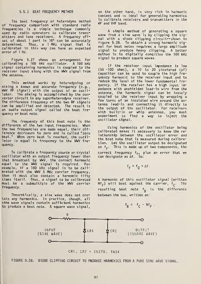
5.5.1 BEAT FREQUENCY METHOD

The beat frequency or heterodyne methodof frequency comparison with standard radiofrequencies is a simple technique commonlyused by radio operators to calibrate trans-mitters and tune receivers. A frequency off-

set of about 1 part in 106 can be accuratelydetermined. Thus, a 1 MHz signal that is

calibrated in this way can have an expectederror of 1 Hz.

Figure 5.27 shows an arrangement forcalibrating a 100 kHz oscillator. A 100 kHzsignal containing harmonics is coupled to thereceiver input along with the WWV signal fromthe antenna.

This method works by heterodyning ormixing a known and accurate frequency (e.g.,WWV RF signal) with the output of an oscil-lator. The mixing is accomplished by the con-verter circuit in any superheterodyne receiver.The difference frequency of the two RF signalscan be amplified and detected. The result is

an audio output signal called the beat fre-quency or beat note.

The frequency of this beat note is thedifference of the two input frequencies. Whenthe two frequencies are made equal, their dif-ference decreases to zero and is called "zerobeat." When zero beat is reached, the oscil-lator is equal in frequency to the WWV fre-quency.

To calibrate a frequency source or crystaloscillator with an output frequency lower thanthat broadcast by WWV, the correct harmonicequal to the WWV signal is required. Forexample, if a 100 kHz signal is to be cali-brated with the WWV 5 MHz carrier frequency,then it must also contain a harmonic fiftytimes itself. Thus, a signal to be calibratedmust be a submultiple of the WWV carrierfrequency.

Theoretically, a sine wave does not con-tain any harmonics. In practice, though, allsine wave signals contain sufficient harmonicsto produce a beat note. A square wave signal,

on the other hand, is very rich in harmoniccontent and is ideal for generating harmonicsto calibrate receivers and transmitters in theHF and VHF band.

A simple method of generating a squarewave from a sine wave is by clipping the sig-nal with a diode clipping ci rcuit—shown in

figure 5.28. To obtain a strong harmonic sig-nal for beat notes requires a large amplitudesignal to produce heavy clipping. A bettermethod is to digitally condition the 100 kHzsignal to produce square waves.

If the receiver input impedance is low(50 -100 ohms), a 10 to 20 picofarad (pf)capacitor can be used to couple the high fre-quency harmonic to the receiver input and toreduce the level of the lower fundamental fre-quency. If the receiver has a high input im-

pedance with unshielded lead-in wire from theantenna, the harmonic signal can be looselycoupled to the receiver input by wrapping a

few turns of an insulated wire around the an-tenna lead-in and connecting it directly tothe output of the oscillator. For receiverswith built-in or whip antennas, you mustexperiment to find a way to inject theosci llator signal

.

Using harmonics of the oscillator beingcalibrated makes it necessary to know the re-

lationship between the oscillator error andthe beat note that is measured during calibra-tion. Let the oscillator output be designatedas fp. This is made up of two components, the

correct frequency f0 , plus an error that wecan designate as Af. So:

fF= f

Q+ Af

.

A harmonic of this oscillator signal (writtenNfp) will beat against the carrier, f^,. The

resulting beat note fg is the difference

between the two, written as:

Nfr

INPUT(SINE WAVE)

OUTPUTSQUARE WAVE)

CR1 , CR2 = IN270, 1 N34

FIGURE 5.28. DIODE CLIPPING CIRCUIT TO PRODUCE HARMONICS FROM A PURE SINE WAVE SIGNAL.

97

The bars mean that a negative sign in theanswer is ignored; that is, the answer is

always a positive number.

Now substitute the first equation intothe second:

fB= f

c- Nf

Q- NAf p .

But Nf0 equals fp

. That's why we multipliedby N. So:

fB= NAf, or

Af =

which says that the error equals the beat thatwe hear divided by N. For example, if a beatfrequency of 100 Hz were measured between theWWV 5 MHz signal and the 50th harmonic of a

100 kHz oscillator signal, the frequency errorof the 100 kHz signal would be:

Af _ 100 Hz _ „ uAf - -gg- - 2 Hz.

The oscillator frequency is in error by 2

Hz. To determine whether the oscillator is

high or low in frequency, the oscillatorfrequency has to be changed to note which waythe beat frequency decreases. If increasingthe oscillator frequency decreases the beatnote, it indicates that the oscillator fre-quency is lower than the WWV/WWVH frequency.

In a receiver with no tuned RF amplifierbetween the mixer stage and the antenna input,a low frequency sine wave signal can enter themixer stage directly and generate unwantedharmonics and confusing beat notes due to thenonlinear characteristics of a mixer circuit.However, a good communications receiver or a

special -purpose WWV receiver generally hastuned RF amplifier stages or preselectorsbefore its first mixer stage. Then, only thedesired beat note from two input signals is

produced.

If the beat note is above 50 Hz, head-phones, a speaker, or a counter can be used.

Below that frequency, a dc oscilloscope can beconnected to the receiver detector. A signalstrength meter can be used and the beatscounted visually. The automatic gain control(AGC) should be disabled, if possible, for themeter fluctuations to be more noticeable. Themanual RF gain can be adjusted to compensatefor loss of the AGC.

To correct the oscillator frequency, theadjustment knob is turned in the direction

which lowers the frequency of the beat note.Between 50 Hz and about 1 Hz, the beat notecannot be heard and the signal strength meterwill begin to respond to the beat note as itapproaches 1 Hz. As zero beat is approached,a very slow rise and fall of the backgroundnoise or the WWV audio tone can also be heardon the speaker. The meter effect is mucheasier to follow. As it approaches zero beat,the very slow rise and fall of the signalstrength may sometimes become difficult todistinguish from signal fading due to propa-gation effects.

To overcome fading effects, the oscilla-tor adjustment can be interpolated. First,adjust the oscillator to a minimum beat fre-quency that can be measured without interfer-ence. For accuracy, count the number of de-flections of the signal strength meter in 10

seconds. The setting of the frequency adjust-ment is then marked. The adjustment is thenmade to pass zero beat until the beat is againvisible on the meter. By obtaining the samenumber of meter deflections as the previousbeat note, the frequency can be set midwaybetween the two adjustments.

The frequency of crystal oscillatorschanges with time. This is commonly referredto as the aging or drift rate. Therefore, all

crystal oscillators must be recalibrated peri-odically if maximum accuracy is desired.

5.5.2 OSCILLOSCOPE LISSAJ0US PATTERN METHOD

Audio oscillators can be calibrated by

using WWV/WWVH audio tones to produce Lissa-jous patterns on an oscilloscope. Lissajouspatterns are fully discussed in Chapter 3.

The WWV audio signal is applied to the verti-cal input of the scope and the oscillatorsignal to be calibrated is used to drive the

horizontal amplifier. The resultant patterntells the user two things: (1) the frequencyratio between his oscillator setting and the

received tone, and (2) movement of the oscil-

lator relative to WWV.

The tones available on WWV nd WWVH are

mainly 500 and 600 Hz. CHU transmits 1 kHz

ticks that last for about one-third second.

If these are used, they will produce an oscil-

loscope pattern at the tick rate; i.e., once

per second. Even the WWV/WWVH ticks can be

used this way. Most important, the user

should be aware of the exact format being

broadcast to avoid making errors. This can be

a problem because WWV and WWVH switch between

500 and 600 Hz in alternate minutes and the

440 Hz is used for only one minute every hour.

In a typical application, the user will

be able to check the accuracy of the dial

98

operation. First, he picks a dial settinggiving a frequency ratio to a WWV tone that is

an integer. Then he turns the dial slowlyuntil the pattern is stationary. By readingthe dial setting, a calibration can be madeand the dial reset to another frequency that

is an integer ratio. The same technique couldbe applied to fixed frequency sources if theyare in correct ratio to the tones on WWV andWWVH. The ratio of the two frequencies is

equal to the ratio of the number of loopsalong two adjacent edges. If the verticalinput frequency is known, the horizontal inputfrequency can be expressed by the equation:

Nv

fh=

N^fv

'

Where: f. = horizontal input frequency

f = vertical input frequency

N = number of loops on the verticaledge

= number of loops on the hori-zontal edge

:

'•• •

m\mmmm

VERTICAL INPUT: WWVH 500 Hz TONEHORIZONTAL INPUT: AUDIO OSCILLATOR

600 Hz TONE

FIGURE 5.29. OSCILLOSCOPE DISPLAY SHOWINGLISSAJOUS PATTERN.

The pattern shown in figure 5.29 has fiveloops on the horizontal edge and six loops onthe vertical edge. The vertical input fre-quency is the WWVH 500 Hz tone. To determinethe horizontal input frequency, the knownvalues are substituted in the above equationand the result is:

f. = | x 500 = 600 Hz.

Therefore, the horizontal input frequency is

600 Hz.

It is possible to calibrate over a ten-

to-one range in frequency both upwards and

downwards from the 500 and 600 Hz audio tonestransmitted by WWV and WWVH; that is, from 50

Hz to 6 kHz. However, not all frequenciesbetween them can be calibrated with the 500

and 600 Hz tones because not all frequencieshave a ratio of integers with less than thenumber ten in the numerator and denominator.For example, a frequency of 130 Hz comparedwith the 500 Hz tone would give a ratio of50:13. It would be impossible to count 50

loops on the horizontal edge. But a frequencyratio of 500 Hz to 125 Hz is possible becausethere will be four loops on the horizontaledge and only one loop on the vertical edge ora ratio of 4:1. A frequency ratio of 1 : 1 pro-duces a less complex pattern of a tilted line,circle, or el 1 ipse.

If the frequencies are exactly equal, thefigure will remain stationary. If one fre-quency is different from the other, the figurewill not remain stationary but will "rotate."Because one complete "rotation" of the figureis equal to one cycle, the number of cyclesper unit of time is the frequency error.

For example : If a Lissajous figure takesten seconds to "rotate" through one cycle andthe frequency being compared is 600 Hz, thefrequency error is:

Af = - = —,= 0.1 Hz

T 10

c _ Relative _ Af _ 0.1 _ , 7 in-4F = c = — = = 1-7 x 10Frequency

f 60Q

Since the error is inversely proportional to

the time it takes to complete one cycle, it is

obvious that the longer it takes to complete a

cycle, the smaller the error will be.

The measurement accuracy of a Lissajouspattern by the comparison method describedabove is inversely proportional to the fre-

quency. For example, if the time required for

a Lissajous figure to "rotate" through one

cycle is ten seconds at a frequency of 1 MHz:

F = Relative Frequency = —f

0.1 Hz _ , 1n-7= z = 1 X 10

1 x 10b

Hz

If, instead of measuring at 1 MHz, we observethe Lissajous pattern at 1 kHz:

Af = f x F = 1 x 103

x 1 x 10" 7= 10" 4 Hz

99

and the observation time would be:

Af 10'4 = 10,000 seconds.

Thus, it would take too long to measure sig-nals with relative frequencies of less than1 x 10- 5 at 1 kHz. A more accurate methodwhich measures the phase shift on an oscillo-scope will be discussed next.

5.5.3 OSCILLOSCOPE PATTERN DRIFT METHOD

The oscilloscope pattern drift method is

good for comparing two frequencies if you havean oscilloscope with external triggering. It

can detect smaller frequency differences thanthe Lissajous pattern at audio frequencies.

The method consists of an oscilloscopewith an accurately calibrated sweep time base.

External triggering is obtained from the sig-nal to be calibrated. This signal can be anyinteger submultiple of the tone being receivedfrom WWV/WWVH. The receiver (tuned to WW) hasits audio output connected to the verticalinput of the oscilloscope. With the sweeprate set at 1 millisecond/division, thetrigger level is adjusted so that a zerocrossover of the corresponding 600 or 500 Hzsignal is near midscale on the scope.

By measuring the phase drift during a

given time interval, the frequency error is

determined. If the zero crossover moves to

the right, the audio signal frequency is

higher than the WWV signal, and if it moves to

the left, the signal is lower in frequency(fig. 5.30).

For example, if during a count of 10

seconds at 500 Hz, the zero crossover advancedfrom left to right by 0.1 millisecond, therelative frequency is:

c _ phase drift _ +0.1 x 103

^, ln-5F c = = +1x10time interval 10

and the frequency difference is

Af = f x 1 x 10" 5= 500 x 10

5= +0.005 Hz.

Therefore, the 500 Hz signal has an error of+0.005 Hz. Under ideal conditions, a relativefrequency of 1 part in 10 6 can be determinedby increasing the observation time.

mmmmw^Ammm

INITIAL FINAL

VERTICAL SIGNAL: WWVH 600 Hz TONETRIGGER: AUDIO OSCILLATOR

600 Hz TONESWEEP RATE: 100 MICROSECONDS/DIVISIONINITIAL ZERO CROSSOVER: 530 MICROSECONDSFINAL ZERO CROSSOVER: 680 MICROSECONDSPERIOD OF MEASUREMENT: 10 SECONDSTOTAL PHASE SHIFT: +150 MICROSECONDS

r +150 X 10 r ln-5F = = +1.5 x 10

10

Af = 600 x 1 .5 x 10-5

900 x 10J= +0.009 Hz

FIGURE 5.30. OSCILLOSCOPE DISPLAY USINGPATTERN DRIFT METHOD.

5.5.4 FREQUENCY CALIBRATIONS BY TIME

COMPARISON OF CLOCKS

For those users who are set up to recover

and maintain time from WWV or WWVH, there is

an alternate way to calibrate the frequency of

the oscillator driving the clock. This is

simply to record the time differences from day

to day and then calculate the frequency rate.

The operation is analogous to telling yourjeweler that your watch gains or loses so many

seconds a day. He then adjusts the rate to

compensate.

The operation proceeds something like

this. Each day, note the amount the clock

output differs from WWV. Then keep an accu-

rate record of the history of the oscillator

in terms of the time gained or lost with re-

spect to WWV ticks. To get accurate data,

readings from several days should be averaged.

For example: If the time error averaged

out to be 1 millisecond per day (say for a 5-

day period), then you could compute the fre-

quency offset by noting that (see Chapter 3):

Af

f

At

T

100

which simply says that the time lost or gained

by a clock whose oscillator is running at fre-

quency f is proportional to the frequencyerror. In our example, putting all the terms

in the same units (in this case, seconds) we

get:

-3At _ 5 x 10 s time error

T 5 x 86,400 s

=1.2xl0-8 =-^f

F, the relative frequency of this oscillatorwould be -1.2 x 10- 8

. So an oscillator thatis off frequency by about a part in 10 8 wouldgain or lose about a millisecond a day. Usingthe techniques outlined in the section on timechecking, this millisecond error would be

quite visible to a user.

This example illustrates that this tech-nique could be extended to other levels ofaccuracy. In fact, data have been obtainedthat allow WWV signals to be used for calibra-tions approaching a part in 10 10 .

We can use our example to illustrateanother side of the time/frequency problem;namely, how to specify frequency error. Assum-ing that our answer was one part in 10 8

, wecan write it mathematically as 1 x 10- 8

, and(if the oscillator were 100 kHz and high in

frequency) our actual numerical frequencywould be 100,000.001 hertz. This can also be

written as 0.000001% frequency error.

In summary then, frequency calibrationscan be made by recording only the time errorproduced by an oscillator. This technique is

recommended for lower quality oscillators andfor situations where the user is already mea-suring time of day from WWV for some otherreason.

5.6 FINDING THE PROPAGATION PATH DELAY

The problem of finding the radio propaga-tion path delay is twofold. First, the greatcircle (curved) distance must be found betweenthe transmitter and receiver. Second, thenumber of times the signal bounces from iono-

|

sphere to earth (hops) must be known. Withthese two facts, we can solve for the totalpath delay. The accuracy we can expect willbe somewhere around a millisecond. We wouldbe hard put to improve that figure very much.

I For groundwave signals at very low frequen-i cies, we could carry a clock and calibrate the

path, but for HF waves of the type transmittedby WWV and CHU, it probably isn't worth the

effort. The reason for this is that at anyparticular time, the path may not be at its

average value. Since the path is constantlychanging by small amounts, it would not pay to

try to measure it with great exactness.

For those users who want time with the

best possible accuracy and who need a methodfor calculating the path delay, the followingmethods will work. The new hand-held calcula-tors that are available will greatly assist in

the computations. However, the math can be

done with a slide rule or a book of tables.Some examples are given to help in thesol ution.

5.6.1 GREAT CIRCLE DISTANCE CALCULATIONS

Using figure 5.31 as a reference:

A and B are two points on the earth.

Pole is one of the two poles, North or

South.

LA = Latitude at point A.

LB

= Latitude at point B.

L0A

= Longitude at point A

L0B

= Longitude at point B

P = L0A " L

0B"

dg

FIGURE 5.31. DIAGRAM FOR GREAT CIRCLEDISTANCE CALCULATIONS.

101

PROBLEM : Using the above information, findthe great circle distance (dg) in

nautical miles between the twopoints A and B. All angles aregiven in degrees.

For points A and B on the same side

of the equator :

dg = 60 cos- 1 (cos cos Lg cos P

+ sin sin Lg) nautical miles.

For points A and B on opposite sides

of the equator :

dg = 60 cos- 1 (cos L^ cos Lg cos P

- sin L^ sin Lg) nautical miles.

CONVERSION TO STATUTE MILES AND KILOMETERS :

1.151 x nautical miles = statute miles.

1.8522 x nautical miles = kilometers.

EXAMPLE : Find the great circle distance fromradio station WWVH, Kauai, Hawaii(point A) to WWV, Fort Collins,Colorado (point B) in statute milesand kilometers.

The coordinates of the two stations are:

Latitude Longitude

LA= 21°59'26" N L

QA= 1 59°46 1 00" W

Lg = 40°40'49" N LQB

= 105°02'27" W

Then, P= 159°46'00" - 105°02'27" = 54°43'33"

SOLUTION : Taking sines and cosines:

sin LA= 0.37445 cos L

ft

= 0. 92725

sin Lg = 0.65184 cos Lg = 0.75836

cos P = 0.57749

dg = 60 cos"1[(0.92725 x 0.75836 x 0.57749)

+ (0.37445 x 0.65184)]

= 60 cos"1[(0.40608) + (0.24408)]

= 60 cos"10.65017 = 60 x 49.44586

= 2966.75 nautical miles

= 3414.73 statute miles

= 5495.00 kilometers

5.6.2 PROPAGATION DELAYS

The delay of high frequency radio wavesdepends on many factors. The height of theionosphere and the distance between transmit-ter and receiver are important. Knowing theexact number of hops is important; otherwise,errors of from 0.5 to 1 millisecond can occur.

The ionosphere is made up of a number oflayers whose actual height varies both dailyand seasonally. This changes the path delay a

lot if the receiver and transmitter are closeto each other. Much of the time, such changesare not important to the person who wants toget time information, but if you are concernedwith errors of about 300 microseconds, youmust take care to account for all delays.

Since the earth is round, there is a max-imum ground distance a single hop can span(fig. 5.33). This is about 4000 kilometers or2200 miles. For greater distances, the radiowaves must obviously be reflected a number oftimes. Any error in the wave path computationfor one hop must be multiplied by the totalnumber of hops.

For minimum error, the frequency used forreception should be selected for the leastnumber of hops. This also results in a

stronger signal due to smaller losses. At anyparticular distance, the user must select the

proper shortwave frequency from WWV/WWVH so

the signal can be received. Some frequencieswill penetrate the ionosphere and not reflect.

Other frequencies will skip over the user. He

is then said to be located in the "skip dis-

tance" for that frequency. A lower frequencymust be selected. Use of the maximum fre-

quency that is receivable assures the least

number of hops. This maximum usable frequencyis called the MUF. A higher frequency will

skip over the receiving station. A frequencyabout 10% below the MUF will provide the bestreception.

For distances under one thousand miles,

the single-hop mode of transmission dominates.

For short distances, the height must be

102

FIGURE 5.32. REFLECTION OF RADIO WAVES AT DIFFERENT IONIZED LAYERS.

estimated carefully. For distances of over1600 kilometers (1000 miles), where only a

single-hop mode of transmission occurs, a muchwider range of error in the height can betolerated.

By estimating height according to timeof day, season, latitude, and sunspot cycle,errors can be reduced. For F 2 -layer reflec-tions, which is the principal layer used,there are several "averages" in height thatcan be used. An average height of 250 km is

reasonable for the winter months when propa-gation conditions are good at 10 MHz andabove. In summer, the average height can beincreased to 350 km. As reception againbegins to improve in the fall, the estimatedheight can be decreased again. Using thisapproximation method, the error in path lengthcomputation can be reduced considerably.

For distances from one to two thousandmiles (3220 km), where multiple-hop transmis-

sion occurs, the method above produces errors.For best results, the height must be deter-mined with greater accuracy. Heights for a

particular latitude, longitude, and time of

day are available from the World Data Center,N0AA, Department of Commerce, Boulder, CO

80303.

By performing a single time comparisonwith a station, the probability of error in

the hundreds of microseconds becomes verygreat due to the changes in propagation. A

high degree of accuracy for a single measure-ment is remote. But, by conducting measure-ments at several times over a period of a weekand by averaging with methods such as the

moving average method, errors can be reduced.

The following equations for determiningwave angle and propagation time delay have beensimplified and are approximate, giving errorsof 2% or less.

103

DEFINITIONS OF SYMBOLS PROPAGATION TIME DELAY

wave angle or angle of radiationin degrees.

$ = angle of incidence in degrees.

TD = 2R sin 0 _d£L

p 299.8 sin $ 299.8 sin

(R and dg in km)

9 = 1/2 central angle subtended byradius R from A to B.

Where:

dg = great circle distance from trans-mitter to receiver in kilometers.

For S3 < 4000 km, 9 < 18 degrees:

N = number of hops to cover distancedg.

4> = 90° - tan- 1 + (approximately)

dg _ great circle distance per hopN (km/hop). SAMPLE CALCULATIONS

h1 = virtual height of ionized layer

(km).

R = 6,370 km, mean radius of earth.

EXAMPLE: Given: dg = 3220 km

h1 =250 km

N = 2

total propagation distance (km). Determine wave angle A and propagation timedelay TD.

TD = propagation time delayp (milliseconds).

A=tan-* (lN^ + |a_) - o.0045 ^= 13.25°,

WAVE ANGLE EQUATIONS

Or, by the approximate method:

A = tan"1

(h

FTTTrn)+ tan

5" e

9(degrees) =fjjjj (^ ) = 0.0045 &

a a (2NIV _ dg_)57 3 = 14 2°A " 1 dg 4RN

;3/ --i

TD_ =p 299.8 sin 0

For ^ < 4000 km or 9 < 18 degrees:But:

* = 90° - tan"1 (2^. + d|_) = 69.

5

C

A = tan"1 (^ + ^_) - 0 0045 4flA zan ( dg 4RN ;

NSo:

TDp

=299.8

3

s?n 69.5=11 - 5ms

For 9 < 20 degrees:

r 2Nh'A S O dg^-) 57 34RN ;

EXAMPLE : Given : dg = 3220 km

h1 = 334 km

N = 1

104

TD = 0QQ"W

•—t= 11.4 ms

p 299.8 sin 0

Thus, the time delay of 2 hops at 250 km vir-tual height and 1 hop at 334 km virtual heightwill differ by only 100 microseconds.

5.7 THE NBS TELEPHONE HME-OF-DAY SERVICE

For those users who cannnot set up a

shortwave receiver for WWV or who have otherdifficulties, NBS operates a telephone time-of-day service. Anyone who dials 303-499-7111will hear the very same signals that arebroadcast over WWV. The machines at FortCollins, Colorado, which generate the WWVformat, are connected via telephone lines to aroom in the Boulder Laboratories where thetelephone equipment is maintained.

This telephone service is widely used,both in the local Denver calling area and vialong distance. The telephone service canhandle eight incoming calls simultaneously.In addition, four lines are available throughthe government switchboard at Boulder for useby other government agencies. These are onFTS number 323-4245.

The actual time you hear on the telephonewill differ by a few milliseconds from thatheard over WWV via radio. This is because ofthe delay in the telephone lines. In addition,if you are calling from any great distance,the way in which the telephone company handlesyour call limits the total accuracy of the WWVtone to a few hertz. This means that if youare trying to make a calibration at 1000 Hz,

you could have an error as great as threecycles per second. This accuracy is not as

good as that which can be achieved using radiomethods. Users are warned about this limit ofaccuracy over the telephone.

Because the telephone service is veryoften fully utilized, you may get a busy sig-nal. If this happens, wait a few minutes andredial. After your call is connected, thesystem will automatically hang up in threeminutes unless you hang up first.

5.8 SUMMARY

As stated early in this chapter, HF radiobroadcasts are commonly used for time and fre-quency calibrations. Accuracies ranging from1 ms for time-of-day to 1 part in 10 7 for fre-quency can be obtained. The NBS telephonetime-of-day service can also be used whenaccuracy requirements are not critical. How-ever, if your requirements are higher, youshould probably use one of the other methodsdiscussed in the following chapters.

105

CHAPTER 6. CALIBRATIONS USING LF AND VLF RADIO TRANSMISSIONS

Along with the widely used high frequencyradio transmissions of WWV and WWVH, theNational Bureau of Standards operates a fre-quency and time service on WWVB, a low fre-quency (LF) radio station. WWVB operates at60 kHz to take advantage of the stable radiopaths in that frequency range. Both frequencyand time signals are provided, but no voicetransmissions are made due to the narrow band-width of the transmitter/antenna combination.Many countries have services in this band,which ranges from 30 to 300 kHz, as well as in

the VLF (very low frequency) band from 3 to 30kHz. In addition to discussing the use ofWWVB, this chapter also covers other VLF sta-tions throughout the world. The Loran-C ser-vice at 100 kHz is discussed in a Chapter 9.

It may seem unusual to send signals in a

frequency band that is almost in the audiorange, and indeed, these signals do pose somespecial problems for the transmitter andreceiver-design engineers. However, lowfrequencies such as the 60 kHz of WWVB areused because of their remarkable stability.Radio waves at low frequencies use the earthand the ionosphere as a waveguide and followthe earth's curvature for long distances.Accuracies of a part in 10 11 or better forfrequency and 500 microseconds for time canbe achieved by using LF or VLF broadcasts.

6.1 ANTENNAS FOR USE AT VLF-LF

At the transmitters, it is difficult to

radiate high power levels. Special largeantenna arrays are used, but even they areinefficient. Resonance of receiving antennasis hard to achieve because of the low frequen-cy and resulting long wavelength. A channel 9

TV antenna is about 2 feet long. At 60 kHz,

an antenna has to be almost 2 miles long (a

quarter-wavelength) to be resonant. This is

obviously impossible so a compromise must be

made.

Since a quarter-wavelength antenna is outof the question, antennas that are electrical-ly "short" are used with tuning boxes andspecial couplers. On vertical antennas, toploading is often used. This consists ofradial wires extending from the top of theantenna to the ground. Often, they serve as

guys. Of course, as with any antenna system, a

good ground is essential. The physical loca-tion of antennas is important. Placement willaffect signal strength and noise. Keep theantenna away from metal objects. Long-wire antennas should be at least 15 to 20 feet

above ground. Several commercial antennasuse preamplifiers so the connecting coaxialcable supplies power to the amplifier. In

those cases, care must be taken to avoidshorting the cable.

Manufacturers of VLF-LF radio receiversuse a variety of antenna types. Long-wireantennas up to several hundred feet are avail-able. Whip antennas 8 to 10 feet long areused where space is a problem. On the otherhand, air loop antennas are able to rejectinterference but do not have as much gain as

whips. This is done by turning the loopantenna so that the null of its figure 8

pattern is pointed at the source of inter-ference. Ferrite loop antennas are becomingmore popular since they are very small com-pared to an air loop, but they can cause someunwanted phase shift due to temperature. If

you want the very best phase record, the kindof antenna and how it is used are importantconsiderations.

All of the above antennas benefit fromhaving couplers and/or amplifiers incorporatedin the antenna structure to allow a match to

be made with the shielded antenna cable. Theusual precautions about placing antennas nearmetal objects or buildings should be observed.Here, the manufacturers' instructions shouldbe followed. Many engineering handbooks andantenna manuals contain details about antennaconstruction.

6.2 SIGNAL FORMATS

Even after the antenna problems are

solved, sanding information on low-frequencycarriers leaves much to be desired. WWVBsends a carrier for frequency information andchanges the level (-10 decibels (dB)) of that

carrier to transmit a time code in the form of

binary "ones" and "zeros." The Navy VLF sta-

tions use on/off keying to send code and some-

times use frequency-shift or minimum-shiftkeying. The Omega Navigation System sends

only the carrier. Receivers for these VLF

signals usually "lock" onto the carrier andthus recover frequency information. In addi-

tion, some means is provided to hear thestation. This is usually just a tone output.

For example, if you were to listen to WWVB,

you would hear the one-second code segments

as a tone that changes from loud to soft.

There are no voice signals on any of the LF

or VLF stations. The bandwidth used cannottransmit voice signals. Almost all VLF-LFstations are controlled by atomic oscillators.

107

TIME(UTC)

FIGURE 6.1. PHASE OF WWVB AS RECEIVED IN MARYLAND.

6.3 PROPAGATION CHARACTERISTICS AND OTHER

PHASE CHANGES

Phase records made of VLF and LF stationsshow changes caused by the daily and seasonalchanges in the propagation path. Among otherthings, LF and VLF signals have regular phaseshifts. These shifts occur when sunrise orsunset occurs on the path from the transmitterto receiver. For instance, as the path is

changing from all darkness to all daylight,the ionosphere lowers. This shortens the pathfrom transmitter to receiver. This shortenedpath causes the received phase to advance.This phase advance continues until the entirepath is in sunlight. The phase then stabil-izes until either the transmitter or receiverenters darkness. When this happens, theionosphere begins to rise, causing a phaseretardation. Figure 6.1 shows a strip chartrecording of the phase of WWVB, Ft. Collins,Colorado, as received in Maryland. The day/night changes are easily seen. The magnitudeof the change is a function of the pathlength, and the rate of the change is a

function of path direction.

A phase recording from a stable VLF or LF

radio station contains a great deal of infor-

mation. The user's job is to sort out thisinformation so that he can understand what is

happening to the frequency source that is

being calibrated. His first assumption is

usually that the signal from the station is

almost perfectly controlled. That is, it

starts on frequency and stays there. This is

not always true. Errors in control at the

transmitter can cause large phase shifts in

the received signal that would make it appearas though the local oscillator were changing.Most stations operate with a near perfectrecord, but they do make mistakes. This hap-

pens just often enough so that the user needsadditional information to help him. Thisinformation takes the form of monthly or

weekly notices of the actual phase of thesignal. This is usually in terms of micro-

seconds advance or retard. A sample of NBSdata for WWVB and other monitored stations is

shown in figure 6.2. U. S. Naval Observatory(USNO) data for its stations are shown in fig-ure 6.3. These data can be obtained free uponrequest.

The implication of possible transmittingerrors to the user is that he cannot hurrythrough calibrations! Certain practices withrespect to LF radio calibrations are highlyrecommended. These include careful attentionto such details as receiver adjustments--donot change knob settings or cabling. Alwaysoperate the equipment continuously if possi-ble. This gives you a continuous chart recordso that you know when to expect sunrise/sunsetphase shifts. You can also detect local

interference and noise conditions. If yourreceiver has a mechanical phase counter, jot

down the readings on the chart. This is a

great help in trying to reconstruct events

that happen on weekends or at night.

A typical occurrence for a trackingreceiver is the cycle phase shift. Since the

receiver is faithfully following a zero cros-sing of the received phase, it doesn't know

which of the thousands of crossings it is

locked to. If it loses lock, it will simply

go to the next crossing that comes along. On

a phase chart this will show up as a shift in

phase equal to one cycle of the carrier.

For WWVB at 60 kHz, a cycle of phaseequals 16.67 microseconds. If the chart

recorder/receiver combination is producing a

chart that is 50 microseconds across, the pen

will move about 1/3 of the way across the

chart for each cycle change. Such changes can

be identified and must be ignored duringcalibration runs. This is due to the fact

that phase charts are always ambiguous by an

amount equal to the period of a carrier cycle.

How does the user tell whether the re-

corded phase difference indicates a change in

his oscillator, the path, or the transmitted

108

3. PHASE DEVIATIONS FOR WWVB AND OTHER NBS-MON ITORED BROADCASTS

WWVB (60 kHz)

Values given for WWVB are the time difference between the time markers of the UTC(NBS) time scale and

the first positive-going zero voltage crossover measured at the transmitting antenna. The uncertaintyof individual measurements is +0.5 microsecond. Values listed are for 1500 UTC.

Omega, North Dakota (13-1 kHz) and Omega, Hawaii (11.8 kHz)

Relative phase values are given for VLF stations and only the change from the previous available day'sreading is published. Days when the data were satisfactory but readings were not taken (for example,on weekends or station maintenance days) are marked (-). If data are lost, continuity is also lost

and the indication is (*) , which means that reading cannot be compared to the previous day.

LORAN-C (DANA), Dana, Indiana (100 kHz) and LORAN-C (FALLON), Fallon, Nevada (100 kHz)

Values for Loran-C (Dana) and Loran-C (Fallon) are the time difference between the UTC(NBS) time pulsesand the 1 pps output of the Loran-C receiver. Uncertainty in the measurements is +_ 0.1 microsecond.

JULY

MJD

UTC(NBS) - WWVB

ANTENNA PHASE

(60 kHz)

(in us)

UTC(NBS) - RECEIVED PHASE (in us)

OMEGA(11.8 kHz)

OMEGA(13.1 kHz)

LORAN-C (DANA)

(100 kHz)

LORAN-C (FALLON)

(100 kHz)

1 43690 5.90 (-) (-) (-) (-)

2 43691 5-99 (-) (-) (-) (-)

3 43692 6.08 + 2.5 + 0.1 73684.84 3949.27

4 43693 5.98 (-). (-) (-)

5 43694 5.88 - 1.5 - 0.1 73685.21 3949.42

6 43695 5.83 + 2.3 + 0.1 73685.22 3949.47

7 43696 5.54 - 3.2 - 0.8 73685.27 3949. 42

8 43697 5.61 - 8.8 (-) (-) (-)

9 43698 5. 68 (-) (") (-) (-)

10 43699 5.75 - 9-6 + 0.3 73685.41 3949.60

1 1 43700 5.93 + 6.4 -0.1 73685.40 3949.59

1 2 43701 5.66 + 4.5 - o.2 73685.41 3949 55

13 43702 5.81 + .4.5 + 0.5 73685.56 3949.67

1* 43703 5.67 + 0.6 0.0 73685.59 3949.69

15 43704 5.70 (-) (-) (-) (-)

16 43705 5.72 (-) (-) (-) (-)

17 43706 5.75 + 0.2 + 0.3 73685.69 3949.77

18 43707 5.66 + 1.5 - 0.2 73685.75 3949.83

19 43708 5.74 - 3-1 + 0.1 73685.80 3949.85

20 43709 5.79 - 0.5 - 0.1 73685.89 3949.81

21 43710 5.72 - 1.0 - 0.1 73685.92 3949.79

22 43711 5.78 (-) (-) (-) (-)

23 43712 5.84 (-) (-) (-) (-)

24 43713 5.90 + 3-1 - 0.1 73685.93 3949.91

25 43714 5.86 - 0.8 - 0.1 73686.00 3949.96

26 43715 5.57 + 1.0 + 0.4 73685.96 3950.06

27 4371.6 5.71 + 0.3 + 0.2 73686.1 1^- 2950. 15

^^J8 ^ —<i^^^7J^ "

FIGURE 6.2. NBS DATA PUBLISHED IN NBS TIME AND FREQUENCY BULLETIN.

109

U. S. NAVAL OBSERVATORYWASHINGTON, O.C. 20390

26 JUL. 1979

DAILY PHASE VALUES AND TIME DIFFERENCES SERIES 4

THE TABLE GIVES: UTC(USNO MC ) - TRANSMITTING STATION

NO. 651

UNIT = ONE MICROSECOND

JUL .

FREQUENCY NV

KHZ (UTC)MJD

16 4407017 4407118 4407219 4407320 44074

21 4407522 4". 0762 3 £ \ C " ?

24 4407c'-

25 44079

FREQUENCYKHZ (UTC)

/9970PAC.

LC/4990CEN. PAC.

LC/9930E. COAST

LC/7970NOR. SEA

LC/7990MED. SEA

LC/7930N. ATL.

LC/9990N < PAC.

JUL .

MJD19 4407320 4407421 4407522 4407623 4407724 4407825 44079

1 00 100 1 00 1 00 1 00 100 10 0

-1.2 C .7 2 .93 — 2 .2 0.2 — 1 . 8 _ 1 ^ c1 • o-1.3 0.5 2.93 -2 .4 0.1 -1 .7 -1.5-1.3 0.5 2 .88 -2 .4 0.1 -1 .9 -1.3-1.4 0.5 2.86 -2 .4 0.1 -1 .8 -1.4-1.4 0.5 2.85 -2 .5 0.0 -1 .9 -1.5

-1.3 0.6 2.87 -2 .3 0.2 -2 .0 -1.8-1.4 0.6 2.83 - -2 .1 -1.8-1.3 0.6 2.90 -2 .2 0.3 -2 .2 -1.8-1.4 0.6 2.88 -2 .2 0.4 -2 .0 -1.9-1.3 2.88 -1 .9

3 1 7 5 6 4 2LC/5990 LC/7960 O/H O/ND Q/ND O/A O/L O/T GBRW.C.CAN GULF AK 11.8 13.1 13.6 13.6 13.6 13.6 1 6. 0

100 1 00 2 5MS + 6MS+ 6MS + 30MS + 25MS + 1 1MS+ 1 9MS+

2.2 1.8 954 425 421 576 141 622 5152.2 1.0 054 425 421 576 142 622 5142.1 1.5 o ; i 424 421 576 143 622 514

1 .6 95j 425 421 574 143 622 5142.1 1.7 953 425 421 575 141 622 515

1.7 953 426 421 575 141 622 514954 425 421 575 141 622 514

LC/9940W.C.USA

100

-5.3-5.4-5. 4-5.4-5.3

-5.3-5.3-5.3-5.3-5.3

8

NLK18.6

12MS +

335

341(1)340340

340340339

(1) NLK 19 JUL. AFTER MAINTENANCE PERIOD STEP ABOUT PLUS 6

(2) PROPAGATION DISTURBANCES WERE OBSERVED NEAR THE FOLLOWING TIMES:20 JUL. 1940/521 JUL. 1110/4. 1340/622 JUL. 1310/5, 1440/5, 1735/4, 1925/5, 2 110/623 JUL. 1435/4, 1645/5, 2055/524 JUL. I'z I >/S25 JUL. 1600/4, 1735/3.

(3) OMEGA STATIONS OFF-AIR TIMES (FROM COAST GUARD ONSOD, WASHINGTON, DC):JAPAN 1 7 JUL. 0039 TO 0041 UT , 0214 TO 0217 UT, 0232 TO 0234 UT.

0918 TO 0920 UTLIBERIA 1 7 JUL. 0240 TO 0242 UT , 0305 TO 0403 UT

21 JUL. 1 610 TO 1 622 UTLA REUNION 1 7 JUL. 0423 TO 0425 UT , 071 7 TO 0 73 1 UT, 0735 TO 0737 UT ,

1 1 36 TO 1 1 59 UT, 1 247 TO 1306 UT, 1412 TO 1415 UT1 8 JUL. 0030 TO 0032 UT , 06 32 TO 0645 UT, 1036 TO 1045 UT19 JUL. 0509 TO 0512 UT, 1 059 TO 1 105 UT, 1439 TO 1441 UT

FIGURE 6.3. USNO PHASE DATA, PUBLISHED WEEKLY.

110

signal? The answer is that he knows fromexperience! If you plan to use VLF or LF

signals for frequency calibrations, you mustbecome very familiar with the characteristicsof the signals you are using. For accuratecalibrations, you must obtain the station datafrom NBS or the USNO. Battery backup for

receivers is highly desirable; in fact, almostnecessary if you plan to calibrate preciseoscillators over a period of many days. All

of this may sound like a hopeless task, but it

isn't. The results are worth the effort whenyou consider that you can perform calibrationsup to 1 part in 10 11 in 24 hours.

6.4 FIELD STRENGTHS OF VLF-LF STATIONS

The field strength of the WWVB signal hasbeen measured along nine radial paths from thestation. These measurements are summarized onthe field contour map shown in figure 6.4.

Not shown is the nonlinear field gradientbetween the 500 microvolt per meter contourand the 100 microvolt per meter contour.

Destructive interference occurs betweenthe first hop skywave and the groundwave at

approximately 1200 km (750 miles) from the

station. On some radial paths, this dip in

field intensity is quite severe and has provento be the cause of signal loss at certaintimes. The distance between the station and

this null varies from day to night. It is

also seasonal. The sharpness of the null is

much less pronounced in the winter. The fieldintensity, in general, is slightly higherduring the winter months. Shown in figures6.5 and 6.6 are the field strengths alongradial s to Brownsville, Texas and Nantucket,Massachusetts, both measured in September.Other radial plots are available to interestedusers.

The signal strength of the L). S. Navy

stations is usually very high unless theyare undergoing repairs. The Omega naviga-tion stations have a high power output also.

But Omega is time shared; that is, the eighttransmitters take turns broadcasting on the

same frequencies. This has the effect of

reducing the available signal power andcommutation is required; that is, you musthave a means of turning the receiver on onlywhen the station you want to track is trans-

mitting.

FIGURE 6.J». MEASURED FIELD INTENSITY COUNTOURS : WWVB @ 13 kW ERP.

Ill

ioo r

MILES FROM ANTENNA

FIGURE 6.5. MEASURED FIELD INTENSITY, NANTUCKET, MASSACHUSETTS RADIAL, WWVB 60 kHz.

112

6.5 INTERFERENCE receive WWVB. Another method is to produce a

unidirectional antenna by combining the volt-

ages induced in a loop and a whip. If these

Some WWVB users along the U. S. Atlantic two voltages are equal and in phase, the

coast have experienced interference from a resultant pattern is a cardioid. Since these

British standard frequency radio station, MSF. voltages are induced into the whip by the

Some years ago, MSF was not only lower pow- electric field, and into the loop by the

ered, but it was also offset in frequency from magnetic field, the phase of the whip voltage

WWVB. However, it now radiates 25 kW of power must be shifted by 90° before combination,

on 60 kHz. There are various ways to tell if Interested readers are advised to consult a

one is receiving MSF instead of WWVB. The 45° suitable antenna manual or to discuss their

phase shift (discussed in Section 6.6.1, fig. problems with the receiver manufacturer.

6.9) should be quite apparent if WWVB is being

received and phase-tracked.6.6 USING WWVB FOR FREQUENCY CALIBRATIONS

One solution is to use a directional

antenna. If a loop is being used, the MSF

signal can be nulled. Eastern U. S. receiving Our discussion of calibrations using low-

locations from Boston south that are using frequency signals begins with WWVB (60 kHz),

loops should be able to null MSF and still Frequency calibrations usually involve phase

FIGURE 6.7. WWVB PHASE RECORDING USING A FIGURE 6.8. TYPICAL WWVB PHASE RECORDING.

HIGH-QUALITY OSCILLATOR.

113

recordings of the received signals. Typical-ly, a special tracking receiver is used to

compare a local oscillator with the receivedWWVB signals. The output of the receiver can

be displayed on its front panel digitally or

as a meter reading. However, this discussionis limited to making a phase record on a chartrecorder. Often, these recorders are builtinto the receivers. Since we are looking at a

phase recording of the received signal, we

will see the effect of any path changes. In

addition, we will see our oscillator phasechange relative to the WWVB signal.

The amount of phase change depends on therelative difference between our oscillator andthe cesium oscillator controlling the WWVBsignal at the transmitter. The sample phasechart shown in figure 6.7 has very littleoscillator drift. This is because a qualityoscillator was being measured. A more typicalrecord would have a whole series of lines

crossing the chart as in figure 6.8. Thisposes a dilemma for the user. If the oscil-lator being calibrated is far off frequencyfrom WWVB, he needs either a fast chart or one

that displays many microseconds of phaseacross the width of paper. For high-qualityfrequency sources, the paper can be sloweddown or the chart width, in microseconds, can

be reduced. The user is encouraged to studythe manuals for the particular receiver he is

using. If the user is planning to buy a

receiver, he should consider the problem of

what the record is going to look like beforeselecting a particular receiver/recordercombination.

Measurements made with VLF-LF signalsshould be done when the path from transmitterto receiver is all in sunlight. An all dark

path would be second choice. The sunrise/sunset phase shifts (called diurnals) will

affect the accuracy of calibrations and mea-surements should not be made during thesetimes. There are other sudden phase shiftsdue to particles entering the ionosphere thatcan affect the signal. These usually last

only ten minutes or a half-hour. This ex-

plains the advantage of having a chart that

runs at least several hours for a calibration.During sudden phase shifts, the signal level

may drop. Most receivers have a meter for

signal strength, but the more elaborate re-

ceivers are able to chart record the signal

amplitude. This is a very useful record if

the calibrations being made are to be withinparts in 10 10 or better. In other words, youneed all the help you can get if you are to

make the very best measurements.

As mentioned earlier, some receivers use

front panel displays to indicate frequencyoffset. Later in this chapter, we mentionmethods that use oscilloscopes for frequencycalibration. Even a zero-beat or Lissajous

method could be used with the WWVB signal.

Remember that what you are getting from WWVBis a standard frequency signal that startedout from a nearly perfect frequency source.

When it arrives, it has been contaminated bypath variations and noise. A chart recordergiving a history of the path and oscillatorchanges is very handy to have. To get thebest resolution from the WWVB signals, a chartrecord is mandatory. The results are worththe effort. As with any measurement, extremecare must be exercised to realize the bestresults.

6.6.1 PHASE-SHIFT IDENTIFICATION

Many WWVB users have phase-trackingreceivers which make use of the stabilized

FIGURE 6.9. WWVB PHASE PLOT SHOWINGPHASE-SHIFT IDENTIFICATION.

114

carrier to provide a frequency reference forcalibration purposes. In order for the userto identify WWVB by its phase track alone, a

45° phase shift is programmed into the trans-mitted phase. This shift occurs at 10 minutespast the hour and returns to nominal value at15 minutes past the hour. Three hours ofstrip chart at a typical user site might looksomething like figure 6.9.

6.6.2 METHODS OF FREQUENCY COMPARISON

Having listed some of the problems in LF

propagation, we can now turn our attention toactual calibration methods. There are twoways to compute relative frequency from theplot in figure 6.1. One can work with theslope of the daytime plot--the straightportion—or one can take the single values atdiscrete points one day apart. On the figure,the 2200 UTC values for June 3 and June 4 aresubtracted to give a value of 1 microsecondchange for the 24-hour period. The relativefrequency, Af/f , is the same as the timeoffset, At/T . In this case:

Af _ At _ 1 us _ 1 us

f T 1 day 86,400 x 106

us

= 1.16 x 10

When the relative frequency is large, a

useable value can be computed using only a fewhours of the daytime slope. If the relativefrequency is very small, many days may have tobe used in the computation. This is especi-ally true when the radio propagation stabilityis poor or the signal is noisy. If many daysare involved in the measurement, cycle jumpsand transmitter phase shifts entered into thephase plot must be carefully taken intoaccount.

If the receiving site has no phase-tracking receiver available, other schemes maybe used. If a tuned radio frequency receiveris available, the actual 60 kHz wave may beobserved on an oscilloscope. If the oscillo-scope is triggered by a local clock, theposition on the oscilloscope face of a par-ticular cycle will change with time. Theamount of the change in any given time will

provide a value of At/T from which the rela-tive frequency may be computed as before. A

standard reference 60 kHz or submultiple, if

available, may be used to trigger theoscilloscope.

Electronic counter techniques can also beused for frequency calibrations. Withoutgoing into detail, these techniques involve

the use of the received signal as one input toa counter while the oscillator being calibra-ted is used as the other. Manufacturers ofreceivers and counters discuss these tech-niques in their manuals and application notes.You may also refer to chapters 1 and 4 of thisbook, which talk about counters and theiruses. Keep in mind that the accuracies youcan get with oscilloscopes and counters willgenerally be much less than those obtained byusing tracking receivers. The cost will beless too. Also, a quick calibration on a

counter cannot identify sudden phase changes,and you lose the big advantage of having a

chart record of the station performance.

6.7 USING OTHER LF AND VLF STATIONS FOR

TIME AND FREQUENCY CALIBRATIONS

6.7.1 THE OMEGA NAVIGATION SYSTEM

The Omega Navigation System is composedof a group of VLF radio stations operating in

the 10 to 15 kHz range. Each station time-shares common frequencies used for navigation.In addition, each station may transmit somefrequencies unique to that particular station.See Table 6.1 for details.

If one wishes to use an Omega station forfrequency calibration, a phase-trackingreceiver is highly recommended. If one of thenavigation frequencies is to be used, then an

Omega commutator must also be used. This is a

device that turns the phase-tracking receiveron and off at the proper times to receive onlythe desired Omega station.

The frequencies and the format segmentsof the Omega stations are derived from cesiumbeam oscillators. The USN0 monitors andreports the Omega stations' phase values.

These stations radiate a nominal 10 kW of

power. This power level should be sufficientto allow the user to receive at least three

stations no matter where he is located.

A. Operating Characteristics of Omega

Omega transmitting stations operate in

the internationally allocated VLF navigationalband between 10 and 14 kHz. This very lowtransmitting frequency enables Omega to pro-

vide adequate navigation signals at muchlonger ranges than other ground-based naviga-

tion systems.

The operating characteristics of the

system can be categorized as follows: signal

format and control, the requirement for lane

identification typical of phase comparison

115

TABLE 6.1. CHARACTERISTICS OF THE OMEGA NAVIGATION SYSTEM STATIONS

STATION LOCATIONLATITUDE,LONGITUDE

POWER(kW) ANTENNA

CARRIERFREQUENCIES* ACCURACY

OMEGA

fi/N

ALDA,

NORWAY

66° 25' N

13° 09' E10

OMNI-

DIRECTIONAL

10.2 A

11-1/3 C

13.6 B

-125 x 10

OMEGA

Q/L

MONROVIA,

LIBERIA

06° 18' N

10° 40' W10

OMNI-

DIRECTIONAL

10.2 B

11-1/3 D

13.6 C

-121 x 10

1

OMEGA

n/H

HAIKU, OAHU,

HAWAII

21° 24' N

157° 50' W10

OMNI-

DIRECTIONAL

10.2 C

11-1/3 E

13.6 D

1 x 10' 12

OMEGA

n/ND

LA MOURE,

NORTH DAKOTA

46° 22' N

98° 20' W10

OMNI-

DIRECTIONAL

10.2 D

11-1/3 F

13.6 E

1 x 10" 12

OMEGA

fi/LR

LA REUNION20° 58' S

55° 17' E10

OMNI-

DIRECTIONAL

10.2 E

11-1/3 G

13.6 F

1 x 10" 12

OMEGA

fi/A

GOLFO NUEVO,

ARGENTINA

43° 03' S

65° IT W10

OMNI-

DIRECTIONAL

10.2 F

11-1/3 H

13.6 G

1 x 10" 12

OMEGA

n/TTRINIDAD**

10° 42' N

31° 38' W1

OMNI-

DIRECTIONAL

10.2 B

11-1/3 D

13.6 C

1 x 10" 12

OMEGA

Q/J

TSUSHIMA IS.

,

JAPAN

34° 37' N

129° 27' E10

OMNI-

DIRECTIONAL

10.2 H

11-1/3 B

13.6 A

1 x 10" 12

*SEE FIGURE 6.10 FOR TRANSMISSION SCHEDULE OF VARIOUS FREQUENCIES.

**TRINIDAD IS A TEMPORARY STATION. PERMANENT STATION WILL BE IN AUSTRALIA.

systems and the process of handling errorsattributable to signal propagation.

All stations now transmit three basicnavigational frequencies (10.2 kHz, 11-1/3

kHz, 13.6 kHz) more or less omnidirectionally.In order to prevent interference, transmis-sions from each station are time-sequenced as

shown in figure 6. 10.

This pattern is arranged so that duringeach transmission interval (approximately 1

second), only three stations are radiating,each at a different frequency. The durationof each transmission varies from 0.9 to 1.2

seconds, depending on the station's assignedlocation within the signal pattern. Witheight stations in the implemented system and a

silent interval of 0.2 second between eachtransmission, the entire cycle of the signalpattern repeats every 10 seconds.

Besides the three basic navigational fre-

quencies, other frequencies have been added to

the Omega signal format. Original plans were

made to transmit two unique frequencies at

each station for the purpose of inter-stationtime synchronization but this requirement has

been removed through use of highly stable

cesium frequency standards.

Present plans call for the incorporationof a fourth navigation frequency, 11.050 kHz,

which will allow for lane resolution capa-

bility as great as 288 nautical miles. In

addition, a unique frequency transmission for

each station can be added which will aid in

time dissemination by providing a beat fre-

quency and a high duty cycle at that frequen-

cy. The changes depicted in figure 6.10,

which are not yet implemented, should be made

by 1979.

116

—__S>egmentStation -

—

A B C D E F G H

Norway (A) 10.2[J

13.6|_j

11 1/3[J

12. T[J 12.1

+

|JH.05

|J 1 2 . 1

+

[j 12.1+|J

Liberia (B)

Hawaii (C)

N. Dakota (D)

La Reunion (E)

Argentina (F)

Australia (G)*

Area

Japan (H)

Tj\_\ 10 -2 U 136 U 111/3 U 12.0+ U 12.0

+U 1105 U 12.0+ U

n. sU ii. sU 10.2(J

ile[J

11 1/3[J

ii .8+

U ii .8+

(Jn-os

[J

11.05[J 13.1

+

L| 13.

1

+

[J102

[J13.6

[J11 1/3

[J 1 3 .1+

|j 13. I

+|_]

12. 3^] 11-05[J 12.

3

+jj 12.3

+U 102 U 136 U 11 1/3 U 1 2 .

3

+|J

2.9"jJ1 2.9

+

[J11.05 [ 12.9

+

U 12.

9

+|J

102|J

ll6|J

11 1/3[J

11 1/3[J

13.

0

+

[J13.

0

+

[J11 05 U 13.0 +

[J H-O^IJ 10.2 13.6|J

13.6[J

11 1/3[J

12.

8

+

[J12.8+

[J11.05

|J1 2 . S "

|_|12. 8

+

|J10.2

|J

p- 0.9-1 p-1.0-H p-l.l-H 1.2 -—IJ*—

1.1 —H p-Q.9-H p— 1.2—H p- 1.0 -H

0.0

Trinidad

temporarily

filling G slot

2.3 3.6 5 0 6.3

Time (seconds)

Proposed full format is shown:— +

is unique frequency at each

station

— 11.05 is fourth navigation

frequency

7.4 10.0

FIGURE 6.10. OMEGA SIGNAL TRANSMISSION FORMAT.

B. Synchronization Contro l

The Omega signal format is designed so

that each station within the network can be

identified by the transmission of a particularfrequency at a prescribed time. In addition,the synchronization of all transmissions is

tightly controlled and the phase relationshipsbetween all signals are maintained to within a

few centicycles. With this high phase stabil-ity in the transmissions, the accuracy of a

navigational fix is then primarily limited to

the receiver and the accuracy of the naviga-tor's propagation correction tables.

All Omega transmitting stations are syn-

chronized by means of very stable cesium beamfrequency standards. These standards or

clocks are referenced to the atomic time scalewhich differs from Coordinated Universal Time(UTC) more commonly in use. Thus, in 1978,the Omega epoch or time reference is sevenseconds ahead of UTC since the yearly adjust-ments for earth motion have not been made to

make Omega Epoch in agreement with UTC.

C. Propagation Characteristics

The propagation characteristics thatpermit the use of Omega at great range also

introduce certain limitations. Two areas that

require special attention are normal time

variations and modal interference. Since

signals are propagated within the waveguideformed by the earth and ionosphere, changes in

propagation parameters such as velocity may be

expected as a result of changes in the iono-

sphere or ground.

The most obvious navigational ly undesir-

able variation is a daily or diurnal phase

change. Normal changes in illumination of the

ionosphere by the sun throughout the day may

cause an uncorrected phase measurement to vary

as much as one complete cycle. Since these

variations are highly repeatable, prediction

and correction are possible.

Unpredictable short-term variations may

also occur. Ninety-five percent of the time,

these are small variations related to random

propagational variations whcih will not de-

grade normal navigational accuracy. Occasion-

ally, however, large disturbances can occur as

a result of solar emission of X-ray or parti-

cle bursts. The emission of X-rays from the

sun occasionally cause a short-term disruption

of Omega signals which is referred to as a

Sudden Phase Anomaly (SPA). The duration of a

SPA is generally not greater than one hour but

an LOP may experience a shift of several

miles. SPA's occur with an average frequency

117

of about 7-10 per month. They usually affectsignals from only a few stations at a timesince X-rays from the sun tend to enter a

limited illuminated portion of the earth'ssurface.

The release of a large quantity of pro-tons from the sun, although an infrequentoccurrence, produces what is known as a PolarCap Disturbance (PCD). The effect of a PCDmay be to shift an LOP 6-8 miles for a periodof several days. This disturbance generallylasts for several days and varies in magnitudeduring the period. PCD's affect only thosetransmissions involving arctic propagationpaths. Because of its possible long durationand large LOP shift, PCD notices are broadcastas navigational warning messages.

Modal interference is a special form ofsignal interference wherein the various wave-guide modes of signal propagation interferewith each other and irregularities appear in

the phase pattern. Ideally, one mode would becompletely dominant at all times and theresultant phase grid would be regular. In

practice, competing modes do not completelydisappear and three situations are recogniz-able:

1. If the competing mode is very small,then the dominant mode will estab-lish a nearly regular phase patternas is intended, and usually this is

what happens during the day.

2. A second possibility is that thecompeting mode may be almost equalto the dominant mode.

3. The potentially serious case is thatin which modal dominance can change.

This may occur, for example, if onemode is dominant during the day anda second mode at night. Clearly,somewhere during sunset and sunrise,the transitional period, the twomodes must be equal. Depending uponphasing of the modes at equality,abnormal transitions may occur in

which cycles are "slipped" or lost.

Positional errors of a full wave-length are possible under suchconditions and use of a station so

affected should be avoided. If thisis not possible, particular atten-tion must be given to proper laneidentification.

Propagation Corrections (PPC's) must beapplied to each Omega receiver reading tocompensate for ionospherical ly induced signalvariations and thereby improve position fixingaccuracy. Omega propagation correction tablesfor each transmitting station (A through H)

contain necessary data for correcting Omegareceiver readouts affected by prevailing

propagation conditions relative to the nominalconditions on which all charts and tables arebased. A brief introduction, which alsodescribes the arrangement and application ofthe corrections together will illustrativeexamples, precedes the tabular data withineach PPC table. For more detailed informationon the Omega Charts and Tables as well as

information on obtaining these charts, writeto: Defense Mapping Agency, HydrographicCenter, Attn: Code DSI-2, Washington, DC.

20390.

D. Omega Notices and Navigational Warnings

As with other navigational aids, infor-mation is disseminated concerning station off-the-air periods, VLF propagation disturbances,and other pertinent data affecting usage ofthe system. Status information on Omega sta-tions can be obtained on the telephone by cal-ling (202) 245-0298 in Washington, D. C.

Omega status messages are also broadcastby various time service stations. NBS sta-tions WWV and WWVH transmit a 40-second mes-sage at 16 minutes and 47 minutes after thehour, respectively. Norway Radio StationRogaland broadcasts notices in internationalmorse code on HF 4 times daily. Other sta-tions in the global time service and maritimeinformation network are expected to be addedin the future.

In addition to the regular issued noticeson station off-air periods, major plannedmaintenance may take place in the monthslisted for each station:

ARGENTINA MARCH

LIBERIA APRIL

HAWAII MAY

LA REUNION JUNE

NORWAY JULY

TRINIDAD FEBRUARY

NORTH DAKOTA - SEPTEMBER

JAPAN OCTOBER

The actual off-air times are disseminatedas noted above sufficiently in advance and may

vary from a few days to several weeks depend-

ing on the maintenance or repairs required.

6.7.2 DCF 77, WEST GERMANY (77.5 kHz)

DCF 77 is located at Mainflingen, about

25 kilometers southeast of Frankfurt/Main. It

is operated by the Physikalisch-TechnischeBundesanstalt (PTB) in Braunschweig.

118

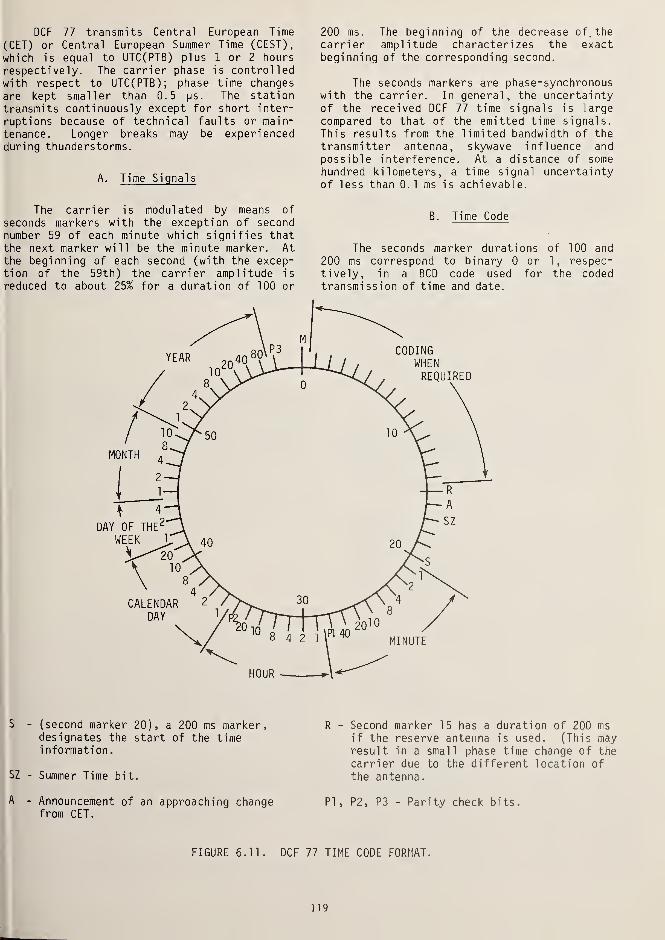
DCF 77 transmits Central European Time

(CET) or Central European Summer Time (CEST),

which is equal to UTC(PTB) plus 1 or 2 hours

respectively. The carrier phase is controlledwith respect to UTC(PTB); phase time changesare kept smaller than 0.5 us. The stationtransmits continuously except for short inter-

ruptions because of technical faults or main-

tenance. Longer breaks may be experiencedduring thunderstorms.

A. Time Signals

The carrier is modulated by means of

seconds markers with the exception of secondnumber 59 of each minute which signifies that

the next marker will be the minute marker. At

the beginning of each second (with the excep-tion of the 59th) the carrier amplitude is

reduced to about 25% for a duration of 100 or

200 ms. The beginning of the decrease of . the

carrier amplitude characterizes the exactbeginning of the corresponding second.

The seconds markers are phase-synchronouswith the carrier. In general, the uncertaintyof the received DCF 77 time signals is largecompared to that of the emitted time signals.

This results from the limited bandwidth of the

transmitter antenna, skywave influence andpossible interference. At a distance of somehundred kilometers, a time signal uncertaintyof less than 0.1 ms is achievable.

B. Time Code

The seconds marker durations of 100 and

200 ms correspond to binary 0 or 1,

respec-tively, in a BCD code used for the codedtransmission of time and date.

S - (second marker 20), a 200 ms marker,designates the start of the timeinformation.

SZ - Summer Time bit.

A - Announcement of an approaching changefrom CET.

R - Second marker 15 has a duration of 200 msif the reserve antenna is used. (This mayresult in a small phase time change of thecarrier due to the different location ofthe antenna.

PI, P2, P3 - Parity check bits.

FIGURE 6.11. DCF 77 TIME CODE FORMAT.

_

119

There are three groups of time informa-tion, each followed by a parity check bit P:

PI = NUMBER OF THE MINUTE

P2 = NUMBER OF THE HOUR

P3 = NUMBERS OF THE CALENDAR DAY,

THE DAY OF THE WEEK, THEMONTH AND THE YEAR

Counting the binary "ones" of the informationgroup concerned and of the corresponding pari-ty check bit yields an even number.

In the case of the transmission of Legal

Time in the form of CEST, seconds marker num-

ber 17 has a duration of 200 ms. During onehour before the change from CET to CEST orfrom CEST to CET, seconds marker 16 has a

duration of 200 ms, thus announcing theapproaching change. The coding is shown in

figure 6.11.

General information about DCF 77 is shownin Table 6.2.

6.7.3 HBG, SWITZERLAND (75 kHz)

HBG in Prangins, Switzerland is operatedby the Observatoire Cantonal in Neuchatel

.

The useful range for clock synchronization is

3000 kilometers.

A. Signal Format

The carrier is interrupted for 0.1 secondat the beginning of each second. An addition-al interruption occurs from 0.2 to 0.3 secondat the beginning of each minute.

B. Time Code

No continuous time code is transmitted.During the weekends of changes to daylightsaving time or back to standard time, a spe-cial code is transmitted, including a separate4-bit address for each European country.Additional details about HBG are shown in

Table 6.2.

6.7.4 JG2AS/JJF-2, JAPAN (40 kHz)

The Radio Research Laboratories in Tokyooperate JG2AS and JJF-2. JJF-2 consists of

telegraph signals; JG2AS broadcasts in the

absence of these telegraph signals. The UTC

time scale is broadcast. The call sign is

transmitted twice each hour (at 15 and 45 min-utes) in Morse code.

(1) Hourly modulation schedule

15 45 O min.

second pulses call sign

Call sign Three times by the Morse code

(2) Wave form of second pulses

mark

space

f- 500 ms

exact time (second)

500 ms— 4" 500 ms ~

exact time (second)

(3) Identification of minute signal

ESI ^ r222_ n a ezli

58s

I

59 s

I

(100 ms duration)

FIGURE 6.12. JG2AS EMISSION SCHEDULE,

120

The 40 kHz carrier frequency (of 500 ms dura-tion) is broadcast at the beginning of eachsecond except for the 59th pulse in each min-ute, which is 100 ms long.

The JG2AS emission schedule is shown in

figure 6.12. Other details are shown in Table6.2.

6.7.5 MSF, ENGLAND (60 kHz)

MSF is located at Rugby, United Kingdom.It is operated by the National Physical Lab-oratory in Teddington, Middlesex. Transmis-sions are continuous except for a maintenanceperiod from 1000-1400 UTC on the first Tuesdayof each month. MSF transmits both a fast codeand a slow code.

A. Fast Code

Calendar information; i.e., month, day,hour, and minute are given, the complete databurst occupying a total of 330 ms at the fastbit rate of 100 bits/second in the 500 msinterval following the minute marker. Thefull format of the code is shown in figure6.13. It includes a control pulse and markerbit to initiate recognition systems in thereceiver, 24 data bits, 2 parity checks (oddparity) and a British Standard Time (BST)indicator (UTC + 1 hour) so transmissions areadvanced when BST is in effect.

B. Slow Code

The slow code operates at a 1 bit/secondrate. The sequence of signals in each minuteof the transmission is shown in figure 6.14.

Pulse length modulation is used, the carrierbeing interrupted for 100 ms for a logic "0"

and for 200 ms for a logic "1." Full calendarand time information is provided; i.e., year,month, day-of-month

,day-of-week, hour, and

minute referred to the minute marker immedi-ately following the code. The minute itselfis identified by an 8-bit precursor transmit-ted in seconds 52 to 59 in the form of thesequence 0111 1110. Exhaustive trials bycomputer simulation have confirmed that thissequence is unique and will not occur as partof the code proper at any time; the identifieris also well protected against a code with oneor two errors present.

The introduction of a minute identifierenables a very simple form of receiver/decoder

to be developed making use of a shift registerwhose length can be adjusted to acquire aslittle or as much of the code as is desired.For example, if the register is only 8 bitslong, this will be sufficient to identify eachminute but will exclude all the other data,which will pass through the shift register butwill not be recognized since the registerresponds only to the combination 0111 1110.When this is received, the next carrier inter-ruption is identified as the minute marker.Similarly a register 21 bits long will extracthour and minute information while the maximumlength of 43 bits is necessary for a fulldecoding of calendar and time-of-day infor-mation.

The code described so far contains thebasic, primary information at what may becalled the first level of coding. However,further subsidiary information is also encodedat a second level where logic "1" is indicatedby a carrier interruption in the interval 200to 300 ms following a seconds marker. Thisform of coding, as shown in figure 6.14, is

applied within the identifier at seconds 54 -

58, inclusive, and includes four parity checksand also a BST indicator. The latter indi-cates the operation of BST, as in the fastcode, but with the difference that the clockgenerating the slow code will be set 1 hourahead of UTC when British Summer Time is in

effect. The second level of coding alsoembraces the DUT1 indication in seconds 1-16,

inclusive, and brings this information intothe same format as the other signals.

The adoption of a minute identifierimmediately preceding the minute createsdifficulties in introducing a leap secondsince a positive leap second would be identi-fied as the following minute marker while a

negative leap second would remove the last bitin the identifier itself. When necessary,therefore, the leap second is inserted follow-ing second 16 where it can be accommodatedwithout disturbance to the coded sequence andidentifier.

Additional details about MSF can be foundin Table 6.2.

6.7.6 U.S. NAVY COMMUNICATION STATIONS

Some of the Navy communication stationsare commonly used to steer frequency sources:

NAA, NDT, NLK, NPM, NSS, and NWC. However,

use of these stations for frequency calibra-tion is strictly secondary to their primaryfunction of military communications. Thesestations are subject to frequency changes,

outages, and changes in schedule. Changes

are announced in advance to interestedusers by the USN0. All stations operate

121

60kHzC

(— H—^ (

M ^

201084214020108421 20108421 108421

- OP

RB

0 25 50

M

R

100

CARRIERHOURMINUTE

BST

PB

200

D

N

R, B

300 330

DAYMONTHMARKER BIT

60kHz+ C

P, B

0, P

M, R

500 ms

PARITY BITCONTROL PULSEMINUTE MARKER

FIGURE 6.13. MSF 60 kHz FAST CODE FORMAT.

_L I I I I I I I I I

40 20 10 8 4

I I I I I I

2 1 10

J L

4 2 1

_L

0 1 2 3 4 5 6 7 8 9 10 1 1 1 2 1 3 14 1 5 16 1 7 1 8 1 9 20 21 22 23 24 25 26 27 28 29

k DUTI J 4DDOW

DOM r ~\ r Nl

20 108 4 2 1 4 2 1 20 1034 2 1 40 20 1034 2 1 0 1 1 1 1 1 1 0' JL_J I I I I I I I I I I I I I I I I I L_l I I L

'

30 31 32 33 34 35 36 37 33 39 40 41 42 43 44 45 46 47 43 49 50 51 52 53 54 55 56 57 58 59

t

—| p- 100 ms G T1 -

~U o

~L200 ms

300 ms

1 - V

2 - V

(DUTI)

BST

H + N

DOWL DOM

—

Y

1 - V

2 - V

1 - V

2 - V

S: SECONDS Y: YEAR G: LOGIC N, I:

N: MINUTE T: DATA L: LEAP SECOND INSERTION S, R:

M: MONTH V: LEVEL P: PARITY CHECK BITS DoM :

DoW :

FIGURE 6 14. MSF 60 kHz SLOW CODE FORMAT

MINUTE IDENTIFIER

SECONDS MARKDAY-OF-MONTHDAY-OF-WEEK

122

continuously except for maintenance periods,

which are shown below:

STATION MAINTENANCE SCHEDULE

NAA 1400-1800 UTC each Monday; resched-

uled for preceding Friday if Monday

is a holiday. Half-power operationson Wednesday and Thursday from 1200-

2000 UTC. Scheduled/unscheduledhalf-power operations as required.

NDT 2200-0600 UTC Thursday/Friday exceptfirst Thursday/Friday of each month,

then 2200-0800 UTC.

NLK 1700-2200 UTC first & third Thursdayof each month.

NPM 2200-0200 UTC each Thursday and

Friday.

NSS 1200-2000 UTC every Tuesday.

NWC C001-0400 UTC every Wednesday.

Other details of these stations are

shown in Table 6. 2.

6.7.7 OMA, CZECHOSLOVAKIA (50 kHz)

0MA in Liblice, Czechoslovakia, transmits

the UTC time scale. The carrier is phase-

locked over a distance of 30 kilometers to the

phase of UTC (TP), the Czechoslovakian. time

scale. As a result, no long-term drift withrespect to UTC(TP) can occur. The rms phasedeviation is of approximately 100 ns; however,

during strong winds the phase excursions may

reach 500 ns since the antenna is not servo-

control led.

A. Time Code

The format of the OMA time code is shown

in figure 6.15. The signal is both amplitude

and phase keyed. Al seconds ticks of 0.1 sec-

ond duration are prolonged to 0.5 second to

identify minutes. A time code representingthe time of day of CET (Central European Time= UTC + 1 hour) is transmitted by means of

phase-reversing the carrier for 0.1 second in

corresponding seconds of the current minute.

Thus, in each minute a series of 4 pulses (PI

to P4) is transmitted.

The pulses, together with the Al minute

pulse (M) form 4 time intervals which, mea-

sured in seconds, represent 4 numbers: units

of minutes (UM), tens of minutes (TM), units

of hours (UH), and tens of hours (TH) of CET.

As shown in figure 6.15, the duration of each

interval is prolonged by 1 second so that the

number 0 may be transmitted as a 1 second

interval. In the illustrated case, 10 hours

01 minute of CET is transmitted which corre-

sponds to the following intervals:

10 h 00 mTIME OF DAY (CET)

-I r

10 h 01 m

0 I

1

l

I I

I I

1 0. 5s > 0.1s

OMA^'

J""

AM SECOND MARK

AM MINUTE MARK

54 55 56 57 58 59 0

0.1s

"pi

1P2X P3 P4Mil

(UM+ls)=2s« /—*-

TM+lsHs(UH+ls

>

= 15 (TH +ls)=2s

HI-

56s DETAIL P2

JM = UNITS OF MINUTESTM = TENS OF MINUTESJH = UNITS OF HOURS"H = TENS OF HOURS

100 150 f 250 ms

PHASE REVERSAL

FIGURE 6.15. TIME CODE FORMAT OF OMA - 50 kHz.

123

P2 - PI (in seconds) = UM + 1

P3 - P2 = TM + 1

P4 - P3 = UH + 1

M - P4 = TH + 1

Completion of the code by the date is plannedfor the near future.

Further details about OMA are shown in

Table 6.2.

6.7.8 RBU (66-2/3 kHz) AND RTZ (50 kHz), USSR

Table 6.2 gives details about these sta-

tions. However, the contents of the UT1 cor-rections are described below:

The information about the value and thesign of the DUT1 + dUTl difference is trans-mitted after each minute signal by the markingof the corresponding second signals by addi-tional impulses. In addition, it is trans-mitted in accordance with CCIR code. Addi-tional information on dUTl is given, specify-ing more precisely the difference UT1 - UTCdown to multiples of 0.02 second, the total

value of the correction being DUTl + dUTl

.

Positive values of dUTl are transmitted bythe marking of "p" seconds markers within therange between the 20th and 25th seconds so

that dUTl = +0.02 second x "p." Negativevalues of DUTl are transmitted by the markingof "q" seconds markers within the range be-

tween the 35th and 40th seconds so that dUTl= -0.02 second x "q."

6.7.9 VGC3 AND VTR3, USSR

These stations operate at 25.0, 25.1,

25.5, 23.0, and 20.5 kHz. Each stationtransmits 40 minutes 4 times/day:

VGC3 from 0036 to 0117, 0336 to 0417, 0636to 0717, and 1736 to 1817 hours UTC;

VTR3 from 0536 to 0617, 1436 to 1517, and1836 to 1917 hours UTC.

Two types of modulation signal are trans-mitted during a duty period: (1) Al signalswith carrier frequency 25 kHz, duration0.0125, 0.025, 0.1, 1, and 10 seconds withrepetition periods of 0.025, 0.1, 1, 10, and

60 seconds respectively; and (2) AO signalswith carrier frequencies 25.0, 25.1, 25.5,

23.0, and 20.5 kHz. The phases of these sig-

nals are matched with the time markers of the

transmitted scale.

No UT1 information is transmitted. See

Table 6.2 for further details about thesestations.

124

CO 5^i CO CO CO

CO <c CO CO CO s; co s: co S~ COz —

1

i i J

CDC\J <C CO <X ^ <I LO <C LU CD <C LU CD <X. LU CO <C

* 1— CO h- h- • 1— O • 1— Q • 1— CD • 1—r-- lu r^v lu r*** lu r-». lu O r^- lu o lu o lu

• Q >- • CD • Q • CD SI • Q SI CD S* CDeo CD zn CD CD CD CD CD CDLU CD Q_ CD CD CD Z CD Z CD Z CD1— z 1—

1

<£ 21 1—

l

Z i—

f

Z HH O Z i~< O Z f—

<

O Z Mo O LU QC O LU O LU O Li_ t—( O LU »—< O LU l-H OLLz CD CO H H CO I—I I—

I

CO •—i i—

i

\— CD LU 1— CD H~ CD f— CD CO I— CD CO 1— CD CO I— CDCD LU _l CD LU CD LU CD LU I—I CD LU I CD LU >—i CD LULU CU LU LU CU LU Cu LU CL SI LU CL. SZ LU CU SZ LU CUCO CO h- CO LO CO CO CO CO CO CO CO CO CO CO LO CO COz z zLU LU C£ LU CU LU od <C LU CU <C LU CC <C LU CdLU O <C LU O LU O LU O C£ LU O OC LU O C£L LU OCO U_ X CO LU CO Lu CO Lu 1— CO LU 1— CO LU 1— CO LU

LU LU

rH LU LU ac LU CO CO LU LU ce: LU CO CO LU LU LU1— Q z CD ZD —J z z Q ZD —

1

Z z ZZD O o CD O O ZD o o CD O O ZD o o oCD CD z (_J U Q Q- z z CD CD CD Q- z z z

ro CNJ CNJ CNJ I—

1

>" i—

1

rHCD l 1 1 1 1 1 1

or •~ r- r- r- -ZDC_J X X X X X X Xcd«^ Ln CNJ CNJ CNJ

COZo lOLO " CO

(-O 00 O CtL

CO o O ZD1—

1 lO OSI X i

— znCO CO o CO CO COZ ZD o o o ZD ZD ZD<C O 1— o o o Oce: ZD o ZD ZD ZDI

—

Z LO CNJ z Z Z —

1

o LO1

—

h- +-> o 1

—

1— I— z z zZD Z 1— 1

—

z z zO LO o o olu o LO - cO CD CD CDO CNJ O LOo o oCO CT) CNJ

s: Os: o Q •

1—

•

O Z \—i— u_ 1— <L~ ZD

co ZLU Ocd r— X. 1 1 1Z <c NUJ ZC z z zzd ZDex CDUJ O Oce: LU SI

C/)

zdQ<C LU Lf) 00 CDQ N CO LO o oZ cn ZL~ r-. r~ CD r- r-- 00<H Cn r-.

I— <£CO CD

AL1 i 1 1z <C <£ <: <c <c <co z Z z z z z zZ o O o o o o o

1—LU 1 CD I— h- I— h- 1

—

I— t—1— I LU 1 CD 1 CD 1 CD 1 CD ( CD 1 CD 1 CDZ z ce HH LU 1—1 LU (—i LU t-H UJ I—i LU I—t LU ( LU<c s: hh z or z or Z Q£ z cn Z cc Z z cr:

O CD s: i—

i

s: >—

i

s: »—

t

s t—• s: i—

i

s: i SI <

O CD O Q O CD O Q o o O CD O CD

_l LuQ£ O —1 O —

1

O OLU ? o o O o lO O ZD O <C CD O CO

CM CO CNJ O LL LO I CNJ i—OQ_

s:- CtL o CD <c z oz • CD Z s_ CD -z

UJ LU U_ Z LU CD 2 3 -><C 2! LU Q_ 2 UJ CD Z 3 z 3 Z LU ^ O Z 3LU Q CD Z CO —

1

zn z LU h-o Q ZD z - - ZL CtL - - CO ""D - - Q£ - LU CD -ZD 1— 1—1 >- r- O ^ CNJ i

—

M LU lO <x ^ CNJ i

—

LU LU 00 1— i—t CO <— cn z cnj lo

h f— _i z o O CNJ I— CD r-vj CNJ -— CO » — LO CNJ — —i Z ro r— S~ Z lO O CD i—< <— LO=c CD LU <C Q z: i

—

cd f— Z z SI o 0 >- LU O O «=C t—i o o ^ O O >- LU 0 O ZD <X 0 0 CO CU O 0 SI CO O Oo <c o H cc o CTt GO h- CNJ r- CtL 3 CD CD <C <C co cn CO 1— CNJ .— us <^ o <t ^j* r^. -—' <C CO <—

1 _J 1 <C LU LO CD t—1 LO Q- CO Q£ co m CD t—( lO cO >- '"D PO CO '"S 3 CNJ

s: cd ZD z z ZD Zq: ZD <c CO ce ZD

CO

zoI

s*. C£ CD CO CNJ <: h- b£h— CO CO <C ( cO <t CD _J<t CD CD zn CNJ Lu z z z1— CD CD '"DCO *D ^0

125

tju lo <l. LU LO SL '

J J

• 1

—

(7) <C en <c• 1

—

Q • 0OO LO

c_> C_>O Ll_ Z 1—

1

O Ll_ O Ll_00 t-< 1—

1

OO I—i I—

1

OO 1—< M 1— t_) h- (_)OO 1— CJ O0 1— C_J OO 1— C_J h- G O LU O LU h— CJ 1— CJ

C_) LU O LUS UJ Q_ 51 luo. 2: lu a. LU Cl_ OO OO 00 00 LU CL LU Q_OO oo oo OO OO OO OO OO OO O0 OO OO OO O0 O0z z z LU OT LU OT

LU LU LU LU LU LUz z z z K Z Zz z z z z z

i—l

1

r-t

o 1o 1o 1o 1o 1O

OL OLt- h—

1— s^.

1

z z z Z3 — z Z z zO h-3 O O0 s:zhq: • LD LO

1— O U_ h-z o ^O UD Z Oo o o s:

0 0st st

1 _l 1 o 0 O O

OOst st OO \ O r-inom 0 <— lt> 0 in

' 0LI) LO OO 1 ' LI) LI) 0O t_0

CSJ CSJ C\J 0\J 0\1 C\J 0\J C\J

z z z z z z zo o o o 0 0 0h- 1— 1— 1— 1— 1— 1—

1 o 1 c_> 1 <_> 1 CJ 1 CJ 1 0 1 CJ

Z oryr" | , ^= ^O Q O Q o a o a 0 0 O Q 0 0

o 0 0

-> >-J Z - - 3 _i - - O - - O

<C i—i inoi o -=t en <C CD O "_l st OO 3"CTl ~r- 00 CO co or O 1— 1— 00

LU OO CD LO O '— st <c< >- 1— LU 1— CJ O <_> Or or CO or or<C 3 o o Z Q£ 0 O OT Q_ OO O 0 i—

i u: o o 00 00 0 0 00 0 0 =t 00 0 0 or 00 0 0=) «£ r— 00 z <: oo lo O <C =3 i— st- —1 C_) o O 00 LO 00 or 00 C\J St nz 00 o<t LU OO LO 00

1

—

|

N

00 00O0 <t ZD M <_> or

s: CO 1— 1—z z z o or or > >

< Q-I— <Hlu n:a o

1-1 oo ora x:<c 1—

LU LO LOO O CJ IDCJ O LU I

CO CJ O0 O

I O I—a. -x orO O LU

o nst C

126

6.8 MONITORING DATA AVAILABILITY

No matter which station is chosen as a

oasis for cal ibration--WWVB, Omega, or VLF--

the user must be on a mailing list to receivenotices of changes in operation schedule.

«/WVB currently operates 24-hours a day everyjay. No changes in operating format are madewithout advance notification. The Omegastations do schedule maintenance outages and

some low-power operations. As the systemoecomes fully operational, these shoulddiminish. Announcements regarding the statusif the various Omega stations in the OmegaNavigation System are given hourly on both WWVand WWVH. See figure 12.1 in Chapter 12 for

announcement times. The Navy VLF stations are

the ones most likely to change their mode of

operation without notification.

Currently, NBS and USNO are monitoringand reporting the phase differences of NLK,

Dmega, and some of the U. S. Loran-C stations.In addition, NBS monitors and reports phasedifferences for WWVB and the USNO offers dataon NAA. These data are available to inter-ested users by contacting the Time and Fre-quency Division of NBS or the USNO.

6.9 USING THE WWVB TIME CODE

WWVB transmits a special binary-coded-decimal time code that provides time informa-tion. This service is used by seismologists,standards labs, commercial power companies,and others interested in synchronizations withaccuracies of the order of 500 microseconds.The code provides information of days, hours,and minutes. Seconds are resolved by countingaits. A correction, applied to the trans-nitted time to obtain earth time, UT1 , is alsoorovided for use by some astronomers andnavigators.

Unlike a code that is designed primarilyfor machine decoding, the WWVB code wasoriginally designed to be manually decodedfrom strip chart recordings or tapes. Tosimplify this process for a human decoder, thebits are placed such that the most significantbit occurs first in each code word. Theactual bit itself, whether a binary zero,binary one, or position identifier, is deter-mined by the duration of the power reductionof the transmitted carrier.

6.9.1 TIME CODE FORMAT

The WWVB time code is generated by chang-ing the power level of the 60-kHz carrier.The carrier power is reduced 10 dB at thebeginning of each second and restored to full

power 200 milliseconds later for a binaryzero, 500 milliseconds later for a binaryone, and 800 milliseconds later for a refer-ence marker or position identifier. Certaingroups of pulses are encoded to representdecimal numbers which identify the minute,hour, and day of year. The binary-to-decimalweighting scheme is 8-4-2-1 with the mostsignificant binary digit transmitted first.Note that this weighting sequence is thereverse of the WWV/WWVH code. The BCD groupsand their basic decimal equivalents are tabu-lated below:

BINARY GROUP DECIMALWEIGHT: 8 4 2 1 EQUIVALENT

0 0 0 0 0

0 0 0 1 1

0 0 10 2

0 0 11 3

0 10 0 4

0 10 1 5

0 110 6

0 111 7

1 0 0 0 8

10 0 1 9

The decimal equivalent of each group is

derived by multiplying the individual binarydigits by the weight factor of their respec-tive columns and then adding the four productstogether. For example, the binary sequence1001 in 8-4-2-1 code is equivalent to (1 x 8)+ (0 x 4) + (0 x 2) + (1 x 1) = 8 + 0 + 0 + 1

= 9, as shown in the table. If fewer thannine decimal digits are required, one or moreof the high-order binary digits may be dis-pensed with.

Once every minute, in serial fashion, thecode format presents BCD numbers correspondingto the current minute, hour, and day on theUTC scale. Two BCD groups identify the minute(00 through 59); two groups identify the hour

(00 through 23); and three groups identify the

day of year (001 through 366). When repre-

senting units, tens, or hundreds, the basic8-4-2-1 weights are multiplied by 1, 10, or

100 respectively. The coded informationrefers to the time at the beginning of theone-minute frame. Within each frame, theseconds may be determined by counting pulses.

Every new minute commences with a framereference pulse which lasts for 0.8 second.Also, every ten-second interval within the

minute is marked by a position identifierpulse of 0.8-second duration.

UT1 corrections to the nearest 0.1 secondare transmitted at seconds 36 through 44 ofeach frame. Coded pulses at 36, 37, and 38

127

seconds indicate the positive or negative

relationship of UT1 with respect to UTC.

Pulses at 36 and 38 seconds are transmitted as

binary ones only if UT1 is early with respect

to UTC, in which case a correction must be

added to the UTC signals to obtain UT1. The

pulse transmitted at 37 seconds is a binary

one if UT1 is late with respect to UTC, in

which case the required UT1 correction must

then be subtracted. The magnitude of the UT1

correction is transmitted as a BCD group at

40, 41, 42, and 43 seconds. Because UT1

corrections are expressed in tenths of sec-

onds, the basic 8-4-2-1 weight of that parti-

cular binary group is multiplied by 0.1 to

obtain its proper decimal equivalent.

Figure 6.16 shows a sample frame of the

time code in rectified or dc form. The

negative-going edge of each pulse coincideswith the beginning of a second. Position

identifiers are labeled P ls P 2 ,P3, P4, P5,

and P 0 . Brackets show the demarcation of the

minutes, hours, days, and UT1 sets. The

applicable weight factor is printed beneath

the coded pulses in each BCD group. Exceptfor the position identifiers and the frame

reference marker, all uncoded pulses are

binary zeros.

In figure 6.16, the most significant dig-

it of the minutes set is (1 x 40) + (0 x 20)+ (0 x 10) = 40; the least significant digit

of that set is (0 x 8) + (0 x 4) + (1 x 2)+ (0 x 1) = 2. Thus, at the beginning of the

frame, UTC was precisely 42 minutes past the

hour. The sets for hours and days reveal fur-

ther that it is the 18th hour of the 258th

day of the year. The UT1 correction is -0.7

second, so at the beginning of the frame the

correct time on the UT1 scale was 258 days, 18

hours, 41 minutes, 59.3 seconds.

6.9.2 TIME TRANSFER USING THE

TRANSMITTED ENVELOPE

There are three ways to use the code.

The first way--also the most expensive—is to

use a WWVB receiver with an automatic decoder

and display unit. There are a number of

manufacturers that produce this type of

equipment. A second level of user equipment

consists of a receiver having internal logic

circuits that provide a level shift code

output. This code may be applied directly to

a strip chart or to an oscilloscope for manual

use. The simplest equipment might consist of

a tuned radio frequency receiver with an

oscilloscope used to observe the amplified

signal

.

Figure 6.17 shows the signal envelope as

seen on an oscilloscope at the transmitter.

The on-time points are easily seen. With the

horizontal scale of the oscilloscope expanded

to 200 microseconds/centimeter, the on-time

point can be determined to about + 2 cycles of

the 60 kHz carrier. Of course, the farther

the receiving site is from the transmitter,

the more the signal-to-noise ratio degrades

1

0

TIME FRAME 1 MINUTE(INDEX COUNT 1 SECOND)

20 30 50

I I I I I I I I I I I I I I I I I I I I I I I I I I

ON TIME POINT A

FRAME REFERENCEMARKER

Po Pi Po

-| |- 0.8 SECOND —j

)-— 0 . 2 SECOND ~| w |— ~] u |- —-( f-

— 0 . 5 SECOND 0.8 SECOND -| (r

~UUli¥TmnTFLJllT¥l^^Q I » <1Q O O O**

' —I Li I T CMINUTES- - HOURS DAYS

o cm —i

L,-UTr

RELAT I 0NSH I

P

BINARY CODED DECIMAL TIME -OF -YEAR CODE W0R0 (23 DIGITS)CONTROL FUNCTIONS (15 DIGITS) USED FOR UT, CORRECTIONS5 PPM POSITION IDENTIFIER MARKERS AND PULSES (P 0 THRU P 5 )

(REDUCED CARRIER 0.8 SECOND DURATION PLUS 0.2 SECOND DURATION PULSE)W - WEIGHTED CODE DIGIT (CARRIER RESTORED IN 0.5 SECOND - BINARY ONE)U - UNWEIGHTED CODE DIGIT (CARRIER RESTORED IN 0.2 SECOND - BINARY ZERO)

UTC AT POINT A

258 DAYS18 HOURS42 MINUTES

UT1 AT POINT A

258 DAYS18 HOURS41 MINUTES59.3 SECONDS

NOTE: BEGINNING OF PULSE IS REPRESENTED BY N EGAT IVE - GOING EDGE.

FIGURE 6.16. WWVB TIME CODE FORMAT

128

MAIN TRANSMITTER

J L J I I

3

ms/cm

J I I I I I1 1 1

20 40 60 80 100

ms/cm

FIGURE 6.17. WWVB ENVELOPES AS TRANSMITTED.

until some averaging techniques must beemployed. Since the WWVB data rate is solow--one bit per second--vi sual integration is

very difficult, especially when the horizontalscale is expanded to allow greater timeresolution. Averaging or signal integrationusing a signal averager or an oscilloscopecamera works quite well at remote receivinglocations. (See Chapters 4 and 5 for moreinformation about these techniques.)

The actual process of time recoveryconsists of viewing the signal envelope on anoscilloscope that is being triggered by a

local clock at the receiving site. Havingpreviously determined the path delay, itsvalue can be subtracted from the total ob-served delay on the oscilloscope to obtain thelocal clock error.

In very noisy locations, where theon-time point is difficult to identify, a

photograph of the waveform can be helpful.Sometimes it is advantageous to allow a numberof oscilloscope traces to be exposed on thesame piece of film. This has an averagingeffect that simplifies the location of theon-time point. However, a single exposure can

be used. Take the photo and draw one horizon-tal line through the average of the waveformamplitude and another line along the averageslope of the dropout. The intersection of

these lines is the on-time point.

Receiving sites that are long distancesfrom the transmitter have an added problemwhen high resolution timing is desired. If

the delay to the receiver site is, say, 15

milliseconds and the sweep speed is set to 1

millisecond/centimeter, the on-time point of

the envelope will be off the oscilloscopeface. This problem can be resolved if a

second clock is available. The auxiliaryclock can be adjusted late so that when usedfor the oscilloscope trigger source, the

on-time point will be near the beginning ofthe trace. The sweep speed can now be in-

creased to obtain the desired resolution. Thetime intervals to be accounted for are the

time between the beginning of the trace and

the on-time point, and the interval betweenthe local clock and the auxiliary clock. Thelocal clock error, At , will be

At = D - At - Ate c

where: D is the propagation delay

At is the interval between the twoclocks

Atg is the trace delay on theosci 1 loscope

If Ate is positive, then the local clock

pulse occurs after the transmitted time pulse.If At is negative, the local clock pulse

occurs first.

6.10 SUMMARY

Although you can get better accuracies byusing LF and VLF broadcasts than you can fromHF broadcasts, use of these signals posesspecial problems that are not encountered atHF. But if you need frequency accuracies of a

part in 10 11 or better, or time synchroniza-tion to 500 microseconds, VLF or LF broadcastsmay suit your needs very well. However, youmust be willing the spend the time, money,and effort necessary to get maximum results.

You do have an alternative, though. Thefrequency calibration service using networktelevision and the TV Line-10 method ofobtaining time and/or frequency may be lessexpensive and easier to use.

130

CHAPTER 7. FREQUENCY CALIBRATIONS USING TELEVISION SIGNALS

One of the newer frequency calibrationservices offered by NBS uses TV signals whichhave some advantages over radio broadcasts:

First, the signals are readily available and

usually very strong. Second, television re-

ceivers and antennas are simple to operate andinstall. Radio signals are carefully con-

trolled at the transmitter, but when receivedby the user, they are sometimes degraded in

quality and difficult to locate in the radiobands. Calibration via television lets theuser concentrate on the calibration and spendless time fussing to get a good signal.

This frequency calibration service usestelevision signals in a transfer mode. If a

user wants to make a calibration, he comparesa TV signal coming from the national networkswith his local oscillator. NBS monitors thesame signal, calibrates it, and tells the userwhat correction to use.

The network signals are controlled byatomic oscillators and change their frequencyvery slowly, so the user needs new correctiondata at infrequent intervals. NBS checks thenetworks daily but publishes the correctionsonly once a month. This is often enough. Theresults obtained by this method of frequencycalibration match or exceed any other methodavailable. Anyone desiring a frequency cali-bration can make one quickly and have confi-dence in the results. Accuracies obtainable

range from a part in 109 to a few parts in

10".

7. 1 HOW THIS FITS INTO OTHER NBS SERVICES

NBS operates radio stations WWV, WWVH,

and WWVB. It also has a TV Line-10 servicewhich is explained in the next chapter. This

service complements the radio broadcasts andLine-10. Users who have the equipment andskill necessary to use radio signals will

probably want to continue to use them. How-

ever, if TV signals are available and theradio services fall short in some respect,then a switch is indicated. Many users canget a good TV signal in their area, but findit difficult to erect a suitable antenna for

the NBS radio signals. This television fre-quency calibration service operates equallywell on cable (CATV) systems, the UHF chan-nels, and in areas of Canada and Mexico thatreceive U.S. network signals. But the re-

ceiver must be a color set.

7.2 BASIC PRINCIPLES OF THE TV

FREQUENCY CALIBRATION SERVICE

The major television networks in the U.S.

use atomic oscillators to generate their ref-

erence signals. These are either cesium or

NBS

SERVICES

NETWORKSERVICES

USER

FUNCTIONS

A NBS FREQUENCY STANDARD

B NETWORK STANDARD

C USER'S OSCILLATOR

FREQUENCY STANDARDS

COMPARE A-C = CALIBRATION OF C

NBSFREQUENCYSTANDARD

NETWORK NETWORK

FREQUENCYCOLOR TV

BROADCASTSSTANDARD

+

USER'SOSCILLATOR

SIGNALSRECEIVED

BS

MONNETSIGM

\s

K

S

I

EASY

INEXPENSIVEACCESS

/ / /

VPHASE

COMPARATOR

(TWO METHODS

COMPARED

NBS

STANDARDVS

NETWORKS

published data

[easy, inexpensive]l access j

USER'SOSCILLATOR

VS

NETWORK

USER'SOSCILLATOR

VS

NBSSTANDARD

ARE DESCRIBED BELOW)

CALIBRATION

USER'SOSCILLATORCALIBRATED

131

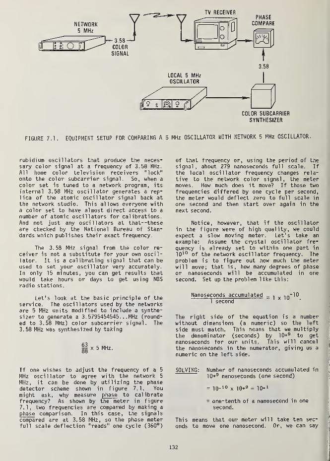
NETWORK5 MHz

3.58

COLORSIGNAL

JV TV RECEIVER

-

-

oo

1—

1

o

LOCAL 5 MHzOSCILLATOR

PHASECOMPARE

3.58

COLOR SUBCARRIER

SYNTHESIZER

FIGURE 7.1. EQUIPMENT SETUP FOR COMPARING A 5 MHz OSCILLATOR WITH NETWORK 5 MHz OSCILLATOR.

rubidium oscillators that produce the neces-sary color signal at a frequency of 3.58 MHz.

All home color television receivers "lock"

onto the color subcarrier signal. So, when a

color set is tuned to a network program, its

internal 3.58 MHz oscillator generates a rep-

lica of the atomic oscillator signal back atthe network studio. This allows everyone witha color set to have almost direct access to a

number of atomic oscillators for calibrations.And not just any oscillators at that--theseare checked by the National Bureau of Stan-dards which publishes their exact frequency.

The 3.58 MHz signal from the color re-

ceiver is not a substitute for your own oscil-lator. It is a calibrating signal that can be

used to set your oscillator very accurately.In only 15 minutes, you can get results thatwould take hours or days to get using NBS

radio stations.

Let's look at the basic principle of the

service. The oscillators used by the networksare 5 MHz units modified to include a synthe-

sizer to generate a 3. 5795454545. .. MHz (round-

ed to 3.58 MHz) color subcarrier signal. The3.58 MHz was synthesized by taking

££ x 5 MHz.

If one wishes to adjust the frequency of a 5

MHz oscillator to agree with the network 5

MHz, it can be done by utilizing the phasedetector scheme shown in figure 7.1. You

might ask, why measure phase to calibratefrequency? As shown by the meter in figure

7.1, two frequencies are compared by making a

phase comparison. In this case, the signalscompared are at 3.58 MHz, so the phase meterfull scale deflection "reads" one cycle (360°)

of that frequency or, using the period of thesignal, about 279 nanoseconds full scale. If

the local oscillator frequency changes rela-

tive to the network color signal, the metermoves. How much does it move? If those two

frequencies differed by one cycle per second,the meter would deflect zero to full scale in

one second and then start over again in the

next second.

Notice, however, that if the oscillatorin the figure were of high quality, we couldexpect a slow moving meter. Let's take an

example: Assume the crystal oscillator fre-

quency is already set to within one part in

10 10 of the network oscillator frequency. Theproblem is to figure out how much the meterwill move; that is, how many degrees of phaseor nanoseconds will be accumulated in one

second. Set up the problem like this:

Nanoseconds accumulated _^ io~^

1 second

The right side of the equation is a number

without dimensions (a numeric) so the left

side must match. This means that we multiply

the denominator (seconds) by 10+9 to get

nanoseconds for our units. This will cancel

the nanoseconds in the numerator, giving us a

numeric on the left side.

SOLVING : Number of nanoseconds accumulated in

10+9 nanoseconds (one second)

= 10- 10 x 10+ 9 = 10- 1

= one-tenth of a nanosecond in one

second.

This means that our meter will take ten sec-

onds to move one nanosecond. Or, we can say

132

LARGE, PHASE JUMPS LOCAL STATION

ORIGINATION

IDEALPHASE PLOT

SLOWCONTINUOUS NETWORK

PATH CHANGE

FIGURE 7.2. ILLUSTRATION OF PHASE INSTABILITIES INTRODUCED BY NETWORK PATH.

that our meter will move full scale (279nanoseconds) in 2790 seconds. This is about46 minutes.

So, measuring electrical phase i_s the wayto go--it is really just another way of sayingthat we are measuring part of a cycle (calledthe relative frequency-Chapter 3), written:

At

T

Af

f

where the relative frequency, Af/f, is oursmall fraction, 1 x 10- 10

. Both methodsdescribed in the following pages are based on

this principle of measuring phase to get fre-

quency. The results for both methods give an

answer as a relative frequency from the

oscillator's nominal value.

If we synthesize 3.58 MHz from our 5 MHzoscillator, the phase of the two 3.58 MHzsignals may be compared either on a meter or

on a chart recorder. If the meter standsstill or the chart recorder draws a straightline, indicating a fixed phase relationshipbetween the two 3.58 signals, it follows that

the two 5 MHz oscillators agree in frequency.

Of course, when we are using off-the-airTV signals, the meter will not stand still andthe chart recorder won't draw a straight line.

Due to instabilities in the propagation path,we will see small "bumps" or jumps in phase.In addition, the oscillator itself will affectthe straightness of the line.

7.2.1 PHASE INSTABILITIES OF THE TV SIGNALS

If the 5 MHz local oscillator were per-fectly matched with the network oscillator so

that the only instabilities were those intro-duced by the network path, a phase chart

recording of the two signals might look some-

thi ng 1 i ke figure 7.2.

There are basically four types of phaseinstability illustrated: large and small

phase jumps, network path length changes, and

local station originations. All of theseinstabilities tend to limit the precision of

phase measurement, and hence, the precisionwith which you can calibrate the frequency of

the local oscillator to the network 3.58 MHz.

The ideal phase plot is shown as a straightdotted line at +30°, constant phase. The

ultimate resolution is limited primarily by

the slow continuous network path change illus-

trated from minutes 11 through 14. In most

cases, resolution is limited to about 10

nanoseconds in 15 minutes. This corresponds

to a resolution of:

Af

f

At

T

10 ns 10 ns

15 min 900 s

10

0.9 x 103 s

= 1.1 x 1011

For measurement times shorter than 15

minutes, the measurement resolution will be

reduced roughly in proportion to the reduction

in measurement time; i.e., 1 x 10- 10 in 1.5

minutes. Note that this resolution represents

about the best one can hope to achieve. If

large and small phase jumps are not taken into

account, the result can be much worse.

The large phase jumps (up to ± 90° or ±

70 ns) are primarily the result of the way the

networks operate. Phase jumps are caused by

switching from one video tape machine or

camera to another, with different lengths of

cable being placed in the path. Most large

phase jumps are caused by changes from a pro-

gram to a commercial and back again. Using TV

requires some attention to what is on the

133

screen— one should be alert to sudden phasejumps coincident with commercials.

Small phase jumps are the result of phasedistortion in the microwave system used to

carry the network programs and to multipathsignals between the local station transmitterand the TV receiver. Differential phase dis-tortion within the TV receiver also contri-butes. The magnitude of small phase jumps is

on the order of 1 to 10 ns, depending on thenetwork and the degree of multipath at thereceiving location. For best results, youshould use an antenna system that minimizes"ghosts."

During station breaks, the received 3.58MHz often originates from the local televisionstation's 3.58 MHz oscillator. Unless thelocal station is one of the few that is equip-ped with a rubidium or cesium oscillator, its

frequency will probably be no better than 1 x10- 7

, and the phase will change more rapidly,about one full cycle per second. No precisionmeasurements can be made on local programming.Many stations record network programs for re-

broadcast at a different time. When networkprograms are "tape delayed," the 3.58 MHz,again, is referenced to the local station'soscillator and is therefore invalid as a pre-cision reference. In any given area of theU.S., a few days of experience will provide a

user with a good idea of local program sched-ules.

7.2.2 TYPICAL VALUES FOR THE U.S. NETWORKS

oscillators. This is not what we want. For

reasons that need not concern us here, the

frequency of the network oscillators differfrom the NBS frequency standard by about -3000

parts in 10 11 . The exact difference is mea-

sured by NBS and published in the monthly NBS

Time and Frequency Bulletin. This publicationcan be obtained, free of charge, by writingthe Time & Frequency Services Group, NBS,

Boulder, CO 80303. In performing a calibra-tion, the oscillator versus TV should give a

difference equal to the published values.

The average relative frequency for thethree commercial networks, with respect to theNBS frequency standard, for the week June 24-

30, was:

NBC

EAST COAST

3013.9 x 1011

CBS

ABC

= -3002.4 x 10-11

= -3000.0 x 10-11

NBC

CBS

ABC

WEST COAST

= -3015.2 x 10

: Not Monitored

= -3000.0 x 10

11

11

In all of the preceding discussions, it

has been assumed that the goal is to calibratea local oscillator and to make it agreeexactly with the frequency of the network

The minus sign preceding the results in-

dicates that the network subcarrier signal is

lower in frequency than the MBS frequencystandard.

ATOM i aOeClLLATOE

METWORK.4TUDI0

DATA

IMfOQMATION(10M4ULTATION DATA +

TV =CALIBRATION

MFGrDEVELOPS fiOMMEKCJAL EQUIPMENT

134

You might ask why there are two sets of

data. Network programs in the Eastern,

Central, and Mountain Time Zones originatefrom New York City. However, in the Pacific

Time Zone, network programs originate from Los

Angeles, so different oscillators are in-

volved. The NBS monitors the networks on both

coasts. Therefore, if you live in the East-

ern, Central, or Mountain Time Zone, youshould use the data published for the EastCoast. The West Coast data are only for thoseusers who live in the Pacific Time Zone.

one beat note to occur. Because of this, we

simply time the period of the beat note to getthe information we need to make a calibration.By measuring the time of the beat note period,we increase our measurement accuracy.

With some simple math, we can see howtime measurements can be used for frequencycalibrations. We will find the length (in

time) of our signals, notice how fast they aremoving, and then solve for the period of thebeat note that results.

To summarize our discussion thus far, a

person who wants to calibrate an oscillatorcan use the television network colorsubcarrier to do so. This is possible becauseNBS checks the network frequencies and pub-lishes the "offset" (or error) of the networkoscillators with respect to the NBS standard.A user would know two things: (1) the differ-ence between his oscillator and the networkoscillator (by measurement), and (2) the dif-ference between the network and NBS (by pub-lication). With this information, he can com-pute the difference between his oscillator andNBS. Thus, his calibration is traceable to

NBS.

So far, we have talked mostly abouthigh-quality oscillators. TV signals areequally good for calibration of low-qualityoscillators. In fact, without even looking at

the NBS calibration data, you can depend on

the color signal from any TV station to be in

error by less than 3 parts per million, evenif it is not showing a network program. TheFCC requires this accuracy from all stations.

Now, for our 3.58 MHz signal, the periodis:

At = — = = 27936 x 10 " seconds.f 3.58 MHz

This tells us how far either of our signalshas to move in time or phase to get one cycleof the beat note. If we know how long it

takes, we can solve for the offset. Recallthat relative frequency is simply the numeri-cal ratio of two frequencies. It can be ob-tained by the next equation (see Chapter 3).

Af _ _ At _ HOW MUCH IT MOVES

f T HOW LONG IT TAKES

_ 1 PERIOD OF THE 3.58 MHz

1 PERIOD OF BEAT NOTE

7.3 HOW RELATIVE FREQUENCY IS MEASURED

The following sections will discuss howinstruments can be constructed to perform TVfrequency calibrations. To have a basis fordiscussing actual instrumentation, two NBS-

designed instruments are described. Commer-cial equipment is based on similar principles.For exact information on a particular instru-ment, the manufacturers' manuals should be

consulted.

Two signals are involved in our measure-ment. One is the calibrated 3.58 MHz signal

from the network via a color TV receiver. Theother is a 3.58 MHz signal that we have gener-ated from our own oscillator. These twosignals will be phase compared and the outputfrom the comparator used as an indicator to

calibrate our oscillator. When you mix two

signals and get their difference frequency, it

is called a beat note. For a violin or piano,the beat note is often a few hertz. But for

our oscillator it is much lower in frequency.In fact, it usually takes about 10 seconds for

We know that Af/f for the U.S. TV networks is

nominally -3000 x 10- 11, so we can rearrange

the equation to see how long a beat note will

take.

At _ 27936 x 10

- (^) 3000 x 10

= 9.31 SECONDS AS THEPERIOD OF THE BEAT NOTE

This means that if the relative frequency of

the network color signal were exactly -3000 x

10- 11, as is the case with ABC, the network

3.58 signal would change one cycle with re-

spect to an NBS-control led 3.58 MHz oscillator

in 9.31 seconds. We now have our time

measurement scheme.

For example, if the network relative fre-

quency were reported as -3010 x 10- 11, the

period of the beat note would be shortened to:

135

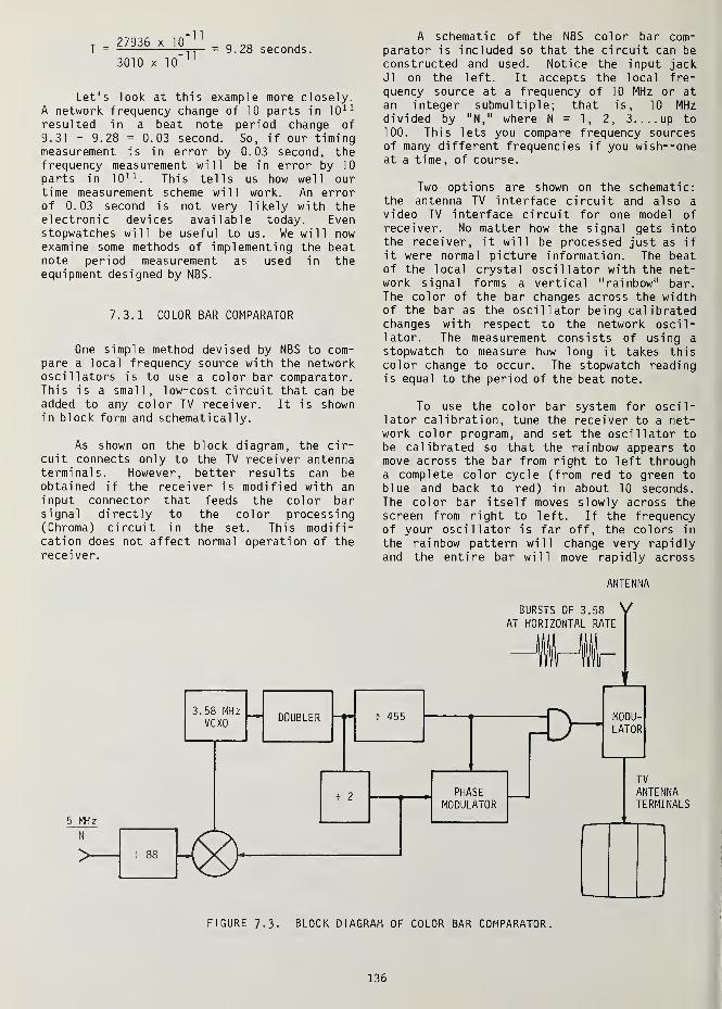
T = 27936 x 10-11

3010 x 10-11

= 9.28 seconds.

Let's look at this example more closely.A network frequency change of 10 parts in 10 11

resulted in a beat note period change of9.31 - 9.28 = 0.03 second. So, if our timingmeasurement is in error by 0.03 second, thefrequency measurement will be in error by 10

parts in 10 11. This tells us how well our

time measurement scheme will work. An errorof 0.03 second is not very likely with theelectronic devices available today. Evenstopwatches will be useful to us. We will nowexamine some methods of implementing the beatnote period measurement as used in theequipment designed by NBS.

7.3.1 COLOR BAR COMPARATOR

One simple method devised by NBS to com-pare a local frequency source with the networkoscillators is to use a color bar comparator.This is a small, low-cost circuit that can beadded to any color TV receiver. It is shownin block form and schematically.

As shown on thecuit connects only to

terminals. However,obtained if the receiinput connector thatsignal directly to

(Chroma) circuit in

cation does not affectrecei ver.

block diagram, the cir-the TV receiver antennabetter results can be

ver is modified with an

feeds the color barthe color processingthe set. This modifi-normal operation of the

3.58 MHz

VCX0

5 MHz

N

D0UBLER

A schematic of the NBS color bar com-parator is included so that the circuit can be

constructed and used. Notice the input jackJl on the left. It accepts the local fre-quency source at a frequency of 10 MHz or atan integer submultiple; that is, 10 MHzdivided by "N," where N = 1, 2, 3 up to100. This lets you compare frequency sourcesof many different frequencies if you wish— oneat a time, of course.

Two options are shown on the schematic:the antenna TV interface circuit and also a

video TV interface circuit for one model ofreceiver. No matter how the signal gets intothe receiver, it will be processed just as if

it were normal picture information. The beatof the local crystal oscillator with the net-work signal forms a vertical "rainbow" bar.The color of the bar changes across the widthof the bar as the oscillator being calibratedchanges with respect to the network oscil-lator. The measurement consists of using a

stopwatch to measure how long it takes thiscolor change to occur. The stopwatch readingis equal to the period of the beat note.

To use the color bar system for oscil-lator calibration, tune the receiver to a net-work color program, and set the oscillator to

be calibrated so that the rainbow appears tomove across the bar from right to left througha complete color cycle (from red to green toblue and back to red) in about 10 seconds.The color bar itself moves slowly across thescreen from right to left. If the frequencyof your oscillator is far off, the colors in

the rainbow pattern will change very rapidlyand the entire bar will move rapidly across

ANTENNA

BURSTS OF 3.58 VAT HORIZONTAL RATE

455 3>PHASE

MODULATOR

FIGURE 7.3- BLOCK DIAGRAM OF COLOR BAR COMPARATOR.

136

FIGURE 7.4. SCHEMATIC, COLOR BAR COMPARATOR

137

the screen in the direction of the colorchanges. The bar can be positioned to themiddle of the screen by the pushbutton labeled"Horizontal Sync Phasing."

With the rainbow repeating colors in

about 10 seconds, carefully adjust the crystaloscillator until the period is:

result. Other versions of the FMC are commer-cially available that use a separate digital

display rather than the TV screen.

The FMC automatically performs the

operation of measuring the period of the 3.58MHz beat note "T," computing At/T, scaling the

result for readout in parts in 10 11, and dis-

playing the one- and ten-period averages onthe TV screen. Readout is a series of 4-digitnumbers, representing the relative frequencybetween the oscillator being calibrated and

the atomically-control led color subcarrier. Byreferring to network data published monthly in

the NBS Time and Frequency Bulletin, a user of

the FMC can set his oscillator to agree withthe NBS standard to better than 1 part in 10 10

in five minutes and 3 parts in 10 11 in fifteenminutes. Radio methods of calibrating oscil-lators traceable to NBS require several daysof "averaging" to achieve this resolution.Measurement uncertainties as a function ofaveraging time that may reasonably be expectedare:

27936 x 1011

seconds.NBS DATA FOR NETWORK BEING VIEWED

If possible, check more than one networkto increase the confidence in calibration.Also, by measuring over ten beat note periods,the effect of reaction time with the stopwatchwill be reduced. Recall that for 1 period, an

error of 0.03 second corresponds to a fre-quency error of 10 parts in 10 11

. For tenperiods, a measurement error of 0.03 secondwill result in a frequency error of 1 part in

10 11 .

AVERAGING TIME

10 seconds

100 seconds

15 minutes

30 minutes

MEASUREMENT UNCERTAINTY

3x10

6x10

2x10

1.5 x 10

10

-11

-11

-11

When making network frequency com-

parisons, the FMC will also accept as input

any oscillator whose frequency is 10/N MHz,

where "N" is any integer from 1 to 100. The

highest available frequency should be used

when there is a choice.

As mentioned before, the rainbow will beof higher quality if the signal is connectedinto the receiver as a video signal. Theimprovement is due to the fact that antennainjection also modulates the received audiocarrier. This results in a visible beat notethat constantly changes with the audio contentof the program. The other example circuitshown connects the signal directly into theChroma bandpass amplifier. The rainbow is

then nearly perfect.

7.3.2 THE NBS SYSTEM 358 FREQUENCY

MEASUREMENT COMPUTER

For those users who require accuraciesapproaching 1 part in 10 11

, another cali-bration method is available. The system 358Frequency Measurement Computer (FMC) computesand displays the oscillator's relative fre-quency directly on the TV screen. The usersimply turns on the unit and waits for 15

minutes. He then comes back, reads off 10

values, and averages them to obtain the

The FMC consists of a 5- inch color TV re-

ceiver with an additional electronics package

mounted to its base. Readout for the FMC is

on the TV screen, with two columns of ten

4-digit numbers, and an additional analog

"phase cursor.

"

A. Block Diagram Overview

The FMC is divided into four main func-

tional parts: relative frequency scaler; beat

note phase comparator and cursor generator;

data store and display; and relative frequency

generator. In this section, the term "offset"

is used interchangeably with "relative fre-

quency."

1. Relative Frequency Scaler . The rela-

tive frequency or offset scaler processes the

beat note and 3.58 MHz signals to generate an

output count proportional to relative fre-

quency x 10- 11. This output count is applied

directly to the single-period 4-digit counter.

138

<smm~—• :

national mmtm or hamoawm. SYSTfM 3M FCfOtSNCY MfASUHMIMr COMWTM.

FIGURE 7.5. THE NBS PROTOTYPE, SYSTEM 358 FREQUENCY MEASUREMENT COMPUTER.

OFFSET SCALER STORE a DISPLAY

4 DIGIT 6x40COUNTER SR

4 DIGIT 6x40COUNTER SR

DISPLAY

LOGIC

VIDEOMIXER

DISPLAYVIDEOTO TV

FIGURE 7.6. BLOCK DIAGRAM, SYSTEM 358 FREQUENCY MEASUREMENT COMPUTER.

139

A new measurement is stored in the 6 x 40single-period shift register (SR) for readout.The output count of the scaler is also appliedto the 4-digit ten-period counter through aninhibit gate and a 7 10 prescaler. Theten-period counter therefore accumulates 1/10of its total count on each single-periodmeasurement.

Theory of the Scaler . The scaleraccepts the beat note and the color subcarrierfrequency, fls from the TV. The variabledivider generates output pulses at the rate R

= Af x 10 4 ; that is, 10,000 times the beatnote frequency. These rate pulses are gatedon for a time equal to 10 7/f 1 . The count out-put to the data store counters is therefore:

— x 1011

(count = R x TG = Af x 104

x —\f f

l

This rate output is accumulated in the 4-digitcounter for a period of time determined by

time gate, TG, which enables the "and" gatepreceding the counter. The total output countfor each measurement cycle can be expressedas:

OUTPUT COUNT = R x TG

lf in4 10'Af x 10 x — ^x 10

11.

Therefore, if Af/f x= 3000 x 10- 11

, the outputcount accumulated will be

— x 1011

= [3000 x lO-11

] x 1011

The objective is to obtain a reading on a

4-digit counter at the output such that eachaccumulated count is equal to 1 part in 10 11

relative frequency between f x and f2 . We canverify that this has been accomplished by thefollowing analysis. First, relative frequencyis defined as:

RELATIVE FREQUENCY = OFFSET =f

l" f

2 Af

The beat note comparator generates f x - f2 =Af. The beat note frequency, Af, is appliedas a start-stop gate to the period counter,"P." The total count accumulated in "P" in

one cycle of Af can be expressed as:

1 pn _f1

x 10

Af

3000 x 10° = 3000 counts.

The scaling factor for the output is theproduct of the 104 divider and 10 7 time gate.

These two factors may be partitioned in otherways--for example, 10 5 and 10 6 or 103 and 10 8

;

however, the partitioning used here is optimumfor the nominal 3000 parts in 10 11 offset to

be measured.

With the partioning used and an offset of

3000 parts in 10 11, the period count will be

3,333 and the time gate, TG, will be on for

0.3 of the beat note period. The maximumoffset that can be measured is 10,000 parts in

10 11 , in which case the time gate is on con-

tinuously, and simultaneously, the 4-digitcounter overflows. The minimum offset that

can be measured is determined by overflow of

the 16-bit period counter, P. This occurs at

an offset of approximately 150 parts in 10 11.

For each cycle of Af, the period count is

latched and applied to the rate generator,where the output rate is

R =

Neither the 3.58 MHz color subcarrier nor

the 10/N MHz input to be compared with it has

been mentioned in the preceding discussion.

Normally, f x is the 3.58 MHz input and f2 is

the harmonically related 10/N MHz input. How-

ever, the unit will work equally well with any

frequencies that have harmonically related

offsets in the range of 150 to 10,000 parts in

10 11 .

The rate of output pulses from divider (-rP)

is:

R =

f, x 10

Af

-4At- = Af x 10

4

10

2. Beat Note Phase Comparator and Phase

Cursor Generator . The phase comparator sec-

tion compares the phase of each 126th cycle of

3.58 MHz from the TV receiver with each 176th

cycle of the "A" input. This circuit performs

the same harmonic synthesis function as the

network oscillators which generate 3.579545454

... MHz by taking 63/88 x 5 MHz. The analog

140

voltage resulting from this phase comparison

is stored in a sample-and-hold integrator.

The analog "beat note" is further processedthrough two paths, the phase cursor path for a

visual indication of the beat note and a

Schmitt trigger to condition the signal for

the TTL offset scaler input.

Illllli4

2999 30003000 30003000 30003005 30003000 30003000 30003000 30002975 30003000 30003000 3000

pleted and the data are loaded into the top 4

digits in the left column. The second 4

digits in the left column will now be inten-sified. On each following 10-second interval,data are loaded into succeeding positions in

the left column until ten single-periodaverages have been accumulated. At this time,

the 10 single-period measurements are averagedand then loaded into the top 4 digits of theright-hand column. This process continuesuntil all 10-period averages have been loaded.

Two operator aids are included in thisNBS equipment. If a large phase jump occursat any time in the sequence, the correspondingsingle-period offset will be read out, butthat measurement wi 1 1 not be incorporated into

the 10-period average. On the next measure-ment cycle, that single-period average will berewritten and the count incremented. The TVspeaker "beeps" as a reminder to the operatoreach time a measurement is completed.

3. Data Store and Display . The gatedfrequency from the offset scler is accumulatedin the two 4- digit counters in the datastore-and-display section. After each beatnote measurement cycle, the single-periodcounter is gated on for 2.79 seconds. Theaccumulated single-period count is then dumpedto the single-period store for readout. The10-period 4-digit counter is preceded by a -HOso on each single-period average, it accumu-lates 1/10 of its total count. At the end often 1-period averages, the 10-period countercontents are dumped to the 10-period store forreadout.

The readout data are presented as two

columns of ten 4-digit numbers. The left

column represents single-period offset read-

outs and the right column represents ten-

period offset readouts. To start a measure-ment sequence, the user pushes the resetbutton. All readouts are reset to zero andthe top 4 digits in each column are inten-sified, indicating that data will be loaded in

these positions.

At the end of approximately 13 seconds,the first single-period measurement is com-

B. Use of FMC with Unstable

Crystal Oscillators

The FMC is primarily intended to cali-

brate with stability of better than 1 part in

10 7 per day. In fact, if the oscillator beingcalibrated will not hold still to better than

1 part in 10 7(± 10,000 parts in 10 11 ), the

digital readout cannot be used. About the

best one can do with a really poor-qualityoscillator is make the cursor "stand still"momentari ly.

If the cursor moves less than one cycle

each three seconds, then the oscillator is

within 1 part in 10 7 of the color subcarrier.

By switching between networks, one can obtain

a "concensus;" however, there is no way to

really verify if the subcarrier is originating

from a network, as can be done by checking a

good oscillator.

The FCC requires all stations to maintain

3. 5795454545. . . MHz ± 10 Hz on their sub-

carriers, so by comparing with several sta-

tions, one is assured of being within 3 parts

in 106 . If the oscillator being calibrated is

stable to 0.001% (1 part in 10 5), it is close

enough.

7.4 GETTING GOOD TV CALIBRATIONS

Although the frequency calibration

service using TV reduces the labor of cali-

brating an oscillator, it does not relieve the

user of the responsibility of verifying that

"good" data are actually being processed. The

user must be sure that the station being used

is actually transmitting network-originated

programs. (See Section 7.5).

141

At the present time, data for three net-

works are available from NBS. The easiestthing to do is to take successive readings, if

possible, on all three networks for 1.5

minutes each and verify that they differ rela-tive to each other by approximately the cor-

rect amount. Nominally, ABC operates at ex-

actly -3000 parts in 10 11.

Assume relative frequency readings weretaken with the following correct results:

FABC

=-3131 xlO

F.,D ~ = -3150 x 10NBC

FrDC = -3130 x 10

The readings are consistent from one networkto another. If one of the three had differedradically from its correct relative value, wecould assume that the station involved was onlocal programming. For example, if thereading for NBC were -2460, then the NBC sta-tion would not be used at that time.

Measurements must be made only whennetwork-originated programs are on the air.Network stations in the Eastern, Central, andPacific time zones typically carry 10 to 14

hours of network-originated programs per day.

The Mountain time zone carries about fourhours per day.

It should be noted that network-originated programs are not necessarily "live"programs (such as football or basketballgames). It simply means that the programs areoriginated from the network centers in eitherLos Angeles or New York City and are not tapedelayed by the local stations. Programsoriginating at the local stations (such as thechannel 7 news as opposed to CBS Evening News)cannot be used.

The best choices are the daytime soap op-eras and quiz shows. These usually are dailyprograms and originate from the New York and/or Los Angeles network centers. Weekly even-ing programs are usual ly network-originatedexcept in the Mountain Time Zone. Once theprogramming schedule in any given city is

identified, a log can be made to indicate whenmeasurements can be made. There is, however,one further word of caution (see below).

7.5 THE DIGITAL FRAME SYNCHRONIZER

Some local stations are now using digitalframe synchronizers on their incoming network

lines. This is true of the ABC stations in

the San Francisco and Chicago areas, whichprovide network feeds to other local stationsin the area, as well as many other local sta-

tions throughout the country.

The frame synchronizer stores one com-

plete TV frame (1/30 second) in digital memoryand "reads" the TV picture under control of

the local station sync generator. Since mostsync generators are driven by a crystal oscil-lator, the color subcarrier is no longer ref-

erenced to the network atomic standard, andthe signals cannot be used for frequency cali-bration.

The ABC stations in Los Angeles and NewYork also use frame synchronizers on theincoming network lines, but these stations areco- located with the network studios and use

the network cesium standards for their 3.58MHz reference. Therefore, WABC and KABC stillprovide stable frequency references and can beused for frequency transfer measurements.

In 1978, a questionnaire was sent to all

network-affiliated TV stations to determinewhich ones are using or plan to use frame syn-chronizers. The results of this survey areavailable upon request from the Time and Fre-

quency Services Group, National Bureau of

Standards, Boulder, CO 80303.

At present, only a few of the largest TVstations have two or more frame synchronizers.The smaller stations that have a single framesynchronizer will use it for their "electronicnews," not to hang across the incoming networkline. Of course, this situation may change in

five years if the price of synchronizersdrops.

If you are using the TV networks for

frequency transfer, the best precaution is

simply to use more than one network so that

data can be verified.

7.6 USNO TV FREQUENCY CALIBRATION SERVICE

The USNO also offers a TV frequency cali-

bration service to users who can receive sta-

tions WTTG (Washington, D.C.), WAPB (Annapo-

lis, MD), or KTTV (Los Angeles, CA). The USNO

has stabilized the frequency of the cesium

standards at these stations, so the service

is somewhat different than the NBS service.

For information, contact the Time ServicesDivision, U. S. Naval Observatory, Washington,

DC 20390.

142

WORKSHEET FOR USE WITHCOLOR BAR COMPARATOR

DATE: START TIME:

NETWORK NBC CBS ABC

ENTERPUBLISHED

DATA

COMPUTEPERIOD*

STOPWATCHTIMES

AVERAGE:

COMPUTERELATIVE

FREQUENCY**

27936 X 10" n

=27936 *

'°"n= XXXX SECONDS BEAT

PUBLISHED DATA XXXXXX NOTE PERIOD.

27936 X 10" n

=27936 * 10

~"= XXXXXX RELATIVE

MEASURED TIME XXXXXX FREQUENCY OF YOUROSCI LLATOR.

Compare PUBLISHED DATA with COMPUTED RELATIVEFREQUENCY to determine difference between youroscillator and the NBS frequency standard.

WORKSHEET FOR USE WITHDIGITAL OFFSET COMPUTER

DATE: START TIME:

NETWORK NBC CBS ABC

ENTERPUBLISHED

DATA

10-PERIODAVERAGES

100-PERIODAVERAGE

YOUR OSC.VS NBS

Compare the 100-period average with PUBLISHED DATAfor each network. If it is higher than PUBLISHEDDATA, then the oscillator being calibrated is toohigh in frequency. If it is lower, then the

oscillator is too low In frequency.

FIGURE 7.7. SAMPLE WORKSHEETS FOR USING TELEVISION SUBCARR I ER FOR FREQUENCY TRANSFER

.

143

CHAPTER 8. FREQUENCY AND TIME CALIBRATIONS USING TV LINE-10

The previous chapter discusses the use of the TVnetwork color subcarrier for frequency calibrations.The television synchronization pulses can also be usedas a transfer standard for both time and frequency.

A television picture is made up of 525 lines whichare scanned or traced to produce the image you see onthe screen. First, the odd lines (called the oddfield) are traced, then the even lines (the even field)are traced in between the odd. This scanning happensso fast (60 times a second) that your eyes cannot de-tect it and you have the illusion of seeing acontinuous picture.

Line- 10 (odd) is one of the 525 lines that makeup each picture; it can be used for both frequency andtime calibrations. It was chosen because it is easyto pick out from the rest of the lines with relativelysimple electronic circuits. To calibrate an oscilla-tor, a clock pulse from the oscillator is compared tothe trailing edge of the Line-10 (odd) synchronizingpulse. Measurements by users of this service, madewith specially-designed equipment, will correspond tomeasurements made at NBS at the same time.

Now that we know what Line-10 is, let's say whatit isn't. It isn't the color subcarrier! In the pre-vious chapter, we discussed using the color subcarrieras a frequency calibration source. Line-10 has nothingto do with the color subcarrier system. Line-10 workswith either color or black and white television sets.Some equipment that is designed for the color subcar-rier system will have a Line-10 output pulse becauseit is handy to do so, but the techniques involved areentirely different for the two TV-based systems. Theydo have one thing in common, though. All measurementsusing either system must be made on network (major U.S.television networks) programming if NBS traceabilityis to be achieved. In addition, Line-10 measurementsmust be made at exactly the same time of day that NBSmakes its measurements. (Neither of these requirementsapply if you are using Line-10 on a local basis.) Thiswill be discussed more fully later on.

Jit

; —JLL / - w >

\u Z__Z2S~

—

t~tt:.;:

—zi '

FIRST THE ODD FIELD IS TRACED.

1^J 2_

THEN THE EVEN FIELD IS TRACED.

FIELDS COMBINE TO FORM

COMPLETE PICTURE.

8.1 HOW THE SERVICE WORKS

Assuming that you have a TV receiver anda Line-10 pulse is available, what do you dowith it? You can use it to set your clock orto measure and/or set the frequency of youroscillator. It provides a means of checkingoscillators to within parts in 10 11

, but theoscillator/clock should be of fairly highquality (1 part in 108 or better).

8.1.1 USING LINE-10 ON A LOCAL BASIS

To understand how the service works,let's discuss a real-life example: The Line-

10 method is used routinely to compare the

NBS frequency standard in Boulder, Colorado,with the clocks at radio stations WWV and

WWVB in Ft. Collins, Colorado. Both locations

are within common view of the Denver televi-

sion stations. Let's assume that the clocks

in Boulder and Ft. Collins are synchronized.

Now suppose we measure the arrival time of the

TV Line-10 synchronization pulse at Boulder(location A) with respect to the NBS standard.

A short time later, this same pulse will

arrive at Ft. Collins (location B) and we can

measure its arrival time with respect to the

Ft. Collins clock. Since the clocks are

synchronized, the difference in the two clock

readings is only the differential propagation

delay, written tR

- t. as shown in figure 8.1.

145

B

FIGURE 8.1 DIFFERENTIAL TIME

DELAY, TB

- TA

.

We now know the propagation delay betweenBoulder and Ft. Collins. If we make anothermeasurement and find that the difference in

the two clock readings is not equal to the

propagation delay, then this means that one of

the clocks is running faster or slower than

the other. The discrepancy represents the

time difference between the clock at

Ft. Collins and the clock at Boulder.

The same technique can be used by anyonewho wants to transfer time and/or frequencyfrom one location to another. This works only

when both locations can see the same TV sig-

nal. An example of using this technique wouldbe a factory with scattered branches that

wants to calibrate an oscillator at one of the

branches that is not within cabling distanceof the main factory. By using two Line- 10

units, the factory and the branch can both

look at a local TV signal and effect the

transfer.

Even if you don't know the propagationdelay, the Line-10 technique can be used to

determine the frequency stability of youroscillator compared to another. Using a

divider, simply operate your oscillator as a

clock. By watching the day-to-day differ-

ences, you can tell if your clock is gaining

or losing with respect to the clock used for

comparison.

Note that such a local signal can be any

kind of TV signal, not necessarily network TV.

Also, the accuracy of transfer using this

method can be very great. The NBS link to Ft.

Collins typically can achieve ten nanoseconds

time transfer. Local use of Line-10 is a

cheap way to distribute frequency and time at

high accuracy levels.

8.1.2 USING LINE-10 FOR NBS TRACEABILITY

In figure 8.1, we assumed that both loca-

tions were within common view of the same

television station. However, in actual prac-

tice, a given TV program can be observed si-

multaneously over a large geographical region

because of the TV microwave distribution net-

work. For example, this technique has been

used to compare clocks in the Boulder and

Washington, D. C. areas by making simultaneous

measurements on programs originating from New

York City (see figure 8.2).

NBS routinely makes readings on the three

major networks on both the East and West

Coasts. These data are published monthly in

the NBS Time and Frequency Bulletin, which is

available upon request. A sample page of the

Bulletin is shown in figure 8.3.

If you want to compare your clock with

the NBS standard, you must make your measure-

ments at the same time as NBS and, in addi-

tion, the measurements must be on programs

NEW YORKORIGINATING STUDIO

-y\p ATOMIC FREQUENCY

Sri CONTROL

MICROWAVE PATH FROMNYC TO DENVER, COLO. 4000-6400 km*VHF PATH FROM DENVER TRANSMITTER TONBS 30 km

•DEPENDING ON NETWORK

WASHINGTON, D.C.

AFFILIATE

FIGURE 8.2 TYPICAL ROUTING OF TV SIGNALS FROM NEW YORK CITY

ORIGINATING STUDIOS TO DISTANT RECEIVERS.

146

UTC.

EAST COAST

AUG.

UTC(NBS) - LINE 10 (ODD) (in microsecond;)

NBC ABC

19:25 00 19:31 00 19: 26 00 1 9 : 32 : 00 19:27 00 19:33:00

15694 75 08672 31 31093 91 24071 .52 15667 06 08644.55

32005 47 24983 03 14018 02 06995.50 31872 57 24850.06

14949 71 07927 26 30308 97 23286.38 14884 43 07861 .91

31260 82 24238 38 13233 12 06210.59 31090 14 24067.63

1 4205 24 07182 67 29523 82 22501 .28 14015 66 06993 • 1

2

29771 69 22749 24 1 1663 10 04640.58 29525 03 22502.51

12715 81 05693 36 27954 14 20931 .62 12450 44 05427.93

29026 94 22004 47 10878 29 03855.73 28742 49 21719.93

12058 43 05035 96 27168 97 20146.43 1 1667 93 04645.40

28282 51 21260 09 10093 04 03070.54 27960 03 20937.53

00259 24 26603 42 25598 64 18616.28 15259 36 O8236.83

16567 44 09542 88 08522 81 01500.38 31551 49 24529.06

32873 49 25851 00 24813 56 17791 .00 14477 22 07454.66

158 14 94 08792 46 07737 72 00715.15 23746.32

32123 48 25101 04 "^^^4029 13 17006.61 06699.40

1

2

3

4

5

6

7

8

9

10

1

1

12

13

14

15

16

17

18

19

20

FIGURE 8.3. NBS LINE-10 DATA FROM NBS TIME & FREQUENCY BULLETIN.

originating from a common source—New YorkCity (for the Eastern, Central, and Mountaintime zones) or Los Angeles (for the PacificTime Zone). Currently, measurements are madeby NBS on the East Coast networks at the fol-lowing times: NBC— 2025 and 2031 UTC; CBS—2026 and 2032 UTC; ABC— 2027 and 2033 UTC(During Daylight Saving Time, the measurementsare made beginning at 1925 UTC.) West Coastmeasurements (furnished by the Hewlett-PackardCompany in Santa Clara, California) are madeat: NBC— 2125 and 2131 UTC; CBS— 2126 and2132 UTC; ABC— 2127 and 2133 UTC (all yearround).

The measurements at NBS are made on thetrailing edge of the horizontal Line- 10 (odd)sync pulse which occurs approximately everyl/30th of a second. This means you mustalready know your time to 1/30 of a second orbetter to be assured that you are measuringthe same pulse that is being measured by NBS.

All of this sounds fairly straightfor-ward, but it isn't all that tidy. First ofall, the calibration isn't available to theuser until he receives the data he needs in

the mail. This means that he must keep care-ful Line-10 records and wait for the results.

Meanwhile the clock must be kept running so

that when the data arrive and the comparisonis made, the clock error can be determined andsomething done about it. This means that theclock involved must be a pretty good one. It

should be as good as 1 part in 108 or better.Otherwise, the whole operation will be labor-intensive and the user will not be able to

predict the time very well. Nor will he knowthe frequency very accurately if the systemhas large variations. Line-10 provides a

means of checking oscillators to within partsin 10 11

, but the oscillators must be of highenough quality to deserve the investment oftime and effort. If you need lower accuracy,there are cheaper ways that require lesseffort.

8.2 EQUIPMENT NEEDED

To use the Line-10 technique, you need a

black and white or color TV receiver, a

line-10 synchronized pulse generator, a digi-tal counter-printer, and a precision clock.Line-10 equipment is commercially available.The TV receiver is adapted to bring out thecomposite video signal that connects to the

147

LOCAL ATOMICCLOCK

LINE-10 PREAMPPULSE GENERATOR

SIGNAL FROMLOCAL TV

TRANSMITTER

FIGURE 8.4 EQUIPMENT NEEDED FOR TV LINE-10 METHOD OF CLOCK SYNCHRONIZATION.

Line-10 pulse generator. This pulse is com-pared on a time-interval counter with a localone-pul se-per-second clock. The display onthe counter (start with local clock, stop withLine-10) will be a series of numbers (seefigure 8. 4).

8.3 TV LINE-10 DATA, WHAT DO

THE NUMBERS MEAN ?

How do we get the numbers and what dothey mean? First of all, let's review thebasis for the frequencies used by commercialtelevision systems in the U. S. The FCCspecifies the frequency used for the chromi-nance subcarrier to be 3.5795454 ... MHz ± 10

Hz. The networks get this number by taking a

5 MHz oscillator and multiplying its output by63 and dividing by 88. Then, the FCC statesthat the horizontal rate for the picture shall

be 2/455 of the color subcarrier. This is

15.7342657 kHz. Next, you get the verticalrate by taking 2/525th of the nominal 15.7kHz, giving a vertical rate of 59.94 Hz. ButLine-10, the one we want, only occurs everyother field so its rate is half of the verti-cal rate, or 29.97 Hz, and has a period ofabout 33 milliseconds— 33.3666666... to beexact.

Now, in our Line-10 instrumentation set-up, we start our time interval counter withour clock at a 1 pps rate and stop it with thenext Line-10 pulse. A stream of Line-10 datais shown in figure 8.5.

A reading occurs each second, each read-ing being slightly different from the one pre-ceding it. Let's look at that difference.Notice the second and third columns which are

reading milliseconds. The number increasesprogressively by 1 millisecond per second.This is because Line-10 occurs at a frequencyrate that is not an integer and appears todrift relative to our 1 pps. When the countapproaches 33 milliseconds total, the timeinterval counter is stopped by the nextLine-10 pulse that comes along, but it mustalways occur before 33 milliseconds elapse.

So instead of reading the number abovethe double line plus the 1 millisecond persecond which would equal 33.3101 + 1.00000 =

34.3101, it must stop at the very next Line-10pulse which appeared at the counter stop inputat 34.3101 - 33.3666 = 0.9435. This is what

NBC LINE-10 (EAST COAST)

FEBRUARY 11

UTC ms ys

20 35:41 025 309.9320 35:42 026 309.9620 35:43 027 309.9920 35:44 028 310.0220 35:45 029 310.0520 35.46 030 310.09

031 310.11032 310.14033 310.17

000 943.53001 943.56002 943.59003 943.62004 943.65

FIGURE 8.5. PRINTOUT OF NBC LINE-10 DATA.

148

AVERAGE RELATIVE FREQUENCY (in parts in 10 1

1

)

MEASUREMENT PERIOD EAST COAST WEST COAST

NBC CBS ABC NBC CBS ABC

2-6 FEBRUARY -301 9.4

9-13 FEBRUARY -3019-5

16 - 20 FEBRUARY -3019.6

-2963.0

-2963.

1

-2963.2

-3012.3

-3012.4

-3012.7

-3019.

3019.

3019.

-3015.2

-3015.4

-3015-7

FIGURE 8.6. TELEVISION NETWORK FREQUENCIES RELATIVE TO THE NBS FREQUENCY STANDARDAS PUBLISHED IN THE NBS TIME & FREQUENCY BULLETIN.

was printed out. The time interval countercannot ever print a number bigger than theperiod of the highest frequency on the "stop"input. Notice, too, that the last column in

the data is also changing. The counter-printer displays 0.01 microsecond in the lastdigit and is changing at a rate of 30 nano-seconds (0.03 microsecond) per second.

How does this happen? In addition to

operating at a frequency that is a non- integer,each TV station will have an error because its

oscillator frequency differs from the NBS fre-quency standard. It differs enough to show up

on a high resolution record like this one. It

shows up on the published NBS data in figure8.6. On the date these data were recorded,NBC's relative frequency was -3019.4 parts in

10 11 ; that is, just over 3 parts in 108 . Justlike any clock that is running at a differentrate, it will accumulate a time error. In

this case, the time error due to the basicfrequency difference between NBS and NBC is

30.194 nanoseconds per second. So our datawill show this amount of change, and it does.Since NBC's frequency is low relative to NBS,and its Line-10 pulse is stopping the clock(our time interval counter, in this case), theLine-10 pulses arrive later and later by the30.194 nanosecond amount each second. This is

evident in the last column of the printout(figure 8.5) as an increasing number since thetime interval counter counts just a littlelonger each second. If local programming is

used, such as between Boulder and Ft. Collins,this number can change by as much as 50 or 60

nanoseconds per second. It can also decreaserather than increase.

Although you can print out several num-bers for each network, only the first numberis used--the one that occurs right on theexact second that NBS is making measurements.Taking several readings insures that theequipment is working properly. Also, if youhappen to miss the first second, you can

reconstruct the data. This is not a recom-mended practice, but it can be done.

8.4 WHAT DO YOU DO WITH THE DATA?

Assume that data are taken daily, carefulrecords are kept, and the clock-oscillatorcombination being used for TV Line-10 data is

not disturbed. After all, if you are record-ing data for 30 days and waiting for a checkwith NBS, you must not alter the setup. Thedata points can be tabulated or, better yet,plotted on graph paper. The accumulated timeerror of the oscillator is a measure of its

frequency offset. Therefore, the data serveto calibrate the relative frequency of theoscillator with respect to NBS. Notice thatwe are making and recording time measurementsto get frequency. As you will read later, we

can also get time, but we must make some

further measurements to get it.

Figure 8.7 shows the raw data for an

oscillator being calibrated with the TV Line-10

system. The counter used for this measurementhad a resolution of 0.1 microsecond. For the

data taken, it appears that the oscillatorchanged about 10 microseconds a day relative

to NBS. This works out to be about 1 part in

10 10 frequency error. Having three major U.S.

networks gives a good self-check on the systemaccuracy. Although the data will be slightly

different for each of the three networks, the

calibration error will be small.

8.5 RESOLUTION OF THE SYSTEM

How good is the system? It has been

known to produce consistent results of around

1 part in 10 11 over a period of several years.

If you are willing to pay attention to de-

tails, you can achieve similar results. Of

course, you must have a fairly good TV signal.

149

NBS LINE- 10 DATA-JUNE

USER'S LOCAL CLOCKLINE- 10 DATA

Dl FFERENCE""NBS -

LOCAL CLOCK

DAI LY

ACCUMULATION(MICROSECONDS)

TOTALACCUMULATION(MICROSECONDS)DAY (NBC) (NBC)

7 02216.54 05339.9 -3123.4 0 0

8 19526.34 22660.

1

-3133.8 -10.4 -10.4

9 02374.93 05518.6 -3143.7 - 9.9 -20.3

10 18779.21 21934.0 -3154.8 -11.1 -31 .4

1

1

01722.58 04888.5 -3165.9 -11.1 -42.5

'Published in NBS Time & Frequency Bui 1 et i n .

-This heading establishes a method for the user to learn if his clock is gaining or

losing time. Since the NBS clock is always "on time," the user's data are subtractedfrom the NBS reading. It is as if a time interval counter produced this column wherethe NBS clock opens the gate and the user's clock closes it.

COMPUTING THE OSCILLATOR FREQUENCY

(Refer to Chapter 3 for explanation of the math)

Us ACCUMULATED IN 5 DAYS: -42.5NO. OF MICROSECONDS (AVERAGE )_ 10^6 = At

But one day has 86,400 x 1 0bmicroseconds. So:

At -10.6 . ..-10- —=- = 7- = -1 .23 x 1

0

86,400 x 10b

., At Af . „. . 1

0

Al so: = —- = 1 .23 x 10

This is the relative frequency of the user's oscillator with respect to NBS. Theactual frequency of the user's oscillator can also be found. If we assume this is

a 2.5 MHz oscillator, then:

Af ^actual ^nominalf f . .

nom 1 na

1

in f '

, - 2.5 x 106

Substituting 1 .23 x 10~' U=

ac™ai

2.5 x 10b

Solving: factual

= 2 - 500 , 000 . 0003075 Hz.

So the user's oscillator is higher than it's nominal value by a very small amount

FIGURE 8.7. COMPUTATION OF OSCILLATOR FREQUENCY USING TV LINE-10 DATA.

150

It also helps your results if you can receiveall three networks and cross-check the resultsfor consistency. On the other end of the spec-

trum, would it be worthwhile to use the Line- 10

system for lower-quality oscillators? Theanswer is yes, but up to a limit. Aside fromthe fact that other frequency calibration ser-

vices are available on radio, the basis for a

decision of whether to use Line-10 or notrests with the amount of time the user is

willing to invest. For, as the oscillatorquality goes down, the amount of attention thesystem requires increases. It becomes neces-sary to look at the data more closely andrecognize and calibrate the larger frequencyshift that will occur.

If the user's oscillator has a frequencyerror of 1 part in 108 , it will gain or loseabout 1 millisecond per day. Since the TVLine-10 pulse is ambiguous (it occurs aboutevery 33 milliseconds), it would not be toohard to keep track of the data. However, if

the local oscillator drifted and was off as

much as 1 part in 106 , the data would getharder to interpret. This would allow a

change of 100 milliseconds per day and a dif-

ferent Line-10 pulse would be viewed by theuser than that seen and reported by NBS. Thisis the case for any clock that has a largetime error. Then, the user is stuck witheither noting the differences and plottingthem or correcting the data for whole periodsof the Line-10 sync signals. This is 33.3666... milliseconds. So, although just about anyclock oscillator can be used, it is not as

simple and straightforward if large clockdrifts are involved.

8.6 GETTING TIME OF DAY FROM LINE-10

Since the Line-10 data are directlytraceable to NBS, it contains time-of-dayinformation. As noted in the above paragraph,it is ambiguous to 33 milliseconds. Thismeans that if you want to set a clock accu-rately (to within microseconds), you mustfirst set it to within 33 milliseconds usingsome other scheme. A good way would be to use

radio station WWV and an oscilloscope. Onceyou are within the ambiguity range of theLine-10 data, you can use Line-10 to set theclock more precisely. You would need to know

I

the path and equipment delays. The path delay

!would just about have to be measured by carry-ing a clock to the NBS in Boulder. Once the

|

delays are known, and if the user records dataregularly from several networks, chances arehe can keep time to within several micro-seconds using Line-10.

The need to calibrate the path and re-

; solve the ambiguity may seem to penalize thissystem and suggest to the user that he usesome other method, but there are not very many

ways to get accurate timing. Chapter 9 de-scribes Loran-C techniques for accurate timesetting. It, too, needs to be calibrated andis ambiguous in the same way. So the stepsare the same and Line-10 costs less.

8.7 THE DIGITAL FRAME SYNCHRONIZER

As discussed in Chapter 7 (page 142),some local TV stations are using digital framesynchronizers which affect the use of thesestations for frequency calibrations. Theframe synchronizer also eliminates the use of

these stations for Line-10 time transfer whenit is in the differential path. The ABC sta-tions in Los Angeles and New York also useframe synchronizers on the incoming networklines so Line-10 reference is lost. For moreinformation on the stations that are usingframe synchronizers, contact the Time andFrequency Services Group, National Bureau ofStandards, Boulder, Colorado 80303.

8.8 MEASUREMENTS COMPARED TO THE USN0

The USN0 also publishes Line-10 measure-ments on the East Coast TV networks originat-ing in New York City. Their measurements aremade at the same time as the NBS measurements.Users desiring to compare their clocks withthe USN0 may obtain the USN0 data from theirTime Services Bulletin, Series 4. For moreinformation, write to the Time ServicesDivision, U. S. Naval Observatory, Washington,D. C. 20390.

8.9 LINE-10 EQUIPMENT AVAILABILITY

There are several manufacturers of TV

Line-10 equipment. The NBS has also designedequipment to recover the Line-10 pulse from a

commercial TV receiver. The circuit diagram

is shown in figure 8.8. The instrument

accepts 0.5 to 1.5 volts of video signal of

either polarity from a TV receiver and makes

available a Line-10 pulse referenced to either

the leading or trailing edge of sync. (Note

that the Line-10 measurements published in the

NBS Time and Frequency Bulletin are referenced

to the trailing edge of the Line-10 sync

pulse.) The problem is that you will have an

error equal to the width of the sync pulse if

you use the leading edge and NBS uses the

trailing edge. This design uses standard TTL

integrated circuits and could be assembled by

a skilled technician.

For more information about manufacturers

of Line-10 equipment, write to the Time and

Frequency Services Group, National Bureau of

Standards, Boulder, CO 80303.

151

FIGURE 3.8. SCHEMATIC OF TV LINE-10 EQUIPMENT DEVELOPED BY NBS.

152

CHAPTER 9. LORAN-C TIME AND FREQUENCY METHODS

Historically, many different radio sig-nals have been used for distributing time andfrequency. Some of the most successfuladapted for this purpose have been those ofthe Loran-C navigation system. In the 1950' s,after its initial development for navigation,work done at NBS showed that Loran-C signalscould be quite stable, and since then, theyhave been controlled and used for frequencyand time calibrations.

The success of Loran-C frequency and timesignals is due to a number of things. Eachstation is controlled by cesium standards.Careful control and monitoring of the signalsby the U. S. Coast Guard and the U. S. NavalObservatory allows a user to achieve rapid,accurate results. Groundwave signals providestate-of-the-art frequency and time calibra-tions. Even the skywave signals, thoughslightly less accurate, can become the basisof excellent high-quality calibrations.Loran-C coverage is increasing with the plannedaddition of new chains.

9. 1 BASIC PRINCIPLES OF THE LORAN-C

NAVIGATION SYSTEM

Loran-C is a radio navigation system thatbroadcasts on a frequency of 100 kHz using abandwidth from 90 to 110 kHz. At this lowfrequency, the radio waves follow the earth'scurvature; thus, they are relatively unboth-ered by the ionosphere and are very stable.

The Loran-C navigation system consistsof many synchronized "chains" or networks ofstations. These chains provide groundwavecoverage of most of the United States, Canada,Europe, the North Atlantic, the islands ofthe Central and West Pacific, the Philippines,and Japan. Information about the variouschains is given in Table 9.1.

One station in each chain is designatedas a "master" station; the remaining stationsare "slaves." The master station transmitsgroups of pulses that are received by theslave stations. The slave stations receivethe master pulse groups and, at later times,transmit similar groups of synchronizedpulses (figure 9.1).

On a ship or plane, the constant timedifferences between the reception of themaster pulses and the corresponding slavepulses establish a line-of-position that is

used for navigation. Signals from threeseparate Loran transmissions are needed todetermine a line-of-position. For frequencyand time applications, only a single Loranstation is needed.

The coverage and accuracy of Loran-Csignals depend upon the characteristics andformat of the transmitted signal. When thesystem was designed, tradeoffs were made to

make the system accurate and reliable. Thecharacteristics and format of the transmittedLoran-C signals can be broken down into thefollowing major elements:

PULSE GROUP FORMAT

MASTER

SECONDARY W

SECONDARY X

SECONDARY Y

SECONDARY Z

-START OF GROUP REPETITION INTERVAL (GRI)

SPACING 1 ,000 ps

I I 1 1 I II v I

2,000 ys

1 G R I-

SPACING 1,000 ys (ALL SECONDARY STATIONS)

I I II I

I I I

I I I I I I I I

I M I I I I I

PHASE CODE

1ST GRI ALTERNATE GRI

MASTER ++ +-4~

SECONDARY -I- ++4-++-

FIGURE 9.1. LORAN-C PULSE GROUP AND PHASE-CODE FORMAT.

153

TABLE 9.1 LORAN-C CHAINS

STATION LOCATION

CTATTON

IDENTIFI-CATION

PEAKRADI-ATFDn 1 LU

POWER(kW)

BASELINE

fODTNG

DELAY

Cm s

)

EMISSIONDELAY

(MS)

NAUTICALMILES

KILO-METERS

PATHLENGTH

(MS)

GREAT LAKES

REPETITION PERIOD:

99,300 |js (SS7)

DANA, IN

39° 51' 8" N

87° 29' 12" W

9930M(9960Z)

*

(OPERA!

400

IONAL FEBR JARY 1980)

MALONE , FL

30° 59' 39" N

85 10' 9" W

9930W(7980M)

*800

14355.1

SENECA, NY

42° 42' 51" N

76° 49' 34" U

9930X(9960M)

*800

31162.1

BAUDETTE, MN

48° 36' 50" N

94° 33' 18" W

9930Y

U. S. WEST COASTREPETITION PERIOD:

99,400 |js (SS6)

FALLON, NV

39° 33' 6" N

118° 49' 56" W

9940M 400

GEORGE, WA

47° 3' 48" N

119 44' 40" W

9940W1 cc\r\loUU 2,797.0 1

1, uuu 1 Q

These stations are members of two or more chains and are therefore dual or triple-rated. They

transmit on two (or three) rates with two (or three) pulse repetition periods.I'

154

STATION LOCATION

STATIONIDENTIFI-CATION

PEAKRADI-ATEDPOWER(kW)

BASELINE

CODINGDELAY(ps)

EMISSIONDELAY

(MS)

NAUTICALMILES

KILO-

METERS

PATHLENGTH

(MS)

MIDDLETOWN, CA

38° 46' 57" W122° 29' 45" W

9940X 400 1 ,094.5 27,000 28094.5

SEARCHLIGHT, NV

35° 19' 18" N

114° 48' 17" W

9940Y 500 1 ,967.2 40,000 41967.3

NORTHEAST U. S.

REPETITION PERIOD:

99,600 ps (SS4)

SENECA, NY

42° 42' 51" N

76° 49' 34" W

9960M(9930X)

*

800

CARIBOU, ME

46° 48' 27" N

67° 55' 38" W

9960W(5930M)

350 2,797.2 11 ,000 13797.2

NANTUCKET, MA

41° 15' 12" N

69° 58' 39" W

9960X(5930X) 275 1 ,969.9 25,000 26969.9

CAROLINA BEACH, NC

34° 3' 46" N

77° 54' 47" W

9960Y(7980Z) 700 3,221.7 39,000 42221.7

DANA, IN**

39° 51' 8" N

87° 29' 13" W

9960Z(9930M) 400 3,162.

1

54,000 57162.1

SOUTHEAST U. S.

REPETITION PERIOD:

79,800 ps (SL2)

MALONE, FL

30° 59' 39" N

85° 10' 9" W

7980M(9930W)

*

800

These stations are members of two chains and are therefore dual-rated. They transmit on two

rates with two pulse repetition periods.

155

STATION LOCATION

STATION

CATION

PEAKRADI-ATEDPUWtK(kW)

BASELINE

CODINGUtLMY

(MS)

EMISSIONUtLAY

(MS)

NAUTICALMILES

KILO-METERS

PATHLENGTH

(US)

GRANGEVILLE, FL

30° 43' 33" N

90° 49' 44" W

7980W 800 • 1 ,809.5 11 ,000 12809.5

RAYMONDVILLE, TX

26° 31'

55" N

97° 50' 0" W

7980X 400 4,443.4 23,000 27443.4

JUPITER, FL

27° 1'

58" N

80° 6' 54" W

7980Y 2752,201.9 43,000 45201.9

CAROLINA BEACH, NC

34° 3' 46" N

77° 54' 47" W

7980Z700 2,542.7 59,000 61542.7

WEST COAST OF CANADAREPETITION PERIOD:

59,900 lis (SHI)

WILLIAMS LAKE, BC

51° 57' 59" N

122° 22' 2" W

5990M 400

SHOAL COVE, AK

55° 26' 21" N

131° 15' 20" W

5990X(7960Y)

it

• 400 2,343.6 11 ,000 13343.6

GEORGE, WA

47° 3' 48" N

119° 44 1 40" W

5990Y 1600 1 ,927.4 27,000 28927.4

CENTRAL PACIFICREPETITION PERIOD:

49,900 us (SI)

JOHNSTON ISLAND

16° 44' 44" N

169° 30' 31" W

4990M 275

UPOLO POINT, HI

20° 14' 49" N

155° 53' 10" W

4990X 275 804.2 1 ,489.3 4,972.2 11 ,000 15972.4

*These stations are members of two chains and are therefore dual-rated. They transmit on two


STATION LOCATION



BASELINE

CODINGDELAY

(MS)

EMISSIONDELAY

(MS)

NAUTICALMILES

KILO-METERS

PATHLENGTH

Cm s )

KURE, MIDWAY ISLAND

ooo oo ' yio" ki*M N

178° 17' 30" W

4990Y 300 849.6 1 ,573.4 5,253.

1

29,000 34253.1

NORTH PACIFICREPETITION PERIOD:

99,900 us (SSI)

ST. PAUL,

PRIBILOFF IS. , AK

oi y 1 U N

170° 14' 60" W

9990M 275

ATTU, AK

kOO A Q 1 A C II KIZ3<L 43 40 n

173° 10' 52" W

9990X 275 3,875.3 11 ,000 14875.3

POINT CLARENCE, AK

CtrO "l/|l /in" KI00 14 4U N

166° 53' 14" W

9990Y 1000 3,069.

1

29,000 32069.1

NARROW CAPE,

KODIAK IS. , AK

C"70 oc i on" KIb/ 2b 20 N

152° 22' 11" W

9990Z

(7960X)

*

400 3,590.5 43,000 46590.5

NORTHWEST PACIFICREPETITION PERIOD:

99,700 (js (SS3)

IWO JIMA, BONIN IS.

o/iO /in I /ill hi24 48 4 N

141° 19' 29" E

9970M 1000

MARCUS ISLAND

O It O 1 T 1 /-ill h I

24 17 8 N

153° 58' 52" E

9970W 1800 692.9 1 ,283.2 4,283.9 11 ,000 15283.9

HOKKAIDO, JAPAN

42° 44' 37" N

143° 43' 09" E

9970X 400 2,002.3 6,685. 1 30,000 36685.1

*



157

STATION LOCATION



BASELINE

CODINGDELAY

(^)

EMISSIONDELAY

(MS)

NAUTICALMILES

KILO-METERS

PATHLENGTH

(MS)

GESASHI, OKINAWA

26° 36' 25" N

128° 8' 56" E

9970Y 400 721.8 1 ,336.8 4,463.2 55,000 59463.2

YAP, CAROLINE IS.

9° 32' 46" N138° 9' 55" E

9970Z 1000 929.4 1 ,721.3 5,746.8 75,000 80746 8

GULF OF ALASKAREPETITION PERIOD:

79,600 ms (SL4)

TOK, AK

63° 19' 43" N

142° 48' 32" W

7960M

NARROW CAPE,KODIAK IS. , AK

57° 26' 20" N

152° 22' 11" W

7960X

(9990Z)

*

400 2,804.5 11 ,000 13804.5i

mi

SHOAL COVE, AK

55° 26' 21" N131° 15' 20" W

7960Y(5990X)

*3,651.

1

26,000

\

C _7U J J. , J.

i

NORTH ATLANTICREPETITION PERIOD:

79,300 ms (SL7)

ANGISSOQ, GREENLAND

59° 59' 17" N

45° 10' 27" W

7930M 1000

!

i

\

SANDUR, ICELAND

64° 54' 27" N

23° 55' 22" W

7930W(7970Y)

*1500 657.9 1 ,218.5 4,068.1 11 ,000

1

15068.1

11.

EJDE, FAROE ISLAND

62° 17' fifl" N

7° 4' 27" W

7930X(7970)

*400 1100.3 2,037.8 6,803.8 21 ,000 27803.8

i>

CAPE RACE,

NEWFOUNDLAND

46° 46' 32" N

53° 10' 28" W

7930Z

(9930X) 1500 843.0 1 ,561.2 5,212.2 43,000

[

48212.2

1



158

STATION LOCATION



BASELINE

CODINGDELAY

(MS)

EMISSIONDELAY(us)

NAUTICALMILES

KILO-METERS

PATHLENGTH

(MS)

NORWEGIAN SEAREPETITION PERIOD:

79,700 us (SL3)

EJDE , FAROE ISLAND

62° 17' 60" N

7° 4' 27" W

7970M(7930X)

*400

BOE, NORWAY

68° 38' 7" N

14° 27' 47" E

7970X 250 654.7 1 ,212.5 4,048.2 11 ,000 i cnyi o oloWo.c

SYLT, F. R. GERMANY

54° 48' 30" N8° 17' 36" E

7970W 275 657.6 1 ,217.8 4,065.7 26,000 ^OOfiR 7JUUOJ . /

SANDUR, ICELAND

64° 54' 27" N

23° 55' 22" W

7970Y(7930W) 1500 476.2 882.0 2,944.5 46,000 48944.

5

JAN MAYEN, NORWAY

70° 54' 53" N

8° 43' 59" E

7970Z 250 520.2 963.4 3,216.3 60,000 62216.3

MEDITERRANEAN SEAREPETITION PERIOD:

79,900 us (SL1)

SELLIA MARINA, ITALY

38° 52' 21" N

16° 43' 6" E

7990M 250

LAMPEDUSA, ITALY

35° 31' 21" N

12° 31' 30" E

7990X 400 284.0 526.0 1 ,756.0 11 ,000

KARGA BARUN, TURKEY

40° 58' 21" N

27° 52' 2" E

7990Y 250 529.4 980.4 3,273.3 29,000 32273 .

3

ESTARTIT, SPAIN

\3° 12' 16" E

7990Z 250 646.9 1 ,198.0 3,999.7 47,000 50999.7

*

These stations are members of two chains and are therefore dual rated. They transmit on two


159

1. Carrier Frequency 4. Phase Code

2. Pulse Shape 5. Blink Codes

3. Pulse Group 6. Spectrum

The characteristics and format of the Loran-C

signals and the important tradeoffs which

were made in their selection are discussed

below.

9.2 BASIC LORAN-C FORMAT

The basic format of the Loran-C trans-

missions, for a single rate, which would be

received at a point in the coverage area of a

Loran-C chain, is shown in the line labeled

"phase code" in figure 9.2. Signals from

other chains (adjacent and distant) would be

superimposed on these signals (because all

Loran-C signals share a carrier frequency of

100 kHz) but would have different Group Repe-

tition Intervals (GRI). Master transmissions

are labeled "M" in the figure and consist of

8 pulses (represented by the short vertical

lines) separated by 1000 microseconds and a

ninth pulse 2000 microseconds after the

eighth. The secondary transmissions are

labeled "S" in the figure and consist of 8

pulses separated by 1000 microseconds. These

pulses have the general envelope shape shown

in the lower right corner of figure 9.2, and

are positively and negatively phase coded as

shown in the middle of the figure. Phase

coding, station occupancy bounds, GRI,

standard track point, etc., will be discussed

in greater detail

.

NOTE: The following information is in-

cluded here for those readers who

have a need to understand Loran-C

operation in detail. An average

frequency and time user may not

wish to pursue this subject in

such depth and may skip to

section 9.3 on page 166.

FIGURE 9.2. LORAN-C SIGNAL FORMAT (CHAIN OF SIX

STATIONS AT GRI CODE 9930).

160

9.2.1 CARRIER FREQUENCY i(t) = 0,t < T

,

All Loran-C transmissions are timeshared(time multiplexed) on a carrier frequency of100 kHz. The choice of carrier frequency andthe propagation medium determine the range to

which the signals will be propagated (ground-waves and skywaves) and how stable they will

be. High frequencies (greater than 200 kHz)

have the best groundwave propagation charac-teristics. The best frequency for the Loran-Cnavigation system might have been in the band150 to 200 kHz, but a frequency in this bandwas not available because it would have inter-fered with existing European broadcast sta-

tions. Loran-C signals at 100 kHz can betransmitted without inordinate difficulty,have good groundwave range and good stabili-ty. Loran-C transmissions may occupy a bandfrom 90-110 kHz (see pulse shape).

9.2.2 TRANSMITTED PULSE SHAPE

The shape of the standard Loran-C pulseenvelope as a function of time is given by:

f / + >, _ t 2 -2t/Atf(t) - t e p,

where Atp is the time to peak of the pulse

and is 65 microseconds for a standard Loran-Cpulse.

This pulse rises to approximately 50% of

its peak amplitude in 25 microseconds. Therise time of the Loran-C pulse should be as

fast as possible to allow maximum pulse ampli-tude at the receiver before the pulse has beencontaminated by the arrival of skywaves. A

squarewave would rise more quickly, but the

20 kHz bandwidth allowed for Loran-C pulseswould be exceeded. The standard Loran-Cpulse offers a good compromise between fastrise time and required bandwidth. Otherpulse shapes having faster rise times thatmeet bandwidth requirements have been pro-

posed, but not adopted. Transmitting equip-ment limitations place additional constraintson the type of pulse selected.

9.2.3 TRANSMITTED PULSE

The Loran-C transmitted pulse shape is

defined in terms of the base current in the

transmitting antenna. The antenna base cur-

rent, i(t), is given by the following:

i(t) = A (^-S

)

exp [-2 (i-^-E )] sin (u>n

t + i»,

where:

T < t < \A is a constant related to the peak

current (in amperes)

t is time (in microseconds)

t is the time origin for the enve-lope; also called ECD (in

microseconds)

t is the time of the pulse envelopep peak (65 + x)

At is the rise time of the pulseP envelope (65 microseconds)

uy. is the angular carrier frequency

(0.2 n radians/microsecond)

(j> is the phase code (0 or n radians,+ 180°)

For time (t) greater than t ,i(t) is con-

trolled to satisfy radiated spectrum require-

ments. To prevent contamination of the lead-

ing edge of a Loran-C pulse by the tail of

the previous pulse, ideally, the amplitude

of the tail should be well attenuated before

the next pulse starts. If the skywave of the

tail of the pulse is considered, then a

Loran-C pulse should be attenuated as fast as

possible after attaining peak amplitude.

Unfortunately, the bandwidth constraint

must be considered. A compromise between

these two requirements is to allow a pulse

length of 500 microseconds. By requiring the

amplitude of the pulse at 500 microseconds to

be down 60 c"3 from the peak of the pulse, the

bandwidth limitation can be met and the pulse-

tail skywave contamination problem can be

avoided. Precise timing control of the lead-

ing edge of the Loran-C pulse is required to

permit users to obtain accurate navigational

i nformation.

161

TRANSMITTERTRIGGER

PULSETIME

REFERENCE13 15

10 20 30 40 50 60 70 80 90

ZERO CROSSINGS IN MICROSECONDS

FIGURE 9.3. STANDARD LORAN-C PULSE (ECD = 0, POSITIVELY PHASE-CODED).

1.0

0.8

0.6

0.4UJQB 0.2

ENVELOPE TAG~ POINT y- (33yS) /

-10

\ r°l T40 50 60 tyS

~ECD = +3yS=T 1 / 1

" D PULSE TIME 1

REFERENCE (PTR) \

FIGURE 9.4. LORAN-C PULSE WITH ECD = +3.0 MICROSECONDS.

162

9.2.4 GRAPHICAL REPRESENTATION Zero Crossing :

A graphical representation of the stan-dard Loran-C pulse is shown in figure 9.3.

The main aspects of the pulse are defined as

follows:

The instant at which the direct coupledvoltage (or current) reaches its zeroDC level.

Pulse Time Reference (PTR): A. Envelope-to-Cycle Difference

The positive-going zero crossing nearestto the 30 microsecond point on the pulseenvelope for a positively phase codedpulse (negative-going zero crossing fora negatively phase coded pulse). In

receivers, this point is often referredto as the "Track Point."

Reference Delay (D ^):

The fixed delay betweentriggers and the PTR.

transmitter

Pulse Start:

The time 30 microseconds minus the alge-braic value of the ECD earlier than the

PTR.

Time-to-Peak

The time interval from pulse start to the

peak value of the envelope of the pulse.

AT is 65 microseconds.P

Pulse Tail:

The portion of the pulse after the peakhas occurred.

Envelope-to-Cycle Difference (ECD) is

the displacement between the start of theLoran-C pulse envelope and a zero crossing ofthe Loran-C carrier. ECD arises because thephase (carrier) velocity and the group (enve-lope) velocity of the Loran-C signal differ.

As the signal propagates over sea water, the

ECD decreases because the phase velocityexceeds the group velocity. ECD shifts overland paths are not always well behaved. TheECD of the transmitted signal is controlled by

pre-distorting the transmitting antenna cur-

rent pulse so that a signal with the desiredECD is obtained in the near far-field. ECD is

illustrated in figure 9.4 (ECD = +3 microsec-onds). In the transformation between the

transmitting antenna base current and the

electric field in the far field, the carrieradvances approximately 2.5 microseconds(because of the imaginary term in the theta

component of the electric field vector) which

results in a shift in ECD of +2.5 microsec-

onds. In general, the ECD of the antenna base

current waveform is adjusted to zero such that

the ECD in the near far-field is +2.5. In

general, this ECD decreases as the signal

propagates such that it is approximately zero

in the prime service area. ECD is an impor-

tant parameter because if it is too great a

TABLE 9.2. ECD TABLE: HALF CYCLE PEAK AMPLITUDE vs ECD

HALFCYCLENO.

NOMINAL TIMEOF HALF CYCLE

us

ECD (us)

-4 -3 -2 -1 0 +1 +2 +3 +4

1 +2.5 + 066 + 050 + 036 + 025 + 016 + 009 + 004 + 001 000

2 +7.5 166 144 122 102 083 066 050 036 025

3 + 12.5 + 290 + 264 + 239 + 214 + 190 + 166 + 144 + 122 + 102

4 +17.5 419 393 367 341 315 290 264 239 214

1-5 +22.5 + 545 + 520 + 496 + 470 + 445 + 419 + 393 + 367 + 341

6 +27.5 659 637 615 592 569 545 520 496 470

7 +32.5 + 758 + 740 + 721 + 701 + 680 +, 659 + 637 + 615 + 592

8 +37.5 840 825 810 793 776 758 740 721 701

NORMALIZED TO PEAK AMPLITUDE (tp

= 65 us); i.e. , AMPLITUDE AT tp

= 1

163

receiver will not be able to identify the

proper "Track Poi nt.

"

B. ECD Determination

A standard measurement process has been

defined to determine the ECD of the Loran-C

pulse. Amplitude samples of the first eight

half cycle peaks or quadrature samples at 2.5

microsecond intervals about the PTR through

the first forty microseconds of the pulse are

taken. A best-fit standard Loran-C pulse is

determined for the measured pulse using a

minimum mean square error (MMSE) estimator. A

cost function which is a function of both peak

pulse amplitude (A) and ECD (t) is minimized.

This cost function is minimized by solving two

partial differential equations. The peakamplitude and ECD of the measured data are

found from this best-fit pulse. An rms pulseshape error computation is associated withthis determination of ECD. Confidence limits

on ECD are being established for various mag-

nitudes of rms pulse error. At Loran-C trans-mitting stations, the ECD is determined by

measuring half cycle peak amplitudes through

the first forty microseconds of the pulse.

C. Pulse Group

Loran-C receivers use carrier phase mea-

surements of the pulsed 100 kHz signals. High

accuracy is achieved by allowing separation of

the groundwave and skywave components of the

Loran-C signal due to pulse modulation. Be-

cause all chains operate on the same frequen-

cy, some method of chain selection is neces-

sary. This is achieved by transmitting sig-

nals from different chains on different group

repetition intervals (GRI) (see figure 9.2).

In selecting the number of pulses to transmit

per GRI and their spacing, tradeoffs had to be

made to maximize the number of pulses per

second which could be received (to increase

effective receiver signal-to-noise ratio (SNR)

for a given peak power), to minimize inter-

ference from first-hop skywaves and multi-hopskywaves, and to provide sufficient time for

receiver recovery (processing).

D. Existing Format

The stations in a particular Loran-C

chain transmit groups of pulses at a specified

group repetition interval (GRI). Possible

TABLE 9.3- GROUP REPETITION INTERVALS

(GRI In Tens of Microseconds)

9999 8999 7999 6999 5999 ^9999998 8998 7998 6998 5998 4998

9997 8997 7997

•

•

6997 5997 4997

•

•

9991 8991

•

7991 6991

•

5991

•

4991

9990 (SSI) 8990 7990 (SL1) 6990 5990 (SHI) 4990 (SI)

9989 8989

•

7989 6989 5989

•

4989

9971 8971 7971 6971 5971 4971

9970 (SS3) 8970 7970 (SL3) 6970 5970 (SH3) 4970 (S3)

9969 8969 7969 6969 5969 4969

9931 8931 7931 6931 5931 4931

9930 (SS7) 8930 7930 (SL7) 6930 5930 (SH7) 4930 (S7)

9929 8929 7929

•

6929

•

5929

•

4929

•

9000

•

8000

•

7000 6000 5000 4000

164

values for GRI range between 40,000 microsec-onds (25 groups per second) and 100,000 micro-seconds (10 groups per second) in steps of 100microseconds. The master station transmits a

total of nine pulses as shown in figure 9.2.The first eight pulses are separated by 1000microseconds and the ninth pulse is separatedfrom the eighth by 2000 microseconds. Theninth pulse is used for identification of themaster signal. Secondary stations transmiteight pulses which are separated by 1000microseconds.

E. GRI

The GRI in Loran-C chains are selected toimprove receiver operation while reducinginterference from adjacent chains (cross rateinterference). The GRI must be long enough toprevent overlap of the master and any secon-dary signals in the coverage area. Time mustbe allowed for between the last secondary'seighth pulse and the master's first pulse inthe next group.

Pulses Per Group

With multiple pulsing in a GRI, it ispossible to increase the effective averagepulse rate and effective average power withoutincreasing the peak power or losing the advan-tages of pulse transmission and timesharing.Each doubling of the number of pulses radiatedresults in twice the previous average radiatedpower (3 dB) and increases the far-fieldstrength by the square root of two. Thus,going from one to eight pulses results in 9 dBmore average power. In this manner, the rangeof the system is maximum for a given peakpower. Groups of pulses in the series 2, 8,16, etc., provide the best phase codes forskywave rejection.

Pulse Spacing

Loran-C pulse spacing is chosen to be1000 microseconds to provide enough time forfirst or second hop skywaves to decay beforethe next pulse arrives.

Phase Coding

Phase coding serves several purposes:

(1) It is a means to identify master andsecondary stations automatically.

(2) It allows for the automatic searchprocess.

(3) It rejects multi-hop skywaves.

Through the use of phase coded signals andcross-correlation techniques in receivers,automatic identification of the master's andsecondaries' signals is possible. Phasecoding extends over a period of two GRI(called the Phase Code Interval (PCI) as shownin figure 9.2. Master and secondary phasecodes are shown in figure 9.5. Basically,when skywaves, whose phase codes differ fromthe desired groundwaves, are received duringreceipt of the groundwave, the skywave signalis cancelled.

STATION

GRI MASTER SECONDARY

A + + -- + - + - + + + + + + __ +

B +--+ + + + + - +_ + _+ + __

FIGURE 9.5. LORAN-C PHASE CODES.

F. Blink Codes

Blinking is used to warn navigation usersthat there is an error in the transmissions ofa particular station. Blink is accomplished

UNUSABLETD(S)

0N-0FF PATTERN

* 12 SECONDS *•

NONE

X

Y

Z

w

XY

xz

xw

YZ

YW

ZW

XYZ

XYW

XZW

YZW

XYZW

m = APPROXIMATELY 0.25 SECONDS ON

mm = APPROXIMATELY 0.75 SECONDS ON

FIGURE 9.6. LORAN-C BLINK CODE.

165

at the master station by turning the ninthpulse on and off in a specified way as shownin figure 9.6. The secondary station of theunusable pair blinks by turning its first twopulses on and off. The first two pulses ofthe secondary station are turned on (blinked)for approximately 1/4 second every 4 seconds.All secondaries use the same code. Mostmodern navigation receivers automaticallydetect secondary station blink only as this is

sufficient to trigger the alarm indicators.

G. Spectrum

The transmitted spectrum is defined tobe the spectral density of the time functionf(t), where f(t) is

t2 -2t/65

1 kHz

125 Hz

1/GRI Hz

1/(2 x GRI) Hz

1000 microsecond pulsespacing

Blocks of 8 pulses with1000 microsecond spacing

Group repetition interval

Phase code interval

NOTE: When observing the spectrum on

analyzers whose minimum IF

bandwidths are greater than thespacing between the spectrallines to be observed, the finespectra will be a result of thespectrum analyzer's IF responserather than the Loran-C signal.

I. Harmonics

The spectral density function is given by

I-

2

|F(u))

s(uo = [IfMi]

'max.

To assure that Loran-C transmissions donot interfere with other services in adjacentparts of the radio spectrum, the spectrallevel of any harmonic relative to the valueat 100 kHz doesn't exceed the followinglevels:

where:

and

F(u») =f f(t) e"jujt

dt

iu = angular frequency (rad/sec).

The Loran-C spectrum follows provisions of theRadio Regulations of the International Tele-communications Union (ITU). The total energyoutside the 90 - 110 kHz band is less than 1%of the total radiated energy. The energybelow 90 kHz and above 110 kHz are no greaterthan 0.5% of the total radiated energy. As apractical matter for Loran-C type signals,this is achieved if the spectral density ofthe radiated signal at 90 kHz and 110 kHz is

down at least 20 dB relative to its value at100 kHz.

H. Fine Spectra

There are several hundred spectral linesin the near band spectrum of the Loran-Csignals. These spectral lines result fromthe various periodic elements of the Loran-Ctransmissions. Among the most significantare 1 ines every:

HARMONIC

2nd

3rd

4th

LEVEL

-70 dB

-80 dB

-85 dB

5th (or greater) -90 dB

9.3 WHAT IS THE EXTENT OF LORAN-C COVERAGE ?

There are two methods of signal propaga-tion: groundwave and skywave. Using the

groundwave, Loran-C timing is possible to

about 1500 miles over land and 2000 miles overthe ocean. Skywave reception beyond 5000miles is possible.

9.3.1 GROUNDWAVE SIGNAL RANGE

Radio energy from each Loran-C transmit-ter radiates in all directions. A portion of

the energy travels out from each transmittingstation parallel to the surface of the earth.

This is the groundwave.

Useful Loran-C groundwave coverage ex-

tends from approximately 1500 to 2000 miles.

During periods of good reception, this range

may be greater and during periods of high

noise and interference, it may be less.

166

However, based on typical noise and interfer-

ence situations, 1500 miles is a reasonable

estimate of the rel iable groundwave range of

Loran-C signals from a station having 300

kilowatts peak pulse power.

The ability of the Loran-C timing re-

ceiver to indicate accurate time readings is

dependent upon the relative strength of the

received signals and the level of the local

noise interference. As the signal-to-noiseratio decreases, the performance of the re-

ceiver decreases. As a result, accuracydeteriorates at receiver locations far awayfrom the stations. For timing purposes,long-term averaging may be employed to reduceerrors.

9.3.2 SKYWAVE SIGNAL RANGE

Some portion of the Loran radio signalradiates upward from the transmitting antennaand is reflected from the electrified layerof the atmosphere known as the ionosphere.This signal is called the skywave. If thegroundwave signal has traveled a long dist-ance, it will be reduced in amplitude andweakened. The receiver will pick up both thegroundwave and the skywave signals. Thereceiver cannot easily lock to the groundwavebecause it is weak and noisy, so it will lockto the skywave signal.

But the skywave signal "moves" aroundbecause it is reflected off the ionosphere.This movement is caused by the correspondingmotion of the ionosphere due to the action ofthe sun. The most pronounced effects occur atsunrise and sunset, but there are also smallerchanges throughout the day and night. Each ofthese path changes looks like a change in thesignal phase at the receiving point.

Because the skywave signals are strongerthan groundwave signals at great distances,skywave lock-on is possible at distancesbeyond where the groundwave signals can bereceived. A strong skywave signal allows thereceiver to average and reproduce its skywavephase plot day after day. What we are sayingis that, even though the skywave signal movesaround, it does so in a predictable way. Withgood record- keeping, the skywaves can yieldvery good time and frequency data.

The next section will explain how Loranworks and how it can be used for timing. Keepin mind that Loran can supply high accuracyfrequency and time calibrations, but underweak or noisy signal conditions, cycle selec-tion is difficult and requires a skilled oper-ator. If this extreme timing accuracy is not

required, other techniques should be examined.

9.4 WHAT DO WE GET FROM LORAN-C?

Loran-C uses several modulation tech-niques to improve its use for navigation.These translate directly into an ability to

disseminate both frequency and time withgreater accuracy. Foremost among its charac-teristics is the fact that the signals aretransmitted as pulses--and pulses at a carrierfrequency as low as 100 kHz are unusual.

FIGURE 9.7. THE 100 kHz LORAN-C PULSE.

Why does Loran use pulses? The accuracyof the system is based on the fact that the

early part of the pulse— the one that leaves

the transmitter first—will travel along the

ground and arrive before the less stable sky-

wave pulse that bounces off the ionosphere--

so, the groundwaves and skywaves can be sortedout at the receiver. If your location or

reception conditions do not permit groundwavereception and use, the timing accuracyachieved by using skywaves may be many times

worse. But, even with skywaves, frequency

calibration accuracy is still very good.

9.4.1 SIGNAL CHARACTERISTICS

In addition to transmitting pulses for

separation of ground and skywave signals, the

pulses are transmitted in groups for identifi-

cation of the particular station being re-

ceived. The slave stations in a particular

Loran-C chain transmit eight pulses to a

group. For identification, the master station

transmits a ninth pulse in each group.

Loran station identification is also

aided by separately phase-coding the master

and slave pulses. Each group of pulses is

coded by a phase reversal process which en-

ables the receiver to eliminate certain types

of interference. Also, since all Loran-C

s

broadcast at 100 kHz, it is possible to re-

ceive many different Loran chains at the same

time. Therefore, the pulses in each chain are

transmitted at slightly different rates so the

receiver can distinguish between them.

167

V

LORAN-CTIMINGRECEIVER

STOP

TRIGGERSSYNCHRONIZEDTO LORAN-C

TIMEINTERVALCOUNTER

1PPS

FREQUENCYSTANDARD

LOCALCLOCK

1 PPS

A START

TRIGGERS SYNCHRONIZEDTO NULL EPHEMER I S TABLE

LORAN RATE

GENERATOR ANDSYNC CIRCUITRY

FIGURE 9.8. INSTRUMENTATION FOR UTILIZING PULSES WITHIN THE

LORAN-C PULSE GROUPS.

All these subtle differences in trans-mission pulse rates give rise to the need fora fairly complex receiving system. Althoughrelatively simple Loran-C navigation equipmentexists, the use of Loran-C for timing requiresgreater interaction by the operator. As mightbe expected, the cost of receiving equipmentis higher than less complex VLF or high fre-quency radio equipment. Manual signal lock-on,which is required with some Loran-C receivers,means that the operator skill required is

fairly high. Still, once the equipment is

installed and the operator gains a littleexperience, the results can be exceptionallyaccurate. As a frequency and time calibrationsystem, Loran-C is almost unequaled.

Figure 9.10 shows how signals from a

Loran-C chain are timed. Plus and minus signsover individual pulses indicate the phasecode, where (+) represents a relative phaseof 0° and (-) represents 180°. All masterstations are phase-coded one way, and all

slaves are phase-coded another.

9.4.2 TIME SETTING

To make time calibrations, the user ofLoran-C must take into account the fact thatthe pulse repetition rates used are not at one

pulse per second, nor are they a convenient

LORAN-C NAVIGATION CHAIN

PHASE

CODE

MASTERIDENTIFIER

MASTER

SLAVE Xf

SLAVE Y

bx

MASTER

• RECEIVER

TIMING OF LORAN-C SIGNALS

• MASTER IDENTIFIER

TT1TTT 1 TTTTTm

SLAVE X SLAVE Y_ MASTER \ SLAVE X( + SLAVER MASTER

1X EMISSION

DELAY« Y EMISSION DELAY

-

GRP-

TTTTTTT TITTTTTT 1 TflTT

z —GROUP INTERVAL A

GROUP INTERVAL

4 ^— GRP-

(SS<}.,GPR=100,000ys)ONE FRAME

Xi< 1 OOOys .

-Qf^t- U/\/\(l(|l/Wfr-

FIGURE 9.9. TIMING OF LORAN-C SIGNALS.

168

IB)

FIGURE 9.10. STEPS IN LOCKING ONTO A LORAN-C

SIGNAL: THE PULSES SHOULD BE

CLEARLY VISIBLE ABOVE THE NOISE,

AS IN (A) . (B) MOVE THE PULSESTO THE LEFT AND INCREASE 'SCOPE

SWEEP SPEED TO 1 ms/cm. (C) SHOWS

THE FIRST OF THE EIGHT PULSES AT A

FASTER 'SCOPE SWEEP SPEED. NOTE

THAT THE SINE WAVES ARE DOUBLED,INDICATING LACK OF CODING. (D)

RESOLVE THIS BY ADJUSTING RECEIVER.

(E) SHOWS THE FINAL STAGE OF PULSEPOSITIONING WITH THE BRIGHT SPOTSON THE WAVEFORM AS THE RECEIVERTRACKING POINT.

169

multiple thereof. Instead, a time of coinci-dence, TOC (when a Loran pulse coincides witha one-second pulse) may occur as infrequentlyas every sixteen minutes. After the receiveris locked to the incoming signal, the onepulse-per-second timing output must be syn-chronized at the time of coincidence. This is

done by pushing a button on the receiver justbefore the correct second arrives. Assumingpower is not lost, and the receiver does notlose lock, the timing pulses will stay "ontime." It is important to keep a batterysupply connected to the receiver to preventloss of synchronization in case of poweroutages.

Loran-C is most often used when therequired timing accuracies are equal to orbetter than ten microseconds. Remember thatany user of a timing system that providesaccuracies of this order must take intoaccount path and equipment delays. In addi-tion, he must pay very close attention to howthe receiving equipment is maintained andhave the necessary battery backups. Simplystated, as with any scheme for time and fre-quency calibrations, if you are looking forhigh accuracies, you must be willing to paythe price in equipment complexity andoperator attention.

The most difficult part of Loran-C timingis recognizing the sample point where the re-

ceiver is locked onto the signal. SinceLoran-C operates at 100 kHz, it is possible tolock onto carrier zero crossings separated bythe 10 microsecond period. An oscilloscopedisplay of Loran-C pulses is helpful and undernoisy conditions, it is of great assistance to

the operator to have a graphical plot made of

the received pulse showing the exact positionof the sample point. Some receiving equipmentsold for Loran timing usually incorporatesthis plotting capability.

Setting Local Time .

In a timing system, it is often conveni-ent or necessary to operate "on time" ratherthan simply with a known time offset. Theequipment needed is basically a clock that has

a display for the time-of-day readout.

The following steps show how to synchro-nize local time by Loran-C:

1. Obtain a coarse clock synchroniza-tion to UTC by reference to WWV.

Allow for propagation and receiverdelays if known.

2. Acquire and track a Loran-C trans-mission from either a slave ormaster transmitter.

3. On an upcoming time-of-coincidence(TOC), operate the clock-sync con-trols so that clock circuits willsynchronize the internal receivertime signal when the TOC occurs.

4. Using Loran-C emission and propaga-tion delay figures (available,along with TOC tables, from USNO,Time Services Division, Washington,DC 20390) and the receiver delayfrom the operating manual, theclock time can be corrected to be"on time.

"

This completes synchronization. Subse-quent "one-second" pulses from the receiverwi 1 1 be "on time.

"

9.4.3 FREQUENCY CALIBRATIONS USING LORAN-C

Frequency calibration using Loran-C is

less complicated than time recovery, but theoperator must still acquire the station andlock the receiver to a correct operatingpoint. Under noisy reception conditions, the

oscilloscope display of the received pulsesmay be too noisy to allow the tracking pointto be positioned accurately. Unless the

operator can identify eight pulses, the

receiver may fail to lock because of the

inherent phase coding.

Assuming that lock-on has been acquired,the receiver will track the local oscillatoragainst the received signal and produce a

phase plot. The chart then simply represents

the beat note between a local standard and

the received Loran signals.

How to Measure Frequency .

The frequency of a local frequency stan-

dard is measured in two steps. First, a

phase-tracking record is prepared using the

signal radiated by a synchronized Loran-C

transmitter. The record should cover a period

that is appropriate to the desired measurement

accuracy. For example, in most locations, a

groundwave phase record extending over twenty-

four hours is adequate for relative frequency

determinations having a probable error of one

or two parts in 10 11 to 10 12 . Shorter periods

may be used—or the skywave rather than the

groundwave may be tracked--when extreme accu-

racy is not needed.

The second step is to reduce the data

provided by the record to yield frequency

difference. The basic expression used for

this purpose, as discussed in Chapter 3, is:

Af = _tZ

" tl

f T

170

'800 1200 1600 2000 0000 0400 0800 1200 1600

2.5 MHz STANDARD VS CAPE FEAR LORAN-C, l/4"/Hr 10 ys FULL SCALE

FIGURE 9.11. SAMPLE RECORD OF RECEIVED LORAN-C SIGNAL, NOON SEPTEMBER 26

THROUGH NOON SEPTEMBER 27, 17-65 MICROSECONDS.

where Af/f is the relative frequency of the

local frequency source, and t x and t 2 are

initial and final phase or time differences,respectively, obtained from the record over

the averaging time interval, T.

A sample phase record is shown in figure

9.12. Here we see that the relative phasebetween the local standard and the Cape Fear

Loran-C signal stood at t x= 4.25 microseconds

at noon. At the following noon (86,400 sec-

onds later), the relative time had moved

across the chart once and then to 5.9 micro-

seconds. Thus, the relative frequency dif-

ference for the indicated twenty- four hour

period was:

Af _ At _ , -(3.45 + 10 + 4.1) v~ ~ v in >

f T 8.64 x 10

=2.03 x 10" 10

9.5 HOW GOOD IS LORAN-C?

The frequency and time services providedby Loran-C are capable of providing calibra-

tions at very high accuracy levels. Of

course the accuracy achieved will depend on

propagation conditions, the path from the

transmitter to the user, and the length of

time over which the measurements are

averaged.

At this writing, Loran-C is one of the

principal methods of intercomparing the

atomic standards at the NBS, the USN0 and the

National Research Council in Canada. This

scheme is also extended to the European Loran

network and affords a means for the BIH

(Paris) to compare all of the world's main

time scales. The results reported for this

system of intercomparison are impressive--

approaching 1 part in 10 13 over several

months.

Typical values for groundwave reception

over land could easily approach a few parts

in 10 12 for a one-day average. Corrections

to Loran data are provided by the USN0, and

the NBS also monitors and reports daily Loran

phase readings. Users who want very accurate

results from Loran-C must correct the

observed data by using the published data.

This information is available by TWX on a

daily basis from the USN0 or by mail weekly

from the USN0 and monthly from NBS.

171

9.5.1 GROUNDWAVE ACCURACY

For timing, the accuracy of the ground-

wave at a particular location depends upon

several factors that contribute to the errors

in the measurements. The approximate errors

are:

1. Error in transmitted signal, 0.2

microseconds.

2. Errors caused by propagation path,

up to 0.2 microseconds over water;

up to 1 microsecond over land.

3. Receiver errors, 0.02 microsecondtypical

.

4. Errors caused by atmospheric noiseand interference, up to 0.5 micro-second for interference. Longeraveraging times can be used withnoisy signals.

9.5.2 SKYWAVE ACCURACY

At frequencies near 100 kHz, skywavestability depends on the reflecting medium--the ionosphere. Frequently, the ionospherecauses small signal amplitude fades or phasevariations for long periods during total day-

light on the path. As a general rule, expec-

ted one- or two-hop skywave stability is

approximately several microseconds and is

quite usable for timing.

9.6 ARE THE DATA VALID?

The Loran-C groundwave, unlike other VLF

or LF transmissions that are used for frequen-

cy calibration, has no characteristic phase

signature such as the diurnal phase shift of

the skywave at VLF or the WWVB-type of peri-

odic phase offset and return. If, in the

absence of "built-in" phase disturbances of

this type, substantiation of the Loran phaserecord is desired, it can be accomplished in

two ways:

1. Some Loran receivers provide for a

signal envelope record showing the

position of tracking points thatcan be made on a second chartrecorder. See figure 9.13.

2. A concurrent record of signal ampli-tude can be made. However, this

does not provide evidence of track-

ing as clearly as the recyclingenvelope trace suggested above.

Shown are two plots of the received Loran

pulse. Notice the sample point where the

- 0

TRACKING POINTAT END OF SECONDCYCLE

FIGURE 9.12. PLOT OF THE RECEIVED LORAN-C SIGNAL.

172

receiver is tracking the signal. Although

this method does not always guarantee cycle

count, it at least will allow the operator to

reset the receiver at the same point after the

signal is lost and reacquired.

9.7 SUMMARY

Loran-C broadcasts provide an excellentsource of signals for both frequency calibra-

tions and time recovery. Loran may not be the

best choice for all users, especially those

who have only routine low- to-medium accuracycalibrations to perform. Balanced againstthis, however, is the fact that there are to

be a number of chains in operation and the

signal strength will be high. It can also be

expected that more Loran manufacturers will

enter the marketplace. This should providelower cost instruments that are easier to

operate.

Like all other services described in this

book, Loran-C requires that the operator

expend more effort for very accurate results.

This is especially true for accurate time

recovery-the user must not confuse the

resolving power of Loran-C (in the nanosecondregion) with the accuracy (1 to 2 microsec-onds) that the average user can achieve. It

is also worth repeating the suggestion to any

potential user of Loran-C (or any other ser-

vice) to use the manufacturer's published

material. If any doubts exist, try to obtain

a receiver on loan and gain some first-hand

experience before investing in any technique

for time and frequency calibration.

173

CHAPTER 10. SATELLITE METHODS OF TIME AND FREQUENCY DISSEMINATION

For many years people have realized thatan earth satellite would be the nearly idealway to broadcast radio signals for time andfrequency calibrations. At this writing, twosystems are operational and another is beingplanned.

NBS provides a continuous time code viathe GOES (Geostationary Operational Environ-mental Satellite) satellites. The U. S. Navyoperates the TRANSIT series of navigationsatellites with major participation by theApplied Physics Laboratory of the Johns Hop-kins University and the U. S. Naval Observa-tory. The operation of these two systems willbe explained in this chapter.

In addition to GOES and TRANSIT, theproposed Global Positioning Satellite System(GPS) is in the experimental stage. When itbecomes operational, it will offer usersseveral advantages. First, its frequencyband, signal strength, and the use of state-of-the-art atomic oscillators on board each ofthe planned 24 satellites will allow high-accuracy calibrations. Second, its predictedpopularity should make available a line ofequipment that will be versatile and easy touse. However, since no firm operational datecan be specified, GPS will not be covered inthis chapter.

10.1 THE GOES SATELLITE TIME CODE

10.1.1 BACKGROUND

A satellite signal is no different thanany other radio signal so far as the user is

concerned. Table 10.1 gives the main specifi-cations for GOES. Note that it broadcasts inthe UHF band (which means small antennas areused), the system supports two satellites atthis time, and the satellites are nearly sta-tionary. That is, if you point the antenna toone part of the sky, you don't have to move itto keep a satellite in view.

The user should not be discouraged by thedifference in frequency or the operating tech-niques needed for frequency and time calibra-tions using GOES. In fact, tests have shownthat GOES is one of the easiest services touse and that it can be used in areas whereother signals are nearly impossible to re-ceive. The equipment provided by manufactur-ers is usually quite sophisticated and nearlyautomatic in its operation.

GOES is an operational descendant ofNASA's Applications Technology Satellites.

TABLE 10.1 SPECIFICATIONS FOR THE GOESSATELLITES

FREQUENCY:468.8250 MHz (Western GOES)400.00/0 MHz (.eastern GUbSJ

POLARIZATION: RIGHT-HAND CIRCULAR

MODULATION: CPSK (± 60°)

DATA RATE: 100 BPS

SATELLITELOCATION:*

135° W (Western GOES)75° W (Eastern GOES)

SIGNALSTRFNGTH

AT EARTH'SSURFACE(OUTPUT FROMISOTROPICANTENNA):

-139 dBm

CODING: MANCHESTER

BANDWIDTH: 400 Hz

*0ther satellite locations may be used occa-sionally when operations must be switched toin-orbit spare satellites.

The GOES satellites are in orbit 36,000 kilo-meters above the equator. They travel atabout 11,000 kilometers per hour and remaincontinuously above nearly the same spot on

earth. They are thus termed geostationary.Since they have the same regions of earth in

constant view, they can provide 24-hour,continuous service.

The advantages of geostationary satel-lites for time broadcasting are numerous.

They are almost always in view and provide a

source of continuous synchronization. Non-

geostationary satellites, on the other hand,

offer exposure to the user only for short

periods of time at intervals ranging from

about one hour to many hours or even days.

Thus, non-geostationary satellite systems

usually have a number of satellites in orbit.

Because of the bandwidth and its centerfrequency, the GOES system operates on the

technique of using time measurements to cali-

brate frequency. As other chapters in this

book explain, a time variation can be trans-

lated into a frequency difference. When the

user buys a GOES receiver, he will have an

instrument that expects the user to connect

his 1 pps clock for comparison. This implies

175

that the user must have such a clock and main-tain it with batteries, etc., in order to usethe GOES signals.

There is nothing to prevent manufacturersfrom using frequency measurements directly andfrom building equipment to do this. However,GOES has a time-code output (perhaps its majorapplication is for its time code) and sincethe manufacturers felt the largest number ofusers wanted the time code, they developedtheir equipment for time recovery. Frequencycalibrations obtained using GOES time datafall into the accuracy range from 1 part permillion to 1 part in 10 9 (for a 1-day measure-ment period) with respect to NBS, depending onthe sophistication of the equipment used.

The path from the NBS master clock to theuser via a geostationary satellite is, in

effect, a 1 ine-of-sight path allowing the useof high carrier frequencies that are largelyunaffected by the ionosphere and troposphere.This means negligible fading and path lengthvariations which are so characteristic ofterrestrial HF signals. The 1 i ne-of-sightpath also means that free space transit timecomputations will work for most timing appli-cations.

The NBS master clock is located on theground rather than in the satellite itself.The satellite is only a "bent pipe" or "trans-ponder" used to relay signals. This allowsfor easy control and maintenance of the sys-tem, thus guaranteeing better performance andrel iabi 1 ity.

Because of these advantages, the GOESsatellite can provide a time message, repeatedcontinuously, to clocks in its view. It cancontrol the frequency rate of the slavedground clock to eliminate the need for high-quality oscillators and can also provide posi-tion data to correct for propagation delays.

10.1.2 COVERAGE

There are three GOES satellites in orbit,two in operational status with a third servingas an in-orbit spare. The two operationalsatellites are located at 135° and 75° WestLongitude and the spare is at 105° West Longi-tude. The western GOES operates on 468.825MHz; the eastern on 468.8375 MHz. The earthcoverages of the two operational satellites

FIGURE 10.1. COVERAGE OF THE GOES SATELLITES.

176

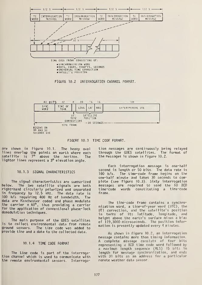
TCWORD

1/2 S

INTERROGATIONMESSAGE

TCWORD

1/2 S

INTERROGAT IONMESSAGE

TCWORD

1/2 S

[ NT E RR OGAT T ONMESSAGE

TCWORD

1/2 S

INTERROGATIONMESSAGE

—30 S

TIME CODE FRAME CONSISTING OF:

•SYNCHRONIZATION WORD•DAYS, HOURS, MINUTES, SECONDS•UNIVERSAL TIME CORRECTION•SATELLITE POSITION

FIGURE 10.2 INTERROGATION CHANNEL FORMAT

.

40 BITS 32 20 16 16 I 08

SYNCWORD

TIME OFYEAR LONG LAT EXPERIMENTAL USE

BEGINS ON00 AND 30SECONDS UTC

UT1TIME

CORRECTIONS

SATELLITEPOSITION

TIME FRAME-30 SECONDS-

FIGURE 10.3 TIME CODE FORMAT.

are shown in figure 10.1. The heavy ovallines overlap the points on earth where eachsatellite is 7° above the horizon. Thelighter lines represent a 3° elevation angle.

10.1.3 SIGNAL CHARACTERISTICS

The signal characteristics are summarizedbelow. The two satellite signals are bothright-hand circularly polarized and separatedin frequency by 12.5 kHz. The data rate is

100 b/s requiring 400 Hz of bandwidth. Thedata are Manchester coded and phase modulatethe carrier ± 60°, thus providing a carrierfor the application of conventional phase-lockdemodulation techniques.

The main purpose of the GOES satellitesis to collect environmental data from remoteground sensors. The time code was added toprovide time and a date to the collected data.

10.1.4 TIME CODE FORMAT

The time code is part of the interroga-tion channel which is used to communicate withthe remote environmental sensors. Interroga-

tion messages are continuously being relayedthrough the GOES satellites. The format of

the messages is shown in figure 10.2.

Each interrogation message is one-halfsecond in length or 50 bits. The data rate is

100 b/s. The time-code frame begins on the

one-half minute and takes 30 seconds to com-

plete (see figure 10.3). Sixty interrogationmessages are required to send the 60 BCD

time-code words constituting a time-codeframe.

The time-code frame contains a synchro-

nization word, a time-of-year word (UTC), the

UT1 correction, and the satellite's position

in terms of its latitude, longitude, and

height above the earth's surface minus a bias

of 119,3000 microseconds. The position infor-

mation is presently updated every 4 minutes.

As shown in figure 10.2, an interrogation

message contains more than timing information.

A complete message consists of four bits

representing a BCD time code word followed by

a maximum length sequence (MLS) 15 bits in

length for message synchronization, and ends

with 31 bits as an address for a particular

remote weather data sensor.

177

20 40

100 120 160 E 180 W 160 140 120 100 80 60

LONGITUDE

0 20 40

FIGURE 10.4. WESTERN SATELLITE POINTING ANGLES.

100 120

LONGITUDE

160 E 180 W 160 140 120 100 80 40 20 20 40

20 40

FIGURE 10.5. EASTERN SATELLITE POINTING ANGLES.

178

LONGITUDE

LONGITUDE

FIGURE 10.6. WESTERN SATELLITE MEAN DELAYS.

For total delay, add 133.5 ms to downlink delays shown.

LONGITUDE

100 120 140 160 E 180 W 160 UO 120 100 80 60 SO .'(1 0 .'() 10

LONGITUDE

FIGURE 10.7. EASTERN SATELLITE MEAN DELAYS.

For total delay, add 124.5 ms to downlink delays shown.

179

10.1.5 ANTENNA POINTING

Pointing an antenna to either satelliteis relatively simple. Because of the largebeamwidths of low-gain antennas (< 10 dB),

pointing into the general direction of the

satellite is usually sufficient. However,the antenna must be located so it has an

unobstructed path to the satellite. Figures10.4 and 10.5 provide detailed information for

antenna pointing with elevation and azimuthangles provided. For example, the pointingdirections to the eastern satellite from San

Francisco can be obtained from figure 10.5 as

approximately 119° azimuth and 24° elevation.Satellite positions may change with time.

Users should check the monthly NBS Time and

Frequency Bulletin for current status.

10.1.6 PERFORMANCE

The GOES time code can be used at threelevels of performance: uncorrected, correctedfor mean path delay only, and fully corrected.

A. Uncorrected

The path delay from point of origin(Wallops Island, Virginia) to the earth via

the satellite is approximately 260,000 micro-

seconds. Since the signals are advanced in

time by this value before transmission from

Wallops Island, they arrive at the earth's

surface nearly on time (within 16 millisec-onds).

B. Corrected for Mean Path Delay

Accounting for the mean path delay to any

point on the earth's surface, but ignoring the

cyclic (24-hour) delay variation, generallyguarantees the signal arrival time to ± 0.5

millisecond. For example, the mean delay to

San Francisco through the eastern satellite is

130.5 milliseconds downlink (from figure 10.7)

plus 124.5 milliseconds uplink delay, for a

total of 255 milliseconds. Since the time is

advanced by 260 milliseconds before leaving

Wallops Island, the time arrives at San

Francisco 5 milliseconds early.

C. Fully Corrected

The cyclic path delay variation on GOES

is a result of the satellite orbit or path

around the earth not being perfectly circular

and not in the plane of the equator. The

orbit is actually an ellipse and has a small

incl ination--usual ly less than 1°. To compen-

sate for these and other effects, the satel-lite position is included with the time mes-

sage for correction of path delay by the user.

(See [18] and [19] for details on how this is

accomplished.) This correction provides pathdelays accurate to ± 10 microseconds undernormal operating conditions. The ultimateaccuracy of the recovered time depends upon

knowledge of user equipment delays and noiselevels as well as path delay.

Typical delay variations for the easternsatellite are shown in figure 10.8. Thepeak-to-peak values change as the satellite'sinclination and eccentricity are varied by

orbit maneuvers and natural perturbations.

10.1.7 EQUIPMENT NEEDED

A. Antennas

Many antennas have been used by NBS witnvarying results. The best performance has

been obtained using a right-hand circularlypolarized helix antenna (fig. 10.9) with about10 dB gain. Excellent results have been ob-

tained with the microstrip antenna shown in

figure 10.10. Dipoles and loops have also

worked at lower levels of performance. All

of these antennas had gains in the range of

3 to 10 dB.

6pm 4pm 2pm 12n 10am 8am 6am 4am 2am 12mn 10pm 8pm 6pm

FIGURE 10.8 TYPICAL DELAY VARIATIONS FOR

THE EASTERN SATELLITE.

180

FIGURE 10.9. RIGHT-HAND CIRCULARLY POLARIZEDHELIX ANTENNA USED TO RECEIVEGOES SIGNALS.

B. Receivers

The NBS-built receiver shown in figure10.11 is completely automatic, requiring notuning or auxiliary equipment to operate. Com-mercial versions of this equipment are alsoavailable. For information on manufacturers,contact the Time and Frequency Services Group,524.06, NBS, Boulder, CO 80303.

10.1.8 SATELLITE-CONTROLLED CLOCK

The clock shown in figure 10.11 wasdesigned to interface with a receiver andachieve bit and frame synchronization, stripthe time code from the interrogation message,

FIGURE 10.10. MICR0STRIP ANTENNA USED TORECEIVE GOES TIME CODE.

FIGURE 10.11. GOES TIME CODE RECEIVER.

181

obtain time code frame sync, and read the timecode message into memory. The clock then up-

dates the memory time by counting cycles ofthe interrogation channel data clock, a 100 Hz

square wave, and verifying its memory timethrough continual comparisons with consecutivetime code messages from the satellite [20].

This clock was designed to address the

majority of user's needs at minimum cost. Thisclock was not designed to "squeeze" the lastbit of performance from the GOES timing sys-

tem. The clock does not directly use thesatellite position data to correct its outputbut can display the data for manual computa-tion of the delay.

A. Delay Corrections

The usefulness of potentially highlyaccurate timing signals relayed through geo-stationary satellites is complicated by thecomputation of the propagation delay from thetransmitter through the satellite back down to

the receiver. Computation of this delay is

usually accomplished through the manipulationof orbital elements. From the orbital ele-ments, six constants which describe thesatellite's position and velocity at a giveninstant of time, and a complete description of

perturbing forces, it is possible to computethe satellite's position at other times.

Once satellite position is known, thefree space propagation delay to any receiverfollows directly from simple geometry. Thecomputation of satellite position from orbitalelements, however, is complicated and bestaccomplished using a digital computer.

This type of computation would be diffi-cult for most of the expected users of theGOES time code. However, NBS has developedprogrammable calculator programs, and a

"smart" clock which uses the satellite'sposition to compute the delay to high accu-racy.

B. Programs for Computing

Free-Space Path Delay

Several programs to compute the total

free space path delay from Wallops Island,Virginia, through the satellite to any pointon the earth's surface are available from theTime and Frequency Services Group, 524.06,NBS, Boulder, CO 80303. These programs arewritten for use with programmable calculators.

10.1.9 SMART CLOCK

A "smart" clock with receiver is shown in

figure 10.12. This is essentially an addition

FIGURE 10.12. SMART CLOCK.

182

of a second microprocessor to the "satellite-

controlled clock" for the calculation of the

free-space propagation delay from the CDA to

the clock via the satellite. This delay value

is then used with a delay generator to com-

pensate for the free-space path delay.

The "smart" clock uses the same type of

four-bit microprocessor as the "satellite-controlled clock." The microprocessor is

interfaced to a large scale integration sci-

entific calculator array (math chip) to pro-

vide the floating arithmetic and mathematicalfunctions required in the delay calculation.

A 1 pps output and satellite position as

longitude, latitude, and distance from a

reference orbit is obtained continuously fromthe satellite-controlled clock operating on

the satellite's transmitted interrogationchannel signal.

User position is entered into the systemvia thumbwheel switches, and transmitter posi-tion (Wallops Island, Virginia) is containedin the microprocessor software. The computeddelay drives a programmable delay generatorto correct the 1 pps from the satellite con-trolled clock. The resultant output from theprogrammable delay generator is a compensated1 pps, adjusted to be in agreement with themaster clock at Wallops Island, which is in

turn referenced to UTC(NBS). The hardware is

a multiprocessor system consisting of two

microprocessors plus a slaved scientific cal-culator chip and a delay generator.

468 MHz \, ^ GOES

S SATELLITES

ANTENNA

The delay calculation is dependent on

knowledge of the broadcasting satellite'sposition. This position is predicted in

advance by a large scale scientific computeroperating on orbital elements obtained from

NOAA and sent to Wallops Island via telephoneline to be broadcast along with the time code

from each satellite. The delay correctionsystem will work with any satellite in a

synchronous orbit as long as the satellite'sposition is known. A calculation is made and

the result is latched into the delay generatoronce per minute. A complete up and down delay

calculation requires the execution of about200 key strokes representing data and mathe-matical operations and functions under the

control of the microprocessor and its associ-ated transistor-transistor-logic (TTL) compo-

nents.

A block diagram of the smart clock, in-

cluding receiver and antenna, is shown in

figure 10.13. The smart clock has been com-

pletely documented (schematics, board layouts,

and software)[19].

10.1.10 CLOCK CALIBRATION

To use the GOES signals to calibrate or

set another clock, one needs to determine the

relationship of the satellite controlled

clock's 1 pps relative to UTC(NBS) and to the

clock being calibrated. The relationship

RECEIVER

USER'S

LONGITUDE LATITUDE

1 0 5 ,, 2 6

THUMBWHEEL

SATELLITE-CONTROLLED

DIGITAL CLOCK

/^.PROCESSOR (4004)

SATELLITE

LONGITUDE,

LATITUDE,

RANGE

4 0 ,, 0 0

SWITCHES

4004 -BASED

DELAY-COMPUTING

/^PROCESSOR

512 kHz

1PPS

UNCORRECTED

POR DELAY

PROGRAMMABLE

DELAY GENERATOR

(TTL)

LSI/MOS

SCIENTIFIC

CALULATOR CHIP

DISPLAY LEDS

2 5 2 4 2 9

/xSECONDS DELAY

1PPS

CORRECTED

FOR DELAY

FIGURE 10.13. SMART CLOCK BLOCK DIAGRAM.

183

between the satellite-controlled clock and theclock being calibrated is usually determinedby use of a time interval counter. For exam-ple, the clock to be calibrated may start thecounter, then the satellite controlled clockstops it. The relationship between UTC(NBS)and the user's clock is then known by combin-ing this measured result with the computeddifference between the satellite clock's 1 ppsand UTC(NBS).

An example of the clock calibrationprocedure is given below. The clock to be

calibrated is located in Boulder, Colorado,where the GOES satellite signals are beingreceived.

Signals received in Boulder (105.26° WLongitude and 40.00° N Latitude) showed thesatellite location to be:

Since the Wallops Island clock is set to

be 260,000 us early with respect to UTC(NBS):

WALLOPS ISLAND CLOCK - UTC(NBS) = + 260,000 us

Then, by adding these two equations:

SATELLITE CLOCK - UTC(NBS) = - 6,351 us (1)

The measured time interval between the user'sclock and the satellite signal is stated as:

134.92° W Longitude

0.38° S Latitude

+46 us Distance

USER'S CLOCK - SATELLITE CLOCK = +6,548 us (2)

Using a calculator, the following delays arecalculated:

WALLOPS ISLAND TO SATELLITE

SATELLITE TO BOULDER

TOTAL PATH DELAY

To this we must add:

MEASURED EQUIPMENT DELAY

to get the total delay fromWallops Island to the user'ssatellite clock 1 pps.

TOTAL DELAY:

133 606 ps

127 553 ps

261 159 ps

+ 5 192 ps

266 351 ps

This result can also be written as:

SATELLITE CLOCK - WALLOPS ISLAND CLOCK

= - 266,351 ps,

where the result is negative because thesatellite clock is late with respect to theWallops Island clock (see Chapter 3 for signconventions)

.

Then, by adding equations (1) and (2):

USER'S CLOCK - UTC(NBS) =+ 197 ps. (3)

The smart clock automatically computesthe relationship between UTC(NBS) and the

output of the satellite-controlled clock and

adjusts the difference to be zero; i.e.,

UTC(NBS) = satellite-controlled clock. The

calibration using the smart clock is thereforeread directly from a time interval counter.

10.1.11 RESULTS

More than two year's of data from several

satellites have been recorded at NBS Boulder

using the measurement configuration shown in

figure 10.14. The results, on strip chart

recorders, have been of the form illustrated

in figure 10.15. The phase shift in the

uncorrected output is clearly evident. The

corrected output is generally a straight line

since the satellite position data are updated

every four minutes. Remember that the time

code message and position data are repeated

every half-minute but new position data are

input once every 4 minutes.

The equation relating the time recovered

from the satellite to the master clock at

Wallops Island is given in eq. (4):

184

ANTENNA

RECEIVER

lpps FROMNBS MASTER CLOCK

"

DATA

DATACLOCK

DIGITALCLOCK

SATELLITEPOSITION

RECEIVINGLOCATION(LONGITUDE& LATITUDE )

1 pps

TIME INTERVAL COUNTER

START STOP

HZ

(UNCORRECTED)

DELAYCORRECTION

lpps (CORRECTED FORFREE SPACEPATH DELAY)

TIME INTERVAL COUNTER

START STOP

3 t

UTC(NBS)-SAT/NBS-(CORRECTED)

FIGURE 10.14. MEASUREMENT OF GOES SIGNALS.

UTC(NBS) - SAT/USER

1

= (UTC - CDA)

/FREE SPACE \

[PROPAGATION)

\ DELAY /

(IONOSPHERE &^

TROPOSPHEREDELAY ,

(CDA EQUIP DELAY)

/ satellite \(transponder)\ DELAY /

/ RECEIVER \I & CLOCK\ DELAY /

Term 1 is known to better than 1 microsecondusing the data logger which compares the CDA

clocks to Loran-C and TV Line-10. This termwill be controlled in the next generatorsystem to be installed at Wallops Island to

± 3 microseconds or better. Terms 2, 4, 5 and6 are expected to remain constants at the fewmicroseconds level and can for the most partbe calibrated out of a user's system. Term 3

can be computed as discussed previously, withits accuracy dependent upon the quality of

the orbital data given to NBS by NOAA. All

measurements to date indicate this term will

be accurate to a few tens of microseconds.

Figure 10.16 shows the results of one

month's data taken at NBS/Boulder using orbitpredictions derived from three sets of orbital

elements extrapolating as much as 22 days from

their date. The results indicate a systemcapability of 10 microseconds. Over a period

\ *s V

CORRCCTED FOR FREE SPACE

. DELAY AT A MIN INTERVALS

FIGURE 10.15. SATELLITE SIGNALS CORRECTED AND UNCORRECTED.

185

UTC(NBS)-G0ES1/NBSCORRECTED FOR CLOCK DRIFT

& EQUIPMENT DELAY CHANGESAT CDA WALLOPS ISLAND, VA

O— AVERAGE OF 48 MEASUREMENTSTAKEN AT HALF HOUR INTERVALS

OF 43019 OF 43033 OF 43040

_J I I I I I 1 I

43031 43035 43039 43043 43047 43051 43055 43059

MJD

FIGURE 10.16. TYPICAL RESULTS.

of one year, charts have deviated from the"straight line" by as much as 25 microseconds.Using two receivers, there was no correlationin the drift of the receiver and we concludethat the problem resides with the receivingequipment only. A better definition of per-formance and accuracy cannot be made until

data are gathered from widely separated loca-tions in the Western Hemisphere.

Because of the spacing of frequencyassignments to the land-mobile users, there is

far less interference to the eastern satellitesignals than to the western satellite. There-fore, the eastern satellite should be used by

those user's situated in large urban areas.

B. Outages

10.1.12 PRECAUTIONS

A. Interference

The "land-mobile" services and the GOESinterrogation channel use the same frequencyallocations (468.8250 and 468.8375 MHz) , whichmeans the time code may suffer interferencefrom land-mobile transmissions. This is par-

ticularly true in urban areas where there is a

high density of land-mobile activity. Thesatellite frequency allocations are secondaryto the land-mobile services. Therefore, any

such interference must be accepted by the time

signal users. Complaints to the FCC will not

result in any adjustments in favor of such

users. The spectrum use by satellite andland-mobile is shown in figure 10.17.

Although the GOES satellites transmitcontinuously, there may be interruptions

during the periods of solar eclipses. The

GOES satellites undergo spring and autumn

eclipses during a 46-day interval at the

vernal and autumnal equinoxes. The eclipsesvary from approximately 10 minutes at the

beginning and end of eclipse periods to a

maximum of approximately 72 minutes at the

equinox (fig. 10.18). The eclipses begin 23

days prior to equinox and end 23 days after

equinox; i.e., March 1 to April 15 and Sep-

tember 1 to October 15. The outages occur

during local midnight for the satellites. In

the future, it is expected that GOES will oper-

ate through eclipse periods using batteries.

There will also be shutdowns for peri-

odic maintenance at the Wallops Island ground

LANDMOBILE-

WESTERNGOES

1

EASTERNGOES

vzzzzzzwzzzzm

LANDMOBILE

YZZZZZZZZZZZZZZA468.8250 468.8375

(MHz)

468.8500

FIGURE 10.17. FREQUENCY USE.

186

MARCH APRIL'

7 17 27 6 16

50

40

30

20

10

//

,

>

vV/PARIECLI

IAL

PSE

//t /

\ >

\\A

/

\\

\\

A \\/

/ /FULL ECLIP 5E

I \

\\

h1

\\

\\

1

1

\\

\\

1\\

\\11

II

f-

- SEPTEMBER -« OCTOBER

FIGURE 10.18. SOLAR ECLIPSE TIME

station. These scheduled outages will be

reduced in the future as redundancy is addedto the Wallops Island facility.

C. Continuity

NBS cannot give an absolute guarantee to

the long-term continuance of the GOES timecode. The GOES satellites belong to N0AA and

are not under the direct control of NBS.

However, NBS and N0AA have agreed to includethe time code in the GOES satellite trans-missions to the maximum extent possible. TheGOES system presently has a sufficient numberof satellites to operate into the late 1980' s,

and it is expected that the time code will be

included throughout this period.

10.2 THE TRANSIT NAVIGATION SYSTEM

10.2.1 GENERAL

These Navy navigation satellites have

been operational since 1964. Known as the

TRANSIT satellites, their design, power level,and coverage provide an excellent source oftime and frequency signals for calibrationpurposes. The signal format used on the sys-tem lends itself well to time recovery fromwhich frequency calibrations can be derivedusing the techniques previously described in

this book.

A major difference between TRANSIT andGOES is that TRANSIT, being an orbiting sys-tem, experiences a much larger Doppler shiftof its radio signal. This is no real problemfor the user since the overall system designtakes this into account and provides enoughinformation to the users so that accurate timerecovery can be achieved.

The biggest difference between GOES andTRANSIT is that the TRANSIT system can only be

used intermittently--when a satellite is in

view of the receiver.

This system is a good candidate for users

who have a worldwide requirement. TRANSIT is,

in fact, the only time and frequency system

that will work anywhere in the world. GOES is

limited at present to the western hemisphereand its oceans.

The satellites broadcast at about 400

MHz. The message sent contains a number of

characteristics which allow position fixing

and also time recovery. As with the GOES

system, TRANSIT allows a user to recover time

signals which can be used as a clock or to

steer an oscillator's frequency. Unlike GOES,

however, the TRANSIT time signal format does

not include day-of-the-year information.

Accuracy of the overall system is comparable

to GOES. Time to better that 10 microseconds

and frequency accuracies to 1 part in 10 10

(for measurement periods of 1 day) can be

achieved.

Although TRANSIT is primarily a naviga-

tion satellite, the responsible Navy group

has recently allowed changes in its operation

to provide even more support for its frequency

and time function. Coupled with this is the

plan to launch additional satellites in the

TRANSIT series. Users planning to obtain

equipment to use TRANSIT, especially at remote

locations, should contact either the U. S.

Naval Observatory or the Navy Astronautics

Group for the latest information on satellite

passes, etc. In addition, manufacturers of

TRANSIT equipment are a good source of infor-

mation.

At this writing, the TRANSIT system is

supported by five orbiting satellites. These

are in a circular polar orbit at an altitude

of about 1100 kilometers. Thus, a user on the

earth will see a satellite every 90 minutes or

so. In contrast to a GOES-type of transponder,

187

TRANSIT SIGNAL GENERATION

OSCILLATOR5 MHi —80 „pm

FREQUENCY MULTX80

399 968 MHi(*400 MHil

149 988 MHr(=1S0 MHilw

FREOUENCV MULTX30

PHASE MODULATION

CLOCK^

RECEIVERFREQUENCY DIVIDE ADJUST

^96 uSEC

MEMORY ~

SATELLITE CLOCK CONTROL SYSTEM

OSCILLATOR

FREQUENCY DIVIDE

1 - 104.159HZ

p - 9.6 uS

INJECT

i » 1627HZ

p - 614.449 »jS

-2 ±4 -321

ADJUST9 6 uSEC .

1. SATELLITE OSCILLATOR DESIGN CENTER FREQUENCY = 4,999,600

2. DIVIDER CHAIN RATIO (READ) = 1 6 x 3 x 2 x 32 x 32 = 98,304

3. 98,304/4,999,600 = 19,662373 ms/BIT

4. 19,662373 x 6103 = 119.9994626 SECONDS

5. 120.0000000 - 119.9994624 = 537.6 MICROSECONDS

6. DIVIDER CHAIN RATIO (DELETE) = 48/4999600 = 9.6 MICROSECONDS

7. 537.6 ys/9.6 ys = 56 CLOCK CORRECTION BITS/2 MIN. INTERVALS

FIGURE 10.19. TRANSIT SATELLITE CLOCK CONTROL SYSTEM.

TRANSIT has an accurate clock on-board eachof its satellites. These are monitored fromearth-control stations and corrections aresent to the satellites periodically to keepthem on time (see fig. 10.19).

In addition to position information, thesatellites send a time mark each two minutes.By monitoring the signals from four ground-monitor stations, the Navy is able to steer

the on-board clocks by special commands. Forthe user, this means that at any time he canbe assured that a TRANSIT signal has beencarefully controlled for accuracy.

There is much redundancy in the overallsystem control. New control data are sentto the satellites every 12 hours or so. Al-most all the ground equipment used for bothnavigation and timing contains a fairly

188

ADD/DROP CONTROL 1 MHZIN

400 MHZIN

MICROCOMPUTER *

NNSSRECEIVER

DATAIN

ENABLE

6 DIGITDECADE COUNTER

DATA

ys COUNT

LATCH

STROBE (FTM*)

FTMDETECTOR

1 PPSOUT

FIGURE 10.20. TRANSIT TIMING RECEIVER BLOCK DIAGRAM.

sophisticated computer-controlled receiverthat allows nearly hands-off operation.

As with the GOES system, the satellitemessage is designed to allow the receiver tosynchronize itself, locate the required bitsin the data stream and produce a time mark.

Accuracy of time recovery using TRANSITdepends on several factors. Again, the poten-tial user is encouraged to talk with manufac-turers and to contact the USNO, Time ServicesDivision, Washington, DC 20390 before proceed-ing. At this writing, time recovery accuracyfalls within from 10 to 50 microseconds. Withsuitable care of an operating clock on theground, this service can provide very valuablecalibration information.

10.2.2 EQUIPMENT NEEDED

Equipment costs are higher for TRANSITthan for GOES, but still not unreasonableconsidering the few alternatives.

Antennas are small, vertical, and omni-directional, making installation simple.

The instrumentation needed by' a userwill depend on his particular application.In general, he will need a frequency sourceand clock. Purchase of a receiver for TRANSITwill then allow comparisons to the specifica-tions of the equipment.

It is expected that manufacturers will

differ in their implementation of TRANSITreceiving equipment, but a typical requirementis that the user obtain the time of day from

another source to within 15 minutes in order

to resolve the time ambiguity of TRANSIT. For

some applications, it may also be necessary to

dial in the user's longitude and latitude.

See figure 10.20 for a typical receiverblock diagram.

189

CHAPTER 11. AN INTRODUCTION TO FREQUENCY SOURCES

An instrument or device that produces a

steady and uniform signal output in whateverform is said to have a frequency of operation.The new quartz crystal wristwatches , for exam-ple, vibrate their crystal frequency source at32,768 times in one second. Most clocks con-tain an identifiable source of frequency, beit balance wheel, crystal, or pendulum.

Frequency sources are also used in

another way. Besides counting their vibra-tions or oscillations for timekeeping, theyare used to set musical instruments and tocalibrate many types of electronic devices. Aradio dial is marked off in frequency units asare the familiar television channels. The TVchannel selector, when set to channel 4, tunesthe receiver to obtain a signal at a frequencyof about 70,000,000 hertz or 70 MHz.

This chapter deals with the properties offrequency sources and their possible applica-tions to real situations. The idea is thatonce you understand what the frequency gener-ator will do, you can more intelligentlychoose the right type of device. Some of thephysics of the devices are discussed andfinally a table is presented that comparesseveral devices.

The first part of this chapter deals withthe use of frequency sources to drive clocks,which is an important application of manyhigh-quality oscillators. There is a strongrelationship between time-ordered events andfrequency division. Communications systemsespecially rely on these two means of separat-ing channels of communications. For example,there are a number of stations on the AM radiodial. These are spaced in frequency at aboutevery 10 kHz. Another way to share the spec-trum would be to have all the stations at thesame frequency, but at different times . Thesame spectrum is thus time-shared. For obvi-ous reasons of cost and convention, we choose

rather to run all the stations at the sametime, but on different frequencies.

Common usage allows manufacturers andwriters to refer to frequency sources as stan-dards. You will see and hear the term fre-quency standard mentioned when what is reallymeant is a frequency source. The word "stan-dard" should properly be reserved for onlythose frequency generators that serve as

references for others. In the U. S. the pri-mary frequency standard resides in Boulder,Colorado, at the National Bureau of StandardsLaboratories. But there can be many secondarystandards that are calibrated with the singleprimary standard. Here is where the popularusage of the term "standard" gets misused.People use it to describe high-quality oscil-lators because their stability is so good thatit approaches that of the nation's standard.It is probably not possible to prevent thismisuse, so the reader should be warned to notecarefully what is meant by the words used todescribe the various frequency sources.

11.1 FREQUENCY SOURCES AND CLOCKS

Notice that most clocks—in particular,the very accurate and precise ones--are basedon high-quality frequency sources. The reasonfor this is the intimate relationship betweenfrequency (symbol v, "nu") and time (symbol

t). See the definition of frequency in theglossary for more information. If we look at

a series of events which are occurring in a

somewhat regular fashion; e.g., the rise of

the sun every morning, we can state how manyof these events occur in a given time period.

This number would be the frequency of this

series of events. In our example, we could

say that the frequency of sunrises is v = 7

events per week, or v = 365 events per year.

"Events per week" or "events per year" would

FREQUENCYSOURCE

5MHz FREQUENCYDIVIDER

60Hz

DIVIDER &

PULSEGENERATOR

1 PULSEPER SECOND

(1Hz)

ELECTRICCLOCK

CLOCK(COUNTER/

ACCUMULATOR)

CLOCK-TICKOUTPUT

FIGURE 11.1. EXAMPLE OF A CLOCK SYSTEM.

191

EVENTS

PERIOD —

H

FREQUENCY = NUMBER OF EVENTS PER UNIT OF TIME

ACCUMULATED CLOCK TIME =TOTAL NUMbER OF EVENTSALLUMULAILU CLUCK IIML

NUMBER OF EVENTS PER UNIT OF TIME

POSSIBLE DEFINITION:

UNIT OF TIME = A SPECIFIC NUMBER OF PERIODS OFA WELL-DEFINED EVENT GENERATOR

FIGURE 11.2. DEFINITION OF TIME AND FREQUENCY.

be called the unit which we used for our fre-quency number. This frequency number is dif-ferent for different units. In our example,we assume that we know somehow what a week ora year is; i.e., we relied on some understooddefinition of our unit of time.

Now, what is the time interval betweenthe events? The answers for our examples aresimple: One sunrise succeeds the other aftert = 1/7 week, or t = 1/365 year, where we used"week" and "year" as two possible choices forour unit of time.

We have learned two things: (a) forperiodic events, the time between the events t

is related to the frequency v of their occur-rence in the following simple way:

1v =

t

and (b) that periodic events can be counted todefine time; i.e., the generator of the peri-odic events-the frequency source--can be usedas a clock. The frequency becomes a clock bythe addition of a counting mechanism for theevents.

In the above example, the frequency usedis that of the rotating earth. The timebetween recurring events is one day. Therotating earth has served mankind for thou-sands of years and remained until very recent-ly the source for the definition of time in-

terval. The counting mechanism which made it

a clock was the recording of days and years.

The need to get along for many days with-out celestial observations, and to measuretime intervals which are very much shorterthan a day, brought about the invention ofclocks. Although there are other types ofclocks like the sand clock or the water clockand the sundial, we will discuss only clocksbased on electronic frequency generators.

The first clocks based on the pendulumwere invented about 400 years ago. This typeof clock is still widely used today. The pen-dulum may be a suspended weight (gravitationalpendulum) like in "grandfather" clocks, or thebalance wheel (torsion pendulum) of modernwri stwatches. The object of our discussionhere is today's most advanced oscillators andclocks; however, a close look at traditionalclocks will show all the essential featureswhich we will recognize again in our laterdiscussion of quartz crystal and atomicclocks.

The pendulum in our clock is the frequen-cy determining element. In order to have a

frequency source, the pendulum has to be setand kept in motion. Thus, a source of energyis necessary together with the means to trans-fer this energy to the frequency-determiningelement. In a wristwatch, this source of

energy is typically the winding spring or

battery. The energy is transferred by a meanswhich is controlled by the pendulum itself(feedback) in order to cause energy transferin the proper amount at the proper time in

synchronism with the movement of the pendulumor balance wheel. We now have a frequencysource. The tick motion of a balance wheel

could be picked up acoustically, for example,and used as a frequency source. This is

actually done by jewelers when they adjust the

rate of a clock: the tick-frequency is com-

pared to some (better) frequency source. In

order to have a clock, a read-out mechanism is

necessary which counts and accumulates the

ticks (more accurately, the time interval

between the ticks) and displays the result.

In our example of a wristwatch, this is accom-

plished by a suitable set of gears and the

moving hands on the clock face or digitally.

We have just discussed how the additionof a mechanism to a frequency source whichcounts and accumulates and possibly displaysthe result creates a clock. This task can

also be performed by an electronic frequency

192

FEEDBACK

ENERGYTRANSFER

ENERGYSOURCE

FREQUENCYDETERMININGELEMENT

FREQUENCYSOURCEOUTPUT

CLOCK(COUNTINGACCUMULATING

DISPLAY )

FIGURE 11.3. FREQUENCY SOURCE AND CLOCK.

11.2 THE PERFORMANCE OF FREQUENCY SOURCES

The performance of a frequency source is

usually described in terms of its accuracy,reproducibility, and stability. These aredefined as:

ACCURACY :

How well does it relate to the defini-tion? In the case of frequency, this meanshow well it relates to the definition of a

second (in terms of cesium) mentionedpreviously.

divider which, for example, derives a frequen-cy of 60 Hz directly from a 5 MHz crystaloscillator (fig. 11.1). The 60 Hz voltage canbe used to drive an electrical clock motorsimilar to those driven by the 60 Hz powerline frequency that we use at home and atwork. Or, an additional electric pulse gen-erator may be used that generates one verysharp electrical pulse per second. The timeinterval of 1 second between the pulses (cor-responding to a frequency of 1 Hz) is derivedfrom the output of our frequency source. Thepulses can be directly used in time compari-sons with those of other similar clocks, orthey can drive a counter/accumulator.

The electric power line is a very goodfrequency source for many applications. Aclock driven from the power line will keepexcellent time. This is because the powersystem is carefully controlled to maintain itsfrequency within definite limits. By increas-ing or decreasing the individual generatorfrequencies, the flow of power in the inter-connected system can be regulated. Each powercompany is notified in advance to set theirfrequency to a particular value so that themillions of clocks on the system—those inhomes and offices across the country—willgain or lose time as required to keep theclocks correct. The time corrections areusually done at night.

The basic unit of time is the second(symbol s). It is defined with reference to a

frequency-determining element. Since 1967, byinternational agreement, this element or"natural pendulum" has been the cesium atom.The second is defined in the official wordingas "the duration of 9,192,631,770 periods ofthe radiation corresponding to the transitionbetween the two hyperfine levels of the groundstate of the cesium-133 atom." Accordingly,the frequency of the cesium pendulum is

9,192,631,770 events per second (the cesiumatom is a very rapidly oscillating pendulum).The unit of frequency is then defined as hertz(symbol Hz) which means the repetitive occur-rence of one event per second (the use of"hertz" is preferred to the older term "cycleper second"

,cps).

REPRODUCIBILITY :

If you built a number of such frequencysources and adjusted them, how well would theyagree in frequency? This term obviouslyapplies to sources that are manufactured andthen tested to see how they differ.

STABILITY :

Once the device is set to a given fre-quency, how well does it generate that valueduring some period of time?

It is obvious from these definitions thatfrequency accuracy will be of great interestin scientific measurements and in the evalu-ation and intercomparison of the most advanceddevices. Good reproducibility is an asset in

applications where it is important to expectsome agreement among several devices. How-

ever, the stability of a frequency source is

usually most important to the user.

The frequency stability (symbol o,

"sigma") of a frequency source will depend on

many things that might cause frequencychanges. Frequency stability can be measuredby taking a reasonably large number of succes-sive readings on an electronic counter whichcounts the frequency of the device to be

evaluated. Each counter reading (in hertz) is

obtained by counting the output frequency for

some specified time (the sampling time "tau",

symbol t). This sampling time can usually be

chosen by simply adjusting a knob on the

counter; for example, a sampling time of 0.1

s or 1 s or 10 s may be chosen. The result

can be expected to change as t changes. So

the stability needs to be defined for a

certain "tau".

Further, it might be expected that vari-

ations in the readings of measured frequency

would tend to average out if observed long

enough. This is not always so. The stability

of the frequency source (sigma or a) will

therefore usually depend on the sampling time

of the measurement and tends to get smaller

with longer sampling times, t. But, again,

there are many exceptions to this.

193

It may happen that the frequency fluctu-ations at some later time are partially causedby, or depend to some degree upon, the previ-ous fluctuations. In this case, the computedvalue of a will depend on the particular wayin which the many counter readings are aver-aged and evaluated. Another influence on mea-sured stability depends on whether the counterstarts counting again immediately after com-pletion of the preceeding count or if sometime elapses ("dead-time") before countingstarts again.

Finally, the electronic circuits used inmeasuring frequency stability will have a fin-ite response time; i.e., they cannot followfrequency fluctuations faster than some givenrate. For example, our eyes cannot registerlight fluctuations which occur faster thanabout every 1/10 of a second; using v = 1/t,we say that the eye has a frequency responseof 10 Hz, or that its bandwidth is only 10 Hz;

i.e., the eye cannot follow frequencies higherthan 10 Hz.

frequency stability of agv

= 10 Hz were mea-

sured at a carrier frequency of v = 5 MHz (MHz= megahertz = million Hz) then the fractionalor relative frequency stability would be

a = o% . =2x10°.y ov/v

We denote the kind of a we are using by a

subscript, 6v ("delta nu"), referring to fre-quency fluctuation (measured in Hz) or 6v/v =

y, referring to relative frequency fluctua-tions (dimensionless). A stability of onepart in a million is thus

ay= 1 x 10" 6

,

and one part in a trillion is written as

a =1x10y

In order to measure frequency stabilitiesfor sampling times smaller than some value x,

our measurement equipment has to provide foran electronic frequency bandwidth which is

larger than 1/t.

To summarize: A recommended way of pro-perly measuring and describing frequency sta-bility is the following: (a) make sure thatthe frequency bandwidth of the total measuringsetup is larger than 1/t, where t is the smal-lest, desired sampling time; (b) use a counterwith a cieadtime as small as possible (thedead-time should be less than the reciprocalbandwidth; if not, use the computation pro-cedures that exist to allow for larger dead-times); (c) take a sufficiently large numberof readings at a given sampling time which is

held constant and compute:

ADDITION OF THE SQUARES OF THE DIFFER-

ENCES BETWEEN SUCCESSIVE READINGS

2 x TOTAL NUMBER OF DIFFERENCES USED

There is a sound basis for using therelative frequency stability o^ instead of

using frequency stability directly, a is

a numeric and is independent of the actualoperating frequency of the oscillator beingdiscussed. Thus, it is possible to comparethe stability of a 10 MHz oscillator with onethat has an output at 10 kHz.

In fact, many high-quality oscillatorshave outputs at 1,5, and 10 MHz. But an

application for these sources might requirethe generation of a different frequency, e.g.,

the television color subcarrier signal at 3.58MHz. If the original source, before the syn-thesis of the TV signal, had a relative fre-

quency stability of one part per million (1 x

10- 6), then the 3.58 MHz signal would have the

same relative frequency stability a .

This assumes, of course, that thesynthesis or generation of new frequenciesdoes not change the stability of the frequencysource. This is generally true for mostappl i cations.

(In the scientific literature this a is oftencalled the square root of the Allan variance.)The counter readings can be taken in Hz; awill then have the dimensions of Hz; (d)repeat step (c) for other sampling times t andtabulate or plot a as it depends on x.

Commonly, a will be expressed as a rela-tive value. Existing literature often usesthe term "fractional" instead of relative, so

the reader should treat the two terms equally;they mean the same thing. The value obtainedfor the frequency stability is divided by thecarrier frequency. For example, if a

11.3 USING RELATIVE FREQUENCY STABILITY DATA

Suppose you have a clock. Let's say its

frequency source is a crystal oscillator, and

you want to know the time error. If you know

enough about the oscillator, you can computethe time error. You can even predict the

error ahead of time— fairly accurately, too.

First, let's define a few things that we

will need to write an equation. There are

only about three things that can happen to our

194

clock—assuming we don't drop it or pull theplug!

1. The clock could be reading the wrong timebecause we didn't set it at all or be-cause we set it wrong. Call this theinitial time error At0 . Until we correctit, we have to have it in our equation asa constant.

3. There is one more possible error. Wasthe oscillator "on frequency" when- itstarted to drift? If it was not, then wemust account for this offset. To do

this, we define the relative frequencyoffset as:

2. The frequency of the oscillator drivingthe clock may be fluctuating. If that is

the case, then we will have a term in ourequation that relates the fluctuation andthe length of time it has been drifting.Let's call this length of time t. It

would be the time from zero time (whenthe clock was right or we measured theerror At 0 ) till now. From what we saidabout the stability, we see that we needa term such as:

ay(T) X t.

Actually, we know the value of t that wewant. It's simply t, the time since welast set the clock. So our term becomesapproximately:

Oy(T ^ t) X t.

This then takes care of the instabilitiesof the oscillator frequency driving ourclock.

This term means that our oscillator mayhave had a frequency error when it

started to drift. In other words, weallow for an arbitrary starting point.

To review then, we have an oscillatorconnected to a clock and it may or maynot have had a time error At in additionto having or not having some drift x t

from either the correct or incorrectfrequency Av/v x t.

Addition of these time errors gives us

the clock error at time t:

At = At + a (t = t) x t + — x t.o y v

' v

The equation shows how the relative fre-

quency offset and stability accumulatetime error as t grows larger. Let's plugin some numbers and see what happens to

our clock. Assume the oscillator was off

frequency by 1 part in 10 11, fluctuates

by 1 part in 10 11 per day, and had a 1

microsecond error yesterday at this time.

Reading the graph we see that our clockerror would be about three microseconds.

FIGURE 11.4. RELATIONSHIPS BETWEEN CLOCK ACCURACY , FREQUENCY

STABILITY, AND FREQUENCY OFFSET.

195

We get almost 1 microsecond error fromfluctuations, 1 microsecond from frequen-cy offset and one from our initial set-ting error.

11.4 RESONATORS

The performance of an oscillator dependsa lot on its basic frequency-determining ele-ment. This element determines the frequencyby its resonance behavior. Thus, it is calleda resonator. Some examples of resonators area rod clamped only at one end that can vi-brate; a block of solid material that can con-tract and expand and thus vibrate; an electri-cal capacitor-coil combination (tank circuit)in which the energy can oscillate back andforth; and a coil in which an electric currentcan create a magnetic field which can oscil-late between its two possible polarities (amagnetic dipole). These devices have onething in common--they will vibrate or oscil-late if they are excited. The method of exci-tation may be a mechanical pulse, an electri-cal pulse, or a sudden surge of an electric or

VIBRATING ROD

V I BRAT I N

BLOCK

OSCILLATINGCAPACITOR-COIL(TANK) CIRCUIT

OSCILLATINGDIPOLE ANTENNA

* *.

U prr>o-rY^ S OSCILLATING MAGNETIC(S)l _oc>_J(N) DIPOLE ANTENNA

FIGURE 11.5. EXAMPLES OF RESONATORS.

OSCILLATION

OF MAX. INTENSITY

EXCITINGPULSE ENDS

DECAYINGOSC ILLATION

OF A RESONATOR

RESONANCEBEHAVIOR OFA RESONATOR

FREQUENCY

FIGURE 11.6. DECAY TIME, LINEWIDTH, AND Q-VALUE OF A RESONATOR.

196

magnetic field. These devices exhibit reso-nance. They are resonators with a well-defined center frequency which is a character-istic of the length of the rod, the thicknessof the block, the size of the capacitor andcoil, or the length of the antennas. Onceexcited, the oscillations will gradually dieout. The decay time is determined by thelosses in the resonator. Some of these lossesare internal friction, or electrical resist-ance. In any case, the oscillation energy is

finally transformed into heat. If there wereno losses, the oscillations would never stopand we would have the ideal resonator. Thegreater the losses, the faster the oscilla-tions will decay. We can use the decay timeof the oscillations (symbol T) to describe thequality of our resonator. The larger T is,

the better the resonator. "Better" for us

means that the device favors one frequencyover all others.

An alternate way of measuring resonancebehavior is to use a separate oscillator,couple it to the resonator, and slowly sweepthe frequency of the oscillator. We will find

a signal frequency at which the resonator will

oscillate, with maximum intensity. Above or

below this resonance frequency, the responseof the resonator will lessen until it ceasesto respond. This frequency interval aroundresonance, for which the resonator response is

relatively strong, is called the resonancelinewidth (symbol W). There is a simple rela-

tionship between W and T, the decay time:

W = - Hz.

T

This equation is an approximation andapplies only to certain types of resonance.

Another factor would have to be inserted if

the resonance curve were different from thatshown in figure 11.6. However, this factor is

nearly equal to one: T is actually defined as

the decay of the amplitude to 37% of its

original value: 37% is 1/e, e is the base of

natural logarithms and equals 2.71828.

As we did in the case of a (page 194),

it is convenient to consider the linewidth in

a fractional way. The fractional linewidthwould be W/vo where the symbol v0 is used for

the resonant frequency. A more popular term

is the "quality factor" (Q) of the device. Qis defined as the reciprocal fractional line-

width

For accurate frequency sources and good

clocks, we want to have elements with very

high Q's. A Q value of one million (106 )

is very common. For example, a 1 MHz crystaloscillator with a Q of a million would have alinewidth of 1 hertz. The oscillator wouldthen favor operation at a frequency within 1

hertz of a megahertz. If this oscillator weremeasured, its frequency should be within its

one hertz range, i.e., within a part permillion. In fact, it can be made much betterthan that. Parts per billion are typical.

In summary then, we want high-qualityresonators if our end product is to have goodaccuracy and stability characteristics. Thediscussion that follows in this section dealswith several types of high-quality frequencysources.

Many kinds of frequency-determiningelements have been and are being used in

frequency sources. They can be grouped intothree classes:

mechanical resonators

electronic resonators

atomic resonators

As far as mechanical resonators are con-cerned, we will only discuss one kind, thequartz crystal. Other mechanical resonatorslike the pendulum and the tuning fork are of

less importance in today's high performancefrequency sources, although they have been

historically very important and are still

widely used in watches. For similar reasons,

we will also omit the discussion of electronicresonators such as LC tank circuits and micro-

wave cavities. Atomic resonators form the

heart of our most accurate frequency sources

and clocks, and will therefore be extensively

discussed.

11.5 PRIMARY AND SECONDARY STANDARDS

At this point, we should briefly discuss

the terms "primary frequency standard" and

"secondary frequency standard". These terms

refer to the application of the devices; any

frequency source, regardless of its accuracy

or stability, can be a primary frequency stan-

dard, if it is used as the sole calibration

reference for other frequency sources. A

secondary frequency standard is a device which

is occasionally calibrated against a primary

frequency standard but operationally serves as

the working reference for other frequency

sources.

The machines used for primary standards,

like those at NBS, Boulder, NRC, Canada, and

in Germany and England, are in a class by

themselves. Because of the way they have been

built and operated, they can be evaluated.

This means that experimental data is taken and

197

FIGURE 11.7. THE U.S. PRIMARY FREQUENCY STANDARD, NBS-6.

PRIMARY DIRECTSTANDARD

CALI BRATION

I

SECONDARYSTANDARDS

OTHERSTANDARDS

FIGURE 11.8. HIERARCHY OF FREQUENCY STANDARDS.

198

used to calculate the errors in their outputfrequency due to all known causes. It is

because of this careful evaluation that theaccuracy can be stated without having to checkthese machines against others. This conceptwill be discussed in detail in connection withthe cesium beam frequency sources.

11.6 QUARTZ CRYSTAL OSCILLATORS

Quartz crystal oscillators are widelyused. They range from the tiny units found in

wristwatches to elaborate instruments in

laboratories. Sometimes they are called cry-stal oscillators and sometimes quartz oscil-lators. Whatever the name, they dominate thefield of good frequency sources.

The quartz crystal in the oscillator is a

mechanical resonator. The resonator's oscil-lations have to be excited and sensed. Thisis done by taking advantage of the piezoelec-tric effect in the quartz crystal. The piezo-electric effect (figure 11.9) results whenmechanical compression of the crystal gener-ates a voltage across the crystal. Converse-ly, the application of an external voltageacross the crystal causes the crystal to

expand or contract depending on the polarityof the voltage. A crystal is not a homogeneousmedium but has a certain preferred direction;thus, the piezoelectric effect has a direc-

QUARTZ

CRYSTAL

APPLIED PRESSURE APPLIED VOLTAGEGENERATES VOLTAGE CAUSES CONTRACTION

FIGURE 11.9. THE PIEZOELECTRIC EFFECT.

tional dependence with respect to the orienta-tion of the crystal. In order to take advan-tage of the piezoelectric effect, one has to

cut a crystal resonator from the originalcrystal block in a well-defined way withrespect to the crystal lographic directions.The raw material used today is natural or

synthetic quartz. A crystal is cut out of theraw crystal material in the desired orienta-

tion with the aid of optical techniques whichallow the determination of the crystal lo-graphic axes. The high-precision, finalorientation of the cut and the tuning to thedesired frequency is then done by grinding andetching, controlled by x-ray methods.

The quartz crystal can be cut and elec-trically excited in a variety of ways. Themost common types of vibrations (modes) arethe longitudinal and thickness modes, theflexure (bending) mode, the torsional mode,and the shear mode. In order to use thepiezoelectric effect, metal electrodes have tobe attached to the crystal surfaces so thatthe desired mode is excited.

The electrodes are typically created asextremely thin metallic coatings by vacuumevaporation of metals. Electric leads areattached to the electrodes by soldering. Theyalso serve as the mounting support, thus free-ly suspending the quartz crystal. In order to

least upset the mechanical vibrations of thecrystal, the electrode-support leads areattached at points where no vibrational motionoccurs (nodes). The crystal is then packagedand the case is either filled with a protec-tive gas or else evacuated.

Using the crystal, an oscillator can be

built by adding an electronic amplifier feed-

back and a power supply. The oscillator out-

put frequency is determined by the quartz cry-

stal resonator. Its frequency in turn is

determined by the physical dimensions of the

crystal together with the properties of the

crystalline quartz used. The actual operating

frequency thus depends on the orientation of

the cut, the particular mode, and the dimen-

sions of the crystal. As an example, we find

that the resonance frequency, for a longitudi-

nal mode of vibration, is approximately:

v = 2.7 x 10 3 x y ,

o L '

where L is the length of the crystal. If L is

in meters, the resonance frequency v 0 will be

in hertz. The equation allows us to estimate

the size of the crystals. For example, a 100

kHz crystal will have a length of just a few

centimeters. We see that the manufacture of

quartz crystals with resonance frequencies

above 10 MHz is hardly possible. However, we

can excite resonators not only in their so-

called fundamental mode (previously dis-

cussed), but also at multiples (overtones) of

this fundamental resonance frequency. An

example of this is the violin string which

also can be caused to vibrate at frequencies

which are multiples of its fundamental.

Quartz crystals which are designed for excita-

tion at multiples of their fundamental reso-

nance are called overtone crystals.

199

FLEXURE

LONGITUDINALTORSIONAL

THICKNESS SHEAR

QUARTZCRYSTAL

V

-ENCLOSURE

ELECTRODE-(THICKNESSEXAGGERATED)

ELECTRICAL-& MOUNTINGLEAD

-SUPPORT

CONTACTLEADS

FIGURE 11.10. PRINCIPAL VIBRATIONAL MODESOF QUARTZ CRYSTALS.

FIGURE 11,11. TYPICAL QUARTZCRYSTAL MOUNT.

FUNDAMENTAL

FEEDBACK

AMPLIFIER

POWERSUPPLY

QUARTZCRYSTAL

RESONATOR-OUTPUT

2nd OVERTONE

3rd OVERTONE

4th OVERTONE

FIGURE 11.12. QUARTZ CRYSTALOSCILLATOR.

FIGURE 11.13. FUNDAMENTAL AND OVERTONERESONANCE FREQUENCIES.

200

11.6.1 TEMPERATURE AND AGING OF CRYSTALS

Temperature and aging are two effects,among others, which are important in the de-sign of crystals and crystal oscillators.There is a temperature dependence of thequartz crystal that affects resonance frequen-cy, and there is also a drift of the resonancefrequency as time goes on.

The temperature dependence is caused by aslight change in the elastic properties of thecrystal. Certain cuts (crystal lographicorientations of the crystal) minimize thiseffect over a rather wide range of tempera-tures, most notably the so-called "AT" and"GT" cuts. Temperature coefficients of lessthan one part in 100 million per degree (Cel-sius or kelvin) are possible. In other words,the fractional frequency change will be lessthan 10- 8 with one degree of temperaturechange. This small effect requires care inthe design of a crystal oscillator if veryhigh frequency stabilities over longer times(hours or days) are desired. If large envi-ronmental temperature fluctuations are to betolerated, the crystals themselves areenclosed in electronically regulated ovenswhich maintain a constant temperature. Incertain crystal oscillators this is done tobetter than 1/1000 of a degree.

An alternate solution to the temperatureproblem is the so-called temperature-compen-sated crystal oscillator or TCX0. An addi-tional frequency-determining element in theoscillator, which can be just a small capaci-tor, allows us to tune the oscillator over a

limited range. If a temperature sensor is

added to cause a change in this capacitor, thechange in resonance frequency of the crystalresonator can be cancelled. Capacitors whosevalues change with an applied voltage (varac-tors) are used. The applied voltage is

derived from a temperature-sensing circuit.

The TCX0 does not necessarily requirefurther temperature control by an oven. How-ever, there is a drawback to this approach.By adding another frequency-determining ele-ment, the crystal resonator loses a corres-ponding part of its control on the output fre-quency of the whole oscillator. The long-termstability (days) of TCXO's is therefore belowthat of crystals with a good oven control.TCXO's are used in small, usually portableunits of relatively lower performance. Theyare used where frequency stabilities from dayto day and frequency changes (over some tensof degrees of temperature) of not better than10- 9 are needed.

Drift, or aging, is a common behavior ofall crystal oscillators. It is a nearlylinear (uniform) change in resonance frequency

with time. Drift often is negative, meaningthat the resonance frequency decreases. Afrequency decrease could be interpreted- as anincrease in the crystal size. Many thingshave been considered as the cause: contami-nation (depositing of foreign material) on thesurfaces; changes in the electrodes or themetallic plating; reforming of loose (fromgrinding and etching) surface material; orchanges in the internal crystal structure.All of these are possibly caused or enhancedby the vibrating motion of the oscillatingcrystal. Recent crystal holder design im-provements, combined with clean vacuum enclo-sures, have led to a reduction of aging toabout 10- 11 per day. For a 5 MHz crystal witha thickness of a little less than a milli-meter, this aging corresponds to an absolutethickness change of only 10- 11 of a milli-meter, or less than 0.1% of the diameter of anatom.

When a crystal oscillator is first turnedon, it will not usually oscillate at its orig-inal frequency. It will exhibit a "warm-up"due to temperature stabilization of the crys-tal resonator and its oven. For some timethen, often many days, a large but diminishingdrift occurs until it reaches its operatingpoint. Its frequency then might also be sub-stantially different (as compared to itsstability and aging performance) from its

frequency before power was turned off.

11.6.2 QUARTZ CRYSTAL OSCILLATOR PERFORMANCE

Crystal resonators have Q-values whichare typically in the range from Q = 10 5 to

almost 10 7. These are very high Q-values as

compared to most other resonators exceptatomic resonators.

These high Q-values are an essential pre-

requisite for the excellent stability perfor-mance of crystal oscillators. The best avail-able oscillators have stabilities of a few

parts in 10 13 for sampling times from one

second to a day. There is some experimental

evidence that some crystal resonators may, in

the future, perform even better! The limita-

tions are primarily caused by noise from elec-

tronic components in the oscillator circuits.

This noise may possibly be reduced by selec-

tion of low-noise components—transistors,capacitors, etc., and by special circuitdesigns. Thus, there is a reasonable chance

that crystal oscillator stability can reach

values of better than 10- 13 for sampling times

of seconds to hours. For times shorter than

one second, stability is often determined by

additive noise in the output amplifiers. This

can be reduced by a crystal filter in the

output. The long-term stability beyond

several hours sampling time is determined by

201

FIGURE 11.14. FREQUENCY STABILITY OF THE BETTER QUARTZ CRYSTAL OSCILLATORS.

aging and by external influences such as linevoltage variations, temperature fluctuations,etc. A specification of accuracy is not easi-ly stated for crystal oscillators. Withoutfrequency calibration, they can be manufac-tured by controlling the dimensions of thequartz used to within 10- 6 of a nominal fre-quency. If they are calibrated against a highaccuracy frequency source, they maintain thiscalibration (accuracy) in accordance withtheir long-term stability characteristics. A

crystal with a low aging characteristic of10- 11 per day will maintain its accuracy to a

few parts in 108 for a year without recali-bration.

It is apparent, therefore, that crystaloscillators require calibration at least oncea year. They may need it more often dependingon the application. Frequency adjustments aremade with a small added capacitor in much thesame way as was discussed in connection withthe TCXO. The most stable crystal oscilla-tors, with the lowest aging rate, cost approx-imately $2,000. They have a volume of a fewthousand cubic centimeters, and require inputpower of about 10 watts. They have an elabor-ate crystal oven for temperature control

,

well-designed electronics, and usually severaloutput frequencies which are derived from theoscillator with frequency dividers and multi-pliers. These high performance devices use2.5 or 5 MHz crystal resonators havingQ-values of a few million.

Cheaper and smaller crystal oscillatorsare available in a variety of designs withcorresponding reductions in frequency stabili-ty and/or environmental insensitivity. Costscan go down to below $100, sizes to a fewcubic centimeters, and power requirements to

less than 0.1 watt. The reliability ofcrystal oscillators is usually not limited bythe crystal itself, but also depends on theaccompanying electronic circuits.

11.7 ATOMIC RESONANCE DEVICES

Commercially available atomic frequencyoscillators are based on resonances in atomsat microwave frequencies— in the range from 1

to 100 GHz (gigahertz or billion hertz). Wemay picture atomic resonance as a magneticdipole antenna. We typically deal with a

great many of these dipole antennas (atomicresonators), and we can, as a simplification,separate them into two kinds: Receivingantennas receive energy from a magnetic fieldthat oscillates at their resonance frequency,much like a TV antenna at home. Transmittingantennas radiate energy at their resonancefrequency just like the transmitting antennaof a broadcast station. A physicist might say

that the atoms that act like a receivingantenna are in the "lower state" and thoseacting like a transmitting antenna are in the

"upper state.

"

There is a peculiarity with atoms:an atom changes from the upper to

the lower state upon emission of a

well-defined amount of energy.Correspondingly, an atom changesfrom the lower to the upper stateafter receiving an equal amount of

energy at the atomic resonancefrequency.

If we have a great many atoms as in a

gas, we will find that the number of upper

202

GAS, CONTAINING AN EQUALAMOUNT OF THE TWOKINDS OF ATOMS

•W.WI•w.wOtQ>0>0»0>OtO>0>0>0«0> >•o*o*o

,o,o*oofo#6*0#o * <:> * <5*0*o«o«o*o*

O O O O O oo o o o o o ATOMIC BEAM

ATOMIC BEAMSOURCE

KIND 1 - ATOMS(LOWER STATE)

MAGNETSTATE SELECTOR)

KIND 2 - ATOMS(UPPER STATE)

VACUUM CHAMBER

FIGURE 11,15. SPATIAL STATE SELECTION.

state atoms is nearly equal to those in a

lower state. This has an important conse-quence: If this gas is placed in a magneticfield that oscillates at the atomic resonancefrequency, all atoms will resonate. Nearlyhalf of the atoms receive (absorb) energy fromthe field, and the other half emit (add)energy of an equivalent amount to the field.The net effect is almost zero. The gas as awhole acts as if it has almost no resonanceeven though the individual atoms do resonate.From this we see that in order to achieveatomic resonance, we have to somehow changethe relative amounts of the two kinds ofatoms. The upper or the lower state has to bein the majority. The way in which this isdone determines the design of our atomicfrequency oscillator.

11.7.1 STATE SELECTION

There are two important methods used toaccomplish what is called state sel ection--thechange in the relative numbers of the twokinds of atoms (upper state and lower state):

Spatial state selection relies on an

actual sorting procedure where the two atomicstates are sorted into different directions in

space. One of the states can then be used;the other is discarded. An actual system mayproduce an atomic gas by heating some sub-stance in an oven. The atoms leave the oventhrough a hole and form an atomic beam in anadjacent vacuum chamber. The atomic beam is

then passed through a rather strong magnetwhich causes the separation of the beam intotwo beams, one containing the upper stateatoms, the other the lower state atoms.

Recall that our picture of an atom is that ofa magnetic dipole antenna. The magnet exertsa force on these magnetic dipoles. The forceacts in opposite directions for the two dif-ferent atomic states (we note this withoutfurther explanation).

Optical state selection takes advantageof the fact that atoms have more than just one

kind of resonance. Other resonances typicallycorrespond to infrared or visible (light)

frequencies. We can excite one of these

resonances by shining intense light of the

LIGHTBEAM

GAS CFALSTATE SELECTEDThROUGH ACTIONOF THE LIGHT

FIGURE 11.16. OPTICAL STATE SELECTION.

203

right frequency on the atoms. If the light is

filtered carefully, very monochromatic--onecolor (a very well-defined frequency)--l ight

is obtained. If the light frequency is chosenproperly, only one kind of atom will resonate.

It will be found that this light frequency is

different from the corresponding light reso-

nance of the other kind of atom. Light reso-

nance can thus "remove" one kind of atom and

provide for the desired majority of the otherkind.

11.7.2 HOW TO DETECT RESONANCE

We are now almost in a position to assem-ble our atomic frequency oscillator. We still

need some means to detect atomic resonance. A

short waveguide or microwave cavity is typi-cally used. Such a cavity has microwave reso-nances which are determined by its physicalsize. The electrical losses of this cavityare determined by the electrical conductivityof the cavity material. A cavity may be

shaped like a cylinder or a box. It resonatesin a way quite similar to an organ pipe in thecase of sound waves. The best known exampleof a microwave cavity is the microwave ovenwhere food is cooked by placing it into theresonance field of a cavity.

In order to observe atomic resonance, wehave to place the state-selected atoms insidethis cavity and subject them, for some speci-fied time, to a microwave radio signal attheir resonance frequency. The microwavesignal will change the relative number of

atoms in the two states. If all atoms were

initially in the upper state, we will find

some in the lower state after the microwavesignal has acted upon them for some time. If

the frequency of the microwave signal equalsthe atomic resonance frequency, the transferof atoms from one state to the other reaches a

maximum. The center of the atomic resonanceis thus found by monitoring the number of

atoms in one of the two states while varyingthe microwave frequency until the number of

atoms in the lower state reaches a maximum, or

the number of atoms in the upper state reachesa minimum. An electric signal can be obtainedfrom the state selector which is fed back to

the crystal oscillator generating the micro-wave signal. Thus, an automatic servo can be

built that keeps the crystal oscillator lockedto the atomic resonance.

Detecting the effect of the microwavesignal on the atoms can be done in three ways.Two of these relate to the methods of stateselection.

In atom detection , the atoms which leavethe cavity as an atomic beam are passedthrough the field of a magnet that spatiallysorts the two states. An atom detector is

placed to intercept one of these states. Theoutput of the detector indicates the number ofatoms in the upper (or lower) state.

With optical detection , the atoms areoptically state selected. A photo-detectorfor light can be placed in a position suchthat the light which has interacted with theatoms is detected. Since the light removesatoms from one of the states, its intensity

NO SIGNAL

STATE SELECTEDATOMIC BEAM

MICROWAVECAVITY

MMAGNET

NO SIGNAL

MICROWAVE SIGNAL(OF ATOMIC RESONANCEFREQUENCY

)

STATE SELECTED !

ATOMIC BEAM !

MICROWAVECAVITY MAGNET

,0*

MAXIMUM SIGNAL

FIGURE 11.17. ATOM DETECTION.

204

NO SIGNAL

FILTEREDLIGHT

GAS CELL

MICROWAVECAVITY

PHOTO

DETECTOR

MAXIMUM SIGNAL

M-ICROWAVE SIGNAL(OF ATOMIC RESONANCE

1 FREQUENCY)

FILTEREDLIGHT

MICROWAVECAVITY

PHOTO

DETECTOR

MINIMUM SIGNAL

GAS CELL

FIGURE 11.18. OPTICAL DETECTION.

will change if atoms that resonate at thelight frequency are added. Such an additiontakes place as a result of the microwavesignal. The microwave, in effect, transfersatoms from a state with no light interactionto another which takes part in the lightresonance. The light at the photo-detector,therefore, is a measure of the number of atomsin one of the states.

For microwave detection , the microwaveradio signal is transmitted through the cavityto a microwave detector. The atoms willeither add energy to the signal if they areinitially in the upper state or subtractenergy if they are initially in the lowerstate. The microwave power level at the

detector is thus a measure of the number ofatoms changing state.

11.7.3 ATOMIC OSCILLATORS

The frequency-determining element is theatomic resonator which consists of a cavitycontaining the state-selected atoms and somemeans of detecting the change in the number of

atoms in the two states. A control signal,related to the number of atoms that changedtheir state due to the action of the microwavesignal, is fed back to the crystal oscillator.The oscillator and the associated frequencymultiplier provide the energy-transferring

means. As discussed before, good crystal

oscillators are available at frequencies of

several megahertz. The atomic resonances are

at gigahertz frequencies. The crystal oscil-

lator frequency therefore has to be multiplied

by a factor of about 1000. Some power supply

has to provide the energy necessary to drive

the oscillator, multiplier, and possibly the

atom state selector.

Very high Q values can be achieved with

atomic resonators. Recall that resonator Q is

related to the time T, which describes the

average duration of oscillations of the reso-

nator. In atomic resonators, we find two

chief causes for the dying out of oscilla-

tions. First is the collision of the resonat-

ing atoms with each other and with surrounding

walls. Each collision usually terminates the

oscillation. The second is rather obvious.

The atoms may simply leave the region of

microwave signal interaction. In an atomic

beam machine, the atoms enter the cavity,

traverse the cavity in a certain time, and

then leave the cavity. As an example, let us

assume that we have a cavity of one meter

length which is traversed by atoms with an

average speed of 100 meters per second (a

typical value). We assume an atomic resonance

frequency of 10 GHz. The interaction time T

is then 1/100 second, the linewidth is 100 Hz,

and the Q value is 10 8. This Q value is con-

siderably better than that of a quartz oscil-

lator.

205

MICROWAVE SIGNAL(OF ATOMIC RESONANCE

FREQUENCY

)

T7

NO ATOMS

MICROWAVERECEIVER

MICROWAVECAV ITY

CONSTANT SIGNAL DUETO MICROWAVE SIGNAL

STATE SELECTED

ATOMIC BEAM «

MICROWAVE SIGNAL(OF ATOMIC RESONANCE

FREQUENCY

)

MICROWAVECAVITY

CHANGE IN SIGNALDUE TO ATOMS

FIGURE 11.19. MICROWAVE DETECTION.

11.7.4 ATOMIC RESONATOR FREQUENCY

STABILITY AND ACCURACY

FEEDBACK

QUARTZ CRYSTALOSCILLATOR

AND FREQUENCYMULTIPLIER

POWERSUPPLY

ATOMICRESONATOR

•OUTPUT

FIGURE 11.20. ATOMIC FREQUENCY OSCILLATOR.

Before we discuss what might cause

changes in the output frequency of an atomic

oscillator, we should make a very important

distinction between quartz crystal and atomic

oscillators: The atomic resonance frequency

itself is given to us by the nature of our

device. Unlike the quartz crystal, it will

not drift or age. Thus, atomic resonators

with Q values of 108 or higher may be expected

to have accuracies of one part in 10 8 or

better. This is because we will not be able

to shift the frequency further away from

resonance than the linewidth.

The following listing is not exhaustive

but gives only the minor perturbing effects on

atomic resonators:

Random noise in the crystal oscillator,

the detector, the microwave cavity, and the

206

frequency synthesizer will cause correspondingchanges of the output frequency of the atomicoscil lator.

The microwave cavity is itself a resona-tor. Thus, we have an additional frequency-determining element in addition to the atoms.The cavity influences the output frequency bypulling the combined resonance frequency to a

value which usually lies between the reso-nances of the atom and cavity. This neces-sitates the tuning of the cavity itself so it

is equal to the atomic resonance. The re-

quirements for tuning are relaxed if the Qvalue of the atomic resonance is as high aspossible and the cavity Q as low as possible.

The microwave signal will never be justone single frequency but will have a certaindistribution of frequencies or spectrum. If

the exciting microwave signal has an unsym-metrical distribution of frequencies, a fre-quency pulling occurs which is much like themechanism of cavity pulling. This effect canbe made negligible, however, by carefulelectronic design.

Collisions between the atoms and betweenthe atoms and the walls of a vessel (gas cell)in which the atoms may be contained will notonly shorten the duration of the oscillationbut also cause a frequency shift. Obviously,these effects can be minimized by having lowatom densities and no walls, if possible.

An apparent change in frequency when thesource moves relative to an observer is calledDoppler effect. Everyone experiences this bylistening to an approaching train whistle orautomobile sounds. Here, the moving objectsare the oscillating atoms and the "observer"is the microwave cavity. The Doppler effectcan be greatly reduced by choosing a particu-lar direction of the atomic beam with respectto the direction of the oscillating magneticmicrowave field in the cavity. In our acous-tic example, this corresponds to the passingof the whistle at some large distance insteadof having the whistle move directly towardsthe observer. An alternate way of reducingthe Doppler effect is the containment of atomsin a region which is small compared to thewavelength of the microwave radiation; e.g.,by placing a gas cell inside of the cavity.

Of the several effects which are dis-cussed here, magnetic field change is the onlyone that directly affects atomic resonance.Recall that we used a small magnetic dipoleantenna as the model for the atomic resonance.If this antenna is placed in an externalstatic magnetic field (as that of a permanentmagnet), the tuning of the antenna changes;that is, the atomic resonance frequencychanges. This necessitates magnetic shield-

ing, which is a characteristic design featureof all presently used atomic frequency oscil-lators. The shielding is usually quite elabo-rate and reduces the effect of magneticfields, such as the earth's magnetic field, to1% or less of their external value. Thisresidual magnetic field can be measured quiteprecisely by using the atomic resonanceitself. In fact, the overall measurementprecision is so good that magnetic fieldeffects do not seriously limit the accuracy of

atomic frequency oscillators. However,changes in the external magnetic field, or themovement of the device through a varyingfield, as in a relocation, may perturb thefrequency of the atomic oscillator.

Generally speaking, one tries to minimizeall of the effects listed above and to keep

their influence as stable with time as possi-ble. Such an approach suffices for mostapplications. But the magnetic effect is anexception. The residual magnetic field insidethe shields must be evaluated and possiblyreset any time after changes in the externalfield occur, say, after moving the device.

The magnetic shields may also have to be

demagnetized. For laboratory standards, how-

ever, where frequency accuracy is the primarypurpose, all effects must be evaluated in a

series of experiments, and reeval uations must

be done occasionally in order to detectchanges.

11.8 AVAILABLE ATOMIC FREQUENCY DEVICES

We will now discuss the design and per-

formance of the three types of atomic frequen-

cy oscillators which are currently in opera-

tional use.

11.8.1 CESIUM BEAM FREQUENCY OSCILLATORS

For a cesium oscillator, atomic resonance

is at 9,192,631,770 Hz. The oscillator is

based on the atomic beam method using spatial

state selection and atom detection. An oven

contains the cesium metal. If heated to about

100°C, enough cesium gas will be produced to

form an atomic beam which leaves the oven

through one or many channels into a vacuum

chamber. This chamber is evacuated to less

than 10- 9 of atmospheric pressure. The beam

traverses first the state-selecting magnet,

then the microwave cavity. Typically, a

cavity with separated interrogation regions is

used. This design offers certain advantages

over a simple cavity of a length equivalent to

the separation of the two regions. In the

cavity, an external microwave signal acts on

the beam. The beam finally reaches the atom

detector after passing another state-selecting

magnet. The atom detector is simply a

207

QUARTZ CRYSTALOSCILLATOR &

FREQUENCYSYNTHESIZER

FEEDBACK

FIGURE 11.21. CESIUM BEAM FREQUENCYOSCILLATOR.

tungsten wire which is heated to about 900°Cby passing an electric current through it.

This wire is biased with a few volts dc andcesium atoms which hit it become electricallycharged or ionized and can be collected on anauxiliary electrode. The stream of electric-ally-charged atoms at this electrode repre-sents an electric current which is amplified,detected, and used in the feedback network.

The speed of the atoms and the length ofthe cavity determine the Q value of the atomicresonator. Typical atom speeds are 100 metersper second. In non- laboratory devices, whichhave to be reasonably small, the cavity is

about 0.2 meter long. The correspondinginteraction time T is two-thousandths of a

second. We can calculate the linewidth as a

few hundred hertz and a Q value of 10 7 (seesection 11.4). In laboratory devices, one can

10

10

10

12

i 10-1 5

10" 10 10 10

J10

H10

=

SAMPLING TIME (SECONDS)—*

a) Typical performance.

b) Typical performance of recentlyavailable high beam intensity tubes.

Individual units may perform slightlyworse or better than shown. Modern lab-

oratory standards perform still better.

FIGURE 11.22. FREQUENCY STABILITY OF

COMMERCIAL CESIUM BEAMFREQUENCY OSCILLATORS.

use very long cavities. Cavities of up to 4

meters long are used, leading to Q values of10 8

. The fractional frequency stability oflaboratory and commercial devices can reachparts in 10 14 at sampling times of less thanone hour to days. The short-term frequencystability is limited by fluctuations in theatomic beam intensity, "shot noise," which is

basic and unavoidable. These fluctuationsaffect the frequency stability less as moreintense atomic beams are used. This approach,which is becoming available in both commercialand laboratory devices, improves the stabili-ty. In contrast to commercial devices, thelaboratory oscillators are designed to allow a

more complete and easier evaluation of all

effects on the frequency. Cesium oscillatorsare used extensively where high reproduci-bility and long-term stability are needed forsampling times of more than a day. For mostapplications, cesium oscillators need not be

calibrated. They are the work horses in mostof today's accurate frequency and time distri-bution services.

11.8.2 RUBIDIUM GAS CELLFREQUENCY OSCILLATORS

Rubidium atomic resonance is at

6,834,682,608 Hz. The oscillator is based on

the gas cell method using optical state selec-tion and optical detection. The gas cell

contains rubidium gas at about 10- 9 of atmos-pheric pressure. In order to reduce theeffect of collisions among the rubidium atoms,

argon, an inert buffer gas, is introduced into

the cell at about 1/1000 of atmospheric pres-

sure. This allows lifetimes of the rubidium

atom oscillations of about 1/100 second. The

oscillation lifetime T is still limited by

atom collisions. We can calculate a corre-

sponding linewidth of about 100 Hz and a Qvalue of 10 7

. Atomic collisions as well as

the simultaneous action of the light and the

microwave signals on the same atom cause

frequency shifts of the order of 10- 9. These



FEEDBACK

LAMP

FILTERCAVITY WITHGAS CELL

FIGURE 11.23. RUBIDIUM GAS CELLFREQUENCY OSCILLATOR.

208

frequency shifts depend strongly on the com-position, temperature, and pressure of the

buffer gas and on the intensity of the light.

As a result, rubidium gas cells vary in theirresonance frequency by as much as 10- 9

,

depending on the particular setting of the

frequency shifting parameters during manufac-ture. Since these influences cannot be

expected to remain unchanged with time, rubid-

ium oscillators need initial calibration and

also recal ibration because they exhibit a

frequency drift or aging like crystal oscil-lators. The stability performance of rubidiumoscillators is nevertheless quite spectacular.At one-second sampling times, they display a

stability of better than 10- 11 and performnear the 10- 13 level for sampling times of up

to a day. For longer averaging times, the

frequency stability is affected by the fre-

quency drift which is typically 1 part in 10 11

per month. This is much less than the driftof crystal oscillators. Commercial deviceswith the above-mentioned performance are

available as well as rubidium oscillators of

lower performance at significantly reducedcosts.

,-'2

J_2 3 4 5

1 10 10 10 10 10

SAMPLING TIME ( SECONDS )—

FIGURE 11.24. FREQUENCY STABILITY OF

COMMERCIAL RUBIDIUM GAS

CELL FREQUENCY OSCILLATORS.

11.8.3 ATOMIC HYDROGEN MASERS

Maser is an acronym meaning "microwaveamplification by stimulated emission of radi-ation." The atomic resonance frequency is at

1,420,405,752 Hz. The oscillator is based onthe atomic beam method using spatial stateselection and microwave detection. All natu-ral hydrogen gas is composed of hydrogenmolecules. Each hydrogen molecule is formedby chemical bonding of two hydrogen atoms.

The beam source is a radio frequency gas dis-

charge in molecular hydrogen. This dischargeproduces atomic hydrogen with high efficiency.The atomic hydrogen beam leaves the sourcethrough one or many channels into a vacuumchamber. The beam then traverses a state-

selecting magnet and enters a storage bulb in

the microwave cavity. The storage bulb is

made from quartz glass which has low electric

losses and thus does not significantly alter

the cavity Q. The storage bulb is evacuatedto less than 10- 11 of atmospheric pressure.

Its inner walls are lined with Teflon. This

coating allows many collisions of the hydrogen

atoms with the walls without significantly

disturbing the oscillations of the atoms. The

underlying physical mechanisms are not yet

fully understood. The storage bulb is typi-

cally 0.15 meter in diameter and dimensioned

in such a way as to hold hydrogen atoms for

about one second.

FEEDBACK



FREQUENCYCOMPARATOR

MICROWAVEOUTPUT

CAVITY WITHSTORAGE BULB

FIGURE 11.25. HYDROGEN MASER OSCILLATOR.

Rubidium oscillators are used wherever

excellent medium-term--minutes to a day-stability is needed. They are used where

reduced costs, size, and weight, as compared

to cesium oscillators, are important. Rubidi-

um devices are used where a crystal oscilla-

tor, with its more frequent needs for recal i-

bration and its greater environmental sensi-

tivity, would not suffice.

After about one second, the atoms leave

the bulb and thus also leave the microwave

cavity. We can calculate a linewidth of about

1 Hz and a Q value of about 10 9. This is the

highest Q value in all presently-used atomic

standards. Higher Q values are realized in

experimental devices such as methane-stabil-

ized helium-neon lasers and ion storage

devices as well as in microwave cavities which

209

FIGURE 11.26. FREQUENCY STABILITY OF A HYDROGEN MASER OSCILLATOR.

The curve is a composite of the best documented per-formances of several differently designed devices.However, there is sufficient evidence to indicatethat a device could be built that performs as indi-cated. Programs are underway twoard this goal.

are cooled to the superconducting state. If

the intensity of the hydrogen beam, whichconsists only of upper state atoms (emittingatoms), is sufficiently large and if thecavity losses are sufficiently low, self-oscillation will start in the cavity. Themaser itself will generate a microwave signal.We then have a maser-oscil lator with an outputfrequency directly derived from the atomicresonance. A crystal oscillator can be lockedto this frequency by frequency comparisontechniques. When compared to a cesium oscil-lator, the hydrogen maser is not quite as

accurate. This is because of experimentaldifficulties in the evaluation of the fre-quency shift due to the collisions of thehydrogen atoms with the Teflon surface ofthe storage bulb. In order to obtain self-oscillation, the cavity Q must be relativelyhigh. Thus, cavity pulling is relativelystrong, and it limits the long-term stabilityover periods longer than several days. Valuesof long-term stability are not better thanthose of cesium oscillators. However, forperiods of a few seconds to a day, the hydro-gen maser has the best stability of all

existing oscillators. Its application is

rather limited to uses where these stabilitiesare critical and where a rather bulky device

is not a handicap. Unlike cesium and rubidiumoscillators, hydrogen masers have not yet beenevaluated under adverse environmental condi-tions. The number of hydrogen masers in useis very small compared to the numbers ofcesium beam and rubidium devices.

11.9 TRENDS

All devices which were discussed in thisreport have improved over the past years in

one or more of the following aspects: relia-bility, size, weight, stability performance,and environmental insensitivity. A consider-able amount of effort is still being expendedto go further in this direction; however, it

would be inappropriate here to try to estimatethe improvement of performance specificationswhich might (or might not) be achieved in the

future.

There are several other devices, designs,

and concepts which have been studied or are

being investigated with some potential for

future use in frequency standards. However,

they will not be discussed here.

210

TABLt 11.1 COMPARISON OF FREQUENCY SOURCES

.

LISTED ARE TYPICAL CHARACTERISTICS OF FREQUENCY SOURCES (1975). THE CRYSTAL OSCILLATORS RANGE FROM SMALL PLUG-INS TO THE BEST

LABORATORY UNITS. VALUES ARE GIVEN FOR THE VERY SMALL CESIUM AND RUBIDIUM OSCILLATORS AS WELL AS THE LARGER STANDARD UNITS. THE

HYDROGEN MASER IS SHOWN FOR COMPARISON SINCE VERY FEW HAVE BEEN SOLD COMMERCIALLY.

CHARACTERISTICS

KIND OF OSCILLATOR

CRYSTAL CESIUMRUBIDIUMGAS CELL

HYDROGENMAS E R

BASIC RESONATOR FREQUENCY 10 kHz TO 100 MHz 9,192,631 ,770 Hz 6, 83*4 ,682 , 608 Hz 1 ,1420 ,405 ,752 Hz

OUTPUT FREQUENCIES PROVIDED 10 kHz TO 100 MHz 1 , 5, 10 MHzTYP 1 CAL

1 , 5 , 10 MHzTYPICAL

1 , 5 , 10 MHzTYPICAL

RESONATOR Qh 6

10 TO 10° 107

TO 108

I07

109

RELATIVE FREQUENCY STABILITY,SHORT-TERM, 1 SECOND

10"6 TO 10" 12 5 x 10~" TO-

1 35 x 10

3

2 x 10 TO- 1 2

5 x 10IZ

5 x lO"13

RELATIVE FREQUENCY STABILITY,LONG-TERM, 1 DAY

10" 6TO I0~

12lO"'

3 TO lO""1

-1 25 x 10 TO

3 x lO"'3

10~' 3 TO 10""*

PRINCIPAL CAUSES OF

LONG-TERM INSTABILITY

AGING OF CRYSTAL,AGING OF ELECTRONICCOMPONENTS, ENVIRON-MENTAL EFFECTS

COMPONENTAGING

LIGHT SOURCE AGING,F 1 LTER 6 GAS CELLAGING, ENVIRON-MENTAL EFFECTS

CAVITY PULLING,ENV 1 RONMENTALEFFECTS

TIME FOR CLOCK TO BE IN

ERROR 1 MICROSECOND1 s TO 10 DAYS

1 WEEK TO1 MONTH

1 TO 10 DAYS1 WEEK TO

1 MONTH

FRACTIONAL FREQUENCYREPRODUCIBILITY

NOT APPLICABLE.MUST CALIBRATE.

1 x 10"" TO

2 x lO"12

1 x lO"'0

5 x lO"'3

FRACTIONAL FREQUENCYDRI FT

1 x 10" 9 TO- 1 1

1 x 10 PER DAY

< 5 x lo"'3

PER YEAR

1 x10""

PER MONTH

< 5 x lO"1

3

PER YEAR

PRINCIPAL ENVIRONMENTALEFFECTS

MOTION,TEMPERATURE,CRYSTAL DRIVELEVEL

MAGNETIC FIELD,ACCELERATIONS,TEMPERATURECHANGE

MAGNETIC FIELD,TEMPEkATURECHANGE, ATMOS-PHERIC PRESSURE

MAGNETIC FIELD,TEMPERATURECHANGE

START-UP AFTERBEING OFF

SECONDS TO HOURS(MAY HAVE SYSTEM-ATIC OFFSET)

30 TO 60 MINUTES 10 TO 60 MINUTES FEW HOURS

RESONATOR RELIABILITY, TIMEBETWEEN REPLACEMENTS

VERY RELIABLE 3 YEARS 3 YEARS NO DATA

tvpitai c i 7c nipir1 It 1 UnL 5 1 it , LUD 1 I

CENTIMETERS10 TO 10,000 10,000 TO 700,000 1 ,000 TO 20 ,000 300,000

TYPICAL WEIGHT IN

KILOGRAMS (POUNDS)

0.1 TO 10

(2 OZ TO 22 LB)

16 TO *t00

(35 TO 70 LB)

1 TO 20

(3 TO 1(5 LB)

200(<t60 LB)

POWER CONSUMED, WATTS 0.1 TO 15 30 TO 200 12 TO 35 1*0 TO 100

ESTIMATED PRICE $100 TO $5000 $15,000 TO $20,000 $3,000 TO $10,000$100,000 TO

$200,000

211

I 7; X 341 4 I

I

I

;

i

1

CHAPTER 12. SUMMARY OF AVAILABLE SERVICES

In the previous chapters, we discussed the various time and frequency dissemination ser-

vices that can be used for calibrations. The following tables should serve as a quick referenceto these services. Table 12.1 summarizes the major characteristics of the different services.Tables 12.2 and 12.3 show the different means of calibrating time and frequency sources and theaccuracies that can be obtained.

TABLE 12.1. CHARACTERISTICS OF THE MAJOR T&F DISSEMINATION SYSTEMS

DISSEMINATION TECHNIQUES

ACCURACYFREQUENCY

ZATION

ACCURACYFORnATFUn 1 L

TRANSFER

AMRTni ITTY

COVERAGEFOR

ACCURACY

VLFRADIO

GBR, NBA, OMEGA,ETC.

1 x 10-11 ENVELOPE1 - 1 fl mc1 1 U 1Mb

1 CYCLENEARLYu LUDn

L

Lp

RADIO

STANDARD FREQUENCYBROADCAST (e.g. , WWVB)

1 x 10"

PHASE 24hENVELOPE1 - 10 ms

YEARUSA - LIMITED

(WWVB)

LORAN-C 5 x 10" 12 1 us (GND)50 us (SKY)

T0C 15 MINPHASE 10 us

SPECIALAREAS

HF/MFRADIO

STANDARD FREQUENCYBROADCAST (e.g. , WW)

1 x 10" 71000 us

CODE -

YEARVOICE - 1 DAYTICK - 1 s

HEMISPHERE

TELE-VISION(VHF/SHFRADIO

PASSIVE LINE-10, -11

1x10 1 us 33 msNETWORKCOVERAGE

COLOR SUBCARRIER 1 x ID'11

NA NA

SATEL-LITE

(UHFRADIO)

GOES o in-103 x 10 30 us 1 YEARWESTERNHEMISPHERE

TRANSIT 3 x 10" 10 30 us 15 MINS

PORTABLECLOCKS

PHYSICALTRANSFER

1 x 10" 13100 ns N/A

LIMITED BY

TRANSPORTATION

213

TABLE 12.2. HOW FREQUENCY IS CALIBRATED

COMMERCIALLY AVAILABLEFREQUENCY SOURCE

ACCURACY NEEDED(RELATIVE)

METHOD OFCALIBRATION

TUNING FORKS1 x 10-2 TO

1 x 10" 3COMMERCIAL FREQUENCY COUNTERS;STANDARD T&F BROADCASTS

ELECTRIC POWER GENERATORS= 2 x 10" 5

(1 x 10" 3Hz IN 60 Hz)

COMMERCIAL FREQUENCY COUNTERS;STANDARD T&F BROADCASTS

QUARTZ OSCILLATORS1 x 10" 3

TO

1 x 10" 10

COMMERCIAL FREQUENCY COUNTER UP

TO 1 x 10- 7; FREE-RUNNING ATOMIC

OSCILLATORS OR STANDARD T&F BROAD-CASTS FOR 1 x 10- 7 OR BETTER

ATOMIC OSCILLATORS 1 x 10-9 TO= 1 x 10-13

COMMERCIAL CESIUM STANDARDS, HYDROGENMASERS AND NATIONAL PRIMARY STANDARDS.RUBIDIUM OSCILLATORS CAN BE CALIBRATEDON SITE WITH A COMMERCIAL CESIUM STAN-DARD OR A HYDROGEN MASER TO AN ACCU-RACY OF ABOUT 5 x 10- 12

. FOR CALIBRA-TION AT A DISTANCE, USE THESE SAMESOURCES AND LINE-OF-SIGHT MICROWAVE ORAN LF OR VLF BROADCAST. FOR ACCURA-CIES IN THE RANGE OF 5 x 10- 12 TO

1 x 10- 13, COMPARE TO A NATIONAL

PRIMARY STANDARD AND USE ON-SITE CALI-BRATION OR LF OR VLF BROADCASTS.

TABLE 12.3. HOW TIME IS CALIBRATEDi

SOURCE OF

TIMEACCURACY NEEDED

METHOD OF

CALIBRATION

REGULAR (ESCAPEMENT)WATCHES AND CLOCKS

10 SEC = 1 x 10_4/DAY

(10 TIMES BETTER THANUSUAL WATCH)

TELEPHONE TIME FROM NBS ORCERTAIN SELECT CITIES;STANDARD RADIO BROADCASTS

ELECTRIC CLOCKS1 SEC = 1 x 10" 5

/DAY(MORE ACCURATE THAN MOSTPOWER COMPANIES CAN HOLD)


QUARTZ WATCHES AND CLOCKS0. 1 SEC = 1 x 10

_6/DAY

(STABILITY THIS GOOD BUT

CAN'T BE SET THIS WELL)


PRECISION QUARTZ CLOCKS 1 (js = 1 x 10_10

/DAYCESIUM CLOCK: STANDARDRADIO BROADCASTS

ATOMIC CLOCKS

FROM = 3 x 10" 3SEC TO

= 3 x 10- 6 SEC ON YEARLYBASIS (i.e. , 1 x lO- 10 TO

1 x 10- 13)

NBS OR USNO TIME SCALES

VIA PORTABLE CLOCK OR LF

OR VLF BROADCASTS

214

WWVH BROADCAST FORMAT

UR IS IDENTIFIED BY

•H< TONE

1 MINUTE IS

1000 Hi TONE

BY

• THE 29th & 69th SECONO PULSE OF EACH MINUTE IS OMITTEO

STATION 10

STATION

\\N0

-. AUOIO

V TONE

BEGINNING Of EACH HOUR IS 1011*11*

0 8 SECONU LONG. 1500 Hi TON*

• BEGINNING Uf EACH MINUTE IS I0EN1

(I 8 SECONO LONG 1?00 H/ TONE

• I »i ?9th » Mttl SECONO hi:'-' 0* E

FIGURE 12.1. WWV/WWVH HOURLY BROADCAST FORMAT.

215

BIBLIOGRAPHY

[1]

[2]

Barnes, J. A., "A Non-mathematicalDiscussion of Some Basic Conceptsof Precise Time Measurement," OnFrequency (published by Tracor,Inc.), Vol. II, No. II (May 1971).

Blair, Byron E. , ed. , Time and Fre-quency : Theory and Fundamentals

,

Nat. Bur. Stand. Monograph 140 (May1974). (Order from: Superintendentof Documents, Government PrintingOffice, Washington, DC 20402, SDCatalog No. C13.44: 140.

)

Bagley, A.,"Frequency and Time Mea-

surements," Handbuch der Physi k,

Vol. XXIII, (Springer-Verlag Co.,Berlin, 1966).

Czech, J. , Osci 1 loscope Measuri ngTechnique : Principles and Appl i ca-tions of Modern Cathode Ray Osci 1 lo-

scopes (Springer-Verlag Co. , NewYork, 1965).

[11] Tolman, J., V. Ptacek, A. Soucek andR. Stecher, "Microsecond Clock Com-parison by Means of TV SynchronizingPulses," IEEE Trans. Instr. andMeas., Vol. IM-16, pp. 247-254(September 1967).

[12] Soucek, A., "Travel Time Stabilityon TV Relay Links," Radio and Tele-vision, No. 5, pp. 29-31 (1969).

[13] Davis, D. D. , J. L. Jespersen andG. Kamas, "The Use of TelevisionSignals for Time and FrequencyDissemination," Proc. IEEE (Letter),Vol. 58, No. 6, pp. 931-933 (June1970).

[14] Davis, D. D. , "Transmission of Time/Frequency Signals in the VerticalInterval," Synopses of Papers (108thTech. Conf. & Equip. Exhibit, Soc.

Mot. Pict. & Tele. Eng. , New York,NY, October 4-9, 1970), Paper No.

43 (October 1970).

Evans, J., "Time and Time Measure-ment," Electronics World, pp. 25-29(July 1966).

[15] Davis, D. D.,

"Frequency StandardHides in Every Color TV Set," Elec-tronics (May 10, 1971).

Willrodt, M. J., "Frequency andFrequency Measurement," ElectronicsWorld, pp. 25-28 (October 1966).

[16] Davis, D. D.,

"Calibrating Crystal

Oscillators with TV Color-referenceSignals," Electronics (March 1975).

Hironaka, N. and C. Trembath, "The [17]

Use of National Bureau of StandardsHigh Frequency Broadcasts for Timeand Frequency Calibrations," Nat.

Bur. Stand. Tech. Note 668 (May1975).

Viezbicke, P. P. , "NBS Frequency-Time Broadcast Station WW, FortCollins, Colorado," Nat. Bur. Stand. [18]

Tech. Note 611 (October 1971).

Howe, Sandra L. , "NBS Time and Fre-quency Dissemination Services," Nat.

Bur. Stand. Spec. Publ. 432 (January

1976).

Davis, D. D. , "A Microprocessor Data

Logging System for Utilizing TV as a

Time/Frequency Transfer Standard. ,"

(Proc. 8th Annual Precise Time and

Time Interval (PTTI) Applications

and Planning Meeting, Goddard Space

Flight Center, Greenbelt, MD, Nov.

30 - Dec. 2, 1976, pp. 167-181).

Hamilton, W. F. and D. W. Hanson,

"A Synchronous Satellite Time Delay

Computer," Nat. Bur. Stand. Tech.

Note 638 (July 1973). (Order from

U.S. Government Printing Office,

Superintendent of Documents, Wash-

ington, DC 20402. SD Catalog No.

C13. 46:638. Price: $.45.

)

Milton, J. B. , "Standard Time and

Frequency: Its Generation, Control,and Dissemination by the NationalBureau of Standards," Nat. Bur.

Stand. Tech. Note 656 (June 1974).

[19] Cateora, J. V., D. W. Hanson and

D. D. Davis, "Automatic Path Delay

Corrections to GOES Satellite Time

Broadcasts," Nat. Bur. Stand. Tech.

Note 1003 (February 1978).

217

[20] Cateora, J. V., D. D. Davis and D.

W. Hanson, "A Satellite-ControlledDigital Clock," Nat. Bur. Stand.

Tech. Note 681 (June 1976).

[26] Siegmann, "An Introduction to Lasers

and Masers," Chapter 2, McGraw-Hill

(1971).

[21] Smith, H. M. , "International Timeand Frequency Coordination," Proc.

IEEE, Vol. 60 (1972).

[22] Howe, D. A., "Frequency Domain Sta-

bility Measurements: A TutorialIntroduction," Nat. Bur. Stand.

Tech. Note 679 (1976).

[23] Allan, D. W. , "The Measurement of

Frequency and Frequency Stability of

Precision Oscillators," Nat. Bur.

Stand. Tech. Note 669 (1975).

[27]

[28]

Gerber, E. A. and R. A. Sykes, "A

Quarter Century of Progress in the

Theory and Development of Crystalsfor Frequency Control and Selec-

tion," Proc. 25th Annual Symp. on

Frequency Control, Ft. Monmouth, NJ

(1971).

Ramsey, N. F.,

"History of Atomic

and Molecular Control of Frequency

and Time," Proc. 25th Annual Symp.

on Frequency Control, Ft. Monmouth,NJ (1971).

[24] Barnes, J. A., et al , "Characteriza-tion of Frequency Stability," IEEE

Trans. Instr. and Meas. , Vol. IM-20

(1971).

[29] Audoin, C. and J. Vanier, "Atomic

Frequency Standards and Clocks," J.

Phys. E: Scientific Instruments,

Vol. 9 (1976).

[25] Allan, D. W. , H. Hellwig and D. J.

Glaze, "An Accuracy Algorithm for an

Atomic Time Scale," Metrologia, Vol.

11 (1975).

[30] Hellwig, H. , "Clocks and Measure-

ments of Time and Frequency," WESCONTechnical Papers, Session 32 (1976).

218

GLOSSARY

The following definitions are offered as

j

an aid to the reader. However, they may not' conform to the definitions as recommended by' the CCIR or other appropriate organizations.

J

Further, we have not attempted to include all

possible unfamiliar terms. Many terms arefully explained in the text and have not beenrepeated here.

! ACCURACY - how well something agrees with thedefinition or standard. In the caseof frequency, an oscillator is saidto be accurate if it agrees with the

I

master oscillator at the NationalBureau of Standards in Boulder,Colorado. There is often confusionabout the definition of the termsresolution, precision, and accuracy.

AGING - the process whereby crystals changetheir characteristics. A quartzcrystal of 100 kHz may age until its

frequency becomes 100.01 kHz. Theprocess of aging is not well under-stood.

AMBIGUITY - the properties of something thatallows it to have more than onepossible meaning. In the case of a

clock, if it displays 3 hours, 5

minutes, it could be morning ornight. The clock is then said to be

ambiguous to the hour. Ambiguity is

overcome in time codes by sendingthe day number. This makes thatparticular time code ambiguous to

the year.

ANALOG FREQUENCY METERS - that class of

instruments that uses needlemovements rather than lighted digitsto indicate frequency. Accuraciesobtained with these meters is oftenless than with their digital coun-

terparts.

AT CUTS - one of the many ways in which bulkquartz material can be sliced to

produce frequency controllingcrystals. The AT cut is usuallyused for frequencies above 500 kHz

and has excellent frequency versustemperature characteristics.

ATOM DETECTION - a process used in atomic

clocks to detect atoms.

ATOMIC TIME (TA) - the time obtained by count-

ing cycles of an atomic clock as

opposed to time based on the earth's

rotation. Atomic time is extremely

uniform.

AUTOMATIC GAIN CONTROL (AGC) - a circuit usedin communications receivers so thatboth weak and strong stations can beheard with nominally equal volume.

BALANCE WHEEL - a small wheel in watches undercontrol of the hairspring. Theoscillating balance wheel determinesthe rate of the watch.

BURST - the name given to a short signalconsisting of a number of cycles.The WWV tick could properly be

cal led a burst.

CALIBRATION - a frequency source can be cali-brated by measuring its frequencydifference with respect to theNational Bureau of Standards fre-quency standard. It is also pos-sible to calibrate one frequencysource against another.

CESIUM STANDARD (Cs) - This term is often usedto describe any oscillator that usescesium to obtain atomic resonance.

CHRONOMETER - a very accurate clock or watch,usually used on ships for naviga-tion. This name has also beenapplied to digital instrumentsdriven from quartz crystals.

COLOR BAR COMPARATOR - an instrument that is

used to compare a user's oscillatorto the television color subcarrier

by putting a colored vertical bar on

the television screen.

CYCLE CORRECTION - the correction applied to

low frequency radio data that allows

for the chance that the receiver may

be locked to the incorrect carrier

cycle. In the case of Loran-C, one

cycle is 10 microseconds. For the

WWV tone, one cycle would be 1

mi 1 1 i second.

DATE - a complete description of the time of

an event. The date should properly

include year, day, hour, minute, and

second. It can be given by day

number in a particular year and also

by Jul i an Day.

DECADE COUNTING ASSEMBLY (DCA) - a circuit

used in counters that counts from 0

to 9 before it overflows. This

enables the counter to display units

of tens, hundreds, etc.

219

DIGITAL PHASE SHIFTER - an instrument usingdigital techniques which causes a

phase shift to occur in a signal.

In the case of 1 MHz, for example,phase shifts usually occur in

one-tenth microsecond steps or less.

DIGITAL SLEWING SYSTEM - a means whereby a

continuous phase shift in a signal

can be caused by digital control.

DIURNAL PHASE SHIFT - the phase shift (diurnalmeans daily) associated with sunriseor sunset on low frequency radiopaths.

DOPPLER EFFECT - an apparent change in fre-

quency caused by motion of eitherthe transmitter or receiver. In thecase of radio waves, a Dopplereffect occurs when the ionospherechanges its position.

DOUBLE CONVERSION - the conversion in twosteps from the radio carrier fre-

quency to the final intermediatefrequency. High quality radioreceivers use double conversion to

avoid reception of image frequen-cies.

DRIFT (FREQUENCY DRIFT) - frequency drift is

the change in frequency of a fre-

quency source—caused by temperatureor aging, for example.

DUT1 - the number to be added to UTC to obtainan approximation of a UT1 date. Thevalue of DUT1 is given on the U. S.

,

Canadian, and most other similarbroadcasts so that a listener cancorrect the time as heard to make it

agree with UT1 within 0.1 second.

EMISSION DELAY - a delay deliberately insertedat the transmitter to time the

various signals being emitted. In

Loran-C, it allows a number of

stations (a chain) to transmit on

the same frequency.

EPHEMERIS TIME (ET) - an astronomical timesystem based on the orbital motionof the earth. See also UniversalTime.

EPOCH - a date selected as a point of refer-ence, usually in astronomy. Thisword is very often used instead ofthe term date or time, but should be

discouraged because of ambiguitiesin its meani ngs.

FADING - the characteristic of radio waveswhich causes their received ampli-tude to decrease. Fading is causedby a combination of several radiowaves that are not in exact phase.

FERRITE LOOP - a loop antenna that uses a rod

made of iron powder. It is commonlyused in small AM broadcast receiv-ers. It can also be used to receiveWWVB at 60 kHz.

FLYWHEEL - an oscillator or frequency sourceused to keep a clock going when its

usual source of frequency is lost.

Many digital clocks use an RC oscil-lator to "flywheel" when the 60

hertz power is disconnected.

FREQUENCY - if T is the period of a repeti-tive phenomena, then the frequencyis f = 1/T. In SI units, the periodis expressed in seconds and the fre-quency is in hertz. Note that dif-ferent symbols can be used (especi-ally in mathematics) to identify a

particular frequency. In this book,

both "f" and "n" have been used (seeChapters 3 and 11). The readershould take note of what is meantin each case.

FREQUENCY DISCRIMINATOR - an instrument or

circuit which can distinguish fre-

quency changes. FM radio circuitsuse discriminators and they are alsoused to measure frequency differ-ences.

FREQUENCY - the name given to an instrumentdeveloped by NBS to measure fre-

quency by use of the color tele-

vision subcarrier.

FREQUENCY-SHIFT KEYING (FSK) - a means of

modulating a radio carrier by

changing its frequency by a small

amount.

FREQUENCY SYNTHESIZERS - instruments or cir-

cuits that change one input fre-

quency to one or more different

output frequencies. A communica-

tions system, for example, could use

a 5 MHz quartz crystal oscillator

and synthesize the carrier or data

frequencies needed for communica-

tions.

GREENWICH MEAN TIME (GMT) - related to solar

time at Greenwich, England, which

has been used extensively in the

past. At this writing, Greenwich

Mean Time can be considered equiva-

lent to Coordinated Universal Time

(UTC) which is broadcast from all

standard time and frequency radio

stations.

220

GROUP REPETITION RATE - the rate of recurrenceof specified groups of pulses. In

the case of Loran-C, the grouprepetition rate is altered betweendifferent chains to avoid inter-ference.

GT CUTS - refers to the direction in which a

quartz crystal blank is cut. GTcrystals have excellent frequencystability but are usually larger in

physical size than the AT cuts.

HARMONIC GENERATOR - an instrument or circuitthat generates harmonics of theinput signal. A harmonic generatorprovides a means of using a lowerfrequency source to calibrate highfrequency signal generators.

HETERODYNE - the means by which new frequen-cies are generated by mixing twosignals in a nonlinear device suchas a vacuum tube, transistor, ordiode mixer. For example, a super-heterodyne receiver converts all

incoming frequencies by heterodyneaction to a common intermediatefrequency.

HETERODYNE CONVERTER - a frequency converterthat uses the heterodyne process toconvert input signals to a rangewhere the instruments can measuretheir frequency.

HYSTERESIS - a lag effect in a body when theforce acting on it is changed.

IMAGE REJECTION - the ability of a superhet-erodyne receiver to reject an un-

wanted signal which is just as faron one side of its local oscillatoras the desired frequency is on theother side.

INTERMEDIATE FREQUENCY (IF) - the frequency in

a superheterodyne receiver to whichallE incoming frequencies are con-verted. The intermediate frequencyis usually a low frequency somewherebetween 450 and 3000 kHz.

IONOSPHERE - the outer part of the earth'satmosphere. The ionosphere consistsof a series of constantly changinglayers of ionized molecules. Manyradio waves reflect back to earthfrom the ionosphere.

JITTER - usually used to describe the small

changes in a signal with time.

Phase jitter

JITTER - usually used to describe the smallchanges in a signal with time.Phase jitter causes a counter to betriggered either early or late.

JULIAN DAY (JD) - the Julian day number is

obtained by counting days with a

starting point of noon January 1,

4713 B.C., which was Julian Dayzero. This is one way of tellingwhat day it is with the least pos-sible ambiguity.

LEADING EDGE - on a narrow pulse like thatfrom a clock, it is the first-occur-ring change and can be either nega-tive or positive-going.

LEAP SECOND - a one-second interval eitherinserted or deleted in a clock to

keep Coordinated Universal Time in

step with earth time, UT1 . This is

usually done only once a year and is

intended to assist navigators.

LINE-10 - the tenth line out of 525 that makeup a television picture. Line-10has been adopted as a measurementpoint for time transfer.

LISSAJOUS PATTERNS - the patterns obtained on

a cathode ray tube by driving boththe horizontal and vertical deflec-tion plates with particular signals.

Lissajous patterns are used for

frequency calibration and phasemeasurement.

LONG-TERM STABILITY - describes the frequencychange of an oscillator that occurs

with time. Long-term usually refers

to changes over times longer than

one second.

LOOP ANTENNA - an antenna used for radio

reception at many different fre-

quencies. It consists of a number

of turns of wire usually in a

shielded or pipe-type of enclosure.

A loop antenna operates in the mag-

netic field of the signal and has a

"figure-8" reception pattern which

enables it to null out undesired

signals.

MASER (MICROWAVE AMPLIFICATION BY SIMULATED

EMISSION OF RADIATION) - a device

that uses the natural oscillations

of atoms and molecules to generate

signals usually in the microwave

region.

221

MAXIMUM USABLE FREQUENCY (MUF) - the highestfrequency that can be used for radiotransmissions without having the

signal escape through the iono-sphere. Signals below the maximumusable frequency will reflect off

the ionosphere.

MEAN SOLAR TIME - time based on a mean solarday, which is the average length of

all solar days in a solar year. Themean solar second is 1/86,400 of a

mean solar day.

MIXER - an electrical circuit that mixes twosignals and produces a new signalthat is usually either the sum orthe difference of the two inputs.

MODIFIED JULIAN DAY (MJD) - this is equal tothe Julian date shifted so its

origin occurs at midnight on Novem-ber 17, 1858. That is, it differsfrom the Julian Day by 2,400,000.5days exactly.

MULTIPATH - propagation of radio waves by morethan one path from transmitter to

receiver. This usually causeseither fading or distortion.

NETWORK TELEVISION PROGRAM - any program thatoriginates at either the East orWest Coast networks of the U. S.

broadcasters. It does not have to

be a live program. It simply has tostart out at the network studios.

NULL DETECTOR - an instrument that is used todetect the absence of a signal.Null detectors are usually moresensitive than peak detectors.

OFFSET (FREQUENCY) - frequency offset is thedifference in the available fre-quency and the nominal frequency.It is often deliberate. In the caseof the U. S. television networks atthis writing, the offset is about-3000 parts in 1011. The term fre-

quency offset is used interchange-ably with the terms relative orfractional frequency.

OMEGA NAVIGATION SYSTEM - a low frequency (10to 20 kHz) navigation system usuallyused in the hyperbolic mode.

OPTICAL DETECTION - detection of signal or its

properties by optical means.

OVERTONE CRYSTALS - crystals designed tooperate at a frequency higher thantheir fundamental. Crystal con-trolled oscillators as distinguishedfrom crystal oscillators often use

overtone crystals.

PERIOD MEASUREMENT - a measurement of fre-quency by measuring the duration ofthe periods in time units of thesignal. Period measurements arealways more accurate than frequencymeasurements unless the frequencybeing measured is as high as thefrequency counter's time base. For

example, a counter with a 1 MHz timebase can be used in the period modefor greater accuracy for frequenciesup to 1 MHz.

PHASE DETECTOR - a circuit or instrument thatdetects the difference in phase(sometimes in degrees or microsec-onds) between two signals. Phasedetection is useful in high resolu-tion frequency detection.

PHASE ERROR MULTIPLIERS - a scheme whereby thedifference in phase between twosignals is enhanced by multiplica-tion and mixing techniques.

PHASE JUMP - the name given to sudden phasechanges in a signal

.

PHASE LOCK - a servo mechanism technique forcausing one signal to followanother. They can be but do not

have to be at the same frequency.Phase locking in terms of frequencysources is analogous to a mechanicalservo where one shaft or wheel

fol lows another.

PHASE SIGNATURE - a deliberate phase offset to

identify a signal. WWVB as broad-

cast is deliberately phase shiftedat 10 minutes after the hour. This

aids the user by letting him know

that he really is tracking WWVB and

not some other signal.

POWER LINE FREQUENCY - In the United States

the power lines are held to a

nominal 60 hertz. Variations in

this of about + 50 ppm occur when

the power system adjusts the fre-

quency to regulate power flow.

PORTABLE CLOCK - any clock which is designedto be tranported. Usually it is an

atomic clock with suitable batter-

ies.

222

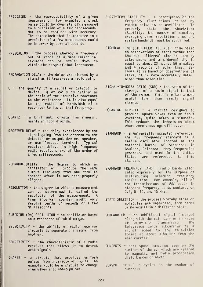
PRECISION - the reproducibility of a givenmeasurement. For example, a clockpulse could be consistently measuredto a precision of a few nanoseconds.Not to be confused with accuracy.The same clock that is measured to a

precision of a few nanoseconds couldbe in error by several seconds.

PRESCALING - the process whereby a frequencyout of range of a measurement in-

strument can be scaled down towithin the range of that instrument.

PROPAGATION DELAY - the delay experienced by a

signal as it traverses a radio path.

Q - the quality of a signal or detector ordevice. Q of coils is defined as

the ratio of the inductive reactanceto the resistance. It is also equalto the ratios of bandwidth of a

resonator to its central frequency.

QUARTZ - a brilliant, crystalline mineral,mainly silicon dioxide.

RECEIVER DELAY - the delay experienced by thesignal going from the antenna to thedetector or output device, speaker,or oscilloscope terminal. Typicalreceiver delays in high frequencyradio receivers are of the order of

a few mi 1 1 i seconds.

REPRODUCIBILITY - the degree to which an

oscillator will produce the sameoutput frequency from one time to

another after it has been properlyal igned.

RESOLUTION - the degree to which a measurementcan be determined is called the

resolution of the measurement. A

time interval counter might onlyresolve tenths of seconds or a few

mi 1 1 i seconds.

RUBIDIUM (Rb) OSCILLATOR - an oscillator basedon a resonance of rubidium gas.

SELECTIVITY - the ability of radio receivercircuits to separate one signal from

another.

SENSITIVITY - the characteristic of a radio

receiver that allows it to detectweak signal s.

SHAPER - a circuit that provides uniformpulses from a variety of inputs. An

example would be a circuit to change

sine waves into sharp pulses.

SHORT-TERM STABILITY - a description of thefrequency fluctuations caused byrandom noise in an oscillator. Toproperly state the short-termstability, the number of samples,averaging time, repetition time, andsystem bandwidth must be specified.

SIDEREAL TIME (SIGH DEER 1 EEE AL) - time basedon observations of stars rather thanthe sun. Sidereal time is used byastronomers and a sidereal day is

equal to about 23 hours, 56 minutes,and 4 seconds of solar time. Be-cause it is based on observations ofstars, it is more accurately deter-mined than solar time.

SIGNAL-TO-NOISE RATIO (SNR) - the ratio of thestrength of a radio signal to thatof the noise. This is often a moreuseful term than simply signal

strength.

SQUARING CIRCUIT - a circuit designed to

produce square waves from an inputwaveform, quite often a sinusoid.This reduces the indecision aboutwhere zero crossings will occur.

STANDARD - a universally accepted reference.The NBS frequency standard is a

cesium oscillator located at the

National Bureau of Standards in

Boulder, Colorado. Many frequenciesgenerated and used in the United

States are referenced to this

standard.

STANDARD FREQUENCY BAND - radio bands allo-

cated expressly for the purpose of

distributing standard frequencyand/or time. For example, all of

the transmissions of WWV occur in

standard frequency bands centered on

2.5, 5, 10, and 15 MHz.

STATE SELECTION - the process whereby atoms or

molecules are separated, from atoms

or molecules in a different state.

SUBCARRIER - an additional signal inserted

along with the main carrier in radio

or television transmission. The

television color subcarrier is a

signal added to the television

format at about 3.58 MHz from the

main carrier.

SUNSPOTS - dark spots sometimes seen on the

surface of the sun which are related

to magnetic and radio propagation

disturbances on earth.

SUNSPOT CYCLES - cycles in the number of

sunspots.

223

SYNCHRONIZATION - in the context of timing,synchronization means to bring two

clocks or data streams into phaseso they agree. They need not be

on time.

TCXO (TEMPERATURE COMPENSATED CRYSTAL OSCIL-LATOR) - a crystal oscillator thatcontains special components to mini-mize the effect of temperature on

the crystal frequency.

TICK - an electrical signal, usually a pulse,designed for use in resetting of

dividers, etc. The WWV tick heardon its radio broadcast consists of 5

cycles of a 1 kHz sine wave.

TIME BASE - in a frequency counter that oscil-lator which provides the timingsignals for measurement and control.The accuracy of the counter is

directly related to the time base.

TIME INTERVAL COUNTER - a counter designed to

measure the time between events,zero crossings for example.

TIME OF COINCIDENCE (LORAN) - that time whenthe Loran signal is coincident withan exact second of CoordinatedUniversal Time. These times of

coincidence will occur about every10 or 15 minutes and have beentabulated by the U. S. Naval Observ-atory.

TRANSFER STANDARDS - the name given to a sig-

nal that is used to perform a cali-bration when it can be referenced to

a standard. An example would be theuse of a VLF frequency source to

transfer frequency to a locationbased on its calibration at NBS.

TRIGGER ERROR - The error associated withfalse triggering caused by phasenoise or jitter on a signal.

TTL INTEGRATED CIRCUITS - a family of integra-ted circuits that uses transistor-transistor logic. At this writingTTL has become the most popularfamily of integrated circuits and is

characterized by fast rise times.

Unless deliberately modified, outputlevels are nominally zero to 5 voltspositive.

UNIVERSAL TIME (UT) FAMILY - Universal Time is

given in several ways. Apparentsolar time is first corrected by theequation of time to mean solar time,UTO. It is then again corrected for

migration of the earth's poles to

obtain UT1 . This is further cor-

rected for periodicity of unknownorigin to obtain UT2.

VFO - variable frequency oscillator as dis-

tinguished from a fixed frequencyoscillator such as a crystal.

WAVE ANGLE - the angle above the surface of

the earth at which a signal is

transmitted from or received by an

antenna.

WAVEMETER - a meter for measuring frequency.Wavemeters usually work by having a

coil that collects part of the

energy from a transmitter or a

transmission line and displaysresonance on a meter movement.

ZERO BEAT - that condition between two signals

when no beat is heard or seen be-

tween the signals; that is, the

frequencies are equal.

224

INDEX

AT CUT IN CRYSTALSt 201

ACCURACY

ATOMIC RESONATORS ..... 206

CALIBRATION

GOES Satellite Time Code 176,185High Frequency Radio Broadcast 77,78,79,80Loran-C 171,172Low Frequency/Very Low Frequency Radio Broadcast . . . . 107,130Television

Frequency 131 ,145,149Time 147,151

TRANSIT Satellite . . 187,189

CESIUM 208,211

COUNTER 43

DEFINITION 193

HYDROGEN MASER, ATOMIC 209,211

QUARTZ CRYSTAL OSCILLATOR 199,211

RUBIDIUM , 209,211

ADJUSTABLE RATE DIVIDERS 64

AGING, QUARTZ CRYSTAL 201

ALGEBRA OF TIME AND FREQUENCY MEASUREMENTS 27-32

AMBIGUITY

PHASE CHART, WWVB 108

± 1 COUNT 34,44

TELEVISION LINE-10 148,151

ANALOG FREQUENCY METER, DIRECT-READING 58

ANTENNAS

GOES Satellite 180

HF (High Frequency) ........... 82

LF/VLF (Low/Very Low Frequency). ........ 107

TO REDUCE INTERFERENCE AT LF/VLF 113

APPARENT SOLAR TIME ]7

ASTRONOMICAL OBSERVATORIES

ASTRONOMICAL TIME ]7

225

ASTRONOMY, USE OF TIME SCALES FOR 22

ATOMIC

BEAM, CESIUM 207

CLOCK

Cesium 198,207World's First 18

FREQUENCY SOURCES 205-211

HYDROGEN MASER . . 209

OSCILLATORS 205

Cesium 207Hydrogen 209Rubidium 208

RESONATOR 206

RUBIDIUM OSCILLATOR 208

TIME (TA) 18

TIME SCALES (See TIME SCALES)

ATOMIC RESONANCE, ACHIEVING 204

AUTOMATIC TRANSFER OSCILLATOR 37

AVERAGER, SIGNAL 65

BIH (BUREAU INTERNATIONAL DE L'HEURE)

ROLE IN INTERNATIONAL COORDINATION OF TIME AND FREQUENCY ... 23

TIME SCALE, TAI(BIH) 18

BAND, RADIO FREQUENCY 10

BASE UNITS OF MEASUREMENT 5

BASIC STANDARDS 5

BEAM, CESIUM 207

BEAT FREQUENCY METHOD 97

BROADCAST STATIONS (See RADIO BROADCASTS, Using for Calibration)

BULLETIN, NBS TIME AND FREQUENCY

MONITORING DATA FOR TRACEABILITY TO NBS

GOES Satellite 180

Loran-C 171

Omega . 108,127

Television

Color Subcarrier Frequency ....... 134,138

Line-10 146

226

WWVB 108,127WWV/WWVH 95

BULLETIN, USNO TIME SERVICES

MONITORING DATA FOR TRACEABILITY TO USNO

Loran-C 170,171NAA/NLK 127Omega 127Television Line-10 .......... 151

TRANSIT Satellite 187

BUREAU INTERNATIONAL DE L'HEURE (See BIH)

CGPM (GENERAL CONFERENCE ON WEIGHTS AND MEASURES) 18

CABLE, DISTRIBUTION OF TIME AND FREQUENCY VIA 11

CALIBRATION

ACCURACY

GOES Satellite ....HF Broadcasts (Time and Frequency)LF/VLFLoran-C .....Television

Frequency 131 ,143,145,149Time 146,147,151

TRANSIT Satellite 187,189

DEFINITION 8

CALIBRATION TECHNIQUES

ELECTRONIC FREQUENCY COUNTER, USE OF

FREQUENCY

HF (High Frequency) Broadcasts.

Beat Frequency MethodOscilloscope MethodsTime Comparison of Clocks.

LF/VLF (Low/Very Low Frequency) Broadcasts

Television

Color Subcarrier ....Line-10

FREQUENCY COMPARISONS

OSCILLOSCOPE

PHASE LOCK

TIME

HF Broadcasts (WWV/WWVH, CHU) .

WWV Time Code

Loran-C .......Satellite .......Television Line-10 .....WWVB Time Code

176,18569,77-80,105107,125,126,130171 ,172

33

96-101

97

98TOO

113-126

131-143145-152

50

48

66

86-92

92

168175-189145-152127

227

CARRIER FREQUENCIES

GOES SATELLITE

HF (HIGH FREQUENCY) BROADCAST STATIONS .

LORAN-C

LF/VLF (LOW/VERY LOW FREQUENCY) BROADCAST STATIONS

OMEGA

TRANSIT SATELLITE ......CATHODE-RAY OSCILLOSCOPE

CESIUM BEAM FREQUENCY OSCILLATORS ....CHAIN, LORAN-C

CHRONOMETER

CLOCK

AGING

ATOMIC

First .......Cesium .......Coordination ......Definition ......As Frequency Source .....Master .......Portable .......Primary .......Secondary . . . .

CODE, TIME (See TIME CODE)

COLOR

BAR COMPARATOR, TV

SUBCARRIER, TV

TELEVISION SIGNALS FOR FREQUENCY CALIBRATION .

COMMERCE, U. S. DEPARTMENT OF

COMPARATORS, FREQUENCY

COMPARISONS, FREQUENCY

OSCILLOSCOPE

HF (HIGH FREQUENCY)

WWVB

CONVENTIONS OF TIME AND FREQUENCY MEASUREMENT

228

CONVERSIONS

PREFIX

PARTS PER... TO PERCENTS

9

9

CONVERTERS, HETERODYNE 35

COORDINATED UNIVERSAL TIME, UTC . . . . 19

COORDINATION OF TIME AND FREQUENCY ACTIVITIES, INTERNATIONAL ... 6

BIH 23

NBS 23

USNO 34

VIA LORAN-C 171

CORRECTIONS, UT1 (See UT1 CORRECTIONS)

COUNTERS, ELECTRONIC FREQUENCY 33

ACCURACY 43

ERRORS 34,43,44,45

FUNCTIONAL PARTS 33

MEASUREMENTS USING

Frequency 34

Period 39

Phase 42

Pulse-Width Determination ........ 43

Time Interval ........... 40

PRINTOUT AND RECORDING 48

COVERAGE

GOES SATELLITE 176

HF (HIGH FREQUENCY) BROADCASTS 69

LORAN-C

Groundwave ........... 166

Skywave ............ 167

TRANSIT SATELLITE 187

WWVB HI

CRYSTAL, QUARTZ, OSCILLATORS (See QUARTZ CRYSTAL OSCILLATORS)

CYCLE PHASE SHIFT, RECEIVER 108

DATE 4-17

DEAD TIME ^

DECADE COUNTING ASSEMBLY IN COUNTERS 33

229

DEFENSE, DEPARTMENT OF 24

DEFINITIONS

ACCURACY 193

CLOCKS 191

DATE 4

FREQUENCY 4,10,193

FREQUENCY STANDARD 191

HERTZ 193

LEAP SECOND 19

PRECISION 223

Q 197,223

REPRODUCIBILITY 193

SECOND 4,193

STABILITY 193

SYNCHRONIZATION 21

TIME 4

TIME SCALE 17

STANDARD 5

DELAY

CABLE 12

DIFFERENTIAL PATH 146

NBS TELEPHONE TIME-OF-DAY . 105

RADIO PROPAGATION PATH (See Propagation Path Delay Measurement)

RECEIVER TIME 86

TELEPHONE LINE 12

TELEVISION SIGNALS 146

DELAYED TRIGGER METHOD OF TIME CALIBRATION 90

DETECTOR, PHASE 62

DIGITAL FRAME SYNCHRONIZER 142,151

DIGITAL OFFSET COMPUTER, TV 138

DIRECT FREQUENCY MEASUREMENT

USING ELECTRONIC COUNTER 35

USING OSCILLOSCOPE ..... 50

DIRECT-READING ANALOG FREQUENCY METER 58

ELECTRONIC AUDIO 58

RADIO FREQUENCY 59

230

DIRECT-TRIGGER METHOD OF TIME CALIBRATION 88

DISCRIMINATOR, FREQUENCY 60

DISSEMINATION TECHNIQUES

GOES SATELLITE

HF (HIGH FREQUENCY) BROADCASTS

LORAN-C

LF/VLF (LOW/VERY LOW FREQUENCY) BROADCASTS

TV

Color Subcam'er Frequency ........ 131-143

Line- 10 Time and Frequency ........ 145-152

TRANSIT SATELLITE 187-189

DISTANCE, GREAT CIRCLE CALCULATIONS 101

DISTRIBUTION OF TIME AND FREQUENCY

CABLE

HF (HIGH FREQUENCY) RADIO BROADCASTS

LF/VLF (LOW/VERY LOW FREQUENCY) RADIO BROADCASTS

TELEPHONE

TELEVISION

Frequency Using TV Color Subcarrier ...... 131-143

Time and Frequency Using TV Line-10 ...... 145-152

TO UNITED STATES 7

DIVIDER

DIGITAL 63

Adjustable Rate 64

Analog ............ 63

FREQUENCY 63

DRIFT, FREQUENCY 11,44

QUARTZ CRYSTAL OSCILLATORS 201

DUTI (UT1) 17

CORRECTIONS ON WWV/WWVH 19,80,94

CORRECTIONS ON WWVB 127

DETERMINATION OF 23,24

ET (EPHERMERIS TIME) 18

ELECTRONIC AUDIO FREQUENCY METER

ELECTRONIC COUNTERS (See COUNTERS, ELECTRONIC FREQUENCY)

175-187

69-105

153-173

107-130

11

69-105

107-130

105

231

ENVELOPE (WWVB) 128

EPHEMERIS TIME (ET) 18

EQUATION OF TIME 17

EQUIPMENT FOR MAKING CALIBRATIONS

ADJUSTABLE RATE DIVIDER 64

COUNTER, ELECTRONIC 33

DIRECT-READING ANALOG FREQUENCY METER 58

Electronic Audio .......... 58Radio Frequency .......... 59

FREQUENCY COMPARATOR 60

FREQUENCY DIVIDER 63

FREQUENCY SYNTHESIZER 60

HETERODYNE FREQUENCY METER 57

OSCILLOSCOPE 48

PHASE DETECTOR . .' ; . 62

PHASE ERROR MULTIPLIER 61

RECEIVER

LF/VLF (Low/Very Low Frequency) . . . . . . . 113HF (High Frequency) .......... 81

TV

Frequency 136,138,147Time 147

SIGNAL AVERAGER ... . . . ..... 65

WAVEMETER 56

ERROR

COUNTER TIME BASE 34,43

GATE 44

NOISE 34,40

± 1 COUNT AMBIGUITY 34,44

PROPAGATION (See PROPAGATION PATH DELAY MEASUREMENT)

RECEIVER . 86

TIME BASE 34,43

TRIGGER 45

F 28

FCC 8

REQUIREMENTS FOR TV BROADCASTS 141

FADING OF HF SIGNALS 69

FIELD STRENGTH, WWVB Ill

232

FRACTIONAL FREQUENCY (See RELATIVE FREQUENCY)

|

FRAME SYNCHRONIZER, DIGITAL 142,151

!

1 FREQUENCY

ACCURACY OF CALIBRATION

GOES Satellite . 176HF (High Frequency) Broadcasts. . . . . . . . 69,105LF/VLF (Low/Very Low Frequency) . . . . . . 107,130Loran-C 171

AGING EFFECTS 11,201

BANDS, RADIO 10

BEAT OR DIFFERENCE 97

CALIBRATION (See CALIBRATION TECHNIQUES, FREQUENCY)

COMPARATORS 60

COMPARISONS 50

HF (High Frequency) .......... 96Oscilloscope 50,98WWVB 115

DEFINITION . 4,10,193

DIFFERENCE 28

DISCRIMINATOR 60

DIVIDER 63

DRIFT 44,193

HERTZ 4,10

MEASUREMENT (See CALIBRATION TECHNIQUES)

METER, HETERODYNE 57

MULTIPLIER 60

OFFSETS OF TV NETWORKS 134

RADIO BANDS TO

RADIO CARRIER (See CARRIER FREQUENCIES)

SERVICES (see also SERVICES) .

SOURCE (See SOURCE, FREQUENCY)

STABILITY

Atomic ResonatorMeasuring ....Quartz Crystal Oscillator.

SYNTHESIZER ....ZERO-BEAT METHOD

I GT CUT IN CRYSTALS ....|

GATE ERROR

GENERATOR

RF SIGNAL

TIME-BASE, CALIBRATING

5

193

206

193

201

60

37,97

201

44

54

49

233

GOES SATELLITE

ACCURACY 176,185

ANTENNAS 180

CLOCK CALIBRATION, for ... ' 183

CONTINUITY 187

COVERAGE 176

EQUIPMENT NEEDED 180

INTERFERENCE 186

OUTAGES 186

PERFORMANCE 180

RECEIVER MANUFACTURERS 181

SATELLITE-CONTROLLED CLOCK 181

SIGNAL CHARACTERISTICS 177

SMART CLOCK 182

TIME CODE FORMAT 177

GREAT CIRCLE DISTANCE CALCULATIONS 101

GREENWICH, ENGLAND MERIDIAN 17,22

GREENWICH MEAN TIME (See UK)

GROUNDWAVE

COVERAGE, LORAN-C 166

Accuracy ............ 172

DEFINITION 166

HERTZ 4,10,193

HETERODYNE

CONVERTER 35

FREQUENCY METER 57

HF (HIGH FREQUENCY) BROADCASTS, STANDARD TIME AND FREQUENCY

ACCURACY (See ACCURACY, Calibration)

ANTENNAS 82

CALIBRATIONS USING

Frequency............ 96-101

Time 86-93

Time Code 93-95

IONOSPHERIC EFFECTS ON RECEPTION 69,102

RECEIVER SELECTION 81

SIGNAL CHARACTERISTICS 82

STATIONS .69-80

ATA . 71

CHU 70

234

IAM 72

IBF 72

JJY 72

OMA 74VNG 74

WWV/VH 69,81-105,215

HYDROGEN MASER, ATOMIC 209

IRIG TIME CODE 13

INTERFERENCE

HF RADIO BROADCAST 69

LF/VLF RADIO BROADCAST 113

INTERNATIONAL ATOMIC TIME SCALE (TAI) 18

INTERNATIONAL COORDINATION OF TIME AND FREQUENCY ACTIVITIES (SeeCOORDINATION OF TIME AND FREQUENCY ACTIVITIES, INTERNATIONAL)

IONOSPHERE, EFFECTS ON HF RECEPTION 69,102

JITTER 40,44

LF/VLF RADIO BROADCAST

ACCURACY (See ACCURACY, Calibration)

ANTENNAS 107

CALIBRATIONS USING

Frequency . . . . . . . . . . . . 113

Time Code WWVB 127

FIELD STRENGTH Ill

SIGNAL FORMAT 107

STATIONS 107-126

DCF 77 118

HBG 120

JG2AS/JJF-2 120

Loran-C 153-173

MSF 121

OMA 123

Omega Navigation System . . . . . . . . • 115

RBU, RTZ 124

U.S. Navy Communication Stations (NAA, NDT, NLK, NPM, NSS, NWC) . 121

VGC3, VTR3 . 124

WWVB 107-115,127-130

LEAP SECOND 19

LINE-10 SERVICE, TELEVISION

ACCURACY 146,149

EQUIPMENT NEEDED 147

GETTING TIME-OF-DAY 151

235

REFERENCED TO

NBS 146USNO 151

LISSAJOUS PATTERNS 50,98

LONG-TERM STABILITY 44

LORAN-C NAVIGATION SYSTEM (100 kHz)

ACCURACY, CALIBRATION

Frequency ............ 171Time 172

CARRIER FREQUENCIES 161

CHAINS 154-159

CONTROL BY USNO AND U.S. COAST GUARD 153

COVERAGE 166

FREQUENCY CALIBRATION 170

GROUNDWAVE SIGNAL RANGE 166

MASTER STATION 153

PULSE SHAPE 161

SIGNAL CHARACTERISTICS 153,167

SKYWAVE SIGNAL RANGE 167

SLAVE STATION 153

TIME SETTING 168

MASER, ATOMIC HYDROGEN 209

MASTER

CLOCK 7

STATION, LORAN-C 153

MEAN SOLAR TIME 17

MEASUREMENT

TIME INTERVAL (See also CALIBRATION TECHNIQUES) 40

Direct Frequency .......... 35

Period 39

Phase 42

Pulse-Width Determination. . . ...... 43

MERIDIAN OF GREENWICH, ENGLAND ' 17,22

METER

DIRECT-READING ANALOG FREQUENCY

Electronic AudioRadio Frequency

HETERODYNE FREQUENCY.

WAVE

58

5859

57

56

236

METHODS OF CALIBRATION (See CALIBRATION TECHNIQUES)

MONITORING DATA AVAILABILITY (See BULLETIN, NBS or USNO)

MULTIPLE-PERIOD AVERAGING 39,45

MULTIPLIER

PHASE ERROR 61

FREQUENCY 60

NBS (NATIONAL BUREAU OF STANDARDS)

ATOMIC CLOCK 6

FREQUENCY STANDARD .... 6,191

NBS-6 6,198

RADIO BROADCASTS

WWV/WWVH 69,81-105WWVB 107-115,127-130

ROLE (See NBS TIME AND FREQUENCY DIVISION, Responsibilities)

SERVICES

Calibration ........... 23GOES Satellite Time Code 175-187Television

Frequency Calibration via Color Subcarrier .... 131-143

Line- 10 Time and Frequency ....... 145-152

WWV/WWVH 69,81-105WWVB 107-115,127-130

SYSTEM 358 FREQUENCY MEASUREMENT COMPUTER 138

TIME AND FREQUENCY DIVISION 23

Organization ........... 23

Responsibilities . . . . . . . . . . 7,23

TIME CODE

GOES Satellite 177

WWV/WWVH 14,92

WWVB 14,127

TIME STANDARD 6

NATIONAL BUREAU OF STANDARDS (See NBS)

NAVAL OBSERVATORY, U.S. (See USNO)

NAVIGATION

SYSTEM

Loran-COmegaTRANSIT Satellite

USE OF TIME SCALES FOR

153-173115

187-189

22

237

NETWORK TELEVISION BROADCASTS, USES

FREQUENCY CALIBRATION 131-143,145-152

TIME CALIBRATION . . . 145-152

NOAA (NATIONAL OCEANIC AND ATMOSPHERIC ADMINISTRATION) 187

NOISE

ERRORS 34,40

QUARTZ CRYSTAL OSCILLATOR 201

NULL DETECTORS 37

OBSERVATORIES, ASTRONOMICAL 23

OMEGA NAVIGATION SYSTEM

FORMAT, BROADCAST

MONITORING DATA

NOTICES AND NAVIGATIONAL WARNINGS

OPERATING CHARACTERISTICS

PROPAGATION CHARACTERISTICS

SYNCHRONIZATION CONTROL

ORGANIZATION OF TIME AND FREQUENCY ACTIVITIES, INTERNATIONAL (SeeCOORDINATION OF TIME AND FREQUENCY ACTIVITIES, INTERNATIONAL)

OSCILLATOR

ATOMIC 6,205

AUDIO 54

CESIUM BEAM 207,211

HYDROGEN MASER . 209,211

QUARTZ CRYSTAL (See QUARTZ CRYSTAL OSCILLATOR)

RUBIDIUM 208,211

TELEVISION NETWORK 132

TRANSFER 37

VARIABLE FREQUENCY (VFO) 37

OSCILLOSCOPE, CATHODE-RAY 48

OSCILLOSCOPE, METHODS OF CALIBRATION USING

DIRECT MEASUREMENT OF FREQUENCY

FREQUENCY COMPARISON

LISSAJOUS PATTERNS ....PHOTOGRAPHY

PATTERN DRIFT

SWEEP FREQUENCY CALIBRATION .

127

118

115

117

117

50

50,98

92

100

55

238

TIME BASE, CALIBRATING 49

TIME INTERVAL »....,< 56

PTTI (PRECISE TIME AND TIME INTERVAL) 24

PATH DELAY, RADIO PROPAGATION (See PROPAGATION PATH DELAY MEASUREMENT)

PATTERN DRIFT METHOD OF CALIBRATION 100

PATTERNS, LISSAJOUS . 50,98

PERIOD MEASUREMENT 39

PHASE

CHANGES, WWVB, LF/VLF 108

DETECTOR 53,62

ERROR MULTIPLIER 53,61

INSTABILITY OF TV SIGNALS 133

JUMPS, TELEVISION 133

LOCK LOOP 66

LOCK TECHNIQUE 66

MEASUREMENT 42,132

RECORDINGS FOR FREQUENCY CALIBRATION, WWVB 113

RETARDATION, LF/VLF 108

SHIFT IDENTIFICATION, WWVB 114

SHIFT

LF/VLF 108

Cycle 108

TRACKING RECEIVER 66

PHOTOGRAPHY, OSCILLOSCOPE 92

PIEZOELECTRIC EFFECT 199

± 1 COUNT AMBIGUITY 34,44

PORTABLE CLOCK . . . . 5,24

PRECISION, DEFINITION 223

PRESCALING 35

PRIMARY

CLOCK 6

FREQUENCY STANDARD 6,197

239

PRINTER-RECORDER 48

PROPAGATION

CHARACTERISTICS

HF .

LF/VLF

DIFFERENTIAL PATH DELAY

PATH DELAY MEASUREMENT

HFTime Code .

PUBLICATIONS (See Bulletin, NBS or USNO)

PULSE-WIDTH DETERMINATION MEASUREMENT 43

Q, RESONATOR

CESIUM 208

DEFINITION. 197

HYDROGEN 209

QUARTZ CRYSTAL 201

REQUIREMENTS 60

RUBIDIUM 208

QUARTZ CRYSTAL OSCILLATOR

ACCURACY 201,211

AGING 11,43,201

CHARACTERISTICS. .

'

. . . . . . . . . . 199

COST 202,211

DRIFT 11,43

FREQUENCY STABILITY 201

LONG-TERM DRIFT 44

PERFORMANCE 201

PROPERTIES 199

Q 201

SHORT-TERM STABILITY 44

TEMPERATURE EFFECTS 201

RADIO ASTRONOMY OBSERVATORY 23

RADIO BROADCASTS (USING FOR CALIBRATION)

HF 69-105

LF/VLF 107-130

LORAN-C 153-173

NBS 69-105,107-130

OMEGA NAVIGATION SYSTEM 115

69

108

146

87,10115

240

RADIO FREQUENCY

BAND .

METER.

10

59

RADIO PROPAGATION DELAY MEASUREMENT (See PROPAGATION PATH DELAY MEASUREMENT)

RECEIVER

CYCLE PHASE SHIFT, LF/VLF.

DELAY

SELECTION (HF) .

TIME DELAY MEASUREMENTS .

108

15,86

81

87

RELATIVE FREQUENCY

DIFFERENCE.

F

28

28

REPRODUCIBILITY 193

RESONANCE

ATOMIC

DETECTING .

202

204

RESONATOR

ATOMIC

Accuracy .

Detecting ResonanceStability .

State Selection.

QUARTZ CRYSTAL .

206204206

203

199

RESPONSIBILITIES IN TIME AND FREQUENCY COORDINATION (See COORDINATIONOF TIME AND FREQUENCY ACTIVITIES, INTERNATIONAL)

RUBIDIUM GAS CELL OSCILLATOR

S, RELATIVE FREQUENCY DIFFERENCE

208

28

SCALE, TIME (See TIME SCALE)

SCHMITT TRIGGER. 46

SECOND

DEFINITION.

LEAP .

193

19

241

SECONDARY

CLOCK 7

FREQUENCY STANDARD 197

SECONDS TICK, WWV/WWVH 86

SERVICES

NBS

GOES Satellite Time Code 175-187Telephone Time-of-Day ......... 105

Television

Frequency Calibration, Color Subcarrier ..... 131-143

Time and Frequency Calibration, Line-10 ..... 131-143

Time and Frequency Division . . . . . . 23WWV/WWVH 69,81-105WWVB . 107-115,127-130

RADIO BROADCAST

HF 69-105LF/VLF 107-130Loran-C 153-173Omega. . 115

USNO 24,142,151,170,171,187

SHIFT, DIURNAL, LF/VLF 108

SHORT-TERM STABILITY 44

SIDEREAL TIME 17

SIGNAL

AVERAGER 65

CHARACTERISTICS

HF 82

LF/VLF 1 08

Loran-C ............ 153

Television. ........... 133

WWVB 108

SKYWAVE

COVERAGE, LORAN-C

Accuracy .

DEFINITION.

HOPS, HF .

SLAVE STATION, LORAN-C ^^^^HH ...... 153

SOLAR TIME 17

167

172

167

102

242

SOURCE, FREQUENCY

ATOMIC OSCILLATOR

Cesium Beam ........... 207Hydrogen Maser........... 209Rubidium . 208

COMPARISONS OF 211

PERFORMANCE . . . . 193

PRIMARY AND SECONDARY STANDARDS 197


RESONATORS 196

STABILITY (See STABILITY)

SPECIFICATIONS, STABILITY 44

STABILITY

ATOMIC OSCILLATOR

Cesium Beam 207,211Hydrogen Maser 209,211Rubidium 208,211

DEFINITION 193

FRACTIONAL FREQUENCY 194

INFLUENCES ON . 193,194


SPECIFICATIONS

Long-Term............. 44Short-Term. ........... 44

TELEVISION COLOR SUBCARRIER 141

STANDARDS

ATOMIC 6

BASIC. . 5

CESIUM BEAM 207

DEFINITION 5,191

FREQUENCY 6

HYDROGEN MASER 209

NBS TIME AND FREQUENCY 6

PRIMARY (DEFINED) 197

RUBIDIUM 208

SECONDARY (DEFINED) 197

STATE SELECTION, ATOMIC 203

STATE STANDARDS LABS 7

SUBCARRIER, COLOR TELEVISION, 3.58 MHz 131

SUNDIAL

243

17

SWEEP FREQUENCY CALIBRATION 55

SYNTHESIZER, FREQUENCY . 60

SYNCHRONIZATION, SYSTEMS 21

TA (ATOMIC TIME) 18

TAI (INTERNATIONAL ATOMIC TIME) 18

TCXO (TEMPERATURE-CONTROLLED CRYSTAL OSCILLATOR) 201

TABLES

CHARACTERISTICS OF THE MAJOR TIME AND FREQUENCY DISSEMINATION SYSTEMS . 213

CHARACTERISTICS OF THE OMEGA NAVIGATION SYSTEM STATIONS. . . . 116

COMPARISON OF FREQUENCY SOURCES 211

CONVERSION TO HERTZ 10

HOW FREQUENCY IS CALIBRATED 214

HOW TIME IS CALIBRATED 214

IMAGE FREQUENCIES FOR WWV/WWVH 82

LORAN-C CHAINS 154

LORAN-C ECD TABLE: HALF CYCLE PEAK AMPLITUDE vs ECD . . 163

LORAN-C GROUP REPETITION INTERVALS 164

PARTS PER. . . TO PERCENT CONVERSION . 9

PREFIX CONVERSION 9

RADIO FREQUENCY BANDS 10

READINGS OBTAINED WITH VARIOUS SETTINGS OF TIME BASE AND PERIODMULTIPLIER CONTROLS ... 40

STANDARD FREQUENCY AND TIME SIGNAL BROADCASTS IN THE HIGH FREQUENCY BAND 77-80

STANDARD FREQUENCY AND TIME SIGNAL BROADCASTS IN THE LOW FREQUENCY BAND 125-126

TECHNIQUES, CALIBRATION (See CALIBRATION TECHNIQUES)

TELEPHONE

DISTRIBUTION OF TIME AND FREQUENCY 11

NBS TIME-OF-DAY SERVICE ... 12,105

TELEVISION


Color Subcarrier, Frequency ........ 131,138

Line-10

Frequency 145,149

Time 147,151

COLOR

Bar Comparator 136

Subcarrier, 3.58 MHz 132

244


Frequency

Color Subcarrier .

Line- 10

Time, Line-10

DIGITAL FRAME SYNCHRONIZER .

DIGITAL OFFSET COMPUTER

FREQUENCY OFFSET

PHASE INSTABILITY OF SIGNAL .

SYSTEM 358 FREQUENCY MEASUREMENT COMPUTER

TRACEABILITY OF CALIBRATION

NBSUSNO

USNO TV FREQUENCY CALIBRATION SERVICE .

TEMPERATURE

COMPENSATED CRYSTAL OSCILLATOR (TCXO)

EFFECTS ON CRYSTALS

EFFECTS ON TIME BASE OSCILLATORS .

TIME


GOES Satellite Time Code .

HF Radio Broadcasts .

LF/VLF Radio Broadcasts .

Loran-C .......Television Line-10 . . . . .

TRANSIT Satellite Navigation System.

ATOMIC

CALIBRATION (See CALIBRATION TECHNIQUES, TIME)

CODE (See TIME CODE)

OF-DAY

DEFINITION

DELAY (See DELAY)

EPHEMERIS

EQUATION OF

FREQUENCY DIVISION, NBS

INTERVAL

Definition. ......Measurement ......

SERVICE DIVISION, USNO

SERVICES (see also SERVICES) . . . .

SIDEREAL

SOLAR

STANDARD

TELEPHONE TIME-OF-DAY SERVICE .

131-143145-151

151

142,151

138

134

133

138

135,146151

142

201

201

43

184

69,77-80,105107,125-126,130172

147,151189

18

4,86

4

18

17

23

4

40,56

24

5,23,24

17

17

6

105

245

TRANSFER

Using WWVB Transmitted Envelope 128Using Television Line-10 145-152

UNIVERSAL . . . . . 19

ZONES 20

TIME BASE

CALIBRATION 49

ERROR 34,43

FUNCTION IN COUNTERS 33

TIME CALIBRATION (See CALIBRATION TECHNIQUES, TIME)

TIME CODE

ACCURACY 15

DEFINITION 13

GOES Satellite 177

IRIG 13

RECOVERING

WWV/WWVH 92WWVB 127

UTILITY OF 15

WWV/WWVH 14,92

WWVB 14,127

Time Transfer Using Transmitted Envelope. . . . . . 128

TIME OF COINCIDENCE (TOC), LORAN-C 170

TIME COMPARISON FOR FREQUENCY CALIBRATION 100

TIME SCALE

ASTRONOMICAL 17

ATOMIC

TA, TAI 18

UTC 19

DEFINITION 17

HISTORY 17

NAVIGATOR'S 17

UNIFORMITY. 17

USES 21

TRACEABILITY

DEFINITION 8

246

ESTABLISHING

NBS

Time and Frequency Bulletin

Loran-C ....Television Color SubcarrierTelevision Line- 10

Omega.WWVB .

USNO

Time Services Bulletin

LF/VLF BroadcastsLoran-CTelevision Line-10TRANSIT Satellite

TRANSIT SATELLITE NAVIGATION SYSTEM.

TRIGGER LEVEL ERRORS.

UTC (COORDINATED UNIVERSAL TIME)

TIME SCALE

RADIO BROADCASTS

UT1

CORRECTIONS

WWV/WWVH ....WWVB

DETERMINATION ....USNO (U.S. NAVAL OBSERVATORY)

MONITORING DATA (See BULLETIN, USNO)

LINE-10 SERVICE 151

PTTI COORDINATION GROUP . 24

ROLE IN INTERNATIONAL COORDINATION OF TIME AND FREQUENCY ... 24

Determination of UT1 24

TIME SERVICES DIVISION 24

TV FREQUENCY CALIBRATION SERVICE 142

UNIVERSAL

TIME, COORDINATED 19

TIME FAMILY 17

U.S. NAVAL OBSERVATORY (See USNO)

VFO (VARIABLE FREQUENCY OSCILLATOR) 37

VLF RADIO BROADCASTS, CALIBRATIONS USING 107-130

134,138146

127127

127

170,171151

187

187

42,45

19

77-80,125-126

19,94127

22,24

247

WAVELENGTH. 10

WAVEMETER 56

WWV/WWVH

ANTENNAS 82


Frequency 96Time 86Time Code 92

CHARACTERISTICS, SIGNAL 82

FORMAT ... 69,215

Time Code 93

TIME-OF-DAY ANNOUNCEMENTS 86

TELEPHONE TIME SERVICE 105

PROPAGATION PATH DELAY 101

WWVB

ANTENNAS 107


Frequency . . . . . . . . . . . . 113

Time Code 127

CHARACTERISTICS 108

FIELD STRENGTH . . . Ill

FORMAT 107

Time Code 127

PHASE SHIFT IDENTIFICATION 114

YEARLY UTC OFFSET (PRIOR TO 1972) 19

ZERO BEAT METHOD OF FREQUENCY COMPARISON 37,97

ZERO OFFSET OF UTC TIME SCALE 19

ZONES, TIME 20

248

NBS-114A (rev. 0-78)

U.S. DEPT. OF COMM.

BIBLIOGRAPHIC DATASHEET

1. PUBLICATION OR REPORT NO.

SPECIAL PUBLICATION 559n. " ,-.

4. TITLE AND SUBTITLE 5. Publication Date

November 1979

TIME & FREQUENCY USERS' MANUAL

7. AUTHOR(S)

George Kamas and Sandra L. Howe, eds.

8. Performing Organ. Report No.

9. PERFORMING ORGANIZATION NAME AND ADDRESS

NATIONAL BUREAU OF STANDARDSDEPARTMENT OF COMMERCEWASHINGTON, DC 20234

10. Project/ Unit No.

11. Contract/Grant No.

12. SPONSORING ORGANIZATION NAME AND COMPLETE ADDRESS (Street, city, state, ZIP)

Same as 9.

13. Type of Report & Period Covered

log *«ency Code

. I I. ... Illl II ^I I —

15. SUPPLEMENTARY NOTES

Library of Congress Number 79-600169Supersedes TN 695

I |Document describes a computer program; SF-185, FIPS Software Summary, is attached.

16. ABSTRACT (A 200-word or leas factual summary of moat significant information. If document includes a significant bibliography or

literature survey, mention it here.)

This manual has been written for the person who needs information on

making time and frequency measurements. It has been written at a

level that will satisfy those with a casual interest as well as

laboratory engineers and technicians who use time and frequency every

day. It gives a brief history of time and frequency, discusses the

roles of the National Bureau of Standards, the U. S. Naval Observatory,

and the International Time Bureau, and explains how time and frequency

are internationally coordinated. It also explains what time and

frequency services are available and how to use them. It discusses

the accuracies that can be achieved using the different services as

well as the pros and cons of using various calibration methods.

17. KEY WORDS (six to twelve entries; alphabetical order; capitalize only the first letter of the first key word unless a proper name;

separated by aemicolona)

Frequency calibration; high frequency; Loran-C; low frequency; radio broadcasts;

satellite broadcasts; standard frequencies; television color subcarrier; time

and frequency calibration methods; time calibration; time signals.

18. AVAILABILITY Unlimited

I IFor Official Distribution. Do Not Release to NTIS

[X] Order From Sup. of Doc, U.S. Government Printing Office, Washington, D.C.20402, SD Stock No. SN003-003-02137-1

I IOrder From National Technical Information Service (NTIS), Springfield,

VA. 22161

19. SECURITY CLASS(THIS REPORT)

UNCLASSIFIED

20. SECURITY CLASS(THIS PAGE)

UNCLASSIFIED

21. NO. OFPRINTED PAGES

256

22. Price

$6

INSERT STOCKUSCOMM-DC

Waste Heat

Management

Guidebook

A typical plant can save about 20 percent of its

fuel—just by installing waste heat recovery equip-

ment. But with so much equipment on the market,

how do you decide what's right for you?

Find the answers to your problems in the WasteHeat Management Guidebook, a new handbookfrom the Commerce Department's National Bureauof Standards and the Federal Energy Administra-tion.

The Waste Heat Management Guidebook is de-

signed to help you, the cost-conscious engineer or

manager, learn how to capture and recycle heat

that is normally lost to the environment during in-

dustrial and commercial processes.

The heart of the guidebook is 14 case studies of

companies that have recently installed waste heat

recovery systems and profited. One of these appli-

cations may be right for you, but even if it doesn't

fit exactly, you'll find helpful approaches to solving

many waste heat recovery problems.

In addition to case studies, the guidebook contains

information on:

• sources and uses of waste heat

• determining waste heat requirements• economics of waste heat recovery• commercial options in waste heat recoveryequipment

• instrumentation

• engineering data for waste heat recovery• assistance for designing and installing waste

heat systems

To order your copy of the Waste Heat ManagementGuidebook, send $2.75 per copy (check or moneyorder) to Superintendent of Documents, U.S. Gov-ernment Printing Office, Washington, D.C. 20402.A discount of 25 percent is given on orders of 100 1

copies or more mailed to one address.

The Waste Heat Management Guidebook is part ofi|fr„

the EPIC industrial energy management programaimed at helping industry and commerce adjust to

the increased cost and shortage of energy.

ill

U.S. DEPARTMENT OF COMMERCE/ National Bureau of StandardsFEDERAL ENERGY ADMINISTRATION/ Energy Conservation and Environment

There'sanewlook

/ y 1 / ' ' ' montr, 'y

/ / / magazine of the Nation-' ^/ a ' Bureau of Standards.

f / Still featured are special ar-

^M^^^k^r/ tides of general interest on\ ^1 / current topics such as consum-\ y / er product safety and building

technology. In addition, new sec-

tions are designed to . . . PROVIDESCIENTISTS with illustrated discussions

of recent technical developments andwork in progress . . . INFORM INDUSTRIAL

MANAGERS of technology transfer activities in

Federal and private labs. . . DESCRIBE TO MAN-UFACTURERS advances in the field of voluntary and

mandatory standards. The new DIMENSIONS/NBS also

carries complete listings of upcoming conferences to beheld at NBS and reports on all the latest NBS publications,

with information on how to order. Finally, each issue carries

a page of News Briefs, aimed at keeping scientist and consum-alike up to date on major developments at the Nation's physi-

cal sciences and measurement laboratory.

(please detach here)

SUBSCRIPTION ORDER FORM

Enter my Subscription To DIMENSIONS/NBS at $11.00. Add $2.75 for foreign mailing. No additional

postage is required for mailing within the United States or its possessions. Domestic remittances

should be made either by postal money order, express money order, or check. Foreign remittances

should be made either by international money order, draft on an American bank, or by UNESCOkoupons.

Send Subscription to:

NAME-FIRST, LAST

I I I I I l I I I I I I I I I I I I I I I I I I I I I I I

O Remittance Enclosed

(Make checks payable

to Superintendent of

Documents)

O Charge to my Deposit

Account No.

COMPANY NAME OR ADDITIONAL ADDRESS LINE

STREET ADDRESS

I I I M I I I I I I I ! i

I M ! i I I I I I i I i I I

PLEASE PRINT

MAIL ORDER FORM TO:

Superintendent of Documents

Government Printing Office

Washington, D.C. 20402

ft U.S. Government Printing Office: 1979—303-857

NBS TECHNICAL PUBLICATIONS

PERIODICALS

JOURNAL OF RESEARCH—The Journal of Research of the

National Bureau of Standards reports NBS research and develop-

ment in those disciplines of the physical and engineering sciences in

which the Bureau is active. These include physics, chemistry,

engineering, mathematics, and computer sciences. Papers cover a

broad range of subjects, with major emphasis on measurementmethodology and the basic technology underlying standardization.

Also included from time to time are survey articles on topics

closely related to the Bureau's technical and scientific programs.

As a special service to subscribers each issue contains complete

citations to all recent Bureau publications in both NBS and non-

NBS media. Issued six times a year. Annual subscription: domestic

$17; foreign $21.25. Single copy, $3 domestic; $3.75 foreign.

NOTE: The Journal was formerly published in two sections: Sec-

tion A "Physics and Chemistry" and Section B "Mathematical

Sciences."

DIMENSIONS/NBS—This monthly magazine is published to in-

form scientists, engineers, business and industry leaders, teachers,

students, and consumers of the latest advances in science andtechnology, with primary emphasis on work at NBS. The magazine

highlights and reviews such issues as energy research, fire protec-

tion, building technology, metric conversion, pollution abatement,

health and safety, and consumer product performance. In addi-

tion, it reports the results of Bureau programs in measurementstandards and techniques, properties of matter and materials,

engineering standards and services, instrumentation, andautomatic data processing. Annual subscription: domestic $11;

foreign $13.75.

NONPERIODICALS

Monographs— Major contributions to the technical literature on

various subjects related to the Bureau's scientific and technical ac-

tivities.

Handbooks—Recommended codes of engineering and industrial

practice (including safety codes) developed in cooperation with in-

terested industries, professional organizations, and regulatory

bodies.

Special Publications— Include proceedings of conferences spon-

sored by NBS, NBS annual reports, and other special publications

appropriate to this grouping such as wall charts, pocket cards, andbibliographies.

Applied Mathematics Series— Mathematical tables, manuals, andstudies of special interest to physicists, engineers, chemists,

biologists, mathematicians, computer programmers, and others

engaged in scientific and technical work.

National Standard Reference Data Series— Provides quantitative

data on the physical and chemical properties of materials, com-piled from the world's literature and critically evaluated.

Developed under a worldwide program coordinated by NBS under

the authority of the National Standard Data Act (Public Law90-396).

NOTE: The principal publication outlet for the foregoing data is

the Journal of Physical and Chemical Reference Data (JPCRD)published quarterly for NBS by the American Chemical Society

(ACS) and the American Institute of Physics (AIP). Subscriptions,

reprints, and supplements available from ACS, I 155 Sixteenth St.,

NW, Washington, DC 20056.

Building Science Series— Disseminates technical information

developed at the Bureau on building materials, components,

systems, and whole structures. The series presents research results,

test methods, and performance criteria related to the structural andenvironmental functions and the durability and safety charac-

teristics of building elements and systems.

Technical Notes—Studies or reports which are complete in them-

selves but restrictive in their treatment of a subject. Analogous to

monographs but not so comprehensive in scope or definitive in

treatment of the subject area. Often serve as a vehicle for final

reports of work performed at NBS under the sponsorship of other

government agencies.

Voluntary Product Standards— Developed under procedures

published by the Department of Commerce in Part 10, Title 15, of

the Code of Federal Regulations. The standards establish

nationally recognized requirements for products, and provide all

concerned interests with a basis for common understanding of the

characteristics of the products. NBS administers this program as a

supplement to the activities of the private sector standardizing

organizations.

Consumer Information Series— Practical information, based on

NBS research and experience, covering areas of interest to the con-

sumer. Easily understandable language and illustrations provide

useful background knowledge for shopping in today's tech-

nological marketplace.

Order the above NBS publications from: Superintendent oj Docu-

ments, Government Printing Office, Washington, DC 20402.

Order the following NBS publications—FIPS and NBSIR's—fromthe National Technical Information Services, Springfield, VA 22161

.

Federal Information Processing Standards Publications (FIPS

PUB)— Publications in this series collectively constitute the

Federal Information Processing Standards Register. The Register

serves as the official source of information in the Federal Govern-

ment regarding standards issued by NBS pursuant to the Federal

Property and Administrative Services Act of 1949 as amended.

Public Law 89-306 (79 Stat. 1127), and as implemented by Ex-

ecutive Order 11717(38 FR 12315, dated May II, 1973) and Part 6

of Title 15 CFR (Code of Federal Regulations).

NBS Interagency Reports (NBSIR)—A special series of interim or

final reports on work performed by NBS lor outside sponsors

(both government and non-government). In general, initial dis-

tribution is handled by the sponsor: public distribution is by the

National Technical Information Services, Springfield, VA 22161,

in paper copy or microfiche form.

BIBLIOGRAPHIC SUBSCRIPTION SERVICES

The following current-awareness and literature-survey bibliographies

are issued periodically by the Bureau:

Cryogenic Data Center Current Awareness Service. A literature sur-

vey issued biweekly. Annual subscription: domestic $25; foreign

$30.

Liquefied Natural Gas. A literature survey issued quarterly. Annual

subscription: $20.

Superconducting Devices and Materials. A literature survej issued

quarterly. Annual subscription: $30. Please send subscription or-

ders and remittances for the preceding bibliographic services lo the

National Bureau of Standards, Cryogenic Data Center (736)

Boulder, CO 80303.

U.S. DEPARTMENT OF COMMERCENational Bureau of StandardsWashington. D.C. 20234

OFFICIAL BUSINESS

Penalty for Private Use. $300

POSTAGE AND FEES PAIDU.S. DEPARTMENT OF COMMERCE

COM-215U.S.MAIL

SPECIAL FOURTH-CLASS RATEBOOK

1298

Time and frequency users manual

Documents

Transcript of Time and frequency users manual