ieee transactions on ultrasonics, ferroelectrics, and frequency control, vol. 54, no. 11, november 2007 2257

Mechanical Properties of Single Cells byHigh-Frequency Time-Resolved Acoustic

MicroscopyEike C. Weiss, Pavlos Anastasiadis, Gotz Pilarczyk, Robert M. Lemor, and Pavel V. Zinin

Abstract—In this paper, we describe a new, high-frequency, time-resolved scanning acoustic microscope de-veloped for studying dynamical processes in biological cells.The new acoustic microscope operates in a time-resolvedmode. The center frequency is 0.86 GHz, and the pulse du-ration is 5 ns. With such a short pulse, layers thicker than3 �m can be resolved. For a cell thicker than 3 �m, the frontecho and the echo from the substrate can be distinguishedin the signal. Positions of the first and second pulses areused to determine the local impedance of the cell modeledas a thin liquid layer that has spatial variations in its elas-tic properties. The low signal-to-noise ratio in the acousticalimages is increased for image generation by averaging thedetected radio frequency signal over 10 measurements ateach scanning point. In conducting quantitative measure-ments of the acoustic parameters of cells, the signal canbe averaged over 2000 measurements. This approach en-ables us to measure acoustical properties of a single HeLacell in vivo and to derive elastic parameters of subcellularstructures. The value of the sound velocity inside the cell(1534�5� 33�6 m/s) appears to be only slightly higher thanthat of the cell medium (1501 m/s).

I. Introduction

Mechanical factors play an important role in the reg-ulation of cell physiology, including cell division, cell

motility, and cell adhesion [1]–[5]. Recently, the effects ofthe cell pathophysiology, in particular the effect of can-cer on cell viscoelasticity, have attracted the attention ofbiomedical researchers due to the fact that direct connec-tions between single-cell biomechanics and human cancerhave been discovered [2], [6]–[9]. Despite the numeroustechniques currently available for studying the mechanicalproperties of biological cells (see review papers [9], [10]):micropipette technique [4]; magnetic twisting cytometry[11]; optical traps, optical tweezers [12], laser tweezers, oroptical clamps [12]; optical stretcher [13]; atomic force mi-croscopy [14], [15]; most of these techniques are used formeasuring mechanical properties only of cell membranes(micropipette technique, atomic force microscopy), or the

Manuscript received December 14, 2006; accepted June 20, 2007.This work was supported in part by the European Framework Pro-gram 6 Project “CellProm” under the contract no. NMP4-CT-2004-500039. The financial support provided by “Alexander von HumboldtFoundation” of Germany is gratefully acknowledged.

E. C. Weiss, P. Anastasiadis, G. Pilarczyk, and R. M. Lemorare with Biomedical Ultrasound Research, Fraunhofer-Institute forBiomedical Technology, St. Ingbert, Germany.

P. V. Zinin is with the School of Ocean and Earth Sci-ence and Technology, University of Hawaii, Honolulu, HI. (e-mail:zinin@soest.hawaii.edu).

Digital Object Identifier 10.1109/TUFFC.2007.530

combined mechanical properties of the cell membranes andthe cytoskeleton.

Scanning acoustic microscopy (SAM) is one of the fewtechniques that allows studying the mechanical propertiesof a single cell’s interior (cytoskeleton, cytoplasm, and nu-cleus) [16]. An ideal modification of the SAM that enablesmeasuring all necessary parameters of a cell is the time-resolved acoustic microscope [17]–[19]. In time-resolvedacoustic microscopy, the echo signal from the layered sys-tem is recorded. The use of a short pulse instead of longburst signals pulse allows measuring cell thickness, varia-tion of sound velocity, attenuation, and density inside thecell simultaneously [17]–[19]. Time-resolved SAM with afrequency of 500 MHz [18] has been used for measuring theelastic properties of thin fibroblast cells whose thicknessdid not exceed 5 µ [18]. The pulse reflected from the topside of the cell has been detected and recorded. However,the resolution at 500 MHz was not sufficient to discern theinternal structure of the cell. In order to achieve a bet-ter, nearly optical resolution, and to measure the acousticproperties of different cell structures, a shorter pulse witha central frequency of about 1 GHz is required. Due tothe high attenuation of sound in water in the gigahertzfrequency range [20] and the small difference in the acous-tical impedance between cell and coupling liquid, the pulsereflected from the top cell’s surface is weak and its ampli-tude becomes comparable with the level of noise in theacoustical system [21], [22]. Therefore, the main challengein constructing a time-resolved SAM operating at 1 GHzis to reduce the signal-to-noise ratio.

In this paper, we describe a new version of the high-frequency, time-resolved scanning acoustic microscope de-veloped for studying dynamical processes in biologicalcells, that operates in the gigahertz frequency range. Forimaging the low signal-to-noise ratio in the acoustical im-ages was reduced by averaging the detected radio fre-quency signal over 10 measurements at each scanningpoint. However, for conducting quantitative measurementsof the acoustic parameters of cells, the signal had to be av-eraged over 2000 measurements. This approach enables usto measure acoustical properties of a single cell in vivo andto probe elastic parameters of subcellular structures.

II. Time-Resolved Acoustic Microscopy

Acoustic microscopy was invented for studying the me-chanical microstructure of transparent and nontranspar-ent objects with nearly optical resolution in 1972 [23], and

0885–3010/$25.00 c© 2007 IEEE

2258 ieee transactions on ultrasonics, ferroelectrics, and frequency control, vol. 54, no. 11, november 2007

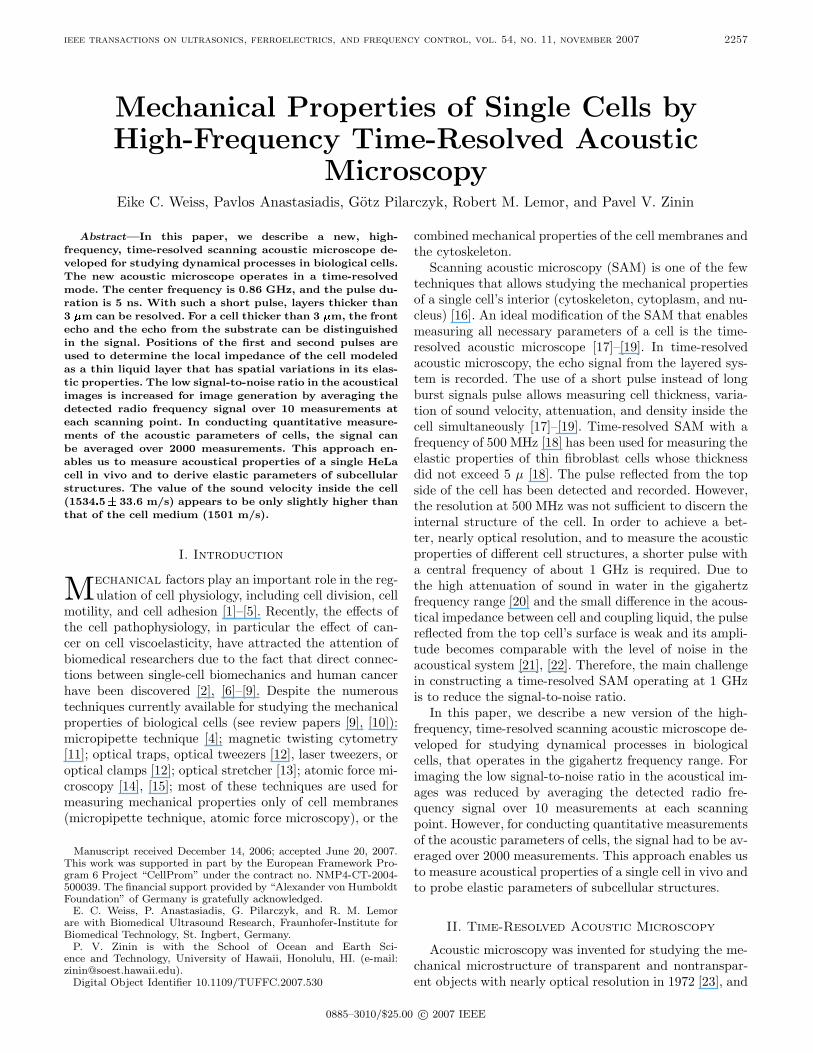
Fig. 1. The setup for quantitative, time-resolved, acoustic mi-croscopy: t0 is the arrival time of the echo reflected from the glasssubstrate outside the cell (“reference echo”) is shown; t1 is the arrivaltime of the echo reflected from the top surface of the cell (top echo); t2is the arrival time of the echo reflected from the cell/substrate inter-face (bottom echo); and d is the cell thickness. The three-dimensionalcoordinate system (x, y, z) is originated at the focal point of the lens.The axis z is normal to the sample surface and directed away fromthe lens, and x and y are parallel to the surface. The axis y is notshown because it is perpendicular to the surface of the diagram. Thedistance Z is the lens defocus.

from its introduction it has been used for mapping theelasticity of living cells [20], [24], [25]. A complete descrip-tion of the basic principles of SAM operation can be foundelsewhere [17], [23], [26]. In the three-dimensional coordi-nate system (x, y, z) with the origin at the focal point(Fig. 1), the distance from the focal plane to the planeobject is called defocus and is notated as Z [27]. The axisz is normal to the sample surface and directed away fromthe lens, and x and y are parallel to the sample surface.Several SAM techniques have been invented for measuringacoustical parameters of cells:

• sound velocity can be deduced from the sum and dif-ferences of the amplitudes in adjacent constructive anddestructive interference fringes in high-frequency SAMimages [28];

• longitudinal wave speed, attenuation, and thicknessprofile of a biological cell are obtained from the voltage(V ), versus frequency (f) at fixed Z or V (f, Z) curves[29], [30]; or

• a combination of C-scans and scans in the sagittal (x-z) plane, when sound wave velocity in the cells is cal-culated from the location of the interference fringe onthe C-mode images and the fringe shift on the x-z scanat 450 MHz [21].

However, each of these techniques have limitations.Quantitative measurements using interference fringes canbe used only for the peripheral area of a cell [31] becausethe central part lacks the fringes. Measurements of theV (f) curve are based on the assumption that the positionof the focus is determined with high accuracy, which is

in practice difficult to achieve [32]. Moreover, techniquesbased on interference fringes were applied only for char-acterizing large cells, such as XT2 fibroblasts, which areabout 100 µ in length. It appears that it cannot be usedfor smaller cells. Another disadvantage of the fringes tech-niques is related to the fact that in reflection acoustic mi-croscopy the signal is never monochromatic. The same lensshould irradiate an acoustical signal and receive it reflectedback from the sample. Therefore, a short pulse excitationis used in reflection acoustic microscopy. A special tech-nique should be applied to measure the amplitude of thesignal at the operational frequency [17].

In quantitative, time-resolved acoustic microscopy, thegoal is to use pulses that are sufficiently short to allowthe reflections from the top and the bottom of the cell tobe separated in the time domain [17]–[19]. Notations fordifferent echoes measured by the time-resolved SAM arepresented in Fig. 1. Let τ1 be the time delay between topand reference echoes (τ1 = t0 − t1), τ2 be the time delaybetween bottom and reference echoes (τ2 = t0−t2), and τ12be the time delay between bottom and top echoes (τ12 =t2 − t1). If the sound velocity in the coupling medium, cw,is known, the measurement of the time delay τ1 allowsthe determination of the cell thickness d at any scanningposition of the microscope (x, y) using a simple geometricaloptics formulation:

d(x, y) =cwτ1(x, y)

2. (1)

Obviously, the time delay τ1 is also a function of thescanning position (x, y): τ1(x, y). When the thickness ofthe cell is known, the longitudinal sound velocity of thespecimen can be derived by measuring either the time de-lay τ12:

c(x, y) =2d(x, y)τ12(x, y)

=cwτ1(x, y)τ12(x, y)

, (2)

or the time delay τ2 from the expression:

τ2(x, y) = 2d

(1c

− 1cw

)= τ1(x, y)

(cw

c− 1

), (3)

c = cw

(τ2(x, y)τ1(x, y)

+ 1)

. (4)

We note that τ2 is negative when the velocity inside thecell is higher than that outside. The velocity of ultrasonicwaves in the cellular fluid, which is similar in the den-sity and compressibility to the immersion fluid, is deter-mined by contributions of various kinds of intra- and inter-molecular interactions [33]. The longitudinal sound speedis closely related to the elastic bulk modulus K of the cell,and its expression can be formulated as:

K = ρc2. (5)

Eq. (5) is valid under the assumption that shear wave ve-locities are much lower than the longitudinal wave veloc-ities, and this holds for several cell types whose interior

weiss et al.: properties of single cells by high-frequency, time-resolved acoustic microscopy 2259

Fig. 2. A photograph of the combined optical (Olympus IX81) andtime-resolved scanning acoustic microscope. The scanning part ofthe microscope is inside a Plexiglas chamber to ensure a constanttemperature of 37◦C.

behaves as a liquid or a material with a small, shear mod-ulus [16], [17]. For instance, the velocity of shear waves inmyocytes is 15 times lower than that of longitudinal waves[34]. Detailed discussion about the use of (5) for cells andthe effect of the sound attenuation on the bulk moduluscan be found elsewhere [33], [35], [36].

III. Materials and Methods

A. Combined Optical and Acoustic Microscope

To evaluate the measurement possibilities of time-resolved acoustic microscopy on living cells, a high-frequency, time-resolved acoustic microscope SAarlandScanning Acoustic Microscopy (SASAM) has been de-signed (Fig. 2). Briefly, the conventional scanning acous-tic microscope is an imaging system in which a radio-frequency (RF) electrical pulse is used to excite acousticalwaves in a lens. The lens contains a spherical cavity [17]that focuses sound onto a spot whose size is comparable tothe acoustic wavelength in the fluid. The acoustic echoesreflected by the object are collected by the same lens andare detected (in a phase-sensitive way) by the piezoelectrictransducer. The lens is scanned over the sample mechani-cally line by line in a raster pattern. During the scan, theRF-signal is recorded for each position. The integral ofthe envelope of the RF-signals can be used to reconstructa grey scale image [17], [26].

This new microscope can be characterized by a com-bination of operating principles and design features dis-tinguishing it from other high-frequency acoustic micro-scopes. These principles are:

• it operates in time-resolved mode;• it is designed as an attachment to an inverse optical

microscope;• it is fully automated, so it can remember the positions

of several cells and acquire acoustical images of thesecells for several hours or even days;

• measurements can be done at 37◦C.

Such a combination is of importance for studying dy-namical processes in biological cells [37], [38]. The design ofthe new microscope is different from that of conventionalacoustical microscopes in that it has a modular structure.The microscope consists of four main modules (Fig. 3):acoustical lens, optical module, scanning unit, and high-frequency electronics.

1. Acoustical Lens: The main component of the high-frequency SAM is the acoustical lens. A detailed descrip-tion of the lens operation can be found elsewhere [39]. Inthis study, we used a high-frequency lens with a semiaper-ture angle of 45◦ manufactured by Kramer Scientific In-struments (Herborn, Germany). The spectrum of the lensis a smoothly varying function around a center frequencyof 860 MHz and a −6 dB bandwidth of 30% [Fig. 4(b)].At this frequency the lens provides a lateral resolution of1.5 µm [26].

2. Optical Module: The optical module consists ofan inverted optical microscope Olympus IX81 (Olympus,Tokyo, Japan) with a scanning unit attached to a rotatingcolumn that allows switching between the condenser andthe acoustical lens. The inverted optical microscope hastwo modes of operation and, therefore, two light paths:reflection mode when the light is coming from the lens lo-cated below the sample, and transmission mode, when thelight from a condenser (located above the sample) passesthrough a sample then is collected by a lens (located be-low the sample) (see Figs. 1 and 3). As a general rule, thetransmission mode provides a good contrast for cell in-terfaces and, therefore, the optical images of the cells areobtained in the transmission mode before starting acous-tical imaging. Imaging in the reflection mode is used inthis microscope for adjusting the focus of the acousticalmicroscope and for aligning the optical axis of the opti-cal microscope and the vertical axis of the acoustical mi-croscope (see below). This setup makes it possible to ob-tain optical trans-illumination, epi-fluorescence, confocaloptical, and acoustical images, in conjunction with syn-chronous acoustic data acquisition from the same cell [37].A part of the optical microscope with the microscope stageis covered by a special chamber (Solent Scientific Limited,Segensworth, UK) (Fig. 2). This configuration providestemperature control for the cells placed on the optical mi-croscope stage. Inside the chamber the temperature can bekept constant at room temperature or 37± 0.5◦C. Opticalimages were acquired using a digital camera with on-chipimage amplification from Hamamatsu Photonics (Hama-matsu, Japan).

2260 ieee transactions on ultrasonics, ferroelectrics, and frequency control, vol. 54, no. 11, november 2007

Fig. 3. The schematic of the combined optical and acoustic microscope.

Fig. 4. Echo signal (a) and amplitude of the Fourier spectra of an echo signals of glass (b) measured with the sample in focus.

weiss et al.: properties of single cells by high-frequency, time-resolved acoustic microscopy 2261

3. Scanning Module: The scanner used to perform theraster movement of the lens over the sample consists of amanual mechanical stage for aligning the acoustic lens andthe optical path (OWIS, Staufen, Germany), a piezo scan-ning stage for the lateral (x-y) scanning and one mechani-cal stage with a direct current (DC) motor performing themovement of the lens in the vertical (z) direction with aresolution of 0.1 µm (Physik Instrumente, Karlsruhe, Ger-many). The acoustic scanner has approximately the sizeof an optical condenser and, therefore, can be attached toalmost any commercially available inverted optical micro-scope (Figs. 2 and 3).

The piezo scanning stage has a scanning range of100 µm × 100 µm and a resonant frequency of severalhundred hertz. The lateral position of the lens is detectedwith a capacitive position sensor with resolution of severalnanometers and is controlled by a power supply developedfor atomic force microscopes.

4. High-Frequency Electronics Module: The high-frequency electronics module for generating and receiv-ing short acoustical pulses is shown as a block diagramin Fig. 3. It consists of a short-pulse generator with 1 nspulse duration, 1 GHz center frequency, 10 Vpp ampli-tude, and a pulse repetition frequency of 500 or 800 kHz;acoustical lens; a high-frequency switch; a broadband lownoise amplifier (Miteq, Hauppauge, NY) with amplifica-tion of 40 dB; and a fast analogue-to-digital (A/D) con-verter DC211 (Acqiris, Geneva, Switzerland). After ampli-fication, the echo signal is digitized. The digitization ratefor the amplified RF signal is 4 GSamples/second and thedigitization resolution is 8 bits. The trigger signals and thesignals for driving the piezo stage are generated by a mi-crocontroller. The step size of the raster pattern can bearbitrarily set between 0.05 and 5 µm.

B. Data Acquisition

Due to the high attenuation of sound in the gigahertzfrequency range and to the small difference in the acous-tical impedance between cell and surrounding liquid, theacoustical images of the cells are typically noisy [21]. Ata frequency of 1 GHz, the total loss due to attenuationin the coupling medium and due to conversion of electri-cal to acoustical energy and vice versa is about −33 dB[39] for a lens with a focal length of 100 µm. Assuming areflection coefficient of a cell surface of 1%, the receivedvoltage is only 5 ∗ 10−6 of the excitation voltage, which isabout 10 V. The signal would be 50 µV compared to 20 µVthermal noise in the electronic circuit. Therefore, the mainchallenge in developing the high-frequency, time-resolvedSAM for biological applications is to increase the powerlevel of the signal associated with the reflection from thetop of the cell to a level higher than that of the systemnoise. In this acoustic microscope multifold averaging (upto 2000) of the signal recorded at each scanning point wasused to increase the signal-to-noise ratio and, therefore,allows detection of the echo reflected from the surface of acell.

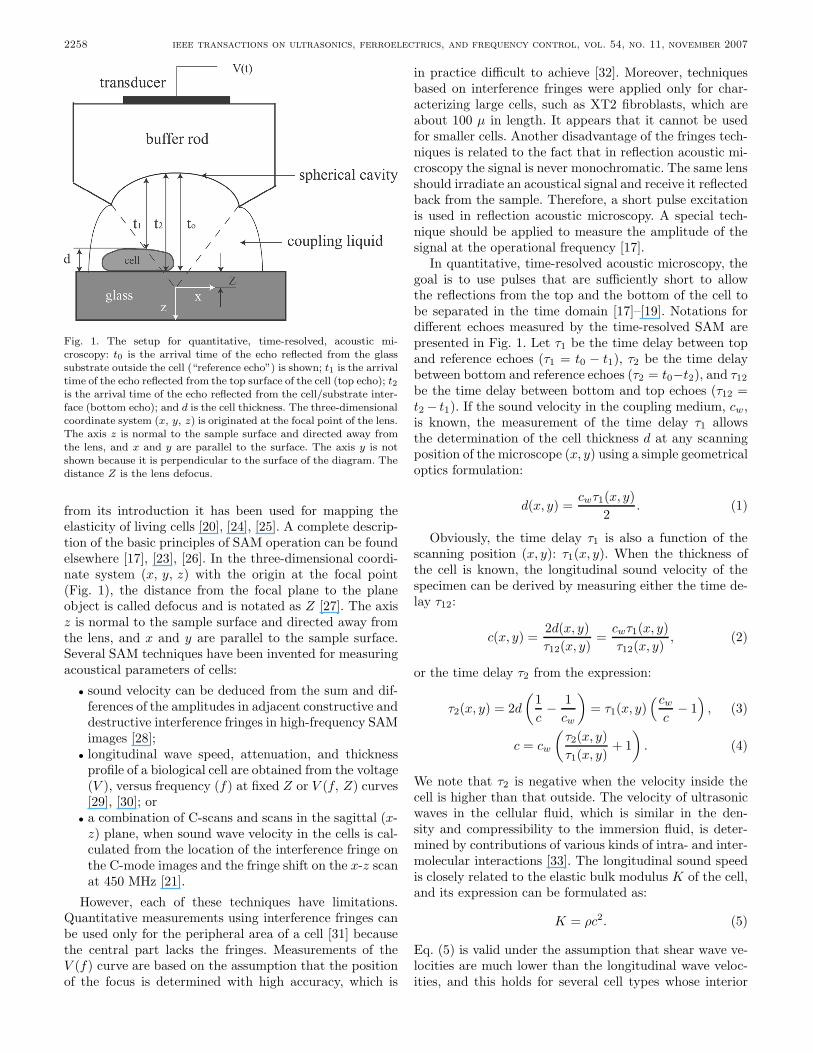
Fig. 5. Echo signal for the HeLa cell with resolved echoes from the topand bottom of the cell measured in focus. The first (“top”) echo is dueto reflection from the surface of the cell. The large echo (“bottom”)comes from the cell/substrate interface. The waveform or envelope ofthe RF signal also is shown. The time delay between top and bottomechoes was determined using the maxima of the waveform function.

Acoustical images are generated from a fixed numberof pixels, small squares assigned specific grey level anda specific coordinate on the image plane (xi, yi), and ar-ranged as a grid. The coordinates (xi, yi) determine theposition of the pixel on the grid. Two operating modes areimplemented in this acoustic microscope: C-scan and RF-scan. The C-scan is obtained when the acoustic microscopemechanically scans the sample in a plane parallel to thesample surface at a fixed defocus position (Z). By vary-ing the defocus position, it is possible to produce acous-tical images of different layers within the sample (three-dimensional imaging). A tenfold averaging of the signalswas used to increase the signal-to-noise ratio on these im-ages. It takes approximately 16 seconds to scan an areaof 50 µm × 50 µm with a step increment of 0.2 µm. TheC-scan is a mode with relatively fast scanning speed andlow rate of signal averaging. It was designed to provide afast acoustic image of the cell.

In the C-scan, grey images are generated from the ul-trasonic datasets. Let Z be the defocus of the lens (Fig. 1),and s(t, xi, yi, Z) be the RF signal measured at any pixelpositions (xi, yi) as a function of time t. The brightness ofthe acoustical images at the defocus Z and at any pixelposition (xi, yi), I(xi, yi, Z), is an integral over time of thesquared RF signal sn(t, xi, yi, Z):

I(xi, yi, Z) =1N

N∑n

∫∆T

[sn(t, xi, Yi, Z)]2 , (6)

where N is the total number of measurements taken at thesame position, and ∆T is the time gate shown in Fig. 5.Further integration over 3–5 images can be used to sup-

2262 ieee transactions on ultrasonics, ferroelectrics, and frequency control, vol. 54, no. 11, november 2007

press noise in the images caused by mechanical vibrationsof the system.

Another mode developed in this microscope is the RF-scan, a mode with relatively slow scanning speed and ahigh rate of signal averaging. It was designed for quanti-tative measurements of sound velocity and sound attenua-tion inside the cells. The collection of the data during theRF-scan is conducted in the following manner: the defo-cus Z is fixed, and the RF signal is recorded at each pixelposition. The RF signal measured at one point inside theHeLa cells is shown in Fig. 5. It is to be noted that theecho signal with a strong top echo shown in Fig. 5 can bedetected only within small areas of the cell.

It takes approximately 2 minutes to get one scan(50 µm × 50 µm) with 0.5-µm step in the x-direction and1-µm step in the y-direction, with 2000-fold averaging ateach pixel position.

From the recorded RF signals, a cross section of the cellalong one scan line can be generated by taking the averageof the positive part of the RF signals:

IB(t, xB , y, Z) =1N

N∑n

sn(t, xB , y, Z). (7)

In the B-scan shown in Fig. 7(d), the scan line is verticaland crosses the bump seen in Fig. 7(a). At each pixel po-sition, the signal was averaged over 2000 times: N = 2000.On the B-scan, the echo reflected from the top surfaceof the cell is well resolved from that reflected from thecell/substrate interface.

The positions and values of the maxima of the echo-signals reflected from the top and the cell/substrate inter-face (see Fig. 5) can be obtained by using the Hilbert trans-form H(s) [40]. The length of the pulse in Fig. 4. is 7 ns(defined as the −20 dB width of the Hilbert-transformedenvelope signal). The imaging procedure in the acousticmicroscope starts by taking optical images of cells with theoptical microscope operating in transmission mode. Theoperation of the optical and acoustic microscopes (move-ment of the lens in the z direction, scanning area, scanningspeed, number of the signal averaging, type of scanning,etc.) is controlled by our custom developed software calledSASAM acoustic investigator. The software allows record-ing the positions of several cells. Subsequently, the acousti-cal lens can be moved to the saved positions for conductingacoustical imaging. After having obtained the optical im-ages of the selected cells, the optical condenser is replacedwith the acoustical lens using the rotating column (seeFig. 3). Subsequently, the optical microscope can operateonly in reflection mode. The reflection optical mode is usedfor two purposes: to safely bring the sample to the focusof the acoustical lens without crushing into the acousticallens, and to align the optical and acoustic microscopes. Inthe reflection mode, the focus of the optical microscope canbe adjusted to see either the cells or the spherical cavityof the acoustical lens. Although the contrast in the opticalimages of the cells is weak, focusing on the cells allows usto determine the position of the cells relative to the acous-

tical lens. When the spherical cavity of the acoustical lensis seen in focus of the optical microscope, the optical andthe acoustical axes of the microscopes can be aligned bymoving the image of the lens to the center of the opticalimage.

C. Attenuation Measurements

In order to estimate the attenuation of the sound wavesinside the HeLa cells we need to separate the contribu-tion associated with the attenuation inside the cell fromthat associated with reflection from a cell and refractionthrough the cell/substrate interface. It was mentioned ear-lier that a reduced reflection coefficient can be caused bya better matching of the acoustic impedances between thecell and the glass substrate at the adhesion focal contacts[41]. The contribution of the attenuation to the reductionof the signal reflected from a cell is difficult to evaluatetheoretically, as was originally reported by Bereiter-Hahnand Blase [16]. However, the variation of brightness of theacoustical image at any pixel position (xi, yi), I(xi, yi, Z)in (6) due to reflection and refraction can be evaluated us-ing a simplified model of the cell proposed by Hildebrand[41] and extended by Kundu et al. [29]. In this model, thecell is considered as a thin liquid layer, and it is assumedthat only rays normal to the glass substrate contribute tothe SAM signal. Such a model is justified for a case whenthe focus of SAM is located above the cell [42]. The reflec-tion coefficient R of the liquid layer for normal incidencehas a simple form [43]:

R(f) =(Zin − Z1)

(Zin + Z1), Zin =

Z2(Z3 − iZ2 tanϕ)

(Z2 − iZ3 tanϕ),

(8)

where ω is the circular frequency, ω = 2πf , ϕ = (ωd/c),Z1 = ρW cW , Z2 = ρc, Z3 = ρScS , d is the thickness of thecell, c is the sound velocity inside the cell, ρ is the densityof the cell, cw is the sound velocity, ρw is the density ofthe coupling liquid, cS is the sound velocity, and ρS is thedensity of the substrate.

An expression for the reflection coefficient is obtainedfor the frequency domain and, therefore, it is easier tomodel the brightness of the acoustical images at any pixelposition (xi, yi), I(xi, yi) in the frequency domain. Thiscan be done using the Parseval’s theorem:

I(xi, yi) =

∞∫−∞

|s(xi, yi, t)|2 dt

=

∣∣∣∣∣∣∞∫

−∞

V (xi, yi, f)df

∣∣∣∣∣∣2

,

(9)

where V (f) is the output signal of SAM as a function offrequency, often called “V (f) curve” [44]. For our simula-tion we used a simplified expression for the output signalof SAM described in [29], in which the absolute value ofthe Fourier spectrum of the output signal was written as:

weiss et al.: properties of single cells by high-frequency, time-resolved acoustic microscopy 2263

|V (f)| = R(f)‖S(f)|, (10)

where the reflection coefficient, R(f), can be calculatedfrom (13) and the |S(f)| was measured on glass [Fig. 4(b)].The factor exp(−2ikzZ), kz is the z component of the wavevector in coupling liquid [26], and it is omitted in (11) asit is the same for all pixels in the C-scan image.

IV. Materials

HeLa cells, epithelial-like cells growing in monolayers[45], were seeded on cell culture dishes in 90% RPMI1640 Medium (1X) liquid (Invitrogen, Karlsruhe, Ger-many) with L-glutamine medium supplemented with 10%fetal bovine serum, 50 I.U./mL−1 penicillin and 50 mgmL−1 streptomycin, and incubated in a humidified atmo-sphere of 95% air, 5% CO2 at a temperature of 37◦C. Theculture medium was replaced every 3 days, and the cellswere passed to avoid confluence. Confluent cells were har-vested, dissociated by trypsin/EDTA and plated at a con-centration of 1–2 × 106/25 cm2.

Cells from culture dishes were transferred to a Lab-Tek�II (Nunc, Gmbh & Co, Wiesbaden, Germany) cham-bered coverglass 24 to 72 hours prior to an experiment andincubated in a humidified atmosphere of 95% air, 5% CO2at a temperature of 37◦C. For the experiment, the cul-ture medium was replaced by a medium containing 90%RPMI 1640 Medium (1X) liquid with L-glutamine mediumsupplemented with 10% fetal bovine serum, 25 mM Hepes(Invitrogen, Karlsruhe, Germany), 50 I.U./mL−1 penicillinand 50 mg mL−1 streptomycin and the cambered cover-glass transferred to the microscope at which they weremaintained at 37◦C during all measurements.

V. Experimental Results

We investigated HeLa cells after 24 hours of ultrasoundexposure and studied the division and migration of thecells. The cells did not show signs of stress during contin-uous observation, which is in agreement with many otherstudies with high-frequency SAM (see [16]–[18], [29], [35],[46]). These did not report any temperature-induced bio-logical effects caused by the ultrasound focused in the cell(see also theoretical simulation [47]).

A. C-Scanning of HeLa Cells

The acoustical and optical images of HeLa cells areshown in Fig. 6, in which two daughter cells are shown aftercell division. Shortly after the cell division, the daughtercells have nearly spherical shapes, and subsequently theyspread over the substrate. Different features can be distin-guished in the optical and acoustical images. Dark areasin the acoustical images taken in focus [Fig. 6(a)] are nu-clei of the HeLa cells not visible in the optical image. Theacoustical images of the HeLa cells at Z = 5 µm have a

different contrast, showing mostly cell surface features. Itis the convention in acoustic microscopy that, when thesubstrate of the object is in focus, Z is assigned the valueof zero, Z = 0. The negative defocus (Z < 0) indicatesthat the focus is located below the glass surface, and viceversa (see Fig. 1), Z > 0, when the focus is above theglass/water interface. The cell located in the lower leftcorner has different optical and acoustical contrasts fromthe other cells, which is presumably in early G1 phase. Itsshape is nearly spherical and, therefore, it has a bright rimin the optical image, showing the size of the cell [48]. In theacoustical image, the cell interior consists of a dark areathat occupies half of the volume, and a bright rim. Thevariation of the acoustical parameters during cell divisionis a subject for future investigation. The low intensity ofthe reflected signal (dark area) is probably a result of thehigh attenuation of the sound for the high concentrationof DNA within this area. This concentration occurs whenthe nucleus of the new cell begins to be formed.

The optical image [Fig. 6(f)] shows the cells before tak-ing the acoustical images. It reveals that cells have startedspreading over the substrate. Internal structure of the cellsis not seen as they have a hemispherical shape. Figs. 6(a)and (c) are acoustical images of the cells at different defo-cus positions. When cells are in focus [Fig. 6(a)], the nu-clei are well defined (dark areas). On the defocused image[Figs. 6(d)], numerous small circular shaped organelles arevisible. These may be lyposomes or lipid granules [25]. Nu-cleoli become visible (as bright spots) on the defocused im-age [Fig. 6(c)]. Acoustical images in Figs. 6(b) and (d) wereobtained within a time frame of 10 minutes from those inFigs. 6(a) and (c). In the defocused image [Fig. 6(d)], onlythe surface of the cells is seen and not the internal struc-ture, indicating that the acoustical focus is above the cellsurface. It was below the cell’s surface in Fig. 6(c). It ishypothesized that the cells are getting thinner as they arespreading over the substrate. The spreading of the cellsalso can be monitored by a method proposed by Karl andBereiter-Hahn [49], who used subtraction of acoustical im-ages for tracing cell movement. Fig. 6(e) is a result ofsubtraction of the image in Fig. 6(a) from the image inFig. 6(c). The brightest margins in Fig. 6(e) (showing thehighest variation of the signal) represent the area of thecell expansion.

B. RF-Scan of HeLa Cells

The imaging mode is very important for understandingthe variation of the acoustical parameters of cells duringdifferent dynamical processes; however, quantitative infor-mation on the mechanical properties of cells can be ob-tained only from time-resolved measurements or RF-scans.The RF-scan represents a collection of the RF signals, col-lected by SAM at all pixel positions, when the SAM scansthe sample along the x-y plane at a fixed defocus Z po-sition. Using RF-scan of the cell at the fixed defocus Z,the B- and C-scans of the top surface of the cell can bereconstructed. The B-scan represents the collection of the

2264 ieee transactions on ultrasonics, ferroelectrics, and frequency control, vol. 54, no. 11, november 2007

Fig. 6. C-scans and optical image of a HeLa cell: (a) C-scan was taken in focus (z = 0). (b) C-scan of the same cell was taken in focus 10minutes after image a. (c) Acoustical image taken at Z = 5 µm 6 minutes after image a. (d) C-scan of the same cell taken at Z = 5 µm6 minutes after image b. (e) The image obtained by subtracting image a from image c. (f) An optical image taken before the acousticalexperiment. Field of view of the acoustical image is 50 × 50 µm. Magnification of the optical image is 40×.

weiss et al.: properties of single cells by high-frequency, time-resolved acoustic microscopy 2265

Fig. 7. C-scans, B-scan, and the intensity of the first echo of a HeLa cell. (a) Acoustical image (intensity) made at Z = 0. (b) Single frequency(900 MHz) acoustical image of the same cell at Z = 0 µm. (c) Intensity of the first echo. The duration of the time-line is 140 ns. (d) B-scantaken at the horizontal line crossing the central bump of the cell.

RF signals (Figs. 4 and 5), when the microscope mechan-ically scans the sample at the fixed Z along a chosen line[26], [50]. For instance, the x coordinate is fixed, x = xB ,then a B-scan is taken along the y-axis, and vice versa.The B-scan produces a section view through the sample.

The C-scan can be obtained by calculating the integral(6) at each pixel position (xi, yi), on the x-y plane. Wecall such images “intensity images”. Fig. 7(a) shows the“intensity images” of the HeLa cells for which the inten-sity at each point of the image was obtained using (6).Images in Figs. 7(a) and (b) appear similar. However, theacoustical image in Fig. 7(b) was obtained using differ-ent algorithms. The acoustical micrograph in Fig. 7(b) isthe “single-frequency image” and was obtained by choos-ing the amplitude of the Fourier transform [see Fig. 4(b)]at the central frequency |S(f = 860 MHz, xi, yi, Z)|, forwhich |S| is the amplitude of the Fourier transform ofthe RF-signals: S = F (s(t, xi, yi, Z)) measured at eachpixel position. It is interesting to note the similarity in thesingle-frequency image and the intensity images.

Fig. 7(c) is a B-scan derived from the RF-scan of thesame HeLa cell. In this image, the horizontal axis corre-sponds to the direction of the line scan (x is changed and

y is fixed y = yB). The vertical axis corresponds to thetime measured for individual reflections to return to thetransducer. The duration of the time-line is 50 ns. Usingthe envelope of the RF signal obtained with Hilbert trans-form, we can find amplitude and position of the maximaon the envelope, shown as dots in Fig. 5. The relative po-sitions of the maxima provide the arrival times t1 and t2,and the ratio between values of maxima provides intensityshown in Fig. 7(d), which we call “intensity of the firstecho”. It represents the distribution of the maximum in-tensity of the pulse reflected from the top surface. Contrastin image Fig. 7(d) reflects the distribution of the acousticalimpedance over the cell surface. The area of the image ob-tained from the top surface is smaller than the area of thecell. It is the area in which the echo reflected for the top ofthe cell can be distinguished from that reflected from thecell/substrate interface.

In the case when the signal can be resolved, interpreta-tion of the acoustical images is straightforward. For exam-ple, the intensity image in Fig. 7(a) shows the cell surfacehas a bright spot in the central part of the cell. This areaalso has the highest acoustical impedance over the cell[Fig. 7(d)]. The B-scan reveals the nature of this bump.

2266 ieee transactions on ultrasonics, ferroelectrics, and frequency control, vol. 54, no. 11, november 2007

From the B-scan, it is apparent that the bottom echo hasa sharp hump in the area of the bright spot on C-scan,but the top echo does not have such a hump, indicatingthat the cell surface is smooth over this area. The shapeof the bottom echo signal suggests that the sound velocityinside the bump is higher than that in the adjacent partof the cell. The high speed velocity can be attributed toa subsurface organelle (possibly the nucleus). The bright-ness comes from the high sound velocity inside the nucleusas can be seen from the B-scan [Fig. 7(c)].

C. Sound Velocity Measurements

Measurements of the sound velocity in biological me-dia or ultrasonic velocimetry [33], have direct applica-tion in three complementary aspects of the physics ofbiopolymers: the study of the structure, the equilibriumconformational fluctuations, and the thermodynamics ofbiomolecules and biomolecular processes. The variation ofthe sound velocity inside living cells has not yet been stud-ied; moreover, it can provide information on the thermo-dynamic processes that occur during a cell cycle.

The determination of the sound velocity of the cell fromthe time-resolved measurements requires a calibration ofthe system. This includes: measuring the velocity of soundin the physiological medium, introducing corrections re-lated to the substrate inclination (glass), and removing theRF signal due to the reverberation in the RF cable. Mea-surements of the sound velocity in the phosphate bufferedsaline (Invitrogen, Karlsruhe, Germany) were conductedseparately and yield a sound velocity of 1.501 km/s. Mea-surement of the sound velocity from the RF-scan assumesthat the substrate is parallel to the scanning plane. If thesubstrate has an inclination, further corrections are nec-essary. For the inclined substrate, the time arrivals fromthe glass can be written as a simple form—plane in threedimensional space (x, y, t):

to(x, y) = Ax + By + D, (11)

where constants A, B, and D can be determined usingthe multiple linear regression technique [51]. As before,arrival time corresponds to the main maximum of the RFsignal (Fig. 5). The arrival time of the echo (t1(x, y)) fromthe substrate should be measured over the area on theacoustical not covered by cells. If the constants A and Bare not equal to zero, the glass surface is inclined. A simplelinear transformation can be applied to compensate for theinclination: at each pixel position the (xi, yi) time scaleshould be shifted by Axi + Byi. Hence, the data of theRF-scan can be used for the sound velocity measurements.

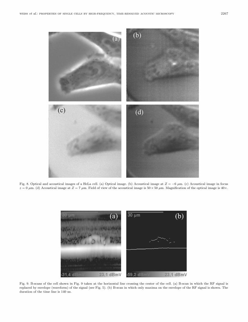
Measurements of the sound velocity consist of two steps.The first step is to determine the thickness of the cell. Itcan be done by measuring the time delay between top andreference (τ1) and using (1). Acoustical images of the HeLacell chosen for sound velocity measurements are shown inFig. 8. As can be seen in Fig. 8, the acoustical contraststrongly depends on the focus position. For measuring thesound velocity, we collect the RF-scan at a positive defocus

of Z = 7 µm, when the focus of the SAM is above the cellsurface. The amplitude of the signal at a positive defocusis lower than that in the focus. However, positive defocusensures simple image interpretation. Only the contributionfrom rays normal to the glass surface should be taken intoaccount, thus (3) can be used for measuring sound velocityfrom the time-resolved SAM measurements.

Two types of the B-scan derived from the RF-scan takenat Z = 7 µm are shown in Fig. 9. Fig. 9(a) is the B-scanin which the RF signal at each pixel point is replaced by awaveform obtained with the use of the Hilbert transform,(8)–(11). Note that the brightness is proportional to theamplitude of the waveform. The bright line on Fig. 9(b)traces the maxima of the waveform shown in Fig. 9(a). Thearrival times t0, t1, and the delay time τ1(xi, yi) = t1 − t0of the HeLa cell as a function of the position on the x-y plane were determined from the position of the maximaon the envelope of the RF signal obtained with the Hilberttransform (see Section III-B). Using time delay τ1, the cellthickness d(xi, yi) can be determined at each pixel on thex-y plane, (1). When the thickness d(xi, yi) and the timedelay τ2(xi, yi) = t2 − t1 are determined at each pixel po-sition, the sound velocity inside the cell can be obtainedfrom (4). The distribution of the sound velocity in theHeLa cell (Fig. 8) is shown in Fig. 10. By averaging over thearea of the cell, we obtain the sound velocity inside the cell,1534.5 ± 33.6 m/s. This value is only slightly higher thanthat of the medium described in Section IV-A (1501 m/smeasured at 37◦C). To estimate the error of the sound ve-locity measurements inside the cell we measured the errorof arrival time determination. Measurements with a glassslide as reflector shows that the arrival time error is 50 psat 37◦C. The average time delay between the echo reflectedfrom the top of the cell and the echoes reflected from theglass substrate, τ1 is 7 ns, providing an average thicknessof the cell of d = 5.25 µm. For such a cell, the relativeerror of the time delay τ1 measurements is less than 1%(∼0.007) assuming averaging (N = 2000) minimizes errorsrelated to the noise in the system. From (1) it follows thatrelative error of the cell thickness measurements is of thesame order: ∆d/d = ∆τ1/τ1. Using (2), we estimate therelative error of the sound velocity measurements. Simplemanipulation provides the following equation for the rel-ative error: ∆c/c =

√(∆τ1/τ1)2 + (∆τ12/τ12)2. Since the

difference between the arrival times τ1 and τ12 is small(∼0.25 ns) the relative error for the sound velocity couldbe rewritten as ∆c/c = (∆τ1/τ1)2

√2, giving exactly 1%

for the relative error of the sound velocity measurements.Obviously, the error of the sound velocity measurementwould be greater for cells thinner than 5 µm cells and lessfor thicker cells.

D. Attenuation in the HeLa Cells

Another important parameter that can be obtainedfrom time-resolved measurements is sound attenuation. Inmany liquids, including water, the attenuation of soundis determined by viscosity [16], [52]. Attenuation of sound

weiss et al.: properties of single cells by high-frequency, time-resolved acoustic microscopy 2267

Fig. 8. Optical and acoustical images of a HeLa cell. (a) Optical image. (b) Acoustical image at Z = −6 µm. (c) Acoustical image in focusz = 0 µm. (d) Acoustical image at Z = 7 µm. Field of view of the acoustical image is 50× 50 µm. Magnification of the optical image is 40×.

Fig. 9. B-scans of the cell shown in Fig. 9 taken at the horizontal line crossing the center of the cell. (a) B-scan in which the RF signal isreplaced by envelope (waveform) of the signal (see Fig. 5). (b) B-scan in which only maxima on the envelope of the RF signal is shown. Theduration of the time line is 140 ns.

2268 ieee transactions on ultrasonics, ferroelectrics, and frequency control, vol. 54, no. 11, november 2007

Fig. 10. A map of the sound velocity distribution in HeLa cell shownin Fig. 8(d).

TABLE IAcoustical Properties of Coupling Liquid, HeLa Cell, and

Substrate.

ρ (kg/m3) cL (m/s)

Coupling liquid1 1000 1501HeLa cells 11002 15343

Glass substrate (silica)4 2250 5968

1Current study.2[52].3Current study.4[17].

inside the HeLa cells has not been studied. Recent stud-ies [53], [54] suggested that a more detailed understandingof this parameter is needed with respect to complex, bio-logical substances. For example, the sound attenuation ofactin gels does not directly follow viscosity values duringpolymerization [16], [53].

Simulation of the signal brightness (11), I, as a functionof cell thickness is presented in Fig. 11. Acoustical proper-ties of the HeLa cells, coupling liquid, and silica substratereported in the literature and measured in this study, arelisted in Table I. The simulations were done under the as-sumption that the attenuation inside the cell is negligible.The value of density of the HeLa cells was taken slightlyhigher than that of erythrocytes [52]. The numerical simu-lation reveals that the ratio of the intensity of the echo re-flected from the cell and that reflected from glass decreasesas the thickness of the layer increases. A reduced reflectioncoefficient (dark area) is caused by a better matching of

Fig. 11. Ratio between the intensity of the signal reflected from thecell (Icell) and that reflected from a glass substrate (Iglass) as afunction of the cell thickness.

the acoustic impedances between the cell and the glasssubstrate and that of the coupling liquid [41]. Accordingto the simulations shown in Fig. 11, the decrease of the sig-nal intensity inside cells due to matching effects should notbe higher that 3% compared to that from the glass sub-strate. The values of the ratio Icell/Iglass averaged overthe cell surface in Fig. 8(d) is 0.87 and it is 0.06 in thedarkest spot inside the cell in Fig. 8(d). Therefore, the de-crease of the signal intensity inside the cell (or contrastof the of the “intensity images”) can be attributed to thesound attenuation inside the cell rather than the matchingeffects.

VI. Conclusions

The ability to measure the sound velocity within cellswill provide important information on processes such asdivision, cell migration, or attachment and provide novelinsights into the polymerization state of the cytosol orthe kernel [33]. Currently, the application of acoustic mi-croscopy to examine the elastic properties of single cells ona subcellular level was limited. We have developed a com-bined acoustic and optical microscope to investigate theelastic properties of cells and their connection to chem-ical properties or structures of the cell found with syn-chronous optical microscopy. The new acoustic microscopeoperates in a time-resolved mode. The carrier frequencyequals 0.86 GHz, and the duration of the sound burst isnot longer than 5 ns. With such a short pulse, cells thickerthan 3 µm can be resolved. For a cell thicker than 3 µm,the front echo and the echo from the substrate can be dis-tinguished in the signal. Positions of the first and secondpulses were used to determine the local impedance of thecell modeled as a thin liquid layer that has spatial varia-tions of elastic properties.

The measurements conducted with high-frequency,time-resolved SAM provide a value of the sound velocity

weiss et al.: properties of single cells by high-frequency, time-resolved acoustic microscopy 2269

in HeLa cells of 1534.5 ± 33.6 m/s. This value is close tothe value of sound velocity (∼1540 m/s) in human skindermal fibroblasts measured by time-resolved SAM witha central frequency of 500 MHz [18], and to sound veloc-ities measured in live, human, aortic, smooth-muscle cellsunder various conditions [21]: growing (1571 ± 14 m/s);differential (1624 ± 16 m/s); and on hypotonic loading(1585±8 m/s). However, this value is lower than the localvalue of sound velocity in fibroblasts measured with thefringes technique (see [16]).

The technique provides an opportunity to determine theattenuation of ultrasound in the cell. To conduct quantita-tive measurements of the sound attenuation inside a cell,a rigorous fluid model that takes diffraction effects in thefocal region into account should be used for the echo sig-nal [26].

The use of digitized pulse-echo data in combination withdigital signal processing substantially increases the flexi-bility of the system as it allows analyzing different partsof the RF signal. Moreover, the system is more robust be-cause the high-frequency electronic block consists only of apulse generator and an amplifier. These quantitative mea-surements of the elastic properties of the cells and long-time (up to 24 hours) observation of dynamical processesof the cells such as cell division.

An additional advantage of this application of acousticmicroscopy in cell biology is that no intensive light illumi-nation is needed for ultrasound imaging. Intensive light,including blue and green, has been reported to stress theilluminated cell, hence, induce stress-specific proteins re-sulting in unwanted light induced activation of cell-specificdifferentiation protocols.

References

[1] Y. C. Fung, Biomechanics. Mechanical Properties of Living Tis-sues. New York: Springer-Verlag, 1993.

[2] G. Bao and S. Suresh, “Cell and molecular mechanics of biolog-ical materials,” Nature Mater., vol. 2, pp. 715–725, 2003.

[3] C. G. Pearson, P. S. Maddox, E. D. Salmon, and K. Bloom,“Budding yeast chromosome structure and dynamics during mi-tosis,” J. Cell Biol., vol. 152, pp. 1255–1266, 2001.

[4] E. A. Evans and R. Skalak, Mechanics and Thermodynamics ofBiomembranes. Boca Raton, FL: CRC Press, 1980.

[5] D. Boal, Mechanics of the Cell. Cambridge: Cambridge Univ.Press, 2002.

[6] G. Zhang, M. Long, Z.-Z. Wu, and W.-Q. Yu, “Mechanical prop-erties of hepatocellular carcinoma cells,” World J. Gastroenter.,vol. 8, pp. 243–246, 2002.

[7] M. Beil, A. Micoulet, G. von Wichert, S. Paschke, P. Walther,M. B. Omary, P. P. Van Veldhoven, U. Gern, E. Wolff-Hieber,J. Eggermann, J. Waltenberger, G. Adler, J. Spatz, and T.Seufferlein, “Sphingosylphosphorylcholine regulates keratin net-work architecture and visco-elastic properties of human cancercells,” Nat. Cell Biol., vol. 5, pp. 803–811, Sep. 2003.

[8] S. Suresh, J. Spatz, J. P. Mills, A. Micoulet, M. Dao, C. T. Lim,M. Beil, and T. Seufferlein, “Connections between single-cellbiomechanics and human disease states: Gastrointestinal cancerand malaria,” Acta Biomaterialia, vol. 1, pp. 15–30, 2005.

[9] J. Guck, S. Schinkinger, B. Lincoln, F. Wottawah, S. Ebert,M. Romeyke, D. Lenz, H. M. Erickson, R. Ananthakrishnan, D.Mitchell, J. Kas, S. Ulvick, and C. Bilby, “Optical deformabil-ity as an inherent cell marker for testing malignant transfor-mation and metastatic competence,” Biophys. J., vol. 88, pp.3689–3698, May 2005.

[10] K. J. Van Vliet, G. Bao, and S. Suresh, “The biome-chanics toolbox: experimental approaches for living cells andbiomolecules,” Acta Mater., vol. 51, pp. 5881–5905, Nov. 2003.

[11] M. Puig-De-Morales, M. Grabulosa, J. Alcaraz, J. Mullol, G. N.Maksym, J. J. Fredberg, and D. Navajas, “Measurement of cellmicrorheology by magnetic twisting cytometry with frequencydomain demodulation,” J. Appl. Phys., vol. 91, pp. 1152–1159,2001.

[12] A. Ashkin and J. M. Dziedzic, “Optical trapping and manipula-tion of viruses and bacteria,” Science, vol. 235, pp. 1517–1520,1987.

[13] J. Guck, R. Ananthakrishnan, T. J. Moon, C. C. Cunningham,and J. Kas, “Optical deformability of cells,” Biophys. J., vol. 78,p. 368A, Jan. 2000.

[14] M. Radmacher, M. Fritz, and P. K. Hansma, “Imaging soft sam-ples with the atomic-force microscope—Gelatin in water andpropanol,” Biophys. J., vol. 69, pp. 264–270, 1995.

[15] A. Ebert, B. R. Tittmann, J. Du, and W. Scheuchenzuber,“Technique for rapid in vitro single-cell elastography,” Ultra-sound Med. Biol., vol. 32, pp. 1687–1702, Nov. 2006.

[16] J. Bereiter-Hahn and C. Blase, “Ultrasonic characterization ofbiological cells,” in Ultrasonic Nondestructive Evaluation: En-gineering and Biological Material Characterization. T. Kundu,Ed. Boca Raton, FL: CRC Press, 2003, pp. 725–759.

[17] A. Briggs, Acoustic Microscopy. Oxford: Clarendon Press, 1992.[18] G. A. D. Briggs, J. Wang, and R. Gundle, “Quantitative acoustic

microscopy of individual living human cells,” J. Microscopy, vol.172, pp. 3–12, 1993.

[19] C. S. Jorgensen, J. E. Assentoft, D. Knauss, H. Gregersen,and G. A. D. Briggs, “Small intestine wall distribution ofelastic stiffness measured with 500 MHz scanning acousticmicroscopy,” Ann. Biomed. Eng., vol. 29, pp. 1059–1063,Dec. 2001.

[20] R. A. Lemons and C. F. Quate, “Acoustic microscopy. Biomed-ical application,” Science, vol. 188, pp. 905–914, 1975.

[21] A. Kinoshita, S. Senda, K. Mizushige, H. Masugata, S.Sakamoto, H. Kiyomoto, and H. Matsuo, “Evaluation of acousticproperties of the live human smooth-muscle cell using scanningacoustic microscopy,” Ultrasound Med. Biol., vol. 24, pp. 1397–1405, 1998.

[22] H. Kanngiesser and M. Anliker, “Ultrasound microscopy of bio-logical structures with weak reflecting properties,” in AcousticalImaging. vol. 19, H. Ermert and H. P. Harjes, Eds. New York:Plenum, 1992, pp. 517–522.

[23] R. A. Lemons and C. F. Quate, “Acoustic microscope-scanningversion,” Appl. Phys. Lett., vol. 24, pp. 163–165, 1974.

[24] R. L. Johnston, A. Atalar, J. Heiserman, V. Jipson, and C.Quate, “Acoustic microscopy: Resolution of subcellular de-tail,” in Proc. Natl. Acad. Sci. USA, vol. 76, pp. 3325–3329,1979.

[25] J. A. Hildebrand, D. Rugar, R. N. Johnston, and C. F. Quate,“Acoustic microscopy of living cells,” in Proc. Nat. Acad. Sci.USA—Biol. Sci., vol. 78, pp. 1656–1660, 1981.

[26] P. V. Zinin and W. Weise, “Theory and applications of acous-tic microscopy,” in Ultrasonic Nondestructive Evaluation: En-gineering and Biological Material Characterization. T. Kundu,Ed. Boca Raton, FL: CRC Press, 2004, pp. 654–724.

[27] P. V. Zinin, “Quantitative acoustic microscopy,” in ModernAcoustical Techniques for the Measurement of Mechanical Prop-erties. vol. 39, M. Levy and H. E. Bass, Eds. New York: Aca-demic, 2001, pp. 135–187.

[28] J. Litniewski and J. Bereiterhahn, “Measurements of cells inculture by scanning acoustic microscopy,” J. Microscopy-Oxford,vol. 158, pp. 95–107, 1990.

[29] T. Kundu, J. Bereiter-Hahn, and I. Karl, “Cell property de-termination from the acoustic microscope generated voltageversus frequency curves,” Biophys. J., vol. 78, pp. 2270–2279,May 2000.

[30] T. Kundu, J. P. Lee, C. Blase, and J. Bereiter-Hahn, “Acous-tic microscope lens modeling and its application in determiningbiological cell properties from single- and multi-layered cell mod-els,” J. Acoust. Soc. Amer., vol. 120, pp. 1646–1654, Sep. 2006.

[31] J. Litniewski and J. Bereiterhahn, “Measurements of cells inculture by scanning acoustic microscopy,” J. Microscopy, vol.158, pp. 95–107, 1990.

2270 ieee transactions on ultrasonics, ferroelectrics, and frequency control, vol. 54, no. 11, november 2007

[32] O. Lefeuvre, “Characterisation of stiffening layers by acousticmicroscopy and brillouin spectroscopy,” in Department of Ma-terials. Oxford: Univ. Oxford, 1998, pp. 9–12.

[33] A. P. Sarvazyan, “Ultrasonic velocimetry of biological com-pounds,” Annu. Rev. Biophys. Biophys. Chem., vol. 20, pp. 321–342, 1991.

[34] C. S. Hall, M. J. Scott, G. M. Lanza, J. G. Miller, and S. A.Wickline, “The extracellular matrix is an important source of ul-trasound backscatter from myocardium,” J. Acoust. Soc. Amer.,vol. 107, pp. 612–619, Jan. 2000.

[35] J. Bereiter-Hahn, “Probing biological cells and tissues withacoustic microscopy,” in Advances in Acoustic Microscopy. vol.I, A. Briggs, Ed. New York: Plenum, 1995, pp. 79–115.

[36] S. Temkin, “Attenuation and dispersion of sound in dilute sus-pensions of spherical particles,” J. Acoust. Soc. Amer., vol. 108,pp. 126–146, July 2000.

[37] E. C. Weiss, R. M. Lemor, G. Pilarczyk, P. Anastasiadis, andP. V. Zinin, “Imaging of focal contacts of chicken heart musclecells by high-frequency acoustic microscopy,” Ultrasound Med.Biol., vol. 33, pp. 1320–1326, 2007.

[38] P. V. Zinin, E. C. Weiss, P. Anastasiadis, and R. M. Lemor, “Me-chanical properties of HeLa cells at different stages of cell circleby time-resolved acoustic microscope,” J. Acoust. Soc. Amer.,vol. 120, p. 3320, 2006.

[39] A. Briggs, An Introduction to Scanning Acoustic Microscopy.Oxford: Oxford Univ. Press: Royal Microscopical Society, 1985.

[40] B. M. Lempriere, Ultrasound and Elastic waves. FrequentlyAsked Questions. Amsterdam, The Netherlands: Academic,2002.

[41] J. A. Hildebrand, “Observation of cell-substrate attachmentwith the acoustic microscope,” IEEE Trans. Sonics Ultrason.,vol. 32, pp. 332–340, 1985.

[42] W. Weise, P. Zinin, and S. Boseck, “Modeling of inclinedand curved surfaces in the reflection scanning acoustic micro-scope,” J. Microscopy, vol. 176, pp. 245–253, 1994.

[43] J. D. N. Cheeke, Fundamentals and Applications of UltrasonicWaves. Boca Raton, FL: CRC Press, 2002.

[44] P. B. Nagy and L. Adler, “Acoustic material signature fromfrequency analysis,” J. Appl. Phys., vol. 67, pp. 3876–3878, 1990.

[45] P. A. Scherer, “Studies on the propagation in vitro of poliomyeli-tis viruses. IV. Viral multiplication in a stable strain of humanmalignant epithelial cells (strain HeLa) derived from an epider-moid carcinoma of the cervix,” J. Exp. Med., vol. 97, p. 695,1953.

[46] J. Bereiterhahn, J. Litniewski, K. Hillmann, A. Krapohl, and L.Zylberberg, “What can scanning acoustic microscopy tell aboutanimal-cells and tissues,” Acoust. Imag., vol. 17, pp. 27–38, 1989.

[47] R. G. Maev and K. I. Maslov, “Temperature effects in the fo-cal region of the acoustic microscope,” IEEE Trans. Ultrason.,Ferroelect., Freq. Contr., vol. 38, pp. 166–171, 1991.

[48] P. Zinin, W. Weise, O. Lobkis, and S. Boseck, “The theoryof three-dimensional imaging of strong scatterers in scanningacoustic microscopy,” Wave Motion, vol. 25, pp. 213–236, 1997.

[49] I. Karl and J. Bereiter-Hahn, “Tension modulates cell surfacemotility: A scanning acoustic microscopy study,” Cell Motil. Cy-toskeleton, vol. 43, pp. 349–359, 1999.

[50] P. Zinin, M. H. Manghnani, C. Newtson, and R. A. Livingston,“Acoustic microscopy of steel reinforcing bar in concrete,” J.Nondestruc. Eval., vol. 31, pp. 153–161, 2002.

[51] N. R. Draper and H. Smith, Applied Regression Analysis. NewYork: Wiley, 1998.

[52] P. V. Zinin, “Theoretical analysis of sound attenuation mech-anisms in blood and in erythrocyte suspensions,” Ultrasonics,vol. 30, pp. 26–34, 1992.

[53] O. Wagner, H. Schuler, P. Hofmann, D. Langer, P. Dancker,and J. Bereiter-Hahn, “Sound attenuation of polymerizing actinreflects supramolecular structures: Viscoelastic properties ofactin gels modified by cytochalasin D, profilin and alpha-actinin,” Biochem. J., vol. 355, pp. 771–778, May 1, 2001.

[54] O. Wagner, J. Zinke, P. Dancker, W. Grill, and J. Bereiter-Hahn,“Viscoelastic properties of f-actin, microtubules, f-actin/alpha-actinin, and f-actin/hexokinase determined in microliter volumeswith a novel nondestructive method,” Biophys. J., vol. 76, pp.2784–2796, May 1999.

Eike Christian Weiss was born in Han-nover, Germany. He studied physics at theUniversity of Braunschweig, Braunschweig,Germany, and the University of Saarland,Saarbrucken, Germany, where he received hisDiploma in Physics in 2002. Since then he hasbeen working at the Fraunhofer Institute forBiomedical Technology in St. Ingbert, Ger-many.

His research interests include high-frequencyultrasound, cell biology, and cell mechanics.

Pavlos Anastasiadis was born in Lever-kusen, Germany. He has finished his studies inInformatics and obtained his Diploma in 2000.Currently, he is studying Computational Bi-ology and Molecular Biology at the Univer-sity of Saarland, Saarbrucken, Germany. Since2005 he has been working at the FraunhoferInstitute for Biomedical Technology in St.Ingbert, Germany. His research interests in-clude cell and systems biology, computationalbiology, oncogenomics, mathematical model-ing in biology, and ontology translation for life

science databases. He is a member of the German Society for Com-puter Science, the German Society for Cell Biology, the InternationalSociety for Bioinformatics and the German Society of Natural Sci-entists.

Gotz Pilarcyzk studied biology in Heidel-berg, Germany, at Ruprecht-Karls University.He conducted his diploma thesis in coopera-tion with the local Ruprecht-Karls Universityand the European Molecular Biology Labora-tory (EMBL), Heidelberg, Germany, on theapparative development for moss cultivationon a microscope stage. His Ph.D. studies wereon calcium regulation in heart muscle cells bylaser irradiation at the Institute for MolecularBiotechnology (IMB), Jena, Germany. Aftercompletion of his doctoral studies and some

postdoctoral research at IMB, he held a position at the FraunhoferInstitute for Biomedical Engineering (IBMT), Berlin, Germany, To-tal Internal Reflection Fluorescence (TIRF), conducting research onconfocal, microscopy as well as time-lapse light microscopy on cellsafter live staining.

Currently, he is at the Institute for Analytical Chemistry inGiessen, Germany, investigating advanced laser-based mass spec-trometry for microscopy in the life sciences.

Robert M. Lemor was born in Germanyon July 23, 1974. He studied mechanicalengineering and physics at the Universityof Braunschweig, Braunschweig, Germany,and the University of Kansas City-Missouri,Kansas City, MO, where he received his M.S.degree in physics in 1997. In 2001 he re-ceived his Ph.D. degree in biophysics from theHumboldt University, Berlin, Germany. Since1999 he has been employed at the Fraunhofer-Institute for Biomedical Technology in St. In-gbert, Germany and has been head of the

biomedical ultrasound research group since 2002 and the Depart-ment of Ultrasound since 2005. Since 2002 he has held a lecturerposition in ultrasound technology and medical imaging at the Uni-versity of Saarland, Saarbrucken, Germany.

His research interests are ultrasound technology in technical, bi-ological, and medical applications. His current work is on high reso-lution and molecular imaging.

weiss et al.: properties of single cells by high-frequency, time-resolved acoustic microscopy 2271

Pavel V. Zinin was born in Moscow, Rus-sia, on December 20, 1955. He received a com-bined B.S. and M.S. degree in physics fromMoscow State University, Moscow, RussianFederation, in 1980 and a Ph.D. degree inphysics and mathematics from the Moscow In-stitute of Physics and Technology, Moscow,Russian Federation, in 1987. From 1987 to1993, he worked as a researcher at the Insti-tute of Chemical Physics, Russian Academyof Sciences, Moscow, Russia. In 1993, he re-ceived the Alexander von Humboldt fellow-

ship (1993–1994, University of Bremen, Bremen, Germany). From1987 to 1993, he was a research fellow at the Department of Ma-terials of University of Oxford, Oxford, UK. In 1998, he joined theHigh-Pressure Mineral Physics and Materials Science Laboratory atthe Institute of Geophysics and Planetology, University of Hawaii,Honolulu, Hawaii. He is currently an associate researcher at the in-stitute.

His research interests include theoretical acoustics, phase tran-sition under high pressure, Brillouin and Raman spectroscopies ofnovel and geological materials, and the acoustic microscopy of bio-logical cells.

He is co-author of Chapter VIII in vol. 1, Handbook of Elas-tic Properties of Solids, Liquids, and Gases (2001), Chapter IV invol. 39, Experimental Methods in the Physical Sciences (2001), Chap-ters 10 and 11 in Ultrasonic Nondestructive Evaluation: Engineeringand Biological Material Characterization (2004), and Chapter VII inRecent Advances in Materials Characterization (2006).

Dr. Zinin is a member of the Acoustical Society of America, theAmerican Physical Society, and the Materials Research Society.