Paleomagnetic analysis using SQUID microscopy

Paleomagnetic analysis using SQUID microscopy

Benjamin P. Weiss,1 Eduardo A. Lima,1,2 Luis E. Fong,2 and Franz J. Baudenbacher 2,3

Received 16 January 2007; revised 14 May 2007; accepted 19 June 2007; published 19 September 2007.

[1] Superconducting quantum interference device (SQUID) microscopes are a newgeneration of instruments that map magnetic fields with unprecedented spatial resolutionand moment sensitivity. Unlike standard rock magnetometers, SQUID microscopesmap magnetic fields rather than measuring magnetic moments such that the samplemagnetization pattern must be retrieved from source model fits to the measured field data.Here we present the first direct comparison between paleomagnetic analyses onnatural samples using joint measurements from SQUID microscopy and momentmagnetometry. We demonstrate that in combination with a priori geologic andpetrographic data, SQUID microscopy can accurately characterize the magnetization oflunar glass spherules and Hawaiian basalt. The bulk moment magnitude and directionof these samples inferred from inversions of SQUID microscopy data match directmeasurements on the same samples using moment magnetometry. In addition, theseinversions provide unique constraints on the magnetization distribution within the sample.These measurements are among the most sensitive and highest resolution quantitativepaleomagnetic studies of natural remanent magnetization to date. We expect that thistechnique will be able to extend many other standard paleomagnetic techniques topreviously inaccessible microscale samples.

Citation: Weiss, B. P., E. A. Lima, L. E. Fong, and F. J. Baudenbacher (2007), Paleomagnetic analysis using SQUID microscopy,

J. Geophys. Res., 112, B09105, doi:10.1029/2007JB004940.

1. Introduction

[2] Superconducting quantum interference devices (SQUIDs)are the most sensitive magnetometers available for makingquantitative measurements of magnetic fields [Braginskiand Clarke, 2004; Wikswo, 2004]. Over the last twodecades, SQUID moment magnetometers, whichtypically measure the three components of the moment ofa �1 cm3 sample with a sensitivity of 10�12 Am2 [Clem etal., 2006; Fagaly, 2006], have become standard in state-of-the-art paleomagnetics laboratories. These magnetometersmeasure only the net moment of the sample and cannotdiscern the potentially highly variable spatial distribution ofmicroscale magnetization within the sample. Of late, a newgeneration of scanning superconducting magnetometerscalled SQUID microscopes has appeared that, instead ofdirectly measuring a sample’s net moment, generate highresolution, high sensitivity maps of the magnetic field abovethe sample. SQUID microscopes typically raster a micro-fabricated sensor at a constant height above a sample,measuring the vertical component of the magnetic field ina planar grid of locations.

[3] SQUID microscopes capable of measuring samples atcryogenic temperatures at very high spatial resolution (4 mmor better) have been in use for some time [Kirtley andWikswo, 1999]. Such instruments have limited use forpaleomagnetism since the samples must be cooled downbelow 80 K, which usually severely alters their naturalremanent magnetization (NRM). At such low temperatures,many crystals that are superparamagnetic at room temper-ature become single domain (and possibly magnetized), andmany common minerals experience phase changes or mag-netic transitions (like hematite’s Morin transition at �260 Kand magnetite’s Verwey transition at �125 K). Untilrecently, SQUID microscopes capable of measuring roomtemperature samples were limited to spatial resolutions ofseveral mm [Cochran et al., 1993; Egli and Heller, 2000;Nowaczyk et al., 1998; Thomas et al., 1992].[4] A decade ago, a new generation of SQUID micro-

scopes capable of submillimeter resolution appeared, firstusing high-transition temperature (high-Tc) SQUIDs [Leeet al., 1996; Wellstood et al., 1997], and then usingthe more sensitive low-transition-temperature (low-Tc)SQUIDs [Baudenbacher et al., 1998; Dechert et al.,1999]. Among the first of these low-Tc microscopes wasthat of Baudenbacher et al. [Baudenbacher et al., 2002a,2002b, 2003; Fong et al., 2004, 2005] (hereafter, SQUIDMicroscope, or SM). The SM can now measure the field ofroom temperature samples with a spatial resolution of betterthan 100 mm and SB

1/2 = 1.5 pT/Hz1/2 at frequencies above�0.5 Hz, where S

B1/2 is the square root of the magnetic field

spectral power density (which measures the magnitude of

JOURNAL OF GEOPHYSICAL RESEARCH, VOL. 112, B09105, doi:10.1029/2007JB004940, 2007

1Department of Earth, Atmospheric, and Planetary Sciences,Massachusetts Institute of Technology, Cambridge, Massachusetts, USA.

2Department of Physics and Astronomy, Vanderbilt University,Nashville, Tennessee, USA.

3Department of Biomedical Engineering, Vanderbilt University,Nashville, Tennessee, USA.

Copyright 2007 by the American Geophysical Union.0148-0227/07/2007JB004940$09.00

B09105 1 of 20

the magnetic field noise fluctuations per root frequencyinterval). We quickly found the SQUID Microscope to be apowerful tool for paleomagnetic and geologic investigations[Weiss et al., 2000, 2001, 2002; Gattacceca et al., 2006].[5] The SQUID Microscope can detect the fields of

dipoles with moments weaker than 10�15 Am2, making itmore than three orders of magnitude more sensitive than thebest superconducting moment magnetometers (see Appen-dix A). This impressive moment sensitivity means thatSQUID microscopy offers two particular advantages withrespect to moment magnetometry. First, SQUID microscopycan detect small, isolated samples and small magnetizedregions within larger samples (rock fragments, dustparticles, and single crystals) which, by virtue of their size,have weak magnetic moments. Second, SQUID microscopycan potentially be used to place constraints on the finespatial variability of magnetization within a large-scalesample. These two advantages are linked in that SQUIDmicroscopy is able to detect the fields of weak dipolar pointsources as a result of its ability to map magnetic fields athigh resolution [Weiss et al., 2001]. Because the sensitivityof SQUID sensors to uniform fields scales with the size ofthe sensor area, this also means that SM is less sensitivethan moment magnetometry to large (cm-sized) sampleswith spatially uniform magnetization.[6] This possibility of mapping magnetization with high

spatial resolution cannot be taken for granted: it is wellknown that magnetic field maps are not sufficient foruniquely inferring the spatial distribution of magnetizationwithin the sample. The non-uniqueness of the magneticinverse problem is intrinsic to Maxwell’s equations ratherthan to SQUID microscopy techniques. This imposes lim-itations on the reconstruction algorithms that are inherent tomagnetic data.[7] For current distribution reconstructions, [Kress et al.,

2002] demonstrate that the null-space associated with theBiot-Savart operator is nontrivial. A nontrivial null-spacemeans that multiple current distributions yield the samemagnetic field, or equivalently, that there are current dis-tributions which are magnetically silent. Those silent sour-ces can be added to or subtracted from the original sourcewithout changing the overall magnetic field [Lima et al.,2006]. Similarly, it is straightforward to verify the existenceof different magnetization distributions which generate thesame magnetic field. For instance, it is well known that thefield outside of a uniformly magnetized sphere is identicalto that of a magnetic dipole located at the center of thesphere. Consider two nested, centered spheres of differentsizes that are each uniformly magnetized. Because theirexternal magnetic fields each have the same dipolar geom-etry, it is clearly impossible to distinguish between the twosources based on magnetic field measurements made out-side of the larger sphere. Furthermore, it is also impossibleto distinguish those sources from their equivalent dipole.[8] There are two main approaches to dealing with this

nonuniqueness. A single magnetization solution can some-times be obtained if additional geophysical or geochemicalconstraints are applied to the solution beyond simplyrequiring that the residual sum of squares is minimized[Aster et al., 2005; Blakely, 1996; Hansen, 1998, 2001;Lima et al., 2006; Parker, 1994]. A second approach is tosolve for unique model properties that are shared by all

possible magnetization solutions [Parker, 1977]. Forinstance, field measurements over all space with infinites-imal spatial resolution and zero noise uniquely constrain thenet moment of the sample [Parker, 1971, 1988; Parker etal., 1987].[9] A large variety of methods in both the space and

frequency domains have been developed by the planetaryremote sensing community to retrieve crustal magnetizationfrom crustal field measurements [Langel and Hinze, 1998;Parker, 1994]. Frequency domain inversion techniqueshave recently been extended to inversions of SQUIDmicroscopy imaging of current and magnetization distribu-tions [Chatraphorn et al., 2002; Egli and Heller, 2000;Fleet et al., 2001; Roth et al., 1989; Sepulveda et al., 1994;Tan et al., 1996; Wikswo, 1996]. However, all previousSQUID microscopy inversion techniques have focused onretrieving the special case of magnetization with only twocomponents (e.g., current loops confined to the sampleplane or, equivalently, magnetization solutions orientedperpendicular to the plane) rather than the magnetizationdistributions with components in all three spatial directions.In the two-dimensional case, a unique solution can beobtained from noise-free data because a continuity equationprovides a second independent constraint linking the twounknown current or moment distribution components [Limaet al., 2006], whereas no additional independent equationexists for the three dimensional case. To our knowledge, noSQUID microscopy spatial domain inversion techniqueshave been previously described.[10] Here we present the first application of regularized

space domain inversions to the SQUID microscopy problemof inverting magnetic field data for a full three dimensionalmagnetization distribution. We apply these techniques totwo relatively simple kinds of geological samples: two�100 mm diameter glass spherules from the Moon and a30-mm thin section of basalt from the Mauna Loa volcano.We show that using reasonable assumptions about themagnetization (as inferred from petrographic, rock magneticand other geologic data), the net moment direction andintensity measured directly with a 2G Enterprises Super-conducting Rock Magnetometer (2G) can be retrieved froma constrained least squares inversion of SQUID microscopefield maps of these samples. The sensitivity and imagingcapabilities of SQUID microscopy make it a powerfulnew paleomagnetic tool that that is complementary to thenet moment measurements provided by SQUID momentmagnetometry.

2. Measurement Methods

[11] In a typical SM paleomagnetic application, we scanplanar samples using a horizontal grid spacing of 50–100 mmat a sample-to-sensor distance of 80–200 mm. SM measure-ments of non-planar samples (like the lunar spherulesdescribed here) are sometimes taken at higher distancesdepending on the shape and roughness of the samples. Tokeep the scanning distance small and constant, we use aspring-loaded mechanism to push planar samples up againstthe sapphire window that separates the room temperaturesample from the 4.2 K SQUID sensor [see Fong et al.,2005, Figure 6]. We usually place a 2.5-mm mylar film ontop of the sample to reduce friction and avoid scratching its

B09105 WEISS ET AL.: PALEOMAGNETISM USING SQUID MICROSCOPY

2 of 20

B09105

surface. In this configuration, the SQUID Microscope issufficiently sensitive that it can readily detect the magneticfields of typical 30-mm thin sections of rock.[12] Thin sections are ideal for SQUID microscopy in that

they (a) can later be analyzed with a wide variety ofstandard analytical tools that are valuable for constrainingthe nature of the magnetic carriers and petrography, (b) aresufficiently thin relative to the sensor-to-sample distancethat their magnetization as imaged by the SM can be treatedto a first approximation as being confined to an infinitelythin plane, thereby regularizing the inverse problem (seebelow), and (c) are sufficiently smooth that they can bescanned at a well-defined and constant sample-to-sensordistance without risking damage to the SM sapphire win-dow. As such, we usually scan doubly polished thin sectionsspecially prepared using a process designed to preserve theNRM. We use room temperature cyanoacrylate cementinstead of heat-treated epoxy as a binder, all of our cuttingand grinding is conducted using nonmagnetic blades andtools, we use amorphous silica as a final polishing step toremove any magnetostrictive surface layer [e.g., Krasa,2002], and our sections are mounted on nonmagnetic GE124 quartz slides. Our SM study of the basalt describedbelow confirms that the thin section making process indeeddid not substantially alter its NRM. Although it is possiblethat the thin section shape could impart some grossmagnetic anisotropy to the sample, we did not observe thiseffect in the one anisotropy study we have conducted so far(on Martian meteorite ALH84001 [Weiss et al., 2005]).

3. Least Squares Methods

[13] In the following section we develop the least squaresequations for retrieving magnetization from SQUID micros-copy data. Because both SQUID microscopy data and sam-ples typically have a planar geometry, the equations areexpressed in Cartesian coordinates. We begin in section 3.1by presenting the general inverse problem of retrievinga three-component magnetization pattern from single-component magnetic field measurements of planar samples.In section 3.2 we discuss the restricted problem of fitting foran unresolved dipolar source of unknown location usingnonlinear least squares techniques. Then in section 3.3 wereview the matrix methods for solving the discretized linearleast squares problem using the equivalent source formalismin which we make no assumptions about the magnetizationsolution beyond requiring that the dipole locations be fixed.We rely on the fact that an arbitrarily complex magnetiza-tion pattern can always be expressed as the sum one ormore dipolar sources. As discussed in section 3.4, thisproblem is typically so ill-posed that without further con-straints on the sample magnetization it is not practicallyuseful. In sections 3.5 and 3.6 we reformulate the basicequations under the additional assumption of either aunidirectional magnetization or uniform magnetization.

3.1. Magnetic Field of a Resolved Source: TheEquivalent Source Formalism

[14] Nearly all existing SQUID microscopes (with theexception of [Ketchen et al., 1997]) measure only thevertical component Bz of the magnetic field. Therefore wewill restrict the discussion to inversion of Bz data only. At a

measurement position ~a = (xa, ya, za) near a magnetizedsample of volume V we have

Bz ~að Þ ¼ZV

~Gz ~a;~b� �

� ~M ~b� �

dV ð1Þ

where ~M (~b) is the magnetization at location ~b = (xb, yb, zb)within the sample and ~Gz (~a, ~b) is the Green’s functionwhich expresses the dependence of the z-component of themagnetic field at the location ~a on the magnetizationelement at location ~b:

~Gz ~a;~b� �

¼ m0

4p3~r za � zbð Þ � r2k̂

r5ð2Þ

Here~r = ~a �~b, k̂ is a unit vector oriented along the z axis(vertical), and m0 is the permeability of free space. Supposethe sample has no thickness in the vertical direction and isleveled (e.g., it is a point source or plane whose normalpoints toward the sensor). Setting x = xa � xb, y = ya � yb,and z = za � zb (= the constant sample-to-sensor distance, h),we see that

Bz ~að Þ ¼ m0

4p

ZA

3zx

r5M 0

x xb; yb; zbð Þ þ 3zy

r5M 0

y xb; yb; zbð Þ�

þ 3z2

r5� 1

r3

� �M 0

z xb; yb; zbð Þ�dA ð3Þ

where A is the surface area of the sample, andMx0 ,My

0 , andMz0

are the three Cartesian components of the moment per unitarea of the sample. Our approach is to discretize this integralby representing the magnetization as being due to Qindividual dipole moments ~mj with field measurements Bzi

at each of P locations:

Bzi ¼XQj¼1

~Gzij ~a;~b� �

� ~mj~b� �

¼ m0

4p

XQj¼1

3zijxij

r5ijmxj þ

3zijyij

r5ijmyj þ

3z2ij

r5ij� 1

r3ij

!mzj ð4Þ

where xij = xai � xbj, yij = yai � ybj, zij = zai � zbj (= h for a

planar sample), rij =ffiffiffiffiffiffiffiffiffiffiffiffiffiffiffiffiffiffiffiffiffiffiffiffix2ij þ y2ij þ z2ij

q, and mxj, myj, and mzj are

the three Cartesian components of ~mj. Using mxj = mj sin qjcos fj,myj =mj sin qj sin fj, andmzj =mj cos qjwhere q and fare the direction angles of ~m, we can also express (4) as

Bzi ~að Þ ¼ m0

4p

XQj¼1

3zijxij

r5ijmj sin qj cosfj þ

3zijyij

r5ijmj sin qj sinfj

þ3z2j

r5ij� 1

r3ij

!mj cos qj ð5Þ

In the least squares approach we seek the set of moments ~mj*

whichminimize the squared Euclidean norm of the differencebetween the data and model:

D2 ¼XPi¼1

B̂zi �XQj¼1

~Gzij ~a;~b� �

� ~mj* ~b� �" #2

ð6Þ


3 of 20

B09105

where B̂zi are the (possibly noisy) measurements of thevertical component of the field. For our least squares fitspresented in section 4, we calculate the residual root meansquare (RMS) = D/

ffiffiffiP

pas a measure of the misfit.

[15] The components Bzi are linear in mx, my , and mz butare nonlinear functions of the position~r and dipole angularorientation q and f. Therefore for fixed dipole locations wecan use standard linear least squares techniques to obtain thebest fit Cartesian dipole moment components for a given setof Cartesian magnetic field data. This approach is known asthe equivalent source formalism [Dampney, 1969; Emilia,1973; Mayhew, 1979; Nicolosi et al., 2006; von Frese et al.,1981], which has long been in use for modeling geomag-netic anomalies but has not yet, to our knowledge, been

adapted for SQUID microscopy. This is the technique wewill use in section 3.3 to obtain constraints on the magne-tization of the basalt thin section.

3.2. Net Moment of an Unresolved Source

[16] If the dipole positions are allowed to vary, the leastsquares problem is nonlinear. Because computational tech-niques for solving nonlinear problems are generally muchless well developed than for linear problems, this is usuallyto be avoided. However, for sources composed of a smallnumber of individually unresolved dipolar sources, this canbe an extremely fast and powerful way of obtaining thesample magnetization. It is also unique [Lima et al., 2006].[17] In section 4.2, we use this approach to solve for the

net moments of two small lunar spherules each representedby a single dipole source using equation (5). We used adipolar source because our samples are approximatelyspherical, and as previously noted the external field of auniformly magnetized sphere is identical to that of a centralpoint dipole of the same moment. In actuality, the spheruleshapes depart from a perfect sphere by no more than �30%of their diameters (�70 mm). This is �7 times smaller thenthe sensor-to-sample distance such that the observed field isnearly purely dipolar. Fitting for the dipole moment there-fore should give an excellent estimate of the mean magneticmoment of the spherule [Parker, 1971; Parker et al., 1987].Our least squares fits validate this approximation becausethe residuals are within the measurement uncertainties (seesection 4.2).

3.3. Unrestricted Solution

[18] Assume we have measurements of only thez-component of the magnetic field at P locations. In the caseof SQUID microscopy, these are usually in a regularrectangular grid at a fixed height above the sample. Wewish to fit for the three components of each of Q dipoleswith fixed positions distributed throughout the sample, for atotal of 3Q parameters.[19] As described above, this is a linear least squares

problem which requires solving the system of equation (4).

This system can be expressed in matrix form Ad = b̂, whereA is the M N Jacobian (also known as the Green’s matrixor source function matrix), d is an N 1 vector containingthe parameters, and b̂ is an M 1 vector containing thefield measurements:

d ¼ mx1 my1 mz1 mx2 my2 mz2 � � � mzQ

� �Tand

b̂ ¼ B̂z1 B̂z2 � � � B̂zP

� �TThe Jacobian is given by:

A ¼

@Bz1=@mx1 @Bz1=@my1 @Bz1=@mz1 @Bz1=@mx2 @Bz1=@my2 @Bz1=@mz2 � � � @Bz1=@mzQ

@Bz2=@mx1

@Bz3=@mx1...

..

.

@BzP=@mx1 � � � @BzP=@mzQ

26666664

37777775

where from (4)

@Bzi=@mxi ¼ m03zijxij=4pr5ij

@Bzi=@myi ¼ m03zijyij=4pr5ij

@Bzi=@mzi ¼ m03z2ij=4pr

5ij � m0=4pr

3ij ð7Þ

Here we have M = P and N = 3Q. In the linear least squaresapproach, we search for the solution d* which minimizesthe Euclidean norm of the difference between the data andmodel Ad* � b̂

�� .[20] Solving equation (4) for an otherwise unconstrained

magnetization solution is in general a rank-deficient prob-lem since the unknown moment distribution ~mj may be acontinuous function and therefore should be represented byan infinite number of dipoles rather than the finite matrix d[Parker, 1977]. Only for certain moment distributions withspecial properties (i.e., those with no components in theplane of the sample [Roth et al., 1989], or those with asingle dipole point source (e.g., lunar spherules) will therebe a unique solution [Lima et al., 2006]. In the equivalentsource scheme, Q is in practice limited to a value such thatthe spacing between dipoles is less than the distance of thedipoles to the sensor, h [Bott and Hutton, 1970; Langel etal., 1984; Mayhew, 1982; Mayhew and Galliher, 1982].Even so, this often still leaves the unconstrained inverseproblem ill-posed without some other form of regularization.

3.4. Approach to Nonuniqueness

[21] In the next two sections, we discuss two possibleassumptions that can be made about the solution thatregularize the inversion. Our approach is similar in philoso-phy to that developed by Parker for understanding shipbornemagnetic surveys of seamounts [Hildebrand and Parker,1987; Parker, 1988, 1991, 1994; Parker et al., 1987]. Weseek to learn something about the magnetic properties andNRM of a geological sample from a set of measurements ofits external magnetic field. Although there are infinitelymany possible magnetization patterns inside of the sample

ð7Þ


4 of 20

B09105

that can yield the observed field data set, additional con-straints may enable us to eventually place bounds on thetrue magnetization which are useful for paleomagnetism.For instance, we can assess hypotheses that the magnetiza-tion is (i) uniform in intensity and orientation, (ii) unidirec-tional, or (iii) neither uniform nor unidirectional. We canselect from among these possibilities by comparing theresidual errors of the least squares fits for each of thesecases with the expected measurement error. For somesamples, as Parker found during his seamount inversions,depending on the nature of the magnetization and itsintensity relative to instrument noise, we may not be ableto distinguish between these possibilities, while for othersthe choice may be clear.[22] Any additional information about the sample beyond

that of the magnetic field measurements will further con-strain the nature of the magnetization solution (and so maybe used to distinguish among possibilities i– iii). In thisregard, SQUID microscopy has a number of advantagesrelative to shipborne and satellite surveys. Here, we knowthe physical bounds of the sample to relatively high accu-racy, need only solve for a magnetization distribution overtwo spatial dimensions rather than three (when measuringthin sections and unresolved sources), and have the possibil-ity of obtaining a wealth of high resolution mineralogical andpetrological data on the very same sample we are scanningusing a wide variety of other analytical instruments.[23] Also, we have yet another powerful tool at our

disposal: we can give the sample an artificial magnetizationin a known direction in the laboratory. This gives us twoadditional advantages. First, it permits us to use SQUIDmicroscopy to infer the rock magnetic properties of thesample, which indirectly constrains the mineralogy of themagnetic sources. Secondly, if we magnetize the sample inthe vertical direction (for instance by giving it a saturationisothermal remanent magnetization (sIRM)), then in thecase of perfect measurements we can then uniquely solvefor the sIRM by requiring the moment to be vertical andsimply fitting for intensity. This is analogous to solving forplanar current distributions [Egli and Heller, 2000; Fleet etal., 2001; Lima et al., 2006; Roth et al., 1989]. If we canassume that the sources carrying the imposed magnetizationwere also carrying the NRM, then the knowledge of thelocations of the sources in the artificial magnetization scancan also be used to constrain the locations of the sources inthe NRM map. In this way, the number of dipoles used inthe equivalent source scheme could be reduced, therebyregularizing the NRM solution and also saving computationtime.

3.5. Unidirectional Solution

[24] Suppose we fix the orientation of all the dipoles in asingle direction (q, f) while letting their magnitudes inde-pendently vary. By fixing the moment orientation, it is thennatural to require the individual moments to always benonnegative (mj � 0 for all j). This magnetization, which isunidirectional (uniform in direction) but nonuniform inintensity [Emilia and Massey, 1974; McNutt, 1986; Parker,1991], has

d ¼ m1 m2 � � � mQ

� �T

and

A ¼

@Bz1=@m1 @Bz1=@m2 � � � @Bz1=@mQ

@Bz2=@m1

..

. ...

@BzP=@m1 � � � @BzP=@mQ

26664

37775

where the entries in A are now given by:

@Bzi

@mj

¼ m0

4p3zijxij

r5ijsin q cosfþ m0

4p3zijyij

r5ijsin q sinf

þ m0

4p

3z2ij

r5ij� 1

r3ij

!cos q ð8Þ

We see that for all j,

mzj ¼cot qcosf

mxj and myj ¼ mxj tanf ð9Þ

so that although we still have M = P measurements, we nowhave only N = Q parameters to fit because of the 2Qadditional constraints imposed by (9). Note that byrequiring the moments to be unidirectional and nonnegative,there is no longer a guarantee that a solution exists whoseresidual RMS is less than our measurement uncertainty[Parker, 1991]. This permits us to test the hypothesis thatthe magnetization in a sample is unidirectional.

3.6. Uniform Solution

[25] Suppose we make the strict requirement that all thedipoles not only must have the same direction but also haveidentical moment intensities. Assuming the dipoles areuniformly distributed throughout the sample, this is theuniform magnetization solution first described by Vacquier[Vacquier, 1962]. Here we simply have

d ¼ mx my mz

� �Tand

A ¼

@Bz1=@mx @Bz1=@my @Bz1=@mz

@Bz2=@mx @Bz2=@my @Bz2=@mz

..

. ... ..

.

@BzP=@mx @BzP=@my @BzP=@mz

26664

37775

where the entries in A are given by:

@Bzi=@mx ¼3m0

4p

XQj¼1

zijxij=r5ij

@Bzi=@my ¼3m0

4p

XQj¼1

zijyij=r5ij

@Bzi=@mz ¼m0

4p

XQj¼1

3z2ij=r5ij � 1=r3ij ð10Þ

We still haveM = P measurements but now have onlyM = 3parameters to fit. Once again, there is no longer a guaranteethat a solution exists whose residual RMS is less than our

ð10Þ


5 of 20

B09105

measurement uncertainty [Parker, 1991]. This permits us totest the hypothesis that the magnetization in a sample isuniform.

4. Application to Geological Samples

[26] We now describe paleomagnetic analyses of twokinds of geological samples that are representative ofscience targets ideally suited for SQUID microscopy: twolunar glass spherules (unresolved dipole sources withextremely weak magnetization) and a �1.5 cm diameter30-mm thin section of Hawaiian basalt (a resolved sourcewith a spatially variable magnetization distribution). Byimplementing the techniques described in section 3, weplaced constraints on the magnetization within these sam-ples from SQUID Microscope field measurements in com-bination with contextual constraints from petrography,geochronology, and direct moment measurements usingboth a 2G Enterprises Superconducting Rock Magnetometerand a borehole fluxgate magnetometer (2G). A comparisonbetween the SM, 2G and borehole magnetometry datademonstrates that in the case of the present two samples,SQUID microscopy can be used to recover paleomagneticdirections and magnitudes that match those measured di-rectly by standard moment magnetometers.

4.1. Measurement Methods

[27] Moment magnetometry measurements were takenwith a 2G Enterprises Superconducting Rock Magnetometer760 inside a magnetically shielded room with a single layerof transform steel (DC field <1000 nT). Because its threepairs of sensory Helmholtz coils envelop the sample, the 2Guniquely measures the net magnitude and direction ofsample moment. Although the weakest moment detectablewith the 2G is 10�12 Am2, the nonuniformity of theresponse of the 2G Helmholtz pickup coils means that evenfor stronger moments the accuracy is limited to �1–5% forcm3-sized samples [Kirschvink, 1992]. Because 2G meas-urements are fairly standard, we refer the reader to [Clem etal., 2006; Fagaly, 2006; Fuller et al., 1985] for furtherdetails.

[28] The SQUID Microscope was used to measure thevertical component of the magnetic field in a uniformrectangular grid pattern at a constant height above thesamples [see Weiss et al., 2001, 2002; Baudenbacher etal., 2002a, 2003; Fong et al., 2005; Gattacceca et al.,2006]. The scans of both the spherules and basalt wereconducted inside a three m-metal layer magneticallyshielded room with DC field <50 nT. The end of eachscanning line was preset to be several mm beyond thesample edge such that the field from the sample at theendpoints is negligible. The voltage measured in this zerofield region, as well as its first derivative (estimated fromthe difference between the zero field voltages measured atthe beginning of adjacent scanning lines), were each sub-tracted from the data in each scanning line. All of the scanspresented here and associated analyses are from data setspreprocessed in this way.[29] All of the SM measurements presented here were

also conducted at sample-to-sensor distances whichexceeded the sensor diameter. In this configuration, thespatial resolution of the measurements is limited by thesmoothing effect of scanning a harmonic field at a distancerather than by the horizontal averaging from the finitesensor diameter. As a result, we found in practice that therewas little benefit to be gained from deconvolving the effectof the finite sensor diameter from the magnetic fields scans[Lima et al., 2006; Roth et al., 1989] (for a contrastingscenario, see [Egli and Heller, 2000]). This is not true forcloser sample-to-sensor distances, and so we expect decon-volution will play an important role in our data analysistechniques in the future.

4.2. Lunar Glass Spherules

[30] Our analyses of two lunar glass spherules demonstratethe power of SQUID microscopy to detect the momentsof extremely weakly magnetic unresolved samples. Thespherules, labeled 1 and 2, had diameters of 110 and220 mm, respectively, and were taken from regolith sample14163 from at the Apollo 14 landing site [Cavarretta et al.,1972; Labotka et al., 1980]. This regolith forms part of theFra Mauro Formation, is enriched in KREEP-type materials

Figure 1. SQUID Microscope (SM) measurements of two lunar glass spherules from Apollo 14 regolith sample 14163.Shown is the vertical component of the magnetic field as measured �500 mm above the centers of the spherules. (a) Scan ofthe natural remanent magnetization (NRM) field of Spherule 1. The black circle shows the approximate shape and locationof the spherule with respect to the scan. (b) Forward modeled SM scan using best fit parameters for the NRM of Spherule 1(see Table 1). (c) Residuals for least squares NRM fit to Spherule 1 (difference between scans in (a) and (b)). (d) Scan ofSpherule 1 after it had been exposed to a saturating magnetic field (600 mT) oriented toward the top of the page as shown.This is the saturation isothermal remanent magnetization (sIRM) field. The black circle shows the approximate shape andlocation of the spherule with respect to the scan. (e) Forward modeled SM scan using best fit parameters for the sIRM ofSpherule 1 (see Table 1). (f) Residuals for least squares sIRM fit to Spherule 1 (difference between scans in (d) and (e)).(g) Scan of the NRM field of Spherule 2. The black circle shows the approximate shape and location of the spherule withrespect to the scan. (h) Forward modeled SM scan using best fit parameters for the NRM of Spherule 2 (see Table 1).(i) Residuals for least squares NRM fit to Spherule 2 (difference between scans in (g) and (h)). (j) Scan of the sIRM field ofSpherule 2. The black circle shows the approximate shape and location of the spherule with respect to the scan. (k) Forwardmodeled SM scan using best fit parameters for the sIRM of Spherule 2 (see Table 1). (l) Residuals for least squares sIRM fitto Spherule 2 (difference between scans in (j) and (k)). (m) Equal area plot showing average of four repeat 2G sIRMmeasurements on Spherule 1 and SM NRM and sIRM measurements for Spherule 1 (b,e) (black circles) and Spherule 2(h, k) (grey circles). These directions are listed in Table 1. Filled circles are on the lower hemisphere and open circles are onthe upper hemisphere. Scale bar for (a-l) is 0.5 mm. Note that the scans pictured here are actually extracted from the centralportion of the full scans used for the inversion. The surrounding data points have near zero field values (no more than a few% of the peak values in the shown scans).


6 of 20

B09105

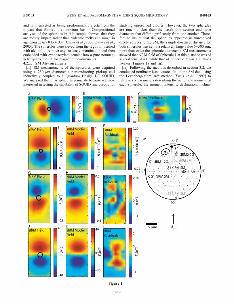
and is interpreted as being predominantly ejecta from theimpact that formed the Imbrium basin. Compositionalanalyses of the spherules in this sample showed that theyare mostly impact rather than volcanic melts and range inage from nearly 0 to 4 B.y. [Culler et al., 2000; Levine et al.,2005]. The spherules were sieved from the regolith, washedwith alcohol to remove any surface contamination and thenembedded with cyanoacrylate cement into a pure nonmag-netic quartz mount for magnetic measurements.4.2.1. SM Measurements[31] SM measurements of the spherules were acquired

using a 250-mm diameter superconducting pickup coilinductively coupled to a Quantum Design DC SQUID.We analyzed the lunar spherules primarily because we wereinterested in testing the capability of SQUID microscopy for

studying unresolved dipoles. However, the two spherulesare much thicker than the basalt thin section and havediameters that differ significantly from one another. There-fore to insure that the spherules appeared as unresolveddipole sources to the SM, the sample-to-sensor distance forboth spherules was set to a relatively large value (�500 mm,more than twice the spherule diameters). SM measurementsshowed that NRM field of Spherule 1 at this distance was ofseveral tens of nT, while that of Spherule 2 was 100 timesweaker (Figures 1a and 1g).[32] Following the methods described in section 3.2, we

conducted nonlinear least squares fits to the SM data usingthe Levenberg-Marquardt method [Press et al., 1992] toretrieve six parameters describing the net dipole moment ofeach spherule: the moment intensity, declination, inclina-

Figure 1


7 of 20

B09105

tion, two horizontal position coordinates and vertical dis-tance from the sensor. We fit for the three position coor-dinates of the dipole because the location of each spherulewas imprecisely known and we found in practice thatmaking this a free variable reduced our residual RMSwithout destabilizing the solution.[33] The NRM fits are shown in Figures 1b, 1h and the fit

parameters listed in Table 1. The moment of Spherule 2 is8.6 10�13 Am2, which is below the sensitivity of the 2G.The noise level of the SM scan far away from the dipole is0.05–1 nT (see the uncorrelated variations in pixel intensityat lower right corner of Figures 1g and 1i), about 10 timesless than the field of the spherule. Given that this scan wasmeasured at a sensor-to-sample distance 5 times greater thanour minimum currently achievable distance, the cubic falloffof dipole fields with distance means that we can detectdipoles with moments 103 times weaker than that ofSpherule 2. This exemplifies (although of course does notprove) the SM system noise level of 10�15 Am2 quoted insection 1.[34] The NRM fit for Spherule 2 was the only spherule fit

whose residual intensities were at the instrument noise level(Figure 1i) and normally distributed to >95% confidenceaccording to the Jarque-Bera test [Judge et al., 1988]. Incontrast, the NRM residuals for Spherule 1 were about afactor of 8 above the sensor noise, have a non-Gaussianintensity distribution, and most importantly are spatiallycorrelated. (Figure 1c).[35] Following the NRM measurements, the spherules

were given a saturation isothermal remanent magnetizationby briefly exposing them to a 600 mT field in the scanningplane toward the top of the page. The spherules were thenscanned with the SM again (Figures 1d and 1j). Leastsquares fitting (Figures 1e, 1f, 1k, and 1l) showed that themoments had increased by two orders of magnitude androtated into alignment with the applied field (Table 1). ThesIRM residuals for both spherules were again above thesensor noise, did not pass the Jarque-Bera test for beingnormally distributed at the 95% confidence level, and werehighly spatially correlated.[36] All but one of our spherule scans had spatially

correlated residuals with intensities exceeding the SQUIDsensor noise. One possible explanation for the high resid-uals is that they result from our idealized approximation ofthe spherules as magnetized spheres. However, a series ofleast squares experiments on artificial data (not shown)demonstrated that even if the spherule shapes were so

distorted as to have length-to-width ratios as great as 2:1,this still would lead to residuals with intensities only �1%of the data. As described in Appendix A, the computedresiduals have roughly the intensity expected from positionnoise. Position noise, which scales with moment intensity,would also explain why the much weaker NRM of Spherule2 does not have high intensity, spatially correlated residuals.4.2.2. 2G Measurements[37] After storage in a magnetically shielded lab for six

months, Spherule 1 was measured with the 2G. Theintensity was found to be about half and the direction 20�divergent from that inferred from the SM scan of the sIRM(Figure 1m). Given the abundant superparamagnetic iron inlunar glasses [Fuller and Cisowski, 1987], these differencesare almost certainly due to viscous decay of the spherule’smoment. Therefore we again exposed the spherule to anintense magnetic field (370 mT) and remeasured it imme-diately with the 2G. The average of this and three morerepeated applications of the field followed by 2G measure-ments gave a moment intensity and direction that matchedthat of the SM within the uncertainty associated with thesuperparamagnetic decay of the moment. This simple ex-periment is the first direct demonstration that momentmeasurements inferred from SQUID microscopy matchmeasurements on the same sample with a standard momentmagnetometer.

4.3. Basalt Thin Section

4.3.1. Sample Description[38] This 30-mm thin section of tholeiitic basalt was taken

from the Hawaii Scientific Drilling Project (HSDP) 2 corethrough the Mauna Kea volcano, Hawaii. The sample isfrom the interior of an aphyric pillow originating from adepth of 2421.4 m below sea level (core box 829, run 828)[DePaolo et al., 1999]. Like the rest of the HSDP core, oursample is geographically oriented in inclination but notdeclination. Rock magnetic studies of samples from thispart of the HSDP2 core indicate that the primary remanencecarrier is pseudo single domain titanomagnetite (xFe2TiO4 �(1 � x)Fe3O4 with x � 0.6) with a Curie temperature of100–200�C, a bulk coercivity of �20 mT, and a squareness(ratio of saturation remanence to saturation magnetization)of �0.4 [Kontny et al., 2003; Tauxe and Love, 2003].Thellier-Thellier paleointensity studies of pillow interiorsamples from this depth indicate that the remanence isalmost entirely a viscous remanent magnetization (VRM)that formed in a field with a paleointensity of 50–60 mT

Table 1. Summary of Paleomagnetic Analyses of Two Lunar Spherulesa

Sample Remanence Instrument M N Q m, Am2 i, � d, � Residual RMS, nT

Spherule 1 NRM SM 1170 6 1 6.9 10�11 �14 168 0.76Spherule 2 NRM SM 260 6 1 8.6 10�13 8 83 0.06Spherule 1 sIRM SM 810 6 1 7.5 10�9 11 267 48Spherule 1 sIRM 2G - - - 1.3 10�8 7 ± 9 273 ± 9 -Spherule 2 sIRM SM 494 6 1 8.8 10�11 �2 89 2.4

aThe first column lists the name of the sample, followed in the next two columns by the type of remanence (natural remanent magnetization (NRM) orsaturation isothermal remanent magnetization (sIRM)) and the instrument with which it was measured. The sIRM was produced by the application of asaturating field oriented toward i = 0, d = 270�. The next three columns specify the number of data points in the fit scan, M, the number of parameters, N,and the number of dipoles, Q. The last four columns give the moment as a result of the least squares fits (for SM scans) or direct measurements (for the 2G).Here m = dipole moment, i = inclination, d = clockwise declination (right = 0�). The moment listed for the 2G are the average and circular standarddeviation of four repeated measurements, each preceded by a reapplication of the saturating field.


8 of 20

B09105

[Tauxe and Love, 2003]. By analogy with previous compo-sitional studies of HSDP basalts [Baker et al., 1996], oursample consists of predominantly a groundmass of olivine,pyroxene, plagioclase, chromian spinel, and titanomagnetiteand has abundant vesicles filled with a variety of essentiallynonmagnetic secondary minerals (i.e., zeolites, smectite,apatite, and Ca-silicates [Walton and Schiffman, 2003]).The results of [Sharp and Renne, 2005] indicate that it hasan 40Ar/39Ar age of extrusion of �500 ka.[39] Our basalt thin section has a surface area of

several cm2 and was prepared using cyanoacrylate cement(without any heating) and mounted on a pure quartz slide(see section 2 for more details). Its NRM and sIRM wereeach measured with the SM. We found that the thin sectionwas sufficiently magnetic that we were also able to measureboth its NRM and sIRM with the 2G.4.3.2. 2G and Borehole Measurements[40] We begin by summarizing the moment magnetometry

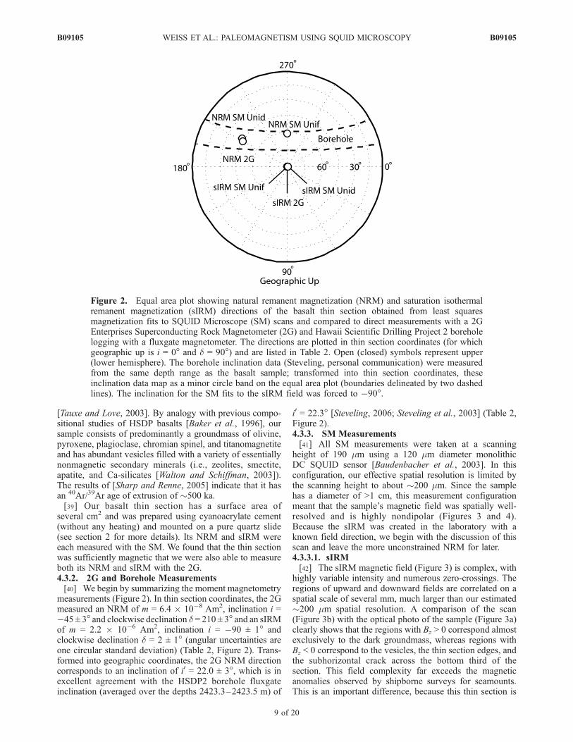
measurements (Figure 2). In thin section coordinates, the 2Gmeasured an NRM of m = 6.4 10�8 Am2, inclination i =�45 ± 3� and clockwise declination d = 210 ± 3� and an sIRMof m = 2.2 10�6 Am2, inclination i = �90 ± 1� andclockwise declination d = 2 ± 1� (angular uncertainties areone circular standard deviation) (Table 2, Figure 2). Trans-formed into geographic coordinates, the 2G NRM directioncorresponds to an inclination of i0 = 22.0 ± 3�, which is inexcellent agreement with the HSDP2 borehole fluxgateinclination (averaged over the depths 2423.3–2423.5 m) of

i0 = 22.3� [Steveling, 2006; Steveling et al., 2003] (Table 2,Figure 2).4.3.3. SM Measurements[41] All SM measurements were taken at a scanning

height of 190 mm using a 120 mm diameter monolithicDC SQUID sensor [Baudenbacher et al., 2003]. In thisconfiguration, our effective spatial resolution is limited bythe scanning height to about �200 mm. Since the samplehas a diameter of >1 cm, this measurement configurationmeant that the sample’s magnetic field was spatially well-resolved and is highly nondipolar (Figures 3 and 4).Because the sIRM was created in the laboratory with aknown field direction, we begin with the discussion of thisscan and leave the more unconstrained NRM for later.4.3.3.1. sIRM[42] The sIRM magnetic field (Figure 3) is complex, with

highly variable intensity and numerous zero-crossings. Theregions of upward and downward fields are correlated on aspatial scale of several mm, much larger than our estimated�200 mm spatial resolution. A comparison of the scan(Figure 3b) with the optical photo of the sample (Figure 3a)clearly shows that the regions with Bz > 0 correspond almostexclusively to the dark groundmass, whereas regions withBz < 0 correspond to the vesicles, the thin section edges, andthe subhorizontal crack across the bottom third of thesection. This field complexity far exceeds the magneticanomalies observed by shipborne surveys for seamounts.This is an important difference, because this thin section is

Figure 2. Equal area plot showing natural remanent magnetization (NRM) and saturation isothermalremanent magnetization (sIRM) directions of the basalt thin section obtained from least squaresmagnetization fits to SQUID Microscope (SM) scans and compared to direct measurements with a 2GEnterprises Superconducting Rock Magnetometer (2G) and Hawaii Scientific Drilling Project 2 boreholelogging with a fluxgate magnetometer. The directions are plotted in thin section coordinates (for whichgeographic up is i = 0� and d = 90�) and are listed in Table 2. Open (closed) symbols represent upper(lower hemisphere). The borehole inclination data (Steveling, personal communication) were measuredfrom the same depth range as the basalt sample; transformed into thin section coordinates, theseinclination data map as a minor circle band on the equal area plot (boundaries delineated by two dashedlines). The inclination for the SM fits to the sIRM field was forced to �90�.


9 of 20

B09105

taken from the subaqueous portion of the HSDP2 core andso was part of Mauna Kea when that volcano was just sucha seamount! Of course, the reason for the higher fieldcomplexity of the SM scan relative to the ship surveys isthe factor of 107 difference in sample-to-sensor distance.[43] Decades of least squares analyses of magnetic survey

data and paleomagnetic analyses of seamount rocks haveshown that a uniform magnetization model provides a poordescription for seamounts, even for those formed during asingle polarity chron [Gee et al., 1989; Kono, 1977; Parkeret al., 1987]. We therefore hardly expected it to be a goodmodel for the SM scan. As shown below, this was clearlyborne out by our magnetization inversions.[44] Using an equivalent source approach (section 3) and

assuming a uniform magnetization solution, we fit for thethree components of each of Q = 20,439 dipoles distributedin a grid whose boundaries coincide with the edges of thethin section. These edges were determined from a visualinspection of an optical photo of the section spatiallyregistered with respect to the SM scan. The dipole gridspacing was set to 100 mm (about half the sensor-to-sampledistance such that the magnetization can be captured athigh spatial resolution but without the instabilities that set infor finer spacings) and the horizontal position of each dipolewas located directly under each measurement. All least

squares fits to the basalt were computed in MATLABusing the large-scale algorithms that are part of the lsqlinfunction (we found that the nonnegative least squaresroutine lsqnonneg, used by Parker [Parker, 1991] for hisunidirectional solution, to be far too slow for use with ourrelatively much larger data sets). The heart of lsqlin is apreconditioned conjugate gradient analysis subroutine[Press et al., 1992; Purucker et al., 1996] that is computa-tionally efficient when used with sparse matrices.[45] Because the uniform solution requires fitting for only

N = 3 parameters (mx, my and mz), by far the mostcomputationally intensive part of the process is calculatingthe Jacobian A (equation (10)). This time can be reduced bycomputing an approximation of the Jacobian, Ay, by trun-cating the long-range interactions of the dipole moments: allelements Aij for which dipole-datum distances rij exceededsome threshold, r0, were set to zero. This truncation,commonly used for inverting large satellite magnetic fielddata sets [Purucker et al., 1996], is even more useful for ourunidirectional solutions described below; truncation permitsthe unidirectional Jacobians to be not only calculated morequickly but much more importantly makes them sparse.This sparsity dramatically reduced our memory require-ments and permitted us to take advantage of fast matrixarithmetic techniques. We empirically determined the opti-

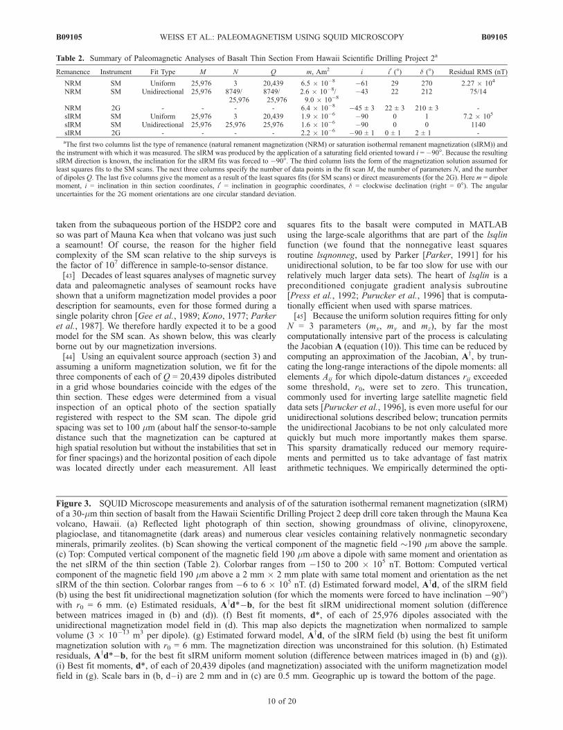
Figure 3. SQUID Microscope measurements and analysis of of the saturation isothermal remanent magnetization (sIRM)of a 30-mm thin section of basalt from the Hawaii Scientific Drilling Project 2 deep drill core taken through the Mauna Keavolcano, Hawaii. (a) Reflected light photograph of thin section, showing groundmass of olivine, clinopyroxene,plagioclase, and titanomagnetite (dark areas) and numerous clear vesicles containing relatively nonmagnetic secondaryminerals, primarily zeolites. (b) Scan showing the vertical component of the magnetic field �190 mm above the sample.(c) Top: Computed vertical component of the magnetic field 190 mm above a dipole with same moment and orientation asthe net sIRM of the thin section (Table 2). Colorbar ranges from �150 to 200 105 nT. Bottom: Computed verticalcomponent of the magnetic field 190 mm above a 2 mm 2 mm plate with same total moment and orientation as the netsIRM of the thin section. Colorbar ranges from �6 to 6 105 nT. (d) Estimated forward model, Ayd, of the sIRM field(b) using the best fit unidirectional magnetization solution (for which the moments were forced to have inclination �90�)with r0 = 6 mm. (e) Estimated residuals, Ayd*�b, for the best fit sIRM unidirectional moment solution (differencebetween matrices imaged in (b) and (d)). (f) Best fit moments, d*, of each of 25,976 dipoles associated with theunidirectional magnetization model field in (d). This map also depicts the magnetization when normalized to samplevolume (3 10�13 m3 per dipole). (g) Estimated forward model, Ayd, of the sIRM field (b) using the best fit uniformmagnetization solution with r0 = 6 mm. The magnetization direction was unconstrained for this solution. (h) Estimatedresiduals, Ayd*�b, for the best fit sIRM uniform moment solution (difference between matrices imaged in (b) and (g)).(i) Best fit moments, d*, of each of 20,439 dipoles (and magnetization) associated with the uniform magnetization modelfield in (g). Scale bars in (b, d–i) are 2 mm and in (c) are 0.5 mm. Geographic up is toward the bottom of the page.

Table 2. Summary of Paleomagnetic Analyses of Basalt Thin Section From Hawaii Scientific Drilling Project 2a

Remanence Instrument Fit Type M N Q m, Am2 i i0 (�) d (�) Residual RMS (nT)

NRM SM Uniform 25,976 3 20,439 6.5 10�8 �61 29 270 2.27 104

NRM SM Unidirectional 25,976 8749/25,976

8749/25,976

2.6 10�8/9.0 10�8

�43 22 212 75/14

NRM 2G - - - - 6.4 10�8 �45 ± 3 22 ± 3 210 ± 3 -sIRM SM Uniform 25,976 3 20,439 1.9 10�6 �90 0 1 7.2 105

sIRM SM Unidirectional 25,976 25,976 25,976 1.6 10�6 �90 0 0 1140sIRM 2G - - - - 2.2 10�6 �90 ± 1 0 ± 1 2 ± 1 -aThe first two columns list the type of remanence (natural remanent magnetization (NRM) or saturation isothermal remanent magnetization (sIRM)) and

the instrument with which it was measured. The sIRM was produced by the application of a saturating field oriented toward i = �90�. Because the resultingsIRM direction is known, the inclination for the sIRM fits was forced to �90�. The third column lists the form of the magnetization solution assumed forleast squares fits to the SM scans. The next three columns specify the number of data points in the fit scan M, the number of parameters N, and the numberof dipoles Q. The last five columns give the moment as a result of the least squares fits (for SM scans) or direct measurements (for the 2G). Here m = dipolemoment, i = inclination in thin section coordinates, i0 = inclination in geographic coordinates, d = clockwise declination (right = 0�). The angularuncertainties for the 2G moment orientations are one circular standard deviation.


10 of 20

B09105

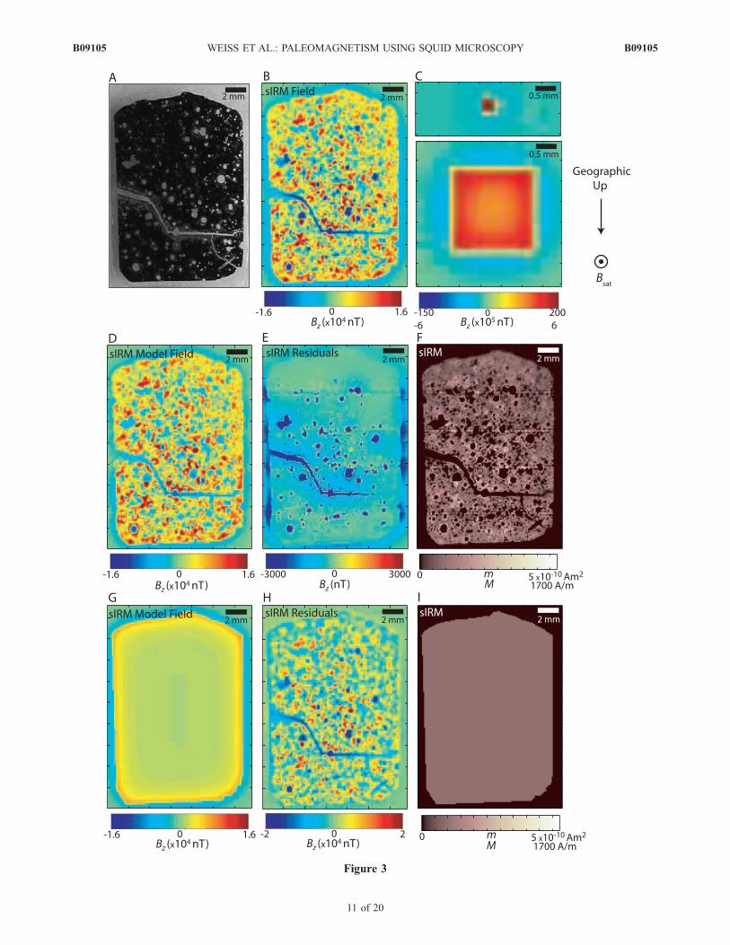
Figure 3


11 of 20

B09105

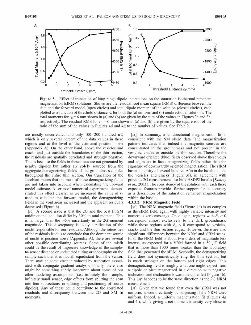
mum truncation threshold by conducting a series of trial fitson the sIRM data using various threshold distances r0(Figure 5). For all scans we found that for r0 � 6 mm,the residual RMS showed negligible improvement while thetotal fit moment of the scan converged toward the sIRMmeasured with the 2G. We note that because the minimumacceptable value of r0 depends on the sample size andscanning geometry (for instance, it should grow withincreasing horizontal sample size), it will need to bedetermined for each new sample analyzed with SQUIDmicroscopy.[46] The resulting uniform sIRM magnetization model

field Ayd* (Figure 3g) (calculated from forward modelingthe best fit solution (Table 2, Figures 2 and 3i)) has none ofthe zero-crossings and intensity variations seen in the data.This failure is manifested by highly spatially correlated,non-Gaussian residuals (Ayd* � b̂) (Figure 3h) whoseintensities range up to several tens of thousands of nT, farexceeding our expected measurement errors. Using Appen-dix equation A1, the total errors (which should be domi-nated by position errors) should only be of order 100 nT.[47] Nonetheless, there are some gross features about the

solution which are qualitatively consistent with our expect-ations. A vertically magnetized dipole and a verticallymagnetized plate both generate fields with positive Bz abovethe magnetized region and negative Bz (‘‘demagnetizingfield’’) that symmetrically rings the edges of the magneti-zation (Figure 3c). The thin section edges in both the data(Figure 3b) and uniform solution (Figure 3g) show thisapproximately symmetric demagnetizing field (blue). Infact, the uniform sIRM fit is within the angular uncertaintyof the 2G sIRM measurement (Figure 2). A second positivefeature of the uniform solution is that its net moment (thesum of all dipoles in Figure 3i) is only 14% less than the 2Gmeasurement (Table 2), although this is still outside the 5%uncertainty (�10�7 Am2) of the 2G. The lower moment ofthe sIRM scan cannot be easily explained by viscous decaybecause it was found that after even several years of zero-field storage following the original 2G sIRM measurementthe moment of the sample had decayed by only 3%.[48] Because we created the sIRM using a spatially

constant field, we might expect that a unidirectional solution

would provide a better description of its magnetization. Wecan hypothesize that like many other basalts, our samplemight have only weak anisotropy of remanence and there-fore would everywhere have magnetized parallel to thedirection of the applied field. Indeed, the 2G sIRM mea-surement demonstrates that this is true of the net moment.All of this would predict that our sample is unidirectionallymagnetized. To test this hypothesis, we solved for the bestfit unidirectional solution (see section 3.5). Unlike for theuniform solution, we assigned a dipole to a location underevery measurement (including those measurements off theedge of the thin section), for a total of Q = 25,976 dipoles.As before, the dipoles were spaced at 100 mm intervals.Because the applied field was oriented out of the plane ofthe thin section, the sIRM magnetization solution wasrequired to have inclination i = �90�. We then fit for theintensity of each dipole for a total of M = 25,976 measure-ments and N = 25,976 parameters. Computing a leastsquares fit for such a large Jacobian has memory andcomputational speed requirements that far outstrip ournew desktop computer (a dual core 3.4 GHz Intel 64-bitprocessor with 4 GB of RAM and several hundred GB ofvirtual memory). Once again, we used sparse matrix techni-queswith r0 = 6mm to estimate the Jacobian asAy (Figure 5b)and the lsqlin routine, which reduced the computation time toseveral weeks. Even so, we unfortunately had to split the scaninto four subsections and invert each separately, resulting inhigher residuals at the subsection boundaries.[49] The resulting residuals appear to be within our noise

limits. It is difficult to make this statement definitivebecause we were unable to calculate the full (non-sparse)Jacobian, which meant that it was also not possible for us toexactly calculate the forward model (Figure 3d) and, as aresult, the residuals (Figure 3e). The estimate of the forwardmodel Ayd* therefore is of high quality only at locationsthat are close to dipole sources with substantial moments.Because the magnetization is concentrated in the ground-mass (Figure 3f), the forward model is a poor estimate forlocations above vesicles, cracks, and the thin section edgeswhere the field is dominantly downward. This can beclearly seen from an examination of our estimated residuals,Ad* � b̂. Above the groundmass, the residuals (Figure 3e)

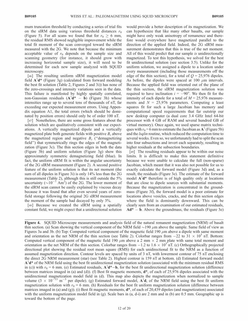
Figure 4. SQUID Microscope measurements and analysis field of the natural remanent magnetization (NRM) of basaltthin section. (a) Scan showing the vertical component of the NRM field �190 mm above the sample. Same field of view asFigures 3a and 3b. (b) Top: Computed vertical component of the magnetic field 190 mm above a dipole with same momentand orientation as the net NRM of the thin section (see Table 2). Colorbar ranges from �22 to 31 105 nT. Bottom:Computed vertical component of the magnetic field 190 mm above a 2 mm 2 mm plate with same total moment andorientation as the net NRM of the thin section. Colorbar ranges from �1.2 to 1.6 105 nT. (c) Orthographically projecteddirectional plot showing the residual root mean square (RMS) for each unidirectional fit to the NRM as a function ofassumed magnetization direction. Contour levels are spaced by units of 3 nT, with lowermost contour of 75 nT enclosingthe direct 2G NRM measurement (star) (see Table 2). Highest contour is 159 nT at bottom. (d) Estimated forward modelAyd* of the NRM field using the best fit unidirectional magnetization solution (associated with the minimum residual RMSin (c)) with r0 = 6 mm. (e) Estimated residuals, Ayd*�b, for the best fit unidirectional magnetization solution (differencebetween matrices imaged in (a) and (d)). (f) Best fit magnetic moments, d*, of each of 25,976 dipoles associated with theunidirectional magnetization model field in (d). This map also depicts the magnetization when normalized to samplevolume (3 10�13 m�3 per dipole). (g) Estimated forward model, Ayd, of the NRM field using the best fit uniformmagnetization solution with r0 = 6 mm. (h) Residuals for the best fit uniform magnetization solution (difference betweenmatrices imaged in (a) and (g)). (i) Best fit magnetic moments, d*, of each of 20,439 dipoles (and magnetization) associatedwith the uniform magnetization model field in (g). Scale bars in (a, d-i) are 2 mm and in (b) are 0.5 mm. Geographic up istoward the bottom of the page.


12 of 20

B09105

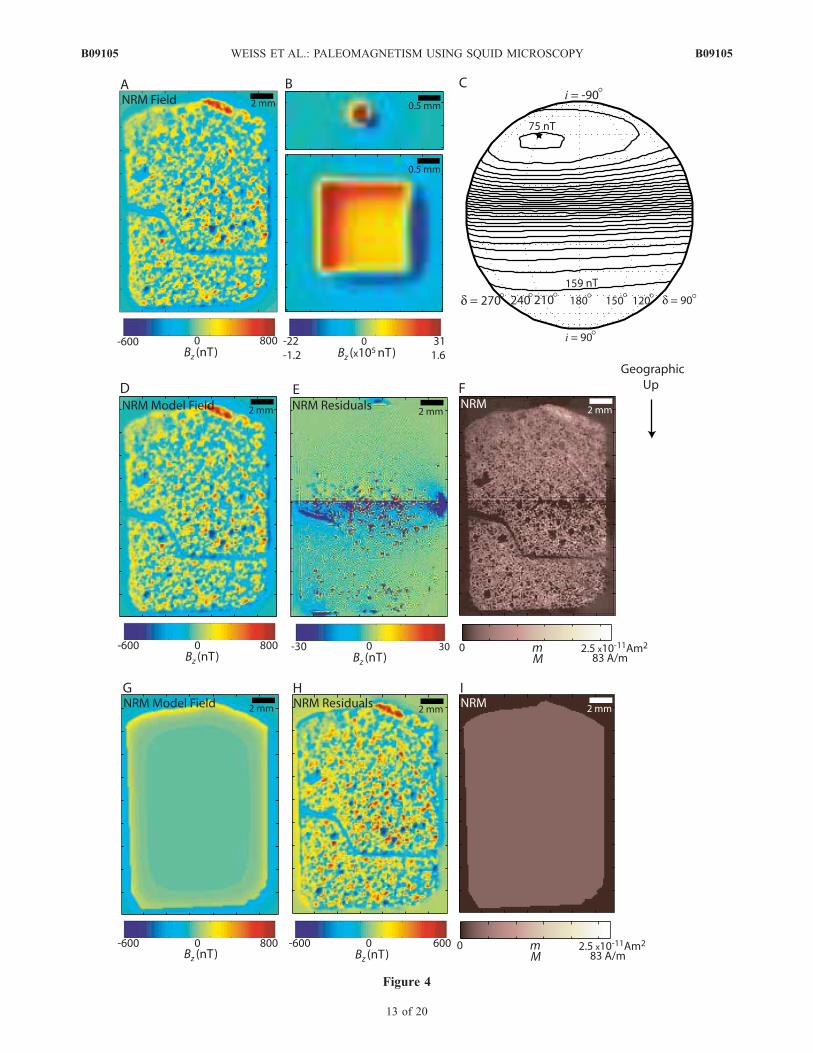
Figure 4


13 of 20

B09105

are mostly uncorrelated and only 100–200 hundred nT,which is only several percent of the data values in theseregions and at the level of the estimated position noise(Appendix A). On the other hand, above the vesicles andcracks and just outside the boundaries of the thin section,the residuals are spatially correlated and strongly negative.This is because the fields in these areas are not generated bynearby dipoles but rather are solely sourced from theaggregate demagnetizing fields of the groundmass dipolesthroughout the entire thin section. Our truncation of theJacobian means that the most of these demagnetizing fieldsare not taken into account when calculating the forwardmodel estimate. A series of numerical experiments demon-strated this effect clearly: as we increased the value of r0used to calculate the forward model, the demagnetizingfields in the void areas increased and the apparent residualsdecreased (Figure 6).[50] A second issue is that the 2G and the best fit SM

unidirectional solution differ by 30% in total moment. Thisis far larger than the �5% uncertainty in the 2G momentmagnitude. This discrepancy is likely a reflection of themisfit responsible for our residuals. Although the intensitiesof the residuals lead us to conclude that the dominant sourceof misfit is position noise (Appendix A), there are severalother possible contributing sources. Some of the misfitcould be the result of imprecise knowledge of the sample-to-sensor distance or undetected tilting or topography on thesample such that it is not all equidistant from the sensor.There may be some error introduced by truncation associ-ated with conjugate gradient analysis. Finally, there alsomight be something subtly inaccurate about some of ourother modeling assumptions (i.e., infinitely thin sample,infinitely small sensor, edge effects from splitting the scaninto four subsections, or spacing and positioning of sourcedipoles). Any of these could contribute to the correlatedresiduals and discrepancy between the 2G and SM fitmoments.

[51] In summary, a unidirectional magnetization fit isconsistent with the SM sIRM data. The magnetizationpattern indicates that indeed the magnetic sources areconcentrated in the groundmass and not present in thevesicles, cracks or outside the thin section. Therefore thedownward oriented (blue) fields observed above these voidsand edges are in fact demagnetizing fields rather than thesignature of downwardly oriented magnetization. The sIRMhas an intensity of several hundred A/m in the basalt outsidethe vesicles and cracks (Figure 3f), in agreement withprevious 2G measurements for bulk HSDP2 basalts [Kontnyet al., 2003]. The consistency of the solution with each theseexpected features provides further support for its accuracyas a description of the saturation remanent magnetizationwithin the basalt.4.3.3.2. NRM Magnetic Field[52] The NRM magnetic field (Figure 4a) is as complex

as the sIRM field, again with highly variable intensity andnumerous zero-crossings. Once again, regions with Bz > 0correspond almost exclusively to the dark groundmass,while those regions with Bz < 0 correspond to vesicles,cracks and the thin section edges. However, there are alsosignificant differences between the NRM and sIRM scans.First, the NRM field is about two orders of magnitude lessintense, as expected for a VRM formed in a 50 mT fieldthat is more than 1000 times weaker than the laboratoryfield that generated the sIRM. Secondly, the demagnetizingfield does not symmetrically ring the thin section, butis much stronger on the bottom and right edges. Thisdemagnetizing field is roughly what one might expect froma dipole or plate magnetized in a direction with negativeinclination and declination toward the upper left (Figure 4b).This just happens to be the same direction as the 2G NRMmeasurement.[53] Given that we found that even the sIRM was not

uniform, it would certainly be surprising if the NRM wereuniform. Indeed, a uniform magnetization fit (Figures 4gand 4i), while giving a net moment intensity very close to

Figure 5. Effect of truncation of long range dipole interactions on the saturation isothermal remanentmagnetization (sIRM) solutions. Shown are the residual root mean square (RMS) difference between thedata and the forward model (open circles) and total dipole moment of the solution (closed circles), eachplotted as a function of threshold distance r0 for both the (a) uniform and (b) unidirectional solutions. Thetotal moments for r0 = 6 mm shown in (a) and (b) are given by the sum of the values in Figures 3e and 3h,respectively. The residual RMS for r0 = 6 mm shown in (a) and (b) are given by the square root of theratio of the sum of the values in Figures 4d and 4g to the number of values. See Table 2.


14 of 20

B09105

that measured with the 2G (Table 2), has a direction that is�60� divergent and has residuals (Figure 4h) that are highlycorrelated and far exceed our measurement uncertainty of10 nT.[54] Because the basalt sample is young (has existed

during only the current polarity chron), unbrecciated, rela-tively unaltered, and has a compositionally homogenousgroundmass at the centimeter scale, we might also predictthat its NRM would also be unidirectional to within ourmeasurement uncertainties. Because its NRM is actually aVRM, the NRM is the vector sum of components whichcould be multidirectional due to secular variation on atimescale shorter than the lifetime of its VRM. However,if the distribution of titanomagnetite crystals in the ground-mass is homogenous on the scale of our spatial resolution,then a unidirectional solution would still be successful atfitting the data. This is another hypothesis we can test byfitting for a unidirectional magnetization.[55] In principle, we do not a priori know the NRM

direction unless we use the 2G NRM measurement as aconstraint. We chose not to do so because by allowing thefits to select a best fit direction, we could test the unidirec-tional hypothesis by not only the standard method ofexamining the residuals but by an additional criterion: theagreement in net direction with the known (2G) value.Therefore the magnetization was not specified for ourunidirectional NRM fits.

[56] Rather, the unit sphere was uniformly tiled following[Rakhmanov et al., 1994; Saff and Kuijlaars, 1997] and abest fit intensity solution was separately obtained for eachorientation direction. The best fit direction is that with thelowest residual RMS, and the best fit intensity is theintensity solution associated with this direction [Parker,1991]. Because unidirectional fits can exhibit numerouslocal minima on the unit sphere [Parker, 1991], it isimportant for the angular search grid to be fairly fine. Alltold, we obtained a unidirectional solution for 666 searchdirections. Because even a single such fit using sparsematrix methods with r0 = 6 mm would require a week oftime on our computer (i.e., the sIRM fit), we had to makefurther approximations to make the calculations tractable.Instead of using one dipole for each of the 25,976 measure-ments, we began by only placing dipoles at locations wheredata values Bz exceeded 150 nT. This reduced the number ofdipoles to 8,749 and restricted their location to within thegroundmass and outside the vesicles and cracks. Thisshortcut is justified for two reasons: petrographic data showthat the vesicles and crack areas are nonmagnetic, and thesIRM magnetization unidirectional solution (Figure 3f)indicates that there are essentially no magnetic carriers inthese same locations.[57] The results (Figure 4c) showed a single global

minimum with inclination i = �43� and clockwise declina-tion d = 212� that is very close to the 2G NRM measure-

Figure 6. Various estimates of the forward model, Ayd*, and residuals, Ayd*�b, for the saturationisothermal remanent magnetization (sIRM) field. All estimates here were computed using a solution d*that was originally computed from a Jacobian Ay estimated with r0 = 6 mm. (a) Estimated forward modelfor r0 = 0.5 mm. (b) Estimated residuals associated with forward model in (a). (c) Estimated forwardmodel for r0 = 1 mm. (d) Estimated residuals associated with forward model in (c). (e) Estimated forwardmodel for r0 = 8 mm. (f) Estimated residuals associated with forward model in (e).


15 of 20

B09105

ment as well as the borehole fluxgate inclination (Figure 2).This corresponds to an inclination of i0 = 22� in geographiccoordinates, which is roughly what one would expect for asample from Hawaii with a VRM acquired in the Earth’spresent field (the actual inclination at Mauna Kea today is37�). However, the net moment intensity for this solutionwas about half the 2G value (Table 2). Because wesuspected this discrepancy was the result of our computa-tional shortcut of artificially reducing the number of dipoles,we conducted a second fit using 25,976 dipoles (one foreach measurement) but restricting the orientation to thepreviously identified best fit-direction. To alleviate memoryand computational demands, the scan was divided into twosubsections and each section was fit separately. The result-ing solution was four times more intense than the previoussolution and in fact 28% more intense than the 2G mea-surement. Again, this disagreement in total moment must beat least partly a result of position noise, and it couldpotentially be eliminated by improving the SM hardwareor bounding the SM solution norm to within the uncertain-ties of the 2G moment magnitude. For the same reasonsstated during the discussion about the NRM fitting, it ispossible that part of this misfit is a result of our modelingassumptions or computational shortcuts. Away from theboundary separating the two subsections, the residuals(Figure 4e) are mostly uncorrelated and of order 10 nT,close to our expected measurement noise.[58] We would like an estimate of the uncertainty on the

best-direction for the unidirectional solution. Parker [Parker,1991] approached this by setting the uncertainty to thatcontour on the residual plot corresponding to the measure-ment uncertainty. However, our residual plot is only anestimate of the true residuals because of the reduced numberof dipoles with respect to our final solution. Worse, even theresiduals for our final solution with the full number of dipoles(Figure 4e) are themselves an estimate because of thetruncation of the Jacobian (see above). Therefore we wereunable to place a bound on the accuracy of the best fitdirection except to note again its superb agreement with the2G measurement.[59] The NRM unidirectional fit corresponds to a mag-

netization of �10–20 A/m in the basalt outside the vesiclesand cracks (Figure 4f), consistent with what has beenpreviously measured for HSDP basalts [Kontny et al.,2003]. As with the sIRM, the magnetization is concentratedin the groundmass, such that the fields with negative Bz

above the voids, cracks, and section edges are demagnetiz-ing fields rather than the result of oppositely orientedmagnetization. Again, the consistency of the solution witheach these expected features provides additional support forthe use of a unidirectional model for the NRM.4.3.4. Uniqueness of Unidirectional Solutions[60] We have argued that the magnetization solutions

retrieved from the sIRM and NRM data are within theuncertainties of our measurements. Therefore our data areconsistent with the hypothesis that the sIRM and NRM areunidirectional throughout the basalt. As pointed out byParker, there is no guarantee that a nonnegative unidirec-tional magnetization solution will fit a particular magneticfield data set (note that the same is not true for unidirec-tional solutions without the nonnegativity constraint).Therefore using SQUID microscopy we have indeed

learned something unique about the magnetization withinthe basalt that would not have been knowable from the 2Gdata alone.[61] We have already addressed the uniqueness of the

magnetization orientation in section 4.3.3. However, for agiven orientation, how unstable is the intensity pattern ofthe magnetization solution? As is true for essentially alliterative least squares methods, we found that the natureof the solution depends on the number of iterations. Inparticular, it has often been observed for conjugate gradientmethods that as number of iterations is increased, theresidual RMS drops while the solution norm (or othermeasures of instability) increases [Hansen, 1998]. Thereforeconjugate gradient methods are inherently regularizing,with the number of iterations serving as a regularizationparameter.[62] One would not expect our unidirectional solutions to

be highly unstable because the nonnegativity requirementprevents the solution from having the high-frequency, high-amplitude positive and negative oscillations that are typicalof less constrained magnetization inversions [Parker, 1994].To confirm this, for a subset of the sIRM data (lower leftcorner of Figure 6a) we computed a series of solutions byvarying the number maximum number of iterations. Foreach solution we calculated the residual RMS as a measureof misfit and three different measures of solution instability:the Euclidean norm d*k k, standard deviation stdev(d*), andthe summed gradient

Prmk k. We found that as the

number of iterations increased, the residual RMS decreasedwhile the solution became slowly less smooth, particularlyaround the edges of the magnetization (compare Figures 7a,7b, 7c). This decrease in smoothness is reflected in agradual increase in the standard deviation and the summedgradient (Figure 7d). This functional behavior is similar inshape but far smaller in magnitude than L-curves typical ofill-posed problems [Hansen, 1998]. The solution which bestfulfills the tradeoff between smoothness and residual is thatpictured in Figure 7b. Interestingly, although the solutionnorm does not show this same L-curve behavior, its min-imum occurs just at the same solution. Therefore we havethree different indicators that this solution is optimal.Because the instability indicators do not vary much as afunction of iteration number, we can see that the unidirec-tional intensity solution for the sIRM is reasonably smooth.4.3.5. Future Improvements[63] There are at least four simple ways to improve our

future magnetization inversions. The first is to modify theSM hardware to reduce the position noise. The second is torequire the SM solution to have a total moment within theuncertainties of the 2G moment (lsqlin has the capability toput upper and lower bounds on d). We chose not to imposesuch constraints on d here since our intention was not toobtain the most realistic fit but rather to demonstrate thatSM data are validated by 2G measurements. The third is toconstrain our space domain solutions using frequencydomain inversions. When conducted using field data thathave been measured on both sides of a thin section,frequency domain techniques can uniquely calculate thevertical component of the magnetization per unit area [Egliand Heller, 2000]. Our unidirectional space domainmagnetization solutions could then be forced to havez-components that match those mandated by the frequency


16 of 20

B09105

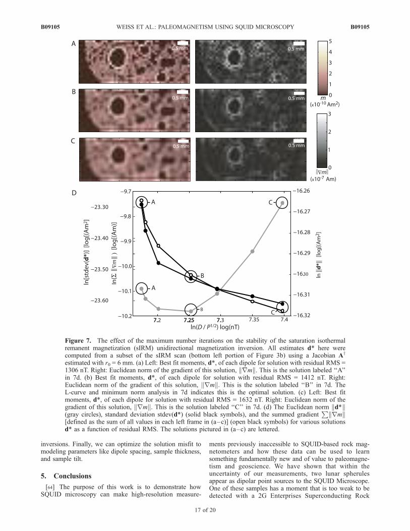
inversions. Finally, we can optimize the solution misfit tomodeling parameters like dipole spacing, sample thickness,and sample tilt.

5. Conclusions

[64] The purpose of this work is to demonstrate howSQUID microscopy can make high-resolution measure-

ments previously inaccessible to SQUID-based rock mag-netometers and how these data can be used to learnsomething fundamentally new and of value to paleomagne-tism and geoscience. We have shown that within theuncertainty of our measurements, two lunar spherulesappear as dipolar point sources to the SQUID Microscope.One of these samples has a moment that is too weak to bedetected with a 2G Enterprises Superconducting Rock

Figure 7. The effect of the maximum number iterations on the stability of the saturation isothermalremanent magnetization (sIRM) unidirectional magnetization inversion. All estimates d* here werecomputed from a subset of the sIRM scan (bottom left portion of Figure 3b) using a Jacobian Ay

estimated with r0 = 6 mm. (a) Left: Best fit moments, d*, of each dipole for solution with residual RMS =1306 nT. Right: Euclidean norm of the gradient of this solution, rmk k. This is the solution labeled ‘‘A’’in 7d. (b) Best fit moments, d*, of each dipole for solution with residual RMS = 1412 nT. Right:Euclidean norm of the gradient of this solution, rmk k. This is the solution labeled ‘‘B’’ in 7d. TheL-curve and minimum norm analysis in 7d indicates this is the optimal solution. (c) Left: Best fitmoments, d*, of each dipole for solution with residual RMS = 1632 nT. Right: Euclidean norm of thegradient of this solution, rmk k. This is the solution labeled ‘‘C’’ in 7d. (d) The Euclidean norm d*k k(gray circles), standard deviation stdev(d*) (solid black symbols), and the summed gradient

Prmk k

[defined as the sum of all values in each left frame in (a–c)] (open black symbols) for various solutionsd* as a function of residual RMS. The solutions pictured in (a–c) are lettered.


17 of 20

B09105

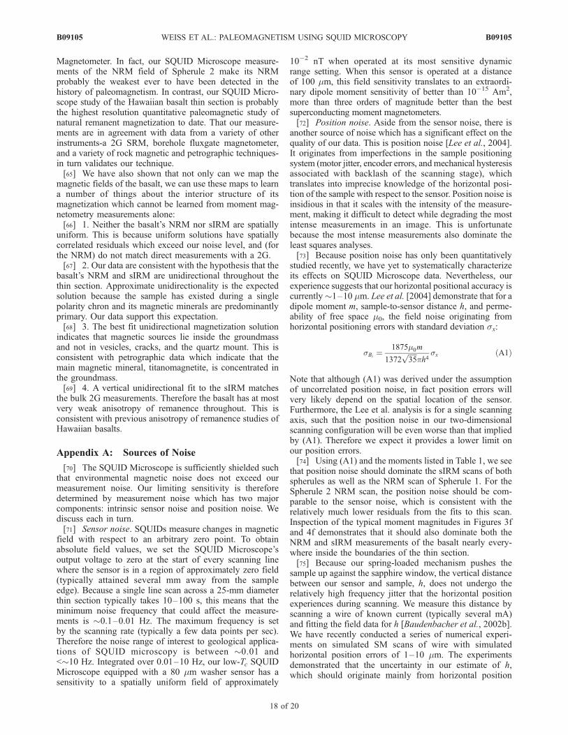
Magnetometer. In fact, our SQUID Microscope measure-ments of the NRM field of Spherule 2 make its NRMprobably the weakest ever to have been detected in thehistory of paleomagnetism. In contrast, our SQUID Micro-scope study of the Hawaiian basalt thin section is probablythe highest resolution quantitative paleomagnetic study ofnatural remanent magnetization to date. That our measure-ments are in agreement with data from a variety of otherinstruments-a 2G SRM, borehole fluxgate magnetometer,and a variety of rock magnetic and petrographic techniques-in turn validates our technique.[65] We have also shown that not only can we map the

magnetic fields of the basalt, we can use these maps to learna number of things about the interior structure of itsmagnetization which cannot be learned from moment mag-netometry measurements alone:[66] 1. Neither the basalt’s NRM nor sIRM are spatially

uniform. This is because uniform solutions have spatiallycorrelated residuals which exceed our noise level, and (forthe NRM) do not match direct measurements with a 2G.[67] 2. Our data are consistent with the hypothesis that the

basalt’s NRM and sIRM are unidirectional throughout thethin section. Approximate unidirectionality is the expectedsolution because the sample has existed during a singlepolarity chron and its magnetic minerals are predominantlyprimary. Our data support this expectation.[68] 3. The best fit unidirectional magnetization solution

indicates that magnetic sources lie inside the groundmassand not in vesicles, cracks, and the quartz mount. This isconsistent with petrographic data which indicate that themain magnetic mineral, titanomagnetite, is concentrated inthe groundmass.[69] 4. A vertical unidirectional fit to the sIRM matches

the bulk 2G measurements. Therefore the basalt has at mostvery weak anisotropy of remanence throughout. This isconsistent with previous anisotropy of remanence studies ofHawaiian basalts.

Appendix A: Sources of Noise

[70] The SQUID Microscope is sufficiently shielded suchthat environmental magnetic noise does not exceed ourmeasurement noise. Our limiting sensitivity is thereforedetermined by measurement noise which has two majorcomponents: intrinsic sensor noise and position noise. Wediscuss each in turn.[71] Sensor noise. SQUIDs measure changes in magnetic

field with respect to an arbitrary zero point. To obtainabsolute field values, we set the SQUID Microscope’soutput voltage to zero at the start of every scanning linewhere the sensor is in a region of approximately zero field(typically attained several mm away from the sampleedge). Because a single line scan across a 25-mm diameterthin section typically takes 10–100 s, this means that theminimum noise frequency that could affect the measure-ments is �0.1–0.01 Hz. The maximum frequency is setby the scanning rate (typically a few data points per sec).Therefore the noise range of interest to geological applica-tions of SQUID microscopy is between �0.01 and<�10 Hz. Integrated over 0.01–10 Hz, our low-Tc SQUIDMicroscope equipped with a 80 mm washer sensor has asensitivity to a spatially uniform field of approximately

10�2 nT when operated at its most sensitive dynamicrange setting. When this sensor is operated at a distanceof 100 mm, this field sensitivity translates to an extraordi-nary dipole moment sensitivity of better than 10�15 Am2,more than three orders of magnitude better than the bestsuperconducting moment magnetometers.[72] Position noise. Aside from the sensor noise, there is

another source of noise which has a significant effect on thequality of our data. This is position noise [Lee et al., 2004].It originates from imperfections in the sample positioningsystem (motor jitter, encoder errors, andmechanical hysteresisassociated with backlash of the scanning stage), whichtranslates into imprecise knowledge of the horizontal posi-tion of the sample with respect to the sensor. Position noise isinsidious in that it scales with the intensity of the measure-ment, making it difficult to detect while degrading the mostintense measurements in an image. This is unfortunatebecause the most intense measurements also dominate theleast squares analyses.[73] Because position noise has only been quantitatively

studied recently, we have yet to systematically characterizeits effects on SQUID Microscope data. Nevertheless, ourexperience suggests that our horizontal positional accuracy iscurrently�1–10 mm. Lee et al. [2004] demonstrate that for adipole moment m, sample-to-sensor distance h, and perme-ability of free space m0, the field noise originating fromhorizontal positioning errors with standard deviation sx:

sBi¼ 1875m0m

1372ffiffiffiffiffi35

pph4

sx ðA1Þ

Note that although (A1) was derived under the assumptionof uncorrelated position noise, in fact position errors willvery likely depend on the spatial location of the sensor.Furthermore, the Lee et al. analysis is for a single scanningaxis, such that the position noise in our two-dimensionalscanning configuration will be even worse than that impliedby (A1). Therefore we expect it provides a lower limit onour position errors.[74] Using (A1) and the moments listed in Table 1, we see

that position noise should dominate the sIRM scans of bothspherules as well as the NRM scan of Spherule 1. For theSpherule 2 NRM scan, the position noise should be com-parable to the sensor noise, which is consistent with therelatively much lower residuals from the fits to this scan.Inspection of the typical moment magnitudes in Figures 3fand 4f demonstrates that it should also dominate both theNRM and sIRM measurements of the basalt nearly every-where inside the boundaries of the thin section.[75] Because our spring-loaded mechanism pushes the

sample up against the sapphire window, the vertical distancebetween our sensor and sample, h, does not undergo therelatively high frequency jitter that the horizontal positionexperiences during scanning. We measure this distance byscanning a wire of known current (typically several mA)and fitting the field data for h [Baudenbacher et al., 2002b].We have recently conducted a series of numerical experi-ments on simulated SM scans of wire with simulatedhorizontal position errors of 1–10 mm. The experimentsdemonstrated that the uncertainty in our estimate of h,which should originate mainly from horizontal position


18 of 20

B09105

errors, is less than 0.1%. Therefore imprecise knowledge ofh is likely not the dominant noise source for scans of planarsamples.

[76] Acknowledgments. We thank R. Bennett-Calorio andM. Pendleton for administrative assistance, J. Wikswo for open access tothe VIIBRE facilities for the past seven years, C. Dwyer and K. McBridefor assistance with the magnetic measurements of the spherules, E. Stevelingfor sharing his unpublished HSDP2 borehole magnetic data, T. Scheider forhelpful discussions about inverse theory, I. Ceraj for introducing us to theworld of 64 bit computing, N. Gitahi and C. Seaman for assistance withsampling the HSDP core, and the HSDP team for access to its valuablesamples. B. Weiss and F. Baudenbacher thank the NSF Geophysics, NSFInstrumentation and Facilities, NASA Mars Fundamental Research, and theNASA Planetary Major Equipment Programs.

ReferencesAster, R. C., B. Borchers, and C. H. Thurber (2005), Parameter Estimationand Inverse Problems, 301 pp., Elsevier Academic Press, Burlington.

Baker, M. B., S. Alves, and E. M. Stolper (1996), Petrology and petrographyof the Hawaii Scientific Drilling Project lavas: Inferences from olivinephenocryst abundances and compositions, J. Geophys. Res., 101,11,715–11,727.

Baudenbacher, F. J., N. T. Peters, J. P. Wikswo, and M. Radparvar (1998),High resolution LTS-SQUID magnetometer, Bull. Am. Phys. Soc., 43,1626.

Baudenbacher, F. J., N. T. Peters, and J. P. Wikswo (2002a), High resolutionlow-temperature superconductivity superconducting quantum interfer-ence device microscope for imaging magnetic fields of samples at roomtemperatures, Rev. Sci. Instrum., 73, 1247–1254.

Baudenbacher, F., N. T. Peters, P. Baudenbacher, and J. P. Wikswo (2002b),High resolution imaging of biomagnetic fields generated by action cur-rents in cardiac tissue using a LTS-SQUID microscope, Physica C, 368,24–31.

Baudenbacher, F., L. E. Fong, J. R. Holzer, and M. Radparvar (2003),Monolithic low-transition-temperature superconducting magnetometersfor high resolution imaging magnetic fields of room temperature samples,Appl. Phys. Lett., 82, 3487–3489.

Blakely, R. J. (1996), Potential Theory in Gravity and Magnetic Applica-tions, 441 pp., Cambridge Univ. Press, New York.

Bott, M. H. P., and M. A. Hutton (1970), Limitations on the resolutionpossible in the direct interpretation of marine magnetic anomalies, EarthPlanet. Sci. Lett., 8, 317–319.

Braginski, A., and J. Clarke (2004), Introduction, in The SQUID Handbook,edited by J. Clarke and A. I. Braginski, pp. 1–28, Wiley-VCH, Weinheim.

Cavarretta, G., A. Coradini, R. Funiciello,M. Fulchignoni, A. Taddeucci, andR. Trigila (1972), Glassy particles in Apollo 14 soil 14163,88: Peculiaritiesand genetic considerations, Proc. Lunar Sci. Conf., 3, 1085–1094.

Chatraphorn, S., E. F. Fleet, and F. C. Wellstood (2002), Relationshipbetween spatial resolution and noise in scanning superconducting quan-tum interference device microscopy, J. Appl. Phys., 92, 4731–4740.

Clem, T. R., C. P. Foley, and M. N. Keene (2006), SQUIDs for geophysicalsurvey and magnetic anomaly detection, in The SQUID Handbook, editedby J. Clarke and A. I. Braginski, pp. 481–543, Wiley-VCH, Weinheim.

Cochran, A., G. B. Donaldson, S. Evanson, and R. J. P. Bain (1993), First-generation SQUID-based nondestructive testing system, IEEE Proc. A,140, 113–120.

Culler, T. S., T. A. Becker, R. A. Muller, and P. R. Renne (2000), Lunarimpact history from 40Ar/39Ar dating of glass spherules, Science, 287,1785–1788.

Dampney, C. N. G. (1969), The equivalent source technique, Geophysics,34, 39–53.

Dechert, J., M. Mueck, and C. Heider (1999), A scanning SQUID micro-scope for samples at room temperature, IEEE Trans. Appl. Supercond., 9,4111–4114.

DePaolo, D. J., E. M. Stolper, D. M. Thomas, and M. O. Garcia (1999),Hawaii Scientific Drilling Project: Core logs and summarizing data,Pasadena.

Egli, R., and F. Heller (2000), High-resolution imaging using a high-Tcsuperconducting quantum interference device (SQUID) magnetometer,J. Geophys. Res., 105, 25,709–25,727.

Emilia, D. A. (1973), Equivalent sources used as an analytic base forprocessing total magnetic field profiles, Geophysics, 38, 339–348.

Emilia, D. A., and R. L. Massey (1974), Magnetization estimation fornonuniformly magnetized seamounts, Geophysics, 39, 223–231.

Fagaly, R. (2006), Superconducting quantum interference device instru-ments and applications, Rev. Sci. Instrum., 77, 101101.

Fleet, E. F., S. Chatraphorn, F. C. Wellstood, and C. Eylem (2001), Deter-mination of magnetic properties using a room-temperature scanningSQUID microscope, IEEE Trans. Appl. Supercond., 11, 1180–1183.

Fong, L. E., J. R. Holzer, K. K. McBride, E. A. Lima, F. Baudenbacher, andM. Radparvar (2004), Multiloop low-transition-temperature SQUID sen-sor for imaging biomagnetic fields with submillimeter resolution, Appl.Phys. Lett., 84, 3190–3193.

Fong, L. E., J. R. Holzer, K. K. McBride, E. A. Lima, and F. Baudenbacher(2005), High resolution room-temperature sample scanning supercon-ducting interference device microscope configurable for geological andbiomagnetic applications, Rev. Sci. Instrum., 76, 053703.

Fuller, M., and S. M. Cisowski (1987), Lunar paleomagnetism, in Geomag-netism, edited by J. A. Jacobs, pp. 307–455, Academic Press, Orlando.

Fuller, M., W. S. Goree, and W. L. Goodman (1985), An introduction to theuse of SQUID magnetometers in biomagnetism, in Magnetite Biominer-alization and Magnetoreception in Organisms: A New Biomagnetism,edited by J. L. Kirschvink et al., pp. 103–151, Plenum Press, New York.

Gattacceca, J., M. Boustie, B. P. Weiss, P. Rochette, E. A. Lima, L. E. Fong,and F. J. Baudenbacher (2006), Investigating impact demagnetizationthrough laser impacts and SQUID microscopy, Geology, 34, 333–336.

Gee, J., H. Staudigel, and L. Tauxe (1989), Contribution of induced mag-netization to magnetization of seamounts, Nature, 342, 170–173.

Hansen, P. C. (1998), Rank-Deficient and Discrete Ill-Posed Problems:Numerical Aspects of Linear Inversion, 247 pp., Society for Industrialand Applied Mathematics, Philadelphia.

Hansen, P. C. (2001), Regularization Tools: A Matlab Package for Analysisand Solution of Discrete Ill-Posed Problems, Version 3.1 for Matlab 6.0,109 pp., available online at http://www.imm.dtu.dk/~pch.

Hildebrand, J. A., and R. L. Parker (1987), Paleomagnetism of CretaceousPacific seamounts revisited, J. Geophys. Res., 92, 12,695–12,712.

Judge, G. G., R. C. Hill, W. E. Griffiths, H. Lutkepohl, and T.-C. Lee (1988),Introduction to the Theory and Practice of Econometrics, Wiley, New York.

Ketchen, M. B., J. R. Kirtley, and M. Bhushan (1997), Miniature vectormagnetometer for scanning SQUID microscopy, IEEE Trans. Appl.Supercond., 7, 3139–3142.

Kirschvink, J. L. (1992), Uniform magnetic fields and double-wrapped coilsystems: Improved techniques for the design of bioelectromagneticexperiments, Bioelectromagnetics, 13, 401–411.

Kirtley, J. R., and J. P. Wikswo (1999), Scanning SQUID microscopy,Annu. Rev. Mater. Sci., 29, 117–148.

Kono, M. (1977), Paleomagnetism of DSDP Leg 55 basalts and implica-tions for the tectonics of the Pacific Plate, Initial Rep. Deep Sea Drill.Project, 55, 737–758.

Kontny, A., C. Vahle, and H. de Wall (2003), Characteristic magneticbehavior of subaerial and submarine lava units from the Hawaiian Scien-tific Drilling Project (HDSP-2), Geochem. Geophys. Geosyst., 4(2), 8703,doi:10.1029/2002GC000304.

Krasa, D. (2002), Partial self-reversal of the NRM in basalts: Identifying theresponsible mineral phases, IRM Quarterly, 12, 3–4.

Kress, R., L. Kuhn, and R. Potthast (2002), Reconstruction of a currentdistribution from its magnetic field, Inverse Problems, 18, 1127–1146.

Labotka, T. C., M. J. Kempa, C. White, J. J. Papike, and J. C. Laul (1980),The lunar regolith: Comparative petrology of the Apollo sites, ProcLunar Planet. Sci. Conf., 11, 1285–1305.

Langel, R. A., and W. J. Hinze (1998), The Magnetic Field of the Earth’sLithosphere, 429 pp., Cambridge Univ. Press, Cambridge.

Langel, R. A., E. V. Slud, and P. J. Smith (1984), Reduction of satellitemagnetic anomaly data, J. Geophys., 54, 207–212.

Lee, T. S., E. Dantsker, and J. Clarke (1996), High-transition temperaturesuperconducting quantum interference device microscope, Rev. Sci.Instrum., 67, 4208–4215.

Lee, S.-Y., J. Mathews, and F. C. Wellstood (2004), Position noise inscanning superconducting quantum interference device microscopy, Appl.Phys. Lett., 84, 5001–5003.

Levine, J., T. A. Becker, R. A. Muller, and P. R. Renne (2005), 40Ar/39Ardating of Apollo 12 impact spherules, Geophys. Res. Lett., 32, L15201,doi:10.1029/2005GL022874.

Lima, E. A., A. Irimia, and J. P. Wikswo (2006), The magnetic inverseproblem, in The SQUIDHandbook, edited by J. Clarke andA. I. Braginski,pp. 139–267, Wiley-VCH, Weinheim.

Mayhew, M. A. (1979), Inversion of satellite magnetic anomaly data,J. Geophys., 45, 119–128.

Mayhew, M. A. (1982), An equivalent layer magnetization model for theUnited States derived from satellite altitude magnetic anomalies, J. Geo-phys. Res., 87, 4837–4845.

Mayhew, M. A., and S. C. Galliher (1982), An equivalent layer magnetiza-tion model for the United States derived from Magsat data, Geophys. Res.Lett., 9, 311–313.

McNutt, M. (1986), Nonuniform magnetization of seamounts: A leastsquares approach, J. Geophys. Res., 91, 3686–3700.


19 of 20

B09105

Nicolosi, I., I. Blanco-Montenegro, A. Pignatelli, and M. Chiappini (2006),Estimating the magnetization direction of crustal structures by means ofan equivalent source algorithm, Phys. Earth Planet. Inter., 155, 163–169.

Nowaczyk, N. R., H.-U. Worm, A. Knecht, and J. H. Hinken (1998),Imaging distribution patterns of magnetic minerals by a novel high-Tc-SQUID-based field distribution measuring system: Applications to Per-mian sediments, Geophys. J. Int., 132, 721–726.

Parker, R. L. (1971), The determination of seamount magnetism, Geophys.J. R. Astron. Soc., 24, 321–324.

Parker, R. L. (1977), Understanding inverse theory, Annu. Rev. Earth Pla-net. Sci., 5, 35–64.

Parker, R. L. (1988), A statistical theory of seamount magnetism, J. Geo-phys. Res., 93, 3105–3115.

Parker, R. L. (1991), A theory of ideal bodies for seamount magnetism,J. Geophys. Res., 96, 16,101–16,112.

Parker, R. L. (1994), Geophysical Inverse Theory, 386 pp., Princeton Univ.Press, Princeton.

Parker, R. L., L. Shure, and J. A. Hildebrand (1987), The application ofinverse theory to seamount magnetism, Rev. Geophys., 25, 17–40.

Press, W. H., S. A. Teukolsky, W. T. Vetterling, and B. P. Flannery (1992),Numerical Recipes in Fortran 77: The Art of Scientific Computing,933 pp., Cambridge Univ. Press, Cambridge.

Purucker, M. E., T. J. Sabaka, and R. A. Langel (1996), Conjugate gradientanalysis: A new tool for studying satellite magnetic data sets, Geophys.Res. Lett., 23, 507–510.

Rakhmanov, E. A., E. B. Saff, and Y. M. Zhou (1994), Minimal discreteenergy on the sphere, Math. Res. Lett., 1, 647–662.

Roth, B. J., N. G. Sepulveda, and J. P. Wikswo Jr. (1989), Using a mag-netometer to image a two-dimensional current distribution, J. Appl. Phys.,65, 361–372.

Saff, E. B., and A. B. J. Kuijlaars (1997), Distributing many points on asphere, The Mathematical Intelligencer, 19, 5–11.

Sepulveda, N. G., I. M. Thomas, and J. P. Wikswo (1994), Magnetic sus-ceptibility tomography for three-dimensional imaging of diamagnetic andparamagnetic objects, IEEE Trans. Mag., 30, 5062–5069.

Sharp, W. D., and P. R. Renne (2005), The 40Ar/39Ar dating of core re-covered by the Hawaii Scientific Drilling Project (phase 2), Hilo, Hawaii,Geochem. Geophys. Geosyst., 6, Q04G17, doi:10.1029/2004GC000846.

Steveling, E. (2006), personal communication.Steveling, E., J. B. Stoll, and M. Leven (2003), Quasi-continuous depthprofiles of rock magnetization from magnetic logs in the HSDP-2 bore-hole, Island of Hawaii, Geochem. Geophys. Geosyst., 4(4), 8708,doi:10.1029/2002GC000330.

Tan, S., Y. P. Ma, I. M. Thomas, and J. P. Wikswo (1996), Reconstructionof two-dimensional magnetization and susceptibility distributions fromthe magnetic field of soft magnetic materials, IEEE Trans. Mag., 32,230–234.

Tauxe, L., and J. J. Love (2003), Paleointensity in Hawaiian ScientificDrilling Project Hole (HSDP2): Results from submarine basaltic glass,Geochem. Geophys. Geosyst., 4(2), 8702, doi:10.1029/2001GC000276.

Thomas, I. M., T. C. Moyer, and J. P. Wikswo (1992), High resolutionmagnetic susceptibility imaging of geological thin sections: Pilot studyof a pyroclastic sample from the Bishop Tuff, Geophys. Res. Lett., 19,2139–2142.

Vacquier, V. (1962), A machine method for computing the magnitude anddirection of magnetization of a uniformly magnetized body from its shapeand a magnetic survey, in Proceedings of the Benedum Earth MagnetismSymposium, edited, pp. 123–137, Univ. of Pittsburgh Press, Pittsburgh.

von Frese, R. R. B., W. J. Hinze, and L. W. Braile (1981), Spherical Earthgravity and magnetic anomaly analysis by equivalent point source inver-sion, Earth Planet. Sci. Lett., 53, 69–83.

Walton, A. W., and P. Schiffman (2003), Alteration of hyaloclastites in theHSDP 2 Phase 1 Drill Core - 1. Description and paragenesis, Geochem.Geophys. Geosyst., 4(5), 8709, doi:10.1029/2002GC000368.

Weiss, B. P., J. L. Kirschvink, F. J. Baudenbacher, H. Vali, N. T. Peters, F. A.MacDonald, and J. P. Wikswo (2000), A low temperature transfer ofALH84001 from Mars to Earth, Science, 290, 791–795.

Weiss, B. P., F. J. Baudenbacher, J. P. Wikswo, and J. L. Kirschvink (2001),Magnetic microscopy promises a leap in sensitivity and resolution, EosTrans. AGU, 82, 513–518.

Weiss, B. P., H. Vali, F. J. Baudenbacher, J. L. Kirschvink, S. T. Stewart,and D. L. Shuster (2002), Records of an ancient Martian magnetic field inALH84001, Earth Planet. Sci. Lett., 201, 449–463.

Weiss, B. P., L. E. Fong, E. A. Lima, F. J. Baudenbacher, and H. Vali(2005), Paleointensity of the Martian field from SQUID microscopy,Eos Trans. AGU, 86, Fall Meeting Suppl., Abstract GP41C-04.

Wellstood, F. C., Y. Gim, A. Amar, R. C. Black, and A. Mathai (1997),Magnetic microscopy using SQUIDs, IEEE Trans. Appl. Supercond., 7,3134–3138.

Wikswo, J. P. (1996), The magnetic inverse problem for NDE, in SQUIDSensors: Fundamentals and Frontiers, edited by H. Weinstock, pp. 629–695, Kluwer Academic Publishers, Dordrecht.

Wikswo, J. P. (2004), SQUIDs remain best tools for measuring brain’smagnetic field, Physics Today, 57, 15–17.

��F. J. Baudenbacher, Department of Biomedical Engineering, Vanderbilt

University, Nashville, TN 37235, USA.L. E. Fong, Department of Physics and Astronomy, Vanderbilt

University, Nashville, TN 37235, USA.E. A. Lima and B. P. Weiss, Department of Earth, Atmospheric, and

Planetary Sciences, Massachusetts Institute of Technology, Cambridge, MA02139, USA. ([email protected])


20 of 20

B09105

Paleomagnetic analysis using SQUID microscopy

Documents

Transcript of Paleomagnetic analysis using SQUID microscopy