Quantifying Selection Acting on a Complex Trait Using AlleleFrequency Time Series DataChristopher J.R. Illingworth,1 Leopold Parts,1 Stephan Schiffels,2 Gianni Liti,3 and Ville Mustonen∗,1

1Wellcome Trust Sanger Institute, Hinxton, Cambridge, United Kingdom2Institut fur Theoretische Physik, Universitat zu Koln, Koln, Germany3Laboratory of Biology and Pathology of Genomes, CNRS UMR 6267, INSERM U998, University of Nice Sophia Antipolis, Nice, France

*Corresponding author: E-mail: vm5@sanger.ac.uk.

Associate editor: Rasmus Nielsen

AbstractWhen selection is acting on a large genetically diverse population, beneficial alleles increase in frequency. This fact can beused to map quantitative trait loci by sequencing the pooled DNA from the population at consecutive time points andobserving allele frequency changes. Here, we present a population genetic method to analyze time series data of allele fre-quencies from such an experiment. Beginning with a range of proposed evolutionary scenarios, the method measures theconsistency of each with the observed frequency changes. Evolutionary theory is utilized to formulate equations of motionfor the allele frequencies, following which likelihoods for having observed the sequencing data under each scenario are de-rived. Comparison of these likelihoods gives an insight into the prevailing dynamics of the system under study. We illus-trate the method by quantifying selective effects from an experiment, in which two phenotypically different yeast strainswere first crossed and then propagated under heat stress (Parts L, Cubillos FA, Warringer J, et al. [14 co-authors]. 2011. Re-vealing the genetic structure of a trait by sequencing a population under selection. Genome Res). From these data, we dis-cover that about 6% of polymorphic sites evolve nonneutrally under heat stress conditions, either because of their link-age to beneficial (driver) alleles or because they are drivers themselves. We further identify 44 genomic regions contain-ing one or more candidate driver alleles, quantify their apparent selective advantage, obtain estimates of recombinationrates within the regions, and show that the dynamics of the drivers display a strong signature of selection going be-yond additive models. Our approach is applicable to study adaptation in a range of systems under different evolutionarypressures.

Key words: adaptive molecular evolution, fitness effects of mutations, artificial selection.

Researcharticle

IntroductionFitness differences between individuals enable natural selec-tion to increase the frequency of beneficial variants within apopulation over time. The specifics of this process, however,are often complex, with the fitness difference conferred bya variant potentially depending on time, space, the geneticbackground of the individual, the genotypic composition ofthe population, and other species in the vicinity (Hartl andClark 2007). Furthermore, other evolutionary forces such asmutation and genetic drift contribute to allele frequencychanges, and their effects can mask those arising from dif-ferences in fitness.

For these reasons, the importance of studying the fitnesseffects of mutations and evolution in controlled laboratorysettings is well known. One of the most celebrated of theseexperiments is the “E. coli long-term evolution experiment,”which so far covers over 50,000 generations (Woods et al.2011). Deep sequencing data from this and other experi-ments have provided an unprecedented level of insight intothe processes of molecular evolution (Barrick et al. 2009;Burke et al. 2010; Hietpas et al. 2011). However, despite thisprogress in the quantitative study of evolution, fundamen-tal challenges still remain.

A first challenge in studying fitness effects is the timescaleit can take for evolution to increase the frequency of a

mutation. Consider for instance, a hypothetical variant inEscherichia coli with a fitness advantage of σ0 ≡ fmutant −fwildtype = 10−5. Supposing the variant to have survived ge-netic drift, and neglecting the effects of other mutations,in a population of size N = 108, the variant would take∼106 generations to fix, representing hundreds of yearsof evolution. While in population genetic terms, such avariant would be considered strongly beneficial (with theratio of timescales associated with genetic drift and se-lection, σ0N � 1); in a laboratory setting, it wouldbe barely detectable within the lifetime of the researcher.For this reason, knowledge of fitness effects of that sizeis derived via analysis of intra- and interspecies variation(Sawyer et al. 2003; Eyre-Walker 2006; Eyre-Walker andKeightley 2007; Mustonen and Lassig 2007; Sella et al. 2009).

A second challenge is posed by the mutation rate, which isoften small, such that variance within a population is createdslowly. The low initial frequency of a new mutant renderseven strongly beneficial mutations susceptible to elimina-tion through genetic drift, while, as noted above, mutantsescaping drift take time to grow to detectable frequencies.Waiting for a well-adapted initial population to “find”beneficial mutations, and for these to become visible, mayrequire long-term experiments. Use of mutagens (Weigandand Sundin 2009) or increasing the overall number of

c© The Author(s) 2011. Published by Oxford University Press on behalf of the Society for Molecular Biology and Evolution.This is an Open Access article distributed under the terms of the Creative Commons Attribution Non-Commercial License(http://creativecommons.org/licenses/by-nc/3.0), which permits unrestricted non-commercial use, distribution, andreproduction in any medium, provided the original work is properly cited. Open AccessMol. Biol. Evol. 29(4):1187–1197. 2012 doi:10.1093/molbev/msr289 Advance Access publication November 23, 2011 1187

Illingworth et al. ∙ doi:10.1093/molbev/msr289 MBE

individuals in the population can alter the number ofmutations entering the population (Perfeito et al. 2007).

One means of increasing the rate of adaptation is to ap-ply artificial selection on a system by imposing environ-mental stress (Kishimoto et al. 2010; Bell and Gonzalez2011) or nutritional restriction (Kao and Sherlock 2008).A recently described method, examining heat tolerancein yeast, combines this approach with the addition of ar-tificial variance generated by genetic crosses (Parts et al.2011), crossing two strains of yeast, and propagating the re-sulting population asexually under heat stress conditions.Conceptually, this factorizes the evolutionary dynamics:Mutations have accumulated over a long time period sincethe last common ancestor of the parental strains; recombi-nation during the two-way crossing protocol ensures thatvariants not in close proximity are reasonably unlinked andat substantial frequencies, and strong selective pressure canbe applied. As the population adapts to the selected condi-tion, multiple changes in allele frequencies can be observed.The process can be traced at a single nucleotide resolutionby deep sequencing the pooled DNA from the populationat consecutive time points.

This concept, of applying artificial selection to an arti-ficially mixed population in order to identify quantitativetrait loci (QTLs), has previously been applied to the malariaparasite (Culleton et al. 2005) and to yeast (Segre et al.2006; Ehrenreich et al. 2010). As performed in the instanceanalyzed here (Parts et al. 2011), the method offers theadvantages of a high genomic resolution and, extra to pre-vious studies, time-resolved sequencing data, with allele fre-quencies measured at four distinct time points. In order tofully exploit the time series aspect of these new data, furthermethodological development is required.

In this paper, we develop an approach, based onpopulation genetic theory, to investigate data from suchan experiment. Examining changes in the frequencies ofsegregating alleles over time, we derive measurementsof the fitness effects that different alleles confer forheat tolerance and identify the presence of nonaddi-tive fitness effects. As the data we analyze are from theasexual version of the experiment, the qualitative pic-ture of the dynamics is simple. During the crossing, alarge pool of recombinant genotypes are created. Un-der selective pressure, the genotypes acquire some un-known haplotype fitness distribution, which leads to arelative proliferation of the fitter, at the cost of the less fit,genotypes. However, to obtain a quantitative picture of thedynamics is challenging: Sequencing of the pool gives onlydata of allele frequencies, not of genotypes. As will be shown,success depends on several factors, the most important be-ing the population size. Another key issue is whether theinitial pool contained enough variation in the high fitnesspart of the population for no single clone to dominate thepopulation by the end of the experiment; if this were thecase, changes in allele frequency would not allow for dis-crimination between selected and nonselected alleles in theclone. Here, we perform our analysis from the perspective ofalleles but go on to use the allele picture to seek evidence of

more complex selective scenarios such as those acting ongenotypes. While in this case, the evolution is clearly drivenby haplotype selection (which we can, however, analyzestarting from an allelic viewpoint), for a sexually propa-gated population, an important consideration is whether an“allele selection” or a “genotype selection” mode of evolu-tion dominates (Neher and Shraiman 2009).

In focusing on standing variation generated by the cross-ing of strains, important questions concerning de novomutation processes are not addressed. Simultaneously, werecognize that it is not clear how important such ex-treme selection pressures are for organisms over macroevo-lutionary timescales. However, experiments such as thisundoubtedly provide an exciting opportunity to studystrong fitness effects, both quantitatively and systematically,at the molecular level. Here, we address this opportunity toquantify the fitness effects acting on the heat tolerance traitin yeast within a set of more than 30,000 segregating sites.

Materials and MethodsTrajectory ProbabilitiesGiven observations of allele counts at a locus i, we canwrite the corresponding trajectory probability under someevolution model M:

P(ni|M) =T∏

t=t0

P(ni(t)|Ngi (t),M), (1)

where P is binomial probability distribution, Ngi (t) denotes

number of draws, that is, sequence read depth at locus iat time t, and the true underlying population frequencyof the allele qa

i (t) depends on the model M, which fixesthe time evolution of the system. The evolution of qa

i (t)can be influenced by alleles at other loci depending on thespecifics ofM. We can then write the probability for the to-tal observation given M, which we, to serve as an example,take here to be the driver and passengers model defined inequations (4–7):

logP(n|Mi) = logP(ni|Mdri.i )

+∑

j 6=i

logP(nj|Mpass.j ,Mdri.

i ),

(2)

where Mi = {Mdri.i ,Mpass.}, Mdri.

i = {σi, ρ, qai (t0)},

and Mpass.j = {qb

j (t0)}. Thus, we can form a log-likelihoodscore of the model Mi given the observation:

L(Mi|n) = logP(Mdri.i |ni)

+∑

j 6=i

logP(Mpass.j ,Mdri.

i |nj).

(3)

This is the function underlying our maximum likelihoodinference. The structure of the log-likelihood is such thatthe driver i (index i also to be learned) influences every pas-senger trajectory j, but given the driver dynamics, we canindependently maximize likelihoods of the passengertrajectories, which only have their initial conditions (and ifso desired their linkage to the driver, Dij) as free parameters.

1188

Quantifying Selection Acting on a Complex Trait Using Allele Frequency Time Series Data ∙ doi:10.1093/molbev/msr289 MBE

Overview of the ExperimentTwo diverged strains of Saccharomyces cerevisiae, NorthAmerican (NA) and West African (WA), were crossedfor 12 generations to create a large pool of segregants (Partset al. 2011). After the crossing, the pool was put underheat stress (40 ◦C) for a period of T = 288 h with re-plating (after mixing) of 10% of the pool every 48 h, DNAfrom the remainder of the pool being sequenced at timepoints t0 = 0 h, t1 = 96 h, t2 = 192 h, t3 = 288 h.Estimating the number of generations (gen) that T corre-sponds to is difficult however, it should in any case be lessthan 102 gen. In order to avoid the need to convert the unitof time from hours to generations (which would be themore natural choice in terms of population genetics), wehere measure rates in units of 1/(96h). During the selectionprotocol, the population size N varied from ∼107 aftereach replating to ∼108 before replating. In the following, wedenote the NA allele with index 0 and WA allele with index1. Substantial allele frequency changes were observed overthe course of the experiment (Parts et al. 2011).

Modeling the Observed Time EvolutionTimescales of the ProcessesA simple calculation suggests the likely role of genetic driftand de novo mutations in the selection process to be neg-ligible. We first note that the duration of the experiment,T, is between five to six orders of magnitude smaller thanthe population size, N. As such, genetic drift, which changesallele frequencies at timescales of ∼N generations (Kimura1964), most likely has very little effect across the courseof the selection experiment. Considering next the possi-bility of de novo mutation, the mutation rate is knownto be small (Drake et al. 1998; Lang and Murray 2008;Lynch et al. 2008). Estimating a worst-case scenario by mod-eling the deterministic growth of a mutant at the out-set of the experiment, we note that selection pressures of∼1/T log (N/Ng) are required to reach frequency 1/Ng

within time T (as can be derived from eq. 8), where Ng

is the mean sequencing read depth. This means that thevariant would need to have ∼0.03 growth rate advantageper hour to reach detection threshold during the experi-ment (for this data, Ng ∼ 102). We contend that muta-tions with so large an effect are likely to be extremely rareand assume that changes in allele frequencies are driven bypopulation variation existing in the initial population (wedemonstrate later that de novo mutations do not play asubstantial role directly from the data). Data from a bio-logical replica of the experiment supported this conclusion(Parts et al. 2011).

In order to analyze the allele frequency changes observedin the experiment, we considered a variety of scenariosdescribed by deterministic evolutionary dynamics in con-junction with a stochastic sampling process resulting fromfinite sequencing depth. For the reasons argued above, theevolution of the system was taken to be driven by fit-ness differences between segregating alleles in the initialpopulation.

Driver and PassengersWe consider first a system with a single driver at locus i withtwo possible alleles a ∈ {0, 1}, influencing all passengermutations which are in linkage disequilibrium with it. Werecall from deterministic single locus theory that the driverevolves according to the equation (Hartl and Clark 2007):

dq1i /dt = σiq

1i q0

i , (4)

where the frequency of the allele 1 is denoted with q1i ,

(q0i = 1 − q1

i ), and the selection coefficient σi equals theMalthusian fitness difference f1

i − f0i between the alleles.

The general mathematical framework to compute theeffect of a deterministic driver on linked neutral variationhas been introduced in classical work on genetic hitchhik-ing (Smith and Haigh 1974; Barton 2000). Here, we use thecase with zero recombination because during the artificialselection phase, the population evolves asexually and no fur-ther recombination takes place. Therefore, given the timeevolution of the driver, we can write down equations ofmotion for the passengers:

qbj (t) =

∑

a∈{0,1}

qai (t)

qabij (t0)

qai (t0)

, j 6= i, (5)

where qabij denotes a two locus haplotype at loci i, j with al-

leles a, b ∈ {0, 1}. Equation (5) follows simply by noticingthat the passenger locus has by definition zero selection (itsalleles would stay at their initial frequency without linkageto the driver), such that the passenger’s initial linkage to thedriver dictates its motion. We note that the two locus hap-lotype frequencies at the initial pool can be written in termsof allele frequencies and linkage disequilibrium:

qabij (t0) = qa

i (t0)qbj (t0) + (−1)a+bDij. (6)

As such, the dynamics of the passengers given the driver arefully fixed by Dij. Values of Dij can be inferred directly foreach locus or parametrized in terms of the recombination,which took place during the crossing:

Dij(ρ, Δij) = D′ij(1 − ρΔij)

Ncrossing , (7)

where D′ij = min{q0

i (0)q1j (0), q1

i (0)q0j (0)} is the maxi-

mum linkage disequilibrium attainable, Δij denotes the dis-tance between the loci in base pairs (bp), ρ measures therecombination rate during the crossing process in units of1/(bp × gen), and Ncrossing denotes the number of crossingrounds (for ρΔij > 1, we set Dij = 0). Equation (7) as-sumes an infinite population size but is nevertheless a gooddescription for the system due to the large number of indi-viduals in the initial pool. (See supplementary text, Supple-mentary Material online, for analysis of finite populationsby means of computer simulation. The population size re-quired to correctly decide whether a marker moved due tolinkage to a nearby selective sweep or just due to drift hasbeen calculated; Logeswaran and Barton 2011.)

In a case where full sequences from the initial pool wereavailable, the initial linkage pattern could be included di-rectly by measuring the linkage, circumventing equation (7),which from the inference framework most critically relies ona large population size.

1189

Illingworth et al. ∙ doi:10.1093/molbev/msr289 MBE

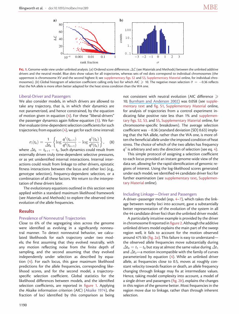
FIG. 1. Genome-wide view under unlinked analysis. (a) Ordered score differences ΔL (see Materials and Methods) between the unlinked additivedrivers and the neutral model. Blue dots show values for all trajectories, whereas sets of red dots correspond to individual chromosomes (theuppermost is chromosome XV and the second highest II; see supplementary figs. S2 and S3, Supplementary Material online, for individual chro-mosomes). (b) Global histogram of selection coefficient calling only loci for which AIC > 10. The negative mean selection σ = −0.36 reflectsthat the NA allele is more often better adapted for the heat stress condition than the WA one.

Liberal-Driver and PassengersWe also consider models, in which drivers are allowed totake any trajectory, that is, in which their dynamics arenot parametrized, and hence constrained, by the equationof motion given in equation (4). For these “liberal-drivers”the passenger dynamics again follow equation (5). We fur-ther evaluate time-dependent selection coefficients for suchtrajectories; from equation (4), we get for each time interval:

σi(tk) =1

Δtk

{

logq1(tk+1)q0(tk+1)

− logq1(tk)q0(tk)

}

, (8)

where Δtk = tk+1 − tk. Such dynamics could result fromexternally driven truly time-dependent selective pressures,or as yet unidentified internal interactions. Internal inter-actions could result from linkage to other drivers, epistaticfitness interactions between the locus and other loci (e.g.,genotype selection), frequency-dependent selection, or acombination of all these factors. We return to the interpre-tation of these drivers later.

The evolutionary equations outlined in this section wereapplied within a standard maximum likelihood framework(see Materials and Methods) to explore the observed timeevolution of the allele frequencies.

ResultsPrevalence of Nonneutral TrajectoriesClose to 6% of the segregating sites across the genomewere identified as evolving in a significantly nonneu-tral manner. To detect nonneutral behavior, we calcu-lated likelihoods for each trajectory under two mod-els; the first assuming that they evolved neutrally, withany motion reflecting noise from the finite depth ofsampling, and the second assuming that they evolvedindependently under selection as described by equa-tion (4). For each locus, this gave maximum likelihoodpredictions for the allele frequencies, corresponding like-lihood scores, and for the second model, a trajectory-specific selection coefficient. Global statistics for thelikelihood differences between models, and the identifiedselection coefficients, are reported in figure 1. Applyingthe Akaike information criterion (AIC) (Akaike 1974), thefraction of loci identified by this comparison as being

not consistent with neutral evolution (AIC difference >10; Burnham and Anderson 2002) was 0.058 (see supple-mentary text and fig. S1, Supplementary Material online,for analysis of trajectories from a control experiment in-dicating false positive rate less than 1% and supplemen-tary figs. S2, S3, and S5, Supplementary Material online, forchromosome-specific breakdown). The average selectioncoefficient was −0.36 (standard deviation [SD] 0.63) imply-ing that the NA allele, rather than the WA one, is more of-ten the beneficial allele under the imposed condition of heatstress. The choice of which of the two alleles has frequencyq1 is arbitrary and sets the direction of selection (see eq. 4).

This simple protocol of assigning a selection coefficientto each locus provided an instant genome-wide view of thedata set, allowing for the rapid identification of genomic re-gions of interest. Using the log-likelihood scores generatedunder each model, we identified 44 candidate driver foci forfurther examination (see supplementary text, Supplemen-tary Material online).

Including Linkage—Driver and PassengersA driver–passenger model (eqs. 4–7), which takes the link-age between nearby loci into account, gave a substantiallybetter representation of the evolution of the system in allthe 44 candidate driver foci than the unlinked driver model.

A particularly intuitive example is provided by the driverin chromosome II reported in figure 2. Although the additiveunlinked drivers model explains the main part of the sweepregion well, it fails to account for the motion observedaround 475 kb (fig. 2a). This failure is easy to understand—the observed allele frequencies move substantially duringΔt0 = t1 − t0 but stay at almost the same value during Δt1

and Δt2—a motion incompatible with the family of curvesparameterized by equation (4). While an unlinked driverallele, at frequencies close to 0.5, moves at roughly con-stant velocity towards fixation or death, an allele frequencychanging through linkage may fix at intermediate values.Hence, taking model complexity into account, a model ofa single driver and passengers (fig. 2b), explains the changesin this region of the genome better. Most frequencies in theregion move due to linkage, rather than through inherentselection.

1190

Quantifying Selection Acting on a Complex Trait Using Allele Frequency Time Series Data ∙ doi:10.1093/molbev/msr289 MBE

FIG. 2. An example of unlinked additive drivers versus driver and pas-sengers models. Allele frequencies in the depicted chromosome IIregion moved substantially during the experiment. (a) Unlinked addi-tive drivers model where every trajectory follows equation (4): Thickdashed lines (t0-red, t1-green, t2-blue, and t3-black) show the data andthe corresponding solid lines the maximum likelihood predictions forthe motion. The blue vertical line denotes the location of the largest σ(for the full selection profile, see supplementary fig. S5, SupplementaryMaterial online). The model explains the motion close to the sweepfocus well; however, it fails qualitatively in the region ∼475 kb. As ex-plained in the text, the motion in that region is not compatible withmodes provided by equation (4). (b) Driver and passengers model asparameterized by equations (4–7). The red vertical line denotes the in-ferred driver location and as can be seen the region ∼475 kb is muchbetter explained than by the unlinked additive drivers model. The dif-ference between the AIC scores was 466 in favor of the driver andpassenger model, the large difference indicating the importance ofincluding linkage between nearby loci in the model. Data shown areaveraged over a sliding window of 5; however, all inferences are donewith the raw data.

Distributions of Selection Coefficients andRecombination RatesWe inferred estimates for driver selection coefficients foreach of the candidate driver foci using the driver and pas-sengers model with linkage parametrized by recombinationrate (fig. 3a). Furthermore, inference in each case gave amaximum likelihood estimate of the local recombinationrate (fig. 3b). The inferred selection coefficient was nega-tive for 29 of the 44 regions (mean σ = −0.2, SD 0.6), re-flecting the advantage conferred by the NA allele. A meanmagnitude of selection of |σ| = 0.44 indicated that thedrivers evolve under substantial selection. The maximumlikelihood estimates for recombination rates (mean ρ =1.6×10−6(bp×gen)−1, SD 1.1×10−6) are consistent with

estimates from the literature (Ruderfer et al. 2006; Manceraet al. 2008).

Liberal-Driver and PassengersIn the majority of cases (38/44 regions), the liberal-drivermodel gave a significantly improved fit to the observationsafter allowing for the additional two degrees of freedom(having three σi values compared with one, see supplemen-tary table S1, Supplementary Material online). In the ex-ample of chromosome II, discussed above, a single driverwith a constant recombination rate appeared to explainthe observed changes in frequencies very well. Nevertheless,the liberal-driver model explained the motion much better(gain of 166 units of log-likelihood, see supplementary fig.S4, Supplementary Material online). However, in chromo-some XIII, the second example in which the identified driver(almost) fixed within the experimental time frame, a gainof only 3 units of score was achieved, favoring the standarddriver and passengers model once degrees of freedom weretaken into account.

Apart from these events, other driver alleles were foundat intermediate frequencies by the end of the experiment.This observation has two possible explanations. First, all can-didate drivers could evolve according to trajectories de-fined by equation (4) but with values of σi too low toobserve fixation during the length of the experiment. Sec-ond, candidate drivers could evolve according to somealternative equations of motion. Application of the liberal-driver model suggested the latter explanation to be correctfor the majority of candidate drivers. While the liberal-drivermodel introduces two additional degrees of freedom, useof this model produced a mean score gain per region of 26(see supplementary table S1, Supplementary Material on-line), more than compensating for the gain in parameters.Figure 4 shows an example within chromosome XV wherethe liberal-driver model gave a substantial improvement.

Averaged across the duration of the experiment, theselection coefficients inferred for the liberal-drivers, ex-pressed as in equation (8), were very similar to thoseshown in figure 3 from the driver and passengers model(mean −0.19 SD 0.68). Estimates of local recombinationrates obtained using liberal-drivers were also very similar(mean 1.5 × 10−6 SD 1.9 × 10−6). To gain an insightto the underlying reason for the liberal drivers’ superiorlog-likelihood scores, we studied the process at the level ofindividual time intervals Δt.

Time-dependent selection coefficients were used toobtain point estimates of fitness flux, φ, a measure of theamount of ongoing adaptation in the system at a given timepoint expressed as φ(tk) =

∑i∈drivers σi(tk)Δq1

i (tk)/Δtk

(Mustonen and Lassig 2007; Mustonen and Lassig 2010).The estimates of fitness flux over the three measured timeintervals differ noticeably between the two models (fig. 5a).Whereas, under the standard-driver model, most adapta-tion takes places in the first time interval, for liberal-drivers,the second time interval dominates. Most interestingly,under the liberal-driver model, the fitness flux almostvanishes for the last time interval, suggesting that by the

1191

Illingworth et al. ∙ doi:10.1093/molbev/msr289 MBE

FIG. 3. Statistics of selection and recombination under the driver and passengers model. (a) Histogram of selection coefficients for the driver foci(mean σ = −0.2 SD 0.6). (b) Histogram of inferred recombinations rates for these regions (mean ρ = 1.6 × 10−6, SD 1.1 × 10−6).

end of the experiment, the system had almost equilibrated.This point is further demonstrated by the distribution ofthe inferred motion of the drivers under both standardand liberal scenarios during the last time interval, shown infigure 5b.

We suggest that the apparent equilibration observedhere should be understood in the sense of separation oftimescales, in that it represents the completion, withinsequencing resolution, of the first phase of adaptation(due to the finite sequencing depth, we would notobserve movement slower than . (read depth)−1/Δt).Given further propagation of the system, deviation fromthis equilibrium would be observed through the arrival ofnew mutations; however, as discussed later, we do not findevidence for these at substantial frequencies within thetime frame of the experiment.

The observation of candidate driver alleles reaching equi-librium at intermediate frequencies suggests the presenceof interactions between drivers in different locations of thegenome. An alternative scenario exists, in which driversdo not interact with one another but instead evolve withgenuinely time-dependent selection coefficients. However,while behavior of this kind might be observed in responseto changes in the external environment, the consistencyof the experimental conditions suggests its occurrencehere to be unlikely, interactions between drivers being themost likely source of the observed allele frequency changes.Different effects leading to interactions between drivers arediscussed later.

New Beneficial MutationsWe contended earlier, based on a simple calculation, that denovo mutations are unlikely to play a substantial role for theallele frequency dynamics during the experiment becausethey would need to carry fitness advantage&3%/ h to be de-tectable during the experiment. However, in the measuredspectrum of fitness effects in figure 3, we observe selectioncoefficients as large as to be ≈2.4%/ h, raising the possibil-ity that novel mutations might have beneficial effects strongenough to have a measurable effect. We thus took furthersteps to rule out this possibility.

As there is no recombination during the selection pro-tocol, any de novo mutation would lead to a global

perturbation of the allele frequency dynamics, one of thetwo alleles at each segregating site being fully linked tothe new mutation. This would lead to a large effect,

FIG. 4. An example of standard-driver versus liberal-driver models. Al-lele frequencies in the depicted chromosome XV region moved sub-stantially during the experiment. Thick dashed lines (t0-red, t1-green,t2-blue, and t3-black) show the data and the corresponding solid linesthe maximum likelihood predictions for the motion; vertical lines de-note the inferred driver location. (a) Driver and passengers model: Themodel explains the motion overall quite well; however, it fails qualita-tively near the sweep focus at 172 kb. The motion, which, as is evidentby the visible overlap between the blue and black dashed lines, seemsto reach equilibrium at an intermediate frequency, is not compatiblewith models provided by equation (4). (b) Liberal-driver and passen-gers model: The trajectories near the focus are much better explainedthan by the standard-driver model. The liberal-driver interpretationgives a gain of 79 units in log-likelihood at a cost of two extra degreesof freedom and is thus strongly supported statistically. Data shown areaveraged over a sliding window of 5; however, all inferences are donewith the raw data.

1192

Quantifying Selection Acting on a Complex Trait Using Allele Frequency Time Series Data ∙ doi:10.1093/molbev/msr289 MBE

FIG. 5. Adaptation under drivers versus liberal-drivers interpretation. (a) Estimates of fitness flux: In the standard-driver interpretation (eqs. 4–7),most adaptation took place during the first time interval, Δt0, whereas liberal-drivers adapt most during Δt1 and have a higher total fitness flux.It is also apparent that while standard-drivers continue to sustain a fitness flux during the last interval Δt2, the flux generated by liberal-drivershas all but vanished. (b) Inferred motion of the drivers (red) and liberal-drivers (green) during the last time interval supports the observation thatunder the liberal-driver interpretation the system has almost reached equilibrium (in the sense discussed in the text).

increasing as a function of time, on the movement ofthe allele frequencies. We thus calculated genome-widestatistics of absolute changes in allele frequency at thethree time intervals (i.e., |q(tk) − q(tk−1)|) from thetrajectories inferred under the unlinked driver model.The statistics showed that the absolute movement of al-lele frequencies slightly decreased throughout the courseof the experiment, with mean values of 0.032, 0.032,0.030, respectively, reflecting our inference that 94% ofallele frequencies evolved in a manner compatible withneutral (no motion) evolution with the remaining 6%evolving as discussed. This decrease suggests that denovo mutations did not significantly affect the allelefrequency dynamics during the time interval reported.

Spatial Uncertainty of Identified DriversLikelihood calculations suggested that, using the (liberal)driver passenger models, the precise location of a drivercould be identified on average to within an accuracy of 12kb. Due to linkage, alleles at nearby loci are likely to move in asimilar manner, leading to uncertainty in the precise choiceof location of a driver locus. This uncertainty was quantifiedby taking the maximum likelihood drivers inferred underthe standard- and liberal-driver models and checking

the next 20 segregating sites both up- and downstream,assigning each in turn to be the driver, reoptimizing theremaining degrees of freedom, and calculating the resultinglikelihoods. Figure 6a shows for standard-drivers that,using a log-likelihood cutoff of three units (95% confidenceinterval), the driver allele can on average be located within awindow of 12 kb centered on the maximum likelihood loca-tion. This means that on average 38 segregating sites remainto be further studied for each driver focus (see supplemen-tary text, Supplementary Material online, for details howthis number of segregating sites was calculated). However,region-specific uncertainty strongly depends on the selec-tive strength of the driver, local recombination rate, andon the allele read numbers from sequencing—variability ofthese factors leads to substantial variance in the accuracyof the inferred driver location (fig. 6a). Nevertheless, forregions with strong drivers, the small number of segre-gating sites to be further studied reflects the efficiency ofrecombination breaking linkage when advanced intercrosslines are used in the experimental design (Darvasi and Soller1995). Comparison of driver locations under each of the twomodels, shown in figure 6b, revealed differences that weremostly within the uncertainty range, with mean absolutedistance ∼2 kb.

FIG. 6. Driver location uncertainty. (a) Inferred sizes of the regions containing loci that when fixed to be the driver are within a distance of 3 unitsof score (95% confidence interval) from the maximum likelihood value (with reoptimization of the remaining degrees of freedom). Data shownare for standard-drivers. Variability in the magnitude of selection and local recombination rates leads to substantial variation in the uncertainty ofthe driver locations. (b) Distances between the maximum likelihood driver locations inferred under the standard-driver and liberal-driver models.For most foci, the two models gave predictions agreeing within variability identified in panel (a).

1193

Illingworth et al. ∙ doi:10.1093/molbev/msr289 MBE

Analysis of a Biological Replicate Experiment andEstimates of False Positive RatesOne great advantage of artificial selection protocols isthe opportunity to analyze biological replicates to gaugerobustness of inferences made. We analyzed data froma biological replicate experiment and show that inferredstatistics of selection replicate well (see supplementary text,Supplementary Material online, for details). However, as thereplicate data set had fewer time-points, and was thus notfully comparable to the one discussed so far, we performedcomputer simulations to estimate false positive rates forthe analyzed 44 driver set. This resulted in an estimatedfalse positive rate for our driver region detection to be lessthan ∼2% for populations of size 107. In these simulations,we chose the number of segregating sites, number of driversand their estimated selection strengths, and recombinationrates to mimic the ones found from the experimental data(see supplementary text, Supplementary Material online,for details).

The 44 regions called in our analysis as containing driverloci are significantly larger than the more conservative 21 (allthese regions are in our list) obtained by Parts et al. (2011),who, for example, only call QTLs observed in both the pri-mary and the replica data sets. The existence of a highernumber of regions under selection than previously re-ported is supported by the false positive rate identified fromsimulated data.

DiscussionQuantifying Selection from Time-Resolved AlleleFrequenciesWe performed the first, single nucleotide resolution,genome-wide population genetic analysis of time seriesallele frequency data from an evolving outbred popula-tion under selection. The analysis revealed several insightsinto the dynamics of the population at the molecular level.First, we estimated that close to 6% of the over 30,000segregating sites are affected by the selection pressure asidentified via deviation from a neutral null model. Sec-ond, we demonstrated the main force causing this motionto be genetic linkage, which causes passenger alleles tohitchhike with driver alleles. Third, using a driver andpassenger model, we quantified the selective advantageof the found drivers, the amount of linkage disequilib-rium within the regions that they reside, and the uncer-tainty in their locations. The method we describe offersa first-order approach to examining selection in such anexperiment.

Extending the above, by allowing driver alleles to evolvearbitrarily, we found substantial statistical evidence offitness effects going beyond those compatible with stan-dard additive models of selection, such that many of thedriver alleles evolve under an effectively time-dependent fit-ness seascape (Mustonen and Lassig 2009). We next discusspossible scenarios underlying the observed liberal-driverdynamics.

Linkage Pattern in the Initial PoolOne explanation for the inferred liberal-drivers (or in-deed the standard drivers) signal would be the existenceof linkage disequilibrium between candidate drivers. Suchlinkage could result from stochastic effects during thecrossing, arising due to the finite population size, a sce-nario which equation (7) would not capture. Numeri-cal simulations (reported in supplementary text, Supple-mentary Material online) showed that population sizesfrom ∼106 upwards are sufficient to rule out distortionto the global selection statistics arising from such noise,on the assumption that the numbers of segregating sitesand drivers, driver selection strengths, and recombina-tion rates are close to those inferred from the real data.Furthermore, analysis of data from a biological replicategave overall statistics of selection consistent with thoseinferred, supporting the conclusion that drift-generatedlinkage disequilibrium is not causing the signal (see sup-plementary text, Supplementary Material online, for moredetails).

From our simulations, we do note, however, that a largenumber of false positives would be generated due to drift-generated linkage in population of size 105. Therefore, insmaller populations, our method should be applied onlyfor identifying the largest fitness effects to avoid beingswamped by false positives (which would reflect mistakenmeasurements of selection rather than any underlying fit-ness land- or seascape) or in combination with full sequencedata from the initial pool to fix the linkage. The populationsize required to correctly decide whether a marker moveddue to linkage to a nearby selective sweep or just due to drifthas been calculated (Logeswaran and Barton 2011).

Another possible reason for a nontrivial linkage patternin the initial pool could come from unknown selection pres-sures during the crossing protocol. Given that such selectioncould in principle be arbitrarily complex, our analyses of thedata here remain to some extend vulnerable to this. How-ever, there is no statistical evidence for interchromosomalpairwise linkages between genotype data of 19 QTL loci (allpart of our candidate driver foci list) from 960 individualsat time point (t2 + t3)/2 as reported in Parts et al. (2011).Therefore, worst-case scenarios where all but one of thecandidate drivers were linked to, and thus would merelyhitchhike with, one of the two nearly fixing drivers are notsupported by the data. Similarly to nonlocal linkage dise-quilibrium generated by small populations, possible effectsof selection during the crossing to allele dynamics underthe artificial selection phase could be easily included to thepresent method given suitable data. Extending the methodto cover simultaneous recombination and selection is pos-sible but remains a topic for further investigation.

Clonal InterferenceIn asexually evolving populations, recombination cannotcombine beneficial mutations that are on different haplo-types. This leads to so-called clonal interference where somebeneficial mutations will be removed from the populationdue to them being interfered with stronger ones in different

1194

Quantifying Selection Acting on a Complex Trait Using Allele Frequency Time Series Data ∙ doi:10.1093/molbev/msr289 MBE

backgrounds (Fisher 1930; Muller 1932). The dynamics ofclonal interference are complex and both its experimentaland its theoretical study has long been an active researchtopic (for recent reviews see Park et al. 2010; Sniegowski andGerrish 2010).

For the results presented here, the large number ofdrivers make it unlikely to have a large number (or indeedany) individuals with all the beneficial alleles in a populationof size∼107–108, so that such interference seems inevitable.However, simulation and sequencing data both suggest thatclonal interference does not account for the liberal-driversignal observed here.

Analyzing simulated data with the number of drivers (ad-ditive in fitness) and their strengths comparable to thoseinferred from the real experiment, we concluded that theobserved liberal-driver dynamics does not reflect effectsprimarily caused by clonal interference. We reached thisconclusion by analyzing the simulated data under bothstandard and liberal-driver models (see supplementary text,Supplementary Material online). With both models, wewere able to discover the “true” driver set and reproduce thecorrect selection strengths for the drivers. However, usinga liberal-driver model to infer selection from the simulateddata, we did not see the decrease in fitness flux observedfor the real system (contrast fig. 5 and supplementary fig.S14, Supplementary Material online). For this reason, we be-lieve that clonal interference is not the primary explanationfor the stronger performance of the liberal-driver model formost candidate driver regions in the real data. Supportingthis conclusion, genotyping data of 24 loci from 960 indi-viduals from time point (t2 + t3)/2 showed that no sin-gle genotype (clone) dominated the population at that time(maximum count observed was 6), a considerable diversityof 787 unique haplotypes being detected and the data be-ing consistent with the expectation under a hypothesis ofindependent sites (Parts et al. 2011).

Given the absence of recombination, it is inevitable thatclonal interference would, after sufficient time had passed,have a significant influence on the evolution of driver al-lele frequencies. However, given additive drivers of thesize and number that we find from the real system, thatpoint would not have been reached by the end of theexperiment.

Clonal interference between (possible) multiple benefi-cial alleles within a driver focus remains a possibility butwould not stop the dominant combination of these mu-tations from fixing and as such is not consistent withthe liberal-driver signal. Extension of the method to covermultiple drivers will be required to study such effects and isbeyond the scope of this manuscript.

Epistasis and Other More Complex Selective ScenariosGiven that linkage or clonal interference between driverfoci do not satisfactorily explain the observed dynamics, webelieve that the liberal-driver signal is likely to be causedby fitness effects going beyond additive models of selec-tion. For instance, one such complex selection scenariocould be that of epistatic interactions between drivers

(Weinreich et al. 2005), encompassing combinations of pairsor potentially multiple drivers, while the possibility of gen-uinely time-dependent or frequency-dependent selectioncannot be definitively ruled out. Models could be developedto examine the likelihood of each of these potential scenar-ios. However, inference of a correct model based on the dataavailable presents a substantial challenge, such that the pre-cise nature of the observed time dependency remains to beshown.

Comparable Events at Macroevolutionary TimescalesThe adaptive dynamics studied here consisted of driver al-leles at loci under strong selection for heat resistance andneutral passengers alleles linked to the drivers. As can beseen in the frequency profiles in figures 2 and 4 and sup-plementary fig. S5, Supplementary Material online, genomicregions around the drivers have substantially reduced al-lelic variance. The experiment and the observed dynamicstook place over timescale of days. Nevertheless, a similarpattern of the hitchhiking effect has been described theo-retically (Kim and Stephan 2002) and found, among others,in the case of Drosophila, where individual selective sweepsin the recent past leave remnant genomic valleys of reducedvariability (Svetec et al. 2009; Macpherson et al. 2007). How-ever, while in the case of selective sweeps, variability is re-moved completely from the genomic locality, in many of thecases studied here, a substantial degree of variance remainsin the immediate vicinity of the sweep locus after the adap-tive event: The genomic signature resembles that of a softsweep (Hermisson and Pennings 2005), where the beneficialdriver allele is initially linked to many different backgroundgenotypes.

From Driver Locations to BiologyIn the data considered here, the average spatial resolutionwhich can be attained in identifying driver locations is about12 kb (see fig. 6). As such, identification of individual variantsresponsible for the inferred fitness advantages would re-quire further experimental or bioinformatic analysis, suchdownstream analysis being very important in terms of thebiological insight that can be collected from this data. Anal-ysis of some of the large events observed in the data has beencarried out in earlier work (Parts et al. 2011), showing themto be biologically interesting with respect to heat tolerance.While mapping the precise locations of the drivers are im-portant for the biology of the trait in question, we note thatinference of selection as was done here is not sensitive inthis respect and thus, the resulting estimates for selectionare robust.

ConclusionsOur analysis here has been of time-resolved allele frequencydata from a yeast population under heat stress. However,the method presented has potential application to a rangeof organisms under a variety of selection pressures. Sev-eral conditions were necessary for our analysis to be sensi-ble: efficient recombination during the crossing to break uplinkage and create variation, a large population size and high

1195

Illingworth et al. ∙ doi:10.1093/molbev/msr289 MBE

initial allele frequencies to reduce the effect of genetic driftand clonal interference, the duration of the experiment,which does not allow de novo mutations to start interfering,and finally, the application of strong selection. The methodcan be extended to sexually propagated populations by con-sidering selection and recombination simultaneously, and insuch a setting, the key conditions enumerated above will be-come somewhat more lenient.

The focus on quantifying selection and utilizing multi-ple consecutive time points distinguishes our method froma standard QTL mapping design, although such a mappingwould be a natural biological application. We see the com-bination of the experiment with multiple time points andthe approach presented here as a model for the quantita-tive study of the fitness effects of mutations and their pos-sible interactions. Time resolution is key to our analyses; ifdata had been collected only from the initial and final pool,we would not have been able to show that majority of thedrivers are not compatible with a standard model of addi-tive selection. Under the framework of experiment and dataanalysis described here, alterations to study other variableswould be possible; for example, the effect of drift could beexamined through modulating the population size.

With the imminent arrival of deep population samples oftime-resolved full genome sequences from evolution exper-iments, the possibility emerges of scaling up our measure-ments of the fitness effects of mutations to include complexmultilocus interactions. Application of population genetictheory will be central to making the best possible use of suchdata.

Supplementary MaterialSupplementary text, figs. S1–S14, and table S1 are availableat Molecular Biology and Evolution online (http://www.mbe.oxfordjournals.org/).

AcknowledgmentsWe would like to thank the anonymous referees for helpfulcomments. C.J.R.I. and V.M. would like to acknowledge theWellcome Trust for support under grant reference 098051.L.P. was supported by the Wellcome Trust (grant numberWT077192/Z/05/Z). G.L. was supported by CNRS and ATIP-AVENIR. This research was also supported in part by theNational Science Foundation under Grant No. NSF PHY05-51164 during a visit (C.J.R.I., S.S., and V.M.) at the KavliInstitute of Theoretical Physics (KITP, Santa Barbara, CA).We would like to thank Richard Durbin and participantsof the KITP program on Microbial and Viral Evolution fordiscussions.

ReferencesAkaike H. 1974. A new look at the statistical model identification. IEEE

Trans Automat Contr. 19:716–723.Barrick JE, Yu DS, Yoon SH, Jeong H, Oh TK, Schneider D, Lenski RE,

Kim JF. 2009. Genome evolution and adaptation in a long-termexperiment with Escherichia coli. Nature 461:1243–1247.

Barton NH. 2000. Genetic hitchhiking. Philos Trans R Soc Lond B BiolSci. 355:1553–1562.

Bell G, Gonzalez A. 2011. Adaptation and evolutionary rescuein metapopulations experiencing environmental deterioration.Science 332:1327–1330.

Burke MK, Dunham JP, Shahrestani P, Thornton KR, Rose MR, LongAD. 2010. Genome-wide analysis of a long-term evolution experi-ment with drosophila. Nature 467:587–590.

Burnham KP, Anderson DR. 2002. Model selection and multimodel in-ference: a practical information-theoretic approach. 2nd ed. NewYork: Springer.

Culleton R, Martinelli A, Hunt P, Carter R. 2005. Linkage group se-lection: rapid gene discovery in malaria parasites. Genome Res.15:92–97.

Darvasi A, Soller M. 1995. Advanced intercross lines, an exper-imental population for fine genetic mapping. Genetics 141:1199–1207.

Drake JW, Charlesworth B, Charlesworth D, Crow JF. 1998. Rates ofspontaneous mutation. Genetics 148:1667–1686.

Ehrenreich IM, Torabi N, Jia Y, Kent J, Martis S, Shapiro JA, GreshamD, Caudy AA, Kruglyak L. 2010. Dissection of genetically com-plex traits with extremely large pools of yeast segregants. Nature464:1039–1042.

Eyre-Walker A. 2006. The genomic rate of adaptive evolution. TrendsEcol Evol. 21:569–575.

Eyre-Walker A. Keightley PD. 2007. The distribution of fitness effectsof new mutations. Nat Rev Genet. 8:610–618.

Fisher RA. 1930. The genetical theory of natural selection. Oxford:Clarendon Press.

Hartl D, Clark A. 2007. Principles of population genetics. Sunderland(MA): Sinauer.

Hermisson J, Pennings PS. 2005. Soft sweeps: molecular populationgenetics of adaptation from standing genetic variation. Genetics169:2335–2352.

Hietpas RT, Jensen JD, Bolon DNA. 2011. Experimental illumination ofa fitness landscape. Proc Natl Acad Sci U S A. 108:7896–7901.

Kao KC, Sherlock G. 2008. Molecular characterization of clonal inter-ference during adaptive evolution in asexual populations of Sac-charomyces cerevisiae. Nat Genet. 40:1499–1504.

Kim Y, Stephan W. 2002. Detecting a local signature of genetic hitch-hiking along a recombining chromosome. Genetics 160:765–777.

Kimura M. 1964. Diffusion models in population genetics. J ApplProbab. 1:177–232.

Kishimoto T, Iijima L, Tatsumi M, et al. (14 co-authors). (2010). Transi-tion from positive to neutral in mutation fixation along with con-tinuing rising fitness in thermal adaptive evolution. PLoS Genet.6:e1001164.

Lang GI, Murray AW. 2008. Estimating the per-base-pair mutation ratein the yeast Saccharomyces cerevisiae. Genetics 178:67–82.

Logeswaran S, Barton NH. 2011. Mapping Mendelian traits in asex-ual progeny using changes in marker allele frequency. Genet Res.93:221–232.

Lynch M, Sung W, Morris K, et al. (11 co-authors). 2008. A genome-wide view of the spectrum of spontaneous mutations in yeast. ProcNatl Acad Sci U S A. 105:9272–9277.

Macpherson JM, Sella G, Davis JC, Petrov DA. 2007. Genomewidespatial correspondence between nonsynonymous divergence andneutral polymorphism reveals extensive adaptation in Drosophila.Genetics 177:2083–2099.

Mancera E, Bourgon R, Brozzi A, Huber W, Steinmetz LM. 2008. High-resolution mapping of meiotic crossovers and non-crossovers inyeast. Nature 454:479–485.

Muller HJ. 1932. Some genetic aspects of sex. Am Nat. 66:118–138.Mustonen V, Lassig M. 2007. Adaptations to fluctuating selection in

drosophila. Proc Natl Acad Sci U S A. 104:2277–2282.Mustonen V, Lassig M. 2009. From fitness landscapes to seascapes:

non-equilibrium dynamics of selection and adaptation. TrendsGenet. 25:111–119.

1196

Quantifying Selection Acting on a Complex Trait Using Allele Frequency Time Series Data ∙ doi:10.1093/molbev/msr289 MBE

Mustonen V, Lassig M. 2010. Fitness flux and ubiquity of adaptive evo-lution. Proc Natl Acad Sci U S A. 107:4248–4253.

Neher RA, Shraiman BI. 2009. Competition between recombinationand epistasis can cause a transition from allele to genotype selec-tion. Proc Natl Acad Sci U S A. 106:6866–6871.

Park SC, Simon D, Krug J. 2010. The speed of evolution in large asexualpopulations. J Stat Phys. 138:381–410.

Parts L, Cubillos FA, Warringer J, et al. (14 co-authors). 2011. Revealingthe genetic structure of a trait by sequencing a population underselection. Genome Res. 21:1131–1138.

Perfeito L, Fernandes L, Mota C, Gordo I. 2007. Adaptive mutations inbacteria: high rate and small effects. Science 317:813–815.

Ruderfer DM, Pratt SC, Seidel HS, Kruglyak L. 2006. Population ge-nomic analysis of outcrossing and recombination in yeast. NatGenet. 38:1077–1081.

Sawyer SA, Kulathinal RJ, Bustamante CD, Hartl DL. 2003. Bayesiananalysis suggests that most amino acid replacements inDrosophila are driven by positive selection. J Mol Evol. 57(Suppl 1):S154–S164.

Segre AV, Murray AW, Leu J-Y. 2006. High-resolution mutation map-ping reveals parallel experimental evolution in yeast. PLoS Biol.4:e256.

Sella G, Petrov DA, Przeworski M, Andolfatto P. 2009. Perva-sive natural selection in the Drosophila genome? PLoS Genet.5:e1000495.

Smith JM, Haigh J. 1974. The hitch-hiking effect of a favourable gene.Genet Res. 23:23–35.

Sniegowski PD, Gerrish PJ. 2010. Beneficial mutations and the dynam-ics of adaptation in asexual populations. Philos Trans R Soc Lond BBiol Sci. 365:1255–1263.

Svetec N, Pavlidis P, Stephan W. 2009. Recent strong positive selec-tion on Drosophila melanogaster HDAC6, a gene encoding a stresssurveillance factor, as revealed by population genomic analysis.Mol Biol Evol. 26:1549–1556.

Weigand MR, Sundin GW. 2009. Long-term effects of induciblemutagenic DNA repair on relative fitness and phenotypic di-versification in Pseudomonas cichorii 302959. Genetics 181:199–208.

Weinreich D, Watson R, Chao L. 2005. Perspective: sign epistasisand genetic constraint on evolutionary trajectories. Evolution 59:1165–1174.

Woods RJ, Barrick JE, Cooper TF, Shrestha U, Kauth MR, Lenski RE.2011. Second-order selection for evolvability in a large escherichiacoli population. Science 331:1433–1436.

1197