arX

iv:1

402.

2905

v4 [

stat

.ME

] 7

Dec

201

4

Multiple Quantitative Trait Analysis Using Bayesian Networks

A “Methods, Technology, and Resources” Article submitted to Genetics

Marco Scutari∗, Phil Howell†, David J. Balding∗, Ian Mackay†

December 9, 2014

∗Genetics Institute, University College London (UCL), United Kingdom

†National Institute of Agricultural Botany (NIAB), Cambridge, United Kingdom

1

Running Head: Multiple Trait Analysis With BNs

Key Words: Multiple Traits, Quantitative Traits, Bayesian Networks, Genome-Wide Predic-

tions.

Corresponding Author:

Marco Scutari

UCL Genetics Institute (UGI)

University College London

Gower Street

London WC1E 6BT

United Kingdom

tel.: +44(0)2067692212

email: m.scutari@ucl.ac.uk

2

Abstract

Models for genome-wide prediction and association studies usually target a single phe-

notypic trait. However, in animal and plant genetics it is common to record information on

multiple phenotypes for each individual that will be genotyped. Modeling traits individually

disregards the fact that they are most likely associated due to pleiotropy and shared biolog-

ical basis, thus providing only a partial, confounded view of genetic effects and phenotypic

interactions. In this paper we use data from a Multiparent Advanced Generation Inter-Cross

(MAGIC) winter wheat population to explore Bayesian networks as a convenient and inter-

pretable framework for the simultaneous modeling of multiple quantitative traits. We show

that they are equivalent to multivariate genetic best linear unbiased prediction (GBLUP),

and that they are competitive with single-trait elastic net and single-trait GBLUP in pre-

dictive performance. Finally, we discuss their relationship with other additive-effects models

and their advantages in inference and interpretation. MAGIC populations provide an ideal

setting for this kind of investigation because the very low population structure and large

sample size result in predictive models with good power and limited confounding due to

relatedness.

3

INTRODUCTION

Understanding the behavior of complex traits involves modeling a web of interactions among

the effects of genes, environmental conditions and other covariates. Ignoring one or more of

these factors may substantially impact the accuracy and the generality of the conclusions

that can be drawn from the model (Hartley et al., 2012; Alimi et al., 2013; Li et al.,

2006), both in the context of genome-wide association studies (GWAS) and genomic se-

lection (GS). Indeed a lot of attention has been devoted in recent literature to improving

traditional additive genetic models, which were originally defined using only allele counts

(e.g. Meuwissen et al., 2001), by supplementing them with additional information. Some

examples include marker-based kinship coefficients (Speed et al., 2012), spatial heterogene-

ity and dominance (Finley et al., 2009), and gene expression data (Druka et al., 2008).

However, most studies in plant and animal genetics still focus on a single phenotypic trait

at a time despite the availability of a set of simultaneously measured traits for each genotyped

individual. Models for analyzing multiple traits have been available sinceHenderson and Quaas

(1976) introduced the multivariate extension of the genetic best linear unbiased prediction

(GBLUP) models, and have been investigated as recently as Stephens (2013) in the context

of GWAS. More recent additions include structural equation models (SEM; Li et al., 2006),

a Bayesian extension of seemingly unrelated regression (SUR; Banerjee et al., 2008), the

MultiPhen ordinal regression (O’Reilly et al., 2012) and spatial models (Banerjee et al.,

2012).

In this paper we will use Bayesian networks (BNs;Pearl, 1988;Koller and Friedman,

2009) to build a multivariate dependency model that accounts for simultaneous associa-

tions and interactions among multiple single nucleotide polymorphisms (SNPs) and pheno-

typic traits. BNs have been applied to the analysis of several kinds of genomic data such

as gene expression (Friedman, 2004), protein-protein interactions (Jansen et al., 2003;

Sachs et al., 2005), pedigree analysis (Lauritzen and Sheehan, 2004) and the integra-

tion of heterogeneous genetic data (Chang and McGeachie, 2011). Their modular nature

4

makes them ideal for analyzing large marker profiles. As far as SNPs are concerned, BNs have

been used to investigate linkage disequilibrium (LD; Morota et al., 2012; Mourad et al.,

2011) and epistasis (Han et al., 2012), and to determine disease susceptibility for anemia

(Sebastiani et al., 2005), leukemia (Chang and McGeachie, 2011), and hypertension

(Malovini et al., 2009). The same BN can simultaneously highlight SNPs potentially in-

volved in determining a trait (e.g. for association purposes) and be used for prediction (e.g.

for selection purposes): a network capturing the relationship between genotypes and pheno-

types can be used to compute the probability that a new individual with a particular genotype

will have the phenotype of interest (Lauritzen and Sheehan, 2004; Cowell et al., 2007).

MATERIALS AND METHODS

A Bayesian network (BN) is a probabilistic model in which a directed acyclic graph G is

used to define the stochastic dependencies quantified by a probability distribution (Pearl,

1988; Koller and Friedman, 2009). The variables X = Xi under investigation in this

context include T traits Xt1 , . . . , XtT and S SNPs Xs1, . . . , XsS , each of which is associated

with a node in G. The arcs between the nodes represent direct stochastic dependencies, and

determine how the global distribution of X decomposes into a set of local distributions,

P(X) =∏

P(Xi |ΠXi); (1)

one for each variable Xi, depending only on its parents ΠXi. This modular representation

can capture direct and indirect associations between SNPs and phenotypes; and associations

between SNPs due to linkage and population structure.

In the spirit of commonly used additive genetic models for quantitative traits (e.g.

Meuwissen et al., 2001), we make some further assumptions on the BN:

1. each variable Xi is normally distributed, and X is multivariate normal;

2. stochastic dependencies are assumed to be linear;

5

3. traits can depend on SNPs (i.e. Xsi → Xtj ) but not vice versa (i.e. not Xtj → Xsi),

and they can depend on other traits (i.e. Xti → Xtj , i 6= j);

4. SNPs can depend on other SNPs (i.e. Xsi → Xsj , i 6= j).

We also assume that dependencies between traits broadly follow the temporal order in which

they are measured; for instance, traits that are measured when a plant variety is harvested

can depend on those that are measured while it is still in the field (and obviously on the

markers as well), but not vice versa. In other words, Assumptions 3 and 4 define BNs

that describe the dependencies of phenotypes on genotypes in a prognostic model, as op-

posed to a diagnostic model in which genotypes depend on phenotypes. The latter is often

preferred over the former because it results in simpler models when the Xi are discrete

(Sebastiani and Perls, 2008); in that setting, the number of parameters grows exponen-

tially with the number of parents of each node. However, this is not the case here due to

Assumptions 1 and 2. Under these assumptions, the local distribution P(Xti |ΠXti) of each

trait is a linear model of the form

Xti = µti+ΠXti

βti+ εti (2)

= µti+Xtjβtj + . . .+Xtkβtk︸ ︷︷ ︸

traits

+Xslβsl + . . .+Xsmβsm︸ ︷︷ ︸

SNPs

+ εti , εti ∼ N(0, σ2

tiI)

where I is the identity matrix. SNPs will typically be coded using their allele counts (0, 1, 2),

although extensions to multiallelic SNPs and to account for dominance are trivial. Similarly,

the local distribution P(Xsi |ΠXsi) of each SNP is

Xsi = µsi+Xslβsl + . . .+Xsmβsm︸ ︷︷ ︸

SNPs

+ εsi, εsi ∼ N(0, σ2

siI). (3)

Therefore, each parent only adds one parameter to a local distribution.

The regression parameters in (2) and (3) can be estimated in different ways. When

G is sparse, ordinary least squares (OLS) are often used because each local distribution

is estimated independently and contains few regressors. Otherwise, penalized estimators

6

such as ridge regression (RR; Hoerl and Kennard, 1970) can be used when G is dense.

The resulting BN can then be considered a flexible implementation of multivariate ridge

regression, which has a number of of desirable properties over OLS (Brown and Zidek,

1980).

Equivalently, we can describe a BN using its global distribution, denoted with P(X) in

(1). Following Assumption 1, X has a multivariate normal distribution, say X ∼ N(µ,Σ).

In addition, by definition graphical separation of two nodes Xi and Xj in G implies the

conditional independence of the corresponding variables given the rest. As a result, some

elements of the precision matrix Ω = Σ−1 will be equal to zero and some will be strictly

positive according to the structure of G. The link with the parameterisation based on the

local distributions arises from the fact that in each P(Xi |ΠXi) the regression coefficient

associated with Xj will be βj = −Ωij/Ωii; so βj = 0 if and only if the (i, j) element of Ω is

itself equal to zero (Cox and Wermuth, 1996, pp. 68–69).

It is interesting to note that this formulation defines BNs that are equivalent to multivari-

ate GBLUP models (Henderson and Quaas, 1976). For simplicity of notation, assume we

are modeling only two traits Xt1 and Xt2 with a common set of SNP genotypes XS. In this

case a multivariate GBLUP model has the form

Xt1

Xt2

=

µt1

µt2

+

ZS O

O ZS

ut1

ut2

+

εt1

εt2

(4)

where ut1 ,ut2 are the random effects for the two traits; ZS is the design matrix of the

genotypes XS; µt1,µt2

are the population means; and εt1 , εt2 are the error terms. ut1 ,ut2

and εt1 , εt2 are independent of each other and distributed as multivariate normals with zero

mean and covariance matrices

COV

ut1

ut2

=

Gt1t1 Gt1t2

GTt1t2

Gt2t2

and COV

εt1

εt2

=

σ2

t1I σ2

t1t2I

σ2

t2t1I σ2

t2I

. (5)

The covariance matrix Gt1t2 models the pleiotropic effects of the SNPs on traits, potentially

increasing the accuracy of multivariate GBLUP compared to a single-trait model.

7

As was the case in (2), each traitXti , i = 1, 2 has a population mean µtiand an error term

εti that is normally distributed and independent of the SNP effects. The residual variance

σ2

tiis also specific to each trait. The two traits depend directly on each other because of

the covariances σ2

t1t2, σ2

t2t1; and indirectly through the covariance structure of the SNP effects

Gt1t2 . If we denote COV([ut1ut2 ]T ) as G and COV([εt1εt2 ]

T ) as R, we can write

Σ = COV

Xt1

Xt2

ut1

ut2

=

ZSGZTS+R ZSG

(ZSG)T G

(6)

which is the covariance matrix of the global distribution. The structure of the BN defined

over X = Xt1 , Xt2 ,ut1 ,ut2 and corresponding to the multivariate GBLUP in (4) arises from

Ω = Σ−1 as discussed above. Finally, it is important to note that even though GBLUP does

not model the SNP effects using the allele counts directly as in (2) and (3), when Gt1,t1 and

Gt2,t2 have the form XSXST the linear dependence on ZSuti can be equivalently expressed as

a random regression in the allele counts (Piepho, 2009; Piepho et al., 2012). The form of

Gt1,t1 ,Gt2,t2 determines how the allele counts are scaled or weighted in the regression. This

formulation of GBLUP results in a more natural interpretation of SNP effects, which is in

fact analogous to the interpretation they are given in a BN (Scutari et al., 2013).

Another interesting property of the BN defined above is that the covariance matrix of

the SNP genotypes, which is a submatrix ΣSS of Σ (the global covariance matrix), is used in

computing Ω and determines which arcs are present in G between the SNPs. Furthermore,

ΣSS encodes the LD patterns between the SNPs as measured by the squared allelic correlation

r2. This has been shown to be useful in exploring complex LD patterns in an inbred Holstein

cattle population, albeit with a discrete BN (Morota et al., 2012) and measuring LD in a

way that is closer to D and D′ (Falconer and Mackay, 1995). Such patterns are reflected

in the BN through Ω, providing an intuitive representation of LD as well as of genetic effects

on phenotypes as a single, coherent whole.

8

BNs present two other advantages over classic multivariate regression models such as

multivariate GBLUP and ridge regression. Firstly, there is a vast literature on performing

causal modeling with BNs from both experimental and observational data (Pearl, 2009).

Given the lack of a formal distinction between response and explanatory variables in BNs,

the same algorithms can be used for inference on the traits based on the genotypes and vice

versa. The former includes the estimation of phenotypic EBVs, which is the basis of genomic

selection; the latter can be used for association mapping in polygenic traits and when the

desired phenotype is a combination of conditions on several traits. Secondly, the fundamental

properties of BNs do not depend on the distributional assumptions of the data. Therefore,

accommodating heterogeneous traits (discrete, ordinal and continuous) in the model only

requires to specify the form of the local distributions.

Estimating a BN from data is typically performed as a two-step process. The first step

consists in finding the graph G that encodes the conditional independencies present in the

data, and is called structure learning. This can be achieved using conditional independence

tests (constraint-based learning), goodness-of-fit scores (score-based learning) or both (hybrid

learning) to identify statistically significant arcs. The second step is called parameter learning

and deals with the estimation of the parameters of the local distributions; G is known from

the previous step and defines which variables are included in each one. In addition, we

propose to use structure learning to retain in the BN only those SNPs that are required

to make inference on the traits and that make the remaining SNPs redundant. For each

trait, such a subset is called the Markov blanket (B(Xti); Pearl, 1988), and includes the

parents, the children and the other nodes that share a child with the trait. Therefore, we can

disregard all the SNPs that are not part of any such Markov blanket and reduce drastically

the dimension of the model. We have shown in previous work (Scutari et al., 2013) how

Markov blankets are effective when used in this setting.

From these considerations, we used the R packages bnlearn (Scutari, 2010) and pe-

nalized (Goeman, 2012) to implement the following hybrid approach to BN learning.

9

1. Structure Learning.

(a) For each trait Xti , use the SI-HITON-PC algorithm (Aliferis et al., 2010) to

learn the parents and the children of the trait; this is sufficient to identify B(Xti)

because the only nodes that can share a child with Xti are other traits or SNPs

that are parents of other traits due to Assumption 3. The choice of SI-HITON-

PC is motivated by its similarity to single-SNP analysis, which is improved on

with a subsequent backward selection to remove false positives. Dependencies are

assessed with Student’s t-test for Pearson’s correlation (Hotelling, 1953) and

α = 0.01, 0.05, 0.10.

(b) Drop all the markers which are not in any B(Xti).

(c) Learn the structure of the BN from the nodes selected in the previous step, setting

the directions of the arcs according to the Assumptions 3 and 4. We identify the

optimal structure as that which maximizes the Bayesian information criterion

(BIC; Schwarz, 1978).

2. Parameter Learning. Learn the parameters of the local distributions using OLS and

RR.

For comparison, we also fitted an elastic net (ENET) model (Zou and Hastie, 2005)

and a univariate GBLUP individually on each trait and on all the available SNPs using

the glmnet (Friedman et al., 2010) and synbreed (Wimmer et al., 2012) R packages.

Since we have shown BNs to be equivalent to a multivariate GBLUP, we did not fit the

latter as a separate model. We investigated the properties of the resulting models using, in

each case, 10 runs of 10-fold cross-validation. Predictive power was assessed by averaging

the cross-validated correlations arising from the 10 runs and computing confidence intervals

as in Hooper (1958). In the case of BNs, predictions in the cross-validation folds were

performed jointly on all traits, and in two different ways: by conditioning only on the SNPs

10

in the BN, to provide a measure of genetic predictive ability (ρG) and a fair comparison with

single-trait models; and by conditioning on the parents of each trait, which may in turn be

traits themselves, to provide a tentative measure of causal predictive ability (ρC).

In order to perform inference, we produced an averaged BN using the 100 networks we

obtained in the course of cross-validation. First, we created an averaged network structure

using their graphs as in Scutari and Nagarajan (2013): we kept only those arcs that

appear with a frequency higher than a threshold estimated from the graphs themselves.

SNPs which ended up as isolated nodes (i.e. they were not connected to any other SNP

or trait) were dropped. We then estimated the parameters of the averaged BN with RR

using the whole data set. We used the resulting BN to generate samples of 106 random

observations from the conditional distributions of various traits and SNPs with either logic

sampling or likelihood weighting (Koller and Friedman, 2009), in order to explore their

properties and interplay under different conditions. Statistics estimated from such a big

sample are very precise and can capture even small differences reliably.

We based our analysis on a winter wheat population produced by the UK National

Institute of Agricultural Botany (NIAB) comprising 15877 SNPs for 720 genotypes. Seven

traits were measured: yield (YLD; t/ha), flowering time (FT; 6 − 54, aggregate of 5 scores

taken at 3-7 day intervals), height (HT; cm), yellow rust in the glasshouse (YR.GLASS;

1− 9) and in the field (YR.FIELD; 1− 9), fusarium (FUS; 1− 9) and mildew (MIL; 1− 9).

Disease scores from 1 to 9 reflect increasing level of infection, and flowering time scores from

6 to 54 increasing lateness in flowering. The population was created using a Multiparent

Advanced Generation Inter-Cross (MAGIC) scheme. Such a scheme is designed to produce a

mapping population from several generations of intercrossing among 8 founders, and has the

potential to improve quantitative trait loci (QTL) mapping precision (for more details see

Mackay et al., 2014). The use of multiple founder varieties results in a population which

is segregating for more QTLs and traits than a biparental population; and the balanced

crossing used in each generation reduces LD and family structure by ensuring each founder

11

has an equal opportunity to contribute to each genotype.

SNPs were preprocessed by removing those with minor allele frequencies < 1% and

those with > 20% missing data. Missing data in the remaining SNPs were imputed using

the impute R package (Hastie et al., 2013). Other widely used imputation methods in

genetics, such as that implemented in MaCH (Li et al., 2010), could not be used because of

the lack of precise mapping information at the time of the analysis; a 90K consensus map has

just been submitted for publication (Wang et al., 2014). Subsequently, we removed one SNP

from each pair whose allele counts have correlation > 0.95 to increase the numerical stability

of the models. In the end, 3164 SNPs were left for analysis. Phenotypes were adjusted

for kinship using a univariate BLUP model for each trait based on pedigree information,

thus accounting for population structure. Individuals with missing pedigree information or

phenotypes were dropped from the analysis, leaving 600 individuals with complete records.

RESULTS

Table 1 shows genetic predictive correlations (ρG) and causal predictive correlations (ρC)

for single-trait ENET, single-trait GBLUP and BNs fitted with α = 0.01, 0.05, 0.10. Only

the results for BNs whose parameters are estimated with RR are reported, because using

OLS provides essentially the same performance. The average ρG obtained with RR across

all traits is 0.324 for α = 0.01, 0.327 for α = 0.05 and 0.331 for α = 0.10, all with a standard

deviation of ±0.004; with OLS we obtain 0.322 for α = 0.01, 0.325 for α = 0.05 and 0.324

for α = 0.10, again with a standard deviation of ±0.004. Similar considerations can be made

for ρC .

First of all, we note that BNs and single-trait ENET have comparable predictive power

for ρG: BNs are best for YLD, YR.GLASS and YR.FIELD, while ENET is best for FT,

HT, MIL, and FUS. Overall, the average ρG across all 7 traits is 0.343 ± 0.004 for ENET

and 0.331 ± 0.004 for BNs with α = 0.10. Therefore, while ENET outperforms BNs on

average, BNs still provide the best ρG in 3 traits out of 7. In addition, both ENET and

12

YLD FT HT YR.FIELD YR.GLASS MIL FUS

ENET ρG 0.15 0.30 0.48 0.39 0.59 0.21 0.27

GBLUP ρG 0.10 0.15 0.19 0.22 0.32 0.21 0.12

BN,0.01ρG 0.20 0.29 0.46 0.37 0.60 0.12 0.22

ρC 0.38 0.29 0.45 0.44 0.62 0.13 0.33

BN,0.05ρG 0.18 0.27 0.46 0.39 0.61 0.12 0.25

ρC 0.34 0.27 0.45 0.44 0.63 0.14 0.32

BN,0.10ρG 0.18 0.28 0.45 0.40 0.62 0.13 0.25

ρC 0.34 0.28 0.45 0.45 0.63 0.14 0.31

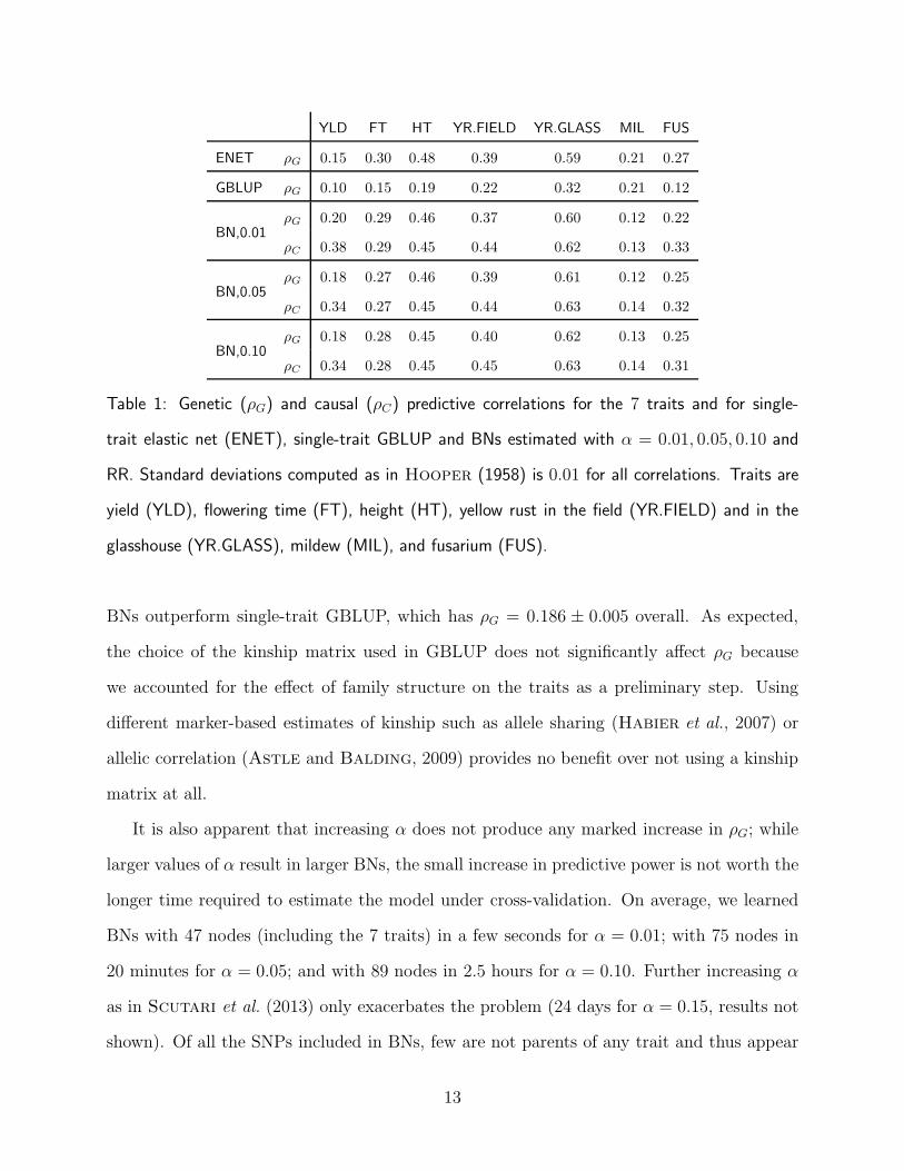
Table 1: Genetic (ρG) and causal (ρC) predictive correlations for the 7 traits and for single-

trait elastic net (ENET), single-trait GBLUP and BNs estimated with α = 0.01, 0.05, 0.10 and

RR. Standard deviations computed as in Hooper (1958) is 0.01 for all correlations. Traits are

yield (YLD), flowering time (FT), height (HT), yellow rust in the field (YR.FIELD) and in the

glasshouse (YR.GLASS), mildew (MIL), and fusarium (FUS).

BNs outperform single-trait GBLUP, which has ρG = 0.186 ± 0.005 overall. As expected,

the choice of the kinship matrix used in GBLUP does not significantly affect ρG because

we accounted for the effect of family structure on the traits as a preliminary step. Using

different marker-based estimates of kinship such as allele sharing (Habier et al., 2007) or

allelic correlation (Astle and Balding, 2009) provides no benefit over not using a kinship

matrix at all.

It is also apparent that increasing α does not produce any marked increase in ρG; while

larger values of α result in larger BNs, the small increase in predictive power is not worth the

longer time required to estimate the model under cross-validation. On average, we learned

BNs with 47 nodes (including the 7 traits) in a few seconds for α = 0.01; with 75 nodes in

20 minutes for α = 0.05; and with 89 nodes in 2.5 hours for α = 0.10. Further increasing α

as in Scutari et al. (2013) only exacerbates the problem (24 days for α = 0.15, results not

shown). Of all the SNPs included in BNs, few are not parents of any trait and thus appear

13

to be false positives: 1 out of 40 (2.5%) for α = 0.01, 2 out of 68 (2.9%) for α = 0.05 and

4 out of 82 (4.8%) for α = 0.10. The dimension of the BNs is in stark contrast with the

average number of non-zero SNP effects in the ENET models: 110 non-zero coefficients for

YR.GLASS, 2661 for YLD, 55 for HT, 105 for YR.FIELD, 333 for FUS, 1725 for MIL and

24 for FT.

As far as causal predictive correlations ρC are concerned, we observe a distinct improve-

ment compared to ρG for 3 traits: YLD, YR.FIELD and FUS. As for the other 4 traits, the

difference between ρG and ρC is not as marked, even though it is statistically significant in

all cases except flowering time. Overall, ρC = 0.373± 0.004 which is higher than both BN’s

ρG = 0.331± 0.04 for α = 0.10 and the ENET’s ρG = 0.343± 0.004.

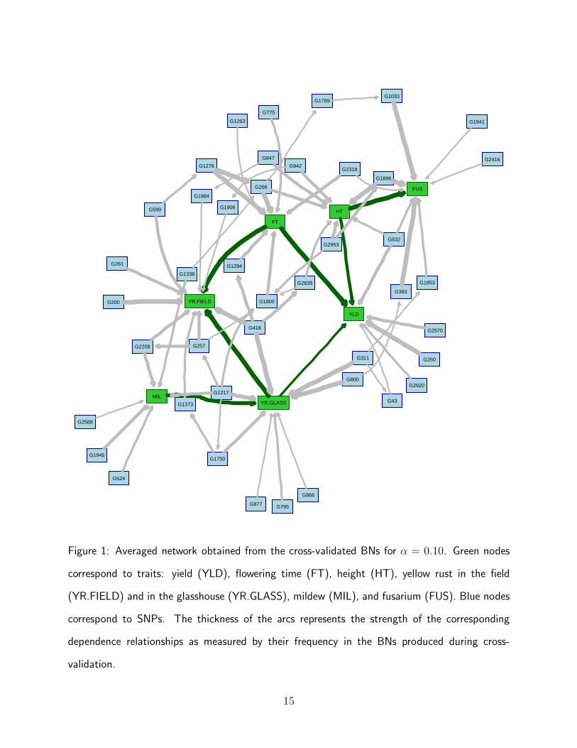
The averaged BN for α = 0.10 is shown in Figure 1; it has 50 nodes and 78 arcs. For

ease of plotting, the SNP names corresponding to the labels used in the figure are reported

in Table 2. The dimension of the BN is comparable to that obtained for α = 0.01 (30 nodes,

44 arcs) and α = 0.05 (44 nodes, 66 arcs). In all three cases the threshold for arc inclusion

estimated as in Scutari and Nagarajan (2013) is 0.49, which is close to the intuitive

choice of including in the averaged BN those arcs that appear in more than half of the BNs

obtained during cross-validation. All SNPs in the averaged BN are linked with at least one

trait, with the exception of G1789 (D contig28346 467). Their minor allele frequencies range

from 0.02 (G2208; IAAV1322) to 0.47 (G1945; Excalibur c29304 176). Furthermore, the BN

is small enough that RR and OLS parameter estimates are practically equivalent.

As far as phenotypic traits are concerned, the averaged BN captures several known rela-

tionships. YR.FIELD is influenced by FT (FT → YR.FIELD in Figure 1); early flowering

genotypes will have their leaves exposed to the pathogens for a longer time than later geno-

types, resulting in higher yellow rust scores even if they have the same level of true disease

resistance. This is substantiated by the posterior distribution of the disease score condi-

tional on flowering time being in the bottom quartile ([21.0, 29.7]) or in the top quartile

([33.8, 42.0]): it has mean 2.54 in the first case and 2.33 in the second. Standard deviation

14

YR.GLASS

HT

FUS

MIL

FT

G418

G311

G800

G877

G866

G795

G2570

G260

G832

G1896

G2953

G942

G266

G847

G2835

G200

G2208 G257

G1906

G261

G1984

G599

G383

G2416

G1033

G1941

G1853

G1338

G524

G1945

G1276

G1789

G2318

G1800

G1294

G775

YLD

YR.FIELD

G1750

G43G1373

G1217

G2588

G1263

G2920

Figure 1: Averaged network obtained from the cross-validated BNs for α = 0.10. Green nodes

correspond to traits: yield (YLD), flowering time (FT), height (HT), yellow rust in the field

(YR.FIELD) and in the glasshouse (YR.GLASS), mildew (MIL), and fusarium (FUS). Blue nodes

correspond to SNPs. The thickness of the arcs represents the strength of the corresponding

dependence relationships as measured by their frequency in the BNs produced during cross-

validation.

15

LABEL NAME LABEL NAME

G418 BobWhite c5756 516 G311 BobWhite c37358 208

G800 BS00022299 51 G877 BS00022830 51

G866 BS00022703 51 G795 BS00022270 51

G2570 Kukri c7241 322 G260 BobWhite c29014 241

G832 BS00022473 51 G1896 Excalibur c19078 210

G2953 Tdurum contig64772 417 G942 BS00024496 51

G266 BobWhite c30043 150 G847 BS00022562 51

G2835 RFL Contig4790 1091 G200 BobWhite c22728 78

G2208 IAAV1322 G257 BobWhite c28819 733

G1906 Excalibur c20837 868 G261 BobWhite c2905 590

G1984 Excalibur c37696 192 G599 BS00009575 51

G383 BobWhite c47401 491 G2416 Kukri c100613 331

G1033 BS00035141 51 G1941 Excalibur c27950 459

G1853 Excalibur c11795 934 G1338 BS00066211 51

G524 BS00000721 51 G1945 Excalibur c29304 176

G1276 BS00064538 51 G1789 D contig28346 467

G2318 IACX11305 G1800 D GBUVHFX01DSLGX 212

G1294 BS00065110 51 G775 BS00022148 51

G1750 CAP12 c2800 262 G43 BobWhite c11692 148

G1373 BS00067203 51 G1217 BS00062679 51

G2588 Kukri rep c102953 304 G1263 BS00064140 51

G2920 Tdurum contig42584 1190

Table 2: SNPs included in the averaged BN. The labels are those used in Figure 1, while the

SNP names are from Mackay et al. (2014) and Wang et al. (2014).

16

is 0.47 in both cases. The same is true for YR.GLASS, which has means 2.50 and 2.48 for

early and late flowering genotypes; standard deviation is 0.43. The network structure sug-

gests that the YR.GLASS is not influenced directly by FT (i.e. there is no FT→ YR.GLASS

arc). The two yellow rust scores (YR.GLASS→ YR.FIELD) are positively correlated (0.34),

likely because of durable resistance. In addition, we note that YR.FIELD summarizes adult

resistance to a mixed population of pathotypes, which may include the specific pathotype

used to measure juvenile resistance in YR.GLASS.

We can also see from Figure 1 that YLD depends directly on both HT (HT→ YLD) and

FT (FT→ YLD); but it is affected only indirectly by all the disease scores except YR.GLASS.

Conditional on the combinations of bottom and top quartiles for FT and HT ([64.3, 74.5] and

[79.5, 87.7]), the expected yield is 7.54, 7.71, 7.15 and 7.33 respectively. Standard deviation

is 0.47 in all four scenarios. Therefore, we observe a marginal increase in YLD of about

0.15 when comparing short and tall genotypes, and a marginal decrease of about 0.4 when

comparing early and late flowering genotypes; this is consistent with Flintham et al. (1997)

and Snape et al. (2001). The interplay between HT and FT appears to be negligible in

determining yield. Conditioning on the bottom and top quartiles of the disease scores, we

see a difference in the mean YLD of +0.08 (FUS), −0.02 (MIL), −0.01 (YR.GLASS) and

−0.10 (YR.FIELD).

The apparent increase in YLD associated with high FUS scores is the result of the

confounding effect of HT, which is directly linked to both variables in the BN (FUS ←

HT → YLD). This is expected because susceptibility to fusarium is known to be positively

related to HT (Srinivasachary et al., 2009), which in turn affects YLD. Conditional on

each quartile of HT, FUS has a negative effect on YLD ranging from −0.04 to −0.06.

The last interaction between phenotypes in the BN is between MIL and YR.GLASS

(MIL→ YR.GLASS). This can be explained by the increased susceptibility to one disease in

genotypes that are weakened by the onset of the other, by disease resistance being controlled

by shared regions in the genome (Spielmeyer et al., 2005; Lillemo et al., 2008) and to

17

a lesser extent by the influence of weather conditions (Beest et al., 2008). The BN in

Figure 1 identifies 9 SNPs that are linked to at least one of MIL and YR.GLASS, and

may possibly be tagging pleiotropic QTLs for disease resistance. By contrasting low and

high level of both diseases (scores 6 1.5 and > 3.5, respectively), we can infer which allele

may be linked with resistance to both diseases using the conditional expected allele counts,

nLOW and nHIGH. For 3 of the 9 genes the difference between the two is marked: G418

(BobWhite c5756 516; nLOW = 0.5, nHIGH = 1.9), G311 (BobWhite c37358 208; nLOW =

1.1, nHIGH = 1.7) and G1217 (BS00062679 51; nLOW = 0.8, nHIGH = 1.7). The 90K consensus

map inWang et al. (2014) locates G418 in chromosome 2D along with other SNPs conferring

resistance to YR.GLASS. The same is true also for G311 in chromosome 2B, and for G2127

in chromosome 2A. As for the other 6 SNPs, |nLOW−nHIGH| < 0.5, which suggests that their

individual effects are small and that they might work in concert with other genes producing

polygenic effects.

Similar analyses on the other traits identify two more SNPs with |nLOW − nHIGH| 6 0.5

that may be tagging known genes. G1896 (Excalibur c19078 210) has nLOW = 0.3, nHIGH =

1.2 when contrasting top and bottom quartiles for HT; and has nLOW = 0.2, nHIGH = 1.7

when contrasting the bottom quartile of HT and FUS > 3.5 with the top quartile of HT

and FUS 6 1.5. The latter pair of scenarios is motivated by the fact that taller plants are

less susceptible to fusarium than shorter plants. The LD analysis in Mackay et al. (2014)

suggests that this SNP is located in chromosome 4D in this population, and that it may be

tagging Rht-D1b, a dwarfing gene which is also closely associated with resistance to fusarium

(Srinivasachary et al., 2009). In addition, G266 (BobWhite c30043 150) appears to be

located in chromosome 2D and to be tagging Ppd-D1, which controls photoperiod response.

Contrasting the bottom quartiles of both FT and HT with the top quartiles we have nHIGH =

0 and nLOW = 0.8.

18

DISCUSSION

Modeling multiple quantitative traits simultaneously has been known to result in better

predictive power than targeting one trait at a time in the context of additive genetic models

(Henderson and Quaas, 1976). BNs provide a general framework to estimate and analyze

such models. They also provide an accompanying graphical representation that is intuitive

yet rigorous; a plot such as that in Figure 1 can be very useful for exploratory analysis, to

disseminate results and to motivate further quantitative and qualitative analyses in GWAS

and GS studies.

From a theoretical point of view, BNs are more versatile than additive models in com-

mon use. By assuming variables are normally distributed, we have shown that BNs are

in fact equivalent to multivariate GBLUP and, by extension of single-trait GBLUP. Fur-

thermore, the separation between structure and parameter learning makes it possible to

accommodate different parametric assumptions with relatively few changes, and subsume

models such as univariate and multivariate ridge-regression (Hoerl and Kennard, 1970;

Brown and Zidek, 1980). As far as inference is concerned, several established methods

from the literature can be used to predict traits from SNPs and vice versa; two examples

are logic sampling and likelihood weighting (Koller and Friedman, 2009). Both allow

to explore complex scenarios of practical relevance by estimating informative statistics from

the corresponding conditional distributions of traits and SNPs. This is made easier by the

lack of a formal distinction between response and explanatory variables in the BN, which is

central in traditional linear models. As a result, BNs can be used for association studies as

well as genomic prediction. In the former, we can condition on some complex combination

of traits and predict the expected allele counts of SNPs. Such an approach has the potential

of detecting which SNPs tag relevant QTLs and which of their alleles are favourable. In

the latter, we have shown that BNs are competitive with a state-of-the-art model such as

single-trait ENET when predicting traits from SNPs, and that they outperform single-trait

GBLUP for the population analysed in this paper. As evidenced by the difference between

19

ρG and ρC , using BNs as a multi-trait model and performing predictions based on those

variables identified as putative causal for each trait outperforms ENET as well by leverag-

ing pleiotropic effects (Hartley et al., 2012). This shows it is possible to improve genomic

selection for traits that are expensive to measure by incorporating cheaper ones in the predic-

tions. Clearly, the impact of correlated phenotypes on the predictive power of BNs depends

on the strength of their correlation.

Based on the BN in Figure 1, we can also observe some interesting properties of BNs as

genetic models. Firstly, the difference in the number of SNPs included in the BNs compared

to the ENET models can be attributed to the limited ability of BNs to capture small epistatic

effects (Han et al., 2012). Consider, for instance, a polygenic effect in which two SNPs are

jointly associated with a trait but in which each SNP is not significant on its own. Such an

effect will not be captured because both SNPs will be discarded by the single-SNP screening

performed at the beginning of feature selection. As observed in other studies, this does

not have a significant impact on predictive ability if a large enough α threshold is used,

as Markov blankets are very effective at feature selection (Chang and McGeachie, 2011;

Scutari et al., 2013). Secondly, SNPs with pleiotropic effects are included in the BN even

when association with a single phenotype is detected; at that point they can be linked to

all relevant phenotypes. This is the case of the SNPs controlling resistance to both mildew

and yellow rust discussed above. Furthermore, direct and indirect effects of such SNPs and

of traits are correctly separated for the observed traits, as in the case of the fusarium effect

on yield.

MAGIC populations provide an ideal starting point for fitting BNs. On the one hand,

the particular pattern of crosses used to produce a MAGIC population results in a very

low population structure. This reduces the confounding effect of relatedness on the estima-

tion of SNP effects (Astle and Balding, 2009) and on mapping approaches based on LD

(Mackay et al., 2014). On the other hand, the size of of the population is large enough to

detect weak associations and associations with rare variants. Both are in fact present in the

20

averaged BN, which includes SNPs with minor allele frequencies as low as 0.02 and SNPs

which are significant (e.g. for MIL and YR.GLASS) only when considering multiple traits

at the same time.

Finally, SNPs of interest can be made to segregate in the population by choosing the

founders appropriately, since balanced crosses ensure opportunities for recombination among

the founders. This is particularly important in modeling multiple phenotypes, as we need

to ensure as many relevant QTLs and genes as possible are tagged to correctly dissect their

genetic layout.

ACKNOWLEDGMENTS

The work presented in this paper forms part of the MIDRIB project, which is funded by the

UK Technology Strategy Board (TSB) and Biotechnology & Biological Sciences Research

Council (BBSRC), grant TS/I002170/1. The MAGIC population was developed within

BBSRC Crop Science Initiative project BB/E007201/1. Field trials and SNP genotyping

were funded by the NIAB Trust.

LITERATURE CITED

Aliferis, C. F., A. Statnikov, I. Tsamardinos, S. Mani, and X. D. Xenofon, 2010

Local causal and Markov blanket induction for causal discovery and feature selection for

classification part I: algorithms and empirical evaluation. J. Mach. Learn. Res. 11: 171–

234.

Alimi, N. A., M. C. A. M. Bink, J. A. Dieleman, J. J. Magan, A. M. Wubs,

A. Palloix, and F. A. van Eeuwijk, 2013 Multi-trait and multi-environment QTL

analyses of yield and a set of physiological traits in pepper. Theor. Appl. Genet. 126 (10):

2597–2625.

Astle, W. and D. J. Balding, 2009 Population structure and cryptic relatedness in

genetic association studies. Stat. Sci. 24 (4): 451–471.

21

Banerjee, S., A. O. Finley, P. Waldmann, and T. Ericsson, 2012 Hierarchical spa-

tial process models for multiple traits in large genetic trials. J. Am. Stat. Assoc. 105 (490):

506–521.

Banerjee, S., B. S. Yandell, and N. Yi, 2008 Bayesian quantitative trait loci mapping

for multiple traits. Genetics 179 (4): 2275–2289.

Beest, D. E. T., N. D. Paveley, M. W. Shaw, and F. van den Bosch, 2008 Disease-

weather relationships for powdery mildew and yellow rust on winter wheat. Phytopatol-

ogy 98: 609–617.

Brown, P. J. and J. V. Zidek, 1980 Adaptive multivariate ridge regression. Ann.

Stat. 8 (1): 64–74.

Chang, H.-H. and M. McGeachie, 2011 Phenotype prediction by integrative network

analysis of SNP and gene expression microarrays. In Proceedings of the 33rd Annual Inter-

national Conference of the IEEE Engineering in Medicine and Biology Society (EMBC),

pp. 6849–6852. IEEE Press, New York.

Cowell, R. G., A. P. Dawid, S. L. Lauritzen, and D. J. Spiegelhalter, 2007

Probabilistic Networks and Expert Systems. Springer-Verlag, New York.

Cox, D. R. and N. Wermuth, 1996 Multivariate Dependencies: Models, Analysis and

Interpretation. Chapman & Hall, Boca Raton.

Druka, A., I. Druka, A. Centeno, H. Li, Z. Sun, W. Thomas, N. Bonar,

B. Steffenson, S. Ullrich, A. Kleinhofs, R. Wise, T. Close, E. Potokina,

Z. Luo, C. Wagner, G. Schweizer, D. Marshall, M. Kearsey, R. Williams,

and R. Waugh, 2008 Towards systems genetic analyses in barley: integration of pheno-

typic, expression and genotype data into GeneNetwork. BMC Genet. 9 (1): 73.

22

Falconer, D. S. and T. F. C. Mackay, 1995 Introduction to Quantitative Genetics (4th

ed.). Prentice Hall, Harlow, UK.

Finley, A. O., S. Banerjee, P. Waldmann, and T. Ericsonn, 2009 Hierarchical

Spatial Modeling of Additive and Dominance Genetic Variance for Large Spatial Trial

Datasets. Biometrics 61 (2): 441–451.

Flintham, J. E., A. Borner, A. J. Worland, and M. D. Gale, 1997 Optimiz-

ing wheat grain yield: effects of Rht (Gibberellin-Insensitive) dwarfing genes. J. Agr.

Sci. 128 (1): 11–25.

Friedman, J. H., T. Hastie, and R. Tibshirani, 2010 Regularization paths for gener-

alized linear models via coordinate descent. J. Stat. Soft. 33 (1): 1–22.

Friedman, N., 2004 Inferring cellular networks using probabilistic graphical models. Sci-

ence 303 (5659): 799–805.

Goeman, J. J., 2012 penalized R package. R package version 0.9-41.

Habier, D., R. L. Fernando, and J. C. M. Dekkers, 2007 The impact of genetic

relationship information on genome-assisted breeding values. Genetics 177: 2389–2397.

Han, B., X. Chen, Z. Talebizadeh, and H. Xu, 2012 Genetic studies of complex

human diseases: characterizing SNP-disease associations using Bayesian networks. BMC

Syst. Biol. 6 (Suppl 3): S14.

Hartley, S. W., S. Monti, C.-T. Liu, M. H. Steinberg, and P. Sebastiani, 2012

Bayesian methods for multivariate modeling of pleiotropic SNP associations and genetic

risk prediction. Front. Genet. 3 (176): 1–17.

Hastie, T., R. Tibshirani, B. Narasimhan, and G. Chu, 2013 impute: imputation for

microarray data. R package version 1.36.0.

23

Henderson, C. R. and R. L. Quaas, 1976 Multiple trait evaluation using relatives’

records. J. Anim. Sci. 43: 1188–1197.

Hoerl, A. E. and R. W. Kennard, 1970 Ridge regression: biased estimation for

nonorthogonal problems. Technometrics 12 (1): 55–67.

Hooper, J. W., 1958 The sampling variance of correlation coefficients under assumptions

of fixed and mixed variates. Biometrika 45 (3/4): 471–477.

Hotelling, H., 1953 New light on the correlation coefficient and its transforms. J. Roy.

Stat. Soc. B 15 (2): 193–232.

Jansen, R., H. Yu, D. Greenbaum, Y. Kluger, N. J. Krogan, S. Chung, A. Emili,

M. Snyder, J. F. Greenblatt, and M. Gerstein, 2003 A Bayesian networks ap-

proach for predicting protein-protein interactions from genomic data. Science 302 (5644):

449–453.

Koller, D. and N. Friedman, 2009 Probabilistic Graphical Models: Principles and Tech-

niques. MIT Press, Cambridge.

Lauritzen, S. L. and N. A. Sheehan, 2004 Graphical models for genetic analysis. Stat.

Sci. 18: 489–514.

Li, R., S.-W. Tsaih, K. Shockley, I. M. Stylianou, J. Wergedal, B. Paigen, ,

and G. A. Churchill, 2006 Structural model analysis of multiple quantitative traits.

PLoS Genet. 2 (7): e114.

Li, Y., C. J. Willer, J. Ding, P. Scheet, and G. R. Abecasis, 2010 MaCH: using

sequence and genotype data to estimate haplotypes and unobserved genotypes. Genet.

Epidemiol. 34: 816–834.

Lillemo, M., B. Asalf, R. P. Singh, J. Huerta-Espino, X. M. Chen, Z. H. He,

and A. Bjørnstad, 2008 The adult plant rust resistance loci Lr34/Yr18 and Lr46/Yr29

24

are important determinants of partial resistance to powdery mildew in bread wheat line

Saar. Theor. Appl. Genet. 116: 1155–1166.

Mackay, I., P. Bansept-Basler, T. Barber, A. Bentley, J. Cockram, N. Gos-

man, A. Greenland, R. Horsnell, R. Howells, D. O’Sullivan, G. Rose, and

P. Howell, 2014 An eight-parent multiparent advanced generation intercross population

for winter-sown wheat: creation, properties and first results. G3. In print.

Malovini, A., A. Nuzzo, F. Ferrazzi, A. Puca, and R. Bellazzi, 2009 Phenotype

forecasting with SNPs data through gene-based Bayesian networks. BMC Bioinformat-

ics 10 (Suppl 2): S7.

Meuwissen, T. H. E., B. J. Hayes, and M. E. Goddard, 2001 Prediction of total

genetic value using genome-wide dense marker maps. Genetics 157: 1819–1829.

Morota, G., B. D. Valente, G. J. M. Rosa, K. A. Weigel, and D. Gianola, 2012

An assessment of linkage disequilibrium in holstein cattle using a Bayesian network. J.

Anim. Breed. Genet. 129 (6): 474–487.

Mourad, R., C. Sinoquet, and P. Leray, 2011 A hierarchical Bayesian network ap-

proach for linkage disequilibrium modeling and data-dimensionality reduction prior to

genome-wide association studies. BMC Bioinformatics 12 (1): 16.

O’Reilly, P. F., C. J. Hoggart, Y. Pomyen, F. C. F. Calboli, P. Elliott, M.-R.

Jarvelin, and L. J. M. Coin, 2012 MultiPhen: joint model of multiple phenotypes can

increase discovery in GWAS. PLoS One 7 (5): e34861.

Pearl, J., 1988 Probabilistic Reasoning in Intelligent Systems: Networks of Plausible

Inference. Morgan Kaufmann, San Francisco.

Pearl, J., 2009 Causality: Models, Reasoning and Inference (2nd ed.). Cambridge Uni-

versity Press.

25

Piepho, H.-P., 2009 Ridge regression and extensions for genomewide selection in maize.

Crop Sci. 49 (4): 1165–1176.

Piepho, H.-P., J. O. Ogutu, T. Schulz-Streeck, B. Estaghvirou, A. Gordillo,

and F. Technow, 2012 Efficient computation of ridge-regression best linear unbiased

prediction in genomic selection in plant breeding. Crop Sci. 52 (3): 1093–1104.

Sachs, K., O. Perez, D. Pe’er, D. A. Lauffenburger, and G. P. Nolan, 2005

Causal protein-signaling networks derived from multiparameter single-cell data. Sci-

ence 308 (5721): 523–529.

Schwarz, G. E., 1978 Estimating the dimension of a model. Ann. Stat. 6 (2): 461 – 464.

Scutari, M., 2010 Learning Bayesian networks with the bnlearn R package. J. Stat.

Soft. 35 (3): 1–22.

Scutari, M., I. Mackay, and D. J. Balding, 2013 Improving the efficiency of genomic

selection. Stat. Appl. Genet. Mol. Biol. 12 (4): 517–527.

Scutari, M. andR. Nagarajan, 2013 On identifying significant edges in graphical models

of molecular networks. Artif. Intell. Med. 57 (3): 207–217.

Sebastiani, P. and T. T. Perls, 2008 Complex genetic models. In O. Pourret, P. Naım,

and B. Marcot (Eds.), Bayesian Networks: a Practical Guide to Applications, pp. 53–72.

Wiley, Hoboken.

Sebastiani, P., M. F. Ramoni, V. Nolan, C. T. Baldwin, and M. Steinberg, 2005

Genetic dissection and prognostic modeling of overt stroke in sickle cell anemia. Nat.

Genet. 37 (4): 435–440.

Snape, J. W., K. Butterworth, E. Whitechurch, and A. J. Worland, 2001 Wait-

ing for fine times: genetics of flowering time in wheat. Euphytica 119 (1–2): 185–190.

26

Speed, D., G. Hermani, M. R. Johnson, and D. J. Balding, 2012 Improved heri-

tability estimation from genome-wide SNPs. Am. J. Hum. Genet. 91 (6): 1011–1021.

Spielmeyer, W., R. A. McIntosh, J. Kolmer, and E. S. Lagudah, 2005 Powdery

mildew resistance and Lr34/Yr18 genes for durable resistance to leaf and stripe rust coseg-

regate at a locus on the short arm of chromosome 7D of wheat. Theor. Appl. Genet. 111:

731–735.

Srinivasachary, N. Gosman, A. Steed, T. W. Hollins, R. Bayles, P. Jennings,

and P. Nicholson, 2009 Semi-dwarfing Rht-B1 and Rht-D1 loci of wheat differ signifi-

cantly in their influence or resistance to fusarium head blight. Theor. Appl. Genet. 118:

695–702.

Stephens, M., 2013 A unified framework for association analysis with multiple related

phenotypes. PLoS One 8 (7): e65245.

Wang, S., D. Wong, K. Forrest, A. Allen, S. Chao, E. Huang, M. Maccaferri,

S. Salvi, S. Milner, L. Cattivelli, A. M. Mastrangelo, A. Whan, S. Stephen,

G. Barker, R. Wieseke, J. Plieske, IWGSC, M. Lillemo, D. Mather, R. Ap-

pels, R. Dolferus, G. Brown-Guedira, A. Korol, A. R. Akhunova, C. Feuil-

let, J. Salse, M. Morgante, C. Pozniak, M. Luo, , J. Dvorak, M. Morell,

J. Dubcovsky, M. Ganal, R. Tuberosa, C. Lawley, I. Mikoulitch, C. Ca-

vanagh, K. J. Edwards, M. Hayden, and E. Akhunov, 2014 Characterization of

polyploid wheat genomic diversity using a high-density 90,000 SNP array. Plant Biotech.

J. 12 (6): 787–796.

Wimmer, V., T. Albrecht, H.-J. Auinger, and C.-C. Schon, 2012 synbreed: frame-

work for the analysis of genomic prediction data using R. Bioinformatics 18 (15): 2086–

2087.

27

Zou, H. and T. Hastie, 2005 Regularization and variable selection via the elastic net. J.

Roy. Stat. Soc. B 67 (2): 301–320.

28