arX

iv:1

411.

5548

v1 [

cs.N

I] 2

0 N

ov 2

014

1

Learning Based Frequency- and Time-DomainInter-Cell Interference Coordination in HetNets

Meryem Simsek‡, Mehdi Bennis†, andIsmail Guvenc‡‡Department of Electrical & Computer Engineering, Florida International University, USA

†Centre for Wireless Communications, University of Oulu, FinlandEmail: meryem.simsek@ieee.org, bennis@ee.oulu.fi, and iguvenc@fiu.edu

Abstract—In this article, we focus on inter-cell interferencecoordination (ICIC) techniques in heterogeneous network (Het-Net) deployments, whereby macro- and picocellsautonomouslyoptimize their downlink transmissions, with loose coordination.We model this strategic coexistence as a multi-agent system,aiming at joint interference management and cell association.Using tools from Reinforcement Learning (RL), agents (i.e.,macro- and picocells) sense their environment, and self-adaptbased on local information so as to maximize their networkperformance. Specifically, we explore both time- and frequencydomain ICIC scenarios, and propose atwo-level RL formulation.Here, picocells learn their optimal cell range expansion (CRE)bias and transmit power allocation, as well as appropriatefrequency bands for multi-flow transmissions, in which a userequipment (UE) can be simultaneously served by two or morebase stations (BSs) from macro- and pico-layers. To substantiateour theoretical findings, Long Term Evolution Advanced (LTE-A) based system level simulations are carried out in which ourproposed approaches are compared with a number of baselineapproaches, such as resource partitioning (RP), static CRE, andsingle-flow Carrier Aggregation (CA). Our proposed solutionsyield substantial gains up to 125% compared to static ICICapproaches in terms of average UE throughput in the time-domain. In the frequency-domain our proposed solutions yieldgains up to 240% in terms of cell-edge UE throughput.

Index Terms—LTE-A, Reinforcement Learning, HeterogeneousNetworks, Cell Range Expansion, Inter-Cell Interference Coor-dination (ICIC), Carrier Aggregation (CA), Multi-Flow Tra ns-mission.

Learning Based Frequency- and Time-Domain Inter-CellInterference Coordination in HetNets

I. I NTRODUCTION

Driven by the network densification and increasing numberof smart-phones, tablets and netbooks, mobile operators arecompelled to find viable solutions to maximize their net-work performance in a cost-effective manner. Heterogeneousnetwork (HetNets) deployments combining various cell sizes(femto, pico, relays) and radio access technologies (3G/4G/Wi-Fi), are expected to become cornerstones for future hetero-geneous wireless cellular networks, aiming at substantiallyhigher data rates and spatial reuse [1]. HetNets are currentlystudied within the3rd Generation Partnership Project (3GPP)standardization body, where mechanisms including time- andfrequency-domain intercell interference coordination (ICIC)with adaptive resource partitioning, cell range expansion(CRE), and interference coordination/cancellation take centralstage [2]. In this article, we focus on one of these important

aspects, namely self-organizing networks (SON).3GPP hasdefined SON as one of the most important standardizationfeatures for mobile operators today for the operation, manage-ment, and maintenance of their radio access networks (RANs)cost-efficiently, without relying on human intervention [3].SON in HetNets is expected to gain more importance asnetworks are getting denser and becoming more heterogeneousin size, access technology, and backhauls. Endowed withself-configuring, self-optimizing and self-healing capabilities,mobile operators can optimize their networks in a totallydecentralized manner, in which the traffic load is balancedamong tiers, significantly reducing their operation and capitalexpenditures (OPEX/CAPEX), and ultimately satisfying users’quality-of-service (QoS) requirements.

Based on the self-organizing capabilities of HetNets, wepropose solutions tosmartly offload traffic to open accesspicocells and thereby achieve cell splitting gains for bothtime- and frequency-domain ICIC techniques. We focus onthe downlink transmission as this has been identified as amore critical intercell interference scenario within HetNets [5].Open access picocells are cells that provide access to any userequipment (UE) within their coverage area. As UEs generallyconnect to the cell that provides the strongest downlink (DL)received signal, DL intercell interference can be reduced.However, if all UEs connect to the macrocell due to theirlarge transmit power, rather than to picocells at shorter distancewith lesser number of UEs, the traffic load will be unevenlydistributed in the network. As a result, the macrocell will beoverloaded whereas picocells will be under-utilized [6]–[8].As a remedy to this, the concept of CRE was proposed as acell selection procedure, in which a positive bias is added tothe picocell’s DL received signal to increase its DL footprint.This bias balances the load among the macro- and picocelltier by forcing mobile users to handover to picocells, even ifthe picocell’s DL received signal is lower. Nevertheless, anaggressive range expansion may cause high interference topicocell UEs (PUEs) located in the picocell expanded regions(ER); this is because ER PUEs do not connect to the cellswith the strongest DL received signal, thus suffering fromlow DL Signal-to-Interference-plus-Noise Ratios (SINRs)[9].In addition, due to the non-uniform traffic and user distribu-tion, picocells need to self-organize for effectively offloadingmacrocell’s traffic. With this in mind,intelligent and flexiblecell range expansion techniques across time and frequencymust be devised for macro- and picocells, to mitigate excessive

2

DL inter-cell interference suffered by ER PUEs, while at thesame time not jeopardizing PUE QoS requirements.

II. RELATED WORK AND CONTRIBUTIONS

In this section, we summarize the concepts of range ex-pansion and time/frequency domain ICIC in HetNets anddiscuss related works from the literature to better presentourcontributions.

A. Picocell Range Expansion and Inter-Cell Interference Co-ordination

In order to benefit from the deployment of heterogeneousand small cell networks, range expansion ICIC techniques havebeen proposed, in which picocells increase their footprintsoas to balance the load among tiers and achieve cell-splittinggains. In what follows, we revisit and summarize both therange expansion and ICIC concepts.3GPP has studied the concept of CRE through handover

biasing and resource partitioning among nodes with differentlevels of transmission powers [16]–[18]. The biasing mecha-nism allows load balancing among tiers, where depending onthe bias value, more UEs can be associated to picocells. Inthis approach, the bias value is an offset added to the receivedpower of picocells in order to increase its DL coverage area.CRE significantly reduces the DL signal quality of those usersin the expanded region (i.e., ER PUEs), because they areconnected to cells that do not provide the best DL receivedsignal. These interference problems may significantly degradethe overall network performance, calling for intelligent ICICschemes to benefit from range expansion and improve theperformance of ER PUEs. Since ICIC schemes specified in3GPP LTE Release8− 9 do not specifically consider HetNetsettings, enhancements of these techniques have been proposedto efficiently mitigate interference in subsequent releases of theLTE standard [27]. In particular, the ICIC techniques in3GPPRelease10 − 12, can be grouped into four categories: time-domain, frequency-domain, power based and antenna/spatial-based techniques [28], [29].

B. Literature Review

There is a sizeable body of literature on the use of CREfor traffic load balancing in HetNets; see e.g. [6]–[15] and thereferences listed therein. In [6], closed-form expressions arederived to calculate CRE bias values for different range expan-sion strategies. Moreover, a cooperative scheduling scheme isproposed to mitigate interference caused by macrocells ontoER PUEs. To improve DL capacity and users’ fairness, theauthors propose a new subframe blanking based cell selec-tion procedure in [7]. Using tools from stochastic geometry,analytical models accounting for base station (BS) and UElocations have been studied to analyze spectral efficienciesin range expanded picocell networks in [11], which has laterbeen extended to ICIC scenarios in [13]–[15]. In [12], thethroughput performance of different CRE values and differentratios of protected resources were carried out based on systemlevel simulations.

In addition to time domain interference coordination ap-proaches, frequency domain interference coordination tech-niques have also been considered in the literature for in-terference management and load balancing purposes. In thiscontext, multi-flow carrier aggregation (CA), in which usersare served by different layers on different component carriers(CCs), has and remains an open and challenging problem. Arelated approach to provide an efficient and flexible networkperformance improvement is to split the control and user plane(C-and U-plane). This concept was introduced and discussedin [30], [31] whereby, the C-plane is provided at low frequencyband to maintain good connectivity and mobility. On the otherhand, the U-plane is provided by both the macrocells andthe small cells (deployed at higher frequency bands) for datatransfer. Since small cells are not configured with cell-specificsignals and channels, they are namedPhantom Cells[31].

C. Contribution

The main contribution of this article is to propose decen-tralized solutions for joint power control and cell associationin a HetNet scenario, in both time and frequency domain. Inthe time-domain, Pico Base Stations (PBSs)optimally learntheir CRE bias and power allocation, while satisfying theirown PUEs’ QoS requirements. In turn, the macrocell self-organizes so as to serve its own macro UEs (MUEs), whileadhering to the picocell interference constraint. In contrastto the homogeneouscase where all PBSs use the same biasvalue, the proposed solution is dynamic and self-organizingin nature, where the RAN autonomously optimizes the CREbias values of the picocells through a loose coordination withthe macrocell tier. The UE adds these bias values to itsmeasurements, to check whether a measurement report needsto be sent to its serving BS. The PBSs, upon coordination withthe MBS, learn the CRE bias values and notify the MBS viathe X2 interface.

In the frequency-domain, we consider: (a) the single-flowCA, where users are served by only one BS at a time, and(b) the multi-flow CA, in which a UE can be simultaneouslyserved by two (or more) BSs from different layers/tiers, buton two different CCs. Our proposed learning based solutionis validated using a long term evolution advanced (LTE-A)system level simulator, through a comparison with a numberof benchmark solutions such as resource partitioning and staticCRE.

It is worth noting that most of the existing ICIC andload balancing techniques are simulated in simplified HetNetscenarios with homogeneity inside the macro layer as well asthe pico layer; by considering the same CRE for all picocellsin the network. The major difference between our contributionand existing techniques is that we propose a joint optimiza-tion approach, in which each picocell individually learns itsoptimum ICIC strategy. This is achieved by optimizing thepicocells CRE bias selection and power allocation strategiesin coordination with the macrocell. In contrast to existingapproaches, our solution is based on Reinforcement learning,which is a widely accepted tool in dynamic wireless networksand allows to investigate how BSs interact over time and

3

PBS

PBS

PBS

PBS

PBS

PBS

MBS

ER

PUEPUE

MUE

MUE

PUE

PUE

PUE

PUE

PUE

MUE

MUE

MUE

MUE

ER

PUE

ER

PUE

ER

PUE

ER

PUE

ER

PUE

ER

PUE

Pico cell

area

with CRE

Pico cell area

without CRE

Fig. 1: A heterogeneous scenario with cell range expansion(CRE).

attempt to optimize their utility [32]. We propose a reinforce-ment learning framework, in which not only the picocells butalso the macrocell perform load balancing and power control.The challenge of this approach lies in effectively offloading theUEs from the macrocells, while simultaneously maintainingthe QoS requirements of PUEs. By enabling coordinationbetween both layers and considering the performance of MUEsand PUEs, the proposed techniques are seen as a promisingapproach to overcome this challenge.

The remainder of this paper is organized as follows: SectionIII summarizes the key assumptions in the considered system-level HetNet scenario. In Section IV, the proposed time-domain dynamic RL based ICIC procedure is introduced.Additionally, a satisfaction equilibrium based time-domainICIC technique enabling BSs to guarantee a minimum QoSlevel is presented. Section V presents the proposed dynamicRL based ICIC procedure in frequency-domain. In Section VI,the proposed solutions are validated in an LTE-A system levelsimulator, which is aligned with the simulation assumptions in3GPP standardization studies [18], and Section VII concludesthe paper.

III. SYSTEM MODEL AND PROBLEM FORMULATION

In this section, we present our system model and problemformulation for jointly optimizing the power allocation andtraffic load among tiers. The goal of our learning basedapproaches in Section IV and Section V is to develop strategiesto solve the optimization problem formulation presented inthissection.

A. System Model

We focus our analysis on a network deployment with mul-tiple picocells overlaying a macrocellular network consistingof three sectors per macrocell. A network consisting of a setofM = {1, . . . ,M} macrocells and a set ofP = {1, . . . , P}uniformly randomly distributed co-channel picocells per macrosector is considered, as depicted in Fig. 1. We consider thatthe total bandwidth (BW) is divided into subchannels with

bandwidth∆f = 180 kHz. Orthogonal frequency divisionmultiplexing (OFDM) symbols are grouped into resourceblocks (RBs). Both macro- and picocells operate in the samefrequency band and have the same number of available RBs,denoted byR. Without loss of generality, we consider thatall transmitters and receivers have a single-antenna [33].Aset of UEsU = {1, . . . , U} is defined, whereby the UEs aredropped according to scenario #4b in [18], i.e.2

3 of UEs areuniformly dropped within a hotspot around picocells and theremaining UEs are uniformly dropped within the macrocellulararea. All UEs (and BSs) are assumed to be active from thebeginning of the simulations. We denote byu(m) an MUE,while u(p) refers to a PUE. We denote bypmr (tk) andppr(tk)the downlink transmit power of MBSm and PBSp in RB rat time instanttk, respectively. Hereby,tk = kTs is a timeinstant withk = [1, . . . ,K], andTs = 1 ms. The SINR at anMUE u allocated in RBr of macrocellm over one subframeduration, calculated over the subframe indexk is given by:

γur (tk) =

pm,u,Mr (tk)g

MMm,u,r(tk)

M∑

j=1,j 6=m

pj,u,Mr (tk)gMMj,u,r(tk)

︸ ︷︷ ︸

IM

+P∑

p=1

pp,u,Pr (tk)gPMp,u,r(tk)

︸ ︷︷ ︸

IP

+σ2

.

(1)In (1), gMM

m,u,r(tk) indicates the channel gain between thetransmitting MBSm and its MUEu(m); gMM

j,u,r(tk) indicatesthe link gain between the transmitting MBSj and MUE uin the macrocell at BSm; gPM

p,u,r(tk) indicates the link gainbetween the transmitting PBSp and MUEu of macrocellm;andσ2 is the noise power. The interference terms caused by theMBSs and the PBSs are denoted byIM andIP, respectively.

The SINR at an PUEu allocated in RBr of picocellp overone subframe duration, calculated over the subframe indexkis given by:

γur (tk) =

pp,u,Pr (tk)gPPp,u,r(tk)

P∑

j=1,j 6=p

pj,u,Pr (tk)gPPj,u,r(tk)

︸ ︷︷ ︸

IP

+M∑

m=1

pm,u,Mr (tk)g

MPm,u,r(tk)

︸ ︷︷ ︸

IM

+σ2

.

(2)In (2), gPP

p,u,r(tk) indicates the link gain between the transmit-ting PBSp and its PUEu; gPP

j,u,r(tk) indicates the link gainbetween the transmitting PBSj and PUEu in the picocellat PBSp; and gMP

m,u,r(tk) indicates the link gain between thetransmitting MBSm and PUEu of PBSp.

In the scenario of Fig. 1, cell association is performedaccording to the maximum biased reference signal receivedpower (RSRP) [19], [24], [25]. In particular, a UE-u is handedover from cellj to cell l if the following condition is fulfilled:

Pj,RSRP(u) [dBm] + βj [dB] < Pl,RSRP(u) [dBm] + βl [dB],(3)

wherePj,RSRP(u) ( Pj,RSRP(u)) is theu-th UE’s RSRP fromcell j ( l) in dBm, andβj andβl are the range expansion biasof cell j and l in dB, respectively.

4

B. Problem Fromulation

We focus on joint interference management and cellassociation in HetNets relying on both, the time- andfrequency-domain ICIC mechanisms. Interference manage-ment is achieved by power control at both tiers, and cellassociation is optimized by REBβp adjustment per picocell.The considered optimization problem aims at achieving atarget SINR for each UEu(n) ∈ U associated to BSn. Thefollowing joint power allocation and load balancing optimiza-tion problem formulation calculated over time instantstk foreach BSn is defined as follows:

minβplin

pnr (tk),pmr (tk)

K∑

k=1

∑

u(n)∈U

|γu(n)r (tk)− γtarget| (4)

subject to:

R∑

r=1

pnr (tk) ≤ pnmax ∀n (5)

βplin = 10β

p/10, with βp ∈ {0, 6, 12} dB (6)

with∑R

r=1 pnr (tk) = pntot being the total transmit power

of BS n, and the SINR after the biased cell association isγu(n)r (tk) = {γ

u(m)r (tk), γ

u(p)r (tk)}.

The optimization problem formulation in (4) aims at achiev-ing a target SINR for each UE by joint power allocationand REB value adaptation for load balancing. Our systemmodel focuses on a co-channel HetNet deployment, in whichincreasing the power level of a BS in one RB will causeinterference to a UE scheduled on the same RB by anotherBS, so that the target SINR cannot be achieved by simplyincreasing the transmit power levels. Additionally, constraint(5) implies that the total transmit power of a BS is limited.

IV. T IME-DOMAIN ICIC: A REINFORCEMENTLEARNING

PERSPECTIVE

In this section, we first describe the time-domain ICICapproach in order to introduce our self-organizing learningprocedures in time domain. Our first approach leverages adynamic reinforcement learning procedure in which picocellsoptimally learn their CRE bias in a heterogeneous deploymentof picocells. Moreover, the macrocell learns which MUEsto schedule and on which RBs, while taking into accountthe picocell resource allocation. To do that, we consider atwo-levelapproach with loose coordination among macro andpicocell tiers, in which the RAN autonomously optimizes theCRE bias value of picocells. At the same time the picocellsdynamically learn their transmit power levels to maximize theoverall system performance.

We propose aQ-learning formulation, which consists ofa setP of PBSs and a setM of MBSs, denoted as theplayers/agents. We define a set of statesS and actionsAaiming at finding a policy that minimizes the observed costsover the interaction time of the players. Every player exploresits environment, observes its current states, and takes asubsequent actiona according to its decision policyπ : s→ a.For all players, individualQ-tables maintain their knowledgeof the environment to take autonomous decisions based on

local and limited information. It has been shown that theQ-learning appraoch converges to optimal values for Markovdecision processes (MDPs) [26], where the goal of a playeris to find anoptimal policy π∗(s) for each states, so as tominimize the cumulative costs over time.

In some cases, optimality is not aimed at, and thus lesscomplex algorithms are preferred, in which agents are solelyinterested in guaranteeing a certain level of satisfactionto theirusers. Therefore, our second approach considers a satisfaction-based learning procedure based on game theory, which is adecentralized algorithm allowing players to self-configure soas to achieve satisfaction equilibria. This approach guaran-tees that the QoS requirements are satisfied in the network.The idea of satisfaction equilibrium was introduced in [37],[38], in which agents having partial or no knowledge abouttheir environment are solely interested in the satisfaction ofsome individual performance constraints instead of individualperformance optimization. Here, we consider a satisfactionbased game formulation that enables players (i.e., PBSs) toautonomously adapt their strategies to guarantee a certainlevelof QoS to UEs when optimality is not aimed for.

The main difference betweenQ-learning and satisfactionlearning stems from the fact the former approach minimizesthe total cost over time by trying different actions (trialsand errors) as well as striking a balance between explorationand exploitation. As its name suggests, the latter algorithmguarantees that a given PBS does not update its strategy as longas its performance metric is satisfied. The rationale for usingboth algorithms is to underscore the tradeoffs of optimalityvs. satisfaction. Rest of this section briefly summarizes theoperation of classical time domain ICIC, and subsequentlyprovides further details about the proposedQ-learning and sat-isfaction based learning time-domain ICIC and load balancingtechniques.

A. Classical Time-Domain ICIC

The basic idea of time-domain ICIC is that an aggressornode (i.e. MBS) creates protected subframes for a victim node(i.e. PBS) by reducing its transmission power in certain sub-frames. These subframes are called Almost Blank Subframes(ABS). Notably, in co-channel deployments, ABSs are usedto reduce interference created by transmitting nodes whileproviding full legacy support. Fig. 2 depicts an ABS examplewith a duty cycle of50%. During ABS subframes, BSs donot transmit data but may transmit reference signals, criticalcontrol channels, and broadcast information. For the examplescenario in Fig. 2, if the PBS schedules its PUEs which havelow SINRs in subframes#1,#3,#5,#7,#9, it protects suchPUEs from strong inter-cell interference.

B. Q-Learning based Time-Domain ICIC

For the problem formulation ofQ-learning, we divide theproblem into a bias value selection and power allocation sub-problems. These two sub-problems are inter-related in whicheach picocell, as a player, individually selects first a biasvaluefor CRE by considering its own PUEs’ QoS requirements, afterwhich the transmit power is optimally allocated. Additionally,

5

ABS #2 ABS#0 ABS #6 ABS#4 #8 ABS

#0 #1 #2 #3 #4 #5 #6 #7 #8 #9

Frame duration

Macro

Pico

Subframe duration

Time

PicoMacro

(a) (b) Desired link

Interfering link

Expanded range

Fig. 2: Time-Domain ICIC in LTE-A with (a) Subframe structure, (b) Transmission by the picocell and the macrocell.

we consider the MBS as a second type of player, whichperforms learning after the picocell has selected its bias valuesand transmit power levels per RB. We name this learningapproach asdynamicQ-learning, in which the picocell informsthe MBS which RBs are used for scheduling ER PUEs throughthe X2 interface. These RBs will be protected by the MBS byusing lower power levels. In case of more than one PBS, theMBS considers the protected RBS of all PBSs, and optimizesits transmit power allocation on these protected RBs as wellas on the remaining RBs. Formally speaking, the player,state, action and perceived cost associated to the Q-learningprocedure are defined as follows:

• Player: PBSp, ∀1 ≤ p ≤ P and MBSm, ∀1 ≤ m ≤M .• State: The state representation of playern at time tk in

RB r is given by the vector state~s nr = {I

u(p)r , I

u(m)r }.

Iu(n)r =

0, if Γu(n)r < Γtarget− 2 dB

1, if Γtarget− 2 dB≤ Γu(n)r ≤ Γtarget+ 2 dB

2, otherwise

,

(7)wheren = {p,m}, Γu(n)

r = 10 log(

γu(n)r

)

is the instan-taneous SINR of UEu in dB in RB r, andΓtarget = 20dB is the target SINR value. In our state definition, weconsider both MUE and PUE interference levels, whichimplies that both players optimize both type of UEs’states. We consider a target SINR of 20 dB and define arange within which the instantaneous SINR is satisfied.This range is selected to be small, i.e.,±2 dB [40], tobe close to the target SINR. The main motivation fordefining such a range is that it is very difficult to maintainexact SINR values for each of the UEs at each BS. Inparticular, even when a UE’s SINR is very close to thetarget SINR, if an exact SINR is aimed, the UE will beconsidered not to be in the targeted state, hence yieldingstability problems. We consider the range of±2 dB to beacceptable, because we target a BLER of10%, which isrequired for LTE systems [39]. According to our link-to-system level mapping look-up table, this target BLER stillholds for the second largest CQI value 14. In this case,the SINR decreases by 2 dB. Hence, we selecta 2 dBdegradation as an acceptable range for the target SINRand since the cost function is parabolic, we consider a

symmetric range of±2 dB.• Action: For player PBS, the action set is defined asAp ={βp, apr}r∈{1,...,R}, whereapr is the transmit power levelof PBS p over a set of RBs{1, ..., R}, and βp is thebias value for CRE of PBSp. It has to be pointed outthat the bias value setting will influence the convergencebehavior of the learning algorithm and that the presentedbias values have been selected experimentally. For playerMBS, the action set is defined asAm = {amr }r∈{1,...,R},whereamr is the transmit power level of MBSm over aset of RBs{1, ..., R}. Different power levels are definedfor protected RBs.

• Cost: The considered cost in RBr of playern is givenby

cnr =

{

500, if Pntot > Pmax

(Γu(n)r − Γtarget)

2, if otherwise. (8)

The rationale behind this cost function is that theQ-learning aims to minimize its cost, so that the SINR at UEu is close to a selected target valueΓtarget. Considering acost function with a minimum as target SINR as in (8),will enable the player to develop a strategy that leadsto SINR values close to the target SINR. The targetSINR is set to be 20 dB, and this corresponds to amaximum CQI level of 15 in typical look-up tables [40].Therefore, setting an SINR target of20 dB is consideredas a reasonable optimization goal for the proposedQ-learning approach. The considered cost of 500 is only forthe case that the total transmit powerPn

tot is larger thanthe maximum transmit power of a BS. It provides the bestperformance and convergence trade-off in our simulationsas shown in Section VI-D and has been heuristicallyselected [34].

Being in states after selecting actiona and receiving theimmediate costc, the agent updates its knowledgeQ(s, a) forthis particular state-action pair as follows:

Qn(s, a)← (1− α)Qn(s, a) + α[cn + λmina

Qn(s′, a)], (9)

whereα = 0.5 is the player’s willingness to learn from itsenvironment,λ = 0.9 is the discount factor, ands′ is the nextstate [34], [35]. Hereby, the agent’s previous knowledge aboutthe state-action pair(s, a) is represented by the first term in

6

(9). On the other hand, the second term represents the agent’slearned value, which consists of the received costcn afterexecuting actiona and the estimated minimum future costmina Q

n(s′, a). Hence,Q-learning is an iterative procedurein which the previous knowledge (Qn(s, a)) is updated byconsidering the newly obtained knowledge represented by thecost valuec and estimates of future costsmina Q

n(s′, a).In addition to theQ-learning formulation, referred to as

dynamic QLin the following, we also consider the scenariowhere there is only one player: the PBS. In this approach, onlythe PBS is carrying out the decentralized learning procedure,and informs the MBS about the RBs allocated to ER PUEs tobe considered as ABSs. Subsequently, the MBS uses thoseABS patterns on these RBs and uniformly distributes itstransmit power over the remaining RBs. Through the restof the paper, this variation of theQ-learning formulation isrefered asstatic QL.

C. Satisfaction Based Learning in Time-Domain ICIC

As discussed before, theQ-learning based ICIC procedureaims at optimality by achieving a target SINR for the MUEs,we propose another approach that guarantees a level of QoSsatisfaction. This approach does not achieve the target SINRvalues as defined for theQ-learning based ICIC procedure,however, it is less complex than theQ-learning based ap-proach in terms of memory and computational requirements.Compared toQ-learning the agents do not have to store a tablereflecting their knowledge for each state-action combination.Instead, a probability distribution over all actions is stored.Hence, instead of|S|× |A| only 1× |A| information is storedin the satisfaction based learning. A discussion about thememory and computational requirements of both approachesis presented in Appendix B.

The satisfaction based learning algorithm is defined as agame in satisfaction-form

G = {P , {Ap}p∈P , {up}p∈P}. (10)

The setAp = {A(1)p , . . . , A

(Np)p } represents the set ofNp

actions PBSp can select. An action profile is a vectora =(a1, . . . , aP ) ∈ A, whereA = A1 × . . .×AP . For all p ∈ P ,the functionup : A → R+ is the utility function of PBSp(see definition in (11) for time-domain ICIC algorithm at timetk).

We decompose our satisfaction based learning algorithminto two inter-related sub-problems. The PBS first selects abias value for CRE by considering its own PUEs’ QoS re-quirements. Subsequently, it selects the transmit power onRBr according to a discrete probability distributionπp

r,np(tk) =

(πpr,1(tk), . . . , π

pr,|Ap|

(tk)). Here,πpr,np

(tk) is the probabilitywith which the PBSp chooses actionapr,np

(tk) on RB r attime instanttk, which are the same power levels as in theQ-learning algorithm. And,np ∈ Np , {1, . . . , |Ap|} is theelement’s index of each setAp, ∀p ∈ P . We define playerp’sutility function up(tk) at time instanttk as the achievable rate

up(tk) =∑

r∈R

log2(1 + γu(p)r (tk)). (11)

The proposed satisfaction-based time-domain ICIC tech-nique is carried out as follows. First, at time instanttk = 0,each playerp sets its initial probability distributionπp

np(0)1,

and selects its initial actionapnp(0) following an arbitrary

chosen probability distribution per RBr. Subsequently, attime instanttk > 0, each player chooses its actionapnp

(tk)according to its probability distributionπp

np(tk). This prob-

ability distribution is updated if the target utilityutarget =∑

r∈R log2

(

1 + 10Γtarget10

)

is not achieved, following the stepsize of probability updating rule. For the considered problemformulation, the step size is given by:

bp(tk) =umax,p + up(tk)− utarget

2umax,p, (12)

whereup(tk) is the observed utility andumax,p is the highestutility the PBS p can achieve in a single player scenario.Subsequently, every PBSp updates its actionapnp

(tk) at eachtimetk according to a probability update functiondp(πp

np(tk)),

which is defined as follows:

dp(πpnp

(tk)) = πpnp

(tk) + τp(tk)bp(tk)(

1{apnp (tk)=a

pnp} − πnp(tk)

)

,

(13)where∀p ∈ P, τp(tk) =

1tk+Ts

is the learning rate of the PBSp. The rationale behind this probability update function is toupdate the probability of selecting actionapnp

(tk) based on thestep sizebp(tk) in (12), which is a function of the observedutility.

If the observed utilityup(tk) is larger than the target utility,i.e. if the agent is satisfied, the PBS selects the same actionas at timetk − Ts as described in the first condition of (14).Otherwise it selects the action according to the probabilitydistribution functionπp

np(tk), as follows:

apnp(tk) =

{

apnp(tk − Ts), if up(tk) ≥ utarget

apnp(tk) ∼ πp

np(tk) otherwise

, (14)

where ∼ means according to the probability distributionπpnp(tk). The probability distribution is then updated as fol-

lows:

πpnp(tk) =

{

πpnp(tk), if up(tk) ≥ Γtarget

dp(πpnp(tk − Ts)) otherwise

. (15)

Finally, this learning procedure is repeated until conver-gence, which is proven based on the following proposition.

Proposition - 1:The behavioral rule in equation (14)-(15)with probability distributionsπpr,np

(tk) = (πpr,1(tk), . . . , π

pr,|Ap|

(tk)) ∈ Ap, withp ∈ P , converges to an equilibrium of the gameG = {P , {Ap}p∈P , {up}p∈P} in finite time if for all p ∈ Pand for allnp ∈ {1, . . . , |Ap|}, it holds thatπp

r,np(tk) > 0.

Proof: See Appendix A.�

1For brevity, let the RB indexr be dropped from the formulation in thesequel

7

V. FREQUENCY-DOMAIN ICIC: A REINFORCEMENT

LEARNING PERSPECTIVE

In this section, after describing the classical frequency-domain ICIC as defined in 3GPP, we introduce new frequencydomain ICIC and load balancing algorithms based on RLtechniques. In contrast to existing frequency-domain ICICsolutions like single-flow CA (where PBSs select one CC andapply a fixed CRE bias), we consider a heterogeneous casewhere different CRE bias values are used across different CCsin a self-organizing manner. In such a scenario, we formulatedynamic frequency-domain ICIC approaches applied both, tosingle and multi-flow CA settings. On the other hand, theQ-learning based ICIC is considered in a similar way as it wasdiscussed for the time-domain ICIC.

A. Classical Frequency-Domain ICIC

In 3GPP Release 12, frequency-domain ICIC is performedthrough the concept of CA. In [36], CA is studied as a functionof bias values and frequency band deployment, in which CAenables UEs to connect to several carriers simultaneously.Two different methods are considered, namely the single- andmulti-flow CA. In single-flow CA, the MBS is the aggressorcell and the PBS is the victim cell as depicted in Fig. 3 (a). ThePBS performs CRE on CC1 to offload the macrocell and servesits ER PUE on this CC, so that the MBS is the interfering BSin CC1. In CC2, the PBS does not perform CRE, so that theER PUE is only served on CC1 and the remaining PUEs canbe served on CC2. Hence, single-flow CA enables UEs toconnect to one BS at a time.

A recent feature in 3GPP Release-12, referred to as multi-flow CA, enables a better use of resources and improvessystem capacity. As depicted in Fig. 3 (b), in multi-flow CAmultiple BSs (from different tiers) simultaneously transmitdata to a UE on different CCs [20]–[23]. While the MBSremains still the aggressor cell on CC1, in which PBS performCRE, it becomes the serving cell on CC2. Hence, in single-flow CA, UEs associate with only one of the available tiersat a given time and in multi-flow CA based HetNets, UEscan be served by both macro- and picocells at the same time.This necceciates a smart mechanism in which the differenttiers coordinate their transmission through adaptive cellrangeexpansion across different CCs.

B. Dynamic Frequency-Domain ICIC for Single-Flow CA

We divide the single-flow CA problem into primary CCselection, bias value selection and power allocation sub-problems. These three sub-problems are inter-related in whichthe PBS and MBS (as players) learn their optimal ICICstrategy, which is presented in Algorithm I. The PBS firstselects its optimal CC to perform CRE, then the bias valuefor CRE in the selected CC, after which the transmit poweris allocated accordingly. Hence, we consider a three-stagedecision making process, in which the MBS is informed aboutthe PBS’s primary CC via the X2 interface. The MBS selectsPBS’s secondary CC as its primary CC and learns its optimalpower allocation strategy. In a network with more than one

Algorithm 1 DynamicQ-learning based ICIC algorithm forsingle-/multi-flow CA.

1: loop2: for playerp do3: Select primary CCCp ∈ {1, 2}4: Select bias valuebp for primary CCCp

5: Select power levelapr according toargmina∈Ap Qp(s, a)

on both CCs6: end for7: Inform playerm about primary CCCp

8: for playerm do9: Select playerp’s secondary CC as primary CCCm

10: if multi-flow CA then11: Select bias valuebm for primary CCCm

12: end if13: Select power level am

r ∈ Am according toargmina∈Am Qm(s, a)

14: end for15: Receive an immediate costc16: Observe the next states′

17: Update the table entry according to equation (9)18: s = s′

19: end loop

PBS and more than one CC, each PBS may select differentCCs as their primary CC. In this case, we propose that theMBS selects that CCs as its primary CC, which has beenselected by less number of PBSs. In case of equality, theCC which will lead to larger performance degradation causedmy MBS interference is selected. While MBS selects lowpower levels on its secondary (PBS’s primary) CC, it selectshigher power levels on its primary CC. The rationale behindconsidering two different power levels for MBS’s primary andsecondary CC, is to reduce interference on ER PUEs, whichare served on PBS’s primary CC. The main difference withthe dynamic time domain ICIC learning procedure discussedin Section IV is in the action definition. Hence, we redefineour action formulation as follows:

• Action: For player PBSp the action set is defined as,Ap = {Cp

i , βp, apr}r∈{1,...,R}, whereCp

ii∈{1,2}is the se-

lected component carrier to perform CRE on the selectedCC, βp ∈ {0, 6, 12} dB is the bias value for CRE onselectedCp

i of PBSp andapr is the transmit power levelof PBSp over a set of RBs{1, ..., R}. Hence, the PBSswill independently learn which CC it performs rangeexpansion, with which bias value, and how to optimallyperform power allocation.For player MBSm the action set is defined as,Am ={amr,Ci

}r∈{1,...,R}, whereamr,Ciis the transmit power level

of MBS m over a set of RBs{1, ..., R} on CC Ci.Different power levels are defined for MBS’s primary andsecondary CCs.

C. Dynamic Frequency-Domain ICIC for Multi-Flow CA

In contrast to the single-flow CA in which the MBS isalways the aggressor cell, in multi-flow CA either the MBSor the PBS is the aggressor cell. This is because both MBSand PBS perform CRE on their primary CCs, so that a UEcan be served on different CCs by different BSs based on its

8

victim

victim

CC1

CC2

aggressor

aggressor

Pico

Macro

Macro

Single flow CA

aggressor

victim

victim

aggressor

CC1

CC2

Pico

Pico

Macro

Macro

Multi flow CA

Pico

Desired link

Interfering link

(a) (b)

Expanded range

ER PUE

ER PUE

MUE

Fig. 3: Scheduling of an ER PUE (in case of CRE)/cell-edge MUE(in case of no CRE) in frequency-domain ICIC with (a)single-flow and (b) multi-flow CA.

biased received power. Similar to the single-flow CA learningalgorithm, the multi-flow CA based ICIC learning algorithmassumes PBS and MBS as players. The main difference withthe single-flow CA based ICIC learning algorithm, is the actiondefinition, which is highlighted in the IF-condition in line11of Algorithm 1.

• Action: For player PBSp the action set is defined as,Ap = {Cp

i , βp, apr}r∈{1,...,R}, and for player MBSm the

action set is defined as,Am = {Cmi , βm, amr }r∈{1,...,R},

whereCii∈{1,2}is the component carrier index that can

be selected in order to perform CRE on the selectedCC, β ∈ {0, 6, 12} dB is the bias value for CRE onselected CCCi, andar is the transmit power level overa set of RBs{1, ..., R}. Hence, the PBSs and MBS willindependently learn which CC they perform range expan-sion, with which bias value and how to optimally performthe power allocation. Since, both PBS and MBS can beaggressor cells, different power levels are considered forCCs on which the BSs perform CRE, and the regular CCswhich do not have CRE.In addition, we consider the case of one player formula-tion, in which the PBS is the player. In this case, PBScarries out the multi-flow CA basedQ-learning procedureand informs MBS about its primary CC and MBS usesreduced power levels on this CC. However, even if noCRE is performed by the MBS, a UE can be served byboth PBS and MBS on different CCs at the same time.This learning algorithm will be coined asMF static QLwhile the two player algorithm is namedMF dynamicQL.

VI. SIMULATION RESULTS

In this section, the proposed solutions are validated in a3GPP-compliant LTE-A system-level simulator. First, time-domain ICIC results are discussed followed by frequencydomain ICIC results. The system-level simulator is basedon snapshots, i.e. in each iteration the transmission timeinterval (TTI) of 1 ms is simulated [41]. All system layout,channel model and BS assignment methods are based on 3GPPconfigurations [18]. A time- and frequency selective channelis considered with shadowing correlation of 0.5 between

cells and shadowing standard deviation of 8 dB. The userassociation is based on the strongest (biased) reference signalreceived power (RSRP).

The scenario used in our system-level simulations is basedon configuration#4b in [18]. We consider a macrocell con-sisting of three sectors andP = {2, 4, 8} PBSs per macrosector, uniformly randomly distributed within the macrocel-lular environment.NUE = 30 mobile users are generatedwithin each macro sector from whichNhotspot= ⌈

23 ·NUE/P ⌉

are randomly and uniformly dropped within a 40 m radiusof each PBS. The remaining UEs are uniformly distributedwithin the macrocellular area. All UEs have an average speedof 3 km/h. A full buffer traffic model is assumed. Withoutlost of generality, we do not consider any (feedback) delaysthroughout the simulations due to computational limitations.Since a velocity of3 km/h is assumed, the channel conditionsdo not change significantly within milliseconds, so that theshape of the presented results will remain the same/similarifdelays are considered. Further details about the system levelsimulation parameters are provided in Table I.

A. Benchmark Solutions

For the performance comparison of our proposed self-organizing solutions, the following benchmark referencesareconsidered:

• Resource Partitioning (RP):The MBS and the PBSsuniformly distribute their transmit powers among RBs.Half of the RBs are used by the macrocell, and theother half is reused by the picocells. This way, cross-tierinterference is avoided [7].

• No ICIC with CRE:Cell range expansion is performedwithout any inter-cell interference coordination. Here, abias of β = [0; 6; 12] dB is added to the UE’s the DLreceived signal strength by PBSs;β = 0 dB means noCRE.

• Fixed ABS with CRE: An ABS ratio of{1/10, 3/10, 7/10} with CRE is considered, whichdescribes the ratio between ABS and the total number ofdownlink subframes in a frame, i.e. TTIs in which theMBS does not transmit. The PBS transmits with uniformpower allocation over all RBs in all TTIs.

9

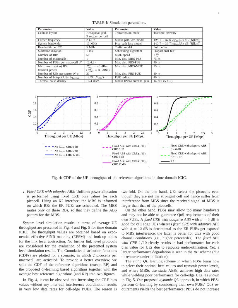
TABLE I: Simulation parameters.

Parameter Value Parameter ValueCellular layout Hexagonal grid, Transmission mode Transmit diversity

3 sectors per cellCarrier frequency 2 GHz Macro path loss model 128.1 + 37.6 log10(R) dB (R[km])System bandwidth 10 MHz Pico path loss model 140.7 + 36.7 log10(R) dB (R[km])Bandwidth per CC 5 MHz Traffic model Full bufferSubframe duration 1 ms Scheduling algorithm Proportional fairNumber of RBs 50 MUE speed 3 km

hNumber of macrocells 1 Min. dist. MBS-PBS 75 mNumber of PBSs per macrocellP {2,4,8} Min. dist. PBS-PBS 40 mMax. macro (pico) BS PM

max = 46 dBm Min. dist. MBS-MUE 35 mtransmit power (PP

max = 30 dBm)Number of UEs per sectorNUE 30 Min. dist. PBS-PUE 10 mNumber of hotspot UEsNhotspot ⌈2/3 ·NUE/P ⌉ PUE radius 40 mThermal noise density -174 dBm Macro (Pico) antenna gain 14 dBi (5 dBi)

0 1 2 3 2 2,5 30

0.2

0.4

0.6

0.8

1

CD

F

Throughput per UE [Mbps]

No ICIC; CRE 0 dB

No ICIC; CRE 6 dB

No ICIC; CRE 12 dB

0 1 2 3 2 2,5 30

0.2

0.4

0.6

0.8

1

Throughput per UE [Mbps]0 1 2 3 2 2,5 3

0

0.2

0.4

0.6

0.8

1

Throughput per UE [Mbps]

Fixed ABS with CRE (1/10);CRE 0 dB

Fixed ABS with CRE (1/10);CRE 6 dB

Fixed ABS with CRE (1/10);CRE 12 dB

Fixed CRE with adaptive ABS;β = 6 dB

Fixed CRE with adaptive ABS;β = 12 dB

RP

Fig. 4: CDF of the UE throughput of the reference algorithms in time-domain ICIC.

• Fixed CRE with adaptive ABS: Uniform power allocationis performed using fixed CRE bias values for eachpicocell. Using an X2 interface, the MBS is informedon which RBs the ER PUEs are scheduled. The MBSmutes only on these RBs, so that they define the ABSpattern for the MBS.

System level simulation results in terms of average UEthroughput are presented in Fig. 4 and Fig. 5 for time domainICIC. The throughput values are obtained based on expo-nential effective SINR mapping (EESM) and look-up tablesfor the link level abstraction. No further link level protocolsare considered for the evaluation of the presented systemlevel simulation results. The Cumulative distribution functions(CDFs) are plotted for a scenario, in which2 picocells permacrocell are activated. To provide a better overview, wesplit the CDF of the reference algorithms (except RP) andthe proposedQ-learning based algorithms together with theaverage best reference algorithms (and RP) into two figures.

In Fig. 4, it can be observed that increasing the CRE biasvalues without any inter-cell interference coordination resultsin very low data rates for cell-edge PUEs. The reason is

two-fold. On the one hand, UEs select the picocells eventhough they are not the strongest cell and hence suffer frominterference from MBS since the received signal of MBS islarger than that of the picocells.

On the other hand, PBSs may allow too many handoversand may not be able to guarantee QoS requirements of theirown PUEs. Afixed CRE with adaptive ABSwith β = 6 dB isgood for cell edge UEs whereasfixed CRE with adaptive ABSwith β = 12 dB is detrimental as the ER PUEs get exposedto MBS interference; the latter is better for UEs with goodchannel conditions (i.e., higher percentiles). Thefixed ABSwith CRE 1/10 clearly results in bad performance for eachbias value for UEs due to resource under-utilization. Yet, alarger performance degradation is seen in theRPscheme (dueto resource under-utilization).

The static QL learning scheme in which PBSs learn howto select their optimal beta values and transmit power levels,and where MBSs use static ABSs, achieves high data rateswhile yielding poor performance for cell-edge UEs, as shownin Fig. 5. Our proposeddynamic QLapproach, in which PBSsperformQ-learning by considering their own PUEs’ QoS re-quirements yields the best performance; PBSs do not increase

10

0 0,5 1 1,5 2 2,5 3 3,50

0.2

0.4

0.6

0.8

1C

DF

Throughput per UE [Mbps]

No ICIC; CRE 12 dBFixed CRE with adaptive ABSβ = 12 dB

RP

Fixed ABS with CRE (1/10);CRE 12 dBStatic QLDynamic QL

QL based

Fig. 5: CDF of the UE throughput of theQ-learning basedalgorithms in comparison with reference algorithms in time-domain ICIC.

the beta values, without considering QoS requirements of theirPUEs. On average, we obtain a gain of125% compared to theRP and 23% compared to theFixed CREwith β = 12 dB.The rationale is that the PBS informs the MBS which RBs areused for scheduling its ER PUEs, leading the MBS to reduceits power levels. Ultimately, the highest data rates are achievedby the proposeddynamicQL approach while not being worsethan any of the reference scheme. Finally, it is worth notingthat the proposed self-organization approach hinges on a loosecoordination in the form of RB indices used for ER PUEs’among macro and picocell tiers, and depending on traffic loadevery PBS adopts a different CRE bias value so as to optimizeits serving QoS requirements.

B. ABS Power Reduction

We also evaluate the performance of our proposed time do-main algorithms for the ABS ratios 3/10 and 7/10 with reducedMBS transmission power in a HetNet scenario consisting of2 picocells per macro sector. The ABS ratio describes theratio between subframes in which the MBS mutes and regulardownlink subframes in which transmission is performed byMBS. We plot in Fig. 6 (a) and (b) the, 50-th % and 5-th %UE throughput performance versus the ABS power reductionfor the static algorithms withfixed CREof 6 dB and 12 dB,Q-learning based and satisfaction based ICIC schemes. In allsimulations, the MBS transmission power reduction in ABSis {0, 6, 9, 12, 18, 24} dB.

Fig. 6 (a) plots the 50-th% UE throughput. It can be seenthat a mix of CRE bias values among picocells yields alwaysbetter average UE throughput in both ICIC techniques. It isobserved that low power ABS reduces the sensitivity to ABSratio. Reduced ABS ratio sensitivity is also observed in thesatisfaction based ICIC algorithm for low power ABS, whereasthe Q-learning based ICIC technique is almost insensitive tothe ABS ratio for all ABS power reduction values.

0 5 10 15 20 250.2

0.4

0.6

0.8

1

1.2

1.4

1.6

ABS power reduction [dB]

50−

th %

UE

thro

ughp

ut [M

bps]

CRE 6 dB ABS 30%CRE 6 dB ABS 70%CRE 12 dB ABS 30%CRE 12 dB ABS 70%Static QL ABS 30%Static QL ABS 70%Satisfaction ABS 30%Satisfaction ABS 70%

(a)

0 5 10 15 20 250

0.1

0.2

0.3

0.4

0.5

ABS power reduction [dB]

Cel

l−ed

ge U

E th

roug

hput

[Mbp

s]

CRE 6 dB ABS 30%CRE 6 dB ABS 70%CRE 12 dB ABS 30%CRE 12 dB ABS 70%Static QL ABS 30%Static QL ABS 70%Satisfaction ABS 30%Satisfaction ABS 70%

(b)

Fig. 6: (a) 50-th % UE throughput as a function of the ABSpower reduction in time domain ICIC, and (b) Cell-edge UEthroughput as a function of the ABS power reduction in timedomain ICIC.

The 5-th% UE throughput results are shown in Fig. 6 (b).For thefixed CREtechnique it can be observed that there existsan optimum ABS power setting for each combination of CREbias and ABS ratio; which is 6 dB to 9 dB power reduction.The corresponding optimum ABS ratios are 3/10 for 6 dB CREbias and 7/10 for 12 dB CRE bias. For a ABS ratio of 3/10,the proposed ICIC techniques perform very similarly, whilefor ABS ratio of 7/10 the satisfaction based ICIC algorithmoutperforms all cases. Especially, in the optimum region ofthefixed CREtechnique, the proposed learning algorithms cannotshow any enhancement, except the satisfaction based ICIC,with ABS ratio 7/10.

C. Impact of Number of Picocells

The impact of the number of picocells per macro sector isevaluated next. We consider 2, 4 and 8 picocells per macrosector and compare our results with the case when no picocellis activated. Figs. 7 (a) - (c) show the results for thestatic QL,dynamic QLand satisfactionbased algorithms, respectively.While we distinguish between picocell and macrocell averagecell throughput on the left y-axis, we depict the cell-edge (5-th%) UE throughput of all UEs in the system on the right

11

0

20

40

60

Ave

rage

cel

l−th

roug

hput

[Mbp

s]

Macro only 2 PBS 4 PBS 8 PBS0

200

400

600

800

1000

1200

Cel

l−ed

ge U

E th

roug

hput

[kbp

s]MUEPUECell−edge UE

(a)

0

20

40

60

Ave

rage

cel

l−th

roug

hput

[Mbp

s]

Macro only 2 PBS 4 PBS 8 PBS0

200

400

600

800

1000

1200

Cel

l−ed

ge U

E th

roug

hput

[kbp

s]MUEPUECell−edge UE

(b)

0

20

40

60

Ave

rage

cel

l−th

roug

hput

[Mbp

s]

Macro only 2 PBS 4 PBS 8 PBS0

200

400

600

800

1000

1200

Cel

l−ed

ge U

E th

roug

hput

[kbp

s]MUEPUECell−edge UE

(c)

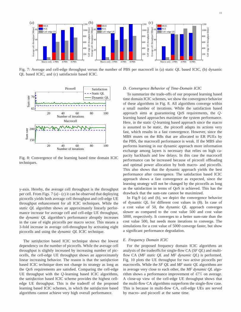
Fig. 7: Average and cell-edge throughput versus the number of PBS per macrocell in (a) static QL based ICIC, (b) dynamicQL based ICIC, and (c) satisfactoin based ICIC.

20 40 60 80 100

65

70

Picocell

Number of iterations

Sum

rat

e

20 40 60 80 100

150

200

Macrocell

Number of iterations

Sum

rat

e

SatisfactionStatic QLDynamic QL

Fig. 8: Convergence of the learning based time domain ICICtechniques.

y-axis. Hereby, the average cell throughput is the throughputper cell. From Figs. 7 (a) - (c) it can be observed that deployingpicocells yields both average cell throughput and cell-edge UEthroughput enhancement for all ICIC techniques. While thestatic QL algorithm shows an approximately linearly perfor-mance increase for average cell and cell-edge UE throughput,the dynamic QLalgorithm’s performance abruptly increasesin the case of eight picocells per macro sector. This means a3-fold increase in average cell-throughput by activating eightpicocells and using thedynamic QLICIC technique.

The satisfactionbased ICIC technique shows the lowestdependency on the number of picocells. While the average cellthroughput is slightly increased by increasing number of pic-ocells, the cell-edge UE throughput shows an approximatelylinear increasing behavior. The reason is that thesatisfactionbased ICIC technique does not change its strategy as long asthe QoS requirements are satisfied. Comparing the cell-edgeUE throughput with theQ-learning based ICIC algorithms,the satisfactionbased ICIC scheme provides the highest cell-edge UE throughput. This is the tradeoff of the proposedlearning based ICIC schemes, in which thesatisfactionbasedalgorithms cannot achieve very high overall performance.

D. Convergence Behavior of Time-Domain ICIC

To summarize the trade-offs of our proposed learning basedtime domain ICIC schemes, we show the convergence behaviorof these algorithms in Fig. 8. All algorithms converge withina small number of iterations. While the satisfaction basedapproach aims at guaranteeing QoS requirements, theQ-learning based approaches maximize the system performance.Here, in the staticQ-learning based approach since the macrois assumed to be static, the picocell adapts its actions veryfast, which results in a fast convergence. However, since theMBS mutes on the RBs that are allocated to ER PUEs bythe PBS, the macrocell performance is weak. If the MBS alsoperforms learning in our dynamic approach more informationexchange among layers is necessary that relies on high ca-pacity backhauls and low delays. In this case the macrocellperformance can be increased because of picocell offloadingand optimal power allocation by both macro- and picocells.This also shows that the dynamic approach yields the bestperformance after convergence. The satisfaction based ICICapproach shows a fast convergence as expected, since thelearning strategy will not be changed by the picocells as longas the satisfaction in terms of QoS is achieved. This has thedrawback that the sum-rate cannot be maximized.

In Fig.9 (a) and (b), we depict the convergence behaviorof dynamic QL for different cost values in (8). In case ofa cost value of 50, the dynamic QL approach convergesslower as compared to the cost value 500 and cost value5000, respectively. It converges to a better sum-rate than thecost value 500, but needs more iterations to converge. Thesimulations for a cost value of 5000 converge faster, but showa significant performance degradation.

E. Frequency Domain ICIC

For the proposed frequency domain ICIC algorithms ananalysis of the tradeoffs for single-flow CA (SF QL) and multi-flow CA (MF static QL and MF dynamic QL) is performed.Fig. 10 plots the UE throughput for two active picocells permacrocells. While theSF QLandMF static QLalgorithms arein average very close to each other, theMF dynamic QLalgo-rithm shows a performance improvement of47% on average.A close-up view of the cell-edge UE throughput shows thatthe multi-flow CA algorithms outperform the single-flow case.This is because in multi-flow CA, cell-edge UEs are servedby macro- and picocell at the same time.

12

0 20 40 60 80 100140

150

160

170

180

190

200

210

220

Number of iterations

Sum

−ra

te [M

bps]

Dynamic QL − 50Dynamic QL − 500Dynamic QL − 5000

(a)

0 20 40 60 80 10064

65

66

67

68

69

70

Number of iterations

Sum

−ra

te [M

bps]

Dynamic QL − 50Dynamic QL − 500Dynamic QL − 5000

(b)

Fig. 9: Convergence of the sum-rate of dynamic QL for different cost values for (a) macrocells, and (b) picocells.

0 2 4 6 8 10 120

0.1

0.2

0.3

0.4

0.5

0.6

0.7

0.8

0.9

1

Throughput per UE [Mbps]

CD

F

0 0.02 0.04 0.06 0.08 0.1 0.120

0.02

0.04

Cell−edge UE throughput

MF−Macro+Pico LearningMF−Pico LearningSF

Fig. 10: CDF of the UE throughput forthe single-flow and multi-flow ICIC learningalgorithm for2 picocells per macrocell.

2 3 4 5 6 7 8

100

150

200

250

300

350

Tot

al th

roug

hput

[Mbp

s]

Number of picocells

0

50

100

150

200

250

Cel

l−ed

ge U

E th

roug

hput

[kbp

s]

0

50

100

150

200

250

0

50

100

150

200

250MF dynamic QLMFdynamic QL (cell−edge)MF static QLMF static QL (cell−edge)SF QLSF QL (cell−edge)

Fig. 11: Total-throughput and cell edge throughput versus thenumber of picocells in frequency domain ICIC.

The behavior of the learning based frequency domain ICICalgorithms when increasing the number of picocells per macro-cell is depicted in Fig. 11. Here, the solid curves belong tothe left ordinate showing the total throughput and the dashedcurves refer to the right ordinate reflecting the cell-edge UEthroughput. It can be observed that theMF dynamic QLalgorithm outperforms the other algorithms in terms of totalthroughput while theSF QL algorithm is slightly better thanthe MF static QLalgorithm for less number of picocells (andvice versa for large numbers). TheSF QL algorithm showsthe lowest performance for cell-edge UE throughput. It canbe concluded that cell-edge UEs benefit more from multi-flowCA than from single-flow CA. Interestingly, it can be observedthat theMF static QLalgorithm outperforms theMF dynamicQL for larger number of picocells. This is because in the two-player case, the MBS cannot fully adapt to the ICIC strategiesof all PBSs in the system, when the number of PBS large.

VII. C ONCLUSION

In this paper, we investigated the performance of two-tierHetNets in which decentralizedQ-learning and satisfactionbased procedures were proposed for both time and frequencydomain ICIC. The proposed approach in which PBSs optimallylearn their optimal CRE bias and transmit power allocation,isshown to outperform the static ICIC solutions in time domain.While the satisfaction based approach improves the 5% UEthroughput and guarantees QoS requirements, the dynamicQ-learning based approach increases network capacity relyingon high capacity backhauls. In the frequency domain case,the single and multi-flow CA demonstrate that the dynamicQ-learning based multi-flow approach outperforms the single-flow case. Improvements of60% in the total throughput and240% in the cell-edge UE throughput are obtained in thecase of multi-flow dynamicQ-learning with 8 picocells permacrocell. The proposed algorithms can be extended to anK-

13

tier HetNet. However, in this case it has to be defined whichplayer selects first its primary CC and how coordination isperformed. In our future work, we will extend the currentframework to the non-ideal backhaul considering delays.

VIII. A PPENDIX

A. Proof of Proposition - 1

Before presenting the proof of convergence to one of theequilibrium of the game, we define the following hypothesisof the gameG = {P , {Ap}p∈P , {up}p∈P}:

1) The gameG = {P , {Ap}p∈P , {up}p∈P} has at least oneequilibrium in pure strategies.

2) For all p ∈ P , it holds that∀ap′ 6=p ∈ Ap′ 6=p, the setup(p

′ 6= p) is not empty.3) The setsP and{Ap}p∈P are finite.

The first hypothesis ensures that the learning problem is well-posed, in which the players are assigned a feasible task. Thesecond hypothesis refers to the fact that, each player is alwaysable to find a transmit configuration with which it can beconsidered satisfied, given the transmit configuration of all theother players. The third hypothesis is considered in order toensure that our algorithm is able to converge in finite time.

The proof of the proposition in section IV-C follows fromthe fact that the conditionπp

r,np(tk) > 0 implies that every

action profile will be played at least once with nonzero proba-bility during a large time interval. Because of the assumptionthat at least on SE exists, this action profile will be playedat least once. From equation (14), it follows that once anequilibrium is played, no player changes its current action.Thus, convergence is observed.

B. Memory and Computational Requirements

We present in what follows the memory and computationalrequirements of the proposedQ-learning and satisfactionbased learning approaches when considering digital signalprocessors (DSPs). A theoretical estimation of the operationalrequirements for the mathematical operations required in thelearning approaches is presented, assuming that every basicDSP instruction takes one DSP cycle [42].

The memory requirements of learning methods are directlyrelated to the knowledge representation mechanisms of agents.In Q-learning, the agent’s knowledge is represented byQ-tables which have the size of|S| × |A|. In the presentedtwo-player game this results in a memory requirement of(|Sm| × |Am|+ |Sp| × |Ap) · R memory units per game andover all RBs. In case of satisfaction based learning, theagent’s knowledge is represented by the probability distribu-tion over all actions. This results in a memory requirement of(1× |Ap|)·R memory units. Hence, satisfaction based learningrequires significantly less memory thanQ-learning.

The presented computational analysis does not take intoaccount the compiler optimizations and the ability of DSPsto execute various instructions per clock cycle. Therefore,the analysis provides an upper bound for the computationalresources that are needed by the algorithms [42]. The com-putational requirements of the learning methods are givenby the operations they have to execute in order to fulfill

TABLE II: Computational requirement forQ-learning andsatisfaction based learning.

Operations Required instructions forQ-learning satisfaction based learning

Identification of current and 2 -next state in the Q-tableMemory access 2 · |A| 2 · |A|Comparison 2 · (|A| − 1) 2Sum 3 2Multiplication 2 2Storage 1 1Total number of operations 4|A|+ 6 2|A|+ 7

0 10 20 30 40 500

100

200

300

Req

uire

d in

stru

ctio

ns

Total number of actions |A|

Q−learningSatisfaction

Fig. 12: Required instructions of learning approaches fordifferent number of actions.

the representation of the acquired knowledge in one learningiteration. Table II summarizes the total number of operationsrequired per RB for oneQ-learning iteration through equation(9). In satisfaction based learning, one learning iteration isbased on the probability update function in equation (13),which is only updated if the system is not satisfied. The thirdcolumn of Table II summarizes for this case the total numberof operations required per RB. The total number of operationsrequired for Q-learning and satisfaction based learning is4|A|+6 and2|A|+7, respectively. Since|A| > 0, satisfactionbased learning requires less operations thanQ-learning. Fig.12 depicts the required instructions over different numberofactions for both learning approaches.

IX. A CKNOWLEDGMENT

This work is supported by the SHARING project under theFinland grant 128010 and was supported in part by the U.S.National Science Foundation under the grant CNS-1406968.

REFERENCES

[1] A. Ghosh, R. Ratasuk, B. Mondal, N. Mangalvedhe and T. Thomas, “LTE-Advanced: Next-Generation Wireless Broadband Technology,” IEEEWireless Comm. Mag., vol. 17, no. 3, pp. 1022, Jun. 2010.

[2] A. Damnjanovic, J. Montojo, W. Yongbin, J. Tingfang, L. Tfao andM. Vajapeyam, “A Survey on 3GPP Heterogeneous Networks,”IEEEWireless Comm. Mag., vol. 18, no. 3, pp. 10-21, Jun. 2011.

[3] S. Hamalainen, H. Sanneck, C. Sartori (editors), “LTE Self-OrganisingNetworks (SON),”John Wiley & Sons Ltd, First Edition, 2012.

[4] C. U. Castellanos et. al.,“Performance of uplink fractional power controlin UTRAN LTE,” in Proc. IEEE Vehicular Technology Conference (VTC),Singapore, May 2008.

[5] D. Lopez-Perez, I. Guvenc, G. de la Roche, M. Kountouris,T. Q. S. Quekand J. Zhang, “Enhanced Inter-Cell Interference Coordination Challengesin Heterogeneous Networks,”IEEE Wireless Comm. Mag., vol. 18, no 3,pp. 22-30, Jun. 2011.

14

[6] D. Lopez-Perez, X. Chu and I. Guvenc, “On the Expanded Region ofPicocells in Heterogeneous Networks,”IEEE Journal of Selected Topicsin Signal Processing, vol. 6, no. 3, pp. 281-294, Mar. 2012.

[7] I. Guvenc, J. Moo-Ryong, I. Demirdogen, B. Kecicioglu and F. Watanabe,“Range Expansion and Inter-Cell Interference Coordination (ICIC) forPicocell Networks,” in Proc. IEEE Vehicular Technology Conference(VTC Fall), San Francisco, CA, Dec. 2011.

[8] S. Brueck, “Heterogeneous Networks in LTE-Advanced,”in Proc. IEEEInternational Symposium on Wireless Communication System(ISWCS),Aachen, Germany, Nov. 2011.

[9] R. Madan, J. Borran, A. Sampath, N. Bhushan, A. Khandekarand J.Tingfang, “Cell Association and Interference Coordination in Heteroge-neous LTE-A Cellular Networks,”IEEE Journal on Selected Areas inCommunications, vol. 28, no. 9, pp. 1479 - 1489, Dec. 2010.

[10] A. Damnjanovic, J. Montojo, C. Joonyoung, J. Hyoung, Y.Jin and Z.Pingping, “UE’s Role in LTE Advanced Heterogeneous Networks,” IEEEWireless Comm. Mag., vol. 50, no. 2, pp. 164-176, Feb. 2012.

[11] S. Mukherjee and I. Guvenc, “Effects of Range Expansionand Interfer-ence Coordination on Capacity and Fairness in Heterogeneous Networks,”in Proc. IEEE Asilomar Conf. on Signals, Systems and Computers, PacificGrove, CA, Nov. 2011.

[12] M. Shirakabe, A. Morimoto, and N. Miki, “Performance Evaluationof Inter-Cell Interference Coordination and Cell Range Expansion inHeterogeneous Networks for LTE-Advanced Downlink,”in Proc. IEEEInternational Symposium on Wireless Communication System(ISWCS),Aachen, Germany, Nov. 2011.

[13] A. Merwaday, S. Mukherjee, and I. Guvenc, “On the capacity analysisof HetNets with range expansion and eICIC,” in Proc.IEEE GlobalTelecommun. Conf. (GLOBECOM), Atlanta, GA, Dec. 2013.

[14] A. Merwaday, S. Mukherjee, and I. Guvenc, “HetNet capacity withreduced power subframes,” in Proc.IEEE Wireless Commun. NetworkingConf. (WCNC), Istanbul, Turkey, Apr. 2014.

[15] A. Merwaday, S. Mukherjee, and I. Guvenc, “Capacity analysis of LTE-Advanced HetNets with reduced power subframes and range expansion,”CoRR, vol. abs/1403.7802, 2014.

[16] 3GPP R1-113806, “Performance Study on ABS with ReducedMacroPower,” Panasonic, San Francisco, USA, Nov. 2011.

[17] 3GPP, R1-113118, “Performance Evaluation of Cell Range Expansion inCombination with ABS Ratio Optimization,” Panasonic, Zhuhai, China,Oct. 2011.

[18] 3GPP TR 36.814, “Evolved Universal Terrestrial Radio Access (EU-TRA); Further advancements for E-UTRA Physical Layer Aspects,”V9.0.0, 2010.

[19] 3GPP TR 36.839, “Evolved Universal Terrestrial Radio Access (EU-TRA); Mobility Enhancements in Heterogeneous Networks,” V11.1.0,2012.

[20] 3GPP TS 25.211, “Physical Channels and Mapping of Transport Chan-nels onto Physical Channels (FDD)(Release 11),” V11.3.0, 2013.

[21] 3GPP TS 25.212, “Multiplexing and Channel Coding (FDD)(Release11),” V11.4.0, 2012.

[22] 3GPP TS 25.213, “Spreading and Modulation (FDD)(Release 11),”V11.4.0, 2012.

[23] 3GPP TS 25.214, “Physical Layer Procedures (FDD)(Release 11),”V11.5.0, 2013.

[24] H.-S. Jo, Y. J. Sang, P. Xia, J. G. Andrews, “Heterogeneous cellularnetworks with flexible cell association: A comprehensive downlink SINRanalysis”, IEEE Transactions on Wireless Communications, vol. 10, no.11, pp. 3484-3495, 2012.

[25] S. Singh, H. S. Dhillon, J. G. Andrews, “Offloading in HeterogeneousNetworks: Modeling, Analysis, and Design Insights”,IEEE Transactionson Wireless Communications, vol. 12, no. 5, pp. 2484-2497, 2013.

[26] M. E. Harmon and S. S. Harmon, “Reinforcement Learning:A Tutorial,”2000.

[27] 3GPP RP-100383, “New work item proposal: Enhanced ICICfor non-CA Based Deployments of Heterogeneous Networks for LTE,” CMCC,Vienna, Austria, Mar. 2010.

[28] 3GPP R1-104968, “Summary of the Description of Candidate eICICSolutions,” Madrid, Spain, Aug. 2010.

[29] 3GPP R1-111031, “On advanced UE MMSE receiver modelinginsystem simulations,” Nokia Siemens Networks, Taipei, Taiwan, Feb. 2011.

[30] NTT DOCOMO, Inc., “Requirements, Candidate Solutions,and Technology Roadmap for LTE Rel. 12 Onward,”3GPP Workshop on Release 12 and Onwards, Jun. 2012.http://www.3gpp.org/ftp/workshop/2012-06-1112RANREL12/Docs/RWS-120010.zip

[31] H. Ishii, Y. Kishiyama, and H. Takahashi, “A Novel Architecture forLTE-B: C-plane/U-plane Split and Phantom Cell Concept,”in Proc. IEEE

Globecom - International Workshop on Emerging Technologies for LTE-Advanced and Beyond-4G, 2012.

[32] Z. Han, D. Niyato, W. Saad, T. Basar, and A. Hjorungnes. “GameTheory in Wireless and Communication Networks: Theory, Models, andApplications”. Cambridge University Press, Oct. 2011.

[33] M. Simsek, M. Bennis, and A. Czylwik, “Coordinated BeamSelectionin LTE-Advanced HetNets: A Reinforcement Learning Approach,”IEEEGlobecom Workshops: The 4th IEEE International Workshop onHetero-geneous and Small Cell Networks (HetSNets), Dec. 2012

[34] A. Galindo-Serrano and L. Guipponi,“Distributed Q-learning for In-terference Control in OFDMA-based Femtocell Networks,”IEEE 71stVehicular Technology Conference, Taipei, Taiwan, May 2010.

[35] M. Simsek, A. Galindo-Serrano, A. Czylwik and L. Giupponi, “Im-proved Decentralized Q-learning Algorithm for Interference Reductionin LTE-Femtocells,” in Proc. Wireless Advanced (WiAd), London, UK,Jun. 2011.

[36] X.Lin, J. G. Andrews and A. Ghosh, “Modeling, Analysis and Designfor Carrier Aggregation in Heterogeneous Cellular Networks,” IEEETransactions on Communications, vol. 61, no. 9, pp. 4002-4015, Sept.2013.

[37] S. Ross and B. Chaib-draa, “Satisfaction Equilibrium :AchievingCooperation in Incomplete Information Games,”in Proc. 19th CanadianConf. on Artificial Intelligence, Quebec, CA, June 2006.

[38] S. Ross and B. Chaib-draa, “Learning to Play a Satisfaction Equilib-rium,” in Proc. Workshop on Evolutionary Models of Collaboration, India,Jan. 2007.

[39] 3GPP TS 36.213, “Evolved Universal Terrestrial Radio Access (E-UTRA); Physical layer procedures ”, V12.2.0, 2014.

[40] C. Mehlfhrer, M. Wrulich, J. C. Ikuno, and D. Bosanska, “Simulatingthe long term evolution physical layer”,European Signal ProcessingConference, EURASIP, pp. 1471-1478, 2009.

[41] M. Simsek, T. Akbudak, B. Zhao, and A. Czylwik, “An LTE-femtocellDynamic System Level Simulator,”in Proc. International ITG Workshopon Smart Antennas (WSA), 2010,

[42] A. Galindo-Serrano, “Self-organized Femtocells: a Time DifferenceLearning Approach,” Ph.D. dissertation, Universitat Politecnica deCatalunya (UPC), Barcelona, Spain, 2013.

[43] H. S. Dhillon, R. K. Ganti, F. Baccelli and J. G. Andrews,“Modelingand Analysis of K-Tier Downlink Heterogeneous Cellular Networks”,IEEE Journal on Selected Areas in Communications, vol. 30, no. 3, pp.550-560, Apr. 2012.