Damage Identification in Elastic Suspended Cables through Frequency Measurement
Upload
khangminh22Category
view
0download
0
#
Time and
Frequency Measurement &
;r
Edited by Christine Hackman and
Donald B. Sullivan
American Association of Physics Teachers
Time and Frequency Measurement 0 1996 American Association of Physics Teachers
American Association of Physics Teachers One Physics Ellipse College Park, MD 20740-3845
ISBN 0-917853-67-9
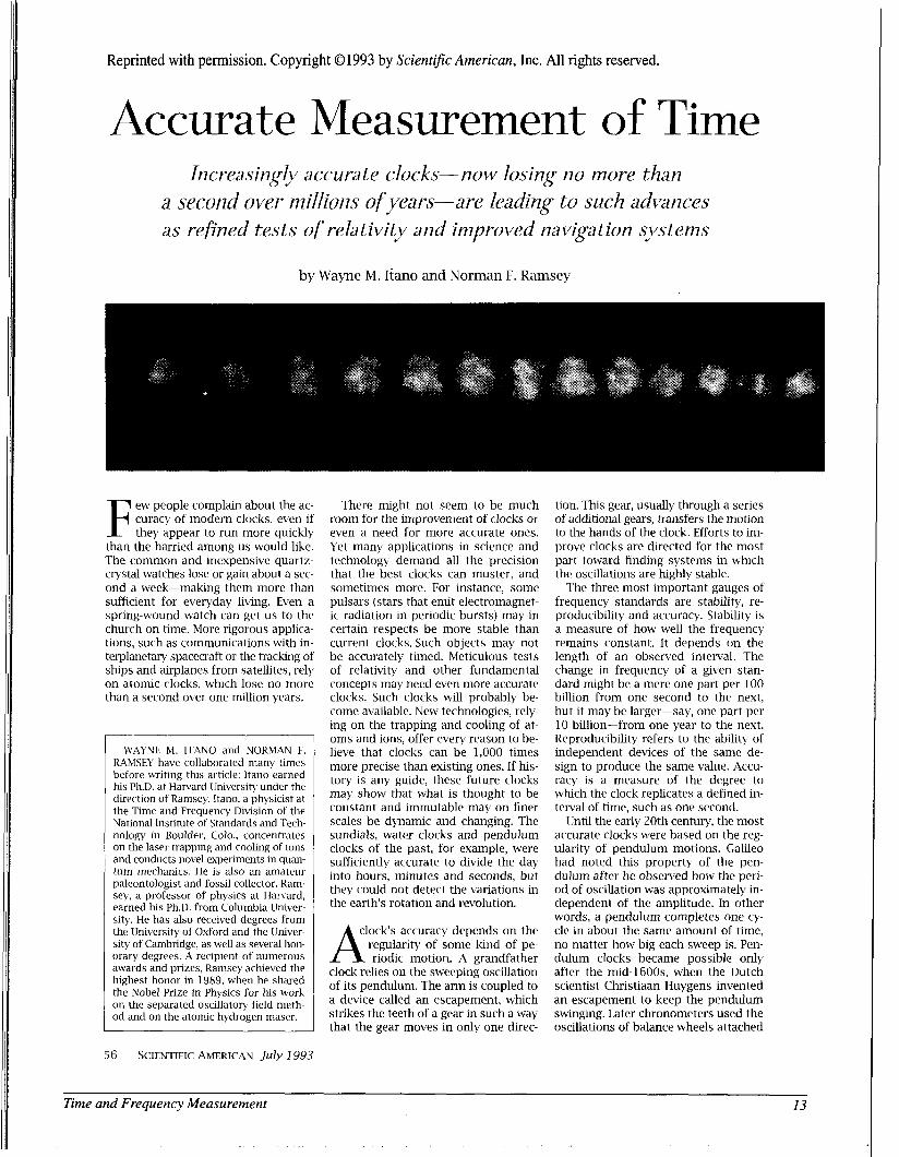
On the Cover The repeated image appearing on the background of the cover shows mercury ions in a linear electromagnetic trap. This string of trapped 199 Hg ions is being studied as a possible atomic frequency standard. The ions are illuminated with laser radiation at 194 nm and fluoresce to produce this image in an ultraviolet imaging system. Studies involving both microwave and ultraviolet transitions indicate strong potential for higher-accuracy frequency standards. The gaps in the string result from the presence of impurity ions, most likely other isotopes of mercury that do not fluoresce at the same frequency as does 199 Hg.
Photo appears courtesy of the National Institute of Standards and Technology (NIST).
Cover design by Rebecca Heller Rados.
Contents Resource Letter TFM-1: Time and Frequency Measurement
Christine Hackman and Donald B. Sullivan. . . . . . . . . . . . . . . . . . . . . . . . . . . . . . . . . . . . . . . . . . . . . . 1
Accurate Measurement of Time WM.ItanoandN. ERamsey . . . . . . . . . . . . . . . . . . . . . . . . . . . . . . . . . . . . . . . . . . . . . . . . . . . . . . . . . 13
The Method of Successive Oscillatory Fields N.ERamsey . . . . . . . . . . . . . . . . . . . . . . . . . . . . . . . . . . . . . . . . . . . . . . . . . . . . . . . . . . . . . . . . . . . . . . 21
Trapped Ions, Laser Cooling, and Better Clocks D.J. Wineland . . . . . . . . . . . . . . . . . . . . . . . . . . . . . . . . . . . . . . . . . . . . . . . . . . . . . . . . . . . . . . . . . . . . 27
Hydrogen-Maser Principles and Techniques D. Kleppnel; H.C. Berg, S.B. Crampton, N.E Ramsey, R.EC. Vessot, H.E. Peters, and J. Vanier . . . . 33
Environmental Sensitivities of Quartz Oscillators EL. Walls and J.-J. Gagnepain. . . . . . . . . . . . . . . . . . . . . . . . . . . . . . . . . . . . . . . . . . . . . . . . . . . . . . .45
Optical Frequency Measurements D.A. Jennings, K.M. Evenson, and D.J.E. Knight. . . . . . . . . . . . . . . . . . . . . . . . . . . . . . . . . . . . . . . . .54
Time Generation and Distribution D.B.SullivanandJ. Levine . . . . . . . . . . . . . . . . . . . . . . . . . . . . . . . . . . . . . . . . . . . . . . . . . . . . . . . . . . 66
The BIPM and the Accurate Measurement of Time ~ J . Q u i n n . . . . . . . . . . . . . . . . . . . . . . . . . . . . . . . . . . . . . . . . . . . . . . . . . . . . . . . . . . . . . . . . . . . . . . . 75
GPS Time Transfer W Lewandowski and C. Thomas. . . . . . . . . . . . . . . . . . . . . . . . . . . . . . . . . . . . . . . . . . . . . . . . . . . . . .87
A Frequency-Domain View of Time-Domain Characterization of Clocks and Time and Frequency Distribution Systems
D.W Allan, M.A. Weiss, and J.L. Jespersen . . . . . . . . . . . . . . . . . . . . . . . . . . . . . . . . . . . . . . . . . . . . . 97
Characterization Synchronization and Relativity
G.M.R. Winkler . . . . . . . . . . . . . . . . . . . . . . . . . . . . . . . . . . . . . . . . . . . . . . . . . . . . . . . . . . . . . . . . . . 109
Applications of Highly Stable Oscillators to Scientific Measurements R.EC. Vessot . . . . . . . . . . . . . . . . . . . . . . . . . . . . . . . . . . . . . . . . . . . . . . . . . . . . . . . . . . . . . . . . . . . . 120
Scientific Measurements Time and Frequency in Fundamental Metrology
B.WPetley . . . . . . . . . . . . . . . . . . . . . . . . . . . . . . . . . . . . . . . . . . . . . . . . . . . . . . . . . . . . . . . . . . . . . 134
RESOURCE LElTER Roger H. Stuewer, Editor School of Physics and Astronomy, 116 Church Street Universiry of Minnesota, Minneapolis, Minnesota 55455
This is one of a series of Resource Letters on different topics intended to guide college physicists, astronomers, and other scientists to some of the literature and other teaching aids that may help improve course content in specified fields. [The letter E after an item indicates elementary level or material of general interest to persons becoming informed in the field. The letter I, for intermediate level, indicates material of somewhat more specialized nature; and the letter A, indicates rather specialized or advanced material.] No Resource letter is meant to be exhaustive and complete; in time there may be more than one letter on some of the main subjects of interest. Comments on these materials as well as suggestions for future topics will be welcomed. Please send such communications to Professor Roger H. Stuewer, Editor, AAPT Resource Letters, School of Physics and Astronomy, 116 Church Street SE, University of Minnesota, Minneapolis, MN 55455.
Resource Letter: TFM-1: Time and frequency measurement Christine Hackman and Donald B. Sullivan Time and Frequency Division, National Institute of Standards and Technology, Boulder, Colorado 80303
(Received 26 August 1994; accepted 5 December 1994)
This Resource Letter is a guide to the literature on time and frequency measurement. Journal articles and books are cited for the following topics: frequency standards; methods of characterizing performance of clocks and oscillators; time scales, clock ensembles, and algorithms; international time scales; frequency and time distribution; and applications. [The letter E after an item indicates elementary level or material of general interest. The letter I, for intermediate level, indicates material of somewhat more specialized nature, and the letter A indicates rather specialized or advanced material. The designations E/I and I/A are used to indicate that the article contains material at both levels, so that at least part of the article is written at the lower of the two levels.]
I. INTRODUCTION
Archeological evidence indicates that since prehistoric times man has been devising progressively better means of keeping track of the passage of time. In the earliest stages this involved observation of the apparent motion of the sun, but finer subdivision of the day later involved devices such as water clocks, hourglasses, and calibrated candles. After long development with many variations, mechanical methods for keeping time, in the form of pendulum clocks, achieved excellent precision (a fraction of a second per day). How- ever, with the invention of the two-pendulum clock in 1921 by William Hamilton Shortt, the practical performance limit of such mechanical clocks was reached. The distinction be- tween frequency standard and clock (between frequency and time) is easily recognized in the pendulum clock. The con- stant frequency of oscillation of the pendulum constitutes a frequency standard. The mechanism used to count the ticks and display their accumulation as seconds, minutes, hours, days, and years converts this frequency standard into a clock.
The modern era of timekeeping began with the develop-
306 Am. J. Phys. 63 (4), April 1995
ment of the quartz crystal oscillator. In a 1918 patent appli- cation, Alexander M. Nicholson disclosed a piezoelectric crystal as the control element in a vacuum tube oscillator. The first clock controlled by a quartz crystal was subse- quently developed in 1927 by Joseph W. Horton and Warren A. Marrison. Since the introduction of the quartz oscillator, the performance of frequency standards has advanced by many orders of magnitude, and industry and science have come to rely on the timing made possible by them.
Many modern technological applications require that geo- graphically distributed systems have the same time (synchro- nization) or run at the same rate (syntonization). Thus, an important consideration in time and frequency measurement has been the precise transfer of timing between separated stations. This has led to an interplay between the develop- ment of the two key technologies, (1) frequency standards and clocks and (2) methods of time and frequency transfer. Comparisons between early quartz timepieces were accom- plished with adequate precision using signals transmitted by terrestrial radio waves.
Quartz crystal oscillators remained at the performance
306
Time and Frequency Measurement I
forefront for only a short time. In 1949, the atomic- timekeeping era began with the construction of the first atomic clock. This standard, based on a resonance in the ammonia molecule, was constructed at the National Bureau of Standards in a project led by Harold Lyons. The ammonia standard was quickly superseded by the cesium-beam fre- quency standard that forms the current basis for defining the second.
Atomic standards progressed rapidly in accuracy and sta- bility through the 1950s and 1960s. By the mid-1970s the best atomic standards were realizing the definition of the second with an uncertainty of allowing timekeeping uncertainty of 10 ns over the period of one day. But the existing methods of time transfer could not easily support comparison of performance between geographically sepa- rated devices. At the time, the most convenient method for comparing standards over long distances involved LORAN-C navigation signals. Separated stations could si- multaneously monitor the same highly stable LORAN-C broadcast to achieve comparison of the standards, but time comparison errors as large as 500 ns were observed. Clocks could be compared more precisely using portable atomic clocks, but since this involved flying a fully operational clock from one laboratory to another, it was expensive and impractical to do more often than a few times per year.
The most recent thrust forward was fostered by two devel- opments. More precise time transfer using GPS satellites in a “common-view” mode was developed in the early 1980s. This provided the means for precise comparisons of stan- dards constructed in different laboratories. During this same period, physicists were developing methods for using lasers to control the atomic states and the motions of atoms and ions. These new methods offer promise of dramatic advances in accuracy of atomic standards, and evidence of such ad- vances is just beginning to appear. With these new concepts for improved standards and the technology required to com- pare the performance of separated standards, physicists have gained new motivation to build better atomic clocks, and work is progressing rapidly in many laboratories.
Significant improvements have been made in cesium- beam standards by replacing magnetic state selection and state detection with optical selection and detection. But still greater advances will come with the practical realization of entirely new concepts that have been demonstrated in the laboratory. Radiatively cooled ions stored in electromagnetic traps provide the ultimate answer to Doppler-shift problems, but the atomic-fountain standard that uses laser-cooled neu- tral atoms offers substantial promise as well.
The pace of improvement in atomic standards, an increase in accuracy by a factor of nearly 10 every 7 years, is ex- pected to continue. The most advanced concepts promise ac- curacy improvement of three to four orders of magnitude. Frequency is already the most accurately realized unit of measure, so it is surprising to find such great potential for improvement. Since even modest frequency accuracy is of- ten well beyond the accuracy with which other measure- ments are made, other quantities are often converted (trans- duced) to frequency to achieve better precision, resolution, and ease of measurement. Length and voltage are examples of units now based on frequency measurements.
The atomic definition of the second has provided the means to improve frequency accuracy, but in many applica- tions the only requirement is for frequency stability. In this case, what matters is that two or more oscillators stay at the
307 Am. J. Phys., Vol. 63, No. 4, April 1995
same, although not necessarily accurate, frequency. While high accuracy ensures good relative stability, it is not essen- tial for it. Thus, in responding to application requirements, developers of atomic and quartz devices have often empha- sized frequency stability rather than frequency accuracy.
Time plays a major role in physical theory, and better clocks have provided physicists with improved means for testing their theories. Over the last 45 years, progress in atomic clock technology has been driven more by scientific than by industrial requirements, but clever engineers have taken good advantage of the advancing technology. A good example is the exceptional navigational accuracy provided by the Global Positioning System (GPS). This accuracy is critically dependent on atomic-clock technology. Other areas benefitting from this technology include telecommunications and electrical-power distribution.
In this resource letter we address time and frequency stan- dards and measurement methods, the special statistical meth- ods used for handling noise in clocks and oscillators, and the distribution of time and frequency signals. Signal distribu- tion is included because a large fraction of measurements made in this field rely on timing signals transmitted from central sources to the points of measurement. Articles in many of the areas covered by this resource letter are pub- lished in well-known journals, but in some instances we are forced to refer to papers presented at conferences, the pro- ceedings of which are not widely available in libraries. In these instances, we provide an address where the proceed- ings can be obtained. In our selection of articles we recog- nize that biases will be evident, and we apologize for these biases. There are a great number of papers that could have been cited, but are not because of space limitations.
11. JOURNALS
The majority of papers on time and frequency topics are
IEEE Transactions on Ultrasonics, Ferroelectrics and
IEEE Transactions on Instrumentation and Measurement Journal of Applied Physics Metrologia Physical Review Physical Review Letters Physics Today Proceedings of the IEEE Radio Science Science Scientific American Four special issues of IEEE journals (the first four refer-
ences below) have been devoted exclusively to time and fre- quency topics. Many of the invited articles in these issues were written as reviews of specialized subtopics and are therefore very readable. l b o other special issues on the broader subject of radio measurement methods and standards are also included because they contain a number of useful and easy-to-read articles on time and frequency.
1. Time and Frequency, Special Issue of Proc. IEEE
2. Frequency Control, Special Issue of IEEE Trans.
3. Time and Frequency, Special Issue of Proc. IEEE
4. Frequency Stability, Special Issue of Proc. IEEE
found in the following journals:
Frequency Control
79(7) (1991).
UFFC UFFC-34(6) (1987).
60(5) (1972).
54(2) (1966).
C. Hackman and D. B. Sullivan 307
2 l ime and Frequency Measurement
__ _ _ ~ ~- __ .
5. Radio Measurement Methods and Standards, Spe-
6. Radio Measurement Methods and Standards, Spe- cial Issue of Proc. IEEE 74(1) (1986).
cial Issue of Proc. IEEE 55(6) (1967).
111. CONFERENCE PROCEEDINGS
Conference proceedings in this field contain a good mix of specialized articles and an occasional review article. The fol- lowing series of conferences contain the largest concentra- tion of time-and-frequency papers.
A. IEEE International Frequency Control Symposium
The IEEE International Frequency Control Symposium is the best-known conference in the field. It was previously known as the Annual Symposium on Frequency Control. Through 1994, there have been 48 conferences in this series. The proceedings of the last 12 of these conferences are avail- able from IEEE, 445 Hoes Lane, Piscataway, NJ 08854. The most recent eight and three others cited later are listed here.
7.1994 IEEE Int. Freq. Control Symp., IEEE Catalogue
8.1993 IEEE Int. Freq. Control Symp., IEEE Catalogue
9.1992 IEEE Int. Freq. Control Symp., IEEE Catalogue
10. 45th Annu. Symp. Freq. Control, IEEE Catalogue
11. 44th Annu. Symp. Freq. Control, IEEE Catalogue
12. 43rd Annu. Symp. Freq. Control, IEEE Catalogue
13. 42nd Annu. Symp. Freq. Control, IEEE Catalogue
14. 41st Annu. Symp. Freq. Control, IEEE Catalogue
15. 38th Annu. Symp. Freq. Control, IEEE Catalogue
16. 36th Annu. Symp. Freq. Control, Document No. AD-A130811, available from National Technical In- formation Service, 5285 Port Royal Road, Sills Build- ing, Springfield, VA 22161 (1982).
17. 35th Annu. Symp. Freq. Control, Document No. AD-A110870, available from same source as Ref. 16 (1981).
No. 94CH3446-2 (1994).
NO. 93CH3244-1 (1993).
NO. 92CH3083-3 (1992).
NO. 91CH2965-2 (1991).
NO. 90CH2818-3 (1990).
NO. 89CH2690-6 (1989).
NO. 88CH2588-2 (1988).
NO. 87CH2427-3 (1987).
NO. 84CH2062-8 (1984).
B. European Frequency and Time Forum (EFTF)
This is the major European conference in the field. Through 1994 there have been eight meetings in this series. Printed proceedings are not readily available in libraries, but can be obtained from the EFTF Secretariat at: FSRM, Rue de I’Orangerie 8, CH-2000, Neuchitel, Switzerland. Three vol- umes cited later are:
18. Proc. 7th European Freq. and Time Forum (1993). 19. Proc. 5th European Freq. and Time Forum (1991). 20. Proc. 4th European Freq. and Time Forum (1990).
C. Conference on Precision Electromagnetic Measurements (CPEM)
This biennial international conference covers a wide range of measurement topics, but includes a substantial number of useful articles on time and frequency topics. The conference focus on measurements makes this a particularly important
308 Am. J. Phys., Vol. 63, No. 4, April 1995
reference. Since 1962 the proceedings of this biennial con- ference have been published in the IEEE Transactions on Instrumentation and Measurement. References to the last seven conferences are given below.
21. Proceedings of CPEM’92, IEEE Trans. Instrum.
22. Proceedings of CPEM’90, IEEE Trans. Instrum.
23. Proceedings of CPEM’88, IEEE Trans. Instrum.
24. Proceedings of CPEM’86, IEEE Trans. Instrum.
25. Proceedings of CPEM’84, IEEE Trans. Instrum.
26. Proceedings of CPEM’82, IEEE Trans. Instrum.
27. Proceedings of CPEM’80, IEEE Trans. Instrum.
Meas. 42(2) (1993).
Meas. 40(2) (1991).
Meas. 38(2) (1989).
Meas. IM-36(2) (1987).
Meas. IM-34(2) (1985).
Meas. IM-32(1) (1983).
Meas. IM-29(4) (1980).
D. Symposium on Frequency Standards and Metrology
Although a few other subjects have been covered, this symposium is devoted primarily to the physics of frequency standards. The four conferences in the series have been sepa- rated by 5 to 7 years, reflecting the symposium philosophy that very significant progress in the field should occur before each meeting is held. The proceedings of the first and second of these are not widely available, but the 1988 and 1981 proceedings are available in book form.
28. Frequency Standards and Metrology: Proceedings of the Fourth Symposium, edited by A. De Marchi (Springer-Verlag, New York, 1989).
29. Third Symposium on Frequency Standards and Metrology, J. Phys. 42, Colloque C-8, Supplement no. 12 (1981).
E. Annual Precise Time and Time Interval Applications and Planning Meeting
The proceedings of these military/NASA planning meet- ings have been published by NASA in recent years. Through 1993 there have been 25 meetings in the series. Copies of the proceedings are available from the U.S. Naval Observatory, Time Service, 3450 Massachusetts Ave., N.W., Washington, D.C. 20392-5420. The most recent five and three others cited later are noted here. Three of these do not have publication numbers.
30. 25th Annual PTIl Meeting, NASA Conf. Publ. 3267
31.24th Annual PTTI Meeting, NASA Conf. Publ. 3218
32.23rd Annual P’ITI Meeting, NASA Conf. Publ. 3159
33.22nd Annual P’ITI Meeting, NASA Conf. Publ. 3116
34. 21st Annual P’ITI Meeting, (1989). 35. 18th Annual P’ITI Meeting, (1986). 36. 15th Annual P’ITI Meeting, (1983). 37.13th Annual P’ITI Meeting, NASA Conf. Publ. 2220
(1993).
(1992).
(1991).
(1990).
(1981).
F. Other special conferences
in India, should also be noted. ’ b o special conferences, one held in Finland and the other
C. Hackman and D. B. Sullivan 308 1
Time and Frequency Measurement 3
38. First Open Symposium on Time and Frequency of URSI Commission A, Radio Science 14(4) (1979).
39. International Symposium on Time and Frequency, J. Inst. Elec. Telecomm. Eng. 27(10) (1981).
IV. BOOKS
40. The Quantum Physics of Atomic Frequency Stan- dards, 2 Vols., J. Vanier and C. Audoin (Adam Hilger, Bristol, England, 1989). The most comprehensive re- source available on atomic standards. (A)
41. Precision Frequency Control, 2 Vols., edited by E. A. Gerber and A. Ballato (Academic, New York, 1985). Very comprehensive coverage of the entire field. (A)
42. From Sundials to Atomic Clocks, J. Jespersen and J. Fitz-Randolph (Dover, New York, 1982). Comprehen- sive coverage with an easily readable style. Laced with sketches that effectively convey concepts. (E)
43. Frequency and Time, P. Kartaschoff (Academic, New York, 1978). Comprehensive coverage of the entire field. (A)
44. Quartz Crystals for Electrical Circuits, edited by R. A. Heising (Van Nostrand Co., New York, 1946). An old, yet useful, book covering many fundamental con- cepts. (I)
45. Molecular Beams, N. F. Ramsey (Clarendon, Oxford, 1956). Important background for atomic-beam fre- quency standards. (A)
46. Systems with Small Dissipation, V. B. Braginsky, V. P. Mitrofanov, and V. I. Panov (University of Chicago, Chicago, 1985). Treats high-Q resonators that are im- portant in several different frequency standards. (I/A)
V. CURRENT RESEARCH TOPICS
A. General review articles
There is no single review paper that covers the field com- prehensively. A full review of the field can be found in sev- eral of the books cited above. The articles listed below pro- vide good reviews of limited segments of the field. m o of these papers review the history of development of atomic standards and in the process give good introductions to their principles of operation.
47. “Accurate Measurement of Time,” W. M. Itano and N. F. Ramsey, Sci. Am. 269(1), 56-65 (1993). A popular review article. (E)
48. “Time Generation and Distribution,” D. B. Sullivan and J. Levine, Proc. IEEE 79(7), 906-914 (1991). Re- views current trends in the field. (E)
49. “Standard Time and Frequency Generation,” P. Kart- aschoff and J. A. Barnes, Proc. IEEE 60(5), 493-501 (1972). An older but concise review. (I)
50. “History of Atomic and Molecular Standards of Fre- quency and Time,” N. F. Ramsey, IEEE Trans. In- strum. Meas. IM-21(2), 90-99 (1972). The early his- tory of atomic standards from one of the key contributors to the development of the concepts. (E/I)
51. “A Historical Review of Atomic Frequency Stan- dards,” R. E. Beehler, Proc. IEEE 55(6), 792-805 (1967). Another early history of atomic standards. (EA)
309 Am. J. Phys., Vol. 63, No. 4, April 1995
52. “Time, Frequency and Physical Measurement,” H. Hellwig, K. M. Evenson, and D. J. Wineland, Phys. Today 31(12), 23-30 (1978). A popular review article.
53. “Frequency and Time Standards,” R. E C. Vessot, Chap. 5.4 in Methods of Experimental Physics, Vol. 12, Astrophysics, Part C: Radio Observations (Aca- demic, New York, 1976), pp. 198-227. An older, but useful review. (I/A)
54. “Timekeeping and Its Applications,” G. M. R. Win- kler, in Advances in Electronics and Electron Phys- ics, Vol. 44 (Academic, New York, 1977), pp. 33-97. An older, but useful review. (I/A)
55. “Communications Frequency Standards,’’ S. R. Stein and J. R. Vig, The FroehlicWKent Encyclopedia of Telecommunications, Vol. 3, edited by F. E. Froehlich and A. Kent (Marcel Dekker, New York, 1992), pp. 445-500. A good review with emphasis on quartz- oscillator technology. (E)
(E/I)
B. Frequency standards
The different frequency standards (oscillators) are orga- nized into seven categories. These are arranged roughly in ascending order of complexity and cost.
1. Quartz oscillators
Quartz oscillator development has been characterized by slow, steady improvement for many years and this pace of improvement is likely to continue into the future. Their small size, low power consumption, and excellent short-term per- formance make quartz oscillators suitable for a large number of applications: more than 2X10⁹ units are produced annu- ally. However, quartz oscillators exhibit long-term aging and are sensitive to environmental changes, so they are not suit- able for some applications.
With special attention to packaging and environmental control (at some expense) quartz oscillators can provide a frequency stability of lo-” to lo-’’ for averaging times of one day. The most comprehensive collection of articles on this subject are found in the two-volume set edited by Gerber and Ballato (Ref. 41). Reference 55 includes a more concise review of the topic.
56. “Introduction to Quartz Frequency Standards,” J. Vig, in Tutorials from the 23rd Annual PTTI Applications and Planning Meeting, pp. 1-49 (1991). (This specific section of the publication is available from the Na- tional Technical Information Service, 5285 Port Royal Rd., Springfield, VA 22161.) A very useful introduc- tion. (E/I)
57. “Quartz Crystal Oscillators from Their Design to Their Performances,” J.-J. Gagnepain, in Ref. 20, pp. 121-129. A general review paper. (I)
58. “Environmental Sensitivities of Quartz OscillQors,” F. L. Walls and J.-J. Gagnepain, IEEE Trans. UFFC 39(2), 241-249 (1992). A good review including the basic model of quartz oscillators. Contains a good ref- erence list. (I)
59. “Fundamental Limits on the Frequency Instabilities of Quartz Crystal Oscillators,” J. R. Vig and F. L. Walls, in Ref. 7, pp. 506-523. A good review including the basic model of quartz oscillators. Contains a good ref- erence list. (I)
C. Hackman and D. B. Sullivan 309
4 Time and Frequency Measurement
60. “Spectral Purity of Acoustic Resonator Oscillators,” T. E. Parker and G. K. Montress, in Ref. 9, pp. 340-348. A survey of state-of-the-art oscillators. (I)
61. “Quartz Crystal Resonators and Oscillators, Recent Developments and Future Trends,” R. J. Besson, J. M. Groslambert, and F. L. Walls, Ferroelectrics 43, 57-65 (1982). A review of development trends. (I)
62. “Filters and Resonators-A Review: I. Crystal Reso- nators,” E. Hafner, IEEE Trans. Son. Ultrason. SU- 21(4), 220-237 (1974). A review of quartz resonators. (UA)
63. “The Evolution of the Quartz Crystal Clock,” W. A. Marrison, Bell Sys. Tech. J. 27(3), 510-588 (1948). An excellent early history of quartz oscillator develop- ment. (E)
2. Rubidium standards
Rubidium frequency standards are the least costly of the atomic standards. In terms of long-term noise and drift, ru- bidium standards are generally better than quartz, but not nearly as good as other atomic standards. The traditional rubidium standard relies on optical pumping of atomic states by a discharge lamp. Recent research suggests that substan- tial improvement in performance can be achieved by pump- ing the states with a spectrally pure source such as a laser. Rubidium standards are typically passive devices, but they can also be operated in an active (masing) mode.
64. “The Optically Pumped Rubidium Vapor Frequency Standard,” M. E. Packard and B. E. Swartz, IRE Trans. Instrum. I-11(3&4), 215-223 (1962). A useful description of an early rubidium standard. (E/I)
65. “Rubidium Frequency Standards,” J. Vanier and C. Audoin, Chap. 7 in Ref. 40, Vol. 2, pp. 1257-1409. Comprehensive review with extensive reference list.
66. “Fundamental Stability Limits for the Diode-Laser- Pumped Rubidium Atomic Frequency Standard,” J. C. Camparo and R. P. Frueholz, J. Appl. Phys. 59(10), 3313-3317 (1986). Basic model of the rubidium stan- dard including projected performance when pumped by a narrow-line source. (A)
67. “Experimental Study of the Laser Diode Pumped Ru- bidium Maser,” A. Michaud, P. Tremblay, and M. T h , IEEE Trans. Instrum. Meas. 40(2), 170-173 (1991). Operation as a maser. (I)
(A)
3. Cesium standards
Since 1967, the second has been defined as “the duration of 9 192 631 770 periods of the radiation corresponding to the transition between two hyperfine levels of the ground state of the cesium-I33 atom.” Thus it is not surprising to find a large body of literature on cesium frequency standards.
Cesium standards are passive devices, that is, the atoms play a passive role wherein an external oscillator scans through a range of frequencies and some detection scheme then indicates when the oscillator is on the atomic resonance. Cesium standards typically use the method of separated os- cillatory fields, a special mode of interaction of the atoms with the external oscillating field, to produce an especially narrow resonance. This reduces sensitivity to dc and oscillat- ing field inhomogeneities. Elementary introductions to the
310 Am. J. Phys., Vol. 63, No. 4, April 1995
principles of operation of cesium-beam frequency standards can be found in many of the general review articles cited above in Sec. V A.
The best traditional cesium frequency standards (based on atomic-beam methods) now realize the definition of the sec- ond with a relative uncertainty of about 1 X The pri- mary source of this uncertainty is associated with the mo- tions of the atoms. Substantial improvements in cesium standards will require slowing of the atoms. The most prom- ising avenue for such improvement involves the cesium- fountain standard. In this device atoms are laser cooled and then lofted vertically. The resonance is detected as the atoms first rise and then fall under the influence of gravity. Such an approach increases observation time by two orders of mag- nitude compared to traditional atomic-beam devices, and also dramatically reduces the Doppler shift. A number of laboratories are working on this concept.
68. “The Method of Successive Oscillatory Fields,” N. F. Ramsey, Phys. Today 33(7), 25-30 (1980). Good de- scription of the state-interrogation concept used in ce- sium frequency standards. (ED)
69. “The Caesium Atomic Beam Frequency Standard,” J. Vanier and C. Audoin, Chap. 5 in Ref. 40, Vol. 2, pp. 603-947. Comprehensive review with extensive refer- ence list. (A)
70. “Atomic Beam Frequency Standards,” R. C. Mockler in Advances in Electronics and Electron Physics, Vol. 15 (Academic, New York, 1961), pp. 1-71. Deals primarily with the theory of the cesium-beam fre- quency standard. (A)
71. “CS2: The PTB’s New Primary Clock,” A. Bauch, K. Dorenwendt, B. Fischer, T. Heindorff, E. K. Muller, and R. Schroder, IEEE Trans. Instrum. Meas. IM- 36(2), 613-616 (1987). Description of an excellent primary standard of traditional design. (I)
72. “The NIST Optically Pumped Cesium Frequency Standard,” R. E. Drullinger, D. J. Glaze, J. P. Lowe, and J. H. Shirley, IEEE Trans. Instrum. Meas. 40(2), 162-164 (1991). An optically pumped version of the cesium-beam frequency standard. (I)
73. “Design of an Optically Pumped Cs Laboratory Fre- quency Standard,” E. de Clercq, A. Clairon, B. Dah- mani, A. Girard, and P. Aynii, in Ref. 28, pp. 120- 125. Provides good detail on design. (I)
74. “Ramsey Resonance in a Zacharias Fountain,” A. Clairon, C. Salomon, S. Guellati, and W. D. Phillips, Europhys. Lett. 16(2), 165-170 (1991). Description of a fountain frequency standard with potential for use as a primary frequency standard. (I)
75. “Laser-Cooled Neutral Atom Frequency Standards,” S. L. Rolston and W. D. Phillips, Proc. IEEE 79(7), 943-51 (1991). Includes a review of the fountain con- cept. (I)
76. “Laser-Cooled Cs Frequency Standard and a Measure- ment of the Frequency Shift Due to Ultracold Colli- sions,” K. Gibble and S. Chu, Phys. Rev. Lett. 70(12), 1771-1774 (1993). Identifies atomic-collision limit to the accuracy of fountain standards. (I)
77. “Observation of the Cesium Clock Transition Using Laser-Cooled Atoms in a Vapor Cell,” C. Monroe, H. Robinson, and C. Wieman, Opt. Lett. 16(1), 50-52 (1991). Suggests a simple cell concept for a cooled- cesium frequency standard. (I)
C . Hackman and D. B. Sullivan 310
Time and Frequency Measurement 5
5. Stored-ion standards
A particularly promising approach to the problem of Doppler-shift and interrogation-time limitations encountered in cesium-beam standards involves the use of trapped ions. Positive ions can be trapped indefinitely in electromagnetic traps thus eliminating the first-order Doppler shift. They can then be cooled through collisions with a buffer gas to modest temperatures or laser cooled to extremely low temperatures; even the second-order Doppler shift is thus reduced substan- tially. Using these methods, the systematic energy shifts in transitions in certain ions can be understood with an uncer- tainty of lXlO-’* implying the potential for a frequency standard with this uncertainty.
The construction of such a stored-ion standard poses a very difficult engineering challenge. A key problem to over- come is the lower signal strength associated with the smaller number of particles (ions) involved in most of these stan- dards. Improvement in signal-to-noise ratio can be achieved by increasing the signal and decreasing the noise. Traps of linear geometry readily provide increased signal strength since they store more ions. A proposal has been made to reduce noise using squeezed-state methods.
88. “Atomic Ion Frequency Standards,” W. M. Itano, Proc. IEEE 79(7), 936-42 (1991). A brief review. (I)
89. “Trapped Ions, Laser Cooling, and Better Clocks,” D. J. Wineland, Science 226(4673), 395-400 (1984). A brief review. (E/I)
90. “ATrapped Mercury 199 Ion Frequency Standard,” L. S. Cutler, R. P. Giffard, and M. D. McGuirre, in Ref. 37, pp. 563-578. Description of the first buffer-gas- cooled ion standard. (E/I)
91. “Initial Operational Experience with a Mercury Ion Storage Frequency Standard,” L. S. Cutler, R. P. Gif- fard, P. J. Wheeler, and G. M. R. Winkler, in Ref. 14, pp. 12-19. Performance of a buffer-gas-cooled ion standard. (EA)
92. “Linear Ion Trap Based Atomic Frequency Standard,” J. D. Prestage, G. J. Dick, and L. Maleki, IEEE Trans. Instrum. Meas. 40(2), 132-136 (1991). Improved signal-to-noise performance through use of linear trap geometry. (I)
93. “A 303-MHz Frequency Standard Based on Trapped Be’ Ions,” J. J. Bollinger, D. J. Heinzen, W. M. Itano, S. L. Gilbert, and D. J. Wineland, IEEE Trans. In- strum. Meas. 40(2), 126-128 (1991). Description of the first laser-cooled ion standard. (I)
94. “Hg+ Single Ion Spectroscopy,” J. C. Bergquist, F. Diedrich, W. M. Itano, and D. J. Wineland, in Ref. 28, pp. 287-291. Concepts for ultra-high-accuracy stan- dards. (I)
95. “Squeezed Atomic States and Projection Noise in Spectroscopy,” D. J. Wineland, J. J. Bollinger, W. M. Itano, and D. J. Heinzen, Phys. Rev. A 50(1), 67-88 (1994). Suggests a fundamental noise-reduction method that could have impact on atomic clocks. (A)
4. Hydrogen masers
The most common type of hydrogen-maser frequency standard differs from other atomic standards in that it oscil- lates spontaneously and therefore exhibits very high signal- to-noise ratio. This results in excellent short-term stability. With proper servo control of the resonance of the microwave cavity, the hydrogen maser can also provide exceptional long-term stability. Hydrogen masers can also be operated in a passive mode wherein a local oscillator is tuned to the peak of the transition.
Hydrogen atoms in the maser cavity are contained within a bulb. The atoms interact numerous times with the walls of the bulb, resulting in a very long interrogation time. Since interaction with the walls produces a small frequency shift, the wall coating of the bulb limits the frequency accuracy of the maser. Much work on masers has focused on polymer (PTFE, Teflon) wall coatings. Recent studies indicate that large performance improvements might be achieved through use of a superfluid liquid-helium wall coating.
78. “The Atomic Hydrogen Maser,” N. F. Ramsey, IRE Trans. Instrum. I-11(3&4), 177-182 (1962). A short review of early work on hydrogen masers. (I)
79. “The Hydrogen Maser,” J. Vanier and C. Audoin, Chap. 6 in Ref. 40, Vol. 2, pp. 949-1256. Comprehen- sive review with an extensive reference list. (A)
80. “Theory of the Hydrogen Maser,” D. Kleppner, H. M. Goldenberg, and N. F. Ramsey, Phys. Rev. 126(2), 603-615 (1962). A classic paper on hydrogen maser theory. (A)
81. “Hydrogen-Maser Principles and Techniques,” D. Kleppner, H. C. Berg, S. B. Crampton, N. F. Ramsey, R. F. C. Vessot, H. E. Peters, and J. Vanier, Phys. Rev. A 138(4A), 972-983 (1965). A good overview of early design principles. (I/A)
82. “The Active Hydrogen Maser: State of the Art and Forecast,” J. Vanier, Metrologia 18(4), 173-186 (1982). A good general review with an extensive ref- erence list. (VA)
83. “Frequency Standards Based on Atomic Hydrogen,” F. L. Walls, Proc. IEEE 74(1), 142-146 (1986). A brief review covering both active and passive masers.
84. “Experimental Frequency Stability and Phase Stability of the Hydrogen Maser Standard Output as Affected by Cavity Auto-Tuning,’’ H. B. Owings, P. A. Kop- pang, C. C. MacMillan, and H. E. Peters, in Ref. 9, pp. 92-103. Demonstrates enhanced long-term stability through servo control of the cavity resonance. (I)
85. “Spin-Polarized Hydrogen Maser,” H. F. Hess, G. P. Kochanski, J. M. Doyle, T. J. Greytak, and D. Klepp- ner, Phys. Rev. A 34(2), 1602-1604 (1986). One of three pioneering efforts on the development of a cryo- genic hydrogen maser. (I)
86. “The Cold Hydrogen Maser,” R. F. C. Vessot, E. M. Mattison, R. L. Walsworth, and I. E Silvera, in Ref. 28, pp. 88-94. One of three pioneering efforts on the development of a cryogenic hydrogen maser. (I)
87. “Performance of the UBC Cryogenic Hydrogen Ma- ser,’’ M. c. Hurlimann, w. N. Hardy, M. E. Hayden, and R. W. Cline, in Ref. 28, pp. 95-101. One of three pioneering efforts on the development of a cryogenic hydrogen maser. (I)
(1)
311 Am. J. Phys., Vol. 63, No. 4, April 1995
6. Other oscillators The superconducting-cavity-stabilized oscillator and the
cooled-sapphire oscillator do not fit neatly into previous cat- egories and they are not yet widely used. However, the po- tential for extremely good short-term stability has been dem- onstrated for both, and they could play a role in the future, so they are mentioned here.
C. Hackman and D. B. Sullivan 311
6 Time and Frequency Measurement
96. “Development of the Superconducting Cavity Maser as a Stable Frequency Source,” G. J. Dick and D. M. Strayer, in Ref. 15, pp. 435-446. Provides design de- tails. (I)
97. “Ultra-Stable Performance of the Superconducting Cavity Maser,” G. J. Dick and R. T. Wang, IEEE Trans. Instrum. Meas. 40(2), 174-177 (1991). De- scription of performance. (I)
98. “Ultra-Stable Cryogenic Sapphire Dielectric Micro- wave Resonators,” A. G. Mann, A. N. Luiten, D. G. Blair, and M. J. Buckingham, in Ref. 9, pp. 167-71. Design and performance description. (I)
99. “Low-Noise, Microwave Signal Generation Using Cryogenic, Sapphire Dielectric Resonators: an Up- date,” M. M. Driscoll and R. W. Weinert, in Ref. 9, pp. 157-162. Design and performance description. (I)
7. Optical-frequency standards and optical-frequency measurement
Many of the techniques described above can be used with optical (rather than microwave) transitions to produce optical-frequency standards. We include a section on this topic because optical-frequency standards have a special niche within the field: their development burgeoned after re- searchers first measured the speed of light c by measuring the frequency and wavelength of a visible laser. After the accuracy of measurement of c was improved through many measurements, an international agreement defined the speed of light as a constant and redefined the meter in terms of c and the second.
But the interest in optical-frequency standards goes well beyond the redefinition of the meter. Because of their higher Q (or narrower relative linewidth Aflf), frequency standards based on optical transitions have the potential for achieving higher performance than those based on microwave transi- tions. The key disadvantage in using optical transitions is that most applications require access to a frequency in the microwave or lower range. An optical-frequency standard thus requires an auxiliary frequency-synthesis system to ac- curately relate the optical frequency to some convenient lower frequency. With current technology this is very diffi- cult. Nonetheless, work on optical-frequency standards pro- ceeds with the assumption that the frequency-synthesis meth- ods will be simplified or that optical-frequency standards can be directly useful in the optical region. In fact, good optical- frequency measurements already contribute to more accurate spectral measurements that support a wide range of impor- tant applications.
100. “Resource Letter RMSL-1: Recent Measurements of the Speed of Light and the Redefinition of the Meter,” H. E. Bates, Am. J. Phys. 56(8), 682-687 (1988). A good review of the subject with an excel- lent reference list. (E)
101. “Speed of Light from Direct Frequency and Wave- length Measurements of the Methane-Stabilized La- ser,” K. M. Evenson, J. S. Wells, F. R. Petersen, B. L. Danielson, G. W. Day, R. L. Barger, and J. L. Hall, Phys. Rev. Lett. 29(19), 1346-1349 (1972). First measurement of c using this technique. (I)
102. “Laser Frequency Measurements and the Redefini- tion of the Meter,” P. Giacomo, IEEE Trans. Instrum. Meas. IM-32(1), 244-246 (1983). A good brief re- view. (E)
312 Am. J. Phys., Vol. 63, No. 4, April 1995
103. “Documents Concerning the New Dcfinition of the Metre,” Metrologia 19(4), 163-178 (1984). Report of the international agreement redefining the meter.
104. “Microwave to Visible Frequency Synthesis,” J. J. Jimenez, Radio Science 14(4), 541-560 (1979). A good review. (I)
105. “Optical Frequency Measurements,” D. A. Jennings, K. M. Evenson, and D. J. E. Knight, Proc. IEEE 74(1), 168-179 (1986). A comprehensive review. (I)
106. “Infrared and Optical Frequency Standards,” V. P. Chebotayev, Radio Science 14(4), 573-584 (1979). A good description of high-stability lasers. (I)
107. “Optical Frequency Standards,” J. Helmcke, A. Morinaga, J. Ishikawa, and F. Riehle, IEEE Trans. Instrum. Meas. 38(2), 524-532 (1989). A good re- view focusing on more recent work. (I)
108. “Resolution of Photon-Recoil Structure of the 6573-A Calcium Line in an Atomic Beam with Op- tical Ramsey Fringes,” R. L. Barger, J. C. Bergquist, T. C. English, and D. J. Glaze, Appl. Phys. Lett. 34(12), 850-852 (1979). Describes application of optical Ramsey fringes (three standing waves) in re- solving a calcium line that is currently considered to be an ideal reference for optical-frequency standards.
109. “Optical Ramsey Fringes with Traveling Waves,” C. J. Bordi, C . Salomon, S. Avrillier, A. Van Leberghe, C. Breant, D. Bassi, and G. Scoles, Phys. Rev. A 30(4), 1836-1848 (1984). Theory for optical Ramsey fringes with four traveling waves. (A)
(E)
(1)
C. Methods of characterizing performance of clocks and oscillators
1. Estimation of systematic effects and random noise Oscillators and clocks are subject to both systematic ef-
fects and random noise. In evaluating the performance of a particular device, we commonly first estimate and remove systematic effects, and then examine the residuals to assess the magnitude of random noise. For most physical systems, the standard variance is used to characterize the random noise and in such systems we usually find that a longer av- eraging time leads to a lower uncertainty. Unfortunately, the standard variance cannot be applied to clocks and oscillators because this variance is appropriate only if the noise in the system is white, that is, if the noise power is constant over the Fourier frequency interval to which the system is sensi- tive. Clocks and oscillators exhibit white noise over some frequency range, but for lower frequencies (or longer aver- aging times) noise components more often depend on nega- tive powers cf- ’, f -’, etc.) of the Fourier frequency. In such cases continued averaging of the data can result in progres- sively poorer results. While the source of the f-’ behavior is partially understood for some devices, there is only specula- tion that the higher-order, nonwhite noise terms are the result of environmental changes affecting systematic terms.
To handle this nonwhite noise, special statistical- characterization techniques have been developed. In the time domain the two-sample (Allan) variance is used to character- ize this type of noise. Modifications of this variance have been developed to deal with special situations, but the differ- ent variances now in use are all closely related. In the fre- quency domain, noise in oscillators is characterized by com-
C. Hackman and D. B. Sullivan 312
l’ime and Frequency Measurement 7
puting the spectral density of either the phase or frequency fluctuations. Spectral density remains a well-behaved quan- tity in the face of nonwhite noise processes. The choice of approach (time domain versus frequency domain) depends on the physical measuring system (as discussed below) and the application. The time-domain specification is most useful for discussing performance in the long term while the frequency-domain measures are most useful for describing short-term behavior. These measures have been the subject of considerable confusion, so the field has adopted standards for terminology and characterization.
Oscillators and clocks respond to changes in environment, so this aspect of characterization is also important. Perfor- mance in the face of temperature change is probably of broadest concern, but some applications demand relative in- sensitivity to, for example, magnetic field, acceleration, and humiditv.
110.
111.
112.
113.
114.
115.
116.
“Time and Frequency (Time-Domain) Characteriza- tion, Estimation, and Prediction of Precision Clocks and Oscillators,” D. W. Allan, IEEE Trans. UFFC UFFC-34(6), 647-654 (1987). A review of clock/ oscillator models and time-domain methods for char- acterization. (I) “ A Frequency-Domain View of Time-Domain Char- acterization of Clocks and Time and Frequency Dis- tribution Systems,” D. W. Allan, M. A. Weiss, and J. L. Jespersen, in Ref. 10, pp. 667-678. Provides a very useful frequency-domain interpretation of the two-sample variances. Introduces a variance useful for characterizing time-transfer systems. (I) “Characterization of Frequency Stability in Precision Frequency Sources,” J. Rutman and F. L. Walls, Proc. IEEE 79(6), 952-960 (1991). Review of time- domain and frequency-domain techniques and their relationships. (I) “The Measurement of Linear Frequency Drift in Os- cillators,” J. A. Barnes, in Ref. 36, pp. 551-582. Demonstrates difficulty in estimating linear drift. (I) “Confidence on the Second Difference Estimation of Frequency Drift,” M. A. Weiss, D. W. Allan, and D. A. Howe, in Ref. 9, pp. 300-305. Improved method for estimating drift. (I/A) “Characterization of Clocks and Oscillators,” NIST Technical Note 1337, edited by D. B. Sullivan, D. W. Allan, D. A. Howe, and E L. Walls (1990). (Avail- able from the Superintendent of Documents, US . Government Printing Office, Washington, D. C. 20402-9325.) A collection of reprints with an intro- ductory guide and errata for all of the reprints. (E/ I/A) “Characterization of Frequency Stability,’” J. A. Bar- nes, A. R. Chi, L. s. Cutler, D. J. Healey, D. B. Lee- son, T. E. McGunigal, J. A. Mullen, Jr., W. L. Smith, R. L. Sydnor, R. E C. Vessot, and G. M. R. Winkler, IEEE Trans. Instrum. Meas. IM-20(2), 105-120 (1971). Until the late 1980s, this served as the de facto standard for defining measures of performance for clocks and oscillators. Some nomenclature has since changed. (A)
117. “Standard-Terminology for Fundamental Frequency and Time Metrology,” D. W. Allan, H. Hellwig, P. Kartaschoff, J. Vanier, J. Vig, G. M. R. Winkler, and N. E Yannoni, in Ref. 13, pp. 419-425. This paper is identical to IEEE Standard 1139-1988. (I)
313 Am. J. Phys., Val. 63, No. 4, April 1995
118. “IEEE Guide for Measurement of Environmental Sensitivities of Standard Frequency Generators,” IEEE Standard 1193. (Available from IEEE, 445 Hoes Lane, Piscataway, NJ 08854.) Describes stan- dard methods €or characterizing response to changes in environment. (E)
2. Measurement systems Measurement systems used to characterize clocks and os-
cillators can be classified into three general categories. These are (1) direct measurements where no signal mixers are used, (2) heterodyne measurements where two unequal frequencies are mixed, and (3) homodyne measurements where two equal frequencies are mixed. The first are by far the simplest, but lack the resolution of the other methods. Measurement methods can also be categorized as being in the time domain or the frequency domain. The time-domain-measurement systems, on the one hand, usually acquire time-series data through repeated time-interval-counter measurements. Proper analysis of these data yields the performance as a function of data-averaging time 7. Such time-domain analy- sis is most useful for looking at medium-term to long-term noise processes. Frequency-domain measures, on the other hand, use fast Fourier transforms (FFTs) and spectrum ana- lyzers, and are effective for looking at higher-frequency noise processes. Caution must be used when quantitative re- sults are derived from spectrum analyzers, since the type of measurement window used by each instrument affects the results.
119. “Properties of Signal Sources and Measurement Methods,” D. A. Howe, D. W. Allan, and J. A. Bar- nes, in Ref. 17, pp. Al-A47. A very good tutorial.
120. “Frequency and Time-Their Measurement and Characterization,” S. R. Stein, Chap. 12 in Ref. 41, Vol. 2, pp. 191-232. A comprehensive review of measurement concepts. (UA)
121. “Phase Noise and AM Noise Measurements in the Frequency Domain,”A. L. Lance, W. D. Seal, and E Labaar, Chap. 7 in Infrared and Millimeter Waves, Vol. 11, edited by K. J. Button (Academic, New York, 1984), pp. 239-289. A comprehensive review.
122. “Performance of an Automated High Accuracy Phase Measurement System,” S. Stein, D. Glaze, J. Levine, J. Gray, D. Hilliard, D. Howe, and L. Erb, in Ref. 16, pp. 314-320 A method for high-accuracy phase mea- surement. (I)
123. “Biases and Variances of Several FFT Spectral Esti- mators as a Function of Noise Q p e and Number of Samples,” F. L. Walls, D. B. Percival, and W. R. Irelan, in Ref. 12, pp. 336-341. Demonstrates the effect of window shape on FFT spectral measure- ments. (A)
@/I)
(1)
D. Time scales, clock ensembles, and algorithms
Since all clocks exhibit random walk of time at some level, any two independent clocks will gradually diverge in time. Thus, the operation of several clocks at a single site poses a major question: Which clock should be trusted? Timekeeping, furthermore, requires extreme reliability. When a timekeeping system fails, the time must be reac- quired from another source. This can be very difficult for
C. Hackman and D. B. Sullivan 313
8 Time and Frequency Measurement
high-accuracy timekeeping. Thus, methods for increasing re- Uability have great appeal to those charged with maintaining national time scales. To improve reliability and timekeeping performance, a number of national laboratories combine the data from many standards to form something referred to as a clock ensemble. The problem is how to integrate the data from different clocks SO as to produce the best possible en- semble time scale.
Combining data from several clocks requires an algorithm that assigns an appropriate weight to each clock and com- bines the data from all of the clocks in a statistically sound manner. Such algorithms have evolved over the past two decades, and systems based on these algorithms deliver an ensemble performance that is statistically better and much more reliable than that of any single clock in the ensemble.
124. “ A Study of the NBS Time Scale Algorithm,” M. A. Weiss, D. W. Allan, and T. K. Peppler, IEEE Trans. Instrum. Meas. 38(2), 631-635 (1989). A study of one of the earliest time-scale algorithms. (I/A)
125. “Comparative Study of Time Scale Algorithms,” P. Tavella and C. Thomas, Metrologia 28(2), 57-63 (1991). Comparisons of the international algorithm (ALGOS) and the NIST algorithm (AT1). (I/A)
126. “Report on the Time Scale Algorithm Test Bed at USNO,” S. R. Stein, G. A. Gifford, and L. A. Brea- kiron, in Ref. 34, pp. 269-288. Comparison of the performance of two algorithms including description of one of the algorithms. (A)
127. “Sifting Through Nine Years of NIST Clock Data with TA2,” M. A. Weiss and T. P. Weissert, Metrolo- gia 31(1), 9-19 (1994). Study of an improved algo- rithm. (I/A)
128. “An Accuracy Algorithm for an Atomic Time Scale,” D. W. Allan, H. Hellwig, and D. J. Glaze, Metrologia 11, 133-138 (1975). The addition of frequency- accuracy considerations to a time-scale ensemble. (A)
E. International time scales
Until 1967 the world’s timekeeping system was based on the motions of the earth (see Chap. 7 of Ref. 42 for details on the history of this period). After the stability of atomic time- keeping was recognized to be far superior to that defined by the earth’s motions, the world redefined the second in terms of the cesium atom as noted in Sec. V B 3. Subsequent de- cisions then gave the world the atomic-time scales denoted as International Atomic Time (TAI) and Coordinated Univer- sal Time (UTC). TAI is a purely atomic scale derived from data from the best atomic clocks in the world. UTC is simi- larly derived, but incorporates a provision for addition or deletion of “leap seconds” that are needed to keep the world’s atomic-timekeeping system in synchronization with the motions of the earth. UTC has the stability of atomic time with a simple means for adjusting to the erratic motions of our planet. This world time scale replaces the familiar Greenwich Mean Time. The Bureau International des Poids et Mesures (BIPM) in Paris serves as the central agent for this international timekeeping activity.
Many laboratories throughout the world contribute raw clock data to the BIPM for the computation of UTC. Most of these in turn steer their own output time signals to UTC, assuring that their broadcast time signals are in very close agreement with this international scale. Each laboratory des-
314 Am. J. Phys., Vol. 63, No. 4, April 1995
ignates its output signal as UTC(XXXX) where XXXX des- ignates the laboratory. Thus, UTC(N1ST) is NIST’s best rep- resentation of UTC.
129. “Standards of Measurement,” A. V. Astin, Sci. Am. 218(6), 2-14 (1968). Contains a brief discussion of the atomic definition of the second. (E)
130. “The BIPM and the Accurate Measurement of Time,” T. J. Quinn, Proc. IEEE 79(7), 894-905 (1991). A good review of international timekeeping. @/I)
131. “Establishment of International Atomic Time,” BIPM Annu. Rep., D1-D22 (1988). (Available upon request from the Director, BIPM, Pavillon de Breteuil, F-92312 Skvres Cedex, France.) Descrip- tion of how TAI is generated. Other parts of this re- port give a good description of the process of inter- national timekeeping. Includes extensive data for the year. (I/A)
F. Frequency and time distribution
Once a national laboratory generates its estimate of UTC, any of a number of methods can be employed to deliver it to the user. The complexity of the method selected is deter- mined by the accuracy and precision required by the user. At the highest accuracy, the synchronization of widely separated clocks involves consideration of relativistic effects.
132. “Characterization and Concepts of Time-Frequency Dissemination,” J. L. Jespersen, B. E. Blair, and L. E. Gatterer, Proc. IEEE 60(5), 502-521 (1972). An older, but very useful review of the topic. (E/I)
133. “Synchronization and Relativity,” G. M. F . WinMer, Proc. IEEE 79(7), 1029-1039 (1991). A good review.
134. “Practical Implications of Relativity for a Global Co- ordinate Time Scale,” N. Ashby and D. w. Allan, Radio Science 14(4), 649-669 (1979). A good re- view. (I/A)
1. One-way time transfer In “one-way” time transfer, the user receives a broadcast
signal that corresponds to a given time scale and then com- pares the clock to be set with the received time signal. To obtain higher accuracy, some estimate of the time delay as- sociated with transmission is often factored into the setting of the clock. Short-wave broadcasts of timing signals are but one example of this type of time transfer. Such broadcasts usually include a digital time code so that the clock-setting process is readily automated. Several types of one-way broadcasts are described below.
a. Shortwave and low-frequency broadcasts. In the United States, WWV, WWVH, and WWVB, stations oper- ated by NIST, provide broadcasts in the short-wave and low- frequency (LF) regions. The best achievable uncertainty for such broadcasts is about lo-” for frequency and about 100 pus for time. Similar stations are operated by many other countries, and the broadcasts from these stations are regu- lated by the International Telecommunications Union (ITU).
135. NIST Time and Frequency Services, NIST Special Publication 432 revised (1990), R. E. Beehler and M. A. Lmnbardi (1991). (Available from the Superinten- dent of Documents, U. S. Government Printing Of- fice, Washington, D. C. 20402-9325.) Outlines all NIST time-and-frequency dissemination services.
(1)
@/I)
C. Hackman and D. B. Sullivan 314
Time and Frequency Measurement 9
136. “The Role of the Consultative Committee on Inter- national Radio (CCIR) in Time and Frequency,” R. E. Beehler, in Ref. 32, pp. 321-330. Describes the international coordination of timing-signal broad- casts. (E)
Geostation- ary satellites have been used effectively for broadcasts of timing signals of moderate accuracy. Such broadcasts gener- ally include regularly updated information on the location of the satellite so that the receiver, knowing its location and that of the satellite, can correct for the propagation delay. The timing uncertainty (typically 100 ,us) of such systems is lim- ited by the accuracy of the satellite position broadcast with the time signal.
137. “NBS Time to the Western Hemisphere by Satellite,” D. W. Hanson, D. D. Davis, and J. V. Cateora, Radio Sci. 14(4), 731-740 (1979). Describes dissemination of timing signals through weather satellites. (E)
138. “Satellite Time Broadcasting of Time and Frequency Signals,” A. Sen Gupta, A. K. Hanjura, and B. S. Mathur, Proc. IEEE 79(7), 973-981 (1991). De- scribes a service operated by India. (EA)
c. Digital time codes by telephone. Clocks in computers can be conveniently set using a digital code transmitted by telephone. The first service of this type was developed in Canada. One U.S. version of this service is the Automated Computer Time Service (ACT’S). We include this under one- way methods because such services can be operated in that mode. However, a number of these services include provi- sion for operation in the more-accurate two-way mode as described in the next section. More recently, time services of this type have been added to the INTERNET. For informa- tion on one such service see the directory /pub/daytime at the INTERNET address time.nist.gov.
139. “A Telephone-Based Time Dissemination System,” D. Jackson and R. J. Douglas, in Ref. 35, pp. 541- 553. Description of a Canadian system. (E)
140. “The NIST Automated Computer Time Service,” J. Levine, M. Weiss, D. D. Davis, D. W. Allan, and D. B. Sullivan, J. Res. NIST 94(5), 311-321 (1989). De- scription of a U.S. service. (E)
141. “Keeping Time on Your PC,” M. A. Lombardi, Byte 18(11), 57-62 (1993). A popular review article that describes telephone and other timing delivery meth- ods. (E)
d. LORAN-C. LGRAN-C is a U.S. Coast Guard radio- navigation system consisting of many stations located throughout the Northern He-nisphere. Special LORAN-C re- ceivers allow a user to precisely determine frequency relative to that of a specific LORAN-C frequency. Since the LORAN-C frequencies are themselves regulated by atomic clocks and carefully steered in frequency to each other, this represents a very useful and readily available frequency ref- erence. With an averaging eriod of 1 day, frequency uncer- tainty approaching 1 X lo-’ can be achieved.
142. “Precise Time and Frequency Dissemination via the LORAN-C System,” C. E. Potts and B. Wieder, Proc. IEEE 60(5), 530-539 (1972). A review of LORAN-C timing. (E)
143. Traceable Frequency Calibrations: How to Use the NBS Frequency Measurement System in the Calibration Lab, NBS Special Publication 250-29, G. Kamas and M. A. Lombardi, (U. S. Department of Commerce, Washington, D. C., 1988). (Available
b. Broadcasts from geostationary satellites.
315 Am. J. Phys., Vol. 63, No. 4, April 1995
from the Superintendent of Documents, U. S. Gov- ernment Printing Office, Washington, D. C. 20402- 9325.) Description of a service based on LORAN-C.
The Global Posi- tioning System (GPS) is a system of satellites operated by the U. S. Department of Defense. These satellites are used for navigation and timing purposes. With a GPS receiver, one can determine local time relative to that of the GPS system clock. The GPS system clock is traceable to a time scale maintained by the U. S. Naval Observatory.
The GPS signal is subject to Selective Availability, an in- tentional degradation aimed at reducing the real-time accu- racy available to civilian users of the system. With the cur- rent level of Selective Availability, timing uncertainty may approach 100 to 200 ns under favorable conditions. With the character of degradation (noise) now used, local averaging can improve the accuracy, but there is no guarantee that the character of the degradation will remain the same.
144. “Using a New GPS Frequency Reference in Fre- quency Calibration Operations,” T. N. Osterdock and J. A. Kusters, in Ref. 8, pp. 33-39. GPS for fre- quency measurement. (E)
145. “A Precise GPS-Based Time and Frequency Sys- tem,” J. McNabb and E. Fossler, in Ref. 18, pp. 387- 389. GPS for time and frequency. (E)
146. “Real-Time Restitution of GPS Time Through a Kal- man Estimation,” C. Thomas, Metrologia 29(6), 397-414 (1992). Description of a process for im- proving the accuracy of GPS time signals. (A)
f: Wide Area Augmentation System (WAAS). In the near future, a signal very similar to that used in GPS will be broadcast from a number of commercial geosynchronous communications satellites. Satellites covering the U.S. and adjacent regions will be operated by the U.S. Federal Avia- tion Administration (FAA). The primary purpose of this sat- ellite system is to provide critical information on the integ- rity of GPS signals so that GPS can be used for commercial air navigation. Fortunately, among other features of this ser- vice, the FAA is including provisions for delivery of highly accurate timing signals. The timing accuracy achievable us- ing these signals, while yet to be demonstrated, should be at least comparable to and perhaps better than that of GPS.
147. “Precise Time Dissemination Using the INMARSAT Geostationary Overlay,” A. Brown, D. W. Allan, and R. Walton, in Ref. 8, pp. 55-64. Describes prelimi- nary experiments demonstrating the utility of WAAS for timing applications. (I/A)
(E) e. Global Positioning System (GPS).
2. Common-view time transfer
In common-view time transfer, two sites compare their time and frequency by recording the times (according to the clock of each lab) of arrival of signals emanating from a single source that is in view of both sites.
A well-established method of common-view time-and- frequency transfer uses GPS signals. In common-view GPS time transfer, most of the effects of selective availability are canceled out. This comparison method can yield uncertain- ties in time comparison of 1-10 ns for an averaging time of 1 day and can compare the fre uency of the clocks with an uncertainty on the order of IO-’. The Russian counterpart to GPS is known as GLONASS. Common-view time transfer using GLONASS has also been studied, but only more re-
C. Hackman and D. B. Sullivan 315
10 Time and Frequency Measurement
cently. The availability of this second independent satellite system for use in time transfer should prove useful in the future.
148. “GPS Time Transfer,” W. Lewandowski and C. Tho- mas, Proc. IEEE 79(7), 991-1000 (1991). Discussion of performance of common-view time transfer. (I).
149. “GPS Time Closure Around the World Using Precise Ephemerides, Ionospheric Measurements and Accu- rate Antenna Coordinates,” W. Lewandowski, G. Petit, C. Thomas, and M. A. Weiss, in Ref. 19, pp. 215-220. An exacting test of the accuracy of GPS common-view time transfer. (I)
150. “Precision and Accuracy of GPS Time Transfer,” W. Lewandowski, G. Petit, and C. Thomas, IEEE Trans. Instrum. Meas. 42(2), 474-479 (1993). A good re- view. (I)
151. “An NBS Calibration Procedure for Providing Time and Frequency at a Remote Site by Weighting and Smoothing of GPS Common View Data,” M. A. Weiss and D. W. Allan, IEEE Trans. Instrum. Meas. IM-36(2), 572-578 (1987). A report on the earliest work on the subject. (I)
152. “Comparison of GLONASS and GPS Time Trans- fers,” P. Daly, N. B. Koshelyaevsky, W. Lewan- dowski, G. Petit, and C. Thomas, Metrologia 30(2), 89-94 (1993). Comparison of time transfer using the Russian and U.S. systems. (I)
3. Two-way time transfer
The two-way method assumes that the path connecting the two participants is reciprocal, that is, that the signal delay through the transmission medium in one direction is the same as that in the reverse direction. In two-way time trans- fer, each of two sites transmits and receives signals. The timing of the transmitted signal at each site is linked to the site’s time scale. If these transmissions occur at nearly the same time, the transmission delay between the sites cancels when the data recorded at the two sites are compared. The result is a time comparison dependent only on imperfections in the transmission hardware along the path and on second- order effects relating to reciprocity.
Several of the telephone time services described in Sec. V F 1 c above include a provision for two-way operation that allows them to achieve an uncertainty approaching 1 ms rather than the 10 to 30 ms normally encountered in the one-way mode. The two-way method produces much higher accuracy when used with satellite or optical-fiber links.
Commercial communication satellites are typically used for this time transfer. Properly implemented, such time transfer should achieve a time-comparison uncertainty of less than 1 ns and stability of a few hundred picoseconds.
153. “Telstar Time Synchronization,” J. McA. Steele, W. Markowitz, and C. A. Lidback, IEEE Trans. Instrum. Meas. IM-13(4), 164-170 (1964). An early two-way experiment. (E/I)
154. “Two-way Time Transfer Experiments Using an IN- TELSAT Satellite in a Inclined Geostationary Orbit,” F. Takahashi, K. Imamura, E. Kawai, C. B. Lee, D. D. Lee, N. S. Chung, H. Kunimori, T. Yoshino, T. Otsubo, A. Otsuka, and T. Gotoh, IEEE Trans. In- strum. Meas. 42(2), 498-504 (1993). A Japanese- Korean experiment. (I)
a. Two-way time transfer using satellites.
316 Am. J. Phys., Vol. 63, No. 4, April 1995
155. “NIST-USNO Time Comparisons Using %o-Way Satellite Time Transfers,” D. A. Howe, D. W. Han- son, J. L. Jespersen, M. A. Lombardi, W. J. Klepc- zynski, P. J. Wheeler, M. Miranian, W. Powell, J. Jeffries, and A. Meyers, in Ref. 12, pp. 193-198. A U.S. experiment. (I)
156. “Comparison of GPS Common-view and ’ho-way Satellite Time Transfer Over a Baseline of 800 km,” D. Kirchner, H. Ressler, P. Grudler, E Baumont, C. Veillet, W. Lewandowski, W. Hanson, W. Klepczyn- ski, and P. Uhrich, Metrologia 30(3), 183-192 (1993). A comparison of the two methods. (I)
b. Two-way time transfer in optical fiber. The two-way method has also been applied to time transfer in optical fiber. The broad bandwidth of optical fiber and its immunity to pickup of electromagnetic noise make it an attractive option for linking sites that must be tightly synchronized. Further- more, since optical fiber is used so widely in telecommuni- cations, telecommunications synchronization might one day take advantage of this method.
157. “Characteristics of Fiber-optic Frequency Reference Distribution Systems,” R. A. Dragonette and J. J. Suter, in Ref. 18, pp. 379-382. Local-area timing distribution. (I)
158. “Precise Frequency Distribution Using Fiber Op- tics,” R. L. Sydnor and M. Calhoun, in Ref. 18, pp. 399-407, Local-area timing distribution. (I)
159. “Accurate Network Synchronization for Telecommu- nications Networks Using Paired Paths,” M. Kihara and A. Imaoka, in Ref. 18, pp. 83-87. Description of long-line (2000 km) timing experiments. (I)
VI. APPLICATIONS
In a technological society, the need for accurate time and frequency is ubiquitous. The uses of frequency and time range from the commonplace need to know when it is time to go to lunch to scientifically demanding tests of relativity theory. In fact, science has often been the driving force be- hind many of the major advances in timekeeping, but indus- try has quickly commercialized much of this technology for applications involving transportation, navigation, power gen- eration and distribution, and telecommunications. The fol- lowing references discuss some of the more notable commer- cial and scientific applications. These are offered without comment.
160. “Time, The Great Organizer,” J. Jespersen and J. Fitz-Randolph, Chap. 11 in Ref. 42, pp. 99-109. (E)
161. “Atomic Frequency Standards in Technology, Sci- ence and Metrology,” J. Vanier and C. Audoin, Chap. 9 in Ref. 40., Vol. 2, pp. 1531-1543. (Ell)
162. “Uses of Precise Time and Frequency in Power Sys- tems,” R. E. Wilson, Proc. IEEE 79(7), 1009-1018 (1991). (ED)
163. “Field Experience with Absolute Time Synchronism Between Remotely Located Fault Recorders and Se- quence of Events Recorders,” R. 0. Burnett, Jr., IEEE Trans. Power App. Syst. PAS-103(7), 1739- 1742 (1984). (I)
164. “Synchronization in Digital Communications Net- works,” P. Kartaschoff, Proc. IEEE 79(7), 1019- 1028 (1991). (E/I)
165. “Network Synchronization,” W. C. Lindsey, F. Ghaz- vinian, W. C. Hagmann, and K. Dessouky, Proc. IEEE 73(10), 1445-1467 (1985). (A)
C . Hackman and D. B. Sullivan 316
Time and Frequency Measurement 11
166. “Network Timing and Synchronization,” D. R. Smith, Chap. 10 in Digital Transmission Systems (Van Nostrand Reinhold, New York, 1985), pp. 439- 490. (I)
167. “Military Applications of High Accuracy Frequency Standards and Clocks,” J. R. Vig, IEEE Trans. UFFC 40(5), 522-527 (1993). (E)
168. “Very Long Baseline Interferometer Systems,” J. M. Moran, Chap. 5.3 in Methods of Experimental Physics, Vol. 12, Astrophysics, Part C: Radio Obser- vations (Academic, New York, 1976), pp. 174-197.
169. “Applications of Highly Stable Oscillators to Scien- tific Measurements,” R. F. C. Vessot, Proc. IEEE
170. “Time, Frequency and Space Geodesy: Impact on the Study of Climate and Global Change,” P. F. MacDo- ran and G. H. Born, Proc. IEEE 79(7), 1063-1069 (1991). (I)
171. “Test of Relativistic Gravitation with a Space-Borne Hydrogen Maser,” R. E C. Vessot, M. W. Levine, E.
(1)
79(7), 1040-1053 (1991). (A)
M. Mattison, E. L. Blomberg, T. E. Hoffman, G. U. Nystrom, B. F. Farrel, R. Decher, P. B. Eby, C. R. Baugher, J. W. Watts, D. L. Teuber, and F. D. Wills, Phys. Rev. Lett. 45(26), 2081-2084 (1980). (UA)
172. “Experimental Test of the Variability of G Using Viking Lander Ranging Data,” R. W. Hellings, P. J. Adams, J. D. Anderson, M. S. Keesey, E. L. Lau, E. M. Standish, V. M. Canuto, and J. Goldman, Phys. Rev. Lett. 51(18), 1609-1612 (1983). (A)
173. “Test of the Principle of Equivalence by a Null Gravitational Red-Shift Experiment,” J. P. Turneaure, C. M. Will, B. E Farrell, E. M. Mattison, and R. F. C. Vessot, Phys. Rev. D 27(8), 1705-1714 (1983). (A)
174. “Millisecond Pulsars: Nature’s Most Stable Clocks,” J. H. Taylor, Jr., Proc. IEEE 79(7), 1054-1062 (1991). (I)
175. “Time and Frequency in Fundamental Metrology,” B. W. Petley, Proc. IEEE 79(7), 1070-1076 (1991). (1)
317 Am. J. Phys. 63 (4), April 1995 0 1995 American Association of Physics Teachers 317
12 fime and Frequency Measurement
Reprinted with permission. Copyright 01993 by Scient@ American, Inc. All rights reserved.
Accurate Measurement of Time Increasingb accurate clocks- now losing no more than
a second over millions of years-are leading to such advances as refined tests of relativity and improved navgation systems
by Wayne M. Itano and Norman F. Ramsey
ew people complain about the ac- curacy of modern clocks, even if F they appear to run more quickly
than the harried among us would like. The common and inexpensive quartz- crystal watches lose or gain about a sec- ond a week-malung them more than sufficient for everyday living. Even a spring-wound watch can get us to the church on time. More rigorous applica- tions, such as communications with in- terplanetary spacecraft or the tracking of shps and airplanes from satellites, rely on atomic clocks, whch lose no more than a second over one d l i o n years.
WAYNE M. ITANO and NORMAN F. RAMSEY have collaborated many times before writing this article: Itano earned his Ph.D. at Haward University under the direction of Ramsey. Itano, a physicist at the Time and Frequency DiLision of the National Institute of Standards and Tech- nology in Boulder, Colo., concentrates on the laser trapping and cooling of ions and conducts novel experiments in quan- tum mechanics. He is also an amateur paleontologist and fossil collector. Ram- sey, a professor of physics at Haward, earned his Ph.D. from Columbia Univer- sity. He has also received degrees from the Iiniversity of Oxford and the Univer- sity of Cambridge, as well as several hon- orary degrees. A recipient of numerous awards and prizes, Ramsey achieved the highest honor in 1989, when he shared the Nobel Prize in Physics for his work on the separated oscillatory field meth- od and on the atomic hydrogen maser.
56 SCIENTIFIC AMERICAN July 199
There might not seem to be much room for the improvement of clocks or even a need for more accurate ones. Yet many applications in science and technology demand all the precision that the best clocks can muster, and sometimes more. For instance, some pulsars (stars that emit electromagnet- ic radialion in periodic bursts) may in certain respects be more stable than current clocks. Such objects may not be accurately timed. Meticulous tests of relativity and other fundamental concepts may need even more accurate clocks. Such clocks hill probably be- come available. New technologies, rely- ing on the trapping and cooling of at- oms and ions, offer every reason to be- lieve that clocks can be 1,000 times more precise than existing ones. If his- tory is any guide, these future clocks may show that what is thought to be constant and immutable may on finer scales be dynamic and changing. The sundials, water clocks and pendulum clocks of the past, for example, were sufficiently accurate to divide the day into hours, minutes and seconds, but they could not detect the variations in the earths rotation and revolution.
clock’s accuracy depends on the regularity of some lund of pe- A riodic motion. A grandfather
clock relies on the sweeping oscillation of its pendulum. The arm is coupled to a device called an escapement, which strikes the teeth of a gear in such a way that the gear moves in only one direc-
tion. T h s gear, usually through a series of ad&tional gears, transfers the motion to the hands of the clock. Efforts to im- prove clocks are directed for the most part toward finding systems in whch the oscillations are highly stable.
The three most important gauges of frequency standards are stability, re- producibility and accuracy. Stability is a measure of how well the frequency remains constant. It depends on the length of an observed interval. The change in frequency of a given stan- dard might be a mere one part per 100 billion from one second to the next, but it may be larger-say, one part per 10 billion-from one year to the next. Reproducibility refers to the ability of independent devices of the same de- sign to produce the same value. Accu- racy is a measure of the degree to whch the clock replicates a defined in- terval of time, such as one second.
Until the early 20th century, the most accurate clocks were based on the reg- ularity of pendulum motions. Galileo had noted t h s property of the pen- dulum after he observed how the peri- od of oscillation was approximately in- dependent of the amplitude. In other words, a pendulum completes one cy- cle in about the same amount of time, no matter how big each sweep is. Pen- dulum clocks became possible only after the mid-l600s, when the Dutch scientist Christiaan Huygens invented an escapement to keep the pendulum swinging. Later chronometers used the oscillations of balance wheels attached
Time and Frequency Measurement 13
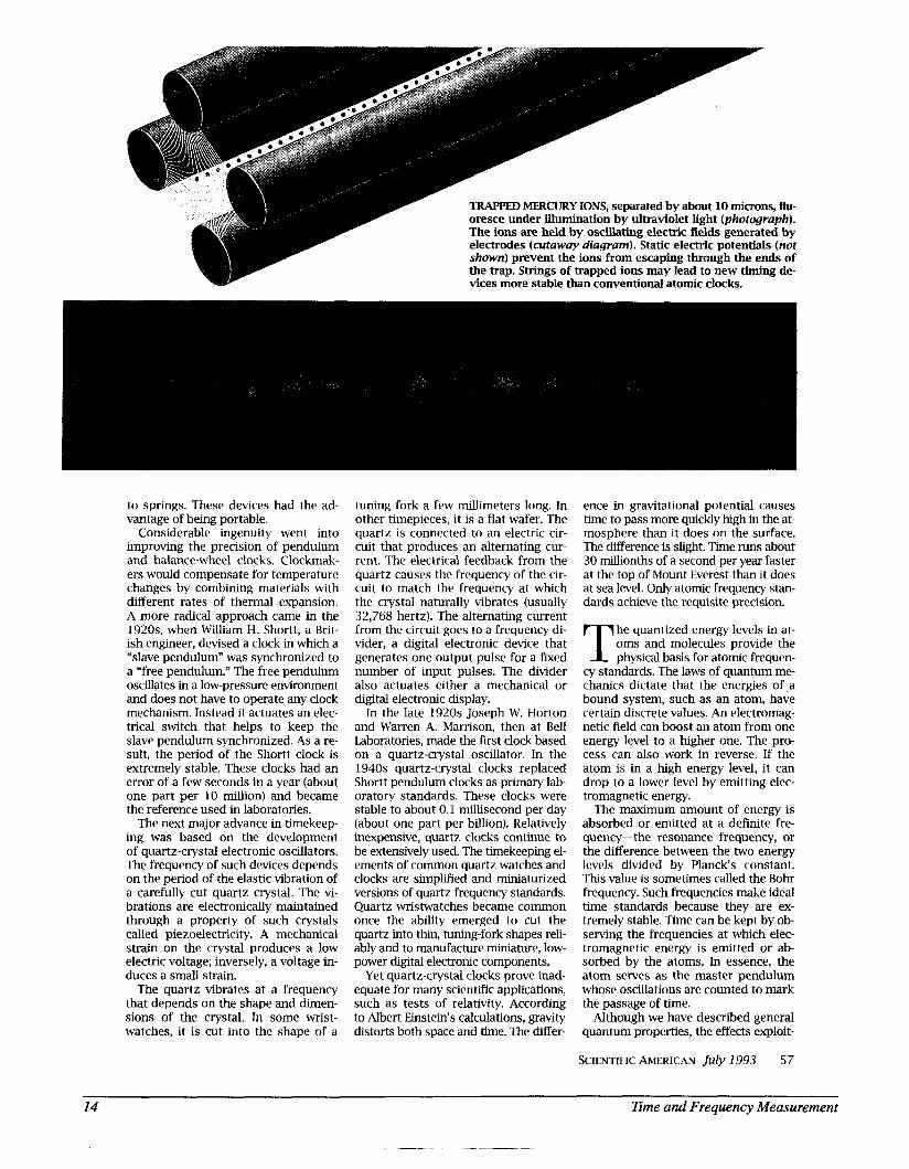
TRAPPED MERCURY IONS, separated by about 10 microns, flu- oresce under illumination by ultraviolet light (photograph). The ions are held by oscillating electric fields generated by electrodes (cutaway diagram). Static electric potentials (not shown) prevent the ions from escaping through the ends of the trap. Strings of trapped ions may lead to new timing de- vices more stable than conventional atomic clocks.
to springs. These devices had the ad- vantage of being portable.
Considerable ingenuity went into improving the precision of pendulum and balance-wheel clocks. Clockmak- ers would compensate for temperature changes by combining materials with different rates of thermal expansion. A more radical approach came in the 192Os, when William H. Shortt, a Brit- ish engineer, devised a clock in which a “slave pendulum” was synchronized to a “free pendulum.” The free pendulum oscillates in a low-pressure environment and does not have to operate any clock mechanism. Instead it actuates an elec- trical switch that helps to keep the slave pendulum synchronized. As a re- sult, the period of the Shortt clock is extremely stable. These clocks had an error of a few seconds in a year (about one part per 10 million) and became the reference used in laboratories.
The next major advance in timekeep ing was based on the development of quartz-crystal electronic oscillators. The frequency of such devices depends on the period of the elastic vibration of a carefully cut quartz crystal. The vi- brations are electronically maintained through a property of such crystals called piezoelectricity. A mechanical strain on the crystal produces a low electric voltage; inversely, a voltage in- duces a small strain.
The quartz vibrates at a frequency that depends on the shape and dimen- sions of the crystal. In some wrist- watches, it is cut into the shape of a
tuning fork a few millimeters long. In other timepieces, it is a flat wafer. The quartz is connected to an electric cir- cuit that produces an alternating cur- rent. The electrical feedback from the quartz causes the frequency of the cir- cuit to match the frequency at which the crystal naturally vibrates (usually 32,768 hertz). The alternating current from the circuit goes to a frequency di- vider, a digital electronic device that generates one output pulse for a k e d number of input pulses. The divider also actuates either a mechanical or digital electronic &splay.
In the late 1920s Joseph W. Horton and Warren A. Marrison, then at Bell Laboratories, made the first clock based on a quartz-crystal oscillator. In the 1940s quartz-crystal clocks replaced Shortt pendulum clocks as primary lab- oratory standards. These clocks were stable to about 0.1 millisecond per day (about one part per billion). Relatively inexpensive, quartz clocks continue to be extensively used. The timekeeping el- ements of common quartz watches and clocks are simplified and miniaturized versions of quartz frequency standards. Quartz wristwatches became common once the ability emerged to cut the quartz into thin, tuning-fork shapes reli- ably and to manufacture miniature, low- power digital electronic components.
Yet quartz-crystal clocks prove inad- equate for many scientific applications, such as tests of relativity. According to Albert Einstein’s calculations, gravity distorts both space and time. The differ-
ence in gravitational potential causes time to pass more quickly high in the at- mosphere than it does on the surface. The difference is slight. Time runs about 30 millionths of a second per year faster at the top of Mount Everest than it does at sea level. Only atomic frequency stan- dards achieve the requisite precision.
he quantized energy levels in at- oms and molecules provide the T physical basis for atomic frequen-
cy standards. The laws of quantum me- chanics dictate that the energies of .a bound system, such as an atom, have certain discrete values. An electromag- netic field can boost an atom from one energy level to a higher one. The pro- cess can also work in reverse. If the atom is in a high energy level, it can drop to a lower level by emitting elec- tromagnetic energy.
The maximum amount of energy is absorbed or emitted at a definite fre- quency-the resonance frequency, or the difference between the two energy levels divided by Planck’s constant. This value is sometimes called the Bohr frequency. Such frequencies make ideal time standards because they are ex- tremely stable. Time can be kept by ob- serving the frequencies at which elec- tromagnetic energy is emitted or ab- sorbed by the atoms. In essence, the atom serves as the master pendulum whose oscillations are counted to mark the passage of time.
Although we have described general quantum properties, the effects exploit-
SCIENTIFIC AMERICAN July 1993 5 7
I4 lime and Frequency Measurement
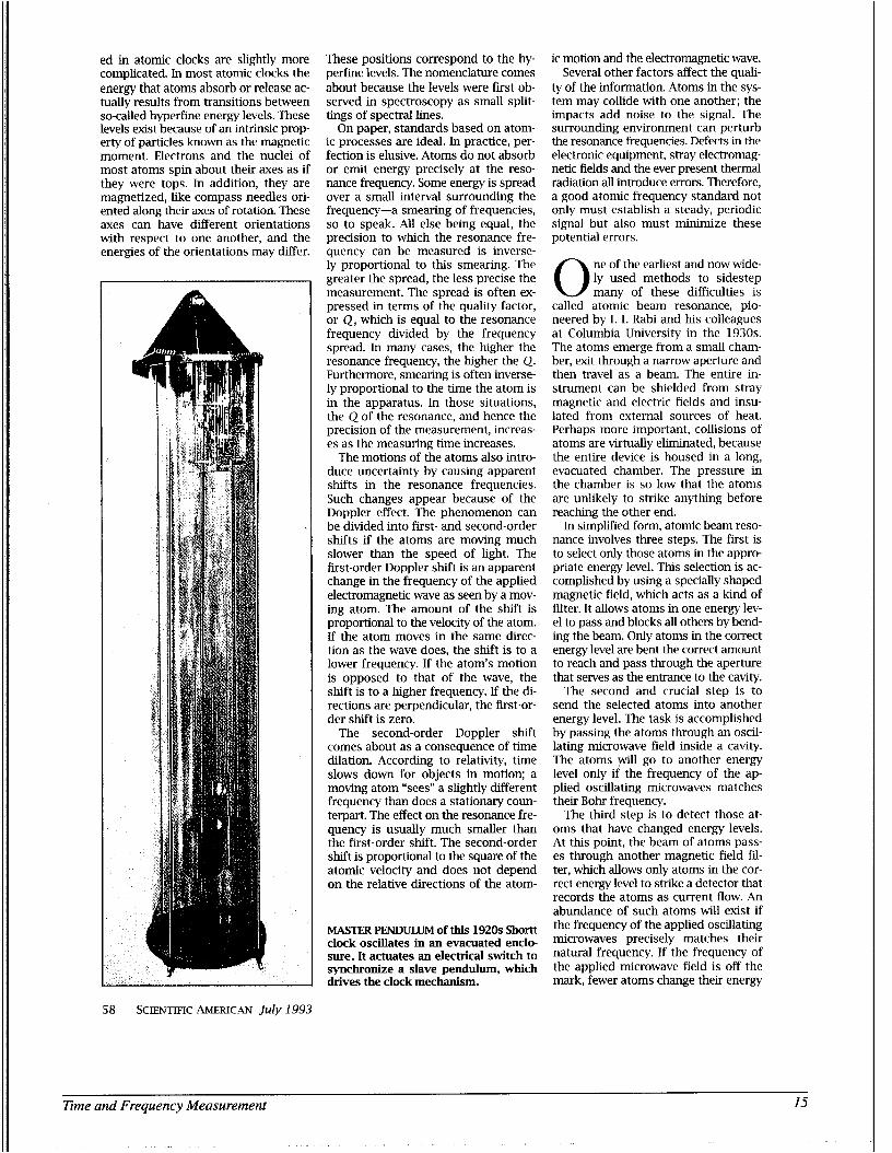
ed in atomic clocks are slightly more complicated. In most atomic clocks the energy that atoms absorb or release ac- tually results from transitions between so-called hyperfine energy levels. These levels exist because of an intrinsic prop- erty of particles known as the magnetic moment. Electrons and the nuclei of most atoms spin about their axes as if they were tops. In addition, they are magnetized, like compass needles ori- ented along their axes of rotation. These axes can have different orientations with respect to one another, and the energies of the orientations may dffer.
4
These positions correspond to the hy- perfine levels. The nomenclature comes about because the levels were first ob- served in spectroscopy as small split- tings of spectral lines.
On paper, standards based on atom- ic processes are ideal. In practice, per- fection is elusive. Atoms do not absorb or emit energy precisely at the reso- nance frequency. Some energy is spread over a small interval surrounding the frequency-a smearing of frequencies, so to speak. All else being equal, the precision to which the resonance fre- quency can be measured is inverse- ly proportional to this smearing. The greater the spread, the less precise the measurement. The spread is often ex- pressed in terms of the quality factor, or Q, which is equal to the resonance frequency divided by the frequency spread. In many cases, the higher the resonance frequency, the higher the Q. Furthermore, smearing is often inverse- ly proportional to the time the atom is in the apparatus. In those situations, the Q of the resonance, and hence the precision of the measurement, increas- es as the measuring time increases.
The motions of the atoms also intro- duce uncertainty by causing apparent shf ts in the resonance frequencies. Such changes appear because of the Doppler effect. The phenomenon can be divided into first- and second-order shifts if the atoms are moving much slower than the speed of light. The first-order Doppler shift is an apparent change in the frequency of the applied electromagnetic wave as seen by a mov- ing atom. The amount of the shift is proportional to the velocity of the atom. If the atom moves in the same direc- tion as the wave does, the shift is to a lower frequency. If the atom’s motion is opposed to that of the wave, the shift is to a higher frequency. If the di- rections are perpendicular, the first-or- der shift is zero.
The second-order Doppler shift comes about as a consequence of time dilation. According to relativity, time slows down for objects in motion; a moving atom “sees” a slightly different frequency than does a stationary coun- terpart. The effect on the resonance fre- quency is usually much smaller than the first-order shift. The second-order shift is proportional to the square of the atomic velocity and does not depend on the relative directions of the atom-
MASTER PENDULUM of this 1920s Shortt clock oscillates in an evacuated enclo- sure. It actuates an electrical switch to synchronize a slave pendulum, which drives the clock mechanism.
ic motion and the electromagnetic wave. Several other factors affect the quali-
ty of the information. Atoms in the sys- tem may collide with one another; the impacts add noise to the signal. The surrounding environment can perturb the resonance frequencies. Defects in the electronic equipment, stray electromag- netic fields and the ever present thermal radiation all introduce errors. Therefore, a good atomic frequency standard not only must establish a steady, periodic signal but also must minimize these potential errors.
0 ne of the earliest and now wide- ly used methods to sidestep many of these difficulties is
called atomic beam resonance, pio- neered by I. I. Rabi and his colleagues at Columbia University in the 1930s. The atoms emerge from a small cham- ber, exit through a narrow aperture and then travel as a beam. The entire in- strument can be shielded from stray magnetic and electric fields and insu- lated from external sources of heat. Perhaps more important, collisions of atoms are virtually eliminated, because the entire device is housed in a long, evacuated chamber. The pressure in the chamber is so low that the atoms are unlikely to strike anything before reaching the other end.
In simplified form, atomic beam reso- nance involves three steps. The first is to select only those atoms in the appro- priate energy level. This selection is ac- complished by using a specially shaped magnetic field, whch acts as a kind of filter. It allows atoms in one energy lev- el to pass and blocks all others by bend- ing the beam. Only atoms in the correct energy level are bent the correct amount to reach and pass through the aperture that serves as the entrance to the cavity.
The second and crucial step is to send the selected atoms into another energy level. The task is accomplished by passing the atoms through an oscil- lating microwave field inside a cavity. The atoms yill go to another energy level only if the frequency of the ap- plied oscillating microwaves matches their Bohr frequency.
The third step is to detect those at- oms that have changed energy levels. At this point, the beam of atoms pass- es through another magnetic field fil- ter, which allows only atoms in the cor- rect energy level to strike a detector that records the atoms as current flow. An abundance of such atoms will exist if the frequency of the applied oscillating microwaves precisely matches their natural frequency. If the frequency of the applied microwave field is off the mark, fewer atoms change their energy
58 SCIENTIFIC AMEMCAN July 1993
Time and Frequency Measurement I5
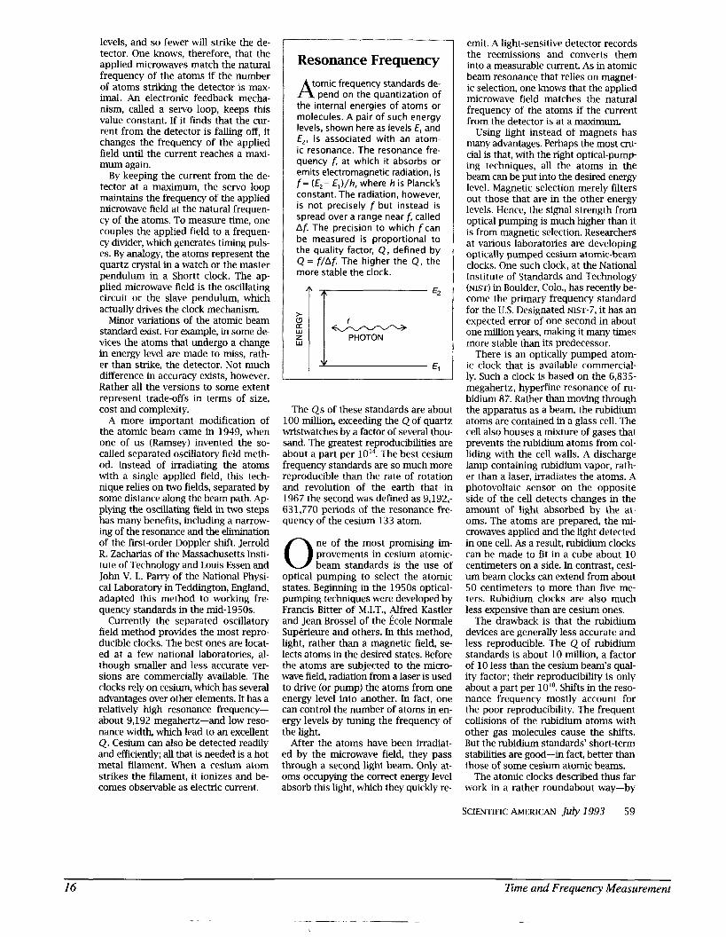
levels, and so fewer will strike the de- tector. One knows, therefore, that the applied microwaves match the natural frequency of the atoms if the number of atoms striking the deteclor is max- imal. An electronic feedback mecha- nism, called a servo loop, keeps this value constant. If it finds that the m- rent from the detector is falling off, it changes the frequency of the applied field until the current reaches a maxi- mum again.
By keeping the current from the de- tector at a maximum, the servo loop maintains the frequency of the applied microwave field at the natural frequen- cy of the atoms. To measure time, one couples the applied field to a frequen- cy divider, which generates timing puls- es. By analogy, the atoms represent the quartz crystal in a watch or the master pendulum in a Shortt clock. The ap- plied microwave field is the oscillating circuit or the slave pendulum, which actually drives the clock mechanism.
Minor variations of the atomic beam standard ais t . For example, in some de- vices the atoms that undergo a change in energy level are made to miss, rath- er than strike, the detector. Not much difference in accuracy exists, however. Rather all the versions to some extent represent trade-offs in terms of size, cost and complexity.
A more important modification of the atomic beam came in 1949, when one of us (Ramsey) invented the so- called separated oscillatory field meth- od. Instead of irradiating the atoms with a single applied field, this tech- nique relies on two fields, separated by some distance along the beam path. Ap- plying the oscillating field in two steps has many benefits, including a narrow- ing of the resonance and the elimination of the first-order Doppler shift. Jerrold R. Zacharias of the Massachusetts Insti- tute of Technology and Louis Essen and John V. L. Parry of the National Physi- cal Laboratory in Teddington, England, adapted this method to working fre- quency standards in the mid-1950s.
Currently the separated oscillatory field method provides the most repro- ducible clocks. The best ones are locat- ed at a few national laboratories, al- though smaller and less accurate ver- sions are commercially available. The clocks rely on cesium, which has several advantages over other elements. It has a relatively high resonance frequency- about 9,192 megahertz-and low reso- nance width, which lead to an excellent Q. Cesium can also be detected readily and efficiently; all that is needed is a hot metal filament. When a cesium atom strikes the filament, it ionizes and be- comes observable as electric current.
Resonance Frequency tomic frequency standards de- A pend on the quantization of
the internal energies of atoms or molecules. A pair of such energy levels, shown here as levels E, and E,, is associated with an atom- ic resonance. The resonance fre- quency f , at which it absorbs or emits electromagnetic radiation, is f = (€*- E,)/h, where h is Planck's constant. The radiation, however, is not precisely f but instead is spread over a range near f , called Af. The precision to which fcan be measured is proportional to the quality factor, Q , defined by Q = f / A f . The higher the Q , the more stable the clock.
The Qs of these standards are about 100 million, exceeding the Q of quartz wristwatches by a factor of several thou- sand. The greatest reproducibilities are about a part per The best cesium frequency standards are so much more reproducible than the rate of rotation and revolution of the earth that in 1967 the second was defined as 9,192,- 631,770 periods of the resonance fre- quency of the cesium 13 3 atom.
ne of the most promising im- provements in cesium atomic- 0 beam standards is the use of
optical pumping to select the atomic states. Beginning in the 1950s optical- pumping techniques were developed by Francis Bitter of M.I.T., Alfred Kastler and Jean Brossel of the Ecole Normale Superieure and others. In this method, light, rather than a magnetic field, se- lects atoms in the desired states. Before the atoms are subjected to the micro- wave field, radiation from a laser is used to drive (or pump) the atoms from one energy level into another. In fact, one can control the number of atoms in en- ergy levels by tuning the frequency of the light.
After the atoms have been irradiat- ed by the microwave field, they pass through a second light beam. Only at- oms occupying the correct energy level absorb this light, which they quickly re-
emit. A light-sensitive detector records the reemissions and converts them into a measurable current. As in atomic beam resonance that relies on magnet- ic selection, one knows that the applied microwave field matches the natural frequency of the atoms if the current from the detector is at a maximum.
Using light instead of magnets has many advantages. Perhaps the most cru- cial is that, with the right optical-pump- ing techniques, all the atoms in the beam can be put into the desired energy level. Magnetic selection merely filters out those that are in the other energy levels. Hence, the signal strength from optical pumping is much higher than it is from magnetic selection. Researchers at various laboratories are developing optically pumped cesium atomic-beam clocks. One such clock, at the National Institute of Standards and Technology (NIST) in Boulder, Colo., has recently be- come the primary frequency standard for the U.S. Designated NIST-7, it has an expected error of one second in about one million years, making it many times more stable than its predecessor.
There is an optically pumped atom- ic clock that is available commercial- ly. Such a clock is based on the 6,835- megahertz, hyperfine resonance of ru- bidium 87. Rather than moving through the apparatus as a beam, the rubidium atoms are contained in a glass cell. The cell also houses a mixture of gases that prevents the rubidium atoms from col- liding with the cell walls. A discharge lamp containing rubidium vapor, rath- er than a laser, irradiates the atoms. A photovoltaic sensor on the opposite side of the cell detects changes in the amount of light absorbed by the at- oms. The atoms are prepared, the mi- crowaves applied and the light detected in one cell. As a result, rubidium clocks can be made to fit in a cube about 10 centimeters on a side. In contrast, cesi- um beam clocks can extend from about 50 centimeters to more than five me- ters. Rubidium clocks are also much less expensive than are cesium ones.
The drawback is that the rubidium devices are generally less accurate and less reproducible. The Q of rubidium standards is about 10 million, a factor of 10 less than the cesium beam's qual- ity factor; their reproducibility is only about a part per 10". Shifts in the reso- nance frequency mostly account for the poor reproducibdity. The frequent collisions of the rubidium atoms with other gas molecules cause the shifts. But the rubidium standards' short-term stabilities are good-in fact, better than those of some cesium atomic beams.
The atomic clocks described thus far work in a rather roundabout way-by
SCIENTIFIC AMERICAN July 1993 59
16 Eme and Frequency Measurement
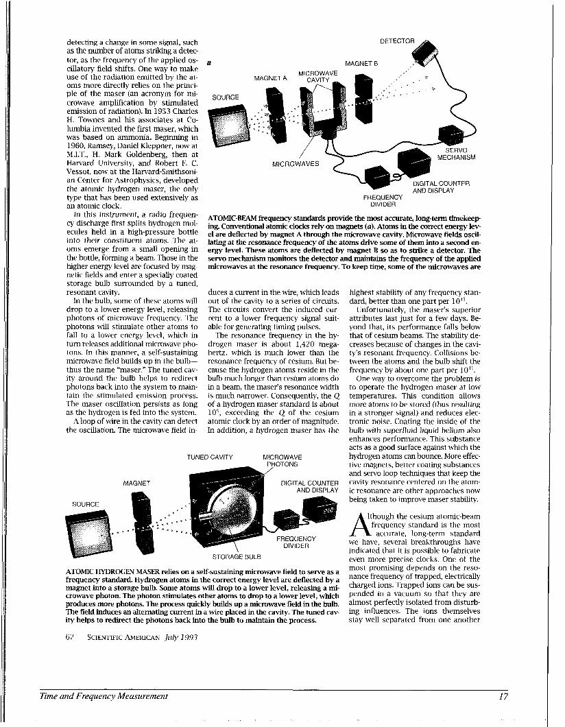
detecting a change in some signal, such as the number of atoms striking a detec- tor, as the frequency of the applied os- cillatory field shifts. One way to make use of the radiation emitted by the at- oms more directly relies on the princi- ple of the maser (an acronym for mi- crowave amplification by stimulated emission of radiation). In 1953 Charles H. Townes and his associates at Co- lumbia invented the first maser, which was based on ammonia. Beginning in 1960, Ramsey, Daniel Kleppner, now at M.I.T., H. Mark Goldenberg, then at Harvard University, and Robert F. C. Vessot, now at the Harvard-Smithsoni- an Center for Astrophysics, developed the atomic hydrogen maser, the only type that has been used extensively as an atomic clock.
In this instrument, a radio frequen- cy discharge first splits hydrogen mol- ecules held in a high-pressure bottle into their constituent atoms. The at- oms emerge from a small opening in the bottle, forming a beam. Those in the higher energy level are focused by mag- netic fields and enter a specially coated storage bulb surrounded by a tuned, resonant cavity.
In the bulb, some of these atoms wdl drop to a lower energy level, releasing photons of microwave frequency. The photons will stimulate other atoms to fall to a lower energy level, which in turn releases additional microwave pho- tons. In t h s manner, a self-sustaining microwave field builds up in the bulb- thus the name “maser.” The tuned cav- ity around the bulb helps to redirect photons back into the system to main- tain the stimulated emission process. The maser oscillation persists as long as the hydrogen is fed into the system.
A loop of wire in the cavity can detect the oscillation. The microwave field in-
a
DETECT0
MAGNET B
. .. .. FREQUENCY
DIVIDER
ATOMIC-BEAM frequency standards provide the most accurate, long-term timekeep ing. Conventional atomic clocks rely on magnets (a). Atoms in the correct energy lev- el are deflected by magnet A through the microwave cavity. Microwave fields oscil- lating at the resonance frequency of the atoms drive some of them into a second en- ergy level. These atoms are deflected by magnet B so as to strike a detector. The servo mechanism monitors the detector and maintains the frequency of the applied microwaves at the resonance frequency. To keep time, some of the microwaves are
duces a current in the wire, which leads out of the cavity to a series of circuits. The circuits convert the induced cur- rent to a lower frequency signal suit- able for generating timing pulses.
The resonance frequency in the hy- drogen maser is about 1,420 mega- hertz, whch is much lower than the resonance frequency of cesium. But be- cause the hydrogen atoms reside in the bulb much longer than cesium atoms do in a beam, the maser’s resonance width is much narrower. Consequently, the Q of a hydrogen maser standard is about log, exceeding the Q of the cesium atomic clock by an order of magnitude. In addition, a hydrogen maser has the
TUNED CAVITY MICROWAVE
MAGNET DIGITAL COUNTER
FREQUENCY
ATOMIC HYDROGEN MASER relies on a self-sustaining microwave field to serve as a frequency standard. Hydrogen atoms in the correct energy level are deflected by a magnet into a storage bulb. Some atoms will drop to a lower level, releasing a mi- crowave photon. The photon stimulates other atoms to drop to a lower level, which produces more photons. The process quickly builds up a microwave field in the bulb. The field induces an alternating current in a wire placed in the cavity. The tuned cav- ity helps to redirect the photons back into the bulb to maintain the process.
62 SCIENTIFIC AMERICAN July 1993
highest stabihty of any frequency stan- dard, better than one part per
Unfortunately, the maser’s superior attributes last just for a few days. Be- yond that, its performance falls below that of cesium beams. The stability de- creases because of changes in the cavi- ty’s resonant frequency. Collisions be- tween the atoms and the bulb sh f t the frequency by about one part per 10”.
One way to overcome the problem is to operate the hydrogen maser at low temperatures. This condition allows more atoms to be stored (thus resulting in a stronger signal) and reduces elec- tronic noise. Coating the inside of the bulb with superfluid liquid helium also enhances performance. Ths substance acts as a good surface against which the hydrogen atoms can bounce. More effec- tive magnets, better coating substances and servo loop techniques that keep the cavity resonance centered on the atom- ic resonance are other approaches now being taken to improve maser stability.
lthough the cesium atomic-beam frequency standard is the most A accurate, long-term standard
we have, several breakthroughs have inhcated that it is possible to fabricate even more precise clocks. One of the most promising depends on the reso- nance frequency of trapped, electrically charged ions. Trapped ions can be sus- pended in a vacuum so that they are almost perfectly isolated from disturb- ing mfluences. The ions themselves stay well separated from one another
Time and Frequency Measurement 17
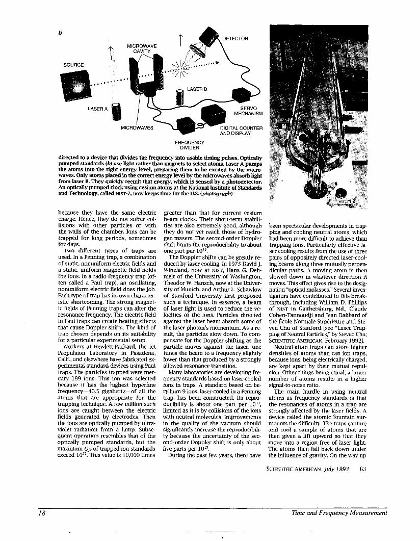
b
SOURCE
LASER
T .....*
A
MICROWAVE CAVITY
TAL COUNTER MICROWAVES J
SERVO MECHANISM
FREQUENCY DIVIDER
directed to a device that divides the frequency into usable timing pulses. Optically pumped standards (b) use light rather than magnets to select atoms. Laser A pumps the atoms into the right energy level, preparing them to be excited by the mi- waves. Only atoms placed in the correct energy level by the microwaves absorb light from laser B. They quickly reemit that energy, which is sensed by a photodetector. An optically pumped clock using cesium atoms at the National Institute of Standards and Technology, called NIST-~, now keeps lime for the U.S. (photograph).
because they have the same electric charge. Hence, they do not suffer col- lisions with other particles or with the walls of the chamber. Ions can be trapped for long periods, sometimes for days.
Two different types of traps are used. In a Penning trap, a combination of static, nonuniform electric fields and a static, uniform magnetic field holds the ions. In a radio frequency trap (of- ten called a Paul trap), an oscillating, nonuniform electric field does the job. Each type of trap has its own character- istic shortcoming. The strong magnet- ic fields of Penning traps can alter the resonance frequency. The electric field in Paul traps can create heating effects that cause Doppler shifts. The kind of trap chosen depends on its suitability for a particular experimental setup.
Workers at Hewlett-Packard, the Jet Propulsion Laboratory in Pasadena, Calif., and elsewhere have fabricated ex- perimental standard devices using Paul traps. The particles trapped were mer- cury 199 ions. This ion was selected because it has the highest hyperfine frequency-40.5 gigahertz-of all the atoms that are appropriate for the trapping technique. A few &on such ions are caught between the electric fields generated by electrodes. Then the ions are optically pumped by ultra- violet radiation from a lamp. Subse- quent operation resembles that of the optically pumped standards, but the maximum Qs of trapped-ion standards exceed lo’*. This value is 10,000 times
greater than that for current cesium beam clocks. Their short-term stabili- ties are also extremely good, although they do not yet reach those of hydro- gen masers. The second-order Doppler shift limits the reproducibility to about one part per
The Doppler shifts can be greatly re- duced by laser cooling. In 1975 David J. Wineland, now at NIST, Hans G. Deh- melt of the University of Washington, Theodor W. Hhsch, now at the Univer- sity of Munich, and Arthur L. Schawlow of Stanford University first proposed such a technique. In essence, a beam of laser light is used to reduce the ve- locities of the ions. Particles directed against the laser beam absorb some of the laser photon’s momentum. As a re- sult, the particles slow down. To com- pensate for the Doppler shifting as the particle moves against the laser, one tunes the beam to a frequency slightly lower than that produced by a strongly allowed resonance transition.
Many laboratories are developing fre- quency standards based on laser-cooled ions in traps. A standard based on be- ryllium 9 ions, laser-cooled in a Penning trap, has been constructed. Its repro- ducibility is about one part per 1013, limited as it is by collisions of the ions with neutral molecules. Improvements in the quality of the vacuum should sigmiicantly increase the reproducibili- ty because the uncertainty of the sec- ond-order Doppler shift is only about five parts per 10ls.
During the past few years, there have
been spectacular developments in trap- ping and cooling neutral atoms, which had been more difficult to achieve than trapping ions. Particularly effective la- ser cooling results from the use of three pairs of oppositely directed laser-cool- ing beams along three mutually perpen- dicular paths. A moving atom is then slowed down in whatever direction it moves. This effect gives rise to the desig- nation “optical molasses.” Several inves- tigators have contributed to this break- through, including William D. Phillips of NIST in Gaithersburg, Md., Claude Cohen-Tannoudji and Jean Dalibard of the kale Normale SupCrieure and Ste- ven Chu of Stanford [see “Laser Trap- ping of Neutral Particles,” by Steven Chu; SCIU\ITIFIC AMERICAN, February 19921.
Neutral-atom traps can store higher densities of atoms than can ion traps, because ions, being electrically charged, are kept apart by their mutual repul- sion. Other things being equal, a larger number of atoms results in a higher signal-to-noise ratio.
The main hurdle in using neutral atoms as frequency standards is that the resonances of atoms in a trap are strongly affected by the laser fields. A device called the atomic fountain sur- mounts the difficulty. The traps capture and cool a sample of atoms that are then given a lift upward so that they move into a region free of laser light. The atoms then fall back down under the influence of gravity. On the way up
SCIENTIFIC AMERICAN July 1993 63
18 Time and Frequency Measurement
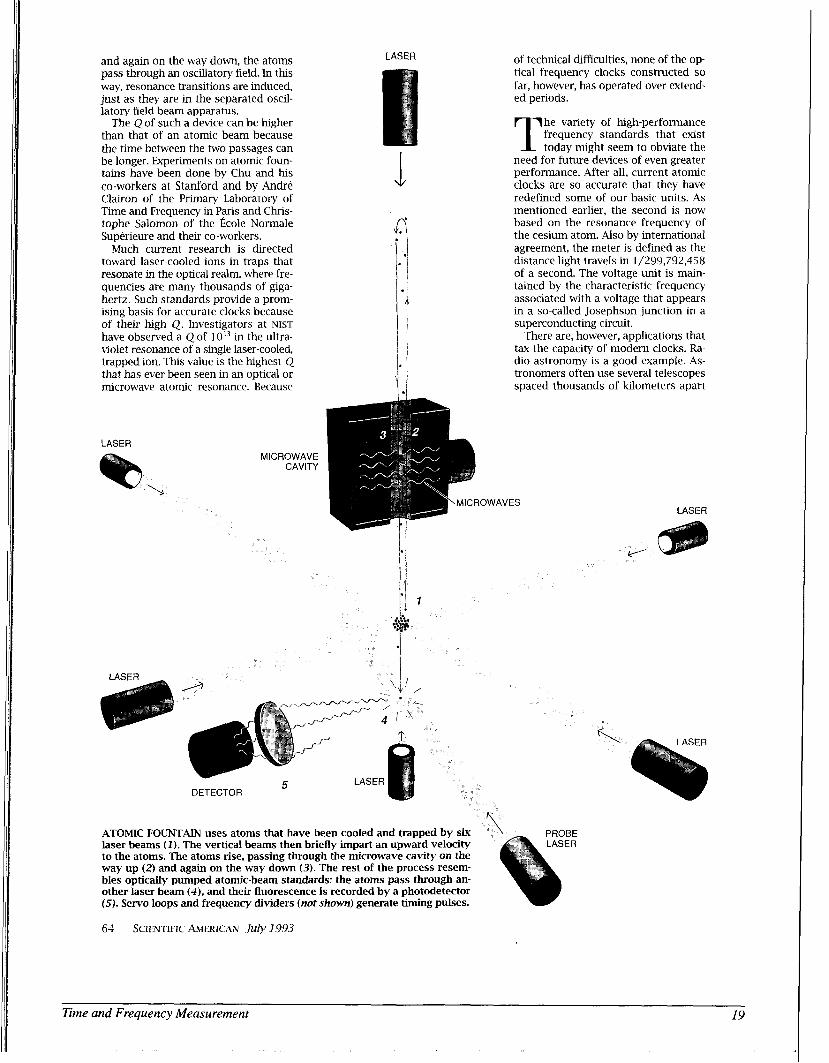
and again on the way down, the atoms pass through an oscillatory field. In t h s way, resonance transitions are induced, just as they are in the separated oscil- latory field beam apparatus.
The Q of such a device can be hgher than that of an atomic beam because the time between the two passages can be longer. Experiments on atomic foun- tains have been done by Chu and his co-workers at Stanford and by Andre Clairon of the Primary Laboratory of Time and Frequency in Paris and Chris- tophe Salomon of the Ecole Normale Superieure and their co-workers.
Much current research is directed toward laser-cooled ions in traps that resonate in the optical realm, where fre- quencies are many thousands of giga- hertz. Such standards provide a prom- ising basis for accurate clocks because of their h g h Q. Investigators at NIST have observed a Qof 1013 in the ultra- violet resonance of a single laser-cooled, trapped ion. This value is the hghest Q that has ever been seen in an optical or microwave atomic resonance. Because
LASER
1 x i
of technical difficulties, none of the op- tical frequency clocks constructed so far, however, has operated over extend- ed periods.
he variety of hgh-performance frequency standards that e ~ s t T today might seem to obviate the
need for future devices of even greater performance. After all, current atomic clocks are so accurate that they have redefined some of our basic units. As mentioned earlier, the second is now based on the resonance frequency of the cesium atom. Also by international agreement, the meter is defined as the distance light travels in 1/299,792,458 of a second. The voltage unit is main- tained by the characteristic frequency associated with a voltage that appears in a so-called Josephson junction in a superconducting circuit.
There are, however, applications that tax the capacity of modern clocks. Ra- dio astronomy is a good example. As- tronomers often use several telescopes spaced thousands of kilometers apart
LASER
1
LASER I , I'
ATOMIC FOUNTAIN uses atoms that have been cooled and trapped by six laser beams ( 1 ) . The vertical beams then briefly impart an upward velocity to the atoms. The atoms rise, passing through the microwave cavity on the way up (2) and again on the way down (3). The rest of the process resem- bles optically pumped atomic-beam standards: the atoms pass through an- other laser beam ( 4 ) , and their fluorescence is recorded by a photodetector (5). Servo loops and frequency dividers (not shown) generate timing pulses.
64 SCIENTIFIC AMERICAN July 1993
Time and Frequency Measurement 19
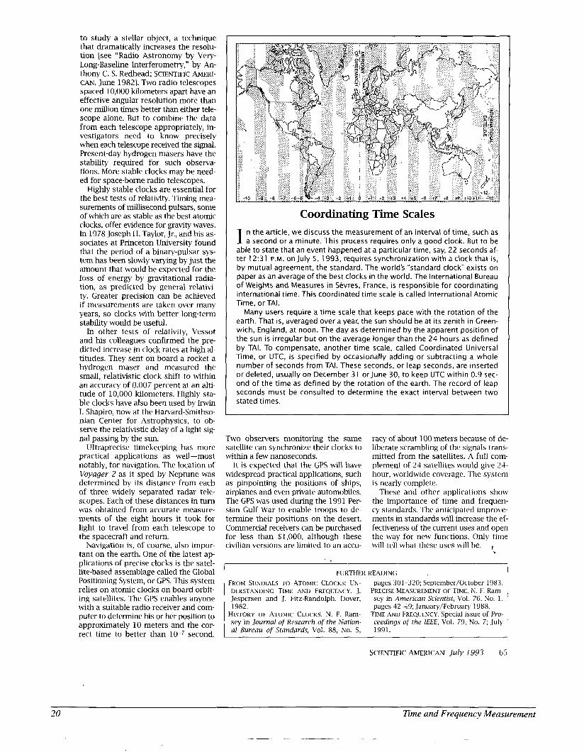
to study a stellar object, a technique that dramatically increases the resolu- tion [see “Radio Astronomy by Very- Long-Baseline Interferometry,” by An- thony C. S. Redhead; SCIENTIFIC AMERI- CAN, June 19821. Two radio telescopes spaced 10,000 kilometers apart have an effective angular resolution more than one million times better than either tele- scope alone. But to combine the data from each telescope appropriately, in- vestigators need to know precisely when each telescope received the signal. Present-day hydrogen masers have the stability required for such observa- tions. More stable clocks may be need- ed for space-borne radio telescopes.
Highly stable clocks are essential for the best tests of relativity. Timing mea- surements of millisecond pulsars, some of which are as stable as the best atomic clocks, offer evidence for gravity waves. In 1978 Joseph H. Taylor, Jr., and hs as- sociates at Princeton University found that the period of a binary-pulsar sys- tem has been slowly varymg by just the amount that would be expected for the loss of energy by gravitational radia- tion, as predicted by general relativi- ty. Greater precision can be achieved if measurements are taken over many years, so clocks with better long-term stability would be useful.
In other tests of relativity, Vessot and his colleagues confirmed the pre- dicted increase in clock rates at high al- titudes. They sent on board a rocket a hydrogen maser and measured the small, relativistic clock sh f t to within an accuracy of 0.007 percent at an alti- tude of 10,000 kilometers. Highly sta- ble clocks have also been used by Irwin I. Shapiro, now at the Harvard-Smithso- nian Center for Astrophysics, to ob- serve the relativistic delay of a light sig- nal passing by the sun.
Ultraprecise timekeeping has more practical applications as well-most notably, for navigation. The location of Voyager 2 as it sped by Neptune was determined by its distance from each of three widely separated radar tele- scopes. Each of these distances in turn was obtained from accurate measure- ments of the eight hours it took for light to travel from each telescope to the spacecraft and return.
Navigation is, of course, also impor- tant on the earth. One of the latest ap- plications of precise clocks is the satel- lite-based assemblage called the Global Positioning System, or GPS. Ths system relies on atomic clocks on board orbit- ing satellites. The GPS enables anyone with a suitable radio receiver and com- puter to determine his or her position to approximately 10 meters and the cor- rect time to better than 10-7 second.
Coordinating Time Scales n the article, we discuss the measurement of an interval of time, such as I a second or a minute. This process requires only a good clock. But to be
able to state that an event happened at a particular time, say, 22 seconds af- ter 12:31 P.M. on July 5, 1993, requires synchronization with a clock that is, by mutual agreement, the standard. The world’s “standard clock” exists on paper as an average of the best clocks in the world. The International Bureau of Weights and Measures in Sevres, France, is responsible for coordinating international time. This coordinated time scale is called International Atomic Time, or TAL
Many users require a time scale that keeps pace with the rotation of the earth. That is, averaged over a year, the sun should be at its zenith in Creen- wich, England, at noon. The day as determined by the apparent position of the sun i s irregular but on the average longer than the 24 hours as defined by TAI. To compensate, another time scale, called Coordinated Universal Time, or UTC, is specified by occasionally adding or subtracting a whole number of seconds from TAL These seconds, or leap seconds, are inserted or deleted, usually on December 31 orJune 30, to keep UTC within 0.9 sec- ond of the time as defined by the rotation of the earth. The record of leap seconds must be consulted to determine the exact interval between two stated times.
Two observers monitoring the same satellite can synchronize their clocks to within a few nanoseconds.
It is expected that the GPS will have widespread practical applications, such as pinpointing the positions of ships, auplanes and even private automobiles. The GPS was used during the 1991 Per- sian Gulf War to enable troops to de- termine their positions on the desert. Commercial receivers can be purchased for less than $1,000, although these civilian versions are limited to an accu-
racy of about 100 meters because of de- liberate scrambling of the signals trans- mitted from the satellites. A full coni- plement of 24 satellites would give 24- hour, worldwide coverage. The system is nearly complete.
These and other applications show the importance of time and frequen- cy standards. The anticipated improve- ments in standards will increase the ef- fectiveness of the current uses and open the way for new functions. Only time will tell what these uses wdl be. ,
I FURTHER READING FROM SUNDIALS TO ATOMIC CLOCKS: UN-
Jespersen and J. Fitz-Randolph. Dover, 1982. pages 42-49; January/February 1988.
HISTORY OF ATOMIC CLOCKS. N. F. Ram- sey in Journal of Research of the Nation- a/ Bureau of Standards, Vol. 88, No. 5,
pages 301-320; September/October 1983.
sey in American Scientist, Vol. 76, No. 1,
TIME AND FREQWNCY. Special issue of Pro- ceedings of the IEEE, Vol. 79, No. 7; July 1991.
DERSTANDING TIME AND FREQUENCY. J. PRECISE MEASUREMENT OF TIME. N. F. Ram-
~ ~
SCIENTIFIC AMERICAN July 1993 65
Time and Frequency Measurement
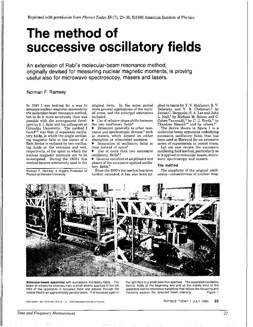
Reprinted with permission from Physics Today 33 (7), 25-30,01980 American Institute of Physics.
The method of successive oscillatory fields An extension of Rabi's molecular-beam resonance method, originally devised for measuring nuclear magnetic moments, is proving useful also for microwave spectroscopy, masers and lasers.
Norman F. Ramsey
In 1949 I was looking for a way to measure nuclear magnetic moments by the molecular-beam resonance method, but to do it more accurately than was possible with the arrangement devel- oped by I. I. Rabi and his colleagues a t Columbia University. The method I found'.' was that of separated oscilla- tory fields, in which the single oscillat- ing magnetic field in the center of a Rabi device is replaced by two oscillat- ing fields at the entrance and exit, respectively, of the space in which the nuclear magnetic moments are to be investigated. During the 1950's this method became extensively ilsed in the
Norman F. Ramsey is Higgins Professor of Physics at Harvard University.
original form. In the same period more general applications of the meth- od arose, and the principal extensions included: b Use of relative phase shifts between the two oscillatory fields3 b Extension generally to other reso- nance and spectroscopic devices: such as masers, which depend on either absorption or stimulated emission b Separation of oscillatory fields in time instead of space4 b Use of more than two successive oscillatory field^^,^ b General variation of amplitudes and phases of the successive applied oscilln. tory fields5
Since the 1950's the method has been further extended; it has also been ap-
plied to lasers by Y. V. Baklanov, B. V. Dubetsky and V. B. Chebotsev: by James C. Bergquist, S. A. Lee and John L. Hall: by Michael M. Salour and C. Cohen-Tannoudji: by C. J . Bord6: by Theodore Hansch" and by others."
The device shown in figure 1 is a molecular-beam apparatus embodying successive oscillatory fields that has been used at Harvard for a n extensive series of experiments in recent years.
Let me now review the successive oscillating field method, particularly as it is applied to molecular beams, m i c m wave spectroscopy and masers.
The method Tbe simplicity of the original appli-
cation-measurement of nuclear mag-
Molecular-beam apparatus with successive oscillatory fields. The beam of molecules emerges from a small source aperture in the left third of the apparatus, is focussed there and passes through the middle third in an approximately parallel beam. It is focussed again in
the right third to a small detection aperture. The separated oscillatory electric fields at the beginning and end of the middle third of the apparatus lead to resonance transitions that reduce the focussing and therefore weaken the detected beam intensity. Figure 1
0031-9228 I 8 0 1 0 7 2 5 4 6 / SO0 50 (.j 1980 American lns!ntute of Physics PHYSICS TODAY I JULY 1980 25
Time and Frequency Measurement 21
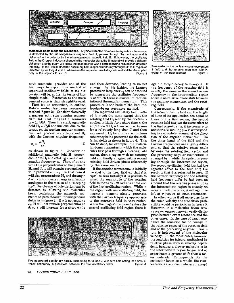
Molecular-beam magnetic resonance. A typical detected molecule emerges from the source, is deflected by the inhomogeneous magnetic field A, passes through the collimator and is deflected to the detector by the inhomogeneous magnetic field B. If, however, the oscillatory field in the C region induces a change in the molecular state, the B magnet will provide a different deflection and the beam will follow the dashed lines with a corresponding reduction in detected intensity. In the Rabi method the oscillatory field is applied uniformly throughout the C region as indicated bv the lona ti lines F. whereas in the separated oscillatory field method the ti is applied only in t h e regions E and G.
netic moments-provides one of the best ways to explain the method of separated oscillatory fields, so my dis- cussion will be, at first, in terms of this simple model. Extension to the more general cases is then straightforward.
First let us remember, in outline, Rabi’s molecular-beam resonance method (figure 2). Consider classically a nucleus with spin angular momen- t u m %J a n d magne t i c m o m e n t p = (p/J)J. Then in a static magnetic field H, = H,k the nucleus, due to the torque on the nuclear angular momen- tum, will precess like a top about H, with the Larmor angular frequency
PHO wo= - fiz
as shown in figure 3. Consider an additional magnetic field HI perpen- dicular to H, and rotating about it with angular frequency o. Then, if at any time H is perpendicular to the plane of H,, and J, it will remain perpendicular to it provided o = 0,. In that case J will also precess about HI and the angle 4 will continuously change in a fashion analogous to the motion of a “sleeping top”; the change of orientation can be detected by allowing the molecular beam containing the magnetic mo- ments to pass through inhomogeneous fields as in figure 2. If o is not equal to o,, H will not remain perpendicular to J; so q5 will increase for a short while
Figure 2
and then decrease, leading to no net change. In this fashion the Larmor precession frequency o, can be detected by measuring the oscillator frequency w at which there is maximum reorien- tation of the angular momentum. This procedure is the basis of the Rabi mo- lecular-beam resonance method.
The separated oscillatory field meth- od is much the same except that the rotating field HI seen by the nucleus is applied initially for a short time T, the amplitude of HI is then reduced to zero for a relatively long time T and then increased to HI for a time 7, with phase coherency being preserved for the oscil- lating fields as shown in figure 4. This can be done, for example, in a molecu- lar-beam apparatus in which the mole- cules first pass through a rotating field region, then a region with no rotating field and finally a region with a second rotating field driven phase coherently by the same oscillator.
If the angular momentum is initially parallel to the fixed field (so that q5 is equal to zero initially) it is possible to select the magnitude of the rotating field so that 4 is s/2 radians at the end of the first oscillating region. While in the region with no oscillating field, the magnetic moment simply precesses with the Larmor frequency appropriate to the magnetic field in that region. When the magnetic moment enters the second oscillating field region there is
Two separated oscillatory fields, each acting for a time r, with zero field acting for a time T. Figure 4 Phase coherency is preserved between the two oscillatory fields.
Precession of the nuclear angular momentum J (left) and the rotating magnetic field H,
Figure 3 (right) in the Rabi method.
again a torque acting to change 4. If the frequency of the rotating field is exactly the same as the mean Larmor frequency in the intermediate region there is no relative phase shift between the angular momentum and the rotat- ing field.
Consequently, if the magnitude of the second rotating field and the length of time of its application are equal to those of the first region, the second rotating field has just the same effect as the first one-that is, i t increases 4 by another s/2, making 4 = s, correspond- ing to a complete reversal of the direc- tion of the angular momentum. On the other hand, if the field and the Larmor frequencies are slightly differ- ent, so that the relative phase angle between the rotating field vector and the precessing angular momentum is changed by s while the system is pass- ing through the intermediate region, the second oscillating field has just the opposite effect to the first one; the result is that q5 is returned to zero. If the Larmor frequency and the rotating field frequency differ by just such an amount that the relative phase shift in the intermediate region is exactly an integral multiple of 2s,4 will again be left at s just as at exact resonance.
In other words if all molecules have the same velocity the transition prob- ability would be periodic as in figure 5. However, in a molecular beam reso- nance experiment one can easily distin- guish between exact resonance and the other cases. In the case of exact reso- nance the condition for no change in the relative phase of the rotating field and of the precessing angular momen- tum is independent of the molecular velocity. In the other cases, however, the condition for integral multiple of 2s rektive phase shift is velocity depen- dent, because a slower molecule is in the intermediate region longer and so experiences a greater shift than a fas- ter molecule. Consequently, for the molecular beam as a whole, the reor- ientations are incomplete in all except
26 PHYSICS TODAY / JULY 1980
22 Eme and Frequency Measurement
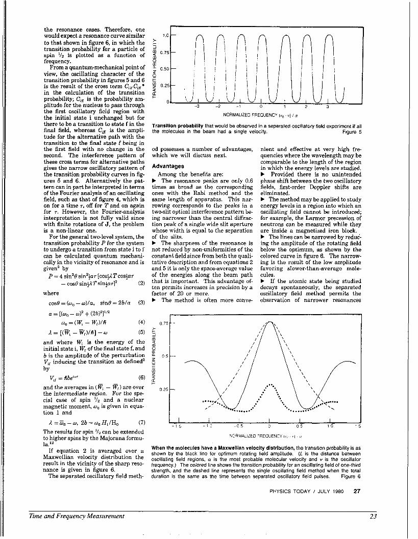
the resonance cases. Therefore, one would expect a resonance curve similar to that shown in figure 6, in which the transition probability for a particle of spin is plotted as a function of frequency.
From a quantum-mechanical point of view, the oscillating character of the transition probability in figures 5 and 6 is the result of the cross term C,i, Ci, in the calculation of the transition probability; Ci, is the probability am- plitude for the nucleus to pass through the first oscillatory field region with the initial state i unchanged but for there to be a transition to state f i n the final field, whereas Ci, is the ampli- tude for the alternative path with the transition to the final state f being in the first field with no change in the second. The interference pattern of these cross terms for alternative paths gives the narrow oscillatory pattern of the transition probability curves in fig- ures 5 and 6. Alternatively the pat- tern can in part be interpreted in terms of the Fourier analysis of an oscillating field, such as that of figure 4, which is on for a time r, off for T and on again for r. However, the Fourier-analysis interpretation is not fully valid since with finite rotations of J, the problem is a non-linear one.
For the general two-level system, the transition probability P for the system to undergo a transition from state i to f can be calculated quantum mechani- cally in the vicinity of resonance and is given' by
P = 4 sin20 sin2?p [cosgT cos@r - cos$ s i n g T sinjarI2 (2)
where cos0 = (w, - @)/a, sin0 = 2b/a (3)
(4)
a = [(W, - W)' + (2b)21'fl w, = (w, - W,)/fi
and where Wi is the energy of the initial state i, W, of the final state f, and b is the amplitude of the perturbation V,, inducing the transition as defined2 by
V,, = tibe'"' (6) and the averages in (w, - wf) are over the intermediate region. For the spe- cial case of spin ' / z and a nuclear magnetic moment, o0 is given in equa- tion l and
(7) The results for spin '/2 can be extended to higher spins by the Majorana formu- la.12
If equation 2 is averaged over a Maxwellian velocity distribution the result in the vicinity of the sharp reso- nance is given in figure 6.
The separated oscillatory field meth-
1 =Go - w, 26 = woHl/Ho
NORMALIZED FREQUENCY ( y o . v ) / n
Transition probability that would be observed in a separated oscillatory field experiment if all the molecules in the beam had a single velocity. Figure 5
od possesses a number of advantages, which we will discuss next.
Advantages
b The resonance peaks are only 0.6 times as broad as the corresponding ones with the Rabi method and the same length of apparatus. This nar- rowing corresponds to the peaks in a two-slit optical interference pattern be- ing narrower than the central diffrac- tion peak of a single wide slit aperture whose width is equal to the separation of the slits. b The sharpness of the resonance is not reduced by non-uniformities of the constant field since from both the quali- tative description and from equations 2 and 5 it is only the space-average value of the energies along the beam path that is important. This advantage of- ten permits increases in precision by a factor of 20 or more. b The method is often more conve-
Among the benefits are:
nient and effective at very high fre- quencies where the wavelength may be comparable to the length of the region in which the energy levels are studied. b Provided there is no unintended phase shift between the two oscillatory fields, first-order Doppler shifts are eliminated. b The method may be applied to study energy levels in a region into which an oscillating field cannot be introduced; for example, the Larmor precession of neutrons can be measured while they a re inside a magnetized iron block. b The lines can be narrowed by reduc- ing the amplitude of the rotating field below the optimum, as shown by the colored curve in figure 6. The narrow- ing is the result of the low amplitude favoring slower-than-average mole- cules. b If the atomic state being studied decays spontaneously, the separated oscillatory field method permits the observation of narrower resonances
I I I I I - 1 5 - 1 0 - 0 5 0 0 5 1 0 1
UCRMALIZED FREQUENCY ( I , > - 1.1 ; i i
When the molecules have a Maxwelllan velocity dlstrlbution, the transition probability is as shown by the black line for optimum rotating field amplitude. (L is the distance between oscillating field regions, a is the most probable molecular velocity and v is the oscillator frequency.) The colored line shows the transition probability for an oscillating field of one-third strength, and the dashed line represents the single oscillating field method when the total duration is the same as the time between separated oscillatory field pulses. Figure 6
PHYSICS TODAY / JULY 1980 27
Time and Frequency Measurement 23
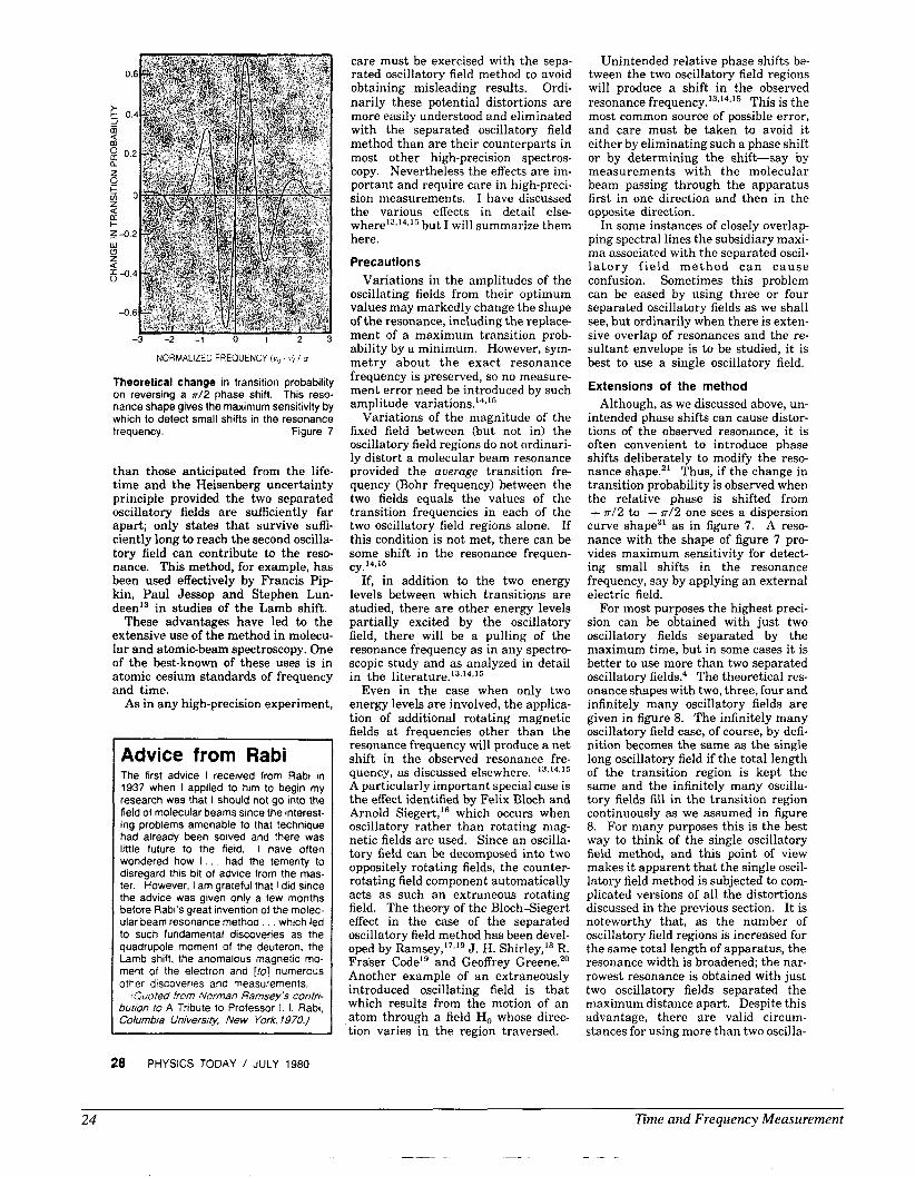
-3 -2 -1 0 1 2 3
NORMALIZED FREQUENCY O 0 - r) / u
Theoretical change in transition probability on reversing a 7r/2 phase shift. This reso- nance shape gives the maximum sensitivity by which to detect small shifts in the resonance irequency. Figure 7
than those anticipated from the life- time and the Heisenberg uncertainty principle provided the two separated oscillatory fields are sufficiently far apart; only states that survive suffi- ciently long to reach the second oscilla- tory field can contribute to the reso- nance. This method, for example, has been used effectively by Francis P i p kin, Paul Jessop and Stephen Lun- deenI3 in studies of the Lamb shift.
These advantages have led to the extensive use of the method in molecu- lar and atomic-beam spectroscopy. One of the best-known of these uses is in atomic cesium standards of frequency and time.
As in any high-precision experiment,
Advice from Rabi The first advice I received from Rabi in 1937 when I applied to him to begin my research was that I should not go into the field of molecular beams since the interest- ing problems amenable to that technique had already been solved and there was little future to the field. I have often wondered how I . . . had the temerity to disregard this bit of advice from the mas- ter. However, I am grateful that I did since the advice was given only a few months before Rabi's great invention of the molec- ular beam resonance method. . . which led to such fundamental discoveries as the quadrupole moment of the deuteron, the Lamb shift, the anomalous magnetic mo- ment of the electron and [to] numerous other discoveries and measurements.
!Quofed from Norman Ramsey's confri- bumon lo A Tribute to Professor I . I . Rabi. Columbia Universiw, New York, 1970.)
28 PHYSICS TODAY / JULY 1980
care must be exercised with the sepa- rated oscillatory field method to avoid obtaining misleading results. Ordi- narily these potential distortions are more easily understood and eliminated with the separated oscillatory field method than are their counterparts in most other high-precision spectros- copy. Nevertheless the effects are im- portant and require care in high-preci- sion measurements. I have discussed the various effects in detail else- here'^,'^,'^ but I will summarize them here.
Precautions Variations in the amplitudes of the
oscillating fields from their optimum values may markedly change the shape of the resonance, including the replace- ment of a maximum transition prob- ability by a minimum. However, sym- metry about t he exact resonance frequency is preserved, so no measure- ment error need be introduced by such amplitude variations.'"16
Variations of the magnitude of the fixed field between (but not in) the oscillatory field regions do not ordinari- ly distort a molecular beam resonance provided the average transition fre- quency (Bohr frequency) between the two fields equals the values of the transition frequencies in each of the two oscillatory field regions alone. If this condition is not met, there can be some shift in the resonance frequen-
If, in addition to the two energy levels between which transitions are studied, there are other energy levels partially excited by the oscillatory field, there will be a pulling of the resonance frequency as in any spectro- scopic study and as analyzed in detail in the l i t e r a t ~ r e . ' ~ . ' ~ , ' ~
Even in the case when only two energy levels are involved, the applica- tion of additional rotating magnetic fields at frequencies other than the resonance frequency will produce a net shift in the observed resonance fre- quency, as discussed elsewhere. 1 3 . 1 4 5 1 5
A particularly important special case is the effect identified by Felix Bloch and Arnold Siegert," which occurs when oscillatory rather than rotating mag- netic fields are used. Since an oscilla- tory field can be decomposed into two oppositely rotating fields, the counter- rotating field component automatically acts as such an extraneous rotating field. The theory of the BlochSiegert effect in the case of the separated oscillatory field method has been devel- oped by Ramsey,I7," J. H. Shirley," R. Fraser CodeIg and Geoffrey Greene." Another example of an extraneously introduced oscillating field is that which results from the motion of an atom through a field H, whose direc- tion varies in the region traversed.
cy,14.15
Unintended relative phase shifts be- tween the two oscillatory field regions will produce a shift in the observed resonance f r e q ~ e n c y . ' ~ . ' ~ . ' ~ This is the most common source of possible error, and care must be taken to avoid it either by eliminating such a phase shift or by determining the shift-say by measurements with the molecular beam passing through the apparatus first in one direction and then in the opposite direction.
In some instances of closely overlap- ping spectral lines the subsidiary maxi- ma associated with the separated oscil- l a to ry f ie ld me thod c a n c a u s e confusion. Sometimes this problem can be eased by using three or four separated oscillatory fields as we shall see, but ordinarily when there is exten- sive overlap of resonances and the re- sultant envelope is to be studied, it is best to use a single oscillatory field.
Extensions of the method Although, as we discussed above, un-
intended phase shifts can cause distor- tions of the observed resonance, it is often convenient to introduce phase shifts deliberately to modify the reso- nance shape." Thus, if the change in transition probability is observed when the relative phase is shifted from + 7r/2 to - 7r/2 one sees a dispersion
curve shapez1 as in figure 7. A reso- nance with the shape of figure 7 pro- vides maximum sensitivity for detect- ing small shifts in the resonance frequency, say by applying an external eiectric field.
For most purposes the highest preci- sion can be obtained with just two oscillatory fields separated by the maximum time, but in some cases it is better to use more than two separated oscillatory fields4 The theoretical res- onance shapes with two, three, four and infinitely many oscillatory fields are given in figure 8. The infinitely many oscillatory field case, of course, by defi- nition becomes the same as the single long oscillatory field if the total length of the transition region is kept the same and the infinitely many oscilla- tory fields fill in the transition region continuously as we assumed in figure 8. For many purposes this is the best way to think of the single oscillatory field method, and this point of view makes it apparent that the single oscil- latory field method is subjected to com- plicated versions of all the distortions discussed in the previous section. It is noteworthy that, as the number of oscillatory field regions is increased for the same total length of apparatus, the resonance width is broadened; the nar- rowest resonance is obtained with just two oscillatory fields separated the maximum distance apart. Despite this advantage, there are valid circum- stances for using more than two oscilla-
24 Time and Frequency Measurement
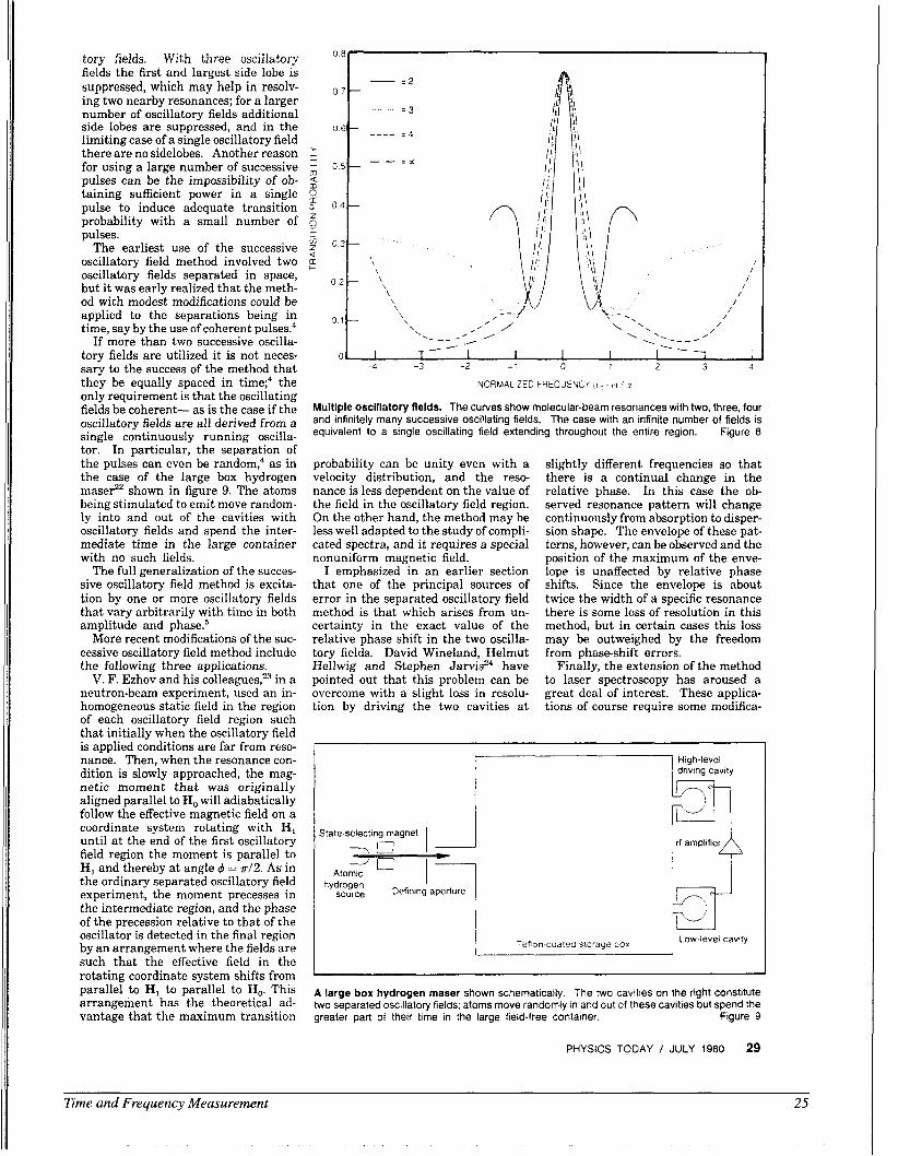
tory fields. With three oscillatory fields the first and largest side lobe is suppressed, which may help in resolv- ing two nearby resonances; for a larger number of oscillatory fields additional side lobes are suppressed, and in the limiting case of a single oscillatory field there are no sidelobes. Another reason for using a large number of successive pulses can be the impossibility of ob- taining sufficient power in a single pulse to induce adequate transition probability with a small number of pulses.
The earliest use of the successive oscillatory field method involved two oscillatory fields separated in space, but it was early realized that the meth- od with modest modifications could be applied to the separations being in time, say by the use of coherent pulse^.^
If more than two successive oscilla- tory fields are utilized it is not neces- sary to the success of the method that they be equally spaced in time;4 the only requirement is that the oscillating fields be coherent- as is the case if the oscillatory fields are all derived from a single continuously running oscilla- tor. In particular, the separation of the pulses can even be random: as in the case of the large box hydrogen mase?' shown in figure 9. The atoms being stimulated to emit move random- ly into and out of the cavities with oscillatory fields and spend the inter- mediate time in the large container with no such fields.
The full generalization of the succes- sive oscillatory field method is excita- tion by one or more oscillatory fields that vary arbitrarily with time in both amplitude and phase.5
More recent modifications of the suc- cessive oscillatory field method include the following three applications.
V. F. Ezhov and his c0lleayes,2~ in a neutron-beam experiment, used an in- homogeneous static field in the region of each oscillatory field region such that initially when the oscillatory field is applied conditions are far from resc- nance. Then, when the resonance con- dition is slowly approached, the mag- netic moment tha t was originally aligned parallel to H, will adiabatically follow the effective magnetic field on a coordinate system rotating with HI until at the end of the first oscillatory field region the moment is parallel to HI and thereby at angle q5 = ~ / 2 . As in the ordinary separated oscillatory field experiment, the moment precesses in the intermediate region, and the phase of the precession relative to that of the oscillator is detected in the final region by an arrangement where the fields are such that the effective field in the rotating coordinate system shifts from parallel to H, to parallel to H,. This arrangement has the theoretical ad- vantage that the maximum transition
NORMALIZED FRECUEYC'V ( b o - I 1 3
Multiple oscillatory fields. The curves show molecular-beam resonances with two, three, four and infinitely many successive oscillating fields. The case with an infinite number of fields is equivalent to a single oscillating field extending throughout the entire region. Figure 8
probability can be unity even with a velocity distribution, and the reso- nance is less dependent on the value of the field in the oscillatory field region. On the other hand, the method may be less well adapted to the study of compli- cated spectra, and i t requires a special nonuniform magnetic field.
I emphasized in an earlier section that one of the principal sources of error in the separated oscillatory field method is that which arises from un- certainty in the exact value of the relative phase shift in the two oscilla- tory fields. David Wineland, Helmut Hellwig and Stephen JarvisZ4 have pointed out that this problem can be overcome with a slight loss in resolu- tion by driving the two cavities at
slightly different frequencies so that there is a continual change in the relative phase. In this case the ob- served resonance pattern will change continuously from absorption to disper- sion shape. The envelope of these pat- terns, however, can be observed and the position of the maximum of the enve- lope is unaffected by relative phase shifts. Since the envelope is about twice the width of a specific resonance there is some loss of resolution in this method, but in certain cases this loss may be outweighed by the freedom from phase-shift errors.
Finally, the extension of the method to laser spectroscopy has aroused a great deal of interest. These applica- tions of course require some modifica-
State-selecting magnet
7n Atomic
hydrogen I Defining aperture
~ Low-level cavity Teflon-coalea storage zox
A large box hydrogen maser shown schematically. The two cavities on the right constitute two separated oscillatory fields; atoms move randomly in and out of these cavities but spend the greater part of their time in the large field-free container. Figure 9
PHYSICS TOOAY / JULY 1980 29
Time and Frequency Measurement 25
tions from the form of the technique most widely applied to molecular beams,610 due to differences in wave- lengths, state lifetimes and so on. How- ever, the necessary modifications have been made and the method continues to be of real value in laser spectroscopy- particularly in cases where the extra effort required is justified by the need for multiple pulses or high precision.
* I *
This article is an adaptation of a paper presented at the Tenth International Quan- tum Electronics Conference, held in Atlanta, Georgia, in May 1978.
References 1. N. F. Ramsey, Phys. Rev. 76,996 (1949). 2. N. F. Ramsey, Phys. Rev. 78,695 (1950). 3. N. F. Ramsey, H. B. Silsbee, Phys. Rev
4. N. F. Ramsey, Rev. Sci. Instr. 28, 57
5. N. F. Ramsey, Phys. Rev. 109,822 (1958). 6. Y. V. Baklanov. B. V. Dubetskv. V. B.
84, 506 (1951).
(1957).
Chebotsev, Appl. Phys. 9,171 (1676) and 11, 201 (1976).
7. J. C. Bergquist, S. A. Lee, J. L. Hall, Phys. Rev. Lett. 38,159 (1977) and Laser Spectroscopy 111, 142 (1978).
8. M. M. Salour, C. Cohen-Tannoudji, Phys. Rev. Lett. 38,757 (1977), Laser Spectroe copy III, 135 (1978), Appl. Phys. 16,119 (1978) and Phys. Rev. A17, 614 (1978).
9. C. J. Bordb, C. R. Acad. Sci. Paris 284B, 101 (1977).
10. T. W. Hkinsch, Laser Spectroscopy III, 149 (1978).
11. V.P Chebotayev, A.V. Shishayev, B.Y. Yurshin, L.S. Vasilenko, N.M. Dyuba, M.I. Skortsov, Appl. Phys. 15, 43, 219 and 319 (1987).
12. S. R. Lundeen, P. E. Jessop, F. M. P ip kin, Phys. Rev. Lett. 34, 377 and 1368 (1975).
13. N. F. Ramsey, Molecular Beams, Oxford University Preas (1956).
14. N. F. Ramsey, Le Journal de Physique et Radium 19, 809 (1958).
15. N. F. Ramsey, in Recent Research in Molecular Beams (I. Estermann, ed.) Academic Press, New York (1958); page 107.
16. F. Bloch, A. Siegert, Phys. Rev. 57,522 (1940).
17. N. F. Ramsey, Phys. Rev. 100, 1191 (1955).
18. J. H. Shirley, J . Appl. Phys. 34, 783 (1963).
19. R. F. Code, N. F. Ramsey, Phys. Rev. A4, 1945 (1971).
20. G. Greene, Phys. Rev. A18, 1057 (1978). 21. N. F. Ramsey, H. B. Silsbee, Phys. Rev.
84, 506 (1951). 22. E. E. Uzgiris, N. F. Ramsey, Phys. Rev.
Al, 429 (1970). 23. V. F. Ezhov, S. N. Ivanov, I. M. Loba-
shov, V. A. Nazarenko, G. D. Porsev, A. P. Serebrov, R. R. Toldaev, Sov. Phys.- JETP 24, 39 (1976).
24. S. Jarvis Jr., D. J. Wineland, H. Hellwig, 0 J. Appl. Phys. 48, 5336 (1977).
26 Time and Frequency Measurement
-~ - ~-
Reprinted with permission from Science 226 (4673), 395400,01984 American Association for the Advancement of Science.
26 October 1984, Volume 226, Number 4673 SCIENCE
Trapped Ions, Laser Cooling, and Better Clocks
D. J. Wineland
In a recent experiment ( I ) at the Na- tional Bureau of Standards (NBS) in Boulder, Colorado, the frequency of a particular hyperfine transition in the ground state of beryllium atomic ions was measured with an inaccuracy of only about one part in In this experi- ment, the ions were confined or “trapped” in a small region of space by
tenths of a percent. On the experimental side, about 8 years ago a measurement (3) of beryllium ion hyperfine structure to an accuracy of 3 ppm (parts per mil- lion) was made. Since the accuracy of this previous measurement is presum- ably good enough to satisfy the theorists for quite some time in the future, one can logically ask why anyone would want to
Summary. Ions that are stored in electromagnetic “traps” provide the basis for extremely high resolution spectroscopy. By using lasers, the kinetic energy of the ions can be cooled to millikelvin temperatures, thereby suppressing Doppler frequency shifts. Potential accuracies of frequency standards and clocks based on such experiments are anticipated to be better than one part in
using static electromagnetic fields and their kinetic temperature was lowered to less than 1 K by a process sometimes called “laser cooling.” In all of physics, only a few measurements can boast a higher accuracy; those experiments mea- sure similar transitions in neutral cesium atoms.
Experimental spectroscopy (the study of the interaction between radiation and matter) has traditionally provided a means of checking the theory of quan- tum mechanics which predicts the inter- nal energy structure of atoms and mole- cules. In the case of hyperfine structure, which represents the magnetic coupling between the nucleus and atomic elec- trons, the theory quickly becomes very complicated. For alkali-like ions, the most sophisticated calculations (2) agree with experiment at a level of only a few
The author is a research physicist in the Time and Frequency Division of the National Bureau of Stan- dards, Boulder, Colorado 80303
26 OCTOBER 1984
make a better measurement. Briefly, I will give three of the reasons.
1) The primary driver in several labo- ratories (including NBS) is to provide better clocks and frequency standards. The principal use of atomic clocks is in navigation and communications, where requirements have continued to press the state of the art. The way an atomic clock works is perhaps apparent in the internationally agreed on definition of the second: “The second is the duration of 9,192,631,770 periods of the radiation corresponding to the transition between the two hyperfine levels of the ground state of the cesium-133 atom.” A simpli- fied model for the practical realization of the second involves making a device (an atomic beam apparatus) which allows one to induce and detect transitions be- tween the two ground-state hyperfine energy levels. When the frequency of the radiation for maximum transition proba- bility is attained, the cycles are electroni-
cally counted; when 9,192,631,770 cy- cles have occurred, 1 second has passed. Several laboratories are trying to apply this same idea to the internal energy levels of ions; there is reason to believe that the inaccuracy of a time standard based on stored ions can eventually be much smaller than that of the cesium clock, which can have an accuracy of about one part in I O i 3 or less (4 ) .
2) With the extreme accuracy attained with stored ion techniques, it may be possible to measure various small effects which would otherwise be masked by measurement imprecision. As an exam- ple, it should be possible to measure nuclear magnetic susceptibility as a small perturbation to atomic hyperfine structure (5 ) . Nuclear magnetic suscepti- bility, which has not been measured pre- viously, could give a new kind of infor- mation about nuclear structure. Trapped ions may provide a way to make the required precise measurements.
3) The system itself, laser-cooled stored ions, is intrinsically interesting and may provide the basis for other experiments which are only peripherally related to spectroscopy. An example is the study of strongly coupled three-di- mensional plasmas ( 6 ) .
For brevity, this article will only touch on some aspects of stored ion spectros- copy where laser cooling is employed and how they are related to better clocks and frequency standards. A recent re- view article (3 includes many interesting trapped ion experiments which are not discussed here.
Trapped Ions
The principal attraction of the stored ion technique is that charged particles, including electrons and atomic ions, can be stored for long periods of time (days are not uncommon) without the usual perturbations associated with confine- ment [for example, the frequency shifts associated with the collisions of ions with buffer gases in a more traditional optical pumping experiment (S)].
Storage has principally been accom- plished in four types of “traps”: the RF (radio frequency) or Paul trap, the Pen-
395
Time and Frequency Measurement 27
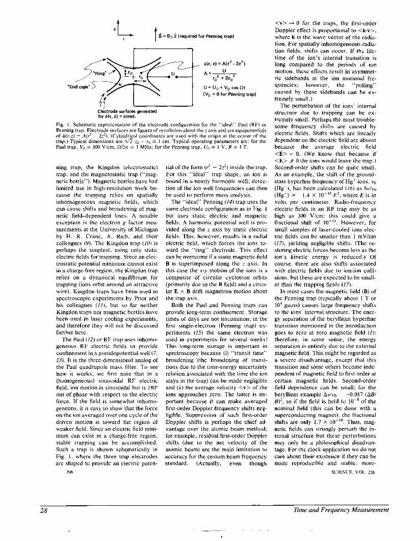
6 = BO 2 (required for Penning trap) t , @tr, z) = Atr ‘ - 22‘)
u = u, + v, cos nt (Vo = 0 for Penning trap)
Electrode surfaces generated by @ ( r , z) = const.
Fig. I . Schematic representation of the electrode configuration for the “ideal” Paul (RF) or Penning trap. Electrode surfaces are figures of revolution about the z axis and are equipotentials of &(r,z) = A(? - 2 ~ ’ ) . (Cylindrical coordinates are used with the origin at the center of the trap.) Typical dimensions are z, = r, = I cm. Typical operating parameters are: for the Paul trap, V, I= 300 Vlcm, W27r = 1 MHz; for the Penning trap, U , = 1 V , B = 1 T.
ning trap, the Kingdon (electrostatic) trap, and the magnetostatic trap (“mag- nefic bottle”). Magnetic bottles have had limited use in high-resolution work be- cause the trapping relies on spatially inhomogeneous magnetic fields, which can cause shifts and broadening of mag- netic field-dependent lines. A notable exception is the electron g factor mea- surements at the University of Michigan by H. R. Crane, A. Rich, and their colleagues ( 9 ) . The Kingdon trap (10) is perhaps the simplest, using only static electric fields for trapping. Since an elec- trostatic potential minimum cannot exist in a charge-free region, the Kingdon trap relies on a dynamical equilibrium for trapping (ions orbit around an attractive wire). Kingdon traps have been used in spectroscopic experiments by Prior and his colleagues ( ] I ) , but so far neither Kingdon traps nor magnetic bottles have been used in laser cooling experiments, and therefore they will not be discussed further here.
The Paul (12) or R F trap uses inhomo- geneous RF electric fields to provide confinement in a pseudopotential well (7, 13). It is the three-dimensional analog of the Paul quadrupole mass filter. To see how it works, we first note that in a (homogeneous) sinusoidal RF electric field, ion motion is sinusoidal but is 180” out of phase with respect to the electric force. If the field is somewhat inhomo- geneous, it is easy to show that the force on the ion averaged over one cycle of the driven motion is toward the region of weaker field. Since an electric field mini- mum can exist in a charge-free region, stable trapping can be accomplished. Such a trap is shown schematically in Fig. 1, where the three trap electrodes are shaped to provide an electric poten-
396
tial of the form (2 - 2z2) inside the trap. For this “ideal” trap shape, an ion is bound in a nearly harmonic well; detec- tion of the ion well frequencies can then be used to perform mass analysis.
The “ideal” Penning (14) trap uses the same electrode configuration as in Fig. 1 but uses static electric and magnetic fields. A harmonic potential well is pro- vided along the z axis by static electric fields. This, however, results in a radial electric field, which forces the ions to- ward the “ring” electrode. This effect can be overcome if a static magnetic field B is superimposed along the z axis. I n this case the x-y motion of the ions is a composite of circular cyclotron orbits (primarily due to the B field) and a circu- lar E x B drift magnetron motion about the trap axis.
Both the Paul and Penning traps can provide long-term confinement. Storage times of days are not uncommon; in the first single-electron (Penning trap) ex- periments (15) the same electron was used in experiments for several weeks! This long-term storage is important in spectroscopy because (i) “transit time’’ broadening (the broadening of transi- tions due to the time-energy uncertainty relation associated with the time the ion stays in the trap) can be made negligible and (ii) the average velocity <v> of the ions approaches zero. The latter is im- portant because it can make averaged first-order Doppler frequency shifts neg- ligible. Suppression of such first-order Doppler shifts is perhaps the chief ad- vantage over the atomic beam method; for example, residual first-order Doppler shifts (due to the net velocity of the atomic beam) are the main limitation to accuracy for the cesium beam frequency standard. (Actually, even though
<v> + 0 for the traps, the first-order Doppler effect is proportional to <k.v>, where k is the wave vector of the radia- tion. For spatially inhomogeneous radia- tion fields, shifts can occur. If thc: life- time of the ion’s internal transition is long compared to the periods of ion motion, these effects result in asymmet- ric sidebands at the ion motional fre- quencies; however, the “pulling” caused by these sidebands can be ex- tremely small.)
The perturbation of the ions’ internal structure due to trapping can be ex- tremely small. Perhaps the most trouble- some frequency shifts are caused by electric fields. Shifts which are linearly dependent on the electric field are absent because the average electric field <E> = 0. (We know that because if <E> # 0 the ions would leave the trap.) Second-order shifts can be quite small. As an example, the shift of the ground- state hyperfine frequency of Hg’ ions, uo (Hg’), has been calculated (16) as Gu/uo (Hg’) -1.4 x IO-’’ E*, where E is in volts per centimeter. Radio-frequency electric fields in an R F trap may be as high as 300 V/cm; this could give a fractional shift of However, for small samples of laser-cooled ions elec- tric fields can be smaller than I mV/cm (13, yielding negligible shifts. (The re- storing electric forces become less as the ion’s kinetic energy is reduced.) Of course, there are also shifts associated with electric fields due to ion-ion colli- sions, but these are expected to be small- er than the trapping fields (17) .
In most cases the magnetic field (B) of the Penning trap (typically about 1 T or lo4 gauss) causes large frequency shifts to the ions’ internal structure. The ener- gy separation of the beryllium hyperfine transition mentioned in the introduction goes to zero at zero magnetic field (I); therefore, in some sense, the energy separation is entirely due to the external magnetic field. This might be regarded as a severe disadvantage, except that this transition and some others become inde- pendent of magnetic field to first order at certain magnetic fields. Second-order field dependence can be small; for the beryllium example Au/uo = -0.017 (AB/ B)’, so if the field is held to of the nominal field (this can be done with a superconducting magnet), the fractional shifts are only 1.7 x Thus, mag- netic fields can strongly perturb the in- ternal structure but these perturbations may only be a philosophical disadvan- tage. For the clock application we do not care about their existence if they can be made reproducible and stable; more-
SCIENCE. VOL. 226
28 Eme and Frequency Measurement
over, these perturbations are physically interesting since they can sometimes be calculated with high precision.
A third feature of the traps may be regarded as either a disadvantage or ad- vantage. Typically, the number of ions that can be trapped is rather small. Den- sities in the range of IO’ to lo7 are typical: therefore the total number of ions may be quite small. Fortunately, atomic ions can be sensitively detected; this is apparent in the single-ion experi- ments discussed below. In many spec- troscopic experiments it is anticipated that the signal-to-noise ratio can ap- proach the theoretical limit (Id)-that is, that it can be limited only by the statisti- cal fluctuations in the number of ions that make the transition. We note that if we could obtain much higher densities by using larger confining fields then we would lose one of the advantages of the technique because electric field frequen- cy shifts would become troublesome in very high resolution work.
The small sample sizes can actually be regarded as an advantage in a couple of ways. First, the small numbers imply that the ions can be confined to a small region of space-down to dimensions on the order of 1 km or less for single ions (19, 20). This means that field imperfec- tions-deviations from the quadratic electric potential or deviation from uni- formity of the magnetic field in Penning traps-can be quite small over the ion sample. Therefore accuracy in magnetic field-dependent studies (mass spectros- copy, g factor measurements) can be extremely high. Second, in single-photon absorption spectra it is desirable to satis- fy the Lamb-Dicke criterion (21)-that is, confinement to dimensions 5A/2~r , where A is the wavelength of the radia- tion. When the Lamb-Dicke criterion is satisfied, first-order Doppler effects (broadening or sideband generation) are suppressed. For optical wavelengths this condition can be met only for single confined ions.
For high-resolution spectroscopy, Paul and Penning traps have many desir- able features in common, but they differ in some important respects. The magnet- ic field of the Penning trap may be a disadvantage in some experiments but it may also be the clear choice for magnetic field-dependent studies. The RF trap is able to provide tighter spatial confine- ment and may be the best choice for optical frequency standards (where it is desirable to satisfy the Lamb-Dicke cri- terion), although the Penning trap can nearly satisfy the Lamb-Dicke criterion on optical transitions in certain cases.
26 OCTOBER 1984
Heating mechanisms in the Paul trap (due to the large RF fields) are typically more severe than in the Penning trap. This can be an important problem for large numbers of stored ions.
Laser Cooling
The experiments of Dehmelt and col- laborators (13) in the 1960’s showed the ability of the stored ion technique to obtain very high resolution in atomic spectra. Prior to 1970, the ground-state hyperfine transition in the 3He’ (yo = 8.7 GHz) ion was measured in an RF trap with a line width of only 10 Hz (22), but the accuracy was limited by the second-order Doppler shift ( A h o = -112<v’>/cz) to 10 Hz (c = speed of light). The second-order Doppler effect is due to relativistic time dilation. Be- cause the atoms are moving, their time proceeds slower than a laboratory ob- server; this effect must be accounted for. The relatively large second-order Dopp- ler frequency shifts imposed by the high velocities of the stored ions and the difficulty of measuring their velocity dis- tribution have historically been the main limitation to achieving high accuracy in stored ion spectra.
In 1975 proposals were made (23, 24) to get around this general problem of the second-order Doppler shift by a process commonly called laser (or sideband) cooling. The idea is outlined for the case of an atom with internal (optical) transi- tion frequency Y , having natural (radia- tive) line width Ava. Assume that the atom is constrained to move in a har- monic well along the z axis (one-dimen- sional model of the ion trap). Therefore its velocity is given by vZ = vu cos 2nuVf, where u, is its oscillation frequency in the well and we assume v,>>Av,. When observed along the direction of the mo- tion, the spectrum in the laboratory con- tains the central resonance line (at fre- quency v,) with sidebands generated by the first-order Doppler effect at frequen- cies v, + nv, having intensity J,’(v~vP1 cv,) (with n a positive or negative inte- ger): here, J, is the Bessel function of order n. This spectrum is a simple fre- quency modulation (FM) spectrum where the frequency modulation is sup- plied by the first-order Doppler effect (21) . If we irradiate the atom with pho- tons offrequency vL = v;, + nv,, the fre- quencies of the resonantly scattered pho- tons occur at v, and nearly symmetrical- ly around v, at the sideband frequencies u, 2 v,, v, i 2v,, . . . . Therefore, al- though photons of energy h(v, + nv,)
are absorbed, on the average photons of energy hv, are reemitted; when n is negative, this energy difference causes the kinetic energy of the atom to de- crease by nhu, per scattering event.
This explanation in terms of sidebands (24) is easily visualized for v,>>Av,. For all experiments done so far Av,>>u,; however, the above conclu- sion is still valid. An alternative explana- tion (23) for this limit (note that when u, + 0 the atoms are free) is that when vL.<u,, the atom predominantly interacts with the incident radiation when it moves toward the source of radiation and Doppler shifts the frequency into resonance-that is, when uL,(1 + V J C )
= va. In the absorption process, the pho- ton momentum is hrst transferred to the atom, causing its momentum to change by M A , where h is Planck’s constant. Since the remission occurs nearly sym- metriLally in the ? z directions, the net effect is to change the velocity of the atom by = h/MA ( M = mass of the atom). If Avz<<vz, then the kinetic ener- gy of the absorber decreases by an amount Mv,Av, = nhu,. The cooling process is weak in that it takes about lo4 scattering events to do substantial cool- ing below room temperature; it is strong in that, for allowed transitions, the reso- nant scattering rate can approach 10’ sec-’. Clearly, however, we require a situation where a two-level system is approached in order to have IO4 scatter- ing cycles: hence we usually think in terms of simple atomic systems.
Laser cooling was first observed in 1978 in experiments at both NBS (Boul- der) and Heidelberg University. In the NBS experiments (25). the temperature of Mg’ ions was monitored by observing the induced currents (26) in the trap electrodes of a Penning trap. At magnet- ic fields of about 1 T a two-level system is formed in I4Mgt (the most abundant isotope) by driving the 3s2S~ ,2 ( M J =
-112) c-) 3pzP312 ( M J = -312) transition with linearly polarized light (see inset in Fig. 2) . From the selection rule AMJ = 0, t I . the ion must fall back to the original ground state. In addition, because other allowed transitions are driven weakly, about 16/17 of the ions are pumped into the MJ = -112 ground state (27) . In these experiments, cooling to -40 K was observed and was limited by the noise in the induced current de- tection.
In the first Heidelberg experiments (28), cooling was observed through the increased storage time of Bat ions in a miniature Paul trap. (Separation between the end caps 2zo I- 0.5 mm.) The line
397
Time and Frequency Measurement 29
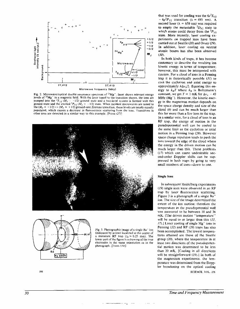
+ + + + + + r i+++ i I + i
x 0
m
+ + + + + + + +
+ + +
Microwave frequency (MHr)
Fig. 2 . Microwaveioptical double resonance spectrum of 24Mg+. Inset shows relevant energy levels of 24Mg+ in a magnetic field. With the laser tuned to the transition shown, the ions are pumped into the 2S1,2 ( M , = -112) ground state and a two-level system is formed with this ground state and the excited 2P312 ( M , = -312) state. When incident microwaves are tuned to the ( M , = - 112) cf ( M , = + 112) ground-sate Zeeman transition, these levels are nearly equally populated, which causes a decrease in fluorescence scattering from the ions. Transitions in other ions are detected in a similar way to this example. [From (27)]
e-
Fig. 3 . Photographic image of a single Ba’ ion (indicated by arrow) localized at the center of a miniature R F trap (ro 0.25 mm). The lower part of the figure is a drawing of the trap electrodes in the same orientation as in the photograph. [From (19)]
398
that was used for cooling was the 6s2Sl/Z - 6p2P112 transition (A = 493 nm). A second laser (A = 650 nm) was required to empty the metastable 2D3iz state to which atoms could decay from the state. More recently, laser cooling ex- periments on trapped ions have been carried out at Seattle (20) and Orsay (29). In addition, laser cooling on neutral atomic beams has also been observed
In both kinds of traps, it has become customary to describe the resulting ion kinetic energy in terms of temperature; however, this must be interpreted with caution. For a cloud of ions in a Penning trap it is theoretically possible (31) to cool the cyclotron and axial energy to approximately hAua/2. Equating this en- ergy to kBT where k~ is Boltzmann’s constant, we get T = 1 mK for Aua = 43 MHz (Mg’). However, the kinetic ener- gy in the magnetron motion depends on the space charge density and size of the cloud (6) and can be much larger than this for more than a few ions in the trap. In a similar vein, for a cloud of ions in an RF trap, the energy of motion in the pseudopotential well can be cooled to the same limit as the cyclotron or axial motion in a Penning trap (28). However space charge repulsion tends to push the ions toward the edge of the cloud where the energy in the driven motion can be much larger than this. These problems ( 1 7 ) which can cause undesirable sec- ond-order Doppler shifts can be sup- pressed in both traps by going to very small numbers of ions-down to one.
(30).
Single Ions
In subsequent Heidelberg experiments (19) single ions were observed in an RF trap by laser fluorescence scattering. Figure 3 is a photograph of a single Ba’ ion. The size of the image determined the extent of the ion motion; therefore the temperature in the pseudopotential well was measured to be between 10 and 36 mK. [The driven motion “temperature” will be equal to or larger than this ( I S , Zn.1 Laser cooling of single Mg+ ions in Penning (32) and RF (20) traps has also been accomplished. The lowest tempera- tures attained are those of the Seattle group (20), where the temperature in at least two directions of the pseudopoten- tial motion was determined to be less than 20 mK. [Cooling in all directions will be straightforward (19).] In both of the magnesium experiments, the tem- perature was determined from the Dopp- ler broadening on the optical cooling
SCIENCE, VOL. 226
30 Time and Frequency Measurement
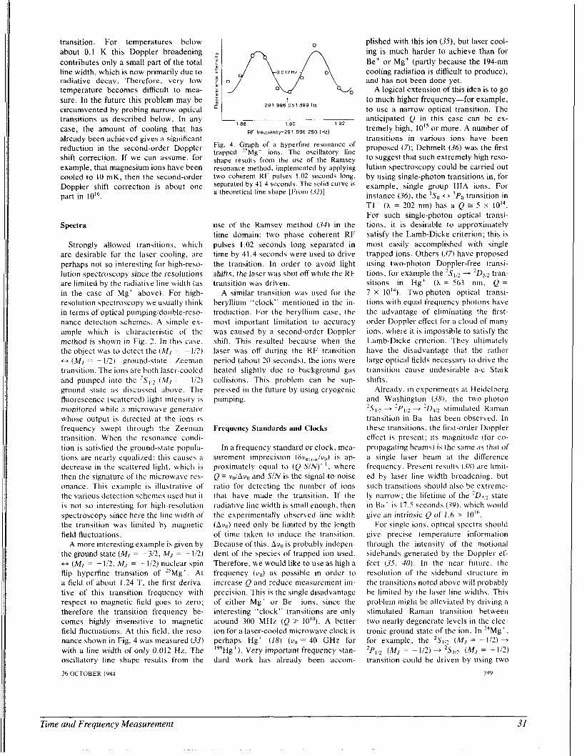
transition. For temperatures below about 0.1 K this Doppler broadening contributes only a small part of the total line width, which is now primarily due to radiative decay. Therefore, very low temperature becomes difficult to mea- sure. In the future this problem may be circumvented by probing narrow optical transitions as described below. In any case, the amount of cooling that has already been achieved gives a significant reduction in the second-order Doppler shift correction. If we can assume, for example, that magnesium ions have been cooled to I O mK, then the second-order Doppler shift correction is about one part in 10''.
Spectra
Strongly allowed transitions, which are desirable for the laser cooling. are perhaps not so interesting for high-reso- lution spectroscopy since the resolutions are limited by the radiative line width (as in the case of Mg' above). For high- resolution spectroscopy we usually think in terms of optical pumpingidouble-reso- nance detection schemes. A simple ex- ample which is characteristic of the method is shown i n Fig. 2. In this case, the object was to detect the ( M J = - 112)
( M , = +ID) ground-state Zeeman transition. The ions are both laser-cooled and pumped into the (M. , = -112) ground state as discussed above. The fluorescence (scattered) light intensity is monitored while a microwave generator whose output is directed at the ions is frequency swept through the Zeeman transition. When the resonance condi- tion is satisfied the ground-state popula- tions are nearly equalized: this causes ii
decrease in the scattered light, which is then the signature of the microwave res- onance. This example is illustrative of the various detection schemes used but it is not so interesting for high-resolution spectroscopy since here the line width of the transition was limited by magnetic field fluctuations.
A more interesting example is given by the ground state ( M , = -312, MJ = +I/?) ++ ( M , = - 112, MJ = + 112) nuclear spin flip hyperfine transition of "Mg'. At a field of about 1.24 T. the first deriva- tive of this transition frequency with respect to magnetic field goes to zero; therefore the transition frequency be- comes highly insensitive to magnetic field fluctuations. At this field. the reso- nance shown in Fig. 4 was measured (33) with a line width of only 0.012 Hz. The oscillatory line snape results from the 26 OCTOBER 1984
0
1.88 1.90 1.92
RF frequency-291 996 250 (Hz)
Fig. 4. Graph of a hyperfine resonance of trapped *'Mg+ ions. The oscillatory line shape results from the use of the Ramsey resonance method, implemented by applying two coherent RF pulses 1.02 seconds long, separated by 41.4 seconds. The solid curve is a theoretical line shape [From (SZ)]
use of the Ramsey method (34) in the time domain: two phase coherent RF pulses 1.02 seconds long separated in time by 41.4 seconds were used to drive the transition. In order to avoid light shifts, the laser was shut off while the RF transition was driven.
A similar transition was used for the beryllium "clock" mentioned in the in- troduction. For the beryllium case, the most important limitation to accuracy was caused by a second-order Doppler shift. This resulted because when the laser was off during thc RF transition period (about 20 seconds). the ions were heated slightly due to background gas collisions. This problem can be sup- pressed in the future by using cryogenic pumping.
Frequency Standards and Clocks
In a frequency standard or clock, mea. surement imprecision (6v,,,,,,/vo) is ap- proximately equal to (Q SIN)- I. where Q E vtJhuo and SIN is the signal-to-noise ratio for detecting the number of ions that have made the transition. If the radiative line width is small enough, then the experimentally observed line width (Avo) need only be limited by the lcngth of time taken to induce the transition. Because of this. Avo is probably indepen- dent of the species of trapped ion used. Therefore. we would like to use as high a frequency ( u 0 ) as possible in order to increase Q and reduce measurement im- precision. This is the single disadvantage of either Mg' or Be ' ions, since the interesting "clock" transitions are only around 300 MHz (Q 2 10"'). A better ion for a laser-cooled microwave clock is perhaps Hg' (18) (vi) = 40 GHz for I9'Hg ' ). Very important frequency stan- dard work has already been accom-
plished with this ion ( 3 3 , but laser cool- ing is much harder to achieve than for Be' or Mg~' (partly because the 194-nm cooling radiation is difficult to produce), and has not been done yet.
A logical extension of this idea is to go to much higher frequency-for example, to use a narrow optical transition. The anticipated (2 in this case can be ex- tremely high, 10" or more. A number of transitions in various ions have been proposed (7); Dehmelt (36) was the first to suggest that such extremely high reso- lution spectroscopy could be carried out by using single-photon transitions in, for example, single group IIIA ions. For instance (36), the 'So - 'Po transition in TIt ( A = 202 nm) has a Q For such single-photon optical transi- tions, it is desirable to approximately satisfy the Lamb-Dicke criterion; this is most easily accomplished with single trapped ions. Others (37) have proposed using two-photon Doppler-free transi- tions, for example the + 2D5:2 tran- sitions in Hg' ( A = 563 nm, Q =
7 x Two-photon optical transi- tions with equal frequency photons have the advantage of eliminating the first- order Doppler effect for a cloud of many ions, where it is impossible to satisfy the Lamb-Dicke criterion. They ultimately have the disadvantage that the rather large optical fields necessary to drive the trlinsition cause undesirable a-c Stark shifts .
Already. in experiments at Heidelberg and Washington (38), the two-photon
+ ' P I,2 + '113;? stimulated Raman transition in Bat has been observed. In these transitions, the first-order Doppler effect is present; its magnitude (for co- propagating beams) is the same as that of a single laser beam at the difference frequency. Present rewlts (38) are limit- ed by laser line width broadening. but such transitions should also be extreme- ly narrow: the lifetime of the ' I ) ? ? state in Ba' i \ 17.5 second5 (3Y) , which would give an intrinsic Q of 1.6 x IO".
For single ions, optical spectra should give precise temperature information through the intensity of the motional sidebands generated by the Doppler ef- fect (35. 40). In the near future, the resolution of the sideband structure in the transitions noted above will probably be limited by the laser line widths. This problem might be alleviated by driving a stimulated Raman transition between two nearly degenerate levels in the elec- tronic ground state of the ion. In 24Mg', for example, the 'Sl,? (MJ = -112) +
( M I = -l/2) --f 'S1/2 ( M I = +I121 transition could be driven by using two
5 x
399
Time and Frequency Measurement 31
laser beams separated in frequency by the MJ = - 112, and M j = + 112 ground- state frequency difference. The effects of the laser line width would be suppressed by generating the two laser lines with a phase modulator (41); the line width of the overall transition would be limited by the ground-state lifetime. The intensity of the motional sidebands would depend on v . (kl - kz) , where k l and kz are the wave vectors of the two laser beams and v is the ion velocity. Thus the angle between the beams could be chosen to optimize the temperature information.
Conclusions
The projected accuracy for optical fre- quency standards is extremely high. As an example, in I n + , the line width of the ‘SO + ’PI “cooling” transition is about 1.3 MHz; this implies a second-order Doppler shift of or lower. Other systematic shifts can occur (1, 7, 13, 16, 18, 33, 35-38, 42) but it is not unreason- able to think they will be controllable to this level. These extreme accuracies make important the problem of measure- ment imprecision, since the signal-to- noise ratio on a single ion will be about one for each measurement cycle. Practi- cally speaking, this means that a long averaging time will be required to reach a measurement precision equal to these accuracies. In fact, for a while, the accu- racy and resolution may be limited by laser line width characteristics (line width and line width symmetry); howev- er, the potential for extremely narrow lasers also exists ( 4 3 ) .
With the great potential for the optical frequency standards, one can logically ask why we bother thinking about R F or microwave frequency standards, where the desired large numbers of ions (to increase signal-to-noise and measure- ment precision) causes unwanted sec- ond-order Doppler effects (17). At pre- sent, the answer concerns the utility of optical frequency standards within cur- rent technological limitations. To use such devices as clocks as in communica- tions and navigation, one must count cycles of the radiation. At microwave frequencies this is straightforward. At
optical frequencies it is technically feasi- ble but very hard (44); it has not been done yet. To illustrate further, one might also have asked why we do not push the frequency even higher, that is, make a clock based on narrow Mossbauer tran- sitions in bound nuclei. Here, however, the technological problems become even more apparent. In spite of the technical problems of making an optical “clock,” optical frequency standards will, of course, find many immediate uses. An obvious class of experiments are cosmo- logical in nature; for example. more pre- cise measurements of the gravitational red shift will arise. In any case, the potential accuracy for stored ion spec- troscopy in all spectral regions seems extremely high. Frequency standards and clocks with inaccuracy of one part in I O ” appear very reasonable; eventually they could be orders of magnitude better than this.
References and Notes
I . J . J . Bollinger. W. M. Itano. D. 1 . Wineland, Proc. 37rhAnnu. Symp. Frey . Contro l (1983) , p. 37 (copies available from Systematics General Corporation. Brinley Plaza, Route 38, Wall Township, N.J. 07719).
2 . S. Garpman. 1. Lindgren. J . Lindgren, J . Morri- son, Z. Phys. A 276, 167 11976): S. Ahmad e / a/ . , Phys. Rei,. A 27. 2790 (1983).
3. J . Vetter. H . Ackermann. G . ZuPutlitz, E. W. Weber, Z. P h y s . A 276, 161 (1976).
4. A. G . Mungall and C C. Costain. IEEE Trans. Instrum. Meus. IM-32. 224 11983): G. Becker, Proc. 10th I n / . Congr. Chronomrrry 2 , 33 (1979): D. J. Wineland. D. W. Allan, U. 1. Glaze, H. Hellwig. S . Jarvis. Jr.. IEEE T r a m Insrrum. Meus. IM-25, 453 (1976).
5 . D. J . Larson. Bull. A m . Phys. S O [ . 19, 1193 (1974).
6. J . J . Bollinger and D. I . Wineland. Phya. R e v . L ~ r l . 53, 348 11984).
7 D. 1. Wineland, W. M. Itano. R. S. Van Dyck. Jr.. Adi. . A t . M o l Phy.\. 19, 135 (1983).
8. E. W. Weber. Plrys. Rep. 32. 123 11977). 9. A. Rich and J . C . Wesley, R ~ i l . Mod. Phy.\. 44.
250 11972). IO. K. H . Kingdon. Phv\ . f h . 21. 408 (1923). I I . M. H . Prior and E . C. Wang. P h v a . Rei,. A 16. 6
(1977). 12. E. Fisher. 2. Phya. 156. I (1959); R. F.
Wuerker. H. Shelton. R. V. Langmuir. J. Appl. Phy.5. 30, 342 11959).
13. H. G . Dehmelt. Ad,,. A i . M o l . P h y ~ . 3, 53 (1967): ibid. 5 , 109 11969).
14. F. M. Penning. Phy.si~.u 3. 873 11936). ’
15. P. Ekstrom and D. Wineland. S i . Am. 243 (No. 2). 104 (1980); D. J . Wineland, P. Ekstrom. H. Dehmelt, Phy.5. Ret,. L e / / . 31. 1279 11973).
16. W. M. Itano. L. L. Lewis. D. J . Wineland, Phyx Rei, . A 25, 1233 l1982).
17. D. 1. Wineland. N o t / . Bnr. Srund. IU.S.i Pirbl.
20. W. Nagourney. G. Janik. H. Dehmelt, Proc. Nut/. Acad. Sei. U .S .A . 80, 643 11983).
21. R. H . Dicke, Phys. Rev. 89. 472 (1953). 22. H . A. Schuessler, E. N . Fortson, H . G. Deh-
melt, ibid. 187, 5 (1969). 23. T. W. Hansch and A. L . Schawlow, Opt. Com-
mun. 13, 68 (1975). 24. D. J . Wineland and H . G. Dehmelt, Bull. A m .
Phys. Sor. 20, 637 (1975). 25. D. J. Wineland, R. E. Drullinger, F . L. Walls,
Phys. Rev . Letr. 40, 1639 (1978). 26. H. G . Dehmelt and F. L. Walls. ibid. 21, 127
11968); D . A. Church and H . G . Dehmelt, J . Appl. Phys. 40, 3421 11969).
27. D. J . Wineland. J . C . Bergquist, W. M. Itano, R. E . Drullinger, Opr. Lrrr. 5 . 245 11980).
28. W. Neuhauser. M. Hohenstatt, P. Toschek, H. Dehmelt, Phys. Rev. Ler t . 41, 233 (1978).
29. F. Plumelle, Abstracts for the 15th European Group on Atomic Spectroscopy Conference. Madrid, 5 to 8 July 1983.
30. S. V. Andreev. V. I . Balykin, V. S. Letokhov. V. G . Minogin. JETP Letr. 34, 442 (1981): J . V. Prodan. W. D. Phillips, H. 1. Metcalf. Phvs. Rev. Lrrr. 49, 1149 (1982): J . L. Hall W. Ertmer, R. Blatt. in preparation: W. D. Phhips , Ed.. “Laser-cooled and trapped atoms,” Nurl. Bur. Srand. (U.S.) Spec. Publ. 653 (1983).
31. W. M. Itano and D. J . Wineland, Phys. Re,,. A 25. 35 (1982).
32. D. J . Wineland and W. M. Itano. Phys. Lett. A 82. 75 (1981).
33. W. M. Itand and D. J. Wineland, Phys. Rri , . A 24. 1364 11981).
34. N . F. Ramsey; Molrculur Beams (Oxford Univ. Press, London, 1956).
3 5 . F. G . Major and G. Werth. Phys. Rev. Lett. 30, 1155 11973): M. D. McGuire. R. Petsch. G . Werth. Phys. Rev. A 17, 1999 (1978): M. Jardino er ul . , Appl. Phgs. 24. 107 (1981): L. S. Cutler, R. P. Giffard. M. D. McGuire, Proc. 37th Annii . Symp. Frey. Control (1983). p. 32 (copies avail- able from Systematics General Corporation, Brinley Plaza, Route 38. Wall Township, N.J. 07719); M . Jardino, F. Plumelle. M. Desaintfus- cien, J . L. Duchine, Pro<,. 38rh Annu. Svmp. F r e y . Conrrol (Philadelphia, 1984). in press.
36. H. Dehmelt, IEEE Trrms. In.s/rrim. Meas. IM. 31 R7 (19R2)
37. P~’i . -Bend&erul . , Bit//. A m . Phys. Sor. 21, 599 ( 1976).
38. W. Neuhauser, M. Hohenstatt. P. E . Toschek, H. Dehmelt, in Spectrul Line Shapes, B. Wende. Ed. (deGruyter. Berlin. 1981): W. Na- gourney. Biill. A m . PhyJ. Soc. 29. 815 (1984).
39. R. Schneider and G. Werth, Z. P h y s . A 293, 103 (1979).
40. H. A. Schuessler. Appl. Phy.s. Lerr. 18. I17 (1971): F. G . Major and J. L. Duchene. J. P h v s . ( O r I n v J 36, 953 (1975): H. S. Lakkaraju a n d H . A. Schuessler. J . Appl. Phy.\. 53. 3967 (1982): M. Jardino. F Plumelle. M. Desaintfuscien. in Loser Spw/ro.\copy V I . H . P. Weber and W. Luthy, Eds. (Springer-Verlag. New York. 1983). p. 173.
41. J . E. Thomas er u l . , P / i y ~ . Rev. L e / / . 48, 867 (1982).
42. D J. Wineland and W . M. Itano. Bull. A m . Phy.\. So<. 27. 864 (1982).
43. J . L. Hall. L. Hollberg, Ma Long-Shen. T. Baer. H. G . Robinson. J . Phvs. (Orsriy) 42. C8-59 11981); A. Yariv and K. Vahala. I E E E J . puonr. Elec./ron. QE-19. 889 11983): R . W. P. Drever er ( I / . , Appl. Phys. B 31, 97 11983): J . Hough et n l . , ibid. 33. 179 (1984).
6/7. in pre\a. 18. D . J . Wineland, W. M. llano, J . C . Bergquijt, F .
L . Wall\, Pro< 3.7rh Annir. Symp. Freq. Conlrol (1981). p. 602 (copies available from Electronic Industrie5 Association. 2001 Eye Street. NW, Washineton. D.C. 20006).
19. W. Neihauser. M. Hohenstatt, P. Toschek, H. Dehmelt. Pliy,\. Reb,. A 22. 1137 (1980). comment\ on the manuscript
44. See Proceeding5 of the Third Sympo5ium on Frequency Standards and Metrology. J. Phi,.\. 42, Colloque C-8, December 1981: V. P. Chebo- tayev cr d. , Appl. Plry.i. B 29. 63 (1982); D. A. Jenning, c r u l . , Opr. L e u . 8. 136 11983); K. M. Baird, Phys. Today 36 INo. I ) , 52 11983).
45. I gratefully acknowledge the support of the Office of Naval Research and the Air Force Office of Scientific Re\earch. I also thank J . J . Bollinger. I . C. Bergquist, J Cooper, W. M. Itano. J . D. Presage. and S. R. Stein for helpful
SCIENCE, VOL. 226 400
32 Time and Frequency Measurement
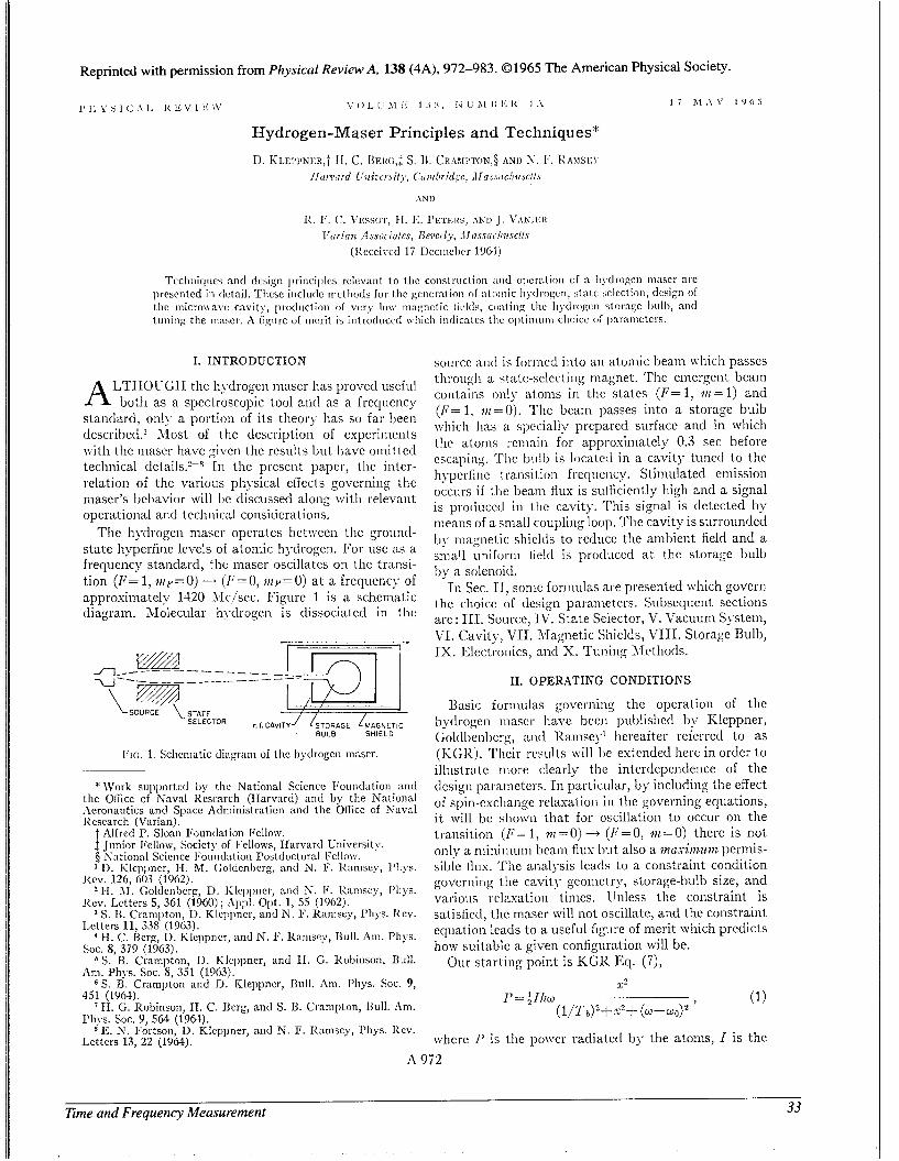
Reprinted with permission from Physical Review A, 138 (4A), 972-983. 01965 The American Physical Society.
Tccliniq~ics and dcsign principles rclevant to tlic construction :ind tilieration oi a I i~ .dr (~gcn niiiscr arc prcscntcd in tlctail. Tlicsc inclutlc nictliods for thc gcncration ni atomic Iiydi-ofi~n, s t n t c sclcctinri, design oi the micro\\ a\.c cavity, production of very I r i n ~ niagnctic licltls, c(iating t I IC Iiydr-ogcn storagc bull), ant1 tuning the ni;iscr. '1 figurc of iiicrit is iiitroduced \~ l i ich int1ic;itcs tlic o l ) t i n ~ u n i clioicc of ~)aranictcrs.
I. INTRODUCTION
I,TI-LOL1C;I-I the l i ~ drogen maser has pioved useiul A both as a spectroscopic tool aiitl as a frccliiency standard, only a portion of its theory has so far been describetl.' Most of the description of experiments with the maser have given the results but have omitted technical In the present paper, the inter- relation of the various physical effect s governing the maser's behavior will b r discussed along with relevant operational and technical consitlerations.
The hydrogen maser operates between the ground- state hyperfine levels of atoiiiic hydrogen. For use as a frequency standard, t hc maser oscillates on the transi- tion (F= 1, m p = O ) -' ( F = O , m F = O ) a t a frequent), of approximately 1420 Mc/sec. Figure 1 is a scheniatic diagram. Alolecular h>-drogeii is dissociated in the
I I
---__ __ - - - m 1;x. 1. Schcniatic tli;qyam of thc I~yclrogcn mnser.
* \Vork supported by the National Science Foundation antl t he Olfice of Naval Rcscwch (IIarvard) antl by the Natioiial .\eronautics and Spacc Administration and t he Office of N'rval Research (Varian).
t Alfred P. Sloan I"m(1ation I.'ellom. 2 Junior Fellow, Society of Fellows, Harvartl University. 5 Nntioiial Science I~ount1,ttion Postdoctoral 1;cllow. 1 D. Klcppner, 11. M. Goldcnl)erg, and N. F. 1<amsey, I ' h ~ s .
2 H. AI. Coldenberg, D. I<lcppner, antl N. I'. Kaniscy, I'liys.
S. I$. Crampton, D. Klclqincr, and N . F. Kanisey, I'hys. Rev.
H. C. Berg, I). Rleppncr, and N. I'. Iiamsey, Bull. Am. I'hys.
Ir S. B. Crampton, D. Klcppncr, and H. G. Robinson, Bull.
S. B. Cramnton and D. Kleppncr, null. Am. Phys. SOC 9,
Rcv 126, 603 (1962).
Rev. Letters 5, 361 (1960) ; Appl. Opt. 1, 55 (1962).
Lcttcrs 11, 338 (1963).
SOC. 8, 379 (1963).
ihn. P h ~ s . SOC. 8, 351 (1963). _ _ I
451 (1961). E€. G. Robinson. H. C. Ncrr. and S. B. Cranir)ton. Hull. Ani.
"I
I'hys. Soc. Y, 564 (f961).
Letters 13, 22 (1964). E. hr. I'ortson, D. Kleppner, and 3. F. Iiamscy, l'llys. Rev.
source aiid is formcd into an atoiiiic beam wliidi passes throuqli a ~tatc-selecting magnet. 'I'lie emergent beam contains only atoms in the states (F=l , m=1) and (f;=l, m = 0 ) . The beam passes into a storage bulb w l i i ~ h has a spcciall>. prepared surface and in which the at onis remain for approxiniately 0.3 sec before cscapiiiq. The 1)iilI) is locatul in a cavity tuned to the Iiypcrfiiic transit ion frecluciicy. Stimulated emission occurs if the beam flux is sufficiently high and a signal is protlucccl in the cavity. This signal is detected by ineatis of a sniall coupling loop. The cavity is surrounded 1)). niagnetic shields to reduce the ambient field and a sniall unifoini field is protluccd a t the storage bulb by a solenoid.
In Sec. 11, some fotniulas are presented which govern the choice of de5ign parameters. Subsequent sections arc: 111. Source, 1V. State Selector, V. Vacuum System, VI. Cavity, VII. Magnetic Shields, VI I I . Storage Bulb, IX. Electri~nics, and X. Tuning hfcthods.
11. O P E R A T I N G C O N D I T I O N S
Basic forniulas governiiig the operation of the hydrogen niascr have been published by Kleppner, C;oldl)ciibci E, ant1 Iianisey' hereafter referred to as (KGR). 'l'heir results will he exteiided here in order to illustrate niore dearly the interdependence of the design parameters. Tii particular, by including the effect of spin-eschange relaxation in the governing equations, i t will be shown that for oscillation to occur on the transition (I;= 1, nz=O) + ( J ;=O, nz=O) there is not only a niiiiiniuni beam flux h i t also a iiiaxiiizziiiz permis- sililc flus. 'I'he analjrsis leads to a constraint condition governing the cavity geonicti y, storage-bulb size, and various relaxation times. linless the constraint is satislied, the maser will not oscillate, and the coiistraint equation leads to a useful figure of merit which predicts how suitable a given configuration will be.
Our starting point is KGR Eq. (7), I?
I'= a J/Iw-- (1) ( 1 / I ' h ) ? + N 2 + (w-w0)2 '
wheie P is the power radiated by the atoms, I is the A 972
33 Eme and Frequency Measurement
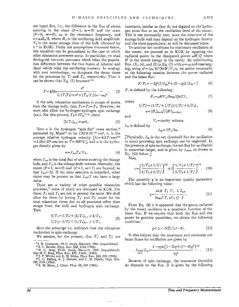
€I - M A S I3 IC 1' R I X C I P L E S A N D T 1: C 1-1 N I Q U E S A 973
net input flux, Le., the difference in the flux of atoms entering in the s ta te (F=l, m = O ) and the s ta te (F=O, m=O), w o is the resonance frequency, and x= poH,/h, where H , is the oscillating field amplitude. Tb is the mean storage time of the bulb (denoted by y-I in KGR). Under the assumptions discussed below, this equation can be generalized to the case in which other relaxation processes occur. I n particular, we shall distinguish between processes which relax the popula- tion difference between the two states of interest and those which relax the oscillating moment. I n analogy with nmr terminology, we designate the decay tinies for the processes by TI and Tz, respectively. Then it can be shown that Ec4. (1) becomesgJO
xz P = 4 I A W * (2)
1/(TiTz)+x:'+ ( T Z / T J ( W - W ) ~
If the only relaxation mechanism is escape of atoms from the storage bulb, then T I = Tz= Tb. However, we must also allow for hydrogen-hydrogen spin exchange (s.e.). For this process, Tz= 2T1,11J2 where
(l/Tl)8.e.=?kTGr. (3)
Here Q is the hydrogen "spin-flip" cross section,13 estimated by M a 2 0 ~ ~ to be 2.85>(10-15 cm?, & is the average relative hydrogen velocity [iir= 4(KT/~nz)l'~ =3.58X lo5 cm/sec at T= 30SOK.1, and 12. is the hydro- gen density given by
I z = I t o t T b / v b , (4 where Itot is the tota1,flux of atoms elitering the storage bulb, and vb is the storage-bulb volume. Normally, the states (F= 1, m = O ) and (F= 1, m= 1) are focused, so that Itot= 21. If the state selection is imperfect, other states may be present so that Itot/I can have a large value.
There are a variety of other possible relaxation processes,11 some of which are discussed in RGR. For these, TI and T Z are not in general the same. We shall allow for them by letting TI' and Tp' stand for the total relaxation times due to all processes other than escape from the bulb and hydrogen spin exchange. Tlien
TI= 1/Ti'+ (1/Ti)s.t..+ 1/T/, , 1/Tz= 1/T,'+ (1/7'~)s.c,.+ 1/r/,. (5 )
Here the subscript S.C. indicates that the rclaxation
We assume, for the present, that TI' and TZ' are mechanism is spin exchange.
S. R. Crampton, Ph.D. thesis, Harvard, 1364 (unpublished).
H. C. Berg, P1i.D. thesis, Narvnrd, 1964 (unpublisbcd). lop. 1,. Bender, Phys. Rev. 132, 2151 (1963).
Also H. C. Berg. Phw. Rev. 137. A1621. (1965). l2 T. P. Wit& and R. H. Dicke. Phvs. Rev. 103. 620 (1956). l3 L. C. Balling, R. J. Hanson, 'and-1'. hf. l ' ipkh, Phys. gev .
132. 2154 (1964). 14R. M.'Mazo, J. Chem. Phys. 31, 169 (1961).
constants, insofar as they do not depend on the hydro- gen atom flux or on the oscillation level of the maser. This is not necessarily true, since the structure of the storage-bulb wall may depend on the hydrogen density and the s ta te populations, as will be discussed below.
To analyze the conditions for stationary oscillation of the maser, we proceed as in KGR b y equating the radiated power to the dissipated power w V / @ where JV is the stored energy in the cavity. By substituting Eqs. (3), (4), and ( 5 ) in Eq. ( 2 ) with W = W O and rearrang- ing, using xz= ( ~ o / h ) ~ (8~1V/ VCj,, we arrive eventually a t the following relation between the power radiated and the beam flux:
P/Pc= - - q 2 ( r / I t h ) * + ( I - C q ) I / I t h - 1. (6)
P, is defined b y the following :
Pc=w?~pV,/8~~,,~Q1iTt2, ( 7)
q = (nz)boIb5/(a')ea\.ity 2 (8)
where 1/Tt'= TI'+ 1/Tb) (1/T,'+ 1/Tb),
and
It,, is defined by
[Physically, I t h is the net threshold flus for oscillation to occur providing spin exchange can be neglected. I n the presence of spin exchange, tlie net flux for oscillation is somewhat larger, and is given b y Imin, as shown in Eq. (13) below.]
Vc= cavity volume.
I t h = 2PcjhW. (9)
Also,
.=[ 1/"l/T1']''' 3-2 [ 1/Tb+1/1"]"? (10)
1/Tb+I/T?' 1/Ta+l/T1'
The quantity q is a n important quality parameter which has the following value :
o8,h Tb l r c 1 Itot Q=--------* (11)
8 ~ 0 ~ Tt V ~ ' L Q I
From Eq. (6) i t is apparent that the power radiated by the maser oscillator is a quadratic function of the beani flux. If we require tha t both the flux and the power be positive quantities, we obtain the following condition :
q< (c-2lo)/(,,Z-8). (1 3)
It also follows that the maximum and minimum net beam fluxes for oscillation are given by
l-ccpf[1-2cq+ (c'-S)q2l1'? I m ? x / I t h = . (13)
4 q2 111111
Because of spin exchange, the resonance linewidth Av depends on the flux. It is given by the following
34 l ime and Frequency Measurement
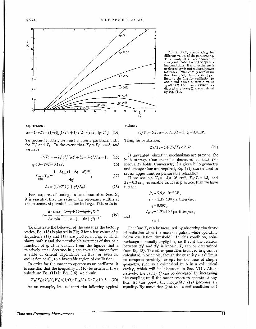
A 974 I i L E P P N E I Z e l a l .
7 - // I / /a = 0.05
5 1 / / ’
.I 3 /L/f0.E -/ q = 0.14
FIG. 2. P/P , versus I / I ta for different values of the parameter q. This family of curves shows the strong influence of p on the operat- ing conditions. If spin exchange is neglected, q=O and radiated power increases monatonically with beam flux. For q>O, there is an upper limit to the flux for oscillation to occur and above a certain value (0=0.172) the maser cannot ra- diate a t any beam flux. p is defined by Eq. (11).
expression : values :
Av= 1 / ~ T 2 = (1 /~) [ ( l jT2’+1/Tb)+ (I/Ith)q/Tt]. (14) Vc/ Vb= 6.7, q= 3, Itot/I = 2, Q= 3X 10‘.
To Droceed further, we must choose a particular ratio Then, for oscillation, for TI‘ and T2‘. I n the event that T1‘= T2’, G = 3, and we have
If unwanted relaxation mechanisms are present, the bulb storage time must be decreased SO tha t this
q < 3 - 2 ~ 2 = 0 . 1 7 2 , (16) inequality holds. Conversely, if a given bulb geometry and storage time are required, Eq. (21) can be used to set an upper limit on permissible relaxation.
If we assume VC=1.3X10* cm3, Tb/Tt=1.3, and Ta= 0.3 sec, reasonable values in practice, then we have
I‘/P,= -2$(I,’ItlJ2+ (1-3q)I/Itb- 1 , (15)
1-3qf(1-6q+q2)1’2 9 (17) Imax/I, , = -
4P2 nun
AY = (I/nTt> (1 +qI/Itth) (18) further
For purposes of tuning, to be discussed in Sec. X, i t is essential that the ratio of the resonance widths a t the extremes of permissible flux be large, This ratio is
P c = 5.9 X Ith= 1 . 3 x lo1? particles/sec,
W ,
q= 0.097,
To illustrate the behavior of the maser as the factor q varies, Eq. (15) is plotted in Fig. 2 for a few values of q. Equations (17) and (19) are plotted in Fig. 3, which shows both r and the permissible extremes of flux as a function of q. It is evident from the figures that a relatively small decrease in q can take the maser from a state of critical dependence on flux, or even no oscillation at all, to a favorable region of oscillation.
I n order for the maser t o operate as an oscillator, i t is essential that the inequality in (16) be satisfied. If we substitute Eq. (11) in Eq. (16), we obtain
(20)
As an example, let lis insert the following typical
Ta/TtX Vc/ (7 Va) X l /QXItoc/I < 3.47X 1W4.
The time T 2 can be measured by observing the decay of radiation when the maser is pulsed while operating below oscillation threshold.” I n this condition, spin- exchange is usually negligible, so that if the relation between T; and T i is known, Tt can be determined from Eq. (8). The other quantities involved in q can be calculated in principle, though the quantity q is difficult to compute precisely, except for the case of simple geometry, such as a cylindrical bulb in a cylindrical cavity, which will be discussed in Sec. VIII. Alter- natively, the cavity Q can be decreased by increasing the coupling until the maser ceases to operate at any flux. At this point, the inequality (12) becomes an equality. By measuring Q a t this cutoff condition and
Time and Frequency Measurement 35
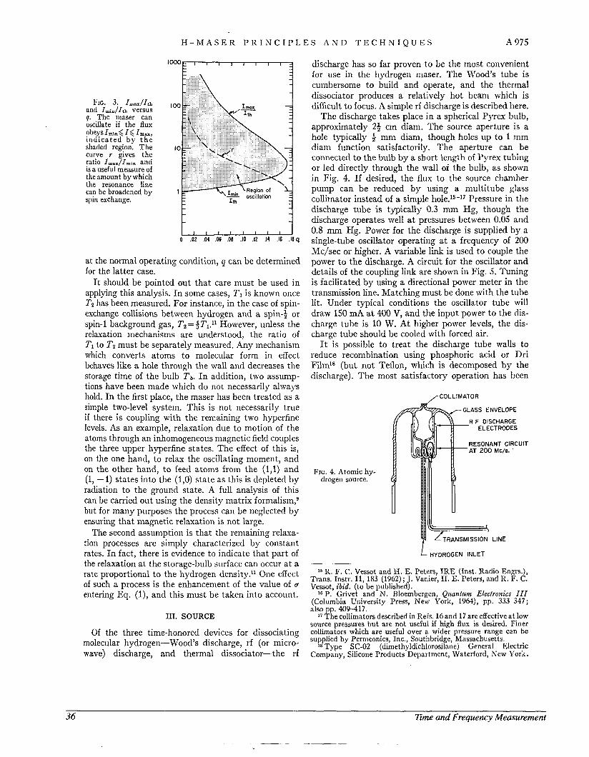
H - M A S E R P R I N C I P L E S A N D T E C H N I Q U E S A 975
I?lG. 3. Imnx/Ith and Imi,/Ith versus q. The maser can oscillate if the flux obeysImi,< I< I,,, i n d i c a t e d b y t h e shaded region. T h e curve r gives the ratio Imax/I,in and is a useful measure of the amount by which the resonance line can be broadened by spin exchange.
100
IO
1
u 0 .02 .04 .06 .Ob .IO .I2 .14 .I6 ,111
at the normal operating condition, q can be determined for the latter case.
I t should be pointed out that care must be used in applying this analysis. I n some cases, T I is known once Tz has been measured. For instance, in the case of spin- exchange collisions between hydrogen and a spin-3 or spin-1 background gas, T2= +T1.l1 However, unless the relaxation mechanisms are understood, the ratio of T I to T2 must be separately measured. Any mechanism which converts atoms to molecular form in effect behaves like a hole through the wall and decreases the storage time of the bulb Ta. I n addition, two assunip- tions have been made which do not necessarily always hold. I n the first place, the maser has been treated as a simple two-level system. This is not necessarily true if there is coupling with the remaining two hyperfine levels. As a n example, relaxation due to motion of the atoms through an inhomogeneous magnetic field couples the three upper hyperfine states. The effect of this is, on the one hand, to relax the oscillating moment, and on the other hand, to feed atoms from the (1,1) and (1, - 1) states into the (1,O) state as this is depleted by radiation to the ground state. A full analysis of this can be carried out using the density matrix forr~ialism,~ but for many purposes the process can be neglected by ensuring that magnetic relaxation is not large.
The second assumption is that the remaining relaxa- tion processes are simply characterized b y constant rates. I n fact, there is evidence to indicate that part of the relaxation a t the storage-bulb surface can occur a t a rate proportional t o the hydrogen density." One effect of such a process is the enhancement of the value of u entering Eq. (l), and this must be taken into account.
111. SOURCE
Of the three time-honored devices for dissociating molecular hydrogen-Wood's discharge, rf (or niicro- wave) discharge, and thermal dissociator-the rf
discharge has so far proven to be the most convenient for use in the hydrogen maser. The Wood's tube is cumbersome to build and operate, and the thermal dissociator produces a relatively hot beam which is difficult t o focus. A simple rf discharge is described here.
The discharge takes place in a spherical Pyrex bulb, approximately 23 cm diam. The source aperture is a hole typically + mm diam, though holes up to 1 mm diam function satisfactorily. The aperture can be connected to the bulb b y a short length of Pyrex tubing or led directly through the wall of the bulb, as shown in Fig. 4. If desired, the flux to the source chamber pump can be reduced b y using a multitube glass collimator instead of a simple Pressure in the discharge tube is typically 0.3 mm Hg, though the discharge operates well a t pressures between 0.05 and 0.8 m m Hg. Power for the discharge is supplied by a single-tube oscillator operating a t a frequency of 200 Mc/sec or higher. A variable link is used to couple the power t o the discharge. A circuit for the oscillator and details of the coupling link are shown in Fig. 5. Tuning is facilitated by using a directional power meter in the transmission line. Matching must be done with the tube lit. Under typical conditions the oscillator tube will draw 150 mA a t 400 V, and the input power to the dis- charge tube is 10 W. At higher power levels, the dis- charge tube should be cooled with forced air.
I t is possible to treat the discharge tube walls to reduce recombination using phosphoric acid or Dri Filmls (but no t Teflon, which is deconiposed b y the discharge). The most satisfactory operation has been
/ CO L L I MAT0 R
FIG. 4. Atomic hy- drogen source.
GLASS ENVELOPE
R F DISCHARGE ELECTRODES
RESONANT CIRCUIT AT 200 MC/S. '
'HYDROGEN INLET
16 R. F. C . Vessot and H. E. Peters, I R E (Inst. Radio Engrs.), Trans. Instr. 11, 1S3 (1962); J. Vanier, H. E. Peters, and R. F. C. Vessot, ibid. (to be published).
16 P. Grivet and N. Bloembergen, Qicanliim Electronics 111 (Columbia University Press, New York, 1964), pp. 333-347; also pp. 409-417.
T h e collimators described in Refs. 16 and 17 are effective a t low source Dressures bu t are not useful if high flux is desired. Finer collimaiors which are useful over a wid& pressure range can be supplied by Permeonics, Inc., Southbridge, Massachusetts.
18 Type SC-02 (dimethyldichlorosilane) General Electric Company, Silicone Products Department, Waterford, New York .
36 Time and Frequency Measurement
__ ~- ~- - .
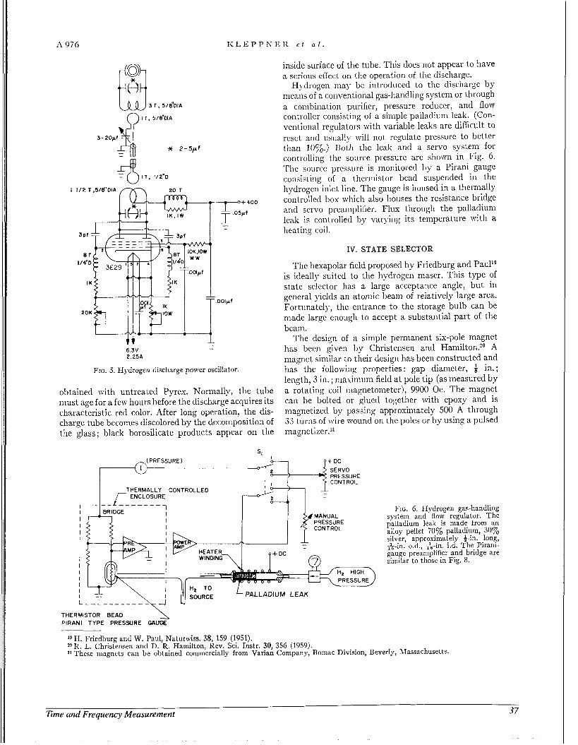
A 976 K L E P P N E R e t u l
3 T , S/e"DIA $ I T . 5/8"OlA
4 11, 1/2*D
3-2Opf
X 2-5pf
- 6.3V - 2.25A
FIG. 5. Hydrogen discharge power oscillator.
obtained with untreated Pyrex. Normally, the tube must age for a few hours before the discharge acquires its characteristic red color. After long operation, the dis- charge tube becomes discolored by the deconipositioii of the glass ; black borosilicate products appear on the
inside surface of the tube. This does not appear to have a serious effect 011 the operation of the discharge.
Hydrogen ma)- be introduced to the discliarge by means of a conventional gas-handling system or through a combination purifier, pressure reducer, and flow controller consisting of a simple palladium leak. (Con- ventional regulators with variable leaks are difficult to reset a~itl usually will not regulate pressure to better than IO%.) Both the lcak and a servo system for controlliiig the source pressure are shown in Fig. 6. 'rile soiirce pressure is monitored by a Pirani gauge consisting of a thermistor bead suspended in the hydrogen inlet line. The gauge is housed in a thermally controlled box which also houses the resistance bridge and scrvo preampliiier. Flux through the palladium lcak is controlled by varying its temperature with a heating coil.
IV. STATE SELECTOR
The hexapolar field proposed by Friedburg and Paul1g is ideally suited to the hydrogen maser. This type of state selector has a large acceptance angle, bu t in general yields an atomic beam of relatively large area. Fortunately, the entrance to the storage bulb can be made large enough to accept a substantial par t of the beam.
The design of a simple permanent six-pole magnet has been given by Christensen and I-Iainilton.'O A magnet similar to their design has been constructed and has the following properties : gap diameter, in. ; length, 3 in. ; niaxiniuin field a t pole tip (as measured by a rotating coil magnetometer), 9900 Oe. The magnet can be bolted or glued together with e p o q and is magnetized by passing approximately 500 A through 33 turns of wire wound on the poles or by using a pulsed magnetizer.21
THERMALLY CONTROLLED
FIG. 6. Hydrogen gas-handling system and flow regulator. T h e palladium leak is made from an alloy pellet 70% palladium, 30% silver, approximately $-in. long,
gauge preamplifier and bridge are similar to those in Fig. 8.
_ _ ,",-in. o.d., &-in. i.d. T h e Piranl-
PALLADIUM LEAK
THERMISTOR BEAD PIRANI TYPE PRESSURE GAUGE
l9 H. Friedburg and W. Paul, Naturwiss. 38, 159 (1951). 2''R. L. Christcnsen and I). R. Hamilton, Kcv. Sci. Instr. 30, 356 (1959). 21 These mugnets can be obtained commercially from Varian Company, Bomac Division, Beverly, Massachusetts.
37 Time and Frequency Measurement
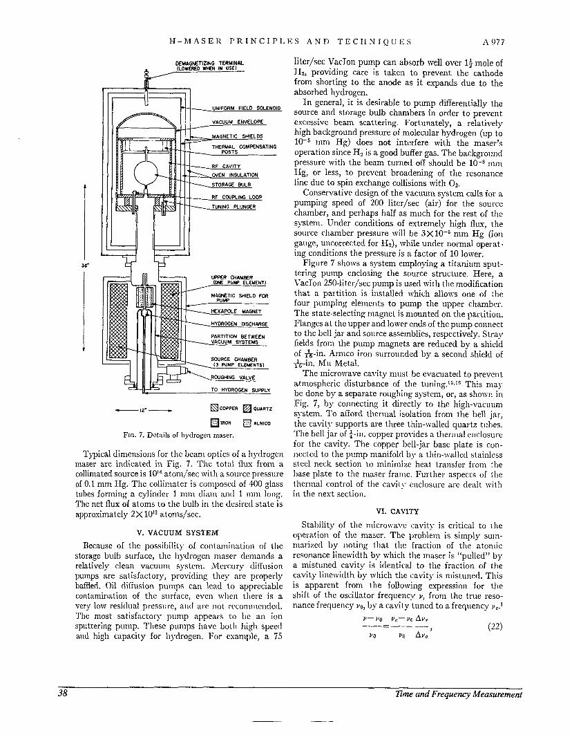
H - M A S E R P R I N C I P L E S A N D T E C H N I Q U E S A 0 7 7
7
MMAGNETIZING TERMINAL (LOWEREO WHEN IN USE)
< TUNING PLUNGER t-
fl-1 I U
m.- -UNIFORM FIELD SOLENOID
VACUUM ENVELOPE
1-
COPPER OUARTZ - 12’ - IRON 0 ALNICO
FIG. 7. Dctails of hydrogen maser.
l’qpical dimensions for the beam optics of a hydrogen inaser are indicated in Fig. 7. The total flux from a collimated source is 10l6 atom/sec with a source pressure oi 0.1 mm Hg. The colliniater is composed of 400 glass tubes forming a cylinder 1 nini tliain antl 1 311111 long. The net flux of atonis to the bulb in the desired s ta te is approximately 2X IOi2 atoms/sec.
V. VACUUM SYSTEM
Because of thc possibility of coritaiiiin:~tioii of the storage bulb surface, the hydrogen maser dcniands a relatively clean vacuiini system. A4ercury diffusion puinps are satisfactory, providing they are properly baaed. Oil diffusion pumps can lead to appreciable contamination of the surface, even when there is a very low residual pressure, antl are not rccomnientled. ‘I’he most satisfactory p u n y appears to 1 ) ~ ‘ an ion sputtering pump. These pumps have both high speed and high capacity for hjdrogen. For example, a 75
liter/sec VacTon punip can absorb well over 14 mole of Hz, providing care is taken to prevent the cathode from shorting to the anode as it expands due to the absorbed hydrogen.
I n general, i t is desirable t o pump differentially the source and storage bulb chambers in order to prevent excessive beam scattering. Fortunately, a relatively high background pressure of molecular hydrogen (up to le5 nini Hg) does not intcrfere with the maser’s operation since H2 is a good buffer gas. The backgromcl pressure with the beam turned off should be ~ n n i Hg, or less, to prevent broadening of the resonance line due to spin exchange collisions with 02.
Conservative design of the vacuum system calls for a pumping speed of 200 liter/sec (air) for the source chamber, and perhaps half as much for the rest of the system. Under conditions of extremely high flux, the source chamber pressure will be 3 X W 5 mni Hg (ion gauge, uncorrected for Hz), while under normal operat- ing conditions the pressure is a factor of 10 lower.
Figure 7 shows a system employing a titanium sput- tering pump enclosing the source structure. Here, a VacIon 250-liter/sec pump is used with the modification that a partition is installed which allows one of the four pumping elements to pump the upper chamber. The state-selecting magnet is mounted on the partition. Flanges at the upper and lower ends of the pump connect to the bell jar and source assemblies, respectively. Stray fields from tlie pump magnets are reduced by a shield of &-in. Arinco iron surrounded b y a second shield of &-in. Mu Metal.
The microwave cavity must be evacuated to prevent atmospheric disturbance of the t ~ n i n g . ~ ~ J ~ This niay be done by a separate roughing system, or, as shown in Fig. 7, by connecting i t directly to the high-vacuum system. To afford thermal isolation from the bell jar, the cavity supports are three thin-walled quartz tubes. ‘The bell jar of $-in. copper provides a thennal enclosure for the cavity. The copper bell-jar base plate is con- nected to the pump nianifoltl by a thin-\valled stainlcss steel neck section to minimize heat transfer from the base plate to the maser frame. Further aspects of the t hernial control of the cavitj- txclosure are dealt w i t h in tlie next section.
VI. CAVITY
Stability of the niicrowave cavity is critical to the operation of the maser. T h e Ixoblein is simply sum- ninrizctl by noting that 1l1e fraction of the atomic resonance linewidth by which the maser is “pulled” by a mistuned cavity is identical to the fraction of the cavity linewidth by which the cavity is niistuned. This is apparent from the following elrpression for the shift of the oscillator frequency v, from the true reso- nance frequency YO, by a cavity tuned to a frequency vC.l
V- vo vC- vo Avr
vo vo A v ~ 1 ( 2 2 ) - -
38 lime and Frequency Measurement
__-
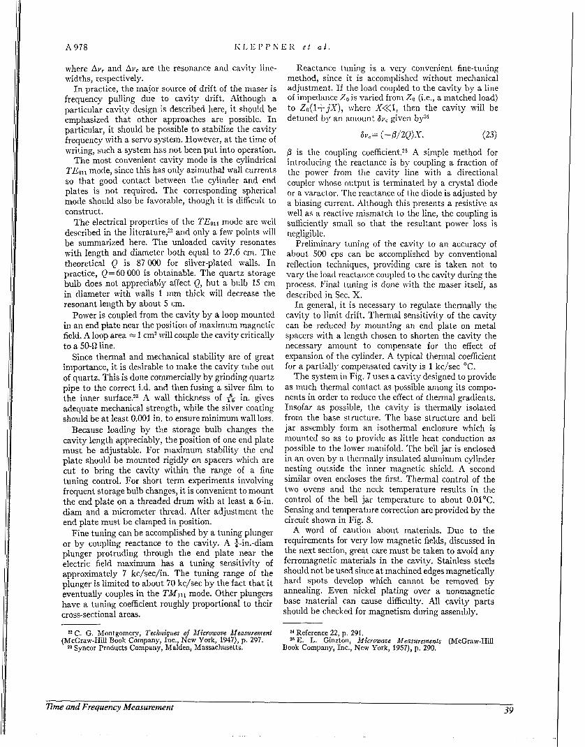
where A I J ~ and Av, are the resonance and cavity line- widths, respectively.
I n practice, the major source of drift of the maser is frequency pulling due to cavity drift. Although a particular cavity design is described here, i t should be emphasized tha t other approaches are possible. I n particular, i t should be possible to stabilize the cavity frequency with a servo system. However, a t the time of writing, such a system has not been pu t into operation.
T h e most convenient cavity mode is the cylindrical TEoll mode, since this has only azimuthal wall currents so that good contact between the cylinder and end plates is not required. The corresponding spherical mode should also be favorable, though i t is difficult to construct.
T h e electrical properties of the TEOU mode are well described in the l i t e r a t ~ r e , ' ~ and only a few points will be summarized here. The unloaded cavity resonates with length and diameter both equal to 27.6 cm. The theoretical Q is 87 000 for silver-plated walls. In practice, Q= 60 000 is obtainable. The quartz storage bulb does not appreciably affect Q, but a bulb 15 cm in diameter with walls 1 mm thick will decrease the resonant length by about 5 cm.
Power is coupled from the cavity by a loop mounted in an end plate near the position of maximum magnetic field. A loop area = 1 cm2 will couple the cavity critically to a 50-Q line.
Since thermal and mechanical stability are of great importance, i t is desirable to make the cavity tube out of quartz. This is done cormercially by grinding quartz pipe to the correct i.d. and then fusing a silver film to the inner ~ur face .2~ A wall thickness of in. gives adequate mechanical strength, while the silver coating should be a t least 0.001 in. to ensure minimum wall loss.
Because loading by the storage bulb chan, ves the cavity length appreciably, the position of one end plate must be adjustable. For maximum stability the end plate should be mounted rigidly on spacers which are cut t o bring the cavity within the range of a fine tuning control. For short term experiments involving frequent storage bulb changes, i t is convenient to mount the end plate on a threaded drum with a t least a 6-in. diam and a micrometer thread. After adjustment the end plate must be clamped in position.
Fine tuning can be accomplished by a tuning plunger or by coupling reactance to the cavity. A $-in.-diam plunger protruding through the end plate near the electric field maximum has a tuning sensitivity of approximately 7 kc/sec/in. The tuning range of the plunger is limited to about 70 kc/sec by the fact tha t i t eventually couples in the TMlll mode. Other plungers have a tuning coefficient roughly proportional to their cross-sectional areas.
Reactance tuning is a very convenient fine-tuning method, since i t is accomplished without mechanical adjustment. If the load coupled to the cavity by a line of impedance Z0 is varied from Z O ( i t . , a matched load) to Zo(l+jX), where X<<l, then the cavity will be detuned by an amount 6v, given byz4
0 is the coupling ~oefficient.2~ A simple method for introducing the reactance is by coupling a fraction of the power from the cavity line with a directional coupler whose output is terminated by a crystal diode or a varactor. The reactance of the diode is adjusted by a biasing current. Although this presents a resistive as well as a reactive mismatch to the line, the coupling is sufficiently small so that the resultant power loss is negligible.
Preliminary tuning of the cavity to an accuracy of about 500 cps can be accomplished by conventional reflection techniques, providing care is taken not to vary the load reactance coupled to the cavity during the process. Final tuning is done with the maser itself, as described in Sec. X.
I n general, i t is necessary to regulate thermally the cavity to limit drift. Thermal sensitivity of the cavity can be reduced by mounting an end plate on metal spacers with a length chosen to shorten the cavity the necessary amount to compensate for the effect of expansion of the cylinder. A typical theiiiial coefficient for a partially compensated cavity is 1 kc/sec "C.
The system in Fig. 7 uses a cavity designed to provide as much thermal contact as possible among its compo- nents in order to reduce the effect of thermal gradients. Insofar as possible, the cavity is thermally isolated from the base structure. The base structure and bell jar assembly form an isothermal enclosure which is mounted so as to provide as little heat conduction as possible to the lower manifold. The bell jar is enclosed in an oven by a thermally insulated aluminum cylinder nesting outside the inner magnetic shield. A second similar oven encloses the first. Thermal control of the two ovens and the neck temperature results in the control of the bell jar temperature to about 0.01"C. Sensing and temperature correction are provided by the circuit shown in Fig. 8.
A word of caution about materials. Due to the requirements for very low magnetic fields, discussed in the next section, great care must be taken to avoid any ferromagnetic materials in the cavity. Stainless steels should not be used since a t machined edges magnetically hard spots develop which cannot be removed by annealing. Even nickel plating over a nonmagnetic base material can cause difficulty. All cavity parts should be checked for magnetism during assembly.
22 C. G. Montgomery, Teclziriqztes of Microwave Afeasiweritent (McCraw-Hill Book Company, Inc., New York, 1947), p. 297.
Syncor Products Company, Malden, Massachusetts.
Reference 22, p. 291. 26 E. L. Ginzton, Microwave Measiminents (McGraw-Hill
Book Company, Inc., New York, 1957), p. 290.
Eme and Frequency Measurement 39
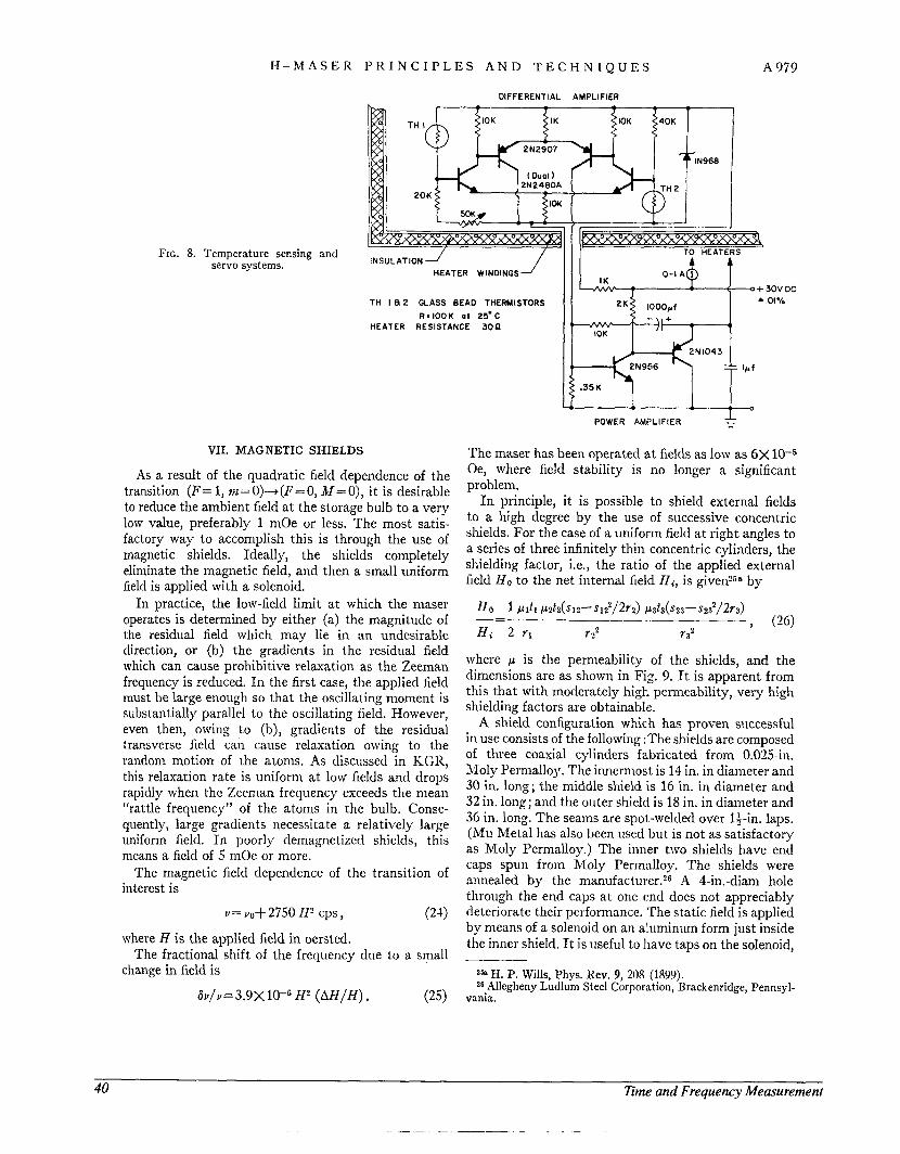
1 3 - M A S E R P R I N C I P L E S A N D T E C H N I Q U E S A 979
FIG. 8. Temperature sensing servo systems.
and
DIFFERENTIAL AMPLIFIER
IOK IK IOK 40K
INSULATION HEATER WINDINGS
T H I a 2 GLASS BEAD THERMISTORS
R=IOOK at 25.C HEATER RESISTANCE son
1 1 1 POWER AMPLIFIER - - I "
VII. MAGNETIC SHIELDS
As a result of the quadratic field dependence of the transition ( F = 1, wz=O)+(F=O, M = O ) , i t is desirable to reduce the ambient field a t the storage bulb to a very low value, preferably 1 mOe or less. The most satis- factory way to accomplish this is through the use of magnetic shields. Ideally, the shields completely eliminate the magnetic field, and then a small uniform Geld is applied with a solenoid.
I n practice, the low-field limit a t which the maser
The maser has been operated a t fields as low as 6X 1 0 - 5 Oe, where field stability is no longer a significant problem.
I n principle, it is possible to shield external fields to a high degree by the use of successive concentric shields. For the case of a uniform field a t right angles to a series of three infinitely thin concentric cylinders, the shielding factor, Le., the ratio of the applied external field No to the net internal field Hi, is given258 by
H~ 1 p l t l p 2 t z ( s 1 2 - - s 1 ~ / 2 r z ) 1 ( 3 t 3 ( S 2 3 - S 2 3 2 / 2 r 3 )
operates is determined by either (a) the magnitude of -=- - , (26) the residual field which mav lie in a n undesirable H i 2 71 722 r3'
direction, or (b) the gradieits in the residual field which can cause prohibitive relaxation as the Zeeman frequency is reduced. I n the first case, the applied field must be large enough so that the oscillating moment is substantially parallel to the oscillating field. However, even then, owing t o (b), gradients of the residual transverse field can cause rclaxation owing to the random motion of the atoms. As discussed in KGR, this relaxation rate is uniform a t low fields and drops rapidly when the Zeeman frequency exceeds the mean "rattle frequency" of the atoms in the bulb. Conse- quently, large gradients necessitate a relatively large uniform field. I n poorly demagnetized shields, this means a field of 5 mOe or more.
The magnetic field dependence of the transition of interest is
V = vo+2750 ZI' CPS , (2-1.)
where H is the applied field in oersted.
change in field is The fractional shift of the frequency due to a small
6lJ/v=3.9X 10-6 I12 ( A H I H ) . (25 )
where p is the permeability of the shields, and the dimensions are as shown in Fig. 9. It is apparent from this that with moderately high permeability, very high shielding factors are obtainable.
A shield configuration which has proven successful in use consists of the following :The shields are composed of three coaxial cylinders fabricated from 0.025-in. Moly Permalloy. The innermost is 14 in. in diameter and 30 in. long; the middle shield is 16 in. in diameter and 32 in. long; and the outer shield is 18 in. in diameter and 36 in. long. The seams are spot-welded over 13-in. laps. (iMu Metal has also been used but is not as satisfactory as Moly Permalloy.) The inner two shields have end caps spun from Moly Perinulloy. The shields were annealed b y the A 4-in.-diam hole through the end caps a t one m d does not appreciably deteriorate their perfomiance. The static field is applied by means of a solenoid on an aluminum form just inside the inner shield. I t is useful to have taps on the solenoid,
zb H. P. Wills, Phys. Rev. 9, 208 (1809). z6.Allegheny Ludlum Steel Corporation, Brackenridge, Pennsyl-
vania.
40 Time and Frequency Measurement
- -
A 080
I'Ic. 9. Gconictry of concentric cyliii- tlr i c a l n i a g n c t i c shields.
so tha t a few turns ai each end can be energized separately. 'Yliese coils can be used to reduce end effects. They are also useful for pioviding a small gradient for the magnetic-quenchi~lg tuning technique which will be described in Sec. X.
Proper deniagnetization is critical to the shield's performance. A 60-cps dcmagnetizing current is passed through the center of the shields, using the vauiuiii can as a conductor. The resulting field is azimuthal, so tha t the deniagnetizing flux lies completely in the shields. Current is obtained iroiii a transformer made by winding seven turns of No. 4 copper Lable around the toroidal core of a 20-11 autotransformer. For fine current control, two Variacs in series are used to drive the transformer. Best results are obtained by slowly raising the current to i ts maximum value and then decreasing i t to zero, taking about 1 min altogether.
Current up to 103 A is required to saturate the shields, bu t such strong demagnetizing current is seldom necessary. The best results are obtained by demagnetizing with maximum current of about 150 A. The residual fields appear to be caused primarily by spots of remnant magnei ization in the shields. These spots vary in position and intensity from one demagnet- ization to another bu t arc most commonly found along the seam of the innelmost shield. The residual trans- verse field is generally quite nonuniforin. Its maximum value is tjpically le5 to 1W4 Oe, based on measure- ments of the low-field radiation lifetiine. Lower values ai e obtained from time to time.
13y the demagnetization procedure described, very large external fields can bc shielded. For instance, a powerful horseshoe magnet placed directly on the shields will cause a serious disturbance, bu t the distur- bance is alinost completely eliminated by demagnetiza- tion. Likewise, fields due to nearby large magnets on Vaclon pumps can be shielded without undue difficulty. Apparently, the chief function of demagnetization is to raise the flux level to a point where the shield magnetiza- tion can favorably reorient itself.
Although large permanent fields are effectively reduced by the shields, they are much less effective at reducing small variations in the field, since the incre- mental permeability drops off rapidly a t low fields. Addition of merely another shield does not liclp matters, sincc its shielding contribution is counterbalanced by the decrease in penlieability of the inner shields which
now operate a[ a lonm field. JIcasurcments made with a magnetometer indicate a shielding factor for small changes in the amhicnt field of about 600. (With the innermost shield matlc of Mu Rletal, this figure is about 100.) I h r i n g operat ion at favorable times, the field fluctua~ions at the storage bulb are about Oc, as measured with the maser when it is operating on the fieltl-tlcpciidcnl traii5it ion with ti 10-scc sanipling time. The rim fluctuations are almost 10 times smaller.
VIII. STORAGE BULB
A. Bulb Design A number of considerations are involved in designing
the storage bulb. The dimensions must be chosen so that the rcstriction on q given by Eq. (12) is satisfied, and preferably so that q is as small as possible. For this reason, i t is desirahle to iiiasiinize the filling factorz7 7' given by
(~zz ) ,> " , l>z Vb
(27) 71=p - (11 ')cTv i t 1
A spherical bulb is the easiest to construct, and 7' for that case may be determined using the plot of 7 in RGR (note the correction in footnote 27). For a cylindrical bulb of radius r and length I in a cylindrical cavity of radius R and length L, the following expression can be derived :
32 J I 2 ( k y ) sin2(a/2) (Z/L) L 7'=-p . (28 )
T' Jo2(KR) [l+ (T /KL)~] lk2R2
J n ( x ) is the uth-order I3essel function, J1(kR) = 0. From this i t follows that I' is niasimiaed by the choice r = 0.52RJ I = 0.74L. Although the above formula neglects distortion of the fields in the cavity by the storage bulb, more detailed calculations show tha t q' is not significantly altered, providing the dimensions inserted in (28) refcr to the actual dimensions of the cavity when i t is loaded by the storage bulb. Two other considerations which enter the bulb design are the desired storage time and the collision rate. I n order to avoid increasing q, the storage time must not be made long compared to the radiation lifetime. Because the wall shift is proportional to the collision rate, i t is desir- able to keep the bulb dimensions as large as possible. For this reason, a bulb somewhat larger than needed to maximize Eq. (7) may be desirable. The storage time TI, and mean distance between wall collisions X are given by
Tb= 4 lia/tA , (29)
(30) X = 4V7,/.4 b . Here Vb=storage bulb volume, Ab=surface area of
27 The symbol 7' is chosen since 7 is t he conventional nmr symbol for t he filling factor. Unfortunately, t) was used in KGIi for the ratio of the field averages. The vcrtical scale of the plot of 7 in KG11 11:~s an error runt1 should be divided by two.
Time and Frequency Measurement 41
P I - 3 1 A S E R P R I N C I P L E S A N D T E C I-I N I Q U E S A 981
bulb, A,=area of the exit aperture, v= average velocity = ( 8 k T / ~ v z ) ~ ' ~ . These formulas are derived in Appendix A. If a collimating tube is used instead of a simple aperture, then flow is reduced by a factor K , so that
T b = (l/K)(4Vb/&la). (31)
A table of values of K for tubes of various sizes is given by Dushman.28 A collimating tube will also slightly alter X, and a correction for this is presentetl in Ap- pendix A.
The storage bulb is generally made of fused quartz with a diameter between 3+ and 6; in. and a wall thickness of about 0.040 in. Atoms enter the bulb through a tube whose diameter and length are chosen for the desired lifetime. If i t is important to make eficient use of the beam flux, the entrance aperture can be enlarged and several thin-walled tubes introduced to make a simple collimator.
B. Wall Coating
A number of materials have been used successfully for coating the storage bulb wall. At room temperature, both long-chain paraffin2 and Dri-Film15 surfaces have been used and yield times Tz' of about 0.3 sec in a l6-cn1- diam bulb. The limit appears to be set by the chemical reaction of hydrogen with the wall. This problem is diminished by the use of Tellon, a fluorocarbon which also has the advantage of an appreciably smaller wall shift than paraffin or Dri-Film. At 35"C, a 16-cm-diam Teflon-coated storage bulb has a time TZ' of abut 3 sec stid a fractional wall shifts of -2.1X10⁻¹¹. .At higher temperatures, there is a decrease both in the wall shift and in the lifetime. At lOO"C, 7'2' is reduced by a factor of approximately 2, and the fractional wall shift is reduced by a factor of 3. The nature of the wall relasa- tioii is discussed in Kef. 11.
The method for applying a Teflon film has been previously reported.2g However, new techniques have h e n developed since then which simplify the procedure. The coating technique described in Ref. 29 is for T F E Teflon (du Pont T F E clear finish 852-201). The procedure described is improved by the use of hot white fuming nitric acid as the cleaning agent, rather than glass-cleaning solutio 11. 130 wever, t 11 e en ti re coati rig process is simplified by the use.of FEP Teflon (du I'ont ITP Teflon product Code 120), since this forms a more uniform coat and several coats can be applied succes- sively." The FEP suspension is applictl as tlescribetl in Ref. 29. However, during the fusing process clean air iq circulated through the bulb. I>ecomposition and waste products are thereby oxidized and removed as gases. 'I'he fusing oven temperature is brought u p to 360°C tluring the course of an hour, held a t that temperature for about 20 min, and then cooled, during the course of
2* S. Dushman, ScientiJi'c Fozmdaliotzs of Vac11zm Technique
*$I-T. C. I k r g and 1). Kleppner, Rev. Sci. Instr. 33, 24s (1962). (John Wiley & Sons, Tnc., New York, 1962), p. 93.
'another hour. The film is strong and transparent and is inert to hot fuming nitric acid; however, i t can be removed bodily by heating in the bulb a solution of 20% HF and 20% HN03.
T h e collimating tube in the neck of the bulb can be machined from solid Teflon, or i t can be made by coating a pyrex plug. The latter procedure is preferable, since solid Teflon tends to outgas for several days.
Although the wall-coating procedure described here is quite reliable, the surfaces are not entirely inert, and i t is possible that this is clue to a contaminant in the Teflon. N'ew surfaces are currently 1)eing investigated.
IX. ELECTRONICS
Systems for processing the maser signal will not be described in detail, since the procedure depends on the type of measurement to be made, and often to a large extent on the available equipment. However, there are a few points of general interest.
I t is important to keep the maser operating into a constant load since reactance changes will cause frequency pulling, as discussed in Sec. VI. An isolator is invaluable for this purpose. The isolator is also helpful in decoupling two masers which are operating into converters powered by a common local oscillator. Isolation requirements are stringent, if frequency locking of the inasers is to be avoidcd. This can be seen by the following argument : The initial phase of a maser is random, since the maser originally turns on due to noise signals. The phase of the maser is constantly perturbed by thermal noise power lying within the resonance bandwidth KTAv,. A coherent signal of less power cannot lock the maser, since random fluctuations due to noise are sufficient to randomize the maser phase with respect to the incident signal. Therefore, isolation sufficient to reduce the unwanted signal to less than kTAv, will completely prevent locking. This required 80 to 90 d B of isolation. Fortunately, isolators with less than 1 dI3 of insertion loss and up to 60 dR of isolation are available.Y0 I t is usually possible to obtain the remaining 30 d n of isolation through the use of balanced mixers and balanced power divitlers. If the maser frequencies are offset, the isolation requirements are considerably tlecreased. A number 01' systems for proces- sing the maser signals are desciihed i n Refs. 1.5, 16, 31, and 32.
X. TUNING METHODS
Tuning the maser involves sei ting the magnetic field to a given value, and tuning the cavity. The magnetic field is easily measured I i y applying a small audio signal to the bulb by a single turn of wire placed
30 Ferrotec, Inc., Newton, Massachusetts; also Mel. Lnhs.,
32 R. F. C. Vessot, H. Peters, and J. Vanier, Frequency 2, 33
I'alo i\lto, California.
(1961).
Frequency 1, 28 (1963).
42 Time and Frequency Measurement
around the cavity for that purpose. When the signal is a t the Zeeinan frequency, the oscillation level is markedly changed ; usually the power is decreased. Alteniatively, resonance of the Zeeman signal may be detected by using thi: fact that the hyperfine frequency is “pulled” when the Zeenian signal is close to resonance. The pulling is zero a t resonance. Because the Zeernaii line is as narrow as 1 cps uncler favorable conditions, i t is convenient to apply :i standard Zeeman frequency and tlien trim the magnetic field to resonance.
Cavity tuning is a more involved procedure. Nor- mally, it is done using two masers, one acting as a frequency reference while the other is tuned. The most accurate tuning methods make use of the frequency pulling effect described in Eq. (21). The resonance width is varied by a method described below, and the cavity is tuned until the maser frequency is unperturbed by variations in the linewidth.
The following two-part method has proven useful : (1) The resonance zdlz is altered by operating the
maser under two separate conditions (which we will denote by A and I<), and the ratio Ii=Avn/Av,, is determined.
(2) The difference in pulling of the maser freqzreucy under conditions A and B is measured. Knowledge of this figure, along with R, is sufficient to set the cavitj. to the correct frequency.
Here are details of the method : (1) Deterniiizatioiz of R. This is accomplished by
offsetting the cavity frequency by some amount, typically 1 kc/sec. (The actual value of the offset need not be determined.) One simple way of accomplishing this is by switching an extra current through the diode of the reactance tuner described in Sec. VI. The amount by which the frequency of the maser changes as the cavity frequency is offset is measured. We denote this quantity by 6. 6 is measured for each of the two operat- ing conditions, A and 13. From Eq. (ZZ), it is easy to sliow that
R= 6*/6n. (32)
(2) Settiizg the cazlitp. The cavity tuning is now left undisturbed, and thc amount by which the frequency is shifted when the inaser’s condition is changed from A to 73 is measured. We denote this quantity by A.
Next, the maser i.; returned to condition A, and the frequency of the cavity is trimmed so that the maser frequency is increased by an amount
6tri,n=A/(R- 1) . (33)
At this point, the cavity is tuned. This can be checked by confirming that there is no frequency shift in going from A to B.
Any method for varying the resonance linewidth without shifting the resonance frequency can be used for the above procedure. However, for good sensitivity,
the linewidth must be changed appreciably; R (or 1/R) must be large compared to 1.
One method for varying the linewidth is to use spin exchange broadening. States A and B correspond to the maser operating near maximum and minimum flux, respectively. In this case, R is close to the quantity r introduced in SCC. 11. [Since R is known from the result of Ey. (32) , this method also allows us to find the quantity parameter (1.3 Another method for broadening the line is to apply an inhomogeneous magnetic field, providing care is taken not to shift the average field appreciably. The latter method has the advantage of convenience, but does not afford as much sensitivity as the former method.
A third method for cavity tuning is to plot Y versus vc for different values of A Y ~ , as given in Eq. (21). The result is a family .of straight lines intersecting a t the point vc= v0.31J3
An important feature of all the above methods for cavity tuning is that the effect of a spin exchange frequency shift is eliminated ; the cavity will be mis- tuned by just the right aniount to cause the maser to oscillate on the true hyperfine frequency, regardless of
How well the maser can be tuned by these or other methods depends 011 how far q is below the critical value. Unless q is substantially below the maximum permissible value, the operating range is small, and the results will not be satisfactory.
flux.3.9 &>
ACKNOWLEDGMENTS
The authors wish to thank the following for their contributions to the work described in this paper : A. 0. hlcCoubrey, H . G. Robinson, E. Recknagel, E. N. Fortson, 13. S. hlathur, and L. LMueller.
APPENDIX : LIFETIME AND MEAN COLLISION DIS-
We assume that we have an enclosed region of space (i.e., a storage bulb) in which atoms are introduced and from which they effuse through a small aperture. I t is assumed for the present that the mean free pa th is sufhciently long and the aperture is sufficiently small so tha t the density of atonis throughout the bulb is constant. Let Vh=voluine of the liulb, Ab= total area of the enclosed surface, A , = area of aperture, i;=mean velocity of atoms, A’= total number of atoms in the bulb. Then the rate of loss of atoms from the bulb is $(i17/V&4a, and this can be shown to be equal to NIT, where T is the mean lifetime of atoms in the bulb. Hence
T = 4 V,,/iA a.
It follows that the mean distance traveled by an atom before escape is L= T/i=4Vb/A,. However, we also
33 J. Vanier and R. F. C. Vessot, Apj’l. Phys. Letters 4, 122 (1964).
TANCE OF ATOMS I N A STORAGE BULB
(29)
Time and Frequency Measurement 43
1-1 - nr AS E 1z I’ I< I N c 1 1’ L E s A N D 1’ E c H N I Q u E s A 083
have L=itX, where IZ is the niean number of collisions an atom makes before escape, and X is the mean distance between collisions. It czn be shown that 12= ( A b+A = ) / A .%A b/A Equating these two expres- sions for L then yields
= 4 Vb/A I,. (30)
Application of this formula to a few simple geometries gives : Sphere of radius R : X = 4R/3. Cylinder of radius R and length L : X = 2R/ (1+ R/2L).
Cube of side L : X = 21;/3.
The use of a collimating tube a t the bulb entrance will increase the lifetime as described by Eq. (31) in the text. I t also modifies A, since the derivation above assumes a constant density throughout the bulb. I n the neck, the density falls unifornily from the equilibrium density to 0, so that the average density is one-half t ha t in the bulb. Since the rate of wall collision is propor- tional to the density, the mean wall collision rate is increased by a factor l+$(Vt/V,) , where V t is equal to the volume of the collimating tube and we have assumed Vt<<Vb. The distance between collisions is then given by
4vb 1 A = - -
A b l+ ’ , ( v t /Vb) ’
~
44 Time and Frequency Measurement
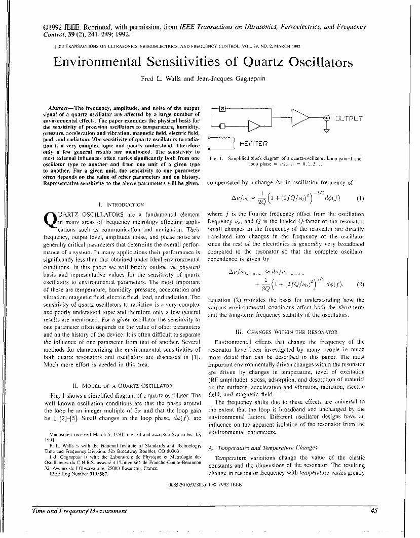
0 1992 IEEE. Reprinted, with permission, from IEEE Transactions on Ultrasonics, Ferroelectrics, and Frequency Control, 39 (2), 241-249; 1992.
11 ; L IKANSACIIONS ON ULIKA5ONICS. btKKObLIL1IIICS. AND FKbUUENCY CONTROL, VOL 39, NO 2, MARCH 1992
Environmental Sensitivities of Quartz Oscillators Fred L. Walls and Jean-Jacques Gagnepain
Abstmct-The frequency, amplitude, and noise of the output signal of a quartz oscillator are affected by a large number of environmental effects. The paper exaniincs the physical basis for the sensitivity of precision oscillators to temperature, humidity, pressure, acceleration and vibration, magnetic field, electric field, load, and radiation. The sensitivity of quartz oscillators to radia- tion is a very complex topic and poorly understood. Therefore only a few general results are mentioned. The sensitivity to most external influences often varies significantly both from one oscillator type to another and from one unit of a given type to another. For a given unit, the sensitivity to one parameter often depends on the value of other parameters and on history. Representative sensitivity to the above parameters will be given.
I. INTRODUCTION
UARTZ OSCILLATORS are a fundamental element in many areas of frequency metrology affecting appli- cations such as communication and navigation. Their
frequency, output level, amplitude noise, and phase noise are generally critical parameters that determine the overall perfor- mance of a system. I n many applications their performance is significantly less than that obtained under ideal environmental conditions. In this paper we will briefly outline the physical basis and representative values for the sensitivity of quartz oscillators to environmental parameters. The most important of these are temperature, humidity, pressure, acceleration and vibration, magnetic field, electric field, load, and radiation. The sensitivity of quartz oscillators to radiation is a very complex and poorly understood topic and therefore only a few general results are mentioned. For a given oscillator the sensitivity to one parameter often depends on the value of other parameters and on the history of the device. I t is often difficult to separate the influence of one parameter from that of another. Several methods for characterizing the environmental sensitivities of both quartz resonators and oscillators are discussed i n [l]. Much more effort is needed in this area.
Q
11. MODEL OF A QUARTZ OSCILLATOR
Fig. 1 shows a simplified diagram of a quartz oscillator. The well known oscillation conditions are that the phase around the loop be an integer multiple of 2.ir and that the loop gain be 1 [2]-[5]. Small changes in the loop phase, cl$(f), are
Manuscript received March 5 , 1991; revised and accepted September 13, 19Yl.
F. L. Walls is with the National Institute of Stand;irds and Technology, Time and Frequency Division, 325 Broadway Bouldcr, CO 80303. .I.-]. Gagncpain is with thc Lahoratoire de Physique ct Mctrologie dcs
Oscillateurs du C.N.R.S. associC 5 I'UniversitC de Fr:inche-Comtc-Bes;incon 32, Avenue de I'Observatoire, 25000 BesanGon, France.
IEEE Log Number 0105587.
7 HERTER
Fig. I . Simplified block diagram of a quartz-oscillator. Loop gain=] and loop phase = u2r I t = 0 . 1 . 2 . . .
compensated by a change Au in oscillation frequency of
where f is the Fourier frequency offset from the oscillation frequency vor and Q is the loaded Q-factor of the resonator. Small changes in the frequency of the resonator are directly translated into changes in the frequency of the oscillator since the rest of the electronics is generally very broadband compared to the resonator so that the complete oscillator dependence is given by
~ ~ l ~ O " , < , I , , , , , = (~I / /~O, , , , , , , , t , ,
Equation (2) provides the basis for understanding how the various environmental conditions affect both the short-term and the long-term frequency stability of the oscillators.
Iir. CHANGES WITHIN THE RESONATOR
Environmental effects that change the frequency of the resonator have been investigated by many people in much more detail than can be described in this paper. The most important environmentally driven changes within the resonator are driven by changes in temperature, level of excitation (RF amplitude), stress, adsorption, and desorption of material on the surfaces, acceleration and vibration, radiation, electric field, and magnetic field.
The frequency shifts due to these effects are universal to the extent that the loop is broadband and unchanged by the environmental factors. Different oscillator designs have an influence on the apparent isolation of the resonator from the environmental parameters.
A. Temperature and Temperature Changer Temperature variations change the value of the elastic
constants and the dimensions of the resonator. The resulting change in resonator frequency with temperature varies greatly
0885-3010/Y2$03.00 0 1992 IEEE
Time and Frequency'Measurement 4s
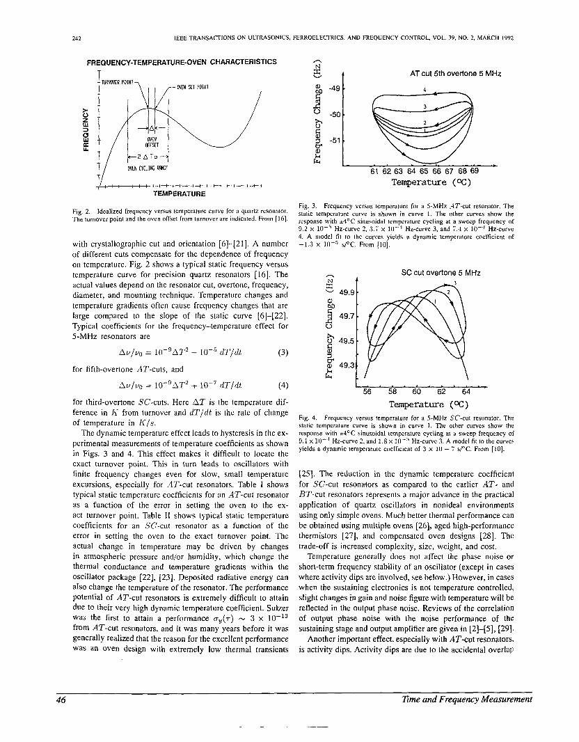
242 IEEE TRANSACTIONS O N ULTRASONICS, FERROELECTRICS, A N D FREQUENCY CONTROL. VOL. 39. NO. 2. MARCH IY(J2
FREQUENCY-TEMPERATURE-OVEN CHARACTERISTICS
T
Fig. 2. Idealized frequency versus temperature curve for a quartz resonator. The turnover point and the own offset from turnover are indicated. From [ 161.
with crystallographic cut and orientation [6]-[21]. A number of different cuts compensate for the dependence of frequency on temperature. Fig. 2 shows a typical static frequency versus temperature curve for precision quartz resonators [ 161. The actual values depend on the resonator cut, overtone, frequency, diameter, and mounting technique. Temperature changes and temperature gradients often cause frequency changes that are large compared to the slope of the static curve [6]-[22]. Typical coefficients for the frequency-temperature effect for 5-MHz resonators are
for fifth-overtone AT-cuts, and
Av/vo = 10-"T2 + lo-' dT/rlt (4)
for third-overtone SC-cuts. Here A T is the temperature dif- ference in Ii from turnover and dT/dt is thc rate of change of temperature in K / s .
The dynamic temperature effect leads to hysteresis in the ex- perimental measurements of temperature coefficients as shown in Figs. 3 and 4. This effect makes it difficult to locate the exact turnover point. This in turn leads to oscillators with finite frequency changes even for slow, small temperature excursions, especially for AT-cut resonators. Table I shows typical static temperature coefficients for an AT-cut resonator as a function of the error in setting the oven to the ex- act turnover point. Table I I shows typical static temperature coefficients for an SC-cut resonator as a function of the error in setting the oven to the exact turnover point. The actual change in temperature may be driven by changes in atmospheric pressure and/or humidity, which change the thermal conductance and temperature gradients within the oscillator package [22], [23]. Deposited radiative energy can also change the temperature of the resonator. The performance potential of AT-cut resonators is extremely difficult to attain due to their very high dynamic temperature coefficient. Sulzer was the first to attain a performance oy(.) N 3 x from AT-cut resonators, and it was many years before i t was generally realized that the reason for the excellent performance was an oven design with extremely low thermal transients
A
2 AT cut 5th overtone 5 MHz - t
61 62 63 64 65 66 67 68 69 Temperature ( O C )
Fig. 3. Frequency vcrsus temperature for a 5-MHz ,IT-cut resonator. The spatic temperature curve is shown in curve 1 . The other curves show the response with =4'C sinusoidal temperature cycling at a sweep frequency of 3.2 x Hz-curve 2, 3.7 x IO-' Hz-curve 3, and 7.4 x IO-" Hz-curve 4. A model fit 10 Ihc curves yields a dynamic temperature coefficient of - 1 . 3 x lo-' s/OC. From [lo].
- SC cut overtone 5 MHz - 49.9 a, 1 49.7 u 3 49.5 %
2 ?$ 49.3 --
56 58 60 62 64 Temperature ( O C )
Fig. 4. Frequency versus temperature for a 5-MHz SC-cut resonator. The static temperature curve is shown in curve 1 . The other curves show the response with t4'C sinusoidal temperature cycling at a sweep frequency of 3.1 x IO-' Hz-curve 2. and 1.6 x IO-' Hz-curve 3. A model f i t to the curves yields a dynamic temperature coefficient of 3 x 10 - 7 s/OC. From [ 101.
[25]. The reduction in the dynamic temperature coefficient for SC-cut resonators as compared to the earlier AT- and BT-cut resonators represents a major advance in the practical application of quartz oscillators in nonideal environments using only simple ovens. Much better thermal performance can be obtained using multiple ovens [26], aged high-performance thermistors [27], and compcnsated oven designs (281. Thc trade-off is increased complexity, size, weight, and cost.
Temperature generally does not affect the phase noise or short-term frequency stability of an oscillator (except in cases where activity dips are involved, see below.) However, in cases when the sustaining electronics is not temperature controlled, slight changes in gain and noise figure with temperature will be reflected in the output phase noise. Reviews of the correlation of output phase noise with the noise performance of the sustaining stage and output amplifier are given in [2]-151, [29].
Another important effect, especially with AT-cut resonators, is activity dips. Activity dips are due to the accidental overlap
46 l'ime and Frequency Measurement
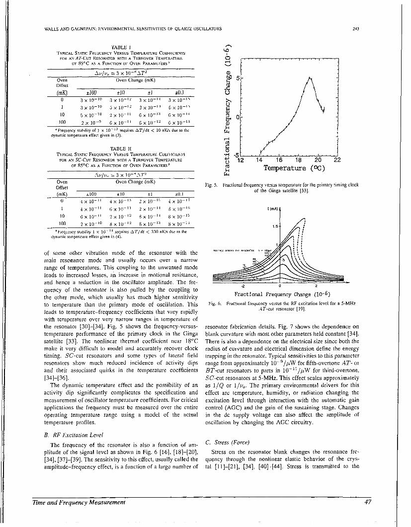
WALLS AND GAGNEI'AIN: ENVII<ONMENTAL SENSITIVIIIES 01. QUAKTZ OSCILLATORS 243
TABLE I TYPICAL STATIC FREOUENCY V E R S U S TEMPERATURE COEFFICIENTS
FOR AN AT-CUT RESONATOR WIT11 A TURNOVER TEMl'CR,\TURE OF 85OC AS A FUNCTION OF OVEN PARAMETERS"
TABLE I1 TYPICAL STATIC FREQUENCY VERSUS TEMPERATURE COEFFICIENTS
FOR AN SC-CUT RESONATOR WITH A TURNOVER TEMPERATURE OF 85OC A S A FUNCTION OF O V E N PARAMETERS''
Al//I,,, = 3 x 10-*12-' Oven Oven Change (mK)
of some other vibration mode of the resonator with the main resonance mode and usually occurs over a narrow range of temperatures. This coupling to the unwanted mode leads to increased losses, an increase in motional resistance, and hence a reduction in the oscillator amplitude. The fre- quency of the resonator is also pulled by the coupling to the other mode, which usually has much higher sensitivity to temperature than the primary mode of oscillation. This leads to temperature-frequency coefficients that vary rapidly with temperature over very narrow ranges in temperature of the resonator [30]-[34]. Fig. 5 shows the frequency-versus- temperature performance of the primary clock in the Ginga satellite [33]. The nonlinear thermal coefficient near 18°C make it very difficult to model and accurately recover clock timing. SC-cut resonators and some types of lateral field resonators show much reduced incidence of activity dips and their associated quirks in the temperature coefficients
The dynamic temperature effect and the possibility of an activity dip significantly complicates the specification and measurement of oscillator temperature coefficients. For critical applications the frequency must be measured over the entire operating temperature range using a model of the actual temperature profiles.
B. RF Excitatiori Level
[34]-[36].
The frequency of the resonator is also a function of am- plitude of the signal level as shown in Fig. 6 [16], [18]-[20], [34], [37]-[39]. The sensitivity to this effect, usually called the amplitude-frequency effect, is a function of a large number of
Temperature ( O C ) k Frc
Fig. 5. Fractional frequency versus temperature for the primary timing clock of the Ginga satellite [33].
Fractional Frequency Change (10-6)
.-1T-cut resonator 1191. Fig. 6. Fractional frequency versus the RF excitation level for a 5-MHz
resonator fabrication details. Fig. 7 shows the dependence on blank curvature with most other parameters held constant [34]. There is also a dependence on the electrical size since both the radius of curvature and electrical dimension define the energy trapping in the resonator. Typical sensitivities to this parameter range from approximately 10-g//~W for fifth-overtone AT- or BT-cut resonators to parts in 10-ll/pW for third-overtone, SC-cut resonators at 5-MHz. This effect scales approximately as 1/(2 or 1/v0. The primary environmental drivers for this effect are temperature, humidity, or radiation changing the excitation level through interaction with the automatic gain control (AGC) and the gain of the sustaining stage. Changes in the dc supply voltage can also affect the amplitude of oscillation by changing the AGC circuitry.
C. Stress (Force) Stress on the resonator blank changes the resonance fre-
quency through the nonlinear elastic behavior of the crys- tal [Ill-[21], [34], [40]-[44]. Stress is transmitted to the
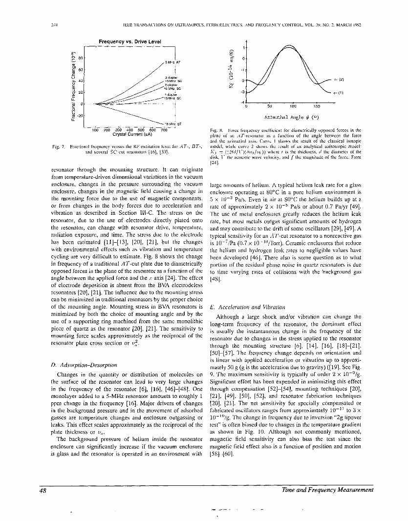
Frequency vs. Drive Level r ' ~ . ~ ~ ~ ~ ~
-4 1 0 50 100 150
Azimuthal Angle J I (0) I .
100 200 300 400 500 600 700 Crystal Current (@A)
Fig. 7. Fractional frcqucncy vcrsus the RF excitation lcvcl for .4T-, OT-, and scveral SC-cut resonators [ 161, [33].
resonator through the mounting structure. It can originate from temperature-driven dimensional variations in the vacuum enclosure, changes in the pressure surrounding the vacuum enclosure, changes in the magnetic field causing a change in the mounting force due to the use of magnetic components, or from changes in the body forces due to acceleration and vibration as described in Section 111-C. The stress on the resonator, due to the use of electrodes directly plated onto the resonator, can change with resonator drive, temperature, radiation exposure, and time. The stress due to the elcctrode has been estimated [11]-[13], (201, [21], but the changes with environmental effects such as vibration and temperature cycling are very difficult to estimate. Fig. 8 shows the change in frequency of a traditional AT-cut plate due to diametrically opposed forces in the plane of the resonator as a function of the angle between the applied force and the T axis [24]. The effect of electrode deposition is absent from the BVA electrodeless resonators [20], [21]. The influence due to the mounting stress can be minimized in traditional resonators by the proper choice of the mounting angle. Mounting stress in BVA resonators is minimized by both the choice of mounting angle and by the use of a supporting ring machined from the same monolithic piece of quartz as the resonator [20], [21]. The sensitivity to mounting force scales approximately as the reciprocal of the resonator plate cross section or 11,'.
D. Adsorption-Desorption Changes in the quantity or distribution of molecules on
the surface of the resonator can lead to very large changes i n the frequency of the resonator [6], [16], [46]-[48]. One monolayer added to a 5-MHz resonator amounts to roughly 1 ppm change in the frequency [16]. Major drivers of changes i n the background pressure and in the movement of adsorbed gasses are temperature changes and enclosure outgassing or leaks. This effect scales approximately as the reciprocal of the plate thickness or v,.
The background pressure of helium inside the resonator enclosure can significantly increase if the vacuum enclosure is glass and the resonator is operated in an environment with
Fig. 8. I:orcc-lrcquciicy coclliciciit for tliamcrrioally (ipposcd forces in the plaiic o l ;in ..IT-rcsonator ;is ;I function of thc anglc bctwcen tlic force and the eziniuthal axis. Curvu 1 shows the rcsult of lhc classical isotopic niodcl, wliilc ctirvc 2 shows lhc rcsult of an analytical anisotropic model: I<, = ( ( ~ t i / / l . ) ( , ~ i / ~ ~ / i / , l ) ) wlicre t is the thickness, the diameter of the disk, 1- thc acoustic wave vclociLy, and f Ihc magnitude of the force. From 1231.
large amounts of helium. A typical helium leak rate for a glass enclosure operating at 80°C in a pure helium environment is 5 x lop3 Pa/s. Even in air at 80OC the helium builds up at a rate of approximately 2 x lops Pa/s or about 0.7 Pa/yr [49]. The use of metal enclosures greatly reduces the helium leak rate, but most metals outgas significant amounts of hydrogen and may contributc to the drift of some oscillators [29], [49]. A typical scnsitivity for an AT-cut resonator to a nonreactive gas is lO-?/Pa (0.7 x IO-"'/Torr). Ceramic enclosures that reduce the helium and hydrogen leak rates to negligible values have been developed [46]. There also is some question as to what portion of the residual phase noise i n quartz resonators is due to time varying rates of collisions with the background gas [481.
E. Accckrution and Vibration
Although a large shock and/or vibration can change the long-term frequency of the resonator, the dominant effect is usually the instantaneous change in the frequency of the resonator due to changes in the stress applied to the resonator through the mounting structure [6], [14], [16], [18]-[21], [50]-[57]. The frequency change depends on orientation and is linear with applied acceleration or vibration up to approxi- mately 50 g (g is the acceleration due to gravity) ([19]. See Fig. 9. The maximum sensitivity is typically of order 2 x lO-'/g. Significant effort has been expended in minimizing this effect through compensation [52]-[54], mounting techniques [20], [21], [49], [50], [52], and resonator fabrication techniques [20], [21]. The net sensitivity for specially compensated or fabricated oscillators ranges from approximately to 3 x 10p'o/g. The change in frcqucncy due to inversion "2g tipover test" is often biased due to changes in the temperature gradient as shown in Fig. 10. Although not commonly mentioned, magnetic field sensitivity can also bias the test since the magnetic field effect also is a function of position and motion [ 58]-[60].
48 Time and Frequency Measurement
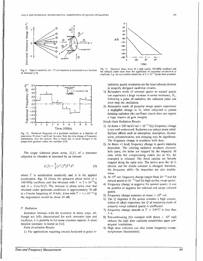
WALLS AND G,\CiNEPAIN: E N V I K O N M E N l A L SIJNSITIV1Tll.S OF OUAIITZ (IS('ILLATC)KS 245
,. h
s: v
B
::
/
Orientation a. Connector up
2.0 1.0 0.0
g -2.0 .o -3.0 2 -4.0 c
e L - 5 . 0 1 ' ' ' ' I ' ' ' '
0 1 2 3 4 5 6 7 8 9 10
Time (1000s)
Fig. 10. Fractional frequency of a precision oscillator as a funclion of orientation. Position 1 and 6 are the same. Note the slow change of frequency immediately after the rotation. This is likely due to small changes in the temperature gradient within the oscillator (231.
The single sideband phase noise, ,C(f), of a resonator subjected to vibration is increased by an amount
where I? is acceleration sensitivity and A is the applied acceleration. Fig. 11 shows the quiescent phase noise of a 100-MHz oscillator and that obtained with I' = 2 x lO-'/g and il = 2 c o s 2 ~ f t . The increase in phase noise over that obtained under quiescent conditions is approximately 70 dB at a Fourier frequency of 10 kHz. Even with r = 1 x lO-"/g the degradation would be about 24 dB.
F. Radiation
Radiation interacts with the resonator in many ways. Al- though not fully characterized for each resonator type and oscillator, it is possible to list some common aspects. A more detailed summary is found in [16].
Pulse Irradiation Results 1) For applications requiring circuits hardcned to pulse ir-
radiation, quartz resonators are the least tolerant element in properly designed oscillator circuits.
2) Resonators made of unswept quartz or natural quartz can experience a large increase in series resistance, R,, following a pulse of radiation; the radiation pulse can even stop the oscillation.
3) Resonators made of properly swept quartz experience a negligible change in R, when subjected to pulsed ionizing radiation (the oscillator circuit does not require a large reserve of gain margin).
Steady-State Radiation Results 1) At doses < 100 rad (1 rad = lop2 Gy) frequency change
is not well understood. Radiation can induce stress relief. Surface effects such as adsorption, desorption, dissoci- ation, polymerization, and charging may be significant. The frequency change is nonlinear with dose.
2) At doses 21 krad, frequency change is quartz impurity dependent. The ionizing radiation produces electron- hole pairs; the holes are trapped by the impurity AI sites while the compensating cation (Li or Na, for example) is released. The freed cations are loosely trapped along the optic axis. The lattice near the AI is altered, and the elastic constant is changed; therefore, the frequency shifts. Ge impurities are also trouble- some.
3 ) At loti rad, frequency change ranges from 10-'l/rnd for natural quartz to 10-'4/rad for high quality swept quartz.
4) Frequency change is negative for natural quartz; it can be positive or negative for cultured and swept cultured quartz.
5) Frequency change saturates at doses > 10G rad. 6) The Q degrades if the quartz contains a high concen-
tration of alkali impurities; the Q of resonators made of properly swept cultured quartz is unaffected.
7) Frequency change anneals at T > 240°C in less than 3 h.
8) Preconditioning (for example with doses > 10' rad) reduces the high dose radiation sensitivities upon sub- sequent irradiations.
9) High dose radiation can also rotate frequency-vcrsus- temperature characteristic.
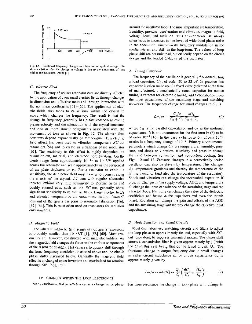
IEEI: TRANSA(1IONS ON UUI{ASONICS. l'I:I<ROELK-IRICS. AND FKEUUENCY CONTROL, VOL. 39, NO. 2, MARCH IY92
Fig. 12. Fractional frequency changes iis a function of applied voltagc. The slow variation after the change in voltage is due to the movement of ions within the resonator. From [ I ] .
G. Electric Field The frequency of certain resonator cuts are directly affected
by the application of even small electric fields through changes in dimension and effective mass and through interaction with the nonlinear coefficients [61]-[65 1. The application of elec- tric fields also tends to cause ions within the crystal to move which changes the frequency. The result is that the change in frequency generally has ~a fast component due to piezoelectricity and the interaction with the crystal constants and one or more slower components associated with the movement of ions as shown in Fig. 12. The shorter time constants depend exponentially on temperature. This electric field effect has been used to vibration compensate SC-cut resonators [54] and to create an ultralinear phase modulator [61]. The sensitivity to this effect is highly dependent on resonator cut, material, and electrode configuration. Coeffi- cients range from approximately lo-'' to lO-'/V applied across the resonator and scale approximately as the reciprocal of the plate thickness or v,. For a resonator to exhibit a sensitivity, the dc electric field must have a component along the z axis of the crystal. AT-cuts with regular electrodes therefor exhibit very little sensitivity to electric fields and doubly rotated cuts, such as the SC-cut, generally show significant sensitivity to dc electric fields. Large electric fields and elevated temperatures are sometimes used to "sweep" ions out of the quartz bar prior to resonator fabrication [16], [62]-[64]. This is most often used on resonators for radiation environments.
H. Magnetic Field The inherent magnetic field sensitivity of quartz resonators
is probably smaller than lO-"/T [l], [58]-[60]. Most res- onators are, however, constructed with magnetic holders. As the magnetic field changes the force on the various components of the resonator changes. This causes a frequency shift through the force-frequency coefficient discussed above and the circuit phase shifts discussed below. Generally the magnetic field effect is unchanged under inversion and maximized for rotation through YO" [%I, [59].
Iv. CHANGES WITHIN THE LOOP ELECTRONICS Many environmcntal parameters cause a change in the phase
around the oscillator loop. The most important are temperature, humidity, pressure, acceleration and vibration, magnetic field, voltage, load, and radiation. This environmental sensitivity often leads to increases in the level of wide-band phase noise in thc short-tcrnm, random-walk frequency modulation in the medium-term, and drift in the long-term. The values of loop phasc shift arc not universal, but critically depend on the circuit design itnd the loadcd ()-factor of the oscillator.
A. Tuning Capacitor The frequency of the oscillator is generally fine-tuned using
a load capacitor, CL, of order 20 to 32 pF. In practice this capacitor is often made up of a fixed value (selected at the time of manufacture), a mechanically tuned capacitor for coarse tuning, a varactor for electronic tuning, and a contribution from the input capacitance of the sustaining stage and matching networks. The frequency change for small changes in CL is
where CO is the parallel capacitance and C1 is the motional capacitance. It is not uncommon for the first term in (6) to be of order lo-' [16]. in this case a change in CL of only results in a frequency change of lo-'. Primary environmental parameters which change CL are temperature, humidity, pres- sure, and shock or vibration. Humidity and pressure change the ratio between convection and conduction cooling. See Figs. 10 and 13. Pressure changes in a hermetically sealed oscillator can also be driven by temperature. This changes the temperature gradients and thereby the temperature of the tuning capacitor (and also the temperature of the resonator). Shock and vibration can change the mechanical capacitor, if present. Changes in the supply voltage, AGC, and temperature all change the input capacitance of the sustaining stage and the varactor diode. Humidity can change the value of the dielectric coefficient and losses in the capacitors and even the circuit board. Radiation can change the gain and offsets of the AGC and the sustaining stage and thereby change the effective input capaci tancc.
B. Mode Selection and Tuned Circuits Most oscillators use matching circuits and filters to adjust
the loop phase to approximately On and, especially with SC- cut resonators, to suppress unwanted modes. The phase shift across a transmission filter is given approximately by (1) with the Q in this case being that of the tuned circuit, Qc. The fractional change in output frequency due to small changes in either circuit inductance L, or circuit capacitance C, is approximately given by
Far from rcsonance the change in loop phase with change in
50 Time and Frequency Measurement
-. -___- -
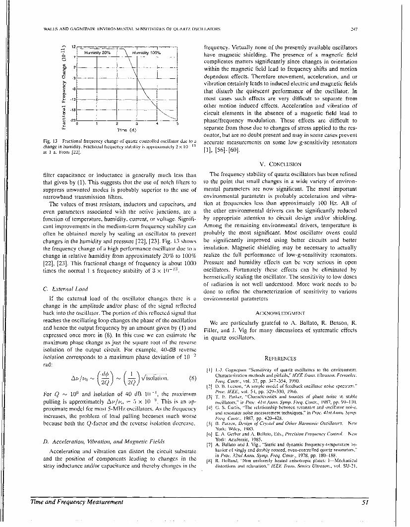
- 12 4 I ‘ “ I . ’ ’
.-I Humidity 20% Humidity 100%
5 7 - 7 -
Tim (d) 6
Fig. 13 Fractional frequency changc 01’ quarlz controlled oscil1;ilor due IO ;I
change in humidity. Fractional l‘rrcquency stability is approximately 2 x l ( 1 - I ’ ’ at 1 s. From 122).
filter capacitance or inductance is generally much less than that given by (1). This suggests that the use of notch filters to suppress unwanted modes is probably superior to the use of narrowband transmission filters.
The values of most resistors, inductors and capacitors, and even parameters associated with the active junctions, are a function of temperature, humidity, current, o r voltage. Signifi- cant improvements in the medium-term frequency stability can often be obtained merely by sealing an oscillator to prevent changes i n the humidity and pressure [22], [23]. Fig. 13 shows the frequency change of a high performance oscillator due to a change in relative humidity from approximately 20% to 100% [22], [23]. This fractional change of frequency is about 1000 times the normal 1 s frequency stability of 3 x lO-”.
C. Extenz(i1 Lorid
If the external load of the oscillator changes there is a change i n the amplitude and/or phase of the signal reflected back into the oscillator. The portion of this rcRectcd signal that reaches the oscillating loop changes the phase of the oscillation and hence the output frequency by an amount given by ( 1 ) and expressed once more in (8). In this case we can estimate the maximum phase change as just the square root of the reverse isolation of the output circuit. For exaniplc, 40-dB reverse isolation corresponds to a maximum phase deviation of 1 V ’ rad:
For C) - loG and isolation of 40 dB lo-,’, the niaxiniiim pulling is approximately Ai////(, = 5 x IO-!’. ’This is ;in ap- proximate model for most 5-MHz oscillators. As the frequency increases, the problem of load pulling becomes much worse because both the Q-factor and the revcrsc isolation decrease.
D. Acceleration, Vibrntiorz, citicl Mcigrietic Fields
Acceleration and vibration can distort the circuit substrate and the position of components leading to changes in the stray inductance and/or capacitance and thcrchy changes in the
frequency. Virtually none of the presently available oscillators have magnetic shielding. The presence of a magnetic field complicates matters significantly since changes in orientation within the magnetic field lead to frequency shifts and motion dependent effects. Therefore movement, acceleration, and or vibration certainly leads to induced electric and magnetic fields that disturb the quiescent performance of the oscillator. In most cases such effects are very difficult to separate from other motion induced effects. Acceleration and vibration of circuit elements in the absence of a magnetic field lead to phase/frequency modulation. These effects are difficult to separate from those due to changes of stress applied to the res- onator, but are no doubt present and may in some cases prevent accurate measurements on some low-g-sensitivity resonators [I] , [561-[601.
V. CONCLUSION The frequency stability of quartz oscillators has been refined
to the point that small changes in a wide variety of environ- mental parameters are now significant. The most important environmental parameter is probably acceleration and vibra- tion at frequencies less than approximately 100 Hz. All of the other environmental drivers can be significantly reduced by appropriate attention to circuit design and/or shielding. Among the remaining environmental drivers, temperature is probably the most significant. Most oscillator ovens could be significantly improved using better circuits and better insulation. Magnetic shielding may be necessary to actually realize the full performance of low-g-sensitivity resonators. Pressure and humidity effects can be very serious in open oscillators. Fortunately these effects can be eliminated by hernieticnlly sealing the oscillator. The sensitivity to low doses of radiation is not well understood. More work needs to be done to refine the characterization of sensitivity to various cnvironinental parameters
ACKNOWLEDGMENT
We are particularly grateful to A. Ballato, R. Besson, R. Filler, and J . Vig for many discussions of systematic effects in quartz oscillators.
REFERENCES
J.-J. Gagncpain “Sensilivity o f quartz oscillators to the environmenl: Characterizition mclhods and pitfalls,” IEEE T ~ N I I S . Ulfrtrsort. Ferroekc. F r q . C ~ i / r . . wI. 37, pp. 347-354, 1990. D. 13. Leeson, “A simple model of feedback oscillalor noise spectruni.” Pro(.. IEEI,’, vol. 54, pp. 329-330. 1966. T. E. Parker, “Ch;iracteristics and sources of phase noise in stable oscil1;itors.” in /’roc.. 4 h f A r i r r r r . Symp. F r q . Corit r.. 1987, pp. 90-1 IO. G. S. Curtis, “The re1;itionship between rcsonator and oacillator iioizc, and resonator noise measurement techniques,” in Proc. 41s f A m u . Swrp. F r q . Curifr., 1987, pp. 420428. B. I’arzcn. Desigti of Crystlil nrrd Otlier Harmonic Osci/hors. New York: Wiley. 1‘183. E. A. Gcrher and A. Ballalo, Eds., Precisiori Freqrrericy Corrfrol. N e w York: Ac:\dcmic, 1985. A. 13all;ito and J. Vig., “Static and dynamic frequency-temperature be- havior CIC singly and doubly rotated, oven-controlled quartz rcsonaton,” i n I’roc. 32nd Amit . Syrrip. Freq Coirfr., 1978, pp. 180-188. R. 1 loll;intl, “Non uniformly heated anisotropic plates: I-Mechanical di\kirtions and relitxiition,” /EEE Triiris. Sorrics Ulrrasori.. vol. SU-21,
I E t E KKANSACI ION> ON ULTRASONICS. FI;KRUELECI KICS. / \ND F R t Q U E N C Y CON.TROL. VOL. 3Y. NO. 2. MARCH 1 Y Y 2
1974. R. Holland, “Nan uniformly heated anisotropic plates: 11-Frcquency transients in AT and BT quartz plates,” Ultrasofrics Synip. Proc., pp. 592-598. IEEE Cat. # 74 CHO 896-ISU 1974. G. Thiobald, G. Marianneau, R. Prttot, and J. J. Gagncpain, “Dynamic thermal behavior of quartz rcsonators,” in PI-oc. 33rd A i i m Symp. Frcq. Cuntr., 1979, pp. 239-246. J. Kusters, “Transient thermal compensation for quartz resonators,” IEEE Trniis. Sottics Ullrasun., vol. SU-23, pp. 273-276 1976. J. A. Kusters and J. G . Leach, “Further experimental d;tta on stress and tIierm;il gradient compcnsated crystals,” i r i Pruc. IEEE, 1077, pp. 282-284. E. P. EerNissc, ‘Quartz resonator frequency shifts arising from electrode stress.” in 29th Pruc. Afrnu. Syinp. Freq. Cuirtr., 1975, pp. 1-4. A. Ballato. “Static and dynamic behavior of quartz resonators.” lEEE Traiis. Sonics Ulfrason., vol. SU-26, p. 299, 1979. B. K. Sinha and H. F. Tiersten, “Transient thermally induccd frcquency excursions in doubly-rot:itctl quartz thickness mode resonators,” in Proc. 341h Airiirr. Syinp. Freq. Coritr., 1980, pp. 393402. J. R. Vig, “Quartz crystal resonators and oscillators for frequency control and timing applications, a tutorial,” Mar. 1991. Available from US Army Electronics Technology and Devices, SLCET-EQ, Ft. Monniouth, NJ 07703-5000, and from NTIS, AD A231 604.. J. P. Valentin, G. Thiobald, and J. J. Gagnepain, “Frequency shifts aris- ing from in-plane temperature gradient distribution in quartz resonators,” in Proc. 38th Annu. Symp. Freq. Cofrtr. 1984, pp. 157-163. J. J. Gagnepain, R. Besson, “Nonlinear effects in piezoelectric quartz crystal,” Physical Acoustics, Vol XI, W.P. Mason, Ed. Academic, 1975, pp. 245-288. J. J. Gagnepain, “Nonlinear properties of quartz crystal and quartz resonators: A review,” in Proc. 35th Arrtrti. Symp. Freq. Cuirtr., 1981, pp. 14-30. R. Besson, “A new piezoelectric resonator design,” in Pruc. 30th Airfur. Synrp. Freq. Cum. , 1976, pp. 78-83. R. Besson and U. R. Peier, “Further advances on B.V.A. quartz resonators,” in Pruc. 34fh Annu, Symp. Freq. Contr., 1980, pp. 175-182. F. L. Walls, “The influence of pressure and humidity on the medium and long-term frequency stability of quartz oscillators,” in Proc. 42fid Airnu. Symp. Freq. Conlr., 1988, pp. 279-283. F. L. Walls, “Environmental effects on the medium and long term frequency stability of quartz oscillators,” in Proc. 2nd Eur. Freq. atid Time Forum, Neuchatel, Switzerland, Mar. 1989, pp. 719-727. S. Ballandras, “Sensitivity of BAW devices to radial in-plane stress distribution, comparison between analytical and finite element results,” in Proc. 51h Eur. Freq. nnd Time Forum, BesanGon, Mar. 1991. M. R. Bloch, J. C. Ho, C. S. Stone, A. Syed, and F. L. Walls, “Stability of High Quality Quartz Crystal Oscillators: An Update,” in Proc. 43rd Annu. Symp. Frey. Contr., 1989, pp. 80-84. G. Marianneau and J.-J. Gagnepain. “Digital temperature control for ultrastable quartz oscillators,” in Proc. 34th Anfur. Symp. Freq. Contr., 1980, pp. 52-57. J. F. Schooley, T/rerniometry. F. L. Walls, “Analysis of high performance compensated thermal enclosures,” in Proc. 41st Annu. Syinp. Freq. Contr., 1988, pp. 439443. F. L. Walls and J. J. Gagncpain, “Special applications, precision fte- quency control,” in Precisiofr Frequency Control, (E. A. Gerber and A. Ballato, Eds. New York: Academic Press, 1985, ch. 15, pp. 287-296. A. F. 9. Wood and A. See, “Activity dips in AT-cut crystals,” in Proc. 21st Atrnu. Symp. Freq. Cuutr., 1967, pp. 420-435. C. Franx, “On activity dips of AT Crystals at high levels of drive,” in Proc. 22frd Aiinrr. Symp. Freq. Contr., 1967, pp. 43Gl54. J. Birch and D. A. Weston, “Frequency/temperature, activity/temperature anomalies in high frequency quartz crystal units,” in Proc. 3Urh Annu. Symp. Freq. Cunlr., 1978, pp. 32-39. J. E. Deeter and H. Inoue, “Temperature dependence of the ginga clock rate,” ISAS Res. Note 430, Jan. 1990. J. A. Kusters, “The SC-cut crystal-An overview,” in Pruc. IEEE Ultrason. Symp., 1981, pp. 402409. A. W. Warner, Jr. and B. Goldfrank, “Lateral field resonators,” in Pruc. 39th Annu. Synrp. Freq. Cmitr., 1985, pp. 473-474. A. W. Warner, “Measurement of plano-convex SC quartz blanks using lateral field excitation,” in Pruc. 4 2 d Amru. Symp. Freq. Coiitr., 1988, pp. 202-204. J. J. Gagnepain, J . C. Poncot, C. PCgeot, “Amplitude-frequency behavior of doubly rotated quartz resonators,” in Pruc. 3lst Annu. Synrp. Freq. Contr., 1977, pp. 17-22. R. L. Filler, “The amplitude-frequency effect in SC-cut resonators,” in Proc. 39th Aftnu. Symp. Freq. Confr., 1985, pp. 311-316. R. J. Besson, J. M. Groslambert, and F. L. Walls, “Quartz crystal
Boca Raton, FL: CRC Press, 1986.
resonators and oscillators, recent developments and future trends,” Ferruclectrics vol. 43, pp. 57-65, 1982. J. M. Ratajski, “Force-frequency coefficient of singly-rotated vibrating quartz crystals,” IBM J . Res. Dev. Val. 12, p. 92, 1968. C. R. Dauwaltcr, “The temperature dependence of the force scnsitivity of AT-cut quartz crystals,” in Proc. 26th A w u . Symp. Freq. Confr., 1972,
A. Ballato, E. P. Eernisse, and T. Lukaszek, “The force-frequency effect in doubly rotated-quartz resonators,” in Proc. 31s1 Annu. Symp. Freq. Cuiitr., 1977, pp. 8-16. A. 13:iIlxto. “Forcc-frcqucncy ci~mpensitlion applied to four-point mount- ing of AT-cut resonators,” IEEE Traits. Sonics Ultrasun., vol. SU-25, 233, 1978. E. P. EerNisse, “Temperature dependence of the force frequency effect for thc rotated X-cut,” in Proc. 33rd Airnu. Synrp. Freq. Contr,, 1979,
J. J. Gagnepain, M. Olivicr, and F. L. Walls, “Excess noise in quartz crystal resonators,” in Pruc. 37th Annu. Synip. Frcq. Curtfr., 1983, pp. 2 18-225. R. L. Filler, L. J . Keres, T. M. Snowden, and J. R. Vig, “Ceramic flatpack enclosed AT and SC-cut resonators,” in Proc. IEEE Ultrason. Syiiip., 1980. J. R. Vig, “UViOzone cleaning of surfaces,’’ J . Vac. Sci. Technol. vol. A3, pp. 1027-1034, 1985. Y. K. Yong and J. R. Vig, “Resonator surface contamination-A cause of frequency lluctuations,” in Proc. 42nd Anrtu. Symp. Freq. Cuiitr., 1988,
W. G. Perkins, “Permeation and outgassing of vacuum materials,” J . Vac. Sci. Techfro/., vol. 10, pp. 543-556, 1973. A. Ballato, “Resonators compensated for acceleration fields,” in Pruc. 33rd Anrru. Symp. Freq. Cuirtr., 1979, pp. 322-336. R. L. Filler, “The acceleration sensitivity of quartz crystal oscillators: A review,” IEEE Tram Ultrasun., Ferruelec., Freq. Contr., vol. 35, pp. 297-305, 1988. F. L. Walls and J . R. Vig, “Acceleration insensitive oscillator,” U. S. Pat. No. 4,575,690, 1986. J . M. Pryjemski, “Improvement in system performance using a crystal oscillator compensated for acceleration sensitivity,” i n Proc. 32ndAnnu. Symp. Freq. Confr., 1978, pp. 42-30. V. J. Rosati and R. L. Filler, “Reduction in the effects of vibration on SC-cut quartz oscillators,” in Proc. 35th Atmu. Symp. Freq. Contr., 1981, pp. 117-121. Y. S. Zhou and H. F. Tiersten, “On the influence of a fabrication imperfection on the normal acceleration sensitivity of contoured quartz resonators with rectangular supports,” in Proc. 44th Antru. Symp. Freq. Cuntr., 1990, pp. 452453. (See also H. F. Tiersten and Y. S. Zhou, “An analysis of the in-plane acceleration sensitivity of contoured quartz resonators with rectangular supports,” same proceedings, pp. 461467.) J. K. Vig, C. Audoin, M. Driscoll, E. P. EerNisse, R. L. Filler, M. Garvey, W. Riley, R. Sniythe, and R. D. Weglein, “The effects of accel- eration on precision frequency sources,” LABCOM RiD Tech. Report SLCET-TR-91-3, Mar. 1991, available from U.S. Army, Electronics Technol. and Devices Lab., Labcom, Ft. Monmouth, NJ. M. H. Watts, E. P. EerNisse, R. W. Ward, and R. B. Wiggins, “Technique for measuring the acceleration sensitivity of SC-cut quartz resonators,” in Proc. 421idAirnu. Synrp. Freq. Cumr., 1988, pp. 442-446. R. Brendel, C. El Hassani, M. Brunet, and E. Robert, “Influence of magnetic field on quartz crystal oscillators,” in Proc. 43rdAmu. Symp. Freq. Cutrtr., 1989, pp. 268-274. F. Deyzac, “Magnetic sensitivity of quartz oscillators,” in Pruc. 4th Anrru. Eur. Foruni on Time and Freq., Mar. 1990, pp. 255-258. A. Ballato, T. J. Lukaszek, and G. J. lafrate, “Subtle effects in high stability vibrators,” in Proc. 3411~ Annu. Symp. Freq. Conrr., 1980, pp. 431444 J. Lowe and F. L. Walls, “Ultralinear small angle phase modulator,”in Proc. 45th Annu. Symp. Frcq. Contr., 1991. R. Brendel, and J.-J. Gagnepain, “Electroelastic effects and impurity relaxation in quartz resonators,” in Pruc. 36fhAiinu. Symp. Freq. Contr., 1982, pp. 97-107. J. J. Martin, “Electrodiffusion (sweeping) of ions in quartz,” /EEE Trans. Ultrmon., Ferruelec., Freq. Contr., vol. 35, 288-296, 1988. J. G. Gualtieri, “Sweeping quartz crystals,” in Proc. 1989 IEEE Ultrason. Symp., 1989, pp. 381-391. C. K. Hruskn and M. Kucera, “the dependence of the polarizing effect on the frequency of quartz resonators,” J . Canadian Ceramic Socier), vol. 55, pp. 3941, 1986. R. Brendel, J.-J.Gagnepain, J. P. Aubry, “Impurity migration study in quartz crystal resonators by using electroelastic effect,” in Proc. 40th Airittr. Symp. Freq. Cuntr., 1986, pp. 121-126.
pp. 108-112.
pp. 30(&305.
pp. 397-403.
52 Time and Frequency Measurement
\V,\LI.S ANI) CAGNEI'AIN. liNVII<ONMIINTAl, SI:.NSI'lIVI'I IES 0 1 : (JIJARI'7, 0SCII.L.AIORS 239
Fred L. Walls wa? born in Portldnd, OR, on Oc- tober 29, 1940 He received the B S , M S , and Ph D degrees in physic5 i n 1958, 1964. a n d 1970, reqxctively, from the University of WJ\hingliiil, Seattle H i s Ph D them wa\ on the dcvclopmcnt of long-term stordge and nondemuctive detcctiun techniquec for electron5 atored in Penning trdp "I the first measurement5 of the anomalou5 magnttic (g-2) moment of low energy stored electron5
Since 1973, he has betn d Stdff MembLr of the Time and Frequency Division of the Nation:il
Institute of Standards and Technology (formerly the National Uureau of Standards), Boulder, CO. He is presently engaged in research and development of hydrogen maser devices and cesium beam standards for use as ultrastahle clocks, quartz oscillators with improved short- and long-term stability, Iuw- noise microwave oscillators, frequency synthesis from RF to infrared, low- noise frequency stability measurement systems, and accurate plinse-noise metrology. From 1970 to 1Y73, he was il Postd(1ctora1 Fcllow at the Joint Institute for Laboratory Astrophysics, Boulder, CO. This work focused on
developing techniques lro long-term storage and nondestructive detection of fragile atomic ions stored in Penning traps for low-energy collision studies.
Dr. Walls is a member of the American Physical Society. He has publisher more t h a n 70 scientific papers and holds three piitcnts.
Jean-Jacques Gagnepain "as born in Montbeliard, France, in 1942. He received the Ph.D. degree in electrical engineering i n 1972 from the University of Besanpn, Bcsanqon, Frmce.
He joined the Centre National de la Recherche Scientifique in 1976 and he is presently Director of the Laboratoire de Physique et Mttrologie des Oscillateurs. He was a Guest Worker at the National Bureau of Standards, Buuldcr, CO, in 1075-1976.
Time and Frequency Measurement 53
0 1986 IEEE. Reprinted, with permission, from Proceedings of the IEEE: Special Issue on Radio Measurement Methods andStandards, 74 (l), 168-179; 1986.
Optical Frequency Measurements
DONALD A. JENNINGS, KENNETH M. EVENSON, AND DAVID J. E. KNIGHT
Invited Paper
This paper is review of the history of the measurement of tinuous-wave (CW) laser oscillation in the infrared regions
plies laser device, this is therefore review of laser frequency lavan et in 1961 was followed by the discovery measurement. The development of frequency measurement from the Cs frequency sfandard to the visible is traced, rw0 of cw laser oscillation in the visible [3] and far-infrared aspects of optical frequency measurements, the speed of light and regions [4] of the spectrum. The coherence of laser radia- the redefinition of the meter, are also discussed. t ion brought about the possibility of the measurement of
the frequency of this "coherent" radiation. The first such I. INTRODUCTION measurement of a laser frequency (rather than the wave-
coherent OpliCd/ freqUenCi.3. Since Coherent Optical frequency im- of the electromagnetic regions in He-Ne gas mixture by
length) was reported by Hocker et a/ . , in 1967 [SI. The frequencies of single-mode emissions at 890 and 964 GHz
mOnic with silicon-point contact diodes,
The absolute frequency measurement of radiation at fre-
source of "coherent" radiation [I]. The discovery of con- quencies above 500 was made possible by the laser: a (337 and 317 pm) were measured using submillimeter bar-
similar to those developed [6] to generate submillimeter
These frequency measurements made it possible to use
lasers for measuring the speed of light in vacuum co. The most reliable measurement of the speed of light at that time was considered to be that made by Froome i n 1958 [7]
Manuscript received November 19,1984; revised August 14,1985. radiation by harmonic generation from millimeter radiation. D. A. Jennings and K. M. Evenson are with Time and Frequency
Division, National Bureau of Standards, Boulder, CO 80303, USA. D. I . E. Knight i s with the Division of Quantum Metrology,
National Physical Laboratory, Teddingtin, Middlesex, TWII OLW, United Kingdom.
0016-9219/86/0100-0168$01.00 0 British Crown Copyright 1986
168 PROCECDINGS OF THE IFEE, VOI 74. NO I . IANUARY Iqffi
54 Time and Frequency Measurement
I in which t l ie frequency f and the vacuum wavelength A, were measured for stabilized microwave radiation in the 4-mm band. The result was given by c, = fX,. The main source of uncertainty in this experiment was in the wave- length determination, due to diffraction in the interferome- ter apertures and from the correction for the refractive index of the air. Froome's one-sigma uncertainty was k 3 parts in IO7 , but there was disagreement with other results, particularly long-baseline ones (Bergstrand) [a]. The speed of light is used for electromagnetic distance measurement, especially in critical applications such as geodetic-survey baseline measurements, which were at that time limited by the uncertainty of c.
It was apparent by the mid-1960s that a more accurate determination of X could be made at the shorter wave- length afforded by laser radiation; hence a more accurate value of c could be obtained. This possibility enabled the development of laser frequency measurement programs at various national standards laboratories such as the National Bureau of Standards at Boulder, CO, USA, the National Physical Laboratory, Teddington, UK, and the National Re- search Council, Ottawa, Canada.
Important steps in the development of laser frequency measurements were the introduction of the metal-insula- tion-metal (MIM) diode and the demonstration of high- order mixing (12th harmonic of the HCN laser against an H,O laser at 28 pm) by Evenson et a/. [9]. Cryogenic Joseph- son junctions were proving useful for very-high-order mix- ing with submillimeter lasers [IO], [ I l l . In 1972 accurate frequency measurements were extended to 3.39 pm [I 21, with a chain of five lasers using MIM diode harmonic mixing devices to generate the laser harmonics.
For accurate frequency measurements it was necessary to have sufficiently stable "targets" to measure. These were provided by narrow atomic or molecular absorption or emission features used to stabilize ("lock") the frequency of the laser. Narrow references were provided by satur- ated-absorption features observed in passive gas cells at low pressure. These were free of the first-order Doppler effect. Particularly important were the methane-stabilized He-Ne laser at 3.39 pm [I31 and the CO, laser locked to a saturated fluorescence absorption in CO, itself [14]. The methane-stabilized laser was notable for i t s reproducibility (_+ a few parts in IO") and compactness, and the stabilized CO, laser was a very useful device because of the large number of closely spaced emissions that could be accu- rately characterized. The I,-stabilized He-Ne laser oscillat- ing at 633 nm (red) [IS] was used as a wavelength standard for laboratory length measurement; but the measurement of its higher optical frequency was foreseen as a much more challenging problem.
"Optical" frequency measurements, therefore, consist of the measurements of these narrow spectral features used to stabilize the lasers, and the metrological landmarks consist of accurate measurements of these features. Most of the early measurements were aimed at determining the speed of light. The first of these highly accurate determinations of the speed of light was made in 1972 at the National Bureau of Standards in Boulder by measuring the frequency and wavelength of the 88-THz (3.39-pm) methane transition. A value for the speed of light (299792458 m/s) was recom- mended the following year by the Consulative Committee
for tl ie Definition of the Meter (CCDM) [I&]. This value was eventually to become the "fixed" value c, used in the redefinition of the meter. It originally had an uncertainty of f4 parts in IO9 which arose almost entirely from difficulty in comparing wavelengths with the &Kr emission used as the length standard. The recommended value was based on the NBS Boulder speed of light measurement together with values of the wavelength from three other laboratories. The CO, frequency measurement used to measure methane was also confirmed by an independent measurement at NPL, Teddington (17).
The 1973 recommendation for c, was made to meet the requirements of astronomers using lasers to measure astro- nomical distances. They used the speed of light to convert electromagnetic wave transit times into distance. (The time to the moon and back was being measured to about 1 part in Various speed of light determinations then in progress were completed and the methane frequency at 88 THz was directly checked by a measurement at NPL [18]. There was excellent agreement in a l l these measurements.
After the initial speed of light determinations, work on optical frequency measurement followed three broad direc- tions. These were first to extend frequency measurement to higher frequencies than 88 THz, particularly towards the visible region, in the hope of unifying the standards of time and length. Second, the more accurate stabilized lasers were of interest as potential frequency standards and i t i s desirable to know their frequencies to accuracies close to their reproducibilities. A third direction was the use of laser frequency measurements for ultra-high-resolution, high- accuracy spectroscopy. The technique i s extremely im- portant in understanding complicated molecular spectra such as those from SF, and OsO, [19]-[21], and SiF, [22].
The extension of optical frequency measurements to 260 THz (1.15 pm) was performed at NBS Boulder through a sequence of gas lasers at 2.03, 1.52, and 1.15 pm [23]. Harmonic mixing was not obtained in the MIM diode above 200 T I i z ('I .5 pm) consequently, phase-matched second- order effects in nonlinear crystals were used for frequency addition or doubling above 200 THz. An I, transition at 520 T I i z (576 nm) in the yellow-green region was shown to be an excellent stabilization reference for frequency-doubled light from the 1.5-pm He-Ne laser at the National Research Council (NRC), Ottawa 1241. This was followed by a joint NBS-NRC experiment in 1979 which measured the fre- quency of this transition to provide the first frequency measurement of a visible radiation 1251.
A series of measurements of the methane transition used to stabilize the He-Ne laser at 88 THz was achieved be- tween 1978 and 1981 at NPL [26], the Laboratoire Pour Temps et Frbquences (LPTF) [27] Paris, France, and in two laboratories in the USSR (281-(301. The methane-stabilized laser was used as a standard a t NBS Boulder in making a more accurate measurement of the visible l2 transition at 520 THz (576 nm) and a red I,-stabilized He-Ne laser at 474 THz (634.3 nm) [31], [32]. The uncertainty in these measure- ments was ( k l . 6 X IO-"), and provided frequency values 10 times more accurate than the corresponding wavelength could be determined from the Krypton-86 length standard. The latter experiment made use of excited Ne atoms for resonant three-frequency addition of 88, 125, and 260 THz (3.39, 2.39, and 1.15 pm, respectively) [33]. The NBS experi-
PROCEEDINGS O F THE IEEE. VOL 74. NO 1. IANUARY 1986 169
Time and Frequency Measurement 55
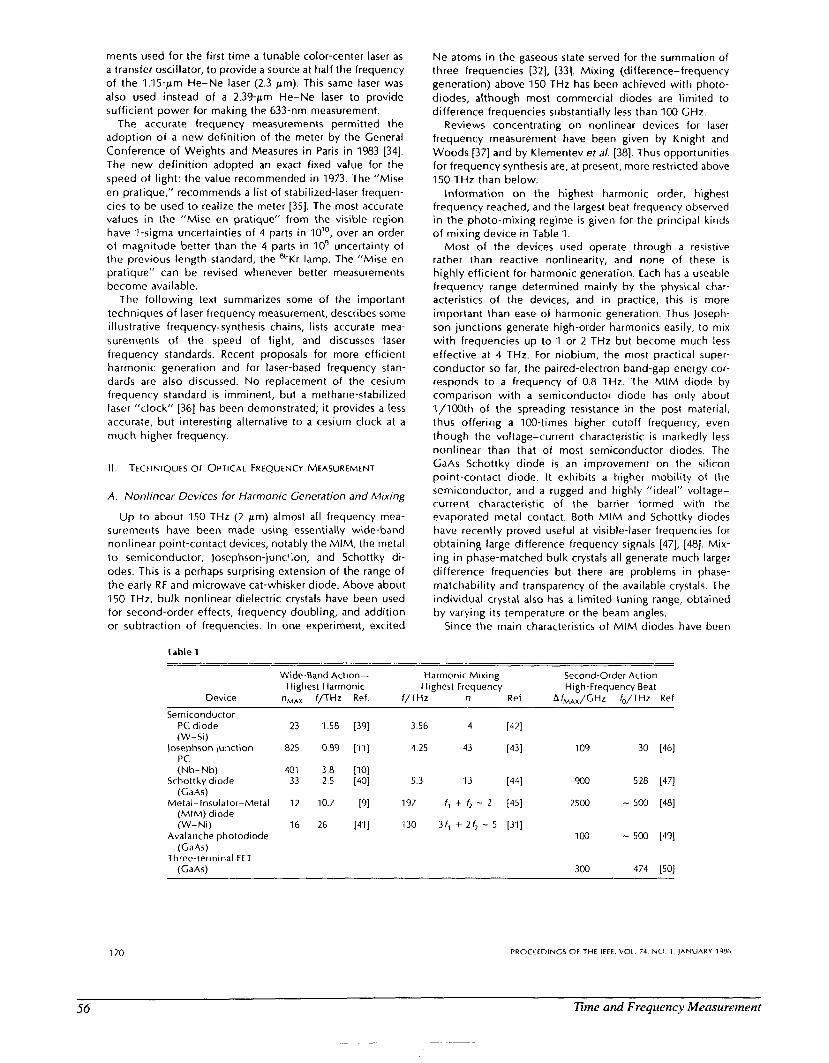
ments used for the first time a tunable color-center laser as a transfer oscillator, to provide a source at half the frequency of the 1.15-pm He-Ne laser (2.3 pm). This same laser was also used instead of a 2.39-pm He-Ne laser to provide sufficient power for making the 633-nm measurement.
The accurate frequency measurements permitted the adoption of a new definition of the meter by the General Conference of Weights and Measures in Paris in 1983 1341. The new definition adopted an exact fixed value for the speed of light: the value recommended in 1973. The “Mise e n pratique,” recommends a l ist of stabilized-laser frequen- cies to be used to realize the meter [35]. The most accurate values in the “Mise en pratique” from the visible region have I-sigma uncertainties of 4 parts in IO’O, over an order of magnitude better than the 4 parts in IO9 uncertainty of the previous length standard, the ffiKr lamp. The “Mise en pratique” can be revised whenever better measurements become available.
The following text summarizes some of the important techniques of laser frequency measurement, describes some illustrative frequency-synthesis chains, lists accurate mea- surements of the speed of light, and discusses laser frequency standards. Recent proposals for more efficient harmonic generation and for laser-based frequency stan- dards are also discussed. No replacement of the cesium frequency standard is imminent, but a methane-stabilized laser “clock” [36] has been demonstrated; it provides a less accurate, but interesting alternative to a cesium clock at a much higher frequency.
11. TECHNIQUES OF OPTICAL FREQUENCY MEASURE MEN^
A. Nonlinear Devices for Harmonic Generation and Mixing
Up to about 150 THz (2 pm) almost all frequency mea- surements have been made using essentially wide-band nonlinear point-contact devices, notably the MIM, the metal to semiconductor, Josephson-junction, and Schottky di- odes. This is a perhaps surprising extension of the range of the early R F and microwave cat-whisker diode. Above about 150 THz, bulk nonlinear dielectric crystals have been used for second-order effects, frequency doubling, and addition or subtraction of frequencies. In one experiment, excited
Table 1
Ne atoms in the gaseous state served for the summation of three frequencies [32], [33]. Mixing (difference-frequency generation) above 150 THz has been achieved with photo- diodes, although most commercial diodes are limited to difference frequencies substantially less than 100 GHz.
Reviews concentrating on nonlinear devices for laser frequency measurement have been given by Knight and Woods [37] and by Klementev et a / . [38]. Thus opportunities for frequency synthesis are, at present, more restricted above 150 THz than below.
Information on the highest harmonic order, highest frequency reached, and the largest beat frequency observed in the photo-mixing regime i s given for the principal kinds of mixing device in Table 1.
Most of the devices used operate through a resistive rather than reactive nonlinearity, and none of these is highly efficient for harmonic generation. Each has a useable frequency range determined mainly by the physical char- acteristics of the devices, and in practice, this i s more important than ease of harmonic generation. Thus Joseph- son junctions generate high-order harmonics easily, to mix with frequencies up to 1 or 2 THz but become much less effective at 4 THz. For niobium, the most practical super- conductor so far, the paired-electron band-gap energy cor- responds to a frequency of 0.8 THz. The MIM diode by comparison with a semiconductor diode has only about 1/100th of the spreading resistance in the post material, thus offering a 100-times higher cutoff frequency, even though the voltage-current characteristic is markedly less nonlinear than that of most semiconductor diodes. The GaAs Schottky diode is an improvement on the silicon point-contact diode. It exhibits a higher mobility of the semiconductor, and a rugged and highly “ideal” voltage- current characteristic of the barrier formed with the evaporated metal contact. Both MIM and Schottky diodes have recently proved useful at visible-laser frequencies for obtaining large difference frequency signals [47], [48]. Mix- ing in phase-matched bulk crystals all generate much larger difference frequencies but there are problems in phase- matchability and transparency of the available crystals. The individual crystal also has a limited tuning range, obtained by varying i t s temperature or the beam angles.
Since the main characteristics of MIM diodes have been
Wide-Band Action- Harmonic Mixing Second-Order Action Highest Harmonic Highest Frequency High-Frequency Beat
Device nMAX f/THz Ref. f/THz n Ref Af,,,/CHz f,,/THz Ref
Semiconductor PC diode (W-Si)
PC (Nb-Nb)
Schottky diode (CaAs)
Metal-Insulator-Metal (MIM) diode (W-Ni)
(GaAs)
(GaAs)
Josephson junction
Avalanche photodiode
Three-terminal FET
23 1.58 [39] 3 56 4 [421
825 0 8 9 [11] 4 25 43 [431 109 30 [46]
401 3 8 [IO] 33 2 5 [40] 5 3 13 [441 900 528 (471
12 10.7 [9] 197 f, + f2 - 2 I451 2500 - 500 I481
16 26 [41] 130 3 f , + 2f2 - 5 [31] 100 - 5 0 0 (491
300 474 [SO]
PROCEEDINGS OF T H E IEEF. V O L 74. NO 1 . JANUARY 198h 170
56 Eme and Frequency Measurement
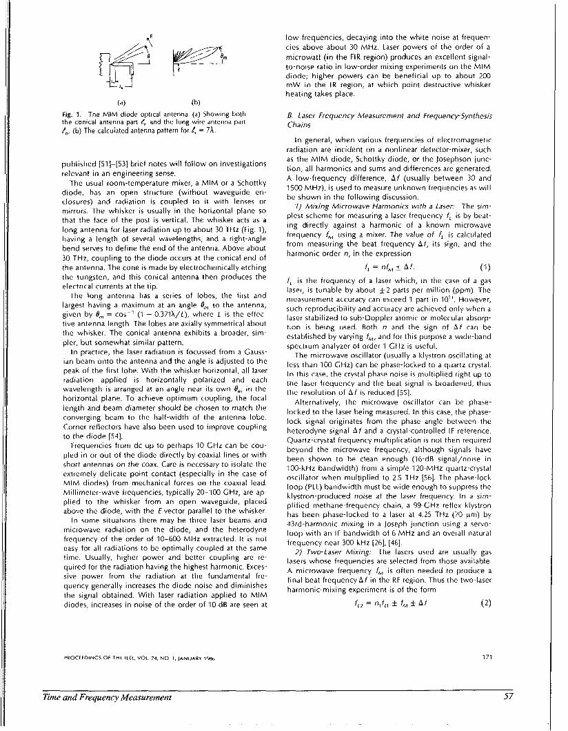
(a) (b) Fig. 1. The MIM diode optical antenna. (a) Showing both the conical antenna part C, and the long wire antenna part Ib. (b) The calculated antenna pattern for e, = 7 h .
published (51)-[53] brief notes wil l follow on investigations relevant in an engineering sense.
The usual room-temperature mixer, a MIM or a Schottky diode, has an open structure (without waveguide en- closures) and radiation i s coupled to i t with lenses or mirrors. The whisker i s usually in the horizontal plane so that the face of the post i s vertical. The whisker acts as a long antenna for laser radiation up to about 30 THz (Fig. I), having a length of several wavelengths, and a right-angle bend serves to define the end of the antenna. Above about 30 THz, coupling to the diode occurs at the conical end of
l ow frequencies, decaying into the white noise at frequen- cies above about 30 MHz. Laser powers of the order of a microwatt (in the FIR region) produces an excellent signal- to-noise ratio in low-order mixing experiments on the MIM diode; higher powers can be beneficial up to about 200 m W in the I R region, at which point destructive whisker heating takes place.
6. Laser Frequency Measurement and FrequencrSynthesis Chains
In general, when various frequencies of electromagnetic radiation are incident on a nonlinear detector-mixer, such as the MIM diode, Schottky diode, or the Josephson junc- tion, all harmonics and sums and differences are generated. A low-frequency difference, A f (usually between 30 and 1500 MHz), i s used to measure unknown frequencies as wil l be shown in the following discussion.
7) Mixing Microwave Harmonics with a Laser: The sim- plest scheme for measuring a laser frequency f , i s by beat- ing directly against a harmonic of a known microwave frequency fM using a mixer. The value of f, is calculated from measuring the beat frequency A f , its sign, and the harmonic order n, in the expression
. - the antenna. The cone is made by electrochemically etching f , = nf, A f . (I I the tungsten, and this conical antenna then produces the electrical currents at the tip.
The long antenna has a series of lobes, the first and largest having a maximum at an angle OM to the antenna, given by OM = cos-’ (1 - 0.371X/L), where L is the effec- tive antenna length. The lobes are axially symmetrical about the whisker. The conical antenna exhibits a broader, sim- pler, but somewhat similar pattern.
In practice, the laser radiation is focussed from a Gauss- ian beam onto the antenna and the angle is adjusted to the peak of the f irst lobe. With the whisker horizontal, all laser radiation applied i s horizontally polarized and each wavelength is arranged at an angle near i t s own 0, in the horizontal plane. To achieve optimum coupling, the focal length and beam diameter should be chosen to match the converging beam to the half-width of the antenna lobe. Corner reflectors have also been used to improve coupling to the diode [54].
Frequencies from dc up to perhaps 10 GHz can be cou- pled in or out of the diode directly by coaxial lines or with short antennas on the coax. Care i s necessary to isolate the extremely delicate point contact (especially in the case of MIM diodes) from mechanical forces on the coaxial lead. Millimeter-wave frequencies, typically 20-100 GHz, are ap- plied to the whisker from an open waveguide, placed above the diode, with the h e c t o r parallel to the whisker.
In some situations there may be three laser beams and microwave radiation on the diode, and the heterodyne frequency of the order of 10-600 MHz extracted. I t i s not easy for all radiations to be optimally coupled at the same time. Usually, higher power and better coupling are re- quired for the radiation having the highest harmonic. Exces- sive power from the radiation at the fundamental fre- quency generally increases the diode noise and diminishes the signal obtained. With laser radiation applied to MIM diodes, increases in noise of the order of 10 dB are seen at
f , is the frequency of a laser which, in the case of a gas laser, i s tunable by about k2 parts per million (ppm). The measurement accuracy can exceed 1 part in IO”. However, such reproducibility and accuracy are achieved only when a laser stabilized to sub-Doppler atomic or molecular absorp- tion is being used. Both n and the sign of A f can be established by varying f,, and for this purpose a wide-band spectrum analyzer of order 1 CHz is useful.
The microwave oscillator (usually a klystron oscillating at less than 100 CHz) can be phase-locked to a quartz crystal. In this case, the crystal phase noise is multiplied right up to the laser frequency and the beat signal is broadened, thus the resolution of A f is reduced [55].
Alternatively, the microwave oscillator can be phase- locked to the laser being measured. In this case, the phase- lock signal originates from the phase angle between the heterodyne signal A f and a crystal-controlled IF reference. Quartz-crystal frequency multiplication i s not then required beyond the microwave frequency, although signals have been shown to be clean enough (16-dB signal/noise in 100-kHz bandwidth) from a simple 120-MHz quartz-crystal oscillator when multiplied to 2.5 THz (561. The phase-lock loop (PLL) bandwidth must be wide enough to suppress the klystron-produced noise at the laser frequency. In a sim- plified methane-frequency chain, a 99-GHz reflex klystron has been phase-locked to a laser at 4.25 THz (70 pm) by 43rd-harmonic mixing in a joseph junction using a servo- loop with an IF bandwidth of 6 MHz and an overall natural frequency near 300 kHz [26], (461.
2) Two-Laser Mixing: The lasers used are usually gas lasers whose frequencies are selected from those available. A microwave frequency f,,,, i s often needed to produce a final beat frequency A f in the R F region. Thus the two-laser harmonic-mixing experiment is of the form
f i 2 = qf,, f f , -t. A f ( 2)
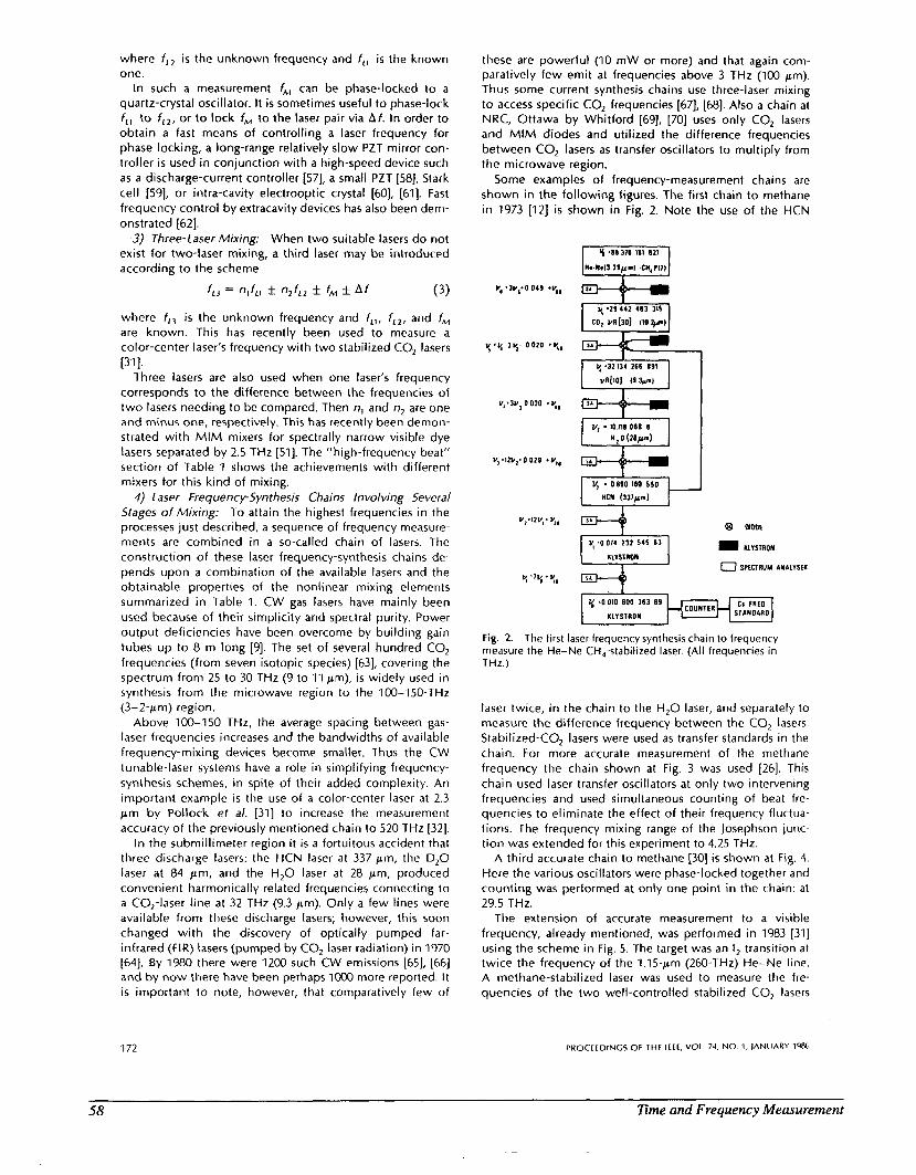
where f,, i s the unknown frequency and f,, is the known one.
In such a measurement f, can be phase-locked to a quartz-crystal oscillator. It is sometimes useful to phase-lock f,, to f,,, or to lock f, to the laser pair via A f . In order to obtain a fast means of controlling a laser frequency for phase locking, a long-range relatively slow PZT mirror con- troller i s used in conjunction with a high-speed device such as a discharge-current controller [57], a small PZT [58], Stark cell [59], or intra-cavity electrooptic crystal [60], (611. Fast frequency control by extracavity devices has also been dem- onstrated [62].
3) Three-Laser Mixing: When two suitable lasers do not exist for two-laser mixing, a third laser may be introduced according to the scheme
f,, = n l f l l f n,f,, * f,, f Af (3)
where f,, i s the unknown frequency and f,,, f,,, and f, are known. This has recently been used to measure a color-center laser's frequency with two stabilized CO, lasers
Three lasers are also used when one laser's frequency corresponds to the difference between the frequencies of two lasers needing to be compared. Then n, and nz are one and minus one, respectively. This has recently been demon- strated with MIM mixers for spectrally narrow visible dye lasers separated by 2.5 THz [51). The "high-frequency beat" section of Table 1 shows the achievements with different mixers for this kind of mixing.
4) Laser FrequencrSynthesis Chains Involving Several Stages of Mixing: To attain the highest frequencies in the processes just described, a sequence of frequency measure- ments are combined in a so-called chain of lasers. The construction o f these laser frequency-synthesis chains de- pends upon a combination of the available lasers and the obtainable properties of the nonlinear mixing elements summarized in Table 1. CW gas lasers have mainly been used because of their simplicity and spectral purity. Power output deficiencies have been overcome by building gain tubes up to 8 m long [9]. The set of several hundred CO, frequencies (from seven isotopic species) [63], covering the spectrum from 25 to 30 THz (9 to 11 pm), is widely used in synthesis from the microwave region to the 100-'150-THz (3-2-pm) region.
Above 100-150 THz, the average spacing between gas- laser frequencies increases and the bandwidths of available frequency-mixing devices become smaller. Thus the CW tunable-laser systems have a role in simplifying frequency- synthesis schemes, in spite of their added complexity. An important example i s the use of a color-center laser at 2.3 p m by Pollock et a/ . [31] to increase the measurement accuracy of the previously mentioned chain to 520 THz 1321.
In the submillimeter region it i s a fortuitous accident that three discharge lasers: the HCN laser a t 337 pm, the D,O laser at 84 pm, and the H,O laser at 28 pm, produced convenient harmonically related frequencies connecting to a C0,-laser line at 32 THz (9.3 pm). Only a few lines were available from these discharge lasers; however, this soon changed with the discovery of optically pumped far- infrared (FIR) lasers (pumped by CO, laser radiation) in 1970 [64]. By 1980 there were 1200 such CW emissions [65], [66] and by now there have been perhaps 7ooO more reported. I t is important to note, however, that comparatively few of
[31 I.
172
these are powerful ( I O mW or more) and that again com- paratively few emit at frequencies above 3 THz (100 pm). Thus some current synthesis chains use three-laser mixing to access specific CO, frequencies [67], [68]. Also a chain at NRC, Ottawa by Whitford [69], [70] uses only COz lasers and MIM diodes and utilized the difference frequencies between CO, lasers as transfer oscillators to multiply from the microwave region.
Some examples of frequency-measurement chains are shown in the following figures. The first chain to methane in 1973 [I21 i s shown in Fig. 2. Note the use of the HCN
U, *Iu,*O 049 +It,,
y * y 1% 0020 'I,
v..lu,ooIo *$,
u, *12v,.o 029 'U,,
u, :w,. v,,
y ' 7% - ys
0 mow = l l Y S l R O M
0 SPECTRUM ANALYSER
y * O 010 600 363 69
Fig. 2. The first laser frequency synthesis chain to frequency measure the He-Ne CH,-stabilized laser. (All frequencies in THz.)
laser twice, in the chain to the H,O laser, and separately to measure the difference frequency between the CO, lasers. Stabilized-CO, lasers were used as transfer standards in the chain. For more accurate measurement of the methane frequency the chain shown at Fig. 3 was used [26]. This chain used laser transfer oscillators at only two intervening frequencies and used simultaneous counting of beat fre- quencies to eliminate the effect of their frequency fluctua- tions. The frequency mixing range of the Josephson junc- t ion was extended for this experiment to 4.25 THz.
A third accurate chain to methane [30] i s shown at Fig. 4. Here the various oscillators were phase-locked together and counting was performed at only one point in the chain: at 29.5 THz.
The extension of accurate measurement to a visible frequency, already mentioned, was performed in 1983 [31] using the scheme in Fig. 5. The target was an I, transition at twice the frequency of the 1.15-pm (260-THz) He-Ne line. A methane-stabilized laser was used to measure the fre- quencies of the two well-controlled stabilized CO, lasers
PROCEEDINGS OF T H E I E E E . VOL 74. NO 1. IANl lARY 19ffi
58 lfme and Frequency Measurement
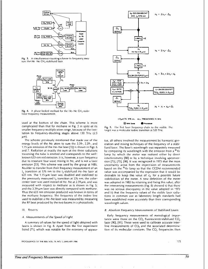
4.25 TU2 r m F m
29 THz 10.7pm
Fig. 3. sure the He-Ne CH,-stabilized laser.
A simultaneous-counting scheme to frequency mea-
FI-Y I
NVm
&I" L.
Fig. 4. A phase-locked method for the He-Ne CH,-stabi- lized frequency measurement.
used at the bottom of the chain. This scheme i s complicated than that for methane in Fig. 3 in spite
more of its
smaller frequency-multiplication range, because of the limi- tation to frequency-doubling stages above 130 THz (2.3
The scheme previously mentioned that made use of the energy levels of the Ne atom to sum the 3.39-, 2.39-, and 1.15-pm emission of the He-Ne laser [32] is shown in Figs. 6 and 7. Radiation at exactly the sum of the three radiations traversing the tube i s emitted and corresponds to the well- known 633-nm red emission. It is, however, a sum frequency due to resonant four-wave mixing in Ne, and is not a laser emission [33]. This scheme was used by the group at NBS, Boulder to transfer from their frequency measurement of an I L transition at 576 nm to the I,-stabilized He-Ne laser at 633 nm. The 1.15-pm laser was doubled and stabilized to the previously measured Iz transition at 576 nm; the color- center laser w a s used instead of He-Ne at 2.39 pm, and was measured with respect to methane as is shown in Fig. 5; and the 3.39-pm laser was directly compared with methane. Thus the 633-nm emission produced was known in terms of the methane frequency. The frequency of the iodine line used to stabilize a He-Ne laser was measured by measuring the RF beat produced by the two beams in a photodiode.
am).
111. RESULTS
A. Measurements of the Speed of Light
A summary of values for the speed of light obtained with lasers i s shown in Fig. 8. Apart from the first experiment listed [71], which was notable for the economy of appara-
PROCEEDINGS OF T H E I E E E . VOL 74, NO 1, JANUARY 1%
y. 520206808.547 V, - 2y.o A,
V, - 1539
ANALYZER SPECTRUM * 3v, 2v2
U,.26035339978m 'YO,. P,(50). (I I 5 p m i
V, * V, V,.+A,
v, ' 3 V , 2V*. V,
II 5pm TO 576 nm. ALL FREWENCIES IN MU2
B M ~ M D D ~ . emdod. Fig. 5. The first laser frequency chain to the visible. The target was a molecular iodine transition at 520 THz .
tus, a l l others involved the measurement by harmonic gen- eration and mixing techniques of the frequency of a stabi- lized laser. The laser's wavelength was separately measured by comparing i t s wavelength with the emission from a "Kr lamp by which the meter was realized either by direct interferometry [88] or by a technique involving upconver- sion 1731, [75], [98]. It was recognized in 1973 that the main uncertainty arose from the imprecision of measurements based on the '"Kr lamp so that the CCDM recommended value was accompanied by the expression that it would be desirable to keep this value of co for a possible future redefinition of the meter. A new definition of the meter was adopted in 1983 by retaining and fixing this value, after the intervening measurements (Fig. 8) showed i) that there was no serious discrepancy in the value adopted in 1973 and ii) that the frequency values of the visible laser radia- tions in common use as laboratory length standards had been established more accurately than their corresponding wavelength values.
6. Absolute Frequency Measurements of Stabilized Lasers
Early frequency measurements of metrological impor- tance were those on the CO, fluorescence-stabilized CO, laser [%I, [91]. These were used to calibrate accurate inter- line measurements of CO, and the associated determina- tion of its molecular constants. The CO, frequencies then
173
Time and Frequency Measurement 59
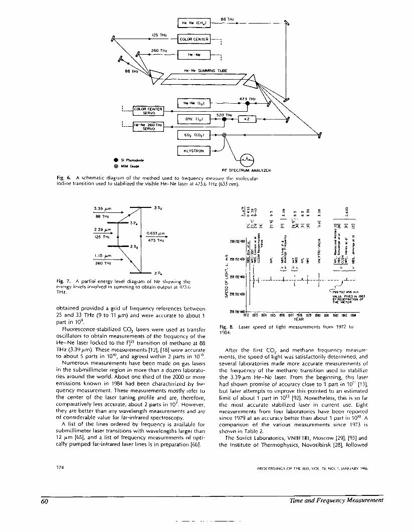
260 THz
174
\\\ I
0 SI Pholoaodc 8 MLM bode
RF SPECTRUM ANALYZER
Fig. 6. A schematic diagram of the method used to frequency measure the molecular iodine transition used to stabilized the visible He-Ne laser at 473.6 THz (633 nm).
3.39 prn
€36 THz
1.15 p m
260 THz ___..
ZP,
Fig. 7. A partial energy level diagram of Ne showing the energy levels involved in summing to obtain output at 473 6 THz.
obtained provided a grid of frequency references between 25 and 33 THz (9 to 11 pm) and were accurate to about 1 part in io9.
Fluorescence-stabilized CO, lasers were used as transfer oscillators to obtain measurements of the frequency of the He-Ne laser locked to the Fi2) transition of methane at 88 THz (3.39 pm). These measurements [12], [I81 were accurate to about 5 parts in I O I O , and agreed within 2 parts in
Numerous measurements have been made on gas lasers in the submillimeter region in more than a dozen laborato- ries around the world. About one third of the 2000 or more emissions known in 1984 had been characterized by fre- quency measurement. These measurements mostly refer to the center of the laser tuning profile and are, therefore, comparatively less accurate, about 2 parts in IO’. However, they are better than any wavelength measurements and are of considerable value for far-infrared spectroscopy.
A l ist of the lines ordered by frequency i s available for submillimeter laser transitions with wavelengths larger than 12 pm [65], and a l is t of frequency measurements of opti- cally pumped far-infrared laser lines i s in preparation [66].
J L
.1-.
4 . 1.. v v
VALUE FIXEO m RBJ BY REDEFNITWN OF THE METER
299 r92 4 4 0 4 . . . . . . . . , . . . 1912 1913 PI14 1915 1116 1911 1918 1979 1984 1981 1911 I983 1964
YEAR
Fig. 8. 1984.
laser speed of light measurements from 1972 to
After the first CO, and methane frequency measure- ments, the speed of light was satisfactorily determined, and several laboratories made more accurate measurements of the frequency of the methane transition used to stabilize the 3.39-pm He-Ne laser. From the beginning, this laser had shown promise of accuracy close to 1 part in IO” 1131, but later attempts to improve this pointed to an estimated l imit of about 1 part in IOl3 [92]. Nonetheless, this is so far the most accurate stabilized laser in current use. Eight measurements from four laboratories have been reported since 1979 at an accuracy better than about 1 part in IO”. A comparison o f the various measurements since 1973 is shown in Table 2.
The Soviet Laboratories, VNIIFTRI, Moscow [29], [93] and the Institute o f Thermophysics, Novosibirsk [28], followed
PROCTEOINCS OF THC IEEE, VOI 74. NO 1. IANUARY IW,
60 Z m e and Frequency Measurement
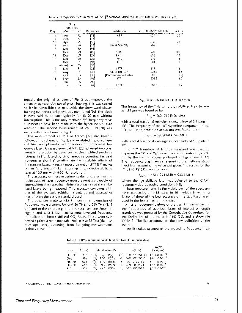
surements discussed above and will be seen to assign a greater uncertainty than those of individual frequency mea- surements. The reasons are that i) a three-sigma uncertainty i s given, rather than the usual one-sigma value, ii) the measurements of methane disagreed by about three times one-sigma, and iii) for some visible frequencies additional data were taken into account.
The uncertainties in Table 3 are about an order of magni- tude larger than the accuracies claimed for the lasers them- selves, so that improved measurements can be expected in the future.
Schemes to measure the frequencies of stabilized lasers in the visible spectral region are being explored at various laboratories. A suitable stabilized laser at 576 nm has been evaluated at NPL [97] and a frequency synthesis experiment has been described [68].
A summary of stabilized-laser frequency measurements traceable to cesium, and with accuracies exceeding 3 parts in IO9, has been compiled [98]. Recent measurements of high accuracy have been made on an OsO, transition near 29 THz (10.3 pm) [67] and on the methane E line at 88.373 THz (3.39 pm) 1951, [96].
IV. DISCUSSION
A. Sources o f Error in Laser Frequency Measurement
I ) Inexactitude in Frequency-Mixing Devices: When the nonlinear properties of systems with well-defined energy levels are being used for frequency mixing i t i s important to guard against quanta characteristic of the mixing device (as opposed to those of the input frequencies) contributing to the output frequency. Checks can be made, by varying the input frequencies, for example.
On devices used for harmonic generation, some experi- mental checks have been made for differences of this type. An indirect check on the agreement between Josephson- junction harmonic mixing and the use of entirely room- temperature harmonic mixers is afforded by the results for the 88-THz methane frequency in Table 2. The measure- ments from NPL alone used the Josephson junction. In a specific test at NPL, see 176, pt. I, Appendix], frequency multiplication to 0.89 THz in a Josephson junction was found to agree with that in an MIM diode within a I-sigma uncertainty of 41.2 parts in IO”. (The test was primarily to compare frequency measurement by frequency division and counting with that by observation of a beat on a spectrum analyzer, but the harmonic mixers were also different.)
A comparison of frequency doubling in a bulk nonlinear crystal and in an MIN diode has been made by Edwards and colleagues at NPL [61]. A CO, laser’s emission was doubled in a crystal of CdGeAs, and was also doubled in an MIM diode. Then the two frequencies were compared. Any net difference arising in the two frequency-doubling processes was found to be less than 7 parts in IOi6.
2) Effect o f Phase Noise in Sources Used for Frequency Multiplication: The problem of spectral broadening in harmonics as a result of phase noise in the fundamental-sig- nal oscillator showed at an early stage in laser frequency measurement. Lasers provided clean local oscillators with which to observe harmonic signals multiplied from quartz crystals, for example, and from microwave oscillators.
In the beginning, phase noise from quartz crystals used for phase-locking klystrons was a problem, but by using
7 76
simplified high-frequency quartz-crystal oscillators (near 100 MHz) and straight frequency multipliers (avoiding some kinds of synthesizers) clean signals could be observed to 2.5 THz [56].
Studies on the special requirements of laser frequency measurement and on the properties of multiplied quartz- crystal noise [55] have helped to clarify the problem, specifi- cally as to the point of catastrophic spectral broadening.
The use of downward phase-lock loops has diminished demands on upward frequency multiplication. High loop bandwidths of order 300 kHz have permitted downward phase locking a 99.6-GHz reflex klystron to a 4.25-THz laser via 43rd-harmonic mixing in a Josephson junction [46].
3) Doppler Effect and Time-Dependent Phase Shifts: At high accuracies it i s necessary to guard against the effects of relative motion of different parts of the apparatus which might not cancel for the different methods used to observe signals, such as stored spectrum analyzer displays. Another potential source of error i s from phase shifts in signal paths or filters which drift monotonically with time, as from a slowly changing temperature. Discrepancies at the level of 1 part - 10l2 have been observed 126, Appendix I].
4) Phase-lock l o o p Errors: Phase-lock errors are actual mistakes and can usually be corrected: however, we will mention them anyway. A possible source of error i s to lock on a loop-oscillation sideband. The least offset likely in this way would be comparable with the natural frequency of the loop, typically from 10 kHz upwards. Such an error is relatively easily resolved in the more accurate experiments and thus wil l generally be detected by the experimenter, Another problem arises from spurious modulation of weak signals used to phase-lock oscillators. For example, silicon- controlled rectifer spikes can cause intermittent unlock for say half-a-line-frequency period which could alter the mean locked frequency over a typical 1 - s count-averaging time 1461. Careful spectrum analyzer checks are required in such circumstances. The direction of the error is, however, usu- ally random so that accuracy increases with repeated mea- surement.
V. SUMMARY
Many hundreds of laser frequencies and stabilization reference frequencies have now been measured, and accu- rate measurements have even been extended as high as the visible, yellow-green, portion of the spectrum.
This has permitted the recent (1983) redefinition of the meter fixing the value of co exactly, so that length and wavelength are based on the same physical standard as time and frequency. Thus length is now referred to the most accurate physical standard available-the cesium clock. Substantial immediate improvements in realizing the meter have been obtained. Also, in such activities as time- of-flight ranging in space, the conversion from time to length does not increase the uncertainty.
Laser frequency measurement spans a spectral range from about 0.5-500 THz. These three orders of magnitude are comparable with the entire frequency span of microwave measurements 0.5-500 GHz; or, in a linear scale, frequency measurements represent a thousand-fold increase. This is extremely significant for communications purposes. The extension of frequency measurements to higher frequencies and improved accuracies is especially important for future experiments to seek frequency standards better than cesium.
PROCIlIXNGS OF 1 H t IEFE. VOL 74. NO 1, IANUARY 1%
62 Time and Frequency Measurement
_ _ _ _ ~ ~
The methane clock, current fundamental work towards new frequency standards using heavy molecules in the IO-pm band, and work on trapped ions at visible or higher fre- quencies [99] al l point towards possible frequency standards with reproducibilities and accuracies exceeding that of the current Cs frequency standard.
ACKNOWLEDGMENT
One of the authors (DIEK) would like to thank W. R. C. Rowley for helpful comments.
REFERENCES
T. H. Maiman, “Stimulated optical radiation in ruby,” Nature,
A. Javan, W. R. Bennett, Jr., and D. R. Harriott, “Population inversion and continuous optical maser oscillation in a gas discharge containing a He-Ne mixture,” Phys. Rev. Lett., vol. 6, pp. lO6-110. 1961. A. D. White and 1. D Rigden, “Continuous gas maser oper- ation in the visible,” Proc. IRE., vol. 50, p. 1697, 1962. A. Crocker, H A. Cebbie, M. F. Kimmitt, and L. E. S Mathias, ”Stimulated emission in the far infrared,” Nature, vol. 201, pp. 250-251, 1964 L. 0 Hocker, A. Javan, D. Ranochandra Rao, L. Frenkel, and T. Sullivan, ”Absolute frequency measurement and spectroscopy of gas laser transitions in the far infrared,” Appl. Phys. Lett.,
C. Jones and W. Cordy, ”Extension of submillimetre wave spectroscopy below a half millimetre wavelength,” Phys. Rev., vol. 135A, p. 295, 1964 K 0. Froome, “ A new determination of the free-space veloc- ity of electromagnetic waves,” Proc. Roy. Soc., Ser. A, vol. 247, pp. 109-122, 1958 E Bergstrand, “A determination of the velocity of light,” Arkiv for Fysik, vol. 2, 119- 150, 1950. K. M. Evenson, J . 5. Wells, L. M. Matarrese, and L B. Elwell, “Absolute frequency measurements on the 28 and 78 pm cw watcr vapour laser lines,” Appl. Phys. Left., vol. ‘16, pp 159-162, 1970 D. C. McDonald, A. S. Risley, J . D. Cupp, K. M. Evenson. and J R. Ashley, “four-hundredth-order harmonic mixing of nii- crowave and infrared laser radiation using a Josephson junc- tion and a maser,” Appl. Phys. Lett., vol. 20, pp. 296-299, 1972. T. C. Blaney and D. 1. E. Knight, ”Direct 825th harmonic mixing of a 1 CHz source with an HCN laser in a Josephson junction,” 1. Phys. D, vol. 7, pp. 1882-1886, 1974. K . M. Evenson, J. 5. Wells, F. R. Petersen, B. L. Danielson, and C. W. Day, “Accurate frequencies of molecular transitions used in laser stabilization: the 3.39 pm transition in CH., and the 9.33- and 10.18-pm transitions in CO,,” Appl. Phys Let t , vol. 22, pp 192-195, 1973. R. L. Barger and J. L. Hall, ”Pressure shift and broadening of methane line at 3.39 pm studied by laser-saturated niolecular absorption,” Phys. Rev. Lett., vol. 22, pp 4-8, 1969. C. Freed and A. Javan, “Standing-wave saturation resonances in the CO, 10.6 pm transitions observed in a low-pressure room temperature absorber gas,” Appl. Phys. Left., vol. 17, pp. 53-56, and 511, 1970. C. R. HJnCS and C. E. Dahlstrom, “Iodine hypcrfinc structure observed in Saturated absorption at 633 nni,” Appl. Phys. Lett., vol. 14, 362, 1969. Comite Consultatif pour IJ Definition du Metre, 5th Session, BIPM, Stvres, France, 1973. T. C. Blaney, C. C. Bradley, C. 1. Edwards, D. I E. Knight, P. T. Woods, and 6. W. Jolliffe, “Absolute frequency measurement of the R(12) transition of CO, at 9.3 pm,” Nature, vol. 214, p. 504, Aug. 24, 1973. T. C. Blaney, C. 1. Edwards, E. W. Jolliffe, D J . E. Knight, and P. T. Woods, “Absolute frequencies of the methane-stabilized He-Ne laser (3.39 pm) and the CO,, R(32) stabilized laser
VOI. 187, pp. 493-494, 1960.
VOI. IO , pp. 147-149, 1967.
(10.17 pm),” 1. Phys. D., vol. 9, pp. 1323-’1330. 1976, and NdtUrP, vol. 254, no. 5501, pp 584-585, Apr. 17, .1975. Ch. I. Bord6, M. Ouhayoun, A. Van Lerberghe, C. Salomon, 5. Avrillier, C. D. Cantrell, and J. Bordb, “High resolution saturated spectroscopy with CO, lasers. Application to the v, bands of SF, and OsO,,” in Laser Spectroscopy /V (Series in Optical Sciences, vol. 21), H . Walther and K . W. Rothe, Eds. Berlin: Springer-Verlag, 1979, pp. 142-153. A. Clairon, A. Van Lerberghe, C. Salomon, M. Ouhayoun, and Ch. 1. BordC., “Towards a new absolute frequency reference grid in the 28 THz range,” Opt. Commun., vol. 35, no. 3, pp. 368-372, Dec. 1980. J. Bord6 and Ch. RordC, “Superfine and hyperfine structures in the vj band of 32SF,,” Chem. Phys., vol. 71, pp. 417-441,1982. R. 5. McDowell, C. W. Patterson, N. C. Nereson, F. R. Petersen, and 1, S. Wells, “CO, laser coincidences with v3 of SiF, near 9.7 pm,” Opf. Lett., vol. 6, no. 9, pp. 422-424, Sept. 1981. D. A. Jennings, F R. Petersen, and K. M. Evenson, “Frequency measurement of the 260 THz (1.15 am) He-Ne laser,” Opt. Letf., vol. 4, pp. 129-130, 1979. C. R. Hanes, “Doubly-resonant intracavity generation of sec- ond harmonic of 1153 nm radiation with stabilization on h.1.s. components of 1 2 7 1 1 , ” Appl. Opf., vol. 18, pp. 3970-3974, 1979. K. M Baird, K. M. Evenson, G. R. Hanes, D. A. Jennings, and F. R. Petersen, “Extension of absolute frequency measure- ments to the visible: frequencies of ten hyperfine coinpo- nents of iodine,” Opt. Lett., vol. 4, pp. 263-264, 1979. 0. I. E. Knight, C. J. Edwards, P. R. Pearce, and N. R. Cross, ”Measurement of the frequency of the 3.39 pm methane- stabilized laser to _+parts in 10”,” /€€€ Trans. Instrum. Meas., vol. IM-29, pp. 257-264, Dec. 1980. A. Clairon, B . Dahmani, and J. Rutman, “Accurate absolute frequency measurements on stabilized CO, and He-Ne in- frared lasers,” /€E€ Trans. Insfrum. Meas., vol. IM-29, pp.
V. P Chebotayev, “Optical time scale,” /. Phys. (Colloq. CS), supplement to vol 42, no 12, pp. C8-505-C8-512, Dec. 1981. V C. Col’dort, V. F. Zakhar’yash, V. M. Klement’ev, M. V. Nikitin, B. A. Timchenko, and V. P. Chebotaev, Pis’ma Zh. fksp. Fiz., vol. 8, pp. 157-161, l982, trans/ ”Development of an optical tinie scale,” Sov. Tech. Phys. Left., vol. 8, no 2, pp 68-69. 1982. Yu. 5. Domnin, N. 8. Koshelyaevskii, V. M. Tatarenkov, and P. 5. Shumyatskii, Pis’ma Zh. Eksp. Tror. Fiz.. vol. 30, no. 5, pp. 273-275, Sept. 5, 1979. trans/ “Absolute measuremcwts of I R laser frequencies,” JETP Lett., vol. 30, no. 5, pp. 253-255, Sept. 5, 1979. Yu. S Domnin, N. B. Koshelyaevskii, V. M. Tatarenkov, and P. 5. Shumyatskii, Pis’ma Zh. Eksp. Teor. Fiz., vol. 34, no. 4, pp. 175-178, Aug. 20, 1981, trans/ “Measurement of the frequency of a He-Ne/CH, laser,” JETP Lett., vol. 34, no. 4 pp. 167-’170. Aug. 20, 1981. C. R. Pollock, D. A. Jennings, F. R. Petersen, J. 5. Wells, R. E. Drullinger, E. C. Beaty, and K . M. Evenson, “Direct frequency measurements of transitions at 520 THz (576 nm) in iodine, and 260 THZ (1.15 pm) in neon,” Opt. Lett., vol. 8, pp. 133-135.1483. D. A. Jennings, C. R. Pollock, F. R. Petersen, R. E. Drullinger, K . M. Evenson, J 5. Wells. I . L. Hall, and H. P. Layer, “Direct frequency measurement of the I,-stabilized He-Ne 473 THz (633 nm) laser,” Opt. Left., vol. 8, pp. 136-138, 1983. V. M. Klementyev, Yu. A . Matyugini, and V. P. Chebotayev, P d m a Z h . E k p . Teor. Fiz., vol. 24, no. 1, pp 8-12, July 5, 1976, trans/, “Mixing of the frequencies 88.37 THz ( A = 3.39 pni), 125.13 THz ( A = 2.39 pm), and 260.1 THz ( A = 1.15 pm) in a gas, and production of continuous cd~(wn t cmi5sion with combined frequency 473 6 THz ( A = 0.63 pm),” JETP Left., vol. 24, no. 1, pp. 5-8, July 5, 1976. V. P. Chebotayev, V. M. Klementyev, Yu. C. Kolpakov, and Y . A. Matyugin, "Frequency synthrsis of 0 63 iini radialinn by mixing optical frcquencies in gas and nonlinear crystals,” in Proc. 2nd Frequency Sfandards and Metrology Symp. (Copper Mountain, CO, July 5-7, 1976. Boulder, CO: Nat. Bur. Stand., Frequency and Time Standards Section, Nov. l976), pp. 368-384. Compfes Rcridus des Sfances de la 17“ CCPM, BIPM, Sevres,
268-272, 1980.
PROCECOINCS Of T H E IECE. VOL. 74, NO. 1 . IANUARY i98b 177
Time and Frequency Measurement 63
France, 1983. BtPM, “Documents concerning the new definition of the metre,” Metrologid, vol. 19, pp. 163-177, 1984. S. N. Bagayev, 6. D. Borisov, V. G. Gol’dort, A. Yu. Gusev, A. S. Dychkov, V. F. Zakharyash, V. M. Klementyev, M. U. Nikitin, 6. A. Tinchenko, V. P. Chebotayev, and V. V. Yumin, USSR Academy of Sciences, Siberian Branch, Institute of Thermo- physics, Preprint 78-82, Novosibirsk, 1982, publ. “Optical time standard,” USSR Acad. Sci. Avtometriya, no. 3, pp. 37-58, May-June ‘1983. trans/ Automatic Monitoring and Measure- ment (98). D. J. E. Knight and P. T. Woods, “Application of nonlinear devices to optical frequency measurement,” /. Phys. E., vol. 9,
V. M. Klement’ev, Yu. A. Matyugin, and V. P. Chebotaev, Kvanl. Necktron., vol. 5, no. 8, pp. 1671-1681, Aug. 1978, trans/ “Frequency measurements in the optical range: Current status and prospects,” Sov. 1. Quantum Electron., vol. 8, no. 8, pp. 953-958, Aug. 1978. 1. 0. Hocker. D. R. Rao, and A. Javan, “Absolute frequency measurement of the 190 pm and 194 pm gas laser transitions,”
ti. R. Fcttrrman, 6. I. Clifton, P. E. Trannrnwald. and C. D. Parker, “Submillimeter detection and mixing using Schottky diodes,” Appl. Phys. Lett., vol. 24, pp. 70-72,1974, K. M. Evenson, unpublished. L. 0. Hocker, 1. G. Small, and A. Javan, “Extension of absolute frequency measurements to the 84 pm range,” Phys. Letf., vol.
T. C. Blaney, N. R. Cross, D. I. E. Knighf, C. J. Edwards, and P. R. Pearce “Frequency measurement at 4.25 T t i z (705 pm) using a Josephson harmonic mixer and phase-lock tech- niques,”]. Phys. D Appl. Phys., vol. 13, pp. 1365-1370, 1980. C. 0. Wciss and A. Codone, ”Harmonic mixing and detection with Schoftky diodes up to the 5 THz range,” / € € E , J Quatum Elec-tron, vol. QE-20, pp. 97-99, 1984. K. M. Evenson, D. A. Jennings, F. R. Petersen, and J. 5. Wells, ”Laser frequency measurements: A review, limitations, exten- sion to 197 THz (.IS pm),” in Laser Spectroscopy 111. J t . Hall and J. L. Carlsten, Eds. Berlin, Germany: Springer-Verlag,
D. G. McDonald, F. R. Petersen, J. D. Cupp, 6. L. Danielson, and E. C. johnson, “Iosephson junctions at 45 times the rnergy-gap frcquency,” Appl. Phys. Lett., vol. 24, pp 335-337, 1974. H-U. Daniel, 6. Maurer, and M. Steiner, “A broadband Schot- tky point contact mixer for visible laser light and microwave harmonics,” Appl. Phys., vol. 8-30, pp. l89-193, 1983. R. E. Drullinger, K. M. Evenson, D. A. Jennings, F. R . Petersen, J. C. Bergquist, L. Burkins, and H. U. Daniel, “2.5 THz frequency difference measurements in the visible using metal-insulator- metal diodes,” Appl. Phys. Lett., vol. 42, pp. 137-138, ‘1983. 5. W. Wang, Lasers and Applications, vol. 111, no. IO, p. 6 (late news), Oct., 1984; see also; S. Y. Wang, D. M. Bloom, and D. M. Collins, “20-CHz bandwidth GaAs photodiode,” Appl. Phys. Lett., vol. 42, no. 2, pp. 190-192, Jan. 15, 1983. A. Chu, H. R. Fetterman, D. D. Peck, and P. E. Tannerwald, ”Heterodyne experiments from millimetre wave to optical frequencies using CaAs MESFETs above f,,” in / E € € Conf. Preprint (Dallas MTT, 1982), pp. 25-28, 1982. K. 1. Siemsen and H. 0. Riccus. “Experiments with point-con- tact diodes in the 30-130 THz frequency region,” Appl. Phys., vol. A35, pp. 177-187, l984. H. D. Riccus and K. J. Siemsen, “Point-contact diodes,” Appl. Phys., vol. A35, pp. 67-74, 1984. K. M. Evenson, M. Inguscio, arid D. A. Jennings, “Point-con- tact diode at laser frequencies,“ J. Appl. Phys., vol. 57, pp. 956-960, 1985. H. R. Fetterman, P. E. Tannenwald, 6. J. Clifton, C. D. Parker and W. D. Fitzgerald, “Far-IR heterodyne radiometric mea- surements with quasioptical Schotty diode mixers,” Appl. Phys. Lett., vol. 33, pp. 151-154, 1978. F. L. Walls, and A. DeMarchi, “ R F spectrum of a signal after frequency multiplication; measurement and comparison with a simple calculation,” / E € € Trans. Instrum. Meas., vol. IM-24, pp. 210-2.17. 1975.
110. 11, pp. 898-916, 1976.
Phys. Lett., VOI. A-24, pp. 690-691, 1967.
A-29, pi>. 321-322, 1969.
1977, pp. 56-58.
T. C. Blaney, N. R. Cross, and D. I. Knight, “Harmonic mixing and frequency measurements a t 2.5 THz using Josephson junctions,” /. Phys. 0, vol. 9, pp. 2175-2180, 1976. J. 5. Wells, “A stabilized HCN laser for infrared frequency synthesis,” /€€E Trans. Instrum. Meas., vol. IM-22, pp. 113-118, 1973. V. C. Col’dort,V. F. Zakhar’yash, and 6. A. Kurnevich, Priboryi Tekhnika Eksp., no. 2, pp. 244-248, Mar.-Apr. 1979, t rans/ . : “ Wideband unit for phase-frequency locking of lasers,” ln- strum. and Exper. Techno/.. no. 2, pp. 557-562, Mar.-Apr. 1979. 5. R. Stein, A. S. Risley, H. Van de Stadt, and F. Strumia, “High speed frequency frequency modulation of far-infrared lasers using the Stark effect,” Appl. Opt., vol. 16, pp 1893-1896, July 1977. W. R. Leeb, H. K. Phillipp, A. L. Scholtz, and E. Bonek, “Frequency synchronization and phase locking of CO, lasers,”
D J . E . Knight, “Optical frequency synthesis at NPL,” 1. Phys. (Colloq. C8), supplement to vol. 42, no. 12, pp. C8-495-C8- 503, Dec. l981. J L. Hall and T. W. HHnsch, “External dye-laser frequency stabilizcr,” Opt. Lctt,, vol. 9, no. 11, pp. 502-504, Nov. 198.1. C. Freed, L. C. Bradley, and R. C. O’Donnell, “Absolute frequencies of lasing transitions in seven CO, isotopic species,” / E € € / . Quantum Nectron., vol. QE-16, pp. 1195-1206, 1980. T. Y. Chang and T. J. Bridges, “Laser action at 452, 496 and 531 pm in optically pumped CH,F,” Opt. Commun., vol. 1, no. 9, pp 423-426, Apr. 1970. D. J. E. Knight, “Ordered list of far-infrared laser lines (con- tinuous, lambda 7 1 2 pm),” NPL Rep. QU, 45, 1982, National Physical Laboratory Teddington, Middlesex. TW1 1 OLW, UK, Feb. 1981, reprinted with added pump-ordered list Sept. 1982 -, “Far-infrared lasers,“ in Cas Lasers (vol. II of Handbook Series of Lasrr 5cience and Technology), M. J. Webber, Ed. Boca Raton, FL: CRC Press, 1982, pp. 421-491. The latter list IS
ordwed separately by lasing atom or molecule. M. Inguscio, C. Moruzzi, K . M. Evenson, and D. A. Jennings, a review paper on frequency measurement5 of optically pumped FIR laser lines, in preparation, for Appl. Phys. Rev. A. Clairon. B . Dahmani, A. Filimon, and J. Rutman, “Pr rc i s r frrqucncy mcasurements of CO,/OsO,, and Hr-Ne/CtI, stabilized lasers,” / E € € Trans. lnstrum. Meas., vol. IM-34, pp. 265-268, June 1985. D. J. E. Knight, G. J. Edwards, P. R. Pearce, K. I. Pharaoh, C. P. Barwood, N R. Cross, Fan Xi-Sheng, and J. A. Colby, “Progress in an experiment to measure the frequency of a n I,-stabilized dye laser a t 520 THz (576 nm),” presented at the Vlllth Vavilov Conf., Novosibirsk, USSR, July 26-28, 1984, submitted to lzvestia Akad, Nauk 555R (Seriya Fizicheskaya). B. C. Whitford, “Simultaneous phase-lock of five CO, lasers to a primary Cs frequency standard,” Appl. Phys., vol 8-35,
-, “Measurement of the absolute frequencies of CO, laser transitions by multiplication of CO, laser difference frequencies,” / € € E Trans. Instrum. Meas., vol. IM-29, no. 3, pp 168-176, Sept. 1980. 2. Bay, G. C. Luther, and J. A. White, ”Measurement of an optical frequency and the speed of light,” Phys. Rev. Lett., vol. 29, pp. 189-192, 1972. K. M. Baird, H. D. Riccius, and K. I. Siemsen, “CO, wavr- lengths and the velocity of light,” Opt. Commun., vol. 6, pp. 91-95, 1972. J. D. Cupp, B L. Danielson, C. W. Day, L . 6. Elwell, K. M. Evenson, D. C. McDonald, L . 0. Mullen, F. R. Petersen, A. S. Risley, and I. S Wells, “The speed of light: Progress in the measurement of the frequency of the methane stabilizrd He-Ne laser at 3.39 pm,” in Proc. Conf. on Precision €lecfro- magnetic Measurements (Boulder, CO, USA), pp. 79-80, 1972. K. M. Evenson, 1. S. Wells, F. R . Petersen, 6. L. Danielson, G. W. Day, R. L. Barger, and J. L. Hall, “Speed of light from direct frequency and wavelength measurements of the methane stabilized laser,” Phys. Rev. Lett., vol. 29, p. 1336, 1972. T. C. Blaney, C. C. Bradley, G. J. Edwards, 6. W. Jolliffe, D. J. E .
Appl. Phys. Lett., VOI. 41, no. 7, pp. 592-594, Oct. 1, 1982.
pp. 119-122, 1984.
PROCFfDINGS OF T H F I f E E , VOL 74. N O 1 I A N I ’ A R Y 1%f*
64 Time and Frequency Measurement
1761
Knight, W. R. C. Rowley, K. C. )hotton, and P. T. Woods, “Measurement of the speed of light,” Nature, vol. 251, no. 5470, p. 46, Sept 6, 1974. T. C. Blaney, C. C. Bradley, C. J Edwards, E. W. Jolliffe, D. J. E. Knight, W. R. C Rowley, K. C. Shotton, and P. T. Woods, “Measurement of the speed of light I . introduction and frequency measurement of a carbon dioxide laser,” and “11. Wavelength measurement and conclusion,” Proc. Roy. Soc. Lond. A , vol. 355, pp. 61-88, and 89-114,1977. H. P. Layer, R. D. Deslattes, and W. G. Schweitzer, Jr,, ”Laser wavelength comparison by high resolution interferometry,”
J P. Monchalin, M. 1 Kelly, 1. E. Thomas, N A. Kurnit, A. Szoke, A. javan, F. Zermike, and P. H. Lee, “Determination of the speed of light by absolute wavelength measurement of the R(14) line of the CO, 9.4 pm band and the known frequency of the line,” Opt. Lett., vol. 1, pp. 5-7 and 140, 1977. 1. P. Monchalin, M. J. Kelly, J. E . Thomas, N. A. Kurnit, A. Szoke, F . Zernike, P. H. Lee, and A. lavan, ”Accurate laser wavelrngth measurement with a precision two-beam scan- ning Michelson interferometer,” Appl. Opt., vol. 20, no. 5, pp. 736-757, Mar. 1, .1981. F R. Prtersen, D. C. McDonald, 1. D. Cupp, and B. L . Danielson, “Laser spectroscopy,” in Proc. Vail (CO) Conf.. R . C. Brewer and A. Mooradian, Eds. New York: Plenum, 1973, pp. 555-569. P. T. Woods, K . C. Shotton and W R. C. Rowley, ”Frequency determination of visible laser light by interferometric com- parison with upconverted CO, laser radiation,” Appl. Opt., vol. ‘17, no. 7, pp. 1048-1054, Apr. 1 , 1978. Note: The speed of light uncertainty excludes a coritribution that arises from the practical variation between laboratories in realizing the meter from i t s definition using the &Kr Idnip. With this contribu- tion, about + 4 parts in IO’, the uncertainty becomes k l . 2 m/s. K. M Baird, D. S Smith, and 8. C. Whitford, “Confirmation of the currently dccrpted value 299 792 458 metres per second for the speed of light,” Opf. Commun., vol. 31, pp. 367-368, 1979. V. M. Tatarenkov, V. C. ll’in, V. I. Kiparenko, V. K. Korobov, dnd S. B. Pushkin, Izmeritel’naya Teknika, no. 2, pp. 15-19, Feb. 1980, fransl.. “Current state and prospects for frequency measurement in the optical range,” Mras. Techniques (USSR), vol. 23, no. 2, pp. 108-114, Feh 1980. V P Kapralov. C M Malyshev, P. A. Pavlov. V. E Privalov, Va. A kovanov, and I Sh. Etsin, Opt. Spekfrosk., vol. 50, pp 67-72, Jan. 1981, trans/.: “Measurement of the wavelength ratio of lasers stabilized by saturated absorption in iodine and methane,“ Opt. Spectrosc. (USSR), vol. 50, no. 1, pp 34-37, Jan. 1981. W. R. C. Rowley and A . J. Wallard, “Wavelength values of the 633 nm laser, stabilized with ‘‘’I, saturated absorption,” /.
App/. Opt., vOI. 15, pp. 734-743, 1976.
1961
Pliys., vol. €6, pp. 647-652, 1973. W C. Schweitzer, Jr., E. C. Kessler, Jr., R. D. De,ldttes, H. P Layer, and 1. R Whetstone, “Description, performance, and wavelengths of iodine stabilized lasers,” Appl Opt., vol. 12, pp. 2927-2938, 1973. C R Hanes, K. M. Baird, and 1. DeRemigis, “Stability, repro- ducibility, and absolute wavelength of a 633 nm He-Ne laser stabilized to a n iodine hyperfine component,” Appl. Opt ,
R. L Barger and I. L. Hall, “Wavelength of the 3.39 pm laser-saturated absorption line of methane,” Appl. Phys. Lett,, vol. 22, pp. 196-199, 1973. K. M. Baird. D. S. Smith, and W. E. Berger, ”Wavelengths of the CH, line at 3.39pm,” Opt. Commun, vol. 7, pp, 107-109, 1973. F . R. Petersen, D. C. McDonald, J, D. Cupp, and E. L. Danielson, “Rotational constants for 12C1602 from heats be- tween Lamb-dip-stahilized lasers,“ Phys. Rev. Left., vol. 31,
F. R. Petersen. D. C. McDonald, 1. D. Cupp, and E. L. Danirlson. “Accurate rotational constants, frequencies, and wavelengths from ”C”0, lasers stabilized by saturated ab- sorption,” in Laser Spectroscopy, R. C. Brewer and A. Mooradian, Eds J I.. Hall, “Problems with atomic frequency standards of extreme accuracy and a new atomic beam interaction geome- try,” Opt. Commun., vol. 18, no. 1 , pp. 62-63, July 1976. Y u . S. Domhin, N. B. Koshelyaevskii, V. M. Tatarenkov, and P 5. Shumyatsky, “Precise frequency measurements in sub- millimetre and infrared region,” /€€€ Trans. lnstrum. Meas.,
V. P. Chebotayev, “Optical time scale,” j , de Phys. (Colloq. C8), supplement to vol. 42, no. 12, pp. C8-505-C8-512, Dec. 198.1 V. F . Zakhar’yasli, V. M Klement’ev, M V Nikitin, B. A. Timchenko, and V. P. Chebotaev, Zh. Tekh. f iz . , vol. 53, no. I I , pp. 2241-2244, Nov. ‘1983, t rans/ ”Absolute frequency measurement of the E-line of methane,” Sov. Phys. Tech. Phys., vol. 28, no. 11, pp. 1374-1375, Nov. 1983 V. P. Chebotayev, V. M. Klementyev, M. V. Nikitin, E. A. 1 imchrnko, and V. F. Zakharyash, “Comparison of frequency stabilities of the Rh standard and of the Ne-Ne/CH, laser stabilized to the E line in methane,” Appl. Phys. 8, vol. 36, pp.
C. P. Barwood and W. R. C. Rowley, “Characteristics of a ”’t,-stabilized dye laser a t 576 nm,” Metrologid, vol. 20, pp. 19-23, 1984. D. J E . Knight, “A tabulation of absolute laser frequency measurements,” Preprint, Aug. 1985 (submitted to Mrtrologia). D. J. Wineland, W. M. llano, J. C. Bergquist, J. J. Bollinger, and H. Hemmati, “Frequency standard research using stored ions,” Progr. Quant. Elecfron., vol. 8, pp. 139-142, 1984.
VOI. 12, pp. 1600-1605, 1973.
pp 573-576,1973.
New York: Plenum, 1973, pp. 555-569.
VOI. IM-29, pp. 264-267,1980.
59-61, 1985.
PROCEEDINGS OF T t i L I L E t . VOL 74. NO I, IANUARY 1986 179
Time and Frequency Measurement 65
0 1991 IEEE. Reprinted, with permission, from Proceedings of the IEEE: Special Issue on Time and Frequency, 79 (7), 906-914; 1991.
Time Generation and Distribution DONALD B. SULLIVAN AND JUDAH LEVINE Invited Paper
This paper presents a broad overview of time and frequency technology, particularly those trendF relating to the generation and distribution of time and frequency signals. The characterization of components and systems is also addressed.
I. INTRODUCXION Recent progress in time and frequency technology indi-
cates that developments taking place today are more far reaching than any of those of the last two decades. The development of laser methods for manipulating the states and motions of atoms should provide dramatic advances in the performance of atomic standards. Advances in satellite time transfer now provide for transfer accuracy and stability well beyond the performance of most atomic frequency standards. Further progress in time transfer should sup- port the application of even the most advanced frequency standards. In parallel with this activity, there is greatly renewed interest in substantially improving the synchro- nization of telecommunication networks, navigation net- works, and electrical power networks. This paper provides a general look at these trends and, when practical, suggests where they are leading. We refer the reader to other papers, particularly to those in this issue, for greater detail.
For brevity, we will use the shorthand approach of simply referring to time measurement or time transfer to imply frequency measurement or frequency transfer as well. Similarly, we loosely use the term synchronization (same time) to imply syntonization (same frequency). Clearly, the requirements for each differ, and a distinction must be made when addressing a specific application.
11. BACKGROUND
A. Accuracy and Stability We first emphasize the difference between accuracy and
stability. Consider the performance of a cesium-beam fre- quency standard. The accuracy of the standard describes its ability to generate a frequency where the systematic uncertainties (frequency shifts) relative to the ideal (the model) are known. An accuracy statement involves an
Manuscript received November 1, 1990; revised March 18, 1991. The authors are with the Time and Frequency Division, National
IEEE Log Number 9101204. Institute of Standards and Technology, Boulder, CO 80303.
upper and lower limit for deviations of the standard from the model. In simple terms, the frequency stability of the standard is a measure of its ability to stay within specific frequency limits for some sampling time, T . The evaluation of the accuracy of a standard is based on a physical model of the standard. The accuracy statement involves a proper combination of all of the errors derived from independent measurements and the theoretical predictions of the model. Such evaluations are inevitably checked through comparisons among the independently developed primary standards of the world. If a standard is highly accurate, it obviously has very good long-term stability. In the world’s standards laboratories many take the unproven, but intuitively appealing, position that the best approach to long-term stability is to improve accuracy. The basis for this position is the idea that long-term variations in output are caused by variations in the systematic offsets. By reducing and controlling the offsets, we thus improve both accuracy and long-term stability. Clearly, the accuracy of a standard can be no better than its long-term stability.
Outside the standards laboratory, in practical situations, stability is often the key consideration. For example, if several nodes in a telecommunications system must be properly timed for synchronous communication, it matters little whether the time delivered to the nodes is accurate. All that really matters is that all nodes measure the same time. If, however, the network is very large (many nodes) and synchronization is acquired from several alternate sources, then it may be necessary to require accuracy as well.
Kartaschoff and Barnes [l], in the last special issue of this journal covering time and frequency, present a broader discussion of accuracy and stability. The measures of stability used in this field have matured to the point where they are now the subject of an IEEE standard [2], [3]. The precursor to this standard is a highly referenced paper by Barnes et al. (41. In the historical development of these measures, time-domain methods have dominated. In this issue, two papers are devoted to the statistical characterization of frequency standards. Rutman and Walls [5] describe both measurement methods and the conceptual framework in which they are made. Percival[6] focusses on the characterization of frequency stability in the frequency domain.
906
U.S. Government Work Not Protected by US. Copyright
PROCEEDINGS OF THE IEEE, VOL. 79, NO. 7, JULY 1991
Time and Frequency Measurement 66
- _ _ _ - ~ _-
B. Frequency Standards
The major advances in timekeeping in this century have been the development of the quartz-crystal oscillator and the development of the atomic clock. Quartz oscillators are used in almost all timing systems. The number of quartz os- cillators produced annually is measured in millions of units, far more than any other type of oscillator. Quartz-oscillator technology has been evolving steadily over a long period. The likelihood is the technology will continue this steady improvement as better crystals and clever compensation schemes are developed (see, for example, Vig [7]).
In order of increasing cost, the four main classes of currently used standards are quartz oscillators, rubidium frequency standards, cesium-beam frequency standards, and hydrogen masers. In general, this is the same as the ascending order of performance, except that the cesium standards provide the best accuracy and long-term stability while hydrogen masers provide the best short-term stability. The volume of atomic standards produced annually is measured in thousands of units.
The atomic clocks of today share two common char- acteristics: 1) The atoms in all of them move at thermal velocities commensurate with room or higher temperatures. This means that Doppler shifts (and corrections for them) are extremely important. 2) The required difference in the population of atoms in the excited and ground states in clocks is achieved through a pumping or selection process which itself adds complications. For example, the Stern- Gerlach magnets used in cesium standards introduce a transverse velocity dispersion which, through the cavity phase shift, produces a frequency error. In another example, the discharge-lamp pumping of rubidium standards involves excess, broad-spectrum light which complicates the pump- ing process, and the aging of the discharge lamp contributes to drift and instability. The various types of standards are discussed in greater detail by Lewis [8] in this issue.
We are now on the threshold of a revolution in the design of atomic frequency standards. At the heart of this revolution lies laser control of the motions and atomic states of ions and atoms. Some very general aspects of this revolution are described in Section 111.
C. Time Transfer Systems
Ten years ago, the methods for time comparison of widely separated clocks involved uncertainties which were greater than the performance of the best primary standards. In this environment, the development of better standards was largely an academic exercise. Signals could not be reliably transferred to other locations and accuracy claims could not be checked by comparison with other standards. The development of accurate satellite time transfer systems, which has taken place over the past two decades, has changed this. Common-view time transfer using the Global Positioning System (GPS) satellites, pioneered by NIST [9], has proven to be extremely accurate offering global coverage with an uncertainty on the order of 10 ns. The
SULLIVAN AND LEVINE: TIME GENERATION AND DISTRIBUTION
two-way method for time transfer [IO], [ll], which uses standard satellite communication channels, promises even higher performance. These systems put the accuracy and stability of time transfer (or time comparison) ahead of time generation. The development of better standards is thus no longer academic.
D. Network Synchronization
One of the key practical challenges to time and fre- quency technology is the synchronization of nodes in major networks such as computer networks, telecommuni- cations networks, electrical power networks, and navigation networks. In the transfer of information in a communica- tions system, synchronous operation provides for higher throughput. Synchronization in electrical power networks supports fault location, event recording, and control of sys- tem stability. Better synchronization in navigation networks obviously results in more accurate navigation. In this issue Kartaschoff et al. [12] address the synchronization of digital communications networks, Wilson [ 131 discusses timing for electrical power networks, and MacDoran and Born [14] deal with some aspects of ranginghavigation systems. There are a few general network synchronization issues which underlie all of these systems.
Systems for network synchronization can be divided into two broad categories: 1) peer organizations in which groups of nominally identical nodes exchange time data so as to establish a single self-consistent time scale, and 2) stratified, client-server arrangements in which the time of each node is obtained from a relatively small number of sources or possible a single primary source. By using time servers, the time distribution problem boils down to the determination of the errors introduced by the individual delays between the source and the network nodes. The success of the method will depend on how well these errors can be determined. Although groups of peers must also determine the delays between the nodes, the increased symmetry of this configuration may simplify the problem somewhat since the time of a single node is generally compared to the time of several other nodes connected by different paths with different delays. At least in principle, it is possible to perform a dynamic least-squares adjustment which minimizes the average errors over all the nodes. In either configuration, the reliability and short-term stability of the system is substantially improved if the central timing signal is used to steer a local clock at the node rather than being used to directly control the operations at the node. If the central synchronization signal is interrupted, the local clock can carry the system at that node for some period before synchronization is completely lost. Furthermore, the higher frequency noise inherent in time transfer systems substantially compromises the short-term stability of the received signal. Virtually all network synchronization relies on this approach (the control of a local clock by the synchronization signal). The quality of the local clock and the sophistication of the steering are choices dictated by the reliability required in the application.
907
Time and Frequency Measurement 67
Where reliability of synchronization is paramount, a second (or even third) independent distribution system (with or without a second independent reference clock) can be used. With two synchronization signals delivered to each node, the loss of one distribution system (or central clock) simply forces each node to rely on the alternate source.
111. TIME GENERATION Current studies at a number of laboratories are demon-
strating principles which, when applied to standards and os- cillators, will certainly result in improved performance. For example, Doppler shifts can now be minimized by reducing velocities of beams of atoms and the thermal motions of trapped ions. Newer methods for optical state selection and detection eliminate some of the negative side effects of current methods. In this issue, Ramsey [15] presents a brief history of the development of atomic standards and projects the future development of these standards. Also in this issue, Itano [16] and Rolston and Phillips [17] describe progress toward cooled-ion and cooled-atom standards. In the following sections, we present brief discussions of the various types of clocks and oscillators, indicating the status and directions of work. Finally, Lewis [8], in this issue presents a comprehensive description of the various types of atomic standards and their characteristics.
A. Cesium-Beam Standards Primary cesium-beam standards are approaching certain
practical limitations. For example, in a typical primary standard the correction for the second-order Doppler shift is about 2 x For a system with a design accuracy of 1 x this correction is not too difficult to make, but at a level of 1 x it becomes a substantial problem. The narrowest linewidths for the cesium clock transition (- 9.2 GHz) are typically tens of hertz, so at an accuracy of 1 x the clock servo system must find line center with an accuracy approaching 1 x These are but a few of the reasons we cannot expect to see the performance of these standards go much beyond 1 x Drullinger [18], [19], Ohshima et al. [ZO], and de Clerq et al. [21] are building thermal beam systems which use optical state selection and detection rather than the conventional magnet selection. This approach, as well as other variations on the conventional technology, should allow achievement of the
accuracy, but they do not really avoid the problems noted previously.
The real solution to these limitations lies in slowing the atoms so that the Doppler shift is reduced and longer observation times can yield narrower resonance linewidths. Itano [16], in this issue, describes a most direct solution, the trapping and cooling of positive ions. This concept has matured to the point where high-performance prototype standards have been demonstrated. Phillips [17], also in this issue, discusses an approach involving the slowing of neutral atoms. The lack of a suitable trap for neutral atoms limits the achievable linewidth. One proposal for a cooled- atom standard involves a fountain where slowed atoms are
908
lofted vertically and interrogated as they rise and then fall under the influence of gravity. With slowed neutral-atom standards the potential signal-to-noise ratio is better than with trapped ions. Furthermore, the definition of the second is now based on neutral cesium, so primary standards based on slowed cesium atoms would continue to be favored unless other standards prove to be greatly superior.
The two areas in which new concepts will likely affect practical cesium standards (field standards) in the next ten years involve optical state selection/detection and closed- cell standards in which cesium atoms are cooled sufficiently to reduce transition linewidth and Doppler shift. A key advantage of optical state selection and detection is that it can support the use of all atoms in the atomic beam. In conventional magnetic selection, 15/16 of the beam is in the wrong atomic state and has to be discarded. The more efficient use of the beam atoms means that signal-to-noise ratio can be greatly increased (at the same beam flux), or the lifetime of the standard can be increased by operating at lower oven flux (while maintaining respectable signal-to- noise performance). The cesium-cell concept developed by Monroe et al. [22] uses slowed cesium atoms contained in a closed envelope similar to that used in rubidium standards (see the discussion of rubidium standards by Lewis [8] in this issue). The cell approach is likely to result in a simpler overall system (once the laser diodes are sufficiently simplified) of very good medium-term stability.
B. Stored Ion Standards The most readily understood advantages of using trapped
ions as frequency standards are that 1) the first-order Doppler shift is eliminated because the ions remain fixed in position and 2) the transition linewidth is dramatically reduced by long observation times. Furthermore, trapped ions can be readily laser cooled minimizing the effect of the second-order Doppler shift. The use of radiation pressure to cool trapped ions was first demonstrated in 1978 by Wineland et al. [23] and Neuhauser et af . [24]. The cooling of neutral atoms, first demonstrated in 1981 [25], (261, also uses radiation pressure. In these ion and neutral-atom experiments, the fundamental cooling concept is the same, but the implementations are quite different. The ion-storage technology is clearly more mature, and demonstrations of high accuracy and high stability performance already push the performance of conventional cesium standards.
Bollinger et al. [27] demonstrated the first high-accuracy prototype ion standard using Be+ ions. The accuracy was equal to that of NBS-6, the present U.S. primary standard. Cutler et al. [28] have demonstrated a very high stability ion standard (not laser cooled) which outperforms cesium in the medium term. Prestage et af . [29] have further developed this type of standard. But the real promise for ion standards still lies in the future. The NIST group [30] in studies of an optical-frequency transition in single trapped Hg+ ions anticipate that systematic frequency shifts can be determined to 1 x The linewidth of this optical transition is 2 Hz providing an inherent Q factor of 1015. Bergquist et af . [31] have locked a laser to this transition
PROCEEDINGS OF THE IEEE, VOL. 79, NO. 7, JULY 1991
68 i'ime and Frequency Measurement
and achieved a linewidth of 80 Hz limited by the linewidth of the laser. This represents the narrowest laser linewidth and the highest-Q atomic or molecular transition ever observed. Optical transitions are appealing for frequency standards because they offer the highest Q factors, but there is a fundamental problem in working in the optical region. This is the difficulty of precisely relating the output frequency to a frequency in the microwave frequency region where the performance can be applied to practical electronic metrology. Frequency synthesis (or division) between the microwave and optical regions is extremely difficult. It must be dramatically simplified before optical frequency standards are widely accepted. The Hg+ ion also has a clock transition at 40.5 GHz. This can be used in standards that do not look too different (electronically) from conventional rubidium standards. Using laser cooling to narrow the linewidth, a clock based on this transition should achieve an accuracy of better than 1 x
One disadvantage of ion standards is that the highest- accuracy, single-ion systems exhibit rather poor signal- to-noise ratios. Prestage et a l . [29] have shown that a modification of the usual trap to one of linear geometry allows trapping of a larger number of ions without a substantial decrease in the potential accuracy. The larger number of ions provides for a higher output signal and a better signal-to-noise ratio. Preliminary experiments sug- gest that ion standards based on a linear trap might even challenge active hydrogen masers (see the following) in short term stability.
C. Other Atomic Standards Two other classes of atomic standards, hydrogen masers
and rubidium standards, play a significant role in science and technology. Hydrogen masers are the common choice where very high short-term stability is required, and rubid- ium standards now provide a cost-effective performance which is better than that of quartz oscillators, although below that of cesium. (Superconducting-cavity-stabilized oscillators [32] actually show the best short-term stability, but they are not yet in common use.)
There are two types of hydrogen masers. Active hydrogen masers are distinguished by the fact that they oscillate spontaneously. Passive masers use an external oscillator to probe the hydrogen resonance. Active masers are critical to very long-baseline interferometry (VLBI), where obser- vations of radio-emitting stars must be time tagged with very high short-term stability. Passive hydrogen masers developed during the last decade are smaller (comparable to the size of a cesium standard) and less expensive than active masers. Their niche is intermediate-term stability, which is generally better than that of cesium standards.
Much of the research surrounding present maser de- velopment involves the wall coatings of the bulbs which contain the hydrogen within the microwave cavity. A key characteristic of masers is the very long interrogation time of the hydrogen transition which results from the fact that individual hydrogen atoms can suffer many collisions with the walls in the bulb without disturbing the atomic
SULLIVAN AND LEVINE: TIME GENERATION AND DISTRIBUTION
state in a major way. There is, nevertheless, an energy (frequency) shift associated with the wall interaction. The stability of this shift has long been a source of study and discussion. Wall coating, often more an art than a science, has played a key role in maser performance, and future improvement in maser performance is critically dependent upon it. Masers developed recently in the Soviet Union [33] have performances which suggest a substantial improvement in wall coating. Another approach to the wall problem has been the development of masers which use liquid 'He as the wall coating [34], [35]. Preliminary experiments with these cryogenic masers look promising. Yet the technology is still very difficult, and it will probably be many years before such masers are ready for practical applications.
Conventional rubidium standards, optically pumped by special discharge lamps, use a passive buffer gas to slow the diffusion of rubidium atoms. This increases the lifetime of the atomic states in the interrogation region resulting in a narrower linewidth. Because these standards perform better than quartz oscillators and sell for only a fraction of the price of cesium standards, they fill an important gap in the technology. However, they do suffer aging effects which give rise to substantial drift, and the excess spectrum of light from the pump lamp adversely affects the signal-to- noise ratio.
Recent research [36], [37] suggests that some of these problems might be overcome through replacement of the discharge lamp with a suitably controlled diode laser oper- ating at the rubidium transition frequency. This appears to minimize (or even eliminate) both the lamp-aging problem and the excess light which affects the signal-to-noise ratio. Some people suggest that the rubidium standard might some day achieve a short term performance challenging that of today's active hydrogen masers.
D. Quartz Oscillators
The state of development of quartz-crystal oscillators is reviewed by Vig [7]. Steady improvements over many years have involved improvement in the quality of ma- terials, introduction of different cuts of crystals, better mounting and packaging, and improvements in temperature control and vibration isolation. Clever schemes for tem- perature compensation have given rise to the Temperature- Compensated Crystal Oscillator (TCXO), an advance which significantly reduces drift. More recently, microprocessors have been combined with quartz oscillators to yield the Microcomputer-Compensated Crystal Oscillator (MCXO). The microprocessor in this device stores the frequency- versus-temperature characteristics of the crystal, and, using a second mode of the crystal as a thermometer, makes temperature measurements to arrive at more accurate com- pensation.
Considering the present state of development of quartz oscillators, there is no reason to expect anything other than steady, small improvements in performance. Unlike the atomic standards, there are no new physical principles offering promise of order-of-magnitude advances.
909
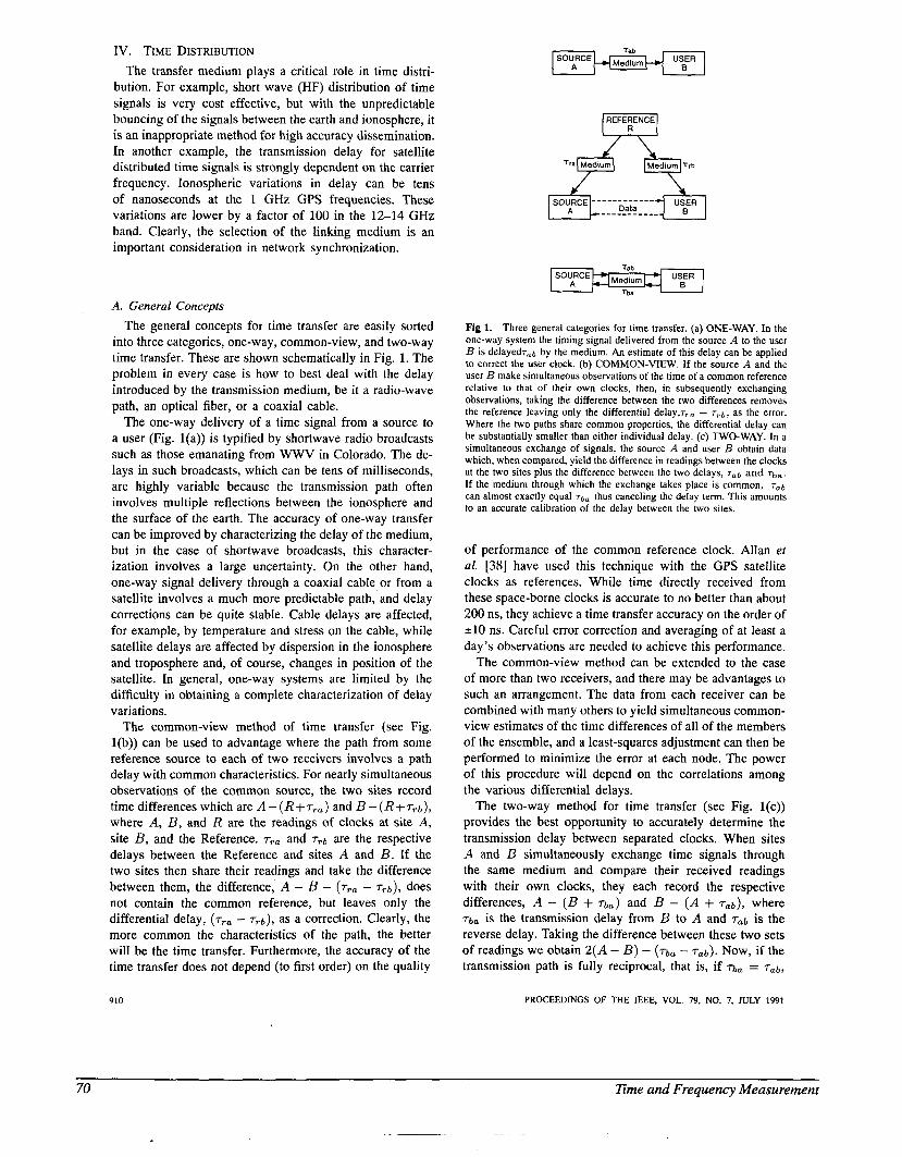
IV. TIME DISTRIBUTION The transfer medium plays a critical role in time distri-
bution. For example, short wave (HF) distribution of time signals is very cost effective, but with the unpredictable bouncing of the signals between the earth and ionosphere, it is an inappropriate method for high accuracy dissemination. In another example, the transmission delay for satellite distributed time signals is strongly dependent on the carrier frequency. Ionospheric variations in delay can be tens of nanoseconds at the 1 GHz GPS frequencies. These variations are lower by a factor of 100 in the 12-14 GHz band. Clearly, the selection of the linking medium is an important consideration in network synchronization.
A. General Concepts
The general concepts for time transfer are easily sorted into three categories, one-way, common-view, and two-way time transfer. These are shown schematically in Fig. 1. The problem in every case is how to best deal with the delay introduced by the transmission medium, be it a radio-wave path, an optical fiber, or a coaxial cable.
The one-way delivery of a time signal from a source to a user (Fig. l(a)) is typified by shortwave radio broadcasts such as those emanating from WWV in Colorado. The de- lays in such broadcasts, which can be tens of milliseconds, are highly variable because the transmission path often involves multiple reflections between the ionosphere and the surface of the earth. The accuracy of one-way transfer can be improved by characterizing the delay of the medium, but in the case of shortwave broadcasts, this character- ization involves a large uncertainty. On the other hand, one-way signal delivery through a coaxial cable or from a satellite involves a much more predictable path, and delay corrections can be quite stable. Cable delays are affected, for example, by temperature and stress on the cable, while satellite delays are affected by dispersion in the ionosphere and troposphere and, of course, changes in position of the satellite. In general, one-way systems are limited by the difficulty in obtaining a complete characterization of delay variations.
The common-view method of time transfer (see Fig. l(b)) can be used to advantage where the path from some reference source to each of two receivers involves a path delay with common characteristics. For nearly simultaneous observations of the common source, the two sites record time differences which are A - ( R + T , , ) and B-(R+T,~) , where A, B, and R are the readings of clocks at site A, site B, and the Reference. T , ~ and Tvb are the respective delays between the Reference and sites A and B. If the two sites then share their readings and take the difference between them, the difference, A - B - ( T ~ ~ - T r b ) , does not contain the common reference, but leaves only the differential delay, ( T ~ ~ - Trb) , as a correction. Clearly, the more common the characteristics of the path, the better will be the time transfer. Furthermore, the accuracy of the time transfer does not depend (to first order) on the quality
Fig 1. Three general categories for time transfer. (a) ONE-WAY. In the one-way system the timing signal delivered from the source A to the user B is delayedrab by the medium. An estimate of this delay can be applied to correct the user clock. (b) COMMON-VIEW. If the source A and the user B make simultaneous observations of the time of a common reference relative to that of their own clocks, then, in subsequently exchanging observations, taking the difference between the two differences removes the reference leaving only the differential delay,Tr, - T,b, as the error. Where the two paths share common properties, the differential delay can be substantially smaller than either individual delay. (c) TWO-WAY. In a simultaneous exchange of signals, the source A and user B obtain data which, when compared, yield the difference in readings between the clocks at the two sites plus the difference between the two delays, Tab and If the medium through which the exchange takes place is common, Tab can almost exactly equal Tba thus canceling the delay term. This amounts to an accurate calibration of the delay between the two sites.
of performance of the common reference clock. Allan et al . [38] have used this technique with the GPS satellite clocks as references. While time directly received from these space-borne clocks is accurate to no better than about 200 ns, they achieve a time transfer accuracy on the order of 210 ns. Careful error correction and averaging of at least a day's observations are needed to achieve this performance.
The common-view method can be extended to the case of more than two receivers, and there may be advantages to such an arrangement. The data from each receiver can be combined with many others to yield simultaneous common- view estimates of the time differences of all of the members of the ensemble, and a least-squares adjustment can then be performed to minimize the error at each node. The power of this procedure will depend on the correlations among the various differential delays.
The two-way method for time transfer (see Fig. l(c)) provides the best opportunity to accurately determine the transmission delay between separated clocks. When sites A and B simultaneously exchange time signals through the same medium and compare their received readings with their own clocks, they each record the respective differences, A - ( B + Tba) and B - ( A + Tab), where Tba is the transmission delay from B to A and is the reverse delay. Taking the difference between these two sets of readings we obtain 2 ( A - B ) - (qa - ~ ~ b ) . Now, if the transmission path is fully reciprocal, that is, if 7ba = Tab,
910 PROCEEDINGS OF THE IEEE, VOL. 79, NO. 7, JULY 1991
70 l lme and Frequency Measurement
then the difference, A - B, is known perfectly and the value of the transmission delay is also determined. The two-way method should provide for near-real-time synchronization of clocks at nanosecond or greater accuracy.
The common-view and two-way methods impose different requirements on the transmission medium. The common-view method depends on the relatively high correlation between the paths from the transmitter to the two receivers. The paths may include arbitrary delays and need not be reciprocal. The two-way method, on the other hand, places a premium on reciprocity and does not depend on the correlation between the delays in different portions of the path. Although there are areas of overlap, each technique also has a domain in which it can provide better performance. The common-view method, for example, is likely to be more robust in computer networks, which have large transmission delays and poor reciprocity. The two- way method is probably the method to choose when signals follow cable or line-of-sight paths.
B. Applications of the Time Transfer Concepts
In the discussion above we used several examples to illustrate the different time transfer methods. But the con- cepts are general, and each can be applied to a variety of transmission schemes. The discussion in this section is not meant to be comprehensive, but rather to indicate a few of the real and potential applications of the concepts.
Jackson and Douglas [39] and Levine et al . [40] describe two-way methods for synchronizing remote clocks through the telephone system. They both use the following variation of the two-way idea. Rather than accomplish the two- way exchange through simultaneous transmissions, these systems send a time signal from site A to site B where it is echoed (reflected) back to site A. Site A then has a measurement of the round-trip delay which, assuming reciprocity in the lines (an assumption good to better than 1 ms for many systems), is divided by 2 in order to provide a direct measure of the delay. The main difference between the methods described in the two publications above is that one takes care of the correction at each receiver and the other makes the corrections at the transmitting end.
Using a similar scheme in cable-connected systems, two- way time transfer can push the stability and accuracy of synchronization into the picosecond regime, even for systems with very long cables. Where the demand for accuracylstability of distribution of time are high, the use of this method along with optical fiber connections [41] is especially appealing since the fiber transmission provides excellent immunity to noise introduced by ground-isolation problems.
Navigation or ranging systems which are based upon time of flight of radio or optical signals can often be used for time transfer. For ranging applications these systems assume that the time references are known and solve for relative positions of base stations. For time transfer, the known locations of the base stations are given and the relative time at the stations is then determined. This is the basis for the GPS Common-View Method of time transfer described
SULLIVAN AND LEVINE: TIME GENERATION AND DISTRIBUTION
earlier [38]. The common-view technique of VLBI, used to obtain high-resolution images of distant radio stars or relative positions of observation sites, provides another means for highly stable time transfer [42]. In this technique, signals received at two sites from a set of common radio stars are cross correlated (in a computer) in the same fashion that optical signals are combined in an optical interferometer. A key product of this computation is a very precise measure of the relative phase of arrival of signals at the two sites. This can be used to provide an extremely stable measure of the relative stability of clocks operating at the two sites. With the very high cost of radio telescopes and peripheral equipment and the need for extensive computer processing of data, this is an extremely expensive approach, and it is generally used only as a research tool. MacDoran et al . [43] have developed a short- baseline interferometer which relies on the same concept. Their scheme uses common-view observations of signals from GPS satellites. Receiver costs are reasonable, but, as with the VLBI technique, this interferometric method still involves substantial computation.
For satellite time transfer, the one-way method remains attractive because of the simplicity of equipment at the re- ceiving site [44]. Two-way time transfer requires broadcast- ing to a satellite from each station, a process which requires more equipment and special government licensing. The common-view methods call for exchange of information between sites as well as substantial averaging to obtain good accuracy and stability. A one-way satellite dissemination system which promises very good performance has been proposed by Hanson and Howe [45]. They suggest use of commercial communication satellites in the 12-14 GHz region. At these frequencies the ionospheric variation in delay is only a few nanoseconds. The technology for these geostationary satellites has been widely developed for direct-broadcast television, so receivers should be particu- larly simple and inexpensive. A key facet of their proposal involves the tracking of the satellite (geostationary satellites do move about somewhat) from three sites using the two- way time transfer method. The two-way exchange of signals between all three stations provides ranging information which can establish the position of the satellite. This position is then broadcast with the time signal so that the receiver can correct for variations in the path between the receiver and the satellite. The accuracy of such time transfer should be better than 100 ns and the stability might well be better than 10 ns.
C. Practical Synchronization Limits
Given adequate clocks, the synchronization of two nodes or a network is iikely to be limited by the transmission medium and/or the time-transfer method. In many cases it is possible to gain auxiliary information which might allow for a refinement of the estimate of time delay. For example, knowledge of the temperature of a coaxial cable along with an understanding of the delay-temperature relationship can provide for an improvement in one-way synchronization through coaxial cables. In another example, a model of
911
Time and Frequency Measurement 71
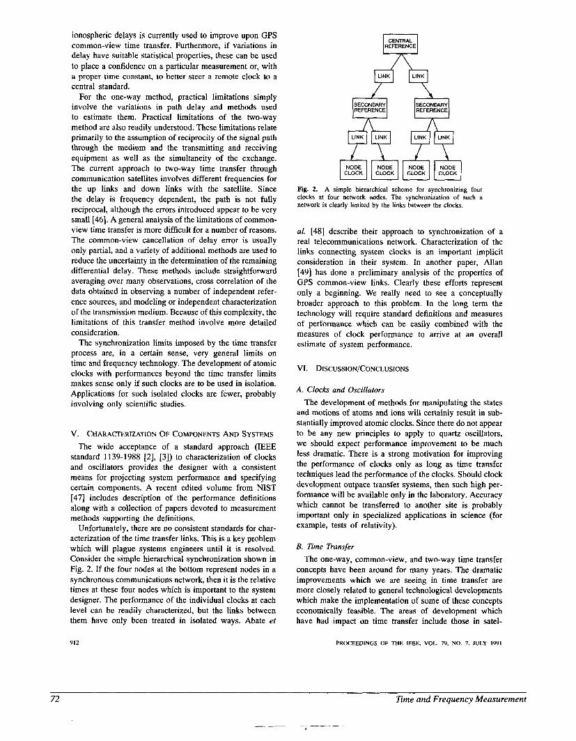
ionospheric delays is currently used to improve upon GPS common-view time transfer. Furthermore, if variations in delay have suitable statistical properties, these can be used to place a confidence on a particular measurement or, with a proper time constant, to better steer a remote clock to a central standard.
For the one-way method, practical limitations simply involve the variations in path delay and methods used to estimate them. Practical limitations of the two-way method are also readily understood. These limitations relate primarily to the assumption of reciprocity of the signal path through the medium and the transmitting and receiving equipment as well as the simultaneity of the exchange. The current approach to two-way time transfer through communication satellites involves different frequencies for the up links and down links with the satellite. Since the delay is frequency dependent, the path is not fully reciprocal, although the errors introduced appear to be very small [46]. A general analysis of the limitations of common- view time transfer is more difficult for a number of reasons. The common-view cancellation of delay error is usually only partial, and a variety of additional methods are used to reduce the uncertainty in the determination of the remaining differential delay. These methods include straightforward averaging over many observations, cross correlation of the data obtained in observing a number of independent refer- ence sources, and modeling or independent characterization of the transmission medium. Because of this complexity, the limitations of this transfer method involve more detailed consideration.
The synchronization limits imposed by the time transfer process are, in a certain sense, very general limits on time and frequency technology. The development of atomic clocks with performances beyond the time transfer limits makes sense only if such clocks are to be used in isolation. Applications for such isolated clocks are fewer, probably involving only scientific studies.
v. CHARACTERIZATION OF COMPONENTS AND SYSTEMS The wide acceptance of a standard approach (IEEE
standard 1139-1988 [2], [3]) to characterization of clocks and oscillators provides the designer with a consistent means for projecting system performance and specifying certain components. A recent edited volume from NIST [47] includes description of the performance definitions along with a collection of papers devoted to measurement methods supporting the definitions.
Unfortunately, there are no consistent standards for char- acterization of the time transfer links. This is a key problem which will plague systems engineers until it is resolved. Consider the simple hierarchical synchronization shown in Fig. 2. If the four nodes at the bottom represent nodes in a synchronous communications network, then it is the relative times at these four nodes which is important to the system designer. The performance of the individual clocks at each level can be readily characterized, but the links between them have only been treated in isolated ways. Abate et
912
+pkl CLOCK CLOCK
Fig. 2. A simple hierarchical scheme for synchronizing four clocks at four network nodes. The synchronization of such a network is clearly limited by the links between the clocks.
al. [48] describe their approach to synchronization of a real telecommunications network. Characterization of the links connecting system clocks is an important implicit consideration in their system. In another paper, Allan [49] has done a preliminary analysis of the properties of GPS common-view links. Clearly these efforts represent only a beginning. We really need to see a conceptually broader approach to this problem. In the long term the technology will require standard definitions and measures of performance which can be easily combined with the measures of clock performance to arrive at an overall estimate of system performance.
VI. DISCUSSION/CONCLUSIONS
A. Clocks and Oscillators
The development of methods for manipulating the states and motions of atoms and ions will certainly result in sub- stantially improved atomic clocks. Since there do not appear to be any new principles to apply to quartz oscillators, we should expect performance improvement to be much less dramatic. There is a strong motivation for improving the performance of clocks only as long as time transfer techniques lead the performance of the clocks. Should clock development outpace transfer systems, then such high per- formance will be available only in the laboratory. Accuracy which cannot be transferred to another site is probably important only in specialized applications in science (for example, tests of relativity).
B. Time Transfer
The one-way, common-view, and two-way time transfer concepts have been around for many years. The dramatic improvements which we are seeing in time transfer are more closely related to general technological developments which make the implementation of some of these concepts economically feasible. The areas of development which have had impact on time transfer include those in satel-
PROCEEDINGS OF THE IEEE, VOL. 79, NO. 7, JULY 1991
72 l ime and Frequency Measurement
lite communications, computers and microprocessors, and optical fibers. The focal problem in time transfer continues to be the characterization of the delay through the time transfer medium.
C. Characterization of Components
Because of the importance to network synchronization, we can expect to see efforts directed toward the develop- ment of consistent methods for describing the performance of time transfer links. Without standard means for character- ization of these links, network synchronization will have to rely on excessive engineering margins, and synchronization levels will remain below the potential of the technology.
REFERENCES [1] P. Kartaschoff and J. A. Barnes, “Standard time and frequency
generation,” Proc. IEEE, vol. 60, pp. 493-501, May 1972. [2] IEEE Standard Definitions of Physical Quantities for Funda-
mental Frequency and Time Metrology IEEE Standard 1139- 1988, 1988. (Available from IEEE Service Center, 445 Hoes Lane, P. 0. Box 1331, Piscataway, NJ 08855-1331.)
[3] D. Allan, H. Hellwig, P. Kartaschoff, J. Vanier, J. Vig, G. M. R. Winkler, and N. Yannoni, “Standard terminology for fundamental frequency and time metrology,” in 42nd Ann. Symp. on Frequency Control, IEEE Catalogue No. 88CH2588-2, June 1988, pp. 419-425.
141 J. A. Barnes, A. R. Chi, L. S. Cutler, D. J. Healey, D. B. Leeson, L 1
T. E. McGunigal, J. A. Mullen, Jr., W. L. Smith, R. L. Sydnor, R. F. C. Vessot, and G. M. R. Winkler, “Characterization of frequency stability,” IEEE Trans. Instrum. Meas., vol. IM-20, pp. 105-120, May 1971.
[5] J. Rutman and F. L. Walls, “Characterization and measurement of frequency stability,” Proc. IEEE, vol. 79, this issue.
[6] D. B. Percival, “Characterization of frequency stability: fre- quency domain estimation of stability measures,” Proc. IEEE, vol. 79, this issue.
[7] J. Vig, “Quartz crystal oscillators and resonators for frequency control and timing-a tutorial,” AD A218090, 1990. (Available from National Technical Information Service, 5285 Port Royal Rd., Springfield, VA 22161.)
181 L. L. Lewis, “An introduction to frequency standards,” Proc. ~~
IEEE, vol. 79, this issue. 191 M. A. Weiss and D. W. Allan, “An NBS calibration procedure . _
for providing time and frequency at a remote site by weighting and smoothing of GPS common view data,” IEEE Trans. Instrum. Meas., vol. IM-36, pp. 572-578, June 1987.
[ lo] D. W. Hanson, “Fundamentals of two-way time transfers by satellite,” in 43rd Ann. Symp. on Frequency Control, IEEE Catalogue No. 89CH2690-6, June 1989, pp. 174-178
[ l l ] Y. Saburi, M. Yamamoto, and K. Harada, “High-precision time comparison via satellite and observed discrepancy of synchronization,” IEEE Trans. Instrum. Meas., vol. IM-25, pp. 473477, Dec. 1976.
[12] P. Kartaschoff, “Synchronization in digital communications networks,” Proc. IEEE, vol. 79, this issue.
[13] R. E. Wilson, “Use of precise time and frequency in power systems,” Proc. IEEE, vol. 79, this issue.
[14] P. F. MacDoran and C. H. Bom, “Time, frequency and space geodesy: impact on the study of climate and global change,” Proc. IEEE, vol. 79, this issue.
[15] N. F. Ramsey, “The past, present and future of atomic time and frequency,” Proc. IEEE, vol. 79, this issue.
1161 W. M. Itano, “Atomic ion frequency standards,” Proc. IEEE, ~~
vol. 79, this issue. 1171 S. L. Rolston and W. D. Phillips, “Laser-cooled neutral atom . -
frequency standards,” Proc. IEEE, vol. 79, this issue. [ 181 R. E. Drullinger, “Frequency standards based on optically
pumped cesium,”Proc. IEEE, vol. 74, pp. 140-142, Jan. 1986. [19] R. E. Drullinger, D. J. Glaze, J. P. Lowe, and J. H. Shirley, “The
new NIST optically pumped cesium frequency standards,” IEEE Trans. Instrum. Meas., vol. 40, pp. 162-164, Apr. 1991.
[20] S. Ohshima, Y. Nakadan, T. Ikegami, Y. Koga, R. Drullinger, and L. Hollberg, “Characteristics of an optically pumped Cs
SULLIVAN AND LEVINE: TIME GENERATION AND DISTRIBUTION
frequency standard at the NRLM,” IEEE Trans. Insfrum. Meas., vol. IM-38, pp. 533-536, Apr. 1989. E. de Clercq, A. Clairon, B. Dahmani, A. Gerard, and P. AyniC, “Design of an optically pumped Cs laboratory frequency standard,” in Frequency Standards and Metrology, Proc. of 4th Symp., A. De Marchi, Ed. New York: Springer-Verlag, 1989, pp. 120-125. C. Monroe, H. Robinson, and C. Wieman, “Observation of the cesium clock transition using laser-cooled atoms in a vapor cell,” Optics Lett., vol. 16, pp. 50-52, Jan. 1991. D. J. Wineland, R. E. Drullinger, and F. L. Walls, “Radiation- pressure cooling of bound resonant absorbers,” Phys. Rev. Lett., vol. 40, pp. 1639-1642, June 1978. W. Neuhauser, M. Hohenstatt, P. Tsohek, and H. Dehmelt, “Optical-sideband cooling of visible atom cloud confined in a parabolic well,’’ Phys. Rev. Lett., vol. 41, pp. 233-236, July 1978. S. V. Andreev, V. I. Balykin, V. S. Letokhov, and V. G. Minogin, “Radiative slowing and reduction of the energy spread of a beam of sodium atoms to 1.5K in an oppositely directed laser beam,” JETP Lett., vol. 34, pp. 442445, Oct. 1981. W. D. Phillips and H. Metcalf, “Laser deceleration of an atomic beam,” Phys. Rev. Lett., vol. 48, pp. 596-599, Mar. 1982. J. J. Bollinger, D. J. Heinzen, W. M. Itano, S. L. Gilbert, and D. J. Wineland, “A 303-MHz frequency standard based on trapped Be+ ions,” IEEE Trans. Instrum. Meas., vol. 40, pp. 126-128, Apr. 1991. L. S. Cutler, R. P. Giffard, P. J. Wheeler, and G. M. R. Winkler, ‘‘Initial operational experience with a mercury ion storage fre- quency standard,” in Proc. 4Ist Ann. Symp. Frequency Control, IEEE Catalog No. CH2427-3, May 1987, pp. 12-17. J. D. Prestage, G . J. Dick, and L. Maleki, “Linear ion trap based atomic frequency standard,” IEEE Trans. Instrum. Meas., vol. 40, pp. 132-136, Apr. 1991. D. J. Wineland, J. C. Bergquist, J. J. Bollinger, W. M. Itano, D. J. Heinzen, S. L. Gilbert, C. H. Manney, and M. G. Raizen, “Progress at NIST toward absolute frequency standards using stored ions,” IEEE Trans. Ultrason., Ferroelect., Freq. Contr., vol. 37, pp. 515-523, Nov. 1990. J. C. Bergquist, F. Dietrich, W. M. Itano, and D. J. Wineland, “Hg+ Single Ion Spectroscopy,” in Proc. 9th Int. Conf Laser Spectroscopy, Bretton Woods, NH, M. S. Feld, J. E. Thomas, and A. Mooradian, Eds. San Diego, CA: Academic, June 1989, pp. 274-277 G. J. Dick and R. T. Wang, “Ultra-stable performance of the superconducting cavity maser,” IEEE Trans. Instrum. Meus., vol. 40, pp. 174-177, Apr. 1991. A. A. Belyaev, N. A. Demidov, B. A. Sakharov, V.Yu. Mak- simov, M.Yu. Fedotov, and A. E. Yampol’skii, “Chl-76 small- size passive hydrogen frequency and time standard,” Meas. Tech., vol. 30, pp. 767-772, Aug. 1987 and B. A. Gaigerov, L. P. Elkina, and S. B. Pushkin, “Metrological characteristics of a group of hydrogen clocks,” Meas. Tech., vol. 25, pp. 23-25, Jan. 1982. R. F. C. Vessot, E. M. Mattison, R. L. Walswortb, and I. F. Silvera, “The cold hydrogen maser,” in Frequency Standards and Metrology, A. De Marchi, Ed. New York: Springer- Verlag, 1989, pp. 88-94, M. C. Hiirlimann, W. N. Hardy, M. E. Hayden, and R. W. Cline, “Performance of the UBC cryogenic hydrogen maser,” in Frequency Standards and Metrology, A. De Marchi, Ed. New York: Springer-Verlag, 1989, pp. 95-101. J. C. Camparo and R. P. Frueholz, “Fundamental stability limits for the diode-laser-pumped rubidium atomic frequency standard,” J. Appl. Phys., vol. 59, pp. 3313-3317, May 1986. M. Hashimoto and M. Ohtsu, “Improvements in short-term and long-term frequency stab es of diode laser pumped rubidium atomic clock,” in Frequency Standards and Metrology, A. De Marchi, Ed. New York: Springer-Verlag. 1989, pp. 434-435. D. W. Allan, D. D. Davis, M. Weiss, A. Clements, B. Guinot, M. Granveaud, K. Dorenwendt, B. Fischer, P. Hetzel, S. Aoki, M. K. Fujimoto, L. Charron, and N. Ashby, “Accuracy of In- ternational time and frequency comparisons via global position- ing system satellites in common-view,’’ IEEE Trans. Insfrum. Meas., vol. IM-34, pp. 118-125, June 1985. D. Jackson and R. J. Douglas, “A telephone-based time dissem- ination system,” in Proc. 18th Precise Time and Time Interval Meeting, pp. 541-547, Dec. 1986. (Available from Time Ser-
913
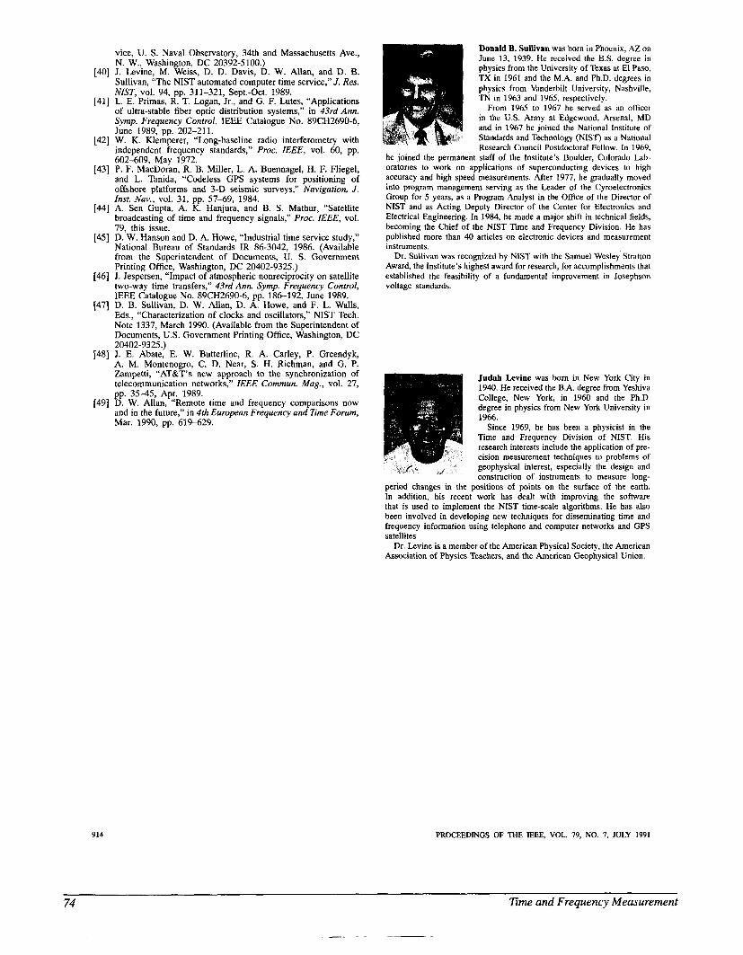
vice, U. S. Naval Observatory, 34th and Massachusetts Ave., N. W., Washington, DC 20392-5100.)
[40] J. Levine, M. Weiss, D. D. Davis, D. W. Allan, and D. B. Sullivan, “The NIST automated computer time service,” J. Res. NIST, vol. 94, pp. 311-321, Sept.-Oct. 1989.
1411 L. E. Primas, R. T. Logan, Jr., and G. F. Lutes, “Applications of ultra-stable fiber optic distribution systems,” in 43rd Ann. Symp. Frequency Control, IEEE Catalogue No. 89CH2690-6, June 1989, pp. 202-211.
1421 W. K. Klemuerer. “Lone-baseline radio interferometrv with c 1
independent hequency s&ndards,” Proc. IEEE, vol. 60, pp. 602-609, May 1972.
[431 P. F. MacDoran, R. B. Miller, L. A. Buennagel, H. F. Fliegel, -~ and L. Tanida, “Codeless GPS systems f& positioning- of offshore platforms and 3-D seismic surveys,” Navigation, J. Inst. Nav., vol. 31, pp. 57-69, 1984.
[44] A. Sen Gupta, A. K. Hanjura, and B. S. Mathur, “Satellite broadcasting of time and frequency signals,’’ Proc. IEEE, vol. 79, this issue.
[45] D. W. Hanson and D. A. Howe, “Industrial time service study,” National Bureau of Standards IR 86-3042, 1986. (Available from the Superintendent of Documents, U. S. Government Printing Office, Washington, DC 20402-9325.)
[46] J. Jespersen, “Impact of atmospheric nonreciprocity on satellite two-way time transfers,” 43rd Ann. Symp. Frequency Control, IEEE Catalogue No. 89CH2690-6, pp. 186-192, June 1989.
(471 D. B. Sullivan, D. W. Allan, D. A. Howe, and F. L. Walls, Eds., “Characterization of clocks and oscillators,” NIST Tech. Note 1337, March 1990. (Available from the Superintendent of Documents, U.S. Government Printing Office, Washington, DC 20402-9325.)
1481 J. E. Abate, E. W. Butterline, R. A. Carley, P. Greendyk, A. M. Montenogro, C. D. Near, S. H. Richman, and G. P. Zampetti, “AT&T’s new approach to the synchronization of telecommunication networks.” IEEE Commun. Map.. vol. 27.
Y l
pp. 35-45, Apr. 1989. [49] D. W. Allan, “Remote time and frequency comparisons now
and in the future,” in 4th European Frequency and Time Forum, Mar. 1990, pp. 619-629. ~
914
Donald B. Sullivan was born in Phoenix, AZ on June 13, 1939 He received the B S degree in physics from the University of Texas at El Paso, TX in 1961 and the M A and Ph D degrees in physics from Vanderhilt University, Nashville, TN in 1963 and 1965, respectively
From 1965 to 1967 he served as an officer in the U S Army at Edgewood, Arsenal, MD and in 1967 he joined the National Institute of Standards and Technology (NIST) a? a National Research Council Postdoctoral Fellow In 1969,
he joined the permanent staff of the Institute’s Boulder, Colorado Lab- oratones to work on applications of superconducting devices to high accuracy and high speed measurements After 1977, he gradually moved into program management serving as the Leader of the Cyroelectronics Group for 5 years, as a Program Analyst in the Office of the Director of NIST and as Acting Deputy Director of the Center for Electronics and Electrical Engineenng In 1984, he made a major shift in technical fields, becoming the Chief of the NIST Time and Frequency Division He has published more than 40 articles on electronic devices and measurement instruments
Dr Sullivan was recognued by NIST with the Samuel Wesley Stratton Award, the Institute’s highest award for research, for accomplishments that established the feasibility of a fundamental improvement in Josephson voltage standards
Judah Levine was bom in New York City in 1940. He received the B.A. degree from Yeshiva College, New York, in 1960 and the Ph.D. degree in physics from New York University in 1966.
Since 1969, he has been a physicist in the Time and Frequency Division of NIST. His research interests include the application of pre- cision measurement techniques to problems of geophysical interest, especially the design and construction of instruments to measure long-
period changes in the positions of points on the surface of the earth. In addition, his recent work has dealt with improving the software that is used to implement the NIST time-scale algorithms. He has also been involved in developing new techniques for disseminating time and frequency information using telephone and computer networks and GPS satellites
Dr. Levine is a member of the American Physical Society, the American Association of Physics Teachers, and the American Geophysical Union.
,
PROCEEDINGS OF THE IEEE, VOL. 79, NO. 7, JULY 1991
74 Eme and Frequency Measurement
0 1991 IEEE. Reprinted, with permission, from Proceedings of the IEEE: Special Issue on Time and Frequency, 79 (7), 894-905; 1991.
The BIPM and the Accurate Measurement of Time TERRY J. QUINN
Invited Paper
Accurate measurements in science and technology require world- wide agreement on standards and units. The role of the Bureau International des Poids et Mesures (BIPM) in assuming the unifor- mity and reliability of the world’s measurement system is described. A brief discussion follows on the meaning of the term accurate measurement. The development of atomic time scales is outlined with particular reference to the Bureau International de I’Heure and the origins of TAI and UTC. The article ends with a brief description of the work currently being carried out at the BIPM, which includes the regular establishment of TAI, its diffusion with UTC, and the associated research work aimed at improving these scales and their accessibility.
I. INTRODUCTION The ability to make precise measurements is one of
the prerequisites for the development of advanced tech- nology. While few people would seriously dispute this assertion, few people also would be aware of how precise measurements are made or the extent of the human and other resources that are necessary to enable them to be made. In this introductory article to the special issue on time and frequency, a description will first be given of the organizational structure within which the world’s measurement system is maintained and then what it means to make a precise measurement will be briefly examined. This will be followed by an outline of the role played by the Bureau International de 1’Heure (BIH) in the establishment of international time scales, and the origins of Intema- tional Atomic Time (TAI) and Coordinated Universal Time (UTC). Finally a brief description will be given of the present day work undertaken at the Bureau International des Poids et Mesures (BIPM) to establish and improve TAL
Trade, both national and international, in high technology products, the establishment of communication and navi- gation networks, the exchange of scientific information, as well as a multitude of pure and applied scientific and technological projects carried out on an international basis, are all highly dependent upon precise measurement.
Manuscript received December 13, 1990; revised February 6, 1991. The author is with the Bureau International des Poids et Mesures,
IEEE Log Number 9100243. Pavillon de Breteuil, France.
The manufacture of high technology products is itself dependent upon the existence of a traceable chain of precise measurements from the factory floor to national and international standards.
All of this has long been recognized and the increas- ing demands for national and international uniformity in measurement standards was behind the establishment of the national standards laboratories in the then advanced industrialized countries at the end of the 19th and begin- ning of the 20th centuries. Principal among these were the Physikalisch-Technische Reichsanstalt (Berlin) founded in 1887, the National Physical Laboratory (Teddington) in 1900, and the Bureau of Standards (Washington) in 1901. Preceding the establishment of these institutes, how- ever, was the setting up of an international agreement on measurement standards and the founding of the Bureau International des Poids et Mesures (BIPM) in 1875 under the Convention du Mbtre. Before returning to the question of the meaning of the term “precise measurement” which is fundamental to the whole enterprise of metrology, we first look briefly at the organizational structure established by the Convention du Mbtre to ensure worldwide uniformity of measurement.
11. THE CONVENTION Du M ~ T R E The Convention du Mbtre was signed in Paris in 1875 by
representatives of seventeen nations. As well as founding the BIPM and laying down the way in which the activities of the BIPM should be financed and managed, the Con- vention du Mbtre established a permanent organizational structure for member Governments to act in common accord on all matters relating to units of measurement (see Fig. 1). The Convention, modified slightly in 1921, remains the basis of all international agreement on units of measurement. There are now forty-six member nations of the Convention which includes all the major industrialized countries. Under the terms of the Convention, the BIPM operates under the exclusive supervision of the ComitC International des Poids et Mesures (CIPM) which itself is elected by and comes under the supervision of the
0018-9219/91/0700-0894$01.00 0 1991 IEEE
894 PROCEEDINGS OF THE IEEE, VOL. 79, NO. 7. JULY 1991
Time and Frequency Measurement 75
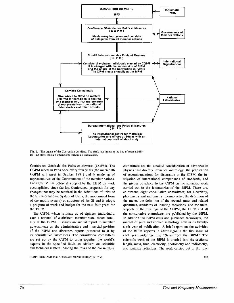
CONVENTION DU METRE
1875
Comite International des Poids et Mesures ( C I P M )
Diplomatic Treaty
I I
Governments of Member Nations
Conference Generale des Poids et Mesures ( C G P M )
Meets everv four vears and consists I of delegates from all member nations I I I
International Organizations Consists of eighteen individuals elected by CGPM
It is charged with the supervision of BIPM and the affairs of the Convention du Metre 1 The ClPM meets annually at the BIPM
+ I Comites Consultatifs
Give advice to ClPM on matters referred to them.Each is chaired
bv a member of ClPM and con=;=+= National 4 Laboratories I of representatives from national
laboratories and other experts
Bureau International des Poids et Mesures ( B I P M )
The international centre for metrology Laboratories and offices at Sevres,with an
international staff of about sixty
Fig. 1. the thin lines indicate interactions between organizations.
The organs of the Convention du Metre. The thick line indicates the line of responsibility,
Conference GCnCrale des Poids et Mesures (CGPM). The CGPM meets in Paris once every four years (the nineteenth CGPM will meet in October 1991) and is made up of representatives of the Governments of the member nations. Each CGPM has before it a report by the CIPM on work accomplished since the last Conference, proposals for any changes that may be required in the definitions of units of the SI (International System of Units, the modernized form of the metric system) or structure of the SI and it adopts a program of work and budget for the next four years for the BIPM.
The CIPM, which is made up of eighteen individuals, each a national of a different member state, meets annu- ally at the BIPM. It issues an annual report to member governments on the administrative and financial position of the BIPM and discusses reports presented to it by its consultative committees. The consultative committees are set up by the CIPM to bring together the world’s experts in the specified fields as advisers on scientific and technical matters. Among the tasks of the consultative
QUI”: BIPM AND THE ACCURATE MEASUREMENT OF TIME
committees are the detailed consideration of advances in physics that directly influence metrology, the preparation of recommendations for discussion at the CIPM, the in- stigation of international comparisons of standards, and the giving of advice to the CIPM on the scientific work carried out in the laboratories of the BIPM. There are, at present, eight consultative committees; for electricity, photometry and radiometry, thermometry, the definition of the meter, the definition of the second, mass and related quantities, standards of ionizing radiations, and for units. Reports of the meetings of the CGPM, the CIPM and all the consultative committees are published by the BIPM. In addition the BIPM edits and publishes Metrologia, the journal of pure and applied metrology now in its twenty- sixth year of publication. A brief report on the activities of the BIPM appears in Metrologia in the first issue of each year under the title “News from the BIPM.” The scientific work of the BIPM is divided into six sections: length, mass, time, electricity, photometry and radiometry, and ionizing radiations. The work carried out in the time
895
76 Time and Frequency Measurement
section is described below; for the rest, the interested reader is referred to [l].
111. THE NEED FOR PRECISE MEASUREMENT Having briefly laid out the organizational structure within
which the industrialized nations of the world work to ensure uniformity of measurement standards we now come back to the question of why such work is necessary and what is implied by the term “precise measurement.” At one level the problem is a very simple one and can be sketched out in the following way. Suppose that in one locality at a certain time someone makes a measurement of a physical quantity. In a different place at a different time someone else makes a measurement of what is thought to be the same physical quantity and the need arises for the results of these two measurements to be compared. What assurance can we give that these measurements should be the same and how do we find out whether or not they are? To give any answer to these questions we must first be clear as to what it is that we are trying to compare.
In the usual formalism of quantity calculus [2], whose origin is to be found in the work of Maxwell, we write that a quantity having a symbol Q is expressed as a numerical value {Q} multiplied by a unit [Q]
We can then write
or
(3)
and so on. In terms of the questions posed above we can see that for any useful statement to be made about the results of the two measurements, two conditions must be fulfilled. The first is that the physical quantities being measured must be of the same nature and the second is that the units in which the result of the measurements are expressed must also be the same.
At a trivial level, both of these conditions are easily fulfilled, but we do not have to look very far in the real world to find that neither is straightforward. For example, the measurement of the diameter of apertures for radiometric purposes poses particular problems because it is difficult to characterize the quantity that is being measured. The best apertures from the optical point of view should be made of an opaque material having a sharp edge, Le., zero thickness. Apertures having very thin edges can be made but by their very nature thin edges have no strength and so the position of the edge can only be measured by a noncontact method. The only noncontact method that seems feasible is an optical one, but as is well known the apparent position of an edge when measured optically can change depending upon the conditions of illumination and wavelength of the light used to observe it. The quantity we are trying to measure, namely the diameter of an aperture, thus appears to be a function of one of the parameters of the
896
measuring system. Not only that, but if the aperture is to be used to define a beam of electromagnetic radiation its cross sectional area is given by 7r[R.(X)l2 where its radius R(X) is indeed a function of the wavelength of the radiation. In fact the accuracy of the most precise optical radiometry is at present limited by the accuracy of the measurement of the cross-sectional area of apertures [3]!
Suppose that we wish to determine the ratio of the magnitude of the two quantities (assumed now to be the same) expressed by (2) . This requires that the unit [Q] is the same when the two quantities Q1 and Qz are being measured. If Q1 is about the same size as Q 2 this may not be too difficult to check, but if Q1 lo6 x Q2 it is by no means easy to verify that the units are the same. The present limiiation to the accuracy of our knowledge of the Rydberg constant R, is set by just this problem. The most accurate measurement of R, is that obtained by Biraben et al. [4] using Doppler-free two-photon spectroscopy of Rydberg levels ( 2 s - n D , n = 8,lO) in hydrogen and deuterium atoms. The accuracy of the spectroscopy in the visible is set by the accuracy in the knowledge of the frequency of an iodine stabilized laser at a wavelength of about 633 nm namely 1.6 parts in 10”. The estimated accuracy in the practical realization of the SI second is about three orders of magnitude better than this but in a frequency domain itself some five orders of magnitude different. The establishment of the frequency chain between the caesium clock at a frequency of about 9 x lo9 Hz and the frequency of certain transitions in molecular iodine at about 10’’ Hz has been, and remains, one of the major challenges of fundamental metrology.
Thus in order to make what we have loosely termed precise measurements we have first to specify closely the quantity to be measured and second establish a convenient unit whose multiples and submultiples can be obtained over the whole range of the values of the quantity normally encountered. The definition of a unit of mass in terms of the mass of the proton despite its many attractions, is of little practical use as we do not yet know how to relate such a mass (m = kg) to that of everyday objects (m = 1 kg) with a sufficient accuracy.
We have so far considered only the problem of making measurements of one physical quantity. We require much more than this before we can discuss what is meant by the term “precise measurement.” One of the basic postulates underpinning our understanding of the external world is that nature is internally self-consistent and continuous in space and time. For our theories of physics to be consistent with nature, the results of observations or measurements made of one quantity in one domain must be consistent with observations and measurements made of other quantities in other domains. The system of measurement through which this consistency is confirmed is based upon the notion that a small number of base quantities may be considered dimensionally independent and may be described in terms of a set of the same number of arbitrary chosen base units. The latter together with their multiples and submultiples, the various derived units and supplementary units and rules
PROCEEDINGS OF THE IEEE, VOL. 79, NO. 7, JULY 1991
Erne and Frequency Measurement 77
for their use make up the International System of Units (SI) [SI. The SI units form a coherent set of units in the sense normally attributed to the word “coherent,” Le., a system of units mutually related by rules of multiplication and division without any numerical factor. The set of seven SI base units are by convention regarded as dimensionally independent.
The requirement for mutual consistency among the prac- tical realizations of the units of the SI can easily be demonstrated. Suppose that we set up a blackbody at a thermodynamic temperature T and measure the total radiant exitance M ( T ) , which has the units of watt per square meter, using an electrically calibrated radiometer based upon laboratory realizations of the volt and the ohm. We can also calculate the total radiant exitance of the blackbody from the Stefan-Boltzmann Law
2T5k4 T4 M ( T ) = - 15h3c2 (4)
To do this, however, we must use measured values of the Boltzmann constant k [(1.380 658 f 0.000 012) x
J K-’1 and the Planck constant h [(6.626 075 5 f 0.000 004) x J SI. The mutual consistency of the practical realization of our system of units can be checked by carrying out such an experiment, since the measured values of k and h rely upon quite different combinations of constants and units from that of (4).
The extent to which measured values of different quan- tities involving different units and fundamental physical constants are in agreement is a measure, and the only one, of the accuracy, i.e., the closeness to the real physical world of our measurement system. This is what we mean by the term “accuracy.”
Estimates of accuracy based upon judgements of the uncertainty of all the components of a measurement must always be made, of course, but experience shows that these estimates have a tendency of giving optimistic estimates of accuracy, when finally verified by experiments of the sort mentioned above.
A less demanding requirement, which under certain con- ditions may be all that is necessary, is that of reproducibil- ity. A measurement made under particular conditions by instruments of similar design can often appear to be very reproducible. It is often claimed that for most practical purposes in industry reproducibility is all that is needed. In the short term and within a limited locality, this may well be true. The reliance upon reproducibility alone, however, can never guarantee long-term stability or worldwide uni- formity. It is only by firmly linking measurement standards through physics to the invariant natural world that these can be assured and therefore we must ensure that our measurement standards are “accurate” in the strict sense defined above.
The higher the accuracy that we demand, the more com- plete must our understanding be of that part of the physical world we are dealing with. In few areas of measurement is this more evident than in the one of time and frequency with which we deal. It is striking that not so many years
QUI”: BIPM AND THE ACCURATE MEASUREMENT OF TIME
ago the general theory of relativity was considered by most physicists as abstruse and academic, far from the world of practical experience. Of course, it explained the anomaly in the precession of the perihelion of the planet Mercury, but its predictions of other measurable effects were few indeed. The development of atomic clocks, their use in earth satellites and, above all, in the GPS for time transfer have brought the time and frequency community face to face with the consequences of both special and general relativity in a way undreamed of before. For example, the question of reference frames, central to the relativistic view of the world, is by no means a simple one in the context of high-accuracy time-transfer and is now the subject of detailed study [6]. In the particular field of accurate time measurement, however, the use of quantity algebra as represented by (2) and (3), for example, is by no means straightforward. As we shall see, International Atomic Time, Coordinated Universal Time, and Ephemeris Time, and pulsar time are all different physical quantities, which we need to relate to the same unit, the SI second. But, the SI second is a unit whose value depends upon the reference frame within which it is established. Much of the conceptual, and often real, difficulty in accurate time measurement thus stems from the problem of ensuring that the quantities are properly specified and are indeed being measured in the same units. For a more extended discussion on the needs for accurate measurement in science and industry see [7] and [8].
Iv. THE BUREAU INTERNATIONAL DE L’HEURE AND THE FIRST ATOMIC TIME SCALES
The Bureau International de 1’Heure (BIH) has played a central role in the establishment of the world’s time scales since it was founded before the first World War. The initiative for its creation came from the French Bureau des Longitudes which in 1912 called for an international confer- ence to consider the worldwide unification of time-keeping. This conference took place in 1912 and agreement was reached on the principle of establishing an international or- ganization for time. This scientific conference was quickly followed by a diplomatic conference in 1913 at which an international convention was adopted by thirty-two nations creating an Association Internationale de 1’Heure under which would be established a Bureau International de 1’Heure. This diplomatic convention, however, was never ratified by the participating governments owing to the outbreak of the first World War.
Nevertheless, the BIH, foreseen in the Convention, be- gan operations at the Paris Observatory. When, in 1919, the International Astronomical Union was created a Time Commission was immediately set up within the IAU to give these operations a more formal setting. The BIH was thus finally established on an international basis on January 1, 1920. From then until the 1950’s, the international time scale was based wholly upon astronomical observations of the rotation of the Earth. Correlation of observations of the rotation of the Earth was, therefore, one of the main
897
78 Eme and Frequency Measurement
activities of the BIH. The unit of time, the second, was also defined in terms of astronomical data and distributed by ob- servatories. After the development of operational caesium clocks, it very quickly became apparent to some that the world’s time scale would in the future be based upon atomic clocks. Even before the caesium clock, however, long and difficult studies of orbital motions in the solar system had led to the conclusion that the rotation of the Earth is not uniform in the long term. In the 1930’s, pendulum clocks had just about reached the level at which the seasonal variations in the Earth’s rotation rate could be observed. Such variations became very clear just before the second World War with the advent of quartz clocks. Even with the development of the first atomic clocks, and much improved quartz clocks in the 1950’s, efforts continued to maintain the astronomical basis for time. By changing in 1960 from a definition in terms of the rotation of the Earth about its axis to one in terms of the orbit of the Earth about the Sun (ephemeris time), it was hoped to overcome problems set by the nonuniformity of the rotation of the Earth. This was to no avail, however, and only seven years later at the thirteenth CGPM the SI unit of time was redefined in terms of the frequency of a hyperfine transition of the ground state of the caesium 133 atom.
By this time the BIH was already involved with the comparison of atomic time scales. Since 1955 it had been providing a mean atomic time scale based upon frequency comparisons using the very low frequency carriers (3 to 30 kHz) used for long distance communications and radio navigation. This scale was disseminated by issuing corrections to the times of emission of radio time signals. The accuracy of reading was about 1 ms and the scale was, in the beginning, first designated AM (1955-1957) and then A3 (1958-1968).
v. INTERNATIONAL ATOMIC TIME AND ITS TRANSFER To THE BIPM
The accuracy with which clocks could be compared on a routine basis improved considerably with the introduction in 1969 of the Loran C system across the Atlantic Ocean and the calibration of propagation delays by means of clock transportation. It became possible to establish an accurate atomic time scale based upon an average of clock readings. From 1969 to 1972, the BIH time scale was the average of between three and seven laboratory atomic time scales, each based upon several caesium clocks. This time scale was called Temps Atomique (TA) or TA(B1H) until 1970 and thenceforth Temps Atomique International (TAI) or International Atomic Time. This scale could be read to a few tenths of a microsecond. In 1973 the BIH began processing the data of individual clocks using a new algo- rithm designed to give the best possible long-term stability. This algorithm, ALGOS, includes a general data processing scheme and an adaptive statistical treatment which has been regularly updated to match the performances of the clocks. It remains today the algorithm with which TAI is derived. Soon after ALGOS was introduced, improvements in the
898
performance of clocks showed that the TAI frequency was too high by about one part in 10l2 and on January 1, 1977 this was corrected by a reduction of exactly one part in 10l2 in the TAI frequency. At the same time a procedure (known as “steering”) was introduced for maintaining the TAI frequency accuracy.
Although the IAU had effectively taken responsibility for the world’s time scale when it took responsibility for the BIH in 1920, the change from an astronomical basis to an atomic clock basis which began in the 1950’s would inevitably lead to a change in the responsibility for the world’s time scale. This began with the establishment in 1956 of the ComitC Consultatif pour la DCfinition de la Seconde (CCDS), a committee which includes representa- tives of national standards laboratories and the scientific unions, principally the IAU. From the beginning of atomic time, the CCDS has provided the technical guidance first to the BIH and now to the BIPM through a working group of the CCDS specially established for this purpose. Finally in 1987 when the CGPM took responsibility for TAI after the whole of the work had been transferred from the Paris Observatory to the BIPM, the IAU also adopted a resolution transferring responsibility to the BIPM. On January 1, 1988, the BIH ceased to exist, and a new International Earth Rotation Service (IERS) was established based in part upon the section of the BIH at the Paris Observatory previously concerned with Earth rotation.
VI. COORDINATED UNIVERSAL TIME (UTC) So much for the development and formal aspects of TAL
Before coming to the technical aspects of the present day work at the BIPM on TAI we must mention Coordinated Universal Time (UTC).
When caesium clocks began to run on a continuous basis they had, like any other clocks, to be set to time. It was agreed that the new atomic time scales should be set so that atomic time was approximately equal to UT2 (Universal Time UT1 which is derived from transit times of stars, corrected for seasonal variations) at 0 hour UT on January 1, 1958. The scale unit, the second, of the new atomic time was chosen to be equal to the second of ephemeris time which was in fact the value of the second calculated from astronomical observations averaged over the eighteenth and nineteenth centuries! The rate of rotation of the Earth since about the beginning of the nineteenth century had already decreased significantly and thus the scale unit of the new atomic time was already significantly different from the second calculated from the rate of Earth rotation in 1958. This explains the relatively large divergence between atomic time and universal time since 1958 illustrated in Fig. 2. In addition to this large divergence due to the initial offset, smaller changes in the Earth rotation rate have occurred since 1958 and these account for the slope changes visible in Fig. 2. Those users of Universal Time needing precise real time values of UT1-TAI, for space navigation for example, can be kept fully informed by means of rapid data processing and fast communication
PROCEEDINGS OF THE IEEE, VOL. 79, NO. 7, JULY 1991
Time and Frequency Measurement 79
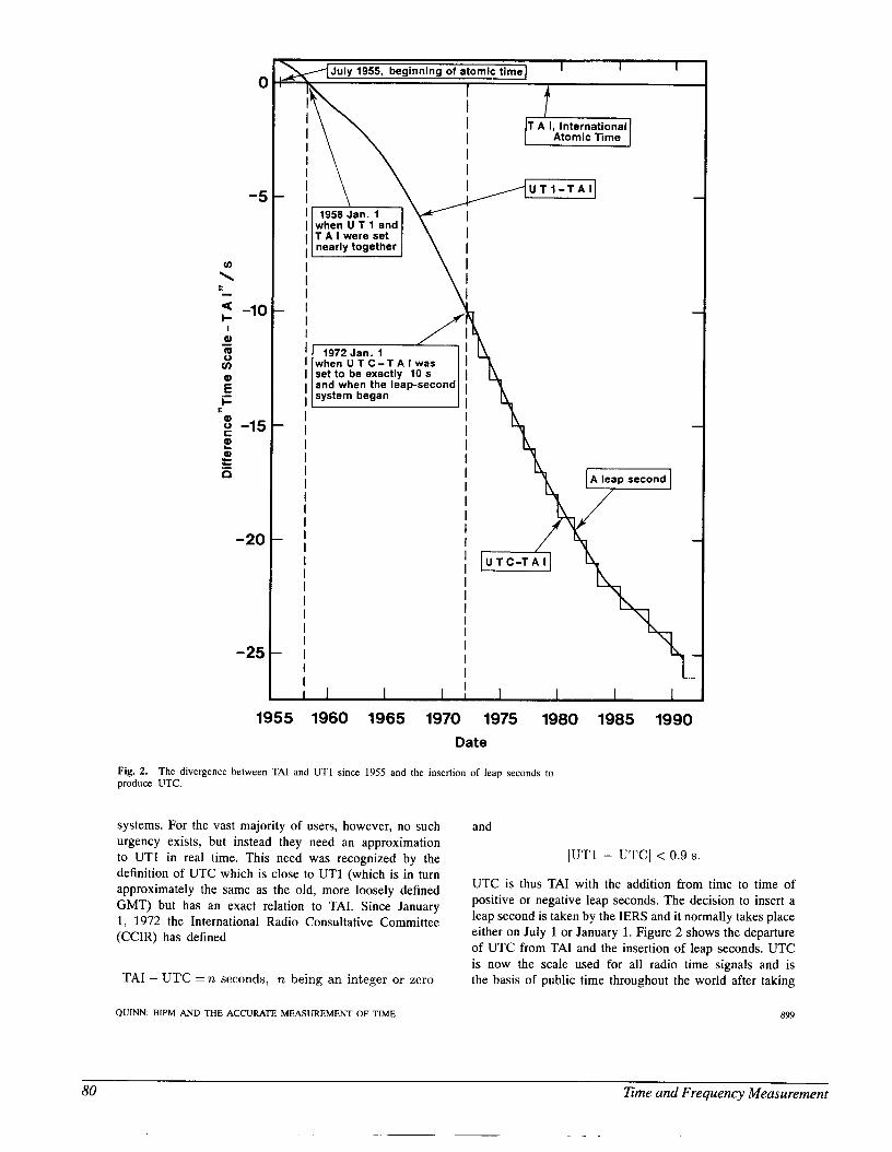
(I
-5
u)
\ - -10 I-
I Q Q 0 v)
-
; ,i=
Q
E
Q
0
0 -15 2 E
-20
-25
July 1955, beginning of atomic time] I I I
T A I , International
\ \
I I I I I I I I I I 1 I I I 1 I I I I I
I T A I w e r e s e t 1 \ : nearly together I
\ I
/ i 4 / ; h
1972 Jan. 1 I w h e n U T C - T A I w a s 1 4
‘b I 4 I I 1 I I I I I I I I I I I I I I I I
4 A leap second
t
1955 1960 1965 1970 1975 1980 1985 1990 Date
Fig. 2. The divergence between TAI and UT1 since 1955 and the insertion of leap seconds to produce UTC.
systems. For the vast majority of users, however, no such urgency exists, but instead they need an approximation to UT1 in real time. This need was recognized by the definition of UTC which is close to UT1 (which is in turn approximately the same as the old, more loosely defined GMT) but has an exact relation to TAL Since January 1, 1972 the International Radio Consultative Committee (CCIR) has defined
TAI - UTC = n seconds, n being an integer or zero
QUINN: BIPM AND THE ACCURATE MEASUREMENT OF TIME
and
lUTl - UTCl < 0.9 S .
UTC is thus TAI with the addition from time to time of positive or negative leap seconds. The decision to insert a leap second is taken by the IERS and it normally takes place either on July 1 or January 1. Figure 2 shows the departure of UTC from TAI and the insertion of leap seconds. UTC is now the scale used for all radio time signals and is the basis of public time throughout the world after taking
a99
80 Time and Frequency Measurement
-_.__ ~~
into account the differences of integral numbers of hours required by the time zone system.
VII. TAI AND THE WORK OF THE BIPM Coming now to the work of the BIPM, we can divide
the activities into two parts, the first is the establishment of TAI and the diffusion of TAI and UTC to users through the monthly Circular T, and second is the research work which supports and contributes to TAL
A . The Production of TAl
TAI is a time scale established on the basis of clock comparison data supplied to the BIPM by participating laboratories and a particular algorithm for treating the data known as ALGOS. TAI is a coordinate time scale defined in a geocentric reference frame with the SI second as realized on the rotating geoid as the scale unit. This statement that TAI is a coordinate as opposed to a proper time scale was made by the CCDS in 1980 and provides the necessary information for evaluating the relativistic terms in the establishment of TAI and for its use in nonterrestrial reference frames.
The main aim of TAI is to provide a time scale that is accurate, i.e., having its unit as close as possible to the SI second, reliable and above all stable in the long term. In order to optimize the long-term stability of the scale, at the expense of short-term accessibility, TAI is calculated using data covering an extended period. Clock-comparison data are sent to the BIPM every ten days, on the Modified Julian Dates ending with the figure 9 (01.01.91 is MJD 48257) but blocks of data covering 60 days are taken for the calculation of the scale. The period of 60 days was chosen to place the effective integration time of the scale at the transition between the flicker floor and the random walk frequency modulation of caesium clocks. Stability would not therefore be improved by a longer integration time (see Fig. 3). A period of 60 days is long enough, however, to smooth out the noise coming from the time links (Loran C and GPS) and the white frequency modulation of the clocks. The monthly BIPM Circulars T thus alternate between provisional, based upon only 30 days’ data, and definitive based upon a full period of 60 days’ data.
The establishment of TAI takes place in three steps: the calculation using a post-processing and iterative procedure of an intermediate time scale, known as Echelle Atomique Libre (EAL) or Free Atomic Scale, using the clock comparison data and ALGOS; the evaluation of the duration of the scale unit of EAL using data from primary frequency standards and an optimum filter; the production of TAI from EAL by applying, if necessary, a correction to the scale interval of EAL to give a value as close as possible to the SI second. This correcting of the scale interval is known as “steering” and is in fact only done at infrequent intervals.
The following gives a brief outline of how TAI is established and is based upon a more detailed description
900
given in [9], but see also [lo] and [ll]. 1 ) Structure of TAZ: The time on EAL at a time t of some
reference time scale, EALf(t), is defined in terms of the readings of h,(t) of a group of N clocks, H,, by
5 PSh%(t) + h:(t)I EAL(t) = ‘=’ N (5)
C Pa 2 = 1
where p , is the statistical weight assigned to clock H , and h:(t) is a time correction designed to ensure time and frequency continuity of the scale when either the weightings of individual clocks or the total number of clocks is changed
However, (5) cannot be used directly because the mea- sured quantities that provide the basic data for the calcula- tion of the scale are not the readings of individual clocks but are the results of comparisons between pairs of clocks. At time t , the slowly varying differences & ( t ) between the readings of clocks H , and H3 are written
[Ill.
We let the output of the calculation of EAL be a set of N values of the differences z l ( t ) defined by
z z ( t ) = EAL(t) - hi(t) (7)
where z, are the differences between the readings of the individual clocks and the time defined by EAL. Thus (6) can be written
and the defining (1) can be transformed into N N
(9) 2 = 1 1=1
In the practical computation, a nonredundant system of N - 1 time links is employed and (8) and (9) have a strict solution.
2) Weighting procedure: The weight assigned to each clock is calculated in such a way as to favor the long-term stability of the resulting scale and to minimize the annual fluctuations and the drift in its frequency with respect to primary frequency standards. An important feature of ALGOS is that the evaluation of the weight of the clock, although based upon data covering a whole year, takes into account the 60 days of data for which EAL is being computed. It is thus possible to judge clocks on their actual performance during the interval of time during which EAL is being established. It is also possible to take account of any abnormal behavior observed in an individual clock by adjusting its weight, if necessary to zero. This has proved useful on many occasions. The weight is normally based on the variance ~7,2(6,7) of mean rate (see (12)) with respect to E A L calculated over six two-monthly samples. This variance, instead of the usual pair variance, was chosen because it gives a greater reduction in the weights of clocks
PROCEEDINGS OF THE IEEE, VOL. 79, NO. 7, JULY 1991
Time and Frequency Measurement 81
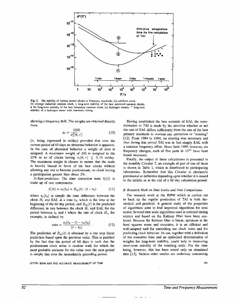
I I I I I I I I I
r(0
Effective integration time for the calculation
- 1 1 min lhour lday lmonth lyear
I I I I I I I I I I I I I
1 IO lo2 lo3 lo4 lo5 lo6 lo7 io8 T/s
Fig. 3. The stability of various atomic clocks or frequency standards: (a) rubidium clock; (b) average industrial caesium clock, o long-term stability of the best industrial caesium clocks, 0 the long-term stability of the best laboratory caesium clock; (c) hydrogen masers, * long-term stability of a hydrogen maser with automatic tuning.
showing a frequency drift. The weights are obtained directly from
(oa being expressed in ns/day) provided that over the current period of 60 days no abnormal behavior is apparent. In the case of abnormal behavior a weight of zero is assigned. A maximum weight of 100 is assigned to the 15% or so of clocks having a i ( 6 , ~ ) 5 3,16 ns/day. The maximum weight is chosen to ensure that the scale is heavily biased in favor of the best clocks without allowing any one to become predominant, no clock having a participation greater than about 2%.
3) Ratepredict ion: The time correction term h:(t) is made up of two components
h:(t) = Ui(t0) + B i P ( t ) . (t - t o ) (11)
where ai( t0) is simply the time difference between the clock Hi and EAL at a time to, which is the time at the beginning of the 60 day period, and Bip(t) is the predicted difference in rate between the clock Hi and EAL for the period between t o and t where the rate of clock Hi, for example, is defined by
The prediction of Bip(t) is obtained by a one step linear prediction based upon the previous value. This is justified by the fact that the period of 60 days is such that the predominant clock noise is random walk for which the most probable estimate for the value over the next period is simply that over the immediately preceding period.
QUINN: BIPM AND THE ACCURATE MEASUREMENT OF TIME
Having established the best estimate of EAL the trans- formation to TAI is made by the decision whether or not the rate of EAL differs sufficiently from the rate of the best primary standards to warrant any correction or “steering” [12]. From 1984 to 1989, no steering was necessary and thus during this period TAI was in fact simply EAL with a constant frequency offset. Since June 1989, however, six frequency changes, each of five parts in 1015 have been found necessary.
Finally, the output of these calculations is presented in the monthly Circular T, an example of part of one of these is shown in Table 1, which is distributed to participating laboratories. Remember that this Circular is alternately provisional or definitive depending upon whether it is issued in the middle or at the end of a 60 day calculation period.
B. Research Work on Time Scales and Time Comparisons
The research work at the BIPM which is carried out to back up the regular production of TAI is both the- oretical and practical. A general study of the properties of algorithms aims to find improved algorithms for time scales. Several time scale algorithms used in national timing centers and based on the Kalman filter have been ana- lyzed. Because the Kalman filter is linear, optimum in the least squares sense and recursive, it is an efficient and well-adapted tool for smoothing out clock noise and for predicting clock behavior. Its use, together with a definition of the ensemble time and an optimized determination of weights for long-term stability, could help in improving short-term stability of the resulting scale. For the time being, however, this has been tested only on simulated data [ 131. Various other studies are underway concerning
901
82 Time ana’ Frequency Measurement
- ~~ -
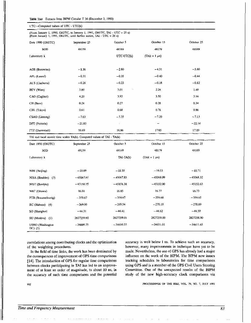
Table l(a) Extracts from BIPM Circular T 34 (December 3, 1990) ~~
UTC-Computed values of UTC - UTC(k)
(From January 1, 1990, OhUTC, to January 1, 1991, OhUTC, TAI - UTC = 25 s) (From January 1, 1991, OhUTC, until further notice, TAI - UTC = 26 s)
Date 1990 (OhUTC) September 25 October 5
MJD
Laboratory k
48159 48169
UTC-UTC(k)
AOS (Borowiec) -1.36 -2.80
APL (Laurel)
AUS (Canberra)
BEV (Wien)
CAO (Cagliari)
CH (Bern)
CRL (Tokyo)
CSAO (Lintong)
DPT (Pretoria)
ITZ (Darmstadt)
.-0.31
-0.26
3.80
4.20
0.24
0.61
-7.63
-21.83
16.69
-0.35
-0.23
3.01
3.93
0.27
0.68
-7.35
-
16.86
October 15
48179
(Unit = 1 ps)
-4.31
-0.40
-0.18
2.26
3.50
0.28
0.76
-7.20
-
17.05
October 25
48189
-5.80
-0.44
-0.12
1.48
3.16
0.34
0.86
-7.13
-22.14
17.19
TAI and local atomic time scales TA(k). Computed values of TAI - TA(k)
Date 1990 (OhUTC) September 25 October 5 October 15 October 25
MJD 48159 48169 48179 48189
Laboratory k TAI-TA(k) (Unit = 1 ps)
NIM (Beijing) -10.09 -10.30 -10.53 -10.71
NISA (Boulder) (3) -45067.61 -45067.85 -45068.09 -45068.32
NIST (Boulder) -45150.75 -45151.38 -45152.00 -45 152.63
NRC (Ottawa) 16.91 16.85 16.77 16.73
PTB (Braunschweig) -359.67 -359.67 -359.68 -359.65
RC (Habana) (4) -269.00 -269.54 -270.19 -270.89
SO (Shanghai) -44.31 -44.41 -44.62 -44.59
2827258.90 SU (Moskva) (1) 2827259.02 2827259.01 2827259.00
USNO (Washington -34609.75 -34610.37 -3461 1.01 -3461 1.65 DC) (5)
correlations among contributing clocks and the optimization of the weighting procedures. In the field of time links, the work has been dominated by
the consequences of improvement of GPS time comparisons [14]. The introduction of GPS for regular time comparisons between clocks participating in TAI has led to an improve- ment of at least an order of magnitude, to about 10 ns, in the accuracy of such time comparisons and the potential
accuracy is well below 1 ns. To achieve such an accuracy, however, many improvements in technique have yet to be made. Nevertheless, the use of GPS has already had a major influence on the work of the BIPM. The BIPM now issues tracking schedules to laboratories for time comparisons using GPS and is a member of the GPS Civil Users Steering Committee. One of the unexpected results of the BIPM study of the new high-accuracy clock comparisons via
902 PROCEEDINGS OF THE IEEE, VOL. 79, NO. 7, JULY 1991
Time and Frequency Measurement 83
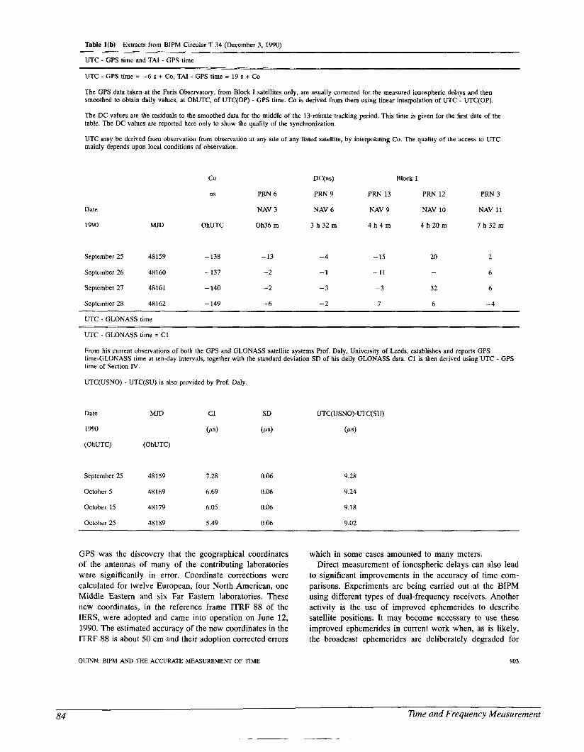
Table l(b)
UTC - GPS time and TAI - GPS time
Extracts from BIPM Circular T 34 (December 3, 1990)
UTC - GPS time = -6 s + Co, TAI - GPS time = 19 s + Co
The GPS data taken at the Paris Observatory, from Block I satellites only, are usually corrected for the measured ionospheric delays and then smoothed to obtain daily values, at OhUTC, of UTC(0P) - GPS time. Co is derived from them using linear interpolation of UTC - UTC(0P)
The DC values are the residuals to the smoothed data for the middle of the 13-minute tracking period. This time is given for the first date of the table. The DC values are reported here only to show the quality of the synchronization.
UTC may be derived from observation from observation at any site of any listed satellite, by interpolating Co. The quality of the access to UTC mainly depends upon local conditions of observation.
co DC(ns) Block I
ns PRN 6 PRN 9 PRN 13 PRN 12 PRN 3
Date NAV 3 NAV 6 NAV 9 NAV 10 NAV 11
1990 MJD OhUTC Oh36 m 3 h 3 2 m 4 h 4 m 4 h 2 0 m 7 h 3 2 m
September 25 48159 - 138 - 13 -4 - 15 20 2
September 26 48160 - 137 -2 -1 -11 - 6
September 27 48161 -140 -2 -3 -3 32 6
September 28 48162 - 149 -6 -2 7 6 -4
UTC - GLONASS time
UTC - GLONASS time = C1
From his current observations of both the GPS and GLONASS satellite systems Prof. Daly, University of Leeds, establishes and reports GPS time-GLONASS time at ten-day intervals, together with the standard deviation SD of his daily GLONASS data. C1 is then derived using UTC - GPS time of Section 1V.
UTC(USN0) - UTC(SU) is also provided by Prof. Daly.
Date MJD c1
1990 (w) (OhUTC) (OhUTC)
UTC(USN0)-UTC(SU)
( I 4
September 25 48159 7.28 0.06 9.28
October 5 48169 6.69 0.08 9.24
October 15 48179 6.05 0.06 9.18
October 25 48189 5.49 0.06 9.02
GPS was the discovery that the geographical coordinates of the antennas of many of the contributing laboratories were significantly in error. Coordinate corrections were calculated for twelve European, four North American, one Middle Eastern and six Far Eastern laboratories. These new coordinates, in the reference frame ITRF 88 of the IERS, were adopted and came into operation on June 12, 1990. The estimated accuracy of the new coordinates in the ITRF 88 is about 50 cm and their adoption corrected errors
which in some cases amounted to many meters. Direct measurement of ionospheric delays can also lead
to significant improvements in the accuracy of time com- parisons. Experiments are being carried out at the BIPM using different types of dual-frequency receivers. Another activity is the use of improved ephemerides to describe satellite positions. It may become necessary to use these improved ephemerides in current work when, as is likely, the broadcast ephemerides are deliberately degraded for
QUI": BIPM AND THE ACCURATE MEASUREMENT OF TIME 903
84 Time and Frequency Measurement
- --
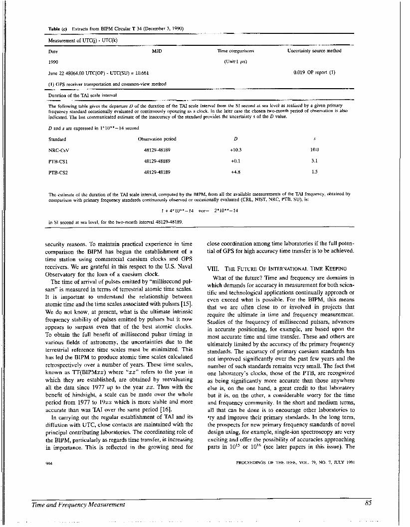
Table (d Extracts from BIPM Circular T 34 (December 3. 1990) ~~ ~~
Measurement of UTCG) - UTC(k)
Date MJD Time comparisons Uncertainty source method
1990 (Unit:l ps)
June 22 48064.00 UTC(0P) - UTC(SU) = 10.661
(1) GPS receiver transportation and common-view method
0.019 OP report (1)
Duration of the TAI scale interval
The following table gives the departure D of the duration of the TAI scale interval from the SI second at sea level as realized by a given primary frequency standard occasionally evaluated or continuously operating as a clock. In the later case the chosen two-month period of observation is also indicated. The last communicated estimate of the inaccuracy of the standard provides the uncertainty s of the D value.
D and s are expressed in 1*10**--14 second
Standard Observation period D S
NRC-CsV 48129-48189 +10.3 10.0
PTB-CS1 48129-48189 to . l 3.1
PTB-CS2 48129-48189 +4.8 1.5
The estimate of the duration of the TAI scale interval, computed by the BIPM, from all the available measurements of the TAI frequency, obtained by comparison with primary frequency standards continuously observed or occasionally evaluated (CRL, NIST, NRC, PTB, SU), is:
1 + 4*10**-14 +or- 2*10**-14
in SI second at sea level, for the two-month interval 48129-48189.
security reasons. To maintain practical experience in time comparison the BIPM has begun the establishment of a time station using commercial caesium clocks and GPS receivers. We are grateful in this respect to the U.S. Naval
close coordination among time laboratories if the full poten- tial of GPS for high accuracy time transfer is to be achieved.
vIII. THE FUTURE oF I~~~~~~~~~~~ uEPING Observatory for the loan of a caesium clock.
The time of arrival of pulses emitted by “millisecond pul- sars” is measured in terms of terrestrial atomic time scales. It is important to understand the relationship between atomic time and the time scales associated with pulsars [ 151. We do not know, at present, what is the ultimate intrinsic frequency stability of pulses emitted by pulsars but it now appears to surpass even that of the best atomic clocks. To obtain the full benefit of millisecond pulsar timing in various fields of astronomy, the uncertainties due to the terrestrial reference time scales must be minimized. This has led the BIPM to produce atomic time scales calculated retrospectively over a number of years. These time scales, known as TT(B1PMxx) where “xx” refers to the year in which they are established, are obtained by reevaluating all the data since 1977 up to the year xx. Thus with the benefit of hindsight, a scale can be made over the whole period from 1977 to 19x2 which is more stable and more accurate than was TAI over the same period [16].
In carrying out the regular establishment of TAI and its diffusion with UTC, close contacts are maintained with the principal contributing laboratories. The coordinating role of the BIPM, particularly as regards time transfer, is increasing in importance. This is reflected in the growing need for
904
What of the future? Time and frequency are domains in which demands for accuracy in measurement for both scien- tific and technological applications continually approach or even exceed what is possible. For the BIPM, this means that we are often close to or involved in projects that require the ultimate in time and frequency measurement. Studies of the frequency of millisecond pulsars, advances in accurate positioning, for example, are based upon the most accurate time and time transfer. These and others are ultimately limited by the accuracy of the primary frequency standards. The accuracy of primary caesium standards has not improved significantly over the past few years and the number of such standards remains very small. The fact that one laboratory’s clocks, those of the PTB, are recognized as being significantly more accurate than those anywhere else is, on the one hand, a great credit to that laboratory but it is, on the other, a considerable worry for the time and frequency community. In the short and medium terms, all that can be done is to encourage other laboratories to fry and improve their primary standards. In the long term, the prospects for new primary frequency standards of novel design using, for example, single-ion spectroscopy are very exciting and offer the possibility of accuracies approaching parts in 1015 or 10l6 (see later papers in this issue). The
PROCEEDINGS OF THE IEEE, VOL. 79, NO. 7, JULY 1991
Time and Frequency Measurement 85
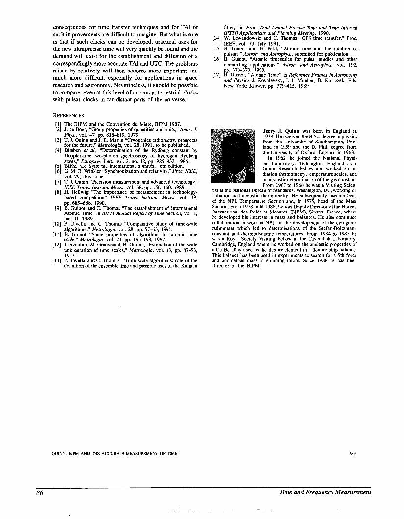
consequences for time transfer techniques and for TAI of such improvements are difficult to imagine. But what is sure is that if such clocks can be developed, practical uses for the new ultraprecise time will very quickly be found and the demand will exist for the establishment and diffusion of a correspondingly more accurate TAI and UTC. The problems raised by relativity will then become more important and much more difficult, especially for applications in space research and astronomy. Nevertheless, it should be possible to compare, even at this level of accuracy, terrestrial clocks with pulsar clocks in far-distant parts of the universe.
REFERENCES 1 The BIPM and the Convention du Mbtre, BIPM 1987. 2 J. de Boer, “Group properties of quantities and units,”Amer. J.
Phys., vol. 47, pp. 818-819, 1979. [3] T. J. Quinn and J. E. Martin “Cryogenics radiometry, prospects
for the future,” Metrologia, vol. 28, 1991, to be published. [4] Biraben et al., “Determination of the Rydberg constant by
Doppler-free two-photon spectroscopy of hydrogen Rydberg states,” Europhys. Lett., vol. 2, no. 12, pp. 925-932, 1986.
5 BIPM “Le Systk me international d’unitks,” 6th edition. 6 G. M. R. Winkler “Synchronization and relativity,” Proc. IEEE,
vol. 79, this issue. [7] T. J. Quinn “Precision measurement and advanced technology”
IEEE Trans. Instrum. Meas., vol. 38, pp. 156-160, 1989. [8] H. Hellwig “The importance of measurement in technology-
based competition” IEEE Trans. Instrum. Meas., vol. 39, pp. 685-688, 1990.
[9] B. Guinot and C. Thomas “The establishment of Intemational Atomic Time’’ in BIPM Annual Report of Time Section, vol. 1, part D, 1989.
[lo] P. Tavella and C. Thomas “Comparative study of time-scale algorithms,” Metrologia, vol. 28, pp. 57-63, 1991.
[ l l ] B. Guinot “Some properties of algorithms for atomic time scale,” Metrologia, vol. 24, pp. 195-198, 1987.
[12] J. Azoubib, M. Granveaud, B. Guinot, “Estimation of the scale unit duration of time scales,” Metrologia, vol. 13, pp. 87-93, 1977.
[13] P. Tavella and C. Thomas, “Time scale algorithms: role of the definition of the ensemble time and possible uses of the Kalman
[ I
[ I
QUINN: BIPM AND THE ACCURATE MEASUREMENT OF TIME
filter,” in Proc. 22nd Annual Precise Time and Time Interval (PTTI) Applications and Planning Meeting, 1990.
[14] W. Lewandowski and C. Thomas “GPS time transfer,” Proc. IEEE, vol. 79, July 1991.
[15] B. Guinot and G. Petit, “Atomic time and the rotation of pulsars,” Astron. and Astmphys., submitted for publication.
[16] B. Guinot, “Atomic timescales for pulsar studies and other demanding aoolications.” Astron. and Astrovhvs.. vol. 192.
1 , 1
pp. 370-373,’i988. ‘
[17] B. Guinot, “Atomic Time” in Reference Frames in Astronomy and Physics J. Kovalevsky, I. I. Mueller, B. Kolaczek, Eds. New York: Kluwer, pp. 379-415, 1989.
tist at the National Bure
Terry J. Quinn was born in England in 1938. He received the B.Sc. degree in physics from the University of Southampton, Eng- land in 1959 and the D. Phil. degree from the University of Oxford, England in 1963.
In 1962, he joined the National Physi- cal Laboratory, Teddington, England as a Junior Research Fellow and worked on ra- diation thermometry, temperature scales, and on acoustic determination of the gas constant. From 1967 to 1968 he was a Visiting Scien-
au of Standards, Washington, DC, working on radiation and acoustic thermometry. He subsequently became hkad of the NPL Temperature Section and, in 1975, head of the Mass Section. From 1978 until 1988, he was Deputy Director of the Bureau International des Poids et Mesures (BIPM), Skres , France, where he developed his interests in mass and balances. He also continued collaboration in work at NPL on the development of the cyrogenic radiometer which led to determinations of the Stefan-Boltzmann constant and thermodynamic temperatures. From 1984 to 1985 he was a Royal Society Visiting Fellow at the Cavendish Laboratory, Cambridge, England where he worked on the anelastic properties of a Cu-Be alloy used as the flexure element in a flexure strip balance. This balance has been used in experiments to search for a 5th force and anomalous mass in spinning rotors. Since 1988 he has been Director of the BIPM.
905
86 Time and Frequency Measurement
- - - -__ -
0 1991 IEEE. Reprinted, with permission, from Proceedings of the IEEE: Special Issue on Time and Frequency, 79 (7), 991-1000; 1991.
GPS Time Transfer ~ ~~
WLODZIMIERZ LEWANDOWSKI AND CLAUDINE THOMAS
Over the past ten years GPS satellites have become the principal tool for national and international comparisons of atomic clocks. Using GPS, time transfer is now ten times more accurate than it used to be using LORAN-C. For the first time, the best frequency standards in the world have been compared in a way which exploits their full level of performance. The present accuracy of GPS time transfer is of the order 10-20 ns for intercontinental distances and 2-3 ns within one continent. Although many improvements have been introduced during the past decade, the next should bring still further improvements leading to an ultimate accuracy at the subnanosecond level.
LIST OF
BIPM CCDS
CRL cv
DMA GPS
IERS ITRF MJD NIST
NBS NRC
NSWC OP SA
TAI USNO
UTC UTC(i)
VLBI WGS
ACRONYMS AND ABBREVIATIONS Bureau International des Poids et Mesures. ComitC Consultatif pour la Definition de la Sec- onde. Communications Research Laboratory, Tokyo. Common view. Defense Mapping Agency. Global Positioning System. International Earth Rotation Service. IERS Terrestrial Reference Frame. Modified Julian Day. National Institute of Standards and Technology, Boulder, CO. National Bureau of Standards (now NIST). National Research Council, Ottawa, Canada. Naval Surface Warfare Center. Observatoire de Paris. Selective Availability of GPS. International Atomic Time. U.S. Naval Observatory, Washington, DC. Coordinated Universal Time. Coordinated Universal Time as realized by labo- ratory i. Very Long Base Interferometry. World Geodetic System.
Manuscript received November 10, 1990; revised March 1, 1991. The authors are with the Bureau International des Poids et Mesures,
IEEE Log Number 9100237. 92312 S h e s Cedex, France.
I. INTRODUCTION The excellence of worldwide unification of time realized
by the establishment of International Atomic Time (TAI) and Coordinated Universal Time (UTC), depends on the quality of the participating atomic clocks and the means of time comparison. In the pre-GPS era (until the beginning of the 1980’s) the technology of atomic clocks was always ahead of that of time transfer. The uncertainties of the long-distance time comparisons, by LORAN-C, were some hundreds of nanoseconds, and large areas of the earth were not covered. The introduction of GPS has led to a major improvement of world-wide time metrology in precision, accuracy and coverage. With GPS, time comparisons are performed with an accuracy of a few nanoseconds for short baselines (up to 1000 km) and 10-20 ns for intercontinental distances. This makes it possible to compare the best standards in the world at their full level of performance: for integration times of only 10 days, the frequency differences between atomic clocks are measured at the level one part in
But this is by no means the limit to the possibilities of GPS. The inaccuracy of long-distance time comparisons performed with CIA-code (see Section 11-A-2) receivers can be reduced to the level of a few nanoseconds by the reduction of some remaining systematic errors. Some of the actions required for this improvement will, in any case, be necessary when voluntary degradation known as Selective Availability (SA) (see Section V) is put into operation. On the other hand, geodesists, using a new generation of receivers, expect to measure pseudoranges with uncertainties of 10 cm or less and then to reduce ephemeride errors to less than 10 cm. These developments bring the hope that time comparisons may be achieved with uncertainties of 300 ps or less. Such an accuracy exceeds the present needs but could meet the challenge of the new generation of time and frequency technology.
In this paper, after a brief introduction to GPS, the principles of GPS time transfer are described with emphasis being placed on the so-called common view method. The sources of error during GPS time transfer are discussed and
0018-9219/91/0700-O991$01 .OO 0 199 1 IEEE
Time and Frequency Measurement 87
the various possibilities of reducing them are investigated. Some possibilities for overcoming SA are also discussed. GPS is additionally shown to be an outstanding tool for the dissemination of UTC.
11. BACKGROUND
A. GPS Outline The NAVSTAR Global Positioning System, GPS, is
a military satellite navigation system based on satellite ranging using on-board atomic clocks (cesium or rubidium). In its final stage it will provide position, velocity and time instantaneously and continuously anywhere on or above the earth. The system consists of three major segments: a space segment (satellites transmitting radio signals), a control segment (a control station and several monitor stations) and a user segment which extracts the desired information (position, velocity, time) from the received satellite signals.
I) The Satellites: The first GPS spacecraft was launched in February 1978. By the end of 1990, 15 satellites were operating. Six satellites belong to the old Block I and nine to the new Block 11 which is subject to the voluntary degradation known as Selective Availability (see Section V). When fully operational in 1993 the system will consist of 21 satellites equally spaced in 6 orbital planes inclined at 55” to the equator. There will also be 3 active spares. The spacecrafts orbit the earth at about 20 183 km above its surface and have sidereal period. This has a practical impact on the organization of GPS time comparisons (see Section 111).
2) Transmitted Signals: The space vehicle clock fre- quency is 10.23 MHz, from which all other frequencies are derived. Each satellite transmits two navigational signals, namely an L1 signal at a frequency of 1575.42 MHz (10.23 MHz x 154) and an L2 signal at a frequency of 1227.6 MHz (10.23 MHz x 120) [1,2]. Signal L1 is modulated with the P-code (Precise or Protected code) and the CIA-code (ClearlAcquisition code also known as “civilian code”); signal L2 is modulated with P-code only; both codes are of pseudorandom noise (PRN) type. The CIA-code with a chip-rate of 1.023 MHz and a repetition rate of one millisecond has a fast acquisition time, but it does not provide the high accuracy of the P-code which has a chip-rate of 10.23 MHz and a repetition rate of 267 days.
3) Navigation Message: Signals L1 and L2 are continu- ously modulated with a navigational data stream at 50 b/s in frames of 1500 b lasting 30 s and formatted into five sub-frames of 6 s each. A complete data message requires the transmission of 25 frames and takes 12.5 min. The navigation message generated by the control segment and uploaded to the satellites every day contains all the data required by a user for the computation of position. The mes- sage stream includes information on the status of the space vehicle, the parameters for the clock correction needed to compute GPS time (see Section 11-B), the ephemerides of the satellite and the parameters for computing signal delay due to the ionosphere. The relationship between GPS
992
time and UTC(USN0) (see Sections 11-B and IV) is also contained in the navigation message.
Future GPS signals will be voluntarily degraded (SA) in order to deny unauthorized users access to the full accuracy of instantaneous positioning (see Section V). Authorized users will be able to perform instantaneous positioning with uncertainties of several meters while unauthorized users are limited to uncertainties of 100 m.
To determine a position in three space dimensions and time, a user must receive the signal from four satellites. However, if a user has a known position it is necessary only to track one satellite in order to determine time. In this way, GPS can be used as a time distribution system.
B. GPS Time GPS time is a time scale established by the Control Seg-
ment and related to UTC(USN0). GPS time is a continuous time (not corrected by leap seconds) measured in weeks from the GPS time zero point defined as 0 h UTC(USNO), January 5,1980. At the end of 1990, GPS time was ahead of UTC(USN0) by 6 s. The Control Segment should control GPS time to be within 1 ps of UTC(USN0) (modulo 1 s).
The navigation message contains a correction to be added to the readings of the on-board satellite clocks in order to obtain GPS time (see Section 11-C). This realization of GPS time through the GPS constellation shows a peak-to-peak discrepancy, at a given instant, of up to 30 ns.
The navigation message also contains data giving access to UTC(USN0) in real time with an accuracy of 100 ns.
C. GPS Time Receivers Most GPS time receivers are one channel CIA-code
devices because such devices are simple and of reasonable cost. In addition CIA-code is accessible to everyone while P-code only to authorized users.
The time difference between the user clock connected with GPS time receiver and the GPS time is given by the following relationship:
DT = pr - ( r / c + dS + d l + dT) - d D + dc (1)
where
Pr
r
C
as
dI
measured “pseudorange” or an apparent propaga- tion time, which is determined by measuring the difference of two identical codes, one generated by the receiver, the other one contained in the signal emitted by the satellite and received by the receiver; each of these codes is synchronized by its own clock, range between the satellite and the station com- puted from broadcast ephemerides and the known coordinates of the receiver antenna, speed of light, correction due to the rotation of the Earth (Sagnac
propagation delay due to the ionosphere; since the CIA code is transmitted on only one frequency (L1)
ef fc t ) PI,
PROCEEDINGS OF THE IEEE, VOL. 79, NO. 7, JULY 1991
88 Time and Frequency Measurement
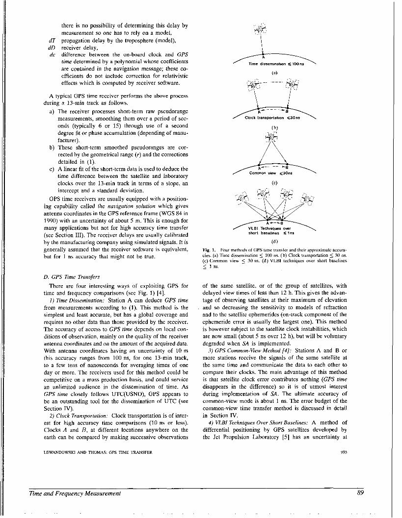
there is no possibility of determining this delay by measurement so one has to rely on a model,
dT propagation delay by the troposphere (model), dD receiver delay, dc difference between the on-board clock and GPS
time determined by a polynomial whose coefficients are contained in the navigation message; these co- efficients do not include correction for relativistic effects which is computed by receiver software.
A typical GPS time receiver performs the above process
a) The receiver processes short-term raw pseudorafige measurements, smoothing them over a period of sec- onds (typically 6 or 15) through use of a second degree fit or phase accumulation (depending of manu- facturer).
b) These short-term smoothed pseudoranges are cor- rected by the geometrical range (r) and the corrections detailed in (1).
c) A linear fit of the short-term data is used to deduce the time difference between the satellite and laboratory clocks over the 13-min track in terms of a slope, an intercept and a standard deviation.
GPS time receivers are usually equipped with a position- ing capability called the navigation solution which gives antenna coordinates in the GPS reference frame (WGS 84 in 1990) with an uncertainty of about 5 m. This is enough for many applications but not for high accuracy time transfer (see Section 111). The receiver delays are usually calibrated by the manufacturing company using simulated signals. It is generally assumed that the receiver software is equivalent, but for 1 ns accuracy that might not be true.
during a 13-min track as follows.
D. GPS Time Transfers There are four interesting ways of exploiting GPS for
time and frequency comparisons (see Fig. 1) [4]. I ) Time Dissemination: Station A can deduce GPS time
from measurements according to (1). This method is the simplest and least accurate, but has a global coverage and requires no other data than those provided by the receiver. The accuracy of access to GPS time depends on local con- ditions of observation, mainly on the quality of the receiver antenna coordinates and on the amount of the acquired data. With antenna coordinates having an uncertainty of 10 m this accuracy ranges from 100 ns, for one 13-min track, to a few tens of nanoseconds for averaging times of one day or more. The receivers used for this method could be competitive on a mass production basis, and could service an unlimited audience in the dissemination of time. As GPS time closely follows UTC(USNO), GPS appears to be an outstanding tool for the dissemination of UTC (see Section IV).
2) Clock Transportation: Clock transportation is of inter- est for high accuracy time comparisons (10 ns or less). Clocks A and B, at different locations anywhere on the earth can be compared by making successive observations
LEWANDOWSKI AND THOMAS: GPS TIME TRANSFER
Time dissemination < 100 os
(d ) Fig. 1. Four methods of GPS time transfer and their approximate accura- cies. (a) Time dissemination 5 100 ns. (b) Clock transportation 5 30 ns. (c) Common view 5 30 ns. (d) VLBI techniques over short baselines 5 1 ns.
of the same satellite, or of the group of satellites, with delayed view times of less than 12 h. This gives the advan- tage of observing satellites at their maximum of elevation and so decreasing the sensitivity to models of refraction and to the satellite ephemerides (on-track component of the ephemeride error is usually the largest one). This method is however subject to the satellite clock instabilities, which are now small (about 5 ns over 12 h), but will be voluntary degraded when SA is implemented.
3) GPS Common-View Method [4]: Stations A and B or more stations receive the signals of the same satellite at the same time and communicate the data to each other to compare their clocks. The main advantage of this method is that satellite clock error contributes nothing (GPS time disappears in the difference) so it is of utmost interest during implementation of SA. The ultimate accuracy of common-view mode is about 1 ns. The error budget of the common-view time transfer method is discussed in detail in Section IV.
4) VLBI Techniques Over Short Baselines: A method of differential positioning by GPS satellites developed by the Jet Propulsion Laboratory [5] has an uncertainty at
993
Time and Frequency Measurement 89
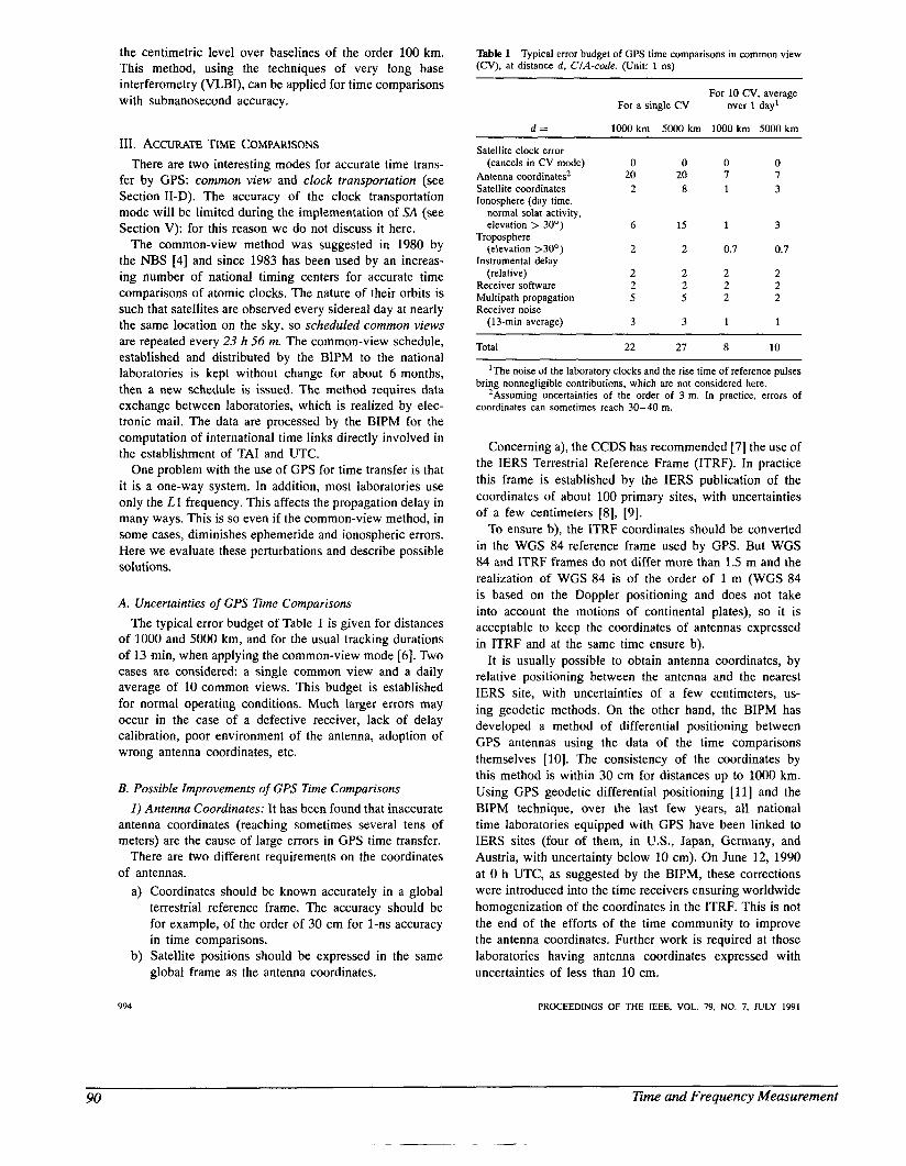
the centimetric level over baselines of the order 100 km. This method, using the techniques of very long base interferometry (VLBI), can be applied for time comparisons with subnanosecond accuracy.
111. ACCURATE TIME COMPARISONS There are two interesting modes for accurate time trans-
fer by GPS: common view and clock transportation (see Section 11-D). The accuracy of the clock transportation mode will be limited during the implementation of SA (see Section V): for this reason we do not discuss it here.
The common-view method was suggested in 1980 by the NBS [4] and since 1983 has been used by an increas- ing number of national timing centers for accurate time comparisons of atomic clocks. The nature of their orbits is such that satellites are observed every sidereal day at nearly the same location on the sky, so scheduled common views are repeated every 23 h 56 m. The common-view schedule, established and distributed by the BIPM to the national laboratories is kept without change for about 6 months, then a new schedule is issued. The method requires data exchange between laboratories, which is realized by elec- tronic mail. The data are processed by the BIPM for the computation of international time links directly involved in the establishment of TAI and UTC.
One problem with the use of GPS for time transfer is that it is a one-way system. In addition, most laboratories use only the L1 frequency. This affects the propagation delay in many ways. This is so even if the common-view method, in some cases, diminishes ephemeride and ionospheric errors. Here we evaluate these perturbations and describe possible solutions.
A. Uncertainties of GPS Time Comparisons The typical error budget of Table 1 is given for distances
of 1000 and 5000 km, and for the usual tracking durations of 13 min, when applying the common-view mode [6]. Two cases are considered: a single common view and a daily average of 10 common views. This budget is established for normal operating conditions. Much larger errors may occur in the case of a defective receiver, lack of delay calibration, poor environment of the antenna, adoption of wrong antenna coordinates, etc.
B. Possible Improvements of GPS Time Comparisons 1 ) Antenna Coordinates: It has been found that inaccurate
antenna coordinates (reaching sometimes several tens of meters) are the cause of large errars in GPS time transfer.
There are two different requirements on the coordinates of antennas.
Coordinates should be known accurately in a global terrestrial reference frame. The accuracy should be for example, of the order of 30 cm for I-ns accuracy in time comparisons. Satellite positions should be expressed in the same global frame as the antenna coordinates.
Table 1 (CV), at distance d, CIA-code. (Unit: 1 ns)
Typical error budget of GPS time comparisons in common view
For 10 CV, average over 1 day' For a single CV
d = 1000 km 5000 km 1000 km 5000 km
Satellite clock error
Antenna coordinates2 Satellite coordinates Ionosphere (day time,
normal solar activity, elevation > 30°)
(elevation >30°)
(relative)
(cancels in CV mode)
Troposphere
Instrumental delay
Receiver software Multipath propagation Receiver noise
(13-min average)
0 20
2
6
2
2 2 5
3
0 0 20 7
8 1
15 1
2 0.7
2 2 2 2 5 2
3 1
0 7 3
3
0.7
2 2 2
1
Total 22 27 8 10
'The noise of the laboratory clocks and the rise time of reference pulses
'Assuming uncertainties of the order of 3 m. In practice, errors of bring nonnegligible contributions, which are not considered here.
coordinates can sometimes reach 30-40 m.
Concerning a), the CCDS has recommended [7] the use of the IERS Terrestrial Reference Frame (ITRF). In practice this frame is established by the IERS publication of the coordinates of about 100 primary sites, with uncertainties of a few centimeters [8], [Y].
To ensure b), the ITRF coordinates should be converted in the WGS 84 reference frame used by GPS. But WGS 84 and ITRF frames do not differ more than 1.5 m and the realization of WGS 84 is of the order of 1 m (WGS 84 is based on the Doppler positioning and does not take into account the motions of continental plates), so it is acceptable to keep the coordinates of antennas expressed in ITRF and at the same time ensure b).
It is usually possible to obtain antenna coordinates, by relative positioning between the antenna and the nearest IERS site, with uncertainties of a few centimeters, us- ing geodetic methods. On the other hand, the BIPM has developed a method of differential positioning between GPS antennas using the data of the time comparisons themselves [IO]. The consistency of the coordinates by this method is within 30 cm for distances up to 1000 km. Using GPS geodetic differential positioning [ 1 I] and the BIPM technique, over the last few years, all national time laboratories equipped with GPS have been linked to IERS sites (four of them, in U S . , Japan, Germany, and Austria, with uncertainty below 10 cm). On June 12, 1990 at 0 h UTC, as suggested by the BIPM, these corrections were introduced into the time receivers ensuring worldwide homogenization of the coordinates in the ITRF. This is not the end of the efforts of the time community to improve the antenna coordinates. Further work is required at those laboratories having antenna coordinates expressed with uncertainties of less than 10 cm.
PROCEEDINGS OF THE IEEE, VOL. 79, NO. 7, JULY 1991
90 Time and Frequency Measurement
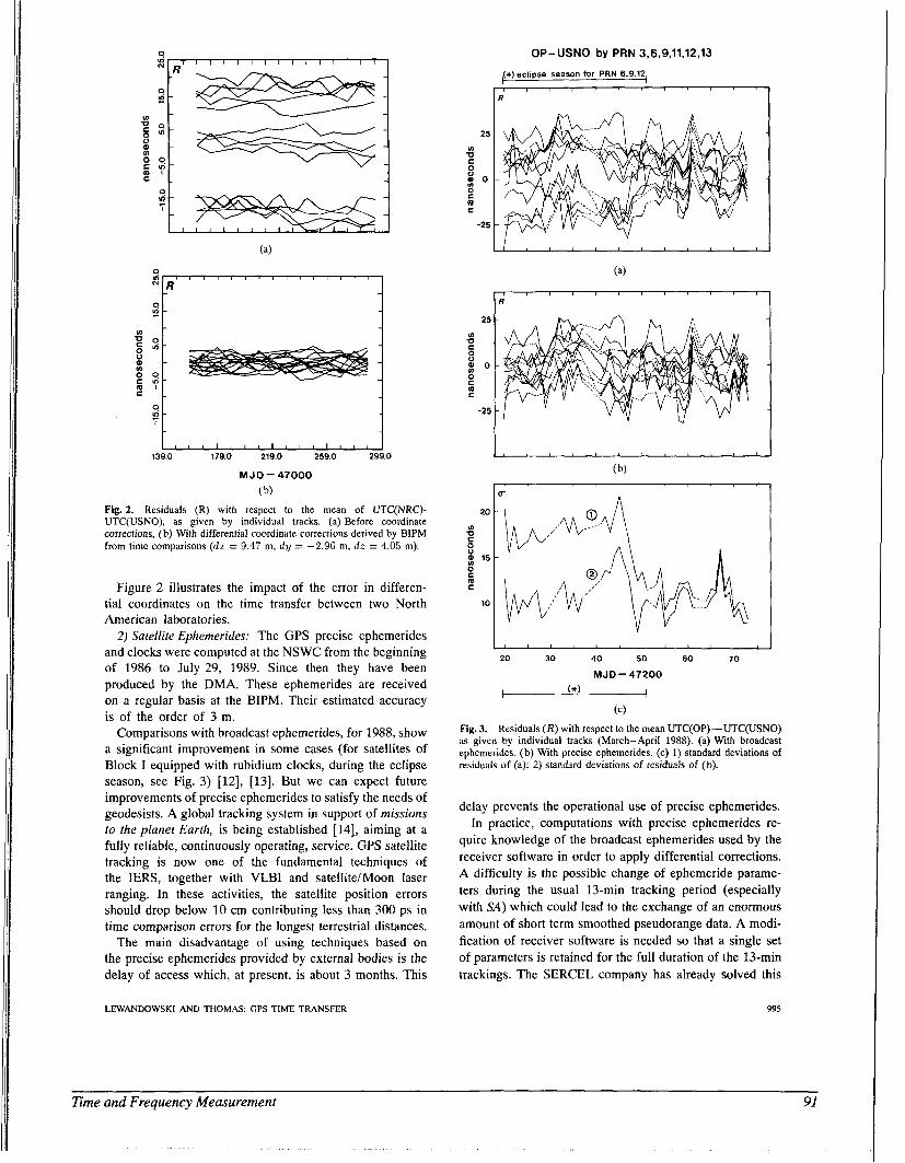
1 1 , 1 1 1 1 1 1 1 1 1
139.0 179.0 219.0 259.0 299.0
MJD-47000
( b)
Fig. 2. Residuals (R) with respect to the mean of UTC(NRC)- UTC(USNO), as given by individual tracks. (a) Before coordinate corrections, (b) With differential coordinate corrections derived by BIPM from time comparisons ( d r = 9.47 m, d y = -2.96 m, dz = 4.05 m).
Figure 2 illustrates the impact of the error in differen- tial coordinates on the time transfer between two North American laboratories.
2) Satellite Ephemerides: The GPS precise ephemerides and clocks were computed at the NSWC from the beginning of 1986 to July 29, 1989. Since then they have been produced by the DMA. These ephemerides are received on a regular basis at the BIPM. Their estimated accuracy is of the order of 3 m.
Comparisons with broadcast ephemerides, for 1988, show a significant improvement in some cases (for satellites of Block I equipped with rubidium clocks, during the eclipse season, see Fig. 3) [12], [13]. But we can expect future improvements of precise ephemerides to satisfy the needs of geodesists. A global tracking system in support of missions to the planet Earth, is being established [14], aiming at a fully reliable, continuously operating, service. GPS satellite tracking is now one of the fundamental techniques of the IERS, together with VLBI and satellite/Moon laser ranging. In these activities, the satellite position errors should drop below 10 cm contributing less than 300 ps in time comparison errors for the longest terrestrial distances.
The main disadvantage of using techniques based on the precise ephemerides provided by external bodies is the delay of access which, at present, is about 3 months. This
LEWANDOWSKI AND THOMAS: GPS TIME TRANSFER
OP- USNO by PRN 3,6,9,11,12,13
(+)eclipse season for PRN 6.9,12
R
25 -
u) D 0
0 - 0
G -25 -
, I I I I I I , , , , , ,
20 3 0 40 5 0 60 70
MJD- 47200
I (*I I ( 4
Fig. 3. Residuals (R) with respect to the mean UTC(0P)-UTC(USN0) as given by individual tracks (March-April 1988). (a) With broadcast ephemerides. (b) With precise ephemerides. (c) 1) standard deviations of residuals of (a); 2) standard deviations of residuals of (b).
delay prevents the operational use of precise ephemerides. In practice, computations with precise ephemerides re-
quire knowledge of the broadcast ephemerides used by the receiver software in order to apply differential corrections. A difficulty is the possible change of ephemeride parame- ters during the usual 13-min tracking period (especially with SA) which could lead to the exchange of an enormous amount of short term smoothed pseudorange data. A modi- fication of receiver software is needed so that a single set of parameters is retained for the full duration of the 13-min trackings. The SERCEL company has already solved this
995
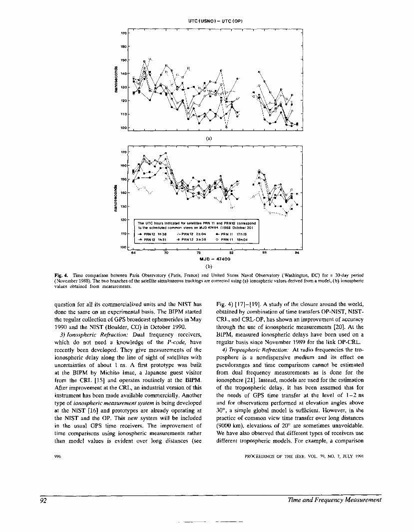
UTC (USNO) - UTC (OP)
170 '1 160 1 150 -
120 - 110 -
100 - -
110 lZ0I The UTC hours indicated lor satellites PRN 11 and PRNlZ correspond to the scheduled common views ~1 MJO 47464 I1988 October 30)
+PRNlZ l h 3 8 4-PRN12 2h04 +PRN11 17h19 6-PRN12 l h 5 l a P R N 1 2 2 h 3 8 U P R N 1 1 l8h04
l o o , , , L , , , , , , , , , , , , 64 70 76 82 88 94
MJD - 47400
( b)
Fig. 4. Time comparison between Paris Observatory (Paris, France) and United States Naval Observatory (Washington, DC) for a 30-day period (November 1988). The two branches of the satellite simultaneous trackings are corrected using (a) ionospheric values derived from a model, (b) ionospheric values obtained from measurements.
question for all its commercialized units and the NIST has done the same on an experimental basis. The BIPM started the regular collection of GPS broadcast ephemerides in May 1990 and the NIST (Boulder, CO) in October 1990.
3) Ionospheric Refraction: Dual frequency receivers, which do not need a knowledge of the P-code, have recently been developed. They give measurements of the ionospheric delay along the line of sight of satellites with uncertainties of about 1 ns. A first prototype was built at the BIPM by Michito Imae, a Japanese guest visitor from the CRL [15] and operates routinely at the BIPM. After improvement at the CRL, an industrial version of this instrument has been made available commercially. Another type of ionospheric measurement system is being developed at the NIST [16] and prototypes are already operating at the NIST and the OP. This new system will be included in the usual GPS time receivers. The improvement of time comparisons using ionospheric measurements rather than model values is evident over long distances (see
996
Fig. 4) [17]-[19]. A study of the closure around the world, obtained by combination of time transfers OP-NET, NIST- CRL, and CRL-OP, has shown an improvement of accuracy through the use of ionospheric measurements [20]. At the BIPM, measured ionospheric delays have been used on a regular basis since November 1989 for the link OP-CRL.
4) Tropospheric Refraction: At radio frequencies the tro- posphere is a nondispersive medium and its effect on pseudoranges and time comparisons cannot be estimated from dual frequency measurements as is done for the ionosphere [21]. Instead, models are used for the estimation of the tropospheric delay. It has been assumed that for the needs of GPS time transfer at the level of 1-2 ns and for observations performed at elevation angles above 30°, a simple global model is sufficient. However, in the practice of common view time transfer over long distances (9000 km), elevations of 20" are sometimes unavoidable. We have also observed that different types of receivers use different tropospheric models. For example, a comparison
PROCEEDINGS OF THE IEEE, VOL. 79, NO. 7, JULY 1991
92 Time and Frequency Measurement
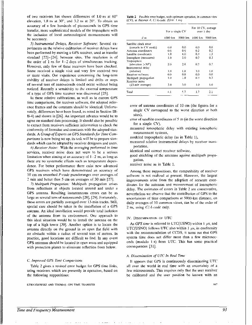
of two receivers has shown differences of 1.0 ns at 60" elevation, 1.8 ns at 30", and 3.2 ns at 20". To obtain an accuracy of a few hundreds of picoseconds in GPS time transfer, more sophisticated models of the troposphere with the inclusion of local meteorological measurements will be necessary.
5) Instrumental Delays, Receiver Software: Several ex- periments on the relative calibration of receiver delays have been performed by moving a GPS receiver, used as transfer standard [22]-[24], between sites. The resolution is of the order of 1 ns for 1-2 days of simultaneous tracking. However, only few of these receivers have been checked. Some received a single visit and very few received two or more visits. Our experience concerning the long-term stability of receiver delays is limited and drifts or steps of several tens of nanoseconds could occur without being noticed. Recently a sensitivity to the external temperature of a type of GPS time receiver was discovered [25].
In these relative calibrations, as well as in current GPS time comparisons, the receiver software, the adopted refer- ence frames and the constants should be identical. Unfortu- nately, differences have been found, as noted in Section III- B-4) and shown in [26]. An important advance would be to agree on standard data processing. It should also be possible to extract from receivers sufficient information to check the conformity of formulae and constants with the adopted stan- dards. A Group of Experts on GPS Standards for Time Com- parisons is now being set up, its task will be to prepare stan- dards which can be adopted by receiver designers and users.
6) Receiver Noise: With the averaging performed in time services, receiver noise does not seem to be a serious limitation when aiming at an accuracy of 1-2 ns, as long as there are no systematic effects such as temperature depen- dence. For better performance there exist new advanced GPS receivers which have demonstrated an accuracy of 10 cm on smoothed P-code pseudoranges over averages of 2 min and better than 5 cm on averages of 30 min [27].
7) Multipath Propagation: Multipath propagation arises from reflections at objects located around and under a GPS antenna. Resulting instantaneous errors can be as large as several tens of nanoseconds [28], [29]. Fortunately, these errors are partially averaged over 13-min tracks. Still, special care should be taken in the installation of a GPS antenna. An ideal installation would provide total isolation of the antenna from its environment. One approach to this ideal situation would be to install the antenna on the top of a high tower [30]. Another option is to locate the antenna directly on the ground in an open flat field with no obstacle within a radius of several tens of meters. In practice, good locations are difficult to find. In any event GPS antennas should be located in open areas and equipped with protection planes to eliminate reflection from below.
C. Improved GPS Time Comparisons Table 2 gives a revised error budget for GPS time links,
using receivers which are presently in operation, based on the following suppositions:
LEWANDOWSKI AND THOMAS: GPS TIME TRANSFER
Table 2 (CV), at distance d , CiA-code. (Unit: 1 ns)
Possible error budget, with optimum operation, in common view
For 10 CV, average over 1 day For a single CV
d = ion0 km 5000 km inno km 5000 km
Satellite clock error
Antenna coordinates 0.6 0.6 0.2 0.2 Satellite coordinates 1.0 4.0 0.3 1.3 Ionosphere (measures) 1 .o 1 .o 0.3 0.3 Troposphere
(elevation >30°) 2.0 2.0 0.7 0.7 Instrumental delay
(relative) 1.0 1 .o 1.0 1 .0 Receiver software 0.0 0.0 0.0 0.0 Multipath propagation 1.0 1 .o 0.3 0.3
(13-min average) 3 .O 3.0 1.0 1 .0
(cancels in CV mode) 0.0 0.0 0.0 0.0
Receiver noise
Total 4.1 5.7 1.7 2.1
error of antenna coordinates of 10 cm (the figures for a single CV correspond to the worst direction at both sites),
error of satellite coordinates of 5 m (in the worst direction for a single CV),
measured ionospheric delay with existing ionospheric measurement systems,
modeled tropospheric delay (as in Table l), measured relative instrumental delays by receiver trans-
identical and correct receiver software, good shielding of the antennas against multipath propa-
receiver noise as in Table 1.
Among these suppositions, the compatibility of receiver software is not realized at present. However, the largest improvements arise from the adoption of accurate coor- dinates for the antennas and measurement of ionospheric delay. The estimates of errors in Table 2 are conservative, nevertheless we observe that the contribution of GPS to the uncertainties of time comparisons at 5000-km distance, on daily averages of 10 common views, can be of the order of 2 ns, using CIA-code only.
portation,
gation,
IV. DISSEMINATION OF UTC As GPS time is referred to UTC(USN0) within 1 ps, and
UTC(USN0) follows UTC also within 1 ,us, in conformity with the recommendation of CCDS, it turns out that GPS system time does not differ more than a few microsec- onds (modulo 1 s) from UTC. This has some practical consequences [31].
A. Dissemination of UTC In Real Time It appears that GPS is continuously disseminating UTC
all over the world in real time with an uncertainty of a few microseconds. This requires only that the user receiver be calibrated and the user position be known with an
997
Time and Frequency Measurement 93
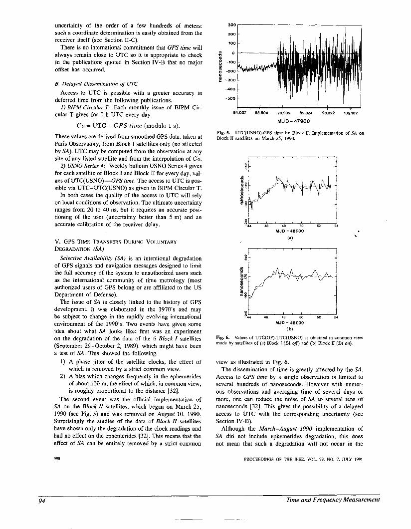
uncertainty of the order of a few hundreds of meters: such a coordinate determination is easily obtained from the receiver itself (see Section 11-C).
There is no international commitment that GPS time will always remain close to UTC so it is appropriate to check in the publications quoted in Section IV-B that no major offset has occurred.
B. Delayed Dissemination of UTC
deferred time from the following publications.
cular T gives for 0 h UTC every day
Access to UTC is possible with a greater accuracy in
I ) BIPM Circular T: Each monthly issue of BIPM Cir-
Co = UTC - GPS time (modulo 1 s).
These values are derived from smoothed GPS data, taken at Paris Observatory, from Block I satellites only (no affected by SA). UTC may be computed from the observation at any site of any listed satellite and from the interpolation of Co.
2) USNO Series 4: Weekly bulletin USNO Series 4 gives for each satellite of Block I and Block I1 for every day, val- ues of UTC(USN0)-GPS time. The access to UTC is pos- sible via UTC-UTC(USN0) as given in BIPM Circular T.
In both cases the quality of the access to UTC will rely on local conditions of observation. The ultimate uncertainty ranges from 20 to 40 ns, but it requires an accurate posi- tioning of the user (uncertainty better than 5 m) and an accurate calibration of the receiver delay.
V. GPS TIME TRANSFERS DURING VOLUNTARY DEGRADATION (SA)
Selective Availability (SA) is an intentional degradation of GPS signals and navigation messages designed to limit the full accuracy of the system to unauthorized users such as the international community of time metrology (most authorized users of GPS belong or are affiliated to the US Department of Defense).
The issue of SA is closely linked to the history of GPS development. It was elaborated in the 1970's and may be subject to change in the rapidly evolving international environment of the 1990's. Two events have given some idea about what SA looks like: first was an experiment on the degradation of the data of the 6 Block I satellites (September 29-October 2, 1989), which might have been a test of SA. This showed the following.
1) A phase jitter of the satellite clocks, the effect of which is removed by a strict common view.
2) A bias which changes frequently in the ephemerides of about 100 m, the effect of which, in common view, is roughly proportional to the distance [32].
The second event was the official implementation of SA on the Block II satellites, which began on March 25, 1990 (see Fig. 5) and was removed on August 10, 1990. Surprisingly the studies of the data of Block II satellites have shown only the degradation of the clock readings and had no effect on the ephemerides [32]. This means that the effect of SA can be entirely removed by a strict common
3 0 0
2 0 0 I
1 I I I
-500 I'
54.007 63.504 79.935 89.824 98.822 109.182
M J D - 47900
Fig. 5. Block I1 satellites on March 25, 1990.
UTC(USN0)-GPS time by Block 11. Implementation of SA on
i
'44 46 48 50 52 54
M J D - 4 8 0 0 0 !
(a) \.
[ " ' " " " I
844 46 48 50 52 54
MJD - 4 8 0 0 0
( b) Fig. 6. mode by satellites of (a) Block I (SA off) and (b) Block I1 (SA on).
Values of UTC(0P)-UTC(USN0) as obtained in common view
view as illustrated in Fig. 6. The dissemination of time is greatly affected by the SA.
Access to GPS time by a single observation is limited to several hundreds of nanoseconds. However with numer- ous observations and averaging time of several days or more, one can reduce the noise of SA to several tens of nanoseconds [32]. This gives the possibility of a delayed access to UTC with the corresponding uncertainty (see Section IV-B).
Although the March-August 1990 implementation of SA did not include ephemerides degradation, this does not mean that such a degradation will not occur in the
PROCEEDINGS OF THE IEEE, VOL. 79, NO. 7, JULY 1991
Time and Frequency Measurement 94
__ -. ~ --
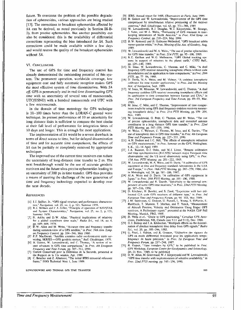
future. To overcome the problem of the possible degrada- tion of ephemerides, various approaches are being studied [ 131. The corrections to broadcast ephemerides affected by SA can be derived, as noted previously in Section III-B- 2), from precise ephemerides. But another possibil i ty can also be considered: this is the availability of differential corrections representing the bias introduced for SA. Such corrections could be made available within a few days and would restore the quality of the broadcast ephemerides without SA.
VI. CONCLUSIONS The use of GPS for time and frequency control has
already demonstrated the outstanding potential of this sys- tem. The permanent operation, worldwide coverage, low equipment cost and fully automatic reception makes GPS the most effective system of time dissemination. With SA 08 GPS is permanently and in real time disseminating GPS time with an uncertainty of several tens of nanoseconds, UTC(USN0) with a hundred nanoseconds and UTC with a few microseconds.
In the domain of time metrology the GPS technique is 10-100 times better than the LORAN-C ground wave technique. Its present performance of 10 ns uncertainty for long distance links is sufficient to compare the best clocks at their full level of performance for integration times of 10 days and longer. This is enough for most applications.
The implementation of SA would be a severe drawback in terms of direct access to time, but for delayed dissemination of time and for accurate time comparisons, the effects of SA can be partially or completely removed by appropriate techniques.
The improved use of the current time receivers can reduce the uncertainty of long-distance time transfer to 2 ns. The next breakthrough would be the use of accurate geodetic receivers and the future ultra-precise ephemerides leading to an uncertainty of 300 ps in time transfer. GPS thus provides a means of meeting the challenge of the new generation of time and frequency technology expected to develop over the next decade.
REFERENCES
[ 11 J. J. Spilker, Jr., “GPS signal structure and performance characteris- tics,” Navigafion, vol. 25, no. 2, p. 121, Summer 1978.
[2] R. J. Miliken and C. J . Zoller, “Principle of operation of NAVSTAR and System Characteristics,” Navigation, vol. 25, no. 2 , p. 121, Summer 1978.
[3] N. Ashby and D. W. Allan, “Practical implications of relativity for a global coordinate time scale,” Radio Sei., vol. 14, no. 4, pp. 649-669, 1979.
[4] D. W. Allan and M. Weiss, “Accurate time and frequency transfer during common-view of a GPS satellite,” in Proc. 34th Ann. Symp. on Frequency Control, pp. 334-346, May 1980.
[5] P. F. MacDoran, “Satellite emission radio inerferometric earth sur- veying, SERIES-GPS geodetic system,” Bull. Gtodt%ique, 1979.
[6] B. Guinot, W. Lewandowski, and C. Thomas, “A review of re- cent advances in GPS time comparisons,” in Proc. 4th European Frequency and Time Forum, pp. 307-312, 1990.
171 Comitt Consultatif pour la Dtfinition de la Seconde, presented at the Rapport de la l l e session, Apr. 1989.
[8] C. Boucher and Z. Altamimi, “The initial IERS terrestrial reference frame,” IERS Technical Note 1, June 1989.
LEWANDOWSKI AND THOMAS: GPS TIME TRANSFER
[9] IERS, Annual report for 1988, Observatoire de Paris, June 1989. [lo] B. Guinot and W. Lewandowski, “Improvement of the GPS time
comparisons by simultaneous relative positioning of the receiver antennas,” Bull. GPodtsique, vol. 63, pp. 371-386, 1989.
[ l l ] W. Lewandowski, R. J. Douglas, W. J. Klepczynski, W. Strange, J. Suter, and M.A. Weiss, “Positioning of CPS antennas in time- keeping laboratories of North America,” in Proc. 43rd Symp. on Frequency Control, pp. 218-224, May 1989.
[12] B. W. Remondi and B. Hofmann-Wellenhof, “GPS broadcast orbits versus precise orbits,’’ in Proc. Meeting oflnt. Ass. of Geodesy, Aug. 1989.
1131 W. Lewandowski and M. A. Weiss, “The use of precise ephemerides for GPS time transfer,” in Proc. 21st PTTI, pp. 95-106, 1989.
[14] R. E. Keilhan and W. G. Melbourne, “GPS Global tracking sys- tems in support of missions to the planet earth,” CSTG Bull., pp. 129-140, 1989.
[15] M. Imae, W. Lewandowski, C. Thomas, and C. Miki, “A dual frequency GPS receiver measuring ionospheric effects without code demodulation and its application to time comoarisons,” in Proc. 20th Pi’TI, pp. 77-86, 1988.
[16] D. Davis, M. A. Weiss, and M. Vidmar, “A codeless ionospheric calibrator for time transfer applications,” in Proc. 2nd Int. Meeting Inst. of Navigation, Sept. 1989.
[17] M. Imae, M. Miranian, W. Lewandowski, and C. Thomas, “A dual frequency codeless GPS receiver measuring ionospheric effects and its application to time comparison between Europe and USA,” in Proc. 3rd European Frequency and Time Forum, pp. 89-93, Mar. 1989.
[18] M. Imae, C. Miki, and C. Thomas, “Improvement of time compar- isons results by using GPS dual frequency codeless receivers measur- ing ionospheric delay,” in Proc. 22st PTTI Meeting, pp. 199-204, Nov. 1989.
1191 W. Lewandowski, G. Petit, C. Thomas, and M. Weiss, “The use of precise ephemerides, ionospheric data and corrected antenna coordinates in a long distance GPS time transfer,” in Proc. 22nd P V I Meeting, pp. 547-558, 1990.
[20] M. Weiss, T. Weissert, C. Thomas, M. Imae, and K. Davies, “The use of ionospheric data in GPS time transfer,” in Proc. 4th European Time and Frequency Forum, pp. 327-333, 1990.
[21] A. H. Dodson and J. C. Hill, “The effects of atmospheric refraction on GPS measurements,” in Proc. Seminar on the GPS, Nottineham.
I
U.K., 12-14 April 1989. [22] J. A. Buisson, 0. J. Oaks, and M. J. Lister, “Remote calibration
and time synchronization (R-CATS) between major European time observatories and the US naval observatory using GPS,” in Proc. 17th Ann. PTTI Meeting, pp. 201-222, 1985.
[23] W. Lewandowski, M. A. Weiss, and D. Davis, “A calibration of GPS equipment at time and frequency standards laboratories in the USA and Europe,” in Proc. 18th PTTIMeeting, pp. 265-279, 1986; also in Metrologia, vol. 24, pp. 181-186, 1987.
(241 M.A. Weiss and D. Davis, “A calibration of GPS equipment in Japan,” in Proc. 20th PWI Meeting, pp. 101-106, 1988.
[25] W. Lewandowski and R. Tourde, “Sensitivity to the external tem- perature of some GPS time receivers,” in Proc. 22nd PTTI Meeting, pp. 307-316, 1990.
[26] D. Kirchner, H. Bessler, and S. Fassl, “Experience with two col- located C/A code GPS receivers of different type,” in Proc. 3rd European Time and Frequency Forum, pp. 94-103, Mar. 1989.
[27] J. M. Srinivasan, C. Duncan, G. Purcell, L. Young, S. DiNardo, E. Hushbeck, T. Munson, T. Meehan, and T. Yunck, “Measurement of Aircraft Position, Velocity and Orientation Using Rogue GPS receivers, A Preliminary report,” presented at the NASA CDP Fall Meeting, Munich, FRG, 1988.
[28] D. Wells ef al., “Guide to GPS positioning,” Canadian GPS Asso- ciates, Fredericton, NB, Canada (see 9.11 and 9.12), Dec. 1986.
[29] G. J. Bishop and J. A. Klobuchar, “Multipath effects on the determi- nation of absolute ionospheric time delay from GPS signals,” Radio Sei., vol. 20, pp, 388-396, 1985.
[30] G. Nard, J. Rabian, and R. Gounon, “Utilisation des signaux du GPS en mode difftrentiel instantant pour les applications temps- frtquence de haute prtcision,” in Proc. 1st European Time and Frequency Forum, pp. 237-248, 1987.
1311 B. Guinot, “Time transfers by GPS,” to be published in Proc. GPS Workshop, European Centre for Geodynamics and Seismology, 20-21 Nov. 1989, to be published.
[32] D. W. Allan, M. Granveaud, W. J. Klepczynski and W. Lewandowski, “GPS time transfer with implementation of selective availability,” in Proc. 22nd PTTI meeting, pp. 145-156, 1990.
999
Time and Frequency Measurement 95
Wlodzimien Lewandowski was horn in Lower Claudine Thomas was born in 1955 In Lugnv Silesia, Poland, in 1949. He received the masters degree in geodetic science from the Warsaw Polytechnic in 1976, and the doctorate degree in geographical science from the French Geo- graphical Institute (IGN) in 1980.
He joined the staff of the Earth Rotation Section of the Bureau lnternational de I’Heure (BIH) in Paris in 1982. In 1985 he moved to the newly created Time Section of the Bureau International des Poids et Mesures (BIPM) in
Sbvres, following the transfer of International Atomic Time (TAI) from the BIH to the BIPM. Since then he has participated in the elaboration and diffusion of the TAI and the UTC international time scales. He has also engaged in research on the use of space techniques for time transfer, especially on the use of the GPS. In 1989 he spent six months with the Time and Frequency Division of the National Institute of Standards and Technology in Boulder, Colorado. Since 1988, he has participated in the work of the Civil GPS Service Steering Committee.
1000
- , Champagne, France. She studied fundamental physics at the Ecole Normale Supkrieure and the Pierre et Marie Curie University in Paris from 1975 to 1979. She received the Agrtgation de Physique in 1979.
In October 1980, she took a position as Assis- tant at the Ecole Normale Suptrieure where her teaching duties were mainly classical mechanics and electromagnetism. At that time she was involved in a research project on atomic physics
at the Laboratoire Aim6 Cotton in Orsay near Paris, where she completed her Thhe de Troisikme Cycle in 1981. She received the doctorate degree in 1987, her dissertation described the behavior of Rydberg atoms in the presence of a strong magnetic field. She joined the Time Section of the Bureau International des Poids et Mesures as a Physicist in March 1987. In October 1990, she became Principal Physicist and Head of the Time Section where she is now responsible for the elaboration and diffusion of the international time references TAI and UTC. Her personal research is concerned mainly with time scale algorithms and time comparisons.
PROCEEDINGS OF THE IEEE, VOL. 79, NO. 7, JULY 1991
96 Time and Frequency Measurement
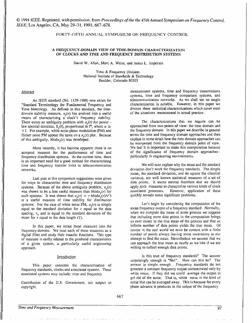
0 1991 IEEE. Reprinted, with permission, from Proceedings of the the 45th Annual Symposium on Frequency Control, IEEE Los Angeles, CA, May 29-31,1991; 667-678.
FORTY-FIFTH A N N U A L S Y M P O S I U M O N F R E Q U E N C Y C O N T R O L
A FREQUENCY-DOMAIN VIEW OF TIMEDOMAIN CHARACTERIZATION OF CLOCKS AND TIME AND FREQUENCY DISTRIBUTION SYSTEMS
David W. Allan, Marc A. Weiss, and James L. Jespersen
Time & Frequency Division National Institute of Standards & Technology
Boulder, Colorado 80303
Abstract
An IEEE standard (No. 1139-1988) now exists for "Standard Terminology for Fundamental Frequency and Time Metrology. As defined in this standard, the time- domain stability measure, u,(T) has evolved into a useful means of characterizing a clock's frequency stability. There exists an ambiguity problem with uy(7) for power - law spectral densities, S,(f), proportional to fa, where cr 2 + 1. For exampIe, white noise phase modulation (PM) and flicker noise PM appear the same on a u,(T) plot. Because of this ambiguity, Moduy(r) was developed.
More recently, it has become apparent there is no accepted measure for the performance of time and frequency distribution systems. At the current time, there is an important need for a good method for characterizing time and frequency transfer links in telecommunication networks.
Last year at this symposium suggestions were given for ways to characterize time and frequency distribution systems. Because of the above ambiguity problem, uY(7) was shown to be a less useful measure than Moduy(.r) for such systems. It was shown that ux(7) = 7.Moduy(7)h/3 is a useful measure of time stability for distribution systems. For the case of white noise PM, ~ ~ ( 7 ) is simply equal to the standard deviation for 7 equal to the data spacing, ro and is equal to the standard deviation of the mean for 7 equal to the data length (T).
In this paper, we recast these measures into the frequency-domain. We treat each of these measures as a digital filter and study their transfer functions. This type of measure is easily related to the passband characteristics of a given system, a particularly useful engineering approach.
Introduction
This paper concerns the characterization of frequency standards, clocks and associated systems. These associated systems may include: time and frequency
Contribution o f the U.S. Government, not subject to copyright.
measurement systems, time and frequency transmissions systems, time and frequency comparison systems, and telecommunication networks. As we shall see no single characterization is suitable. However, in this paper we discuss three statistical characterizations which cover most of the situations encountered in actual practice.
The characterizations that we require can be approached from two points of view: the time domain and the frequency domain. In this paper we describe in general terms the time and frequency domain approaches and then explain in some detail how the time domain approaches can be interpreted from the frequency domain point of view. We feel it is important to make this interpretation because of the significance of frequency domain approaches-- particularly in engineering environments.
We will next explain why the mean and the standard deviation don't work for frequency standards. The simple mean, the standard deviation, and its square the classical variance, are well known statistical measures of a set of data points. It seems natural therefore that we should apply such measures to characterize various kinds of clock associated processes. However, application of these quickly reveals some significant problems.
Let's begin by considering the computation of the mean frequency output of a frequency standard. Normally, when we compute the mean of some process we suppose that including more data points in the computation brings us ever closer to the true mean of the process and that an infinite number of data points yields the true mean. Of course in the real world we must be content with a finite number of points always leaving some uncertainty in our attempt to find the mean. Nevertheless we assume that we can approach the true mean as nearly as we like if we are willing to collect enough data points.
Is this true of frequency standards? The answer surprisingly enough is "No!". How can this be? The answer is simple enough. Frequency standards do not generate a constant frequency output contaminated only by white noise. If they did we could average the output to get rid of the noise. That is, white noise is the kind of noise that can be averaged away. This is because for every phase advance it produces in the output of the frequency
667
Eme and Frequency Measurement 97
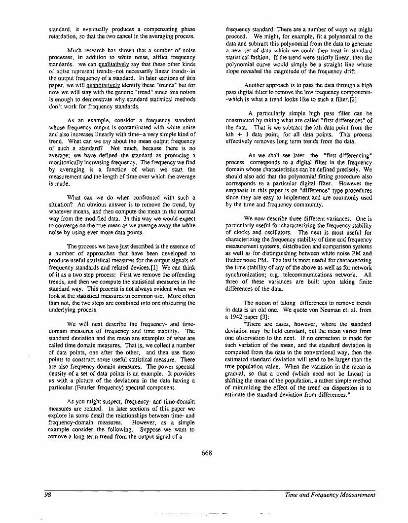
standard, it eventually produces a compensating phase retardation, so that the two cancel in the averaging process.
Much research has shown that a number of noise processes, in addition to white noise, afflict frequency standards. we can qualitatively say that these other kinds of noise represent trends--not necessarily linear trends--in the output frequency of a standard. In later sections of this paper, we will auantitatively identify these "trends" but for now we will stay with the generic "trend" since this notion is enough to demonstrate why standard statistical methods don't work for frequency standards.
As an example, consider a frequency standard whose frequency output is contaminated with white noise and also increases linearly with time--a very simple kind of trend. What can we say about the mean output frequency of such a standard? Not much, because there is no average; we have defined the standard as producing a monitonically increasing frequency. The frequency we find by averaging is a function of when we start the measurement and the length of time over which the average is made.
What can we do when confronted with such a situation? An obvious answer is to remove the trend, by whatever means, and then compute the mean in the normal way from the modified data. In this way we would expect to converge on the true mean as we average away the white noise by using ever more data points.
The process we have just described is the essence of a number of approaches that have been developed to produce useful statistical measures for the output signals of frequency standards and related devices. [ 11 We can think of it as a two step process: First we remove the offending trends, and then we compute the statistical measures in the standard way. This process is not always evident when we look at the statistical measures in common use. More often than not, the two steps are combined into one obscuring the underlying process.
We will next describe the frequency- and time- domain measures of frequency and time stability. The standard deviation and the mean are examples of what are called time domain measures. That is, we collect a number of data points, one after the other, and then use these points to construct some useful statistical measure. There are also frequency domain measures. The power spectral density of a set of data points is an example. It provides us with a picture of the deviations in the data having a particular (Fourier frequency) spectral component.
As you might suspect, frequency- and time-domain measures are related. In later sections of this paper we explore in some detail the relationships between time- and frequency-domain measures. However, as a simple example consider the following. Suppose we want to remove a long term trend from the output signal of a
frequency standard. There are a number of ways we might proceed. We might, for example, fit a polynomial to the data and subtract this polynomial from the data to generate a new set of data which we could then treat in standard statistical fashion. If the trend were strictly linear, then the polynomial curve would simply be a straight line whose slope revealed the magnitude of the frequency drift.
Another approach is to pass the data through a high pass digital filter to remove the low frequency components- -which is what a trend looks like to such a filter.[2]
A particularly simple high pass filter can be constructed by taking what are called "first differences" of the data. That is we subtract the kth data point from the kth + 1 data point, for all data points. This process effectively removes long term trends from the data.
As we shall see later the "first differencing" process corresponds to a digital filter in the frequency domain whose characteristics can be defined precisely. We should also add that the polynomial fitting procedure also corresponds to a particular digital filter. However the emphasis in this paper is on "difference" type procedures since they are easy to implement and are commonly used by the time and frequency community.
We now describe three different variances. One is particularly useful for characterizing the frequency stability of clocks and oscillators. The next is most useful for characterizing the frequency stability of time and frequency measurement systems, distribution and comparison systems as well as for distinguishing between white noise PM and flicker noise PM. The last is most useful for characterizing the time stability of any of the above as well as for network synchronization; e.g. telecommunications network. All three of these variances are built upon taking finite differences of the data.
The notion of taking differences to remove trends in data is an old one. We quote von Neuman et. al. from a 1942 paper [3]:
"There are cases, however, where the standard deviation may be held constant, but the mean varies from one observation to the next. If no correction is made for such variation of the mean, and the standard deviation is computed from the data in the conventional way, then the estimated standard deviation will tend to be larger than the true population value. When the variation in the mean is gradual, so that a trend (which need not be linear) is shifting the mean of the population, a rather simple method of minimizing the effect of the trend on dispersion is to estimate the standard deviation from differences. "
668
98 Time and Frequency Measurement
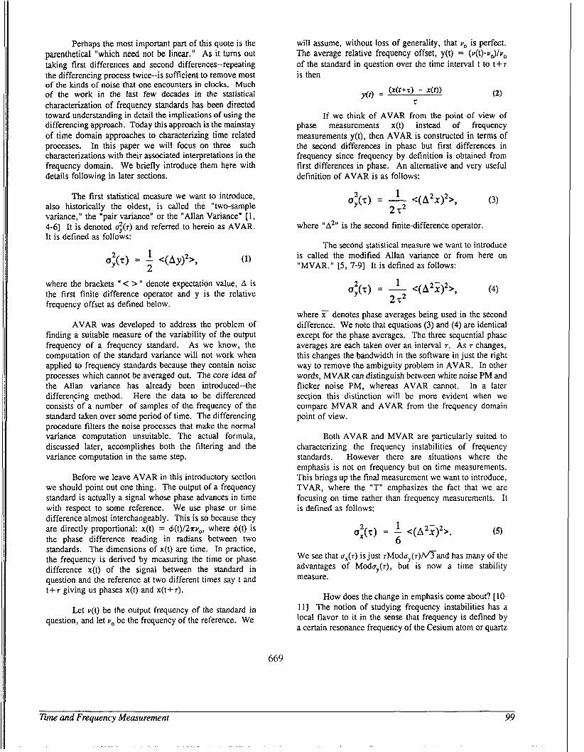
Perhaps the most important part of this quote is the parenthetical "which need not be linear." As it turns out taking first differences and second differences--repeating the differencing process twice--is sufficient to remove most of the kinds of noise that one encounters in clocks. Much of the work in the last few decades in the statistical characterization of frequency standards has been directed toward understanding in detail the implications of using the differencing approach. Today this approach is the mainstay of time domain approaches to characterizing time related processes. In this paper we will focus on three such characterizations with their associated interpretations in the frequency domain. We briefly introduce them here with details following in later sections.
The first statistical measure we want to introduce, also historically the oldest, is called the "two-sample variance," the "pair variance" or the "Allan Variance" [l, 4-61 It is denoted <(r) and referred to herein as AVAR. It is defined as follows:
(1) 2 1 a,(.) = - <(AY)~> ,
2 where the brackets ' I < > " denote expectation value, A is the first finite difference operator and y is the relative frequency offset as defined below.
AVAR was developed to address the problem of finding a suitable measure of the variability of the output frequency of a frequency standard. As we know, the computation of the standard variance will not work when applied to frequency standards because they contain noise processes which cannot be averaged out. The core idea of the Allan variance has already been introduced--the differen,cing method. Here the data to be differenced consists of a number of samples of the frequency of the standard taken over some period of time. The differencing procedure filters the noise processes that make the normal variance computation unsuitable. The actual formula, discussed later, accomplishes both the filtering and the variance computation in the same step.
Before we leave AVAR in this introductory section we should point out one thing. The output of a frequency standard is actually a signal whose phase advances in time with respect to some reference. We use phase or time difference almost interchangeably. This is so because they are directly proportional: x(t) = 4(t)/2rv0, where 4(t) is the phase difference reading in radians between two standards. The dimensions of x(t) are time. In practice, the frequency is derived by measuring the time or phase difference x(t) of the signal between the standard in question and the reference at two different times say t and t+r giving us phases x(t) and x(t+r).
Let v(t) be the output frequency of the standard in question, and let vo be the frequency of the reference. We
will assume, without loss of generality, that v, is perfect. The average relative frequency offset, y(t) = (v(t)-vo)/vo of the standard in question over the time interval t to t+r is then
(2) W + s ) - m) 7
If we think of AVAR from the point of view of phase measurements x(t) instead of frequency measurements y(t), then AVAR is constructed in terms of the second differences in phase but first differences in frequency since frequency by definition is obtained from first differences in phase. An alternative and very useful definition of AVAR is as follows:
YO) =
(3) 2 1 2 2 u,(T) - <(A X ) >, 2 T2
where "A2" is the second finite-difference operator.
The second statistical measure we want to introduce is called the modified Allan variance or from here on "MVAR." [5, 7-91 It is defined as follows:
(4) u,(T) 2 = - 1 <(A 2- X ) 2 >, 2 T2
where X denotes phase averages being used in the second difference. We note that equations (3) and (4) are identical except for the phase averages. The three sequential phase averages are each taken over an interval r. As r changes, this changes the bandwidth in the software in just the right way to remove the ambiguity problem in AVAR. In other words, MVAR can distinguish between white noise PM and flicker noise PM, whereas AVAR cannot. In a later section this distinction will be more evident when we compare MVAR and AVAR from the frequency domain point of view.
Both AVAR and MVAR are particularly suited to characterizing the frequency instabilities of frequency standards. However there are situations where the emphasis is not on frequency but on time measurements. This brings up the final measurement we want to introduce, TVAR, where the "T" emphasizes the fact that we are focusing on time rather than frequency measurements. It is defined as follows:
(5) &T) = - 1 <(A 2 - 2 x ) '. 6
We see that uX(7) is just 7Moduy(r)A6and has many of the advantages of Modu,(r), but is now a time stability measure.
How does the change in emphasis come about? [IO- 111 The notion of studying frequency instabilities has a local flavor to it in the sense that frequency is defined by a certain resonance frequency of the Cesium atom or quartz
669
Eme and Frequency Measurement 99
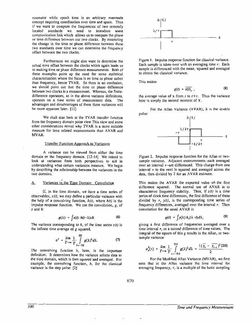
resonator while epoch time is an arbitrary manmade concept requiring coordination over time and space. Thus if we want to compare the frequencies of two remotely located standards we need to introduce some communication link which allows us to compare the phase or time difference betwcen our two clocks. By measuring the change in the time or phase difference between these two standards over time we can determine the frequency offset between the two clocks.
Furthermore we might also want to determine the actual time offset between the clocks which again leads us to making time or phase difference measurements. Both of these examples point up the need for some statistical characterization where the focus is on time or phase rather than frequency, hence TVAR. So there is no confusion, we should point out that the time or phase difference between two clocks is a measurement. Whereas, the finite- difference operators, as in the above variance definitions, operates on a time series of measurement data. The advantages and disadvantages of these three variances will be more apparent later. [ I 13
We shall also look at the TVAR transfer function from the frequency domain point view This view and some other considerations reveal why TVAR is a more suitable measure for time related measurements than AVAR and MVAR.
Transfer Function Approach to Variances
A variance can be viewed from either the time domain or the frequency domain. [12-141 We intend to look at variances from both perspectives to aid in understanding what certain variances measure. We begin by describing the relationship between the variances in the two domains.
- A. Variances in the Time Domain: Convolution
If, in the time domain, we have a time series of observables, x(t), we may define a particular variance with the help of a convolving function, h(t), where h(f) is the impulse response function. We use the convolution, g, of x and h:
g(1) = /x(r) .h(t-A)dt. (6)
The variance corresponding to h, of the time series x(t) is the infinite time average of g squared,
The convolving function h, here, is the important definition. It determines how the variance selects data in the time domain, which is then squared and averaged. For example, the convolving function, h, for the classical variance is the step pulse: [2]
67 0
I 7
Figure 1. Impulse response function for classical variance. Each sample is taken over with an averaging time 7. Each sample is differenced with the mean, squared and averaged to obtain the classical variance.
This makes
S(t) = x(t>, 2 (8)
the average value of x from t to f + T . Thus the variance here is simply the second moment of X.
For the Allan Variance (AVAR), h is the double pulse:
i"
Figure 2. Impulse response function for the Allan or two- sample variance. Adjacent measurements-each averaged over an interval T--are differenced. This change from one interval T to the next is squared and averaged across the data, then divided by 2 for an AVAR estimate.
This makes the AVAR the expected value of. the first difference squared. The normal use of AVAR is to characterize frequency stability. Thus, if x(f) is a time series of clock time differences, the first difference of these divided by 7, y(c), is the corresponding time series of frequency differences, averaged over the interval T. Then convolution for the usual AVAR is
giving a first difference of frequencies averaged over a time interval T, or a second difference of time values. The integral of the square of this g results in the Allan, or two- sample variance
For the Modified Allan Variance (MVAR), we first note that in the Allan variance the time interval for averaging frequency, T, is a multiple of the basic sampling
100 Time and Frequency Measurement
~ ~
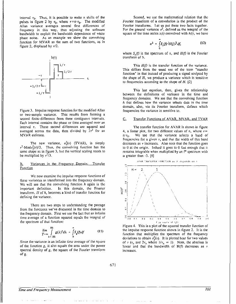
interval r0. Thus, it is possible to make n shifts of the pulses in figure 2 by 70, where 7 = n ~ ~ . The modified Allan variance averages several first differences of frequency in this way, thus adjusting the software bandwidth to exploit the bandwidth dependence of white phase noise. As an example we show the convolving function for MVAR as the sum of two functions, as in figure 2, displaced by 7 / 2 .
Second, we use the mathematical relation that the Fourier transform of a convolution is the product of the Fourier transforms. Let us put these two facts together. For the general variance 2, defined as the integral of the square of the time series x(r) convolved with h(t), we have
"
o2 = /S#)*!H(f)pdJ (12) 0
where Sxfl is the spectrum of x, and Hlf) is the Fourier transform of h.
I
Figure 3. Impulse response function for the modified Allan or two-sample variance. This results from forming a second finite-difference from three contiguo9s intervals. Each interval contains the phase or time averaged over an interval 7. These second differences are squared and averaged across the data, then divided by 2 2 for an MVAR estimate.
The new variance, U?(T) (TVAR), is simply &MOd<(7)/3. Thus, the convolving function has the same shape as in figure 3; but the vertical scaling needs to be multiplied by 2/3.
& Variances in the Freauencv Domain: Transfer Function
We now examine the impulse response functions of these variances as transformed into the frequency domain. We will see that the convolving function h again is the important definition. In this domain, the Fourier transform, H of h, becomes a kind of transfer function for defining the variance.
There are two steps to understanding the passage from the functions we've discussed in the time domain to the frequency domain. First we use the fact that an infinite time average of a function squared equals the integral of the spectrum of that function:
-
Since the variance is an infinite time average of the square of the function g, it also equals the area under the power spectral density of g, the square of the Fourier transform of g.
This HO) is the transfer function of the variance. This differs from the usual use of the term "transfer function" in that instead of producing a signal sculpted by the shape of H , we produce a variance which is sensitive to frequencies according to the shape of H. [2]
This last equation, then, gives the relationship between the definitions of variance in the time and frequency domains. We see that the convolving function h that defines how the variance selects data in the time domain, also, via its Fourier transform, defines which frequencies the variance is sensitive to.
s;L Transfer Functions of AVAR. MVAR. and TVAR
The transfer function for AVAR is shown in figure 4, a linear plot, for two different values of n, where T=
n.7,. We see that the variance selects a band of frequencies for a given T, and that the width of this band decreases as 7 increases. Also note that the function goes to 0 at the origin. Indeed it goes to 0 fast enough that it remains integrable when multiplied by an fn spectrum with a greater than -3. 161
IAVAH I H A N s k C H I U N C l l O N a r 11 d e p e n d s 011 i
N - n = 2 1 'P
O a o 0 1 0 2 0 3 0 4 0 5 i i 6 0 7 O B 0 9 1 0
I rn u n i t s ,of I / r
Figure 4. This is a plot of the squared transfer function of the impulse response function shown in figure 2. It is the function that multiplies the spectrum of the frequency deviations to obtain <(T). It is plotted hear for two values of 7 (7, and 27, where 1/~, = 1). Note, the abscissa is linear and that the bandwidth of H(f) decreases as 7
increases.
67 1
Time and Frequency Measurement 101
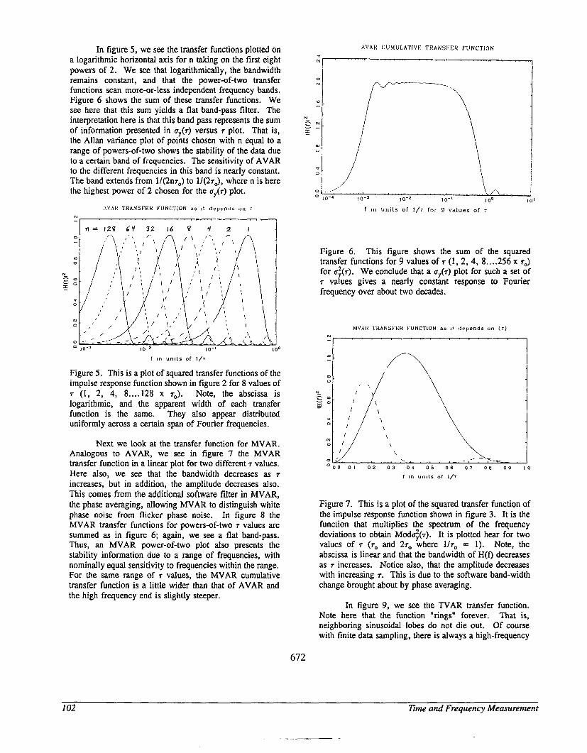
In figure 5 , we see the transfer functions plotted on a logarithmic horizontal axis for n taking on the first eight powers of 2. We see that logarithmically, the bandwidth remains constant, and that the power-of-two transfer functions scan more-or-less independent frequency bands. Figure 6 shows the sun1 of these transfer functions. We see here that this sum yields a flat band-pass filter. The interpretation here is that this band pass represents the sum of information presented in u , ( ~ ) versus 7 plot. That is, the Allan variance plot of points chosen with n equal to a range of powers-of-two shows the stability of the data due to a certain band of frequencies. The sensitivity of AVAR to the different frequencies in this band is nearly constant. The band extends from 1/(2n7,) to 1/(27J, where n is here the highest power of 2 chosen for the u,(r) plot.
\ \ ' A t < 'TRANSFER FUNCTION as 11 d e p e n d s o n r N -
n = 128 k f 32 1 6 8 4 2 I I
A V A R CUMU1.ATIVF TRANSFER FUNCTION -r N
10-2 10-1 I O 0
I in u n i t s of I/'
Figure 5 . This is a plot of squared transfer functions of the impulse response function shown in figure 2 for 8 values of 7 (1, 2, 4, 8 .... 128 x 7,). Note, the abscissa is logarithmic, and the apparent width of each transfer function is the same. They also appear distributed uniformly across a certain span of Fourier frequencies.
Next we look at the transfer function for MVAR. Analogous to AVAR, we see in figure 7 the MVAR transfer function in a linear plot for two different 7 values. Here also, we see that the bandwidth decreases as 7
increases, but in addition, the amplitude decreases also. This comes from the additional software filter in MVAR, the phase averaging, allowing MVAR to distinguish white phase noise from flicker phase noise. In figure 8 the MVAR transfer functions for powers-of-two T values are summed as in figure 6; again, we see a flat band-pass. Thus, an MVAR power-of-two plot also presents the stability information due to a range of frequencies, with nominally equal sensitivity to frequencies within the range. For the same range of 7 values, the MVAR cumulative transfer function is a little wider than that of AVAR and the high frequency end is slightly steeper.
672
/ ,/
I
0;- ' , , , ,,,
10-3 10-2 10-1 100 I O ' O 10.'
f in u n i t s of 1 / ~ f o r 9 v a l u e s of T
Figure 6. This figure shows the sum of the squared transfer functions for 9 values of 7 (1, 2, 4, 8....256 x 73 for r$(7). We conclude that a uJ7) plot for such a set of 7 values gives a nearly constant response to Fourier frequency over about two decades.
M V A R TRANSFER FUNCTION a s 1 1 d r p e n d s on ( r ) N - I
I in un i t s of I/T
Figure 7. This is a plot of the squared transfer function of the impulse response function shown in figure 3. It is the function that multiplies the spectrum of the frequency deviations to obtain Mod+(r). It is plotted hear for two values of 7 (7, and 27, where lh, = 1). Note, the abscissa is linear and that the bandwidth of H(f) decreases as 7 increases. Notice also, that the amplitude decreases with increasing 7. This is due to the software band-width change brought about by phase averaging.
In figure 9, we see the TVAR transfer function. Note here that the function "rings" forever. That is, neighboring sinusoidal lobes do not die out. Of course with finite data sampling, there is always a high-frequency
I02 Eme and Frequency Measurement
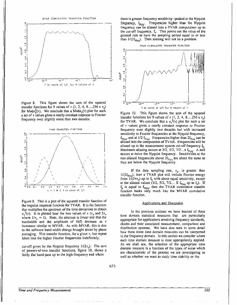
MVAR CUMIII.ATIVE TRANSFER FUNCTION
::I
o c / \ /
f In u n i t s of I/T f o r 9 v a l u e s of T
Figure 8. This figure shows the sum of the squared transfer functions for 9 values of 7 (1, 2, 4, 8....256 x 7,) for Mod4(.r). We conclude that a Moda,(.r) plot for such a set of 7 values gives a nearly constant response to Fourier frequency over slightly more than two decades.
TVAR TRANSFER VIINCTION r J
v N
\ \
\ \ \ , \
Figure 9. This is a plot of the squared transfer function of the impulse response function for TVAR. It is the function that multiplies the spectrum of the time deviations to obtain a,'(.). It is plotted hear for two values of 7 ( T ~ and 27, where UT, = 1). Note, the abscissa is linear and that the bandwidth and the amplitude of H(9 decrease as 7 increases--similar to MVAR. As with MVAR, this is due to the software band-width change brought about by phase averaging. This transfer function, for a given 7, has repeat lobes into the higher Fourier frequencies indefinitely.
cut-off given by the Nyquist frequency 1/(27,). The sum of powers-of-two transfer functions, figure 10, shows a fairly flat band-pass up to the high-frequency end where
67 3
there is greater frequency sensitivity--peaked at the Nyquist frequency, fNys. Frequencies higher than the Nyquist frequency can be aliased into a TVAR computation up to the cut-off frequency, fh. This points out the value of the general rule to have the sampling period equal to or less than 1/(2fNyq). Then aliasing will not be a problem.
TVAR CUMULATIVE TRANSFER FUNCTION m -
L O IO-' lo-' 10-2 lo-' I ow 10'
I in units of 1/7 for 9 v a l u e s of T
Figure 10. This figure shows the sum of the squared transfer functions for 9 values of 7 (1, 2, 4, 8....256 x 7,) for TVAR. We conclude that a 0,2(7) plot for such a set of 7 values gives a nearly constant response to Fourier frequency over slightly two decades but with increased sensitivity to Fourier frequencies at the Nyquist frequency, fNyq, and at 1/2 fNyq. Frequencies higher than 2fYy, can be aliased into the computation of TVAR. Frequencies will be aliased up to the measurement system cut-off frequency fh. Maximum aliasing occurs at 3/2, 5/2, 7/2 ... x fNuq. A null occurs at twice the Nyquist frequency. Sensitivities at the non-aliased frequencies above 2fNyq are about the Same as they are below the Nyquist frequency.
If the data sampling rate, 7,, is greater than 1/(2fNyq), then a TVAR plot will include Fourier energy from 1 / (2n~J up to fh with about equal sensitivity, except at the aliased values (312, 512, 7/2 ... X fNy up to fh). If fh is equal to fNyq, then the TVAR cumulative transfer function looks very much like the MVAR cumulative transfer function.
Applications and Discussion
In the previous sections we have learned of three time domain statistical measures that are particularly appropriate for applications involving frequency standards, clocks and their associated measurement, comparison and distribution systems. We have also seen in some detail how these three time domain measures can be interpreted in the frequency domain. In this section we consider where each time domain measure is most appropriately applied. As we shall see, the selection of the appropriate time domain measure is a function of the types of noise which are characteristic of the process we are investigating as well as whether we want to study time stability or the
Time and Frequency Measurement 103
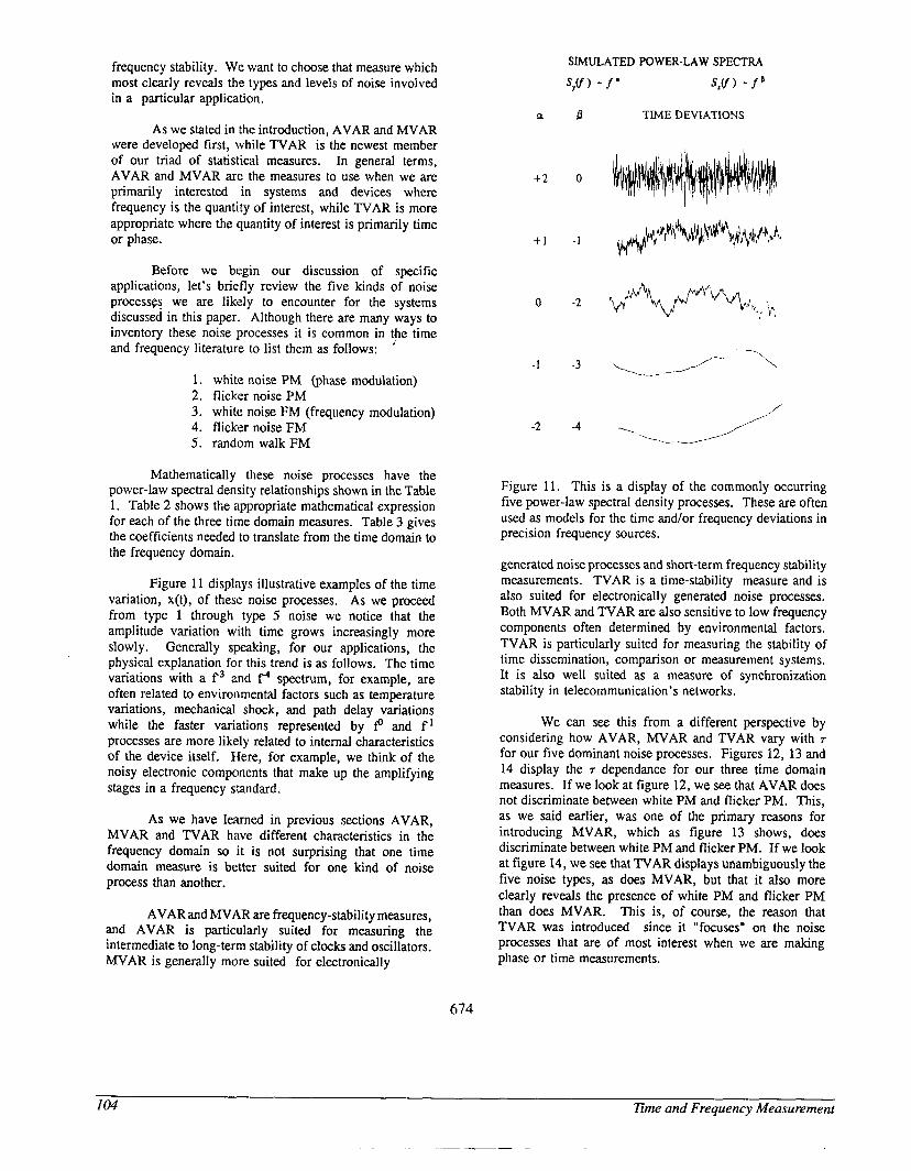
frequency stability. We want to choose that measure which most clearly reveals the types and levels of noise involved in a particular application.
As we stated in the introduction, AVAR and MVAR were developed first, while TVAR is the newest member of our triad of statistical measures. In general terms, AVAR and MVAR arc the measures to use when we are primarily interested in systems and devices where frequency is the quantity of interest, while TVAR is more appropriate where the quantity of interest is primarily time or phase.
Before we begin our discussion of specific applications, let’s briefly review the five kinds of noise processes we are likely to encounter for the systems discussed in this paper. Although there are many ways to inventory these noise processes it is common in the time and frequency literature to list them as follows:
’
1. white noise PM @hase modulation) 2. flicker noise PM 3. white noise FM (frequency modulation) 4. flicker noise FM 5. random walk FM
Mathematically these noise processes have the power-law spectral density relationships shown in the Table 1. Table 2 shows the appropriate mathematical expression for each of the three time domain measures. Table 3 gives the coefficients needed to translate from the time domain to the frequency domain.
Figure 11 displays illustrative examples of the time variation, x(t), of these noise processes. As we proceed from type 1 through type 5 noise we notice that the amplitude variation with time grows increasingly more slowly. Generally speaking, for our applications, the physical explanation for this trend is as follows. The time variations with a f3 and f4 spectrum, for example, are often related to environmental factors such as temperature variations, mechanical shock, and path delay variations while the faster variations represented by P and f’ processes are more likely related to internal characteristics of the device itself. Here, for example, we think of the noisy electronic components that make up the amplifying stages in a frequency standard.
As we have learned in previous sections AVAR, MVAR and TVAR have different characteristics in the frequency domain so it is not surprising that one time domain measure is better suited for one kind of noise process than another.
AVAR and MVAR are frequency-stability measures, and AVAR is particularly suited for measuring the intermediate to long-term stability of clocks and oscillators. MVAR is generally more suited for electronically
ff
+ 2
+ 1
0
- 1
-2
SIMULATED POWER-LAW SPECTRA s,v, - f * s,v, - f
B
0
-1
-2
-3
-4
TIME DEVIATIONS
Figure 11. This is a display of the commonly occumng five power-law spectral density processes. These are often used as models for the time andlor frequency deviations in precision frequency sources.
generated noise processes and short-term frequency stability measurements. TVAR is a time-stability measure and is also suited for electronically generated noise processes. Both MVAR and TVAR are also sensitive to low frequency components often determined by environmental factors. TVAR is particularly suited for measuring the stability of time dissemination, comparison or measurement systems. It is also well suited as a measure of synchronization stability in telecommunication’s networks.
We can see this from a different perspective by considering how AVAR, MVAR and TVAR vary with T for our five dominant noise processes. Figures 12, 13 and 14 display the T dependance for our three time domain measures. If we look at figure 12, we see that AVAR does not discriminate between white PM and flicker PM. This, as we said earlier, was one of the primary reasons for introducing MVAR, which as figure 13 shows, does discriminate between white PM and flicker PM. If we look at figure 14, we see that TVAR displays unambiguously the five noise types, as does MVAR, but that it also more clearly reveals the presence of white PM and flicker PM than does MVAR. This is, of course, the reason that TVAR was introduced since it “focuses“ on the noise processes that are of most interest when we are making phase or time measurements.
674
IO4 Time and Frequency Measurement
~
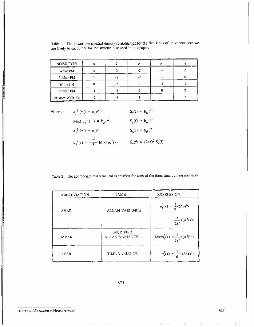
Table 1. The power-law spectral density relationships for the five kinds of noise processes we are likely to encounter for the systems discussed in this paper.
NOISE TYPE a B P
White PM 2 0 -2
Flicker PM 1 -1 -2
White FM 0 -2 -1
Flicker FM -1 -3 0
Random Walk FM -2 -4 1
1
2
3
P’
-3
-2
-1
0
1
Table 2. The appropriate mathematical expression for each of the three time domain measures.
ABBREVIATION NAME
AVAR
MVAR
TVAR
ALLAN VARIANCE
MODIFIED ALLAN VARIANCE
TIME VARIANCE
675
I1 ~ ~~
EXPRESSION
ay(r) 2 = -<(Ay)’> 1 2
= -<(A2x)2> 1
2r2
2 1 Mods,( r ) =--<(A 2?)2> 2 T2
Eme and Frequency Measurement I05
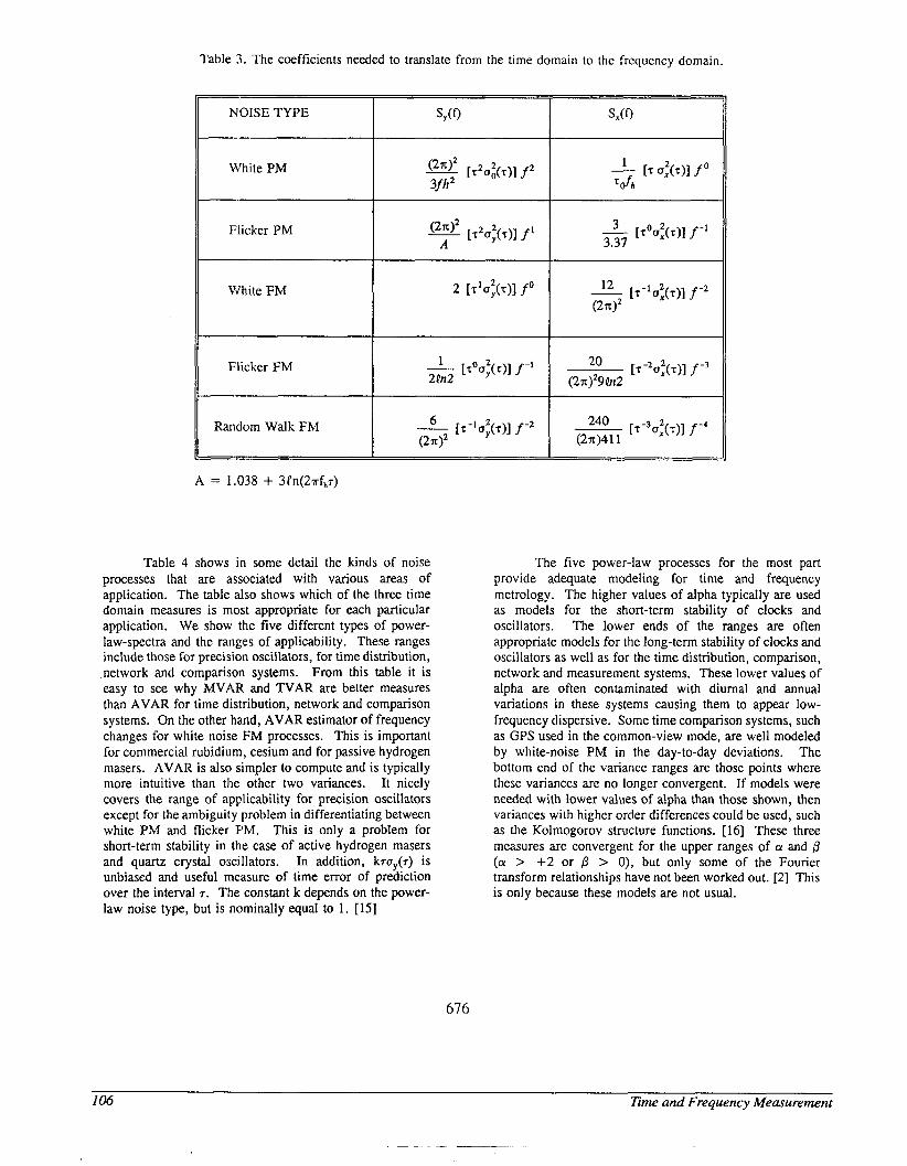
Table 3. The coefficients needed to translate from the time domain to the frcquency domain.
Random Walk FM
A = 1.038 + 3Pn(2.irfh7)
Table 4 shows in some detail the kinds of noise processes that are associated with various areas of application. The table also shows which of the three time domain measures is most appropriate for each particular application. We show the five different types of power- law-spectra and the ranges of applicability. These ranges include those for precision oscillators, for time distribution, network and comparison systems. From this table it is easy to see why MVAR and TVAR are better measures than AVAR for time distribution, network and comparison systems. On the other hand, AVAR estimator of frequency changes for white noise FM processes. This is important for commercial rubidium, cesium and for passive hydrogen masers. AVAR is also simpler to compute and is typically more intuitive than the other two variances. It nicely covers the range of applicability for precision oscillators except for the ambiguity problem in differentiating between white PM and flicker PM. This is only a problem for short-term stability in the case of active hydrogen masers and quartz crystal oscillators. In addition, k7uy(7) is unbiased and useful measure of time error of prediction over the interval 7 . The constant k depends on the power- law noise type, but is nominally equal to 1. [I51
The five power-law processes for the most part provide adequate modeling for time and frequency metrology. The higher values of alpha typically are used as models for the short-term stability of clocks and oscillators. The lower ends of the ranges are often appropriate models for the long-term stability of clocks and oscillators as well as for the time distribution, comparison, network and measurement systems. These lower values of alpha are often contaminated with diurnal and annual variations in these systems causing them to appear low- frequency dispersive. Some time comparison systems, such as GPS used in the common-view mode, are well modeled by white-noise PM in the day-to-day deviations. The bottom end of the variance ranges are those points where these variances are no longer convergent. If models were needed with lower values of alpha than those shown, then variances with higher order differences could be used, such as the Kolmogorov structure functions. [I61 These three measures are convergent for the upper ranges of a and /3 (a > + 2 or p > 0), but only some of the Fourier transform relationships have not been worked out. [2] This is only because these models are not usual.
676
106 Time and Frequency Measurement
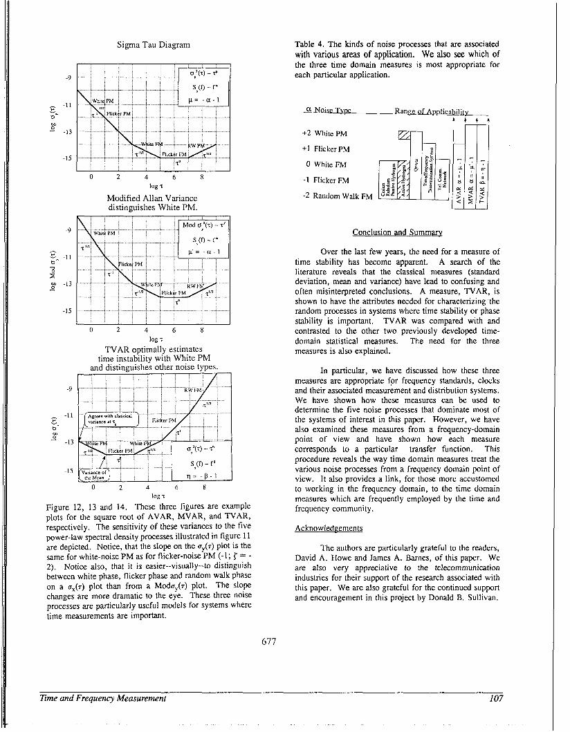
Sigma Tau Diagram
-9
-11 t. v
0-
- -13 2
-15
0 2 4 6 8 log 'T
Modified Allan Variance distinguishes White PM.
-9
h
c. -11 0-
2 -13 - -15
-9
-11 r v
0-
- -13 M
-15
0 2 4 6 8 log T
TVAR optimally estimates time instability with White PM
and distinguishes other noise types.
0 2 4 6 8 log T
Figure 12, 13 and 14. These three figures are example plots for the square root of AVAR, MVAR, and TVAR, respectively. The sensitivity of these variances to the five power-law spectral density processes illustrated in figure 11 are depicted. Notice, that the slope on the uy(r) plot is the same for white-noise PM as for flicker-noise PM (-1; = - 2). Notice also, that it is easier--visually--to distinguish between white phase, flicker phase and random walk phase on a (rX(r) plot than from a Moday(r) plot. The slope changes are more dramatic to the eye. These three noise processes are particularly useful models for systems where time measurements are important.
677
Table 4. The kinds of noise processes that are associated with various areas of application. We also see which of the three time domain measures is most appropriate for each particular application.
-EhiscType Range of Applicability
+2 White PM t
+1 FlickerPM 1 - a r
L
Conclusion and Summary
Over the last few years, the need for a measure of time stability has become apparent. A search of the literature reveals that the classical measures (standard deviation, mean and variance) have lead to confusing and often misinterpreted conclusions. A measure, TVAR, is shown to have the attributes needed for characterizing the random processes in systems wherc time stability or phase stability is important. TVAR was compared with and contrasted to the other two previously developed time- domain statistical measures. The need for the three measures is also explained.
In particular, we have discussed how these three measures are appropriate for frequency standards, clocks and their associated measurement and distribution systems. We have shown how these measures can be used to determine the five noise processes that dominate most of the systems of interest in this paper. However, we have also examined these measures from a frequency-domain point of view and have shown how each measure corresponds to a particular transfer function. This procedure reveals the way time domain measures treat the various noise processes from a frequency domain point of view. It also provides a link, for those more accustomed to working in the frequency domain, to the time domain measures which are frequently employed by the time and frequency community.
Acknowledgements
The authors are particularly grateful to the readers, David A. Howe and James A. Barnes, of this paper. We are also very appreciative to the telecommunication industries for their support of the research associated with this paper. We are also grateful for the continued support and encouragement in this project by Donald B. Sullivan.
l ime and Frequency Measurement 107
References
131
141
PI
[71
1141
J. Rutman and F. L. Walls, "Characterization of Frequency Stability in Precision Frequency Sources," submitted to Proc. of the IEEE, 1991. L. S. Cutler and C. L. Searle, "Some Aspects of the Theory and Measurement of Frequency Fluctuations in Frequency Strandards, " Proceedings of the IEEE, Vol. 54, No. 2, pp. 136-154, Feb. 1966. J. von Neuman, R. H. Kent, H. R. Bellinson, and B. I. Hart, "The Mean Square Successive Difference," Ann. Math. Stat. 2, 153-162 (1942). D. W. Allan, "Statistics of Atomic Frequency Standards," Proc. of the IEEE, s, 221-231 (1966). "Characterization of Clocks and Oscillators, " Eds. D. B. Sullivan, D. W. Allan, D. A. Howe, and F. L. Walls, NIST Tech Note 1337, 1990. J.A. Barnes, A.R. Chi, L.S. Cutler, D.J. Healey, D.B. Leeson, T.E. McGunigal, J.A. Mullen, Jr., W.L. Smith, R.L. Sydnor, R.F.C. Vessot, and G.M.R. Winkler, Characterization of Frequency Stability, IEEE Transactions on Instrumentation and Measurement, IM-20, No. 2, 105-120, 1971. D.W. Allan and J.A. Barnes, A Modified "Allan Variance" with Increased Oscillator Characterization Ability, Proceedings of the 35th Annual Frequency Control Symposium,, 470-475, 1981. P. Lesage and T. Ayi, "characterization of Frequency Stability: Analysis of the Modified Allan Variance and Properties of Its Estimate," IEEE Trans. on Instrum. & Meas., IM-33, 332-336 (1984). L. G . Bernier, "Theoretical Analysis of the Modified Allan Variance," Proc. of the 41st Annual Frequency Control Symposium, 1987, pp. 116-121. D. W. Allan, D. D. Davis, J. Levine, M. A. Weiss, N. Hironaka, and D. Okayama, "New Inexpensive Frequency Calibration Service from NIST," Proc. of the 44th Annual Frequency Control Symposium, 1990, pp. 107-116. D. W. Allan, "Time and Frequency Metrology: Current Status and Future Considerations," submitted to Proc. of 5th European Frequency and Time Forum, March 13-15, Bescanson, France, 1991. D. B. Percival, "Reappraisal of Frequency Domain Techniques for Assessing Stability Measures," Proc. of the KITI, 1987, pp. 69-80. J. Rutman, "Characterization of Phase and Frequency instabilities in Precision Frequency Sources: Fifteen Years of Progress," Proc. of the IEEE, Vol. 66, No. 9, pp. 1048-1075, September 1978. J. Rutman, "characterization of Frequency Stability: A Transfer Function Approach and Its Application to Measurements via Filtering of Phase Noise," IEEE Trans. on I & M, Vol. IM-23, No. 1, March 1974, pp. 40-48.
[Is] D.W. Allan, Time and Frequency (Time-Domain) Characterization, Estimation, and Prediction of Precision Clocks and Oscillators, IEEE Transactions on Ultrasonics, Ferroelectrics, and Frequency Control, UFFC-34, 647-654, 1987.
1161 W. C . Lindsey and C. M. Chie, "Theory of Oscillator Instability Based Upon Structure Functions," IEEE @, 1652-1666 (1976)..
67 8
108 Time and Frequency Measurement
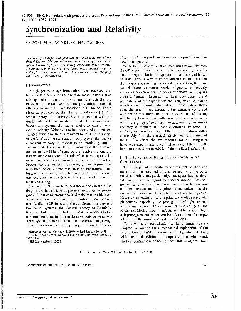
0 1991 IEEE. Reprinted, with permission, from Proceedings of the IEEE: Special Issue on Time and Frequency, 79 (7), 1029-1039; 1991.
Synchronization and Relativity GERNOT M. R. WINKLER, FELLOW, IEEE
The use of coticepts and fortiiirlae of (lie Special otid of the Gmeral Theory of Relativity lras become a tiecessify itr electrotiic systems tliat use liigli precisiotl tiniitig, especially space systems. Jhe priticiplrs iti\tolved will be reviewed wiili etiipliusis 011 pruc- tical applications atid operational standards itsed in tiniekeepirig and remote sytichronizaiion.
I. INTRODUCTION In high precision synchronization over extended dis-
tances, certain corrections to the time measurements have to be applied in order to allow for metric effects that are mainly due to the relative speed and gravitational potential difference between the two locations to he linked. These effects are predicted by the Theory of Relativity [I]. The Special Theory of Relativity (SR) is concerned with the lransformations that are needed to relate the measurements between two systems that move relative to each other at constant velocity. Velocity is to be understood as a vector, and dgravitational field is assumed to exist. I n this case, we speak of two inertial systems. Any system that moves at constant velocity in respect to an inertial system is also an inertial system. I t is obvious that the distance measurements will be affected by the relative motion, and it seems simple to account for this effect if we express the measurements of one system in the coordinates of the other. However, contrary to “common sense,’’ and to the principles of classical physics, time must also be transformed; this has given rise to many misundcrstandiiigs. The wcll known notorious twin paradox (shown later) is based on such a misunderstanding.
The basis for the coordinate transformations i n the SR is the principle that all laws of physics, including the propa- gation af light or electromagnetic signals, must be identical for two observers that are in uniform motion relative to each other. While the SR deals with the transformations between two inertial systems, the General Theory of Relativity (GR) goes further and includes all possible motions in the transformations, not just the uniform velocity between two inertia systems as in SR. It includes the effects of gravity. In fact, it has been accepted by many as the modern theory
Manuscripl received November 1, 1990; revised January 16, 1991. G. M. R. Winkler is with the U.S. Naval Observatory, Washington, 1)C
IEEE Log Number 9100238. 20392.5100.
of gravity [2] that produces more accurate predictions than Newtonian gravity.
While the SR is somewhat counter-intuitive and abstract, the GR is even more abstract. It is mathematically sophisti- cated; it requires for its full appreciation a mastery of tensor analysis. This is why there are differences in details in the interpretation among the experts. In addition, there are several alternative metric theories of gravity, collectively known as Post-Newtonian theories of gravity. Will [3] has given a thorough discussion of these developments and particularly of the experiments that can, or could, decide which one is the most realistic description of nature. Ilow- ever, the practitioner, especially the engineer concerned with timing measurements, at the present state of the art, will hardly have to deal with these further developments within the group of relativity theories, even if the utmost accuracy is required in space electronics. In terrestrial applications, none of these different formulations differ appreciably from the classical, Einsteinian formulation of the GR. The effects that are important for the timing user have been experimentally verified in many different tests, in some cases down to 0.01% of the predicted effects [4].
11. TIE PRINCIPLE OF RELATIVITY AND SOME OF ITS CONSEQUENCES
The principle of relativity recognizes that position and motion can be specified only i n rcspect to sonic otlicr material bodies, and particularly, that space has no abso- lute significance in regard to uniform motion. Classical mcchanics, of course, uses the concept of inertial systems and the classical relativity principle recognizes that the mechanical laws must be identical in all inertial systems. However, an extension of this principle to electromagnetic phenomena, especially the propagation of light, created a dilemma because the experimental evidence (e.g., the Michelson-Morley experiment), the actual behavior of light as i t propagates, contradicts our intuitive notions of a simple addition of the signal and system velocities.
For a while, a reconciliation of the dilemma was at- tempted by looking for a mechanical explanation of the propagation of light by means of the hypothetical ether, which required additional assumptions of an ether wind, physical contractions of bodies under this wind, etc. HOW-
U.S. Governiilcnl Work Not I’roteclcil by U.S. Copyriglit
PROCEEDINGS OF TlIE IEEE, VOI.. 79, NO 6. JUNE I W I
Time and Frequency Measurement 109
ever, Einstein recognized in 1905 that a most elegant resolution of the dilemma was possible by including the propagation of light in thc postulate, and thereby niodifying our basic concepts of classical mechanics, because this step requires the transformation of the time measure between inertial systems. In the meantime, the postulate of perfect relativity (which includes the propagation of light) has been established as correct in countless experiments and it is now known as Einstein’s Principle of Relativity, in contrast to the mechanical principle mentioned before. Again, the dif- ference bctwecn the two is that Einstein’s version includes all phenomena, particularly the propagation of light. The reason for thc failure of our intuition is simply that the speed of light (c) is so great that the “relativity effects” do not show up until we deal with speeds that approach c and/or unt i l our measurement precision is very high indccd.
The experience that the physical plienoniena are not affected by a uniform motion through space, i.e., that space has no absolute meaning in respect to unaccelerated motion, has as one of the consequences that time also cannot have an absolute meaning. It is an abstract measure of the state of processes in nature, such as motion of bodies or changes in temperature, that we introduce on the basis of standard processes (clock readings) and we have to find out how to extend this measure consistently into distant regions of space. It is clear that this extension requires the use of some signaling and, therefore, the problem of the speed of signaling is inseparable from the problem of transformation.
We need transformation forniulae for the coordinates if we want to refer measurements taken in one inertial system to thc coordinates of another (primed) system that nioves at velocity, v, in respect to the first. This transformation of the space and time Coordinates of an event must depend on the velocity 71 as parameter:
Furthermore, the transformation of the coordinates into the primed coordinates must be done so that each new coordi- nate is a linear function of the old (unprimed) coordinates. The linearity is needed so that we maintain the linearity in the description of a uniform, i.e., unaccelerated motion. In order to emphasize that time ( t ) must be part of these transformations, we will consider it as a fourth coordinate.
There are two conventions in use for the choice of the time index: zero or four. In either case, the combination of time and space coordinates leads to the understanding of the four components
za(o to go from 0 to 3, or from 1 to 4)
as the components of a four-dimensional coordinate vector, z. We call this vector a worldvector in space-time. It should also be noted that we must be prepared to distin- guish between upper and lower indexes which designate contravariant and covariant components respectively, a dis- tinction that will be necessary whenever we deal with a nonEuclidean geometry, such as in the Minkowski space and especially in the GR, which uses Riemannian geometry.
1030
A general linear transformation between two vecton is accomplished by multiplication with a transformation matrix, L, (that in our case must be some function of w)
2’ = Lx (1)
where the two coordinate vectors are taken as column vec- tors. I t is remarkable that Einstein’s relativity principle, in conjunction with the required linearity, already determines the transformation matrix, L. We can see this in a plausible way (for details see [2] or (51) if we express the spherical wave front of a light flash in the coordinates of two, initially coincident, inertial systems. This equation is (c is the speed of light in vacuum):
AT = c . At or in greater detail for I ) ~ ~ I ~ systellls :
Ax: - c2At2 = 0
= - c2At‘’ = s2( i = 1 to 3).
(2)
In other words, the transformation requires that the flash can be seen as propagating isotropically in both systems. This, of course, is exactly the point where our intuition tells us that this is not possible. However, we have to respect the fact that all experiments conducted so far to test this, or its consequences, have been in agreement with Einstein’s relativity principle. An interesting analysis of the testing problem is given in (61. If we accept Einstein’s expression of the relativity principle as an established fact, and we must do so on the basis of all evidence, then the rest is just a necessary mathematical consequence.
The two conventions about time as a fourth (generalized) coordinatc arc due to diffcrent ways of looking at the mathematics. Minkowski pointed out that the simplest way to understand the transformation is to consider it as a rotation in four-dimensional space-time, a transformation that keeps the length, s, of the worldvector 2 constant. In order to reduce this to the rotation case, we take as the fourth coordinate
(3)
The factor c means that we measure all coordinates in me- ters; it would be equally legitimate to measure everything in light time, Le., in seconds, by applying c as a divisor to the space coordinates instead of using it as a factor of the time coordinate. At any rate, the transformation we seek must accomplish that s, as defined previously, remain constant or, equivalently, that s is invariant. The invariance of s under the transformation is a cornerstone of the SR. This is in striking contrast to the classical concepts, where length and time diffcrenccs are invariant independently. Here, it is only the four-dimensional space-time interval s that is invariant. Using OUT coordinate convention, the invariance of s is expressed by
PROCEEDINGS OF TIlE IEEE. VOL.. 79. NO. 7. JULY 1941
110 Eme and Frequency Measurement
with the summation index i going now from 1 to 4. The invariant interval s can be seen as the radius of a four-dimensional sphere, which is formally zero in all legitimate coordinate systems. However, this is true only for the intervals that connect two events which are at the ends of a light ray. We must also remember that this Minkowski space-time is a complex space and its geometry is, therefore, only pseudo-Euclidean. If s = 0 in this space, then it does not at all mean that the three-dimensional distance between the two events is zero in our inertial system. One of them could be here and the other on a distant galaxy, but they would be connected by a light ray.
While the mathematical “trick” (3) is most helpful for rhe purposes of the SR, it is not feasible to extend the Minkowski convention to the problems of general trans- formations with which the GR has to deal. For this reason, most workers today, including [2], use the other convention in which
xo = c . t.
In this case, the transformation matrix will, of course, be slightly different. In any case, a transformation that includes time will necessarily treat i t as a pseudo-geometric coordinate, which allows us to bring the whole power of the general geometrical formulations to bear upon the problems. But conceptually we must always remember that time and space are not equivalent, even though the mathematical union in which they find themselves under the transformation (1) is due to the fact that time and distance measurements cannot be made independently from each other.
We have seen that the interval s of two events connected by a light ray vanishes in every inertial system because of the relativity principle. However, it can be shown that every interval, s, must be a constant (must be an invariant). Let us consider the infinitesimal intervals between two events as expressed in two inertial systems. They must be proportional because they are of the same order:
ds2 = a . d d 2 .
The factor a cannot depend on the coordinates because this would violate the homogeneity of space and time. It can only depend on IwI. But if we consider more than two such systems, then the respective factors, each depending on the respective velocity differences, can be expressed as ratios of two other a’s. While these ratios do not depend on the angles between these velocities, the velocity difference of our last pair would depend on the angle between their
velocities, which would make the expression as ratios of theother a’s inconsistent. Therefore, the a’s must be a constant, and the constant can only be 1. This implies, therefore,that every s must be an invariant under coordinate transformations, a most important result.
For events that are separated by s # 0, two possibilities must be distinguished:
WINKLER SYNCIIRONIZATION AND REI.ATlVITY
Case 1:
Case 2:
The time component is greater than the space part-this is a time-like interval, and we form the difference:
r2 = At2 - (1/c2) . Ax:. (6)
The space component is greater than the time part-we have a space-like interval, and we form the other difference:
o2 = Ax? - c2At2. (7)
We have used the time measure in the first case, and the space measure in the second, as i t is advisable according to the needs of the application. Whatever we do, both the magnitude and the kind of interval are invariant and the possible transformations can only change the magnitude of one component at the expense of the other. Moreover, these transformations can only go so far that the smaller of the two components vanishes (as i t was observed above, the two components are not equivalent), and not beyond that, Le., they cannot make a time-like interval into a space-like and vice versa (this limit is due to o being limited to w < c). In the case of a space-like interval, it is possible to chose coordinates that make the events simultaneous (At2 = 0) at a spatial distance equal to (T. This distance is the shortest possible distance in any frame. A time-like interval allows a transformation to coordinates in which the events occur at the same location (EAxT = 0), with a “proper time” (see the following) difference T = At2. This time difference is the briefest time measure in any system. In other words, simultaneity is relative to the system chosen, and there is no simultaneity possible if the interval between the events is time-like. By using the invariance of s, we can derive the connection of the time measure At’ in a moving vehicle (not necessarily assuming uniform motion) as it looks from an inertial reference At. The invariable interval between two events is always s; however, as we just saw, this s is composed of the two components, the time part and the space part. If we denote the system in which the clock is at rest as the “proper” system, then an inertial system used as reference is the “coordinate” system. It is customary to denote the proper time as T . This is always the time that is kept directly by a clock (which is at rest in its own rest frame). The interval between two events at the location of the clock is then expressed in the two systems as
As2 = Ar2 - 0 (proper time)
= At2 - (1/c2) C A x : f ( s u m over 1 to 3)
(coordinate time). (8) The motion of the clock while it traverses the coordinate distance Jm takes place during the coordinate time At at speed v2 = CAx2/At2, which allows regrouping of our formula
A r = A t . Jm. (9) This is the transformation of the increments of the readings
Eme and Frequency Measurement 111
of a stationary clock (the proper time of this clock) in terms of coordinate time. It is the time part of the general coordinate transformation (the matrix L ) that is known as the Lorentz transformation. The details of the Lorentz transformation are amply discussed in the references. The moving clock will always have smaller numerical readings (it will be late) as seen from the coordinate frame. On the other hand, a moving proper length 1 in the direction of the velocity of the “moving” (of course, it is a relative motion) system will always measure less in the coordinate system; that is the Lorentz contraction. Dimensions perpendicular to the motion will not be affected.
One of the experimental demonstrations of the invariance of s under coordinate transformation consists of the obser- vation that a certain type of elementary particle, K-mesons, are so short lived s) that, after their production in the laboratory, they can move only a few meters before they decay. However, they can be observed on the surface of the Earth, even though their natural origin is high in the upper atmosphere. The explanation is found in the change in the space-time measure due to the extreme speed, very close to c. In the meson comoving system, the distance to the surface is Lorentz contracted by the high relative speed of the Earth system; the terrestrial observer, on the other hand, sees the mesons last longer because of the time dilation due to their high speed relative to us. But, the meson always travels the distance I = v . At as seen in either system; Le., we can write this equation in unprimed and primed magnitudes: I‘ = v . At‘ is seen in one system, and 1 = v - At in the other. Commensurate with the slowing down of the time measure, the distance is also shortened, as measured in the other system. Only v is the same (with opposite signs) in both systems. Atomic frequency standards will, therefore, appear Doppler-shifted by the same amount as observed in the other system. The situation is exactly the same in both systems, in accordance with the principle of relativity.
An observation regarding the time dilation may be useful. Very often its effects are described in a way which suggests that we deal with physical effects upon the moving clock, that the moving clock is slowed down. This is misleading. Clocks always measure proper time. It is not a physical effect upon the clock if its time measures appear to slow down as its speed increases relative to us. It is merely a metric effect due to the transformation from one system to the other. The same clock will, at the same time, appear to operate at different rates if seen from different reference systems; therefore, the effect is not located in the clock but is purely a metric result due to the relative speed of the coordinate systems chosen.
It is expedient to abbreviate factors that appear repeatedly in the transformation as follows:
In the simple case of two systems with parallel axes, coinciding initially, but moving at relative velocity v along the z-axis, the complete transformation in the case of
1032
convention (3) becomes;
It can be seen, that in this special case, only the first and the fourth coordinates will be affected. As expected, L is a linear coordinate transformation. It is orthogonal and the inverse is obtained by exchanging v with -v.
In the zo to z3 convention, the matrix must, of course, be different:
/ a -ap 0 0\
The more general transformations, with v not in the di- rection of the z-axis, can be derived through multipli- cation with rotation matrices, as explained in detail in [7]. However, it must be stressed that the appearance of similarity between the two forms is somewhat deceptive. Mathematically they are quite different and the Minkowski convention has been criticized for reasons given in [2], where the authors want to see it discontinued altogether. However, there are many applications where the Minkowski convention of using an imaginary fourth coordinate, even though useless in the GR, produces simpler formulations in the SR. This has been advocated in [7].
We must note a second important result: the velocity of light plays the role of a limiting maximum velocity beyond which our formulae would produce imaginary results. By the same token, velocities do not add algebraically. We assume a speed u’ in the primed system in the same direction as v at which the primed system moves away from the unprimed. This speed will then be transformed as
u = (21’ + v)/ (1 + u’v/c2) .
This addition of velocities is also limited by the velocity of light. The limiting role of c is a direct consequence of the relativity principle, which includes the propagation of light as an invariant phenomenon. In the limiting case of traveling photon, in its proper frame, there is no time interval between emission and reception, as there is no distance covered, a remarkable result indeed, but only the logical equivalent of Einstein’s relativity principle (because we used it as basis for our mathematical derivations).
The next step can easily lead to a fatal error, made by many people, even experts, the error of the clock paradox. We can integrate the increments of the time readings of the previously mentioned formula even for nonuniform motions of the proper clock, where v is a function of t , as long as we use an inertial reference:
71 - 70 = I./-. d t (14) t o
But we are not allowed to reverse the procedure by using the system of the nonuniformly moving clock as reference
PROCEEDINGS OF THE IEEE, VOL. 79. NO. 7, JULY 1991
l ime and Frequency Measurement 112
lor an analogous computation of the coordinate clock as Ken by the proper clock. Only inertial systems can be used IS a basis for time-space coordinates. The reason is simple: l e relativity principle is not valid for accelerated frames of reference. This is almost obvious: we certainly can feel the acceleration, as we also will find that other phenomena do not remain unaffected by the acceleration. The basis for our concepts derived so far is not valid under acceleration. l l is solid fact, the nonvalidity of the relativity principle d e r acceleration, invalidates a reversal of the previously mentioned conclusion that the stationary clock’s reading would also be slow if seen from the moving system. Claims that “relativity” means that the relative situation is the same, are false. The situation is clearly not symmetric: the clock that moves nonuniformly is always slow compared to an inertial clock. Problems such as a reverse computation, which cannot be done in the SR because it includes the tction of accelerations, have contributed to the development of the GR, which includes the treatment of accelerations due to gravity.
Additional general comments are possibly important. The tvents in the life of a physical particle are points in the four-dimensional space-time world, and these points form a worldline with differential increments, ds, which are time-like. As projected upon an external coordinate system, the increments have time and space components, but the interval itself is invariant. The invariance of s under transformation has the consequence that the splitting of space-time into space and time coordinates depends upon the reference system chosen. The transformation has the group property, Le., two successive Lorentz transformations correspond to a one-step transformation of the same kind, and a reverse transformation is obtained by changing the sign of the relative velocity, w. However, the transformation group is not commutative, the result of two successive transformations depends on their order (general coordinate rotation is not commutative [7]). Even more important is that what is simultaneous in one system will not be simultaneous in a system that moves in respect to the first. In other words, simultaneity has no absolute significance, it is relative to the system used. A failure to remember his relativity of simultaneity can easily lead to errors in Ihe reduction of signal times coming from satellites. These errors can occur if the reduction formulae use an Earth- centered, fixed reference in which assumed simultaneities of distant events would be different from what the receiver must use for its own data reduction.
The Lorentz transformation of the coordinates also has a most profound and fundamental importance for science: I n physical theory, we cannot continue to allow actions at I distance because the position of the distant body that acts upon the phenomenon under investigation depends upon the reference used. Moreover, the action can not be instantaneous because of the limiting role of c. Only field leories can be allowed from now on because in this case, the action is caused by the local field environment. This is ilso connected with the fact that the Maxwell equations are intrinsically Lorentz-invariant.
UINKLER: SYNCHRONIZATION AND RELATIVITY
111. THE GENERAL THEORY OF RELATIVITY Einstein’s principle of relativity is the fundament upon
which the SR has been built. The GR enlarges upon this in two ways: the basic geometry is generalized to allow for arbitrary transformations, and second, i t includes the principle of equivalence as the basis for the treatment of the effects of gravitation.
The basic formula for the computation of the four- dimensional infinitesimal interval, or line element, was
ds2 = c2 dt2 - dtq
For a treatment of general transformations we must write this equation in a style that treats time and space parts uni- formly. We will use affine coordinates with implied oblique axes and distinction between covariant and contravariant components and vectors and we use the real convention (5) for the time coordinate, as used also in [2] or [4]:
where gap is the metric tensor. The summation is to go over both, N and p, going from 0 to 3 (latin indexes will go usually from 1 to 3). Einstein introduced the convention to imply summation over indices that repeat in any term. With this convention one writcs the equation without the capital sigma. We have included t in one of the four z coordinates as discussed above by using the real value convention, and it is obvious that until now, most of the coefficients g are zero because in a flat space with Cartesian coordinates we have no mixed terms, only sums of squares of the coordinates. Therefore, the metric tensor for the SR is
It is clear that if we use transformed coordinates, we could also expect to end up with changed coefficients, g, of this quadratic form because the interval is invariant. However, this is not so. The Lorentz transformation, because it is a linear orthogonal transformation in four-space, keeps the metric tensor (the g matrix) invariant. This is just a sophis- ticated way of saying that the geometry in thc space is not affected and remains flat, i.e., pseudo-Euclidean, because the absence of mixed terms maintains the validity of the sums of squares composition o f the interval evcrywhcrc. The space is pseudo-Euclidean because the quadratic form for the ds is not positive definite. To recapitulate, (16) with the metric tensor given in (17) is valid whether we use original coordinates or coordinates that have been transformed by using (1) with (12).
But, this is only true for inertial frames (for the SR) and if we want to follow Einstein’s program to find general transformations that can handle any reference system and any coordinate system, then we must be prepared to give up this restricted form. This is, indeed, necessary and the GR uses a general Riemannian coordinate space where the
1033
Time and Frequency Measurement 113
9 matrix, the metric tensor, can have different values in 10 of the I6 componcnts (it is a symmetric tensor), and they will be functions of the coordinate chosen. Unfortunately, this makes the GR transformations nonlinear because of the mixed terms, a most serious complication. But, having 10 parameters available in every point of the four-space provides for the possibility of using geometry for the representation of physical effects as envisioned by Riemann in his famous lecture in 1854, and Einstein used this in his treatment of gravitation. The distribution of mass is reflected in a tensor field where the metric tensor is a function of the mass distribution.
But why are the nonlinear transformations which nec- essarily use all available terms in gap needed at all? If, as desired, an accelerated frame is to be used, then the transition between such frames cannot be represented by coordinate transformations that are linear in the time coordinate. And why do we want to use accelerated frames? Because we want to deal with motion in gravitational fields. And here it was Einstein’s ingenious insight that in a local area, represented as differentials of the interval, s, a gravitational field is indistinguishable from the effects of a frame that is accelerated.
This is Einstein’s principle of equivalence, and its posi- tion in the GR is as fundamental as is Einstein’s relativity for the SR. Its mathematical meaning is that in a local area we can always find a coordinate transformation that will diagonalize the quadratic form (16). In other words, locally we can transform away a gravitational field with a trans- formation that makes the coordinates into a local inertial coordinate system. But we cannot hope to do this globally with one and the same transformation because the gag are functions of the location. (However, a diagonalization of the form (16) by itself is not a sufficient condition for reaching a pure inertial system.)
The use of the geometrical formalism leads to the next step. In the absence of nongravitational fields such as electromagnetic fields, a free particle will follow a line of “shortest” interval (in view of the indefiniteness of ds, it is an extreme value), i.e., a geodesic which will be its gravitational worldline. Such a geodesic worldline will satisfy the condition which makes s a maximum:
6s = 6 ds = 0. i A
Again, s is the interval, and it will not be zero (we only set the variation to zero) unless the events A and L3 are at the ends of a light ray. The solution of (18) presents extreme difficulties, but a considerable simplification is possible in the case of weak fields and slow (planetary or satellite) motion: We must expect the terms of the metric tensor to be very close to their values in flat space-time because the GR must deviate very little from classical Newtonian solutions. We will also be able to neglect terms with p2, and mixed, square, and higher terms in the Asap. This leads to the
1034
following assumptions:
gap = 0 for a # p
gaa = -(I + Agoo)
goo = 1 + b o o
Furthermore, if we assume only a slowly changing field, we can also set the time derivatives of the gcxp to zero. With these assumptions, (18) reduces to classical Newtonian equations with
U = - k M / r = (c2/2)Agoo (20)
for a central body M at distance T. Only one gam, .9m appears, and this is the reason why the scalar potential U is a sufficient approximation for most problems in celestial mechanics. For our purposes, (16) will now give us the effect of a gravitational potential upon the measuremen1 of proper time T in relation to a coordinate time t of a comoving free frame without the potential:
or
dt = d r . [l - ( u / c 2 ) ] . (221
We use only the first-order approximation in addition to (19) and (20). In other words, the potential U will product a slower rate for the proper-time clock in respect to a clock outside the potential (which is a negative quantity). This result can also be obtained without the apparatus of GR by picturing the photon as having an effective mass E / c 2 = h f / c 2 , which will suffer an energy loss bj climbing the potential wall:
AE = m ’ AU = IL f AU/c2.
This produces a relative frequency change (the redshift) of
A f / f = A E / E = AU/c2. (23,
There is an essential difference between these two deriva- tions, however. Only the GR predicts a change in thr clock rate that will accumulate the reading differences. It is a metric effect that arises because of the potential U distorting the space-time structure, which affects the relative time readings. The classical picture only speaks about a gravitational “Doppler” shift of the individual photons without necessarily saying anything about the clock readings. Experiments, described in [9] and [lo], have unequivocally decided for the correctness of the GR model.
The assumptions which led to (19) mean, of course, that we have linearized the problem (in addition to the other restrictions), and that the effects, not only the gravitational potential effect, can be added separately. A good examplr for this is given in (9): the estimate of the magnitude of thc combined effect of orbital speed and gravitational potential
PROCEEDINGS OF THE IEEE, VOI.. 79. NO. 7. J1II.Y IWI
114 lime and Frequency Measurement

difference on the frequency received from an Earth satellite r is the radius of the Earth, 16 is the satellite altitude):
A f / f = 3.5 . 1 0 - " [ 3 ~ / ( ~ + 11) - 21. (24)
For low altitudes, we have a shift to higher frequency because the speed effect predominates; above h = r /2 , the shift is towards lower frequencies (red shift) because at high altitudes the satellite speed is smaller and the potential dif- ference is larger, and the two effects have the opposite sign.
W. THE SAGNAC EFFECT A special case of an accelerated frame is particularly
important for terrestrial timing applications. On the Earth, we operate on a rotating reference system, and this will affect clock synchronization. Up to now we have assumed that ordinary clock transport will lead to the same result regardless of the route taken as long as we allow for the corrections due to the speed of travel and the height of the clock in the gravitational potential. In an inertial system, the time transfer is independent of how we travel. Moreover, the result is the same if we exchange timing signals by radio if we take the propagation time delay into account. This is done according to the Einstein convention: we send a signal to and from the remote station and assign IO the remote clock as time for the reception the midtime between transmission and reception at the home station.
In a rotating system, this independence from the path of synchronization is not assured. In addition, if we syn- chronize station 2 to station 1 and station 3 to station 2, then station 3 will not necessarily be synchronized with 1. This transitivity of synchronization is, however, absolutely required in any time ordered system. On the Earth, however, if we use a path around the globe, we would discover a timing discontinuity that depends on the location (latitude and direction) of the path. Consistency, Le., a useful coordinate time system can be obtained, however, if small corrections are applied to the synchronization procedure.
The same effect exists in the propagation of light. In fact, it was with light Sagnac made the original experiments in 1914. He showed that on a rotating system, the velocity of light must be added to (or subtracted from) the speed due to rotation, an effect that produces a time difference for two rays that travel in opposite directions around a closed path. This is, of course, exactly the same effect that allows the operation of LASER gyroscopes.
The reason for all this is that in the rotating system, we cannot ignore the cross terms in our line element ds (15). In other words, accelerations have an effect on timekeeping and on the propagation of light. It is instructive to study this in some detail. The line element in an appropriate coordinate system, ct, T , cp, z (coordinates that correspond with our previous zo, d, etc.), is in primed coordinates for a nonrotating system:
ds2 = c2 &I2 - drI2 - TI' dpt2 - dzj2. (25)
In the system that rotates around the z axis at angular
VINKLER: SYNCHRONIZATION AND RELATIVITY
velocity 0, we have T = T', z = z', and cp = cp' + Rt'. By inserting this in (25) we obtain in unprimed coordinates:
ds2 = (c2 - R2r2) dt2 - 2Rr2 dcp dt - dr2 - r2 dp2 - dz2. (26)
From this we can identify the terms of the metric tensor SOP
(27) 1 900 = c2 - R 2 T 2
902 = -2Rr2 911 = -1
Q33 = -1
2 922 = --T
If we remember (8) and its application in (14), we can do the same in the present more general case, except that we use the new expression for the line element (the interval ds) to compute the proper time:
For the computation of the time delays in a synchroniza- tion worldline, one would start with (16) and solve for dzo. This is a quadratic equation with two solutions that reflect the coordinate time for the beginning and the end of the worldline. After a few algebraic transformations given in [4], one can derive the time delay in coordinate time for a closed path in the same sense as the rotation, where 12 is the angular velocity of the rotating frame, and E is the enclosed area, projected upon the plane of rotation:
A t = A s + 2 . R / c 2 . E. (29)
This effect is independent of the speed of transfer. There- fore, the speed effect on the readings of a portable clock would be in addition to this. We can also see that in the case of the Earth, a synchronization path along the meridians will not produce this effect at all. This is conceptually useful because we can base our standard synchronization procedure on the rotating Earth on a virtual portable clock synchronization that proceeds only along meridians, to and from the pole. Synchronization that has been reduced to this model will produce a consistent coordinate clock system on the rotating Earth without discontinuities. This is the meaning of correcting synchronization measurements according to (29).
V. STANDARDS FOR WORLDWIDE SYNCHRONIZATION The main bodies that are concerned with the interna-
tional coordination of time are the International Consulta- tive Committee for Radio (CCIR), a body working under the International Telecommunications Union (ITU), and the International Conference for Weights and Measures (CIPM), the executive body under the General Conference for Weights and Measures (CGPM), also known as the Metric Convention. The consultative group concerned with
1035
Rme and Frequency Measurement 115
time is the Consultative Committee for the Definition of the Second (CCDS), which reports to the CIPM. Both groups, the CCIR and the CCDS, have issued recommen- dations and definitions pertinent to the precise meaning of synchronization and global timekeeping, and formulae to account for relativity effects. These recommendations are based to a large degree upon work that was caused by the requirements of precision timing of remote systems, e.g., of new satellite navigation systems, especially the Global Positioning System (GPS) [9], [lo], [ l l ] , [12], [13], [14],
The CCIR Study Group VI1 has issued a report [18] that deals in some detail with the cases of a portable clock near thc surface of thc Earth, and with clcctromagnetic signals used for remote synchronization.
The CCDS has clarified the principles involved, and has defined the International Atomic Time (TAI) as a coordinate (and coordinated) time. The wording (translated from the French) is:
[151, [ w , ~ 7 1 .
“The TAI is the temporal reference coordinate established by the Bureau International de 1’Heure (BIH) on the basis of the readings of atomic clocks that operate in various establishments in conformance with the definition of the second, the unit of time of the International System of Units (SI).” (Recommendation S 2, 1970).
TAI is now established by BIH’s successor organization, the Bureau International des Poids et Mesures (BIPM). This definition of TAI has been augmented with a declaration in 1980 that is to clarify the meaning in the relativistic context. This became necessary because the above wording only implies the reference tinie TAI to be coordinated because TAI is defined on the basis of the clock readings in the contributing establishments. The uni t of time, as it is defined as a base unit of the SI, however, necessarily refers to proper time. W erever we operate a Cesium frequency standard, i t gives us the time measure as a proper unit, even though this also was not explicitly spelled out in the original definition. This CCDS declaration is as translated [19]:
3
“TAI is a coordinate time scale, defined in a geocentric reference frame with the SI second as scale unit as it is realized on the rotating geoid. Therefore, i t can be extended to a fixed or moving point in the vicinity of the Earth with sufficient accuracy at the present state of the art by the application of the first order corrections of the General Theory of Relativity; Le., the corrections for the differences in the gravitational potential and the differences of speed, in addition to the rotation of the Earth.”
Following this declaration, a note explains the mathematical formulae for these first-order corrections.
1. For a traveling clock we have:
At = E.2R/c2+ 1 [l - a+ c2 2c2
trajectory
where T is the vector from the center of the Earth to the clock, ds is the proper time differential of the clock, AU(T)
1036
is the potential difference between the clock’s location and the geoid (positive for a positive altitude), c is the velocity of light, v is the velocity of the clock in respect to the Earth, R is the angular velocity of the Earth, and iE is the equatorial projection of the area covered by T in an Earth- fixed coordinate system. In the computation, the differential of the area will be taken as positive if the projection of I moves towards East:
E=2- 2 J ~ T ~ V E . COS cp . ds (311 trajectory
where I T [ is the length of the vector T , V E is the east component of v, and ~p is the geocentric latitude.
The formula represents the relativistic effects during transport with a relative uncertainty of less than one part in ten to the fourteen. For clock altitudes of less than 24 km, one can take
AU(r) = gn . h
where h is the altitude of the clock above the geoid, and gn is the normal acceleration due to gravity.
The CCIR Report [ 181 is consistent with the CCDS note, but gives a more complete computation for AU(T) that can be used for greater altitudes and that includes the effects of latitude and the quadrupole moment of the Earth J2.
2. In case of synchronization by electromagnetic sig- nals, the coordinate time delay between transmission and reception is
C2 C J dg (33, 2R
A t = - E + - trajrctory
where da is the coordinate length differential along the trajectory, with the other magnitudes the same as in the first case, with the exception of CE which, in practice, is the equatorial projection of the triangle between thecfnter of the Garth, the transmitter, and the receiver of the signal The area E is positive if the equatorial projection of the line between the transmitter and the receiver has an eastward component. It is also noted that in practice, the termdue to da can be eliminated by sending the signal backand forth (the simultaneous two-way method). In this case, the formula leads to uncertainties of less than 1 ns, evenfor connections with artificial satellites.
3. The standard numerical values for the above quantities are:
c = 2.99792458 x 10’ m/s (299.792458 m/ps, in vacuum)
2R/c2 = 1.6227 x s/m2 (1.6227 fs/kn12) gn = 9.81 m/s2 This is an approximate
value for mid - latitudes. The standard formula for the acceleration a t sea level is:
g(cp) = 9.780 + 0.052 sin2 cp(m/s2) where cp is the geographical latitude. (34)
PROCEEDINGS OF THE IEEE, VOL. 79, NO. 7, JULY IW
116 Time and Frequency Measurement
4. Discussion and Examples. The approximation given hove treats the metric corrections as linear superposition of the three components: the speed effect, the effect due to Le gravitational potential difference, and the Sagnac effect due to the motion, or light propagalion, as seen in a rotating frame of reference. Taken each h y itself, one can summarize lhese effects in the following way. A clock that moves at sea level at speed i i will appear to he low in frequency compared with the standard frequency (the clock will be {low), Le., we have to add to its frequency
(35)
An altitude of li meters above sea level will produce an apparent approximate increase of its frequency of
This latter correction is an important item in the inter- national comparison of fundamental (primary) frequency itandards. One of the major contributors, the National Institute of Standards and Technology (NIST) operates a primary frequency standard in Boulder, CO. At the altitude of 1650 m, the frequency will appear to he high in respect lo sea level (the TAI reference) by 1.8 parts i n ten to the Ihirteenth, which is more than ten times the uncertainty of the absolute frequency. Even larger are, of course, the offsets that must be included i n atomic frequency standards that are to operate in satellites [ I I ] .
If a traveling clock has an east component TIE in its motion, then we must add to the time of the moving clock a delay due to the Sagnac effect. This delay is (with latitude Q and altitude IL) proportional to distance traveled towards rhe East L> i n km:
At x 2 0 7 . 4 ~ 0 ~ c p . D / ( 2 ~ ( 6 3 7 8 + / L ) ) (11s). (37)
The 207.4 ns is the delay accumulatcd by a clock that circumnavigates the Earth on the equator in an easterly direction. In practice, one will compute E and use (30). For a signal that is transmitted via satellites, the effect will be greater, of course. The timing receivers for the GPS must have corresponding corrections for the time transfer huilt into thcir reduction software i n order lor time transl'crs to he useful in the terrestrial coordinate time. A test to this extent was perfornicd by Allan, Wciss, and Ashhy [16], with results that indicated that this was indccd the case for !he receivers used.
VI. CLOCK TIME SCAIXS FOR ASTRONOMICAL AND
SPACE APPIKATIONS The International Astronomical Union (IAU) has been
concerned with time scales, originally as the sole provider of time standards, now in regard to their use in very-long- baseline interferometry (VLBI) and as reference for the prediction o f celestial phenomena, such as orbital motions and pulsar timing. The old Ephemeris Time (ET), that was introduced in the 1950's as a uniform time scale and as
the time argumcnt for orbital computations, was replaced in 1977 by Dynamical Time, which included relativity considerations with scaling (changing the rate of the clocks to compensate for the gravitational potential at the point of origin for the purpose of avoiding a secular runoff; see [21]). Ilowevcr, the new space applications ol precise time, particularly in pulsar research, suggest further evolution. This is very significant because by far the most stringent requirements for long-term clock stability and accuracy in the relativity corrections that must be applied in the reduction of observations come from astrodynamics and astronomical research. Guinot and Seidelmann [22] discuss the history and propose further developments.
Proposals have now been formulated at the IAU Collo- quium on Reference Systems [23] for putting the whole system of space-time references on a systematic basis in the explicit framework of the GR. The Conceptual Recommendation G1 recommends
'' . . . the four space-time coordinates (x" = c t , . r ' , .I.',.?) be selected in such a way that in each coordinate system centered at the baryccnter of an ensemble of niasses exerting the main action, the interval (1s' be expressed at the minimum degree of approximation in the form:
where , . . 11 is the sum of the gravitational potentials (taken here as positive) . . . "
Recommendation G2 specifically mentions two coordinate systems, the (solar) barycentric and a geocentric system; i t specifies that the SI (i.e., the second, the meter, c, etc.) should be extended to outer space without scaling factors; and i t links the time coordinates to atomic clocks that operate in conformance with the definition of the second.
Recommendations T I and T2 establish a consistent nomenclature for the various time-like arguments that need to be distinguished as a consequence of the above recommendations. This nomenclature takes into account the previously introduced time-like arguments that are used in thc cphcnicridcs: Tcrrcstriiil Dyn;imic;il Time (TIIT), mid Darycenti-ic Dynamical Time ('TDB), the former originally taken as TAI + 32.184 s, and usually considered as the relativistic successor to ET. TDB is reckoned at the SI rate with scaling (which effectively assigns ii number to the Cesium standard frequency that is different from the SI). T1 and T2 also introduce new arguments in conformance with G1 and G2: Geocentric Coordinate Time (TCG), and Barycentric Coordinate Time (TCB). And lastly, i t also introduces an ideal Terrestrial Time (TT) that is practically TAI hut without the very small errors of implementation.
First of all, i t must be noted that the French names determine the abbreviations. And even though this seems like a bewildering profusion of different time sc;iles, the method is clearer by grouping them in the following way (see also Tahle 1).
FINKLFR: SYNCIIRONIZATION ANI) REI ATIVI'I'Y 1037
Time and Frequency Measurement 11 7
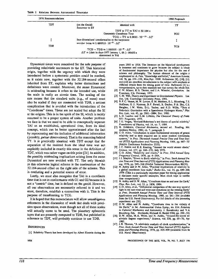
Table 1 Relations Between Astronomical Timescales
1976 Recommendations 1990 Proposals
TDT (on the Geoid) identical with -IT Successor to ET
TDT f TT x TAI + 32.184 s Geocentric Coordinate Time TCG
TCG - TT x 6.9693. lo-’’ * A T 1 four-dimensional transformation to the barycenter
secular t em E 1.480813. lo-’ . A T f
TDB TCB TCB - TDB 1.550505 . lo-’ . A T
A T = (date in days-1977 January 1, Oh ) e86400 s determined in TAI
Dynamical times were conceived for the sole purpose of providing relativistic successors to the ET. This historical origin, together with the urgency with which they were introduced before a systematic position could be reached, as it exists now, together with the 32.184-second offset inherited from ET, explains why better distinctions and definitions were needed. Moreover, the name Dynamical is misleading because it refers to the intended use, while the scale is really an atomic time. The scaling of the rate means that the standard units (e.g., of mass) must also be scaled if they are connected with TDB, a serious complication that is avoided with the introduction of the “Coordinate” times. These are not scaled but adopt the SI at the origins. This is in the spirit of the SI, which is tacitly assumed to be a proper system of units. Another problem we face is that we need to be able to conceptually separate TAI as an established, operational time, from its ideal concept, which can be better approximated after the fact by reprocessing and the inclusion of additional information (possibly, pulsar observations). That is the reasoning behind TT’. It is practically identical with TDT except that the separation of the realized from the ideal time was not explicitly included in exactly this sense in the definition of TDT, which was rather vague on this point [21]. In addition, the possibly misleading implications arising from the name Dynamical are now avoided with TT. The only blemish in this otherwise logical scheme is the continuation of the 32.184-second offset on the right side of the scheme. This is confusing and a potential source of error.
Lastly, we must also recognize that TAI is a coordinate time that is not in conformance with G1 and G2 because it is not a “centric” time, but is defined on the geoid. However, all our observations are necessarily referred to it and we must, therefore, establish a connection with it. This is the purpose of transforming to TCG.
It is hoped that this nomenclature will allow unambiguous references in the discussion of work that deals with preci- sion space observations, even though not all of these scales will actually come to be used. The planetary ephemeris tapes that are presently computed to TDB, but published in reference to TDT, will probably continue to use TDB.
REFERENCES
111 Relativity Theory has been developed by Albert Einstein during the
1038
years 1905 to 1916. The literature on the historical developmcnb is immense and continues to grow because the subject is clearly of fundamental importance for physics but also for the rest of science and philosophy. The human element of the origins is emphasized in: A. Pais, “Knowledge and belief,” American Scient& vol. 76, pp. 154-158, Mar./Apr. 1990. References [8], [lo], 119, and (121 are excellent introductions to the subject with emphasis on different details from the timing point of view. Reference [2] is I comprehensive, up-to-date standard text that covers the whole field
[2] C. W. Misner, K. S. Thome, and J.A. Wheeler, Gravitation. br Francisco, C A Freeman, 1973.
[3] C. M. Will, Theory and Experiment in Gravitational Physics. Loo. don, U K . Cambridge University Press, 1981.
[4] R. F. C. Vessot, M. W. Levine, E. M. Mattison, E. L. Blomberg, T.E Hoffman, G. U. Nystrom, B. F. Farrell, R. Decher, P. B. Eby, C. R Baugher, J.W. Watts, D.L. Teuber, and F.D. Willis, “Tests ol Relavistic Gravitation with a Spaceborne Hydrogen Maser,” Phys. Rev. Lett., vol. 45, pp. 2081-2084, Dec. 1980.
[SI L. D. Landau and E. M. Lifshitz. The Classical Theory of Fields. N Y Pergamon, 1975.
[6] J. G. Vargas, “Revised Robertson’s test theory of special relativity,” Foundations of Physics, vol. 14, no. 7, 1984.
[7] H. Goldstein, Classical Mechanics, second ed. Reading, MA: Addison-Wesley, 1980, ch. 7, paragraph 3.
[SI C. 0. Alley, “Introduction to some fundamental concepts of general relativity and to their required use in some modern timekeeping systems,” in Proc. Thirteenth Annual Precise Time and Time Inter. Val ( P l T ) Applications and Planning Meeting, 1981, pp. 687-711 (NASA Conference Publication 2220).
[9] J. C. Hafele and R. E. Keating, “Around the world atomic clocks,” Science, vol. 177, pp. 166-170, July 1972.
(101 C. 0. Alley, “Relativity and clocks,” in Prm. 33rd Annual Symp Frequency Control, 1979, pp. 4-39A.
[ l l ] I. 1. Shapiro, “Down to Earth relativity,” in Proc. Tenth Annual Pn. cke lime and Time interval (PlTi) Applications and Planning Meet. ing, 1978, pp. 549-568 (NASA Technical Memorandum 80250).
[I21 N. Ashby and D. W. Allan, “Practical implications of relativity for a global coordinate time scale,” Radio Sci, vol. 14, pp. 649-669, 1979. (This is a particularly important paper for timing applications: it discusses many specific examples, from clock trips to satellite time comparisons.)
[13] N. Ashby and D. W. Allan, “Coordinate time on and near the Earth,” Phys. Rev. Lett., vol. 53, p. 1858, 1984.
[14] C. 0. Alley, et aL, “Differential comparison of the one-way speed of light in the east-west and west-east directions on the rotating Earth,” in Proc. Dventieth Annual Precise lime and lime Interval (Pl7’lJ Applications and Planning Meeting, 1988. pp. 261 -286 (available from the U.S. Naval ObServatory). For full details of this interestiog experiment see [20].
[IS] D. W. Allan and N. Ashby, “Coordinate time in the vicinity of the Earth,” in Int. Astronomical Union Symp., no. 114 Relativiq in Celestial Mechanics and Astmmetry, J . Kovalevsky and V. k Brumberg, Eds. Dordrecht, Holland: D. Reidel 1986, pp. 299-313.
1161 D. W. Allan, M. A. Weiss, and N. Ashby, “Around-the-world rel- ativistic Sagnac experiment,” Science, vol. 228, pp. 69-70, Apr. 1985.
1171 J. B. Thomas, “A relativistic analysis of clock synchronization,” in Proc. Skth Annual Precise T i e and T i e interval (PlTI) Applica. lions and Planning Meeting, 1974, pp. 4-39 (available from the U.S. Naval Observatory).
PROCEEDINGS OF THE IEEE. VOL 79. NO. 7, JULY 1991
I18 Time and Frequency Measurement
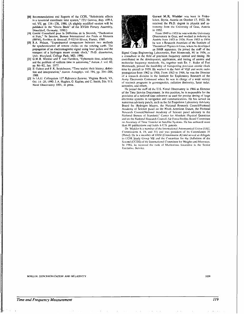
\IS] Recommendations and Reports of the CCIR, “Relativistic effects in a terrestrial coordinate time system,” ITU Geneva, Rep. 439-4, vol. VII, pp. 134-138, 1986. (A slightly modified version will be published in the “Green Book” of the XVIIth Plenary Assembly, Diisseldorf, Germany, 1990.)
1191 Camit6 Consultatif pour la Definition de la Seconde, “Declaration et Note,” 9e Session, Bureau International des Poids et Mesures (BIPM), Pavillon de Breteuil, F-92310 Sevres, France, 1980.
1201 R. A. Nelson, “Experimental comparison between two methods for synchronization of remote clocks on the rotating earth: The propagation of an electromagnetic signal using laser pulses and the transport of a hydrogen maser atomic clock,” Ph.D. dissertation, Univ. Maryland, College Park, MD, 1990.
[tlj G.M. R. Winkler and T. van Flandern, “Ephemeris time, relativity, and the problem of uniform time in astronomy,” Asrrm. J . vol. 82, pp. 84-92, Jan. 1977.
1121 B. Guinot and P. K. Seidelmann, “Time scales: their history, defini- tion and interpretation,” Asfro!!. Asrrophys. vol. 194, pp. 304-308, 1988.
(231 In I.A.U. Colloquium 127 Reference Sysrettrs, Virginia Beach, VA, Oct. 14-20, 1990. J.A. ilughes, G. Kaplan, and C. Smith, Eds. U.S. Naval Observatory 1991, in press.
WINKLER: SYNCHRONIZATION AND RELATIVITY
Cernot M.R. Winkler was born in Frohn- leiten, Styria, Austria on October 17, 1922. He received the P1i.D. degree in physics and as- tronomy from the University of Graz, Austria in 1952.
From 1949 to 1953 tie was with the University Ohservatory in Graz, and worked in industry in Austria from 19.53 to 1956. From 1953 lo 1956 he was a Research Associate of the Institute of Theorctical Physics in Graz, where he developcd an NMR apparatus. He joined the staff of the
Signal Corps Engineering Laboratories, Fort Monmouth, N1 in 1956. as a consultant in the field of precision frequency control and timing. He contributed to tlie development, application, and testing of atomic and molecular frequency standards. He, together with Dr. F. Reder of Fort Monmouth, proved the feasibility of transporting precision atomic clock tinie by aircraft i n 1959. IIe worked in the field of VLF and arctic radio propagation from 1962 to 1966. From 1963 to 1966, he was the Director of a research division in the Institute for Exploratory Research of the Army Electronics Command where he was in charge of a widc variety of research programs in geomagnetics, radiation dosimetry, lunar radar, acoustics, and others.
He joined the staff of the U S . Naval Observatory in 1966 as Director of the Time Service Department. I n this position, he is responsible for the provision of a national time reference as used for precise timing of large electronic systems in navigation and communications. He has served on nunierous advisory panels. such as the Jet Propulsion Laboratory Advisory Board for Hydrogen Masers, the National Research CounciVNational Academy of Science panel on the North American Datum, the National Research Council/National Academy of Science panel advisory to the National Bureau of Standards’ Center for Absolute Physical Quantities and on the National Research Council Air Force Studies Board Committee o n Accuracy of Time Triinsfcr in Satcllite Systcms. Ile has authored more than 80 publications and holds 6 U.S. patents.
Dr. Wiiiklcr is ;I mcnilicr of the Internation;il Astronomical Union ( M U , Commissions 4, 19, and 31) and was president of its Coniniission 31 (Time). IIc is a n i t “ of URSl (Commission A) and served iis delegate to CCIR Study Group VI1 and tlie Committee for the Definition of tlie Second (CCDS) 01 the Iiiteriiiitiiin;il Committee for Weights and Measures. I n IOXJ, Iic received [lie rank (11 Meritorious Executive i n the Senior Executive Service.
1039
Time and Frequency Measurement 119
0 1991 IEEE. Reprinted, with permission, from Proceedings of the IEEE: Special Issue on Time and Frequency, 79 (7), 1040-1053; 1991.
Applications of Highly Stable Oscillators to Scientific Measurements
~
ROBERT F. C . VESSOT
Invited Paper
I. INTRODUCTION
A. The Technological Basis for Experiments with Clocks
The frequency stability of highly stable oscillators has improved by a factor of about 10 every decade since the 1960 era, when atomic clocks were first introduced. While the frequency accuracy and precision of replication of the most stable oscillators has also improved, the emphasis in this discussion will be on applications of highly stable oscillators.
Most experimental procedures involving oscillators in- volve measurements of a time varying, or of a modulated, parameter that affects the frequency of the signal from an oscillator. The most useful measures of the error in the measurement process resulting from oscillator instability is the Allan standard deviation, oY(7), and mod gY(7) This is the one-sigma expectation of the fractional frequency difference (designated by the subscript, y) between time- adjacent frequency measurements, each made over time intervals of duration, T . The functional relationship of oy(.) versus ( T ) depends on the Fourier spectrum of of the phase variations [l].
The statistical representation of oscillator performance given by uY(.) or mod oY(7) can provide estimates of the limits imposed on the precision of measurements when comparisons are made of data of some time dependent phenomenon averaged sequentially every T s. Figure 1 shows sigma versus tau plots for recently developed stored ion devices [2], atomic hydrogen masers [3], and for the binary pulsar [4].
This figure also includes the Allan standard deviation of the disturbance caused by fluctuations in the earth’s troposphere and ionosphere on a signal traversing vertically. In the discussion of experimental techniques, the H maser performance data in Fig. 1 will be used as a basis for numerical examples.
Manuscript received January 12, 1991; revised April 4, 1991. The author is with the Smithsonian Astrophysical Observatory, Cam-
IEEE Log Number 9101203. bridge MA 02138.
B. Applications of Long-and Short-Term Stability The Long and the Short of I t
I) Binary pulsar measurements referenced to terrestrial time scales: Rapidly rotating neutron stars emit bursts of mi- crowave signals that can be detected by radio telescopes [4]. During the past 14 years the frequencies of a num- ber of these pulsars have been monitored. These celestial oscillators have become a new astrophysical laboratory. Measurements of their frequency variations with time have provided information to test the predictions of general relativity. Results from eight years of timing a millisecond pulsar have shown that, once the drift rate has been deter- mined and removed, the frequency stability of this object challenges the long-term stability of the best available ensemble of atomic clocks, as shown in Fig. 1. It is now evident that terrestrial clocks having better frequency stability for intervals beyond one year are needed to resolve a number of cosmological question such as the existence of a Cosmic Gravitational-Wave Background [5 ] and the possibility of a variability of the gravitational constant (61. Progress in the new technology of atomic clocks based on trapped and cooled ions, and of levitated atoms, is well under way to fulfill these needs for long term frequency stability. 2) Cryogenic oscillators and short-term performance: The other end of the stability plot, where intervals less than about an hour are of interest, is becoming the domain of cryogenic oscillators. These devices include supercon- ductive cavity stabilized oscillators [7], sapphire dielectric cavity resonators with superconductive coatings [8] and uncoated sapphire disc resonators operating with inter- nal dielectric reflection in the “whispering gallery” mode [9] . Operating at cryogenic temperatures, resonator quality factors in the lo9 domain have been achieved. These resonators, when combined with a low-noise amplifier such as a ruby laser [lo], [ll] provide high-level signals of extraordinary spectral purity.
Another oscillator that shows promise is the cryogeni- cally cooled atomic hydrogen maser that operates at about
US. Government Work Not Protected by U.S. Copyright
1040 PROCEEDINGS OF THE IEEE, VOL. 79, NO. 7, JULY 1991
120 Time and Frequency Measurement
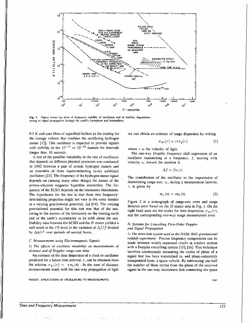
1 '\ \
-16 IO
\ PULSAR DATA \
TAYLOR \ OW NOISE l983-84\
t DRIFT REMOVED
I 1 l l l i l l l l I b 1 1 1 1 1 1 1 I f I 3 t L * 8 I I I , t , , , I I I 1 1 1 1 ' t J ' I I 1 1 1 1 1 1 1 I 1 1
\ ROPO V GPS
SPACE
\ E O R ~ EESIUM PERFORMANCE - - - - - - - AS MEASURED
\ \
t-
b S A 0 VLG-)I
Y
0.5 K and uses films of superfluid helium as the coating for the storage volume that confines the oscillating hydrogen atoms [12]. This oscillator is expected to provide signals with stability in the to domain for intervals longer than 10 seconds.
A test of the possible variability in the rate of oscillators that depends on different physical processes was conducted in 1982 between a pair of atomic hydrogen masers and an ensemble of three superconducting cavity stabilized oscillators [13]. The frequency of the hydrogen maser signal depends on (among many other things) the nature of the proton-electron magnetic hyperfine interaction. The fre- quency of the SCSO depends on the resonators dimensions. The hypotheses for the test is that these two frequency- determining properties might not vary in the same manner in a varying gravitational potential, Ad [14]. The varying gravitational potential for this test was that of the sun, owing to the motion of the laboratory on the rotating earth and of the earth's eccentricity in its orbit about the sun. Stability data between the SCSO and the H-maser yielded a null result at the 1% level in the variation of A f / f divided by A4/c2 over periods of several hours.
C. Measurements using Electromagnetic Signals 1 ) The effects of oscillator instability on measurements of distance and of Doppler range-rate data:
An estimate of the time dispersion of a clock or oscillator predicted for a future time interval, T , can be obtained from the relation c r ~ ~ ( ~ ) N T o, (T) . In the case of distance measurements made with the one-way propagation of light
VESSOT APPLICATIONS OF OSCILLATORS M MEASUREMENTS
we can obtain an estimate of range dispersion by writing
where c is the velocity of light. The one-way Doppler frequency shift expression of an
oscillator transmitting at a frequency, f , moving with velocity v, toward the receiver is
Af = fv,/c.
The contribution of the oscillator to the imprecision of determining range rate, v,, during a measurement interval, 7 , is given by
ov, (TI = coy (2). (2)
Figure 2 is a nomograph of range-rate error and range distance error based on the N-maser data in Fig. 1 . On the right hand axes are the scales for time dispersion, OA~(T), and the corresponding one-way range measurement error.
D. Systems for Cancelling First-Order Doppler and Signal Propagation 1 ) The three-link system used in the N A S I SA0 gravitational reakhifi experiment: Precise frequency comparisons can be made between widely-separated clocks in relative motion with a Doppler cancelling system [15], [16]. This technique involves continuously measuring the cycles of phase of a signal that has been transmitted to, and phase-coherently transponded from, a space vehicle. By subtracting one-half the number of these cycles from the phase of the received signal in the one-way microwave link connecting the space
1041
Time and Frequency Measurement 121
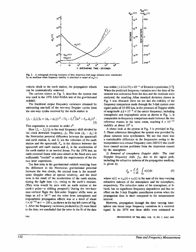
1 I I I I I
I IO lo2 to3 lo4 to5 to6 T-AVERAGING TIME - SECONDS
Fig. 2. by an oscillator when frequency stability is described in terms of ~ ~ ( 7 ) .
A nomograph showing estimates of time dispersion and range distance error contributed
vehicle clock to the earth station, the propagation effects can be systematically removed.
The cartoon shown as Fig. 3, describes the system that was used in the 1976 SAO-NASA test of the gravitational redshift.
The fractional output frequency variations obtained by subtracting one-half of the two-way Doppler cycles from the one-way cycles received by the earth station is
2 (fs - j e ) / f o = (4y - 4e)/c2 - I - v’, I /2c2 - 7ye.iie/c2 .
(3) This expression is accurate to order c2.
Here (f3 - fe)/fo is the total frequency shift divided by the clock downlink frequency, fo, The term (4y - q5e) is the Newtonian potential difference between the spacecraft and earth station, v’, and v’, are the velocities of the earth station and the spacecraft, FSe is the distance between the spacecraft and earth station and ?ie is the acceleration of the earth station in an inertial frame. For the 1976 test, an earth centered frame with axes aimed at the fixed stars was sufficiently “inertial” to satisfy the requirements of the the two hour experiment.
The first term is the gravitational redshift resulting from the difference in the Newtonian gravitational potential between the two clocks, the second term is the second- order Doppler effect of special relativity, and the third term is the result of the acceleration of the earth station, during the light time T/C, owing to the earth’s rotation. (This term would be zero with an earth station at the earth’s poles-a chilling prospect!) During the two-hour near-vertical flight the first-order Doppler shifts were as large as f 2 x and the noise from ionospheric and tropospheric propagation effects was at a level of about 1 x at T - 100 s, as shown in the top left curve of Fig. 1. After the frequency variations predicted in (3) were fitted to the data, we concluded that the error in the fit of the data
1042
was within (+2.5*70) x of Einstein’s prediction [ 171. When the predicted frequency variation over the time of the mission was subtracted from the data and the residuals were analyzed, the resulting Allan standard deviation shown in Fig. 4 was obtained. Here we see that the stability of the frequency comparison made through the 3-link system over signal paths of 10 000 km, in the presence of Doppler shifts of magnitude f 2 x of the carrier frequency, including ionospheric and tropospheric noise as shown in Fig. 1, is comparable to frequency comparison made between the two reference masers in the same room, reaching 6 x stability at about lo3 s.
A closer look at the system in Fig. 3 is provided in Fig. 5. Phase coherence throughout the system was provided by phase coherent ratio synthesizers. We see that there was a considerable difference in the frequencies owing to the transponders turn around frequency ratio 240/221 that could have caused serious problems from the dispersion caused by the ionosphere.
2) Removal of ionospheric Doppler shifts: The total Doppler frequency shift, fo, due to the signal path, including the refractive indexes of the propagation medium, is given by
(4)
where n(t) = n ~ ( t ) + n,(t) is the sum of the time-varying refractive indexes of the atmosphere and the ionosphere, respectively. The refractive index of the atmosphere, at S- band, has no significant frequency dependence and has no effect on the 3-link Doppler cancellation system when the propagation time is short compared to the measurement interval.
However, propagation through the time varying iono- sphere can cause large frequency variations in a received signal. In the 1976 test these shifts were estimated to
PROCEEDINGS OF THE IEEE, VOL. 79, NO. 7. JULY 1991
122 Eme ana‘ Frequency Measurement
__ _ _ _ _ _ __-
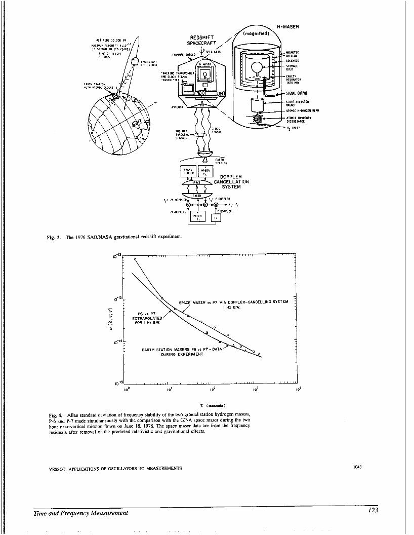
n H-MASER (magnified)
REDSHIFT //
Fig. 3. The 1976
fARTH f i t I f OOVVLtR fit f WPVLLR
f s - '1
2 f .WVVLtR f OOPVLLR
SAOMASA gravitational redshift experiment.
10-12 . I I I
10-l~ :
- - I HZ B.W. b - r - N- FOR I Hz B.W. b -
EXTRAPOLATED - -
EARTH STATION MASERS P6 VI P7 - DATA DURING EXPERIMENT
10-l4 :
'5 (d)
Fig. 4. Allan standard deviation of frequency stability of the two ground station hydrogen masers, P-6 and P-7 made simultaneously with the comparison with the GP-A space maser during the two hour near-vertical mission flown on June 18, 1976. The space maser data are from the frequency residuals after removal of the predicted relativistic and gravitational effects.
VESSOT APPLICATIONS OF OSCILLATORS TO MEASUREMENTS 1043
123 Eme and Frequency Measurement
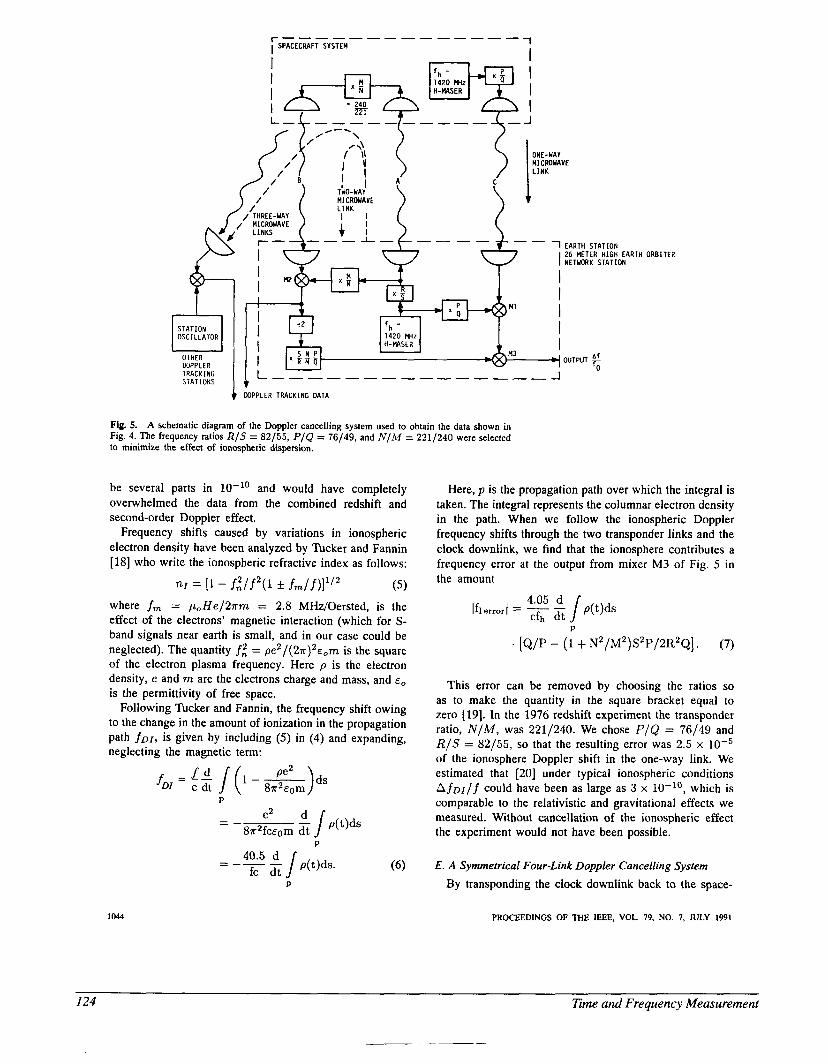
ORBITER
STATION OSCILLATOR
OTHER WPPLER TRACK I NG r STATIONS
WPPLER TRACKING DATA
Fig. 5. A schematic diagram of the Doppler cancelling system used to obtain the data shown in Fig. 4. The frequency ratios R/S = 82/55, PI& = 76/49, and N / M = 2211240 were selected to minimize the effect of ionospheric dispersion.
be several parts in lo-’’ and would have completely overwhelmed the data from the combined redshift and second-order Doppler effect.
Frequency shifts caused by variations in ionospheric electron density have been analyzed by Tucker and Fannin [18] who write the ionospheric refractive index as follows:
nr = f;t/f2(1 fm/f)]”2 ( 5 ) where fm = poHe/2?rm = 2.8 MHz/Oersted, is the effect of the electrons’ magnetic interaction (which for S- band signals near earth is small, and in our case could be neglected). The quantity f: = pe2/(27r)2~0m is the square of the electron plasma frequency. Here p is the electron density, e and m are the electrons charge and mass, and E,
is the permittivity of free space. Following Tucker and Fannin, the frequency shift owing
to the change in the amount of ionization in the propagation path f o r , is given by including (5) in (4) and expanding, neglecting the magnetic term:
Here, p is the propagation path over which the integral is taken. The integral represents the columnar electron density in the path. When we follow the ionospheric Doppler frequency shifts through the two transponder links and the clock downlink, we find that the ionosphere contributes a frequency error at the output from mixer M3 of Fig. 5 in the amount
. (Q/P - (1 + N2/M2)S2P/2R2Q]. (7)
This error can be removed by choosing the ratios so as to make the quantity in the square bracket equal to zero [19]. In the 1976 redshift experiment the transponder ratio, N / M , was 2211240. We chose PI& = 76/49 and R / S = 82/55, so that the resulting error was 2.5 x lo-’ of the ionosphere Doppler shift in the one-way link. We estimated that [20] under typical ionospheric conditions AfDI l f could have been as large as 3 x lo-‘’, which is comparable to the relativistic and gravitational effects we measured. Without cancellation of the ionospheric effect the experiment would not have been possible.
E. A Symmetrical Four-Link Doppler Cancelling System By transponding the clock downlink back to the space-
PROCEEDINGS OF THE IEEE, VOL. 79, NO. 7, JULY 1991
124 Time and Frequency Measurement
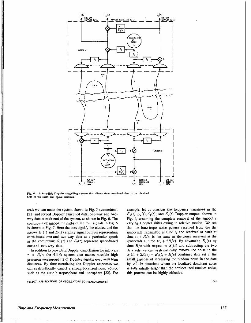
7
I I I I I I I L
r I I I I I I L 4 ’ONE-YAY
MTA WPPLER
Fig. 6. both at the earth and space terminal.
A four-link Doppler cancelling system that allows time correlated data to be obtained
craft we can make the system shown in Fig. 5 symmetrical [Zl] and record Doppler cancelled data, one-way and hvo- way data at each end of the system, as shown in Fig. 6. The continuum of space-time paths of the four signals in Fig. 6 is shown in Fig. 7. Here the dots signify the clocks, and the arrows E1 (t) and &(t) signify signal outputs representing earth-based one-and two-way data at a particular epoch in the continuum; S,(t) and S2(t) represent space-based one-and two-way data.
In addition to providing Doppler cancellation for intervals T < R/c, the 4-link system also makes possible high precision measurements of Doppler signals over very long distances. By time-correlating the Doppler responses we can systematically cancel a strong localized noise source such as the earth’s troposphere and ionosphere [22]. For
VESSOT APPLICATIONS OF OSCILLATORS TO MEASUREMENTS
example, let us consider the frequency variations in the El( t ) , Ez(t) , S l ( t ) , and &(t) Doppler outputs shown in Fig. 4, assuming the complete removal of the smoothly varying Doppler shifts owing to relative motion. We see that the iono-tropo noise pattern received from the the spacecraft transmitted at time ti and received at earth at time t; + R/c, is the same as the noise received at the spacecraft at time (ti + 2R/c). By advancing El( t ) by time R/c with respect to S,( t ) and subtracting the two data sets we can systematically remove the noise in the
+ 2R/c) - &(ti + R/c) combined data set at the small expense of increasing the random noise in the data by A. In situations where the localized dominant noise is substantially larger than the nonlocalized random noise, this process can be highly effective.
1045
Time and Frequency Measurement 125
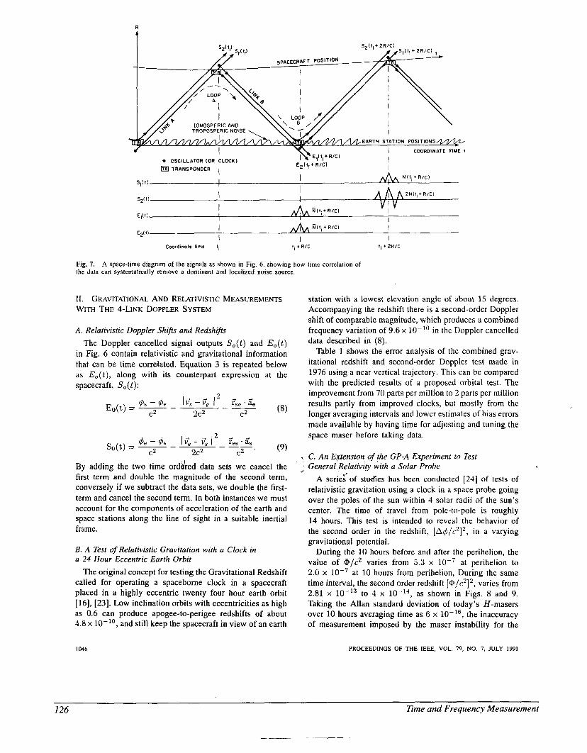
R
t
@ TRANSPONDER I I ~
N l l i + R / C l I I I
SI( I 1
I I I V I v S * i I l
€ , ( I 1
- N i l i + R I C l I I
I I I
I I I I I
E ~ i l l
Coordinale time t i t i + R/C li t 2R/C
11. GRAVITATIONAL AND RELATIVISTIC MEASUREMENTS WITH THE 4-LINK DOPPLER SYSTEM
A. Relativistic Doppler Shifts and Redshifts The Doppler cancelled signal outputs S,(t) and E,(t)
in Fig. 6 contain relativistic and gravitational information that can be time correlated. Equation 3 is repeated below as E,(t), along with its counterpart expression at the spacecraft, S,(t):
By adding the two time ordyred data sets we cancel the first term and double the magnitude of the second term, conversely if we subtract the data sets, we double the first- term and cancel the second term. In both instances we must account for the components of acceleration of the earth and space stations along the line of sight in a suitable inertial frame.
’,
J
Fig. 7. the data can systematically remove a dominant and localized noise source.
A space-time diagram of the signals as shown in Fig. 6, showing how
B. A Test of Relativistic Gravitation with a Clock in a 24 Hour Eccentric Earth Orbit
The original concept for testing the Gravitational Redshift called for operating a spaceborne clock in a spacecraft placed in a highly eccentric twenty four hour earth orbit [16], [23]. Low inclination orbits with eccentricities as high as 0.6 can produce apogee-to-perigee redshifts of about 4 . 8 ~ and still keep the spacecraft in view of an earth
1046
time correlation of
station with a lowest elevation angle of about 15 degrees. Accompanying the redshift there is a second-order Doppler shift of comparable magnitude, which produces a combined frequency variation of 9.6 x lo-’’ in the Doppler cancelled data described in (8).
Table 1 shows the error analysis of the combined grav- itational redshift and second-order Doppler test made in 1976 using a near vertical trajectory. This can be compared with the predicted results of a proposed orbital test. The improvement from 70 parts per million to 2 parts per million results partly from improved clocks, but mostly from the longer averaging intervals and lower estimates of bias errors made available by having time for adjusting and tuning the space maser before taking data.
C. An Extension of the GP-A Experiment to Test General Relativin, with a Solar Probe
A serieLof studies has been conducted [24] of tests of relativistic gravitation using a clock in a space probe going over the poles of the sun within 4 solar radii of the sun’s center. The time of travel from pole-to-pole is roughly 14 hours. This test is intended to reveal the behavior of the second order in the redshift, (A4/c2I2, in a varying gravitational potential.
During the 10 hours before and after the perihelion, the value of @/c2 varies from 5.3 x at perihelion to 2.0 x at 10 hours from perihelion, During the same time interval, the second order redshift [@/c2]*, varies from 2.81 x to 4 x as shown in Figs. 8 and 9. Taking the Allan standard deviation of today’s H-masers over 10 hours averaging time as 6 x the inaccuracy of measurement imposed by the maser instability for the
PROCEEDINGS OF THE IEEE. VOL. 79, NO. 7, JULY 1991
126 Eme and Frequency Measurement
___ - _ c - - -
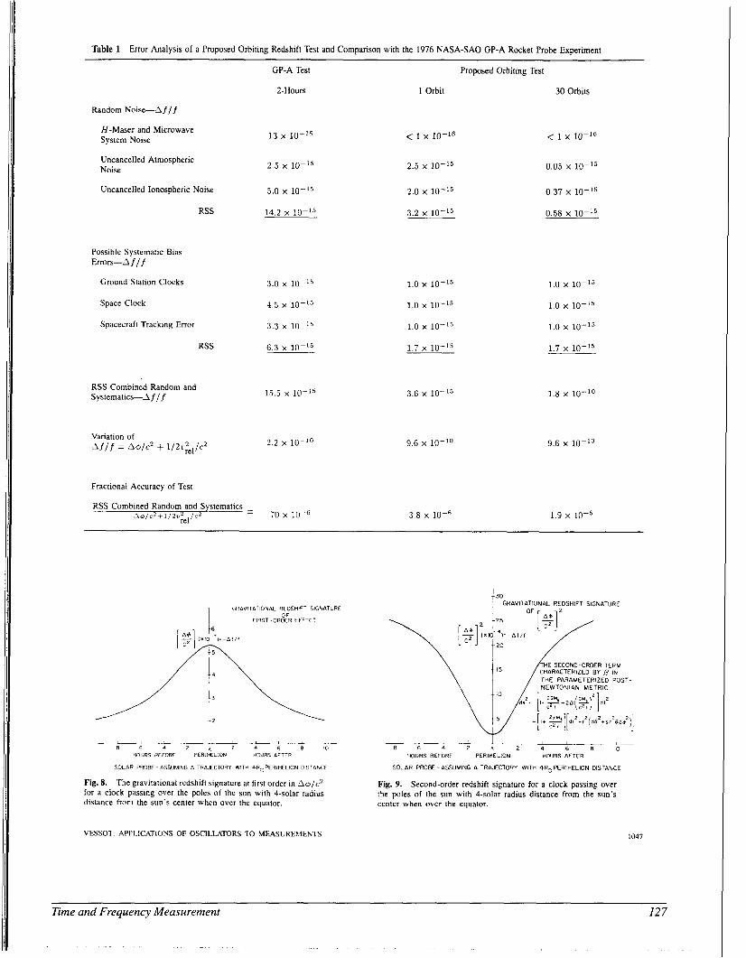
Table 1 Error Analysis of a Proposed Orbiting Redshift Test and Comparison with the 1976 NASA-SA0 GP-A Rocket Probe Experiment
GP-A Test
2-Hours
Random Noise-Aflf
13 x 10-15 H-Maser and Microwave System Noise
Uncancelled Atmospheric Noise 2.5 x 10⁻¹⁵
Uncancelled Ionospheric Noise 5.0 x 10⁻¹⁵
RSS 14.2 x 10⁻¹⁵
Possible Systematic Bias Errors-A f / f
Ground Station Clocks
Space Clock
Spacecraft Tracking Error
RSS
RSS Combined Random and Systematics-Af/ f
Variation of 3flf = A6/c2 + 1 / 2 ~ $ ~ / / ~
3.0 x 10⁻¹⁵
4.5 x 10⁻¹⁵
3.3 x 10⁻¹⁵
6.3 x 10⁻¹⁵
15.5 x 10⁻¹⁵
2 . 2 x 10⁻¹⁰
Fractional Accuracy of Test
RSS Combined Random and Systematics - 70 x 10-6 :el'c2 .Im/c2i1/2,,
Proposed Orbiting Test
1 Orbit 30 Orbits
< 1 x 10-16
2.5 x 10⁻¹⁵
2.0 x 10⁻¹⁵
3.2 x 10⁻¹⁵
1.0 x 10⁻¹⁵
1.0 x 10⁻¹⁵
1.0 x 10⁻¹⁵
1.7 x 10⁻¹⁵
3.6 x 10⁻¹⁵
9.6 x lo-''
< 1 x 10-16
0.05 x 10⁻¹⁵
0.37 x 10⁻¹⁵
0.56 x 10⁻¹⁵
1.0 x 10⁻¹⁵
1.0 x 10⁻¹⁵
1.0 x 10⁻¹⁵
1.7 x 10⁻¹⁵
1.6 x lo-''
9.6 x lo-"
1.9 x 10⁻⁶ 3.6 x
1 GRAVITATIONAL REDSHIFT SIGNATURE OF
FIRST-OPVER EFFECT I
8 6 4 2 2 4 6 8 IO HOURS BEFORE PERIHELION HOURS AFTER
SOLAR PROBE -ASSUMING A TRAJECTORY WITH 4ROPERIHELION DISTANCE
Fig. 8. The gravitational redshift signature at first order in Ao/Cz for a clock passing over the poles of the sun with 4-solar radius distance from the sun's center when over the equator.
VESSOT: APPLICATIONS OF OSCILLATORS TO MEASUREMENTS
IJ0GRAVITATIONAL REDSHIFT SIGNATURE
\ 1 / N E W T O N I A N M E T R I C
I I 8 6 4 2 A 2 4 6 8 IO
HOURS BEFORE PERIHELION HOURS AFTER
SOLAR PROBE -ASSUMING A TRAJECTORY WITH 4ROPERlHEL10N DISTANCE
Fig. 9. Second-order redshift signature for a clock passing over the poles of the sun with 4-solar radius distance from the sun's center when over the equator.
1047
Time and Frequency Measurement 127
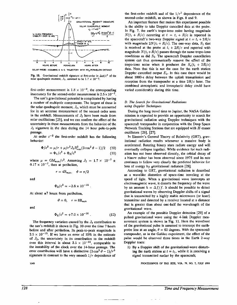
GRAVITATIONAL REDSHIFT SIGNATURE
lo CLOCK FREOVENCY STABILITY OVER 0 HRS
I I I I I 1 ,
first-order measurement is 1.8 x the corresponding inaccuracy for the second-order measurement is 2.5 x
The sun's gravitational potential is complicated by having a number of multipole components. The largest of these is the solar quadrupole moment, J2, which must be accounted for in an accurate measurement of the second order term in the redshift. Measurements of J2 have been made from solar oscillations [25], and we can confirm the effect of the uncertainty in these measurements from the behavior of the J2 signature in the data during the 14 hour pole-to-pole passage.
At order c - ~ the first-order redshift has the following behavior:
O/c2 = p / r + p/r3J2R~,,,(3cos2 29 - 1 ) / 2 (10) = -I- ' p Z / C 2 (11)
where p = GMSUn/c2 . Assuming J2 = 1.7 x lod7 f 0.17 x then at perihelion,
r = 4&,,,, 29 = a / 2
and
@ 2 / c 2 = -2.8 x 10-l~ . At about t 7 hours from perihelion,
29=0, r=8Kun
and
@2/c2 = +7.0 x . (12)
The frequency variation caused by the 52 contribution to the sun's redshift is shown in Fig. 10 over the time 7 hours before and after perihelion. Its peak-to-peak magnitude is 3.5 x If we have an error of 10% in the estimate of J2, the uncertainty in its contribution to the redshift over this interval is about 3.5 x comparable to the instability of the clock over the 14-hour passage. The error contribution will have a distinctive (3 cos2 29 - l ) / r 3 signature in contrast to the very smooth 1/r dependence of
1048
the first-order redshift and of the l l r2 dependence of the second-order redshift, as shown in Figs. 8 and 9.
An important feature that makes this experiment possible is the ability to take Doppler cancelled data at the probe. In Fig. 7, the earth's tropo-iono noise having magnitude N(t i + R / c ) occurring at t = ti + R / c is reported in the spacecraft's two-way Doppler signal at t = t , + 2 R / c with magnitude 2N(ti + R / c ) . The one-way data, SI that is received at the probe at ti + 2 R / c and reported with magnitude N ( t i + R / c ) passes through the same tropo-ion0 conditions as did S2. The spacecraft Doppler cancellation system can thus systematicnfly remove the effect of the tropo-iono noise when it produces the So(& + 2 R / c ) data. Note that this is not the case for the earth station Doppler cancelled output E,. In this case there would be about 1000-s delay between the uplink transmission and reception from the transponder at a time 2 R / c later. The combined atmospheric and ionospheric delay could have varied considerably during this time.
D. The Search for Gravitational Radiations using Doppler Techniques
During the long travel time to Jupiter, the NASA Galileo mission is expected to provide an opportunity to search for gravitational radiation using Doppler techniques with the spacecraft transponder in conjunction with the Deep Space Network Tracking Stations that are equipped with H-maser oscillators [26], [27].
In Einstein's General Theory of Relativity (GRT), grav- itational radiation results whenever a massive body is accelerated. Rotating binary stars radiate energy and will eventually collapse together. While evidence for such radi- ation has not been observed directly, the orbital decay of a hinarv ~ u l s a r has been observed since 1975 and its rate continues to follow very closely the predicted behavior for loss of energy by gravitational radiation [28].
According to GRT, gravitational radiation is described as a wavelike distortion of space-time traveling at the speed of light. When a gravitational wave intercepts an electromagnetic wave, it distorts the frequency of the wave by an amount h = Af/f . It should be possible to detect gravitational waves by observing Doppler shifts of a signal that is transmitted by a highly stable microwave (or laser) transmitter and detected by a receiver located at a distance that is greater than about one-half the wavelength of the gravitational wave.
An example of the possible Doppler detection [29] of a pulsed gravitational wave using the 4-link Doppler mea- surement system is shown in Fig. 11. Here the wavefront of the gravitational pulse is assumed to intercept the earth- probe line at an angle, 0 = 60 degrees. With the spacecraft transponder, as in the Galileo experiment, the effect of the pulse would be observed three times in the Earth 2-way Doppler trace:
1 ) By a Doppler shift of the gravitational-wave disturb- ing the earth station at t = t l , while it is receiving a signal transmitted earlier by the spacecraft;
PROCEEDINGS OF THE IEEE, VOL 79. NO. 7, JULY 1991
128 lime ana' Frequency Measurement
~- __ -
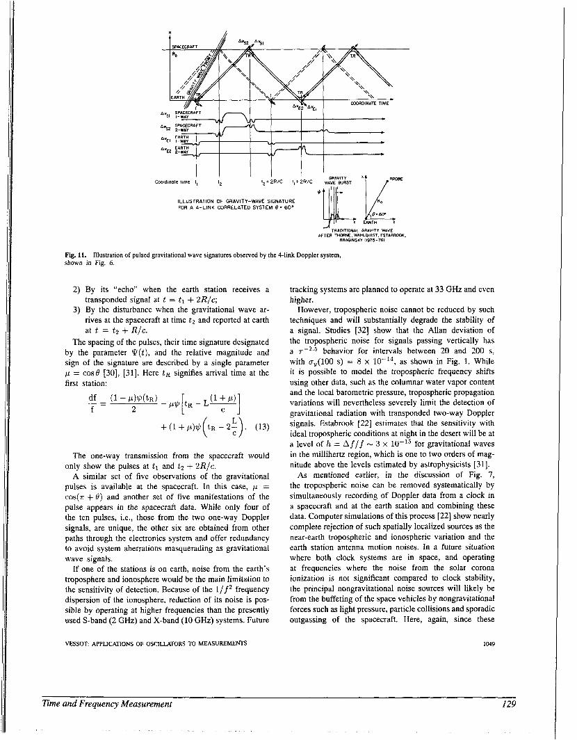
GRAVITY I
Coordinate time t1 l2 t2+2R/C t1+2R/C WAVE BURST
ILLUSTRATION OF GRAVITY-WAVE SIGNATURE FOR A 4-LINK CORRELATED SYSTEM 0 = 60’
EARTH z: e. 60. 2
TRADITIONAL GRAVITY WAVE AFTER THORNE. WAHLWIST. ESTABROOK.
BRAGINSKI 11975-761
Fig. 11. shown in Fig. 6.
Illustration of pulsed gravitational wave signatures observed by the 4-link Doppler system,
2) By its “echo” when the earth station receives a transponded signal at t = tl + 2R/c;
3) By the disturbance when the gravitational wave ar- rives at the spacecraft at time t 2 and reported at earth at t = t 2 + R / c .
The spacing of the pulses, their time signature designated by the parameter @(t ) , and the relative magnitude and sign of the signature are described by a single parameter p = cos6 [30], [31]. Here t R signifies arrival time at the first station:
The one-way transmission from the spacecraft would only show the pulses at t l and t 2 + 2Rlc.
A similar set of five observations of the gravitational pulses is available at the spacecraft. In this case, p = cos(.rr + 6) and another set of five manifestations of the pulse appears in the spacecraft data. While only four of the ten pulses, Le., those from the two one-way Doppler signals, are unique, the other six are obtained from other paths through the electronics system and offer redundancy to avoid system aberrations masquerading 2s gravitational wave signals.
If one of the stations is on earth, noise from the earth’s troposphere and ionosphere would be the main limitation to the sensitivity of detection. Because of the 1/ f frequency dispersion of the ionosphere, reduction of its noise is pos- sible by operating at higher frequencies than the presently used S-band (2 GHz) and X-band (10 GHz) systems. Future
VESSOT APPLICATIONS OF OSCILLATORS TO MEASUREMENTS
tracking systems are planned to operate at 33 GHz and even higher.
However, tropospheric noise cannot be reduced by such techniques and will substantially degrade the stability of a signal. Studies [32] show that the Allan deviation of the tropospheric noise for signals passing vertically has a 7-2.5 behavior for intervals between 20 and 200 s, with ~~~(100 s) = 8 x lo-’*, as shown in Fig. 1. While it is possible to model the tropospheric frequency shifts using other data, such as the columnar water vapor content and the local barometric pressure, tropospheric propagation variations will nevertheless severely limit the detection of gravitational radiation with transponded two-way Doppler signals. Estabrook [22] estimates that the sensitivity with ideal tropospheric conditions at night in the desert will be at a level of h = A f / f - 3 x for gravitational waves in the millihertz region, which is one to two orders of mag- nitude above the levels estimated by astrophysicists [31].
As mentioned earlier, in the discussion of Fig. 7, the tropospheric noise can be removed systematically by simultaneously recording of Doppler data from a clock in a spacecraft and at the earth station and combining these data. Computer simulations of this process [22] show nearly complete rejection of such spatially localized sources as the near-earth tropospheric and ionospheric variation and the earth station antenna motion noises. In a future situation where both clock systems are in space, and operating at frequencies where the noise from the solar corona ionization is not significant compared to clock stability, the principal nongravitational noise sources will likely be from the buffeting of the space vehicles by nongravitational forces such as light pressure, particle collisions and sporadic outgassing of the spacecraft. Here, again, since these
1049
Time and Frequency Measurement 129
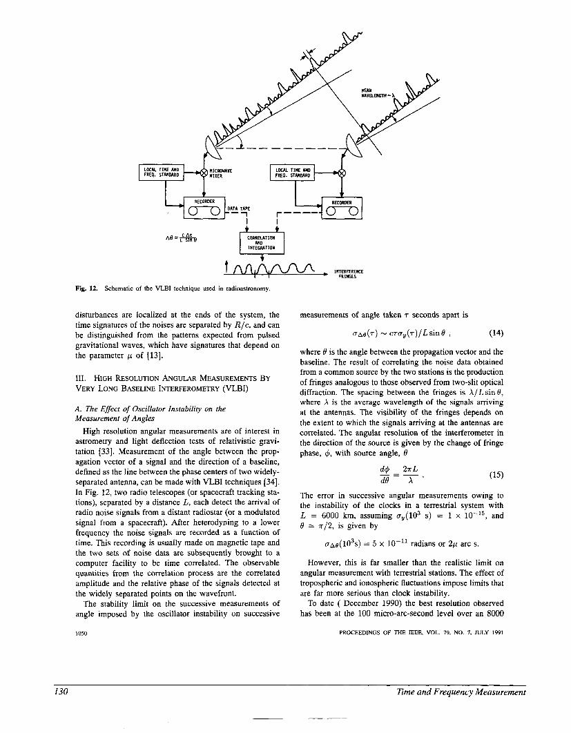
INTERFERENCE FRIWGES
Fig. 12. Schematic of the VLBI technique used in radioastronomy.
disturbances are localized at the ends of the system, the time signatures of the noises are separated by Rlc, and can be distinguished from the patterns expected from pulsed gravitational waves, which have signatures that depend on the parameter p of [13].
111. HIGH RESOLUTION ANGULAR MEASUREMENTS BY VERY LONG BASELINE INTERFEROMETRY (VLBI)
A. The Effect of Oscillator Instability on the Measurement of Angles
High resolution angular measurements are of interest in astrometry and light deflection tests of relativistic gravi- tation [33]. Measurement of the angle between the prop- agation vector of a signal and the direction of a baseline, defined as the line between the phase centers of two widely- separated antenna, can be made with VLBI techniques [34]. In Fig. 12, two radio telescopes (or spacecraft tracking sta- tions), separated by a distance L, each detect the arrival of radio noise signals from a distant radiostar (or a modulated signal from a spacecraft). After heterodyning to a lower frequency the noise signals are recorded as a function of time. This recording is usually made on magnetic tape and the two sets of noise data are subsequently brought to a computer facility to be time correlated. The observable quantities from the correlation process are the correlated amplitude and the relative phase of the signals detected at the widely separated points on the wavefront.
The stability limit on the successive measurements of angle imposed by the oscillator instability on successive
1050
measurements of angle taken T seconds apart is
where 0 is the angle between the propagation vector and the baseline. The result of correlating the noise data obtained from a common source by the two stations is the production of fringes analogous to those observed from two-slit optical diffraction. The spacing between the fringes is XILsin0, where X is the average wavelength of the signals arriving at the antennas. The visibility of the fringes depends on the extent to which the signals arriving at the antennas are correlated. The angular resolution of the interferometer in the direction of the source is given by the change of fringe phase, q5, with source angle, 6
dq5 27rL d0 X '
_ - - -
The error in successive angular measurements owing to the instability of the clocks in a terrestrial system with L = 6000 km, assuming ay(103 s ) = 1 x and 0 = ~ 1 2 , is given by
oa8(103s) = 5 x radians or 2 p arc s.
However, this is far smaller than the realistic limit on angular measurement with terrestrial stations. The effect of tropospheric and ionospheric fluctuations impose limits that are far more serious than clock instability.
To date ( December 1990) the best resolution observed has been at the 100 micro-arc-second level over an 8000
PROCEEDINGS OF THE IEEE, VOL. 79, NO. 7, JULY 1991
130 Erne and Frequency Measurement
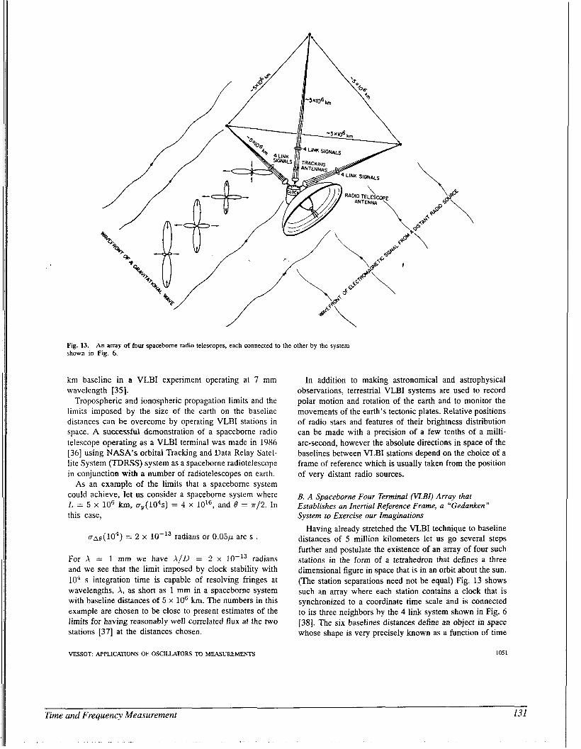
Fig. 13. shown in Fig. 6.
An array of four spaceborne radio telescopes, each connected to the other by the system
km baseline in a VLBI experiment operating at 7 mm wavelength (351.
Tropospheric and ionospheric propagation limits and the limits imposed by the size of the earth on the baseline distances can be overcome by operating VLBI stations in space. A successfu\ demonstration of a spaceborne radio telescope operating as a VLBI terminal was made in 1986 [36] using NASA‘s orbital Tracking and Data Relay Satel- lite System (TDRSS) system as a spaceborne radiotelescope in conjunction with a number of radiotelescopes on earth.
As an example of the limits that a spacebome system could achieve, let us consider a spacebome system where L = 5 x lo6 km, a,(104s) = 4 x and 0 = ~ / 2 . In this case,
C T A ~ ( ~ O ~ ) = 2 x radians or 0 . 0 5 ~ arc s .
For A = 1 mm we have AID = 2 x radians and we see that the limit imposed by clock stability with IO4 s integration time is capable of resolving fringes at wavelengths, A, as short as 1 mm in a spaceborne system with baseline distances of 5 x lo6 km. The numbers in this example are chosen to be close to present estimates of the limits for having reasonably well correlated flux at the two stations [37] at the distances chosen.
VESSOT APPLICATIONS OF OSCILLATORS TO MEASUUMENTS
In addition to making astronomical and astrophysical observations, terrestrial VLBI systems are used to record polar motion and rotation of the earth and to monitor the movements of the earth’s tectonic plates. Relative positions of radio stars and features of their brightness distribution can be made with a precision of a few tenths of a milli- arc-second, however the absolute directions in space of the baselines between VLBI stations depend on the choice of a frame of reference which is usually taken from the position of very distant radio sources.
B. A Spaceborne Four Terminal (VZBI) Array that Establishes an Inertial Reference Frame, a “Gedanken ” System to Exercise our Imaginations
Having already stretched the VLBI technique to baseline distances of 5 million kilometers let us go several steps further and postulate the existence of an array of four such stations in the form of a tetrahedron that defines a three dimensional figure in space that is in an orbit about the sun. (The station separations need not be equal) Fig. 13 shows such an array where each station contains a clock that is synchronized to a coordinate time scale and is connected to its three neighbors by the 4 link system shown in Fig. 6 [38]. The six baselines distances define an object in space whose shape is very precisely known as a function of time
1051
Time and Frequency Measurement 131
from distance measurements made by measuring the phase of the two-way signals at the stations defining the ends of each baseline.
The orientation of the array of six baselines poses an interesting problem. It should be possible to determine changes in the orientation of the array in terms of an inertial frame defined by the constancy and isotropy of the velocity of light by invoking the Sagnac effect [39]. This effect is the basis for today’s laser gyroscopes.. To describe the effect, we can visualize the arrival times of light signals sent in opposite senses about a closed path. If the transmitter and receiver are on a surface rotating at R rad/s, and their signals go about a path with projected area, A, on that surface, the difference in the arrival times of light signals going around its perimeter is A7 = 4RA/c2. If we measure the difference in arrival times of signals going in opposite senses about the triangle defining one face of the tetrahedron, we can obtain the component of rotation for that face. From the four triangles that define the tetrahedron we have four rotation components that allow us to measure the rotation vector, and, because the measurement is overdetermined, we can estimate the accuracy of its measurement.
The limit of precision in the determination of the rotation rate imposed by the maser frequency stability performance described in Fig. 1 depends on how the system is operated. If the signals originate from a single clock and are simulta- neously transmitted about the three legs in opposite senses and arrive at the point of origin with time difference, T ,
the error in the determination of T , u ~ ~ ( T ) , is given by the time dispersion plot shown in Fig. 2. For intervals up to about 20 s, the white phase noise of the maser oscillator dominates and u ~ ~ ( T ) is constant at about 2 x s. The corresponding error owing to oscillator instability in the determination of in the component of the rotation vector, R, normal to plane A of the array, is given by U ~ O ( T ) = uaT(7)c2/4A = 4 x rad/s. If the array is in a solar orbit with radius 1 AU, the measurement would have to account for the Einstein-deSitter precession of 2 x arc s/yr (3 x rad/s) owing to the bending of space-time by the suns gravity.
This array offers possibilities for astrometric observations rather than imaging of radio sources. However, it may have other applications. Essentially it compares the frame of ref- erence defined by the most distant radio sources using VLBI with an inertial frame defined by the local isotropy and constancy of the velocity of light. This comparison opens, in a modem context, the question of inertial frames raised long ago by Bishop Berkeley, Emst Mach, and others. This system may provide a way to observe some aspects of the behavior of the missing matter in the universe, which is alleged to have mass overwhelmingly greater than the mass of celestial bodies observed by electromagnetic means. We look to theorists to provide scenarios of processes that could interact with this system by considering effects due to various hypothetical types of missing matter.
This system could be extended to detect pulsed gravita- tional radiation. Here the array of baselines could provide
1052
as many as 60 manifestations of the signature from a single pulse and give information about the speed of propagation, the direction, and the polarization of the gravitational wave.
IV. CONCLUSION Since the mid-1960’s the frequency stability of atomic
clocks (or oscillators) has been improving with no end in sight. The units of time and frequency, and the now redefined unit of distance through the velocity of light, are solidly based on atomic frequency standards. This metrology, in a local sense, has been made consistent with the present concepts of gravitation and relativity. Measure- ments of astronomical and astrophysical quantities near the edges of our universe are now being made in terms of quantum phenomena that occur in particles whose physics encompass staggeringly smaller distance scales. As the performance of atomic clocks improves (and, hopefully, as our national willingness to support fundamental science in space) we should expect some surprises about the nature of our universe, including the relationship between gravitation and the three other known fundamental forces.
There are also new frontiers to explore in spectroscopy, especially in low temperature atomic spectroscopy with the advent of new techniques in cryogenics, laser cooling, and trapping, where the physics of ultralow energy particle interaction will undoubtedly also surprise us.
ACKNOWLEDGMENT The writer gratefully thanks his colleagues, E. M. Matti-
son, R. R . Reasenberg, R . L. Walsworth, and J. M. Moran for many helpful discussions and J. Janjigian for her help in preparing the manuscript.
REFERENCES
J. Rutman and F. L. Walls, “Characterization of frequency stability in precision frequency sources,” Proc. IEEE, vol. 79, this issue. D. J. Wineland, J. C. Bergquist, J. J. Bollinger, W. M. Itano, D. J. Heinzen, S. L. Gilbert, C. H. Manney, and M. G. Raizen, “Progress at NIST toward absolute frequency standards using stored ions,” IEEE Trans. Ultrason. Ferroelec. Freq. Confr., vol. 37, Nov. 1990. R. F. C. Vessot, E. M. Mattison, W. J. Klepczynski, G. M. R. Winkler, I. F. Silvera, H. P. Godfried, and R. L. Walsworth, “Present clock stability and realistic prospects for the future,” in Proc. Fourth Marcel Grossman Meeting on General Relativity, R. Ruffini, Ed., Rome, Italy, June 17-21, 1985. L. A. Rawley, J. H. Taylor, M. M. Davis, D. W. Allan, “Millisecond pulsar PSR 1937 + 21: A highly stable clock,” Science, vol. 238. D. R. Stinebring, M. F. Ryba, J . H. Taylor, and R. W. Romani, “Cosmic gravitational-wave background: limits from millisec- ond pulsar timing,” Phys. Rev. Lett., v o l 6 5 , no. 3, pp. 285-288, 1988. T. Damour, G. W. Gibbons, and J. H. Taylor, “Limits on the variability of G using binary-pulsar data,” Phys. Rev. Lett., vol. 61, no. 10, pp. 151-154, 1988. J . P. Tumeaure and S. R. Stein, Atomic Masses and Fundamen- tal Constants, J. H. Sanders and A. H. Wapstra, Eds. New York: Plenum, vol. 5, 1976, p. 636. S. Thakoor, D. M. Strayer, G. D. Dick, and J. Mercereau, “A lead-on-sapphire superconducting cavity of superior quality,” J. Appl. Phys., vol. 59, pp. 854-858, 1986.
PROCEEDINGS OF THE IEEE. VOL. 7Y. NO. 7, JULY 1991
I32 Eme and Frequency Measurement
_ _
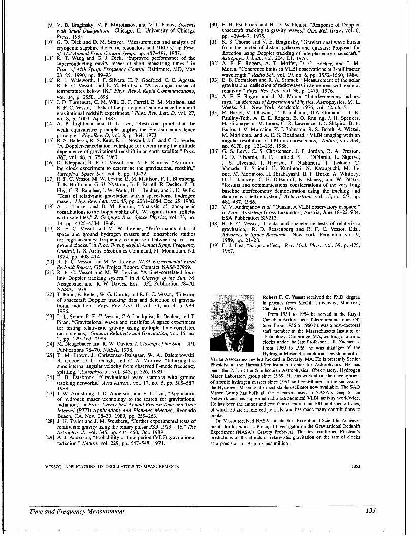
V. B. Braginsky, V. P. Mitrofanov, and V. I. Panov, Systems with Small Dissipation. Chicago, I L University of Chicago Press, 1985. G. D. Dick and D. M. Strayer, “Measurements and analysis of cryogenic sapphire dielectric resonators and DRO’s,” in Proc. of 41st Annual Freq. Control Symp., pp. 487-491, 1987. R. T. Wang and G. J. Dick, “Improved performance of the superconducting cavity maser at short measuring times,” in Proc. of 44th Symp. Frequency Control, Baltimore, MD, May
R. L. Walsworth, I. F. Silvera, H. P. Godfried, C. C. Agosta, R. F. C. Vessot, and E. M. Mattison, “A hydrogen maser at temperatures below lK,” Phvs. Rev A Rapid Communications,
23-25. 1990, pp. 89-93
~ 0 1 . ~ 3 4 , p. 2550, 1896. . J. D. Tumeaure, C. M. Will, B. F. Farrell, E. M. Mattison, and R. F. C. Vessot,.“Tests of the principle of equivalence by a null gravitational redshift experiment,” Phys. Rev. Lett. D, vol. 27, no. 8, p. 1009, Apr. 1983. A. P. Lightman and D. L. Lee, “Restricted proof that the weak eauivalence orinciole imolies the Einstein eauivalence principld,” Phys.Rev. D , bol. 8,’p. 364, 1973. R. S. Badessa, R. S. Kent, R. L. Nowell, J. C. and C. L. Searle, “A Doppler-cancellation technique for determining the altitude denendence of eravitational redshift in an earth satellite.” h o c . I&, vol. 48, 758, 1960. D. Kleppner, R. F. C. Vessot, and N. F. Ramsey, “An orbit- ing clock experiment to determine the gravitational redshift,” Astrophys. Space Sci., vol. 6, pp. 13-32. R. F. C. Vessot, M. W. Levine, E. M. Mattison, E. L. Blomberg, T. E. Hoffmann, G. U. Nystrom, B. F. Farrell, R. Decher, P. B. Eby, C. R. Baugher, J. W. Watts, D. L. Teuber, and F. D. Wills, “Tests of relativistic gravitation with a space-borne hydrogen maser,” Phys. Rev. Lett., vol. 45, pp. 2081-2084, Dec. 29, 1980. A. J. Tucker and B. M. Fannin, “Analysis of ionospheric contributions to the Doppler shift of C. W. signals from artificial earth satellites,” J. Geophys. Res., Space Physics, vol. 73, no. 13, pp. 43254334, 1968. R. F. C. Vessot and M. W. Levine, “Performance data of space and ground hydrogen masers and ionospheric studies for high-accuracy frequency comparison between space and ground clocks,” in Proc. Twenty-eighth Annual Symp. Frequency Control, U. S . Army Electronics Command, Ft. Monmouth, NJ, 1974, pp. 408-414. R. F. C. Vessot and M. W. Levine, NASA Experimental Final Redshifr Reporr, GPA Project Report, Contract NAS8-27969. R. F. C. Vessot and M. W. Levine, “A time-correlated four- link Doppler tracking system,” in A Closeup of the Sun, M. Neugebauer and R. W. Davies, Eds. JPL Publication 78-70, NASA, 1978. T. Piran, E. Reiter, W. G. Unruh, and R. F. C. Vessot, “Filtering of spacecraft Doppler tracking data and detection of gravita- tional radiation,” Phys. Rev. Lett. D, vol. 34, no. 4, p. 984, 1986. L. L. Smarr. R. F. C. Vessot, C.A Lundquist, R. Decher, and T. Piran, “Gravitational waves and redshifts: A space experiment for testing relativistic gravity using multiple time-correlated radio signals,” General Relativity and Gravitation, vol. 15, no. 2, pp. 129-163, 1983. M. Neugebauer and R. W. Davies, A Closeup ofrhe Sun. JPL Publications 78-70, NASA, 1978. T. M. Brown, J. Christensen-Dalsgaar, W. A. Dziembowski, R. Goode, D. 0. Gough, and C. A. Morrow, “Inferring the suns internal angular velocity from observed P-mode frequency splitting,” Astrophys. J., vol. 343, p. 526, 1989. F. B. Estabrook, “Gravitational wave searches with ground tracking networks,” Acta Astron., vol. 17, no. 5, pp. 585-587, 1988. J. W. Armstrong, J. D. Anderson, and E. L. Lau, “Application of hydrogen maser technology to the search for gravitational radiation,” in Proc. Twenty-first Annual Precise Time and Time Interval (PITI) Applications and Planning Meeting, Redondo Beach, CA, Nov. 28-30, 1989, pp. 259-263. J. H. Taylor and J. M. Weisberg, “Further experimental tests of relativistic gravity using the binary pulsar PSR 1913 + 16,” The Astrophys. J., vol. 345, pp. 434-450, Oct. 1989. A. J. Anderson, “Probability of long period (VLF) gravitational radiation,“ Naiure, vol. 229, pp. 547-548, 1971.
[30] F. B. Estabrook and H. D. Wahlquist, “Response of Doppler spacecraft tracking to gravity waves,” Gen. Rel. Grav., vol. 6, pp. 439-447, 1975.
[31] K. S . Thorne and V. B. Braginsky, “Gravitational-wave bursts from the nuclei of distant galaxies and quasars: Proposal for detection using Doppler tracking of interplanetary spacecraft,” Astrophys. J. Lett., vol. 204, L1, 1976.
[32] A. E. E. Rogers, A. T. Moffet, D. C. Backer, and J. M. Moran, “Coherence limits in VLBI observations at 3-millimeter wavelength,” Radio Sci., vol. 19, no. 6, pp. 1552-1560, 1984.
[33] E. B. Formalont and R. A. Sramek, “Measurement of the solar gravitational deflection of radiowaves in agreement with general relativity,” Phys. Rev. Lett. vol. 36, p. 1475, 1976.
[34] A. E. E. Rogers and J. M. Moran, “Interferometers and ar- rays,” in Methods of Experimental Physics, Astrophysics, M. L. Weeks, Ed.
[35] N. Bartel, V. Dhawan, T. Krichbaum, D.A Graham, I. I. K. Pauliny-Toth, A. E. E. Rogers, B. 0. Rnn ng, J. H. Spencer, H. Hirabayashi, M. Inoue, C. R. Lawrence, I. I. Shapiro, B. F. Burke, J. M. Marcaide, K. J. Johnston, R. S. Booth, A. Witzel, M. Morimoto, and A. C. S. Readhead, “VLBI imaging with an angular resolution of 100 microarcseconds,” Nature, vol. 334, no. 6178, pp. 131-135, 1988.
[36] G. S. Levy, C. S. Christensen, J. F. Jordan, R. A. Preston, C. D. Edwards, R. P. Linfield, S. J. DiNardo, L. Skjerve, J. S. Ulvestad, T. Hayashi, T. Nishimura. T. Taskano, T. Yamada, T. Shiomi, H. Kunimori, N. Kawaguchi, M. In- oue, M. Morimoto, H. Hirabayashi, B. F. Burke, A. Whitney, D. L. Jauncey, C. H. Ottenhoff, K. Blaney, and W. Peters, “Results and communications considerations of the very long baseline interferometry demonstration using the tracking and data relay satellite system,” Acta Astron., vol. 15, no. 6/7, pp.
New York: Academic, 1976, vol. 12, ch. 5.
~. 481-487; 1986.
1371 V. V. Andreianov et al. “Quasat, A VLBI observatory in space.” L .
in Proc. Wo;kshop Gross Enzersdorf, Austria, June i8-221984, ESA Publication SP-213.
[38] R. F. C. Vessot, “Clocks and spacebome tests of relativistic gravitation,” R. D. Reasenberg and R. F. C. Vessot, Eds., Advances in SDace Research. New York: Pereamon. vol. 9. - . 1989, pp. 21-28,
1967. [39] E. J. Post, “Sagnac effect,” Rev. Mod. Phys., vol. 39, p. 475,
Robert F. C. Vessot received the Ph.D. degree In physics from McGill University, Montreal, Canada in 1956.
From 1951 to 1954 he served in the Royal Canadian Airforce as a Telecommunications Of- ficer From 1956 to 1960 he was a post-doctoral staff member at the Massachusetts Institute of Technology, Cambridge, MA, workmg of atomic clocks under the late Professor J R Zacharias From 1960 to 1969 he was manager of the Hydrogen Maser Research and Development of
Vanan Associates/Hewlett Packard in Beverly, MA. He is presently Senior Physicist at the Harvard-Smithsonian Center for Astrophysics. He has been the P I of the Smithsonian Astrophysical Observatory, Hydrogen Maser Laboratory group since 1969 He has worked on the development of atomic hydrogen masers since 1961 and contributed to the success of the Hydrogen Maser as the most stable oscillator now available. The SA0 Maser Group has built all the H-masers used in NASA’s Deep Space Network and has supported radio astronomical VLBI activity worldwlde He has been the author and coauthor of more than 100 published articles, of which 33 are in refereed journals, and has made many contnbutions to books.
Dr Vessot received NASA’s medal for “Exceptional Scientific Achieve- ment” for his work as Principal Investigator on the Gravitational Redshift Experiment (NASA‘s Gravity Probe-A). This test confirmed Einstein’s predictions of the effects of relativistic gravitation on the rate of clocks at a precision of 70 parts per million
VESSOT APPLICATIONS OF OSCILLATORS TO MEASUREMENTS 1053
Time and Frequency Measurement 133
0 1991 IEEE. Reprinted, with permission, from Proceedings of the IEEE: Special Issue on Time and Frequency, 79 (7), 1070-1076; 1991.
Time and Frequency in Fundamental Metrology BRIAN W. PETLEY
Invited Paper
The role of time and frequency in a wide range of measurements is discussed, particularly those involving the International System of Units (SI) and fundamental physical constants.
I. INTRODUCTION Modern science and technology are placing increas-
ingly stringent demands on our measurement system and associated units. The International System of Units (SI) [ l ] is almost universally used and other unit systems have generally been defined to have an exact relation- ship to the SI. The ultimate arbiters for the SI are the General Conference on Weights and Measures (CGPM), the International Committee on Weights and Measures (CIPM), and the Consultative Committee on Units (CCU). The SI embodies seven base units: those of time, length, mass, quantity of electricity, thermodynamic temperature, amount of substance, and luminous intensity. There is a second class, the supplementary units which provide units of angle and solid angle. These are regarded as dimensioned or dimensionless according to the choice of the user. Along with these there are now some nineteen named combinations of the base units which are known as derived units.
There are three distinct time units in the SI, these are: the base unit, the second (13th CGPM, 1967) which is the unit of time and time interval; the derived unit known as the hertz (11th CGPM, 1960), used to characterize the frequency of periodic phenomena; the derived unit of activity known as the becquerel (15th CGPM, 1975) which is used for the stochas- tic phenomenon of radioactive decay related to the number of disintegrations per second.
Manuscript received November 13, 1990; revised February 26, 1991. This work is based on a talk presented at the 6th European Conference on Time and Frequency, Neuchitel, Switzerland, March 13-15, 1990.
The author is with the Centre for Basic Metrology, Division of Quantum Metrology, National Physical Laboratory, Teddington, Middlesex T W l l OLW, U.K.
IEEE Log Number 9100246.
1070
Attempts to metricate other time units (happily) failed, and units such as the minute (60 s), hour (3600 s), and day (86 400 s) were recognized by the CIPM in 1969 as being units used alongside the SI. The week, month, and year, remain in common use.
Although the meter and kilogram were carefully defined by the CGPM at their first meeting in 1889, the second does not appear to have been explicitly defined by them. Everyone “knew” that it was:
((equal to the fraction I / 86 400 of the mean solar day))
and left the astronomers to define precisely what was meant by the phrase “mean solar day.” In 1956 the CIPM followed the decision of the 1955 General Assembly of the IAU, and decided that:
((the second is the fraction 1/31 556 925.9747 of the tropical year
for 1900 January 0 at 12 hours ephemeris time)).
This somewhat inaccessible definition was adopted by the 11th CGPM in 1960. This definition only endured until 1967 when the 13th CGPM decided that metrology needed a better unit of time than astronomy could provide and, by its resolution 1, decided that
((The second is the duration of 9 192 631 770 periods of the radiation corresponding to the transition
between the two hyperfine levels of the caesium- 133 atom)).
At the same time the earlier definition was abrogated. Metrology is the phrase used to describe the rapidly
evolving art and science of accurate measurement. Viewed from a distance it is readily apparent that:
1) accuracy with which we are able to make measure- ments has been increasing over the centuries;
2) this process has been speeding up, the present rate corresponding roughly to a tenfold improvement ev- ery fifteen years.
0018-9219/91/0700-1070%01.00 0 1991 IEEE
PROCEEDINGS OF THE IEEE, VOL. 79, NO. 7, JULY 1991
134 Zme and Frequency Measurement
~ ~-
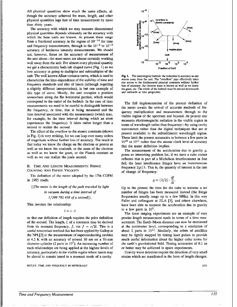
All physical quantities show much the same effects, al- though the accuracy achieved for mass, length, and other physical quantities lags that of time measurement by more than thirty years.
The accuracy with which we may measure dimensioned physical quantities depends ultimately on the accuracy with which the base units are known. At present these range from a fractional accuracy in the region of for time and frequency measurements, through to the to accuracy of luminous intensity measurements. We should not, however, focus on the accuracy of measurement of the unit alone-for most users are almost certainly working well away from the unit. For almost every physical quantity we get a characteristic bath-tub shaped curve (Fig. 1) as we lose accuracy in going to multiples and submultiples of the unit. The well known Allan-variance curve, which is used to characterize the time-dependence of the stability of time and frequency standards and also of lasers (although requiring a slightly different interpretation), is but one example of this type of curve. Mostly, the unit occupies a position somewhere along the flat horizontal portion, which would correspond to the outlet of the bathtub. In the case of time measurements we need to be careful to distinguish between the frequency, or time, that is being measured and the time interval associated with the measurement (which may, for example, be the time interval during which an atom experiences the frequency). It takes rather longer than a second to realize the second.
The effect of the overflow to the atomic constants (shown in Fig. 1) is very striking, for we can leap over many orders of magnitude without further loss of accuracy. The result is that today we know the charge on the electron or proton as well as we know the coulomb, or the mass of the electron as well as we know the gram, or the Planck constant as well as we can realize the joule second.
11. COUNTING AND FRINGE VELOCITY
TIME AND LENGTH MEASUREMENTS: FRINGE
The definition of the meter adopted by the 17th CGPM in 1983 reads:
((The meter is the length of the path traveled by light in vacuum during a time interval of
11299 792 458 of a second)).
This invokes the relationship:
l = c . t
so that our definition of length requires the prior definition of the second. The length, 1, of a resonator may be derived from its resonant frequency, f , via f = c/21. This is a useful noncontact method that has been applied by Gallop at the NPL[2] to the measurement of superconducting cavities at 4.2 K with an accuracy of around 10 nm on a 50” diameter cylinder (2 parts in lo7). An increasing number of such relationships are being applied at the highest levels of accuracy, particularly in the visible region where lasers may be slaved to remain tuned to a resonant mode of a cavity.
PETLEY: TIME AND FREQUENCY IN METROLOGY
(overflow to
(time)
(time)
waste-plpa
-15 l o o lo3 l o 6
10
Fraction of Unit
Fig. 1. The metrological bathtub: the reduction in accuracy as one moves away from the unit. The “overflow” pipe effectively takes one across to the fundamental physical constants without further loss of accuracy: the electron mass is known as well as we know the gram, etc. The whole of the bathtub must be moved downwards and outwards as time progresses.
The full implementation of the present definition of the meter awaits the arrival of accurate methods of fre- quency multiplication and measurement through to the visible region of the spectrum and beyond. At present one measures electromagnetic radiation in the visible region in terms of wavelength rather than frequency-by using cavity wavemeters rather than the digital techniques that are at present available to the submillimeter wavelength region. These limit the present accuracies to between a few parts in 10’O or lo1’ rather than the atomic clock level of accuracy that the meter definition implies.
The measurement of the acceleration due to gravity g, poses an interesting problem for, if we have a cube comer reflector that is part of a Michelson interferometer in free fall, the laser interference fringes have an instantaneous frequency 2 g t l X . That is, the quantity of interest is the rate of change of frequency:
df g = (X/2) ’ ---. dt
Up to the present the time for the cube to traverse a set number of fringes has been measured instead (the fringe frequencies usually range up to a few MHz). In this way Faller and colleagues at JILA [3], and others elsewhere, have been able to measure the acceleration due to gravity to a few parts in io9.
The lunar ranging experiments are an example of very precise length measurement made in terms of a time mea- surement. The Earth-Moon distance can now be monitored at the centimeter level, corresponding to a resolution of about 2 parts in loll . Similarly, the orbits of satellites may be tightly mapped by timing laser pulses to provide much useful information about the higher order terms for the earth’s gravitational field. Timing accuracies of 0.1 ns or better may be achieved in space experiments.
Gravity wave detectors require the detection of very small strains which are manifested in the form of length changes.
1071
Time and Frequency Measurement 135
Detectors having strain sensitivities of between to 10-l' are being constructed in several locations. Some of these map length changes into frequency changes and therefore make strong demands on the short-term stability of the frequency discriminator. They require frequency discrimination and sensitivity rather than absolute accuracy.
111. ELECTRICAL AND OTHER MEASUREMENTS AND THE RADIAN PER SECOND
The radian per second is the unit of angular frequency and, although it often occurs in theoretical discussions, there is little necessity to produce and measure exact angular frequencies in radian per second (except as below). Many users prefer to express measurements in terms of alternative units such as degrees per second. An example of the measurement of small angular dis-
placement rates would be in gyroscopes. The sensitivities of gyroscopes are normally expressed in "/h rather than rads, the conversion factor being approximately l0/h = 5O.1Ow6 rad/s. Sensitivities of better than "/h are required for ship navigation, and "/h in aircraft. For the latter this corresponds to less than one nautical mile of drift error per hour.
The optical gyroscopes [4] make use of the Sagnac (1913) effect to detect small angular velocities. The time difference At in an area A and angular velocity R is given by:
At = 4AR2/c2 .
Michelson and Gale demonstrated this effect in 1925 by using an interferometer to detect the Earth's rotation rate of 15 "/h. For A = 1 m2, and R = 15 O / h , AL(= cat) is about m.
Fiber optic systems require phase detection sensitivities corresponding to about 10-8X in a 109X path length in order to achieve sensitivities of 0.050 "/h. The very best suspended electrical gyroscopes achieve around "/h, although the present-day active laser, passive laser, and fiber optic ring-gyroscopes have around a 100 times poorer sensitivity they are capable of further refinement. In laser ring gyroscopes, the counter-rotating beat frequencies of < 1 mHz have been measured, enabling long term stabilities of "/h to be achieved. Performance in some cases is approaching the quantum noise limit of
The transfer across from resistance involves the equa- tions:
"/(h)'".
R = WL and R = l /wC.
Obviously, if C, L, and R for electrical standards are all to be nearly exact multiples of the unit, then w must also be an integral number of radians per second. Consequently, a rational frequency in rad/s rather than hertz is used experimentally to help make the transfer from resistance to and from capacitance and inductance standards. An angular frequency of lo4 radians per second is convenient for this. One often finds that specifications for ac electrical measurements require that the measurements are made at, or within 1 Hz, of 1592 Hz. This frequency is regarded as
1072
being sufficiently close to the desired angular frequency of lo4 radian per second. No attempt is made to synthesize the exact angular frequency to much better than this.
A. The Realization of the Volt, Ampere, and Ohm The accuracy with which the electrical units could be
realized in the past was limited by the requirement to mea- sure the linear dimensions of coils of wire very accurately. For many years the ohm, for example, was realized via a precisely constructed mutual inductor until the advent of the Thompson and Lampard calculable capacitor meant that the farad could be realized instead. The capacitance so realized was (107/[4?rc2])~ln2 F/m (about 1.953 pF/m) and was ob- tained by moving a screening electrode whose displacement was readily measured by counting laser fringes. (Frequency enters the measurement via the 1592-Hz source energizing the ac bridges).
In this way the realizations of the ohm have been improved to yield fractional accuracies of the order of a few parts in 10'. It ought to be possible to improve the accuracy further, particularly by measuring the length change as a change in frequency, for example, by changing the length of a resonant cavity. The advent of the quantized Hall resistance for MOSFET semiconductors, operated at low temperatures and strong magnetic fields, has enabled the drift of resistance standards to be confirmed as being of the order of 0.05 ,& per year-the present ability to detect such small resistance drifts and allow for them promises well for the future.
Until recently the volt was realized by some form of attracted electrode electrometer (the most accurate of these being the attracted mercury surface determination of Cloth- ier, Sloggett, and others at the NML[S] in Australia), while the ampere was realized via some traditional form of current balance. These are likely to be replaced by the realization of the watt.
B. The Watt Kibble at the NPL proposed [6] the method which forms
the basis for recent electrical realizations of the watt. Essentially, a coil of wire is suspended from one arm of a mass balance such that it is partially in the field provided by a magnet (both superconducting magnets and permanent magnets are being used).
A current I, whose value is known in terms of the laboratory representation of the ampere, is passed through the coil and the force on the coil balanced by adding or removing mass m, from the scale-pan. The coil is then displaced vertically with a uniform velocity v , and the induced emf E, measured in terms of the laboratory as maintained representation of the volt. The product of the voltage and the current are then given by:
E a = mgv
where g is the acceleration due to gravity. Thus the power is known in terms of both the laboratory maintained repre- sentation of the watt, Kw watt, and the mechanical watt.
PROCEEDINGS OF M E IEEE, VOL. 79, NO. 7, JULY 1991
136 Eme ana' Frequency Measurement
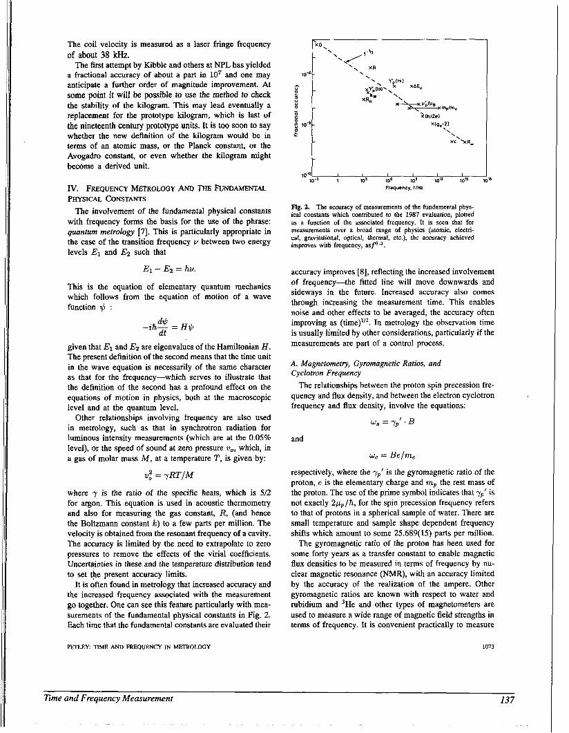
The coil velocity is measured as a laser fringe frequency of about 38 kHz.
The first attempt by Kibble and others at NPL has yielded a fractional accuracy of about a part in lo7 and one may anticipate a further order of magnitude improvement. At some point it will be possible to use the method to check the stability of the kilogram. This may lead eventually a replacement for the prototype kilogram, which is last of the nineteenth century prototype units. It is too soon to say whether the new definition of the kilogram would be in terms of an atomic mass, or the Planck constant, or the Avogadro constant, or even whether the kilogram might become a derived unit.
Iv. m Q U E N C Y METROLOGY AND THE FUNDAMENTAL PHYSICAL CONSTANTS
The involvement of the fundamental physical constants with frequency forms the basis for the use of the phrase: quantum metrology [7]. This is particularly appropriate in the case of the transition frequency u between two energy levels El and E2 such that
El - E2 = hv.
This is the equation of elementary quantum mechanics which follows from the equation of motion of a wave function 11 :
given that E1 and E2 are eigenvalues of the Hamiltonian H. The present definition of the second means that the time unit in the wave equation is necessarily of the same character as that for the frequency-which serves to illustrate that the definition of the second has a profound effect on the equations of motion in physics, both at the macroscopic level and at the quantum level.
Other relationships involving frequency are also used in metrology, such as that in synchrotron radiation for luminous intensity measurements (which are at the 0.05% level), or the speed of sound at zero pressure v,, which, in a gas of molar mass M , at a temperature T , is given by:
II,” = y R T / M
where y is the ratio of the specific heats, which is 512 for argon. This equation is used in acoustic thermometry and also for measuring the gas constant, R, (and hence the Boltzmann constant k) to a few parts per million. The velocity is obtained from the resonant frequency of a cavity. The accuracy is limited by the need to extrapolate to zero pressures to remove the effects of the virial coefficients. Uncertainties in these and the temperature distribution tend to set the present accuracy limits.
It is often found in metrology that increased accuracy and the increased frequency associated with the measurement go together. One can see this feature particularly with mea- surements of the fundamental physical constants in Fig. 2. Each time that the fundamental constants are evaluated their
PETLEY TIME AND FREQUENCY IN METROUXjY
rxG. 1
. XC \XR_
Fig. 2. The accuracy of measurements of the fundamental phys- ical constants which contributed to the 1987 evaluation, plotted as a function of the associated frequency. It is seen that for measurements over a broad range of physics (atomic, electri- cal, gravitational, optical, thermal, etc.), the accuracy achieved improves with frequency, a ~ f ~ , ~ .
accuracy improves [8], reflecting the increased involvement of frequency-the fitted line will move downwards and sideways in the future. Increased accuracy also comes through increasing the measurement time. This enables noise and other effects to be averaged, the accuracy often improving as (time)”’. In metrology the observation time is usually limited by other considerations, particularly if the measurements are part of a control process.
A. Magnetometry, Gyromagnetic Ratios, and Cyclotron Frequency
The relationships between the proton spin precession fre- quency and flux density, and between the electron cyclotron frequency and flux density, involve the equations:
and
wc = Befm,
respectively, where the yp’ is the gyromagnetic ratio of the proton, e is the elementary charge and mp the rest mass of the proton. The use of the prime symbol indicates that yp’ is not exactly 2 p p / h , for the spin precession frequency refers to that of protons in a spherical sample of water. There are small temperature and sample shape dependent frequency shifts which amount to some 25.689(15) parts per million.
The gyromagnetic ratio of the proton has been used for some forty years as a transfer constant to enable magnetic flux densities to be measured in terms of frequency by nu- clear magnetic resonance (NMR), with an accuracy limited by the accuracy of the realization of the ampere. Other gyromagnetic ratios are known with respect to water and rubidium and 3He and other types of magnetometers are used to measure a wide range of magnetic field strengths in terms of frequency. It is convenient practically to measure
1073
Time and Frequency Measurement 137
and express the frequencies in hertz and their values are usually tabulated in both hertz and radians per second.
The accuracy of flux density measurements by this method is partly limited by the accuracy of the realization of the volt. The water sample shape, its temperature, the effects of the container, and impurities in the water (dissolved oxygen in particular), limit the accuracy to about a part in lo8-much depends on the nature of the substitution method involved.
Although not requiring accurate frequency measurement, SQUID magnetometers operate at carrier frequencies up to the microwave region and enable magnetic flux to be measured in terms of the magnetic flux quantum h/2e (around Wb). These are relative devices since it is difficult to measure the area through which the flux is passing.
B. Ratio Experiments and Mass Spectrometry There are some important measurements which involve
the ratios of ion cyclotron frequencies and/or spin preces- sion frequencies. These include the g - 2 measurements for the electron, positron and muon, and the ratio of the proton to electron mass. The accuracy of such measurements made a major leap forward through the pioneering work on ion traps by Dehmelt, Van Dyck, and others at the University of Washington and elsewhere. Some of the improvement can also be attributed to the use of higher flux densities, with correspondingly higher frequency discrimination.
Conventional mass spectrometry achieved its lo-’ frac- tional accuracy by setting very stringent geometric require- ments on the ion orbit, by using beam defining slits, etc., so that the arrival of the ion at the detector depended critically on its starting phase with respect to the applied cyclotron frequency. Thus in the ion substitution mass syn- chrometers of Lincoln Smith in Princeton and of Mamyrin in Leningrad, the ions made only two revolutions, taking around a microsecond, before being detected. The timing discrimination (or the equivalent phase discrimination) was effectively of the order of s for a fractional resolution of a part in lo8. Ion substitution was achieved by changing both the applied ac and dc potentials, and ac frequencies. Ion traps are beginning to allow the properties of antimatter to be explored and no doubt the findings of these studies will impact on metrology.
C. Josephson Effects The prediction in 1962 of the Josephson tunneling effects
in superconductivity, and their subsequent validation at the part per million level at the University of Pennsylvania, the NPL, and elsewhere by the end of 1969, meant that there was a very precise relation between the potential difference between two closely separated superconductors in the presence of a microwave frequency f given by:
2eV = hf
where n was an integer, h the Planck constant and e the elementary charge. This equation has been verified in
1074
various ways to the very highest levels of precision, includ- ing independence of the operating conditions (temperature, material, frequency), and by now must be one of the most accurately verified effects in physics.
Meanwhile, one of the most accurate measurements in- volving frequency to date has been made via a null mea- surement by Lukens and others at Stony Brook [SI, which involved verifying that the change in the gravitational potential of a microwave photon in traversing a vertical distance of about a centimeter was the same as the change in potential of the electron pair wave. The discrimination achieved was of the order of a part in needless to say the interpretation of such a measurement is slightly open to debate! We have arrived at the situation in electrical metrology where the volt is maintained in terms of agreed values of the Josephson effect K J , and the ohm in terms of the quantized Hall resistance von Klitzing constant &.[lo]
D. Can We Measure h Directly In Terms of the Mechanical Units?
The quantum equation relating energy to frequency:
E = hv
occurs so frequently in modern physics that one wonders whether it can be verified directly in terms of the joule (regarded as a mechanical unit). The equation can and has, of course, been verified for cases where the energy involved is primarily an electrical energy, most frequently as an energy in electron-volts.
If the voltage EJ across a Josephson junction (which is biased onto the nth voltage step when irradiated with a microwave frequency f) is maintained at a value equal to the voltage across a von Klitzing device which is biased onto the second quantized Hall resistance step, then the power in the Hall resistor is:
E:/RH = n2 f 2 h / 2 . Today the volt is maintained via the Josephson effect KJ and the ohm via the quantized Hall resistance R K , and the numerical relationships between these and the units are exactly specified [lo]. Consequently, we see that the above realization of the watt by Kibble and others limits our knowledge of h, always provided, of course, that the Josephson and von Witzing relationships are exact.
v. METROLOGY AND TIME VARIATIONS OF THE FUNDAMENTAL CONSTANTS
Following their interpretation in terms of Dirac’s “big numbers” some 55 years ago, there is always considerable interest in the question of whether or not the fundamental constants are constant. The evidence to date is that they are constant on the level of less than one percent over the age of the universe. Some measurements have put even tighter constraints. In each case one must interpret the results with care. This is particularly so for any dimensioned quantity since one cannot say whether it is the unit or the quantity that has varied (equally a null effect may result if they
PROCEEDINGS OF THE IEEE, VOL. 79, NO. 7, JULY 1991
138 Time and Frequency Measurement
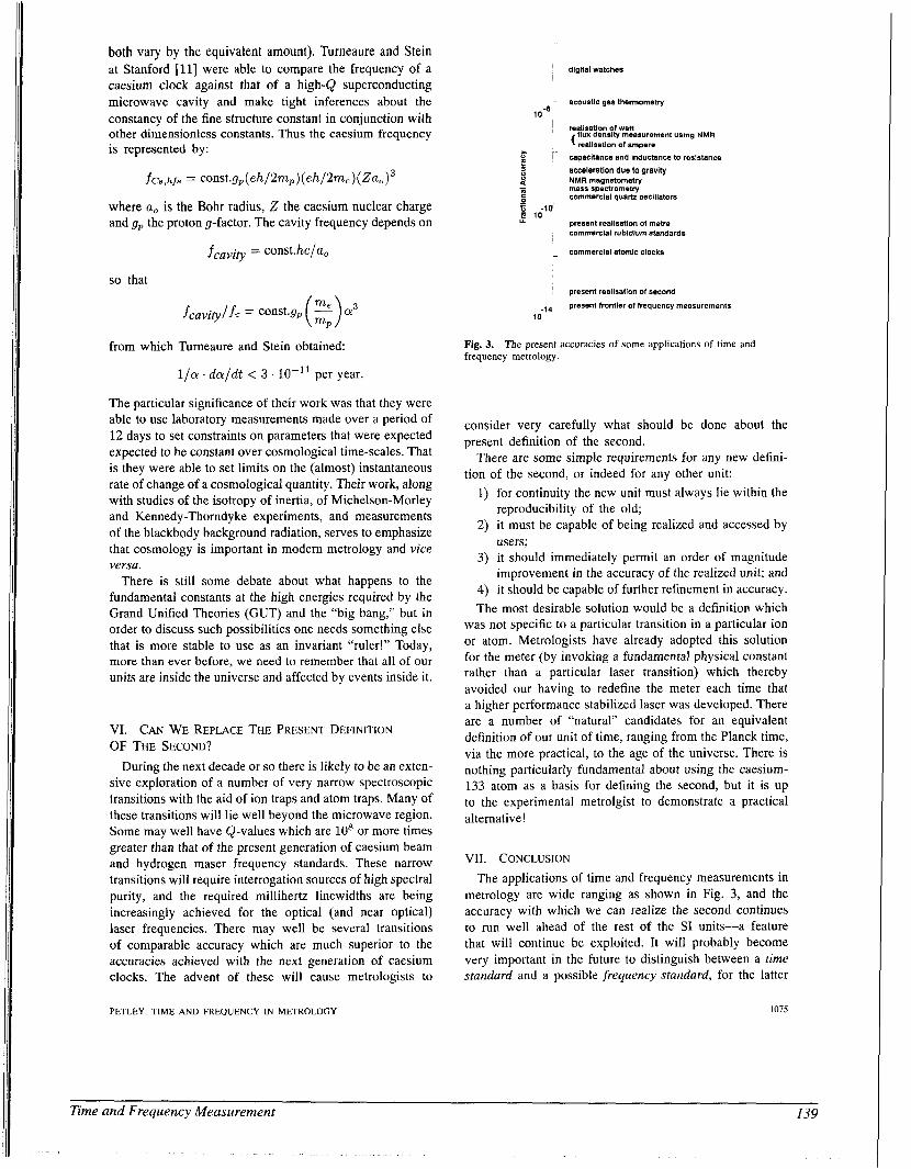
both vary by the equivalent amount). Turneaure and Stein at Stanford [ll] were able to compare the frequency of a caesium clock against that of a high-Q superconducting microwave cavity and make tight inferences about the constancy of the fine structure constant in conjunction with other dimensionless constants. Thus the caesium frequency is represented by:
fcs,hfs = const.g, ( e h / 2 m p ) (eh/2me)( Za , )3
where a, is the Bohr radius, 2 the caesium nuclear charge and gp the proton g-factor. The cavity frequency depends on
so that
from which Turneaure and Stein obtained:
1/a . d a / d t < 3 . lo-’’ per year.
The particular significance of their work was that they were able to use laboratory measurements made over a period of 12 days to set constraints on parameters that were expected expected to be constant over cosmological time-scales. That is they were able to set limits on the (almost) instantaneous rate of change of a cosmological quantity. Their work, along with studies of the isotropy of inertia, of Michelson-Morley and Kennedy-Thorndyke experiments, and measurements of the blackbody background radiation, serves to emphasize that cosmology is important in modern metrology and vice versa.
There is still some debate about what happens to the fundamental constants at the high energies required by the Grand Unified Theories (GUT) and the “big bang,” but in order to discuss such possibilities one needs something else that is more stable to use as an invariant “ruler!” Today, more than ever before, we need to remember that all of our units are inside the universe and affected by events inside it.
VI. CAN WE REPLACE THE PRESENT DEFINITION OF THE SECOND?
During the next decade or so there is likely to be an exten- sive exploration of a number of very narrow spectroscopic transitions with the aid of ion traps and atom traps. Many of these transitions will lie well beyond the microwave region. Some may well have Q-values which are lo8 or more times greater than that of the present generation of caesium beam and hydrogen maser frequency standards. These narrow transitions will require interrogation sources of high spectral purity, and the required millihertz linewidths are being increasingly achieved for the optical (and near optical) laser frequencies. There may well be several transitions of comparable accuracy which are much superior to the accuracies achieved with the next generation of caesium clocks. The advent of these will cause metrologists to
PETLEY: TIME AND FREQUENCY IN METROLOGY
’ digital watches
acoustic gas thermometry
’ realisation of wan {flux denriw measurement using NMR
reallsation of ampere E i capacitance and Inductance to resistance
acceleration due to gravity 4“
1 commercial quartz osciiiators
1 present reallsation of metre
NMR magnetometry mass spectrometry
B -10- e 10
commerclal rubldlum standards
commercial atomic clocks
,
’ present realisallon of second
-,4 present frontier of frequency measurements 10
Fig. 3. frequency metrology.
The present accuracies of some applications of time and
consider very carefully what should be done about the present definition of the second.
There are some simple requirements for any new defini- tion of the second, or indeed for any other unit:
1) for continuity the new unit must always lie within the reproducibility of the old;
2 ) it must be capable of being realized and accessed by users;
3) it should immediately permit an order of magnitude improvement in the accuracy of the realized unit; and
4) it should be capable of further refinement in accuracy. The most desirable solution would be a definition which
was not specific to a particular transition in a particular ion or atom. Metrologists have already adopted this solution for the meter (by invoking a fundamental physical constant rather than a particular laser transition) which thereby avoided our having to redefine the meter each time that a higher performance stabilized laser was developed. There are a number of “natural” candidates for an equivalent definition of our unit of time, ranging from the Planck time, via the more practical, to the age of the universe. There is nothing particularly fundamental about using the caesium- 133 atom as a basis for defining the second, but it is up to the experimental metrolgist to demonstrate a practical alternative!
VII. CONCLUSION The applications of time and frequency measurements in
metrology are wide ranging as shown in Fig. 3, and the accuracy with which we can realize the second continues to run well ahead of the rest of the SI units-a feature that will continue be exploited. It will probably become very important in the future to distinguish between a time standard and a possible frequency standard, for the latter
1075
Time and Frequency Measurement I39
need not operate continuously! As we have seen, there are an increasing number of quantum effects which may be produced sufficiently cleanly in the laboratory to enable them to be used for purposes of defining or maintaining the SI units. We can expect in a general way that this process is likely to continue and that the definitions of most of the other base units will rely on time in some way.
As the accuracy of measurement advances it will be necessary to take general and special relativity more into account than before in metrology and elsewhere. That is, it will be more important to take care to use coordinate time, internal time, proper time, and so on, as is appropriate to the particular circumstances of the measurement. The studies of the stability of the millisecond Pulsars (which provide a longer term “flywheel” against which we may look for un- expected secular variations in our time standards) serve as a strong reminder that the whole of our terrestrial physics is modulated by changes in our gravitational potential-such as result from the rotation of the Earth and Moon about one another and about the Sun. Hopefully we will eventually be able to detect such effects solely by laboratory based measurements without recourse to Pulsars. We may expect to have to consider in the future such questions as that of the granularity of time (when measuring the highest frequencies in the X-ray region and beyond), or the reasons for the direction of ‘‘the arrow of time,” and their implications for quantum physics and metrology.
Progress must slow eventually, but there are probably some seven or more orders of magnitude to go before we reach the ultimate accuracy limits for frequency measure- ment. These may well be reached when the averaging time for the ultimate transition is about the working life of a metrologist! At the present rate of progress that condition may well be reached well before the end of the next century, meanwhile our endeavors to attain such accuracies will provide a lot of technological applications and knowledge, and also provide plenty of fun!
REFERENCES [l] Le Systeme International d’llnites (SZ), 5th ed., Paris: BIPM,
1985. [2] J. C. Gallop and W. J. Radcliffe, “Shape and dimensional
measurement using microwaves,” J. Phys. E: Sci. Instrum., vol. 43, pp. 413416, 1986.
I. Marson and J. E. Faller, “The acceleration of gravity: its measurement and its importance,” J. Phys. E: Sci Instrum., vol. 19, pp. 22-32, 1988. J. Faucheux, D. Fayoux, and J. J. Roland, “The ring laser gyro,”
W. K. Clothier, G. J. Sloggett, H. Baimsfather, M. F. Currey, and D. J. Benjamin, “A determination of the volt,” Metrologia, vol. 26, pp. 9-46, 1989. B. P. Kibble, I. A. Robinson, and J. H. Belliss, “A realization of the SI watt by the NPL moving-coil balance,” NPL Report DES 88, 1988. B. W. Petley, The Fundamental Constants and the Frontier of Measurement. Adam Hilger: London, U.K., 1988. E. R. Cohen and B. N. Taylor, “The 1986 evaluation of the fundamental physical constants,” Rev. Mod. Phys., vol. 57, pp.
A. K. Jain, J. E. Lukins, and J . 4 . Tsai, ‘Test for relativistic gravitational effects on charged particles,” Phys. Rev. Lett., vol.
B. N. Taylor and T. 1. Witt, New international electrical reference standards based on the Josephson and Quantum Hall Effects,” Metrologia, vol. 26, pp. 47-62, 1989. J. P. Tumeaure and S. R. Stein, “An experimental test of the time variation of the fine-structure constant,” in Atomic Masses and Fundamental Constants 5, J . H. Sanders and A. H. Wapstra, Eds.
J. Opt., V O ~ . 19, pp. 101-115, 1988.
1121-1148, 1988.
58, pp. 1165-1168, 1987.
London, U.K.: Plenum, 1976, pp. 636-642.
Brian W Petley was born in Dover, England and obtained the Ph.D. degree from Imperial College for work in high energy nuclear physics.
Following a period at the Electrical Research Association he moved to the National Physi- cal Laboratory, where his active research in- terests and publications include topics in basic metrology, dielectrics, the Jose hson effects and
try, atomic hydrogen beam work, and the mea- surement of fundamental physical constants. He
heads the Centre for Basic Metrology at the NPL, is a member of the CODATA Task Group on Fundamental Physical Constants, and is Chair- man of the IUPAP Commission C2, the Commission on Symbols, Units, Nomenclature, Atomic Masses, and Fundamental Physical Constants. He has also written a book on The Fundamental Physical Constants and the Frontier of Measurement and another on An Introduction to the Josephson Effects
Dr. Petley is a member of the Editorial Boards of Measurement Science and Technology, and Metrologia, and a Member of the Editorial Review Committee of IEEE TRANSACTIONS ON INSTRUMENTATION AND MEASUREMENT.
SQUID’S, laser spectroscopy, P He magnetome-
1076 PROCEEDINGS OF THE IEEE, VOL. 79, NO. 7, JULY 1991
140 7ime and Frequency Measurement
Copyright © 2022 FDOKUMEN