The use of Geological and Hydrogeological Modelsin ...

The use of Geological and Hydrogeological Models in Environmental Studies

Geological Modelling Systems Team

Internal Report IR/10/022

BRITISH GEOLOGICAL SURVEY

GEOLOGICAL MODELLING SYSTEMS TEAM

INTERNAL REPORT IR/10/022

The National Grid and other Ordnance Survey data © Crown Copyright and database rights 2012 are used with the permission of the Controller of Her Majesty’s Stationery Office. Licence No: 100021290

Keywords

Models, Geology, Hydrogeology.

Front cover

Model of the Chalk group showing watertable

Bibliographical reference

MATHERS, S.J., KESSLER H., MACDONALD, D.M.J., HUGHES, A., JACKSON, C & ROBINS, N.S. 2010. Geological and Hydrogeological models. British Geological Survey Internal Report, IR/10/022. 102pp.

Copyright in materials derived from the British Geological Survey’s work is owned by the Natural Environment Research Council (NERC) and/or the authority that commissioned the work. You may not copy or adapt this publication without first obtaining permission. Contact the BGS Intellectual Property Rights Section, British Geological Survey, Keyworth, e-mail [email protected]. You may quote extracts of a reasonable length without prior permission, provided a full acknowledgement is given of the source of the extract.

Maps and diagrams in this book use topography based on Ordnance Survey mapping.

The use of Geological and Hydrogeological Models in Environmental Studies

S.J.Mathers, H.Kessler, D.M.J. Macdonald, A.Hughes, C.Jackson & N.S.Robins

© NERC 2012. All rights reserved Keyworth, Nottingham British Geological Survey 2012

The full range of our publications is available from BGS shops at Nottingham, Edinburgh, London and Cardiff (Welsh publications only) see contact details below or shop online at www.geologyshop.com

The London Information Office also maintains a reference collection of BGS publications, including maps, for consultation.

We publish an annual catalogue of our maps and other publications; this catalogue is available online or from any of the BGS shops.

The British Geological Survey carries out the geological survey of Great Britain and Northern Ireland (the latter as an agency service for the government of Northern Ireland), and of the surrounding continental shelf, as well as basic research projects. It also undertakes programmes of technical aid in geology in developing countries.

The British Geological Survey is a component body of the Natural Environment Research Council.

British Geological Survey offices

BGS Central Enquiries Desk

Tel 0115 936 3143 Fax 0115 936 3276

email [email protected]

Kingsley Dunham Centre, Keyworth, Nottingham NG12 5GG

Tel 0115 936 3241 Fax 0115 936 3488 email [email protected]

Murchison House, West Mains Road, Edinburgh EH9 3LA

Tel 0131 667 1000 Fax 0131 668 2683 email [email protected]

Natural History Museum, Cromwell Road, London SW7 5BD

Tel 020 7589 4090 Fax 020 7584 8270 Tel 020 7942 5344/45 email [email protected]

Columbus House, Greenmeadow Springs, Tongwynlais, Cardiff CF15 7NE

Tel 029 2052 1962 Fax 029 2052 1963

Maclean Building, Crowmarsh Gifford, Wallingford OX10 8BB

Tel 01491 838800 Fax 01491 692345

Geological Survey of Northern Ireland, Colby House, Stranmillis Court, Belfast BT9 5BF

Tel 028 9038 8462 Fax 028 9038 8461

www.bgs.ac.uk/gsni/

Parent Body

Natural Environment Research Council, Polaris House, North Star Avenue, Swindon SN2 1EU

Tel 01793 411500 Fax 01793 411501 www.nerc.ac.uk

Website www.bgs.ac.uk Shop online at www.geologyshop.com

BRITISH GEOLOGICAL SURVEY

XX/00/00; Draft 0.1 Last modified: 2012/11/20 10:14

i

Foreword

This report is the published product of a study by the British Geological Survey (BGS) for the Environment Agency.

Acknowledgements

The authors wish to express their sincere thanks to their colleagues in both the British Geological Survey and the Environment Agency who have provided advice on the scope, content and delivery of this scoping study.

In particular we thank the following Agency staff for sparing time to discuss their various roles and requirements for geological and hydrogeological modelling during this study and in recent years:

Tim Besien, Giles Bryan, Rolf Farrell, Mark Grout , Alwyn Hart, Sarah Hepburn, Nigel Hoad, Paul Hulme, Phil Humble, Nigel Johnson, Michael Kehinde, Travis Kelly, Fiona Lobley, Keith Seymour, Martin Shepley, Rob Ward and Mark Whiteman.

Figures within this document may use Ordnance Survey topography material with the permission of Ordnance Survey on behalf of The Controller of Her Majesty’s Stationery Office. © Crown Copyright Licence Number: 100021290.

Figures within this document may portray elevation data taken form Intermap’s NEXTMap Britain data.

Contents

1 Background ................................................................................................................................. 1

1.1Terms of Reference ............................................................................................................. 1

1.2The Modelling Workflow ................................................................................................... 1

1.3Drivers for Groundwater Management ............................................................................... 2

1.4The Agency’s requirement for subsurface information ...................................................... 8

2 Data Resources and Formats ................................................................................................... 13

2.1Geological maps ................................................................................................................ 13

2.2Borehole databases ............................................................................................................ 15

2.3Digital Elevation Models (DTM’S) .................................................................................. 16

2.4Existing models and surfaces ............................................................................................ 18

2.5Geophysical Data .............................................................................................................. 24

2.6Topology ........................................................................................................................... 27

3 Geological 3D Models ............................................................................................................... 28

3.1Background ....................................................................................................................... 28

3.2Implicit and Explicit Modelling ........................................................................................ 30

3.3Main geological modelling softwares ............................................................................... 30

3.4Interoperability between Geological Modelling Softwares .............................................. 36

3.5Geological Domains .......................................................................................................... 38


ii

3.6Uncertainty in 3D Geological Models .............................................................................. 49

3.7Data and Model delivery ................................................................................................... 51

3.8BGS Future modelling plans ............................................................................................. 54

4 Conceptual Models ................................................................................................................... 55

4.1Development of Conceptual models ................................................................................. 55

4.2Current best practice ......................................................................................................... 58

4.3Uses for Conceptual models by the Environment Agency ............................................... 59

5 Numerical (Groundwater Flow) models ................................................................................ 61

5.1Introduction ....................................................................................................................... 61

5.2Testing conceptual models of groundwater flow and solute transport ............................. 61

5.3Scale .................................................................................................................................. 62

5.4Complexity ........................................................................................................................ 63

5.5Representation of geological complexity in groundwater models .................................... 65

6 Case Studies and costs .............................................................................................................. 65

6.1Oxford Flooding Project ................................................................................................... 66

6.2Chichester .......................................................................................................................... 70

6.3Manchester Hydrogeological Pathway Model .................................................................. 72

6.4Lichfield Permo-Trias model ............................................................................................ 74

6.5The London Chalk Model ................................................................................................. 75

6.6Vale of York Fence diagram ............................................................................................. 77

6.7Factors affecting cost ........................................................................................................ 78

7 Recommendations .................................................................................................................... 79

8 References cited ........................................................................................................................ 80

9 GSI3D Bibliography ................................................................................................................. 85

10 Glossary ................................................................................................................................... 90

FIGURES

Figure 1 The Geological and Hydrogeological modelling workflow (modified from Sharpe et al. 2002) ......................................................................................................................................... 3

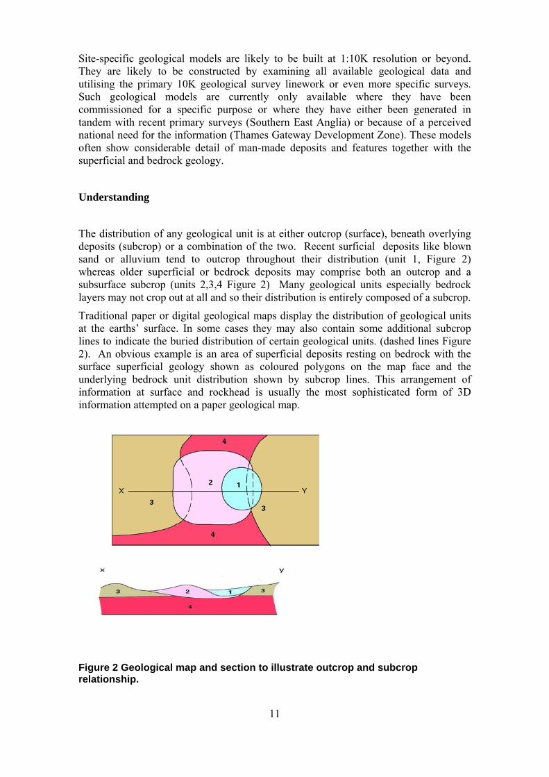
Figure 2 Geological map and section to illustrate outcrop and subcrop relationship. .................. 11

Figure 3 Relationship between 2D and 3D data ............................................................................ 12

Figure 4 BGS 1:10 000 and 1:50 000 DiGMapGB availability OS topography © Crown Copyright ................................................................................................................................ 14

Figure 6 BoGe data input using a MS Access front end. .............................................................. 16

Figure 7 Example of Digital Elevation Models, from Intermap’s NEXTMap Britain data of London (top) and Agency LiDAR dtm of Kingston upon Hull showing anthropogenic structures (below) ................................................................................................................... 18

Figure 8 Example ASCII grid viewed in a text editor ................................................................... 18


iii

Figure 9 The BGS national 1Million resolution LithoFrame model ............................................. 19

Figure 10 Example LithoFrame 250 model covering the Weald and adjacent parts of the English Channel ................................................................................................................................... 19

Figure 13. Schematic section showing effective depth of modelling and definition across the LithoFrame 250-50-10 resolutions ......................................................................................... 23

Figure 14 The stacking of LithoFrame models and the major disciplines involved in their construction. ........................................................................................................................... 24

Figure 18 The York urban model (LithoFrame 10) nested inside the Vale of York regional fence diagram (from Cooper et al. 2007) commissioned by the Agency. ........................................ 29

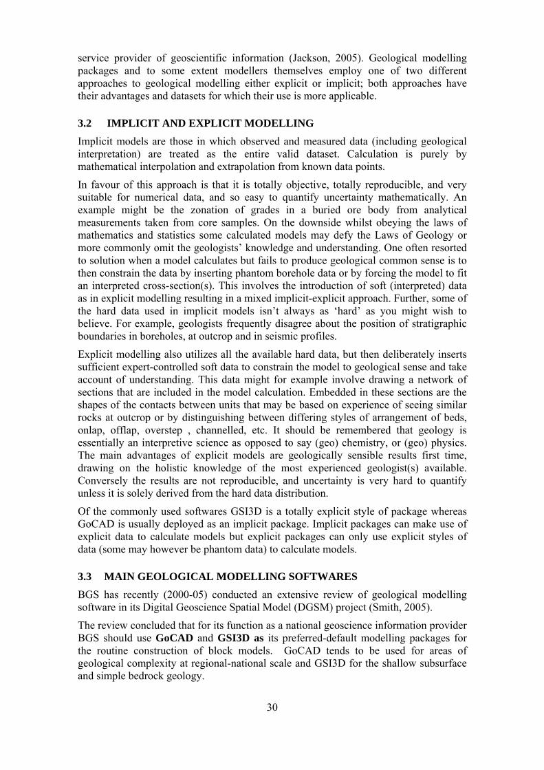
Figure 19 The GSI3D software interface ...................................................................................... 32

Figure 20 The GSI3D workflow ................................................................................................... 33

Figure 21 The GoCAD Interface ................................................................................................... 35

Figure 22 GoCAD model visualised in GSI3D ............................................................................. 36

Figure 23 The London LithoFrame 50 model displayed in GoCAD ............................................ 37

Figure 24 Synthetic GSI3D section from Cheshire to Kent through and a synthetic borehole in East Anglia (vertical scale 1:1). .............................................................................................. 37

Figure 26 Detailed LithoFrame 10 model of the area south of York showing the lacustrine deposit of Lake Humber (orange) and the terminal moraine at York (blue). ......................... 40

Figure 27 The Southern East Anglia LithoFrame 10 resolution model, as delivered to the Anglian Region of the Agency ............................................................................................................. 41

Figure 29 Representation of groundwater flooding using observed groundwater levels .............. 43

Figure 30 Conceptual model of the catchment area. ..................................................................... 43

Figure 31 The London LithoFrame 50 model covering 2400 sq km ............................................ 44

Figure 32 The Cirencester-Stroud Model under construction ....................................................... 46

Figure 33 The Bromsgrove project model of a 25x25 km block of Permo-Triassic strata at the northern end of the Worcester Graben around Bromsgrove. The highly faulted Triassic Bromsgrove Sandstone aquifer is shown in yellow and the Droitwich Halite (confined to the Worcester Graben) is shown in blue. ...................................................................................... 47

Figure 34 The Plynlimon model showing folded and faulted basal stratigraphic surfaces for units, produced as a testbed for the ongoing GSI3D Bedrock development from Mathers et al. 2008. ....................................................................................................................................... 49

Figure 35 Uncertainty assessment showing drill locations and drill type as well as a grid of the average assumed error for geological surfaces (from Lelliott et al 2009). ............................ 50

Figure 36 Uncertainty drape on 25 km2 LithoFrame 10 model of central Glasgow ..................... 51

Figure 37 The BGS LithoFrame Data Portal ................................................................................ 51

Figure 38 The Subsurface Viewer Interface showing the Southern East Anglia Model in the Subsurface Viewer with stratigraphic (top) and permeability attribution (bottom) ............... 52

Figure 39 Options for delivery of BGS models ............................................................................ 53

Figure 41 Standard model development flowchart. ...................................................................... 56

Figure 42 Environment Agency Conceptual Model development “spiral” (after Hulme et al., 2003). ...................................................................................................................................... 57


iv

Figure 43 The floodplain of the River Thames and tributaries in the Oxford area ....................... 66

Figure 44 GSI3D model of superficial deposits in the Oxford area ............................................. 67

Figure 45 Depth to groundwater within the floodplain superficial deposits in the Oxford valley67

Figure 47 Superficial geology in the Oxford valley Figure 14 OS topography © Crown Copyright ................................................................................................................................ 69

Figure 48. Estimated peak flood water elevation during the July 2007 flood event ..................... 69

Figure 49 The Chichester model showing surface geology (top), alluvial fan in ochre middle) and folded bedrock geology including chalk aquifer in green (bottom) ....................................... 71

Figure 50 Geological model of the Manchester area covering 15 x 5 km. ................................... 72

Figure 51 Targeted cross-section along the Manchester Ship Canal showing predicted flow paths73

Figure 52 Conceptual flow model produced from the geological model and hydrogeological pathway understanding. .......................................................................................................... 74

Figure 53 GoCAD model of the Permo-Triassic strata of the Southern Needwood Basin around Lichfield .................................................................................................................................. 75

Figure 55 The London Chalk Model showing faulted layers within the Chalk Group aquifer. ... 76

Figure 56 Base of Seaford Chalk showing principal faults ........................................................... 77

Figure 57 The Vale of York fence diagram in the map, 3D and section window of GSI3D. ....... 78

TABLES

Table 1 Long term strategies, policy and legislation relevant to groundwater management and their delivery mechanisms, with the highest Environment Agency priority indicated. ........... 6

Table 2 Geological units in the National LithoFrame 1 Million model ....................................... 18

Table 3 Main features of the LithoFrame resolutions ................................................................... 21

Table 4 Geological detail possible at the various LithoFrame resolutions. .................................. 22

Table 5 Advantages and drawbacks to modelling in GSI3D and GoCAD ................................... 35

Table 6 Codes and descriptions of types of embankments from the BGS Lexicon ...................... 38

Table 7 Summary of the range of the Conceptual models routinely developed by the Environment Agency. ............................................................................................................. 60

Table 8 Comparison between model “couplets” of different types .............................................. 64


v

Summary

Many duties of the Environment Agency involve a thorough understanding of water and its movement through the geosphere.

The Agency has identified the development of conceptual models as the primary building blocks for their management of the water environment. Where appropriate these conceptual models provide the basis for numerical models for simulation and forecasting. Geological models play a key role in the development of the conceptual understanding and models in relation to groundwater systems under the CAMS process and the Water Framework Directive. Geological models are also useful to communicate sub-surface conditions and investigate site-specific problems in a variety of other Agency activities.

By its very nature, the geometry and properties of the geosphere remain hidden from the observer and can therefore only be approximated using observations such as boreholes, surface outcrop and proxy measurements of its properties such as geophysical conductivity. In most cases the available data are not sufficient to create a data driven geological model and geologists with understanding of geological processes and the evolution of a particular area are required to complete the jigsaw puzzle of hard facts and conception to create an explicit understanding of the subsurface arrangement of rocks – the validated geological model.

In recent years great advances in technology and geological-hydrogeological modelling mean that affordable models can now be produced across all of England and Wales. It is now also recognised that there are clear benefits in basing conceptual and numerical (groundwater flow) models on digital 3D geological models not only because of the formalisation of the geological interpretation but also because of the clarity of vision and understanding the 3D geological model provides.

The British Geological Survey is the nation’s statutory body for the understanding of Britain’s geology. In this unique role it manages considerable data holdings including borehole logs, well data, seismic sections, geophysical datasets and digital geological linework. These datasets are the building blocks for 3D geological models. Amongst national geological survey organisations BGS has pioneered the development of 3D geological models, modelling software and the application of models. BGS is fully committed through its new strategy document (2009) to transforming its’ standard geoscience information delivery from 2D geological map outputs to 3-4D geological and process models.

This scoping study summarises the present methodologies and softwares used in the construction of geological and hydrogeological models both at BGS and elsewhere. It makes key recommendations for the closer integration of the varied styles of models, together with improvements in data formats, exchange mechanisms and enhanced collaboration between the Agency, consultants and BGS towards delivery of the business mission of the Agency.

1

1 Background

1.1 TERMS OF REFERENCE

This report has been produced by staff at the British Geological Survey commissioned by the Agency to undertake a scoping study into the use of geological and hydrogeological models within the Agency. The key requirements of this study were specified as follows

A brief review of the capabilities of and potential or existing uses for 3 dimensional subsurface models in the context of Agency operational and policy work.

Consideration of the basis of existing Agency uses of 3D models in existing Regions including costs and benefits of their use.

A review of available 3D model softwares and frameworks including the conceptual understanding of subsurface structures in 3 dimensions and how this is achieved in “traditional” geological settings.

The report should also focus on how models may affect future flow modelling work at the Agency. There is a need to achieve an improved representation of the geological setting in order to improve groundwater flow and transport understanding in our groundwater bodies.

Development of conceptual approaches for locations or catchments where little or no hydrogeological data is available

A review of cost and resource implications for implementation of 3D geological modelling in England and Wales at a variety of scales, for example local site scale versus catchment scale.

Recommendations for future work and use of appropriate conceptual and software models.

1.2 THE MODELLING WORKFLOW

Geological and groundwater models are an important input into the conceptualisation and management of catchments and water bodies The workflows and methodologies described in this report are concerned principally with the development of geological,

2

conceptual and numerical models that ultimately lead to an improved Quantitative Understanding and Management of the Environment.

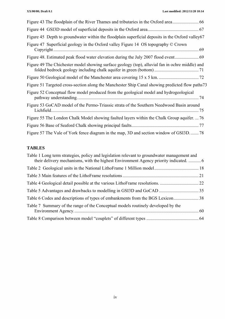
The terms for the different sorts of models involved in geological and hydrogeological studies, and the workflow and relationship between them are defined here. The generally accepted workflow to produce Numerical (Groundwater Flow) models and Quantitative Understanding is shown in Figure 1.

This linear approach is to a degree theoretical and in practice iteration can be a very important part of any modelling process for example as expressed in other approaches such as the Spiral (iterative) methodology (Environment Agency 2003). However this linear approach works well in establishing conceptual models from geological models and other key datasets in regional-catchment scale assessments required for example for the CAMS process and WFD. The linear approach is however less well suited for problem solving and monitoring of systems where a more iterative workflow is to be expected. The workflow (Figure 1) comprises

1. Assembly of available geological data resources in formats appropriate to the modelling software(s).

2. Construction of a 3D Geological (block) model which depicts the geological units present as volumes or objects using geological modelling softwares such as GSI3D, GoCAD, Earthvision, Geomodeller etc.. A variety of scales or resolutions of models are possible; other simpler means of depicting the geological structure can be through the use of cross-sections, fence diagrams or generalised sections.

3. The geological model is used together with other baseline datasets such as land-use and drainage to produce a Conceptual groundwater model that attempts to summarise understanding of likely patterns of water flow through the strata, together with inputs and outflows.

4. A layered Numerical (Groundwater Flow) model is produced from this understanding using flow modelling software such as MODFLOW and ZOOM, this predicts flow paths and water balances in the system.

5. The product is Quantitative Understanding of the Environment and its processes. This enhanced knowledge leads in turn to better informed decision making about environmental issues

As noted above in many cases the Conceptual and Numerical models inform the geological models in an iterative fashion, thereby ensuring total consistency throughout the workflow from baseline data to prediction. This also means that all parts of the modelling workflow should be of dynamic design utilising standard formats thus ensuring easy data transfer between systems and models.

3

Figure 1 The Geological and Hydrogeological modelling workflow (modified from Sharpe et al. 2002)

1.3 DRIVERS FOR GROUNDWATER MANAGEMENT

The Agency has identified the development of Conceptual models as the primary building blocks for the management of the water environment. Where appropriate these conceptual models provide the basis for simulation and forecasting models. Geological models can play an important role in developing a conceptual understanding, in particular in relation to groundwater systems.

Those issues for which development of Conceptual models underpin the management of groundwater, and are therefore key drivers, include:

ensuring groundwater abstractions do not adversely affect river flows and water availability for terrestrial ecosystems.

trends in pollution of groundwater by nutrients from diffuse agricultural and non-agricultural sources and measures to reverse them to improve quality of water supply and baseflow.

4

the direct and indirect (socio-economic) impacts of climate change on groundwater resources and the role in adaptation and mitigation.

addressing the environmental impacts of major infrastructure projects, in particular related to energy generation.

the legacy of historic land use, including contaminated land and mine water rebound.

assessing the efficacy of resource management plans related to the activities of the water industry.

addressing the role of groundwater in flood risk management.

Table 1 outlines the key legislative drivers for England and Wales relevant to groundwater management. The table also outlines delivery mechanisms related to legislation and the major long term strategies.

The two main linked themes that are of particular relevance to the current review, as identified by the Environment Agency, are the EU Water Framework Directive (WFD) and abstraction licensing policy. Both require as their basis a conceptual understanding of the groundwater system and how this interacts with aquatic and terrestrial ecosystems.

EU Water Framework Directive

The WFD came into force in 2000 (European Union, 2000).Its aim is to improve and integrate the way water bodies are managed throughout Europe. It requires that all inland and coastal waters within defined River Basin Districts reach at least good status by 2015 and defines how this should be achieved through the establishment of environmental objectives and ecological targets for surface waters and groundwater. It was transposed into law in England and Wales via the Water Environment Regulations 2003.

The key stages defined in addressing the requirements of the Directive, relevant to this review, are:

Characterisation (delivered Dec 2004): the identification of water bodies and their physical characteristics; and the assessment of pressures and impacts on rivers, lochs, estuaries, coasts, groundwater and wetlands.

Monitoring (delivered Dec 2006): programmes to establish an overview of water status of each River Basin District and to classify the status of individual water bodies, in relation to groundwater, through a water level monitoring network and surveillance and operational monitoring of chemical status

River Basin Management Plans (due Dec 2009): management plans for each River Basin District, including environmental objectives for each water body and summary of programme of measures to ensure delivery (reviewed and updated every 6 years thereafter)

Programmes of measures (due Dec 2012): programmes of measures for each River Basin District, to include wide-ranging actions such as management of specific

5

pressures, control regimes or environmental permitting systems, water demand management measures and economic instruments.

The new Groundwater Directive (GD) is a daughter Directive of the WFD which clarifies certain objectives of the WFD relating to prevention and control of groundwater pollution. It is transposed into national law by the revised Groundwater Regulations and will run alongside the Groundwater Directive (1980) until 2013. The new Groundwater Directive takes a slightly more comprehensive and more risk-based approach to pollution prevention and control than the 1980 Directive.

Guidance in implementation of the WFD and GD is provided by the UK Technical Advisory Group (UKTAG) which builds on work undertaken at the European level through the Common Implementation Strategy. Guidance identifies conceptual models as underpinning much of the work involved with characterising, monitoring and developing programmes of measures in relation to groundwater bodies.

Abstraction Licensing Policy

In the late 1990s the Government recognised that significant changes were required to the water authorisation system to ensure sustainable use of water. These changes were outlined in the document ‘Taking Water Responsibly’, published in March 1999. Many of the announced changes were implemented within legislation that was current at the time (Water Resources Act 1991 and Environment Act 1995), but others needed legislative changes.

The primary legislative changes were addressed through the introduction of the Water Act 2003. The key changes within the Act included:

time limits for all new abstraction licences;

facility to revoke abstraction licences causing serious environmental damage without compensation;

greater flexibility to raise or lower licensing thresholds;

small and environmentally insignificant abstractions deregulated;

licensing extended to abstractors of significant quantities previously outside the licensing system;

water company drought plans and water resource management plans becoming a statutory requirement.

Other non-legislative changes that resulted from Taking Water Responsibly that have been taken forward by the Environment Agency include:

Restoring Sustainable Abstraction Programme (RSA)

The RSA Programme was set up by the Environment Agency in 1999 to identify and catalogue those sites which may be at risk from abstraction and where required, modify or revoke environmentally damaging licences. Sites include SACs and SPAs as required by the Habitats Directive review of consents.

Catchment Abstraction Management Strategies (CAMS)

The CAMS process was developed by the Environment Agency to provide a consistent and structured approach to local water resources management, recognising the

6

reasonable needs of abstractors and the needs of the environment. CAMS enable the consideration of how much water can be abstracted from watercourses without damaging the environment. They provide more local detail on the availability of water, and allow assessment of where action may be needed to deal with problems of over abstraction.

The CAMS process has been recently changed to fit better with the needs of the Water Framework Directive. It is no longer produced on a six year cycle but part of the day-to-day business of Area Environment Planning Teams. Resource Assessment Management (RAM) provides information not just on catchment resources for new licence applications but also informs WFD reporting. RAM is the stage in the CAMS process which provides a consistent way to identify resource availability. It takes into account existing abstraction licences, discharge consents and river needs to calculate a resource balance. Catchment conceptualisation is the starting point of the RAM framework; it is a recorded understanding of the water interaction and movement in the catchment (abstractions, transfers, reservoirs, surface groundwater interaction). This conceptual understanding This is then translated and simplified in the RAM models and used to guide the management of water resources. This work contributes to the conceptual understanding of the River Basin District required by the WFD groundwater resources and groundwater/surface water interactions. This contributes to the conceptual understanding of the River Basin District required by the WFD.

Table 1 Long term strategies, policy and legislation relevant to groundwater management and their delivery mechanisms.

Driver Description

Government water strategy: Future Water

Government’s view on how it ‘wants the water sector to look by 2030’. Includes aspects such as demand management, water supply, water quality in the natural environment, surface water drainage and river and coastal flooding. On the whole refers to existing or proposed legislation, the relevant of which are described below.

EU Water Framework Directive

Requires that all inland and coastal waters within defined river basin districts must reach at least good status by 2015 and defines how this should be achieved through the establishment of environmental objectives and ecological targets for surface waters. Transposed into law (in England and Wales) via the Water Environment (Water Framework Directive) (England and Wales) Regulations 2003. The draft River Basin Management Plans are due for publication in December 2008 for consultation.

EU Groundwater Directive (1980) new EU Groundwater Directive (2006) Groundwater Regulations (1998)

The new Groundwater Directive clarifies certain objectives of the WFD relating to prevention and control of groundwater pollution. It is required to be transposed into national law by January 2009 and will run alongside the Groundwater Directive (1980) until 2013. The new Groundwater Directive takes a slightly more comprehensive and more risk-based approach to pollution prevention and control than the 1980 Directive. A consultation is currently ongoing on revisions to the Groundwater Regulations necessary to address the requirements of the new Groundwater Directive.

EU Priority Substances Directive (proposed daughter Directive to the WFD)

The proposed Directive includes environmental quality standards for the concentrations of priority substances posing a threat to or via the aquatic environment. It will replace five existing Directives.

EU Integrated A regulatory system that employs an integrated approach to control the

7

Driver Description

Pollution Prevention and Control Directive

environmental impact to air, land and water of emissions arising from industrial activities

EU Nitrate Directive Aims to reduce water pollution caused by nitrogen from agricultural sources and to prevent such pollution in the future through: designation of Nitrate Vulnerable Zones of all land draining to waters that are affected by nitrate pollution; establishment of a voluntary code of good agricultural practice; and an Action Programme of measures for the purposes of tackling nitrate loss from agriculture reviewed at least every four years. Implemented in England via regulations which are due to be updated by the Nitrate Pollution Prevention Regulations 2008 which will come into force in January 2009.

Common Agricultural Policy Reform

It is recognised that even with recent changes in farming practice the CAP still has a negative impact on the environment and there are ongoing reforms to try to address this.

Catchment Sensitive Farming

Land management that keeps diffuse emissions of pollutants to levels consistent with the ecological sensitivity and uses of rivers, groundwater and other aquatic habitats, both in the immediate catchment and further downstream. There are a number of approaches to ensuring that these practices are adopted: advice, scheme and regulation, and these are all managed through the Catchment Sensitive Farming Programme. Fifty priority catchments in England form part of a delivery initiative.

Groundwater Protection: Policy and Practice

A framework for the EA’s regulation and management of groundwater.

Planning Policy ‘Town and Country Planning’ is the land use planning system by which government seek to maintain a balance between economic development and environmental quality. Current planning legislation for England and Wales is consolidated in the Town and Country Planning Act 1990. National planning policies are set out in new-style Planning Policy Statements (PPS), which are gradually replacing Planning Policy Guidance Notes (PPG). The Planning Bill will introduce a package of proposals for reform of the planning system. It will establish a new, single consent regime for nationally significant transport, energy, water and waste infrastructure projects. The case for nationally significant infrastructure, integrating social, economic and environmental policies will be set out in eleven National Policy Statements including one on ‘water supply and waste water treatment’.

Water Resources Act 1991

Sets out the responsibilities of the Environment Agency in relation to water pollution, resource management, flood defence, fisheries, and in some areas, navigation. The Act regulates discharges to controlled waters, namely rivers, estuaries, coastal waters, lakes and groundwater.

Water Act 2003 Aims to improve water conservation, protect public health and the environment, and improve the service offered to consumers. The Act is in three parts relating to water resources, regulation of the water industry and other provisions. This includes significant changes to the water abstraction authorisation, with water company drought plans and water resource management plans becoming statutory requirements. Came out of ‘Taking Water Responsibly’ and ‘Tuning Water Taking’.

Restoring Sustainable Abstraction Programme

Following Taking Water Responsibly, the Government instructed the Environment Agency to use its powers to revoke damaging abstraction licences. The Restoring Sustainable Abstraction (RSA) Programme was set up by the Environment Agency in 1999 to identify and catalogue those sites which may be at risk from abstraction. The RSA programme is a way of prioritising and progressively examining and resolving these concerns.

Catchment Abstraction Management

Provide a consistent and structured approach to local water resources management, recognising the reasonable needs of abstractors and the needs of the environment

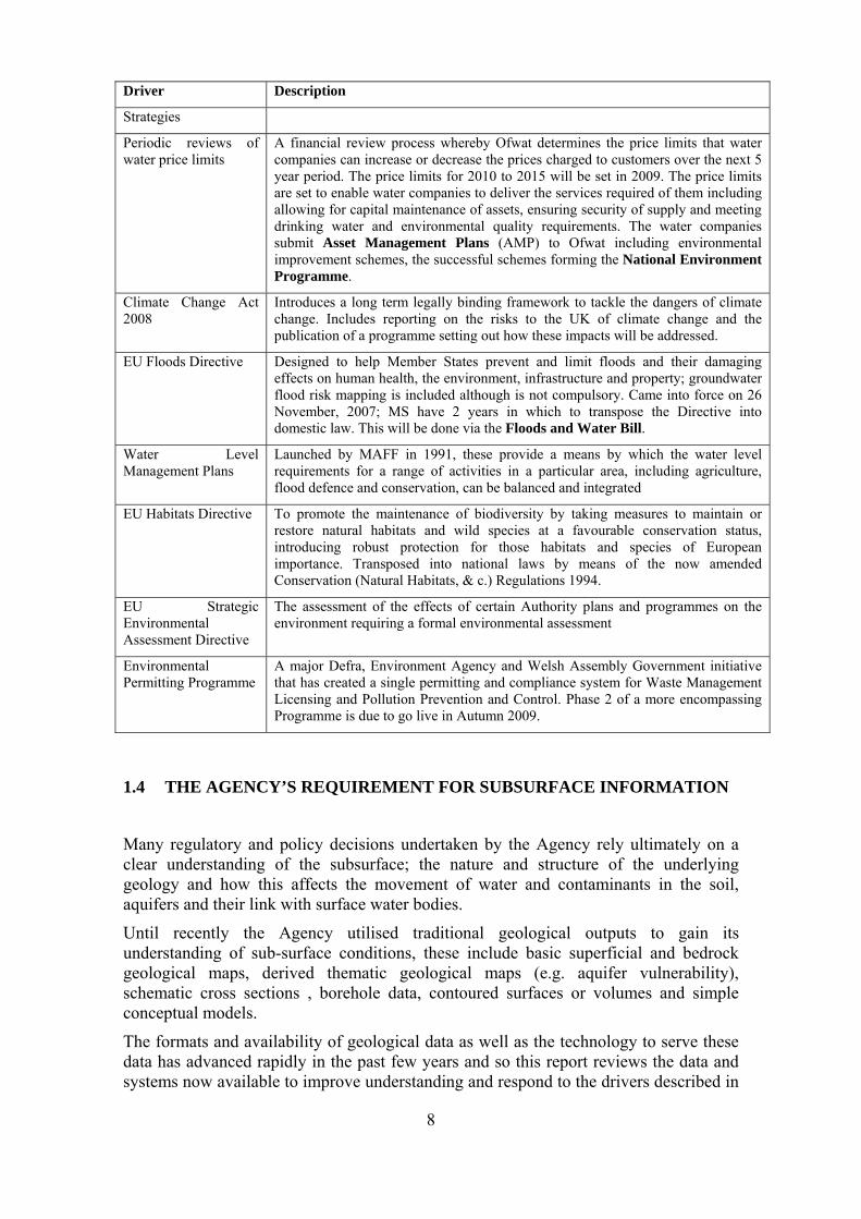
8

Driver Description

Strategies

Periodic reviews of water price limits

A financial review process whereby Ofwat determines the price limits that water companies can increase or decrease the prices charged to customers over the next 5 year period. The price limits for 2010 to 2015 will be set in 2009. The price limits are set to enable water companies to deliver the services required of them including allowing for capital maintenance of assets, ensuring security of supply and meeting drinking water and environmental quality requirements. The water companies submit Asset Management Plans (AMP) to Ofwat including environmental improvement schemes, the successful schemes forming the National Environment Programme.

Climate Change Act 2008

Introduces a long term legally binding framework to tackle the dangers of climate change. Includes reporting on the risks to the UK of climate change and the publication of a programme setting out how these impacts will be addressed.

EU Floods Directive Designed to help Member States prevent and limit floods and their damaging effects on human health, the environment, infrastructure and property; groundwater flood risk mapping is included although is not compulsory. Came into force on 26 November, 2007; MS have 2 years in which to transpose the Directive into domestic law. This will be done via the Floods and Water Bill.

Water Level Management Plans

Launched by MAFF in 1991, these provide a means by which the water level requirements for a range of activities in a particular area, including agriculture, flood defence and conservation, can be balanced and integrated

EU Habitats Directive To promote the maintenance of biodiversity by taking measures to maintain or restore natural habitats and wild species at a favourable conservation status, introducing robust protection for those habitats and species of European importance. Transposed into national laws by means of the now amended Conservation (Natural Habitats, & c.) Regulations 1994.

EU Strategic Environmental Assessment Directive

The assessment of the effects of certain Authority plans and programmes on the environment requiring a formal environmental assessment

Environmental Permitting Programme

A major Defra, Environment Agency and Welsh Assembly Government initiative that has created a single permitting and compliance system for Waste Management Licensing and Pollution Prevention and Control. Phase 2 of a more encompassing Programme is due to go live in Autumn 2009.

1.4 THE AGENCY’S REQUIREMENT FOR SUBSURFACE INFORMATION

Many regulatory and policy decisions undertaken by the Agency rely ultimately on a clear understanding of the subsurface; the nature and structure of the underlying geology and how this affects the movement of water and contaminants in the soil, aquifers and their link with surface water bodies.

Until recently the Agency utilised traditional geological outputs to gain its understanding of sub-surface conditions, these include basic superficial and bedrock geological maps, derived thematic geological maps (e.g. aquifer vulnerability), schematic cross sections , borehole data, contoured surfaces or volumes and simple conceptual models.

The formats and availability of geological data as well as the technology to serve these data has advanced rapidly in the past few years and so this report reviews the data and systems now available to improve understanding and respond to the drivers described in

9

Section 1.2. As well as adopting the right technical solutions it is important that a consistent and “fit for purpose” approach is developed that is capable of being implemented across the Agency.

A key factor “in fitness for purpose“ is that the scale-resolution of the geological information is appropriate to the needs of the specific situation, problem or study.

Scale-resolution of geological information can be broadly classified as national, regional, detailed and site-specific. These categories broadly reflect those of the Traditional range of geological maps scales and also the emerging range of geological model products offered by BGS under the brand name. LithoFrame. These new LithoFrame block model products are produced at 1Million (National), 250K (Regional), 50K (Detailed) and 10K (Detailed-Site specific) resolutions. The existing model availability and characteristics of these varied resolutions are described below in Sections 2 and 3.

BGS LithoFrame models are built fit for any purpose rather than fir for a purpose. The geological classification adopted follows that of the units distinguished during surveys and published on existing geological maps of the same resolution; this is primarily a lithostratigraphic classification (mapable units). 3D models and their component geological volumes can be readily attributed for use in a range of applied applications however it is essential that the intended useful scale-resolution of the model is always born in mind

These four resolutions of geological information are now discussed with relevance to drivers and the specific and varied needs of the Agency.

National

National geological maps-models are generally most useful in overall visualisation of the geology and this is often crucial for communicating with central Government departments, politicians, CEO’s and boards of utility companies and senior policy and decision makers within the Agency HQ, the general public, and other scientific disciplines

BGS has published a national 1M resolution geological model that covers all of England and Wales, in addition small scale maps of Britain’s geology are also available at I Million and 1:625K scales. The model is generated from surface information, deep boreholes, seismic profiles and other geophysical datasets. The model extends to 25km depth but it is only the upper 1-2 km that is likely to be of practical use to the Agency. This 1M resolution national model classifies the strata on the basis of geological age lumping together many important and lithologically distinct units.

The model is useful to explain features such the fact that most of Wales and much of western England is underlain by old crystalline impermeable strata where the available water resources are generally found within Quaternary deposits along the valley floors and from surface water abstraction utilising reservoirs. Conversely in eastern and southeastern England groundwater aquifers such as the Triassic Sherwood Sandstone and the Cretaceous Chalk are very important for public water supply and these aquifers have important surface and sub-surface extents as revealed by the shape of the strata in the model. This reveals for example that the Chalk continues at depth beneath younger strata across the London and Hampshire Basins but is absent (eroded) from the domed area of the Weald.

10

Regional

Geological maps-models at this scale-resolution are likely to be most useful to the regional offices of the Agency in their initial appreciation of the extent and overall surface and sub-surface geometry of their main geological units. At this scale superficial deposits are generally not depicted, but the form of important bedrock aquifers is likely to be clearly shown and useful in the initial conceptualisation of groundwater bodies as required by the Water Framework Directive and the Resource Assessment and Management Stage (RAM) of the CAMS process and specifically the development of catchment conceptualisation reports (Environment Agency, 2008a, b).

Regional geological information is depicted by the 250K bedrock map series available across the country, together with assorted regional models covering areas such as northern and southeast England as discussed below in Section 2 (Figure 11), These models are mainly constructed from a small number of deep boreholes often sunk for hydrocarbon exploration coupled with geophysical data such as seismic profiles, gravity and magnetic anomaly maps.

Detailed

The 50K scale- resolution is the standard published map scale for BGS and serves the need for systematic knowledge across the nation at a resolution likely to inform most detailed decision making processes. BGS has produced a number of geological models at this resolution covering parts of the Midlands, the north East, East Anglia and the London Basin (see Section 2 below).

Models at this scale can be readily attributed with hydrogeological data such as watertables, watertable variability, catchment divides etc. The use of these models is most likely to be in the detailed conceptualisation of groundwater bodies as required by the Water Framework Directive and the Resource Assessment and Management Stage (RAM) of the CAMS process. They can also act as a decision support tool for investigating aspects such as recharge, aquifer protection, orphan abstraction, flow pathways for water and contaminants and groundwater flooding potential.

Further examples of likely use might include the response to Planning applications at local and regional scales and contextual (catchment upstream) information on factors affecting wetlands whose sustainable management form one of the key purposes of the Habitats Directive (European Union, 1992).

In particular, in advance of the second round of river basin management plans for the WFD the Agency needs to improve the conceptual and numerical understanding of the hydrogeological setting in order to develop control measures where these are needed.

Site-specific

The main utilisation of these models is likely to be in problem solving and monitoring of sites. Likely drivers are the need to manage wetlands sites, landfill, pollution plume, contaminated land assessment and monitoring and to predict site engineering conditions in the construction of major infrastructure including flood defences.

Site-specific models require considerable amounts of data and measurement to be useful and the expression of risk and uncertainty are an integral part of such studies.

11

Site-specific geological models are likely to be built at 1:10K resolution or beyond. They are likely to be constructed by examining all available geological data and utilising the primary 10K geological survey linework or even more specific surveys. Such geological models are currently only available where they have been commissioned for a specific purpose or where they have either been generated in tandem with recent primary surveys (Southern East Anglia) or because of a perceived national need for the information (Thames Gateway Development Zone). These models often show considerable detail of man-made deposits and features together with the superficial and bedrock geology.

Understanding

The distribution of any geological unit is at either outcrop (surface), beneath overlying deposits (subcrop) or a combination of the two. Recent surficial deposits like blown sand or alluvium tend to outcrop throughout their distribution (unit 1, Figure 2) whereas older superficial or bedrock deposits may comprise both an outcrop and a subsurface subcrop (units 2,3,4 Figure 2) Many geological units especially bedrock layers may not crop out at all and so their distribution is entirely composed of a subcrop.

Traditional paper or digital geological maps display the distribution of geological units at the earths’ surface. In some cases they may also contain some additional subcrop lines to indicate the buried distribution of certain geological units. (dashed lines Figure 2). An obvious example is an area of superficial deposits resting on bedrock with the surface superficial geology shown as coloured polygons on the map face and the underlying bedrock unit distribution shown by subcrop lines. This arrangement of information at surface and rockhead is usually the most sophisticated form of 3D information attempted on a paper geological map.

Figure 2 Geological map and section to illustrate outcrop and subcrop relationship.

12

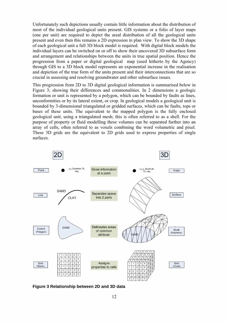
Unfortunately such depictions usually contain little information about the distribution of most of the individual geological units present. GIS systems or a folio of layer maps (one per unit) are required to depict the areal distribution of all the geological units present and even then this remains a 2D expression in plan view. To show the 3D shape of each geological unit a full 3D block model is required. With digital block models the individual layers can be switched on or off to show their uncovered 3D subsurface form and arrangement and relationships between the units in true spatial position. Hence the progression from a paper or digital geological map (used hitherto by the Agency) through GIS to a 3D block model represents an exponential increase in the realisation and depiction of the true form of the units present and their interconnections that are so crucial in assessing and resolving groundwater and other subsurface issues.

This progression from 2D to 3D digital geological information is summarised below in Figure 3; showing their differences and commonalities. In 2 dimensions a geologic formation or unit is represented by a polygon, which can be bounded by faults as lines, unconformities or by its lateral extent, or crop. In geological models a geological unit is bounded by 3-dimensional triangulated or gridded surfaces, which can be faults, tops or bases of these units. The equivalent to the mapped polygon is the fully enclosed geological unit, using a triangulated mesh; this is often referred to as a shell. For the purpose of property or fluid modelling these volumes can be separated further into an array of cells, often referred to as voxels combining the word volumetric and pixel. These 3D grids are the equivalent to 2D grids used to express properties of single surfaces.

Figure 3 Relationship between 2D and 3D data

13

In addition to the provision of suitable geological information it is also important that key agency staff understand how geological maps and models are produced and constraints on their use (e.g. scale) in order to make full and best use of the information and the varied types of derived outputs. With this in mind some guidance on commissioning 3D geological models is offered at Appendix 2.

In summary getting a good geological and consequently hydrogeological understanding of any study area - natural system is an essential early stage in any investigation relating to the groundwater and surface water issues faced by the Agency. 3D geological models offer a considerable advance in the visualisation and conceptualisation of sub-surface conditions and rock body geometry; they also provide an analytical decision support system for monitoring and resolving site-specific environmental problems.

2 Data Resources and Formats

In order to construct 3D geological and hydrogeological models it is essential to have all data available in usable digital form. These are likely to include borehole logs, published geological maps and sections, seismic profiles, topographic maps and a digital terrain model at an appropriate resolution.

It is recognised that in addition to the BGS data holdings: http://www.bgs.ac.uk/GeoIndex/ described below much valuable data is held by individuals, commercial companies, the Agency and other public sector organisations. The only basic requirements for use of this data in 3D modelling are that the data need to be spatially referenced and follow a logical and consistent schema.

2.1 GEOLOGICAL MAPS

The BGS national digital map holdings are the only available digital geological map datasets and are referred to as DiGMapGB products; they contain their information in up to 4 separate layers listed below. These can be either used individually, or merged into theme layers (e.g. surface geology) as required.

Artificial

Mass-movement

Superficial deposits

Bedrock geology

These data are available for licensing from BGS. The available scales commonly used in modelling are 1:250K (bedrock layer only, available nationally) 1:50K (all 4 layers available for most of England and Wales and 1:10K (all 4 layers, available for parts of

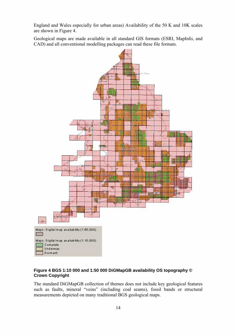
14

England and Wales especially for urban areas) Availability of the 50 K and 10K scales are shown in Figure 4.

Geological maps are made available in all standard GIS formats (ESRI, MapInfo, and CAD) and all conventional modelling packages can read these file formats.

Figure 4 BGS 1:10 000 and 1:50 000 DiGMapGB availability OS topography © Crown Copyright

The standard DiGMapGB collection of themes does not include key geological features such as faults, mineral “veins” (including coal seams), fossil bands or structural measurements depicted on many traditional BGS geological maps.

15

2.2 BOREHOLE DATABASES

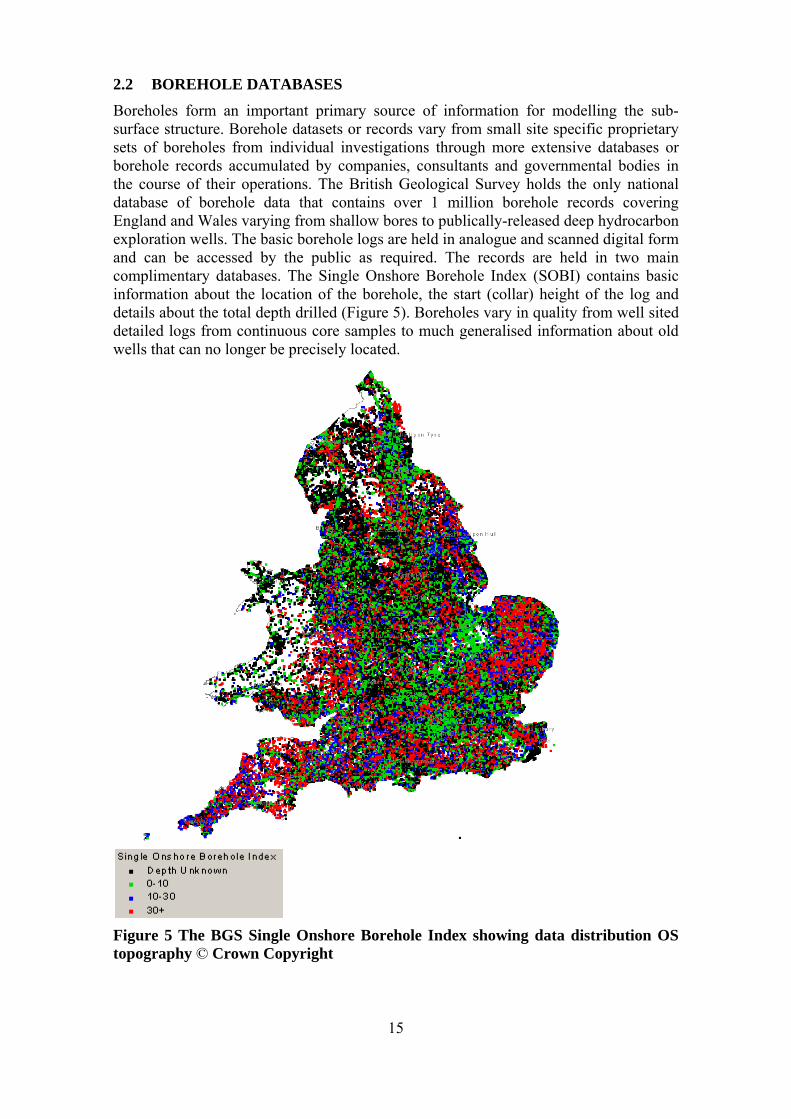
Boreholes form an important primary source of information for modelling the sub-surface structure. Borehole datasets or records vary from small site specific proprietary sets of boreholes from individual investigations through more extensive databases or borehole records accumulated by companies, consultants and governmental bodies in the course of their operations. The British Geological Survey holds the only national database of borehole data that contains over 1 million borehole records covering England and Wales varying from shallow bores to publically-released deep hydrocarbon exploration wells. The basic borehole logs are held in analogue and scanned digital form and can be accessed by the public as required. The records are held in two main complimentary databases. The Single Onshore Borehole Index (SOBI) contains basic information about the location of the borehole, the start (collar) height of the log and details about the total depth drilled (Figure 5). Boreholes vary in quality from well sited detailed logs from continuous core samples to much generalised information about old wells that can no longer be precisely located.

Figure 5 The BGS Single Onshore Borehole Index showing data distribution OS topography © Crown Copyright

16

The second key database is the Borehole Geology (BoGe) database which contains a downhole interpretation of the stratigraphic sequence encountered by the borehole (Figure 6). This is supported by lexicons and dictionaries for the description of lithology and stratigraphy available on the intranet.

Figure 6 BoGe data input using a MS Access front end.

A further BGS database is Wellmaster containing hydrogeological data related to over 105,000 boreholes and wells listed in the SOBI database. Information in Wellmaster includes casing, pump tests water chemistry, water levels and basic lithological information. This dataset is already licenced to the Agency and updated on a regular basis via CD ROM.

In building a 3D Geological Model all available borehole data should be examined. Boreholes that contribute reliable information on of the rock body geometry model should be included in the model. When working in areas with poorly understood stratigraphy the coding of just lithological descriptions is recommended rather than trying to interpret the unknown.

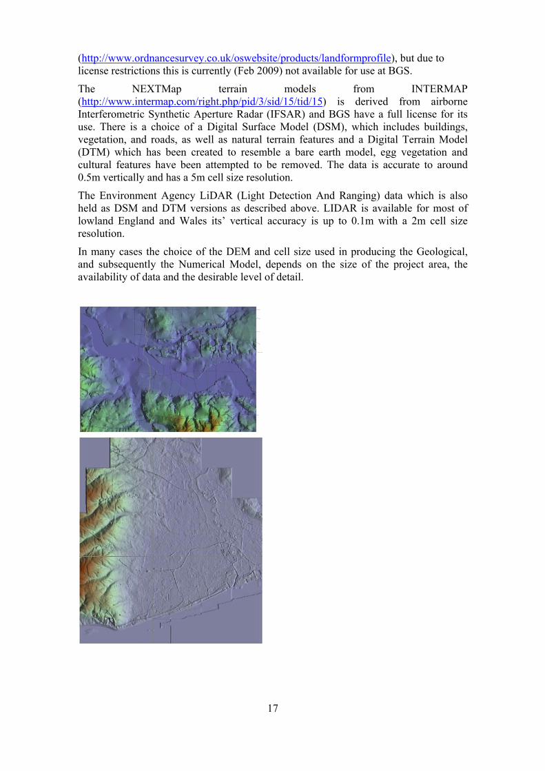
2.3 DIGITAL ELEVATION MODELS (DTM’S)

A Digital Elevation Model of the earth’s surface forming the top of the geology (geosphere) is essential for a geological modelling project (Figure 7). There is a choice of DTMs available for England and Wales.

The Ordnance Survey (OS) provide a baseline dataset called LandForm Profile derived from OS contours and spot heights

17

(http://www.ordnancesurvey.co.uk/oswebsite/products/landformprofile), but due to license restrictions this is currently (Feb 2009) not available for use at BGS.

The NEXTMap terrain models from INTERMAP (http://www.intermap.com/right.php/pid/3/sid/15/tid/15) is derived from airborne Interferometric Synthetic Aperture Radar (IFSAR) and BGS have a full license for its use. There is a choice of a Digital Surface Model (DSM), which includes buildings, vegetation, and roads, as well as natural terrain features and a Digital Terrain Model (DTM) which has been created to resemble a bare earth model, egg vegetation and cultural features have been attempted to be removed. The data is accurate to around 0.5m vertically and has a 5m cell size resolution.

The Environment Agency LiDAR (Light Detection And Ranging) data which is also held as DSM and DTM versions as described above. LIDAR is available for most of lowland England and Wales its’ vertical accuracy is up to 0.1m with a 2m cell size resolution.

In many cases the choice of the DEM and cell size used in producing the Geological, and subsequently the Numerical Model, depends on the size of the project area, the availability of data and the desirable level of detail.

18

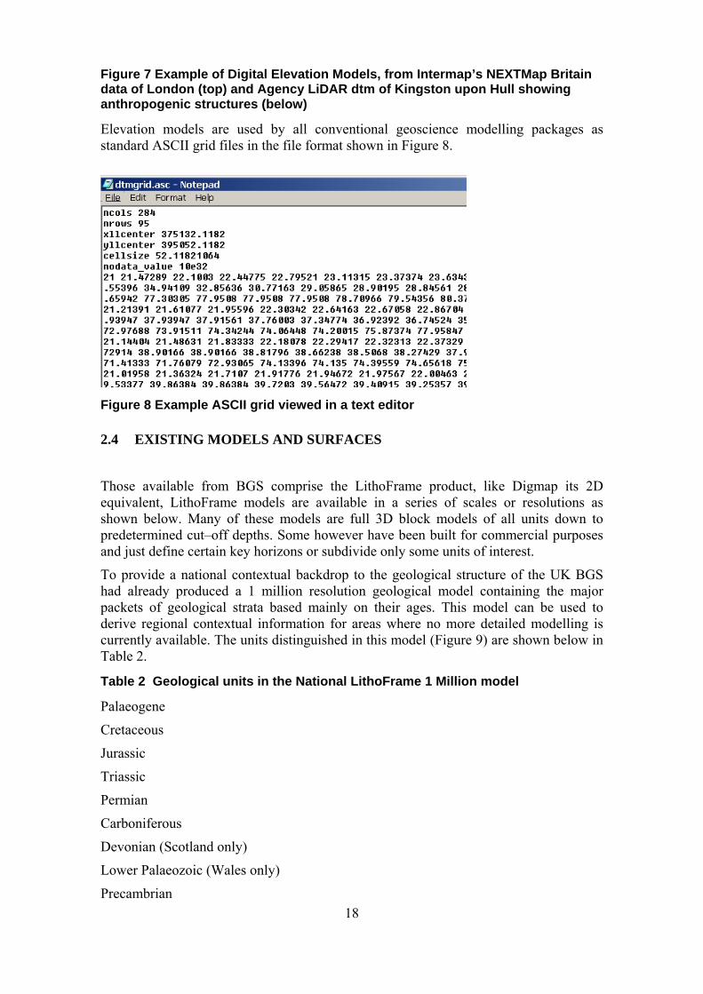
Figure 7 Example of Digital Elevation Models, from Intermap’s NEXTMap Britain data of London (top) and Agency LiDAR dtm of Kingston upon Hull showing anthropogenic structures (below)

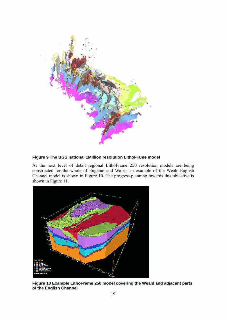
Elevation models are used by all conventional geoscience modelling packages as standard ASCII grid files in the file format shown in Figure 8.

Figure 8 Example ASCII grid viewed in a text editor

2.4 EXISTING MODELS AND SURFACES

Those available from BGS comprise the LithoFrame product, like Digmap its 2D equivalent, LithoFrame models are available in a series of scales or resolutions as shown below. Many of these models are full 3D block models of all units down to predetermined cut–off depths. Some however have been built for commercial purposes and just define certain key horizons or subdivide only some units of interest.

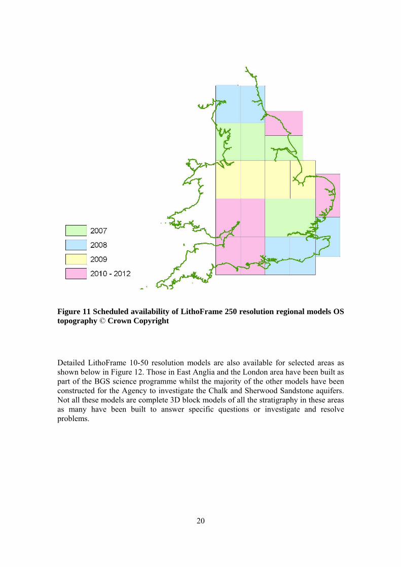
To provide a national contextual backdrop to the geological structure of the UK BGS had already produced a 1 million resolution geological model containing the major packets of geological strata based mainly on their ages. This model can be used to derive regional contextual information for areas where no more detailed modelling is currently available. The units distinguished in this model (Figure 9) are shown below in Table 2.

Table 2 Geological units in the National LithoFrame 1 Million model

Palaeogene

Cretaceous

Jurassic

Triassic

Permian

Carboniferous

Devonian (Scotland only)

Lower Palaeozoic (Wales only)

Precambrian

19

Figure 9 The BGS national 1Million resolution LithoFrame model

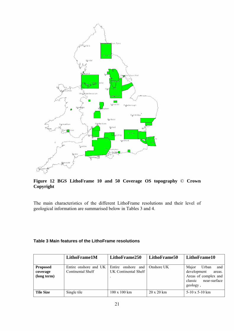
At the next level of detail regional LithoFrame 250 resolution models are being constructed for the whole of England and Wales, an example of the Weald-English Channel model is shown in Figure 10. The progress-planning towards this objective is shown in Figure 11.

Figure 10 Example LithoFrame 250 model covering the Weald and adjacent parts of the English Channel

20

Figure 11 Scheduled availability of LithoFrame 250 resolution regional models OS topography © Crown Copyright

Detailed LithoFrame 10-50 resolution models are also available for selected areas as shown below in Figure 12. Those in East Anglia and the London area have been built as part of the BGS science programme whilst the majority of the other models have been constructed for the Agency to investigate the Chalk and Sherwood Sandstone aquifers. Not all these models are complete 3D block models of all the stratigraphy in these areas as many have been built to answer specific questions or investigate and resolve problems.

21

Figure 12 BGS LithoFrame 10 and 50 Coverage OS topography © Crown Copyright

The main characteristics of the different LithoFrame resolutions and their level of geological information are summarised below in Tables 3 and 4.

Table 3 Main features of the LithoFrame resolutions

LithoFrame1M LithoFrame250 LithoFrame50 LithoFrame10

Proposed coverage (long term)

Entire onshore and UK Continental Shelf

Entire onshore and UK Continental Shelf .

Onshore UK Major Urban and development areas. Areas of complex and classic near-surface geology ,

Tile Size Single tile 100 x 100 km 20 x 20 km 5-10 x 5-10 km

22

Resolution of grid output

1Km 500m 100 –200m 50-100m

Depth 50km 5 - 10km 1-2km 100 - 200m or base of superficial deposits if deeper

Uses Visualisation, national- international collaboration, public understanding of science - education

Visualisation, popular science, overviews for the energy and water sectors, deep structural studies .

Analysis, the standard output, hydrocarbons,, aggregates, bulk minerals, aquifers, planning, major infrastructure.

Detailed analysis and problem solving. Site specific/detailed studies of all kinds,

Key Datasets Geological linework Digmap 625 Deep Seismic lines national-regional magnetic and gravity data, very deep boreholes

Geological linework Digmap 250 Seismic lines and regional magnetic and gravity data, deep boreholes.

Geological linework Digmap 50 Seismic lines, boreholes, deep mining data

Geological linework DIigmap10 All boreholes and mining data

Commercial

Potential

Low, popular publications, atlases

Modest, contextual models for energy , water sectors

Moderate-High the standard product for the geoscientist and allied professions

Very high, bespoke models to resolve problems and deliver geoscience solutions at a detailed-site specific level

Table 4 Geological detail possible at the various LithoFrame resolutions.

LithoFrame1M LithoFrame250 LithoFrame50 LithoFrame10

Stratigraphic resolution

(bedrock)

Major stratigraphic systems and deep crustal layers to the Moho picking out overall structure

Group level is likely to be the most commonly applied level especially for concealed strata .

Formation level is likely to be the most commonly applied level especially for concealed strata

Members and scientifically or economically important beds down to 1m thick, lenses.

Stratigraphic resolution

(superficial)

Not depicted Superficial undivided Major units modelled Detailed modelling of beds, lenses etc as required

Unconformities Delineated at major system boundaries

Major unconformities delineated by stratigraphic boundaries

Unconformities delineated by stratigraphic boundaries

Minor unconformities revealed by detailed stratigraphic units

Folding Depicted by overall form of major sedimentary packets

Depicted by overall form of major sedimentary packets

Detailed form depicted using structural observations in Digmap 50

Very detailed form depicted .by thin sedimentary packets and structural observations at Digmap 10 scale

Faulting Major faults bounding domains of British geology, e.g. Great Glen, Highland Boundary faults. Vertical

Those with throws of hundreds metres or lateral displacement of several kms are likely to be included in the model

Faults that have throws of more than 50m. also slightly smaller faults where these are laterally persistent or strongly

Faults that have throws of more than 10-15 m. also slightly smaller faults where these are laterally persistent or strongly

23

displacements of kms and/or significant lateral displacements of 100 km.

influence the outcrop pattern. Sub parallel faults amalgamated where their spacing is less than 200 m

influence the outcrop pattern. Sub parallel faults amalgamated where their spacing is less than 50 m

Intrusions-lavas Major plutons such as the SW England and Lake District batholiths. covering several hundred 1 km2 in extent and linked at depth

Plutons with outcrops-subcrops of at least 10 km2 should be included, Major lava piles

Plutons with outcrops-subcrops of at least 5 km2 should be included, thick lava sequences and major sheet intrusions

Plutons with outcrops-subcrops of at least 1 km2 sheet intrusions at least 5m thick and individual lava flows and sheet intrusions

Artificial ground Not shown Not shown Large pits-quarries worked and/or infilled, and extensive thick areas of made ground

Quarries worked and/or infilled, and large mapable areas of made ground

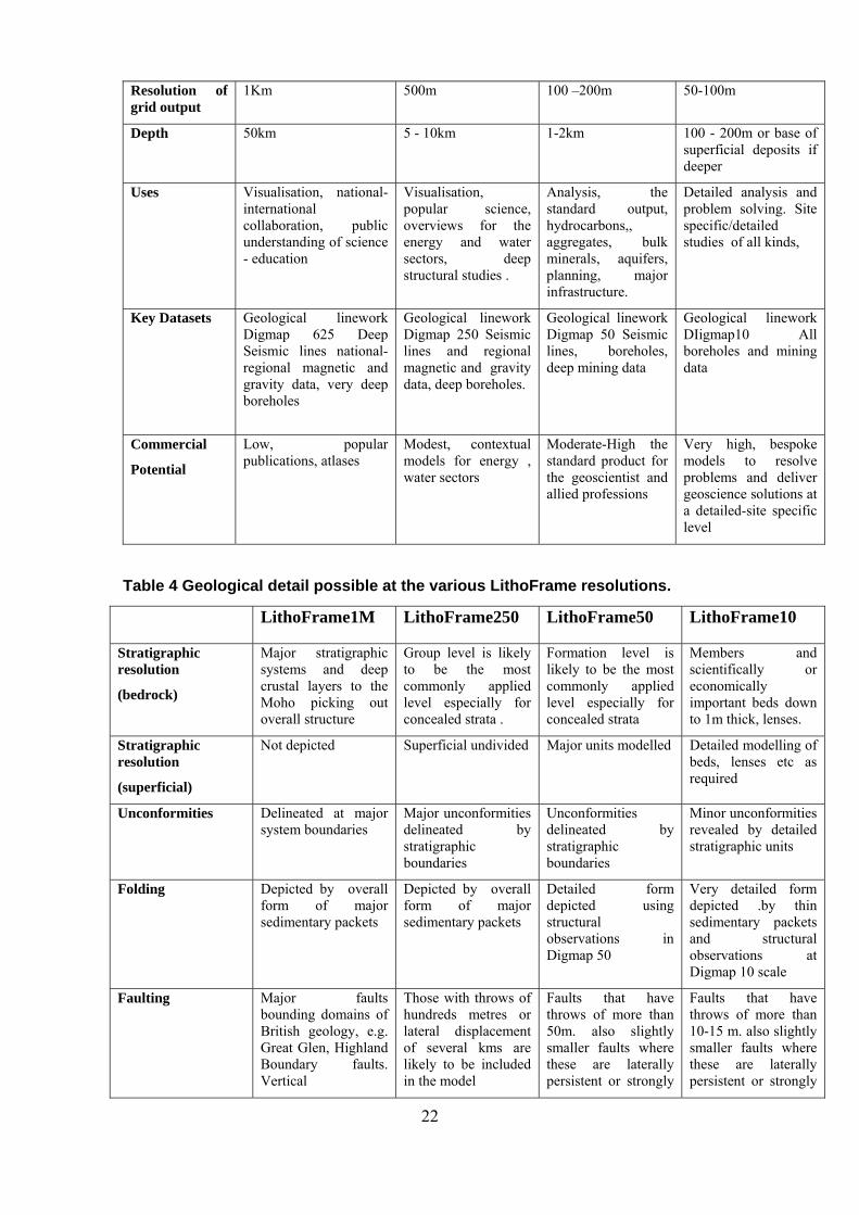
The effective depth of modelling and definition across several LithoFrame resolutions is shown in Figures 13 and 14. Central to the LithoFrame concept is that the varied resolutions of LithoFrame are consistent with each other so that collectively they form a seamless transition from general national model to a detailed site specific one. Figure 13 shows that the definition of highest order Stratigraphic units shown in dashed red lines should be defined first and included in all models of a higher resolution. Here the major stratigraphic boundaries selected at LithoFrame 250 are applied to the higher resolution 50 and 10 models. At LithoFrame 50 more detail is applied showing 7 rather than 2 units but this detail is likely to be resolved to a shallower depth. These units then extend through the more detailed LithoFrame 10 model and more detail (here 17 units) is nested within them in the shallow subsurface. Similar simplification of fault networks is shown on the right hand side of Figure 13.

Figure 13. Schematic section showing effective depth of modelling and definition across the LithoFrame 250-50-10 resolutions

24

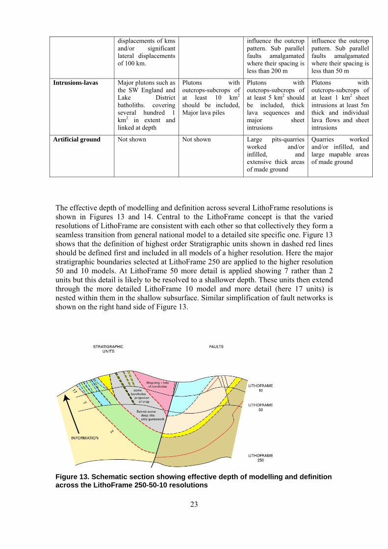
The depth of modelling effectively reflects the available data and the importance of seismic lines and deep boreholes building low definition models whereas the detailed LithoFrame 50 and 10 resolutions rely more heavily on surface geological mapping and shallow boreholes. Hence deeply buried surfaces constructed at LithoFrame 250 resolution in some areas may be built considering all the available data, they can therefore be magnified to form the deeper parts of a higher resolution LithoFrame 50 and 10 models if required. This effect of surfaces from a model forming the deeper part of the model at the next level of resolution is referred to here as the ‘LithoFrame Flow’ in Figure 14..

Figure 14 The stacking of LithoFrame models and the major disciplines involved in their construction.

2.5 GEOPHYSICAL DATA

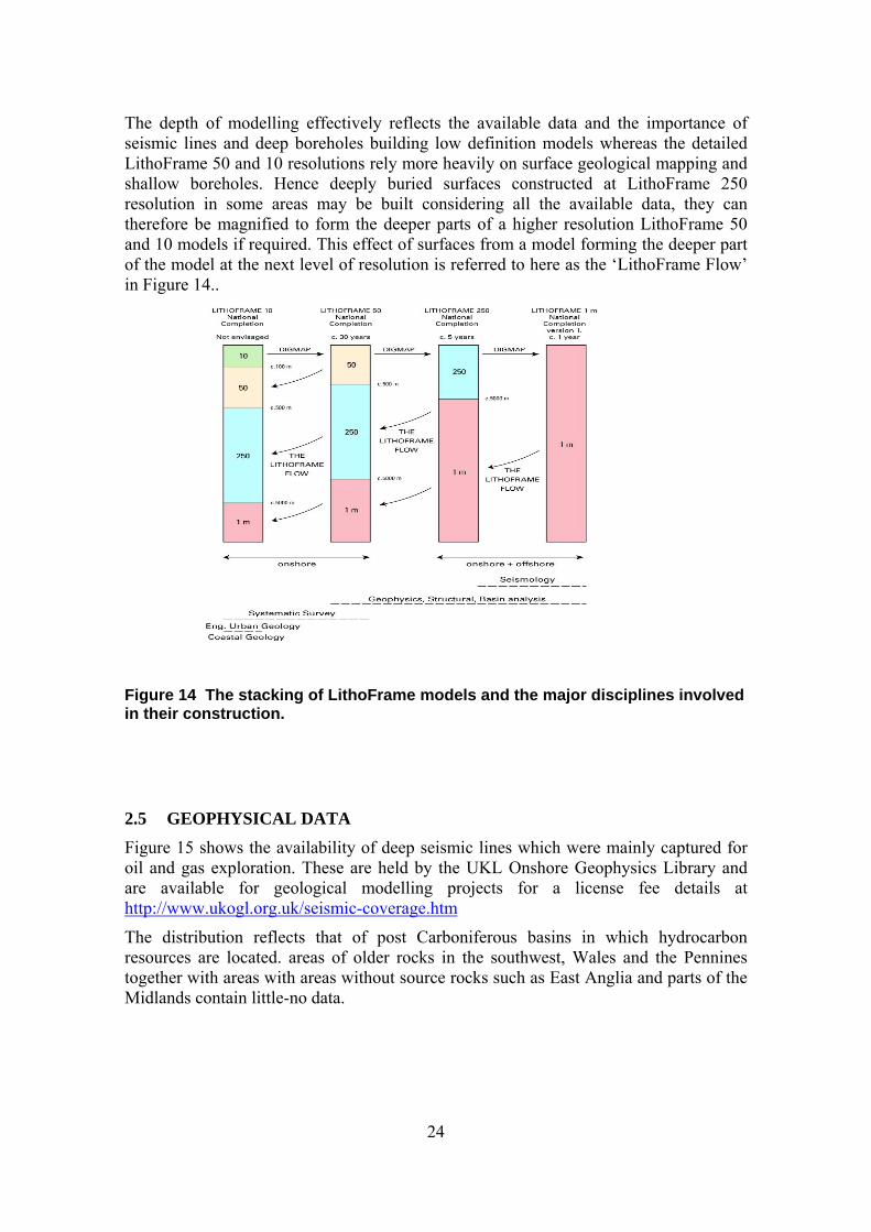
Figure 15 shows the availability of deep seismic lines which were mainly captured for oil and gas exploration. These are held by the UKL Onshore Geophysics Library and are available for geological modelling projects for a license fee details at http://www.ukogl.org.uk/seismic-coverage.htm

The distribution reflects that of post Carboniferous basins in which hydrocarbon resources are located. areas of older rocks in the southwest, Wales and the Pennines together with areas with areas without source rocks such as East Anglia and parts of the Midlands contain little-no data.

25

Figure 15 The UKOGL dataset OS topography © Crown Copyright

Figure 16 below shows the location of boreholes for which BGS holds downhole geophysical data that may be of use in interpreting the stratigraphy and hence model construction.

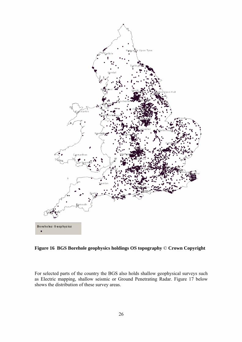
26

Figure 16 BGS Borehole geophysics holdings OS topography © Crown Copyright

For selected parts of the country the BGS also holds shallow geophysical surveys such as Electric mapping, shallow seismic or Ground Penetrating Radar. Figure 17 below shows the distribution of these survey areas.

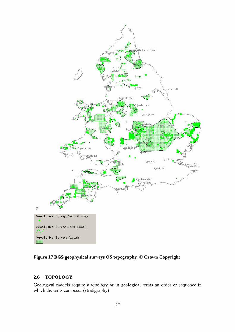
27

Figure 17 BGS geophysical surveys OS topography © Crown Copyright

2.6 TOPOLOGY

Geological models require a topology or in geological terms an order or sequence in which the units can occur (stratigraphy)

28

The topology is produced by the modeller, evolving throughout the project and finally contains all units in their correct and unique super-positional order as the order itself defines the ‘model stack’ that is calculated to make the 3D Geological Model. This can be a lithostratigraphical order or a chronology of artificial (man-made) deposits.

This tab separated file contains not only the standard geological attributes such as Stratigraphy and Lithology but also Aquifer properties, Permeability and other applied attributes of the geological units. This file enables the Geological Model to be converted to a “hydrostratigraphic model” and then be exported to Numerical groundwater modelling software such as ZOOM.

The layout below shows the essential elements of the Geological Vertical Sequence (GVS) file used in GSI3D modelling:

Name Id

Stratigraphy Lithology Genesis Free text

Alv 10 ALV CZ Fluv Overbank...

Lgfg 20 LGFG SV Glac_fluv Sheet sands...

Loft 30 LOFT CSZV Glac Lodgement till…

Sand_lens_t -150 SAND_L S Glac_fluv Intra till lense (top)

Sand_lens_b 150 SAND_L S Glac_fluv Intra till lense (base)

3 Geological 3D Models

3.1 BACKGROUND

In the broadest sense any depiction of the sub-surface geology can be considered a model because it is a representation produced from incomplete information. Thus a single borehole interpretation or a constructed cross-section is a form of model and can be used to represent conditions at a site or covering a small area where the geology is known to be fairly consistent. Such cross-sections are sometimes schematic and so represent information about the arrangement of the strata over a wider area. Such representations however can only be used for relatively small areas within which geological conditions can be assumed to be relatively constant. An example might be that of a river terrace overlying g a single bedrock units along a stretch of river valley. Here only two layers are present and their thickness and lithology might well be reasonably consistent. In reality such cases are rare and fence diagrams-block models are a far more effective and spatially accurate way of communicating geological information and structure in particular when models are intended for onward use in GIS or numerical modelling systems.

Fence diagrams normally constructed of two intersecting sets of sub-parallel sections enabling the three dimensional structure of an area to be appreciated in a way that is not possible with a single section (Figure 18). For example in an area of gently dipping folded bedrock strata one set would be aligned across the fold structure to show its

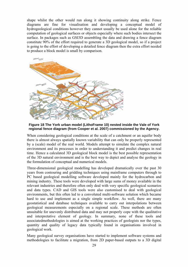
29

shape whilst the other would run along it showing continuity along strike. Fence diagrams are fine for visualisation and developing a conceptual model of hydrogeological conditions however they cannot usually be used alone for the reliable computation of geological surfaces or objects especially where such bodies intersect the surface. In packages such as GSI3D assembling the data and drawing a fence diagram constitute 90% of the effort required to generate a 3D geological model, so if a project is going to the effort of developing a detailed fence diagram then the extra effort needed to produce a block model is small by comparison.

Figure 18 The York urban model (LithoFrame 10) nested inside the Vale of York regional fence diagram (from Cooper et al. 2007) commissioned by the Agency.

When considering geological conditions at the scale of a catchment or an aquifer body there is almost always spatially known variability that can only be properly represented by a (scale) model of the real world. Models attempt to simulate the complex natural environment and its processes in order to understanding it and predict changes in real time. Hence a calculated 3D geological block model is the best possible representation of the 3D natural environment and is the best way to depict and analyse the geology in the formulation of conceptual and numerical models.

Three-dimensional geological modelling has developed dramatically over the past 30 years from contouring and gridding techniques using mainframe computers through to PC based geological modelling software developed mainly for the hydrocarbon and mining industry. These tools were developed with large sums of money available in the relevant industries and therefore often only deal with very specific geological scenarios and data types. CAD and GIS tools were also customised to deal with geological environments, but this often led to a convoluted multi-software solution which became hard to use and implement as a single simple workflow. As well, there are many geostatistical and database techniques available to carry out interpolations between geological measurements especially on a regional scale. These methods are often unsuitable for unevenly distributed data and may not properly cope with the qualitative and interpretative element of geology. In summary, none of these tools and associatedmethodologies is aimed at the working practices of geologists nor the types, quantity and quality of legacy data typically found in organisations involved in geological work.

Many geological survey organisations have started to implement software systems and methodologies to facilitate a migration, from 2D paper-based outputs to a 3D digital

30

service provider of geoscientific information (Jackson, 2005). Geological modelling packages and to some extent modellers themselves employ one of two different approaches to geological modelling either explicit or implicit; both approaches have their advantages and datasets for which their use is more applicable.

3.2 IMPLICIT AND EXPLICIT MODELLING

Implicit models are those in which observed and measured data (including geological interpretation) are treated as the entire valid dataset. Calculation is purely by mathematical interpolation and extrapolation from known data points.

In favour of this approach is that it is totally objective, totally reproducible, and very suitable for numerical data, and so easy to quantify uncertainty mathematically. An example might be the zonation of grades in a buried ore body from analytical measurements taken from core samples. On the downside whilst obeying the laws of mathematics and statistics some calculated models may defy the Laws of Geology or more commonly omit the geologists’ knowledge and understanding. One often resorted to solution when a model calculates but fails to produce geological common sense is to then constrain the data by inserting phantom borehole data or by forcing the model to fit an interpreted cross-section(s). This involves the introduction of soft (interpreted) data as in explicit modelling resulting in a mixed implicit-explicit approach. Further, some of the hard data used in implicit models isn’t always as ‘hard’ as you might wish to believe. For example, geologists frequently disagree about the position of stratigraphic boundaries in boreholes, at outcrop and in seismic profiles.

Explicit modelling also utilizes all the available hard data, but then deliberately inserts sufficient expert-controlled soft data to constrain the model to geological sense and take account of understanding. This data might for example involve drawing a network of sections that are included in the model calculation. Embedded in these sections are the shapes of the contacts between units that may be based on experience of seeing similar rocks at outcrop or by distinguishing between differing styles of arrangement of beds, onlap, offlap, overstep , channelled, etc. It should be remembered that geology is essentially an interpretive science as opposed to say (geo) chemistry, or (geo) physics. The main advantages of explicit models are geologically sensible results first time, drawing on the holistic knowledge of the most experienced geologist(s) available. Conversely the results are not reproducible, and uncertainty is very hard to quantify unless it is solely derived from the hard data distribution.

Of the commonly used softwares GSI3D is a totally explicit style of package whereas GoCAD is usually deployed as an implicit package. Implicit packages can make use of explicit data to calculate models but explicit packages can only use explicit styles of data (some may however be phantom data) to calculate models.

3.3 MAIN GEOLOGICAL MODELLING SOFTWARES

BGS has recently (2000-05) conducted an extensive review of geological modelling software in its Digital Geoscience Spatial Model (DGSM) project (Smith, 2005).

The review concluded that for its function as a national geoscience information provider BGS should use GoCAD and GSI3D as its preferred-default modelling packages for the routine construction of block models. GoCAD tends to be used for areas of geological complexity at regional-national scale and GSI3D for the shallow subsurface and simple bedrock geology.

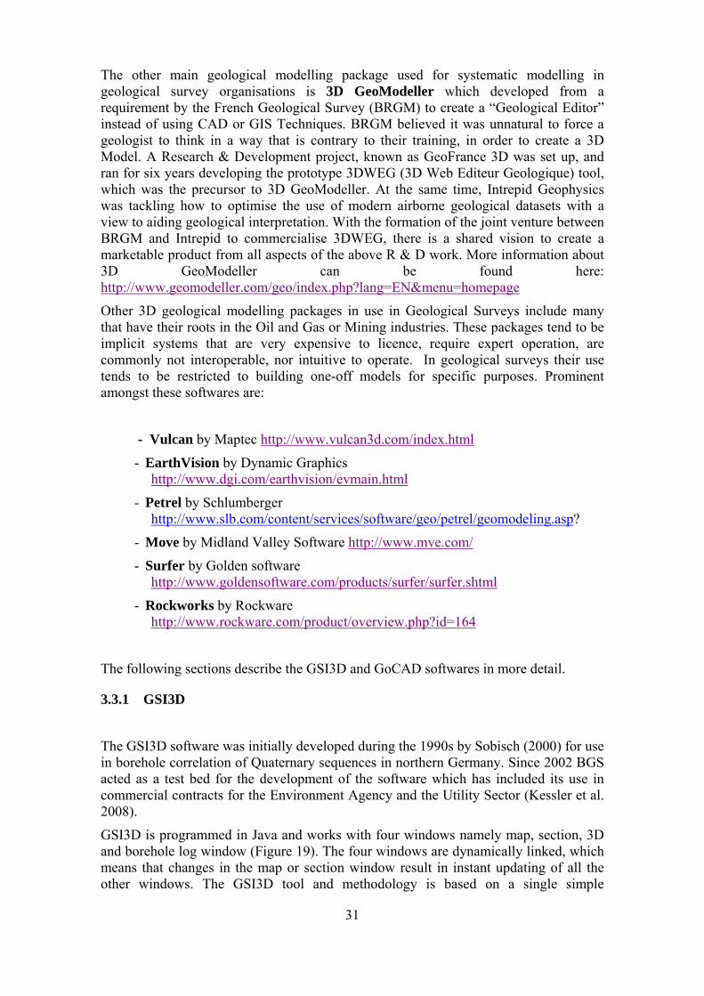
31

The other main geological modelling package used for systematic modelling in geological survey organisations is 3D GeoModeller which developed from a requirement by the French Geological Survey (BRGM) to create a “Geological Editor” instead of using CAD or GIS Techniques. BRGM believed it was unnatural to force a geologist to think in a way that is contrary to their training, in order to create a 3D Model. A Research & Development project, known as GeoFrance 3D was set up, and ran for six years developing the prototype 3DWEG (3D Web Editeur Geologique) tool, which was the precursor to 3D GeoModeller. At the same time, Intrepid Geophysics was tackling how to optimise the use of modern airborne geological datasets with a view to aiding geological interpretation. With the formation of the joint venture between BRGM and Intrepid to commercialise 3DWEG, there is a shared vision to create a marketable product from all aspects of the above R & D work. More information about 3D GeoModeller can be found here: http://www.geomodeller.com/geo/index.php?lang=EN&menu=homepage

Other 3D geological modelling packages in use in Geological Surveys include many that have their roots in the Oil and Gas or Mining industries. These packages tend to be implicit systems that are very expensive to licence, require expert operation, are commonly not interoperable, nor intuitive to operate. In geological surveys their use tends to be restricted to building one-off models for specific purposes. Prominent amongst these softwares are:

- Vulcan by Maptec http://www.vulcan3d.com/index.html

- EarthVision by Dynamic Graphics http://www.dgi.com/earthvision/evmain.html

- Petrel by Schlumberger http://www.slb.com/content/services/software/geo/petrel/geomodeling.asp?

- Move by Midland Valley Software http://www.mve.com/

- Surfer by Golden software http://www.goldensoftware.com/products/surfer/surfer.shtml

- Rockworks by Rockware http://www.rockware.com/product/overview.php?id=164

The following sections describe the GSI3D and GoCAD softwares in more detail.

3.3.1 GSI3D

The GSI3D software was initially developed during the 1990s by Sobisch (2000) for use in borehole correlation of Quaternary sequences in northern Germany. Since 2002 BGS acted as a test bed for the development of the software which has included its use in commercial contracts for the Environment Agency and the Utility Sector (Kessler et al. 2008).

GSI3D is programmed in Java and works with four windows namely map, section, 3D and borehole log window (Figure 19). The four windows are dynamically linked, which means that changes in the map or section window result in instant updating of all the other windows. The GSI3D tool and methodology is based on a single simple

32

philosophy - the construction of geological sub-surface models has to proceed with an understanding of the complete geological sequence and the likely geomorphological evolution of the study area (see also Fookes, 1997).

Figure 19 The GSI3D software interface

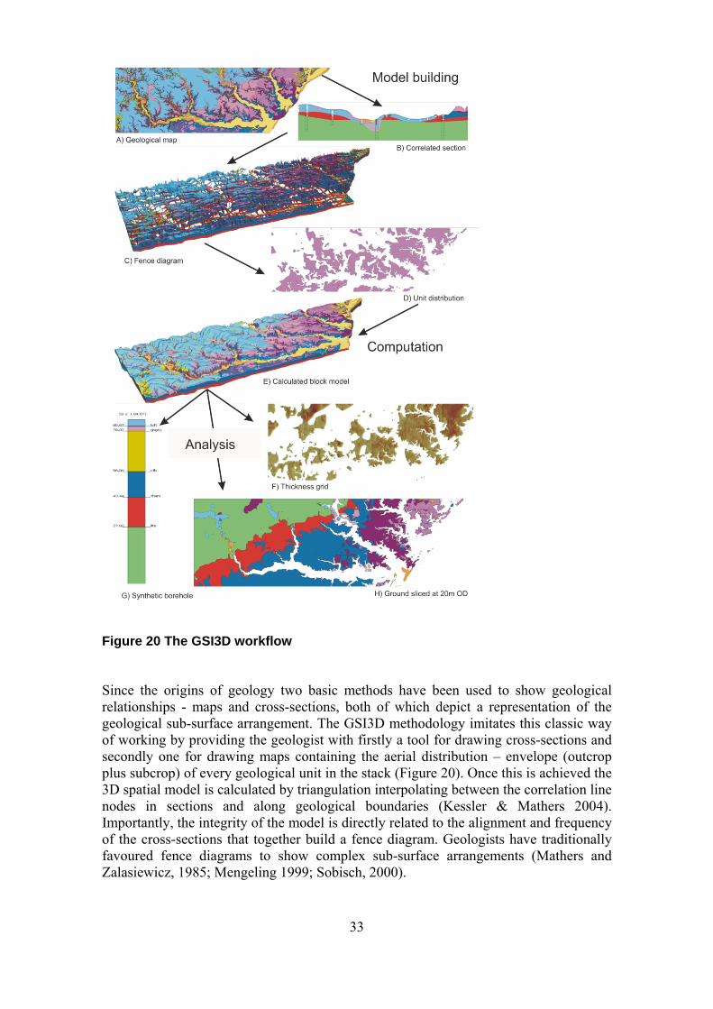
33

Figure 20 The GSI3D workflow

Since the origins of geology two basic methods have been used to show geological relationships - maps and cross-sections, both of which depict a representation of the geological sub-surface arrangement. The GSI3D methodology imitates this classic way of working by providing the geologist with firstly a tool for drawing cross-sections and secondly one for drawing maps containing the aerial distribution – envelope (outcrop plus subcrop) of every geological unit in the stack (Figure 20). Once this is achieved the 3D spatial model is calculated by triangulation interpolating between the correlation line nodes in sections and along geological boundaries (Kessler & Mathers 2004). Importantly, the integrity of the model is directly related to the alignment and frequency of the cross-sections that together build a fence diagram. Geologists have traditionally favoured fence diagrams to show complex sub-surface arrangements (Mathers and Zalasiewicz, 1985; Mengeling 1999; Sobisch, 2000).

34

In many Quaternary and sedimentary settings it is only possible to correlate the geometry of individual units when the topography, surface mapping and borehole logs are viewed in relation to each other in a 3D environment. This is because superficial deposits, such as glacial, fluvial and coastal deposits, are rarely identifiable through fossils or unique lithological markers. In these environments 3D modelling is virtually impossible without a cross-section approach.

GSI3D forces the geologist very effectively to check the numerous intersections between the cross-sections to produce a properly connected and internally consistent framework. At the same time the model is totally consistent with the surface and subcrop mapping of the geologist. For the actual model calculation a digital terrain model (or any other capping surface) and the GVS file (see above) must be present. Another key strength of GSI3D is that if the GVS and a DTM are present the cross-section displays the evolving 3D geology instantaneously.

Interpolating between the x,y,z nodes along the sections and those along the limits of the envelopes of each unit produces a series of triangulated irregular networks (TINs), each corresponding to the base of one of the geological units present. The use of TIN structures to describe geological objects is described by Turner (2003). GSI3D deploys a bespoke Delaunay-triangulation based on a Quad-edge algorithm (Green and Sibson, 1978). The creation of 3D objects, tops and base combined (a.k.a. volumes, shells) is then simply achieved by capturing the base(s) of the immediately overlying units (or the DTM where the unit is at outcrop). Where units extend beyond the project boundary vertical walls are inserted to close the 3D object. The resulting object is the logical equivalent to a polygon describing a geological unit in 2D.

In summary, GSI3D simply replaces existing analogue working practices of geologists with buttons in software, so it is easy to train people to use the software leading to widespread acceptance and implementation as demonstrated at BGS. Furthermore GSI3D is programmed to work quickly and in a truly dynamic way, allowing it to be part of a systematic, iterative and interpretative survey process.

Based on the acceptance of the software and the increasing demand for 3D models across a wide range of geological settings in the UK, BGS has now embarked on a 3-year R&D project (2007-10) to extend the capability of GSI3D. This will include functionality to model more complex bedrock environments including structures such as normal, reverse and scissor faults, fold axes, overturned strata, and cross-cutting intrusive bodies. The intention however is to maintain the simple intuitive approach of the software and methodology to enable deployment to all BGS’s scientists.

3.3.2 GoCAD

The GoCAD (Geological Object Computer Aided Design) software (Figure 21) was developed during the 1990's, and is now owned by Paradigm Geophysical. Most new technology created in the GoCAD Research Group is made available through plugins of the GoCAD software.

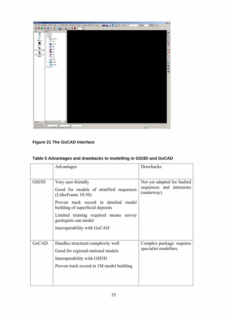
35

Figure 21 The GoCAD Interface

Table 5 Advantages and drawbacks to modelling in GSI3D and GoCAD

Advantages Drawbacks

GSI3D Very user-friendly

Good for models of stratified sequences (LithoFrame 10-50)

Proven track record in detailed model building of superficial deposits

Limited training required means survey geologists can model

Interoperability with GoCAD

Not yet adapted for faulted sequences and intrusions (underway).

GoCAD Handles structural complexity well

Good for regional-national models

Interoperability with GSI3D

Proven track record in 1M model building

Complex package requires specialist modellers.

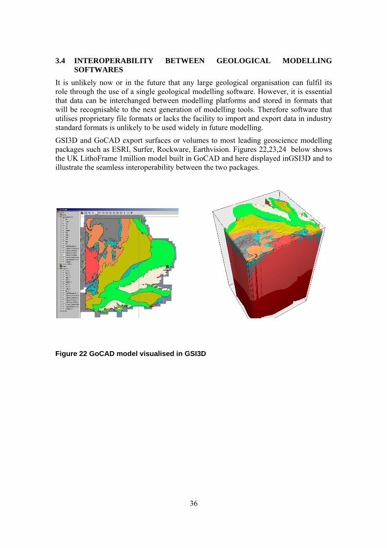
36

3.4 INTEROPERABILITY BETWEEN GEOLOGICAL MODELLING SOFTWARES

It is unlikely now or in the future that any large geological organisation can fulfil its role through the use of a single geological modelling software. However, it is essential that data can be interchanged between modelling platforms and stored in formats that will be recognisable to the next generation of modelling tools. Therefore software that utilises proprietary file formats or lacks the facility to import and export data in industry standard formats is unlikely to be used widely in future modelling.

GSI3D and GoCAD export surfaces or volumes to most leading geoscience modelling packages such as ESRI, Surfer, Rockware, Earthvision. Figures 22,23,24 below shows the UK LithoFrame 1million model built in GoCAD and here displayed inGSI3D and to illustrate the seamless interoperability between the two packages.

Figure 22 GoCAD model visualised in GSI3D

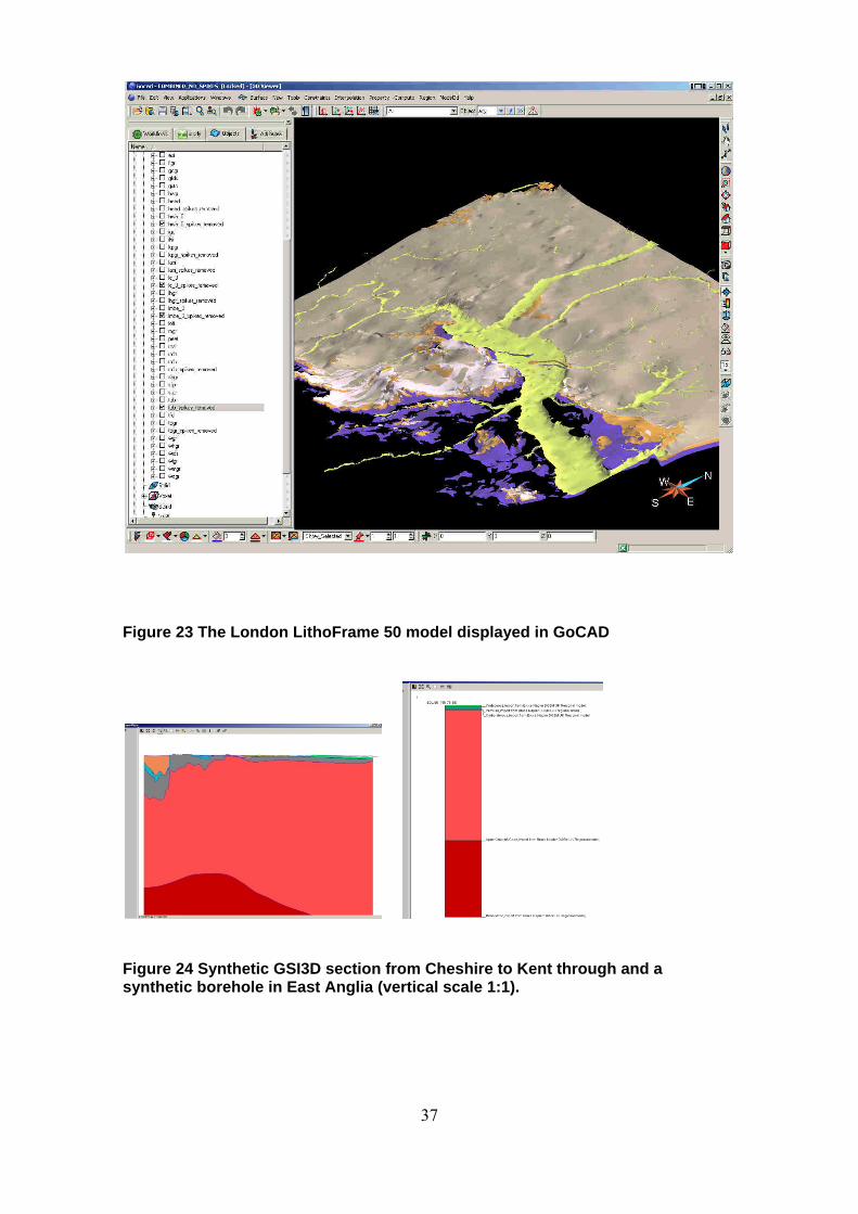
37

Figure 23 The London LithoFrame 50 model displayed in GoCAD

Figure 24 Synthetic GSI3D section from Cheshire to Kent through and a synthetic borehole in East Anglia (vertical scale 1:1).

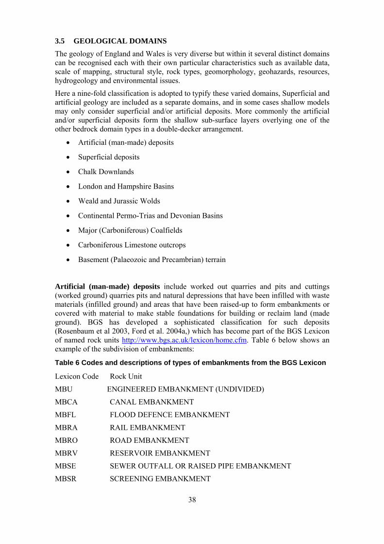
38

3.5 GEOLOGICAL DOMAINS

The geology of England and Wales is very diverse but within it several distinct domains can be recognised each with their own particular characteristics such as available data, scale of mapping, structural style, rock types, geomorphology, geohazards, resources, hydrogeology and environmental issues.

Here a nine-fold classification is adopted to typify these varied domains, Superficial and artificial geology are included as a separate domains, and in some cases shallow models may only consider superficial and/or artificial deposits. More commonly the artificial and/or superficial deposits form the shallow sub-surface layers overlying one of the other bedrock domain types in a double-decker arrangement.

Artificial (man-made) deposits

Superficial deposits

Chalk Downlands

London and Hampshire Basins

Weald and Jurassic Wolds

Continental Permo-Trias and Devonian Basins

Major (Carboniferous) Coalfields

Carboniferous Limestone outcrops

Basement (Palaeozoic and Precambrian) terrain

Artificial (man-made) deposits include worked out quarries and pits and cuttings (worked ground) quarries pits and natural depressions that have been infilled with waste materials (infilled ground) and areas that have been raised-up to form embankments or covered with material to make stable foundations for building or reclaim land (made ground). BGS has developed a sophisticated classification for such deposits (Rosenbaum et al 2003, Ford et al. 2004a,) which has become part of the BGS Lexicon of named rock units http://www.bgs.ac.uk/lexicon/home.cfm. Table 6 below shows an example of the subdivision of embankments:

Table 6 Codes and descriptions of types of embankments from the BGS Lexicon

Lexicon Code Rock Unit

MBU ENGINEERED EMBANKMENT (UNDIVIDED)

MBCA CANAL EMBANKMENT

MBFL FLOOD DEFENCE EMBANKMENT

MBRA RAIL EMBANKMENT

MBRO ROAD EMBANKMENT

MBRV RESERVOIR EMBANKMENT

MBSE SEWER OUTFALL OR RAISED PIPE EMBANKMENT

MBSR SCREENING EMBANKMENT

39

Since about 1970 artificial deposits have been usually recorded by the 1:10 000 scale primary surveys of urban areas, also extensive areas of artificial ground are commonly associated with quarrying especially along river valleys where aggregate resources have been extracted. It is often possible to distinguish several types of for example made ground depending on the material used as fill; in addition a chronology of events may also be established often from knowledge of local history and detailed OS maps going back up to 150 years.

In practice artificial deposits can only be modelled effectively in the most detailed models (LithoFrame 10 scale and beyond). A key requisite for modelling artificial deposits is a very accurate and up to date dtm, depicting human constructions such as embankments and canals. Artificial ground has been modelled successfully at about 1:10 000 resolution in Manchester-Mersey Corridor (Figure 25), and the Thames Gateway. Reasons for detailed modelling of artificial ground include the prediction and suitability of foundations conditions, the effect of the deposits on the migration of water and/or pollutants and identification of pathways for recharge.

Figure 25 High-resolution 3D model showing areas of artificial ground (in grey) including infilled pits, quarries, waste tips and canals overlying Sherwood Sandstone aquifer in Warrington, north-west England (Price et al 2008). OS topography © Crown Copyright

Superficial deposits comprise mainly coastal, river, slope and glacial deposits and are widespread in England and Wales especially in lower lying areas. Areas with extensive superficial deposits include the Lancashire-Cheshire Plain, the Vale of York, the Midlands, the Wash and East Anglia together with low lying coastal areas. Typically unconsolidated the deposits vary from coarse classic sands and gravels to silts and clays but also include organic-rich deposits such as peats and diameters which are mixtures of

40

pebbles, sand, silt and clay most commonly deposited by ice-sheets (till, boulder clay) and as mass-movement slope and residual deposits (head, clay with flints).

Most superficial deposits are less than 10m thick and often comprise a simple geometric arrangement of lithologies such as river terrace sand and gravel deposits overlain by thin silt and clay overbank deposits along the active courses of many of the main rivers of England and Wales. In such straightforward geological scenarios understanding can often be expressed by a simple cross section or fence diagram without the need for construction of a 3D block model. However thicker and much more complex sequences of glacial deposits are found associated with the advance and decay of several former ice-sheets. When the margin of an ice-sheet is stationary for a protracted period very complex sequences of hydrogeologically variable till, glacifluvial sand and gravel and glacilacustrine deposits result as exemplified by the LithoFrame 10 scale model of the York area (Figure 26).

Figure 26 Detailed LithoFrame 10 model of the area south of York showing the lacustrine deposit of Lake Humber (orange) and the terminal moraine at York (blue).

Locally superficial deposits reach 50 m in thickness such as in central East Anglia where a thick regional sheet of till is present and also beneath the present river courses of many of East Anglia’s rivers where over-deepened glacial channels are commonly found. These deep structures can act as lateral barriers to groundwater movement.

Modelling of superficial deposits is heavily dependant on good surface geological mapping often that is often based on geomorphological expression and shallow boreholes. The models may contain relatively simple superficial sequences that require only modest effort such as the superficial deposits in the London LithoFrame 50 model to the more complex sequences in the Southern East Anglia model where some 30 different superficial layers and lenses are recognised (Figure 27). In the case of predominantly rural areas like the 1800 sq km Southern East Anglia model it is feasible to examine all available borehole data and classify all logs that have the potential to contribute to the model. About 8000 boreholes were examined in thus study area and

41

about 40% of these were included in the model at an average density of about 2 per sq km. To achieve a similar density of borehole control in Greater London would involve coding perhaps only 5-10% of the available boreholes using GIS SQL queries and effects such as buffering to try and establish as even a spread of data as possible.

Figure 27 The Southern East Anglia LithoFrame 10 resolution model, as delivered to the Anglian Region of the Agency

Chalk Downlands are widespread in southern and eastern England forming the hills encircling the London and Hampshire basins and along the coast of Yorkshire and through Lincolnshire. The distribution of these downlands includes the North and South Downs, Salisbury Plain and the Chilterns. The Chalk also extends at depth beneath the London and Hampshire Basins (synclines) and is also present beneath a thick cover of superficial deposits in Norfolk and Lincolnshire.

In the chalk downlands modelling draws most heavily on the data provided from the geological surveying. Using geomorphological expression, lithology, exposures, palaeontology and to a lesser extent borehole data it is possible to subdivide the Chalk into 9-10 consistent Formations across the Downs of most of South-east England, measurements of dip and the detection of faults from surface evidence are also important for modelling. The layer-cake arrangement of the gently dipping strata results in fairly simple models of these strata as they lack the structural complexity of older rocks.. Subdivision of the Chalk has been achieved to-date for the South Downs and the Salisbury Plain areas but work is still needed to achieve this refinement in the Chilterns and parts of the North Downs. . The sequence exposed in Yorkshire differs

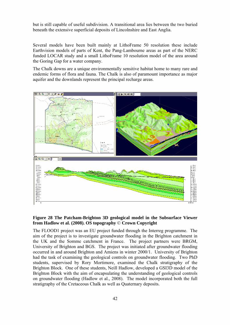
42

but is still capable of useful subdivision. A transitional area lies between the two buried beneath the extensive superficial deposits of Lincolnshire and East Anglia.

Several models have been built mainly at LithoFrame 50 resolution these include Earthvision models of parts of Kent, the Pang-Lambourne areas as part of the NERC funded LOCAR study and a small LithoFrame 10 resolution model of the area around the Goring Gap for a water company.

The Chalk downs are a unique environmentally sensitive habitat home to many rare and endemic forms of flora and fauna. The Chalk is also of paramount importance as major aquifer and the downlands represent the principal recharge areas.

Figure 28 The Patcham-Brighton 3D geological model in the Subsurface Viewer from Hadlow et al. (2008). OS topography © Crown Copyright

The FLOOD1 project was an EU project funded through the Interreg programme. The aim of the project is to investigate groundwater flooding in the Brighton catchment in the UK and the Somme catchment in France. The project partners were BRGM, University of Brighton and BGS. The project was initiated after groundwater flooding occurred in and around Brighton and Amiens in winter 2000/1. University of Brighton had the task of examining the geological controls on groundwater flooding. Two PhD students, supervised by Rory Mortimore, examined the Chalk stratigraphy of the Brighton Block. One of these students, Neill Hadlow, developed a GSI3D model of the Brighton Block with the aim of encapsulating the understanding of geological controls on groundwater flooding (Hadlow et al., 2008). The model incorporated both the full stratigraphy of the Cretaceous Chalk as well as Quaternary deposits.

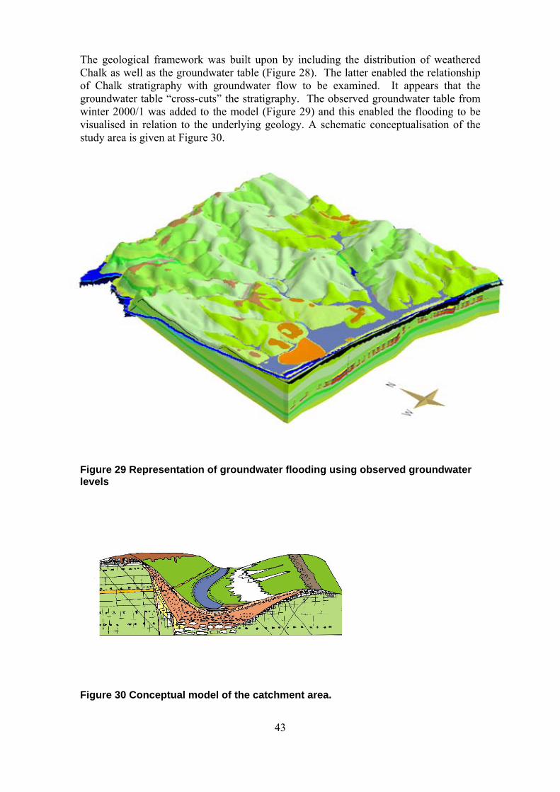
43

The geological framework was built upon by including the distribution of weathered Chalk as well as the groundwater table (Figure 28). The latter enabled the relationship of Chalk stratigraphy with groundwater flow to be examined. It appears that the groundwater table “cross-cuts” the stratigraphy. The observed groundwater table from winter 2000/1 was added to the model (Figure 29) and this enabled the flooding to be visualised in relation to the underlying geology. A schematic conceptualisation of the study area is given at Figure 30.

Figure 29 Representation of groundwater flooding using observed groundwater levels

Figure 30 Conceptual model of the catchment area.

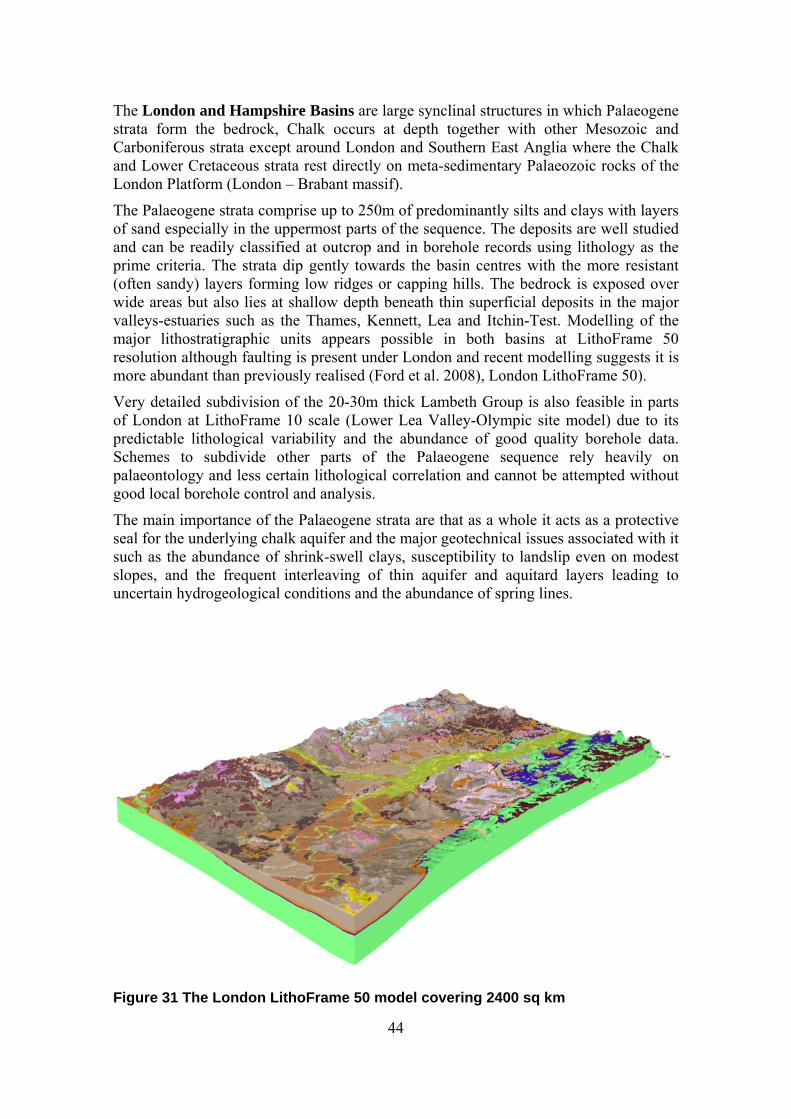
44

The London and Hampshire Basins are large synclinal structures in which Palaeogene strata form the bedrock, Chalk occurs at depth together with other Mesozoic and Carboniferous strata except around London and Southern East Anglia where the Chalk and Lower Cretaceous strata rest directly on meta-sedimentary Palaeozoic rocks of the London Platform (London – Brabant massif).

The Palaeogene strata comprise up to 250m of predominantly silts and clays with layers of sand especially in the uppermost parts of the sequence. The deposits are well studied and can be readily classified at outcrop and in borehole records using lithology as the prime criteria. The strata dip gently towards the basin centres with the more resistant (often sandy) layers forming low ridges or capping hills. The bedrock is exposed over wide areas but also lies at shallow depth beneath thin superficial deposits in the major valleys-estuaries such as the Thames, Kennett, Lea and Itchin-Test. Modelling of the major lithostratigraphic units appears possible in both basins at LithoFrame 50 resolution although faulting is present under London and recent modelling suggests it is more abundant than previously realised (Ford et al. 2008), London LithoFrame 50).

Very detailed subdivision of the 20-30m thick Lambeth Group is also feasible in parts of London at LithoFrame 10 scale (Lower Lea Valley-Olympic site model) due to its predictable lithological variability and the abundance of good quality borehole data. Schemes to subdivide other parts of the Palaeogene sequence rely heavily on palaeontology and less certain lithological correlation and cannot be attempted without good local borehole control and analysis.

The main importance of the Palaeogene strata are that as a whole it acts as a protective seal for the underlying chalk aquifer and the major geotechnical issues associated with it such as the abundance of shrink-swell clays, susceptibility to landslip even on modest slopes, and the frequent interleaving of thin aquifer and aquitard layers leading to uncertain hydrogeological conditions and the abundance of spring lines.

Figure 31 The London LithoFrame 50 model covering 2400 sq km

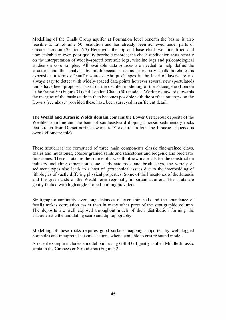
45

Modelling of the Chalk Group aquifer at Formation level beneath the basins is also feasible at LithoFrame 50 resolution and has already been achieved under parts of Greater London (Section 6.5) Here with the top and base chalk well identified and unmistakable in even poor quality borehole records; the chalk subdivision rests heavily on the interpretation of widely-spaced borehole logs, wireline logs and paleontological studies on core samples. All available data sources are needed to help define the structure and this analysis by mutli-specialist teams to classify chalk boreholes is expensive in terms of staff resources. Abrupt changes in the level of layers are not always easy to detect with widely-spaced data points however several new (postulated) faults have been proposed based on the detailed modelling of the Palaeogene (London LithoFrame 50 (Figure 31) and London Chalk (50) models. Working outwards towards the margins of the basins a tie in then becomes possible with the surface outcrops on the Downs (see above) provided these have been surveyed in sufficient detail.

The Weald and Jurassic Wolds domain contains the Lower Cretaceous deposits of the Wealden anticline and the band of southeastward dipping Jurassic sedimentary rocks that stretch from Dorset northeastwards to Yorkshire. In total the Jurassic sequence is over a kilometre thick.

These sequences are comprised of three main components classic fine-grained clays, shales and mudstones, coarser grained sands and sandstones and biogenic and bioclastic limestones. These strata are the source of a wealth of raw materials for the construction industry including dimension stone, carbonate rock and brick clays, the variety of sediment types also leads to a host of geotechnical issues due to the interbedding of lithologies of vastly differing physical properties. Some of the limestones of the Jurassic and the greensands of the Weald form regionally important aquifers. The strata are gently faulted with high angle normal faulting prevalent.

Stratigraphic continuity over long distances of even thin beds and the abundance of fossils makes correlation easier than in many other parts of the stratigraphic column. The deposits are well exposed throughout much of their distribution forming the characteristic the undulating scarp and dip topography.

Modelling of these rocks requires good surface mapping supported by well logged boreholes and interpreted seismic sections where available to ensure sound models.

A recent example includes a model built using GSI3D of gently faulted Middle Jurassic strata in the Cirencester-Stroud area (Figure 32).

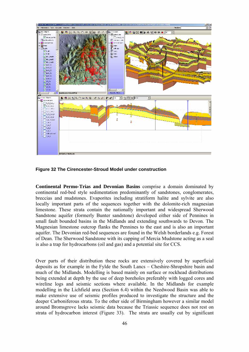
46

Figure 32 The Cirencester-Stroud Model under construction

Continental Permo-Trias and Devonian Basins comprise a domain dominated by continental red-bed style sedimentation predominantly of sandstones, conglomerates, breccias and mudstones. Evaporites including stratiform halite and sylvite are also locally important parts of the sequences together with the dolomite-rich magnesian limestone. These strata contain the nationally important and widespread Sherwood Sandstone aquifer (formerly Bunter sandstone) developed either side of Pennines in small fault bounded basins in the Midlands and extending southwards to Devon. The Magnesian limestone outcrop flanks the Pennines to the east and is also an important aquifer. The Devonian red-bed sequences are found in the Welsh borderlands e.g. Forest of Dean. The Sherwood Sandstone with its capping of Mercia Mudstone acting as a seal is also a trap for hydrocarbons (oil and gas) and a potential site for CCS.

Over parts of their distribution these rocks are extensively covered by superficial deposits as for example in the Fylde the South Lancs – Cheshire-Shropshire basin and much of the Midlands. Modelling is based mainly on surface or rockhead distributions being extended at depth by the use of deep boreholes preferably with logged cores and wireline logs and seismic sections where available. In the Midlands for example modelling in the Lichfield area (Section 6.4) within the Needwood Basin was able to make extensive use of seismic profiles produced to investigate the structure and the deeper Carboniferous strata. To the other side of Birmingham however a similar model around Bromsgrove lacks seismic data because the Triassic sequence does not rest on strata of hydrocarbon interest (Figure 33). The strata are usually cut by significant

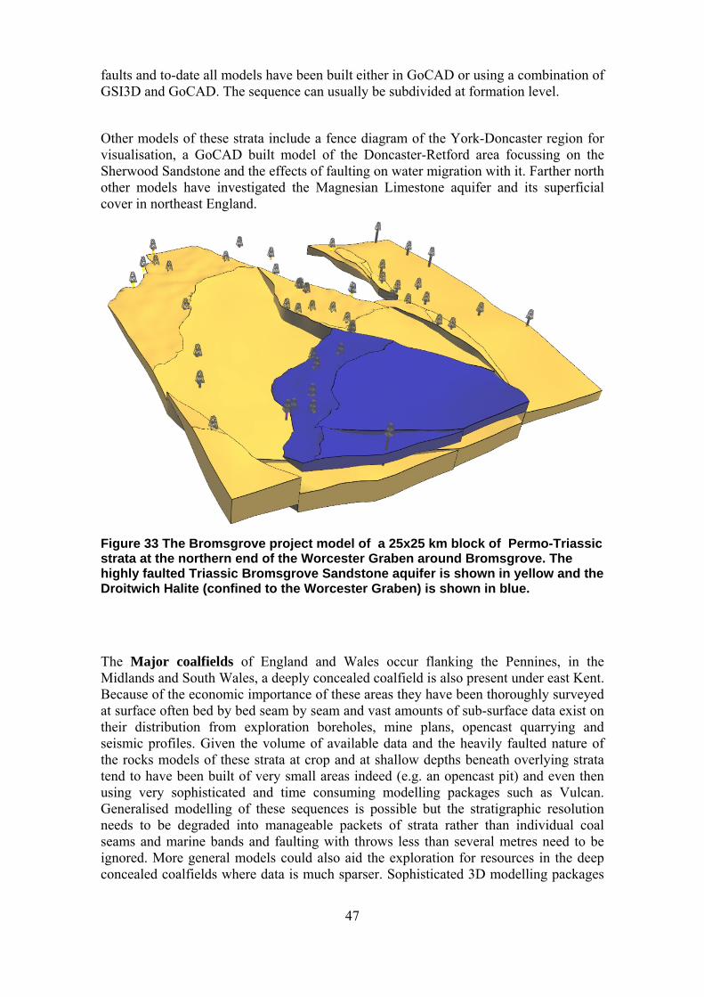
47

faults and to-date all models have been built either in GoCAD or using a combination of GSI3D and GoCAD. The sequence can usually be subdivided at formation level.

Other models of these strata include a fence diagram of the York-Doncaster region for visualisation, a GoCAD built model of the Doncaster-Retford area focussing on the Sherwood Sandstone and the effects of faulting on water migration with it. Farther north other models have investigated the Magnesian Limestone aquifer and its superficial cover in northeast England.

Figure 33 The Bromsgrove project model of a 25x25 km block of Permo-Triassic strata at the northern end of the Worcester Graben around Bromsgrove. The highly faulted Triassic Bromsgrove Sandstone aquifer is shown in yellow and the Droitwich Halite (confined to the Worcester Graben) is shown in blue.

The Major coalfields of England and Wales occur flanking the Pennines, in the Midlands and South Wales, a deeply concealed coalfield is also present under east Kent. Because of the economic importance of these areas they have been thoroughly surveyed at surface often bed by bed seam by seam and vast amounts of sub-surface data exist on their distribution from exploration boreholes, mine plans, opencast quarrying and seismic profiles. Given the volume of available data and the heavily faulted nature of the rocks models of these strata at crop and at shallow depths beneath overlying strata tend to have been built of very small areas indeed (e.g. an opencast pit) and even then using very sophisticated and time consuming modelling packages such as Vulcan. Generalised modelling of these sequences is possible but the stratigraphic resolution needs to be degraded into manageable packets of strata rather than individual coal seams and marine bands and faulting with throws less than several metres need to be ignored. More general models could also aid the exploration for resources in the deep concealed coalfields where data is much sparser. Sophisticated 3D modelling packages

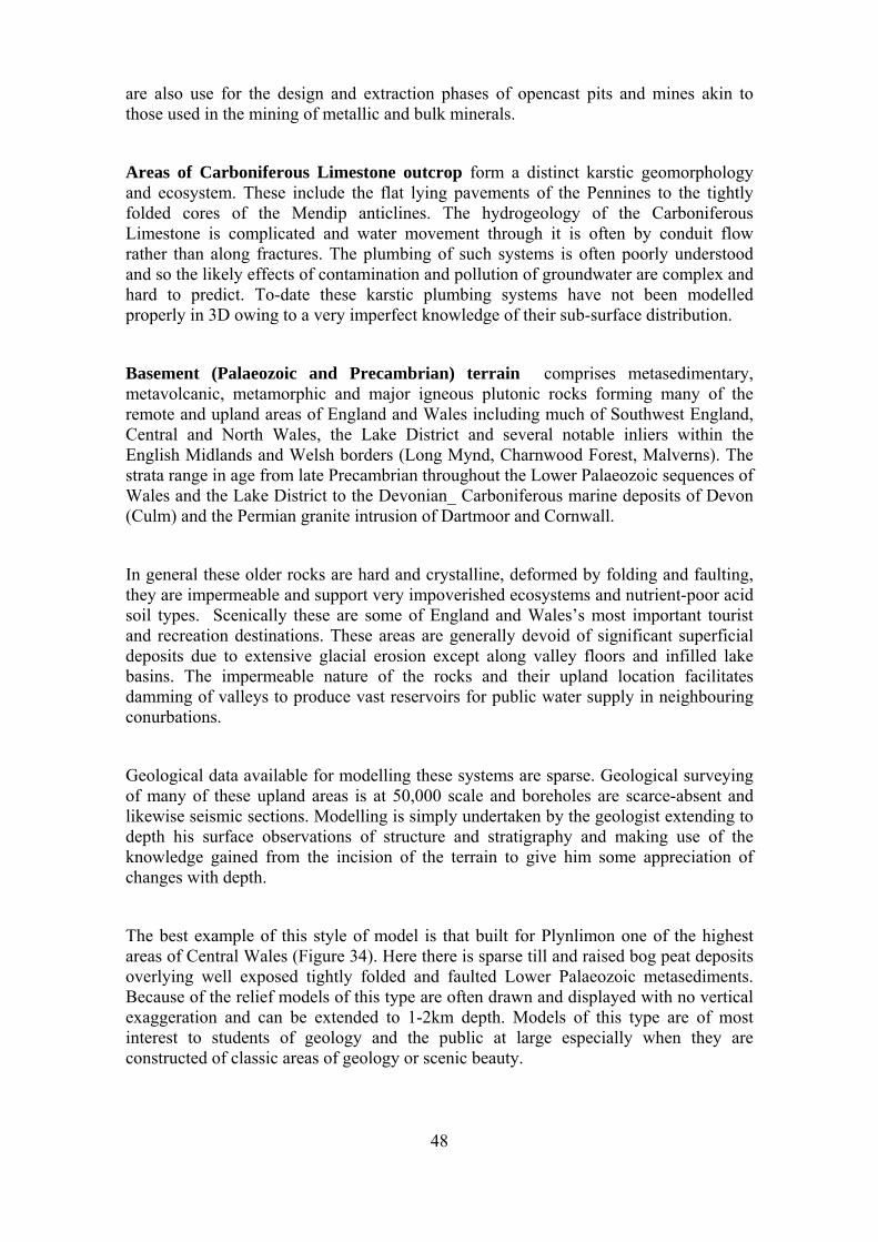
48

are also use for the design and extraction phases of opencast pits and mines akin to those used in the mining of metallic and bulk minerals.

Areas of Carboniferous Limestone outcrop form a distinct karstic geomorphology and ecosystem. These include the flat lying pavements of the Pennines to the tightly folded cores of the Mendip anticlines. The hydrogeology of the Carboniferous Limestone is complicated and water movement through it is often by conduit flow rather than along fractures. The plumbing of such systems is often poorly understood and so the likely effects of contamination and pollution of groundwater are complex and hard to predict. To-date these karstic plumbing systems have not been modelled properly in 3D owing to a very imperfect knowledge of their sub-surface distribution.

Basement (Palaeozoic and Precambrian) terrain comprises metasedimentary, metavolcanic, metamorphic and major igneous plutonic rocks forming many of the remote and upland areas of England and Wales including much of Southwest England, Central and North Wales, the Lake District and several notable inliers within the English Midlands and Welsh borders (Long Mynd, Charnwood Forest, Malverns). The strata range in age from late Precambrian throughout the Lower Palaeozoic sequences of Wales and the Lake District to the Devonian_ Carboniferous marine deposits of Devon (Culm) and the Permian granite intrusion of Dartmoor and Cornwall.

In general these older rocks are hard and crystalline, deformed by folding and faulting, they are impermeable and support very impoverished ecosystems and nutrient-poor acid soil types. Scenically these are some of England and Wales’s most important tourist and recreation destinations. These areas are generally devoid of significant superficial deposits due to extensive glacial erosion except along valley floors and infilled lake basins. The impermeable nature of the rocks and their upland location facilitates damming of valleys to produce vast reservoirs for public water supply in neighbouring conurbations.

Geological data available for modelling these systems are sparse. Geological surveying of many of these upland areas is at 50,000 scale and boreholes are scarce-absent and likewise seismic sections. Modelling is simply undertaken by the geologist extending to depth his surface observations of structure and stratigraphy and making use of the knowledge gained from the incision of the terrain to give him some appreciation of changes with depth.

The best example of this style of model is that built for Plynlimon one of the highest areas of Central Wales (Figure 34). Here there is sparse till and raised bog peat deposits overlying well exposed tightly folded and faulted Lower Palaeozoic metasediments. Because of the relief models of this type are often drawn and displayed with no vertical exaggeration and can be extended to 1-2km depth. Models of this type are of most interest to students of geology and the public at large especially when they are constructed of classic areas of geology or scenic beauty.

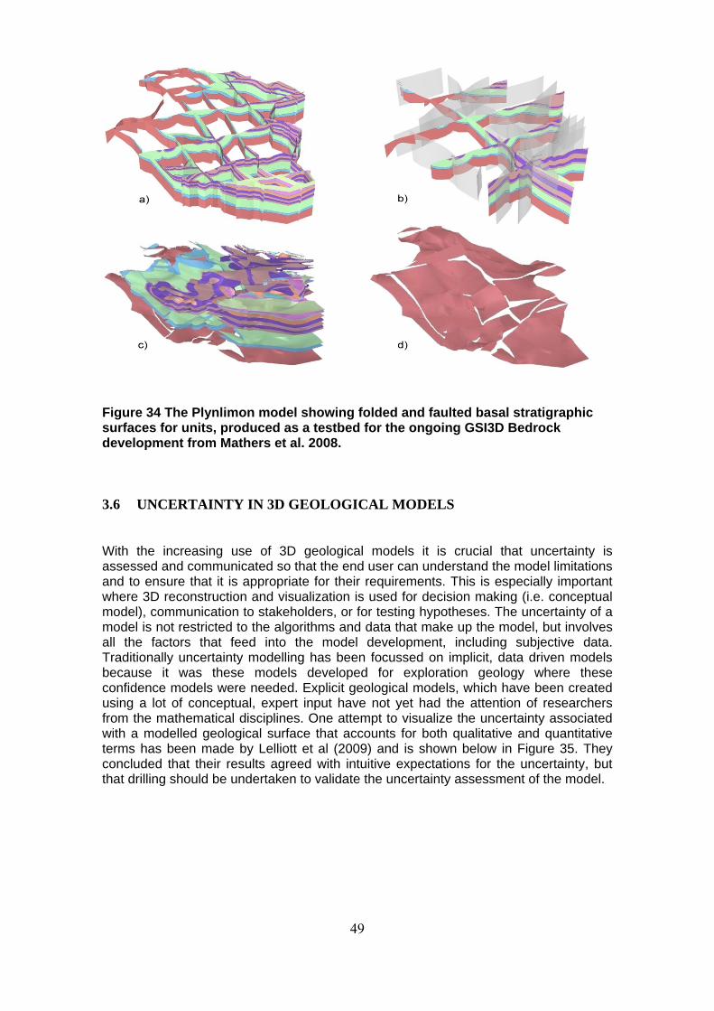
49

Figure 34 The Plynlimon model showing folded and faulted basal stratigraphic surfaces for units, produced as a testbed for the ongoing GSI3D Bedrock development from Mathers et al. 2008.

3.6 UNCERTAINTY IN 3D GEOLOGICAL MODELS

With the increasing use of 3D geological models it is crucial that uncertainty is assessed and communicated so that the end user can understand the model limitations and to ensure that it is appropriate for their requirements. This is especially important where 3D reconstruction and visualization is used for decision making (i.e. conceptual model), communication to stakeholders, or for testing hypotheses. The uncertainty of a model is not restricted to the algorithms and data that make up the model, but involves all the factors that feed into the model development, including subjective data. Traditionally uncertainty modelling has been focussed on implicit, data driven models because it was these models developed for exploration geology where these confidence models were needed. Explicit geological models, which have been created using a lot of conceptual, expert input have not yet had the attention of researchers from the mathematical disciplines. One attempt to visualize the uncertainty associated with a modelled geological surface that accounts for both qualitative and quantitative terms has been made by Lelliott et al (2009) and is shown below in Figure 35. They concluded that their results agreed with intuitive expectations for the uncertainty, but that drilling should be undertaken to validate the uncertainty assessment of the model.

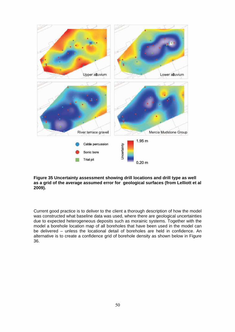
50

Figure 35 Uncertainty assessment showing drill locations and drill type as well as a grid of the average assumed error for geological surfaces (from Lelliott et al 2009).

Current good practice is to deliver to the client a thorough description of how the model was constructed what baseline data was used, where there are geological uncertainties due to expected heterogeneous deposits such as morainic systems. Together with the model a borehole location map of all boreholes that have been used in the model can be delivered – unless the locational detail of boreholes are held in confidence. An alternative is to create a confidence grid of borehole density as shown below in Figure 36.

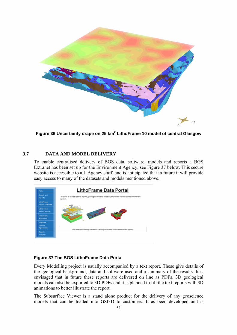
51

Figure 36 Uncertainty drape on 25 km2 LithoFrame 10 model of central Glasgow

3.7 DATA AND MODEL DELIVERY

To enable centralised delivery of BGS data, software, models and reports a BGS Extranet has been set up for the Environment Agency, see Figure 37 below. This secure website is accessible to all Agency staff, and is anticipated that in future it will provide easy access to many of the datasets and models mentioned above.

Figure 37 The BGS LithoFrame Data Portal

Every Modelling project is usually accompanied by a text report. These give details of the geological background, data and software used and a summary of the results. It is envisaged that in future these reports are delivered on line as PDFs. 3D geological models can also be exported to 3D PDFs and it is planned to fill the text reports with 3D animations to better illustrate the report.

The Subsurface Viewer is a stand alone product for the delivery of any geoscience models that can be loaded into GSI3D to customers. It as been developed and is

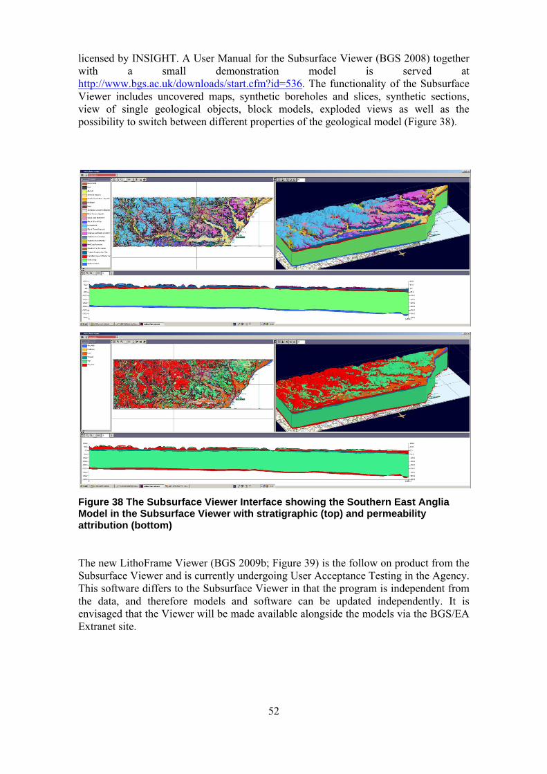
52

licensed by INSIGHT. A User Manual for the Subsurface Viewer (BGS 2008) together with a small demonstration model is served at http://www.bgs.ac.uk/downloads/start.cfm?id=536. The functionality of the Subsurface Viewer includes uncovered maps, synthetic boreholes and slices, synthetic sections, view of single geological objects, block models, exploded views as well as the possibility to switch between different properties of the geological model (Figure 38).

Figure 38 The Subsurface Viewer Interface showing the Southern East Anglia Model in the Subsurface Viewer with stratigraphic (top) and permeability attribution (bottom)

The new LithoFrame Viewer (BGS 2009b; Figure 39) is the follow on product from the Subsurface Viewer and is currently undergoing User Acceptance Testing in the Agency. This software differs to the Subsurface Viewer in that the program is independent from the data, and therefore models and software can be updated independently. It is envisaged that the Viewer will be made available alongside the models via the BGS/EA Extranet site.

53

Figure 39 Options for delivery of BGS models

Currently the most common interaction of 3D modelling package outputs is with GIS systems. The following table lists the possible exports and their file formats.

Output Data type and format

Envelopes (geological unit extent – subcrop plus outcrop)

ESRI shape file

Horizontal slices ESRI shape file or geo-registered JPEG image

Sub and Supercrop maps ESRI shape file or geo-registered JPEG image

Grids of the base, top or thickness of geological units. Combined units.

ASCII/ESRI grids

GSI3D can exports all geological units (envelopes, base, top and thickness) as standard ESRI shapes and ASCII grids after model calculation. Any map view in GSI3D can be directly exported as a geo-registered tiff image for quick visualisation in GIS by clicking the save map window as image icon in the map window toolbar.

The use of these exports in GIS software is manifold and new ideas are being developed all the time. Below one example is shown where a full 3D model has been analysed to create a hydrogeological domains map (Figure 40). The approach taken in producing these domain maps is described in detail by Lelliott et al (2006).

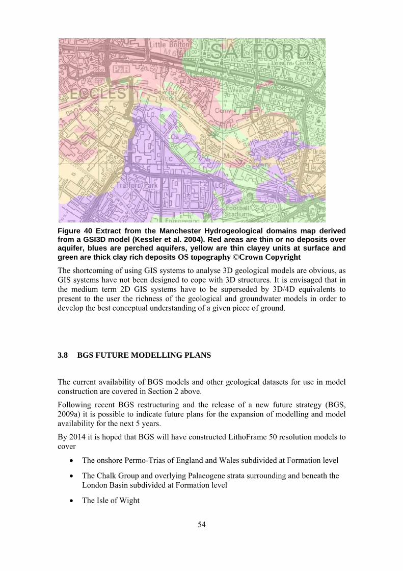
54

Figure 40 Extract from the Manchester Hydrogeological domains map derived from a GSI3D model (Kessler et al. 2004). Red areas are thin or no deposits over aquifer, blues are perched aquifers, yellow are thin clayey units at surface and green are thick clay rich deposits OS topography ©Crown Copyright

The shortcoming of using GIS systems to analyse 3D geological models are obvious, as GIS systems have not been designed to cope with 3D structures. It is envisaged that in the medium term 2D GIS systems have to be superseded by 3D/4D equivalents to present to the user the richness of the geological and groundwater models in order to develop the best conceptual understanding of a given piece of ground.

3.8 BGS FUTURE MODELLING PLANS

The current availability of BGS models and other geological datasets for use in model construction are covered in Section 2 above.

Following recent BGS restructuring and the release of a new future strategy (BGS, 2009a) it is possible to indicate future plans for the expansion of modelling and model availability for the next 5 years.

By 2014 it is hoped that BGS will have constructed LithoFrame 50 resolution models to cover

The onshore Permo-Trias of England and Wales subdivided at Formation level

The Chalk Group and overlying Palaeogene strata surrounding and beneath the London Basin subdivided at Formation level

The Isle of Wight

55

The Jurassic and Triassic strata of the Cleveland Basin

Plans for further regional LithoFrame 250 scale models are shown in Section 2 (Figure 11).

In addition commercial and co-funded modeling contracts will add to this envisaged coverage and add detail to specific models.

Workflows and procedures are being identified to streamline the construction, validation, approval, storage and dissemination of 3D models as standard BGS products. Standardization of existing and legacy models is also a key task envisaged for 2010-11.

In addition to its development of the GSI3D software and methodology BGS is actively building a GSI3D – ZOOM interface to enable geological models to be translated into a numerical hydrogeological modelling package

Using the interface any ZOOM grid is imported in to GSI3D and the values for top and bottom of each layer as well as the hydraulic properties of the layer are exported from GSI3D. The stratigraphic sequence file in GSI3D is attributed by the user to allow the hydrogeological units to be identified from the geological units. The ZOOM setup program, ZETUP has been modified to accept the data from GSI3D and to create the input files for ZOOM in the correct format. The whole process is no more difficult than setting up a ZOOM model using a GIS.

4 Conceptual Models

4.1 DEVELOPMENT OF CONCEPTUAL MODELS

Introduction

This section aims to introduce the Conceptual Model of groundwater flow and solute transport and how they are developed and used. A conceptual understanding of any groundwater system is important to develop as they contain the essence of the knowledge of how the system operates. Conceptual models vary considerably as they depend on the purpose for which the study is being undertaken. This means that the scale and complexity of the Conceptual Model will vary. The Conceptual Model developed has to be “fit for purpose” and suited to answer the questions being posed for the study as well as the resources available (time and staff).

The process by which a conceptual understanding is developed is really one of getting to know the system how the system behaves. Data are collected, collated and examined and from this an understanding developed. The process, whilst often presented as a logical, well defined process is iterative and can be chaotic. Data sets are often incomplete and do not provide the correct amount of detail where it is required. Therefore more data has to be collected and the understanding further developed. Once a satisfactory Conceptual Model has been developed, then it needs to be tested. The techniques used for testing Conceptual models are detailed in subsequent sections.

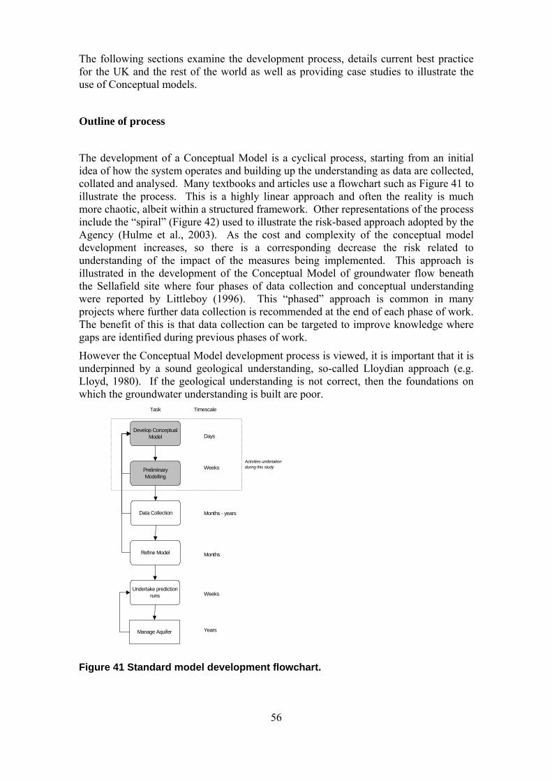
56

The following sections examine the development process, details current best practice for the UK and the rest of the world as well as providing case studies to illustrate the use of Conceptual models.

Outline of process

The development of a Conceptual Model is a cyclical process, starting from an initial idea of how the system operates and building up the understanding as data are collected, collated and analysed. Many textbooks and articles use a flowchart such as Figure 41 to illustrate the process. This is a highly linear approach and often the reality is much more chaotic, albeit within a structured framework. Other representations of the process include the “spiral” (Figure 42) used to illustrate the risk-based approach adopted by the Agency (Hulme et al., 2003). As the cost and complexity of the conceptual model development increases, so there is a corresponding decrease the risk related to understanding of the impact of the measures being implemented. This approach is illustrated in the development of the Conceptual Model of groundwater flow beneath the Sellafield site where four phases of data collection and conceptual understanding were reported by Littleboy (1996). This “phased” approach is common in many projects where further data collection is recommended at the end of each phase of work. The benefit of this is that data collection can be targeted to improve knowledge where gaps are identified during previous phases of work.

However the Conceptual Model development process is viewed, it is important that it is underpinned by a sound geological understanding, so-called Lloydian approach (e.g. Lloyd, 1980). If the geological understanding is not correct, then the foundations on which the groundwater understanding is built are poor.

Figure 41 Standard model development flowchart.

Task Timescale

Develop Conceptual Model

Preliminary Modelling

Data Collection

Refine Model

Undertake prediction runs

Manage Aquifer

Days

Weeks

Months - years

Months

Weeks

Years

Activities undertaken during this study

57

Figure 42 Environment Agency Conceptual Model development “spiral” (after Hulme et al., 2003).

Fitness for purpose

It is important for the success of any modelling process that consideration must be given as to the purpose of the model. A clear question or set of questions that are being addressed by the modelling process enables the model development to be properly focussed. The development of the Conceptual Model is no exception. Typical questions that need to be addressed include what is the model being used for, why is it being developed and how is it to be developed. The development of any model is successful when a well formed question is used as its basis. The question posed will define the approach adopted including the scale of the problem (or range of scales) and the complexity of the approach.

Scale vs. complexity

An understanding of scale is extremely important in groundwater based problems. To understand groundwater flow both spatial and temporal scales need to be addressed. It is likely that a series of Conceptual models will be developed to represent different spatial scales as well as different stages in the development of the groundwater system. It is also likely that the understanding of groundwater flow will evolve as understanding increases and more data becomes available. Therefore, any project that is well resourced will produce a number of conceptual models that vary in time, spatial extent and complexity.

For spatial scales, a ranges of scales need to be considered. Groundwater system are measured and exploited on a local scale (~ metres), but groundwater flow and solute transport occurs on a regional scale (~ 10 kilometres). Typically groundwater exploitation will occur at a localised scale from a well-field or spring system. However, other problems need to be addressed at a larger scale, e.g. 100-1000 metres. Examples of problems at this scale include wetlands, quarries, metal mines, etc. Therefore any

Initial ideas

Best Conceptual Model

First Conceptual Model

Better Conceptual Model

Development Cycle for Conceptual models

Pro

cess

NGWCLC 19/03/02NGWCLC 19/03/02

58

understanding of the groundwater system has to encompass both these scales and also those in between, as required. For example, examining groundwater flow at a catchment or river-reach scale may be important. Work has been undertaken on the perception of different spatial scales and how they are perceived. Geoscience students were assessed to see how they defined the different boundaries between scales (Dickerson et al., 2005).

Similarly for temporal scales, then different Conceptual models need to be developed to address changes with time. The groundwater system will be modified based on the external influences. For example quarrying, the associated dewatering and the recovery in groundwater heads once dewatering ceases. Conceptual models may need to be developed before the quarrying was started, during the dewatering process and after quarrying has ceased.

4.2 CURRENT BEST PRACTICE

United Kingdom

The term Conceptual Model was first used in the UK for the South Humber Bank salinity study and adopted by John Lloyd (University of Birmingham, 1978). The idea of developing a Conceptual Model has been taken up by the UK hydrogeological community with a vengeance in the last decade. The development of the conceptual model has been built into Agency contracts for groundwater modelling since 1999. To support this activity a best practice guide was written and first published in 2002 (Hulme et al., 2002). The guide was aimed at groundwater professionals working as Agency staff and contractors and the aim of the guide was to achieve consistency in developing Conceptual models and their subsequent testing by encapsulating them in numerical models. This guide was developed in conjunction with Prof. Ken Rushton and the ideas he developed during this time influenced his most recent book (Rushton, 2003). The best practice guide was designed as a repository for information and a document that could evolve as experience with using it increased. The guide is in the process of being revised (Rolf Farrell, pers. comm.) and it being split into different parts aimed at different audiences. For example, a less detailed description of model development has been developed for managers who are not familiar with groundwater modelling techniques.

Another notable use of Conceptual modelling within the UK is the work undertaken for NIREX to characterise the proposed underground waste repository at Sellafield (NIREX, 1997). Due to the timescales for radioactivity to reach the surface (>100000s years) and the uncertainty involved in the groundwater flow system, multiple conceptual models were developed. Conceptual models were developed at different scales (from the repository to the regional flow) and to represent the uncertainty in the understanding for the same part system in different ways (e.g. Littleboy, 1996; Black and Brightman, 1996; Heathcote et al., 1996). These multiple Conceptual models were an important way of dealing with the uncertainty involving the groundwater flow and subsequent transport of radionuclides to the surface.

Influenced by the NIREX approach of multiple possible Conceptual models, BGS has adopted similar approaches for work in the Thames Basin in both the Swanscombe project (Bloomfield et al., 2002) and for assessing the impact of abstraction on river flows at Gatehampton (Jackson et al., 2007). Due to the uncertainty in the system,

59

multiple conceptual models of groundwater flow were proposed and then tested against field observations to arrive at a likely set of conceptual models.

Europe

Best practice guides for the application of groundwater modelling including the development of conceptual models have been developed by a range of European organisations. These include those funded by the EU such as HarmoniQua (Packman and Old, 2005) and those developed by particular organisations. Examples of the latter include Public Interaction Guides for clients, modellers and auditors (Delft).

There is also a growing literature on conceptual model uncertainty, with examples including those examining the relationship between conceptual model uncertainty and parametric uncertainty (Højberg, 2004) and developing methods to incorporate conceptual uncertainty in models (Rojas et al., 2008).

America

Early examples of mention of conceptual models in the hydrogeological literature include that of White (1969). Echoing the developments in Europe, a significant number of best practice guides have been developed by US organisations. A useful summary is provided by Hill et al. (2004). Examples of US best practice include American Society for Testing and Materials, United States Geological Survey (USGS) US Army Corps of Engineers and the US Environmental Protection Agency . The USGS also produces examples of conceptual model reports such as the Colville River Project (Ely and Kahle, 2004).

Examples in the literature include that of multiple conceptual models in the Nuclear industry e.g. Stirewalt and Shepard (2004), methods of examining different conceptual models, Helton et al. (1995) and systems that can examine different options for conceptual models to address uncertainty (Chmakow et al., 2007).

Rest of the world

There are various examples of best practice guides in Australasia. The most notable is that developed for the Murray-Darling Basin Study (Middlemis, 2001). The author of this study also conducted a review of current best practice in 2004 (Middlemis, 2004) as part of a Churchill Fellowship.

4.3 USES FOR CONCEPTUAL MODELS BY THE ENVIRONMENT AGENCY

The Agency develops and uses a number of different conceptual models at a range of scales. Table 7 summarises the range of Conceptual models that are routinely developed. The majority of the Conceptual models are local scale ones that sit within a catchment or regional context. However, the development of these conceptual models has to fit into the implementation of a policy and so have to be consistent on a national scale.

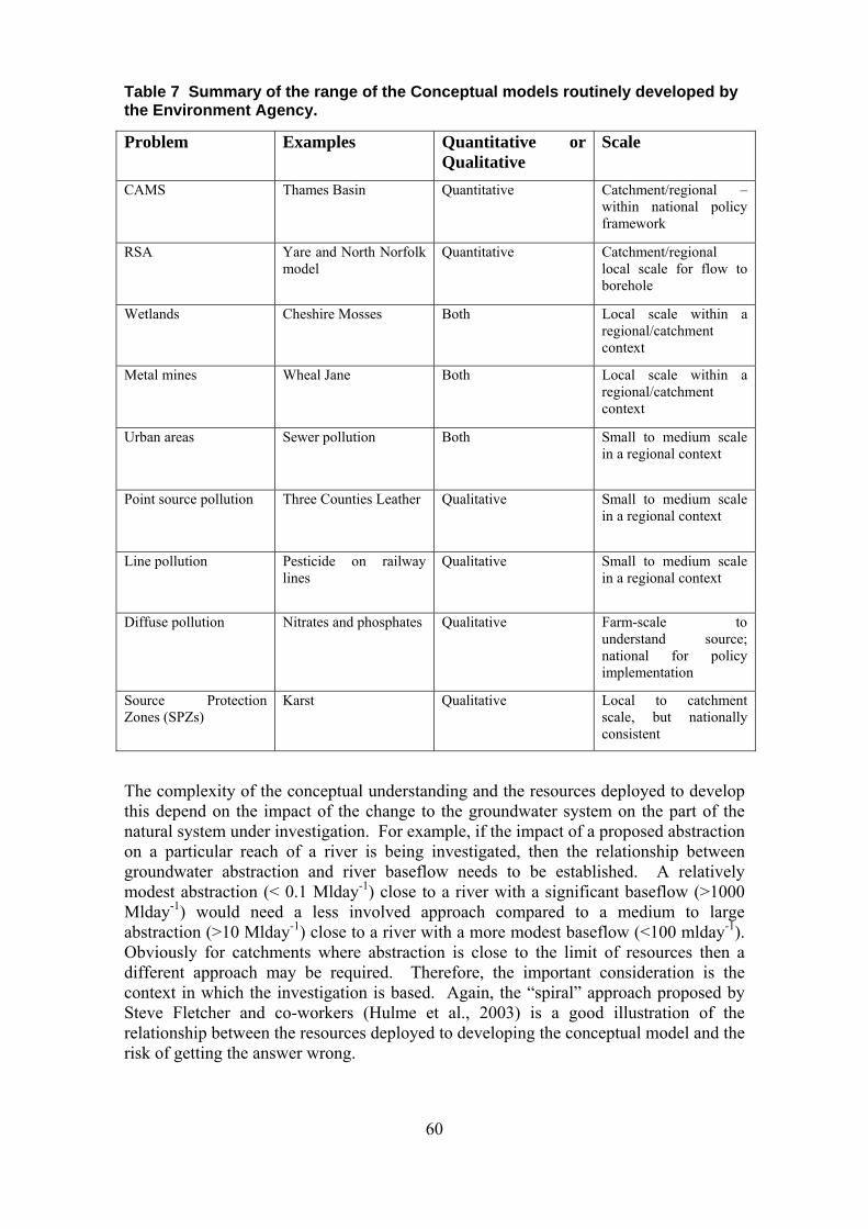
60

Table 7 Summary of the range of the Conceptual models routinely developed by the Environment Agency.

Problem Examples Quantitative or Qualitative

Scale

CAMS Thames Basin Quantitative Catchment/regional – within national policy framework

RSA Yare and North Norfolk model

Quantitative Catchment/regional local scale for flow to borehole

Wetlands Cheshire Mosses Both Local scale within a regional/catchment context

Metal mines Wheal Jane Both Local scale within a regional/catchment context

Urban areas Sewer pollution Both Small to medium scale in a regional context

Point source pollution Three Counties Leather Qualitative Small to medium scale in a regional context

Line pollution Pesticide on railway lines

Qualitative Small to medium scale in a regional context

Diffuse pollution Nitrates and phosphates Qualitative Farm-scale to understand source; national for policy implementation

Source Protection Zones (SPZs)

Karst Qualitative Local to catchment scale, but nationally consistent

The complexity of the conceptual understanding and the resources deployed to develop this depend on the impact of the change to the groundwater system on the part of the natural system under investigation. For example, if the impact of a proposed abstraction on a particular reach of a river is being investigated, then the relationship between groundwater abstraction and river baseflow needs to be established. A relatively modest abstraction (< 0.1 Mlday-1) close to a river with a significant baseflow (>1000 Mlday-1) would need a less involved approach compared to a medium to large abstraction (>10 Mlday-1) close to a river with a more modest baseflow (<100 mlday-1). Obviously for catchments where abstraction is close to the limit of resources then a different approach may be required. Therefore, the important consideration is the context in which the investigation is based. Again, the “spiral” approach proposed by Steve Fletcher and co-workers (Hulme et al., 2003) is a good illustration of the relationship between the resources deployed to developing the conceptual model and the risk of getting the answer wrong.

61

5 Numerical (Groundwater Flow) models

5.1 INTRODUCTION

This section aims to introduce numerical modelling of groundwater flow and solute transport. It aims to provide the context for the discussion of how to use geological modelling to enhance the development of groundwater models. Two issues have become apparent from the discussion with Agency groundwater staff: scale and complexity. The former requires that groundwater has to be studied on the regional scale, but managed on the local scale. Therefore a modelling system has to be developed that encompasses both small and large scale groundwater processes. Different levels of complexity are required to deal with the problems faced by the Environment Agency. For example the inclusion of wetlands requires both surface water and groundwater systems to be represented in a model. The treatment of geological complexity in the development of understanding of groundwater system requires consideration. For this issue scale and complexity are related. Depending on the problem being addressed, then a large scale, low complexity geological model needs to be developed, or a small scale, more detail model may be required. The former would be required for a national policy issue such as groundwater vulnerability and the latter would be used for a site-specific investigation.

5.2 TESTING CONCEPTUAL MODELS OF GROUNDWATER FLOW AND SOLUTE TRANSPORT

The conceptual model is developed by an iterative process. The problem to be tackled is first identified, the question to be considered is framed, then based on the appropriate data an understanding of the groundwater flow system is developed. This understanding needs to be tested. The testing of the conceptual model can take many forms from a simple calculation (so-called “back of the fag packet”) through to a sophisticated numerical model involving all aspects of the hydrological cycle and solute transport. The method used to test the conceptual understanding depends on a number of factors, including the question being posed and the resources available to undertake the testing. It requires judgement based on the skill and experience of the person undertaking or leading the process. Guidance provided by documents such as the “Groundwater Resources Modelling: Guidance Notes and Template Project Brief” (Hulme et al., 2002) can provide support for this process.

However the most important consideration is that the method of testing the conceptual model numerically must be “fit for purpose”. This idea requires that the appropriate method is chosen based on the outcome that is required. Consideration of the scale and complexity of the problem play an important role in determining which method to choose. For example a national scale conceptual model is likely to be tested with a simpler model than a highly localised study. The CAMS process is undertaken on a catchment basis but with a national coverage. This means the method is a relatively simple water balance. The opposite end of the spectrum would be mine water discharge to a river. To model this process may involve a groundwater flow and solute transport model with geochemical processes coupled with a river model with an assessment of the impact of changing surface water chemistry on the ecology. To justify using this approach would require deploying significant resources to develop the understanding and the associated modelling system to test the understanding.

62

5.3 SCALE

Using models based on Finite-Difference Methods (FDM) to refine in particular areas produces a significant number of nodes outside of the area of interest. This is not computationally efficient as groundwater head is solved where it isn’t required. Various approaches have been adopted to solve this problem. The basic idea is to refine the model in the area of interest without affecting the rest of the model. This means the mesh density (number of nodes per unit area) is increased locally without affecting the gridding in the rest of the model.

An early example of this technique is Telescopic Mesh Refinement (TMR), e.g. Ward et al, 1987. This technique involves creating two models: a parent model (large scale) and a child model (small scale). Heads from the parent model are passed to the child model to form the boundary conditions for the child model. The disadvantage of this method, apart from having two separate models, is that abstraction in the child model will cause changes in the boundary conditions which will not be passed through to the parent model.

To solve this problem schemes that link the parent-child model have been developed. Examples include Szlecky (1998) and the developments for MODFLOW (e.g. Mehl and Hill, 2002). This technique is known as Local Grid Refinement (LGR) and allows the explicit connection of models of different scales and the impact of changes in the child model to be passed back to the parent model and vice versa. This connection ensures that the flow balance in the model is preserved by iterative exchange of heads between the parent and child models. Schemes have been developed that allow both two dimensional and three dimensional model linkages to be undertaken. The limitation of this technique is that requires two separate models to be set up.

A further development of the LGR concept has been implemented in the ZOOM suite of models (e.g. Jackson and Spink, 2004). Using object-oriented techniques, the implementation of LGR within the flow model ZOOMQ3D represents grids as objects and any number of parent-child relationships can be implemented (Jackson, 2000). The flow across the boundaries is defined by a modified Finite-Difference technique. This modified scheme allows the simultaneous solution of heads within the model domain (Jackson, 2000). The disadvantage of the technique is that a new model has to be built using the ZOOMQ3D code.

Other numerical techniques which allow the scale issue to be addressed include Finite-Element Method (FEM) and the Finite-Volume (FV) technique. FEM allow the use of triangular and quadrilateral meshes which can be unstructured. This meshing system can represent non-uniform shapes much easier than the orthogonal FDM. Examples of the use of FEM include the design of structures for civil engineering works and examining flow in complex structures (Computational Fluid Dynamics). Examples of codes used within the groundwater community include FEFLOW, FEMWAT, etc. The disadvantage of FEM is the problem with achieving a flow balance.

Finite-Volume methods are a hybrid between FEM and FDM, triangular and quadrilateral meshes can be used and these are transformed to an orthogonal mesh. This transformation allows the flow balance be preserved whilst implementing anon-uniform meshing. FV methods, therefore, appear to offer potential in representing complex geometry as found in geological systems.

63

5.4 COMPLEXITY

The WFD requires that the inclusion of different mechanisms is necessary to simulate a catchment on a holistic basis. To address the issue of complexity a number of modelling approaches need to be adopted. The main modelling approaches are threefold: developing a modelling system that includes all the mechanisms required, coupling existing models together to produce a hard-coded system, or linking models using a flexible method. Each of these different approaches has their own advantages and disadvantages. However, one of the accepted practices is that complexity should be increased step-wise. By increasing the complexity in a controlled manner, the model user can “learn” how the system works and this enables the effects of each change to be determined. This approach is even more important where different types of systems (i.e. surface water and groundwater) are linked. Whilst each system may be understood and simulated on an individual basis, when put together then one system can affect the other and vice versa.

Models that include a significant proportion of the hydrological cycle “all-inclusive” models

Examples of these models include Mike-SHE (DHI), Système Hydrologique Européen TRANsport (SHE-TRAN) (University of Newcastle; NCL) and Hydrogeosphere (Waterloo). Mike-SHE was designed originally to examine solute transport in catchments and developed as a series of highly complex models. The system has evolved to include simpler models for each part of the hydrological cycle (e.g. lumped parameter representation of the groundwater system). The Mike-SHE system can model the whole hydrological cycle including riverflow, overland flow, unsaturated zone and the saturated zone. Solute transport modelling can be undertaken. DHI, the developers of Mike-SHE, are involved in the OpenMI project (see below) and significant parts of Mike-SHE are OpenMI compliant.

SHE-TRAN is a variant of Mike-SHE, developed by Newcastle University. The original SHE modelling system was a three-way project between DHI-NCL- SOGREAH, with NCL continuing to develop their own variant. This has a similar capability to Mike-SHE, but focussing on flow in fractured media (Ewan et al., 2000).

HydroGeoSphere is based upon FRAC3DVS (Therrien et al., 2008). The surface flow module is based on MODHMS (Panday and Huyakorn, 2004), which is itself an enhancement the MODFLOW code. HydroGeoSphere uses the finite element approach to simulate coupled surface water-groundwater flow. Three dimensional simulations of variably-saturated fractured or granular aquifers have been performed (see for example Li et al., 2008) with good accuracy. The model provides several spatial discretisation options; from simple rectangular domains, to irregular domains with complex geometry and layering. Mixed element types provide an efficient mechanism for simulating flow and transport processes in different environments (fractures, pumping/injection wells, streams or tile drains). External flow stresses can be included (specified rainfall rates, hydraulic head and flux, infiltration and evapo-transpiration, drains, wells, streams and seepage faces). HydroGeoSphere includes options for adaptive-time stepping. The model is a robust simulator of variable saturated conditions and surface water-groundwater interactions which has proven accurate for a variety of spatial and temporal scales (Gleeson and Manning, 2008). The project partners also have links to the GEOIDE project.

64

The advantage of these modelling systems is that they combine a large number of different mechanisms which can be ideal if they provide the solution to the problem under consideration. The disadvantage is that they are unwieldy pieces of code which are highly complex, inflexible and require large computational resources.

Hard coded model “couplets”

There has been a recent trend to solve the problem of combining surface water and groundwater models by joining two or more models together. This is defined as a hard-coded explicit link and allows the user access to models that are well used, documented and validated in combination. Table 8 shows examples of these model “couplets”. Predominately these models are surface water models linked to MODFLOW.

The advantages of this approach are that they consist of well used codes and will solve a particular problem. However, the disadvantage is that they are hard-coded, inflexible and can be cumbersome.

Table 8 Comparison between model “couplets” of different types

Model Developer Description Website

MODHMS Hydrogeologic Based on MODFLOW-SURFACT, but includes 2-D overland flow and 1-D channel flow

www.modhms.com/software.htm

IHSim Hydrogeologic Finite Element version of MODHMS

www.modhms.com/software.htm

IHM Intera, AQUATERRA and the Uni of South Florida

Couples MODFLOW with the surface water code Hydrologic Simulated Program (Fortran) or HSP-F

www.intera.com/techology_ihm.php

SFWMD & SFHSM

South Florida Water Management District

See description above www.sfwmd.gov/org/pld/hsm/hsm.html

Wash123D Professor George Yeh, Uni of Central Florida

FEM model (based on FEMWATER) coupled with 1-D river and 2-D overland surface flow models

people.cecs.ucf.edu/yeh/

GSFLOW USGS Couples MODFLOW with the surface water code PRMS

water.usgs.gov/nrp/gwsoftware

MOSDEW RIVERTWIN

Couples MODFLOW with the surface water model HBV

www.rivertwin.de

Common interface systems

To help solve the problem of the WFD, the EU funded HarmonIT project investigated how to link models of different types. This project developed the OpenMI standard which is a data exchange protocol. An implementation of this protocol was created in

65

C#. Models which are OpenMI compliant are made into objects and can exchange data such as flows at runtime. This system is extremely powerful and facilitates the setting up of a modelling system that consists of models of different types. The complexity of each model used and also the number of models can be increased as the understanding of the system improves. The disadvantage of this approach is that an investment is required to make each model OpenMI compliant as well as the computation penalty of exchanging data at runtime via an interface. However, the OpenMI system offers a flexible method of dealing with scale and complexity. For example a detailed model of a wetland (e.g. surface water model built using Mike-SHE) can be linked to a groundwater model with grid refinement (e.g. ZOOMQ3D).

5.5 REPRESENTATION OF GEOLOGICAL COMPLEXITY IN GROUNDWATER MODELS

The representation of geological volumes in groundwater models has been recognised as being poor. Recently, systems have been developed to enable the better representation of geological complexity within groundwater flow models. A good example of this is the development of grid-independent user interfaces. These systems allow the user to develop a conceptual model of the geology that isn’t related to the gridding used in the numerical model. Examples of this type of system include Groundwater Modelling System (Richards and Jones, 1996), PETREL (Schlumberger pre-processor for ECLIPSE) and ARGUS-ONE. Direct linkages have been developed between geological modelling systems and groundwater flow models for example GSI3D and ZOOM; (Hughes et al., 2008).

One of the limitations that have been identified by the process of linking geological models to FDM is that layered models cannot properly represent the complexity observed in geological systems. To a certain extent this can be solved by using FEM, but problems still remain.

6 Case Studies and costs

This section discusses Case Studies illustrating the use of Geological models to aid the development of conceptual understanding and other aspects of Agency work in recent years. Summaries of six diverse case studies are presented together with generalised costs of these projects, finally a brief discussion of the main factors influencing the costs of commissioning models is presented. It should be stressed however that as available model coverage grows models will increasingly be able to be licensed from off the shelf at costs often less than 10% of the cost of commissioning the building of an entire model. Details of other Agency geological modelling contracts completed by BGS in recent years are included at Appendix 1. At the most detailed is the Oxford flooding project, which examines the impact of the groundwater system on flooding in Oxford. The second example Chichester is a detailed model of a 10 x 10 km block to indentify groundwater pathways into the underlying Chalk aquifer. Identification of pathways were the major outcome of the Manchester model, whilst more regional studies are represented by the Permo-Trias model of the Southern Needwood Basin around Lichfield, the London Chalk model both of which are to aide conceptualisation

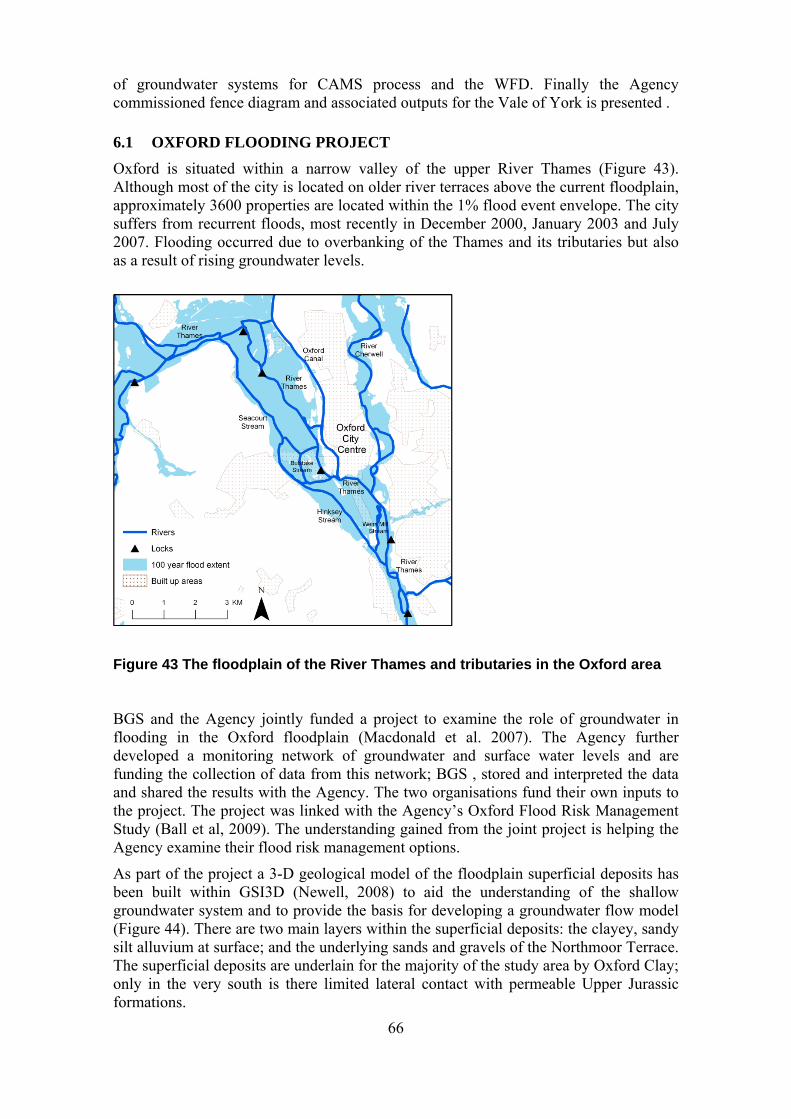
66

of groundwater systems for CAMS process and the WFD. Finally the Agency commissioned fence diagram and associated outputs for the Vale of York is presented .

6.1 OXFORD FLOODING PROJECT

Oxford is situated within a narrow valley of the upper River Thames (Figure 43). Although most of the city is located on older river terraces above the current floodplain, approximately 3600 properties are located within the 1% flood event envelope. The city suffers from recurrent floods, most recently in December 2000, January 2003 and July 2007. Flooding occurred due to overbanking of the Thames and its tributaries but also as a result of rising groundwater levels.

Figure 43 The floodplain of the River Thames and tributaries in the Oxford area

BGS and the Agency jointly funded a project to examine the role of groundwater in flooding in the Oxford floodplain (Macdonald et al. 2007). The Agency further developed a monitoring network of groundwater and surface water levels and are funding the collection of data from this network; BGS , stored and interpreted the data and shared the results with the Agency. The two organisations fund their own inputs to the project. The project was linked with the Agency’s Oxford Flood Risk Management Study (Ball et al, 2009). The understanding gained from the joint project is helping the Agency examine their flood risk management options.

As part of the project a 3-D geological model of the floodplain superficial deposits has been built within GSI3D (Newell, 2008) to aid the understanding of the shallow groundwater system and to provide the basis for developing a groundwater flow model (Figure 44). There are two main layers within the superficial deposits: the clayey, sandy silt alluvium at surface; and the underlying sands and gravels of the Northmoor Terrace. The superficial deposits are underlain for the majority of the study area by Oxford Clay; only in the very south is there limited lateral contact with permeable Upper Jurassic formations.

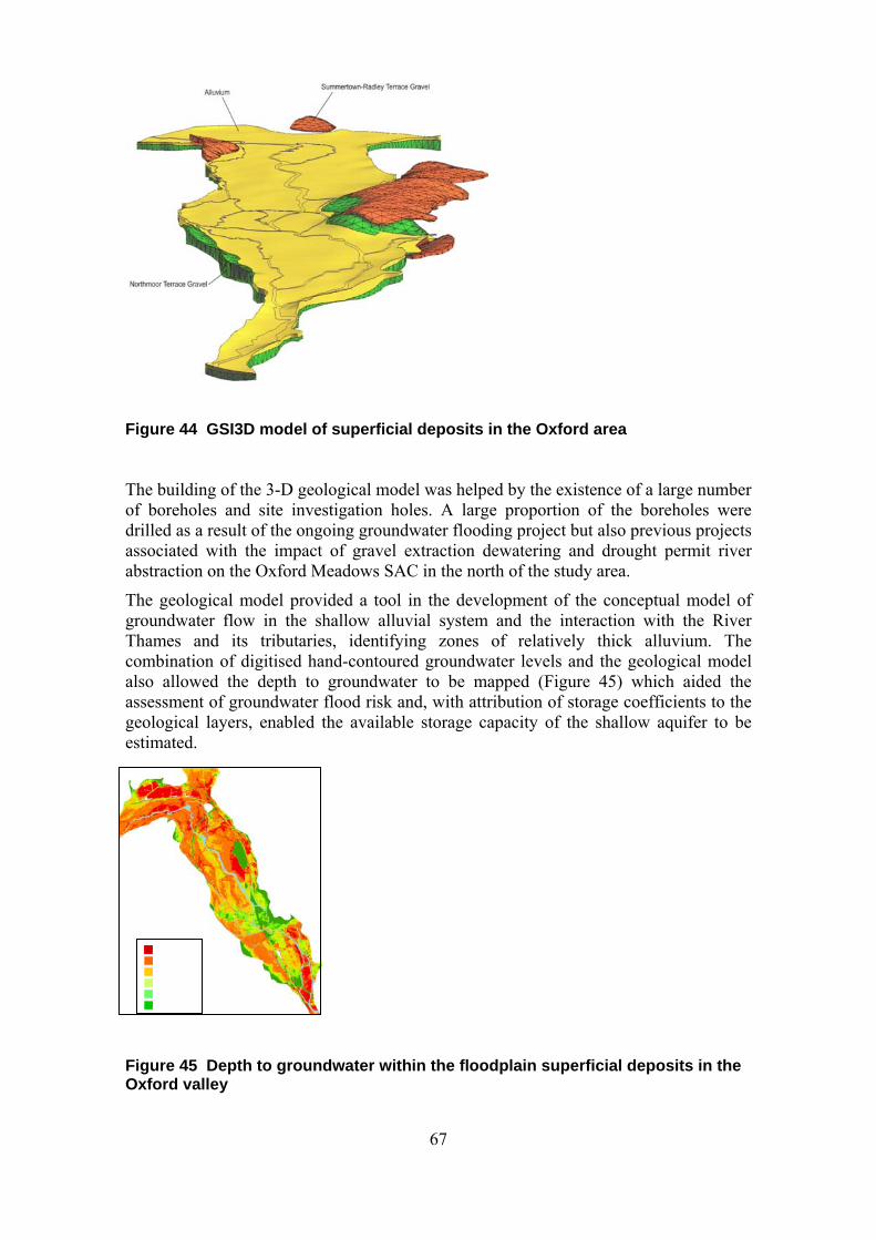
67

Figure 44 GSI3D model of superficial deposits in the Oxford area

The building of the 3-D geological model was helped by the existence of a large number of boreholes and site investigation holes. A large proportion of the boreholes were drilled as a result of the ongoing groundwater flooding project but also previous projects associated with the impact of gravel extraction dewatering and drought permit river abstraction on the Oxford Meadows SAC in the north of the study area.

The geological model provided a tool in the development of the conceptual model of groundwater flow in the shallow alluvial system and the interaction with the River Thames and its tributaries, identifying zones of relatively thick alluvium. The combination of digitised hand-contoured groundwater levels and the geological model also allowed the depth to groundwater to be mapped (Figure 45) which aided the assessment of groundwater flood risk and, with attribution of storage coefficients to the geological layers, enabled the available storage capacity of the shallow aquifer to be estimated.

Figure 45 Depth to groundwater within the floodplain superficial deposits in the Oxford valley

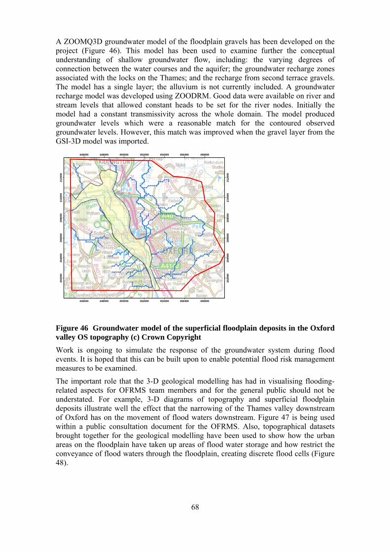
68

A ZOOMQ3D groundwater model of the floodplain gravels has been developed on the project (Figure 46). This model has been used to examine further the conceptual understanding of shallow groundwater flow, including: the varying degrees of connection between the water courses and the aquifer; the groundwater recharge zones associated with the locks on the Thames; and the recharge from second terrace gravels. The model has a single layer; the alluvium is not currently included. A groundwater recharge model was developed using ZOODRM. Good data were available on river and stream levels that allowed constant heads to be set for the river nodes. Initially the model had a constant transmissivity across the whole domain. The model produced groundwater levels which were a reasonable match for the contoured observed groundwater levels. However, this match was improved when the gravel layer from the GSI-3D model was imported.

Figure 46 Groundwater model of the superficial floodplain deposits in the Oxford valley OS topography (c) Crown Copyright

Work is ongoing to simulate the response of the groundwater system during flood events. It is hoped that this can be built upon to enable potential flood risk management measures to be examined.

The important role that the 3-D geological modelling has had in visualising flooding-related aspects for OFRMS team members and for the general public should not be understated. For example, 3-D diagrams of topography and superficial floodplain deposits illustrate well the effect that the narrowing of the Thames valley downstream of Oxford has on the movement of flood waters downstream. Figure 47 is being used within a public consultation document for the OFRMS. Also, topographical datasets brought together for the geological modelling have been used to show how the urban areas on the floodplain have taken up areas of flood water storage and how restrict the conveyance of flood waters through the floodplain, creating discrete flood cells (Figure 48).

446000

446000

448000

448000

450000

450000

452000

452000

454000

454000

456000

456000

458000

458000

202

000

202

000

204

000

204

000

20

600

0

20

600

0

20

800

0

20

800

0

210

000

210

000

212

00

0

212

00

0

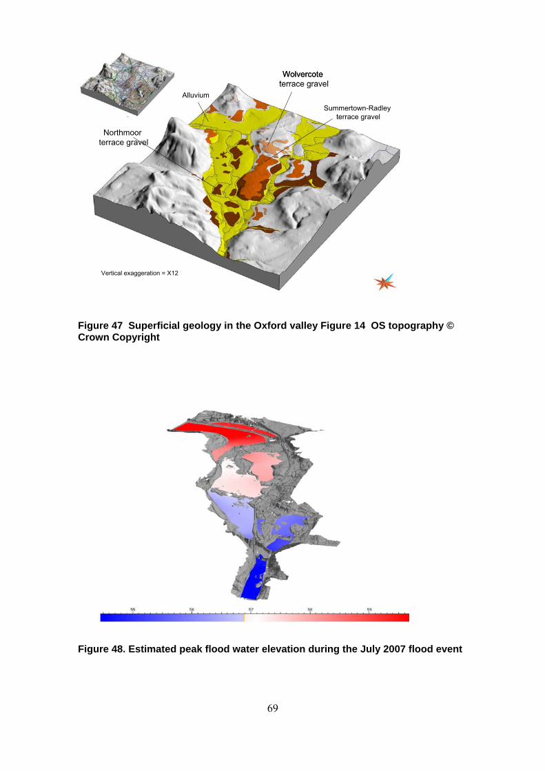
69

Figure 47 Superficial geology in the Oxford valley Figure 14 OS topography © Crown Copyright

Figure 48. Estimated peak flood water elevation during the July 2007 flood event

Alluvium

Wolvercoteterrace gravel

Summertown-Radleyterrace gravel

Northmoorterrace gravel

Vertical exaggeration = X12

Alluvium

Wolvercoteterrace gravel

Summertown-Radleyterrace gravel

Northmoorterrace gravel

Vertical exaggeration = X12

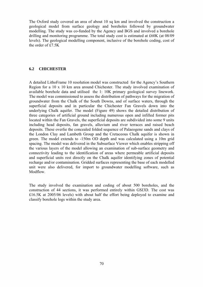
70

The Oxford study covered an area of about 10 sq km and involved the construction a geological model from surface geology and boreholes followed by groundwater modelling. The study was co-funded by the Agency and BGS and involved a borehole drilling and monitoring programme. The total study cost is estimated at £60K (at 08/09 levels). The geological modelling component, inclusive of the borehole coding, cost of the order of £7.5K

6.2 CHICHESTER

A detailed LithoFrame 10 resolution model was constructed for the Agency’s Southern Region for a 10 x 10 km area around Chichester. The study involved examination of available borehole data and utilised the 1: 10K primary geological survey linework. The model was commissioned to assess the distribution of pathways for the migration of groundwater from the Chalk of the South Downs, and of surface waters, through the superficial deposits and in particular the Chichester Fan Gravels down into the underlying Chalk aquifer. The model (Figure 49) shows the detailed distribution of three categories of artificial ground including numerous open and infilled former pits located within the Fan Gravels, the superficial deposits are subdivided into some 9 units including head deposits, fan gravels, alluvium and river terraces and raised beach deposits. These overlie the concealed folded sequence of Palaeogene sands and clays of the London Clay and Lambeth Group and the Cretaceous Chalk aquifer is shown in green. The model extends to -150m OD depth and was calculated using a 10m grid spacing. The model was delivered in the Subsurface Viewer which enables stripping off the various layers of the model allowing an examination of sub-surface geometry and connectivity leading to the identification of areas where permeable artificial deposits and superficial units rest directly on the Chalk aquifer identifying zones of potential recharge and/or contamination. Gridded surfaces representing the base of each modelled unit were also delivered, for import to groundwater modelling software, such as Modflow.

The study involved the examination and coding of about 500 boreholes, and the construction of 44 sections, it was performed entirely within GSI3D. The cost was £16.5K at 2005/06 levels) with about half the effort being deployed to examine and classify borehole logs within the study area.

71

Figure 49 The Chichester model showing surface geology (top), alluvial fan in ochre middle) and folded bedrock geology including chalk aquifer in green (bottom)

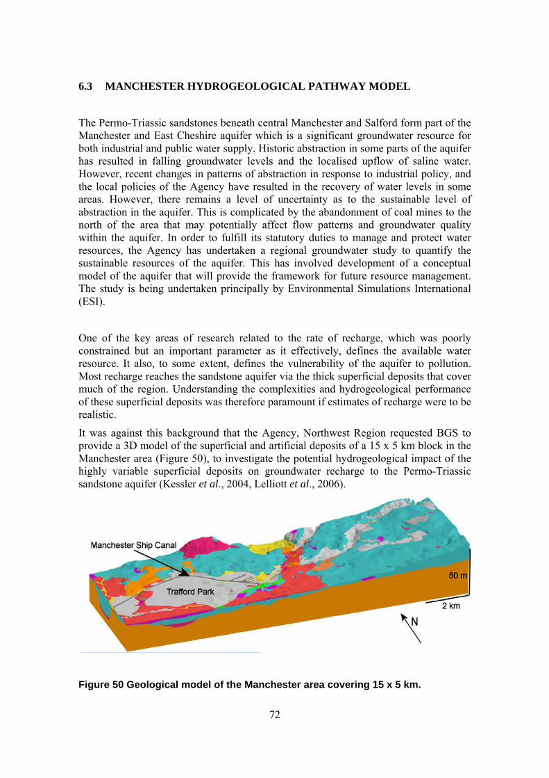
72

6.3 MANCHESTER HYDROGEOLOGICAL PATHWAY MODEL

The Permo-Triassic sandstones beneath central Manchester and Salford form part of the Manchester and East Cheshire aquifer which is a significant groundwater resource for both industrial and public water supply. Historic abstraction in some parts of the aquifer has resulted in falling groundwater levels and the localised upflow of saline water. However, recent changes in patterns of abstraction in response to industrial policy, and the local policies of the Agency have resulted in the recovery of water levels in some areas. However, there remains a level of uncertainty as to the sustainable level of abstraction in the aquifer. This is complicated by the abandonment of coal mines to the north of the area that may potentially affect flow patterns and groundwater quality within the aquifer. In order to fulfill its statutory duties to manage and protect water resources, the Agency has undertaken a regional groundwater study to quantify the sustainable resources of the aquifer. This has involved development of a conceptual model of the aquifer that will provide the framework for future resource management. The study is being undertaken principally by Environmental Simulations International (ESI).

One of the key areas of research related to the rate of recharge, which was poorly constrained but an important parameter as it effectively, defines the available water resource. It also, to some extent, defines the vulnerability of the aquifer to pollution. Most recharge reaches the sandstone aquifer via the thick superficial deposits that cover much of the region. Understanding the complexities and hydrogeological performance of these superficial deposits was therefore paramount if estimates of recharge were to be realistic.

It was against this background that the Agency, Northwest Region requested BGS to provide a 3D model of the superficial and artificial deposits of a 15 x 5 km block in the Manchester area (Figure 50), to investigate the potential hydrogeological impact of the highly variable superficial deposits on groundwater recharge to the Permo-Triassic sandstone aquifer (Kessler et al., 2004, Lelliott et al., 2006).

Figure 50 Geological model of the Manchester area covering 15 x 5 km.

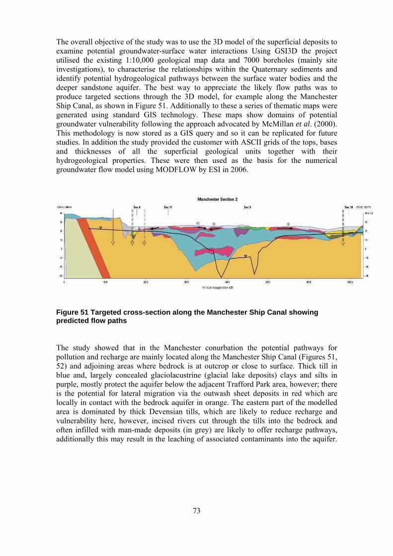
73

The overall objective of the study was to use the 3D model of the superficial deposits to examine potential groundwater-surface water interactions Using GSI3D the project utilised the existing 1:10,000 geological map data and 7000 boreholes (mainly site investigations), to characterise the relationships within the Quaternary sediments and identify potential hydrogeological pathways between the surface water bodies and the deeper sandstone aquifer. The best way to appreciate the likely flow paths was to produce targeted sections through the 3D model, for example along the Manchester Ship Canal, as shown in Figure 51. Additionally to these a series of thematic maps were generated using standard GIS technology. These maps show domains of potential groundwater vulnerability following the approach advocated by McMillan et al. (2000). This methodology is now stored as a GIS query and so it can be replicated for future studies. In addition the study provided the customer with ASCII grids of the tops, bases and thicknesses of all the superficial geological units together with their hydrogeological properties. These were then used as the basis for the numerical groundwater flow model using MODFLOW by ESI in 2006.

Figure 51 Targeted cross-section along the Manchester Ship Canal showing predicted flow paths

The study showed that in the Manchester conurbation the potential pathways for pollution and recharge are mainly located along the Manchester Ship Canal (Figures 51, 52) and adjoining areas where bedrock is at outcrop or close to surface. Thick till in blue and, largely concealed glaciolacustrine (glacial lake deposits) clays and silts in purple, mostly protect the aquifer below the adjacent Trafford Park area, however; there is the potential for lateral migration via the outwash sheet deposits in red which are locally in contact with the bedrock aquifer in orange. The eastern part of the modelled area is dominated by thick Devensian tills, which are likely to reduce recharge and vulnerability here, however, incised rivers cut through the tills into the bedrock and often infilled with man-made deposits (in grey) are likely to offer recharge pathways, additionally this may result in the leaching of associated contaminants into the aquifer.

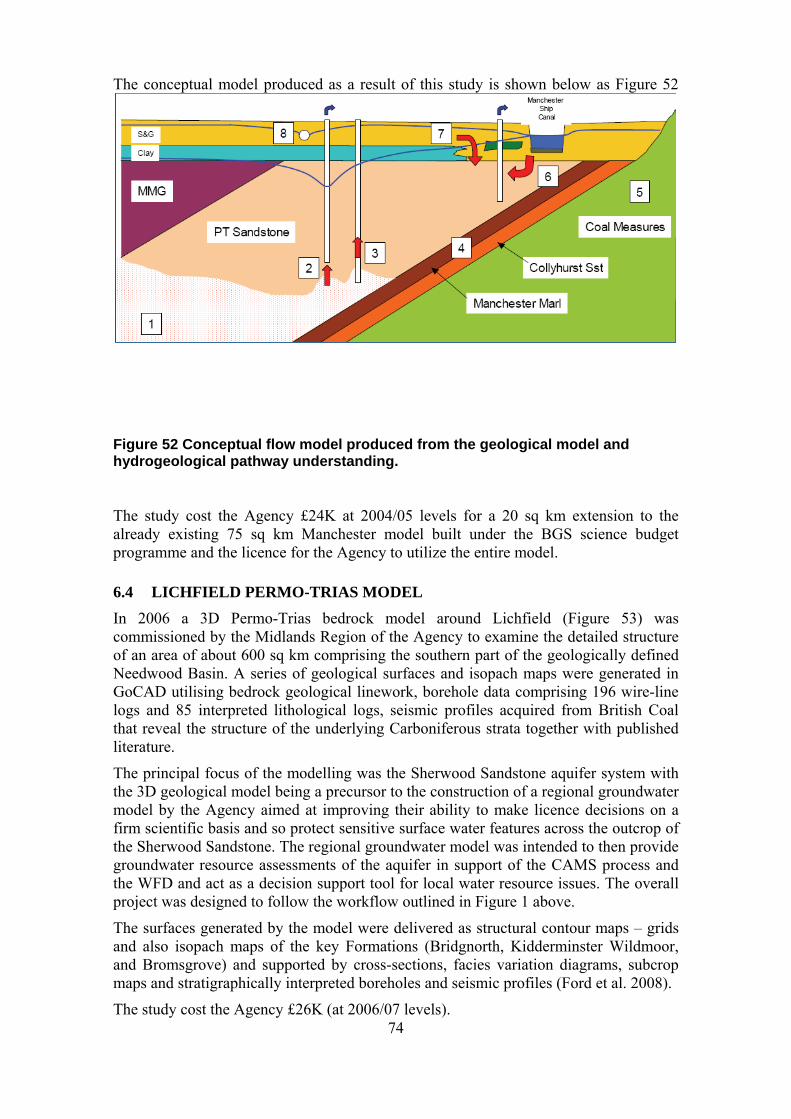
74

The conceptual model produced as a result of this study is shown below as Figure 52

Figure 52 Conceptual flow model produced from the geological model and hydrogeological pathway understanding.

The study cost the Agency £24K at 2004/05 levels for a 20 sq km extension to the already existing 75 sq km Manchester model built under the BGS science budget programme and the licence for the Agency to utilize the entire model.

6.4 LICHFIELD PERMO-TRIAS MODEL

In 2006 a 3D Permo-Trias bedrock model around Lichfield (Figure 53) was commissioned by the Midlands Region of the Agency to examine the detailed structure of an area of about 600 sq km comprising the southern part of the geologically defined Needwood Basin. A series of geological surfaces and isopach maps were generated in GoCAD utilising bedrock geological linework, borehole data comprising 196 wire-line logs and 85 interpreted lithological logs, seismic profiles acquired from British Coal that reveal the structure of the underlying Carboniferous strata together with published literature.

The principal focus of the modelling was the Sherwood Sandstone aquifer system with the 3D geological model being a precursor to the construction of a regional groundwater model by the Agency aimed at improving their ability to make licence decisions on a firm scientific basis and so protect sensitive surface water features across the outcrop of the Sherwood Sandstone. The regional groundwater model was intended to then provide groundwater resource assessments of the aquifer in support of the CAMS process and the WFD and act as a decision support tool for local water resource issues. The overall project was designed to follow the workflow outlined in Figure 1 above.

The surfaces generated by the model were delivered as structural contour maps – grids and also isopach maps of the key Formations (Bridgnorth, Kidderminster Wildmoor, and Bromsgrove) and supported by cross-sections, facies variation diagrams, subcrop maps and stratigraphically interpreted boreholes and seismic profiles (Ford et al. 2008).

The study cost the Agency £26K (at 2006/07 levels).

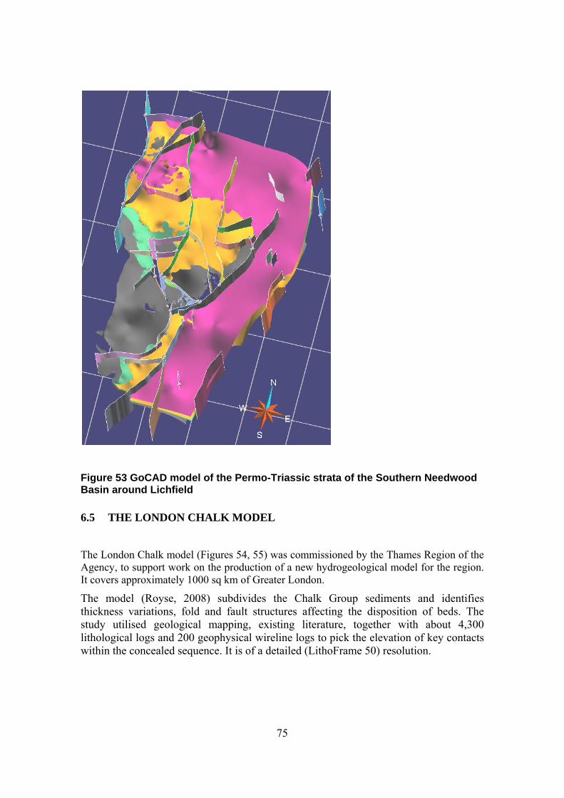
75

Figure 53 GoCAD model of the Permo-Triassic strata of the Southern Needwood Basin around Lichfield

6.5 THE LONDON CHALK MODEL

The London Chalk model (Figures 54, 55) was commissioned by the Thames Region of the Agency, to support work on the production of a new hydrogeological model for the region. It covers approximately 1000 sq km of Greater London.

The model (Royse, 2008) subdivides the Chalk Group sediments and identifies thickness variations, fold and fault structures affecting the disposition of beds. The study utilised geological mapping, existing literature, together with about 4,300 lithological logs and 200 geophysical wireline logs to pick the elevation of key contacts within the concealed sequence. It is of a detailed (LithoFrame 50) resolution.

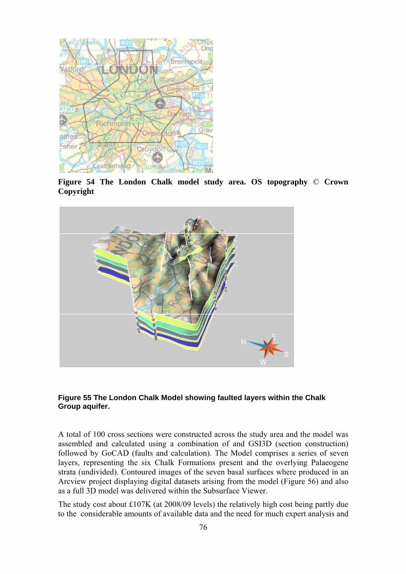
76

Figure 54 The London Chalk model study area. OS topography © Crown Copyright

Figure 55 The London Chalk Model showing faulted layers within the Chalk Group aquifer.

A total of 100 cross sections were constructed across the study area and the model was assembled and calculated using a combination of and GSI3D (section construction) followed by GoCAD (faults and calculation). The Model comprises a series of seven layers, representing the six Chalk Formations present and the overlying Palaeogene strata (undivided). Contoured images of the seven basal surfaces where produced in an Arcview project displaying digital datasets arising from the model (Figure 56) and also as a full 3D model was delivered within the Subsurface Viewer.

The study cost about £107K (at 2008/09 levels) the relatively high cost being partly due to the considerable amounts of available data and the need for much expert analysis and

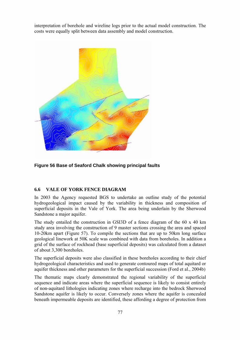
77

interpretation of borehole and wireline logs prior to the actual model construction. The costs were equally split between data assembly and model construction.

Figure 56 Base of Seaford Chalk showing principal faults

6.6 VALE OF YORK FENCE DIAGRAM

In 2003 the Agency requested BGS to undertake an outline study of the potential hydrogeological impact caused by the variability in thickness and composition of superficial deposits in the Vale of York. The area being underlain by the Sherwood Sandstone a major aquifer.

The study entailed the construction in GSI3D of a fence diagram of the 60 x 40 km study area involving the construction of 9 master sections crossing the area and spaced 10-20km apart (Figure 57). To compile the sections that are up to 50km long surface geological linework at 50K scale was combined with data from boreholes. In addition a grid of the surface of rockhead (base superficial deposits) was calculated from a dataset of about 3,300 boreholes.

The superficial deposits were also classified in these boreholes according to their chief hydrogeological characteristics and used to generate contoured maps of total aquitard or aquifer thickness and other parameters for the superficial succession (Ford et al., 2004b)

The thematic maps clearly demonstrated the regional variability of the superficial sequence and indicate areas where the superficial sequence is likely to consist entirely of non-aquitard lithologies indicating zones where recharge into the bedrock Sherwood Sandstone aquifer is likely to occur. Conversely zones where the aquifer is concealed beneath impermeable deposits are identified, these affording a degree of protection from

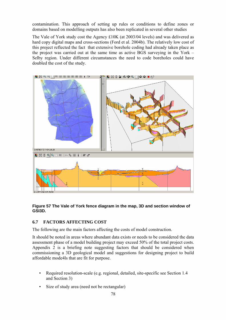
78

contamination. This approach of setting up rules or conditions to define zones or domains based on modelling outputs has also been replicated in several other studies

The Vale of York study cost the Agency £10K (at 2003/04 levels) and was delivered as hard copy digital maps and cross-sections (Ford et al. 2004b). The relatively low cost of this project reflected the fact that extensive borehole coding had already taken place as the project was carried out at the same time as active BGS surveying in the York – Selby region. Under different circumstances the need to code boreholes could have doubled the cost of the study.

Figure 57 The Vale of York fence diagram in the map, 3D and section window of GSI3D.

6.7 FACTORS AFFECTING COST

The following are the main factors affecting the costs of model construction.

It should be noted in areas where abundant data exists or needs to be considered the data assessment phase of a model building project may exceed 50% of the total project costs. Appendix 2 is a briefing note suggesting factors that should be considered when commissioning a 3D geological model and suggestions for designing project to build affordable mode4ls that are fit for purpose.

• Required resolution-scale (e.g. regional, detailed, site-specific see Section 1.4 and Section 3)

• Size of study area (need not be rectangular)

79

• Stratigraphic resolution (level of detail)

• Data Availability

• Need for specialised data interpretation (e.g. wire-line logs, seismic interpretation and stratigraphic expertise)

• Geological Domain type – homogenous or variable, degree of structural complexity

• Need to licence external datasets for use e.g. dtm, topographic maps

• Staff availability (most importantly in short-term small commissions)

7 Recommendations

Recommendations for the EA

Implement training courses on the use of 3D geological and groundwater models in order to raise the geological and environmental understanding and awareness of the subsurface geology in the Agency. In particular the CAMS process will benefit from the use of 3D geological models.

Exploit the benefits of 3D visualisation for the communication of complex environmental issues to stakeholders, managers and the public.

Consider the implications of the evolution from 2D geological data to 3D geological data for Easymap, the Water Resources GIS and other internal systems.

Promote the use of the LithoFrame Viewer and geological models across all parts of the Agency in particular with regard to Flood Defence, Contaminated Land and Planning.

Recommendations for BGS

Make available all geological map and borehole data and their metadatato the Agency in a simple and accessible manner. It is important to also include information on the lineage (how it was derived) and limitations (how it should be used) of the data.

Create a homogenised national model from the 1Mio and 250K LithoFrame models for use by the Agency as a backdrop for regional conceptualisation of catchments and major aquifers – akin to the use the national 625K map has at present.

Consider the creation of a full subcrop map of all major aquifers for use in the CAMS process as an interim 2.5 D measure.

Consider the creation of a national fence diagram (lines of sections and section spacing to be decided in conjunction with the Agency) to aid conceptualisation of catchments, especially in areas where no models exist.

Make available an index level dataset of all regional and detailed models that exist in the BGS to the Agency via the EXTRANET.

80

Homogenise and make available all existing Agency commissioned models and their accompanying reports via the EA/BGS extranet site using the LithoFrame Viewer.

Consider obtaining a copy of NGMS for its own use and to assess potential synergies with GSI3D, ZOOM and the BGS IT infrastructure as a whole.

For both parties

Consider merging the functionality of the LithoFrame Viewer and the NGMS into a single integrated subsurface visualisation system. Achieve this through a joint project between the Agency, BGS, DELTARES (owners of NGMS) and INSIGHT (owner of GSI3D). EU INTERREG funding could be targeted for this.

Promote exchanges of staff on a temporary basis to benefit both parties as this would provide greater transfer of knowledge and understanding of functions than can be achieved through dialogue, commissioned reports and models.

8 References cited

BALL, L.G.A., CLEGG, M.J., LEWIS, L. and BELL, G. 2008. Finding a long term solution to flooding in Oxford: the challenges faced. Proceedings of the European Conference on Flood Risk Management: Research into Practice. 30 September - 2 October 2008 Keble College, Oxford, UK.

BRITISH GEOLOGICAL SURVEY 2008. The Subsurface Viewer – User Manual. Available from http://www.bgs.ac.uk/downloads/start.cfm?id=537 [ Accessed 2 February 2009]

BRITISH GEOLOGICAL SURVEY 2009a The British Geological Survey Strategy 2009-2014. Applied geoscience for our changing Earth. BGS 28pp.

BRITISH GEOLOGICAL SURVEY 2009b. The LithoFrame Viewer 1.0 – User’s Guide Available from http://extranet.bgs.ac.uk/ea3d [Secure EXTRANET site]

BLACK J.H. AND BRIGHTMAN M.A., 1996. Conceptual model of the hydrogeology of Sellafield The Geology and Hydrogeology of the Sellafield Area Proceedings of the Nirex Seminar, 11 May 1994. Quarterly Journal Engineering Geology, 29 Supplement 1, May 1996.

BLOOMFIELD J.P., HUGHES A.G. AND JONES H.K.. 2002. Swanscombe Phase 2A Task 7 Conceptualisation of the Swanscombe area aquifer. BGS Report CR/02/020C

CHMAKOW S., SYCHEV, P., HESCH W. AND LIMA M. 2007. Conceptual Approach to Groundwater Modeling – A new generation of Waterloo Hydrogeologic Software. Zhttp://www.slb.com/media/services/additional/water/software/groundwater/conceptual_modeling.pdf) [Accessed 11 March 2009]

COOPER, A., FORD, J., PRICE, S., HALL, M., BURKE, H., AND KESSLER, H. 2007. The digital approach to understanding the Quaternary evolution of the Vale of York, UK. [Poster] Nottingham, UK, British Geological Survey. Available from http://nora.nerc.ac.uk/4077/1/Vale_of_York_(5).pdf [ Accessed 2 February 2009]

81

DICKERSON D., CHALLAHAN T.J., Van SICKLE M. AND HAY G. 2005. Students’ Conceptions of Scale Regarding Groundwater, Journal of Geoscience Education, 53/4, 374-380.

ELY, D.M. AND KAHLE, S.C., 2004. Conceptual Model and Numerical Simulation of the Ground-Water-Flow System in the Unconsolidated Deposits of the Colville River Watershed, Stevens County, Washington: United States Geological Survey Scientific Investigations Report 2004-5237, 73 p.

ENVIRONMENT AGENCY 2008a. Future CAMS process and method of delivery Operational Instruction 208_08. 22p

ENVIRONMENT AGENCY 2008b. Operational Instruction 924_08 RAM 4 Part C: How to produce a catchment conceptualisation report. Operational Instruction 924_08 33p.

EUROPEAN UNION 1992. Council Directive 92/43/EEC of 21 May 1992 on the conservation of natural habitats and of wild fauna and flora. Official Journal L 206 , 22/07/1992 p.7-50.

EUROPEAN UNION 2000. Water Framework Directive – Integrated River Basin Management for Europe. Directive 2000/60/EC of the European Parliament and of the Council establishing a framework for the community action in the field of water policy. Official Journal of the European Union L327, (23 October 2000).

FOOKES P.G. 1997. The First Glossop Lecture: Geology for Engineers: the Geological Model, Prediction and Performance. Quarterly Journal Engineering Geology 30, 293-431.

FORD, J.R.; KESSLER, H.; COOPER, A.H.; PRICE, S.J AND HUMPAGE, A.J. 2004a. An enhanced classification for artificial ground : British Geological Survey Report IR/04/038

FORD, J.R., KESSLER, H., PRICE S.J., LAWLEY, R.S., COOPER A.H., PHAROAH, T.C., DORAN, S.K. RICARDSON, A.E. AND BURKE, H.F. 2004b. Vale of York 3-D Borehole Interpretation and Cross-sections Study. British Geological Survey Commercial Report CR/03/251. 26pp.

FORD, J.R., SMITH, N.J.P., TERRINGTON, R.L. AND BRAYSON, J. 2008. 3D Bedrock geology model of the Permo-Triassic of the Lichfield district, English West Midlands. British Geological Survey Commercial Report CR/08/167. 27pp.

GLEESON, T., AND MANNING, A. H., 2008. Regional Groundwater Flow in Mountainous Terrain: Three dimensional simulations of topographic and hydrogeological controls. Water Resources Research, 44, 1-16.

GREEN P.J. AND SIBSON R. 1978. Computing Dirichlet tessellations in the plane. Computer Journal, 21/2, 168-173.

HADLOW, N., MOLYNEUX, I., GALLAGHER, A. AND ROBELIN, C. 2008. The development of chalk catchment ground models in southern England and northern France. In Mathers, S.J. (Ed) p 24-25. Extended Abstracts of the 2nd International GSI3D Conference. BGS Open-file Report OR/08/054 31pp.

HEATHCOTE J.A., JONES M.A. AND HERBERT A.W., 1996. Modelling groundwater flow in the Sellafield area. The Geology and Hydrogeology of the Sellafield Area Proceedings of the Nirex Seminar, 11 May 1994. Quarterly Journal Engineering Geology 29 Supplement 1, May 1996.

82

HELTON J. C., ANDERSON D. R., BAKER B. L., BEAN J. E., BERGLUND J. W., BEYELER W., GARNER J. W., IUZZOLINO H. J., MARIETTA M. G., RECHARD R. P.,ROACHE P. J., RUDEEN D. K., SCHREIBER J. D., SWIFT P. N., TIERNEY M. S. AND VAUGHAN P. 1995. Effect of alternative conceptual models in a preliminary performance assessment for the waste isolation pilot plant. Nuclear engineering and design, 154/3, 251-344.

HILL, M.C., MIDDLEMIS, H., HULME, P., POETER, E., RIEGGER, J., NEUMAN, S.P., WILLIAMS, H. AND ANDERSON, M., 2004. Brief overview of selected groundwater modeling guidelines, in Kovar, K., and Hrkal, Z., eds., Finite-Element Models, MODFLOW, and More 2004 - solving Ground Water Problems 2004 [Proceedings, September 13-16, 2004]: Karlovy Vary, Czech Republic, p. 105-120.

HUGHES A., GRAHAM, M., JACKSON, C., MANSOUR, M. AND VOUNAKI, T. 2008 ZOOM in to GSI3D: using 3D geological models to better parameterise groundwater models In Mathers, S.J. (Ed) p 28-29. Extended Abstracts of the 2nd International GSI3D Conference. BGS Open-file Report OR/08/054 31pp.

HULME, P., JOHNSON, D. AND FLETCHER, S. 2003. Challenging our misunderstandings through modelling - lessons learned from the Environment Agency national groundwater modelling programme. In MODFLOW 2003 - Proceedings, International Groundwater Modelling Center (IGWMC), September 16-19, 2003.

HULME P., GROUT M., SEYMOUR K., RUSHTON K., BROWN L. AND LOW R. 2002. Groundwater Resources Modelling: Guidance Notes and Template Project Brief (Version 1). Environment Agency R&D Guidance Notes W213.

JACKSON C.R. 2000. A novel grid refinement method for regional groundwater flow using object-oriented technology. School of Civil Engineering, University of Birmingham.

JACKSON C.R. AND SPINK A.E.F. 2004. User’s manual for the groundwater flow model ZOOMQ3D. British Geological Survey Internal Report IR/04/140.

JACKSON C.R, HUGHES A.G., JONES, M.A .AND PEACH D.W., 2007. The use of data and conceptual understanding at different scales to develop a groundwater flow model of a well-field next to a large river, Extended Abstract, ModelCARE 2007, Copenhagen, Denmark.

JACKSON, I. 2005. Addressing the real needs of all the users of geological information: the opportunities, issues and problems. p. 59-68 In: Ostaficzuk, S. (Ed). The Current Role of Geological Mapping in Geosciences. Proceedings of the NATO Advanced Research Workshop on Innovative Applications of GIS in Geological Cartography, Kazimierz Dolny, Poland, November 2003. Springer, Dordrecht. 288pp.

KESSLER, H, BRIDGE, D, BURKE H. BUTCHER, A., DORAN S.K., HOUGH, E. LELLIOTT, M, MOGDRIDGE, R.T. PRICE, S.J. RICHARDSON, A.E. ROBINS, N AND SEYMOUR, K. 2004. EA Urban Manchester Hydrogeological Pathways Project. BGS Commissioned Report CR/04/044, 64pp.

KESSLER, H. AND MATHERS S.J. 2004. The 3-D geological map - finally capturing the Geologists’ Vision. Geoscientist 14/10 4-6.

KESSLER, H., MATHERS, S.J. AND H.-G. SOBISCH. 2008. The capture and dissemination of integrated 3D geospatial knowledge at the British Geological Survey using GSI3D software and methodology. Computers & Geosciences. Available on-line: http://dx.doi.org/10.1016/j.cageo.2008.04.005

83

LELLIOTT, M.R., BRIDGE D.MCC, KESSLER, H., PRICE S.J. AND SEYMOUR, K.J. 2006. The application of 3D geological modelling to aquifer recharge assessments in an urban environment. Quarterly Journal of Engineering Geology and Hydrogeology, 39, 293–302. http://qjegh.lyellcollection.org/cgi/content/abstract/39/3/293

LELLIOTT, M., CAVE, M. AND WEALTHALL. G. 2009. A structured approach to the measurement of uncertainty in 3D geological models. Quarterly Journal of Engineering Geology and Hydrogeology, 42, 95–105.

LITTLEBOY A, 1996. The geology and hydrogeology of the Sellafield area; development of the way forwad. The Geology and Hydrogeology of the Sellafield Area Proceedings of the Nirex Seminar, 11 May 1994. Quarterly Journal Engineering Geology. 29, Supplement 1, May 1996.

LLOYD, J. W. 1980. The influence of Pleistocene deposits on the hydrogeology of major British aquifers. Journal. Institute Water Engineering Science. 34, 346-56.

MACDONALD, D.M.J., HALL, R., CARDEN, D., DIXON, A., CHEETHAM, M., CORNICK, S. AND CLEGG, M. 2007. Investigating the inter-dependencies between surface and groundwater in the ox-ford area to help predict the timing and location of ground-water flooding and to optimise flood mitigation measures. Proceedings of 42nd Defra Flood and Coastal Management Conference.

MATHERS, S.J. 2008. (Ed) Extended Abstracts of the 2nd International GSI3D Conference. BGS Open-file Report OR/08/054. 31pp.

MATHERS, S.J., SOBISCH, H-G., WOOD, B. AND KESSLER, H. 2008. The past, present and future of GSI3D. In Mathers, S.J. (Ed) p. 6-7 Extended Abstracts of the 2nd International GSI3D Conference. BGS Open-file Report OR/08/054. 31pp.

MATHERS, S.J. AND ZALASIEWICZ, J.A. 1985. Producing a comprehensive geological map, a case study – The Aldeburgh - Orford area of East Anglia. Modern Geology 9, 207-220.

MEHL, S. AND HILL, M.C. 2002. Development and evaluation of a local grid refinement method for blockcentered finite-difference groundwater models using shared nodes, Advances in Water Resources, 25, 497-511

MENGELING, H. 1999. Geologische Karte von Niedersachachsen 1:25 000 Erläuterungen zu Blatt 3508 Nordhorn.-; NLFB, Hannover. (Geological map of Sheet 3508 Nordhorn, Lower Saxony at 1:25 000 scale).

MIDDLEMIS, H. 2001. Groundwater flow modelling guideline: Murray-Darling Basin Commission, Perth, Australia, Project No. 125, 133p.

MIDDLEMIS H. 2004. Benchmarking Best Practice for Groundwater Flow Modelling. 2004. Churchill Fellow Report. (http://www.churchilltrust.com.au/res/File/Fellow_Reports/Middlemis%20Hugh%202004.pdf). [Accessed 11 March 2009]

NEWELL, A.J. 2007. Morphology and Quaternary geology of the Thames floodplain around Oxford. British Geological Survey Open Report, OR/08/030.

PACKMAN J. AND OLD G. 2005. European Quality Assurance Standards in River Basin Modelling, D-WP4-6, www.HarmoniQua.org [Accessed 11 March 2009]

PANDAY, S., AND HUYAKORN, P. S., 2004. A fully coupled physically-based spatially-distributed model for evaluating surface/subsurface flow. Advanced Water Resources, 27, 361-382

84

PRICE, S. J., TERRINGTON, R.L, FORD, J.R., CROFTS, R.G., DIAMOND, K . AND SEYMOUR, K J. 2008. A 3D assessment of urban aquifer vulnerability using geological and buried asset models: Knowsley Industrial Park, NW England. Available from http://nora.nerc.ac.uk/4997/1/025.pdf [Accessed 2 February 2009]

RICHARDS D.R, AND JONES N.L.,1996. The DoD Groundwater Modeling System: a conceptual model approach, Proceedings of the ASCE North American Water and Environment Congress, Anaheim, California, June 22-28, 6 pp

ROJAS, R. FEYEN, L. AND DASSARGUES, A. 2008. Conceptual model uncertainty in groundwater modeling: Combining generalized likelihood uncertainty estimation and Bayesian model averaging, Water Resources. Research, 44, W12418, doi:10.1029/2008WR006908.

ROYSE, K.R. 2008. The London Chalk Model. British Geological Survey Commissioned Report CR/08/125. 21pp.

ROSENBAUM, M.S., MCMILLAN, A. A., POWELL, J.H. COOPER, A.H., CULSHAW M.G. AND NORTHMORE. K..J.. 2003. Classification of artificial (man-made) ground. In: Engineering Geology, Volume 69, Issues 3-4, June 2003, pp. 399-409.

RUSHTON, K.R. 2003. Groundwater Hydrology: Conceptual and Computational Models, Wiley Blackwell, pp 430.

SHARPE, D.R., HINTON, M.J., RUSSELL, H.A.J., AND DESBARATS, A.J., 2002. The need for basin analysis in regional hydrogeological studies: Oak Ridges Moraine, Southern Ontario: Geoscience Canada, v. 29, no. 1, p. 3-20.

SMITH, I. F. (ED.), 2005. Digital Geoscience Spatial Model Project Final Report, British Geological Survey Occasional Publication 9, British Geological Survey, Keyworth, UK. 56pp. Available from http://www.bgs.ac.uk/science/3Dmodelling/dgsm.html [Accessed 2 February 2009]

SOBISCH, H-G. 2000. Ein digitales raeumliches Modell des Quartaers der GK25 Blatt 3508 Nordhorn auf der Basis vernetzter Profilschnitte. (A digital spatial model of the Quaternary at 1:25 000 scale of Sheet 3508 Nordhorn based on intersecting cross-sections). Shaker Verlag, Aachen, Germany. 113pp

STIREWALT, G.L. AND SHEPARD, J.C. 2004. Conceptual model development and identification of groundwater pathways for monitoring system design at a nuclear materials processing facility using 3d geospatial models, Geological Society of America Abstracts with Programs, 36/5, p. 567.

THERRIEN, R., MCLAREN, R.G., SUDICKY, E.A., PANDAY, S.M., 2008. HydroGeoSphere: A Three-dimensional Numerical Model Describing Fully-integrated Subsurface and Surface Flow and Solute Transport. Groundwater Simulations Group.

TURNER, A. K. 2003. Definition of the modelling technologies In: Rosenbaum, M. S., Turner, A. K. (EDs). New Paradigms in Subsurface Prediction: Characterisation of the Shallow Subsurface: Implications for Urban Infrastructure and Environmental Assessment. Lecture Notes in Earth Sciences, 99. Springer, Berlin, 27-40.

UNIVERSITY OF BIRMINGHAM, 1978. South Humberbank Salinity Study, Unpublished Report.

WARD D.S., BUSS D.R., MERCER J.W., AND HUGHES S.S. 1987. Evaluation of a Groundwater Corrective Action at the Chem-Dyne Hazardous Waste Site Using a

85

Telescopic Mesh Refinement Modeling Approach. Water Resources Research 23(4): 603-617.

WHITE W.B. 1969. Conceptual Models for Carbonate Aquifers, Ground Water, 7/ 3, 15–21.

9 GSI3D Bibliography

This bibliography is as listed on the GSI3D Wikipedia as at 1 March 2009.

Lelliott, M., Cave, M. & G. Wealthall. 2009. A structured approach to the measurement of uncertainty in 3D geological models. Quarterly Journal of Engineering Geology and Hydrogeology, 42, 95–105.

Wycisk, P., Hubert, T., Gossel, W., and C. Neumann. 2009. High-resolution 3D spatial modeling of complex geological structures for an environmental risk assessment of abundant mining and industrial mega sites. Computers & Geosciences Computers & Geosciences, Vol. 35, 165–182. http://dx.doi.org/10.1016/j.cageo.2007.09.001

Fiorini, E., Onida, M., Borzi, B., Pacor, F., Luzi, L., Meletti, C., D’Amico, V., Marzorati, S. & G. Ameri. 2008. Microzonation study for an industrial site in southern Italy. Abstract presented at the 14th World Conference on Earthquake Engineering October 12-17, 2008, Beijing, China. http://www.earth-prints.org/bitstream/2122/4325/1/04-02-0081.pdf

Price, S., Terrington, R., Ford, J., Crofts, R., Diamond, K. & K. Seymour. 2008. A 3D assessment of urban aquifer vulnerability using geological and buried asset models : a case study from Knowsley Industrial Park, NW England. In: European econference of the International Association for Engineering geology, Madrid, Spain, 15-20 Sept 2008. http://nora.nerc.ac.uk/4997/1/025.pdf

Williams, J., Scheib, A. 2008. Application of near-surface geophysical data in GSI3D : case studies from Shelford and Talla Linnfoots. British Geological Survey Open File Report(OR/08/068), 29pp. http://nora.nerc.ac.uk/5347/1/OR_08_068.pdf

Boon, D., Kessler, H., Raines, M., Kuras, O., Auton, C., Williams, J., Nice, S., Pearson, S., Weller, A. & S. Arkley. 2008. Modelling Scottish peat stratigraphy using integrated electrical geophysics. [Lecture] In: Reinforced Water : Engineering And Environmental Considerations In Construction Over Peat, Edinburgh, Scotland, 11 March 2008. http://nora.nerc.ac.uk/4830/1/ModellingScottishPeatAbstact_Final.pdf

Mathers, S. & H. Kessler. 2008. GSI3D the software and methodology to build systematic near-surface 3-D geological models - Version 2.6. British Geological Survey, (OR/08/064) 130pp. http://nora.nerc.ac.uk/4903/1/OR08064.pdf

Turner, A. K., Price, S., Kessler, H., & M. Culshaw. 2008. Creating 3D Geological Subsurface Models for Urban Areas. GSA Houston Annual Meeting. http://gsa.confex.com/gsa/2008AM/finalprogram/abstract_146137.htm

Royse, K., Rutter, H. & D. Entwisle. 2008. Property attribution of 3D geological models in the Thames Gateway, London: new ways of visualising geoscientific information.

86

Bulletin of Engineering Geology and the Environment. Available on-line: http://dx.doi.org/10.1007/s10064-008-0171-0

Ford, J., Burke, H., Royse, K. & S.J. Mathers. 2008. The 3D geology of London and the Thames Gateway : a modern approach to geological surveying and its relevance in the urban environment. In: Cities and their underground environment : 2nd European conference of International Association of engineering geology: Euroengeo 2008, Madrid, Spain, 15-20 Sept 2008. http://nora.nerc.ac.uk/3717/1/FORT3D.pdf

Kessler, H., Turner, A.K., Culshaw, M. & K. Royse. 2008. Unlocking the potential of digital 3D geological subsurface models for geotechnical engineers. In: Cities and their underground environment : 2nd European conference of International Association of engineering geology: Euroengeo 2008, Madrid, Spain, 15-20 Sept 2008. http://nora.nerc.ac.uk/3817/1/EUROENGEO_2008_Kessler_et_al.pdf

Smith, B. et al. 2008. 3D Modelling of geology and soils - A case study from the UK. In: A.E. Hartemink et al. (eds.), Digital Soil Mapping with Limited Data, Springer. 436pp. http://www.globalsoilmap.net/Riobook.html

Mathers, S.J., Kessler, H. & H -G. Sobisch. 2008. The geological maps of the future: 3D modelling at BGS using the GSI3D software and methodology. Presentation at the International Geological Congress, Oslo, 6th-14th August 2008. http://www.cprm.gov.br/33IGC/1257345.html

Mathers, S.J. (editor). 2008. Extended Abstracts of the 2nd International GSI3D Conference, 2-3 September 2008.British Geological Survey Open File Report (OR/08/054), 30pp. http://www.bgs.ac.uk/downloads/browse.cfm?sec=1&cat=79

Kessler, H., Mathers, S.J. & H.-G. Sobisch. 2008. The capture and dissemination of integrated 3D geospatial knowledge at the British Geological Survey using GSI3D software and methodology. Computers & Geosciences. Available on-line: http://dx.doi.org/10.1016/j.cageo.2008.04.005

Kessler, H., Mathers, S.J. & H.-G. Sobisch. 2008. GSI3D : The software and methodology to build systematic near-surface 3-D geological models - Version 2. British Geological Survey Open File Report (OR/08/001), 144pp. http://nora.nerc.ac.uk/3737/

Royse, K. 2008. Unlocking the potential of 3D Geology. In: GeoConnexionUK Magazine, July 2008. http://www.geoconnexion.com/uploads/unlocking-pot_olymv1.pdf

Campbell, D., Monaghan, A., Entwisle, D., Merritt, J. & M. Browne. 2008. Geoscience for decision making. In: GeoConnexionUK Magazine, February/March 2008. http://www.geoconnexion.com/uploads/geoscience_ukv6i1.pdf

AG Hydro- und Umweltgeologie, Martin-Luther-Universität Halle-Wittenberg. 2007. Raummodelle als Grundlage gekoppelter Modellierung. On-line publication. http://www2.uzu.uni-halle.de/3D_Geology/Raummodelle/Text.pdf

Kessler, H., Mathers, S., Napier, B., Terrington, R. & Sobisch, H.-G. 2007. The present and future construction and delivery of 3D geological models at the British Geological Survey. GSA Denver Annual Meeting. [Poster]. http://nora.nerc.ac.uk/3756/1/Present_future_3Dmodels_(3).pdf

Wollmann, A. (2007). lithosphere-east -- applied 3D geological surveying. http://lithosphere-east.com/andreas_wollmann/home/lithosphere_eng.pdf

87

Cooper, A., Ford, J., Price, S., Hall, M., Burke, H., & Kessler, H. 2007. The digital approach to understanding the Quaternary evolution of the Vale of York, UK. [Poster] Nottingham, UK, British Geological Survey. http://nora.nerc.ac.uk/4077/1/Vale_of_York_(5).pdf

Wycisk, P., Gossel, W., Schlesier, D. & Neumann, C. 2007. Integrated 3D modelling of subsurface geology and hydrogeology for urban groundwater management. International Symposium on New Directions in Urban Water Management. http://www.kwra.or.kr/pds/download.php3?file_name=Wycisk%20et%20al..pdf

Scheib A. J., Ambrose K., Boon D. P., Kessler H., Kuras O., Lelliott M., Nice S. E., Palmer R. C., Raines M. G., Smith B. 2007. 3D Digital Soil-Geology Models of the Near Surface Environment; Abstract for Pedometrics Biannual Conference of Commission 1.5 Pedometrics, International Union of Soil Sciences, Germany. p85. https://archive.ugent.be/retrieve/4564/Book+of+Abstracts.pdf

Kessler, H., Mathers, S., Lelliott, M., Hughes, A. & MacDonald, D. 2007. Rigorous 3D geological models as the basis for groundwater modelling. In: Three-dimensional geologic mapping for groundwater applications, Workshop extended abstracts, Denver, Colorado. http://nora.nerc.ac.uk/4129/1/kessler.pdf http://www.isgs.uiuc.edu/research/3DWorkshop/2007/powerp/kessler.ppt

Smith, B., Campbell, S., Fordyce, F., Kessler, H., Price, S., Entwisle, D. & K. Royse. 2007. Understanding heterogeneity and structure in urban environments: a tool for the assessment of risk and interpretation of geochemical data. British Geological Survey [Poster]http://nora.nerc.ac.uk/849/1/heterogeneity.pdf

Merritt, J.E., Monaghan, A., Entwisle, D., Hughes, A., Campbell, D. & Browne, M. 2007. 3D attributed models for addressing environmental and engineering geoscience problems in areas of urban regeneration – a case study in Glasgow, UK. In: First Break, Special Topic Environmental and Engineering Geoscience, Volume 25, August 2007. pp 79-84. http://www.firstbreak.org/files/special_3d_aug2007.pdf?HPSESSID=110b2385a454ad1ee6dbdf13a2c6ed5b на русском языке: http://www.firstbreak.nl/files/special_3D_rusaug2007.pdf?HPSESSID=f17310cfceb26d294ecc2392bda7123c

Merritt, J.E. & Whitbread, K. 2007. Combining ARC GIS maps and attributed 3D geological models to provide geoscience solutions in the urban environment: Examples from the City of Glasgow and North-east England. In: Coors, V, Rumor, M, Fendle, E.M, & Zlatanova S (eds). 2007. Urban and Regional Data Management. UDMS Annual (Taylor & Francis Group, London). pp 185-192

Giles, J. 2006. Geological Map Database – A Practitioner’s Guide to Delivering the Information. In: David R. Soller (ed.) Digital Mapping Techniques ‘06 - Workshop Proceedings. USGS Open-File Report 2007-1285. pp 77-84. http://pubs.usgs.gov/of/2007/1285/pdf/Giles.pdf http://ngmdb.usgs.gov/Info/dmt/docs/giles06.pdf (presentation)

Kessler H. 2006. Tools for building and delivering 3D models - Perspectives by the BGS. Presentation at the GGIPAC Workshop, Geoscience Australia, Canberra. http://www.geoscience.gov.au/pdf/G_Holger_Kessler.pdf

Kessler H. & S.J. Mathers. 2006. The past, present and future of 3D Geology in BGS In: Open University Geological Society Journal Volume 27(2), Symposium Edition 2006.

88

Merritt, J., Entwisle, D. & A. Monaghan. 2006. Integrated geoscience data, maps and 3D models for the City of Glasgow, UK. IAEG 2006 Conference Paper No. 394. http://www.iaeg.info/iaeg2006/PAPERS/IAEG_394.PDF

Royse, K., Entwisle, D., Price, S., Terrington, R. & J. Venus. 2006. Gateway to Olympic success. Geoscientist, 16 (5). 4-10. http://nora.nerc.ac.uk/219/

Bridge, D.M., Seymour, K., Kessler, H., Shepley, M., Price, S. J., Lelliott, M., Banks, V.J. & G. Wildman. 2006. 3-D geoscience models and their application to hydrogeological domains mapping. In: The pursuit of science : building on a foundation of discovery, Philadelphia, USA, 22-25 Oct 2006.

Neber, A., Aubel, J., Classon, F., Hoefer, S., Kunz, A. & Sobisch H.-G. 2006. From the Devonian to the present: Landscape and technogenic relief evolution in an urban environment. IAEG 2006 Conference Paper No. 517. http://www.iaeg.info/iaeg2006/PAPERS/IAEG_517.PDF

Perk, M. 2006. Feld-Kalibrierung geophysikalischer Daten auf kontaminierten Flächen mit Hilfe des GIS-gestützten Visualisierungswerkzeugs GSI3D. Dissertation -> http://kups.ub.uni-koeln.de/frontdoor.php?source_opus=2124

Lelliott, M.R., Bridge D.McC, Kessler, H., Price S.J., Seymour, K.J. 2006. The application of 3D geological modelling to aquifer recharge assessments in an urban environment. Quarterly Journal of Engineering Geology and Hydrogeology, 39, 293–302. http://qjegh.lyellcollection.org/cgi/content/abstract/39/3/293

Neber, A., Classon, F. & Howahr, M. 2006. Construction and usage of geological near-surface models with GSI3D - applied (hydro-)geological information for land sites and urban areas. Austrian Journal of Earth Sciences, 99, 62-69. http://www.univie.ac.at/ajes/download/volume_99/

Neber, A. & Howahr, M. 2006. Construction and Usage of geological near-surface models with GSI3D - applied (hydro-)geological information for land sites and urban areas. COG 2006, Salzburg, Austria. http://www.geol-ges.at/cog-2006/kurzfassung-neber-howahr.pdf

Classon, F., Brunotte, E., Sobisch, H.-G. & Neber, A. 2005. Zur dreidimensionalen Modellierung von anthropogenen Ablagerungen in urbanen Räumen am Beispiel des rechtsrheinischen Köln. Geotechnik 2005/2, 93-100.

Culshaw, M.G. 2005. From concept towards reality: developing the attributed 3D geological model of the shallow subsurface. Quarterly Journal of Engineering Geology and Hydrogeology, 38, 231-284.

Kessler, H. et al. 2005. 3D geoscience models and their delivery to customers. In: Three dimensional geologic mapping for groundwater applications, Workshop extended abstracts, Salt Lake City, Utah, 15 October 2005. Geological Survey of Canada, 2005. p. 39-42. http://crystal.isgs.uiuc.edu/research/3DWorkshop/2005/pdf-files/kessler2005.pdf, http://www.isgs.uiuc.edu/research/3DWorkshop/2005/pdf-files/kessler_15_10_2005-ppt.pdf

Riddick, A., Laxton, J., Cave, M., Wood, B., Duffy, T., Bell, P., Evans, C.J., Howard, A., Armstrong, B., Kirby, G., Monaghan, A., Ritchie, C., Jones, D., Napier, B., Jones, N., Millward, D., Clarke, S., Leslie, G., Mathers, S., Royse, K., Kessler, H., Newell, A., Dumpleton, S., Loudon, V. & J. Aspden. 2005. Digital geoscience spatial model project final report. Keyworth, British Geological Survey, 56pp. (BGS Occasional Publication No. 9) http://nora.nerc.ac.uk/2366/1/DGSM_Final.pdf

89

Kessler, H. & Mathers, S.J. 2004. Maps to Models. Geoscientist, 14/10, pp. 4-6. http://www.bgs.ac.uk/science/3Dmodelling/mapstomodels.html

Kessler, H., Mathers, S.J & H.-G. Sobisch. 2004. GSI3D - The software and methodology to build near-surface 3-D geological models. British Geological Survey (IR/04/029), 96pp. http://nora.nerc.ac.uk/4019/1/IR04029.pdf

Hough, E., Kessler, H., Lelliott, M., Price, S., Reeves, H. & D. Bridge. 2003. Look before you leap. In: Moore, H. M., Fox, H. R. & S. Elliott (editors). Land reclamation: Extending the boundaries. pp. 369-375.

Bridge, D., Hough, E., Kessler, H., Price, S. & Reeves, H. 2003. Urban Geology: Integrating Surface and Sub-Surface Geoscientific Information for Development Needs. In: NATO Science Series IV: Earth and Environmental Sciences. Stanisław R. Ostaficzuk: The Current Role of Geological Mapping in Geosciences. Proceedings of the NATO Advanced Research Workshop on Innovative Applications of GIS in Geological Cartography Kazimierz Dolny, Poland 24–26 November 2003. http://www.springerlink.com/content/l186w2713238206r, http://kgp.wnoz.us.edu.pl/ARW/ARW_Bridge.doc

Ellison, R.A., McMillan, A.A., Lott, G.K., Kessler, H. & R.S. Lawley. 2002. Ground characterisation of the urban environment: a guide to best practice. Urban Geoscience and Geological Hazards Programme. Keyworth, British Geological Survey Research Report (RR/02/2005), 37pp. http://nora.nerc.ac.uk/2365/1/groundchar.pdf

Sobisch, H.-G. 2000. Ein digitales raeumliches Modell des Quartaers der GK25 Blatt 3508 Nordhorn auf der Basis vernetzter Profilschnitte. Shaker Verlag, Aachen.

Hinze, C., Sobisch, H.-G. & Voss, H-H. 1999. Spatial modelling in Geology and its practical use. Mathematische Geologie, 4, pp. 51-60. http://www.cp-v.de/mg/mgvn4.htm

90

10 Glossary

ASCII American Standard Code for Information Interchange

Base The lower boundary of a particular geological unit GSI3D deals exclusively with the base of geological units

BoGe Corporate ORACLE table containing standard stratigraphical and lithological data for geological units

CAMS Catchment Abstraction Management Strategies

CEH-DTM A loosely used term to refer to the nationally available DTM based on OS (Ordnance Survey) 10 metre contour data that has been hydrologically corrected by the Centre of Ecology and Hydrology in Wallingford using additional height information of rivers, streams and watersheds.

DEM Digital Elevation Model. Collective term for DTMs and DSMs

DGSM Digital Geoscientific Spatial Model. Major BGS programme to standardise BGS data formats and working practices. LINK

Digmap The digital geological map of Great Britain (DiGMapGB) a database in 4 layers (mass movement, artificial deposits, superficial deposits, bedrock) and 3 standard scales (250K, 50K and 10K). Served on the S: drive and available as ARC and MapInfo polygons

Domain A 2D area of similar setting or equal processes. In BGS usually derived to satisfy a particular customer need by interpreting a number of data sources. (e.g. Groundwater Vulnerability zones, Ground stability maps, etc)

DTM Digital Terrain Model – Model of surface of the solid Earth (generally the boundary between geosphere and atmosphere or hydrosphere). This is traditionally derived from OS contours and spot heights and should therefore exclude all buildings, trees, hedges, crops, animals etc. Sometimes also referred to as ‘bald earth’ models

Drift Obsolete term for superficial/ quaternary deposits

91

DSM Digital Surface Models are elevation models that include height information from surface objects, such as trees and buildings, as well as from the terrain itself. Examples include unfiltered LIDAR, NEXTMap and photogrammetry produced elevation models

GEOENTRY

Microsoft ACCESS based front end to SOBI, and BoGe

GeoSciML Geoscience Mark-up Language

GSI3D Geological Surveying and Investigation in 3-D

GML Geoscience Mark-up language

GoCAD Geoscience modelling package developed by a French-led consortium

Grid A rectangular grid attributed with elevation or thickness values of a particular geological unit. GSI3D exports grids as ‘ASCII grids’ (*.asc) or SURFER grids (*.grd)

GSIPR Workspace project file type generated by GSI3D

GXML The GSI3D mark-up schema and file extension for legacy project and TIN files and viewer model exports.

IMAU Industrial Minerals Assessment Unit. Major BGS unit in the 1970s and 80s that carried out widespread assessment of aggregate resources on behalf of the Department of the Environment. Downhole log data is available on BoGe, map data is available as digital polygons and grading data is available on a CD as an MS ACCESS database.

Lexicon Short for Lexicon of Named Rock Units. Mega ORACLE table containing the codes, names, definitions and parent/child relationships of all mapped or recorded stratigraphic units in the UK.

LIDAR Light Detection and Ranging. Laser measured high accuracy (<50cm), high spatial resolution (1/2m) DSM acquired from airborne platform.

LithoFrame Viewer

Second generation viewer developed form the Sub-surface Viewer

92

LOCUS London Computerised Underground and Surface Geology .Major BGS project at the beginning of the 1990s generating 4 major geological surfaces for the London area within the M25.

NEXTMap Suite of elevation datasets and imagery products produced using airborne IFSAR (Interferometric Synthetic Aperture Radar). 5 metre cell size DSM and DEM (filtered) with 1 metre vertical accuracy. Also 1.25 ORI (Orthorectified Radar Imagery) product. Available for the whole of the England and Wales and southern Scotland with plans for complete UK coverage.

Objects Geological units in a model stack comprising top, base and walls (a.k.a Volumes).

Outcrop The area where a geological unit is intersected by the earth’s surface (DTM).

RAM Resource Assessment Management, an initial stage of the CAMS process

RCS Rock Classification Scheme (in 4 volumes) describing and defining all ‘Rock types’ occurring in BGS datasets . These have been codified into an ORACLE table and are published on the www.

Rockhead Loose term referring to the surface at the top of the bedrock (solid geology) where Superficial Deposits (drift) are present it corresponds to their base.

Section Defined here as a vertical x, z plane

Shells The outer bounding surface or skin of a 3D object or volume

Slice Defined here for a horizontal x, y plane

SOBI Single Onshore Borehole Index. BGS corporate database containing the ‘header information’ to all BGS borehole records.

Solid Obsolete term for the bedrock or rock units corresponds broadly to pre-Quaternary units.

Start Height

Term used in SOBI for the level at the top of a borehole, usually equates with the height of the surface (DTM) but not always. Equivalent to the collar height.

93

Subcrop The distribution of a buried/concealed geological unit beneath younger deposits.

Subsurface Viewer

An independent software produced by INSIGHT GmbH used to package finished models for sale to customers. The viewer enables basic slicing and dicing analysis of the model which is encrypted within the software. The model cannot be altered or import additional data, the software is not available in a stand-alone form at present.

Supercrop The distribution of a buried/concealed geological unit above older deposits.

Superficial Deposits

Term used to describe the Quaternary, generally unconsolidated deposits. This has traditionally been called drift

TIN Triangular Irregular Network. GSI3D exports TINs in Indexed Triangle Mesh format (VRML97)

Volumes Geological units in a calculated model stack comprising top, base and walls (a.k.a Objects).

WFD Water Framework Directive

XML Extended Mark-up language.

XMML Extended Mining and Exploration Mark-up language

The use of Geological and Hydrogeological Modelsin ...

Documents

Transcript of The use of Geological and Hydrogeological Modelsin ...