The time evolution of the size distribution of droplets effects on the thermal explosion of...

Applied Mathematical Modelling 36 (2012) 1068–1084

Contents lists available at SciVerse ScienceDirect

Applied Mathematical Modelling

journal homepage: www.elsevier .com/locate /apm

The time evolution of the size distribution of droplets effectson the thermal explosion of polydisperse fuel spray

Ophir Nave a,⇑, Vladimir Gol’dshtein a, Yaron Lehavi b

a Department of Mathematics, Jerusalem College of Technology, Ben-Gurion University of the Negev, P.O. Box 653, Beer-Sheva 84105, Israelb Department of Physics, The David Yellin Academic College of Education, Israel

a r t i c l e i n f o a b s t r a c t

Article history:Received 17 September 2010Received in revised form 4 July 2011Accepted 12 July 2011Available online 29 July 2011

Keywords:Diesel enginesThermal radiationMethod of integral manifoldsProbability density function

0307-904X/$ - see front matter � 2011 Elsevier Incdoi:10.1016/j.apm.2011.07.057

⇑ Corresponding author. Fax: +972 8 647 7648.E-mail addresses: [email protected] (O. Nave),

In this paper we investigate the problem of thermal explosion in a two-phase polydispersecombustible mixture (oxygen and fuel concentrations are takes into account). The currentwork presents a new, simplified model of the thermal explosion in a combustible gaseousmixture containing vaporizing fuel droplets of different radii (polydisperse). The polydis-persity is modeled using a probability density function (PDF). The evolution of the size dis-tribution of droplets due to the evaporation process is described by the kinetic equation forthe PDF. An explicit expression of the critical condition for thermal explosion limit isderived analytically and represents a generalization of the critical parameter of the classi-cal Semenov theory.

� 2011 Elsevier Inc. All rights reserved.

1. Introduction

The practical importance and the large number of possible application of the problem of thermal explosion in acombustible gas mixture with fuel droplets, attracted the researchers to this area [1]. The investigations of models of spraycombustion are separated into two areas: monodisperse spray, and polydisperse spray. The first model enables one toemploy very detailed models for the description of chemical reaction, evaporation, and molecular transport (of mass andenergy) in the gas phase, in the droplet, and in the interface. The second area should be included all of the physical processessuch as: jet breakup, droplet dispersion, droplet evaporation, turbulent mixing, gas-phase chemical kinetics, etc. All thesefactors are described by a simplified model, which called a global or reduced model [2,3]. Three possible categories describethe properties of liquid spray: the two-continua formalism, the discrete particle formalism and the probabilistic formalism[4–6]. The example for the discrete approximation is the ‘‘parcel’’ approximation model [7]. Another approach to model thediscrete polydisperse fuel spray is to approximate the actual polydisperse spray as being equivalent to a monodisperse spraywith all droplets therein having some averaging diameter the so-called Sauter Mean Diameter (SMD) [8]. The SMD is basedon the ratio between the total droplet volume and the total droplet surface area of all the droplets in the polydisperse spray.The analysis of these models has been mainly performed using modern computers. They have been incorporated into variousCFD packages and allowed to take into account heat and mass transfer and combustion processes in the mixture of the gasand fuel droplets in a self-consistent manner [9–15]. This approach, however, is not particularly helpful in aidingunderstanding of the relative contribution of various processes. An alternative approach to the problem is to analyze theequations in some limiting cases. This cannot replace the CFD methods but can complement them. For example, thegeometrical asymptotic method of integral manifolds can be used [16]. Sazhin [14] applied this method to the specificproblem of modelling the ignition processes in diesel engines. These authors combined the analytical approach, based on

. All rights reserved.

[email protected] (V. Gol’dshtein).

http://dx.doi.org/10.1016/j.apm.2011.07.057

mailto:[email protected]

mailto:[email protected]

http://dx.doi.org/10.1016/j.apm.2011.07.057

http://www.sciencedirect.com/science/journal/0307904X

http://www.elsevier.com/locate/apm

Nomenclature

A pre-exponential rate factor (s�1)B universal gas constant (J kmol�1 K�1)C molar concentration (kmol m�3)c specific heat capacity (J kg�1 K�1)E activation energy (J kmol�1)j mass flow of matter from the droplet surface (kg/sm)J defined in Eq. (2.9)L liquid evaporation energy (i.e., latent heat of evaporation, enthalpy of evaporation) (J kg�1)n number of droplets per unit volume (m�3)Nu Nusselt numberP(�) probability density function (PDF), also defined as PR, and for dimensionless form as ePr

Q combustion energy (J kg�1)q heat flux (kg m2 s�3)R radius of droplet (m)r dimensionless radiusRe Reynolds numberT temperature (K)t time (s)treact characteristic reaction time (s) defined in Eq. (2.29)

Greek symbolsa dimensionless volumetric phase contentb dimensionless reduced initial temperature (with respect to the so-called activation temperature E/B)P slow surfacec dimensionless parameter that represents the reciprocal of the final dimensionless adiabatic temperature of the

thermally insulated system after the explosion has been completedd solution of Eq. (2.11)�i for i = 1, . . . ,7 dimensionless parameters defined in Eq. (2.29)g dimensionless fuel concentrationf dimensionless oxygenh dimensionless temperaturej1 average efficiency factor of absorptionk thermal conductivity (W m�1 K�1)l molar mass (kg kmol�1)m dimensionless parameter defined in Eq. (2.29)n parameter that takes into account the fraction of heat that is spent on droplet heating and defined in Eq. (2.6)q density (kg m�3)r Stefan–Boltzmann constant (W m�2 K�4)s dimensionless timeW represents the internal characteristics of the fuel (the ratio of the specific combustion energy and the latent heat

of evaporation) defined in Eq. (2.29)� distribution parameter defined in Eq. (2.29)u defined in Eq. (4.2)v defined in Eq. (4.3)- defined in Eq. (4.4)x defined in Eq. (4.5)

Subscriptsb boilingc convectiond liquid fuel dropletsext externalf combustible gas component of the mixtureg gas mixturel liquid phaseox oxygenp under constant pressurer radiations saturation line (surface of droplets)

O. Nave et al. / Applied Mathematical Modelling 36 (2012) 1068–1084 1069

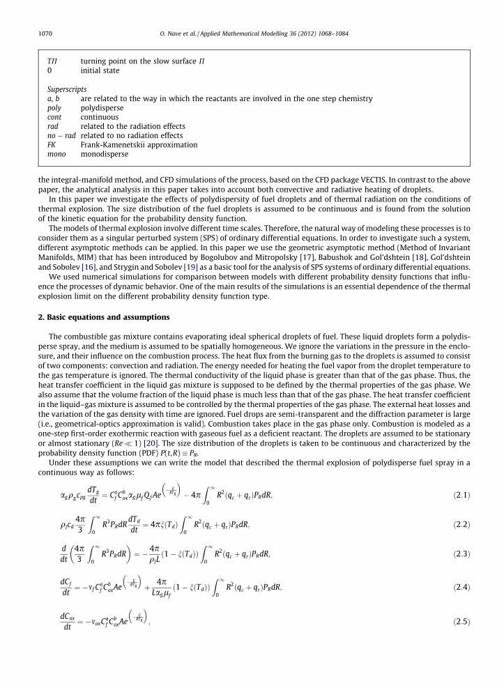
TP turning point on the slow surface P0 initial state

Superscriptsa, b are related to the way in which the reactants are involved in the one step chemistrypoly polydispersecont continuousrad related to the radiation effectsno � rad related to no radiation effectsFK Frank-Kamenetskii approximationmono monodisperse

1070 O. Nave et al. / Applied Mathematical Modelling 36 (2012) 1068–1084

the integral-manifold method, and CFD simulations of the process, based on the CFD package VECTIS. In contrast to the abovepaper, the analytical analysis in this paper takes into account both convective and radiative heating of droplets.

In this paper we investigate the effects of polydispersity of fuel droplets and of thermal radiation on the conditions ofthermal explosion. The size distribution of the fuel droplets is assumed to be continuous and is found from the solutionof the kinetic equation for the probability density function.

The models of thermal explosion involve different time scales. Therefore, the natural way of modeling these processes is toconsider them as a singular perturbed system (SPS) of ordinary differential equations. In order to investigate such a system,different asymptotic methods can be applied. In this paper we use the geometric asymptotic method (Method of InvariantManifolds, MIM) that has been introduced by Bogolubov and Mitropolsky [17], Babushok and Gol’dshtein [18], Gol’dshteinand Sobolev [16], and Strygin and Sobolev [19] as a basic tool for the analysis of SPS systems of ordinary differential equations.

We used numerical simulations for comparison between models with different probability density functions that influ-ence the processes of dynamic behavior. One of the main results of the simulations is an essential dependence of the thermalexplosion limit on the different probability density function type.

2. Basic equations and assumptions

The combustible gas mixture contains evaporating ideal spherical droplets of fuel. These liquid droplets form a polydis-perse spray, and the medium is assumed to be spatially homogeneous. We ignore the variations in the pressure in the enclo-sure, and their influence on the combustion process. The heat flux from the burning gas to the droplets is assumed to consistof two components: convection and radiation. The energy needed for heating the fuel vapor from the droplet temperature tothe gas temperature is ignored. The thermal conductivity of the liquid phase is greater than that of the gas phase. Thus, theheat transfer coefficient in the liquid gas mixture is supposed to be defined by the thermal properties of the gas phase. Wealso assume that the volume fraction of the liquid phase is much less than that of the gas phase. The heat transfer coefficientin the liquid–gas mixture is assumed to be controlled by the thermal properties of the gas phase. The external heat losses andthe variation of the gas density with time are ignored. Fuel drops are semi-transparent and the diffraction parameter is large(i.e., geometrical-optics approximation is valid). Combustion takes place in the gas phase only. Combustion is modeled as aone-step first-order exothermic reaction with gaseous fuel as a deficient reactant. The droplets are assumed to be stationaryor almost stationary (Re� 1) [20]. The size distribution of the droplets is taken to be continuous and characterized by theprobability density function (PDF) P(t,R) � PR.

Under these assumptions we can write the model that described the thermal explosion of polydisperse fuel spray in acontinuous way as follows:

agqgcpgdTg

dt¼ Ca

f Cboxaglf Q f Ae

� EBTg

� �� 4p

Z 1

0R2ðqc þ qrÞPRdR; ð2:1Þ

qlcd4p3

Z 1

0R3PRdR

dTd

dt¼ 4pnðTdÞ

Z 1


ddt

4p3

Z 1

0R3PRdR

� �¼ � 4p

qlLð1� nðTdÞÞ

Z 1


dCf

dt¼ �mf C

af Cb

oxAe� E

BTg

� �þ 4p

Laglfð1� nðTdÞÞ

Z 1


dCox

dt¼ �moxCa

f CboxAe

� EBTg

� �; ð2:5Þ


where the parameter n(Td) takes into account the fraction of heat that is spent on the droplet heating. Following the authorsof [21] n(�) has the form of:

nðTdÞ ¼Tb � Td

Tb � Td0; ð2:6Þ

where Tb, Td, and Td0 are the boiling, current and initial temperature of droplets, respectively.The evolution of the size distribution of droplets due to the evaporation process is described by the kinetic equation for

the PDF [3],

@PR

@t¼ @

@Rjm

qlPR

� �: ð2:7Þ

The approximation of this equation as suggested in [22] is:

@PR

@t¼ @

@RJm

qlPR

� �; ð2:8Þ

where:

Jm ¼R1

0 R2jmPRdRR10 R2PRdR

: ð2:9Þ

Eq. (2.8) coincides with Eq. (2.7) in the case when the rate of evaporation does not depend on the droplet radius, and thedroplets are treated as a monodisperse system. However, the averaging of jm is performed in such a manner that Eq. (2.8)would yield the same balance equation for the mass of the liquid equation i.e., Eq. (2.3) as that yielded by Eq. (2.7). Theintegro-differential Eq. (2.8) with (2.9) has a self-similar solution that satisfies the initial distribution PR(0,R) = PR0(R),

PR ¼ PR0ðRþ dÞ; d ¼Z t

0

Jm

qldt; ð2:10Þ

and d is found from the solution of the equation:

dddt¼ Jm

ql; dð0Þ ¼ 0: ð2:11Þ

The complete system is as follows:

agqgcpgdTg

dt¼ Ca

f Cboxaglf Q f Ae

� EBTg

� �� 4p

Z 1


qlcd4p3

Z 1

0R3PRdR

dTd

dt¼ 4pnðTdÞ

Z 1


dCf

dt¼ �mf Ca

f CboxAe

� EBTg

� �þ 4p

Laglfð1� nðTdÞÞ

Z 1


dCox

dt¼ �moxCa

f CboxAe

� EBTg

� �; ð2:15Þ

dddt¼ 1

qlL

R10 R2ðqc þ qrÞPRdRR1

0 R2PRdR; ð2:16Þ

the system of the above governing equations is closed with the initial conditions of the form:

t ¼ 0 : Tg ¼ Tg0; Td ¼ Td0; Cf ¼ Cf 0; Cox ¼ Cox0; d ¼ 0: ð2:17Þ

The assumption that the pressure variations are negligible implies that the equation of state for the gaseous medium can besimplified to the form of: qgTg = qg0Tg0 = constant and kg ¼ kg0 Tg=Tg0

� �12, where kg0 is the thermal conductivity at Tg = Tg0.

The assumptions that Re� 1 and Nu = 2 [23] enable us to simplify the expression for qc as:

qc ¼ kgTg � Td

R: ð2:18Þ

The expression for qr can be written as qr ¼ rQai T4ext � T4

d

� �[21], where Qai is the average efficiency factor of absorption. In

the case of optically thick gas one can assume that Text = Tg. Otherwise, Text can be considered as constant, and the whole anal-ysis would be simplified. The value of Qai depends on the physical model that is chosen. This expression can be generalized


according to [15,24,25] by taking the term Qai as Q ai ¼ aRbd, where a and b are quadratic functions of the external gas tem-

perature. Hence, using these authors notations the term of the thermal radiation has the form of:

qr ¼ k1rT4ext; ð2:19Þ

where

k1 ¼ aRbd;

a ¼ a0 þ a1Text

103

� �þ a2

Text

103

� �2

;

b ¼ b0 þ b1Text

103

� �þ b2

Text

103

� �2

:

ð2:20Þ

For diesel engines the coefficients ai and bi,i = 0, 1, 2 can be taken as follows: a0 = 0.104 (m� b), a1 = �0.05432 (m�b K�1),a2 = 0.008 (m�b K�2), b0 = 0.49162 (m�b), b1 = 0.098369 (K�1), b2 = �0.007857 (K�2), Text = 2500 (K).

In our numerical simulation we used the approximation of the heat flux according to [26] as:

qr ¼ rRbd 103k10 � k11Tg

� �T4

g � T4d

� �; ð2:21Þ

where r is the Stefan–Boltzmann constant. If (lm) units are used then k10 = 7 � 10�5, k11 = 2 � 10�5 (K�1), and if (m) unitsare used then k10 = 0.28, k11 = 0.08 (K�1). b is a quadratic function of the external gas temperature.

In order to simplify the analysis, the entire heat flux that is delivered to the droplet surface is fully spent for evaporationi.e.,

qc þ qr ¼ Ljm: ð2:22Þ

2.1. Dimensionless model

Eqs. (2.1)–(2.5) can be rewritten in dimensionless form as:

cdhg

ds¼ gafbe

hg1þbhg

� �� 1ðhg � hdÞ

ffiffiffiffiffiffiffiffiffiffiffiffiffiffiffiffi1þ bhg

q Z 1

0rePr0ðr þ � Þdr � �1�4

4bðm� ð1þ bhgÞÞ

� ð1þ bhgÞ4 � ð1þ bhdÞ4� �Z 1

0rbþ2ePr0ðr þ � Þdr; ð2:23Þ

dhd

ds¼ �1�3�5�6nðhdÞ�7R1

0 r3ePr0ðr þ � Þdrhg � hd� � ffiffiffiffiffiffiffiffiffiffiffiffiffiffiffiffi

1þ bhg

q Z 1

0rePr0ðr þ � Þdr þ �1�3�4�5�6nðhdÞ

4�7bR1

0 r3ePr0ðr þ � Þdrm� ð1þ bhgÞ� �

� 1þ bhg� �4 � 1þ bhdð Þ4� �Z 1


dgds¼ � 1

~mfgafbe

hg1þbhg

� �þW�1ðhg � hdÞ


qð1� nðhdÞÞ

Z 1

0rePr0ðr þ � Þdr þW�1�4

4b1� nðhdÞð Þ m� ð1þ bhgÞ

� �� ð1þ bhgÞ4 � 1þ bhdð Þ4� �Z 1

0rbþ2ePr0 r þ �ð Þdr; ð2:25Þ

dfds¼ � 1

~moxgafbe

hg1þbhg

� �; ð2:26Þ

d�ds¼�1�2ðhg � hdÞ


p3R1

0 r2ePr0ðr þ � Þdrð1� nðhdÞÞ

Z 1

0rePr0ðr þ � Þdr þ �1�2�4

12bR1

0 r2ePr0ðr þ � Þdrð1� nðhdÞÞðm� ð1þ bhgÞÞ

� ð1þ bhgÞ4 � ð1þ bhdÞ4� �Z 1

0rbþ2ePr0ðr þ � Þdr: ð2:27Þ

The parameter n(hd) is a modified form of the parameter (2.6), and it is given by:

nðhdÞ ¼hb � hd

hb � hd0: ð2:28Þ

The following dimensionless parameters have been introduced:


b ¼ BTg0

E; s ¼ t

treact; treact ¼

e1=b

ACa�1

2ff C

b�12

ox

; r ¼ RR0; ePr0 ¼

R0

nd0PR0;

c ¼ bcpgTg0qgffiffiffiffiffiffiffiffiffiffiffiffiffiCff Cox

pQ f lf

; W ¼

ffiffiffiffiffiffiffiffiffiCff

Cox0

sQf

L; R0 ¼

R10 R3PR0dRR1

0 PR0dR; f ¼ Cox

Cox0;

hg ¼1b

Tg � Tg0

Tg0; hd ¼

1b

Td � Tg0

Tg0; ~mf ¼

1mf

ffiffiffiffiffiffiffiffiffiCff

Cox0

s; ~mox ¼

1mox

ffiffiffiffiffiffiffiffiffiCox0

Cff

s;

g ¼ Cf

Cff; m ¼ k10103

k11Tg0; Cff ¼

4p3

ql

lf

Z 1

0R3PR0dRþ Cf 0;

�1 ¼4pkg0R0bTg0nd0

Caff Cb

ox0AQ f Cf 0aglf

e1bð Þ; �2

ffiffiffiffiffiffiffiffiffiffiffiffiffiffiCff Cox0

pQ f lf ag

4p3 R3

0nd0qlL;

�3 ¼ 3kg0expð1=bÞ

AcdqlR20

; �4 ¼4rk11T4

g0Rbþ10

kg0; �5 ¼

Acdql

R0nd0kg0;

�6 ¼ffiffiffiffiffiffiffiffiffiffiffiffiffiffiCff Cox0

pQ f lf ag

e1=bqlL; �7 ¼

4pcdTg0bL

; � ¼ dR0:

ð2:29Þ

The non-dimensional initial conditions are:

ats ¼ 0 : hg ¼ 0; hd ¼ hd0; g ¼ g0; f ¼ f0; � ¼ 0: ð2:30Þ

3. Analysis of the system

3.1. Reduction the model (energy integral procedure), Frank-Kamenetskii approximation

3.1.1. Energy integral of the systemAn appropriate combination of the system (2.23)–(2.27) enable of reduction the model by the procedure of the energy

integral as follows: sum Eqs. (2.23) with (2.25) and divided by the sum of Eq. (2.24)

cdhg þ ~mf dgdhd

¼W~mf 1� nðhdÞð Þ � 1

�7R1

0 r3ePr0ðr þ � Þdr�3�5�6nðhdÞ

: ð3:1Þ

By integrating the above equation with respect to the initial conditions (2.30) we derived an explicit expression for the fuelconcentration g as a function of the droplet and gas temperature in the form of:

gðhg ; hd; � Þ ¼ �chg þ ~mf g0 þ�7

�3�5�6

Z hd

hd0

W~mf ð1� nðsÞÞ � 1 R1

0 r3ePr0ðr þ � ÞdrnðsÞ ds: ð3:2Þ

The same procedure can be applied to the Eqs. (2.23), (2.26) and (2.24) to get an explicit equation to the oxygen f as a func-tion of hg and hd:

f hg ; hd; ��

¼ �chg þ ~moxf0 ��7

�3�5�6

Z hd

hd0

R10 r3ePr0ðr þ � Þdr

nðsÞ ds: ð3:3Þ

This procedure enable us to reduce the system (2.23)–(2.27) from six equations to four equations only.

3.1.2. Frank-Kamenetskii approximationBy applying the Frank-Kamenetskii approximation [27] i.e., bhg� 1 we derived the following model:

cdhg

ds¼ gðhg ; hdÞaf hg ; hd

� �behg � �1ðhg � hdÞZ 1

0rePr0ðr þ � Þdr � �1�4ðm� 1Þ hg � hd

� � Z 1


dhd

ds¼ �1�3�5�6n hdð Þ�7R1

0 r3ePr0ðr þ � Þdrðhg � hdÞ

Z 1

0rePr0ðr þ � Þdr þ �1�3�4�5�6nðhdÞ

�7R1

0 r3ePr0ðr þ � Þdrðm� 1Þ hg � hd

� � Z 1

0rbþ2ePr0ðr þ � Þdr;

ð3:5Þ

d�ds¼ �1�2ðhg � hdÞ

3R1

0 r2ePr0ðr þ � Þdrð1� nðhdÞÞ

Z 1

0rePr0ðr þ � Þdr þ �1�2�4

3R1

0 r2ePr0ðr þ � Þdrð1� nðhdÞÞðm� 1Þðhg � hdÞ

�Z 1

0rbþ2ePr0ðr þ � Þdr: ð3:6Þ


3.2. Application of the method of integral manifolds: Analytical expression of the thermal explosion limit

The analysis of Eqs. (3.4)–(3.6), is based on the geometrical version of the method of integral manifold. Following the geo-metrical version of the integral manifolds method, an arbitrary trajectory may be subdivided into fast and slow parts. Thefast part is characterized by a constant value of the slow variables. The slow part is quasi stationary for the fast variableand it is located on the integral manifold. The exact location of the integral manifold of the system is unknown. The generaltheory of the integral manifolds states that the zeroth-order approximation of the manifold lies within the c-neighbourhoodof the exact manifold position. The zeroth-order approximation of the manifold c = 0 is called the slow surface. Hence in ourcase, the slow surface PFK of the system (3.4)–(3.6) is given by the equation:

PFK hg ; hd; ��

¼ gðhg ; hdÞafðhg ; hdÞbehg � �1 hg � hd

� � Z 1

0rePr0ðr þ � Þdr � �1�4ðm� 1Þ hg � hd

� � Z 1

0rbþ2ePr0ðr þ � Þdr ¼ 0:

ð3:7Þ

The shape and the position of the slow surface PFK(hg,hd,�) depends on the combination of the values of the followingparameters: �1; �2; �3; �4; �5; �6; �7; ~mf ; ~mox; c;W; and on the initial conditions: g0, f0, hd0, and �(0).

According to the methods of the integral manifold, the so-called turning points � TPFK on the slow surface are defined asthe points where the slow surface has the horizontal tangent PFK(hg,hd,�) = @PFK(hg,hd,�)/@hg:

@PFK hg ; hd; �� @hg

¼ g hg ; hd

� �af hg ; hd

� �behg � �1

Z 1

0rePr0ðr þ � Þdr � �1�4ðm� 1Þ

Z 1

0rbþ2ePr0ðr þ � Þdr ¼ 0: ð3:8Þ

The turning points divide the slow surface into stable parts and unstable parts. The stable parts attract the trajectories of thesystem and the unstable one repel them. From the solution of (3.7) and (3.8) it is follows that the slow surface PFK has thesingle turning point where hg = 1 + hd. The value of the hd on the stable part of the slow surface is hd0. The critical condition ofthe thermal explosion, which corresponds to the ignition of combustible medium at the initial moment of time is determinedfrom the equation of the slow surface at hd0 and �(0) = 0. Hence, substituting this value of hg in (3.7) and hd0 in Eqs. (3.2) and(3.3) gives the condition for thermal explosion limit in the form of:

�1 ¼~mf g0

� �a ~moxf0ð Þbe1þhd0R10 rePr0ðrÞdr þ �4ðm� 1Þ

R10 rbþ2ePr0ðrÞdr

; ð3:9Þ

which means that a thermal explosion occurs if the following condition is valid:

4pkg0R0bTg0nd0

Caff Cb

ox0AQf Cf 0aglf

eE

BTg0

� �<

~mf g0

� �a ~moxf0ð Þbe1þhd0R10 rePr0ðrÞdr þ �4ðm� 1Þ

R10 rbþ2ePr0ðrÞ

:

ð3:10Þ

In the opposite case a complicated behavior of the system can be expected and it refers to the so-called the delay time [28].

3.3. The delay time of the system

The delay time according to [28] is the period when the trajectory moves along the slow surface/curve until the fastexplosion state is reached, i.e., as the period between the intersection point of the trajectory on the slow surface/curve untilthe turning point. In order to get an explicit expression for the delay time we rewrite Eq. (3.6)

d�ds¼ �2ð1� nðhdÞÞ

3R1

0 r2ePr0ðr þ � Þdrf�1ðhg � hdÞ

Z 1

0rePr0ðr þ � Þdr þ �1�4ðm� 1Þðhg � hdÞ

Z 1

0rbþ2ePr0ðr þ � Þdrg: ð3:11Þ

The expression in the brackets in the right-hand-side of Eq. (3.11) can be written in an alternative form recalling the equationfor the slow surface:

Table 1Comparison the delay time between the following continuous models: the Normal PDF, Exponentialdistribution and Nukiyama-Tanasawa distribution.

Model scon-raddelay scon-no-rad

delay

1. Exponential 0.00774159 0.010877892. Normal 0.00665379 0.009502193. Nukiyama–Tanasawa 0.00606774 0.00711404

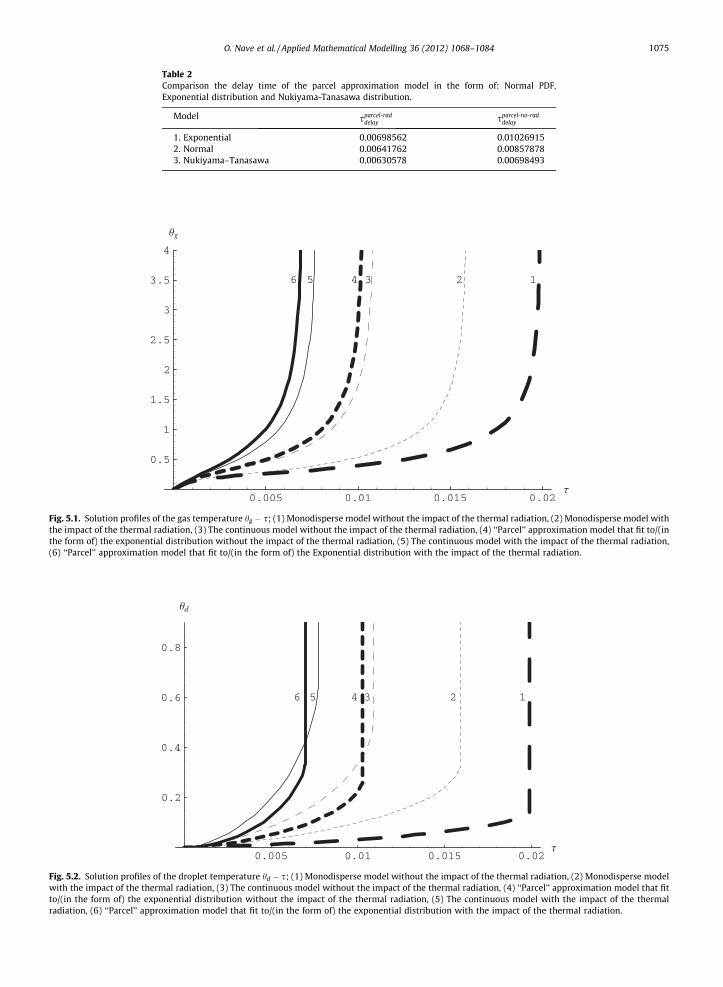
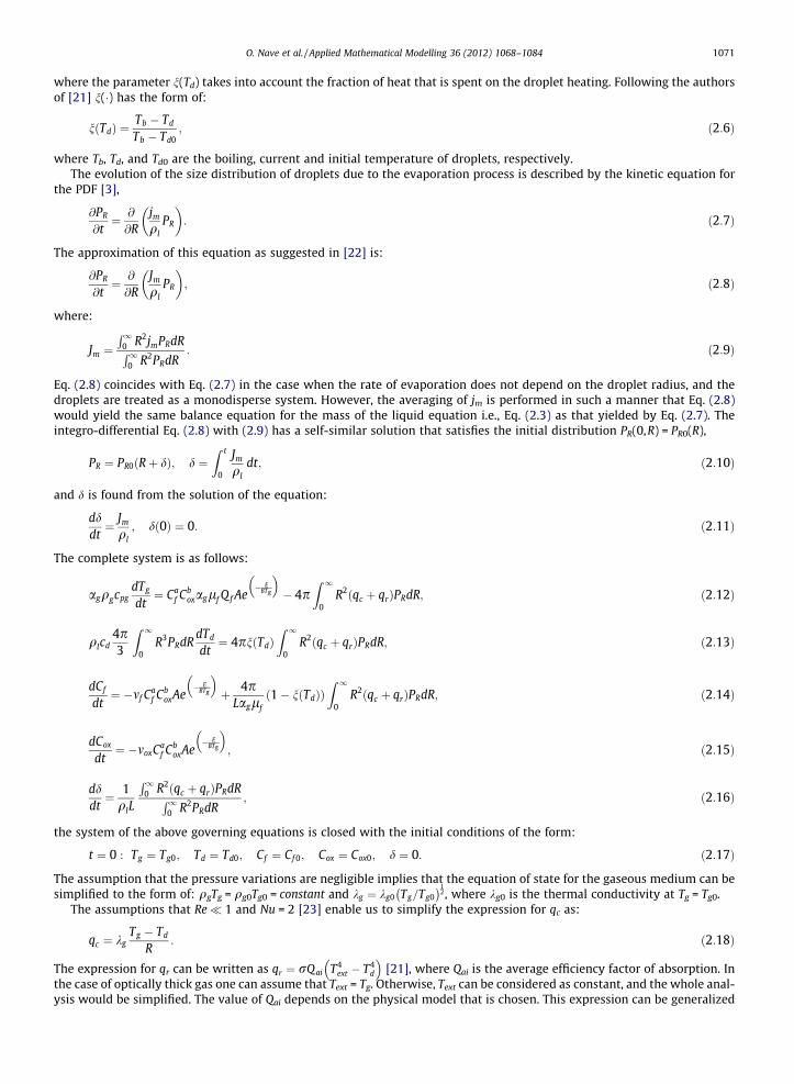
Table 2Comparison the delay time of the parcel approximation model in the form of: Normal PDF,Exponential distribution and Nukiyama-Tanasawa distribution.

Model sparcel-raddelay sparcel-no-rad

delay

1. Exponential 0.00698562 0.010269152. Normal 0.00641762 0.008578783. Nukiyama–Tanasawa 0.00630578 0.00698493

Fig. 5.1. Solution profiles of the gas temperature hg � s; (1) Monodisperse model without the impact of the thermal radiation, (2) Monodisperse model withthe impact of the thermal radiation, (3) The continuous model without the impact of the thermal radiation, (4) ‘‘Parcel’’ approximation model that fit to/(inthe form of) the exponential distribution without the impact of the thermal radiation, (5) The continuous model with the impact of the thermal radiation,(6) ‘‘Parcel’’ approximation model that fit to/(in the form of) the Exponential distribution with the impact of the thermal radiation.

Fig. 5.2. Solution profiles of the droplet temperature hd � s; (1) Monodisperse model without the impact of the thermal radiation, (2) Monodisperse modelwith the impact of the thermal radiation, (3) The continuous model without the impact of the thermal radiation, (4) ‘‘Parcel’’ approximation model that fitto/(in the form of) the exponential distribution without the impact of the thermal radiation, (5) The continuous model with the impact of the thermalradiation, (6) ‘‘Parcel’’ approximation model that fit to/(in the form of) the exponential distribution with the impact of the thermal radiation.


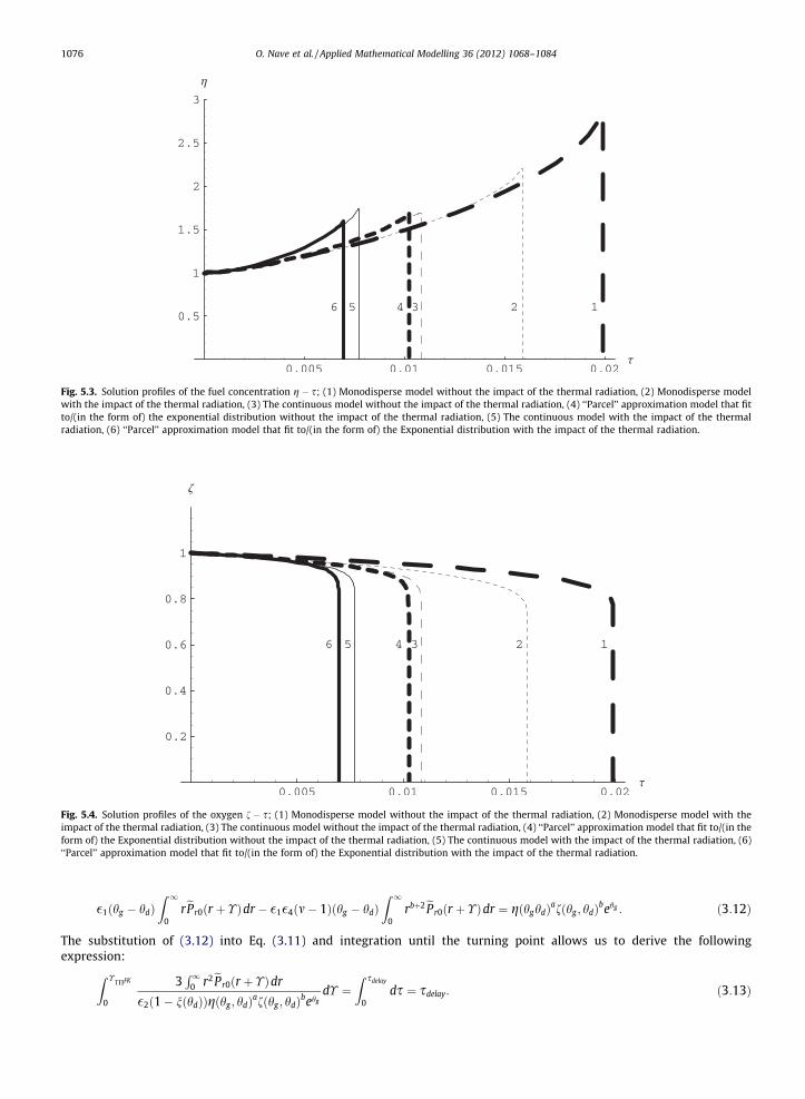
Fig. 5.3. Solution profiles of the fuel concentration g � s; (1) Monodisperse model without the impact of the thermal radiation, (2) Monodisperse modelwith the impact of the thermal radiation, (3) The continuous model without the impact of the thermal radiation, (4) ‘‘Parcel’’ approximation model that fitto/(in the form of) the exponential distribution without the impact of the thermal radiation, (5) The continuous model with the impact of the thermalradiation, (6) ‘‘Parcel’’ approximation model that fit to/(in the form of) the Exponential distribution with the impact of the thermal radiation.

Fig. 5.4. Solution profiles of the oxygen f � s; (1) Monodisperse model without the impact of the thermal radiation, (2) Monodisperse model with theimpact of the thermal radiation, (3) The continuous model without the impact of the thermal radiation, (4) ‘‘Parcel’’ approximation model that fit to/(in theform of) the Exponential distribution without the impact of the thermal radiation, (5) The continuous model with the impact of the thermal radiation, (6)‘‘Parcel’’ approximation model that fit to/(in the form of) the Exponential distribution with the impact of the thermal radiation.


�1ðhg � hdÞZ 1

0rePr0ðr þ � Þdr � �1�4ðm� 1Þðhg � hdÞ

Z 1

0rbþ2ePr0ðr þ � Þdr ¼ gðhghdÞafðhg ; hdÞbehg : ð3:12Þ

The substitution of (3.12) into Eq. (3.11) and integration until the turning point allows us to derive the followingexpression:
Z �
TPFK

0

3R1

0 r2ePr0ðr þ � Þdr

�2ð1� nðhdÞÞgðhg ; hdÞafðhg ; hdÞbehgd� ¼

Z sdelay

0ds ¼ sdelay: ð3:13Þ

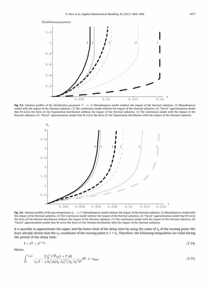
Fig. 5.5. Solution profiles of the distribution parameter � � s; (1) Monodisperse model without the impact of the thermal radiation, (2) Monodispersemodel with the impact of the thermal radiation, (3) The continuous model without the impact of the thermal radiation, (4) ‘‘Parcel’’ approximation modelthat fit to/(in the form of) the Exponential distribution without the impact of the thermal radiation. (5) The continuous model with the impact of thethermal radiation, (6) ‘‘Parcel’’ approximation model that fit to/(in the form of) the Exponential distribution with the impact of the thermal radiation.

Fig. 5.6. Solution profiles of the gas temperature hg � s; (1) Monodisperse model without the impact of the thermal radiation, (2) Monodisperse model withthe impact of the thermal radiation, (3) The continuous model without the impact of the thermal radiation, (4) ‘‘Parcel’’ approximation model that fit to/(inthe form of) the Normal distribution without the impact of the thermal radiation, (5) The continuous model with the impact of the thermal radiation, (6)‘‘Parcel’’ approximation model that fit to/(in the form of) the Normal distribution with the impact of the thermal radiation.


It is possible to approximate the upper and the lower limit of the delay time by using the value of hg of the turning point. Wehave already shown that the hg-coordinate of the turning point is 1 + hd. Therefore, the following inequalities are valid duringthe period of the delay time:

1 < ehg < e1þhd0 : ð3:14Þ

Hence,
Z �TPFK
0

3R1


�2 1� nðhdÞð Þg hg ; hd� �a

fðhg ; hdÞbe0d� P sdelay; ð3:15Þ

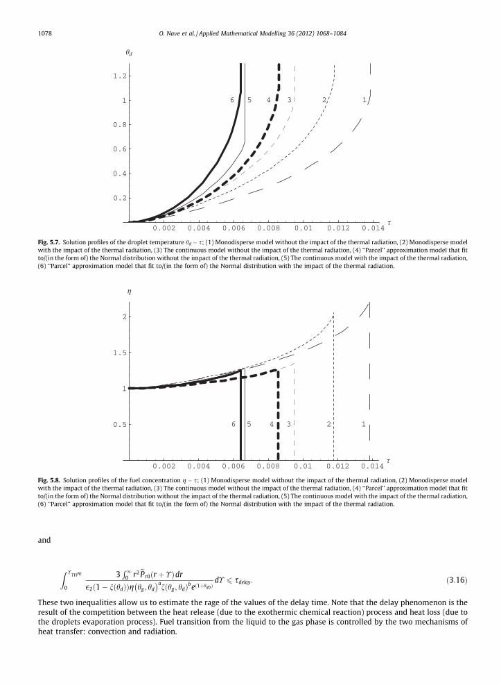
Fig. 5.7. Solution profiles of the droplet temperature hd � s; (1) Monodisperse model without the impact of the thermal radiation, (2) Monodisperse modelwith the impact of the thermal radiation, (3) The continuous model without the impact of the thermal radiation, (4) ‘‘Parcel’’ approximation model that fitto/(in the form of) the Normal distribution without the impact of the thermal radiation, (5) The continuous model with the impact of the thermal radiation,(6) ‘‘Parcel’’ approximation model that fit to/(in the form of) the Normal distribution with the impact of the thermal radiation.

Fig. 5.8. Solution profiles of the fuel concentration g � s; (1) Monodisperse model without the impact of the thermal radiation, (2) Monodisperse modelwith the impact of the thermal radiation, (3) The continuous model without the impact of the thermal radiation, (4) ‘‘Parcel’’ approximation model that fitto/(in the form of) the Normal distribution without the impact of the thermal radiation, (5) The continuous model with the impact of the thermal radiation,(6) ‘‘Parcel’’ approximation model that fit to/(in the form of) the Normal distribution with the impact of the thermal radiation.


and

Z �TPFK

0

3R1


�2ð1� nðhdÞÞg hg ; hd� �a

fðhg ; hdÞbeð1þhd0Þd� 6 sdelay: ð3:16Þ

These two inequalities allow us to estimate the rage of the values of the delay time. Note that the delay phenomenon is theresult of the competition between the heat release (due to the exothermic chemical reaction) process and heat loss (due tothe droplets evaporation process). Fuel transition from the liquid to the gas phase is controlled by the two mechanisms ofheat transfer: convection and radiation.

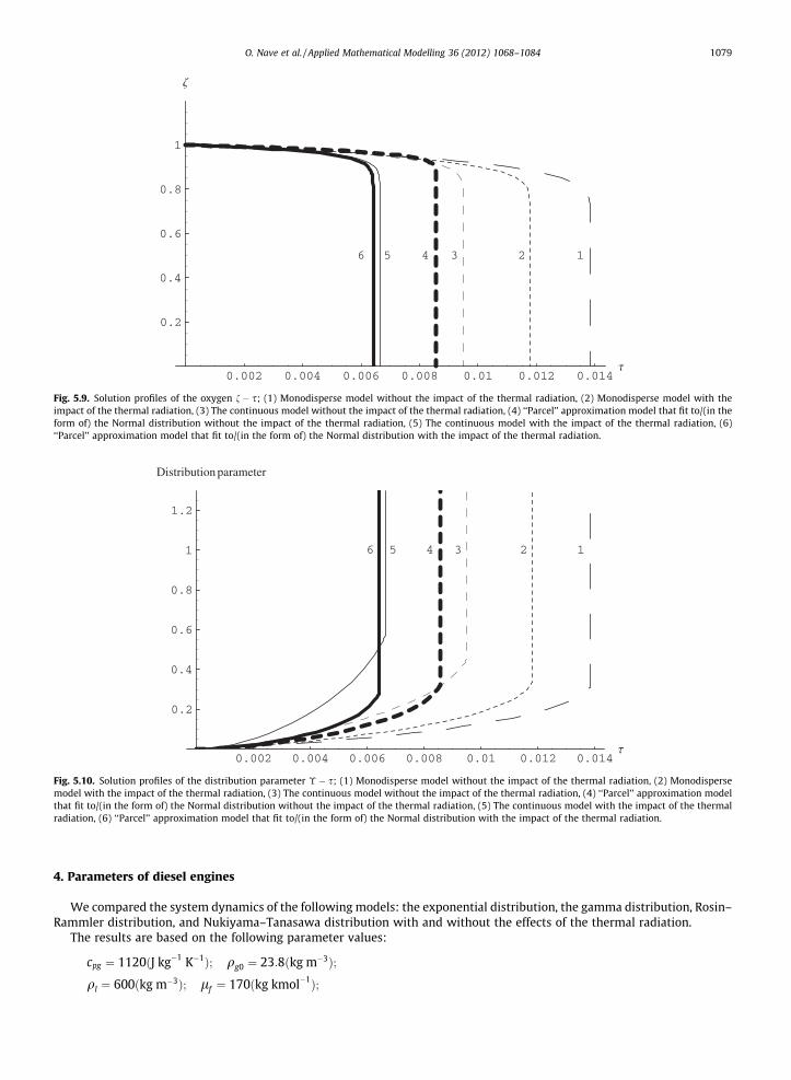
Fig. 5.9. Solution profiles of the oxygen f � s; (1) Monodisperse model without the impact of the thermal radiation, (2) Monodisperse model with theimpact of the thermal radiation, (3) The continuous model without the impact of the thermal radiation, (4) ‘‘Parcel’’ approximation model that fit to/(in theform of) the Normal distribution without the impact of the thermal radiation, (5) The continuous model with the impact of the thermal radiation, (6)‘‘Parcel’’ approximation model that fit to/(in the form of) the Normal distribution with the impact of the thermal radiation.

Fig. 5.10. Solution profiles of the distribution parameter � � s; (1) Monodisperse model without the impact of the thermal radiation, (2) Monodispersemodel with the impact of the thermal radiation, (3) The continuous model without the impact of the thermal radiation, (4) ‘‘Parcel’’ approximation modelthat fit to/(in the form of) the Normal distribution without the impact of the thermal radiation, (5) The continuous model with the impact of the thermalradiation, (6) ‘‘Parcel’’ approximation model that fit to/(in the form of) the Normal distribution with the impact of the thermal radiation.


4. Parameters of diesel engines

We compared the system dynamics of the following models: the exponential distribution, the gamma distribution, Rosin–Rammler distribution, and Nukiyama–Tanasawa distribution with and without the effects of the thermal radiation.

The results are based on the following parameter values:

cpg ¼ 1120ðJ kg�1 K�1Þ; qg0 ¼ 23:8ðkg m�3Þ;

ql ¼ 600ðkg m�3Þ; lf ¼ 170ðkg kmol�1Þ;

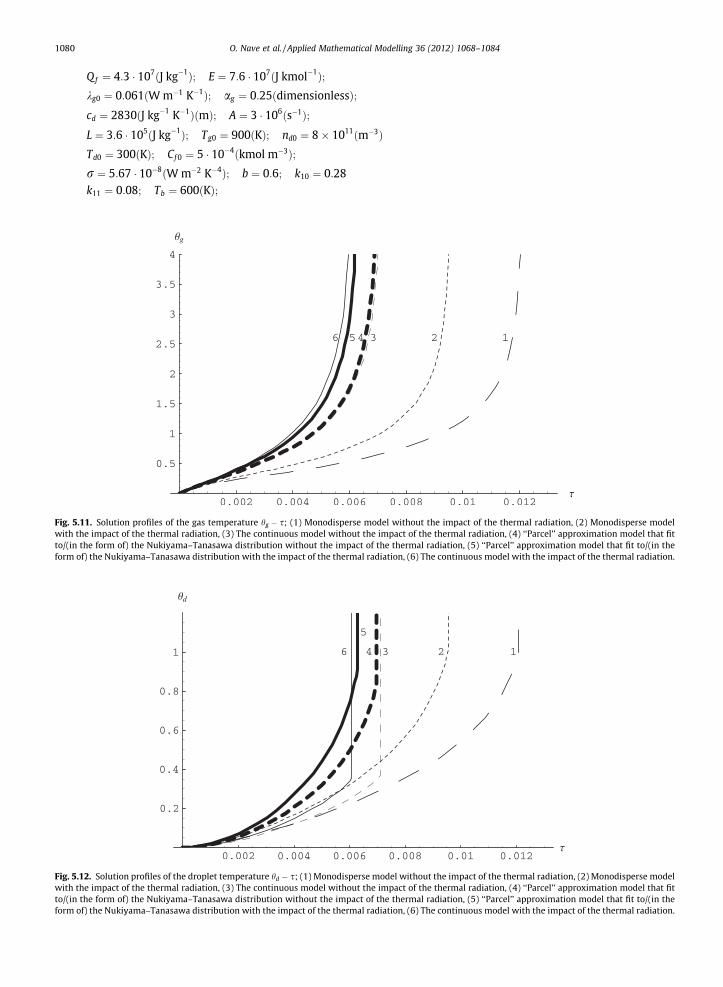
Fig. 5.1with thto/(in tform of



Qf ¼ 4:3 � 107ðJ kg�1Þ; E ¼ 7:6 � 107ðJ kmol�1Þ;kg0 ¼ 0:061ðW m�1 K�1Þ; ag ¼ 0:25ðdimensionlessÞ;cd ¼ 2830ðJ kg�1 K�1ÞðmÞ; A ¼ 3 � 106ðs�1Þ;L ¼ 3:6 � 105ðJ kg�1Þ; Tg0 ¼ 900ðKÞ; nd0 ¼ 8� 1011ðm�3ÞTd0 ¼ 300ðKÞ; Cf 0 ¼ 5 � 10�4ðkmol m�3Þ;r ¼ 5:67 � 10�8ðW m�2 K�4Þ; b ¼ 0:6; k10 ¼ 0:28k11 ¼ 0:08; Tb ¼ 600ðKÞ;

1. Solution profiles of the gas temperature hg � s; (1) Monodisperse model without the impact of the thermal radiation, (2) Monodisperse modele impact of the thermal radiation, (3) The continuous model without the impact of the thermal radiation, (4) ‘‘Parcel’’ approximation model that fithe form of) the Nukiyama–Tanasawa distribution without the impact of the thermal radiation, (5) ‘‘Parcel’’ approximation model that fit to/(in the) the Nukiyama–Tanasawa distribution with the impact of the thermal radiation, (6) The continuous model with the impact of the thermal radiation.

2. Solution profiles of the droplet temperature hd � s; (1) Monodisperse model without the impact of the thermal radiation, (2) Monodisperse modele impact of the thermal radiation, (3) The continuous model without the impact of the thermal radiation, (4) ‘‘Parcel’’ approximation model that fithe form of) the Nukiyama–Tanasawa distribution without the impact of the thermal radiation, (5) ‘‘Parcel’’ approximation model that fit to/(in the) the Nukiyama–Tanasawa distribution with the impact of the thermal radiation, (6) The continuous model with the impact of the thermal radiation.


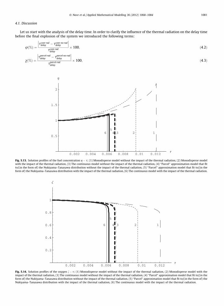
4.1. Discussion

Let us start with the analysis of the delay time. In order to clarify the influence of the thermal radiation on the delay timebefore the final explosion of the system we introduced the following terms:


Fig. 5.1impactform ofNukiya

uð%Þ ¼scont-rad

delay � scont-no-raddelay

�� scont-rad

delay

� 100; ð4:2Þ

vð%Þ ¼sparcel-rad

delay � sparcel-no-raddelay

�� sparcel-rad

delay

� 100; ð4:3Þ

3. Solution profiles of the fuel concentration g � s; (1) Monodisperse model without the impact of the thermal radiation, (2) Monodisperse modele impact of the thermal radiation, (3) The continuous model without the impact of the thermal radiation, (4) ‘‘Parcel’’ approximation model that fithe form of) the Nukiyama–Tanasawa distribution without the impact of the thermal radiation, (5) ‘‘Parcel’’ approximation model that fit to/(in the) the Nukiyama–Tanasawa distribution with the impact of the thermal radiation, (6) The continuous model with the impact of the thermal radiation.

4. Solution profiles of the oxygen f � s; (1) Monodisperse model without the impact of the thermal radiation, (2) Monodisperse model with theof the thermal radiation, (3) The continuous model without the impact of the thermal radiation, (4) ‘‘Parcel’’ approximation model that fit to/(in the) the Nukiyama–Tanasawa distribution without the impact of the thermal radiation, (5) ‘‘Parcel’’ approximation model that fit to/(in the form of) thema–Tanasawa distribution with the impact of the thermal radiation, (6) The continuous model with the impact of the thermal radiation.

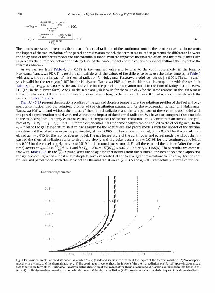
Fig. 5.1modelthat fitform of


-ð%Þ ¼sparcel-rad

delay � scont-raddelay

�� scont�rad

delay

� 100; ð4:4Þ

xð%Þ ¼sparcel-no-rad

delay � scont-no-raddelay

�� scont-no-rad

delay

� 100: ð4:5Þ

The term u measured in percents the impact of thermal radiation of the continuous model, the term v measured in percentsthe impact of thermal radiation of the parcel approximation model, the term - measured in percents the difference betweenthe delay time of the parcel model and the continuous model with the impact of thermal radiation, and the term x measuredin percents the difference between the delay time of the parcel model and the continuous model without the impact of thethermal radiation.

As we can see from Table 4, u � 0.172 is the smallest value and belongs to the continuous model in the form ofNukiyama–Tanasawa PDF. This result is compatible with the values of the difference between the delay time as in Table 1with and without the impact of the thermal radiation for Nukiyama–Tanasawa model, i.e., jDsdelayj � 0.001. The same anal-ysis is valid for the term v � 0.107 for the Nukiyama–Tanasawa PDF and again this result is compatible with the result inTable 2, i.e., jDsdelayj � 0.0006 is the smallest value for the parcel approximation model in the form of Nukiyama–TanasawaPDF (i.e., in the discrete form). And also the same analysis is valid for the value of x for the same reasons. In the last term -the results become different and the smallest value of - belong to the normal PDF - � 0.03 which is compatible with theresults in Tables 1 and 2.

Figs. 5.1–5.15 present the solutions profiles of the gas and droplets temperature, the solutions profiles of the fuel and oxy-gen concentration, and the solutions profiles of the distribution parameters for the exponential, normal and Nukiyama–Tanasawa PDF with and without the impact of the thermal radiations and the comparisons of these continuous model withthe parcel approximation model with and without the impact of the thermal radiation. We have also compared these modelsto the monodisperse fuel spray with and without the impact of the thermal radiation. Let us concentrate on the solution pro-files of hg � s, hd � s, g � s, f � s, � � s for the exponential PDF (the same analysis can be applied to the other figures). In thehg � s plane the gas temperature start to rise sharply for the continuous and parcel models with the impact of the thermalradiation and the delay time occurs approximately at s � 0.0065 for the continuous model, at s � 0.0071 for the parcel mod-el, and at s � 0.015 for the monodisperse model. The gas temperature of the continuous and parcel models without the im-pact of the thermal radiation starts to rise more slowly and the delay occurs at s � 0.0108 for the continuous model, ats � 0.095 for the parcel model, and at s � 0.019 for the monodisperse model. For all these model the ignition (after the delaytime) occurs at hg � 3 i.e., EðTg�Tg0Þ

BT2go� 3 and for Tg0 = 900, b = E/(BTg0) � 9.87 � 10�2 at Tg � 1165(K). These results are compat-

ible with Tables 1–3. In the hd � s plane, after the delay time that derives from the results of the loss of heat for evaporationthe ignition occurs, when almost all the droplets have evaporated, at the following approximations values of hd: for the con-tinuous and parcel model with the impact of the thermal radiation at hd � 0.65 and hd � 0.3, respectively. For the continuous

5. Solution profiles of the distribution parameter � � s; (1) Monodisperse model without the impact of the thermal radiation, (2) Monodispersewith the impact of the thermal radiation, (3) The continuous model without the impact of the thermal radiation, (4) ‘‘Parcel’’ approximation modelto/(in the form of) the Nukiyama–Tanasawa distribution without the impact of the thermal radiation, (5) ‘‘Parcel’’ approximation that fit to/(in the) the Nukiyama–Tanasawa distribution with the impact of the thermal radiation, (6) The continuous model with the impact of the thermal radiation.

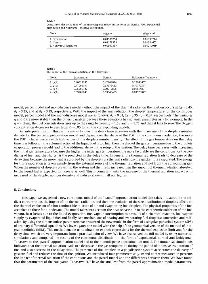
Table 3Comparison the delay time of the monodisperse model in the form of: Normal PDF, Exponentialdistribution and Nukiyama-Tanasawa distribution.

Model sMono-raddelay sMono-no-rad

delay

1. Exponential 0.01589754 0.019907142. Normal 0.01178373 0.013846523. Nukiyama-Tanasawa 0.00957367 0.01210089

Table 4The impact of the thermal radiation on the delay time.

Model Exponential Normal Nukiyama–Tanasawa

1. u(%) 0.40512345 0.42808684 0.172436522. v(%) 0.47004131 0.33675412 0.107702773. x(%) 0.05596122 0.09717865 0.018148614. -(%) 0.09765048 0.03549405 0.03923042


model, parcel model and monodisperse model without the impact of the thermal radiation the ignition occurs at hd � 0.45,hd � 0.25, and at hd � 0.19, respectively. With the impact of thermal radiation, the droplet temperature for the continuousmodel, parcel model and the monodisperse model are as follows: hd � 0.61, hd � 0.35, hd � 0.37, respectively. The variablesg and f are more stable then the others variables because these equations has no small parameter as c for example. In theg � s plane, the fuel concentration rises up to the range between g � 1.53 and g � 1.75 and then it falls to zero. The Oxygenconcentration decreases to zero from f � 0.85 for all the corresponding models.

Our interpretations for this results are as follows: the delay time increases with the increasing of the droplets numberdensity for the parcel approximation model and depends on the shape of the PDF in the continuous model, i.e., the morethe PDF includes parcels with high values of the droplets number density. The effect of the gas temperature on the delaytime is as follows: if the volume fraction of the liquid fuel is too high then the drop of the gas temperature due to the dropletsevaporation process would lead to the additional delay in the setup of the ignition. The delay time decreases with increasingthe initial gas temperature because the higher the initial gas temperature, the more favorable are the conditions for the oxi-dizing of fuel, and the shorter is the predicted in the delay time. In general the thermal radiation leads to decrease of thedelay time because the more heat is absorbed by the droplets via thermal radiation-the quicker it is evaporated. The energyfor this evaporation is taken mainly from the external source of the thermal radiation and not from the surrounding gas.When the number of droplets present in the system and their radii increase, then the amount of thermal radiation absorbedby the liquid fuel is expected to increase as well. This is consistent with the increase of the thermal radiation impact withincreased of the droplet number density and radii as shown in all our figures.

5. Conclusions

In this paper we suggested a new continuous model of the ‘‘parcel’’ approximation model that takes into account the oxi-dizer concentration, the impact of the thermal radiation, and the time evolution of the size distribution of droplets effects onthe thermal explosion of a hot combustible mixture of air and evaporating fuel droplets. The physical properties of the fuelare taken to those for n-dodecane. The model takes into account the heat release due to the exothermic oxidation of the fuelvapour, heat losses due to the liquid evaporation, fuel vapour consumption as a results of a chemical reaction, fuel vapoursupply by evaporated liquid fuel and finally two mechanisms of heating and evaporating fuel droplets: convection and radi-ation. By using the dimensionless parameters we presented the new model in the form of a singular perturbed system (SPS)of ordinary differential equations. We investigated the model with the help of the geometrical version of the method of inte-gral manifolds (MIM). This method enable us to obtain an explicit expressions for the thermal explosion limit and for thedelay time, which are very important from a practical point of view. We have also solved the full model by using numericalsimulations and compared the results of the continuous distribution in the form of exponential, normal and Nukiyama–Tanasawa to the ‘‘parcel’’ approximation model and to the monodisperse approximation model. The numerical simulationsindicated that the thermal radiation leads to a decrease in the gas temperature during the period of intensive evaporation offuel and also decrease in the delay time. The presence of fine droplets in a polydisperse system accelerates the delivery ofgaseous fuel and reduces the time of the ignition. We introduced four parameters u, v, - and x that measured in percentsthe impact of thermal radiation of the continuous and the parcel model and the differences between them. We have foundthat the parameters of the Nukiyama–Tanasawa PDF have the smallest from the parcel approximation model parameters.


References

[1] S.K. Aggrawal, A review of spray ignition phenomena: present status and future research, Prog. Energy Combust. Sci. 24 (1998) 565–600.[2] J. Warnatz, U. Maas, R.W. Dibble, Combustion Physical and Practical Fundamentals, Modeling and Simulation, Experiments, Pollutant Formation,

Springer, 2006.[3] F.A. William, Combustion Theory: The Fundamental Theory of Chemically Reacting Flow System, The Benjamin/Cummings Publishing Company, Menlo

Park, CA, 1985.[4] O. Nave, V.M. Gol’dshtein, B. Vitcheslav, A probabilistic model of thermal explosion in polydisperse fuel spray, Appl. Math. Comp. 217 (2010) 2698–

2709.[5] O. Nave, V.M. Gol’dshtein, The flammable spray effect on thermal explosion of combustible gas-fuel mixture, Combus. Sci. Tech. 183 (2011) 519–539.[6] W.A. Sirignano, Fluid Dynamics and Transport of Droplets and Sprays, CUP, Cambridge, 1999.[7] V. Bykov, I. Goldfarb, V.M. Gol’dshtein, B.J. Greenberg, Auto-ignition of a polydisperse fuel spray, Proc. Combust. Ins. 31 (2007) 2257–2264.[8] A.H. Lefebvre, Atomization and Spray, Hemisphere Corp., New-York, 1989.[9] S.C. Kong, Z. Han, R.D. Rreitz, The Development and Application of a Diesel Ignition and Combustion Model for Multidimensional Engine Simulation,

SAE Technical Paper SAE950278, Society of Automotive Engineers, USA, 1996.[10] H. Barth, C. Hasse, N. Peters, Computational fluid dynamics modeling of non-premixed combustion in direct injection, Ins. J. Engine Res. 1 (2000) 249–

267.[11] E.M. Sazhina, S.S. Sazhin, M.R. Heikal, V.I. Babushok, R. Johns, A details modeling of the spray ignition process in diesel engines, Combust. Sci. Technol.

160 (2000) 317–344.[12] S.M. Correa, M. Sichel, The group combustion of a spherical cloud of monodisperse fuel droplets, in: 19h Symposium (International) on Combustion 19

(1982) 981–991.[13] T. Kristyadi, V. Deprédurand, G. Castanet, F. Lemoine, S.S. Sazhin, A. Elwardany, E.M. Sazhina, M.R. Heikal, Monodisperse monocomponent fuel droplet

heating and evaporation, Fuel, in press.[14] S. Sazhin, Modelling of heating, evaporation and ignition of fuel droplets: combined analytical, asymptotic and numerical analysis, J. Phys. Con. Series

22 (2005) 174–193.[15] S.S. Sazhin, G. Feng, M.R. Heikal, I. Goldfarb, V.M. Gol’dshtein, G. Kuzmenko, Thermal ignition analysis of a monodisperse spray with radiation,

Combust. Flame. 124 (2001) 684–701.[16] V.M. Gol’dshtein, V.A. Sobolev, Singularity theory and some problems of functional analysis, Am. Math. Soc. 153 (1992) 73–92.[17] N.N. Bogolubov, Y.A. Mitropolsky, Asymptotic Methods in the Theory of Non-linear Oscillations, Gordon and Breach, New York, 1974.[18] V.I. Babushok, V.M. Gol’dshtein, Structure of the thermal explosion limit, Combust. Flame 72 (1988) 221–226.[19] B.B. Strygin, V.A. Sobolev, Decomposition of Motion by the Integral Manifolds Method, Nauka, Moscow, 1988.[20] S.S. Sazhin, G. Feng, M.R. Heikal, A model for fuel spray penetration, Fuel 80 (2001) 2171–2180.[21] I. Goldfarb, V.M. Gol’dshtein, A. Zinoviev, Delayed thermal explosion in porous media: method of invariant manifolds, IMA J. Appl. Math. 67 (2002)

263–280.[22] E.P. Volkov, L.I. Zaichik, V.A. Pershukov, Simulations of Solid Fuel Combustion, Nauka, Moscow, 1994.[23] F.G. Incoperra, D.P. DeWitt, Fundamental of Heat and Mass Transfer, Wiley, New York, 1996.[24] S.S. Sazhin, W.A. Abdelghaffar, E.M. Sazhina, S.V. Mikhalovsky, S.T. Meikle, C. Bai, Radiative heating of semi-transparent diesel fuel droplets, ASME J.

Heat Transfer 126 (2004) 105–110.[25] L.A. Dombrovsky, S.S. Sazhin, E.M. Sazhina, G. Feng, M.R. Heikal, M.E.A. Bardsley, S.V. Mikhalovsky, Heating and evaporation of semi-transparent diesel

fuel droplets in the presence of thermal radiation, Fuel 80 (2001) 1535–1544.[26] I. Goldfarb, S.S. Sazhin, A. Zinoviev, Delayed thermal explosion in flammable gas containing fuel droplets: asymptotic analysis, J. Eng. Math. 50 (2004)

399–414.[27] D.A. Frank-Kamenetskii, Diffusion and Heat Exchange in Chemical Kinetics, Plenum Press, New York, 1969.[28] I. Goldfarb, V.M. Gol’dshtein, D. Katz, S. Sazhin, Radiation effect on thermal explosion in a gas containing evaporation fuel droplets, Int. J. Therm. Sci. 46

(2007) 358–370.

The time evolution of the size distribution of droplets effects on the thermal explosion of...

Documents

Transcript of The time evolution of the size distribution of droplets effects on the thermal explosion of...