Laser-initiated Coulomb explosionimaging

of small molecules

by

Jean-Paul Brichta

A thesispresented to the University of Waterloo

in fulfillment of thethesis requirement for the degree of

Doctor of Philosophyin

Physics

Waterloo, Ontario, Canada, 2008

c© Jean-Paul Brichta 2008

I hereby declare that I am the sole author of this thesis. This is a true copy of thethesis, including any required final revisions, as accepted by my examiners.

I understand that my thesis may be made electronically available to the public.

ii

Abstract

Momentum vectors of fragment ions produced by the Coulomb explosion ofCOz+

2 (z = 3 − 6) and CSz+2 (z = 3 − 13) in an intense laser field (∼50 fs, 1 x 1015

W/cm2) are determined by the triple coincidence imaging technique. The molecu-lar structure from symmetric and asymmetric explosion channels is reconstructedfrom the measured momentum vectors using a novel simplex algorithm that can beextended to study larger molecules. Physical parameters such as bend angle andbond lengths are extracted from the data and are qualitatively described using anenhanced ionization model that predicts the laser intensity required for ionizationas a function of bond length using classical, over the barrier arguments.

As a way of going beyond the classical model, molecular ionization is examinedusing a quantum-mechanical, wave function modified ADK method. The ADKmodel is used to calculate the ionization rates of H2, N2 and CO2 as a function ofinitial vibrational level of the molecules. A strong increase in the ionization rate,with vibrational level, is found for H2, while N2 and CO2 show a lesser increase. Theprospects for using ionization rates as a diagnostic for vibrational level populationare assessed.

iii

Acknowledgements

Many individuals contributed to the development of the ultrafast imaging sys-tem. Upon my arrival at the University of Waterloo in 2003, the instrument wasin a very early stage of development. The design of the detector hardware wasinitiated by undergraduate student Robin Helsten and the early software develop-ment was performed by undergraduate Ian Szufnara. I took charge of the projectand saw to the completion and debugging of the hardware and debugging of thedata acquisition software. Assistance in the software development was provided byundergraduates Dwight Koji Fujita and James Nesbitt.

Early version data acquisition software and implementation of the mySQL database was completed in 2005. Katia Bassenko provided assistance with the mySQLwinnowing routine which selects triple coincidence events from the data. WhileI wrote the initial version of the simplex algorithm for fast molecular structureanalysis, further development was provided by Aden Seaman.

Many other individuals made contributions to the system as it evolved. Pro-fessor Joseph Sanderson offered valuable advice and assistance throughout devel-opment. The laser system was constructed by Stephen Walker and Dr. XiaomingSun. Fabrication of the vacuum chamber, time-of-flight mass spectrometer anddetector mount was performed by the staff of the Science Machine Shop. Fundingfor various research projects was provided by the Natural Science and EngineeringResearch Council, the Canadian Fund for Innovation and the Premier’s ResearchExcellence Award.

Dr. Michael Spanner was ever a source of encouragement and provided vitalprogramming assistance. Our discussions were particularly useful during the devel-opment of the ADK theoretical work. He is a champion bread-maker.

My father, Frank Brichta, provided moral and financial support throughout myeducation. Thanks for everything, Dad.

iv

Dedication

This is dedicated to Jessica.

v

Contents

List of Tables x

List of Figures xi

1 Overview of Molecular Imaging 1

1.1 The Structure of Matter . . . . . . . . . . . . . . . . . . . . . . . . 1

1.2 Frequency Domain Spectroscopy . . . . . . . . . . . . . . . . . . . . 2

1.3 Scattering Techniques . . . . . . . . . . . . . . . . . . . . . . . . . . 2

1.4 Coulomb Explosion Imaging . . . . . . . . . . . . . . . . . . . . . . 3

1.4.1 Beam-foil . . . . . . . . . . . . . . . . . . . . . . . . . . . . 3

1.4.2 Highly charged ion . . . . . . . . . . . . . . . . . . . . . . . 4

1.5 Laser-Initiated Dissociation . . . . . . . . . . . . . . . . . . . . . . 7

1.5.1 Early work . . . . . . . . . . . . . . . . . . . . . . . . . . . . 7

1.5.2 Covariance mapping . . . . . . . . . . . . . . . . . . . . . . 8

1.5.3 Theoretical advances . . . . . . . . . . . . . . . . . . . . . . 10

1.5.4 Mass-resolved molecular imaging . . . . . . . . . . . . . . . 14

1.5.5 Image labeling . . . . . . . . . . . . . . . . . . . . . . . . . . 18

1.5.6 Coincidence techniques . . . . . . . . . . . . . . . . . . . . . 19

1.5.7 Molecular dynamics . . . . . . . . . . . . . . . . . . . . . . . 23

2 Ultrafast Imaging Apparatus 26

2.1 Laser System . . . . . . . . . . . . . . . . . . . . . . . . . . . . . . 26

2.1.1 Peak intensity . . . . . . . . . . . . . . . . . . . . . . . . . . 26

2.2 Vacuum System . . . . . . . . . . . . . . . . . . . . . . . . . . . . . 27

2.3 Time-of-Flight Mass Spectrometer . . . . . . . . . . . . . . . . . . . 28

2.3.1 Single-stage extraction . . . . . . . . . . . . . . . . . . . . . 28

vi

2.3.2 Physical dimensions . . . . . . . . . . . . . . . . . . . . . . . 29

2.3.3 Theoretical description and ion calibration . . . . . . . . . . 32

2.4 Position Sensitive Detector . . . . . . . . . . . . . . . . . . . . . . . 36

2.4.1 Microchannel plates . . . . . . . . . . . . . . . . . . . . . . . 36

2.4.2 Modified backgammon technique with weighted capacitorsreadout pad . . . . . . . . . . . . . . . . . . . . . . . . . . . 37

2.4.3 Resistive film anode . . . . . . . . . . . . . . . . . . . . . . 39

2.5 Data Capture . . . . . . . . . . . . . . . . . . . . . . . . . . . . . . 40

2.5.1 Pre-amplifiers . . . . . . . . . . . . . . . . . . . . . . . . . . 40

2.5.2 Gage oscilloscope cards . . . . . . . . . . . . . . . . . . . . . 40

2.5.3 Event identification, ion impact time and position . . . . . . 41

2.5.4 Detector calibration . . . . . . . . . . . . . . . . . . . . . . . 43

2.5.5 Frames of reference . . . . . . . . . . . . . . . . . . . . . . . 43

2.5.6 Three-dimensional momentum determination . . . . . . . . . 46

2.6 Data Processing and Analysis . . . . . . . . . . . . . . . . . . . . . 46

2.6.1 Correlated ion events . . . . . . . . . . . . . . . . . . . . . . 48

2.6.2 Fragmentation channel and momentum . . . . . . . . . . . . 48

2.6.3 Geometry reconstruction . . . . . . . . . . . . . . . . . . . . 49

3 Molecular Geometry Reconstruction 51

3.1 Introduction . . . . . . . . . . . . . . . . . . . . . . . . . . . . . . . 51

3.2 Molecular Fragmentation Model . . . . . . . . . . . . . . . . . . . . 51

3.2.1 Approximations . . . . . . . . . . . . . . . . . . . . . . . . . 51

3.2.2 Interaction potential . . . . . . . . . . . . . . . . . . . . . . 52

3.2.3 System Hamiltonian . . . . . . . . . . . . . . . . . . . . . . 53

3.2.4 Simulated time evolution of a linear system . . . . . . . . . 54

3.2.5 Solving for the initial molecular structure . . . . . . . . . . . 56

3.3 Nonlinear Optimization . . . . . . . . . . . . . . . . . . . . . . . . . 56

3.3.1 Least squares . . . . . . . . . . . . . . . . . . . . . . . . . . 56

3.3.2 Gradient descent . . . . . . . . . . . . . . . . . . . . . . . . 57

3.3.3 Simplex method . . . . . . . . . . . . . . . . . . . . . . . . . 58

3.4 Simplex Test Scenarios . . . . . . . . . . . . . . . . . . . . . . . . . 59

3.4.1 Linear molecule test case . . . . . . . . . . . . . . . . . . . . 59

vii

3.4.2 Bent molecule test case . . . . . . . . . . . . . . . . . . . . . 60

3.4.3 Asymmetrically stretched, bent molecule . . . . . . . . . . . 62

3.5 Experimental Data Processing . . . . . . . . . . . . . . . . . . . . . 63

3.5.1 Geometric operations to rotate explosion plane . . . . . . . . 64

3.5.2 Computation efficiency . . . . . . . . . . . . . . . . . . . . . 64

3.6 Limitations . . . . . . . . . . . . . . . . . . . . . . . . . . . . . . . 65

4 Ultrafast Imaging of Multielectronic Dissociative Ionization of CO2

in an Intense Laser Field 67

4.1 Introduction . . . . . . . . . . . . . . . . . . . . . . . . . . . . . . . 67

4.2 Experimental . . . . . . . . . . . . . . . . . . . . . . . . . . . . . . 68

4.3 Data Reduction . . . . . . . . . . . . . . . . . . . . . . . . . . . . . 69

4.4 Results . . . . . . . . . . . . . . . . . . . . . . . . . . . . . . . . . . 69

4.4.1 Coulomb explosion of CO2 . . . . . . . . . . . . . . . . . . . 69

4.4.2 Molecular geometry reconstruction . . . . . . . . . . . . . . 71

4.5 Discussion . . . . . . . . . . . . . . . . . . . . . . . . . . . . . . . . 74

4.6 Conclusion . . . . . . . . . . . . . . . . . . . . . . . . . . . . . . . . 80

5 Concerted and Sequential Multielectronic Dissociative Ionizationof CS2 in an Intense Laser Field 81

5.1 Introduction . . . . . . . . . . . . . . . . . . . . . . . . . . . . . . . 81

5.2 Experimental . . . . . . . . . . . . . . . . . . . . . . . . . . . . . . 82

5.3 Results . . . . . . . . . . . . . . . . . . . . . . . . . . . . . . . . . . 82

5.3.1 Coulomb explosion of CS2 . . . . . . . . . . . . . . . . . . . 82

5.3.2 Molecular geometry reconstruction . . . . . . . . . . . . . . 84

5.4 Discussion . . . . . . . . . . . . . . . . . . . . . . . . . . . . . . . . 87

5.5 Conclusion . . . . . . . . . . . . . . . . . . . . . . . . . . . . . . . . 91

6 Comparison of ADK Ionization Rates as a Diagnostic for SelectiveVibrational Level Population Measurement 93

6.1 Introduction . . . . . . . . . . . . . . . . . . . . . . . . . . . . . . . 93

6.2 Molecular Systems . . . . . . . . . . . . . . . . . . . . . . . . . . . 94

6.3 ADK Tunneling Ionization . . . . . . . . . . . . . . . . . . . . . . . 96

6.4 Results . . . . . . . . . . . . . . . . . . . . . . . . . . . . . . . . . . 100

6.5 Conclusion . . . . . . . . . . . . . . . . . . . . . . . . . . . . . . . . 102

viii

7 Summary 105

7.1 Future Work . . . . . . . . . . . . . . . . . . . . . . . . . . . . . . . 107

Appendicies 109

A Data Acquisition Algorithms 109

A.1 FindEvent . . . . . . . . . . . . . . . . . . . . . . . . . . . . . . . . 109

A.2 Detector Geometry Calibration . . . . . . . . . . . . . . . . . . . . 110

B Simplex Algorithm and Graphical Representation 112

B.1 Simplex Algorithm . . . . . . . . . . . . . . . . . . . . . . . . . . . 112

B.2 Graphical Representation of Basic Simplex Algorithm . . . . . . . . 113

B.3 Graphical Representation of Dynamic Simplex Algorithm . . . . . . 114

B.3.1 Expansion in the optimal direction . . . . . . . . . . . . . . 114

B.3.2 Contraction in the optimal direction . . . . . . . . . . . . . 114

B.3.3 Contraction of simplex . . . . . . . . . . . . . . . . . . . . . 115

References 117

ix

List of Tables

2.1 Detector outputs and Gage board inputs . . . . . . . . . . . . . . . 41

3.1 Simplex guess solutions . . . . . . . . . . . . . . . . . . . . . . . . . 60

3.2 Bent molecule guess solutions . . . . . . . . . . . . . . . . . . . . . 62

3.3 Asymmetric, bent molecule guess solutions . . . . . . . . . . . . . . 63

3.4 Asymmetric, bent test geometries . . . . . . . . . . . . . . . . . . . 63

5.1 Mean kinetic energy released . . . . . . . . . . . . . . . . . . . . . . 86

6.1 Ionization potentials in eV for diatomics and CO2 . . . . . . . . . . 98

x

List of Figures

1.1 cos χ distribution of H+ + H+ + O+ . . . . . . . . . . . . . . . . . 5

1.2 Symmetric vs. asymmetric fragmentation . . . . . . . . . . . . . . . 7

1.3 Covariance map of N2 . . . . . . . . . . . . . . . . . . . . . . . . . 9

1.4 Model of I+2 in a laser field . . . . . . . . . . . . . . . . . . . . . . . 11

1.5 Theoretically predicted vibrational excitation of H+2 produced by

tunnelling ionization of H2 in intense laser fields . . . . . . . . . . . 15

1.6 Illustration of the MRMI procedure . . . . . . . . . . . . . . . . . . 16

1.7 MRMI map of SO2 . . . . . . . . . . . . . . . . . . . . . . . . . . . 17

1.8 Momentum distribution from image labeling . . . . . . . . . . . . . 20

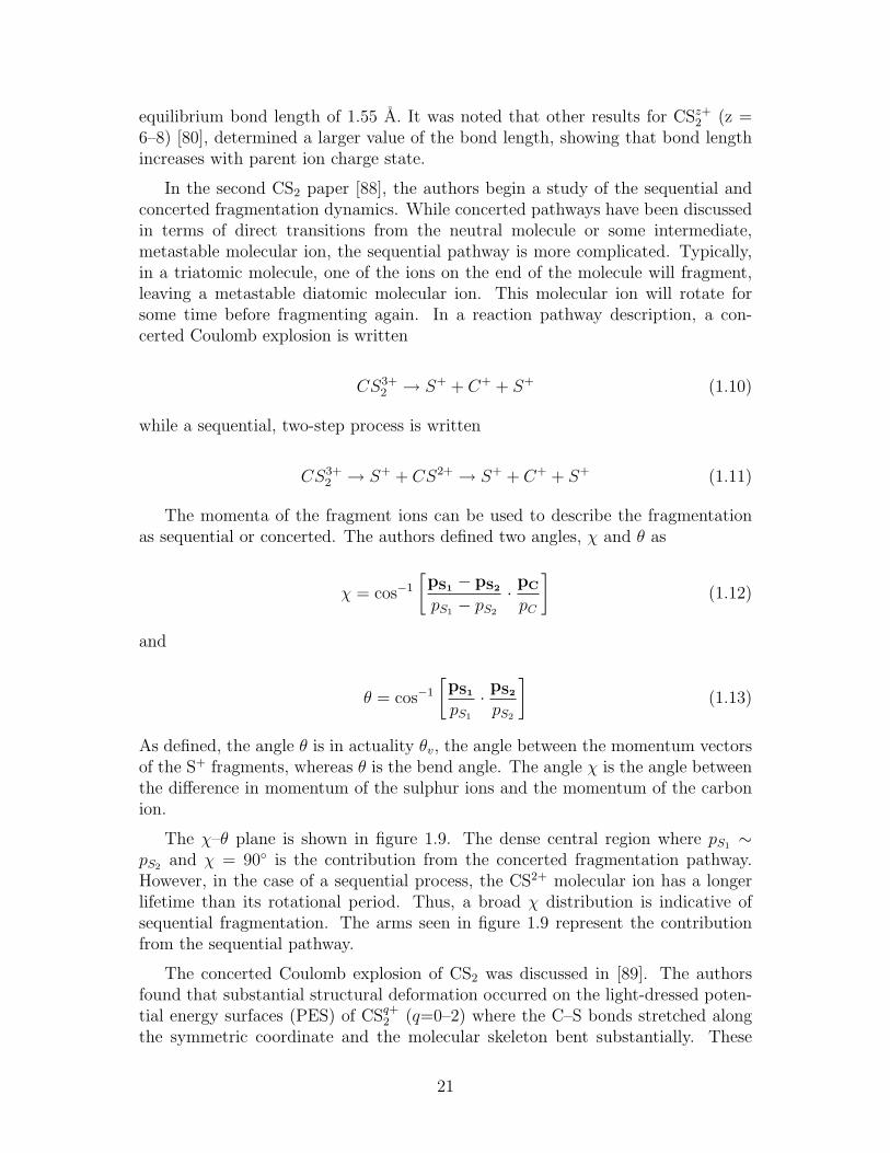
1.9 Map of χ–θv correlation . . . . . . . . . . . . . . . . . . . . . . . . 22

1.10 Structure of SO2 from pump-probe imaging . . . . . . . . . . . . . 25

2.1 Vacuum chamber - schematic . . . . . . . . . . . . . . . . . . . . . 28

2.2 Time-of-flight mass spectrometer components . . . . . . . . . . . . 30

2.3 Time-of-flight mass spectrometer . . . . . . . . . . . . . . . . . . . 31

2.4 Time-of-flight mass spectrometer schematic . . . . . . . . . . . . . . 32

2.5 Time-of-flight spectrum for xenon . . . . . . . . . . . . . . . . . . . 34

2.6 Ion calibration . . . . . . . . . . . . . . . . . . . . . . . . . . . . . . 34

2.7 Maxwell-Boltzmann distribution . . . . . . . . . . . . . . . . . . . . 35

2.8 Original configuration of position-sensitive detector . . . . . . . . . 36

2.9 Backgammon method . . . . . . . . . . . . . . . . . . . . . . . . . . 38

2.10 Modified configuration of position-sensitive detector . . . . . . . . . 40

2.11 Triple event signal. . . . . . . . . . . . . . . . . . . . . . . . . . . . 42

2.12 Recovered ion positions . . . . . . . . . . . . . . . . . . . . . . . . . 42

2.13 Calibration mask. . . . . . . . . . . . . . . . . . . . . . . . . . . . . 43

xi

2.14 Recovered calibration mask. . . . . . . . . . . . . . . . . . . . . . . 44

2.15 Spatial origin of nitrogen gas. . . . . . . . . . . . . . . . . . . . . . 45

2.16 Spatial origin determination. . . . . . . . . . . . . . . . . . . . . . . 45

2.17 Nitrogen momentum component distribution. . . . . . . . . . . . . 47

3.1 Three particle system . . . . . . . . . . . . . . . . . . . . . . . . . . 53

3.2 Time evolution of position . . . . . . . . . . . . . . . . . . . . . . . 55

3.3 Time evolution of momentum . . . . . . . . . . . . . . . . . . . . . 55

3.4 Solution error as a function of iteration . . . . . . . . . . . . . . . . 60

3.5 Progress of simplex algorithm . . . . . . . . . . . . . . . . . . . . . 61

3.6 Error as a function of iteration for bent geometry . . . . . . . . . . 62

3.7 Rotation of momentum plane . . . . . . . . . . . . . . . . . . . . . 65

4.1 2D representation of triple coincidence map . . . . . . . . . . . . . 70

4.2 Released kinetic energy distributions . . . . . . . . . . . . . . . . . 72

4.3 Recovered molecular geometry mapped directly from observed coin-cidence momentum imaging . . . . . . . . . . . . . . . . . . . . . . 73

4.4 Bend-angle (θ) distribution obtained from (1,1,1) explosion channel 74

4.5 Bend-angle (θ) distribution obtained from the six explosion channels 75

4.6 Bond length (r) distribution obtained from the six explosion channels 76

4.7 Bend-angle (θ) distribution obtained from the (2,2,2) explosion channel 77

4.8 Ionization laser intensity as a function of bond length for the sixchannels under investigation . . . . . . . . . . . . . . . . . . . . . . 78

4.9 Kinetic energy spectra for the (1,1,1) and (1,2,1) channels . . . . . 79

5.1 χ angle distribution . . . . . . . . . . . . . . . . . . . . . . . . . . . 84

5.2 Theoretical χ angle for a given bend angle θ . . . . . . . . . . . . . 85

5.3 Ratio of KER measured in previous HCI experiment . . . . . . . . 87

5.4 Symmetric and asymmetric fragmentation likelihood . . . . . . . . . 88

5.5 Channel-resolved mean bond length and bend angle distributions . 89

5.6 Point plot of r1 versus r2 from the recovered geometries of the (3,2,3)fragmentation channel . . . . . . . . . . . . . . . . . . . . . . . . . 90

5.7 Bend angle versus mean bond length for the (3,2,3) channel . . . . 91

5.8 Ionization laser intensity as a function of bond length . . . . . . . . 92

xii

6.1 Ground-state potential energy curves of N2 (X1Σ+g ) and N+

2 (X1Σ+g ) 95

6.2 Ground-state potential energy curves of CO2 and CO+2 . . . . . . . 96

6.3 Normalized H2 ionization signal enhancement ratios showing the ef-fect of bond softening . . . . . . . . . . . . . . . . . . . . . . . . . . 99

6.4 Ionization enhancement ratios for H2 . . . . . . . . . . . . . . . . . 100

6.5 N2 ionization signal enhancement ratios . . . . . . . . . . . . . . . . 101

6.6 CO2 ionization signal enhancement ratios . . . . . . . . . . . . . . . 102

6.7 CO2 ionization enhancement ratios after shifting the CO+2 curve . . 103

6.8 Ionization enhancement ratios for CO2, comparing the volume ratiowith the vibrational averaging . . . . . . . . . . . . . . . . . . . . . 104

B.1 Initial 2-D basic simplex . . . . . . . . . . . . . . . . . . . . . . . . 113

B.2 Updated 2-D basic simplex . . . . . . . . . . . . . . . . . . . . . . . 114

B.3 Dynamic simplex with expansion point . . . . . . . . . . . . . . . . 115

B.4 Dynamic simplex with contraction point . . . . . . . . . . . . . . . 115

B.5 Dynamic simplex with system contraction . . . . . . . . . . . . . . 116

xiii

Chapter 1

Overview of Molecular Imaging

This chapter will introduce the structure of matter from a historical perspective,expanding in greater detail some of the common techniques for analyzing matter.The chapter will then delve into the details of Coulomb explosion imaging includingprevious significant experiments. The future of molecular imaging is hinted at witha brief description of the work to date on the imaging of molecular dynamics.

1.1 The Structure of Matter

Investigating the structure of matter is one of the fundamental tasks in chemistryand physics. The first atomic theories were developed in the 6th century BC byancient Indian philosophers such as Kanada and Pakudha Katyayana. Indian atom-ists believed an atom could be one of six elements, with each element having upto twenty-four properties. They developed theories how atoms could combine intopairs, react, vibrate and perform other actions. They also suggested the idea ofsplitting an atom [1]. The earliest Western atomic theory was proposed by Leu-cippus of Miletus or Abdera in the first half of the 5th century BC. Leucippusbelieved that everything was composed of various imperishable, indivisible partscalled atoms [2]. His student, Democritus of Abdera (BC 450-370) was responsiblefor the publication of the first atomic theory, and furthermore argued that atomsonly possessed relatively few inherent properties, namely size, shape and mass.Other properties of matter, such as colour and taste, are the result of complexinteractions between our bodies and the matter being observed [3].

The last three centuries have seen numerous advances in our understanding ofatomic structure. Rudjer Boscovich [4] developed a modern atomic theory in the18th century based largely on the principles of Newtonian mechanics [5]. In 1808,John Dalton [6] applied the atomic theory to chemistry and posited fundamentalideas such as the atomic uniqueness of different elements, indivisibility of atomsand combining atoms to create compounds. Ludwig Boltzmann contributed to thekinetic theory and developed the Maxwell-Boltzmann distribution for molecular

1

speeds in a gas independently from James Clerk Maxwell. Further advances wouldfollow, including Rutherford’s gold foil experiment in 1911 [7] which proved thatmost of an atom’s mass was located in the nucleus, Bohr’s model of the atom in 1913[8] and Chadwick’s discovery of the neutron in 1932 [9]. In 1916, Lewis providedthe electron pair model for chemical bonding [10].

Despite these myriad advances in our understanding, our basic model still bearsmore than a passing resemblance to that of the earliest philosophers, that is that amolecule’s composition is made of atoms which combine in various ways by chemicalbonds.

1.2 Frequency Domain Spectroscopy

Although relatively recent measurement techniques such as atomic force microscopyallow for direct measurement of surfaces on the atomic scale, most of our knowledgeof molecular structure comes from the study of periodic molecular motion, motion inthe frequency domain. The simple Newtonian analogy of two balls joined by a springhas proven very robust for modeling diatomic molecules. In the simple model, if themasses are known, the force constant and length of the spring can be ascertained bymeasuring the vibrational and rotational frequencies [11]. Similarly, the vibrationaland rotational spectra can be used to determine a molecule’s equilibrium bondlength and the strength of the bond [12]. While this model is very robust fordiatomic molecules, polyatomic molecules can stretch, bend and oscillate in manyways. These additional degrees of freedom make molecular structure determinationsexponentially more difficult as the number of atoms increases. Early pioneers suchas Herzberg used pre-laser techniques to determine the structure of most smallmolecules by the middle of the twentieth century [13, 14, 15]. The invention andapplication of the laser in 1960 ushered in the era of high-resolution spectroscopy.

Although spectroscopy has been called “the study of the interaction of lightwith matter” [12], it has influenced many areas of modern science. The struggle tounderstand molecular spectra provided a direction for early quantum mechanics.Group theory found an application in the classification of molecular geometries.Observational astronomy was revolutionized with the new-found ability to analyzethe chemical composition of stars and galaxies.

1.3 Scattering Techniques

While both spectroscopy and scattering techniques are used to measure molecularstructure, they do so in complementary ways. As indicated earlier, the utilityof frequency domain spectroscopy suffers when determining the structure of largemolecules since the spectra are too complicated. To address this problem, severaldiffraction techniques were developed in parallel to spectroscopy [16, 17, 18]. In a

2

diffraction experiment, a molecular sample is bombarded with electrons, neutrons orX-rays whose de Broglie wavelength is shorter than the internuclear distance withinthe target. By analyzing the diffraction pattern, the molecular structure can bedetermined. The structure of countless crystalline materials have been determinedover the last century by scattering techniques.

Biomolecules are a target of much interest and our structural knowledge ofthem is largely derived from scattering. X-ray diffraction was used to measurethe structures of DNA [19], proteins [20] and enzymes [21]. Synchrotrons built inthe 1960’s provided an X-ray source for scattering experiments with improved fluxand spatial resolution. However, synchrotrons are not viable for determining themolecular structure of large biomolecules. The x-ray diffraction process works beston large arrays of regularly spaced units with long range order. However, most largebiomolecules cannot be crystallized and the subsequent x-ray diffraction signal istoo low to measure even from large synchrotron sources. Furthermore, even if asufficiently powerful synchrotron source did exist, its large X-ray flux would destroythe sample during the measurement process [22]. Fourth generation free-electronlasers will provide pulses of x-rays. The European X-ray Laser Project (XFEL) inGermany is presently under construction and is scheduled for completion in 2013.

1.4 Coulomb Explosion Imaging

Coulomb explosion imaging (CEI) is the general technique wherein a molecule isionized and fragmented. The structure of the molecule is then inferred from themeasurement of fragment momenta. Three methods have been used to initiateCoulomb explosions for the purpose of studying molecular structure. These meth-ods are beam-foil, collision with highly charged ions, and laser-initiated explosion.The advent of each technique corresponded with technological maturation of par-ticle and laser physics, respectively. The three approaches share several character-istics:

• only molecules in the gas phase are examined

• the interaction that initiates the Coulomb explosion is short and non-perturbative

• molecular structure is inferred from measurement of fragment momenta

Each technique and important results that were produced will be described in detail.

1.4.1 Beam-foil

Developed in 1978 at Argonne National Laboratory (USA) and the WeizmannInstitute (Israel) [23], beam-foil CEI is a non-scattering technique that determines

3

molecular structure using nuclear and particle physics methods [24, 25]. In a beam-foil CEI experiment, a negatively charged molecular ion is accelerated to a kineticenergy on the order of MeV before impinging on an ultrathin (∼100 A) foil target.Within an interaction time of ∼0.1 fs, many electrons are stripped off the molecularion as it passes through the foil. Once it exits the foil, the molecular ion explodesdue to the Coulomb repulsion of its positively charged atomic cores. By measuringthe three-dimensional momentum of each fragment, the structure of the molecularfragment prior to explosion can be computed. Due to technological constraints,beam-foil CEI can only be used to measure the structure of small molecules whichfrequency domain spectroscopy has already been used to measure. Furthermore,the necessity to utilize highly energetic molecular ions limited the feasibility andscientific impact of the technique. Nevertheless, the technique did reveal previouslyunknown information about the structure of weakly bound molecules such as C2H2

and CH2. Beam-foil CEI cannot measure molecular dynamics.

1.4.2 Highly charged ion

Beam-foil experiments require that sample molecules be accelerated to MeV ener-gies and necessitate the use of a particle accelerator that costs millions of dollars. Amuch less expensive option is to fragment the sample molecule via collision with ahighly charged ion (HCI). Like beam-foil, HCI cannot be used to measure dynamics.

When a highly charged ion (HCI) collides with a triatomic molecule, the moleculemay be multiply ionized and then fragment into atomic ions each possessing rela-tively large kinetic energies. For example,

X8+ + CO2 → COm+2 → Op+ + Cq+ + Or+, (1.1)

where m = p+q+r. Throughout this work, the notation used to describe explosionchannels will be written (p, q, r).

The simplest technique used to measure fragment kinetic energy is time-of-flight mass spectrometry (TOFMS) [26]. However, when a bent triatomic moleculeCoulomb explodes, it is impossible to extract unambiguous momentum informationfrom just the TOF signal. This is because the molecular fragments move in a plane,not just along the axis of the detector. During the mid-1990s, major advances weremade in detector technology. Time-of-flight and position sensitive detection werecombined so that it became possible to record the (x, y, t) information for each ionicfragment following a Coulomb explosion [27, 28].

Early work by Becker et al. [28] measured the double ionization and fragmen-tation of H2 by 200 keV H+ and He+ ions. They found that the kinetic energyspectra of correlated protons emitted from the collisions was identical, regardlessof whether H+ or He+ was used as the colliding ion. However, the kinetic energymeasured was still somewhat lower than for a purely Coulombic process. The samegroup studied water shortly afterwards [29, 30]. Of particular interest were the

4

dynamics of the complete fragmentation process H2O → H+ + H+ + Oq+ (q ≥ 1).In [29], the authors defined a practical choice of characteristic variables as shownin figure 1.1. Defined in velocity space, these variables are the angles χ and θv andcontain a great deal of information about the fragmentation process. In particular,the angle χ between the velocity of the of the Oq+ ion and the H+–H+ relative veloc-ity was used to determine if the two H–O bonds broke simultaneously (concerted)or in a step-wise (sequential) manner. The concerted process is said to occur ifboth bonds break in a time which is short on the rotational and vibrational timescales of molecular motion. Two limiting cases illustrate the physics surroundingχ. If a concerted fragmentation always produced the same momentum values inall fragments, the cos χ distribution would look like a δ function. On the otherhand, if sequential fragmentation always occurs, the OH fragment will have timeto rotate about its centre of mass one or more times. In this case, cos χ will be aflat distribution. The results shown in figure 1.1 show that the fragmentation ofwater by 100 keV H+ ions is largely concerted – the cos χ distribution is sharplypeaked at χ = 90, with a characteristic width. For the (1,1,1) explosion channel,the angle θv was measured to be somewhat more bent than the equilibrium bondangle θ0 ∼ 105. This was attributed to the strong H+–H+ repulsion. When highermolecular charge states were analysed, θv approaches the equilibrium bond angle.Finally, the authors noted the weakness of the pure Coulomb model when report-ing the kinetic energy distribution of coincident fragments. The measured kineticenergy distribution was narrower than that predicted using an MCSCF calculationtaking into account the nine lowest molecular states of the intermediate H2O

3+ ion.

Figure 1.1: cos χ distribution of H+ + H+ + O+ coincidences from collisions of100 keV He+ on H2O (solid line). The dashed line is a simulationbased on a MCSCF calculation assuming a concerted breakup ofboth H–O bonds. Reprinted with permission from [29]. c© 1995The American Physical Society.

Sanderson et al. [31] measured the structure of COq+2 (q=3–6) created by col-

lision with 120 keV Ar8+ ions and reported a number of significant observations.

5

The bend angle or θ distribution of the (2,2,2) fragmentation pathway was seen tobe extremely close to the zero-point motion for a neutral molecule. Furthermore,the kinetic energy of carbon ions should increase as the molecular skeleton is bent.The authors reproduced this trend and showed that the measured fragment kineticenergies were close to those expected from a purely Coulombic interaction. Byconsidering the momentum vectors of two equally charged oxygen ions, the authorsobserved that the fragmentation process was largely concerted, not sequential. Fi-nally, the authors reported the signal strengths of the various dissociation channels.However, these were not the true fragmentation cross-sections as the trigger proba-bility of the data acquisition oscilloscope depended directly on the number of Augerelectrons ejected from the collision. Therefore, higher charged molecular ions weremore likely to be detected. Similarly, the structure of the bent NO2 was studied [32]and, despite poor statistics, the authors observed satisfactory agreement betweenthe reconstructed and zero-point bend angles.

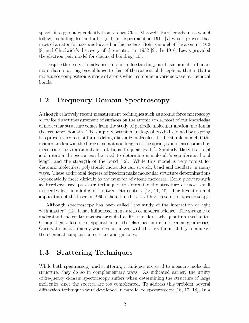
Rajgara et al. [33, 34] undertook a detailed investigation of the fragmenta-tion dynamics of CSq+2 (q=3–10) using 120 keV Ar6,8+ as the HCI . The authorsnoted that the bend angles reported in [31] and [32] approached the equilibriumbend angles when the charge state of the intermediate molecular ion was large.For this reason, they postulated that CS2, which has a low single-ionization en-ergy of 10.08 eV, would be an excellent candidate to study for high-charge stateexperiments. In particular, the authors hoped to test the validity of the Coulombpotential for fragmentation of highly charged molecular ions and note the rela-tionship between parent charge state and recovered bend angle. The kinetic energyrelease (KER) was measured for the different fragmentation channels and comparedwith a pure Coulombic model where the equilibrium geometry was assumed and abinitio, quantum-chemical calculations based on an all-electron, self-consistent field(SCF) molecular orbital computation. The measured KER values were consistentwith the Coulombic values, and, in most cases, more than the calculated ones. Theauthors postulated this discrepancy was due to ignoring higher electronic states.Therefore, it was suggested that their experimental findings pointed to the forma-tion of precursor ions in electronically excited states. Another important findingwas the likelihood of a particular molecular ion to fragment into a symmetric orasymmetric channel, as shown in figure 1.2. For example, CS5+

2 could fragment sym-metrically into (2,1,2) or asymmetrically into (2,2,1). The data suggested that amolecular ion will preferentially fragment along the most exothermically favourablepathway. The χ-angle distribution indicated that fragmentation was instantaneousand concerted. The bend angle distributions were all 5–10 more bent than themost probable bend angle of 175.2.

Chirality is an attribute of an object that is non-superimposable on its mirrorimage. The most common example are human hands. Chiral molecules are referredto as enantiomers and have substantial significance in fields such as pharmaceuti-cals. As traditional methods such as frequency domain spectroscopy cannot deducea molecule’s chirality, CEI was proposed as a potential solution. Kitamura et al.demonstrated the ability to determine a molecule’s absolute chirality using CEI

6

Figure 1.2: Propensity for fragmentation into symmetric (solid symbols andlines) and asymmetric channels (unfilled symbols and broken lines)for different molecular charge states. Reprinted with permissionfrom [34]. c© 2001 The American Physical Society.

[35] on CD4. While CD4 is not a chiral molecule in its equilibrium geometry, theauthors observed a geometry where all C–D bonds were different due to zero-pointvibrations. This was termed “dynamic” chirality, in contrast to the more common“static” chirality. Although the authors were only able to measure three of the fourdeuterium ions as well as the carbon ion, this was sufficient information to extractthe handedness of each molecule.

1.5 Laser-Initiated Dissociation

This section will describe in detail the efforts of various experimental and theoreticalresearch groups to describe the physical processes surrounding molecular ionizationand fragmentation. The structure of this review is overwhelmingly chronologicalwith emphasis placed on emerging techniques and key findings.

1.5.1 Early work

Pioneering work in the field was done by Frasinski et al. [36, 37, 38, 39]. Us-ing long, intense pulses (600 nm, 0.6 ps, 3 x 1015 W cm−2), Codling et al. [36]attempted to distinguish between sequential and direct ionization using HI and

7

produced a molecular parent ions up to HI6+. If the ionization were direct, six elec-trons would be rapidly removed and the H+ ion would be separated from the I5+

ion by the ground-state equilibrium bond distance of 1.61 A. In this circumstance,the Coulomb repulsion would produce protons with 45 eV of kinetic energy. In thecase of a sequential ionization, the molecule would ionize as it dissociated. The finalinter-ion distance would be larger and the proton energy correspondingly smaller.During the experiment, the maximum proton energy measured was 21 eV, lead-ing to the conclusion that ionization was sequential. Furthermore, the ionizationsequence HI2+ → HI6+ occurred on a timescale of ∼ 20 fs.

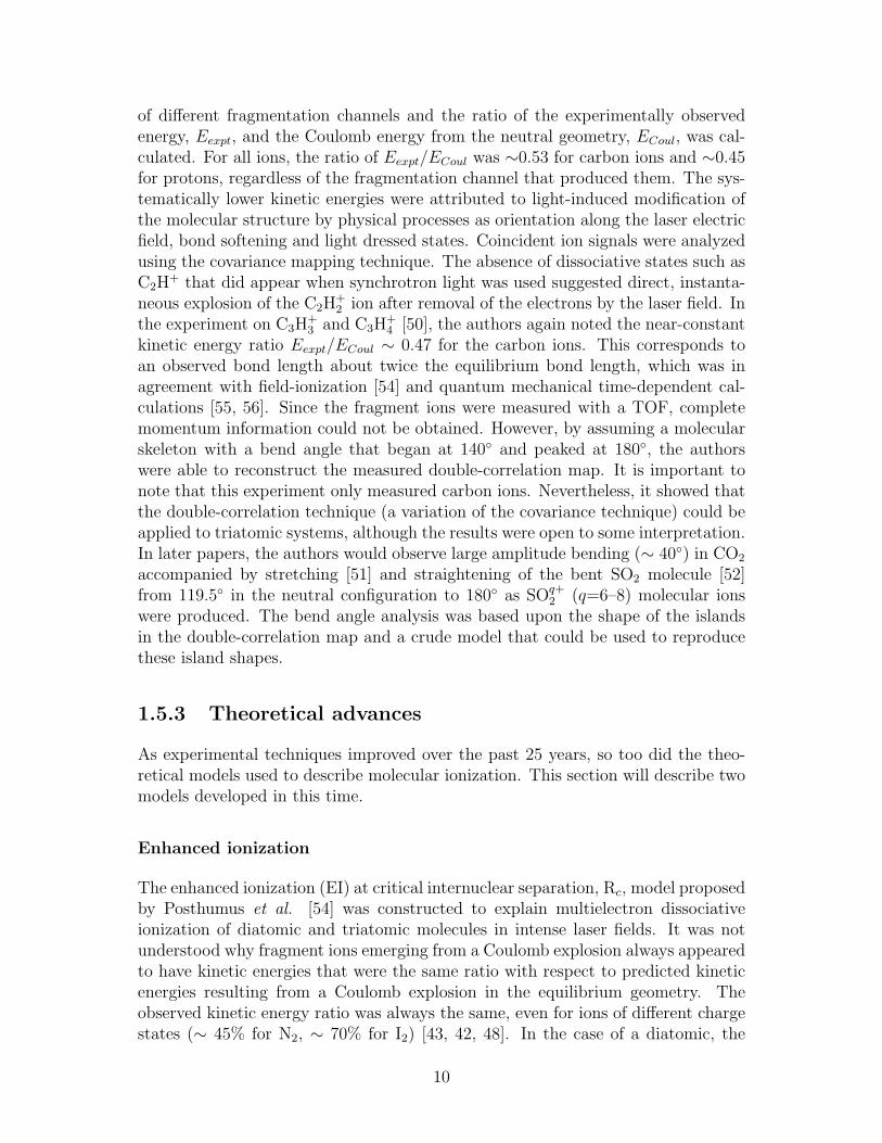
Frasinski et al. [37] studied nitrogen using the same laser system. They deducedthe molecular charge states and kinetic energy release from a simple TOF. Theauthors were able to create molecular ions with charge states as high as N6+

2 . Usinga simple Coulomb model, the ionization sequence N2+

2 → N6+2 was determined to

take ∼ 30 fs. The authors proposed the following sequence of events:

N2 → [N2+2 ] → N+ +N+ + 7 eV

↓[N3+

2 ] → N+ +N2+ + 14 eV

↓[N4+

2 ] → N2+ +N2+ + 25 eV

↓[N6+

2 ] → N3+ +N3+ + 38 eV

The square brackets denote transient molecular ions and vertical arrows indicatethe possibility of a particular ion ionizing again as it dissociates.

1.5.2 Covariance mapping

To better understand the multiple ionization pathways, Frasinski et al. [40] realizedthe necessity to observe correlated Coulomb explosion products with high detectionefficiency. Using the original TOF design, the authors aligned the E field of theirlaser along the TOF axis. In this configuration, the fragment ions were ejectedpreferentially along the TOF axis, and a DC electric field ensured that both “for-ward” and “backward” ions hit the detector, with the “forward” ions arriving first.This resulted in pairs of ions seen in the time-averaged TOF spectrum of figure 1.3along with a covariance map.

The covariance mapping technique [38] is a graphical technique of seeing corre-lations between all of the fragment ions. The various channels appear as separateislands on the covariance map and momentum conservation requires that corre-lated pairs lie along a straight line. The islands are labelled as: 1, N+

b + N+f (b

= backward, f = forward); 2, N+b + N2+

f ; 3, N+f + N2+

b ; 4, N2+b + N2+

f ; 5, N2+b +

8

Figure 1.3: Covariance map of N2 with the TOF spectrum placed along the x-and y-axes. Reprinted with permission from [40]. c© 1989 ElsevierB.V.

N3+f ; 6, N2+

f + N3+b ; 7, N3+

b + N3+f . The power of the technique is demonstrated by

considering the N+b ions in islands 1 and 2. Even if the ions in these features had

identical energies and would therefore be indistinguishable in a conventional TOFspectrum, a covariance map unambiguously associates the N+

b ions with either N2+2

or N3+2 molecular ions. This group would continue to apply this technique to a

variety of systems including CO [41], I2 [42] and CO2 [43].

With improvements in laser pulse compression techniques [44] and wider use ofTi:sapphire lasers, Coulomb explosion experiments with laser pulses in the 100 fsregime became realizable by the mid-1990s. The Saclay, France group performed anumber of important experiments [45, 46, 47, 48, 49, 50, 51, 52] that would verifythe general applicability of laser-initiated CEI, in particular for larger molecularsystems.

Cornaggia et al. performed a series of experiments on hydrocarbon ions, specifi-cally, C2H

+2 [49], C3H

+3 and C3H

+4 [50] using intense laser pulses from a Ti:sapphire

source (790 nm, 130 fs, 2.5 x 1016 W cm−2). Fragment ions were collected in aWiley-McLaren TOF [53]. The kinetic energy released was measured for a number

9

of different fragmentation channels and the ratio of the experimentally observedenergy, Eexpt, and the Coulomb energy from the neutral geometry, ECoul, was cal-culated. For all ions, the ratio of Eexpt/ECoul was ∼0.53 for carbon ions and ∼0.45for protons, regardless of the fragmentation channel that produced them. The sys-tematically lower kinetic energies were attributed to light-induced modification ofthe molecular structure by physical processes as orientation along the laser electricfield, bond softening and light dressed states. Coincident ion signals were analyzedusing the covariance mapping technique. The absence of dissociative states such asC2H

+ that did appear when synchrotron light was used suggested direct, instanta-neous explosion of the C2H

+2 ion after removal of the electrons by the laser field. In

the experiment on C3H+3 and C3H

+4 [50], the authors again noted the near-constant

kinetic energy ratio Eexpt/ECoul ∼ 0.47 for the carbon ions. This corresponds toan observed bond length about twice the equilibrium bond length, which was inagreement with field-ionization [54] and quantum mechanical time-dependent cal-culations [55, 56]. Since the fragment ions were measured with a TOF, completemomentum information could not be obtained. However, by assuming a molecularskeleton with a bend angle that began at 140 and peaked at 180, the authorswere able to reconstruct the measured double-correlation map. It is important tonote that this experiment only measured carbon ions. Nevertheless, it showed thatthe double-correlation technique (a variation of the covariance technique) could beapplied to triatomic systems, although the results were open to some interpretation.In later papers, the authors would observe large amplitude bending (∼ 40) in CO2

accompanied by stretching [51] and straightening of the bent SO2 molecule [52]from 119.5 in the neutral configuration to 180 as SOq+

2 (q=6–8) molecular ionswere produced. The bend angle analysis was based upon the shape of the islandsin the double-correlation map and a crude model that could be used to reproducethese island shapes.

1.5.3 Theoretical advances

As experimental techniques improved over the past 25 years, so too did the theo-retical models used to describe molecular ionization. This section will describe twomodels developed in this time.

Enhanced ionization

The enhanced ionization (EI) at critical internuclear separation, Rc, model proposedby Posthumus et al. [54] was constructed to explain multielectron dissociativeionization of diatomic and triatomic molecules in intense laser fields. It was notunderstood why fragment ions emerging from a Coulomb explosion always appearedto have kinetic energies that were the same ratio with respect to predicted kineticenergies resulting from a Coulomb explosion in the equilibrium geometry. Theobserved kinetic energy ratio was always the same, even for ions of different chargestates (∼ 45% for N2, ∼ 70% for I2) [43, 42, 48]. In the case of a diatomic, the

10

Coulomb energy is given by Ee = kQ1Q2/Re, where Q1 and Q2 are the chargesof the ions and Re is the equilibrium interatomic distance of the neutral molecule.Two possibilities exist for a reduction in the Coulomb energy. First, screening couldoccur at each ionization step, effectively reducing the values of Q1 and Q2. Second,the molecular ion could relax to a critical distance, Rc, where subsequent ionizationoccurs.

Figure 1.4: Model of I+2 in a laser field. The full curve represents the potentialenergy of the outermost electron in the combined field of two pointlike I+ ions and the laser. The internuclear distance, Rc, and thefield, Fc, have critical values such that the electron energy level, ELtouches both the inner potential barrier, Ui and the outer potentialbarrier, Uo. Reprinted with permission from [54]. c© 1995 Instituteof Physics and J. Posthumus.

Consider, the dissociation of the molecular ion I+2 on the rising edge of a laserfield that is polarized along the molecular axis. The outermost electron is free tomove in the double well formed by combining the remaining electrons and nucleiinto two point-like atomic ions. As the ions move apart, the inner barrier rises andimpedes the motion of the electron. The electron can no longer follow the fieldand the system makes a transition. Figure 1.4 shows the situation where the ionshave moved to the critical distance and the inner potential barrier, Ui touches theelectron level, EL. In general, the double-well potential energy is given by

U = − Q1

|x+Rc/2|− Q2

|x−Rc/2|− Fcx (1.2)

where Fc is the electric field amplitude. The position of the electron energy levelin this double well can be approximated by

11

EL ≈(−E1 −Q2/Rc) + (−E2 −Q1/Rc)

2(1.3)

where E1 and E2 are the known ionization potentials of the atomic ions that arelowered by the Coulomb potential of the neighbouring ion, Q/Rc. This model issometimes known as the over the barrier ionization (OBI) model and will be usedin a later chapter.

As the laser field increases, the molecule will ionize again. The next electron hasa much higher binding energy but since one of the atomic ions is more positivelycharged, the inner potential barrier is lower. To good approximation, these twoeffects reproduce the previous situation and the critical distance Rc is virtuallyunchanged. This continues through the multiple ionization process.

The authors compare their model to previously reported experimental resultsfor N2 [46], Cl2 [48], O2 [45], I2 [42], CO [45, 41] and CO2 [47, 43]. In general, theagreement is quite good.

A different interpretation has been proposed [55], in which the lowest unoccupiedmolecular orbital (LUMO) is Stark shifted by the electric field of the laser. As themolecule expands, population exchange can occur nonadiabatically between thehighest occupied molecular orbital (HOMO) and LUMO. Once the LUMO is abovethe Coulomb barrier, ionization proceeds. Experimental studies of N2 and I2 [57, 58]have revealed the tendency for these molecules to ionize along asymmetric pathways.Analogous to the HOMO and LUMO in EI, the authors postulate strong couplingbetween g− u symmetry states, as well as an internal rescattering mechanism thationizes an inner electron and leaves the molecule in an excited state.

ADK tunnelling ionization

Unlike enhanced ionization, which can be classically described as an over the barriermodel, the quasi-static theory of Ammosov, Delone and Krainov (ADK) [59] isbased on the calculation of the tunnelling ionization rate in the presence of a staticelectric field. In this regime, the potential barrier formed by the core of the atomor molecule and the electric field of the laser becomes small enough for tunnellingto become possible. Due to a field-ionization process, the electron is “pulled off”.However, there is an important difference between a static field and an oscillatingfield of the same magnitude. A tunnelling current will always build up in a staticfield. In an oscillating field, the starting tunnelling current is pushed back in thenext half-cycle unless it is fast enough to reach the other side of the barrier. TheADK approximation is justified for low laser frequency when ionization occurs at atime scale that is small compared to the laser period.

For the simplest case of a hydrogen atom in its ground state, the tunnellingionization rate in the presence of a static electric field F in atomic units is [60]

12

Wstat(F ) =4

Fexp

(− 2

3F

). (1.4)

In a low frequency field F cos ωt, the ionization rate can be calculated from aver-aging over the static rate over half a cycle of the laser oscillation:

W (F ) =1

π

∫ π/2

−π/2dτWstat(F cos τ) =

1

π

∫ π/2

−π/2dτ

4 sec τ

Fexp

(−2 sec τ

3F

), (1.5)

where τ = ωt. For F 1, this integral can be evaluated using the method ofsteepest descent, yielding the result [61]

W (F ) =

√3

πFWstat(F ). (1.6)

ADK generalized this result to the case of complex atoms and ions [59], and theirtheory has been successful in describing atomic ionization [62, 63]. This theoryhas also been shown to be applicable to small molecules [64, 65, 66, 67, 68]. TheADK theory has recently been modified to include the effects of symmetry of themolecular system and the asymptotic behaviour of the molecular electronic wavefunction, resulting in the MO-ADK theory [69, 70, 71]. For our purpose, the simplerADK theory, taking into account the dependence of the ionization potential of themolecule on the nuclear coordinates, suffices. The ADK tunnel ionization rate,wADK , is given in atomic units by [59]:

wADK(R, I) =

(3e

π

)3/2Z2

n∗9/2

(4eZ3

n∗4F

)2n∗−3/2

exp

(− 2Z3

3n∗3F

), (1.7)

where e = 2.718. . . , Z is the ionic charge, and I = (c/8π)F 2 is the laser intensity.The effective quantum number, n*, is related to Ip, the ionization potential of thesystem, by

n∗ = Z/√

2Ip(R). (1.8)

A particularly compelling example of the experimental applicability of ADK wasseen in the work of Urbain et al. in 2004 [72]. The authors examined the tunnelionization of H2 and in so doing, challenged the assertion that the vibrationalexcitation of molecular ions follows the Franck-Condon principle in this regime. Ifthe laser-molecule interaction can be described by a field-ionization process, themolecular ion will be in its electronic ground state and the vibrational wave packetwill be conserved. For H+

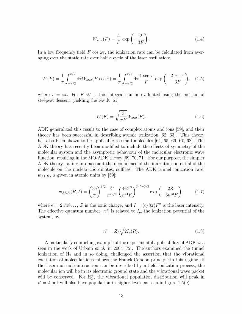
2 , the vibrational population distribution will peak inv′ = 2 but will also have population in higher levels as seen in figure 1.5(e).

13

The authors contended that the Franck-Condon principle was unable to explainthe results of ionization in the tunnelling regime since the rate of tunnelling asgiven in 1.7 is strongly dependent upon bond length, R. Furthermore, as laserintensity increases, molecular alignment becomes ever more important. Moleculesaligned parallel to the laser field will experience a non-resonant coupling effectknown as bond-softening. Bond-softening has the effect of readily dissociating avibrationally excited molecular ion. Molecules that are aligned perpendicular tothe laser field are not subject to bond-softening, but do experience shifts in thevibrational excitation population distribution. As can be seen in figure 1.5(a)–(d),as laser intensity increases, the distribution of the perpendicularly aligned moleculesapproaches the distribution obtained with electron impact ionization (e).

1.5.4 Mass-resolved molecular imaging

The University of Tokyo group in Japan contributed a great deal of experimentalwork to the field in the late 1990s and early 2000s [75, 76, 77, 78, 79, 80]. The grouppioneered a new technique called mass-resolved momentum imaging (MRMI) andprovided a theoretical basis for molecular deformation by using a sophisticated po-tential energy surface dynamical model. The MRMI technique was later improvedby the University College London group [81, 82] to make quantitative studies ofwater and carbon dioxide.

Hishikawa et al. studied the momentum characteristics of ionic fragments pro-duced by CEI of N2 [75, 76] and SO2 [75] using intense, short pulses (795 nm, ∼50fs, 7 x 1015 W cm−2) and the MRMI technique. The MRMI technique utilizesa zero-order half-wave plate to rotate the laser polarization with respect to theTOF detection axis. The half-wave plate was rotated in 6 increments and 15 high-resolution TOF spectra were recorded to create the MRMI map. By construction, asymmetric MRMI pattern is expected when viewing the line connecting the 0 and180 positions. Any indication of asymmetry suggests variation of experimentalconditions during the repetitive TOF data acquisition. An example of an MRMImap for N2+ is shown in figure 1.6.

The MRMI technique in [75] clearly showed that the momentum of the chargedatomic Nq+ (q=1–3) fragments increased as the charge number increased. This wasdue to the larger kinetic energies that are released from the Coulomb explosionsof highly charged parent molecular ions. Furthermore, the ejection arc of the frag-ments became smaller as the charge number increased. This was attributed to theN–N molecular axis being more aligned with the laser polarization. In fact, anotherinterpretation is that for randomly aligned N2 molecules, those molecules that areparticularly well aligned with the laser field will preferentially ionize.

The fragmentation dynamics of SO2 were then analyzed as shown in figure 1.7.The plots (a) and (b) reveal how different areas of an MRMI plot correspond todifferent dissociation channels. However, they also reveal a weakness of the MRMItechnique. The technique is not coincident, and the fragmentation pathway cannot

14

Figure 1.5: (a)–(d) Theoretically predicted vibrational excitation of H+2 pro-

duced by tunnelling ionization of H2 in intense laser fields. Cal-culations for molecules aligned parallel and perpendicular to thelaser E field are presented. The laser intensities are (a) 3.5 x 1013

W cm−2, (b) 5.4 x 1013 W cm−2, (c) 7.8 x 1013 W cm−2, and (d)1.06 x 1014 W cm−2. The vibrational excitation of H+

2 produced byelectron impact ionization (E0 = 10–1500 eV) of H2 as measuredby Dunn and Van Zyl [73] and interpreted by von Busch and Dunn[74] is shown in (e). Reprinted with permission from [72]. c© 2004The American Physical Society.

15

Figure 1.6: Illustration of the MRMI procedure. An MRMI map is constructedfrom momentum-scaled TOF spectra measured with the laser po-larization at various angles α with respect to the detector axis. Onthe left-hand side of the MRMI map are five experimental TOFspectra of N2+ with angles of α = 1, 13, 25, 49, and 91. EachTOF spectra corresponds to the cross-section of the MRMI map atthe angle α. Typically, 17 momentum-scaled TOF spectra are usedto make an MRMI map. Reprinted with permission from [76]. c©1998 Elsevier B.V.

be determined with absolute confidence. In figure 1.7(c), the shape of the MRMIpattern is different that the others. The crescent patterns are in the directionperpendicular to the laser polarization. Since the molecular axis of the SO2 moleculeshould be aligned with the laser polarization direction, the authors interpreted thesecrescents as evidence of the Coulomb explosion process occurring from a highlybent geometry. Using the MRMI maps, the authors deduced the bond angle to beθ = 130 for the (2,3,2) channel and θ = 110 for the (1,3,1) channel. Althoughthese were close to the equilibrium value of θe = 119.5 for the neutral molecule,the authors admitted there were large uncertainties due to the large momentumdistributions. Hishikawa et al. also found that the S–O bond lengths were abouttwice the equilibrium bond lengths, in agreement with the findings of Cornaggia etal. [52]. Hishikawa et al. provided additional experimental details in their follow-uppaper [76]. Further MRMI work on COq+

2 [77] and NOq+2 [78] would suggest in both

cases that the molecular ions became straighter as q increased and that the bondlengths stretched as q increased. The authors attempted to explain these results interms of the light dress potential energy surfaces (LDPES). At low laser intensity,molecular ions with smaller q are formed. In this case, the authors postulated thatthe laser field coupled to the bending coordinate, producing a substantially bent

16

geometry. However, near the focal spot, higher intensities produce molecular ionswith larger q values. In this case, the laser field coupled with the linear stretchingcoordinate. Iwamae et al. studied the branching ratios of NO with MRMI [79]while formalizing the detector efficiency a hitherto free parameter that had notbeen discussed.

Figure 1.7: MRMI map of SO2 with chamber pressure 1.5 x 10−7 Torr. Thevertical arrow in (a) represents the direction of the laser polar-ization vector. (a) O+ / S2+ channel: two pairs of crescents arevisible in the polarization direction which result mostly from thethree body explosion of SO2 but are also attributed to the channelsSO2+

2 → SO+ + O+ and SO3+2 → SO2+ + O+. (b) SO2+ channel:

a pair of the crescents located in the polarization direction repre-sent the SO3+

2 → SO2+ + O+ explosion pathway while the centralregion which is lower in energy is attributed to the neutral pathwaySO2+

2 → SO2+ + O. (c) S3+ channel: prominent crescents locatedin the direction perpendicular to the laser polarization indicate abent molecular structure prior to Coulomb explosion. Reprintedwith permission from [75]. c© 1998 Elsevier B.V.

The final MRMI study done by the group was on CS2 [80] wherein they at-tempted to understand the mechanisms of alignment, ionization and skeletal defor-mation. This study was unique in that the authors used ns-laser light pulses (1064nm, 7 ns, 1.9 x 1012 W cm−2) to initiate the processes of alignment and skeletaldeformation. These two processes were then probed using circularly polarized fspulses (795 nm, 100 fs, 5.5 x 1014 W cm−2). In this way, the authors ensured thatany alignment of the molecules was done by the ns-laser light. Furthermore, theMRMI maps were created by rotating the polarization of the ns pulses. By examin-ing the (3,2,3) fragmentation using only the circularly polarized light, the authorsfound the interatomic C–S bond length to be twice the equilibrium length. Thebend angle distribution was centred at 180 and had a half-width of ∼9. However,

17

when the ns-pulse and fs-pulse were both used, another pattern emerged in theMRMI maps. When the fs-pulse arrived on the rising or falling edge of the ns-pulse(4 ns from the peak), the MRMI maps showed a nearly isotropic distribution, withonly a very slightly larger distribution along the ns-pulse polarization direction.When the fs-pulse arrived at the peak of the ns-pulse, the S3+ ions were stronglyaligned with the laser polarization while the C2+ ions were ejected perpendicularto the polarization. While the derived C–S bond lengths were nearly identical tothe case where no ns-pulse was used, the bend angle distribution was substantiallywider with a half-width of ∼15. The authors attributed this increased bending tocoupling of the X1Σ+

g ground electronic state of CS2 with the B1B2 excited statevia a three-photon absorption at 1064 nm. This explanation is plausible given theequilibrium bend angle of the B1B2 state is 163.

Sanderson et al. examined water using an improved MRMI technique [81] withintense pulses (790 nm, 50 fs, 3 x 1016 W cm−2). Unlike previous MRMI maps,the authors recorded TOF spectra at many different polarization angles, producingMRMI maps that were much more detailed and less reliant on linear interpolation.The authors postulated that the very intense laser field was able to reorient the lightH2O molecule on a femtosecond time scale. The bent nature of the H2O moleculeswas reconstructed by the MRMI maps and based on simulation, the maximumof the bend angle distribution was 130 for the (1,1,1) channel while the (1,2,1)channel had a maximum of 140 in its bend angle distribution. This change fromthe equilibrium bend of 104 was attributed to a single photon transition from thebent X2B1 ground state to the excited A2A1 state which has a straight equilibriumgeometry. Using the same laser system, the authors performed an extensive studyof CO2 [82] using covariance and MRMI techniques. This paper was the first studyof CO2 that did not report a linear configuation. In fact, the authors pointedout that a perfectly linear configuration should never occur due to the absence ofphase space at 180. They compare their bend angle distributions to the long-pulseexperiments of Cornaggia [51] and the HCI experiment of Sanderson et al. [31] andfind better agreement with the HCI bend angle distribution. They attribute this, inpart, to Cornaggia using a deliberately simple distribution for ease of calculation.Nevertheless, the authors report a peak in their bend angle distribution at 171,somewhat less than the true equilibrium bend angle of 174.6.

1.5.5 Image labeling

In 2001, the University of Maryland group introduced a novel technique called imagelabeling [83]. Described as a two-dimensional analogue of covariance mapping, thistechnique consists of an ultrafast laser (800 ns, 100 fs, 1014–1016 W cm−2), a TOFspectrometer equipped with imaging grade MCPs, a phosphor screen and a CCDcamera. Fragment ions are accelerated toward the MCP by a DC electric field.The operating voltage on the MCPs is gated to allow the study of specific ionicspecies and charge states. The temporal resolution is a somewhat coarse 100 ns,but this is sufficient to separate low mass ions (H, C, N, O) into their various charge

18

states. Evidently, the mass resolution of this detector was quite poor. Along thelaser polarization axis (shown in figure 1.8), energetic ions appear in the image ata distance from the centre given by

r = 2√Lε/qF (1.9)

where ε is the ion’s kinetic energy, q is the charge on the ion, F is the DC electricfield strength and L is the distance between the focal point and the detector. Theangular distribution is independent of the azimuthal angle about the polarizationaxis, φ, so equation 1.9 only holds for polar angles θ = 0 and π. It is possible todeconvolve images so that equation 1.9 applies for all values of θ. In their initialpaper, the authors measured the bend angle of CO2 to be ∼ 170 [83].

The authors used their new technique to study the charge-symmetric fragmen-tation of CO6+

2 → O2+ + C2+ + O2+ [84]. Correlation images were created byselecting a C2+ ion (the square areas in figure 1.8) with a specific p⊥. In this casep‖ ≡ 0. Frames with the specified C2+ ions were averaged along with the correlatedO2+ ions. Since the ions are ejected simultaneously, momentum and energy areconserved. Therefore, p‖ for the two groups of O2+ ions along the polarization axisare equal and opposite. Similarly, p⊥ for the C2+ ion must equal the sum of theP⊥ for the O2+ ions.

The authors examined their results in terms of the charge defect, σ ≡ Z(1 −√Req/Rc), where Z is the ionic charge, Req is the equilibrium bond length and

Rc is the critical bond length. From their data, Rc = 2.15 A and σ = 0.5. Thevalue of Rc was nearly independent of the bend angle. This suggests that theRc or enhanced ionization model more accurately reproduces their findings as thedynamic screening model [85, 86] predicts that σ should decrease as the bend angledecreases. Based on the measured bend angle of 145, the authors estimate thebending level to be v=9, corresponding to about half the photon energy. Thislarge bending motion is attributed to electron-molecule rescattering, similar to thethree-step model that produces high harmonics in the strong-field regime.

While this technique is certainly novel, no other groups have adopted it as ofthis writing. This may be because the technique requires that bent target moleculesbe in a particular orientation i.e. parallel to the MCP plane. Alternatively, itmay be because the results of image labeling are somewhat more ambiguous thanmeasurements taken with a coincident ultrafast imaging technique, described in thenext section.

1.5.6 Coincidence techniques

The group from the University of Tokyo performed a number of studies on CS2

and N2O using a device which combined a TOF with a position-sensitive detector[87, 88, 89, 90] similar to that used by Rajgara et al. [34]. The developmentof this instrument was made possible, in part, thanks to the development of new

19

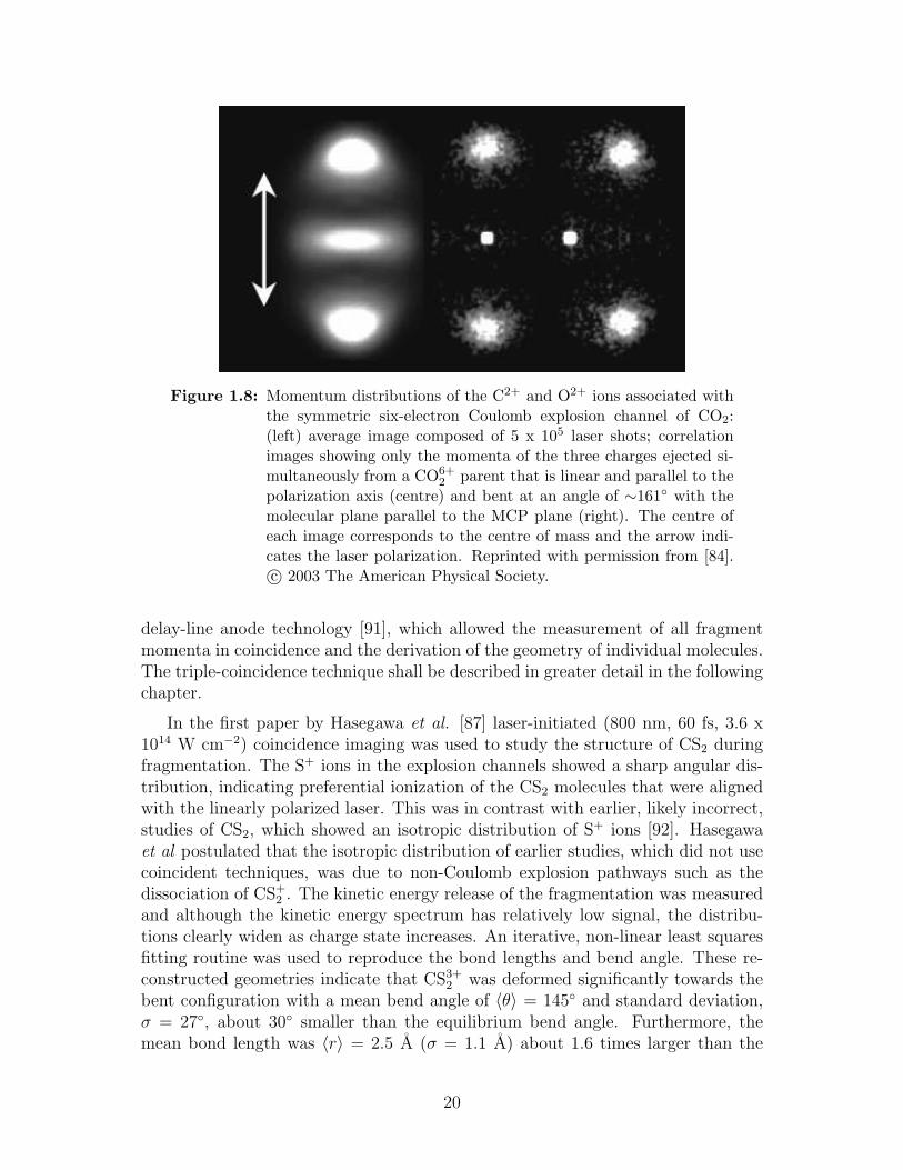
Figure 1.8: Momentum distributions of the C2+ and O2+ ions associated withthe symmetric six-electron Coulomb explosion channel of CO2:(left) average image composed of 5 x 105 laser shots; correlationimages showing only the momenta of the three charges ejected si-multaneously from a CO6+

2 parent that is linear and parallel to thepolarization axis (centre) and bent at an angle of ∼161 with themolecular plane parallel to the MCP plane (right). The centre ofeach image corresponds to the centre of mass and the arrow indi-cates the laser polarization. Reprinted with permission from [84].c© 2003 The American Physical Society.

delay-line anode technology [91], which allowed the measurement of all fragmentmomenta in coincidence and the derivation of the geometry of individual molecules.The triple-coincidence technique shall be described in greater detail in the followingchapter.

In the first paper by Hasegawa et al. [87] laser-initiated (800 nm, 60 fs, 3.6 x1014 W cm−2) coincidence imaging was used to study the structure of CS2 duringfragmentation. The S+ ions in the explosion channels showed a sharp angular dis-tribution, indicating preferential ionization of the CS2 molecules that were alignedwith the linearly polarized laser. This was in contrast with earlier, likely incorrect,studies of CS2, which showed an isotropic distribution of S+ ions [92]. Hasegawaet al postulated that the isotropic distribution of earlier studies, which did not usecoincident techniques, was due to non-Coulomb explosion pathways such as thedissociation of CS+

2 . The kinetic energy release of the fragmentation was measuredand although the kinetic energy spectrum has relatively low signal, the distribu-tions clearly widen as charge state increases. An iterative, non-linear least squaresfitting routine was used to reproduce the bond lengths and bend angle. These re-constructed geometries indicate that CS3+

2 was deformed significantly towards thebent configuration with a mean bend angle of 〈θ〉 = 145 and standard deviation,σ = 27, about 30 smaller than the equilibrium bend angle. Furthermore, themean bond length was 〈r〉 = 2.5 A (σ = 1.1 A) about 1.6 times larger than the

20

equilibrium bond length of 1.55 A. It was noted that other results for CSz+2 (z =6–8) [80], determined a larger value of the bond length, showing that bond lengthincreases with parent ion charge state.

In the second CS2 paper [88], the authors begin a study of the sequential andconcerted fragmentation dynamics. While concerted pathways have been discussedin terms of direct transitions from the neutral molecule or some intermediate,metastable molecular ion, the sequential pathway is more complicated. Typically,in a triatomic molecule, one of the ions on the end of the molecule will fragment,leaving a metastable diatomic molecular ion. This molecular ion will rotate forsome time before fragmenting again. In a reaction pathway description, a con-certed Coulomb explosion is written

CS3+2 → S+ + C+ + S+ (1.10)

while a sequential, two-step process is written

CS3+2 → S+ + CS2+ → S+ + C+ + S+ (1.11)

The momenta of the fragment ions can be used to describe the fragmentationas sequential or concerted. The authors defined two angles, χ and θ as

χ = cos−1

[pS1 − pS2

pS1 − pS2

· pC

pC

](1.12)

and

θ = cos−1

[pS1

pS1

· pS2

pS2

](1.13)

As defined, the angle θ is in actuality θv, the angle between the momentum vectorsof the S+ fragments, whereas θ is the bend angle. The angle χ is the angle betweenthe difference in momentum of the sulphur ions and the momentum of the carbonion.

The χ–θ plane is shown in figure 1.9. The dense central region where pS1 ∼pS2 and χ = 90 is the contribution from the concerted fragmentation pathway.However, in the case of a sequential process, the CS2+ molecular ion has a longerlifetime than its rotational period. Thus, a broad χ distribution is indicative ofsequential fragmentation. The arms seen in figure 1.9 represent the contributionfrom the sequential pathway.

The concerted Coulomb explosion of CS2 was discussed in [89]. The authorsfound that substantial structural deformation occurred on the light-dressed poten-tial energy surfaces (PES) of CSq+2 (q=0–2) where the C–S bonds stretched alongthe symmetric coordinate and the molecular skeleton bent substantially. These

21

Figure 1.9: Map of the χ–θv correlation for the three-body Coulomb explo-sion of CS3+

2 . The two curved arms extending from the densecentral region are the contribution from sequential explosion pro-cesses. The solid curve represents the theoretical χ–θv trajectoryobtained by the classical equations of motion assuming that thesecond S+ ion and the C+ ion are ejected from the metastableCS2+. The open circles are (χ, θv)s for the five rotational angles,φ = 0, π/4, π/2, 3π/4, π, between the molecular C–S axis of CS2+

and pseq1 . Reprinted with permission from [88]. c© 2002 ElsevierB.V.

results were explained by using a model for CO2 developed by Kono et al. [93, 94]which showed that the PES of CO2+

2 is deformed by light fields through the mix-ing of a large number of electronic states and opening an energetically favourablepathway along the bending coordinate.

A similar investigation was performed on N2O3+ [90] in which the authors iden-

tify the N2O dissociation pathways and observe, as above, evidence of a sequentialpathway where the N–N bond dissociates first. The lifetime of the NO2+ molecularion was estimated to be 0.38 ps. The N–N and N–O bonds stretched by factorsbetween 1.34 and 1.68 while the bend angle decreased from 170 to 100. Therelationship between the stretching and bending was remarkably linear.

The National Research Council group in Ottawa, Canada performed structuralstudies of D2O and SO2 [95] using 40 fs and 8 fs laser pulses from a hollow-corefibre [96]. To generate ∼ 8 fs pulses, the output of a Ti:sapphire regenerativeamplifier (810 nm, 40 fs, 250 µJ, 500 Hz repetition rate) was coupled into a 250

22

µm diameter hollow-core fibre with a length of 1 m. The hollow-core fibre wasfilled with argon at a pressure of 1 atm. When the 40 fs pulse entered the fibre,self-phase modulation broadened the bandwidth from 30 nm to 200 nm. Oncethe pulse was compressed, few-cycle pulses with a duration of 8 fs were obtained.The results of [95] are interesting for two reasons. First, by employing a few-cyclelaser pulse, the authors were able to measure bond lengths shorter than predictedby the Rc model and thereby set a limit on the validity of the model. Secondly,the authors utilized ab initio potential energy surfaces to recover the structure ofD2O. The recovered bend angle distribution for D2O

4+ compared poorly to thatexpected from the neutral v = 0 stationary state. The authors attributed this to acontribution from electronic states in intermediate charge states during the multipleionization, in effect, the same argument used by Kono et al. [93, 94] to describeCO2.

1.5.7 Molecular dynamics

A molecule’s dynamical nature will have a significant influence on its participationin chemical processes. If the aim is to understand and coherently control thesechemical processes, the motion of a molecule must be imaged on the timescale thatit occurs.

The first time-resolved approach for observation of molecular dynamics occurredin the late 1980’s with the advent of time domain spectroscopy. Developed byseveral groups [97, 98, 99], the technique utilizes ultrashort laser pulses. Analogousto a photographic camera, an ultrashort laser pulse can be used to “freeze” adynamical process. Time domain spectroscopy makes use of two femtosecond pulsesin a “pump-probe” arrangement. The first pulse (pump) initiates some dynamicalprocess such as vibration, rotation, etc. in the target molecule which continues untilthe second (probe) pulse arrives. The molecule is further excited by the probe pulseand either absorbs or emits a spectrum which can be used to infer the molecularstructure. By varying the delay between the pump and probe pulses, the timeevolution of the molecule’s structure can be measured.

Ahmed Zewail’s pioneer work on pump-probe time domain spectroscopy helpedwin him the 1999 Nobel Prize in Chemistry. Unfortunately, the technique requiresprecise knowledge of molecular potential energy surfaces, polarizabilities, dipolemoments and transition dipole moments to correctly interpret a molecule’s struc-ture from the measured spectrum. Structure measurements for small moleculesderived from time domain spectroscopy are typically open to interpretation whilethe structures of large molecules are impossible to determine.

Laser-initiated CEI combined with pump-probe provided a unique solution tothe problem of measuring molecular dynamics. Much like Zewail’s method, dy-namics are observed by imaging a molecule’s structure at different times using apump-probe method. A femtosecond pulse is used to initiate the dynamics while a

23

second, delayed pulse serves as the probe pulse. The probe pulse is sufficiently in-tense that a Coulomb explosion occurs. By necessity, both pump and probe pulsesmust be as short as possible, with few-cycle pulses (∼ 8 fs) typically achievable. Ifthe pulses are much longer, the dynamics will be “blurred” in the same way that acamera with a slow shutter will produce blurred photographs of moving objects.

Numerous advances in ultrafast dynamic imaging were achieved by the NationalResearch Council group. The system used to perform the experiments is describedin some detail in [100], where the authors measured rotational wave packets inN2, O2 and, later, D2 [101]. Legare et al [102, 103] examined the D2 moleculeusing a pump-probe technique to gain insight into the dynamics. Using few-cyclepulses with an intensity of I = 3 x 1014 W cm−2, the molecule was excited tothe D+

2 X2Σ+g state. By delaying the arrival time of the probe pulse, which had

intensity I = 1 x 1015 W cm−2, the D+2 wavepacket could evolve along the X2Σ+

g

potential energy curve before being ionized again to the dissociative D+ + D+ curve.D+

2 has a vibrational period of 24 fs and from simulation, the wavepacket shoulddephase within 60 fs. By measuring the kinetic energy release of the fragments,the interatomic distance could be calculated. By varying the pump-probe delaybetween 0 and 75 fs, the mean bond length was observed to oscillate between 0.9A and 1.6 A. The oscillations had a vibrational period of ∼ 24 fs as expected andby 75 fs, the mean bond length was 1.25 A and oscillations were no longer evident,indicating dephasing of the wavepacket.

Legare et al [102, 103] studied the dynamics of SO2 using a pump-probe tech-nique. An 8 fs, 1 x 1015 W cm−2 pump pulse was used to create SO2+

2 and SO3+2

molecular ions. The probe pulse, with intensity I = 5 x 1015 W cm−2, was delayedin time with respect to the pump from 0 fs to 220 fs and created a charge stateof SO7+

2 . They studied the kinetic energy release of the correlated oxygen frag-ments and found three features in the energy plot. The lower energy feature, whereEO1 ∼ EO2 , came from concerted, three-body fragmentation. The off-diagonal fea-tures, where EO1 > EO2 or vice versa, come from sequential fragmentation. Theangle, θv, between the O2+ ions indicated the presence of two concerted channels.The first, with a narrower θv distribution, came from the higher energy fragmenta-tion of SO3+

2 → O+ + S+ + O+. The lower energy fragmentation of SO2+2 → O+

+ S+ + O had a wider θv distribution. SO2 has an equilibrium geometry of rSO =1.43 A and θ = 119. By using few-cycle laser pulses and a 0 fs delay between pumpand probe, Legare et al recovered a geometry of rSO = 1.7 A and θ = 120 (seefigure 1.10(a)). This was a significant step forward, as it showed that structuraldeformation due to enhanced ionization could be overcome for molecules with lightatoms by employing few-cycle laser pulses. Previously, this was only possible forheavy molecules, such as I2 [104]. The pump-probe technique allowed some inves-tigation of symmetric and asymmetric dynamics. As seen in figure 1.10(b), 60 fsafter the initiation of the asymmetric break-up of SO2+

2 → O+ + SO+, θ ∼ 70,rSO = 2 A and the distance between fragments was ∼ 3.7 A. These dynamics werequite different in the three-body breakup of SO3+

2 → O+ + S+ + O+ where after45 fs, rSO = 4.1 A and θ = 100, shown in figure 1.10(c).

24

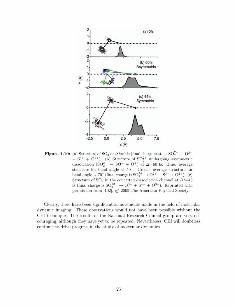
Figure 1.10: (a) Structure of SO2 at ∆t=0 fs (final charge state is SO7+2 → O2+

+ S3+ + O2+). (b) Structure of SO2+2 undergoing asymmetric

dissociation (SO2+2 → SO+ + O+) at ∆=60 fs. Blue: average

structure for bend angle < 50. Green: average structure forbend angle > 70 (final charge is SO7+

2 → O2+ + S3+ + O2+). (c)Structure of SO2 in the concerted dissociation channel at ∆t=45fs (final charge is SO10+

2 → O3+ + S4+ + O3+). Reprinted withpermission from [102]. c© 2005 The American Physical Society.

Clearly, there have been significant achievements made in the field of moleculardynamic imaging. These observations would not have been possible without theCEI technique. The results of the National Research Council group are very en-couraging, although they have yet to be repeated. Nevertheless, CEI will doubtlesscontinue to drive progress in the study of molecular dynamics.

25

Chapter 2

Ultrafast Imaging Apparatus

2.1 Laser System

The multi-gigawatt femtosecond laser system used in this work was developed byStephen J. Walker and is described in detail in his Master thesis [105]. Briefly, theKerr lens mode-locked Ti:sapphire oscillator (Femtolasers Femtosource ScientificPro) is pumped by a 5 W Nd:YVO4 (Spectra-Physics Millennia, 532 nm, M2 < 1.1)and produces 9.2 fs, 5 nJ, 800 nm pulses with a repetition rate of 75 MHz. Unlike atypical chirped pulse amplification scheme [106], no stretcher is used. Instead, thepulse is stretched by the transmissive optical elements in the regenerative amplifier.The regenerative amplifier consists of a Brewster-cut Ti:sapphire crystal pumpedby a 20 W frequency-doubled Nd:YLF (Quantronix Falcon, 527 nm, 20 mJ, M2 <17), two curved end mirrors, a polarizing beam splitter and a Pockels cell operatingas either a quarter or half wave plate. The Pockels cell rejects the majority of theseed pulses from the oscillator and only a single seed pulse will circulate within thecavity at any given time. A seed pulse switched into the cavity will make sixteenpasses through the Ti:sapphire crystal and acquires ∼ 400 µJ of energy beforebeing switched out by the Pockels cell. A double prism-pair is used to compressthe amplifier output and yields compressed pulses with ∼ 300 µJ of energy, arepetition rate of 1 kHz and a pulse duration as low as 40 fs.

2.1.1 Peak intensity

50 fs laser pulses were focused by a parabolic mirror (f = 2.1 cm, φ = 14 mm)located within the time-of-flight spectrometer (described in a later section). Thelaser power, P , is defined as:

P = E/t (2.1)

where E is the energy per pulse and t is the pulse duration. Many molecularphenomena are determined by the intensity of the focused laser spot, I, defined as:

26

I =P

A

where A is the area of the focus. For a Gaussian beam, the on-axis peak intensityis given by

I(z) =2P

πw2(z)(2.2)

where w(z) is the beam radius. If the minimum spot size of the incoming Gaussianbeam, w0, is located at the mirror, the spot size at the focus, wf , is related to thefocal length of the parabolic mirror, f and the wavelength of the light, λ, accordingto

wf ∼=λf

πw0

(2.3)

where we have assumed that the focal distance is large with respect to the Rayleighrange [107]. Upon substituting the parameters of our laser system into equations2.2 and 2.3, we find the maximum intensity within the focus to be ∼ 2.4 x 1015 Wcm−2.

2.2 Vacuum System

The experimental apparatus is a stainless steel vacuum chamber designed and fab-ricated by the Science Machine Shop at the University of Waterloo (figure 2.1). Thechamber is cylindrical with a height of 12”, and a diameter of 6”. The chamber isequipped with an 8” ConFlat top flange from which the time-of-flight mass spec-trometer is suspended, two 4.5” ConFlat side flanges, and six 2.75” ConFlat flangesfor view ports and instrumentation. The 4.5” and 2.75” flanges sit in two “decks”.A turbomolecular pump (Pfeiffer Vacuum, TMU 071 P, 50 L/s) mounted to oneof the chamber’s side 4.5” ConFlat flanges evacuates the chamber to an ultimatepressure of 7 x 10−10 Torr. A cold cathode gauge (MKS Instruments, HPS 943) isused for pressure monitoring. The laser propagation axis passes through centre oftwo of the 2.75” ConFlat flanges on the lower deck. The windows are zero profilequartz (1.4” diameter, 0.125” thick). The experimental target gas is introducedeffusively through a leak valve, which is attached to one of the 2.75” flanges on thelower deck. Kapton wiring in the detector limit the chamber’s bake-out tempera-ture to ∼ 150 C. A gas manifold is attached to the vacuum chamber to allow upto three experimental targets to be mounted to the system simultaneously.

27

Figure 2.1: Schematic diagram of vacuum chamber. The topmost figure showsthe chamber integrated into the vacuum system, with the front ofthe chamber pointing towards the top of the page. The lower leftand lower right diagrams show only the chamber, with the upperand lower flange decks offset by 45.

2.3 Time-of-Flight Mass Spectrometer

Laser pulses are focussed within a high-resolution time-of-flight mass spectrometer.Ions produced by laser-molecule interaction are accelerated towards the position-sensitive detector by the spectrometer’s static electric field.

2.3.1 Single-stage extraction

Conventional Wiley-McLaren spectrometers include one or two acceleration regionsand a field-free or “drift” region [53]. The instrument created for this work differsin that it is composed of a single acceleration region with no internal grids andno drift region. Since the ultimate goal was to produce high-quality images withthe position-sensitive detector, internal grids were not employed as these tend toact as lenses, scattering ions enroute to the detector. Unlike traditional Wiley-McLaren instruments, the single-stage, no-drift design does not permit space- or

28

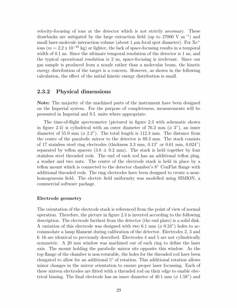
velocity-focusing of ions at the detector which is not strictly necessary. Thesedrawbacks are mitigated by the large extraction field (up to 27000 V m−1) andsmall laser-molecule interaction volume (about 1 µm focal spot diameter). For Xe+

ions (m = 2.2 x 10−25 kg) or lighter, the lack of space-focusing results in a temporalwidth of 0.1 ns. Since the ultimate temporal resolution of the detector is 1 ns, andthe typical operational resolution is 2 ns, space-focusing is irrelevant. Since ourgas sample is produced from a nozzle rather than a molecular beam, the kineticenergy distribution of the target is a concern. However, as shown in the followingcalculation, the effect of the initial kinetic energy distribution is small.

2.3.2 Physical dimensions

Note: The majority of the machined parts of the instrument have been designedon the Imperial system. For the purpose of completeness, measurements will bepresented in Imperial and S.I. units where appropriate.

The time-of-flight spectrometer (pictured in figure 2.3 with schematic shownin figure 2.4) is cylindrical with an outer diameter of 76.2 mm (φ 3”), an innerdiameter of 55.9 mm (φ 2.2”). The total length is 112.3 mm. The distance fromthe centre of the parabolic mirror to the detector is 89.3 mm. The stack consistsof 17 stainless steel ring electrodes (thickness 3.3 mm, 0.13” or 0.61 mm, 0.024”)separated by teflon spacers (3.8 ± 0.2 mm). The stack is held together by fourstainless steel threaded rods. The end of each rod has an additional teflon plug,a washer and two nuts. The centre of the electrode stack is held in place by ateflon mount which is connected to the detector chamber’s 8” ConFlat flange withadditional threaded rods. The ring electrodes have been designed to create a near-homogeneous field. The electric field uniformity was modelled using SIMION, acommercial software package.

Electrode geometry

The orientation of the electrode stack is referenced from the point of view of normaloperation. Therefore, the picture in figure 2.3 is inverted according to the followingdescription. The electrode furthest from the detector (the end plate) is a solid disk.A variation of this electrode was designed with two 6.1 mm (φ 0.24”) holes to ac-commodate a lamp filament during calibration of the detector. Electrodes 2, 3 and6–16 are identical to previously described. Electrodes 4 and 5 are not cylindricallysymmetric. A 20 mm window was machined out of each ring to define the laseraxis. The mount holding the parabolic mirror sits opposite this window. As thetop flange of the chamber is non-rotatable, the holes for the threaded rod have beenelongated to allow for an additional 5 of rotation. This additional rotation allowsminor changes in the mirror orientation to ensure proper laser focussing. Each ofthese sixteen electrodes are fitted with a threaded rod on their edge to enable elec-trical biasing. The final electrode has an inner diameter of 40.1 mm (φ 1.58”) and

29

Figure 2.2: Time-of-flight mass spectrometer components. The majority of thecomponents in the electrode stack are rings as shown in (a). Thelast electrode has a thickness of 0.024” and includes a tungstenmesh to ensure electric field uniformity (not shown). The end plate,shown in (c), has identical thickness to the rings. Under normaloperation, (c) is used, however, a variant (d) allows for a lampfilament to be placed at the bottom of the electrode stack for useas an ion source.

a thickness of 0.61 mm (0.024”). The aperture on this electrode is covered withtungsten mesh (Unique Wire Weaving, 40 x 40 wires per inch, φ 0.001”, 92.2% openarea), which is clamped in place with a small stainless steel spacer. The design ofthe last, or top electrode is similar to those in the detector and it includes a tabfor electrical biasing.

On-axis parabolic mirror

The on-axis parabolic mirror (aluminum-coated glass, φ 14 mm, 21 mm focal length)is mounted in a custom teflon holder that is attached to the fourth electrode in thestack. The metallic surface of the mirror is biased at the average potential of thefourth and fifth electrodes.

30

Figure 2.3: Time-of-flight mass spectrometer. The 17 electrodes are separatedby teflon spacers (white areas in photograph). The electrode stackis cradled by the teflon frame. The frame is suspended from the8” ConFlat flange by four threaded rods. The bright disk near thetop is the parabolic mirror. The resistors used for electrical biasingcan be seen down the right-hand side of the stack.

Electrode biasing

The electrode stack is electrically isolated to allow flexibility when biasing the spec-trometer. Under typical operation when ions are collected, the bottom electrodeis biased at a positive voltage while the top electrode is independently biased toa near-zero voltage. Two power supplies (Fluke model 415B) are used to generatehigh voltages (0–3 kV) corresponding to a maximum acceleration voltage of 270V cm−1. A uniform electric field is created by decreasing the potential of eachelectrode with a voltage divider network. Adjacent electrodes are connected with 2MΩ ultrahigh vacuum-compatible resistors (Riedon Inc., 2 MΩ ± 0.5%, uncoated,P/N MF2207). Once mounted to the electrodes, as seen on the right side of figure2.3, the entire electrode stack can be biased using only two electrical feedthroughs.The parabolic mirror, located between the fourth and fifth electrodes, is biasedusing resistors chained to the electrode stack. Two resistors in parallel connect themirror to the fourth electrode and another pair of resistors in parallel connect the

31

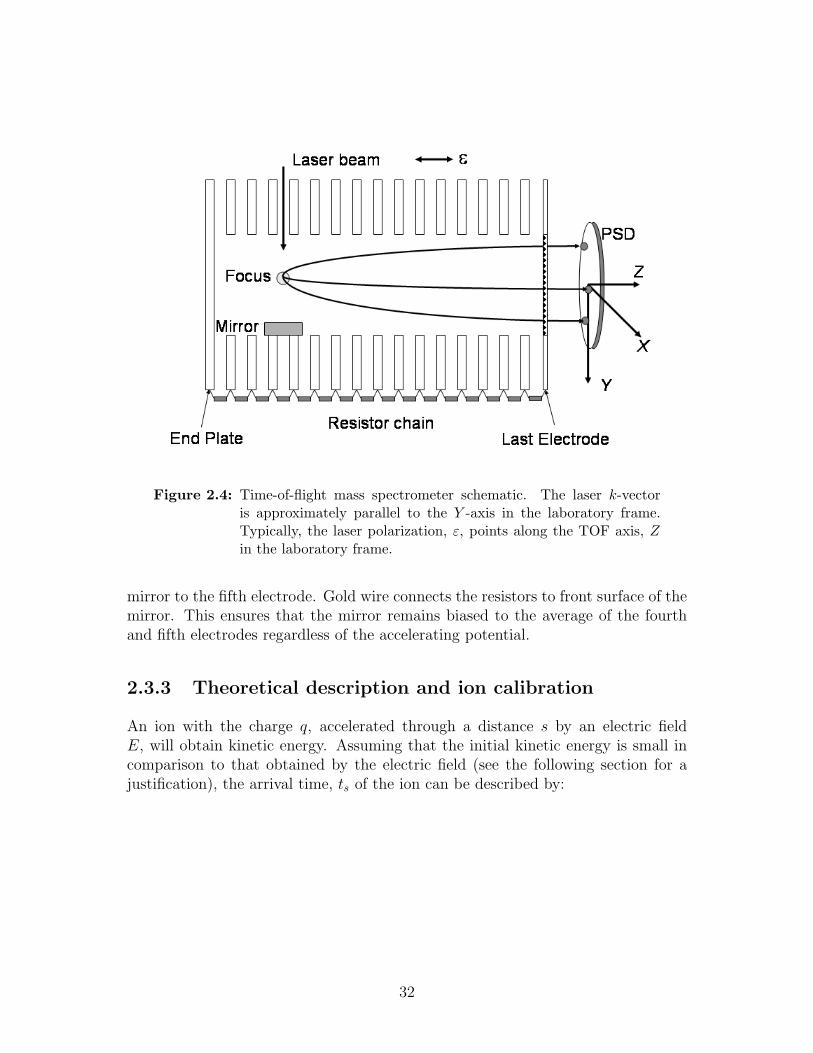
Figure 2.4: Time-of-flight mass spectrometer schematic. The laser k-vectoris approximately parallel to the Y -axis in the laboratory frame.Typically, the laser polarization, ε, points along the TOF axis, Zin the laboratory frame.

mirror to the fifth electrode. Gold wire connects the resistors to front surface of themirror. This ensures that the mirror remains biased to the average of the fourthand fifth electrodes regardless of the accelerating potential.

2.3.3 Theoretical description and ion calibration

An ion with the charge q, accelerated through a distance s by an electric fieldE, will obtain kinetic energy. Assuming that the initial kinetic energy is small incomparison to that obtained by the electric field (see the following section for ajustification), the arrival time, ts of the ion can be described by:

32

KE = qEs1

2mv2 = qEs

ds

dt= v =

√2qEs

m∫ ts

t0

dt =

√m

2qE

∫ s

0

ds√s

ts − t0 =

√2ms

qE

ts =

√2ms

qE+ t0 (2.4)

It should be noted that equation 2.4 is not exact since there is a small gapbetween the top electrode and the input of the detector. However, by applying asmall positive voltage to the top electrode, the homogeneous electric field can beextended to the input of the detector, even though the detector and electrode stackare electrically isolated. Therefore, s can be taken to be the distance between thefocus of the parabolic mirror and the detector input (' 89.3 mm). The magnitudeof the electric field, E, is given by V/L, where V is the accelerating voltage and Lis the total length of the electrode stack, 112.3 mm.

Referring to equation 2.4, calibration of the instrument is performed by plottingthe arrival time, ts of a series of ions versus

√m/q for a known composition of gas.

Typically, one will use background ions and noble gas ions, for example H+2 , N+

2 ,O+

2 , H2O+ and Xe+. If the mass and charge assignments of the ions is correct, the

plot will be linear with a slope of√E/2s and an intercept of

√E/2st0. In the

case of figure 2.6, the y-axis has been plotted with m and q in natural numbers.For this reason, the slope of the graph is

√q0E/2m0s, where q0 is the charge on an

electron and m0 is one atomic mass unit. Similarly, the intercept is√q0E/2m0st0.

The quantity t0 is the delay between the trigger signal from the Pockels cell driverand the pump laser firing.

Based on the peak width in figure 2.5, the mass resolution of the spectrometeris ' 125 using a sampling rate of 250 MS s−1. Under typical operating conditions,a faster sampling rate of 500 MS s−1 is used to acquire data, giving a temporalresolution two times better than indicated here.

Justification of small initial kinetic energy

Let us assume that a singly charged carbon ion (m = 1.993 x 10−26 kg, e = 1.602 x10−19 C) is accelerated through a distance of s = 8.93 x 10−2 m by an electric fieldE = 18000 V m−1. The kinetic energy picked up by such a particle would be:

33

2.4 2.6 2.8 3 3.2 3.4 3.60

0.5

1

1.5

2x 10

4

ts / µs

Cou

nts

Xe2+

Xe+

Figure 2.5: Time-of-flight spectrum for xenon isotopes with charge 2+ (firstgroup) and charge 1+ (second group). Within each group, thepeaks correspond to Xe129, Xe131,132, Xe134 and Xe136. The rel-ative abundances of each isotope agrees with the observed signal.The widths of the isotope peaks correspond to a mass resolution ofm/∆m ∼ 125.

0 1 2 3 4−2

0

2

4

6

8

10

12

14

Time / µs

(m/q

)1/2

Figure 2.6: Ion calibration graph. Using isotopes of xenon, as well as hydrogenand water, the empirical scaling factor of the spectrometer can beextracted. Noting that the y-axis of this graph has been plottedin natural numbers, the slope is 3.826 x 106 with an intercept of-1.5145.

34

KE = eEs

KE = 2.58 x 10−16 J (2.5)

The Maxwell-Boltzmann distribution of speeds for particles of mass m, withspeed v at temperature T (in Kelvin) is written:

f(v) = 4πm

2πkT

3/2

v2exp

[−mv2

2kT

](2.6)

0 500 1000 1500 2000 2500

Speed / m s−1

Pro

babi

lity

Figure 2.7: Maxwell-Boltzmann distribution for C+ ions at 25C. The mostprobable speed is 735.4 m s−1.

The speed probability is plotted in figure 2.7. The most probable speed at 25Cis 735.4 m s−1. This gives a kinetic energy of:

KE =1

2mv2 (2.7)

KE = 5.39 x 10−21 J (2.8)

Thus, the thermal kinetic energy is about four orders of magnitude less thanthe kinetic energy imparted by the electric field. Furthermore, since the mostprobable speed decreases with particle mass and the kinetic energy imparted bythe electric field increases with charge state, the thermal kinetic energy will becomemore negligible if we examine larger particles or more highly charged ions.

Another, perhaps more critical comparison, is the momentum of the fragmentsat the moment of explosion in comparison to the ion energies after extraction. Thatis, the initial momentum should satisfy, pz

√2mqEs [108]. Using the same ion

35

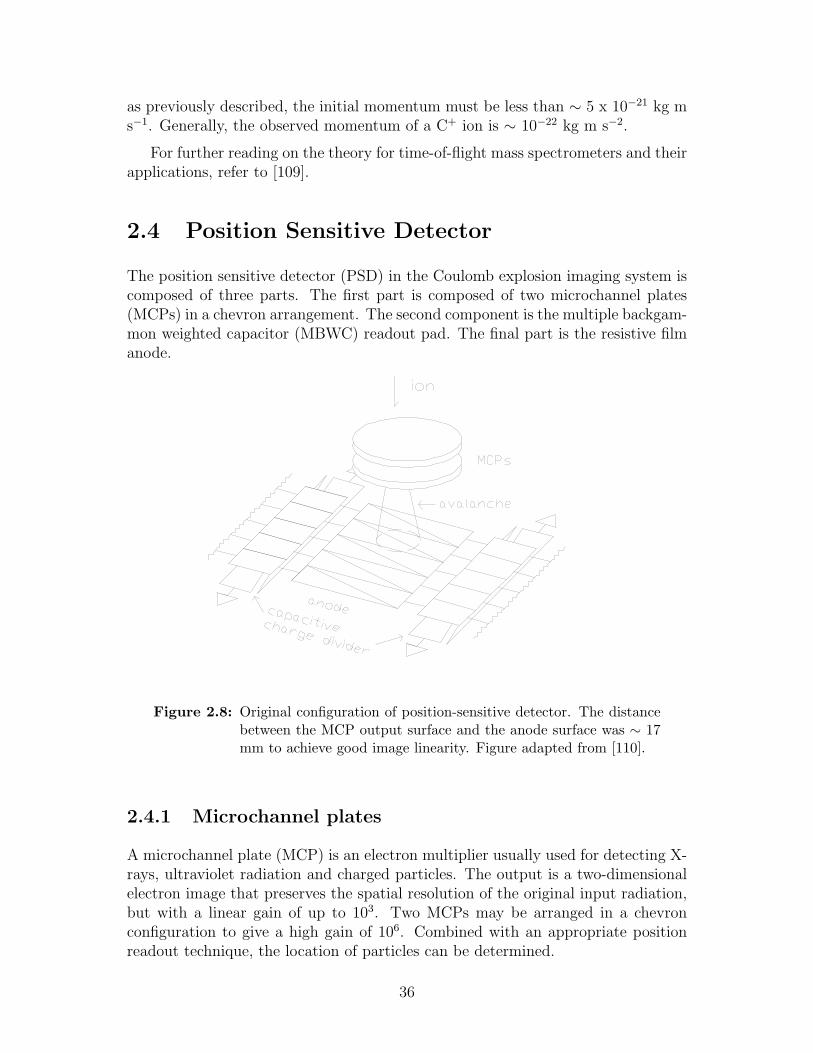
as previously described, the initial momentum must be less than ∼ 5 x 10−21 kg ms−1. Generally, the observed momentum of a C+ ion is ∼ 10−22 kg m s−2.

For further reading on the theory for time-of-flight mass spectrometers and theirapplications, refer to [109].

2.4 Position Sensitive Detector

The position sensitive detector (PSD) in the Coulomb explosion imaging system iscomposed of three parts. The first part is composed of two microchannel plates(MCPs) in a chevron arrangement. The second component is the multiple backgam-mon weighted capacitor (MBWC) readout pad. The final part is the resistive filmanode.

Figure 2.8: Original configuration of position-sensitive detector. The distancebetween the MCP output surface and the anode surface was ∼ 17mm to achieve good image linearity. Figure adapted from [110].

2.4.1 Microchannel plates

A microchannel plate (MCP) is an electron multiplier usually used for detecting X-rays, ultraviolet radiation and charged particles. The output is a two-dimensionalelectron image that preserves the spatial resolution of the original input radiation,but with a linear gain of up to 103. Two MCPs may be arranged in a chevronconfiguration to give a high gain of 106. Combined with an appropriate positionreadout technique, the location of particles can be determined.

36

Each plate consists of an array of tiny glass tubes fused together to form a thindisc. Both faces of the disc are metallized to provide parallel electrical connectionsto all channels. In a vacuum, and with a potential difference of 800 V ∼ 1400 Vacross the plate, each channel becomes a continuous dynode electron multiplier,operating on the same principle of electron avalanche as the single-channel electronmultiplier.

The MCPs (part number G12-46DT/13/E/A, channel diameter 12µm, plate sizeφ 46 mm, aspect ratio 80:1, bias angle 13, engineering grade, resistance 177 MΩ)for the PSD were purchased from Photonis Imaging Sensors. They are resistancematched.

2.4.2 Modified backgammon technique with weighted ca-pacitors readout pad

To perform position readout measurements, one must use MCPs in conjunctionwith a position sensitive anode. To date, a number of position sensitive anodeshave been developed, including resistive anodes [111], delay lines [112], crossed-wire detectors [28] and wedge-and-strip anodes [113]. The latter three types areused if high temporal resolution is required. The best temporal and positionalresolutions attained by the delay-line method are reported to be 0.6 ns and 30 µm,respectively.

In 1992, Mizogawa et al. reported a new anode described as the “modifiedbackgammon method with weighted capacitors” (MBWC) anode [27]. The MBWCanode is based on two previous techniques, the weighted coupling capacitors (WCC)method [114, 115] and the backgammon method [116]. Our MBWC anode is basedon Mizogawa’s design and was acquired from Tokyo Metropolitan University. Com-mercial anodes are distributed through Optima Corporation.

Backgammon method

The backgammon method is a well-known one-dimensional position-readout tech-nique. The anode of a MCP-based charged-particle detector is divided into tworegions by a zigzag insulating line, shown in figure 2.9. The pitch of the zigzag is2–3 mm, creating two groups of many sharp wedges, the tips of which are pointedleft for one group and right for the other. An incoming particle will interact withthe MCPs, creating a charge cloud. This charge cloud falls onto the plane andcovers several repetitions of the zigzag, separating into two charge fractions (right,or QR, and left, or QL). The ratio of this geometrical charge separation dependson the position of the charge cloud centroid in a linear fashion. Therefore, the twocharge signals provide one-dimensional position information.

37

Figure 2.9: Schematic of one-dimensional backgammon method. The electroncloud falls on the zigzag pattern and splits into two, QL and QR.The position of the centroid of the electron cloud, as measured fromthe left edge of the anode, would be QR/(QR +QL).

Two-dimensional position readout

The backgammon method can be modified to provide two-dimensional position in-formation. Mizogawa et al. [27] adopted the WCC method [114], creating the com-bined two-dimensional technique the modified backgammon method with weightedcoupled capacitors (MBWC), as shown in figure 2.8. The use of appropriate read-out electrodes coupled by capacitance allows the pattern printed on the anode tobe a simple iteration of the wedges. The result is good imaging linearity and veryhigh positional resolution in most of the active area of the MCP. Under ideal con-ditions, one can resolve the capillaries of the MCP, providing an unmatched spatialresolution of 10∼15 µm [110] and has been used in a variety of Coulomb explosionexperiments [117, 32, 31, 35, 33, 34].

38

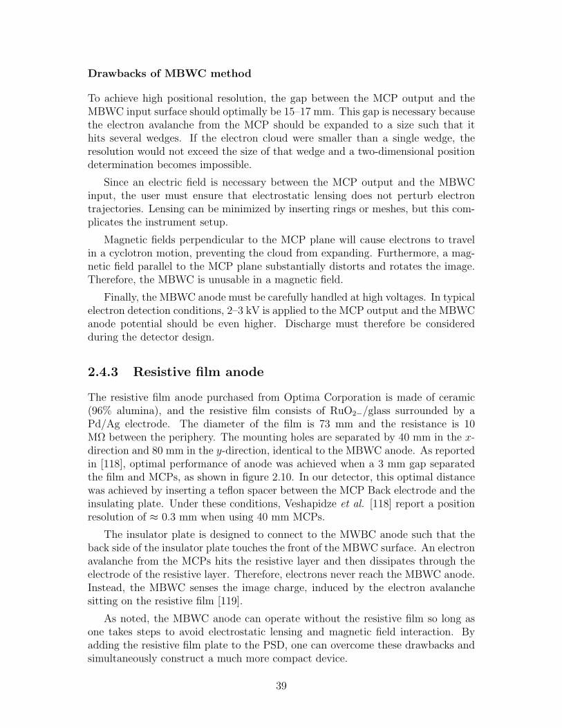
Drawbacks of MBWC method

To achieve high positional resolution, the gap between the MCP output and theMBWC input surface should optimally be 15–17 mm. This gap is necessary becausethe electron avalanche from the MCP should be expanded to a size such that ithits several wedges. If the electron cloud were smaller than a single wedge, theresolution would not exceed the size of that wedge and a two-dimensional positiondetermination becomes impossible.

Since an electric field is necessary between the MCP output and the MBWCinput, the user must ensure that electrostatic lensing does not perturb electrontrajectories. Lensing can be minimized by inserting rings or meshes, but this com-plicates the instrument setup.

Magnetic fields perpendicular to the MCP plane will cause electrons to travelin a cyclotron motion, preventing the cloud from expanding. Furthermore, a mag-netic field parallel to the MCP plane substantially distorts and rotates the image.Therefore, the MBWC is unusable in a magnetic field.

Finally, the MBWC anode must be carefully handled at high voltages. In typicalelectron detection conditions, 2–3 kV is applied to the MCP output and the MBWCanode potential should be even higher. Discharge must therefore be consideredduring the detector design.

2.4.3 Resistive film anode

The resistive film anode purchased from Optima Corporation is made of ceramic(96% alumina), and the resistive film consists of RuO2−/glass surrounded by aPd/Ag electrode. The diameter of the film is 73 mm and the resistance is 10MΩ between the periphery. The mounting holes are separated by 40 mm in the x-direction and 80 mm in the y-direction, identical to the MBWC anode. As reportedin [118], optimal performance of anode was achieved when a 3 mm gap separatedthe film and MCPs, as shown in figure 2.10. In our detector, this optimal distancewas achieved by inserting a teflon spacer between the MCP Back electrode and theinsulating plate. Under these conditions, Veshapidze et al. [118] report a positionresolution of ≈ 0.3 mm when using 40 mm MCPs.

The insulator plate is designed to connect to the MWBC anode such that theback side of the insulator plate touches the front of the MBWC surface. An electronavalanche from the MCPs hits the resistive layer and then dissipates through theelectrode of the resistive layer. Therefore, electrons never reach the MBWC anode.Instead, the MBWC senses the image charge, induced by the electron avalanchesitting on the resistive film [119].

As noted, the MBWC anode can operate without the resistive film so long asone takes steps to avoid electrostatic lensing and magnetic field interaction. Byadding the resistive film plate to the PSD, one can overcome these drawbacks andsimultaneously construct a much more compact device.

39

Figure 2.10: Modified configuration of position-sensitive detector. The dis-tance between the MCP output surface and the anode surfacewas 3 mm to achieve good image linearity.

2.5 Data Capture

The four output signals from the readout pads of the MBWC are connected to BNCconnectors on the 8” top flange of the experimental chamber. The output signalsare amplified by preamplifiers and fed to the PC oscilloscope cards. Once acquired,the data is stored on the hard disk and analysed by software.

2.5.1 Pre-amplifiers

The pre-amplifiers (Ortec Model 142B) used in the system have two outputs, energy(E) and timing (T). Only the energy output is used, so the timing output mustbe terminated in 50 Ω for optimal performance. The energy output signal fromthe pre-amplifier is a fast-rise-time voltage step with an exponential return to thebaseline. The timescale of this return is ∼ 1 ms. The polarity of these outputpulses is inverted from the signal polarity at the detector output. In our case, thepositive bias polarity is used for the detector, thus the E output of the preamplifieris positive.

2.5.2 Gage oscilloscope cards

Data capture is performed by the PC oscilloscope cards (Gage CS82G), purchasedfrom Gage Applied Inc. Two cards are linked in a master-slave arrangement suchthat signals from four channels can be captured simultaneously. Data is acquired

40

for each shot of the laser system, which has a repetition rate of 1 kHz. Oncetriggered by the Pockels cell driver, the PC cards will acquire data, 10-bit in timeand 8-bit in voltage. Typically, the sampling rate is set to 500 MS/s, giving a totalacquisition time of just over 2 µs and a temporal resolution of 2 ns.

Since all raw data is saved for each acquisition, a large amount of storage spaceis required. In fact, 4 MB of data are generated each second, and a typical 25minute data run consumes ∼ 5 GB. Once data has been acquired, it is filtered andanalysed to conserve hard disk space.

2.5.3 Event identification, ion impact time and position

Signals are read from the four outputs of the detector are recorded by the Gageboards as digitized traces with 10 bits of horizontal (time) resolution and 8 bits ofvertical (voltage) resolution. The four outputs are described in terms of a Cartesianrepresentation of the detector. The connections between detector outputs and Gageboard inputs are given in table ??.

Output Board ChannelIxy 1 AIxy 1 BIxy 2 AIxy 2 B

Table 2.1: Detector outputs and Gage board inputs. Note that for entries inthe first column, the notation x indicates the output in the negativex-direction.

Figure 2.11 shows a typical signal trace from the four channels of the detector.Ion impacts are indicated by large steps in the detector signal.

Although the total vertical resolution is 8-bits, the signal height of a typicalevent ranges between 10∼80. For a given event, the position (x0, y0) is given by

x0 =Ixy + Ixy∑

I(2.9)

y0 =Ixy + Ixy∑

I(2.10)

where

∑I = Ixy + Ixy + Ixy + Ixy (2.11)

Equations 2.9 and 2.10 will give the position of an ion in arbitrary units. Thatis, the scaling of the voltages will return x0 and y0 values in the range of 0 to 1.

41

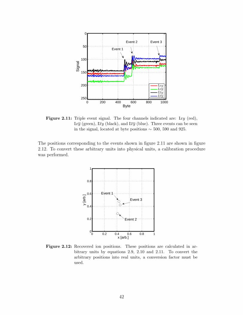
0 200 400 600 800 1000

0

50

100

150

200

250

Byte

Sig

nal

IxyIxyIxyIxy

Event 1

Event 2 Event 3

Figure 2.11: Triple event signal. The four channels indicated are: Ixy (red),Ixy (green), Ixy (black), and Ixy (blue). Three events can be seenin the signal, located at byte positions ∼ 500, 590 and 925.

The positions corresponding to the events shown in figure 2.11 are shown in figure2.12. To convert these arbitrary units into physical units, a calibration procedurewas performed.

0 0.2 0.4 0.6 0.8 10

0.2

0.4

0.6

0.8

1

x [arb.]

y [a

rb.] Event 1

Event 3

Event 2

Figure 2.12: Recovered ion positions. These positions are calculated in ar-bitrary units by equations 2.9, 2.10 and 2.11. To convert thearbitrary positions into real units, a conversion factor must beused.

42

2.5.4 Detector calibration

Once the detector was installed, calibration was performed using a tungsten lampfilament mounted on the bottom plate of the electrode stack. The filament actedas an ion source independent of the laser and gas target.

A stainless steel mask (see figure 2.13) was mounted in front of the MCP inputon the detector. The mask consisted of a regular array of φ 0.25 mm, φ 0.5 mm,and φ 1 mm holes. The centres of the holes were separated by 5 mm. The axis ofthe array is offset from the x− y axis of the detector by 10.

Figure 2.13: Calibration mask. The mask consists of a regular array of φ 0.25mm, φ 0.5 mm, and φ 1 mm holes. The centres of the holes wereseparated by 5 mm. The array was offset from the x − y axisof the detector by an angle of 10. The mask was not four-foldsymmetric. One of the holes near the centre of the mask was madesmaller than the others to assist with identifying the orientation.

Approximately 106 ion events were used to reproduce the mask geometry, shownin figure 2.14. The recovered hole positions were matched to the known maskgeometry by employing a series of linear transformations (see following section).The numerical values of the matrix elements used in the stretch and shear matrixwere obtained by fitting the two data sets with a least squares fitting routine.

Refer to Appendix A for the algorithm used for geometry correction based onthe calibration above.

2.5.5 Frames of reference

Two frames of reference are important in an ultrafast imaging system. The first isthe laboratory frame (X, Y, Z) where measurements are made. The second is themolecular frame (x, y, z) where structure and dynamics are viewed.

43

−20 −10 0 10 20

−20

−10

0

10

20

x / mm

y / m

m

Figure 2.14: Recovered calibration mask. The blue dots and holes correspondto the machined mask geometry. The red dots and mask corre-spond to the recovered geometry once the calibration factor hasbeen included. A micromesh, accompanied by a more complicatedalgorithm could also be used to calibrate a detector.

The laboratory axes correspond to the natural axes of the spectrometer anddetector. The detector has an x− and y−axis, as indicated in the proceedingsection. These are the X- and Y -axes in the laboratory frame. The Z-axis is theflight axis of the spectrometer. The origin of the laboratory frame is directly belowthe geometric centre of the detector, level with the laser focus. While convenient, itis not necessary for the laser focus to be located beneath the centre of the detector.The X- and Y -coordinates of the laser focus can be determined by singly ionizinga background gas within the chamber. The centre of the ion impact distributioncorresponds to the coordinates of the laser focus. The measurement was performedusing nitrogen gas (N+

2 ) and, as indicated by figure 2.15, show the focal coordinatesat (-2.4 mm,-4.9 mm).

In order to calculate momentum values in the molecular frame, the spatialorigins (X0,Y0) must be determined for each applicable species of ion. A robustalgorithm was employed to make precise determination of the spatial origins. Usingfigure 2.15 as an example, the number of ion impacts are histogrammed as a functionof the X- and Y -coordinates to produce H(X) and H(Y ). A nonlinear fitnessfunction is evaluated for each coordinate using the histogram. The fitness functionis:

A(X) =20∑

δ=−20

H(X + δ)H(X − δ) (2.12)

The functions H(X), A(X), H(Y ) and A(Y ) are plotted in figure 2.16. Notethat A(X) and A(Y ) are not designed to recreate the width of H(X) or H(Y ),

44

10

20

30

40

50

60

70

−4 −3.5 −3 −2.5 −2 −1.5 −1−6.5

−6

−5.5

−5

−4.5

−4

−3.5

x / mm

y / m

m

Figure 2.15: Spatial origin of nitrogen gas. The ion impact distribution result-ing from N+

2 is shown. Since the mean velocity of the backgroundgas is zero, the centre of the distribution (-2.4 mm,-4.9 mm) islocated above the laser focus.

but will simply find the peak value. This example used simple histograms, but thealgorithm in equation 2.12 will also find the maximum value for double-peaked his-tograms, which would result from using linearly polarized light with its polarizationvector parallel to the detector plane.

−4 −3 −2 −10

0.2

0.4

0.6

0.8

1

X / mm

Sig

nal [

arb.

]

−6 −5 −40

0.2

0.4

0.6

0.8

1

Y / mm

(a) (b)

Figure 2.16: Spatial origin determination. Histograms of the X− andY−positions for N+

2 ions are shown in (a) and (b) respectively(blue, solid line) along with the calculated A(X) and A(Y ) (red,broken line). The spatial origin (-2.4 mm, -4.9 mm) correspondsto the peak positions of A(X) and A(Y ).

45

2.5.6 Three-dimensional momentum determination

The ability to determine three-dimensional fragment momenta is essential for ul-trafast imaging. Measured in the laboratory frame, (X, Y, Z), the ion momentumcomponents immediately following ionization are given by:

pX = m(X −X0)

t

pY = m(Y − Y0)

t

pZ =qE

2

(t20 − t2)t

(2.13)

In equations 2.13, m is the fragment mass, (X, Y ) is the ion impact positionin the laboratory frame, (X0, Y0) is the ion-dependent spatial origin, t is the flighttime, E is the electric field, q is the charge and t0 is the arrival time for a zero-kinetic energy ion with the same m/q ratio determined via mass calibration of thetime-of-flight spectrum.

Fragment momentum calibration

To establish the uniformity of the electric field, nitrogen gas was multiply ionizedusing linearly polarized laser pulses. Since the nitrogen molecules were not alignedprior to ionization, only molecules that were initially aligned with the electric fieldof the laser would ionize. The linearly polarized beam was rotated with a half-wave plate in 10 increments. At each position, approximately 106 uncorrelated ionimpacts were recorded and their momentum was calculated according to 2.13. Wecan define a new coordinate system, (X ′, Y ′, Z), where the laser beam propagationaxis was in the Y ′−direction, while the polarization was rotated in the X ′−Z plane.Recalling that X and Y are defined as the axes of the detector, the angle betweenthe X and X ′ axis is θ, while the angle between Y and Y ′ is φ. Two-dimensionalhistograms of the fragment momenta were computed, normalized and summed toproduce figure 2.17. The general shape of the plots is as expected. If θ = φ = 0,the pX vs. pY plots should be a horizontal line, while the pX vs. pZ plots shouldbe a circle and the plots of pY vs. pZ should be a vertical line. From the shape offigure 2.17(g), the angle θ is approximately 14, while from figure 2.17, the angle φis approximately 3.

2.6 Data Processing and Analysis

This section outlines data analysis algorithms common to all experiments withthe apparatus. These algorithms include (a) identifying triple coincidences, (b)

46

Figure 2.17: Nitrogen momentum component distribution. Different chargestates and momentum components are plotted in each figure. N+

is plotted in (a)–(c), with pY vs. pX in (a), pZ vs. pX in (b) and pZvs. pY in (c). Similarly, (d)–(f) plots the momentum componentsof N2+ fragments while the momentum components of the N3+

fragments are plotted in (g)–(i). The 14 tilt that is evident inthe pY vs. pX plots is due to the rotation of the laser-mirror axiswith respect to the X − Y axis of the detector. The 3 tilt in thepZ vs. pY plots is due to the laser not being perfectly parallelwith the plane of the detector. These tilts can be removed withsoftware during processing. Horizontal white areas in the plotscannot be measured in coincidence due to the dead time of thedetector.

47

identifying ion mass and charge, (c) transforming ion impact data into the three-dimensional momentum information. Specialized software has been developed tofacilitate the collection and analysis of all data from the instrument.

2.6.1 Correlated ion events

Correlated events are those in which two or more events are detected for a singlelaser shot. In the case of triatomic molecules, three events must be detected toreconstruct the geometry. Given the ultimate detector efficiency of 50% per event,the probability of collecting all fragments from the Coulomb explosion of a tri-atomic molecule is, at best, 12.5%. Uncorrelated ion events, which may arise frommetastable ions, impurities such as water, and Coulomb explosions where not allfragments are detected are ignored at this stage. Approximately 5% of all lasershots produce a triple coincidence event.

Locating correlated ion events

The raw data from the Gage cards is recorded onto the PC hard disk in the pro-prietary .SIG file format using the “gagescan” program. Once a 30-minute datarun is completed, the raw data must be filtered to locate the time of ion impacts.“FindEvent” program was written to perform high-speed filtering and analysis ofthe raw data files. The algorithm used for filtering data is given in Appendix A.

2.6.2 Fragmentation channel and momentum

Once correlated triple events have been identified, it is necessary to determine thefragmentation channel and the momentum of each of the fragments.

Determining fragmentation channel

For a given correlated triple event, the fragmentation channel can be deduced fromthe arrival times of the three fragment ions. If the arrival times of the fragmentions are well separated (∼100 ns, the dead time that arises from post-event ripplesin the voltage signal), the fragmentation channel can be deduced directly. However,for highly charged ions with large kinetic energy, it is common for the arrival timesof several species to be quite close to one another. In the time-of-flight spectrum,this produces peaks which will partially overlap. Therefore, a general techniquewas developed to account for ambiguous correlated triple events.

For each arrival time in the triple event, fragments ions that could arrive atthat time are identified. Permutations of possible fragments are created and anynonphysical permutations are removed. For example, if the molecule CS2 was underinvestigation, there must be exactly one carbon fragment and two sulphur fragments

48

for a permutation to be physical. If the molecule is aligned along the axis of thetime-of-flight spectrometer, a further constraint can be imposed. When a linearmolecule such as CS2 explodes, one of the sulphur fragments will be pointing inthe direction of the detector while the other will point in the opposite direction.If both sulphur ions have the same charge, one will arrive first and this is knownas the “forwards” ion. The other sulphur ion must be turned around by the DCelectric field and will arrive later. Therefore, the second sulphur ion is known asthe “backwards” ion. We make use of this “forwards-backwards” condition to seta further constraint to the identification algorithm. That is, each triple event mustconsist of exactly one carbon ion, one forwards sulphur ion and one backwardssulphur ion.

This algorithm will typically produce one or two physical fragmentation channelsfor each triple event. If more than one possibility is generated, false events will beeliminated once the fragment momentum is calculated.

Calculating momentum vector components

With the fragmentation channel determined, the masses, mi, and charges, qi, ofeach ion are known. The flight times, ti, and positions, (xi, yi), are known directlyfrom the detector. Combined with the flight time, t0, and position, (x0, y0), of anion with zero initial kinetic energy, the initial momenta for the ith fragment can becalculated according to:

pxi = mi(xi − x0i)

ti(2.14)

pyi = mi(yi − y0i)

ti(2.15)

pzi =qE

2

(t20i − t2i )ti

(2.16)

Note that just like t0, (x0, y0) are ion-specific. Refer to the earlier calibrationsection for details.

2.6.3 Geometry reconstruction

Once the asymptotic momentum vectors have been identified for a particular ex-plosion channel, the molecular geometry just after the Coulomb explosion can becalculated. In this case, we refer to the molecule’s internal geometry and no longerconsider the orientation of the molecule with respect to the laboratory frame. Inpractice, the laser polarization points along the Z-axis, and randomly orientedmolecules that are aligned with the laser field will preferentially ionize. The gen-eral procedure for geometry reconstruction is described by the following steps:

49

1. Assume an initial geometry. Usually, this will be the equilibrium geometry ofthe neutral parent molecule.

2. Assume a potential energy surface for the fragment ions to evolve on. In thiswork, a Coulomb potential is used exclusively. Other groups have computedab initio potential energy surfaces, which, they asserted, usually have greateraccuracy for lower charge states [102].

3. Allow the system to evolve in time using classical dynamics. This will in-volve using an ordinary differential equation (ODE) solver to compute thetrajectories of the charged fragments according to the Hamiltonian of thesystem.

4. Compare the final computed momenta with the measured momenta. Thenearness of this comparison will act as a fitness parameter for the initialgeometry.

5. Repeat this process for four more guess geometries. The set of five guessgeometries will form a basis for a simplex algorithm. The simplex algorithmexplores the solution space defined by the guess geometries until the optimumgeometry is computed. The simplex algorithm is described in more detail ina later chapter.

Once the final geometry has been calculated, relevant information such as meanbond lengths and bend angles can be extracted.

50

Chapter 3

Molecular GeometryReconstruction

3.1 Introduction

Once fragment momenta have been recorded and the fragmentation channel hasbeen determined, one has, in principle all the necessary information to reconstructthe molecular geometry at the moment of the Coulomb explosion provided themolecule’s initial momentum is zero. To achieve good statistical data, a viableultrafast imaging system must be able to perform this reconstruction procedurequickly. Ideally, “on-the-fly” reconstructions should be possible.

This chapter is composed of two sections. The first section describes the classicalmodel of molecular fragmentation used throughout this work. The second sectionintroduces the concept of nonlinear optimization and the simplex algorithm. Thethird section describes the development of the simplex algorithm that was used toquickly derive initial molecular geometries from measured fragment momenta. Thefinal section outlines some limits of applicability one must consider when applyingthe algorithm to experimental results.

3.2 Molecular Fragmentation Model

This section describes the model used to approximate molecular fragmentation dy-namics. To good approximation, the dynamics involved in a Coulomb explosion canbe described classically. This provides the double benefit of producing a completelytractable problem while retaining the ability to observe interesting physics.

3.2.1 Approximations

Several important approximations were included in the model of molecular dy-namics. To a large extent, these approximations were included to improve the

51

tractability of a complex, nonlinear problem.

• Molecules are quantum systems, where dynamics are best described by wavepackets and probabilities. However, fully quantum mechanical descriptions,particularly in the case of molecular systems are computationally demandingand are accompanied by another series of approximations such as the StrongField Approximation (SFA) and Single Active Electron (SAE) which must beemployed to produce equations which can be computed numerically. However,the adoption of a classical treatment produces a problem that is computable.Ions are treated as infinitesimally small charged particles which will evolveaccording to a well-defined interaction potential.

• A molecule hit by laser pulse will be ionized multiple times on the risingedge of the pulse, so long as the intensity of the pulse is sufficiently large.Assuming that the intensity profile of the pulse has a Gaussian profile in time,the timescale of these ionization events is determined by the pulse durationand peak pulse intensity. For a laser pulse that has a duration of 50 fs, thetime between successive ionization events may be 5 fs or less. Rather thankeep track of the dynamics of the molecule during ionization, simulationsproceed directly to the final ionization state.

• The nuclei are considered to be fixed at their equilibrium positions until thefinal ionization. The ions gain no momentum as a result of their interactionpotential or from the laser field. By demanding that the initial momentum bezero for all particles, the reconstruction procedure is greatly simplified. Thisapproximation is significant; an attempt to correct for this approximation ismade for CO2.

• In the time-of-flight spectrometer, a DC electric field is used to accelerate theions toward a position-sensitive detector. The ions will gain momentum asthey move through the electric field. However, while the total flight time ofthe ions is on the order of µs, the fragmentation process we model will takeplace in 10 ps. Over the time period of the fragmentation, the ions will gainnegligible momentum from the electric field.

• During the ionization process, several electrons will be stripped from themolecule due to the influence of the intense laser pulse. The momentum ofthese electrons is ∼1% of the momentum of the ions and is neglected.

3.2.2 Interaction potential

The interaction between the three positively charged particles is described by aCoulomb potential. While more sophisticated ab initio potential surfaces can becomputed using commercial software such as Gaussian, the validity of these ab ini-tio potentials is unclear for highly charged molecular species. Although at least

52

one group has used ab initio potential energy surfaces to analyze their Coulombexplosion data [102], most previous work has been done by assuming a Coulom-bic interaction. Also, it has been shown for highly charged ion experiments onCSq+2 (q=3–10) [34], that a simple Coulomb model accurately predicts the kineticenergy released by the explosion fragments. Finally, the Coulomb interaction pro-vides an analytic description for the potential energy surface of the ionic moleculeand therefore allows fast computation of the ordinary differential equations of thesystem.

3.2.3 System Hamiltonian

For the remainder of this chapter, all geometric notation refers to the molecularframe. Although the laser polarization vector is aligned with the TOF axis, and weverify that molecules preferentially fragment along the laser polarization direction,we will ignore the laboratory frame until later in the chapter.

Consider the system shown in figure 3.1. Particles 1, 2 and 3 are described byposition vectors r1, r2 and r3 and momentum vectors p1, p2 and p3. The positionand momentum vectors are defined in terms of some arbitrary origin, which isusually taken to be the centre of mass of the molecule.

r1

r2

r3

p1

p2

p3

Figure 3.1: A simple system of three particles. The origin is located at thecentre of mass of the system.

The Hamiltonian of the system is the sum of all energies in the system. In thiscase, we have the kinetic energies of each of the particles and the Coulomb potentialfrom each of the ions. The total Hamiltonian is described by equation (3.1):

H =1

2m1

∣∣p21

∣∣+ 1

2m2

∣∣p22

∣∣+ 1

2m3

∣∣p23

∣∣+ k

[q1q2|r1 − r2|

+q1q3|r1 − r3|

+q2q3|r2 − r3|

](3.1)

53

The change in position with respect to time is given by the gradient of theHamiltonian with respect to momentum. Therefore for the ith particle:

•ri = ∇pi

H =pimi

(3.2)

The change in momentum with respect to time is given by the gradient of theHamiltonian with respect to position. Some care must be taken with the deriva-tive of the position, since we must consider the difference in the position betweenparticles.

f (r1) =1

|r1 − r2|(3.3)

−∇rif (r1) = − r1 − r2

|r1 − r2|3(3.4)

Using equations (3.3) and (3.4), we get for the derivative of particle 1’s momen-tum vector:

•p1 = −∇r1H = −k

[q1q2 (r1 − r2)

|r1 − r2|3+q1q3 (r1 − r3)

|r1 − r3|3

](3.5)

This is given more generally in equation (3.6):

•pi = −∇ri

H = −∑j 6=i

kqiqj (ri − rj)

|ri − rj|3(3.6)

3.2.4 Simulated time evolution of a linear system

Once the Hamiltonian of the system is described by 3.1, it is a straightforwardprocedure to simulate the evolution of the system over time. Consider a carbondioxide molecule in its equilibrium geometry of r12 = 1.16 A, r23 = 1.16 A, θ = 180,m1 = 16 amu, m2 = 12 amu, m3 = 16 amu. Now assume the molecule is ionized tothe CO3+

2 state, and that each ion carries a charge of +1. The carbon ion is locatedat the origin. The Matlab function ode23, a third-order Runge-Kutta ordinarydifferential equation solver is used to perform the calculation by numerically solvingequations 3.2 and 3.6. During the calculation, the time between successive stepsbegins at 1 attosecond (10−18 s) and increases as the system approaches the asymp-totic momentum condition. Since the molecular ion is initially placed in a lineargeometry, the repulsive Coulomb force will accelerate the oxygen ions in either thepositive or negative x-direction. The carbon ion, which experiences an identicalforce from left and right, will not experience a change in momentum and will notmove. The early stages of this motion can be seen in figure 3.2.

54

0 20 40 60 80−10

−5

0

5

10

Time / fs

x po

sitio

n / Å

O+

O+

C+

Figure 3.2: Time evolution of the linear system. The carbon ion starts at theposition x = 0, while the two oxygen ions start at x = ±1.16 A.The motion of the ions is computed for 10 ps.

The momentum of the system is computed in a similar fashion. As stated above,the initial momentum of the system is taken to be zero. As seen in figure 3.3, theoxygen ions are accelerated in opposite directions until they reach the point wherethe Coulomb interaction is no longer experienced. The carbon ion, located betweenthe oxygen ions, never experiences an unbalanced force and does not move from itsinitial position.

0 1 2 3 4 5−4

−3

−2

−1

0

1

2

3

4x 10

−22

Time / ps

x m

omen

tum

/ kg

m s

−1

O+

O+

C+

Figure 3.3: Time evolution of the particle momentum. The ions will have al-most reached their asymptotic momentum after 1 ps, when theionic separations are approximately 100 times larger than the equi-librium bond lengths. The ODE solver continues the calculationuntil 10 ps have elapsed, after which the asymptotic momentum isobserved.

55

These results are illustrative of a typical Coulomb repulsion scenario. The ionswill achieve their asymptotic momentum vectors within several ps of the Coulombexplosion. Typically, the ODE solver will compute 10 ps of motion, at which pointthe asymptotic condition is satisfied in general.

3.2.5 Solving for the initial molecular structure

In determining the initial structure of the molecule prior to Coulomb explosion,the asymptotic momenta for all the particles must match the value determined bymeasurement in the lab. Solving this system of equations is a highly nonlinearproblem. Since the amount of data is quite large, an efficient system for findinglocal minima is required.

3.3 Nonlinear Optimization

Given the final positions and momenta of all fragments in a Coulomb explosionand a Hamiltonian for the system, one is in principle able to determine the initialmolecular structure. However, this is a highly nonlinear problem where small per-turbations in the initial bond lengths and bend angle will result in large changesin the final momenta. Furthermore, as the ordinary differential equations (andtheir first derivatives, depending upon the solution method) must be solved, theprocess is computationally intensive. For this work, a nonlinear optimization algo-rithm was developed to determine the initial bond lengths and bend angles fromtriatomic molecular fragmentation. Several nonlinear methods were examined todetermine the most suitable algorithm.

3.3.1 Least squares

The least squares method minimizes the sum of the residuals to determine the valuesof unknown quantities in a statistical model. Least squares is widely employed instatistics to determine the behaviour of linear systems.

To employ least squares, one must have a data set containing n points (yi,xi)with i = 1, 2, ..., n. Here, y is the dependent variable while x are the independentvariables. A model function is constructed such that y = f(x, a) where a are theadjustable parameters to be optimized. The sum square error S,

S =n∑i=1

(yi − f(xi, a))2 (3.7)

is minimized with respect to the parameters a [120].

56

Weaknesses of least squares

The least squares technique is best suited for solving linear systems. However, anon-linear system can be solved using a least squares algorithm by dividing theproblem into linear and non-linear problem. The linear problem has a closed formsolution. The general, non-linear, unconstrained problem does not possess a closedform solution and supplementary, recursive techniques must be employed to deter-mine a suitable solution. Due to these additional complications, the least squarestechnique was abandoned as the solution algorithm.

3.3.2 Gradient descent

The gradient descent or method of steepest descent is an optimization algorithmused to find the local minimum of a function. At each iteration of the algorithm,one takes a step proportional to the negative of the gradient of the function at thecurrent point.

Given a real-valued function f that is defined and differentiable in the neigh-borhood of the point a, f(x) will decrease fastest if one goes from a in the directionof −∇f(a). If

b = a− γ∇f(a) (3.8)

for γ > 0 and small, then

f(a) ≥ f(b) (3.9)

By starting with a guess for the local minimum, x0, it should be possible to forma sequence of guesses x0,x1,x2, ... such that

xn+1 = xn − γn∇f(xn), n ≥ 0 (3.10)

By equation 3.9 and allowing γn to vary at each step, it follows that

f(x0) ≥ f(x1) ≥ f(x2) ≥ ... (3.11)

so that a local minimum is reached [121]. Ideally, several runs should be performedon the surface to verify that the local minimum is a global minimum.

Weaknesses of gradient descent

The gradient descent algorithm has several weaknesses. The first weakness is thatthe algorithm can take many iterations to converge on a local minimum, particularly

57

in the case where the curvature is very different in different directions. The secondweakness of the algorithm is that the step-size, γ should be optimized at each stepof the algorithm. This can be a very time-consuming operation. Using a fixed γ isnot advisable as it can lead to poor results in finding the true local minimum. Thefinal weakness stems from the necessity to calculate ∇f(xn) at each point of theminimization. This is also a time-consuming operation and would be particularlyunfavourable in systems with many independent variables.

3.3.3 Simplex method

The simplex method for unconstrained non-linear optimization has been in theliterature for more than 40 years. Suggested by Spendley et al. [122], the algorithmcan be applied to problems of minimizing f(x),x ∈ Rn, where f is a function ofthe decision variables x = (x1, x2, ...xn). It has been successfully applied to a widevariety of real, physical systems such as chemical processes which can be difficultto describe analytically [123].

A simplex is a convex hull of n + 1 points, x1, x2, x3, ..., xn+1 in Rn such thatx2 − x1, x3 − x1, ..., xn+1 − x1 is a linearly independent set. A convex hull is amathematical construction that is most easily visualized for points in a plane. Fora group of points, the convex hull may be visualized by an elastic band stretchedto encompass all the points. When the elastic is released, it assumes the shape ofthe convex hull. For three linearly independent points in a plane, the convex hullis simply a triangle. Higher dimension convex hulls are more difficult to visualize.A number of different solutions that form a simplex are maintained and used togenerate a new and better solution. This better solution will replace one of thecurrent solutions in a new simplex on the next iteration.

Consider a case where there are N parameters to be set. Let x1, x2, ...xN+1 bethe points in RN that form the current simplex. The algorithm will replace theworst point xW (the point having the highest function value) among the N + 1points with a new and better point. The replacement of the point involves threetypes of operations: reflection, expansion, and contraction. Each of these operationsseeks to explore the phase space of the parameters in the most optimal way. Theoperations require a reflection coefficient α > 0, an expansion coefficient β > 1, anda contraction coefficient γ < −1. The complete algorithm is stated in Appendix B.

Benefits of the simplex method

There are a number of reasons for choosing the simplex method over, for instance,an algorithm based on the steepest descent of the function or a random, shotgunapproach. Using the simplex algorithm, only function values need to be evalu-ated. There is no need to compute derivatives. Furthermore, only n + 1 linearlyindependent points are required to make the simplex. Finally, each iteration of the

58

algorithm only generates one new point. Taken together, these characteristics allowfor efficient solving of the molecular geometry.

3.4 Simplex Test Scenarios

In the simple charged particle model, each particle has three unconstrained degreesof freedom, giving nine independent variables that must be determined. While a 10-dimensional simplex could solve such a problem, the computational time requiredscales according to the dimensionality. It is therefore beneficial to place constraintson the system that will lower the dimensionality while still producing physicallymeaningful calculations.

Constraints will be placed on the system in several test scenarios. These testscenarios will provide concrete examples to illustrate the operation of the simplexalgorithm.

3.4.1 Linear molecule test case

Using our classical model, the asymptotic fragment momenta for a three-body sys-tem can be calculated for an arbitrary geometry. For a simple yet illustrative testcase, the breakup dynamics of the CO3+

2 molecular ion into three charged frag-ments are investigated by placing the fragment ions at the equilibrium geometry.As previously mentioned, this sets r12 = 1.16 A, r23 = 1.16 A, θ = 180, m1 =16 amu, m2 = 12 amu, and m3 = 16 amu. For simplicity, all ions were placedon the x-axis, with the carbon ion at the origin. With the Hamiltonian definedaccording to Equation 3.1, the system was allowed to evolve for 10 ps. The com-puted asymptotic momentum vectors were p = ± 3.633 x 10−22 kg m s−1 for theoxygen fragments and zero for the carbon fragment. Ideally, these are the valueswe will reproduce by assuming guess geometries and allowing the simplex to evolvean optimal geometry.

With the carbon ion fixed at the origin, there are only two independent variablesin the system, r12 and r23. Therefore, three linearly independent guess solutionsare required to initialize the simplex algorithm. Furthermore, these initial guesssolutions should span a large part of the phase space [121]. The guess solutiongeometries are given in Table 3.1.

The fitness of the jth solution, Fj, is defined according to a least-squares con-dition

Fj =2∑i=1

(pi − f(xj))2 (3.12)

where f is the function that numerically produces the asymptotic momentum values.A particular geometry xp, will approach the true geometry as Fp → 0. A graphical

59

Solution r12 r23

1 0.5 A 0.5 A2 8 A 0.5 A3 0.5 A 8 A

Table 3.1: Guess solutions used for simplex algorithm. The bond lengths ineach solution have not been chosen individually for physical likeli-hood. Rather, the solution set has been chosen to collectively spana large range of physically likely bond length values.

representation of how quickly the algorithm converges is shown in figure 3.4. Inidealized situations, convergence is typically achieved in less than 100 iterations.

0 10 20 30 40 50 60 7010

−52

10−50

10−48

10−46

10−44

10−42

Iteration

Err

or

FBest

FMid

FWorst

Figure 3.4: Solution error as a function of algorithm iteration. The error as-sociated with the best (solid line), middle (dashed line), and worst(dot-dashed line) solutions is calculated according to Equation 3.12.Typically, the algorithm stops when an error of 10−51 or less isachieved.

The test case can also be used to illustrate the progress of the algorithm as itexplores the two-dimensional phase space. Figure 3.5 demonstrates how the simplexrapidly collapses until the final geometry is obtained. Some effort may be takento optimize the coefficients that govern the evolution of the simplex and therebyreduce the number of iterations. However, this process can be tedious and non-intuitive. In this particular case, the reflection coefficient, α = 1, the expansioncoefficient, β = 2, and the contraction coefficient, γ = -0.5.

3.4.2 Bent molecule test case

In the previous section, the simplex algorithm was demonstrated to recover thegeometry of simple triatomic molecules where explosion dynamics are constrained

60

0 1 2 3 4 5 6 7 80

1

2

3

4

5

6

7

8

r12

/ Å

r 23 /

Å

Finalsolution

Figure 3.5: Progress of simplex algorithm towards final (best) geometry. Theinitial simplex, consisting of the guess geometries is shown dotted inblack. Subsequent operations are indicated by colour-coded trian-gles. Expansions are shown in red, reflections in blue, contractionsin green and compression operations are in black. As can be seen,most early operations are contractions while operations near thefinal geometry are largely expansions and reflections.

along the molecular axis. In effect, this motion is equivalent to a stretch along themolecular axis. The next test is to examine whether the algorithm can accommo-date bent geometries. The challenge is that this will introduce new variables thatthe simplex must solve.

As before, the position of the carbon ion was fixed at the origin. The oxygenions were placed at positions in the x− y plane that correspond to the equilibriumgeometry of the CO2 molecule. That is, r12 = 1.16 A, r23 = 1.16 A, and θ =174. The x- and y-coordinates of the oxygen ions were used as the independentvariables. The guess geometries used are given in Table 3.2. Experimentally, ithas been observed that molecules tend to bend as they stretch [90] and this wasconsidered when choosing the guess geometries.

Once again, the simplex algorithm was able to deduce the correct geometry infewer than 100 iterations, as shown in figure 3.6. This is remarkable given thatthe algorithm had four variables to solve. This test was successfully repeated for avariety of bond lengths and bend angles. Note that the stretch in the bond lengthswas always symmetric.

61

Solution r12 r23 θ

1 0.5 A 0.5 A 180

2 1 A 1 A 170

3 3 A 3 A 160

4 5 A 5 A 150

5 10 A 10 A 140

Table 3.2: Guess solutions used for simplex algorithm in bent molecule test. Wehave used the physically observed relation that as molecules bend,they also stretch symmetrically [90].

0 10 20 30 40 50 60 7010

−54

10−52

10−50

10−48

10−46

10−44

10−42

Iteration

Err

or

FBest

FMid

FWorst

Figure 3.6: Solution error as a function of algorithm iteration for bent geome-try. The plotted lines styles are the same as in figure 3.4.

3.4.3 Asymmetrically stretched, bent molecule

The ultimate test of the algorithm is to recover the geometry of a triatomic moleculethat is bent and has different bond lengths. While the number of independentvariables is the same as the bent, symmetric molecule, the guess geometries mustbe chosen with somewhat more care. In the previous test, all of the guess geometrieshad symmetric bond lengths. If this solution set is used for an asymmetric molecule,the simplex algorithm will return a symmetric geometry with bond lengths equalto the average of the true bond lengths.

An alternative approach to generating a trial solution set is to individuallyadjust a single variable from one trial to another. This has the benefit of guaran-teeing that each solution in the set is linearly independent. Once again, the x- andy-coordinates of the oxygen ions were used as the independent variables while thecarbon was fixed at the origin.

To verify that the trial solution set in Table 3.3 is applicable for a large numberof geometries, a variety of test cases were assembled. The results are shown in

62

Solution xO1 yO1 xO2 yO2

1 0.9986 A 0.0523 A -0.9986 A 0.0523 A2 4.9931 A 0.0523 A -0.9986 A 0.0523 A3 0.9986 A 0.2617 A -0.9986 A 0.0523 A4 0.9986 A 0.0523 A -4.9931 A 0.0523 A5 0.9986 A 0.0523 A -0.9986 A 0.2617 A

Table 3.3: Guess solutions used for simplex algorithm in asymmetric, bentmolecule test. The first solution is the equilibrium geometry forCO2, with slightly shortened bond lengths (r12 = 1 A, r23 = 1 A, θ= 174). The second solution replaces xO1 with 5xO1 . This proce-dure is repeated for the other trial solutions.

Table 3.4. As can be seen, the simplex algorithm was able to successfully recoverall of the test case geometries, although at the cost of longer computation times.

Trial r12 r23 θ Iterations

1 1.16 A 1.16 A 174 912 1.16 A 2.32 A 174 1073 1.16 A 1.16 A 160 1524 1.16 A 1.16 A 140 2565 2.32 A 1.16 A 140 1606 3.48 A 1.16 A 140 2677 5.80 A 1.16 A 140 241

Table 3.4: Asymmetric, bent test geometries. Based on these test results, themaximum number of iterations allowed for experimental data setswas set to 300.

3.5 Experimental Data Processing

Recall that for a given Coulomb explosion where all fragments are detected, theultrafast imaging apparatus determines the charge state and asymptotic momentumof each fragment. Ideally, this information is all that is required for the simplexalgorithm to produce the correct molecular structure. In reality, a small amount ofpreprocessing is necessary before the algorithm can be employed.

In general, real molecules are randomly oriented in space. Given an isotropicdistribution, any preference in alignment will be determined by the polarization ofthe electric field of the laser. Circularly polarized light will isotropically ionize anensemble of gas phase molecules that are in a plane normal to the laser’s k vector.By contrast, if linearly polarized light is used to initiate a Coulomb explosion,

63

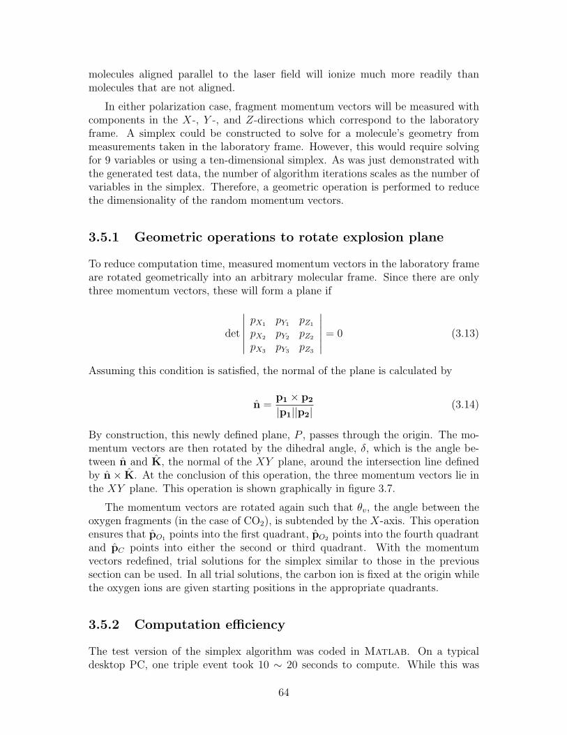
molecules aligned parallel to the laser field will ionize much more readily thanmolecules that are not aligned.

In either polarization case, fragment momentum vectors will be measured withcomponents in the X-, Y -, and Z-directions which correspond to the laboratoryframe. A simplex could be constructed to solve for a molecule’s geometry frommeasurements taken in the laboratory frame. However, this would require solvingfor 9 variables or using a ten-dimensional simplex. As was just demonstrated withthe generated test data, the number of algorithm iterations scales as the number ofvariables in the simplex. Therefore, a geometric operation is performed to reducethe dimensionality of the random momentum vectors.

3.5.1 Geometric operations to rotate explosion plane

To reduce computation time, measured momentum vectors in the laboratory frameare rotated geometrically into an arbitrary molecular frame. Since there are onlythree momentum vectors, these will form a plane if

det

∣∣∣∣∣∣pX1 pY1 pZ1

pX2 pY2 pZ2

pX3 pY3 pZ3

∣∣∣∣∣∣ = 0 (3.13)

Assuming this condition is satisfied, the normal of the plane is calculated by

n =p1 × p2

|p1||p2|(3.14)

By construction, this newly defined plane, P , passes through the origin. The mo-mentum vectors are then rotated by the dihedral angle, δ, which is the angle be-tween n and K, the normal of the XY plane, around the intersection line definedby n× K. At the conclusion of this operation, the three momentum vectors lie inthe XY plane. This operation is shown graphically in figure 3.7.

The momentum vectors are rotated again such that θv, the angle between theoxygen fragments (in the case of CO2), is subtended by the X-axis. This operationensures that pO1 points into the first quadrant, pO2 points into the fourth quadrantand pC points into either the second or third quadrant. With the momentumvectors redefined, trial solutions for the simplex similar to those in the previoussection can be used. In all trial solutions, the carbon ion is fixed at the origin whilethe oxygen ions are given starting positions in the appropriate quadrants.

3.5.2 Computation efficiency

The test version of the simplex algorithm was coded in Matlab. On a typicaldesktop PC, one triple event took 10 ∼ 20 seconds to compute. While this was

64

Figure 3.7: Rotation of momentum plane through dihedral angle. The plane,P , is defined by the determinant of the momentum vectors in equa-tion 3.13. The original momentum vectors are rotated through thedihedral angle, δ, so they lie in the XY plane.

sufficient for test purposes, a large data set from an experiment would take days,even when the calculations were distributed over several workstations. The workingcode was reproduced in C, using some routines from the GNU Scientific Library.This resulted in much faster analysis times and large data sets could be completedin two hours instead of days.

3.6 Limitations

As shown in previous sections, the algorithm has proven to be an excellent toolfor solving for geometric structures. Nevertheless, some issues remain. These re-maining issues stem from the semi-chaotic nature of the 3-body problem. Thatis, small changes in the initial structure can lead to large changes in the asymp-totic momenta. During testing, the simplex algorithm did not accurately recoverthe geometry of extremely bent molecules. When the bend angle was less than ∼100, the algorithm became confused and did not converge. Also, the algorithmfailed to converge when the fragment masses were too large, approximately 100amu. The algorithm was perfectly capable of deducing the geometry of small, lin-ear molecules. Having assessed what the algorithm can and cannot do, we focus

65

our attention on light, linear molecules as the geometry of these molecules shouldbe readily recoverable.

66

Chapter 4

Ultrafast Imaging ofMultielectronic DissociativeIonization of CO2 in an IntenseLaser Field

This chapter is adapted from an article that was printed in J. Phys. B: At. Mol.Opt. Phys., 40:117-129, 2007, produced in collaboration with Stephen J. Walker,Robin Helsten and Joseph H. Sanderson.

4.1 Introduction

Studies on polyatomic molecules have shown that interaction with an intense (∼1014-1016 W cm−2) laser field leads to substantial geometric deformation that occurs onthe timescale of ultrafast laser pulses [49, 51, 52, 77, 78, 81, 82, 124, 80]. Whileseveral triatomic systems have been investigated, CO2 has remained a target ofspecial interest [47, 125, 77, 82, 84, 126].

It is well established when laser pulse durations are on the order of 50-100 fs,the kinetic energy released in multi-electron dissociative ionization the observedexplosion energies are considerably lower than would be expected from a Coulombexplosion of the molecule from its equilibrium geometry. The observed explosionenergies are consistent with separations RC ' 2Req – 3Req, where RC is the so-called critical distance and Req is the equilibrium bond length. If reconstructionof the equilibrium geometry is the ultimate goal, recent work by Legare et al [95]has shown that bond length distributions less than RC can be recovered if 7 ∼ 8fs laser pulses are employed. The mechanism that gives rise to RC is describedby enhanced ionization which has been explained using both classical [54] andquantum mechanical models [56, 55]. Previous long pulse measurements of CO2

have reported an RC value somewhat lower than the calculated value of 3.5 A[77].

67

In this work, we exploit the ability of the complete momentum coincidence imag-ing technique to make the first complete momentum coincidence imaging measure-ments of fragment ions produced from CO2 in an intense laser field. This allowsus to make the first unambiguous measurement of the structure of CO2 and revealsignificant differences to previous incomplete methods, in terms of the most likelygeometry and the extent of molecular deformation in a laser pulse.

4.2 Experimental

The experimental apparatus has been described in a previous chapter. Unique tothis experiment, a laser intensity ∼ 1015 W cm−2 was used. This intensity wasverified by examining the time-of-flight signal from multiply ionized xenon. Thevoltages applied to the first (3020 V) and sixteenth (20 V) rings are adjusted togive a field strength of approximately 260 V cm−1. This field strength ensures allfragment ions are collected within ∼1.5 µs.

With a MCP diameter of 40 mm φ, we are able to detect O+ ions with amomentum perpendicular to the TOF axis of ∼5 x 10−22 kg m s−1 and C+ ionswith a momentum perpendicular to the TOF axis of ∼4.3 x 10−22 kg m s−1. Sinceour laser polarization was parallel to the TOF axis, and CO2 molecules will alignwith the laser polarization, it is the perpendicular momentum of the C+ ions whichwill limit the detection efficiency. The DC field in the TOF is therefore set toensure 100% collection efficiency of perpendicularly ejected fragments.

The four signals from the anode are amplified (Ortec 142B) then recorded bytwo PC oscilloscope cards (Gage Applied Dual Compuscope CS82G, time resolution1 ns) at a rate of 1000 laser shots per second. We are therefore able to take fulladvantage of our kHz amplifier by recording ion fragment information from eachlaser shot. Events are discriminated after data collection using software, and morethan 10 fragments per laser shot can be detected. In practice, we only analyzetriple coincidence data, that is, where exactly three ions are detected from thesame laser shot. By capturing and analyzing data in parallel, event discriminationis performed in real-time. For the purposes of this experiment, we set a 40 nsinterval between successive events.

To ensure all fragment ions originate from a single parent ion, the chamberpressure must be held low enough so that the number of molecules in the laserfocus is less than one. The main chamber is pumped to a base pressure as low as7 x 10−10 Torr. Room temperature CO2 gas is introduced effusively through a leakvalve and typical experimental pressures are 5 x 10−8 Torr. At this temperature,over 90% of the CO2 molecules will be in the ground vibrational level (000), withthe remainder in the lowest bending mode (010) [127]. Although we only considerthe bend angle distribution of the (000) vibrational level, we postulate that we mayobserve slightly more bent geometries.

68

The data presented in this chapter consists of ∼2 x 104 triple coincidence events,generated using ∼106 laser shots.

4.3 Data Reduction

For each fragment ion, the position is determined as described in [128]. With theposition and time information, the momentum vector p = (pX , pY , pZ) of a singlefragment is calculated according to [91]. Briefly, for a fragment of mass m, andcharge q, the momentum components along the X -, Y - and Z-axes in the laboratoryframe are given by

pX = m(X −X0)

t, pY = m

(Y − Y0)

t, pZ =

qE

2

(t20 − t2)t

(4.1)

where t is the measured arrival time, X and Y are the displacements of the fragmentwith respect to an ion with pX = pY = 0, E is the constant electric field in thetime-of-flight tube, and t0 is the flight time of a fragment with pZ = 0. We havecalibrated our energy measurements with other molecular targets.

Channel-resolved coincidence imaging maps are produced by collecting the eventsin which all fragment ions are detected. For example, ions created via the (2,2,2)Coulomb explosion pathway, CO6+

2 → O2++C2++O2+, are identified by eventswhere two O2+ ions and one C2+ ion hit the detector after a single laser shot.False coincidences, which can result from the presence of more than one targetmolecule in the laser focus, noise or background gases, are suppressed by filteringevents according to the momentum sum of the Coulomb explosion. An event is in-terpreted as a false coincidence if the sum

∑p′i of the observed momenta is greater

than 5 x 10−23 kg m s−1. 95% of events are positive coincidences.

4.4 Results

4.4.1 Coulomb explosion of CO2

Figure 4.1 shows a two dimensional representation of the triple coincidence mapfor CO2. At the present laser intensity, ∼ 1015 W cm−2, charge states up to CO6+

2

can be obtained. As can been clearly seen, three O+ peaks are apparent. The O+f

and O+b peaks correspond to oxygen fragments coming from the (1,1,1) Coulomb

explosion channel. The O+m peak comes from other dissociative processes. The

forward-backward peak pattern is also evident in the higher charge state.

The coincidence imaging technique is a direct method to identify all fragmentsfrom a single Coulomb explosion event with a specific charge number. The mostprominent explosion pathways are:

69

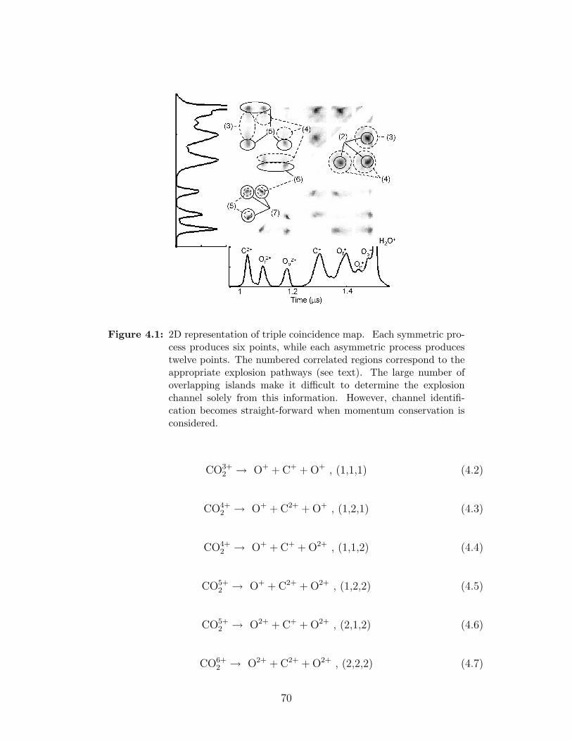
Figure 4.1: 2D representation of triple coincidence map. Each symmetric pro-cess produces six points, while each asymmetric process producestwelve points. The numbered correlated regions correspond to theappropriate explosion pathways (see text). The large number ofoverlapping islands make it difficult to determine the explosionchannel solely from this information. However, channel identifi-cation becomes straight-forward when momentum conservation isconsidered.

CO3+2 → O+ + C+ + O+ , (1,1,1) (4.2)

CO4+2 → O+ + C2+ + O+ , (1,2,1) (4.3)

CO4+2 → O+ + C+ + O2+ , (1,1,2) (4.4)

CO5+2 → O+ + C2+ + O2+ , (1,2,2) (4.5)

CO5+2 → O2+ + C+ + O2+ , (2,1,2) (4.6)

CO6+2 → O2+ + C2+ + O2+ , (2,2,2) (4.7)

70

Of these six pathways, (4.2), (4.3), (4.6) and (4.7) will be described as symmetricprocesses while (4.4) and (4.5) are asymmetric processes.

Since the momenta of all the fragment ions pi is known, the total kineticenergy released can be readily calculated by Ekin =

∑|pi|2 /(2mi) where m i is

the mass of the ith fragment ion. The energy distributions for the six explosionpathways are shown in figure 4.2. These kinetic energy release (KER) distributionscan be compared with the results of Bryan et al [82] and the calculated kineticenergy release (CKE) which assumes the initial geometry is that of the ground stateneutral molecule. Our results compare well with Bryan et al for those explosionchannels where the carbon fragment has been singly ionized. Of particular interest,we note definite structure within the energy distributions, such as a low energyshoulder in the (1,1,1) signal, a high energy shoulder in the (1,2,1) signal and inthe case of the (2,2,2) signal we observe a low energy feature close to the noise level.We have good statistics for the (1,1,1) and (1,2,1) channels, but the statistics aresomewhat worse for the (2,2,2) channel so the low energy feature seen there maybe exaggerated.

In those channels with doubly charged carbon fragments, the detected KERis somewhat lower than reported by Bryan et al. It is clear from our resultsthat the measured KER increases substantially when an oxygen fragment is doublyionized, for example as with (1,1,1) → (1,1,2), but not nearly as much when acarbon is doubly ionized, as with (1,1,1) → (1,2,1). As expected, the CKE valuesare substantially larger than the measured KER values, due to the assumption ofequilibrium bond lengths and pure Coulombic dissociation.

4.4.2 Molecular geometry reconstruction

With the three-dimensional momentum vectors of the fragments now determined,it is straightforward to reconstruct the apparent molecular geometry just before theCoulomb explosion. The momentum of the ion fragments is then calculated bynumerically solving the classical equations of motion in the Coulomb field for someinitial set of guesses at the molecular structure, assuming the initial momentumis zero. A more accurate but computationally demanding approach utilizes an abinitio potential energy surface [95], but here we use the simpler Coulomb approxi-mation to better compare with previous results. The parameter space defined bythis set of guesses for the molecular structure is explored using a simplex algorithm[122] until the observed asymptotic momentum vectors are reproduced.

The distributions of the molecular structures of the six explosion channels areshown in figure 4.3. As far as we are aware, this the first time channel re-solved molecular structures have been derived from an experiment of laser initiatedCoulomb explosions. As seen in (c) and (e) of figure 4.3, the explosion channels(1,1,2) and (2,1,2) have average bond lengths much closer to the equilibrium bondlength than the other channels. Also, the variation in bond length and bend an-gle does not appear to be smoothly changing with charge state. Furthermore,

71

0

400

800

0

100

200

0

100

200

0

50

0 50 100 1500

50

0 50 100 1500

20

40

Energy (eV)

Cou

nts

(1,1,1) (1,2,1)

(1,1,2) (1,2,2)

(2,1,2) (2,2,2)

Figure 4.2: Released kinetic energy distributions for the (1,1,1), (1,2,1), (1,1,2),(1,2,2), (2,1,2) and (2,2,2) Coulomb explosion pathways. Experi-mental data has been smoothed using a three-point triangle filter.Included for comparison are the kinetic energy release values from[82] (dotted), as well as theoretical kinetic energies assuming frag-mentation proceeds from the equilibrium geometry (dot-dash).

the (1,2,1) channel shows evidence of a localization in the distribution around 2.5A. Based on figure 4.2 and figure 4.3, we can say that substantial changes in theenergy spectrum follow from double ionization of the oxygen fragments, while thegeometric distributions can be qualitatively grouped according to the charge of thecarbon fragment. For a more quantitative analysis of the geometric data, bendangle and bond length distributions are examined independently.

Figure 4.4 shows in detail the bend angle distributions from other long-pulseexperiments [51, 77, 82]. The results of Bryan et al are similar to ours whilethe data reported by Cornaggia and Hishikawa et al have a somewhat wider bendangle distribution than was measured in this work. Furthermore, Bryan et alclosely agrees with our value of ∼171, while Cornaggia and Hishikawa et al reporta peak bend angle of 180. The ground state bend angle distribution as calculatedby [129] is also included for comparison. The ground state distribution, whichaccounts for all normal modes of vibration, has a width (∼13) and peak (∼174)similar to our results.

Figure 4.5 plots the channel dependence of the bend angle distribution. We seeunambiguously the narrowing of the bend angle distribution with increasing chargestate and the peak of the distribution approaching the ground state equilibrium

72

0

1

Figure 4.3: Recovered molecular geometry mapped directly from observed co-incidence momentum imaging. The channels shown are (a) (1,1,1),(b) (1,2,1), (c) (1,1,2), (d) (1,2,2), (e) (2,1,2), (f) (2,2,2). In eachplot, the carbon fragment is at the origin, while the higher chargedoxygen fragment lies along the positive x -axis. The equilibriumgeometry has been included for comparison (open circles). Notethat these are density plots, each comprising ∼1000 triple events.

value of 174, beginning at 170 for the (1,1,1) channel and ending at about 177

for the (2,2,2) channel. This narrowing trend agrees qualitatively with Hishikawaet al [77], whose results indicated that multiply charged parent ions have a halfmaximum deviation from the linear geometry, σ, determined to be σ = 45 − 35

for COz+2 charge states of z = 4− 6.

The bond length distribution for the six explosion channels is shown in figure 4.6.The distributions peak ∼ 2Req – 3Req, but there is no clear relationship betweenbond length and charge state. The recovered bond length distributions have goodagreement with the distributions of Bryan et al [82] and Cornaggia [51], particularlyfor the singly charged carbon channels. There is somewhat variable agreementwith the results of Hishikawa et al [77], who reports shorter bond lengths thanwere seen in other experiments. We observe additional structure not previouslyvisible because all previous techniques rely on fitting a triangular or Gaussian curveto describe their data. While this observed structure may be due to somewhat lowstatistics (particularly for the (1,2,2) channel which has ∼103 events), the currenttechnique should be more sensitive because in other techniques the structure isdrowned out by the contribution of other channels. In particular, the shape of the

73

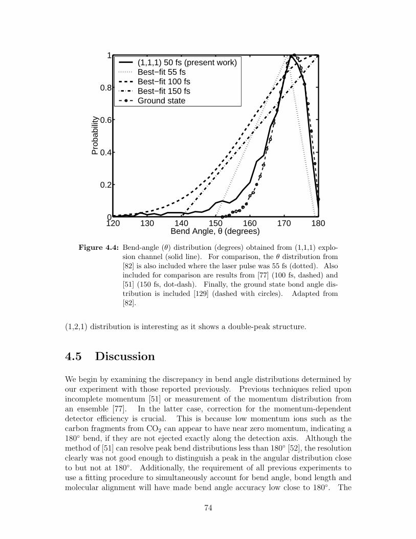
120 130 140 150 160 170 1800

0.2

0.4

0.6

0.8

1

Bend Angle, θ (degrees)

Pro

babi

lity

(1,1,1) 50 fs (present work)Best−fit 55 fsBest−fit 100 fsBest−fit 150 fsGround state

Figure 4.4: Bend-angle (θ) distribution (degrees) obtained from (1,1,1) explo-sion channel (solid line). For comparison, the θ distribution from[82] is also included where the laser pulse was 55 fs (dotted). Alsoincluded for comparison are results from [77] (100 fs, dashed) and[51] (150 fs, dot-dash). Finally, the ground state bond angle dis-tribution is included [129] (dashed with circles). Adapted from[82].

(1,2,1) distribution is interesting as it shows a double-peak structure.

4.5 Discussion

We begin by examining the discrepancy in bend angle distributions determined byour experiment with those reported previously. Previous techniques relied uponincomplete momentum [51] or measurement of the momentum distribution froman ensemble [77]. In the latter case, correction for the momentum-dependentdetector efficiency is crucial. This is because low momentum ions such as thecarbon fragments from CO2 can appear to have near zero momentum, indicating a180 bend, if they are not ejected exactly along the detection axis. Although themethod of [51] can resolve peak bend distributions less than 180 [52], the resolutionclearly was not good enough to distinguish a peak in the angular distribution closeto but not at 180. Additionally, the requirement of all previous experiments touse a fitting procedure to simultaneously account for bend angle, bond length andmolecular alignment will have made bend angle accuracy low close to 180. The

74

0

0.5

1

0

0.5

1

0

0.5

1

0

0.5

1

120 140 160 1800

0.5

1

120 140 160 1800

0.5

1

Bend Angle, θ (degrees)

Pro

babi

lity

(1,1,1) (1,2,1)

(1,1,2) (1,2,2)

(2,1,2) (2,2,2)

Figure 4.5: Bend-angle (θ) distribution (degrees) obtained from the six explo-sion channels. The results of this work are shown with a solid line.For comparison, the θ distribution from [82] is included (dottedline) as well as the distribution from [51] (dash-dotted line) andfrom [77] (dashed line). The ground state distribution is also in-cluded on each plot [129] (dashed with circles).

corrected momentum mapping technique of Bryan et al [82], which does attemptto account for the detection efficiency, records a peak in angular distribution closeto ours in the case of the (1,1,1) channel. However, the technique of [82] doesunderestimate the bend angle for higher charge states and ensemble fitting is againthe most likely cause of discrepancy.

Previous work with sub-7 fs pulses has shown the tendency for molecular geom-etry to be more accurately recovered from higher charge states due to these states’spotential energy surfaces closely resembling a purely Coulombic repulsion [95]. Wemight expect this would also hold for our long pulse experiment but this would ne-glect the molecular dynamics during dissociation of the molecule. Assuming thatthe final ionization takes place at the peak of the laser pulse, for each channel, themolecule from the (1,1,1) channel will spend the most time in a bound ionizationstate, either CO2+

2 or CO2+ [130]. The theoretical work of Kono et al [93] sug-gests that structural deformation occurs in charge states as low as CO2+

2 , and thatelongation of the C-O bond is accompanied by bending of the molecular skeleton.Evidence for this interesting phenomenon has been experimentally observed [84].This tendency for the molecule to bend in these low states may be countered by theinclination of it to straighten as it undergoes linear dissociation on the (1,1,1) and

75

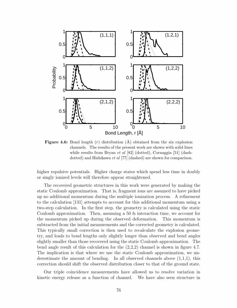
0

0.5

1

0

0.5

1

0

0.5

1

0

0.5

1

0 5 100

0.5

1

Bond Length, r [Å]

Pro

babi

lity

0 5 100

0.5

1

(1,1,1) (1,2,1)

(1,1,2) (1,2,2)

(2,1,2) (2,2,2)

Figure 4.6: Bond length (r) distribution (A) obtained from the six explosionchannels. The results of the present work are shown with solid lineswhile results from Bryan et al [82] (dotted), Cornaggia [51] (dash-dotted) and Hishikawa et al [77] (dashed) are shown for comparison.

higher repulsive potentials. Higher charge states which spend less time in doublyor singly ionized levels will therefore appear straightened.

The recovered geometric structures in this work were generated by making thestatic Coulomb approximation. That is, fragment ions are assumed to have pickedup no additional momentum during the multiple ionization process. A refinementto the calculation [131] attempts to account for this additional momentum using atwo-step calculation. In the first step, the geometry is calculated using the staticCoulomb approximation. Then, assuming a 50 fs interaction time, we account forthe momentum picked up during the observed deformation. This momentum issubtracted from the initial measurements and the corrected geometry is calculated.This typically small correction is then used to recalculate the explosion geome-try, and leads to bond lengths only slightly longer than observed and bend anglesslightly smaller than those recovered using the static Coulomb approximation. Thebend angle result of this calculation for the (2,2,2) channel is shown in figure 4.7.The implication is that where we use the static Coulomb approximation, we un-derestimate the amount of bending. In all observed channels above (1,1,1), thiscorrection should shift the observed distribution closer to that of the ground state.

Our triple coincidence measurements have allowed us to resolve variation inkinetic energy release as a function of channel. We have also seen structure in

76

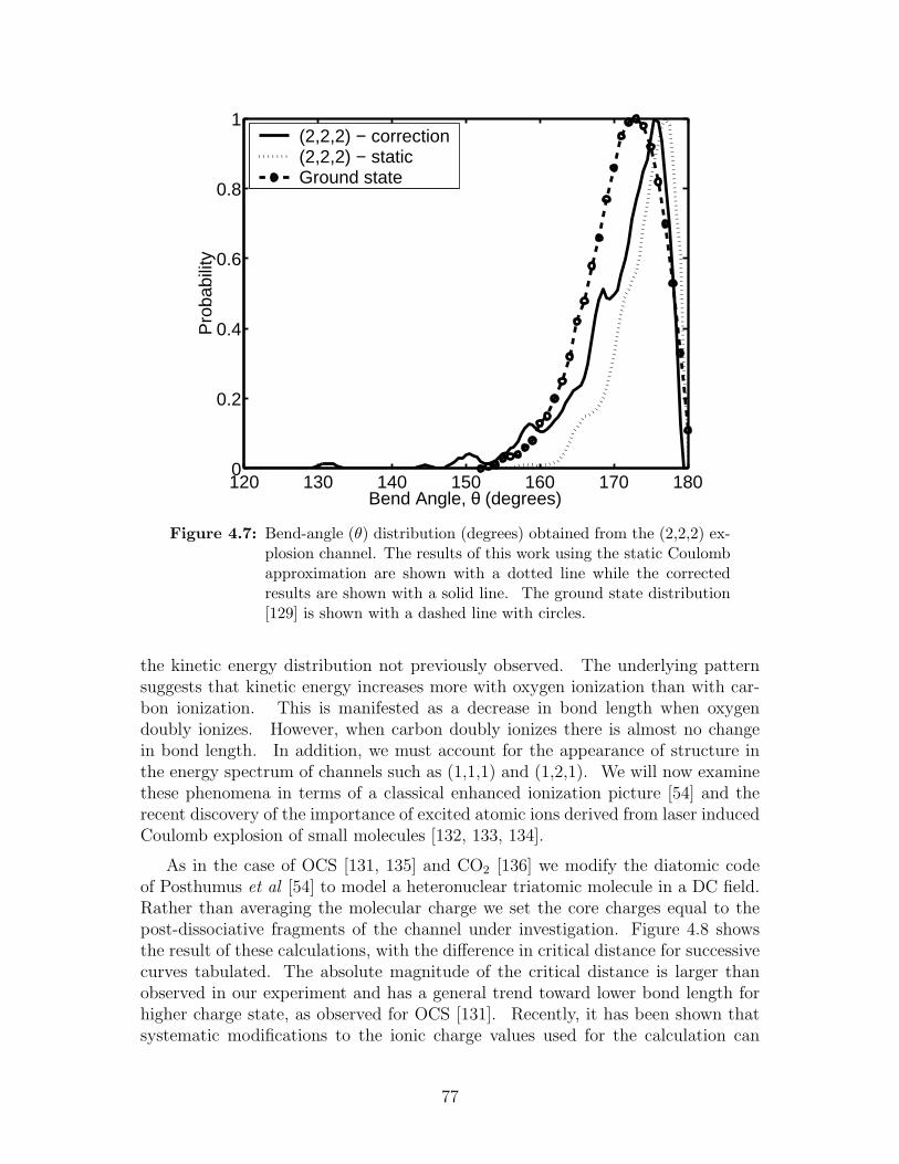
120 130 140 150 160 170 1800

0.2

0.4

0.6

0.8

1

Bend Angle, θ (degrees)

Pro

babi

lity

(2,2,2) − correction(2,2,2) − staticGround state

Figure 4.7: Bend-angle (θ) distribution (degrees) obtained from the (2,2,2) ex-plosion channel. The results of this work using the static Coulombapproximation are shown with a dotted line while the correctedresults are shown with a solid line. The ground state distribution[129] is shown with a dashed line with circles.

the kinetic energy distribution not previously observed. The underlying patternsuggests that kinetic energy increases more with oxygen ionization than with car-bon ionization. This is manifested as a decrease in bond length when oxygendoubly ionizes. However, when carbon doubly ionizes there is almost no changein bond length. In addition, we must account for the appearance of structure inthe energy spectrum of channels such as (1,1,1) and (1,2,1). We will now examinethese phenomena in terms of a classical enhanced ionization picture [54] and therecent discovery of the importance of excited atomic ions derived from laser inducedCoulomb explosion of small molecules [132, 133, 134].

As in the case of OCS [131, 135] and CO2 [136] we modify the diatomic codeof Posthumus et al [54] to model a heteronuclear triatomic molecule in a DC field.Rather than averaging the molecular charge we set the core charges equal to thepost-dissociative fragments of the channel under investigation. Figure 4.8 showsthe result of these calculations, with the difference in critical distance for successivecurves tabulated. The absolute magnitude of the critical distance is larger thanobserved in our experiment and has a general trend toward lower bond length forhigher charge state, as observed for OCS [131]. Recently, it has been shown thatsystematic modifications to the ionic charge values used for the calculation can

77

1 2 3 4 5

1014

1015

Bond length (Å)

Inte

nsity

(W

cm

−2 )

(1,1,1)(1,2,1)(1,1,2)(1,2,2)(2,1,2)(2,2,2)

Channel ∆rmin

(Å)

(1,1,1) − (1,2,1) −0.1 (1,2,1) − (1,1,2) −0.4 (1,1,2) − (1,2,2) 0.0 (1,2,2) − (2,1,2) −0.3 (2,1,2) − (2,2,2) 0.1

Figure 4.8: Ionization laser intensity as a function of bond length for the sixchannels under investigation, modeled using the classical enhancedionization theory of [54]. In order of increasing intensity, the chan-nels are: (1,1,1), solid line; (1,2,1), dotted line; (1,1,2), dashed line;(1,2,2), dash-dotted line; (2,1,2), dashed line with circles; (2,2,2),dashed line with triangles. The inset table shows the bond lengthdifference at the minimum of each channel.

reproduce the experimentally observed trend [135] in the case of OCS. This reduc-tion in charge is physical as it mimics the effect of deviation from pure Coulombicof the ion interaction potentials for low charge states [137]. Beyond this generaltrend to shorter bond lengths, there is a startling qualitative correlation betweenthe way RC changes depending on whether a carbon or an oxygen is ionized further.It should be noted that these transitions are not indicative of sequential states ofionization. Rather, it is the change from the (1,2,1) to the (1,1,2) and from the(1,2,2) to the (2,1,2) channels that gives rise to a much larger reduction in RC thanany other transitions. All other steps are either close to zero or slightly positiveas observed experimentally. We therefore attribute these observations to effect ofenhanced ionization.

While theoretical work has been done on the fragmentation pathways of CO2+2

[138, 139, 140], little information is available for the potential energy surfaces ofhigher charge states. However, for the lower charge states, there are several path-ways that can lead to dissociation, each of which lead to ionic fragments in differentexcited states. This multi-path dissociation should follow for higher charge states

78

0 20 400

0.2

0.4

0.6

0.8

1

Energy (eV)

Sig

nal (

arb)

0 20 400

0.2

0.4

0.6

0.8

1

Energy (eV)

Sig

nal (

arb)

(1,1,1) (1,2,1) (b)

(c)

(a)(d)

(e)

(f)

Figure 4.9: Kinetic energy spectra for the (1,1,1) and (1,2,1) channels, shownwith solid lines, smoothed using a three-point triangle filter. Eachspectrum has been deconvolved into three Gaussian peaks (dashed),the sum of which is shown with circles. The energy values for thesix peaks are: (a) 4 eV; (b) 11.5 eV; (c) 22 eV; (d) 5 eV; (e) 14 eV;(f) 23.5 eV.

as well. Therefore, the structure in the kinetic energy spectra may be explainedby considering the molecular ions dissociating into one or more excited atomic ionsas was previously done for N2 and O2 [57, 132].

If we consider the kinetic energy spectra of the (1,1,1) and (1,2,1) channels,each spectrum can be deconvolved using three Gaussian peaks. Since excitedfragments have less kinetic energy than fragments in the ground state, we canmake reasonable guesses as to the identity of spectra peaks. In particular, welook for atomic transitions that will sum to the observed energy differences, givingpreference to transitions that are of lower energy. For the (1,1,1) channel, the highenergy peak, labeled (c), corresponds to each ion’s ground state, O+(4S) + C+(2P)+ O+(4S). The next lowest peak, labeled (b), corresponds to ejection of two 5.02eV oxygen ions in the (2P) state or to ejection of two 3.32 eV oxygen ions in the(2D) state with a 5.33 eV carbon ion in the (4P) state. Finally, the lowest energypeak (a), corresponds to ejection of two (2P) oxygen ions as in (b), as well as a9.28 eV carbon ion in the (2D) state. A similar analysis can be performed withthe peaks in the (1,2,1) spectrum. If we again identify the highest energy peak(f) as the ground state, O+(4S) + C2+(1S) + O+(4S), the middle peak (e) once

79

again corresponds to ejection of two 5.02 eV oxygen ions in the (2P) state or toejection of two 3.32 eV oxygen ions in the (2D) state with a 6.49 eV carbon ion inthe (3P) state. The lowest energy peak (d), corresponds to ejection of two (2P)oxygen ions and a 6.48 eV (3P) carbon ion. Although the kinetic energy spectraof the higher channels show interesting structure, the statistics are inadequate topermit this analysis. While the exact identification of the final excited states isunclear, the excited state fragmentation model [141, 142] adequately describes ourexperimental results.

4.6 Conclusion

A triple coincidence imaging technique has been used to investigate dynamics ofmolecules as they interact with intense laser fields. The channel-resolved kinetic en-ergy distributions show a step-wise KER increase and the resultant change in bondlength can be interpreted using the classical enhanced ionization model. However,we observe structure in the kinetic energy distributions which we attribute to thepresence of excited states in the fragment ions. The successful application of thesetwo individual models suggests the possibility to combine the theories of excitedstate fragmentation and enhanced ionization into a single, simple model that canpredict the behaviour of multielectronic molecules dissociated in ultrashort pulses.

80

Chapter 5

Concerted and SequentialMultielectronic DissociativeIonization of CS2 in an IntenseLaser Field

5.1 Introduction

Carbon disulfide (CS2) is a linear, triatomic molecule of much interest [143, 34, 87,88, 144, 145]. In the ground electronic state, X1Σg, the equilibrium C–S bond lengthis 1.55 A with a bending-mode frequency of 397 cm−1. The electronic configura-tion of the ground electronic state is (core)22(5σg)

2(4σu)2(6σg)

2(5σu)2(2πu)

4(2πg)4.

During a laser-molecule interaction, it is expected that the CS2 molecules will havethe carbon atom displaced from its equilibrium geometry by the bending-mode vi-brational motion, the lowest energy mode. The most probable value of the bendangle in the v = 0 level is 175.2. Since our experiment was conducted at roomtemperature, where approximately 23% of the population will be in the v = 1 vibra-tional level with a most probable bend angle of 171.7 [34], we expect to measure amean bend angle somewhere near 174. Highly charged ion studies [34] have shownthat the measured kinetic energy release (KER) values in higher charge states areapproximately the same as those predicted by a pure Coulomb explosion. However,these same studies showed that the bend angle is shifted towards smaller values,that is, the molecular skeleton is bent, possibly due to excitation in the bendingmode of the precursor molecular ion. Furthermore, the degree of bending dependsupon the ionization channel achieved. For symmetric channels, where the sulfurions have the same charge, the recovered bend angle was reported to be ∼ 170.In the case of asymmetric channels, the mean bend angle was typically ∼ 165.Non-coincident laser-initiated Coulomb explosion studies of low charge states [87]have shown substantial deformation occurs along the bending mode. While mo-mentum imaging of higher charge states has shown that substantial bending can

81

be initiated in the neutral by pumping the parent molecule with a non-resonant,linearly polarized pulse (1064 nm, 7 ns, 414 mJ) before probing with an intense,circularly polarized pulse (795 nm, 100 fs, 0.3 mJ) [80]. Molecules that were probedwithout the ns pulse did not exhibit a strongly bent character. Throughout thispaper, we will discuss ionization channels according to the convention SCS(m+n+p)+

→ Sm++Cn++Sp+, and refer to this as the (m,n, p) channel.

5.2 Experimental

The experimental apparatus has been described in greater detail in a previouschapter. The spectrometer extraction field was set to 180 V cm−1. CS2 vaporenters the chamber effusively through a leak valve and the experimental pressure isset to 1.5 x 10−8 Torr. Software is used to discriminate events after collection andonly explosion events where three ions hit the detector in coincidence are retained.The data is filtered again to suppress false coincidences, defined as when the sumof the observed momenta,

∑p, exceeds 10−22 kg m s−1.

5.3 Results

5.3.1 Coulomb explosion of CS2

At the present laser intensity, charge states up to CS13+2 can be achieved. We focus

attention on the formation and fragmentation of the highly charged CSz+2 molecularions by monitoring channels that result in three fragment ions. Several explosionchannels were recorded with 103 ∼ 104 triple coincidence events in each channel.A useful parameter for correlating fragment ions is the χ angle, defined as theangle between the momentum vector of the carbon ion and the difference of themomentum vectors of the two sulphur ions. The χ angle is calculated according to

cosχ =pC · (pS1 − pS2)

|pC||pS1 − pS2 |(5.1)

Physically, the angle χ indicates the direction of the outgoing carbon ion withrespect to the line joining the S–S nuclei. In a symmetric fragmentation channel,where each sulphur ion has the same charge, the angle χ is indicative of whetheror the not the dissociation process is sequential or concerted. In the event ofa perfectly concerted Coulomb explosion, pS1 = pS2 and χ = 90. However, ifthe bond lengths are unequal, or the sulphur ions have unequal momenta, χ 6= 90.The experimental χ distribution of the (3,2,3) channel is shown in figure 5.1(a), andwhile the most probable value is 90, the standard deviation is σ = 30, indicatingsome mixture of concerted and sequential processes. During asymmetric processes,the most probable value of χ should not be 90 due to the differing recoil velocities

82

of the fragment ions. In [34], the most probable values of χ were reported to be95–110. Adopting the same definition, the χ distribution for the (2,2,3) is plottedin figure 5.1(b). As can be seen, the most probable value for χ is approximately100. Using a classical model, the χ angle of the (3,2,3) and (2,2,3) channels can bepredicted by assuming a variety of initial bend angles, θ, and bond lengths, r1,2. Weassume that the Coulomb explosion proceeds by instantaneous multiple ionization,with all fragment ions initially at rest. The effect of sequential ionization is builtinto the model by allowing the bond lengths r1 and r2 to be different. The resultsof this calculation are shown in figure 5.2. For the (3,2,3) channel, for bend anglesnear to the zero-point bend angle θ0 = 175.2, we expect to see χ ∼ 70–110 (dueto symmetry about χ = 90), depending upon the degree of sequential ionization.In the case of the (2,2,3) channel, for bend angles near to the zero-point bend angleθ0 = 175.2, we expect to see χ ∼ 60–120, once again depending upon the degreeof sequential ionization. Thus, we have good agreement with the most probablevalue of the observed χ distribution. Moreover, we expect to see strong sequentialcharacter in the recovered molecular geometries.

Once the explosion channel and momentum of each fragment are known, theKER for each Coulomb explosion can be calculated by summing the kinetic energyof each fragment according to

∑p2i /2mi. Table 5.1 lists the mean KER for each

of the measured channels and comparison with previous highly charged ion results[34] and ultrafast laser Coulomb explosion results [87, 80]. Our results are lowerthan [87] but compare well with [80]. Figure 5.3 plots the ratios of HCI KER from[34] and from this work for a series of fragmentation channels. As a consequenceof the short interaction time, HCI experiments produce KER values similar tothose predicted by Coulomb repulsion of the ionic fragments from their equilibriumgeometry. By contrast, CEI experiments performed with laser pulses in the the 10–100 fs regime produce KER values indicating bond lengths 2–3 times larger thanequilibrium due to enhanced ionization. Since KER is inversely proportional to thebond length, we expect to measure KERHCI/KERCEI ∼ 2–3. Almost all of theobserved channels fall into the expected range.

Figure 5.4 shows the likelihood of a molecular ion in a particular charge state tofragment into a symmetric or asymmetric channel. Symmetric channels are thosewhere the charge on the sulphur ions is the same, such as (2,3,2). Asymmetricchannels are those where the charge on the sulphur ions is different, such as (2,1,4).As discussed in the HCI experiment [34], the energy involved in the fragmentationplays a large role in determining the branching ratio of a channel. For q ≤ 10,our data in figure 5.4 can be directly compared with data from [34] which hasbeen rescaled onto the same scale. For q ≤ 8, the agreement is excellent, despitethe differing method of initiating Coulomb explosions. For higher values of q, thestatistics of [34] are somewhat low and comparison becomes problematic.

83

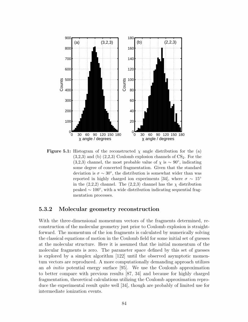
0 30 60 90 120 150 1800

20

40

60

80

100

120

140

160

180

χ angle / degrees

Cou

nts

0 30 60 90 120 150 1800

100

200

300

400

500

600

700

800

900

χ angle / degrees

Cou

nts

(3,2,3) (2,2,3)(a) (b)

Figure 5.1: Histogram of the reconstructed χ angle distribution for the (a)(3,2,3) and (b) (2,2,3) Coulomb explosion channels of CS2. For the(3,2,3) channel, the most probable value of χ is ∼ 90, indicatingsome degree of concerted fragmentation. Given that the standarddeviation is σ ∼ 30, the distribution is somewhat wider than wasreported in highly charged ion experiments [34], where σ ∼ 15

in the (2,2,2) channel. The (2,2,3) channel has the χ distributionpeaked ∼ 100, with a wide distribution indicating sequential frag-mentation processes.

5.3.2 Molecular geometry reconstruction

With the three-dimensional momentum vectors of the fragments determined, re-construction of the molecular geometry just prior to Coulomb explosion is straight-forward. The momentum of the ion fragments is calculated by numerically solvingthe classical equations of motion in the Coulomb field for some initial set of guessesat the molecular structure. Here it is assumed that the initial momentum of themolecular fragments is zero. The parameter space defined by this set of guessesis explored by a simplex algorithm [122] until the observed asymptotic momen-tum vectors are reproduced. A more computationally demanding approach utilizesan ab initio potential energy surface [95]. We use the Coulomb approximationto better compare with previous results [87, 34] and because for highly chargedfragmentation, theoretical calculations utilizing the Coulomb approximation repro-duce the experimental result quite well [34], though are probably of limited use forintermediate ionization events.

84

160 165 170 175 18040

50

60

70

80

90

100

110

120

130

140

θ / degrees

χ / d

egre

es

160 165 170 175 18040

50

60

70

80

90

100

110

120

130

140

θ / degrees

χ / d

egre

es

r2 = r

1

r2 = 1.5 r

1

r2 = 2 r

1

r2 = 2.5 r

1

r2 = 5 r

1

r2 = r

1

r2 = 1.5 r

1

r2 = 2 r

1

r2 = 2.5 r

1

r2 = 5 r

1

(a) (b)(3,2,3) (2,2,3)

Figure 5.2: Theoretical χ angle for a given bend angle θ for the (a) (3,2,3) and(b) (2,2,3) channel. For the determination of χ, we are concernedonly with the relative values of the two bond lengths. The casewhere r2 = r1 is plotted with large dots. Sequential ionization isinvestigated for the cases where r2 = 1.5 r1 (solid line), r2 = 2 r1(dotted line), r2 = 2.5 r1 (dashed line), and r2 = 5 r1 (dash-dottedline). Note that in the case of the (2,2,3) channel, the S2+–C2+

bond length is defined as r1, while the C2+–S3+ bond length isdefined as r2.

Channel-resolved histograms of mean bond length and bend angle are shown infigure 5.5 and the bend angle distributions are compared with theoretical zero-pointcalculations from [34] and, in the case of (3,2,3), the recovered distribution of [80].The peak of the mean bond length distribution for each channel is in the range of 3– 4.5 A(∼ 2.2Req –3 Req), a reasonable result given our laser pulse length is whereEI dominates. Hasegawa et al. [87] report a mean bond length of only r = 2.5 Afor CS3+

2 , using laser pulses similar to ours. By contrast, Iwasaki et al. reporteda bond length of 3.1 A for the (3,2,3) fragmentation channel, which, while shorterthan our result, is still within the range predicted by EI.

The most probable bend angle from the recovered geometries is θ = 175 – 179.The (2,2,2) and (3,3,3) fragmentation channels each have a bend angle distributionsimilar to that of the neutral molecule’s X1Σg ground state. There is a generaltrend towards straightening of the molecule as charge state increases, particularlyin the case of the (4,1,4) channel. As a general trend, we observe that explosionchannels with a carbon charge that is lower that the sulfur charges appear straighter

85

FragmentationChannel KER (eV) 100 fs (eV) 60 fsF (eV) HCI (eV)(1,1,1) 9.3 15.3 19.0(1,1,2) 11 22.4 37.1(1,2,1) 20(1,2,2) 21 59.6(2,1,2) 23 56.6(2,1,3) 39 73.9(1,2,3) 23 93.4(2,2,2) 41 44 90.7(3,1,3) 90.5(2,1,4) 41 108(2,2,3) 44 53 118(2,3,2) 50 125(3,1,4) 113(2,2,4) 60 63 134(2,3,3) 50 139(3,2,3) 63 67 153(4,1,4) 95 140(3,2,4) 62 146(3,3,3) 80 180(3,3,4) 99 165(4,2,4) 88 180(3,4,3) 92(5,1,5) 86(3,4,4) 97(4,3,4) 120(4,3,5) 85(4,4,4) 154(4,4,5) 92

Table 5.1: Mean kinetic energy released (KER) in eV, measured upon fragmen-tation of CSq+2 molecular ions. Included for comparison are otherultrafast results (100 fs [80], 60 fs [87] and HCI results [34]. Notethat the technique used in [80] is not channel resolved and the listedKER have been computed from the appropriate fragment momenta.

with a bend angle distribution narrower than predicted by theory. These results aresomewhat different than were reported in the HCI experiments [34], which measuredslightly more bent geometries with a wider distribution for the (2,2,2) and (3,1,2)fragmentation channels. Furthermore, for the fragmentation of CS3+

2 , Hasegawa etal. [87] reported a much more distorted molecular skeleton, with a mean bend angleof θ = 145 and a standard deviation of σ = 27. In studies of CS8+

2 , Iwasaki et al.[80] reported a most probable bend angle of 180 with a half-width of ∼ 9 in theabsence of a ns pump pulse. Although we do not measure a most probable angle of180 for our (3,2,3) channel, our half maximum bend angle value is ∼ 171, givingan angular range similar to that seen in [80].

An interesting observation is made by comparing the results of figure 5.1 andfigure 5.5 with those of figure 5.2. Since the recovered bend angle distribution givesa range of θ ∼ 170 – 179.5, we might infer from the χ distribution in figure 5.1

86

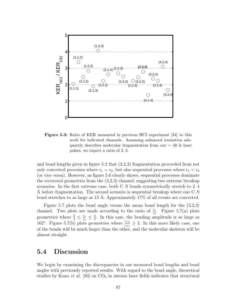
0

1

2

3

4

5

KE

RH

CI /

KE

RC

EI

(1,1,1)

(1,1,2)

(2,1,2)

(1,2,2)

(2,1,3)

(1,2,3)

(2,2,2)

(2,1,4) (2,2,3)

(2,3,2)(2,2,4)

(3,2,3)

(2,3,3)(2,3,3)

(4,1,4)

(3,2,4)

(3,3,3)

(4,2,4)

(3,3,4)

Figure 5.3: Ratio of KER measured in previous HCI experiment [34] to thiswork for indicated channels. Assuming enhanced ionization ade-quately describes molecular fragmentation from our ∼ 50 fs laserpulses, we expect a ratio of 2–3.

and bond lengths given in figure 5.2 that (3,2,3) fragmentation proceeded from notonly concerted processes where r1 = r2, but also sequential processes where r1 < r2

(or vice versa). However, as figure 5.6 clearly shows, sequential processes dominatethe recovered geometries from the (3,2,3) channel, suggesting two extreme breakupscenarios. In the first extreme case, both C–S bonds symmetrically stretch to 2–4A before fragmentation. The second scenario is sequential breakup where one C–Sbond stretches to as large as 15 A. Approximately 17% of all events are concerted.

Figure 5.7 plots the bend angle versus the mean bond length for the (3,2,3)channel. Two plots are made according to the ratio of r1

r2. Figure 5.7(a) plots

geometries where 34≤ r1

r2≤ 4

3. In this case, the bending amplitude is as large as

162. Figure 5.7(b) plots geometries where r1,2

r2,1≥ 3. In this more likely case, one

of the bonds will be much larger than the other, and the molecular skeleton will bealmost straight.

5.4 Discussion

We begin by examining the discrepancies in our measured bond lengths and bendangles with previously reported results. With regard to the bend angle, theoreticalstudies by Kono et al. [93] on CO2 in intense laser fields indicates that structural

87

4 5 6 7 8 9 10 11 12 13 0

20

40

60

80

100

q

Coi

ncid

ence

sig

nal (

arb)

Symmetric, HCIAsymmetric, HCISymmetric, this workAsymmetric, this work

Figure 5.4: Previously reported [34] likelihood for fragmentation into symmet-ric (black filled circles with solid lines) and asymmetric channels(black open squares with dotted lines) for different molecular chargestates q in HCI experiment. The results of [34] have been rescaledso that each molecular charge state (CSq+2 ) has been normalized.The results of this work are shown in red (symmetric are opencircles with dotted lines, asymmetric are filled squares with dash-dotted lines). Symmetric channels are those where the sulphur ionshave identical charge. Conversely, the sulphur ions have differentcharges in asymmetric channels.

deformation occurs primarily in the doubly charged state CO2+2 where elongation

of the molecular bond is accompanied by bending. Indeed, studies of CS3+2 [87]

and N2O3+ [90] have reported this to be the case. Based on figure 5.7(a), we see

some evidence of geometries that are bend and stretched in (3,2,3) fragmentationchannel. While the degree of bending is not as large as reported in HCI experiments[34], it is clear that bending has occurred. Furthermore, the bond lengths arenearly symmetrically stretched to between 2–4 A, within the range predicted byEI. The physical reason is inferred from [93]. Assuming that the final ionizationtakes place at the peak of the laser pulse, the lower channels, that is, (1,1,1) willspend the most time in a bound ionization state, such as CS2+

2 , where bendingis energetically favourable. When these molecular ions fragment, they do so in aconcerted process. The early onset of sequential dissociation of molecular ions thatfragment into (3,2,3) for instance does not permit coupling of the bending modewith the laser field. Therefore, highly charged channels appear straightened. Thisalso explains the linear geometry previously seen by Iwasaki et al. [80] in the study

88

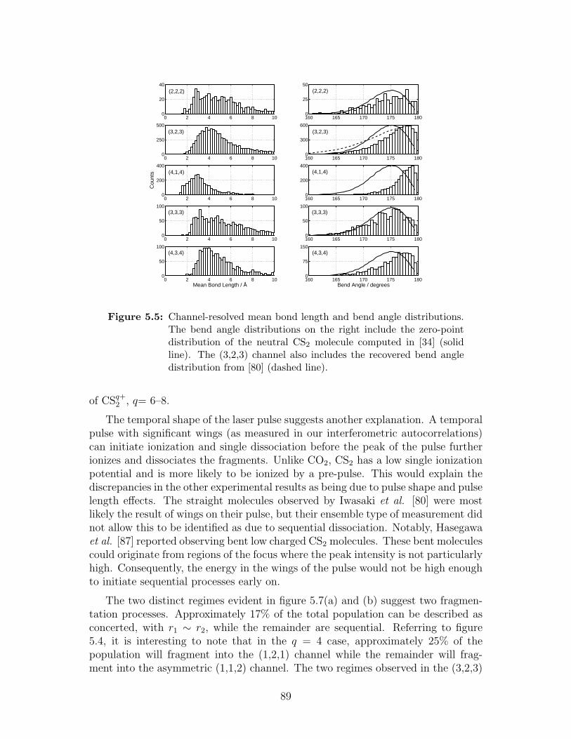
0 2 4 6 8 100

20

40

160 165 170 175 1800

25

50

0 2 4 6 8 100

250

500

160 165 170 175 1800

300

600

0 2 4 6 8 100

200

400

Cou

nts

160 165 170 175 1800

200

400

0 2 4 6 8 100

50

100

160 165 170 175 1800

50

100

0 2 4 6 8 100

50

100

Mean Bond Length / Å160 165 170 175 1800

75

150

Bend Angle / degrees

(2,2,2)

(3,2,3)

(4,1,4)

(3,3,3)

(4,3,4)

(2,2,2)

(3,2,3)

(4,1,4)

(3,3,3)

(4,3,4)

Figure 5.5: Channel-resolved mean bond length and bend angle distributions.The bend angle distributions on the right include the zero-pointdistribution of the neutral CS2 molecule computed in [34] (solidline). The (3,2,3) channel also includes the recovered bend angledistribution from [80] (dashed line).

of CSq+2 , q= 6–8.

The temporal shape of the laser pulse suggests another explanation. A temporalpulse with significant wings (as measured in our interferometric autocorrelations)can initiate ionization and single dissociation before the peak of the pulse furtherionizes and dissociates the fragments. Unlike CO2, CS2 has a low single ionizationpotential and is more likely to be ionized by a pre-pulse. This would explain thediscrepancies in the other experimental results as being due to pulse shape and pulselength effects. The straight molecules observed by Iwasaki et al. [80] were mostlikely the result of wings on their pulse, but their ensemble type of measurement didnot allow this to be identified as due to sequential dissociation. Notably, Hasegawaet al. [87] reported observing bent low charged CS2 molecules. These bent moleculescould originate from regions of the focus where the peak intensity is not particularlyhigh. Consequently, the energy in the wings of the pulse would not be high enoughto initiate sequential processes early on.

The two distinct regimes evident in figure 5.7(a) and (b) suggest two fragmen-tation processes. Approximately 17% of the total population can be described asconcerted, with r1 ∼ r2, while the remainder are sequential. Referring to figure5.4, it is interesting to note that in the q = 4 case, approximately 25% of thepopulation will fragment into the (1,2,1) channel while the remainder will frag-ment into the asymmetric (1,1,2) channel. The two regimes observed in the (3,2,3)

89

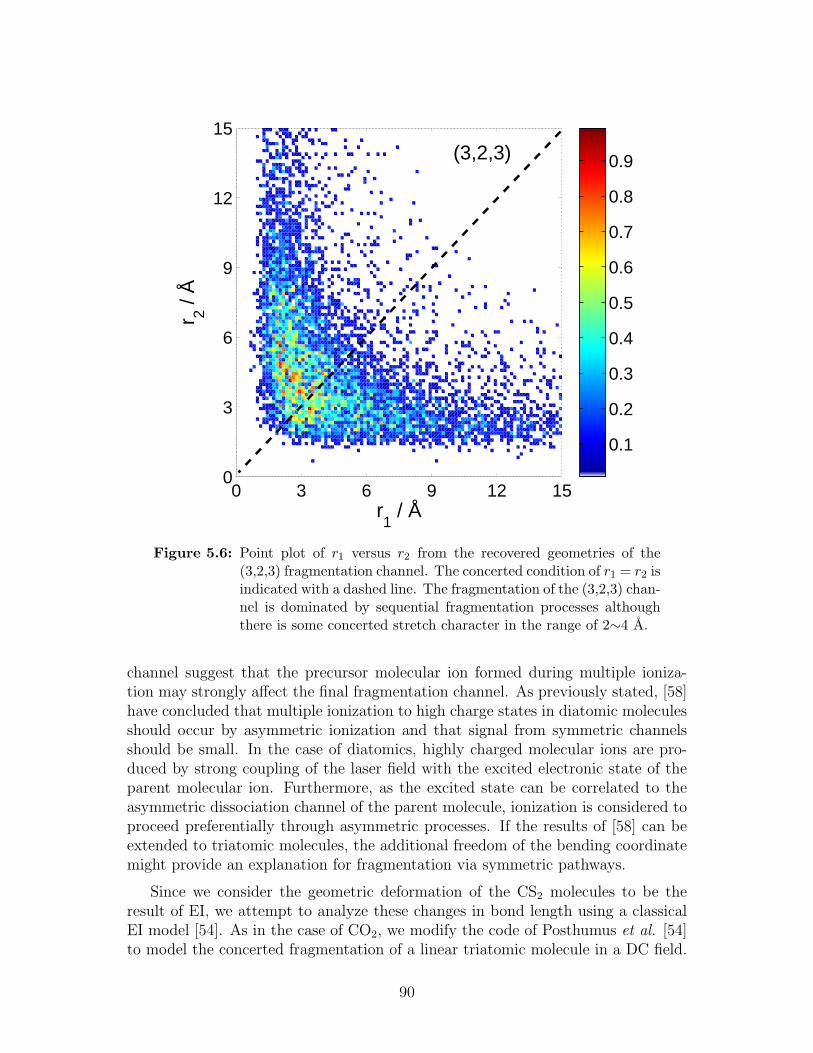
0 3 6 9 12 150

3

6

9

12

15

r1 / Å

r 2 / Å

0.1

0.2

0.3

0.4

0.5

0.6

0.7

0.8

0.9(3,2,3)

Figure 5.6: Point plot of r1 versus r2 from the recovered geometries of the(3,2,3) fragmentation channel. The concerted condition of r1 = r2 isindicated with a dashed line. The fragmentation of the (3,2,3) chan-nel is dominated by sequential fragmentation processes althoughthere is some concerted stretch character in the range of 2∼4 A.

channel suggest that the precursor molecular ion formed during multiple ioniza-tion may strongly affect the final fragmentation channel. As previously stated, [58]have concluded that multiple ionization to high charge states in diatomic moleculesshould occur by asymmetric ionization and that signal from symmetric channelsshould be small. In the case of diatomics, highly charged molecular ions are pro-duced by strong coupling of the laser field with the excited electronic state of theparent molecular ion. Furthermore, as the excited state can be correlated to theasymmetric dissociation channel of the parent molecule, ionization is considered toproceed preferentially through asymmetric processes. If the results of [58] can beextended to triatomic molecules, the additional freedom of the bending coordinatemight provide an explanation for fragmentation via symmetric pathways.

Since we consider the geometric deformation of the CS2 molecules to be theresult of EI, we attempt to analyze these changes in bond length using a classicalEI model [54]. As in the case of CO2, we modify the code of Posthumus et al. [54]to model the concerted fragmentation of a linear triatomic molecule in a DC field.

90

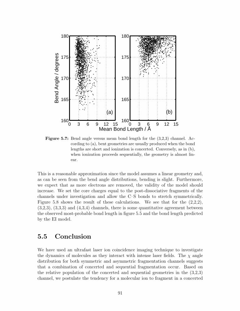
0 3 6 9 12 15160

165

170

175

180

Mean Bond Length / Å

Ben

d A

ngle

/ de

gree

s

0 3 6 9 12 15160

165

170

175

180

(a) (b)

Figure 5.7: Bend angle versus mean bond length for the (3,2,3) channel. Ac-cording to (a), bent geometries are usually produced when the bondlengths are short and ionization is concerted. Conversely, as in (b),when ionization proceeds sequentially, the geometry is almost lin-ear.

This is a reasonable approximation since the model assumes a linear geometry and,as can be seen from the bend angle distributions, bending is slight. Furthermore,we expect that as more electrons are removed, the validity of the model shouldincrease. We set the core charges equal to the post-dissociative fragments of thechannels under investigation and allow the C–S bonds to stretch symmetrically.Figure 5.8 shows the result of these calculations. We see that for the (2,2,2),(3,2,3), (3,3,3) and (4,3,4) channels, there is some quantitative agreement betweenthe observed most-probable bond length in figure 5.5 and the bond length predictedby the EI model.

5.5 Conclusion

We have used an ultrafast laser ion coincidence imaging technique to investigatethe dynamics of molecules as they interact with intense laser fields. The χ angledistribution for both symmetric and asymmetric fragmentation channels suggeststhat a combination of concerted and sequential fragmentation occur. Based onthe relative population of the concerted and sequential geometries in the (3,2,3)channel, we postulate the tendency for a molecular ion to fragment in a concerted

91

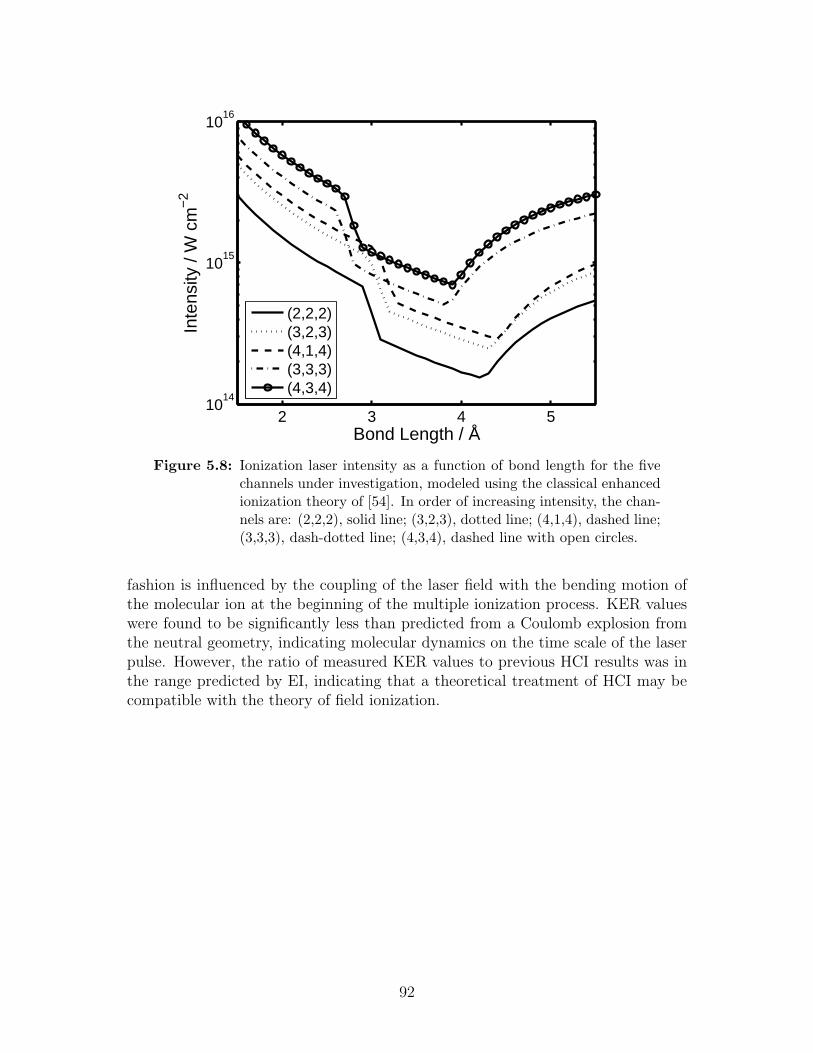
2 3 4 510

14

1015

1016

Bond Length / Å

Inte

nsity

/ W

cm

−2

(2,2,2)(3,2,3)(4,1,4)(3,3,3)(4,3,4)

Figure 5.8: Ionization laser intensity as a function of bond length for the fivechannels under investigation, modeled using the classical enhancedionization theory of [54]. In order of increasing intensity, the chan-nels are: (2,2,2), solid line; (3,2,3), dotted line; (4,1,4), dashed line;(3,3,3), dash-dotted line; (4,3,4), dashed line with open circles.

fashion is influenced by the coupling of the laser field with the bending motion ofthe molecular ion at the beginning of the multiple ionization process. KER valueswere found to be significantly less than predicted from a Coulomb explosion fromthe neutral geometry, indicating molecular dynamics on the time scale of the laserpulse. However, the ratio of measured KER values to previous HCI results was inthe range predicted by EI, indicating that a theoretical treatment of HCI may becompatible with the theory of field ionization.

92

Chapter 6

Comparison of ADK IonizationRates as a Diagnostic for SelectiveVibrational Level PopulationMeasurement

This chapter is adapted from an article that was printed in J. Phys. B: At. Mol.Opt. Phys., 39:3769-3779, 2006, produced in collaboration with Wing-Ki Liu, AsifA. Zaidi, Alexandre Trottier and Joseph H. Sanderson.

6.1 Introduction

The ready availability of femtosecond laser systems and the ability to control andmanipulate the phase of their pulses has led to an increasing effort to use them astools to control matter. One obvious property that might change with vibrationalexcitation is the ionization rate of a molecule. This dependence on vibrationallevel would be a consequence of the dependence of ionization rate on bond length.Recent work on H+

2 [146, 147, 72] provides convincing evidence for strong bondlength dependence on ionization rate, leading to a non-Franck-Condon distributionof product ions, although the observed deviation from a Franck-Condon distributioncan also be explained by taking into account the intensity distribution of the ioniza-tion laser pulses [148]. Also, the phenomenon of enhanced ionization of molecularions [55, 54] is now well established.

A previous attempt has been made to use ionization rate to diagnose vibrationalexcitation [149] using a simple over-the-barrier ionization (OBI) model, also knownas the barrier suppression model [62, 150, 151]. Here we examine three molecularsystems using a method based on the popular Ammosov-Delone-Krainov (ADK)tunneling approximation [59] for describing the ionization process. As Hanson[152] remarked, the tunneling rate is critically dependent upon the difference in the

93

neutral and ion electronic potentials, which varies as a function of the internuclearbond length R. This method, proposed by Saenz [146], calculates the ionizationrate by averaging the ADK R-dependent rate over the probability amplitude of thevibrational state of the molecule.

The quantity that can be used as diagnostic for vibrational excitation of amolecule is the enhancement ratio of the ionization signal of the molecule in thevibrational state v to that in the ground vibrational state. Such ratios can becomputed using the OBI in conjunction with focal volume considerations [62, 150,149, 151]. We compare the enhancement ratios obtained by the ADK and the OBImethods for the H2 molecule, and discuss the analysis for N2 and CO2.

6.2 Molecular Systems

Simple diatomic molecules are the most appropriate systems to study as their vi-bration is in only one dimension. H2 and N2 represent diatomic molecules whoseionization potentials vary substantially (H2) or very little (N2) with internucleardistance. For triatomic molecules, the additional degrees of freedom greatly com-plicate the situation. Here we have considered the symmetric stretch of CO2 andconsider only this normal mode, ignoring other vibrational degrees of freedom. Thiswas done for two reasons. First, by considering only the symmetric stretch mode,the vibration of CO2 can be treated in the same way as a diatomic system. Second,in previous work [149], it was the symmetric stretch mode which was believed tobe preferentially excited. For the diatomic systems, the potential energy curvesof the neutral and ion species were obtained from the literature [153, 154]. ForCO2 and CO+

2 , potential energy surfaces (PES) for nuclear motion were calcu-lated from the variational data of Zuniga et al. [155] and Brommer et al. [156].Cuts were then taken through these PES along the symmetric stretching coordinate(RCO1 = RCO2). Thus we ignore any anharmonic coupling to other normal modesof vibration. The potential energy curves for N2 and CO2 are shown in figures 6.1and 6.2.

In the presence of an intense laser field, the electric field of the laser will couplewith the electric dipole of the molecule and can modify the potential energy curves.This laser-induced bond softening has the effect of reducing the potential energygap between the neutral energy level and the ground electronic state of the ionat large R values. The case of H+

2 is well-known [150, 151, 157]: the ground andexcited state potential curves will distort according to

V1,2 =1

2(Vg + Ve)∓

1

2

√(Ve − Vg)2 + 4V 2

eg (6.1)

where Vg is the potential energy of the 1sσg ground state, and Ve is the potentialenergy of the 2pσu repulsive excited state. Veg is the dipole coupling between theground and excited states, and for large R, Veg ≈ 1

2RF where F is the electric field

94

0.5 1 1.5 2−30

−20

−10

0

10

20

30

RNN

[Å]

N2 Energy Levels

Ene

rgy

[eV

]

N2 X1 Σ

g+

N2+ X2 Σ

g+

Difference

Figure 6.1: Ground-state potential energy curves of N2 (X1Σ+g , solid) and N+

2

(X1Σ+g , dotted). These curves were calculated based on [154]. Over

the range of the vibrational levels of interest, the difference (dashed)in the potential energy curves is almost independent of vibrationallevel.

amplitude. V1 will be the new lower potential energy curve and V2 will be the newupper potential energy curve. Under the influence of the static field, the V1 potentialenergy curve will not have as many bound vibrational levels as the Vg potentialenergy curve. As a result, vibrationally excited molecules will dissociate muchmore easily on V1. This process is known as bond-softening. Recently, Saenz [158]presented three-dimensional ab initio calculation of the ionization rates and energyshifts of a H2 molecule in a static electric field oriented parallel to the molecular axis,and demonstrated similar bond-softening effect for the neutral molecule. Unlike theH+

2 case where the ground and excited states (the charge resonance states) becomedegenerate as R→∞, for the neutral molecule it is the energetically higher excitedstates with ionic characters and having the same symmetry as the ground state(1Σ) that would couple by the electric field to the ground state, giving rise to curvecrossings and the bond-softening effect. The incorporation of this effect is essentialto successfully explain the results of recent observation on the vibrational excitationof H+

2 in strong field ionization experiments of H2 [146, 147, 72]. The bond-softeningeffect observed by Saenz [158] appears at a higher field intensity (≥ 1014 W cm−2)for the neutral H2 molecule than the molecular ion (≥ 1013 W cm−2) [147]. In thispaper we are concerned with laser intensities 1013 W cm−2 < I < 1014 W cm−2,

95

1 1.1 1.2 1.3 1.4 1.5

0

5

10

15

20

25CO

2 Energy Levels

RCO

[Å]

Ene

rgy

[eV

]

CO2 X1 Σ

gCO

2+ X2 Π

gDifference

Figure 6.2: Ground-state potential energy curves of CO2 (solid) and CO+2 (dot-

ted) based on the data of [155] and [156] respectively. Here wehave selected cuts along the symmetric stretch coordinate (RCO2 =RCO2) of the potential energy surfaces. As with N2, the difference(dashed) in the potential energy curves is largely constant over therange of interest.

and we ignore the bond-softening effect for the neutral molecules. For nitrogenand carbon dioxide, no ab initio calculation of bond-softening effect in the presenceof a strong electric field exists to the best of our knowledge. However, the field-free potential curves for N+

2 [159] indicate that the bond-softening effect will onlybecome important at nuclear separations which are beyond the range of vibrationallevels of interest here. For CO+

2 , the excited electronic states are separated from theground state by several eV [160], and bond-softening effect is expected to becomesignificant only at higher laser intensities [158]. Hence we ignore the effect of bond-softening for N2 and CO2 in this study. It will be desirable to have ab initio studiesof bond-softening for these systems.

6.3 ADK Tunneling Ionization

Recall from a previous chapter that the ADK tunnel ionization rate, wADK , is givenin atomic units by [59]:

96

wADK(R, I) =

(3e

π

)3/2Z2

n∗9/2

(4eZ3

n∗4F

)2n∗−3/2

exp

(− 2Z3

3n∗3F

), (6.2)

where e = 2.718. . . , Z is the ionic charge, and I = (c/8π)F 2 is the laser intensity.The effective quantum number, n*, is related to Ip, the ionization potential of thesystem, by

n∗ = Z/√

2Ip(R). (6.3)

Crucially, Ip varies with the internuclear separation R and we can calculate thisusing the technique described in [146, 147, 72], by computing the energy gap be-tween the ground state neutral electronic level and the first ionization state. Thedifference in the potential curves in figures 6.1 and 6.2 gives the ionization energyas a function of bond length R for N2 and CO2. These ionization energy values werethen inserted into the ADK formula to produce the ionization rate as a function ofbond length.

Since we are interested in a technique that will act as a diagnostic for ionizationas a function of neutral vibrational level population, we recast the above calculationto determine the ionization rate as a function of vibrational level in the neutralmolecule.

A satisfactory method to calculate the vibrational dependence of the ionizationrate is to average the R-dependent rate over the probability distribution of themolecule in R [146]. This is equivalent to calculating the expectation value of theADK rate for a given vibrational state v described by the nuclear wave functionΨv(R). For each vibrational level, Ψv(R) was calculated using the computer pro-gram LEVEL [161]. In this case, the vibrationally averaged (VA) ionization ratebecomes [146, 147]

w(v, I) =

∫dR|Ψv(R)|2wADK(R, I) (6.4)

where wADK(R, I) is given by equation (6.2).

We wish to compare results of the OBI model with the ADK calculations. In theOBI model [54, 150, 151], the multi-well potential experienced by the outer electronat r of a molecule in the presence of a static electric field F can be modeled by[54, 131]

U(r) = −na∑i=1

Z

|r −Ri|− F · r , (6.5)

where na is the number of atomic ions of the molecule, Ri is the position vector ofthe ith atomic ion, and Z is the average nuclear charge of the atomic ions. Thedelocalized energy level of this electron is approximated by

97

εL = − 1

na

na∑i=1

[Ipi +

na∑j 6=i

Zi|Ri −Rj|

], (6.6)

where Zi and Ipi are the charge and ionization potential of the ith atomic ion,respectively. Thus, εL is the sum of the average ionization potential of the atomicions and the average potential due to the Coulomb attraction of the neighbouringatomic ions. If any of the inner barriers within the well of U(r) rises above εL,εL will be replaced by the Stark-shifted atomic level. Table 6.1 shows the ion-ization potentials (−εL) for several diatomic molecules (na=2) and CO2 (na=3),in their equilibrium configurations, predicted by equation (6.6). The agreement isreasonable for diatomics and adequate for CO2, given the simplicity of the model.

Molecule Calculated−εL

Accepted−εL

Per cent difference

H2 16.37 15.43 +6.26O2 12.75 12.07 +5.63N2 13.74 15.58 -11.9CO 12.57 14.01 -10.4I2 7.93 9.31 -14.8Hg2 7.91 9.10 -13.1CO2 11.54 13.78 -16.3

Table 6.1: Ionization potentials in eV for diatomics and CO2. Accepted valuesare taken from [162].

The appearance intensity is determined by finding the electric field for which theouter potential barrier of U(r) just falls below εL, so that the electron is free fromthe Coulomb attraction and the molecule is ionized. This way, we can determinethe appearance intensity IA(v) for a given vibrational level v by substituting Rv, thebond length at the outer turning point, into equations (6.5) and (6.6). Assumingthat the laser beam has a Gaussian spatial distribution with peak intensity I0, beamwaist w0 and wavelength λ, the focal volume with intensity between IA(v) and I0is given by [62, 65, 150]

V (IA(v), I0) =V0

3

(2c+

c3

3− 2 tan−1c

), (6.7)

where V0 = 2π2w40/λ and c =

√(I0/IA(v))− 1. Assuming that the molecules would

not ionize until they experience a laser intensity I ≥ IA(v), after which all of themwill ionize, the measured signal enhancement between the ground vibrational leveland an excited vibrational level v will be given by

SOBI(v) = V (IA(v), I0)/V (IA(0), I0). (6.8)

98

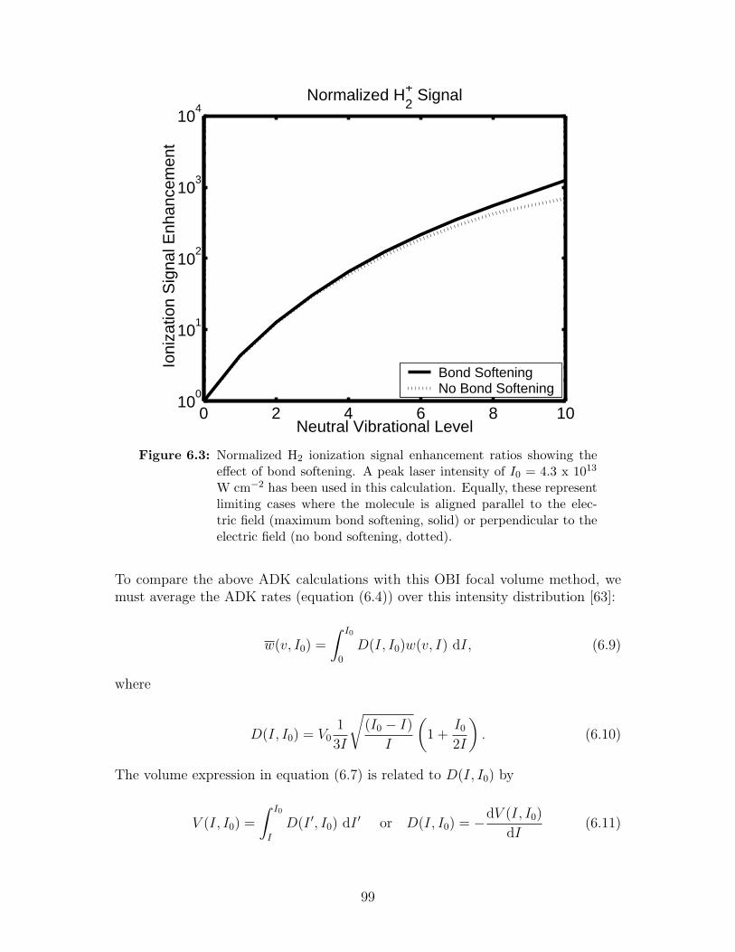
0 2 4 6 8 1010

0

101

102

103

104

Normalized H2+ Signal

Neutral Vibrational Level

Ioni

zatio

n S

igna

l Enh

ance

men

t

Bond SofteningNo Bond Softening

Figure 6.3: Normalized H2 ionization signal enhancement ratios showing theeffect of bond softening. A peak laser intensity of I0 = 4.3 x 1013

W cm−2 has been used in this calculation. Equally, these representlimiting cases where the molecule is aligned parallel to the elec-tric field (maximum bond softening, solid) or perpendicular to theelectric field (no bond softening, dotted).

To compare the above ADK calculations with this OBI focal volume method, wemust average the ADK rates (equation (6.4)) over this intensity distribution [63]:

w(v, I0) =

∫ I0

0

D(I, I0)w(v, I) dI, (6.9)

where

D(I, I0) = V01

3I

√(I0 − I)

I

(1 +

I02I

). (6.10)

The volume expression in equation (6.7) is related to D(I, I0) by

V (I, I0) =

∫ I0

I

D(I ′, I0) dI ′ or D(I, I0) = −dV (I, I0)

dI(6.11)

99

0 2 4 6 8 100

100

200

300

400

500

600

Ioni

zatio

n S

igna

l Enh

ance

men

t

Neutral Vibrational Level

Normalized H2+ Signal

Volume RatioVibrational AverageVA Volume CorrectSaenz

Figure 6.4: Ionization enhancement ratios for H2 using the volume ratiomethod (solid) and the ADK vibrational averaging (dotted)method. The effect of volume correction on the vibrational av-erage is shown with a dashed line. The ab initio results from [158]are included for comparison (crosses). In each case, the peak laserintensity is assumed to be I0 = 8 x 1013 W cm−2

6.4 Results

We first study the ionization of the hydrogen molecule. In figure 6.3, the ionizationenhancement of H2 as a function of vibrational level is plotted at intensity I = 4.3x 1013 W cm−2. The ionization rate increases rapidly with the vibrational level vsince the ionization potential Ip decreases with v. Also shown is the effect of bondsoftening on the enhancement ratio. It is clear that bond softening affects the highervibrational levels more that the lower vibrational levels, since the molecular bondlength is larger for higher vibrational states and bond softening is more pronouncedat large R.

In figure 6.4, we compare the enhancement ratio predicted by the simple OBIprocedure with ADK calculations for H2. The enhancement ratios are monotonicincreasing functions of v, showing that they can be used to estimate the extentof vibrational excitations in experiments for this molecule. We observe that thefocal volume corrected ratios S(V0, I0) = w(v, I0)/w(0, I0), are higher than the cor-responding ratios S(v, I0) = w(v, I0)/v(0, I0) assuming a constant intensity profile,since the averaging in equation (6.9) affects the upper vibrational levels with lower

100

0 2 4 6 8 101

1.1

1.2

1.3

1.4

1.5

1.6

Neutral Vibrational Level

Ioni

zatio

n S

igna

l Enh

ance

men

t

Normalized N2+ Signal

I = 4.3x1013 W/cm2

I = 5.4x1013 W/cm2

Figure 6.5: N2 ionization signal enhancement ratios, assuming laser peak inten-sities of I0 = 4.3 x 1013 W cm−2 (solid) and I0 = 5.4 x 1013 W cm−2

(dotted). Note that when normalized signal enhancements are con-sidered, higher laser intensities produce lower signal enhancements.

ionization potentials more than the vibrational ground level. We have also includedthe ab initio results [68] of Saenz (at a slightly higher intensity of 1014 W cm−2)and the agreement with our S(v, I0) result is satisfactory, taking into account thatthe enhancement ratio decreases with increasing laser intensity [68]. However, thesimple OBI results are consistently lower than the ADK results, and thus predictionusing the OBI procedure tends to over-estimate the vibrational excitation for thissystem.

The enhancement ratios as a function of vibrational level are plotted for N2 infigure 6.5 and for CO2 in figure 6.6. The increase in ionization rates, and thusenhancement, for these systems is much less than that in H2 since their ionizationpotential decreases with R much more slowly. For both N2 and CO2, the ionizationrate changes so slowly that even if it were possible to coherently transfer 100% ofthe vibrational population from v = 0 to v = 10, the ionization signal would onlyincrease by at most 50%. For CO2, such small increase would not be able to accountfor the experimentally observed enhancements [149] realistically. Since the potentialcurves used for CO2 and CO+

2 are determined from different sources, it is a usefulexercise to determine how much change in the ionization signal would occur if theion potential were shifted slightly while its shape remained unaltered [146]. The

101

0 2 4 6 8 101

1.05

1.1

1.15

1.2

1.25

1.3

1.35

1.4

Neutral Vibrational Level

Ioni

zatio

n S

igna

l Enh

ance

men

t

Normalized CO2+ Signal

I = 4.3x1013 W/cm2

I = 5.4x1013 W/cm2

Figure 6.6: CO2 ionization signal enhancement ratios, assuming laser peak in-tensities of I0 = 4.3 x 1013 W cm−2 (solid) and I0 = 5.4 x 1013 Wcm−2 (dotted). Again, the tendency for higher laser intensities toproduce lower signal enhancements is apparent.

results are striking. As figure 6.7 shows, when the equilibrium bond length in CO+2

is increased by 0.04 A (3.5 %), the ionization signal enhancement grows by a factorof about 5, which would fall into the range observed experimentally. It should beemphasized again that we consider the symmetric stretch of CO2 only and ignoreany anharmonic coupling to other normal modes, thus allowing us to use the simpleconsideration as in the case of a diatomic molecule. For highly excited vibrationalstates, anharmonic effect becomes important and a more sophisticated treatment ofthe vibrational motion is necessary. Finally, in figure 6.8 we show the enhancementratios for CO2, using the potentials of figure 6.2, calculated from the simple OBIconsideration for a Gaussian laser pulse, as well as from ADK methods. In contrastto the case of H2 in figure 6.4, the OBI enhancement ratios are consistently higherthan those obtained from the ADK procedures.

6.5 Conclusion

We have studied the dependence on the vibrational level of the ionization rate,and more importantly as a diagnostic tool the enhancement ratio, based on theADK tunneling ionization theory suitably adapted to molecules. For molecules

102

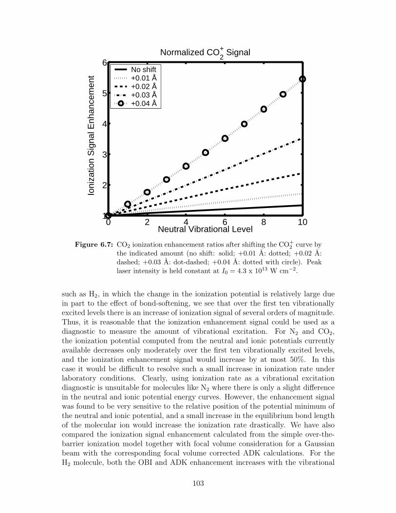
0 2 4 6 8 101

2

3

4

5

6

Neutral Vibrational Level

Ioni

zatio

n S

igna

l Enh

ance

men

t

Normalized CO2+ Signal

No shift+0.01 Å+0.02 Å+0.03 Å+0.04 Å

Figure 6.7: CO2 ionization enhancement ratios after shifting the CO+2 curve by

the indicated amount (no shift: solid; +0.01 A: dotted; +0.02 A:dashed; +0.03 A: dot-dashed; +0.04 A: dotted with circle). Peaklaser intensity is held constant at I0 = 4.3 x 1013 W cm−2.

such as H2, in which the change in the ionization potential is relatively large duein part to the effect of bond-softening, we see that over the first ten vibrationallyexcited levels there is an increase of ionization signal of several orders of magnitude.Thus, it is reasonable that the ionization enhancement signal could be used as adiagnostic to measure the amount of vibrational excitation. For N2 and CO2,the ionization potential computed from the neutral and ionic potentials currentlyavailable decreases only moderately over the first ten vibrationally excited levels,and the ionization enhancement signal would increase by at most 50%. In thiscase it would be difficult to resolve such a small increase in ionization rate underlaboratory conditions. Clearly, using ionization rate as a vibrational excitationdiagnostic is unsuitable for molecules like N2 where there is only a slight differencein the neutral and ionic potential energy curves. However, the enhancement signalwas found to be very sensitive to the relative position of the potential minimum ofthe neutral and ionic potential, and a small increase in the equilibrium bond lengthof the molecular ion would increase the ionization rate drastically. We have alsocompared the ionization signal enhancement calculated from the simple over-the-barrier ionization model together with focal volume consideration for a Gaussianbeam with the corresponding focal volume corrected ADK calculations. For theH2 molecule, both the OBI and ADK enhancement increases with the vibrational

103

0 2 4 6 8 101

2

3

4

5

6

Neutral Vibrational Level

Ioni

zatio

n S

igna

l Enh

ance

men

t

Normalized CO2+ Signal

Volume RatioVibrational AverageVA Volume Correct

Figure 6.8: Ionization enhancement ratios for CO2, comparing the volume ratio(OBI model, solid) with the vibrational averaging (ADK model,dotted) and the volume corrected vibrational averaging (dashed).Peak laser intensity is held constant at I0 = 4.3 x 1013 W cm−2.

level v. However, the OBI result is consistently below the ADK enhancementratio, and the simple OBI procedure would over-estimate the vibrational excitationfor this system. For the CO2 molecule, the OBI and ADK enhancement bothincrease with vibrational level v, but the OBI result is consistently greater thanthe ADK enhancement ratio. Thus, it appears that the OBI calculations whichgave good results for atoms [62, 150, 151] would not be adequate for a quantitativedetermination of the vibrational excitation of molecules, although it may still beuseful for a qualitative estimation. Fortunately, the ADK procedures used in thispaper are relatively easy to use, provided accurate potential energy surfaces for theneutral and ionic species are available.

104

Chapter 7

Summary

A triple coincidence imaging technique has been used to investigate fragmentationdynamics of CO2 and CS2 as they interact with intense laser fields.

In the case of CO2, we have used the triple coincidence Coulomb imaging tech-nique to examine a variety of phenomena as well as make the first-of-its-kind com-plete molecular geometry measurement for the molecule. The data have revealedimportant aspects of molecular behavior in the laser field. Firstly, we have seen thatthe charge state which gives bend angle distribution closest to theory is the lowestCoulomb channel (1,1,1); all other channels show a higher degree of straightening.We interpret this as being a result of competition between bending on the doublyionized potential [93] and straightening during molecular dissociation. The mea-surement settles disagreement between the previous experiments of Hishikawa etal. [77] and Bryan et al. [82]. Higher channels show the dissociation deformationdominates and the molecular skeleton straightens. Also, by measuring the totalenergy released during fragmentation of each channel, we can clearly see evidenceof multiple excitation channels which confirms preliminary observations in OCS[135] and also fits in with interpretations of multiple electronic processes in N2 [57].Alternatively, by following the bond length dependence on charge state we can seethat there is a good fit with the behavior predicted by a simple over-the-barrierionization mechanism. Finally, in order to account for the non-zero energy of themolecular fragments before the final ionization takes place, we have implementeda novel iterative technique to measure the molecular geometry at the point of finalionization.

In the case of CS2, the Coulomb explosion imaging apparatus has made it pos-sible to undertake the most systematic study of multi-electronic dissociative ion-ization to date. We clearly show that for our relatively long pulse we measure akinetic energy release predicted by enhanced ionization while the sensitive triple co-incidence Coulomb imaging method allows us to see much more details of the lasermolecule interaction. Using the χ parameter, we have investigated the propen-sity of a molecule to dissociate into both concerted and sequential channels in thelaser field. We then used the additional information available in the complete mo-

105

mentum measurements to show quantitatively that molecules undergoing concertedthree body dissociation are bending. This confirms the previous observation [77]that bond length increases as bend angle decreases. However, we have shown thatthis simple trend does not represent a complete description; sequential dissocia-tion processes can coexist alongside the concerted ones. The large degree of bondlength asymmetry for high charge channels is attributed to pre-pulses evident inthe interferometric autocorrelation. If these pre-pulses were sufficiently energetic,they could initiate a single dissociation before the arrival of the main pulse. Thestraight molecules observed by Iwasaki et al. [80] were most likely the result ofwings on their pulse, but their ensemble type of measurement did not allow thisto be identified as due to sequential dissociation. Notably, Hasegawa et al. [87]reported observing bent low charged CS2 molecules. These bent molecules couldoriginate from regions of the focus where the peak intensity is not particularlyhigh. Consequently, the energy in the wings of the pulse would not be high enoughto initiate sequential processes early on. The ratios of symmetric to asymmetriccharge states is interesting because it compares well with HCI experiment [34] eventhough many of the molecules we are measuring are clearly very dissociated beforethe final ionization takes place; this is not the case for HCI. Despite the differentmechanism for initiating fragmentation, very dissociated molecular ions show thepropensity to occupy the lowest energy states, identical with HCI.

We have studied the influence of vibrational level on the rate of ionization basedon the ADK tunneling ionization theory suitably adapted to molecules. More im-portantly, we explored the applicability of ionization rate as a diagnostic tool forvibrational excitation. For molecules such as H2, in which the change in the ioniza-tion potential is relatively large due in part to the effect of bond-softening, we seethat over the first ten vibrationally excited levels there is an increase of ionizationsignal of several orders of magnitude. Thus, it is reasonable that the ionization en-hancement signal could be used as a diagnostic to measure the amount of vibrationalexcitation. Under laboratory conditions, it would be difficult to use this techniquefor molecules such as N2 and CO2, since the ionization potential computed fromthe neutral and ionic potentials currently available decreases only moderately overthe first ten vibrationally excited levels; the ionization enhancement signal wouldincrease by at most 50%. The enhancement signal was found to be very sensitiveto the relative position of the potential minimum of the neutral and ionic potential,and a small increase in the equilibrium bond length of the molecular ion would in-crease the ionization rate drastically. We have also compared the ionization signalenhancement computed from the simple over-the-barrier ionization model togetherwith focal volume consideration for a Gaussian beam with the corresponding focalvolume corrected ADK calculations. For the H2 molecule, both the OBI and ADKenhancement increases with the vibrational level v. However, the OBI result is con-sistently below the ADK enhancement ratio, and the simple OBI procedure wouldover-estimate the vibrational excitation for this system. For the CO2 molecule, theOBI and ADK enhancement both increase with vibrational level v, but the OBIresult is consistently greater than the ADK enhancement ratio. Thus, it appears

106

that the OBI calculations which gave good results for atoms [62, 150, 151] wouldnot be adequate for a quantitative determination of the vibrational excitation ofmolecules, although it may still be useful for a qualitative estimation. Fortunately,the ADK procedures used in this paper are relatively easy to use, provided accuratepotential energy surfaces for the neutral and ionic species are available.

7.1 Future Work

Coulomb explosion imaging is still in its infancy and many technological challengesmust be overcome before the complete reconstruction of large molecules can beattempted. Image clarity can be improved by using cold molecules produced froma pulsed valve or supersonic molecular beam. Few-cycle pulses must be available atmulti-kHz repetition rates with matching electronic data-grabbing. Experimentalfacilities presently exist at the Advanced Laser Light Source in Varennes, Quebecthat fulfill these requirements. Ideally, reliable diagnostics must exist to measuresingle-shot autocorrelations in coincidence with explosion data. The deduction ofthe structure of a large molecule from its fragment momenta is feasible if difficult.The requirement of recording all fragment momenta becomes exponentially moredifficult according to the number of fragments. However, the simplex algorithmdescribed in this work is extensible and could be applied to larger molecules ofarbitrary symmetry provided that sufficient computational resources are available.

107

Appendices

108

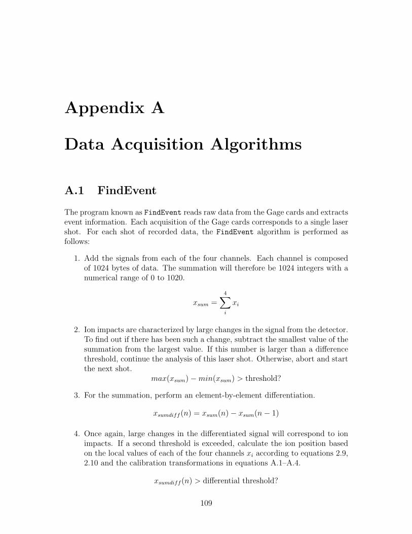
Appendix A

Data Acquisition Algorithms

A.1 FindEvent

The program known as FindEvent reads raw data from the Gage cards and extractsevent information. Each acquisition of the Gage cards corresponds to a single lasershot. For each shot of recorded data, the FindEvent algorithm is performed asfollows:

1. Add the signals from each of the four channels. Each channel is composedof 1024 bytes of data. The summation will therefore be 1024 integers with anumerical range of 0 to 1020.

xsum =4∑i

xi

2. Ion impacts are characterized by large changes in the signal from the detector.To find out if there has been such a change, subtract the smallest value of thesummation from the largest value. If this number is larger than a differencethreshold, continue the analysis of this laser shot. Otherwise, abort and startthe next shot.

max(xsum)−min(xsum) > threshold?

3. For the summation, perform an element-by-element differentiation.

xsumdiff (n) = xsum(n)− xsum(n− 1)

4. Once again, large changes in the differentiated signal will correspond to ionimpacts. If a second threshold is exceeded, calculate the ion position basedon the local values of each of the four channels xi according to equations 2.9,2.10 and the calibration transformations in equations A.1–A.4.

xsumdiff (n) > differential threshold?

109

5. A series of six numbers describing the ion impact is stored to a file. Thesevalues are: ID, the unique identifier of that experiment; Shot, the uniqueidentifier of the laser shot; Ion, indicating that this ion is the nth ion to hitthe detector for that laser shot; t, x and y, corresponding to the temporaland position information for that ion.

data set = (ID, Shot, Ion,t, x,y)

6. The data is loaded into a mySQL database and is filtered once more so thatonly correlated sets of triple events are retained. Correlated triple events arethose where exactly three ions originating from the same laser shot hit thedetector. The mySQL algorithm uses the ID, Shot and Ion values to performthe event sorting. Once the sorting is complete, these values are extraneous.Therefore, triple event data is composed only of time and position data. Ninenumbers characterize each correlated triple event.

data set = (t1, x1, y1, t2, x2, y2, t3, x3, y3)

7. Note that the data set is always ordered such that t1 < t2 < t3.

A.2 Detector Geometry Calibration

The following series of translations and matrix transformations are necessary totake the data from the detector in arbitrary units and and map it to physicalquantities.

1. Calculate x0, y0 according to Equations 2.9 and 2.10.

2. Move the centre of the mask to the origin. To do this, perform the translation(x1

y1

)=

(x0

y0

)−(

0.4800.516

)(A.1)

3. Multiply by a stretch and shear matrix to orient the mask to the x− andy−axes. This transformation will return the position in units of mm.(

x2

y2

)=

(101.85 −6.36218.17 43.17

)(x1

y1

)(A.2)

4. Rotate the recovered positions by 10. This is the angle between the axes ofthe mask and the detector.(

x3

y3

)=

(0.9851 0.17190.1719 0.9851

)(x2

y2

)(A.3)

110

5. Finally, remove the discrepancy between the centres of the mask and detector.That is, an event with all four channels having equal height must produce aresult of (0,0). This final translation corrects the origin.(

x4

y4

)=

(x3

y3

)+

(−2.0504

0.6903

)(A.4)

111

Appendix B

Simplex Algorithm and GraphicalRepresentation

B.1 Simplex Algorithm

Mathematically, the simplex procedure can be stated as follows:

1. Choose initial points x1,x2,x3, ...xN+1 to form a simplex in RN .

2. If a given stopping condition is satisfied, stop. Otherwise, find xB,xW ∈x1,x2,x3, ...xN+1 such that f(xB) = minj=1,...N+1 f(xj) and f(xW ) = maxj=1,...,N+1 f(xj).Let x =

∑j 6=W xj/N.

3. Let xR = x + α(x − xW ). If maxj=1,...N+1f(xj)j 6=W ≥ f(xR), then replacexW with xR (reflection) to form a new simplex and go to step 4. Otherwise,go to step 5.

4. Let xE = x + β(x − xW ). If f(xB) > f(xR) > f(xE), replace xR which wasxW before the reflection step on step 3) with xE (expansion) to form a newsimplex. Go to step 2.

5. Let x′ be defined by f(x′) = minxR,xW and let xC = x + γ(x − x′). Iff(xC) ≤ f(x′), then replace xW with xC (contraction) to form a new simplex.Otherwise, replace xj with xj + (xB − xj)/2 for j = 1, ..., N + 1. Go to step2.

The procedure will conclude on step 2 if either of the following conditions aresatisfied: (i) if the points forming the current simplex converge to a point, within agiven tolerance; (ii) the total number of iterations reaches a predetermined number.

112

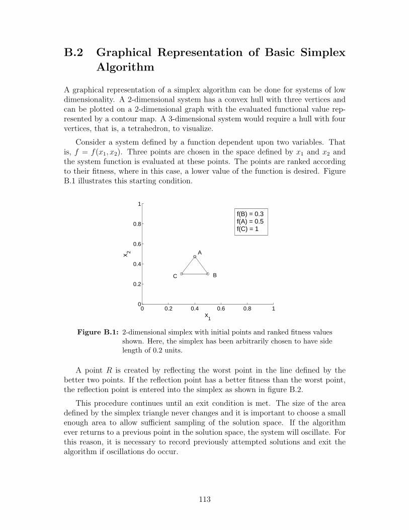
B.2 Graphical Representation of Basic Simplex

Algorithm

A graphical representation of a simplex algorithm can be done for systems of lowdimensionality. A 2-dimensional system has a convex hull with three vertices andcan be plotted on a 2-dimensional graph with the evaluated functional value rep-resented by a contour map. A 3-dimensional system would require a hull with fourvertices, that is, a tetrahedron, to visualize.

Consider a system defined by a function dependent upon two variables. Thatis, f = f(x1, x2). Three points are chosen in the space defined by x1 and x2 andthe system function is evaluated at these points. The points are ranked accordingto their fitness, where in this case, a lower value of the function is desired. FigureB.1 illustrates this starting condition.

0 0.2 0.4 0.6 0.8 10

0.2

0.4

0.6

0.8

1

x1

x 2 A

BC

f(B) = 0.3f(A) = 0.5f(C) = 1

Figure B.1: 2-dimensional simplex with initial points and ranked fitness valuesshown. Here, the simplex has been arbitrarily chosen to have sidelength of 0.2 units.

A point R is created by reflecting the worst point in the line defined by thebetter two points. If the reflection point has a better fitness than the worst point,the reflection point is entered into the simplex as shown in figure B.2.

This procedure continues until an exit condition is met. The size of the areadefined by the simplex triangle never changes and it is important to choose a smallenough area to allow sufficient sampling of the solution space. If the algorithmever returns to a previous point in the solution space, the system will oscillate. Forthis reason, it is necessary to record previously attempted solutions and exit thealgorithm if oscillations do occur.

113

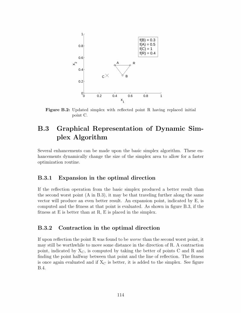
0 0.2 0.4 0.6 0.8 10

0.2

0.4

0.6

0.8

1

x1

x 2 A

BC

f(B) = 0.3f(A) = 0.5f(C) = 1f(R) = 0.4

R

Figure B.2: Updated simplex with reflected point R having replaced initialpoint C.

B.3 Graphical Representation of Dynamic Sim-

plex Algorithm

Several enhancements can be made upon the basic simplex algorithm. These en-hancements dynamically change the size of the simplex area to allow for a fasteroptimization routine.

B.3.1 Expansion in the optimal direction

If the reflection operation from the basic simplex produced a better result thanthe second worst point (A in B.3), it may be that traveling further along the samevector will produce an even better result. An expansion point, indicated by E, iscomputed and the fitness at that point is evaluated. As shown in figure B.3, if thefitness at E is better than at R, E is placed in the simplex.

B.3.2 Contraction in the optimal direction

If upon reflection the point R was found to be worse than the second worst point, itmay still be worthwhile to move some distance in the direction of R. A contractionpoint, indicated by XC , is computed by taking the better of points C and R andfinding the point halfway between that point and the line of reflection. The fitnessis once again evaluated and if XC is better, it is added to the simplex. See figureB.4.

114

0 0.2 0.4 0.6 0.8 10

0.2

0.4

0.6

0.8

1

x1

x 2 A

B

f(B) = 0.3f(A) = 0.5f(R) = 0.4f(E) = 0.35

R

E

Figure B.3: Updated simplex with reflected point R having been replaced byexpansion point E.

0 0.2 0.4 0.6 0.8 10

0.2

0.4

0.6

0.8

1

x1

x 2 A

B

f(B) = 0.3f(A) = 0.5f(C) = 1f(R) = 0.6f(X

C) = 0.4

R

C

XC

Figure B.4: Updated simplex with compression point XC . In this case, thepoint R was found to have a worse fitness than the second worstpoint in the original simplex, point A.

B.3.3 Contraction of simplex

If the reflection, expansion and contraction operations are unable to locate a betterpoint than the worst point in the simplex, the simplex is contracted in the directionof the best point. This operation usually occurs when the algorithm is near to theoptimal solution and has a relatively minor change on the system. This is showngraphically in figure B.5.

115

0 0.2 0.4 0.6 0.8 10

0.2

0.4

0.6

0.8

1

x1

x 2

A

B

f(B) = 0.3f(A) = 0.45f(C) = 0.8

C

Figure B.5: Updated simplex with system compression. In this case, all previ-ous operations have failed to produce a point better than the pointC. The system is contracted in the direction of the best point, B.

116

References

[1] A. L. Basham. Cultural History of India. Oxford University Press, 1999. 1

[2] A. A. Long, editor. The Cambridge Companion to Early Greek Philosophy.1979. 1

[3] N. Melchert. The Great Conversation: A Historical Introduction to Philoso-phy. McGraw Hill, 2002. 1

[4] R. Boscovich. Theoria philosophiae naturalis redacta ad unicam legem viriumin natura existentium. 1758. 1

[5] I. Newton. Principia. 1687. 1

[6] J. Dalton. New System of Chemical Philosophy. 1808. 1

[7] E. Rutherford. Philos. Mag., 6(21):669–688, 1911. 2

[8] N. Bohr. Philos. Mag., 6(26):1–25, 1913. 2

[9] J. Chadwick. Proc. Roy. Soc., A, 136:692–708, 1932. 2

[10] G. N. Lewis. J. Am. Chem. Soc., 38:762, 1916. 2

[11] R. A. Serway. Physics for Scientists and Engineers with Modern Physics.Saunders College Publishing, third edition, 1992. 2

[12] P. F. Bernath. Spectra of Atoms and Molecules. Oxford University Press,second edition, 2005. 2

[13] G. Herzberg. Molecular Spectra and Molecular Structure: Spectra of DiatomicMolecules. Krieger Publishing, second edition, 1989. 2

[14] G. Herzberg. Molecular Spectra and Molecular Structure: Electronic Spectraand Electronic Structure of Polyatomic Molecules. Krieger Publishing, 1991.2

[15] G. Herzberg. Molecular Spectra and Molecular Structure: Infrared and RamanSpectra of Polyatomic Molecules. Krieger Publishing, 1991. 2

[16] E. G. Stout and L. H. Jensen. X-Ray Structure Determination: A PracticalGuide. Macmillan, 1968. 2

117

[17] J. P. Glusker and K. N. Trueblood. Crystal Structure Analysis. OxfordUniversity Press, 1972. 2

[18] P. Goodman, editor. Fifty Years of Electron Diffraction. Reidel, 1981. 2

[19] J. D. Watson and F. H. C. Crick. Molecular structure of nucleic acids: Astructure for deoxyribose nucleic acid. Nature, 171:737–738, 1953. 3

[20] J. C. Kendrew, G. Bodo, H. M. Dintzis, R. G. Parrish, H. Wyckoff, and D. C.Phillips. A three-dimensional model of the myoglobin molecule obtained byX-ray analysis. Nature, 181:662–666, 1958. 3

[21] C. C. Blake, D. F. Koenig, G. A. Mair, A. C. North, D. C. Phillips, andV. R. Sarma. Structure of hen egg-white lysozyme: A three-dimensionalFourier synthesis at 2 a resolution. Nature, 206:757–761, 1965. 3

[22] R. Henderson. The potential and limitations of neutrons, electrons and X-rays for atomic-resolution microscopy of unstained biological molecules. Q.Rev. Biophys., 28:171–193, 1995. 3

[23] E. P. Kanter, P. J. Cooney, D. S. Gemmell, K. O. Groeneveld, W. J. Pietsch,A. J. Ratkowski, Z. Vager, and B. J. Zabranski. Role of excited electronicstates in the interactions of fast (MeV) molecular ions with solids and gases.Phys. Rev. A, 20:834–854, 1979. 3

[24] Z. Vager, R. Naaman, and E. P. Kanter. Coulomb explosion imaging of smallmolecules. Science, 244:426–431, 1989. 4

[25] D. Zajfman and Z. Amitay. Measurement of the vibrational populations ofmolecular ions and its application to dissociative recombination in storagerings. Phys. Rev. A, 52:839–842, 1995. 4

[26] J. H. Sanderson, R. V. Thomas, W. A. Bryan, W. R. Newell, P. F. Taday,and A. J. Langley. Multielectron-dissociative-ionization of SF6 by intensefemtosecond laser pulses. J. Phys. B: At. Mol. Opt. Phys., 30:4499–4507,1997. 4

[27] T. Mizogawa, Y. Ayawa, Y. Isozumi, R. Katano, S. Ito, and N. Maeda. Newreadout technique for 2-dimensional position-sensitive detectors. Nucl. In-strum. Methods Phys. Res., Sect. A, 312:547–552, 1992. 4, 37, 38

[28] J. Becker, K. Beckord, U. Werner, and H. O. Lutz. A system for correlatedfragment detection in dissociation experiments. Nucl. Instrum. Methods Phys.Res., Sect. A, 337:409–415, 1994. 4, 37

[29] U. Werner, K. Beckord, J. Becker, and H.O. Lutz. 3D imaging of the collision-induced coulomb fragmentation of water molecules. Phys. Rev. Lett., 74:1962–1965, 1995. Online abstract: http://prola.aps.org/abstract/PRL/v74/i11/p1962_1. 4, 5

[30] U. Werner, K. Beckord, J. Becker, H.O. Folkerts, and H.O. Lutz. Ion-impact-induced fragmentation of water molecules. Nucl. Instrum. Methods Phys.Res., Sect. B, 98:385–388, 1995. 4

118

[31] J. H. Sanderson, T. Nishide, H. Shiromaru, Y. Achiba, and N. Kobayashi.Near-Coulombic behaviour in the dissociative ionization of CO2 due to impactby Ar8+. Phys. Rev. A, 59:4817–4820, 1999. 5, 6, 18, 38

[32] H. Shiromaru, T. Nishide, T. Kitamura, J. H. Sanderson, Y. Achiba, andN. Kobayashi. Dissociation scheme of highly charged triatomic molecules.Phys. Scr. T., 80A:110–113, 1999. 6, 38

[33] T. Nishide, F. A. Rajgara, T. Kitamura, H. Shiromaru, Y. Achiba, andN. Kobayashi. Dissociation of highly charged CS2 formed by low energycollisions with HCI. Phys. Scr. T., 92:415–419, 2001. 6, 38

[34] F. A. Rajgara, M. Krishnamurthy, D. Mathur, T. Nishide, T. Kitamura,H. Shiromaru, Y. Achiba, and N. Kobayashi. Fragmentation dynamics ofCSq+2 (q=3-10) molecular ions. Phys. Rev. A, 64:032712, 2001. Online ab-stract: http://link.aps.org/abstract/PRA/v64/e032712. 6, 7, 19, 38, 53,81, 83, 84, 85, 86, 87, 88, 89, 106

[35] T. Kitamura, T. Nishide, H. Shiromaru, Y. Achiba, and N. Kobayashi. Directobservation of “dynamic” chirality by Coulomb explosion imaging. J. Chem.Phys., 115:5–6, 2001. 7, 38

[36] K. Codling, L. J. Frasinski, P. A. Hatherly, and J. R. M. Barr. On the major-mode of multiphoton multiple ionization. J. Phys. B: At. Mol. Opt. Phys,20:L525–L531, 1987. 7

[37] L. J. Frasinski, K. Codling, P. Hatherly, J. Barr, I. N. Ross, and W. T.Toner. Femtosecond dynamics of multielectron dissociative ionization by useof picosecond laser. Phys. Rev. Lett, 58:2424–2427, 1987. 7, 8

[38] L. J. Frasinski, K. Codling, and P. A. Hatherly. Covariance mapping - a corre-lation method applied to multiphoton multiple ionization. Science, 246:1029–1031, 1989. 7, 8

[39] K. Codling and L. J. Frasinski. Dissociative ionization of small molecules inintense laser fields. J. Phys. B: At. Mol. Opt. Phys, 26:783–809, 1993. Seealso references therein. 7

[40] L. J. Frasinski, K. Codling, and P. A. Hatherly. Multiphoton multiple ioniza-tion of N2 probed by covariance mapping. Phys. Lett. A, 142:499–503, 1989.8, 9

[41] P. A. Hatherly, L. J. Frasinski, K. Codling, A. J. Langley, and W. Shaikh.The angular-distribution of atomic ions following the multiphoton ionizationof carbon-monoxide. J. Phys. B: At. Mol. Opt. Phys., 23:L291–L295, 1990.9, 12

[42] P. A. Hatherly, M. Stankiewicz, K. Codling, L. J. Frasinski, and G. M. Cross.The multielectron dissociative ionization of molecular-iodine in intense laserfields. J. Phys. B: At. Mol. Opt. Phys., 27:2993–3003, 1994. 9, 10, 12

119

[43] L. J. Frasinski, P. A. Hatherly, K. Codling, M. Larsson, A. Persson, and C. G.Wahlstrom. Multielectron dissociative ionization of CO2 in intense laser fields.J. Phys. B: At. Mol. Opt. Phys., 27:L109–L114, 1994. 9, 10, 12

[44] W. H. Knox, R. S. Knox, J. F. Hoose, and R. N. Zare. Observation of the0-fs pulse. Opt. Photonics News, 1:44–45, 1990. 9

[45] C. Cornaggia, J. Lavancier, D. Normand, J. Morellec, P. Agostini, J. P. Cham-baret, and A. Agonetti. Multielectron dissociative ionization of diatomic-molecules in an intense femtosecond laser field. Phys. Rev. A, 44:4499–4505,1991. 9, 12

[46] C. Cornaggia, D. Normand, and J. Morellec. Role of the molecular electronicconfiguration in the Coulomb fragmentation of n2, c2h2 and c2h4 in an intenselaser field. J. Phys. B: At. Mol. Opt. Phys., 25:L415–L422, 1992. 9, 12

[47] C. Cornaggia, M. Schmidt, and D. Normand. Coulomb explosion of CO2 inan intense femtosecond laser field. J. Phys. B: At. Mol. Opt. Phys., 27:L123–L130, 1994. 9, 12, 67

[48] M. Schmidt, D. Normand, and C. Cornaggia. Laser-induced trapping ofchlorine molecules with picosecond and femtosecond pulses. Phys. Rev. A,50:5037–5045, 1994. 9, 10, 12

[49] C. Cornaggia, M. Schmidt, and D. Normand. Laser-induced nuclear motionsin the Coulomb explosion of C2H

+2 ions. Phys. Rev. A, 51:1431–1437, 1995.

9, 67

[50] C. Cornaggia. Carbon geometry of C3H+3 and C3H

+4 molecular-ions probed

by laser-induced Coulomb explosion. Phys. Rev. A, 52:R4328–R4331, 1995.9, 10

[51] C. Cornaggia. Large-amplitude nuclear motions in the laser-induced Coulombexplosion of carbon dioxide molecules. Phys. Rev. A, 54:R2555–R2558, 1996.9, 10, 18, 67, 72, 73, 74, 75, 76

[52] C. Cornaggia, F. Salin, and C. Le Blanc. Changes in the SO2 geometryduring the laser-induced multiple ionization and fragmentation. J. Phys. B,29:L749–L754, 1996. 9, 10, 16, 67, 74

[53] W. C. Wiley and I. H. McLaren. Time-of-flight mass spectrometer withimproved resolution. Rev. Sci. Instr., 26:1150–1157, 1955. 9, 28

[54] J. H. Posthumus, L. J. Frasinski, A. J. Giles, and K. Codling. Dissociativeionization of molecules in intense laser fields - a method of predicting ionkinetic energies and appearance intensities. J. Phys. B: At. Mol. Opt. Phys.,28:L349–L353, 1995. 10, 11, 67, 77, 78, 90, 92, 93, 97

[55] T. Zuo and A. D. Bandrauk. Charge-resonance-enhanced ionization of di-atomic molecular ions by intense lasers. Phys. Rev. A, 52:R2511–R2514,1995. 10, 12, 67, 93

120

[56] T. Seideman, M. Yu. Ivanov, and P. B. Corkum. Role of electron localizationin intense-field molecular ionization. Phys. Rev. Lett., 75:2819–2822, 1995.10, 67

[57] J. P. Nibarger, S. V. Menon, and G. N. Gibson. Comprehensive analysis ofstrong-field ionization and dissociation of diatomic nitrogen. Phys. Rev. A,63:053406, 2001. 12, 79, 105

[58] S. V. Menon, J. P. Nibarger, and G. N. Gibson. A framework for under-standing molecular ionization in strong laser fields. J. Phys. B: At. Mol. Opt.Phys., 35:2961–2974, 2002. 12, 90

[59] M. V. Ammosov, N. B. Delone, and V. P. Krainov. Tunnel ionization ofcomplex atoms and atomic ions in a varying electromagnetic-field. Zh. Eksp.Teor. Fiz., 91:2008–2013, 1986. 12, 13, 93, 96

[60] L. D. Landau and E. M. Lifshitz. Quantum Mechanics, Non-RelativisticTheory, volume section 77. Oxford: Pergamon, 1991. 12

[61] A. M. Perelomov, V. S. Popov, and M. V. Terentev. Sov. Phys. – JETP,23:924, 1965. 13

[62] S. Augst, D. D. Meyerhofer, D. Strickland, and S. L. Chin. Laser ionization ofnoble-gases by Coulomb-barrier suppression. J. Opt. Soc. Am. B, 8:858–867,1991. 13, 93, 94, 98, 104, 107

[63] M. Protopapas, C. H. Keitel, and P. L. Knight. Atomic physics with super-high intensity lasers. Rep. Prog. Phys., 60:389–486, 1997. 13, 99

[64] S. L. Chin, Y. Liang, J. E. Decker, F. A. Ilkov, and M. V. Ammosov. Tunnelionization of diatomic-molecules by an intense CO2-laser. J. Phys. B: At.Mol. Opt. Phys., 25:L249–L255, 1992. 13

[65] P. Dietrich and P. B. Corkum. Ionization and dissociation of diatomic-molecules in intense infrared-laser fields. J. Chem. Phys., 97:3187–3198, 1992.13, 98

[66] P. Dietrich, D. T. Strickland, and P. B. Corkum. Multiphoton ionization ofinertially confined molecular-ions. J. Phys. B: At. Mol. Opt. Phys., 92:2323–2334, 1993. 13

[67] M. Ivanov, T. Seideman, F. Ilkov, P. Dietrich, and P. Corkum. Explosiveionization of molecules in intense laser fields. Phys. Rev. A, 54:1541–1550,1996. 13

[68] A. Saenz. Behavior of molecular hydrogen exposed to strong dc, ac, orlow-frequency laser fields. II. Comparison of ab initio and Ammosov-Delone-Krainov rates. Phys. Rev. A, 66:063408, 2002. 13, 101

[69] X. M. Tong, Z. X. Zhao, and C. D. Lin. Theory of molecular tunnelingionization. Phys. Rev. A, 66:033402, 2002. 13

121

[70] Z. X. Zhao, X. M. Tong, and C. D. Lin. Alignment-dependent ionizationprobability of molecules in a double-pulse laser field. Phys. Rev. A, 67:043404,2003. 13

[71] K. Mishima, K. Nagaya, M. Hayashi, and S. H. Lin. Theoretical studies ofhigh-power laser ionization of molecules in the tunneling region. Phys. Rev.A, 70:063414, 2004. 13

[72] X. Urbain, B. Fabre, E. M. Staicu-Casagrande, N. de Ruette, V. M. Andria-narijaona, J. Jureta, J. H. Posthumus, A. Saenz, E. Baldit, and C. Cornaggia.Intense-laser-field ionization of molecular hydrogen in the tunneling regimeand its effect on the vibrational excitation of H+

2 . Phys. Rev. Lett., 92:163004,2004. Online abstract: http://link.aps.org/abstract/PRL/v92/e163004.13, 15, 93, 95, 97

[73] G. H. Dunn and B. Van Zyl. Electron impact dissociation of H+2 . Phys. Rev.,

154:40–51, 1967. 15

[74] F. von Busch and G. H. Dunn. Photodissociation of H+2 and D+

2 - experiment.Phys. Rev. A, 5:1726–1743, 1972. 15

[75] A. Hishikawa, A. Iwamae, K. Hoshina, M. Kono, and K. Yamanouchi. Mass-resolved two-dimensional momentum imaging of the Coulomb explosion of N2

and SO2 in an intense laser field. Chem. Phys. Lett., 282:283–291, 1998. 14,17

[76] A. Hishikawa, A. Iwamae, K. Hoshina, M. Kono, and K. Yamanouchi.Coulomb explosion dynamics of N2 in intense laser field by mass-resolvedmomentum imaging. Chem. Phys., 231:315–329, 1998. 14, 16

[77] A. Hishikawa, A. Iwamae, and K. Yamanouchi. Ultrafast deformation of thegeometrical structure of CO2 induced in intense laser fields. Phys. Rev. Lett.,83:1127–1130, 1999. 14, 16, 67, 72, 73, 74, 75, 76, 105, 106

[78] A. Hishikawa, A. Iwamae, and K. Yamanouchi. Ultrafast structural defor-mation of NO2 in intense laser fields studied by mass-resolved momentumimaging. J. Chem. Phys., 111:8871–8878, 1999. 14, 16, 67

[79] A. Iwamae, A. Hishikawa, and K. Yamanouchi. Extraction of molecular dy-namics in intense laser fields from mass-resolved momentum imaging maps:application to Coulomb explosion of NO. J. Phys. B: At. Mol. Opt. Phys.,33:223–240, 2000. 14, 17

[80] A. Iwasaki, A. Hishikawa, and K. Yamanouchi. Real-time probing of align-ment and structural deformation of CS2 in intense nanosecond laser fields.Chem. Phys. Lett., 346:379–386, 2001. 14, 17, 21, 67, 82, 83, 85, 86, 88, 89,106

[81] J.H. Sanderson, A. El-Zein, W.A. Bryan, W.R. Newell, A.J. Langley, andP.F. Taday. Geometry modifications and alignment of H2O in an intensefemtosecond laser pulse. Phys. Rev. A, 59:R2567–R2570, 1999. 14, 18, 67

122

[82] W.A. Bryan, J.H. Sanderson, A. El-Zein, W.R. Newell, P.F. Taday, and A.J.Langley. Laser-induced Coulomb explosion, geometry modification and reori-entation of carbon dioxide. J. Phys. B, 33:745–766, 2000. 14, 18, 67, 71, 72,73, 74, 75, 76, 105

[83] K. Zhao, G. Zhang, and W. T. Hill III. Image labeling: a graphical interfaceto correlation in multiparticle ejection dynamics. Opt. Express, 9:42–48, 2001.18, 19

[84] K. Zhao, G. Zhang, and W. T. Hill III. Strong-field dissociative ionization of alinear triatomic molecule: Relationship between Coulomb-explosion energiesand bond angle. Phys. Rev. A, 68:063408, 2003. Online abstract: http://link.aps.org/abstract/PRA/v68/e063408. 19, 20, 67, 75

[85] M. Brewczyk, K. Rzazewski, and C. W. Clark. Multielectron dissociativeionization of molecules by intense laser radiation. Phys. Rev. Lett., 78:191–194, 1997. 19

[86] Ph. Hering, M. Brewczyk, and C. Cornaggia. Hydrodynamic descriptionof laser-induced Coulomb explosion for small molecules. Phys. Rev. Lett.,85:2288, 2000. 19

[87] H. Hasegawa, A. Hishikawa, and K. Yamanouchi. Coincidence imaging ofCoulomb explosion of CS2 in intense laser fields. Chem. Phys. Lett., 349:57–63, 2001. 19, 20, 81, 83, 84, 85, 86, 88, 89, 106

[88] A. Hishikawa, H. Hasegawa, and K. Yamanouchi. Sequential three-bodyCoulomb explosion of CS2 in intense laser fields appearing in momentumcorrelation map. Chem. Phys. Lett., 361:245–250, 2002. 19, 21, 22, 81

[89] A. Hishikawa, H. Hasegawa, and K. Yamanouchi. Nuclear dynamics on thelight-dressed potential energy surface of CS2 by coincidence momentum imag-ing. Chem. Phys. Lett., 388:1–6, 2004. 19, 21

[90] M. Ueyama, H. Hasegawa, A. Hishikawa, and K. Yamanouchi. Concertedand sequential Coulomb explosion processes of N2O in intense laser fields bycoincidence momentum imaging. J. Chem. Phys., 123:154305, 2005. 19, 22,61, 62, 88

[91] R. Dorner, V. Mergel, O. Jagutzi, L. Spielberger, J. Ullrich, R. Moshammer,and H. Schmidt-Bocking. Cold Target Recoil Ion Momentum Spectroscopy:a ‘momentum microscope’ to view atomic collision dynamics. Phys. Rep.,330:96–192, 2000. 20, 69

[92] H. Hasegawa, A. Hishikawa, and K. Yamanouchi. Unpublished data. 20

[93] H. Kono, S. Koseki, M. Shiota, and Y. Fujimura. A theoretical study ofelectronic dynamics and deformation of CO2 in intense laser fields. J. Phys.Chem. A, 105, 2001. 22, 23, 75, 87, 88, 105

[94] Y. Sato, H. Kono, S. Koseki, and Y. Fujimura. Description of molecular dy-namics in intense laser fields by the time-dependent adiabatic state approach:Application to simultaneous two-bond dissociation of CO2 and its control. J.Am. Chem. Soc., 125, 2003. 22, 23

123

[95] F. Legare, Kevin F. Lee, I. V. Litvinyuk, P. W. Dooley, S. S. Wesolowski,P. R. Bunker, P. Dombi, F. Krausz, A. D. Bandrauk, D. M. Villeneuve, andP. B. Corkum. Laser Coulomb-explosion imaging of small molecules. Phys.Rev. A, 71:013415, 2005. 22, 23, 67, 71, 75, 84

[96] B. Schenkel, J. Biegert, U. Keller, C. Vozzi, M. Nisoli, G. Sansone, S. Stagira,S. De Silvestri, and O. Svelto. Generation of 3.8-fs pulses from adaptivecompresssion of a cascaded hollow fiber supercontinuum. Opt. Lett., 28, 2003.22

[97] A. H. Zewail. Femtochemistry: Ultrafast Dynamics of the Chemical Bond.World Scientific, Singapore, 1994. 23

[98] V. Sundstrom, editor. Femtochemistry and Femtobiology: Ultrafast ReactionDynamics at Atomic-Scale Resolution. World Scientific, Singapore, 1994. 23

[99] A. W. Castleman Jr. and V. Sundstrom. Special issue on ten years of femto-chemistry. J. Phys. Chem. A, 102:4021, 1998. 23

[100] P. W. Dooley, I. V. Litvinyuk, Kevin F. Lee, D. M. Rayner, M. Spanner,D. M. Villeneuve, and P. B. Corkum. Direct imaging of rotational wave-packet dynamics of diatomic molecules. Phys. Rev. A, 68:023406, 2003. 24

[101] Kevin F. Lee, F. Legare, D. M. Villeneuve, and P. B. Corkum. Measuredfield-free alignment of deuterium by few-cycle pulses. J. Phys. B: At. Mol.Opt. Phys., 39:4081–4086, 2006. 24

[102] F. Legare, Kevin F. Lee, I. V. Litvinyuk, P. W. Dooley, A. D. Bandrauk, D. M.Villeneuve, and P. B. Corkum. Imaging the time-dependent structure of amolecule as it undergoes dynamics. Phys. Rev. A, 72:052717, 2005. Onlineabstract: http://link.aps.org/abstract/PRA/v72/e052717. 24, 25, 50,53

[103] F. Legare, Kevin F. Lee, A. D. Bandrauk, D. M. Villeneuve, and P. B.Corkum. Laser Coulomb explosion imaging for probing ultra-fast molecu-lar dynamics. J. Phys. B: At. Mol. Opt. Phys., 39:S503–S513, 2006. 24

[104] H. Stapelfeldt, H. Sakai, E. Constant, and P. B. Corkum. Formation andmeasurement of molecular quantum picostructures. Phys. Rev. A, 55:R3319–R3322, 1997. 24

[105] S. J. Walker. Development and characterization of a regeneratively ampli-fied ultrafast laser system with an all-glass stretcher and compressor. Mas-ter’s thesis, University of Waterloo, Waterloo, Ontario, Canada, 2006. URIhttp://hdl.handle.net/10012/2981. 26

[106] D. Strickland and G. Mourou. Compression of amplified chirped opticalpulses. Opt. Commun., 56:219–221, 1985. 26

[107] O. Svelto. Principles of Lasers. Plenum Press, fourth edition, 1989. 27

[108] M. Gisselbrecht, A. Huetz, M. Lavollee, T. J. Reddish, and D. P. Seccombe.Optimization of momentum imaging systems using electric and magneticfields. Rev. Sci. Instrum., 76:013105, 2005. 35

124

[109] Robert J. Cotter. Time-of-Flight Mass Spectrometry - Instrumentation andApplications in Biological Research. American Chemical Society, Washington,DC, 1997. 36

[110] T. Mizogawa, M. Sato, M. Yoshino, Y. Ito, and Y. Awaya. A two-dimensionalposition-sensitive anode for microchannel plates based on the “MBWC” tech-nique. Nucl. Instrum. Methods Phys. Res., Sect. A, 387:395–400, 1997. 36,38

[111] C. Firmani, E. Ruiz, C. W. Carlson, M. Lampton, and F. Paresce. High-resolution imaging with a two-dimensional resistive anode photon counter.Rev. Sci. Instrum., 53:570–574, 1982. 37

[112] O. Jagutzki, V. Mergel, K. Ullmann-Pfleger, L. Spielberger, U. Meyer,R. Dorner, and H. Schmidt-Bocking. A broad-application microchannel-platedetector system for advanced particle or photon detection tasks: large areaimaging, precise multi-hit timing information and high detection rate. Nucl.Instrum. Methods Phys. Res., Sect. A, 477:244–249, 2002. 37

[113] C. Martin, P. Jelinsky, M. Lampton, R. F. Malina, and H. O. Anger. Wedge-and-strip anodes for centroid-finding position-sensitive photon and particledetectors. Rev. Sci. Instrum., 52:1067–1074, 1981. 37

[114] M. Yamamoto and E. Tanaka. Two-dimensional position-sensitive propor-tional chamber using weighted coupling capacitor read-out. Radioisotopes,24:379–385, 1975. [Japanese]. 37, 38

[115] M. Yamamoto. Influence of amplifier noise on multi-wire proportional cham-ber using weighted coupling capacitor read-out. Radioisotopes, 24:386–390,1975. [Japanese]. 37

[116] R. Allemand and G. Thomas. New position detector - backgammon device.Nucl. Instrum. Methods, 137:141–149, 1976. [French]. 37

[117] H. Shiromaru, K. Kobayashi, M. Mizutani, M. Yoshino, T. Mizogawa,Y. Achiba, and N. Kobayashi. An apparatus for position sensitive TOFmeasurements of fragment ions produced by Coulomb explosion. Phys. Scr.T., 73:407–409, 1997. 38

[118] G. Veshapidze, T. Nishide, H. Shiromaru, N. Kobayashi, and T. Mizogawa.A time- and position-sensitive detector using a resistive film anode combinedwith a “modified backgammon with weighted capacitors” readout pad. Jpn.J. Appl. Phys., 41:871–875, 2002. 39

[119] G. Veshapidze. Private communication. 39

[120] O. Bretscher. Linear Algebra With Applications, 3rd ed. Upper Saddle RiverNJ: Prentice Hall, 1995. 56

[121] J. A. Snyman. Practical Mathematical Optimization: An Introduction to Ba-sic Optimization Theory and Classical and New Gradient-Based Algorithms.Springer Publishing, 2005. 57, 59

125

[122] W. Spendley, G.R. Hext, and F.R. Himsworth. Sequential application ofsimplex design of optimization and evolutionary operations. Technometrics,4:441–461, 1962. 58, 71, 84

[123] F. H. Walters Jr., L. R. Parker, S. L. Morgan, and S. N. Demming. SequentialSimplex Optimization: A Technique for Improving Quality and Productivityin Research, Development, and Manufacturing. Boca Raton, FL: CRC Press,1991. 58

[124] S. Liu, A. Hishikawa, A. Iwamae, and K. Yamanouchi. Advances in Multipho-ton Processes and Spectroscopy. World Scientific, Singapore, 2001. Editors:Y. Fujimura and R. J. Gordon. 67

[125] J. H. Sanderson, R. V. Thomas, W. A. Bryan, W. R. Newell, A. J. Langley,and P. F. Taday. Alignment and bending of CO2 by intense femtosecond laserpulses. J. Phys. B: At. Mol. Opt. Phys., 31:L599–L606, 1998. 67

[126] A. S. Alnaser, C. M. Maharjan, X. M. Tong, B. Ulrich, P. Ranitovic, B. Shan,Z. Chang, C. D. Lin, C. L. Cocke, and I. V. Litvinyuk. Effects of orbitalsymmetries in dissociative ionization of molecules by few-cycle laser pulses.Phys. Rev. A, 71:031403(R), 2005. 67

[127] W. M. Johnstone, N. J. Mason, and W. R. Newell. Electron-scatteringfrom vibrationally excited carbon-dioxide. J. Phys. B: At. Mol. Opt. Phys.,26:L147–L152, 1993. 68

[128] T. Mizogawa, Y. Awaya, Y. Isozumi, R. Katano, S. Ito, and N. Maeda. Newreadout technique for 2-dimensional position-sensitive detectors. Nucl. Inst.and Meth. A, 312:547–552, 1992. 69

[129] B. Siegmann, U. Werner, H. O. Lutz, and R. Mann. Complete Coulombfragmentation of CO2 in collisions with 5.9 MeV u−1 Xe18+ and Xe43+. J.Phys. B: At. Mol. Opt. Phys., 35:3755–3765, 2002. 72, 74, 75, 77

[130] C. Cornaggia and Ph. Hering. Nonsequential double ionization of smallmolecules induced by a femtosecond laser field. Phys. Rev. A, 62:023403,2000. 75

[131] J. H. Sanderson, T. R. J. Goodworth, A. El-Zein, W. A. Bryan, W. R. Newell,A. J. Langley, and P. F. Taday. Coulombic and pre-Coulombic geometryevolution of carbonyl sulfide in an intense femtosecond laser pulse, determinedby momentum imaging. Phys. Rev. A, 65:043403, 2002. 76, 77, 97

[132] C. Cornaggia and L. Quaglia. Experimental observation of non-Coulombicstates of transient multicharged molecular ions N4+

2 and O4+2 . Phys. Rev. A,

63:030702, 2001. 77, 79

[133] L. Quaglia, O. Chiappa, G. Granucci, V. Brenner, Ph. Millie, and C. Cor-naggia. Non-Coulombic states of N4+

2 and O4+2 ions probed by laser-induced

multi-ionization of N2 and O2. J. Phys. B: At. Mol. Opt. Phys., 35:L145–L151,2002. 77

126

[134] R. N. Coffee and G. N. Gibson. Identifying fragment vuv excitations withdissociative channels from the strong-field ionization of N2. Phys. Rev. A,72:011401, 2005. 77

[135] W. A. Bryan, W. R. Newell, J. H. Sanderson, and A. J. Langley. Observationof multiple ionization pathways for OCS in an intense laser field resolved bythree-dimensional covariance mapping and visualized by hierarchical ioniza-tion topology. Phys. Rev. A, 74:053409, 2006. 77, 78, 105

[136] J. P. Brichta, W-K Liu, A. A. Zaidi, A. Trottier, and J. H. Sanderson. Com-parison of ADK ionization rates as a diagnostic for selective vibrational levelpopulation measurement. J. Phys. B: At. Mol. Opt. Phys., 39:3769–3779,2006. 77

[137] J. S. Wright, G. A. DiLabio, D. R. Matusek, P. B. Corkum, M. Yu. Ivanov,Ch. Ellert, R. J. Buenker, A. B. Alekseyev, and G. Hirsch. Dissociation ofmolecular chlorine in a Coulomb explosion: Potential curves, bound states,and deviation from Coulombic behaviour for Cln+

2 (n=2,3,4,6,8,10). Phys.Rev. A., 59:4512–4521, 1991. 78

[138] P. Millie, I. Nenner, P. Archirel, P. Lablanquie, P. G. Fournier, and J. H. D.Eland. Theoretical and experimental studies of the triatomic doubly chargedions CO2+

2 , OCS2+ and CS2+2 . J. Chem. Phys., 84:1259–1269, 1986. 78

[139] H. Hogreve. Stability properties of CO2+2 . J. Phys. B: At. Mol. Opt. Phys.,

28:L263–L270, 1995. 78

[140] M. Hochlaf, F. R. Bennett, G. Chambaud, and P. Rosmus. Theoretical studyof the electronic states of CO++

2 . J. Phys. B: At. Mol. Opt. Phys., 31:2163–2175, 1998. 78

[141] J. P. Nibarger, M. Li, S. Menon, and G. N. Gibson. Direct observationof excited state fragments following molecular ionization and dissociation instrong fields. Phys. Rev. Lett., 83:4975–4978, 1999. 80

[142] L. Quaglia and C. Cornaggia. Experimental evidence of excited multichargedatomic fragments coming from laser-induced Coulomb explosion of molecules.Phys. Rev. Lett., 20:4565–4568, 2000. 80

[143] S. Banerjee, G. R. Kumar, and D. Mathur. Dynamic and geometric alignmentof CS2 in intense laser fields of picosecond and femtosecond duration. Phys.Rev. A, 60:R3369–R3372, 1999. 81

[144] C. Y. Wu, H. Z. Ren, T. T. Liu, R. Ma, H. Yang, H. B. Jiang, and Q. H.Gong. Field induced ionization and Coulomb explosion of carbon disulfide.Opt. Communications, 216:133–138, 2003. 81

[145] J. X. Chen, R. Ma, H. Z. Ren, X. Li, C. Y. Wu, H. Yang, and Q. H. Gong.Kinetic energy release of diatomic and linear triatomic molecules in intensefemtosecond laser fields. Chinese Phys., 13:24–29, 2004. 81

127

[146] A. Saenz. On the influence of vibrational motion on strong-field ionizationrates in molecules. J. Phys. B: At. Mol. Opt. Phys., 34:4365–4372, 2000. 93,94, 95, 97, 101

[147] J. H. Posthumus, L. F. Frasinski, and K. Codling. Super Intense Laser-AtomPhysics (Silap 2000) NATO Science Series, volume 12. Dordrect: Kluwer,2001. 93, 95, 97

[148] T. K. Kjeldsen and L. B. Madsen. Vibrational excitation of diatomic molec-ular ions in strong field ionization of diatomic molecules. Phys. Rev. Lett.,95:073004, 2005. 93

[149] J. F. Xia, J. H. Sanderson, W.-K. Liu, and D. Strickland. Experimentalobservation of Raman chirped adiabatic rapid passage. J. Phys. B: At. Mol.Opt. Phys., 36:L409–L414 and references therein, 2003. 93, 94, 101

[150] J. H. Posthumus and J. F. McCann. Molecules and Clusters in Intense LaserFields. Cambridge: Cambridge University Press, 2001. 93, 94, 97, 98, 104,107

[151] J. H. Posthumus. The dynamics of small molecules in intense laser fields.Rep. Prog. Phys., 67:623–665, 2004. 93, 94, 97, 104, 107

[152] G. R. Hanson. Dissociative field-ionization of H2 and HD. J. Chem. Phys.,62:1161–1180, 1975. 93

[153] T. E. Sharp. Potential-energy curves for molecular hydrogen and its ions. At.Data, 2:119–169, 1971. 94

[154] K. P. Huber and G. Herzberg. Molecular Spectra and Molecular Structure,volume 4. Princeton, NJ: Van Nostrand-Reinhold, 1979. 94, 95

[155] J. Zuniga, A. Bastida, M. Alacid, and A. Requena. Variational calculationsof rovibrational energies for CO2. J. Mol. Spectrosc., 205:62–72, 2001. 94, 96

[156] M. Brommer, G. Chambaud, E.-A. Reinsch, P. Rosmus, A. Spielfiedel,N. Feautrier, and H.-J. Werner. Theoretical potential energy function androvibronic spectrum for CO+

2 X2Πg. J. Chem. Phys., 94:8070–8082, 1991. 94,96

[157] R. S. Mulliken. Intensities of electronic transitions in molecular spectra II.Charge-transfer spectra. J. Chem. Phys., 7:20–34, 1939. 94

[158] A. Saenz. Behavior of molecular hydrogen exposed to strong dc, ac, or low-frequency laser fields: I. Bond softening and enhanced ionization. Phys. Rev.A, 66:063407, 2002. 95, 96, 100

[159] E. W. Thulstrup and A. Andersen. Configuration interaction studies ofbound, low-lying states of N−2 , N2, N+

2 and N2+2 . J. Phys. B: At. Mol. Phys.,

8:965–976, 1975. 96

128

[160] J. Liu, W. Chen, M. Hochlaf, X. Qian, C. Chang, and C. Y. Ng. Unimoleculardecay pathways of state-selected CO+

2 in the internal energy range of 5.2-6.2eV: An experimental and theoretical study. J. Chem. Phys., 118:149–163,2003. 96

[161] R. J. Le Roy. Level 7.5: a computer program for solving the radial Schrodingerequation for bound and quasibound levels, 2002. University of WaterlooChemical Physics Research Report CP-655 (the source code and manual forthis program may be obtained for the ‘Computer Programs’ link on the wwwsite http://leroy.uwaterloo.ca). 97

[162] NIST Chemistry WebBook http://webbook.nist.gov/chemistry. 98

129